Problem Chosen 2021 Team Control Number A Summary Sheet

Problem Chosen 2021 Team Control Number

A MCM/ICM 2103767Summary Sheet

Decomposition Rate of Multi-Fungal Species and Its Interfering Factors

Summary

Fungi play a very important role in the cycle of ecosystem as decomposer which can supply raw materialsto producers. In this paper, we use logistic curve, Volterra model and chemical kinetics to study thedecomposition rate of multi-species community under different climate conditions. By using Matlab,we constructed the Single Species Decomposition Rate Model, the Multi-Species Decomposition RateModel and the model of total decomposition rate of fungi under comprehensive weather and competition.Take five species of fungi as example, the change of the number of each species caused by competition andthe change of the total decomposition rate with temperature under five kinds of climate can be calculated.Finally, some reasonable suggestions are given based on the actual situation.

For Problem 1, we construct the Single Species Decomposition Rate Model by combining logisticcurve with the relationship between decomposition rate, growth rate and density, and calculate the curvesof decomposition rate of five specific fungi with density without considering the interaction by Matlab.

For Problem 2 and 3, we first establish the autonomous system of ordinary differential equationsof different fungi under competition by analogy with Volterra equation, and construct the CompetitionModel. The logarithm numerical solution of the equation is obtained by Matlab, and the change of thenumber of each species with time can be obtained, so as to predict the dominant and disadvantagedspecies of the community in the short and long term.

For Problem 4, we first use the model of enzyme-catalyzed reaction in chemical kinetics to determinethe coefficient I(T,m), which is affected by the mass of decomposed products and temperature. Combinedwith the humidity and the moisture niche width of each species, and considering the two models above,we construct the Complete Multi-Species Decomposition Rate Model in the ecosystem. Finally, weuse Matlab to calculate and the decomposition rate of community with temperature under five kinds ofclimate was plotted. The dominant species were determined by observing the decomposition rate of eachspecies in different climate.

For Problem 5, we combine modeling results above to change the number of fungal species underspecific climate, plot the curves of decomposition rate of communities with the numbers of fungal specieswith temperature through Matlab, and conclude that species diversity is of great significance for thehealthy and stable development of ecosystem.

Finally, we analyze the sensitivity of the model, and evaluate its advantages and disadvantages.Meanwhile, we make a statement about the possible development and perfection for future researchersbased on our model.

The characteristic of this paper lies in the comprehensive use of mathematics, chemistry and ecologyknowledge to construct the actual problems and the results are in good agreement with the actual situation,which is embodied in: Our method integrates the research of some ecological problems and makesreasonable extrapolation; in the idea of model construction, we have widely considered the influence anddegree of various parameters on the model and the method we use in sensitivity analysis.

Keywords: decomposition rate of fungi; logistic curve; Volterra model; chemical kinetics; Matlab

Team # 2103767

Contents1 Introduction 1

1.1 Background . . . . . . . . . . . . . . . . . . . . . . . . . . . . . . . . . . . . . . . . . 11.2 Problem Restatement . . . . . . . . . . . . . . . . . . . . . . . . . . . . . . . . . . . . 11.3 Our Work . . . . . . . . . . . . . . . . . . . . . . . . . . . . . . . . . . . . . . . . . . 1

2 Assumptions and Notations 22.1 Assumptions . . . . . . . . . . . . . . . . . . . . . . . . . . . . . . . . . . . . . . . . 22.2 Notations . . . . . . . . . . . . . . . . . . . . . . . . . . . . . . . . . . . . . . . . . . 2

3 Model 1: Ideal Single Species Decomposition Rate Model 33.1 Model Construction . . . . . . . . . . . . . . . . . . . . . . . . . . . . . . . . . . . . . 33.2 Solution of Problem 1 . . . . . . . . . . . . . . . . . . . . . . . . . . . . . . . . . . . . 43.3 Result . . . . . . . . . . . . . . . . . . . . . . . . . . . . . . . . . . . . . . . . . . . . 4

4 Model 2: Ideal Multi-Species Decomposition Rate Model 54.1 Model Construction . . . . . . . . . . . . . . . . . . . . . . . . . . . . . . . . . . . . . 5

4.1.1 Competition Model . . . . . . . . . . . . . . . . . . . . . . . . . . . . . . . . . 54.1.2 Ideal Multi-Species Decomposition Rate Model . . . . . . . . . . . . . . . . . . 6

4.2 Solution and Result of Problem 2 . . . . . . . . . . . . . . . . . . . . . . . . . . . . . . 74.3 Result of Problem 3 . . . . . . . . . . . . . . . . . . . . . . . . . . . . . . . . . . . . . 9

5 Model 3: Complete Multi-Species Decomposition Rate Model 95.1 Model Construction . . . . . . . . . . . . . . . . . . . . . . . . . . . . . . . . . . . . . 9

5.1.1 Temperature and Decomposed Products Model . . . . . . . . . . . . . . . . . . 95.1.2 Humidity Model . . . . . . . . . . . . . . . . . . . . . . . . . . . . . . . . . . 105.1.3 Complete Model . . . . . . . . . . . . . . . . . . . . . . . . . . . . . . . . . . 11

5.2 Solution and Result of Problem 4 . . . . . . . . . . . . . . . . . . . . . . . . . . . . . . 115.2.1 Complete Result of Decomposition Rate in Competition Considering Climate . . 115.2.2 Prediction of Dominant Species and Combination in Different Climates . . . . . 12

5.3 Solution and Result of Problem 5 . . . . . . . . . . . . . . . . . . . . . . . . . . . . . . 13

6 Sensitivity Analysis 136.1 Sensitivity of Temperature . . . . . . . . . . . . . . . . . . . . . . . . . . . . . . . . . 136.2 Sensitivity of Humidity . . . . . . . . . . . . . . . . . . . . . . . . . . . . . . . . . . . 14

7 Model Evaluation 147.1 Strength and Weakness . . . . . . . . . . . . . . . . . . . . . . . . . . . . . . . . . . . 14

7.1.1 Strength . . . . . . . . . . . . . . . . . . . . . . . . . . . . . . . . . . . . . . . 147.1.2 Weakness . . . . . . . . . . . . . . . . . . . . . . . . . . . . . . . . . . . . . . 14

7.2 Future Work . . . . . . . . . . . . . . . . . . . . . . . . . . . . . . . . . . . . . . . . . 14

Article: Decomposition Rate of Fungi and Its Interfering Factor 15References 17Appendix 18

Team # 2103767 Page 1 of 22

1 Introduction1.1 BackgroundDecomposer plays a very important role in the cycle of ecosystem, which can decompose complex organiccompounds which contain carbon, nitrogen, phosphorus and so on into simple inorganic substances so thatproducers can reuse them and release energy. A very important part in this process is the decompositionof plant materials and wood fibers into carbon dioxide, water, and inorganic salts by fungi. [1] Thecorrosion decomposition of plant materials and material fibers by fungi are affected by numerous factors.Temperature and the amount of decomposed products can affect the progress of the reaction, whilehumidity can affect the process to different degrees according to different fungi. Meanwhile, the growthrate, the density of different fungi and the interaction relationship between various fungi can also affectthe decomposition. Studying the above factors has important implications for the physical cycle of anecosystem as well as for the healthy development of the system.

1.2 Problem RestatementIn order to describe the decomposition rate of fungi under different conditions and the relationshipbetween them, we need to solve the following problems.

• Problem 1: By introducing relevant variables, establish a model to express the ability of singlespecies of fungi to decompose ground litter and wood fibers.

• Problem 2: Establish a model to represent the competition among various fungi, and link thedecomposition ability of various fungi to establish the decomposition rate model of multiple fungi.

• Problem 3: At the same time, the dynamic characteristics of the interaction between fungi can beexpressed and predicted in different time periods.

• Problem 4: Establish a model that can express the influence of climate conditions and differentenvironmental conditions on the decomposition rate of fungi. Predict the relative advantages anddisadvantages for each species and their relationship under different kinds of climate.

• Problem 5: Point out the influence of fungal community diversity on the overall decompositionefficiency, and predict the significance of biodiversity to the environment when it changes.

Finally, analyze the environmental sensitivity and give an evaluation.

1.3 Our Work

Climate ModelI ( T, m )

Temperature

HumidityMass of Decomposed Products

Ideal Single Species Decomposition Rate Model

Species Growth Rate Species DensityAction

Reaction

Competition Model

Complete Multi-Species Decomposition Rate Model

Moisture Niche Width

+

Internal Factors (Fungi)

Ideal Multi-Species Decomposition Rate Model

External Factors (Climate)

++

Figure 1 Solving strategies

Team # 2103767 Page 2 of 22

To solve the problem, here are the steps we follow.• Under the condition of no climate impact, we only consider the internal factors of a single species,

and use relevant ecological and mathematical knowledge to build the model.• Introduce a competition model to connect different kinds of fungi and build the ideal multi-species

model.• Consider external factors and build a model based on ecology and chemistry. Then put all the

models together to obtain the complete model.• Analysis the model we have constructed through sensitivity, strengths and weaknesses.

2 Assumptions and Notations2.1 Assumptions

• Assuming that there is no matter other than ground litter and wood fibers in the growing soil andthe initial value of decomposed products in each unit volume of soil is uniform.

• Assuming that when a single species of fungi exists in the soil alone and the environmental factorsdo not change, the mycelial elongation rate of the fungus remains constant.

• Assuming that there is only competition among different kinds of fungi in the soil.• Assuming that the decrease of the growth rate of various fungi has a linear relationship with the

number of competitors of other fungi when there is competition among them.• Assuming that the soil water content in the model is totally expressed by precipitation.• Assuming that only temperature, humidity and the mass of decomposed products are considered

in the model of environment.

2.2 NotationsTable 1 Notations

Symbol Description

R total decomposition rateR f un decomposition rate of fungi without considering climateR0 the maximum decomposition rate of a single species

RE M the total decomposition rate of 50% fungi which do not reach the fastest decomposition ratei, j the kind of fungir growth rate of fungiρ density of fungiθ the coefficient of moisture niche width of fungix the number of each species of fungiξ population growth potential indexK environmental capacity of fungiS area of the investigated landµ intrinsic reproduction coefficient of fungusλi j the competition factor of fungi i caused by the introduction of fungus j( j , i)I temperature(T) and decomposed product(m) factork reaction rate constantα reaction order

Team # 2103767 Page 3 of 22

(Continued)

Symbol Description

Ea reaction activation energyJ moisture niche widthR̂ humidity(l) factor

3 Model 1: Ideal Single Species Decomposition Rate Model3.1 Model ConstructionWe used the amount of decomposed products change per unit time to characterize the decompositionrate of fungi, that is

R = R(t) = −dmdt

(1)

where the negative sign indicates the decrease of ground litter and woody fibers. From the nature offungi, the decomposition rate is related to the growth rate, the number in unit space, that is, the densityand the moisture niche width. Among them, with the growth of fungi, its density will increase, and theincrease of density will slow down the growth rate of fungi [2], while both are related to time.

Rf un(t) = Rf un(r, ρ) r = r(t) ρ = ρ(t) (2)

The decomposition rate is positively related to the growth rate as R(t) ∝ r(t) and as the density increases,the decomposition rate will decline along the negative index as R(t) ∝ e−ρ(t). For a particular species, wetake θ as a constant. Therefore, R(t) is expressed as

Rf un(t) = θ · r(t) · e−aρ(t) (a > 0, θ > 0) (3)

where a is decomposition restraining coefficient.Next, we model the relationship between r and ρ. Based on the positive and negative correlation

mentioned above and the analogy with the S-type logistic curve of the relationship between populationgrowth rate and population density described by Felchester in 1833 [2], we consider that r and ρ shouldalso satisfy this relationship, that is

dxdt=ξx(K − x)

K(4)

x(t) = CKeξt

1 + CKeξt(5)

where C =x(t = 0)

K − x(t = 0) > 0 is a constant. Due to r =dxdt

and ρ =xS

, then

r =ξSKρ(K − ρS) (6)

It is obvious that when ρ =K2S

, the maximum growth rate is obtained.

Therefore, take (6) into (3), we have

Rf un(t) =ξSθKρ(K − ρS) · e−aρ (a > 0) (7)

Team # 2103767 Page 4 of 22

3.2 Solution of Problem 1There are two zero points of (7), which are 0 and

KS

, and we can see that limρ→0

Rf un = limρ→∞

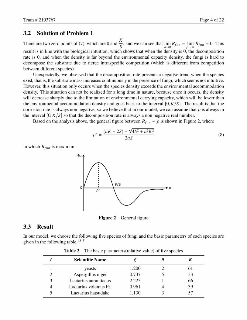
Rf un = 0. Thisresult is in line with the biological intuition, which shows that when the density is 0, the decompositionrate is 0, and when the density is far beyond the environmental capacity density, the fungi is hard todecompose the substrate due to fierce intraspecific competition (which is different from competitionbetween different species).

Unexpectedly, we observed that the decomposition rate presents a negative trend when the speciesexist, that is, the substrate mass increases continuously in the presence of fungi, which seems not intuitive.However, this situation only occurs when the species density exceeds the environmental accommodationdensity. This situation can not be realized for a long time in nature, because once it occurs, the densitywill decrease sharply due to the limitation of environmental carrying capacity, which will be lower thanthe environmental accommodation density and goes back to the interval [0,K/S]. The result is that thecorrosion rate is always non negative, so we believe that in our model, we can assume that ρ is always inthe interval [0,K/S] so that the decomposition rate is always a non negative real number.

Based on the analysis above, the general figure between Rf un ∼ ρ is shown in Figure 2, where

ρ∗ =(aK + 2S) −

√4S2 + a2K2

2aS(8)

in which Rf un is maximum.

0 ρ

Rfun

ρ*K/S

Figure 2 General figure

3.3 ResultIn our model, we choose the following five species of fungi and the basic parameters of each species aregiven in the following table. [3–5]

Table 2 The basic parameters(relative value) of five species

i Scientific Name ξ θ K

1 yeasts 1.200 2 612 Aspergillus niger 0.737 5 533 Lactarius aurantiacus 2.225 1 664 Lactarius volemus Fr. 0.961 4 395 Lactarius hatsudake 1.130 3 57

Team # 2103767 Page 5 of 22

0 0.5 1 1.5 2 2.5 3 3.5 4Relative Density

0

0.05

0.1

0.15

0.2

0.25

0.3

0.35

0.4

Dec

ompo

sitio

n R

ate

yeastsAspergillus nigerLactarius aurantiacusLactarius volemus Fr.Lactarius hatsudake

Figure 3 Relationship between the decomposition rate and relative density of each species of fungi

In this way, we can make the relationship between the decomposition rate and density of five fungiwhen they exist alone through Matlab based on the analysis from 3.1.As we can see, Figure 3 "seems"different from Figure 2. Because according to the derivative of the image, we cannot know whether thefunction is higher convex or lower convex in the vicinity of K/S. Therefore, the lower convex tends to 0again when it passes through the horizontal axis, which is the case for all of these five fungi. However,when ρ has reached a relatively large value at K/S, Rf un is extremely close to 0 considering the influencefrom e−aρ, so it is difficult to distinguish the image passing through the second zero point, which leadsto this "illusion".

4 Model 2: Ideal Multi-Species Decomposition Rate Model4.1 Model Construction

Single Model 1

Fungus 1

Single Model 2

Fungus 2Competition Model

Multi-Species Decomposition

Rate Model

Figure 4 Construction idea of Multi-Species Decomposition Rate Model

4.1.1 Competition ModelOn the basis of the single species decomposition rate model, we introduce more fungi, in which thesespecies compete with each other for resources and space. We define the intrinsic reproduction rate of fungias the inherent reproduction rate under the condition of no external natural enemies and sufficient food.Therefore, based on xi, µi and λi j , we can get the following autonomous systems of ordinary differential

Team # 2103767 Page 6 of 22

equation by analogy with the Volterra equations [6] between species with predation relationship.

dx1

dt= x1 (µ1 − λ12x2 − λ13x3 − · · · − λ1nxn)

dx2

dt= x2 (µ2 − λ21x1 − λ23x3 − · · · − λ2nxn)

...dxndt= xn

(µn − λn1x1 − λn2x2 − · · · − λn,n−1xn−1

)(9)

Transform (9) into the form of summation is

dxidt= xi

[µi −

n∑j=1(j,i)

(λi j xj

) ](10)

and the form of matrix is dxdt= xTµ − xT

Ψx (11)

where x = [x1, x2 · · · xn]T, µ = [µ1, µ2 · · · µn]T, and

Ψ =

0 λ12 · · · λ1nλ21 0 · · · λ2n...

.... . .

...λn1 λn2 · · · 0

Therefore, we can express the relationship between xi in the form of differential equation, and finallyget a function about xi. For the system with n species of fungi, if we plot the function, we will get an(n + 1)−dimensional image. So we will solve the binary system in detail first.

For the two species system, we havedx1

dt= x1 (µ1 − λ12x2)

dx2

dt= x2 (µ2 − λ21x1)

(12)

By eliminating t, we can get the relation between x1 and x2.dx2

dx1=

x2(µ2 − λ21x1)x1(µ1 − λ12x2)

⇒(µ1

x2− λ12

)dx2 =

(µ2

x1− λ21

)dx1 (13)

Integral, and defineH(x1, x2) = h = λ12x2 − λ21x1 + µ2 ln x1 − µ1 ln x2 (14)

which is a constant. Therefore, it can be considered that the relationship between x1 and x2 is related tothe release of the two species at the initial time.

4.1.2 Ideal Multi-Species Decomposition Rate ModelBase on (9), we can get the numerical solution xi = xi(t) by Matlab. Divided by the area, the density of

species i is ρi(t) =xi(t)

S. Therefore, by combining the density and (7), in the competition model with n

Team # 2103767 Page 7 of 22

fungi, we only need to stack the decomposition rates of different fungi to calculate the total rate in thismodel (Do not consider the environment temporarily).

Rf un(t) =n∑i=1

Rf un,i(t) =n∑i=1

ξiSθiKi

ρi(t)(Ki − ρi(t)S) · e−aρi (t) (15)

4.2 Solution and Result of Problem 2We use (9) to calculate the decomposition rate of total decomposed products under competitive conditions.Specifically, we choose 5 species to establish the following matrixes [7]

x = [x1, x2, x3, x4, x5]T µ = [1,0.5,1.2,0.6,0.8]T Ψ =

0 0.1 0.02 0.08 0.01

0.02 0 0.03 0.01 0.20.06 0.08 0 0.15 0.060.01 0.05 0.25 0 0.060.09 0.05 0.1 0.16 0

and solve the numerical solution of the equation group by the numerical solution analysis method. Theimage of the number of species of five fungal species changing with time and the results of fitting fivecurves to the equation with the power of 6 are as follows.

0 0.5 1 1.5 2 2.5 3 3.5 4 4.5 5Time

0

2

4

6

8

10

12

14

16

18

20

Rel

ativ

e Q

uant

ity o

f Fun

gi

x1(t)x2(t)x3(t)x4(t)x5(t)

Figure 5 A schematic diagram of the statistical distribution of the number of fungi with differentdecomposition rates

Table 3 Results of five curves

i Result of xi(t)1 x1(t) = 0.0958t6 − 1.57t5 + 10t4 − 31.1t3 + 48.3t2 − 34.5t + 8.492 x2(t) = 0.0172t6 − 0.278t5 + 1.78t4 − 5.86t3 + 10.5t2 − 11t + 8.833 x3(t) = 0.0932t6 − 0.983t5 + 4.73t4 − 11.3t3 + 16t2 − 9.99t + 7.894 x4(t) = 0.0198t6 − 0.328t5 + 2.14t4 − 7.08t3 + 13t2 − 14t + 7.815 x5(t) = 0.0193t6 − 0.364t5 + 2.66t4 − 9.35t3 + 16.2t2 − 14t + 8.73

Team # 2103767 Page 8 of 22

So far, we have obtained the total corrosion rate curves without considering the competition ofmultiple species under the climate conditions.

On the other hand, we are more concerned about the competitive relationship between two speciesbecause it is much more easier for the two species to draw a phase diagram to describe the periodiccharacteristics of the competitive model. Specifically, we give two specific coefficients [7] (the matrix Prepresents the competitive ability of the two species is close and Q represents there is a great gap betweentheir competitive strength) of (14) as follows

P =[µ1 λ12λ21 µ2

]=

[4096 8891296 3321

]Q =

[µ3 λ34λ43 µ4

]=

[2048 89899 1331

]With these coefficients, we can draw the diagram of H and the contour section diagrams (i.e. the phasetrajectory diagrams) as shown.

Figure 6 The result of competition between two species of fungi

Under the condition of P, we can clearly find out that the trajectory description is stable with the saddlepoint (the blue circle of Figure 6)

(x1, x2) =(4096889,33211296

)= (4.6074,2.56725)

Team # 2103767 Page 9 of 22

Combined with (12), we can get the conclusion of quantity change as shown in the table below.

Table 4 The quantity change of Figure P

Condition Conclusion Condition Conclusion

x1 > x1 x2 ↓ x2 > x2 x1 ↓x1 < x1 x2 ↑ x2 < x2 x1 ↑

which is in line with the actual laws of biology. On this basis, we notice that λ12 is similar to λ21, whileλ43 >> λ34. It shows that the existence of Species 4 has little influence on Species 3, so it can be predictedtheoretically that Species 3 should be the dominant species compared with Species 4, while Species 1and 2 are more comparable than 3 and 4.

From Figure 6, we can see that although the saddle point between Species 3 and 4 (23.011, 1.4805)has deviated to the outside (this is precisely because of the great disparity in the competition). Whenx3 is extremely large, x4 decreases sharply and even has the possibility of extinction, but Species 3 stillkeeps growing. This situation is very easy to meet because the horizontal coordinate of the saddle pointis very small. Therefore, Species 3 is the dominant species between 3 and 4, which is in line with ourprediction.

4.3 Result of Problem 3Based on Figure 5, we can draw the following conclusions.

• When t → ∞, x3 is much larger than xi of other related species, while xi(i = 1,2,4,5) is closeto zero, which indicates that Aspergillus niger (Species 3) is more likely to become the dominantspecies.

• When t is around 0.5, Species 3 gets minimum. Therefore, in the short term, Species 3 may not bedominant, or even be at a competitive disadvantage due to the initial value of each species.

• In conclusion, from the perspective of dominant species combination, we suggest that speciesexcepted 3 are more likely to combine to achieve dominant.

5 Model 3: Complete Multi-Species Decomposition Rate Model5.1 Model ConstructionThere are three main climatic factors in the fungi decomposition model-temperature, humidity and massof decomposed products. For the decomposition reaction of fungi [8]

DP(decomposed products) fungi−−−−−→enzyme H2O + IS(inorganic salt) (16)

and based on chemical reaction thermodynamics and kinetics, the reaction rate is influenced by tem-perature and mass of decomposed products. Meanwhile, because different fungi have different nichewidths, when the precipitation changes, humidity will also affect the decomposition rate of decomposedproducts. [9] So we divide the climate model into two parts.

5.1.1 Temperature and Decomposed Products ModelIn chemical reaction kinetics, the reaction rate is related to the amount of reactants and the reaction order.

I = kmα (17)

Team # 2103767 Page 10 of 22

And k is related to T as Arrhenius equation [10, 11]

d ln kdT

=Ea

RT2 ⇔ k = Ae−EaRT (18)

where gas constant R = 8.314J/(mol·K) is a constant and k is usually measured by experiments. In acertain temperature range, Ea can also be regarded as a constant. So I can be given as

I(T,m) = Ae−EaRT mα (19)

Since this is an enzyme catalyzed reaction and the content of enzymes in organisms is usually stable,α is related to the concentration of substrate and satisfies the following general rules by Michaelis andMenten. [10, 11]

• When m is very small, the reaction is a first order reaction and α = 1.• When m is very large, the reaction is a zero order reaction and α = 0.

5.1.2 Humidity ModelWe first define the maximum decomposition rate of a single species as

R0 = supt>0

R(t) (20)

For humidity, we use precipitation to characterize. For different fungi, they have different moisture nichewidths. According to the definition of moisture niche width, when l ∈ J

R̂ = 50%R0 + RE M (21)

Decomposition Rate0

Num

ber

of F

ungi

R0/2 R0

Figure 7 A schematic diagram of the statistical distribution of the number of fungi with differentdecomposition rates

According to the principle of statistics, we consider that these 50% fungi meet the normal distribution,so the expected decomposition rate of them is

12

R0. Then R̂ = 50%R0+25%R0 = 75%R0. When l < J, it

can be considered that the whole community satisfies the normal distribution, so its expectation is12

R0.

R̂ ={

75%R0 (l ∈ J)50%R0 (l < J) (22)

Team # 2103767 Page 11 of 22

5.1.3 Complete ModelBased on 5.1.1 and 5.1.2, we consider that for a single community of fungi, the complete model can beregarded as

R = I(T,m)R̂ (23)

where R̂ is related to humidity.Now considering n fungal communities with competitive relationship under the influence of climate,

we can determine I(T,m) for the same decomposition reaction. But for the humidity caused by thesame precipitation, different kinds of fungi have different moisture niche widths. Assuming that l ∈J1, J2, · · · , Jν(ν < n) and l < Jν+1, Jν+2, · · · , Jn, the complete model of multi-species can be regarded as

R = I(T,m)[

ν∑i=1

R̂i +

n∑j=ν+1

R̂j

]= I(T,m)

[ν∑i=1

0.75R0,i +

n∑j=ν+1

0.5R0, j

](24)

where R0,i and R0, j can be obtained by (20).

5.2 Solution and Result of Problem 45.2.1 Complete Result of Decomposition Rate in Competition Considering ClimateBased on the results in 4.2 and the relevant data in Table 2, we can get the relationship between thedecomposition rate of 5 species of fungi and time in the competition.And R0 of each species are

R0,1 = 0.2797 R0,2 = 0.4291 R0,3 = 1.729 × 10−7 R0,4 = 0.4467 R0,5 = 0.2444

0 1 2 3 4 5 6 7 8 9Time

0

0.05

0.1

0.15

0.2

0.25

0.3

0.35

0.4

0.45

0.5

Dec

ompo

sitio

n R

ate

yeastsAspergillus nigerLactarius aurantiacusLactarius volemus Fr.Lactarius hatsudake

Figure 8 The relationship between the decomposition rate of 5 species and time in the competition

On the other hand, introducing the influence of environment, we consider that the precipitation from aridclimate to tropical rainforest climate meets the following conditions:

• the precipitation of arid remains the least, and larid < Ji(i = 1,2,3,4,5).• lsemi−arid ∈ Ji(i = 4,5) and lsemi−arid < Jj(i = 1,2,3).

Team # 2103767 Page 12 of 22

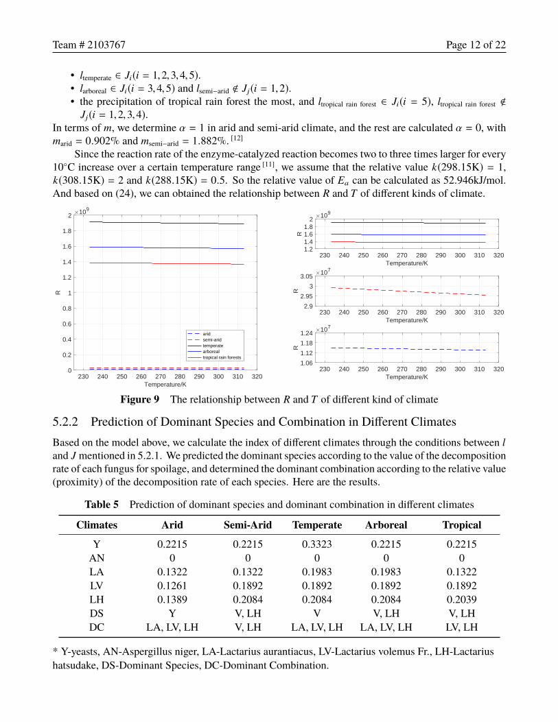
• ltemperate ∈ Ji(i = 1,2,3,4,5).• larboreal ∈ Ji(i = 3,4,5) and lsemi−arid < Jj(i = 1,2).• the precipitation of tropical rain forest the most, and ltropical rain forest ∈ Ji(i = 5), ltropical rain forest <

Jj(i = 1,2,3,4).In terms of m, we determine α = 1 in arid and semi-arid climate, and the rest are calculated α = 0, withmarid = 0.902% and msemi−arid = 1.882%. [12]

Since the reaction rate of the enzyme-catalyzed reaction becomes two to three times larger for every10◦C increase over a certain temperature range [11], we assume that the relative value k(298.15K) = 1,k(308.15K) = 2 and k(288.15K) = 0.5. So the relative value of Ea can be calculated as 52.946kJ/mol.And based on (24), we can obtained the relationship between R and T of different kinds of climate.

230 240 250 260 270 280 290 300 310 320Temperature/K

0

0.2

0.4

0.6

0.8

1

1.2

1.4

1.6

1.8

2

R

109

aridsemi-aridtemperatearborealtropical rain forests

230 240 250 260 270 280 290 300 310 320Temperature/K

1.06

1.12

1.18

1.24

R

107

230 240 250 260 270 280 290 300 310 320Temperature/K

2.9

2.95

3

3.05

R

107

230 240 250 260 270 280 290 300 310 320Temperature/K

1.21.41.61.8

2

R

109

Figure 9 The relationship between R and T of different kind of climate

5.2.2 Prediction of Dominant Species and Combination in Different ClimatesBased on the model above, we calculate the index of different climates through the conditions between land J mentioned in 5.2.1. We predicted the dominant species according to the value of the decompositionrate of each fungus for spoilage, and determined the dominant combination according to the relative value(proximity) of the decomposition rate of each species. Here are the results.

Table 5 Prediction of dominant species and dominant combination in different climates

Climates Arid Semi-Arid Temperate Arboreal Tropical

Y 0.2215 0.2215 0.3323 0.2215 0.2215AN 0 0 0 0 0LA 0.1322 0.1322 0.1983 0.1983 0.1322LV 0.1261 0.1892 0.1892 0.1892 0.1892LH 0.1389 0.2084 0.2084 0.2084 0.2039DS Y V, LH V V, LH V, LHDC LA, LV, LH V, LH LA, LV, LH LA, LV, LH LV, LH

* Y-yeasts, AN-Aspergillus niger, LA-Lactarius aurantiacus, LV-Lactarius volemus Fr., LH-Lactariushatsudake, DS-Dominant Species, DC-Dominant Combination.

Team # 2103767 Page 13 of 22

5.3 Solution and Result of Problem 5We only take the temperate zone as example, and other kinds of climate are similar. We plot onespecies (R0,4), three species (R0,1,R0,2,R0,5) and five species (R0,1,R0,2,R0,3,R0,4,R0,5) of fungi under thetemperate climate.

230 240 250 260 270 280 290 300 310 320Temperature

0.4

0.6

0.8

1

1.2

1.4

1.6

1.8

2

2.2

Dec

ompo

sitio

n R

ate

109

1 Species3 Species5 Species

Figure 10 The influence of the number of species (biodiversity)

According to the curves, we can clearly see that there is a certain gap between the values of thethree curves. This shows that the more species there are, the faster to decompose, and the more efficientof decomposition ecosystem, which is also consistent with biological intuition.

6 Sensitivity Analysis

0 10 20 30 40 50 60 70 80 90Time

1.885

1.89

1.895

1.9

1.905

1.91

1.915

Dec

ompo

sitio

n R

ate

109

230 240 250 260 270 280 290 300 310 320Temperature

1.2

1.3

1.4

1.5

1.6

1.7

1.8

1.9

2

Dec

ompo

sitio

n R

ate

109

Case 1Case 2Case 3Case 4

(a) Sensitivity of Temperature (b) Sensitivity of HumidityFigure 11 The sensitivity analysis

6.1 Sensitivity of TemperatureIn order to represent the fluctuation of temperature, we assume that temperature is a function of time,and the fluctuation of temperature is represented by the change of time. For trigonometric function is a

Team # 2103767 Page 14 of 22

specific periodic fluctuation function, temperature and time were triangulated, which indicates a drastictemperature change of the studied soil. When the T changes in the whole cycle in [233.15K, 313.15K],select T(t) = 80 | sin t | + 233.15. In order to ensure that T(t) still changes in the above interval in thesame time range, the simple linear relationship is selected T(t) = t + 233.15, where t belongs to [0,26π].Therefore, the sensitivity curves of decomposition rate to temperature are obtained in Figure 11 (a). Aswe can see, the blue curve fluctuates violently.

6.2 Sensitivity of HumidityHaving theorized that the moisture niche width for each species contains or does not contain the precipi-tation when there is a dramatic change in humidity, we take a few typical examples and shown in Figure11 (b), where the 4 cases are plotted by different optional parameters. As we can see, there are gapsbetween different curves.

7 Model Evaluation7.1 Strength and Weakness7.1.1 Strength

• The usage of the logistic curve to establish the model of single species decomposition rate, whichincreases the fitting degree and accuracy between the model and the actuality.

• The usage of the Volterra model to study the competition between fungi more accurately reflectsthe influence of competition and makes the model more accurate.

• The combination between ecology and chemistry. We consider the decomposition reaction mecha-nism and add the relationship between reaction rate constant and temperature to modify the modelto make the result more practical.

• The high sensitivity of temperature which can reflect the accuracy.

7.1.2 Weakness• Some complex environmental conditions (such as the types of organic compounds and complex

climate factors) are appropriately simplified and idealized.• The corresponding changes of the model according to the change of humidity are not smooth and

continuous and the sensitivity of humidity is not as good as temperature.• The model can not directly show the change trend of the number of each species over time, and the

dominant species reflected by the decomposition rate will have a certain deviation from the realquantity statistics.

7.2 Future WorkIn this model, we’ve discussed the relationship between the decomposition rate of five species of fungiand the internal and external factors. In the future work, it is feasible to study more environmentalvariables, fungal species and other survival relationships among different species. This will be of greatsignificance to our understanding of the importance of biodiversity and the necessity to protect theecological environment.

Team # 2103767 Page 15 of 22

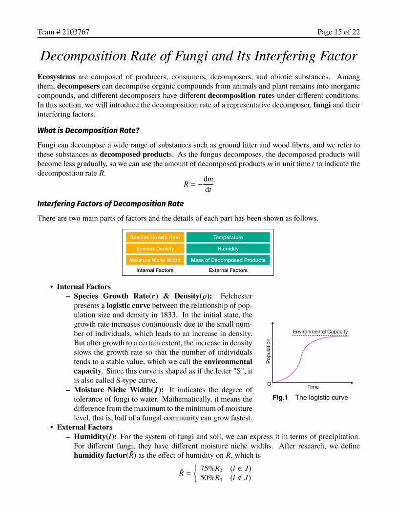
Decomposition Rate of Fungi and Its Interfering FactorEcosystems are composed of producers, consumers, decomposers, and abiotic substances. Amongthem, decomposers can decompose organic compounds from animals and plant remains into inorganiccompounds, and different decomposers have different decomposition rates under different conditions.In this section, we will introduce the decomposition rate of a representative decomposer, fungi and theirinterfering factors.

What is Decomposition Rate?Fungi can decompose a wide range of substances such as ground litter and wood fibers, and we refer tothese substances as decomposed products. As the fungus decomposes, the decomposed products willbecome less gradually, so we can use the amount of decomposed products m in unit time t to indicate thedecomposition rate R.

R = −dmdt

Interfering Factors of Decomposition RateThere are two main parts of factors and the details of each part has been shown as follows.

I ( T, m )

Temperature

HumidityMass of Decomposed Products

Species Growth Rate

Action

Reaction +

Internal Factors External Factors

++

Species Density

Moisture Niche Width

Temperature

Humidity

Mass of Decomposed Products

0 ρ

R

ρ*K/S

O Time

Popu

latio

n

Environmental Capacity

Fig.1 The logistic curve

• Internal Factors– Species Growth Rate(r) & Density(ρ): Felchester

presents a logistic curve between the relationship of pop-ulation size and density in 1833. In the initial state, thegrowth rate increases continuously due to the small num-ber of individuals, which leads to an increase in density.But after growth to a certain extent, the increase in densityslows the growth rate so that the number of individualstends to a stable value, which we call the environmentalcapacity. Since this curve is shaped as if the letter "S", itis also called S-type curve.

– Moisture Niche Width(J): It indicates the degree oftolerance of fungi to water. Mathematically, it means thedifference from the maximum to the minimum of moisturelevel, that is, half of a fungal community can grow fastest.

• External Factors– Humidity(l): For the system of fungi and soil, we can express it in terms of precipitation.

For different fungi, they have different moisture niche widths. After research, we definehumidity factor(R̂) as the effect of humidity on R, which is

R̂ ={

75%R0 (l ∈ J)50%R0 (l < J)

Team # 2103767 Page 16 of 22

where R0 is the maximum of R without considering humidity.– Temperature(T ) & Mass of Decomposed Products(m): Since decomposition is essentially

an enzyme catalyzed reaction within the fungal body,DP(decomposed products) fungi−−−−−→enzyme H2O + IS(inorganic salt)

the reaction rate is only related to m andreaction rate = kma

where k is called the reaction rate constant and can be calculated by Arrhenius Equationd ln kdT

=Ea

RT2 ⇔ k = Ae−EaRT

In a certain temperature range, Ea can be regarded as a constant.For the enzyme catalyzed reaction, α is related to the concentration of substrate and satisfiedthe general rules by Michaels and Menten.

∗ When m is very small, the reaction is a first order reaction and α = 1.∗ When m is very large, the reaction is a zero order reaction and α = 0.

Besides, different fungi will compete with each other for resources and space, while external factors(such as climate) play an important role as well. Based on the factors above, we can model the profileof change in decomposition rate of fungi with the following equation according to research.

R = kmα

[ν∑i=1

0.75R0,i +

n∑j=ν+1

0.5R0, j

]where l ∈ J1, J2, · · · , Jν(ν < n) and l < Jν+1, Jν+2, · · · , Jn.

ExampleTo describe the factors better, we choose five species of fungi (yeasts, Aspergillus niger, Lactarius auran-tiacus, Lactarius volemus Fr. and Lactarius hatsudake) and five climates (arid, semi-arid, temperature,arboreal and tropical rain forests). We can see from Fig.2 that the species are on one another’s length(where Lactarius aurantiacus goes extinct after a period of time). And from Fig.3, we can see the decom-position rate under different climates, which was slow under arid and semi-arid due to little decomposedproducts, while in the other three climates where the decomposed products are sufficient, the humidityof the rainforest was too large to cause many species’ l < J resulting in decomposition rates slower thantemperate. So we can conclude that the ecosystem is in dynamic equilibrium and tends to a balance influctuation under the selection of environment.

0 1 2 3 4 5 6 7 8 9

Time

0

0.05

0.1

0.15

0.2

0.25

0.3

0.35

0.4

0.45

0.5

De

co

mp

ositio

n R

ate

yeasts

Aspergillus niger

Lactarius aurantiacus

Lactarius volemus Fr.

Lactarius hatsudake

230 240 250 260 270 280 290 300 310 320

Temperature/K

0

0.2

0.4

0.6

0.8

1

1.2

1.4

1.6

1.8

2

R

109

arid

semi-arid

temperate

arboreal

tropical rain forests

Fig.2 The competition curve Fig.3 The climate curve

Team # 2103767 Page 17 of 22

References[1] Cai X M. Ecosystem Ecology [M]. Science Press, 2000.[2] Kingsland. The Refractory Model - The Logistic Curve and the History of Population Ecology[J].

QUART REV BIOL, 1982.[3] Xu Y J. Growth Performance of Three Laclarius Deliciosus Strains in Different Culture Medium[J].

Seed, 2020, 39(11):107-109.[4] Zhang H, Wang B X, Dong B, et al. Comparing Growth of Three Fungi in Oil-tea Cake Fermenta-

tion[J]. Forestry and Environmental Science, 2020, 36(05):48-53.[5] Xia T L, Jiang M, Wang H X, et al. Shelf Life Establishment of Fresh-Cut Purple Sweet Potatoes

by Use of Predictive Microbiological Models for Yeast and Lactic Acid Bacteria[J]. Food Science,2014, 35(18):252-257.

[6] Ding T R, Li C Z. Ordinary Differential Equations Tutorial (2nd Edition)[M]. Higher EducationPress, 2004:57-62.

[7] Shan Y L, Tang J D. Numerical Solution of Bait-Predator Model Derived from Three BiologicalPopulations Based on MATLAB[J]. Exploitation and Application of Software, 2007(12):94-96.

[8] Sun Z J, Wang C. Essential Ecology[M]. Chemical Industry Press, 2007:202-207.[9] Lustenhouwer N, Maynard D S, Bradford M A, et al. A trait-based understanding of wood decompo-

sition by fungi[J]. Proceedings of the National Academy of Sciences, 2020, 117(21):11551-11558.[10] P. Atkins, J. de Paula. Atkin’s Physical Chemistry, 8th Edition. W. H. Freeman and Company,

2009:807-809,840-845.[11] Fu X C, Shen W X, Yao T Y. Physical Chemistry (5th Edition). Volume 2 [M]. Higher Education

Press, 2006:191-194,292-296.[12] Liu J C, Yang J Q, Zhang X M. Decomposition of Organic Material in Soil in Semi-arid Areas[J].

Journal of Shanxi Agricultural Sciences, 1984(3).

Team # 2103767 Page 18 of 22

AppendixListing 1 Code for the relationship between R f un and ρ of five species of fungi by Matlab

1 clear

2 clc

3 rho=linspace(0,50);

4 a=3.14;

5 theta1=2;theta2=5;theta3=1;theta4=4;theta5=3; %the coefficient of

moisture niche width of fungi

6 ksi1=1.2;ksi2=0.737;ksi3=2.225;ksi4=0.961;ksi5=1.13; %population growth

potential index

7 k1=61;k2=53;k3=66;k4=39;k5=57; %environmental capacity of fungi

8 R1=ksi1∗theta1.∗rho.∗(k1−rho).∗exp(−a.∗rho)/k1;9 R2=ksi2∗theta2.∗rho.∗(k2−rho).∗exp(−a.∗rho)/k2;

10 R3=ksi3∗theta3.∗rho.∗(k3−rho).∗exp(−a.∗rho)/k3;11 R4=ksi4∗theta4.∗rho.∗(k4−rho).∗exp(−a.∗rho)/k4;12 R5=ksi5∗theta5.∗rho.∗(k5−rho).∗exp(−a.∗rho)/k5;13 xx=0:0.001:4;

14 RR1=spline(rho,R1,xx);




18 RR5=spline(rho,R5,xx); %cubic spline interpolation

19 hold on;grid on;box on;

20 plot(xx,RR1,'linewidth',1);





25 axis([0 4,0 0.42]);

26 legend('yeasts','Aspergillus niger','Lactarius aurantiacus','Lactarius

volemus Fr.','Lactarius hatsudake', 'FontSize',12);

27 xlabel('Relative Density', 'FontSize',14);

28 ylabel('Decomposition Rate', 'FontSize',14);

29 set(gca,'XTick',[0:0.5:4] , 'FontSize',14);

30 set(gca,'YTick',[0:0.05:0.42] , 'FontSize',14);

Listing 2 The numerical solution analysis method by Matlab1 function [dx] = rigid(t,x)

2 dx=zeros(5,1);

3 mu1=1;mu2=0.5;mu3=1.2;mu4=0.6;mu5=0.8;lambda12=1;lambda13=0.02;lambda14

=0.08;lambda15=0.01;lambda21=0.02;lambda23=0.03;lambda24=0.01;lambda25



=0.05;lambda53=0.1;lambda54=0.16;

4 dx(1)=x(1)∗(mu1−lambda12∗x(2)−lambda13∗x(3)−lambda14∗x(4)−lambda15∗x(5));5 dx(2)=x(2)∗(mu2−lambda21∗x(1)−lambda23∗x(3)−lambda24∗x(4)−lambda25∗x(5));6 dx(3)=x(3)∗(mu3−lambda31∗x(1)−lambda32∗x(2)−lambda34∗x(4)−lambda35∗x(5));

Team # 2103767 Page 19 of 22

7 dx(4)=x(4)∗(mu4−lambda41∗x(1)−lambda42∗x(2)−lambda43∗x(3)−lambda45∗x(5));8 dx(5)=x(5)∗(mu5−lambda51∗x(1)−lambda52∗x(2)−lambda53∗x(3)−lambda54∗x(4));9 end

1011 clear

12 clc

13 options=odeset('RelTol',1e−4,'AbsTol',[1e−4,1e−4,1e−4,1e−4,1e−4]);14 [t,x]=ode15s(@rigid,[0,5],[10,9,8,8,9]);

15 plot(t,x(:,1),'−',t,x(:,2),'−',t,x(:,3),'−',t,x(:,4),'−',t,x(:,5),'−','linewidth',1);

16 legend('x1(t)','x2(t)','x3(t)','x4(t)','x5(t)','FontSize',12);


18 axis([0 5,0 20]);

19 xlabel('Time','FontSize',14);

20 ylabel('Relative Quantity of Fungi','FontSize',14);

21 set(gca,'XTick',[0:0.5:5] , 'FontSize',14);

22 set(gca,'YTick',[0:2:20] , 'FontSize',14);

Listing 3 Code for the relationship between two species of fungi with competition1 clear

2 clc

3 %Plot the 3D figures

4 subplot(2,2,[1,2]);

5 x=linspace(1,10);y=linspace(1,10);

6 [X,Y]=meshgrid(x,y);

7 Z=1296∗Y−889∗X+4096∗log(X)−3321∗log(Y);8 mesh(Z)

9 hold on;grid on;

10 Z=899∗Y−89∗X+2048∗log(X)−1331∗log(Y);11 mesh(Z);

12 xlabel('x:Number of Species 1(or 3)','FontSize',14);

13 ylabel('y:Number of Species 2(or 4)','FontSize',14);

14 zlabel('H(x,y)','FontSize',14);

15 set(gca,'XTick',[0:20:100] , 'FontSize',14);


17 set(gca,'ZTick',[0:2000:10000] , 'FontSize',14);

18 legend('P(Lower)','Q(Upper)','FontSize',12);

19 %Plot the 2D figures

20 subplot(2,2,3);

21 syms x1 x2;

22 f=1296∗x2−889∗x1+4096∗log(x1)−3321∗log(x2);23 ezcontour(f,[0,10],30);

24 hold on;grid on; box on;

25 a=4096/889;b=3321/1296; %The transverse and longitudinal of saddle point

26 plot(a,b,'o','MarkerSize',10);

27 xlabel('Number of Species 1','FontSize',14);

28 ylabel('Number of Species 2','FontSize',14);

29 title('P','FontSize',14);


Team # 2103767 Page 20 of 22


32 subplot(2,2,4);

33 syms y1 y2;

34 f=899∗y2−89∗y1+2048∗log(y1)−1331∗log(y2);35 ezcontour(f,[0,10],30);

36 hold on; grid on; box on;

37 xlabel('Number of Species 3','FontSize',14);

38 ylabel('Number of Species 4','FontSize',14);

39 title('Q','FontSize',14);



Listing 4 Code for the relationship between the decomposition rate of 5 species of fungi and time inthe competition by Matlab

1 clear

2 clc

3 a=3.14;

4 theta1=2;theta2=5;theta3=1;theta4=4;theta5=3;

5 ksi1=1.2;ksi2=0.737;ksi3=2.225;ksi4=0.961;ksi5=1.13;

6 k1=61;k2=53;k3=66;k4=39;k5=57;

7 t=[0:0.001:9.5];

8 rho1=0.0958∗t.^6−1.57∗t.^5+10∗t.^4−31.1∗t.^3+48.3∗t.^2−34.5∗t+8.49;9 rho2=0.0172∗t.^6−0.278∗t.^5+1.78∗t.^4−5.86∗t.^3+10.5∗t.^2−11∗t+8.83;

10 rho3=0.0932∗t.^6−0.983∗t.^5+4.73∗t.^4−11.3∗t.^3+16∗t.^2−9.99∗t+7.89;11 rho4=0.0198∗t.^6−0.328∗t.^5+2.14∗t.^4−7.08∗t.^3+13∗t.^2−14∗t+7.81;12 rho5=0.0193∗t.^6−0.364∗t.^5+2.66∗t.^4−9.35∗t.^3+16.2∗t.^2−14∗t+8.73;13 R1=ksi1∗theta1.∗rho1.∗(k1−rho1).∗exp(−a.∗rho1)/k1;14 R2=ksi2∗theta2.∗rho2.∗(k2−rho2).∗exp(−a.∗rho2)/k2;15 R3=ksi3∗theta3.∗rho3.∗(k3−rho3).∗exp(−a.∗rho3)/k3;16 R4=ksi4∗theta4.∗rho4.∗(k4−rho4).∗exp(−a.∗rho4)/k4;17 R5=ksi5∗theta5.∗rho5.∗(k5−rho5).∗exp(−a.∗rho5)/k5;18 hold on;grid on;box on;

19 plot(t,R1,'−','linewidth',1);plot(t,R2,'−','linewidth',1);plot(t,R3,'−','linewidth',1);plot(t,R4,'−','linewidth',1);plot(t,R5,'−','linewidth',1);

20 axis([0,9.5,0,0.5])

21 xlabel('Time', 'FontSize',14);ylabel('Decomposition Rate', 'FontSize',14);

22 set(gca,'XTick',[0:1:9.5] , 'FontSize',14);

23 set(gca,'YTick',[0:0.05:0.5] , 'FontSize',14);

24 legend('yeasts','Aspergillus niger','Lactarius aurantiacus','Lactarius

volemus Fr.','Lactarius hatsudake', 'FontSize',10);

Listing 5 Code for the relationship between R and T of different kinds of climate by Matlab1 clear

2 clc

3 R01=0.2797;R02=0.4291;R03=1.729e−07;R04=0.4467;R05=0.2444;4 Rcli1=0.5∗(R01+R02+R03+R04+R05);

5 Rcli2=0.75∗(R04+R05)+0.5∗(R01+R02+R03);

6 Rcli3=0.75∗(R01+R02+R03+R04+R05);

7 Rcli4=0.75∗(R03+R04+R05)+0.5∗(R01+R02);

Team # 2103767 Page 21 of 22

8 Rcli5=0.75∗R05+0.5∗(R01+R02+R03+R04);

9 T=linspace(233.15,313.15);

10 k=exp(52945.916/(8.314∗298.15))∗exp(−52945.916.\(8.314.∗T));11 I1=k.∗0.00902;I2=k.∗0.01882;I3=k;I4=k;I5=k;

12 R1=I1.∗Rcli1;R2=I2.∗Rcli2;R3=I3.∗Rcli3;R4=I4.∗Rcli4;R5=I5.∗Rcli5;

13 %Plot

14 subplot(3,2,[1,3,5]);hold on; grid on; box on;

15 plot(T,R1,'b−−','linewidth',1);plot(T,R2,'r−−','linewidth',1);16 plot(T,R3,'k−','linewidth',1);plot(T,R4,'b−','linewidth',1);17 plot(T,R5,'r−','linewidth',1);18 legend('arid','semi−arid','temperate','arboreal','tropical rain forests', '

FontSize',10);

19 axis([225,320,0,20e8]);

20 set(gca,'XTick',[230:10:320],'FontSize',14);

21 set(gca,'YTick',[0:2e8:20e8],'FontSize',14);

22 xlabel('Temperature/K', 'FontSize',14);ylabel('R', 'FontSize',14);

23 subplot(3,2,6);


25 plot(T,R1,'b−−','linewidth',1);26 axis([225,320,1.06e7,1.24e7]);


28 set(gca,'YTick',[1.06e7:0.06e07:1.24e7],'FontSize',14);


30 subplot(3,2,4);


32 plot(T,R2,'r−−','linewidth',1);33 axis([225,320,2.9e7,3.05e7]);




37 subplot(3,2,2);hold on; grid on; box on;

38 plot(T,R3,'k−','linewidth',1);plot(T,R4,'b−','linewidth',1);39 plot(T,R5,'r−','linewidth',1);40 axis([225,320,1.2e9,2e9]);


42 set(gca,'YTick',[1.2e9:0.2e9:2e9],'FontSize',14);


Listing 6 Code for the influence of biodiversity by Matlab1 clear

2 clc

3 R01=0.2797;R02=0.4291;R03=0;R04=0.4467;R05=0.2444;

4 T=linspace(233.15,313.15);

5 k=exp(52945.91608/(8.314∗298.15))∗exp(−52945.91608.\(8.314.∗T));6 R1=0.75∗R04.∗k;

7 R2=0.75∗(R01+R02+R05).∗k;

8 R3=0.75∗(R01+R02+R03+R04+R05).∗k;


10 plot(T,R1,'−−','linewidth',1);plot(T,R2,'−−','linewidth',1);plot(T,R3,'−−',

Team # 2103767 Page 22 of 22

'linewidth',1);

11 axis([230,320,0.4e9,2.2e9]);



14 xlabel('Temperature', 'FontSize',14);


16 legend('1 Species','3 Species','5 Species','FontSize',10);

Listing 7 Code for sensitivity analysis of the model to temperature by Matlab1 clear

2 clc

3 R01=0.2797;R02=0.4291;R03=1.729e−07;R04=0.4467;R05=0.2444;4 Rcli=0.75∗(R01+R02+R03+R04+R05);

5 t=linspace(0,26∗pi);

6 T=t+233.15;

7 Tchange=80.∗abs(sin(t))+233.15;

8 k=exp(52945.916/(8.314∗298.15))∗exp(−52945.916.\(8.314.∗T));9 kchange=exp(52945.916/(8.314∗298.15))∗exp(−52945.916.\(8.314.∗Tchange));

10 I=k;

11 Ichange=kchange;

12 R=I.∗Rcli;

13 Rchange=Ichange.∗Rcli;

14 plot(t,R,'−.r','linewidth',2);15 hold on;grid on;box on;

16 plot(t,Rchange,':','linewidth',2);



19 xlabel('Time', 'FontSize',14);ylabel('Decomposition Rate', 'FontSize',14);

Listing 8 Code for sensitivity analysis of the model to humidity by Matlab1 clear

2 clc

3 R01=0.2797;R02=0.4291;R03=0;R04=0.4467;R05=0.2444;

4 T=linspace(233.15,313.15);

5 k=exp(52945.91608/(8.314∗298.15))∗exp(−52945.91608.\(8.314.∗T));6 R1=0.5∗(R01+R02+R03+R04+R05).∗k;

7 R2=0.75∗(R01+R02+R03+R04+R05).∗k;

8 R3=0.75∗(R01+R05).∗k+0.5∗(R02+R04).∗k;

9 R4=0.75∗(R02+R05).∗k+0.5∗(R01+R04).∗k;


11 plot(T,R1,'−−','linewidth',1);plot(T,R2,'−−','linewidth',1);12 plot(T,R3,'−−','linewidth',1);plot(T,R4,'−−','linewidth',1);13 set(gca,'XTick',[230:10:321],'FontSize',14);

14 set(gca,'YTick',[1.2e9:0.1e9:2e9],'FontSize',14);

15 xlabel('Temperature', 'FontSize',14);


17 legend('Case 1','Case 2','Case 3','Case 4','FontSize',10);

Documents

Problem Chosen 2021 Team Control Number A Summary Sheet