Embed Size (px)
Citation preview

PROBING PARTICLE PRODUCTION IN
Au+Au COLLISIONS AT√sNN = 200 GeV
USING SPECTATORS
A thesis Submittedin Partial Fulfilment of the Requirements
for the Degree of
MASTER OF SCIENCE
by
Somadutta Bhatta
to the
School of Physical Sciences
National Institute of Science Education and Research
Bhubaneswar
Date: 10.05.2018

DEDICATION
I dedicate this work to my loving parents and teachers.
i
DECLARATION
I hereby declare that I am the sole author of this thesis in partial fulfillment of the
requirements for a postgraduate degree from National Institute of Science Education
and Research (NISER). I authorize NISER to lend this thesis to other institutions or
individuals for the purpose of scholarly research.
Signature of the Student
Date:
The thesis work reported in the thesis entitled “Probing particle production in
Au+Au collisions at√sNN = 200 GeV using spectators” was carried out under my
supervision, in the school of physical sciences at NISER, Bhubaneswar, India.
Signature of the thesis supervisor
School:
Date:
ii
ACKNOWLEDGEMENTS
First and foremost, I wish to thank my supervisor Prof. Bedangadas Mohanty for
introducing me to the exciting field of Experimental High Energy Physics and super-
vising this work. Without his encouragement, support and advice this work would
not have been possible. I would also like to take this chance to express my gratitude
to all the Experimental High Energy Physics lab members at NISER, especially Vipul
Bairathi and Md. Nasim for their help, guidance, and discussions during the course
of this work. Next, a big thanks to all my friends who continue to believe in me
and have kept my spirit high during difficult times. I also acknowledge the support
and love my parents have shown during the period of my M.Sc at NISER and have
continually pushed me to achieve my full potential.
Finally, I would like to thank my luck for allowing me to interact with and learn from
some of the best teachers, here at NISER. Their continuous support, care, guidance
and most importantly their passion for science will always continue to inspire me.
iii

ABSTRACT
Events in heavy ion collisions are categorized into centralities, usually based on
charged particle multiplicity. But, there are event-by-event fluctuations in the initial
event conditions for a given centrality. The access to these variations are limited and
it is very difficult to select particular events with definite initial configuration. The
categorization of events into centralities allows us to obtain centrality averaged values
only.
A study done recently [1] demonstrated that by performing a further binning over
spectator neutrons count in addition to the standard centrality binning based on
charged particle multiplicity, it is possible to probe the fireball with different initial
state conditions. This study was done for Pb+Pb collision at√sNN= 2.76 TeV
using a multiphase transport model (AMPT). This thesis explores a similar approach
in probing initial state using the actual experimental data from Au+Au collision
at√sNN= 200 GeV through the spectator neutron number (measured by the Zero
Degree Calorimeter (ZDC)) in the STAR detector.
We find that in the data collected from STAR detector for Au+Au collisions at
200 GeV, this novel method of binning gives us a better handle at selecting events
with specific initial conditions. The initial states that can be accessed by this new
procedure cannot be accessed even by finer centrality definition (by multiplicity).
This new procedure of choosing initial conditions strongly breaks some previously
postulated scaling relations between v2/ε2 vs 1sdNch
dηand acoustic scaling relation for
centrality (by multiplicity) averaged values. The proposed study in this thesis allows
for access to new initial conditions in heavy-ion collisions that can be studied in detail
in future.
iv

Contents1 Introduction 1
2 Standard Model 32.0.1 QCD . . . . . . . . . . . . . . . . . . . . . . . . . . . . . . . . 52.0.2 Quark Gluon Plasma . . . . . . . . . . . . . . . . . . . . . . . 92.0.3 Signatures of QGP . . . . . . . . . . . . . . . . . . . . . . . . 10
3 STAR Detector 15
4 Measurement of Elliptic FlowCoefficients 17
5 MC Glauber Model 21
6 Kinematics 24
7 Event Qualitative Analysis 30
8 Data Analysis 49
9 Conclusion 74
10 Future Plan 75
References 76
v

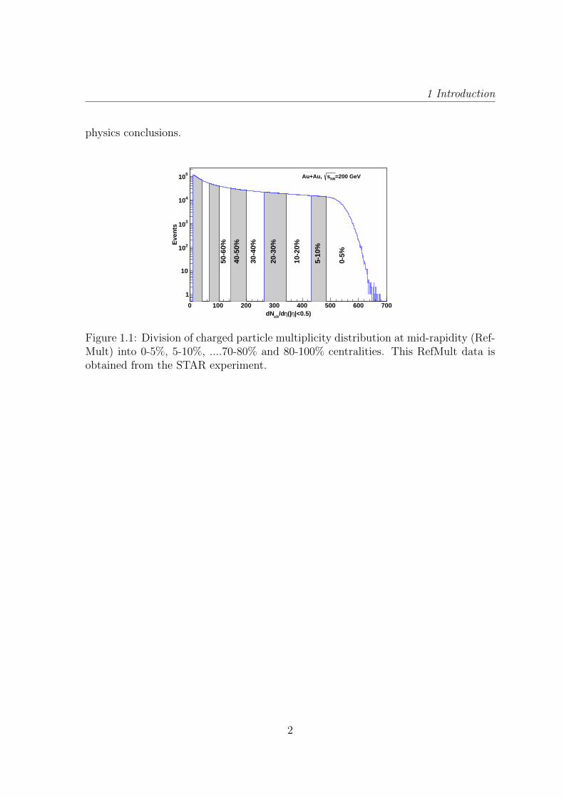
List of Figures1.1 Division of charged particle multiplicity distribution at mid-rapidity
(RefMult) into 0-5%, 5-10%, ....70-80% and 80-100% centralities. ThisRefMult data is obtained from the STAR experiment. . . . . . . . . . 2
2.1 Feynman diagrams of interaction between quarks and gluons. . . . . . 52.2 The experimentally measured values of the effective gauge coupling
αs(q) confirm the theoretically expected behaviour at high energies(compilation of the Particle Data Group) [7]. . . . . . . . . . . . . . . 7
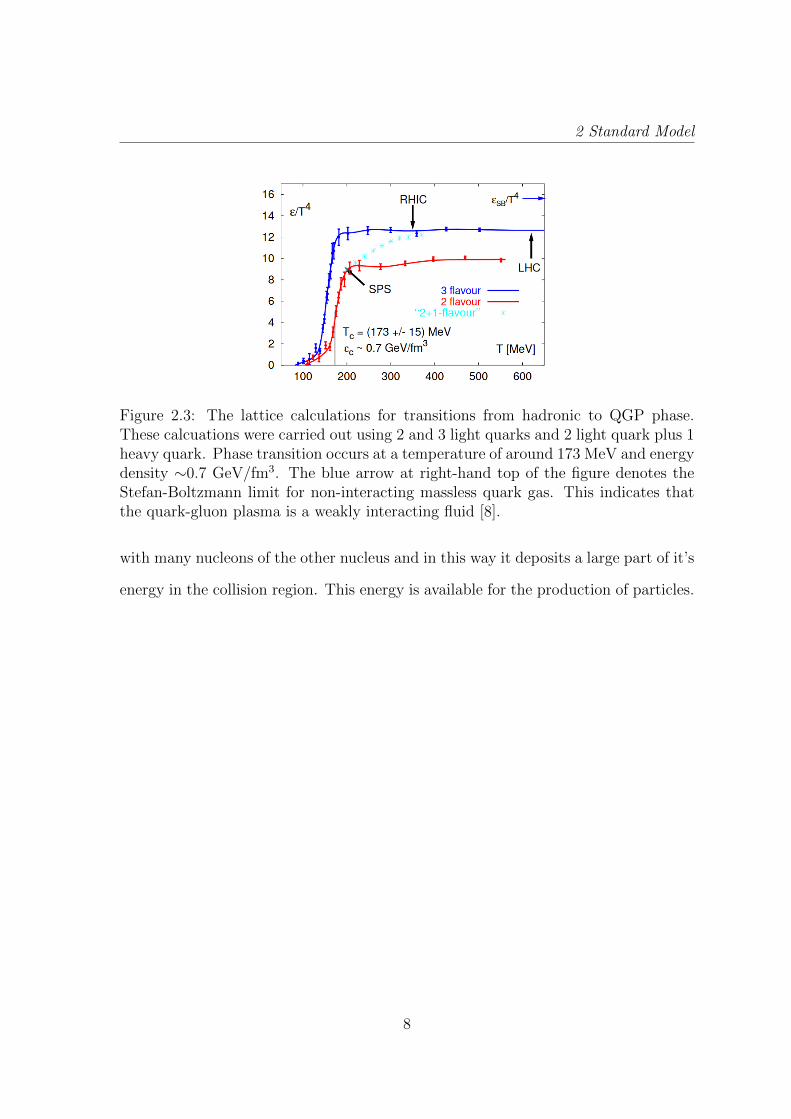
2.3 The lattice calculations for transitions from hadronic to QGP phase.These calcuations were carried out using 2 and 3 light quarks and 2 lightquark plus 1 heavy quark. Phase transition occurs at a temperature ofaround 173 MeV and energy density ∼0.7 GeV/fm3. The blue arrowat right-hand top of the figure denotes the Stefan-Boltzmann limit fornon-interacting massless quark gas. This indicates that the quark-gluon plasma is a weakly interacting fluid [8]. . . . . . . . . . . . . . 8
2.4 Space-time evolution after the heavy ion collision. The scenario on leftrepresents the case where no QGP is formed (T < Tc) and on right isthe case with QGP formation (T > Tc) [6]. . . . . . . . . . . . . . . . 9
2.5 Data from the STAR experiment show angular correlations betweenpairs of high transverse-momentum charged particles, referenced to a“trigger”particle that is required to have pT greater than 4 GeV. Theproton-proton and deuteron-gold collision data indicate back-to-backpairs of jets (a peak associated with the trigger particle at ∆φ = 0degrees and a somewhat broadened recoil peak at 180 degrees). Thecentral gold-gold data indicate the characteristic jet peak around thetrigger particle, at 0 degrees, but the recoil jet is absent [9]. . . . . . . 11
2.6 Non-central collisions leads to spatial anisotropy which leads to anisotropyin momentum space. . . . . . . . . . . . . . . . . . . . . . . . . . . . 12
2.7 The first four flow harmonics in the transverse plane in polar coordi-nates (top left: n=1, top right: n=2, bottom left: n=3, bottom right:n=4). . . . . . . . . . . . . . . . . . . . . . . . . . . . . . . . . . . . 14
2.8 Measurements of v2(pT ) for identified particles in Au+Au collisions for0-80% centrality at RHIC. The lines are the results from hydrodynamicmodel calculation [10]. . . . . . . . . . . . . . . . . . . . . . . . . . . 14
3.1 The cross-section view of the STAR detector. . . . . . . . . . . . . . 15
5.1 Multiplicity distribution from data collected for Au+Au collisions at√sNN = 200 GeV compared with multiplicity distribution obtained
from Glauber model for the same system [13]. npp, x, k and efficiencyare the different parameters that are varied to match multiplicity dis-tributions obtained from data and Glauber model. . . . . . . . . . . . 23
7.1 Magnetic Field applied for the data taken. . . . . . . . . . . . . . . . 317.2 Number of events in each centrality before cuts (left) and after cuts
(right) are applied. . . . . . . . . . . . . . . . . . . . . . . . . . . . . 32
vi
LIST OF FIGURES
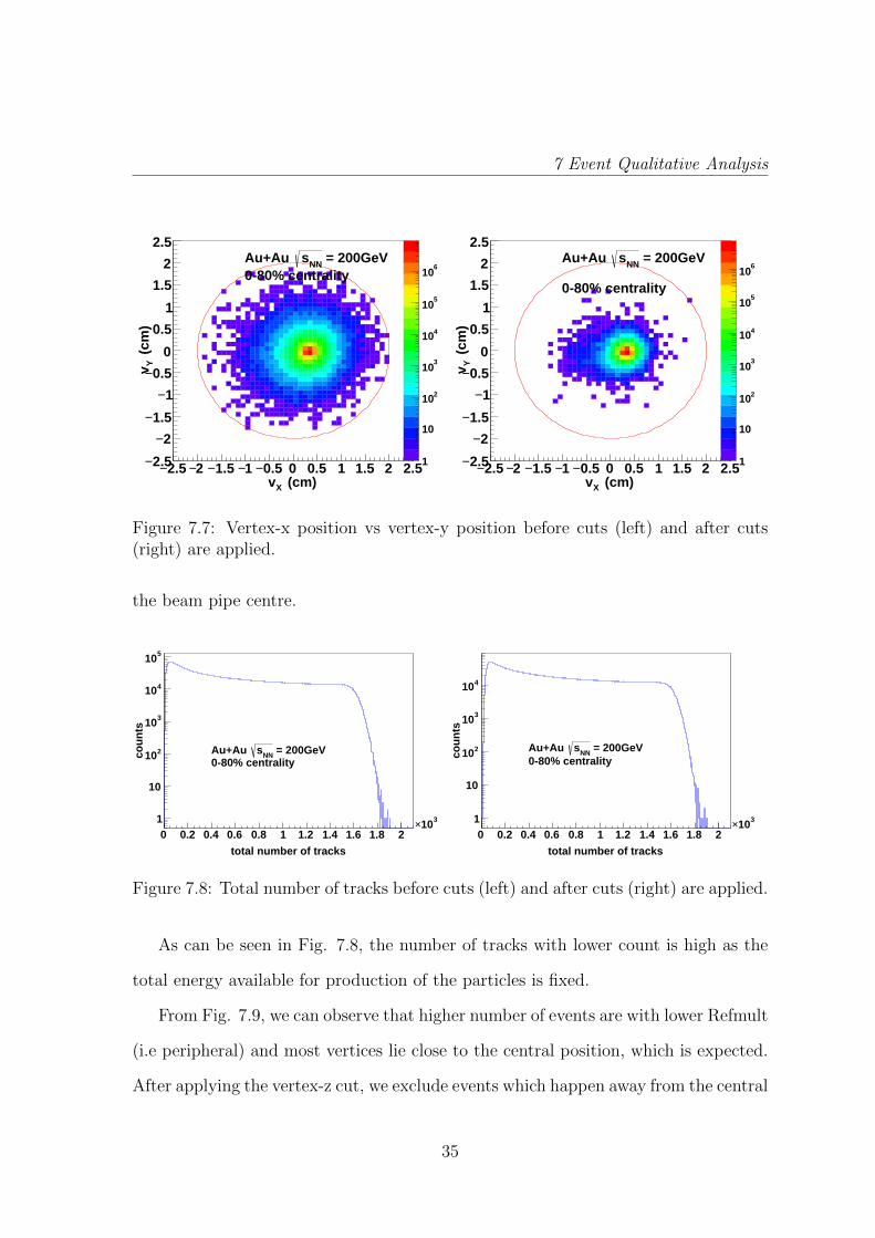
7.3 Reference Multiplicity before cuts (left) and after cuts (right) are applied. 337.4 Vertex-Z positions before cuts (left) and after cuts (right) are applied. 337.5 Vertex-x positions before cuts (left) and after cuts (right) are applied. 347.6 Vertex-y positions before cuts (left) and after cuts (right) are applied. 347.7 Vertex-x position vs vertex-y position before cuts (left) and after cuts
(right) are applied. . . . . . . . . . . . . . . . . . . . . . . . . . . . . 357.8 Total number of tracks before cuts (left) and after cuts (right) are
applied. . . . . . . . . . . . . . . . . . . . . . . . . . . . . . . . . . . 357.9 Refmult Vs vertex-z position before cuts (left) and after cuts (right)
are applied. . . . . . . . . . . . . . . . . . . . . . . . . . . . . . . . . 367.10 Refmult vs TOFmult before cuts (left) and after cuts (right) are applied. 367.11 Vertex Z position from VPD before cuts (left) and after cuts (right)
are applied. . . . . . . . . . . . . . . . . . . . . . . . . . . . . . . . . 377.12 Vpd-vZ vs Vertex Z position from TPC hits reconstruction before cuts
(left) and after cuts (right) are applied. . . . . . . . . . . . . . . . . . 377.13 Left going spectator neutrons before cuts (left) and after cuts (right)
are applied. . . . . . . . . . . . . . . . . . . . . . . . . . . . . . . . . 387.14 Left Going spectator Neutrons before cuts (left) and after cuts (right)
are applied. . . . . . . . . . . . . . . . . . . . . . . . . . . . . . . . . 387.15 Total number of Spectator neutrons (east going+west going) before
cuts (left) and after cuts (right) are applied. . . . . . . . . . . . . . . 397.16 Left going spectator neutrons vs right going spectator neutrons from
ZDC before cuts (left) and after cuts (right) are applied. . . . . . . . 397.17 Refmult vs spectator neutrons count (from ZDC) before cuts (left) and
after cuts (right) are applied. . . . . . . . . . . . . . . . . . . . . . . 407.18 Px distribution before cuts (left) and after cuts (right) are applied. . . 407.19 Py distribution before cuts (left) and after cuts (right) are applied. . . 417.20 Pz distribution before cuts (left) and after cuts (right) are applied. . . 417.21 Py vs Px before cuts (left) and after cuts (right) are applied. . . . . . 427.22 Transverse Momentum distribution before cuts (left) and after cuts
(right) are applied. . . . . . . . . . . . . . . . . . . . . . . . . . . . . 427.23 Total Momentum (P=
√P 2x + P 2
y + P 2z ) before cuts (left) and after cuts
(right) are applied. . . . . . . . . . . . . . . . . . . . . . . . . . . . . 437.24 Pseudorapidity (η) before cuts (left) and after cuts (right) are applied. 437.25 φ distribution before cuts (left) and after cuts (right) are applied. . . 447.26 θ distribution before cuts (left) and after cuts (right) are applied. . . 457.27 η vs φ distribution before cuts (left) and after cuts (right) are applied. 457.28 η vs pT distribution before cuts (left) and after cuts (right) are applied. 467.29 dE
dxvs P×q (rigidity) distribution for particle identification (with all
the cuts). . . . . . . . . . . . . . . . . . . . . . . . . . . . . . . . . . 467.30 Mass2 vs momentum distribution for particle identification (with cuts). 477.31 Mass2 vs pT distribution for particle identification (with cuts). . . . . 48
8.1 ψ2east and ψ2west distribution. . . . . . . . . . . . . . . . . . . . . . . 498.2 Recenter corrected ψ2east and ψ2west. . . . . . . . . . . . . . . . . . . 508.3 Shift corrected event planes for both the η ranges. . . . . . . . . . . . 508.4 Flattened event plane fitted to the function and the parameters are
shown on the top.For ψ2east, |p0.p1|= 16.46 and |p0.p2|= 2.19 and forψ2west, |p0.p1|= 7.18 and |p0.p2|= 0.137. . . . . . . . . . . . . . . . . . 51
vii

LIST OF FIGURES
8.5 ψ2 resolution in different centralities and comparison with publisheddata. . . . . . . . . . . . . . . . . . . . . . . . . . . . . . . . . . . . . 52
8.6 ψ3east and ψ3west distribution after applying recenter and shift correction. 528.7 Flattened event plane fitted to the function and the parameters are
shown on the top.For ψ3east, |p0.p1|= 5.7 and |p0.p2|= 2.4 and for ψ3west,|p0.p1|= 0.78 and |p0.p2|= 2.0561. . . . . . . . . . . . . . . . . . . . . 53
8.8 ψ3 resolution values in each centrality. . . . . . . . . . . . . . . . . . 538.9 Left: v2 vs pT plot, Right: v3 vs pT plot for different centralities and
minimum bias. . . . . . . . . . . . . . . . . . . . . . . . . . . . . . . 548.10 Minimum bias v2 vs pT compared with the published data [17]. . . . . 558.11 Left: v2 vs η, Right: v3 vs η for different centralities and minimum bias. 558.12 Left: The L+R distribution for minimum bias, Right: The spectator
distribution for each centrality (by multiplicity) being shown in differ-ent colors. . . . . . . . . . . . . . . . . . . . . . . . . . . . . . . . . . 56
8.13 Left: v2 vs charged particle multiplicity, Right: v2 vs Spectator Neu-trons for all events. . . . . . . . . . . . . . . . . . . . . . . . . . . . . 56
8.14 Left: v2 vs Multiplicity, Right: v2 vs L+R for 10-20% centrality. . . . 578.15 The % binning of L+R distribution in each centrality (by multiplicity). 588.16 Left: ψ2 Resolution, Right: ψ3 Resolutions variations in L+R bins
from each centrality. . . . . . . . . . . . . . . . . . . . . . . . . . . . 598.17 Variation of multiplicity for spectator binning in each centrality. . . . 598.18 Left: v2 vs multiplicity, Right: v3 vs multiplicity, for different central-
ities and L+R binning on top of centrality bins. . . . . . . . . . . . . 608.19 Spectator distribution for each centrality (by multiplicity) from Glauber
model subdivided into bins of 0-5%,5-10%,10-20%,....70-80% and 80-100%. . . . . . . . . . . . . . . . . . . . . . . . . . . . . . . . . . . . 61
8.20 Left: Comparison of overlap region area obtained from data and glaubermodel [13], Right: Comparison of ε2 obtained from data and glaubermodel [13]. . . . . . . . . . . . . . . . . . . . . . . . . . . . . . . . . . 62
8.21 Comparison of multiplicity obtained from data and glauber model. . . 628.22 Left: < v2 > / < ε2 > vs scaled multiplicity, Right: < v3 > / < ε3 >
vs scaled multiplicity for different centralities and L+R binning on topof centrality bins. . . . . . . . . . . . . . . . . . . . . . . . . . . . . . 63
8.23 Left: v2 vs Npart, Right: v3 vs Npart for different centralities and sub-sequent L+R binning in each centrality. . . . . . . . . . . . . . . . . . 63
8.24 The dependence of impact parameter (b) on number of participatingnucleons (Npart). . . . . . . . . . . . . . . . . . . . . . . . . . . . . . . 64
8.25 Left: ε2 vs Ncoll, Right: ε3 vs Ncoll for centrality bins and SubsequentL+R bins for each centrality. . . . . . . . . . . . . . . . . . . . . . . . 65
8.26 Left: ε2 vs Npart, Right: ε3 vs Npart for centrality bins and SubsequentL+R bins for each centrality. . . . . . . . . . . . . . . . . . . . . . . . 65
8.27 Left: ε2 vs Charged particle multiplicity, Right: ε3 vs Charged particlemultiplicity for different centralities and subsequent L+R bins in eachcentrality. . . . . . . . . . . . . . . . . . . . . . . . . . . . . . . . . . 66
8.28 Overlap region area vs charged particle multiplicity. . . . . . . . . . . 668.29 Left: σx vs Npart Right: σy vs Npart, for centrality binning and subse-
quent L+R binning for each centrality. . . . . . . . . . . . . . . . . . 678.30 Multiplicity vs Npart. . . . . . . . . . . . . . . . . . . . . . . . . . . . 688.31 Multiplicity scaled by number of participating nucleons(Npart) vs Npart. 68
8.32 Left: Ncoll vs Npart, Right: Ncoll/N4/3part vs Npart. . . . . . . . . . . . . . 69
viii

LIST OF FIGURES
8.33 Ncoll/Npart vs Npart for different centralities and subsequent L+R bins. 698.34 Left: Ncoll/Npart vs ε2, Right: Ncoll/Npart vs ε3 in centrality binning
and subsequent spectator binning. . . . . . . . . . . . . . . . . . . . . 708.35 Left: v2 vs ε2, Right: v3 vs ε3 for centrality binning and subsequent
L+R binning. . . . . . . . . . . . . . . . . . . . . . . . . . . . . . . . 71
8.36 Left: v2/ε2 vs Npart, Right: v2/ε2
N1/3part
vs N1/3part for centrality averages and
L+R binning for each centrality. . . . . . . . . . . . . . . . . . . . . . 718.37 Left: v2 vs v3, Right: ε2 vs ε3 for different centralities and subsequent
L+R bins. . . . . . . . . . . . . . . . . . . . . . . . . . . . . . . . . . 728.38 Left: v2/ε2 vs 1/ΛT , Right: v3/ε3 vs 1/ΛT for Different centralities and
subsequent L+R bins in each centrality. . . . . . . . . . . . . . . . . . 73
ix

List of Tables7.1 Selection cuts used in the analysis. . . . . . . . . . . . . . . . . . . . 307.2 Number of events in each centrality after applying all the cuts. . . . . 32
x

Chapter 1
IntroductionIn Heavy Ion Collisions (HIC), we have several experimental observables. Some are
“Event variables” like azimuthal anisotropy of produced particles, multiplicity and
some are “Track variables” like momentum etc. But, the information on the initial
state of the collisions is highly limited. Although the energies of the colliding nuclei are
fixed, their geometrical orientation with respect to each other (eg: impact parameter
(b)) and nucleon positions inside them cannot be determined on an event to event
basis. These variables are very important for studying the event structure in greater
details.
In HIC, the events are categorized based only on their centralities (based on
multiplicity). This is indicative of the impact parameter of the events (Fig. 1.1).
Measurement of experimental variables within each centrality provides their central-
ity averaged values. But, characteristics of events within each centrality believed to
be of similar initial conditions, vary from each other. The access to these variations
are limited. In order to study these variations in each centrality in details, we look for
other initial state observables. The total number of “Spectator Neutrons” for each
event is the observable which is considered in this analysis. We have tried to im-
plement categorization of events on the basis of Left going spectator neutrons+Right
going spectator neutrons (L+R) on top of the standard categorization on basis of cen-
tralities based on charged particle multiplicity. Using this new procedure, we check
how these new bins add-up to show the cumulative property of the whole centrality
bins and if this new categorization of events challenges some previously established
1
1 Introduction
physics conclusions.
0 100 200 300 400 500 600 700|<0.5)η(|η/dchdN
1
10
210
310
410
510E
ven
ts=200 GeVNNsAu+Au,
0-5%
5-10
%
10-2
0%
20-3
0%
30-4
0%
40-5
0%
50-6
0%
Figure 1.1: Division of charged particle multiplicity distribution at mid-rapidity (Ref-Mult) into 0-5%, 5-10%, ....70-80% and 80-100% centralities. This RefMult data isobtained from the STAR experiment.
2

Chapter 2
Standard ModelThe standard model is a theoretical model which attempts to explain different fun-
damental constituent particles of matter around us and the forces that govern the
interaction between them. Both experimental and theoretical branches of high en-
ergy physics have contributed towards it’s formulation. The standard model has been
successful in explaining electromagnetic, weak and strong interactions and forms the
foundation of our understanding of the forces and fundamental particles of nature. It
has not unified gravitational force with other three forces yet and is unable to explain
many observations and postulations like non-zero neutrino mass, the presence of dark
matter, hierarchy problem etc.
Elementary particles in the standard model are divided into 3 generations. These
three generations differ only in their masses from each other. Each generation is di-
vided into two quarks and two leptons. So in total, there are 6 types of quarks called
flavours: up (u) and down (d), charm (c) and strange (s), top (t) and bottom (b).
The top quark is the heaviest (mass∼177 GeV) and therefore was discovered long
after the discovery of the bottom quark (which is of much smaller mass ∼4.18 GeV),
when accelerators with high enough energy became available. The leptons are the
electron (e), muon (µ), tau (τ) and their corresponding neutrinos (νe, νµ, ντ ). There
are four fundamental forces: the electromagnetic force, mediated by the photon (γ),
the weak force, mediated by the W and Z gauge bosons (W+, W−, Z0), the strong
force, mediated by the gluons (g) and gravitational force, mediated by the not yet
discovered Gravitons. The photon and the gluons are massless, while the W and Z
3

2 Standard Model
bosons are massive. The force mediators (γ, W+, W−, Z0, g) have spin 1. The Gravi-
ton is proposed to have spin 2. All the elementary particles can interact via the weak
force, those who are electrically charged interact additionally via the electromagnetic
force and the quarks can also have interactions via the strong force.
The standard model includes a formalism to describe the electromagnetic and weak
forces with Electro-Weak theory and it describes the strong force with quantum chro-
modynamics (QCD). Gravity and electromagnetism are long-range forces while the
weak and strong interactions are short-ranged. The weak interaction is seen in ra-
dioactive decays and the strong interaction binds the quarks together in hadrons and
the nucleons inside the nucleus of an atom.
The strength of a force is characterised by its coupling, α. This coupling depends on
the energy involved in the interaction. At energies which can be observed in daily
life, the coupling of all forces is very different. If the coupling αs for the strong in-
teractions is taken to be of order 1, then for the electromagnetic interactions αem =
10−3 , for the weak interactions αw = 10−16 and for gravity it is lowest (αg= 10−41).
However, as the energy goes up, the coupling constants approach each other and
may at some high energy be equal. This might make it possible to describe all forces
in a single formalism: a Grand Unified Theory. But this can happen only at energies
around 1019 GeV [2].
4

2 Standard Model
QCD
The strong force binds quarks together by the exchange of gluons. The gluons being
coloured can also interact with each other (just like two charged particles can interact
by electromagnetic interaction). The charge, in this case, is called colour charge and it
comes in 3 varieties: red (r), green (g) and blue (b). Quarks have a colour charge and
anti-quarks have anti-colour (anti-red (r), anti-green (g) and anti-blue (b)) charge.
The gluons have a colour and an anti-colour charge (Fig. 2.1) [3].
Figure 2.1: Feynman diagrams of interaction between quarks and gluons.
So, there can be the following gluons:
(rb+ br)/√
2
(rg + gr)/√
2
(gb+ bg)/√
2
(rr − bb)/√
2
−i(rb− br)/√
2
−i(rg − gr)/√
2
−i(bg − gb)/√
2
(rr + bb− 2gg)/√
6
This can also be explained by existence of only and exactly 8 independent SU(3)
(hermitian matrices with 0 trace) matrices (each of which represents a gluon). The
5

2 Standard Model
above combinations can be obtained from the following 8 matrices if we consider the
three horizontal lines to be consisting of r, b, g and the three columns as r, b and g.
1 0 00 −1 00 0 0
0 0 00 1 00 0 −1
,1 0 0
0 0 00 0 −1
,0 −i 0i 0 00 0 0
,
. 0 0 i0 0 0−i 0 0
0 0 00 0 i0 −i 0
0 −1 01 0 00 0 0
0 0 10 0 0−1 0 0
0 0 00 0 10 −1 0
.
But from the first three matrices, only two are linearly independent. Therefore, there
are exactly 8 types of gluons, not 9[3].
The coupling constant of strong interaction is given as [4]:
αs =12π
(11n− 2f)ln(|Q2|/Λ2)
Where ‘Q2’ is the amount of momentum transfer, ‘n’ is the number of colours and ‘f’
is the number of flavours and ‘Λ’ is the scale parameter. Λ is experimentally deter-
mined to be ∼217 MeV [5].
The potential due to the strong force between two quarks increases as they are sepa-
rated, while the potential due to the electromagnetic force between two charged parti-
cles diminishes with distance. With increasing distance the potential energy between
the two quarks increases without limit. It would therefore, take an infinite amount of
energy to separate them completely. This is why they are never seen as a single parti-
cle but are always confined in a colour neutral hadron. This is called confinement.
However, when two quarks are close to one another, as they are inside a hadron, they
interact only weakly. Within this small volume they almost resemble free particles.
This is known as asymptotic freedom. Under high momentum/energy transfer (i.e
low α), the quarks show asymptotic freedom (the logarithmic decay of the coupling
with increase in energy transferred) (Fig. 2.2), and for the low momentum transfer
6

2 Standard Model
they show confinement [6].
Figure 2.2: The experimentally measured values of the effective gauge coupling αs(q)confirm the theoretically expected behaviour at high energies (compilation of theParticle Data Group) [7].
Calculations from Lattice QCD (at high αs i.e in low energy transfer regime)
predict that a phase transition can occur from hadronic matter to a system of decon-
fined quarks and gluons (Fig. 2.3) as the deconfinement leads to availability of higher
numbers of degrees of freedom.
When the nuclei collide at ultra-relativistic energy, it results in high temperature
or density or both. This state is thought to consist of asymptotically free quarks and
gluons, which are the basic building blocks of matter. This state of matter is called
Quark Gluon Plasma (QGP).
Ions of heavy elements, such as lead or gold, consist of many nucleons. Collision be-
tween two heavy ions can be viewed as a superposition of many independent nucleon-
nucleon collisions (although the scenario is not that simple and the collisions that the
nucleons can experience are not independent). A nucleon of one nucleus can collide
7
2 Standard Model
Figure 2.3: The lattice calculations for transitions from hadronic to QGP phase.These calcuations were carried out using 2 and 3 light quarks and 2 light quark plus 1heavy quark. Phase transition occurs at a temperature of around 173 MeV and energydensity ∼0.7 GeV/fm3. The blue arrow at right-hand top of the figure denotes theStefan-Boltzmann limit for non-interacting massless quark gas. This indicates thatthe quark-gluon plasma is a weakly interacting fluid [8].
with many nucleons of the other nucleus and in this way it deposits a large part of it’s
energy in the collision region. This energy is available for the production of particles.
8

2 Standard Model
Quark Gluon Plasma
The energy density in the collision region can become very high due to the deposited
energy. If it is high enough (∼ 0.7 GeV/fm3), QGP can be formed, which will exist
only for a short time because the system cools as it expands after the collision. When
the system gets below the critical temperature it enters a mixed phase (if the transition
is first order) or a cross-over until all quarks are again bound inside hadrons.
As the energy in the system decreases, at Tc (Critical temperature) the hadrons
start to form. Upon further cooling, at Tch (chemical freezeout temperature) the
inelastic interactions between hadrons stop and relative abundances remain fixed.
After this the elastic collisons goes on till Tkin (Kinetic freezeout temperature) and
then kinetic freezeout happens (Fig. 2.4). At Tkin, the momentum distribution of
particles gets fixed. After this, the produced particles stream freely to reach the
detectors.
Figure 2.4: Space-time evolution after the heavy ion collision. The scenario on leftrepresents the case where no QGP is formed (T < Tc) and on right is the case withQGP formation (T > Tc) [6].
9
2 Standard Model
Signatures of QGP
As QGP cannot be observed directly, we check for different indirect observations to
see whether QGP is formed. These signatures of QGP are as follows:
1) Jet Quenching:
Partons with high momentum generate high momentum hadrons. However, when
these partons traverse the dense QGP system they lose energy resulting in a reduced
yield of high momentum hadrons [6].
The effects of parton energy loss can be seen in the azimuthal distribution of back-
to-back jets that are formed. If the parton loses energy by traversing the QGP before
hadronisation, the resulting jet will have a lower total energy, i.e the jet is quenched.
It can also be totally stopped inside the system. In events where jets are produced
back-to-back, at the edge of the collision volume, the path through the system of one
of the partons leading to a jet is much longer than for the other. This jet is quenched
or totally suppressed while the other suffers almost no quenching (Fig. 2.5). Such
quenching is not present in proton-proton collisions and thus points to the formation
of a dense system.
2) Strangeness Enhancement:
In a proton-proton collision, strange quark pairs (ss) can be formed from the avail-
able kinetic energy. Strange quarks are not present in the protons before the collision.
The probability to form a strange quark pair is small and therefore the number of
strange particles, produced in the collision is also small [3]. In a medium with QGP,
the increased probability of gg combination gives rise to an increased strange quark
yield.
3) J/ψ Suppression:
The J/ψ particle is a bound state of c and c. J/ψ yield would be suppressed in a
10

2 Standard Model
Figure 2.5: Data from the STAR experiment show angular correlations between pairsof high transverse-momentum charged particles, referenced to a “trigger” particlethat is required to have pT greater than 4 GeV. The proton-proton and deuteron-goldcollision data indicate back-to-back pairs of jets (a peak associated with the triggerparticle at ∆φ = 0 degrees and a somewhat broadened recoil peak at 180 degrees).The central gold-gold data indicate the characteristic jet peak around the triggerparticle, at 0 degrees, but the recoil jet is absent [9].
deconfined medium due to the Debye screening of the attractive colour force which
binds the c and c quarks together. J/ψ suppression is an interesting signature of QGP
formation because it probes the state of matter in the earliest stages of the collision,
since cc pairs can only be produced at that time (from hard scatterings).
4) Collective Flow:
If in a heavy ion collision a system is formed in which particles undergo multiple in-
teractions, leading to local thermal equilibrium and a common velocity distribution,
that system will show collective effects in its subsequent evolution. The evolution of
the system can then be described by hydrodynamics. This collective flow, is sensitive
to the strength of the interactions between particles and the hydrodynamical equa-
tion of state of the system. At low centre of mass energies, collective flow mostly
reflects the properties of hadronic matter whereas at higher centre of mass energies
the contribution from a partonic phase (possibly the QGP) becomes more and more
dominant.
11

2 Standard Model
The system formed in a heavy ion collision is surrounded by vacuum. This gives
rise to a pressure gradient from the dense centre to the boundary of the system. In
central heavy ion collisions this pressure gradient is radially symmetric and gives a
boost to all particles that are formed in the system, pushing them radially outward.
This means that on top of their thermal motion (governed by classical Maxwell-
Boltzmann statistics), the particles get a radial velocity component.
The radial velocity component results in an increase of the momentum (p = mv)
which is proportional to the mass of the particle. Therefore, the effect of radial
flow is most pronounced for heavy particles. The transverse momentum spectra of
hadrons, in particular heavy particles, are influenced by radial flow, flattening them
at low transverse momentum (pT ). For peripheral collisions, the interaction region is
elliptically shaped (Fig. 2.6). Thus, the pressure gradient along the smaller axis is
higher than the pressure gradient along the longer axis of this elliptical region. This
pressure difference along the two axis pushes the particles outwards more along the
shorter axis than along the longer axis. Thus, the initial spatial anisotropy leads to
a final momentum space anisotropy. This azimuthal angle anisotropy in number of
particles is called elliptic flow.
Figure 2.6: Non-central collisions leads to spatial anisotropy which leads to anisotropyin momentum space.
For non-central heavy ion collisions the shape of the interaction region depends
on the impact parameter ‘b’ of the collision. The impact parameter is defined by
the distance between the centres of the two colliding nuclei. Together with the z-axis
(beam direction) it defines the reaction plane, of which the azimuthal angle is ψR. In
12

2 Standard Model
the middle, the reaction volume is elliptically shaped, while the spectators (particles
outside the overlap between the two nuclei) continue in the beam direction z.
In a collision between two protons, particles are produced isotropically in the
transverse plane. This means that in a heavy ion collision, where many protons
collide, particle production is isotropic as well if all these proton-proton collisions are
independent of each other. If on the other hand, in the collision system particles
undergo multiple interactions the azimuthal transverse momentum distribution is
modified due to the anisotropy of the reaction volume (Fig. 2.7).
This can be characterised by the Fourier expansion of the momentum distribution
with respect to the reaction plane angle ψR,
The nth flow coefficient is given by:
vn = 〈〈cos(n(φ− ψR))〉p〉evt.
The brackets denote an average over all particles ‘p’ in the event and all events. Note
that vn, being the average of a cosine, is always smaller than 1. At zero impact
parameter the reaction volume is spherical resulting in a uniform azimuthal distribu-
tion of particles, while at a finite impact parameter the reaction volume is anisotropic
and the coefficients vn will be nonzero. Each Fourier coefficient (harmonic) reflects a
different type of anisotropy (Fig. 2.7).
The first harmonic v1 represents an overall shift of the distribution in the trans-
verse plane and is called directed flow. The second harmonic v2 represents an elliptical
volume and is called elliptic flow. The third harmonic (triangular flow) gives a trian-
gular modulation and the fourth a squared modulation. For matter at midrapidity
(around η = 12lnP+Pz
P−Pz= −ln[tan( θ
2)]=0) the second harmonic, elliptic flow, is domi-
nant.
The data from RHIC (Relativistic Heavy Ion Collision) experiment for v2 vs trans-
13

2 Standard Model
1− 0.5− 0 0.5 10
4π
2π
4π3
π
4π5
2π3
4π7
1− 0.5− 0 0.5 10
4π
2π
4π3
π
4π5
2π3
4π7
1− 0.5− 0 0.5 10
4π
2π
4π3
π
4π5
2π3
4π7
1− 0.5− 0 0.5 10
4π
2π
4π3
π
4π5
2π3
4π7
Figure 2.7: The first four flow harmonics in the transverse plane in polar coordinates(top left: n=1, top right: n=2, bottom left: n=3, bottom right: n=4).
verse momentum (pT ) is shown in Fig. 2.8:
Figure 2.8: Measurements of v2(pT ) for identified particles in Au+Au collisions for0-80% centrality at RHIC. The lines are the results from hydrodynamic model calcu-lation [10].
14

Chapter 3
STAR DetectorThe STAR detector was built to study behaviour of strongly interacting matter at
high energy density and to search for the signatures of QGP. To achieve this, nuclei
are collided with each other at high energies resulting in formation of a large number
of particles from partonic interactions. The temperature in the region of nuclei-nuclei
collision becomes so high that it mimics the temperature at the early stage of universe.
This magnificent detector (Fig. 3.1) is as seen below:
Figure 3.1: The cross-section view of the STAR detector.
A room temperature solenoidal magnet with a uniform magnetic field of maxi-
mum value 0.5 T provides for charged particle momentum analysis. Charged particle
tracking close to the interaction region is accomplished by a Silicon Vertex Tracker
(SVT) consisting of 216 silicon drift detectors arranged in three cylindrical layers at
distances of approximately 7, 11 and 15 cm from the beam axis. The silicon detectors
cover a pseudo-rapidity |η| <1 with complete azimuthal coverage. Silicon tracking
close to the interaction allows precision localization of the primary interaction ver-
15

3 STAR Detector
tex and identification of secondary vertices from weak decays. A large volume Time
Projection Chamber (TPC) for charged particle tracking and particle identification
is located at a radial distance from 50 to 200 cm from the beam axis. The TPC is
4 m long and it covers a pseudo-rapidity range of |η| < 1.8 for tracking with com-
plete azimuthal symmetry. The electromagnetic calorimeter helps in measurement
of the transverse energy of events and measures high transverse momentum photons,
electrons, and electromagnetically decaying hadrons. This has a coverage of |η| < 1.
The Zero-Degree Calorimeters (ZDC) are installed on both ends of the detector at
an angle of ∼0.8 mRad and helps in detection of incoming spectator neutrons and
protons [11]. But protons being charged particles, bend in the magnetic field and hit
the walls before being incident on the detector. The beam pipe radius is 4 cm.
16

Chapter 4
Measurement of Elliptic FlowCoefficientsParticles produced in an heavy-ion collision are detected by the detector and thus
we get information on their azimuthal distribution. For non-central collisions, the
evolution of the system formed after collision is dependent upon its initial spatial
anisotropy. Due to the interaction of the particles in the reaction volume, the medium
thermalises. This allows us to describe the system in terms of thermodynamic quan-
tities. The region has high temperature and pressure. The anisotropy of the reaction
volume and the existing vaccum outside this volume causes a pressure gradient in-
side this reaction volume. For the elliptical overlap region (peripheral collisions), as
minor axis is smaller than the major axis, a pressure gradient develops. This leads to
a subsequent momentum space anisotropy. Thus, the initial spatial anisotropy gives
rise to final momentum space anisotropy. We measure this anisotropy with reference
to a particular plane, namely “Reaction Plane”. This plane is defined for each event
by the impact parameter (vector from the center of one of the colliding nuclei to the
center of the other nucleus) and the beam axis (z-axis).
Following is a derivation of the flow coefficients [12]:
Because the physical quantity of interest here is azimuthal distribution of the pro-
duced particles, i.e r(φ) and it has periodicity of 2π, we expand it with a Fourier series.
r(φ) =x0
2π+
1
π
∞∑n=1
[xn.cos(nφ) + yn.sin(nφ)]
17

4 Measurement of Elliptic FlowCoefficients
where, xn =∫ 2π
0r(φ)cos(nφ)dφ and yn =
∫ 2π
0r(φ)sin(nφ)dφ.
For a given pair of (xn, yn), the flow vector is defined as
vn =√x2n + y2
n
We can write,
〈cos(nφ)〉 =
∫ 2π
0r(φ)cos(nφ)dφ∫ 2π
or(φ)dφ
=1πvn
∫ 2π
0cos2(nφ)dφ∫ 2π
0r(φ)dφ
=vnv0
where we used∫ 2π
0cos(mx)cos(nx)dx = πδmn.
We can use a normalised distribution r(φ), for which v0 =∫ 2π
0r(φ)dφ = 1. Thus
obtaining vn = 〈cos(nφ)〉. For n=1, we get directed flow, for n=2 we get elliptic flow
and for n=3 we get triangular flow coefficients and so on. When flow harmonics are
considered as a function of transverse momentum and rapidity vn(pT , y), we refer to
them as differential flow.
Hence, the elliptic flow coefficient is defined as
v2 = 〈〈cos[2(φ−ΨR)]〉〉
where ΨR is the reaction plane angle, i.e the angle formed by the impact parameter
vector and x-axis. The double average is over all the particles in an event and over
all the events
So, it is crucial to calculate ΨR for each event to calculate v2. As the impact parameter
vector cannot be measured in the experiment, the reaction plane angle required for
the v2 calculation cannot be obtained. So, we use a proxy for reaction plane, namely
“Event plane”. The event plane angle is calculated as follows;
18

4 Measurement of Elliptic FlowCoefficients
We define flow vectors Qn such that
xn = Qn.cos(nψn) =n∑i=1
wi.cos(nφi)
and
yn = Qn.sin(nψn) =n∑i=1
wi.sin(nφi)
where wi is the weight and N is the total number of produced particles in a given
event used for flow vector calculation. The weight is most often taken as pT (φ, η are
also taken in several other analysis with different methods of applying those weights).
From the values of xn and yn we calculate the nth order reaction plane angle ψn as
ψn =1
ntan−1(
∑ni=1 wi.sin(nφi)∑ni=1 wi.cos(nφi)
) =1
ntan−1 yn
xn
where ψn ε [0, 2πn
].
In this analysis, we have used the Eta-Sub event plane method of event plane
calculation in which we divide all the events (between |η| < 1) in two parts −1 <
η < −0.05 and 0.05 < η < 1. We call the event plane in these ranges ψa and ψb
respectively. We leave a gap of ∆η=0.1 so as to remove the autocorrelation between
particles in the final calculation of elliptic flow coefficient.
After getting the event plane angle, generally it is not smooth (as impact param-
eter is random, we expect the event plane distribtion to be uniform). This arises
due to detector bias and limited acceptance. To correct/compensate for this depen-
dence, we carry out two types of corrections, “Recenter Correction” and “Shift
Correction”.
In Recenter correction, we subtract the mean values of xn and yn (averaged over
all events) from the respective values of xn and yn for each event. These recentered
values of xn and yn are then used to calculate ψn. But still then the event plane
19

4 Measurement of Elliptic FlowCoefficients
doesn’t become completely flat. This happens due to presence of higher harmonics
from the distribution of event plane angle.
To correct for the presence of the higher harmonics we carry out “Shift Correction”.
In short, the shift correction fits the unweighted laboratory distribution of the event
planes, summed over all events, to a Fourier expansion and devises an event-by-event
shifting of the planes needed to make the final distribution isotropic.
The formula for shift correction for one of the eta-ranges is as follows:
ψan,final =m∑i=1
2
n[−1
i〈sin(niψ)〉cos(niψ) +
1
i〈cos(niψ)〉sin(niψ)]
and likewise for ψbn,final(‘n’ stands for the order of the event plane angle to be shift
corrected and m stands for the order of the harmonics upto which the correction is
to be applied).
As the number of particles detected in the experiment is limited, there is a limita-
tion on the accuracy upto which the true reaction plane can be found. This introduces
a “Resolution” factor into the calculation of v2. A resolution of 1 means that the
reaction plane is equal to the event plane angle. The resolution factor “R” is given
by :
R =√〈cos[n(ψan,final − ψbn,final)]〉
(here n=2 for elliptic flow and n=3 for triangular flow). Because the number of
particles are different for different centralities, the resolution value is also different for
different centralities.
20

Chapter 5
MC Glauber ModelIn heavy ion collision experiments it is impossible to measure the initial condi-
tions/configurations such as impact parameter (b), number of binary nucleon-nucleon
collisions (Ncoll), number of participating nucleons (Npart), eccentricity (ε), overlap re-
gion area (σ)etc. So, numerical methods are developed to extract these values from
a given system for heavy ion collision by considering the multiple-scattering of nucle-
ons. One such model is the Glauber model.
There are two kinds of Glauber models, namely
1. Optical Glauber Model:
In this model, it is assumed that at sufficiently high energies, the nucleons will carry
sufficient momentum that they will pass undeflected through each other. Another as-
sumption is that the nucleons move independently in the nucleus and that the size of
the nucleus is large compared to the extent of the nucleon-nucleon force. The hypoth-
esis of independent linear trajectories of the constituent nucleons makes it possible to
develop simple analytic expressions for the nucleus-nucleus interaction cross section,
the number of interacting nucleons and the number of nucleon-nucleon collisions in
terms of the basic nucleon-nucleon cross section.
2. Monte Carlo Glauber Model:
In the Monte Carlo Glauber model, the two colliding nuclei are assembled in the com-
puter by distributing the nucleons of nucleus A and nucleus B in three dimensional co-
ordinate system according to their respective nuclear density distribution. A random
21

5 MC Glauber Model
impact parameter ‘b’ is then drawn from the distribution dσdb
= 2πb. A nucleus-nucleus
collision is treated as a sequence of independent binary nucleon-nucleon collisions and
the inelastic nucleon-nucleon cross-section is assumed to be independent of the num-
ber of collisions a nucleon underwent before. In the simplest version of the Monte
Carlo approach a nucleon-nucleon collision takes place if their distance ‘d’ in the plane
orthogonal to the beam axis satisfies
d ≤√σNN,inelastic
π
where σNN,inelastic is the total inelastic nucleon-nucleon cross-section.
The basic inputs for Glauber Models are as follows:
1. Nuclear Charge Densities:
In Glauber models the nuclear density is modelled by three prameter Fermi distribu-
tion
ρ(r) = ρ0.1 + w( r
R)2
1 + exp( r−Ra
)
where ρ0 corresponds to nuclear density at the center of nucleus, ‘R’ corresponds
to nuclear radius, ‘a’ to the “skin depth” and ‘w’ characterizes deviations from a
spherical shape.
In the Monte Carlo procedure the radius of a nucleon is randomly drawn from the
distribution 4πr2ρ(r). The impact parameter of the collision is chosen randomly from
a distribution dNdb∝ b up to some large maximum bmax > 2RA, where RA is the radius
of partcipating nucleus.
2. Inelastic Nucleon-Nucleon Cross-Section:
In the context of high energy nuclear collisions, we are typically interested in multi-
particle nucleon-nucleon processes. As the cross section involves processes with low
momentum transfer, it is impossible to calculate this using perturbative QCD. Thus,
22

5 MC Glauber Model
the measured inelastic nucleon-nucleon cross section σNN,inelastic is used as an input,
and provides the only non-trivial beam-energy dependence for Glauber calculations.
By changing the parameters we match the multiplicity distribution obtained from
data with the multiplicity distribution obtained from Glauber Model. Once they
match (Fig. 5.1), we then used the multiplicity distribution to define centrality classes
in data obtained from MC Glauber model simulation. Then, the values for different
initial variables for the collisions (eg. eccentricity (ε) impact parameter (b), Npart,
system size (σ) etc.) in different centralities and different L+R bins within each
centrality were obtained.
It is important to note the mismatch between multiplicity distribution for glauber
model and data for very low and very high multiplicity. At low multplicity, the
mismatch arises due to detector inefficiency whereas at high multplicity the mismatch
arises due to low statistics.
Figure 5.1: Multiplicity distribution from data collected for Au+Au collisions at√sNN = 200 GeV compared with multiplicity distribution obtained from Glauber
model for the same system [13]. npp, x, k and efficiency are the different parametersthat are varied to match multiplicity distributions obtained from data and Glaubermodel.
23

Chapter 6
KinematicsHigh energy collisions can be characterised by distributions of certain kinetic vari-
ables. Some of these kinematic variables are discussed here. The kinematic variables
are plotted in this report for Au+Au collisions at√sNN = 200 GeV using ROOT
framework [14].
1) center of mass energy (√s):
This is the total energy possesssed by the colliding atoms in their center of mass
frame.
2) Impact parameter (b):
Imapct parameter is the distance between the centres of two colliding heavy nuclei.
Smaller the b, higher is the centrality of the collision
3) Multiplicity (N):
Multiplicity is defined as the total number of particles produced per event.
4) Phi (φ):
This denotes the azimuthal angle of the particle in the transverse plane around the
beam axis with the x-axis.
φ = tan−1(PyPx
)
5) theta (θ):
This denotes the angle made by the particle with the z axis (generally taken as the
direction of beam) and is defined as
θ = cos−1(Pzp
)
24

6 Kinematics
6) Rapidity (y):
It is defined as
y =1
2lnE + PzE − Pz
This quantity is very useful in high energy experiments as the difference in rapidity
of two particles is same in all the frames (invariant) as we prove below:
we have from special theory of relativity;
1− β2 =1
γ2
so we can take γ = cosh(α) and βγ = sinh(α); So that
tanh(α) = β
and therefore
α = tanh−1(β)
which is also called the ‘Rapidity Parameter’ as we just have to calculate this to go
from one frame to another.
Lets assume that we have in one frame,
y =1
2lnE + PzE − Pz
and in another frame,
y′ =1
2lnE ′ + p′zE ′ − p′z
So,substituting
E ′ = γE − βγPz
and
P ′z = γPz − βγE
25

6 Kinematics
We get;
y =1
2ln
(1− β)(E + Pz)
(1 + β)(E − Pz)
=1
2[ln
(E + Pz)
(E − Pz)− ln(1 + β)
(1− β)] = y − 1
2ln
(1 + β)
(1− β)= y − α
Therefore
y′ = y − α
and
y2 − y1 = y′2 − y′1
for two events with same α.
7) Pseudo-rapidity (η):
It is defined as
η =1
2lnP + PzP − Pz
We have, cosθ = Pz
P. So, P+Pz
P−Pz= 1+cosθ
1−cosθ = cot2 θ2.
Therefore,
η = −ln(tan(θ/2))
Also,
−2η = 2lntan(θ/2) =⇒ e−2η = tan2(θ/2)
Using addendo dividendo;
1− e−2η
1 + e−2η=
1− tan2(θ/2)
sec2(θ/2)
⇒ tanh(η) = cos(θ) =PzP
so,
η = tanh−1PzP
In the η distribution, we generally observe a dip close to maxima of the η distribution,
26

6 Kinematics
which can be explained as follows:
We have
y =1
2ln[
(√m2 + p2
T cosh(η)) + pT sinh(η)
(√m2 + p2
T cosh(η))− pT sinh(η)]
using E2 = P 2 +m2, |P | = pT cosh(η) and Pz = pT sinh(η).
dNdη
= dNdy
dydη
= dNdy
PE
We have
P
E=
√E2 −m2
E
=
√1− m2
E2=
√1− (
m√p2T +m2cosh(y)
)2
so,
dN
dη=dN
dy
dy
dη=dN
dy
√1− (
m√p2T +m2coshy
)2
Also from expression of conversion between y and η differentiating y with respect
to η, we get,
dy
dη=
1
2[(√m2 + p2
T cosh(η))− pT sinh(η)
(√m2 + p2
T coshη) + pT sinh(η)]d
dη[(√m2 + p2
T cosh(η)) + pT sinh(η)
(√m2 + p2
T cosh(η))− pT sinh(η)]
=1
2.[
1
(√m2 + p2
T cosh(η)) + pT sinh(η)
d
dη[(√m2 + p2
T cosh(η)) + pT sinh(η)]
− 1
(√m2 + p2
T cosh(η))− pT sinh(η)
d
dη[(√m2 + p2
T cosh(η))− pT sinh(η)]
=1
2.[
1
(√m2 + p2
T cosh(η)) + pT sinh(η)× (
p2t cosh(η)sinh(η)
p2T cosh
2(η) +m20
+ pT cosh(η))
− 1
(√m2 + p2
T cosh(η))− pT sinh(η)× (
p2t cosh(η)sinh(η)
p2T cosh
2(η) +m20
− pT cosh(η))
=1
2
1
p2T +m2
2(p2T +m2)pT cosh(η)√pT cosh2(η) +m2
=pT cosh(η)√
pT cosh2(η) +m2
27

6 Kinematics
Therefore,
dN
dη=dN
dy
√1− (
m√p2T +m2cosh(y)
)2
so, near 0 of η axis on dN/dη vs η distribution, this jacobian term causes a deviation
from dN/dy distribution and causes a dip near the maxima of the distribution.
8) Transverse Momentum (pT ):
Transverse momentum gives the amount of momentum in the plane transverse (xy
plane) to the beam axis (z axis). It is given by:
pT =√
(P 2x + P 2
y )
9) Transverse Mass (mt):
This is given by√E2 − P 2
z and is lorentz invariant as it is equal to√p2T +m2 which
is lorentz invariant.
In high energy collisions√S is the centre of mass energy and is given by:
S = (p1 + p2)2 = (E1 + E2)2 − ( ~P1
2+ ~P2
2)
= m21 +m2
2 + 2E1E2 − 2 ~P1. ~P2
In centre of mass (CM) frame, ~P1 + ~P2=0.So,√S = E1 + E2.
If m1 = m2 ⇒ E1 = E2 = E ⇒√S = 2E
In CM frame, | ~P1| = | ~P2| = Pcm.
So,E1 =√P 2cm +m2
1 and E2 =√P 2cm +m2
2
So, substituting in S = m21 +m2
2 + 2E1E2 − 2 ~P1. ~P2 and solving we get,
Pcm =1
2√S
√[(S − (m1 −m2)2)(S − (m1 +m2)2)]
28

6 Kinematics
If m1 = m2 = m, Pcm = 12
√S − 4m2.
from Pcm, E1 = 12√S
(S +m21 −m2
2) and E2 = 12√S
(S +m22 −m2
1).
In this case also, if m1 = m2, E1(cm) = E2(cm) =√S/2.
In fixed target frame, ~P2 = 0, E2 = m2
Implies,
S = m21 +m2
2 + 2E1m2
and
E1 = E1(kin) +m1
For high energy experiments, the beams can be of two different energy and at such
high energies masses of particles can be neglected. So, from
S2 = (p1 + p2)2 = (E1 + E2)2 − ( ~P1
2+ ~P2
2)
we get,√S ≈
√4E1E2
29

Chapter 7
Event Qualitative AnalysisThe data analysed is obtained from STAR experiment for Au+Au collision at
√sNN=
200 GeV.
To ensure that the physics deductions obtained from the data is not dependent upon
detector descrepancies, we select data only in that region of parameter space (η, φ)
in which detector acceptance and particle detection is uniform.
To select good events, we apply several track cuts and event cuts as follows (Table 7.1):
EVENT CUTS TRACK CUTS|Vz| < 30 cm pT < 10 GeV/c
Vertex radius < 2 cm |Charge|= 1 e−
TOF Multiplicity > 2 TPC nHitsFit > 15|Vz-VPD Vz| < 3 cm |η| < 1
0.52 < (nHitsFit/nHitsPossible) < 1.05|Distance of Closest Approach (DCA)| < 1 cm
Table 7.1: Selection cuts used in the analysis.
Vz stands for the distance Z projection of the vertex from the point of collision
(0,0). We put a Vz cut to select good events all of which emerge from around the same
collision point. Also, the Vz cut selects a region in which the detector has uniform
coverage. To avoid beam-pipe contaminations, we put a vertex radius cut of 2 cm.
For selecting good tracks, we select those tracks with atleast 15 hits in TPC (Time
Projection Chamber) and to avoid tracks that might have undergone Track Splitting
or Track Merging, we put the (nHitsFit/nHitsPossible) cut. If one true particle goes
through two sectors of TPC and thus gives rise to two different tracks upon recon-
30

7 Event Qualitative Analysis
struction, then nHitsFit is less than NHitsPossible. We only take those tracks which
do not show splitting beyond 0.52. Similarly, track merging give rise to more number
of NHitsFit than NHitsPossible. So we choose tracks only within the above specified
range. The η range selected here is the region in which the detector acceptance is
uniform. For event plane calculation we have taken 0.05< |η| <1 and for flow co-
efficient calculation, we have taken |η| <0.5. The multiplicity of an event is taken
from the RefMult class provided in the STAR framework which selects tracks with
the following cuts: |η| < 0.5, |DCA| < 3 cm and nHitsFit (TPC)>=10.
We plot all the experimental observables as follows without cuts and with cuts and
compare them to confirm that our cuts select events/tracks with minimal detector
biases.
Although for QA plots we have shown a pT <10 GeV cut, for event plane determina-
tion and flow coefficient calculations we have used 0.2< pT <2 GeV and pT <2 GeV
respectively.
6− 4− 2− 0 2 4 6 0.1 T) ×B (
0
2
4
6
8
10
12
14
610×
cou
nts
BEntries 1.484089e+07
Mean 4.987−
Std Dev 0.002478
= 200GeV NNsAu+Au
0-80% centrality
Figure 7.1: Magnetic Field applied for the data taken.
The STAR detector is run at reverse-full field of 0.5 T for the data taken (Fig.
7.1).
In Fig. 7.2, the number of events in each centrality class is shown. After applying
31

7 Event Qualitative Analysis
1 2 3 4 5 6 7 8 9 10 11Centrality index
0
0.5
1
1.5
2
2.5610×
Eve
nts
CentCountEntries 1.881206e+07
Mean 5.291
Std Dev 2.334
= 200GeV NNsAu+Au
0-80% centrality
1 2 3 4 5 6 7 8 9 10 11Centrality index
0
0.20.4
0.60.8
1
1.21.4
1.61.8
2
610×
Eve
nts
CentCountEntries 1.484089e+07
Mean 5.341
Std Dev 2.327
= 200GeV NNsAu+Au
0-80% centrality
Figure 7.2: Number of events in each centrality before cuts (left) and after cuts (right)are applied.
the cuts, the number of events decreases (Fig. 7.2). In the last two centrality bins,
the number of events are small because they are of centrality gap of 5 each (0-5% and
5-10%) while others are of an interval of 10 each. In the most peripheral centrality
(70-80%, bin no. 1), the number of events are low due to detector inefficiency.
The number of events in each centrality are as follows after cuts (Table 7.2):
Centrality Centrality Bin Number No. of events0-5% 9 1.0097 ×10⁶
5-10% 8 1.0583 ×10⁶
10-20% 7 2.0780 ×10⁶
20-30% 6 1.9959 ×10⁶
30-40% 5 1.9869 ×10⁶
40-50% 4 1.9323 ×10⁶
50-60% 3 1.8279 ×10⁶
60-70% 2 1.6754 ×10⁶
70-80% 1 1.2762 ×10⁶
Table 7.2: Number of events in each centrality after applying all the cuts.
In Fig. 7.3, Refmult distribution is shown. The nature of distribution for refmult
remains the same before and after the cuts, although a small change is visible for very
32

7 Event Qualitative Analysis
0 100 200 300 400 500 600 700|<0.5)η (|η/dchdN
1
10
210
310
410
510
610
Eve
nts
0 100 200 300 400 500 600 700|<0.5)η (|η/dchdN
1
10
210
310
410
510
610
Eve
nts
= 200GeVNNsAu+Au
0-80% centrality
0 100 200 300 400 500 600 700|<0.5)η (|η/dchdN
1
10
210
310
410
510
610
Eve
nts
0 100 200 300 400 500 600 700|<0.5)η (|η/dchdN
1
10
210
310
410
510
610
Eve
nts
= 200GeVNNsAu+Au
0-80% centrality
Figure 7.3: Reference Multiplicity before cuts (left) and after cuts (right) are applied.
high and very low values of multiplicity.
100− 80− 60− 40− 20− 0 20 40 60 80 100 (cm)Zv
1−10
1
10
210
310
410
510
Co
un
ts
= 200GeV NNsAu+Au
0-80% centrality
50− 40− 30− 20− 10− 0 10 20 30 40 50 (cm)Zv
1−10
1
10
210
310
410
510
Co
un
ts
= 200GeV NNsAu+Au
0-80% centrality
Figure 7.4: Vertex-Z positions before cuts (left) and after cuts (right) are applied.
Vertex-Z denotes the position of the interaction points along beam axis. So, for
a good event, most of the interactions should take place near the central region. As
there is variation in the distribution before aplying cuts, we choose events within the
range in which number of events is uniform (eg. detector coverage is uniform) (Fig.
7.4).
Vertex-X denotes the ‘x’ position of the interaction points inside beam pipe. So,
for a good event, most of the interactions should take place near the central region.
33

7 Event Qualitative Analysis
2.5− 2− 1.5− 1− 0.5− 0 0.5 1 1.5 2 2.5 (cm)Xv
1
10
210
310
410
510
610
710
Co
un
ts
= 200GeV NNsAu+Au
0-80% centrality
2− 1.5− 1− 0.5− 0 0.5 1 1.5 2 (cm)Xv
1
10
210
310
410
510
610
710
Co
un
ts
= 200GeV NNsAu+Au 0-80% centrality
Figure 7.5: Vertex-x positions before cuts (left) and after cuts (right) are applied.
But in this case, the peak can be seen a little away from centre (Fig. 7.5). This
implies misallignment of beam with the beam-pipe. For analysis we take only those
events which are close to the centre by applying cuts. Also, the vertex-x cut minimises
the contamination from beam pipe (of radius=4 cm).
2.5− 2− 1.5− 1− 0.5− 0 0.5 1 1.5 2 2.5 (cm)Yv
1
10
210
310
410
510
610
710
Co
un
ts
= 200GeV NNsAu+Au
0-80% centrality
2.5− 2− 1.5− 1− 0.5− 0 0.5 1 1.5 2 2.5 (cm)Yv
1
10
210
310
410
510
610
710
Co
un
ts
= 200GeV NNsAu+Au 0-80% centrality
Figure 7.6: Vertex-y positions before cuts (left) and after cuts (right) are applied.
We apply the vertex-y cut for exactly similar reasons for which we apply the
vertex-x cut (Fig. 7.6).
As was shown in vertex-x and vertex-y disributions, the beam is misalligned with
the beam-pipe axis. This can be clearly noticed in above distribution (Fig. 7.7). For
selecting good events, we consider those events whose vertices lie within 2 cm from
34
7 Event Qualitative Analysis
2.5− 2− 1.5− 1− 0.5− 0 0.5 1 1.5 2 2.5 (cm)Xv
2.5−
2−1.5−
1−0.5−
0
0.5
1
1.5
2
2.5
(cm
)Yv
1
10
210
310
410
510
610
= 200GeV NNsAu+Au 0-80% centrality
2.5− 2− 1.5− 1− 0.5− 0 0.5 1 1.5 2 2.5 (cm)Xv
2.5−
2−1.5−
1−0.5−
0
0.5
1
1.5
2
2.5
(cm
)Yv
1
10
210
310
410
510
610
= 200GeV NNsAu+Au
0-80% centrality
Figure 7.7: Vertex-x position vs vertex-y position before cuts (left) and after cuts(right) are applied.
the beam pipe centre.
0 0.2 0.4 0.6 0.8 1 1.2 1.4 1.6 1.8 2
310×
total number of tracks
1
10
210
310
410
510
cou
nts
= 200GeV NNsAu+Au 0-80% centrality
0 0.2 0.4 0.6 0.8 1 1.2 1.4 1.6 1.8 2
310×
total number of tracks
1
10
210
310
410
cou
nts
= 200GeV NNsAu+Au 0-80% centrality
Figure 7.8: Total number of tracks before cuts (left) and after cuts (right) are applied.
As can be seen in Fig. 7.8, the number of tracks with lower count is high as the
total energy available for production of the particles is fixed.
From Fig. 7.9, we can observe that higher number of events are with lower Refmult
(i.e peripheral) and most vertices lie close to the central position, which is expected.
After applying the vertex-z cut, we exclude events which happen away from the central
35

7 Event Qualitative Analysis
Figure 7.9: Refmult Vs vertex-z position before cuts (left) and after cuts (right) areapplied.
position.
Figure 7.10: Refmult vs TOFmult before cuts (left) and after cuts (right) are applied.
There should be a strictly linear correlation between the Refmult (from TPC)
and multiplicity obtained from Time of Flight (TOF) detector. By applying cuts we
exclude most of those events which show deviation from the expected linearity (Fig.
7.10).
Just like Vertex-Z distribution, we apply the VPD Vz cut to select events within
the range in which the VPD (Vertex Position Detector) coverage for the determination
of the vertex position is almost uniform(Fig. 7.11).
36

7 Event Qualitative Analysis
80− 60− 40− 20− 0 20 40 60 80 (VPD) (cm)Zv
0
0.05
0.1
0.15
0.2
0.25
0.3
0.35
0.4
0.45610×
cou
nts
= 200GeV NNsAu+Au
0-80% centrality
40− 30− 20− 10− 0 10 20 30 40 (VPD) (cm)Zv
0
0.05
0.1
0.15
0.2
0.25
0.3
0.35
0.4
0.45610×
cou
nts
= 200GeV NNsAu+Au
0-80% centrality
Figure 7.11: Vertex Z position from VPD before cuts (left) and after cuts (right) areapplied.
100− 80− 60− 40− 20− 0 20 40 60 80 100 (VPD) (cm)Zv
100−
80−60−
40−20−
0
20
40
60
80
100
(T
PC
) (c
m)
Zv
1
10
210
310
= 200GeV NNsAu+Au
0-80% centrality
30− 20− 10− 0 10 20 30 (VPD) (cm)Zv
30−
20−
10−
0
10
20
30
(T
PC
) (c
m)
Zv
1
10
210
310
= 200GeV NNsAu+Au 0-80% centrality
Figure 7.12: Vpd-vZ vs Vertex Z position from TPC hits reconstruction before cuts(left) and after cuts (right) are applied.
Values of Vertex-Z positions obtained from TPC and VPD should match strictly
in the ideal case and we should expect a linear behaviour. By applying (Vz-VPD Vz)
cut we exclude those events which show large deviations from the expected linearity
(Fig. 7.12).
Calorimeter measurements are categorised as “destructive measurements” as the
particle deposits all its energy inside the calorimeter.
The zero degree calorimeter measures the energy deposited by incident spectator
nucleons. This is also called ZDC response. As spectators move in both direction
37

7 Event Qualitative Analysis
0 0.5 1 1.5 2 2.5 3
310×
eastZDC
1
10
210
310
410
510
cou
nts
= 200GeV NNsAu+Au 0-80% centrality
0 0.5 1 1.5 2 2.5 3
310×
eastZDC
1
10
210
310
410
510
cou
nts
= 200GeV NNsAu+Au 0-80% centrality
Figure 7.13: Left going spectator neutrons before cuts (left) and after cuts (right) areapplied.
along the z-axis, ZDC are situated at both ends of the detector to measure left and
right going spectators.
After cuts the number of events decrease but the nature of distribution remains
the same for left going neutrons(Fig. 7.13).
0 0.5 1 1.5 2 2.5 3
310×
westZDC
1
10
210
310
410
510
cou
nts
= 200GeV NNsAu+Au 0-80% centrality
0 0.5 1 1.5 2 2.5 3
310×
westZDC
1
10
210
310
410
510
cou
nts
= 200GeV NNsAu+Au 0-80% centrality
Figure 7.14: Left Going spectator Neutrons before cuts (left) and after cuts (right)are applied.
Just like left going neutrons we expect a similar behaviour for right going neutrons
(Fig. 7.14).
Fig. 7.15 corresponds to the total number of spectator nucleons which is similar
in nature to both left and right going neutrons individually.
38

7 Event Qualitative Analysis
0 0.5 1 1.5 2 2.5 3 3.5 4 4.5 5
310×
east+westZDC
1
10
210
310
410
510
cou
nts
= 200GeV NNsAu+Au 0-80% centrality
0 0.5 1 1.5 2 2.5 3 3.5 4 4.5 5
310×
east+westZDC
1
10
210
310
410
510
cou
nts
= 200GeV NNsAu+Au
0-80% centrality
Figure 7.15: Total number of Spectator neutrons (east going+west going) before cuts(left) and after cuts (right) are applied.
Figure 7.16: Left going spectator neutrons vs right going spectator neutrons fromZDC before cuts (left) and after cuts (right) are applied.
From Fig. 7.16 it can be observed that the number of spectators incident on the
left and the right ZDC detector follow an approximately linear trend as expected.
As total number of nucleons in a nucleus is fixed, approximately equal number of
spectators are expected to be incident on both detectors for a given event.
From Fig. 7.17 it can be observed that as the number of spectators decrease,
multiplicity increases. This happens because the number of nucleons in a nucleon is
fixed and for high-multiplicity events more nucleons will have to interact leaving only
a few spectators. By applying cuts, we want to reduce the number of such events
39

7 Event Qualitative Analysis
Figure 7.17: Refmult vs spectator neutrons count (from ZDC) before cuts (left) andafter cuts (right) are applied.
which show lower multiplcity with lower number of spectators.
0 2 4 6 8 10 12 14 16 18 20 (GeV/c)xP
1
10
210
310
410
510
610
710
810
cou
nts
= 200GeV NNsAu+Au
0-80% centrality
0 2 4 6 8 10 12 (GeV/c)xP
10
210
310
410
510
610
710
810
cou
nts
= 200GeV NNsAu+Au
0-80% centrality
Figure 7.18: Px distribution before cuts (left) and after cuts (right) are applied.
The number of particles with higher momentum along x direction is low and lower
momentum is high (Fig. 7.18) as there is only a fixed amount of energy available to
be taken away by produced particles.
The number of particles with higher momentum along y is low and lower momen-
tum is high (Fig. 7.19) as there is only a fixed amount of energy available to be taken
away by produced particles.
The number of particles with higher momentum along Z is low and lower momen-
40

7 Event Qualitative Analysis
0 2 4 6 8 10 12 14 16 18 20 (GeV/c)yP
1
10
210
310
410
510
610
710
810
cou
nts
= 200GeV NNsAu+Au
0-80% centrality
0 2 4 6 8 10 12 (GeV/c)yP
10
210
310
410
510
610
710
810
cou
nts
= 200GeV NNsAu+Au
0-80% centrality
Figure 7.19: Py distribution before cuts (left) and after cuts (right) are applied.
0 2 4 6 8 10 12 14 16 18 20 (GeV/c)zP
1
10
210
310
410
510
610
710
810
cou
nts
= 200GeV NNsAu+Au
0-80% centrality
0 2 4 6 8 10 12 14 16 18 20 (GeV/c)zP
1
10
210
310
410
510
610
710
810
cou
nts
= 200GeV NNsAu+Au
0-80% centrality
Figure 7.20: Pz distribution before cuts (left) and after cuts (right) are applied.
tum is high (Fig. 7.20) as there is only a fixed amount of energy available to be taken
away by produced particles.
Fig. 7.21 shows that the particle production in the transverse plane is almost
uniform. The 12 sectors of the TPC detector can be clearly seen.
41
7 Event Qualitative Analysis
10− 5− 0 5 10 (GeV/c)xP
10−
5−
0
5
10
(G
eV/c
)y
P
1
10
210
310
410
510
610
710 = 200GeV NNsAu+Au
0-80% centrality
10− 5− 0 5 10 (GeV/c)xP
10−
5−
0
5
10
(G
eV/c
)y
P1
10
210
310
410
510
610
710 = 200GeV NNsAu+Au
0-80% centrality
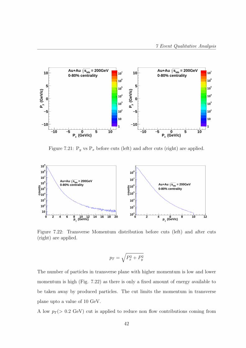
Figure 7.21: Py vs Px before cuts (left) and after cuts (right) are applied.
0 2 4 6 8 10 12 14 16 18 20 (GeV/c)
Tp
10
210
310
410
510
610
710
810
910
cou
nts
= 200GeV NNsAu+Au 0-80% centrality
0 2 4 6 8 10 12 (GeV/c)
Tp
210
310
410
510
610
710
810
cou
nts
= 200GeV NNsAu+Au 0-80% centrality
Figure 7.22: Transverse Momentum distribution before cuts (left) and after cuts(right) are applied.
pT =√P 2x + P 2
y
The number of particles in transverse plane with higher momentum is low and lower
momentum is high (Fig. 7.22) as there is only a fixed amount of energy available to
be taken away by produced particles. The cut limits the momentum in transverse
plane upto a value of 10 GeV.
A low pT (> 0.2 GeV) cut is applied to reduce non flow contributions coming from
42

7 Event Qualitative Analysis
resonance decays and to remove inefficiency of TPC. The high pT (< 10 GeV or < 2
GeV) cut is applied to reduce non-flow contributions coming from jets.
0 2 4 6 8 10 12 14 16 18 20P (GeV/c)
10
210
310
410
510
610
710
810
cou
nts
= 200GeV NNsAu+Au
0-80% centrality
0 2 4 6 8 10 12 14 16 18 20P (GeV/c)
1
10
210
310
410
510
610
710
810
cou
nts
= 200GeV NNsAu+Au 0-80% centrality
Figure 7.23: Total Momentum (P=√P 2x + P 2
y + P 2z ) before cuts (left) and after cuts
(right) are applied.
The total momentum distribution displays similar nature as Px, Py, Pz or pT (Fig.
7.23).
The Px, Py, Pz, pT and total momentum distributions follow an exponential dis-
tribution in the lower momentum limit and a power law distribution in the higher
momentum limit.
2− 1.5− 1− 0.5− 0 0.5 1 1.5 2η
0
50
100
150
200
250
610×
cou
nts
= 200GeV NNsAu+Au
0-80% centrality
0.6− 0.4− 0.2− 0 0.2 0.4 0.6η
020406080
100120140160180200220240
610×
cou
nts
= 200GeV NNsAu+Au
0-80% centrality
Figure 7.24: Pseudorapidity (η) before cuts (left) and after cuts (right) are applied.
43

7 Event Qualitative Analysis
η = ln(P + PzP − Pz
)
We put a pseudorapidity cut to select only those particles which are produced within
|η| < 1 because the detector acceptance is uniform in this range (Fig. 7.24).
3− 2− 1− 0 1 2 3 (radian)φ
0
10
20
30
40
50
60
70
80
90
610×
cou
nts
= 200GeV NNsAu+Au
0-80% centrality
3− 2− 1− 0 1 2 3 (radian)φ
0
5
10
15
20
25
30
35610×
cou
nts = 200GeV NNsAu+Au
0-80% centrality
Figure 7.25: φ distribution before cuts (left) and after cuts (right) are applied.
φ = tan−1(PyPx
)
The azimuthal angle distribution of particles should be uniform throughout(as seen
from Px vs Py distribution (Fig. 7.21)). But the dip observed in the φ distribution
(Fig. 7.25) can be attributed to detector malfunctioning.
θ = cos−1(PzP
)
We observe the dip in the middle close to π/2 because it corresponds to the beam
direction. Most of the particles are produced in the transverse plane and their number
decreases as we move towards the beam direction (Fig. 7.26).
From Fig. 7.27, it is re-emphasized that the |η| cut provides us with a region of
uniform particle production. By applying cuts we also overcome the non-uniformness
of particle production in φ.
44
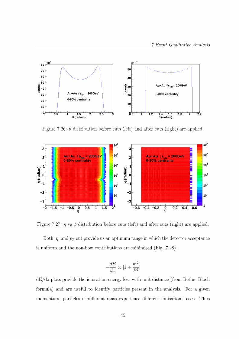
7 Event Qualitative Analysis
0 0.5 1 1.5 2 2.5 3 (radian)θ
0
10
20
30
40
50
60
70
80610×
cou
nts
= 200GeV NNsAu+Au
0-80% centrality
0.8 1 1.2 1.4 1.6 1.8 2 2.2 (radian)θ
0
10
20
30
40
50
610×
cou
nts = 200GeV NNsAu+Au
0-80% centrality
Figure 7.26: θ distribution before cuts (left) and after cuts (right) are applied.
2− 1.5− 1− 0.5− 0 0.5 1 1.5 2 η
3−
2−
1−
0
1
2
3
(ra
dia
n)
φ
1
10
210
310
410
510
610
= 200GeV NNsAu+Au 0-80% centrality
0.6− 0.4− 0.2− 0 0.2 0.4 0.6 η
3−
2−
1−
0
1
2
3
(ra
dia
n)
φ
1
10
210
310
410
510
610
= 200GeV NNsAu+Au 0-80% centrality
Figure 7.27: η vs φ distribution before cuts (left) and after cuts (right) are applied.
Both |η| and pT cut provide us an optimum range in which the detector acceptance
is uniform and the non-flow contributions are minimised (Fig. 7.28).
−dEdx∝ [1 +
m2
P 2]
dE/dx plots provide the ionisation energy loss with unit distance (from Bethe- Bloch
formula) and are useful to identify particles present in the analysis. For a given
momentum, particles of different mass experience different ionisation losses. Thus
45

7 Event Qualitative Analysis
2− 1.5− 1− 0.5− 0 0.5 1 1.5 2η
0
5
10
15
20
25
30
(G
eV/c
)T
p
1
10
210
310
410
510
610
710 = 200GeV NNsAu+Au 0-80% centrality
0.6− 0.4− 0.2− 0 0.2 0.4 0.6 0.8η
0
2
4
6
8
10
12
(G
eV/c
)T
p
1
10
210
310
410
510
610
710 = 200GeV NNsAu+Au 0-80% centrality
Figure 7.28: η vs pT distribution before cuts (left) and after cuts (right) are applied.
Figure 7.29: dEdx
vs P×q (rigidity) distribution for particle identification (with all thecuts).
different particles form different bands in Fig. 7.29. In figure 7.29, starting from the
bottom (right half), the lines denote bands for pion, kaon, proton, deuteron, tritum,
He3 etc. The bands on the left half correspond to the respective anti-particles.
46

7 Event Qualitative Analysis
0 0.5 1 1.5 2 2.5 3 3.5 4 4.5 5P (GeV/c)
0
1
2
3
4
5
2 )2 cG
eV (2
mas
s
1
10
210
310
410
510
610
710 = 200GeV NNsAu+Au
0-80% centrality
Figure 7.30: Mass2 vs momentum distribution for particle identification (with cuts).
Fig. 7.30 shows bands for different particles such as (starting from bottom) elec-
tron, pion, kaon, proton and deuteron. The identification can be done owing to the
mass of particles and can be thus verified regarding which band belongs to which
particle.
p=γmv =⇒ pc
= γmvc
= γmβ.
So, m2 = p2
c2γ2β2 .
Also, 1γ2β2 = 1
β2 − 1.
Therefore,m2 = p2
c2( 1β2 − 1). We get value of momentum from TOF and β = v = ∆L
∆T
is obtained from TOF, where ∆L is the length traversed in TOF chamber and ∆T is
the time taken for traversing the distance ∆L.
TOF detector gives m2 vs pT distributions which we use to identify the particles
present in our analysis.
47

7 Event Qualitative Analysis
0.5 1 1.5 2 2.5 3 3.5 4 4.5 5 (GeV/c)
Tp
0
1
2
3
4
5
2 )2 cG
eV (2
mas
s
1
10
210
310
410
510
610
710 = 200GeV NNsAu+Au
0-80% centrality
Figure 7.31: Mass2 vs pT distribution for particle identification (with cuts).
Fig. 7.31 is just like the previous particle identifiction (PID) figures, except that
the bands in this figure is clearer to observe. In this plot too we can identify the
particles detected in our experiment.
48
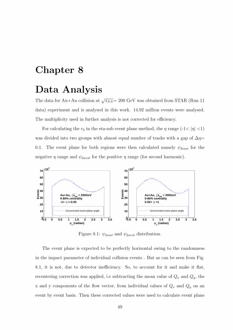
Chapter 8
Data AnalysisThe data for Au+Au collision at
√sNN= 200 GeV was obtained from STAR (Run 11
data) experiment and is analysed in this work. 14.92 million events were analysed.
The multiplicity used in further analysis is not corrected for efficiency.
For calculating the v2 in the eta-sub event plane method, the η range (-1< |η| <1)
was divided into two groups with almost equal number of tracks with a gap of ∆η=
0.1. The event plane for both regions were then calculated namely ψ2east for the
negative η range and ψ2west for the positive η range (for second harmonic).
0.5− 0 0.5 1 1.5 2 2.5 3 3.5 (radian)
2ψ
0
10
20
30
40
50
60
70310×
Eve
nts
= 200GeVNNsAu+Au, 0-80% centrality
<-0.05 η-1<
Uncorrected event plane angle
0.5− 0 0.5 1 1.5 2 2.5 3 3.5 (radian)
2ψ
0
10
20
30
40
50
60
70310×
Eve
nts
= 200GeVNNsAu+Au, 0-80% centrality
<1 η0.05<
Uncorrected event plane angle
Figure 8.1: ψ2east and ψ2west distribution.
The event plane is expected to be perfectly horizontal owing to the randomness
in the impact parameter of individual collision events . But as can be seen from Fig.
8.1, it is not, due to detector inefficiency. So, to account for it and make it flat,
recentering correction was applied, i.e subtracting the mean value of Qx and Qy, the
x and y components of the flow vector, from individual values of Qx and Qy on an
event by event basis. Then these corrected values were used to calculate event plane
49
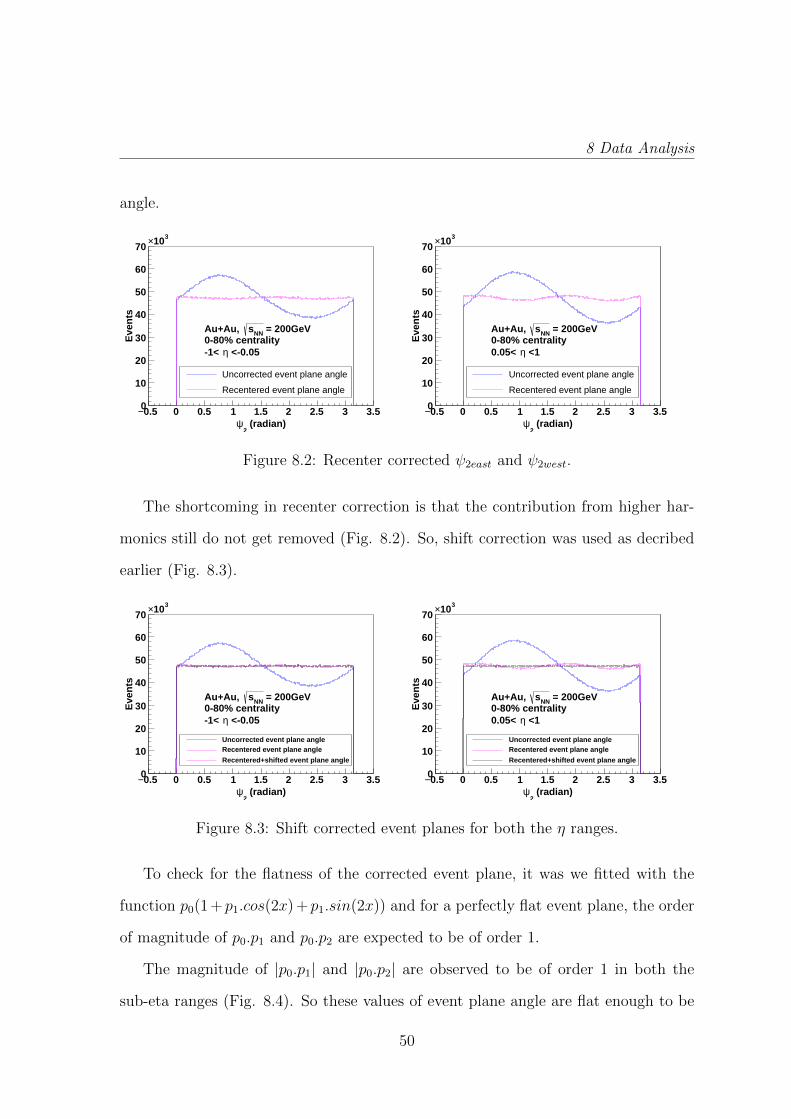
8 Data Analysis
angle.
0.5− 0 0.5 1 1.5 2 2.5 3 3.5 (radian)
2ψ
0
10
20
30
40
50
60
70310×
Eve
nts
= 200GeVNNsAu+Au, 0-80% centrality
<-0.05 η-1<
Uncorrected event plane angle
Recentered event plane angle
0.5− 0 0.5 1 1.5 2 2.5 3 3.5 (radian)
2ψ
0
10
20
30
40
50
60
70310×
Eve
nts
= 200GeVNNsAu+Au, 0-80% centrality
<1 η0.05<
Uncorrected event plane angle
Recentered event plane angle
Figure 8.2: Recenter corrected ψ2east and ψ2west.
The shortcoming in recenter correction is that the contribution from higher har-
monics still do not get removed (Fig. 8.2). So, shift correction was used as decribed
earlier (Fig. 8.3).
0.5− 0 0.5 1 1.5 2 2.5 3 3.5 (radian)
2ψ
0
10
20
30
40
50
60
70310×
Eve
nts
= 200GeVNNsAu+Au, 0-80% centrality
<-0.05 η-1<
Uncorrected event plane angleRecentered event plane angle
Recentered+shifted event plane angle
0.5− 0 0.5 1 1.5 2 2.5 3 3.5 (radian)
2ψ
0
10
20
30
40
50
60
70310×
Eve
nts
= 200GeVNNsAu+Au, 0-80% centrality
<1 η0.05<
Uncorrected event plane angleRecentered event plane angle
Recentered+shifted event plane angle
Figure 8.3: Shift corrected event planes for both the η ranges.
To check for the flatness of the corrected event plane, it was we fitted with the
function p0(1 + p1.cos(2x) + p1.sin(2x)) and for a perfectly flat event plane, the order
of magnitude of p0.p1 and p0.p2 are expected to be of order 1.
The magnitude of |p0.p1| and |p0.p2| are observed to be of order 1 in both the
sub-eta ranges (Fig. 8.4). So these values of event plane angle are flat enough to be
50

8 Data Analysis
/ ndf 2χ 8154 / 309
p0 1.229e+01± 4.716e+04 p1 0.000370±0.003486 − p2 04− 3.677e±05 − 4.645e
0.5− 0 0.5 1 1.5 2 2.5 3 3.5 (radian)
2ψ
0
10
20
30
40
50
60
70310×
Eve
nts
/ ndf 2χ 8154 / 309
p0 1.229e+01± 4.716e+04 p1 0.000370±0.003486 − p2 04− 3.677e±05 − 4.645e
/ ndf 2χ 8154 / 309
p0 1.229e+01± 4.716e+04 p1 0.000370±0.003486 − p2 04− 3.677e±05 − 4.645e
= 200GeVNNsAu+Au, 0-80% centrality
<1 η0.05< -5 10×=4.64
2, p-3 10×=-3.49
1, p4 10×=4.716
0p
Recentered+shifted event plane angle
Sin(2x)}2
Cos(2x)+p1
{1+p0
p
/ ndf 2χ 303 / 309
p0 1.230e+01± 4.724e+04
p1 0.0003697±0.0001525 −
p2 04− 3.671e±06 −2.899e−
0.5− 0 0.5 1 1.5 2 2.5 3 3.5 (radian)
2ψ
0
10
20
30
40
50
60
70310×
Eve
nts
/ ndf 2χ 303 / 309
p0 1.230e+01± 4.724e+04
p1 0.0003697±0.0001525 −
p2 04− 3.671e±06 −2.899e−
/ ndf 2χ 303 / 309
p0 1.230e+01± 4.724e+04
p1 0.0003697±0.0001525 −
p2 04− 3.671e±06 −2.899e−
= 200GeVNNsAu+Au, 0-80% centrality
<-0.05 η-1< -6 10×=-2.899
2, p-5 10×=-1.52
1, p4 10×=4.72
0p
Recentered+shifted event plane angle
Sin(2x)}2
Cos(2x)+p1
{1+p0
p
Figure 8.4: Flattened event plane fitted to the function and the parameters are shownon the top.For ψ2east, |p0.p1|= 16.46 and |p0.p2|= 2.19 and for ψ2west, |p0.p1|= 7.18and |p0.p2|= 0.137.
used to calculate v2.
The resolution obtained for different centralities and used throughout the calculation
of v2 is shown in Fig. 8.5. The resolution value is observed to be increasing initially
with the number of tracks (going from right to left). But, as the collision region
becomes more and more spherical with decreasing centrality values, pinpointing the
φ for the particular track becomes more difficult, hence the resolution decreases.
The calculated values of ψ2 resolution from data varies from published result by
3% within errors [15].
Similarly, for calculating v3, the ψ3 was first calculated and recenter and shift
corrections were applied (Fig. 8.6). v3 was calculated using the corrected value for
ψ3.
Just like for ψ2, the linearity of ψ3 was checked in both η ranges (by fitting it with
p0(1 + p1.cos(3x) + p1.sin(3x))) and was ensured that it is flat before doing further
analysis:
The magnitude of |p0.p1| and |p0.p2| are observed to be of order 1 in both the
sub-eta ranges (Fig. 8.7). So, this value of event plane angle is flat enough to be used
51

8 Data Analysis
0 10 20 30 40 50 60 70 80
Centrality (%)
0.1
0.2
0.3
0.4
0.5
0.6
0.7 R
esol
utio
n2
ψ
= 200GeVNNsAu+Au, 0-80% centrality
| <1 η0.05< |
resolution2
ψpublished data
0 10 20 30 40 50 60 70 80Centrality (%)
1.01
1.02
1.03
1.04
1.05
1.06
1.07
rat
io (
obs
/ pub
lishe
d)
p0 0.0001808± 1.032 p0 0.0001808± 1.032
Figure 8.5: ψ2 resolution in different centralities and comparison with published data.
0.5− 0 0.5 1 1.5 2 2.5 (radian)
3ψ
0
10
20
30
40
50
60
70
80
90310×
Eve
nts
= 200GeVNNsAu+Au, 0-80% centrality
<-0.05 η-1<
Uncorrected event plane angleRecentered event plane angle
Recentered+shifted event plane angle
0.5− 0 0.5 1 1.5 2 2.5 (radian)
3ψ
0
10
20
30
40
50
60
70
80
90
100310×
Eve
nts
= 200GeVNNsAu+Au, 0-80% centrality
<1 η0.05< Uncorrected event plane angleRecentered event plane angle
Recentered+shifted event plane angle
Figure 8.6: ψ3east and ψ3west distribution after applying recenter and shift correction.
to calculate v3.
The ψ3 resolution values obtained for different centralities are shown in Fig. 8.8:
52

8 Data Analysis
/ ndf 2χ 164.5 / 197
p0 1.887e+01± 7.086e+04 p1 04− 3.853e±05 −8.044e− p2 04− 3.676e±05 −3.394e−
0.5− 0 0.5 1 1.5 2 2.5 (radian)
3ψ
0
10
20
30
40
50
60
70
80
90
100310×
Eve
nts
/ ndf 2χ 164.5 / 197
p0 1.887e+01± 7.086e+04 p1 04− 3.853e±05 −8.044e− p2 04− 3.676e±05 −3.394e−
/ ndf 2χ 164.5 / 197
p0 1.887e+01± 7.086e+04 p1 04− 3.853e±05 −8.044e− p2 04− 3.676e±05 −3.394e−
= 200GeVNNsAu+Au, 0-80% centrality
<1 η0.05<
-5 10×= -3.4
2, p
-5 10×= -8.04
1, p4 10×= 7.09
0p
Recentered+shifted event plane angle
Sin(3x)}2
Cos(3x)+p1
{1+p0
p
/ ndf 2χ 159.3 / 197
p0 1.887e+01± 7.086e+04 p1 04− 3.853e±05 −1.102e− p2 04− 3.676e±05 − 2.883e
0.5− 0 0.5 1 1.5 2 2.5 (radian)
3ψ
0
10
20
30
40
50
60
70
80
90
100310×
Eve
nts
/ ndf 2χ 159.3 / 197
p0 1.887e+01± 7.086e+04 p1 04− 3.853e±05 −1.102e− p2 04− 3.676e±05 − 2.883e
/ ndf 2χ 159.3 / 197
p0 1.887e+01± 7.086e+04 p1 04− 3.853e±05 −1.102e− p2 04− 3.676e±05 − 2.883e
= 200GeVNNsAu+Au, 0-80% centrality
<1 η0.05<
-5 10×= 2.9
2, p
-5 10×= -1.1
1, p4 10×= 7.09
0p
Recentered+shifted event plane angle
Sin(3x)}2
Cos(3x)+p1
{1+p0
p
Figure 8.7: Flattened event plane fitted to the function and the parameters are shownon the top.For ψ3east, |p0.p1|= 5.7 and |p0.p2|= 2.4 and for ψ3west, |p0.p1|= 0.78 and|p0.p2|= 2.0561.
Figure 8.8: ψ3 resolution values in each centrality.
Next, v2 vs pT and v3 vs pT was plotted using the values obtained for resolution
for different centralities and different L+R bins.
The value of v2 is expected to increase initially before becoming flat. This is
expected because high pT particles are produced early in the collision system and
53

8 Data Analysis
0.5 1 1.5 2 2.5 3 (GeV/c)
Tp
0
0.05
0.1
0.15
0.2
0.25
2V
= 200GeVNNsAu+Au,
0-5%5-10%10-20%20-30%30-40%
40-50%50-60%60-70%min bias
0.5 1 1.5 2 2.5 3 (GeV/c)
Tp
0
0.02
0.04
0.06
0.08
0.1
0.12
0.14
3V
= 200GeVNNsAu+Au,
0-5%5-10%10-20%20-30%30-40%
40-50%50-60%60-70%min bias
Figure 8.9: Left: v2 vs pT plot, Right: v3 vs pT plot for different centralities andminimum bias.
hence can’t experience the collectivity. Also, we have the functional dependence from
hydrodynamic calculations [16].
v2 ∝ (pT − vmT )
where, m2T = m2 +p2
T . From this functional dependence we expect the plot to show a
rise at low pT , followed by a maxima at intermediate pT and drop to zero for higher
pT values.
The value of v2 is observed to be increasing as pT increases until about 3GeV/c, before
it starts to drop (Fig. 8.9). The v2 shows a strong centrality dependence whereas it is
not so for v3. Because v3 arises from fluctuations in initial state, the values of v3 for
0-5% centrality can be observed to be higher than the values of v2 for 0-5% centrality
(Fig. 8.9).
The calculated values for v2 vs pT in minimum bias was compared with the pub-
lished data [17] and was found out to be agreeing well with it (Fig. 8.10).
In v2 vs η and v3 vs η distributions, the effects of vn is expected to be most
54

8 Data Analysis
0 0.5 1 1.5 2 2.5 3 (GeV/c)
Tp
0.02
0.04
0.06
0.08
0.1
0.12
0.14
0.16
0.18
0.22
V
= 200GeVNNsAu+Au,
min bias
min. bias published data
Figure 8.10: Minimum bias v2 vs pT compared with the published data [17].
pronounced in the transverse plane, i.e for η=0.
0.6− 0.4− 0.2− 0 0.2 0.4 0.6 η
0.02
0.04
0.06
0.08
0.1
0.12
0.14
2V
= 200GeVNNsAu+Au,
0-5% centrality5-10% centrality10-20% centrality20-30% centrality30-40% centrality40-50% centrality50-60% centrality60-70% centrality70-80% centrality0-80% centrality
0.6− 0.4− 0.2− 0 0.2 0.4 0.6 η
10
15
20
25
30
35
40
45
50
55
603−10×
3V
= 200GeVNNsAu+Au,
0-5% centrality5-10% centrality10-20% centrality20-30% centrality30-40% centrality40-50% centrality50-60% centrality60-70% centrality70-80% centrality0-80% centrality
Figure 8.11: Left: v2 vs η, Right: v3 vs η for different centralities and minimum bias.
As can be inferred from Fig. 8.11, the value of v2 and v3 in all the centralities is
highest at η = 0 and decreases as we move away from the centre.
55

8 Data Analysis
The minimum bias L+R distribution was taken and the L+R distribution for each
centrality was extracted (using multiplicity cuts for centrality definition) (Fig. 8.12).
ZDCeastpwestEntries 1.484066e+07
Mean 2286
Std Dev 539.5
0 0.5 1 1.5 2 2.5 3 3.5 4 4.5
310×
L+R values
1
10
210
310
410
coun
ts (
log)
ZDCeastpwestEntries 1.484066e+07
Mean 2286
Std Dev 539.5
=200 GeVNNsAu+Au @
0 0.5 1 1.5 2 2.5 3 3.5 4 4.5 5
310×
L+R values
1
10
210
310
410
coun
ts (
Log)
centrality0-5% 5-10%10-20% 20-30%30-40% 40-50%50-60% 60-70%70-80%
= 200GeVNNsAu+Au,
Figure 8.12: Left: The L+R distribution for minimum bias, Right: The spectatordistribution for each centrality (by multiplicity) being shown in different colors.
The minimum bias distributions for v2 vs charged particle multiplicity and v2 vs
total spectator neutrons (ZDC) are as follows (Fig. 8.13):
Figure 8.13: Left: v2 vs charged particle multiplicity, Right: v2 vs Spectator Neutronsfor all events.
During categorisation of the events into centrality classes, the corresponding dis-
tribution in a centrality (10-20% shown as an example) is as follows (Fig. 8.14):
While taking centrality averages of different experimental observables or initial
conditions such as vn, multiplicity or ε2, Npart, the different characteristics that dif-
56

8 Data Analysis
Figure 8.14: Left: v2 vs Multiplicity, Right: v2 vs L+R for 10-20% centrality.
ferent events have in a centrality gets averaged, resulting in a loss of valuable infor-
mation. This can be verified from Fig. 8.14.
Therefore to investigate the events more deeply, the L+R distribution for each
centrality was further divided (by multiplicity) on the basis of L+R (total number of
spectator neutrons) values in bins of 0-5%, 5-10%,10-20%, ... 70-80% and 80-100%
each (Fig. 8.15). The 0-5% bin is the first shaded bin from left in the L+R distribution
for each centrality (Fig. 8.15). Because the L+R distribution corresponds to the
calorimetric response coming from spectator neutrons and we can only obtain the total
number of spectator nucleons from Glauber model, we have chosen the % binning (of
L+R distribution for each centrality) to ensure that we select corresponding events
from data and Glauber model for further analysis.
As can be seen in Fig. 8.16, the resolution varies differently in subsequent L+R
binning after centrality binning. The ψ2 resolution values show an increasing trend
with increasing L+R for 0-5%, 5-10%, 10-20% and 20-30% while it remains almost
constant for all subsequent centralities. For ψ3, the values for resolution remains al-
most a constant for all subsequent centralities starting from 10-20%. For 0-5% and
5-10% centralities the ψ3 resolution increases with increasing L+R.
57

8 Data Analysis
0 0.5 1 1.5 2 2.5 3 3.5 4 4.5
310×
L+R values
1
10
210
310
coun
ts
0-5% centrality
0 0.5 1 1.5 2 2.5 3 3.5 4 4.5
310×
L+R values
1
10
210
310
coun
ts
5-10% centrality
0 0.5 1 1.5 2 2.5 3 3.5 4 4.5
310×
L+R values
1
10
210
310
coun
ts
10-20% centrality
0 0.5 1 1.5 2 2.5 3 3.5 4 4.5
310×
L+R values
1
10
210
310
coun
ts
20-30% centrality
0 0.5 1 1.5 2 2.5 3 3.5 4 4.5
310×
L+R values
1
10
210
310
coun
ts
30-40% centrality
0 0.5 1 1.5 2 2.5 3 3.5 4 4.5
310×
L+R values
1
10
210
310
coun
ts
40-50% centrality
0 0.5 1 1.5 2 2.5 3 3.5 4 4.5
310×
L+R values
1
10
210
310
coun
ts
50-60% centrality
0 0.5 1 1.5 2 2.5 3 3.5 4 4.5
310×
L+R values
1
10
210
310
coun
ts
60-70% centrality
0 0.5 1 1.5 2 2.5 3 3.5 4 4.5
310×
L+R values
1
10
210
310
coun
ts
70-80% centrality
Figure 8.15: The % binning of L+R distribution in each centrality (by multiplicity).
The multiplicity is generally expected to decrease with increasing spectator num-
bers. But upon plotting charged particle multiplicity for each L+R bin in each cen-
trality, it was observed that the multiplicity decreases with increasing number of
spectators for 0-5%, 5-10%,...40-50% but increases with increasing spectator number
in the subsequent centralities (Fig. 8.17). This observation is for charged particle
multiplicity uncorrected for inefficiencies.
The v2 vs multiplicity and v3 vs multiplicity were plotted to check whether L+R
binning on top of centrality binning (by multiplicity) follow the centrality binning
trend. The white open circles in all the following plots denote the centrality averaged
values (wherever they appear) whereas the points of particular colour and shape
(as given in legend) denote the averaged values for different L+R bins within each
58

8 Data Analysis
0 10 20 30 40 50 60 70 80
% of L+R
0.3
0.4
0.5
0.6
0.7
0.8
Res
olut
ion
2Ψ
= 200GeVNNsAu+Au, Centrality
0-5% 5-10%
10-20% 20-30%
30-40% 40-50%
50-60% 60-70%
0 10 20 30 40 50 60 70 80
% of L+R
0.05
0.1
0.15
0.2
0.25
0.3
0.35
0.4
0.45
Res
olut
ion
3Ψ
= 200GeVNNsAu+Au, Centrality
0-5% 5-10%
10-20% 20-30%
30-40% 40-50%
50-60% 60-70%
70-80%
Figure 8.16: Left: ψ2 Resolution, Right: ψ3 Resolutions variations in L+R bins fromeach centrality.
0 10 20 30 40 50 60 70 80
% of L+R
0
100
200
300
400
500
600
Mul
tiplic
ity
= 200GeVNNsAu+Au,
centralities
0-5% 5-10%
10-20% 20-30%
30-40% 40-50%50-60% 60-70%
70-80%
Figure 8.17: Variation of multiplicity for spectator binning in each centrality.
centrality (by multiplicity).
As can be observed from Fig. 8.18, the v2 peaks at intermediate value of centrality
in agreement to the fact that the v2 is proportional to the product of ε2 and particle
number density. In the most central event, particle density is high but eccentricity
59

8 Data Analysis
0 50 100 150 200 250 300 350 400 450
ηdch
dN
0.02
0.03
0.04
0.05
0.06
0.07
0.08
0.09
2v
= 200GeVNNsAu+Au,
Centrality0-5% 5-10%10%-20% 20-30%30-40% 40-50%50-60% 60-70%centrality avg
0 50 100 150 200 250 300 350 400 450
ηdch
dN
0.015
0.02
0.025
0.03
0.035
3v
= 200GeVNNsAu+Au,
L+R bins for Centrality bins0-5% 5-10%10%-20% 20-30%30-40% 40-50%50-60% 60-70%centrality avg
Figure 8.18: Left: v2 vs multiplicity, Right: v3 vs multiplicity, for different centralitiesand L+R binning on top of centrality bins.
is low and vice-versa for peripheral collisions. The centrality average only reflects an
averaged-out effect of all the L+R bins in all the centrality bins. The L+R binning
breaks the trend followed by centrality averaged values.
Fig. 8.18 also allows us to conclude that including the L+R binning on top of the
centrality binning allows us to more selectively choose events with particular Initial
conditions.
Alongwith similar conclusion for v3 vs multiplicity, the variation of dependency
from v2 vs multiplicity points towards a change in nature of distribution of flow
coefficients for different ‘n’ in each centrality.
The vn is proportional to initial overlapping region elliptic-anisotropy, ε and 1SdNch
dη
for low particle density, i.e
v2
ε2∝ 1
S
dNch
dy
where S = πRx.Ry is the overlapping region area.
To extract overlap region area alongwith other experimental initial conditions (eg:
eccentricity, Npart, Npart etc.) Glauber MC model was used. 105 events were gener-
ated and analysed. Just like the L+R distribution for each centrality was further
subdivided in data obtained from STAR experiment, the spectator nucleon distribu-
60

8 Data Analysis
tion in each centrality obtained from Glauber MC model was also sub-divided (Fig.
8.19):
0 20 40 60 80 100 120 140
L+R values
1
10
210
coun
ts (
log)
0-5% centrality
0 20 40 60 80 100 120 140
L+R values
1
10
210
coun
ts (
log)
0-5% centrality
0 20 40 60 80 100 120 140
L+R values
1
10
210
coun
ts (
log)
0-5% centrality
0 20 40 60 80 100 120 140
L+R values
1
10
210
coun
ts (
log)
0-5% centrality
0 20 40 60 80 100 120 140
L+R values
1
10
210
coun
ts (
log)
0-5% centrality
0 20 40 60 80 100 120 140
L+R values
1
10
210
coun
ts (
log)
0-5% centrality
0 20 40 60 80 100 120 140
L+R values
1
10
210
coun
ts (
log)
0-5% centrality
0 20 40 60 80 100 120 140
L+R values
1
10
210
coun
ts (
log)
0-5% centrality
0 20 40 60 80 100 120 140
L+R values
1
10
210
coun
ts (
log)
0-5% centrality
Figure 8.19: Spectator distribution for each centrality (by multiplicity) from Glaubermodel subdivided into bins of 0-5%,5-10%,10-20%,....70-80% and 80-100%.
Following the sub-division of L+R distribution in each centrality, the experimental
observables were extracted from each L+R sub-bin from Glauber model and was
implemented in the subsequent analysis.
For checking whether the simulated data is correct, results from Glauber MC were
compared with published data (Fig. 8.20) [13].
The extracted values for σ varies from published data by 2.9% within error limits
whereas the ε2 values varies from published data by 3.2% within error limits (Fig.
8.20).
To validate the Glauber model calculations, the multiplicity obtained from data
61
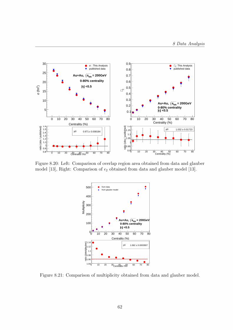
8 Data Analysis
0 10 20 30 40 50 60 70 80
Centrality (%)
5
10
15
20
25
30
)2
(fm
σ
= 200GeVNNsAu+Au,
0-80% centrality
| <0.5 η|
: This Analysisσpublished data
0 10 20 30 40 50 60 70 80Centrality (%)
0.8
0.91
1.1
1.21.31.4
1.51.6
rat
io (
obs
/ pub
lishe
d)
p0 0.008184± 0.971 p0 0.008184± 0.971
0 10 20 30 40 50 60 70 80Centrality (%)
0.1
0.2
0.3
0.4
0.5
0.6
0.7
0.8
0.9
2∈
= 200GeVNNsAu+Au, 0-80% centrality
| <0.5 η|
: This Analysis2∈published data
0 10 20 30 40 50 60 70 80Centrality (%)
0.9
0.95
1
1.05
1.1
1.15
1.2 r
atio
(ob
s / p
ublis
hed)
p0 0.01723± 1.032 p0 0.01723± 1.032
Figure 8.20: Left: Comparison of overlap region area obtained from data and glaubermodel [13], Right: Comparison of ε2 obtained from data and glauber model [13].
0 10 20 30 40 50 60 70 80
Centrality (%)
0
100
200
300
400
500
Mul
tiplic
ity
= 200GeVNNsAu+Au, 0-80% centrality
| <0.5 η|
from data
from glauber model
0 10 20 30 40 50 60 70 80Centrality (%)
1.04
1.06
1.08
1.1
1.12
1.14
rat
io (
data
/gla
uber
)
p0 0.0003907± 1.062 p0 0.0003907± 1.062
Figure 8.21: Comparison of multiplicity obtained from data and glauber model.
62

8 Data Analysis
and the multiplicity obtained from Glauber model were compared in each centrality
(Fig. 8.21). The extracted values for multiplicity from Glauber model varies from
the multiplicity (uncorrected for efficiency) collected from STAR experiment by 6.2%
within error limits (Fig. 8.21).
4 6 8 10 12 14 16
ηdch
dN s
1
0.1
0.15
0.2
0.25
0.3
0.35
0.4
2∈/2v
= 200GeVNNsAu+Au,
centrality0-5% 5-10%10-20% 20-30%30-40% 40-50%50-60% 60-70%centrality avg
4 6 8 10 12 14 16
ηdch
dN s
1
0.05
0.1
0.15
0.2
0.25
0.3
3∈/3v
= 200GeVNNsAu+Au,
centrality0-5% 5-10%10-20% 20-30%30-40% 40-50%50-60% 60-70%centrality avg
Figure 8.22: Left: < v2 > / < ε2 > vs scaled multiplicity, Right: < v3 > / < ε3 >vs scaled multiplicity for different centralities and L+R binning on top of centralitybins.
Previous analysis of experimental data with centrality binning have indeed found
very good scaling relation between 〈v2〉〈ε2〉 vs 1
sdNch
dηfor different systems like Cu+Cu
and Au+Au [18]. 〈v2〉〈ε2〉 increases with 1
sdNch
dyin centrality binning (Fig. 8.22). This
figure shows that although the scaling relation is obeyed by the centrality binning, it
is strongly broken in the spectator bins. We observe similar trend for 〈v3〉〈ε3〉 vs 1SdNch
dy.
0 50 100 150 200 250 300 350
partN
0.02
0.03
0.04
0.05
0.06
0.07
0.08
0.09
2v
= 200GeVNNsAu+Au,
centrality
0-5% 5-10%
10-20% 20-30%
30-40% 40-50%
50-60% 60-70%
centrality avg
0 50 100 150 200 250 300 350
partN
0.014
0.016
0.018
0.02
0.022
0.024
0.026
0.028
0.03
0.032
3v
= 200GeVNNsAu+Au,
centrality
0-5% 5-10%
10-20% 20-30%
30-40% 40-50%
50-60% 60-70%
centrality avg
Figure 8.23: Left: v2 vs Npart, Right: v3 vs Npart for different centralities and subse-quent L+R binning in each centrality.
63

8 Data Analysis
In Fig. 8.23, v2 and v3 are plotted vs Npart. For centrality averaged values, as
we move from central to peripheral events, v2 increases with decrease in Npart until
mid-centralities where the effect of decreasing number of particle sets in. But, the
spectator bins break this dependence. With same Npart, events with different v2 can
be chosen using spectator binning (Fig. 8.23).
The v3 varies more closely in each centrality compared to v2 with Npart. With
same Npart, we can also choose events with different v3 using spectator binning (Fig.
8.23).
As impact parameter decreases the number of participating nucleons is expected
to increase.
0 50 100 150 200 250 300 350
partN
2
4
6
8
10
12
b (f
m)
= 200GeVNNsAu+Au,
centrality0-5% 5-10%10-20% 20-30%30-40% 40-50%50-60% 60-70%centrality avg
Figure 8.24: The dependence of impact parameter (b) on number of participatingnucleons (Npart).
In Fig. 8.24 we have impact parameter vs number of participating nucleons. We
observe that the centrality trend perfectly matches with the subsequent L+R binning
values for each centrality.
For eccentricity vs Ncoll plot(Fig. 8.25), as we move from central to peripheral
collisions, the eccentricity of the overlap region increases and the number of binary
64

8 Data Analysis
0 200 400 600 800 1000
collN
0.1
0.2
0.3
0.4
0.5
0.6
2∈
= 200GeVNNsAu+Au,
centrality0-5% 5-10%10-20% 20-30%30-40% 40-50%50-60% 60-70%centrality avg
0 200 400 600 800 1000
collN
0.05
0.1
0.15
0.2
0.25
0.3
0.35
0.4
3∈
= 200GeVNNsAu+Au,
centrality0-5% 5-10%10-20% 20-30%30-40% 40-50%50-60% 60-70%centrality avg
Figure 8.25: Left: ε2 vs Ncoll, Right: ε3 vs Ncoll for centrality bins and SubsequentL+R bins for each centrality.
collisions decreases. The centrality dependence for eccentricity vs Ncoll is slightly
broken by the spectator binning in each centrality.
For ε3, the variation in each centrality is tighter compared to ε2 vs Ncoll. But still
there is a slight deviation from centrality trend.
0 50 100 150 200 250 300 350
partN
0
0.1
0.2
0.3
0.4
0.5
0.6
2∈
= 200GeVNNsAu+Au,
centrality0-5% 5-10%10-20% 20-30%30-40% 40-50%50-60% 60-70%centrality avg
0 50 100 150 200 250 300 350
partN
0.1
0.15
0.2
0.25
0.3
0.35
3∈
= 200GeVNNsAu+Au,
centrality0-5% 5-10%10-20% 20-30%30-40% 40-50%50-60% 60-70%centrality avg
Figure 8.26: Left: ε2 vs Npart, Right: ε3 vs Npart for centrality bins and SubsequentL+R bins for each centrality.
For eccentricity vs Npart (Fig. 8.26), there is a slight deviation in trend followed
by L+R bins when compared with the centrality binning trend. For ε3, vs Npart there
is lighter centrality trend breaking when compared with the extent of centrality trend
breaking in ε2 vs Npart.
For eccentricity vs charged particle multiplicity, as the eccentricity decreases, mul-
65
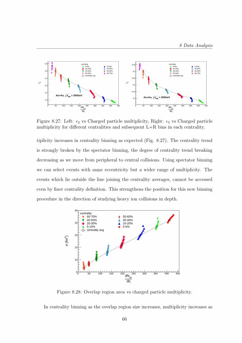
8 Data Analysis
0 50 100 150 200 250 300 350 400 450
ηdch
dN
0.1
0.2
0.3
0.4
0.5
0.6
2∈
= 200GeVNNsAu+Au,
centrality0-5% 5-10%10-20% 20-30%30-40% 40-50%50-60% 60-70%centrality avg
0 50 100 150 200 250 300 350 400 450
ηdch
dN
0.1
0.15
0.2
0.25
0.3
0.35
3∈
= 200GeVNNsAu+Au,
centrality0-5% 5-10%10-20% 20-30%30-40% 40-50%50-60% 60-70%centrality avg
Figure 8.27: Left: ε2 vs Charged particle multiplicity, Right: ε3 vs Charged particlemultiplicity for different centralities and subsequent L+R bins in each centrality.
tiplicity increases in centrality binning as expected (Fig. 8.27). The centrality trend
is strongly broken by the spectator binning, the degree of centrality trend breaking
decreasing as we move from peripheral to central collisions. Using spectator binning
we can select events with same eccentricity but a wider range of multiplicity. The
events which lie outside the line joining the centrality averages, cannot be accessed
even by finer centrality definition. This strengthens the position for this new binning
procedure in the direction of studying heavy ion collisions in depth.
0 50 100 150 200 250 300 350 400 450
ηdch
dN5
10
15
20
25
30
)2
(fm
σ
= 200GeVNNsAu+Au,
centrality60-70% 50-60%40-50% 30-40%20-30% 10-20%5-10% 0-5%centrality avg
Figure 8.28: Overlap region area vs charged particle multiplicity.
In centrality binning as the overlap region size increases, multiplicity increases as
66

8 Data Analysis
expected (Fig. 8.28). The centrality trend is strongly broken by the spectator binning,
the strength of centrality trend breaking being different for different centralities. We
can obtain events with same overlap region but different multiplicities using spectator
binning. The L+R binning thus gives us an access to those events whose overlap
region area were not accessible as they do not fall on the centrality averaged trend.
Similarly, if we observe the distribution for σx and σy vs Npart (Fig. 8.29), we
observe that in centrality binning, as the Npart increases, overlap region size along x
and y both increase as expected.
0 50 100 150 200 250 300 350
partN
1
1.5
2
2.5
3
(fm
)xσ
= 200GeVNNsAu+Au,
centrality60-70% 50-60%40-50% 30-40%20-30% 10-20%5-10% 0-5%centrality avg
0 50 100 150 200 250 300 350
partN
1.6
1.8
2
2.2
2.4
2.6
2.8
3
(fm
)yσ
= 200GeVNNsAu+Au,
centrality60-70% 50-60%40-50% 30-40%20-30% 10-20%5-10% 0-5%centrality avg
Figure 8.29: Left: σx vs Npart Right: σy vs Npart, for centrality binning and subsequentL+R binning for each centrality.
L+R binning mildly breaks the centrality trend for σx and σy vs Npart. The overlap
region area spread along y is more than the spread along x.
For charged particle multiplicity vs Ncoll, charged particle multiplicity increases
with increasing number of participating nucleons in centrality binning (Fig. 8.30).
The centrality trend is strongly broken by the spectator binning. By applying L+R
binning on top of conventional centrality (based on charged particle multiplicity)
binning, we can access those events which cannot be accessed even by finer centrality
definitions. Fig. 8.30 also shows that multiplicity is also guided by factors other than
participating nucleons.
Another way of observing the same effect in greater detail is to plot the dNch
dη/Npart
67

8 Data Analysis
0 50 100 150 200 250 300 350
partN
0
50
100
150
200
250
300
350
400
450
500
ηdch
dN
= 200GeVNNsAu+Au,
centrality0-5% 5-10%10-20% 20-30%30-40% 40-50%50-60% 60-70%centrality avg
Figure 8.30: Multiplicity vs Npart.
vs Npart as shown in Fig. 8.31:
0 50 100 150 200 250 300 350
partN
0.5
0.6
0.7
0.8
0.9
1
1.1
1.2
1.3
1.4
1.5
part
/ Nηdch
dN
/ ndf = 0.009509 / 62χconstant 0.02481± 1.065
slope 0.0001254± 0.0004455
/ ndf = 0.009509 / 62χconstant 0.02481± 1.065
slope 0.0001254± 0.0004455
/ ndf = 0.009509 / 62χconstant 0.02481± 1.065
slope 0.0001254± 0.0004455
/ ndf = 0.009509 / 62χconstant 0.02481± 1.065
slope 0.0001254± 0.0004455
/ ndf = 0.009509 / 62χconstant 0.02481± 1.065
slope 0.0001254± 0.0004455
/ ndf = 0.009509 / 62χconstant 0.02481± 1.065
slope 0.0001254± 0.0004455
= 200GeVNNsAu+Au,
centrality
0-5% 5-10%
10-20% 20-30%
30-40% 40-50%
50-60% 60-70%
centrality avg
Figure 8.31: Multiplicity scaled by number of participating nucleons(Npart) vs Npart.
In centrality binning, multiplicity seems to be linearly dependent upon Npart. But
this linearity is strongly broken in the spectator bins, the degree of centrality trend
breaking increasing with decreasing centrality (Fig. 8.31).
It is propsed that Ncoll varies as N4/3part [19]. For a check, we plot Ncoll vs Npart and
observe that the proportionality is obeyed in both Centrality binning and spectator
68
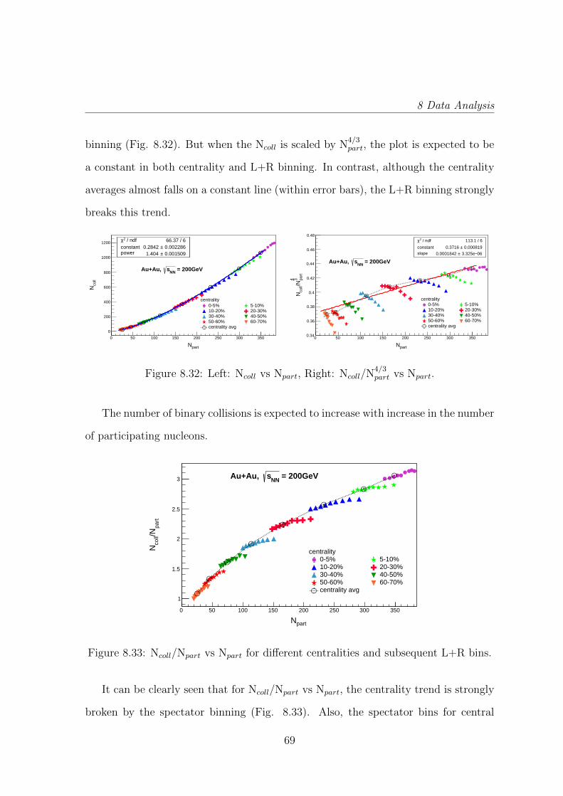
8 Data Analysis
binning (Fig. 8.32). But when the Ncoll is scaled by N4/3part, the plot is expected to be
a constant in both centrality and L+R binning. In contrast, although the centrality
averages almost falls on a constant line (within error bars), the L+R binning strongly
breaks this trend.
0 50 100 150 200 250 300 350
partN
0
200
400
600
800
1000
1200
coll
N
/ ndf 2χ 66.37 / 6constant 0.002286± 0.2842 power 0.001509± 1.404
/ ndf 2χ 66.37 / 6constant 0.002286± 0.2842 power 0.001509± 1.404
/ ndf 2χ 66.37 / 6constant 0.002286± 0.2842 power 0.001509± 1.404
/ ndf 2χ 66.37 / 6constant 0.002286± 0.2842 power 0.001509± 1.404
/ ndf 2χ 66.37 / 6constant 0.002286± 0.2842 power 0.001509± 1.404
/ ndf 2χ 66.37 / 6constant 0.002286± 0.2842 power 0.001509± 1.404
= 200GeVNNsAu+Au,
centrality0-5% 5-10%10-20% 20-30%30-40% 40-50%50-60% 60-70%centrality avg
0 50 100 150 200 250 300 350
partN
0.34
0.36
0.38
0.4
0.42
0.44
0.46
0.48
part
34
/Nco
llN
/ ndf 2χ 113.1 / 6
constant 0.000819± 0.3716 slope 06− 3.325e± 0.0001842
/ ndf 2χ 113.1 / 6
constant 0.000819± 0.3716 slope 06− 3.325e± 0.0001842
= 200GeVNNsAu+Au,
centrality0-5% 5-10%10-20% 20-30%30-40% 40-50%50-60% 60-70%centrality avg
Figure 8.32: Left: Ncoll vs Npart, Right: Ncoll/N4/3part vs Npart.
The number of binary collisions is expected to increase with increase in the number
of participating nucleons.
0 50 100 150 200 250 300 350
partN
1
1.5
2
2.5
3
part
/Nco
llN
= 200GeVNNsAu+Au,
centrality0-5% 5-10%10-20% 20-30%30-40% 40-50%50-60% 60-70%centrality avg
Figure 8.33: Ncoll/Npart vs Npart for different centralities and subsequent L+R bins.
It can be clearly seen that for Ncoll/Npart vs Npart, the centrality trend is strongly
broken by the spectator binning (Fig. 8.33). Also, the spectator bins for central
69

8 Data Analysis
collisions have larger value of Ncoll compared to a mid-central collisions. This is
because in bins with same Npart but higher centrality, the participant nucleons are
accumulated in a smaller area leading to higher Ncoll.
0.1 0.2 0.3 0.4 0.5 0.6
2∈
1
1.5
2
2.5
3
part
/Nco
llN
= 200GeVNNsAu+Au,
centrality0-5% 5-10%10-20% 20-30%30-40% 40-50%50-60% 60-70%centrality avg
0.1 0.15 0.2 0.25 0.3 0.35
3∈
1
1.5
2
2.5
3
part
/Nco
llN
= 200GeVNNsAu+Au,
centrality0-5% 5-10%10-20% 20-30%30-40% 40-50%50-60% 60-70%centrality avg
Figure 8.34: Left: Ncoll/Npart vs ε2, Right: Ncoll/Npart vs ε3 in centrality binning andsubsequent spectator binning.
In centrality binning, as eccentricity decreases, Ncoll/Npart increases as expected
(Fig. 8.34). The spectator binning strongly breaks the centrality trend. The spectator
bins for a higher centrality have larger values of Ncoll/Npart compared to a lower
centrality. In bins with similar value of ε2 but higher centrality, the participant
nucleons are accumulated in a smaller area leading to higher Ncoll. Also, we can
select events with similar Ncoll/Npart for a wide range of eccentricity using L+R bins.
The centrality trend is also broken by the L+R binning for Ncoll/Npart vs ε3.
Elliptic flow is proportional to the eccentricity of the overlap region and the mul-
tiplicity of the event. So we expect the centrality averages of v2 to increase with ε2
until mid centralities before starting to decrease.
As can be seen in centrality bins, v2 increases with ε2 until mid-centralities (Fig.
8.35). But, the spectator bins strongly break this dependence. Using spectator bin-
ning we can select events with same ε2 but different v2. We can also select events
with specific (v2,ε2) which cant be accessed by finer centrality definition.
As v3 comes from fluctuations in each centrality its magnitude does not vary as
70

8 Data Analysis
0.1 0.2 0.3 0.4 0.5 0.6
2∈
0.02
0.03
0.04
0.05
0.06
0.07
0.08
0.09
2v
= 200GeVNNsAu+Au,
centrality
0-5% 5-10%
10-20% 20-30%
30-40% 40-50%
50-60% 60-70%
centrality avg
0.05 0.1 0.15 0.2 0.25 0.3 0.35
3∈
0.016
0.018
0.02
0.022
0.024
0.026
0.028
0.03
3v
= 200GeVNNsAu+Au,
centrality
0-5% 5-10%
10-20% 20-30%
30-40% 40-50%
50-60% 60-70%
centrality avg
Figure 8.35: Left: v2 vs ε2, Right: v3 vs ε3 for centrality binning and subsequent L+Rbinning.
much as v2. The v3 vs ε3 values in L+R bins lie closer to centrality trend as compared
to those for v2 vs ε2 .
It is proposed that v2/ε2 shows a scaling relation with N1/3part [20]. In Fig. 8.36,
we observe that v2/ε2 follows the proposed scaling within errors. But, the spectator
binning breaks that trend (Fig. 8.36). Moreover the resulting independence of v2/ε2
N1/3part
on N1/3part is also not followed in the spectator bins for any centrality.
0 50 100 150 200 250 300 350
partN
0.1
0.15
0.2
0.25
0.3
0.35
0.4
0.45
0.5
2∈/2v
/ ndf 2χ 0.0001805 / 6constant 0.002954± 0.04687 power 0.01204± 0.3197
/ ndf 2χ 0.0001805 / 6constant 0.002954± 0.04687 power 0.01204± 0.3197
= 200GeVNNsAu+Au,
centrality0-5% 5-10%
10-20% 20-30%30-40% 40-50%50-60% 60-70%centrality avg
0 50 100 150 200 250 300 350
partN
0.035
0.04
0.045
0.05
0.055
0.06
0.065
0.07
part
1/3
. N2∈
2v
/ ndf 2χ 123.7 / 7
constant 0.0001306± 0.04521 slope 07− 8.273e±06 −9.275e−
/ ndf 2χ 123.7 / 7
constant 0.0001306± 0.04521 slope 07− 8.273e±06 −9.275e−
= 200GeVNNsAu+Au,
centrality0-5% 5-10%10-20% 20-30%30-40% 40-50%50-60% 60-70%70-80% centrality avg
Figure 8.36: Left: v2/ε2 vs Npart, Right: v2/ε2
N1/3part
vs N1/3part for centrality averages and
L+R binning for each centrality.
v2/ε2
N1/3part
vs Npart is a proposed scaling to check thermalisation of the system. In case
of thermalisation it has no dependency on Npart [20]. As can be seen it is almost a
constant for centrality binning. But the Spectator binning breaks this linearity (Fig.
71

8 Data Analysis
8.36).
0.03 0.04 0.05 0.06 0.07 0.08
2v
0.016
0.018
0.02
0.022
0.024
0.026
0.028
0.03
3v
centrality0-5% 5-10%10-20% 20-30%30-40% 40-50%50-60% 60-70%centrality avg
= 200GeVNNsAu+Au,
0.1 0.2 0.3 0.4 0.5 0.6
2∈
0.1
0.15
0.2
0.25
0.3
0.35
3∈
centrality0-5% 5-10%10-20% 20-30%30-40% 40-50%50-60% 60-70%centrality avg
= 200GeVNNsAu+Au,
Figure 8.37: Left: v2 vs v3, Right: ε2 vs ε3 for different centralities and subsequentL+R bins.
From the figure for v2 vs v3 (Fig. 8.37), we can observe that many L+R averaged
values lie away from the centrality average trend. Thus, L+R binning allows us to
select events with a wider range of very specific (v2 ,v3) compared to only centrality
binning. These events with highly specific (v2 ,v3) cannot be selected from even the
finest of centrality definition (eg. 0-1%, 1-2%, ....79-80%) alone as the points extracted
from any fine centrality definition (using multiplicity) will lie on the centrality trend
line. From ε2 vs ε3 plot(Fig. 8.37) it can be observed that the L+R binning closely
follows the centrality trend.
The ratio vn/εn is also expected to exhibit acoustic scaling [21-22] and receives viscous
corrections that grow exponentially as n2 and 1/Λ
ln(vnεn
) ∼ −4
3
n2η
ΛTTs
where ΛT =√
1σ2x
+ 1σ2y. Such acoustic scaling is found in data across a wide range
of beam energies and the shear viscosity to entropy density ratio, η/s is extracted
from the slope of the plot, ln(v2/ε2) vs 1/ΛT . These studies were done with centrality
binning alone. The Acoustic scaling was checked by plotting v2/ε2 and v3/ε3 vs 1/ΛT
72

8 Data Analysis
(Fig. 8.38) for each entrality and each L+R bin within all centralities.
0.5 0.6 0.7 0.8 0.9 1 1.1
)-1 (fm2yσ
1 + 2xσ
1
2.2−
2−
1.8−
1.6−
1.4−
1.2−
1−
2∈2vln
= 200GeVNNsAu+Au,
centrality0-5% 5-10%10-20% 20-30%30-40% 40-50%50-60% 60-70%centrality avg
0.5 0.6 0.7 0.8 0.9 1 1.1
)-1 (fm2yσ
1 + 2xσ
1
2.8−
2.6−
2.4−
2.2−
2−
1.8−
1.6−
1.4−
3∈3vln
= 200GeVNNsAu+Au,
centrality0-5% 5-10%10-20% 20-30%30-40% 40-50%50-60% 60-70%centrality avg
Figure 8.38: Left: v2/ε2 vs 1/ΛT , Right: v3/ε3 vs 1/ΛT for Different centralities andsubsequent L+R bins in each centrality.
The slope for bins of different L + R but a particular centrality is different from
those of a different centrality resulting in a mild breaking of the acoustic scaling.
Thus, the introduction of the L+R bins can enable a more refined extraction of η/s
from data.
73

Chapter 9
ConclusionThe centrality binning highly limits our capabilities at accessing the variation of
characteristics of events in heavy ion collision. It can be concluded from the ob-
servations in this work that these variations of events in each centralities can be
accessed by this new procedure of categorization of events. The L+R binning on top
of centrality binning allows us to access those events which could not be accessed
even by finer centrality definitions. Moreover, this novel binning procedure also al-
lows us to study some previously postulated scaling relations for centrality averaged
values such as (vnεn
) vs 1SdNch
dηand acoustic scaling relations in greater details.
74

Chapter 10
Future PlanWe are currently trying to obtain and use the efficiency corrected charged particle
multiplicity. Moreover, the ZDC distribution used in this work corresponds to the
ADC counts coming from the ZDC in both directions whereas the spectator number
distribution obtained from Glauber model consists of total number of neutrons and
protons. Although the binning is done in a way to take corresponding events from
data and Glauber MC model for analysis, we need to develop a formulation to obtain
the spectator number distribution from ZDC data too for a better comparison. These
will surely add to the robustness of the new binning procedure. Also, we wish to study
in future if the reverse order of binning in data affects our conclusions.
75
Bibliography
1. Vipul Bairathi et al., Phys. Lett. B 754, 144-150 (2016).
2. S. L. Glashow, Nucl. Phys. 22, 579 (1961). A. Salam and J.C. Ward, Phys.Lett., 168 168 (1964).
3. N.V.D Kolk thesis, Utrecht University (2011), link.
4. Coupling Constants for the Fundamental Forces, link.
5. H. Fritzsch, Phys.Usp. 52, 359-367 (2009).
6. Rihan Haque’s thesis, National Institute of Science Education and Research(2015), link.
7. Popular Information from Nobel Prize Org., link.
8. Gines Martinez, arXiv:1304:1452v1 [nucl-ex]. (2013).
9. Deuteron-gold collisions clarify ’jet quenching’ results, link.
10. J. Adams et al., Phys.Rev.C 72, 014904 (2005).
11. K.H. Ackermann et al., Nucl.Instrum.Meth. A 499, 624-632 (2003).
12. Voloshin, Poskanzer, Phys.Lett. B 474, 27-32 (2000).
13. H. Masui et.al, Phys.Lett.B 679, 440-444 (2009).
14. ROOT users guide, (https://root.cern.ch/guides/users-guide).
15. L Adamczyk et.al., Phys Rev C. 94, 034908 (2016).
16. Jean-Yves Ollitrault, Eur.J.Phys. 29, 275-302 (2008).
17. B.I. Abelev et al, Phys.Rev.C 77, 054901 (2008).
18. Huichao Song et. al, Phys. Rev. Lett. 106, 192301 (2011).
19. Miller et.al., Ann.Rev.Nucl.Part.Sci. 57, 205-243 (2007).
20. Maya Shimomura et.al, Nucl.Phys.A 830, 183c-186c (2009).
21. R. A. Lacey, A. Taranenko et. al., arXiv:1105.3782 [nucl-ex], (2011).
22. R. A. Lacey et al., arXiv:1301.0165 [nucl-ex], (2018).
76