DEPARTMENT OF ECONOMICS

Probability Weighting Functions*

Ali al-Nowaihi, University of Leicester, UK Sanjit Dhami, University of Leicester, UK

Working Paper No. 10/10 April 2010

Probability Weighting Functions�

Ali al-Nowaihiy Sanjit Dhamiz

16 April 2010

Abstract

In this paper we begin by stressing the empirical importance of non-linear weight-

ing of probabilities, which expected utility theory (EU) is unable to accommodate.

We then go on to outline three stylized facts on non-linear weighting that any al-

ternative theory of risk must address. These are that people: overweight small

probabilities and underweight large ones (S1); do not choose stochastically domi-

nated options when such dominance is obvious (S2); ignore very small probabilities

and code extremely large probabilities as one (S3). We then show that the concept

of a probability weighting function (PWF) is crucial in addressing S1-S3. A PWF

is not, however, a theory of risk. PWF�s need to be embedded within some the-

ory of risk in order to have signi�cant predictive content. We ouline the two main

alternative theories that are relevant in this regard: rank dependent utility (RDU)

and cumulative prospect theory (CP). RDU and CP explain S1,S2 but not S3. We

conclude by outlining the recent proposal for composite prospect theory (CPP) that

uses the composite Prelec probability weighting function (CPF). CPF is axiomati-

cally founded, and is �exible and parsimonious. CPP can explain all three stylized

facts S1,S2,S3.

�Dr. Sanjit Dhami would like to acknowledge a one semester study leave provided by the Universityof Leicester. He also wishes to thank the International School of Economics (ISET) at Tbilisi StateUniversity, Georgia for their excellent hospitality and academic environment during the time that he wasa visiting Professor in the spring of 2010.

yDepartment of Economics, University of Leicester, University Road, Leicester. LE1 7RH, UK. Phone:+44-116-2522898. Fax: +44-116-2522908. E-mail: aa10@le.ac.uk.

zDepartment of Economics, University of Leicester, University Road, Leicester. LE1 7RH, UK. Phone:+44-116-2522086. Fax: +44-116-2522908. E-mail: Sanjit.Dhami@le.ac.uk.

Contents

1 Setting out the basics . . . . . . . . . . . . . . . . . . . . . . . . . . . . . . . . . 31.1 Expected utility theory (EU) . . . . . . . . . . . . . . . . . . . . . . . . . . 31.2 The Allais paradox and setting out the stylized facts . . . . . . . . . . . . 41.3 A brief note on prospect theory (PT) . . . . . . . . . . . . . . . . . . . . . 6

2 The importance of low probability events and problems for existing theory: Adiscussion . . . . . . . . . . . . . . . . . . . . . . . . . . . . . . . . . . . . . . . 72.1 Insurance for low probability events . . . . . . . . . . . . . . . . . . . . . . 82.2 Becker (1968) Paradox . . . . . . . . . . . . . . . . . . . . . . . . . . . . . 82.3 Evidence from jumping red tra¢ c lights . . . . . . . . . . . . . . . . . . . 92.4 Driving and talking on car mobile phones . . . . . . . . . . . . . . . . . . . 92.5 Other examples . . . . . . . . . . . . . . . . . . . . . . . . . . . . . . . . . 102.6 Conclusion from these disparate contexts . . . . . . . . . . . . . . . . . . . 10

3 A look ahead and the notion of a probability weighting function (PWF) . . . . . 104 Addressing stylized fact S1 . . . . . . . . . . . . . . . . . . . . . . . . . . . . . 124.1 Axiomatic derivations of Prelec�s PWF . . . . . . . . . . . . . . . . . . . . 16

5 Addressing stylized fact S2 . . . . . . . . . . . . . . . . . . . . . . . . . . . . . . 185.1 Rank dependent utility (RDU) . . . . . . . . . . . . . . . . . . . . . . . . . 185.2 Cumulative prospect theory (CP) . . . . . . . . . . . . . . . . . . . . . . . 20

5.2.1 The utility function in CP . . . . . . . . . . . . . . . . . . . . . . . 215.2.2 Construction of decision weights under CP . . . . . . . . . . . . . . 225.2.3 The objective function under prospect theory . . . . . . . . . . . . 22

6 Addressing stylized fact S3 . . . . . . . . . . . . . . . . . . . . . . . . . . . . . . 24

2

Under expected utility theory (EU) decision makers weight probabilities linearly. How-ever, the evidence suggests that decision makers weight probabilities in a non-linear man-ner. Consider, for instance, the following example from Kahneman and Tversky (1979, p.283). Suppose that one is compelled to play Russian roulette. One would be willing topay much more to reduce the number of bullets from one to zero than from four to three.However, in each case, the reduction in probability of a bullet �ring is 1/6 and, so, underEU, the decision maker should be willing to pay the same amount. One possible explana-tion is that decision makers do not weight probabilities in a linear manner as under EU.There is also emerging evidence of the neuro-biological foundations for such behavior.1 Wenow explore this idea more formally below.

1. Setting out the basics

1.1. Expected utility theory (EU)

Let X = fx1; x2; :::; xng be a �xed, �nite, set of real numbers, which can be interpreted asthe possible monetary outcomes or possible wealth levels. We will assume throughout thatthe outcomes are arranged so that x1 < x2 < ::: < xn. The assumption that X is a �niteset is not restrictive in practice because �nite sets can be extremely large. The decisionmaker has a set of feasible actions, A. Any action in A induces a probability distribution(p1; p2; :::; pn), pi � 0 and

Pni=1 pi = 1, over the real numbers x1; x2; :::; xn.

We then write a lottery, L, as

L = (x1; p1;x2; p2; :::;xn; pn) , (1.1)

with the interpretation that outcome xi occurs with probability pi. Let L be the set ofsuch lotteries. How should the decision maker decide which action in the set A to choose?EU postulates the existence of an expected utility functional, EU : L ! R. Under wellknown assumptions, this functional takes the following form

EU(L) =Pn

i=1 piu (xi) , (1.2)

where u (xi) is the utility of the outcome xi. EU predicts that the decision maker willchoose that action (or lottery) which leads to the highest real number according to thefunctional, (1.2). The axioms required in the derivation of (1.2) can be found in manystandard references, e.g., Fishburn (1982), MasCollel, Whinston and Green (1995), andVarian (1992). A key axiom that is relevant for us is the independence axiom.

De�nition 1 (Independence axiom): Suppose that � is a preference relation de�ned overthe set of lotteries. Then for all lotteries L1, L2, L, and all p 2 (0; 1], L1 � L2 ,(L1; p;L; 1� p) � (L2; p;L; 1� p) :

1See, for instance, Berns et al (2008).

3

The independence axiom is often empirically violated. Alternatives to EU that weconsider below, have in the main, relaxed the independence axiom. Two main features ofEU stand out. (1) There is additive separability across outcomes, an assumption that EUshares with many alternative theories. (2) The objective function is linear in probabilities.

1.2. The Allais paradox and setting out the stylized facts

Most alternatives to EU relax the second feature, i.e., linearity in probabilities. Theinterested reader can consult Kahneman and Tversky (2000) and Starmer (2000) for amore detailed set of examples. We consider here the following example (problems 3 and4) from Kahneman and Tversky (1979), based on the famous experiments of Allais.Problem 3: 95 experimental subjects were asked to choose among the following two

lotteries:A = (4000; 0:8; 0; 0:2) or B = (3000; 1)

20% of the subjects choose A while the remaining 80% choose BProblem 4: 95 experimental subjects were asked to choose among the following two

lotteries:C = (4000; 0:2; 0; 0:8) or D = (3000; 0:25; 0:0:75)

65% of the subjects choose C while the remaining 35% choose D.Notice that Problem 4 di¤ers from Problem 3 only in that the probabilities in the latter

are scaled down by a quarter. Hence, given that probabilities are weighted linearly underEU, if A is preferred to B then C should be preferred to D. Conversely if B is preferredto A then D should be preferred to C. A simple substitution in (1.2) con�rms this. Butthis pattern of preferences is violated by the experimental evidence. Most decision makersprefer B to A and C to D.One possibility that can potentially explain the Allais paradox is that decision mak-

ers violate the linear weighting of probabilities in EU. To explore this reasoning further,suppose that the decision maker assigns decision weights �(p) : [0; 1] ! [0; 1] that arenon-linear, continuous functions of probabilities with �(0) = 0; �(1) = 1. The majoritypreference in Problem 3 can then be written as

�(0:8)u(4000) < �(1)u(3000), �(0:8)

�(1)<u(3000)

u(4000): (1.3)

The majority preferences in Problem 4 can be written as:

�(0:2)u(4000) > �(0:25)u(3000), �(0:2)

�(0:25)>u(3000)

u(4000)(1.4)

4

From (1.3), (1.4) one can explain the preferences in Problems 3, 4 if the decision weightssatisfy the following restriction:

�(0:8)

�(1)<�(0:2)

�(0:25). (1.5)

A property of decision weights, subproportionality (see, Kahneman and Tversky (1979), p.282), implies that

�(pq)

�(p)� �(rpq)

�(rp); r � 1: (1.6)

Clearly subproportionality implies that (1.5) is satis�ed (for p = 1; q = 0:8; r = 0:25).Subproportionality is, however, quite strong. As Kahneman and Tversky (1979) pointout, it holds if and only if ln � is a convex function of ln p.Hence, decision weights provided an explanation for the sort of puzzles associated with,

say, the Allais paradox. But this solution, had one drawback (in addition to the strongrestrictions on �(:)). Decision makers who use such non-linear decision weights couldchoose stochastically dominated options even when such dominance is obvious, as thefollowing example shows.

Example 1 (Problems with non-linear weighting of probabilities) Consider the lottery(x; p; y; 1� p), 0 < p < 1. Let �(p) denote decision weights such that �(p) : [0; 1]! [0; 1].Let u be a utility function over sure outcomes. Denote by U , the non-expected utilityfunctional, de�ned as U = � (p)u (x) + � (1� p)u (y). Let strict preferences induced byU over the set of all lotteries be denoted by �U and the indi¤erence relation be �U .(a) For the special case, x = y, we get U = [� (p) + � (1� p)]u (x). In general, for non-EUtheories, � (p) + � (1� p) 6= 1. Typically, for 0 < p < 1, � (p) + � (1� p) < 1, hence(x; p;x; 1� p) �U (x; 1). But any �sensible�theory of risk should give (x; p;x; 1� p) �U(x; 1).(b) Take y = x+�, � > 0. Then, clearly, (x; 1) �1 (x; p;x+ �; 1� p), where �1 denotes �rstorder stochastic dominance. Now, U (x; p;x+ �; 1� p) = � (p)u (x) + � (1� p)u (x+ �).Assuming u is continuous (and, as in (a), � (p)+� (1� p) < 1), we get lim

�!0U (x; p;x+ �; 1� p) =

� (p)u (x)+� (1� p)u (x) = [� (p) + � (1� p)]u (x) < U (x). Hence, for su¢ ciently small� > 0, U (x; p;x+ �; 1� p) < U (x). Thus, (x; 1) �1 (x; p;x+ �; 1� p) but U (x; 1) �UU (x; p;x+ �; 1� p). Hence, monotonicity is violated.

Based on the discussion so far, we summarize our �rst two stylized facts, S1, S2.

S1 Decision makers weight probabilities in a non-linear manner. In particular, theevidence suggests that decision makers overweight low probabilities and underweighthigh probabilities. For further evidence, the reader could consult Kahneman andTversky (2000) and Starmer (2000).

5

S2. Incorporation of non-linear probabilities into a prototype non-expected utility model(that induces, say, the preference ordering �U in Example 1) is problematic. Whendecision weights transform objective probabilities, the decision maker might be leadto choose stochastically dominated options. In actual practice when such dominanceis obvious, decision makers do not choose the dominated option. We leave open thequestion here of what decision makers do when stochastic dominance is not obvious.The interested reader can consult Dhami and al-Nowaihi (2010a) for further details.

We now highlight yet another important stylized fact on non-linear weighting of prob-abilities that has great signi�cance at the end points of the probability interval [0; 1].

S3. For events close to the boundary of the probability interval [0; 1], extensive evidence,that we brie�y review below, suggests the following. Decision makers (i) ignoreevents of extremely low probability and, (ii) treat extremely high probability eventsas certain.

Stylized facts S1 and S2 have been well documented in the literature. However, S3 isless well documented and theoretical models that incorporate it formally have only justabout started to appear as discussion papers. For that reason, we discuss it in some detailhere.

1.3. A brief note on prospect theory (PT)

Stylized fact S3 is given prominence in the Nobel prize winning work on prospect theory(PT), due to Kahneman and Tversky (1979). PT is a psychologically rich theory and it wasthe outcome of many years of experiments conducted by Kahneman, Tversky, and others.The psychological foundations of PT rest, in an important manner, on the distinctionbetween an editing and an evaluation/decision phase. In PT, the term prospects can,for the time being, be thought to refer to our standard lotteries (we make the formaldistinction between prospects and lotteries, later in our paper).From our perspective, the most important and interesting aspect of the editing phase

takes place when decision makers decide which improbable events to treat as impossible andwhich probable events to treat as certain. This is exempli�ed in the quote from Kahnemanand Tversky (1979, p.282): �the simpli�cation of prospects can lead the individual to discardevents of extremely low probability and to treat events of extremely high probability as ifthey were certain.�Suppose that we have a lottery (x; p; y; 1� p) whose value to the decision maker is

given by the value function V = �(p)u(x) + �(1 � p)u(y). In the editing phase, amongother things, Kahneman and Tversky (1979) were interested in the decision weights, �(p),assigned by individuals to very low and very high probability events. They drew �(p) as

6

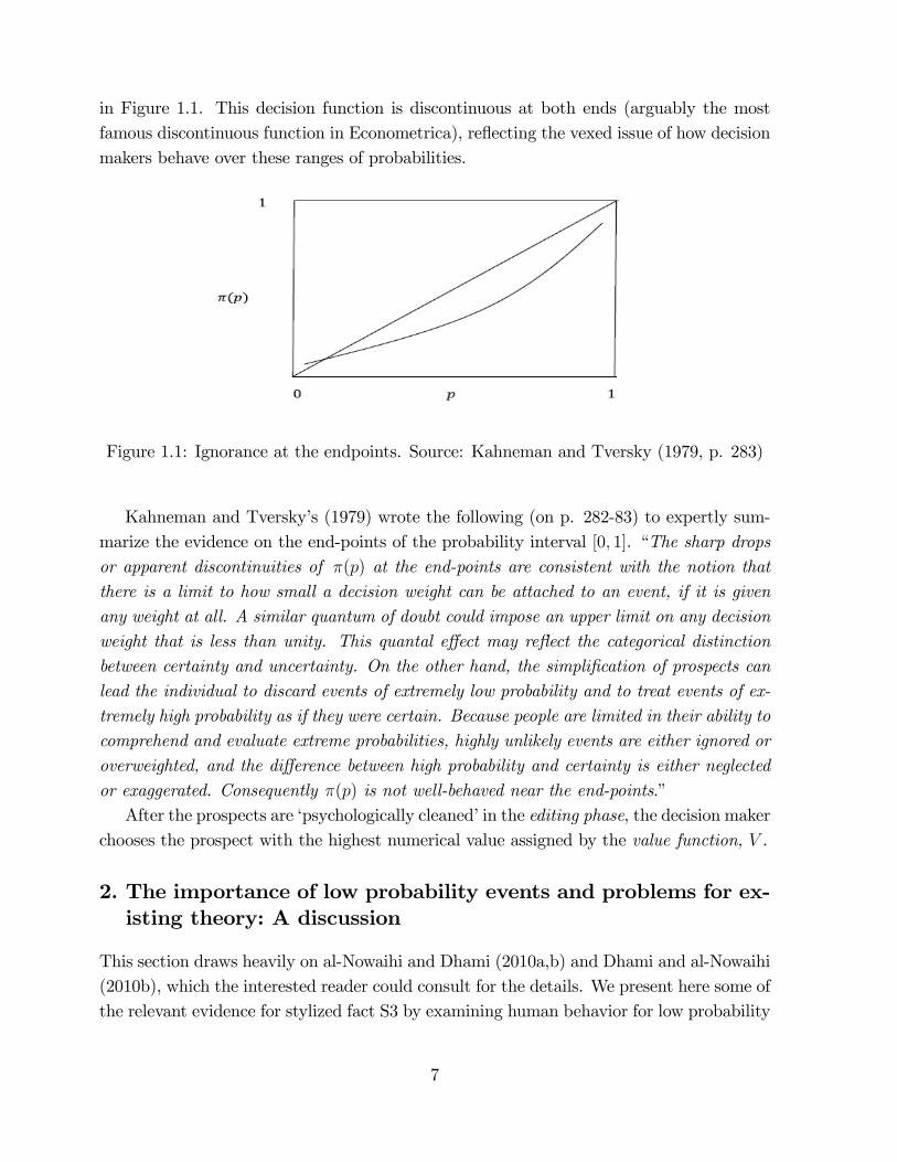
in Figure 1.1. This decision function is discontinuous at both ends (arguably the mostfamous discontinuous function in Econometrica), re�ecting the vexed issue of how decisionmakers behave over these ranges of probabilities.

Figure 1.1: Ignorance at the endpoints. Source: Kahneman and Tversky (1979, p. 283)

Kahneman and Tversky�s (1979) wrote the following (on p. 282-83) to expertly sum-marize the evidence on the end-points of the probability interval [0; 1]. �The sharp dropsor apparent discontinuities of �(p) at the end-points are consistent with the notion thatthere is a limit to how small a decision weight can be attached to an event, if it is givenany weight at all. A similar quantum of doubt could impose an upper limit on any decisionweight that is less than unity. This quantal e¤ect may re�ect the categorical distinctionbetween certainty and uncertainty. On the other hand, the simpli�cation of prospects canlead the individual to discard events of extremely low probability and to treat events of ex-tremely high probability as if they were certain. Because people are limited in their ability tocomprehend and evaluate extreme probabilities, highly unlikely events are either ignored oroverweighted, and the di¤erence between high probability and certainty is either neglectedor exaggerated. Consequently �(p) is not well-behaved near the end-points.�After the prospects are �psychologically cleaned�in the editing phase, the decision maker

chooses the prospect with the highest numerical value assigned by the value function, V .

2. The importance of low probability events and problems for ex-isting theory: A discussion

This section draws heavily on al-Nowaihi and Dhami (2010a,b) and Dhami and al-Nowaihi(2010b), which the interested reader could consult for the details. We present here some ofthe relevant evidence for stylized fact S3 by examining human behavior for low probability

7

events from several economic and non-economic contexts. This is not an exhaustive list ofsuch events but one that should su¢ ce.

2.1. Insurance for low probability events

The insurance industry is of tremendous economic importance. Yet, despite impressiveprogress, existing theoretical models are unable to explain the stylized facts on the take-up of insurance for low probability events. The seminal study of Kunreuther et al. (1978)provides striking evidence of individuals buying inadequate, non-mandatory, insuranceagainst low probability events (e.g., earthquake, �ood and hurricane damage in areasprone to these hazards).EU predicts that a risk-averse decision maker facing an actuarially fair premium will,

in the absence of transactions costs, buy full insurance for all probabilities, however small.Kunreuther et al. (1978, chapter 7) presented subjects with varying potential losses withvarious probabilities, keeping the expected value of the loss constant. Subjects facedactuarially fair, unfair or subsidized premiums. In each case, they found that there isa point below which the take-up of insurance drops dramatically, as the probability ofthe loss decreases (and as the magnitude of the loss increases, keeping the expected lossconstant). These results were shown to be robust to a very large number of perturbationsand factors; see al-Nowaihi and Dhami (2010b) for the details.Arrow�s own reading of the evidence in Kunreuther et al. (1978) is that the problem

is on the demand side rather than on the supply side. Arrow writes (Kunreuther et al.,1978, p.viii): �Clearly, a good part of the obstacle [to buying insurance] was the lack ofinterest on the part of purchasers.�Kunreuther et al. (1978, p. 238) write: �Based onthese results, we hypothesize that most homeowners in hazard-prone areas have not evenconsidered how they would recover should they su¤er �ood or earthquake damage. Ratherthey treat such events as having a probability of occurrence su¢ ciently low to permit themto ignore the consequences.�This behavior is in close conformity to the observations ofKahneman and Tversky (1979) outlined above.

2.2. Becker (1968) Paradox

A celebrated result, the Becker (1968) proposition, states that the most e¢ cient way todeter a crime is to impose the �severest possible penalty with the lowest possible probability�.By reducing the probability of detection and conviction, society can economize on thecosts of enforcement such as policing and trial costs. But by increasing the severity ofthe punishment (e.g., �nes), which is not costly, the deterrence e¤ect of the punishmentis maintained. Indeed, under EU, and allowing for in�nitely severe punishments, theBecker proposition implies that crime would be deterred completely, however small the

8

probability of detection and conviction. Kolm (1973) memorably phrased this propositionas: it is e¢ cient to hang o¤enders with probability zero. Empirical evidence, however, is notsupportive of the Becker proposition; see, for example, Radelet and Ackers (1996), Levitt(2004), Polinsky and Shavell (2007: 422-23). For the details see Dhami and al-Nowaihi(2010b)

2.3. Evidence from jumping red tra¢ c lights

Bar-Ilan (2000) and Bar-Ilan and Sacerdote (2001, 2004) provide near decisive evidencethat the alternative explanations (except the implication that individuals ignore low prob-ability events) cannot explain the Becker paradox; see Dhami and al-Nowaihi (2010b).They estimate that there are approximately 260,000 accidents per year in the USA causedby red-light running with implied costs of car repair alone of the order of $520 millionper year. It stretches plausibility to assume that these are simply mistakes. In runningred lights, there is a small probability of an accident, but, the consequences are self in-�icted and potentially have in�nite costs. Rephrased, running red tra¢ c lights is similarto hanging oneself with a very small probability, which is similar to the Becker proposition.Using Israeli data, Bar-Ilan (2000) calculated that the expected gain from jumping one

red tra¢ c is, at most, one minute (the length of a typical light cycle). Given the knownprobabilities they �nd that: �If a slight injury causes a loss greater or equal to 0.9 days,a risk neutral person will be deterred by that risk alone. However, the correspondingnumbers for the additional risks of serious and fatal injuries are 13.9 days and 69.4 daysrespectively�. To this must be added other costs arising from an accident. Dhami andal-Nowaihi (2010b) show that most of the attempts to explain the Becker paradox cannotwork in this case because the punishment under jumping red tra¢ c lights is self in�icted.A far more natural explanation, along the lines of our framework, is that stylized fact

S3 applies. Thus, red tra¢ c light running is simply caused by some individuals ignoring(or seriously underweighting) the very low probability of an accident.

2.4. Driving and talking on car mobile phones

Consider the usage of mobile phones in moving vehicles. A user of mobile phones facespotentially in�nite punishment (e.g., loss of one�s and/or the family�s life) with low proba-bility, in the event of an accident. The Becker proposition applied to this situation wouldsuggest that drivers of vehicles will not use mobile phones while driving or perhaps usehands-free phones, and so, avoid the self in�icted punishment. However, the evidence isto the contrary; see the Royal Society for the Prevention of Accidents (2005) and Pöys-tia et al. (2004). A natural explanation is the individuals simply ignore or substantiallyunderweight the low probability of an accident as in stylized fact S3.

9

2.5. Other examples

People were reluctant to use seat belts prior to their mandatory use despite publicly avail-able evidence that seat belts save lives. Prior to 1985, in the US, only 10-20% of motoristswore seat belts voluntarily, hence, denying themselves self-insurance; see Williams andLund (1986). Car accidents may be perceived by individuals as low probability events, par-ticularly if they are overcon�dent of their driving abilities. Overcon�dence is supportedfrom a wide range of contexts; see for instance Dhami and al-Nowaihi (2010a).Even as evidence accumulated about the dangers of breast cancer (which has a low

unconditional probability) women took up the o¤er of breast cancer examination, onlysparingly. In the US, this changed after the greatly publicized events of the mastectomiesof Betty Ford and Happy Rockefeller; see Kunreuther et al. (1978, p. xiii, p. 13-14).

2.6. Conclusion from these disparate contexts

Two main conclusions arise from the discussion in this section. First, human behavior forlow probability events cannot be easily explained by the existing mainstream theoreticalmodels of risk. al-Nowaihi and Dhami (2010a,b) show that EU and the associated auxiliaryassumptions are unable to explain the stylized facts. And furthermore, the leading non-expected utility alternatives such as rank dependent utility (RDU), prospect theory (PT)and cumulative prospect theory (CP) make the problem even worse. Second, a naturalexplanation for these phenomena seems to be that individuals simply ignore or seriouslyunderweight very low probability events (stylized fact S3).There is some evidence of a bimodal perception of risks that could o¤er a potential

explanation.2 Some individuals focus more on the probability and others on the size ofthe loss. The former do not pay attention to losses that fall below a certain probabilitythreshold, while for the latter, the size of the loss is relatively more salient. Hence, styl-ized fact S3 applies to the former set of individuals, which given the evidence, seem topredominate but are not the only types.

3. A look ahead and the notion of a probability weighting function(PWF)

Stylized facts S1, S2, S3 would seem to be the minimum requirements that a theory ofrisk should address. It would seem di¢ cult to explain these stylized facts using linearweighting of probabilities, as in EU. Most alternatives to EU that use non-linear weight-ing of probabilities, such as rank dependent utility (RDU), prospect theory (PT) andcumulative prospect theory (CP) invoke the concept of a probability weighting function

2See Camerer and Kunreuther (1989) and for the evidence, see Schade et al (2001).

10

to incorporate stylized facts S1 and S2. None of these theories can incorporate all of thethree stylized facts S1,S2,S3. We examine below emerging work due to al-Nowaihi andDhami (2010a,b), and Dhami and al-Nowaihi (2010b) who propose composite cumulativeprospect theory (CCP) and discuss applications that are able to address S1,S2,S3.

Remark 1 It is important to note that a probability weighting function (PWF), by itself,is NOT a theory of risk. It needs to be embedded within other theories, such as RDU,PT, CP for it to have signi�cant predictive content in concrete economic situations.

We begin with some simple de�nitions.

De�nition 2 (Probability weighting function, PWF): By a probability weighting functionwe mean a strictly increasing function w(p) : [0; 1] onto! [0; 1].

A simple proof, that we omit, can be used to demonstrate the following properties ofa PWF (for the proofs, see al-Nowaihi and Dhami, 2010a).

Proposition 1 : A probability weighting function has the following properties:(a) w (0) = 0, w (1) = 1. (b) w has a unique inverse, w�1, and w�1 is also a strictlyincreasing function from [0; 1] onto [0; 1]. (c) w and w�1 are continuous.

The following de�nitions will prove useful to address stylized fact S3 and will alsoillustrate why standard PWF�s are unable to address S3.

De�nition 3 : The function, w(p), (a) in�nitely-overweights in�nitesimal probabilities, iflimp!0

w(p)p=1, and (b) in�nitely-underweights near-one probabilities, if lim

p!11�w(p)1�p =1.

De�nition 4 : The function, w(p), (a) zero-underweights in�nitesimal probabilities, iflimp!0

w(p)p= 0, and (b) zero-overweights near-one probabilities, if lim

p!11�w(p)1�p = 0.

De�nition 5 : (a) w(p) �nitely-overweights in�nitesimal probabilities, if limp!0

w(p)p2 (1;1),

and (b) w(p) �nitely-underweights near-one probabilities, if limp!1

1�w(p)1�p 2 (1;1).

De�nition 6 : (a) w(p) positively-underweights in�nitesimal probabilities, if limp!0

w(p)p2

(0; 1), and (b) w(p) positively-overweights near-one probabilities, if limp!1

1�w(p)1�p 2 (0; 1).

11

4. Addressing stylized fact S1

Data from experimental and �eld evidence typically suggest that decision makers exhibitan inverse S-shaped probability weighting over outcomes (stylized fact S1). Tversky andKahneman (1992) propose the following probability weighting function, where the lowerbound on comes from Rieger and Wang (2006).

De�nition 7 : The Tversky and Kahneman probability weighting function is given by

w (p) =p

[p + (1� p) ]1

; 0:5 � < 1; 0 � p � 1. (4.1)

A simple proof leads to the following proposition.

Proposition 2 : The Tversky and Kahneman (1992) probability weighting function (4.1)in�nitely overweights in�nitesimal probabilities and in�nitely underweights near-one prob-abilities, i.e., lim

p!0w(p)p=1 and lim

p!11�w(p)1�p =1, respectively.

Remark 2 (Standard probability weighting functions): A large number of other proba-bility weighting functions have been proposed, e.g., those by Gonzales and Wu (1999) andLattimore, Baker and Witte (1992). Like the Tversky and Kahneman (1992) function,they all in�nitely overweight in�nitesimal probabilities and in�nitely underweight near-one probabilities. We shall call these as the standard probability weighting functions. Allthese functions violate stylized fact S3.

We now consider the most satisfactory PWF that helps to address stylized fact S1.This is the Prelec (1998) PWF, which is also a standard probability weighting functionin the sense of remark 2. The Prelec (1998) PWF has the following merits: parsimony,consistency with much of the available empirical evidence (in the sense of stylized fact S1)and an axiomatic foundation.

De�nition 8 (Prelec, 1998): By the Prelec function we mean the probability weightingfunction w(p) : [0; 1]! [0; 1] given by

w (0) = 0, w (1) = 1; (4.2)

w (p) = e��(� ln p)�

, 0 < p � 1, � > 0, � > 0. (4.3)

The following Proposition is straightforward to check, so we omit the proof.

Proposition 3 : The Prelec function (De�nition 8) is a probability weighting function inthe sense of De�nition 2.

12

0.0 0.1 0.2 0.3 0.4 0.5 0.6 0.7 0.8 0.9 1.00.0

0.2

0.4

0.6

0.8

1.0

p

w

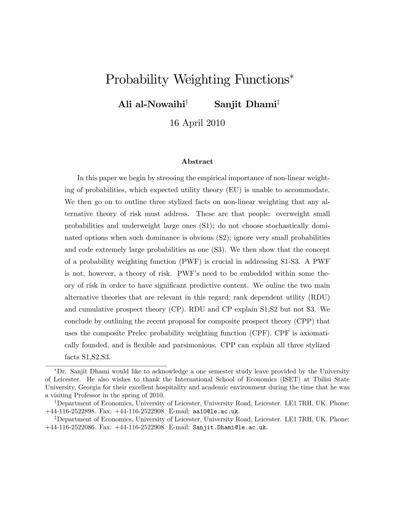
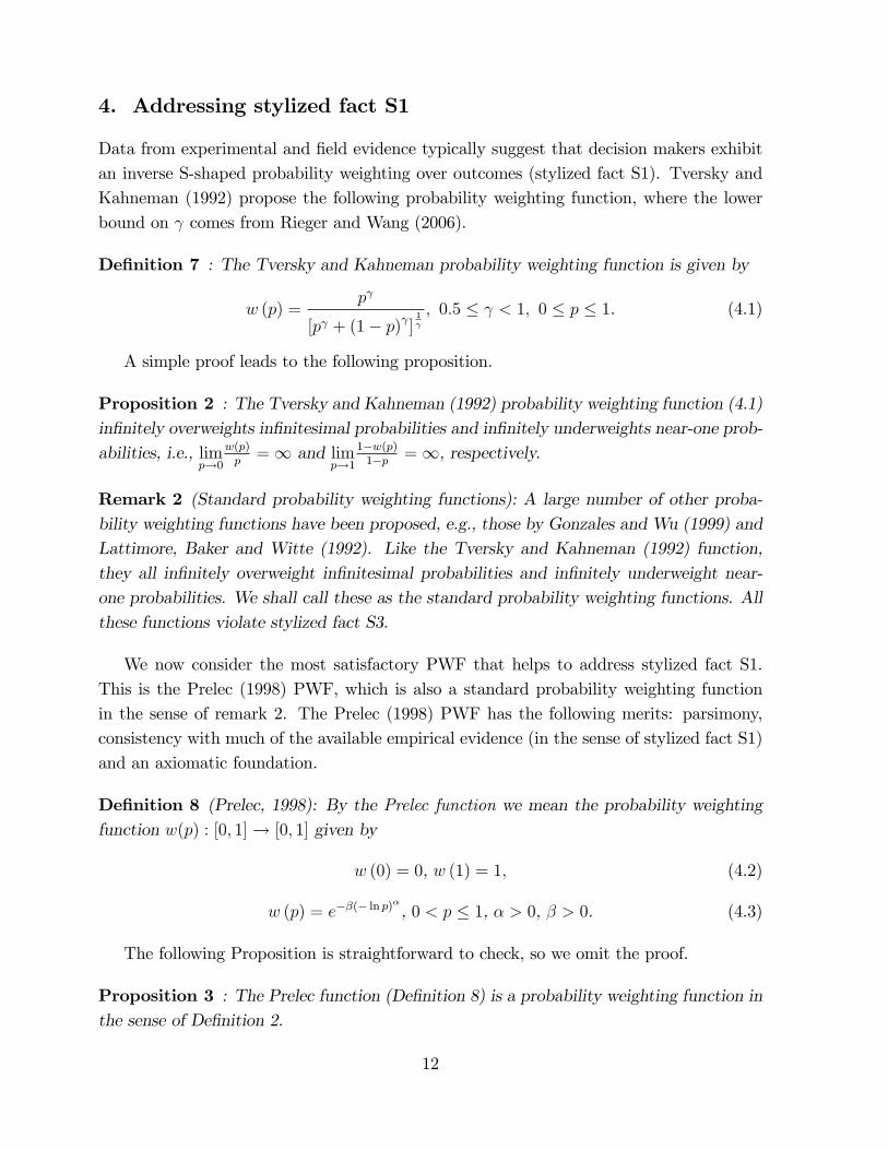
Figure 4.1: A plot of the Prelec (1988) function, w (p) = e�(� ln p)12 .

We plot the Prelec (1998) PWF in Figure 4.1 which is a plot of w (p) = e�(� ln p)0:5, i.e.,

� = 1 and � = 0:5 (see (4.3)) and the probability p 2 [0; 1].

Remark 3 (Axiomatic foundations): Prelec (1998) gave an axiomatic derivation of (4.2)and (4.3) based on �compound invariance�, Luce (2001) provided a derivation based on�reduction invariance�and al-Nowaihi and Dhami (2006) give a derivation based on �powerinvariance�. Since the Prelec function satis�es all three, �compound invariance�, �reduc-tion invariance�and �power invariance�are all equivalent. Note, in particular, that thesederivations do not put any restrictions on � and � other than � > 0 and � > 0.

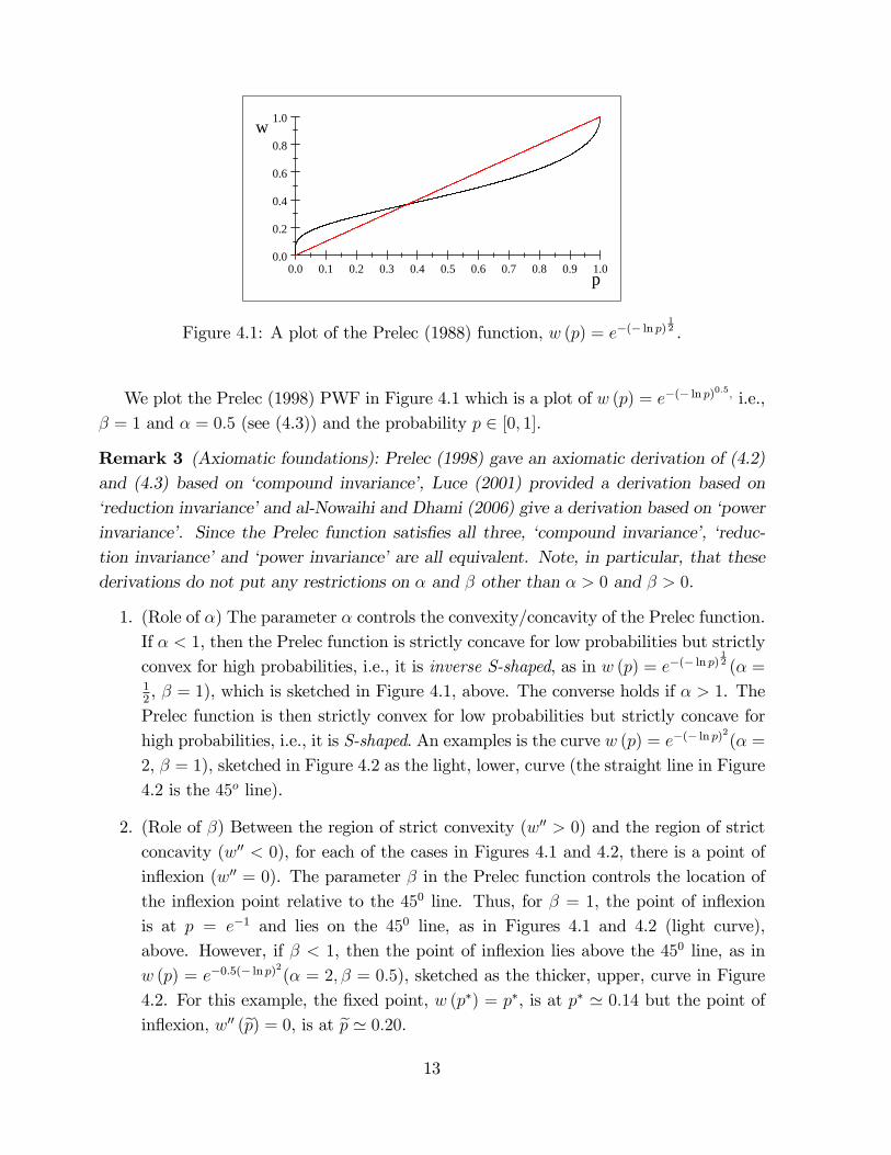
1. (Role of �) The parameter � controls the convexity/concavity of the Prelec function.If � < 1, then the Prelec function is strictly concave for low probabilities but strictlyconvex for high probabilities, i.e., it is inverse S-shaped, as in w (p) = e�(� ln p)

12 (� =

12, � = 1), which is sketched in Figure 4.1, above. The converse holds if � > 1. ThePrelec function is then strictly convex for low probabilities but strictly concave forhigh probabilities, i.e., it is S-shaped. An examples is the curve w (p) = e�(� ln p)

2

(� =2, � = 1), sketched in Figure 4.2 as the light, lower, curve (the straight line in Figure4.2 is the 45o line).

2. (Role of �) Between the region of strict convexity (w00 > 0) and the region of strictconcavity (w00 < 0), for each of the cases in Figures 4.1 and 4.2, there is a point ofin�exion (w00 = 0). The parameter � in the Prelec function controls the location ofthe in�exion point relative to the 450 line. Thus, for � = 1, the point of in�exionis at p = e�1 and lies on the 450 line, as in Figures 4.1 and 4.2 (light curve),above. However, if � < 1, then the point of in�exion lies above the 450 line, as inw (p) = e�0:5(� ln p)

2

(� = 2; � = 0:5), sketched as the thicker, upper, curve in Figure4.2. For this example, the �xed point, w (p�) = p�, is at p� ' 0:14 but the point ofin�exion, w00 (ep) = 0, is at ep ' 0:20.

13

0.0 0.1 0.2 0.3 0.4 0.5 0.6 0.7 0.8 0.9 1.00.0

0.2

0.4

0.6

0.8

1.0

p

w

Figure 4.2: A plot of w (p) = e�12(� ln p)2 and w (p) = e�(� ln p)

2

.

Sometimes, the respective roles of � and � are also referred to as the curvature andelevation properties of a probability weighting function; see Gonzalez and Wu (1999) andKilka and Weber (2001). Not all PWF�s allow for a clear separation between curvature andelevation. This is particularly the case for PWF�s that involve one parameter rather thantwo parameters. Some single parameter PWF�s that have been proposed are: Karmarkar(1979), Röell (1987), Currim and Sarin (1989), Tversky and Kahneman (1992), Luce,Mellers and Chang (1993), Hey and Orme (1994), and Safra and Segal (1998). Among thetwo parameter PWF�s are those by Goldstein and Einhorn (1987), Lattimore, Baker andWitte (1992) and Prelec (1998).The full set of possibilities for the Prelec (1998) function is established by the following

two propositions, which should be self-evident in the light of the discussion above. For thedetailed proofs, the reader is referred to al-Nowaihi and Dhami (2010a).

Proposition 4 : For � = 1, the Prelec probability weighting function (De�nition 8) takesthe form w (p) = p�, is strictly concave if � < 1 but strictly convex if � > 1. In particular,for � = 1, w (p) = p (as under expected utility theory).

Proposition 5 : Suppose � 6= 1, then the Prelec PWF (De�nition 8) has the followingproperties.

(a) There are three �xed points, at respectively, 0, p� = e�(1� )

1��1

and 1.(b) There is a unique in�exion point, ep 2 (0; 1) at which w00(ep) = 0.(c) If � < 1, the Prelec function is strictly concave for p < ep and strictly convex for p > ep(inverse S-shaped). If � > 1, then the converse holds(d) For the cases � < 1, � = 1, � > 1, the respective in�exion points, ep, lie above(ep < w (ep)), on (ep = w (ep)) and below (ep > w (ep)) the 450 line.Table 1, below, exhibits the various cases established by Proposition 5.

14

� < 1 � = 1 � > 1

� < 1inverse S-shapeep < w (ep) inverse S-shapeep = w (ep) inverse S-shapeep > w (ep)

� = 1strictly concavep < w (p)

w (p) = pstrictly convexp > w (p)

� > 1S-shapeep < w (ep) S-shape

w (ep) = ep S-shapeep > w (ep)Table 2, below, gives representative graphs of the Prelec function, w (p) = e��(� ln p)

�

,for each of the cases in Table 1.

� = 12

� = 1 � = 2

� = 12

0.0 0.5 1.00.0

0.5

1.0

p

w

w (p) = e�12(� ln p)

12

0.0 0.5 1.00.0

0.5

1.0

p

w

w (p) = e�(� ln p)12 .

0.0 0.5 1.00.0

0.5

1.0

p

w

w (p) = e�2(� ln p)12

� = 1

0.0 0.5 1.00.0

0.5

1.0

p

w

w (p) = p12

0.0 0.5 1.00.0

0.5

1.0

p

w

w (p) = p

0.0 0.5 1.00.0

0.5

1.0

p

w

w (p) = p2

� = 2

0.0 0.5 1.00.0

0.5

1.0

p

w

w (p) = e�12(� ln p)2.

0.0 0.5 1.00.0

0.5

1.0

p

w

w (p) = e�(� ln p)2

.

0.0 0.5 1.00.0

0.5

1.0

p

w

w (p) = e�2(� ln p)2

Table 2: Representative graphs of w (p) = e��(� ln p)�

.

Corollary 1 : Suppose � 6= 1. Then ep = p� = e�1 (i.e., the point of in�exion and the�xed point, coincide) if, and only if, � = 1. If � = 1, then:(a) If � < 1, then w is strictly concave for p < e�1 and strictly convex for p > e�1 (inverse-S shape, see Figure 4.1).

15

(b) If � > 1, then w is strictly convex for p < e�1 and strictly concave for p > e�1 (Sshape, see Figure 4.2).

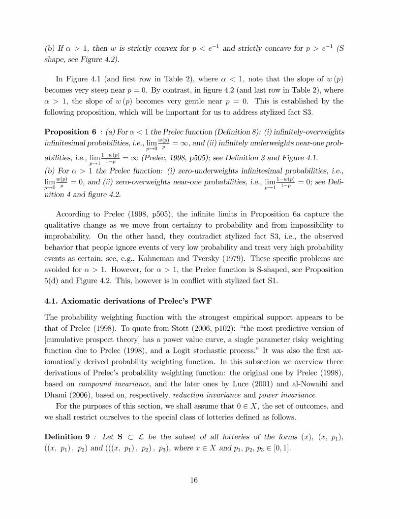
In Figure 4.1 (and �rst row in Table 2), where � < 1, note that the slope of w (p)becomes very steep near p = 0. By contrast, in �gure 4.2 (and last row in Table 2), where� > 1, the slope of w (p) becomes very gentle near p = 0. This is established by thefollowing proposition, which will be important for us to address stylized fact S3.

Proposition 6 : (a) For � < 1 the Prelec function (De�nition 8): (i) in�nitely-overweightsin�nitesimal probabilities, i.e., lim

p!0w(p)p=1, and (ii) in�nitely underweights near-one prob-

abilities, i.e., limp!1

1�w(p)1�p =1 (Prelec, 1998, p505); see De�nition 3 and Figure 4.1.

(b) For � > 1 the Prelec function: (i) zero-underweights in�nitesimal probabilities, i.e.,limp!0

w(p)p= 0, and (ii) zero-overweights near-one probabilities, i.e., lim

p!11�w(p)1�p = 0; see De�-

nition 4 and �gure 4.2.

According to Prelec (1998, p505), the in�nite limits in Proposition 6a capture thequalitative change as we move from certainty to probability and from impossibility toimprobability. On the other hand, they contradict stylized fact S3, i.e., the observedbehavior that people ignore events of very low probability and treat very high probabilityevents as certain; see, e.g., Kahneman and Tversky (1979). These speci�c problems areavoided for � > 1. However, for � > 1, the Prelec function is S-shaped, see Proposition5(d) and Figure 4.2. This, however is in con�ict with stylized fact S1.

4.1. Axiomatic derivations of Prelec�s PWF

The probability weighting function with the strongest empirical support appears to bethat of Prelec (1998). To quote from Stott (2006, p102): �the most predictive version of[cumulative prospect theory] has a power value curve, a single parameter risky weightingfunction due to Prelec (1998), and a Logit stochastic process.� It was also the �rst ax-iomatically derived probability weighting function. In this subsection we overview threederivations of Prelec�s probability weighting function: the original one by Prelec (1998),based on compound invariance, and the later ones by Luce (2001) and al-Nowaihi andDhami (2006), based on, respectively, reduction invariance and power invariance.For the purposes of this section, we shall assume that 0 2 X, the set of outcomes, and

we shall restrict ourselves to the special class of lotteries de�ned as follows.

De�nition 9 : Let S � L be the subset of all lotteries of the forms (x), (x; p1),((x; p1) ; p2) and (((x; p1) ; p2) ; p3), where x 2 X and p1; p2; p3 2 [0; 1].

16

To simplify notation, we shall refer to ((x; p1) ; p2) and (((x; p1) ; p2) ; p3) by (x; p1; p2)and (x; p1; p2; p3), respectively. Thus, (x) is the lottery whose outcome is x for sure,(x; p1) is the lottery whose outcomes are x with probability p1 and 0 with probability1�p1, (x; p1; p2) is the lottery whose outcomes are (x; p1) with probability p2 and 0 withprobability 1 � p2 and (x; p1; p2; p3) is the lottery whose outcomes are (x; p1; p2) withprobability p3 and 0 with probability 1� p3.Given a strictly increasing function, u : X ! R, and a probability weighting function,

w, we can extend u to a function, U : S! R, by the following de�nition.

De�nition 10 : U (x) = u (x), U (x; p1) = w (p1)U (x), U (x; p1; p2) = w (p2)U (x; p1)and U (x; p1; p2; p3) = w (p3)U (x; p1; p2).

De�nition 11 : Let � be the order on S induced by U , i.e., for all L1; L2 2 S, L1 �L2 , U (L1) � U (L2).

We are now in a position to introduce three apparently di¤erent axioms that, however,all lead to the Prelec probability weighting function.

De�nition 12 (Prelec, 1998): The preference relation, �, satis�es compound invarianceif, for all outcomes x, y, x0, y0 2 X, probabilities p, q, r, s 2 [0; 1] and integers n � 1,the following holds. If (x; p) � (y; q) and (x; r) � (y; s), then (x0; pn) � (y0; qn) implies(x0; rn) � (y0; sn).

De�nition 13 (Luce, 2001): The preference relation, �, satis�es reduction invariance if,for all outcomes x 2 X, probabilities p1; p2; q 2 [0; 1] and � 2 f2; 3g: (x; p1; p2) � (x; q))�x; p�1 ; p

�2

���x; q�

�.

De�nition 14 (al-Nowaihi and Dhami, 2006): The preference relation, �, satis�es powerinvariance if, for all outcomes x 2 X, probabilities p; q 2 [0; 1] and � 2 f2; 3g: (x; p; p) �(x; q))

�x; p�; p�

���x; q�

�and (x; p; p; p) � (x; q))

�x; p�; p�; p�

���x; q�

�.

It is easy to check that for w (p) = p compound invariance, reduction invariance andpower invariance are all satis�ed in EU. Hence, each of these constitutes a weakening (orgeneralization) of EU.

Proposition 7 : A probability weighting function, w, is the Prelec probability weight-ing function if, and only if, the induced preference relation, �, satis�es either compoundinvariance, reduction invariance or power invariance.

17

Comparing De�nitions 13 and 14, we see that power invariance is simpler in that itrequires two probabilities (p; q) instead of three (p1; p2; q). On the other hand, powerinvariance requires two stages of compounding, instead of the single stage of reductioninvariance. By contrast, compound invariance (De�nition 12) involves no compoundingbut four probabilities and four outcomes. However, it follows from Proposition 7 thatall three assumptions are equivalent. It is interesting to see that each of three a-prioridi¤erent behavioral assumptions lead to Prelec�s probability weighting function. We, thus,have a menu of testing options. Depending on the situation, one assumption may be moreappropriate to test than the others. For further developments, the interested reader couldfurther pursue Stott (2006) and Diecidue, Schmidt and Zank (2009).

5. Addressing stylized fact S2

There are two main ways of addressing S2. Either one uses rank dependent expected utilitytheory (RDU) or cumulative prospect theory (CP).

5.1. Rank dependent utility (RDU)

Quiggin (1982, 1993) for the �rst time, provided a coherent theory of behavior with non-linear weighting of probabilities. By �coherent�is meant, among other things, that decisionmakers do not choose stochastically dominated options when such dominance is obvious.Quiggen�s main insight was that it is not individual probabilities that should be trans-formed (which gave rise to the problem in Example 1) but rather, cumulative probabilities.When EU is applied to the transformed cumulative probabilities, we get what is nowknown as RDU.RDU was a major advance in that it could easily solve some (though not all) of the

paradoxes of EU. A major advantage of RDU over other behavioral decision theories isthat the whole, and extensive, machinery of EU can be utilized (though applied to thetransformed probabilities). By contrast, for other behavioral decisions theories, all thesetools of economic analysis must be developed afresh. We now explain.Let x be a random variable with distribution function F (x). Then F is (1) non-

decreasing, (2) right-continuous, and (3) F (�1) = 0; F (1) = 1. Let w be a PWF.De�ne � by

� (x) = 1� w (1� F (x)) . (5.1)

Using the properties of a weighting function in De�nition 2 it is simple to check that �also satis�es those properties. Notice that, � is a legitimate distribution function. Thus,we can de�ne a new random variable, ex, by:

Pr(ex � x) = � (x) = 1� w (1� F (x)) . (5.2)

18

Consider the lottery (x1; p1;x2; p2; :::;xn; pn), where x1 < x2 < ::: < xn; pi is, of course,the probability that x = xi. Let �i be the probability that ex = xi. Then

�i = �(xi)� � (xi�1)= [1� w (1� F (xi))]� [1� w (1� F (xi�1))]= w (1� F (xi�1))� w (1� F (xi))= w

��nj=i pj

�� w

��nj=i+1 pj

�.

(5.3)

The above considerations justify the following de�nitions (recall at this point, from thede�nition of a weighting function, that w (0) = 0 and w (1) = 1).

De�nition 15 : Consider the lottery (x1; p1;x2; p2; :::;xn; pn), where x1 < x2 < ::: < xn.Let w be the probability weighting function. For RDU, the decision weights, �i, are de�nedas follows.�n = w (pn),�n�1 = w (pn�1 + pn)� w (pn),:::

�i = w��nj=i pj

�� w

��nj=i+1 pj

�,

:::

�1 = w��nj=1 pj

�� w

��nj=2 pj

�= w (1)� w

��nj=2 pj

�= 1� w

��nj=2 pj

�.

De�nition 16 (rank dependent utility, RDU): Consider the lottery (x1; p1;x2; p2; :::;xn; pn),where x1 < x2 < ::: < xn. Let w be the probability weighting function. Let �i,i = 1; 2; :::; n, be given by De�nition 15. The decision maker�s rank dependent expectedutility is given by

U (x1; p1;x2; p2; :::;xn; pn) = �ni=1�iu (xi) . (5.4)

From De�nition 15, we get that,

�j � 0 andPn

j=1 �j = 1. (5.5)

Remark 4 : The result in (5.5) does not apply to the case of Example 1 because in thelatter we transformed objective probabilities while in the former we transformed cumulativeprobabilities.

Remark 5 An alternative is to de�ne (x) = w (F (x)). The decision weights wouldthen be �i = w

��nj=i pj

��w

��nj=i�1 pj

�. But the apparently more complex (5.1) to (5.3)

are actually slightly more convenient.

We now state the �rst main result of this section.

19

Proposition 8 : A decision maker who uses RDU, as in de�nition 16, never chooses sto-chastically dominated options. Hence, such a decision maker uses non-linear transforma-tions of cumulative probability but nevertheless is not subjected to the problem illustratedin Example 1. In other words, there is no problem with explaining stylized fact S2 for sucha decision maker.

The proof of Proposition 8 is not di¢ cult but it is not too short either. For that reasonwe refer the interested reader to Quiggen (1982). A clearer proof can be found in Dhamiand al-Nowaihi (2010a).

5.2. Cumulative prospect theory (CP)

The Nobel prize winning work of Kahneman and Tversky (1979), which is the second mostcited paper in economics, su¤ered from the problem illustrated in Example 1. Namely, thatdecision makers could choose stochastically dominated options, even when such dominancewas obvious. This did not go down too well with the profession. However, Quiggen�s workon RDU provided Kahneman and Tversky with the means to address this problem by usingcumulative transformations of probability. This, they duly did in their cumulative versionof prospect theory, which they called as cumulative prospect theory (CP); see Tversky andKahneman (1992); see also Starmer and Sugden (1989).However, Tversky and Kahneman (1992) paid a heavy price for this desirable feature.

Recalling the discussion in section 1.3 above, CP dropped the editing phase altogether,hence, also, giving up the psychological richness of PT. Tversky and Kahneman had nochoice but to do so in order to address S2. In PT, the decision weights (see Figure 1.1) arediscontinuous at both ends. However, in order to incorporate S2 using Quiggen�s insightson cumulative transformations of probability they needed a continuous function. This, inturn, meant that editing of prospects, which created discontinuities at both ends had tobe dispensed with.The most persuasive contributory role played by a PWF, in terms of addressing a wide

range of problems in economics arises when it is embedded within CP. We now outline,brie�y, the basics of CP. Consider a lottery of the form

L = (y�m; p�m; y�m+1; p�m+1; :::; y�1; p�1; y0; p0; y1; p1; y2; p2; :::; yn; pn) ,

where y�m < ::: < y�1 < y0 < y1 < ::: < yn are the outcomes or the �nal positions ofaggregate wealth and p�m; :::; p�1; p0; p1; :::pn are the corresponding objective probabilities,such that

Pni=�m pi = 1 and pi � 0. In CP, decision makers derive utility from wealth

relative to a reference point for wealth, y0, which could be initial wealth, status-quo wealth,average wealth, desired wealth, rational expectations of future wealth etc. depending onthe context.

20

De�nition 17 (Lotteries in incremental form) Let xi = yi � y0; i = �m;�m + 1; :::; n

be the increment in wealth relative to y0 and x�m < ::: < x0 = 0 < ::: < xn. Let therestriction on probabilities be �ni=�mpi = 1, pi � 0, i = �m;�m+1; :::; n. Then, a lotteryis presented in incremental form if it is represented as:

L = (x�m; p�m; :::;x�1; p�1;x0; p0;x1; p1; :::;xn; pn) . (5.6)

De�nition 18 (Lotteries and prospects): Lotteries that are represented in incrementalform are known as prospects.

De�nition 19 (Set of Lotteries): Denote by LP the set of all prospects of the form givenin (5.6) subject to the restrictions in de�nition 17.

De�nition 20 (Domains of losses and gains): The decision maker is said to be in thedomain of gains if xi > 0 and in the domain of losses if xi < 0. x0 lies neither in thedomain of gains nor in the domain of losses.

5.2.1. The utility function in CP

De�nition 21 (Tversky and Kahneman, 1979). A utility function, v(x), is a continuous,strictly increasing, mapping v : R! R that satis�es:1. v (0) = 0 (reference dependence).2. v (x) is concave for x � 0 (declining sensitivity for gains).3. v (x) is convex for x � 0 (declining sensitivity for losses).4. �v (�x) > v (x) for x > 0 (loss aversion).

Tversky and Kahneman (1992) propose the following utility function:

v (x) =

�x if x � 0

�� (�x)� if x < 0(5.7)

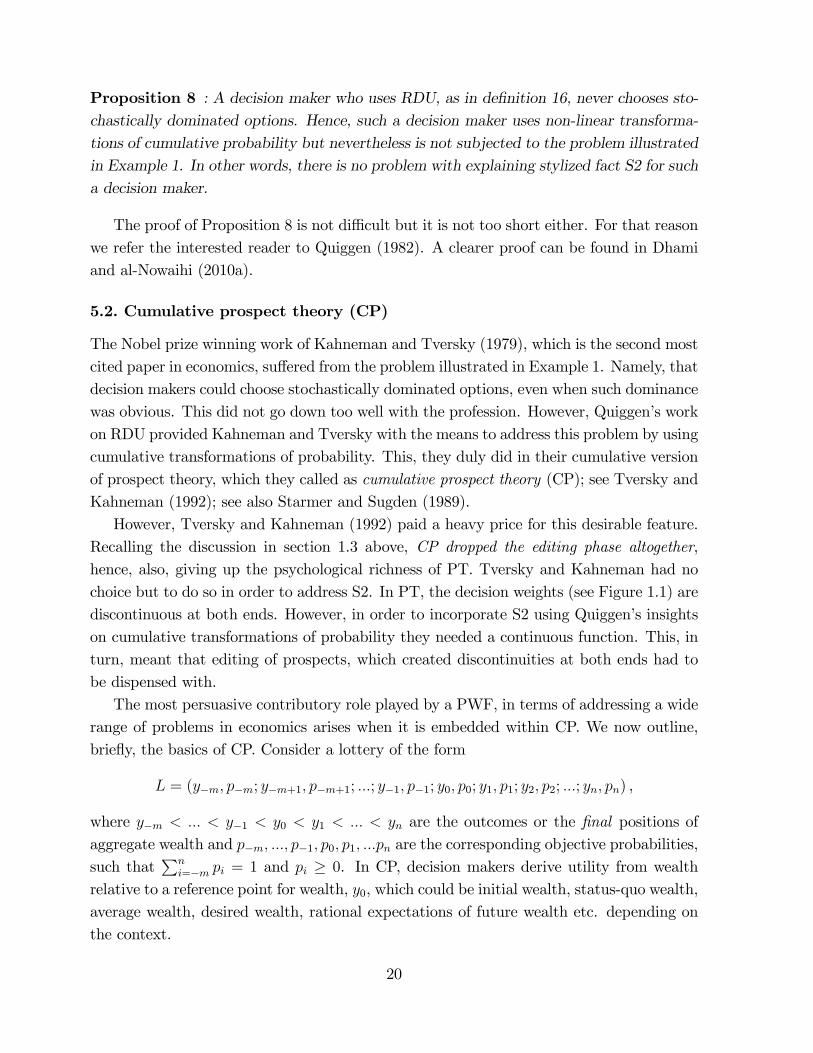
where ; �; � are constants. The coe¢ cients of the power function satisfy 0 < < 1; 0 <� < 1. � > 1 is known as the coe¢ cient of loss aversion. Tversky and Kahneman (1992)assert (but do not prove) that the axiom of preference homogeneity ((x; p) � y ) (kx; p) �ky) generates this value function. al-Nowaihi et al. (2008) give a formal proof, as wellas some other results (e.g. that is necessarily identical to �). Tversky and Kahneman(1992) estimated that ' � ' 0:88 and � ' 2:25. The reader can visually check theproperties listed in de�nition 21 for the utility function, (5.7), plotted in �gure 5.1 for thecase: �

v(x) =

px if x � 0

�2:5p�x if x < 0

(5.8)

21

­5 ­4 ­3 ­2 ­1 1 2 3 4 5

­6

­4

­2

2

x

v(x)

Figure 5.1: The utility function under CCP for the case in (5.8)

5.2.2. Construction of decision weights under CP

Let w(p) be a PWF, such as the Prelec PWF in De�nition 8. We could have di¤erentweighting functions for the domain of gains and losses, respectively, w+ (p) and w� (p).However, we make the empirically founded assumption that w+ (p) = w� (p); see Prelec(1998).

De�nition 22 (Tversky and Kahneman, 1992). For CP, the decision weights, �i, arede�ned as follows:

Domain of Gains Domain of Losses�n = w (pn) ��m = w (p�m)�n�1 = w (pn�1 + pn)� w (pn) ::: ��m+1 = w (p�m + p�m+1)� w (p�m) :::�i = w

��nj=i pj

�� w

��nj=i+1 pj

�::: �j = w

��ji=�m pi

�� w

��j�1i=�m pi

�:::

�1 = w��nj=1 pj

�� w

��nj=2 pj

���1 = w

���1i=�m pi

�� w

���2i=�m pi

�5.2.3. The objective function under prospect theory

As in EU, a decision maker using CP maximizes a well de�ned objective function, calledthe value function, which we now de�ne.

De�nition 23 (The value function under CP) The value of the prospect, LP , to the deci-sion maker is given by

V (LP ) = �ni=�m�iv (xi) . (5.9)

22

Note that the decision weights across the domain of gains and losses do not necessarilyadd up to 1. This contrasts with the case of RDU, in which there is no conception ofdi¤erent domains of gains and losses and the decision weights add up to one. To see this,from de�nition 22, we get thatPn

j=�m �j = w��nj=1 pj

�+ w

���1i=�m pi

�6= 1 (5.10)

If all outcomes were in the domain of gains then we getPn

j=1 �j = w��nj=1 pj

�= 1 because

�nj=1 pj = 1 and w(1) = 1 (as in RDU). If all outcomes were in the domain of losses thensimilarly

P�1j=�m �j = w

���1j=�m pj

�= 1 because ��1j=�m pj = 1 and w(1) = 1 (as in RDU).

For the general case when there are some outcomes in the domain of gains and others inloss then, since v (0) = 0, the decision weight on the reference outcome, �0, can be chosenarbitrarily. We have found it technically convenient to de�ne �0 = 1� ��1i=�m�i � �ni=1�i,so that �ni=�m�i = 1:We now give the analogue of Proposition 8 for the case of CP and show that CP, too,

can address S2. For the proof, see Dhami and al-Nowaihi (2010a).

Proposition 9 : A decision maker who uses CP does not chooses stochastically dominatedoptions. Hence, CP is able to address stylized fact S2.

Remark 6 : Using any of the standard probability weighting functions, CP (and RDU)can explain S1 but not S2.

The PWF plays an important role in determining a rich set of attitudes towards riskunder CP. Under EU, attitudes to risk are determined purely by the curvature of the utilityfunction. So, given De�nition 21(2),(3), it might be tempting to conclude that under CPthe decision maker is risk averse in the domain of gains and risk loving in the domain oflosses. This turns out not to be true because of the role played by the interaction of thePWF and the curvature of the utility function under CP, in determining attitudes to risk.The following four-fold pattern of risk preferences can be show under CP; see Kahnemanand Tversky (2000). The decision maker is risk loving for small probabilities in the domainof gains and non-small probabilities in the domain of losses. He/she is also risk averse fornon-small probabilities in the domain of gains and small probabilities in the domain oflosses. The following example shows experimental evidence supporting these results.Let C be the certainty equivalent of a prospect and E the expected value. As is well

known from elementary microeconomics, for a risk averse decision maker, C < E while fora risk loving decision maker C > E.

Example 2 (The four fold pattern of attitudes to risk; Tversky and Kahneman, 1992).

23

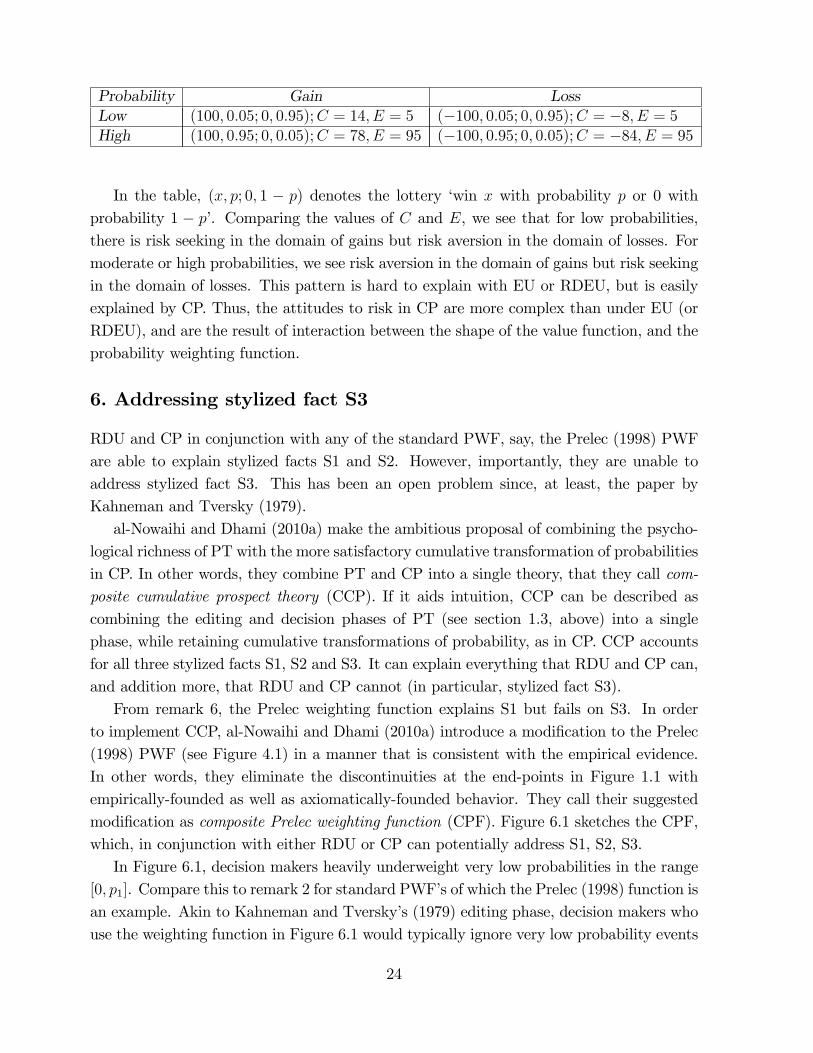
Probability Gain LossLow (100; 0:05; 0; 0:95);C = 14; E = 5 (�100; 0:05; 0; 0:95);C = �8; E = 5High (100; 0:95; 0; 0:05);C = 78; E = 95 (�100; 0:95; 0; 0:05);C = �84; E = 95

In the table, (x; p; 0; 1 � p) denotes the lottery �win x with probability p or 0 withprobability 1 � p�. Comparing the values of C and E, we see that for low probabilities,there is risk seeking in the domain of gains but risk aversion in the domain of losses. Formoderate or high probabilities, we see risk aversion in the domain of gains but risk seekingin the domain of losses. This pattern is hard to explain with EU or RDEU, but is easilyexplained by CP. Thus, the attitudes to risk in CP are more complex than under EU (orRDEU), and are the result of interaction between the shape of the value function, and theprobability weighting function.

6. Addressing stylized fact S3

RDU and CP in conjunction with any of the standard PWF, say, the Prelec (1998) PWFare able to explain stylized facts S1 and S2. However, importantly, they are unable toaddress stylized fact S3. This has been an open problem since, at least, the paper byKahneman and Tversky (1979).al-Nowaihi and Dhami (2010a) make the ambitious proposal of combining the psycho-

logical richness of PT with the more satisfactory cumulative transformation of probabilitiesin CP. In other words, they combine PT and CP into a single theory, that they call com-posite cumulative prospect theory (CCP). If it aids intuition, CCP can be described ascombining the editing and decision phases of PT (see section 1.3, above) into a singlephase, while retaining cumulative transformations of probability, as in CP. CCP accountsfor all three stylized facts S1, S2 and S3. It can explain everything that RDU and CP can,and addition more, that RDU and CP cannot (in particular, stylized fact S3).From remark 6, the Prelec weighting function explains S1 but fails on S3. In order

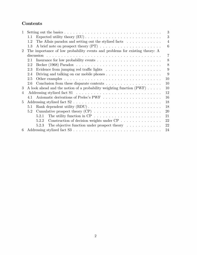
to implement CCP, al-Nowaihi and Dhami (2010a) introduce a modi�cation to the Prelec(1998) PWF (see Figure 4.1) in a manner that is consistent with the empirical evidence.In other words, they eliminate the discontinuities at the end-points in Figure 1.1 withempirically-founded as well as axiomatically-founded behavior. They call their suggestedmodi�cation as composite Prelec weighting function (CPF). Figure 6.1 sketches the CPF,which, in conjunction with either RDU or CP can potentially address S1, S2, S3.In Figure 6.1, decision makers heavily underweight very low probabilities in the range

[0; p1]. Compare this to remark 2 for standard PWF�s of which the Prelec (1998) function isan example. Akin to Kahneman and Tversky�s (1979) editing phase, decision makers whouse the weighting function in Figure 6.1 would typically ignore very low probability events

24

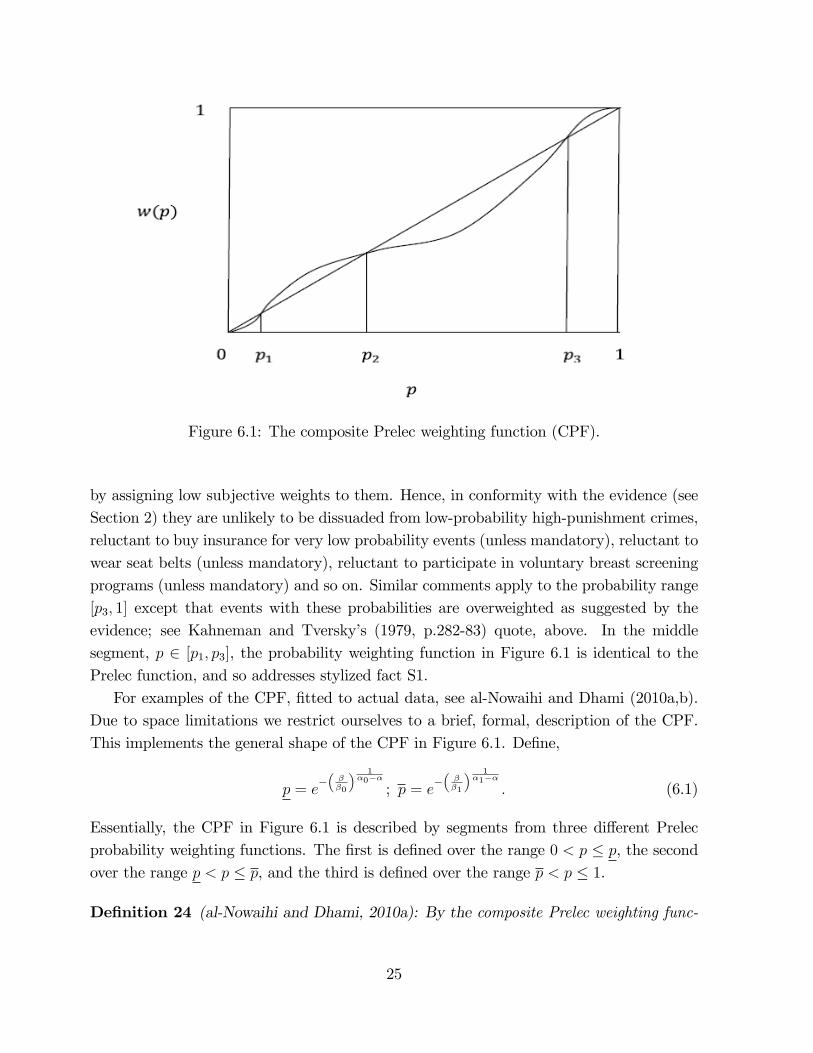
Figure 6.1: The composite Prelec weighting function (CPF).

by assigning low subjective weights to them. Hence, in conformity with the evidence (seeSection 2) they are unlikely to be dissuaded from low-probability high-punishment crimes,reluctant to buy insurance for very low probability events (unless mandatory), reluctant towear seat belts (unless mandatory), reluctant to participate in voluntary breast screeningprograms (unless mandatory) and so on. Similar comments apply to the probability range[p3; 1] except that events with these probabilities are overweighted as suggested by theevidence; see Kahneman and Tversky�s (1979, p.282-83) quote, above. In the middlesegment, p 2 [p1; p3], the probability weighting function in Figure 6.1 is identical to thePrelec function, and so addresses stylized fact S1.For examples of the CPF, �tted to actual data, see al-Nowaihi and Dhami (2010a,b).

Due to space limitations we restrict ourselves to a brief, formal, description of the CPF.This implements the general shape of the CPF in Figure 6.1. De�ne,

p = e����0

� 1�0��

; p = e����1

� 1�1��

: (6.1)

Essentially, the CPF in Figure 6.1 is described by segments from three di¤erent Prelecprobability weighting functions. The �rst is de�ned over the range 0 < p � p, the secondover the range p < p � p, and the third is de�ned over the range p < p � 1.

De�nition 24 (al-Nowaihi and Dhami, 2010a): By the composite Prelec weighting func-

25

tion we mean the probability weighting function w : [0; 1]! [0; 1] given by

w (p) =

8>><>>:0 if p = 0

e��0(� ln p)�0

if 0 < p � pe��(� ln p)

�

if p < p � pe��1(� ln p)

�1if p < p � 1

(6.2)

where p and p are given by (6.1) and

0 < � < 1, � > 0; �0 > 1, �0 > 0; �1 > 1, �1 > 0; �0 < 1=��0�11�� , �1 > 1=�

�1�11�� . (6.3)

Since a PWF (De�nition 2) is one to one and onto over the interval, [0; 1], De�nition24 implies that w(1) = 1.

Proposition 10 (al-Nowaihi and Dhami, 2010a): The composite Prelec function is aprobability weighting function.

The restrictions in (6.3) are required by the axiomatic derivations of the Prelec function(see section 4.1) and to ensure continuity of the CPF; see al-Nowaihi and Dhami (2010a)for the details.De�ne p1, p2, p3 that correspond to the notation used for the general shape of a CPF

in Figure 6.1.

p1 = e��1�0

� 1�0�1

, p2 = e�( 1� )

1��1, p3 = e

��1�1

� 1�1�1

(6.4)

Proposition 11 (al-Nowaihi and Dhami, 2010a): (a) p1 < p < p2 < p < p3. (b) p 2(0; p1) ) w (p) < p. (c) p 2 (p1; p2) ) w (p) > p. (d) p 2 (p2; p3) ) w (p) < p. (e)p 2 (p3; 1)) w (p) > p.

By Proposition 10, the CPF in (6.2), (6.3) is a PWF in the sense of De�nition 2.By Proposition 11, a CPF overweights low probabilities, i.e., those in the range (p1; p2),and underweights high probabilities, i.e., those in the range (p2; p3). Thus, it accountsfor stylized fact S1. But, in addition, and unlike all the standard probability weightingfunctions, it underweights probabilities near zero, i.e., those in the range (0; p1), andoverweights probabilities close to one, i.e., those in the range (p3; 1) as required in S3.

Proposition 12 (al-Nowaihi and Dhami, 2010a): The CPF (6.2):(a) zero-underweights in�nitesimal probabilities, i.e., lim

p!0w(p)p= 0 (De�nition 4a),

(b) zero-overweights near-one probabilities, i.e., limp!1

1�w(p)1�p = 0 (De�nition 4b).

al-Nowaihi and Dhami (2010a) show that their proposed probability weighting functionin Figure 6.1 is axiomatic, parsimonious and �exible. The axiomatic derivation uses theaxiom of local power invariance, which is a variant of the axiom that al-Nowaihi and Dhami(2006) use in the proof of the Prelec PWF.

26

De�nition 25 (al-Nowaihi and Dhami, 2010a): Otherwise standard CP, when combinedwith a CPF is called composite cumulative prospect theory (CCP). Analogously, otherwisestandard RDU, when combined with a CPF, is referred to as composite rank dependentutility (CRDU).

al-Nowaihi and Dhami (2010a) prove the following proposition, whose intuition wouldby now be largely clear to the reader from our discussion of the CPF. Because probabil-ities in the middle ranges are weighted as in Prelec (1998), stylized fact S1 is explained.Because cumulative transformations of probability are undertaken in CCP and CRDU, S2is explained. And because of the property of the CPF in Proposition 12, S3 is explained.

Proposition 13 (al-Nowaihi and Dhami, 2010a): CCP and CRDU can explain S1, S2and S3.

Blavatskyy (2005) shows that the St. Petersberg paradox re-emerges under CP. al-Nowaihi and Dhami (2010a) show that the St. Petersberg paradox can be resolved underCCP mainly through the role played by the CPF. Rieger and Wang (2006) also propose aPWF that resolves the St. Petersberg paradox but it cannot explain stylized fact S3.In comparison to CRDU, CCP, in addition, incorporates reference dependence, loss

aversion and richer attitudes towards risk. Hence, it can explain everything that CRDUcan, but the converse is false. Furthermore, because CCP explains S1, S2 and S3, whileCP (and RDU) can only explain S1, S2, CCP can explain everything that CP (and RDU)can, but the converse is false. In light of these observations it is interesting to note theobservation in Machina (2008) that �RDU is currently the most popular decision theoryunder risk.�

References

[1] al-Nowaihi, A., Dhami, S., (2010a) Composite prospect theory: A proposal to combineprospect theory and cumulative prospect theory. University of Leicester DiscussionPaper.

[2] al-Nowaihi, A., Dhami, S., (2010b) Insurance behavior for low probability events.University of Leicester Discussion Paper.

[3] al-Nowaihi, A., Dhami, S., (2006) A simple derivation of Prelec�s probability weightingfunction. The Journal of Mathematical Psychology 50 (6), 521-524.

[4] al-Nowaihi, A., Dhami, S. and Bradley, I., (2008) �The Utility Function UnderProspect Theory�, Economics Letters 99, p.337�339.

27

[5] Bar Ilan, Avner (2000) �The Response to Large and Small Penalties in a NaturalExperiment�, Department of Economics, University of Haifa, 31905 Haifa, Israel.

[6] Bar Ilan, Avner and Bruce Sacerdote (2001) �The response to �nes and probability ofdetection in a series of experiments�National Bureau of Economic Research WorkingPaper 8638.

[7] Bar Ilan, Avner and Bruce Sacerdote (2004) �The response of criminals and noncrim-inals to �nes�Journal of Law and Economics, Vol. XLVII, 1-17.

[8] Becker, Gary (1968) �Crime and Punishment: an Economic Approach, �Journal ofPolitical Economy, 76, 169-217.

[9] Berns, G. S., Capra, C. M., Chappelow, J., Moore, and Noussair, C. (2008) Nonlinearneurobiological probability weighting functions for aversive outcomes. Neuroimage,39: 2047-57.

[10] Blavatskyy, P.R., (2005) Back to the St. Petersburg paradox? Management Science,51, 677-678.

[11] Camerer, Colin F. (2000) Prospect theory in the wild: Evidence from the �eld. In D.Kahneman and A. Tversky (eds.), Choices, Values, and Frames, Cambridge UniversityPress; Cambridge.

[12] Camerer, C. and Kunreuther, H. (1989) Experimental markets for insurance. Journalof Risk and Uncertainty, 2, 265-300.

[13] Currim, Imran S. and Rakesh K. Sarin (1989), �Prospect Versus Utility,�ManagementScience 35, 22-41

[14] Diecidue Enrico, Ulrich Schmidt and Horst Zank (2009) "Parametric Weighting Func-tions," Journal of Economic Theory 144, 1102-1118.

[15] Dhami, S. and al-Nowaihi, A. (2010a) Behavioral Economics: Theory, Evidence andApplications, Book manuscript in progress.

[16] Dhami, S. and al-Nowaihi, A. (2010b) The Becker paradox reconsidered through thelens of behavioral economics. University of Leicester Discussion Paper.

[17] Fishburn, Peter C. (1982) The foundations of expected utility. D. Reidel PublishingCompany. Dordrecht: Holland/Boston: U.S.A. London: England.

[18] Goldstein, W. M., and Einhorn, H. J. (1987), �Expression Theory and the PreferenceReversal Phenomena,�Psychological Review 94, 236-254.

28

[19] Gonzalez, R., Wu, G., (1999) On the shape of the probability weighting function.Cognitive Psychology 38, 129-166.

[20] Hey, John D. and Chris Orme (1994), �Investigating Generalizations of ExpectedUtility Theory Using Experimental Data,�Econometrica 62, 1291-1326.

[21] Kahneman, D., and Tversky, A. (Eds.). (2000). Choices, values and frames. New York:Cambridge University Press.

[22] Kahneman D., Tversky A., (1979) Prospect theory : An analysis of decision underrisk. Econometrica 47, 263-291.

[23] Karmarkar, Uday S. (1979), �Subjectively Weighted Utility and the Allais Paradox,�Organizational Behavior and Human Performance 24, 67-72.

[24] Kilka, Michael and Martin Weber (2001), �What Determines the Shape of the Prob-ability Weighting Function under Uncertainty?�Management Science 47, 1712-1726.

[25] Kolm, Serge-Christophe (1973) "A Note on Optimum Tax Evasion," Journal of PublicEconomics, 2, 265-270.

[26] Kunreuther, H., Ginsberg, R., Miller, L., Sagi, P., Slovic, P., Borkan, B., Katz, N.,(1978) Disaster insurance protection: Public policy lessons, Wiley, New York.

[27] Lattimore, J. R., Baker, J. K., Witte, A. D. (1992) The in�uence of probability onrisky choice: A parametric investigation. Journal of Economic Behavior and Organi-zation 17, 377-400.

[28] Levitt, S. D. (2004) �Understanding why crime fell in the 1990�s: Four factors thatexplain the decline and six that do not.�Journal of Economic Perspectives, 18: 163-190.

[29] Luce, R. D. (2001) Reduction invariance and Prelec�s weighting functions. Journal ofMathematical Psychology 45, 167-179.

[30] Luce, R. Duncan, Barbara A. Mellers, and Shi-Jie Chang (1993), �Is Choice theCorrect Primitive? On Using Certainty Equivalents and Reference Levels to PredictChoices among Gambles,�Journal of Risk and Uncertainty 6, 115-143.

[31] Machina, M. J. (2008) Non-expected utility theory. in Durlaf, S. N. and Blume, L.E. (eds.) The New Palgrave Dictionary of Economics, 2nd Edition, Macmillan (Bas-ingstoke and New York).

29

[32] Mas-Collel, Andreu, Michael D. Whinston, and Jerry R. Green. (1995) MicroeconomicTheory, New. York: Oxford Univ. Press.

[33] Polinsky, Mitchell and Steven Shavell (2007) �The theory of public enforcement oflaw.�Chapter 6 in Polinsky, Mitchell and Steven Shavell (eds.) Handbook of Law andEconomics, Vol. 1, Elsevier.

[34] Pöystia, L., Rajalina, S., and Summala, H., (2005) �Factors in�uencing the use ofcellular (mobile) phone during driving and hazards while using it.�Accident Analysis& Prevention, 37: 47-51.

[35] Prelec, D., (1998) The probability weighting function. Econometrica 60, 497-528.

[36] Quiggin, J. (1982) A theory of anticipated utility. Journal of Economic Behavior andOrganization 3, 323-343.

[37] Quiggin, J. (1993) Generalized Expected Utility Theory, Kluwer Academic Publishers.

[38] Radelet, M. L. and R. L. Ackers, (1996) "Deterrence and the Death Penalty: TheViews of the Experts." Journal of Criminal Law and Criminology 87 : 1-16.

[39] Rieger, M.O., Wang, M. (2006) Cumulative prospect theory and the St. Petersburgparadox. Economic Theory 28, 665-679.

[40] Röell, Ailsa (1987), �Risk Aversion in Quiggin and Yaari�s Rank-Order Model ofChoice under Uncertainty,�Economic Journal 97, 143-160.

[41] Royal Society for the Prevention of Accidents (2005) �The risk of using a mobile phonewhile driving�. Full text of the report can be found at www.rospa.com.

[42] Safra, Zvi and Uzi Segal (1998), �Constant Risk Aversion,� Journal of EconomicTheory 83, 19-42.

[43] Schade, C., Kunreuther, H., and Kaas, K. P. (2001) Low-Probability Insurance: AreDecisions Consistent with Normative Predictions? mimeo. University of Humboldt.

[44] Starmer, C. (2000) "Developments in Non-expected Utility Theory: The Hunt fora Descriptive Theory of Choice under Risk," Journal of Economic Literature, 38:332-382.

[45] Starmer, Chris and Robert Sugden (1989), �Probability and Juxtaposition E¤ects:An Experimental Investigation of the Common Ratio E¤ect,� Journal of Risk andUncertainty 2, 159-178.

30

[46] Stott, H.P. (2006) Choosing from cumulative prospect theory�s functional menargerie.Journal of Risk and Uncertainty 32 (2006) 101-130.

[47] Tversky, A., Kahneman D. (1992) Advances in prospect theory : Cumulative repre-sentation of uncertainty. Journal of Risk and Uncertainty 5, 297-323.

[48] Varian, Hal. 1992. Microeconomic Analysis, New York: W. W. Norton.

[49] Williams. A. and Lund, A. (1986) �Seat belt use laws and occupant crash protectionin the United States.�American Journal of Public Health, 76: 1438-42.

31