Embed Size (px)
Citation preview
Probability Theory
Kalle Kytola
1

Contents
Foreword ivGlossary of notations vi
Chapter O. Introduction ixO.1. What are the basic objects of probability theory? ixO.2. Informal examples of the basic objects in random phenomena xO.3. Probability theory vs. measure theory xiii
Chapter I. Structure of event spaces 1I.1. Set operations on events 1I.2. Definition of sigma algebra 2I.3. Generating sigma algebras 3
Chapter II. Measures and probability measures 7II.1. Measurable spaces 7II.2. Definition of measures and probability measures 8II.3. Properties of measures and probability measures 13II.4. Identification and construction of measures 16
Chapter III. Random variables 21III.1. Measurable functions and random variables 22III.2. Indicator random variables 23III.3. Constructing random variables 24III.4. Simple functions 30
Chapter IV. Information generated by random variables 35IV.1. Definition of σ-algebra generated by random variables 36IV.2. Doob’s representation theorem 37
Chapter V. Independence 39V.1. Definition of independence 39V.2. Verifying independence 42V.3. Borel – Cantelli lemmas 43
Chapter VI. Events of the infinite horizon 47VI.1. Definition of the tail σ-algebra 47VI.2. Kolmogorov’s 0-1 law 50
Chapter VII. Integration theory 55VII.1. Integral for non-negative simple functions 57VII.2. Integral for non-negative measurable functions 59VII.3. Integral for integrable functions 63VII.4. Convergence theorems for integrals 65VII.5. Integrals over subsets and restriction of measures 69VII.6. Riemann integral vs. Lebesgue integral 70
i
ii CONTENTS
Chapter VIII. Expected values 71VIII.1. Expected values in terms of laws 72VIII.2. Applications of convergence theorems for expected values 75VIII.3. Space of p-integrable random variables 78
Chapter IX. Product spaces and Fubini’s theorem 81IX.1. Product sigma algebra 82IX.2. Product measure 84
Chapter X. Probability on product spaces 93X.1. Joint laws 93X.2. Variances and covariances of square integrable random variables 97X.3. Independence and products 99X.4. A formula for the expected value 103
Chapter XI. Probabilistic notions of convergence 107XI.1. Notions of convergence in stochastics 107XI.2. Weak and strong laws of large numbers 110XI.3. Proof of the weak law of large numbers 111XI.4. Proof of the strong law of large numbers 113XI.5. Kolmogorov’s strong law of large numbers 115
Chapter XII. Central limit theorem and convergence in distribution 117XII.1. Characteristic functions 118XII.2. Convergence in distribution 125XII.3. Central limit theorem 125
Appendix A. Set theory preliminaries 127A.1. Intersections and unions of sets 127A.2. Set differences and complements 127A.3. Images and preimages of sets under functions 128A.4. Cartesian products 128A.5. Power set 129A.6. Sequences of sets 129A.7. Countable and uncountable sets 130
Appendix B. Topological preliminaries 137B.1. Topological properties of the real line 137B.2. Metric space topology 140
Appendix C. Dynkin’s identification and monotone class theorem 145C.1. Monotone class theorem 145C.2. Auxiliary results 145C.3. Proof of Dynkin’s identification theorem 147C.4. Proof of Monotone class theorem 148
Appendix D. Monotone convergence theorem 149D.1. Monotone convergence theorem for simple functions 149D.2. Monotone convergence theorem for general non-negative functions 150
Appendix E. Orthogonal projections and conditional expected values 155E.1. Geometry of the space of square integrable random variables 155E.2. Conditional expected values 160
CONTENTS iii
Appendix F. Characteristic functions 165F.1. Levy’s inversion theorem 165F.2. Equivalent conditions for convergence in distribution 169
Appendix. Index 175
Appendix. References 179
iv CONTENTS
Foreword
These lecture notes are primarily intended for the regular M.Sc. level course MS-E1600 Probability Theory at Aalto University.
The principal aim of the course is to familiarize the students with the mathematicalfoundations of randomness. The reasons why one should study such a theoreticalformalism vary according to the ambitions of the individual. The development of alogically solid theory of random phenomena should perhaps be seen as worthwhile inits own right. We will stick strictly to the fundamentals, so this course offers quiteideal practice on precise mathematical reasoning, including formulating proofs. Amore pragmatic motivation might be that these theoretical foundations are necessaryfor following many subsequent courses in probability and statistics, and for under-standing more advanced topics. In any case, whether one plans to work in statistics,machine learning, or pure mathematics, relevant research literature often requiresfamiliarity of this theory as a language, e.g., being able to distinguish between con-vergence in probability, convergence in distribution, convergence almost surely, orother notions of convergence of random variables. The present course attempts toprovide just enough of the core mathematical theory to develop an appreciation ofsuch differences.
The course in its current format is very concise: 12 lectures and six sets of exercisesduring a six weeks period. One of the regrettable consequences is that there isalmost no time to enter any of the interesting applications of the theory that is beingdeveloped. There are other courses devoted to more specific topics in probabilitywhich build on the theoretical foundations of the present course and come closer toactual applications.
In order to be prepared to internalize the theory during this concise course, thestudent must have a little bit of mathematical maturity to begin with. Besidessome calculus of infinite series, differentiation, and integration, it is crucial to have aworking knowledge of set theory, especially the notion of countability, and a little bitof familiarity with continuous functions in the context of metric spaces or topologicalspaces, say. Appendices A and B serve as quick reminders of such prerequisites, andbefore engaging in this text beyond the introduction, one should make sure to grasptheir content.
The material in the chapters which correspond to the 12 lectures has been kept tominimum. A number of basic results that do not fit in these are left to Appen-dices C – F. The material in the main chapters can be considered as the minimumof what the students are expected to internalize during the short course, while thematerial in these appendices is something that one can expect to encounter soonafter this basic course, and it can then be quickly picked up with a little bit offurther effort.
There is already a vast number of textbooks in probability theory, and the con-tents of mathematics courses at advanced B.Sc. or early M.Sc. level have becomequite standard. For the students of the present course we recommend in particu-lar [JP04], because it is a very concise account of probability theory quickly coveringvery much the same topics as the present course. A slightly more challenging alterna-tive is [Wil91], which is a remarkably well-written, mathematically elegant accountof probability that manages incorporate fascinating and important probabilistic in-sights into a brief text. Both the theory and a significant number of interesting
FOREWORD v
and relevant examples and applications are covered in [Dur10]. The present lecturenotes borrow shamelessly from all of the above sources. And the purpose of thesenotes is not to replace the best textbooks on the subject, but rather to provide thestudents an account that follows the structure and scope of the concise six weeksprobability theory course as closely as possible.
The structure of these notes is largely based on an earlier version of the coursetaught by Lasse Leskela, and on parts of the textbook [Wil91]. I have receivedvery valuable comments, especially by Joona Karjalainen, Alex Karrila, and NikoLietzen, as well as many students, which have lead to improvements to the notes.I am, of course, responsible for all remaining mistakes. Still, you could help me —and perhaps more importantly the students who will use this material — by sendingcomments about mistakes, misprints, needs for clarification, etc., to me by email([email protected]).
vi CONTENTS
Glossary of notations
For convenience, we provide here a list of some of the used mathematical notationand abbreviations, together with brief explanations or references to the appropriatedefinitions during the course.
Numbers
Z the set of integers Z = . . . ,−2,−1, 0, 1, 2, . . .
Z≥0 the set of non-negative integers Z≥0 = 0, 1, 2, 3, . . .
N the set of natural numbers N = 1, 2, 3, 4, . . .
Q the set of rational numbers Q =nm
∣∣ n,m ∈ Z, m 6= 0
R the set of real numbers
C the set of complex numbers C =x+ iy
∣∣ x, y ∈ R
i imaginary unit i =√−1 ∈ C
(a, b) open interval (a, b) =x ∈ R
∣∣ a < x < b
[a, b] closed interval [a, b] =x ∈ R
∣∣ a ≤ x ≤ b
(a, b] (a, b] =x ∈ R
∣∣ a < x ≤ b
[a, b) [a, b) =x ∈ R
∣∣ a ≤ x < b
Logical notation
⇒ logical implication (“only if”) P ⇒ Q means:if P is true then also Q is true
⇐ reverse logical implication (“if”) P ⇐ Q means:if Q is true then also P is true
⇔ logical equivalence P ⇔ Q means:P is true if and only if Q is true
∀ “for all” (logical quantifier)
∃ “there exists” (logical quantifier)
s.t. such that
iff if and only if
GLOSSARY OF NOTATIONS vii
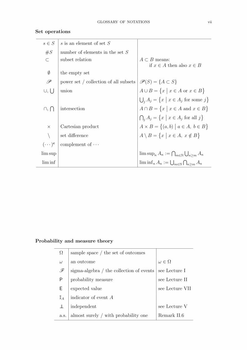
Set operations
s ∈ S s is an element of set S
#S number of elements in the set S
⊂ subset relation A ⊂ B means:if x ∈ A then also x ∈ B
∅ the empty set
P power set / collection of all subsets P(S) = A ⊂ S
∪,⋃
union A ∪B =x∣∣ x ∈ A or x ∈ B
⋃j Aj =
x∣∣ x ∈ Aj for some j
∩,⋂
intersection A ∩B =x∣∣ x ∈ A and x ∈ B
⋂j Aj =
x∣∣ x ∈ Aj for all j
× Cartesian product A×B =
(a, b)
∣∣ a ∈ A, b ∈ B\ set difference A \B =
x∣∣ x ∈ A, x /∈ B
(· · · )c complement of · · ·
lim sup lim supnAn :=⋂m∈N
⋃n≥mAn
lim inf lim infnAn :=⋃m∈N
⋂n≥mAn
Probability and measure theory
Ω sample space / the set of outcomes
ω an outcome ω ∈ Ω
F sigma-algebra / the collection of events see Lecture I
P probability measure see Lecture II
E expected value see Lecture VII
IA indicator of event A
⊥⊥ independent see Lecture V
a.s. almost surely / with probability one Remark II.6
viii CONTENTS
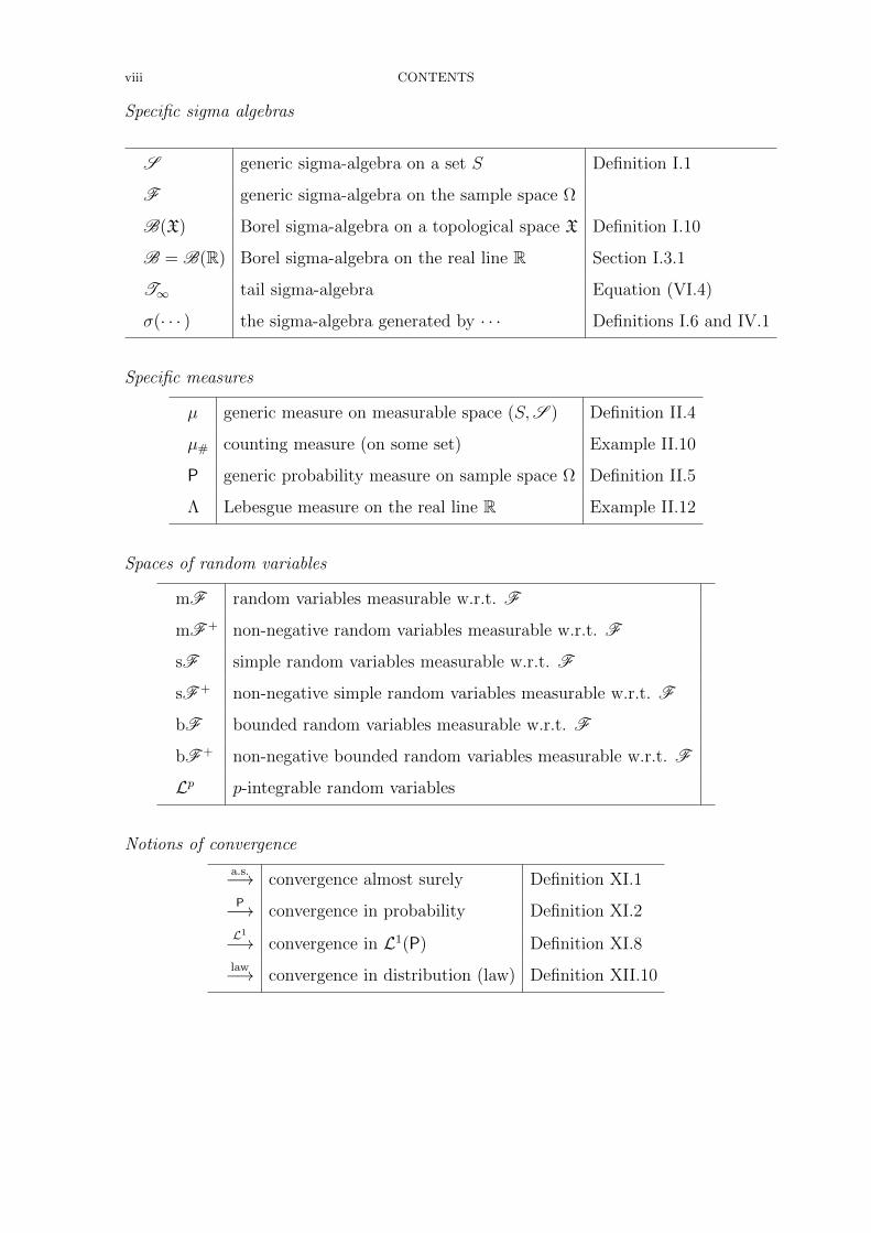
Specific sigma algebras
S generic sigma-algebra on a set S Definition I.1
F generic sigma-algebra on the sample space Ω
B(X) Borel sigma-algebra on a topological space X Definition I.10
B = B(R) Borel sigma-algebra on the real line R Section I.3.1
T∞ tail sigma-algebra Equation (VI.4)
σ(· · · ) the sigma-algebra generated by · · · Definitions I.6 and IV.1
Specific measures
µ generic measure on measurable space (S,S ) Definition II.4
µ# counting measure (on some set) Example II.10
P generic probability measure on sample space Ω Definition II.5
Λ Lebesgue measure on the real line R Example II.12
Spaces of random variables
mF random variables measurable w.r.t. F
mF + non-negative random variables measurable w.r.t. F
sF simple random variables measurable w.r.t. F
sF + non-negative simple random variables measurable w.r.t. F
bF bounded random variables measurable w.r.t. F
bF + non-negative bounded random variables measurable w.r.t. F
Lp p-integrable random variables
Notions of convergence
a.s.−→ convergence almost surely Definition XI.1P−→ convergence in probability Definition XI.2
L1−→ convergence in L1(P) Definition XI.8law−→ convergence in distribution (law) Definition XII.10
Lecture O
Introduction
O.1. What are the basic objects of probability theory?
Probability theory forms the mathematically precise and powerful foundations forthe study of randomness. Its most basic objects — defined and studied in the restof this course — are:
Ω — Outcomes (of a random experiment)An outcome ω of a random experiment represents a single realizationof the randomness involved. The sample space Ω is the set consistingof all possible outcomes.
F — Events1
An event E is a subset E ⊂ Ω of the set of possible outcomes. Theevent E is said to occur if the randomly realized outcome ω ∈ Ω belongsto this subset, i.e., if ω ∈ E. Generally we can not allow all subsets ofΩ as events, but instead we have to select a suitable collection F ofsubsets on which it is possible to have consistent rules of probability.
P — Probability (measure)2
To each event E we assign the probability P[E] of the event, which isa real number between 0 and 1.
In addition to the three basic objects (Ω,F ,P) above, the following two fundamentalnotions will also be indispensable:
Random variable3
Random variables are the quantities of interest in our probabilisticmodel. A random variable is a suitable function X : Ω→ S, associatingto each possible outcome ω ∈ Ω a value X(ω) ∈ S. You may thinkof the Goddess of Chance choosing the outcome ω at random, andthe chosen outcome subsequently determining the value X(ω) of anyquantity of interest.
Expected value4
The expected value E[X] of a real-valued quantity of interest X, i.e., arandom variable X : Ω→ S ⊂ R, represents an average of the possiblevalues of X over all randomness, weighted according to probabilities P.The expected value is an integral with respect to the probability mea-sure P in the sense of Lebesgue, and we will correspondingly use the
1We will address the precise axioms required of the collection F of events in Lecture I.2We will address the precise axioms required of the probability measure P in Lecture II.3Random variables will be defined precisely in Lecture III.4Expected values will be defined precisely in Lecture VII.
ix
x O. INTRODUCTION
following notations interchangeably
E[X]
=
∫Ω
X(ω) dP(ω).
The purpose of this course is to make precise mathematical sense of the abovenotions. Before rushing into the theory, however, we continue with a brief informalintroduction. For the informal examples below, it suffices to have an intuitive ideaof the above notions.
O.2. Informal examples of the basic objects in random phenomena
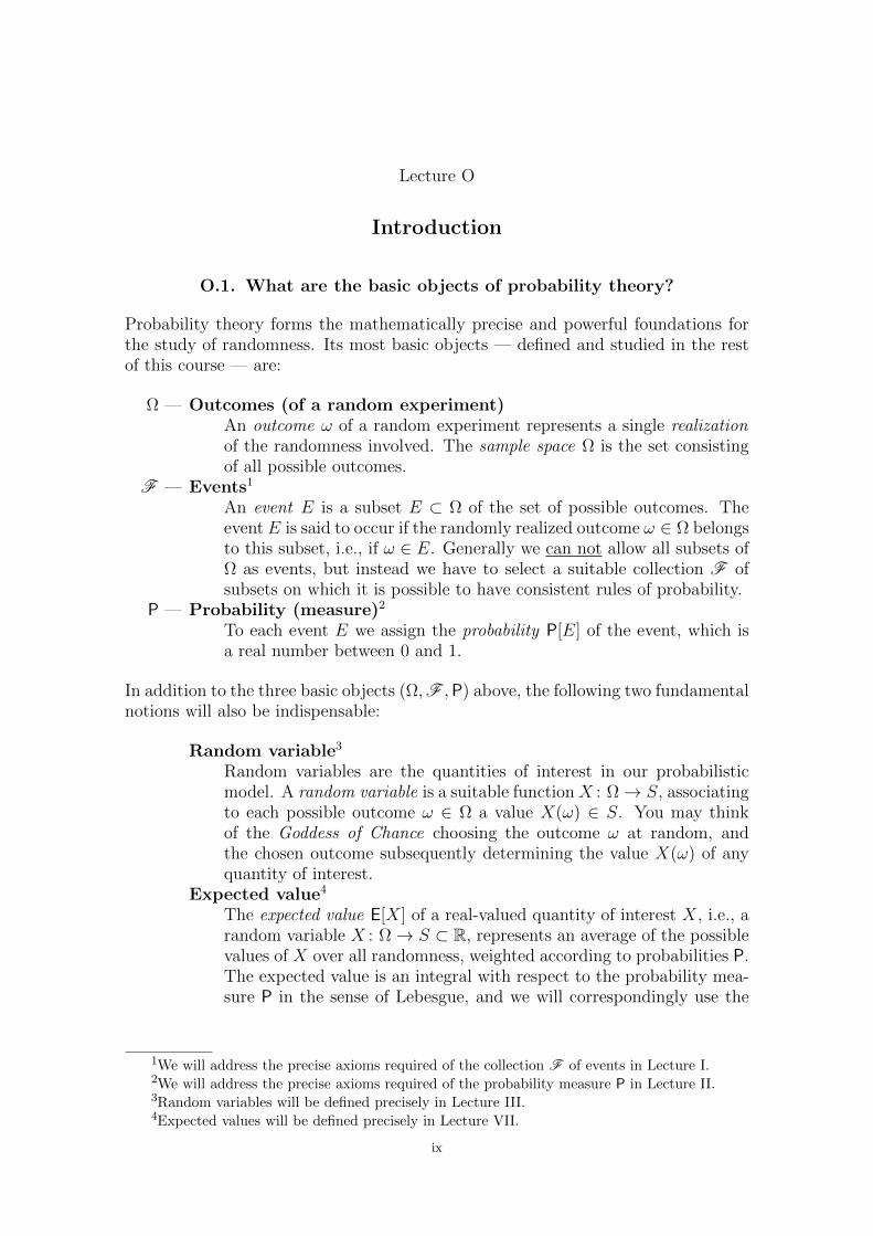
Example O.1 (One coin toss).The possible outcomes of a single coin toss are “heads” and “tails”, abbreviated H and T,respectively. The sample space of a single coin toss experiment would thus be
Ω = H,T .As events, we can in this case allow all subsets of Ω, so the collection of events is
F =∅, H , T , H,T
,
with interpretations of the events:
H the event that the coin toss results in “heads”
T the event that the coin toss results in “tails”
∅ the event that the coin toss results in neither “heads” nor “tails”
H,T the event that the coin toss results in either “heads” or “tails”
The last two events may appear perplexingly trivial, but we want to allow them as events,because logical reasoning with other events may result in impossibilities or certainties. Infact, ∅ ⊂ Ω always corresponds to the impossible event, which is not realized by any possibleoutcome ω ∈ Ω, whereas Ω ⊂ Ω always corresponds to the sure event which is realized byany outcome ω ∈ Ω of the randomness.
A fair coin toss is considered equally likely to result in “heads” or “tails”, and a single faircoin toss is thus unsurprisingly governed by the probability measure P which assigns thefollowing probabilities to the above events:
P[H
]=
1
2, P
[T
]=
1
2, P
[∅]
= 0, P[H,T
]= 1.
This example is not overly exciting, but the distinct roles of the three basic objects Ω, F ,and P should be recognized here!
Example O.2 (Repeated coin tossing).In an experiment where coin tosses are repeated ad infinitum, the possible outcomes areall possible sequences of “heads” and “tails”, i.e., functions from N to H,T. The samplespace of such a repeated coin tossing experiment would be the space of all such functions
Ω = H,TN =ω : N→ H,T
,
O.2. INFORMAL EXAMPLES OF THE BASIC OBJECTS IN RANDOM PHENOMENA xi
which is uncountably infinite (it can be identified with the set of infinite binary sequences,Example A.16). This uncountable cardinality in a rather innocent probabilistic model canbe taken as the first warning that some care is needed in a proper mathematical treatmentof probability.
LetXn denote the relative frequency of heads in the first n coin tosses. The relative frequencyis a function of the outcome ω (as random variables generally are!), given by the ratio
Xn(ω) =#j∣∣ j ≤ n and ω(j) = H
n
.
We may ask whether the frequencyXn tends to 12 in the long run, as n→∞. This is certainly
not true for all ω ∈ Ω = H,TN. For example for the sequence ω′ = (H,H,H,H, . . .) of allheads, we have Xn(ω′) = 1 for all n and therefore limn→∞Xn(ω′) = 1 6= 1
2 . Even worse, forthe sequence
ω′′ = (H,T,T,T︸ ︷︷ ︸3 times
,H,H,H,H,H,H,H,H,H︸ ︷︷ ︸32 times
,T, . . . ,T︸ ︷︷ ︸33 times
, . . .)
the limit limn→∞Xn(ω′′) does not even exists. In view of these “counterexamples”, it shouldbe clear that any statement about Xn tending to 1
2 in the long run must be probabilistic innature (somehow referring to P), rather than pointwise on the entire sample space Ω.
There are various possible probabilistic notions of Xn tending to 12 as n→∞. Compare for
example the following two statements:
(a) For any ε > 0 we have
limn→∞
P[|Xn −
1
2| > ε
]= 0.
(b) We have
P[
limn→∞
Xn =1
2
]= 1.
As we develop the mathematical foundations of probability, we should ask, for example:
• Can we make precise mathematical sense of statements such as (a) and (b) above?• Does one of these two statements imply the other?• Is either of the statements actually true?
(say for the usual probability P governing fair, repeated coin tossing)
The next example further illustrates the types of questions one may want to answerwith the mathematical theory of probability. It concerns a branching populationmodel known as Galton-Watson process.5 In the footnotes we indicate which parts ofthe present course are relevant for the questions that arise, but the reader interestedin the detailed solutions should look them up in books on stochastic processes.
5The idea of using this branching process to illustrate the applicability of probability theoryis borrowed from the excellent textbook [Wil91].
xii O. INTRODUCTION
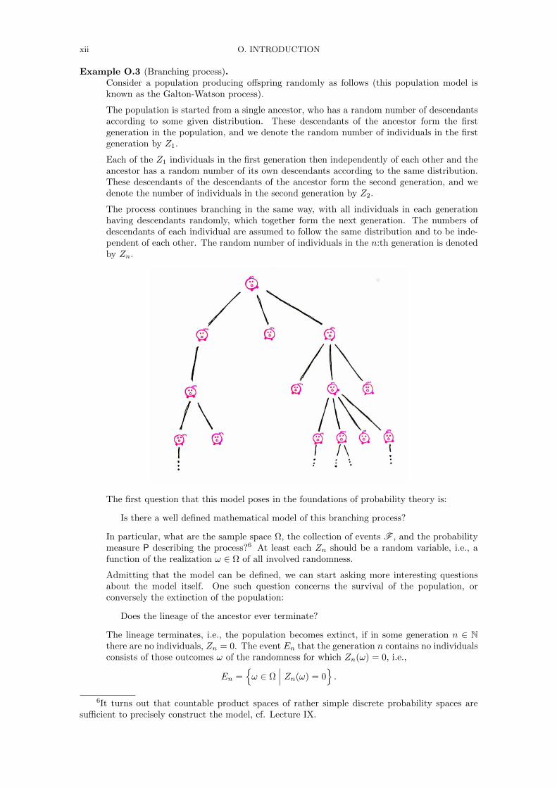
Example O.3 (Branching process).Consider a population producing offspring randomly as follows (this population model isknown as the Galton-Watson process).
The population is started from a single ancestor, who has a random number of descendantsaccording to some given distribution. These descendants of the ancestor form the firstgeneration in the population, and we denote the random number of individuals in the firstgeneration by Z1.
Each of the Z1 individuals in the first generation then independently of each other and theancestor has a random number of its own descendants according to the same distribution.These descendants of the descendants of the ancestor form the second generation, and wedenote the number of individuals in the second generation by Z2.
The process continues branching in the same way, with all individuals in each generationhaving descendants randomly, which together form the next generation. The numbers ofdescendants of each individual are assumed to follow the same distribution and to be inde-pendent of each other. The random number of individuals in the n:th generation is denotedby Zn.
The first question that this model poses in the foundations of probability theory is:
Is there a well defined mathematical model of this branching process?
In particular, what are the sample space Ω, the collection of events F , and the probabilitymeasure P describing the process?6 At least each Zn should be a random variable, i.e., afunction of the realization ω ∈ Ω of all involved randomness.
Admitting that the model can be defined, we can start asking more interesting questionsabout the model itself. One such question concerns the survival of the population, orconversely the extinction of the population:
Does the lineage of the ancestor ever terminate?
The lineage terminates, i.e., the population becomes extinct, if in some generation n ∈ Nthere are no individuals, Zn = 0. The event En that the generation n contains no individualsconsists of those outcomes ω of the randomness for which Zn(ω) = 0, i.e.,
En =ω ∈ Ω
∣∣∣ Zn(ω) = 0.
6It turns out that countable product spaces of rather simple discrete probability spaces aresufficient to precisely construct the model, cf. Lecture IX.
O.3. PROBABILITY THEORY VS. MEASURE THEORY xiii
We may observe that if the generation n contains no individuals, then the next generationn+ 1 can not contain any either, so
Zn(ω) = 0 =⇒ Zn+1(ω) = 0.
Equivalently, for the corresponding events we have the inclusion
En ⊂ En+1.
These events thus form an increasing sequence (of subsets of Ω)
E1 ⊂ E2 ⊂ E3 ⊂ · · · .
The probabilities of the events should increase correspondingly,
P[E1] ≤ P[E2] ≤ P[E3] ≤ · · ·
and as a bounded increasing sequence of real numbers, these probabilities have a limit
limn→∞
P[En].
One natural question is: can we use the events En to construct the event E that extinctionoccurs eventually?7 And is its probability P[E] equal to the above limit limn→∞ P[En]?8
A more ambitious version of the question is: can we concretely calculate the probabilityP[E] of eventual extinction?9
The expected size E[Zn] of generation n turns out to be dn, where d is the expected numberof descendants of one individual. Imagine then that we define the “renormalized size” ofgeneration n as Rn = d−n Zn, so as to have expected value one, E[Rn] = 1. By techniquesthat go just a little bit beyond the present course (martingale convergence theorem) one canshow that there exists a limit of the random variables Rn as n→∞. The limit
limn→∞
Rn
is itself a random variable, which can be interpreted to describe the asymptotic long termsize of the population in units that make the expected sizes equal to one. Given this, it isnatural to wonder whether the expected value of this asymptotic quantity can be calculatedby interchanging the limit and the expected value10
E[
limn→∞
Rn
]?= lim
n→∞E[Rn
]︸ ︷︷ ︸
=1
= 1.
Probability theory provides the means to make sense of and answer the many questions thatarise in this branching process example — as well as in other interesting models.
O.3. Probability theory vs. measure theory
The present course may appear to involve not so much of random phenomena them-selves, but more of dry and formal measure theory instead. Our justification for thisis that virtually all advanced probability and statistics builds on the measure theoret-ical foundations covered in the present course. Frequently used measure theoretical
7It turns out that σ-algebras, studied in Lecture I, permit just flexible enough logical operationsto allow such a construction.
8This indeed turns out to be true, by monotonicity properties of probability measures estab-lished in Lecture II.
9This can be done using generating functions — a close cousin of the characteristic functionsstudied in Lecture XII.
10Whether this can be done turns out to be subtle. In Lectures VII, VIII, and IX we willlearn under which conditions one can interchange the order of limits and expected values (andintegrals and sums, etc.). Such interchanges of order of operations are tremendously useful inmany calculations in practice.
xiv O. INTRODUCTION
tools in stochastics include Dominated Convergence Theorem, Monotone Conver-gence Theorem, Fubini’s theorem, Lp-spaces, etc. The formal foundations also serveas a common and well-defined language across different branches of stochastics. Forexample, various different notions of convergence of random variables used in math-ematical statistics are what we will be ready to introduce in the last two of ourlectures. The role of the present course is to develop the mathematical foundationsof probability mainly for future use!
Since a large number of basic definitions and results in measure theory and probabil-ity theory are literally identical, anyone who has already studied measure theory willrecognize many familiar notions. The overlap may raise the question: are measuretheory and probability theory really separate topics in their own right, and is it nec-essary to study them separately? It would, in fact, be possible to combine measuretheory and probability theory in one extended and coherent course, but the scopeof that could easily become daunting. As the topics are currently taught in separatecourses, it does not matter much whether one first studies measure theory and laterlearns about its applicability to probability, or if one proceeds in the opposite order.
Even concerning abstract measure theoretic notions and results, probability the-ory in fact offers very interesting and useful interpretations. In this course, suchinterpretations include, e.g.,
• product measures interpreted as probabilistic independence• push-forward measures interpreted as laws of random variables• (sub-)sigma-algebras interpreted as (partial) information.
At its best, probabilistic thinking leads to entirely new techniques in mathematics,such as
• coupling arguments• existence proofs relying on random choice.
And finally, probability theory includes inherently stochastic results which do notbelong to the domain of measure theory. Some such results covered in the presentcourse are:
• zero-one laws (Borel-Cantelli lemmas, Kolmogorov’s 0-1 law)• laws of large numbers• central limit theorems.
And despite the similarities, measure theory and probability theory are ultimatelyconcerned with different questions. To highlight just one difference in emphasis,note that the identification of the law of a random variable occupies a much morecentral place in probability theory than the corresponding question does in analysis.In developments beyond this first theoretical course, it becomes even more apparentthat probability theory is not just a subset of measure theory11 — consider, e.g.,martingales, ergodic theory, large deviations, stochastic calculus, optimal stopping,etc. It is also in such further studies, which build on the present foundational course,that the advantages of the theory will become clearer.
11Vice versa, of course, there are topics covered in courses of measure theory such as [Kin16],which are not covered in this course of probability theory, and there are aspects of the theory intowhich one gains valuable insights from analysis. Therefore, especially for serious mathematicians,it is highly recommended to study both topics!

O.3. PROBABILITY THEORY VS. MEASURE THEORY xv
We hope that these reassurances and the occasional genuinely probabilistic inter-pretations and results included in the lectures provide a sufficient motivation toseriously study also the formal (measure theoretical) aspects of probability!

Lecture I
Structure of event spaces
I.1. Set operations on events
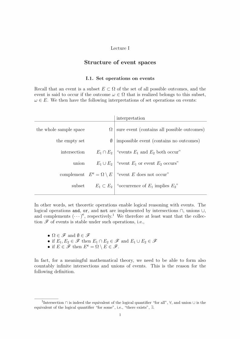
Recall that an event is a subset E ⊂ Ω of the set of all possible outcomes, and theevent is said to occur if the outcome ω ∈ Ω that is realized belongs to this subset,ω ∈ E. We then have the following interpretations of set operations on events:
interpretation
the whole sample space Ω sure event (contains all possible outcomes)
the empty set ∅ impossible event (contains no outcomes)
intersection E1 ∩ E2 “events E1 and E2 both occur”
union E1 ∪ E2 “event E1 or event E2 occurs”
complement Ec = Ω \ E “event E does not occur”
subset E1 ⊂ E2 “occurrence of E1 implies E2”
In other words, set theoretic operations enable logical reasoning with events. Thelogical operations and, or, and not are implemented by intersections ∩, unions ∪,and complements (· · · )c, respectively.1 We therefore at least want that the collec-tion F of events is stable under such operations, i.e.,
• Ω ∈ F and ∅ ∈ F• if E1, E2 ∈ F then E1 ∩ E2 ∈ F and E1 ∪ E2 ∈ F• if E ∈ F then Ec = Ω \ E ∈ F .
In fact, for a meaningful mathematical theory, we need to be able to form alsocountably infinite intersections and unions of events. This is the reason for thefollowing definition.
1Intersection ∩ is indeed the equivalent of the logical quantifier “for all”, ∀, and union ∪ is theequivalent of the logical quantifier “for some”, i.e., “there exists”, ∃.
1
2 I. STRUCTURE OF EVENT SPACES
I.2. Definition of sigma algebra
Definition I.1 (Sigma algebra).A collection F ⊂P(Ω) of subsets of a set Ω is a σ-algebra on Ω if
(Σ-1) : Ω ∈ F
(Σ-c) : if E ∈ F then Ec = Ω \ E ∈ F
(Σ-∪) : if E1, E2, . . . ∈ F then⋃n∈N
En ∈ F .
Remark I.2 (A sigma algebra is stable under countable set operations).Note that properties (Σ-1) and (Σ-c) imply that ∅ ∈ F , since ∅ = Ωc.
Likewise, properties (Σ-∪) and (Σ-c) imply that if E1, E2, . . . ∈ F then also⋂∞n=1En ∈ F ,
since⋂∞n=1En =
(⋃∞n=1En
c)c
by De Morgan’s laws, Proposition A.1.
Also, since ∅ ∈ F , we can extend any finite sequence E1, E2, . . . , Ek ∈ F of members ofthe collection to an infinite sequence by setting En = ∅ for all n > k, and we thus deducefrom (Σ-∪) that the finite union E1 ∪ · · · ∪En ∈ F also belongs to the collection. Similarly,finite intersections E1 ∩ · · · ∩ En of members of the collection remain in the collection.
In view of the definition and remark above, σ-algebras are stable under countable setoperations. Since we will always assume the collection of events to be a σ-algebra,we are thus allowed to perform rather flexible logical constructions with events.
Example I.3 (Examples and counterexamples of sigma algebras).
(i) F = ∅,Ω is a σ-algebra on Ω, albeit not a very interesting one: it only contains theimpossible event ∅ and the sure event Ω.
(ii) F = P(Ω), the collection of all subsets of Ω, is a σ-algebra on Ω. However, when Ωis uncountably infinite, consistent rules of probability can typically only be given on asmaller collection of events.
(iii) F = T (R), the collection of all open subsets of R, is not a σ-algebra on R! You shouldrecall that arbitrary unions of open sets are open, and finite intersections of open setsare also open. However, for example the countable intersection
⋂∞n=1(− 1
n ,1n ) = 0 of
open intervals consists of a single point and is not open. The collection in fact satisfies(Σ-1) and (Σ-∪), but fails to satisfy (Σ-c).
Exercise I.1 (Sigma algebras on small finite sets).Let a, b, c be three distinct points.
(a) Write down all σ-algebras on Ω = a, b.(b) Write down all σ-algebras on Ω = a, b, c.(c) Give an explicit counterexample which shows that the union of two σ-algebras is not
necessarily a σ-algebra.
In probability theory, we require the collection of events F to be a σ-algebra on thesample space Ω. The next examples illustrate what sorts of countable set operationswe might encounter in practice. These examples also give a fair idea of the expressivepower of such operations, when used iteratively.
Example I.4 (The event of branching process extinction).Let us revisit Example O.3 about the branching process. Let Zn denote the random sizeof the population in generation n ∈ N, which, as any random variable, depends on theoutcome ω of the underlying randomness. Consider first an event defined by the condition
I.3. GENERATING SIGMA ALGEBRAS 3
that the generation n contains no individuals
En =ω ∈ Ω
∣∣∣ Zn(ω) = 0.
Extinction happens in some generation in the future if there exists some n ∈ N such thatZn = 0. The corresponding event is
E =ω ∈ Ω
∣∣∣ ∃n ∈ N : Zn(ω) = 0
=⋃n∈N
ω ∈ Ω
∣∣∣ Zn(ω) = 0
=⋃n∈N
En.
We see that the event E of eventual extinction is the union over the countably many gener-ations n ∈ N of the events En that generation n is already extinct.
Countable set operations came to our rescue!
Example I.5 (Long term frequency of heads in coin tossing).Let us revisit Example O.2 about repeated coin tossing. Let Xn be the relative frequencyof heads in the first n coin tosses. Observe that the following are logically equivalent waysof expressing the property that the frequency tends to 1
2 in the long run:
limn→∞
Xn =1
2⇐⇒ ∀ε > 0 ∃k ∈ N such that ∀n ≥ k we have
∣∣Xn −1
2
∣∣ < ε
⇐⇒ ∀m ∈ N ∃k ∈ N such that ∀n ≥ k we have∣∣Xn −
1
2
∣∣ < 1
m.
The last expression requires only quantifiers over countable collections, and is therefore goodfor our purposes. Consider first an event by the condition |Xn − 1
2 | <1m ,
E(m)n :=
ω ∈ H,TN
∣∣∣ 1
2− 1
m< Xn(ω) <
1
2+
1
m
,
we can now express the event E that the frequency tends to 12 in the long run by the following
countable set operations:
E =⋂m∈N
⋃k∈N
⋂n≥k
E(m)n .
So at least provided that each E(m)n belongs to the collection F of admissible events (seems
reasonable) the properties of σ-algebras allow us to construct the more complicated butmuch more interesting event E ∈ F , which contains precise information about the longterm behavior of the frequencies of heads.
Iteratively constructed countable set operations came to our rescue!
I.3. Generating sigma algebras
Definition I.6 (Sigma algebra generated by a collection of subsets).Let C ⊂ P(Ω) be a collection of subsets of Ω. Then we define σ(C ) as thesmallest σ-algebra on Ω which contains the collection C . We call σ(C ) theσ-algebra generated by the collection C .
Remark I.7. The language of the above definition is intended to be as accessible as possible, butlet us make sure that the precise meanings are clear as well:
• We say that a σ-algebra F contains the collection C , if each member of C is a memberin F , i.e., if we have the inclusion C ⊂ F of the collections of sets.
• For two σ-algebras F1 and F2, we say that F1 is smaller than F2 if F1 ⊂ F2.
With these clarifications, the meaning should be unambiguous, but one still has to verify thatσ(C ) becomes well defined. If we want to define σ(C ) as the smallest σ-algebra containing C ,
4 I. STRUCTURE OF EVENT SPACES
we first need to know that such a σ-algebra exists and that it is unique!2 These concernswill be settled in Corollary I.9 below.
One standard use of generated σ-algebras is the following. If C is a collection of somebasic events that we want to be able to discuss, in our definition of a probabilisticmodel we could set F = σ(C ), which is exactly the smallest possible collection ofevents that contains the basic events and behaves well under countable operations.Isn’t this convenient!
In Lecture IV we discuss the interpretation of σ-algebras as describing information.We will realize that the notion of generated σ-algebras corresponds to what informa-tion can be deduced from some initially given pieces of information (the knowledgeabout events in the generating collection C ).
Finally, generated σ-algebras can also be used as a technical tool. It is often verydifficult to describe explicitly all members of even very common and reasonableσ-algebras. Working with suitably chosen generating collections can bring aboutsignificant simplifications.
Having thus motivated the notion of generated σ-algebras, let us finally addresstheir well-definedness. The key observation is that intersections of σ-algebras arethemselves σ-algebras.3
Lemma I.8. Suppose that (Fα)α∈I is a non-empty collection (indexed by I 6= ∅) ofσ-algebras Fα on Ω. Then also the intersection F =
⋂α∈I Fα is a σ-algebra
on Ω.
Proof. By requiring the collection to be non-empty, we ensured that the intersection is well-defined.
We need to verify that the intersection⋂α∈I Fα satisfies the three properties in Defini-
tion I.1. Note that for a subset E ⊂ Ω, we have E ∈ F =⋂α∈I Fα if and only if E ∈ Fα
for all α ∈ I.
We have Ω ∈ Fα for all α ∈ I, and therefore Ω ∈ F . Thus condition (Σ-1) holds for F .
Suppose that E ∈ F . Then for all α ∈ I we have E ∈ Fα. By property (Σ-c) for theσ-algebra Fα we get that Ec ∈ Fα. Since this holds for all α, we conclude Ec ∈ F . Thuscondition (Σ-c) holds for F .
Suppose that E1, E2, . . . ∈ F . Then for all α ∈ I we have E1, E2, . . . ∈ Fα. By property (Σ-∪) for the σ-algebra Fα we get that
⋃∞n=1En ∈ Fα. Since this holds for all α, we conclude⋃∞
n=1En ∈ F . Thus condition (Σ-∪) holds for F .
We are now ready to conclude that Definition I.1 indeed made sense.
Corollary I.9 (Well-definedness of the generated sigma algebra).Let C ⊂P(Ω) be a collection of subsets of Ω. Then the smallest σ-algebra onΩ which contains the collection C exists and is unique.
2Such issues must be taken seriously. To illustrate the existence issue, imagine trying todefine s > 0 as the smallest real number which is strictly positive: no such thing exists, and ifwe disregard that fact, we will soon run into logical contradictions. To illustrate the uniquenessissue, suppose that a, b, c are three distinct elements, and imagine trying to define S ⊂ a, b, c asthe smallest subset which contains an odd number of elements: any of the three singleton subsetsa , b , c ⊂ a, b, c are equally small, so which one should S be?
3By contrast, in Exercise I.1(c) you showed that the union of σ-algebras may fail to be aσ-algebra.
I.3. GENERATING SIGMA ALGEBRAS 5
Proof. The uniqueness part is usual abstract nonsense. Suppose we had two different smallestσ-algebras which contain the collection C , say F1 and F2. Then we would have F1 ⊂ F2
because F1 is smallest and F2 ⊂ F1 because F2 is smallest, so we get that F1 = F2.
It remains to show that a smallest σ-algebra which contains the collection C exists. Considerthe collection S of all σ-algebras F on Ω such that C ⊂ F . This collection S is non-empty,because as in Example I.3(ii), the power set of Ω is such a σ-algebra, i.e., P(Ω) ∈ S. Letus define σ(C ) as the intersection
σ(C ) :=⋂
F∈S
F
of all these σ-algebras. By Lemma I.8, σ(C ) is itself a σ-algebra. Since for each F ∈ Swe have C ⊂ F , the intersection also has this property, C ⊂ σ(C ). If F is any σ-algebrawhich contains C , then clearly σ(C ) is smaller, since F ∈ S appears in the intersection andthus σ(C ) ⊂ F . Thus the intersection σ(C ) is smallest.
I.3.1. Borel sigma algebra
Definition I.10 (Borel sigma algebra).For a topological space X, the Borel σ-algebra on X is the σ-algebra B(X)generated by the collection T (X) of open sets in X.
Arguably the most important σ-algebra in all of probability theory is the Borel σ-algebra on the real line R, because it is needed whenever we consider real valuedrandom variables. We denote simply B = B(R). By definition, B is the smallestσ-algebra on R which contains all opens sets V ⊂ R. The following propositionestablishes that B can alternatively be generated by various convenient collectionsof subsets of the real line.
Proposition I.11 (Generating the Borel sigma algebra on the real line).The Borel σ-algebra B on the real line R is generated by any of the followingcollections of subsets of R:
(i) : C =
(−∞, x]∣∣∣ x ∈ R
, (iii) : C =
(x, y)
∣∣∣ x, y ∈ R, x < y,
(ii) : C =
[x, y]∣∣∣ x, y ∈ R, x ≤ y
, (iv) : C =
(x, y]
∣∣∣ x, y ∈ R, x < y.
Remark I.12. The reader can certainly imagine further variations of generating collections ofintervals, and is invited to think about the modifications needed in the proof below.
Proof of Proposition I.11. We will only explicitly check that the collection (i) generates B, theother cases are similar.
So for the case (i), let C be the collection of all intervals of the form (−∞, x], with x ∈ R.In order to show that σ(C ) = B, we will separately check the two converse inclusionsσ(C ) ⊂ B and σ(C ) ⊃ B.
inclusion σ(C ) ⊂ B: To show that σ(C ) ⊂ B, it is sufficient to show that B contains all intervalsof the form (−∞, x], because σ(C ) is by definition the smallest such σ-algebra.
Note that the set (x,+∞) is open, and thus is contained in the Borel σ-algebra by definition.
The complement of it is((x,+∞)
)c= R \ (x,+∞) = (−∞, x]. Since B is a σ-algebra on R
which contains (x,+∞), by property (Σ-c) it contains also the complement (−∞, x]. Theinclusion σ(C ) ⊂ B follows.
6 I. STRUCTURE OF EVENT SPACES
inclusion σ(C ) ⊃ B: To show that σ(C ) ⊃ B, it is sufficient to show that σ(C ) contains all opensets V ⊂ R, because B is by definition the smallest such σ-algebra. Let us show step bystep that σ(C ) contains all sets of the forms
(a) semi-open intervals intervals (x, y], for x, y ∈ R(b) open intervals (x, z), for x, z ∈ R(c) open sets V ⊂ R.
For case (a), note that
(x, y] = (−∞, y] \ (−∞, x] = (−∞, y] ∩ (−∞, x]c,
so (x, y] is obtained from members of the collection C by countable (in fact finite) intersec-tions and complements. Therefore we have (x, y] ∈ σ(C ).
For case (b), note that
(x, z) =
∞⋃n=1
(x, z − 1
n
],
so the open interval (x, z) is obtained from intervals of type (a) by a countable union. Sinceintervals of type (a) are already known to belong to σ(C ), we get that (x, z) ∈ σ(C ).
Finally, for case (c), note that any open set V ⊂ R is a countable union of open intervals —see Proposition B.5. Since open intervals are already known to belong to σ(C ) by case (b),we also get V ∈ σ(C ). This concludes the proof.
The Borel σ-algebra on R will be needed in particular for real valued random vari-ables. Likewise, for vector valued random variables, we will need the Borel σ-algebraB(Rd) on the vector spaces Rd. Recall that by definition B(Rd) is the smallest σ-algebra on Rd which contains all open sets V ⊂ Rd of the d-dimensional Euclideanspace. The next exercise gives a concrete and useful generating collection for thisσ-algebra, in the case d = 2.
Exercise I.2 (Borel σ-algebra on the two-dimensional Euclidean space).Denote by
C =
(−∞, x]× (−∞, y]∣∣∣ x ∈ R, y ∈ R
.
the collection of closed south-west quadrants in R2. Prove that the collection C of closedsouth-west quadrants generates B(R2), that is, show that B(R2) = σ(C ).
Hint: Compare with the proof of Proposition I.11. You may use the fact that every open set in R2
can be written as a countable union⋃∞n=1Rn of open rectangles of the form Rn = (an, bn)×(a′n, b
′n).
Lecture II
Measures and probability measures
Recall that the basic objects of probability theory are:
Ω — the set of all possible outcomes (sample space)F — the collection of all eventsP — the probability (measure).
The sample space Ω can be any (non-empty) set, which we in our probabilisticmodelling deem representative of the possible outcomes of the randomness involved.
In the previous lecture we explained why the collection F of events should be stableunder countable set operations, i.e., why it must be a σ-algebra on Ω.
In this lecture we examine the last remaining basic object, P, the probability itself.We give the axiomatic properties that P is required to satisfy, and we begin studyingthe consequences. By the axioms, P is a special case of a mathematical object calleda measure, so there is a large amount of overlap between probability theory andmeasure theory. We in fact choose to first develop measure theory in the generalsetup up to some point, because even in stochastics we make use of also othermeasures besides just probability measures.
II.1. Measurable spaces
In the previous lecture, we emphasized the importance of being able to performcountable set operations. This merits a definition in its own right.
Definition II.1 (Measurable space).If S is a set and S is a σ-algebra on S, then we call the pair (S,S ) a measurablespace. A subset A ⊂ S is called measurable if A ∈ S .
Think of measurable spaces as spaces which are ready to accommodate measures.They come equipped with a good collection S of subsets, which behaves well underset operations as discussed in Lecture I, and a measure will assign to each of thesegood subsets a numerical value appropriately quantifying the size of the subset.
For convenience, let us once more unravel the definition and summarize what ameasurable space is:
• S is a set• S ⊂P(S) is a collection of subsets which satisfies
(Σ-1): S ∈ S(Σ-c): if A ∈ S then Ac = S \ A ∈ S .(Σ-∪): if A1, A2, . . . ∈ S then
⋃∞n=1An ∈ S .
7
8 II. MEASURES AND PROBABILITY MEASURES
Let us then give some examples of measurable spaces.
The following simple example is primarily relevant when S is finite or countablyinfinite.
Example II.2 (Measurable spaces where all subsets are measurable).If S is any set and P(S) is the collection of all subsets of S, then by Example I.3(ii), P(S)is a σ-algebra on S. Thus the pair (S,P(S)) is a measurable space.
The following example is extremely important: in integration theory of real valuedfunctions (or real valued random variables) one needs the set of real numbers R tocarry the structure of a measurable space.
Example II.3 (Real line as a measurable space).Consider S = R and let S = B be the Borel σ-algebra on R as in Section I.3.1. Then thepair (R,B) is a measurable space.
The measurable space of Example II.3 will in particular accommodate the usualmeasure of length on the real line R (cf. Example II.12 below).
Finally, the class of examples most relevant for probability theory: any pair (Ω,F )of a sample space Ω together with the collection of events F on it has to be ameasurable space — ready to accommodate a probability measure in the next step!
II.2. Definition of measures and probability measures
The final basic object of probability theory is the probability measure P. In fact,even in probability theory we actually very often use also measures which are notnecessarily probability measures. For example, counting measures are used whenhandling infinite sums, and the (intuitively) familiar measures on R and Rd are usedas references when talking about densities of real valued or vector valued randomvariables, respectively.
Let us therefore first define measures in general.
Definition II.4 (Measure).Let (S,S ) be a measurable space. A measure µ on (S,S ) is a function
µ : S → [0,+∞]
such that
µ[∅]
= 0 (M-∅)
and if A1, A2, . . . ∈ S are disjoint, then
µ[ ∞⋃n=1
An
]=
∞∑n=1
µ[An]. (M-∪)
A probability measure has just one further requirement added: that the total prob-ability must be equal to one.
II.2. DEFINITION OF MEASURES AND PROBABILITY MEASURES 9
Definition II.5 (Probability measure).Let (Ω,F ) be a measurable space. A probability measure P on (Ω,F ) is ameasure on (Ω,F ) such that P
[Ω]
= 1.
Remark II.6 (Sure vs. almost sure).The event Ω is the sure event : it contains all possible outcomes. The additional requirementin the above definition merely says that the probability of the sure event is one: P[Ω] = 1.
It is worth noting that there may be also other events E ∈ F , E ( Ω, which have probabilityone, P[E] = 1. We say that such an event E is almost sure, or alternatively we say that theevent E occurs almost surely . The notion of sure only depends on the sample space Ω itself,but the notion of almost sure depends on the probability measure P as well, so occasionallyit is appropriate to use the more specific terminology P-almost sure and P-almost surely .
Remark II.7 (Abuse of terminology).Often the σ-algebra of the underlying measurable space is clear from the context. Then,rather than saying that µ is a measure on (S,S ), we simply say that µ is a measure on S.Likewise, rather than saying that P is a probability measure on (Ω,F ), we simply say thatP is a probability measure on Ω.
If µ is a measure on (S,S ), then we call the triple (S,S , µ) a measure space.Likewise, if P is a probability measure on (Ω,F ), then we call the triple (Ω,F ,P)a probability space. In particular, any probability space is a measure space, andall results for measure spaces can be used for probability spaces. For this reason,especially in Section II.3 below, we content ourselves to stating basic properties onlyfor measure spaces in general. There are some results which are valid for probabilitymeasures, but not for general measures. Many such results would actually holdunder a milder assumption, described below.
Definition II.8 (Total mass).Let µ be a measure on (S,S ). The value µ[S] ∈ [0,+∞] that the measureassigns to the whole space S is called the total mass of µ.
Definition II.9 (Finite measure).We say that the measure µ on (S,S ) is finite if its total mass is finite,µ[S] < +∞. We then also say that the corresponding measure space (S,S , µ)is finite.
Probability measures, in particular, are finite measures (since P[Ω] = 1 < +∞).
Let us now give a few examples of measures and probability measures.
Example II.10 (Counting measure).Let S be any set. Equip S with the σ-algebra P(S) consisting of all subsets of S. Thenthe counting measure on S is the measure µ#, which associates to any subset A ⊂ S thenumber of elements #A in the subset,
µ#
[A]
= #A.
In particular, for all infinite subsets A ⊂ S we have µ#
[A]
= +∞. Property (M-∅) holdsfor µ#, since the empty set has no elements. Property (M-∪) holds since the number ofelements in a disjoint union of sets is obtained by adding up the numbers of elements ineach set.
10 II. MEASURES AND PROBABILITY MEASURES
The counting measure µ# is a finite measure if and only if the underlying set S is a finiteset.
Example II.11 (Discrete uniform probability measure).Let Ω be any finite non-empty set. Equip it with the σ-algebra P(Ω) consisting of allsubsets of Ω. Then the (discrete) uniform probability measure on Ω is the measure Punif
given by
Punif
[E]
=#E
#Ωfor all E ⊂ Ω.
In other words, the (discrete) uniform probabilitymeasure is just the counting measure normalizedto have total mass one, Punif = 1
#Ω µ#.
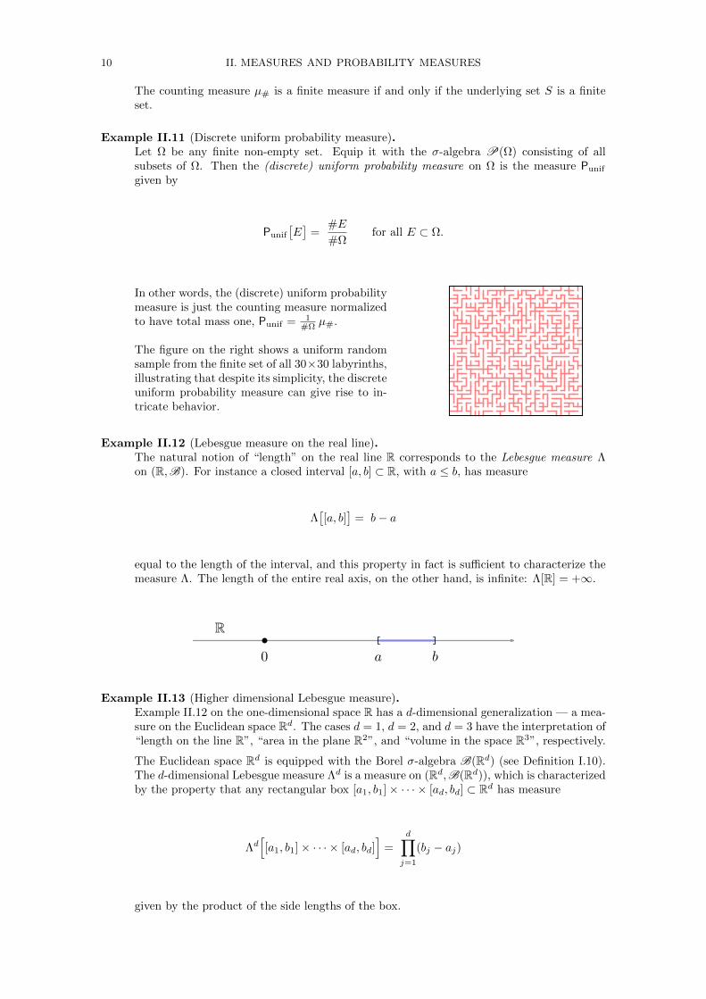
The figure on the right shows a uniform randomsample from the finite set of all 30×30 labyrinths,illustrating that despite its simplicity, the discreteuniform probability measure can give rise to in-tricate behavior.
Example II.12 (Lebesgue measure on the real line).The natural notion of “length” on the real line R corresponds to the Lebesgue measure Λon (R,B). For instance a closed interval [a, b] ⊂ R, with a ≤ b, has measure
Λ[[a, b]
]= b− a
equal to the length of the interval, and this property in fact is sufficient to characterize themeasure Λ. The length of the entire real axis, on the other hand, is infinite: Λ[R] = +∞.
R
0 a b
Example II.13 (Higher dimensional Lebesgue measure).Example II.12 on the one-dimensional space R has a d-dimensional generalization — a mea-sure on the Euclidean space Rd. The cases d = 1, d = 2, and d = 3 have the interpretation of“length on the line R”, “area in the plane R2”, and “volume in the space R3”, respectively.
The Euclidean space Rd is equipped with the Borel σ-algebra B(Rd) (see Definition I.10).The d-dimensional Lebesgue measure Λd is a measure on (Rd,B(Rd)), which is characterizedby the property that any rectangular box [a1, b1]× · · · × [ad, bd] ⊂ Rd has measure
Λd[[a1, b1]× · · · × [ad, bd]
]=
d∏j=1
(bj − aj)
given by the product of the side lengths of the box.
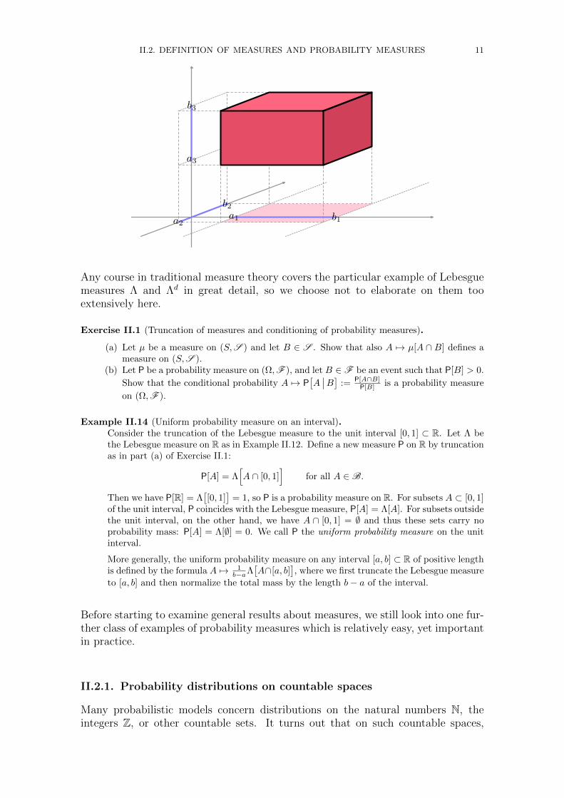
II.2. DEFINITION OF MEASURES AND PROBABILITY MEASURES 11
a1 b1a2
b2
a3
b3
Any course in traditional measure theory covers the particular example of Lebesguemeasures Λ and Λd in great detail, so we choose not to elaborate on them tooextensively here.
Exercise II.1 (Truncation of measures and conditioning of probability measures).
(a) Let µ be a measure on (S,S ) and let B ∈ S . Show that also A 7→ µ[A ∩ B] defines ameasure on (S,S ).
(b) Let P be a probability measure on (Ω,F ), and let B ∈ F be an event such that P[B] > 0.
Show that the conditional probability A 7→ P[A∣∣B] := P[A∩B]
P[B] is a probability measure
on (Ω,F ).
Example II.14 (Uniform probability measure on an interval).Consider the truncation of the Lebesgue measure to the unit interval [0, 1] ⊂ R. Let Λ bethe Lebesgue measure on R as in Example II.12. Define a new measure P on R by truncationas in part (a) of Exercise II.1:
P[A] = Λ[A ∩ [0, 1]
]for all A ∈ B.
Then we have P[R] = Λ[[0, 1]
]= 1, so P is a probability measure on R. For subsets A ⊂ [0, 1]
of the unit interval, P coincides with the Lebesgue measure, P[A] = Λ[A]. For subsets outsidethe unit interval, on the other hand, we have A ∩ [0, 1] = ∅ and thus these sets carry noprobability mass: P[A] = Λ[∅] = 0. We call P the uniform probability measure on the unitinterval.
More generally, the uniform probability measure on any interval [a, b] ⊂ R of positive lengthis defined by the formula A 7→ 1
b−aΛ[A∩[a, b]
], where we first truncate the Lebesgue measure
to [a, b] and then normalize the total mass by the length b− a of the interval.
Before starting to examine general results about measures, we still look into one fur-ther class of examples of probability measures which is relatively easy, yet importantin practice.
II.2.1. Probability distributions on countable spaces
Many probabilistic models concern distributions on the natural numbers N, theintegers Z, or other countable sets. It turns out that on such countable spaces,
12 II. MEASURES AND PROBABILITY MEASURES
we can characterize probabilty measures in an intuitive way using probability massfunctions.
For the rest of this section we therefore assume that Ω is a non-empty countableset. Then there exists an enumeration1 Ω = ω1, ω2, ω3, . . . with distinct elementsω1, ω2, ω3, . . . ∈ Ω. Summation over Ω can be defined using the enumeration,∑
ω∈Ω
a(ω) :=∑j
a(ωj),
and if the terms of the sum are non-negative, a(ω) ≥ 0, then the result of the sumis independent of the chosen enumeration.
Definition II.15 (Probability mass function).A probability mass function (p.m.f.) on Ω is a function
p : Ω→ [0, 1]
such that ∑ω∈Ω
p(ω) = 1.
To a probability mass function p it is natural to associate a measure defined by
P[E] =∑ω∈E
p(ω) for all E ⊂ Ω, (II.1)
and conversely to a probability measure P on (Ω,P(Ω)) it is natural to associatemasses of singleton events ω ⊂ Ω
p(ω) = P[ω
]for all ω ∈ Ω. (II.2)
The following exercise shows that on countable spaces, probability mass functionsare in one-to-one correspondence with probability measures via the above formulas.
Exercise II.2 (Probability distributions on countable spaces).Let Ω be a finite or a countably infinite set, and denote by P(Ω) the collection of all subsetsof Ω.
(a) Show that if p is a probability mass function on Ω, then the set function P definedby (II.1) is a probability measure on (Ω,P(Ω)).
(b) Show that if P is a probability measure on (Ω,P(Ω)), then the function p defined by (II.2)is a probability mass function on Ω.
Example II.16 (Poisson distribution).Let λ > 0. Recalling the power series
∑∞k=0
1k!λ
k = eλ of the exponential function, it is easyto see that the function p given by
p(k) = e−λλk
k!for k ∈ Z≥0 = 0, 1, 2, . . . (II.3)
is a probability mass function on Z≥0.
The Poisson distribution with parameter λ is the probability measure on Z≥0 with the aboveprobability mass function.
1If Ω is finite, the enumeration terminates, Ω = ω1, ω2, . . . , ωn. The more interesting case isif Ω is countably infinite.
II.3. PROPERTIES OF MEASURES AND PROBABILITY MEASURES 13
Example II.17 (Geometric distribution).Let q ∈ (0, 1). Using the geometric series
∑∞k=0 r
k = 11−r with r = 1 − q, it is easy to see
that the function p given by
p(k) = (1− q)k−1q for k ∈ N = 1, 2, 3, . . . (II.4)
is a probability mass function on N.
The geometric distribution with parameter q is the probability measure on N with the aboveprobability mass function.
Example II.18 (Binomial distribution).Let n ∈ N and q ∈ (0, 1). Using the binomial formula
∑nk=0
(nk
)aj bn−j = (a + b)n with
a = q and b = 1− q it is easy to see that the function p given by
p(k) =
(n
k
)qk (1− q)n−k for k ∈ 0, 1, . . . , n− 1, n (II.5)
is a probability mass function on the finite set 0, 1, . . . , n− 1, n.
The binomial distribution with parameters n and q is the probability measure on the finiteset 0, 1, . . . , n− 1, n with the above probability mass function.
II.3. Properties of measures and probability measures
Let us now discuss some of the first properties of measures and probability measures.
Subadditivity of measures and the union bound
For repeated later use, we start by proving the following additivity properties formeasures of disjoint sets, subadditivity properties of measures of (not necessarilydisjoint) sets, as well as related monotonicity and monotone convergence propertiesof measures.
Lemma II.19 (First properties of measures).Let µ be a measure on a measurable space (S,S ). Then we have the following:
(a) Finite additivity: If A1, . . . , An ∈ S are disjoint measurable sets, then wehave:
µ[A1 ∪ · · · ∪ An
]= µ[A1] + · · ·+ µ[An]. (II.6)
(b) Monotonicity: If A,B ∈ S and A ⊂ B, then we have:
µ[A] ≤ µ[B]. (II.7)
(c) Finite subadditivity: If A1, . . . , An ∈ S are any measurable sets, then wehave:
µ[A1 ∪ · · · ∪ An
]≤ µ[A1] + · · ·+ µ[An]. (II.8)
(d) Monotone convergence of measures: Let A1 ⊂ A2 ⊂ · · · be an increasingsequence of measurable sets, An ∈ S for all n ∈ N. Then the measures ofthe increasing limit An ↑ A =
⋃∞j=1Aj of sets constitute the increasing limit
µ[An] ↑ µ[A]. (II.9)
14 II. MEASURES AND PROBABILITY MEASURES
(e) Countable subadditivity: If A1, A2, . . . ∈ S is a sequence of measurablesets (not necessarily disjoint), then we have:
µ[ ∞⋃j=1
Aj
]≤
∞∑j=1
µ[Aj]. (II.10)
Proof of (a): Given the disjoint measurable sets A1, . . . , An ∈ S , let us extend this finite sequenceby empty sets: define An+1 = An+2 = · · · = ∅. Since ∅ ∈ S by properties of σ-algebras,we thus obtain an infinite sequence A1, A2, . . . ∈ S of measurable sets. This sequence ofsets is disjoint (the newly added empty sets do not have common elements with the alreadydisjoint A1, . . . , An). Thus from axiom (M-∪) it follows that
µ[ ∞⋃j=1
Aj
]=
∞∑j=1
µ[Aj].
But on the left hand side, the union is simply⋃∞j=1Aj = A1 ∪ · · · ∪An, because the empty
sets do not contribute to the union. On the right hand side, the sum is∑∞j=1 µ[Aj ] =
µ[A1] + · · · + µ[An], because the measures of the empty sets µ[∅] = 0 do not contribute tothe sum. Assertion (a) follows.
Proof of (b): Assume that A,B ∈ S . Note that then also B \ A = B ∩ Ac ∈ S by properties ofσ-algebras. If A ⊂ B, then B = A ∪ (B \A) is a disjoint union. For these two disjoint sets,we can use part (a) to get
µ[B] = µ[A ∪ (B \A)
](a)= µ[A] + µ
[B \A
].
Since µ[B \A
]≥ 0 by properties of measures, the assertion µ[B] ≥ µ[A] follows.
Proof of (c): We will prove the inequality
µ[A1 ∪ · · · ∪An
]≤ µ[A1] + · · ·+ µ[An].
for all A1, . . . , An ∈ S by induction on the number n of sets in the union.
The case n = 1 is clear — the two sides of the inequality are in fact equal. Now assume theinequality for unions of n sets, and consider A1, . . . , An+1 ∈ S . Define A = A1 ∪ · · · ∪ Anand B = An+1 \ A. Then we have A1 ∪ · · · ∪ An+1 = A ∪ B, where the sets A and B aredisjoint. Thus by part (a) we get
µ[A ∪B
]= µ[A] + µ[B].
The first term on the right hand side is
µ[A] = µ[A1 ∪ · · · ∪An
]≤ µ[A1] + · · ·+ µ[An]
by induction assumption. The second term on the right hand side is µ[B] ≤ µ[An+1]by monotonicity proven in part (b), since B ⊂ An+1. Notice that the right hand sideµ[A∪B
]= µ
[A1∪· · ·∪An+1
]is the measure we are interested in. Therefore, by combining
the observations, we conclude
µ[A1 ∪ · · · ∪An+1
]≤(µ[A1] + · · ·+ µ[An]
)+ µ[An+1],
which finishes the proof of assertion (c) by induction.
Proof of (d): Suppose that A1 ⊂ A2 ⊂ · · · is an increasing sequence of measurable sets, and denoteits limit by A =
⋃∞j=1Aj . Then A is also measurable by properties of σ-algebras. Now write
first B1 = A1, and then B2 = A2 \A1, . . . , Bn = An \An−1, . . . . These sets B1, B2, . . . aredisjoint and An = B1 ∪ · · · ∪Bn for all n ∈ N. From part (a) we get
µ[An] = µ[B1 ∪ · · · ∪Bn
]=
n∑j=1
µ[Bj ].
II.3. PROPERTIES OF MEASURES AND PROBABILITY MEASURES 15
The right hand sides are the partial sums of an infinite sum with non-negative terms, sothey form a sequence increasing to that infinite sum, and we conclude
µ[An] ↑∞∑j=1
µ[Bj ] as n→∞.
On the other hand, by disjointness of B1, B2, . . . and axiom (M-∪), this infinite sum equals
∞∑j=1
µ[Bj ] = µ[ ∞⋃j=1
Bj
]= µ
[ ∞⋃j=1
Aj
]= µ[A].
This proves the assertion (d), µ[An] ↑ µ[A] as n→∞.
Proof of (e): Let A1, A2, . . . ∈ S be a sequence of measurable sets. Form their finite unionsCn = A1 ∪ · · · ∪ An, for all n ∈ N. Then, as a union of measurable sets, each Cn is alsomeasurable. This sequence is clearly increasing C1 ⊂ C2 ⊂ · · · , and its limit is the countablyinfinite union C =
⋃∞j=1Aj . We can therefore apply part (d) to get
µ[Cn] ↑ µ[C] as n→∞. (II.11)
On the other hand, by part (c) we have for all n ∈ N
µ[Cn] = µ[A1 ∪ · · · ∪An
]≤
n∑j=1
µ[Aj ] ≤∞∑j=1
µ[Aj ].
If we denote the value of the infinite sum by c :=∑∞j=1 µ[Aj ], then this bound µ[Cn] ≤ c
for all n implies that for the limit (II.11) we also have µ[C] ≤ c. Recalling what C and care, we have now obtained
µ[ ∞⋃j=1
Aj
]= µ[C] ≤ c =
∞∑j=1
µ[Aj ].
This finishes the proof.
Especially part (e) of the above lemma is, despite its simplicity, so useful in probabil-ity theory that it has been given an affectionate name: “the union bound”. Becauseof its importance, we record this fact once more in the probabilistic context.
Theorem II.20 (The union bound).Let (Ω,F ,P) be a probability space and let E1, E2, . . . ∈ F be a sequence ofevents. Then we have
P[ ∞⋃j=1
Ej
]≤
∞∑j=1
P[Ej]. (II.12)
In other words, the probability that at least one event in a sequence occurs can notexceed the sum of the probabilities of the events in the sequence.
Probability measures enjoy some properties that may not be valid for measures ofinfinite total mass. The following exercise gives a few of them.
Exercise II.3 (Properties specific to probability measures).Let (Ω,F ,P) be a probability space.
(a) Show that for any event E ∈ F we have
P[Ec] = 1− P[E].
(b) Show that for any two events E1, E2 ∈ F we have
P[E1 ∪ E2] = P[E1] + P[E2]− P[E1 ∩ E2].
16 II. MEASURES AND PROBABILITY MEASURES
Monotone convergence of probability measures
Part (d) of Lemma II.19 is a monotone convergence statement of measures for in-creasing sequences of sets. For general measures we do not have the correspondingmonotone convergence for decreasing sequences of sets, as the following counterex-ample shows.
Example II.21. (Decreasing monotone convergence of measures can fail in general)Consider the set N = 1, 2, 3, . . . of natural numbers with the counting measure µ#, asdefined in Example II.10:
µ#[A] = #A for all A ⊂ N.
Consider the subsets An = n, n+ 1, n+ 2, . . . ⊂ N. Each of these is an infinite set, sotheir counting measures are infinite, µ#[An] = +∞. These sets form a decreasing sequence,
A1 ⊃ A2 ⊃ A3 ⊃ · · · ,and the limit is the intersection
A =⋂n∈N
An.
But no natural number m ∈ N belongs to all of An, n ∈ N, (indeed, m /∈ An as soon asn > m). Therefore the intersection is empty, A = ∅. The number of elements in this emptyset is zero, #A = 0. In particular, the sequence of counting measures µ#[An] = +∞ doesnot tend to the counting measure µ#[A] = 0 of the decreasing limit set A.
Exercise II.4. Construct a similar counterexample with the Lebesgue measure Λ on R.
For probability measures, however, monotone convergence of measures holds forboth increasing and decreasing sequences of events.
Theorem II.22 (Monotone convergence of probability measures).Let (Ω,F ,P) be a probability space.
(a) If E1 ⊂ E2 ⊂ · · · is an increasing sequence of events with limit E =⋃n∈NEn,
then we have P[En] ↑ P[E] as n→∞.(b) If E1 ⊃ E2 ⊃ · · · is a decreasing sequence of events with limit E =
⋂n∈NEn,
then we have P[En] ↓ P[E] as n→∞.
Proof. Part (a) follows from part (d) of Lemma II.19, since any probability measure is a measure.Part (b) is left as an exercise.
Exercise II.5. Prove part (b) of Theorem II.22 above.
II.4. Identification and construction of measures
We now turn to the following questions:
• Does a measure with some desired properties exist?(How can we construct measures?)• How can we check whether two measures are the same?
(What does one need to know to uniquely identify a measure?)
II.4. IDENTIFICATION AND CONSTRUCTION OF MEASURES 17
As we noted in Section I.3, it can be complicated to work with σ-algebras. For thepurposes of the above two questions, in particular, we often prefer to work withsimpler collections. For the identification part, the appropriate simpler collectionsare called π-systems (Definition II.23 below)
Courses on traditional measure theory focus quite a lot on the construction of mea-sures. We refer the interested reader to such measure theory courses for details —the dedicated reader will find for example Caratheodory’s extension theorem, withwhich it is possible to construct, e.g., the Lebesgue measure Λ on R (Example II.12)and its multi-dimensional analogue Λd on Rd (Example II.13).
Instead, identification of probability measures is of practical relevance in stochasticsand statistics, so we focus more on this latter question. The proof of the mainidentification result (Dynkin’s identification theorem, Theorem II.26), is not givenimmediately. It can be found in Appendix C, and may be most natural to studytogether with the topics of Lecture IV.
Identification of probability measures
Collections of the following type are good for the purposes of identification of mea-sures.
Definition II.23 (Pi-system).A collection J of subsets of S is called a π-system if the following holds:
(Π-∩) : if A,B ∈J , then also A ∩B ∈J .
Remark II.24. Any σ-algebra S is also a π-system (since the intersection of two sets in a σ-algebra belongs to the σ-algebra). However, not every π-system is a σ-algebra, as thefollowing example shows.
Example II.25 (A pi-system of semi-infinite intervals).Consider the collection
J (R) :=
(−∞, x]∣∣∣ x ∈ R
(II.13)
of semi-infinite intervals (−∞, x] ⊂ R. Then J (R) is a π-system on R: indeed it is clearlya non-empty collection of subsets of R, and given any two intervals from the collection,(−∞, x1] and (−∞, x2], their intersection is the interval
(−∞, x1] ∩ (−∞, x2] = (−∞, z], where z = minx1, x2
which itself belongs to the collection J (R). Thus property (Π-∩) holds for J (R).
In Proposition I.11 we saw that J (R) generates the Borel σ-algebra B on R, i.e., σ(J (R)) =B. It is one of the simplest such π-systems, and for this reason we will use J (R) over andover again, especially when dealing with real valued random variables.
The main result which is used for identification of measures is the following.
Theorem II.26 (Dynkin’s identification theorem).Let P1 and P2 be two probability measures on a measurable space (Ω,F ). As-sume that J is a π-system on Ω such that the σ-algebra σ(J ) generated byit coincides with the σ-algebra F of measurable sets in the measurable space,i.e., σ(J ) = F . Then the following are equivalent:
18 II. MEASURES AND PROBABILITY MEASURES
(i) P1[E] = P2[E] for all E ∈J(ii) the two probability measures are equal, P1 = P2.
Remark II.27. Condition (ii) above is clearly stronger than condition (i). Namely, the equalityof probability measures P1 = P2 means that P1[E] = P2[E] for all E ∈ F , and there are ingeneral more sets E in this σ-algebra F than in the π-system J . The nontrivial part ofthe proof is therefore that condition (i) implies (ii). This will be proven in Appendix C.3.
Cumulative distribution function
In the following we consider a probability measure on the real axis R. Typically sucha probability measure could appear as the law of a real-valued random variable, aswe will discuss later on in the course. In order to have a suitable notation for suchcommon situations, let us denote the probability measure in this case by ν insteadof P.
Definition II.28 (Cumulative distribution function).If ν is a probability measure on (R,B), then the cumulative distribution func-tion (c.d.f.) of ν is the function F : R→ [0, 1] defined by
F (x) := ν[(−∞, x]
].
A simple but important application of Dynkin’s identification theorem is the fol-lowing. This case is applicable, e.g., to the identification of the laws of real-valuedrandom variables.
Corollary II.29 (Cumulative distribution function identify distributions).Let ν1 and ν2 be two probability measures on (R,B), and F1 and F2 their cu-mulative distribution functions, reprectively. Then the following are equivalent:
(i) The cumulative distribution functions are equal, F1 = F2.(ii) The probability measures are equal, ν1 = ν2.
Proof: Equivalence if proved by establishing both implications (i)⇒ (ii) and (ii)⇒ (i).
proof of (ii)⇒ (i): Assuming the probability measures are equal, ν1 = ν2, we get for any x ∈ R
F1(x) := ν1
[(−∞, x]
]= ν2
[(−∞, x]
]=: F2(x).
proof of (i)⇒ (ii): Assume the equality F1 = F2 of cumulative distribution functions, i.e., thatF1(x) = F2(x) for all x ∈ R. Consider the π-system J (R) of Example II.25. A setA = J (R) of this π-system is by definition of the form A = (−∞, x] for some x ∈ R. Forsuch a set, we get
ν1
[(−∞, x]
]=: F1(x) = F2(x) := ν1
[(−∞, x]
],
so we have that ν1 and ν2 coincide on J (R). The σ-algebra σ(J (R)
)generated by the
π-system J (R) coincides with the Borel σ-algebra B by Proposition I.11(i). Theorem II.26then guarantees that ν1 and ν2 coincide on the entire Borel σ-algebra B.
Since cumulative distribution functions characterize probability measures on (R,B)by Corollary II.29 above, it is natural to next ask which functions F can qualify ascumulative distribution functions. There is indeed a rather explicit characterization.
II.4. IDENTIFICATION AND CONSTRUCTION OF MEASURES 19
Deriving the necessary conditions below is an instructive application of the basicproperties of measures which we established in Lemma II.19.
Proposition II.30 (Properties of cumulative distribution functions).If F : R→ [0, 1] is the cumulative distribution function of a probability measureν on (R,B), then it satisfies the following properties:
(a) F is increasing: if x ≤ y then F (x) ≤ F (y)(b) F is right-continuous: if xn ↓ x ∈ R as n→∞, then F (xn) ↓ F (x)(c) limx→+∞ F (x) = 1 and limx→−∞ F (x) = 0.
Exercise II.6. Prove Proposition II.30.Hint: Use appropriate parts of Lemma II.19.

Lecture III
Random variables
Let (Ω,F ,P) be a probability space, i.e.,
Ω — the set of all possible outcomesF — the collection of events (see Lecture I)P — the probability measure (see Lecture II).
The key idea of a random variable is the following two step procedure by whichrandomness is thought to have effect:
1.) “Chance determines the random outcome ω ∈ Ω.”2.) “The outcome ω determines various quantities of interest.”
(random variables)
Therefore, a random variable will be a function X defined on Ω, which to an outcomeω ∈ Ω associates the value X(ω) of some quantity of interest. The function
X : Ω→ S ′
takes values in a suitable set S ′ of possible values of the quantity of interest (someexamples are given below, in Example III.4). Crucially, this function has to besufficiently well-behaved so that we can talk about probabilities with which thequantity assumes certain values. So whenever A′ ⊂ S ′ is a reasonable enough subsetof the possible values, the set of outcomes ω for which X(ω) belongs to A′ shouldconstitute an event, i.e.,
ω ∈ Ω∣∣ X(ω) ∈ A′
∈ F . (III.1)
This requirement of well-behavedness of the function X : Ω→ S ′ is what the notionof measurable function captures (cf. Definition III.1 below).
The set in (III.1) above is just the preimage of A′ under the function X : Ω → S ′:indeed by definition we have
X−1(A′) =ω ∈ Ω
∣∣ X(ω) ∈ A′⊂ Ω.
For simplicity, we will often abbreviate this just as
X ∈ A′ ⊂ Ω.
This last slight abuse of notation is not only shorter, but it also has the advantagethat the probabilistic interpretation
“the value of our (random) quantity of interest X lies in A′”
of the event becomes apparent at a glance.
21
22 III. RANDOM VARIABLES
III.1. Measurable functions and random variables
Let (S,S ) and (S ′,S ′) be two measurable spaces, i.e., S and S ′ are two sets andS and S ′ are σ-algebras on these two respectively.
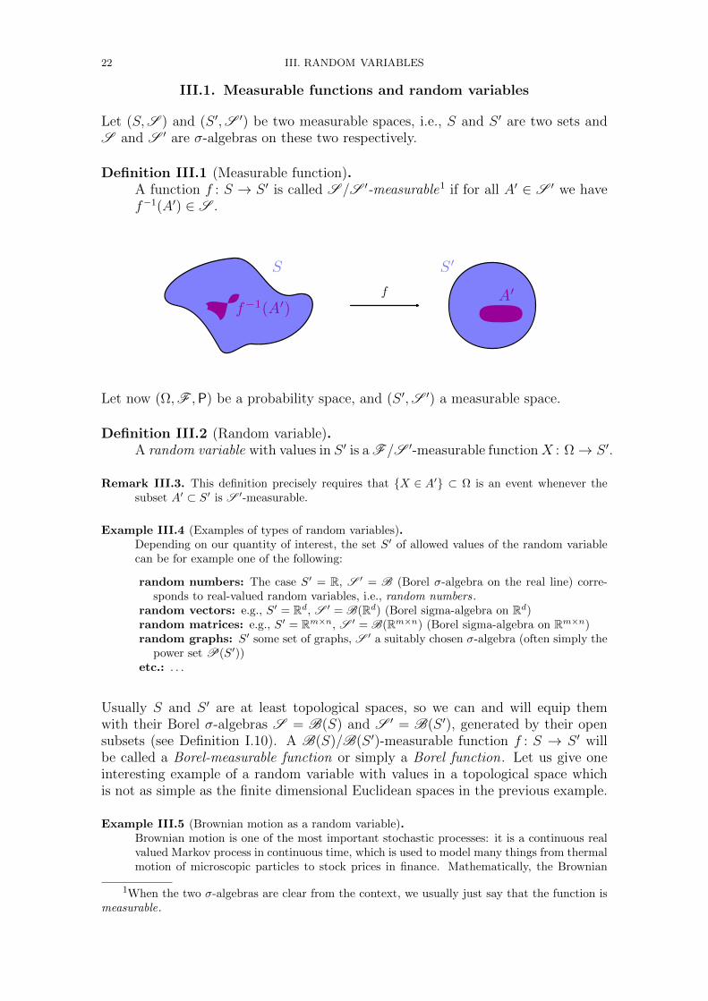
Definition III.1 (Measurable function).A function f : S → S ′ is called S /S ′-measurable1 if for all A′ ∈ S ′ we havef−1(A′) ∈ S .
S
f−1(A′)
S′
A′f
Let now (Ω,F ,P) be a probability space, and (S ′,S ′) a measurable space.
Definition III.2 (Random variable).A random variable with values in S ′ is a F/S ′-measurable functionX : Ω→ S ′.
Remark III.3. This definition precisely requires that X ∈ A′ ⊂ Ω is an event whenever thesubset A′ ⊂ S′ is S ′-measurable.
Example III.4 (Examples of types of random variables).Depending on our quantity of interest, the set S′ of allowed values of the random variablecan be for example one of the following:
random numbers: The case S′ = R, S ′ = B (Borel σ-algebra on the real line) corre-sponds to real-valued random variables, i.e., random numbers.
random vectors: e.g., S′ = Rd, S ′ = B(Rd) (Borel sigma-algebra on Rd)random matrices: e.g., S′ = Rm×n, S ′ = B(Rm×n) (Borel sigma-algebra on Rm×n)random graphs: S′ some set of graphs, S ′ a suitably chosen σ-algebra (often simply the
power set P(S′))etc.: . . .
Usually S and S ′ are at least topological spaces, so we can and will equip themwith their Borel σ-algebras S = B(S) and S ′ = B(S ′), generated by their opensubsets (see Definition I.10). A B(S)/B(S ′)-measurable function f : S → S ′ willbe called a Borel-measurable function or simply a Borel function. Let us give oneinteresting example of a random variable with values in a topological space whichis not as simple as the finite dimensional Euclidean spaces in the previous example.
Example III.5 (Brownian motion as a random variable).Brownian motion is one of the most important stochastic processes: it is a continuous realvalued Markov process in continuous time, which is used to model many things from thermalmotion of microscopic particles to stock prices in finance. Mathematically, the Brownian
1When the two σ-algebras are clear from the context, we usually just say that the function ismeasurable.
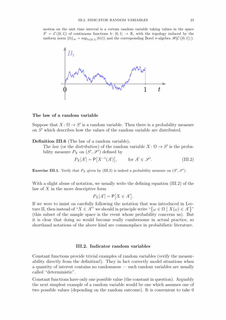
III.2. INDICATOR RANDOM VARIABLES 23
motion on the unit time interval is a certain random variable taking values in the spaceS′ = C ([0, 1]) of continuous functions h : [0, 1] → R, with the topology induced by theuniform norm ‖h‖∞ = supt∈[0,1] |h(t)| and the corresponding Borel σ-algebra B
(C ([0, 1])
).
10 t
Bt
The law of a random variable
Suppose that X : Ω→ S ′ is a random variable. Then there is a probability measureon S ′ which describes how the values of the random variable are distributed.
Definition III.6 (The law of a random variable).The law (or the distribution) of the random variable X : Ω→ S ′ is the proba-bility measure PX on (S ′,S ′) defined by
PX [A′] = P[X−1(A′)
], for A′ ∈ S ′. (III.2)
Exercise III.1. Verify that PX given by (III.2) is indeed a probability measure on (S′,S ′).
With a slight abuse of notation, we usually write the defining equation (III.2) of thelaw of X in the more descriptive form
PX [A′] = P[X ∈ A′
].
If we were to insist on carefully following the notation that was introduced in Lec-ture II, then instead of “X ∈ A′” we should in principle write “
ω ∈ Ω
∣∣ X(ω) ∈ A′
”(this subset of the sample space is the event whose probability concerns us). Butit is clear that doing so would become really cumbersome in actual practice, soshorthand notations of the above kind are commonplace in probabilistic literature.
III.2. Indicator random variables
Constant functions provide trivial examples of random variables (verify the measur-ability directly from the definition!). They in fact correctly model situations whena quantity of interest contains no randomness — such random variables are usuallycalled “deterministic”.
Constant functions have only one possible value (the constant in question). Arguablythe next simplest example of a random variable would be one which assumes one oftwo possible values (depending on the random outcome). It is convenient to take 0
24 III. RANDOM VARIABLES
and 1 as those two values, in which case one speaks of an indicator random variable.For E ⊂ Ω a subset, we define the indicator function IE : Ω→ R of E by
IE(ω) =
1 if ω ∈ E0 if ω /∈ E.
(III.3)
Exercise III.2 (Measurability of indicators).Prove that IE is F -measurable if and only if E ∈ F , i.e., if E ⊂ Ω is an event.
When IE is F -measurable, we call it the indicator random variable of the event E.It “indicates” the occurrence of the event E in the sense that it takes the value 1 ifthe event E occurs and value 0 otherwise.
Exercise III.3 (Indicators of intersections and unions).Let A,B ⊂ Ω.
(a) Show that IA∩B = IA IB .(b) When is it true that IA∪B = IA + IB?
III.3. Constructing random variables
So far we have given the definition of random variables, but we have hardly addressedthe issue of constructing them — we have only left it as an exercise to characterizethe measurability of random variables with values 0 and 1. At this stage one mighttherefore still worry that perhaps the requirements of a measurable function are toostringent for any interesting examples to exist. . . Fortunately, this is not the case:almost all functions that you ever encounter turn out to be measurable. The rest ofthis lecture is devoted to understanding why.
A very easy case
The example here concerns one case in which we do not have to worry about theexistence of random variables at all — when all subsets of the sample space Ω areevents, then every function on Ω is measurable.
Example III.7 (A case when all functions are measurable).Suppose that (Ω,F ,P) is a probability space in which all subsets of Ω are events F = P(Ω).Then any function X : Ω → R is a random variable. Indeed, for any B ∈ B, the preimageX−1(B) ⊂ Ω is a subset, and therefore X−1(B) ∈P(Ω).
As we have mentioned before, we can usually only take F = P(Ω) when Ω iscountable, so Example III.7 only reassures us of the existence of plenty of randomvariables on countable sample spaces. It remains to convince ourselves that inter-esting random variables exist in other common situations.
III.3. CONSTRUCTING RANDOM VARIABLES 25
Composition of measurable functions
Most of the time in practice, we construct more complicated random variables fromsimpler ones. The measurability of the simpler building blocks should ideally directlyimply the measurability of the more complicated construction.
Composition of functions is one such construction.
Proposition III.8 (Composition of measurable functions is measurable).Suppose that (S,S ), (S ′,S ′), and (S ′′,S ′′) are three measurable spaces andthat we are given two measurable functions:
f : S → S ′ is S /S ′-measurable
g : S ′ → S ′′ is S ′/S ′′-measurable.
Then the composite function s 7→ g(f(s)) is also measurable:
g f : S → S ′′ is S /S ′′-measurable.
Proof. We check the measurability of g f directly using the definition. Let A′′ ∈ S ′′ be ameasurable subset of S′′. Then first, by the S ′/S ′′-measurability of g, the preimage underg of A′′ is measurable: we have g−1(A′′) ∈ S ′. Using the S /S ′-measurability of f , itthen follows that also the preimage under f of the measurable set g−1(A′′) is measurable:we have f−1
(g−1(A′′)
)∈ S . It is an easy fact about preimages of composite functions
that f−1(g−1(A′′)
)= (g f)−1(A′′). Therefore we have checked the measurability of the
preimage (g f)−1(A′′) of any measurable subset A′′ ⊂ S′′ under the composite functiong f : S → S′′, which by definition says that the composite function g f is measurable.
We postpone examples until after we have some more tools at our disposal.
Practical verification of measurability
To verify measurability, it is in fact enough to check the defining condition for justsome collection of subsets that generates the σ-algebra on the target space.
Lemma III.9 (A sufficient condition for measurability).Let C ′ ⊂ P(S ′) be a collection of subsets of S ′ that generates the σ-algebraS ′, i.e., σ(C ′) = S ′. Then a function f : S → S ′ is S /S ′-measurable if andonly if f−1(C ′) ∈ S for all C ′ ∈ C ′.
Proof. The condition is clearly necessary for measurability of f : if C ′ ∈ C ′ ⊂ σ(C ′) = S ′ then thedefinition of measurability requires that f−1(C ′) ∈ S . It therefore remains only to provethat the condition is also sufficient.
Assume now that f−1(C ′) ∈ S for all C ′ ∈ C ′. We must prove that then the function f isS /S ′-measurable. Define
G ′ =G′ ∈ S ′
∣∣∣ f−1(G′) ∈ S
26 III. RANDOM VARIABLES
as the collection of the “good” subsets G′ of S′, whose preimages are measurable. Byassumption we have C ′ ⊂ G ′. Now since preimages satisfy the properties
f−1(S′) = S
f−1((G′)c
)=(f−1(G′)
)cf−1
( ∞⋃n=1
G′n
)=
∞⋃n=1
f−1(G′n)
(see Exercise A.2) and S is a σ-algebra (on S), we see that the collection G ′ of subsets of S′
is a σ-algebra (on S′).
The fact that the σ-algebra G ′ contains the collection C ′ implies that it contains alsothe σ-algebra generated by that collection, i.e., σ(C ′) ⊂ G ′. But we have assumed thatσ(C ′) = S ′, so we conclude that S ′ ⊂ G ′. By definition of G ′ this means that everyS ′-measurable subset A′ has the property that f−1(A′) ∈ S . This shows the measurabilityof the function f .
As an application, we see that all continuous functions are good for our purposes.This gives us quite a lot of measurable functions already.
Corollary III.10 (Continuous functions are Borel-measurable).Let X and X′ be two topological spaces (e.g., metric spaces). Then any contin-uous function f : X→ X′ is Borel-measurable.
Proof. Let f : X → X′ be a continuous function and let B(X) and B(X′) be the Borel σ-algebrason X and X′, respectively. Recall that Borel-measurability of the function f means that fis B(X)/B(X′)-measurable.
Recall also that the Borel σ-algebra B(X′) is generated by the collection T (X′) of all opensubsets V ′ ⊂ X′. If f : X→ X′ is continuous, then for any open subset V ′ ⊂ X′ the preimagef−1(V ′) ⊂ X is also open: f−1(V ′) ∈ T (X). As an open set, the preimage is in particularBorel-measurable: f−1(V ′) ∈ B(X). Therefore we have checked that f−1(V ′) ∈ B(X) holdsfor all V ′ in the collection T (X′) which generates B(X′). By Lemma III.9, this is sufficientto show that the function f is B(X)/B(X′)-measurable.
For the case S ′ = R (e.g., random numbers), we can in fact use even simpler collec-tions that generate the Borel σ-algebra.
Corollary III.11 (Measurability of real valued functions).A function f : S → R is S /B-measurable if and only if for all c ∈ R we havef ≤ c ∈ S .
Remark III.12. Recall that the notation f ≤ c is shorthand for
f ≤ c :=s ∈ S
∣∣ f(s) ≤ c⊂ S,
which is also the preimage f−1((−∞, c]
)of the interval (−∞, c].
Proof of Corollary III.11. The collection C =
(−∞, c]∣∣∣ c ∈ R
generates the Borel σ-algebra B
on R by Proposition I.11, so the assertion follows from Lemma III.9 above.
Pointwise operations on measurable functions
Since real numbers have addition and multiplication, we can perform such operationson real-valued functions pointwise. If f1, f2 : S → R are two functions, then the
III.3. CONSTRUCTING RANDOM VARIABLES 27
pointwise sum f1 + f2 : S → R is defined by
(f1 + f2)(s) = f1(s) + f2(s) ∀s ∈ S,the pointwise product f1f2 : S → R by
(f1f2)(s) = f1(s) f2(s) ∀s ∈ S,and if f : S → R is a function and λ ∈ R is a scalar, then the pointwise scalarmultiple λf : S → R is defined by
(λf)(s) = λ f(s) ∀s ∈ S.
Let us denote by mS the set of all S /B-measurable functions S → R. Thepointwise operations allow us to construct new measurable functions from old ones.
Proposition III.13 (Pointwise sums and products preserve measurability).Let (S,S ) be a measurable space. Then the set mS of all measurable realvalued functions on it is stable under taking pointwise sums, pointwise products,and pointwise scalar multiples, i.e., the following hold:
(i) f ∈ mS , λ ∈ R =⇒ λf ∈ mS(ii) f1, f2 ∈ mS =⇒ f1 + f2 ∈ mS
(iii) f1, f2 ∈ mS =⇒ f1f2 ∈ mS .
Proof: We will prove part (ii), and leave parts (i) and (iii) as exercises.
proof of (ii): Suppose that f1, f2 ∈ mS . Note that for c ∈ R and s ∈ S, the condition f1(s) +f2(s) > c holds if and only if there exists a rational number q ∈ Q such that we havef1(s) > q and f2(s) > c− q. In other words, the following two subsets of S are equal
f1 + f2 > c =⋃q∈Q
(f1 > q ∩ f2 > c− q
).
By measurability of the functions f1 and f2, the subsets f1 > q , f2 > c− q ⊂ S aremeasurable. By properties of σ-algebras, then, the set on the right hand side above ismeasurable (note that the set Q of rational numbers is countable). We have thus shownthat f1 + f2 > c ∈ S , and by taking complements we get
f1 + f2 ≤ c = f1 + f2 > cc ∈ S .
By Corollary III.11, this is sufficient to show the measurability of the pointwise sum functionf1 + f2.
Exercise III.4. Prove the assertions (i) and (iii) in Proposition III.13.
We can also use more subtle pointwise operations. If we are given a sequencef1, f2, . . . of functions fn : S → R for n ∈ N, then we can define functions supn fnand infn fn on S by the pointwise supremum and infimum
(supn∈N
fn)(s) = supn∈N
fn(s) and (infn∈N
fn)(s) = infn∈N
fn(s).
These functions, however, may assume values +∞ and −∞ even if each fn takesonly finite real values. Thus the functions
supn∈N
fn : S → [−∞,+∞] and infn∈N
fn : S → [−∞,+∞]
are defined so that their allowed range of values is the extended real line
[−∞,+∞] = R ∪ +∞ ∪ −∞ .
28 III. RANDOM VARIABLES
The extended real line is equipped with the topology of a closed interval, so that forexample the tangent function
tan:[− π
2,π
2
]→ [−∞,+∞]
is a homeomorphism, when we interpret tan(π/2) = +∞ and tan(−π/2) = −∞(see Example B.19). From this topology, we get the Borel σ-algebra B([−∞,+∞])on the extended real line, in the usual way (Definition I.10). It is so convenient tooccasionally allow +∞ and −∞ as possible values that we will slightly abuse thenotation, and write f ∈ mS also for functions
f : S → [−∞,+∞]
that are S /B([−∞,+∞])-measurable.
Likewise, for a sequence f1, f2, . . . of functions S → R we can define the pointwiselim sup and lim inf,
(lim supn
fn)(s) = lim supn
fn(s) and (lim infn
fn)(s) = lim infn
fn(s).
Proposition III.14 (Pointwise supremum and infimum preserve measurability).Let (S,S ) be a measurable space. Suppose that f1, f2, . . . ∈ mS . Then wehave:
(i) supn fn ∈ mS(ii) infn fn ∈ mS
(iii) lim supn fn ∈ mS(iv) lim infn fn ∈ mS .
Proof: We will prove only parts (i) and (iii) — parts (ii) and (iv) are entirely similar.2
proof of part (i). Note that we have supn fn(s) ≤ c if and only if fn(s) ≤ c for all n ∈ N. Thereforewe can write
supnfn ≤ c
=⋂n∈Nfn ≤ c .
For each n ∈ N we have fn ≤ c = f−1n
((−∞, c]
)∈ S , since fn ∈ mS . Therefore
we have supn fn ≤ c ∈ S as a countable intersection of sets in the σ-algebra S . ByCorollary III.11 we conclude that supn fn is a S -measurable function.
proof of part (iii). Recall that we have
lim supn
fn(s) = infn∈N
(supk≥n
fk(s)),
because the sequence of functions g1, g2, . . . defined by
gn(s) = supk≥n
fk(s)
is decreasing (for larger n the supremum contains fewer terms)
g1(s) ≥ g2(s) ≥ g3(s) ≥ · · · .
The function gn is a pointwise supremum of the measurable functions fk ∈ mS , k ≥ n, andthus itself S -measurable by part (i). Consequently, lim supn fn is the pointwise infimum ofthe measurable functions gn ∈ mS , n ∈ N, and thus itself S -measurable by part (ii).
2In the case when values ±∞ do not appear, parts (ii) and (iv) in fact directly followfrom parts (i) and (iii) and Proposition III.13(i) by observing that infn fn = − supn(−fn) andlim infn fn = − lim supn(−fn).
III.3. CONSTRUCTING RANDOM VARIABLES 29
With the above we can conclude the extremely useful fact that pointwise limits ofmeasurable functions are measurable.
Corollary III.15 (Pointwise limits of measurable functions are measurable).Let (S,S ) be a measurable space. Suppose that f1, f2, . . . ∈ mS , and supposethat for all s ∈ S the limit
limn→∞
fn(s)
exists. Then the pointwise limit function is measurable: limn→∞ fn ∈ mS .
Proof. When the assumed limit exists, it coincides with both the lim sup and lim inf (cf. Proposi-tion B.4),
lim infn
fn(s) = limn→∞
fn(s) = lim supn
fn(s).
Therefore the assertion follows from Proposition III.14, part (iii) or (iv).
Let us now revisit earlier examples about repeated coin tossing. The following illus-trates how the operations we studied above allow us to construct rather nontrivialrandom variables starting from very basic ones.
Example III.16 (The question of existence of limit frequency in coin tossing).
Let Ω = H,TN be the sample space for repeated coin tossing as in Examples O.2 and I.5.Let F be the σ-algebra on Ω generated by the events
Ej :=ω ∈ Ω
∣∣∣ ω(j) = H
= “the j:th coin toss is heads”
for j ∈ N, i.e., F = σ( Ej∣∣ j ∈ N
). Then the indicator random variable of Ej ,
IEj (ω) =
1 if ω(j) = H
0 if ω(j) = T,
is F -measurable by Exercise III.2. The relative frequency of heads in the first n coin tosses,
Xn(ω) =1
n
n∑j=1
IEj (ω),
is then also F -measurable by Proposition III.13 (the relative frequency Xn is constructedfrom the indicators IEj by finite sums and a scalar multiple). Therefore also the upper andlower limits
L+(ω) = lim supn
Xn(ω) and L−(ω) = lim infn
Xn(ω)
are random variables, by Proposition III.14. Knowing that these are random variables, dowe learn something interesting about events?
For example, for any r ∈ [0, 1], we should hope to be able to form the event
“relative frequencies of heads tend to r” =
limn→∞
Xn = r
which in more careful notation is the subsetω ∈ Ω
∣∣ limn→∞Xn(ω) = r⊂ Ω. Note that
we have limn→∞
Xn = r
=L+ = r
∩L− = r
,
and since L+ and L− are F -measurable random variables, the two preimagesL+ = r
= (L+)−1(r) and
L− = r
= (L−)−1(r)
are F -measurable events. Thus also their intersection is indeed an event,limn→∞
Xn = r∈ F ,
30 III. RANDOM VARIABLES
and so it will at least be meaningful to talk about the probability (once we introduce aprobability measure P) of the events that the relative frequency tends to a particular limitingvalue r ∈ [0, 1].
In Example I.5 we in fact already reached essentially the same conclusion by direct manip-ulations with events, without using random variables. The present approach, however, hassome advantages. Consider for instance the slight variation:
“relative frequencies have a limit” =∃ limn→∞
Xn
.
To show that this is an event, we may now just notice that the limit exists if and only if thecorresponding upper and lower limits coincide, L+ = L−, i.e. if their difference vanishes
∃ limn→∞
Xn
=L+ − L− = 0
.
This is the preimage of 0 ⊂ R under the pointwise difference L+−L− of random variables,and as such it is measurable,
∃ limn→∞
Xn
∈ F .
It would be more cumbersome to try to conclude the same directly by manipulating eventsusing countable set operations in the spirit of Example I.5.
III.4. Simple functions
In Section III.2 we discussed the measurability of functions assuming two possiblevalues, the indicator functions of subsets A ⊂ S defined by
IA : S → R, IA(s) =
1 if s ∈ A0 if s /∈ A.
In Exercise III.2 the measurability of the indicator functions was characterized: wehave IA ∈ mS if and only if A ∈ S .
From two possible values we next proceed modestly to finitely many possible values.
Definition III.17 (Simple function).A real valued measurable function assuming only finitely many different valuesis called a simple function (or a simple random variable in the probabilisticcontext).
Any finite linear combination of indicator functions
f(s) =m∑k=1
ak IAk (III.4)
of indicators of measurable sets A1, . . . , Am ∈ S is a simple function: it is mea-surable by Proposition III.13, and there are only finitely many real numbers thatcan be expressed as a sum of some of the coefficients a1, . . . , am ∈ R. In fact, if asimple function f : S → R can only assume m different real values a1, . . . , am, thenwe can write it as a linear combination (III.4) with the disjoint measurable setsAk := f−1(ak). Occasionally, choosing this minimal linear combination is veryconvenient, but at other times we might not want to insist on disjointness.
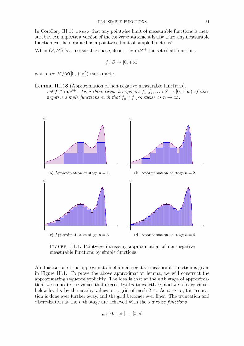
III.4. SIMPLE FUNCTIONS 31
In Corollary III.15 we saw that any pointwise limit of measurable functions is mea-surable. An important version of the converse statement is also true: any measurablefunction can be obtained as a pointwise limit of simple functions!
When (S,S ) is a measurable space, denote by mS + the set of all functions
f : S → [0,+∞]
which are S /B([0,+∞]) measurable.
Lemma III.18 (Approximation of non-negative measurable functions).Let f ∈ mS +. Then there exists a sequence f1, f2, . . . : S → [0,+∞) of non-negative simple functions such that fn ↑ f pointwise as n→∞.
s
f(s)
(a) Approximation at stage n = 1.
s
f(s)
(b) Approximation at stage n = 2.
s
f(s)
(c) Approximation at stage n = 3.
s
f(s)
(d) Approximation at stage n = 4.
Figure III.1. Pointwise increasing approximation of non-negativemeasurable functions by simple functions.
An illustration of the approximation of a non-negative measurable function is givenin Figure III.1. To prove the above approximation lemma, we will construct theapproximating sequence explicitly. The idea is that at the n:th stage of approxima-tion, we truncate the values that exceed level n to exactly n, and we replace valuesbelow level n by the nearby values on a grid of mesh 2−n. As n → ∞, the trunca-tion is done ever further away, and the grid becomes ever finer. The truncation anddiscretization at the n:th stage are achieved with the staircase functions
ςn : [0,+∞]→ [0, n]
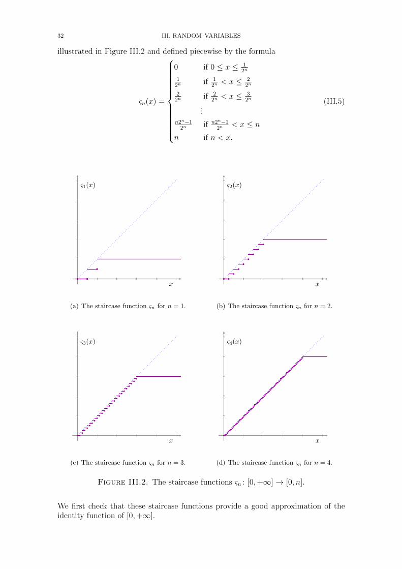
32 III. RANDOM VARIABLES
illustrated in Figure III.2 and defined piecewise by the formula
ςn(x) =
0 if 0 ≤ x ≤ 12n
12n
if 12n< x ≤ 2
2n
22n
if 22n< x ≤ 3
2n
...n2n−1
2nif n2n−1
2n< x ≤ n
n if n < x.
(III.5)
x
ς1(x)
(a) The staircase function ςn for n = 1.
x
ς2(x)
(b) The staircase function ςn for n = 2.
x
ς3(x)
(c) The staircase function ςn for n = 3.
x
ς4(x)
(d) The staircase function ςn for n = 4.
Figure III.2. The staircase functions ςn : [0,+∞]→ [0, n].
We first check that these staircase functions provide a good approximation of theidentity function of [0,+∞].
III.4. SIMPLE FUNCTIONS 33
Lemma III.19 (Properties of the staircase functions).
(a) The staircase functions ςn are simple, Borel-measurable, and left-continuous.(b) For every x ∈ [0,+∞], we have ςn(x) ↑ x as n→∞.
Proof. From the definition (III.5) it is clear that the set of possible values of ςn is the finite setj 2−n
∣∣ j ∈ 0, 1, . . . , n2−n
. Each of the preimages ς−1n (j2−n) is an interval, therefore
a Borel set, so ςn is Borel-measurable and simple. Left continuity
limx′↑x
ςn(x′) = ςn(x) ∀x ∈ [0,+∞] (III.6)
is also clear from the definition (III.5). This proves part (a).
For part (b), we consider the cases x = +∞ and x ∈ [0,+∞) separately.
Consider first x = +∞. For any n ∈ N, we have ςn(+∞) = n by definition (III.5). Thesevalues form an increasing sequence tending to infinity, i.e., we have ςn(+∞) ↑ +∞ as claimed.
Consider then x ∈ [0,+∞). For any n > x, we have |ςn(x)− x| ≤ 2−n by definition (III.5).This shows that ςn(x) → x as n → ∞. It is also easy to see that the sequence of values isincreasing, ς1(x) ≤ ς1(x) ≤ · · · . Thus we have ςn(x) ↑ x as claimed. This finishes the proofof part (b).
With this, we are ready to prove the approximation lemma.
Proof of Lemma III.18 Let f ∈ mS + be a non-negative measurable function. For each n ∈ N,define the function fn = ςn f , i.e.,
fn(s) = ςn(f(s)
)for s ∈ S.
This fn is measurable as the composition of the measurable function f : S → [0,+∞] andthe Borel function ςn : [0,+∞]→ [0, n]. The possible values of fn are contained in the finiteset of possible values of ςn. We conclude that fn is a non-negative simple function.
At any s ∈ S we have f(s) ∈ [0,+∞], and therefore
fn(s) = ςn(f(s)
)↑ f(s) as n→∞
by part (b) of the previous lemma. We have thus constructed the desired sequence f1, f2, . . .of simple functions, which approximates f pointwise in a monotone increasing way.
Remark III.20 (Approximating approximations).For the proof of the approximation lemma itself, it was not really important whether we madethe staircase functions left-continuous or not. Where left-continuity is actually convenient isthe following situation, which appears in particular in the proof of the Monotone convergencetheorem (Theorem VII.8) in Appendix D.
If g1, g2, . . . ∈ mS + is any sequence of non-negative functions such that gn ↑ g as n → ∞,
then we may construct the simple approximations g(r)n := ςr gn, r ∈ N, of each gn,
g(r)n ↑ gn as r →∞
as well as the simple approximations g(r) := ςr g, r ∈ N, of the limit function g,
g(r) ↑ g as r →∞.In this setup, the approximations of the limit function g are the limits of the approximationsof each gn: for every s ∈ S we have by assumption gn(s) ↑ g(s) as n→∞, and therefore byleft-continuity (III.6) of ςn we get, for any r ∈ N,
g(r)n (s) = ςr
(gn(s)
)↑ ςr(g(s)
)= g(r)(s) as n→∞.

Lecture IV
Information generated by random variables
Probability theory offers an important interpretation of σ-algebras: they describeinformation.
Let us first mention a few contexts in which this notion of information is used instochastics. In this course we will first use of the notion in the next Lecture V inrelation to independence: the elementary notion of independence of events is gener-alized to the notion of independence of information. Another common and fruitfuluse of information (see Appendix E) is conditional expected value, which representsthe best estimate of a random number given some (partial) information about it.Finally, stochastic processes are random time-dependent phenomena, and it is oftenrelevant to model how information accumulates as we observe the phenomenon overa period of time — the mathematical notion suitable for this is refining collectionsof σ-algebras indexed by time known as filtrations. There would be yet other con-texts, but it is in fact useful to interpret all σ-algebras as describing information,and relate the notion of measurability of functions to this interpretation. So let usstart with an informal description of the ideas and then proceed to precise definitionand properties.
To describe the idea informally, suppose that (Ω,F ,P) is a probability space andwe have an indexed collection (Yγ)γ∈Γ of random variables Yγ : Ω → R on it.1 Tounderstand what information is contained in these random variables, recall the twostep procedure by which randomness is thought to arise:
1.) “Chance determines the random outcome ω ∈ Ω.”2.) “The outcome ω determines the values Yγ(ω) of quantities of interest Yγ.”
The motivating question about information is then:
“If you do not know the outcome ω of all randomness, but someonetells you the values of the quantities of interest Yγ for all γ ∈ Γ,then for which events E ∈ F are you able to decide whether Eoccurs or not?”
Formulated in this way it makes sense that the information contained in the collec-tion (Yγ)γ∈Γ of random variables is some collection of events — namely those eventswhose occurrence can be decided based on the random variables. Evidently, anyevent of type Yγ ∈ A′ concerning the value of any one of the random variablesYγ can be decided, and thus belongs to the collection. However, in deciding about
1There is no fundamental reason to require that the random variables are real-valued, but weassume this for the sake of concreteness — and in order to avoid the very awkward notation thatwould arise if each random variable Yγ : Ω→ Sγ in the collection would have a different set Sγ ofallowed values (necessarily then also equipped with its own σ-algebra Sγ).
35
36 IV. INFORMATION GENERATED BY RANDOM VARIABLES
events you are furthermore allowed to use logical reasoning (e.g., the logical opera-tions described in Section I.1), so the collection of events that can be decided shoulditself be a σ-algebra. This motivates the following definition.
IV.1. Definition of σ-algebra generated by random variables
Let (Ω,F ,P) be a probability space and (Yγ)γ∈Γ an indexed collection of randomvariables Yγ : Ω→ R on it.
Definition IV.1 (Sigma-algebra generated by random variables).The σ-algebra generated by the collection (Yγ)γ∈Γ of random variables is thesmallest σ-algebra Y on Ω such that for each γ ∈ Γ the random variableYγ is Y -measurable. We denote the σ-algebra generated by the collection byY = σ
((Yγ)γ∈Γ
).
Remark IV.2. Similarly to Section I.3, the smallest σ-algebra with the above property exists andis unique: it is the intersection of all σ-algebras satisfying the property.
Remark IV.3. Since each random variable Yγ is by definition at least F -measurable, we obviouslyhave σ
((Yγ)γ∈Γ
)⊂ F . According to the information interpretation, F represents “full
information” (all events on our probability space), so no amount of random variables couldcontain more information than that.
Remark IV.4. Although we use the notation σ(· · · ) both for the σ-algebra generated by a col-lection of subsets (Definition I.6) and for the σ-algebra generated by a collection of randomvariables (Definition IV.1), we trust that there is no risk of confusion: it should always beclear from the context which of these two closely related notions is meant.
An already interesting special case is a collection which contains only one randomvariable: the σ-algebra generated by Y : Ω → R is the smallest σ-algebra withrespect to which Y is measurable. We denote it simply by σ(Y ).
Exercise IV.1 (The σ-algebra generated by a random number).Let Y be a real-valued random variable defined on a probability space (Ω,F ,P).
(a) Show that the σ-algebra σ(Y ) generated by the random variable Y coincides with the σ-algebra σ
(Y −1(B)
)generated by the collection of events Y −1(B) = Y −1(B)
∣∣B ∈ B.(b) Show that we in fact have the equality σ(Y ) = Y −1(B).
Exercise IV.2 (A π-system to generate the σ-algebra generated by a random number).Let Y be a real-valued random variable defined on a probability space (Ω,F ,P). LetJ (R) =
(−∞, x]
∣∣ x ∈ R
be the π-system on R as in Example II.25 and define
I = Y −1(J (R)
)=Y −1
((−∞, x]
) ∣∣∣ x ∈ R.
Show that I is a π-system on Ω which generates the σ-algebra σ(Y ) generated by therandom variable Y , i.e., σ(I ) = σ(Y ).
IV.2. DOOB’S REPRESENTATION THEOREM 37
IV.2. Doob’s representation theorem
The definition of information contained in random variables may seem abstract.We next state and prove a theorem, which offers a good interpretation for theinformation contained in one real-valued random variable.
Theorem IV.5 (Doob’s representation theorem).Let (Ω,F ,P) be a probability space and Y : Ω → R and Z : Ω → R two realvalued random variables on it. Then Z is σ(Y )-measurable2 if and only if thereexists a Borel function f : R→ R such that
Z = f(Y ).
Remark IV.6. The precise meaning of
Z = f(Y )
is that for all possible outcomes ω ∈ Ω we have
Z(ω) = f(Y (ω)).
In other words, keeping in mind that random variables are ultimately just functions on thesample space Ω, the function Z : Ω→ R is the composition
Z = f Yof functions Y : Ω→ R and f : R→ R
ΩY //
Z=fY33R
f // R .
Theorem IV.5 gives the following interpretation: to say that Z is measurable withrespect to the information contained in Y means that the value of Z could beobtained from the value of Y by applying some deterministic function f .
In the proof we use the Monotone class theorem, which can be found in Appendix C.
Proof of Theorem IV.5. The “if” direction of the statement is easy. Namely, if we have Z = f Yfor some B/B-measurable function f : R → R, then since Y : Ω → R is by definitionσ(Y )/B-measurable, it follows from Proposition III.8 that the composition Z = f Y : Ω→ Ris σ(Y )/B-measurable. It therefore remains to prove the “only if” direction. We first provethe “only if” direction assuming that Z is bounded, and afterwards extend to full generality.
bounded Z: Let us define H as the collection of all those bounded functions Z : Ω→ R which canbe written as Z = f Y for some bounded Borel function f . Our goal is to show that thecollection H contains all σ(Y )-measurable bounded functions.
Denote J = σ(Y ). We start by checking that at least the indicator IE of any event E ∈Jbelongs to H . Recall the fact J = σ(Y ) =
Y −1(B)
∣∣B ∈ B
from Exercise IV.1: any
E ∈ J is of the form E = Y −1(B) for some B ∈ B. Therefore the indicator of E is thefunction
IE(ω) = IY −1(B)(ω) =
1 if ω ∈ Y −1(B)
0 otherwise.(IV.1)
In contrast, the indicator function of B ⊂ R is a function defined on R: in fact, IB : R→ Ris a bounded Borel function. We notice that
IB(Y (ω)
)=
1 if Y (ω) ∈ B0 otherwise.
(IV.2)
2More precisely, σ(Y )/B-measurable.
38 IV. INFORMATION GENERATED BY RANDOM VARIABLES
Comparing (IV.1) and (IV.2) we see that
IE(ω) = IB(Y (ω)
).
This conclusion IE = IB Y shows that the indicator of any E ∈J belongs to the collectionwe are considering, IE ∈H .
We now show that H is a monotone class as defined in Appendix C (see Definition C.1),i.e., it satisfies the three properties (MC-1), (MC-R), and (MC-↑).
The first of these properties is obvious: if we take f to be the constant function f(x) = 1for all x ∈ R then Z = f Y is the constant random variable Z(ω) = f(Y (ω)) = 1 for allω ∈ Ω. Thus indeed the constant function 1 on Ω belongs to H . This is property (MC-1)for H .
The second property is easy, too. If we have Z1, Z2 ∈H , then we can write Z1 = f1 Y andZ2 = f2Y for some bounded Borel-measurable functions f1, f2 : R→ R. Then for c1, c2 ∈ Rwe have c1 Z1 + c2 Z2 = f Y , where f = c1 f1 + c2 f2 is a pointwise linear combinationfunction R → R, which is also bounded and Borel-measurable by Proposition III.13. Thisis property (MC-R) for H .
The last property is checked as follows. Suppose that Zn ↑ Z as n→∞, and that Zn ∈Hfor all n ∈ N, and that 0 ≤ Zn(ω) ≤ K for all ω ∈ Ω and some constant K < ∞. Then wehave Zn = fn Y for some bounded Borel-measurable functions fn : R. We may assume that0 ≤ fn ≤ K pointwise3. Now define f = lim supn fn. Then f : R → R is Borel measurableby Proposition III.14, and it is also bounded: 0 ≤ f ≤ K. Moreover, from our assumptionsit now follows that
Z = limn→∞
Zn = limn→∞
fn Y = lim supn
fn Y = f Y.
We thus obtain that Z ∈H . This is property (MC-↑) for H .
We have shown that H is a monotone class which contains the indicator functions of allsets E in the collection J = σ(Y ). The collection J = σ(Y ) is a σ-algebra and thus inparticular a π-system (Remark II.24). The Monotone class theorem (Theorem C.2) thereforeguarantees that H contains all bounded σ(Y )-measurable functions. In other words, everybounded σ(Y )-measurable Z : Ω → R is of the form Z = f Y for some bounded Borelfunction f : R→ R.
unbounded Z: Consider now the general case, where Z : Ω → R can be unbounded. In that casewe can apply the function
arctan: R→(− π
2,π
2
)and get the bounded random variable
Z = arctan Z.By the composition property, if Z is σ(Y )-measurable, then Z is also (arctan is continuous
and therefore Borel). From the first step of the proof, we thus know that Z = f Y for
some bounded Borel function f : R→ R. Then we have
Z = tan Z = tan f Y = f Y,
where f = tan f . This f is Borel measurable and the proof is complete.
3If fn do not already satisfy this property, we may truncate them. Using the functions
fn(x) :=
0 when fn(x) < 0
fn(x) when 0 ≤ fn(x) ≤ KK when K < fn(x)
instead, we still have Zn = fn Y .
Lecture V
Independence
In the previous lecture (Lecture IV) we saw that probability theory offers an impor-tant interpretation of σ-algebras: they describe information. One of the first uses ofthe notion of information pertains to probabilistic independence: we will generalizethe elementary notion of independence of events to the notion of independence ofinformation.
The intuitive interpretation of probabilistic independence should be familiar frombasic courses in probability and statistics, so we recall the idea only very briefly.Suppose that A and B are two events, and assume also that P[B] > 0 so that the
conditional probability P[A|B] = P[A∩B]P[B]
of the event A given the occurrence of B
can be defined. If the probabilities of the two events satisfy
P[A ∩B] = P[A] P[B],
then we get
P[A|B] =P[A ∩B]
P[B]=
P[A] P[B]
P[B]= P[A],
i.e., the conditional probability of A given B is just the probability of A. Weinterpret this as saying that the knowledge of the occurrence of B does not revealanything that could be used to improve our estimate about the occurrence of A, andwe therefore consider the event A independent of the event B.1
We start this lecture by introducing the abstract and general notion of probabilisticindependence, and we then show its relation to the more familiar elementary notionwhich was also used in the interpretation above. After the definitions and basicproperties, we also discuss the first profound techniques related to independence:the Borel-Cantelli lemmas.
V.1. Definition of independence
Throughout, let (Ω,F ,P) be a probability space.
Let (Gj)j∈J be a collection of σ-algebras, Gj ⊂ F for all j ∈ J . For each j, we thinkof Gj representing some information (for example available to a person j). Whetherthese informations, for different j, are independent of each other with respect to theunderlying probability P is captured by the following definition.
Definition V.1 (Independence of sigma-algebras).The collection (Gj)j∈J of σ-algebras is independent if for any distinct j1, . . . , jn ∈
1 Since the condition P[A ∩ B] = P[A] P[B] is symmetric under interchange of A and B, wealso consider the event B independent of A. It is, in fact, better to use symmetric terminologyand say that events A and B are independent.
39
40 V. INDEPENDENCE
J and any events Aj1 ∈ Gj1 , . . . , Ajn ∈ Gjn we have
P[Aj1 ∩ Aj2 ∩ · · · ∩ Ajn
]= P
[Aj1]P[Aj2]· · ·P
[Ajn]. (V.1)
This is the abstract and general notion of probabilistic independence, on whichother notions of independence are founded. It is important to note that while thecollection of σ-algebras here may be infinite, the formula (V.1) is only ever requiredfor intersections of finitely many events.
To get from the abstract and general notion to a more concrete case, let now (Xj)j∈Jbe a collection of random variables. We need to define what it means for theserandom variables to be independent. For this purpose, we consider the σ-algebraσ(Xj) generated by Xj, for each j ∈ J separately (see Definition IV.1).
Definition V.2 (Independence of random variables).The collection (Xj)j∈J of random variables is independent if the collection(σ(Xj)
)j∈J of σ-algebras generated by them is independent in the sense of
Definition V.1.
Finally, let (Ej)j∈J be a collection of events, Ej ∈ F . To define what it meansfor these events to be independent, we consider the indicator random variablesIEj : Ω→ R of the events Ej, for j ∈ J (see Equation (III.3)).
Definition V.3 (Independence of events).The collection (Ej)j∈J of events is independent if the collection
(IEj)j∈J of
the corresponding indicator random variables is independent in the sense ofDefinition V.2.
Remark V.4 (The elementary notion of independence of events).The σ-algebra generated by the indicator random variable IE : Ω→ R of an event E ⊂ Ω is
σ(IE) = ∅, E,Ec,Ω .
Thus events (Ej)j∈J are independent if and only if the σ-algebras( ∅, Ej , Ec
j ,Ω )
j∈J are
independent. In view of Definition V.1, this amounts to the equalities
P[E?j1 ∩ E
?j2 ∩ · · · ∩ E
?jn
]= P
[E?j1]P[E?j2]· · ·P
[E?jn
], (V.2)
where each E?jk stands for either Ejk or its complement Ecjk
(note that including impossibleevents ∅ in the intersection is unnecessary, since both sides of the equation would then vanishautomatically, and including sure events Ω just amounts to having fewer terms in both theintersection and the product on the two sides of the equation).
For the sake of concreteness, consider now just two events, E1 and E2. If E1 and E2 areindependent, then as a special case of (V.2) we at least have the familiar defining equality
P[E1 ∩ E2] = P[E1] P[E2]. (V.3)
But also conversely, if (V.3) holds then one can derive the equations (V.2) involving possiblecomplements — the reader is invited to directly derive at least the equality P[E1 ∩ Ec
2 ] =P[E1]P[Ec
2 ] from (V.3). Of course, case by case checking the equations (V.2) would beimpractical as well as inelegant, so we instead develop systematic tools in Section V.2 below.
Exercise V.1. Show that the equality P[E1 ∩ Ec2 ] = P[E1]P[Ec
2 ] follows from (V.3).
V.1. DEFINITION OF INDEPENDENCE 41
Exercise V.2 (Independence is preserved under measurable functions).Let X and Y be two R-valued random variables defined on a common probability space(Ω,F ,P).
(a) Show that if X and Y are independent, then f(X) and g(Y ) are independent for anyBorel-measurable functions f, g : R→ R.
(b) Show that if f(X) and g(Y ) are independent for all Borel-measurable functions f, g : R→ R,then X and Y are independent.
Exercise V.3. Assume that X and Y are two R-valued random variables such that we haveP[X + Y = 42
]= 1. Is it possible that X and Y are independent?
Exercise V.4 (Calculations with two independent geometrically distributed numbers).Let X,Y : Ω→ N be two independent random variables with
P[X = j] = P[Y = j] =1
2jfor all j ∈ N = 1, 2, . . ..
(a) Show that P[Y > n] = 12n for any n ∈ N.
Calculate the following probabilities
(b): P[X = Y ] (c): P[min(X,Y ) ≤ k], where k ∈ N(d): P[Y > X] (e): P[X > kY ], where k ∈ N(f): P[X divides Y ]
Hint: The correct final results are among the following:
1
3,
1
2k+1 − 1, 1− 1
4k,
∞∑k=1
1
2k+1 − 1=
∞∑k=1
1
4k − 2k.
Notation
We abbreviate independence by the symbol ⊥⊥. We thus denote:
(Gj)j∈J ⊥⊥ if the collection (Gj)j∈J of σ-algebras is independent(Xj)j∈J ⊥⊥ if the collection (Xj)j∈J of random variables is independent(Ej)j∈J ⊥⊥ if the collection (Ej)j∈J of events is independent.
In the case of enumerated (countable) collections, we use the notation:
G1,G2, . . . ⊥⊥ if the collection (Gj)j∈N of σ-algebras is independentX1, X2, . . . ⊥⊥ if the collection (Xj)j∈N of random variables is independentE1, E2, . . . ⊥⊥ if the collection (Ej)j∈N of events is independent.
In the case of collections of just two members, we use notation:
G1 ⊥⊥ G2 if the collection (Gj)j∈1,2 of σ-algebras is independentX1 ⊥⊥ X2 if the collection (Xj)j∈1,2 of random variables is independentE1 ⊥⊥ E2 if the collection (Ej)j∈1,2 of events is independent.
Exercise V.5 (Pairwise independence does not imply independence).Construct an example in which three σ-algebras G1, G2, G3 are pairwise independent,
G1 ⊥⊥ G2, G1 ⊥⊥ G3, G2 ⊥⊥ G3,
but the collection(Gj)j∈1,2,3 of all three is not independent.
42 V. INDEPENDENCE
V.2. Verifying independence
To check independence, one usually does not want to work directly with the generaldefinition, but rather use an easier sufficient condition.
Proposition V.5 (A sufficient condition for independence).Suppose that I1 and I2 are two π-systems on Ω and let G1 = σ(I1) andG2 = σ(I2) be the σ-algebras generated by them. Then the following conditionsare equivalent:
(i) G1 ⊥⊥ G2
(ii) For all I1 ∈ I1 and I2 ∈ I2, we have P[I1 ∩ I2] = P[I1] P[I2].
Proof. Clearly condition (i) implies (ii), because I1 ⊂ σ(I1) = G1 and I2 ⊂ σ(I2) = G2. σ-algebras It remains to show that (ii) implies (i). Let us therefore assume (ii). According toDefinition V.1, we must prove that then
P[E1 ∩ E2] = P[E1] P[E2]
holds for all E1 ∈ G1, E2 ∈ G2. We do this in two steps: first assuming that E1 is in theπ-system I1, and then for a general E1 ∈ G1.
step 1: Let I1 ∈ I1. In this first step we seek to prove that
P[I1 ∩ E2] = P[I1] P[E2] (V.4)
holds for all E2 ∈ G2. If P[I1] = 0, then equations (V.4) hold trivially, because bothsides vanish. We may therefore assume that P[I1] > 0. Then we define a new probability
measure P2 on (Ω,G2) by the formula
P2[E2] =P[I1 ∩ E2]
P[I1]for E2 ∈ G2 (V.5)
(this is indeed a probability measure by Exercise II.1). From assumption (ii), it follows that
the two probability measures P and P2 coincide on the π-system I2: if I2 ∈ I2 then
P2[I2] =P[I1 ∩ I2]
P[I1]
(ii)=
P[I1] P[I2]
P[I1]= P[I2].
Dynkin’s identification theorem (Theorem II.26) thus implies that they coincide on the entire
σ-algebra G2 generated by this π-system, i.e. P2[E2] = P[E2] for all E2 ∈ G2. This showsthat
P[E2] = P2[E2] =P[I1 ∩ E2]
P[I1],
which upon multiplying by P[I1] gives the desired equality (V.4).
step 2: Let E2 ∈ G2. In this last step we seek to prove, with a method analogous to step 1, that
P[E1 ∩ E2] = P[E1] P[E2] (V.6)
holds for all E1 ∈ G1. This will conclude the proof. We may assume that P[E2] > 0, because
otherwise both sides of (V.6) vanish. Then we again define a new probability measure P1,this time on (Ω,G1), by the formula
P1[E1] =P[E1 ∩ E2]
P[E2]for E1 ∈ G1. (V.7)
By step 1, the two probability measures P and P1 coincide on the π-system I1. FromDynkin’s identification theorem (Theorem II.26) it thus follows that they coincide on theσ-algebra G1 generated by this π-system. This shows that for all E1 ∈ G1 we have
P[E1] = P1[E1] =P[E1 ∩ E2]
P[E2].
V.3. BOREL – CANTELLI LEMMAS 43
Upon multiplying by P[E2] we get the desired equality (V.6), which shows that the σ-algebras G1 and G2 are independent. This establishes the implication (ii) ⇒ (i), and con-cludes the proof.
A typical example application of this is the following (familiar and) practical crite-rion for the independence of two random numbers using their cumulative distributionfunctions.
Corollary V.6 (Independence using cumulative distribution functions).Suppose that X1, X2 : Ω → R are two random variables. Then we have X1 ⊥⊥X2 if and only if
P[X1 ≤ x1, X2 ≤ x2
]= P
[X1 ≤ x1
]P[X2 ≤ x2
](V.8)
for all x1, x2 ∈ R.
Proof. Let J (R) =
(−∞, x]∣∣ x ∈ R
be the π-system on R as in Example II.25. Let
I1 = X−11
(J (R)
)=
ω ∈ Ω
∣∣ X1(ω) ≤ x ∣∣∣∣ x ∈ R
.
Then I1 is a π-system on Ω which generates σ(X1) (see Exercise IV.2). Similarly I2 =X−1
2
(J (R)
)is a π-system on Ω which generates σ(X2). The assumption (V.8) exactly says
that P[A1 ∩ A2] = P[A1] P[A2] for all A1 ∈ I1 and A2 ∈ I2. The statement thereforefollows from Proposition V.5
Similar statements hold for finite collections of π-systems and finite collections ofrandom numbers. To indicate how to deal with more than two σ-algebras, considerthe following exercise.
Exercise V.6 (Independence of three sigma algebras).Let G1,G2,G3 ⊂ F be sigma-algebras on Ω. Assume that Gk is generated by a π-system Ik
which contains Ω.
(a) Show that G1,G2,G3 are independent if and only if
P[I1 ∩ I2 ∩ I3
]= P[I1] P[I2] P[I3]
for all I1 ∈ I1, I2 ∈ I2, I3 ∈ I3.(b) Why did we here require that Ik contains Ω?
Hint: Consider, e.g., the finite set Ω = 1, 2, . . . , 8 and the discrete uniform probability mea-
sure P on it, and three π-systems I1, I2, I3 each consisting of a single event, suitably chosen.
V.3. Borel – Cantelli lemmas
Given a sequence E1, E2, . . . ∈ F of events we occasionally care about whetherinfinitely many of them occur, or whether only finitely many of them occur. Borel –Cantelli lemmas are examples of what are called 0-1 laws in probability theory —they state that under some mild conditions that are often relatively simple to verify,the probability that we are interested in is trivial: either 0 or 1.
Occurrence infinitely often and occurrence eventually
We use the following definitions for a sequence E1, E2, . . . ∈ F of events:
44 V. INDEPENDENCE
• “En occurs infinitely often”, abbreviated “En i.o.”, is the event
“En i.o.” =⋂m∈N
⋃n≥m
En = lim supn
En
=ω ∈ Ω
∣∣ ω ∈ En for infinitely many indices n.
• “En occurs eventually”, abbreviated “En ev.”, is the event
“En ev.” =⋃m∈N
⋂n≥m
En = lim infn
En
=ω ∈ Ω
∣∣ ω ∈ En for all except finitely many n.
These two are related by taking complements: by De Morgan’s laws, we have( ⋂m∈N
⋃n≥m
En
)c=⋃m∈N
⋂n≥m
Ecn, i.e.,(
“En occurs infinitely often”)c
= “Ecn occurs eventually”.
Exercise V.7 (Indicators and upper and lower limits).Consider a sequence E1, E2, . . . ⊂ Ω of subsets. Show that for all ω ∈ Ω we have
lim supn
IEn(ω) = Ilim supEn(ω) and lim infn
IEn(ω) = Ilim inf En(ω).
Use this to show that
lim infn
En ⊂ lim supn
En.
The two Borel – Cantelli lemmas
The first Borel – Cantelli lemma says that whenever the probabilities of the events Endecay fast enough, it is (almost surely) impossible for the events to occur infinitelyoften.
Lemma V.7 (Borel–Cantelli lemma: convergence part).Suppose that E1, E2, . . . ∈ F are such that
∑∞n=1 P[En] < +∞. Then we have
P[“En occurs infinitely often”
]= 0.
Proof. Denote Gm =⋃∞n=mEn, so that the event E = lim supnEn of interest is the decreasing limit
Gm ↓ E as m→∞. By monotone convergence for probability measures, Theorem II.22, wehave
P[E]
= limm→∞
P[Gm].
Now we can use the union bound, Theorem II.20, to estimate
0 ≤ P[Gm]
= P[ ∞⋃n=m
En
]≤∞∑n=m
P[En].
Since the series∑n P[En] is convergent, its tail goes to zero:
∑∞n=m P[En]→ 0 as m→∞.
This shows that limm→∞ P[Gm] = 0 and thus P[E] = 0.
The second Borel–Cantelli lemma says that if the probabilities of the events En donot decay fast and if the events are in addition independent, then the events must(almost surely) occur infinitely often.
V.3. BOREL – CANTELLI LEMMAS 45
Lemma V.8 (Borel – Cantelli lemma: divergence part).Suppose that E1, E2, . . . ∈ F are independent and
∑∞n=1 P[En] = +∞. Then
we haveP[“En occurs infinitely often”
]= 1.
Proof. Instead of the event E =⋂m∈N
⋃n≥mEn of interest, consider first its complement Ec =⋃
m∈N⋂n≥mE
cn. Denote the members in this union by Fm =
⋂n≥mE
cn. The event Fm is
an intersection — but in order to use independence we first need to arrange things to finite
intersections. To achieve this, define Fm,` =⋂`n=mE
cn and note that these finite intersections
decrease to the infinite intersection Fm,` ↓ Fm as `→∞. Now by independence we have
P[Fm,`
]= P
[ ⋂n=m
Ecn
]=∏n=m
P[Ecn
].
Denote pn = P[En] and use the estimate 1− pn ≤ e−pn to get
P[Fm,`
]=∏n=m
(1− pn) ≤∏n=m
e−pn = exp(−∑n=m
pn
).
By the assumption∑n pn = +∞ we have exp
(−∑`n=m pn
)→ 0 as `→∞. Therefore from
Fm,` ↓ Fm and monotone convergence for probability measures, Theorem II.22, we get
P[Fm]
= lim`→∞
P[Fm,`
]= 0.
Now for the complement Ec =⋃m Fm use the union bound, Theorem II.20, to get
P[Ec]
= P[ ∞⋃m=1
Fm]≤∞∑m=1
P[Fm]
=
∞∑m=1
0 = 0.
This result for the complement is what we wanted to show about E:
P[E]
= 1− P[Ec]
= 1− 0 = 1.
Exercise V.8 (Independence assumption is needed in Lemma V.8).Find a sequence E1, E2, . . . ∈ F of events (do not try independent) such that we have∑∞n=1 P[En] = +∞, but P
[“En occurs infinitely often”
]6= 1.
Example V.9 (Records).Consider an annual sports contest, in which one keeps track of the winner’s scores fordifferent years as well as the record score of all past years.
Suppose that the winner’s score for year n is a real-valued random variable Xn, and supposethat X1, X2, . . . are independent and identically distributed — and moreover that the cu-mulative distribution function of Xn is continuous. (These assumptions are not completelyunreasonable!)
Consider the event
En =Xn > maxX1, . . . , Xn−1
that a new record is made in the contest of year n. We leave it as an exercise to the readerto prove that P[En] = 1
n and that E1, E2, . . . are independent.
Then, since the harmonic series diverges∑n P[En] =
∑n
1n = +∞, the divergence part
of Borel – Cantelli lemmas implies that P[En infinitely often] = 1. In other words: almostsurely new records are made infinitely many times.
Consider then the event Fn = En ∩ En+1 that records are broken in the consecutiveyears n and n + 1. By what we know of E1, E2, . . ., we get P[Fn] = 1
n(n+1) , and thus∑n P[Fn] =
∑n
1n2+n < +∞. Now the convergence part of Borel – Cantelli lemmas implies
that P[Fn infinitely often] = 0. In other words: almost surely there are only finitely manytimes that new records are made in consecutive years.
46 V. INDEPENDENCE
Exercise V.9 (Decimal digits of a uniform random number).Let P be the uniform probability measure on the unit interval [0, 1] (cf. Example II.12).Consider the digits Dk(ω), k ∈ N, of the decimal representation of a number ω ∈ [0, 1],so that ω =
∑∞k=1Dk(ω) 10−k. For this exercise you can consider it known (think about
it anyway! ) that the digits D1, D2, . . . are simple random variables (on the sample spaceΩ = [0, 1]), and that they are independent.
Let Zk be the run length of zeroes starting from the k:th digit:
• Zk = 0 if the k:th digit is not zero, Dk 6= 0;• Zk = m if Dk = Dk+1 = · · · = Dk+m−1 = 0 and Dk+m 6= 0.
(a) Show that P[Zk = m
]= 9
10m+1 for all m ∈ Z≥0.
(b) Fix m ∈ Z≥0. Show that P[Zk = m for infinitely many k
]= 1.
(c) Show that P[Zk = k for infinitely many k
]= 0.
Lecture VI
Events of the infinite horizon
Consider a sequence of random variables. The topic of this lecture is:
What information about the sequence is not sensitive to the valuesof any finite number of individual members of the sequence?
Which events can be decided and which random variables are de-termined by such information?
Although it might at first appear surprising, there are in fact many interesting eventsand random variables which are not affected by any finite number of individualvalues. We will give a number of examples.
We will moreover return to profound consequences of independence, and ask:
Assuming moreover that the sequence of random variables is inde-pendent, what can be said about the probabilities of events thatare not sensitive to any finite number of individual values?
Pertaining to the last question, we will prove Kolmogorov’s 0-1 law which statesthat under the independence assumption, any event which is not sensitive to finitelymany individual values has probability either zero or one, and any random variablewhich is not affected by finitely many individual values is almost surely constant.This probabilistic fact underlies some surprising phenomena, in particular relatedto phase transitions in physical systems.
VI.1. Definition of the tail σ-algebra
Throughout, let (Ω,F ,P) be a probability space.
Let X1, X2, X3, . . . be a sequence of random variables. Denote first of all by
X := σ(X1, X2, . . .) = σ((Xn)n∈N
)(VI.1)
the σ-algebra generated by the collection (Xn)n∈N of random variables constitutingthe sequence (recall Definition IV.1). It should be interpreted as the informationcontained in the entire sequence.
We will also consider information contained in various subsets of the collection ofrandom variables in the sequence. Specifically,
Xk := σ(X1, X2, . . . , Xk) = σ((Xn)n=1,...,k
)(VI.2)
describes the information contained in the in the first k members of the sequence,and
Tk := σ(Xk+1, Xk+2, . . .) = σ((Xn)n>k
)(VI.3)
47
48 VI. EVENTS OF THE INFINITE HORIZON
describes the information contained in the sequence without its first k members.In other words, Tk is the information in the sequence which is not affected by thefirst k values.
Our main interest lies in
T∞ :=⋂k∈N
Tk. (VI.4)
As an intersection of the σ-algebras Tk, also T∞ is a σ-algebra by Lemma I.8.It is called the tail σ-algebra of the sequence X1, X2, . . .. Since T∞ contains lessinformation than any Tk, k ∈ N, it describes the information which is not affectedby any finite number of changes in the sequence. The corresponding events E ∈ T∞are called tail events .
We start with examples of all of these different σ-algebras. For the examples, it isimportant to keep in mind that information in the first k members increases with k,
X1 ⊂X2 ⊂X3 ⊂ · · · ⊂Xk ⊂Xk+1 ⊂ · · · ⊂X ,
whereas information without the first k members decreases with k
T∞ ⊂ · · · ⊂ Tk+1 ⊂ Tk ⊂ · · · ⊂ T3 ⊂ T2 ⊂ T1 ⊂X ,
and of course all of these are contained in the information X about the entiresequence (which in turn is contained in complete information F on our probabilityspace).
Example VI.1 (Examples of events and random variables related to a sequence).Suppose for concreteness that the sequence consists of real valued random variables, i.e.,
X1, X2, . . . ∈ mF
are F -measurable functions Ω→ R.
As a warm-up, note that by definition of Xn = σ(X1, . . . , Xn), for any n ≤ ` we have
Xn ∈ mXn ⊂ mX` ⊂ mX .
Because linear combinations of measurable functions are measurable by Proposition III.13,we get thus, for example, the following measurability of (finite) averages
X1 + · · ·+X`
`∈ mX` ⊂ mX . (VI.5)
Also because upper and lower limits of measurable functions are measurable (Proposi-tion III.14), we get the following
lim infn
Xn ∈ mX and lim supn
Xn ∈ mX . (VI.6)
We claim that the random variables (VI.6) are, in fact, measurable even with respect to thetail σ-algebra T∞. For this, observe first that we can write, for any k ∈ N,
lim infn
Xn = supm∈N
(infn≥m
Xn
)= supm>k
(infn≥m
Xn
),
because infn≥mXn is increasing in m (infumum over smaller collections), so omitting finitelyterms corresponding to m = 1, 2, . . . , k does not affect the supremum. Now infn≥mXn is theinfimum of the countable collection of random variables (Xn)n≥m, which are by constructionmeasurable with respect to Tk = σ(Xk+1, Xk+2, . . .) when m > k. Proposition III.14 thenfirst of all implies infn≥mXn ∈ mTk for m > k, and the same proposition applied againto the supremum of these gives lim infnXn = supm>k
(infn≥mXn
)∈ mTk. Since this
holds for any k, and the tail σ-algebra is defined as the intersection T∞ :=⋂k Tk, we get
lim infnXn ∈ mT∞. The limsup is handled similarly, and we conclude
lim infn
Xn ∈ mT∞ and lim supn
Xn ∈ mT∞. (VI.7)
VI.1. DEFINITION OF THE TAIL σ-ALGEBRA 49
Provided that the limit limn→∞Xn exists, it coincides with these, and is also T∞-measurable.
We can use the above observations to check that the event of existence of the limit
E =ω ∈ Ω
∣∣∣ the limit limn→∞
Xn(ω) exists
is a tail event, E ∈ T∞.1 Indeed, the limit limn→∞Xn does not exist if and only if theupper and lower limits are different, which happens if and only if we can find some rationalnumber q ∈ Q such that lim infnXn < q < lim supnXn. The event E of existence of limitis therefore
E =
( ⋃q∈Q
(lim inf
nXn < q
∩
lim supn
Xn > q))c
, (VI.8)
where we are only using finite intersections, countable unions, and complements starting fromthe sets
lim infnXn < q
and
lim supnXn > q
, which belong to the tail σ-algebra T∞
by (VI.7). Thus we indeed have E ∈ T∞.
A slightly less obvious example concerns the limit of averages (VI.5) as the number ` ofterms tends to infinity,
lim`→∞
X1 + · · ·+X`
`.
The limit may or may not exist, so let us instead consider, e.g., lim sup`→∞X1+···+X`
` . Thekey observation is that for fixed k, we have
lim`→∞
X1 + · · ·+Xk
`= 0
(the numerator remains constant as `→∞ while the denominator tends to infinity). Usingthis, we get
lim sup`→∞
X1 + · · ·+X`
`= lim sup
`→∞
(X1 + · · ·+Xk) + (Xk+1 + · · ·+X`)
`
= 0 + lim sup`→∞
Xk+1 + · · ·+X`
`.
The random variables (Xn)n>k are by construction measurable with respect to Tk =
σ(Xk+1, Xk+2, . . .), so their linear combination Xk+1+···+X`` is also Tk-measurable according
to Proposition III.13. By Proposition III.14 we then deduce that that lim sup`→∞X1+···+X`
` =
lim sup`→∞Xk+1+···+X`
` is Tk-measurable. Since this holds for any k, and the tail σ-algebrais the intersection T∞ :=
⋂k Tk, we conclude
lim sup`
X1 + · · ·+X`
`∈ mT∞.
Like before, it follows that the existence of the limit of averages is a tail eventω ∈ Ω
∣∣∣∣ the limit lim`→∞
X1(ω) + · · ·+X`(ω)
`exists
∈ T∞,
and provided the limit exists, it is measurable with respect to the tail σ-algebra T∞.
In particular, the example shows that there are some interesting events in the tailσ-algebra T∞. The following exercise contains a few more examples.
Exercise VI.1 (Tail events).Let X1, X2, X3, . . . be a sequence of random numbers (i.e., R-valued random variables)
1If the sequence X1, X2, . . . is bounded, then there is a slick way to check this. Form thedifference D = lim supnXn − lim infnXn, which is T∞-measurable as a linear combination (useProposition III.13). The limit exists if and only if the difference is zero, D = 0. In other words,the event E is the preimage E = D−1(0) ∈ T∞ (since 0 ∈ B and D ∈ mT∞).
50 VI. EVENTS OF THE INFINITE HORIZON
defined on a probability space (Ω,F ,P). Investigate which of the following events belongto the tail σ-algebra T∞.
(a):ω ∈ Ω
∣∣∣ the series
∞∑n=1
Xn(ω) converges
(b):ω ∈ Ω
∣∣∣ ∞∑n=1
Xn(ω) ≤ −42
(c):ω ∈ Ω
∣∣∣ the sequence X1, X2, . . . is bounded
(d):ω ∈ Ω
∣∣∣ ∀ ` ∈ N ∃n ∈ N such that Xn(ω) = Xn+1(ω) = · · · = Xn+`(ω)
= there exists arbitrarily long repetitions in the sequence X1, X2, . . .
VI.2. Kolmogorov’s 0-1 law
If we assume that the sequence is independent, we get a remarkable result aboutthe probabilities of tail events.
Theorem VI.2 (Kolmogorov’s 0-1 law).Suppose that X1, X2, . . . is a sequence of independent random variables. Thenthe following hold:
(a) For any tail event E ∈ T∞ we have either
P[E] = 1 or P[E] = 0.
(b) Any R-valued random variable T which is measurable with respect to thetail σ-algebra T∞ is almost surely constant, i.e., for some c ∈ R we have
P[T = c
]= 1.
The proof strategy is almost as surprising as the statement: we will show that theinformation in the tail is independent of itself, T∞ ⊥⊥ T∞.
Proof of Theorem VI.2. We will show that T∞ ⊥⊥ T∞. The assertions (a) and (b) can then beconcluded rather easily as follows.
For (a), suppose that E ∈ T∞. Then by the independence property T∞ ⊥⊥ T∞ we have
P[E ∩ E
]= P[E] P[E].
But in view of the obvious fact E ∩E = E, this gives P[E] = P[E]2. The only two solutionsof this quadratic equation are 0 and 1, so we conclude P[E] ∈ 0, 1.
For (b), suppose that T ∈ mT∞. Then for any x ∈ R we have
T ≤ x = T−1((−∞, x]
)∈ T∞,
so by part (a) we have
P[T ≤ x
]∈ 0, 1 .
This shows that the cumulative distribution function of T never takes any other valuesexcept 0 and 1. If we define
c := infx ∈ R
∣∣ P[T ≤ x] = 1,
then by right continuity of cumulative distribution functions (Proposition II.30) we haveP[T ≤ c] = 1 and P[T < c] = 0. This gives
P[T = c
]= P
[T ≤ c
]− P
[T < c
]= 1,
VI.2. KOLMOGOROV’S 0-1 LAW 51
i.e., T = c almost surely as claimed in (b).
The proof will thus be complete once we have shown that T∞ ⊥⊥ T∞. We will do this in anumber of steps.
step 1, Xk ⊥⊥ Tk: We claim that the two σ-algebras Xk and Tk are independent. We will verifytheir independence using two π-systems which generate these σ-algebras.
Let J denote the collection of events of the form
A =ω ∈ Ω
∣∣∣ X1(ω) ∈ B1, X2(ω) ∈ B2, . . . , Xk(ω) ∈ Bk⊂ Ω, (VI.9)
where B1, B2, . . . , Bk ∈ B.
Then J is a π-system, which generates the first of our σ-algebras, σ(J ) = Xk (we leaveit as an exercise2 to the reader to verify this).
Similarly, let J ′ denote the collection of events of the form
A′ =ω ∈ Ω
∣∣∣ Xk+1(ω) ∈ Bk+1, Xk+2(ω) ∈ Bk+2, . . . , Xk+r(ω) ∈ Bk+r
⊂ Ω, (VI.10)
where r ∈ N and Bk+1, Bk+2, . . . , Bk+r ∈ B.
Then J ′ is a π-system, which generates the second of our σ-algebras, σ(J ′) = Tk (weagain leave it as an exercise to the reader to verify this).
Consider now A ∈J and A′ ∈J ′ as in (VI.9) and (VI.10). Note that by independence ofX1, X2, . . . we have
P[A]
= P[X1 ∈ B1, . . . , Xk ∈ Bk
]=
k∏j=1
P[Xj ∈ Bj
]P[A′]
= P[Xk+1 ∈ Bk+1, . . . , Xk+r ∈ Bk+r
]=
k+r∏j=k+1
P[Xj ∈ Bj
].
The probability of the intersection A ∩A′ is similarly computed using independence,
P[A ∩A′
]= P
[X1 ∈ B1, . . . , Xk ∈ Bk, Xk+1 ∈ Bk+1, . . . , Xk+r ∈ Bk+r
]=
k+r∏j=1
P[Xj ∈ Bj
].
These expressions show that P[A ∩ A′
]= P
[A]P[A′]. Since the π-systems J and J ′
generate the σ-algebras Xk and Tk, it follows from Proposition V.5 that Xk and Tk areindependent.
step 2, Xk ⊥⊥ T∞: In step 1 we showed Xk ⊥⊥ Tk. But since we have T∞ ⊂ Tk, we a fortiori havealso Xk ⊥⊥ T∞ (there are now fewer sets for which the condition of Definition V.1 needs tobe verified!).
step 3, X ⊥⊥ T∞: We claim that the two σ-algebras X and T∞ are independent. We will againverify their independence using π-systems.
Consider the collection U =⋃k∈N Xk. We claim that U is a π-system which generates X
(note that U is the union of σ-algebras, but U is generally not a σ-algebra itself).
To check that U is a π-system, suppose that A1, A2 ∈ U . Then since U is defined as theunion of Xk, k ∈ N, we have A1 ∈ Xk1 and A2 ∈ Xk2 for some k1, k2 ∈ N. Recall thatthe sequence of σ-algebras in the union is increasing, X1 ⊂X2 ⊂ · · · . Therefore by settingk0 = max k1, k2, we have A1, A2 ∈Xk0 . Since Xk0 is itself a σ-algebra, we thus have alsoA1 ∩ A2 ∈ Xk0 . Finally, since we have Xk0 ⊂
⋃k∈N Xk = U , we get A1 ∩ A2 ∈ U , which
shows that U is a π-system.
2As a hint for this exercise, it is worth noting that step 3 contains the details of a similarargument in a slightly more complicated situation.
52 VI. EVENTS OF THE INFINITE HORIZON
Let us then check that U generates X , i.e., σ(U ) = X . We do this by showing inclusionsin both directions. Note first that for any n ∈ N we have Xn ∈ mXn directly from thedefinition, and since Xn ⊂
⋃k∈N Xk = U ⊂ σ(U ), we also have Xn ∈ mσ(U ). Thus
σ(U ) is a σ-algebra with respect to which each Xn is measurable, and by definition X =σ((Xk)k∈N
)is the smallest such σ-algebra, so we get X ⊂ σ(U ). On the other hand, for
each k ∈ N we have Xk ⊂ X so also U ⊂ X , and since σ(U ) is the smallest σ-algebrawith this property, we get σ(U ) ⊂X . These two inclusions give the equality σ(U ) = X .
Now we know that U is a π-system which generates X . We use T∞ itself as a π-systemwhich generates T∞, i.e., σ(T∞) = T∞ (recall that any σ-algebra is also a π-system). LetA ∈ U and E ∈ T∞. We have A ∈ Xk for some k ∈ N, because of the definition of U asa union. In step 2 we showed that Xk ⊥⊥ T∞, so we get P[A ∩ E] = P[A] P[E]. It thereforefollows from Proposition V.5 that X and T∞ are independent.
final step, T∞ ⊥⊥ T∞: In step 3 we showed X ⊥⊥ T∞. But since we have T∞ ⊂ X , we a fortiorihave also T∞ ⊥⊥ T∞ (there is less to verify!). This concludes the proof.
Part (b) of Kolmogorov’s 0-1 law is stated in Theorem above for real-valued randomvariables measurable with respect to the tail σ-algebra T∞. This choice was madefor the sake of concreteness — you may verify that the same conclusion holds muchmore generally.
Exercise VI.2. Let X be a complete separable metric space. Assume that a random variableT : Ω → X is T∞/B(X)-measurable, where T∞ is the tail σ-algebra of a sequence of inde-pendent random variables X1, X2, . . .. Prove that T is almost surely constant, i.e., thereexists a point x ∈ X such that P[T = x] = 1.
A few interesting examples
Various random series
Example VI.3 (Random series with independent terms).Suppose that X1, X2, . . . are independent R-valued random variables. Consider the randomseries formed from the sequence,
∞∑n=1
Xn.
Then the event that this series converges,
E =
ω ∈ Ω
∣∣∣∣ ∞∑n=1
Xn(ω) converges
,
belongs to the tail σ-algebra, E ∈ T∞. Since the terms Xn were assumed independent,Kolmogorov’s 0-1 law states that P[E] ∈ 0, 1, i.e., either the series
∑∞n=1Xn converges
almost surely or it diverges almost surely. The theorem does not tell which of these twoextremes occurs.
The following example is a simple but interesting special case of random series inExample VI.3. It in particular shows that both of the two extremes in the exampleare indeed possible.
Example VI.4 (Series with randomly assigned signs).Let a1, a2, . . . ≥ 0 be a sequence of non-negative real numbers and let S1, S2, . . . be a sequenceof independent and identically distributed ±1-valued random variables with
P[Sn = +1
]=
1
2and P
[Sn = −1
]=
1
2.
VI.2. KOLMOGOROV’S 0-1 LAW 53
Consider the following series of an’s with random signs (Sn = ±1),
∞∑n=1
an Sn. (VI.11)
This is a series of the type considered in Example VI.3, with terms Xn = an Sn. Thereforethe series (VI.11) either converges almost surely or diverges almost surely. It depends onthe given sequence (an)n∈N, which of these happens.
Note first that the series (VI.11) can only converge if its terms at least tend to zero. Theabsolute values of the terms are |an Sn| = an, so the terms tend to zero if and only if thegiven sequence (an)n∈N satisfies limn→∞ an = 0. In particular, if we take an = 1 for all n(or anything else which does not tend to zero), then series (VI.11) diverges almost surely.
On the other hand, if the series∑∞n=1 an converges, then the series (VI.11) is always abso-
lutely convergent, whatever the random signs. In particular, if we take an = n−2 for n ∈ N(or anything else which constitutes a convergent series), then series (VI.11) converges almostsurely.
The interesting borderline cases for random series of type (VI.11) are when an → 0 asn → ∞, but we have
∑∞n=1 an = ∞. An example of this is an = n−1 for n ∈ N. Then
Kolmogorov’s 0-1 law still says that we either have almost sure convergence or divergence,but which one is it now?
Another variant of random series is power series with random coefficients. Thesealso have important applications, although we will only use them for the purpose ofexamples.
Example VI.5 (Random power series).Let Y0, Y1, Y2, . . . be a sequence of independent random variables. The power series
F (z) =
∞∑n=0
Yn zn (VI.12)
with these coefficients defines a random function F of a real (or complex) variable z. For anyfixed value of z ∈ R (or z ∈ C), the series (VI.12) is essentially a special case of Example VI.3,with terms Xn = Yn z
n (the only difference is that starting the indexing from n = 0 is morenatural for power series).
We know from the theory of power series that the series (VI.12) has some radius of conver-gence R such that
(VI.12) is convergent for |z| < R and (VI.12) is divergent for |z| > R.
Since the coefficients of the series are random, it seems that the radius of convergence Rshould be random, too. In fact, the Cauchy–Hadamard formula in the theory of power seriestells us that R can be written in terms of the coefficients as
R =1
lim supnn√|Yn|
. (VI.13)
Note that the function y 7→ n√|y| is continuous R→ R, and in particular Borel-measurable
(by Corollary III.10), so n√|Yn| is a (measurable) random variable (by Proposition III.8).
Then also the denominator, lim supnn√|Yn|, is a random variable (by Proposition III.14).
Finally, taking the reciprocal s 7→ 1s is continuous [0,∞]→ [0,∞], so we see that the radius
of convergence R of the random power series (VI.12) is indeed a random variable!
However, the radius of convergence R in (VI.13) is measurable with respect to the tail σ-algebra T∞ (the limsup is insensitive to finite number of changes in the coefficients). There-fore, having assumed independence of the coefficients, we get from Kolmogorov’s 0-1 lawthat R is almost surely equal to some constant c. In conclusion, the radius of convergenceof this random power series is in fact essentially deterministic (non-random)!
54 VI. EVENTS OF THE INFINITE HORIZON
Random walks
Example VI.6 (Escape probability of asymmetric simple random walk).Let θ ∈ [0, 1] be a parameter, and let X1, X2, . . . be a sequence of independent and identicallydistributed ±1-valued random variables with
P[Xn = +1
]= θ and P
[Xn = −1
]= 1− θ.
The argument in Example VI.4 shows that the infinite series∑∞n=1Xn diverges almost surely
(we had θ = 12 , but the same argument works for any θ). In this example we consider a
different but related question.
We think of Xn as the n:th step of a random walker: Xn = +1 is interpreted as a stepforward and Xn = −1 as a step backwards, and the parameter θ gives the probability of aforward step. If the walker starts from the origin, then her position after the first s steps is
Ws :=
s∑n=1
Xn.
Let us consider the question of whether the random walker eventually advances arbitrarilymuch: this is described by the event
ω ∈ Ω
∣∣∣∣ supsWs(ω) = +∞
that the sequence W1,W2, . . . of walker’s positions is not bounded from above. We leave itto the reader to check that this event supsWs = +∞ belongs to the tail σ-algebra T∞.3
Having assumed the independence of the steps X1, X2, . . ., it follows from Kolmogorov’s0-1 law that the probability of advancing arbitrarily much is either zero or one:
P[
supsWs = +∞
]∈ 0, 1 .
In other words, either the walker almost surely advances arbitrarily much, or she almostsurely does not. The theorem does not, however, tell which of these two options is true.The answer turns out to depend on the parameter θ: one can shown that we have
P[
supsWs = +∞
]= 1 if and only if θ ≥ 1
2.
It is natural to refine the question of advancement of the walker slightly. By including alsoconsiderations of lim supsWs and lim infsWs, the reader can show that also
lims→∞
Ws = +∞
and
lims→∞
Ws = −∞
are tail events. The former event describes the walker escaping towards +∞, and the latterdescribes the the walker escaping towards −∞. Concerning these, Kolmogorov’s 0-1 law saysthat either the walker almost surely escapes towards +∞ (resp. −∞), or the probability ofsuch escape is zero. Which is the case again depends on θ. One can shown that
P[
lims→∞
Ws = +∞]
= 1 if and only if θ >1
2.
whereas symmetrically
P[
lims→∞
Ws = −∞]
= 1 if and only if θ <1
2.
This seems to leave just one question: where on earth does that walker go if θ = 12?4
3It is important to note that we still talk about the tail σ-algebra of the sequence X1, X2, . . .of steps, not the tail σ-algebra of the sequence W1,W2, . . . of random walk positions.
4The answer is: all over the place! Namely, at θ = 12 we in fact have
P[
lim sups→∞
Ws = +∞ and lim infs→∞
Ws = −∞]
= 1,
so the walker almost surely advances arbitrarily far in both directions and meanwhile returns tothe origin infinitely often as well.
Lecture VII
Integration theory
Let (S,S , µ) be a measure space. The goal of this lecture is to define, for allreasonable functions f : S → R, the integral∫
f dµ
of the function f with respect to the measure µ — denoted, when we want toemphasize the space S and the variable s ∈ S, also by∫
S
f(s) dµ(s).
This general theory of integration was originally conceived of by Henri Lebesgue.The theory is much more flexible than integration in the sense of Riemann, and itmoreover leads to some remarkably powerful tools.
One of our main motivations for integration in probability theory is to get a precisemathematical definition of the expected value, which we will address in more detailin the next lecture (Lecture VIII). There are, however, also other equally importantuses of the construction — special cases include:
Summation: Integration with respect to the counting measure (Example II.10)is just summation, ∫
S
f(s) dµ#(s) =∑s∈S
f(s).
From the general theory we develop for integrals, we will in particular geta general and precise definition of summation and many useful tools forcalculating with sums.
Riemann integral and generalization: For real-valued functions f on thereal line R, integration with respect to the Lebesgue measure Λ (Exam-ple II.12) generalizes1 the familiar Riemann integral. For this case, wetherefore use also the very familiar notation∫
Rf(x) dΛ(x) =
∫ ∞−∞
f(x) dx.
Expected value: The expected value E[X] of a real valued random vari-able X will be defined as the integral of the function X : Ω → R withrespect to the probability measure P on (Ω,F ),
E[X]
:=
∫Ω
X(ω) dP(ω).
1To be precise, for any Riemann-integrable function f : R→ R such that also |f | is Riemann-integrable, the Riemann integral of f agrees with the integral of f with respect to the Lebesguemeasure Λ. In principle both integrals are defined for somewhat more general functions f , but theLebesgue integral is without a doubt the more fruitful generalization.
55
56 VII. INTEGRATION THEORY
The construction of the integral will proceed by increasing the complexity of theallowed functions step by step:
(1) indicator functions(2) non-negative simple functions(3) non-negative measurable functions(4) all integrable functions.
Many fundamental results about integration are likewise proved step by step — thisproof strategy is affectionately referred to as the “standard machine”.
For these steps, recall also the notations
mS = the set of S -measurable functions S → [−∞,+∞]
mS + = the set of S -measurable functions S → [0,+∞]
sS = the set of simple functions S → RsS + = the set of simple functions S → [0,+∞)
In order to clearly distinguish between the (in principle) different definitions in eachstage, during this lecture we use different notation for the integrals in the differentstages as follows:∫
— the integral for non-negative simple functions (step 2)∫ +— the integral for non-negative measurable functions (step 3)∫— the integral for all integrable functions (step 4).
It will be shown in Lemmas VII.5 and VII.13, however, that the more general def-initions coincide with the earlier ones, so in later lectures there will be no need tomake these distinctions, and we can safely only use the notation
∫.
Besides the construction, we prove some basic properties of the integral. In partic-ular we will show linearity2 ∫
(cf) dµ = c
∫f dµ∫
(f1 + f2) dµ =
∫f1 dµ+
∫f2 dµ
and monotonicity
f ≤ g =⇒∫f dµ ≤
∫g dµ,
which in fact must be verified separately at each step of the construction, i.e., for
the integrals∫
,∫ +
, and∫
.
Finally, in Section VII.4 we establish powerful general convergence theorems forintegrals.
2In the end, the scalar c is allowed to be an arbitrary real number. During the steps whichaddress integrals of non-negative functions, however, it will of course only be meaningful to allownon-negative scalars.
VII.1. INTEGRAL FOR NON-NEGATIVE SIMPLE FUNCTIONS 57
The approximation lemma
Especially when going from step (2) of the construction to step (3), i.e., from non-negative simple functions to all non-negative measurable functions, it will be impor-tant to keep in mind the following approximation result from Lecture III.
Lemma (Lemma III.18). For any non-negative measurable function
f ∈ mS +
there exists a sequence3
f1, f2, f3, . . . ∈ sS +
of non-negative simple functions increasing pointwise to f , i.e.,
fn(s) ↑ f(s) for all s ∈ S.
VII.1. Integral for non-negative simple functions
Definition of integral of non-negative simple functions
For a subset A ⊂ S, the indicator function IA takes the value 1 on A and 0 elsewhere,
IA(s) =
1 if s ∈ A0 if s /∈ A.
If A ∈ S , then we want to define the integral of such a function simply as themeasure of the set A, ∫
IA dµ := µ[A]. (VII.1)
This is step 1 in our definition of the integral. Note that already in this case it ispossible for the integral to become infinite if µ[A] = +∞.
Any non-negative simple function h ∈ sS + can be written as
h =n∑j=1
aj IAj ,
where a1, . . . , an are non-negative coefficients and A1, . . . , An are measurable sets. Toachieve linearity of the integral for simple functions, our only option is the followingdefinition.
Definition VII.1 (Integral of a non-negative simple function).For h =
∑nj=1 aj IAj with a1, . . . , an ∈ [0,+∞) and A1, . . . , An ∈ S , define∫
h dµ :=n∑j=1
aj µ[Aj]. (VII.2)
3 One concrete way of constructing the approximating sequence is to set fn = ςn f , whereςn : [0,+∞]→ [0, n] is the n:th staircase function with steps of size 2−n and truncation at level n —see Equation (III.5) for definition and Figure III.2 for illustration.
58 VII. INTEGRATION THEORY
A priori, this definition depends on the choices made in the expression of h as alinear combination of indicators, so we should verify well-definedness.
Exercise VII.1 (Well-definedness of the integral of non-negative simple functions).Show that if h ∈ sS + can be written in two ways,
h =
n∑j=1
aj IAj and h =
n′∑k=1
a′k IA′k ,
as a non-negative linear combination of indicator functions, then we have
n∑j=1
aj µ[Aj ] =
n′∑k=1
a′k µ[A′k].
Conclude that the integral of h is well-defined by (VII.2).
Properties of integral of non-negative simple functions
Let us then verify the basic properties of the integral defined in (VII.3). These willbe used already in the next step.
Lemma VII.2 (Linearity of the integral for simple functions).
(a) If h ∈ sS + and c ≥ 0, then ch ∈ sS + and∫
(ch) dµ = c
∫
h dµ.
(b) If h, g ∈ sS +, then h+ g ∈ sS + and∫
(h+ g) dµ =
∫
h dµ+
∫
g dµ.
Proof. Both assertions are derived from Definition VII.1 relying on its well-definedness (Exer-cise VII.1), which permits us to use whichever decomposition to linear combination of indi-cators we find the most convenient.
proof of (a): Write h ∈ sS + as a linear combination of indicators with non-negative coefficients,h =
∑nj=1 aj IAj , with aj ≥ 0 and Aj ∈ S for j = 1, . . . , n. Then we have
ch = c
n∑j=1
aj IAj =
n∑j=1
c aj IAj .
Therefore, according to (VII.2), the integral is
∫
(ch) dµ =
n∑j=1
c ajµ[Aj ] = c
n∑j=1
ajµ[Aj ] = c
∫
h dµ.
This proves the assertion (a).
proof of (b): Write h ∈ sS + and g ∈ sS + as linear combinations of indicators with non-negativecoefficients, h =
∑nj=1 aj IAj and g =
∑mk=1 bk IBk . Then we have
h+ g =
n∑j=1
aj IAj +
m∑k=1
bk IBk .
VII.2. INTEGRAL FOR NON-NEGATIVE MEASURABLE FUNCTIONS 59
Therefore, according to (VII.2), the integral is∫
(h+ g) dµ =
n∑j=1
aj µ[Aj ] +
m∑k=1
bk µ[Bk] =
∫
h dµ+
∫
g dµ.
This proves the assertion (b).
Lemma VII.3 (Monotonicity of the integral for simple functions).Suppose that h, g ∈ sS + and h ≤ g pointwise. Then we have∫
h dµ ≤∫
g dµ.
Proof. We can first of all write
h =
n∑j=1
ajIAj
with a1, . . . , an the finitely many different values of h and Aj = h−1(aj) the sets wherethis value is taken. Similarly we can write
g =m∑k=1
bkIBk
with b1, . . . , bm the finitely many different values of g and Bk = g−1(bk). The intersectionsAj ∩Bk are the sets where simultaneously f takes the value aj and g takes the value bk —we can use them as refinements, and write the alternative expressions
h =
n∑j=1
m∑k=1
aj IAj∩Bk and g =
n∑j=1
m∑k=1
bk IAj∩Bk ,
which have the advantage that the same indicators appear in both. Observe that the as-sumption h ≤ g implies that aj ≤ bk whenever Aj ∩ Bk 6= ∅. On the other hand, wheneverAj ∩Bk = ∅ we of course have µ[Aj ∩Bk] = 0, so the desired conclusion∫
h dµ =
n∑j=1
m∑k=1
aj µ[Aj ∩Bk] ≤n∑j=1
m∑k=1
bk µ[Aj ∩Bk] =
∫
g dµ.
follows by comparing the non-zero terms in the sums.
VII.2. Integral for non-negative measurable functions
Definition of integral of non-negative measurable functions
To preserve monotonicity, the integral of a nonnegative function f should be atleast as large as the integral of any simple function h ≤ f below it. The followingdefinition is thus motivated by preserving monotonicity without unnecessarily givingup anything extra.
Definition VII.4 (Integral of a non-negative measurable function).For a non-negative measurable function f ∈ mS + we define∫ +
f dµ := suph∈sS +
0≤h≤f
∫
h dµ. (VII.3)
60 VII. INTEGRATION THEORY
Note that it is possible for the integral defined by the above supremum to becomeinfinite — even for finite measures for which the integrals of all simple functions arefinite.
We start by checking that the new more general definition (VII.3) of integral agreeswith the earlier one (VII.2) whenever both are defined.
Lemma VII.5 (No conflict between the two first definitions of integral).For any non-negative simple function f ∈ sS + we have∫
f dµ =
∫ +
f dµ.
Proof. Assume that f ∈ sS +.
For any h ∈ sS + such that h ≤ f we have by monotonicity, Lemma VII.3,∫
h dµ ≤∫
f dµ.
By taking the supremum over such h as in the definition (VII.3), we get∫ +
f dµ = suph∈sS +
0≤h≤f
∫
hdµ ≤∫
f dµ.
To prove the converse inequality, just consider h = f in the supremum (VII.3), to get∫ +
f dµ = suph∈sS +
0≤h≤f
∫
hdµ ≥∫
f dµ.
Properties of integral of non-negative measurable functions
The key properties of integrals continue to hold. Let us first verify monotonicity.
Proposition VII.6 (Monotonicity of the integral for non-negative functions).Suppose that f, g ∈ mS + and f ≤ g pointwise. Then we have∫ +
f dµ ≤∫ +
g dµ.
Proof. Whenever h ∈ sS + is such that h ≤ f , we also have h ≤ g, so the supremum in thedefinition of the integral of g is over a larger collection than the supremum in the definitionof the integral of f . We get∫ +
f dµ = suph∈sS +
0≤h≤f
∫
hdµ ≤ suph∈sS +
0≤h≤g
∫
hdµ =
∫ +
g dµ.
As a consequence, we get that the only way that a positive function can have van-ishing integral is for the function to be equal to zero almost everywhere (i.e. exceptin a set of measure zero).
VII.2. INTEGRAL FOR NON-NEGATIVE MEASURABLE FUNCTIONS 61
Proposition VII.7 (No nontrivial non-negative function has vanishing integral).If f ∈ mS + and ∫ +
f dµ = 0
then
µ[ s ∈ S
∣∣ f(s) > 0 ]
= 0.
Proof. For n ∈ N, define
An =
s ∈ S
∣∣∣ f(s) ≥ 1
n
= f−1
([ 1
n,+∞
])∈ S .
We can then express the set of interest as
A =s ∈ S
∣∣∣ f(s) > 0
=
∞⋃n=1
An.
Consider the non-negative simple function h = 1n IAn . By construction of An, we have h ≤ f ,
and we can therefore estimate the supremum that defines the integral of f from below by∫ +
f dµ ≥∫ 1
nIAn dµ =
1
nµ[An].
Using the assumption that the integral of f vanishes, we get
0 ≤ µ[An] ≤ n∫ +
f dµ = 0,
so µ[An] = 0. Finally, by the countable subadditivity (II.10) of Lemma II.19 (i.e., “theunion bound”) we get the conclusion
µ[A] = µ[ ∞⋃n=1
An
]≤∞∑n=1
µ[An] =
∞∑n=1
0 = 0.
The converse to Proposition VII.7 also holds.
Exercise VII.2 (Almost everywhere vanishing functions have vanishing integrals).Check directly from Definition VII.4 that if f ∈ mS + and
µ[ s ∈ S
∣∣ f(s) > 0 ]
= 0,
then we have ∫ +
f dµ = 0.
At this stage, yet another fundamentally important property of integration arises,concerning the behavior of integrals under pointwise monotone approximation in theintegrands (i.e., the functions to be integrated). The result, Monotone convergencetheorem (MCT), is at the same time
• “really all there is to integration theory”4
• a very practical tool for calculations.
4This is a quote from David Williams, [Wil91, Section 5.3]. One aspect of Williams’ message iscertainly to stress the importance of the MCT. Another aspect might be to point out that besidesthe MCT, all other steps in the construction of integral and derivation of its basic propertiesare rather intuitive and straightforward. For this latter reason we have chosen to postpone thesomewhat lengthy proof of the Monotone convergence theorem to Appendix D, so that it does notinterrupt the flow of the rest of the steps.
62 VII. INTEGRATION THEORY
Theorem VII.8 (Monotone convergence theorem).If f1, f2, . . . ∈ mS + and fn ↑ f as n→∞, then we have
∫ +
fn dµ ↑∫ +
f dµ as n→∞.
The proof is given in Appendix D.
Recall that by Lemma III.18, any non-negative measurable function f ∈ mS + canbe approximated by simple functions f1, f2, . . . ∈ sS + in a pointwise increasingway, fn ↑ f as n → ∞. Together with the observation of Lemma VII.5, Monotoneconvergence theorem thus gives the expression
∫ +
f dµ = limn→∞
∫
fn dµ
for the integral of f as an increasing limit of integrals (VII.2) of simple functions.This should reassure the reader that integrals, despite their slightly abstract defini-tion, are rather innocent constructions, after all.
It is now easy to verify that also linearity continues to hold.
Proposition VII.9 (Linearity of the integral for non-negative functions).
(a) If f ∈ mS + and c ≥ 0, then cf ∈ mS + and
∫ +
(cf) dµ = c
∫ +
f dµ.
(b) If f, g ∈ mS +, then f + g ∈ mS + and
∫ +
(f + g) dµ =
∫ +
f dµ+
∫ +
g dµ.
Proof. Both parts can be easily verified using the Monotone convergence theorem5 and the corre-sponding properties of integrals of simple functions.
Let us only prove part (b) — the proof of part (a) is similar. So let f, g ∈ mS +. As inLemma III.18, pick sequences f1, f2, . . . ∈ sS + and g1, g2, . . . ∈ sS + of simple functionssuch that fn ↑ f and gn ↑ g as n→∞. Then by linearity of limits, we have also fn+gn ↑ f+gas n→∞. Now apply the Monotone convergence theorem (Theorem VII.8) to each of thesethree monotone approximations, and use also the linearity of integral for simple functions
5The careful reader wary of circular reasoning will now inspect that the proof of the Mono-
tone convergence theorem in Appendix D does not rely on linearity of∫ +
, but instead uses only
properties of∫
and the definition of∫ +
.
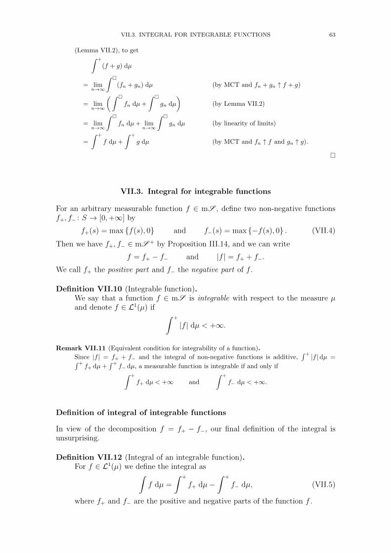
VII.3. INTEGRAL FOR INTEGRABLE FUNCTIONS 63
(Lemma VII.2), to get∫ +
(f + g) dµ
= limn→∞
∫
(fn + gn) dµ (by MCT and fn + gn ↑ f + g)
= limn→∞
(∫
fn dµ+
∫
gn dµ
)(by Lemma VII.2)
= limn→∞
∫
fn dµ+ limn→∞
∫
gn dµ (by linearity of limits)
=
∫ +
f dµ+
∫ +
g dµ (by MCT and fn ↑ f and gn ↑ g).
VII.3. Integral for integrable functions
For an arbitrary measurable function f ∈ mS , define two non-negative functionsf+, f− : S → [0,+∞] by
f+(s) = max f(s), 0 and f−(s) = max −f(s), 0 . (VII.4)
Then we have f+, f− ∈ mS + by Proposition III.14, and we can write
f = f+ − f− and |f | = f+ + f−.
We call f+ the positive part and f− the negative part of f .
Definition VII.10 (Integrable function).We say that a function f ∈ mS is integrable with respect to the measure µand denote f ∈ L1(µ) if ∫ +
|f | dµ < +∞.
Remark VII.11 (Equivalent condition for integrability of a function).
Since |f | = f+ + f− and the integral of non-negative functions is additive,∫ + |f |dµ =∫ +
f+ dµ+∫ +
f− dµ, a measurable function is integrable if and only if∫ +
f+ dµ < +∞ and
∫ +
f− dµ < +∞.
Definition of integral of integrable functions
In view of the decomposition f = f+ − f−, our final definition of the integral isunsurprising.
Definition VII.12 (Integral of an integrable function).For f ∈ L1(µ) we define the integral as∫
f dµ =
∫ +
f+ dµ−∫ +
f− dµ, (VII.5)
where f+ and f− are the positive and negative parts of the function f .
64 VII. INTEGRATION THEORY
By Remark VII.11 above, the two terms in formula (VII.5) are finite, so the expres-sion is well defined.
For non-negative functions f ∈ mS + the new definition of integral coincides withthe earlier one.
Lemma VII.13 (No conflict between the two last definitions of integral).For any non-negative integrable function f ∈ mS + ∩ L1(µ) we have∫
f dµ =
∫ +
f dµ.
Proof. For a non-negative function f ∈ mS + we have f+ = f and f− = 0. Therefore the agreementof the two integrals is obvious from the definition (VII.5).
Properties of integral of integrable functions
Now that the functions involved may have both positive and negative signs, esti-mating integrals by the following triangle inequality becomes important.
Theorem VII.14 (Triangle inequality for integrals).For any integrable function f ∈ L1(µ) we have∣∣∣ ∫ f dµ
∣∣∣ ≤ ∫ |f | dµ.Proof. Observe first that the right hand side is∫
|f | dµ =
∫ +
|f | dµ =
∫ +
(f+ + f−) dµ =
∫ +
f+ dµ+
∫ +
f− dµ.
We will prove∫f dµ ≤
∫|f |dµ and −
∫f dµ ≤
∫|f |dµ, which together imply the assertion∣∣ ∫ f dµ
∣∣ ≤ ∫ |f |dµ.
By (VII.5) and the non-negativity of integral∫f− dµ of the non-negative function f−, we
have ∫f dµ =
∫ +
f+ dµ−∫ +
f− dµ
≤∫ +
f+ dµ+
∫ +
f− dµ =
∫|f | dµ.
Similarly, we have
−∫f dµ = −
∫ +
f+ dµ+
∫ +
f− dµ
≤∫ +
f+ dµ+
∫ +
f− dµ =
∫|f | dµ.
In particular, in proving linearity, we use the triangle inequality to check that thesum of integrable functions is integrable in the first place.
Theorem VII.15 (Linearity of the integral).
VII.4. CONVERGENCE THEOREMS FOR INTEGRALS 65
(a) For any f ∈ L1(µ) and c ∈ R we have cf ∈ L1(µ) and∫cf dµ = c
∫f dµ.
(b) For any f, g ∈ L1(µ) we have f + g ∈ L1(µ) and∫(f + g) dµ =
∫f dµ+
∫g dµ.
Proof of part (a). If c ≥ 0 then we have (cf)+ = cf+ and (cf)− = cf−. Integrability of cf followseasily by Remark VII.11, since∫ +
(cf)+ dµ =
∫ +
cf+ dµ = c
∫ +
f+ dµ︸ ︷︷ ︸<+∞
< +∞
and similarly∫ +
(cf)− dµ < +∞. The asserted formula is also a direct consequence of the
definition (VII.5) of∫
, and linearity of∫ +
(Proposition VII.9),∫ +
cf dµ =
∫ +
cf+ dµ−∫ +
cf− dµ = c(∫ +
f+ dµ−∫ +
f− dµ)
= c
∫f dµ.
If c < 0 then we have (cf)+ = −cf− and (cf)− = −cf+, and one can proceed similarly.
Proof of part (b). Note that |f + g| ≤ |f |+ |g|. If f, g ∈ L1(µ), we thus have∫ +
|f + g| dµ ≤∫ + (
|f |+ |g|)
dµ =
∫ +
|f | dµ+
∫ +
|g| dµ < +∞,
and therefore f+g ∈ L1(µ). The formula for the integral of f+g can be proven by carefullyconsidering which possibilities contribute to the positive and negative parts of f + g.
Also monotonicity continues to hold.
Theorem VII.16 (Monotonicity of the integral).If f, g ∈ L1(µ) and f ≤ g, then we have∫
f dµ ≤∫g dµ.
Proof. If we have the pointwise inequality f ≤ g, then the positive and negative parts of thesefunctions satisfy f+ ≤ g+ and f− ≥ g−. It therefore follows from the defining formula (VII.5)
of∫
, and monotonicity of∫ +
(Proposition VII.6), that∫f dµ =
∫ +
f+ dµ−∫ +
f− dµ
≤∫ +
g+ dµ−∫ +
g− dµ =
∫g dµ.
VII.4. Convergence theorems for integrals
Finally, we establish some of the powerful standard tools of measure theory, whichaddress when it is legitimate to interchange the order of a limit and an integra-tion. Recalling that integration contains as special cases also expected values and
66 VII. INTEGRATION THEORY
summation, we thus ask under what conditions we have
limn→∞
∫fn(s) dµ(s)
?=
∫ (limn→∞
fn(s))
dµ(s)
limn→∞
∞∑k=0
a(n)k
?=
∞∑k=0
(limn→∞
a(n)k
)limn→∞
E[Xn
] ?= E
[limn→∞
Xn
].
In particular, derivatives are limits of difference quotients, so the results can beapplied to justifying the interchange of differentiation and integral, sum, or expectedvalue, i.e.
d
dλ
∫fn(s;λ) dµ(s)
?=
∫d
dλfn(s;λ) dµ(s)
d
dλ
∞∑k=0
ak(λ)?=
∞∑k=0
( d
dλak(λ)
)d
dλE[f(Xn;λ)
] ?= E
[ d
dλf(Xn;λ)
].
To fully appreciate the positive results we will derive, it is advisable to first thinkabout the ways the conclusion could fail.
Exercise VII.3 (Interchanging limit and integration is not always possible).
(a) Consider the Lebesgue measure Λ on R. For n ∈ N, define fn : R→ R by
fn(x) =
n if 0 < x ≤ 1
n
0 otherwise.
Calculate the following
limn→∞
fn,
∫Rfn dΛ,
∫R
(limn→∞
fn)
dΛ, limn→∞
∫Rfn dΛ.
(b) Repeat the calculations of part (a) for the functions√fn and f2
n, instead.(c) Consider Z with the counting measure µ#. For n ∈ N, define gn : Z→ R by
gn(k) =
1 if k = n
0 if k 6= n.
Calculate the following
limn→∞
gn,
∫Zgn dµ#,
∫Z
(limn→∞
gn)
dµ#, limn→∞
∫Zgn dµ#.
We will obtain several results about what conditions are sufficient to permit changinglimits and integration. Besides
(MCT) Monotone convergence theorem (Theorem VII.8)
another such result of great importance is
(DCT) Dominated convergence theorem (Theorem VII.19)
For expected values, there is a very practical special case of the Dominated conver-gence theorem:
(BCT) Bounded convergence theorem (Corollary VII.21)
VII.4. CONVERGENCE THEOREMS FOR INTEGRALS 67
The Monotone convergence theorem was already introduced as a tool in step (3) ofthe construction. The proof of the Dominated convergence theorem relies on it, andanother intermediate result that is occasionally useful on its own right as well:
Fatou’s Lemma (Lemma VII.17)
Fatou’s lemma
Fatou’s lemma is a general convergence result for non-negative integrals, which doesnot even require the limits to exists! It instead addresses lower limits which alwaysexist. A minor drawback is that the conclusion is merely an inequality in onedirection.
Lemma VII.17 (Fatou’s lemma).For any sequence f1, f2, . . . ∈ mS + of non-negative measurable functions, wehave ∫ (
lim infn
fn)
dµ ≤ lim infn
∫fn dµ. (VII.6)
Proof. Define g = lim infn fn. For k ∈ N, define also
gk := infn≥k
fn.
Then we have gk ∈ mS + (by Proposition III.14), and gk ↑ g as k →∞ by construction. Bythe Monotone convergence theorem, we therefore have∫
gk dµ ↑∫g dµ as k →∞.
We have fn ≥ gk for any n ≥ k, so monotonicity of integral gives∫fn dµ ≥
∫gk dµ for
n ≥ k, and thus also
infn≥k
∫fn dµ ≥
∫gk dµ.
In this inequality, take the limit as k →∞ to obtain
lim infn
∫fn dµ ≥ lim
k→∞
∫gk dµ =
∫g dµ,
which is the asserted inequality.
Exercise VII.4 (Strict inequality in Fatou’s lemma).Find an example of a sequence of non-negative functions for which there is a strict inequalityin Fatou’s lemma, (VII.6).
Under suitable additional conditions, we get a result about upper limits of non-negative integrals as well.
Lemma VII.18 (Reverse Fatou’s lemma).Suppose that f1, f2, . . . ∈ mS + is a sequence of non-negative measurable func-tions such that there exists a non-negative measurable function g ∈ mS +
which uniformly bounds the sequence, fn ≤ g for all n ∈ N, and which is itselfintegrable,
∫g dµ < +∞. Then we have
lim supn
∫fn dµ ≤
∫ (lim sup
nfn)
dµ. (VII.7)
68 VII. INTEGRATION THEORY
Proof. Apply Fatou’s lemma to the sequence of functions g − fn, n ∈ N, and cancel the finitenumber
∫g dµ from both sides.
Dominated convergence theorem
Arguably the most practical general convergence result is Lebesgue’s dominatedconvergence theorem: it states that pointwise convergence and uniform boundednessof integrands by an integrable function are sufficient to permit taking the limit insidethe integral.
Theorem VII.19 (Dominated convergence theorem).Suppose that f1, f2, . . . ∈ mS is a sequence of measurable functions such thatthere exists a non-negative measurable function g ∈ mS + which uniformlybounds the absolute values of the sequence, |fn| ≤ g for all n ∈ N, and whichis itself integrable,
∫g dµ < +∞. Then if the pointwise limit f = limn→∞ fn
exists, we have
limn→∞
∫|fn − f | dµ = 0 (VII.8)
and limn→∞
∫fn dµ =
∫f dµ. (VII.9)
Proof. Since |fn| ≤ g for all n ∈ N, and fn → f as n → ∞, we also have |f | ≤ g. Therefore thetriangle inequality gives
|fn − f | ≤ |fn|+ |f | ≤ 2 g.
We have∫
2g < +∞ by integrability of g, so reverse Fatou’s lemma can be applied to thesequence of functions |fn − f |, n ∈ N. Together with the assumed pointwise convergencelimn→∞ |fn − f | = 0, the reverse Fatou’s lemma gives
lim supn
∫|fn − f | dµ ≤
∫ (lim sup
n|fn − f |
)dµ =
∫0 dµ = 0,
which proves the first assertion (VII.8).
Then use linearity and triangle inequality for integrals to get∣∣∣ ∫ fn dµ−∫f dµ
∣∣∣ =∣∣∣ ∫ (fn − f) dµ
∣∣∣ ≤ ∫|fn − f |dµ.
The right hand side tends to zero as n → ∞ by the first part, (VII.8). This proves thesecond assertion (VII.9).
Bounded convergence theorem
For finite measures (see Definition II.9) — and thus probability measures, in partic-ular — there is a very easy and practical special case of the Dominated convergencetheorem, known as the Bounded convergence theorem. The underlying reason forit, as well as many other simplifications in finite measure spaces, is the following.
Lemma VII.20 (Constant functions are integrable on finite measure spaces).Suppose that (S,S , µ) is a finite measure space. Let c ∈ R be a constant, andlet g : S → R be the constant function g(s) = c for all s ∈ S. Then g ∈ L1(µ).
VII.5. INTEGRALS OVER SUBSETS AND RESTRICTION OF MEASURES 69
Proof. The constant function g(s) = c is in particular a simple function, g = c IS , so we have∫ +
|g|dµ =
∫
|c|dµ = |c| µ[S]︸︷︷︸<+∞
< +∞.
In particular, constant functions are legitimate choices for the dominating function gin the Dominated convergence theorem, Theorem VII.19. This immediately yieldsthe following.
Corollary VII.21 (Bounded convergence theorem).Suppose that (S,S , µ) is a finite measure space and f1, f2, . . . ∈ mS is abounded sequence6 of measurable functions such that the pointwise limit func-tion f = limn→∞ fn exists. Then we have
limn→∞
∫fn dµ =
∫f dµ.
VII.5. Integrals over subsets and restriction of measures
Let (S,S , µ) be a measure space.
We adopt the following notation for integrals over subsets : if f : S → R is a functionand if R ⊂ S is a measurable subset, R ∈ S , then the integral of f over R is definedas ∫
R
f(s) dµ(s) :=
∫S
IR(s) f(s) dµ(s) (VII.10)
whenever either IR f ≥ 0 or IR f ∈ L1(µ).
A clear justification for the above convention is obtained in the following exercise.
Exercise VII.5 (Restriction of a measure to a subset).Let (S,S , µ) is a measure space and R ⊂ S a measurable subset, R ∈ S .
(a) Let S ′ consist of those A ⊂ R such that A = B ∩R for some B ∈ S , that is,
S ′ :=B ∩R
∣∣ B ∈ S.
Show that S ′ is a σ-algebra on R.(b) When A = B ∩R for some B ∈ S , set
µ′[A] := µ[B ∩R].
Show that µ′ is a measure on the measurable space (R,S ′).(c) For any function f : S → R, denote by f |R : R→ R the restriction of f to R. Prove that
we have ∫R
f |R dµ′ =
∫S
IR f dµ,
for (1) indicator functions f , (2) non-negative simple functions f , (3) non-negative mea-surable functions f , and finally for (4) all measurable functions f such that f |R ∈ L1(µ′).
6This means that there exists some c ∈ [0,+∞) such that |fn(s)| ≤ c for all s ∈ S and n ∈ N.
70 VII. INTEGRATION THEORY
VII.6. Riemann integral vs. Lebesgue integral
The reader can now verify that the Riemann integral (familiar from undergraduatecalculus) and Lebesgue integral coincide in the following setups.
Exercise VII.6 (Riemann integral and Lebesgue integral on closed intervals).Consider a closed interval [a, b] ⊂ R. Suppose that f : [a, b] → R is a continuous function.Show that ∫ b
a
f(x) dx =
∫[a,b]
f(x) dΛ(x),
where the right hand side denotes the integral of f with respect to the Lebesgue measure Λrestricted to [a, b] ⊂ R, and the left hand side denotes the Riemann integral of f .Hint: The Riemann integral is defined by the condition that the upper and lower Riemann sums
associated to subdivisions of the interval [a, b] tend to the same limit as the meshes of the subdivisions
become finer. First show that these upper and lower Riemann sums associated to a subdivision are
equal to the integrals of certain simple functions. Then use monotonicity to compare the Lebesgue
integral of f to these.
Exercise VII.7 (Improper Riemann integrals and Lebesgue integral).
(a) Suppose that f : [a, b)→ R is continuous. Show that if∫
[a,b)|f |dΛ < +∞, then we have
the following equality of the improper Riemann integral and the Lebesgue integral:∫ b
a
f(x) dx := limε↓0
∫ b−ε
a
f(x) dx =
∫[a,b)
f(x) dΛ(x).
(b) Suppose that f : R → R is continuous. Show that if∫R |f |dΛ < +∞, then we have the
following equality of the improper Riemann integral and the Lebesgue integral:∫ +∞
−∞f(x) dx := lim
r↑+∞
∫ r
−rf(x) dx =
∫Rf(x) dΛ(x).
Hint: Exercise VII.6 and Dominated convergence theorem.
Remark VII.22 (On the relationship between Riemann-integral and Lebesgue integral).
• There are plenty of functions for which the Riemann integral does not exist, while theLebesgue integral is well-defined. A simple example is the indicator function IQ∩[a,b]
of the rational numbers on the interval. The Lebesgue integrals∫IQ∩[a,b] dΛ = 0 and∫
I[a,b]\Q dΛ = b − a reflect the fact that the countable set Q ∩ [a, b] is negligible, in ameasure-theoretic sense, compared to its complement [a, b] \ Q (which, in particular, isuncountable). The Riemann integral fails to account for this “evident” size difference.
• Pointwise limits of Riemann integrable functions need not be Riemann integrable, so onecould not hope to have the general and powerful convergence theorems of Section VII.4for the Riemann integral.7
• The coincidence of Riemann integral and Lebesgue integral for well-behaved functionsallows us to use the familiar techniques such as the fundamental theorem of calculus,integration by parts, etc., without the need to prove them again.
• Given how common integration on the real axis is, it is convenient to have a concisenotation for it. By virtue of the coincidence of the two notions of integration on R forall well-behaved functions, with almost no risk of confusion we can use the notation
dx := dΛ(x)
for integration with respect to Lebesgue measure Λ.
7Besides the generality (at once we constructed, e.g., integrals in all dimensions, expected val-ues, infinite sums, . . . ), arguably the most significant advantage of the integration theory developedin this chapter is indeed the convergence theorems.
Lecture VIII
Expected values
In this lecture we begin examining the role and use of expected values in probabilitytheory.
Let (Ω,F ,P) be a probability space. We will use the notation E for expected values.The expected value of a real-valued random variable X : Ω → R is just the integralwith respect to the probability measure P,
E[X]
:=
∫Ω
X(ω) dP(ω).
Let us summarize how it is constructed step by step for increasingly general randomvariables X : Ω→ R as in the previous lecture (Lecture VII):
(1) If X = IA for an event A ∈ F , then we set E[X] = P[A].(2) If X =
∑nj=1 ajIAj is simple1, then we set E[X] =
∑nj=1 ajP[Aj].
(3) If X is non-negative, then we set
E[X] = supH∈sF+
0≤H≤X
E[H].
(4) If X is integrable, i.e., E[X+] < +∞ and E[X−] < +∞, then we set
E[X] = E[X+]− E[X−].
Since expected value is by definition a special case of integral, the basic propertiesof integrals lead to the corresponding basic properties of expected values:
Linearity: (Proposition VII.9 and Theorem VII.15)For either X, Y ∈ mF + (two non-negative random variables), or for X, Y ∈L1(P) (two integrable random variables), we have
E[X + Y
]= E
[X]
+ E[Y].
For either X ∈ mF + and c ≥ 0, or for X ∈ L1(P) and c ∈ R, we have
E[cX]
= c E[X].
Monotonicity: (Proposition VII.6 and Theorem VII.16)For either X, Y ∈ mF + (two non-negative random variables) or for X, Y ∈L1(P) (two integrable random variables), we have
X ≤ Y =⇒ E[X]≤ E
[Y]
1In Section VII.1 we were careful to only integrate simple functions which are non-negative,in order to avoid undefined expressions of the form +∞ −∞. For expected values, because offiniteness P[Ω] = 1 < +∞ of the total mass of a probability measure, this never causes problems,so formula (VII.2) can be directly taken as a definition of the expected value of any simple function(random variable).
71
72 VIII. EXPECTED VALUES
Triangle inequality: (Theorem VII.14)For X ∈ L1(P), we have∣∣∣E[X] ∣∣∣ ≤ E
[|X|].
Besides these basic properties, also the powerful convergence theorems of Section VII.4continue hold for expected values.
VIII.1. Expected values in terms of laws
Recall from Definition III.6 that the law of a random variable X : Ω → R (or thedistribution of X) is the probability measure PX on R given by
PX [B] = P[X ∈ B
]for B ∈ B.
We next show how the expected value of g(X) can be calculated as an integral withrespect to the law PX .
Theorem VIII.1 (Expected values in terms of laws).Let X : Ω→ R be a random variable with law PX , and let g : R→ R be a Borelfunction. Then we have the equivalence of the following integrability properties
g(X) ∈ L1(P) ⇐⇒ g ∈ L1(PX).
If either (then both) of the above integrability properties holds, then we have
E[g(X)
]=
∫Rg(x) dPX(x).
Proof. The proof follows the “standard machine”, i.e., we verify the statement for (1) indicatorfunctions, (2) simple functions, (3) non-negative measurable functions, and finally (4) allmeasurable functions g.
step 1: Consider an indicator function g = IB of a Borel set B ∈ B. Observe, as in (IV.1)and (IV.2), that IB(X(ω)) = IX−1(B)(ω) for all ω ∈ Ω. Thus we have
E[IB(X)
]= E
[IX−1(B)
](because IB X = IX−1(B))
= P[X−1(B)
](by step 1 of def. of E)
= PX [B] (by def. of PX)
=
∫IB dPX . (by step 1 of def. of integral)
This shows that E[g(X)] =∫g dPX for g = IB .
step 2: Consider a simple Borel function g ∈ sB+. Write g =∑nj=1 ajIBj . We have
E[ n∑j=1
aj IBj (X)]
=
n∑j=1
aj E[IBj (X)
](by linearity of E)
=
n∑j=1
aj
∫IBj dPX (by step 1)
=
∫ ( n∑j=1
aj IBj)
dPX (by linearity of integral).
This shows that E[g(X)] =∫g dPX for g ∈ sB+.
VIII.1. EXPECTED VALUES IN TERMS OF LAWS 73
step 3: Consider a non-negative Borel function g ∈ mB+. Take a monotone increasing pointwiseapproximation gn ↑ g as n → ∞ by non-negative simple Borel functions gn ∈ sB+. Wethen also have gn(X) ↑ g(X), and gn(X) ∈ sF+ are non-negative simple random variables.Using Monotone convergence theorem (Theorem VII.8) both for P and for PX , we get
E[g(X)
]= lim
n→∞E[gn(X)
](by MCT for P)
= limn→∞
∫gn dPX (by step 2)
=
∫g dPX . (by MCT for PX).
step 4: Consider a Borel function g ∈ mB, and let g+, g− ∈ mB+ be its positive and negativeparts. The positive and negative parts of the random variable g(X) = g X are (g(X))+ =g+ X ∈ mF+ and (g(X))− = g− X ∈ mF+. By step 3 we thus have
E[(g(X)
)+
]= E
[g+(X)
]=
∫g+ dPX
and E[(g(X)
)−
]= E
[g−(X)
]=
∫g− dPX .
Therefore we first of all have the equivalent conditions
E[(g(X)
)+
]< +∞ ⇐⇒
∫g+ dPX < +∞
and E[(g(X)
)−
]< +∞ ⇐⇒
∫g− dPX < +∞,
which by Remark VII.11 shows the equivalence g(X) ∈ L1(P) ⇔ g ∈ L1(PX). Moreover,when this integrability holds, step 4 of the definition of the integrals gives
E[g(X)
]= E
[(g(X)
)+
]− E
[(g(X)
)−
]and
∫g dPX =
∫g+ dPX −
∫g− dPX .
These coincide by the above equalities, which finishes the proof.
Exercise VIII.1 (Discrete random numbers).A random variable is discrete if its range A = X(Ω) is finite or countably infinite. Theprobability mass function of a discrete random variable X is defined by pX(x) = P
[X = x
].
Prove that any discrete real-valued random variable satisfies:
(a) E[h(X)
]=∑x∈A h(x) pX(x) for all Borel functions h : R→ [0,∞).
(b) h(X) ∈ L1(Ω,F ,P) if and only if∑x∈A |h(x)| pX(x) <∞.
(c) Explain why the formula in (a) is true for all h ∈ L1(R,B, PX).
Hint: Recall the argument in the proof of Theorem VIII.1.
Exercise VIII.2 (Almost sure equality).Let X and Y be real-valued random variables that are equal almost surely, that is,
P[X = Y
]= 1.
(a) In order to make sure that P[X = Y ] is a meaningful probability, explain first why thesetω ∈ Ω
∣∣ X(ω) = Y (ω)
is measurable.(b) Prove that the laws of X and Y are the same, and conclude that we in particular have
E[X] = E[Y ] (whenever the expected values exist).
74 VIII. EXPECTED VALUES
Probability densities of continuous distributions
Definition VIII.2 (Probability density of a continuous distribution).Let X ∈ mF be a real valued random variable. If there exists a Borel function
fX : R→ [0,+∞)
such that2
PX [B] := P[X ∈ B
]=
∫B
fX(x) dx (VIII.1)
for all B ∈ B, then we say that X has a continuous distribution (or a contin-uous law), and we say that fX is a density function of X.
Example VIII.3 (Gaussian distribution).Let m ∈ R and s > 0. A random variable X is said to have a gaussian distribution withmean m and variance s2 if its distribution is continuous and
fX(x) =1√
2π s2exp
(− 1
2 s2(x−m)2
)is a density function of X.
Gaussian distributions are also called normal distributions, and the particular case of zeromean m = 0 and unit variance s2 = 1 is called the standard normal distribution.
Example VIII.4 (Exponential distribution).Let λ > 0. A random variable X is said to have an exponential distribution with parameterλ if its distribution is continuous and
fX(x) =
λ e−λx for x ≥ 0
0 for x < 0
is a density function of X.
Exercise VIII.3 (Random numbers with continuous distribution).Assume that X has a continuous law with a density function fX .
(a) Show that X is integrable if and only if∫R |x| fX(x) dx <∞.
(b) If X is integrable, show that expectation of X is given by
E[X]
=
∫Rx fX(x) dx.
(c) If X is integrable with expected value m := E[X], show that the variance of X can becomputed as
Var(X) := E[(X − E[X])2
]=
∫R
(x−m)2 fX(x) dx.
(d) Can a random variable with continuous law have more than one density function?
Hint: Remember the hint for Exercise VIII.1, and seek a unified argument leading to (a) and (b) —
perhaps even (c).
Exercise VIII.4 (Expected value and variance of an exponential random variable).Assume that a random variable X has an exponential distribution with parameter λ (seeExample VIII.4). Use the previous exercise to calculate the expected value E[X] and thevariance Var(X) of X.
2The right hand side of (VIII.1) is an integral over the subset B ⊂ R in the sense of (VII.10),∫B
fX(x) dx :=
∫RfX(x) IB(x) dΛ(x).
VIII.2. APPLICATIONS OF CONVERGENCE THEOREMS FOR EXPECTED VALUES 75
Exercise VIII.5 (The absolute value of a random number).Let Y = |X| where X is a real-valued random variable.
(a) Prove that Y is a random variable.(b) Assume that we know the cumulative distribution function FX(x) = P[X ≤ x] of X.
What is the cumulative distribution function of Y ?(c) Assume that X has continuous distribution with a density function fX(x). Does Y also
have a continuous distribution in this case? If yes, write down an expression for a densityfunction fY of Y in terms of fX . If not, explain why not.
VIII.2. Applications of convergence theorems for expected values
In this section we look at a few consequences of the convergence theorems in variousaspects of probability theory.
Expected values of random series with non-negative terms
Let us observe that a non-negative random variable can only have finite expectedvalue if the random variable is almost surely finite.3
Lemma VIII.5 (Finite expected value implies almost sure finiteness).If X ∈ mF + is a non-negative random variable such that E[X] < +∞, thenwe have X < +∞ almost surely, i.e., P
[X < +∞
]= 1.
Proof. Let A =ω ∈ Ω
∣∣ X(ω) = +∞
be the event that the random variable X takes an infinitevalue. Then for any n ∈ N we obviously have X ≥ n IA, so by monotonicity of expectedvalues we get
n P[A] = E[n IA
]≤ E
[X].
Dividing this by n, we get P[A] ≤ 1n E[X]. By assumption X has finite expected value,
E[X]< +∞, so by letting n → ∞ we get P[A] ≤ 0. This shows that P[A] = 0, so passing
to the complement we prove the claim
P[X < +∞
]= P
[Ac]
= 1− P[A] = 1− 0 = 1.
Next we note that in a random sum with non-negative terms, we are allowed tointerchange the order of summation and expected value.
Lemma VIII.6 (Expected value of a series of non-negative random terms).Suppose that X1, X2, . . . ∈ mF + is a sequence of non-negative random vari-ables. Consider the random infinite series
∑∞k=1 Xk. Then we have
E[ ∞∑k=1
Xk
]=∞∑k=1
E[Xk
].
3A similar conclusion holds for integrals generally, not just expected values. We leave it to thereader to precisely formulate the statement and see that the proof carries through.
76 VIII. EXPECTED VALUES
Proof. By definition, these infinite sums are the limits of their finite partial sums, in particular∞∑k=1
Xk(ω) = limn→∞
n∑k=1
Xk(ω) for all ω ∈ Ω.
By non-negativity of the terms, the sequence of partial sums is increasing, i.e.,n∑k=1
Xk(ω) ↑∞∑k=1
Xk(ω) as n→∞, for all ω ∈ Ω.
In this pointwise increasing approximation, we can apply the Monotone convergence theo-rem (MCT), and get
E[ ∞∑k=1
Xk
]= E
[limn→∞
n∑k=1
Xk
](by definition of infinite sum)
= limn→∞
E[ n∑k=1
Xk
](by MCT)
= limn→∞
n∑k=1
E[Xk
](by linearity of expected value)
=
∞∑k=1
E[Xk
]. (by definition of infinite sum)
The assertion is thus proven.
We can combine the above observations to obtain a sufficient condition for almostsure convergence of random series with non-negative terms.
Proposition VIII.7 (Guaranteeing almost sure convergence of a random series).Suppose that X1, X2, . . . ∈ mF + is a sequence of non-negative random vari-ables. Suppose moreover that we have
∞∑k=1
E[Xk
]< +∞.
Then we have almost surely∑∞
k=1Xk < +∞ and almost surely Xk → 0 ask →∞, i.e.,
P[ ∞∑k=1
Xk < +∞]
= 1 and P[
limk→∞
Xk = 0]
= 1.
Proof. Note that the convergence∑∞k=1Xk < +∞ of the series implies that its terms tend to zero,
limk→∞Xk = 0, so for the corresponding events we haveω ∈ Ω
∣∣∣∣ ∞∑k=1
Xk(ω) < +∞
⊂ω ∈ Ω
∣∣∣∣ limk→∞
Xk(ω) = 0
and for their probabilities therefore
P[ ∞∑k=1
Xk < +∞]≤ P
[limk→∞
Xk = 0].
It therefore suffices to show that the probability on the left hand side is equal to one. ByLemma VIII.6 and the assumption of convergence of the series of expected values, we get
E[ ∞∑k=1
Xk
]=
∞∑k=1
E[Xk
]< +∞.
VIII.2. APPLICATIONS OF CONVERGENCE THEOREMS FOR EXPECTED VALUES 77
Lemma VIII.5 therefore implies what we claimed,
1 = P[ ∞∑k=1
Xk < +∞]≤ P
[limk→∞
Xk = 0].
Indicators of events, in particular, are non-negative random variables. The firstBorel – Cantelli lemma can thus be seen as consequence of the above observations.
Lemma (Borel–Cantelli lemma: convergence part, Lemma V.7).Suppose that E1, E2, . . . ∈ F are such that
∑∞k=1 P[Ek] < +∞. Then we have
P[“Ek occurs infinitely often”
]= 0.
Proof. Consider the indicators IEk of the events Ek, k = 1, 2, . . .. Note that the random series
N :=
∞∑k=1
IEk
counts the (random) number N of events in the sequence E1, E2, . . ., which occur. Byassumption, we have
∞∑k=1
E[IEk]
=
∞∑k=1
P[Ek] < +∞.
Therefore by Proposition VIII.7 we in particular have that P[N < +∞] = 1, i.e., almostsurely only finitely many of the events in the sequence E1, E2, . . . occur. The complementaryevent is that infinitely many of the events occur, so we have
P[“Ek occurs infinitely often”
]= P
[N = +∞
]= 1− P
[N < +∞
]= 1− 1 = 0.
This finishes our alternative proof of the first Borel–Cantelli lemma.
Differentiation inside expected values
As an application of the Dominated convergence theorem, the reader can verify thatexchanging the order of expected values and differentiation is permitted for examplein the following situation.
Exercise VIII.6 (Differentiation inside expectation).Let (Ω,F ,P) be a probability space and X : Ω → R a random variable. Suppose thath : R × (a, b) → R is a continuous function, (x, λ) 7→ h(x, λ). Assume that the partialderivative with respect to the second variable, ∂
∂λh : R × (a, b) → R, is also continuous.
Assume moreover, that for some integrable random variable Y ∈ L1(Ω,F ,P) we have
for all λ ∈ (a, b) and ω ∈ Ω :∣∣∣( ∂∂λh)
(X(ω), λ)∣∣∣ ≤ Y (ω).
(a) Show that for any λ, λ′ ∈ (a, b) with λ 6= λ′ we have |h(X,λ′)−h(X,λ)λ′−λ | ≤ Y .
Hint: Write h(x, λ2) − h(x, λ1) =∫ λ2
λ1( ∂∂λh)(x, λ) dλ, and recall the triangle inequality for
integrals.
(b) Show that
d
dλE[h(X,λ)
]= E
[( ∂∂λh)(X,λ)
].
Hint: When λn → λ, consider 1λn−λ
(E[h(X,λn)
]− E
[h(X,λ)
]). Use part (a) and dominated
convergence.
78 VIII. EXPECTED VALUES
Differentiation inside expected value is in particular often used for various generatingfunctions.
Exercise VIII.7 (Differentiating the moment generating function).Define the moment generating function of X : Ω → R by MX(λ) := E
[eλX
]. Assume that
E[eε|X|
]<∞ for some ε > 0.
(a) Show that M ′X(0) = E[X].Hint: Find a way to apply Exercise VIII.6, perhaps by first showing that for |λ| < ε one has
|xeλx| ≤ Ceε|x|.(d) Explain, without detailed calculations, why M ′′X(0) = E[X2]. Find also a similar formula
for E[Xn] for all n ∈ N.
VIII.3. Space of p-integrable random variables
Let X : Ω → R be a random variable. Recall that we say that X is integrable andwrite X ∈ L1(P) if
E[|X|]< +∞.
The following generalization is encountered very often.
Definition VIII.8 (p-integrability).Let p > 0. We say that a random variable X is p-integrable and denoteX ∈ Lp(P) if
E[|X|p
]< +∞. (VIII.2)
In probability spaces, p-integrability implies r-integrability for any r ≤ p, as wewill show in the next lemma. This is used in particular to conclude that if it ismeaningful to talk about the moment E[Xp] of order p, it is also meaningful totalk about all lower order moments E[Xr]. Let us emphasize that in very commonmeasure spaces of infinite total mass, p-integrability does not imply integrability oflower order, so the lemma is specific to probability theory.
Lemma VIII.9 (Finiteness of lower order moments).Let 0 < r < p. Suppose that X ∈ Lp(P). Then we have X ∈ Lr(P), andmoreover
E[|X|r
]≤ 1 + E
[|X|p
].
Proof. Since 0 < r < p, we have that |x|r < |x|p whenever |x| > 1, and |x|r ≤ 1 whenever |x| ≤ 1.Define the event
A =ω ∈ Ω
∣∣∣ |X(ω)| > 1.
Then we have the pointwise estimate
|X(ω)|r ≤ IAc(ω) + IA(ω) |X(ω)|p
≤ 1 + |X(ω)|p.By monotonicity and linearity of the expected value, this gives
E[|X|r
]≤ E
[1 + |X|p
]≤ 1 + E
[|X|p
].
Both asserted results follow from this.
VIII.3. SPACE OF p-INTEGRABLE RANDOM VARIABLES 79
The space Lp(P) of all p-integrable random variables is a vector space.
Lemma VIII.10 (p-integrable random variables form a vector space).Let p ≥ 0. Then we have the following.
(a) If X ∈ Lp(P) and a ∈ R, then aX ∈ Lp(P).(b) If X, Y ∈ Lp(P), then X + Y ∈ Lp(P) and
E[|X + Y |p
]≤ 2p
(E[|X|p
]+ E[|Y |p
])(VIII.3)
Proof. Part (a) is clear, since E[|aX|p
]= |a|p E
[|X|p
]. It therefore only remains to prove (b).
For any x, y ∈ R note that
|x+ y| ≤ |x|+ |y| ≤ 2 max |x|, |y| .
The mapping t 7→ tp is increasing [0,∞)→ [0,∞), so applying it to the above gives
|x+ y|p ≤ 2p max |x|p, |y|p .
This of course implies also
|x+ y|p ≤ 2p(|x|p + |y|p
).
Applying this inequality pointwise to the values of the random variables X and Y gives
|X(ω) + Y (ω)|p ≤ 2p(|X(ω)|p + |Y (ω)|p
)for all ω ∈ Ω.
Taking expected values and using monotonicity and linearity, we get
E[|X + Y |p
]≤ 2p
(E[|X|p
]+ E
[|Y |p
]),
and the assertions of part (b) follow.
Since a constant random variable c is p-integrable for any p > 0, the vector spaceproperty in particular has the following consequence.
Corollary VIII.11 (Adding a constant preserves p-integrability).If X ∈ Lp(P) and c ∈ R is a constant, then also X + c ∈ Lp(P).
The estimates in Lemma VIII.9 were rather crude. The following very often usefulinequality is one way to improve them.
Exercise VIII.8 (Jensen’s inequality).Suppose that I ⊂ R is an interval and φ : I → R is a convex function, i.e., a function suchthat for any x, y ∈ I and λ ∈ (0, 1) we have
φ(λx+ (1− λ) y
)≤ λ φ(x) + (1− λ) φ(y).
Suppose moreover that X : Ω→ I is a random variable with values on the interval I.
(a) Show that for any z ∈ I there exists a number d ∈ R such that φ(x) ≥ φ(z) + (x− z) d.Hint: Consider the left and right derivatives of φ at z.
(b) Show that if X is a random variable with values in I ⊂ R, and both X and φ(X) areintegrable, then we have
φ(E[X]
)≤ E
[φ(X)
].
Hint: Choose z = E[X] and apply part (a) together with monotonicity and linearlity of expected
values.
80 VIII. EXPECTED VALUES
Exercise VIII.9 (The p-norm controls lower norms).Suppose that X ∈ Lp(P) for some p > 0. Let 0 < r < p. Using Exercise VIII.8, show that(
E[|X|r
])1/r
≤(E[|X|p
])1/p
,
Lecture IX
Product spaces and Fubini’s theorem
Imagine observing two random phenomena simultaneously. The set of possible out-comes then is a Cartesian product, it consists of pairs
Ω1 × Ω2 =
(ω1, ω2)∣∣ ω1 ∈ Ω1, ω2 ∈ Ω2
,
whose two components are outcomes of the two phenomena.
Example IX.1 (Two coin tosses).For one coin toss the sample space is H,T, representing the possible outcomes “heads”and “tails”. For two coin tosses the sample space is
H,T × H,T =
(H,H), (H,T), (T,H), (T,T).
In this lecture we treat measures on such Cartesian product spaces. We constructin particular:
• the product σ-algebra on a Cartesian product of measurable spaces• the product measure on a Cartesian product of (σ-finite) measure spaces.
One of the results of great practical importance is Fubini’s Theorem (Theorem IX.9):for two measure spaces (S1,S1, µ1) and (S2,S2, µ2) and a function f : S1×S2 → R,under reasonable conditions the change of order of integration formula∫
S1
(∫S2
f(s1, s2) dµ2(s2))
dµ1(s1) =
∫S2
(∫S1
f(s1, s2) dµ1(s1))
dµ2(s2)
holds. Recalling that expected values and summation are special cases of integration,this implies (under reasonable assumptions) formulas such as∫ ( ∞∑
k=1
fk(s))
dµ(s) =∞∑k=1
∫fk(s) dµ(s),
E[ ∞∑k=1
Xk
]=
∞∑k=1
E[Xk
],
etc.
Key tool: Monotone class theorem
In this lecture, we will repeatedly use the Monotone class theorem (Theorem C.2from Appendix C). Let us recall its statement, and introduce convenient notationfor it.
81
82 IX. PRODUCT SPACES AND FUBINI’S THEOREM
We denote as before
mS — the set of S -measurable functions S → [−∞,+∞]
sS — the set of simple functions S → R
and in addition the set of bounded measurable functions will be denoted by
bS :=f ∈ mS
∣∣∣ |f | ≤ C for some C ∈ R.
We also continue to use the superscript + for the sets of non-negative functions ofthe corresponding types,
mS + :=f ∈ mS
∣∣∣ f ≥ 0
sS + :=f ∈ sS
∣∣∣ f ≥ 0
bS + :=f ∈ bS
∣∣∣ f ≥ 0.
According to Definition C.1, a collection H of functions S → R is said to be amonotone class if:
(MC-1) The constant function 1 belongs to H .(MC-R) The class H is a vector space over R.(MC-↑) If f1, f2, . . . ∈H is an increasing sequence of non-negative functions in H
such that the pointwise limit fn ↑ f is a bounded function f , then f ∈H .
The statement of the Monotone Class Theorem is the following.
Theorem (Monotone class theorem, Theorem C.2).Let H be a monotone class of bounded functions from S to R and let J be aπ-system on S such that σ(J ) = S . Suppose that
IA ∈H for every A ∈J .
Then we have
bS ⊂H .
IX.1. Product sigma algebra
Let (S1,S1) and (S2,S2) be two measurable spaces. As the first step, we have toequip the Cartesian product
S1 × S2 =
(s1, s2)∣∣ s1 ∈ S1, s2 ∈ S2
with a σ-algebra. We think of the coordinate projections
pr1 : S1 × S2 → S1 pr1(s1, s2) = s1
pr2 : S1 × S2 → S2 pr2(s1, s2) = s2
as fundamental, and require that they must be measurable functions to (S1,S1) and(S2,S2), respectively.
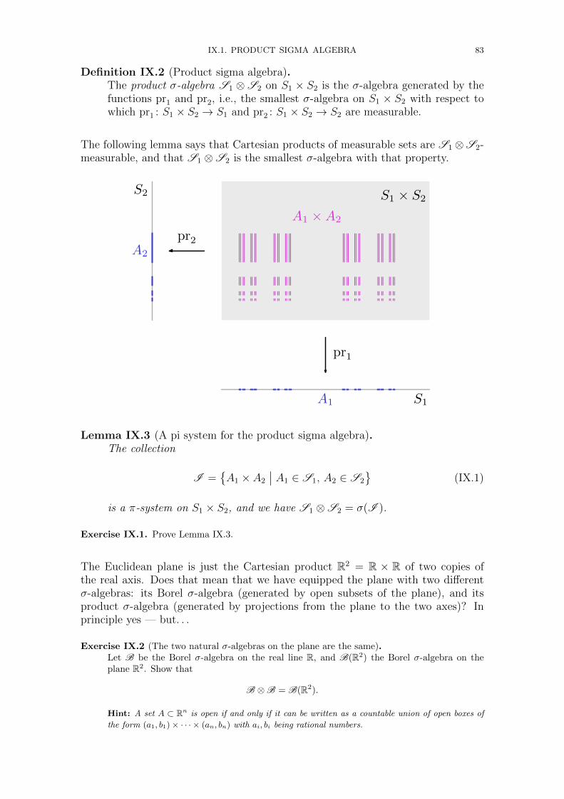
IX.1. PRODUCT SIGMA ALGEBRA 83
Definition IX.2 (Product sigma algebra).The product σ-algebra S1 ⊗S2 on S1 × S2 is the σ-algebra generated by thefunctions pr1 and pr2, i.e., the smallest σ-algebra on S1 × S2 with respect towhich pr1 : S1 × S2 → S1 and pr2 : S1 × S2 → S2 are measurable.
The following lemma says that Cartesian products of measurable sets are S1⊗S2-measurable, and that S1 ⊗S2 is the smallest σ-algebra with that property.
pr2
pr1
S2
S1
A2
A1
A1 ×A2
S1 × S2
Lemma IX.3 (A pi system for the product sigma algebra).The collection
I =A1 × A2
∣∣ A1 ∈ S1, A2 ∈ S2
(IX.1)
is a π-system on S1 × S2, and we have S1 ⊗S2 = σ(I ).
Exercise IX.1. Prove Lemma IX.3.
The Euclidean plane is just the Cartesian product R2 = R × R of two copies ofthe real axis. Does that mean that we have equipped the plane with two differentσ-algebras: its Borel σ-algebra (generated by open subsets of the plane), and itsproduct σ-algebra (generated by projections from the plane to the two axes)? Inprinciple yes — but. . .
Exercise IX.2 (The two natural σ-algebras on the plane are the same).Let B be the Borel σ-algebra on the real line R, and B(R2) the Borel σ-algebra on theplane R2. Show that
B ⊗B = B(R2).
Hint: A set A ⊂ Rn is open if and only if it can be written as a countable union of open boxes of
the form (a1, b1)× · · · × (an, bn) with ai, bi being rational numbers.
84 IX. PRODUCT SPACES AND FUBINI’S THEOREM
Freezing one coordinate
Our first use of the Monotone Class Theorem is to show that with any functionf : S1 × S2 → R which is measurable with respect to the product σ-algebra, keep-ing one of the two coordinates fixed and letting the other vary defines measurablefunctions S1 → R and S2 → R.
Lemma IX.4 (Freezing a coordinate preserves measurability).Let H denote the class of functions f : S1×S2 → R such that f ∈ b(S1 ⊗S2)and
∀s1 ∈ S1 s2 7→ f(s1, s2) is S2-measurable S2 → R∀s2 ∈ S2 s1 7→ f(s1, s2) is S1-measurable S1 → R.
Then we have H = b(S1 ⊗S2).
Proof. By definition of H we have H ⊂ b(S1 ⊗S2), so we must show H ⊃ b(S1 ⊗S2).
Clearly the class H satisfies (MC-1), (MC-R), and (MC-↑). We will show that H containsthe indicator functions of all sets in the π-system I of Lemma IX.3. Since σ(I ) = S1⊗S2,the Monotone Class Theorem then allows us to conclude that H ⊃ b(S1 ⊗S2).
So suppose that A1 ∈ S1 and A2 ∈ S2, and consider the indicator function
IA1×A2: S1 × S2 → R
of the set A1 ×A2 ⊂ S1 × S2. We have
IA1×A2(s1, s2) = IA1(s1) IA2(s2),
so if s1 ∈ A1, the function s2 7→ IA1×A2(s1, s2) is the indicator IA2
of the set A2 ⊂ S2, and ifs1 /∈ A1, it is zero. In either case, s2 7→ IA1×A2(s1, s2) is S2-measurable S2 → R. Similarlyone shows that s1 7→ IA1×A2(s1, s2) is S1-measurable S1 → R, for any s2 ∈ S2. This showsthat the indicator functions of all sets in the π-system I of Lemma IX.3 are in the class H .This finishes the proof.
IX.2. Product measure
Let (S1,S1, µ1) and (S2,S2, µ2) be two measure spaces. Our next goal is to constructa product measure, denoted by µ1⊗µ2, on the measurable space (S1×S2,S1⊗S2).
First, in Section IX.2.1 we do that in the case when the measures are finite, andthen in Section IX.2.2 we relax the assumption of finiteness to σ-finiteness.
IX.2.1. Product of two finite measures
We now consider the case that (S1,S1, µ1) and (S2,S2, µ2) are two finite measurespaces, i.e., we assume that the total masses of the two measures are finite
µ1[S1] < +∞ and µ2[S2] < +∞.This assumption will be used frequently below to conclude that a function which isbounded and measurable is necessarily integrable (recall Lemma VII.20).
Suppose that f : S1 × S2 → R is a bounded S1 ⊗ S2-measurable function, i.e.,f ∈ b(S1 ⊗S2). The functions s2 7→ f(s1, s2) and s1 7→ f(s1, s2) are clearly also
IX.2. PRODUCT MEASURE 85
bounded, and they are measurable by Lemma IX.4. Thus they are integrable, andwe can define the functions
Jf1(s1) :=
∫S2
f(s1, s2) dµ2(s2) (IX.2)
Jf2(s2) :=
∫S1
f(s1, s2) dµ1(s1). (IX.3)
The next lemma shows that these integrals over one of the variables define mea-surable functions. Moreover, it essentially establishes the conclusion of Fubini’stheorem in the particular case of bounded measurable functions on finite measurespaces.
Lemma IX.5 (Fubini’s theorem for bounded functions).Let (S1,S1, µ1) and (S2,S2, µ2) be two finite measure spaces, and let f ∈ b(S1 ⊗S2).We then have the following:
(i) The function s1 7→ Jf1(s1) in (IX.2) is bounded and S1-measurable S1 → R.
(ii) The function s2 7→ Jf2(s2) in (IX.3) is bounded and S2-measurable S2 → R.(iii) We have the equality∫
S1
Jf1(s1) dµ1(s1) =
∫S2
Jf2(s2) dµ2(s2).
Proof. Let H be the collection of functions f ∈ b(S1 ⊗S2) for which (i), (ii), and (iii) hold. Wemust show H = b(S1 ⊗S2), and we will again do this using the Monotone Class Theorem.
We first claim that for any A1 ∈ S1 and A2 ∈ S2, the indicator IA1×A2 : S1 × S2 → R isin the collection H . Recall that IA1×A2
(s1, s2) = IA1(s1) IA2
(s2), fix s1 ∈ S1, and integrateover the variable s2 to get
JIA1×A21 (s1) =
∫S2
IA1(s1) IA2
(s2) dµ2(s2)
= IA1(s1)
∫S2
IA2(s2) dµ2(s2)
= µ2[A2] IA1(s1).
As a constant multiple of an indicator of the measurable setA1, the function s1 7→ JIA1×A21 (s1)
is S1-measurable and bounded, i.e., (i) holds for IA1×A2 . Similarly one shows that
JIA1×A22 (s2) = µ1[A1] IA2
(s2),
and concludes that s2 7→ JIA1×A22 (s2) is S2-measurable and bounded, i.e., (ii) holds for
IA1×A2. For (iii), calculate∫
S1
JIA1×A21 (s1) dµ1(s1) =
∫S1
µ2[A2] IA1(s1) dµ1(s1)
= µ2[A2]
∫S1
IA1(s1) dµ1(s1)
= µ2[A2] µ1[A1],
and similarly ∫S2
JIA1×A22 (s2) dµ2(s2) = µ1[A1] µ2[A2].
These two integrals coincide, so we get that also (iii) holds for IA1×A2 , and thus IA1×A2 ∈H .
It remains to prove that H is a monotone class. Properties (MC-1) and (MC-R) areeasy to verify. For property (MC-↑), suppose that f1, f2, . . . ∈ H are non-negative andfn(s1, s2) ↑ f(s1, s2) for all (s1, s2) ∈ S1 × S2, where f : S1 × S2 → R is bounded. Then for
86 IX. PRODUCT SPACES AND FUBINI’S THEOREM
any s1 ∈ S1, the functions s2 7→ fn(s1, s2) increase pointwise to s2 7→ f(s1, s2) as n → ∞,so by Monotone convergence theorem we get∫
S2
fn(s1, s2) dµ2(s2) ↑∫S2
f(s1, s2) dµ2(s2),
i.e., Jfn1 (s1) ↑ Jf1 (s1). Since fn ∈H , the functions s1 7→ Jfn1 (s1) are S1-measurable, and as
their pointwise limit also the function s1 7→ Jf1 (s1) must therefore be. Moreover, since f is
bounded and the measure µ2 is finite, the function s1 7→ Jf1 (s1) is bounded, so property (i)
holds for f . Similarly one shows that Jfn2 (s2) ↑ Jf2 (s2) for any s2 ∈ S2, and property (ii) forf follows. Finally, use the Monotone convergence theorem twice (once for µ1 and once forµ2) to calculate∫
S1
Jf1 (s1) dµ1(s1) = limn→∞
∫S1
Jfn1 (s1) dµ1(s1) (Jfn1 ↑ Jf1 and MCT for µ1)
= limn→∞
∫S2
Jfn2 (s2) dµ2(s2) (property (iii) for fn ∈H )
=
∫S2
Jf2 (s2) dµ2(s2). (Jfn2 ↑ Jf2 and MCT for µ2)
The equality above proves property (iii) for f , and shows that f ∈H , therefore establishing(MC-↑) and showing that H is indeed a monotone class. This finishes the proof.
Property (iii) of the previous lemma shows that the two formulas below are equal,and the following definition is therefore unambiguous.
Definition IX.6 (Product measure).Let (S1,S1, µ1) and (S2,S2, µ2) be two finite measure spaces. The productmeasure µ1 ⊗ µ2 on S1 × S2 is defined by
(µ1 ⊗ µ2)[B] =
∫S1
(∫S2
IB(s1, s2) dµ2(s2))
dµ1(s1) (IX.4)
=
∫S2
(∫S1
IB(s1, s2) dµ1(s1))
dµ2(s2)
for any B ∈ S1 ⊗S2.
This formula indeed gives rise to a measure on the product space, as we verify next.
Lemma IX.7 (The product measure is a measure).Let (S1,S1, µ1) and (S2,S2, µ2) be two finite measure spaces, and define µ1⊗µ2
by formula (IX.4). Then µ1 ⊗ µ2 is a measure on (S1 × S2,S1 ⊗S2).
Proof. The defining formula (IX.4) only involves integrals of non-negative functions, so clearly(µ1 ⊗ µ2)[B] ∈ [0,+∞] for any B ∈ S1 ⊗S2. We must check the two defining properties ofa measure.
The indicator of the empty set ∅ ⊂ S1 × S2 is the zero function, I∅(s1, s2) = 0. The integralof the zero function is zero, so from (IX.4) we directly get (µ1 ⊗ µ2)[∅] = 0.
Suppose that B1, B2, . . . ∈ S1 ⊗ S2 are disjoint, and let B :=⋃k∈NBk. Consider also
the finite unions Un = B1 ∪ · · · ∪ Bn for n ∈ N, to get an increasing sequence U1 ⊂U2 ⊂ · · · of S1 ⊗S2-measurable sets increasing to
⋃n∈N Un = B. By disjointness we have
IUn =∑nk=1 IBk . We first use this to calculate (µ1 ⊗ µ2)[Un] from (IX.4), using linearity of
IX.2. PRODUCT MEASURE 87
integration,
(µ1 ⊗ µ2)[Un] =
∫S1
(∫S2
IUn(s1, s2) dµ2(s2))
dµ1(s1)
=
∫S1
(∫S2
( n∑k=1
IBk(s1, s2))
dµ2(s2))
dµ1(s1)
=
n∑k=1
(∫S1
(∫S2
IBk(s1, s2) dµ2(s2))
dµ1(s1)
)=
n∑k=1
(µ1 ⊗ µ2)[Bk].
On the other hand, the indicators of the increasing sequence Un of sets increase pointwiseto the indicator of the limit set B, i.e., IUn ↑ IB . We can use this to calculate (µ1 ⊗ µ2)[B]from (IX.4), using Monotone convergence theorems (first for µ2 and then for µ1),
(µ1 ⊗ µ2)[B] =
∫S1
(∫S2
IB(s1, s2) dµ2(s2))
dµ1(s1)
=
∫S1
(∫S2
limn→∞
IUn(s1, s2) dµ2(s2))
dµ1(s1)
=
∫S1
(limn→∞
∫S2
IUn(s1, s2) dµ2(s2))
dµ1(s1) (MCT for µ2)
= limn→∞
∫S1
(∫S2
IUn(s1, s2) dµ2(s2))
dµ1(s1) (MCT for µ1)
= limn→∞
(µ1 ⊗ µ2)[Un].
Combining these two calculations, we have shown that
(µ1 ⊗ µ2)[ ⋃k∈N
Bk]
= (µ1 ⊗ µ2)[B] = limn→∞
(µ1 ⊗ µ2)[Un]
= limn→∞
n∑k=1
(µ1 ⊗ µ2)[Bk] =
∞∑k=1
(µ1 ⊗ µ2)[Bk],
which is the countable additivity property for µ1 ⊗ µ2.
It took some work to construct the product measure, but to characterize it is veryeasy:
Lemma IX.8 (A characterization of the product measure).Let (S1,S1, µ1) and (S2,S2, µ2) be two finite measure spaces. Then the productmeasure µ1 ⊗ µ2 is the unique measure ν on (S1 × S2,S1 ⊗S2) such that forall A1 ∈ S1 and A2 ∈ S2 we have
ν[A1 × A2] = µ1[A1] µ2[A2].
Proof. An easy calculation (done already in the proof of Lemma IX.5) starting from the defini-tion (IX.4) of the product measure gives
(µ1 ⊗ µ2)[A1 ×A2] = µ1[A1] µ2[A2].
Thus µ1 ⊗ µ2 indeed satisfies the asserted formula.
Now if ν is another measure on (S1 × S2,S1 ⊗S2) for which the formula holds, then ν andµ1⊗µ2 coincide on all sets of the π-system (IX.1), I =
A1 ×A2
∣∣ A1 ∈ S1, A2 ∈ S2
. In
particular the total masses are equal, ν[S1×S1] = (µ1⊗µ2)[S1×S1]. We can divide each bythis finite total mass to get two probability measures, which agree on the π-system I . Sinceσ(I ) = S1 ⊗ S2, Dynkin’s identification theorem then guarantees that these probabilitymeasures on (S1 × S2,S1 ⊗S2) are equal. Multiplying the total mass back, we concludethat ν = µ1 ⊗ µ2. This shows the uniqueness of a measure satisfying the formula.
Now we state and prove the main result about product measures.
88 IX. PRODUCT SPACES AND FUBINI’S THEOREM
Theorem IX.9 (Fubini’s theorem).For a function f : S1×S2 → [−∞,+∞], consider the following three integrals:∫
S1×S2
f d(µ1 ⊗ µ2) (IX.5)∫S1
(∫S2
f(s1, s2) dµ2(s2))
dµ1(s1) (IX.6)∫S2
(∫S1
f(s1, s2) dµ1(s1))
dµ2(s2). (IX.7)
We have:
(a) If f is non-negative and measurable, f ∈ m(S1 ⊗S2)+, then the integrals(IX.5), (IX.6), and (IX.7) are all in [0,+∞], and they are all equal.
(b) If f is integrable, f ∈ L1(µ1 ⊗ µ2), then the integrals (IX.5), (IX.6), and(IX.7) are all in R, and they are all equal.
Proof of part (a): We first claim that for all f ∈ b(S1 ⊗S2), then the integrals (IX.5), (IX.6),and (IX.7) are all equal as real numbers. The equality of the last two was in fact shownin part (iii) of Lemma IX.5, and here one proceeds similarly. Consider the collection H offunctions f ∈ b(S1 ⊗S2) for which we have (i), (ii), and
(iii’) The integrals (IX.5), (IX.6), and (IX.7) are all equal as real numbers.
With minor modifications to the proof of Lemma IX.5, one can prove that this collectionH is a monotone class and contains indicators IA1×A2 of sets A1 × A2, and thereforeH = b(S1 ⊗S2).
It in particular follows, because simple functions are necessarily bounded, that all non-negative simple functions satisfy (iii’). For a given non-negative measurable f ∈ m(S1 ⊗S2)
+
we choose a pointwise increasing approximation fn ↑ f by non-negative simple functionsfn ∈ s(S1 ⊗S2)
+. By (iii’), for these approximating functions we have the equalities∫
S1×S2
fn d(µ1 ⊗ µ2) =
∫S1
(∫S2
fn(s1, s2) dµ2(s2))
dµ1(s1)
=
∫S2
(∫S1
fn(s1, s2) dµ1(s1))
dµ2(s2).
We show that these three increase to (IX.5), (IX.6), and (IX.7) for f , respectively, and theassertion (a) then follows. For the first, just use Monotone convergence theorem for theproduct measure µ1 ⊗ µ2∫
S1×S2
fn d(µ1 ⊗ µ2) ↑∫S1×S2
f d(µ1 ⊗ µ2).
Let us consider the second integral in the limit n → ∞. Use first Monotone convergencetheorem for µ2 to get∫
S2
fn(s1, s2) dµ2(s2) ↑∫S2
f(s1, s2) dµ2(s2),
which in particular shows that the inner integral in (IX.6) defines a non-negative measurablefunction of the variable s1, as a pointwise limit of non-negative measurable functions. Usenext the Monotone convergence theorem for µ1 together with the previous result to get∫
S1
(∫S2
fn(s1, s2) dµ2(s2))
dµ1(s1) ↑∫S1
(∫S2
f(s1, s2) dµ2(s2))
dµ1(s1).
The third one is shown similarly, with Monotone convergence theorem for µ1 first and thenfor µ2. This finishes the proof of (a).
IX.2. PRODUCT MEASURE 89
Proof of part (b): Suppose that f ∈ L1(µ1 ⊗ µ2), i.e., that f is S1 ⊗S2-measurable and∫S1×S2
|f | d(µ1 ⊗ µ2) < +∞.
Write f = f+ − f−, where f+, f− ∈ m(S1 ⊗S2)+
are the positive and negative parts of f .From integrability of f , it follows that we have∫
S1×S2
f+ d(µ1 ⊗ µ2) < +∞ and
∫S1×S2
f− d(µ1 ⊗ µ2) < +∞.
We can then apply part (a) to f+ to get that all of the following integrals finite and equal∫S1×S2
f+ d(µ1 ⊗ µ2) =
∫S1
(∫S2
f+(s1, s2) dµ2(s2)︸ ︷︷ ︸=:J
f+1 (s1)
)dµ1(s1)
=
∫S2
(∫S1
f+(s1, s2) dµ1(s1)︸ ︷︷ ︸=:J
f+2 (s2)
)dµ2(s2),
and similarly for f−. In particular this implies that for µ1-almost every s1 we have that
Jf+1 (s1) < +∞ and J
f−1 (s1) < +∞. Noting that the positive and negative parts of Jf1 are
(Jf1 )+ = Jf+1 and (Jf1 )− = J
f−1 , we furthermore see that Jf1 ∈ L1(µ1). Similarly we get
Jf2 ∈ L1(µ2). Then comparing the definition of the integral (IX.5)∫S1×S2
f d(µ1 ⊗ µ2) =
∫S1×S2
f+ d(µ1 ⊗ µ2)−∫S1×S2
f− d(µ1 ⊗ µ2)
with the definitions of the double integrals (IX.6) and (IX.7) in terms of the positive andnegative parts, the asserted equalities follow.
Remark IX.10. In part (b) of Theorem IX.9 we assumed the integrability f ∈ L1(µ1 ⊗ µ2) withrespect to the product measure µ1⊗µ2. By part (a), however, this integrability follows if fis measurable and either one of the double integrals∫
S1
(∫S2
|f(s1, s2)| dµ2(s2))
dµ1(s1) or
∫S2
(∫S1
|f(s1, s2)| dµ1(s1))
dµ2(s2)
of the absolute value are finite.
IX.2.2. Product of two sigma finite measures
In Section IX.2.1 we constructed the product measure assuming that the two mea-sures we started with were finite. Our next goal is to relax the assumption offiniteness. Let us, however, start by pointing out that it is necessary to make someassumptions in order to build a theory powerful enough to allow interchanging orderof integrations. The following exercise contains a counterexample to the validity ofsuch interchange property.
Exercise IX.3 (It is not always possible to change the order of integrations).Consider the following two measure spaces (S1,S1, µ1) and (S2,S2, µ2). The underlyingset for both is the unit interval,
S1 = [0, 1] and S2 = [0, 1],
the σ-algebra for both is the Borel σ-algebra
S1 = B([0, 1]) and S2 = B([0, 1])
of the interval. The first measure is taken to be the restriction of the Lebesgue measure
µ1 = Λ (µ1[(a, b)] = b− a)
90 IX. PRODUCT SPACES AND FUBINI’S THEOREM
to the interval, and the second measure is taken to be the counting measure
µ2 = µ# (µ2[B] = #B)
on the interval. Define the function f : [0, 1]× [0, 1]→ R by
f(x, y) =
1 if x = y
0 if x 6= y.
(a) Verify that that f is a non-negative function, which is S1 ⊗S2-measurable.(b) Calculate both∫
[0,1]
(∫[0,1]
f(x, y) dµ#(y))
dΛ(x) and
∫[0,1]
(∫[0,1]
f(x, y) dΛ(x))
dµ#(y)
and compare the results.
Definition IX.11 (Sigma finite measures and measure spaces).Let (S,S , µ) be a measure space. We say that the measure space is σ-finiteor that the measure µ is σ-finite if there exists a sequence A1, A2, . . . ∈ S ofmeasurable sets which together cover the entire space, S =
⋃∞n=1An, and each
has finite measure, µ[An] < +∞ for all n ∈ N.
Example IX.12 (The Lebesgue measure is sigma finite).The real axis with the Lebesgue measure (R,B,Λ) is a σ-finite measure space. An exampleof a sequence of finite measure sets which covers the real axis is An = [−n,+n], for n ∈ N.
Example IX.13 (The d-dimensional Lebesgue measure is sigma finite).The d-dimensional Euclidean space with the d-dimensional Lebesgue measure (Rd,B(Rd),Λd)is a σ-finite measure space. An example of a sequence of finite measure sets which coversthe real axis is balls An =
x ∈ Rd
∣∣ ‖x‖ ≤ n of radii n centered at the origin, for n ∈ N.
The following (counter-)example underlies the problem encountered in Exercise IX.3.
Example IX.14 (The counting measure is sigma finite only on countable sets).The counting measure µ# on (S,S ) is σ-finite if and only if S is a countable set. (Recallthat the countable union of finite sets is countable!)
Remark IX.15 (Sigma finiteness with disjoint pieces of finite measure).If (S,S , µ) is a σ-finite measure space, then it is possible to choose disjoint measurable
sets A′1, A′2, . . . ∈ S which cover the entire space
⋃∞n=1A
′n = S and each has finite measure
µ[A′n] < +∞ for all n ∈ N. Indeed, if A1, A2, . . . form a sequence as in Definition IX.11,then it suffices to set A′n := An \ (A1 ∪ · · · ∪An−1) to achieve disjointness.
Suppose that (S1,S1, µ1) and (S2,S2, µ2) are two σ-finite measure spaces, and that
A(1)1 , A
(1)2 , . . . ∈ S1 and A
(2)1 , A
(2)2 , . . . ∈ S2 are their disjoint coverings by finite
measure pieces,
S1 =∞⋃n=1
A(1)n , S2 =
∞⋃n=1
A(2)n
µ1
[A(1)n
]< +∞ , µ2
[A(2)n
]< +∞ ∀n ∈ N.
For any n,m ∈ N, the truncation µ(n)1 of µ1 to A
(1)n ⊂ S1 and the truncation µ
(m)2
of µ2 to A(2)m ⊂ S2 are two finite measures (see Exercise II.1), so we know from
IX.2. PRODUCT MEASURE 91
Section IX.2.1 how to construct on the product measure
µ(n)1 ⊗ µ
(m)2 .
The product of the two σ-finite measures can then be defined as the countable sumof these pieces,
(µ1 ⊗ µ2)[B] :=∑n,m∈N
(µ
(n)1 ⊗ µ
(m)2
)[B].
We leave it as an exercise to the reader to check that this definition does not depend
on the chosen pieces A(i)n .1 Fubini’s theorem continues to hold for products of σ-
finite measures. The proof can be done by splitting to the countably many pieces
A(1)n × A(2)
m ⊂ S1 × S2 of finite measure.
1Hint: The formula (µ1⊗µ2)[A1×A2] = µ1[A1]µ2[A2] holds for any sets A1 ∈ S1, A2 ∈ S2 offinite measure, and Dynkin’s identification theorem can then be used to characterize the restrictionsof the product measure to any pieces of finite measure.

Lecture X
Probability on product spaces
In this lecture we look at some of the uses of product sigma algebras, productmeasures, and Fubini’s theorem.
We will in particular consider random vectors and joint distributions of randomvariables.
X.1. Joint laws
Let (Ω,F ,P) be a probability space. Recall from Definition III.6 that, in general,the law of a random variable X : Ω→ S is the probability measure on (S,S ) givenby
PX [B] = P[X ∈ B
].
As an example, for a real valued random variable X : Ω → R, the law PX is aprobability measure on (R,B). To appreciate its role, recall from Theorem VIII.1that for Borel functions h : R→ R we have
E[h(X)
]=
∫Rh(x) dPX(x),
whenever h(X) ∈ L1(P) or equivalently h ∈ L1(PX). Below we generalize theconsiderations to several real valued random variables.
Definition of the joint law of two real random variables
Consider then two real valued random variables X and Y defined on the sameprobability space (Ω,F ,P).
Definition X.1 (Joint law).For X : Ω→ R and Y : Ω→ R, the joint law (or joint distribution) of X andY is the probability measure on (R2,B(R2)) given by
PX,Y [A] = P[(X, Y ) ∈ A
].
Remark X.2 (Joint law as the law of a random vector).The pair (X,Y ) is a “random vector” in R2 — or more precisely
Z : Ω→ R2
ω 7→ Z(ω) =(X(ω), Y (ω)
)is. Indeed, we check that Z : Ω → R2 is F/B(R2)-measurable, and thus really a randomvariable with values in R2. To check this measurability, note first that for any B1, B2 ∈ B,
93
94 X. PROBABILITY ON PRODUCT SPACES
we have
Z−1(B1 ×B2) =ω ∈ Ω
∣∣∣ Z(ω) ∈ B1 ×B2
=ω ∈ Ω
∣∣∣ X(ω) ∈ B1, Y (ω) ∈ B2
= X−1(B1) ∩ Y −1(B2)
which is an event in F by the measurability of X and Y . The collection
J =B1 ×B2
∣∣ B1, B2 ∈ B
generates B⊗B = B(R2) by Lemma IX.3 and Exercise IX.2, so this observation is sufficientfor the measurability of Z : Ω→ R2 according to Lemma III.9.
The joint law PX,Y of X and Y is thus nothing but the law PZ of the random vectorZ = (X,Y ).
Analogously to Theorem VIII.1, for a Borel function h : R2 → R one can write theexpected value of h(X, Y ) in terms of the law PX,Y as
E[h(X, Y )
]=
∫R2
h(x, y) dPX,Y (x, y), (X.1)
provided that h(X, Y ) ∈ L1(P) or equivalently h ∈ L1(PX,Y ). We leave the detailedverification of this to the reader.1
Lemma X.3 (Characterization of joint law).The law PX,Y is uniquely characterized by the property that
PX,Y [B1 ×B2] = P[(X, Y ) ∈ B1 ×B2
]for all B1, B2 ∈ B.
Proof. Recall that the collection J of sets of the form B1 × B2 ⊂ R2 is a π-system which gen-erates the product σ-algebra B ⊗ B (Lemma IX.3). By Dynkin’s identification theorem(Theorem II.26), the probability measure PX,Y is uniquely characterized by its restrictionto a generating π-system, so the assertion follows.
The following example of joint laws is relevant to discrete time Markov processes onvery general state spaces.
Exercise X.1 (Transition probability kernels).Let K be a transition probability kernel on (S,S ), i.e., a mapping S×S → [0,+∞) denotedby (s,A) 7→ Ks[A] such that
• for any A ∈ S , the mapping s 7→ Ks[A] is S -measurable S → [0,+∞)• for any s ∈ S, the mapping A 7→ Ks[A] is a probability measure on (S,S ).
Let µ be a probability measure on (S,S ).
(a) Define µK by
(µK)[A] =
∫S
Ks[A] dµ(s), for A ∈ S .
Show that µK is a probability measure on (S,S ).
1The idea is similar to Theorem VIII.1, but for this case, using the Monotone class theoremmay be more convenient.
X.1. JOINT LAWS 95
(b) Define, for S ⊗S -measurable subsets B ⊂ S × S
ν[B] =
∫S
(∫S
IB(s1, s2) dKs1(s2)
)dµ(s1).
Show that ν is a probability measure on (S × S,S ⊗S ).(c) Let X = (X1, X2) be a random “vector” in S×S with distribution PX = ν given by (b).
Show that the distributions PX1and PX2
of its components X1 and X2 are µ and µK,respectively.
Note: (X1, X2) can be viewed as the first two values of a discrete time Markov process with initial
distribution µ and transition kernel K (a measure valued generalization of transition matrix) on the
state space S. The distribution of any number of first steps of the Markov process can be defined by
generalizing the above construction. The existence of the whole Markov process can then be deduced
from straightforward abstract extension theorems.
The notion of joint law of n real valued random variables is a straightforward gener-alization — and it is nothing but the law of the n-dimensional random vector whosecomponents are the real valued random variables.
Joint densities
Recall from (VIII.1) that a real valued random variable X : Ω → R is said to havea continuous distribution, if there is a Borel-measurable function fX : R→ [0,+∞]such that we have
PX [B] = P[X ∈ B
]=
∫B
fX dΛ for all B ∈ B. (X.2)
In the above formula and below we use the convention (VII.10) for integrals oversubsets. The function fX is called the probability density of (the law of) X.
The Lebesgue measure Λ2 on R2 is the product measure Λ2 = Λ⊗Λ of two Lebesguemeasures on R. It corresponds to the “area measure”, as it is for example determinedby the measures
Λ2[(a1, b1)× (a2, b2)
]= (b1 − a1) (b2 − a2)
of rectangles with a1 ≤ b1, a2 ≤ b2.
Two random variables X : Ω → R and Y : Ω → R are said to have a joint densityfX,Y : R2 → [0,+∞] if we have
PX,Y [A] = P[(X, Y ) ∈ A
]=
∫A
fX,Y dΛ2 for all A ∈ B(R2). (X.3)
The notion of joint density of more than two random variables is a straightforwardgeneralization.
Proposition X.4 (Marginal densities from joint density).If X and Y have a joint density fX,Y : R2 → [0,+∞], then X has densityfX : R→ [0,+∞] given by
fX(x) =
∫RfX,Y (x, y) dΛ(y)
96 X. PROBABILITY ON PRODUCT SPACES
and Y has density fY : R→ [0,+∞] given by
fY (y) =
∫RfX,Y (x, y) dΛ(x).
Proof. We prove this using Fubini’s theorem, Theorem IX.9.
Define fX by the formula in the statement. We have to verify that it is a density for X. LetB ∈ B. Write
PX [B] = P[X ∈ B
]= P
[X ∈ B and Y ∈ R
]= P
[(X,Y ) ∈ B × R
]and then use the fact that fX,Y is a joint density to write this as
PX [B] =
∫B×R
fX,Y dΛ2 =
∫R2
IB×R fX,Y dΛ2.
Now observe that that IB×R(x, y) = IB(x) and recall that Λ2 = Λ⊗Λ is a product measure,and use Fubini’s theorem to get
PX [B] =
∫R2
IB(x) fX,Y (x, y) d(Λ⊗ Λ)(x, y)
=
∫R
(∫RIB(x) fX,Y (x, y) dΛ(y)
)dΛ(x).
The inner integral here is∫RIB(x) fX,Y (x, y) dΛ(y) = IB(x)
∫RfX,Y (x, y) dΛ(y) = IB(x) fX(x).
Therefore, we have obtained
PX [B] =
∫RIB(x) fX(x) dΛ(x) =
∫B
fX(x) dΛ(x),
which shows that fX is a density for X.
The claim about the density of Y is proven similarly.
In summary, Proposition X.4 says that the existence of a joint density for a randomvector guarantees the existence of probability densities for its components (calledmarginal densities). The converse does not hold, in general.
Example X.5 (Marginal densities do not guarantee existence of joint density).Let X be a real valued random variable with continuous distribution and density fX : R→[0,+∞]. Define a two-dimensional random vector Z = (X,X) whose two components areequal. Then both components have continuous distribution with density fX . The jointlaw PX,X , however, is supported on the line
(x, y)
∣∣x = y⊂ R2, which has measure zero
(under the 2-dimensional Lebesgue measure Λ2). From this, it is easy to see that there cannot exist a joint density for Z = (X,X).
Of course not all probability distributions have densities. The following exerciseconcerns a very simple probability distribution in the d-dimensional Euclidean space.
Exercise X.2 (Dirac measure on Rd).The Dirac measure at a point a ∈ Rd is defined by
δa[A] =
1 if a ∈ A,0 otherwise.
(a) Show that δa is a probability measure on (Rd,B(Rd)).(b) Show that any Borel function f : Rd → R is δa-integrable (meaning that
∫Rd |f(x)|dδa(x) <
+∞), and compute the integral∫Rd f(x) dδa(x).
X.2. VARIANCES AND COVARIANCES OF SQUARE INTEGRABLE RANDOM VARIABLES97
Consider now the case d = 1, and fix a ∈ R.
(c) Does the measure δa have a probability density function, i.e., a Borel function g : Rn →[0,+∞] such that δa[A] =
∫R IA(x) g(x) dx for all A ∈ B? If yes, find out an expression
for it. If not, explain why.
X.2. Variances and covariances of square integrable random variables
Variances are important statistics of distributions of real valued random variables,and covariances are important statistics of the joint distributions of pairs of randomvariables. In order for these to be well-defined, we need the second moments of therandom variables to exist.
The general notion of p-integrability was introduced in Definition VIII.8. For thepresent purposes, we are concerned with the particular case p = 2. A randomvariable X ∈ L2(P) is said to be square integrable — we recall that this means thefollowing finiteness of second moment
E[X2]< +∞.
By Lemma VIII.10 we have the vector space property of square integrable ran-dom variables: if X, Y ∈ L2(P) and a, b ∈ R, then also aX + bY ∈ L2(P). ByLemma VIII.9, square integrability implies in particular integrability, and thusL2(P) ⊂ L1(P) is a vector subspace in the space of integrable random variables.
The following is a fundamentally important inequality for square integrable randomvariables.
Theorem X.6 (Cauchy-Schwarz inequality).Suppose that X, Y ∈ L2(P) are two square integrable random variables. Thenthe product XY is integrable, XY ∈ L1(P), and we have∣∣∣E[XY ] ∣∣∣ ≤√E
[X2]E[Y 2]. (X.4)
Proof. For any two real numbers x, y ∈ R we have the following inequality
0 ≤ (x− y)2 = x2 − 2xy + y2.
By moving the cross-term to the other side and dividing by two we get xy ≤ 12x
2 + 12y
2. By
changing the sign of one of the numbers, we get also −xy ≤ 12x
2 + 12y
2. Together these give∣∣xy∣∣ ≤ 1
2x2 +
1
2y2.
Applying the above inequality to the values of the random variables X and Y , we get∣∣X(ω)Y (ω)∣∣ ≤ 1
2X(ω)2 +
1
2Y (ω)2 for all ω ∈ Ω.
Taking the expected values and using monotonicity and linearity, as well as the assumptionX,Y ∈ L2(P), we deduce
E[∣∣X Y
∣∣] ≤ 1
2E[X2]
+1
2E[Y 2]< +∞.
This shows that the product XY is indeed integrable, XY ∈ L1(P).
98 X. PROBABILITY ON PRODUCT SPACES
Next observe that for any t ∈ R and any ω ∈ Ω we have 0 ≤(tX(ω) + Y (ω)
)2. Taking
expected values and using linearity and monotonicity we get that
0 ≤ E[(tX + Y
)2]= E
[t2X2 + 2tXY + Y 2
]= t2 E
[X2]
+ 2t E[XY
]+ E
[Y 2].
This is a quadratic polynomial in t which never becomes negative, so it can have at mostone real root, and its discriminant is therefore either negative (if there are no roots) or zero(if there is one root), i.e.,
4 E[XY
]2 − 4 E[X2]E[Y 2]≤ 0.
Moving the second term to the other side and dividing by 4 yields
E[XY
]2 ≤ E[X2]E[Y 2]. (X.5)
Taking the square roots then gives the asserted inequality.
Corollary X.7 (Square of expected value vs. expected value of square).If X ∈ L2(P), then we have also X ∈ L1(P) and
E[X]2 ≤ E
[X2]. (X.6)
Proof. Note that the constant random variable 1 is square integrable, 1 ∈ L2(P). The assertedinequality is derived by applying the squared Cauchy-Schwarz inequality (X.5) to X and 1as follows
E[X]2
= E[X · 1
]2 (X.5)
≤ E[X2]E[12]︸ ︷︷ ︸
=1
= E[X2].
Suppose now that X, Y ∈ L2(P) are square integrable random variables. Sincewe have L2(P) ⊂ L1(P) (Lemma VIII.9) the expected values E[X] and E[Y ] arewell-defined and finite. Moreover, since adding constants does not affect L2(P)membership (Corollary VIII.11), we have also X − E[X] ∈ L2(P) and Y − E[Y ] ∈L2(P). By Theorem X.6 then, we have (X − E[X])(Y − E[Y ]) ∈ L1(P). Thereforethe following definition makes sense.
Definition X.8 (Variance and covariance).The variance of a square integrable random variable X ∈ L2(P) is
Var(X) = E[(X − E[X]
)2].
The covariance of two square integrable random variables X, Y ∈ L2(P) is
Cov(X, Y ) = E[(X − E[X]
) (Y − E[Y ]
)].
Proposition X.9 (Formulas for variance and covariance).For X ∈ L2(P), we have
Var(X) = E[X2]− E[X]2. (X.7)
For X, Y ∈ L2(P), we have
Cov(X, Y ) = E[X Y
]− E[X]E[Y]. (X.8)
X.3. INDEPENDENCE AND PRODUCTS 99
Proof. The first formula (X.7) is in fact a special case of the second (with Y = X), so it is enoughto prove (X.8). Denote mX = E[X] and mY = E[Y ]. Then calculate, by expanding andusing linearity of expected values,
Cov(X,Y ) = E[(X −mX
) (Y −mY
)]= E
[XY −X mY −mX Y + mX mY
]= E
[XY
]− E[X]︸︷︷︸
=mX
mY −mX E[Y ]︸︷︷︸=mY
+ mX mY
= E[XY
]−mX mY .
This is the asserted formula.
X.3. Independence and products
Equivalent conditions for independence of random numbers
Let (Ω,F ,P) be a probability space, and X, Y : Ω → R two real valued randomvariables on it. Denote the laws of X and Y by PX and PY , respectively, and thejoint law of X and Y by PX,Y .
Theorem X.10 (Independence in terms of laws).For two real valued random variables X, Y : Ω → R, the following conditionsare equivalent:
(i) X and Y are independent (i.e., X ⊥⊥ Y )(ii) PX,Y = PX ⊗ PY
(iii) for all x, y ∈ R we have P[X ≤ x, Y ≤ y
]= P
[X ≤ x
]P[Y ≤ y
].
If moreover X and Y have a joint density fX,Y : R2 → [0,+∞], then (i), (ii),and (iii) are also equivalent to
(iv) X and Y have densities fX and fY , respectively, such that fX,Y (x, y) =fX(x) fY (y) for Λ2-almost all (x, y).
In the proof, we repeatedly use the characterization of the product measure basedon Lemma IX.8: if P and Q are two probability measures on R, then P ⊗Q is theunique measure on R2 such that
(P ⊗Q)[B1 ×B2] = P [B1] Q[B2]
for all B1, B2 ∈ B.
Proof of Theorem X.10: The equivalence “(i) ⇔ (iii)” was already proven in Corollary V.6. Weprove the implications “(i) ⇒ (ii)” and “(ii) ⇒ (iii)” to establish the first assertion aboutthe equivalence of (i), (ii), and (iii). Then, under the additional hypothesis that X and Yhave a joint density fX,Y , we prove the implication “(ii) ⇒ (iv)” and leave it as an exerciseto prove “(iv) ⇒ (iii)”. The second assertion follows.
proof of “ (i) ⇔ (iii)”: Corollary V.6.
100 X. PROBABILITY ON PRODUCT SPACES
proof of “ (i) ⇒ (ii)”: Suppose that we have independence X ⊥⊥ Y . Let B1, B2 ∈ B. Then wehave X−1(B1) ∈ σ(X) and Y −1(B2) ∈ σ(Y ), so independence can be used to calculate
PX,Y [B1 ×B2] = P[X−1(B1) ∩ Y −1(B2)
]= P
[X−1(B1)
]P[Y −1(B2)
](because X ⊥⊥ Y )
= PX [B1] PY [B2].
By Lemma IX.8, the product measure PX⊗PY is the unique measure for which this formulaholds, so we conclude that indeed PX,Y = PX ⊗ PY .
proof of “ (ii) ⇒ (iii)”: Suppose that we have PX,Y = PX ⊗ PY . Let x, y ∈ R, and considerB1 = (−∞, x] and B2 = (−∞, y]. Then we have
P[X ≤ x, Y ≤ y
]= PX,Y
[B1 ×B2
]= PX
[B1
]PY[B2
](since PX,Y = PX ⊗ PY )
= P[X ≤ x
]P[Y ≤ y
],
which is what we needed to show.
proof of “ (iv) ⇒ (iii)” assuming joint density: Exercise.
proof of “ (ii) ⇒ (iv)” assuming joint density: Suppose that PX,Y = PX ⊗ PY , and assume more-over that there exists a joint density fX,Y : R2 → [0,+∞) for X and Y . Recall fromProposition X.4 that X and Y then have densities
fX(x) =
∫RfX,Y (x, y) dΛ(y)
fY (y) =
∫RfX,Y (x, y) dΛ(x).
Define a new measure µ on R2 by the formula
µ[A] :=
∫A
fX(x) fY (y) dΛ2(x, y) for all A ∈ B(R2) = B ⊗B.
By Fubini’s theorem with the positive measurable function (x, y) 7→ fX(x) fY (y) in thisintegral, for any B1, B2 ∈ B we get
µ[B1 ×B2] =
∫B1×B2
fX(x) fY (y) dΛ2(x, y)
=
∫B2
fY (y)(∫
B1
fX(x) dΛ(x)︸ ︷︷ ︸=PX [B1]
)dΛ(y) (Fubini)
= PX [B1]
∫B2
fY (y) dΛ(y)
= PX [B1] PY [B2].
Again, by Lemma IX.8 the product measure PX ⊗ PY is the only measure for which thisformula holds, so we get µ = PX ⊗ PY . But by assumption also PX,Y = PX ⊗ PY . Thisshows that PX,Y = µ, which by the construction of µ shows that (x, y) 7→ fX(x) fY (y) isa joint density of X and Y . Since also fX,Y is a joint density of X and Y , we must havefX,Y (x, y) = fX(x) fY (y) for Λ2-almost all points (x, y) ∈ R2.
Exercise X.3 (Disintegration of independent random variables).Let X and Y be independent real valued random variables with laws PX and PY . Leth : R2 → R be Borel function.
(a) Prove that
E[|h(X,Y )|
]=
∫RE[|h(x, Y )|
]dPX(x) =
∫RE[|h(X, y)|
]dPY (y).
X.3. INDEPENDENCE AND PRODUCTS 101
(b) Prove that when E[|h(X,Y )|
]<∞,
E[h(X,Y )
]=
∫RE[h(x, Y )
]dPX(x) =
∫RE[h(X, y)
]dPY (y).
Hint: You may start from (X.1). Then keep in mind product measure and Fubini’s theorem.
Exercise X.4 (Product of two uniformly distributed numbers).Let U1 and U2 be independent uniformly distributed random variables on [0, 1], so that bothhave the function I[0,1] as their probability density function. Define X = U1 U2.
(a) Calculate the cumulative distribution function FX(x) = P[X ≤ x
].
(b) What is the distribution PX [B] = P[X ∈ B
]of X?
(c) Does X have a probability density function? If yes, find out an expression for it. If not,explain why.
Independence and expected value of product
Theorem X.11 (Expected value of product of independent random variables).Suppose that X, Y : Ω → R are two independent random variables which areintegrable, X, Y ∈ L1(P). Then also their product is integrable, XY ∈ L1(P),and we have
E[XY
]= E
[X]E[Y]. (X.9)
Proof. We prove the statement using the “standard machine”, i.e., successively for (1): indicators,(2): simple random variables, (3): non-negative random variables, and (4): all integrablerandom variables.
step 1 (indicator random variables): If X = IA and Y = IB , then XY = IA∩B . In this case wehave
E[XY
]= E
[IA∩B
]= P[A ∩B].
and
E[X] E[Y ] = E[IA] E[IB ] = P[A] P[B].
Of course A = X−1(1) and B = Y −1(1), so by the assumed independence of X andY , we have P[A ∩ B] = P[A] P[B]. This shows that (X.9) holds for independent indicatorrandom variables.
step 2 (simple random variables): Suppose that X,Y ∈ sF are simple random variables. Write
X =
n∑i=1
ai IAi and Y =
m∑j=1
bj IBj
where a1, . . . , an are the distinct non-zero values of X, and b1, . . . , bm are the distinct non-zero values of Y , and Ai = X−1(ai) and Bj = Y −1(bj). Independence of X and Yshows that Ai ⊥⊥ Bj , and thus also IAi ⊥⊥ IBj . Now calculate, using linearity and the result
102 X. PROBABILITY ON PRODUCT SPACES
of step 0,
E[XY
]= E
[ n∑i=1
m∑j=1
ai bj IAi IBj]
=
n∑i=1
m∑j=1
aibj E[IAiIBj
]=
n∑i=1
m∑j=1
aibj E[IAi ] E[IBj ] (by step 1)
= E[ n∑i=1
aiIAi]E[ m∑j=1
bjIBj]
= E[X] E[Y ].
This shows that (X.9) holds for independent simple random variables.
step 3 (non-negative random variables): Assume that X and Y are non-negative random variables.Let ςn : [0,+∞] → [0, n] be the n:th staircase function, and define the simple functionsXn = ςn X and Yn = ςn Y . Then independence of X and Y implies the independence ofXn and Yn also, by Exercise V.2. Moreover, by construction we have the pointwise increasingapproximations, Xn ↑ X and Yn ↑ Y , and also XnYn ↑ XY . Monotone convergence theoremimplies that as n→∞, we have E[Xn] ↑ E[X], E[Yn] ↑ E[Y ], and E[Xn Yn] ↑ E[XY ]. On theother hand, by step 2, we have
E[Xn Yn
]= E[Xn] E[Yn].
In the limit n→∞ we now get (X.9) for independent non-negative random variables.
step 4 (integrable random variables): Consider finally general integrable random variables X,Y ∈L1(P). Split these to positive and negative parts, X = X+ − X− and Y = Y+ − Y−,with X+, X−, Y+, Y− non-negative. We have X+ = max X, 0 etc., so by Exercise V.2,independence of X and Y implies also the independences X+ ⊥⊥ Y+, X+ ⊥⊥ Y−, X− ⊥⊥ Y+,and X− ⊥⊥ Y−. Then we calculate
E[X Y
]= E
[(X+ −X−
) (Y+ − Y−
)]= E
[X+Y+
]− E
[X+Y−
]− E
[X−Y+
]+ E
[X−Y−
]= E[X+]E[Y+]− E[X+]E[Y−]− E[X−]E[Y+] + E[X−]E[Y−] (by step 3)
=(E[X+]− E[X−]
) (E[Y+]− E[Y−]
)= E[X] E[Y ].
This finishes the proof.
Proposition X.12 (Variance is additive for independent random variables).If X, Y ∈ L2(P) are independent, then we have
Cov(X, Y ) = 0 (X.10)
and
Var(X + Y ) = Var(X) + Var(Y ) (X.11)
Proof. By independence and Theorem X.11, we have E[XY
]= E[X]E[Y ]. Using formula (X.8)
then immediately shows that the covariance vanishes, Cov(X,Y ) = 0.
Then calculate the variance of X + Y using formula (X.7),
Var(X + Y ) = E[(X + Y )2
]− E
[X + Y
]2= E
[X2 + 2XY + Y 2
]−(E[X] + E[Y ]
)2= E[X2] + 2 E[XY ] + E[Y 2]− E[X]2 − 2 E[X] E[Y ]− E[Y ]2.
X.4. A FORMULA FOR THE EXPECTED VALUE 103
Using again the consequence E[XY
]= E[X]E[Y ] of independence, we have a cancellation,
and we get
Var(X + Y ) = E[X2] + E[Y 2]− E[X]2 − E[Y ]2.
This leads to (X.11), if we just recall formula (X.7) for the variances of X and Y .
Exercise X.5 (Additivity of variance for independent random variables).Suppose that X1, . . . , Xn are independent. Show that then Var(
∑nk=1Xk) =
∑nk=1 Var(Xk).
Show also, by finding a counterexample, that the formula does not hold in general withoutthe assumption of independence.
X.4. A formula for the expected value
We finish this lecture by a straightforward, yet often practical use of the Fubini’stheorem in a probabilistic setup. It gives a formula for the expected value of anon-negative random variable in terms of its cumulative distribution function.
Proposition X.13 (Expected value in terms of c.d.f.).Let X : Ω → [0,+∞) be a non-negative random number. Let FX : R → [0, 1]be its cumulative distribution function
FX(x) = P[X ≤ x
].
Then we have
E[X]
=
∫ ∞0
(1− FX(x)
)dx.
Proof. Consider the product space
Ω× [0,+∞),
equipped with the product σ-algebra F ⊗B([0,+∞)) and with the product measure P⊗Λof the probability measure P on the sample space Ω and the Lebesgue measure Λ restrictedto the non-negative real axis [0,+∞).
Define a subset
A :=
(ω, t)∣∣∣ t < X(ω)
⊂ Ω× [0,+∞).
104 X. PROBABILITY ON PRODUCT SPACES
This subset is measurable2, A ∈ F ⊗B([0,+∞)), so its indicator is a non-negative measur-
able function IA ∈ m(F ⊗B([0,+∞))
)+concretely given by
IA(ω, t) =
1 if t < X(ω)
0 if t ≥ X(ω).
By Fubini’s theorem, Theorem IX.9, it does not matter in which order we integrate the twovariables of this function:∫ ∞
0
(∫Ω
IA(ω, t) dP(ω))
dt =
∫Ω
(∫ ∞0
IA(ω, t) dt)
dP(ω). (X.12)
The rest of the proof consists of calculating both of the above expressions separately.
Let us start from the left-hand side of (X.12). The inner integal is calculated as∫Ω
IA(ω, t) dP(ω) =
∫Ω
It<X dP = P[t < X
]= 1− P
[t ≥ X
]= 1− F (t).
The double integral on the left-hand side of (X.12) is therefore∫ ∞0
(1− F (t)
)dt. (X.13)
Consider then the right-hand side of (X.12). The inner integal is calculated as∫ ∞0
IA(ω, t) dt =
∫ ∞0
I[0,X(ω)) dt = Λ[[0, X(ω))
]= X(ω).
The double integral on the right-hand side of (X.12) is therefore∫Ω
X(ω) dP(ω) = E[X]. (X.14)
By (X.12), the results (X.13) and (X.14) are equal, which proves the assertion.
Variations of the idea above are very commonly used. As another example of thesame idea, the following two exercises characterize the p-integrability of a non-negative random variable using its cumulative distribution function.
Exercise X.6 (Moments with cumulative distribution function).Let X be a non-negative random variable, and let F (x) = P[X ≤ x] be its cumulativedistribution function. Prove that for p ≥ 1 we have
E[Xp]
= p
∫ ∞0
tp−1(1− F (t)
)dt
Hint: Try using as few of the following hints as possible:
(1) Find a function f : [0,∞)→ [0,∞) such that for any x ≥ 0 one has xp =∫ x0f(t) dt.
(2) Then we have X(ω)p =∫X(ω)
0f(t) dt for any ω ∈ Ω.
2 Briefly, the measurability follows from writing A as the preimage A = g−1((0,+∞)
)of the
Borel set (0,+∞) under the function g : Ω × [0,+∞) → R defined as g = X pr1 − pr2, which isF ⊗B-measurable. Let us, however, spell out the details below.
Observe first that
(ω, t) 7→ ω and (ω, t) 7→ t
are measurable with respect to the product σ-algebra F⊗B directly according to Definition IX.2 —they are exactly the projections pr1 and pr2 from Ω×[0,+∞) to the two factors. Further composingthe former of these with the measurable function X : Ω → [0,+∞) gives that (ω, t) 7→ X(ω) isalso F ⊗B-measurable. Then as a linear combination of these measurable functions, the functiongiven by g(ω, t) = X(ω)− t is F ⊗B-measurable. Now we can recognize
A =
(ω, t)∣∣∣ X(ω) > t
=
(ω, t)∣∣∣ g(ω, t) > 0
= g−1
((0,+∞)
).
X.4. A FORMULA FOR THE EXPECTED VALUE 105
(3) Now write the expected value of Xp as
E[Xp] = E
[ ∫ X(ω)
0
f(t) dt
],
and try to apply Fubini’s theorem — but can you handle the random upper limit of the integral?(4) Note that you could have alternatively written xp =
∫ x0f(t) dt =
∫∞0
I[0,x)(t) f(t) dt, and theupper limit would not have posed any problems.
Exercise X.7 (Asymptotics of c.d.f. and p-integrability).For a given p ≥ 1, we say that a non-negative random variable X is p-integrable and writeX ∈ Lp if and only if the random variable |X|p is integrable.
Assume that for some α > 0 the cumulative distribution function F of X satisfies
limx→∞
(xα(1− F (x)
))= c > 0.
Prove that X ∈ Lp if and only if p < α.Hint: Use the previous exercise.

Lecture XI
Probabilistic notions of convergence
Very often in stochastics, we want to assert that some sequence of random variablestends to a limit in a suitable probabilistic sense.
Some examples of such contexts could be:
• convergence of averages X1+···+Xnn
as n→∞• convergence of states Xt of a stochastic process as time t increases describes
the long term behavior of the process• limits of various random quantities as some parameter of the model tends
to an idealized value, e.g.,– size of physical system→∞ in thermodynamics and statistical physics– size of input data →∞ in randomized algorithms– signal to noise ratio →∞ in communications.
In this lecture and the next we will treat two very famous and important convergenceresults concerning sums of independent identically distributed real valued randomvariables X1, X2, . . .:
(LLN): “Laws of large numbers”: Under what assumptions and in whichsense do the averages tend to the expected value
1
n
n∑j=1
Xj −→ E[Xi] ?
(CLT): “Central limit theorems”: Under what assumptions and in whichsense do we have the normal approximation
1√n
n∑j=1
(Xj − E[Xj]
)−→ N(0, σ2) ?
XI.1. Notions of convergence in stochastics
For the rest of this section, assume that
X1, X2, X3, . . . and X are real-valued random variables.
Let us then introduce two important probabilistic notions of convergence.
Convergence almost surely
Under any possible outcome ω ∈ Ω, the realized values X1(ω), X2(ω), . . . of therandom variables form a sequence of real numbers. Therefore for a fixed ω, the
107
108 XI. PROBABILISTIC NOTIONS OF CONVERGENCE
meaning of the limit
limn→∞
Xn(ω) = X(ω) (XI.1)
is familiar from undergraduate calculus. Now recall that we can form the event
E =ω ∈ Ω
∣∣∣ limn→∞
Xn(ω) = X(ω)
(XI.2)
consisting of those outcomes ω for which we have the limit (XI.1).
Pointwise convergence Xn → X means that (XI.1) holds for all outcomes, i.e.,that E = Ω. As pointed out already in Example O.2, however, this is often toomuch to ask for. Instead, it is meaningful to ask about the probability P[E] of theevent (XI.2). If this event occurs almost surely, then we talk about almost surelimit.
Definition XI.1 (Convergence almost surely).We say that Xn tends to X almost surely as n→∞, if
P[
limn→∞
Xn = X]
= 1.
In this case we denote Xna.s.−→ X.
This probabilistic notion of a limit should be intuitively easy to understand —we are giving up pointwise convergence only on an exceptional event Ec which hasprobability zero. Although we have thus relaxed the extremely stringent requirementof pointwise convergence, this is still a very strong notion of convergence.
Convergence in probability
Occasionally the notion of almost sure convergence is still too much to hope for.The following notion of convergence is less restrictive.
Definition XI.2 (Convergence in probability).We say that Xn tends to X in probability as n→∞, if for all ε > 0 we have
limn→∞
P[|Xn −X| < ε
]= 1. (XI.3)
In this case we denote XnP−→ X.
Remark XI.3. The limit (XI.3) is equivalent to the following limit of probabilities of complemen-tary events
limn→∞
P[|Xn −X| ≥ ε
]= 0. (XI.4)
Because there exist many techniques to upper bound probabilities, this latter formulationis used more often in practice.
Comparison of the notions of convergence
To understand these notions and to appreciate their differences, it is instructive tounravel the definition of the limit (XI.1) and the limit in the above definition, andcompare the notions:
XI.1. NOTIONS OF CONVERGENCE IN STOCHASTICS 109
pointwise convergence: Xn → X as n→∞ if
∀ω ∈ Ω ∀ε > 0 ∃n0(ω, ε) ∈ N ∀n > n0(ω, ε) :
|Xn(ω)−X(ω)| < ε.
convergence almost surely: Xna.s.−→ X as n→∞ if
P[ω ∈ Ω
∣∣∣ ∀ε > 0 ∃n0(ω, ε) ∈ N ∀n > n0(ω, ε) :
|Xn(ω)−X(ω)| < ε]
= 1.
convergence in probability: XnP−→ X as n→∞ if
∀ε > 0 ∀δ > 0 ∃n0(ε, δ) ∈ N ∀n > n0(ε, δ) :
P[
ω ∈ Ω∣∣∣ |Xn(ω)−X(ω)| < ε
]> 1− δ.
We leave it as an exercise to the reader to verify that convergence almost surely isindeed stronger than convergence in probability.
Exercise XI.1 (Convergence almost surely implies convergence in probability).
Let X1, X2, . . . be real valued random variables such that Xna.s.−→ X. Show that Xn
P−→ X.
The converse is not true in general: convergence in probability does not implyalmost sure convergence. However, it does imply almost sure convergence alongsome subsequence, as the following exercise shows.
Exercise XI.2 (Convergence in probability implies convergence a.s. along a subsequence).
Assume that X1, X2, . . . are real valued random variables and XnP−→ X. Let (ak)k∈N and
(bk)k∈N be two sequences of positive real numbers such that ak ↓ 0 and∑∞k=1 bk < +∞ —
for example ak = 1k and bk = 2−k.
(a) Show that there exists (nk)k∈N so that nk ∈ N for all k and n1 < n2 < · · · and
P[|Xnk −X| ≥ ak
]≤ bk.
(b) With the sequence (nk)k∈N chosen as in part (a), show that
P[|Xnk −X| ≥ ak for infinitely many k
]= 0.
(c) With the sequence (nk)k∈N chosen as in part (a), show that Xnka.s.−→ X as k →∞.
Hint: Recall a suitable Borel-Cantelli lemma.
Most notions of convergence behave well under continuous functions. The followingexercise concerns the case of convergence in probability.
Exercise XI.3 (Continuous transformations and convergence in probability).Let X,X1, X2, . . . be real-valued random variables defined on a probability space (Ω,F ,P).
Suppose that XnP−→ X.
(a) For any uniformly continuous1 h : R→ R, show that we have h(Xn)P−→ h(X).
1The conclusion is actually valid for any continuous h : R→ R. Can you prove that, too?
110 XI. PROBABILISTIC NOTIONS OF CONVERGENCE
(b) For any bounded2 uniformly continuous h : R→ R, show that we have
E[|h(Xn)− h(X)|
]→ 0 and E
[h(Xn)
]→ E
[h(X)
].
XI.2. Weak and strong laws of large numbers
Having introduced the notions of convergence of random variables, we now returnto laws of large numbers. In the rest of this lecture we will prove two versions oflaws of large numbers, which differ primarily by the notion of convergence used.
Theorem XI.4 (Weak law of large numbers with bounded second moments).Let X1, X2, . . . be independent real valued random variables. Assume that forsome m ∈ R and K2 < +∞ we have
E[Xj
]= m and E
[X2j
]≤ K2 for all j ∈ N.
Then we have1
n
(X1 + · · ·+Xn
) P−→ m as n→∞.
Theorem XI.5 (Strong law of large numbers with bounded fourth moments).Let X1, X2, . . . be independent real valued random variables. Assume that forsome m ∈ R and K4 < +∞ we have
E[Xj
]= m and E
[X4j
]≤ K4 for all j ∈ N.
Then we have1
n
(X1 + · · ·+Xn
) a.s.−→ m as n→∞.
Theorem XI.4 is called a weak law of large numbers , because it asserts the conver-gence of the averages in the weaker sense of convergence in probability. Correspond-ingly, Theorem XI.5 is called a strong law of large numbers , because it asserts theconvergence of the averages in the stronger sense of convergence almost surely. Inboth statements, we have chosen to make assumptions on boundedness of suitablemoments, in order to simplify their proofs. Versions of weak and strong laws oflarge numbers could be made with various different assumptions. In particular, inSection XI.5 we present the statement of one of the most general formulations ofsuch results: Kolmogorov’s strong law of large numbers. Such improvements areoccasionally important, but the main objectives for the present lecture are simplyto appreciate the differences in the notions of convergence, and to get a flavor oftechniques that are used in proving laws of large numbers.
The following exercise requires some calculations, but it illustrates that weak andstrong laws of large numbers are valid under different assumptions.
Exercise XI.4 (A subtle sequence of averages).Let X3, X4, . . . be independent random variables such that for k = 3, 4, . . . we have
P[Xk = 0
]= 1− 1
k log(k)and P
[Xk = +k
]=
1
2k log(k)= P
[Xk = −k
].
2 The conclusions are not valid without the assumption of boundedness. Can you give acounterexample in that case?
XI.3. PROOF OF THE WEAK LAW OF LARGE NUMBERS 111
(a) Calculate the expected value and variance of Xk.(b) Show that we have
∞∑j=3
1
j log(j)=∞ and
1
n2
n∑j=3
j
log(j)−→ 0 as n→∞.
Hint: Recall that the integral function of x 7→ 1x log(x)
is x 7→ log(log(x)). Consider breaking
the second sum into two pieces, j ≤ bn and j > bn with a judiciously chosen bn, so that you can
easily estimate the pieces.
For n ≥ 3, define the average
An =1
n− 2
n∑k=3
Xk.
(c) Does the sequence (An)n=3,4,... of averages converge almost surely?(d) Does the sequence (An)n=3,4,... of averages converge in probability?
Hint: For this part you can use Chebyshev’s inequality presented below, in Corollary XI.7.
XI.3. Proof of the weak law of large numbers
The weak law of large numbers, Theorem XI.4, follows easily from inequalities ofMarkov and Chebyshev, which we present below.
Markov’s inequality and Chebyshev’s inequality
While almost obvious, the following observation is extremely useful.
Lemma XI.6 (Markov’s inequality).If X : Ω→ R is a random variable, then for any a > 0 we have
P[|X| ≥ a
]≤ 1
aE[|X|]. (XI.5)
Proof. Let a > 0 and define the event
E =ω ∈ Ω
∣∣∣ |X(ω)| ≥ a
= X−1((−a, a)
c).
For all ω ∈ Ω we then have
|X(ω)| ≥ a IE(ω),
so by monotonicity of expected value we get
E[|X|]≥ E
[a IE
]= aP
[E].
Dividing this by a gives the asserted inequality P[E]≤ 1
a E[|X|].
Markov’s inequality leads to the following upper bound for the probability of fluctu-ations of a random variable X from its mean by more than a multiple of its standarddeviation.
Corollary XI.7 (Chebyshev’s inequality).Suppose that X ∈ L2(P). Denote m := E[X] and s2 := Var(X) = E
[(X −m)2
].
112 XI. PROBABILISTIC NOTIONS OF CONVERGENCE
Then for any c > 0 we have
P[|X −m| ≥ c
]≤ s2
c2. (XI.6)
Proof. Let Y = (X −m)2, so E[|Y |]
= s2. Note that the event of interest can be written as
E =ω ∈ Ω
∣∣∣ |X(ω)−m| ≥ c
=ω ∈ Ω
∣∣∣ |Y (ω)| ≥ c2.
The assertion follows by applying Markov’s inequality (XI.5) to Y with a = c2:
P[|Y | ≥ c2
]≤ 1
c2E[|Y |]
=s2
c2.
Proving the weak law of large numbers with Chebyshev’s inequality
With Chebyshev’s inequality, it is easy to prove a weak law of large numbers.
Proof of Theorem XI.4. Let Sn =∑nj=1Xj and Yn = 1
n Sn. We want to show YnP−→ m. Note
that by linearity of expected value we have
E[Sn]
=
n∑j=1
E[Xj
]︸ ︷︷ ︸=m
= nm and E[Yn]
=1
nE[Sn]
=1
nnm = m.
Note also that by assumption E[X2j
]≤ K2 we get a bound on variance,
Var(Xj) = E[X2j
]− E
[Xj
]2≤ E
[X2j
]≤ K2.
By independence we have (see Proposition X.12 and Exercise X.5)
Var(Sn) =
n∑j=1
Var(Xj)︸ ︷︷ ︸≤K2
≤ nK2 and Var(Yn) = Var( 1
nSn)
=1
n2Var(Sn) ≤ K2
n.
Therefore, applying Chebyshev’s inequality to Yn, we get for any ε > 0
P[|Yn −m| ≥ ε
]≤ Var(Yn)
ε2≤ K2
n ε2−→n→∞
0,
which shows the convergence in probability YnP−→ m.
The ideas in the weak law of large numbers can be used to prove Weierstrass’approximation theorem, which states that polynomials are dense in the space ofcontinuous functions on a compact interval, with respect to the uniform norm ‖ · ‖∞(see Example B.10). The following exercise has the proof broken down to six easysteps.
Exercise XI.5 (Weierstrass’ approximation theorem).Let U1, U2, . . . be independent random variables with uniform distribution on [0, 1]. For
p ∈ [0, 1], consider the events E(p)1 , E
(p)2 , . . . defined by E
(p)j =
Uj ≤ p
.
(a) Define S(p)n =
∑nj=1 IE(p)
j. Calculate the expected value E
[S
(p)n
], and show that the
variance is Var(S(p)n ) ≤ n
4 .
(b) Show that for any δ > 0 we have P[∣∣S(p)
n /n− p∣∣ ≥ δ] ≤ 1
4nδ2 .
Let f : [0, 1]→ R be some function.
(c) Show that Bn(p) := E[f(S
(p)n /n)
]is a polynomial in p.
XI.4. PROOF OF THE STRONG LAW OF LARGE NUMBERS 113
(d) Show that∣∣Bn(p)− f(p)
∣∣ ≤ E[ ∣∣f(S
(p)n /n)− f(p)
∣∣ ].Suppose that f : [0, 1] → R is continuous. By compactness of [0, 1], we know the following.The function f is bounded: there exists a K < +∞ such that |f(p)| ≤ K for all p ∈ [0, 1].Also, f is uniformly continuous: for all ε > 0 there exists a δ > 0 such that |f(p)−f(q)| < εwhenever |p− q| < δ.
(e) Let ε > 0 and choose δ > 0 by uniform continuity of f as above. Consider the event
A(p)n =
∣∣S(p)n /n− p
∣∣ ≥ δ. Show that we have∣∣f(S(p)n /n)− f(p)
∣∣ ≤ 2K IA
(p)n
+ ε IΩ\A(p)
n.
(f) Prove the Weierstrass’ approximation theorem: for any ε > 0 there exists a polyno-mial Bn such that
∣∣f(p)−Bn(p)∣∣ < 2ε for all p ∈ [0, 1].
XI.4. Proof of the strong law of large numbers
Proof of Theorem XI.5. We first prove the statement assuming m = 0, and then reduce the generalcase to this particular case by appropriately centering the random variables.
the case m = 0: Assume m = 0. Denote
Sn =
n∑j=1
Xj .
The assertion of the strong law of large numbers is that the event
E :=
ω ∈ Ω
∣∣∣∣ limn→∞
Sn(ω)
n= 0
occurs almost surely. Instead of considering E directly, however, we will consider anotherevent
E′ :=
ω ∈ Ω
∣∣∣∣∣∞∑n=1
(Sn(ω)
n
)4
< +∞
,
and show that it is almost sure, and that it implies the original event E.
To see that the occurrence of E′ implies the occurrence of E, note that by definition of E′
we have∞∑n=1
(Sn(ω)
n
)4
< +∞ for all ω ∈ E′.
In particular, the terms of this convergent sum must tend to zero,(Sn(ω)
n
)4
−→n→∞
0 for all ω ∈ E′.
Applying furthermore the continuous function t 7→ t1/4 to this limit, we conclude that
Sn(ω)
n−→n→∞
0 for all ω ∈ E′.
This proves that E′ ⊂ E, establishing the desired implication.
To prove that E′ occurs almost surely, the main body of work consists of showing that∞∑n=1
E
[(Snn
)4]< +∞. (XI.7)
Once this is done, Lemmas VIII.6 and VIII.5 imply that we have∑∞n=1
(Snn
)4< +∞ almost
surely, i.e., that P[E′] = 1. This will finish the proof, because we then have
1 = P[E′] ≤ P[E] since E′ ⊂ E.
114 XI. PROBABILISTIC NOTIONS OF CONVERGENCE
It remains to prove (XI.7). Note first of all that since Xj ∈ L4(P) for all j by assumption,Lemma VIII.10 shows that also Sn = X1 + · · · + Xn ∈ L4(P). We will compute the fourthmoment of Sn by expanding the multinomial
S4n =
(X1 + · · ·+Xn
)4=
∑1≤i≤n
X4i +
∑1≤i,j≤ni 6=j
4!
3! 1!X3i Xj +
1
2!
∑1≤i,j≤ni 6=j
4!
2!2X2i X
2j (XI.8)
+1
2!
∑1≤i,j,k≤ni,j,k different
4!
2! 1!2X2i Xj Xk +
1
4!
∑1≤i,j,k,`≤ni,j,k,` different
4!
1!4XiXj XkX`.
We want to take expected values of this expansion, so let us make some observations regard-ing that. By assumption we have Xi ∈ L4(P) for any i ∈ N, so from Lemma VIII.9 we getfiniteness of lower order moments E
[|Xi|
]< ∞, E
[|Xi|2
]< ∞, and E
[|Xi|3
]< ∞ as well.
For any i 6= j the random variables Xi and Xj were assumed independent, so we have alsothe independence of X3
i ∈ L1(P) and Xj ∈ L1(P) (recall Exercise V.2). By Theorem X.11,we then get
E[X3i Xj
]= E
[X3i
]E[Xj
]︸ ︷︷ ︸=m=0
= 0.
Similarly one argues that
E[X2i Xj Xk
]= E
[X2i
]E[Xj
]︸ ︷︷ ︸=0
E[Xk
]︸ ︷︷ ︸=0
= 0
and
E[XiXj XkX`
]= E
[Xi
]︸ ︷︷ ︸=0
E[Xj
]︸ ︷︷ ︸=0
E[Xk
]︸ ︷︷ ︸=0
E[X`
]︸ ︷︷ ︸=0
= 0.
Only two terms of the expansion (XI.8) of the fourth power thus contribute to the expectedvalue,
E[S4n
]=
∑1≤i≤n
E[X4i
]+
1
2!
∑1≤i,j≤ni 6=j
4!
2!2E[X2i X
2j
].
For the first contribution we have the bound E[X4i
]≤ K4 by assumption, and for the second
we use Cauchy-Schwarz inequality
E[X2i X
2j
]≤√E[X4i
]E[X4j
]≤√K4K4 = K4.
This gives
E[S4n
]≤
∑1≤i≤n
K4 +1
2!
∑1≤i,j≤ni6=j
4!
2!2K4 = nK4 + n(n− 1)
1
2!
4!
2!2K4
= nK4 + (3n2 − 3n)K4
≤ 3n2K4.
With this estimate we get
∞∑n=1
E[(Sn
n
)4]=
∞∑n=1
1
n4E[S4n
]≤∞∑n=1
3n2K4
n4= 3K4
∞∑n=1
1
n2< +∞.
This is exactly (XI.7), and the proof is complete for the case m = 0.
the general case: Finally, let us reduce the general case, E[Xj ] = m ∈ R for all j ∈ N, to the case
above. We define Xj = Xj −m. This is a “centered” version of the original term Xj , i.e., ithas vanishing expected value
E[Xj
]= 0.
XI.5. KOLMOGOROV’S STRONG LAW OF LARGE NUMBERS 115
If we can apply the previously proven centered case of the strong law of large numbers, weget
1
n
n∑j=1
Xja.s.−→ 0.
But since Xj = Xj −m, this translates to
1
n
n∑j=1
Xj −ma.s.−→ 0,
which in turn is equivalent to the desired almost sure convergence
1
n
n∑j=1
Xja.s.−→ m.
The proof will thus be complete if we are permitted to apply the previous case to the centered
random variables Xj . The independence of X1, X2, . . . follows from the assumed indepen-dence of X1, X2, . . . (as in Exercise V.2(a)). To derive the boundedness of the fourth mo-
ments of of X1, X2, . . . from the assumed boundedness of the fourth moments of X1, X2, . . .,we use (VIII.3):
E[|Xj |4
]= E
[|Xj −m|4
]≤ 24
(E[|X|4
]+ E
[m4])≤ 16
(K4 + m4
).
We see that there exists a constant K4 < +∞ (given by the last expression above) such that
E[X4j
]≤ K4 for all j ∈ N. This finishes the proof.
XI.5. Kolmogorov’s strong law of large numbers
Our laws of large numbers, Theorems XI.4 and XI.5, were formulated with assump-tions of bounded moments of suitable order. The existence of expected values onlyrequires that the random variables are integrable, X1, X2, . . . ∈ L1(P). We finishby giving the statement of a result of Kolmogorov, which does not use any highermoment assumptions. The result is a strong law of large numbers, because it givesalmost sure convergence, but it also guarantees yet another notion of convergencewhich we introduce before the statement.
Convergence in L1
The following notion of convergence already appeared implicitly in the Dominatedconvergence theorem (Theorem VII.19).
Definition XI.8 (Convergence in L1).Suppose that X1, X2, . . . ∈ L1(P) and X ∈ L1(P). We say that Xn tends to Xin L1 as n→∞, if we have
limn→∞
E[|Xn −X|
]= 0.
In this case we denote XnL1−→ X.
The notion is stronger than convergence in probability.
116 XI. PROBABILISTIC NOTIONS OF CONVERGENCE
Exercise XI.6 (Convergence in L1 implies convergence in probability).
Assume that X1, X2, . . . ∈ L1(P) are integrable random variables and XnL1
−→ X. Show that
XnP−→ X.
Hint: Apply Markov’s inequality.
Statement of Kolmogorov’s strong law of large numbers
Theorem (Kolmogorov’s strong law of large numbers).Let X1, X2, . . . ∈ L1(P) be independent and identically distributed integrablerandom variables with E[Xj] = m for all j ∈ N. Then we have
1
n
(X1 + · · ·+Xn
) a.s.−→ m
and1
n
(X1 + · · ·+Xn
) L1−→ m
as n→∞.
The proof can be found in, e.g., [Wil91, Chapters 12 and 14].
For the expected value to make sense, we had to at least assume Xj ∈ L1(P) in theabove statement. In Theorems XI.4 and XI.5 we assumed more — that Xj ∈ L2(P)and Xj ∈ L4(P), respectively. Note, however, that while the above result is thusrelaxing the moment assumptions, it is not strictly speaking a generalization ofthe strong law of Theorem XI.5, because it assumes that the sequence consists ofidentically distributed random variables. Both formulations are useful.
Lecture XII
Central limit theorem and convergence in distribution
Consider a sequence X1, X2, . . . of independent and identically distributed randomnumbers, and form the sums
Sn = X1 + · · ·+Xn
of the first n members of the sequence. We are interested in the behavior of thesums Sn with a large number n of terms.
If the random variables are integrable, Xj ∈ L1(P), with expected values E[Xj] = m,then we have E[Sn] = nm. The law of large numbers1 then says that the sum Snconcentrates around the value nm, when we look at it in a scale proportional to n,or more precisely
Sn − nmn
−→ 0 (almost surely, in probability, and in L1(P)).
If the random variables are square integrable, Xj ∈ L2(P), with expected valuesE[Xj] = m and variances Var(Xj) = s2, then by the independence of the terms wehave Var(Sn) = ns2. Chebyshev’s inequality then says that the fluctuations of thesum Sn around the value nm do not exceed a scale proportional to
√n, or more
precisely
P
[|Sn − nm|√
n≥ c
]≤ ns2
(c√n)2
=s2
c2(for any c > 0).
To understand the behavior of the sums Sn for large n in detail, it is thereforemeaningful to look at Sn − nm on a scale proportional to
√n. One can show that
Sn − nm√n
does not converge anywhere almost surely or in probability, so in order to de-scribe the limiting behavior, we need another notion of convergence. The appro-priate notion is convergence in distribution (also known as convergence in law orweak convergence). Addressing exactly this, the Central limit theorem asserts thatas n increases, the distribution of Sn−nm√
napproaches a Gaussian distribution (Exam-
ple VIII.3). An elementary interpretation of this is that the cumulative distributionfunctions have the following limit
P
[Sn − nms√n≤ x
]−→n→∞
Φ(x) :=
∫ x
−∞
1√2πe−t
2/2 dt (for all x ∈ R).
The right hand side above is the cumulative distribution of the standard normaldistribution (Gaussian distribution with mean zero and unit variance).
1In this formulation, we need Kolmogorov’s strong law of large numbers.
117
118 XII. CENTRAL LIMIT THEOREM AND CONVERGENCE IN DISTRIBUTION
XII.1. Characteristic functions
An important tool in the proof of the central limit theorem and in various otherplaces in probability theory is characteristic functions. The characteristic function ofa real valued random variable2 is a single function, which encodes its distribution —it is essentially the Fourier transform of the law of the random variable.
Describing distributions in terms of their characteristic functions thus unifies thetreatment of discrete distributions (which can be described by probability massfunctions3) and continuous distributions (which can be described by probabilitydensities4), as well as distributions, which are neither discrete nor continuous!
Complex valued random variables
The characteristic functions are complex valued, so we begin with a few remarksabout complex valued random variables.
The set of complex numbers is denoted by C, and the imaginary unit by i (i ∈ Cis a square root of −1, i.e., i
2 = −1). A complex number z ∈ C can be writtenuniquely as z = x+iy with x, y ∈ R. We call x = <e(z) the real part and y = =m(z)
the imaginary part of z. The absolute value (or modulus) of z is |z| :=√x2 + y2.
We identify C with the Euclidean plane R2 (the set of complex numbers formsthe “complex plane”), so that x and y are the two coordinates of z = x + iy inthe plane. The absolute value |z| is exactly the Euclidean norm, and we equipC with the topology of the plane, and correspondingly with the Borel σ-algebraB(C) ∼= B(R2) = B ⊗B.
A complex valued random variable Z = X + iY is constructed out of a pair X, Y ofreal valued random variables5 (the real and imaginary parts of Z). We say that Z isintegrable if both its real and imaginary parts are, i.e., if X, Y ∈ L1(P). We definethe expected value of an integrable complex random variable Z to be the complexnumber
E[Z]
:= E[X]
+ iE[Y]
whose real and imaginary parts are the expected values of the real and imaginaryparts of Z. Note that for z = x+ iy we have |x+ i y| ≤ |x|+ |y|. From monotonicity,linearity, and triangle inequality we therefore get
E[|Z|]≤ E
[|X|+ |Y |
]= E
[|X|]
+ E[|Y |]<∞,
if Z is integrable.
The exponential of a complex number z ∈ C is defined by the convergent powerseries
ez =∞∑n=0
1
n!zn.
2More generally, characteristic functions of vector valued random variables could be defined,and have properties parallel with what we show in the setup of real valued random variables.
3See Definition II.15 and Exercise VIII.1, in particular.4See Definition VIII.2 and Exercise VIII.3, in particular.5As with random vectors, Z : Ω → C is F/B(C)-measurable if and only if X,Y : Ω → R are
F/B(R)-measurable — see Remark X.2.
XII.1. CHARACTERISTIC FUNCTIONS 119
As a particular case, for z = iφ with φ ∈ R we have Euler’s formula
eiφ = cos(φ) + i sin(φ).
Note that we have∣∣eiφ∣∣ =
√cos2(φ) + sin2(φ) = 1. It is often convenient to write
a complex number z ∈ C in polar coordinates as z = r eiφ, where r = |z| andφ ∈ [0, 2π).
Expected values of complex valued random variables have familiar properties.
Proposition XII.1 (Properties of expected values of complex random variables).
Linearity: If c1, c2 ∈ C are complex numbers and Z1, Z2 are integrable C-valued random variables, then also c1Z1 + c2Z2 is an integrable C-valuedrandom variable and E
[c1Z1 + c2Z2
]= c1 E[Z1] + c2 E[Z2].
Triangle inequality: If Z is an integrable C-valued random variable, thenwe have
∣∣E[Z]∣∣ ≤ E
[|Z|].
Dominated convergence: Suppose that Z1, Z2, . . . are C-valued random vari-ables and X ∈ L1(P) is an integrable random variable which dominatesthe absolute values, |Zn| ≤ X for all n ∈ N. Then if the pointwise limitlimn→∞ Zn exists, we have E
[limn→∞ Zn
]= limn→∞ E[Zn].
Proof. Linearity is proved directly from the definition by splitting each of c1, c2, Z1, Z2 to real andimaginary parts. We leave the details as an exercise.
Triangle inequality can be proved as follows. The expected value is a complex number, sowe can write it in polar coordinates as E[Z] = r eiφ, where r =
∣∣E[Z]∣∣ and φ ∈ [0, 2π). Then
by linearity we have
r = e−iφ E[Z] = E[e−iφZ
]= E
[<e(e−iφZ
)]+ iE
[=m
(e−iφZ
)].
Since r ∈ R by construction, the second term in fact has to vanish: E[=m
(e−iφZ
)]= 0. If
we furthermore use the fact that <e(z) ≤ |z| and monotonicity of real expected values, wethus get
r = E[<e(e−iφZ
)]≤ E
[∣∣e−iφZ∣∣] = E
[∣∣Z∣∣].Remembering that r =
∣∣E[Z]∣∣, this gives the triangle inequality.
Dominated convergence follows by splitting Zn to real and imaginary parts and applyingdominated convergence theorem to these separately: the same integrable random variableX which dominates |Zn| also dominates <e(Zn) and =m(Zn).
Exercise XII.1 (Independent complex random variables).Let Z1 = X1 + iY1 and Z2 = X2 + iY2 be two independent, integrable complex valuedrandom variables. Show that the product Z1Z2 is integrable, and that we have
E[Z1 Z2
]= E
[Z1
]E[Z2
].
Definition and first properties of characteristic functions
Let (Ω,F ,P) be a probability space and X : Ω→ R a real valued random variable.Note that for any θ ∈ R and any ω ∈ Ω, we have
ei θX(ω) = cos(θX(ω)
)+ i sin
(θX(ω)
). (XII.1)
This shows that the real and imaginary parts of ei θX are bounded random variables,and thus in particular integrable. Therefore the following definition makes sense.
120 XII. CENTRAL LIMIT THEOREM AND CONVERGENCE IN DISTRIBUTION
Definition XII.2 (Characteristic function).The characteristic function of X is the function ϕX : R→ C given by
ϕX(θ) = E[ei θX
](XII.2)
= E[
cos(θX)]
+ i E[
sin(θX)].
Remark XII.3. The function x 7→ eiθx is continuous, and therefore a Borel function by Corol-lary III.10 (i.e. the real and imaginary parts x 7→ cos(θx) and x 7→ sin(θx) are). Thereforeby Theorem VIII.1, the expected value in (XII.2) can be written using the distribution PXof X,
ϕX(θ) = E[ei θX
]=
∫Reiθx dPX(x).
This shows that the characteristic function ϕX of X only depends on the distribution PXof X. Soon we will show that ϕX in fact contains enough information to fully determine thedistribution PX .
Let us give a few examples of characteristic functions.
Example XII.4 (Characteristic function of exponential distribution).Suppose that X ∼ Exp(λ) is exponentially distributed with parameter λ > 0 (see Exam-ple VIII.4), i.e., X has a probability density
fX(x) = λ e−λx I[0,+∞)(x).
Let us compute its characteristic function using the formula of Exercise VIII.3,
ϕX(θ) = E[ei θX
]=
∫Rei θx fX(x) dx
=
∫ ∞0
ei θx λ e−λx dx = λ
∫ ∞0
ex(−λ+i θ) dx = λ−1
−λ+ iθ=
1
1 + iθ/λ.
Example XII.5 (Characteristic function of Poisson distribution).Suppose that X ∼ Poisson(λ) is Poisson distributed with parameter λ > 0 (see Exam-ple II.16), i.e., X has a probability mass function
pX(n) = P[X = n
]= e−λx
λn
n!for n ∈ Z≥0 = 0, 1, 2, . . . .
Let us compute its characteristic function using the formula of Exercise VIII.1,
ϕX(θ) = E[ei θX
]=
∞∑n=0
pX(n) eiθn
=
∞∑n=0
e−λλn
n!eiθn = e−λ
∞∑n=0
1
n!
(λeiθ
)n= e−λ eλe
iθ
= exp(λ(eiθ − 1)
).
Exercise XII.2 (The characteristic function of a standard Gaussian random variable).Suppose that X ∼ N(0, 1) is a real valued random variable with standard normal distribution(see Example VIII.3), i.e., a continuous distribution with density function
fX(x) =1√2π
e−12x
2
for x ∈ R.
Hint: You can consider it known that∫ +∞−∞ fX(x) dx = 1, and that the exponential of any complex
number z ∈ C is given by the convergent series ez =∑∞n=0
1n!zn.
(a) Let t ∈ R. Show that E[etX]
= et2/2.
Hint: Express the expected value in terms of the density, and perform a suitable change of
variables x′ = x+ c.
XII.1. CHARACTERISTIC FUNCTIONS 121
(b) For x, t ∈ R, show that e|tx| ≤ etx + e−tx. Using this, prove that for any t ∈ R we have
E[ ∞∑n=0
1
n!|tX|n
]< +∞.
(c) Prove that for any t ∈ R we have
E[etX]
=
∞∑n=0
1
n!tn E[Xn].
(d) By comparing (a) with (c), deduce that for n ∈ N we have
E[Xn] =
∏n/2j=1(2j − 1) if n is even
0 if n is odd.
(e) Prove that
ϕX(θ) = e−12 θ
2
for θ ∈ R.
We now state properties of characteristic functions that hold in general. You maydirectly inspect that the characteristic functions in Examples XII.4, XII.5 and Ex-ercise XII.2 indeed have the stated properties.
Proposition XII.6 (Basic properties of characteristic functions).Characteristic functions have the following properties:
(a) We have ϕX(0) = 1.(b) We have |ϕX(θ)| ≤ 1 for all θ ∈ R.(c) The function ϕX : R→ C is continuous.(d) For any a, b ∈ R we have ϕaX+b(θ) = ei bθ ϕX(aθ) for all θ ∈ R.
(e) We have ϕ−X(θ) = ϕX(θ) for all θ ∈ R.
(f) We have ϕX(−θ) = ϕX(θ) for all θ ∈ R.
Proof. At θ = 0 we of course have θX(ω) = 0 for all ω ∈ Ω and thus ei θX(ω) = 1. We directly getϕX(0) = E[1] = 1, which proves (a).
Part (b) follows from triangle inequality: |ϕX(θ)| =∣∣E[eiθX ]
∣∣ ≤ E[|eiθX |
]= E[1] = 1.
Continuity is proved as follows. We must show that for any sequence θ1, θ2, . . . ∈ R suchthat θn → θ, we have ϕX(θn) → ϕX(θ). Since θn → θ, we get pointwise for all ω ∈ Ω,that ei θnX(ω) → ei θX(ω), using the continuity of the exponential function. But the randomvariables ei θnX are also bounded, so we can use the Bounded convergence theorem (bothreal and imaginary parts are bounded real random variables which converge pointwise):
ϕX(θn) = E[ei θnX
]−→ E
[ei θX
]= ϕX(θ).
This proves part (c), the continuity of ϕX .
For part (d), observe that
ei θ(aX(ω)+b
)= ei θaX(ω) ei θb
and use linearity.
Parts (e) and (f) follow by noting that the complex conjugate of eiθX(ω) is e−iθX(ω).
We can now for instance reduce the calculation of the characteristic function of ageneral Gaussian random variable to that of a standard Gaussian.
122 XII. CENTRAL LIMIT THEOREM AND CONVERGENCE IN DISTRIBUTION
Exercise XII.3 (Characteristic function of a Gaussian random variable).Let m ∈ R and s > 0, and let X ∼ N(m, s2) (see Example VIII.3). Use Exercise XII.2 andProposition XII.6(d) to show that
ϕX(θ) = eimθ−12 s
2θ2 for θ ∈ R.
Another fundamental property of characteristic functions is that the characteristicfunction of a sum of independent terms is the pointwise product of the characteristicfunctions.
Exercise XII.4 (Characteristic function of a sum of independent terms).Suppose that X and Y are independent real valued random variables. Using Exercise XII.1,show that the characteristic function of their sum is
ϕX+Y (θ) = ϕX(θ)ϕY (θ) for θ ∈ R.
Levy’s inversion theorem
A fundamental property of the characteristic function of a random variable is thatit contains all the information about the distribution of the random variable. Thisfact is made explicit by Levy’s inversion theorem, below.
Theorem XII.7 (Levy’s inversion theorem).Let X ∈ mF be a real-valued random variable, PX its distribution (a Borelprobability measure on R), and ϕX : R → C its characteristic function. Thenfor any a, b ∈ R, a < b, we have
limT→+∞
1
2π
∫ +T
−T
e−iθa − e−iθb
i θϕX(θ) dθ
= PX[(a, b)
]+
1
2PX[a
]+
1
2PX[b].
In particular, ϕX uniquely determines PX .
Moreover, if∫R |ϕX(θ)| dθ < +∞, then X has a continuous probability density
function fX given by
fX(x) =1
2π
∫Re−iθx ϕX(θ) dθ.
The proof is given in Appendix F.
Exercise XII.5 (Sum of independent Gaussian random variables).Suppose that X1 ∼ N(m1, s
21) and X2 ∼ N(m2, s
22) are Gaussian random variables which are
independent. Show that X1 +X2 ∼ N(m1 + m2, s21 + s2
2).Hint: Use Levy’s inversion theorem together with Exercises XII.3 and XII.4.
Exercise XII.6 (Sum of i.i.d. Bernoulli random variables).
(a) Let p ∈ [0, 1]. Calculate the characteristic function ϕB(θ) = E[ei θB ] of a random variableB such that P[B = 1] = p and P[B = 0] = 1− p (we denote B ∼ Bernoulli(p)).
(b) Let p ∈ [0, 1] and n ∈ N. Calculate the characteristic function ϕX(θ) = E[ei θX ] of arandom variable X such that P[X = k] =
(nk
)pk(1− p)n−k for all k ∈ 0, 1, 2, . . . , n (we
denote X ∼ Bin(n, p)).
XII.1. CHARACTERISTIC FUNCTIONS 123
(c) Let B1, . . . , Bn be independent and identically distributed, with P[Bj = 1] = p andP[Bj = 0] = 1− p, for all j. Compute the characteristic function of S = B1 + · · · + Bnusing part (a) and Exercise XII.4. Compare with the result of part (b), and concludethat S ∼ Bin(n, p).
Taylor expansion of a characteristic function
By Levy’s inversion theorem, the characteristic function ϕX of a random variable Xcontains all information about the distribution PX of X. In particular, it shouldcontain the information about the expected value, variance, etc. To see why this isat least formally true, write the power series expansion
ei θX(ω) =∞∑n=0
1
n!
(iθX(ω)
)n= 1 + iθX(ω)− 1
2θ2X(ω)2 + · · · for all ω ∈ Ω.
If the expected value could be taken term by term in this expansion, then we wouldget
ϕX(θ) = E[ei θX
]?= 1 + iθ E[X]− 1
2θ2 E[X2] + · · ·
Formally, therefore, the expected value E[X] seems to be encoded in the first orderterm in the Taylor expansion of ϕX(θ) around the point θ = 0, the variance Var(X) =E[X2] − E[X]2 in the terms up to order two, and more generally moment E[Xn] oforder n in the coefficient of θn. Of course, this can only be meaningful if the randomvariable has moments of the correct order, i.e., X ∈ Lp(P) for high enough p ≥ 1.
The following lemma makes precise sense of the above formal observation for squareintegrable random variables.6
Proposition XII.8 (Taylor expansion of characteristic function).Let X ∈ L2(P) be a square integrable random variable and let ϕX : R → C beits characteristic function. Then we have
ϕX(θ) = 1 + iθ E[X]− 1
2θ2 E[X2] + ε(θ), (XII.3)
where the function ε : R→ C is an error term of smaller order than θ2 in thesense that
|ε(θ)||θ|2
−→ 0 as θ → 0.
Proof. The idea is to Taylor expand eiθX up to order two, with a controlled error term.
Start by observing that we have ddue
iθu = iθ eiθu, so for any x ∈ R we have∫ x
0
iθ eiθu du = eiθx − 1.
Let us solve for eiθx, and get
eiθx = 1 + iθ
∫ x
0
eiθu du.
6The reader should think about how to modify the assumptions, statement, and proof to seemoments up to order n in the Taylor expansion of the characteristic function.
124 XII. CENTRAL LIMIT THEOREM AND CONVERGENCE IN DISTRIBUTION
Apply the same observation again to the integrand eiθu, to get
eiθx = 1 + iθ
∫ x
0
(1 + iθ
∫ u
0
eiθv dv)
du
= 1 + iθx− θ2
∫ x
0
(∫ u
0
eiθv dv)
du.
In this expression, write still eiθv = 1 + (eiθv − 1), and perform the integrations of the firstterm to get
eiθx = 1 + iθx− θ2 x2
2− θ2
∫ x
0
(∫ u
0
(eiθv − 1) dv)
du. (XII.4)
The first three terms without integrations are the ones we care about, so let us introducethe following notation for the remainder that we want to get rid of,
R(θ, x) :=
∫ x
0
(∫ v
0
(eiθv − 1) dv)
du
To estimate the magnitude of this remainder, note first that |R(θ,−x)| = |R(θ, x)|, so it isenough to consider x ≥ 0. Then use the triangle inequality for integrals and the observationeiθv − 1 = eiθv/2
(eiθv/2 − e−iθv/2
)= 2i eiθv/2 sin(θv/2) to get the upper bound∣∣R(θ, x)
∣∣ ≤ ∫ |x|0
(∫ v
0
∣∣eiθv − 1∣∣ dv
)du ≤ 2
∫ |x|0
(∫ v
0
∣∣ sin(θv/2)∣∣ dv
)du
If we estimate the integrand in the last expression by∣∣ sin(θv/2)
∣∣ ≤ 1, we find after the twointegrations ∣∣R(θ, x)
∣∣ ≤ |x|2, (XII.5)
and if we estimate it by∣∣ sin(θv/2)
∣∣ ≤ 12 |θ| |v|, we find after integrations∣∣R(θ, x)∣∣ ≤ 1
6|θ| |x|3,
which in particular shows that for any x ∈ R we have∣∣R(θ, x)∣∣ −→ 0 as θ → 0. (XII.6)
Let us now apply (XII.4) pointwise to the values of the random variable X, to get
eiθX(ω) = 1 + iθX(ω)− 1
2θ2X(ω)2 − θ2R
(θ,X(ω)
).
With this, we can write the error term ε(θ) in the approximation (XII.3) in a manageableform. Namely, by linearity of expectation we have
ε(θ) := ϕX(θ)−(
1 + iθ E[X]− 1
2θ2 E[X2]
)= E
[eiθX − 1− iθ X +
1
2θ2X2
]= − θ2 E
[R(θ,X)
].
Then use the triangle inequality for expected values to control the magnitude of the errorterm, ∣∣ε(θ)∣∣ ≤ |θ|2 E
[∣∣R(θ,X)∣∣].
The estimate (XII.5) shows that∣∣R(θ,X)
∣∣ ≤ |X|2 for any θ, so by the assumption X ∈ L2(P)we have an integrable upper bound and we can use the Dominated convergence theorem in
limθ→0
E[∣∣R(θ,X)
∣∣] = E[
limθ→0
∣∣R(θ,X)∣∣] (XII.6)
= E[0] = 0.
We conclude that
|ε(θ)||θ|2
≤ E[∣∣R(θ,X)
∣∣] −→ 0
as θ → 0, and the proof is complete.
XII.3. CENTRAL LIMIT THEOREM 125
XII.2. Convergence in distribution
The notion of convergence in distribution is different from notion of convergencein Lecture XI: it is not strictly speaking about convergence of random variables(functions on the sample space Ω), but rather the convergence of their distributions(measures on R, in the case of real-valued random variables).7
Theorem XII.9 (Equivalent conditions for convergence in distribution).Let X1, X2, . . . and X be real-valued random variables. Let also F1, F2, . . .and F be their cumulative distribution functions, and let ϕ1, ϕ2, . . . and ϕ betheir characteristic functions, respectively. Then the following conditions areequivalent:
(i) For all bounded continuous functions f : R → R we have E[f(Xn)] →E[f(X)] as n→∞.
(ii) We have Fn(x) → F (x) as n → ∞ for all points x ∈ R such that F iscontinuous at x.
(iii) We have ϕn(θ)→ ϕ(θ) as n→∞ for all θ ∈ R.
The proof is given in Appendix F.
Definition XII.10 (Convergence in distribution).Let X1, X2, . . . and X be real-valued random variables. We say that Xn tend
to X in distribution (or in law) as n→∞ and denote Xnlaw−→ X, if any (then
all) of the equivalent conditions of Theorem XII.9 hold.
Remark XII.11 (Convergence in distribution formulated in terms of distributions).Note that a bounded continuous function f : R → R is a Borel function (Corollary III.10),so the expected values E[f(Xn)] and E[f(X)] can be written using the distributions PXnand PX (Theorem VIII.1). Therefore condition (i) of Theorem XII.9 can be written as∫
Rf dPXn −→
∫Rf dPX as n→∞
for all such f . This formulation explains the terminology convergence in distribution.
XII.3. Central limit theorem
We are now ready to state and prove the Central limit theorem (CLT). It is oneof the most central8 theorems in probability and statistics. It is for instance therigorous justification for various normal approximations that are commonly used.
7In fact, for convergence in distribution it is not even necessary that the random variablesare defined on the same probability space: we could have X : Ω → R defined on (Ω,F ,P) butXn : Ωn → R each defined on its own probability space (Ωn,Fn,Pn). In any case, the distributionsPXn are probability measures on the real line R, so the formulation of Remark XII.11 below stillmakes perfect sense. For simplicity of presentation, however, we choose not to keep explicitlymentioning and writing all the (possibly) different probability spaces during this lecture.
8pun intended / hence the name
126 XII. CENTRAL LIMIT THEOREM AND CONVERGENCE IN DISTRIBUTION
Theorem XII.12 (Central limit theorem).Let X1, X2, . . . ∈ L2(P) be independent and identically distributed square inte-grable random variables. Denote
m := E[Xj] and s :=√Var(Xj).
Assume that s > 0.9 For all n ∈ N, let Sn =∑n
j=1Xj. Then we have
Sn − nms√n
law−→ Z as n→∞, (XII.7)
where Z is a random variable with standard normal distribution N(0, 1).
Proof. By considering Xj = Xj − m if necessary, we may assume that m = 0. Likewise, by
consideringXjs if necessary, we may assume that s = 1. The goal is then to show that
Sn√n
law−→ Z. We will prove this by verifying condition (iii) of Theorem XII.9, i.e., the pointwise
convergence of the characteristic functions of Sn√n
.
By the assumption of identical distributions, the characteristic functions of all Xj , j ∈ N,are equal, so let us denote them by
ϕ(θ) := ϕXj (θ) = E[eiθXj
].
By Proposition XII.8 and assumptions m = 0 and s = 1, we have
ϕ(θ) = 1− 1
2θ2 + ε(θ), (XII.8)
where ε(θ)|θ|2 → 0 as θ → 0.
Now calculate the characteristic function of the sum Sn =∑nj=1Xj using independence,
ϕSn(θ) = E[eiθ
∑nj=1Xj
]= E
[ n∏j=1
eiθXj]
(⊥⊥)=
n∏j=1
E[eiθXj
]= ϕ(θ)n.
The characteristic function of Sn√n
is then
ϕSn/√n(θ) = E
[eiθSn/
√n]
= ϕSn
( θ√n
)=
(ϕ( θ√
n
))n.
By (XII.8), we have
ϕ( θ√
n
)= 1− 1
2
( θ√n
)2
+ ε( θ√
n
)= 1− θ2
2n+ rn,
where rn1/n → 0 as n → ∞. By substituting this in the expression for the characteristic
function of Sn√n
, we get
ϕSn/√n(θ) =
(1− θ2
2n+ rn
)n.
The limit in Exercise XII.7 gives
limn→∞
ϕSn/√n(θ) = lim
n→∞
(1− θ2
2n+ rn
)n= e−
12 θ
2
.
Since this is the characteristic function ϕZ(θ) of a standard normal distributed randomvariable Z ∼ N(0, 1) according to Exercise XII.2, the proof is complete.
Exercise XII.7 (Complex exponential as a limit).Let z ∈ C and suppose that r1, r2, . . . ∈ C are such that n rn → 0 as n→∞. Show that
limn→∞
(1 +
z
n+ rn
)n= ez.
9This is always true unless Xj are almost surely constants. The case of almost surely constantrandom variables is not probabilistically interesting.
Appendix A
Set theory preliminaries
This appendix reviews necessary backgound on set theory, in particular the notionof countability, which is crucial in probability theory and measure theory.
A.1. Intersections and unions of sets
Let A,B be two sets. The intersection A∩B is defined as the set of those elementswhich belong to both A and B,
A ∩B =x∣∣ x ∈ A and x ∈ B
.
The union A∪B is defined as the set of those elements which belong to at least oneof the sets A and B,
A ∪B =x∣∣ x ∈ A or x ∈ B
.
More generally, let (Ai)i∈I be a collection of sets Ai indexed by i ∈ I. The union ofthe collection is defined as⋃
i∈I
Ai =x∣∣ x ∈ Ai for some i ∈ I
.
The intersection of the collection is defined provided the collection is non-empty(I 6= ∅) as ⋂
i∈I
Ai =x∣∣ x ∈ Ai for all i ∈ I
.
A collection (Ai)i∈I of sets is said to be disjoint if no two different members of thecollection have common elements, i.e., for all i, j ∈ I, i 6= j, we have Ai ∩ Aj = ∅.If the collection (Ai)i∈I of sets is disjoint, then we say that the union
⋃i∈I Ai is a
disjoint union. Disjoint unions enjoy additivity properties in probability theory andmeasure theory, according to the axiomatic properties in Definitions II.4 and II.5.
A.2. Set differences and complements
Let A,B be two sets. The set difference A\B is defined as the set of those elementswhich belong to A but do not belong to B,
A \B =x∣∣ x ∈ A and x /∈ B
.
When it is clear from the context that we are considering subsets of a particularreference set S (often the sample space S = Ω), then the complement of a subsetA ⊂ S, denoted by Ac, is the set of those elements (of S) which do not belong to A
Ac = S \ A =x ∈ S
∣∣ x /∈ A .127
128 A. SET THEORY PRELIMINARIES
The following basic results of set theory tell how unions and intersections behaveunder complements. They are known as De Morgan’s laws .
Proposition A.1 (De Morgan’s laws).Let (Ai)i∈I be a non-empty indexed collection of subsets Ai ⊂ S of a fixed set S.Then we have(⋃
i∈I
Ai)c
=⋂i∈I
Aci and
(⋂i∈I
Ai)c
=⋃i∈I
Aci .
Exercise A.1. Prove the De Morgan’s laws above.
A.3. Images and preimages of sets under functions
Let S and S ′ be two sets and
f : S → S ′
a function from S to S ′. For A ⊂ S, the image of A under f is the subset f(A) ⊂ S ′
consisting of all those elements s′ ∈ S ′ such that s′ = f(s) for some s ∈ S,
f(A) =f(s)
∣∣ s ∈ A ⊂ S ′.
For A′ ⊂ S ′, the preimage of A′ under f is the subset f−1(A′) ⊂ S consisting of allthose elements s ∈ S whose image f(s) belongs to the subset A′,
f−1(A′) =s ∈ S
∣∣ f(s) ∈ A′⊂ S.
Exercise A.2 (Properties of preimages).Show that
(a) f−1(A′
c)=(f−1(A′)
)c(b) f−1
(⋃i
A′i
)=⋃i
f−1(A′i)
(c) f−1(⋂
i
A′i
)=⋂i
f−1(A′i).
A.4. Cartesian products
Let A,B be two sets. The Cartesian product A×B is defined as the set of orderedpairs (a, b) whose first member a belongs to the set A and second member b belongsto the set B, i.e.,
A×B =
(a, b)∣∣ a ∈ A, b ∈ B .
More generally, when A1, . . . , An are sets, the n-fold Cartesian product A1×· · ·×Anis the set of ordered n-tuples (a1, . . . , an) such that ak ∈ Ak for each k = 1, . . . , n
A1 × · · · × An =
(a1, . . . , an)∣∣ a1 ∈ A1, . . . , an ∈ An
.
Even more generally, if (Aj)j∈J is a collection of sets indexed by j ∈ J , the Cartesianproduct
∏j∈J Aj is the set of indexed collections (aj)j∈J such that aj ∈ Aj for
A.6. SEQUENCES OF SETS 129
each j ∈ J , ∏j∈J
Aj =
(aj)j∈J∣∣ ∀j ∈ J : aj ∈ Aj
.
The axiom of choice states that if all the factors are non-empty, Aj 6= ∅ for all j ∈ J ,then the Cartesian product is also non-empty
∏j∈J Aj 6= ∅.
As a particular case of Cartesian products, if each factor is the same set, Aj = A forall j ∈ J , then the Cartesian product is alternatively denoted by AJ :=
∏j∈J A. In
that case an element of AJ is an indexed collection (aj)j∈J of elements of A, whichcan be naturally identified with the function j 7→ aj from J to A. Therefore AJ isidentified with the set of functions from J to A,
AJ = f : J → A function .
A.5. Power set
Given a set S, the set P(S) of all subsets A ⊂ S of it is called the power set of S,
P(S) =A∣∣ A ⊂ S
.
A subset A ⊂ S can be specified by indicating for each element s ∈ S whether itbelongs to A or not, so it is natural to identify the the power set P(S) of S with
the set 0, 1S of functions S → 0, 1. In particular if S is a finite set with #S = nelements, then its power set is a finite set with #P(S) = 2n elements.
It is good to keep in mind that the power set readily provides an easy first exampleof many notions introduced in probability theory. For instance, in view of Defini-tions I.1, II.23, and C.3, the collection P(S) of all subsets of S is obviously a sigmaalgebra on S, a π-system on S, a d-system on S, etc.
A.6. Sequences of sets
A sequence A1, A2, . . . of sets is said to be increasing if
A1 ⊂ A2 ⊂ A3 ⊂ · · · .
In this case we denote
An ↑ A,where the limit A of the increasing sequence of sets is defined as the union
A =∞⋃n=1
An.
Likewise, a sequence A1, A2, . . . of sets is said to be decreasing if
A1 ⊃ A2 ⊃ A3 ⊃ · · · .
In this case we denote
An ↓ A,
130 A. SET THEORY PRELIMINARIES
where the limit A of the decreasing sequence of sets is defined as the intersection
A =∞⋂n=1
An.
Sequences of sets which are either increasing or decreasing are said to be monotone.
Exercise A.3 (Characterization of limits of monotone sequences of sets).Show that the limits of monotone sequences of sets can be characterized as follows.
(a) Suppose that An ↑ A. Show that
x ∈ A ⇐⇒ ∃m ∈ N such that ∀n ≥ m : x ∈ Anx /∈ A ⇐⇒ ∀n ∈ N : x /∈ An.
(b) Suppose that An ↓ A. Show that
x ∈ A ⇐⇒ ∀n ∈ N : x ∈ Anx /∈ A ⇐⇒ ∃m ∈ N such that ∀n ≥ m : x /∈ An.
For a sequence A1, A2, . . . of sets, we define its upper limit as
lim supn
An :=⋂m∈N
⋃n≥m
An.
Note that if we define Cm =⋃n≥mAn, then the sequence C1, C2, . . . of sets is de-
creasing, and its limit⋂m∈NCm is precisely lim supnAn.
We also define the lower limit of the sequence of sets as
lim infn
An :=⋃m∈N
⋂n≥m
An.
Note that if we define Dm =⋂n≥mAn, then the sequence D1, D2, . . . of sets is
increasing, and lim infnAn is its limit.
Exercise A.4 (Characterization of upper and lower limits of sequences of sets).Show that the limsup and liminf of a sequence A1, A2, . . . of sets can be characterized asfollows:
(a): lim supn
An =s∣∣ ∀m ∈ N : ∃n ≥ m : s ∈ An
(b): lim inf
nAn =
s∣∣ ∃m ∈ N : ∀n ≥ m : s ∈ An
.
A.7. Countable and uncountable sets
In probability theory we need to distinguish between sets of different sizes: finitesets, countably infinite sets, and uncountably infinite sets. In fact, if one had tosummarize probability theory (and measure theory) in a single phrase, it might be:
All countable operations in probability theory are defined to behavejust as intuition dictates.
A.7. COUNTABLE AND UNCOUNTABLE SETS 131
Comparison of cardinalities
Cardinality is the set-theoretic notion of the size or “number of elements” of a set.The idea is that when comparing the sizes of two sets A and B, we attempt tomatch the elements of A to the elements of B by functions f : A → B. Under asurjective function, each element of B has at least some element(s) of A matchedto it, and we then would interpret that A has at least as many elements as B.Under an injective function f , all elements of A are matched to some elements ofB without any two different elements ever being matched to the same element, andthen we would interpret that A has at most as many elements as B. Comparison ofcardinalities is done by asking about the existence of such functions.
Definition A.2 (Comparison of cardinalities).Let A and B be sets. We say that the cardinality of A is less than or equal tothe cardinality of B if there exists an injective function f : A→ B.
Remark A.3 (Comparison of cardinalities of finite sets).Suppose that A and B are two finite sets. Let n = #A be the number of elements in A andm = #B be the number of elements in B. Then it is easy to see that there exists an injectivefunction f : A → B if and only if we have n ≤ m. Thus for finite sets, the comparison ofcardinalities amounts to just the comparison of the number of elements.
Example A.4 (Subsets can not have larger cardinality).If A is a subset of B, A ⊂ B, then the cardinality of A is less than or equal to the cardinalityof B, because the inclusion mapping ι : A→ B defined by ι(x) = x for all x ∈ A is injective.
Example A.5 (Transitivity of comparison of cardinalities).Let A, B, C be sets. Suppose that the cardinality of A is less than or equal to the cardinalityof B and the cardinality of B is less than or equal to the cardinality of C. In that case thereexists injective functions f : A→ B and f : B → C. The composition f f : A→ C is alsoinjective, so we get that the cardinality of A is less than or equal to the cardinality of C. Inother words, the comparison of cardinalities is transitive.
As suggested before Definition A.2, instead of requiring the existence of injectivefunctions in the comparison of cardinalities, one can alternatively require the exis-tence of surjective functions in the opposite direction. The following two exercisesestablish this alternative characterization. To solve these exercises, you are allowedto use the axiom of choice.
Exercise A.5 (Comparison of cardinalities with surjective functions: necessity).Show that if the cardinality of a non-empty set A 6= ∅ is less than or equal to the cardinalityof a set B, then there exists a surjective function g : B → A.
Exercise A.6 (Comparison of cardinalities with surjective functions: sufficiency).Show that if there exists a surjective function g : B → A, then the cardinality of the set Ais less than or equal to the cardinality of the set B.
132 A. SET THEORY PRELIMINARIES
Equal cardinalities
Definition A.6 (Equal cardinalities).We say that A and B have equal cardinalities if there exists an injective func-tion f : A→ B and an injective function g : B → A.
Clearly if there exists a bijective function f : A→ B, then A and B have equalcardinalities (we may then take g = f−1). The converse is also true, but it is notas obvious. The Schroder - Bernstein theorem states that if A and B have equalcardinalities, then there exists a bijective function f : A→ B (you could try to provethis as an exercise).
Countable sets
For the purposes of probability theory and measure theory, countable cardinalitiesare the most crucial. We begin with the definition.
Definition A.7 (Countability).A set A is said to be countable if the cardinality of A is less than or equal tothe cardinality of the set N = 1, 2, 3, . . . of natural numbers.
Example A.8 (Subsets of natural numbers are countable).From Example A.4 it follows that any subset S ⊂ N, including the set N of natural numbersitself, is countable.
Since countable sets are so important, we unravel the definition once more, andprovide an alternative characterization and two useful sufficient conditions.
Lemma A.9 (Criteria for countability).
(a) A set A is countable if and only if there exists an injective function f : A→ N.(b) A non-empty set A 6= ∅ is countable if and only if there exists a surjective
function g : N→ A.(c) If B is a countable set and there exists an injective function f : A→ B,
then also the set A is countable.(d) If B is a countable set and there exists a surjective function g : B → A, then
also the set A is countable.
Proof. Assertion (a) follows directly by combining Definitions A.2 and A.7.
Assertion (b) follows by combining Definition A.7 with the characterization of Exercises A.5and A.6.
Assertions (c) and (d) are similarly obtained using the transitivity in Example A.5.
Enumerations of countable sets
If A is countable and non-empty, then from Exercise A.5 it follows that there existsa surjective function g : N → A. We see that all elements of A are obtained in thefollowing “list”
A = g(1), g(2), g(3), . . . .
A.7. COUNTABLE AND UNCOUNTABLE SETS 133
Note, however, that repetitions are allowed in the above “list”, as g does not haveto be injective. It is possible to remove repetitions and obtain an enumeration ofthe elements of A. To do this, one defines ak ∈ A as the k:th value in the list aboveomitting repetitions. If the set A is finite, however, then there are only finitely manydifferent values and the enumeration terminates at some point. Thus, for a finiteset A with n elements, we have an enumeration
A = a1, a2, . . . , an .An infinite set which is countable is said to be countably infinite, and for such a setA, we have an enumeration
A = a1, a2, a3, . . . .
Note also that if the elements of A can be enumerated as above without repetition,then the mapping ak 7→ k is well defined and injective A → N. Therefore any setwhose elements can be enumerated is countable.
Operations that preserve countability
In probability theory and measure theory, countable operations work well. It istherefore crucial to understand clearly which set theoretic operations preserve count-ability.
Suppose that A1 and A2 are countable sets. By definition, there exists injectivefunctions f1 : A1 → N and f2 : A2 → N. Consider the union A1 ∪ A2, and note thatit can be expressed as A1∪A2 = A1∪ (A2 \A1), where the latter is a disjoint union.The function f : A1 ∪ A2 → N defined “piecewise” by
f(x) =
2f1(x) if x ∈ A1
2f2(x) + 1 if x ∈ A2 \ A1
is clearly injective: it maps elements of A1 injectively to even natural numbers andthe remaining elements injectively to odd natural numbers. From the existence ofsuch an injective function we conclude that the union A1∪A2 is countable. Using thisargument inductively, we get that finite unions of countable sets remain countable.
Lemma A.10 (Finite unions of countable sets are countable).Let A1, . . . , An be countable sets. Then the union
A1 ∪ · · · ∪ An =n⋃j=1
Aj
is also countable.
Example A.11 (The set of integers is countable).Consider the three sets:
A1 = 1, 2, 3, . . .A2 = 0A3 = −1,−2,−3, . . . .
Each of them is countable: the set A1 = N is countable by Example A.8, the set A2 iscountable because it is finite, and the set A3 is countable because it is in bijection with Nvia x 7→ −x. The set of all integers is the union of these three
Z = . . . ,−2,−1, 0, 1, 2, . . . = A1 ∪A2 ∪A3
134 A. SET THEORY PRELIMINARIES
and as such Z is itself countable by Lemma A.10
Consider now the set N × N, the Cartesian product of the set of natural numberswith itself. We claim that N × N is countable. To see this, note that the elementscan be enumerated
N× N =
(n,m)∣∣ n,m ∈ N
=
(1, 1),
(2, 1), (1, 2),
(3, 1), (2, 2), (1, 3),
(4, 1), (3, 2), (2, 3), (1, 4),
· · ·.
The enumeration shows that N×N is also countable, as it gives rise to an injectivefunction h : N× N→ N.
Suppose now that A1 and A2 are countable sets. Then there exists injective functionsf1 : A1 → N and f2 : A2 → N. Now define f : A1 × A2 → N by
f(x1, x2) = h(f1(x1), f2(x2)
)for x1 ∈ A1, x2 ∈ A2,
where h : N × N → N is the injective function given by the above enumerationof N × N. The function f : A1 × A2 → N is injective, and we thus see that theCartesian product A1×A2 of countable sets A1 and A2 is again countable. Using thisobservation inductively, we get that Cartesian products of finitely many countablesets remain countable.
Proposition A.12 (Finite Cartesian produts of countable sets are countable).Let A1, . . . , An be countable sets. Then the Cartesian product
A1 × · · · × Anis also countable.
Example A.13 (The d-dimensional integer lattice Zd is countable).Let d ∈ N. The set
Zd = Z× · · · × Z︸ ︷︷ ︸d times
=
(x1, . . . , xd) ∈ Rd∣∣∣ x1, . . . , xd ∈ Z
of points with integer coordinates in the d-dimensional Euclidean space Rd is countable,since it is the Cartesian product of d copies of the countable set Z.
Example A.14 (The set of rational numbers is countable).Consider the set Q ⊂ R of rational numbers. The mapping g : Z × N → Q defined byg(n,m) = n
m is surjective onto Q. As a Cartesian product of the countable sets Z and N,the set Z × N is countable by Proposition A.12. From Lemma A.9(d) and the existence ofthe surjective function g we get that also the set Q of rational numbers is countable.
Using the above proposition about Cartesian products of countable sets we canstrengthen our earlier observation about unions of countable sets: it turns out thatcountable unions of countable sets remain countable.
A.7. COUNTABLE AND UNCOUNTABLE SETS 135
Proposition A.15 (Countable unions of countable sets are countable).Let A1, A2, A3, . . . be countable sets. Then the union
∞⋃j=1
Aj = A1 ∪ A2 ∪ A3 ∪ · · ·
is also countable.
Proof. We may assume that the sets Aj are non-empty, Aj 6= ∅, for all j ∈ N (empty terms can beomitted from the union). Then, for each j ∈ N there exists a surjective function
gj : N→ Aj .
We now define a function g on N× N by
g(j, k) = gj(k) for j, k ∈ N,and observe that this function
g : N× N→∞⋃j=1
Aj
is surjective onto the union⋃∞j=1Aj . This shows that the cardinality of
⋃∞j=1Aj is less than
or equal to the cardinality of N × N. Since N × N is countable, this shows that the union⋃∞j=1Aj is also countable.
Uncountable sets
A set which is not countable is said to be uncountable. Since all finite sets arecountable, an uncountable set is necessarily infinite.
In the previous section we saw that some rather nontrivial set theoretic operationspreserve countability. We now provide examples of uncountable sets by a useful stan-dard argument known as Cantor’s diagonal extraction. The argument shows thatcountable Cartesian products of countable sets (or even of finite sets) are generallynot countable.
Example A.16 (The set of binary sequences is uncountable).For each j ∈ N, let Aj = 0, 1. Consider the Cartesian product
B =
∞∏j=1
Aj = 0, 1N =
(b1, b2, . . .)∣∣∣ b1, b2, . . . ∈ 0, 1
of the sets A1, A2, . . ., which is most concretely interpreted as the set of infinite binarysequences b = (b1, b2, . . .) of zeroes and ones. The set B is a countable Cartesian product offinite sets. We claim that B itself is uncountable.
The diagonal argument proceeds by supposing, on the contrary, that B is countable. If thiswere the case, then we could find an enumeration
B =b(1), b(2), b(3), . . .
,
where the m:th element b(m) is a binary sequence
b(m) = (b(m)1 , b
(m)2 , b
(m)3 , . . .).
Now define a binary sequence b′ = (b′1, b′2, b′3, . . .) by choosing for each j ∈ N the j:th “digit”
b′j ∈ 0, 1 to be different from b(j)j , the j:th “digit” of the j:th element b(j) in the enumer-
ation. This construction of b′ ∈ B is known as diagonal extraction. Now for any m ∈ N,the binary sequence b′ differs from b(m) at least in the m:th digit, so b′ 6= b(m). But theelement b′ ∈ B should appear in the enumeration of B, so we have derived a contradiction.We conclude that B can not be enumerated. Therefore B is in fact uncountable.
136 A. SET THEORY PRELIMINARIES
Example A.17 (The set of real numbers is uncountable).
Let B = 0, 1N be the set of binary sequences as in the previous example. Consider alsothe subset B′ ⊂ B of those binary sequences which contain infinitely many zeroes,
B′ =
(b1, b2, . . .) ∈ 0, 1N∣∣∣ ∀m ∈ N : ∃n ≥ m : bn = 0
.
We first claim that B′ is also uncountable.
The complement B \B′ is the set of binary sequences which end with repeated ones,
B \B′ =
(b1, b2, . . .) ∈ 0, 1N∣∣∣ ∃m ∈ N : ∀n ≥ m : bn = 1
.
Let
Rm =
(b1, b2, . . .) ∈ 0, 1N∣∣∣ ∀n ≥ m : bn = 1
.
denote the set of sequences where a repetition of ones has started by the m:th “digit”. Notethat Rm is a finite set, #Rm = 2m−1, since we are only free to choose the values of the firstm− 1 “digits”. As a countable union of these finite sets, the complement
B \B′ =
∞⋃m=1
Rm.
is countable by Proposition A.15. Now if B′ would be countable, then the union B =B′ ∪ (B \ B′) would also be countable, which is a contradiction with the conclusion ofExample A.16. We thus conclude that B′ is uncountable.
To prove that the set of real numbers is uncountable, we note that any real number has abinary expansion. More specifically, any number x ∈ [0, 1) has a binary expansion with its“digit sequence” in B′. Indeed, define a function f on [0, 1) by
f(x) = (b1, b2, . . .) where bj =⌊2jx⌋.
The sequence f(x) = (b1, b2, . . .) is a binary expansion of x,
x =
∞∑j=1
bj 2−j .
It is easy to see that f(x) ∈ B′ and that f : [0, 1)→ B′ is surjective onto B′ (for b ∈ B′ andx =
∑∞j=1 bj 2−j we indeed have f(x) = b). Therefore we conclude that the cardinality of
B′ is less than or equal to the cardinality of [0, 1). But since B′ is uncountable, also the set[0, 1) is uncountable.
Since [0, 1) ⊂ R is a subset and [0, 1) is uncountable, also the set R of real numbers isuncountable.
Appendix B
Topological preliminaries
This appendix reviews necessary backgound on topological notions, in particularproperties of real numbers.
B.1. Topological properties of the real line
The set R of real number inherits its topology from the natural notion of distanceof points on the line: the distance %(x, y) of two numbers x, y ∈ R is the absolutevalue of their difference
%(x, y) := |x− y|.
The distance function % : R×R→ [0,+∞) is called the metric on R, see Section B.2for a summary of metric space topology more generally. Here we first remind thereader of some fundamental properties of the topology of the real line specifically.
Extended real line
Frequently during the present course it is convenient to extend the real line R bytwo symbols, −∞ and +∞, and consider the extended real line
R = R ∪ −∞ ∪ +∞ . (B.1)
We also alternatively denote the extended real line by R = [−∞,+∞], because ithas the topology of a closed interval with −∞ and +∞ as its endpoints, as will bedetailed later in Example B.19. Likewise, we denote
[−∞,+∞) = R ∪ −∞(−∞,+∞] = R ∪ +∞(−∞,+∞) = R.
Supremum and infimum
One of the key defining properties of real numbers is the completeness property thatnon-empty bounded subsets have least upper bounds and greatest lower bounds. Inthe present text, supremum and infimum are used for these notions generalized tothe setup of the extended real line, and to a setup where we do not even requirenon-emptiness and boundedness of the subset.
137
138 B. TOPOLOGICAL PRELIMINARIES
Definition B.1 (Supremum and infimum).
Let A ⊂ R be a subset of the extended real line.
The supremum, sup(A), is the least upper bound of A, i.e., the smallestM ∈ [−∞,∞] such that x ≤M for all x ∈ A.
The infimum, inf(A), is the greatest lower bound of A, i.e., the greatestM ∈ [−∞,∞] such that x ≥M for all x ∈ A.
For non-empty subsets ∅ 6= A ⊂ R of the real line, we have sup(A) ∈ (−∞,+∞],whereas for the empty set ∅ we have sup(∅) = −∞. Likewise, for non-empty subsets∅ 6= A ⊂ R of the real line, we have inf(A) ∈ [−∞,+∞), whereas for the emptyset ∅ we have inf(∅) = +∞.
For indexed collections (xj)j∈J , we denote the supremum and infimum also by
supj∈J
xj := sup(
xj∣∣ j ∈ J) and inf
j∈Jxj := inf
(xj∣∣ j ∈ J).
Sequences of numbers
In probability theory, we frequently encounter sequences of real numbers. Crualialnotions about sequences include in particular convergence (limits), monotonicity,and upper and lower limits (limsup and liminf).
Convergence of sequences of numbers
The usual notion of limit of a sequence of real numbers is the following.
Definition B.2 (Convergence of real number sequences).Let x1, x2, x3, . . . be a sequence of real numbers.
The sequence is said to converge to (or tend to) a limit x ∈ R if for all ε > 0there exists n0 = n0(ε) ∈ N such that for all n ≥ n0 we have |xn − x| < ε. Wethen denote
limn→∞
xn = x or xn −→n→∞
x.
In addition to the above usual notion of limit of the sequence inside R, we consideralso limits +∞ and −∞.
Definition B.3 (Convergence of real number sequences towards infinities).Let x1, x2, x3, . . . be a sequence of real numbers.
The sequence is said to converge to (or tend to) +∞ if for all M > 0 thereexists n0 = n0(M) ∈ N such that for all n ≥ n0 we have xn > M . We thendenote limn→∞ xn = +∞ or xn → +∞.
The sequence is said to converge to (or tend to) −∞ if for all M < 0 thereexists n0 = n0(M) ∈ N such that for all n ≥ n0 we have xn < M . We thendenote limn→∞ xn = −∞ or xn → −∞.
B.1. TOPOLOGICAL PROPERTIES OF THE REAL LINE 139
Monotone sequences of numbers
A sequence x1, x2, x3, . . . of real numbers is said to be increasing if
x1 ≤ x2 ≤ x3 ≤ · · · .
If the sequence x1, x2, x3, . . . is increasing, then it has a limit x ∈ (−∞,+∞], andwe denote
xn ↑ x.It is easy to see that the limit of an increasing sequence is its supremum
x = supn∈N
xn.
Likewise, a sequence x1, x2, x3, . . . of real numbers is said to be decreasing if
x1 ≥ x2 ≥ x3 ≥ · · · .
If the sequence x1, x2, x3, . . . is decreasing, then it has a limit x ∈ [−∞,+∞), andwe denote
xn ↓ x.It is easy to see that the limit of a decreasing sequence is its infimum
x = infn∈N
xn.
Sequences of numbers which are either increasing or decreasing are said to be mono-tone.
Upper and lower limits of sequences
For a sequence x1, x2, x3, . . . of real numbers, we define the upper limit
lim supn
xn := infm∈N
(supn≥m
xn
)Note that if we define cm = supn≥m xn, then the sequence c1, c2, . . . of numbers in(−∞,+∞] is decreasing, and its limit is limm→∞ cm = lim supn xn.
We also define the lower limit
lim infn
xn := supm∈N
(infn≥m
xn
)Note that if we define dm = infn≥m xn, then the sequence d1, d2, . . . of numbers in[−∞,+∞) is increasing, and its limit is limm→∞ dm = lim infn xn.
Proposition B.4 (Limit in terms of upper and lower limits).For any sequence x1, x2, x3, . . . of real numbers we have
lim infn
xn ≤ lim supn
xn.
The equality above holds if and only if the sequence is convergent, and it thiscase lim infn xn = lim supn xn = limn→∞ xn.
Exercise B.1. Prove Proposition B.4.
140 B. TOPOLOGICAL PRELIMINARIES
Countability properties on the real line
We make use of the following facts on a few occasions.
Exercise B.2 (Open subsets of the real line are countable unions of open intervals).Show that any open set V ⊂ R is the union of at most countably many open intervals.
Hint: Show that every point x ∈ V is contained in some interval (a, b) ⊂ V with rational endpoints
a, b ∈ Q.
Proposition B.5 (Open sets as countable unions of disjoint open intervals).Any open set V ⊂ R is the union of countably many disjoint open intervals.
Exercise B.3. Give a proof of the above proposition, using the following steps.
(a) Show that any open set V ⊂ R is the union of countably many open intervals.Hint: Show that every point x ∈ V is contained in some interval (a, b) ⊂ V with rational
endpoints a, b ∈ Q.
(b) Show that any open set V ⊂ R is the union of countably many disjoint open intervals.Hint: Show that every point x ∈ V is contained in a unique maximal interval (a, b) within
the set V . Use part (a) to show that there are at most countably many different such maximal
intervals.
Proposition B.6 (Monotone functions have countably many discontinuities).A monotone function f : R→ R has countably many points of discontinuity.
Exercise B.4. Prove the above proposition.Hint: Consider f restricted to an interval [k, k + 1]. For a given m ∈ N, how many jumps of size
at least 1m
can f have on such an interval?
B.2. Metric space topology
Basic concepts of metric space topology
Recall that a metric space is a set X equipped with a metric, i.e., a function% : X× X→ [0,∞) such that
%(x, y) = 0 ⇔ x = y (%-Sep)
%(x, y) = %(y, x) ∀x, y ∈ X (%-Sym)
%(x, y) ≤ %(x, z) + %(z, y) ∀x, y, z ∈ X. (%-Tri)
Example B.7 (Real line as a metric space).The set of real numbers R equipped with the usual metric %(x, y) = |x−y| is a metric space.
Example B.8 (Euclidean space as a metric space).Consider the d-dimensional real vector space Rd. The Euclidean norm of a vector x =(x1, . . . , xd) ∈ Rd is
‖x‖ =√x2
1 + · · ·+ x2d.
The space Rd equipped with the metric %(x, y) = ‖x− y‖ is a metric space.
B.2. METRIC SPACE TOPOLOGY 141
Example B.9 (Discrete metric).Let S be any set. If we think of the points of S as discrete, then we may define the discretemetric on S by
%dis(x, y) =
1 if x 6= y
0 if x = y.
The set S equipped with the metric %dis is a metric space.
Example B.10 (Uniform norm).Consider the space of continuous real-valued functions on a closed interval [a, b] ⊂ R
C ([a, b]) := f : [a, b]→ R continuous .
The supremum norm (or uniform norm) of a function f ∈ C ([a, b]) is
‖f‖∞ = supx∈[a,b]
|f(x)|.
The space C ([a, b]) equipped with the metric %(f, g) = ‖f − g‖∞ is a metric space.
Exercise B.5. Verify in each of the examples above that the given metric indeed satisfies theaxioms (%-Sep), (%-Sym), and (%-Tri).
We will use the following topological notions in metric spaces.
Definition B.11 (Open balls).Let x ∈ X and r > 0. The (open) ball of radius r centered at x is the subset
Br(x) =y ∈ X
∣∣ %(x, y) < r.
Definition B.12 (Open sets).A subset A ⊂ X is open, if for all its points some ball centered at that pointis contained in the set A (i.e., ∀x ∈ A ∃r > 0 : Br(x) ⊂ A).
Exercise B.6 (Open balls are open sets).Prove that any open ball Br(x) ⊂ X is an open set.
Definition B.13 (Closed sets).A subset A ⊂ X is closed , if its complement X \ A is open.
Note that for example the empty set ∅ ⊂ X and the whole space X are both openand closed. There are also sets which are neither open nor closed.
Definition B.14 (Limit of a sequence).A sequence (xn)n∈N of points xn ∈ X converges to x ∈ X if %(xn, x) → 0 asn→∞. We then call x the limit of the sequence and denote
limn→∞
xn = x or xn −→n→∞
x.
Exercise B.7 (The limit of a real number sequence in terms of metric).Verify that the usual notion of a limit of a sequence of real numbers given in Definition B.2coincides with Definition B.14 in the special case when the metric space is R (Example B.7).
142 B. TOPOLOGICAL PRELIMINARIES
Definition B.15 (Continuous functions between metric spaces).If (X(1), %(1)) and (X(2), %(2)) are two metric spaces, then a function f : X(1) →X(2) is continuous if for any convergent sequence (xn)n∈N of points xn ∈ X(1)
the sequence (f(xn))n∈N converges in X(2) and
limn→∞
f(xn) = f( limn→∞
xn).
The notions of convergence of sequences and continuity of functions can be formu-lated in purely topological terms, without reference to metric, only using the notionof open sets.
Proposition B.16 (Topological characterization of continuity).A function f : X(1) → X(2) between two metric spaces (X(1), %(1)) and (X(2), %(2))is continuous if and only if for every open set V in X(2), the preimage f−1(V ) =x ∈ X(1)
∣∣ f(x) ∈ V
is open in X(1).
Proposition B.17 (Topological characterization of limits).A sequence (xn)n∈N of points in a metric space (X, %) converges to x ∈ X if andonly if for every open set U ⊂ X containing the point x, there exists n0 = n0(U)such that for all n ≥ n0 we have xn ∈ U .
Exercise B.8. Verify that the convergence of a sequence and continuity of a function can beequivalently defined in terms of open sets as stated in Propositions B.17 and B.16 above.
Definition B.18 (Homeomorphism).If (X(1), %(1)) and (X(2), %(2)) are two metric spaces, then a function f : X(1) →X(2) is a homeomorphism if f is bijective and both f : X(1) → X(2) and itsinverse f−1 : X(2) → X(1) are continuous. Two spaces are homeomorphic ifthere exists a homeomorphism between them.
According to Proposition B.16, for a bijective function f to be a homeomorphism,a characterizing property is that a subset U ⊂ X(1) is open if and only if its imagef(U) ⊂ X(2) is open. Since all topological properties can be formulated using thenotion of open sets, homeomorphisms are exactly the mappings which preserve alltopological properties.
Example B.19 (The topology of the extended real line).Consider the function h : [−π2 ,+
π2 ]→ [−∞,+∞] defined by
h(s) =
−∞ if s = −π2tan(s) if − π
2 < s < +π2
+∞ if s = +π2 .
It is easy to see that h is bijective.
The restriction of the function h to the open interval (−π2 ,+π2 ) is continuous (it is the
trigonometric function tan: (−π2 ,+π2 ) → R) and has continuous inverse (the inverse is
arctan: R → (−π2 ,+π2 )). It is therefore provides a homeomorphism from the open interval
(−π2 ,+π2 ) to the real line R.
We can define a topology on the extended real line R = [−∞,+∞] by requiring that
h : [−π2 ,+π2 ]→ R is a homeomorphism. With this definition, in particular, a subset A ⊂ R

B.2. METRIC SPACE TOPOLOGY 143
is open if and only if h−1(A) ⊂ [−π2 ,+π2 ] is open. The topology of R can be obtained for
example using the metric %(x, y) = |h−1(x)− h−1(y)|, but since this choice of metric is not
canonical and in particular does not agree with the usual metric on the subset R ⊂ R, we
usually prefer not to use an explicitly chosen metric on R.
Exercise B.9 (Convergence on the extended real line).Verify that our definition of convergence of a real sequence (xn)n∈N to +∞ (respectivelyto −∞) in Definition B.3 is equivalent to the convergence of that sequence in the topological
space R to the point +∞ ∈ R (resp. to −∞ ∈ R).

Appendix C
Dynkin’s identification and monotone class theorem
In this appendix we give the proof of Dynkin’s identification theorem (Theorem II.26)and we state and prove a related result, the Monotone class theorem (Theorem C.2below), which was used in Lectures IV and IX.
It is possible to study Sections C.2 and C.3 immediately after Lecture II, whereDynkin’s identification theorem was stated.
Another option is to study this entire appendix after Lecture IV, where the Mono-tone class theorem is first used. This latter approach may be more convenient, sincethe techniques of proofs of both results are very closely related.
C.1. Monotone class theorem
Definition C.1 (Monotone class).A collection H of bounded functions from S to R is said to be a monotoneclass if it satisfies the following conditions:
(MC-1) The constant function 1 belongs to H .(MC-R) The class H is a vector space1 over R.(MC-↑) If f1, f2, . . . ∈H is an increasing sequence of non-negative functions in H
such that the pointwise limit f = limn→∞ fn is a bounded function, thenf ∈H .
Theorem C.2 (Monotone class theorem).Suppose that H is a monotone class of bounded functions from S to R. Let Jbe a π-system on S. Then if H contains the indicator function IA of every setA ∈ J in the π-system, then H contains all bounded σ(J )/B-measurablefunctions.
C.2. Auxiliary results
In the proof of both Dynkin’s identification theorem and Monotone class theorem,we use the following definitions and auxiliary observations.
Definition C.3 (D-system).A collection D of subsets of S is said to be a d-system on S if it satisfies thefollowing conditions:
1That H is a vector space means that it is stable under taking linear combinations of functions:if we have f1, f2 ∈H and c1, c2 ∈ R, then we also have c1f1 + c2f2 ∈H .
145
146 C. DYNKIN’S IDENTIFICATION AND MONOTONE CLASS THEOREM
(D-1) S ∈ D(D-d) if A,B ∈ D and A ⊂ B, then B \ A ∈ D(D-↑) if A1, A2, . . . ∈ D is an increasing sequence of subsets and A =
⋃n∈NAn is
its limit, then A ∈ D .
Proposition C.4 (A characterization of sigma algebras).A collection C of subsets of S is a σ-algebra if and only if it is both a d-systemand a π-system.
Proof. The “if” direction is obvious: a σ-algebra clearly satisfies both the conditions of a d-systemand of a π-system. It thus suffices to prove the “only if” part.
Suppose that C is both a π-system and a d-system. We must show that C is a σ-algebra.
By property (D-1) we have S ∈ C , so C satisfies condition (Σ-1) of σ-algebras. If A ∈ C ,then we have Ac = S \A ∈ C by properties (D-1) and (D-d), so C satisfies condition (Σ-c)of σ-algebras. It remains to show condition (Σ-∪), i.e., that C is stable under countableunions.
Consider first the union of just two sets A1, A2 ∈ C in the collection. We have Ac1, A
c2 ∈ C
by d-system properties and then Ac1 ∩ Ac
2 ∈ C by π-system properties. Using De Morgan’slaw we then observe that
A1 ∪A2 = S \ (Ac1 ∩Ac
2) ∈ C ,
again by d-system properties. From this, by induction one gets that C is stable under finiteunions.
Now consider a countable sequence of sets A1, A2, . . . ∈ C . Denote Gn = A1 ∪ · · · ∪ An.The induction above allows to conclude that Gn ∈ C . Then G1 ⊂ G2 ⊂ · · · is an increasingsequence of subsets belonging to the collection C , so by d-system property (D-↑) we get thatalso the limit G =
⋃n∈NGn belongs to the collection C . But by construction
⋃n∈NGn =⋃
n∈NAn, so we conclude that⋃n∈NAn ∈ C . This shows that C also satisfies condition
(Σ-∪) of σ-algebras, and finishes the proof.
Definition C.5 (D-system generated by a collection of subsets).The d-system generated by a collection I of subsets of S is the smallest d-system D which contains the collection I . We denote the d-system generatedby the collection I by d(I ).
Remark C.6 (Well-definedness of generated d-systems).The definition makes sense again essentially because the intersection of d-systems is a d-system. The smallest d-system with the property that they contain the collection I is theintersection of all such d-systems (the intersection is over a non-empty collection since atthe very least the power set P(S) is such a d-system).
Lemma C.7 (Dynkin’s lemma).Suppose that J is a π-system. Then the d-system d(J ) generated by J andthe σ-algebra σ(J ) generated by J coincide, d(J ) = σ(J ).
Proof. Since any sigma-algebra is a d-system, we clearly have d(J ) ⊂ σ(J ). By Proposition C.4it thus suffices to show that d(J ) is also a π-system. We show this in two steps.
In the first step our goal is to show that whenever B ∈ d(J ) and C ∈ J , we haveB ∩ C ∈ d(J ). Define therefore the collection
D1 =B ∈ d(J )
∣∣∣ B ∩ C ∈ d(J ) for all C ∈J
C.3. PROOF OF DYNKIN’S IDENTIFICATION THEOREM 147
of sets B with this property. Rephrasing our goal, we wish to show that this collection issimply D1 = d(J ). By construction we have D1 ⊂ d(J ). Moreover, since J is a π-system,we have J ⊂ D1. Since d(J ) is the smallest d-system containing J , showing that D1 isa d-system will thus achieve our goal: D1 = d(J ).
For any C ∈ J we have S ∩ C = C ∈ J ⊂ d(J ), so we get that S ∈ D1, i.e., property(D-1) holds for D1. If A,B ∈ D1 and A ⊂ B and C ∈J , then we have(
B \A)∩ C =
(B ∩ C︸ ︷︷ ︸∈ d(J )
)\(A ∩ C︸ ︷︷ ︸∈ d(J )
)∈ d(J )
by property (D-d) of d-system d(J ). We get B \ A ∈ D1, and we thus see that property(D-d) holds for D1. If A1, A2, . . . ∈ D1 is an increasing sequence of subsets and C ∈ J ,then we have ( ⋃
n∈NAn
)∩ C =
⋃n∈N
(An ∩ C︸ ︷︷ ︸∈ d(J )
)∈ d(J )
by property (D-↑) of d-system d(J ). We get⋃n∈NAn ∈ D1, and we thus see that property
(D-↑) holds for D1. We conclude that D1 is a d-system, and therefore that D1 = d(J ),which was our first goal.
In the second step our goal is to show that whenever A,B ∈ d(J ), we have A∩B ∈ d(J ).Define therefore the collection
D2 =A ∈ d(J )
∣∣∣ A ∩B ∈ d(J ) for all B ∈ d(J )
of sets A with this property. Rephrasing our second goal, we wish to show that this collectionis simply D2 = d(J ). From the first step we got that J ⊂ D2 and by construction wehave D2 ⊂ d(J ). Since d(J ) is the smallest d-system containing J , showing that D2 isa d-system will thus achieve our second goal: D2 = d(J ). The proof that D2 is a d-systemis exactly parallel to the similar argument in the first step.
The conclusion of the second step precisely says that d(J ) is a π-system, and the proof isthus complete.
C.3. Proof of Dynkin’s identification theorem
Recall the statement of the nontrivial direction of Dynkin’s identification theorem(Theorem II.26): we assume that
• P1 and P2 are two probability measures on a measurable space (Ω,F )• J is a π-system on Ω such that σ(J ) = F• for all E ∈J we have P1[E] = P2[E].
Then the claim is that the two probability measures are in fact identical,
P1 = P2,
i.e., that the equalities P1[E] = P2[E] hold for all events E ∈ F .
Proof of Dynkin’s identification theorem (Theorem II.26). Let
D =E ∈ F
∣∣∣ P1[E] = P2[E]
be the collection of those E for which the desired equality P1[E] = P2[E] holds. To showthat P1 = P2 we must show that this collection contains all events, D = F .
We claim that D is a d-system on Ω. The defining properties are checked as follows:
• We have P1[Ω] = 1 = P2[Ω] by definition of probability measures. Therefore we see thatΩ ∈ D , which shows property (D-1) for D .
148 C. DYNKIN’S IDENTIFICATION AND MONOTONE CLASS THEOREM
• Suppose that A,B ∈ D and A ⊂ B. Write B = A ∪ (B \ A), which is a disjoint union,so by finite additivity of probabilities for disjoint sets (Lemma II.19) we get
P1[B] = P1[A] + P1[B \A]
and similarly for P2. We solve this for the probability of B \A and get
P1[B \A] = P1[B]− P1[A]
= P2[B]− P2[A] (because A,B ∈ D)
= P2[B \A].
This shows that B \A ∈ D , and establishes property (D-d) for D .• Suppose that A1, A2, . . . ∈ D and An ↑ A. By monotone convergence of probabilities
(Theorem II.22) we get P1[An] ↑ P1[A] and similarly for P2. Therefore we have
P1[A] = limn→∞
P1[An]
= limn→∞
P2[An] (because An ∈ D)
= P2[A].
This shows that A ∈ D , and establishes property (D-↑) for D .
We have shown that D is a d-system. By assumption, J is contained in it, J ⊂ D , soalso the d-system generated by J must be contained in it, d(J ) ⊂ D . Since J is a π-system, we get from Dynkin’s lemma (Lemma C.7) that d(J ) = σ(J ), and by assumptionwe have σ(J ) = F . Therefore we conclude F ⊂ D . By definition of D this means thatP1[E] = P2[E] hold for all events E ∈ F .
C.4. Proof of Monotone class theorem
With the preparations in Section C.2 we can prove also the Monotone class theorem.It is worth observing that the proof steps are exactly those of the “standard machine”of integration theory (see Lecture VII).
Proof of Theorem C.2 (Monotone class theorem). Let H be a monotone class of bounded func-tions from S to R. Define D as the collection of subsets A ⊂ S whose indicator belongs tothe monotone class, IA ∈H . Properties (MC-1), (MC-R), and (MC-↑) of H imply that Dhas properties (D-1), (D-d), and (D-↑), i.e., D is a d-system.
Now assume, as in the statement, that J is a π-system such that H contains the indicatorfunction of each member of J . Then we have J ⊂ D . Since D is a d-system, also d(J ) ⊂D . Furthermore d(J ) = σ(J ) by Dynkin’s lemma, so we actually have σ(J ) ⊂ D . Inother words, all indicator functions of sets in σ(J ) are in the monotone class H .
Any bounded simple σ(J )/B-measurable function is a finite linear combination of indi-cator functions of sets in σ(J ), so by the above observation σ(J ) ⊂ D and the vectorspace property (MC-R) we have that the monotone class H contains such bounded simplefunctions.
If f : S → R is a non-negative bounded σ(J )/B-measurable function, by the approximationlemma (Lemma III.18) we may find a sequence f1, f2, . . . of non-negative simple σ(J )/B-measurable functions such that fn ↑ f . We observed that the simple functions are in themonotone class, fn ∈H . Therefore, by property (MC-↑), their limit is as well, f ∈H .
We have shown that H contains all non-negative bounded σ(J )/B-measurable functions.For a general bounded σ(J )/B-measurable function f , write f = f+ − f− where f+ =max(f, 0) and f− = max(−f, 0) are non-negative, bounded and σ(J )/B-measurable. Asthis linear combination, f itself belongs to the monotone class, f ∈ H . This finishes theproof.
Appendix D
Monotone convergence theorem
This appendix is devoted to the proof of the Monotone convergence theorem fromLecture VII. Let us recall its statement.
Theorem (Monotone convergence theorem, Theorem VII.8).If f1, f2, . . . ∈ mS + and fn ↑ f as n→∞, then we have∫ +
fn dµ ↑∫ +
f dµ as n→∞.
We will prove this in a number of steps, gradually increasing the generality of thenon-negative limit function f as well as the non-negative approximating functions fn.
D.1. Monotone convergence theorem for simple functions
First, notice that the Monotone convergence theorem for integrals is certainly closelyrelated to the following monotone convergence of measures, which we proved inLecture II.
Proposition (Part (II.9) of Lemma II.19).If A1, A2, . . . ∈ S and An ↑ A as n→∞, then we have µ[An] ↑ µ[A].
With this initial observation, our first step is the following monotone convergenceresult for simple functions approximating an indicator function.
Lemma D.1 (Monotone convergence for simple approximations of an indicator).If we have A ∈ S , and if h1, h2, . . . ∈ sS + are such that hn ↑ IAas n → ∞,then we have ∫
hn dµ ↑ µ[A] as n→∞.
Proof. Since we have hn ≤ IA, the monotonicity of the integral∫
(Lemma VII.3) yields∫
hn dµ ≤∫
IA dµ = µ[A],
so it suffices to prove that
lim infn
∫
hn dµ ≥ µ[A].
Let 0 < ε < 1. Define An =s ∈ S
∣∣ hn(s) > 1− ε
. Then by the assumption hn ↑ IA, wehave An ↑ A. Monotone convergence of measures (Lemma II.19) thus gives µ[An] ↑ µ[A].
149
150 D. MONOTONE CONVERGENCE THEOREM
Note also that hn ≥ (1−ε) IAn by construction of An, so the monotonicity of the integral∫
gives ∫
hn dµ ≥ (1− ε)µ[An].
Taking the lower limit as n→∞ of this inequality and recalling µ[An] ↑ µ[A], we get
lim infn
∫
hn dµ ≥ (1− ε)µ[A].
Since ε > 0 can be taken arbitrarily small, we conclude that
lim infn
∫
hn dµ ≥ µ[A],
which finishes the proof.
Next we prove the monotone convergence theorem for simple functions.
Lemma D.2 (Monotone convergence theorem for simple functions).If h1, h2, . . . ∈ sS + and hn ↑ h ∈ sS + as n→∞, then we have∫
hn dµ ↑∫
h dµ as n→∞.
Proof. Write h =∑mk=1 ak IAk , with a1, . . . , am > 0 and A1, . . . , Am ∈ S disjoint. Then we have
that 1ak
IAkhn ↑ IAk as n → ∞ by assumption hn ↑ h. Now the assertion follows fromLemma D.1 and linearity of the integral.
D.2. Monotone convergence theorem for general non-negative functions
Above we established the Monotone convergence theorem for simple functions. Thenext steps first relax the assumption that the limit function is simple, and then relaxthe assumption that the approximating functions are simple.
Let us start by verifying that for any non-negative measurable function there existsat least some sequence of simple functions for which the conclusion of the Monotoneconvergence theorem holds.
Lemma D.3 (Monotone convergence for some simple approximating sequence).For any f ∈ mS + there exists a sequence g1, g2, . . . ∈ sS + such that asn→∞, we have
gn ↑ f and
∫
gn dµ ↑∫ +
f dµ.
Proof. By Definition VII.4 we have∫ +
f dµ := suph∈sS +
0≤h≤f
∫
hdµ,
so there exists some sequence h1, h2, . . . ∈ sS + such that the integral of f is approximatedas ∫
hn dµ ↑∫ +
f dµ as n→∞. (D.1)
D.2. MONOTONE CONVERGENCE THEOREM FOR GENERAL NON-NEGATIVE FUNCTIONS151
In addition, by the approximation lemma (Lemma III.18), there exists a sequence f1, f2, . . . ∈sS + such that the function f is approximated as
fn ↑ f as n→∞. (D.2)
Define a new sequence g1, g2, . . . ∈ sS + in terms of the two sequences above as
gn := max fn, h1, h2, . . . , hn . (D.3)
By construction this sequence is pointwise increasing, g1 ≤ g2 ≤ · · · . The constructedfunctions are also simple, gn ∈ sS + (the possible values of the maximum of finitely manysimple functions are the finitely many values of these simple functions together).
Moreover, we clearly have fn ≤ gn ≤ f , so from (D.2) we also get
gn ↑ f as n→∞.
Likewise, we clearly have hn ≤ gn ≤ f , so by monotonicity of the integral∫
and definition
of the integral∫ +
we get the inequalities∫
hn dµ ≤∫
gn dµ ≤∫ +
f dµ.
These inequalities, together with (D.1), give∫
gn dµ ↑∫ +
f dµ as n→∞.
This finishes the proof.
In the remaining steps of the proof of the Monotone convergence theorem, we usethe following auxiliary result about monotone increasing arrays twice.
Lemma D.4 (Monotone arrays).
Let(t(r)n
)n∈N,r∈N be an array of numbers t
(r)n ∈ [0,+∞], which is increasing in
both indices:
t(r)1 ≤ t
(r)2 ≤ t
(r)3 ≤ · · · for all r ∈ N (D.4)
t(1)n ≤ t(2)
n ≤ t(3)n ≤ · · · for all n ∈ N. (D.5)
For any r ∈ N, denote the limit of the increasing sequence (D.4) by
t(r) := limn→∞
t(r)n ,
and for any n ∈ N, denote the limit of the increasing sequence (D.5) by
tn := limr→∞
t(r)n .
Then the sequences t(1), t(2), . . . and t1, t2, . . . are both increasing, and theirlimits
t(∞) := limr→∞
t(r) and t∞ := limn→∞
tn
coincide,
t(∞) = t∞.
Proof. We may assume that the array of numbers is uniformly bounded in the sense that for some
M < +∞ we have t(r)n ≤ M for all n ∈ N, r ∈ N (consider for example arctan(t
(r)n ) if the
original table is not uniformly bounded).
Recall the definition tn = limr→∞ t(r)n , for all n ∈ N. Since for any n and r we have
t(r)n ≤ t(r)n+1 ≤M,
152 D. MONOTONE CONVERGENCE THEOREM
taking the limits as r →∞ we get
tn ≤ tn+1 ≤M.
This shows that the sequence t1, t2, . . . is increasing and bounded by M . It therefore has alimit, which we denote by t∞ = limn→∞ tn.
Similarly one shows that the sequence t(1), t(2), . . . is increasing and bounded. Denote itslimit by t(∞) = limr→∞ t(r).
Let ε > 0. Since tn ↑ t∞ as n→∞, we can choose some n0 such that tn0> t∞ − 1
2ε. Then,
since t(r)n0 ↑ tn0
as r → ∞, we can choose some r0 such that t(r0)n0 > tn0
− 12ε. We now see,
because the sequences are increasing, that
t(∞) ≥ t(r0) ≥ t(r0)n0
> tn0− 1
2ε > t∞ − ε.
Since ε > 0 was arbitrary, this shows t(∞) ≥ t∞. Completely symmetrically one obtainsthe opposite inequality t∞ ≥ t(∞). We conclude the equality t∞ = t(∞), and the lemma isproven.
We now improve the result of Lemma D.3, and show that the specific choice of theapproximating sequence of simple functions did not matter.
Lemma D.5 (Monotone convergence for simple approximating sequences).For any f ∈ mS + and any sequence h1, h2, . . . ∈ sS + such that hn ↑ f asn→∞, we have ∫
hn dµ ↑∫ +
f dµ.
Proof. Given f ∈ mS +, use Lemma D.3 to get a sequence g(1), g(2), . . . ∈ sS + such that
g(r) ↑ f and
∫
g(r) dµ ↑∫ +
f dµ as r →∞.
Suppose now that h1, h2, . . . ∈ sS + is another sequence such that hn ↑ f as n→∞. Define,for all n ∈ N and r ∈ N the function
f (r)n := min
hn, g
(r),
which is simple, f(r)n ∈ sS +. Observe that in this situation
f (r)n ↑ hn as r →∞
and f (r)n ↑ g(r) as n→∞.
Also denote the integrals of these functions by
t(r)n :=
∫
f (r)n dµ.
Consider first a fixed r ∈ N. Since f(r)n ↑ g(r) as n → ∞, we can apply the already proven
Monotone convergence theorem for simple functions, Lemma D.2, to get
t(r)n =
∫
f (r)n dµ ↑
∫
g(r) dµ =: t(r) as n→∞.
Now letting r →∞, we have by the choice of the sequence g(1), g(2), . . . that
t(r) =
∫
g(r) dµ ↑∫ +
f dµ =: t(∞) as r →∞.
D.2. MONOTONE CONVERGENCE THEOREM FOR GENERAL NON-NEGATIVE FUNCTIONS153
Consider then a fixed n ∈ N. Since f(r)n ↑ hn as r → ∞, we can again apply the already
proven Monotone convergence theorem for simple functions, Lemma D.2, to get
t(r)n =
∫
f (r)n dµ ↑
∫
hn dµ =: tn as r →∞.
The integrals tn of the functions hn form an increasing sequence (the sequence of functionsis increasing and the integral is monotone), so they have a limit, which we denote by t∞:
tn =
∫
hn dµ ↑ t∞ as n→∞.
It now follows from Lemma D.4 on monotone increasing arrays that t∞ = t(∞). Recallingthe definition of t(∞), we have obtained that as n→∞,∫
hn dµ = tn ↑ t∞ = t(∞) =
∫ +
f dµ
and the proof is complete.
Now, finally, we are ready to prove the Monotone convergence theorem in full gen-erality.
Proof of the Monotone convergence theorem (Theorem VII.8). Let f1, f2, . . . ∈ mS + be a sequenceof non-negative measurable functions, which is pointwise increasing:
0 ≤ f1(s) ≤ f2(s) ≤ · · · for all s ∈ S.
Let f : S → [0,+∞] be the pointwise limit of this increasing sequence,
f(s) := limn→∞
fn(s) for s ∈ S,
so that we have fn ↑ f . By Proposition III.14 this limit function is measurable, f ∈ mS +.
For each n ∈ N, use the staircase function construction of Lemma III.18 to get an increasing
approximation of fn by simple functions: define f(r)n := ςr fn so that
f (r)n ↑ fn as r →∞.
Note also that for a fixed r ∈ N, the r:th staircase function ςr : [0,+∞]→ [0, r] is monotone,so when applied to the increasing sequence f1 ≤ f2 ≤ · · · it produces an increasing sequence
f(r)1 ≤ f (r)
2 ≤ · · · . By left-continuity of ςr, the limit of this increasing sequence is f (r) := ςrf(see Remark III.20), i.e.,
f (r)n ↑ f (r) as n→∞.
In particular, we thus see that the array of simple functions (f(r)n )n∈N,r∈N is pointwise
increasing in both of its indices, n and r.
Now for n ∈ N and r ∈ N, denote
t(r)n :=
∫
f (r)n dµ.
Since the array of functions is increasing in both indices, by the monotonicity of the inte-
gral∫
, also the array (t(r)n )n∈N,r∈N of their integrals is increasing in both indices.
Consider first a fixed r ∈ N. Then we have f(r)n ↑ f (r) as n→∞, where f (r) = ςr f . The
functions here are all simple, so we can apply the already proven Monotone convergencetheorem for simple functions, Lemma D.2, to get that
t(r)n :=
∫
f (r)n dµ ↑
∫
f (r) dµ =: t(r) as n→∞.
The functions f (r) = ςr f themselves constitute an increasing approximation of f by simplefunctions,
f (r) ↑ f as r →∞.
154 D. MONOTONE CONVERGENCE THEOREM
Therefore we can use the already proven Monotone convergence theorem with simple ap-proximating functions, Lemma D.5, to get
t(r) :=
∫
f (r) dµ ↑∫ +
f dµ =: t(∞) as r →∞.
Consider then a fixed n ∈ N. Then we have by construction f(r)n ↑ fn as r → ∞. The
approximating functions here are all simple, so we can apply the already proven Monotoneconvergence theorem with simple approximating functions, Lemma D.5, to get that
t(r)n :=
∫
f (r)n dµ ↑
∫ +
fn dµ =: tn as r →∞.
At this stage we apply again Lemma D.4: it says that as n → ∞ we have tn ↑ t∞ = t(∞).Recalling what tn and t(∞) are, we have obtained∫ +
fn dµ = tn ↑ t∞ = t(∞) =
∫ +
f dµ.
This is exactly the assertion of the Monotone convergence theorem.
Appendix E
Orthogonal projections and conditional expected values
This appendix concerns orthogonal projections in the space L2(P) of square inte-grable random variables, and conditional expected values with respect to σ-algebras.
E.1. Geometry of the space of square integrable random variables
The Cauchy-Schwarz inequality, Equation (X.4) in Theorem X.6,∣∣∣E[XY ] ∣∣∣ ≤√E[X2]E[Y 2]
for X, Y ∈ L2(P)
underlies a lot of familiar geometry in the space L2(P) of square integrable randomvariables. We begin by defining inner products, norm, and distances, and establish-ing results of familiar geometric flavor about them.
Inner product, norm, and distance
Definition E.1 (Inner product and norm for square integrable random variables).For X, Y ∈ L2(P), we denote
〈X, Y 〉 := E[XY
](E.1)
We call this the inner product of the random variables X and Y . If the innerproduct vanishes, 〈X, Y 〉 = 0, then we say that X and Y are orthogonal andwe denote X ⊥ Y .
For X ∈ L2(P), we denote
‖X‖ :=√〈X,X〉 =
√E[X2]
(E.2)
We call this the norm (or more specifically 2-norm) of the random variable X.
In this notation, the Cauchy-Schwarz inequality reads∣∣〈X, Y 〉∣∣ ≤ ‖X‖ ‖Y ‖.Corollary X.7, in turn, amounts to the following bound
E[|X|]≤ ‖X‖
for expected values in terms of the norm.
The norm leads to a notion of distance in L2(P): for two square integrable randomvariables X, Y ∈ L2(P), we interpret the norm of their difference
‖X − Y ‖155
156 E. ORTHOGONAL PROJECTIONS AND CONDITIONAL EXPECTED VALUES
as the distance between the two.1
Note that the distance satisfies the usual triangle inequality.
Lemma E.2 (Triangle inequality).For any X, Y ∈ L2(P), we have
‖X + Y ‖ ≤ ‖X‖+ ‖Y ‖. (E.3)
Proof. We have, by bilinearity of the inner product and Cauchy-Schwarz inequality
‖X + Y ‖2 = 〈X + Y,X + Y 〉 = 〈X,X〉+ 2 〈X,Y 〉︸ ︷︷ ︸≤2 ‖X‖ ‖Y ‖
+〈Y, Y 〉
≤ ‖X‖2 + 2 ‖X‖ ‖Y ‖+ ‖Y ‖2 =(‖X‖+ ‖Y ‖
)2
.
The assertion follows by taking square roots.
Regarding orthogonality, we have the following familiar formula.
Lemma E.3 (Pythagoras’ theorem).If X, Y ∈ L2 are orthogonal, X ⊥ Y , then we have
‖X + Y ‖2 = ‖X‖2 + ‖Y ‖2.
Proof. By direct calculation using bilinearity and symmetry of the inner product, we get
‖X + Y ‖2 = 〈X + Y,X + Y 〉= 〈X,X〉+ 2 〈X,Y 〉︸ ︷︷ ︸
=0
+〈Y, Y 〉 = ‖X‖2 + ‖Y ‖2.
A similar calculation yields another useful formula.
Lemma E.4 (Parallelogram law).If X, Y ∈ L2, then we have
‖X + Y ‖2 + ‖X − Y ‖2 = 2 ‖X‖2 + 2 ‖Y ‖2.
Proof. By direct calculation using bilinearity and symmetry of the inner product, we get
‖X + Y ‖2 + ‖X − Y ‖2 = 〈X + Y,X + Y 〉+ 〈X − Y,X − Y 〉= 2 〈X,X〉+ 0 〈X,Y 〉+ 2 〈Y, Y 〉 = 2 ‖X‖2 + 2 ‖Y ‖2.
1It is common to quotient the space Lp(P) by the equivalence relation
Xa.s.= Y ⇐⇒ P
[ω ∈ Ω
∣∣∣ X(ω) = Y (ω)]
= 1
of almost sure equality. This is quite natural, because we have E[|X|p
]= E
[|Y |p
]whenever
Xa.s.= Y , and moreover we have E
[|X|p
]= 0 if and only if X
a.s.= 0. The quotient space
Lp(P) = Lp(P)/a.s.= is a vector space, and the formula ‖X‖p =
(E[|X|p
])1/pdefines a norm in
it. The statements of Proposition E.6 and Exercise E.1 then assert that L2(P) and Lp(P) areBanach spaces, i.e., a complete normed vector spaces.
There would be certain advantages in identifying random variables which are almost surelyequal. We, however, choose not to use this quotient space — agreeing with [Wil91], we find itpreferable that random variables are functions on Ω instead of equivalence classes of such functions.

E.1. GEOMETRY OF THE SPACE OF SQUARE INTEGRABLE RANDOM VARIABLES 157
The notion of distance, in turn, leads to a notion of convergence of sequences.Compare this notion of convergence in the space L2(P) of square integrable randomvariables with Defition XI.8 on convergence in the space L1(P) of integrable randomvariables.2
Definition E.5 (Convergence in L2).Suppose that X1, X2, . . . ∈ L2(P) and X ∈ L2(P). We say that Xn tends to
X in L2 as n → ∞ and denote XnL2−→ X, if we have ‖Xn − X‖ → 0 or
equivalently E[(Xn −X)2
]→ 0 as n→∞.
Completeness of square integrable random variables
The space of square integrable random variables has the following completenessproperty.
Proposition E.6 (The space of square integrable random variables is complete).Suppose that X1, X2, . . . ∈ L2(P) is a sequence of square integrable randomvariables which is Cauchy in the sense that
limm→∞
supn,n′≥m
‖Xn −Xn′‖ = 0. (E.4)
Then there exists a square integrable random variable X ∈ L2(P) such that we
have XnL2−→ X.
Proof. Assuming (E.4), we can choose m1 < m2 < · · · such that
‖Xn −Xn′‖ ≤ 2−k whenever n, n′ ≥ mk. (E.5)
By Corollary X.7, we then have also
E[∣∣Xn −Xn′
∣∣] ≤√E[(Xn −Xn′
)2]= ‖Xn −Xn′‖ ≤ 2−k for n, n′ ≥ mk.
In particular we get E[∣∣Xmk+1
−Xmk
∣∣] ≤ 2−k and thus
∞∑k=1
E[∣∣Xmk+1
−Xmk
∣∣] < +∞.
According to Lemma VIII.6, it follows that almost surely the series∞∑k=1
(Xmk+1
−Xmk
)converges absolutely. Let Y denote the sum of this almost surely convergent series,
Y =
∞∑k=1
(Xmk+1
−Xmk
)= lim
`→∞
∑k=1
(Xmk+1
−Xmk
)= lim
`→∞
(Xm`+1
−Xm` +Xm` −Xm`−1+ · · ·+Xm3
−Xm2+Xm2
−Xm1
)= lim
`→∞
(Xm`+1
−Xm1
).
2The limit of a sequence converging in L2(P) (or in L1(P), for that matter) is not strictlyspeaking uniquely defined. Rather, if X,X ′ ∈ L2(P) are L2-limits of the same sequence, then
one can only conclude that they are almost surely equal, Xa.s.= X ′. We have chosen to embrace
this slight non-uniqueness of limits. The alternative approach would again be to quotient by the
equivalence relation of almost sure equality,a.s.= .
158 E. ORTHOGONAL PROJECTIONS AND CONDITIONAL EXPECTED VALUES
By setting X = Y +Xm1, we conclude that almost surely
lim`→∞
Xm` = X.
For any n ≥ mk, as a consequence of (E.5) and Fatou’s lemma, we obtain
E[(Xn −X
)2]= E
[lim`→∞
(Xn −Xm`
)2]≤ lim inf
`E[(Xn −Xm`
)2]= lim inf
`‖Xn −Xm`‖2 ≤ 4−k.
This shows first of all that Xn − X ∈ L2(P), so by the vector space property we get thatX = Xn − (Xn −X) is square integrable as well. Moreover, it shows that
limn→∞
E[(Xn −X
)2]= 0,
which completes the proof.
Exercise E.1 (Completeness of Lp).Prove an analoguous statement for Lp(P), using Exercise VIII.9 instead of Corollary X.7.
Orthogonal projections to closed subspaces
Definition E.7 (Closed subspaces of square integrable random variables).A vector subspace V ⊂ L2(P) in the space of square integrable random vari-ables is said to be closed , if for any sequence X1, X2, . . . ∈ V which converges
in L2(P), a limit can be found also within the subspace, i.e., XnL2−→ X ∈ V .
We say that Y ∈ L2(P) is orthogonal to the subspace and denote Y ⊥ V , iffor all X ∈ V we have Y ⊥ X.
Given a random variable and a subspace, the natural notion of projecting the randomvariable to the subspace is obtained by finding the nearest point within the subspace.The existence and almost uniqueness of such a nearest point is guaranteed by thefollowing proposition, which also explains why this is an orthogonal projection.
Proposition E.8 (Orthogonal projection).Let V ⊂ L2(P) be a closed subspace of square integrable random variables andlet Y ∈ L2(P) be a square integrable random variable. Define the distance of Yto the subspace V by
∆ := infX∈V‖Y −X‖. (E.6)
Then for a random variable Z ∈ V the following conditions are equivalent:
(i): ‖Y − Z‖ = ∆ (ii): Y − Z ⊥ V .
Furthermore, there exists a random variable Z ∈ V with these properties, and
if Z ∈ V is another such random variable, then we have Z = Z almost surely.
Proof. We first show the equivalence of the conditions (i) and (ii), then prove the existence of Zsatisfying (ii), and finally prove the almost uniqueness.
E.1. GEOMETRY OF THE SPACE OF SQUARE INTEGRABLE RANDOM VARIABLES 159
proof of (ii)⇒ (i): Suppose that Z ∈ V satisfies (ii). Let Z ′ ∈ V be any other point in thesubspace. Because we have Z − Z ′ ∈ V, property (ii) implies Y − Z ⊥ Z − Z ′. ThereforePythagoras’ theorem gives
‖Y − Z ′‖2 = ‖Y − Z + Z − Z ′‖2
= ‖Y − Z‖2 + ‖Z − Z ′‖2 ≥ ‖Y − Z‖2.
Therefore Z minimizes the distance to Y within the subspace, ‖Y − Z‖ = ∆, i.e., (i) holds.
proof of (i)⇒ (ii): Suppose that Z ∈ V satisfies (i), i.e., ‖Y − Z‖ = ∆. Let V ∈ V, and for t ∈ Rconsider the vector Z + tV ∈ V. Then by definition (E.6) we have
0 ≤ ‖Y − Z − tV ‖2 −∆2
= ‖Y − Z‖2︸ ︷︷ ︸=∆2
−2t 〈Y − Z, V 〉+ t2 ‖V ‖2 −∆2
= − 2t 〈Y − Z, V 〉+ t2 ‖V ‖2.
If 〈Y − Z, V 〉 6= 0, then this polynomial would obtain negative values for small positive orsmall negative t, which is a contradiction. Therefore we must have 〈Y − Z, V 〉 = 0, i.e., (ii)holds.
proof of existence of minimizer: By definition (E.6), we can find a sequence Z1, Z2, . . . ∈ V suchthat
‖Y − Zn‖2 ≤ ∆2 +1
n.
By the parallelogram law, Lemma E.4, for any n, n′ we have
2 ‖Y − Zn‖2 + 2 ‖Y − Zn′‖2 = ‖2Y − Zn − Zn′‖2 + ‖Zn − Zn′‖2.
Note here, that we have ‖2Y −Zn−Zn′‖2 = 4 ‖Y − Zn+Zn′2 ‖2 ≥ 4∆2, since also Zn+Zn′
2 ∈ V.We thus conclude that
‖Zn − Zn′‖2 = 2 ‖Y − Zn‖2 + 2 ‖Y − Zn′‖2 − ‖2Y − Zn − Zn′‖2
≤ 2(∆2 +
1
n
)+ 2(∆2 +
1
n′)− 4∆2
≤ 2
n+
2
n′.
This shows that the sequence Z1, Z2, . . . is Cauchy. Therefore by Proposition E.6, thesequence Z1, Z2, . . . converges in L2(P). Since V is a closed subspace, a limit remains in the
subspace, ZnL2
−→ Z ∈ V.
By triangle inequality, we have
∆ ≤ ‖Y − Z‖ = ‖Y − Zn + Zn − Z‖ ≤ ‖Y − Zn‖︸ ︷︷ ︸→∆
+ ‖Zn − Z‖︸ ︷︷ ︸→0
−→n→∞
∆,
so we conclude that ‖Y − Z‖ = ∆. This shows the existence of a random variable Z ∈ Vsatisfying (i), and therefore also (ii).
proof of almost uniqueness: Suppose that Z, Z ∈ V are two random variables satisfying (i) and (ii).
Then Z − Z ∈ V and thus by (ii) we have Z − Z ⊥ Y − Z. Therefore property (i) andPythagoras theorem again lead to
∆2 = ‖Y − Z‖2 = ‖Y − Z + Z − Z‖2
= ‖Y − Z‖2 + ‖Z − Z‖2 = ∆2 + ‖Z − Z‖2.
This shows that ‖Z − Z‖2 = 0, which implies Z = Z almost surely.
Given Y ∈ L2(P) and a closed subspace V ⊂ L2(P), a random variable Z whichsatisfies (i) and (ii) is called (a version of) the orthogonal projection of Y to V .
160 E. ORTHOGONAL PROJECTIONS AND CONDITIONAL EXPECTED VALUES
E.2. Conditional expected values
Throughout, let (Ω,F ,P) be a probability space. Given an integrable randomvariable Y and a sub-σ-algebra G ⊂ F , we will define and study the conditionalexpected value E[Y |G ] of Y given G . This should be interpreted as the best estimateof Y that can be made based on the information G .3 We start by discussing thecase when Y is square-integrable.
Orthogonal projections as best estimates
Observe that if G ⊂ F is a sub-σ-algebra of F , then the space
L2(P) ∩ mG
of square integrable G -measurable random variables is a closed subspace of L2(P):it is clearly a vector subspace, and satisfies the completeness property of Proposi-tion E.6 — therefore any sequence in it which converges has a limit in it (convergentsequences are necessarily Cauchy).
Suppose now that the σ-algebra G represents information available to us, and our
task is to form an estimate Y of a random quantity Y ∈ L2(P) based on thatinformation. To formalize the property that the estimate is made based on infor-
mation G , we require that Y is a G -measurable random variable.4 The difference
Y − Y between the actual value and our estimate is the error we commit, and thus
the norm ‖Y − Y ‖ tells us about the magnitude of the error.5 In this sense, the
best possible estimate is obtained by choosing Y ∈ L2(P) ∩ mG which minimizes
‖Y − Y ‖. According to Proposition E.8, this is achieved by letting Y be the orthog-onal projection of Y onto the subspace V = L2(P) ∩ mG .
We then observe a key property that the best estimate Y satisfies.
Lemma E.9 (Orthogonal projection to G -measurable random variables).
For G ⊂ F a sub-σ-algebra and Y ∈ L2, let Y be (a version of) the orthogonalprojection of Y to the closed subspace L2(P) ∩ mG of G -measurable squareintegrable random variables. Then for any G ∈ G we have
E[IG Y
]= E
[IG Y
].
Proof. Obviously IG is G -measurable and square integrable, so IG ∈ V := L2(P) ∩ mG . By
definition, Y satisfies property (ii) of Proposition E.8: Y − Y ⊥ V. Thus we in particular
have Y − Y ⊥ IG. This can be explicitly written as
0 = 〈Y − Y , IG〉 = 〈Y, IG〉 − 〈Y , IG〉 = E[Y IG
]− E
[Y IG
].
The asserted equality follows.
This observation is the motivating idea, which underlies the abstract definition ofconditional expected values.
3Recall from Lecture IV the interpretation of σ-algebras as information.4Morally, the value Y of the estimate should be a deterministic function of the known infor-
mation (see Doob’s representation theorem, Theorem IV.5).5In particular, Y must be square integrable for the magnitude of error in this sense to be finite.
E.2. CONDITIONAL EXPECTED VALUES 161
Definition of conditional expected value
Let now Y ∈ L1(P) and let G ⊂ F be a sub-σ-algebra.
Definition E.10 (Conditional expected value).
A random variable Y ∈ L1(P) is said to be (a version of) the conditional
expected value (denoted E[Y |G ]) of Y given G , if Y ∈ mG and
E[IG Y
]= E
[IG Y
]for all G ∈ G . (E.7)
In particular, if Y ∈ L2(P), then by Lemma E.9 the orthogonal projection of Y toL2(P) ∩ mG is (a version of) this conditional expected value. In the general caseof Y ∈ L1(P), we still have to show that such conditional expected values exist.We start, however, by first addressing their uniqueness (up to the usual amount ofambiguity).
Lemma E.11 (Almost uniqueness of conditional expected values).
Suppose that both Y and Y ′ are conditional expected values of Y given G . Then
the two are almost surely equal, Ya.s.= Y ′.
Proof. For n ∈ N, let
Gn :=
ω ∈ Ω
∣∣∣ Y (ω)− Y ′(ω) ≥ 1
n
.
Then we have Gn ∈ G , since Y and Y ′ are G -measurable. By Markov’s inequality, we get
1
nP[Gn] ≤ E
[IGn (Y − Y ′)
]= E
[IGn Y
]− E
[IGn Y ′
]= E
[IGn Y
]− E
[IGn Y
]= 0,
where we used the definition of conditional expected values for both Y and Y ′. We concludethat P[Gn] = 0, and then using the union bound also
P[Y > Y ′
]= P
[ ⋃n∈N
Gn
]≤∑n∈N
P[Gn] =∑n∈N
0 = 0.
By changing the roles of Y and Y ′, one similarly derives P[Y < Y ′
]= 0, and therefore
P[Y 6= Y ′
]= 0.
By passing to the complementary events, this concludes the proof of Ya.s.= Y ′.
We will denote the conditional expected values of Y given G by
E[Y |G ] ∈ L1(P) ∩mG ,
and not worry too much about the possibility that different choices for it could bemade, since any two choices are anyway almost surely equal.
Admitting that conditional expected values exist, the reader can now for exampleverify the following.
Exercise E.2 (Conditional expected value preserves non-negativity).Show that if Y ≥ 0 (almost surely) then also E[Y |G ] ≥ 0 (almost surely).
The remaining task is to show that the conditional expected value E[Y |G ] existsnot only when Y ∈ L2(P), but generally for any Y ∈ L1(P). We first do this by
162 E. ORTHOGONAL PROJECTIONS AND CONDITIONAL EXPECTED VALUES
assuming non-negativity of Y , and then it is routine to deal with the general caseby splitting to positive and negative parts.
Conditional expected value for integrable random variables
Let Y be a non-negative integrable random variable. Denote by Y ∧ n this randomvariable truncated at level n:(
Y ∧ n)(ω) = min Y (ω), n for ω ∈ Ω.
Then Y ∧n is bounded and in particular square integrable, Y ∧n ∈ L2(P). Moreover,we have Y ∧ n ↑ Y as n→∞.
We use this approximation by square integrable random variables to construct theconditional expected value of non-negative integrable Y .
Lemma E.12 (Truncation approximation to conditional expected values).Let Y be a non-negative integrable random variable, and let Zn be the orthog-onal projection of Y ∧ n to the subspace L2(P) ∩ mG . Then there exists anintegrable mG -measurable random variable Z such that Zn ↑ Z as n → ∞(almost surely), and we have
E[IG Z
]= E
[IG Y
]for any G ∈ G .
Proof. Since Y ∧ (n + 1) ≥ Y ∧ n for any n ∈ N, it follows from linearity of projection andExercise E.2 that Zn+1 ≥ Zn (almost surely). Therefore the sequence Z1, Z2, . . . of (almostsurely) non-negative random variables is (almost surely) increasing, and thus has a limit Z.By the mG -measurability of each Zn, the limit Z is also mG -measurable. Now let G ∈ G .Then using Lemma E.9 once and the Monotone convergence theorem twice, we calculate
E[IG Z
]= E
[IG(
limn→∞
Zn)]
= limn→∞
E[IG Zn
]= lim
n→∞E[IG (Y ∧ n)
]= E
[IG(
limn→∞
(Y ∧ n))]
= E[IG Y
].
This is the asserted property of the limit Z, and taking G = Ω in particular shows thatindeed Z ∈ L1(P).
Proposition E.13 (Existence of conditional expected values).For any Y ∈ L1(P), (a version of) the conditional expected value E[Y |G ] exists.
Proof. Decompose Y to its positive and negative parts, Y = Y+ − Y−. Lemma E.12 can be used
to construct conditional expected values Y+ and Y− of the non-negative integrable random
variables Y+ and Y− given G . Then E[Y |G ] := Y+− Y− clearly satisfies the defining propertyof conditional expected value of Y given G .
Properties of conditional expected value
In the following we summarize a number of important properties of conditionalexpected values.
E.2. CONDITIONAL EXPECTED VALUES 163
Theorem E.14 (Properties of conditional expected values).Conditional expected values satisfy the following properties (interpreted in thealmost sure sense), when Y and Y1, Y2, . . . are integrable random variables.
(i) If Y ∈ mG , then we have E[Y |G ] = Y .(ii) We have E
[E[Y |G ]
]= E[Y ].
(iii) For c1, c2 ∈ R, we have E[c1Y1 + c2Y2
∣∣G ] = c1 E[Y |G ] + c2 E[Y2|G ].
(iv) If H ⊂ G ⊂ F are σ-algebras, then we have E[E[Y |G ]
∣∣H ]= E[Y |H ].
(v) If Z ∈ mG and ZY ∈ L1(P), then we have E[ZY |G ] = Z E[Y |G ].(vi) If G ⊥⊥ σ(Y ), then we have E[Y |G ] = E[Y ].
Remark E.15 (Interpretations of the properties of conditional expected values).The properties in the theorem above have rather intuitive interpretations.
(i) The best estimate of a known quantity Y ∈ mG is the quantity Y itself.(ii) The best estimate of a quantity Y is unbiased, in the sense that it has the same expected
value as the quantity Y itself.(iii) The best estimate of a linear combination of quantities is the corresponding linear com-
bination of the best estimates.(iv) Suppose that a person H possesses less information than a person G. If H tries to form
an estimate about the best estimate that G makes about some quantity Y , then the bestshe can do is to use her own best estimate of the quantity Y .
(v) Known quantities can be treated like constants when forming best estimates.(vi) Any information that is independent of Y can not be used to estimate Y any better than
the expected value E[Y ] of Y .
Proof of Theorem E.14. Property (i) is immediate from the defining equation (E.7) and the (al-most) uniqueness of conditional expected value (Lemma E.11).
Property (ii) follows by taking G = Ω ∈ G in the defining equation (E.7) of conditionalexpected value.
Property (iii) is a consequence of the linearity of the defining equation (E.7) and the (almost)uniqueness of conditional expected value (Lemma E.11).
To prove property (iv), note first that both E[Y |H ] and E[E[Y |G ]
∣∣H ]are by construction
H -measurable and integrable, so it only remains to verify the defining equation (E.7). ForH ∈H ⊂ G ⊂ F , using the defining property of conditional expected values, we get
E[IH E
[E[Y |G ]
∣∣H ]]= E
[IH E[Y |G ]
]= E
[IH Y
].
Since conditional expected values are (almost) uniquely defined, this proves that
E[E[Y |G ]
∣∣H ]= E[Y |H ].
We leave it as an exercise to the reader to prove property (v) by the “standard machine”, i.e,by verifying the claim successively when the random variable Z is a G -measurable indicator,a simple random variable, a non-negative random variable, and finally in the full generalityof the assertion.
To prove property (vi), note that the assumed independence G ⊥⊥ σ(Y ) implies that IG ⊥⊥ Yfor any G ∈ G . Therefore we get
E[IG Y
]= E[IG] E[Y ] = E
[IG E[Y ]
],
which by (almost) uniqueness of conditional expected value shows that E[Y |G ] = E[Y ].
Also for example Monotone convergence theorem, Dominated convergence theorem,Fatou’s lemma, Jensen’s inequality, etc. hold in the appropriate form for condi-tional expected values, and their proofs are straightforward modifications of thecorresponding ones for usual expected values.

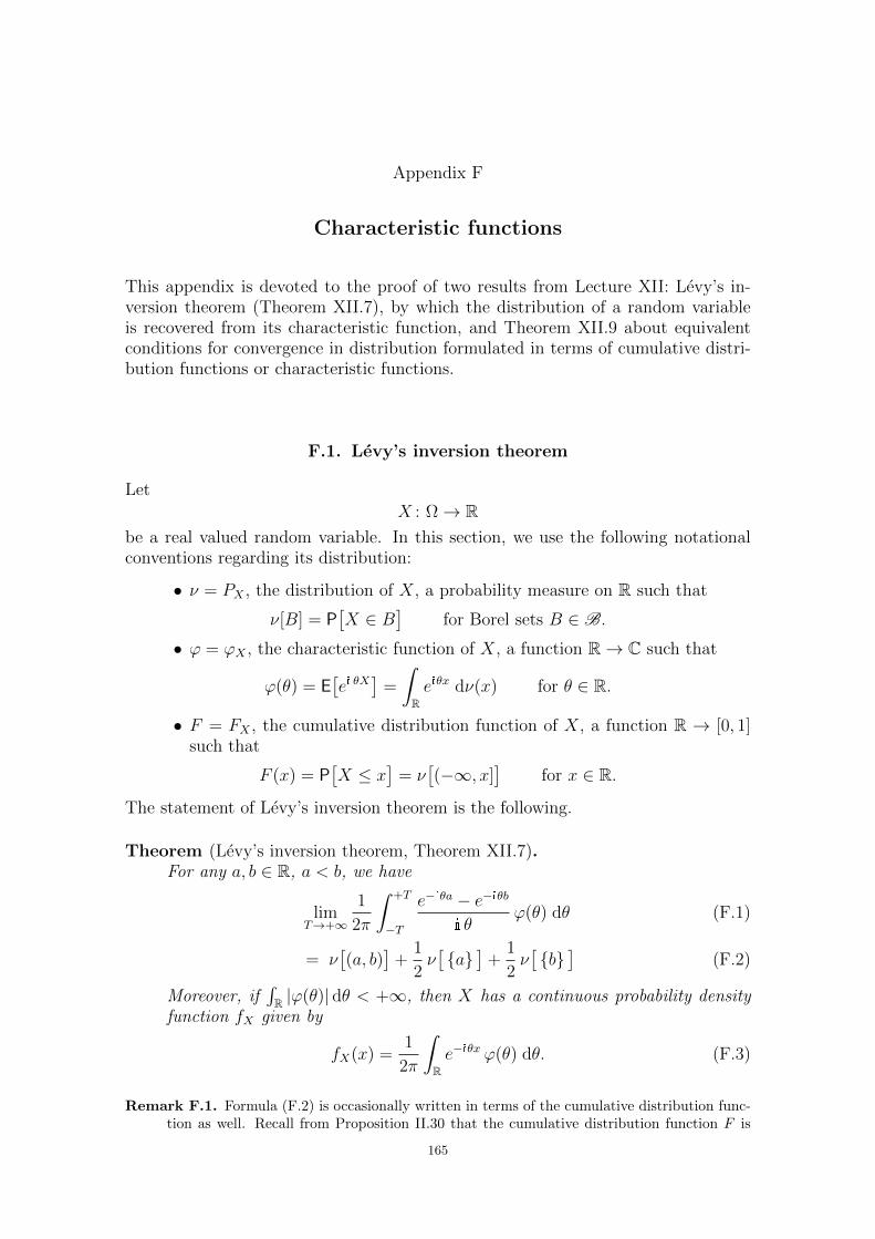
Appendix F
Characteristic functions
This appendix is devoted to the proof of two results from Lecture XII: Levy’s in-version theorem (Theorem XII.7), by which the distribution of a random variableis recovered from its characteristic function, and Theorem XII.9 about equivalentconditions for convergence in distribution formulated in terms of cumulative distri-bution functions or characteristic functions.
F.1. Levy’s inversion theorem
Let
X : Ω→ Rbe a real valued random variable. In this section, we use the following notationalconventions regarding its distribution:
• ν = PX , the distribution of X, a probability measure on R such that
ν[B] = P[X ∈ B
]for Borel sets B ∈ B.
• ϕ = ϕX , the characteristic function of X, a function R→ C such that
ϕ(θ) = E[ei θX
]=
∫Reiθx dν(x) for θ ∈ R.
• F = FX , the cumulative distribution function of X, a function R → [0, 1]such that
F (x) = P[X ≤ x
]= ν
[(−∞, x]
]for x ∈ R.
The statement of Levy’s inversion theorem is the following.
Theorem (Levy’s inversion theorem, Theorem XII.7).For any a, b ∈ R, a < b, we have
limT→+∞
1
2π
∫ +T
−T
e−iθa − e−iθb
i θϕ(θ) dθ (F.1)
= ν[(a, b)
]+
1
2ν[a
]+
1
2ν[b]
(F.2)
Moreover, if∫R |ϕ(θ)| dθ < +∞, then X has a continuous probability density
function fX given by
fX(x) =1
2π
∫Re−iθx ϕ(θ) dθ. (F.3)
Remark F.1. Formula (F.2) is occasionally written in terms of the cumulative distribution func-tion as well. Recall from Proposition II.30 that the cumulative distribution function F is
165
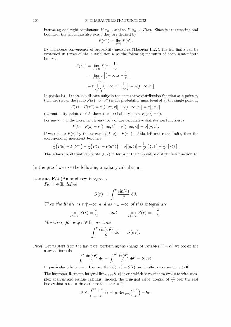
166 F. CHARACTERISTIC FUNCTIONS
increasing and right-continuous: if xn ↓ x then F (xn) ↓ F (x). Since it is increasing andbounded, the left limits also exist: they are defined by
F (x−) := limx′↑x
F (x′).
By monotone convergence of probability measures (Theorem II.22), the left limits can beexpressed in terms of the distribution ν as the following measures of open semi-infiniteintervals
F (x−) = limn→∞
F(x− 1
n
)= lim
n→∞ν[(−∞, x− 1
n
]]= ν
[ ∞⋃n=1
(−∞, x− 1
n
]]= ν
[(−∞, x)
].
In particular, if there is a discontinuity in the cumulative distribution function at a point x,then the size of the jump F (x)−F (x−) is the probability mass located at the single point x,
F (x)− F (x−) = ν[(−∞, x]
]− ν[(−∞, x)
]= ν
[x
](at continuity points x of F there is no probability mass, ν[x] = 0).
For any a < b, the increment from a to b of the cumulative distribution function is
F (b)− F (a) = ν[(−∞, b]
]− ν[(−∞, a]
]= ν
[(a, b]
].
If we replace F (x) by the average 12
(F (x) + F (x−)
)of the left and right limits, then the
corresponding increment becomes
1
2
(F (b) + F (b−)
)− 1
2
(F (a) + F (a−)
)= ν
[(a, b)
]+
1
2ν[a
]+
1
2ν[b
].
This allows to alternatively write (F.2) in terms of the cumulative distribution function F .
In the proof we use the following auxiliary calculation.
Lemma F.2 (An auxiliary integral).For r ∈ R define
S(r) :=
∫ r
0
sin(θ)
θdθ.
Then the limits as r ↑ +∞ and as r ↓ −∞ of this integral are
limr↑+∞
S(r) =π
2and lim
r↓−∞S(r) = −π
2.
Moreover, for any c ∈ R, we have∫ r
0
sin(c θ)
θdθ = S(c r).
Proof. Let us start from the last part: performing the change of variables θ′ = c θ we obtain theasserted formula ∫ r
0
sin(c θ)
θdθ =
∫ cr
0
sin(θ′)
θ′dθ′ = S(c r).
In particular taking c = −1 we see that S(−r) = S(r), so it suffices to consider r > 0.
The improper Riemann integral limr↑+∞ S(r) is one which is routine to evaluate with com-
plex analysis and residue calculus. Indeed, the principal value integral of eiz
z over the realline evaluates to iπ times the residue at z = 0,
P.V.
∫ ∞−∞
eiz
zdz = iπ Resz=0
(eizz
)= iπ.
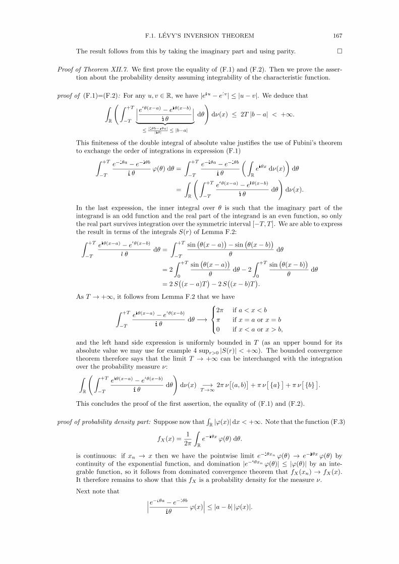
F.1. LEVY’S INVERSION THEOREM 167
The result follows from this by taking the imaginary part and using parity.
Proof of Theorem XII.7. We first prove the equality of (F.1) and (F.2). Then we prove the asser-tion about the probability density assuming integrability of the characteristic function.
proof of (F.1)=(F.2): For any u, v ∈ R, we have |eiu − eiv| ≤ |u− v|. We deduce that∫R
(∫ +T
−T
∣∣∣eiθ(x−a) − eiθ(x−b)
i θ
∣∣∣︸ ︷︷ ︸≤ |iθb−iθa|
|iθ| ≤ |b−a|
dθ
)dν(x) ≤ 2T |b− a| < +∞.
This finiteness of the double integral of absolute value justifies the use of Fubini’s theoremto exchange the order of integrations in expression (F.1)∫ +T
−T
e−iθa − e−iθb
i θϕ(θ) dθ =
∫ +T
−T
e−iθa − e−iθb
i θ
(∫Reiθx dν(x)
)dθ
=
∫R
(∫ +T
−T
eiθ(x−a) − eiθ(x−b)
i θdθ
)dν(x).
In the last expression, the inner integral over θ is such that the imaginary part of theintegrand is an odd function and the real part of the integrand is an even function, so onlythe real part survives integration over the symmetric interval [−T, T ]. We are able to expressthe result in terms of the integrals S(r) of Lemma F.2:∫ +T
−T
eiθ(x−a) − eiθ(x−b)
i θdθ =
∫ +T
−T
sin(θ(x− a)
)− sin
(θ(x− b)
)θ
dθ
= 2
∫ +T
0
sin(θ(x− a)
)θ
dθ − 2
∫ +T
0
sin(θ(x− b)
)θ
dθ
= 2S((x− a)T
)− 2S
((x− b)T
).
As T → +∞, it follows from Lemma F.2 that we have
∫ +T
−T
eiθ(x−a) − eiθ(x−b)
i θdθ −→
2π if a < x < b
π if x = a or x = b
0 if x < a or x > b,
and the left hand side expression is uniformly bounded in T (as an upper bound for itsabsolute value we may use for example 4 supr>0 |S(r)| < +∞). The bounded convergencetheorem therefore says that the limit T → +∞ can be interchanged with the integrationover the probability measure ν:∫
R
(∫ +T
−T
eiθ(x−a) − eiθ(x−b)
i θdθ
)dν(x) −→
T→∞2π ν
[(a, b)
]+ π ν
[a
]+ π ν
[b
].
This concludes the proof of the first assertion, the equality of (F.1) and (F.2).
proof of probability density part: Suppose now that∫R |ϕ(x)|dx < +∞. Note that the function (F.3)
fX(x) =1
2π
∫Re−iθx ϕ(θ) dθ.
is continuous: if xn → x then we have the pointwise limit e−iθxn ϕ(θ) → e−iθx ϕ(θ) bycontinuity of the exponential function, and domination |e−iθxn ϕ(θ)| ≤ |ϕ(θ)| by an inte-grable function, so it follows from dominated convergence theorem that fX(xn) → fX(x).It therefore remains to show that this fX is a probability density for the measure ν.
Next note that ∣∣∣e−iθa − e−iθb
iθϕ(x)
∣∣∣ ≤ |a− b| |ϕ(x)|.
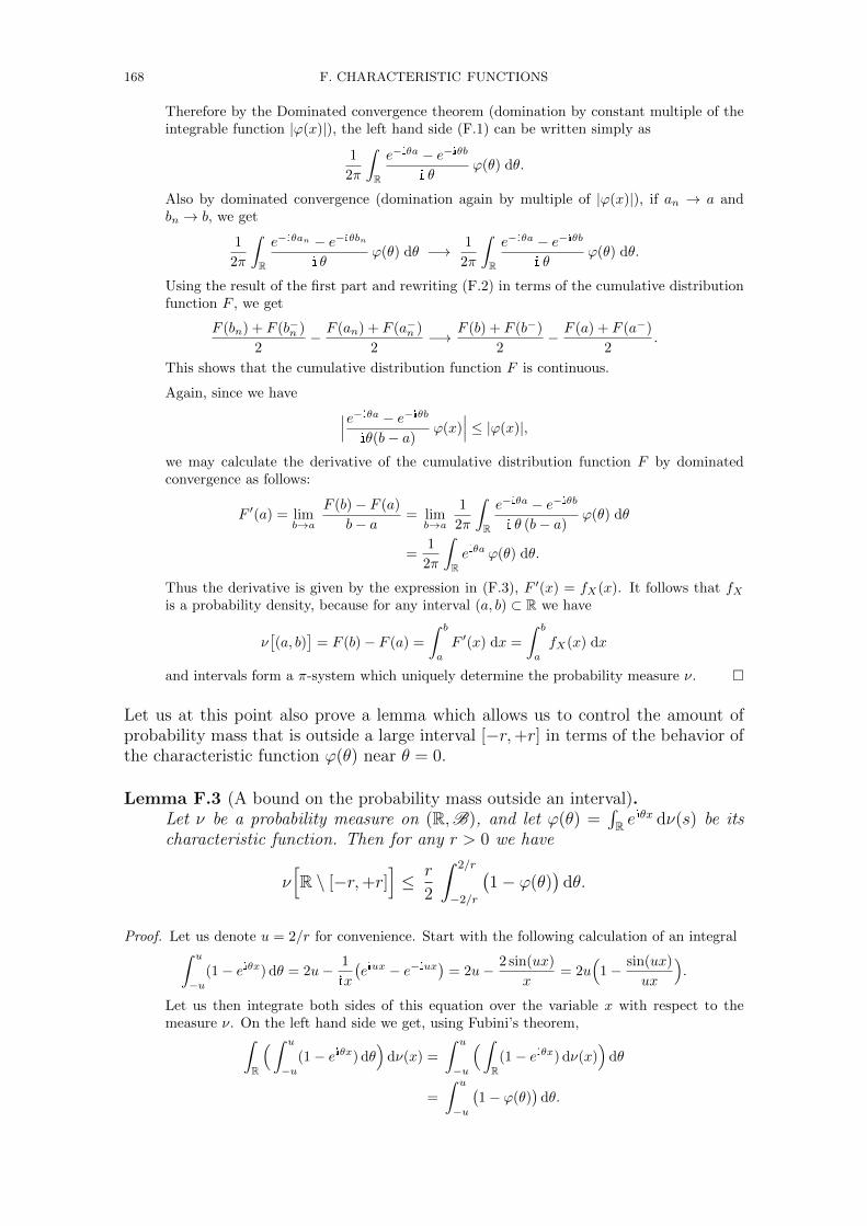
168 F. CHARACTERISTIC FUNCTIONS
Therefore by the Dominated convergence theorem (domination by constant multiple of theintegrable function |ϕ(x)|), the left hand side (F.1) can be written simply as
1
2π
∫R
e−iθa − e−iθb
i θϕ(θ) dθ.
Also by dominated convergence (domination again by multiple of |ϕ(x)|), if an → a andbn → b, we get
1
2π
∫R
e−iθan − e−iθbn
i θϕ(θ) dθ −→ 1
2π
∫R
e−iθa − e−iθb
i θϕ(θ) dθ.
Using the result of the first part and rewriting (F.2) in terms of the cumulative distributionfunction F , we get
F (bn) + F (b−n )
2− F (an) + F (a−n )
2−→ F (b) + F (b−)
2− F (a) + F (a−)
2.
This shows that the cumulative distribution function F is continuous.
Again, since we have ∣∣∣e−iθa − e−iθb
iθ(b− a)ϕ(x)
∣∣∣ ≤ |ϕ(x)|,
we may calculate the derivative of the cumulative distribution function F by dominatedconvergence as follows:
F ′(a) = limb→a
F (b)− F (a)
b− a= lim
b→a
1
2π
∫R
e−iθa − e−iθb
i θ (b− a)ϕ(θ) dθ
=1
2π
∫Reiθa ϕ(θ) dθ.
Thus the derivative is given by the expression in (F.3), F ′(x) = fX(x). It follows that fXis a probability density, because for any interval (a, b) ⊂ R we have
ν[(a, b)
]= F (b)− F (a) =
∫ b
a
F ′(x) dx =
∫ b
a
fX(x) dx
and intervals form a π-system which uniquely determine the probability measure ν.
Let us at this point also prove a lemma which allows us to control the amount ofprobability mass that is outside a large interval [−r,+r] in terms of the behavior ofthe characteristic function ϕ(θ) near θ = 0.
Lemma F.3 (A bound on the probability mass outside an interval).Let ν be a probability measure on (R,B), and let ϕ(θ) =
∫R e
iθx dν(s) be itscharacteristic function. Then for any r > 0 we have
ν[R \ [−r,+r]
]≤ r
2
∫ 2/r
−2/r
(1− ϕ(θ)
)dθ.
Proof. Let us denote u = 2/r for convenience. Start with the following calculation of an integral∫ u
−u(1− eiθx) dθ = 2u− 1
ix
(eiux − e−iux
)= 2u− 2 sin(ux)
x= 2u
(1− sin(ux)
ux
).
Let us then integrate both sides of this equation over the variable x with respect to themeasure ν. On the left hand side we get, using Fubini’s theorem,∫
R
(∫ u
−u(1− eiθx) dθ
)dν(x) =
∫ u
−u
(∫R
(1− eiθx) dν(x))
dθ
=
∫ u
−u
(1− ϕ(θ)
)dθ.
F.2. EQUIVALENT CONDITIONS FOR CONVERGENCE IN DISTRIBUTION 169
Dividing by u and equating with what we get on the right hand side gives
1
u
∫ u
−u
(1− ϕ(θ)
)dθ = 2
∫R
(1− sin(ux)
ux
)dν(x).
Because sin(ξ)ξ ≤ 1 for any ξ ∈ R, we see that the integrand on the right hand side here is
non-negative, 1 − sin(ux)ux ≥ 0. Therefore omitting from the integral over R the part over
[−r, r] ⊂ R yields a lower bound
1
u
∫ u
−u
(1− ϕ(θ)
)dθ ≥ 2
∫R\[−r,r]
(1− sin(ux)
ux
)dν(x).
Then observe that for |x| > r = 2/u we have | sin(ux)ux | ≤
1u|x| ≤
12 , so the integrand on the
remaining part satisfies 1− sin(ux)ux ≥ 1
2 , which yields
1
u
∫ u
−u
(1− ϕ(θ)
)dθ ≥ 2
∫R\[−r,r]
1
2dν(x) = ν
[R \ [−r,+r]
].
Recalling that u = 2/r, this is exactly the asserted inequality.
F.2. Equivalent conditions for convergence in distribution
Theorem (Theorem XII.9).Let X1, X2, . . . and X be real-valued random variables. Let also ν1, ν2, . . . andν be their laws, and let F1, F2, . . . and F be their cumulative distribution func-tions, and let ϕ1, ϕ2, . . . and ϕ be their characteristic functions, respectively.Then the following conditions are equivalent:
(i) For all bounded continuous functions f : R→ R we have∫Rf(x) dνn(x) −→
∫Rf(x) dν(x) as n→∞.
(ii) We have Fn(x) → F (x) as n → ∞ for all points x ∈ R such that F iscontinuous at x.
(iii) We have ϕn(θ)→ ϕ(θ) as n→∞ for all θ ∈ R.
Proof. We first show the equivalence of (i) and (ii) by proving both implications “(i) ⇒ (ii)”and “(ii) ⇒ (i)”.
Then we show that “(i) ⇒ (iii)”. Finally, we show that “(iii) ⇒ (ii)”, making use of thepreviously established implications. The equivalence of all three conditions then follows.
proof of “ (i) ⇒ (ii)”: Assume (i), i.e., that for all bounded continuous functions f : R → R wehave ∫
Rf(x) dνn(x) −→
n→∞
∫Rf(x) dν(x).
Let x0 ∈ R be a continuity point of F . Fix ε > 0. Then by continuity of F at x0, forsome δ > 0 we have
F (x0 − δ) > F (x0)− ε and F (x0 + δ) < F (x0) + ε. (F.4)
Now define two piecewise linear functions f−, f+ : R→ R by
f−(x) =
1 if x ≤ x0 − δx0−xδ if x0 − δ < x < x0
0 if x0 ≤ x, f+(x) =
1 if x ≤ x0
x0+δ−xδ if x0 < x < x0 + δ
0 if x0 + δ ≤ x.
170 F. CHARACTERISTIC FUNCTIONS
These functions are chosen so that we have the pointwise inequalities
I(−∞,x0−δ](x) ≤ f−(x) ≤ I(−∞,x0](x) ≤ f+(x) ≤ I(−∞,x0+δ](x). (F.5)
If we integrate (F.5) over x with respect to the measure ν, the indicators integrate to valuesof the cumulative distribution function F , and by monotonicity of integral, we get
F (x0 − δ) ≤∫f− dν ≤ F (x0) ≤
∫f+ dν ≤ F (x0 + δ).
Combining with inequalities (F.4) and rearranging terms, we derive the estimates∫f+ dν − ε < F (x0) <
∫f− dν + ε.
Similarly we can integrate (F.5) with respect to νn for any n ∈ N to get∫f− dνn ≤ Fn(x0) ≤
∫f+ dνn.
To estimate Fn(x0)− F (x0), we can combine these with the previous inequalities and rear-range to the form∫
f− dνn −∫f− dν − ε < Fn(x0)− F (x0) <
∫f+ dνn −
∫f+ dν + ε.
Now since the functions f− and f+ are bounded and continuous, by our assumption (i)there exists some N such that for n ≥ N we have∣∣∣ ∫ f− dνn −
∫f− dν
∣∣∣ < ε and∣∣∣ ∫ f+ dνn −
∫f+ dν
∣∣∣ < ε.
For n ≥ N , our estimate on Fn(x0)− F (x0) therefore yields
−2ε < Fn(x0)− F (x0) < +2ε.
Since ε > 0 was arbitrary, we can conclude limn→∞ Fn(x0) = F (x0), which establishes (ii).
proof of “ (ii) ⇒ (i)”: Assume (ii), i.e., that limn→∞ Fn(x) = F (x) for all x ∈ D, where D ⊂ R isthe set of continuity points of F . The increasing function F can only have countably manypoints of discontinuity, so the complement R \D is countable, and thus D ⊂ R is dense.1
Let ε > 0. Since F (x) ↓ 0 as x ↓ −∞ and F (x) ↑ 1 as x ↑ +∞ (Proposition II.30), and sinceD ⊂ R is dense, we can choose a, b ∈ D, a < b, such that F (b) − F (a) > 1 − ε. Moreover,since limn→∞ Fn(a) = F (a) and limn→∞ Fn(b) = F (b), there exists some N1 such that wehave
Fn(b)− Fn(a) > 1− 2ε for all n ≥ N1.
Let f : R→ R be bounded and continuous. On the compact interval [a, b] ⊂ R, the function fis uniformly continuous, so for some δ > 0 we have |f(x)−f(y)| < ε whenever |x−y| < δ andx, y ∈ [a, b]. Now choose points a = c0 < c1 < · · · < ck−1 < ck = b such that cj − cj−1 < δand cj ∈ D for all j = 1, . . . , k. Then for any j = 1, . . . , k, we get∣∣f(x)− f(cj)
∣∣ < ε for x ∈ [cj−1, cj ].
Define the simple function h : R→ R by
h(x) =
k∑j=1
f(cj) I(cj−1,cj ](x)
The above estimate shows that |f(x) − h(x)| < ε for all x ∈ [a, b]. By boundedness of f ,there exists a constant K > 0 such that |f(x)| ≤ K for all x ∈ R. Since h vanishes outside(a, b], the triangle inequality for integral with respect to νn gives∣∣∣ ∫
Rf dνn −
∫Rhdνn
∣∣∣ ≤ ∫(a,b]
|f − h|dνn︸ ︷︷ ︸≤ε
+
∫R\(a,b]
|f |dνn︸ ︷︷ ︸≤K νn
[R\(a,b]
].
1In fact, the proof of this implication only relies on having pointwise convergence of the cu-mulative distribution functions in some dense set.
F.2. EQUIVALENT CONDITIONS FOR CONVERGENCE IN DISTRIBUTION 171
When n ≥ N1, we have νn[R \ (a, b]
]= 1− νn
[(a, b]
]= 1− (Fn(b)− Fn(a)) < 2ε, and thus
the triangle inequality implies∣∣∣ ∫Rf dνn −
∫Rhdνn
∣∣∣ ≤ ε+K 2ε = (1 + 2K) ε.
Similarly, integrating now with respect to ν instead, one shows that∣∣∣ ∫Rf dν −
∫Rhdν
∣∣∣ ≤ (1 +K) ε.
It remains to consider the integrals of the function h with respect to both νn and ν. Theseintegrals are expressible in terms of the cumulative distribution functions,∫
Rhdνn =
k∑j=1
f(cj) νn[(cj−1, cj ]
]=
k∑j=1
f(cj)(Fn(cj)− Fn(cj−1)
)and similarly ∫
Rhdν =
k∑j=1
f(cj)(F (cj)− F (cj−1)
).
The difference of the integrals of h with respect to these two can therefore be estimated as∣∣∣ ∫Rhdν −
∫Rhdνn
∣∣∣ =∣∣∣ k∑j=1
f(cj)(F (cj)− Fn(cj)− F (cj−1) + Fn(cj−1)
)∣∣∣≤
k∑j=1
|f(cj)|(∣∣F (cj)− Fn(cj)
∣∣+∣∣F (cj−1) + Fn(cj−1)
∣∣)≤ 2kK max
j=1,...,k
∣∣F (cj)− Fn(cj)∣∣.
By our assumption (ii), we have limn→∞ Fn(cj) = F (cj) for each j = 1, . . . , k, so there existsN2 such that for n ≥ N2 we have maxj=1,...,k |F (cj)− Fn(cj)| < ε
k , and thus∣∣∣ ∫Rhdν −
∫Rhdνn
∣∣∣ ≤ 2Kε.
Combining the estimates we have obtained, for n ≥ max(N1, N2), we have∣∣∣ ∫Rf dν −
∫Rf dνn
∣∣∣≤∣∣∣ ∫
Rf dν −
∫Rhdν
∣∣∣︸ ︷︷ ︸≤(1+K)ε
+∣∣∣ ∫
Rhdν −
∫Rhdνn
∣∣∣︸ ︷︷ ︸≤2Kε
+∣∣∣ ∫
Rhdνn −
∫Rf dνn
∣∣∣︸ ︷︷ ︸≤(1+2K)ε
≤ (2 + 5K)ε.
Since ε > 0 was arbitrary, this shows that∫f dνn →
∫f dν as n → ∞, so we have estab-
lished (i).
proof of “ (i) ⇒ (iii)”: Assume that we have E[f(Xn)]→ E[f(X)] as n→∞ for all bounded con-tinuous functions f : R→ R. In particular, for any fixed θ ∈ R the functions f(x) = cos(θx)and f(x) = sin(θx) are bounded and continuous, so we get
ϕn(θ) = E[
exp(iθXn)]
= E[
cos(θXn)]
+ i E[
sin(θXn)]
−→n→∞
E[
cos(θX)]
+ i E[
sin(θX)]
= ϕ(θ).
proof of “ (iii) ⇒ (ii)”: Assume (iii), i.e., for all θ ∈ R we have ϕn(θ) → ϕ(θ) as n → ∞. Let usdenote by D ⊂ R the set of continuity points of F . Our proof of (ii) consists of proving twoparts:
172 F. CHARACTERISTIC FUNCTIONS
(1) Existence of subsequential limits: Given any subsequence indexed by (nk)k∈N, we can
find a further subsequence indexed by (nk`)`∈N and a cumulative distribution function F
such that Fnk` (x)→ F (x) as `→∞ at all continuity points x of F .
(2) Uniqueness of subsequential limits: If a cumulative distribution function F is the limit
of Fnk along some subsequence, pointwise in the set of continuity points of F , then we
must have F = F .
From these two together we derive that Fn(x) → F (x) for all x ∈ D. Indeed, suppose bycontradiction that there exists x ∈ D such that Fn(x) does not tend to F (x). Then thereexists some ε > 0 and a subsequence (nk)k∈N such that |Fnk(x) − F (x)| ≥ ε for all k ∈ N.
Applying (1) to this subsequence, we find a further subsequence indexed by (nk`)`∈N and F
such that Fnk` → F , pointwise in the set of continuity points of F . Then by (2) we should
have F = F , but this is a contradiction, since |Fnk` (x)−F (x)| ≥ ε holds in the subsequence.
This shows that (1) and (2) indeed imply (ii).
Proving uniqueness of subsequential limits (2) is straightforward using the already estab-lished implications “(ii) ⇒ (i)” and “(i) ⇒ (iii)”. Indeed, suppose that Fnk converges to
F , pointwise in the set of continuity points of F . By the already established “(ii) ⇒ (i)”,this implies the convergence
∫f dνnk →
∫f dν for all bounded continuous f , where the
probability measure ν has F as its cumulative distribution function. This, in turn, by thealready established “(ii) ⇒ (i)”, implies that ϕnk(θ) → ϕ(θ) for all θ ∈ R, where ϕ is thecharacteristic function of ν. But since the entire sequence ϕ1, ϕ2, . . . of characteristic func-tions has limit ϕ, the limit of the subsequence must be the same, ϕ = ϕ. Therefore we also
get ν = ν (by Levy’s inversion theorem) and F = F , and the uniqueness part (2) follows.
It remains to prove the existence of subsequential limits (1). The basic idea is to use Cantor’sdiagonal extraction. In order to keep the notation simpler, let us show how to extract aconvergent subsequence from the entire sequence (Fn)n∈N — the same argument works forextracting a convergent subsequence from any given subsequence. The set Q of rationalnumbers is countable, so let Q =
q(1), q(2), . . .
be an enumeration of it. Observe that for
any rational point q(j) ∈ Q, the sequence(Fn(q(j))
)n∈N of values at this point is a bounded
sequence: 0 ≤ Fn(q(j)) ≤ 1 for all n ∈ N. In particular, considering q(1) ∈ Q first, we can
find a subsequence indexed by (n(1)k )k∈N such that
limk→∞
Fn(1)k
(q(1))
exists. Then considering q(2) ∈ Q, we can find a subsequence of this already chosen subse-
quence, indexed now by (n(2)k )k∈N such that
limk→∞
Fn(2)k
(q(2))
exists, and since this is a subsequence of the previous one, also
limk→∞
Fn(2)k
(q(1)) = limk→∞
Fn(1)k
(q(1)).
Continuing inductively, we find subsequences (n(`)k )k∈N, ` = 1, 2, 3, . . ., such that
the limit limk→∞
Fn(`)k
(q(j)) exists for all j ≤ `.
Then if we consider the subsequence of diagonally selected indices n` := n(`)` , we get that
the limit lim`→∞
Fn`(q(j)) exists for all j ∈ N,
since apart from finitely many first members, the index sequence (n`)`∈N is a subsequence
of (n(j)k )k∈N. The limits
G(q(j)) := lim`→∞
Fn`(q(j))
define a function on the set of rational numbers
G : Q→ [0, 1].
F.2. EQUIVALENT CONDITIONS FOR CONVERGENCE IN DISTRIBUTION 173
As the limit of the increasing functions Fn` (restricted to Q), this function is also increasing:
G(q) ≤ G(q′) when q, q′ ∈ Q and q < q′.
We now claim that G(q) ↓ 0 as q ↓ −∞ and G(q) ↑ 1 as q ↑ −∞ — this is the place wherethe assumption (iii) is used. Let ε > 0. Then, since ϕ(0) = 1 and θ 7→ ϕ(θ) is continuousat θ = 0 (by Proposition XII.6), there exists δ > 0 such that∣∣1− ϕ(θ)
∣∣ < ε when |θ| < δ.
In particular we have
1
δ
∫ δ
−δ
(1− ϕ(θ)
)dθ < ε.
By assumption (iii) we have ϕn(θ)→ ϕ(θ) for all θ. Since we have∣∣1−ϕn(θ)
∣∣ ≤ 1 + |ϕn(θ)| ≤ 2,the Bounded convergence theorem (Corollary VII.21) implies
1
δ
∫ δ
−δ
(1− ϕn(θ)
)dθ −→
n→∞
1
δ
∫ δ
−δ
(1− ϕ(θ)
)dθ,
and we can conclude that there exists an Nε such that for n ≥ Nε we have
1
δ
∫ δ
−δ
(1− ϕn(θ)
)dθ < 2ε.
In view of Lemma F.3 this gives for n ≥ Nενn[R \ [−R,R]
]< 2ε,
where R = 2/δ. For the corresponding cumulative distribution functions this implies
Fn(x) < 2ε for x < −RFn(x) > 1− 2ε for x > −R.
The inequalities inherited by the subsequential limit G(q) = lim`→∞ Fn`(q) are then
G(q) ≤ 2ε for q < −RG(q) ≥ 1− 2ε for q > −R.
Since ε > 0 was arbitrary, this shows that G(q) ↓ 0 as q ↓ −∞ and G(q) ↑ 1 as q ↑ −∞.
The function G is not yet the cumulative distribution function we are looking for: it is onlydefined on the rational numbers, and it is not necessarily right-continuous. But we can useit to define
F (x) = infq>xq∈Q
G(q)
(this in fact defines the smallest right continuous function above G). From the definition itis clear that if q′, q′′ ∈ Q and q′ < x < q′′, then
G(q′) ≤ F (x) ≤ G(q′′).
We leave it to the reader to check that this F is right continuous, increasing, and has limits 0
and 1 at −∞ and +∞, respectively. Therefore F is a cumulative distribution function ofsome probability measure ν on R.
The only remaining claim is that the subsequence (Fn`)`∈N converges to F pointwise in the
set D ⊂ R of continuity points of F . Consider x ∈ D and let ε > 0. Then by continuity
of F at x we have for some δ > 0
F (x− δ) > F (x)− ε and F (x+ δ) < F (x) + ε.
Choose q′ ∈ Q∩ (x− δ, x). Then by the definition G(q′) = lim`→∞ Fn`(q′) there exists some
Lε such that for all ` ≥ Lε we have
Fn`(q′) > G(q′)− ε,
which yields
Fn`(x) ≥ Fn`(q′) > G(q′)− ε ≥ F (x− δ)− ε > F (x)− 2ε.
174 F. CHARACTERISTIC FUNCTIONS
Since ε > 0 was arbitrary, we get
lim inf`
Fn`(x) ≥ F (x).
By choosing q′′ ∈ Q ∩ (x, x+ δ), one can similarly argue that
lim sup`
Fn`(x) ≤ F (x),
and these two combined imply
lim`→∞
Fn`(x) = F (x).
This establishes the existence of subsequential limits (1), and finishes the proof.
Index
π-system, see also pi-systemσ-algebra, see also sigma algebrap-integrable, 78
addition of functions, see also pointwise sumof functions
additivitycountable, 8finite, 13
almost sure, see also almost surelyevent, 9limit, 108
almost surely, 9axiom of choice, 129
ball, 141binary sequence, 135binomial distribution, 13Borel sigma algebra, 5Borel-measurable function, 22
cardinality, 131Cartesian product, 81, 128Cauchy sequence
of square integrable random variables, 155Cauchy-Schwarz inequality, 97central limit theorem, 107characteristic function, 120, 159Chebyshev’s inequality, 111closed set, 141closed subspace, 156complement, 127complex valued random variable, 118conditioned probability measure, 11continuous distribution, 74, 95continuous function, 141convergence
almost surely, 108in L1, 115, 154in probability, 108of a sequence of numbers, 138
convergence in distribution, 117, 125convergence in law, 117, 125convergent sequence, 141countable set, 132countably infinite, 132counting measure, 9, 90
covariance, 98cumulative distribution function, 18, 103
d-system, 143De Morgan’s laws, 128decreasing sequence
of numbers, 139of sets, 129
density function, 74joint, 95marginal, 96
differenceof sets, 127
Dirac measure, 96discrete metric, 141disjoint, 127disjoint union, 127distribution
joint, 93of a random variable, 23, 72
dominated convergence theorem, 68
Euclidean norm, 140ev., see also eventuallyevent, ix, 1, 2eventually, 44expected value, ix, 55, 71exponential distribution, 74extended real line, 27, 137
Fatou’s lemma, 67reverse, 67
finite measure, 9finite measure space, 9
gaussian distribution, 74geometric distribution, 13Goddess of Chance, ix
homeomorphism, 142
i.o., see also infinitely oftenimage of a set under function, 128improper Riemann integral, 70increasing sequence
of numbers, 139of sets, 129
independence, 41
175
176 INDEX
of σ-algebras, 39of events, 40of random variables, 40
indicator random variable, 24inf, see also infimuminfimum, 137, 138infinitely often, 44inner product
of square integrable random variables, 153integrable
complex random variable, 118integrable function, 63integrable random variable, 63, 78integral, 55
of a non-negative function, 59of a simple function, 57of an integrable function, 63over subset, 69
intersection of sets, 127
Jensen’s inequality, 79joint density, 95joint law, 93
Kolmogorov’s strong law of large numbers,116
law, see also distributionof a random variable, 23, 72
law of large numbers, 107Lebesgue integral, 70Lebesgue measure, 10, 90d-dimensional, 10, 90
liminfof events, see also eventuallyof sequence of numbers, 139of sequence of sets, 130
limit, 141of a decreasing sequence of sets, 129of a sequence of numbers, 138of an increasing sequence of sets, 129
limsupof events, see also infinitely oftenof sequence of numbers, 139of sequence of sets, 130
linearityof integral, 56
lower limitof sequence of numbers, 139of sequence of sets, 130
marginal density, see also density function,marginal, 96
Markov process, 94Markov’s inequality, 111MCT, see also Monotone convergence
theoremmeasurable
set, 7
space, 7, 8measurable function, 21, 22measurable space, 7measure, 8measure space, 9moment, 78monotone class, 38, 82, 143Monotone class theorem, 82monotone convergence
of integrals, 62of measures, 13
Monotone convergence theorem, 61, 147monotone sequence
of numbers, 139of sets, 130
monotonicityof integral, 56of measures, 13
multiplication of functions, see alsopointwise product of functions
negative partof a function, 63
normof square integrable random variable, 153
open set, 141orthogonality
of square integrable random variables,153, 156
outcome, ix
pi-system (π-system), 17pointwise product of functions, 27pointwise scalar multiple of functions, 27pointwise sum of functions, 27Poisson distribution, 12positive part
of a function, 63power set, 129preimage of a set under function, 128probability, ixprobability density, 95probability mass function, 12probability measure, 9probability space, 9product measure, 86product of functions, see also pointwise
product of functionsproduct sigma algebra, 83
random number, 22random variable, ix, 21, 22random walk, 54Riemann integral, 70
sample space, ixscalar multiplication of functions, see also
pointwise scalar multiple of functions
INDEX 177
sequencedecreasing, 129, 139increasing, 129, 139monotone, 130, 139of sets, 129
sigma algebragenerated by collection of events, 3generated by random variables, 36
sigma algebra (σ-algebra), 2sigma finite, 90simple function, 30, 57square integrable random variable, 97staircase function, 31standard machine, 56, 146standard normal distribution, 74strong law of large numbers, 110subadditivity
countable, 14finite, 13
sum of functions, see also pointwise sum offunctions
sup, see also supremumsupremum, 137, 138supremum norm, 141sure event, 9
tail event, 48tail sigma algebra, 48tend
seeconverge, 138total mass
of a measure, 9truncated measure, 11
uncountable set, 135uniform norm, 141uniform probability measure
continuous, 11discrete, 10on a finite set, 10
union of sets, 127upper limit
of sequence of numbers, 139of sequence of sets, 130
variance, 98
weak convergence, 117weak law of large numbers, 110Weierstrass’ approximation theorem, 112

References
Bibliography
[Dur10] Richard Durrett. Probability: Theory and Examples. Cambridge University Press, 4thedition, 2010.
[JP04] Jean Jacod and Philip Protter. Probability Essentials. Cambridge Univ. Press, 2nd edition,2004.
[Kin16] Juha Kinnunen. Measure and integral. Aalto University, 2016. https://math.aalto.fi/
~jkkinnun/files/measure_and_integral.pdf.[Wil91] David Williams. Probability with Martingales. Cambridge Univ. Press, 1991.
179