Probability Notes

Compiled by Paul J. Hurtado

Last Compiled: September 6, 2017

About These Notes

These are course notes from a Probability course taught using An Introductionto Mathematical Statistics and Its Applications by Larsen and Marx (5th ed).

These notes are heavily based on notes provided to me by Professor AniaPanorska, who had previously taught that course, plus material I have addedbased on my own materials or material found in other Probability textbooks.

You will undoubtedly find these notes lack many important details. Istrongly urge you to seek out more detailed treatments of thismaterial as needed -- e.g., by reading them along side a textbook or similarlythorough resource -- especially if using these notes for more than a light refresher.

-- Paul J. Hurtado

1

Contents

Basic Definitions 3

Set Operations 3

Probability Function, P() 4Properties of Probability Functions . . . . . . . . . . . . . . . . . . . . . . . . . . . . . . 5

Conditional Probability and Total Probability 5Bayes Rule . . . . . . . . . . . . . . . . . . . . . . . . . . . . . . . . . . . . . . . . . . . 5

Independence 6Independent vs Mutual Exclusive (aka Disjoint) . . . . . . . . . . . . . . . . . . . . . . . 6

Combinatorics: Counting, Ordering, Arranging 7

Random Variables 8Discrete Random Variables . . . . . . . . . . . . . . . . . . . . . . . . . . . . . . . . . . 10Continuous Random Variables . . . . . . . . . . . . . . . . . . . . . . . . . . . . . . . . . 11

Expectation and Expected Values 12Expected Values of Functions of Random Variables . . . . . . . . . . . . . . . . . . . . . 12Properties of Expectation, E() . . . . . . . . . . . . . . . . . . . . . . . . . . . . . . . . . 13Variance . . . . . . . . . . . . . . . . . . . . . . . . . . . . . . . . . . . . . . . . . . . . . 13Moments of a Random Variable . . . . . . . . . . . . . . . . . . . . . . . . . . . . . . . . 14

Multivariate Distributions 15Motivating Examples: Multivariate vs Univariate . . . . . . . . . . . . . . . . . . . . . . 15Density vs Likelihood . . . . . . . . . . . . . . . . . . . . . . . . . . . . . . . . . . . . . . 16Random Vectors and Joint Densities . . . . . . . . . . . . . . . . . . . . . . . . . . . . . 18Independence Revisited . . . . . . . . . . . . . . . . . . . . . . . . . . . . . . . . . . . . . 19Conditional Distributions Revisited . . . . . . . . . . . . . . . . . . . . . . . . . . . . . . 19Expected Values, Variance, and Covariance Revisited . . . . . . . . . . . . . . . . . . . . 20Combining Random Variables: Sums, Products, Quotients . . . . . . . . . . . . . . . . . 21

Special Distributions 22Geometric and Negative Binomial Distributions . . . . . . . . . . . . . . . . . . . . . . . 24Exponential and Gamma Distributions . . . . . . . . . . . . . . . . . . . . . . . . . . . . 25Normal (Gaussian) Distribution . . . . . . . . . . . . . . . . . . . . . . . . . . . . . . . . 26

Convergence Concepts & Laws of Large Numbers 27Convergence Concepts in Probability . . . . . . . . . . . . . . . . . . . . . . . . . . . . . 27Laws of Large Numbers . . . . . . . . . . . . . . . . . . . . . . . . . . . . . . . . . . . . 29Central Limit Theorems (CLTs) . . . . . . . . . . . . . . . . . . . . . . . . . . . . . . . . 29

2

Basic Definitions

Experiment: Any procedure that can be repeated under the same conditions (theoretically)infinite number of times, and such that its outcomes are well defined. By well defined we mean wecan describe all possible outcomes.

Outcome (or Sample Outcome): Any possible outcome of the experiment.

Sample Space: The set of all possible outcomes of an experiment. Usually denoted by S.

Event: A subset of the sample space S. Events are usually denoted by capital letters.

A probability space comprises three parts (S,F ,P ):

1. S is the sample space, the set of all outcomes. (Some texts use Ω instead of S). Ex: Fora coin toss experiment, S = H,T.

2. F is the σ-algebra associated with S. It is the collection of subsets of S (we call thesesubsets events), and includes S and the empty set ∅. This set of events is closed undercountable unions, countable intersections and complementation. Furthermore, F satisfies:

(a) if A ∈ F then Ac ∈ F , and

(b) if A1, A2, ... are in F , then their union⋃iAi is also in F .

NOTE: Together these conditions imply closure under countable intersections. If S iscountable, F is the power set of S, i.e., it is all subsets of S. Mathematicians call these eventsthe measurable sets in S.

3. P is our probability function P : F → [0, 1]. It associates each event (i.e., each subset of Sincluded in F) with a number between 0 and 1. Furthermore, we require that

(a) P is non-negative (P (A) ≥ P (∅) = 0, ∀A ∈ F),

(b) P is countably additive, i.e., for for a countable, disjoint set of events A1, A2, ... thenP (⋃Ai) =

∑i P (Ai)), and

(c) P (S) = 1.

Set Operations

Operations on events (sets): Union, Intersection, Complement.

Definition: Let A and B be two events from sample space S.

1. The union of A and B (A ∪B) is exactly all elements in A or B or both.

2. The intersection of A and B (A ∩B) is exactly all elements in both A and B.

3. The complement of A is the event (set) AC which contains all elements in S not in A.

3

NOTE: We can extend the definition of a union (or intersection) of two events, to any finitenumber of events A1, A2, . . . , Ak defined over the sample space S.

Definition: Events A and B are mutually exclusive if their intersection is empty (A ∩B = ∅).

1. The union of A1, A2, . . . , Ak is the event (set)⋃ki=1Ai = A1 ∪ A2 ∪ . . . ∪ Ak which elements

belong to at least one of the sets A1, A2, . . . , Ak.

2. The intersection of A1, A2, . . . , Ak is the event (set)⋂ki=1Ai = A1 ∩ A2 ∩ . . . ∩ Ak which

elements belong to all the sets A1, A2, . . . , Ak.

Additional properties of unions and intersections:

1. A ∩ (B ∪ C) = (A ∩B) ∪ (A ∩ C) 3. A ∪ (B ∪ C) = (A ∪B) ∪ C

2. A ∪ (B ∩ C) = (A ∪B) ∩ (A ∪ C) 4. A ∩ (B ∩ C) = (A ∩B) ∩ C

DeMorgan’s Laws: Treat complement of a union or intersection.

1. The complement of a union ofA1, A2, . . . , Ak is the intersection of the complementsAC1 , AC2 , . . . , A

Ck ,

that is (⋃ki=1Ai)

C =⋂ki=1A

Ci .

2. The complement of an intersection of A1, A2, . . . , Ak is the union of the complementsAC1 , A

C2 , . . . , A

Ck , that is (

⋂ki=1Ai)

C =⋃ki=1A

Ci .

Probability Function, P()

The probability function P (·) is a function defined on the set of events (subsets of S) which assignsa value in [0,1] to each event A, that is, P (A) ∈ [0, 1].

Kolmogorov’s Axioms. A function P is a probability function if and only if it satisfies thefollowing axioms:

1. Probability of any event A is nonegative: P (A) ≥ 0.

2. Probability of the sample space is 1: P (S) = 1.

3. The probability of a union of two mutually exclusive events A and B is the sum of theirprobabilities: P (A ∪B) = P (A) + P (B) for any mutually exclusive events A and B.

4. The probability of a union of infinitely many pairwise disjoint events, is the sum of theirprobabilities. That is, if A1, A2, . . . are events over S such that Ai ∩ Aj = Ø for i 6= j, thenP (⋃∞i=1Ai) =

∑∞i=1 P (Ai).

NOTE: Axioms 1 - 3 are enough for finite sample spaces. Axiom 4 is necessary when the samplespace is infinite (e.g. the real numbers, R).

4

Properties of Probability Functions

Suppose P is probability function on the subsets of the sample space S, and A and B are eventsdefined over S. Then, the following are true.

1. P (AC) = 1− P (A).

2. P (Ø) = 0.

3. If A ⊂ B, then P (A) ≤ P (B).

4. For any event A, P (A) ≤ 1.

5. If events A1, A2, . . . , Ak are such that Ai ∩ Aj = Ø for i 6= j, then P (⋃ki=1Ai) =

∑ki=1 P (Ai).

6. Addition Rule: For any two events A and B: P (A ∪B) = P (A) + P (B)− P (A ∩B).

Conditional Probability and Total Probability

Definition: The conditional probability of event A given that event B occurred is

P (A|B) =P (A ∩B)

P (B), if P (B) 6= 0.

Theorem: Multiplication Rule: The probability of A and B, P (A ∩ B) can be found usingconditional probability: P (A ∩B) = P (A|B)P (B) = P (B|A)P (A) for P (A 6= 0) and P (B 6= 0).

Theorem: Multiplication Rule for more than 2 events: Let A1, A2, . . . , An be events overS. then P (A1 ∩ A2∩, . . . , An) = P (A1)P (A2|A1) · · ·P (An−1|A1∩, . . . , An−2)P (An|A1∩, . . . , An−1).

Definition: Sets B1, B2, . . . , Bn form a partition of the sample space S if: (1) They ”cover” S,i.e., B1 ∪B2 ∪ . . . ∪Bn = S; and (2) They are pairwise disjoint.

Theorem: Total Probability formula: Let the sets B1, B2, . . . , Bn form a partition of thesample space S. Let A be an event over S. Then

P (A) =n∑i=1

P (A|Bi)P (Bi).

Bayes Rule

Theorem: Bayes Formula: (1) For any events A and B defined on sample space S and suchthat P (B) 6= 0 we have:

P (A|B) =P (B|A)P (A)

P (B),

(2) More generally, if the sets B1, B2, . . . , Bn form a partition of the sample space S, we have

P (Bj|A) =P (A|Bj)P (Bj)∑ni=1 P (A|Bi)P (Bi)

,

for every j = 1, . . . , n.

5

Independence

Definition: Two events A and B are called independent if P (A ∩B) = P (A)P (B).

NOTE: (1) If A and B are independent, then P (A|B) = P (A) and P (B|A) = P (B).

(2) If A and B are independent, then so are their complements AC and BC .

Definition: Events A1, A2, . . . , An are independent if for every subset of them we have

P (Ai1 ∩ Ai2 ∩ . . . ∩ Aik) = P (Ai1)P (Ai2) · · ·P (Aik).

Independent vs Mutual Exclusive (aka Disjoint)

How is independence related to sets being disjoint (i.e., mutually exclusive)?

1. Independence deals with the relationship between the probabilities of events A and B,and the probability of their co-occurrence, P (A ∩B). Independence says something aboutevents that can co-occur, whereas disjoint events, by definition, never co-occur.

2. The notion of sets being disjoint relates to the elements in those events, and whether orany are shared (i.e, whether or not they have an empty intersection). Mutual exclusivitydescribes which outcomes cannot co-occur. Intuition should tell us that disjoint sets areNOT independent! Why? Suppose two events are disjoint. Then knowledge of one eventoccurring tells you quite a bit of information about whether or not the other has occurred(by definition, it has not!). For example, if you are 22 years old, I know that you are not 21years old. In fact, disjoint sets cannot be independent except in the trivial case where oneor both events has probability zero: since P (A ∩ B) = 0 for disjoint events, they can onlysatisfy the definition of independence (P (A ∩B) = P (B)P (A)) if P (A) = 0 or P (B) = 0 (orboth are true).

Example: Consider the experiment defined by one card out of a standard 52 card deck.Let event A be that the card is red (i.e., A is the set of all 26 red cards) and B be the event thatthe card is a king (i.e., B is all four kings).Are A and B independent? Check that they satisfy the definition, P (A ∩B) = P (A)P (B):

P (A ∩B) = P (red king) = 1/26

P (A)P (B) = 1/2 · 4/52 = 1/26

So they are independent events!Are they disjoint? No. Their intersection A ∩B = red king is not empty.

6

Combinatorics: Counting, Ordering, Arranging

Multiplication Rule: If operation A can be performed in n different ways and operation B canbe performed in m different ways, then the sequence of these two operations (say, AB) can beperformed in n ·m ways.

Extension of Multiplication Rule to k operations: If operations Ai, i = 1, . . . , k can be per-formed in ni different ways, then the ordered sequence (operation A1, operation A2, . . ., operationAk) can be performed in n1n2 · · ·nk ways.

Permutations: An arrangement of k objects in a row is called a permutation of length k.

Number of permutations of k elements chosen from a set on n elements: The numberof permutations of length k, that can be formed from a set of n distinct objects is

n(n− 1)(n− 2) · · · (n− k + 1) =n!

(n− k)!.

Number of permutations of n elements chosen from a set on n elements: The numberof permutations of length n (ordered sequences of length n), that can be formed from a set of ndistinct objects is

n(n− 1)(n− 2) · · · (1) = n!.

Approximation for n! (Stirling’s Formula): n! ≈√

2πnn+1/2e−n.

Number of permutations of elements that are not all different: The number of permuta-tions of length n, that can be formed from a set of n1 objects of type 1, n2 objects of type 2, . . ., nkobjects of type k, where

∑ki=1 ni = n, is

n!

n1!n2! · · ·nk!.

Combinations: A set of k unordered objects is called a combination of size k.

Number of combinations of size k of n distinct objects: The number of ways to formcombinations of size k from a set of n distinct objects, no repetitions, is denoted by the Newtonsymbol (or binomial coefficient) (n

k) , and equal to(

nk

)=

n!

k!(n− k)!.

NOTE: The number of combinations of size k of n distinct objects is the number of differentsubsets of size k formed from a set of n elements.

Combinatorial probabilities - classical definition of probability: Suppose there are nsimple outcomes in a sample space S. Let event A consist of m of those outcomes. Suppose alsothat all outcomes are qually likely. Then, the probability of event A is defined as P(A)=m/n.

7

Random Variables

Definition A probability space (S, E , P ) is composed of a sample space S, the algebra E (theset of subsets of S), and a probability function P : E → [0, 1] that satisfies Kolmogorov’s axioms.In practice, we think of random variables (r.v.) in two ways.

1. We commonly think of a random variable as a ‘‘place holder” for the observed outcome of anexperiment. Ex: Let X be the number of heads in 10 coin tosses.

2. Formally, if X is a random variable, it is a real-valued measurable function that maps oneprobability space into another (real-valued) probability space. That is, X : (S, E , P ) →(Ω,F , PX) where Ω ⊆ R and we define

PX(A) = P (s ∈ Ω : X(s) ∈ A) for all events A ∈ F

Q: How are these consistent?

A: We tend to only be explicit about the real-valued representation of the outcome, andfocus on X and PX instead of explicitly defining all of the other details.

Definition: We refer to P as the distribution of the random variable and this often issufficient to imply the structure of the associated probability space and experiment.

Definition A real-valued function X that maps one probability space (S, E) to another probabilityspace (Ω,F) is called a random variable (r.v.) if

X−1(E) ∈ E for all E ∈ F

That is, each event in the ‘‘new” algebra corresponds to (measureable) events in the original space.This ensures that X induces a consistent probability measure on the new space.Definition Suppose r.v. X maps (S, E , P )→ (Ω,F , PX). The probability function (measure) PXis called the probability distribution of X and is given by

PX(A) = P (s ∈ S : X(s) ∈ A) for all A ∈ F .

NOTE: By X being real-valued, we mean that Ω ⊆ R or Ω ⊆ Rn. In the latter case, we call X arandom vector.Example 1: Stating that ‘‘X is a Bernoulli r.v. with probability p of success” implies thatS = 0, 1 and P (X = k) = pk(1− p)1−k. That is, P (X = 1) = p and P (X = 0) = 1− p.

Definition: A Bernoulli process X = (X1, ..., Xn) is a series of n independent and identicallydistributed (iid) Bernoulli trials (Xi) each with probability p of success.

Example 2: Stating that ‘‘Y is a binomial r.v. with parameters n and p” implies that Y =∑n

i=0Xi

is the number of successes in a Bernoulli process of length n, and therefore that S = 0, 1, ..., nand P (X = k) =

(nk

)pk(1− p)n−k for k ∈ S (zero otherwise).

Example 3: If X is a hypergeometric r.v., it represents the number of successes in n draws froma population of size N with K successes. Thus S = 0, ...,min(K,n) and

P (X = k) =

(Kk

)(N−Kn−k

)(Nn

)8

Theorem: The distribution of X is uniquely determined by the cumulative distributionfunction (cdf) of X, denoted ny F or FX :

F (x) = P (X ≤ x) = P ((−∞, x]).

Properties of cdf

1. F is nondecreasing: If x1 ≤ x2, then F (x1) ≤ F (x2);

2. F is right - continuous: for any x, limy→x+ F (y) = F (x);

3. limx→∞ F (x) = 1;

4. limx→−∞ F (x) = 0.

NOTE: Here are two useful rules for computing probabilities:

1. For a sequence of increasing sets A1 ⊂ A2 ⊂ . . . the probability of their union is the limit oftheir probabilities, that is: P (

⋃∞i=1Ai) = limi→∞ P (Ai).

2. For a sequence of decreasing sets A1 ⊃ A2 ⊃ . . . the probability of their intersection is thelimit of their probabilities, that is: P (

⋂∞i=1Ai) = limi→∞ P (Ai).

Types of distributions: There are three main types of distributions / random variables:

1. Discrete r.v.: CDF is a step function, S has at most countable number of outcomes.Examples: Binomial, Poisson

2. Continuous r.v.: CDF is a smooth function, events are typically intervals.Examples: Normal, Exponential

3. Mixed r.v.: CDF is neither continuous nor step function.Example: Zero-inflated Normal

9

Discrete Random Variables

Definition. Suppose a sample space S has finite or countable number of simple outcomes. Let pbe a real valued function on S such that

1. 0 ≤ p(s) ≤ 1 for every element s of S;

2.∑

s∈S p(s) = 1,

Then p is said to be a discrete probability function.

NOTE: For any event A defined on S: P (A) =∑

s∈A p(s).

Definition. A real valued function X : S → R is called a random variable.

Definition. A random variable with finite or countably many values is called a discrete randomvariable.

Definition. Any discrete random variable X is described by its probability density function(or probability mass function), denoted pX(k), which provides probabilities of all values of X asfollows:

pX(k) = P (s ∈ S : X(s) = k).

NOTE: For any k not in the range (set of values) of X: pX(k) = 0.

NOTE: For any t ≤ s, P (t ≤ X ≤ s) =∑s

k=t P (X = k).

NOTATION: For simplicity, we denote pX(k) = P (X = k) thus suppressing the dependence onthe sample space.

Examples:1. Binomial r.v. X with n trials and probability of success equal to p, i.e., X ∼ binom(n, p).

pX(k) = P (k successes in n trials) =

(nk

)pk(1− p)n−k, for k = 0, 1, 2, . . . , n.

2. Hypergeometric random variable X.

Definition. Let X be a discrete random variable. For any real number t, the cumulativedistribution function F of X at t is given by

FX(t) = P (X ≤ t) = P (s ∈ S : X(s) ≤ t).

Linear transformation: Let X be a discrete random variable (rv). let Y=aX+b, where a and bare real constants. Then pY (y) = pX(y−b

a).

10

Continuous Random Variables

Suppose a sample space Ω is uncountable, e.g., Ω = [0, 1] or Ω = R. We can define a randomvariable X : (Ω, E) → (S,B) where the new sample space S is a subset of R and the algebra Bis the Borel sets (all unions, intersections and complements of the open and closed intervals inS). The probability structure on such a space can be described using a special function, f calledprobability density function (pdf).

Definition. If sample space S ⊆ R then we say P is a continuous probability distribution ifthere exists a function f(t) such that for any closed interval [a, b] ⊂ S we have that P ([a, b]) =∫ baf(t)dt. It follows that P (A) =

∫Af(t)dt for all events A.

For a function f to be a pdf, it is necessary and sufficient that the following properties hold:

1. f(t) ≥ 0 for every t;

2.∫∞−∞ f(t)dt = 1.

NOTE: If P (A) =∫Af(t)dt for all A, then P satisfies all the Kolmogorov probability axioms.

Definition: Any function Y that maps S (a subset of real numbers) into the real numbers is calleda continuous random variable. The pdf of Y is a function f such that

P (a ≤ Y ≤ b) =

∫ b

a

f(t)dt.

For any event A defined on S: P (A) =∫Af(t)dt.

Theorem: For any continuous random variable P (X = a) = 0 for any real number a.Definition. The cdf of a continuous random variable Y (with pdf f) is FY (t), given by

FY (y) = P (Y ≤ y) = P (s ∈ S : Y (s) ≤ y) =

∫ y

−∞f(t)dt for any real y.

Theorem. If FY (t) is a cdf and fY (t) is a pdf of a continuous random variable Y , then

d

dtFY (t) = fY (t).

Linear transformation: Let X be a continuous random variable with pdf f . Let Y = aX + b,where a and b are real constants. Then the pdf of Y is: gY (y) = 1

|a|fX(y−ba

).

11

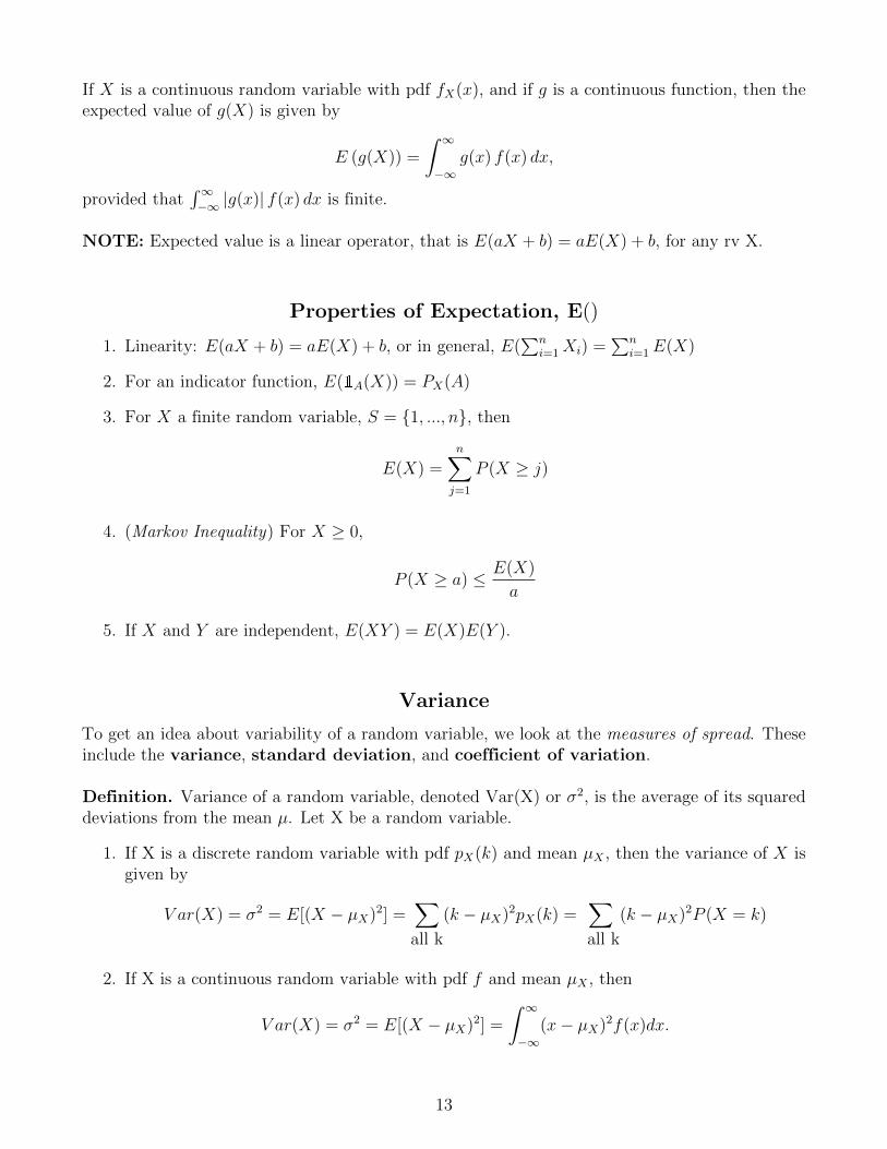
Expectation and Expected Values

We often quantify the central tendency of a random variable using its expected value (mean).

Definition Let X be a random variable.

1. If X is a discrete random variable with pdf pX(k), then the expected value of X is given by

E(X) = µ = µX =∑all k

k · pX(k) =∑all k

k · P (X = k)

2. If X is a continuous random variable with pdf f , then

E(X) = µ = µX =

∫ ∞−∞

x f(x) dx.

3. If X is a mixed random variable with cdf F, then the expected value of X is given by

E(X) = µ = µX =

∫ ∞−∞

xF ′(x)dx+∑all k

k · P (X = k),

where F ′ is the derivative of F where the derivative exists and k’s in the summation are the‘‘discrete” values of X.

NOTE: For the expectation of a random variable to exist, we assume that all integrals and sumsin the definition of the expectation above converge absolutely.

Definition: The median of a random variable is the value at the midpoint distribution of X-- another way to characterize the central tendency of a random variable. Specifically, if X is adiscrete random variable, then its median m is the point for which P (X < m) = P (X > m). Ifthere are two values m and m′ such that P (X ≤ m) = 0.5 and P (X ≥ m′) = 0.5, the median isthe average of m and m′, (m+m′)/2.

If X is a continuous random variable with pdf f , the median is the solution of the equation:∫ m

−∞f(x) dx =

1

2.

Expected Values of Functions of Random Variables

Theorem. Let X be a random variable. Let g(·) be a function of X.If X is discrete with pdf pX(k), then the expected value of g(X) is given by

E (g(X)) =∑all k

g(k) · pX(k) =∑all k

g(k) · P (X = k),

provided that∑

all k |g(k)| pX(k) is finite.

12

If X is a continuous random variable with pdf fX(x), and if g is a continuous function, then theexpected value of g(X) is given by

E (g(X)) =

∫ ∞−∞

g(x) f(x) dx,

provided that∫∞−∞ |g(x)| f(x) dx is finite.

NOTE: Expected value is a linear operator, that is E(aX + b) = aE(X) + b, for any rv X.

Properties of Expectation, E()

1. Linearity: E(aX + b) = aE(X) + b, or in general, E(∑n

i=1Xi) =∑n

i=1E(X)

2. For an indicator function, E(1A(X)) = PX(A)

3. For X a finite random variable, S = 1, ..., n, then

E(X) =n∑j=1

P (X ≥ j)

4. (Markov Inequality) For X ≥ 0,

P (X ≥ a) ≤ E(X)

a

5. If X and Y are independent, E(XY ) = E(X)E(Y ).

Variance

To get an idea about variability of a random variable, we look at the measures of spread. Theseinclude the variance, standard deviation, and coefficient of variation.

Definition. Variance of a random variable, denoted Var(X) or σ2, is the average of its squareddeviations from the mean µ. Let X be a random variable.

1. If X is a discrete random variable with pdf pX(k) and mean µX , then the variance of X isgiven by

V ar(X) = σ2 = E[(X − µX)2] =∑all k

(k − µX)2pX(k) =∑all k

(k − µX)2P (X = k)

2. If X is a continuous random variable with pdf f and mean µX , then

V ar(X) = σ2 = E[(X − µX)2] =

∫ ∞−∞

(x− µX)2f(x)dx.

13

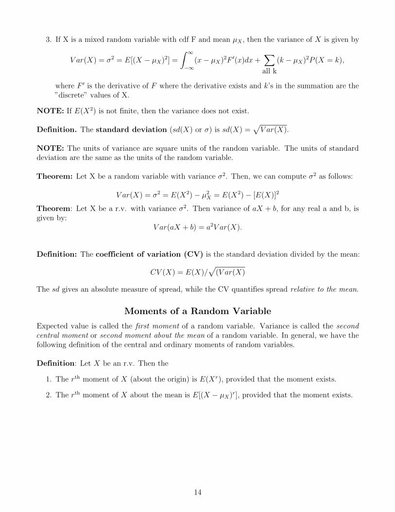
3. If X is a mixed random variable with cdf F and mean µX , then the variance of X is given by

V ar(X) = σ2 = E[(X − µX)2] =

∫ ∞−∞

(x− µX)2F ′(x)dx+∑all k

(k − µX)2P (X = k),

where F ′ is the derivative of F where the derivative exists and k’s in the summation are the”discrete” values of X.

NOTE: If E(X2) is not finite, then the variance does not exist.

Definition. The standard deviation (sd(X) or σ) is sd(X) =√V ar(X).

NOTE: The units of variance are square units of the random variable. The units of standarddeviation are the same as the units of the random variable.

Theorem: Let X be a random variable with variance σ2. Then, we can compute σ2 as follows:

V ar(X) = σ2 = E(X2)− µ2X = E(X2)− [E(X)]2

Theorem: Let X be a r.v. with variance σ2. Then variance of aX + b, for any real a and b, isgiven by:

V ar(aX + b) = a2V ar(X).

Definition: The coefficient of variation (CV) is the standard deviation divided by the mean:

CV (X) = E(X)/√

(V ar(X)

The sd gives an absolute measure of spread, while the CV quantifies spread relative to the mean.

Moments of a Random Variable

Expected value is called the first moment of a random variable. Variance is called the secondcentral moment or second moment about the mean of a random variable. In general, we have thefollowing definition of the central and ordinary moments of random variables.

Definition: Let X be an r.v. Then the

1. The rth moment of X (about the origin) is E(Xr), provided that the moment exists.

2. The rth moment of X about the mean is E[(X − µX)r], provided that the moment exists.

14

Multivariate Distributions

In statistics, we typically worth with data sets with sample sizes greater than one! This naturallyleads us to consider all of these data not as replicates from a single univariate distribution, butas a single vector-valued observation from a multivariate distribution. Before we discuss how theabove material generalizes to N > 1 dimensions, here is some motivation from statistics.

Motivating Examples: Multivariate vs Univariate

Before we discuss random vectors, here is some statistical motivation for caring about multivariatedistributions. These examples emphasize two things: First, linear algebra is fundamental toapplied statistics. Embrace it! Second, a common use of density and probability mass functionsfor parameter estimation are to define likelihoods, which are joint mass (or density) functions butwhere we flip-flop our notions about which quantities in these equations are constants vs variables.

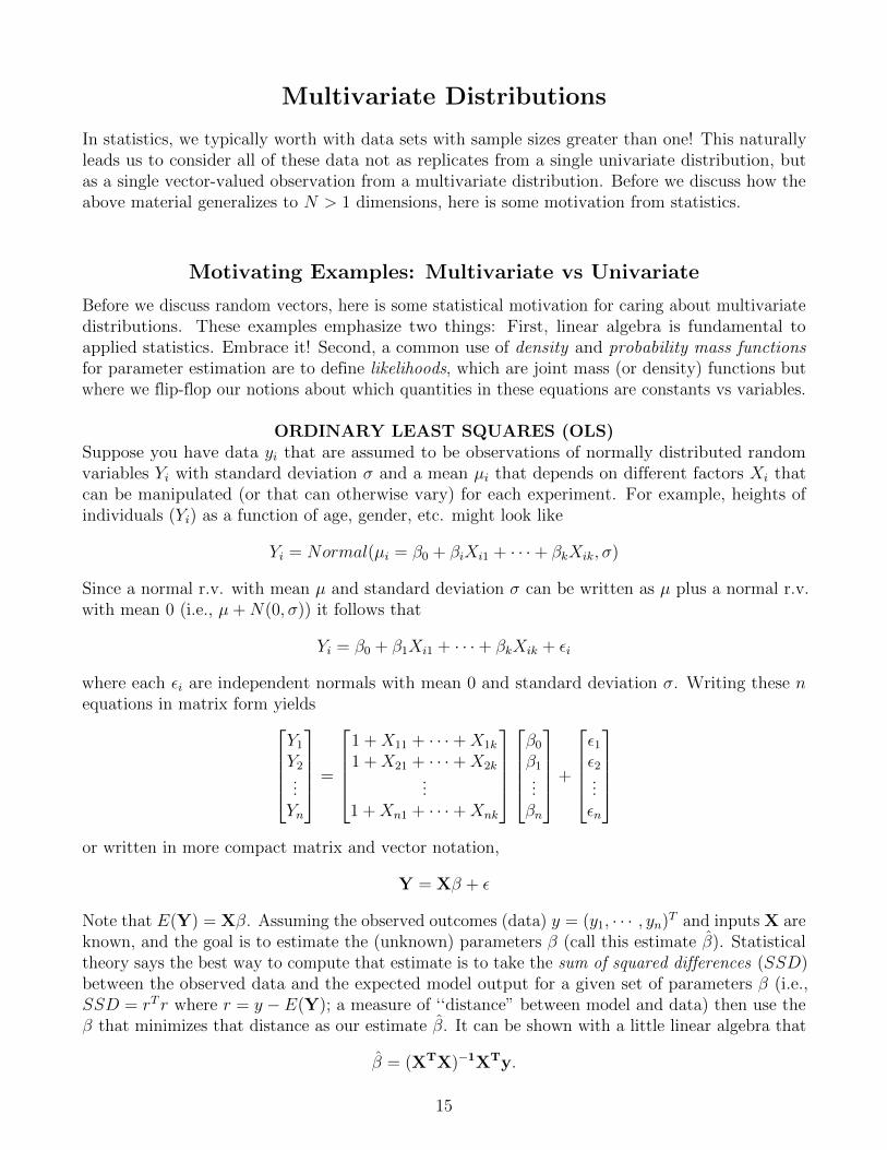
ORDINARY LEAST SQUARES (OLS)Suppose you have data yi that are assumed to be observations of normally distributed randomvariables Yi with standard deviation σ and a mean µi that depends on different factors Xi thatcan be manipulated (or that can otherwise vary) for each experiment. For example, heights ofindividuals (Yi) as a function of age, gender, etc. might look like

Yi = Normal(µi = β0 + βiXi1 + · · ·+ βkXik, σ)

Since a normal r.v. with mean µ and standard deviation σ can be written as µ plus a normal r.v.with mean 0 (i.e., µ+N(0, σ)) it follows that

Yi = β0 + β1Xi1 + · · ·+ βkXik + εi

where each εi are independent normals with mean 0 and standard deviation σ. Writing these nequations in matrix form yields

Y1Y2...Yn

=

1 +X11 + · · ·+X1k

1 +X21 + · · ·+X2k...

1 +Xn1 + · · ·+Xnk

β0β1...βn

+

ε1ε2...εn

or written in more compact matrix and vector notation,

Y = Xβ + ε

Note that E(Y) = Xβ. Assuming the observed outcomes (data) y = (y1, · · · , yn)T and inputs X areknown, and the goal is to estimate the (unknown) parameters β (call this estimate β). Statisticaltheory says the best way to compute that estimate is to take the sum of squared differences (SSD)between the observed data and the expected model output for a given set of parameters β (i.e.,SSD = rT r where r = y − E(Y); a measure of ‘‘distance” between model and data) then use theβ that minimizes that distance as our estimate β. It can be shown with a little linear algebra that

β = (XTX)−1XTy.

15

Therefore we’ve used linear algebra and a little multivariate calculus to turn an optimizationproblem into a relatively simple matrix computation!

Concluding Remark: In practice, statistics is a multivariate endeavor and therefore you shouldbe familiar with these basic probability concepts in a multivariate setting. Also, some basic toolsfrom linear algebra are essential to thinking critically about both theoretical and applied statistics.

Density vs Likelihood

Definition: A random sample of size N is a set of N independent and identically distributed(iid) observations X1 = x1, X2 = x2, . . ., Xn = xn.

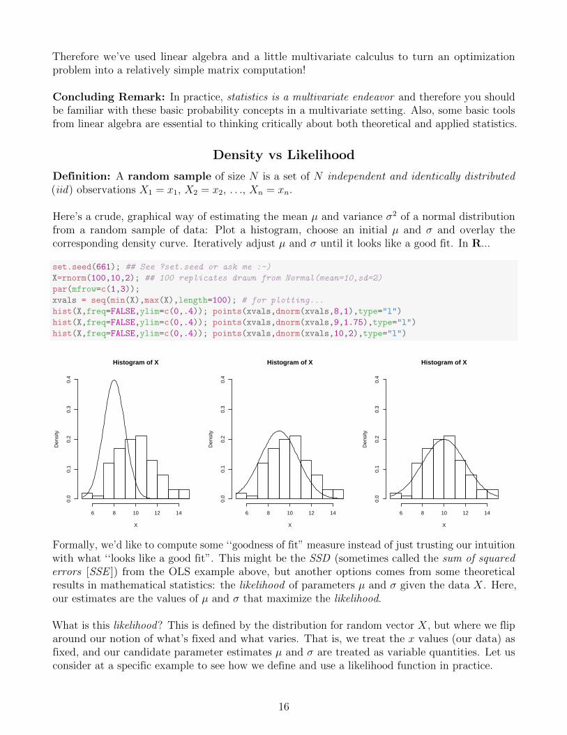
Here’s a crude, graphical way of estimating the mean µ and variance σ2 of a normal distributionfrom a random sample of data: Plot a histogram, choose an initial µ and σ and overlay thecorresponding density curve. Iteratively adjust µ and σ until it looks like a good fit. In R...

set.seed(661); ## See ?set.seed or ask me :-)

X=rnorm(100,10,2); ## 100 replicates drawn from Normal(mean=10,sd=2)

par(mfrow=c(1,3));

xvals = seq(min(X),max(X),length=100); # for plotting...

hist(X,freq=FALSE,ylim=c(0,.4)); points(xvals,dnorm(xvals,8,1),type="l")

hist(X,freq=FALSE,ylim=c(0,.4)); points(xvals,dnorm(xvals,9,1.75),type="l")

hist(X,freq=FALSE,ylim=c(0,.4)); points(xvals,dnorm(xvals,10,2),type="l")

Histogram of X

X

Den

sity

6 8 10 12 14

0.0

0.1

0.2

0.3

0.4

Histogram of X

X

Den

sity

6 8 10 12 14

0.0

0.1

0.2

0.3

0.4

Histogram of X

X

Den

sity

6 8 10 12 14

0.0

0.1

0.2

0.3

0.4

Formally, we’d like to compute some ‘‘goodness of fit” measure instead of just trusting our intuitionwith what ‘‘looks like a good fit”. This might be the SSD (sometimes called the sum of squarederrors [SSE ]) from the OLS example above, but another options comes from some theoreticalresults in mathematical statistics: the likelihood of parameters µ and σ given the data X. Here,our estimates are the values of µ and σ that maximize the likelihood.

What is this likelihood? This is defined by the distribution for random vector X, but where we fliparound our notion of what’s fixed and what varies. That is, we treat the x values (our data) asfixed, and our candidate parameter estimates µ and σ are treated as variable quantities. Let usconsider at a specific example to see how we define and use a likelihood function in practice.

16

Example: Assume all Xi are iid with normal density f(xi;µ, σ). This implies the joint densityfX(x1, ..., xn;µ, σ) =

∏ni=1 f(xi, µ, σ). Here we can write it as a simple product, thanks to the

independence of the individual random variables. This density function defines the likelihoodfunction for parmeters µ and σ

L(µ, σ;x) =n∏i=1

f(xi, µ, σ)

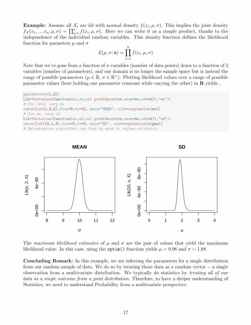
Note that we’ve gone from a function of n variables (number of data points) down to a function of 2variables (number of parameters), and our domain is no longer the sample space but is instead therange of possible parameters (µ ∈ R, σ ∈ R+). Plotting likelihood values over a range of possibleparameter values (here holding one parameter constant while varying the other) in R yields...

par(mfrow=c(1,2))

Lik=Vectorize(function(mu,sd,xs) prod(dnorm(xs,mean=mu,sd=sd)),"mu");

# fix sd=2, vary mu

curve(Lik(x,2,X),from=8,to=12, main="MEAN", xlab=expression(mu))

# fix mu, vary sd

Lik=Vectorize(function(mu,sd,xs) prod(dnorm(xs,mean=mu,sd=sd)),"sd");

curve(Lik(10,x,X),from=0,to=4, main="SD", xlab=expression(sigma))

# Optimization algorithms can then be used to refine estimates.

8 9 10 11 12

0e+

004e

−90

MEAN

µ

Lik(

x, 2

, X)

0 1 2 3 4

0e+

004e

−90

8e−

90

SD

σ

Lik(

10, x

, X)

The maximum likelihood estimates of µ and σ are the pair of values that yield the maximumlikelihood value. In this case, using the optim() function yields µ = 9.98 and σ = 1.88.

Concluding Remark: In this example, we are inferring the parameters for a single distributionfrom our random sample of data. We do so by treating those data as a random vector -- a singleobservation from a multivariate distribution. We typically do statistics by treating all of ourdata as a single outcome from a joint distribution. Therefore, to have a deeper understanding ofStatistics, we need to understand Probability from a multivariate perspective.

17

Random Vectors and Joint Densities

Joint densities describe probability distributions of random vectors. A random vector X is ann-dimensional vector where each component is itself a random variable, i.e., X = (X1, X2, . . . , Xn),where all Xis are rvs.

Discrete random vectors are described by the joint probability density function of Xi (or jointpdf), i = 1, · · · , n denoted by

P (X = x) = P (s ∈ S : Xi(s) = xi for all i) = pX(x1, .., xn)

Another name for the joint pdf of a discrete random vector is joint probability mass function (pmf).

Computing probabilities for discrete random vectors. For any subset A of R2, we have

P ((X, Y ) ∈ A) =∑

(x,y)∈A

P (X = x, Y = y) =∑

(x,y)∈A

pX,Y (x, y).

Continuous random vectors are described by the joint probability density function of X and Y(or joint pdf) denoted by fX,Y (x, y). The pdf has the following properties:

1. fX,Y (x, y) ≥ 0 for every (x, y) ∈ R2.

2.∫∞−∞

∫∞−∞ fX,Y (x, y)dxdy = 1.

3. For any region A in the xy-plane P ((X, Y ) ∈ A) =∫ ∫

AfX,Y (x, y)dxdy.

Marginal distributions. Let (X, Y ) be a continuous/discrete random vector having a jointdistribution with pdf/pmf f(x, y). Then, the one-dimensional distributions of X and Y are calledmarginal distributions. We compute the marginal distributions as follows:If (X, Y ) is a discrete vector, then the distributions of X and Y are given by:

fX(x) =∑all y

P (X = x, Y = y) and fY (y) =∑all x

P (X = x, Y = y).

If (X, Y ) is a continuous vector, then the distributions of X and Y are given by:

fX(x) =

∫ ∞−∞

f(x, y)dy and fY (y) =

∫ ∞−∞

f(x, y)dx.

Joint cdf of a vector (X, Y ). The joint cumulative distribution function of X and Y (or jointcdf) is defined by

FX,Y (u, v) = P (X ≤ u, Y ≤ v).

Theorem. Let FX,Y (u, v) be a joint cdf of the vector (X, Y ). Then the joint pdf of (X, Y ), fX,Y ,

is given by second partial deriveative of the cdf. That is fX,Y (x, y) = ∂2

∂x∂yFX,Y (x, y), provided that

FX,Y (x, y) has continuous second partial derivatives.

18

Independence Revisited

Definition. Two random variables are called independent if and only if (iff ) for any events Aand B in S, it follows that P (X ∈ A and Y ∈ B) = P (X ∈ A)P (Y ∈ B).

Theorem. The random variables X and Y are independent iff

fX,Y (x, y) = fX(x)fY (y),

where f(x, y) is the joint pdf of (X, Y ), and fX(x) and fY (y) are the marginal densities of X andY , respectively.

NOTE: Random variables X and Y are independent iff FX,Y (x, y) = FX(x)FY (y), where F (x, y) isthe joint cdf of (X, Y ), and FX(x) and FY (y) are the marginal cdf’s of the X and Y , respectively.

Independence of more than 2 r.v.s A set of n random variables X1, X2, . . . , Xn are independentiff their joint pdf is a product of the marginal pdfs. That is

fX1,X2,...,Xn(x1, x2, . . . , xn) = fX1(x1)fX2(x2) · · · fXn(xn)

where fX1,X2,...,Xn(x1, x2, . . . , xn) is the joint pdf of the vector (X1, X2, . . . , Xn), and fX1(x1),fX2(x2), · · · , and fXn(xn) are the marginal pdf’s of the variables X1, X2, . . . , Xn.

Conditional Distributions Revisited

Let (X, Y ) be a random vector with some joint pdf or pmf. Consider the problem of finding theprobability that X=x AFTER a value of Y was observed. To do that we develop conditionaldistribution of X given Y=y.Definition. If (X, Y ) is a discrete random vector with pmf pX,Y (x, y), and if P (Y = y) > 0, thenthe conditional distribution of X given Y=y is given by the conditional pmf

pX|Y=y(x) =pX,Y (x, y)

pY (y).

Similarily, if P (X = x) > 0, then the conditional distribution of Y given X=x is given by the

conditional pmf pY |X=x(y) =pX,Y (x,y)

pX(x).

Definition. If (X, Y ) is a continuous random vector with pdf fX,Y (x, y), and if fY (y) > 0, thenthe conditional distribution of X given Y=y is given by the conditional pdf

fX|Y=y(x) =fX,Y (x, y)

fY (y).

Similarly, if fX(x) > 0, then the conditional distribution of Y given X=x is given by the conditional

pdf fY |X=x(y) =fX,Y (x,y)

fX(x).

Independence and conditional distributions. If random variables X and Y are independent,then their marginal pdf/pmf’s are the same as their conditional pdf/pmf’s. That is fY |X=x(y) = fY (y)and fX|Y=y(x) = fX(x), for all y and x where fY (y) > 0 and fX(x) > 0, respectively.

19

Expected Values, Variance, and Covariance Revisited

Definition: Let (X, Y ) be a random vector with pmf p (discrete) or pdf f (continuous). Let g bea real valued function of (X, Y ). Then, the expected value of random variable g(X, Y ) is

E(g(X, Y )) =∑allx

∑ally

g(x, y)p(x, y), in the discrete case, or

E(g(X, Y )) =

∫ ∞−∞

∫ ∞−∞

g(x, y)f(x, y)dxdy, in the continuous case,

provided that the sums and the integrals converge absolutely.

Mean of a sum of random variables. Let X and Y be any random variables, and a and b realnumbers. Then

E(aX + bY ) = aE(X) + bE(Y ),

provided both expectations are finite.

NOTE: Let X1, X2, . . . , Xn be any random variables with finite means, and let a1, a2, . . . , an be aset of real numbers. Then

E(a1X1 + a2X2 + · · ·+ anXn) = a1E(X1) + a2E(X2) + · · ·+ anE(Xn).

Mean of a product of independent random variables. If X and Y are independent randomvariables with finite expectations, then E(XY ) = E(X)E(Y ).

Variance of a sum of independent random variables.Let X1, X2, . . . , Xn be any independent random variables with finite second moments (i.e. E(X2

i ) <∞). Then

V ar(X1 +X2 + · · ·+Xn) = V ar(X1) + V ar(X2) + · · ·+ V ar(Xn).

NOTE: Let X1, X2, . . . , Xn be any independent random variables with finite second moments, andlet a1, a2, . . . , an be a set of real numbers. Then

V ar(a1X1 + a2X2 + · · ·+ anXn) = a21V ar(X1) + a22V ar(X2) + · · ·+ a2nV ar(Xn).

Definition: The covariance of two jointly distributed random variables X and Y is defined as

cov(X, Y ) = E((X − E(X))(Y − E(Y ))) = E(XY )− E(X)E(Y )

Sometimes the notation σ(X, Y ) is used instead of cov(X, Y ).

Definition: The variance-covariance matrix cov(X,Y) for random vectors X and Y is

cov(X,Y) = E((X− E(X)) (Y − E(Y))T ) = E(XYT)− E(X)E(Y)T

The ijth entry in the covariance matrix is the covariance between Xi and Yj. If X = Y, we oftenuse the notation cov(X) = cov(X,X). The diagonal entries of σ(X) are [V ar(X1), . . . , V ar(Xn)].The notation σ(X,Y) or sometimes Σ(X,Y) is often used for cov(X,Y).

Definition: The correlation random variables X and Y is a standardized covariance:

corr(X, Y ) =E((X − E(X))(Y − E(Y )))√

V ar(X)√V ar(Y )

=cov(X, Y )

sd(X) sd(Y )

20

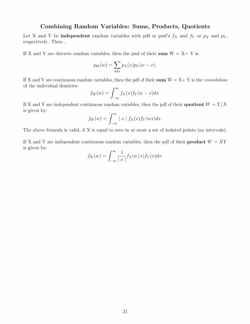
Combining Random Variables: Sums, Products, Quotients

Let X and Y be independent random variables with pdf or pmf’s fX and fY or pX and pY ,respectively. Then...

If X and Y are discrete random variables, then the pmf of their sum W = X+ Y is

pW (w) =∑allx

pX(x)pY (w − x).

If X and Y are continuous random variables, then the pdf of their sum W = X+ Y is the convolutionof the individual densities:

fW (w) =

∫ ∞−∞

fX(x)fY (w − x)dx.

If X and Y are independent continuous random variables, then the pdf of their quotientW = Y/Xis given by:

fW (w) =

∫ ∞−∞| x | fX(x)fY (wx)dx.

The above formula is valid, if X is equal to zero in at most a set of isolated points (no intervals).

If X and Y are independent continuous random variables, then the pdf of their product W = XYis given by:

fW (w) =

∫ ∞−∞

1

| x |fX(w/x)fY (x)dx.

21

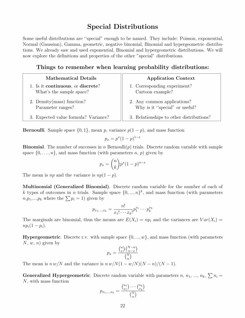
Special Distributions

Some useful distributions are ‘‘special” enough to be named. They include: Poisson, exponential,Normal (Gaussian), Gamma, geometric, negative binomial, Binomial and hypergeometric distribu-tions. We already saw and used exponential, Binomial and hypergeometric distributions. We willnow explore the definitions and properties of the other ”special” distributions.

Things to remember when learning probability distributions:

Mathematical Details

1. Is it continuous, or discrete?What’s the sample space?

2. Density(mass) function?Parameter ranges?

3. Expected value formula? Variance?

Application Context

1. Corresponding experiment?Cartoon example?

2. Any common applications?Why is it ‘‘special” or useful?

3. Relationships to other distributions?

Bernoulli. Sample space 0, 1, mean p, variance p(1− p), and mass function

px = px(1− p)1−x

Binomial. The number of successes in n Bernoulli(p) trials. Discrete random variable with samplespace 0, . . . , n, and mass function (with parameters n, p) given by

px =

(n

k

)px(1− p)n−x

The mean is np and the variance is np(1− p).

Multinomial (Generalized Binomial). Discrete random variable for the number of each ofk types of outcomes in n trials. Sample space 0, ..., nk, and mass function (with parametersn,p1,...,pk where the

∑pi = 1) given by

px1,...,xk =n!

x1! · · · xk!px11 · · · p

xkk

The marginals are binomial, thus the means are E(Xi) = npi and the variances are V ar(Xi) =npi(1− pi).

Hypergeometric. Discrete r.v. with sample space 0, ..., w, and mass function (with parametersN , w, n) given by

px =

(wx

)(N−wn−x

)(Nn

)The mean is nw/N and the variance is nw/N(1− w/N)(N − n)/(N − 1).

Generalized Hypergeometric. Discrete random variable with parameters n, n1, ..., nk,∑ni =

N , with mass function

px1,...,xk =

(n1

x1

)· · ·(nkxk

)(Nn

)22

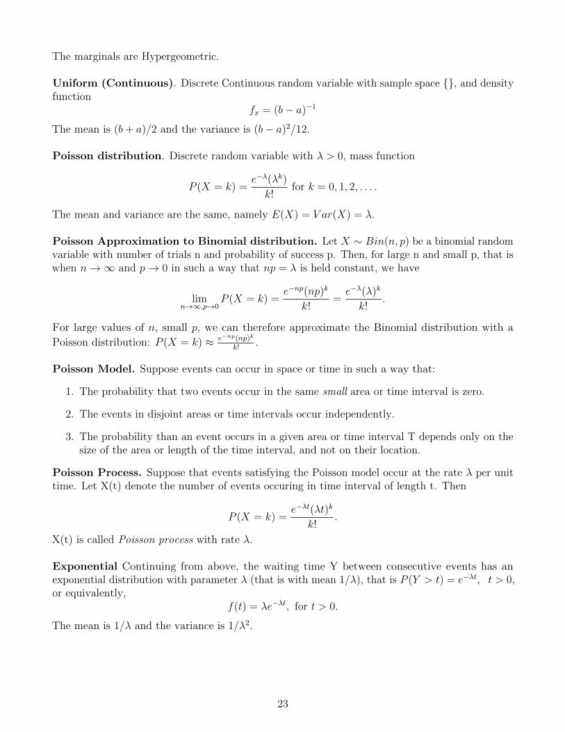
The marginals are Hypergeometric.

Uniform (Continuous). Discrete Continuous random variable with sample space , and densityfunction

fx = (b− a)−1

The mean is (b+ a)/2 and the variance is (b− a)2/12.

Poisson distribution. Discrete random variable with λ > 0, mass function

P (X = k) =e−λ(λk)

k!for k = 0, 1, 2, . . . .

The mean and variance are the same, namely E(X) = V ar(X) = λ.

Poisson Approximation to Binomial distribution. Let X ∼ Bin(n, p) be a binomial randomvariable with number of trials n and probability of success p. Then, for large n and small p, that iswhen n→∞ and p→ 0 in such a way that np = λ is held constant, we have

limn→∞,p→0

P (X = k) =e−np(np)k

k!=e−λ(λ)k

k!.

For large values of n, small p, we can therefore approximate the Binomial distribution with a

Poisson distribution: P (X = k) ≈ e−np(np)k

k!.

Poisson Model. Suppose events can occur in space or time in such a way that:

1. The probability that two events occur in the same small area or time interval is zero.

2. The events in disjoint areas or time intervals occur independently.

3. The probability than an event occurs in a given area or time interval T depends only on thesize of the area or length of the time interval, and not on their location.

Poisson Process. Suppose that events satisfying the Poisson model occur at the rate λ per unittime. Let X(t) denote the number of events occuring in time interval of length t. Then

P (X = k) =e−λt(λt)k

k!.

X(t) is called Poisson process with rate λ.

Exponential Continuing from above, the waiting time Y between consecutive events has anexponential distribution with parameter λ (that is with mean 1/λ), that is P (Y > t) = e−λt, t > 0,or equivalently,

f(t) = λe−λt, for t > 0.

The mean is 1/λ and the variance is 1/λ2.

23

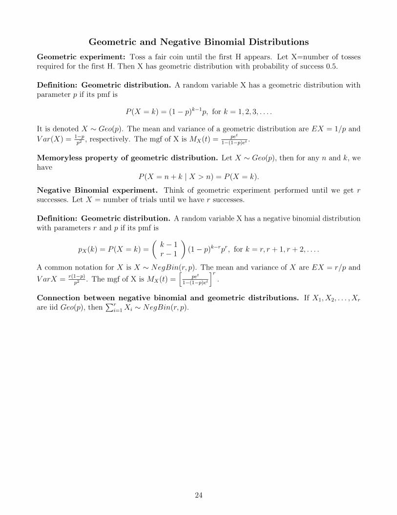
Geometric and Negative Binomial Distributions

Geometric experiment: Toss a fair coin until the first H appears. Let X=number of tossesrequired for the first H. Then X has geometric distribution with probability of success 0.5.

Definition: Geometric distribution. A random variable X has a geometric distribution withparameter p if its pmf is

P (X = k) = (1− p)k−1p, for k = 1, 2, 3, . . . .

It is denoted X ∼ Geo(p). The mean and variance of a geometric distribution are EX = 1/p and

V ar(X) = 1−pp2

, respectively. The mgf of X is MX(t) = pet

1−(1−p)et .

Memoryless property of geometric distribution. Let X ∼ Geo(p), then for any n and k, wehave

P (X = n+ k | X > n) = P (X = k).

Negative Binomial experiment. Think of geometric experiment performed until we get rsuccesses. Let X = number of trials until we have r successes.

Definition: Geometric distribution. A random variable X has a negative binomial distributionwith parameters r and p if its pmf is

pX(k) = P (X = k) =

(k − 1r − 1

)(1− p)k−rpr, for k = r, r + 1, r + 2, . . . .

A common notation for X is X ∼ NegBin(r, p). The mean and variance of X are EX = r/p and

V arX = r(1−p)p2

. The mgf of X is MX(t) =[

pet

1−(1−p)et

]r.

Connection between negative binomial and geometric distributions. If X1, X2, . . . , Xr

are iid Geo(p), then∑r

i=1Xi ∼ NegBin(r, p).

24

Exponential and Gamma Distributions

Definition. The Gamma function. For any positive real number r > 0, the gamma functionof r is denoted Γ(r) and equal to

Γ(r) =

∫ ∞0

yr−1e−ydy.

Theorem. Properties of Gamma function. The Gamma(r) function satifies the followingproperties:

1. Γ(1) = 1.

2. Γ(r) = (r − 1)Γ(r − 1).

3. For r integer, we have Γ(r) = (r − 1)!.

Definition of the Gamma random variable. For any real positive numbers r > 0 and λ > 0,a random variable with pdf

fX(x) =λr

Γ(r)xr−1e−λx, x > 0,

is said to have a Gamma distribution with parameters r and λ, denoted X ∼ Γ(r, λ).Theorem: moments and mgf of a gamma distribution. If X ∼ Γ(r, λ) then

1. EX= r/λ.

2. Var(X)= r/λ2.

3. Mgf of X is MX(t) = (1− t/λ)r.

Theorem. Let X1, X2, . . . , Xn be iid exponential random variables with parameter λ, that is withmean 1/λ. The the sum of Xi’s has a gamma distribution with parameters n and λ. More precisely,∑n

i=1Xi ∼ Γ(r, λ).

Theorem. A sum of independent gamma random variables X ∼ Γ(r, λ) and Y ∼ Γ(s, λ) with thesame λ has a gamma distribution with r′ = r + s and the same λ. That is X + Y ∼ Γ(r + s, λ).

Note: In a sequence of Poisson events occurring with rate λ per unit time/area, the waiting timefor the r’th event has a Γ(r, λ) distribution.

25

Normal (Gaussian) Distribution

Normal (Gaussian) distribution. Continuous random variable X has a normal distributionwith mean µ and variance σ2 if its pdf is of the form:

f(x) =1√2πσ

e−(x−µ)2

2σ2 ,

where µ and σ2 are real valued constants. If X has pdf as above, we denote it: X ∼ N(µ, σ2). Themgf of X is MX(t) = eµt+σ

2t2/2, for any real t.The normal pdf is bell shaped and centered around the mean µ. There is a special Normaldistribution with mean 0 and variance 1, called standard normal distribution, and denoted byZ ∼ N(0, 1). The standard normal pdf is

f(z) =1√2πe−

x2

2 .

The values of the standard normal cdf are tabulated. To find probabilities related to general normalrandom variables, use the following fact:

Theorem. If X ∼ N(µ, σ2), then Z = X−µσ∼ N(0, 1).

Theorem: Linear combinations of independent normal r.v.s are themselves normal.

1. Let X1 ∼ N(µ1, σ21), and X2 ∼ N(µ2, σ

22), with X1 and X2 independent. Then X1 ±X2 ∼

N(µ1 ± µ2, σ21 + σ2

2), and more generally:

2. Let Xi ∼ N(µi, σ2i ), for i = 1, . . . , n, and Xi’s ind. Then Y =

∑ni=1Xi ∼ N(

∑ni=1 µi,

∑ni=1 σ

2i ),

and

3. For any real numbers a1, a2, . . . an, Y =∑n

i=1 aiXi ∼ N(∑n

i=1 aiµi,∑n

i=1 a2iσ

2i ).

4. Let Xi ∼ N(µ, σ2) iid for i = 1, . . . , n. Then X ∼ N(µ, σ2/n).

Normal Approximation to Binomial. Let X ∼ Bin(n, p) and Y ∼ N(np, np(1 − p)). Thenfor large n

P (a ≤ X ≤ b) ≈ P (a ≤ Y ≤ b).

Continuity correction for the normal approximation to binomial. To ”correct” for thefact that binomial is discrete and normal is a continuous distribution, we do the following correctionfor continuity: P (X = x) ≈ P (x− 0.5 < Y < x+ 0.5).

26

Convergence Concepts & Laws of Large Numbers

Before discussing the Central Limit Theorem (CLT), Weak Law of Large Numbers (WLLN) andStrong Law of Large Numbers (SLLN) it helps to know some different convergence concepts thatexist in probability (and measure theory).

We begin with two results that help us bound probabilities when only the mean is known:

Markov Inequality: For any non-negative valued r.v. Y with E(Y ) = µ, then for a > 0

P (Y ≥ a) ≤ E(Y )

a.

Proof (finite-variance, continuous case):

E(Y )

a=

1

a

∫ ∞0

y f(y) dy ≥ 1

a

∫ ∞a

y f(y) dy ≥ 1

a

∫ ∞a

a f(y) dy = P (Y ≥ a)

Chebychev Inequality: For r.v. X with E(X) = µ and V ar(X) = σ2 <∞, then for any k > 0the probability that X deviates more than k from the mean is bounded by

P (|X − µ| ≥ k) ≤ σ2

k2

Sketch of Proof: Apply the Markov Inequality using Y = (X − µ)2 and a = k2.

Convergence Concepts in Probability

Definition: The r.v.s Xn converge in distribution to r.v. X (XnD→ X) if

limn→∞

FXn(x) = FX(x)

for all x where FX(x) is continuous. This is point-wise convergence of cdfs.

Definition: The r.v.s Xn converge in probability to r.v. X (XnP→ X) if, for all ε > 0,

limn→∞

P (|Xn −X| ≥ ε) = 0 ⇔ limn→∞

P (|Xn −X| ≤ ε) = 1.

This convergence of probability values is in measure theory called convergence in measure.

Definition: The r.v.s Xn converges almost surely to r.v. X (Xna.s.→ X) if for all ε > 0

P(

limn→∞

|Xn −X| ≤ ε)≡ P

(all ω ∈ S such that lim

n→∞|Xn(ω)−X(ω)| ≤ ε

)= 1

In measure theory, almost everywhere means a statement holds true for all but a set of measure zero.Thinking of random variables as functions on our sample space, this is just pointwise convergenceof the random variables except perhaps on some set of measure zero.

Theorem: If Xn converges almost surely to X, then it also converges in probability. If Xn

converges in probability to X, the it also converges in distribution.

27

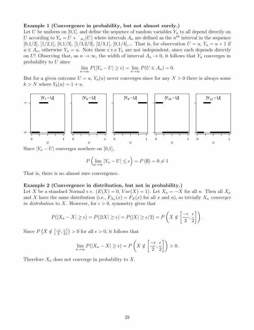
Example 1 (Convergence in probability, but not almost surely.)Let U be uniform on [0,1], and define the sequence of random variables Yn to all depend directly onU according to Yn = U + 1An(U) where intervals An are defined as the nth interval in the sequence[0,1/2], [1/2,1], [0,1/3], [1/3,2/3], [2/3,1], [0,1/4],... That is, for observation U = u, Yn = u+ 1 ifu ∈ An, otherwise Yn = u. Note these r.v.s Yn are not independent, since each depends directlyon U ! Observing that, as n→∞, the width of interval An → 0, it follows that Yn converges inprobability to U since

limn→∞

P (|Yn − U | ≥ ε) = limn→∞

P (U ∈ An) = 0.

But for a given outcome U = u, Yn(u) never converges since for any N > 0 there is always somek > N where Yk(u) = 1 + u.

U

Y7 − U

01

0 1

U

Y8 − U

0 1

U

Y9 − U

0 1

U

Y10 − U

0 1

U

Y11 − U

0 1

Since |Yn − U | converges nowhere on [0,1],

P(

limn→∞

|Yn − U | ≤ ε)

= P (∅) = 0 6= 1

That is, there is no almost sure convergence.

Example 2 (Convergence in distribution, but not in probability.)Let X be a standard Normal r.v. (E(X) = 0, V ar(X) = 1). Let Xn = −X for all n. Then all Xn

and X have the same distribution (i.e., FXn(x) = FX(x) for all x and n), so trivially Xn convergesin distribution to X. However, for ε > 0, symmetry gives that

P (|Xn −X| ≥ ε) = P (|2X| ≥ ε) = P (|X| ≥ ε/2) = P

(X /∈

[−ε2,ε

2

]).

Since P(X /∈

[−ε2, ε2

])> 0 for all ε > 0, it follows that

limn→∞

P (|Xn −X| ≥ ε) = P

(X /∈

[−ε2,ε

2

])> 0.

Therefore Xn does not converge in probability to X.

28

Laws of Large Numbers

Weak Law of Large Numbers (WLLN): Let Xi be iid with mean µ. Then Xn =∑n

i=1Xi

converges in probability to µ, i.e., XnP→ µ. That is, for all positive ε near zero,

limn→∞

P (|Xn − µ| ≥ ε) = 0 ⇔ limn→∞

P (|Xn − µ| ≤ ε) = 1.

Proof (when V ar(X) = σ2 <∞): Apply the Chebychev Inequality. This was first proven in the1700s by Bernoulli, and incrementally generalized by Markov then Chebychev.

Strong Law of Large Numbers (SLLN): Let Xi be iid with mean µ, and let Xn =∑n

i=1Xi.Then Xn converges almost surely to µ. That is, for all positive ε near zero,

P(

limn→∞

|Xn − µ| ≥ ε)

= 0 ⇔ P(

limn→∞

|Xn − µ| ≤ ε)

= 1.

NOTE: Borel gave the first proof of the SLLN, 200 years later, in 1909. It was incrementallyimproved by Cantelli, Khintchine (who named it the SLLN) and Kolmogorov (in the 1930s).

Weak vs Strong: Accordingly, almost sure convergence is called a stronger form of convergencethan convergence in probability, and convergence in distribution is even more weak.

NOTE: The WLLN and SLLN basically both state that the average of n iid random variables(with mean µ < ∞) converges to µ as n → ∞. The Weak LLN states this in the weaker form

(XnP→ µ), while the Strong LLN states this in the (stronger) form (Xn

a.s.→ µ).

Central Limit Theorems (CLTs)

Classic CLT (Lindberg-Levy): Suppose random variables X1, ..., Xn are (1) independent and(2) identically distributed (iid) with (3) finite mean E(Xi) = µ and (4) finite variance V ar(Xi) = σ2.Then the quantity

Sn =

√n

σ

(1

n

(n∑i=1

Xi

)− µ

)converges in distribution to a standard Normal r.v., i.e., Sn

D→ N (0, 1).

NOTE: Other CLTs relax the iid assumptions, but require additional conditions that must bemet. The Lyapunov CLT, for example, relaxes the assumption of identical distributions:

CLT (Lyapunov): Suppose r.v.s X1, ..., Xn are (1) independent, (2) each have finite meanE(Xi) = µi and (3) variance V ar(Xi) = σ2

i . Define sn =√∑n

i=1 σ2i . Then the quantity

Sn =1

sn

n∑i=1

(Xi − µi)

converges in distribution to a standard Normal if the following condition holds for some δ > 0(usually checking δ = 1 is all it takes):

limn→∞

1

s2+δn

n∑i=1

E(|Xi − µi|2+δ

)= 0.

29