Embed Size (px)
Citation preview
Probability in the analysis of CNF
Satisfiability algorithms and properties
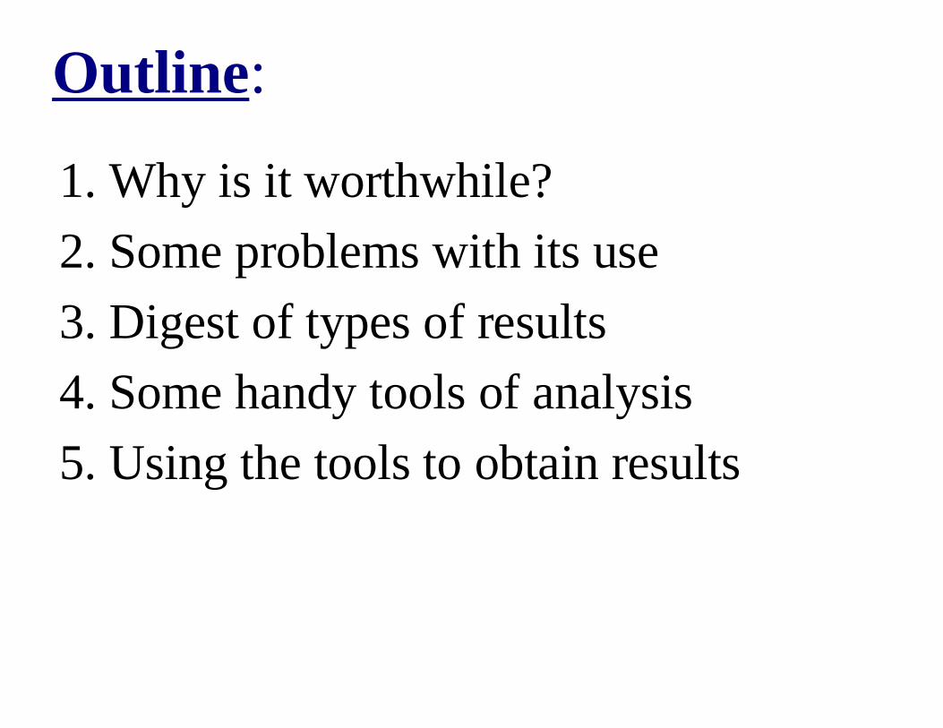
Outline:
1. Why is it worthwhile?
2. Some problems with its use
3. Digest of types of results
4. Some handy tools of analysis
5. Using the tools to obtain results
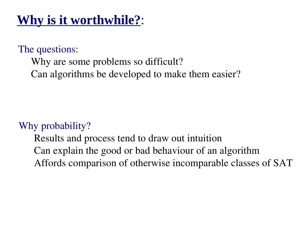
Why is it worthwhile?:
The questions:
Why are some problems so difficult?
Can algorithms be developed to make them easier?
Why probability?
Results and process tend to draw out intuition
Can explain the good or bad behaviour of an algorithm
Affords comparison of otherwise incomparable classes of SAT
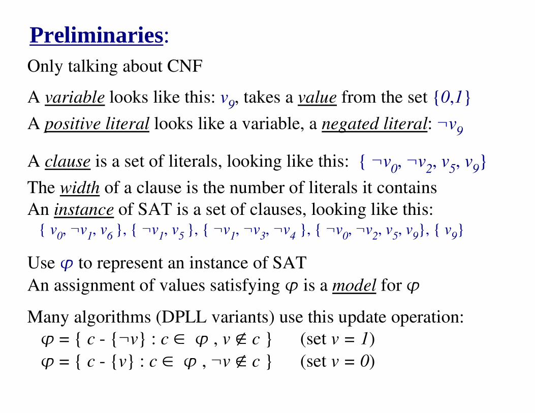
Preliminaries:Only talking about CNF
A variable looks like this: v9, takes a value from the set {0,1}
A positive literal looks like a variable, a negated literal: ¬v9
A clause is a set of literals, looking like this: { ¬v0, ¬v
2, v
5, v
9}
The width of a clause is the number of literals it contains
An instance of SAT is a set of clauses, looking like this: { v
0, ¬v
1, v
6 }, { ¬v
1, v
5 }, { ¬v
1, ¬v
3, ¬v
4 }, { ¬v
0, ¬v
2, v
5, v
9}, { v
9}
Use � to represent an instance of SAT
An assignment of values satisfying � is a model for �
Many algorithms (DPLL variants) use this update operation:
� = { c - {¬v} : c � � , v � c } (set v = 1)
� = { c - {v} : c � � , ¬v � c } (set v = 0)
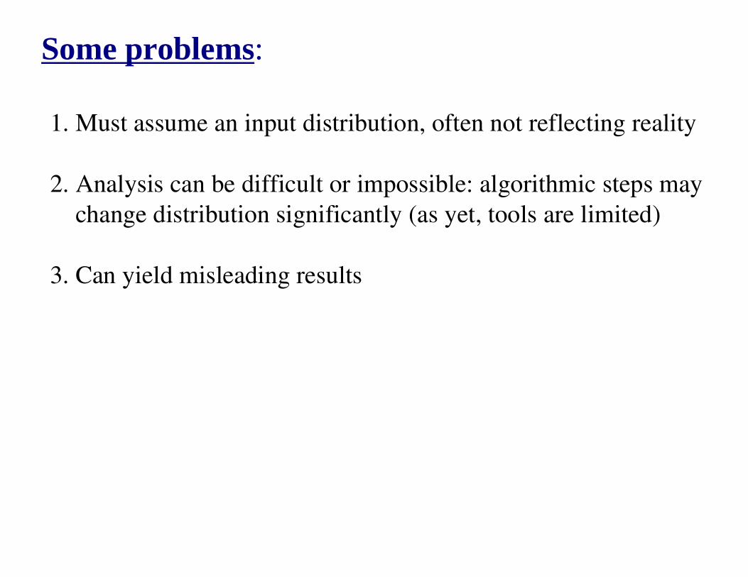
Some problems:
1. Must assume an input distribution, often not reflecting reality
2. Analysis can be difficult or impossible: algorithmic steps may
change distribution significantly (as yet, tools are limited)
3. Can yield misleading results
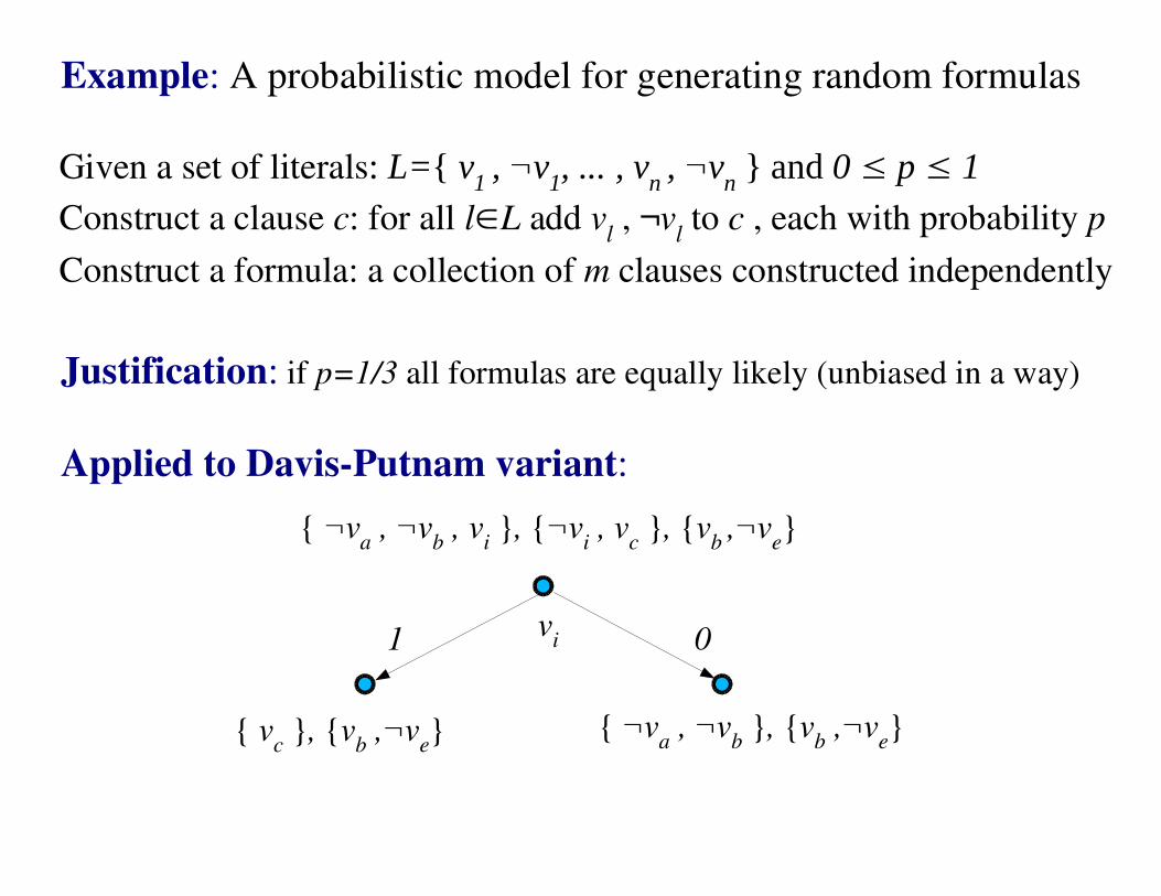
Example: A probabilistic model for generating random formulas
Given a set of literals: L={ v1 , ¬v1, ... , vn , ¬vn } and 0 � p � 1
Construct a clause c: for all l�L add vl , ¬v
l to c , each with probability p
Construct a formula: a collection of m clauses constructed independently
Justification: if p=1/3 all formulas are equally likely (unbiased in a way)
Applied to Davis-Putnam variant:
. vi
{ ¬va , ¬v
b , v
i }, {¬v
i , v
c }, {v
b ,¬v
e}
{ vc }, {v
b ,¬v
e}
1 0
{ ¬va , ¬v
b }, {v
b ,¬v
e}
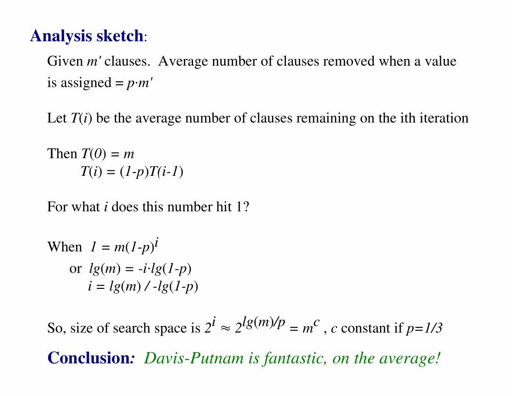
Analysis sketch:
Given m' clauses. Average number of clauses removed when a value
is assigned = p.m'
Let T(i) be the average number of clauses remaining on the ith iteration
Then T(0) = m
T(i) = (1-p)T(i-1)
For what i does this number hit 1?
When 1 = m(1-p)i
or lg(m) = -i.lg(1-p)
i = lg(m) / -lg(1-p)
So, size of search space is 2i � 2lg(m)/p = mc , c constant if p=1/3
Conclusion: Davis-Putnam is fantastic, on the average!
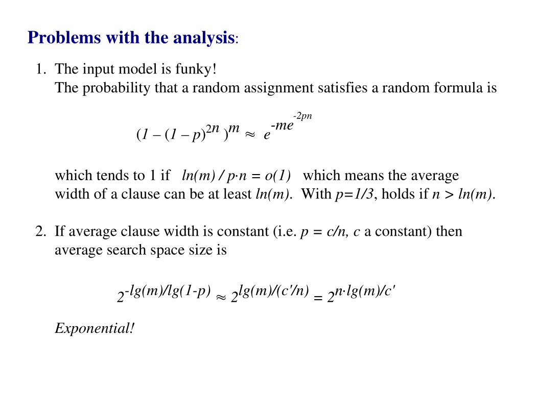
Problems with the analysis:
1. The input model is funky!
The probability that a random assignment satisfies a random formula is
(1 – (1 – p)2n )m � e-me
which tends to 1 if ln(m) / p.n = o(1) which means the average
width of a clause can be at least ln(m). With p=1/3, holds if n > ln(m).
2. If average clause width is constant (i.e. p = c/n, c a constant) then
average search space size is
2-lg(m)/lg(1-p) � 2
lg(m)/(c'/n) = 2n.lg(m)/c'
Exponential!
-2pn
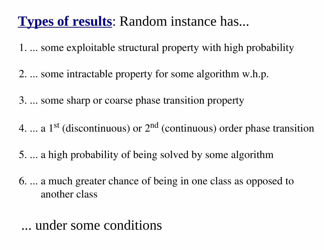
Types of results: Random instance has...
1. ... some exploitable structural property with high probability
2. ... some intractable property for some algorithm w.h.p.
3. ... some sharp or coarse phase transition property
4. ... a 1st (discontinuous) or 2nd (continuous) order phase transition
5. ... a high probability of being solved by some algorithm
6. ... a much greater chance of being in one class as opposed to
another class
... under some conditions
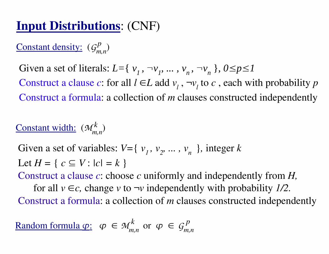
Input Distributions: (CNF)
Given a set of literals: L={ v1 , ¬v1, ... , vn , ¬vn }, 0�p�1
Construct a clause c: for all l �L add vl , ¬v
l to c , each with probability p
Construct a formula: a collection of m clauses constructed independently
Constant density: (Gm,n
)
Constant width: (Mm,n
)
Given a set of variables: V={ v1 , v
2, ... , v
n }, integer k
Let H = { c � V : |c| = k }
Construct a clause c: choose c uniformly and independently from H,
for all v �c, change v to ¬v independently with probability 1/2.
Construct a formula: a collection of m clauses constructed independently
p
k
Random formula �: � � Mm,n
or � �kG
m,n
p
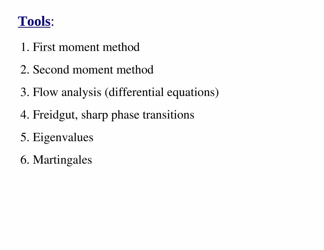
Tools:
1. First moment method
2. Second moment method
3. Flow analysis (differential equations)
4. Freidgut, sharp phase transitions
5. Eigenvalues
6. Martingales
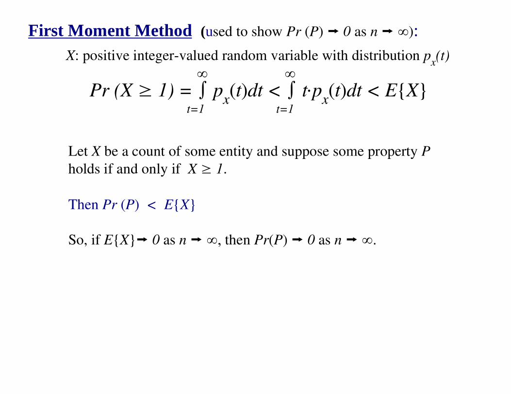
First Moment Method (used to show Pr (P) � 0 as n � �):
Pr (X � 1) = � px(t)dt < � t.p
x(t)dt < E{X}
�
t=1 t=1
�X: positive integer-valued random variable with distribution p
x(t)
Let X be a count of some entity and suppose some property P
holds if and only if X � 1.
Then Pr (P) < E{X}
So, if E{X}� 0 as n � ,� then Pr(P) � 0 as n � �.
Example:
Let � �
Let P be the property that � has a model.
Show Pr (P) � 0 if m/n > -ln(2) / ln(1-2-k)
Let X be the number of models for .�
Let Xi =
Pr (Xi = 1) = ((2k-1) / 2k)m
X = �i X
i , so E{X} = 2nE{X
i} = 2n(1 - 2-k)m
Pr (� a model for �) < 2n(1 - 2-k)m
Pr (� has a model) � 0 if m/n > -ln(2) / ln(1-2-k)
For k=3 � has no model w.h.p. when m/n > 5.19
Mm,nk
{ 1 if ith assignment is a model for �
0 if ith assignment is not a model for �
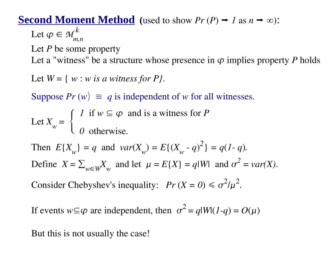
Second Moment Method (used to show Pr (P) � 1 as n � �):Let � � M
m,n
Let P be some property
Let a "witness" be a structure whose presence in � implies property P holds
Let W = { w : w is a witness for P}.
Suppose Pr (w) � q is independent of w for all witnesses.
Let X
w =
Then E{Xw} = q and var(X
w) = E{(X
w - q)2} = q(1- q).
Define X = �w�W
Xw and let � = E{X} = q|W| and �2
= var(X).
Consider Chebyshev's inequality: Pr (X = 0) �2/�2
.
If events w� are independent, then �2 = q|W|(1-q) = O(�)
But this is not usually the case!
k
{ 1 if w � and is a witness for P
0 otherwise.
If � � � as n � � and �z�A(w)
Pr (z|w) = o(�) for arbitrary w
Then Pr (P) � 1 as n � �.
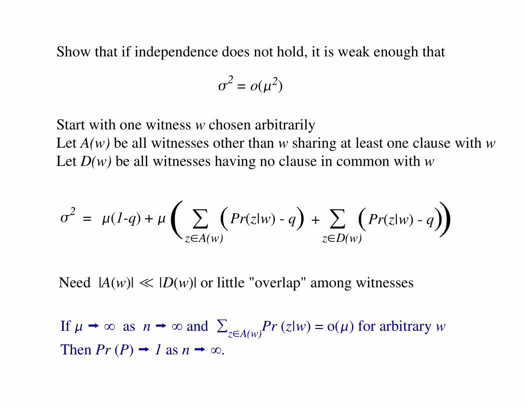
Show that if independence does not hold, it is weak enough that
Start with one witness w chosen arbitrarily
Let A(w) be all witnesses other than w sharing at least one clause with w
Let D(w) be all witnesses having no clause in common with w
�2 = �(1-q) + �( �
z�A(w)
�z�D(w)
(Pr(z|w) - q) (Pr(z|w) - q)+ )
Need |A(w)| � |D(w)| or little "overlap" among witnesses
�2 = o(�2)
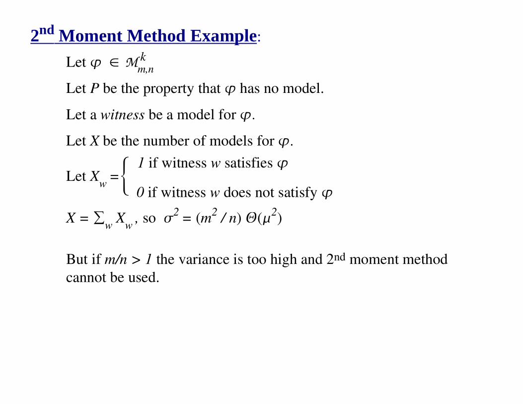
2 nd Moment Method Example:
Let � �
Let P be the property that � has no model.
Let a witness be a model for .�
Let X be the number of models for .�
Let Xw =
X = �w X
w , so �2
= (m2 / n) �(�2
)
But if m/n > 1 the variance is too high and 2nd moment method
cannot be used.
Mm,nk
{ 1 if witness w satisfies �
0 if witness w does not satisfy �
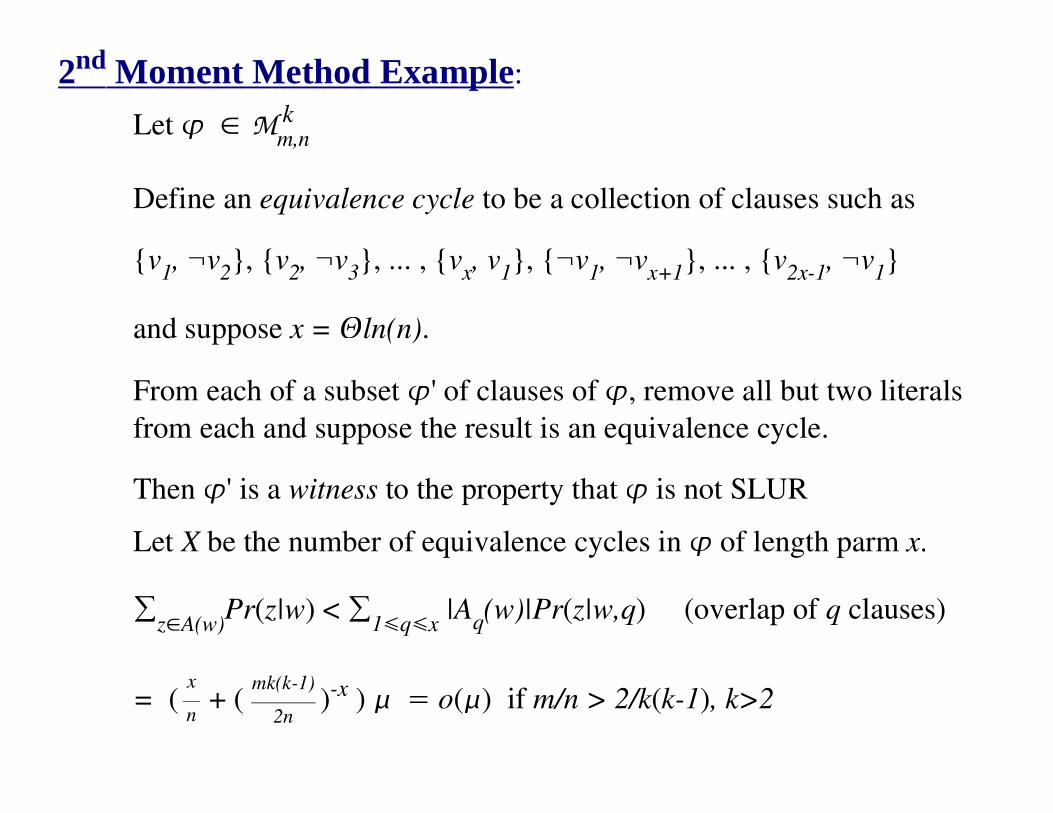
2 nd Moment Method Example:
Let � �
Define an equivalence cycle to be a collection of clauses such as
{v1, ¬v
2}, {v
2, ¬v
3}, ... , {v
x, v
1}, {¬v
1, ¬v
x+1}, ... , {v
2x-1, ¬v
1}
and suppose x = �ln(n).
From each of a subset �' of clauses of �, remove all but two literals
from each and suppose the result is an equivalence cycle.
Then �' is a witness to the property that � is not SLUR
Let X be the number of equivalence cycles in � of length parm x.
�z�A(w)
Pr(z|w) < �1�q�x
|Aq(w)|Pr(z|w,q) (overlap of q clauses)
= ( + ( )-x ) =� o(�) if m/n > 2/k(k-1), k>2
Mm,nk
x
n
mk(k-1)
2n
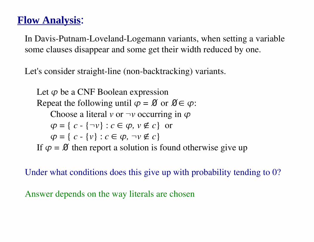
Flow Analysis:
In Davis-Putnam-Loveland-Logemann variants, when setting a variable
some clauses disappear and some get their width reduced by one.
Let's consider straight-line (non-backtracking) variants.
Let � be a CNF Boolean expression
Repeat the following until � = � or �� �:
Choose a literal v or ¬v occurring in � � = { c - {¬v} : c � �, v � c} or
� = { c - {v} : c � �, ¬v � c}
If � = � then report a solution is found otherwise give up
Under what conditions does this give up with probability tending to 0?
Answer depends on the way literals are chosen
Flow Analysis:
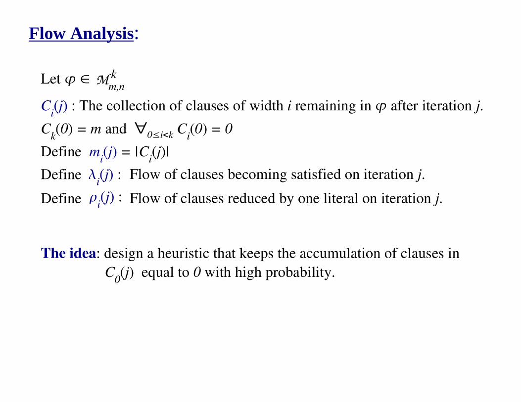
Let � �
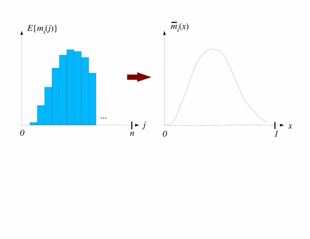
Ci(j) : The collection of clauses of width i remaining in � after iteration j.
Ck(0) = m and �
0�i<k C
i(0) = 0
Define mi(j) = |C
i(j)|
Define
Define
The idea: design a heuristic that keeps the accumulation of clauses in
C0(j) equal to 0 with high probability.
Mm,nk
�i(j) : Flow of clauses becoming satisfied on iteration j.
�i(j) : Flow of clauses reduced by one literal on iteration j.
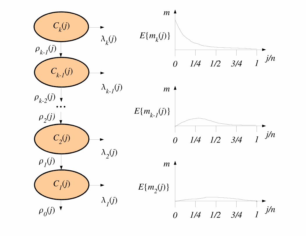
Ck(j)
Ck-1
(j)
C2(j)
C1(j)
...
�k(j)
�k-1
(j)
�2(j)
�1(j)
�k-1
(j)
�k-2
(j)
�2(j)
�1(j)
�0(j)
m
j/n0 1/4 1/2 13/4
m
j/n0 1/4 1/2 13/4
m
j/n0 1/4 1/2 13/4
E{mk(j)}
E{mk-1
(j)}
E{m2(j)}
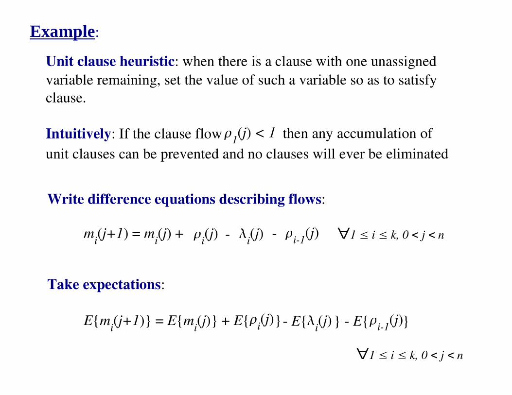
Example:
Unit clause heuristic: when there is a clause with one unassigned
variable remaining, set the value of such a variable so as to satisfy
clause.
Intuitively: If the clause flow �1(j) < 1 then any accumulation of
unit clauses can be prevented and no clauses will ever be eliminated
Write difference equations describing flows:
mi(j+1) = m
i(j) + -�
i(j) �
i(j)- �1 � i � k, 0 < j < n
Take expectations:
E{mi(j+1)} = E{m
i(j)} + E{ �i
(j) �i(j)- E{
�1 � i � k, 0 < j < n
} } - E{ }
�i-1
(j)
�i-1
(j)
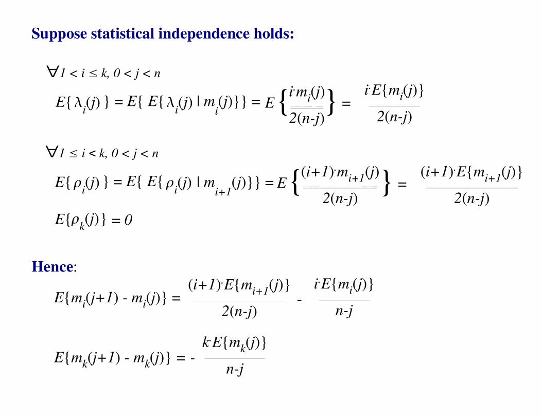
Suppose statistical independence holds:
E{�i(j) } = E{ E{�
i(j) | m
i(j)}} =
�1 < i � k, 0 < j < n
E{�i(j) } = E{ E{�
i(j) | m
i+1(j)}} =
�1 � i < k, 0 < j < n
Hence:
E{mi(j+1) - m
i(j)} =
E{mk(j+1) - m
k(j)} = -
E{�k(j)} = 0
E{i.mi(j)
-------------------- -------
2(n-j)}
i.E{mi(j)}
2(n-j)=
E{(i+1).mi+1
(j)--------------- ---------------
2(n-j)}
(i+1).E{mi+1
(j)}
2(n-j)=
(i+1).E{mi+1
(j)}
2(n-j)-
i.E{mi(j)}
n-j
k.E{mk(j)}
n-j
n0
...
E{mi(j)}
xj10
mi(x)
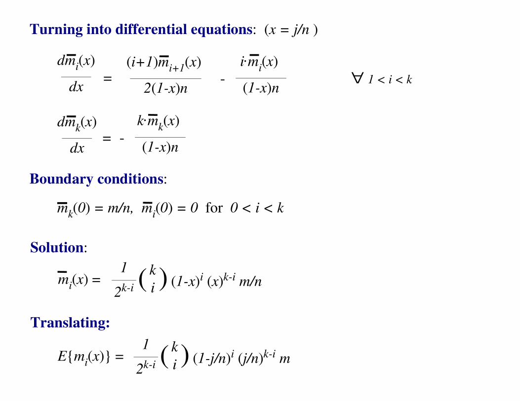
Turning into differential equations: (x = j/n )
dmi(x)
dx=
(i+1)mi+1
(x)
2(1-x)n
i.mi(x)
(1-x)n-
dmk(x)
dx=
k.mk(x)
(1-x)n-
� 1 < i < k
Boundary conditions:
mk(0) = m/n, m
i(0) = 0 for 0 < i < k
Solution:
mi(x) =
1
2k-i
k
i( ) (1-x)i (x)k-i m/n
E{mi(x)} =
1
2k-i
k
i( ) (1-j/n)i (j/n)k-i m
Translating:
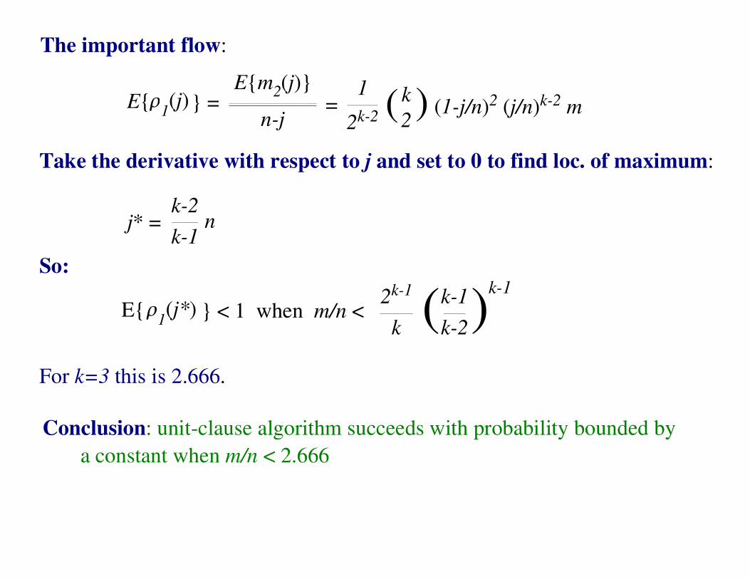
The important flow:
Take the derivative with respect to j and set to 0 to find loc. of maximum:
E{�1(j)
E{m2(j)}
----------------------------------------------------------
n-j} = =
1
2k-2 ( k
2) (1-j/n)2 (j/n)k-2 m
j* = k-2
k-1n
So:
E{�1(j*) } < 1 when m/n <
2k-1
k(k-1
k-2)
k-1
For k=3 this is 2.666.
Conclusion: unit-clause algorithm succeeds with probability bounded by
a constant when m/n < 2.666
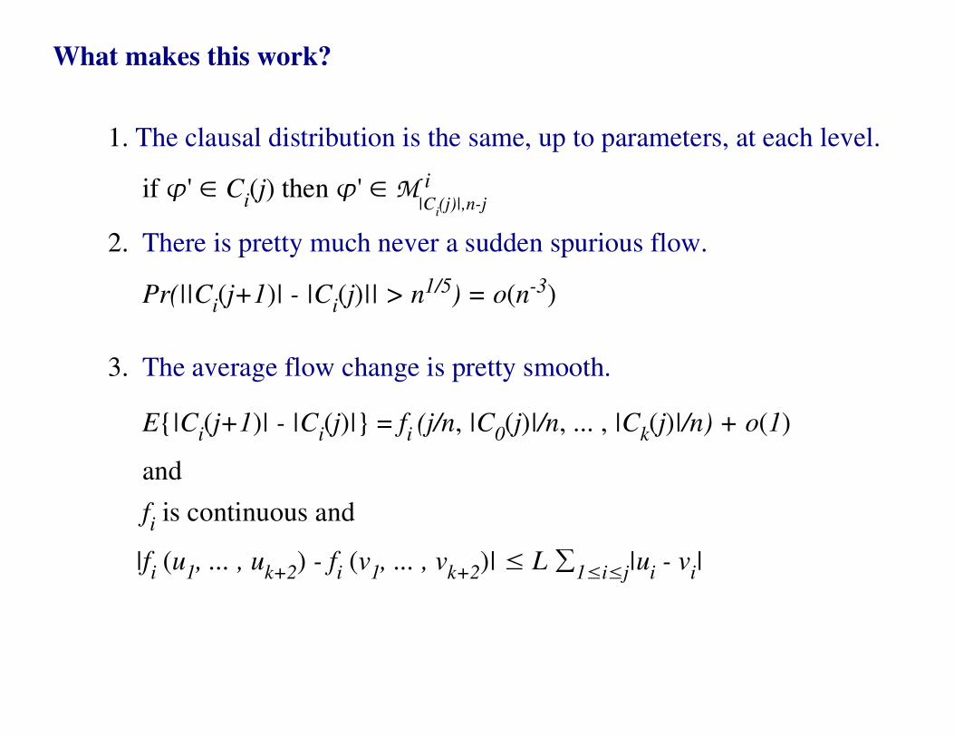
What makes this work?
1. The clausal distribution is the same, up to parameters, at each level.
if �' � Ci(j) then �' � M i
2. There is pretty much never a sudden spurious flow.
Pr(||Ci(j+1)| - |C
i(j)|| > n1/5) = o(n-3)
3. The average flow change is pretty smooth.
E{|Ci(j+1)| - |C
i(j)|} = f
i (j/n, |C
0(j)|/n, ... , |C
k(j)|/n) + o(1)
and
fi is continuous and
|fi (u
1, ... , u
k+2) - f
i (v
1, ... , v
k+2)| � L �
1�i�j|u
i - v
i|
|Ci(j)|,n-j
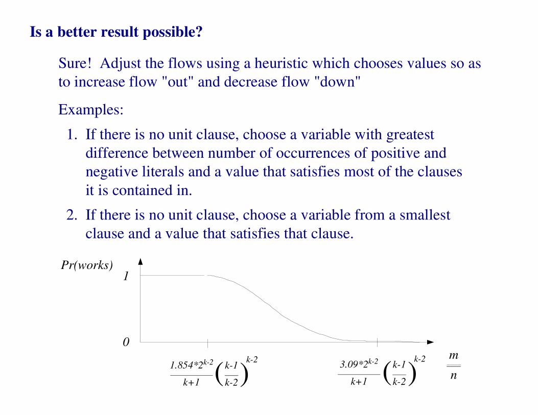
Is a better result possible?
Sure! Adjust the flows using a heuristic which chooses values so as
to increase flow "out" and decrease flow "down"
Examples:
1. If there is no unit clause, choose a variable with greatest
difference between number of occurrences of positive and
negative literals and a value that satisfies most of the clauses
it is contained in.
2. If there is no unit clause, choose a variable from a smallest
clause and a value that satisfies that clause.
1
0
Pr(works)
m-----------
n1.854*2k-2
k+1 (k-1
k-2)k-2
3.09*2k-2
k+1 (k-1
k-2)k-2
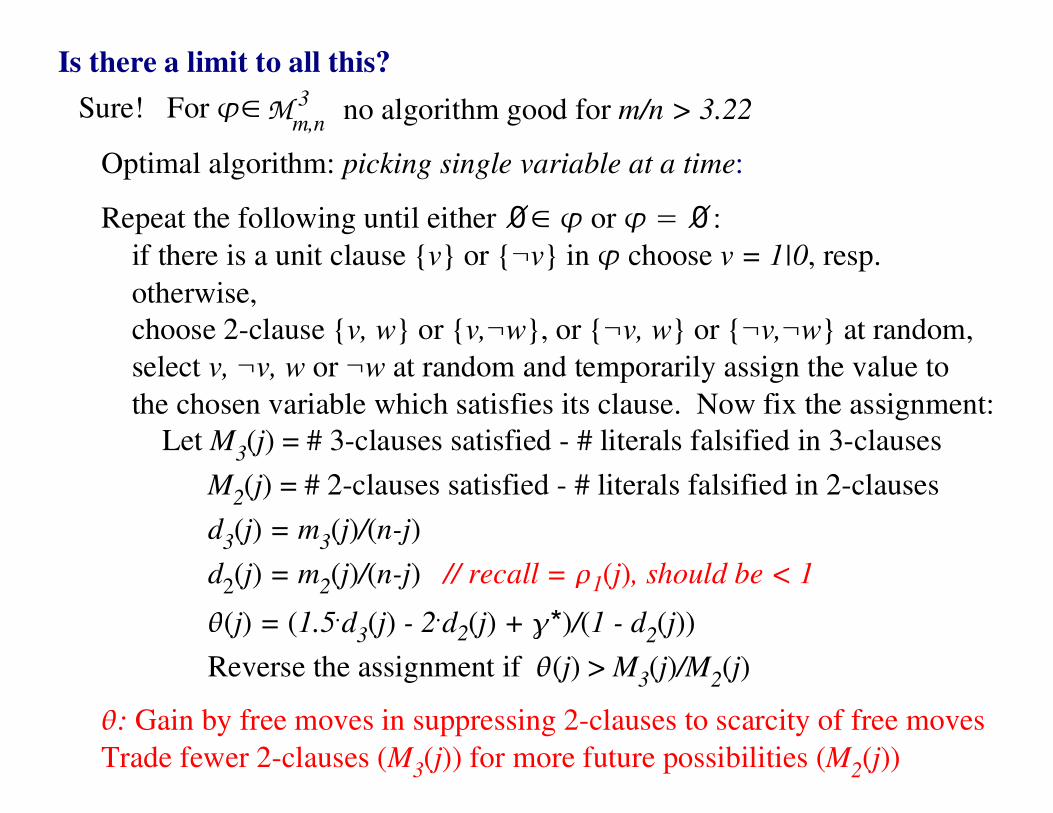
Is there a limit to all this?
Sure! For ��
Optimal algorithm: picking single variable at a time:
Repeat the following until either �� � or � = :� if there is a unit clause {v} or {¬v} in � choose v = 1|0, resp.
otherwise,
choose 2-clause {v, w} or {v,¬w}, or {¬v, w} or {¬v,¬w} at random,
select v, ¬v, w or ¬w at random and temporarily assign the value to
the chosen variable which satisfies its clause. Now fix the assignment:
Let M3(j) = # 3-clauses satisfied - # literals falsified in 3-clauses
M2(j) = # 2-clauses satisfied - # literals falsified in 2-clauses
d3(j) = m
3(j)/(n-j)
d2(j) = m
2(j)/(n-j) // recall = �1(j), should be < 1
�(j) = (1.5.d3(j) - 2.d2(j) + *� )/(1 - d
2(j))
Reverse the assignment if �(j) > M3(j)/M
2(j)
�: Gain by free moves in suppressing 2-clauses to scarcity of free moves
Trade fewer 2-clauses (M3(j)) for more future possibilities (M
2(j))
3Mm,n
no algorithm good for m/n > 3.22
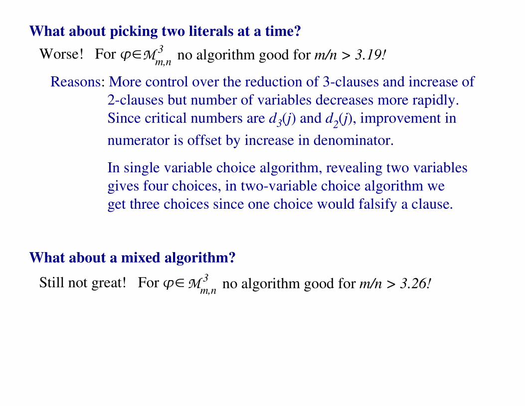
What about picking two literals at a time?
Worse! For ��
Reasons: More control over the reduction of 3-clauses and increase of
2-clauses but number of variables decreases more rapidly.
Since critical numbers are d3(j) and d2(j), improvement in
numerator is offset by increase in denominator.
In single variable choice algorithm, revealing two variables
gives four choices, in two-variable choice algorithm we
get three choices since one choice would falsify a clause.
3Mm,n
no algorithm good for m/n > 3.19!
What about a mixed algorithm?
Still not great! For ��
3Mm,n
no algorithm good for m/n > 3.26!
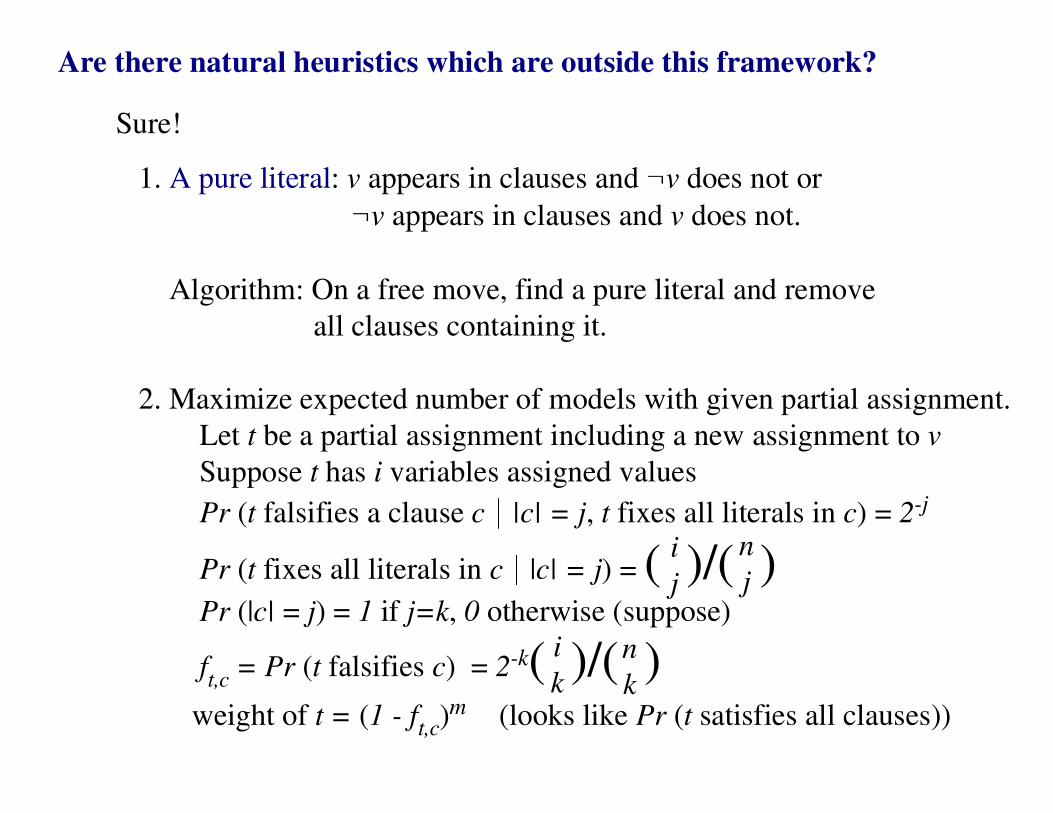
Are there natural heuristics which are outside this framework?
Sure!
1. A pure literal: v appears in clauses and ¬v does not or
¬v appears in clauses and v does not.
Algorithm: On a free move, find a pure literal and remove
all clauses containing it.
2. Maximize expected number of models with given partial assignment.
Let t be a partial assignment including a new assignment to v
Suppose t has i variables assigned values
Pr (t falsifies a clause c � |c| = j, t fixes all literals in c) = 2-j
Pr (t fixes all literals in c � |c| = j) = ( )/( ) Pr (|c| = j) = 1 if j=k, 0 otherwise (suppose)
ft,c
= Pr (t falsifies c) = 2-k( )/( ) weight of t = (1 - f
t,c)m (looks like Pr (t satisfies all clauses))
i
j
n
j
i
k
n
k
Are we stuck? Are myopic results all we can hope for?
Nope! We have a new tool!
Algorithms that make use of the number of appearances of literals
in 3-clauses and 2-clauses, separately, are allowed!
A Greedy Algorithm:
Repeat the following until � = � or �� �:
Let v or ¬v be a literal occurring at least as frequently in � as any
� = { c - {¬v} : c � �, v � c} or
� = { c - {v} : c � �, ¬v � c}
Repeat the following until no unit clauses exist in �:
Select a unit clause {v} or {¬v} and set v to 1 or 0 and
� = { c - {¬v} : c � �, v � c} or
� = { c - {v} : c � �, ¬v � c}
If � = � then report a solution is found otherwise give up
Pr (Greedy algorithm succeeds) > 0 if m/n < 3.42
Friedgut & others: Lift constant, bounded probability results to almost always results
Let s,t be vectors in {0,1}N Say s � t if si � ti holds for all i=0,...,N
Call vector set E monotone increasing if s � E, t � s, then t � E
E expresses some "property" like connectedness
Let w(s) be the Hamming weight of s
Define �p({s}) = (1-p)N-w(s)pw(s), 0 � p � 1
Define �p(E) = �
s�E�
p({s})
What happens to �p(E) as a function of p?
Set fN(p) = �
p(E
N) and let p
c(N) = f
N-1(c)
if limN��(p
1-�(N)-p�(N))/p1/2
(N) = 0, have a sharp threshold
if limN��(p
1-�(N)-p�(N))/p1/2
(N) > c, have a coarse threshold
fN(p)
.5
p.5
p�
�
1-�
p1-�
1
0
Friedgut & others: If E is monotone such that p
1/2(N) = o(1) and the following hold
then E has a sharp threshold:
1. For each c � (0,1) and all positive K,
limN���p (N)
(s�m, m � E and w(m) � K) = 0, alternatively
limN���p (N)
(s�m, m is minimal for E and w(m) � K) = 0
(Few elements of E of bounded Hamming weight appear)
2. For each c � (0,1), all positive K, and all s0 � E with w(s
0)=K,
limN���p (N)
(s�E � s�s0) = c, alternatively
limN���p (N)
(s�E, s�s0�E � s�s
0) = 0
(Probability of being in E is not affected much by conditioning
on a bounded weight element not in E)
c
c
c
c
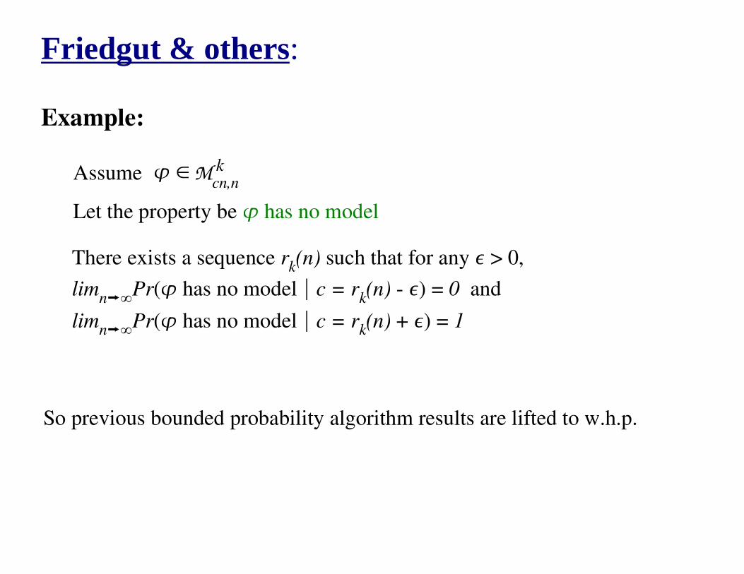
Friedgut & others: Example:
Mcn,nk� �Assume
Let the property be � has no model
There exists a sequence rk(n) such that for any � > 0,
limn��Pr(� has no model � c = r
k(n) - �) = 0 and
limn��Pr(� has no model � c = r
k(n) + �) = 1
So previous bounded probability algorithm results are lifted to w.h.p.
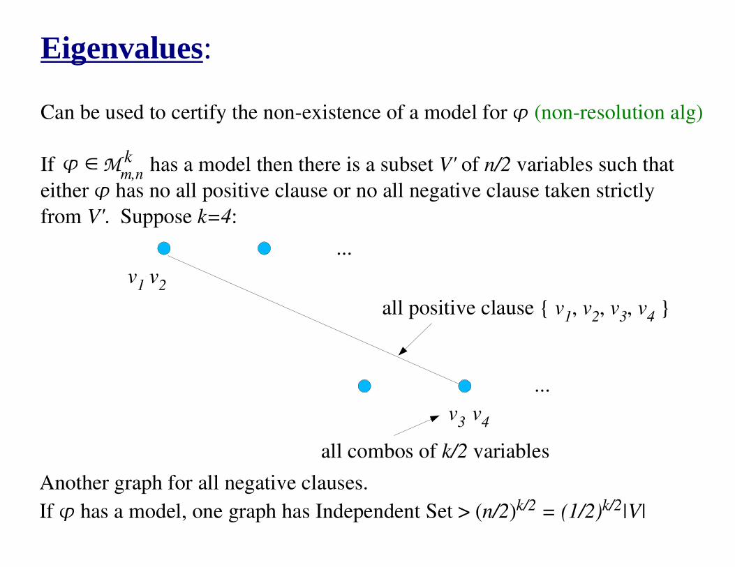
Eigenvalues:
Can be used to certify the non-existence of a model for � (non-resolution alg)
If has a model then there is a subset V' of n/2 variables such that
either � has no all positive clause or no all negative clause taken strictly
from V'. Suppose k=4:
Mm,nk� �
v1
v2
v3
v4
...
...
all positive clause { v1, v
2, v
3, v
4 }
all combos of k/2 variables
Another graph for all negative clauses.
If � has a model, one graph has Independent Set > (n/2)k/2 = (1/2)k/2|V|
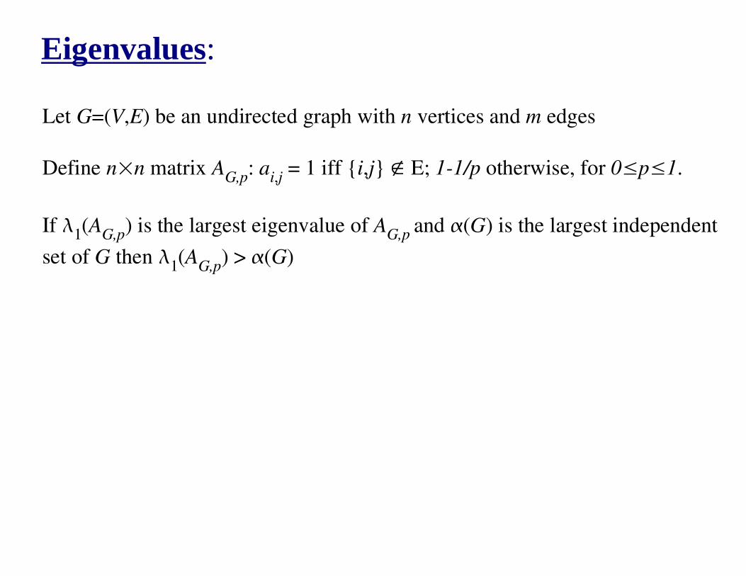
Eigenvalues:
Let G=(V,E) be an undirected graph with n vertices and m edges
Define n×n matrix AG,p
: ai,j
= 1 iff {i,j} � E; 1-1/p otherwise, for 0�p�1.
If �1(A
G,p) is the largest eigenvalue of A
G,p and �(G) is the largest independent
set of G then �1(A
G,p) > �(G)
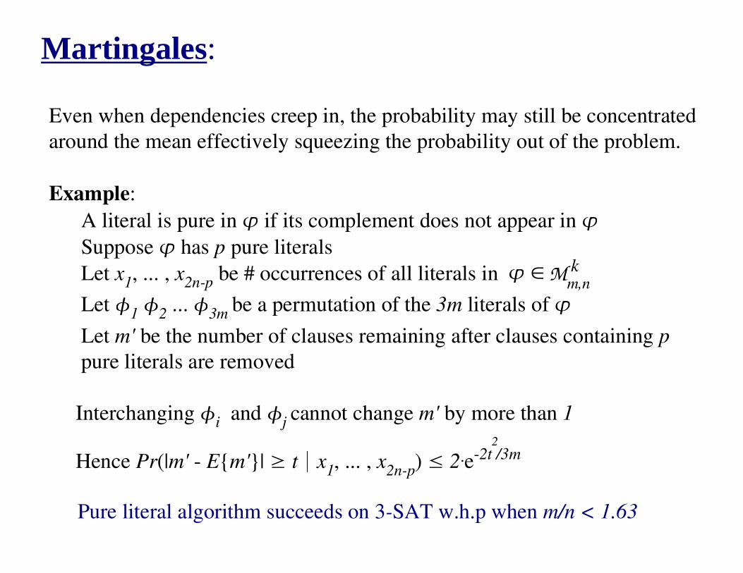
Martingales:
Even when dependencies creep in, the probability may still be concentrated
around the mean effectively squeezing the probability out of the problem.
Example:
A literal is pure in � if its complement does not appear in � Suppose � has p pure literals
Let x1, ... , x
2n-p be # occurrences of all literals in
Let �1 �
2 ... �
3m be a permutation of the 3m literals of �
Let m' be the number of clauses remaining after clauses containing p
pure literals are removed
Interchanging �i and �
j cannot change m' by more than 1
Hence Pr(|m' - E{m'}| � t � x1, ... , x
2n-p) � 2.e-2t /3m
Pure literal algorithm succeeds on 3-SAT w.h.p when m/n < 1.63
Mm,nk� �
2
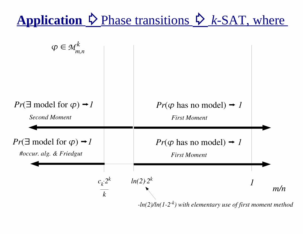
Application �Phase transitions � k-SAT, where
ck.2k
k
ln(2).2k
Pr(� model for �) �1
#occur. alg. & Friedgut
Pr(� has no model) � 1
First Moment
Pr(� has no model) � 1
First Moment
1m/n
-ln(2)/ln(1-2-k) with elementary use of first moment method
Pr(� model for �) �1
Second Moment
Mm,nk� �
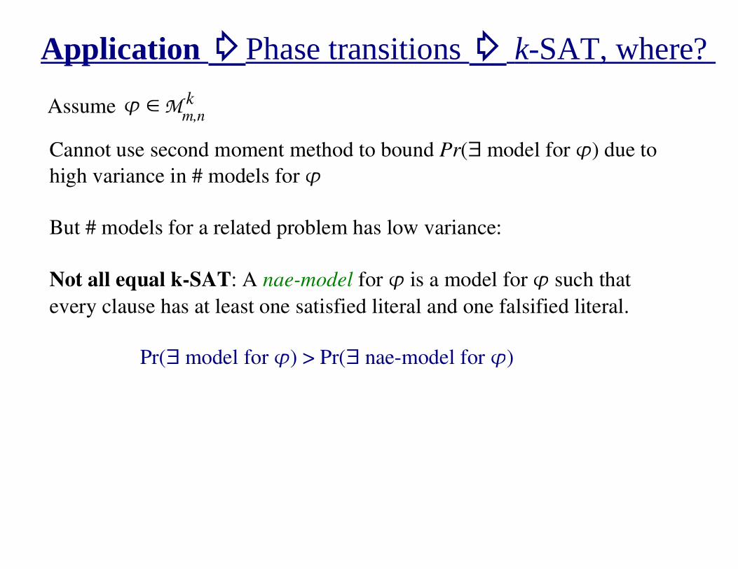
Application �Phase transitions � k-SAT, where?
Cannot use second moment method to bound Pr(� model for �) due to
high variance in # models for �
But # models for a related problem has low variance:
Not all equal k-SAT: A nae-model for � is a model for � such that
every clause has at least one satisfied literal and one falsified literal.
Pr(� model for �) > Pr(� nae-model for �)
Assume Mm,nk� �
Application �Phase transitions � k-SAT, where
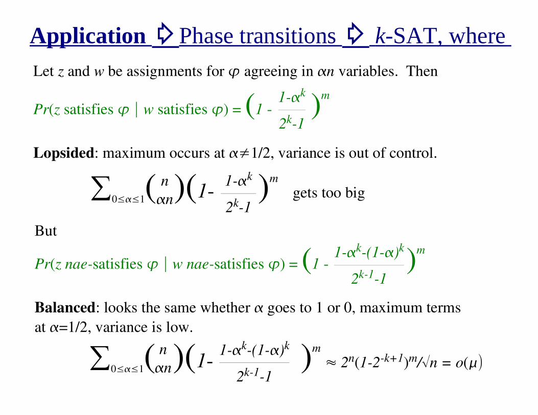
But
Pr(z nae-satisfies � � w nae-satisfies �) = (1 - )m
Balanced: looks the same whether � goes to 1 or 0, maximum terms
at �=1/2, variance is low.
1-�k-(1-�)k
2k-1-1
(
�0���1
( )(1- )m
� 2n(1-2-k+1)m/�n = o( )� 1-�k-(1-�)k
2k-1-1
n
�n
Let z and w be assignments for � agreeing in �n variables. Then
Pr(z satisfies � � w satisfies �) = (1 - )m
Lopsided: maximum occurs at �1/2, variance is out of control.
1-�k
2k-1
�0���1
( )(1- )m
gets too bign
�n
1-�k
2k-1
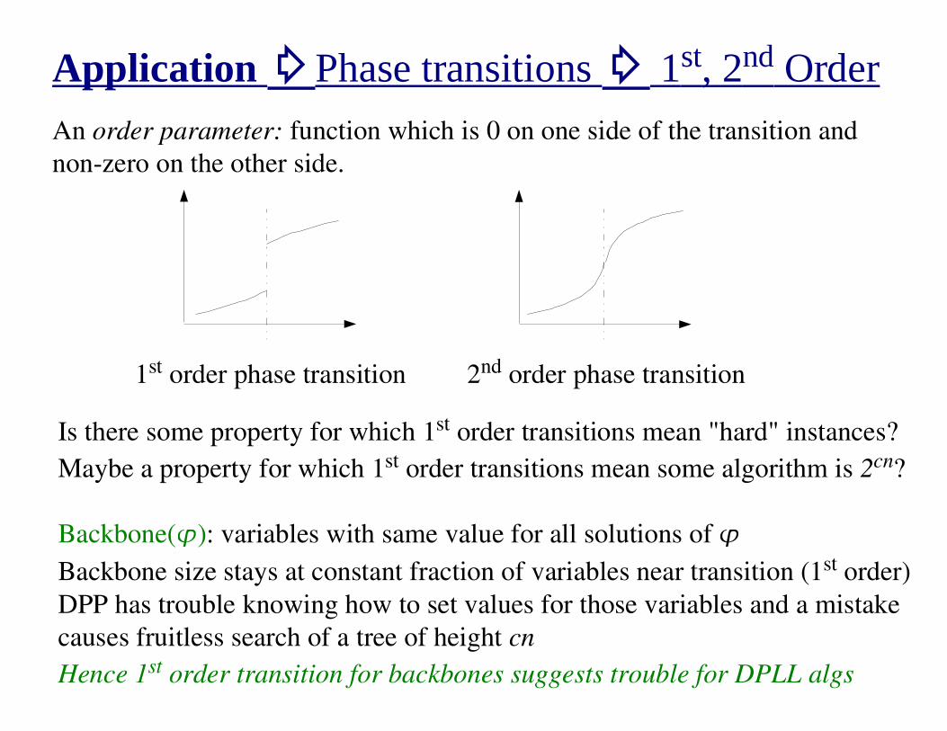
Application �Phase transitions � 1 st, 2 nd Order
An order parameter: function which is 0 on one side of the transition and
non-zero on the other side.
1st order phase transition 2nd order phase transition
Is there some property for which 1st order transitions mean "hard" instances?
Maybe a property for which 1st order transitions mean some algorithm is 2cn?
Backbone(�): variables with same value for all solutions of �Backbone size stays at constant fraction of variables near transition (1st order)
DPP has trouble knowing how to set values for those variables and a mistake
causes fruitless search of a tree of height cn
Hence 1st order transition for backbones suggests trouble for DPLL algs
Application �Phase transitions � 1 st, 2 nd Order
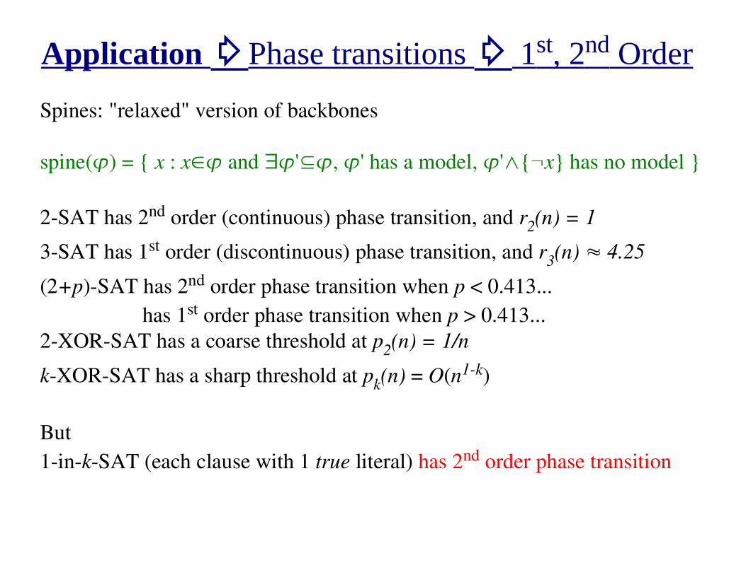
Spines: "relaxed" version of backbones
spine(�) = { x : x�� and ��'��, �' has a model, �'�{¬x} has no model }
2-SAT has 2nd order (continuous) phase transition, and r2(n) = 1
3-SAT has 1st order (discontinuous) phase transition, and r3(n) � 4.25
(2+p)-SAT has 2nd order phase transition when p < 0.413...
has 1st order phase transition when p > 0.413...
2-XOR-SAT has a coarse threshold at p2(n) = 1/n
k-XOR-SAT has a sharp threshold at pk(n) = O(n1-k)
But
1-in-k-SAT (each clause with 1 true literal) has 2nd order phase transition
Application �Phase transitions � 1 st, 2 nd Order
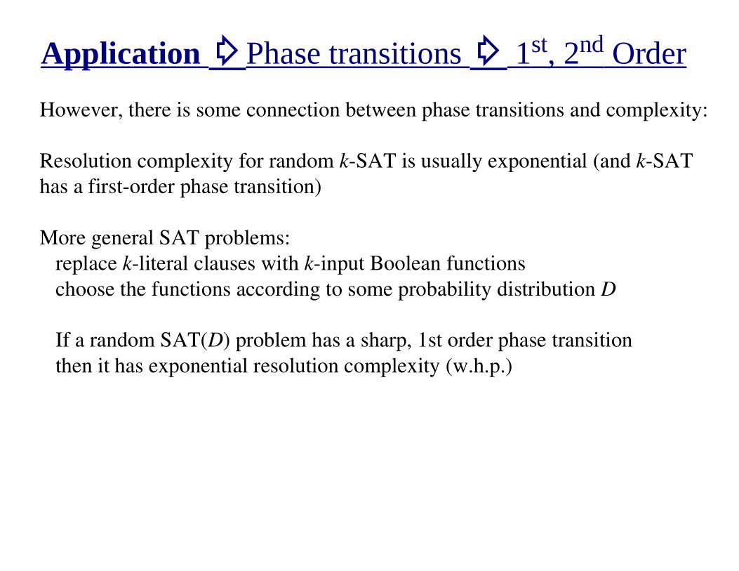
However, there is some connection between phase transitions and complexity:
Resolution complexity for random k-SAT is usually exponential (and k-SAT
has a first-order phase transition)
More general SAT problems:
replace k-literal clauses with k-input Boolean functions
choose the functions according to some probability distribution D
If a random SAT(D) problem has a sharp, 1st order phase transition
then it has exponential resolution complexity (w.h.p.)
Application �Phase transitions � Sharpness
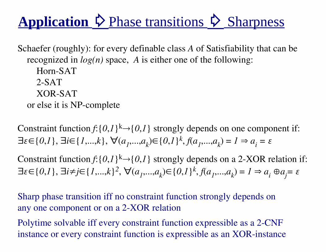
Schaefer (roughly): for every definable class A of Satisfiability that can be
recognized in log(n) space, A is either one of the following:
Horn-SAT
2-SAT
XOR-SAT
or else it is NP-complete
Constraint function f:{0,1}k�{0,1} strongly depends on one component if:
���{0,1}, �i�{1,...,k}, �(a1,...,a
k)�{0,1}k, f(a
1,...,a
k) = 1 � a
i = �
Constraint function f:{0,1}k�{0,1} strongly depends on a 2-XOR relation if:
���{0,1}, �i�j�{1,...,k}2, �(a1,...,a
k)�{0,1}k, f(a
1,...,a
k) = 1 � a
i �a
j= �
Sharp phase transition iff no constraint function strongly depends on
any one component or on a 2-XOR relation
Polytime solvable iff every constraint function expressible as a 2-CNF
instance or every constraint function is expressible as an XOR-instance
Probabilistic analysis of polytime solvable classes can reveal:
1. What vulnerability does a class have? That is, what critically
distinguishes this class from more difficult classes?
2. Is one class much larger than another incomparable class
in some sense?
Application �Property (polytime solvable classes)
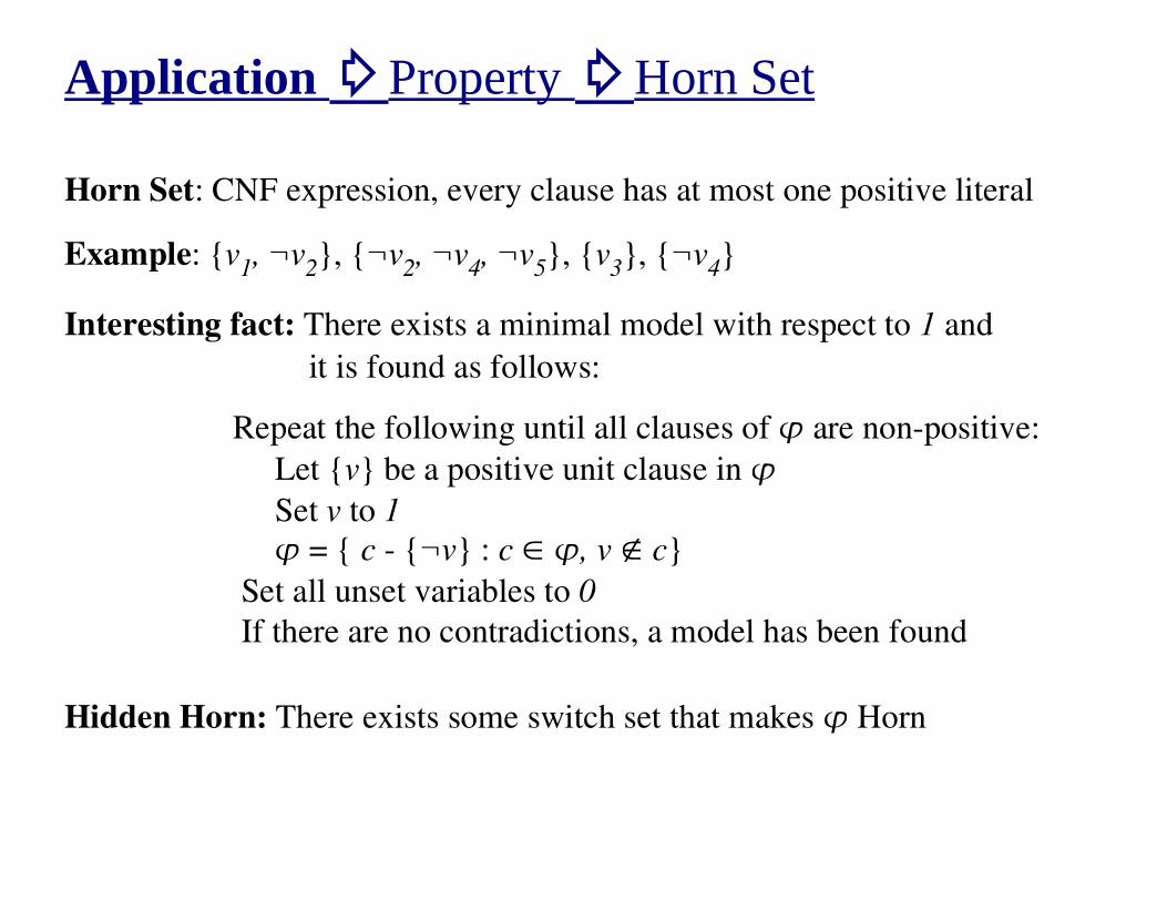
Application �Property �Horn Set
Horn Set: CNF expression, every clause has at most one positive literal
Example: {v1, ¬v
2}, {¬v
2, ¬v
4, ¬v
5}, {v
3}, {¬v
4}
Interesting fact: There exists a minimal model with respect to 1 and
it is found as follows:
Repeat the following until all clauses of � are non-positive:
Let {v} be a positive unit clause in � Set v to 1
Set all unset variables to 0
If there are no contradictions, a model has been found
Hidden Horn: There exists some switch set that makes � Horn
� = { c - {¬v} : c � �, v � c}
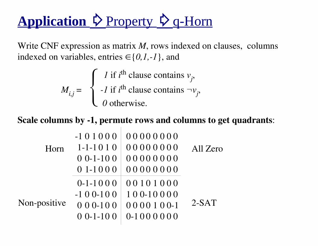
Application �Property �q-Horn
Write CNF expression as matrix M, rows indexed on clauses, columns
indexed on variables, entries �{0,1,-1}, and
1 if ith clause contains v
j,
Mi,j
= -1 if ith clause contains ¬vj,
0 otherwise.
Scale columns by -1, permute rows and columns to get quadrants:
-1 0 1 0 0 0 0 0 0 0 0 0 0 0
1-1-1 0 1 0 0 0 0 0 0 0 0 0
0 0-1-10 0 0 0 0 0 0 0 0 0
0 1-1 0 0 0 0 0 0 0 0 0 0 0
0-1-1 0 0 0 0 0 1 0 1 0 0 0
-1 0 0-10 0 1 0 0-10 0 0 0
0 0 0-10 0 0 0 0 0 1 0 0-1
0 0-1-10 0 0-1 0 0 0 0 0 0
{All Zero
2-SAT
Horn
Non-positive
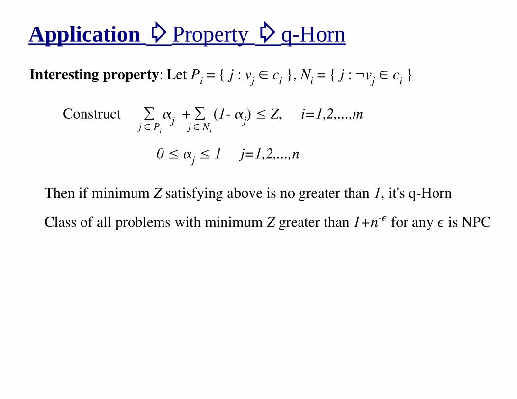
Application �Property �q-Horn
Interesting property: Let Pi = { j : v
j � c
i }, N
i = { j : ¬v
j � c
i }
Construct � �j + � (1- �
j) � Z, i=1,2,...,m
0 � �j � 1 j=1,2,...,n
Then if minimum Z satisfying above is no greater than 1, it's q-Horn
Class of all problems with minimum Z greater than 1+n-� for any � is NPC
j � Pi
j � Ni
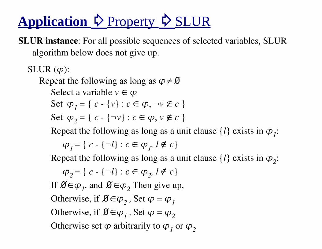
Application �Property �SLURSLUR instance: For all possible sequences of selected variables, SLUR
algorithm below does not give up.
SLUR (�):
Repeat the following as long as ��� Select a variable v � � Set��
1 = { c - {v} : c � ,� ¬v � c }
Set��2
= { c - {¬v} : c � ,� v � c }
Repeat the following as long as a unit clause {l} exists in �1:
�1
= { c - {¬l} : c � �1, l � c}
Repeat the following as long as a unit clause {l} exists in �2:
�2
= { c - {¬l} : c � �2, l � c}
If ���1, and ���
2 Then give up,
Otherwise, if ���2 ,
Set � = �
1
Otherwise, if ���1 ,
Set � = �
2
Otherwise set � arbitrarily to �1 or �
2
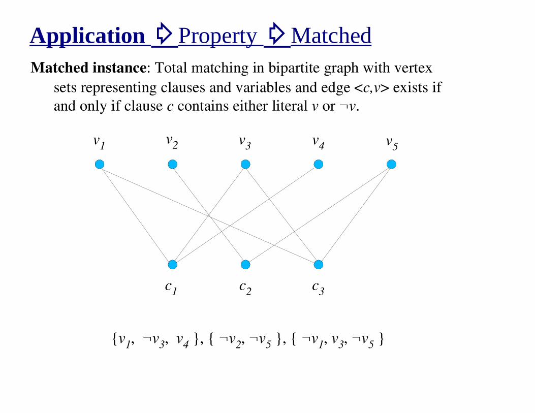
Application �Property �MatchedMatched instance: Total matching in bipartite graph with vertex
sets representing clauses and variables and edge <c,v> exists if
and only if clause c contains either literal v or ¬v.
c1
c2
c3
v1
v2 v
3v
4 v5
{v1, ¬v
3, v
4 }, { ¬v
2, ¬v
5 }, { ¬v
1, v
3, ¬v
5 }
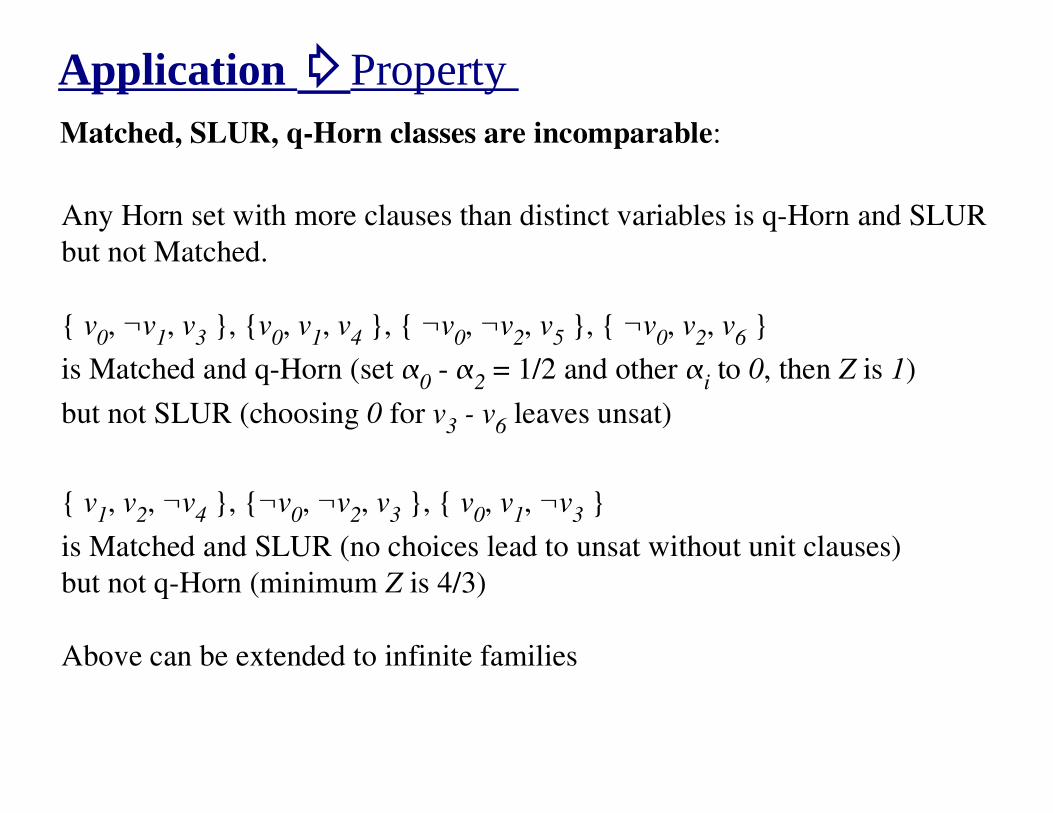
Application �Property Matched, SLUR, q-Horn classes are incomparable:
Any Horn set with more clauses than distinct variables is q-Horn and SLUR
but not Matched.
{ v0, ¬v
1, v
3 }, {v
0, v
1, v
4 }, { ¬v
0, ¬v
2, v
5 }, { ¬v
0, v
2, v
6 }
is Matched and q-Horn (set �0 - �
2 = 1/2 and other �
i to 0, then Z is 1)
but not SLUR (choosing 0 for v3 - v
6 leaves unsat)
{ v1, v
2, ¬v
4 }, {¬v
0, ¬v
2, v
3 }, { v
0, v
1, ¬v
3 }
is Matched and SLUR (no choices lead to unsat without unit clauses)
but not q-Horn (minimum Z is 4/3)
Above can be extended to infinite families
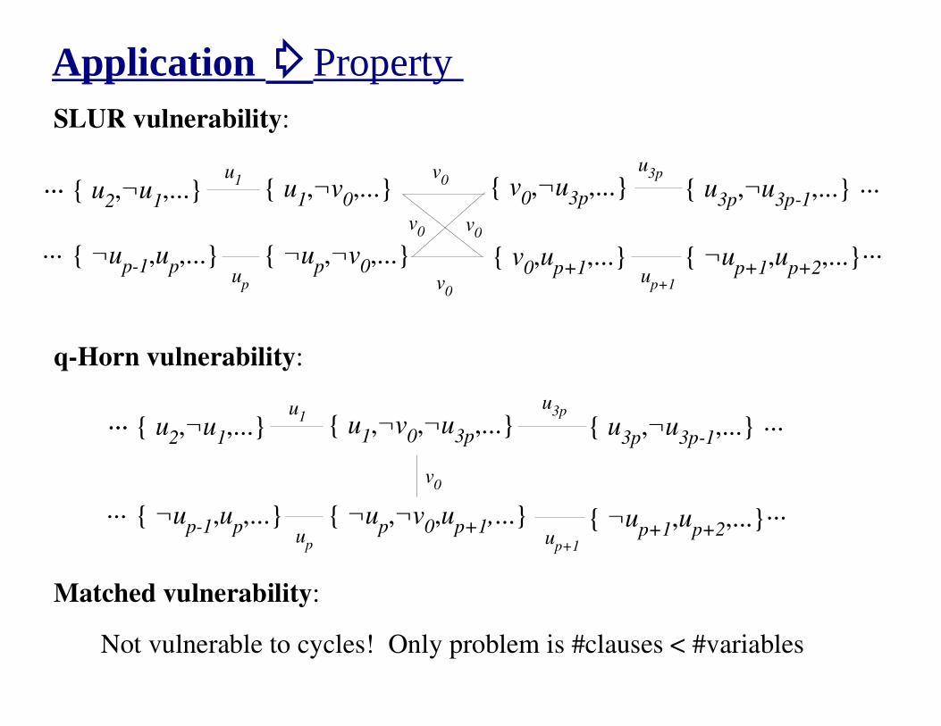
Application �Property SLUR vulnerability:
{ u1,¬v
0,...}
{ ¬up,¬v
0,...}
{ v0,¬u
3p,...}
{ v0,u
p+1,...}
{ u2,¬u
1,...}
{ ¬up-1
,up,...}
{ u3p
,¬u3p-1
,...}
{ ¬up+1
,up+2
,...}
v0
v0
v0 v
0
u3p
up+1
u1
up
......
...
...
...
q-Horn vulnerability:
{ u1,¬v
0,¬u
3p,...}
{ ¬up,¬v
0,u
p+1,...}
{ u2,¬u
1,...}
{ ¬up-1
,up,...}
{ u3p
,¬u3p-1
,...}
{ ¬up+1
,up+2
,...}
u3p
up+1
u1
up
......
...
...
...
v0
Matched vulnerability:
Not vulnerable to cycles! Only problem is #clauses < #variables
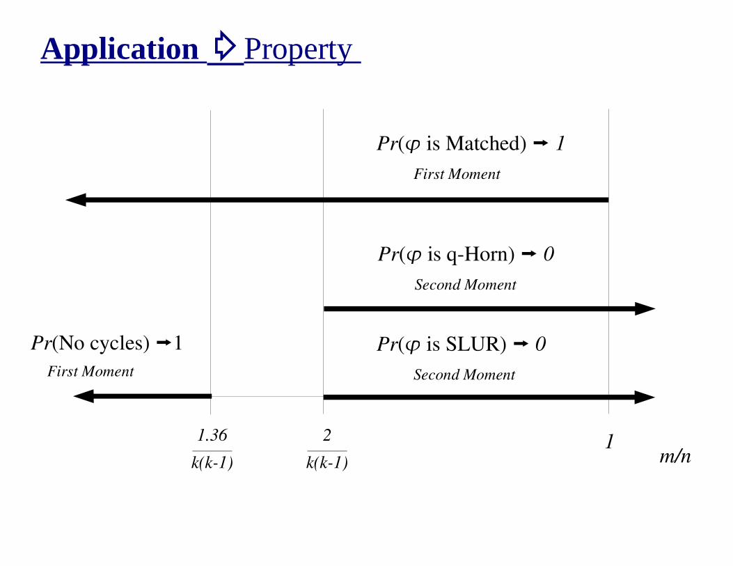
Application �Property
1.36
k(k-1)
2
k(k-1)
Pr(No cycles) �1
First Moment
Pr(� is SLUR) � 0
Second Moment
Pr(� is q-Horn) � 0
Second Moment
1m/n
Pr(� is Matched) � 1
First Moment