Embed Size (px)
Citation preview

Licensed to:

Hayter-15125 07573˙00˙fm December 29, 2005 10:0
Probability and Statistics for Engineers and Scientists, Third EditionAnthony J. Hayter
Acquisitions Editor: Carolyn CrockettTechnology Project Manager: Fiona ChongAssistant Editor: Ann DayExecutive Marketing Manager: Joe RogoveMarketing Assistant: Brian SmithMarketing Communications Manager: Darlene Amidon-BrentManager, Editorial Production: Kelsey McGeeCreative Director: Rob HugelArt Director: Lee FriedmanPrint Buyer: Judy InouyePermissions Editor: Bob Kauser
Production Service and Composition: Interactive CompositionCorporation
Text Designer: Andrew OgusArt Editor: Lisa TorriCopy Editor: Martha WilliamsCover Designer: Laurie AndersonCover Image: Louis Psihoyos/Getty Images,
Science Faction CollectionCover Printing, Printing & Binding: Transcontinental
Printing/Louiseville
© 2007 Duxbury, an imprint of Thomson Brooks/Cole, a part ofThe Thomson Corporation. Thomson, the Star logo, andBrooks/Cole are trademarks used herein under license.
ALL RIGHTS RESERVED. No part of this work covered by thecopyright hereon may be reproduced or used in any form or byany means—graphic, electronic, or mechanical, includingphotocopying, recording, taping, web distribution, informationstorage and retrieval systems, or in any other manner—withoutthe written permission of the publisher.
Printed in Canada1 2 3 4 5 6 7 09 08 07 06 05
For more information about our products, contact us at:Thomson Learning Academic Resource Center
1-800-423-0563
For permission to use material from this text or product, submit arequest online at
http://www.thomsonrights.com.
Any additional questions about permissions can be submitted byemail to [email protected].
Thomson Higher Education10 Davis DriveBelmont, CA 94002-3098USA
Library of Congress Control Number: 2005930896ISBN 0-495-10757-3
Cover Image: Black Pearls in an Oyster Shell, Tahiti. A rarecollection of perhaps some of the best Tahitian black pearls in
the world, hi-graded from a 25-year harvest of 80% of the pearlsthat come out of Tahiti.
iv
Copyright 2010 Cengage Learning. All Rights Reserved. May not be copied, scanned, or duplicated, in whole or in part. Due to electronic rights, some third party content may be suppressed from the eBook and/or eChapter(s).Editorial review has deemed that any suppressed content does not materially affect the overall learning experience. Cengage Learning reserves the right to remove additional content at any time if subsequent rights restrictions require it.
Licensed to:

Hayter-15125 book December 19, 2005 20:30
C H A P T E R O N E
Probability Theory
1.1 Probabilities
1.1.1 Introduction
Jointly with statistics, probability theory is a branch of mathematics that has been developedto deal with uncertainty. Classical mathematical theory had been successful in describingthe world as a series of fixed and real observable events, yet before the seventeenth centuryit was largely inadequate in coping with processes or experiments that involved uncertain orrandom outcomes. Spurred initially by the mathematician’s desire to analyze gambling gamesand later by the scientific analysis of mortality tables within the medical profession, the theoryof probability has been developed as a scientific tool dealing with chance.
Today, probability theory is recognized as one of the most interesting and also one of themost useful areas of mathematics. It provides the basis for the science of statistical inferencethrough experimentation and data analysis—an area of crucial importance in an increasinglyquantitative world. Through its applications to problems such as the assessment of systemreliability, the interpretation of measurement accuracy, and the maintenance of suitable qualitycontrols, probability theory is particularly relevant to the engineering sciences today.
1.1.2 Sample Spaces
An experiment can in general be thought of as any process or procedure for which more thanone outcome is possible. The goal of probability theory is to provide a mathematical structurefor understanding or explaining the chances or likelihoods of the various outcomes actuallyoccurring. A first step in the development of this theory is the construction of a list of thepossible experimental outcomes. This collection of outcomes is called the sample space orstate space and is denoted by S.
Sample Space
The sample space S of an experiment is a set consisting of all of the possibleexperimental outcomes.
The following examples help illustrate the concept of a sample space.
Example 1Machine Breakdowns
An engineer in charge of the maintenance of a particular machine notices that its breakdownscan be characterized as due to an electrical failure within the machine, a mechanical failureof some component of the machine, or operator misuse. When the machine is running, the
1
Copyright 2010 Cengage Learning. All Rights Reserved. May not be copied, scanned, or duplicated, in whole or in part. Due to electronic rights, some third party content may be suppressed from the eBook and/or eChapter(s).Editorial review has deemed that any suppressed content does not materially affect the overall learning experience. Cengage Learning reserves the right to remove additional content at any time if subsequent rights restrictions require it.
Licensed to:
Hayter-15125 book December 19, 2005 20:30
2 CHAPTER 1 PROBABILITY THEORY
engineer is uncertain what will be the cause of the next breakdown. The problem can bethought of as an experiment with the sample space
S = {electrical, mechanical, misuse}Example 2
Defective ComputerChips
A company sells computer chips in boxes of 500, and each chip can be classified as eithersatisfactory or defective. The number of defective chips in a particular box is uncertain, andthe sample space is
S = {0 defectives, 1 defective, 2 defectives, 3 defectives, 4 defectives, . . . ,499 defectives, 500 defectives}
Example 3Software Errors
The control of errors in computer software products is obviously of great importance. Thenumber of separate errors in a particular piece of software can be viewed as having a samplespace
S = {0 errors, 1 error, 2 errors, 3 errors, 4 errors, 5 errors, . . .}
In practice there will be an upper bound on the possible number of errors in the software,although conceptually it is all right to allow the sample space to consist of all of the positiveintegers.
S(0, 0, 0) (1, 0, 0)
(0, 0, 1) (1, 0, 1)
(0, 1, 0) (1, 1, 0)
(0, 1, 1) (1, 1, 1)
FIGURE 1.1
Sample space for power plantexample
Example 4Power Plant Operation
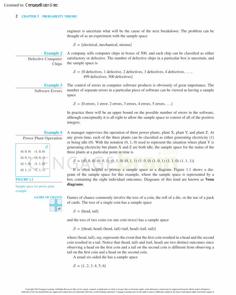
A manager supervises the operation of three power plants, plant X, plant Y, and plant Z. Atany given time, each of the three plants can be classified as either generating electricity (1)or being idle (0). With the notation (0, 1, 0) used to represent the situation where plant Y isgenerating electricity but plants X and Z are both idle, the sample space for the status of thethree plants at a particular point in time is
S = {(0, 0, 0) (0, 0, 1) (0, 1, 0) (0, 1, 1) (1, 0, 0) (1, 0, 1) (1, 1, 0) (1, 1, 1)}
It is often helpful to portray a sample space as a diagram. Figure 1.1 shows a dia-gram of the sample space for this example, where the sample space is represented by abox containing the eight individual outcomes. Diagrams of this kind are known as Venndiagrams.
GAMES OF CHANCE Games of chance commonly involve the toss of a coin, the roll of a die, or the use of a packof cards. The toss of a single coin has a sample space
S = {head, tail}
and the toss of two coins (or one coin twice) has a sample space
S = {(head, head) (head, tail) (tail, head) (tail, tail)}
where (head, tail), say, represents the event that the first coin resulted in a head and the secondcoin resulted in a tail. Notice that (head, tail) and (tail, head) are two distinct outcomes sinceobserving a head on the first coin and a tail on the second coin is different from observing atail on the first coin and a head on the second coin.
A usual six-sided die has a sample space
S = {1, 2, 3, 4, 5, 6}
Copyright 2010 Cengage Learning. All Rights Reserved. May not be copied, scanned, or duplicated, in whole or in part. Due to electronic rights, some third party content may be suppressed from the eBook and/or eChapter(s).Editorial review has deemed that any suppressed content does not materially affect the overall learning experience. Cengage Learning reserves the right to remove additional content at any time if subsequent rights restrictions require it.
Licensed to:

Hayter-15125 book December 19, 2005 20:30
1.1 PROBABILITIES 3
FIGURE 1.2
Sample space for rolling two diceS
(1, 1) (1, 2) (1, 3) (1, 4) (1, 5) (1, 6)
(2, 1) (2, 2) (2, 3) (2, 4) (2, 5) (2, 6)
(3, 1) (3, 2) (3, 3) (3, 4) (3, 5) (3, 6)
(4, 1) (4, 2) (4, 3) (4, 4) (4, 5) (4, 6)
(5, 1) (5, 2) (5, 3) (5, 4) (5, 5) (5, 6)
(6, 1) (6, 2) (6, 3) (6, 4) (6, 5) (6, 6)
FIGURE 1.3
Sample space for choosing one cardS
A♥ 2♥ 3♥ 4♥ 5♥ 6♥ 7♥ 8♥ 9♥ 10♥ J♥ Q♥ K♥
A♣ 2♣ 3♣ 4♣ 5♣ 6♣ 7♣ 8♣ 9♣ 10♣ J♣ Q♣ K♣
A♦ 2♦ 3♦ 4♦ 5♦ 6♦ 7♦ 8♦ 9♦ 10♦ J♦ Q♦ K♦
A♠ 2♠ 3♠ 4♠ 5♠ 6♠ 7♠ 8♠ 9♠ 10♠ J♠ Q♠ K♠
FIGURE 1.4
Sample space for choosing twocards with replacement
S(A♥, A♥) (A♥, 2♥) (A♥, 3♥) · · · (A♥, Q♠) (A♥, K♠)
(2♥, A♥) (2♥, 2♥) (2♥, 3♥) · · · (2♥, Q♠) (2♥, K♠)
(3♥, A♥) (3♥, 2♥) (3♥, 3♥) · · · (3♥, Q♠) (3♥, K♠)
.
.
....
.
.
....
.
.
.
(Q♠, A♥) (Q♠, 2♥) (Q♠, 3♥) · · · (Q♠, Q♠) (Q♠, K♠)
(K♠, A♥) (K♠, 2♥) (K♠, 3♥) · · · (K♠, Q♠) (K♠, K♠)
If two dice are rolled (or, equivalently, if one die is rolled twice), then the sample space isshown in Figure 1.2, where (1, 2) represents the event that the first die recorded a 1 and thesecond die recorded a 2. Again, notice that the events (1, 2) and (2, 1) are both included inthe sample space because they represent two distinct events. This can be seen by consideringone die to be red and the other die to be blue, and by distinguishing between obtaining a 1 onthe red die and a 2 on the blue die and obtaining a 2 on the red die and a 1 on the blue die.
If a card is chosen from an ordinary pack of 52 playing cards, the sample space consistsof the 52 individual cards as shown in Figure 1.3. If two cards are drawn, then it is necessaryto consider whether they are drawn with or without replacement. If the drawing is performedwith replacement, so that the initial card drawn is returned to the pack and the second drawingis from a full pack of 52 cards, then the sample space consists of events such as (6♥, 8♣),where the first card drawn is 6♥ and the second card drawn is 8♣. Altogether there will be52 × 52 = 2704 elements of the sample space, including events such as (A♥, A♥), wherethe A♥ is drawn twice. This sample space is shown in Figure 1.4.
Copyright 2010 Cengage Learning. All Rights Reserved. May not be copied, scanned, or duplicated, in whole or in part. Due to electronic rights, some third party content may be suppressed from the eBook and/or eChapter(s).Editorial review has deemed that any suppressed content does not materially affect the overall learning experience. Cengage Learning reserves the right to remove additional content at any time if subsequent rights restrictions require it.
Licensed to:

Hayter-15125 book December 19, 2005 20:30
4 CHAPTER 1 PROBABILITY THEORY
FIGURE 1.5
Sample space for choosing twocards without replacement
S(A♥, 2♥) (A♥, 3♥) · · · (A♥, Q♠) (A♥, K♠)
(2♥, A♥) (2♥, 3♥) · · · (2♥, Q♠) (2♥, K♠)
(3♥, A♥) (3♥, 2♥) · · · (3♥, Q♠) (3♥, K♠)
.
.
....
.
.
....
.
.
.
(Q♠, A♥) (Q♠, 2♥) (Q♠, 3♥) · · · (Q♠, K♠)
(K♠, A♥) (K♠, 2♥) (K♠, 3♥) · · · (K♠, Q♠)
If two cards are drawn without replacement, so that the second card is drawn from areduced pack of 51 cards, then the sample space will be a subset of that above, as shown inFigure 1.5. Specifically, events such as (A♥, A♥), where a particular card is drawn twice,will not be in the sample space. The total number of elements in this new sample space willtherefore be 2704 − 52 = 2652.
1.1.3 Probability Values
The likelihoods of particular experimental outcomes actually occurring are found by assigninga set of probability values to each of the elements of the sample space. Specifically, eachoutcome in the sample space is assigned a probability value that is a number between zeroand one. The probabilities are chosen so that the sum of the probability values over all of theelements in the sample space is one.
Probabilities
A set of probability values for an experiment with a sample spaceS = {O1, O2, . . . , On} consists of some probabilities
p1, p2, . . . , pn
that satisfy
0 ≤ p1 ≤ 1, 0 ≤ p2 ≤ 1, . . . , 0 ≤ pn ≤ 1
and
p1 + p2 + · · · + pn = 1
The probability of outcome Oi occurring is said to be pi , and this is writtenP(Oi ) = pi .
An intuitive interpretation of a set of probability values is that the larger the probabilityvalue of a particular outcome, the more likely it is to happen. If two outcomes have identicalprobability values assigned to them, then they can be thought of as being equally likely tooccur. On the other hand, if one outcome has a larger probability value assigned to it thananother outcome, then the first outcome can be thought of as being more likely to occur.
Copyright 2010 Cengage Learning. All Rights Reserved. May not be copied, scanned, or duplicated, in whole or in part. Due to electronic rights, some third party content may be suppressed from the eBook and/or eChapter(s).Editorial review has deemed that any suppressed content does not materially affect the overall learning experience. Cengage Learning reserves the right to remove additional content at any time if subsequent rights restrictions require it.
Licensed to:

Hayter-15125 book December 19, 2005 20:30
1.1 PROBABILITIES 5
FIGURE 1.6
Probability values for machinebreakdown example
SElectrical Mechanical Misuse
0.2 0.5 0.3
If a particular outcome has a probability value of one, then the interpretation is that it iscertain to occur, so that there is actually no uncertainty in the experiment. In this case all ofthe other outcomes must necessarily have probability values of zero.
The following examples illustrate the assignment of probability values.
Example 1Machine Breakdowns
Suppose that the machine breakdowns occur with probability values of P(electrical) = 0.2,P(mechanical) = 0.5, and P(misuse) = 0.3. This is a valid probability assignment sincethe three probability values 0.2, 0.5, and 0.3 are all between zero and one and they sum toone. Figure 1.6 shows a diagram of these probabilities by recording the respective probabilityvalue with each of the outcomes. These probability values indicate that mechanical failuresare most likely, with misuse failures being more likely than electrical failures.
In addition, P(mechanical) = 0.5 indicates that about half of the failures will be at-tributable to mechanical causes. This does not mean that of the next two machine breakdowns,exactly one will be for mechanical reasons, or that in the next ten machine breakdowns, exactlyfive will be for mechanical reasons. However, it means that in the long run, the manager can rea-sonably expect that roughly half of the breakdowns will be for mechanical reasons. Similarly,in the long run, the manager will expect that about 20% of the breakdowns will be for electricalreasons, and that about 30% of the breakdowns will be attributable to operator misuse.
Example 3Software Errors
Suppose that the number of errors in a software product has probabilities
P(0 errors) = 0.05, P(1 error) = 0.08, P(2 errors) = 0.35,
P(3 errors) = 0.20, P(4 errors) = 0.20, P(5 errors) = 0.12,
P(i errors) = 0, for i ≥ 6
These probabilities show that there are at most five errors since the probability values arezero for six or more errors. In addition, it can be seen that the most likely number of errors istwo and that three and four errors are equally likely.
It is reasonable to ask how anybody would ever know the probability assignments in theabove two examples. In other words, how would the engineer know that there is a probabilityof 0.2 that a breakdown will be due to an electrical fault, or how would a computer programmerknow that the probability of an error-free product is 0.05? In practice these probabilities wouldhave to be estimated from a collection of data and prior experiences. Later in this book, inChapters 7 and 10, it will be shown how statistical analysis techniques can be employed tohelp the engineer and programmer conduct studies to estimate probabilities of these kinds.
In some situations, notably games of chance, the experiments are conducted in such away that all of the possible outcomes can be considered to be equally likely, so that theymust be assigned identical probability values. If there are n outcomes in the sample spacethat are equally likely, then the condition that the probabilities sum to one requires that eachprobability value be 1/n.
Copyright 2010 Cengage Learning. All Rights Reserved. May not be copied, scanned, or duplicated, in whole or in part. Due to electronic rights, some third party content may be suppressed from the eBook and/or eChapter(s).Editorial review has deemed that any suppressed content does not materially affect the overall learning experience. Cengage Learning reserves the right to remove additional content at any time if subsequent rights restrictions require it.
Licensed to:

Hayter-15125 book December 19, 2005 20:30
6 CHAPTER 1 PROBABILITY THEORY
GAMES OF CHANCE For a coin toss, the probabilities will in general be given by
P(head) = p, P(tail) = 1 − p
for some value of p with 0 ≤ p ≤ 1. A fair coin will have p = 0.5 so that
P(head) = P(tail) = 0.5
with the two outcomes being equally likely. A biased coin will have p �= 0.5. For example, ifp = 0.6, then
P(head) = 0.6, P(tail) = 0.4
as shown in Figure 1.7, and the coin toss is more likely to record a head.S
Head Tail0.6 0.4
FIGURE 1.7
Probability values for a biased coin
A fair die will have each of the six outcomes equally likely, with each being assigned thesame probability. Since the six probabilities must sum to one, this implies that each of the sixoutcomes must have a probability of 1/6, so that
P(1) = P(2) = P(3) = P(4) = P(5) = P(6) = 1
6
This case is shown in Figure 1.8. An example of a biased die would be one for which
P(1) = 0.10, P(2) = 0.15, P(3) = 0.15,
P(4) = 0.15, P(5) = 0.15, P(6) = 0.30
as in Figure 1.9. In this case the die is most likely to score a 6, which will happen roughlythree times out of ten as a long-run average. Scores of 2, 3, 4, and 5 are equally likely, and ascore of 1 is the least likely event, happening only one time in ten on average.
If two dice are thrown and each of the 36 outcomes are equally likely (as will be thecase with two fair dice that are shaken properly), the probability value of each outcome willnecessarily be 1/36. This is shown in Figure 1.10.
If a card is drawn at random from a pack of cards, then there are 52 possible outcomes inthe sample space, and each one is equally likely so that each would be assigned a probabilityvalue of 1/52. Thus, for example, P(A♥) = 1/52, as shown in Figure 1.11. If two cardsare drawn with replacement, and if both the cards can be assumed to be chosen at randomthrough suitable shuffling of the pack before and between the drawings, then each of the52×52 = 2704 elements of the sample space will be equally likely and hence should each beassigned a probability value of 1/2704. In this case P(A♥, 2♣) = 1/2704, for example, asshown in Figure 1.12. If the drawing is performed without replacement but again at random,then the sample space has only 2652 elements and each would have a probability of 1/2652,as shown in Figure 1.13.
S61
1/6
21/6
31/6
51/6 1/6
41/6
FIGURE 1.8
Probability values for a fair die
S1 2 3 4 5 6
0.10 0.15 0.15 0.15 0.15 0.30
FIGURE 1.9
Probability values for a biased die
Copyright 2010 Cengage Learning. All Rights Reserved. May not be copied, scanned, or duplicated, in whole or in part. Due to electronic rights, some third party content may be suppressed from the eBook and/or eChapter(s).Editorial review has deemed that any suppressed content does not materially affect the overall learning experience. Cengage Learning reserves the right to remove additional content at any time if subsequent rights restrictions require it.
Licensed to:

Hayter-15125 book December 19, 2005 20:30
1.1 PROBABILITIES 7
FIGURE 1.10
Probability values for rollingtwo dice
S(1, 1) (1, 2) (1, 3) (1, 4) (1, 5) (1, 6)
1/36 1/36 1/36 1/36 1/36 1/36
(2, 1) (2, 2) (2, 3) (2, 4) (2, 5) (2, 6)1/36 1/36 1/36 1/36 1/36 1/36
(3, 1) (3, 2) (3, 3) (3, 4) (3, 5) (3, 6)1/36 1/36 1/36 1/36 1/36 1/36
(4, 1) (4, 2) (4, 3) (4, 4) (4, 5) (4, 6)1/36 1/36 1/36 1/36 1/36 1/36
(5, 1) (5, 2) (5, 3) (5, 4) (5, 5) (5, 6)1/36 1/36 1/36 1/36 1/36 1/36
(6, 1) (6, 2) (6, 3) (6, 4) (6, 5) (6, 6)1/36 1/36 1/36 1/36 1/36 1/36
FIGURE 1.11
Probability values for choosing onecard
SA♥ 2♥ 3♥ 4♥ 5♥ 6♥ 7♥ 8♥ 9♥ 10♥ J♥ Q♥ K♥1/52 1/52 1/52 1/52 1/52 1/52 1/52 1/52 1/52 1/52 1/52 1/52 1/52
A♣ 2♣ 3♣ 4♣ 5♣ 6♣ 7♣ 8♣ 9♣ 10♣ J♣ Q♣ K♣1/52 1/52 1/52 1/52 1/52 1/52 1/52 1/52 1/52 1/52 1/52 1/52 1/52
A♦ 2♦ 3♦ 4♦ 5♦ 6♦ 7♦ 8♦ 9♦ 10♦ J♦ Q♦ K♦1/52 1/52 1/52 1/52 1/52 1/52 1/52 1/52 1/52 1/52 1/52 1/52 1/52
A♠ 2♠ 3♠ 4♠ 5♠ 6♠ 7♠ 8♠ 9♠ 10♠ J♠ Q♠ K♠1/52 1/52 1/52 1/52 1/52 1/52 1/52 1/52 1/52 1/52 1/52 1/52 1/52
FIGURE 1.12
Probability values for choosing twocards with replacement
S(A♥, A♥) (A♥, 2♥) (A♥, 3♥) · · · (A♥, Q♠) (A♥, K♠)
1/2704 1/2704 1/2704 · · · 1/2704 1/2704
(2♥, A♥) (2♥, 2♥) (2♥, 3♥) · · · (2♥, Q♠) (2♥, K♠)1/2704 1/2704 1/2704 · · · 1/2704 1/2704
(3♥, A♥) (3♥, 2♥) (3♥, 3♥) · · · (3♥, Q♠) (3♥, K♠)1/2704 1/2704 1/2704 · · · 1/2704 1/2704
.
.
....
.
.
....
.
.
.
(Q♠, A♥) (Q♠, 2♥) (Q♠, 3♥) · · · (Q♠, Q♠) (Q♠, K♠)1/2704 1/2704 1/2704 · · · 1/2704 1/2704
(K♠, A♥) (K♠, 2♥) (K♠, 3♥) · · · (K♠, Q♠) (K♠, K♠)1/2704 1/2704 1/2704 · · · 1/2704 1/2704
Copyright 2010 Cengage Learning. All Rights Reserved. May not be copied, scanned, or duplicated, in whole or in part. Due to electronic rights, some third party content may be suppressed from the eBook and/or eChapter(s).Editorial review has deemed that any suppressed content does not materially affect the overall learning experience. Cengage Learning reserves the right to remove additional content at any time if subsequent rights restrictions require it.
Licensed to:

Hayter-15125 book December 19, 2005 20:30
8 CHAPTER 1 PROBABILITY THEORY
FIGURE 1.13
Probability values for choosing twocards without replacement
S(A♥, 2♥) (A♥, 3♥) · · · (A♥, Q♠) (A♥, K♠)
1/2652 1/2652 · · · 1/2652 1/2652
(2♥, A♥) (2♥, 3♥) · · · (2♥, Q♠) (2♥, K♠)1/2652 1/2652 · · · 1/2652 1/2652
(3♥, A♥) (3♥, 2♥) · · · (3♥, Q♠) (3♥, K♠)1/2652 1/2652 · · · 1/2652 1/2652
.
.
....
.
.
....
.
.
.
(Q♠, A♥) (Q♠, 2♥) (Q♠, 3♥) · · · (Q♠, K♠)1/2652 1/2652 1/2652 · · · 1/2652
(K♠, A♥) (K♠, 2♥) (K♠, 3♥) · · · (K♠, Q♠)1/2652 1/2652 1/2652 · · · 1/2652
1.1.4 Problems
1.1.1 What is the sample space when a coin is tossed threetimes?
1.1.2 What is the sample space for counting the number offemales in a group of n people?
1.1.3 What is the sample space for the number of Aces in ahand of 13 playing cards?
1.1.4 What is the sample space for a person’s birthday?
1.1.5 A car repair is performed either on time or late and eithersatisfactorily or unsatisfactorily. What is the sample spacefor a car repair?
1.1.6 A bag contains balls that are either red or blue and eitherdull or shiny. What is the sample space when a ball ischosen from the bag?
1.1.7 A probability value p is often reported as an odds ratio,which is p/(1 − p). This is the ratio of the probability
that the event happens to the probability that the eventdoes not happen.(a) If the odds ratio is 1, what is p?(b) If the odds ratio is 2, what is p?(c) If p = 0.25, what is the odds ratio?
1.1.8 An experiment has five outcomes, I, II, III, IV, and V. IfP(I) = 0.13, P(II) = 0.24, P(III) = 0.07, andP(IV) = 0.38, what is P(V)?
1.1.9 An experiment has five outcomes, I, II, III, IV, and V. IfP(I) = 0.08, P(II) = 0.20, and P(III) = 0.33, what arethe possible values for the probability of outcome V? Ifoutcomes IV and V are equally likely, what are theirprobability values?
1.1.10 An experiment has three outcomes, I, II, and III. Ifoutcome I is twice as likely as outcome II, and outcome IIis three times as likely as outcome III, what are theprobability values of the three outcomes?
1.2 Events
1.2.1 Events and Complements
Interest is often centered not so much on the individual elements of a sample space, but ratheron collections of individual outcomes. These collections of outcomes are called events.
Copyright 2010 Cengage Learning. All Rights Reserved. May not be copied, scanned, or duplicated, in whole or in part. Due to electronic rights, some third party content may be suppressed from the eBook and/or eChapter(s).Editorial review has deemed that any suppressed content does not materially affect the overall learning experience. Cengage Learning reserves the right to remove additional content at any time if subsequent rights restrictions require it.
Licensed to:

Hayter-15125 book December 19, 2005 20:30
1.2 EVENTS 9
FIGURE 1.14
P(A) = 0.10 + 0.15 + 0.30 = 0.55
A
S
0.10
0.10
0.10
0.15 0.30
0.05
0.05
0.15
A′
Events
An event A is a subset of the sample space S. It collects outcomes of particularinterest. The probability of an event A, P(A), is obtained by summing theprobabilities of the outcomes contained within the event A.
An event is said to occur if one of the outcomes contained within the event occurs.Figure 1.14 shows a sample space S consisting of eight outcomes, each of which is
labeled with a probability value. Three of the outcomes are contained within the event A. Theprobability of the event A is calculated as the sum of the probabilities of these three events,so that
P(A) = 0.10 + 0.15 + 0.30 = 0.55
The complement of an event A is taken to mean the event consisting of everything inthe sample space S that is not contained within the event A. The notation A′ is used for thecomplement of A. In this example, the probability of the complement of A is obtained bysumming the probabilities of the five outcomes not contained within A, so that
P(A′) = 0.10 + 0.05 + 0.05 + 0.15 + 0.10 = 0.45
Notice that P(A) + P(A′) = 1, which is a general rule.
Complements of Events
The event A′, the complement of an event A, is the event consisting of everything inthe sample space S that is not contained within the event A. In all cases
P(A) + P(A′) = 1
It is useful to consider both individual outcomes and the whole sample space as also beingevents. Events that consist of an individual outcome are sometimes referred to as elementaryevents or simple events. If an event is defined to be a particular single outcome, then its
Copyright 2010 Cengage Learning. All Rights Reserved. May not be copied, scanned, or duplicated, in whole or in part. Due to electronic rights, some third party content may be suppressed from the eBook and/or eChapter(s).Editorial review has deemed that any suppressed content does not materially affect the overall learning experience. Cengage Learning reserves the right to remove additional content at any time if subsequent rights restrictions require it.
Licensed to:

Hayter-15125 book December 19, 2005 20:30
10 CHAPTER 1 PROBABILITY THEORY
probability is just the probability of that outcome. If an event is defined to be the wholesample space, then obviously its probability is one.
1.2.2 Examples of Events
Example 2Defective Computer
Chips
Consider the following probability values for the number of defective chips in a box of500 chips:
P(0 defectives) = 0.02, P(1 defective) = 0.11,
P(2 defectives) = 0.16, P(3 defectives) = 0.21,
P(4 defectives) = 0.13, P(5 defectives) = 0.08
and suppose that the probabilities of the additional elements of the sample space (6 defectives,7 defectives, . . . , 500 defectives) are unknown. The company is thinking of claiming that eachbox has no more than 5 defective chips, and it wishes to calculate the probability that the claimis correct.
The event correct consists of the six outcomes listed above, so that
correct = {0 defectives, 1 defective, 2 defectives, 3 defectives,4 defectives, 5 defectives} ⊂ S
The probability of the claim being correct is then
P(correct) = P(0 defectives) + · · · + P(5 defectives)= 0.02 + 0.11 + 0.16 + 0.21 + 0.13 + 0.08 = 0.71
Consequently, on average, only about 71% of the boxes will meet the company’s claim thatthere are no more than 5 defective chips. The complement of the event correct is that therewill be at least 6 defective chips so that the company’s claim will be incorrect. This has aprobability of 1 − 0.71 = 0.29.
Example 3Software Errors
Consider the event A that there are no more than two errors in a software product. This eventis given by
A = {0 errors, 1 error, 2 errors} ⊂ S
and its probability is
P(A) = P(0 errors) + P(1 error) + P(2 errors)= 0.05 + 0.08 + 0.35 = 0.48
The probability of the complement of the event A is
P(A′) = 1 − P(A) = 1 − 0.48 = 0.52
which is the probability that a software product has three or more errors.
Example 4Power Plant Operation
Consider the probability values given in Figure 1.15, where, for instance, the probability thatall three plants are idle is P((0, 0, 0)) = 0.07, and the probability that only plant X is idle isP((0, 1, 1)) = 0.18. The event that plant X is idle is given by
A = {(0, 0, 0), (0, 0, 1), (0, 1, 0), (0, 1, 1)}
Copyright 2010 Cengage Learning. All Rights Reserved. May not be copied, scanned, or duplicated, in whole or in part. Due to electronic rights, some third party content may be suppressed from the eBook and/or eChapter(s).Editorial review has deemed that any suppressed content does not materially affect the overall learning experience. Cengage Learning reserves the right to remove additional content at any time if subsequent rights restrictions require it.
Licensed to:

Hayter-15125 book December 19, 2005 20:30
1.2 EVENTS 11
S(0, 0, 0) (1, 0, 0)
0.07 0.16
(0, 0, 1) (1, 0, 1)0.04 0.18
(0, 1, 0) (1, 1, 0)0.03 0.21
(0, 1, 1) (1, 1, 1)0.18 0.13
FIGURE 1.15
Probability values for powerplant example
(1, 1, 1)0.13
(1, 1, 0)0.21
(1, 0, 1)0.18
(1, 0, 0)0.16
(0, 1, 1)0.18
(0, 1, 0)0.03
(0, 0, 1)0.04
(0, 0, 0)0.07
SA
FIGURE 1.16
Event A: plant X idle
(1, 1, 1)0.13
(1, 1, 0)0.21
(1, 0, 1)0.18
(1, 0, 0)0.16
(0, 1, 1)0.18
(0, 1, 0)0.03
(0, 0, 1)0.04
(0, 0, 0)0.07
S
B
FIGURE 1.17
Event B: at least two plantsgenerating electricity
as illustrated in Figure 1.16, and it has a probability of
P(A) = P((0, 0, 0)) + P((0, 0, 1)) + P((0, 1, 0)) + P((0, 1, 1))
= 0.07 + 0.04 + 0.03 + 0.18 = 0.32
The complement of this event is
A′ = {(1, 0, 0), (1, 0, 1), (1, 1, 0), (1, 1, 1)}
which corresponds to plant X generating electricity, and it has a probability of
P(A′) = 1 − P(A) = 1 − 0.32 = 0.68
Suppose that the manager is interested in the proportion of the time that at least two outof the three plants are generating electricity. This event is given by
B = {(0, 1, 1), (1, 0, 1), (1, 1, 0), (1, 1, 1)}
as illustrated in Figure 1.17, with a probability of
P(B) = P((0, 1, 1)) + P((1, 0, 1)) + P((1, 1, 0)) + P((1, 1, 1))
= 0.18 + 0.18 + 0.21 + 0.13 = 0.70
This result indicates that, on average, at least two of the plants will be generating electricityabout 70% of the time. The complement of this event is
B ′ = {(0, 0, 0), (0, 0, 1), (0, 1, 0), (1, 0, 0)}
which corresponds to the situation in which at least two of the plants are idle. The probabilityof this is
P(B ′) = 1 − P(B) = 1 − 0.70 = 0.30
Copyright 2010 Cengage Learning. All Rights Reserved. May not be copied, scanned, or duplicated, in whole or in part. Due to electronic rights, some third party content may be suppressed from the eBook and/or eChapter(s).Editorial review has deemed that any suppressed content does not materially affect the overall learning experience. Cengage Learning reserves the right to remove additional content at any time if subsequent rights restrictions require it.
Licensed to:

Hayter-15125 book December 19, 2005 20:30
12 CHAPTER 1 PROBABILITY THEORY
FIGURE 1.18
Event A: sum equal to 6S
1/36 1/36 1/36 1/36 1/36 1/36
1/36 1/36 1/36 1/36 1/36 1/36
1/36 1/36 1/36 1/36 1/36 1/36
1/36 1/36 1/36 1/36 1/36 1/36
1/36 1/36 1/36 1/36 1/36 1/36
(1, 1) (1, 2) (1, 3) (1, 4) (1, 5) (1, 6)
(2, 1) (2, 2) (2, 3) (2, 4) (2, 5) (2, 6)
1/36 1/36 1/36 1/36 1/36 1/36
(3, 1) (3, 2) (3, 3) (3, 4) (3, 5) (3, 6)
(4, 1) (4, 2) (4, 4) (4, 5) (4, 6)
(5, 1) (5, 3) (5, 4) (5, 5) (5, 6)
(6, 1) (6, 2) (6, 3) (6, 4) (6, 5) (6, 6)
A
(4, 3)
(5, 2)
GAMES OF CHANCE The event that an even score is recorded on the roll of a die is given by
even = {2, 4, 6}For a fair die this event would have a probability of
P(even) = P(2) + P(4) + P(6) = 1
6+ 1
6+ 1
6= 1
2
Figure 1.18 shows the event that the sum of the scores of two dice is equal to 6. This eventis given by
A = {(1, 5), (2, 4), (3, 3), (4, 2), (5, 1)}If each outcome is equally likely with a probability of 1/36, then this event clearly has aprobability of 5/36. A sum of 6 will be obtained with two fair dice roughly 5 times out of 36on average, that is, on about 14% of the throws. The probabilities of obtaining other sums canbe obtained in a similar manner, and it is seen that 7 is the most likely score, with a probabilityof 6/36 = 1/6. The least likely scores are 2 and 12, each with a probability of 1/36.
Figure 1.19 shows the event that at least one of the two dice records a 6, which is seen tohave a probability of 11/36. The complement of this event is the event that neither die recordsa 6, with a probability of 1 − 11/36 = 25/36.
Figure 1.20 illustrates the event that a card drawn from a pack of cards belongs to theheart suit. This event consists of the 13 outcomes corresponding to the 13 cards in the heartsuit. If the drawing is done at random, with each of the 52 possible outcomes being equallylikely with a probability of 1/52, then the probability of drawing a heart is clearly 13/52 =1/4. This result makes sense since there are four suits that are equally likely. Figure 1.21illustrates the event that a picture card (Jack, Queen, or King) is drawn, with a probability of12/52 = 3/13.
Copyright 2010 Cengage Learning. All Rights Reserved. May not be copied, scanned, or duplicated, in whole or in part. Due to electronic rights, some third party content may be suppressed from the eBook and/or eChapter(s).Editorial review has deemed that any suppressed content does not materially affect the overall learning experience. Cengage Learning reserves the right to remove additional content at any time if subsequent rights restrictions require it.
Licensed to:

Hayter-15125 book December 19, 2005 20:30
1.2 EVENTS 13
FIGURE 1.19
Event B: at least one 6 recordedS
1/36 1/36 1/36 1/36 1/36 1/36
1/36 1/36 1/36 1/36 1/36 1/36
1/36 1/36 1/36 1/36 1/36 1/36
1/36 1/36 1/36 1/36 1/36 1/36
1/36 1/36 1/36 1/36 1/36 1/36
(1, 1) (1, 2) (1, 3) (1, 4) (1, 5) (1, 6)
(2, 1) (2, 2) (2, 3) (2, 4) (2, 5) (2, 6)
1/36 1/36 1/36 1/36 1/36 1/36
(3, 1) (3, 2) (3, 3) (3, 4) (3, 5) (3, 6)
(4, 1) (4, 2) (4, 4) (4, 5) (4, 6)
(5, 1) (5, 3) (5, 6)
(6, 1) (6, 2) (6, 3) (6, 4) (6, 5) (6, 6)
B
(5, 2) (5, 4) (5, 5)
(4, 3)
FIGURE 1.20
Event A: card belongs to heart suit
K♠Q♠J♠A♠ 3♠ 4♠ 5♠ 6♠ 7♠ 8♠ 9♠ 10♠2♠
K♦Q♦J♦A♦ 3♦ 4♦ 5♦ 6♦ 7♦ 8♦ 9♦ 10♦2♦
K♣Q♣J♣A♣ 3♣ 4♣ 5♣ 6♣ 7♣ 8♣ 9♣ 10♣2♣
K♥Q♥J♥A♥ 3♥ 4♥ 5♥ 6♥ 7♥ 8♥ 9♥ 10♥A
S
1/52
1/52 1/52 1/52 1/521/52 1/521/52 1/52 1/52 1/52
1/52 1/521/521/521/52 1/521/521/521/521/521/52
1/521/521/521/521/52
1/52 1/521/521/52
1/52
1/52 1/52 1/52 1/52 1/52 1/52 1/52 1/52
1/521/521/521/521/521/521/52
1/52
1/52
1/52 1/52 1/52
2♥
FIGURE 1.21
Event B: picture card is chosenS
B
K♠Q♠J♠A♠ 3♠ 4♠ 5♠ 6♠ 7♠ 8♠ 9♠ 10♠2♠
K♦Q♦J♦A♦ 3♦ 4♦ 5♦ 6♦ 7♦ 8♦ 9♦ 10♦2♦
K♣Q♣J♣A♣ 3♣ 4♣ 5♣ 6♣ 7♣ 8♣ 9♣ 10♣2♣
K♥Q♥J♥A♥ 3♥ 4♥ 5♥ 6♥ 7♥ 8♥ 9♥ 10♥1/52
1/52 1/52 1/52 1/521/52 1/521/52 1/52 1/52 1/52
1/52 1/521/521/521/52 1/521/521/521/521/521/52
1/521/521/521/521/52
1/52 1/521/521/52
1/52
1/52 1/52 1/52 1/52 1/52 1/52 1/52 1/52
1/521/521/521/521/521/521/52
1/52
1/52
1/52 1/52 1/52
2♥
Copyright 2010 Cengage Learning. All Rights Reserved. May not be copied, scanned, or duplicated, in whole or in part. Due to electronic rights, some third party content may be suppressed from the eBook and/or eChapter(s).Editorial review has deemed that any suppressed content does not materially affect the overall learning experience. Cengage Learning reserves the right to remove additional content at any time if subsequent rights restrictions require it.
Licensed to:

Hayter-15125 book December 19, 2005 20:30
14 CHAPTER 1 PROBABILITY THEORY
1.2.3 Problems
1.2.1 Consider the sample space in Figure 1.22 with outcomesa, b, c, d, and e. Calculate:(a) P(b) (b) P(A) (c) P(A′)
A
Sa
0.13
c0.48 d
0.02
e0.22
b?
FIGURE 1.22
1.2.2 Consider the sample space in Figure 1.23 with outcomesa, b, c, d, e, and f . If P(A) = 0.27, calculate:(a) P(b) (b) P(A′) (c) P(d)
A
Sa
0.09
c0.11
d
f0.29
b?
?e0.06
FIGURE 1.23
1.2.3 If birthdays are equally likely to fall on any day, what isthe probability that a person chosen at random has abirthday in January? What about February?
1.2.4 If a fair die is thrown, what is the probability of scoring aprime number (suppose that the number 1 is considered tobe a prime number)?
1.2.5 If two fair dice are thrown, what is the probability that atleast one score is a prime number? What is thecomplement of this event? What is its probability?
1.2.6 Two fair dice are thrown, one red and one blue. What isthe probability that the red die has a score that is strictlygreater than the score of the blue die? Why is thisprobability less than 0.5? What is the complement of thisevent?
1.2.7 If a card is chosen at random from a pack of cards, whatis the probability that the card is from one of the twoblack suits?
1.2.8 If a card is chosen at random from a pack of cards, whatis the probability that it is an Ace?
1.2.9 A winner and a runner-up are decided in a tournament offour players, one of whom is Terica. If all the outcomesare equally likely, what is the probability that(a) Terica is the winner?(b) Terica is either the winner or the runner-up?
1.2.10 Three types of batteries are being tested, type I, type II,and type III. The outcome (I, II, III) denotes that thebattery of type I fails first, the battery of type II next, andthe battery of type III lasts the longest. The probabilitiesof the six outcomes are given in Figure 1.24. What is theprobability that(a) the type I battery lasts longest?(b) the type I battery lasts shortest?(c) the type I battery does not last longest?(d) the type I battery lasts longer than the type II battery?(This problem is continued in Problem 1.4.9.)
S(I, II, III) (I, III, II)
0.11 0.07
(II, I, III) (II, III, I)0.24 0.39
(III, I, II) (III, II, I)0.16 0.03
FIGURE 1.24
Probability values for battery lifetimes
1.2.11 A factory has two assembly lines, each of which is shutdown (S), at partial capacity (P), or at full capacity (F).The sample space is given in Figure 1.25, where, forexample, (S, P) denotes that the first assembly line is
Copyright 2010 Cengage Learning. All Rights Reserved. May not be copied, scanned, or duplicated, in whole or in part. Due to electronic rights, some third party content may be suppressed from the eBook and/or eChapter(s).Editorial review has deemed that any suppressed content does not materially affect the overall learning experience. Cengage Learning reserves the right to remove additional content at any time if subsequent rights restrictions require it.
Licensed to:

Hayter-15125 book December 19, 2005 20:30
1.3 COMBINATIONS OF EVENTS 15
S(S, S) (S, P) (S, F)
0.02 0.06 0.05
(P, S) (P, P) (P, F)0.07 0.14 0.20
(F, S) (F, P) (F, F)0.06 0.21 0.19
FIGURE 1.25
Probability values for assembly line operations
shut down and the second one is operating at partialcapacity. What is the probability that(a) both assembly lines are shut down?(b) neither assembly line is shut down?(c) at least one assembly line is at full capacity?(d) exactly one assembly line is at full capacity?What is the complement of the event in part (b)? What isthe complement of the event in part (c)?(This problem is continued in Problem 1.4.10.)
1.2.12 A fair coin is tossed three times. What is the probabilitythat two heads will be obtained in succession?
1.3 Combinations of Events
In general, more than one event will be of interest for a particular experiment and sample space.For two events A and B, in addition to the consideration of the probability of event A occurringand the probability of event B occurring, it is often important to consider other probabilitiessuch as the probability of both events occurring simultaneously. Other quantities of interestmay be the probability that neither event A nor event B occurs, the probability that at leastone of the two events occurs, or the probability that event A occurs, but event B does not.
1.3.1 Intersections of Events
Consider first the calculation of the probability that both events occur simultaneously. Thiscan be done by defining a new event to consist of the outcomes that are in both event A andevent B.
Intersections of Events
The event A ∩ B is the intersection of the events A and B and consists of theoutcomes that are contained within both events A and B. The probability of this event,P(A ∩ B), is the probability that both events A and B occur simultaneously.
Figure 1.26 shows a sample space S that consists of nine outcomes. Event A consists ofthree outcomes, and its probability is given by
P(A) = 0.01 + 0.07 + 0.19 = 0.27
Event B consists of five outcomes, and its probability is given by
P(B) = 0.07 + 0.19 + 0.04 + 0.14 + 0.12 = 0.56
The intersection of these two events, shown in Figure 1.27, consists of the two outcomes thatare contained within both events A and B. It has a probability of
P(A ∩ B) = 0.07 + 0.19 = 0.26
which is the probability that both events A and B occur simultaneously.
Copyright 2010 Cengage Learning. All Rights Reserved. May not be copied, scanned, or duplicated, in whole or in part. Due to electronic rights, some third party content may be suppressed from the eBook and/or eChapter(s).Editorial review has deemed that any suppressed content does not materially affect the overall learning experience. Cengage Learning reserves the right to remove additional content at any time if subsequent rights restrictions require it.
Licensed to:

Hayter-15125 book December 19, 2005 20:30
16 CHAPTER 1 PROBABILITY THEORY
FIGURE 1.26
Events A and BS
0.180.22
A
B
0.04
0.19
0.140.01
0.12
0.07
0.03
FIGURE 1.27
The event A ∩ BS
0.180.22
A
B
0.04
0.19
0.140.01
0.12
0.07
0.03
Event A′, the complement of the event A, is the event consisting of the six outcomesthat are not in event A. Notice that there are obviously no outcomes in A ∩ A′, and this iswritten
A ∩ A′ = ∅
where ∅ is referred to as the “empty set,” a set that does not contain anything. Consequently,
P(A ∩ A′) = P(∅) = 0
and it is impossible for the event A to occur at the same time as its complement.A more interesting event is the event A′ ∩ B illustrated in Figure 1.28. This event consists
of the three outcomes that are contained within event B but that are not contained withinevent A. It has a probability of
P(A′ ∩ B) = 0.04 + 0.14 + 0.12 = 0.30
which is the probability that event B occurs but event A does not occur. Similarly, Figure 1.29shows the event A ∩ B ′, which has a probability of
P(A ∩ B ′) = 0.01
This is the probability that event A occurs but event B does not.
Copyright 2010 Cengage Learning. All Rights Reserved. May not be copied, scanned, or duplicated, in whole or in part. Due to electronic rights, some third party content may be suppressed from the eBook and/or eChapter(s).Editorial review has deemed that any suppressed content does not materially affect the overall learning experience. Cengage Learning reserves the right to remove additional content at any time if subsequent rights restrictions require it.
Licensed to:

Hayter-15125 book December 19, 2005 20:30
1.3 COMBINATIONS OF EVENTS 17
FIGURE 1.28
The event A′ ∩ BS
0.180.22
A
B
0.04
0.19
0.140.01
0.12
0.07
0.03
FIGURE 1.29
The event A ∩ B ′S
0.180.22
A
B
0.04
0.140.01
0.12
0.03
0.19
0.07
Notice that
P(A ∩ B) + P(A ∩ B ′) = 0.26 + 0.01 = 0.27 = P(A)
and similarly that
P(A ∩ B) + P(A′ ∩ B) = 0.26 + 0.30 = 0.56 = P(B)
The following two equalities hold in general for all events A and B:
P(A ∩ B) + P(A ∩ B ′) = P(A) P(A ∩ B) + P(A′ ∩ B) = P(B)
Two events A and B that have no outcomes in common are said to be mutually exclusiveevents. In this case A ∩ B = ∅ and P(A ∩ B) = 0.
Mutually Exclusive Events
Two events A and B are said to be mutually exclusive if A ∩ B = ∅ so that they haveno outcomes in common.
Figure 1.30 illustrates a sample space S that consists of seven outcomes, three of which arecontained within event A and two of which are contained within event B. Since no outcomesare contained within both events A and B, the two events are mutually exclusive.
Copyright 2010 Cengage Learning. All Rights Reserved. May not be copied, scanned, or duplicated, in whole or in part. Due to electronic rights, some third party content may be suppressed from the eBook and/or eChapter(s).Editorial review has deemed that any suppressed content does not materially affect the overall learning experience. Cengage Learning reserves the right to remove additional content at any time if subsequent rights restrictions require it.
Licensed to:

Hayter-15125 book December 19, 2005 20:30
18 CHAPTER 1 PROBABILITY THEORY
S
BA
FIGURE 1.30
A and B are mutually exclusive events
S
A B
FIGURE 1.31
A ⊂ B
Finally, Figure 1.31 illustrates a situation where an event A is contained within an event B,that is, A ⊂ B. Each outcome in event A is also contained in event B. It is clear that in thiscase A ∩ B = A.
Some other simple results concerning the intersections of events are as follows:
A ∩ B = B ∩ A A ∩ A = A
A ∩ S = A A ∩ ∅ = ∅A ∩ A′ = ∅ A ∩ (B ∩ C) = (A ∩ B) ∩ C
1.3.2 Unions of Events
The event that at least one out of two events A and B occurs, shown in Figure 1.32, is denotedby A ∪ B and is referred to as the union of events A and B. The probability of this event,P(A ∪ B), is the sum of the probability values of the outcomes that are in either of eventsA or B (including those events that are in both events A and B).
Unions of Events
The event A ∪ B is the union of events A and B and consists of the outcomes that arecontained within at least one of the events A and B. The probability of this event,P(A ∪ B), is the probability that at least one of the events A and B occurs.
Notice that the outcomes in the event A ∪ B can be classified into three kinds. They are
1. in event A, but not in event B
2. in event B, but not in event A
3. in both events A and B
Copyright 2010 Cengage Learning. All Rights Reserved. May not be copied, scanned, or duplicated, in whole or in part. Due to electronic rights, some third party content may be suppressed from the eBook and/or eChapter(s).Editorial review has deemed that any suppressed content does not materially affect the overall learning experience. Cengage Learning reserves the right to remove additional content at any time if subsequent rights restrictions require it.
Licensed to:

Hayter-15125 book December 19, 2005 20:30
1.3 COMBINATIONS OF EVENTS 19
A
S
B
FIGURE 1.32
The event A ∪ B
S
B
A
FIGURE 1.33
Decomposition of the event A ∪ B
The outcomes of type 1 form the event A ∩ B ′, the outcomes of type 2 form the event A′ ∩ B,and the outcomes of type 3 form the event A∩B, as shown in Figure 1.33. Since the probabilityof A ∪ B is obtained as the sum of the probability values of the outcomes within these three(mutually exclusive) events, the following result is obtained:
P(A ∪ B) = P(A ∩ B ′) + P(A′ ∩ B) + P(A ∩ B)
This equality can be presented in another form using the relationships
P(A ∩ B ′) = P(A) − P(A ∩ B)
and
P(A′ ∩ B) = P(B) − P(A ∩ B)
Substituting in these expressions for P(A ∩ B ′) and P(A′ ∩ B) gives the following result:
P(A ∪ B) = P(A) + P(B) − P(A ∩ B)
This equality has the intuitive interpretation that the probability of at least one of the events Aand B occurring can be obtained by adding the probabilities of the two events A and B andthen subtracting the probability that both the events occur simultaneously. The probabilitythat both events occur, P(A ∩ B), needs to be subtracted since the probability values of theoutcomes in the intersection A ∩ B have been counted twice, once in P(A) and once in P(B).
Notice that if events A and B are mutually exclusive, so that no outcomes are in A ∩ Band P(A ∩ B) = 0 as in Figure 1.30, then P(A ∪ B) can just be obtained as the sum of theprobabilities of events A and B.
If the events A and B are mutually exclusive so that P(A ∩ B) = 0, then
P(A ∪ B) = P(A) + P(B)
Copyright 2010 Cengage Learning. All Rights Reserved. May not be copied, scanned, or duplicated, in whole or in part. Due to electronic rights, some third party content may be suppressed from the eBook and/or eChapter(s).Editorial review has deemed that any suppressed content does not materially affect the overall learning experience. Cengage Learning reserves the right to remove additional content at any time if subsequent rights restrictions require it.
Licensed to:

Hayter-15125 book December 19, 2005 20:30
20 CHAPTER 1 PROBABILITY THEORY
FIGURE 1.34
The event A ∪ BS
0.180.22
A
B
0.04
0.140.01
0.12
0.03
0.19
0.07
FIGURE 1.35
The event A′ ∪ B ′S
0.180.22
A
B
0.04
0.140.01
0.12
0.03
0.19
0.07
The sample space of nine outcomes illustrated in Figure 1.26 can be used to demonstratesome general relationships between unions and intersections of events. For this example, theevent A∪ B consists of the six outcomes illustrated in Figure 1.34, and it has a probability of
P(A ∪ B) = 0.01 + 0.07 + 0.19 + 0.04 + 0.14 + 0.12 = 0.57
The event (A ∪ B)′, which is the complement of the union of the events A and B, consists ofthe three outcomes that are neither in event A nor in event B. It has a probability of
P((A ∪ B)′) = 0.03 + 0.22 + 0.18 = 0.43 = 1 − P(A ∪ B)
Notice that the event (A∪ B)′ can also be written as A′ ∩ B ′ since it consists of those outcomesthat are simultaneously neither in event A nor in event B. This is a general result:
(A ∪ B)′ = A′ ∩ B ′
Furthermore, the event A′ ∪ B ′ consists of the seven outcomes illustrated in Figure 1.35,and it has a probability of
P(A′ ∪ B ′) = 0.01 + 0.03 + 0.22 + 0.18 + 0.12 + 0.14 + 0.04 = 0.74
However, this event can also be written as (A ∩ B)′ since it consists of the outcomes that arein the complement of the intersection of sets A and B. Hence, its probability could have been
Copyright 2010 Cengage Learning. All Rights Reserved. May not be copied, scanned, or duplicated, in whole or in part. Due to electronic rights, some third party content may be suppressed from the eBook and/or eChapter(s).Editorial review has deemed that any suppressed content does not materially affect the overall learning experience. Cengage Learning reserves the right to remove additional content at any time if subsequent rights restrictions require it.
Licensed to:

Hayter-15125 book December 19, 2005 20:30
1.3 COMBINATIONS OF EVENTS 21
calculated by
P(A′ ∪ B ′) = P((A ∩ B)′) = 1 − P(A ∩ B) = 1 − 0.26 = 0.74
Again, this is a general result:
(A ∩ B)′ = A′ ∪ B ′
Finally, if event A is contained within event B, A ⊂ B, as shown in Figure 1.31, thenclearly A ∪ B = B.
Some other simple results concerning the unions of events are as follows:
A ∪ B = B ∪ A A ∪ A = A A ∪ S = SA ∪ ∅ = A A ∪ A′ = S A ∪ (B ∪ C) = (A ∪ B) ∪ C
1.3.3 Examples of Intersections and Unions
Example 4Power Plant Operation
Consider again Figures 1.15, 1.16, and 1.17, and recall that event A, the event that plant Xis idle, has a probability of 0.32, and that event B, the event that at least two out of the threeplants are generating electricity, has a probability of 0.70.
The event A ∩ B consists of the outcomes for which plant X is idle and at least two outof the three plants are generating electricity. Clearly, the only outcome of this kind is the onewhere plant X is idle and both plants Y and Z are generating electricity, so that
A ∩ B = {(0, 1, 1)}
as illustrated in Figure 1.36. Consequently,
P(A ∩ B) = P((0, 1, 1)) = 0.18
The event A ∪ B consists of outcomes where either plant X is idle or at least two plantsare generating electricity (or both). Seven out of the eight outcomes satisfy this condition, sothat
A ∪ B = {(0, 0, 0), (0, 0, 1), (0, 1, 0), (0, 1, 1), (1, 0, 1), (1, 1, 0), (1, 1, 1)}
as illustrated in Figure 1.37. The probability of the event A ∪ B is thus
P(A ∪ B) = P((0, 0, 0)) + P((0, 0, 1)) + P((0, 1, 0)) + P((0, 1, 1))
+ P((1, 0, 1)) + P((1, 1, 0)) + P((1, 1, 1))
= 0.07 + 0.04 + 0.03 + 0.18 + 0.18 + 0.21 + 0.13 = 0.84
Another way of calculating this probability is
P(A ∪ B) = P(A) + P(B) − P(A ∩ B)
= 0.32 + 0.70 − 0.18 = 0.84
Copyright 2010 Cengage Learning. All Rights Reserved. May not be copied, scanned, or duplicated, in whole or in part. Due to electronic rights, some third party content may be suppressed from the eBook and/or eChapter(s).Editorial review has deemed that any suppressed content does not materially affect the overall learning experience. Cengage Learning reserves the right to remove additional content at any time if subsequent rights restrictions require it.
Licensed to:

Hayter-15125 book December 19, 2005 20:30
22 CHAPTER 1 PROBABILITY THEORY
B
(1, 1, 1)0.13
(1, 1, 0)0.21
(1, 0, 1)0.18
(1, 0, 0)0.16
(0, 1, 1)0.18
(0, 1, 0)0.03
(0, 0, 1)0.04
(0, 0, 0)0.07
SA
FIGURE 1.36
The event A ∩ B
B
(1, 1, 1)0.13
(1, 1, 0)0.21
(1, 0, 1)0.18
(1, 0, 0)0.16
(0, 1, 0)0.03
(0, 0, 1)0.04
(0, 0, 0)0.07
SA
(0, 1, 1)0.18
FIGURE 1.37
The event A ∪ B
Still another way is to notice that the complement of the event A ∪ B consists of the singleoutcome (1, 0, 0), which has a probability value of 0.16, so that
P(A ∪ B) = 1 − P((A ∪ B)′) = 1 − P((1, 0, 0)) = 1 − 0.16 = 0.84
Example 5Television Set Quality
A company that manufactures television sets performs a final quality check on each appliancebefore packing and shipping it. The quality check has two components, the first being anevaluation of the quality of the picture obtained on the television set, and the second beingan evaluation of the appearance of the television set, which looks for scratches or othervisible deformities on the appliance. Each of the two evaluations is graded as Perfect, Good,Satisfactory, or Fail. The 16 outcomes are illustrated in Figure 1.38 together with a set ofprobability values, where the notation (P, G), for example, means that an appliance has aPerfect picture and a Good appearance.
The company has decided that an appliance that fails on either of the two evaluations willnot be shipped. Furthermore, as an additional conservative measure to safeguard its reputation,it has decided that appliances that score an evaluation of Satisfactory on both accounts willalso not be shipped.
An initial question of interest concerns the probability that an appliance cannot be shipped.This event A, say, consists of the outcomes
A = {(F, P), (F, G), (F, S), (F, F), (P, F), (G, F), (S, F), (S, S)}
as illustrated in Figure 1.39. The probability that an appliance cannot be shipped is then
P(A) = P((F, P)) + P((F, G)) + P((F, S)) + P((F, F)) + P((P, F))
+ P((G, F)) + P((S, F)) + P((S, S))
= 0.004 + 0.011 + 0.009 + 0.008 + 0.007 + 0.012 + 0.010 + 0.013= 0.074
In the long run about 7.4% of the television sets will fail the quality check.From a technical point of view, the company is also interested in the probability that
an appliance has a picture that is graded as either Satisfactory or Fail. This event B, say, is
Copyright 2010 Cengage Learning. All Rights Reserved. May not be copied, scanned, or duplicated, in whole or in part. Due to electronic rights, some third party content may be suppressed from the eBook and/or eChapter(s).Editorial review has deemed that any suppressed content does not materially affect the overall learning experience. Cengage Learning reserves the right to remove additional content at any time if subsequent rights restrictions require it.
Licensed to:
Hayter-15125 book December 19, 2005 20:30
1.3 COMBINATIONS OF EVENTS 23
(P, P)
(G, P)
(F, P)
(P, G) (P, S)
(F, S)
(G, S)
(S, S)
(F, G)
(S, F)
(F, F)
(P, F)0.140 0.102 0.157 0.007
0.124 0.139 0.012
0.013 0.010
0.004 0.011 0.009 0.008
(G, F)
S
(G, G)0.141
(S, P) (S, G)0.067 0.056
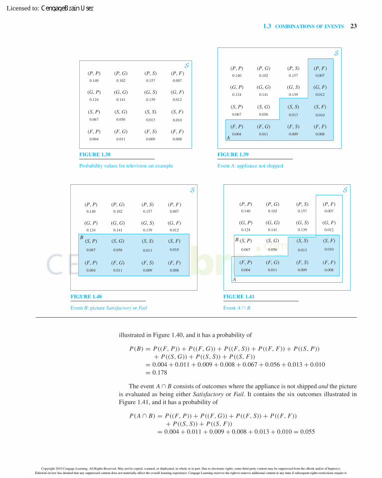
FIGURE 1.38
Probability values for television set example
A
(P, P)
(G, P)
(F, P)
(P, G) (P, S)
(F, S)
(G, S)
(S, S)
(F, G)
(S, F)
(F, F)
(P, F)0.140 0.102 0.157 0.007
0.124 0.139 0.012
0.013 0.010
0.004 0.011 0.009 0.008
(G, F)
S
(G, G)0.141
(S, P) (S, G)0.067 0.056
FIGURE 1.39
Event A: appliance not shipped
(P, P)
(G, P)
(F, P)
(P, G) (P, S)
(F, S)
(G, S)
(S, S)
(F, G)
(S, F)
(F, F)
(P, F )0.140 0.102 0.157 0.007
0.124 0.139 0.012
0.013 0.010
0.004 0.011 0.009 0.008
(G, F)
S
(G, G)0.141
(S, P) (S, G)
0.067 0.056
B
FIGURE 1.40
Event B: picture Satisfactory or Fail
(P, P)
(G, P)
(F, P)
(P, G) (P, S)
(F, S)
(G, S)
(S, S)
(F, G)
(S, F)
(F, F)
(P, F)0.140 0.102 0.157 0.007
0.124 0.139 0.012
0.013 0.010
0.004 0.011 0.009 0.008
(G, F)
S
(G, G)0.141
(S, P) (S, G)
0.067 0.056
A
B
FIGURE 1.41
Event A ∩ B
illustrated in Figure 1.40, and it has a probability of
P(B) = P((F, P)) + P((F, G)) + P((F, S)) + P((F, F)) + P((S, P))
+ P((S, G)) + P((S, S)) + P((S, F))
= 0.004 + 0.011 + 0.009 + 0.008 + 0.067 + 0.056 + 0.013 + 0.010= 0.178
The event A ∩ B consists of outcomes where the appliance is not shipped and the pictureis evaluated as being either Satisfactory or Fail. It contains the six outcomes illustrated inFigure 1.41, and it has a probability of
P(A ∩ B) = P((F, P)) + P((F, G)) + P((F, S)) + P((F, F))
+ P((S, S)) + P((S, F))
= 0.004 + 0.011 + 0.009 + 0.008 + 0.013 + 0.010 = 0.055
Copyright 2010 Cengage Learning. All Rights Reserved. May not be copied, scanned, or duplicated, in whole or in part. Due to electronic rights, some third party content may be suppressed from the eBook and/or eChapter(s).Editorial review has deemed that any suppressed content does not materially affect the overall learning experience. Cengage Learning reserves the right to remove additional content at any time if subsequent rights restrictions require it.
Licensed to:

Hayter-15125 book December 19, 2005 20:30
24 CHAPTER 1 PROBABILITY THEORY
(P, P)
(G, P)
(F, P)
(P, G) (P, S)
(F, S)
(G, S)
(S, S)
(F, G)
(S, F)
(F, F)
(P, F)0.140 0.102 0.157 0.007
0.124 0.139 0.012
0.013 0.010
0.004 0.011 0.009 0.008
(G, F)
S
(G, G)0.141
(S, P) (S, G)0.067 0.056
A
B
FIGURE 1.42
Event A ∪ B
(P, P)
(G, P)
(F, P)
(P, G) (P, S)
(F, S)
(G, S)
(S, S)
(F, G)
(S, F)
(F, F)
(P, F)0.140 0.102 0.157 0.007
0.124 0.139 0.012
0.013 0.010
0.004 0.011 0.009 0.008
(G, F)
S
(G, G)0.141
(S, P) (S, G)0.067 0.056
A
B
FIGURE 1.43
Event A ∩ B ′
The event A ∪ B consists of outcomes where the appliance was either not shipped orthe picture was evaluated as being either Satisfactory or Fail. It contains the 10 outcomesillustrated in Figure 1.42, and its probability can be obtained either by summing the individualprobability values of these ten outcomes or more simply as
P(A ∪ B) = P(A) + P(B) − P(A ∩ B)
= 0.074 + 0.178 − 0.055 = 0.197
Television sets that have a picture evaluation of either Perfect or Good but that cannot beshipped constitute the event A ∩ B ′. This event is illustrated in Figure 1.43 and consists of theoutcomes
A ∩ B ′ = {(P, F), (G, F)}
It has a probability of
P(A ∩ B ′) = P((P, F)) + P((G, F)) = 0.007 + 0.012 = 0.019
Notice that
P(A ∩ B) + P(A ∩ B ′) = 0.055 + 0.019 = 0.074 = P(A)
as expected.
GAMES OF CHANCE The event A that an even score is obtained from a roll of a die is
A = {2, 4, 6}
If the event B, a high score, is defined to be
B = {4, 5, 6}
Copyright 2010 Cengage Learning. All Rights Reserved. May not be copied, scanned, or duplicated, in whole or in part. Due to electronic rights, some third party content may be suppressed from the eBook and/or eChapter(s).Editorial review has deemed that any suppressed content does not materially affect the overall learning experience. Cengage Learning reserves the right to remove additional content at any time if subsequent rights restrictions require it.
Licensed to:

Hayter-15125 book December 19, 2005 20:30
1.3 COMBINATIONS OF EVENTS 25
then
A ∩ B = {4, 6} and A ∪ B = {2, 4, 5, 6}
If a fair die is used, then P(A ∩ B) = 2/6 = 1/3, and P(A ∪ B) = 4/6 = 2/3.If two dice are thrown, recall that Figure 1.18 illustrates the event A, that the sum of the
scores is equal to 6, and Figure 1.19 illustrates the event B, that at least one of the two dicerecords a 6. If all the outcomes are equally likely with a probability of 1/36, then P(A) = 5/36and P(B) = 11/36. Since there are no outcomes in both events A and B,
A ∩ B = ∅
and P(A ∩ B) = 0. Consequently, the events A and B are mutually exclusive.The event A ∪ B consists of the five outcomes in event A together with the 11 outcomes
in event B, and its probability is
P(A ∪ B) = 16
36= 4
9= P(A) + P(B)
If one die is red and the other is blue, then Figure 1.44 illustrates the event C , say, that aneven score is obtained on the red die, and Figure 1.45 illustrates the event D, say, that an evenscore is obtained on the blue die. Figure 1.46 then illustrates the event C ∩ D, which is theevent that both dice have even scores. If all outcomes are equally likely, then this event has aprobability of 9/36 = 1/4. Figure 1.47 illustrates the event C ∪ D, the event that at least onedie has an even score. This event has a probability of 27/36 = 3/4. Notice that (C ∪ D)′, thecomplement of the event C ∪ D, is just the event that both dice have odd scores.
Recall that Figure 1.20 illustrates the event A, that a card drawn from a pack of cardsbelongs to the heart suit, and Figure 1.21 illustrates the event B, that a picture card is drawn.
FIGURE 1.44
Event C : even score on red die
C
S
1/36 1/36 1/36 1/36 1/36 1/36
1/36 1/36 1/36 1/36 1/36 1/36
1/36 1/36 1/36 1/36 1/36 1/36
1/36 1/36 1/36 1/36 1/36 1/36
1/36 1/36 1/36 1/36 1/36 1/36
(1, 1) (1, 2) (1, 3) (1, 4) (1, 5) (1, 6)
(2, 1) (2, 2) (2, 3) (2, 4) (2, 5) (2, 6)
1/36 1/36 1/36 1/36 1/36 1/36
(3, 1) (3, 2) (3, 3) (3, 4) (3, 5) (3, 6)
(4, 1) (4, 2) (4, 4) (4, 5) (4, 6)
(5, 1) (5, 3) (5, 6)
(6, 1) (6, 2) (6, 3) (6, 4) (6, 5) (6, 6)
(5, 4) (5, 5)(5, 2)
(4, 3)
Copyright 2010 Cengage Learning. All Rights Reserved. May not be copied, scanned, or duplicated, in whole or in part. Due to electronic rights, some third party content may be suppressed from the eBook and/or eChapter(s).Editorial review has deemed that any suppressed content does not materially affect the overall learning experience. Cengage Learning reserves the right to remove additional content at any time if subsequent rights restrictions require it.
Licensed to:

Hayter-15125 book December 19, 2005 20:30
26 CHAPTER 1 PROBABILITY THEORY
FIGURE 1.45
Event D: even score on blue die D
S
1/36 1/36 1/36 1/36 1/36 1/36
1/36 1/36 1/36 1/36 1/36 1/36
1/36 1/36 1/36 1/36 1/36 1/36
1/36 1/36 1/36 1/36 1/36 1/36
1/36 1/36 1/36 1/36 1/36 1/36
(1, 1) (1, 2) (1, 3) (1, 4) (1, 5) (1, 6)
(2, 1) (2, 2) (2, 3) (2, 4) (2, 5) (2, 6)
1/36 1/36 1/36 1/36 1/36 1/36
(3, 1) (3, 2) (3, 3) (3, 4) (3, 5) (3, 6)
(4, 1) (4, 2) (4, 4) (4, 5) (4, 6)
(5, 1) (5, 3) (5, 6)
(6, 1) (6, 2) (6, 3) (6, 4) (6, 5) (6, 6)
(5, 5)(5, 4)(5, 2)
(4, 3)
FIGURE 1.46
Event C ∩ D D
S
1/36 1/36 1/36 1/36 1/36 1/36
1/36 1/36 1/36 1/36 1/36 1/36
1/36 1/36 1/36 1/36 1/36 1/36
1/36 1/36 1/36 1/36 1/36 1/36
1/36 1/36 1/36 1/36 1/36 1/36
(1, 1) (1, 2) (1, 3) (1, 4) (1, 5) (1, 6)
(2, 1) (2, 2) (2, 3) (2, 4) (2, 5) (2, 6)
1/36 1/36 1/36 1/36 1/36 1/36
(3, 1) (3, 2) (3, 3) (3, 4) (3, 5) (3, 6)
(4, 1) (4, 2) (4, 4) (4, 5) (4, 6)
(5, 1) (5, 3) (5, 6)
(6, 1) (6, 2) (6, 3) (6, 4) (6, 5) (6, 6)
C
(5, 5)(5, 4)(5, 2)
(4, 3)
If all outcomes are equally likely, then P(A) = 13/52 = 1/4, and P(B) = 12/52 = 3/13.Figure 1.48 then illustrates the event A ∩ B, which is the event that a picture card from theheart suit is drawn. This has a probability of 3/52. Figure 1.49 illustrates the event A ∪ B,the event that either a heart or a picture card (or both) is drawn, which has a probability of22/52 = 11/26. Notice that, as expected,
P(A) + P(B) − P(A ∩ B) = 13
52+ 12
52− 3
52= 22
52= P(A ∪ B)
Copyright 2010 Cengage Learning. All Rights Reserved. May not be copied, scanned, or duplicated, in whole or in part. Due to electronic rights, some third party content may be suppressed from the eBook and/or eChapter(s).Editorial review has deemed that any suppressed content does not materially affect the overall learning experience. Cengage Learning reserves the right to remove additional content at any time if subsequent rights restrictions require it.
Licensed to:

Hayter-15125 book December 19, 2005 20:30
1.3 COMBINATIONS OF EVENTS 27
FIGURE 1.47
Event C ∪ D D
S
1/36 1/36 1/36 1/36 1/36 1/36
1/36 1/36 1/36 1/36 1/36 1/36
1/36 1/36 1/36 1/36 1/36 1/36
1/36 1/36 1/36 1/36 1/36 1/36
1/36 1/36 1/36 1/36 1/36 1/36
(1, 1) (1, 2) (1, 3) (1, 4) (1, 5) (1, 6)
(2, 1) (2, 2) (2, 3) (2, 4) (2, 5) (2, 6)
1/36 1/36 1/36 1/36 1/36 1/36
(3, 1) (3, 2) (3, 3) (3, 4) (3, 5) (3, 6)
(4, 1) (4, 2) (4, 4) (4, 5) (4, 6)
(5, 1) (5, 3) (5, 6)
(6, 1) (6, 2) (6, 3) (6, 4) (6, 5) (6, 6)
C
(5, 5)(5, 4)(5, 2)
(4, 3)
FIGURE 1.48
Event A ∩ B A
B
S
K♠Q♠J♠A♠ 3♠ 4♠ 5♠ 6♠ 7♠ 8♠ 9♠ 10♠2♠
K♦Q♦J♦A♦ 3♦ 4♦ 5♦ 6♦ 7♦ 8♦ 9♦ 10♦2♦
K♣Q♣J♣A♣ 3♣ 4♣ 5♣ 6♣ 7♣ 8♣ 9♣ 10♣2♣
K♥Q♥J♥A♥ 3♥ 4♥ 5♥ 6♥ 7♥ 8♥ 9♥ 10♥1/52
1/52 1/52 1/52 1/521/52 1/521/52 1/52 1/52 1/52
1/52 1/521/521/521/52 1/521/521/521/521/521/52
1/521/521/521/521/52
1/52 1/521/521/52
1/52
1/52 1/52 1/52 1/52 1/52 1/52 1/52 1/52
1/521/521/521/521/521/521/52
1/52
1/52
1/52 1/52 1/52
2♥
FIGURE 1.49
Event A ∪ B A
B
S
K♠Q♠J♠A♠ 3♠ 4♠ 5♠ 6♠ 7♠ 8♠ 9♠ 10♠2♠
K♦Q♦J♦A♦ 3♦ 4♦ 5♦ 6♦ 7♦ 8♦ 9♦ 10♦2♦
K♣Q♣J♣A♣ 3♣ 4♣ 5♣ 6♣ 7♣ 8♣ 9♣ 10♣2♣
K♥Q♥J♥A♥ 3♥ 4♥ 5♥ 6♥ 7♥ 8♥ 9♥ 10♥1/52
1/52 1/52 1/52 1/521/52 1/521/52 1/52 1/52 1/52
1/52 1/521/521/521/52 1/521/521/521/521/521/52
1/521/521/521/521/52
1/52 1/521/521/52
1/52
1/52 1/52 1/52 1/52 1/52 1/52 1/52 1/52
1/521/521/521/521/521/521/52
1/52
1/52
1/52 1/52 1/52
2♥
Copyright 2010 Cengage Learning. All Rights Reserved. May not be copied, scanned, or duplicated, in whole or in part. Due to electronic rights, some third party content may be suppressed from the eBook and/or eChapter(s).Editorial review has deemed that any suppressed content does not materially affect the overall learning experience. Cengage Learning reserves the right to remove additional content at any time if subsequent rights restrictions require it.
Licensed to:

Hayter-15125 book December 19, 2005 20:30
28 CHAPTER 1 PROBABILITY THEORY
FIGURE 1.50
Event A′ ∩ B A
B
S
K♠Q♠J♠A♠ 3♠ 4♠ 5♠ 6♠ 7♠ 8♠ 9♠ 10♠2♠
K♦Q♦J♦A♦ 3♦ 4♦ 5♦ 6♦ 7♦ 8♦ 9♦ 10♦2♦
K♣Q♣J♣A♣ 3♣ 4♣ 5♣ 6♣ 7♣ 8♣ 9♣ 10♣2♣
K♥Q♥J♥A♥ 3♥ 4♥ 5♥ 6♥ 7♥ 8♥ 9♥ 10♥1/52
1/52 1/52 1/52 1/521/52 1/521/52 1/52 1/52 1/52
1/52 1/521/521/521/52 1/521/521/521/521/521/52
1/521/521/521/521/52
1/52 1/521/521/52
1/52
1/52 1/52 1/52 1/52 1/52 1/52 1/52 1/52
1/521/521/521/521/521/521/52
1/52
1/52
1/52 1/52 1/52
2♥
FIGURE 1.51
Three events decompose thesample space into eight regions A
B C
S
12
3
4
56
78
Finally, Figure 1.50 illustrates the event A′ ∩ B, which is the event that a picture card froma suit other than the heart suit is drawn. It has a probability of 9/52. Again, notice that
P(A ∩ B) + P(A′ ∩ B) = 3
52+ 9
52= 12
52= P(B)
as expected.
1.3.4 Combinations of Three or More Events
Intersections and unions can be extended in an obvious manner to three or more events.Figure 1.51 illustrates how three events A, B, and C can divide a sample space into eightdistinct and separate regions. The event A, for example, is composed of the regions 2, 3, 5,and 6, and the event A ∩ B is composed of the regions 3 and 6.
The event A ∩ B ∩ C , the intersection of the events A, B, and C , consists of the outcomesthat are simultaneously contained within all three events A, B, and C . In Figure 1.51 itcorresponds to region 6. The event A ∪ B ∪ C , the union of the events A, B, and C , consistsof the outcomes that are in at least one of the three events A, B, and C . In Figure 1.51 itcorresponds to all of the regions except for region 1. Hence region 1 can be referred to as(A ∪ B ∪ C)′ since it is the complement of the event A ∪ B ∪ C .
Copyright 2010 Cengage Learning. All Rights Reserved. May not be copied, scanned, or duplicated, in whole or in part. Due to electronic rights, some third party content may be suppressed from the eBook and/or eChapter(s).Editorial review has deemed that any suppressed content does not materially affect the overall learning experience. Cengage Learning reserves the right to remove additional content at any time if subsequent rights restrictions require it.
Licensed to:

Hayter-15125 book December 19, 2005 20:30
1.3 COMBINATIONS OF EVENTS 29
In general, care must be taken to avoid ambiguities when specifying combinations of threeor more events. For example, the expression
A ∪ B ∩ C
is ambiguous since the two events
A ∪ (B ∩ C) and (A ∪ B) ∩ C
are different. In Figure 1.51 the event B ∩ C is composed of regions 6 and 7, so A ∪ (B ∩ C)
is composed of regions 2, 3, 5, 6, and 7. In contrast, the event A ∪ B is composed of regions2, 3, 4, 5, 6, and 7, so (A ∪ B) ∩ C is composed of just regions 5, 6, and 7.
Figure 1.51 can also be used to justify the following general expression for the probabilityof the union of three events:
Union of Three Events
The probability of the union of three events A, B, and C is the sum of the probabilityvalues of the simple outcomes that are contained within at least one of the threeevents. It can also be calculated from the expression
P(A ∪ B ∪ C) = [P(A) + P(B) + P(C)]− [P(A ∩ B) + P(A ∩ C) + P(B ∩ C)] + P(A ∩ B ∩ C)
The expression for P(A ∪ B ∪ C) can be checked by matching up the regions in Figure 1.51with the various terms in the expression. The required probability, P(A ∪ B ∪ C), is the sumof the probability values of the outcomes in regions 2, 3, 4, 5, 6, 7, and 8. However, the sumof the probabilities P(A), P(B), and P(C) counts regions 3, 5, and 7 twice, and region 6three times. Subtracting the probabilities P(A ∩ B), P(A ∩ C), and P(B ∩ C) removes thedouble counting of regions 3, 5, and 7 but also subtracts the probability of region 6 three times.The expression is then completed by adding back on P(A∩ B ∩C), the probability of region 6.
Figure 1.52 illustrates three events A, B, and C that are mutually exclusive because notwo events have any outcomes in common. In this case,
P(A ∪ B ∪ C) = P(A) + P(B) + P(C)
because the event intersections all have probabilities of zero. More generally, for a sequenceA1, A2, . . . , An of mutually exclusive events where no two of the events have any outcomes
FIGURE 1.52
Three mutually exclusive events
A
BC
S
Copyright 2010 Cengage Learning. All Rights Reserved. May not be copied, scanned, or duplicated, in whole or in part. Due to electronic rights, some third party content may be suppressed from the eBook and/or eChapter(s).Editorial review has deemed that any suppressed content does not materially affect the overall learning experience. Cengage Learning reserves the right to remove additional content at any time if subsequent rights restrictions require it.
Licensed to:

Hayter-15125 book December 19, 2005 20:30
30 CHAPTER 1 PROBABILITY THEORY
in common, the probability of the union of the events can be obtained by summing theprobabilities of the individual events.
Union of Mutually Exclusive Events
For a sequence A1, A2, . . . , An of mutually exclusive events, the probability of theunion of the events is given by
P(A1 ∪ · · · ∪ An) = P(A1) + · · · + P(An)
If a sequence A1, A2, . . . , An of mutually exclusive events has the additional propertythat their union consists of the whole sample space S, then they are said to be an exhaustivesequence. They are also said to provide a partition of the sample space.
Sample Space Partitions
A partition of a sample space is a sequence A1, A2, . . . , An of mutually exclusiveevents for which
A1 ∪ · · · ∪ An = S
Each outcome in the sample space is then contained within one and only one of theevents Ai .
Figure 1.53 illustrates a partition of a sample space S into eight mutually exclusive events.
Example 5Television Set Quality
In addition to the events A and B discussed before, consider also the event C that an applianceis of “mediocre quality.” The event is defined to be appliances that score either Satisfactoryor Good on each of the two evaluations, so that
C = {(S, S), (S, G), (G, S), (G, G)}The three events A, B, and C are illustrated in Figure 1.54.
Notice that
A ∩ C = {(S, S)} and B ∩ C = {(S, S), (S, G)}
FIGURE 1.53
A partition of the sample space
A
S
8
A1A2
A5A4
A6A7
A3
Copyright 2010 Cengage Learning. All Rights Reserved. May not be copied, scanned, or duplicated, in whole or in part. Due to electronic rights, some third party content may be suppressed from the eBook and/or eChapter(s).Editorial review has deemed that any suppressed content does not materially affect the overall learning experience. Cengage Learning reserves the right to remove additional content at any time if subsequent rights restrictions require it.
Licensed to:

Hayter-15125 book December 19, 2005 20:30
1.3 COMBINATIONS OF EVENTS 31
FIGURE 1.54
Events A, B, and C(P, P)
(G, P)
(F, P)
(P, G) (P, S)
(F, S)
(G, S)
(S, S)
(F, G)
(S, F)
(F, F)
(P, F)0.140 0.102 0.157 0.007
0.124 0.139 0.012
0.013 0.010
0.004 0.011 0.009 0.008
(G, F)
S
(G, G)0.141
(S, P) (S, G)0.067 0.056
A
B
C
Also, the intersection of the three events is
A ∩ B ∩ C = {(S, S)}The fact that the events A ∩ C and A ∩ B ∩ C are identical, both consisting of the singleoutcome (S, S), is a consequence of the fact that A ∩ B ′ ∩ C = ∅. There are no outcomes thatare not shipped (in event A), have a picture rating of Good or Perfect (in event B ′), and are ofmediocre quality (in event C).
The company may be particularly interested in the event D, that an appliance is of “highquality,” defined to be the complement of the union of the events A, B, and C :
D = (A ∪ B ∪ C)′
Notice that this event can also be written as
D = A′ ∩ B ′ ∩ C ′
since it consists of the outcomes that are shipped (in event A′), have a picture rating of Goodor Perfect (in event B ′), and are not of mediocre quality (in event C ′). Specifically, the event Dconsists of the outcomes
D = {(G, P), (P, P), (P, G), (P, S)}and it has a probability of
P(D) = P((G, P)) + P((P, P)) + P((P, G)) + P((P, S))
= 0.124 + 0.140 + 0.102 + 0.157 = 0.523
1.3.5 Problems
1.3.1 Consider the sample space S = {0, 1, 2} and the eventA = {0}. Explain why A �= ∅.
1.3.2 Consider the sample space and events in Figure 1.55.Calculate the probabilities of the events:(a) B (b) B ∩ C(c) A ∪ C (d) A ∩ B ∩ C
(e) A ∪ B ∪ C (f) A′ ∩ B(g) B ′ ∪ C (h) A ∪ (B ∩ C)
(i) (A ∪ B) ∩ C (j) (A′ ∪ C)′
(This problem is continued in Problem 1.4.1.)
1.3.3 Use Venn diagrams to illustrate the equations:(a) A ∪ (B ∩ C) = (A ∪ B) ∩ (A ∪ C)
Copyright 2010 Cengage Learning. All Rights Reserved. May not be copied, scanned, or duplicated, in whole or in part. Due to electronic rights, some third party content may be suppressed from the eBook and/or eChapter(s).Editorial review has deemed that any suppressed content does not materially affect the overall learning experience. Cengage Learning reserves the right to remove additional content at any time if subsequent rights restrictions require it.
Licensed to:

Hayter-15125 book December 19, 2005 20:30
32 CHAPTER 1 PROBABILITY THEORY
FIGURE 1.55
A
B
C
0.040.07
0.05
0.08
0.04
0.01
0.08 0.06
0.13
0.11
0.11
0.07
0.05
0.03
0.02
0.05
S
(b) A ∩ (B ∪ C) = (A ∩ B) ∪ (A ∩ C)
(c) (A ∩ B ∩ C)′ = A′ ∪ B ′ ∪ C ′
1.3.4 Let A be the event that a person is female, let B be theevent that a person has black hair, and let C be the eventthat a person has brown eyes. Describe the kinds ofpeople in the following events:(a) A ∩ B (b) A ∪ C ′
(c) A′ ∩ B ∩ C (d) A ∩ (B ∪ C)
1.3.5 A card is chosen from a pack of cards. Are the events thata card from one of the two red suits is chosen and that acard from one of the two black suits is chosen mutuallyexclusive? What about the events that an Ace is chosenand that a heart is chosen?
1.3.6 If P(A) = 0.4 and P(A ∩ B) = 0.3, what are thepossible values for P(B)?
1.3.7 If P(A) = 0.5, P(A ∩ B) = 0.1, and P(A ∪ B) = 0.8,what is P(B)?
1.3.8 A fair die is thrown. A is the event that an even score isobtained, and B is the event that a prime score isobtained. Give the probabilities:
(a) A ∩ B (b) A ∪ B (c) A ∩ B ′
1.3.9 A card is drawn at random from a pack of cards. A is theevent that a heart is obtained, B is the event that a club isobtained, and C is the event that a diamond is obtained.Are these three events mutually exclusive? What isP(A ∪ B ∪ C)? Explain why B ⊂ A′.
1.3.10 A card is drawn from a pack of cards. A is the event thatan Ace is obtained, B is the event that a card from one of
the two red suits is obtained, and C is the event that apicture card is obtained. What cards do the followingevents consist of?(a) A ∩ B (b) A ∪ C(c) B ∩ C ′ (d) A ∪ (B ′ ∩ C)
1.3.11 A car repair can be performed either on time or late andeither satisfactorily or unsatisfactorily. The probabilityof a repair being on time and satisfactory is 0.26.The probability of a repair being on time is 0.74. Theprobability of a repair being satisfactory is 0.41.What is the probability of a repair being late andunsatisfactory?
1.3.12 A bag contains 200 balls that are either red or blue andeither dull or shiny. There are 55 shiny red balls, 91 shinyballs, and 79 red balls. If a ball is chosen at random,what is the probability that it is either a shiny ball or ared ball? What is the probability that it is a dull blueball?
1.3.13 In a study of patients arriving at a hospital emergencyroom, the gender of the patients is considered, togetherwith whether the patients are younger or older than30 years of age, and whether or not the patients areadmitted to the hospital. It is found that 45% of thepatients are male, 30% of the patients are younger than30 years of age, 15% of the patients are females olderthan 30 years of age who are admitted to the hospital, and21% of the patients are females younger than 30 years ofage. What proportion of the patients are females olderthan 30 years of age who are not admitted to thehospital?
Copyright 2010 Cengage Learning. All Rights Reserved. May not be copied, scanned, or duplicated, in whole or in part. Due to electronic rights, some third party content may be suppressed from the eBook and/or eChapter(s).Editorial review has deemed that any suppressed content does not materially affect the overall learning experience. Cengage Learning reserves the right to remove additional content at any time if subsequent rights restrictions require it.
Licensed to:

Hayter-15125 book December 19, 2005 20:30
1.4 CONDITIONAL PROBABILITY 33
1.4 Conditional Probability
1.4.1 Definition of Conditional Probability
For experiments with two or more events of interest, attention is often directed not only at theprobabilities of individual events, but also at the probability of an event occurring conditionalon the knowledge that another event has occurred. Probabilities such as these are important andvery useful since they provide appropriate revisions of a set of probabilities once a particularevent is known to have occurred.
The probability that event A occurs conditional on event B having occurred is written
P(A|B)
Its interpretation is that if the outcome occurring is known to be contained within the event B,then this conditional probability measures the probability that the outcome is also containedwithin the event A. Conditional probabilities can easily be obtained using the followingformula:
Conditional Probability
The conditional probability of event A conditional on event B is
P(A|B) = P(A ∩ B)
P(B)
for P(B) > 0. It measures the probability that event A occurs when it is known thatevent B occurs.
One simple example of conditional probability concerns the situation in which twoevents A and B are mutually exclusive. Since in this case events A and B have no outcomesin common, it is clear that the occurrence of event B precludes the possibility of event Aoccurring, so that intuitively, the probability of event A conditional on event B must be zero.Since A ∩ B = ∅ for mutually exclusive events, this intuitive reasoning is in agreement withthe formula
P(A|B) = P(A ∩ B)
P(B)= 0
P(B)= 0
Another simple example of conditional probability concerns the situation in which anevent B is contained within an event A, that is B ⊂ A. Then if event B occurs, it is clear thatevent A must also occur, so that intuitively, the probability of event A conditional on event Bmust be one. Again, since A ∩ B = B here, this intuitive reasoning is in agreement with theformula
P(A|B) = P(A ∩ B)
P(B)= P(B)
P(B)= 1
For a less obvious example of conditional probability, consider again Figure 1.26 and theevents A and B shown there. Suppose that event B is known to occur. In other words, supposethat it is known that the outcome occurring is one of the five outcomes contained within theevent B. What then is the conditional probability of event A occurring?
Since two of the five outcomes in event B are also in event A (that is, there are two outcomesin A ∩ B), the conditional probability is the probability that one of these two outcomes occurs
Copyright 2010 Cengage Learning. All Rights Reserved. May not be copied, scanned, or duplicated, in whole or in part. Due to electronic rights, some third party content may be suppressed from the eBook and/or eChapter(s).Editorial review has deemed that any suppressed content does not materially affect the overall learning experience. Cengage Learning reserves the right to remove additional content at any time if subsequent rights restrictions require it.
Licensed to:

Hayter-15125 book December 19, 2005 20:30
34 CHAPTER 1 PROBABILITY THEORY
FIGURE 1.56
P(A|B) = P(A ∩ B)/P(B)
S
0.180.22
A
B
0.04
0.140.01
0.12
0.03
0.07
0.19
rather than one of the other three outcomes (which are in A′ ∩ B). As Figure 1.56 shows, theconditional probability is calculated to be
P(A|B) = P(A ∩ B)
P(B)= 0.26
0.56= 0.464
Notice that this conditional probability is different from P(A) = 0.27. If the event B is knownnot to occur, then the conditional probability of event A is
P(A|B ′) = P(A ∩ B ′)P(B ′)
= P(A) − P(A ∩ B)
1 − P(B)= 0.27 − 0.26
1 − 0.56= 0.023
In the same way that P(A) + P(A′) = 1, it is also true that
P(A|B) + P(A′|B) = 1
This is reasonable because if event B occurs, it is still the case that either event A occurs orit does not, and so the two conditional probabilities should sum to one. Formally, this resultcan be shown by noting that
P(A|B) + P(A′|B) = P(A ∩ B)
P(B)+ P(A′ ∩ B)
P(B)
= 1
P(B)(P(A ∩ B) + P(A′ ∩ B)) = 1
P(B)P(B) = 1
However, there is no general relationship between P(A|B) and P(A|B ′).
S0 defectives
0.02
1 defective0.11
2 defectives0.16
3 defectives0.21
4 defectives0.13
5 defectives0.08
correct
6 defectives?
.
.
.
500 defectives?
FIGURE 1.57
Sample space for computer chipsexample
Finally, the event conditioned on can be represented as a combination of events. Forexample,
P(A|B ∪ C)
represents the probability of event A conditional on the event B ∪ C , that is conditional oneither event B or C occurring. It can be calculated from the formula
P(A|B ∪ C) = P(A ∩ (B ∪ C))
P(B ∪ C)
1.4.2 Examples of Conditional Probabilities
Example 2Defective Computer
Chips
Consider Figure 1.57 that illustrates the sample space for the number of defective chips in abox of 500 chips, and recall that the event correct, with a probability of P(correct) = 0.71,consists of the six outcomes corresponding to no more than five defectives.
Copyright 2010 Cengage Learning. All Rights Reserved. May not be copied, scanned, or duplicated, in whole or in part. Due to electronic rights, some third party content may be suppressed from the eBook and/or eChapter(s).Editorial review has deemed that any suppressed content does not materially affect the overall learning experience. Cengage Learning reserves the right to remove additional content at any time if subsequent rights restrictions require it.
Licensed to:

Hayter-15125 book December 19, 2005 20:30
1.4 CONDITIONAL PROBABILITY 35
The probability that a box has no defective chips is
P(0 defectives) = 0.02
so that if a box is chosen at random, it has a probability of only 0.02 of containing nodefective chips. If the company guarantees that a box has no more than five defective chips,then customers can be classified as either satisfied or unsatisfied depending on whether theguarantee is met. Clearly, an unsatisfied customer did not purchase a box containing nodefective chips. However, it is interesting to calculate the probability that a satisfied customerpurchased a box that contained no defective chips. Intuitively, this conditional probabilityshould be larger than the unconditional probability 0.02.
The required probability is the probability of no defectives conditional on there being nomore than five defectives, which is calculated to be
P(0 defectives|correct) = P(0 defectives ∩ correct)
P(correct)= P(0 defectives)
P(correct)
= 0.02
0.71= 0.028
This conditional probability indicates that whereas 2% of all the boxes contain no defectives,2.8% of the satisfied customers purchased boxes that contained no defectives.
Example 4Power Plant Operation
The probability that plant X is idle is P(A) = 0.32. However, suppose it is known that atleast two out of the three plants are generating electricity (event B). How does this change theprobability of plant X being idle?
The probability that plant X is idle (event A) conditional on at least two out of the threeplants generating electricity (event B) is
P(A|B) = P(A ∩ B)
P(B)= 0.18
0.70= 0.257
as shown in Figure 1.58. Therefore, whereas plant X is idle about 32% of the time, it is idleonly about 25.7% of the time when at least two of the plants are generating electricity.
Example 5Television Set Quality
Recall that the probability that an appliance has a picture graded as either Satisfactory or Failis P(B) = 0.178. However, suppose that a technician takes a television set from a pile of setsthat could not be shipped. What is the probability that the appliance taken by the technicianhas a picture graded as either Satisfactory or Fail?
The required probability is the probability that an appliance has a picture graded as eitherSatisfactory or Fail (event B) conditional on the appliance not being shipped (event A). AsFigure 1.59 shows, this can be calculated to be
P(B|A) = P(A ∩ B)
P(A)= 0.055
0.074= 0.743
so that whereas only about 17.8% of all the appliances manufactured have a picture gradedas either Satisfactory or Fail, 74.3% of the appliances that cannot be shipped have a picturegraded as either Satisfactory or Fail.
GAMES OF CHANCE If a fair die is rolled the probability of scoring a 6 is P(6) = 1/6. If somebody rolls a diewithout showing you but announces that the result is even, then intuitively the chance that a 6has been obtained is 1/3 since there are three equally likely even scores, one of which is a 6.
Copyright 2010 Cengage Learning. All Rights Reserved. May not be copied, scanned, or duplicated, in whole or in part. Due to electronic rights, some third party content may be suppressed from the eBook and/or eChapter(s).Editorial review has deemed that any suppressed content does not materially affect the overall learning experience. Cengage Learning reserves the right to remove additional content at any time if subsequent rights restrictions require it.
Licensed to:
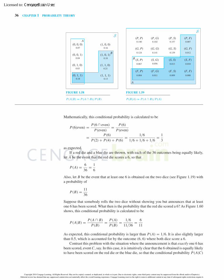
Hayter-15125 book December 19, 2005 20:30
36 CHAPTER 1 PROBABILITY THEORY
B
(1, 1, 1)0.13
(1, 1, 0)0.21
(1, 0, 1)0.18
(1, 0, 0)0.16
(0, 1, 0)0.03
(0, 0, 1)0.04
(0, 0, 0)0.07
SA
(0, 1, 1)0.18
FIGURE 1.58
P(A|B) = P(A ∩ B)/P(B)
(P, P)
(G, P)
(F, P)
(P, G) (P, S)
(F, S)
(G, S)
(S, S)
(F, G)
(S, F)
(F, F)
(P, F)0.140 0.102 0.157 0.007
0.124 0.139 0.012
0.013 0.010
0.004 0.011 0.009 0.008
(G, F)
S
(G, G)0.141
(S, P) (S, G)0.067 0.056
A
B
FIGURE 1.59
P(B|A) = P(A ∩ B)/P(A)
Mathematically, this conditional probability is calculated to be
P(6|even) = P(6 ∩ even)
P(even)= P(6)
P(even)
= P(6)
P(2) + P(4) + P(6)= 1/6
1/6 + 1/6 + 1/6= 1
3
as expected.If a red die and a blue die are thrown, with each of the 36 outcomes being equally likely,
let A be the event that the red die scores a 6, so that
P(A) = 6
36= 1
6
Also, let B be the event that at least one 6 is obtained on the two dice (see Figure 1.19) witha probability of
P(B) = 11
36
Suppose that somebody rolls the two dice without showing you but announces that at leastone 6 has been scored. What then is the probability that the red die scored a 6? As Figure 1.60shows, this conditional probability is calculated to be
P(A|B) = P(A ∩ B)
P(B)= P(A)
P(B)= 1/6
11/36= 6
11
As expected, this conditional probability is larger than P(A) = 1/6. It is also slightly largerthan 0.5, which is accounted for by the outcome (6, 6) where both dice score a 6.
Contrast this problem with the situation where the announcement is that exactly one 6 hasbeen scored, event C , say. In this case, it is intuitively clear that the 6 obtained is equally likelyto have been scored on the red die or the blue die, so that the conditional probability P(A|C)
Copyright 2010 Cengage Learning. All Rights Reserved. May not be copied, scanned, or duplicated, in whole or in part. Due to electronic rights, some third party content may be suppressed from the eBook and/or eChapter(s).Editorial review has deemed that any suppressed content does not materially affect the overall learning experience. Cengage Learning reserves the right to remove additional content at any time if subsequent rights restrictions require it.
Licensed to:

Hayter-15125 book December 19, 2005 20:30
1.4 CONDITIONAL PROBABILITY 37
FIGURE 1.60
P(A|B) = P(A ∩ B)/P(B) B
S
1/36 1/36 1/36 1/36 1/36 1/36
1/36 1/36 1/36 1/36 1/36 1/36
1/36 1/36 1/36 1/36 1/36 1/36
1/36 1/36 1/36 1/36 1/36 1/36
1/36 1/36 1/36 1/36 1/36 1/36
(1, 1) (1, 2) (1, 3) (1, 4) (1, 5) (1, 6)
(2, 1) (2, 2) (2, 3) (2, 4) (2, 5) (2, 6)
1/36 1/36 1/36 1/36 1/36 1/36
(3, 1) (3, 2) (3, 3) (3, 4) (3, 5) (3, 6)
(4, 1) (4, 2) (4, 4) (4, 5) (4, 6)
(5, 1) (5, 3) (5, 4) (5, 5) (5, 6)
(6, 1) (6, 2) (6, 3) (6, 4) (6, 5) (6, 6)A
(5, 2)
(4, 3)
FIGURE 1.61
P(A|C) = P(A ∩ C)/P(C) C
S
1/36 1/36 1/36 1/36 1/36 1/36
1/36 1/36 1/36 1/36 1/36 1/36
1/36 1/36 1/36 1/36 1/36 1/36
1/36 1/36 1/36 1/36 1/36 1/36
1/36 1/36 1/36 1/36 1/36
(1, 1) (1, 2) (1, 3) (1, 4) (1, 5) (1, 6)
(2, 1) (2, 2) (2, 3) (2, 4) (2, 5) (2, 6)
1/36 1/36 1/36 1/36 1/36 1/36
(3, 1) (3, 2) (3, 3) (3, 4) (3, 5) (3, 6)
(4, 1) (4, 2) (4, 4) (4, 5) (4, 6)
(5, 1) (5, 3) (5, 4) (5, 5) (5, 6)
(6, 1) (6, 2) (6, 3) (6, 4) (6, 5)A
(5, 2)
(4, 3)
1/36
(6, 6)
should be equal to 1/2. As Figure 1.61 shows, this is correct since
P(A|C) = P(A ∩ C)
P(C)= 5/36
10/36= 1
2
If a card is drawn from a pack of cards, let A be the event that a card from the heart suit isobtained, and let B be the event that a picture card is drawn. Recall that P(A) = 13/52 = 1/4and P(B) = 12/52 = 3/13. Also, the event A ∩ B, the event that a picture card from theheart suit is drawn, has a probability of P(A ∩ B) = 3/52.
Copyright 2010 Cengage Learning. All Rights Reserved. May not be copied, scanned, or duplicated, in whole or in part. Due to electronic rights, some third party content may be suppressed from the eBook and/or eChapter(s).Editorial review has deemed that any suppressed content does not materially affect the overall learning experience. Cengage Learning reserves the right to remove additional content at any time if subsequent rights restrictions require it.
Licensed to:
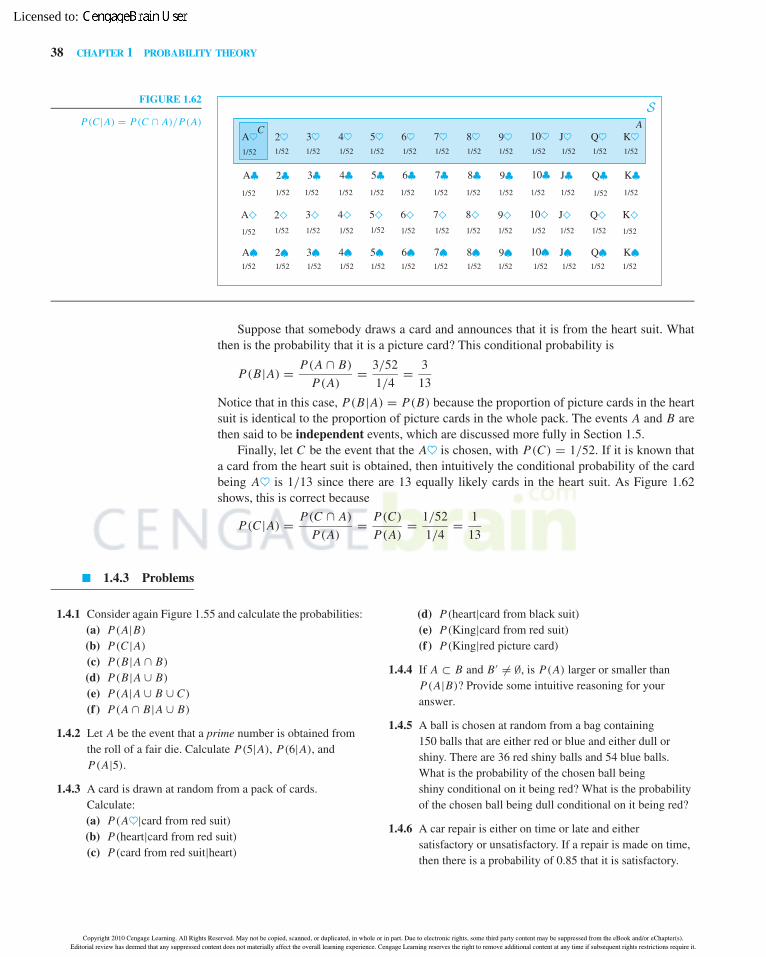
Hayter-15125 book December 19, 2005 20:30
38 CHAPTER 1 PROBABILITY THEORY
FIGURE 1.62
P(C |A) = P(C ∩ A)/P(A)C
S
K♠Q♠J♠A♠ 3♠ 4♠ 5♠ 6♠ 7♠ 8♠ 9♠ 10♠2♠
K♦Q♦J♦A♦ 3♦ 4♦ 5♦ 6♦ 7♦ 8♦ 9♦ 10♦2♦
K♣Q♣J♣A♣ 3♣ 4♣ 5♣ 6♣ 7♣ 8♣ 9♣ 10♣2♣
K♥Q♥J♥A♥ 3♥ 4♥ 5♥ 6♥ 7♥ 8♥ 9♥ 10♥1/52
1/52 1/52 1/52 1/521/52 1/521/52 1/52 1/52 1/52
1/52 1/521/521/521/52 1/521/521/521/521/521/52
1/521/521/521/521/52
1/52 1/521/521/52
1/52
1/52 1/52 1/52 1/52 1/52 1/52 1/52 1/52
1/521/521/521/521/521/521/52
1/52
1/52
1/52 1/52 1/52
2♥A
Suppose that somebody draws a card and announces that it is from the heart suit. Whatthen is the probability that it is a picture card? This conditional probability is
P(B|A) = P(A ∩ B)
P(A)= 3/52
1/4= 3
13
Notice that in this case, P(B|A) = P(B) because the proportion of picture cards in the heartsuit is identical to the proportion of picture cards in the whole pack. The events A and B arethen said to be independent events, which are discussed more fully in Section 1.5.
Finally, let C be the event that the A♥ is chosen, with P(C) = 1/52. If it is known thata card from the heart suit is obtained, then intuitively the conditional probability of the cardbeing A♥ is 1/13 since there are 13 equally likely cards in the heart suit. As Figure 1.62shows, this is correct because
P(C |A) = P(C ∩ A)
P(A)= P(C)
P(A)= 1/52
1/4= 1
13
1.4.3 Problems
1.4.1 Consider again Figure 1.55 and calculate the probabilities:(a) P(A|B)
(b) P(C |A)
(c) P(B|A ∩ B)
(d) P(B|A ∪ B)
(e) P(A|A ∪ B ∪ C)
(f ) P(A ∩ B|A ∪ B)
1.4.2 Let A be the event that a prime number is obtained fromthe roll of a fair die. Calculate P(5|A), P(6|A), andP(A|5).
1.4.3 A card is drawn at random from a pack of cards.Calculate:(a) P(A♥|card from red suit)(b) P(heart|card from red suit)(c) P(card from red suit|heart)
(d) P(heart|card from black suit)(e) P(King|card from red suit)(f ) P(King|red picture card)
1.4.4 If A ⊂ B and B ′ �= ∅, is P(A) larger or smaller thanP(A|B)? Provide some intuitive reasoning for youranswer.
1.4.5 A ball is chosen at random from a bag containing150 balls that are either red or blue and either dull orshiny. There are 36 red shiny balls and 54 blue balls.What is the probability of the chosen ball beingshiny conditional on it being red? What is the probabilityof the chosen ball being dull conditional on it being red?
1.4.6 A car repair is either on time or late and eithersatisfactory or unsatisfactory. If a repair is made on time,then there is a probability of 0.85 that it is satisfactory.
Copyright 2010 Cengage Learning. All Rights Reserved. May not be copied, scanned, or duplicated, in whole or in part. Due to electronic rights, some third party content may be suppressed from the eBook and/or eChapter(s).Editorial review has deemed that any suppressed content does not materially affect the overall learning experience. Cengage Learning reserves the right to remove additional content at any time if subsequent rights restrictions require it.
Licensed to:

Hayter-15125 book December 19, 2005 20:30
1.4 CONDITIONAL PROBABILITY 39
There is a probability of 0.77 that a repair will be madeon time. What is the probability that a repair is made ontime and is satisfactory?
1.4.7 Assess whether the probabilities of the events (i) increase,decrease, or remain unchanged when they are conditionedon the events (ii).(a) (i) It rains tomorrow, (ii) it is raining today.(b) (i) A lottery winner has black hair, (ii) the lottery
winner has brown eyes.(c) (i) A lottery winner has black hair, (ii) the lottery
winner owns a red car.(d) (i) A lottery winner is more than 50 years old, (ii) the
lottery winner is more than 30 years old.
1.4.8 Suppose that births are equally likely to be on any day.What is the probability that somebody chosen at randomhas a birthday on the first day of a month? How does thisprobability change conditional on the knowledge that theperson’s birthday is in March? In February?
1.4.9 Consider again Figure 1.24 and the battery lifetimes.Calculate the probabilities:(a) A type I battery lasts longest conditional on it not
failing first(b) A type I battery lasts longest conditional on a type II
battery failing first(c) A type I battery lasts longest conditional on a type II
battery lasting the longest(d) A type I battery lasts longest conditional on a type II
battery not failing first
1.4.10 Consider again Figure 1.25 and the two assembly lines.Calculate the probabilities:(a) Both lines are at full capacity conditional on neither
line being shut down(b) At least one line is at full capacity conditional on
neither line being shut down(c) One line is at full capacity conditional on exactly one
line being shut down(d) Neither line is at full capacity conditional on at least
one line operating at partial capacity
1.4.11 The length, width, and height of a manufactured part areclassified as being either within or outside specifiedtolerance limits. In a quality inspection 86% of the partsare found to be within the specified tolerance limits forwidth, but only 80% of the parts are within the specifiedtolerance limits for all three dimensions. However, 2% ofthe parts are within the specified tolerance limits forwidth and length but not for height, and 3% of the parts
are within the specified tolerance limits for width andheight but not for length. Moreover, 92% of the parts arewithin the specified tolerance limits for either width orheight, or both of these dimensions.(a) If a part is within the specified tolerance limits for
height, what is the probability that it will also bewithin the specified tolerance limits for width?
(b) If a part is within the specified tolerance limits forlength and width, what is the probability that it willbe within the specified tolerance limits for all threedimensions?
1.4.12 A gene can be either type A or type B, and it can be eitherdominant or recessive. If the gene is type B, then thereis a probability of 0.31 that it is dominant. There is alsoa probability of 0.22 that a gene is type B and it isdominant. What is the probability that a gene is of type A?
1.4.13 A manufactured component has its quality graded on itsperformance, appearance, and cost. Each of these threecharacteristics is graded as either pass or fail. There is aprobability of 0.40 that a component passes on bothappearance and cost. There is a probability of 0.31 that acomponent passes on all three characteristics. There is aprobability of 0.64 that a component passes onperformance. There is a probability of 0.19 that acomponent fails on all three characteristics. There is aprobability of 0.06 that a component passes onappearance but fails on both performance and cost.(a) What is the probability that a component passes on
cost but fails on both performance and appearance?(b) If a component passes on both appearance and cost,
what is the probability that it passes on all threecharacteristics?
1.4.14 An agricultural research establishment grows vegetablesand grades each one as either good or bad for its taste,good or bad for its size, and good or bad for itsappearance. Overall 78% of the vegetables have a goodtaste. However, only 69% of the vegetables have both agood taste and a good size. Also, 5% of the vegetableshave both a good taste and a good appearance, but a badsize. Finally, 84% of the vegetables have either a goodsize or a good appearance.(a) If a vegetable has a good taste, what is the probability
that it also has a good size?(b) If a vegetable has a bad size and a bad appearance,
what is the probability that it has a good taste?
1.4.15 There is a 4% probability that the plane used for acommercial flight has technical problems, and this causes
Copyright 2010 Cengage Learning. All Rights Reserved. May not be copied, scanned, or duplicated, in whole or in part. Due to electronic rights, some third party content may be suppressed from the eBook and/or eChapter(s).Editorial review has deemed that any suppressed content does not materially affect the overall learning experience. Cengage Learning reserves the right to remove additional content at any time if subsequent rights restrictions require it.
Licensed to:

Hayter-15125 book December 19, 2005 20:30
40 CHAPTER 1 PROBABILITY THEORY
a delay in the flight. If there are no technical problemswith the plane, then there is still a 33% probability thatthe flight is delayed due to all other reasons. What is theprobability that the flight is delayed?
1.4.16 In a reliability test there is a 42% probability that acomputer chip survives more than 500 temperature
cycles. If a computer chip does not survive more than500 temperature cycles, then there is a 73% probabilitythat it was manufactured by company A. What is theprobability that a computer chip is not manufactured bycompany A and does not survive more than 500temperature cycles?
1.5 Probabilities of Event Intersections
1.5.1 General Multiplication Law
It follows from the definition of the conditional probability P(A|B) that the probability of theintersection of two events A ∩ B can be calculated as
P(A ∩ B) = P(B) P(A|B)
That is, the probability of events A and B both occurring can be obtained by multiplying theprobability of event B by the probability of event A conditional on event B. It also followsfrom the definition of the conditional probability P(B|A) that
P(A ∩ B) = P(A) P(B|A)
so that the probability of events A and B both occurring can also be obtained by multiplyingthe probability of event A by the probability of event B conditional on event A. Therefore, itdoes not matter which of the two events A or B is conditioned upon.
More generally, since
P(C |A ∩ B) = P(A ∩ B ∩ C)
P(A ∩ B)
the probability of the intersection of three events can be calculated as
P(A ∩ B ∩ C) = P(A ∩ B) P(C |A ∩ B) = P(A) P(B|A) P(C |A ∩ B)
Thus, the probability of all three events occurring can be obtained by multiplying togetherthe probability of one event, the probability of a second event conditioned on the first event,and the probability of the third event conditioned on the intersection of the first and secondevents. This formula can be extended in an obvious way to the following multiplication lawfor the intersection of a series of events.
Probabilities of Event Intersections
The probability of the intersection of a series of events A1, . . . , An can be calculatedfrom the expression
P(A1 ∩ · · · ∩ An) = P(A1) × P(A2|A1) × P(A3|A1 ∩ A2) ×· · · × P(An|A1 ∩ · · · ∩ An−1)
This expression for the probability of event intersections is particularly useful when theconditional probabilities P(Ai |A1 ∩ · · · ∩ Ai−1) are easily obtainable, as illustrated in thefollowing example.
Copyright 2010 Cengage Learning. All Rights Reserved. May not be copied, scanned, or duplicated, in whole or in part. Due to electronic rights, some third party content may be suppressed from the eBook and/or eChapter(s).Editorial review has deemed that any suppressed content does not materially affect the overall learning experience. Cengage Learning reserves the right to remove additional content at any time if subsequent rights restrictions require it.
Licensed to:

Hayter-15125 book December 19, 2005 20:30
1.5 PROBABILITIES OF EVENT INTERSECTIONS 41
Suppose that two cards are drawn at random without replacement from a pack of cards.Let A be the event that the first card drawn is from the heart suit, and let B be the event thatthe second card drawn is from the heart suit. What is P(A∩ B), the probability that both cardsare from the heart suit?
Figure 1.13 shows the sample space for this problem, which consists of 2652 equally likelyoutcomes, each with a probability of 1/2652. One way to calculate P(A ∩ B) is to count thenumber of outcomes in the sample space that are contained within the event A ∩ B, that is,for which both cards are in the heart suit. In fact,
A ∩ B = {(A♥, 2♥), (A♥, 3♥), . . . , (A♥, K♥), (2♥, A♥), (2♥, 3♥), . . . ,
(2♥, K♥), . . . (K♥, A♥), (K♥, 2♥), . . . , (K♥, Q♥)}which consists of 13 × 12 = 156 outcomes. Consequently, the required probability is
P(A ∩ B) = 156
2652= 3
51
However, a more convenient way of calculating this probability is to note that it is theproduct of P(A) and P(B|A). When the first card is drawn, there are 13 heart cards out of atotal of 52 cards, so
P(A) = 13
52= 1
4
Conditional on the first card being a heart (event A), when the second card is drawn there willbe 12 heart cards remaining in the reduced pack of 51 cards, so that
P(B|A) = 12
51
The required probability is then
P(A ∩ B) = P(A) P(B|A) = 1
4× 12
51= 3
51
as before.
1.5.2 Independent Events
Two events A and B are said to be independent events if
P(B|A) = P(B)
so that the probability of event B remains the same whether or not the event A is conditionedupon. In other words, knowledge of the occurrence (or lack of occurrence) of event A doesnot affect the probability of event B. In this case
P(A ∩ B) = P(A) P(B|A) = P(A) P(B)
and
P(A|B) = P(A ∩ B)
P(B)= P(A)P(B)
P(B)= P(A)
Thus, in a similar way, the probability of event A remains the same whether or not event B isconditioned upon, and the probability of both events occurring, P(A ∩ B), is obtained simplyby multiplying together the individual probabilities of the two events P(A) and P(B).
Copyright 2010 Cengage Learning. All Rights Reserved. May not be copied, scanned, or duplicated, in whole or in part. Due to electronic rights, some third party content may be suppressed from the eBook and/or eChapter(s).Editorial review has deemed that any suppressed content does not materially affect the overall learning experience. Cengage Learning reserves the right to remove additional content at any time if subsequent rights restrictions require it.
Licensed to:

Hayter-15125 book December 19, 2005 20:30
42 CHAPTER 1 PROBABILITY THEORY
Independent Events
Two events A and B are said to be independent events if
P(A|B) = P(A), P(B|A) = P(B), and P(A ∩ B) = P(A) P(B)
Any one of these three conditions implies the other two. The interpretation of twoevents being independent is that knowledge about one event does not affect theprobability of the other event.
The concept of independence is most easily understood from a practical standpoint, withtwo events being independent if they are “unrelated” to each other. For example, suppose thata person is chosen at random from a large group of people, as in a lottery, for instance. Let Abe the event that the person is over 6 feet tall, and let B be the event that the person weighsmore than 200 pounds. Intuitively, these two events are not independent because knowledgeof one event influences our perception of the likelihood of the other event. For example, if thelottery winner is known to be over 6 feet tall, then this fact increases the likelihood that theperson weighs more than 200 pounds.
On the other hand, if event C is that the person owns a red car, then intuitively the events Aand C are independent, as are the events B and C . The knowledge that the lottery winner isover 6 feet tall does not change our perception of the probability that the person owns a redcar. Conversely, the knowledge that the lottery winner owns a red car does not change ourperception of the probability that the person is over 6 feet tall.
From a mathematical standpoint, two events A and B can be proven to be independent byestablishing one of the conditions
P(A|B) = P(A), P(B|A) = P(B), or P(A ∩ B) = P(A) P(B)
In practice, however, an assessment of whether two events are independent or not is usuallymade by the practical consideration of whether the two events are “unrelated.”
Events A1, A2, . . . , An are said to be independent if conditioning on combinations of someof the events does not affect the probabilities of the other events. In this case, the expressiongiven earlier for the probability of the intersection of the events simplifies to the product ofthe probabilities of the individual events.
Intersections of Independent Events
The probability of the intersection of a series of independent events A1, . . . , An issimply given by
P(A1 ∩ · · · ∩ An) = P(A1) P(A2) · · · P(An)
Consider again the problem discussed above where two cards are drawn from a pack ofcards, and where A is the event that the first card drawn is from the heart suit and B is theevent that the second card drawn is from the heart suit. Suppose that now the drawings aremade with replacement. What is P(A ∩ B) in this case?
Figure 1.12 shows the sample space for this problem, which consists of 2704 equallylikely outcomes, each with a probability of 1/2704. As before, one way to calculate P(A∩ B)
is to count the number of outcomes in the sample space that are contained within the event
Copyright 2010 Cengage Learning. All Rights Reserved. May not be copied, scanned, or duplicated, in whole or in part. Due to electronic rights, some third party content may be suppressed from the eBook and/or eChapter(s).Editorial review has deemed that any suppressed content does not materially affect the overall learning experience. Cengage Learning reserves the right to remove additional content at any time if subsequent rights restrictions require it.
Licensed to:

Hayter-15125 book December 19, 2005 20:30
1.5 PROBABILITIES OF EVENT INTERSECTIONS 43
A ∩ B. This event is now
A ∩ B = {(A♥, A♥), (A♥, 2♥), . . . , (A♥, K♥), (2♥, A♥), (2♥, 2♥), . . . ,
(2♥, K♥), . . . (K♥, A♥), (K♥, 2♥), . . . , (K♥, K♥)}It consists of 13 × 13 = 169 outcomes, so that the required probability is
P(A ∩ B) = 169
2704= 1
16However, it is easier to notice that events A and B are independent with P(A) = P(B) =
1/4, so that
P(A ∩ B) = P(A) P(B) = 1
4× 1
4= 1
16The independence follows from the fact that with the replacement of the first card and withappropriate shuffling of the pack to ensure randomness, the outcome of the second drawingis not related to the outcome of the first drawing.
If the drawings are performed without replacement, then clearly events A and B are notindependent. This can be confirmed mathematically by noting that
P(B|A) = 12
51and P(B|A′) = 13
51which are different from P(B) = 1/4.
1.5.3 Examples and Probability Trees
Example 2Defective Computer
Chips
Suppose that 9 out of the 500 chips in a particular box are defective, and suppose that 3 chipsare sampled at random from the box without replacement. If each of the 3 chips sampled istested to determine whether it is defective (1) or satisfactory (0), the sample space has eightoutcomes. For example, the outcome (0, 1, 0) corresponds to the first and third chips beingsatisfactory and the second chip being defective.
The probability values of the eight outcomes can be calculated using a probability treeas illustrated in Figure 1.63. The events A, B, and C are, respectively, the events that thefirst, second, and third chips sampled are defective. These events are not independent sincethe sampling is conducted without replacement. The probability tree starts at the left with twobranches corresponding to the events A and A′. The probabilities of these events
P(A) = 9
500and P(A′) = 491
500are recorded at the ends of the branches.
Each of these two branches then splits into two more branches corresponding to theevents B and B ′, and the conditional probabilities of these events are recorded. These condi-tional probabilities are
P(B|A) = 8
499, P(B ′|A) = 491
499, P(B|A′) = 9
499, P(B ′|A′) = 490
499which are constructed by considering how many of the 499 chips left in the box are defectivewhen the second chip is chosen. For example, P(B|A) = 8/499 since if the first chip chosenis defective (event A), then 8 out of 499 chips in the box are defective when the second chipis chosen.
The probability tree is completed by adding additional branches for the events C and C ′,and by recording the probabilities of these events conditional on the outcomes of the first two
Copyright 2010 Cengage Learning. All Rights Reserved. May not be copied, scanned, or duplicated, in whole or in part. Due to electronic rights, some third party content may be suppressed from the eBook and/or eChapter(s).Editorial review has deemed that any suppressed content does not materially affect the overall learning experience. Cengage Learning reserves the right to remove additional content at any time if subsequent rights restrictions require it.
Licensed to:

Hayter-15125 book December 19, 2005 20:30
44 CHAPTER 1 PROBABILITY THEORY
Outcome
(1,1,1)
(1,1,0)
(1,0,1)
(1,0,0)
(0,1,1)
(0,1,0)
(0,0,1)
(0,0,0)
Probability
First chip satisfactory
First chip defective
Second chip defective
Third chip defective
A
B
'AB
B
B'
'
C'
C'
C'
C
C'
C
C
C
Second chip satisfactory
Third chip satisfactory
9
500
491
500
8
499
491
499
9
499
490
499
7
498
491
498
9
498
489
498
8
498
490
498
8
498
490
498
9
500× 8
499× 7
498 4.0 × 10⁻⁶
9
500× 491
499× 490
498 0.0174
9
500× 8
499× 491
498 2.85 × 10⁻⁴
9
500× 491
499× 8
498 2.85 × 10⁻⁴
491
500× 9
499× 8
498 2.85 × 10⁻⁴
491
500× 9
499× 490
498 0.0174
491
500× 490
499× 9
498 0.0174
491
500× 490
499× 489
498 0.9469
1
FIGURE 1.63
Probability tree for computer chip sampling
choices. For example,
P(C |A ∩ B ′) = 8
498
because conditional on the event A ∩ B ′ (the first choice is defective and the second issatisfactory), 8 out of the 498 chips in the box are defective when the third choice is made.
The probability values of the eight outcomes are found by multiplying the probabilitiesalong the branches. Thus, the probability of choosing 3 defective chips is
P((1, 1, 1)) = P(A ∩ B ∩ C) = P(A)P(B|A)P(C |A ∩ B)
= 9
500× 8
499× 7
498= 21
5,177,125 4.0 × 10⁻⁶
The probability of choosing 2 satisfactory chips followed by a defective chip is
P((0, 0, 1)) = P(A′ ∩ B ′ ∩ C) = P(A′)P(B ′|A′)P(C |A′ ∩ B ′)
= 491
500× 490
499× 9
498= 72,177
4,141,700 0.0174
Copyright 2010 Cengage Learning. All Rights Reserved. May not be copied, scanned, or duplicated, in whole or in part. Due to electronic rights, some third party content may be suppressed from the eBook and/or eChapter(s).Editorial review has deemed that any suppressed content does not materially affect the overall learning experience. Cengage Learning reserves the right to remove additional content at any time if subsequent rights restrictions require it.
Licensed to:

Hayter-15125 book December 19, 2005 20:30
1.5 PROBABILITIES OF EVENT INTERSECTIONS 45
Notice that the probabilities of the outcomes (1, 0, 0), (0, 1, 0), and (0, 0, 1) are identical,although they are calculated in different ways. Similarly, the probabilities of the outcomes(1, 1, 0), (0, 1, 1), and (1, 0, 1) are identical. The probability of exactly 1 defective chip beingfound is
P(1 defective) = P((1, 0, 0)) + P((0, 1, 0)) + P((0, 0, 1))
3 × 0.0174 = 0.0522
In fact, if attention is focused solely on the number of defective chips in the sample, then therequired probabilities can be found from the hypergeometric distribution which is discussedin Section 3.3. Finally, it is interesting to note that, in practice, the number of defective chipsin a box will not usually be known, but probabilities of these kinds are useful in estimatingthe number of defective chips in the box. In later chapters of this book, statistical techniqueswill be employed to use the information provided by a random sample (here the number ofdefective chips found in the sample) to make inferences about the population that is sampled(here the box of chips).
Example 6Satellite Launching
A satellite launch system is controlled by a computer (computer 1) that has two identicalbackup computers (computers 2 and 3). Normally, computer 1 controls the system, but if ithas a malfunction then computer 2 automatically takes over. If computer 2 malfunctions thencomputer 3 automatically takes over, and if computer 3 malfunctions there is a general systemshutdown.
The state space for this problem consists of the four situations
S = {computer 1 in use, computer 2 in use, computer 3 in use, system failure}Suppose that a computer malfunctions with a probability of 0.01 and that malfunctions of thethree computers are independent of each other. Also, let the events A, B, and C be, respectively,the events that computers 1, 2, and 3 malfunction.
Figure 1.64 shows the probability tree for this problem, which starts at the left withtwo branches corresponding to the events A and A′ with probabilities P(A) = 0.01 and
0.01
0.99
0.99
0.01
0.01
Computer 1 malfunctions
Computer 2 malfunctions
Computer 3 malfunctions
A
B
C
A
'
B'
C'
Outcome Probability
Computer 1 in use
Computer 2 in use
Computer 3 in use
System failure
0.99
0.01 × 0.99 = 0.0099
0.01 × 0.01 × 0.99 = 0.000099
0.01 × 0.01 × 0.01 = 10 − 6
1
0.99
FIGURE 1.64
Probability tree for computer backup system
Copyright 2010 Cengage Learning. All Rights Reserved. May not be copied, scanned, or duplicated, in whole or in part. Due to electronic rights, some third party content may be suppressed from the eBook and/or eChapter(s).Editorial review has deemed that any suppressed content does not materially affect the overall learning experience. Cengage Learning reserves the right to remove additional content at any time if subsequent rights restrictions require it.
Licensed to:

Hayter-15125 book December 19, 2005 20:30
46 CHAPTER 1 PROBABILITY THEORY
P(A′) = 0.99. The top branch (event A′) corresponds to computer 1 being in use, and thereis no need to extend it further. However, the bottom branch (event A) extends into two furtherbranches for the events B and B ′.
Since events A and B are independent, the probabilities of these second-stage branches(events B and B ′) do not need to be conditioned on the first-stage branch (event A), and sotheir probabilities are just P(B) = 0.01 and P(B ′) = 0.99. The probability tree is completedby adding branches for the events C and C ′ following on from the events A and B.
The probability values of the four situations are obtained by multiplying the probabilitiesalong the branches, so that
P(computer 1 in use) = 0.99P(computer 2 in use) = 0.01 × 0.99 = 0.0099P(computer 3 in use) = 0.01 × 0.01 × 0.99 = 0.000099
P(system failure) = 0.01 × 0.01 × 0.01 = 10−6
The design of the system backup capabilities is obviously conducted with the aim of mini-mizing the probability of a system failure. Notice that a key issue in the determination of thisprobability is the assumption that the malfunctions of the three computers are independentevents. In other words, a malfunction in computer 1 should not affect the probabilities of theother two computers malfunctioning. An essential part of such a backup system is ensuringthat these events are as independent as it is possible to make them.
In particular, it is sensible to have three teams of programmers working independentlyto supply software to the three computers. If only one piece of software is written and thencopied onto the three machines, then the computer malfunctions will not be independent since amalfunction due to a software error in computer 1 will be repeated in the other two computers.
Finally, it is worth noting that this system can be thought of as consisting of three computersconnected in parallel, as discussed in Section 17.1.2, where system reliability is consideredin more detail.
Example 7Car Warranties
A company sells a certain type of car that it assembles in one of four possible locations. Plant Isupplies 20% of the cars; plant II, 24%; plant III, 25%; and plant IV, 31%. A customer buyinga car does not know where the car has been assembled, and so the probabilities of a purchasedcar being from each of the four plants can be thought of as being 0.20, 0.24, 0.25, and 0.31.
Each new car sold carries a one-year bumper-to-bumper warranty. The company hascollected data that show
P(claim|plant I) = 0.05 P(claim|plant II) = 0.11P(claim|plant III) = 0.03 P(claim|plant IV) = 0.08
For example, a car assembled in plant I has a probability of 0.05 of receiving a claim onits warranty. This information, which is a closely guarded company secret, indicates whichassembly plants do the best job. Plant III is seen to have the best record, and plant II the worstrecord. Notice that claims are clearly not independent of assembly location because these fourconditional probabilities are unequal.
Figure 1.65 shows a probability tree for this problem. It is easily constructed because theprobabilities of the second-stage branches are simply obtained from the conditional probabil-ities above. The probability that a customer purchases a car that was assembled in plant I andthat does not require a claim on its warranty is seen to be
P(plant I, no claim) = 0.20 × 0.95 = 0.19
Copyright 2010 Cengage Learning. All Rights Reserved. May not be copied, scanned, or duplicated, in whole or in part. Due to electronic rights, some third party content may be suppressed from the eBook and/or eChapter(s).Editorial review has deemed that any suppressed content does not materially affect the overall learning experience. Cengage Learning reserves the right to remove additional content at any time if subsequent rights restrictions require it.
Licensed to:

Hayter-15125 book December 19, 2005 20:30
1.5 PROBABILITIES OF EVENT INTERSECTIONS 47
FIGURE 1.65
Probability tree for car warrantiesexample
0.20 × 0.05 = 0.0100
0.20 × 0.95 = 0.1900
0.24 × 0.11 = 0.0264
0.24 × 0.89 = 0.2136
0.25 × 0.03 = 0.0075
0.25 × 0.97 = 0.2425
0.31 × 0.08 = 0.0248
0.31 × 0.92 = 0.2852
0.05
0.95
0.11
0.89
0.03
0.97
0.08
0.92
No claim
Plant I
Plant II
Plant III
Plant IV
0.20
0.24
0.25
0.31
Claim
Claim
Claim
Claim
No claim
No claim
No claim
Probability
1
From a customer’s point of view, the probability of interest is the probability that a claimon the warranty of the car will be required. This can be calculated as
P(claim) = P(plant I, claim) + P(plant II, claim) + P(plant III, claim)
+ P(plant IV, claim)
= (0.20 × 0.05) + (0.24 × 0.11) + (0.25 × 0.03) + (0.31 × 0.08)
= 0.0687
In other words, about 6.87% of the cars purchased will have a claim on their warranty. Noticethat this overall claim rate is a weighted average of the four individual plant claim rates, withweights corresponding to the supply proportions of the four plants.
GAMES OF CHANCE In the roll of a fair die, consider the events
even = {2, 4, 6} and high score = {4, 5, 6}Intuitively, these two events are not independent since the knowledge that a high score isobtained increases the chances of the score being even, and vice versa, the knowledge thatthe score is even increases the chances of the score being high. Mathematically, this may beconfirmed by noting that the probabilities
P(even) = 1
2and P(even|high score) = 2
3
are different.
Copyright 2010 Cengage Learning. All Rights Reserved. May not be copied, scanned, or duplicated, in whole or in part. Due to electronic rights, some third party content may be suppressed from the eBook and/or eChapter(s).Editorial review has deemed that any suppressed content does not materially affect the overall learning experience. Cengage Learning reserves the right to remove additional content at any time if subsequent rights restrictions require it.
Licensed to:

Hayter-15125 book December 19, 2005 20:30
48 CHAPTER 1 PROBABILITY THEORY
If a red die and a blue die are rolled, consider the probability that both dice record evenscores. In this case the scores on the two dice will be independent of each other since the scoreon one die does not affect the score that is obtained on the other die. If A is the event that thered die has an even score, and B is the event that the blue die has an even score, the requiredprobability is
P(A ∩ B) = P(A) P(B) = 1
2× 1
2= 1
4
A more tedious way of calculating this probability is to note that 9 out of the 36 outcomes inthe sample space (see Figure 1.46) have both scores even, so that the required probability is9/36 = 1/4.
Suppose that two cards are drawn from a pack of cards without replacement. What is theprobability that exactly one card from the heart suit is obtained? A very tedious way to solvethis problem is to count the number of outcomes in the sample space (see Figure 1.13) thatsatisfy this condition. A better way is
P(exactly one heart) = P(first card heart, second card not heart)+ P(first card not heart, second card heart)
=(
13
52× 39
51
)+
(39
52× 13
51
)= 13
34= 0.382
Since the second drawing is made without replacement, the events “first card heart” and“second card heart” are not independent. However, notice that if the second card is drawn withreplacement, then the two events are independent, and the required probability is
P(exactly one heart) = P(first card heart, second card not heart)+ P(first card not heart, second card heart)
=(
1
4× 3
4
)+
(3
4× 1
4
)= 3
8= 0.375
It is interesting that the probability is slightly higher when the second drawing is made withoutreplacement.
1.5.4 Problems
1.5.1 Two cards are chosen from a pack of cards withoutreplacement. Calculate the probabilities:(a) Both are picture cards.(b) Both are from red suits.(c) One card is from a red suit and one card is from a
black suit.
1.5.2 Repeat Problem 1.5.1, except that the second drawing ismade with replacement. Compare your answers withthose from Problem 1.5.1.
1.5.3 Two cards are chosen from a pack of cards withoutreplacement. Are the following events independent?(a) (i) The first card is a picture card, (ii) the second card
is a picture card.
(b) (i) The first card is a heart, (ii) the second card is apicture card.
(c) (i) The first card is from a red suit, (ii) the secondcard is from a red suit.
(d) (i) The first card is a picture card, (ii) the second cardis from a red suit.
(e) (i) The first card is a red picture card, (ii) the secondcard is a heart.
1.5.4 Four cards are chosen from a pack of cards withoutreplacement. What is the probability that all four cardsare hearts? What is the probability that all four cards arefrom red suits? What is the probability that all four cardsare from different suits?
Copyright 2010 Cengage Learning. All Rights Reserved. May not be copied, scanned, or duplicated, in whole or in part. Due to electronic rights, some third party content may be suppressed from the eBook and/or eChapter(s).Editorial review has deemed that any suppressed content does not materially affect the overall learning experience. Cengage Learning reserves the right to remove additional content at any time if subsequent rights restrictions require it.
Licensed to:

Hayter-15125 book December 19, 2005 20:30
1.5 PROBABILITIES OF EVENT INTERSECTIONS 49
FIGURE 1.66
Switch diagram1 2
3
?0.88 0.92
0.90
1.5.5 Repeat Problem 1.5.4, except that the drawings are madewith replacement. Compare your answers with those fromProblem 1.5.4.
1.5.6 Show that if the events A and B are independent events,then so are the events(a) A and B ′ (b) A′ and B (c) A′ and B ′
1.5.7 Consider the network given in Figure 1.66 with threeswitches. Suppose that the switches operate independentlyof each other and that switch 1 allows a message throughwith probability 0.88, switch 2 allows a message throughwith probability 0.92, and switch 3 allows a messagethrough with probability 0.90. What is the probability thata message will find a route through the network?
1.5.8 Suppose that birthdays are equally likely to be on any dayof the year (ignore February 29 as a possibility). Showthat the probability that two people chosen at randomhave different birthdays is 364/365. Show that theprobability that three people chosen at random allhave different birthdays is
364
365× 363
365
and extend this pattern to show that the probability that npeople chosen at random all have different birthdays is
364
365× · · · × 366 − n
365
What then is the probability that in a group of n people, atleast two people will share the same birthday? Evaluatethis probability for n = 10, n = 15, n = 20, n = 25,n = 30, and n = 35. What is the smallest value of n forwhich the probability is larger than a half? Do you thinkthat birthdays are equally likely to be on any day of theyear?
1.5.9 Suppose that 17 lightbulbs in a box of 100 lightbulbs arebroken and that 3 are selected at random without
replacement. Construct a probability tree for thisproblem. What is the probability that there will be nobroken lightbulbs in the sample? What is the probabilitythat there will be no more than 1 broken lightbulb in thesample? (This problem is continued in Problem 1.7.8.)
1.5.10 Repeat Problem 1.5.9, except that the drawings are madewith replacement. Compare your answers with those fromProblem 1.5.9.
1.5.11 Suppose that a bag contains 43 red balls, 54 blue balls,and 72 green balls, and that 2 balls are chosen at randomwithout replacement. Construct a probability tree for thisproblem. What is the probability that 2 green balls will bechosen? What is the probability that the 2 balls chosenwill have different colors?
1.5.12 Repeat Problem 1.5.11, except that the drawings are madewith replacement. Compare your answers with those fromProblem 1.5.11.
1.5.13 A biased coin has a probability p of resulting in a head. Ifthe coin is tossed twice, what value of p minimizes theprobability that the same result is obtained on boththrows?
1.5.14 If a fair die is rolled six times, what is the probability thateach score is obtained exactly once? If a fair die is rolledseven times, what is the probability that a 6 is notobtained at all?
1.5.15 (a) If a fair die is rolled five times, what is theprobability that the numbers obtained are all evennumbers?
(b) If a fair die is rolled three times, what is theprobability that the three numbers obtained are alldifferent?
(c) If three cards are taken at random from a pack ofcards with replacement, what is the probability thatthere are two black cards and one red card?
Copyright 2010 Cengage Learning. All Rights Reserved. May not be copied, scanned, or duplicated, in whole or in part. Due to electronic rights, some third party content may be suppressed from the eBook and/or eChapter(s).Editorial review has deemed that any suppressed content does not materially affect the overall learning experience. Cengage Learning reserves the right to remove additional content at any time if subsequent rights restrictions require it.
Licensed to:

Hayter-15125 book December 19, 2005 20:30
50 CHAPTER 1 PROBABILITY THEORY
(d) If three cards are taken at random from a pack ofcards without replacement, what is the probabilitythat there are two black cards and one red card?
1.5.16 Suppose that n components are available, and that eachcomponent has a probability of 0.90 of operatingcorrectly, independent of the other components. Whatvalue of n is needed so that there is a probability ofat least 0.995 that at least one component operatescorrectly?
1.5.17 Suppose that an insurance company insures its clients forflood damage to property. Can the company reasonablyexpect that the claims from its clients will be independentof each other?
1.5.18 A system has four computers. Computer 1 works with aprobability of 0.88; computer 2 works with a probabilityof 0.78; computer 3 works with a probability of 0.92;computer 4 works with a probability of 0.85. Supposethat the operations of the computers are independent ofeach other.(a) Suppose that the system works only when all four
computers are working. What is the probability thatthe system works?
(b) Suppose that the system works only if at least onecomputer is working. What is the probability that thesystem works?
(c) Suppose that the system works only if at least threecomputers are working. What is the probability thatthe system works?
1.6 Posterior Probabilities
1.6.1 Law of Total Probability
Let A1, . . . , An be a partition of a sample space S so that the events Ai are mutually exclusivewith
S = A1 ∪ · · · ∪ An
Suppose that the probabilities of these n events, P(A1), . . . , P(An), are known. In addition,consider an event B as shown in Figure 1.67, and suppose that the conditional probabilitiesP(B|A1), . . . , P(B|An) are also known.
An initial question of interest is how to use the probabilities P(Ai ) and P(B|Ai ) tocalculate P(B), the probability of the event B. In fact, this is easily achieved by noting that
B = (A1 ∩ B) ∪ · · · ∪ (An ∩ B)
FIGURE 1.67
A partition A1, . . . , An and anevent B
A
B
1 2
3
n
S
A
AA
Copyright 2010 Cengage Learning. All Rights Reserved. May not be copied, scanned, or duplicated, in whole or in part. Due to electronic rights, some third party content may be suppressed from the eBook and/or eChapter(s).Editorial review has deemed that any suppressed content does not materially affect the overall learning experience. Cengage Learning reserves the right to remove additional content at any time if subsequent rights restrictions require it.
Licensed to:

Hayter-15125 book December 19, 2005 20:30
1.6 POSTERIOR PROBABILITIES 51
where the events Ai ∩ B are mutually exclusive, so that
P(B) = P(A1 ∩ B) + · · · + P(An ∩ B)
= P(A1) P(B|A1) + · · · + P(An) P(B|An)
This result, known as the law of total probability, has the interpretation that if it is known thatone and only one of a series of events Ai can occur, then the probability of another event B canbe obtained as the weighted average of the conditional probabilities P(B|Ai ), with weightsequal to the probabilities P(Ai ).
Law of Total Probability
If A1, . . . , An is a partition of a sample space, then the probability of an event B canbe obtained from the probabilities P(Ai ) and P(B|Ai ) using the formula
P(B) = P(A1) P(B|A1) + · · · + P(An) P(B|An)
Example 7Car Warranties
The law of total probability was tacitly used in the previous section when the probability of aclaim being made on a car warranty was calculated to be 0.0687. If A1, A2, A3, and A4 are,respectively, the events that a car is assembled in plants I, II, III, and IV, then they provide apartition of the sample space, and the probabilities P(Ai ) are the supply proportions of thefour plants.
If B is the event that a claim is made, then the conditional probabilities P(B|Ai ) are theclaim rates for the four individual plants, so that
P(B) = P(A1) P(B|A1) + P(A2) P(B|A2) + P(A3) P(B|A3) + P(A4) P(B|A4)
= (0.20 × 0.05) + (0.24 × 0.11) + (0.25 × 0.03) + (0.31 × 0.08)
= 0.0687
as obtained before.
1.6.2 Calculation of Posterior Probabilities
An additional question of interest is how to use the probabilities P(Ai ) and P(B|Ai ) tocalculate the probabilities P(Ai |B), the revised probabilities of the events Ai conditional onthe event B. The probabilities
P(A1), . . . , P(An)
can be thought of as being the prior probabilities of the events A1, . . . , An . However, theobservation of the event B provides some additional information that allows the revision ofthese prior probabilities into a set of posterior probabilities
P(A1|B), . . . , P(An|B)
which are the probabilities of the events A1, . . . , An conditional on the event B.From the law of total probability, these posterior probabilities are calculated to be
P(Ai |B) = P(Ai ∩ B)
P(B)= P(Ai ) P(B|Ai )
P(B)= P(Ai ) P(B|Ai )∑n
j=1 P(A j ) P(B|A j )
which is known as Bayes’ theorem.
Copyright 2010 Cengage Learning. All Rights Reserved. May not be copied, scanned, or duplicated, in whole or in part. Due to electronic rights, some third party content may be suppressed from the eBook and/or eChapter(s).Editorial review has deemed that any suppressed content does not materially affect the overall learning experience. Cengage Learning reserves the right to remove additional content at any time if subsequent rights restrictions require it.
Licensed to:

Hayter-15125 book December 19, 2005 20:30
52 CHAPTER 1 PROBABILITY THEORY
Bayes’ Theorem
If A1, . . . , An is a partition of a sample space, then the posterior probabilities of theevents Ai conditional on an event B can be obtained from the probabilities P(Ai ) andP(B|Ai ) using the formula
P(Ai |B) = P(Ai ) P(B|Ai )∑nj=1 P(A j ) P(B|A j )
HISTORICAL NOTE
Thomas Bayes was born inLondon, England, in 1702. Hewas ordained and ministered ata Presbyterian church inTunbridge Wells, about 35miles outside London. He waselected a Fellow of the RoyalSociety in 1742 and died onApril 17, 1761. His work onposterior probabilities wasdiscovered in his papers afterhis death.
Bayes’ theorem is an important result in probability theory because it shows how newinformation can properly be used to update or revise an existing set of probabilities. In somecases the prior probabilities P(Ai ) may have to be estimated based on very little informationor on subjective feelings. It is then important to be able to improve these probabilities as moreinformation becomes available, and Bayes’ theorem provides the means to do this.
1.6.3 Examples of Posterior Probabilities
Example 7Car Warranties
When a customer buys a car, the (prior) probabilities of it having been assembled in a particularplant are
P(plant I) = 0.20 P(plant II) = 0.24
P(plant III) = 0.25 P(plant IV) = 0.31
If a claim is made on the warranty of the car, how does this change these probabilities? FromBayes’ theorem, the posterior probabilities are calculated to be
P(plant I|claim) = P(plant I)P(claim|plant I)
P(claim)= 0.20 × 0.05
0.0687= 0.146
P(plant II|claim) = P(plant II)P(claim|plant II)
P(claim)= 0.24 × 0.11
0.0687= 0.384
P(plant III|claim) = P(plant III)P(claim|plant III)
P(claim)= 0.25 × 0.03
0.0687= 0.109
P(plant IV|claim) = P(plant IV)P(claim|plant IV)
P(claim)= 0.31 × 0.08
0.0687= 0.361
which are tabulated in Figure 1.68. Notice that plant II has the largest claim rate (0.11), and itsposterior probability 0.384 is much larger than its prior probability of 0.24. This is expectedsince the fact that a claim is made increases the likelihood that the car has been assembled ina plant that has a high claim rate. Similarly, plant III has the smallest claim rate (0.03), andits posterior probability 0.109 is much smaller than its prior probability of 0.25, as expected.
FIGURE 1.68
Prior and posterior probabilities forcar warranties example
Posterior ProbabilitiesPrior Probabilities Claim No claim
Plant I 0.200 0.146 0.204Plant II 0.240 0.384 0.229Plant III 0.250 0.109 0.261Plant IV 0.310 0.361 0.306
1.000 1.000 1.000
Copyright 2010 Cengage Learning. All Rights Reserved. May not be copied, scanned, or duplicated, in whole or in part. Due to electronic rights, some third party content may be suppressed from the eBook and/or eChapter(s).Editorial review has deemed that any suppressed content does not materially affect the overall learning experience. Cengage Learning reserves the right to remove additional content at any time if subsequent rights restrictions require it.
Licensed to:

Hayter-15125 book December 19, 2005 20:30
1.6 POSTERIOR PROBABILITIES 53
On the other hand, if no claim is made on the warranty, the posterior probabilities arecalculated to be
P(plant I|no claim) = P(plant I)P(no claim|plant I)
P(no claim)
= 0.20 × 0.95
0.9313= 0.204
P(plant II|no claim) = P(plant II)P(no claim|plant II)
P(no claim)
= 0.24 × 0.89
0.9313= 0.229
P(plant III|no claim) = P(plant III)P(no claim|plant III)
P(no claim)
= 0.25 × 0.97
0.9313= 0.261
P(plant IV|no claim) = P(plant IV)P(no claim|plant IV)
P(no claim)
= 0.31 × 0.92
0.9313= 0.306
as tabulated in Figure 1.68. In this case when no claim is made, the probabilities decreaseslightly for plant II and increase slightly for plant III.
Finally, it is interesting to notice that when a claim is made the probabilities are revisedquite substantially, but when no claim is made the posterior probabilities are almost the sameas the prior probabilities. Intuitively, this is because the claim rates are all rather small, and soa claim is an “unusual” occurrence, which requires a more radical revision of the probabilities.
Example 8Chemical Impurity
Levels
A chemical company has to pay particular attention to the impurity levels of the chemicals thatit produces. Previous experience leads the company to estimate that about one in a hundredof its chemical batches has an impurity level that is too high.
To ensure better quality for its products, the company has invested in a new laser-basedtechnology for measuring impurity levels. However, this technology is not foolproof, and itsmanufacturers warn that it will falsely give a reading of a high impurity level for about 5% ofbatches that actually have satisfactory impurity levels (these are “false-positive” results). Onthe other hand, it will falsely indicate a satisfactory impurity level for about 2% of batches thathave high impurity levels (these are “false-negative” results). With this in mind, the chemicalcompany is interested in questions such as these:
■ If a high impurity reading is obtained, what is the probability that the impurity levelreally is high?
■ If a satisfactory impurity reading is obtained, what is the probability that the impuritylevel really is satisfactory?
To answer these questions, let A be the event that the impurity level is too high. Event Aand its complement A′ form a partition of the sample space, and they have prior probabilityvalues of
P(A) = 0.01 and P(A′) = 0.99
Copyright 2010 Cengage Learning. All Rights Reserved. May not be copied, scanned, or duplicated, in whole or in part. Due to electronic rights, some third party content may be suppressed from the eBook and/or eChapter(s).Editorial review has deemed that any suppressed content does not materially affect the overall learning experience. Cengage Learning reserves the right to remove additional content at any time if subsequent rights restrictions require it.
Licensed to:

Hayter-15125 book December 19, 2005 20:30
54 CHAPTER 1 PROBABILITY THEORY
Let B be the event that a high impurity reading is obtained. The false-negative rate thenindicates that
P(B|A) = 0.98 and P(B ′|A) = 0.02
and the false-positive rate indicates that
P(B|A′) = 0.05 and P(B ′|A′) = 0.95
If a high impurity reading is obtained, Bayes’ theorem gives
P(A|B) = P(A) P(B|A)
P(A) P(B|A) + P(A′) P(B|A′)
= 0.01 × 0.98
(0.01 × 0.98) + (0.99 × 0.05)= 0.165
and
P(A′|B) = P(A′) P(B|A′)P(A) P(B|A) + P(A′) P(B|A′)
= 0.99 × 0.05
(0.01 × 0.98) + (0.99 × 0.05)= 0.835
If a satisfactory impurity reading is obtained, Bayes’ theorem gives
P(A|B ′) = P(A) P(B ′|A)
P(A) P(B ′|A) + P(A′) P(B ′|A′)
= 0.01 × 0.02
(0.01 × 0.02) + (0.99 × 0.95)= 0.0002
and
P(A′|B ′) = P(A′) P(B ′|A′)P(A) P(B ′|A) + P(A′) P(B ′|A′)
= 0.99 × 0.95
(0.01 × 0.02) + (0.99 × 0.95)= 0.9998
These posterior probabilities are tabulated in Figure 1.69.
FIGURE 1.69
Prior and posterior probabilities forthe chemical impurities example
Posterior ProbabilitiesPrior Probabilities B: high reading B′: satisfactory reading
A: impurity level too high 0.0100 0.1650 0.0002A′ : impurity level satisfactory 0.9900 0.8350 0.9998
1.0000 1.0000 1.0000
Copyright 2010 Cengage Learning. All Rights Reserved. May not be copied, scanned, or duplicated, in whole or in part. Due to electronic rights, some third party content may be suppressed from the eBook and/or eChapter(s).Editorial review has deemed that any suppressed content does not materially affect the overall learning experience. Cengage Learning reserves the right to remove additional content at any time if subsequent rights restrictions require it.
Licensed to:

Hayter-15125 book December 19, 2005 20:30
1.6 POSTERIOR PROBABILITIES 55
We can see that if a satisfactory impurity reading is obtained, then the probability of theimpurity level actually being too high is only 0.0002, so that on average, only 1 in 5000 batchestesting satisfactory is really not satisfactory. However, if a high impurity reading is obtained,there is a probability of only 0.165 that the impurity level really is high, and the probabilityis 0.835 that the batch is really satisfactory. In other words, only about 1 in 6 of the batchestesting high actually has a high impurity level.
At first this may appear counterintuitive. Since the false-positive and false-negative errorrates are so low, why is it that most of the batches testing high are really satisfactory? Theanswer lies in the fact that about 99% of the batches have satisfactory impurity levels, so that99% of the time there is an “opportunity” for a false-positive result, and only about 1% of thetime is there an “opportunity” for a genuine positive result.
In conclusion, the chemical company should realize that it is wasteful to disregard off-handbatches that are indicated to have high impurity levels. Further investigation of these batchesshould be undertaken to identify the large proportion of them that are in fact satisfactoryproducts.
1.6.4 Problems
1.6.1 Suppose it is known that 1% of the population suffers froma particular disease. A blood test has a 97% chance ofidentifying the disease for diseased individuals, but alsohas a 6% chance of falsely indicating that a healthy personhas the disease.(a) What is the probability that a person will have a
positive blood test?(b) If your blood test is positive, what is the chance that
you have the disease?(c) If your blood test is negative, what is the chance that
you do not have the disease?
1.6.2 Bag A contains 3 red balls and 7 blue balls. Bag B contains8 red balls and 4 blue balls. Bag C contains 5 red balls and11 blue balls. A bag is chosen at random, with each bagbeing equally likely to be chosen, and then a ball is chosenat random from that bag. Calculate the probabilities:(a) A red ball is chosen.(b) A blue ball is chosen.(c) A red ball from bag B is chosen.If it is known that a red ball is chosen, what is theprobability that it comes from bag A? If it is known that ablue ball is chosen, what is the probability that it comesfrom bag B?
1.6.3 A class had two sections. Section I had 55 students ofwhom 10 received A grades. Section II had 45 studentsof whom 11 received A grades. Now 1 of the 100 studentsis chosen at random, with each being equally likely to bechosen.
(a) What is the probability that the student was insection I?
(b) What is the probability that the student received anA grade?
(c) What is the probability that the student received anA grade if the student is known to have been insection I?
(d) What is the probability that the student was in section Iif the student is known to have received an A grade?
1.6.4 An island has three species of bird. Species 1 accounts for45% of the birds, of which 10% have been tagged. Species2 accounts for 38% of the birds, of which 15% have beentagged. Species 3 accounts for 17% of the birds, of which50% have been tagged. If a tagged bird is observed, whatare the probabilities that it is of species 1, of species 2, andof species 3?
1.6.5 After production, an electrical circuit is given a qualityscore of A, B, C, or D. Over a certain period of time,77% of the circuits were given a quality score A,11% were given a quality score B, 7% were given aquality score C, and 5% were given a quality score D.Furthermore, it was found that 2% of the circuits given aquality score A eventually failed, and the failure rate was10% for circuits given a quality score B, 14% for circuitsgiven a quality score C, and 25% for circuits given aquality score D.(a) If a circuit failed, what is the probability that it had
received a quality score either C or D?
Copyright 2010 Cengage Learning. All Rights Reserved. May not be copied, scanned, or duplicated, in whole or in part. Due to electronic rights, some third party content may be suppressed from the eBook and/or eChapter(s).Editorial review has deemed that any suppressed content does not materially affect the overall learning experience. Cengage Learning reserves the right to remove additional content at any time if subsequent rights restrictions require it.
Licensed to:

Hayter-15125 book December 19, 2005 20:30
56 CHAPTER 1 PROBABILITY THEORY
(b) If a circuit did not fail, what is the probability that ithad received a quality score A?
1.6.6 The weather on a particular day is classified as either cold,warm, or hot. There is a probability of 0.15 that it is coldand a probability of 0.25 that it is warm. In addition, oneach day it may either rain or not rain. On cold days there isa probability of 0.30 that it will rain, on warm days there isa probability of 0.40 that it will rain, and on hot days thereis a probability of 0.50 that it will rain. If it is not rainingon a particular day, what is the probability that it is cold?
1.6.7 A valve can be used at four temperature levels. If the valveis used at a cold temperature, then there is a probability of0.003 that it will leak. If the valve is used at a mediumtemperature, then there is a probability of 0.009 that it willleak. If the valve is used at a warm temperature, then thereis a probability of 0.014 that it will leak. If the valve is usedat a hot temperature, then there is a probability of 0.018 thatit will leak. Under standard operating conditions, the valveis used at a cold temperature 12% of the time, at a medium
temperature 55% of the time, at a warm temperature 20%of the time, and at a hot temperature 13% of the time.(a) If the valve leaks, what is the probability that it is
being used at the hot temperature?(b) If the valve does not leak, what is the probability that it
is being used at the medium temperature?
1.6.8 A company sells five types of wheelchairs, with type Abeing 12% of the sales, type B being 34% of the sales,type C being 7% of the sales, type D being 25% of thesales, and type E being 22% of the sales. In addition,19% of the type A wheelchair sales are motorized, 50% ofthe type B wheelchair sales are motorized, 4% of thetype C wheelchair sales are motorized, 32% of the type Dwheelchair sales are motorized, and 76% of the type Ewheelchair sales are motorized.(a) If a motorized wheelchair is sold, what is the
probability that it is of type C?(b) If a nonmotorized wheelchair is sold, what is the
probability that it is of type D?
1.7 Counting Techniques
In many situations the sample space S consists of a very large number of outcomes thatthe experimenter will not want to list in their entirety. However, if the outcomes are equallylikely, then it suffices to know the number of outcomes in the sample space and the number ofoutcomes contained within an event of interest. In this section, various counting techniquesare discussed that can be used to facilitate such computations. Remember that if a samplespace S consists of N equally likely outcomes, of which n are contained within the event A,then the probability of the event A is
P(A) = n
N
1.7.1 Multiplication Rule
Suppose that an experiment consists of k “components” and that the i th component has ni
possible outcomes. The total number of experimental outcomes will then be equal to theproduct
n1 × n2 × · · · × nk
This is known as the multiplication rule and can easily be seen by referring to the tree diagramin Figure 1.70. The n1 outcomes of the first component are represented by the n1 branches atthe beginning of the tree, each of which splits into n2 branches corresponding to the outcomesof the second component, and so on. The total number of experimental outcomes (the size ofthe sample space) is equal to the number of branch ends at the end of the tree, which is equalto the product of the ni .
Copyright 2010 Cengage Learning. All Rights Reserved. May not be copied, scanned, or duplicated, in whole or in part. Due to electronic rights, some third party content may be suppressed from the eBook and/or eChapter(s).Editorial review has deemed that any suppressed content does not materially affect the overall learning experience. Cengage Learning reserves the right to remove additional content at any time if subsequent rights restrictions require it.
Licensed to:

Hayter-15125 book December 19, 2005 20:30
1.7 COUNTING TECHNIQUES 57
FIGURE 1.70
Probability tree illustrating themultiplication rule
branches
endsn
n
n branches
branches
1
2
n1
n1 × n2 ends
k
1 2 k n × n × × n ends...
Multiplication Rule
If an experiment consists of k components for which the number of possible outcomesare n1, . . . , nk , then the total number of experimental outcomes (the size of the samplespace) is equal to
n1 × n2 × · · · × nk
Example 9Car Body Assembly
Line
A side panel for a car is made from a sheet of metal in the following way. The metal sheet isfirst sent to a cleaning machine, then to a pressing machine, and then to a cutting machine.The process is completed by a painting machine followed by a polishing machine. Each of thefive tasks can be performed on one of several machines whose number and location withinthe factory are determined by the management so as to streamline the whole manufacturingprocess.
In particular, suppose that there are six cleaning machines, three pressing machines,eight cutting machines, five painting machines, and eight polishing machines, as illustrated inFigure 1.71. As a quality control procedure, the company attaches a bar code to each panel that
Copyright 2010 Cengage Learning. All Rights Reserved. May not be copied, scanned, or duplicated, in whole or in part. Due to electronic rights, some third party content may be suppressed from the eBook and/or eChapter(s).Editorial review has deemed that any suppressed content does not materially affect the overall learning experience. Cengage Learning reserves the right to remove additional content at any time if subsequent rights restrictions require it.
Licensed to:

Hayter-15125 book December 19, 2005 20:30
58 CHAPTER 1 PROBABILITY THEORY
FIGURE 1.71
Manufacturing process for car sidepanels
Metal sheet Car panel
6 cleaning 3 pressing 8 cutting 5 painting 8 polishing
Total number of pathways is 6 × 3 × 8 × 5 × 8 = 5760.
machines machines machines machines machines
identifies which of the machines have been used in its construction. The number of possible“pathways” through the manufacturing process is
6 × 3 × 8 × 5 × 8 = 5760
The number of pathways that include a particular pressing machine are
6 × 8 × 5 × 8 = 1920
If the 5760 pathways can be considered to be equally likely, then a panel chosen at randomwill have a probability of 1/5760 of having each of the pathways. However, notice that thepathways will probably not be equally likely, since, for example, the factory layout couldcause a panel coming out of one pressing machine to be more likely to be passed on to aparticular cutting machine than panels from another pressing machine.
Example 10Fiber Coatings
Thin fibers are often coated by passing them through a cloud chamber containing the coatingmaterial. The fiber and the coating material are provided with opposite electrical charges toprovide a means of attraction. Among other things, the quality of the coating will depend onthe sizes of the electrical charges employed, the density of the coating material in the cloudchamber, the temperature of the cloud chamber, and the speed at which the fiber is passedthrough the chamber.
A chemical engineer wishes to conduct an experiment to determine how these four factorsaffect the quality of the coating. The engineer is interested in comparing three charge levels,five density levels, four temperature levels, and three speed levels, as illustrated in Figure 1.72.The total number of possible experimental conditions is then
3 × 5 × 4 × 3 = 180
In other words, there are 180 different combinations of the four factors that can be investigated.However, the cost of running 180 experiments is likely to be prohibitive, and the engineer
may have a budget sufficient to investigate, say, only 30 experimental conditions. Nevertheless,
Copyright 2010 Cengage Learning. All Rights Reserved. May not be copied, scanned, or duplicated, in whole or in part. Due to electronic rights, some third party content may be suppressed from the eBook and/or eChapter(s).Editorial review has deemed that any suppressed content does not materially affect the overall learning experience. Cengage Learning reserves the right to remove additional content at any time if subsequent rights restrictions require it.
Licensed to:

Hayter-15125 book December 19, 2005 20:30
1.7 COUNTING TECHNIQUES 59
FIGURE 1.72
Experimental configurations forfiber coatings
3 × 5 × 4 × 3 = 180 possible experimental configurations
3 speed levels5 density levels 4 temperature levels3 charge levels
with an appropriate experimental design and statistical analysis, the engineer can carefullychoose which experimental conditions to investigate in order to provide a maximum amountof information about the four factors and how they influence the quality of the coating. Theanalysis of experiments of this kind is discussed in Chapter 14.
Often the k components of an experiment are identical because they are replications ofthe same process. In such cases n1 = · · · = nk = n, say, and the total number of experimentaloutcomes will be nk . For example, if a die is rolled twice, there are 6 × 6 = 36 possibleoutcomes. If a die is rolled k times, there are 6k possible outcomes.
Computer codes consist of a series of binary digits 0 and 1. The number of different stringsconsisting of k digits is then 2k . For example, a string of 20 digits can have
220 = 1,048,576
possible values. Calculations such as these indicate how much “information” can be carriedby the strings.
Computer passwords typically consist of a string of eight characters, say, which are either1 of the 26 letters or a numerical digit. The possible number of choices for a password is then
368 2.82 × 10¹²
If a password is chosen at random, the chance of somebody “guessing” it is thus negligiblysmall. Nevertheless, a feeling of security could be an illusion for at least two reasons. First,if a computer can be programmed to search repeatedly through possible passwords quicklyin an organized manner, it may not take it long to hit on the correct one. Second, few peoplechoose passwords at random, since they themselves have to remember them.
1.7.2 Permutations and Combinations
Often it is important to be able to calculate how many ways a series of distinguishable k objectscan be drawn from a pool of n objects. If the drawings are performed with replacement, thenthe k drawings are identical events, each with n possible outcomes, and the multiplication ruleshows that there are nk possible ways to draw the k objects.
Copyright 2010 Cengage Learning. All Rights Reserved. May not be copied, scanned, or duplicated, in whole or in part. Due to electronic rights, some third party content may be suppressed from the eBook and/or eChapter(s).Editorial review has deemed that any suppressed content does not materially affect the overall learning experience. Cengage Learning reserves the right to remove additional content at any time if subsequent rights restrictions require it.
Licensed to:

Hayter-15125 book December 19, 2005 20:30
60 CHAPTER 1 PROBABILITY THEORY
If the drawings are made without replacement, then the outcome is said to be a permutationof k objects from the original n objects. If only one object is chosen, then clearly there areonly n possible outcomes. If two objects are chosen, then there will be
n(n − 1)
possible outcomes, since there are n possibilities for the first choice and then only n − 1possibilities for the second choice. More generally, if k objects are chosen, there will be
n(n − 1)(n − 2) · · · (n − k + 1)
possible outcomes, which is obtained by multiplying together the number of choices at eachdrawing.
For dealing with expressions such as these, it is convenient to use the following notation:
Factorials
If n is a positive integer, the quantity n! called “n factorial” is defined to be
n! = n(n − 1)(n − 2) · · · (1)
Also, the quantity 0! is taken to be equal to 1.
The number of permutations of k objects from n objects is given the notation Pnk .
Permutations
A permutation of k objects from n objects (n ≥ k) is an ordered sequence ofk objects selected without replacement from the group of n objects. The number ofpossible permutations of k objects from n objects is
Pnk = n(n − 1)(n − 2) · · · (n − k + 1) = n!
(n − k)!
Notice that if k = n, the number of permutations is
Pnn = n(n − 1)(n − 2) · · · 1 = n!
which is just the number of ways of ordering n objects.
Example 11Taste Tests
A food company has four different recipes for a potential new product and wishes to comparethem through consumer taste tests. In these tests, a participant is given the four types of foodto taste in a random order and is asked to rank various aspects of their taste. This rankingprocedure simply provides an ordering of the four products, and the number of possible waysin which it can be performed is
P44 = 4! = 4 × 3 × 2 × 1 = 24
In a different taste test, each participant samples eight products and is asked to pick thebest, the second best, and the third best. The number of possible answers to the test is then
P83 = 8 × 7 × 6 = 336
Copyright 2010 Cengage Learning. All Rights Reserved. May not be copied, scanned, or duplicated, in whole or in part. Due to electronic rights, some third party content may be suppressed from the eBook and/or eChapter(s).Editorial review has deemed that any suppressed content does not materially affect the overall learning experience. Cengage Learning reserves the right to remove additional content at any time if subsequent rights restrictions require it.
Licensed to:
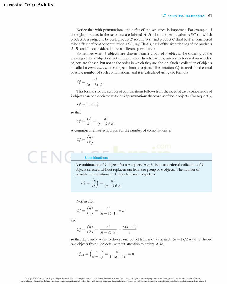
Hayter-15125 book December 19, 2005 20:30
1.7 COUNTING TECHNIQUES 61
Notice that with permutations, the order of the sequence is important. For example, ifthe eight products in the taste test are labeled A–H , then the permutation ABC (in whichproduct A is judged to be best, product B second best, and product C third best) is consideredto be different from the permutation ACB, say. That is, each of the six orderings of the productsA, B, and C is considered to be a different permutation.
Sometimes when k objects are chosen from a group of n objects, the ordering of thedrawing of the k objects is not of importance. In other words, interest is focused on which kobjects are chosen, but not on the order in which they are chosen. Such a collection of objectsis called a combination of k objects from n objects. The notation Cn
k is used for the totalpossible number of such combinations, and it is calculated using the formula
Cnk = n!
(n − k)! k!
This formula for the number of combinations follows from the fact that each combination ofk objects can be associated with the k! permutations that consist of those objects. Consequently,
Pnk = k! × Cn
k
so that
Cnk = Pn
k
k!= n!
(n − k)! k!
A common alternative notation for the number of combinations is
Cnk =
(nk
)
Combinations
A combination of k objects from n objects (n ≥ k) is an unordered collection of kobjects selected without replacement from the group of n objects. The number ofpossible combinations of k objects from n objects is
Cnk =
(nk
)= n!
(n − k)! k!
Notice that
Cn1 =
(n1
)= n!
(n − 1)! 1!= n
and
Cn2 =
(n2
)= n!
(n − 2)! 2!= n(n − 1)
2
so that there are n ways to choose one object from n objects, and n(n − 1)/2 ways to choosetwo objects from n objects (without attention to order). Also,
Cnn−1 =
(n
n − 1
)= n!
1! (n − 1)!= n
Copyright 2010 Cengage Learning. All Rights Reserved. May not be copied, scanned, or duplicated, in whole or in part. Due to electronic rights, some third party content may be suppressed from the eBook and/or eChapter(s).Editorial review has deemed that any suppressed content does not materially affect the overall learning experience. Cengage Learning reserves the right to remove additional content at any time if subsequent rights restrictions require it.
Licensed to:

Hayter-15125 book December 19, 2005 20:30
62 CHAPTER 1 PROBABILITY THEORY
and
Cnn =
(nn
)= n!
0! n!= 1
This last equation just indicates that there is only one way to choose all n objects. It is alsouseful to note that Cn
k = Cnn−k .
Example 11Taste Tests
Suppose that in the taste test, each participant samples eight products and is asked to selectthe three best products, but not in any particular order. The number of possible answers to thetest is then(
83
)= 8!
5! 3!= 8 × 7 × 6
3 × 2 × 1= 56
Example 2Defective Computer
Chips
Suppose again that 9 out of 500 chips in a particular box are defective, and that 3 chips aresampled at random from the box without replacement. The total number of possible samplesis (
5003
)= 500!
497! 3!= 500 × 499 × 498
3 × 2 × 1= 20,708,500
which are all equally likely.The probability of choosing 3 defective chips can be calculated by dividing the number
of samples that contain 3 defective chips by the total number of samples. Since there are 9defective chips, the number of samples that contain 3 defective chips is(
93
)= 9!
6! 3!= 9 × 8 × 7
3 × 2 × 1= 84
so that the probability of choosing 3 defective chips is(
93
)(
5003
) =
(9!
6! 3!
)(
500!
497! 3!
) = 9 × 8 × 7
500 × 499 × 498 4.0 × 10⁻⁶
as obtained before.Also, the number of samples that contains exactly 1 defective chip is
9 ×(
4912
)
since there are 9 ways to choose the defective chip and C4912 ways to choose the 2 satisfactory
chips. Consequently, the probability of obtaining exactly 1 defective chip is
9 ×(
4912
)(
5003
) =
(9 × 491!
489! 2!
)(
500!
497! 3!
) = 9 × 491 × 490 × 3
500 × 499 × 498= 0.0522
as obtained before. These calculations are examples of the hypergeometric distribution that isdiscussed in Section 3.3.
Copyright 2010 Cengage Learning. All Rights Reserved. May not be copied, scanned, or duplicated, in whole or in part. Due to electronic rights, some third party content may be suppressed from the eBook and/or eChapter(s).Editorial review has deemed that any suppressed content does not materially affect the overall learning experience. Cengage Learning reserves the right to remove additional content at any time if subsequent rights restrictions require it.
Licensed to:

Hayter-15125 book December 19, 2005 20:30
1.7 COUNTING TECHNIQUES 63
GAMES OF CHANCE Suppose that four cards are taken at random without replacement from a pack of cards. Whatis the probability that two Kings and two Queens are chosen?
The number of ways to choose four cards is(524
)= 52!
48! 4!= 52 × 51 × 50 × 49
4 × 3 × 2 × 1= 270,725
The number of ways of choosing two Kings from the four Kings in the pack as well as thenumber of ways of choosing two Queens from the four Queens in the pack is(
42
)= 4!
2! 2!= 4 × 3
2 × 1= 6
so that the number of hands consisting of two Kings and two Queens is(42
)×
(42
)= 36
The required probability is thus
36
270,725 1.33 × 10⁻⁴
which is a chance of about 13 out of 100,000.
1.7.3 Problems
1.7.1 Evaluate:(a) 7! (b) 8! (c) 4! (d) 13!
1.7.2 Evaluate:(a) P7
2 (b) P95 (c) P5
2 (d) P174
1.7.3 Evaluate:(a) C6
2 (b) C84 (c) C5
2 (d) C146
1.7.4 A menu has five appetizers, three soups, seven maincourses, six salad dressings, and eight desserts. In howmany ways can a full meal be chosen? In how many wayscan a meal be chosen if either an appetizer or a soup isordered, but not both?
1.7.5 In an experiment to test iron strengths, three differentores, four different furnace temperatures, and twodifferent cooling methods are to be considered.Altogether, how many experimental configurations arepossible?
1.7.6 Four players compete in a tournament and are rankedfrom 1 to 4. They then compete in another tournamentand are again ranked from 1 to 4. Suppose that theirperformances in the second tournament are unrelated totheir performances in the first tournament, so that the twosets of rankings are independent.(a) What is the probability that each competitor receives
an identical ranking in the two tournaments?
(b) What is the probability that nobody receives the sameranking twice?
1.7.7 Twenty players compete in a tournament. In howmany ways can rankings be assigned to the top fivecompetitors? In how many ways can the best fivecompetitors be chosen (without being in any order)?
1.7.8 There are 17 broken lightbulbs in a box of 100 lightbulbs.A random sample of 3 lightbulbs is chosen withoutreplacement.(a) How many ways are there to choose the sample?(b) How many samples contain no broken lightbulbs?(c) What is the probability that the sample contains no
broken lightbulbs?(d) How many samples contain exactly 1 broken
lightbulb?(e) What is the probability that the sample contains no
more than 1 broken lightbulb?
1.7.9 Show that Cnk = Cn−1
k + Cn−1k−1 . Can you provide an
interpretation of this equality?
1.7.10 A poker hand consists of five cards chosen at randomfrom a pack of cards.(a) How many different hands are there?(b) How many hands consist of all hearts?
Copyright 2010 Cengage Learning. All Rights Reserved. May not be copied, scanned, or duplicated, in whole or in part. Due to electronic rights, some third party content may be suppressed from the eBook and/or eChapter(s).Editorial review has deemed that any suppressed content does not materially affect the overall learning experience. Cengage Learning reserves the right to remove additional content at any time if subsequent rights restrictions require it.
Licensed to:
Hayter-15125 book December 19, 2005 20:30
64 CHAPTER 1 PROBABILITY THEORY
(c) How many hands consist of cards all from the samesuit (a “flush”)?
(d) What is the probability of being dealt a flush?(e) How many hands contain all four Aces?(f) How many hands contain four cards of the same
number or picture?(g) What is the probability of being dealt a hand
containing four cards of the same number or picture?
1.7.11 In an arrangement of n objects in a circle, an object’sneighbors are important, but an object’s place in the circleis not important. Thus, rotations of a given arrangementare considered to be the same arrangement. Explain whythe number of different arrangements is (n − 1)!
1.7.12 In how many ways can six people sit in six seats in a lineat a cinema? In how many ways can the six people sitaround a dinner table eating pizza after the movie?
1.7.13 Repeat Problem 1.7.12 with the condition that one of thesix people, Andrea, must sit next to Scott. In how manyways can the seating arrangements be made if Andrearefuses to sit next to Scott?
1.7.14 A total of n balls are to be put into k boxes with theconditions that there will be n1 balls in box 1, n2 balls inbox 2, and so on, with nk balls being placed in box k(n1 + · · · + nk = n). Explain why the number of ways ofdoing this is
n!
n1! × · · · × nk!
Explain why this is just Cnn1
= Cnn2
when k = 2.
1.7.15 Explain why the following two problems are identical andsolve them.(a) In how many ways can 12 balls be placed in 3 boxes,
when the first box can hold 3 balls, the second boxcan hold 4 balls, and the third box can hold 5 balls.
(b) In how many ways can 3 red balls, 4 blue balls, and 5green balls be placed in a straight line?
(See Problem 1.7.14.)
1.7.16 A garage employs 14 mechanics, of whom 3 are neededon one job and, at the same time, 4 are needed on another
job. The remaining 7 are to be kept in reserve. In howmany ways can the job assignments be made?(See Problem 1.7.14.)
1.7.17 A company has 15 applicants to interview, and 3 are to beinvited on each day of the working week. In how manyways can the applicants be scheduled?(See Problem 1.7.14.)
1.7.18 A quality inspector selects a sample of 12 items atrandom from a collection of 60 items, of which 18 haveexcellent quality, 25 have good quality, 12 have poorquality, and 5 are defective.(a) What is the probability that the sample only contains
items that have either excellent or good quality?(b) What is the probability that the sample contains three
items of excellent quality, three items of good quality,three items of poor quality, and three defective items?
1.7.19 A salesman has to visit 10 different cities. In how manydifferent ways can the ordering of the visits be made? Ifhe decides that 5 of the visits will be made one week, andthe other 5 visits will be made the following week, in howmany different ways can the 10 cities be split into twogroups of 5 cities?
1.7.20 Suppose that 5 cards are taken without replacement froma deck of 52 cards. How many ways are there to do this sothat there are 2 red cards and 3 black cards?
1.7.21 A hand of 8 cards is chosen at random from an ordinarydeck of 52 playing cards without replacement.(a) What is the probability that the hand does not have
any hearts?(b) What is the probability that the hand consists of two
hearts, two diamonds, two clubs, and two spades?
1.7.22 A box contains 40 batteries, 5 of which have lowlifetimes, 30 of which have average lifetimes, and 5 ofwhich have high lifetimes. A consumer requires 8batteries to run an appliance and randomly selects themall from the box. What is the probability that among the8 batteries fitted into the consumer’s appliance, there areexactly 2 low, 4 average and 2 high lifetimes batteries?
1.8 Case Study: Microelectronic Solder Joints
Suppose that using a particular production method there is a probability of 0.85 that a solderjoint has a barrel shape, there is a probability of 0.03 that a solder joint has a cylinder shape,and there is a probability of 0.12 that a solder joint has an hourglass shape. If it is knownthat a particular solder joint does not have a barrel shape, what is the probability that it has a
Copyright 2010 Cengage Learning. All Rights Reserved. May not be copied, scanned, or duplicated, in whole or in part. Due to electronic rights, some third party content may be suppressed from the eBook and/or eChapter(s).Editorial review has deemed that any suppressed content does not materially affect the overall learning experience. Cengage Learning reserves the right to remove additional content at any time if subsequent rights restrictions require it.
Licensed to:

Hayter-15125 book December 19, 2005 20:30
1.8 CASE STUDY: MICROELECTRONIC SOLDER JOINTS 65
cylinder shape? This is a conditional probability that can be calculated as
P(cylinder|not barrel) = P(cylinder and not barrel)
P(not barrel)= P(cylinder)
P(cylinder) + P(hourglass)
= 0.03
0.03 + 0.12= 0.2
Furthermore, suppose that after a certain number of temperature cycles in an acceleratedlife test there is a probability of 0.002 that a solder joint is cracked if it has a barrel shape, thereis a probability of 0.004 that a solder joint is cracked if it has a cylinder shape, and there is aprobability of 0.005 that a solder joint is cracked if it has an hourglass shape. This informationcan be represented by the conditional probabilities shown in Figure 1.73.
If a solder joint is known to be cracked, Bayes’ theorem can be used to calculate theprobabilities of it having each of the three shapes. For example, the probability that it has abarrel shape is
P(barrel|cracked)
= P(barrel)P(cracked|barrel)(P(barrel)P(cracked|barrel) + P(cylinder)P(cracked|cylinder)
+P(hourglass)P(cracked|hourglass)
)
= 0.85 × 0.002
(0.85 × 0.002) + (0.03 × 0.004) + (0.12 × 0.005)= 0.70248
Similarly, if a solder joint is known not to be cracked, then Bayes’ theorem can be used tocalculate the probability that it has a cylinder shape, for example, as
P(cylinder|not cracked)
= P(cylinder)P(not cracked|cylinder)(P(barrel)P(not cracked|barrel) + P(cylinder)P(not cracked|cylinder)
+P(hourglass)P(not cracked|hourglass)
)
= 0.03 × 0.996
(0.85 × 0.998) + (0.03 × 0.996) + (0.12 × 0.995)= 0.02995
Figure 1.74 shows all of the shape probabilities conditional on whether the solder joint isknown to be cracked or not cracked. Notice that the probabilities in each column sum to one,and that whereas the knowledge that the solder joint is not cracked has little effect on theshape probabilities, the knowledge that the solder joint is cracked (which is a considerablyrarer event) has much more effect on the shape probabilities.
FIGURE 1.73
Conditional probabilities ofcracking for solder joints
P(cracked|barrel) = 0.002 P(not cracked|barrel) = 0.998
P(cracked|cylinder) = 0.004 P(not cracked|cylinder) = 0.996
P(cracked|hourglass) = 0.005 P(not cracked|hourglass) = 0.995
FIGURE 1.74
Shape probabilities conditional onwhether the solder joint is cracked
or not
No information on whether Solder joint Solder jointthe solder joint is is known to be is known not to becracked or not cracked cracked
P(barrel) = 0.85 P(barrel|cracked) = 0.70248 P(barrel|not cracked) = 0.85036
P(cylinder) = 0.03 P(cylinder|cracked) = 0.04959 P(cylinder|not cracked) = 0.02995
P(hourglass) = 0.12 P(hourglass|cracked) = 0.24793 P(hourglass|not cracked) = 0.11969
Copyright 2010 Cengage Learning. All Rights Reserved. May not be copied, scanned, or duplicated, in whole or in part. Due to electronic rights, some third party content may be suppressed from the eBook and/or eChapter(s).Editorial review has deemed that any suppressed content does not materially affect the overall learning experience. Cengage Learning reserves the right to remove additional content at any time if subsequent rights restrictions require it.
Licensed to:

Hayter-15125 book December 19, 2005 20:30
66 CHAPTER 1 PROBABILITY THEORY
Finally, suppose that an assembly consists of 16 solder joints and that unknown to theresearcher 5 of these solder joints are cracked. If the researcher randomly chooses a sampleof 4 of the solder joints for inspection, then the state space of the number of cracked joints inthe sample is {0, 1, 2, 3, 4}. The total number of different samples that can be chosen is(
164
)= 16!
12!4!= 1820
and the probability that there will be exactly two cracked solder joints in the researcher’ssample is(
52
)×
(112
)(
164
) = 10 × 55
1820= 0.302
This hypergeometric distribution is discussed more comprehensively in Section 3.3.
1.9 Supplementary Problems
1.9.1 What is the sample space for the average score of twodice?
1.9.2 What is the sample space when a winner and a runner-upare chosen in a tournament with four contestants.
1.9.3 A biased coin is known to have a greater probability ofrecording a head than a tail. How can it be used todetermine fairly which team in a football game has thechoice of kick-off?
1.9.4 If two fair dice are thrown, what is the probability thattheir two scores differ by no more than one?
1.9.5 If a card is chosen at random from a pack of cards, whatis the probability of choosing a diamond picture card?
1.9.6 Two cards are drawn from a pack of cards. Is it morelikely that two hearts will be drawn when the drawing iswith replacement or without replacement?
1.9.7 Two fair dice are thrown. A is the event that the sum ofthe scores is no larger than 4, and B is the event that thetwo scores are identical. Calculate the probabilities:(a) A ∩ B (b) A ∪ B (c) A′ ∪ B
1.9.8 Two fair dice are thrown, one red and one blue. Calculate:(a) P(red die is 5|sum of scores is 8)
(b) P(either die is 5|sum of scores is 8)
(c) P(sum of scores is 8|either die is 5)
1.9.9 Consider the network shown in Figure 1.75 withfive switches. Suppose that the switches operateindependently and that each switch allows a messagethrough with a probability of 0.85. What is the probabilitythat a message will find a route through the network?
1.9.10 Which is more likely: obtaining at least one head in twotosses of a fair coin, or at least two heads in four tosses ofa fair coin?
FIGURE 1.75
Switch diagram1 2
3
?
4 5
0.85 0.85
0.85
0.85
0.85
Copyright 2010 Cengage Learning. All Rights Reserved. May not be copied, scanned, or duplicated, in whole or in part. Due to electronic rights, some third party content may be suppressed from the eBook and/or eChapter(s).Editorial review has deemed that any suppressed content does not materially affect the overall learning experience. Cengage Learning reserves the right to remove additional content at any time if subsequent rights restrictions require it.
Licensed to:

Hayter-15125 book December 19, 2005 20:30
1.9 SUPPLEMENTARY PROBLEMS 67
1.9.11 Bag 1 contains 6 red balls, 7 blue balls, and 3 green balls.Bag 2 contains 8 red balls, 8 blue balls, and 2 green balls.Bag 3 contains 2 red balls, 9 blue balls, and 8 green balls.Bag 4 contains 4 red balls, 7 blue balls, and no green balls.Bag 1 is chosen with a probability of 0.15, bag 2 with aprobability of 0.20, bag 3 with a probability of 0.35, andbag 4 with a probability of 0.30, and then a ball is chosenat random from the bag. Calculate the probabilities:(a) A blue ball is chosen(b) Bag 4 was chosen if the ball is green(c) Bag 1 was chosen if the ball is blue
1.9.12 A fair die is rolled. If an even number is obtained, thenthat is the recorded score. However, if an odd number isobtained, then a fair coin is tossed. If a head is obtained,then the recorded score is the number on the die, but if atail is obtained, then the recorded score is twice thenumber on the die.(a) Give the possible values of the recorded score.(b) What is the probability that a score of 10 is recorded?(c) What is the probability that a score of 3 is recorded?(d) What is the probability that a score of 6 is recorded?(e) What is the probability that a score of 4 is recorded if
it is known that the coin is tossed?(f) If a score of 6 is recorded, what is the probability that
an odd number was obtained on the die?
1.9.13 How many sequences of length 4 can be made when eachcomponent of the sequence can take 5 different values?How many sequences of length 5 can be made when eachcomponent of the sequence can take 4 different values? Ingeneral, if 3 ≤ n1 < n2, are there more sequences oflength n1 with n2 possible values for each component, ormore sequences of length n2 with n1 possible values foreach component?
1.9.14 Twenty copying jobs need to be done. If there are fourcopy machines, in how many ways can five jobs beassigned to each of the four machines? If an additionalcopier is used, in how many ways can four jobs beassigned to each of the five machines?
1.9.15 A bag contains two counters with each independentlyequally likely to be either black or white. What is thedistribution of X , the number of white counters in thebag? Suppose that a white counter is added to the bag andthen one of the three counters is selected at random andtaken out of the bag. What is the distribution of Xconditional on the counter taken out being white? What ifthe counter taken out of the bag is black?
1.9.16 It is found that 28% of orders received by a company arefrom first-time customers, with the other 72% comingfrom repeat customers. In addition, 75% of the ordersfrom first-time customers are dispatched within one day,and overall 30% of the company’s orders are from repeatcustomers whose orders are not dispatched withinone day. If an order is dispatched within one day, what isthe probability that it was for a first-time customer?
1.9.17 When asked to select their favorite opera work, 26% ofthe respondents selected a piece by Puccini, and 22%of the respondents selected a piece by Verdi. Moreover,59% of the respondents who selected a piece by Pucciniwere female, and 45% of the respondents who selected apiece by Verdi were female. Altogether, 62% of therespondents were female.(a) If a respondent selected a piece that is by neither
Puccini nor Verdi, what is the probability that therespondent is female?
(b) What proportion of males selected a piece by Puccini?
1.9.18 A random sample of 10 fibers is taken from a collectionof 92 fibers that consists of 43 fibers of polymer A,17 fibers of polymer B, and 32 fibers of polymer C.(a) What is the probability that the sample does not
contain any fibers of polymer B?(b) What is the probability that the sample contains
exactly one fiber of polymer B?(c) What is the probability that the sample contains three
fibers of polymer A, three fibers of polymer B, andfour fibers of polymer C?
1.9.19 A fair coin is tossed five times. What is the probabilitythat there is not a sequence of three outcomes of the samekind?
1.9.20 Consider telephone calls made to a company’s complaintline. Let A be the event that the call is answered within10 seconds. Let B be the event that the call is answeredby one of the company’s experienced telephoneoperators. Let C be the event that the call lasts less than5 minutes. Let D be the event that the complaint ishandled successfully by the telephone operator. Describethe following events.(a) B ∩ C ′ (b) (A ∪ B ′) ∩ D(c) A′ ∩ C ′ ∩ D′ (d) (A ∩ C) ∪ (B ∩ D)
1.9.21 A manager has 20 different job orders, of which 7 mustbe assigned to production line I, 7 must be assigned toproduction line II, and 6 must be assigned to productionline III.
Copyright 2010 Cengage Learning. All Rights Reserved. May not be copied, scanned, or duplicated, in whole or in part. Due to electronic rights, some third party content may be suppressed from the eBook and/or eChapter(s).Editorial review has deemed that any suppressed content does not materially affect the overall learning experience. Cengage Learning reserves the right to remove additional content at any time if subsequent rights restrictions require it.
Licensed to:

Hayter-15125 book December 19, 2005 20:30
68 CHAPTER 1 PROBABILITY THEORY
(a) In how many ways can the assignments be made?(b) If the first job and the second job must be assigned to
the same production line, in how many ways can theassignments be made?
(c) If the first job and the second job cannot be assignedto the same production line, in how many ways canthe assignments be made?
1.9.22 A hand of 3 cards (without replacement) is chosen atrandom from an ordinary deck of 52 playing cards.(a) What is the probability that the hand contains only
diamonds?(b) What is the probability that the hand contains one
Ace, one King, and one Queen?
1.9.23 A hand of 4 cards (without replacement) is chosenat random from an ordinary deck of 52 playing cards.(a) What is the probability that the hand does not have
any Aces?(b) What is the probability that the hand has exactly one
Ace?Suppose now that the 4 cards are taken withreplacement.
(c) What is the probability that the same card is obtainedfour times?
1.9.24 Are the following statements true or false?(a) If a fair coin is tossed three times, the probability of
obtaining two heads and one tail is the same as theprobability of obtaining one head and two tails.
(b) If a card is drawn at random from a deck of cards,the probability that it is a heart increases if it isconditioned on the knowledge that it is an Ace.
(c) The number of ways of choosing five different lettersfrom the alphabet is more than the number of secondsin a year.
(d) If two events are independent, then the probabilitythat they both occur can be calculated by multiplyingtheir individual probabilities.
(e) It is always true that P(A|B) + P(A′|B) = 1.(f) It is always true that P(A|B) + P(A|B ′) = 1.(g) It is always true that P(A|B) ≤ P(A).
1.9.25 There is a probability of 0.55 that a soccer team will wina game. There is also a probability of 0.85 that the soccerteam will not have a player sent off in the game. However,if the soccer team does not have a player sent off, thenthere is a probability of 0.60 that the team will win thegame. What is the probability that the team has a playersent off but still wins the game?
1.9.26 A warehouse contains 500 machines. Each machine iseither new or used, and each machine has either goodquality or bad quality. There are 120 new machines thathave bad quality. There are 230 used machines. Supposethat a machine is chosen at random, with each machinebeing equally likely to be chosen.(a) What is the probability that the chosen machine is a
new machine with good quality?(b) If the chosen machine is new, what is the probability
that it has good quality?
1.9.27 A class has 250 students, 113 of whom are male, and 167of whom are mechanical engineers. There are 52 femalestudents who are not mechanical engineers. There are19 female mechanical engineers who are seniors.(a) If a randomly chosen student is not a mechanical
engineer, what is the probability that the student is amale?
(b) If a randomly chosen student is a female mechanicalengineer, what is the probability that the student is asenior?
1.9.28 A business tax form is either filed on time or late, is eitherfrom a small or a large business, and is either accurate orinaccurate. There is an 11% probability that a form isfrom a small business and is accurate and on time. Thereis a 13% probability that a form is from a small businessand is accurate but is late. There is a 15% probability thata form is from a small business and is on time. There is a21% probability that a form is from a small business andis inaccurate and is late.(a) If a form is from a small business and is accurate,
what is the probability that it was filed on time?(b) What is the probability that a form is from a large
business?
1.9.29 (a) If four cards are taken at random from a pack of cardswithout replacement, what is the probability ofhaving exactly two hearts?
(b) If four cards are taken at random from a pack of cardswithout replacement, what is the probability ofhaving exactly two hearts and exactly two clubs?
(c) If four cards are taken at random from a pack of cardswithout replacement and it is known that there are noclubs, what is the probability that there are exactlythree hearts?
1.9.30 An applicant has a 0.26 probability of passing a test whenthey take it for the first time, and if they pass it they canmove on to the next stage. However, if they fail the test
Copyright 2010 Cengage Learning. All Rights Reserved. May not be copied, scanned, or duplicated, in whole or in part. Due to electronic rights, some third party content may be suppressed from the eBook and/or eChapter(s).Editorial review has deemed that any suppressed content does not materially affect the overall learning experience. Cengage Learning reserves the right to remove additional content at any time if subsequent rights restrictions require it.
Licensed to:

Hayter-15125 book December 19, 2005 20:30
1.9 SUPPLEMENTARY PROBLEMS 69
the first time, they must take the test a second time, andwhen an applicant takes the test for the second time thereis a 0.43 chance that they will pass and be allowed tomove on to the next stage. The applicant is rejected if thetest is failed on the second attempt.(a) What is the probability that an applicant moves on to
the next stage but needs two attempts at the test?(b) What is the probability that an applicant moves on to
the next stage?(c) If an applicant moves on to the next stage, what is the
probability that they passed the test on the firstattempt?
1.9.31 A fair die is rolled five times. What is the probabilitythat the first score is strictly larger than the second scorewhich is strictly larger than the third score which isstrictly larger than the fourth score which is strictly largerthan the fifth score (i.e., the five scores are strictlydecreasing).
1.9.32 A software engineer makes two backup copies of his file,one on a CD and another on a diskette. Suppose that thereis a probability of 0.05% that the file is corrupted when itis backed-up onto the CD, and a probability of 0.1% thatthe file is corrupted when it is backed-up onto thediskette, and that these events are independent of eachother. What is the probability that the engineer will haveat least one uncorrupted copy of the file?
1.9.33 A warning light in the cockpit of a plane is supposed toindicate when a hydraulic pump is inoperative. If thepump is inoperative, then there is a probability of 0.992that the warning light will come on. However, there is a
probability of 0.003 that the warning light will come oneven when the pump is operating correctly. Furthermore,there is a probability of 0.996 that the pump is operatingcorrectly. If the warning light comes on, what is theprobability that the pump really is inoperative?
1.9.34 A hand of 10 cards is chosen at random withoutreplacement from a deck of 52 cards. What is theprobability that the hand contains exactly 2 Aces, 2Kings, 3 Queens, and 3 Jacks?
1.9.35 There are 11 items of a product on a shelf in a retailoutlet, and unknown to the customers, 4 of the items areoverage. Suppose that a customer takes 3 items at random.(a) What is the probability that none of the overage
products are selected by the customer?(b) What is the probability that exactly 2 of the items
taken by the customer are overage?
1.9.36 Among those people who are infected with a certainvirus, 32% have strain A, 59% have strain B, and theremaining 9% have strain C. Furthermore, 21% of peopleinfected with strain A of the virus exhibit symptoms, 16%of people infected with strain B of the virus exhibitsymptoms, and 63% of people infected with strain C ofthe virus exhibit symptoms.(a) If a person has the virus and exhibits symptoms of it,
what is the probability that they have strain C?(b) If a person has the virus but doesn’t exhibit any
symptoms of it, what is the probability that they havestrain A?
(c) What is the probability that a person who has thevirus does not exhibit any symptoms of it?
“When solving mysteries like this one, it’s always a question of prior probabilitiesand posterior probabilities.” (From Inspector Morimoto and the Two Umbrellas,by Timothy Hemion)
Copyright 2010 Cengage Learning. All Rights Reserved. May not be copied, scanned, or duplicated, in whole or in part. Due to electronic rights, some third party content may be suppressed from the eBook and/or eChapter(s).Editorial review has deemed that any suppressed content does not materially affect the overall learning experience. Cengage Learning reserves the right to remove additional content at any time if subsequent rights restrictions require it.
Licensed to:

Hayter-15125 book December 22, 2005 13:39
A N S WERS TO OD D-N U MB ERED PROB LEMS
Chapter 1 Probability Theory
1.1 Probabilities1.1.1 S = {(head, head, head), (head, head, tail), (head, tail, head),
(head, tail, tail), (tail, head, head), (tail, head, tail), (tail, tail,head), (tail, tail, tail)}
1.1.3 S = {0,1,2,3,4}
1.1.5 S = {(on time, satisfactory), (on time, unsatisfactory), (late,satisfactory), (late, unsatisfactory)}
1.1.7 (a) p = 0.5 (b) p = 23 (c) 1
3
1.1.9 0 ≤ P(V ) ≤ 0.39 P(I V ) = P(V ) = 0.195
1.2 Events1.2.1 (a) P(b) = 0.15 (b) P(A) = 0.50 (c) P(A′) = 0.50
1.2.3 1241461 and 113
1461
1.2.5 P(at least one score is a prime number) = 89
P(neither score prime) = 19
1.2.7 P(♠ or ♣) = 12
1.2.9 (a) P(Terica is winner) = 14
(b) P(Terica is winner or runner up) = 12
1.2.11 (a) P(both assembly lines are shut down) = 0.02(b) P(neither assembly line is shut down) = 0.74(c) P(at least one assembly line is at full capacity) = 0.71(d) P(exactly one assembly line at full capacity) = 0.52The complement of “neither assembly line is shut down” consistsof the outcomes
{(S, S), (S, P), (S, F), (P, S), (F, S)}.The complement of “at least one assembly line is at full capac-ity” consists of the outcomes
{(S, S), (S, P), (P, S), (P, P)}.
1.3 Combinations of Events1.3.1 The event A contains the outcome 0 while the empty set does not
contain any outcomes.
1.3.5 Yes No
1.3.7 P(B) = 0.4
1.3.9 YesP(A ∪ B ∪ C) = 3
4
1.3.11 P(O ′ ∩ S′) = 0.11
1.3.13 0.19
1.4 Conditional Probability
1.4.1 (a) P(A | B) = 0.1739 (b) P(C | A) = 0.59375(c) P(B | A ∩ B) = 1 (d) P(B | A ∪ B) = 0.657(e) P(A | A ∪ B ∪ C) = 0.3636(f) P(A ∩ B | A ∪ B) = 0.1143
1.4.3 (a) P(A♥ | red suit) = 126 (b) P(heart | red suit) = 1
2
(c) P(red suit | heart) = 1 (d) P(heart | black suit) = 0(e) P(King | red suit) = 1
13(f) P(King | red picture card) = 1
3
1.4.5 P(shiny | red) = 38
P(dull | red) = 58
1.4.9 (a) 0.512 (b) 0.619(c) 0 (d) 0.081
1.4.11 (a) 0.9326 (b) 0.9756
1.4.13 (a) 0.02 (b) 0.775
1.4.15 P(delay) = 0.3568
781
Copyright 2010 Cengage Learning. All Rights Reserved. May not be copied, scanned, or duplicated, in whole or in part. Due to electronic rights, some third party content may be suppressed from the eBook and/or eChapter(s).Editorial review has deemed that any suppressed content does not materially affect the overall learning experience. Cengage Learning reserves the right to remove additional content at any time if subsequent rights restrictions require it.
Licensed to:

Hayter-15125 book December 22, 2005 13:39
782 ANSWERS TO ODD-NUMBERED PROBLEMS
1.5 Probabilities of Event Intersections1.5.1 (a) P(both cards are picture cards) = 132
2652
(b) P(both cards are from red suits) = 6502652
(c) P(one card is from a red suit and one is fromblack suit) = 26
51
1.5.3 (a) No, they are not independent.(b) Yes, they are independent.(c) No, they are not independent.(d) Yes, they are independent.(e) No, they are not independent.
1.5.5 P(all 4 cards are hearts) = 1256
P(all 4 cards are from red suits) = 116
P(all 4 cards from different suits) = 332
1.5.7 P(message gets through the network) = 0.98096
1.5.9 P(no broken bulbs) = 0.5682P(no more than one broken bulb in the sample) = 0.9260
1.5.11 P(drawing 2 green balls) = 0.180P(two balls different colors) = 0.656
1.5.13 p = 0.5 (a fair coin)
1.5.15 (a) 132 (b) 5
9
(c) 38 (d) 13
34
1.6 Posterior Probabilities1.6.1 (a) P(positive blood test) = 0.0691
(b) P(disease | positive blood test) = 0.1404(c) P(no disease | negative blood test) = 0.9997
1.6.3 (a) P(Section I) = 55100 (b) P(grade is A) = 21
100
(c) P(A | Section I) = 1055 (d) P(Section I | A) = 10
21
1.6.5 (a) 0.4579(b) P(A | did not fail) = 0.7932
1.6.7 (a) P(H | L) == 0.224(b) P(M | L ′) = 0.551
1.7 Counting Techniques
1.7.1 (a) 7! = 5040(b) 8! = 40320(c) 4! = 24(d) 13! = 6, 227, 020, 800
1.7.3 (a) C62 == 15 (b) C8
4 = 70
(c) C52 = 10 (d) C14
6 = 3003
1.7.5 24
1.7.7 1,860,48015504
1.7.13 4872
1.7.15 (a) 27720
1.7.17 168,168,000
1.7.19 3,628,800252
1.7.21 (a) 0.082(b) 0.049
Copyright 2010 Cengage Learning. All Rights Reserved. May not be copied, scanned, or duplicated, in whole or in part. Due to electronic rights, some third party content may be suppressed from the eBook and/or eChapter(s).Editorial review has deemed that any suppressed content does not materially affect the overall learning experience. Cengage Learning reserves the right to remove additional content at any time if subsequent rights restrictions require it.
This page contains answers for this chapter only.


![[Solutions Manual] Probability and Statistics for Engineers and Scientists](https://img.pdfslide.us/doc/110x75/577cc74d1a28aba711a0975e/solutions-manual-probability-and-statistics-for-engineers-and-scientists-578fc6514c0c9.jpg)