Probability and inferenceRandom variables

IPS chapters 4.3 and 4.4

© 2006 W.H. Freeman and Company

Objectives (IPS chapters 4.3 and 4.4)Random variables

Discrete random variables

Continuous random variables

Normal probability distributions

Mean of a random variable

Law of large numbers

Variance of a random variable

Discrete random variables

A random variable is a variable whose value is a numerical outcome

of a random phenomenon.

A basketball player shoots three free throws. We define the random

variable X as the number of baskets successfully made.

A discrete random variable X has a finite number of possible values.

A basketball player shoots three free throws. The number of baskets

successfully made is a discrete random variable (X). X can only take the

values 0, 1, 2, or 3.

The probability distribution of a

random variable X lists the values

and their probabilities:

Requirements of a Discrete Random Variable

The probabilities pi must add up to 1.

Every probability pi is a number between 0 and 1.

Value of X 0 1 2 3

Probability 1/8 3/8 3/8 1/8H

H

H - HHH

M …

M

M - HHM

H - HMH

M - HMM

…

HMM HHMMHM HMH

MMM MMH MHH HHH

A basketball player shoots three free throws. The random variable X is the

number of baskets successfully made.

The probability of any event is the sum of the probabilities pi of the

values of X that make up the event.

A basketball player shoots three free throws. The random variable X is the

number of baskets successfully made.

Value of X 0 1 2 3

Probability 1/8 3/8 3/8 1/8

HMM HHMMHM HMH

MMM MMH MHH HHH

What is the probability that the player

successfully makes at least two

baskets (“at least two” means “two or

more”)?P(X≥2) = P(X=2) + P(X=3) = 3/8 + 1/8 = 1/2

What is the probability that the player successfully makes fewer than three

baskets?

P(X<3) = P(X=0) + P(X=1) + P(X=2) = 1/8 + 3/8 + 3/8 = 7/8 or

P(X<3) = 1 – P(X=3) = 1 – 1/8 = 7/8

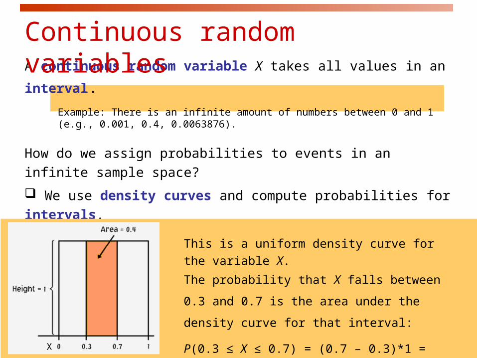
A continuous random variable X takes all values in an interval.

Example: There is an infinite amount of numbers between 0 and 1 (e.g., 0.001, 0.4, 0.0063876).

How do we assign probabilities to events in an infinite sample space?

We use density curves and compute probabilities for intervals.

The probability of any event is the area under the density curve for the

values of X that make up the event.

Continuous random variables

The probability that X falls between 0.3 and 0.7 is

the area under the density curve for that interval:

P(0.3 ≤ X ≤ 0.7) = (0.7 – 0.3)*1 = 0.4

This is a uniform density curve for the variable X.

X

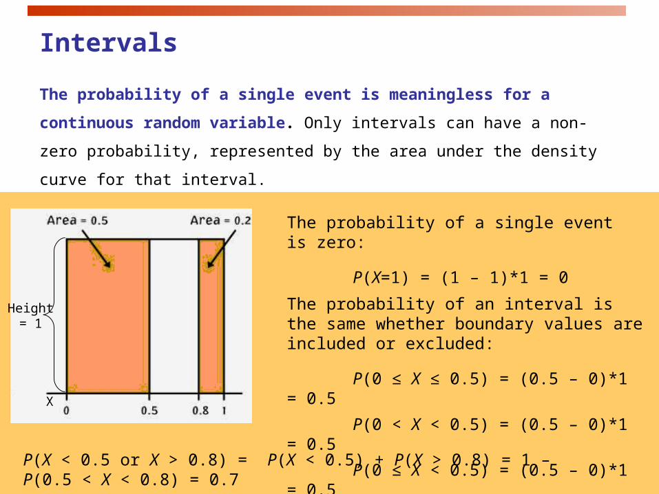
P(X < 0.5 or X > 0.8) = P(X < 0.5) + P(X > 0.8) = 1 – P(0.5 < X < 0.8) = 0.7

The probability of a single event is zero:

P(X=1) = (1 – 1)*1 = 0

Intervals

The probability of a single event is meaningless for a continuous

random variable. Only intervals can have a non-zero probability,

represented by the area under the density curve for that interval.

Height= 1

X

The probability of an interval is the same whether boundary values are included or excluded:

P(0 ≤ X ≤ 0.5) = (0.5 – 0)*1 = 0.5

P(0 < X < 0.5) = (0.5 – 0)*1 = 0.5

P(0 ≤ X < 0.5) = (0.5 – 0)*1 = 0.5

We generate two random numbers between 0 and 1 and take Y to be their sum.

Y can take any value between 0 and 2. The density curve for Y is:

0 1 2

Height = 1. We know this because the

base = 2, and the area under the

curve has to equal 1 by definition.

The area of a triangle is

½ (base*height).

What is the probability that Y is < 1?

What is the probability that Y < 0.5?

0 1 20.5

0.25 0.50.125

0.125

1.5

Y

Because the probability of drawing

one individual at random

depends on the frequency of this

type of individual in the population,

the probability is also the shaded

area under the curve.

The shaded area under a density

curve shows the proportion, or %,

of individuals in a population with

values of X between x1 and x2.

% individuals with X such that x1 < X < x2

Continuous random variable and population distribution

The probability distribution of many random variables is a normal

distribution. It shows what values the random variable can take and is

used to assign probabilities to those values.

Example: Probability

distribution of women’s

heights.

Here since we chose a

woman randomly, her height,

X, is a random variable.

To calculate probabilities with the normal distribution, we will standardize the random variable (z score) and use Table A.

Normal probability distributions

We standardize normal data by calculating z-scores so that any

Normal curve N() can be transformed into the standard Normal curve

N(0,1).

Reminder: standardizing N()

N(0,1)

=>

z

x

N(64.5, 2.5)

Standardized height (no units)

)(

x

z

What is the probability, if we pick one woman at random, that her height will be

some value X? For instance, between 68 and 70 inches P(68 < X < 70)?

Because the woman is selected at random, X is a random variable.

As before, we calculate the z-scores for 68 and 70.

For x = 68",

For x = 70",

z(x )

4.15.2

)5.6468(

z

z(70 64.5)

2.52.2

The area under the curve for the interval [68" to 70"] is 0.9861 − 0.9192 = 0.0669.

Thus, the probability that a randomly chosen woman falls into this range is 6.69%.

P(68 < X < 70) = 6.69%

0.98610.9192

N(µ, ) = N(64.5, 2.5)

Inverse problem:

Your favorite chocolate bar is dark chocolate with whole hazelnuts.

The weight on the wrapping indicates 8 oz. Whole hazelnuts vary in weight, so

how can they guarantee you 8 oz. of your favorite treat? You are a bit skeptical...

To avoid customer complaints and

lawsuits, the manufacturer makes

sure that 98% of all chocolate bars

weigh 8 oz. or more.

The manufacturing process is

roughly normal and has a known

variability = 0.2 oz.

How should they calibrate the

machines to produce bars with a

mean such that P(x < 8 oz.) =

2%?

= ?x = 8 oz.

Lowest2%

= 0.2 oz.

How should they calibrate the machines to produce bars with a mean such that

P(x < 8 oz.) = 2%?

z(x )

x (z * ) . 41.8)2.0*05.2(8 oz

Here we know the area under the density curve (2% = 0.02) and we know x (8 oz.).

We want .

In table A we find that the z for a left area of 0.02 is roughly z = -2.05.

Thus, your favorite chocolate bar weighs, on average, 8.41 oz. Excellent!!!

= ?x = 8 oz.

Lowest2%

= 0.2 oz.

Mean of a random variable

The mean x bar of a set of observations is their arithmetic average.

The mean µ of a random variable X is a weighted average of the

possible values of X, reflecting the fact that all outcomes might not be

equally likely.

Value of X 0 1 2 3

Probability 1/8 3/8 3/8 1/8

HMM HHMMHM HMH

MMM MMH MHH HHH

A basketball player shoots three free throws. The random variable X is the

number of baskets successfully made (“H”).

The mean of a random variable X is also called expected value of X.

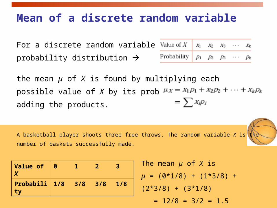
Mean of a discrete random variable

For a discrete random variable X with

probability distribution

the mean µ of X is found by multiplying each possible value of X by its

probability, and then adding the products.

Value of X 0 1 2 3

Probability 1/8 3/8 3/8 1/8

The mean µ of X is

µ = (0*1/8) + (1*3/8) + (2*3/8) + (3*1/8)

= 12/8 = 3/2 = 1.5

A basketball player shoots three free throws. The random variable X is the

number of baskets successfully made.

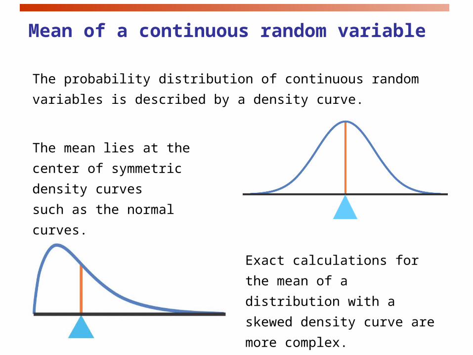
The probability distribution of continuous random variables is

described by a density curve.

Mean of a continuous random variable

The mean lies at the center of

symmetric density curves

such as the normal curves.

Exact calculations for the mean of

a distribution with a skewed

density curve are more complex.

Law of large numbers

As the number of randomly drawn

observations (n) in a sample

increases, the mean of the sample

(x bar) gets closer and closer to

the population mean .

This is the law of large numbers.

It is valid for any population.

Note: We often intuitively expect predictability over a few random observations,

but it is wrong. The law of large numbers only applies to really large numbers.

Variance of a random variable

The variance and the standard deviation are the measures of spread

that accompany the choice of the mean to measure center.

The variance σ2X of a random variable is a weighted average of the

squared deviations (X − µX)2 of the variable X from its mean µX. Each

outcome is weighted by its probability in order to take into account

outcomes that are not equally likely.

The larger the variance of X, the more scattered the values of X on

average. The positive square root of the variance gives the standard

deviation σ of X.

Variance of a discrete random variable

For a discrete random variable X

with probability distribution

and mean µX, the variance σ2 of X is found by multiplying each squared

deviation of X by its probability and then adding all the products.

Value of X 0 1 2 3

Probability 1/8 3/8 3/8 1/8

The variance σ2 of X is

σ2 = 1/8*(0−1.5)2 + 3/8*(1−1.5)2 + 3/8*(2−1.5)2 + 1/8*(3−1.5)2

= 2*(1/8*9/4) + 2*(3/8*1/4) = 24/32 = 3/4 = .75

A basketball player shoots three free throws. The random variable X is the

number of baskets successfully made.

µX = 1.5.

Calculation for means and variances

If X is a random variable and a and b are fixed numbers, then

µa+bX = a + bµX

σ2a+bX = b2σ2

X

If X and Y are two independent random variables, then

µX+Y = µX + µY

σ2X+Y = σ2

X + σ2Y

If X and Y are NOT independent but have correlation ρ, then

µX+Y = µX + µY

σ2X+Y = σ2

X + σ2Y + 2ρσXσY

Investment

You invest 20% of your funds in Treasury bills and 80% in an “index fund” that

represents all U.S. common stocks. Your rate of return over time is proportional

to that of the T-bills (X) and of the index fund (Y), such that R = 0.2X + 0.8Y.

Based on annual returns between 1950 and 2003:

Annual return on T-bills µX = 5.0% σX = 2.9%

Annual return on stocks µY = 13.2% σY = 17.6%

Correlation between X and Yρ = −0.11

µR = 0.2µX + 0.8µY = (0.2*5) + (0.8*13.2) = 11.56%

σ2R = σ2

0.2X + σ20.8Y + 2ρσ0.2Xσ0.8Y

= 0.2*2σ2X + 0.8*2σ2

Y + 2ρ*0.2*σX*0.8*σY

= (0.2)2(2.9)2 + (0.8)2(17.6)2 + (2)(−0.11)(0.2*2.9)(0.8*17.6) = 196.786

σR = √196.786 = 14.03%

The portfolio has a smaller mean return than an all-stock portfolio, but it is also

less risky.