Probabilistic Prediction of Well Performance4)/2015(6.4-09).pdfProbabilistic Prediction of Well Performance Ogbeide Paul Osaze1, Giegbefumwen Peter Uyi2 ... Arp’s model, exponential

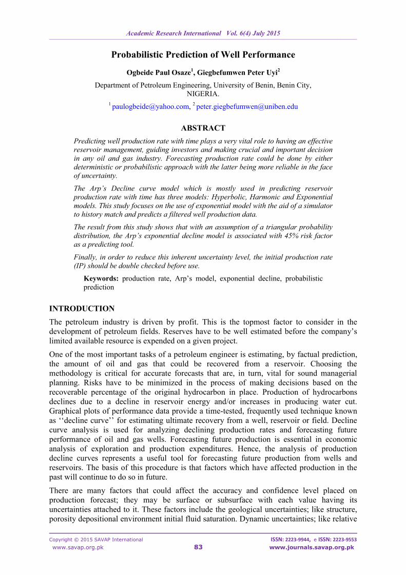
Academic Research International Vol. 6(4) July 2015

____________________________________________________________________________________________________________________________________________________________________________________________________________________________________________________________________________________________________________

Copyright © 2015 SAVAP International ISSN: 2223-9944, e ISSN: 2223-9553

www.savap.org.pk 83 www.journals.savap.org.pk

Probabilistic Prediction of Well Performance

Ogbeide Paul Osaze1, Giegbefumwen Peter Uyi

2

Department of Petroleum Engineering, University of Benin, Benin City,

NIGERIA.

1 [email protected],

2 [email protected]

ABSTRACT

Predicting well production rate with time plays a very vital role to having an effective

reservoir management, guiding investors and making crucial and important decision

in any oil and gas industry. Forecasting production rate could be done by either

deterministic or probabilistic approach with the latter being more reliable in the face

of uncertainty.

The Arp’s Decline curve model which is mostly used in predicting reservoir

production rate with time has three models: Hyperbolic, Harmonic and Exponential

models. This study focuses on the use of exponential model with the aid of a simulator

to history match and predicts a filtered well production data.

The result from this study shows that with an assumption of a triangular probability

distribution, the Arp’s exponential decline model is associated with 45% risk factor

as a predicting tool.

Finally, in order to reduce this inherent uncertainty level, the initial production rate

(IP) should be double checked before use.

Keywords: production rate, Arp’s model, exponential decline, probabilistic

prediction

INTRODUCTION

The petroleum industry is driven by profit. This is the topmost factor to consider in the

development of petroleum fields. Reserves have to be well estimated before the company’s

limited available resource is expended on a given project.

One of the most important tasks of a petroleum engineer is estimating, by factual prediction,

the amount of oil and gas that could be recovered from a reservoir. Choosing the

methodology is critical for accurate forecasts that are, in turn, vital for sound managerial

planning. Risks have to be minimized in the process of making decisions based on the

recoverable percentage of the original hydrocarbon in place. Production of hydrocarbons

declines due to a decline in reservoir energy and/or increases in producing water cut.

Graphical plots of performance data provide a time-tested, frequently used technique known

as ‘‘decline curve’’ for estimating ultimate recovery from a well, reservoir or field. Decline

curve analysis is used for analyzing declining production rates and forecasting future

performance of oil and gas wells. Forecasting future production is essential in economic

analysis of exploration and production expenditures. Hence, the analysis of production

decline curves represents a useful tool for forecasting future production from wells and

reservoirs. The basis of this procedure is that factors which have affected production in the

past will continue to do so in future.

There are many factors that could affect the accuracy and confidence level placed on

production forecast; they may be surface or subsurface with each value having its

uncertainties attached to it. These factors include the geological uncertainties; like structure,

porosity depositional environment initial fluid saturation. Dynamic uncertainties; like relative

http://www.savap.org.pk/

http://www.journals.savap.org.pk/

mailto:[email protected]

mailto:[email protected]


____________________________________________________________________________________________________________________________________________________________________________________________________________________________________________________________________________________________________________



permeability, fluid properties. Operational uncertainties; flow line capacity, allowable

production rate. The challenge is to generate production forecast in spite of these

uncertainties.

Most conventional decline curve analyses are based on the classic works of (Arps, 1970), and

(Fetkovich, 1980). They illustrate the analysis of well performance data using empirically

derived exponential, harmonic and hyperbolic functions. Although the study is completely

empirical, its simplicity and the fact that it requires no knowledge of reservoir or well

parameters make its use widespread in the upstream petroleum industry, particularly for

production prediction and estimating reserves from production decline behavior (Arps, 1970).

The likes of Fraim and Watten Barger (1987), Fetkovich et al (1998) Blasingame et al.

(1991), McCray (1990) , Palacio and Blasingame (1993), Rodriguez and Cinco-Ley (1993),

Camacho et al. (1996) ,Valko et al. (2000) , Li and Home (2005) and (Guo et al. 2007) have

all considered different angles of well performance as it affects productivity using different

assumptions.

The objectives of this work include;

1. To predict the reservoir performance using Exponential Decline Curve Model with

the aid of Risk Software.

2. To estimate the confidence level associated with the models and assumptions

3. To find out using sensitivity analysis which of the input parameters in the

exponential model affect production rate the most.

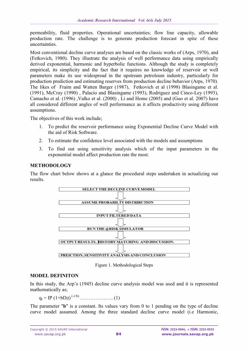
METHODOLOGY

The flow chart below shows at a glance the procedural steps undertaken in actualizing our

results.

Figure 1. Methodological Steps

MODEL DEFINITON

In this study, the Arp’s (1945) decline curve analysis model was used and it is represented

mathematically as;

qt = IP (1+bDit) (-1/b)

……………….. (1)

The parameter "b" is a constant. Its values vary from 0 to 1 pending on the type of decline

curve model assumed. Among the three standard decline curve model (i.e Harmonic,




____________________________________________________________________________________________________________________________________________________________________________________________________________________________________________________________________________________________________________



Hyperbolic and Exponential), the exponential curve was used for this study. For exponential,

b is taken as 0 and equation (1) becomes;

qt = IP exp(-Dt) ……………….. (2)

Furthermore, equation (2) was used in computing the decline rate (D);

t

IP

q

D

t

i

ln

……………….. (3)

DATA GATHERING, FILTERING AND SMOOTHING

For this study, actual production data were collected from a field X in Nigeria in the form of

yearly production rates and the number of days the well was produced. The average oil

production rates per day were calculated for each year.

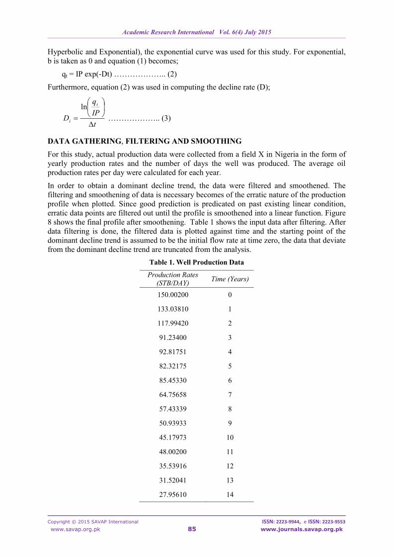
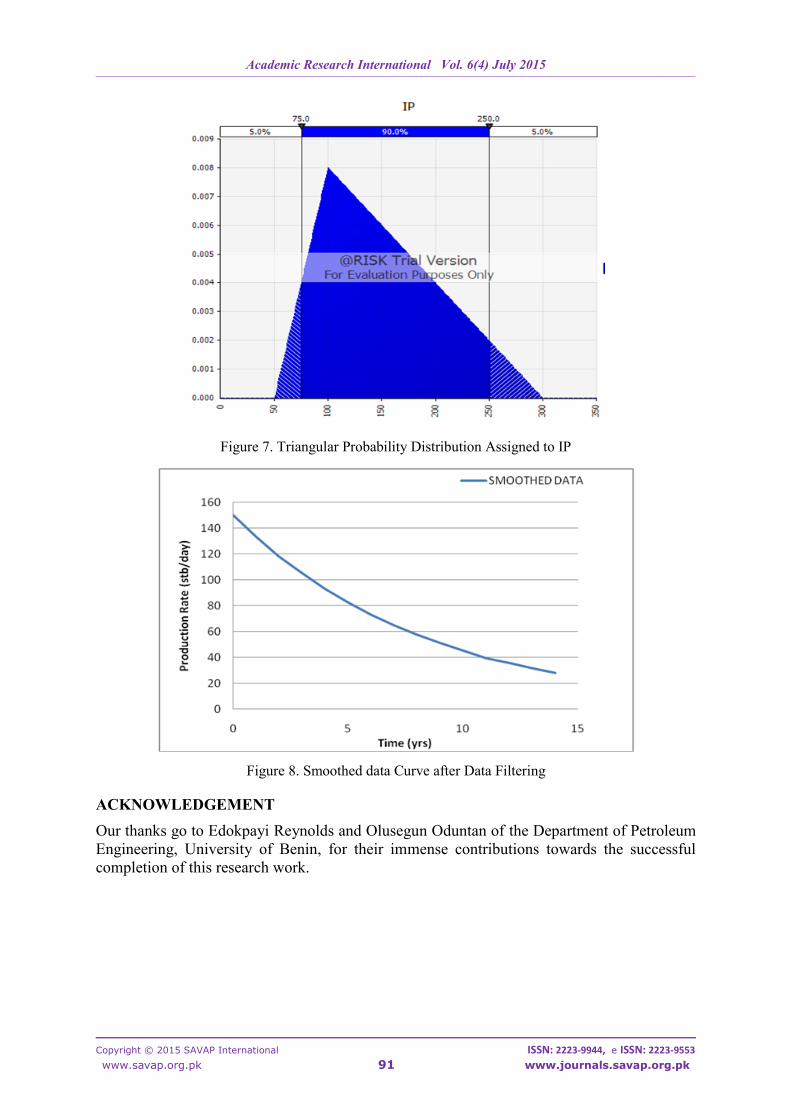
In order to obtain a dominant decline trend, the data were filtered and smoothened. The

filtering and smoothening of data is necessary becomes of the erratic nature of the production

profile when plotted. Since good prediction is predicated on past existing linear condition,

erratic data points are filtered out until the profile is smoothened into a linear function. Figure

8 shows the final profile after smoothening. Table 1 shows the input data after filtering. After

data filtering is done, the filtered data is plotted against time and the starting point of the

dominant decline trend is assumed to be the initial flow rate at time zero, the data that deviate

from the dominant decline trend are truncated from the analysis.

Table 1. Well Production Data

Production Rates

(STB/DAY) Time (Years)

150.00200 0

133.03810 1

117.99420 2

91.23400 3

92.81751 4

82.32175 5

85.45330 6

64.75658 7

57.43339 8

50.93933 9

45.17973 10

48.00200 11

35.53916 12

31.52041 13

27.95610 14




____________________________________________________________________________________________________________________________________________________________________________________________________________________________________________________________________________________________________________



Defining the Assumed Probabilistic Distribution and Quantitative values Assigned to

Each Input Variables before Simulation

Assumption of Probability Distribution

From equation (3) there are four input variables. These are:

1. Decline Rate (D)

2. Initial Production Rate(IP)

3. Arp’s Decline curve Exponent (b)

4. Time (T)

The @Risk software is a probabilistic tool. It requires fundamental probabilistic assumptions

to be made on the input parameters before execution. Based on the frequency of usage in

literature, the triangular distribution was assumed for both the initial production rate (IP) and

the decline constant (D). No distributions were assigned to decline exponent and time

because they are instantaneous variable. Use of triangular distribution is indicated when

upper and lower limits as well as the most likely value can be specified. It is apparent that the

probability of an outcome occurring close to the limits of range generally becomes smaller,

unless the distribution happens to be highly skewed to one side.

Values assigned to each of the variable are discussed below;

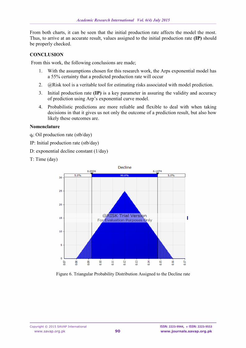
Decline Rate

A triangular distribution requires a minimum of three values for it to be properly defined. In

order to assign appropriate values to the decline rate constant, a little computation has to be

done. Using eqn (3) and data from Table (1), IP = 150.002stb/day, qt = 133.0381stb/day and

∆t = 1day.

Thus, Di= 0.12day-1

.

Based on this result, values assigned to Di were 0.08, 0.12, and 0.16 and the distribution

generated by software is given in figure 6.

Arp’s Decline curve exponent (b)

Decline exponent, b, was assigned zero. The implication of this is that the exponential decline

is being modeled.

Initial Production Rate (qi)

From table (1), the initial production is given as 150stb/day. However, since the triangular

distribution was assumed, two more values have to be logically assumed so that the triangular

distribution can be generated by the software. Values assigned are 50,150 and 300 and the

generated distribution is given in figure 7

Time

The time was given in days;

Software Simulation Run

The model (Eqn 2) and the actual production data (table 1) are imported into the @RISK

software and 10,000 trials were selected. This represents 10,000 possible scenario of

simulation.




____________________________________________________________________________________________________________________________________________________________________________________________________________________________________________________________________________________________________________



History Matching

Figure 2. Plot of the filtered Production Rate with Time

Expected Outcome

It is expected that the forecasted result would be “roughly” equal to the actual well

production rate and not exact due to the inherent limitation associated with probabilistic

simulation.

RESULTS AND DISCUSSION

Validity of the Result

It is expected that the actual filtered production rates for the seven- point data, to be

“roughly” equal to the generated software production rates for each time steps. If this is

achieved that means that all the assumptions made, mathematical model used and procedures

followed are correct. Then the model can confidently be used to predict production rate at any

time.

In an attempt to check for the validity of our approach thus far, variation between the

outputted P55 production rates and the actual data for each time step was computed as shown

in Table 3. It is shown from this table that the initial established deviated points (3rd, 6th and

11th year) have variations greater than ±5 stb/day.

This was expected. Taking a look at Figure 2, it can be seen that these data points were

originally off the decline trend.

In summary, one could deduce that the entire work and study, (i.e. software, assumptions,

model and procedures) are validated.

Table 2. History Matched result @RISK

Rates (STB/DAY)

P (%) 3rd

YR 4th YR 5

th YR 6

th YR 10

th YR 11th YR 12

th YR

5 52.0 45.9 40.5 35.7 21.5 18.81 16.3

55 73.01 92.49 82.08 93.0 44.84 39.66 35.53

95 175.0 155.9 139.10 123.9 79.52 71.3 64.64




____________________________________________________________________________________________________________________________________________________________________________________________________________________________________________________________________________________________________________



History Matching

To ascertain whether the chosen model and assumptions made would give a good forecast,

history matching was carried out before data smoothening. Seven (7) points were chosen

from the filtered data sets. The points chosen include 3rd, 4th, 5th, 6th, 10th, 11th and 12th

year.

Table 2 shows the result of only three of the probable outcomes (P5, P55 and P95) of the

forecasted production rates when the @RISK software was run using the seven- point data. It

is observed that the outputted flow rate was triangularly distributed as shown in appendix A.

With the 10,000 simulated trials, P55 gave the most likely output for seven time steps

considered. Table 2 summarizes the results.

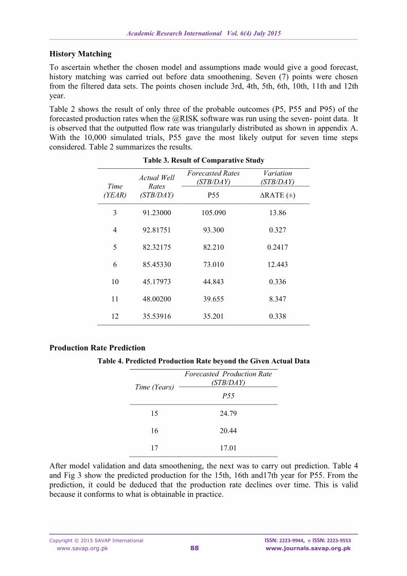
Table 3. Result of Comparative Study

Time

(YEAR)

Actual Well

Rates

(STB/DAY)

Forecasted Rates

(STB/DAY)

Variation

(STB/DAY)

P55 ∆RATE (±)

3 91.23000 105.090 13.86

4 92.81751 93.300 0.327

5 82.32175 82.210 0.2417

6 85.45330 73.010 12.443

10 45.17973 44.843 0.336

11 48.00200 39.655 8.347

12 35.53916 35.201 0.338

Production Rate Prediction

Table 4. Predicted Production Rate beyond the Given Actual Data

Time (Years)

Forecasted Production Rate

(STB/DAY)

P55

15 24.79

16 20.44

17 17.01

After model validation and data smoothening, the next was to carry out prediction. Table 4

and Fig 3 show the predicted production for the 15th, 16th and17th year for P55. From the

prediction, it could be deduced that the production rate declines over time. This is valid

because it conforms to what is obtainable in practice.




____________________________________________________________________________________________________________________________________________________________________________________________________________________________________________________________________________________________________________



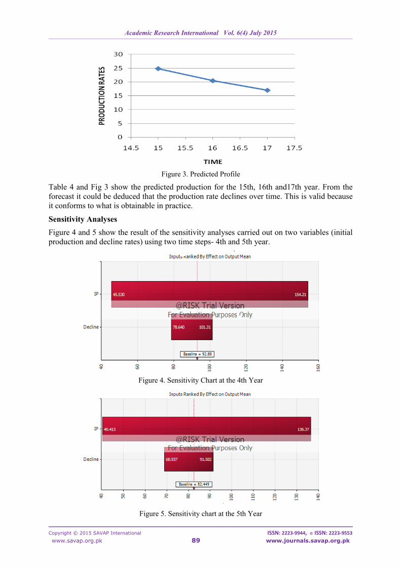
Figure 3. Predicted Profile

Table 4 and Fig 3 show the predicted production for the 15th, 16th and17th year. From the

forecast it could be deduced that the production rate declines over time. This is valid because

it conforms to what is obtainable in practice.

Sensitivity Analyses

Figure 4 and 5 show the result of the sensitivity analyses carried out on two variables (initial

production and decline rates) using two time steps- 4th and 5th year.

Figure 4. Sensitivity Chart at the 4th Year

Figure 5. Sensitivity chart at the 5th Year




____________________________________________________________________________________________________________________________________________________________________________________________________________________________________________________________________________________________________________



From both charts, it can be seen that the initial production rate affects the model the most.

Thus, to arrive at an accurate result, values assigned to the initial production rate (IP) should

be properly checked.

CONCLUSION

From this work, the following conclusions are made;

1. With the assumptions chosen for this research work, the Arps exponential model has

a 55% certainty that a predicted production rate will occur

2. @Risk tool is a veritable tool for estimating risks associated with model prediction.

3. Initial production rate (IP) is a key parameter in assuring the validity and accuracy

of prediction using Arp’s exponential curve model.

4. Probabilistic predictions are more reliable and flexible to deal with when taking

decisions in that it gives us not only the outcome of a prediction result, but also how

likely these outcomes are.

Nomenclature

qt: Oil production rate (stb/day)

IP: Initial production rate (stb/day)

D: exponential decline constant (1/day)

T: Time (day)

Figure 6. Triangular Probability Distribution Assigned to the Decline rate




____________________________________________________________________________________________________________________________________________________________________________________________________________________________________________________________________________________________________________



Figure 7. Triangular Probability Distribution Assigned to IP

Figure 8. Smoothed data Curve after Data Filtering

ACKNOWLEDGEMENT

Our thanks go to Edokpayi Reynolds and Olusegun Oduntan of the Department of Petroleum

Engineering, University of Benin, for their immense contributions towards the successful

completion of this research work.




____________________________________________________________________________________________________________________________________________________________________________________________________________________________________________________________________________________________________________



REFERENCES

[1] Arps, J. J. (1970). Oil and gas property evaluation and reserve estimates (Vol.3,

Reprint Series, pp. 93–1022). Richardson, TX: SPE.

[2] Blasingame, T. A., McCray, T. C., & Lee, W. J. (1991). Decline curve analysis for

variable pressure drop/variable flow rate system. SPE 21513

[3] Camacho, V.R., Rodriguez, F., Galindo, N.A., & Prats, M. (1996). Optimum position

for wells producing at constant wellbore pressure. SPE, 1, pp 155–1685

[4] Fetkovich, M. J. (1980). Decline curve analysis using type curves. JPT,1065–1077

[5] Fetkovich et al. (1998). Decline curve analysis using type-curves.SPE 13169

[6] Fraim, M. L., & Watten, B. R. A. (1987). Gas reservoir decline analysis using type

curves with real gas pseudo-pressure and normalized time. SPEFE (Dec. 1987)620

[7] Guo, B., Lyons, W. C., & Ghalambor, A. (2007). Petroleum production

engineering—a computer-assisted approach. Elsevier Science &Technology Books

Publishers, Amsterdam, pp 98–105

[8] Li, K., & Home, R. N. (2005). Verification of decline curve analysis models for

production prediction. SPE 93878.

[9] McCray, T. L. (1990). Reservoir analysis using production decline data and adjusted

time. MS Thesis, Texas A & M University College Station, TX

[10] Palacio, J. C., & Blasingame, T. A. (1993). Decline curve analysis using type curves.

SPE 25909

[11] Rodriguez, F., & Cinco-Ley, H. (1993). A new model for production decline. SPE

25480

[12] Valko, P. P., Doublet, L. E., & Blasingame, T. A. (2000). Development and

application of the multiwell productivity index (MPI). SPEJ




____________________________________________________________________________________________________________________________________________________________________________________________________________________________________________________________________________________________________________



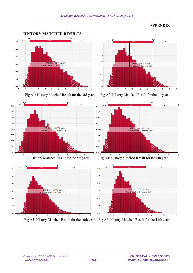
APPENDIX

HISTORY MATCHED RESULTS

Fig A1: History Matched Result for the 3rd year Fig A2: History Matched Result for the 4th year

A3: History Matched Result for the 5th year Fig A4: History Matched Result for the 6th year

Fig A5: History Matched Result for the 10th year Fig A6: History Matched Result for the 11th year




____________________________________________________________________________________________________________________________________________________________________________________________________________________________________________________________________________________________________________



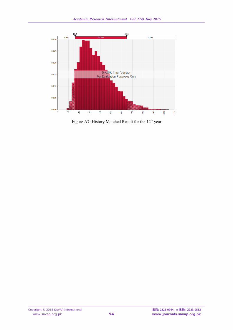
Figure A7: History Matched Result for the 12th year



Documents

Probabilistic Prediction of Well Performance4)/2015(6.4-09).pdfProbabilistic Prediction of Well Performance Ogbeide Paul Osaze1, Giegbefumwen Peter Uyi2 ... Arp’s model, exponential