Embed Size (px)
Citation preview
,
£/O(l/:A II-d- c(--1S"
NASA Contractor Report 198426
Probabilistic Material Strength Degradation Model for Inconel 718 Components Subjected to High Temperature, High-Cycle and Low-Cycle Mechanical Fatigue, Creep and Thermal Fatigue Effects
Callie C. Bast and Lola Boyce The University o/Texas at San Antonio San Antonio, Texas
November 1995
Prepared for Lewis Research Center UnderGrant NAG3-867
"'~ ~ • .•. '-, .. .. ..~~."
National Aeronautics and Space Administration
https://ntrs.nasa.gov/search.jsp?R=19960008692 2018-06-20T07:41:39+00:00Z
Trade names or manufacturers' names are used in this report for identification only. This usage does not constitute an official endorsement, either expressed or implied, by the National Aeronautics and Space AdminiStration.
•
•
PROBABILISTIC MATERIAL STRENGTH DEGRADATION MODEL FOR
INCONEL 718 COMPONENTS SUBJECTED TO HIGH TEMPERATURE, HIGH· CYCLE AND LOW-CYCLE MECHANICAL FATIGUE, CREEP AND
THERMAL FATIGUE EFFECTS
Prepared by:
Callie C. Bast, M.S.M.E., Research Engineer Lola Boyce, Ph. D., P. E., Principal Investigator
Final Technical Report of Project Entitled
Development of Advanced Methodologies for Probabilistic Constitutive Relationships
of Material Strength Models, Phases 5 and 6
NASA Grant No. NAG 3-867, .Supp. 5 and 6
Report Period: June 1992 to January 1995
Prepared for:
NATIONAL AERONAUTICS AND SPACE ADMINISTRATION Lewis Research Center Cleveland, Ohio 44135
The Division of Engineering The University of Texas at San Antonio
San Antonio, TX 78249 January, 1995
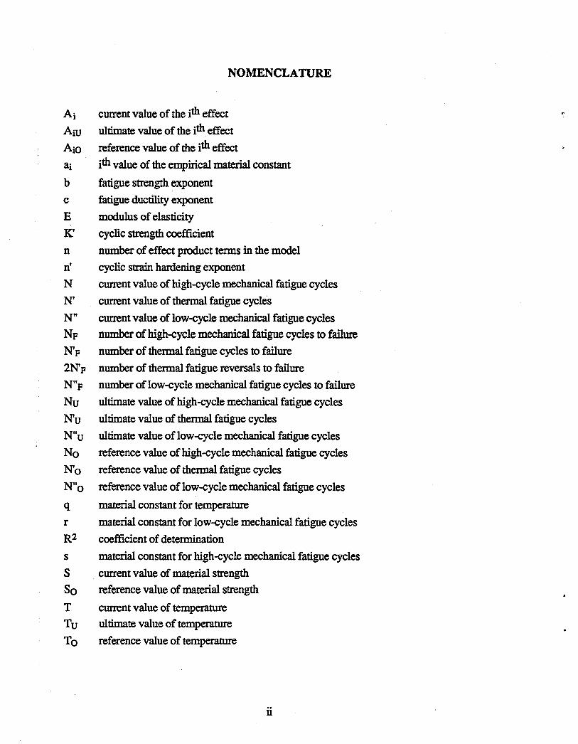
ABSTRACT
The development of methodology for a probabilistic material strength degradation is de
scribed. The probabilistic model, in the form of a postulated randomized multifactor equation,
provides for quantification of uncertainty in the lifetime material strength of aerospace propul
sion system components subjected to a number of diverse random effects. This model is embod
ied in the computer program entitled PROMISS, which can include up to eighteen different
effects. Presently, the model includes five effects that typically reduce lifetime strength: high
temperature, high-cycle mechanical fatigue, low-cycle mechanical fatigue, creep and thermal
fatigue. Results, in the form of cumulative distribution functions, illustrated the sensitivity of
lifetime strength to any current value of an effect. In addition, verification studies comparing
predictions of high-cycle mechanical fatigue and high temperature effects with experiments are
presented. Results from this limited verification study strongly supported that material degrada
tion can be represented by randomized multifactor interaction models.
i
NOMENCLATURE
A i current value of the ith effect
AiU ultimate value of the ith effect
AiO reference value of the ith effect
ai ith value of the empirical material constant
b fatigue strength exponent
c fatigue ductility exponent
E modulus of elasticity
K' cyclic strength coefficient
n number of effect product terms in the model
n' cyclic strain hardening exponent
N current value of high-cycle mechanical· fatigue cycles
N current value of thermal fatigue cycles
N" current value of low-cycle mechanical fatigue cycles
N p number of high-cycle mechanical fatigue cycles to failure
Np number of thermal fatigue cycles to failure
2Np number of thermal fatigue reversals to failure
N"p number of low-cycle mechanical fatigue cycles to failure
Nu ultimate value of high-cycle mechanical fatigue cycles
Nu ultimate value of thermal fatigue cycles
N"u ultimate value of low-cycle mechanical fatigue cycles
No reference value of high-cycle mechanical fatigue cycles
No reference value of thermal fatigue cycles
N"o reference value of low-cycle mechanical fatigue cycles
q material constant for temperature
r material constant for low-cycle mechanical fatigue cycles
R 2 coefficient of determination
s material constant for high-cycle mechanical fatigue cycles
S ClUTent value of material strength
So reference value of material strength
T current value of temperature
Tu ultimate value of temperature
To reference value of temperature
ii
NOMENCLATURE (continued)
t current value of creep time tF number of creep hours to failure
tu ultimate value of creep time
to reference value of creep time
u material constant for thermal fatigue cycles
v material constant for creep time lleJ2 elastic strain amplitude
llep/2 plastic strain amplitude
IleT/2 total strain amplitude
lla/2 stress amplitude e'F fatigue ductility coefficient
J.1 mean
a standard deviation
a'F fatigue strength coefficient
iii
TABLE OF CONTENTS
SECTION PAGE
ABSTRACT .......................•.•..........•.•.•••.....•.•.......•••.••....••..•....•..•.••...•.•.•.••.........•.....••... i
NOMEN~A TURE ..................................................................•..........................•........ ii.
LIST OF FIGURES ........••.•••.....••..•.•........•••••.....................•.•..••••...••.•.•.••.•........... ....•.... 'vi
LIST OF TABLES ...•.........••......•.....•...........•....••.... "' .................••.....•••....••.............. 00...... x
1.0 IN'TRODUCI'ION .............................................................................•.........•....... 1
2.0 TIffiORETICAL BACKGROUND ..•.....••.••••••.........•..•.•.........••••...••.......••.• 0...... 3 ,
3.0 PROMISS COMPU1'ER PROGRAM ...•..............•....•.•..•••....•.....•..........•••.•...•••• 6
4.0 STRENGTH DEGRADATION MODEL FOR INCONEL 718 ...............•....... 10
4.1 "IEMPERA TURE MODEL' ...............•.•.•..•...•........................•...........•....... 10
4.2 IDGH-CYCLE MECHANICAL FATIGUE MODEL ............................. 11
4.3 LOW-CY~E MECHANICAL FATIGUE MODEL ............................. 11
4.4 CREEP MODEL ........................................................................................ 12
4.5 TIiERMAL FATIGUE MODEL ............................................................... 12
4.6 MODEL 1RANSFORMATION ................................................................ 13
5.0 EXPE~NTAL MA"IERIAL DATA ............................................................ 17
5.1 LTI'ERA TURE SEARCH ........................................................................... 17
5.2 INCONEL718 ............................................................................................ 17
5.3 "IEMPERATURE DATA ........................................................................... 18
5.4 IDGH-CY~E MECHANICAL FATIGUE DATA ......................... ~ ....... 20
5.5 LOW-CYCLE MECHANICAL FATIGUE DATA ................................. 22
5.6 CREEP RUPTURE DATA ........................................................................ 24
5.7 TIiERMAL FATIGUE DATA .................................................................. 26
5.8 MODEL CALffiRA TION .......................................................................... 33
iv

TABLE OF CONTENTS (continued)
SECTION PAGE
6.0 ESTIMATION OF EMPIRICAL MATERIAL CONSTANT V ARIA.Bll.,ITY .......•.......•..•.••...•.••.•......•....•...••......•..•••••••••.•. ..•.•..• 39
7.0 PROBABll..ISTIC LIFETIME STRENGTH SENSITIVITY STUDIES ...•••... 44
7.1 '93 SENSITIVITY STUDY FOR HIGH-CYCLE MECHANICAL FATIGUE, CREEP AND THERMAL FATIGUE EFFECTS ......... 44
7.2 '94 SENSITIVITY STUDY FOR HIGH-CYCLE MECHANICAL FATIGUE, LOW-CYCLE MECHANICAL FATIGUE, CREEP, AND TIIERMAL FATIGUE EFFECTS ....•...•.••.•.•...•.•..••••.•••.••..•••••• 50
8.0 MODEL 'VERIF'ICATION STUDY ............................•...........•..........••.•. ~......... 54
9.0 DISCUSSION .............................................•.........................................•.....•....... 62
10.0 CONCLUSIONS .............................•.......................................•...............•........... 65
11.0 ACKNO~EDGMENTS .................................................................................. 67
12.0 APPENDIX ......................................................................................................... 68
13.0 REFERENCES ............................•...................••................••••.............•.•.........•... 72
v
LIST OF FIGURES
FIGURE PAGE
1 Schematic of Data lllustrating the Effect of One Variable 'on Strength ................................•...... -:.............................................................. 4
2 Effect of Temperature (OF) on Yield Strength for Inconel718 ••••....•..••.••.•••••• 18
3 Effect of Temperature (Of')on Yield Strength for Inconel 718. (l.og-wg Plot with Linear Regression)........................................................... 19
4 Effect of High-Cycle Mechanical Fatigue (Cycles) on Fatigue Strength for Inconel 718. ....•.......•..•..........•.......•.......•........••••.•......... ..•..•..•••••••..•...•....•• 20
5 Effect of High-Cycle Mechanical Fatigue (Cycles) on Fatigue Strength for Inconel 718. (Non-sensitized Model Form) ..••.•....••••••••.•••.•..•..•.•.•••••.•..•.••. 21
6 Effect of High-Cycle Mechanical Fatigue (Cycles) on Fatigue Strength for Inconel 718. (Sensitized Model Form) ............•.....••......•....•...•..•••.............. 21
7 Effect ofww-Cycle Mechanical Fatigue (Cycles) on Fatigue Strength for Ineonel 718. •.......•. •••. ..•............ ...•..........• ..•.. .•••••.. .••.....• ...•...•.•.....•.•.....••... 22
8 Effect ofww-Cycle Mechanical Fatigue (Cycles) on Fatigue Strength for Inconel 718. (Non-sensitized Model Form)............................................... 23
9 Effect ofww-Cycle Mechanical Fatigue (Cycles) on Fatigue Strength for Inconel 718. (Sensitized Model Form) .............••••...•...••.•.••..••..•...•.......•.•... 23
10 Effect of Creep Time (Hours) on Rupture Strength for Inconel 718. (Linear Plot) .• .......••.•.. ............ ... .••...•••... ..... .•.•. ... ... ..•....•.. ...•.. 24
11 Effect of Creep Time (Hours) on Rupture Strength for Inconel718. (Non-sensitized Model Form) .............................................. 25
12 Effect of Creep Time (Hours) on Rupture Strength for Inconel 718. (Sensitized Model Form) ..................................................... 25
13 Strain-life Curve for Inconel 718. .......................................••.••......•......•••••..•.. 27
14 Cyclic Stress Strain Curve for Inconel 718. ................................................... 27
15 Regression of Equation (11) Data Yielding Fatigue Ductility Coefficient, elF, and Fatigue Ductility Exponent, c. ........................................................... 28
16 Regression of Equation (12) Data Yielding Cyclic Strength Coefficient, KI, and Cyclic Strain Hardening Exponent, nl. ............................ 29
vi
LIST OF FIGURES (continued)
FIGURE PAGE
17 Regression of Equation (13) Yielding Fatigue Strength Coefficient, a'F, and Fatigue Strength Exponent, b. ....................................... 30
18 Effect of Thermal Fatigue (Cycles) on Thermal Fatigue Strength (i.e., Stress Amplitude at Failure) for Inconel 718 .......................................... 31
19 Effect of Thermal Fatigue (Cycles) on Thermal Fatigue Strength for Inconel718. (Non-sensitized Model Form) .............................................. 32
20 Effect of Thennal Fatigue (Cycles) on Thermal Fatigue Strength for Inconel 718. (Sensitized Model Form) ...................................................... 32
21 Effect of High-Cycle Mechanical Fatigue (Cycles) on Fatigue Strength for Incone1718. (Sensitized Model Form Using Improved Estimates) ........•...... 36
22 Effect of Low-Cycle Mechanical Fatigue (Cycles) on Fatigue Strength for Inconel718. (Sensitized Model Form Using Improved Estimates) ...•••..••.••.• 36
23 Effect of Creep Time (Hours) on Rupture Strength for Inconel 718. (Sensitized Model Form Using Improved Estimates) .................................... 37
24 Effect of Thermal Fatigue (Cycles) on Thermal Fatigue Strength. (Sensitized Model Form Using Improved Estimates) .................................... 37
25 Linear Regression of Temperature Data. ......................................................... 40
26 Postulated Maximum and Minimum Slopes .................................................. 41
27 Postulated Maximum and Minimum Y-intercepts ......................................... 41
28 Probability Density Function of a Normal Distribution. ................................. 42
29 Postulated Envelope of Actual and Simulated Temperature (Of) Data. .........• 43
30 Inconel 718 Model Parameters for High-Cycle Mechanical Fatigue, Cre,ep and Thermal Fatigue Effects. ............................................................... 45
31 Comparison of Various Levels of Uncertainty of High-Cycle Mechanical Fatigue (Cycles) on Probable Strength for Inconel718 for 2000 Thermal Fatigue Cycles and 1000 Hours of Creep at 1000 OF. .................................... 48
vii
LIST OF FIGURES (continued)
FIGURE
32 Comparison of Various Levels of Uncertainty of Creep Time (Hours) on Probable Strength for Inconel718 for lxl()6 High-Cycle Mechanical
PAGE
Fatigue Cycles and 2000 Thermal Fatigue Cycles at 1000 OF. ....................... 48
33 Comparison of Various Levels of Uncertainty of Thermal Fatigue (Cycles) on Probable Strength for Inconel 718 for Ixl06 High-Cycle Mechanical Fatigue Cycles and 1000 Hours of Creep at 1000 OF. .................................... 49
34 Comparison of Various Levels of Uncertainty of High-Cycle Mechanical Fatigue (Cycles) on Probable Strength for Inconel 718 for 1000 Low-Cycle Mechanical Fatigue Cycles, 2000 Thermal Fatigue Cycles and 1000 Hours of Creep at 1000 OF. ••••••••••••••••••••••••••••••••••••••••••••••••••••••••••••••••••••••••••••••••••••••• S2
35 Comparison of Various Levels of Uncertainty of Low-Cycle Mechanical Fatigue (Cycles) on Probable Strength for Inconel 718 for lxl06 High-Cycle Mechanical Fatigue Cycles, 2000 Thermal Fatigue Cycles and 1000 Hours of Creep at 1000 OF ........................................................ ~................................ 52
36 ·Comparison of Various Levels of Uncertainty of Creep Time (Hours) on Probable Strength for Inconel 718 for lx106 High-Cycle Mechanical Fatigue Cycles, 1000 Low-Cycle Mechanical Fatigue Cycles and 2000 Thermal Fatigue Cycles at 1000 °P. •••••••••....••.••••••••••.•••••••.•••..•••••••••.••.••.••••••• S3
37 Comparison of Various Levels of Uncertainty of Thermal Fatigue (Cycles) on Probable Strength for Inconel 718 for lxl06 High-Cycle Mechanical Fatigue Cycles, 1000 Low-Cycle Mechanical Fatigue Cycles and 1000 Hours of Creep at 1000 °P. .....................•..................••••••••.•••.•..................••.• S3
38 Comparison of Various Levels of Uncertainty of High-Cycle Mechanical Fatigue (Cycles) on Probable Strength for Inconel718. (Combination of H-C Mechanical Fatigue and High Temperature Effects by Model) ••••....•..••• 57
39 Comparison of Various Levels of Uncertainty of High-Cycle Mechanical Fatigue (Cycles) on Probable Strength for Inconel718. (Combination of H-C Mechanical Fatigue and High Temperature Effects by Experiment) .•.••• 57
40 Overlay of Results for a Combination of High-Cycle Mechanical Fatigue and Temperature Effects by Model and by Experiment. ................................ 58
41 Overlay of R~sults for a Combination of High-Cycle Mechanical Fatigue and Temperature Effects by Model (Using Estimated Value of s) and by Experiment. ............................•........................................................... 60
viii
LIST OF FIGURES (continued)
BGURE PAGE
42 Overlay of Results for a Combination of High-Cycle Mechanical Fatigue and Temperature Effects by Model (Using Estimated Value of s) and .by Experiment; N=2.SxlOS Cycles. ........................................................ 60
43 Overlay of Results for a Combination of High-Cycle Mechanical Fatigue and Temperature Effects by Model (Using Estimated Value of s) and by Experiment; N=1.0x10⁶ Cycles. ........................................................ 61
44 Overlay of Results for a Combination of High-Cycle Mechanical Fatigue and Temperature Effects by Model (Using Estimated Value of s) and by Experiment; N=1.75x10⁶ Cycles. ...................................................... 61
ix
LIST OF TABLES
TABLE PAGE
1 Variables Available in the "Fixed" Model. ....................................................... 6
2 Variables Available in the "Flexible" Model. ................................................... 7
3 Non-sensitized and Sensitized Terms for High-Cycle Mechanical Fatigue Data. ................................................................................ 14
4 Non-sensitized and Sensitized Terms for Low-Cycle Mechanical Fatigue Data. ................................................................................ 14
5 Non-sensitized and Sensitized Tenns for Creep Rupture Data. ...................... 15
6 Non-sensitized and Sensitized Tenns for Thennal Fatigue Data. .............•..... 16
7 Thermal Fatigue Data for Inconel 718. ........................................................... 26
8 Fatigue Material Properties for Inconel 718. ................................................... 30
9 Initial Estimates for the Ultimate and Reference Values. ................................ 33
10 Initial Estimates for the Empirical Material Constants .................................... 34
11 Improved Estimates for the Ultimate and Reference Values. ......................... 38
12 Improved Estimates for the Empirical Material Constants. ............................ 38
13 '93 Sensitivity Study Input to PROMISS93 for Inconel718; Temperature=l000 OP and N=2.5xlOS Cycles. .............................................. 46
14 '93 Sensitivity Study Input to PROMISS93 for Inconel 718; Temperature=I000°F and N=1.0xl06 Cycles. ............................................... 46
15 '93 Sensitivity Study Input to PROMISS93 for Inconel 718; Temperature=I000°F and N=I.75xl06 Cycles. ............................................. 47
16 Selected Cmrent Values for '93 Sensitivity Study of the Probabilistic Material Strength Degradation Model for Inconel718. .................................. 47
17 Selected Cmrent Values for '94 Sensitivity Study of the Probabilistic Material Strength Degradation Model for Inconel 718. .................................. 51
18 Verification Study Input to PROMISS93 for Inconel 718; Combination by Model, N=2.5xlOS Cycles. .................................................. 55
x
LIST OF TABLES (continued)
TABLE PAGE
19 Verification Study Input to PROMISS93 for Inconel 718; Combination by Model, N=l.Ox106 Cycles. .................................................. 55
20 Verification Study Input to PROMISS93 for Inconel 718; Combination by Model, N=1.75x10⁶ Cycles. ................................................ 55
21 Verification Study Input to PROMISS93 for Inconel 718; Combination by Experiment, N=2.5x1OS Cycles ........................................... 56
22 Verification Study Input to PROMISS93 for Inconel 718; Combination by Experiment, N=1.Ox106 Cycles ........................................... 56
23 Verification Study Input to PROMISS93 for Inconel 718; Combination by Experiment, N=1.75x10⁶ Cycles ......................................... 56
24 Modified Verification Study Input to PROMISS93 for Inconel 718; Combination by Model, N=2.5x1OS Cyc~es. .................................................. 59
25 Modified Verification Study Input to PROMISS93 for Inconel 718; Combination by Model, N=l.Ox106 Cycles. .................................................. 59
26 Modified Verification Study Input to PROMISS93 for Inconel 718; Combination by Model, N=1.75x10⁶ Cycles. ................................................ 59
A.1 Inconel 718 High Temperature Tensile Data. ................................................. 68
A.2 Inconel718 High-Cycle Mechanical Fatigue Data. ........................................ 68
A.3 Inconel 718 Low-Cycle Mechanical Fatigue Data. ......................................... 69
A.4 Inconel718 Thennal Fatigue Data. ................................................................ 69
A.S Irlconel 718 Creep RuptUI"e Data. ................................................................... 70
A.6 Inconel 718 Data S~ary . ........................................................................... 71
xi
1.0 INTRODUCTION
Probabilistic methods, for quantifying the uncertainties associated with the design and
analysis of aerospace propulsion system components, can significantly improve system
performance and reliability. The reusability and durability of aerospace components are of
prime interest for economical, as well as, safety related reasons. Ufe cycle costs including
initial design costs and field replacement costs of aerospace propulsion system components are
driving elements for improving life prediction capability. Accurate prediction of expected
service lifetimes is crucial in the final decision of whether or not to proceed with a particular
design. Inaccurate lifetime strength predictions can result in either a lack of adequate life or an
overly costly design due to inefficient utilization of material.
This work is part of a larger effort to develop a probabilistic approach for lifetime
strength prediction methods [4]. This report presents the on-going development of
methodology that predicts probabilistic lifetime strength of aerospace materials via
computational simulation. A material strength degradation model, in the form of a randomized
multifactor equation, is postulated for strength degradation of structural components of.
aerospace propulsion systems subjected to a number of effects. Some of the typical variables
or effects that propulsion system components are subjected to under normal operating
conditions include high temperature, fatigue and creep. Methodology to calibrate the model
using actual experimental materials data together with regression analysis of that data is also
presented. Material data for the superalloy, Inconel 718, were analyzed using the developed
methodology.
Sections 2 and 3 summarize the theoretical and computational background for the
research. The above-described randomized multifactor equation is embodied in the computer
program, PROMISS [6]. This program was developed using the NASA Lewis Research
Center and the University of Texas System Cray-Y-MP supercomputers. Section 4 discusses
the strength degradation model developed for high temperature, high-cycle mechanical fatigue,
low-cycle mechanical fatigue, creep and thermal fatigue effects, individually. Initial estimates
for ultimate and reference values are determined using available data for Inconel 718. A
transformation to improve model sensitivity is then discussed. Section 5 presents
experimental material data for Inconel 718 and displays the data in the form utilized by the
multifactor equation embodied in PROMISS. Temperature, high-cycle mechanical fatigue,
low-cycle mechanical fatigue, creep and thermal fatigue data for Inconel 718 are presented.
Linear regression of the data is performed to provide first estimates of the empirical material
constants, aio used to calibrate the model. Additional calibration techniques to improve model
1
accuracy are then discussed. In Section 6, methodology for estimating standard deviations of
the empirical material constants is developed as a means for dealing with limited data. These estimated values for the standard deviation, rather than expert opinion, may be used with
greater confidence in the probabilistic material strength degradation model. Section 7 presents
and discusses cases for analysis that resulted from two sensitivity studies. '93 Sensitivity
Study examined the combined effects of high-cycle mechanical fatigue, creep and thermal
fatigue at elevated temperatures, while '94 Sensitivity Study included four effects - low-cycle
mechanical fatigue along with the three previous effects. Results, in the form of cumulative
distribution functions, illustrate the sensitivity of lifetime strength to any current value of an
effect. Section 8 presents and discusses model verification studies that were conducted to
evaluate the ability of the multifactor equation to model two or more effects simultaneously.
Available data allowed for verification studies comparing a combination of high-cycle
mechanical fatigue and temperature effects by model to the combination of these two effects by
experiment. Methodology and results are reiterated and discussed in Section 9. Conclusions
of the current research and recommendations for future research conclude this report. The raw
data for all effects, along with material and heat treatment specifications, are provided in the
appendix.
2
2.0 THEORETICAL BACKGROUND
Previously, a general material behavior degradation model for composite materials,
subjected to a number of diverse effects or variables, was postulated to predict mechanical and
thermal material properties [8,9,13,14]. The resulting multifactor equation summarizes a
proposed composite micromechanics theory and has been used to predict material properties
for a unidirectional fiber-reinforced lamina based on the corresponding properties of the
constituent materials.
More recently, the equation has been modified to predict the lifetime strength of a
single constituent material due to "n" diverse effects or variables [4,5,6]. These effects could
include variables such as high temperature, creep, high-cycle mechanical fatigue, thermal
fatigue, corrosion or even radiation attack. For these variables, strength decreases with an
increase in the variable [12]. The general form of the postulated equation is
n [ ]ai S II A·u-A. , _ 1 1
So - i=l AiU - AiO (1)
where Ah AiU and AiO are the current, ultimate and reference values, respectively, of a
particular effect; ai is the value of an empirical material constant for the ith product terms of
variables in the model; S and So are the current and reference values of material strength. Each
tenn has the property that if the current value equals the ultimate value, the lifetime strength
will be zero. Also, if the current value equals the reference value, the term equals one and
strength is not affected by that variable. The product form of equation (1) assumes·
independence between the individual effects. This equation may be viewed as a solution to a
separable partial differential equation in the variables with the further limitation or
approximation that a single set of separation constants, ait can adequately model the material
properties.
Calibration of the model is achieved by appropriate curve-fitted least squares linear
regression of experimental data [19] plotted in the form of equation (1). For example, data for
just one effect could be plotted on log-log paper. A good fit for the data may be obtained by
linear regression as shown schematically in Figure 1. Dropping the subscript "i" for a single
variable, the postulated equation is obtained by noting the linear relation between log S and
3
log [(Au - Ao)/(Au - A)], as follows:
logS=-a IOg[AU-AO]+IOgSO Au- A
IOg~=-alOg[AU -AO] So Au- A
~=[AU-Aora So Au-A
or,
S Au-A [ ]
a
So = Au-Ao .
log S
log$o
(2a)
(2b)
-a = slope
Fig. 1 Schematic of Data illustrating the Effect of One Variable on Strength.
4
..
This general material strength degradation model, given by equation (1), may be used to estimate the lifetime strength, SISo, of an aerospace propulsion system component operating
under the influence of a number of diverse effects or variables. The probabilistic treatment of
this model includes "randomizing" the deterministic multifactor equation through probabilistic
analysis by simulation and the generation of probability density function (p.d.f.) estimates for lifetime strength, using the non-parametric method of maximum penalized likelihood [20,22].
Integration of the probability density function yields the cumulative distribution function (c.d.f.) from which probability statements regarding lifetime strength may be made. This probabilistic material strength degradation model, therefore, predicts the random lifetime strength of an aerospace propulsion component subjected to a number of diverse random
effects.
The general probabilistic material strength degradation model, given by equation (1),
is embodied in the FORTRAN program, PROMISS (f,mbabilistic M.aterial £trength
S.imulator) [6]. PROMISS calculates the random lifetime strength of an aerospace propulsion component subjected to as many as eighteen diverse random effects. Results are presented in the form of cumulative distribution functions of lifetime strength, S/So-
5
3.0 PROMISS COMPUTER PROGRAM
PROMISS includes a relatively simple "fIxed" model as well as a "flexible" model.
The fIxed model postulates a probabilistic multifactor equation that considers the variables
given in Table 1. The general form of this equation is given by equation (1), wherein there are
now n = 7 product terms, one for each effect listed below. Note that since this model has
seven terms, each containing four parameters of the effect (A, Au, Ao and a), there are a total
of twenty-eight variables. The flexible model postulates the probabilistic multifactor equation
that considers up to as many as n = 18 effects or variables. These variables may be selected to
utilize the theory and experimental data currently available for the particular strength
degradation mechanisms of interest. The specifIc effects included in the flexible model are
listed in Table 2. To allow for future expansion and customization of the flexible model, six
"other" effects have been provided.
Table 1. Variables Available in the ''Fixed'' Model.
ith Primitive Primitive Variable Variable Type
1 Stress due to static load
2 Temperature
3 Chemical reaction
4 Stress due to impact
5 Mechanical fatigue
6 Thennal fatigue
7 Creep
6
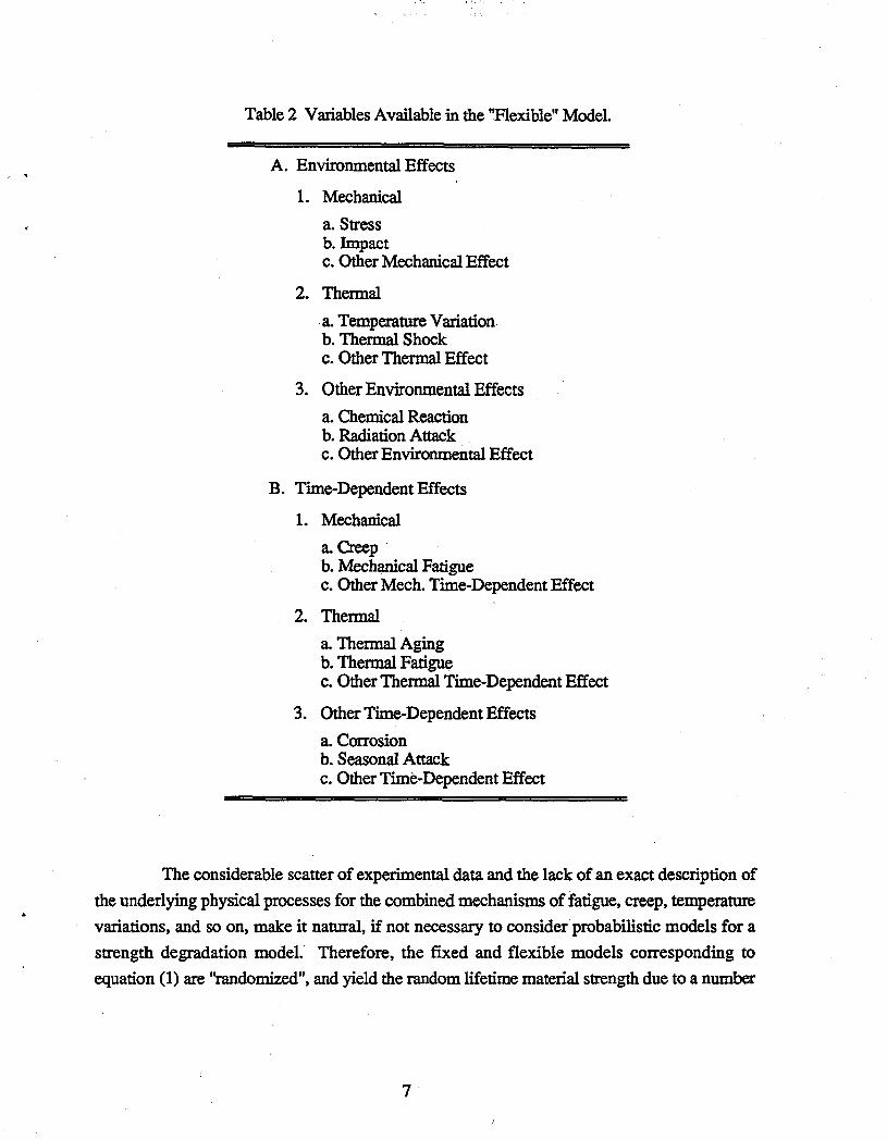
Table 2 Variables Available in the "Flexible" Model.
A. Environmental Effects
1. Mechanical
a. Stress b. Impact c. Other Mechanical Effect
2. Thermal
.a. Temperature Variation. b. Thermal Shock c. Other Thermal Effect
3. Other Environmental Effects
a. Chemical Reaction b. Radiation Attack c. Other Environmental Effect
B. Time-Dependent Effects
1. Mechanical a. Creep . b. Mechanical Fatigue c. Other Mech. Time-Dependent Effect
2. Thermal
a. Thermal Aging b. Thermal Fatigue c. Other Thermal Time-Dependent Effect
3. Other Time-Dependent Effects
a. Corrosion b. Seasonal Attack c. Other Time-Dependent Effect
The considerable scatter of experimental data and the lack of an exact description of
the underlying physical processes for the combined mechanisms of fatigue, creep, temperature
variations, and so on, make it natural, if not necessary to consider probabilistic models for a
strength degradation modeL Therefore, the fixed and flexible models corresponding to
equation (1) are "randomized", and yield the random lifetime material strength due to a number
7
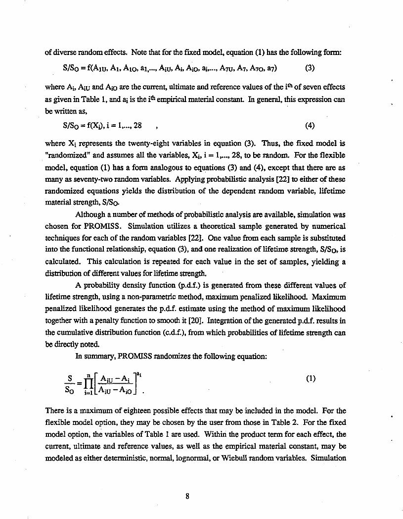
of diverse random effects. Note that for the fIXed model~ equation (1) has the following form:
SISo = f(Am, At. AlQ, aI •... , AiU, Ai. Aio, ai, ... , A7u, A7, A70, a7) (3)
where Ai. AiU and AiO are the current, ultimate and reference values of the ith of seven effects
as given in Table 1, and ai is the ith empirical material constant. In general, this expression can be written as,
8/80 = f(XV, i = 1, ... , 28 (4)
where Xi represents the twenty-eight variables in equation (3). Thus, the fixed model is
"randomized" and assumes all the variables, Xit i = 1, ... , 28, to be random. For the flexible
model~ equation (1) has a form analogous to equations (3) and (4)~ except that there are as
many as seventy-two random variables. Applying probabilistic analysis [22] to either of these
randomized equations yields the distribution of the dependent random variable, lifetime
material strength, 8/So.
Although a number of methods of probabilistic analysis are available, simulation was
chosen for PROMISS. Simulation utilizes a theoretical sample generated by numerical
techniques for each of the random variables [22]. One value from each sample is substituted
into the functional relationship, equation (3), and one realization of lifetime strength, S/So, is
calculated. This calculation is repeated for each value in the set of samples, yielding a
distribution of different values for lifetime strength.
A probability density function (p.d.f.) is generated from these different values of
lifetime strength, using a non-parametric method, maximum penalized likelihood. Maximum
penalized likelihood generates the p.d.f. estimate using the method of maximum likelihood
together with a penalty function to smooth it [20]. Integration of the generated p.d.f. results in
the cumulative distribution function (c.d.f.), from which probabilities of lifetime strength can
be directly noted.
In summary, PROMISS randomizes the following equation:
n [ ]ai S IT A·u-A· _ 1 1
So - i=l AiU - AiO
(1)
There is a maximum of eighteen possible effects that may be included in the model. For the
flexible model option, they may be chosen by the user from those in Table 2. For the flXed
model option, the variables of Table 1 are used. Within the product term for each effect, the
current, ultimate and reference values, as well as the empirical material constant, may be
modeled as either detenninistic, normal, lognormal, or Wiebull random variables. Simulation
8
is used to generate a set of realizations for lifetime random strength, S/So, from a set of
realizations for the random variables of each product term. Maximum penalized likelihood is
used to generate the p.d.f. estimate of lifetime strength, from the set of realizations of lifetime
strength. Integration of the p.d.f. yields the c.d.f., from which probabilities of lifetime strength
can be ascertained. PROMISS also provides information on lifetime strength statistics, such
as the mean, variance, standard deviation and coefficient of variation.
9
4.0 STRENGTH DEGRADATION MODEL FOR INCONEL 718
The probabilistic material strength degradation model, in the form of the multifactor
equation given by equation (1), when modified for a single effect, results in equation (5)
below.
S Au-A Au-Ao [ ]a [ ]-a So = Au-Ao = Au- A
(5)
Appropriate values for the ultimate, Au, and reference quantities, Ao, had to be estimated as
part of the initial calibration of the multifactor equation for Inconel 718. Based on actual
Inconel718 data, these values were selected accordingly for each effect
4.1 Temperature Model
Equation (5), when modified for the effect of high temperature only, becomes:
~=[TU-TO]-q , So Tu- T
(6a)
where Tu is the ultimate or melting temperature of the material, To is a reference or room
temperature, T is the current temperature of the material, and q is an empirical material constant
that represents the slope of a straight line fit of the modeled'data on log-log paper. A logical
choice for the ultimate temperature value is the average melting temperature (2369 oF) of
Inconel718. Therefore, this value was an initial estimate for the ultimate temperature value,
Tu. An estimate of 75°F or room temperature was used for the reference temperature value,
To. Substitution of these values into equation (6a) above results in equation (6b) below. Thus,
equation (6b) models the effect of high temperature on the lifetime strength of the specified
material,InconeI718.
~=[TU -To]-q = [2369-75J-q So Tu -T 2369-T
(6b)
10
4.2 High-Cycle Mechanical Fatigue Model
Equation (5), when modified for the effect of high-cycle mechanical fatigue,
becomes:
(7a)
where Nu is the ultimate number of cycles for which fatigue strength is very small, No is a
reference number of cycles for which fatigue strength is very large, N is the current number of
cycles the material has undergone, and s is the empirical material constant for the high-cycle
mechanical fatigue effect. An initial estimate of lxl010 was used for the ultimate number of
cycles, Nu. since mechanical fatigue data beyond this value was not found for Inconel 718. An
initial estimate of 0.5 or half a cycle was used for the reference number of cycles, No.
Substitution of these values into equation (7 a) results in the high-cycle mechanical fatigue
model for Inconel 718, as given below by equation (7b).
~=[1010 _0.5]-S SO 10lD_N
(7b)
Since the high-cycle fatigue domain is associated with lower loads and longer lives, or high
numbers of cycles to failure (greater than 1()4 or lOS cycles), data consisting of cycle values
less than 5xl()4 fall into the low-cycle fatigue regime and therefore, may be modeled by the
low-cycle mechanical fatigue model presented in Section 4.3.
4.3 Low-Cycle Mechanical Fatigue Model
Equation (5), when modified for the effect of low-cycle mechanical fatigue, becomes:
~ _ [N"u - N"o ]-' - " " , So Nu-N
(8a)
where Nltu is the ultimate number of cycles for which fatigue strength is very low, Nlto is a
reference number of cycles for which fatigue strength is very high, Nit is the current number of
cycles the material has undergone, and r is the empirical material constant for the low-cycle
mechanical fatigue effect. An initial estimate of lxlOS was used for the ultimate number of
cycles, N"u. since niechanical fatigue cycle values beyond this value fall into the high-cycle
fatigue domain. An initial estimate of 0.5 or half a cycle was used for the reference number of
cycles, Nita. Substitution of these values into equation (8a) results in the low-cycle mechanical
11
fatigue model for Inconel 718, as given below by equation (8b).
l. = [1 x lOS - o.~]-r So lx10s-N
4.4 Creep Model
Equation (5), when modified for the effect of creep, becomes:
~=[tu -toJ-v , So tu-t
(8b)
(9a)
where tu is the ultimate number of creep hours for which rupture strength is very small, to is a
reference number of creep hours for which rupture strength is very large, t is the current
number of creep hours, and v is the empirical material constant for the effect of creep. An
initial estimate of 1xl()6 was used for the ultimate number of creep hours, tu, due to the fact
that creep rupture life data beyond this value was not found for Inconel 718. An initial estimate
of 0.25 hours or fifteen minutes was used for the reference number of creep hours, to. Substitution of these values into equation (9a) results in equation (9b) below.
~ = [106 ~ 0.25]-V (9b)
So 10 -t
4.5 Thermal Fatigue Model
The fifth and final effect for which Inconel718 data was obtained is thermal fatigue.
Thermal fatigue has been extensively discussed in the literature [10, 17, 24]. When modified
for the effect of thermal fatigue, equation (5) becomes:
(lOa)
where Nu is the ultimate number of thermal cycles for which thermal fatigue strength is very
small, N'o is a reference number of thermal cycles for which thermal fatigue strength is very
large, N' is the current number of thermal cycles the material has undergone, and u is an
empirical material constant that represents the slope of a straight line fit of the modeled· data on
log-log paper.
Thermal fatigue is in the regime of low-cycle fatigue (less than 1()4 or lOS cycles),
therefore, an intennediate value of 5xl04 cycles was an initial estimate for the ultimate number
12
of thermal fatigue cycles, N'u. An initial estinuLte of 0.5 or half a cycle was used for the
reference number of cycles, N' o. Substitution of these values into equation (lOa) results in the
thermal fatigue model for Inconel7l8, as given by equation (lOb) below.
~=[5XI0:-0·?ru. So 5xlO-N
(lOb)
4.6 Model Transformation
In the case of high-cycle mechanical fatigue, low-cycle mechanical fatigue, creep and
thermal fatigue, the current value and the reference value are small compared to the ultimate
value. Therefore, regardless of the current value used, the term [ Au - A ] remains Au-Ao
approximately constant. In order to sensitize the model for these four effects, the 10glO of each
value was used. As seen in Tables 3 through 6, this transformation significantly increases the
sensitivity of a product term to the data used within it. In addition, this transformation results
in better statistical linear regression fits of the data, as seen later in Figures 6, 9, 12 and 20 of
Section 5. Hence, the general term [ Au -A ] was modified to the sensitized form, Au-Ao
[ 10g(Au) -log(A) ], for these four effects. The program, PROMISS94, modifies the
log(Au) -log(Ao)
program, PROMISS, to allow for the sensitized fonn of these four effects.
13
Table 3 Non-sensitized and Sensitized Terms for High-Cycle Mechanical Fatigue Data.
Test Temperature, Cycles, [ (1OIO)_(N) ] [ Jog(IOIO)_log(N) ] of N (1010)_ (0.5) log(1010
) -log(0.5)
75 lOS 0.99999 0.485388 106 0.9999 0.388311 107 0.999 0.291233 108 0.99 0.194155
1000 lOS 0.99999 0.485388 106 0.9999 0.388311 107 0.999 0.291233 108 0.99 0.194155
1200 105 0.99999 0.485388 106 0.9999 0.388311 107 0.999 0.291233 108 0.99 0.194155
Table 4 Non-sensitized and Sensitized Terms for Low-Cycle Mechanical Fatigue Data.
Test Temperature, OF
1000
Cycles, Nil
200 400 600 800
1000 2000 4000 6000 8000
10000 20000
14
0.998005 0.996005 0.994005 0.992005 0.990005 0.980005 0.960005 0.9400-05 0.920005 0.900005 0.800004
0.509141 0.452354 0.419135 0.395567 0.377285 0.320498 0.263711 0.230493 0.206924 0.188643 0.131856
Table 5 Non-sensitized and Sensitized Terms for Creep Rupture Data.
Test Temperature, Rupture Life, t, [ (106)_( t) ] [ log(106)-log( t) ]
of Hrs (106)-(0.25) log( 106) -log(0.25)
1000 27.8 0.99997 0.69008 133.2 0.99987 0.58701 256.0 0.99974 0.54404 814.9 0.99919 0.46787
1731.0 0.99827 0.41831 8473.0 0.99153 0.31384
21523.6 0.97848 0.25251
1100 28.2 0.99997 0.68914 62.0 0.99994 0.63732
151.9 0.99985 0.57837 367.5 0.99963 0.52025
2327.6 0.99767 0.39883 10606.2 0.98939 0.29906 33990.7 0.96601 0.22245
1200 10.6 0.99999 0.75351 30.8 0.99997 ' 0.68334
150.0 0.99985 0.57920 747.2 0.99925 0.47357
3131.5 0.99687 0.37931 7263.0 0.99274 0.32397
10232.0 0.98977 0.30143
1300 18.0 0.99998 0.71867 70.5' 0.99993 0.62887
182.7 0.99982 0.56623 476.8 0.99952 0.50313 808.0 0.99919 0.46843
2870.7 0.99713 0.38503 6048.0 0.99395 0.33601
15
Table 6 Non-sensitized and Sensitized Terms for Thermal Fatigue Data.
Cycles,
N'
45 140 750
9750
0.999110 0.997210 0.985010 0.805008
16
[
log( 5 x 10⁴
) ~ log( N') ]
log(5 x 10⁴ )-log(0.5)
0.609151 0.510568 0.364782 0.141993
''i. 1.(,
5.0 EXPERIMENT AL MATERIAL DATA
In order to calibrate or anchor the empirical material constants, ai, in the mult:it'actor
equation to particular aerospace materials of interest, it is necessary to collect experimental data.
Since actual experiments were not conducted as part of this research project, data for several
effects were collected from the open literature.
5.1 Literature Search
Initially, a computerized literature search of nickel-base superaIloys was conducted to
obtain existing experimental data op. various material properties. Useful data on high
temperature, high-cycle mechanical fatigue and creep properties were found for several nickel
base superalloys [2, 11, 15,23]. Based on this data, a second computerized literature search of
the superalloy, Inconel 718, was later peIformed. in an attempt to find additional data, especially
data on thermal fatigue effects. Efforts were concentrated on this particular superaIloy for two
primary reasons. First, Inconel 718 was selected as the initial material to be analyzed due to its
extensive utilization by the aircraft and aerospace industries owing to its high peIformance
properties. Secondly, data on Inconel 718 was far more 1;lbundant than for any other
superalloy. As a result, data for four effects, namely, high temperature, high-cycle mechanical
fatigue, low-cycle mechanical fatigue and creep were readily obtained. Data on thermal fatigue
properties, however, was much harder to obtain. Therefore, a third computerized literature
search for Inconel 718 thermal fatigue data was required. This search yielded limited thermal
fatigue data for Inconel718.
5.2 IncoDel 718
Inconel 718 is a precipitation-hardenable nickel-chromium alloy containing
significant amounts of iron, niobium and molybdenum along with lesser amounts of
. aluminum and titanium. It combines corrosion resistance and high strength with outstanding
weldability. Inconel 718 has excellent creep-rupture strength and a high fatigue endurance limit
up to 1300 OF (700 °C). It requires a somewhat complex heat treatment (solution anneal, cool
and duplex age). to produce its high strength properties. Standard production forms are round,
flats, extruded section, pipe, tube, forging stock, plate, sheet, strip and wire. Inconel718
material in various forms is used in gas turbines, rocket engines (including the space shuttle
main engine), spacecraft structural components, nuclear reactors, pumps and tooling. In gas
17
turbine engines, for example, components operate under rigorous conditions of stress and
temperature. The high performance superalloy, Inconel 718, is capable of meeting such
extreme material requirements.
5.3 Temperature Data
The data on high temperature tensile strength properties of Inconel 718 resulted from
tests conducted on hot-rolled round specimens annealed at 1950 OP and aged. [15]. This data,
as well as the data on high-cycle mechanical fatigue, creep, and thermal fatigue strength
properties, were plotted in various forms, one of which was the same as that used by the
multifactor equation in PROMISS. The data plotted in Figures 2 and 3 show the effect of
temperature on yield strength for Incone1718. Figure 2 displays the raw data, while Figure 3
shows the data in the form given by equation (6b). As expected, the yield strength of the
material decreases as the temperature increases. Linear regression of the data, as seen in Figure
3, produced a fll'st estimate of the empirical material constant, q, for the temperature effect.
This estimated value of the material constant, q, is given by the slope of the linear regression
fit. As seen by Figure 3 and corroborated by the high R2 (coefficient of determination [3] )
value, this temperature data, when modeled by equation (6b), does indeed indicate a good
linear relation between yield strength and temperature.
170000
-CiS Do 160000 -:z: .... ~ z 150000 11.1 a: .... en Q
140000 .... 11.1
>=
130000 0 300 600 900 1200 1500
T (OF)
Fig. 2 Effect of Temperature eF) on Yield Strength for Inconel 718.
18
•
-u; a. -::c l-e" Z w a:: I-en Q ..J UI >= e" 0 ..J
5.30
5.25
= 5.2170 - 0.24215x RI\2 = 0.970 5.20
5.15
5.10 +-----~----...,_----..,...~---_ 0.0 0.1 0.2 0.3 0.4
LOG [(2369 -7 5 )/(23 69 - T)]
Fig. 3 Effect of Temperature eF) on Yield Strength for Inconel 718. (Log-Log Plot with Linear Regression)
19
5.4 High-Cycle Mechanical Fatigue Data
The data on high-cycle mechanical fatigue strength properties resulted from fatigue
tests conducted on hot-rolled bar specimens annealed at 1750 of and aged [15]. This data was
plotted in various forms, including non-sensitized and sensitized model forms. Figure 4
presents the raw high-cycle· mechanical fatigue data and displays the effect of mechanical
fatigue cycles on fatigue strength for given test temperatures. As expected, the fatigue
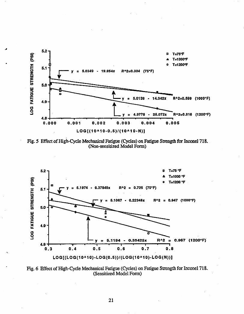
strength of Inconel 718 decreases as the number of cycles increases. Figures 5 and 6 show the
data in the non-sensitized form of equation (7b) and the sensitized model form, respectively.
Linear regression of the data produced f1l'st estimates of the empirical material constant, s, for
the high-cycle mechanical fatigue effect, as given by the slopes of the linear regression fits. As
seen by these regression fits in Figures 5 and 6, the R2 (goodness of fit) values are
significantly higher for the sensitized model form.
In reference to Figure 6, the R2 value corresponding to a temperature of 75 of is
significantly lower than the fits calculated at temperatures of 1000 OF and 1200 OP. In addition,
whereas the slope corresponding to a temperature of 1000 OF is lower than that corresponding
to 1200 OF, the slope obtained at a temperature of 75 OF (s = 0.37848) is higher than that at
both 1000 OF (s = 0.22348) and 1200 OF (s = 0.35425). This is due to the fact that at certain
current cycle values, N, the fatigue strength at a temperature of 75 OF is lower than that at
1000 of. Since this phenomenon is highly improbable, the validity of the high-cycle
mechanical fatigue data obtained at a test temperature of 75 OF is questionable. Thus, the
corresponding high-cycle mechanical fatigue material constant (s = 0.37848) is also
questionable.
140000 -en a. - a T=75 OF ::t 120000 .. T=1000°F l- • T=1200°F 0 z w 100000 I:C I-m w :;:) 80000 c:J
~ II..
60000 1e+4 2e+7 4e+7 6e+7 Se+7 1e+S
N F (CYCLES TO FAILURE)
Fig. 4 Effect of High-Cycle Mechanical Fatigue (Cycles) on Fatigue Strength for Inconel 718.
20
•
-en a. -
5.2
5.1
r y = 5.0349 - 19.954x
a T=75°F • T=1000°F
o T=1200°F
5.0 ~~~==.-==-___ _ L y
l, =
5.0139 • 14.342x RA2=0.589 (1000°F) 4.9
4.9778 - 28.072x RA2=0.916 (1200°F) 4.8;-..... --..... -r ..... ~ ..... ~ .......... ~ ..... ~ ..... ~ ..... ~ ..... -p ..... ~
0.000 0.001 0.002 0.003 0.004 0.005
LOG [(1 OA1 0-0.5)/(1 OA1 O-N)]
Fig. 5 Effect of High-Cycle Mechanical Fatigue (Cycles) on Fatigue Strength for Inconel 718. (Non-sensitized Model Form.)
-~ -5.2
5.1
4.9
= 5.1974 - 0.37848x RA2 = 0.725 (75°F)
5.1067 - 0.22348x RA2
a T=75°F
,. T=1000°F
o T=1200°F
= 0.947 (1000°F)
5.1184 - 0.35425x RA2 = 0.967 (1200°F) 4.8 -I-..... __ ..... -.,.. ..... -p ..... ..;.,. ..... _ ..................... _-__ -..._-....
0.3 0.4 0.5 0.6 0.7 0.8
LOG[(LOG(1 OA1 0)-LOG(0.5»/(LOG (1 OA1 O)-LOG(N»]
Fig. 6 Effect of High-Cycle Mechanical Fatigue (Cycles) on Fatigue Strength for Inconel 718. (Sensitized Model Form.)
21
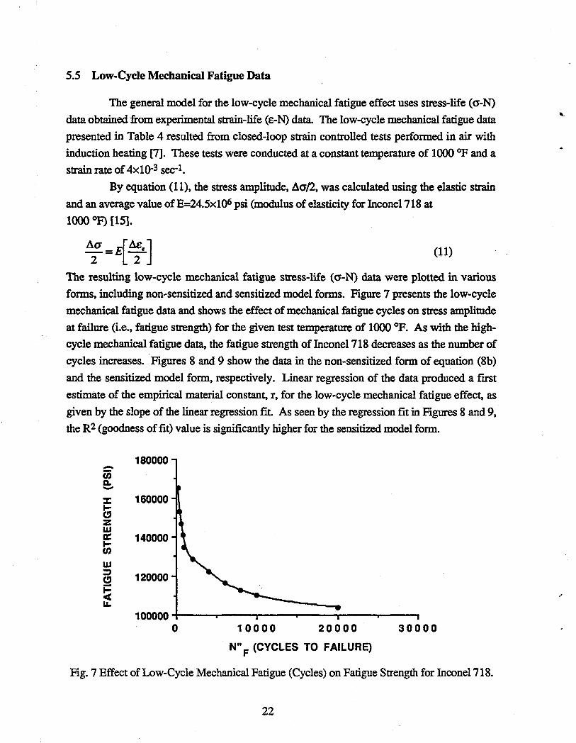
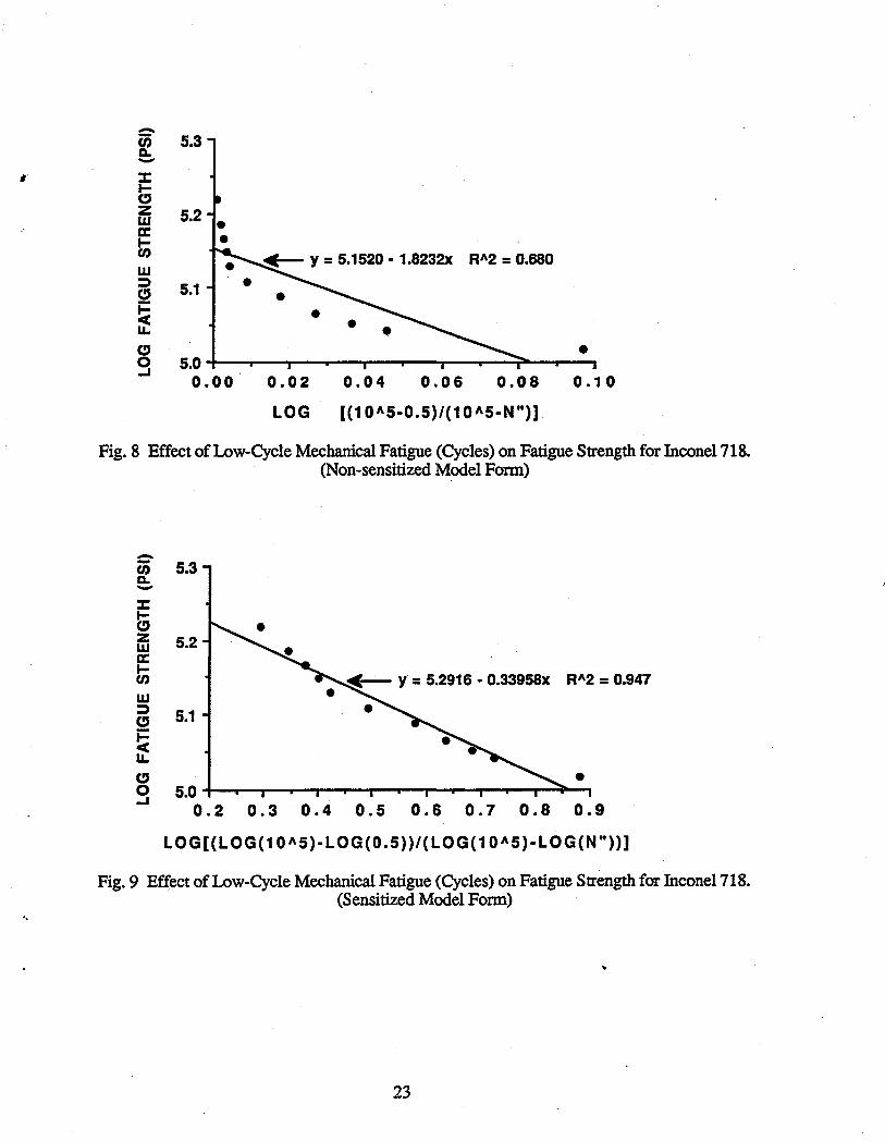
5.5 Low-Cycle Mechanical Fatigue Data
The general model for the low-cycle mechanical fatigue effect uses stress-life (a-N)
data obtained from experimental strain-life (e-N) data. The low-cycle mechanical fatigue data
presented in Table 4 resulted from closed-loop strain controlled tests performed in air with
induction heating [7]. These tests were conducted at a constant temperature of 1000 OF and a
strain rate of 4x10⁻³ sec-I.
By equation (11), the stress amplitude, Aa/2, was calculated using the elastic strain
and an average value ofE=24.5x10⁶ psi (modulus of elasticity for Inconel718 at
1000 oF) [15].
A2a =E[a;e] (11)
The resulting low-cycle mechanical fatigue stress-life (a-N) data were plotted in various
forms, including non-sensitized and sensitized model forms. Figure 7 presents the low-cycle
mechanical fatigue data and shows the effect of mechanical fatigue cycles on stress amplitude
at failure (i.e., fatigue strength) for the given test temperature of 1000 OF. As with the high
cycle mechanical fatigue data, the fatigue strength of Inconel 718 decreases as the number of
cycles increases. Figures 8 and 9 show the data in the non-sensitized form of equation (8b)
and the sensitized model form, respectively. Linear regression of the data produced a fIrst
estimate of the empirical material constant, r, for the low-cycle mechanical fatigue effect, as
given by the slope of the linear regression fIt. As seen by the regression fit in Figures 8 and 9, the R2 (goodness of fit) value is significantly higher for the sensitized model form.
180000 -Ci) a. -:z:: 160000 t; z w a: 140000 t; w ~ 120000
~ u. 100000 -t----,..-----r---""T---...__-__r--_.
o 10000 20000 30000
N" F (CYCLES TO FAILURE)
Fig. 7 Effect of Low-Cycle Mechanical Fatigue ( Cycles) on Fatigue Strength for Inconel 718.
22
,.
-~ 5.3 -5.2
RI\2 = 0.680
5.1 • • • • 5.0
0.00 0.02 0.04 0.06 0.08 0.10
LOG [(1 0"S-0.S)/(1 O"S-N")]
Fig. 8 Effect of Low-Cycle Mechanical Fatigue (Cycles) on Fatigue Strength for Inconel718. (Non-sensitized Model Form)
-u; S.3 c.. -:c I-
" Z W a: t;; w :::;)
" ~ u..
" o ..J
5.2
""",,-... 1-- Y = 5.2916 - 0.33958x RI\2 = 0.947
S.1
S.O +-_--..-r--.,..-__ -.,.. __ -.,--....---.---..-.,......;~..., 0.2 0.3 0.4 O.S 0.6 0.7 0.8 0.9
LOG [(LOG (1 0"S)-LOG(0.5»/(LOG(1 0 1\5)-LOG(N"»]
Fig. 9 Effect of Low-Cycle Mechanical Fatigue (Cycles) on Fatigue Strength for Inconel718. (Sensitized Model Form)
23
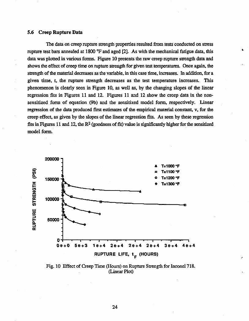
5.6 Creep Rupture Data
The data on creep rupture strength properties resulted from tests conducted on stress
rupture test bars annealed at 1800 of and aged [2]. As with the mechanical fatigue data, this
data was plotted in various forms. Figure 10 presents the raw creep rupture strength data and
shows the effect of creep time on rupture strength for given test temperatures. Once again, the
strength of the material decreases as the variable, in this case time, increases. In addition, for a
given time, t, the rupture strength decreases as the test temperature increases. This
phenomenon is clearly seen in Figure 10, as well as, by the changing slopes of the linear
regression fits in Figures 11 and 12. Figures 11 and 12 show the creep data in the non
sensitized form of equation (9b) and the sensitized model form, respectively. Linear
regression of the data produced first estimates of the empirical material constant, v, for the
creep effect, as given by the slopes of the linear regression fits. As seen by these regression
fits in Figures 11 and 12, the R2 (goodness of fit) value is significantly higher for the sensitized
model form.
-en 0. -:c ... c" Z w a:: t; w a:: ::;) ... 0. ::;) a::
200000 & T=1000 OF a T=1100 OF
150000 0 T=1200 OF
• T=1300°F
100000
50000
O~~--~~--~~--~~--~~--T-----T-~ __ Oe+O 5e+3 1 e+4 2e+4 2e+4 2e+4 3e+4 4e+4
RUPTURE LIFE, t F (HOURS)
Fig. 10 Effect of Creep Time (Hours) on Rupture Strength for Inconel 718. (Linear Plot)
24
-in 11--:c ~ Z w a: ~ w a: ::)
Ii: ::) a: CJ 9
-~ -
5.3
... T=1000°F
5.1618 - 10.922x RA2 = 0.722 a T=1100 of
5.1 0 T=1200 OF
• T=1300°F
4.9
- 11.080x RA2 = 0.701
4.7 Y = 5.0021 - 50.520x RA2 = 0.843
RA2 = 0.806 4.5 0.000 0.005 0.010 0.015 0.020
LOG[(1 OA6-0.25)/(1 0 A 6-t)]
Fig. 11 Effect of Creep Time (Hours) on Rupture Strength for Inconel 718. (Non-sensitized Model Form)
5.3
5.1
4.9
4.7
... T=1000°F a T=1100°F
o T=1200°F
RA2 = 0.994
3x RA2 = 0.992
RA2 = 0.991
• T=1300 OF RA2 = 0.998
4.5;-----~--~~--~----~----~~~~--~----~
0.0 0.2 0.4 0.6 0.8
LOG[LOG(1 OA6)-LOG(0.25»/(LOG(1 OA6)-LOG(t»]
Fig. 12 Effect of Creep Time (Hours) on Rupture Strength for Inconel 718. (Sensitized Model Form)
25
5.7 Thermal Fatigue Data
Low cycle fatigue produces cumulative material damage and ultimate failure in a
component by the cyclic application of strains that extend into the plastic range. Failure
typically occurs under 1()4 or lOS cycles. Low cycle fatigue is often produced mechanically
under isothermal conditions. However, machine components may also be subjected to low
cycle fatigue due to a cyclic thermal field. These cyclic temperature changes produce thermal
expansions and contractions that, if constrained, produce cyclic stresses and strains. These
thermally induced stresses and strains result in fatigue failure in the same manner as those
produced mechanically.
The general model for the thermal fatigue effect uses stress-life (O'-N) data obtained
from experimental strain-life (e-N) data. The thermal fatigue data presented in Table 7 resulted
from thermomechanical fatigue tests conducted on test bars annealed at 1800 OF and aged [17].
The temperature and strain were computer-controlled by the same triangular waveform with
in-phase cycling at a frequency of 0.0056 Hz.. The temperature was cycled between a
minimum temperature of 600 OF and a maximum temperature of 1200 OF, with a mean
temperature of approximately 900 OF. This total strain amplitude data and plastic strain
amplitude data were used to construct the strain-life curves presented in Figure 13.
Table 7 Thermal Fatigue Data for Inconel 718.
Cycles to Total Strain Plastic Strain Stress Failure Amplitude, Amplitude, Amplitude,
N'p &T/2 /:lEp/2 /:lcr/2 (psi)
45 0.0100 0.0050 126,500
140 0.0075 0.0029 116,380
750 0.0050 0.0011 98,670
9750 0.0040 0.0003 93,610
26
.1
III Q ::)
.01 I-::; a. :Ii CC
Z C .001 a: I-eI)
.0001 10
6-
o 6
6 o
o
100 1000
CYCLES TO FAILURE, NF
6 TOTAL STRAIN
o PLASTIC STRAIN
o
10000
Fig. 13 Strain-life Curve for Incone1718.
By equation (12), the stress amplitude, /lo/2, was calculated using total and plastic strain amplitudes, llET/2 and llEp/2, respectively, along with an average value ofE=25xl06 psi
(modulus of elasticity for Inconel 718 at 900 oF) [15].
flo = E[/lET _/lEP] 2 2 2
(12)
The resulting stress amplitude data were then plotted against the plastic strain amplitude data to
produce the cyclic stress-strain curve shown below in Figure 14.
140000
:::-f/) Do -w
120000 c ::)
t:: .... Do :Ii cc f/) 100000 f/) w a: l-f/)
~oo+---~~--~----~----~--~~--~
0.000 0.002 0.004 0.006
PLASTIC STRAIN AMPLITUDE
Fig. 14 Cyclic Stress-Strain Curve for Incone1718.
27
Using power law regression techniques [1] and the data in Table 7, fatigue properties
for Inconel 718 were calculated. These properties were calculated and compared with known
established values in order to check the validity of the data. The plastic portion of the strain-life
curve (Figure 13) may be represented by the following power law function:
6ep • ( .)C T=eF 2NF ' (13)
where 6ep/2 is the plastic strain amplitude and 2NF are the reversals to failure. A power law
regression analysis of the data yielded two fatigue properties, namely, the fatigue ductility coefficient, elF, and the fatigue ductility exponent, c. These two properties are indicated
graphically, along with their coefficient of determination, R2, in Figure 15. Regression
statistics, such as R2, were obtained to indicate whether or not a power law representation of
the relationship between plastic strain amplitude and reversals to failure was appropriate. As
commned by the high R2 value in Figure 15, the power law function of equation (11) well represents the relationship between 6ep/2 and 2NF.
UI C ::)
C
-2.0 RA2 = 0.999
~ -2.5 :IE cc z Ci
~ (.)
i ...J Q.
Cl o ...J
-3.0
-3.5
-4.0 +---....--_--........ ---r----,~-_r_--_-__, 1 2 3 4 5
LOG REVERSALS TO FAILURE
Fig. 15 Regression of Equation (11) Data Yielding Fatigue Ductility Coefficient, elF. and Fatigue Ductility Exponent, c.
28
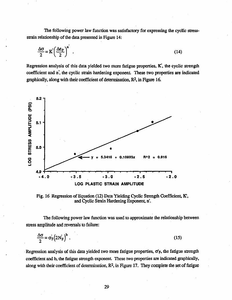
The following power law function was satisfactory for expressing the cyclic stress
strain relationship of the data presented in Figure 14:
(14)
Regression analysis of this data yielded two more fatigue properties, K', the cyclic strength
coefficient and n', the cyclic strain hardening exponent. These two properties are indicated
graphically, along with their coefficient of determination, R2, in Figure 16.
-en a. -w c ::;) I-::::i a. ::e ct tn tn W a: ti CJ 0 ....
5.2
5.1
5.0 • = 5.3416 + 0.10893x RA2 = 0.916
4.9 -I--.---.--....--,...-___ -.---.--....---.r--...._...--.-__ --r---.r--...._ __ -.--, -4.0 -3.5 -3.0 -2.5 -2.0
LOG PLASTIC STRAIN AMPLITUDE
Fig. 16 Regression of Equation (12) Data Yielding Cyclic Strength Coefficient, 1(', and Cyclic Strain Hardening Exponent, n'.
The following power law function was used to approximate the relationship between
stress amplitude and reversals to failure:
/::.a I ( .)b T=crF 2NF . (15)
, Regression analysis of this data yielded two more fatigue properties, aF, the fatigue strength
coefficient and b, the fatigue strength exponent. These two properties are indicated graphically,
along with their coefficient of determination, R2, in Figure 17. They complete the set of fatigue
29
material properties calculated. The complete set of properties are given in Table 8, along with
accepted ranges for the exponents [1].
-c;; D.. -W C ::::» I-::::; D. :!! ct t/) t/) w 0: l-t/)
" 0 ..I
5.2
Y = 5.2031 • 5.7210e-2x RA2 = 0.906
5.1
5.0 •
4.9 1 2 3 4 5
LOG REVERSALS TO FAILURE
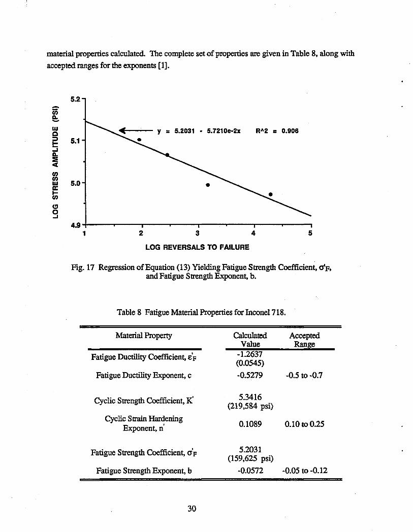
Fig. 17 Regression of Equation (13) Yielding Fatigue Strength Coefficient, ap, and Fatigue Strength Exponent, b.
Table 8 Fatigue Material Properties for Inconel718.
Material Property Calculated Accepted Value Ran~e
Fatigue Ductility Coefficient, e'F -1.2637 (0.0545)
Fatigue Ductility Exponent, c -0.5279 -0.5 to -0.7
Cyclic Strength Coefficient, K' 5.3416 (219,584 psi)
Cyclic Strain Hardening 0.1089 0.10 to 0.25 Exponent, n
I
Fatigue Strength Coefficient, (J'F 5.2031 (159,625 psi)
Fatigue Strength Exponent, b -0.0572 -0.05 to -0.12
30
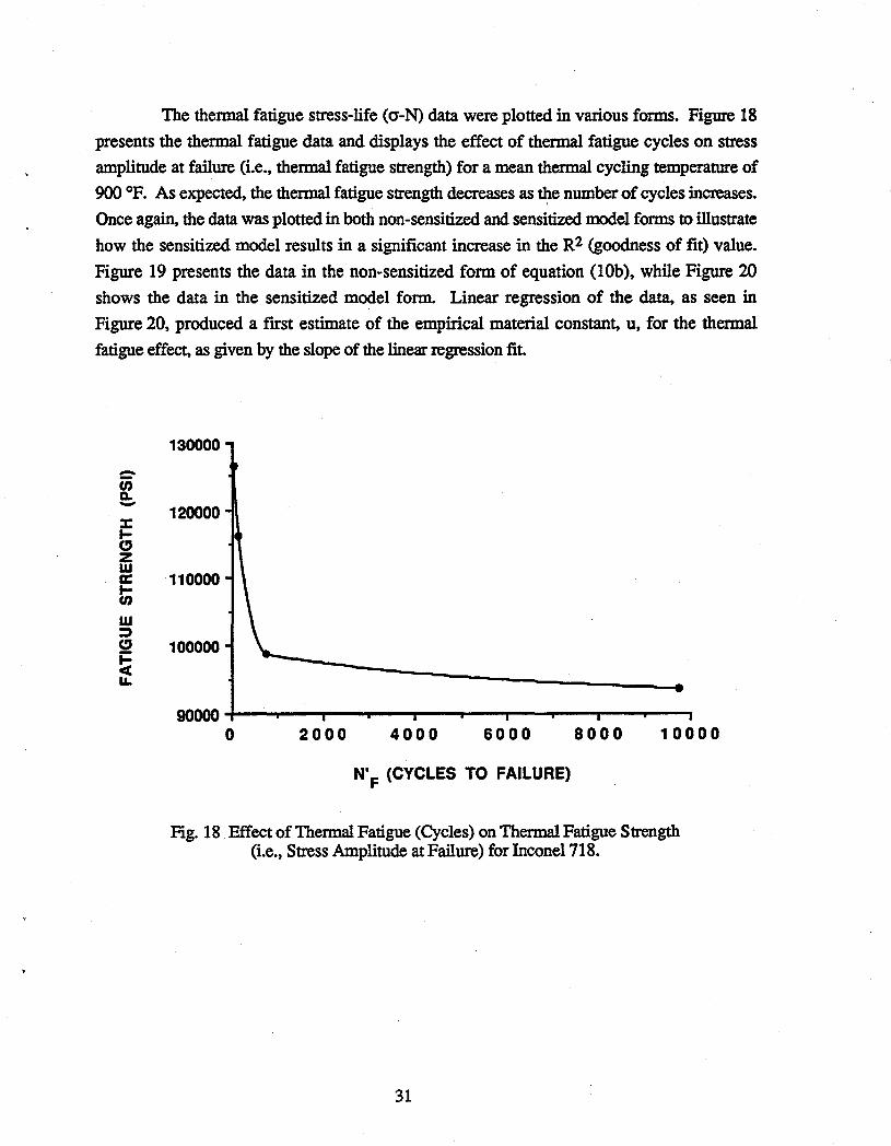
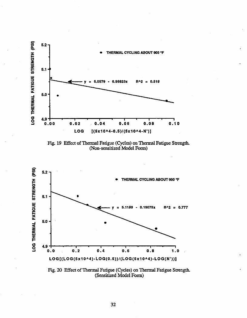
The thermal fatigue stress-life (cr-N) data were plotted in various forms. Figure 18
presents the thermal fatigue data and displays the effect of thermal fatigue cycles on stress
amplitude at failure (i.e., thermal fatigue strength) for a mean thermal cycling temperature of
900 of. As expected, the thermal fatigue strength decreases as the number of cycles increases.
Once again, the data was plotted in both non-sensitized and sensitized model forms to illustrate
how the sensitized model results in a significant increase in the R2 (goodness of fit) value.
Figure 19 presents the data in the non-sensitized form of equation (lOb), while Figure 20
shows the data in the sensitized model form. Linear regression of the data, as seen in
Figure 20, produced a fIrst estimate of the empirical material constant, U, for the thermal
fatigue effect, as given by the slope of the linear regression fit.
-Cii Q. -:c I-CJ Z W a: I-en w :::» CJ
~ u.
130000
120000
110000
100000
~ooo~------~--------~--~------~----~ o 2000 4000 6000 8000 10000
N' F (CYCLES TO FAILURE)
Fig. 18 Effect of Thermal Fatigue (Cycles) on Thermal Fatigue Strength (i.e., Stress Amplitude at Failure) for Inconel 718.
31
-~ 5.2 -
-
• THERMAL CYCLING ABOUT 900 of
5.1
5.0579 - 0.95823x RA2 = 0.518
5.0 •
4.9;---~---r--~--~~--r---~--'---~---r--~
0.00 0.02 0.04 0.06 0.08 0.10
LOG [(5x1 OA4-0.5)/(5x1 01\4-N')]
Fig. 19 Effect of Thermal Fatigue (Cycles) on Thermal Fatigue Strength. (Non-sensitized Model Form)
~ 5.2 -~ w a:
• THERMAL CYCLING ABOUT 900 of
~ 5.1
w ::::)
CJ
~ u.. ..J < ::E a: w ::z:: ... CJ 9
""""-:!E--- Y = 5.1189 - 0.19075x RA2 = 0.777
5.0 •
4.9~--~--~----r---~--~---T--~----r---~--~
0.0 0.2 0.4 0.6 0.8 1.0
LOG [(LOG(5x1 01\4 )-LOG(0.5»/(LOG (5x1 OA4)-LOG(N'»]
Fig. 20 Effect of Thermal Fatigue (Cycles) on Thermal Fatigue Strength. (Sensitized Model Form)
32
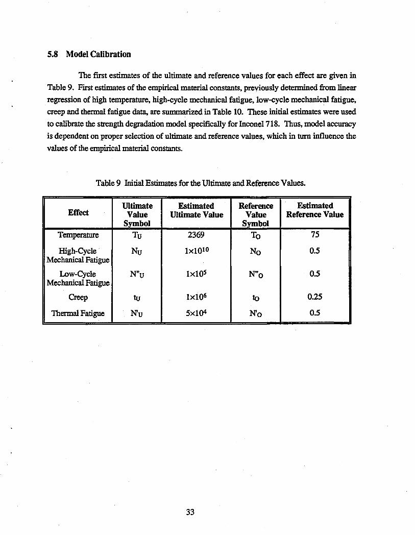
5.8 Model Calibration
The first estimates of the ultimate and reference values for each effect are given in
Table 9. First estimates of the empirical material constants, previously determined from linear regression of high temperature. high-cycle mechanical fatigue. low-cycle mechanical fatigue. creep and thermal fatigue data, are snmmarized in Table 10. These initial estimates were used
to calibrate the strength degradation model specifically for Inconel 718. Thus. model accuracy is dependent on proper selection of ultimate and reference values. which in turn influence the
values of the empirical material constants.
Table 9 Initial Estimates for the Ultimate and Reference Values.
Ultimate Estimated Reference Estimated Effect Value Ultimate Value Value Reference Value
Symbol Symbol Temperature Tu 2369 To 75
High-Cycle Nu lxl010 No 0.5 Mechanical Fatigue
Low-Cycle N"u lxl0s N"o 0.5 Mechanical Fatigue
Creep tu lxl06 to 0.25
Thermal Fatigue Nu 5xl04 No 0.5
33
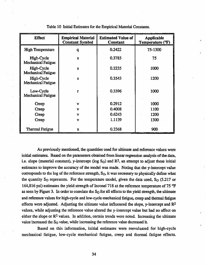
Table 10 Initial Estimates for the Empirical Material Constants.
Effect Empirical Material Estimated Value of Applicable Constant Symbol Constant Temperature (OF)
High Temperature q 0.2422 75-1300
High-Cycle s 0.3785 75 Mechanical Fatigue
High-Cycle s 0.2235 1000 Mechanical Fatigue
High-Cycle s 0.3543 1200 Mechanical Fatigue
Low-Cycle r 0.3396 1000 Mechanical Fatigue
Creep v 0.2912 1000 Creep v 0.4008 1100 Creep v 0.6243 1200 Creep v 1.1139 1300
Thermal Fatigue u 0.2368 900
As previously mentioned, the quantities used for ultimate and reference values were
initial estimates. Based on the parameters obtained from linear regression analysis of the data, i.e. slope (material constant), y-intercept (log So) and R2, an attempt to adjust these initial
estimates to improve the accuracy of the model was made. Noting that the y-intercept value
corresponds to the log of the reference strength, So, it was necessary to physically defme what
the quantity So represents. For the temperature model, given the data used, So (5.217 or
164,816 psi) estimates the yield strength of Inconel 718 at the reference temperature of 75 OF
as seen by Figure 3. In order to correlate the So for all effects to the yield strength, the ultimate
and reference values for high-cycle and low-cycle mechanical fatigue, creep and thermal fatigue
effects were adjusted. Adjusting the ultimate value influenced the slope, y-intercept and R2
values, while adjusting the reference value altered the y-intercept value but had no affect on
either the slope or R2 values. In addition, certain trends were noted. Increasing the ultimate
value increased the So value, while increasing the reference value decreased it
Based on this information, initial estimates were r~evaluated for high-cycle
mechanical fatigue, low-cycle mechanical fatigue, creep and thermal fatigue effects.
34
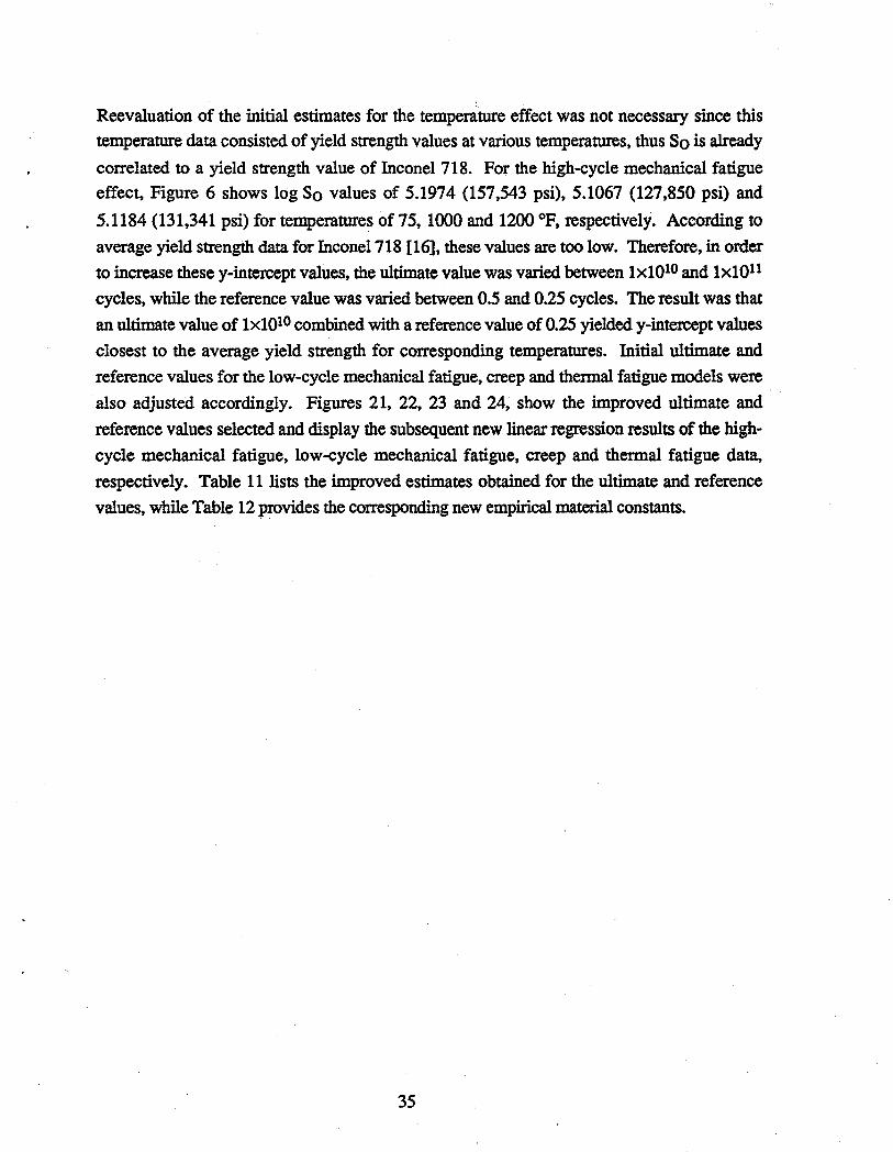
Reevaluation of the initial estimates for the tempe~ture effect was not necessary since this
temperature data consisted of yield strength values at various temperatures, thus So is already
correlated to a yield strength value of Inconel 718. For the high-cycle mechanical fatigue
effect, Figure 6 shows log So values of 5.1974 (157,543 psi), 5.1067 (127,850 psi) and
5.1184 (131,341 psi) for temperatures of 75, 1000 and 1200 OF, respectively. According to
average yield strength data for Inconel718 [16], these values are too low. Therefore, in order
to increase these y-intercept values, the ultimate value was varied between lxl010 and lxl011
cycles, while the reference value was varied between 0.5 and 0.25 cycles. The result was that
an ultimate value of lxl010 combined with a reference value of 0.25 yielded y-intercept values
closest to the average yield strength for corresponding temperatures. Initial ultimate and
reference values for the low-cycle mechanical fatigue, creep and thermal fatigue models were
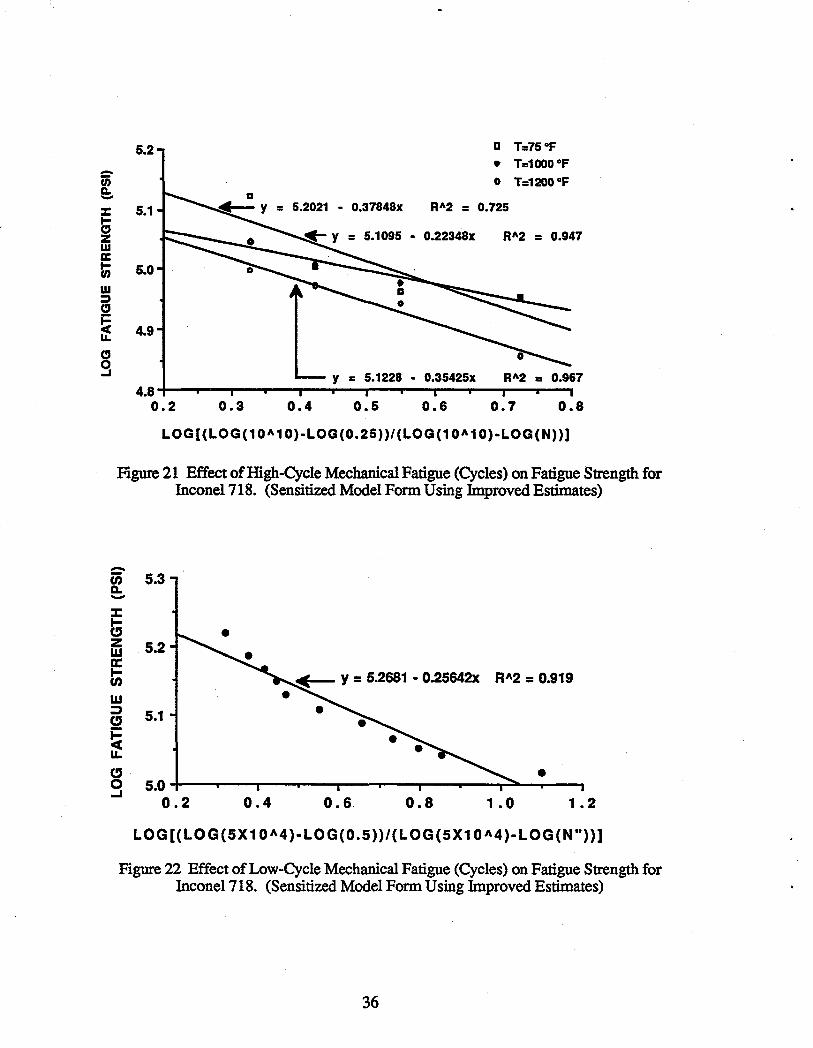
also adjusted accordingly. Figures 21, 22, 23 and 24, show the improved ultimate and
reference values selected and display the subsequent new linear regression results of the high
cycle mechanical fatigue. low-cycle mechanical fatigue, creep and thermal fatigue data,
respectively. Table 11 lists the improved estimates obtained for the ultimate and reference
values, while Table 12 provides the corresponding new empirical material constants.
35
5.2
-en Q, -::c 5.1
i w a: to 5.0 w ::» CJ
~ u. CJ g
4.9
4.8 0.2 0.3 0.4
D T=75°F • T=1000°F
o T=1200°F
- 0.37848x RA2 = 0.725
RA2 = 0.947
y = 5.1228 - 0.35425x RA2 = 0.967
0.5 0.6 0.7 0.8
LOG [(LOG(1 OA1 0)-LOG(0.25»/(LOG(1 OA1 O)-LOG(N»)]
Figure 21 Effect of High-Cycle Mechanical Fatigue (Cycles) on Fatigue Strength for Inconel718. (Sensitized Model Form Using Improved Estimates)
-u; 5.3 Q. -:::I: t; z w a: ti w :::)
e"
~ Ll-
e" o ..J
5.2
RA2 = 0.919
5.1
• 5.0 +----~-....--,.--....--,.--...--~-...----, 0.2 0.4 0.6 0.8 1 .0 1.2
LOG [(LOG( 5X1 01\4 )-LOG(0.5»/(LOG (5X1 01\4)- LOG (Nit»]
Figure 22 Effect of Low-Cycle Mechanical Fatigue (Cycles) on Fatigue Strength for Inconel718. (Sensitized Model Form Using Improved Estimates)
36
5.3
-~ - = 5.2235 - 0.17372x RA2 = 0.974 :c 5.1 l; z w a:
RA2 = 0.961
t; 4.9 w RA2 = 0.994 a: ~
Ii: ~ 4.7 a:
A T=1000°F
a T=1100°F o T=1200°F
• T=1300°F CJ 9
==(/) D. -:c l; z w
5.0671 - 0.75557x RA2 = 1.000
4.5 -I--..-....,---r-...,...-..-___ r--__r~""T"'-_-r____r-..., 0.0 0.2 0.4 0.6 0.8 1.0 1.2
LOG[(LOG(1 OA5)-LOG(0.25»/(LOG(1 0 A5)-LOG(t»]
Figure 23 Effect of Creep Time (Hours) on Rupture Strength for Inconel 718. (Sensitized Model Fonn Using Improved Estimates)
5.2
• THERMAL CYCUNG ABOUT 900 of
a: 5.1 t; w ~ CJ
ti u. .... <I: ::E a: w :c ... 9
~. ____ y = 5.1237 - 0.19075x
5.0 •
4.9;---..--__r---r--_-~r---~--""T"'-~
0.2 0.4 0.6 0.8 1.0
LOG[(LOG(5x1 OA4 )-LOG(0.25»/(LOG(5x1 OA4 )-LOG(N'»]
Figure 24 Effect of Thennal Fatigue (Cycles) on Thennal Fatigue Strength. (Sensitized Model Fonn Using Improved Estimates)
37
Table 11 Improved Estimates for the Ultimate and Reference Values.
Ultimate Estimated Reference Estimated Effect Value Ultimate Value Value Reference Value
Symbol Symbol Temperature Tu 2369 To 75
High-Cycle NO' lxl010 No 0.25 Mechanical Fatigue
Low-Cycle N"u 5xl04 N"o 0.50 Mechanical Fatigue
Creep tu lxlOS to 0.25
Thermal Fatigue N'u 5xl04 N'o 0.25
Table 12 Improved Estimates for the Empirical Material Constants.
Effect Empirical Material Estimated Value of Applicable Constant Symbol Constant Temperature (OF)
High Temperature q 0.2422 75-1300
High-Cycle s 0.3785 75 Mechanical Fatigue
High-Cycle s 0.2235 1000 Mechanical Fatigue
High-Cycle s 0.3543 1200 Mechanical Fatigue
Low-Cycle r 0.2564 1000 Mechanical Fatigue
Creep v 0.1737 1000 Creep v 0.2245 1100 Creep v 0.4136 1200 Creep v 0.7556 1300
Thermal Fatigue u 0.1908 900
38
6.0 ESTIMATION OF EMPIRICAL MATERIAL
CONSTANT VARIABILITY
Due to a lack of sufficient data from which to evaluate the material constants, ait·
methodology to estimate the variability of these constants was developed. This methodology
yields estimates for the standard deviations of the constants. For instance, when modeling
high temperature effects, the material strength degradation model for Inconel 718 is given
below by equation (6a).
or
-.!.=[TU -To]-q So Tu- T
S = So[TU - To ]-q Tu-T
Taking the log of both sides yields equation (14b) below.
(6a)
(16a)
(16b)
It is clearly seen that equation (16b) is a linear equation with slope, -q, and y-intercept, Log So
Using the temperature data presented in Section 5, the linear relationship given by
equation (16b) is shown graphically in Figure 25.
Linear regression of this temperature data yielded two parameters, the slope (-0.2422)
and the y-intercept (5.2170). As previously discussed, the slope was used as a flISt estimate of
the empirical material constant for the temperature degradation model. Due to limited
temperature data, only five data points, concern over the accuracy of this estimated value was
warranted. Therefore, steps were taken to model this material constant as a random variable so
that an estimate of its standard deviation could be calculated.
39
5.30 -en Q. -::c 5.25 ... " Z W Y = 5.2170 - 0.24215x RA2 = 0.970 a:: ti 5.20
Q -I W
>= 5.15
" 0 -I
5.10 ...... -___,r__---r---~-~r__---.---_r_----,r---....., 0.0 0.1 0.2 0.3 0.4
LO G [(2369-75 )/(23 69-T)]
Figure 25 Linear Regression of Temperature Data.
First, maximum and minimum feasible slopes and y-intercepts were determined
from consideration of the data and the linear regression results, such that these extreme
parameters would theoretically enclose or envelope all actual data. Figure 26 shows the linear
regression of the temperature data along with postulated maximum and minimum slopes.
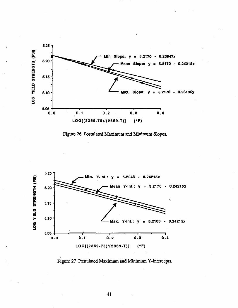
These extreme parameters were obtained by adjusting the slope of the linear regression fit.
Rotating about the y-intercept value, the regression line was adjusted to pass through the outer
most points, resulting in maximum and minimum slopes. Figure 27 shows the linear
regression of the temperature data along with maximum and minimum y-intercepts. These
extreme parameters were obtained by shifting the regression line vertically. While maintaining
the slope, the regression line was shifted to pass through the outer most points, resulting in
maximum and minimum y-intercept values.
40
-en Q. -::c to-CJ Z W a: to-en Q -' W >= CJ 9
-en Q. -~ z w a: t; Q -' W >= CJ 9
5.25
Slope: y = 5.2170 - 0.20847x 5.20
5.2170 - 0.24215x
5.15
LMax• 5.10 Slope: y = 5.2170 - 0.26136x
5.05 -f-----.,.-----.,._----.,-------. 0.0 0.1 0.2 0.3 0.4
LOG[(2369-75)/(2369-T)] (OF)
Figure 26 Postulated Maximum and Minimum Slopes.
5.25 V-Int.: y = 5.2246 0.24215x
5.20 V-Int.: y = 5.2170 - 0.24215x
5.15
5.10 Lx. Y·lnt.: y = 5.2106 - 0.24215x
5.05 +---,r----r---r----.----r--~--.,._---. 0.0 0.1 0.2 0.3 0.4
LOG[(2369-75)/(2369-T» (OF)
Figure 27 Postulated Maximum and Minimum Y -intercepts.
41
Using the values of the parameters obtained from linear regression along with the
extreme maximum and minimum values, random variables for slope (-q) and y-intercept
(log So) were constructed. These random parameters or variables were assumed to have
normal distributions, with mean values given by the linear regression fit in Figure 25.
Standard deviation values for the slope and y-intercept were determined using the extreme
values together with the empirical rule. According to this rule, for a normal distribution, the
mean value (J.1) plus or minus three standard deviations (±30') will contain 99.73% of the
values [18,21]. Therefore, the range of the values (maximum value minus the minimum
value) divided by six yields the standard deviation, 0'. Although the mean value resulting from
linear regression (Figure 25) is not equal to J.1 (one-half the range) due to the nature of the data
and the extreme values obtained, this method provides for an approximation of the standard
deviation.
J.1
Figure 28 Probability Density Function of a Normal Distribution.
Values for the standard deviation of the random parameters, slope and y-intercept,
were estimated as follows:
_ maximum slope - minimum slope _ 0.2614 - 0.2085 _ 0 0088 O'slope - 6 - 6 - .
_maximumy-int - minimumy-int_167,707.20-162,416.67 -88175( .) O'y-int. - 6 - 6 -. pSl
42
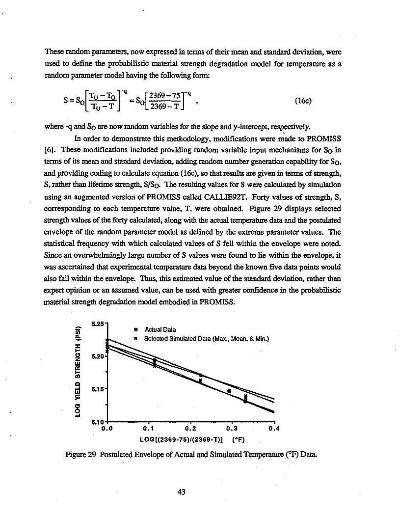
These random parameters, now expressed in terms of their mean and standard deviation, were
used to define the probabilistic material strength degradation model for temperature as a
random parameter model having the following form:
S=S [TU-TO]-q =S [2369-75]-q 0. Tu -T 0 2369-T '
(16c)
where -q and So are now random variables for the slope and y-intercept, respectively • . In order to demonstrate this methodology, modifications were made to PROMISS
[6]. These modifications included providing random variable input mechanisms for So in
terms of its mean and standard deviation, adding random number generation capability for So,
and providing coding to calculate equation (16c), so that results are given in terms of strength,
S, rather than lifetime strength, S/So. The resulting values for S were calculated by simulation
using an augmented version of PROMISS called CALLIE92T. Forty values of strength, S,
corresponding to each temperature value, T, were obtained. Figure 29 displays selected
strength values of the forty calculated, along with the actual temperature data and the postulated
envelope of the random parameter model as defmed by the extreme parameter values. The
statistical frequency with which calculated values of S fell within the envelope were noted.
Since an overwhelmingly large number of S values were found to lie within the envelope, it
was ascertained that experimental temperature data beyond the known five data points would
also fall within the envelope. Thus, this estimated value of the standard deviation, rather than
expert opinion or an assumed value, can be used with greater confidence in the probabilistic
material strength degradation model embodied in PROMISS.
-~ -:c t-
~ UI a: ; Q -' UI >= CJ 9
5.25 • Actual Data • Selected Simulated Data (Max., Mean, & Min.)
5.20
5.15
5.10+----...,..----"..----...,..------, 0 •. 0 0.1 0.2 0.3 0.4
LOG[(2369-75}/(2369-T» (OF)
Figure 29 Postulated Envelope of Actual and Simulated Temperature COF) Data.
43
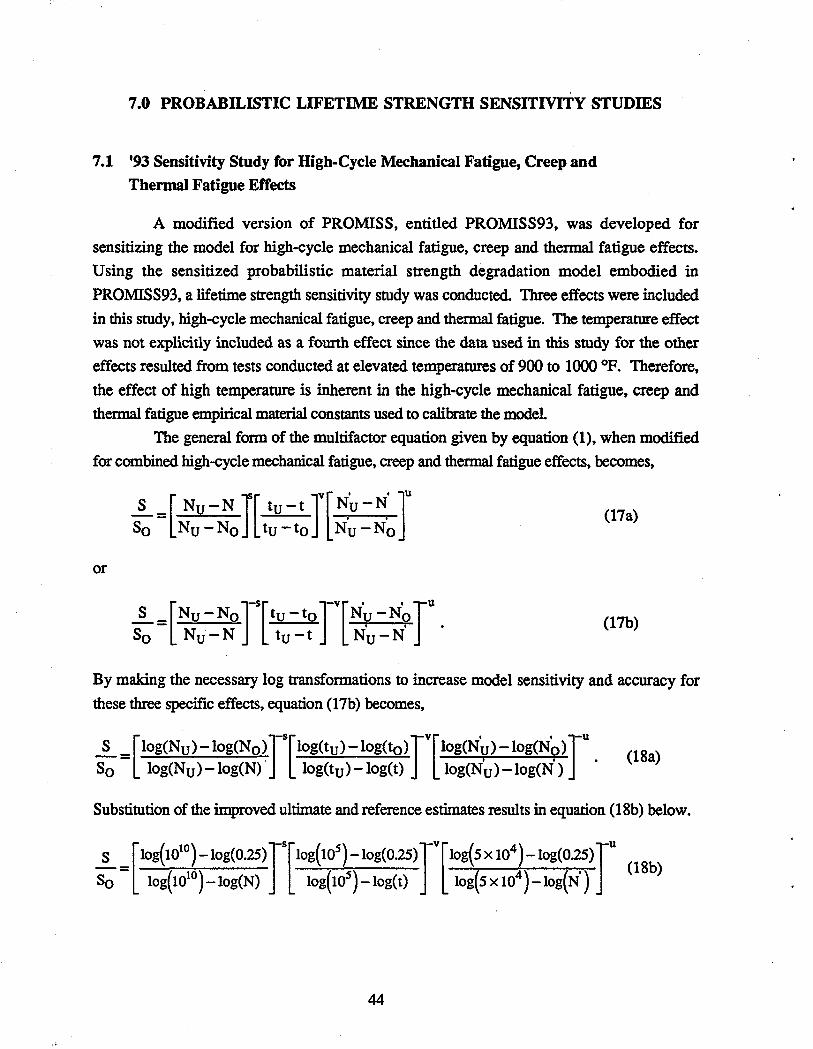
7.0 PROBABILISTIC LIFETIME STRENGTH SENSITIVITY STUDIES
7.1 '93 Sensitivity Study for High-Cycle Mechanical Fatigue, Creep and
Thermal Fatigue Effects
A modified version of PROMISS, entitled PROMISS93, was developed for
sensitizing the model for high-cycle mechanical fatigue, creep and thermal fatigue effects.
Using the sensitized probabilistic material strength degradation model embodied in
PROMISS93, a lifetime strength sensitivity study was conducted. Three effects were included
in this study, high-cycle mechanical fatigue, creep and thermal fatigue. The temperature effect
was not explicitly included as a fourth effect since the data used in this study for the other
effects resulted from tests conducted at elevated temperatures of 900 to 1000 OF. Therefore,
the effect of high temperature is inherent in the high-cycle mechanical fatigue, creep and
thermal fatigue empirical material constants used to calibrate the model.
The general form of the multifactor equation given by equation (1), when modified
for combined high-cycle mechanical fatigue, creep and thermal fatigue effects, becomes,
S Nu-N tu-t Nu- N [ ]S[ ]V[' . ]U
So = Nu-No tu-to N~-N~ (17a)
or
..!.=[NU -NoJS[tu -toJV[N¥ -N9JU . So Nu-N tu- t Nu-N
(17b)
By making the necessary log transformations to increase model sensitivity and accuracy for
these three specific effects, equation (17b) becomes,
..!. = [IOg(Nu)-IOg(No)]-S[IOg(tu) -IOg(to)JV[IOg(N'v) -IOg(N9)]-U . (18a) So 10g(Nu)-log(N) log(tu)-log(t) 10g(Nu)-log(N)
Substitution of the improved ultimate and reference estimates results in equation (18b) below.
S [lOg(1010
) -lOg(O.25)]-S[lOg(lOS) -lOg(O.2S)]-V[lOg(S x 104
) -log(o.2S)]-U -= . (18b) So log(1010)-log(N) log(lOS)-log(t) log(SXI04)-log(N)
44
The ultimate and reference values in equation (18b) became model parameters or
constraints for the multifactor equation when modified for Inconel718. Figure 30 illustrates
these model parameters graphically, wherein each axis represents an effect.
THERMAL FATIGUE (CYCLES)
N'u 5x10 4
N'o 0.25
No Nu ;--+-----+--1 .. MECHANICAL FATIGUE (CYCLES)
0.25 10 10
CREEP (HOURS)
Fig. 30 Inconel 718 Model Parameters for High-Cycle Mechanical Fatigue, Creep and Thermal Fatigue Effects.
Typical sets of input values for the PRO:MISS model represented by equation (18b)
are given in Tables 13, 14 and 15. For example, Table 13 shows PROMISS input data for a
temperature of 1000 OF, a current value of 2.5xlOS high-cycle mechanical fatigue cycles, a
current value of 1000 creep hours, and a current value of 2000 thermal fatigue cycles. As seen
in Tables 13 through 15, the above-mentioned current values remain the same with the
exception of the current value-ofhigh-cycle mechanical fatigue cycles, N. In Tables 14 and 15
the current value of high-cycle mechanical fatigue cycles has been increased to l.Oxl06 and
1.75xl06, respectively. By holding two of the three sets of current values constant, sensitivity
of lifetime strength towards the third set of values, in this case bigh-cycle mechanical fatigue
cycles, can be ascertained. The complete set of current values that were used as input data for
this sensitivity study are given in Table 16. Notice that the fll"St three rows of the table
correspond to the current values listed in Tables 13, 14 and 15, respectively. The next three
rows of Table 16 show how the current values of creep hours were varied, while the last three
rows show how the current values of thermal fatigue cycles were varied. The results of this
study, in the fonn of cumulative distribution functions, are given in Figures 31 through 33.
45
Figure 31 shows the effect of high-cycle mechanical fatigue cycles on lifetirile strength, while
Figures 32 and 33 show the effect of creep hours and thermal fatigue cycles on lifetime strength, respectively. Note that the c.d.f. shifts to the left, indicating a lowering of lifetime
strength, as mechanical fatigue cycles increase. In this manner, results, in the form of c.d.f.'s,
display the sensitivity of lifetime strength to any current value of an effect
Table 13 '93 Sensitivity Study Input to PROMISS93 for Inconel 718; Temperature = 1000 OF and N=2.5x1OS Cycles.
Effect Variable Units Distribution Mean Standard Deviation Symbol Type (Value), (% of Mean)
High-Cycle Nu cycles Normal 1.0x10¹⁰ 1.0x10⁹ 10.0 Mechanical N cycles Normal 2.5x1OS 2.5x10⁴ 10.0 Fatigue No cycles Normal 0.25 0.025 10.0
s dimensionless Normal 0.2235 0.0067 3.0
Creep tu hours Normal 1.0x1Os 1.0x10⁴ 10.0 t hours Normal 1.0x1()3 1.0x10² 10.0 to hours Normal 0.25 0.025 10.0 v dimensionless Normal 0.1737 0.0052 3.0
Thermal N'u cycles Normal 5.0x10⁴ 5.0x1()3 10.0 Fatigue N' cycles Normal 2.0x1()3 2.0x10² 10.0
N'o cycles Normal 0.25 0.025 10.0 u dimensionless Normal 0.191 0.0057 3.0
Table 14 '93 Sensitivity Study Input to PROMISS93 for Ineanel718; Temperature = 1000 OF and N=1.0x10⁶ Cycles.
Effect Variable Units Distribution Mean Standard Deviation Symbol Type (Value), (% of Mean)
High-Cycle Nu cycles Normal 1.0x10¹⁰ 1.0x10⁹ 10.0 Mechanical N cycles Normal 1.0x10⁶ 1.0xlOS 10.0 Fatigue No cycles Normal 0.25 0.025 10.0
s dimensionless Normal 0.2235 0.0067 3.0
Creep tu hours Normal 1.0x1Os 1.0x10⁴ 10.0 t hours Normal 1.0x10³ 1.0x10² 10.0 to hours Normal 0.25 0.025 10.0 v dimensionless Normal 0.1737 0.0052 3.0
Thermal N'u cycles Normal 5.0xl04 5.0xl()3 10.0 Fatigue N' cycles Normal 2.0x10³ 2.0xl02 10.0
N'o cycles Normal 0.25 0.025 10.0 u dimensionless Normal 0.191 0.0057 3.0
46
Table 15 '93 Sensitivity Study Input to PROMISS93 for Inconel 718; Temperature = 1000 of and N=1.75xl06 Cycles
Effect Variable Units Distribution Mean Standard Deviation Symbol Type (Value), (% of Mean)
High-Cycle Nu cycles Normal 1.0xl010 1.0x10⁹ 10.0 Mechanical N cycles Normal 1.75x10⁶ 1.75x1OS 10.0 Fatigue No cycles Normal 0.25 0.025 10.0
s dimensionless Normal 0.2235 0.0067 3.0
Creep tu hours Normal 1.0x1OS 1.0x10⁴ 10.0 t hours Normal 1.0x1()3 1.0xl()2 10.0 to hours Normal 0.25 0.025 10.0 v dimensionless Normal 0.1737 0.0052 3.0
Thermal Nu cycles Normal 5.0x10⁴ 5.0x1()3 10.0 Fatigue N' cycles Normal 2.0xl()3 2.0x1()2 10.0
No cycles Normal 0.25 0.025 10.0 u dimensionless Normal 0.191 0.0057 3.0
Table 16 Selected Current Values for '93 Sensitivity Study of the Probabilistic Material Strength Degradation Model for Inconel 718.
High-Cycle Creep Thermal Fatigue Mechanical Fatigue (Hours) (Cycles)
(Cycles)
2.5 x U)5 1000 2000
1.0 x 10⁶ 1000 2000
1.75 x 10⁶ 1000 2000
1.0 x 10⁶ 250 2000
1.0 x 10⁶ 1000 2000
1.0 x 10⁶ 1750 2000
1.0 x 10⁶ 1000 500 1.0 x 10⁶ 1000 2000
1.0 x 10⁶ 1000 3500
47
1.0 -
0.8 -
0.6 -
0.4 -6 1.75x10 6 CYCLES
o 1.0x10 6 CYCLES 0.2 - 2.5x10 5 CYCLES
0.0 -!----r6 .. iI2A:ta.:;:----r-----.----__ 0.40 0.45 0.50 0.55 0.60 0.65
LIFETIME STRENGTH, SIS 0
Fig. 31 Comparison of Various Levels of Uncertainty of High-Cycle Mechanical Fatigue (Cycles) on Probable Strength for Inconel 718 for 2000 Thermal Fatigue
Cycles and 1000 Hours of Creep at 1000 of.
1.0 -
0.8 -
0.6
0.4 -6 1750 HOURS
o 1000 HOURS 0.2 - 250 HOURS
0.0 -J----4I ... _~~~-___r---_....;......-____. 0.40 0.45 0.50 0.55 0.60 0.65
LIFETIME STRENGTH, SIS 0
Fig. 32 Comparison of Various Levels of Uncertainty of Creep Time (Hours) on Probable Strength for Inconel718 for lxl06 High-Cycle Mechanical
Fatigue Cycles and 2000 Thermal Fatigue Cycles at 1000 OF.
48
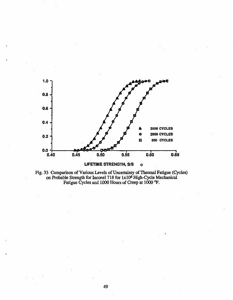
1.0 -
0.8
0.6
0.4
0.2
6 3500 CYCLES
02000 CYCLES
D 500 CYCLES
0.0 -,I----6 .. i5e.:a::~_a:::--r__--.......,r__--__ 0.40 0.45 0.50 0.55 0.60 0.65
UFETIME STRENGTH, SIS 0
Fig. 33 Comparison of Various Levels of Uncertainty of Thermal Fatigue (Cycles) on Probable Strength for Inconel 718 for lx106 High-Cycle Mechanical
Fatigue Cycles and 1000 Hours of Creep at 1000 CP.
49
7.2 '94 Sensitivity Study for High-Cycle Mechanical Fatigue, Low-Cycle Mechanical
Fatigue, Creep and Thermal Fatigue Effects
A modified version of PROMISS93, entitled PROMISS94, was developed for
sensitizing the model for yet another effect, low-cycle mechanical fatigue. Using the sensitized
probabilistic material strength degradation model embodied in PROMISS94, a second lifetime
strength sensitivity study was conducted. Four effects were included in this study, high-cycle
mechanical fatigue, low-cycle mechanical fatigue, creep and thermal fatigue. As before, the
temperature effect was not explicitly included as a flfth effect since the data used in this study
for the other effects resulted from tests conducted at elevated temperatures of 900 to 1000 CP.
Therefore, the effect of high temperature is inherent in the high-cycle mechanical fatigue, low
cycle mechanical fatigue, cre~p and thermal fatigue empirical material constants used to
calibrate the model.
The general form of the multifactor equation given by equation (1), when modified
for combined high-cycle mechanical fatigue, low-cycle mechanical fatigue, creep and thermal
fatigue effects, becomes,
(19a)
or
(19b)
By making the necessary log transformations to increase model sensitivity and accuracy for
these four specific effects, equation (19b) becomes,
~ = [IOg(Nu) -IOg(No)]-:r[IOg(N"~ )-IOg(N"?)]-"[IOg(tu )-IOg(to)]-Y[IOg(N~)-IOg(N~)]-" So log(N u) -log(N) log(N u) -log(N ) log(tu) -log(t) log(N u) -log(N )
(20a)
Substitution of the improved ultimate and reference estimates results in equation (20b) below .
.§... = [lOg(lOID
) -lOg(002S)]-6[lOg(S X 104
) -lOg(OoSO)]_r[lOg(10S
) -lOg(0.25)]-Y[lOg(5 x 10⁴
) -lOg(O.2S)]--
So log ( 101D) - log(N) log( 5 x 10⁴
) - log( N°) log( lOS) -log(t) log( 5 x 10⁴) -log( N' )
(20b)
50
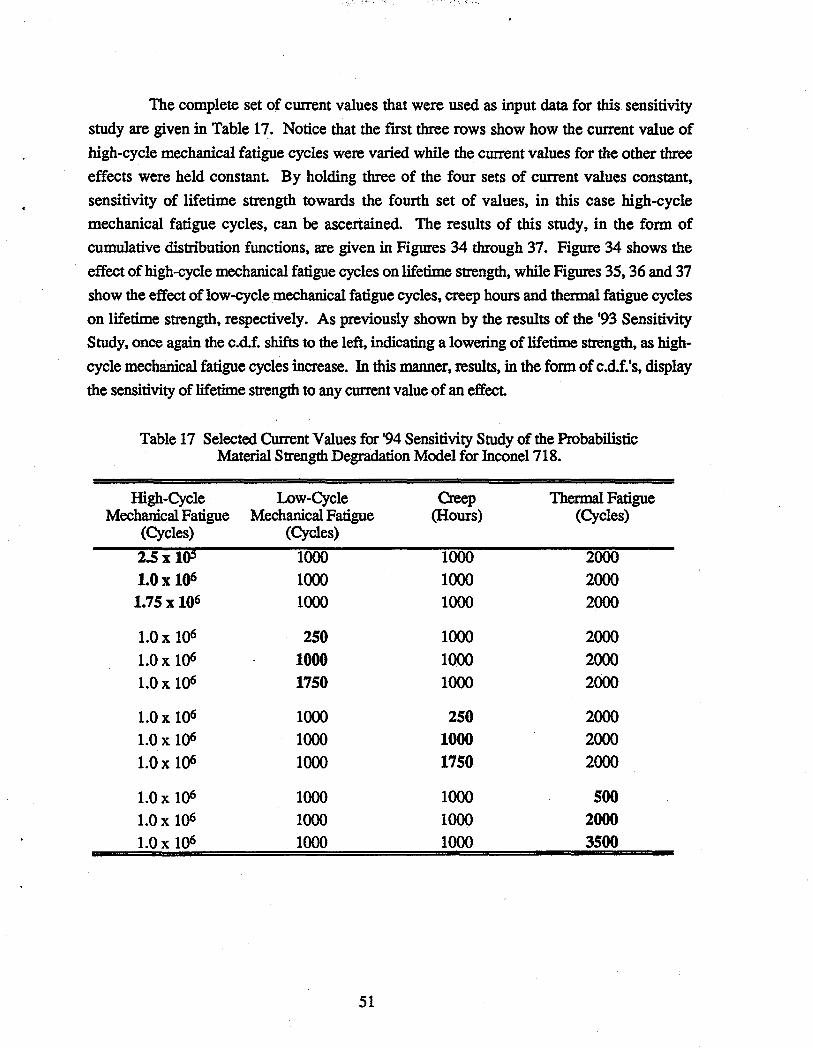
"i, .••
The complete set of current values that were used as input data for this sensitivity
study are given in Table 17. Notice that the fll'st three rows show how the current value of
high-cycle mechanical fatigue cycles were varied while the current values for the other three
effects were held constant. By holding three of the four sets of current values constant,
sensitivity of lifetime strength towards the fourth set of values, in this case high-cycle
mechanical fatigue cycles, can be ascertained. Theresults of this study, in the form of
cumulative distribution functions, are given in Figures 34 through 37. Figure 34 shows the
effect of high-cycle mechanical fatigue cycles on lifetime strength, while Figures 35, 36 and 37
show the effect of low-cycle mechanical fatigue cycles, creep hours and thermal fatigue cycles
on lifetime strength, respectively. As previously shown by the results of the '93 Sensitivity
Study, once again the c.d.f. shifts to the left, indicating a lowering of lifetime strength, as high
cycle mechanical fatigue cycles increase. In this manner, results, in the form of c.dJ. IS, display
the sensitivity of lifetime strength to any current value of an effect.
Table 17 Selected Current Values for '94 Sensitivity Study of the Probabilistic Material Strength Degradation Model for Inconel 718.
High-Cycle Low-Cycle Creep Thermal Fatigue Mechanical Fatigue Mechanical Fatigue (Hours) (Cycles)
(Cycles) (Cycles)
2.5 x 1()5 1000 1000 2000
1.0 x 10⁶ 1000 1000 2000 1.75 x 10⁶ 1000 1000 2000
1.0 x 10⁶ 250 1000 2000
1.0 x 10⁶ 1000 1000 2000
1.0 x 10⁶ 1750 1000 2000
1.0 x 10⁶ 1000 250 2000
1.0 x 10⁶ 1000 1000 2000
1.0 x 10⁶ 1000 1750 2000
1.0 x 10⁶ 1000 1000 500 1.0 x 10⁶ 1000 1000 2000 1.0 x 10⁶ 1000 1000 3500
51
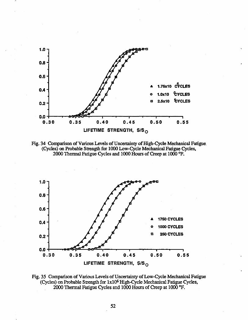
1.0
0.8
0.6
0.4
0.2
A 1.7Sx10 C'tCLES
o 1.Ox10 tYCLES
a 2.Sx10 !CYCLES
0.0 -I--.....-...a_rJ::a:;:....-.......,r---...... -....,.-...... ---,---..--.... 0.30 0.35 0.40 0.45 0.50 0.55
LIFETIME STRENGTH, SIS 0
Fig. 34 Comparison ofVariolls Levels of Uncertainty of High-Cycle Mechanical Fatigue (Cycles) on Probable Strength for 1000 Low-Cycle Mechanical Fatigue Cycles,
2000 Thermal Fatigue Cycles and 1000 Hours of Creep at 1000 of.
1.0
0.8
0.6
0.4
0.2
A 1750 CYCLES
o 1000 CYCLES
a 250 CYCLES
0.0 +--...,.~i=O::C:t:=....-tHI.a:::....--...,...-...,...-_---r----r--..... 0.30 0.35 0.40 0.45 0.50 0.55
LIFETIME STRENGTH, SIS 0
Fig. 35 Comparison of VariOllS Levels of Uncertainty of Low-Cycle Mechanical Fatigue (Cycles) on Probable Strength for 1x10⁶ High-Cycle Mechanical Fatigue Cycles,
2000 Thermal Fatigue Cycles and 1000 Hours of Creep at 1000 of.
52
1.0
0.8
0.6
0.4
0.2
A 1750HOURS
o 1000HOURS
a 250 HOURS
0.0 -I--_.,..,II{;!Dii1::F:IiI=-..--......-.;.....,.._.-,.._.-..-----I..__--.. 0.30 0.35 0.40 0.45 0.50 0.55
LIFETIME STRENGTH, SIS O
Fig. 36 Comparison of Various Levels of Uncertainty of Creep Tune (Hours) on Probable Strength for 1x10⁶ High-Cycle Mechanical Fatigue Cycles, 1000 Low-Cycle Mechanical
Fatigue Cycles and 2000 Thermal Fatigue Cycles at 1000 of.
1.0
0.8
0.6
0.4
0.2
A 3500'CYCLES
o 2000 CYCLES
c 500 CYCLES
0.0 -I--..,..A;o:a::=-e.a::£l=-r-----,~--..,.-__ -__.,..-......... ---. 0.30 0.35 0.40 0.45 0.50 0.55
LIFETIME STRENGTH, SIS 0
Fig. 37 Comparison of Various Levels of Uncertainty of Thermal Fatigue (Cycles) on Probable Strength for 1x10⁶ High-Cycle Mechanical Fatigue Cycles, 1000 Low-Cycle Mechanical Fatigue Cycles and 1000 Hours of Creep at 1000 OF.
53
8.0 MODEL VERIFICATION STUDY
Using the probabilistic material strength degradation model embodied in PROMISS,
a model verification study was conducted. The basic assumption, that two or more effects
acting on the material multiply (i.e., independent variables), was evaluated. Available data
allowed for a verification study comparing a combination of high-cycle mechanical fatigue
effects at 75°F and temperature effects at 1000 OF to high-cycle mechanical fatigue effects at
1000 OF. That is, a combination of high-cycle mechanical fatigue and temperature by model
was compared to the combination of these two effects by experiment. The input values for the
combination of these two effects by model are given in Tables 18 through 20, while the input
values for the combination of these two effects by experiment are provided in Tables 21
through 23. Three different current values of high-cycle mechanical fatigue cycles were used
so that the verification study would encompass a range of fatigue cycle values. The results of
this study, in the form of cumulative distribution functions, are given in Figures 38 through 40.
Figure 38 displays lifetime strength predictions for the combination of high-cycle mechanical
fatigue and temperature by model, while Figure 39 displays results for the combination of
these two effects by experiment. Figure 40 is an overlay of the two sets of results. It is
evident that there is approximately a 20% difference between the two sets of distributions.
Due to the questionable high-cycle mechanical fatigue material constant (s = 0.37848)
used in the combination by model input, a second verification study was conducted. Once
again, a combination of these two effects by model was compared to the combination by
experiment. However, an adjusted high-cycle mechanical fatigue material constant (s = 0.141)
was input in place of the questionable high-cycle mechanical fatigue material constant at a
temperature of 75 OF. This value was estimated by noting the percent difference (37 %)
between the calculated slopes at 1000 OF and 1200 OF. The improved input values for this
second verification study are provided in Tables 24 through 26. The input values for
combination by experiment were the same as before. The results are given by Figures 41
through 44. Figure 41, overlays the results for the combination by model and those by
experiment. The 20% difference was greatly reduced. For clarity, Figures 42,43 and 44
overlay the results for both model and experiment for current mechanical fatigue cycle values
of 2.5xl0s, lxl06 and 1.75xl06 cycles, respectively. A percent difference of less than 5%
was observed for all three current mechanical fatigue cycle values.
54
Table 18 Verification Study Input to PROMISS93 for Inconel718; Combination by Model, N=2.5xl()5 cycles.
Effect Variable Units Distribution Mean Standard Deviation Symbol Type (Value), (% of Mean)
ffigh-Cycle Nu cycle Normal 1.0xl010 1.0xl09 10.0 Mechanical N cycle Normal 2.5xlOS 2.5xl04 10.0 Fatigue No cycle Normal 0.25 0.025 10.0 (at 75 oF) s dimensionless Normal 0.3785 0.0114 3.0
ffigh Tu OF Normal 2369.0 236.90 10.0 Temperature T OF Normal 1000.0 100.00 10.0 (at lOOO~ To OF Normal 75.0 7.50 10.0
9 dimensionless Normal 0.2422 0.0088 3.6
Table 19 Verification Study Input to PROMISS93 for Inconel 718; Combination by Model, N=1.0xl06 cycles.
Effect Variable Units Distribution Mean Standard Deviation Symbol Type (Value), (% of Mean)
ffigh-Cycle Nu cycle Normal 1.0xl010 1.0x10⁹ 10.0 Mechanical N cycle Normal 1.0xl06 1.0xl0s 10.0 Fatigue No cycle Normal 0.25 0.025 10.0 (at 75 oF) s dimensionless Normal 0.3785 0.0114 3.0
High Tu OF Normal 2369.0 236.90 10.0 Temperature T OF Normal 1000.0 100.00 10.0 (at 1000 oF) To OF Normal 75.0 7.50 10.0
q dimensionless Normal 0.2422 0.0088 3.6
Table 20 Verification Study Input to PROMISS93 for Inconel 718; Combination by Model, N=1.75xl06 cycles.
Effect Variable Units Distribution Mean Standard Deviation Symbol Type (Value), (% of Mean)
ffigh-Cycle Nu cycle Normal 1.0xl010 1.0xl09 10.0 Mechanical N cycle Normal 1.75 x 10⁶ 1.75x1()5 10.0 Fatigue No cycle Normal 0.25 0.025 10.0 (at 75 oF) s dimensionless Normal 0.3785 0.0114 3.0
ffigh Tu OF Normal 2369.0 236.90 10.0 Temperature T OF Normal 1000.0 100.00 10.0 (at 1000 OF) To OF Normal 75.0 7.50 10.0
9 dimensionless Nonnal 0.2422 0.0088 3.6
55
Table 21 Verification Study Input to PROMISS93 for Inconel 718; Combination by Experiment, N=2.5xlOS cycles.
Effect Variable Units Distribution Mean Standard Deviation Symbol Type (Value), (% of Mean)
High-Cycle Nu cycle Normal 1.0xl010 1.0xl09 10.0 Mechanical N cycle Normal 2.5xlOs 2.5xl04 10.0 Fatigue No cycle Normal 0.25 0.025 10.0 (at 1000 OJ<) s dimensionless Normal 0.2235 0.0067 3.0
Table 22 Verification Study Input to PROMISS93 for Inconel 718; Combination by Experiment, N=1.0xl06 cycles.
Effect Variable Units Distribution Mean Standard Deviation Symbol Type (Value), (% of Mean)
High-Cycle Nu cycle Normal 1.0xl010 1.0xl09 10.0 Mechanical N cycle Normal 1.0xl06 1.0xlOS 10.0 Fatigue No cycle Normal 0.25 0.025 10.0 (at 1000 oF) s dimensionless Normal 0.2235 0.0067 3.0
Table 23 Verification Study Input to PROMISS93 for Inconel718; Combination by Experiment, N=1.75xlQ6 cycles.
Effect Variable Units Distribution Mean Standard Deviation Symbol Type (Value), (% of Mean)
High-Cycle Nu cycle Normal 1.0xl010 1.0xl09 10.0 Mechanical N cycle Normal 1.75xl06 1.75xlOS 10.0 Fatigue No cycle Normal 0.25 0.025 10.0 (at 1000 oF) s dimensionless Normal 0.2235 0.0067 3.0
56
1.0 •
0.8 •
0.6 •
0.4 •
" 1.75x10 6 CYCLES
0.2 o 1.0x10 6 CYCLES
a 2.5x10 5 CYCLES
0.0 • 0.50 0.55 0.60 0.65 0.70 0.75
LIFETIME STRENGTH, SIS 0
Figure 38 Comparison of Various Levels of Uncertainty of High-Cycle Mechanical Fatigue (Cycles) on Probable Strength for Inconel 718.
(Combination ofH-C Mechanical Fatigue and High Temperature Effects by Model)
1.0 •
0.8 •
0.6 •
0.4 •
0.2 •
A
o c
1.75x10 6 CYCLES
1.0x10 6 CYCLES
2.5x10 5 CYCLES
0.0 ·,I---6641Pl:4:I11=_---..----__,_-----. 0.70 0.75 0.80 0.85 0.90 0.95
LIFETIME STRENGTH, SIS 0
Figure 39 Comparison of Various Levels of Uncertainty of High-Cycle Mechanical Fatigue (Cycles) on Probable Strength for Inconel 718.
(Combination of H-C Mechanical Fatigue and High Temperature Effects by Experiment)
57
1.0 -
0.8 -
0.6 -
0.4 -
0.2
6
o c
MECH. FATIGUE @ 75 of T @ 1000 of
1.75x10 6 CYCLES
1.0x10 6 CYCLES
2.5x10 5 CYCLES MECH. FATIGUE @ 1000 of
o.o-~------~------~----__ ~~--~~~------~ 0.00 0.20 0.40 0.60 0.80 1.00
LIFETIME STRENGTH, SIS 0
Figure 40 Overlay of Results for the Combination of High-Cycle Mechanical Fatigue and Temperature Effects by Model and Experiment.
58
Table 24 Modified Verification Study Input to PROMISS93 for Inconel718; Combination by Model, N=2.5x1OS cycles.
Effect Variable Units Distribution Mean Standard Deviation Symbol Type (Value), (% of Mean)
High-Cycle Nu cycle Normal 1.0x10¹⁰ l.Ox109 10.0 Mechanical N cycle Normal 2.5x1OS 2.5x10⁴ 10.0 Fatigue No cycle Normal 0.25 0.025 10.0 (at 75 oF) s dimensionless Normal 0.141 0.0042 3.0
High Tu OF Normal 2369.0 236.90 10.0 Temperature T OF Normal 1000.0 100.00 10.0 (at 1000 oF) To OF Normal 75.0 7.50 10.0
q dimensionless Normal 0.2422 0.0088 3.6
Table 25 Modified Verification Study Input to PROMISS93 for Inconel718; Combination by Model, N=1.Ox106 cycles.
Effect Variable Units Distribution Mean Standard Deviation Symbol Type (Value), (% of Mean)
High-Cycle Nu cycle Normal 1.0x10¹⁰ l.Ox109 10.0 Mechanical N cycle Normal l.Ox106 l.Ox1OS 10.0 Fatigue No cycle Normal 0.25 0.025 10.0 (at 75 OF) s dimensionless Normal 0.141 0.0042 3.0
High Tu OF Normal 2369.0 236.90 10.0 Temperature T OF Normal 1000.0 100.00 10.0 (at 1000 OF) To OF Normal 75.0 7.50 10.0
q dimensionless Normal 0.2422 0.0088 3.6
Table 26 Modified Verification Study Input to PROMISS93 for Inconel718; Combination by Model, N=1.75x10⁶ cycles.
Effect Variable Units Distribution Mean Standard Deviation Symbol Type (Value), (% of Mean)
High-Cycle Nu cycle Normal 1.0x10¹⁰ l.Ox109 10.0 Mechanical N cycle Normal 1.75x10⁶ 1.75x1OS 10.0 Fatigue No cycle Normal 0.25 0.025 10.0 (at 75 oF) s dimensionless Normal 0.141 0.0042 3.0
High Tu OF Normal 2369.0 236.90 10.0 Temperature T OF Normal 1000.0 100.00 10.0 (at 1000 oF) To OF Normal 75.0 7.50 10.0
dimensionless Normal • 0.2422 0.0088 3.6 9
59
1.0
0.8
0.6
0.4
0.2
0.0
6
0
D
MECH. FATIGUE @ 75 of T @ 1000 of
1.75x10 6 CYCLES
1.0x10 6 CYCLES
2.5x10 5 CYCLES GIltm MECH. FATIGUE 8P.iI @ 1000 of
0.00 0.20 0.40 0.60 0.80 1.00
LIFETIME STRENGTH, SIS 0
Figure 41 Overlay of Results for the Combination of High-Cycle Mechanical Fatigue and Temperature Effects by Model (Using Estimated Value of s) and Experiment.
1.0 -
0.8
0.6 -
0.4
0.2 -C
• 0.0 -
MECH. FATIGUE @ 75 of T @ 1000 of
Combination by Model
Combination by Experiment MECH. FATIGUE @ 1000 of
0.00 0.20 0.40 0.60 0.80 1.00
LIFETIME STRENGTH, SIS 0
Figure 42 Overlay of Results for the Combination of High-Cycle Mechanical Fatigue and Temperature Effects by Model (Using Estimated Value of s)
and Experiment; N=2.SxlOS Cycles.
60
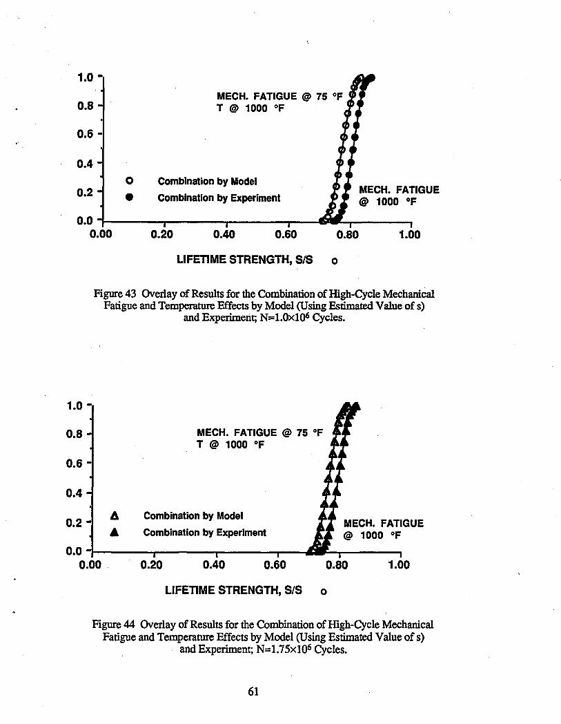
1.0 -
0.8 -
0.6 -
0.4 0
0.2 - • 0.0 -
0.00
MECH. FATIGUE @ 75 of T @ 1000 of
Combination by Model
Combination by Experiment
0.20 0.40 0.60 0.80
LIFETIME STRENGTH, SIS 0
MECH. FATIGUE @ 1000 of
1.00
Figure 43 Overlay of Results for the Combination of High-Cycle Mechanical Fatigue and Temperature Effects by Model (Using Estimated Value of s)
and Experiment; N=1.0xl06 Cycles.
1.0
0.8
0.6
0.4
0.2
0.0
A 6
MECH. FATIGUE @ 75 of T @ 1000 of
Combination by Model
Combination by Experiment MECH. FATIGUE @ 1000 of
0.00 0.20 0.40 0.60 0.80 1.00
LIFETIME STRENGTH, SIS 0
Figure 44 Overlay of Results for the Combination of High-Cycle Mechanical Fatigue and Temperature Effects by Model (Using Estimated Value of s)
and Experiment; N=1.75xl06 Cycles.
61
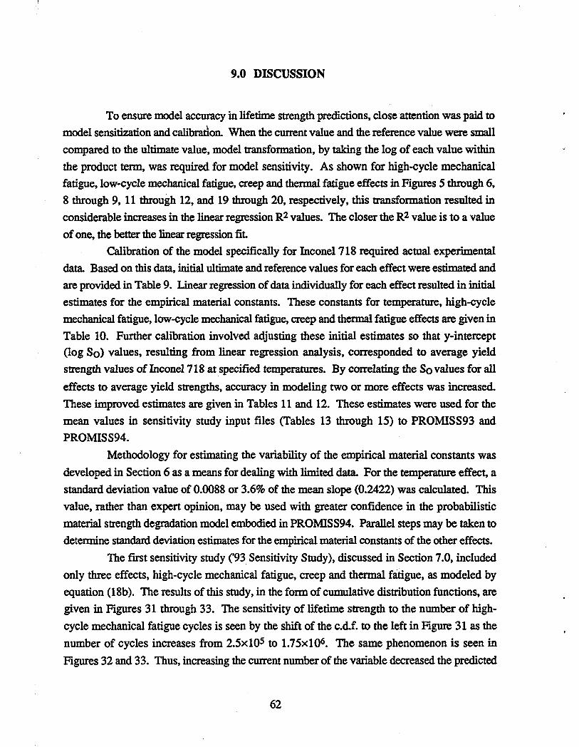
9.0 DISCUSSION
To ensure model accuracy in lifetime strength predictions, close attention was paid to
model sensitization and calibration. When the current value and the reference value were small
compared to the ultimate value, model transformation, by taking the log of each value within
the product term, was required for model sensitivity. As shown for high-cycle mechanical
fatigue, low-cycle mechanical fatigue, creep and thermal fatigue effects in Figures 5 through 6,
8 through 9, 11 through 12, and 19 through 20, respectively, this transformation resulted in
considerable increases in the linear regression R2 values. The closer the R2 value is to a value
of one, the better the linear regression fit.
Calibration of the model specifically for Inconel 718 required actual experimental
data. Based on this data, initial ultimate and reference values for each effect were estimated and
are provided in Table 9. Linear regression of data individually for each effect resulted in initial
estimates for the empirical material constants. These constants for temperature, high-cycle
mechanical fatigue, low-cycle mechanical fatigue, creep and thermal fatigue effects are given in
Table 10. Further calibration involved adjusting these initial estimates so that y-intercept
(log So) values, resulting from linear regression analysis, corresponded to average yield
strength values of Inconel 718 at specified temperatures. By correlating the So values for all
effects to average yield strengths, accuracy in modeling two or more effects was increased.
These improved estimates are given in Tables 11 and 12. These estimates were used for the
mean values in sensitivity study input files (Tables 13 through 15) to PROMISS93 and
PROMISS94.
Methodology for estimating the variability of the empirical material constants was
developed in Section 6 as a means for dealing with limited data. For the temperature effect, a
standard deviation value of 0.0088 or 3.6% of the mean slope (0.2422) was calculated. This
value, rather than expert opinion, may be used with greater confidence in the probabilistic
material strength degradation model embodied in PROMISS94. Parallel steps may be taken to
determine standard deviation estimates for the empirical material constants of the other effects.
The frrst sensitivity study ('93 Sensitivity Study), discussed in Section 7.0, included
only three effects, high-cycle mechanical fatigue, creep and thermal fatigue, as modeled by
equation (18b). The results of this study, in the form of cumulative distribution functions. are
given in Figures 31 through 33. The sensitivity of lifetime strength to the number of high
cycle mechanical fatigue cycles is seen by the shift of the c.d.f. to the left in Figure 31 as the
number of cycles increases from 2.5x10s to 1.75xl06• The same phenomenon is seen in
Figures 32 and 33. Thus, increasing the current number of the variable decreased the predicted
62
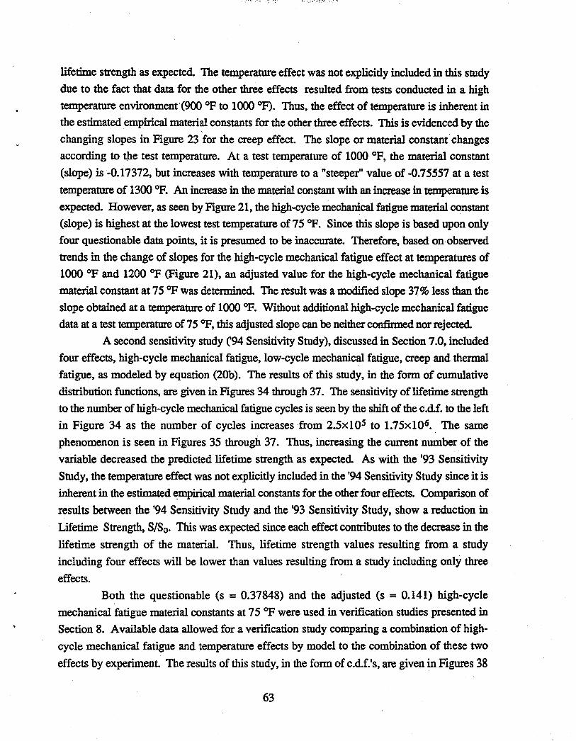
lifetime strength as expected. The temperature effect was not explicitly included in this study
due to the fact that data for the other three effects resulted from tests conducted in a high
temperature environment"(9oo of to 1000 oF). Thus, the effect of temperature is inherent in
the estimated empirical material constants for the other three effects. This is evidenced by the
changing slopes in Figure 23 for the creep effect. The slope or material constant changes
according to the test temperature. At a test temperature of 1000 of, the material constant
(slope) is -0.17372, but increases with temperature to a "steeper" value of -0.75557 at a test
temperature of 1300 of. An increase in the material constant with an increase in temperature is
expected. However, as seen by Figure 21, the high-cycle mechanical fatigue material constant
(slope) is highest at the lowest test temperature of 75 of. Since this slope is based upon only
four questionable data points, it is presumed to be inaccurate. Therefore, based on· observed
trends in the change of slopes for the high-cycle mechanical fatigue effect at temperatures of
1000 OF and 1200 of (Figure 21), an adjusted value for the high-cycle mechanical fatigue
material constant at 75 of was determined. The result was a modified slope 37% less than the
slope obtained at a temperature of 1000 OP. Without additional high-cycle mechanical fatigue
data at a test temperature of 75 OF, this adjusted slope can be neither confirmed nor rejected.
A second sensitivity study C94 Sensitivity Study), discussed in Section 7.0, included
four effects, high-cycle mechanical fatigue, low-cycle mechanical fatigue, creep and thermal
fatigue, as modeled by equation (20b). The results of this study, in the form of cumulative
distribution functions, are given in Figures 34 through 37. The sensitivity of lifetime strength
to the number of bigh-cycle mechanical fatigue cycles is seen by the shift of the c.df. to the left
in Figure 34 as the number of cycles increases from 2.5x10s to 1.75x10⁶• The same
phenomenon is seen in Figures 35 through 37. Thus, increasing the current number of the
variable decreased the predicted lifetime strength as expected. As with the '93 Sensitivity
Study, the temperature effect was not explicitly included in the '94 Sensitivity Study since it is
inherent in the estimated empirical material constants for the other four effects. Comparison of
results between the '94 Sensitivity Study and the '93 Sensitivity Study, show a reduction in
Lifetime Strength, S/So. This was expected since each effect contributes to the decrease in the
lifetime strength of the material. Thus, lifetime strength values resulting from a study
including four effects will be lower than values resulting from a study including only three
effects.
Both the questionable (s = 0.37848) and the adjusted (s = 0.141) high-cycle
mechanical fatigue material constants at 75 OP were used in verification studies presented in
Section 8. Available data allowed for a verification study comparing a combination of high
cycle mechanical fatigue and temperature effects by model to the combination of these two
effects by experiment. The results of this study, in the form of c.dJ.'s, are given in Figures 38
63
through 40. The sensitivity of lifetime strength to the number of current mechanical fatigue
cycles is seen by the shift of the c.d.f. to the left (Figures 38 and 39) as the number of cycles
increases. Thus, increasing the number of current fatigue cycles decreases the predicted
lifetime strength as expected. As seen by the overlay of distributions in Figure 40, there is
approximately a 20% difference between the results obtained by model and those obtained by
experiment. A major possibility for this large discrepancy is the questionable high-cycle
mechanical fatigue material constant at 75 OF. To test this assumption, a second parallel
verification study using the adjusted high~cycle mechanical fatigue material constant value was
conducted. The results are given in Figures 41 through 44. Comparison of Figure 41 to
Figure 40 shows a substantial decrease in the discrepancy between the two sets of
distributions. From Figures 42 through 44, it is apparent that the percent difference between
the results is less than 5% for all three current values of fatigue cycles evaluated. Thus, the
questionable high-cycle mechanical fatigue material constant calculated from the high-cycle
mechanical fatigue data at 75 OP was responsible for a large percent of the discrepancy between
the initial results from the fIrst verification study.
64
10.0 CONCLUSIONS
A probabilistic material strength degradation model, applicable to aerospace
materials, has been postulated for predicting the random lifetime strength of structural
components for propulsion system components sUbjected to a number of effects. This model,
in the form of a randomized multifactor equation, has been developed for five effects, namely,
high temperature, high-cycle mechanical fatigue, low-cycle mechanical fatigue, creep and
thermal fatigue. Inconel 718 data for these effects was obtained from the open literature.
Based on this data, initial ultimate and reference values were estimated. It was determined that
when the current and reference values are small compared to the ultimate value the model is
insensitive. Therefore, a transformation to sensitize the model for the effects of high-cycle and
low-cycle mechanical fatigue, creep and thermal fatigue was required. Model transformation
resulted in significant increases in the R2 (goodness of fit) values. The current version of
PROMISS,entitIed PROMISS94, provides for this transformation for these four effects.
Linear regression of the data for each effect resulted in, estimates for the empirical
material constants, as given by the slope of the linear fit. These estimates, together with
ultimate and reference values, were used to calibrate the model specifically for Inconel 718. By
adjusting these initial estimates so that the y-intercept or So values corresponded to average
yield strength values of Inconel 718, accuracy in modeling two or more effects was improved.
Thus, model accuracy is dependent on the proper selection of ultimate and reference values,
which in tum influence the values of the empirical material constants used in calibration of the
model. Calibration of the model for other materials is also dependent on experimental data and
is not possible without it.
Methodology for estimating the standard deviation of empirical material constants
offered a way for dealing with limited data. This methodology results in better estimates of the
standard deviations based on actual experimental data, rather than expert opinion. Lack. of
sufficient data from which to evaluate the material constants warranted the development of this
methodology.
Results from two separate sensitivity studies involving three and four effects,
respectively, showed that the c.d.f.'s shift to the left, indicating a lowering of lifetime strength,
for increasing current values of an effect. As expected, comparison between the '94 Sensitivity
Study and the '93 Sensitivity Study revealed a reduction in the lifetime strength values. Thus,
the more effects included in a study, the lower the resulting lifetime strength values. Further
development and evaluation of the three and four effect models, as well as other models,
requires that they be compared to real responses of Inconel 718 samples subjected to the same
65
combined effects during experimentation. Thus, additional experimental data is crucial for the
continued development and evaluation of the probabilistic material strength degradation model
presented in this report.
Limited verification studies involving two effects, high-cycle mechanical fatigue and
high temperature, were conducted. Results showed a combination of the two effects by model
to be more conservative than the combination by experiment. The fJIst verification study
yielded a 20% discrepancy between the results obtained by model and those obtained by
experiment. Questionable high-cycle mechanical fatigue data at a temperature of 75 OP is
presumed to be a major cause of the discrepancy. This conclusion was drawn after conducting
a second verification study using an adjusted value in place of the questionable one. The
outcome was a significant reduction in the discrepancy, from 20% to less than 5%, between the
results of a combination of these two effects by model and the combination by experiment.
Therefore, the data, rather than the nature of the model, is the presumed source of error. Thus,
the basic assumption of the model, that two or more effects multiply (Le., effects are
independent), is strongly supported by this limited verification study. The remaining 5%
difference may be due to the lack of uniformity among the specimens tested. As seen by Table
A.5 in the Appendix, specimen shape and heat treatment varied between the effects. Specimen
shape, as well as heat treatment, can influence material properties. Another reason for the 5%
difference may be synergistic effects (i.e., dependence between effects). As previously
discussed, equation (1) is an approximated solution to a separable partial differential equation.
In order to account for synergistic effects and perhaps eliminate this 5% difference, additional
terms would have to be added to equation (1). The resulting reduction in error mayor may not
warrant complication of the model by the inclusion of additional terms. Based on the results
obtained from the second verification study, this complication is not warranted. However,
additional verification studies for the combination of other effects must fJISt be conducted
before a more refined model can be developed. As previously discussed, the availability of
experimental data will determine whether or not further studies can be conducted.
In conclusion, methodology for improving lifetime strength prediction capabilities is
presented. The probabilistic material strength degradation model in the form of a randomized
multifactor equation is developed for five effects and calibrated to best reflect physical reality
for Inconel 718. Systematic and repeatable methods of model calibration and evaluation are
developed. Basic understanding and evaluation of the model is generated through sensitivity
and verification studies. The sensitivity of random lifetime strength to any current value of an
effect can be ascertained. Probability statements in the form of cumulative distribution
functions allow improved judgments to be made regarding the likelihood of lifetime strength,
thus enabling better design decisions to be made.
66
I
"
·11.0 ACKNOWLEDGMENTS
The authors gratefully acknowledge the many helpful conversations with
Dr. Christos C. Chamis and the support of NASA Lewis Research Center.
67
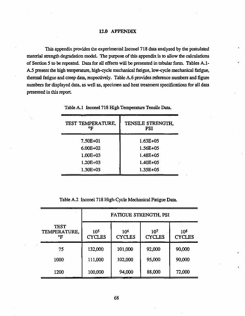
12.0 APPENDIX
This appendix provides the experimental Inconel718 data analyzed by the postulated material strength degradation model. The purpose of this appendix is to allow the calculations of Section S to be repeated. Data for all effects will be presented in tabular form. Tables A.1-
A.S present the high temperature, high-cycle mechanical fatigue, low-cycle mechanical fatigue,
thermal fatigue and creep data, respectively. Table A.6 provides reference numbers and figure
numbers for displayed data, as well as, specimen and heat treatment specifications for all data
presented in this report.
Table A.1 Inconel 718 High Temperature Tensile Data.
TEST TEMPERATURE, OF
7.S0E+01 6.00E+02
1.00E+03 1.20E+03
1.30E+03
TENSILE STRENG1H, PSI
1. 63E+OS
1.S6E+OS
1.48E+OS
1.40E+OS
1.3SE+OS
Table A.2 Inconel 718 High-Cycle Mechanical Fatigue Data.
FATIGUE STRENGTH, PSI
TEST TEMPERATURE, lOS 106 107 108
OF CYCLES CYCLES CYCLES CYCLES
75 132,000 101,000 92,000 90,000
1000 111,000 102,000 95,000 90,000
1200 100,000 94,000 88,000 72,000
68
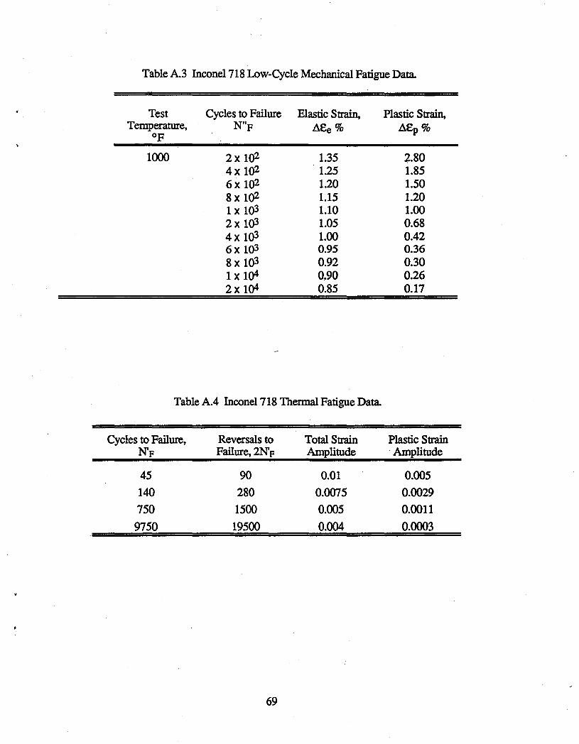
Table A.3 Inconel 718 Low-Cycle Mechanical Fatigue Data.
Test Temperature,
of
1000
Cycles to Failure Elastic Strain, N"p a£e %
2 x 1()2 1.35 4 x 1()2 1.25 6 x 1()2 1.20 8 x 1()2 1.15 1 x 10³ 1.10 2 x 10³ 1.05 4 x 10³ 1.00 6 x 10³ 0.95 8 x 10³ 0.92 1 x lQ4 0.90 2 x lQ4 0.85
Table A.4 Inconel 718 Thermal Fatigue Data.
Cycles to Failure, Reversals to Total Strain N'F Failure, 2NF Amplitude
45 90 0.01
140 280 0.0075
750 1500 0.005
9750 19500 0.004
69
Plastic Strain, a£p%
2.80 1.85 1.50 1.20 1.00 0.68 0.42 0.36 0.30 0.26 0.17
Plastic Strain Amplitude
0.005
0.0029 0.0011
0.0003
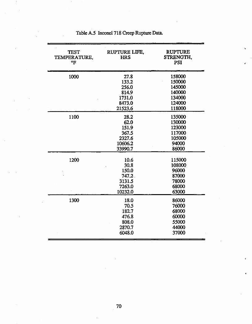
Table A.5 Inconel 718 Creep Rupture Data.
TEST RUPTURE LIFE, RUPTURE TEMPERATURE, HRS STRENGTH,
OF PSI
1000 27.8 158000 133.2 150000 256.0 145000 814.9 140000
1731.0 134000 8473.0 124000
21523.6 118000
1100 28.2 135000 62.0 130000
151.9 123000 367.5 117000
2327.6 105000 10606.2 94000 33990.7 86000
1200 10.6 115000 30.8 108000
150.0 96000 747.2 87000
3131.5 78000 7263.0 68000
10232.0 63000
1300 18.0 86000 70.5 76000
182.7 68000 476.8 60000 808.0 55000
2870.7 44000 6048.0 37000
70
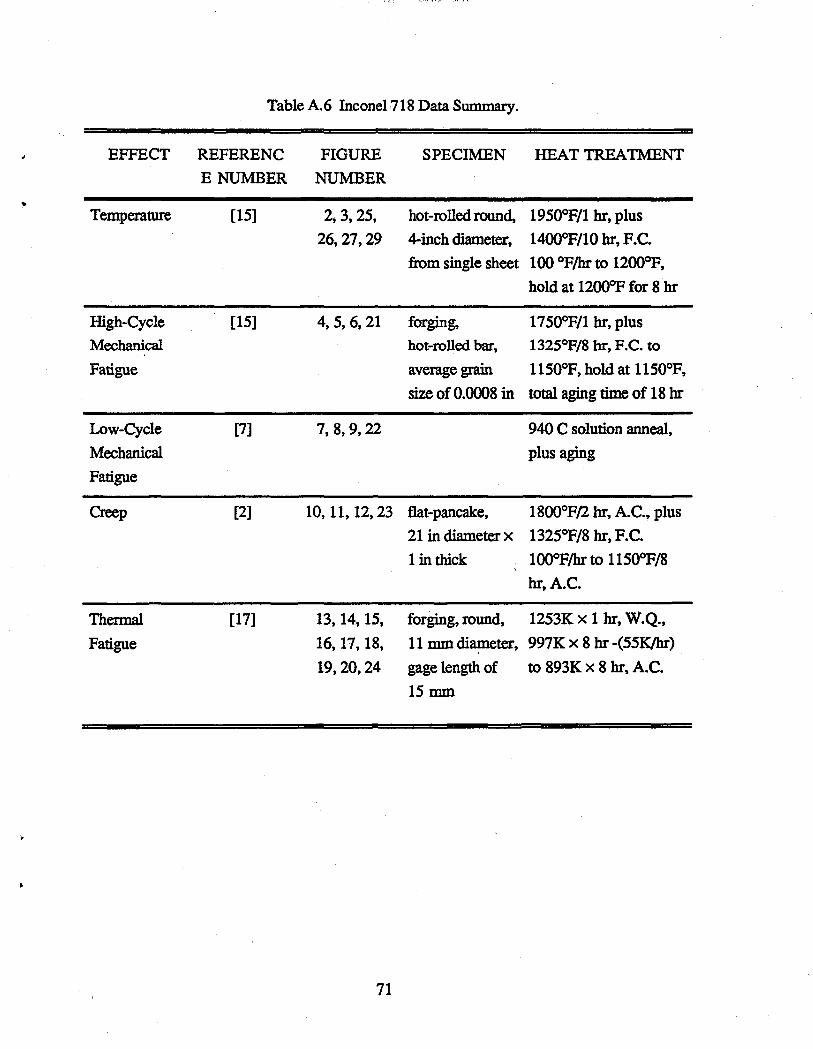
Table A.6 Incone1718 Data Summary.
EFFECT REFERENC FIGURE SPECIMEN HEAT TREATMENT
E NUMBER NUMBER
Temperature [15] 2,3,25, hot-rolled round, 1950oF/l hr, plus
26,27,29 4-inch diameter, 1400°F/l0 hr, F.C.
from single sheet 100 °F/hr to 12OOOP,
hold at 1200°F for 8 hr
High-Cycle [15] 4,5,6,21 forging, 1750oF/l hr, plus
Mechanical hot-rolled bar, 1325°F/8 hr, F.C. to ,
Fatigue average grain 1150°F, hold at 1150°F,
size of 0.0008 in total aging time of 18 hr
Low-Cycle [7] 7,8,9,22 940 C solution anneal,
Mechanical plus aging
Fatigue
Creep [2] 10, 11, 12,23 flat-pancake. 1800oF/2 hr, A.C., plus
21 in diameter x 1325°F/8 hr, F.C.
1 in thick l00°F/hr to 1150°F/8
hr, A.C.
Thermal [17] 13, 14, 15, forging, round, 1253K x 1 hr, W.Q.,
Fatigue 16, 17. 18. 11 mm diameter, 997K x 8 hr -(55K/hr)
19.20,24 gage length of to 893K x 8 hr. A.C.
15mm
71
13.0 REFERENCES
1 Bannantine, J. A., et. al., Fundamentals of Metal Fatigue Analysis, Prentice Hall,
Englewood Cliffs, N.J., 1990, pp. 63 - 66.
2 Barker, J. F., Ross, E.W. and Radavich, J. F., "Long Time Stability ofINCONEL 718,"
Journal of Metals, Jan. 1970, Vol. 22, p. 32.
3 Blank, L. T., Statistical Procedures for Engineering, Management and Science,
McGraw-Hill, N. Y., 1980, pp. 518, 523.
4 Boyce L. and Bast C., "Computational Simulation of Coupled Material Degradation
Processes for Probabilistic Lifetime Strength of Aerospace Materials," NASA CR
1887234, NASA Lewis Research Center, Cleveland, Ohio, March 1992.
5 Boyce, L. and Chamis, C. C., "Probabilistic Constitutive Relationships for Material
Strength Degradation Models," Proceedings of the 30th Structures. Structural Dynamics
and Materials Conference, Mobile, AL, April 1989, pp. 1832 - 1839.
6 Boyce, L., Keating, J., Lovelace, T. and Bast, C., "Probabilistic Lifetime Strength of
Aerospace Materials Via Computational Simulation," NASA CR 187178, NASA Lewis
Research Center, Cleveland, Ohio, Aug. 1991.
7 Brinkman, C.R. and Korth, G.E., "Strain Fatigue and Tensile Behavior of Inconel 718
from Room Temperature to 650 °C," Journal of Testing and Evaluation, JTEVA, Vol. 2,
No.4, July, 1974, pp, 249-259.
8 Chamis, C. C., "Simplified Composite Micromechanics Equations for Strength, Fracture
Toughness, Impact Resistance and Environmental Effects," NASA TM 83696,
Jan. 1984.
9 Chamis, C. C. and Hopkins, D., "Thermoviscoplastic Nonlinear Constitutive
Relationships for Structural Analysis of High Temperature Metal Matrix Composites,"
NASA TM 87291, Nov. 1985.
72
':, "': '. . : :' '.";! ,'. u: .. ~
REFERENCES (continued)
10 Collins, J. A., Failure of Materials in Mechanical Design. Wlley-Interscience Publication, John Wiley & Sons, N.Y., 1981, pp. 391 - 393.
11 Cullen, T. M. and Freeman, J. W., "The Mechanical Properties of INCONEL 718 Sheet
Alloy at 800°F l0000F and 12000F," NASA CR 268, NASA, Washington, DC, 1985, pp.20-34.
12 Flinn, R. A. and Trojan, P. K., Engineering Materials and Their Applications, Houghton Mifflin Co., Dallas, TX, 1990.
13 Hopkins, D. A., "Nonlinear Analysis forHigh-Temperature Multilayered Fiber Composite Structures," NASA TM 83754, Aug. 1984.
14 Hopkins, D. and Chamis, C. C., "A Unique Set of Micromechanics Equations for High
Temperature Metal Matrix Composites," NASA TM 87154, Nov. 1985.
15 INCONEL Alloy 718, Inco Alloys International, Inc., Huntington, WV, 1986, pp. 8-13.
16 Korth, G. E., "Mechanical Properties Test Data of Alloy 718 for Liquid Metal Fast Breeder Reactor Applications," EG&G Report No. EGG-2229, January, 1983.
17 Kuwabara, K., Nitta, A. and Kitamura, T., "Thermal-Mechanical Fatigue Life Prediction in High-Temperature Component Materials for Power Plant," Proceedings of the
Advances in Life Prediction Methods Conference, AS ME, Albany, N. Y., April, 1983,
pp. 131-141.
18 Mendenhall, W., Introduction to Probability and Statistics, Duxbury Press, North
Scituate, Massachusetts, 1979, p. 48.
19 Ross, S. M., Introduction to Probability and Statistics for Engineers and Scientists,
Wiley, New York, 1987, p. 278.
73
REFERENCES (continued)
20 Scott, D. W~, "Nonparametric Probability Density Estimation by Optimization Theoretic Techniques," NASA CR-147763, April 1976.
21 Shigley, J. E. and Mischke C. R., Mechanical Engineering Design, 5th Ed., McGraw
Hill, N. Y., 1989, p. 161.
22 Siddall, J. N., Probabilistic Engineering Design, Marcel Dekker, Inc., New York, 1983.
23 Sims, C. T., Stoloff, N.S. and Hagel, W.C., Superalloys II, Wiley, New York, 1987,
pp. 581-585, 590-595.
24 Swindeman, R. W. and Douglas, D.A., "The Failure of Structural Metals Subjected to Strain-Cycling Conditions," Journal of Basic Engineering, ASME Transactions, 81, Series D, 1959, pp. 203 -212.
74
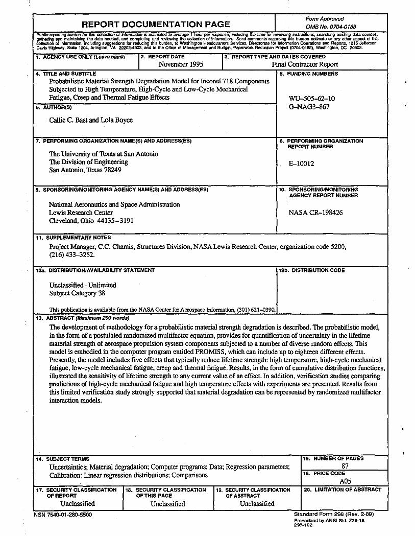
REPORT DOCUMENTATION PAGE Form Approved
OMBNo.0704-0188 Public reporting burden for !/Iis coIl&clion 01 information is estimated to average 1 hour per response. Including the time for reviewing instructions, searching existing data sources, gathering and inalntainl, the data needed, and completing and reviewing the collection 01 information. Send comments regarding this burden estimate or any other aspect of this collection of Information. ncluding sug~estions for reducing this burden. to Washington Headquarters Services. Directorate for Information Operations and Reports, 1215 Jefferson Davis Highway. Suite 1204. Arlington. A 22202-4302. and to the Office of Management and Budget. Paperwork Reduction Project (0704·0188). Washington. DC 20503.
1. AGENCY USE ONLY (Leave blanK) 12. REPORT DATE 13. REPORT TYPE AND DATES COVERED
November 1995 Final Contractor Repon 4. TITLE AND SUBTITLE 5. FUNDING NUMBERS
Probabilistic Material Strength Degradation Model for Inconel718 Components Subjected to High Temperature, High-Cycle and Low-Cycle Mechanical Fatigue, Creep and Thermal Fatigue Effects WU-505-62-10
6. AUTHOR(S) G-NAG3-867
Callie C. Bast and Lola Boyce
7. PERFORMING ORGANIZAnON NAME(S) AND ADDRESS(ES) 8. PERFORMING ORGANIZATION REPORT NUMBER
The University of Texas at San Antonio The Division of Engineering E-lOO12 San Antonio, Texas 78249
9. SPONSORINGIMONITORING AGENCY NAME(S) AND ADDRESS(ES) 10. SPONSORINGIMONITORING AGENCY REPORT NUMBER
National Aeronautics and Space Administration Lewis Research Center NASA CR-198426 Cleveland, Ohio 44135-3191
11. SUPPLEMENTARY NOTES
Project Manager, C.C. Chamis, Structures Division, NASA Lewis Research Center, organization code 5200, (216) 433-3252.
12a. DISTRIBUTION/AVAILABILITY STATEMENT 12b. DISTRIBUTION CODE
Unclassified -Unlimited Subject Category 38
This publication is available from the NASA Center for Aerospace Information, (301) 621-0390.
13. ABSTRACT (Maximum 200 words)
The development of methodology for a probabilistic material strength degradation is described. The probabilistic model, in the form of a postulated randomized multifactor equation, provides for quantification of uncertainty in the lifetime material strength of aerospace propulsion system components subjected to a number of diverse random effects. This model is embodied in the computer program entitled PROMISS, which can include up to eighteen different effects. Presently, the model includes five effects that typically reduce lifetime strength: high temperature, high-cycle mechanical fatigue, low-cycle mechanical fatigue, creep and thermal fatigue. Results, in the form of cumulative distribution functions, illustrated the sensitivity of lifetime strength to any current value of an effect. In addition, verification studies comparing predictions of high-cycle mechanical fatigue and high temperature effects with experiments are presented. Results from this limited verification study strongly supported that material degradation can be represented by randomized multifactor interaction models.
14. SUBJECT TERMS
Uncertainties; Material degradation; Computer programs; Data; Regression parameters; Calibration; Linear regression distributions; Comparisons
17. SECURITY CLASSIFICATION 18. SECURITY CLASSIFICATION 19. SECURITY CLASSIFICATION OF REPORT OF THIS PAGE OF ABSTRACT
Unclassified Unclassified Unclassified
NSN 7540-01-280-5500
15. NUMBER OF PAGES
87 16. PRICE CODE
A05 20. LlMITAnON OF ABSTRACT
Standard Form 298 (Rev. 2-89) Prescribed by ANSI Std. Z39-18 298-102