Embed Size (px)
Citation preview

AD-A247 721 (7
PROBABILISTIC FINITE ELEMENT ANALYSIS
SDTiCFINAL REPORT
submittedto the
Office of Naval Research
ONR Grant No. N00014-89-J-1586
submittedby
Prof. John M. Niedzwecki
Department of Civil EngineeringTexas A & M University
College Station, Texas 77843-3136
S ./.p~,r. -: IAprorri...a
Distri ed
February 28, 1992
4 92-05903
PROBABILISTIC FINITE ELEMENT ANALYSIS
FINAL REPORT
P submittedto the
Office of Naval Research
ONR Grant No. N00014-89-J-1586
submittedby
Prof. John M. Niedzwecki
Department of Civil Engineering 7.Texas A k- M University 6t &
College Station, Texas 77843-3136
February 28, 1992 w<.O 'rit '~i91
Statement A per telecon
Dr. Steven Ramnberg
ONR/Code 1121Arlington, VA 22217-5000
NWW 3/19/92
EXECUTIVE SUMMARY
This report contains much of the technical information developed under a research
investigation sponsored by ONR Grant N00014-89-J-1586. Additional information
on various aspects of this study will continue to appear in the open literature in
conference proceeding and forthcoming journal articles.
This research investigation, entitled: Probabilistic Finite Element Analysis, fo-
cused upon the continued development of recently introduced variational based tech-
niques. Of particular interest was the development of this methodology in the general
area of structural mechanics and for ocean related structural problems. The PFE
approach holds much promise for complex science and engineering problems since,
variabilities in materials and loads can be handled in a very rational manner incorpo-
rating probability density functions. Further, the methodology is a computationally
efficient alternative to tedious Monte Carlo simulations.
Significant issues presented and addressed as part of this research investigation
include: 1.) the definition of appropriate correlation lengths for the PFE model, 2.)
the integration of random field concepts, 3.) the development of the methodology
to treat significant multi-degree-of- freedom (MDOF) models, 4.) the formulation
and computation of second order stress estimates, 5.) the comparison of zeroth order
and combined zeroth and second order response estimates for MDOF simulations
with Monte Carlo simulations, 6.) the introduction of probability density functions
to prescribe both material and load variability, and 7.) the formulation of the force
model required to handle long flexible structural members subject to oscillatory flow
field kinematics.
An interesting aspect which was demonstrated is that this PFE technology can
be incorporated as an add-on to existing finite element software.
PROBABILISTIC FINITE ELEMENT ANALYSISOF
MARINE RISERS
A Thesis
by
H. VERN LEDER
Submitted to the Office of Graduate Studies ofTexas A&M University
in partial fulfillment of the requirements for the degree of
MASTER OF SCIENCE
December 1990
Major Subject: Ocean Engineering

PROBABILISTIC FINITE ELEMENT ANALYSISOF
MARINE RISERS
A Thesis
bv
H. VERN LEDER
Approved as to style and content by:
John M. Niedzweiki(Chair of Committee)
Loren D. Lutes(Member)
Robert 0. Reid(Member)
'Ja es T. . ao(Head of Department)
December 1990
111
ABSTRACT
Probabilistic Finite Element Analysis of Marine Risers. (December 1990)
F. Vern Leder, B.S., Texas A&M University;
Chair of Advisory Committee: Dr. J.M. Niedzwecki
The finite element method has been used extensively in structural analyses.
Traditionally, the properties of the systems which have been modeled using finite
elements have been assumed to be deterministic. The uncertainties in the struc-
tural response behavior estimates which result from uncertainties in the properties
of the system have been accounted for in design using safety and reduction factors.
As structures become more complex and industry makes use of materials such as
composites, which are known to have random material properties, an alternative
approach to design which quantifies the distributions in response may be required.
Probabilistic finite element techniques, which are capable of assessing the dis-
tributions in response behavior for systems with random material properties, loads
and boundary conditions are presented in this thesis. One particular method
termed second-moment analysis is examined in detail. This method includes per-
turbation techniques and is used to compute the expected values and covariance
matrices of probabilistic response behavior. Second-moment analyses in conjunc-
tion with the finite element method require as input the expected values of the
random processes inherent to the system and their covariance matrices. Methods
are also presented to compute these parameters for local element averages of the
random processes which describe the uncertainty in the system.
The offshore industry has assessed the responses and stresses in marine drilling
risers using deterministic finite element techniques for many years. This thesis
iv
implements probabilistic finite element techniques as developed in the study to
predict the probabilistic response behavior of marine riser systems in which, cer-
tain aspects of the problem are considered probabilistic. Specifically, in one set
of examples the tension applied to the top of the riser is assumed to be a random
variable and in a second set of examples the unit weight of the drilling mud is
assumed to vary along the length of the riser. The probabilistic solutions are
compared to deterministic solutions for the same riser systems as published by
the American Petroleum Institute. Monte Carlo simulations are also performed
as a basis of comparison for the probabilistic estimates.
0
0
SvV
ACKNOWLEDGEMENTS
The author expresses his gratitude to Professor John M. Niedzwecki for his
guidance and support. The author also acknowledges Dr. Loren D. Lutes and Pro-
fessor Robert 0. Reid for their valued comments. Appreciation is also expressed
to Dr. Rick Mercier and Arun Duggal for their assistance.
This research study was supported by the Office of Naval Research. Contract
Number N00014-89-J-1586.

vi
TABLE OF CONTENTS
Page
1 INTRODUCTION ............................. 1
1.1 Literature Review ..................... .... .. 3
1.2 Research Study .. .. ....... .. .... ... .. . .. .. . 10
2 FORMULATION OF THE SECOND-MOMENT ANALYSIS METHOD 13
2.1 Finite Element Equations ...................... 14
2.2 Random Vector Formulation ..................... 14
2.3 The Correlation Function ...................... 17
2.4 Random Field Discretization ..................... 19
2.5 Taylor Series Expansion ...... ....................... 21
2.6 Zeroeth-Order Equation ...... ....................... 22
2.7 First-Order Equations ...... ........................ 23
2.8 Second-Order Equation ...... ....................... 23
2.9 Probability Distributions of Response Estimates ............. 24
2.10 Computational Aspects of the Probabilistic Finite Element Method 25
3 SIMPLE ILLUSTRATIVE EXAMPLE ....................... 28
4 APPLICATION OF PROBABILISTIC FINITE ELEMENT METHODS
TO MARINE RISER ANALYSES ...... .................... 38
4.1 Finite Element Model ............................... 41
4.1.1 Formulation of the Equation of Motion .............. 41
4.1.2 Finite Element Discretization ..... ................ 44
4.1.3 Development of the Mass and Stiffness Matrices ........ 46
4.1.4 Development of the Damping Matrix ................ 48
4.1.5 Development of the Force Vector .................. 48
vii
4.1.6 Solution to the Finite Element Equations ............. 51
4.2 Applications of Response Predictions ..................... 52
4.2.1 Stress Estimates ...... ....................... 52
4.2.2 Displacement and Stress Envelopes ................ 53
4.3 Second-Moment Solution Procedures Specific to the Marine Riser
Problem ....... ................................. 53
4.3.1 Zeroeth-Order Predictions ....................... 54
4.3.2 Evaluation of the Sensitivity Vectors ................ 54
4.3.3 Second-Order Response Predictions ................. 60
4.3.4 First-Order Accurate Covariance Predictions ........... 65
4.3.5 Application of Probabilistic Results ................ 66
4.4 Probabilistic Solutions to Marine Riser Problems ............ 67
4.4.1 Top Tension Modeled as a Random Variable ........... 70
4.4.2 Unit Weight of Drilling Mud Modeled as a Random Field . 76
5 CONCLUSIONS ........ .............................. 85
6 REFERENCES ....... ............................... 88
7 VITA ......... .................................... 91

VIII
LIST OF TABLES
Table Page
1 Summary of stochastic finite element techniques .............. 5
2 Riser input data specifications ....... .................... 69
ix
LIST OF FIGURES
Figure Page
1 Beam with stochastic properties .................... 16
2 Definition of distances in expression for covariances between spatial
averages ........... ................................ 18
3 Schematic of the probabilistic finite element method .......... 27
4 Random 2-DOF oscillator ............................. 29
5 Displac-;ment of node 1 of 2-DOF oscillatc ................. 34
6 Displacement of node 2 of 2-DOF oscillator ................. 35
7 Standard deviation in displacement of node 1 of 2-DOF oscillator. 36
8 Standard deviation in displacement of node 2 of 2-DOF oscillator. 37
9 Marine drilling riser ........ .......................... 39
10 Differential element of marine drilling riser ................... 43
11 Element coordinate system and nodal degrees of freedom...... ... 45
12 Global coordinate system for marine riser analysis ............ 56
13 Maximum displacement and bounds for riser with random top ten-
sion in 500 feet of water ....... ......................... 71
14 Maximum displacement and bounds for riser with random top ten-
sion in 3000 feet of water ....... ........................ 72
15 Minimum displacement and bounds for riser with random top ten-
sion in 500 feet of water ....... ......................... 74
16 Standard deviations to be added to zeroeth-order and Monte Carlo
response envelopes for riser in 3000 feet of water .............. 75
17 Bending stress envelopes for riser with random top tension in 500
feet of water ........ ............................... 77
9

X
18 Bending stress envelopes for riser with random top tension in 3000
feet of water ......... ............................... 78
19 Maximum bending stress and bounds for riser with random top
tension in 500 feet of water ...... ....................... 79
20 Maximum bending stress and bounds for riser with random top
tension in 3000 feet of water ....... ...................... 80
21 Maximum displacement and bounds for riser with mud weight mod-
eled as a random field in 500 feet of water ................... 83
22 Maximum bending stress and bounds for riser with mud weight
modeled as a random field in 500 feet of water ................ 84

1 INTRODUCTION
The finite element method provides engineers with the ability to model and ob-
tain computer solutions to complex engineering problems. To date, virtually all
structural finite element software packages are formulated within a determinis-
tic framework such that structural material and geometrical properties, damping,
loads and boundary conditions are considered in terms of averages, neglecting
variations about the average. Since uncertainties are inherent in all phenomena.
the effect of variation about the averages is accounted for in design t hrough con-
cepts such as the factor of safety or load factor (Nigaln 198:3). This approach has
proven adequate for many engineering problems where the level of uncertainty
is thought to be low. For many other structural problems, however, the degree
of randomness is high and the usual deterministic approaches are inadequate for
design.
A promising technique which can be used to address these types of problems
involves probabilistic methodologies in combination , . ,ilte element methods.
These require the engineer to identify excessive sources of randomness, construct
their probability models, and incorporate the probabilistic distributions into the
formulation of the problem (Nigam 198.3). Although current finite element soft-
ware packages do not accommodate this systematic treatment of uncertainty,
probabilistic analytical and numerical techniques, consistent with the finite el-
ement method, are currently under development. For most complex. probabilis-
tic, structural problems where finite element analysis is required. Monte Carlo
simulations and probabilistic, also termed stochastic, finite element methods are
suitable. In conjunction with the finite element method, these techniques are used
The following citations follow the style and format of the .Journal of StructuralEngineering, ASCE.
2
to assess the probabilistic distributions of structural behavior. They require as
input knowledge of the probability distributions of the random parameters inher-
ent to the problem of interest. This includes expected values and variances of
random variables and, additionally, correlation functions of random fields. Monte
Carlo simulations are fairly straightforward and have been used to solve practical
engineering problems, whereas stochastic finite element techniques are a current
area of research and only recently, have been developed to the point where they
can be used to solve meaningful engineering design problems.
Monte Carlo simulations have been employed in structural analyses where the
level of uncertainty was high and a probabilistic distribution of response behav-
ior was required. The technique is suitable for analyses of structures with large
displacements, nonlinear material properties and arbitrarily shaped boundaries
(Astill 1972). In brief, probabilistic distributions of the sources of randomness
are used to generate sample variables or fields which describe the uncertainties;
these, in turn, are used as input for the finite element analysis. A distribution of
output describing the response behavior is then quantified in terms of statistical
parameters. The advantage of Monte Carlo simulation is that no additional formu-
lation to the governing equations of the problem is required. They are, however,
computationally repetitive due to the large number of samples of input random
variables or fields necessary to achieve statistical stability. In this respect, Monte
Carlo simulations are not an entirely attractive approach for estimating complex,
probabilistic, structural behavior.
Prob-'i:stic, or stochastic, finite element methods are also applicable tech-
niques for obtaining the probabilistic distributions of structural behavior. These
methodologies either formulate probabilistic aspects of the problem directly into
the finite element discretization, or incorporate probabilistic formulations into
4b

3
existing finite element software. As a result, these methods require far less com-
putations than Monte Carlo simulations. Since the techniques are a current area
of research, only a limited number of structural problems have been addressed and
only at a very fundamental level. Extension of these methodologies, including the
numerical techniques involved, is required to develop their full potential. Thus,
further research into probabilistic finite element methods is necessary so that a
broad range of structural problems can be addressed. Many areas of structural
mechanics involve probabilistic aspects. This is particularly true of ocean struc-
tures which must routinely operate and survive harsh environmental conditions.
Generally, these structures require a dynamic analysis where the degree of uncer-
tainty in many aspects of the problem is high. Stochastic finite element methods
provide a numerical technique which quantifies this uncertainty in structural be-
havior predictions. To date, only Monte Carlo simulations have been used and
only to a limited extent in probabilistic offshore-related structural problems.
1.1 Literature Review
At present, development of stochastic finite element analysis methods is a dy-
namic area of interest in the structural mechanics field. Of particular interest is
randomness associated with structural material and geometrical properties as well
as stochastic loads, damping and boundary conditions and the overall effects of
uncertainty on response estimates. Numerous researchers have contributed to the
development of various aspects of stochastic finite element methodologies, and a
summary of the more pertinent studies is presented in Table 1. The major thrust
of their research has involved characterizing sources of randomness in terms of
their probability models and formulating the governing equations of structural
4
response behavior, consistent with the finite element method, in terms of these
distributions.
Many sources of uncertainty inherent to most structures can be modeled as
stochastic processes which are functions of space rather than time. These specific
processes are the primary focus of stochastic finite element methods. They are
generally termed random fields and are explicitly defined in the context of this
study as random processes where the random parameter is a function of the spatial
coordinates over a structure. In stochastic finite element applications random
fields are generally discretized where the discrete values are taken as element
averages (Vanmarcke 1984). This requires large correlation distances as compared
with element lengths. The techniques employed to characterize these processes
as well as other sources of uncertainty found in most structures, as applied to
finite element response predictions, are relatively new and therefore the available
literature is limited.
Monte Carlo simulations in combination with finite element analyses are one
means of obtaining probabilistic solutions to complex, probabilistic, structural
problems. Astill, Nossier and Shinozuka (1972) developed a Monte Carlo method
capable of assessing structural behavior in problems with spatial variations in
material properties. The technique was shown to be completely compatible with
the finite element method and thus capable of assessing the effects of irregular
boundaries, nonlinear material properties and finite displacements. The authors
presented a method to generate digital representations of bivariate random pro-
cesses from their specified cross-spectral density or equivalent cross-correlation
matrix. A large set of conceptual test cylinders with spatially varying modulus
and material density were generated in this manner and subjected to an impact
load. A finite element analyses was performed on each to determine the stress in

co .W0V.0O
C'4 C
00 0d Id m
(f ti 0 F a
C rdIV 0. -
n . m ~ 14 uNC X X
4 4) CC 0-~ I 00
U ~ ~ 0 - 0- - - *
14 z 4-4
0 ~~ ~ 3: ---C) 4 44
z 4.1 - 7,. U -C) C) v
X 0 0 E E rd r
w 4t
0) 4-10 - -.
14 - . C ~~ 4QE E Z z
iId .004
0e 0. 4 4
C m .21(C0.0 *~
41 1-3: - c4 Q.~~1 'o o) -. 4)3:0- C 4 0Ec~ Z c: - -0 w
Id. 2- .= -- !:-- .0 11 - -7-~ = :- r w 0
41 = .- -2~ LZE

6
the cylinder. Useful statistics were extracted from the test results including the
mean and standard deviation in stress.
Although the Monte Carlo method is a useful technique for addressing struc-
tures with stochastic properties, it is often computationally prohibitive. For ex-
ample, the ensemble of sample structures must be sufficiently large to accurately
describe the random processes in a statistical sense. This requires extensive com-
puter time for both generating the realizations and proceeding with the finite
element analyses. Thus, other researchers have attempted to implement the prob-
abilistic aspects of structural analysis directly into the finite element formulation,
requiring far less computational effort.
Second-moment analysis, involving perturbation techniques has attracted con-
siderable attention in research involving probabilistic finite element analyses. The
method applies to both static and dynamic structural problems where stochastic
parameters are described by either random variables or correlated random fields.
In short, the second-moment analysis allows for computation of the first-order co-
variance matrix of structural response, stress, and strain and the expected values
of these parameters up to and including second-order. If the random properties
are Gaussian, then this method only requires, as input, the first two moments of
the random variables or discrete random fields (Yamazaki and Shinozuka 1986).
If the relationship between the random parameters inherent to the system and the
response behavior is linear, then the method is exact (Ma 1986). For this special
case the method is exact for any distribution of the random parameters inherent
to the system. In the event that the relationship is nonlinear, the method should
prove adequate provided the variances in the random parameters associated with
the system are small (Ma 1986). In the case of correlated random fields, the
method requires a large correlation distance as compared with element lengths.

7
The random variables and the discretized stochastic fields are represented by one
random vector. The first-order means of structural behavior are obtained using
local element averages as input to the finite element analysis. Next, sensitivity
vectors are computed by differentiating the parameters of interest with respect to
each discrete element of the random vector, where the differentials are evaluated
at the mean values of the discrete random elements. For dynamic problems the
differentials of the kinematics and stresses can be obtained using implicit time in-
tegration techniques which require that the number of time integrations be equal
to the dimension of the random vector (Liu, Belytschko and Mani 1985, 1986). In
cases involving nonlinear systems or when analytical differentiation of the system
matrices is difficult, differentiation of the parameters of interest can be performed
using finite difference techniques (Liu, Belytschko and Mani 1985, 1986). At this
point, the covariance matrices of the parameters of interest are obtainable. The
second-order means, which are estimated from a truncated Taylor series expan-
sion about the mean values of the parameters of interest, are then calculated. If
the discrete random fields are uncorrelated, the procedure is simplified. In this
case the covariance matrix representing the random vector is a diagonal, thus
reducing computational effort (Liu, Belytschko and Mani 1985, 1986). In the
second-moment method, the superposition of the covariances of the response for
two different, uncorrelated (to each other) random fields of a structure is the same
as when both random fields are present simultaneously (Liu, Belytschko and Mani
1987), thus allowing for multiple uncorrelated random fields representing random
matcr.al properties, loads and boundary conditions.
Second-moment methods consistent with the finite element method have been
developed to assess a two-dimensional foundation settlement analysis with a spa-
tially varying modulus of elasticity (Baecher and Ingra 1981). In this problem the

0
8
variation about the mean trend of the modulus was treated as one realization of
a two-dimensional, second-order stationary random field.
Second-moment analysis techniques have also been used to obtain the proba-
bilistic distributions of dynamic, transient response of truss structures (Liu, Be-
lytschko and Mani 1985, 1986). For problems of this type, consisting of discrete
structural elements, the computational procedures are simplified by assuming that
the random parameters are uncorrelated. Improved computational procedures
have been developed further which enhance the second-moment methodology.
To simplify the analysis in problems involving correlated random fields, the full
covariance is transformed into a diagonai variance matrix (Liu, Belytschko and
Mani 1987). The discretized random vector is, therefore, transformed into an
uncorrelated random vector via an eigenvalue orthogonalization procedure. Com-
putations using the second-moment analysis are further reduced due to the fact
that only the largest eigenvalues are necessary to represent the random field. It is
also possible to discretize the random field using shape functions (Liu, Belytschko
and Mani 1987). Further computational efficiency is accomplished by reducing the
probabilistic finite element equations to a smaller system of tridiagonal equations 0
using the Lanczos reduction technique (Liu, Besterfield and Belytschko 1988a).
This algorithm provides a reduced basis from the system eigenproblem. It also
provides a means to eliminate secular terms in higher-order estimates of expected
dynamic response parameters, which are known to arise in some specific problems
when using second-moment analysis.
A probabilistic Hu-Washizu variational principle formulation has also been
used in conjunction with the second-moment analysis to assess probability dis-
tributions of response (Liu, Besterfield and Belvtschko 1988a). Probabilistic dis-
tributions for the compatibility condition, constitutive law, equilibrium, domain

9
and boundary conditions are incorporated into the variational formulation. Solu-
tion of the three stationary conditions for the compatibility relation, constitutive
law and equilibrium yield the variations in three fields: displacement; strain and
stress. The second-order means and first-order covariance are also computed as
above.
Another stochastic finite element method utilizes a Neumann expansion of the
operator matrix (Shinozuka and Dasgupta 1986). Again, the random geometri-
cal and material structural properties are represented in terms of a discretized
random field with a large correlation distance as compared with element lengths.
Unlike second-moment analyses, no partial differentiation is required. The au-
thors first considered the static equation where the response vector was written in
terms of a recursive formulation involving the mean response, the inverted mean
system stiffness matrix and the deviatoric parts of the corresponding elements
in the stiffness matrix. The expected values of displacement, strain and stress
vectors of any order and the covariance matrices of these variables can be as-
sessed using this method. A consistent Monte Carlo method was employed to
generate the deviatoric stiffness matrices from the normalized fluctuations of the
discretized random field about its mean (Shinozuka and Dasgupta 1986). This
methodology has also been applied to a prismatic bar with a random modulus
subjected to a deterministic static load (Shinozuka and Deodatis 1988). By as-
suming a power spectrum which described the stochastic field, the covariance
matrix of the response displacement vector was calculated analytically as a func-
tion of the number of finite elements, thereby eliminating the necessity for Monte
Carlo simulations. The method was also used to assess the probabilistic response
parameters of a structure with its modulus defined by a two-dimensional random
field (Yamazaki, Shinozuka and Dasgupta 1986). In this paper comparisons were

7
10
made with Monte Carlo simulations and perturbation techniques.
Further approaches to the development of stochastic finite element methods
involved representation of homogeneous random fields in terms of the dimension-
less variance function and related scale of fluctuation (Vanmarcke 1984). This
approach was formulated for one and two-dimensional random fields. The vari-
ance function was shown to measure the "point variance" under local averaging
and the scale of fluctuation was defined as the element length times the variance
function as the element length approaches infinity. Although these serve as the
definitions for the two functions, other interpretations were given, as were models
of the variance function for wide-band processes (Vanmarcke 1984). These param-
eters permit computation of the covariance matrix of "element averages." A shear 0
beam with random rigidity subjected to concentrated and uniformly distributed
loads was assessed using this technique (Vanmarcke and Grigoriu 1983).
The procedures mentioned above provide a means for efficient solution of prob-
abilistic structural problems using stochastic finite element analysis. In each
method where the random fields are correlated over the structure, the element
size is required to be smaller than the maximum length over which apprecia-
ble correlation occurs. For problems involving structural dynamics, Monte Carlo
methods and second-moment analysis appear to have received the most attention.
1.2 Research Study
Current research into probabilistic finite element methodologies has resulted in
computationally efficient techniques which quantify uncertainty in structural prob-
lems. The variety of problems considered in the literature is quite limited and,
in general, assumptions concerning random structural parameters are required.
Research directed at extending and applying the methods to a broader range of

11
problems would benefit the structural engineer. Of particular interest is the use of
probabilistic finite element techniques for offshore applications. Loading scenar-
ios within this environment are stochastic resulting from wind, wave, current and
foundation excitation. Uncertainty also exists in the overall damping and force
coefficients, necessary for load predictions. Furthermore, material and geometrical
uncertainties inherent to structural members also require consideration.
This study focuses on the development and application of stochastic finite
element techniques to problems involving offshore structures. A review of the lit-
erature indicates that Monte Carlo simulations and second-moment analyses are
suitable methods for obtaining the probabilistic distributions of dynamic struc-
tural behavior. The second-moment analysis technique is more efficient in terms
of computation time, but is untested in offshore related problems. This method,
therefore, requires further development where Monte Carlo simulations are useful
to provide checks in accuracy.
It is the objective of this thesis study to build upon previous theoretical de-
velopments and to implement a stochastic finite element technique which can0 be directly applied to offshore structural analysis. The stochastic finite element
methodology is specifically formulated to address problems involving probabilistic
response predictions for an offshore drilling riser. The riser model is described in
an American Petroleum Institute (API) bulletin which compares eight industrial
riser programs (API 1977). All aspects of the problem in the API bulletin are
considered deterministic. For this study, certain parameters in the problem are
considered to be probabilistic. One set of examples examines the sensitivity in
response behavior to a random pretension applied at the top of the riser. In a
second set of examples the unit weight of the drilling mud contained within the
riser is assumed to vary along the length of the riser. Probabilistic finite ele-

12
ment software is developed to estimate the second-order means and first-order
variances in responses and stresses. Monte Carlo simulations are also used for
comparison of these results. Thus, using probabilistic finite element techniques, a
quantitative assessment of uncertainty is achieved. The sensitivity of the overall
dynamic response to each of these probabilistic parameters is also obtained. Com- 0
parison of probabilistic predictions with those made using deterministic programs
developed by industry indicate the relative importance of probabilistic analyses
in riser response predictions. It is worth noting that many uncertainties exist in 0
the design and analysis of offshore risers. For this study, only those sources of
uncertainty which appear to have the most significant impact on the behavior of
the structure are selected for numerical simulations. 0
0
13
2 FORMULATION OF THE SECOND-MOMENT ANALYSIS
METHOD
Probabilistic finite element methods involve application of second-moment anal-
ysis techniques in conjunction with the finite element method in order to assess
the probabilistic distributions of response behavior for stochastic systems. In this
chapter the second-moment analysis method is developed in detail and is incor-
porated into the conventional finite element formulation. The probabilistic finite
element method which results is applicable to both static and dynamic problems
where the response distributions can be predicted as functions of uncertainties
inherent to the system. Sources of randomness include geometrical and material
properties, excitation, damping and boundary conditions. Second-moment tech-
niques are exact if a linear relationship exists between the random parameters
and the predicted response behavior. If this relationship is moderately nonlin-
ear, then the method should prove adequate for coefficients of variation in the
random structural properties less than 0.2 (Ma 1987), where the coefficient of
variation is the ratio of standard deviation to the mean. Second-moment analy-
ses require information concerning the distributions of the sources of uncertainty;
more specifically the mean and variance for random variables and, additionally,
the correlation function for correlated random fields. The correlation distance
for random fields is required to be large as compared with the length of discrete
elements. Formulation for the probabilistic finite element method incorporating
second-moment analysis, as developed by Liu, Belytschko and Mani (1985), is
presented below. A probabilistic mass matrix, not addressed by these authors, is
also considered.

14
2.1 Finite Element Equations
Upon completion of a finite element discretization of a structure, the n-degree of
freedom equations of motion can be written in matrix form as
M~i(t) + C.+(t) + Kx(t) = F(t), (1)
where M, C, and K represent the mass, damping and stiffness matrices. The
force vector, F(t), and the displacement vector, x(t), are functions of time, t,
where the superscript dots represent time derivatives.
If the system matrices and force vector are random functions of uncertainties
inherent to the structure, the probabilistic finite element approach may be appli-
cable. Probabilistic distributions of all sources of randomness are incorporated
into a q-dimensional random vector, b, such that the equation of motion now can
be expressed as
M(b) (b,t) + C (b) i(b,t) + K(b)z(6,t) = F(b, t). (2)
2.2 Random Vector Formulation
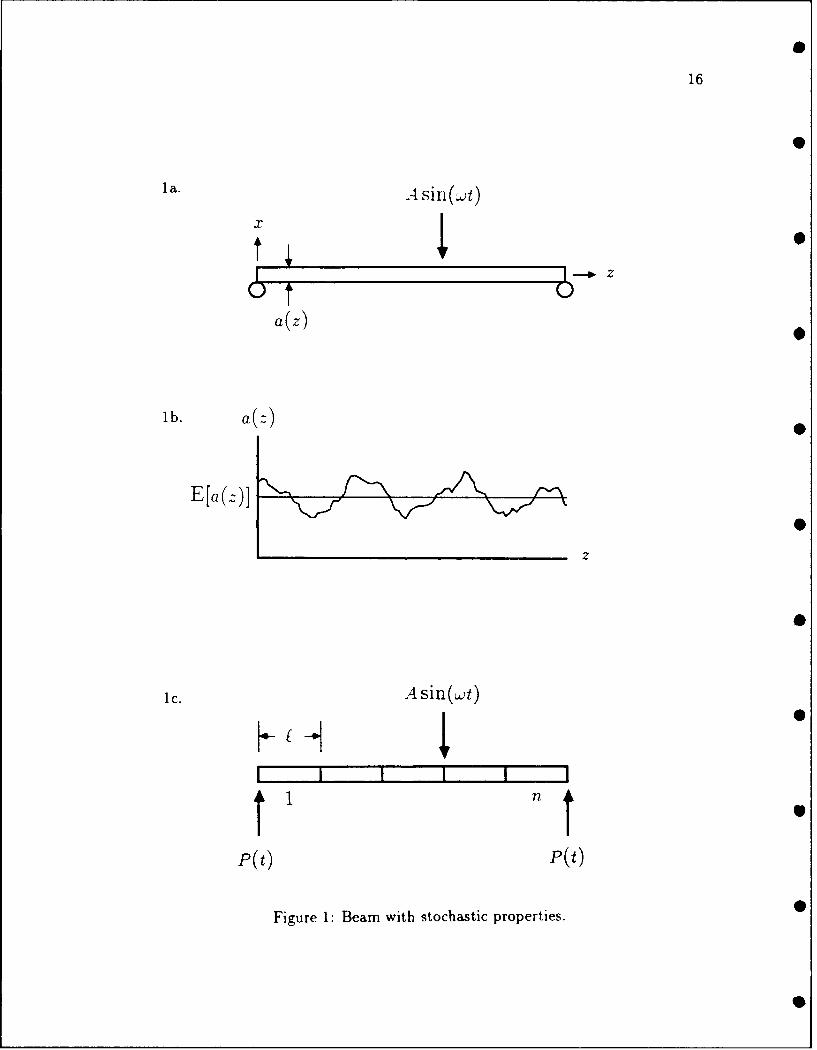
Formulation of the random vector can be visualized by considering Figure 1. In
Figure la the beam, whose thickness is a homogeneous random function of the
axial coordinate, is subject to a harmonic point load with a random amplitude.
The process corresponding to the beam thickness, a(z) is shown in Figure 1b,
where the mean trend is specified as E[a(z)]. If the mean trend is extracted from
the process corresponding to the beam thickness, then the constant variance is
denoted var[a] and the correlation of a(z) is represented by the function pa(r),
where r is an arbitrary correlation length. The distribution of the random force

15
amplitude, A, is specified in terms of its mean, E[A], and its variance, var[A].
Once all of the significant sources of randomness and their probability models
have been identified, the random vector, b, can be formulated. The elements of b
represent correlated distributions of local spatial averages of stochastic properties
(i.e., beam thickness), or distributions of random variables (i.e., force amplitude).
From Figure 1c, the beam is discretized into n elements where the length of
element z is t,. The process representing the beam thickness is then averaged over
each element such that the variable, a, represents the distribution of the average
of a(z) over element z. If the process is assumed to be ergodic in the mean, the
expected value of a, is equal to E[a(z)].
For this example the dimension of the random vector becomes (n + 1), where
the first n elements of b represent correlated discrete distributions of the mean
beam thickness over elements (1,..., n) and the (n + 1)th element of b represents
the distribution of the force amplitude. Thus, b is equal to (bi,..., b,, bn+l) and
represents the distributions of (a,... , a,, A).
The vector, 6, is defined as a mean vector where each element of b represents
the expected value of the corresponding element in the random vector (i.e., b, =
E[b,]). A probabilistic analysis requires, in addition to b, the covariance between
the elements of b, and b.. Since the random field, a(z), is correlated with itself
and uncorrelated to the harmonic excitation amplitude, the covariance matrix,
Cov[b,, b,], becomes
I Cov[a,,aj] ifz<n n
Cov[b,, b,]= var[A] if z = . = n + 1 (3)0 otherwise
16
1 a. 4 sin(wt)
xI
Ut Ua(z)
lb. a z)
z
1C. Asin(w.t)
P(t) P(t)
Figure 1: Beam with stochastic properties.
17
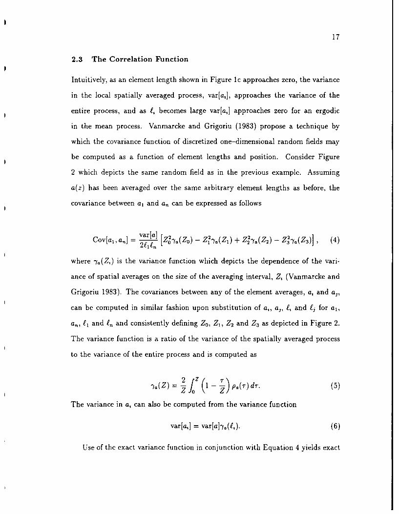
2.3 The Correlation Function
Intuitively, as an element length shown in Figure Ic approaches zero, the variance
in the local spatially averaged process, var[a,], approaches the variance of the
entire process, and as f, becomes large var[a,] approaches zero for an ergodic
in the mean process. Vanmarcke and Grigoriu (1983) propose a technique by
which the covariance function of discretized one-dimensional random fields may
be computed as a function of element lengths and position. Consider Figure
2 which depicts the same random field as in the previous example. Assuming
a(z) has been averaged over the same arbitrary element lengths as before, the
covariance between a, and a,, can be expressed as follows
Cov~1,a] -var[a] [Zo2%(Z 0) - Z a(Z1) + Z %a(Z2) - Z32a(Z 3 )] , (4)Cov[al, a,,] = 2ara]2l 2(4
where -Ya(Z,) is the variance function which depicts the dependence of the vari-
ance of spatial averages on the size of the averaging interval, Z, (Vanmarcke and
Grigoriu 1983). The covariances between any of the element averages, a, and a.,
can be computed in similar fashion upon substitution of a,, a., t, and £j for al,
an, £1 and f, and consistently defining Z0 , Z1 , Z2 and Z3 as depicted in Figure 2.
The variance function is a ratio of the variance of the spatially averaged process
to the variance of the entire process and is computed as
la(Z) = 2jz (1 - )Pa(r)dr.(5)
The variance in a, can also be computed from the variance function
var[a,] = var[a]-Ya(£,). (6)
Use of the exact variance function in conjunction with Equation 4 yields exact

S
18
a(z)
Z0
I Iz
f -z 1 -j f
H Z2 0,I
j 4 - Z 3 - .,
S
Figure 2: Definition of distances in expression for covariances between spatial
averages.

19
results for the covariances of element properties (Vanmarcke and Grigoriu 1983).
Unfortunately, adequate information concerning the correlation function is seldom
available to the analyst. Vanmarcke (1983) has proposed approximate expressions
for the variance function which are exact for many wide band processes so that a
detailed description of the correlation function is not required. The methodology
has also been extended to two-dimensional random fields (Vanmarcke 1983).
It should be noted that as the element lengths are increased, the sampling vari-
ability is reduced and important information may be lost. Thus, the correlation
length, L,, which represents the maximum correlation distance over which appre-
ciable correlation occurs, is required to be large as compared with the lengths
of the elements. Several probabilistic finite element studies have examined the
sensitivity of probabilistic response estimates to the correlation length (Baecher
and Ingra 1981, Shinozuka and Deodatis 1988, etc.)
2.4 Random Field Discretization
An alternative approach to the random vector discretization involves the use of
interpolation functions to approximate the random field (Liu, Belytschko and
Mani 1987). The method can be used to predict the expected value and the
covariance functions for a continuous random field provided the expected value and
covariance function for discrete values of the random field are known. Consider
the case of a beam where the thickness, a(z), varies along the axial coordinate,
z. If the process is discretized such that a discrete value of the beam thickness is
denoted as a,, where z = 1, ... , q, then the beam thickness can be approximated
at any point using the discretization
20
q
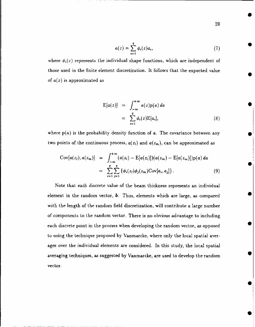
a(z) = , (z)a,, (7)S=1
where 6,(z) represents the individual shape functions, which are independent of
those used in the finite element discretization. It follows that the expected value
of a(z) is approximated as
E[a(z)] = +a(z)p(a)da
q
= Z,(z)E[a,], (8)
where p(a) is the probability density function of a. The covariance between any
two points of the continuous process, a(zi) and a(z,), can be approximated as
Cov[a(z,),a(zm)] = (a(zi) - E[a(zi)])(a(z,) - E[a(zm)])p(a)da
q q
= ZZ f (zi) k(zm)Cov[a,,a,] (9)t=1 1=1
Note that each discrete value of the beam thickness represents an individual
element in the random vector, b. Thus, elements which are large, as compared
with the length of the random field discretization, will contribute a large number
of components to the random vector. There is no obvious advantage to including
each discrete point in the process when developing the random vector, as opposed
to using the technique proposed by Vanmarcke, where only the local spatial aver-
ages over the individual elements are considered. In this study, the local spatial
averaging techniques, as suggested by Vanmarcke, are used to develop the random
vector.

21
2.5 Taylor Series Expansion
Application of second-moment analysis in the development of probabilistic finite
element methods involves expanding all random functions about the mean value of
each element of b via a Taylor series expansion and retaining up to and including
second-order terms. For a small parameter, -y , the discrete random displacement
vector, z(b, t), is expanded about b via a second-order perturbation as follows
~(bt)~(t±y { b 8) Ab1} ± 12± { a2Xw Abt X 1 1 (10)2- l =I1 bb bJ
where the vector t(t) is the zeroeth-order displacement given by z(b,t). The
partial derivatives a2() and t are evaluated at b and represent the first-8h, 8bb, lutda badrprsn hefrt
order variation of displacement with respect to b, and the second-order variation
of displacement with respect to b, and b., respectively. The variable Ab, represents
the first-order variation of b, about E[b,]. Similar expressions can be developed for
velocity and acceleration vectors by taking first and second-order time derivatives
of Equation 10. The mass, stiffness and damping matrices and the stochastic force
vector can also be obtained using second-order perturbation techniques
M(b)= +yt-q am Ab, +1 _7_. q b, b, AbAb , (11)
abl b2 =I 3=1 a~b
C(b)=q c6 Ab, + 1 2{ 2C Ab, Ab, (12)
(b) =F 'y F)1 2 q q 92 Kb3 1K(b) =k + I IK1 Ab, + _' E F 0, AXb,Abjl , (13)1=1 b Ab2j =l 3=1 b b(
F(b,t) = I M+ + 1 q q 2tA b, (14)"F() Ib_2 ab~bl
22
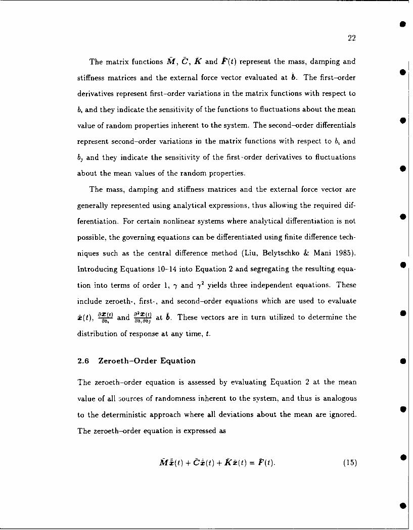
The matrix functions M, C, k and F(t) represent the mass, damping and
stiffness matrices and the external force vector evaluated at b. The first-order
derivatives represent first-order variations in the matrix functions with respect to
b, and they indicate the sensitivity of the functions to fluctuations about the mean
value of random properties inherent to the system. The second-order differentials
represent second-order variations in the matrix functions with respect to b, and
b. and they indicate the sensitivity of the first-order derivatives to fluctuations
about the mean values of the random properties.
The mass, damping and stiffness matrices and the external force vector are
generally represented using analytical expressions, thus allowing the required dif-
ferentiation. For certain nonlinear systems where analytical differentiation is not
possible, the governing equations can be differentiated using finite difference tech-
niques such as the central difference method (Liu, Belytschko & Mani 1985).
Introducing Equations 10-14 into Equation 2 and segregating the resulting equa- 0
tion into terms of order 1, -/ and -t2 yields three independent equations. These
include zeroeth-, first-, and second-order equations which are used to evaluate
;i(t), '9"() and at 6. These vectors are in turn utilized to determine the 0ab, ab,clbj
distribution of response at any time, t.
2.6 Zeroeth-Order Equation 0
The zeroeth-order equation is assessed by evaluating Equation 2 at the mean
value of all sources of randomness inherent to the system, and thus is analogous
to the deterministic approach where all deviations about the mean are ignored.
The zeroeth-order equation is expressed as
M +(t) + C (t) + K:(t) = F(t). (15)

23
Solutions for the kinematics are obtained using a numerical time integration tech-
nique such as the implicit Newmark method (Bathe 1982).
2.7 First-Order Equations
To obtain the first-order equations of motion, Equation 2 is differentiated with
respect to each element of the random vector. Thus, the sensitivity in the kine-
matics to b, are computed from the following first-order equation
___ W a(t)K (t)
A abx A ab,(16)0 bb - b =(t +
The sensitivity vectors, 8b, i' ab, b c pb, uted using the same
numerical time integration technique as employed to solve the zeroeth-order equa-
* tion. Note that the total number of first-order equations to be solved is equal to
the dimension of the random vector.
2.8 Second-Order Equation
The second-order equation is assessed to obtain second-order deviations about
the mean response, A (t), and is computed from the following equation
MrAi(t) + CAX(t) + kA:(t) = AlF(t), (17)
where
24
-E11 ' Cov[b,, bi}
q q f ['9 16 + +Cl q" 6 ' , Cov[b,,b,]l=I8= b -bb 8b, b -bb ob, b
1 E q 2 a8 2C a2 K1Sb 8 a b X ( t ) + bb x M(t) + obb t(t) Cov[b,,bj, (18)2 =1 3=l tb
and /t(t) can be written as
t=--1 1=1
Upon substitution of the zeroeth-order kinematics, sensitivity vectors and second-
order differentials of the system matrices and force vector, all evaluated at 6, into
Equation 18, the second-order equation of motion, Equation 17, can be computed
in terms of At(t), AX(t) and Ai(t) using the same numerical time integration
scheme.
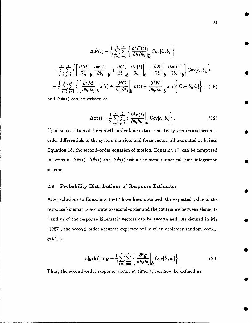
2.9 Probability Distributions of Response Estimates
After solutions to Equations 15-17 have been obtained, the expected value of the
response kinematics accurate to second-order and the covariance between elements
1 and m of the response kinematic vectors can be ascertained. As defined in Ma
(1987), the second-order accurate expected value of an arbitrary random vector,
g(b), is
E[g(b)] + g + q I 82g Cov[b,,b . (20)
Thus, the second-order response vector at time, t, can now be defined as
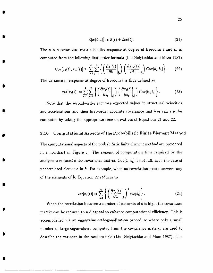
25
E[x(b, t)] -_ t(t) + A i(t). (21)
The n x n covariance matrix for the response at degree of freecioms I and m is
computed from the following first-order formula (Liu Belytschko and Mani 1987)
COV[XL~t),Xm~t) q q 6,t 8COV[Iqt) X )) o ) Cov[b,,b]j. (22)
v 't)t))(t)t=l j=1 i b
The variance in response at degree of freedom I is thus defined as
var[x(t)]zz (I ( a t) ( 8x,(t) Cov[b., b]}. (23)
Note that the second-order accurate expected values in structural velocities
and accelerations and their first-order accurate covariance matrices can also be
computed by taking the appropriate time derivatives of Equations 21 and 22.
2.10 Computational Aspects of the Probabilistic Finite Element Method
The computational aspects of the probabilistic finite element method are presented
in a flowchart in Figure 3. The amount of computation time required by the
analysis is reduced if the covariance matrix, Cov[b,, b,] is not full, as in the case of
uncorrelated elements in b. For example, when no correlation exists between any
of the elements of b, Equation 22 reduces to
var[xj(t)] - 1: 9 , )var[b,]}. (24)
When the correlation between a number of elements of b is high, the covariance
matrix can be reduced to a diagonal to enhance computational efficiency. This is
accomplished via an eigenvalue orthogonalization procedure where only a small
number of large eigenvalues, computed from the covariance matrix, are used to
describe the variance in the random field (Liu, Belytschko and Mani 1987). The

26
dimension of b is reduced by the number of eigenvalues discarded, thus reducing
the number of time integrations. -
Further, note that the effective stiffness matrix in Equations 15-17 remains
unchanged; therefore, only one factorization of the stiffness matrix is required.
Furthermore, response kinematics and their differentials with respect to the ele- -
ments of b are used in the "force vector" of each subsequent equation, and thus
Equations 15-17 could most efficiently be solved in parallel. If analytical differ-
entiation is possible, then the entire probabilistic finite element method requires
q + 2 time integrations: one to solve the zeroeth-order equation; q to solve for the
sensitivity vectors and one more to solve the second-order equation. For certain
non-linear systems analytical differentiation with respect to the elements of b is S
impossible and explicit numerical differentiation techniques, such as the central
difference method, are required (Liu, Belytschko & Mani 1985). Similar proce-
dures can also be developed to compute the probabilistic distributions of stresses,
but this method can prove computationally expensive (Liu, Belytschko and Mani
1985).

27
Structure with inherent uncertainties
IDetermine expected values and
correlation functions forsources of uncertainty
'IFor random fields, compute local
averages and correlation functionsfor local averages
Assemble the random vector
Solve the zeroeth-order equationat the mean value of the
random vector
Solve for thefirst-order
sensitivity vectors
Solve the second-order equationto compute second-order deviations
from the zeroeth-order response
Compute the first-orderaccurate covariances in
the response field
Compute the second-orderaccurate
response field
Figure 3: Schematic of the probabilistic finite element method.
28
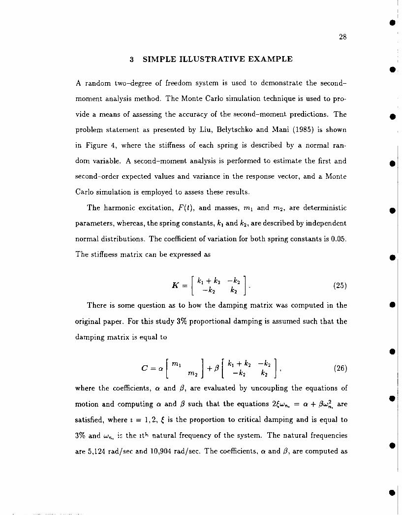
3 SIMPLE ILLUSTRATIVE EXAMPLE
A random two-degree of freedom system is used to demonstrate the second-
moment analysis method. The Monte Carlo simulation technique is used to pro-
vide a means of assessing the accuracy of the second-moment predictions. The 0
problem statement as presented by Liu, Belytschko and Mani (1985) is shown
in Figure 4, where the stiffness of each spring is described by a normal ran-
dom variable. A second-moment analysis is performed to estimate the first and
second-order expected values and variance in the response vector, and a Monte
Carlo simulation is employed to assess these results.
The harmonic excitation, F(t), and masses, mn and in2 , are deterministic
parameters, whereas, the spring constants, k, and k2, are described by independent
normal distributions. The coefficient of variation for both spring constants is 0.05.
The stiffness matrix can be expressed as
K=[k 1+ k2 - k2 ] (25)K= -k2 k2
There is some question as to how the damping matrix was computed in the 0
original paper. For this study 3% proportional damping is assumed such that the
damping matrix is equal to
C mi + [ ,+k2 -k 2 (26)rr12 I- k2 k2
where the coefficients, a and /3, are evaluated by uncoupling the equations of
motion and computing a and /3 such that the equations 2w, = a + O3w , are
satisfied, where z = 1,2, is the proportion to critical damping and is equal to
3% and w, , .- the zth natural frequency of the system. The natural frequencies
are 5,124 rad/sec and 10,904 rad/sec. The coefficients, a and /, are computed as
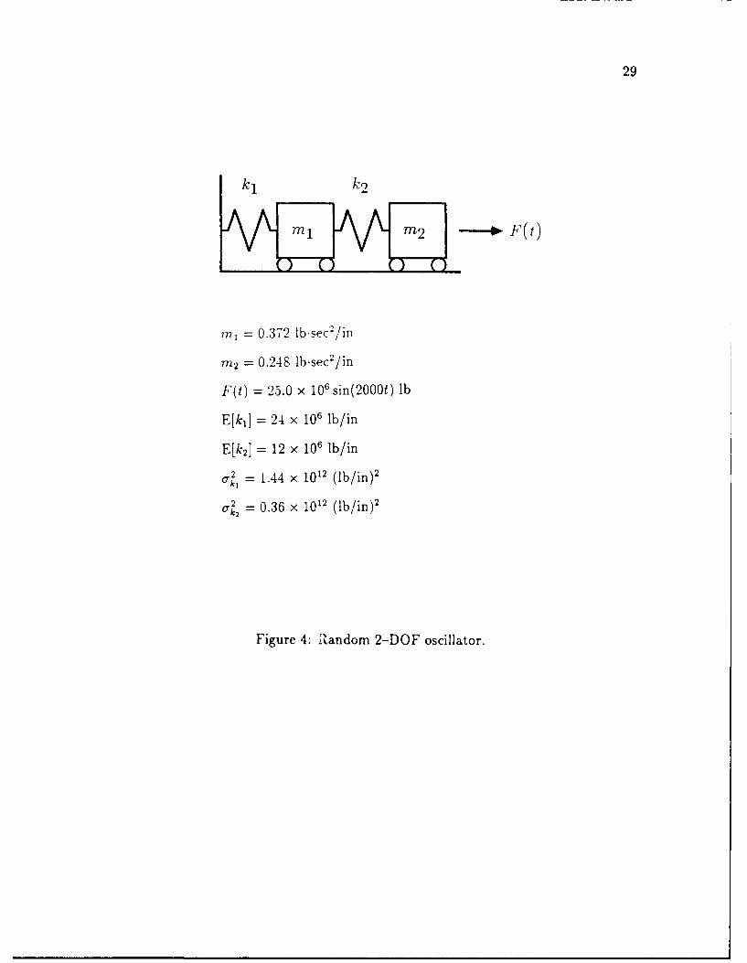
29
kj k
ml -2 F(t)
= 0.372 lb-sec 2 /in
M2= 0.248 lb-sec 2 /in
F(t) =25.0 x 10' sin(2000t) lb
E[ki] 24 x 106 lb/in
E[k2] 12 x 106 lb/in
2 1012 (bn)2
2 )O~2= 0.36 x 10¹² (lb/in)
Figure 4: Rtandom 2-DOF oscillator.

30
209.15 and 3.7434 x 10⁻⁶, respectively.
The random vector denoted by k represents the distributions of the spring
stiffnesses. Note that the covariance between k, and k, is equal to zero. The
equation of motion for this probabilistic system is
Mi (k,t) + C(k) c(k,t) + K(k) x(k,t) = F(t). (27)
The zeroeth-order equation is evaluated at k and computed as follows
Mx(t) + Co(t) + Kj(t) = F(t). (28)
A second-moment analysis is performed to evaluate the following: 1) zeroeth-
order mean response vectors; 2) sensitivity vectors; 3) variance in response vectors 0
and 4) second-order mean response vectors. Equation 28 is evaluated to obtain the
zeroeth-order kinematics. Sensitivity vectors are obtained by differentiating both
sides of Equation 27 with respect to k,, evaluating the differentials of the system •
matrices at k, and solving the resulting differential equations. Differentiating
with respect to k, and rearranging terms such that the sensitivity vectors are on
the left-hand side of the equation, the sensitivity vectors are computed from the 0
following first-order formula
M- (t) + (t) A + z(t) =- { -C :(t) + K k(t)l, (29)Okk k, A, k k, k Ak,k J
where
(9K [1 (30)49k, - 0 0
OK -1 (31) 0
Ak2

31
a [ c] (32)ak, 0 0'
and
ac [ i~;] (33)Ok2 -
Zeroeth-order estimates of mean response kinematics are determined using the
Newmark time integration method (Bathe 1982). The variance in the zeroeth-
order response of xi(t) is computed from the first-order equation
var[xI(t)] 4 ±{( k var[k,]. (34)
The second-order mean response vectors are computed by solving the second-
order equation
MAX(t) + Cz i(t) + KLSk(t) =
+ var[k,] (35)-_I C kk Ik , k'r L1
and the expected value of the response vector, accurate to second-order, is
E [x(k, t)] (t) + Ak(t). (36)
A Monte Carlo simulation is also performed to estimate the expected value
and variance in the response vectors. Two independent normal distributions of
random spring stiffnesses are generated, each with 400 samples, and each pair
of random stiffnesses is substituted into the equation of motion to compute a
distribution of response vectors. After 400 time integrations have been completed
the mean, mean squared and variance in the response of x1(t) can be computed

32
as1400
E[xi(t)] = 1 ,(t) (37)400 =I...
400- (XI, (t)) (38)E[(,())' =400 =
var[xi(t)] = E[(xj(t))2] - E[xj(t)]2 . (39)
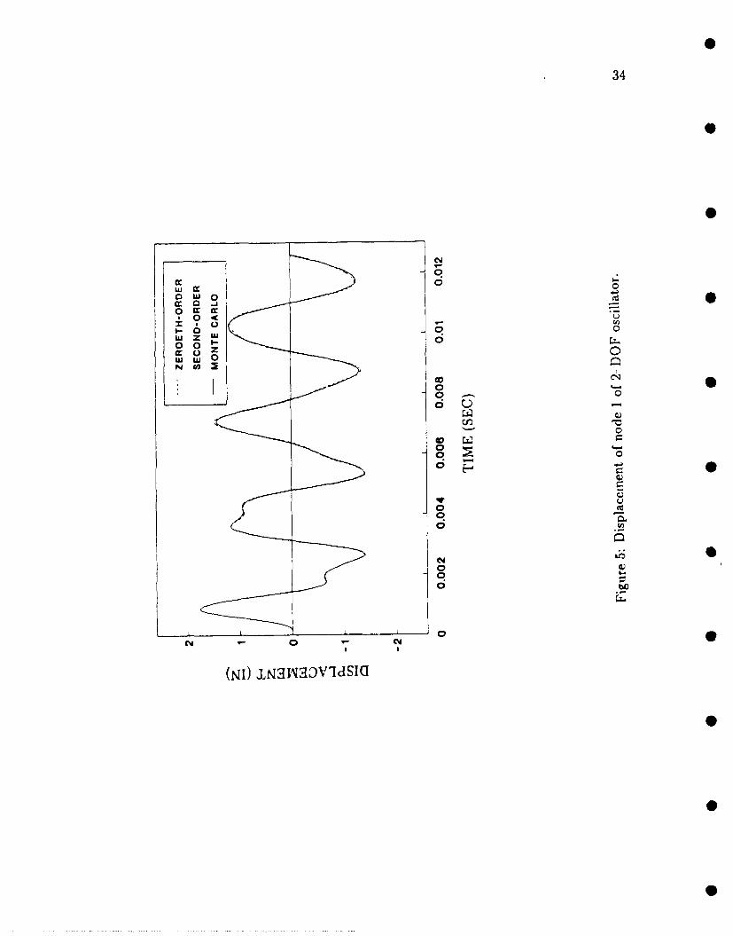
The results from the second-moment analysis and Monte Carlo simulations are
plotted in Figures 5-8. Figures 5 and 6 indicate the zeroeth-order and second-
order response of x, (t) and x 2 (t), respectively, and the expected response predicted
by the Monte Carlo simulation. The differences between the second-order mean
response and the mean response predicted using the Monte Carlo method are
negligible, but there is a notable difference between these two estimates of mean
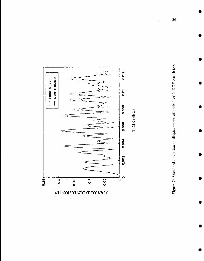
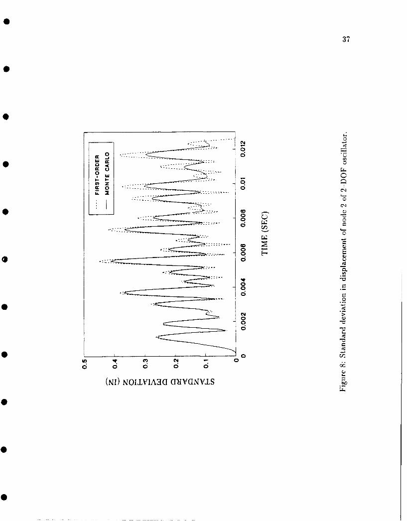
response and the zeroeth-order response. The standard deviation in response
estimates of xi(t) and x 2(t) is shown in Figures 7 and 8, respectively The second-0
moment analysis estimates tend to overshoot those obtained using Monte Carlo
simulations at large times. This phenomena is a result of resonant excitation
in the first-order equation, Equation 29, which estimates the sensitivity vectors
(Liu, Belytschko and Mani 1985). The resonant excitation is present in Equation
29 because the natural frequencies of Equations 28 and 29 are identical and the
kinematics obtained by solving Equation 28 are used in the excitation of Equation
29. The kinematics predicted by Equation 28 thus reflect the natural frequency
of the system and act as a resonant excitation.
The resonant excitation is present in all equations above the zeroeth-order.
However, it is negligible in structures with a large amount of damping and in anal-
yses which do not extend to large times where steady state response is prevalent
(Liu, Belytschko and Mani 1985). A technique based on Fourier analysis has been
0

33
developed to remove these secular terms from higher-order response estimates
(Liu, Besterfield and Belytschko 1986).
34
CY0
00
0 w -mw 0 -0 cc
I0~ -C
0 .-cc 0Z
00
co00
0o 0
c;~
00
0oV
0m 0 C
(N LNHUvdl
.. ... ... ..

35
a ui 0
0 0 -
X L 0
M 0 0
00*0C;-
0
co 1
C! E
0
0
4o v C4 0 CYi co.
(NI) lNaMOVU~SIU
36
---------
---- ---- ----
LIJ -- -- ---
------ --
0
CY in
oi 000
(NO NUVIAM(I-gVINVJ
37
LU
Ow
I. 0-- - - - -
OD C)
0
cow
0 ESq
0 0 0 66~
(NO) NOILVIA3U UaIVUNV1LS
38
4 APPLICATION OF PROBABILISTIC FINITE ELEMENT
METHODS TO MARINE RISER ANALYSES
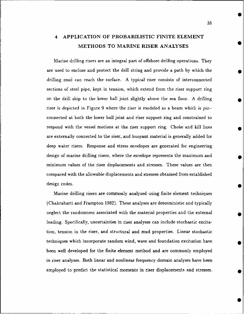
Marine drilling risers are an integral part of offshore drilling operations. They
are used to enclose and protect the drill string and provide a path by which the
drilling mud can reach the surface. A typical riser consists of interconnected
sections of steel pipe, kept in tension, which extend from the riser support ring
on the drill ship to the lower ball joint slightly above the sea floor. A drilling
riser is depicted in Figure 9 where the riser is modeled as a beam which is pin-
connected at both the lower ball joint and riser support ring and constrained to
respond with the vessel motions at the riser support ring. Choke and kill lines
are externally connected to the riser, and buoyant material is generally added for
deep water risers. Response and stress envelopes are generated for engineering
design of marine drilling risers, where the envelope represents the maximum and
minimum values of the riser displacements and stresses. These values are then
compared with the allowable displacements and stresses obtained from established
design codes.
Marine drilling risers are commonly analyzed using finite element techniques
(Chakrabarti and Frampton 1982). These analyses are deterministic and typically
neglect the randomness associated with the material properties and the external
loading. Specifically, uncertainties in riser analyses can include stochastic excita-
tion, tension in the riser, and structural and mud properties. Linear stochastic
techniques which incorporate random wind, wave and foundation excitation have 0
been well developed for the finite element method and are commonly employed
in riser analyses. Both linear and nonlinear frequency domain analyses have been
employed to predict the statistical moments in riser displacements and stresses.
0

39
*riser support ring
wave and current0direction
riser
lower ball joint
Figure 9: Marine drilling riser

40
In linear analyses only the first-order approximation of the hydrodynamic drag
force spectra is considered and relative motion between the structure and the wave
is neglected. The numerical simulations involved in nonlinear frequency domain
analyses of marine risers are significantly more complicated than those for linear
analyses. Nonlinear stochastic analyses can include higher-order approximations
of the drag force spectra (Niedzwecki and Leder 1990) and relative motion (Sandt
and Niedzwecki 1990). Time domain analyses do not require linearization of the
equation of motion and can be used to assess the probabilistic distributions of
displacements and stresses and to estimate extreme return period events. Com-
parative studies have been performed which demonstrate the range in response
and stress predictions of analogous riser simulations using various industrial finite
element procedures (API 1977).
Sources of uncertainty related to structural properties have received far less
attention than those related to the stochastic excitation and, in general, are either
assumed small and ignored, or conservative estimates are employed thiroughout
analyses. As drilling progresses into extreme water depths these latter sources of
randomness could necessitate a probabilisic analysis of the riser, particularly if
composites which are known to possess highly random material properties become
a viable alternative to steel.
In this chapter the second-moment analysis, as developed in Chapter 2, in
combination with finite element techniques, is specifically developed for a prob-
abilistic analysis of an offshore drilling riser. Monte Carlo simulations are also
employed as a means of comparing results. An assessment of the significance
of inclusion of sources of uncertainty on the distributions of response behavior,
excluding stochastic excitation, is also made.
0

41
4.1 Finite Element Model
4.1.1 Formulation of the Equation of Motion
The governing equations adapted for this study are based on those for a vibrating
uniform beam with linear variations in axial tension (Gardner & Kotch 1976).
The approach incorporates axial tension and compression effects and ignores shear
effects. Assumptions regarding the finite element solution require:
i) the angle between the riser and vertical axis remain below ten degrees;
ii) choke and kill lines externally attached to the riser do not contribute to the
bending stiffness and
iii) effects of the drill string, kept in constant tension, are ignored and variations
in top tension propagate instantaneously throughout the riser.
The finite element equations which directly follow are developed within a deter-
ministic framework and then the probabilistic formulations are incorporated.
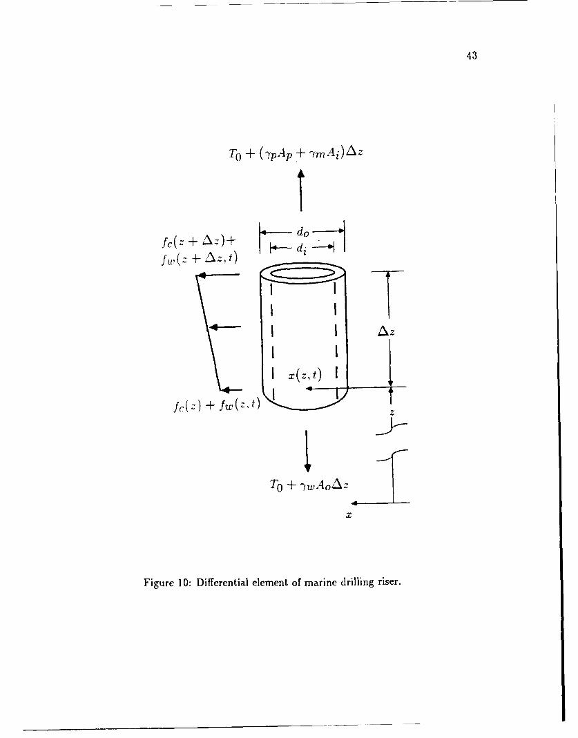
A differential riser element of length Az is shown in Figure 10, where for
simplicity, the choke and kill lines are not shown and the element is considered
completely immersed in water and filled with mud. The water depth is denoted
as d and the mud column is assumed to span the entire length of the riser, L. The
specific weights of the water, mud, and riser pipe are defined as %, ym and 1,
respectively. The riser is attached to the lower ball joint at an elevation, z0, above
the sea floor and the displacement at any point on the riser at elevation z above
the sea floor at time t is denoted as x(z, t). Externally, the riser is subject to
hydrostatic pressure, a static current force, f,(z), and hydrodynamic wave loads,
f,(z, t). The internal walls of the riser are also subject to static pressure resulting
from the mud column. The riser is initially pre-tensioned at the riser support ring
to some value Ttop in order to support the net weight and to increase the stiffness.
42
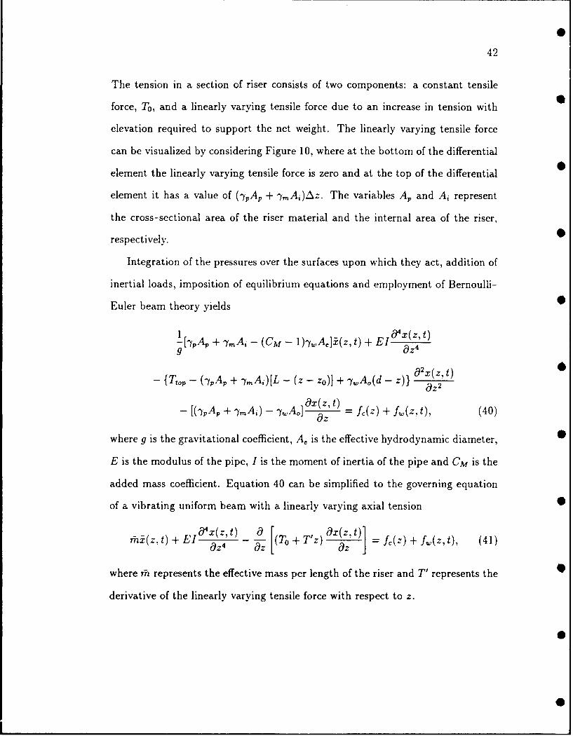
The tension in a section of riser consists of two components: a constant tensile
force, To, and a linearly varying tensile force due to an increase in tension with
elevation required to support the net weight. The linearly varying tensile force
can be visualized by considering Figure 10, where at the bottom of the differential
element the linearly varying tensile force is zero and at the top of the differential
element it has a value of (-yAp + "tmAi)Az. The variables Ap and Ai represent
the cross-sectional area of the riser material and the internal area of the riser,
respectively.
Integration of the pressures over the surfaces upon which they act, addition of
inertial loads, imposition of equilibrium equations and employment of Bernoulli-
Euler beam theory yields
1[yjA, + ymAi - (CM - 1)7YA,]i(z,t) + EI X(z t)
g (z
-T - (yIAp + -,A,)[L - (z - zo)] + -y.A(d - z)} 8x(z'i)t"P az 2
- [(-pAp + 3(mA,) - "Amo~ax(z ' t)a----z- - f (z) + f, (z,t), (40)
where g is the gravitational coefficient, A, is the effective hydrodynamic diameter,
E is the modulus of the pipe, I is the moment of inertia of the pipe and CM is theadded mass coefficient. Equation 40 can be simplified to the governing equation
of a vibrating uniform beam with a linearly varying axial tension
fi(z, t) + EIa 4 x(z,t) _ I(To + T'z) = f(z) + f. (z,t), (41)t)+ O, Oz (T +aTz j
where ih represents the effective mass per length of the riser and T' represents the
derivative of the linearly varying tensile force with respect to z.
0
43
To + (ypAp + ymAi)A z
_- _do .---
f.(z + z,) d
I II I x
4- I I
I x(z,t) I
fc(z) + fw(z,t)
TO + " ,AoA z
x
Figure 10: Differential element of marine drilling riser.
44
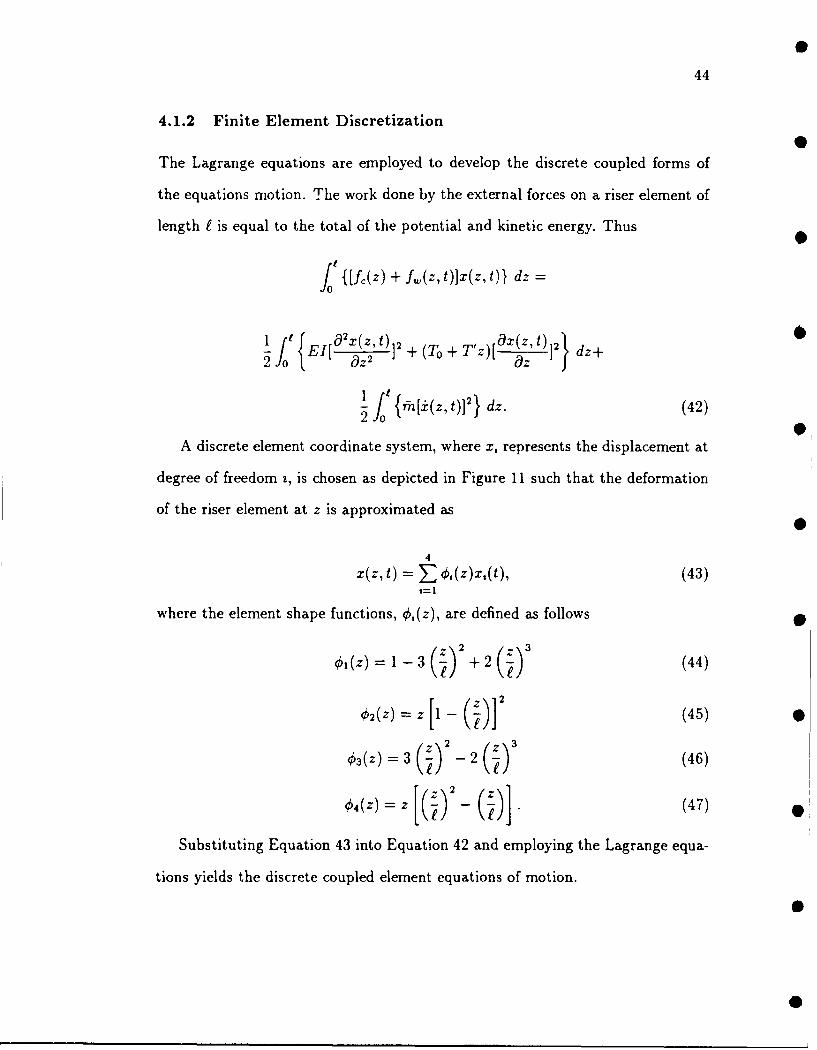
4.1.2 Finite Element Discretization
The Lagrange equations are employed to develop the discrete coupled forms of
the equations motion. The work done by the external forces on a riser element of
length e is equal to the total of the potential and kinetic energy. Thus
{[fI(z) + f,(z, t)]x(z, t)} dz =
.of {[Ox(z't)] if O~~t
1 EI[ a t) + (To + T'z)[ ]2 dz+
1 fn [(z't)]2} dz. (42)
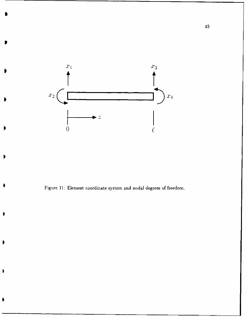
A discrete element coordinate system, where x, represents the displacement at
degree of freedom z, is chosen as depicted in Figure 11 such that the deformation
of the riser element at z is approximated as
4
x(z,t) = 0 ,(z)x,(t), (43)
where the element shape functions, 0,(z), are defined as follows
0(z) =1-3 + 2 (44)
(z) z [- -(Z)]2
03(Z) = 3 - 2 (z) (46)
4(Z) = z 4)- (
Substituting Equation 43 into Equation 42 and employing the Lagrange equa-
tions yields the discrete coupled element equations of motion.
I
45
p
X X3
X2 X4
F 1- E
I0 (
Figure 11" Element coordinate system and nodal degrees of freedom.

46
4.1.3 Development of the Mass and Stiffness Matrices
The elements in the mass matrix are computed by evaluating the integral
M'3= ifnO(z)0(z)dz. (48)
The resulting symmetrical element mass matrix can be expressed as
[156 22f 54 -13t4? 40 13t? -3 2
M T24- 156 -22t (49)442
where fn is the effective mass per length. It is dependent upon whether or not the
element is submerged and is computed as
fnp + fn. + hfna for z < dm= p + fn forz>d ' (50)
where the mass per unit length of the riser and mud and the added mass are 0
denoted rhp, fn, and fh, respectively.
The element stiffness matrix is divided into three components which include
contributions from the bending stiffness, the average constant tension and the 0
linear variation in tension. This can be expressed as
k, = E I ¢'(z) (z) dz
+ TO0 j (z)O,(z)dz + T' j ,(z)0,(z)z dz. (51)
The element stiffness matrix can be evaluated by integrating each of the com-
ponents to obtain the appropriate matrix expressions. Adding these together
yields the final element stiffness matrix. The element bending stiffness matrix is
found to beS

47
6 3U -6 3U
[k]E 2EI 20 -3t J (52)tkm 3 6 -3t 52
2t2
The constant tension element stiffness matrix is computed at the bottom node of
the element relative to the sea floor. Evaluating the second term in Equation 51
yields the following expression
36 3 -36 3To 4OV2 -3t -2(
[kiT0 = 3 36 -3t (53)
402
wherewhr Ttop - {(-yapA + t,A,)[L - (z - zo)]}
T +-y,,,Ao(d- z) for z < d (54)
Ttop - {(QpAp + ,.A,)[L (z - zo)]} forz > d
Finally, the element stiffness matrix accounting for contributions from the linear
variation in axial tension is computed by evaluating the third term in Equation
51 as follows
3 t 3 05 1? 5
[kIT, = T' 30o 1 0 (55)10
whereT'= ypAp + -yA, - -y,,Ao forz<d
[YPAp + ymA, for z > d (
The total element stiffness matrix can now be assembled, that is
[k] = [k]EI + [k]T0 + [k-]T'- (57)
After evaluating the mass and stiffness matrices for all of the elements, the global
mass and stiffness matrices are assembled. The global mass matrix is denoted as

0
48
M and the global stiffness matrix is denoted as K.
4.1.4 Development of the Damping Matrix
Structural damping is incorporated into the solution of the marine riser system by
introducing Rayleigh proportional damping (James, Smith, Wolford and Whaley
1989). The damping matrix, C, is assumed to be of the form aM +,3K. For sim-
plicity with regard to the probabilistic formulations which follow, the coefficients,
a and /3, are evaluated by predicting, in a least squared sense, the best fit to the
equation 2w, ,, = a + 13w2 where the variables , and Wn, respectively, represent
the proportion to critical damping and the natural frequency of the zth mode.
For the cases examined in this thesis, , is assumed to be constant for the first 0
four modes, and only the first four natural frequencies are used to approximate
the coefficients, a and /3. The predicted modal damping values for the first four
modes, computed using the estimates of a and /3, are approximately equal to the 0
actual values. For higher modes the predicted modal damping values are less than
the actual values.
0
4.1.5 Development of the Force Vector
If the external forces are assumed to vary linearly over the elements, then the
external force vector, F,(t), for element degree of freedom z is approximated by
evaluating the following integral
F,(t) = fo(t) k0,(z)dz + f'(t) JO (z)zdz, (58)
where fo(t) is the constant force per unit length over the element and f'(t) is
the linear variation in the force per unit length. The element force vector is thus
computed as
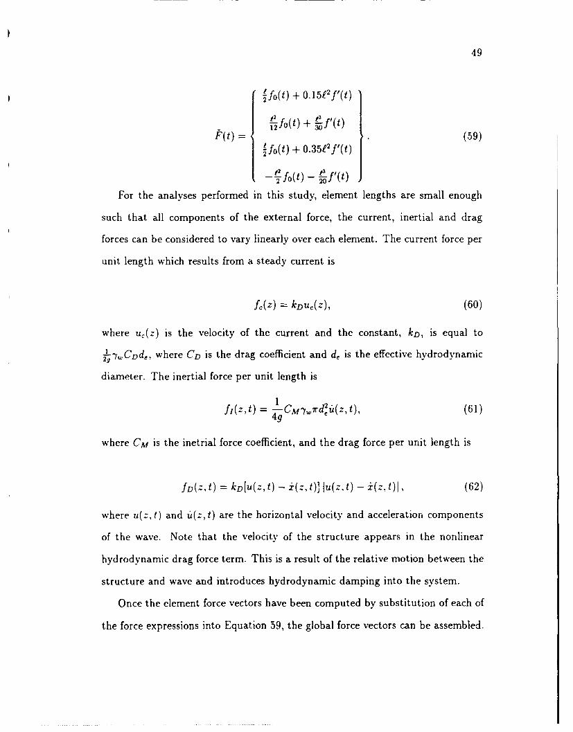
49
2fo(t) + 0.15f 2f'(t)12
3
Ufo(t) + f (t)P(t) 30 (59)
'fo(t) + 0.3512f'(t)
2 O) - -f'(t)
For the analyses performed in this study, element lengths are small enough
such that all components of the external force, the current, inertial and drag
forces can be considered to vary linearly over each element. The current force per
unit length which results from a steady current is
f (z) . kDu,(z), (60)
where u,(z) is the velocity of the current and the constant, kD, is equal to
-71 , CDd, where CD is the drag coefficient and d, is the effective hydrodynamic
diameter. The inertial force per unit length is
1f( z,t) = - CM y.rd'it(z, t), (61)
4g
where CM is the inetrial force coefficient, and the drag force per unit length is
fD(z-,t) = kD[u(z,t) - i(z,t)] u(z,t) - X(z.t)1, (62)
where u(z, t) and 1(z, t) are the horizontal velocity and acceleration components
of the wave. Note that the velocity of the structure appears in the nonlinear
hydrodynamic drag force term. This is a result of the relative motion between the
structure and wave and introduces hydrodynamic damping into the system.
Once the element force vectors have been computed by substitution of each of
the force expressions into Equation 59, the global force vectors can be assembled.

50
The global steady current vector is F,. The time dependant global wave force
vector is F (t) and includes the inertial force vector, F(t), and the drag force
vector, FD(t).
The top node of the riser corresponding to the riser support ring is considered
to respond with the surge motion of the drill ship. The penalty method is used
to impose these translations (Bathe 1982, McCoy 1985). A fictitious stiffness
several orders of magnitude larger than the element in the global stiffness matrix
corresponding to the degree of freedom of the imposed top translation is added to
the element in the global stiffness matrix corresponding to the degree of freedom
of the imposed top translation. Thus, for a specified displacement at the global
degree of freedom z, the corresponding element in the stiffness matrix can be
computed as
K,, = Kit + KhA,,, (63)
where K is a large constant. The product of the fictitious stiffness and the specified
displacement are also added to the element of the force vector corresponding to
the degree of freedom of the imposed top translation. The element in the force
vector corresponding to the degree of freedom of the specified displacement can
be computed as
F,(t) = F,(t) + tcK,,f(t), (64)
where f(t) represents the specified displacement. A new global force vector is
defined which represents the horizontal force necessary to produce the specified
displacement. The new vector, F(t), is expressed as
T
F,(t) = { 00... r Kif (t) ... 00 (65)
S
51
where all terms are zero except for the force expression at the degree of freedom
corresponding to the specified displacement.
4.1.6 Solution to the Finite Element Equations
The discretized finite element equation of motion can now be written as
M~i(t) + Ci (t) + Kx (t) = F, + F,(t) + F,(t). (66)
For numerical simulations the static and dynamic components in Equation 66
are segregated. The static equation is written as
Kz, = F, + F,(0), (67)
where z, is the vector representing the static offset. The equation of motion which
contains only the dynamic components of Equation 66 can be expressed as
Mid(t) + Caid(t) + Kzd(t) = F,(t) + F,(t) - F,(0), (68)
where Xd(t) represents the displacement vector resulting from the hydrodynamic
wave force contributions. The total dynamic response of the riser, z(t), is thus
Z, + Zd(t).
The Newmark method is employed to solve Equation 68 for the structural kine-
matics (Newmark 1959, Bathe 1982). As a result of relative motion, the nonlinear
drag force contributions to the wave force vector are functions of the velocity of
the structure. An iterative approach to the solutions for the kinematic vectors is
required if the governing equations are not linearized. The Newmark method can
be modified to iterate until the velocity vectors converge. The algorithm of the
steps required to compute the structural kinematics at time t, is shown below.

52
1.) Compute the kinematic vectors at time t,, where the dynamic force
vector is assembled assuming that the velocity of the structure can be
computed from zd(t,-1).
2.) If the new estimate of the velocity vector converges with the old esti-
mate, then increment the time step.
3.) If the new estimate of the velocity vector does not converge with the
old estimate, then reassemble the force vector using the new velocity
estimates and recompute the kinematic vectors.
4.) Repeat steps 2 and 3 as necessary.
4.2 Applications of Response Predictions
4.2.1 Stress Estimates
The response vector, x(t), computed using the finite element method can be used
to predict the stresses in the riser at time t. The maximum bending stress in the
outer wall of the riser can be computed from the general equation a = ,where
a is the bending stress, c is the radius to the outer wall of the riser and M is the
bending moment. The bending moment, M(z, t), can be computed at elevation z
and time t using the following equation
E1M(z,t) = z) (69)
p(Z't)'
where p(z, t) is the radius of curvature. The radius of curvature can be obtained
from the following expression
1 9 Xa (z,t) = 0 (z,t)p(z,t) z2 Z(70)
where 9(z,t) is the rotation of the riser in the x-z plane. The expression cz
can be evaluated at the midpoint of element I using the numerical approximation

53
ao(z,t) O(zi + AzIt) - O(z - Az,t) (71)az 2Azj 71
I ,
where z, is the vertical coordinate of the midpoint of element 1 and 2Az is the
length of element 1. The expressions O(zj + Azi, t) and O(zj - Azi, t) are the
rotations at the top and bottom of element 1, respectively. These are computed
directly in the finite element solution. The stress at the midpoint of element 1 and
at time t can now be approximated as
al(t) - Ec O(zj + AzI, t) - O(zj - Az, t) (72)2Az(
4.2.2 Displacement and Stress Envelopes
Displacement and stress envelopes are required for the engineering design of ma-
rine risers. For this study these parameters are estimated during the steady state
response of the riser. The maximum and minimum peak displacements are com-
puted for each translational degree of freedom and the maximum and minimum
peak stresses are computed at their respective elevations.
4.3 Second-Moment Solution Procedures Specific to the Marine Riser
Problem
Once the finite element equations have been formulated, and the sources of un-
certainty in the marine riser system have been identified, the second-moment
method can be applied. The random vector, b, must be formulated as described
in Chapter 2 and then the probabilistic analysis is used to predict the first- and
second-moments and the covariances in the discrete displacement fields. From
these results, the expected values of the discrete stresses and approximations for

54
the variances in the stresses can be made.
4.3.1 Zeroeth-Order Predictions
The zeroeth-order kinematics are estimated after the expected values of the el-
ements in the random vector are substituted into the appropriate finite element
expressions. An approximation of the expected stress at the midpoint of element
1 is obtained by taking the expected value of both sides of Equation 72. The
expected value for the stress at midpoint of element I is
EcE[a(t)] ;z: {E[O(zi + Az, t)] - E[O(zi - Az, t)]} , (73)
2Azj
where it is assumed that E and c are deterministic. If these parameters were
random then they would be replaced by their expected values in Equation 73.
4.3.2 Evaluation of the Sensitivity Vectors
The sensitivity vectors for the response kinematics are computed as described in
Chapter 2. The first-order equations are assembled by differentiating the riser
finite element equation with respect to each element of the random vector and
evaluating the resulting equations at b, where b represents a vector whose ele-
ments are the expected values of the elements in b. Each first-order equation is
solved in terms of ' (t) I and 8z(,) which represent the sensitivity in8b. b' 86a b,
the response, velocity and acceleration vectors, respectively, to element b, in the
random vector.
Differentiation of the mass, damping and stiffness matrices with respect to each
element in the random vector is required, and the differentials are evaluated at b.
The procedure used in this study to evaluate the differentials was to differentiate
55
the element mass and stiffness matrices, evaluate the resulting expressions at 6,and assemble the global matrices aM b and 8K.1b" The corresponding expression
aC I M I Kfor the global damping matrix, 2 b' was then computed as a M b + b i"
Differentiation of the steady current force vector, the hydrodynamic inertia
wave force vector, and the force vector used to produce the specified displacements
is straightforward. The element force vectors are differentiated with respect to the
elements in the random vector and evaluated at the expected values of the elements
in the random vector. The global force vectors, aE 0F/b and 0b, Care86, b , a b,
then assembled.
Differentiation of the nonlinear hydrodynamic drag force vector is more com-
plicated. Recall that the general expression for the drag force per length, Equation
62, is
fD(z,t) = kD[u(z,t) - id(Z,t)] Iu(z,t) - id(z,t)l . (74)
The drag force per length at the top and bottom of element 1 can be expressed
in terms of their global coordinates, fD 2,.l (t) and fD,_- (t), respectively, where a
representation of the displacements and drag force in the global coordinate system
is shown in Figure 12. The horizontal velocities of the wave at the top and bottom
of element 1 are u2i+j (t) and u21- 1 (t), and the horizontal velocities of the structure
at the top and bottom of element I are i2l+I(t) and i32 1_ 1(t). The drag force per
length at the top of element I can thus be written as
fD2,+I(t) = kD[u21+l(t) - i 2t+l(t)] Iu2i+1(t) - i 21+I(t)j (75)
and the drag force per length at the bottom of element I can be written as
_,f2 _ (t) = kD[U21-1(t) - i 2 _1 (t) u2 (t)- i21-(t) • (76)
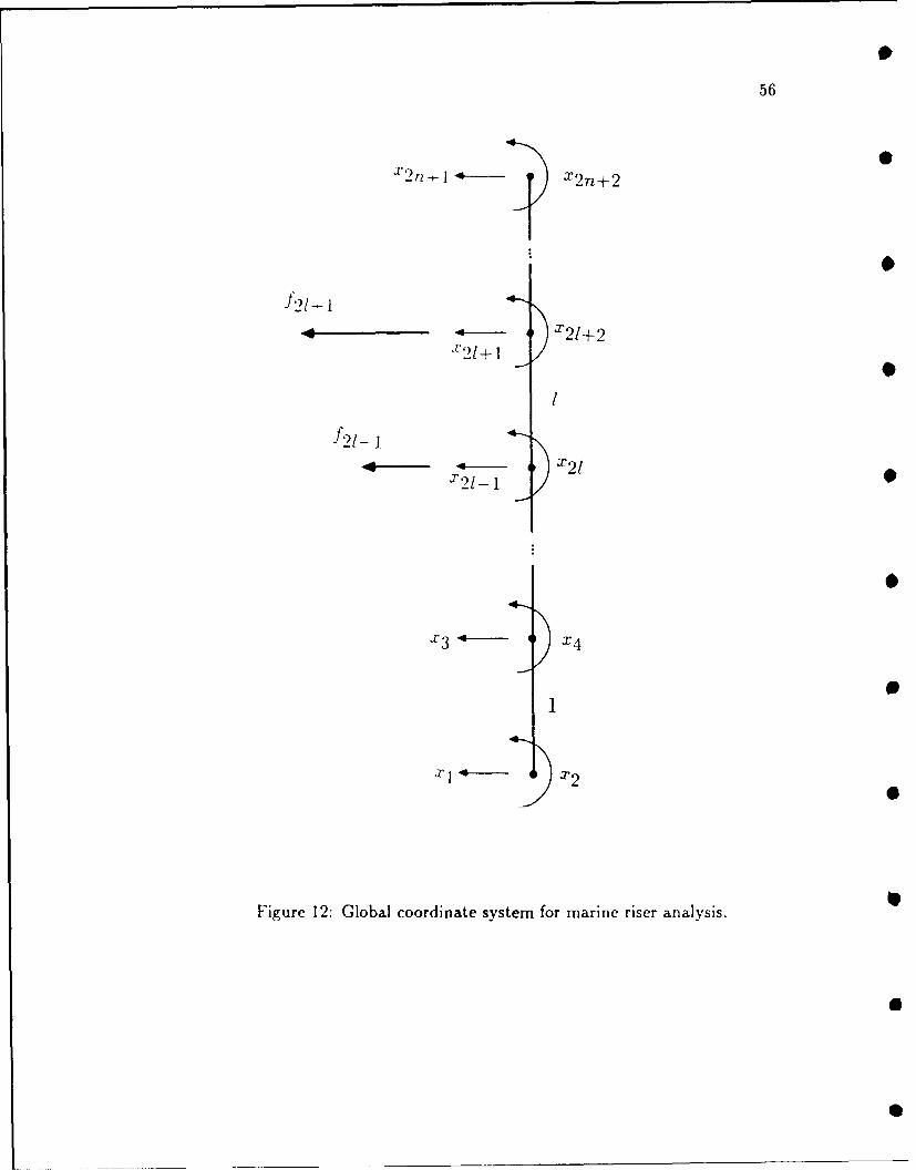
56
f'2 -
X~l~r~lX--)0
x3 'a /
f2'-1 X
Figure 12: Global coordinate system for marine riser analysis.
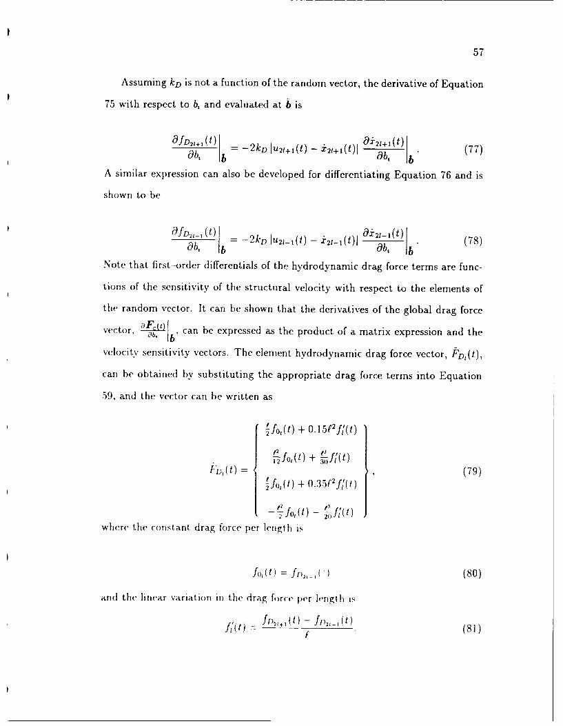
57
Assuming kD is not a function of the random vector, the derivative of Equation
75 with respect to b, and evaluated at 6 is
Of D21+, 1 92+ (t)
Ob, ) = -2kD Iu21+x(t) - 2 t 2 +1(t) (77)Obbb, b"
A similar expression can also be developed for differentiating Equation 76 and is
shown to be
(9fD21 , (tI M 2kD IU21-1(1) - 'i2 l-1(0) 1xiI (78)O9b, L = -- (7s)bDb b, b"
Note that first-order differentials of the hydrodynamic drag force terms are func-
tions of the sensitivity of the structural velocity with respect to the elements of
the random vector. It can be shown that the derivatives of the global drag force
vector, ab, b' can be expressed as the product of a matrix expression and the
velocity sensitivity vectors. The element hydrodynamic drag force vector, FD(t),
can be obtained by substituting the appropriate drag force terms into Equation
59, and the vector can be written as
fo,(t) + O.15 f 2 f 1 (t)
- 2 f o, (t) 3 fjt, ,)Fv1 (t) = (79)+ f 1 (t
Ffo,(t) + 0.35 2f(t)
-- foM(t)- fJ(t)
where the constant drag force per length is
= to, _ ( ) (80)
an(d the linear variation in the drag force per length is
f It -- f ,(+,) - fD21-(t) (8F
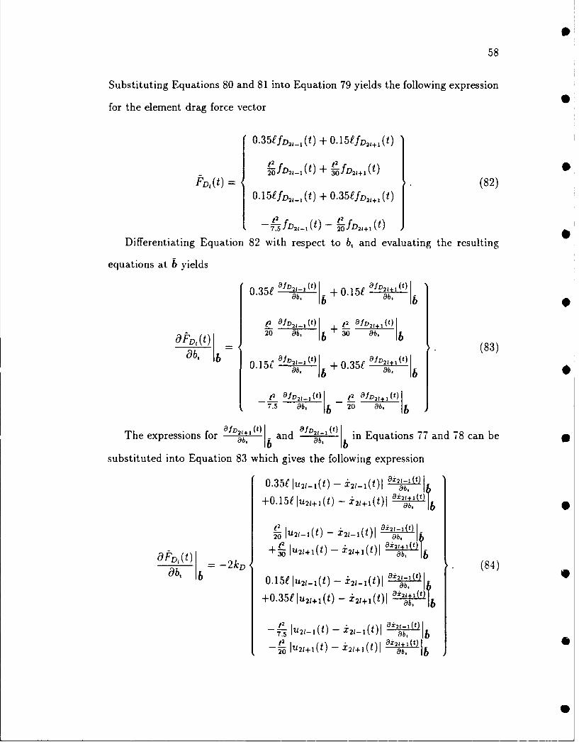
58
Substituting Equations 80 and 81 into Equation 79 yields the following expression
for the element drag force vector
0. 3 5ffD2,_(t) + 0.15ifD2 ,+,(t)12 -
FDT(t) fD 21 -1(t) + LfD21+1 (t) (82=D (82)O.15e fD2, -1 (t) + 0.35efD,+, ()
t 2fD2 2 2, _ ( t) - 2 f ( t )
75 /2 -1( J L
Differentiating Equation 82 with respect to b, and evaluating the resulting
equations at b yields
0 f 2 f(t) + 0.15t fD2,+1 (t)b, b +b, b
t20 f%2 z_(t) +L 2 i f_ 1+_ (t)
PD(t) 20 b. +6 30 , 6b (30b, b IA f2- t 0.3 f f2,, (t) (83)
b9, + 05 b, 6
t2 afD2 _ (t) L 2 afD2 .11 (t).5 6, Ib - 2 86, b
The expressions for of + (t) and fD21 in Equations 77 and 78 can be
b, 6 ab, in
substituted into Equation 83 which gives the following expression
0.35f lu 21,_(t) - i 21-1(t)l ab2l.I(t)+0.15t lIu 21+ (t)- i 21+I(t)j ai'a bj
P@
j- u2 1 (t) - - 21-(t) .2 t+ () "i2+1(t1 (t)
OPD ,(t) 6 -2kD 0.5f Iu21..(t) 21I (t)j ab, (84)
+0.351u 21-1(t) - (x2 + 1(t)I 8gt
-,35 1u2 1+(t) - 2 1+(t)I 8ab. Ib
ab, b
t2p

59
The sensitivity expressions for the velocity terms can be separated out ofEquation 84 resulting in a new expression for F which can be written as
ab, b
a8i2 l 2 (t) I
ab, lb
abb a-2+
o =tab, Ib
where the matrix [Rj](t) represents the matrix
0.35t u 21.. (t) - i 21- 1(t) 0 0.15f 1u21+i(t)- X21+1(t)l 0
To Iu2t-1(t) - i 21- 1(t) 0 30 Iu21+1(t) - i 21+1(t) 0
[Ri](t) = . (86)O.1S u2 _ 1(t) - i 2 - 1 (t)j 0 0.35f Ju21+1(t) - i 2:+1(t)1 0
- u21-1(t) - i2l-l(t)j 0 11 Iu21+1(t) - i21+1(01l 0
Upon inspection of Equation 86, it can be shown that the element matrices, [R](t),
can be assembled into a global matrix, R(t), using the same assembly procedures
as used for the mass and stiffness matrices. The expression for the global hydro-
dynamic force vector, differentiated with respect to b, and evaluated at b can now
be written as
OFD(t) = -2kDR(t) (87)
b b = -b, l "
In the first-order equations of motion, the 'damping force' was expressed as
' az(t) b' A new damping matrix C'(t) is defined and is expressed as
C'(t) = C + 2kDP 1 (t). (88)

60
The first-order equations of motion now become
(9F, aF1(t) aF,(t) + , (t) + C =K+C t + X(t) (89)
ob, + ob, 6 ob, -A A ab, 1b
Note that the static and dynamic components in Equation 89 must be separated to
be consistent with the prescribed solution procedure. Thus, the sensitivity vectors
obtained by solving the static first-order equation include the static offset sensi-
tivity vectors, ax. 1b and the sensitivity kinematic vectors computed by solving
the dynamic first-order equations. These include the dynamic response, velocityand acceleration sensitivity vectors, and 2 jb respectively.7 b, 1b' ab, b'a b, b epciey
4.3.3 Second-Order Response Predictions
Once the sensitivity vectors have been computed, the second-order deviations
about the zeroeth-order response predictions can be obtained. These predictions
require second-order partial differentiation of the system matrices and force vec-
tors with respect to b, and b, where the resulting expressions are evaluated at
__M_ 82C a2K a2F.b. It is not difficult to obtain expressions for 86-' 8, 6' b1' o6,16
82Fl(t) an 82F e 8(t)ab.an, b nd b However, obtaining the solution for 8b,8b 6 is compli-
cated.
The second-order derivative of the hydrodynamic force per length at the top
of element I is obtained by differentiating Equation 75 with respect to b, and b.
and evaluating the resulting expression at 6. This can be expressed as
a'fD 1 +'+ (t) = -2kD 1u21+1(t) - -i21+1(t)l 0b, i2+ M
6 8b18b, a a(9
+ 2kD sgn[u21+1 (t) - '21+1(01 89, 1 b (t) b 1 b' (90)
Ob, b Ob,
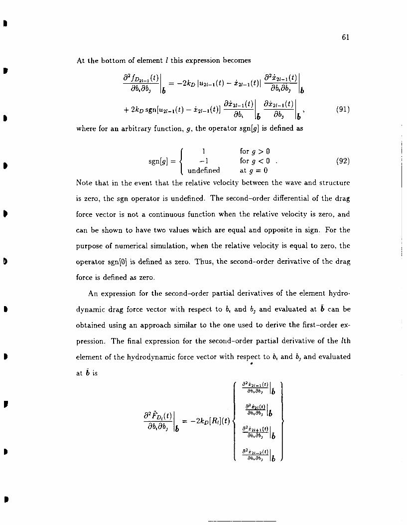
61
At the bottom of element 1 this expression becomes
,92 fD.- W(t) = --2kD.u2,-.(t)- 2-(t) 2 1 (t)ab1 abi a bab, Ib
+ 2kD sgn[u 2. 1(t) - 421.- 1(t)] ai21 1 (t) a 2 1 (t) b (91)ab Ib c~b Ib
where for an arbitrary function, g, the operator sgn[g] is defined as
for g > 0
sgn[g]= -1 for g < 0 (92)undefined at g = 0
Note that in the event that the relative velocity between the wave and structure
is zero, the sgn operator is undefined. The second-order differential of the drag
force vector is not a continuous function when the relative velocity is zero, and
can be shown to have two values which are equal and opposite in sign. For the
purpose of numerical simulation, when the relative velocity is equal to zero, the
operator sgnO is defined as zero. Thus, the second-order derivative of the drag
force is defined as zero.
An expression for the second-order partial derivatives of the element hydro-
dynamic drag force vector with respect to b, and b, and evaluated at b can be
obtained using an approach similar to the one used to derive the first-order ex-
pression. The final expression for the second-order partial derivative of the lth
element of the hydrodynamic force vector with respect to b, and b, and evaluated
at 6 is
82b, b
a2fDl(t)] 2 -2kD[R,(t) ,
ab~a, b8 2i~ 4~t) ba,
8b8b
8b :-8b1 b
Ib b
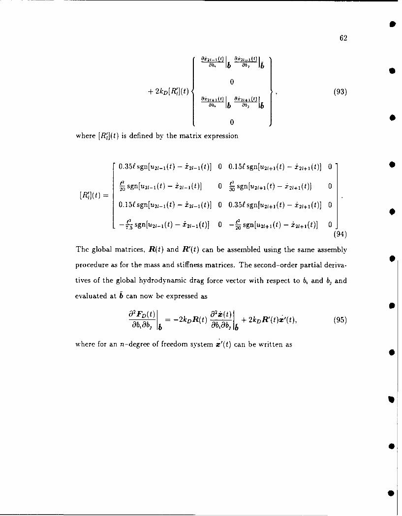
62
86, 16 ab, lb
0+ 2kD[R"1,](t) (93)
ah, a b,
where [R1](t) is defined by the matrix expression
r 0.35fsgn[u 2j_,(t) - i 211 (t)] 0 0.15gsgn[u2,+1 (t)- i 2,+(t)] 012 g
Tsgn[u 2.,_(t) - i 2 1- 1(t)] 0 Isgn[u2 1+(t) - .i21+I(t)] 0
[R'](t) =0.15tsgn[u21.l(t) - xi2,,_(t)] 0 0.351sgn[u21+1(t) - 21+I(t)] 0
t2 t;- .--sg _(t) - i 2 1- 1 (t)] 0 -Lsgn[u 21+1 (t) - i 2l+I(t)] 0
(94)
The global matrices, R(t) and R'(t) can be assembled using the same assembly
procedure as for the mass and stiffness matrices. The second-order partial deriva-
tives of the global hydrodynamic drag force vector with respect to b, and b, and
evaluated at b can now be expressed as
D2FD, = -2kDR(t) 4abt b + 2kDR'(t)z'(t), (95)
where for an n-degree of freedom system X'(t) can be written as
0
0

63
POb, lb 8, lb
0
8b, lb ab, lbII
0
'()= •(96)ah, Ib ' I, b
0
ab, Ib 1I
0
Recall that the second-order equation of motion as developed in Chapter 2
was shown to be
MAX(t) + CA(t) + kAi(t) = AF(t), (97)
where
I q I -F ,) C [ ++ b.]}
,=1,= J=l Ic jb b - ' O:1 q M Ot(t) + W 8 (t)+ K Cov[b,, .
2b, b bO 0, Oh, Ob, C b1~{ OM (t+0 2 :j 'K (tl CbIb}.(8
Upon substitution of Equation 95 into the second-order equation, the second-
order deviation about the mean drag force vector can be expressed as
I { b b q=} av2kD{ b, b b Cov[b,, b,]
_2(b 9 2,F-E 4b 9

64
+ 2kDR'(t) y _ {X'(t)Cov[b,, bI}. (99)
The form of this equation can be simplified, where the new equation is
1 q q a2 FD(t) Cov[b, b -2kDR(t)A (t)
1 q q
+ 2kDR'(t) -E E {'(t)Cov[b,, b,]}. (100)
The second-order equation of motion can now be expressed as
MAX(t) + C'(t)Axi(t) + kAi(t) =
AP(t) + 2kDR'()" y Y {'(t)Cov[b,, b,} (101)2 =1 e=l
where
I qq 1{o2(F (t) + re F,(t))bCOV[b, b21}
iM O (t) OC O(t) 9K O,() 1b=b, ab b - ab, + O jb
'C ___ + '9 ('b]io
r q 91M a2C(a2- E I: X(j + dc (t) + x(t) Cov[b,,b]}. (102)2 =I 1= abab a (! b,0-- ab,0abj b
Note that the static and dynamic components in Equation 102 must be sepa-
rated to be consistent with the prescribed solution procedure. The second-order
deviations in the static offset vector are obtained by solving the second-order
equation with only the static components, and the second-order static response is
written as Ax,. The second-order deviations in the dynamic response, Azd(t) are
computed by solving Equation 101 using only those components which contribute
to the dynamic response. The total expected response of the riser accurate to
second-order can now be written as
E[x(t)] = zk + A, + ;kd(t) + AXd(t). (103)

65
A better approximation for the expected values in the stresses can be ob-
tained by substituting the appropriate second-order accurate expected values of
the rotations into Equation 73.
4.3.4 First-Order Accurate Covariance Predictions
The covariances for the discrete displacement fields can be computed as described
in Chapter 2. The covariance between any two displacements x,(t) and x,(t) at
time t are computed from the following formula
Cov[Xj( t), x,,( t)]
q q_ ( X, X , (t)b) ( ca( X .- + X b ( ) Cov[b bu]} " (104)
One method for obtaining the covariances in the stress field is to employ the
second-moment analysis techniques. The first-order equation is obtained by dif-
ferentiating both sides of Equation 72 with respect to each of the elements in the
random vector and evaluating the resulting expressions at the expected values of
the random vector. Thus, the first-order equation for the stress at the midpoint
of element 1 at time t, assuming E and c are deterministic, can be expressed as
(t) I _ ---',Ec 90(zi+ A ZIt)ob- - --A ztt)t "(105)
O b b 2A, b, b b
The first-order accurate covariance in the stresses at the midpoints of elements
I and rn are computed as
Cov[Uj,(t), r
Y Oa, bi a ,(t) b Cov[b,,bj] . (106)
In this study, only the variances in the stresses at the midpoint of the elements
are required and a more direct method is used to compute these values. Squaring
66
both sides of Equation 72 and taking the expected value of the resulting expression
yields
E[t Ec )2 E[{O(z, + Az,t) - O(zj - Az, t))']. (107)
(2AzI
Equation 107 can be expanded, and assuming the means have been removed from
the rotations, the variance in the stresses at the midpoint of element I and at time
t can be computed as
var[a,(t)] - {var[O(z, + Az,,t)] + var[0(z, - Azt,t)]}
-2 (Ec 2 {COv[0(zI + Azt),O(z, - AzI, t)]}. (108)
4.3.5 Application of Probabilistic Results
The probabilistic finite element results for the marine riser displacements and
stresses can be used to assess the displacement and stress envelopes typically
developed for design. The zeroeth-order solutions obtained in the probabilistic
analysis would represent those obtained using a deterministic approach. The
zeroeth-order displacement envelope can be estimated using the zeroeth-order
displacement solutions. The stress envelope can also be developed where the
stresses are predicted from the time histories of the zeroeth-order rotations.
Upper and lower bounds to the displacement and stress envelopes can also be
computed. An upper bound time history for the displacements and stresses may
be generated by adding the standard deviation to the zeroeth-order predicted
values at time t. Similarly, a lower bound time history is created by subtracting
the standard deviation from the time histories. Using these estimates for the
maximum and minimum displacements and stresses at time t, upper and lower
bounds for the displacement and stress envelopes can be estimated.
40
67
A better approximation for the displacement envelope is obtained using the
second-order expected values of the responses. Similarly, a better approximation
for the stress envelope is obtained using the stresses computed from the second-
order rotations. These envelopes are then bounded as before. The upper bounds
are computed from the sum of the second-order time histories and the first-
order standard deviation time histories. The lower bounds are computed from the
difference between the second-order time histories and the first-order standard
deviation time histories.
4.4 Probabilistic Solutions to Marine Riser Problems
There are numerous commercial computer codes available for the analysis of ma-
rine riser systems. In an attempt to compare the predictive capabilities of the off-
shore industry, the American Petroleum Institute (API), posed a set of standard
problems to which it solicited industry solutions. API then prepared a bulletin
based upon the numerical results it received (API 1977). The bulletin contains
predictions for riser systems designed for 500, 1500 and 3000 feet of water. Sinceall the models require empirical data and the computer programs covered a wide
range of solution techniques, the solutions were presented in terms of envelopes
of displacement and stress.
The probabilistic finite element method, as developed in the preceding text, is
used to predict the response behavior of marine riser systems which are considered
to have random properties. Two marine riser systems are considered, the first in
500 feet of water and the second in 3000 feet of water. The riser system in
3000 feet of water includes external buoyant material. For each water depth the
API bulletin shows a number of solutions submitted by the offshore industry in
the form of response and stress envelopes. For the purpose of comparison, the
68
solutions shown in the API bulletin are presented on the appropriate graphs in
this study. The mean values of the parameters which are necessary to perform
the analyses are specified in the API bulletin and are tabulated in Table 2. The
probabilistic solutions are compared with results obtained in an API bulletin on
marine riser analyses. Monte Carlo simulations are also performed as a means of
assessing the probabilistic results.
To be consistent with the results in the API bulletin and to show results
which are meaningful to engineers who design marine riscrs, response and stress
envelopes are generated and bounded by one standard devif;on. Zeroeth-order
predictions which are analogous to the deterministic solutions predicted in the
API bulletin are shown, as are the second-order approximations. The standard
deviations in the response parameters are obtained by taking the root of the first-
order accurate variance. The bounds to the displacement and stress envelopes
computed in this study are obtained by bounding the appropriate time series with
one standard deviation computed at time t, and then computing the envelopes for
these solutions.
The finite elemcnt riser models are assembled using twenty-four elements and
fifty degrees of freedom. The models are assembled such that the individual
elements are concentrated in the regions wheic the maximum stresses are expected
to occur. These regions are dictated by the imposed boundary conditions and are
located near the top and bottom of the risers. The el-ment lengths for the 500
foot water depth case range from 10 to 30 feet and the element lengths for the
3000 foot water depth case range from 20 feet to 200 feet.

69
Table 2: Riser input data specifications.
A. Constant with water depthRiser data
Diameters, inchesriser pipe outside diameter 16.0riser pipe inside diameter 14.75choke line outside diameter 4.0choke line inside diameter 2.7kill line outside diameter 4.0kill line outside diameter 2.7buo:. ant material outside diameter 24.0
Modulus of elasticity of pipe, psi x 106 30Densities, pounds/cubic foot
sea water 64drilling mud 89.8
Hydraulic force constantsdrag coefficient 0.7added mass coefficient 1.5effective diameter, inches 26
Weight (includes mud in external lines), pounds / footunbuoved 172.4buoyed 188.1
Linear current profile:velocity at the surface, knots 0.5velocity at the lower ball joint, knots 0
Vertical distances, feetmean water level to riser support ring 50sea floor to lower ball joint
B. Varying with water depthTop tension, kips
500 foot water depth 1203000 foot water depth 500
Static offset, 3% of water depthC. Dynamic
wave height, feet 20wave period, seconds 9vessel surge amplitude, feet 2phase lag between vessel and wave, degrees 15
70
4.4.1 Top Tension Modeled as a Random Variable0
To demonstrate the predictive capability of the probabilistic finite element method,
two marine riser systems are examined in which the tension applied to the top
of the risers is considered to fluctuate. The water depths considered are 500 and
3000 feet and the properties of the risers are given in Table 2. The distributions
of the random top tensions are considered to be Gaussian and the coefficient of
variation in the top tension for both cases is assumed to be 0.1.
Monte Carlo simulations are performed to assess the second-moment results.
The Monte Carlo technique is identical to the one used in the Chapter 3. It was
determined that the second-moment solutions converge within 400 simulations.9
Figures 13 and 14 show the maximum steady state response predicted by the
zeroeth- and second-order solutions and the Monte Carlo solutions for the 500
foot and 3000 foot water depth cases, respectively. For each response estimate.9
one standard deviation in response is added. Thus the lower curve represents
the response estimate and the upper curve represents a possible 'upper bound'
to the estimate. The API response predictions are also shown. As expected, the
zeroeth-order solution falls within the bounds of the API solutions. There is some
deviation in the zeroeth-order solutions and those predicted using the Monte Carlo
simulation. The second-order solutions do converge to those predicted from the9
Monte Carlo simulations. It should be noted that when one standard deviation
in response, predicted using second-moment techniques or by the Monte Carlo
simulation, is added to the appropriate mean response prediction, the upper bound
of the API solutions is exceeded.
Figure 15 represents the minimum steady state response for the riser in 500 feet
of water. The second-order solutions converge to those predicted in the Monte
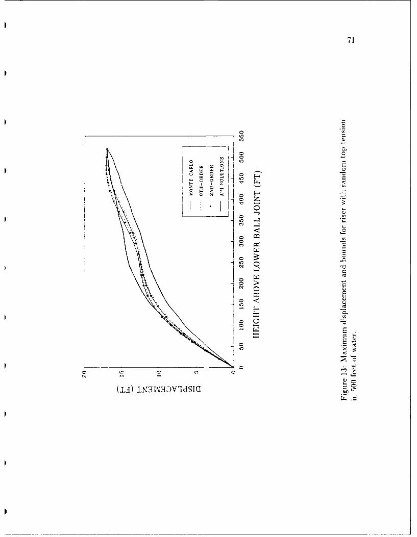
71
CQC
0r
0 C
(J-4 J"N3mjwds0

72
0 C
CI
C-2
0cjn
-U
0 --
0< E
cl0
(,L~) JL31,gowlls0
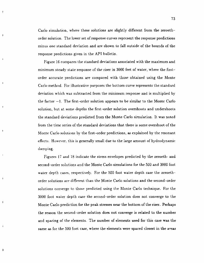
73
Carlo simulation, where these solutions are slightly different from the zeroeth-
order solution. The lower set of response curves represent the response predictions
minus one standard deviation and are shown to fall outside of the bounds of the
response predictions given in the API bulletin.
Figure 16 compares the standard deviations associated with the maximum and
minimum steady state response of the riser in 3000 feet of water, where the first-
order accurate predictions are compared with those obtained using the Monte
Carlo method. For illustrative purposes the bottom curve represents the stand trd
deviation which was subtracted from the minimum response and is multiplied by
the factor -1. The first-order solution appears to be similar to the Monte Carlo
solution, but at some depths the first-order solution overshoots and undershoots
the standard deviations predicted from the Monte Carlo simulation. It was noted
from the time series of the standard deviations that there is some overshoot of the
Monte Carlo solutions by the first-order predictions, as explained by the resonant
effects. However, this is generally small due to the large amount of hydrodynamic
damping.
Figures 17 and 18 indicate the stress envelopes predicted by the zeroeth- and
second-order solutions and the Monte Carlo simulations for the 500 and 3000 foot
water depth cases, respectively. For the 500 foot water depth case the zeroeth-
order solutions are different than the Monte Carlo solutions and the second-order
solutions converge to those predicted using the Monte Carlo technique. For the
3000 foot water depth case the second-order solution does not converge to the
Monte Carlo prediction for the peak stresses near the bottom of the riser. Perhaps
the reason the second-order solution does not converge is related to the number
and spacing of the elements. The number of elements used for this case was the
same as for the 500 foot case, where the elements were spaced closest in the areas
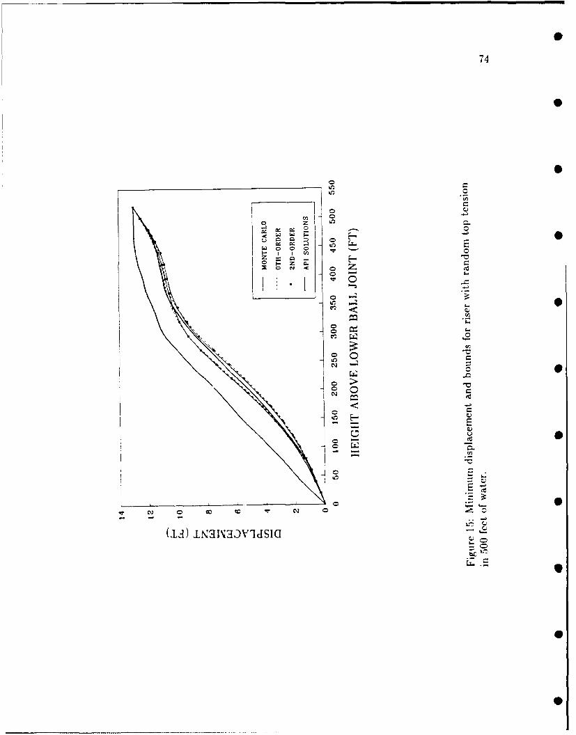
74
CC
C~C
'0
oL E
I
75
p
* 0I-
* I -~
o 0~ 0
< 00 0 ~' -~
I c~0 iI r..
- I -- 2: I-.
2:
/ I HK: Z0~
-1~ Q tp -~ 0
OC.IL.C\J~
o 0 -e oo
I-,
000
I I~ <I / H=
0 -
~ 0 -
/ -e ~-0~
_________________-______________
- Tci:
~,I11WT~Jfl TWfl~.i1,1C' -5~ -,
ci:
p
I
p
76
where the maximum stresses were expected to occur. In this study the maximum
number of elements permitted for higher-order response predictions was twenty-
four. Both the zeroeth- and second-order predictions of the maximum stress at
the top of the riser converge to the Monte Carlo results.
Figures 19 and 20 indicate the maximum zeroeth- and second-order stresses
and those predicted using the Monte Carlo simulations for the 500 and 3000 foot
water depth case, respectively. The upper set of curves represents one standard
deviation in addition to the value of the mean estimate. The bounds from the API
solutions are also shown. For the 500 foot water depth case t is seen that the
second-order solutions converge to Monte Carlo solutions. Note that the peak
stress predicted from the zeroeth-order solution lies within the bounds of the
API solutions and that the second-order and Monte Carlo solutions are outside
the bounds. Further, note that with the addition of one standard deviation to
mean stresses, the probabilistic estimates can exceed the estimates obtained in
conventional analyses by a significant amount. For the 3000 foot case where the
variation in the stresses is much smaller than for the 500 foot case, the predictions
appear to be within the range of the ! PI solutions. •
4.4.2 Unit Weight of Drilling Mud Modeled as a Random Field
To further demonstrate the possibilities for simulation using probabilistic finite
element methods, another type of marine riser simulation is presented. In this
case a riser system in 500 feet of water, as specified in Table 2, is examined
assuming that the unit weight of the drilling mud varies along the riser according
to a definable statistical process. A first-order autoregressive model, AR(1), is
used to account for the fluctuations. Accordingly, the fluctuations in the weight
per unit length of the drilling mud, t,,(z) at an elevation z, above the sea floor

I'
10p ~ C
II. ~0 F-
00'Ir~
~- z'0 N
7C
0 -~
K' I-00~
5-
a.-4-/ C
1 N CC
~0<
04..
'p
bO
* A -~
/
00 C\1 0 C~4- - I I I --
-(IsM) SS3}LLS DNIUN3~
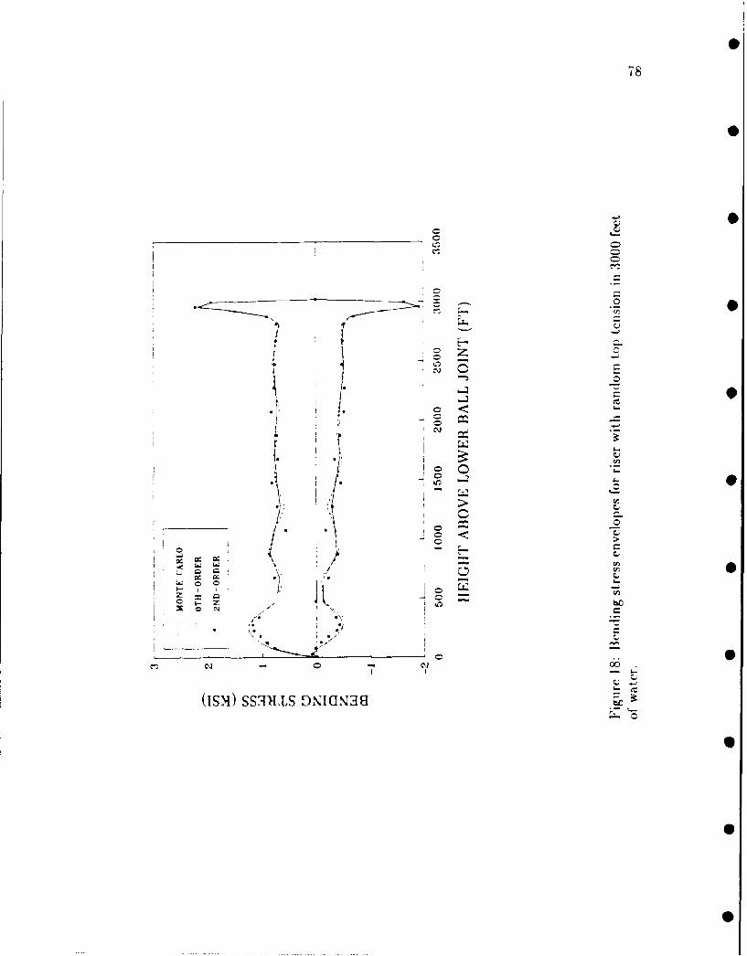
S
78
0
S__________ 0_______________________________________ 0
0
0
.~5 0
0I. .- ~
4.) I
NI ~L.
I I-
.7 U,IC ~ 4-
P 0 4-
- 4..-, 4..~
- 0______ 1~ '4.- -
0 - 0Jo <o ~1,
~. A U, U, S/ 0
'4. 4-F ~ 00 -
I.' 0-oo~ 0 C'~ 7
4. F
.4. 4.7~
0 - 0N - C - N
I I - I-
4-
(IsM) 5531115 9NIU~38- -
S
S
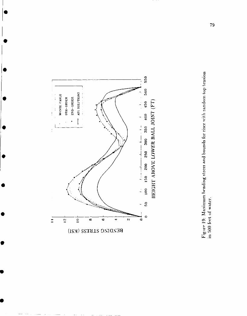
79
0c
00
C ',
* ~ -. ~- _
UONO SS1i ON.3
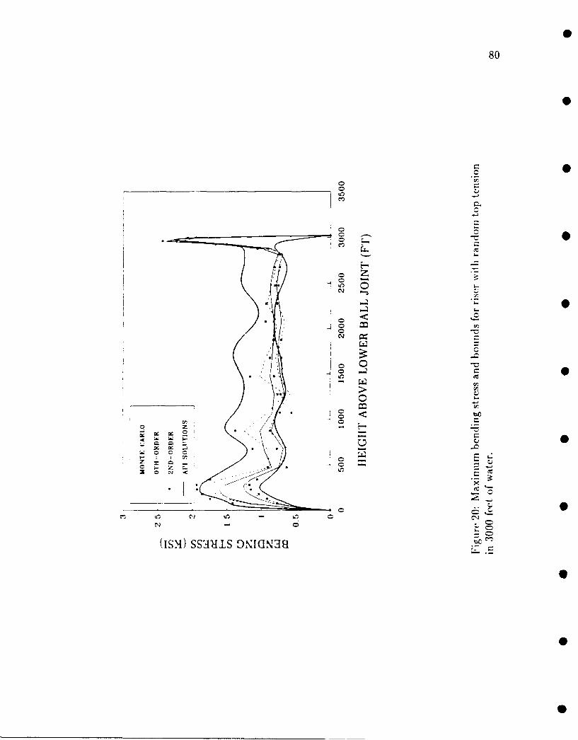
80
Cd
00
C
or 0ed
1^
(i~)S~us9NII3E

81
were simulated using the AR(1) recursive formulation as
lhm(z,) = WN(z,) - ait-vm(Z,_i), (109)
where WN(z,) is Gaussian white noise and a, is the first-order autoregressive coef-
ficient (Newton 1988). The correlation function for an AR(1) process is described
by an exponentially decaying function expressed as
p[r] = (-ol) = e -(/LC), (110)
where
(Yl = -e - 1 , ( 111 )
and L, is the correlation distance. For this example p[LI = e- 1, and L, is arbitrar-
ily chosen to be 75 feet. The coefficient of variation for the process representing
the unit weight in the drilling mud is 0.2.
For this example the second-moment analysis requires as input the local spa-
tial averages of the process and the covariance matrix between the local spatial
averages. In order to predict the local spatial averages, the weight per unit length
of the drilling mud is assumed to be a stationary process so that the local spa-
tial averages were equal to the expected value of the entire process. In order
to compute the covariances between the local spatial averages, the dimensionless
variance function, which represents the ratio of the variance in the local spatial
averages to the variance in the entire process, is required (see Chapter 2). The
dimensionless variance function is computed analytically using Fq"ltion 5. The
covariances between the local spatial averages are then computed using Equation
4.
For the Monte Carlo simulations, an AR(1) model is used to simulate 400
realizations of the mud weight per unit length. Each process is averaged over
82
the appropriate elements and the element averages are used in the finite element
analyses.
A comparison of the zeroeth- and second-order solutions and the Monte Carlo
predictions for the maximum displacement for the riser in 500 feet of water is
presented in Figure 21. The maximum displacement plus one standard deviation
is also shown. The zeroeth- and second-order estimates appear to be very near
the Monte Carlo solution. For the most part the API solution bounds all of the
probabilistic estimates including those which show the maximum displacement
plus one standard deviation.
The maximum zeroeth- and second-order stresses and the stresses predicted
using the Monte Carlo method are presented in Figure 22. The upper bounds for
these predictions are also shown. The zeroeth- and second-order solutions with
the addition of one standard deviation are slightly higher than the Monte Carlo
estimates of the maximum stress plus one standard deviation. Note that these
upper bounds for the maximum stress are significantly higher than maximum
stress shown in the API solution.

83
00
0 0 -Q
0 ttIJL,) IN 1ODVdSIC
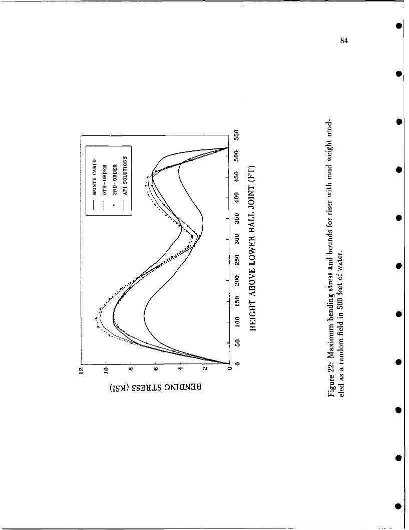
84
0 0
01
o --
U2
cq -
oE
0
~~ H
(ism Sod~ -
0IN
85
5 CONCLUSIONS
The second-moment analysis method is shown to be a viable approach for estimat-
ing the probabilistic distributions in response for systems with random material
properties, loads and boundary conditions. The computational aspects of the
second-moment analysis method and the sequence in which they are to be imple-
mented is shown in Figure 3. In second-moment analyses, the distributions of the
sources of uncertainty are expressed in terms of their first- and second-moments,
where explicit knowledge of the probability density function is not required. The
correlation function must also be identified for sources of randomness which vary
over the spatial coordinates.
In general, second-moment analyses are derived presuming that a linear re-
lationship exists between the response and the sources of uncertainty. If the
relationship is linear then the solutions are exact. The method may also be ap-
plied if the relationship is moderately nonlinear, provided that the coefficient of
variation in the sources of uncertainty is small. If the relationship is linear then
the zeroeth-order response predictions and the covariance in response obtained
using the second-moment method are exact, regardless of the distributions of the
sources of uncertainty. For nonlinear systems, the approximations may be im-
proved by including higher order terms which may require that the analysis be
extended beyond second-order.
Second-moment analyses require the formulation of a random vector which
represents the distributions of all sources of randomness inherent to the system.
The elements of the random vector correspond to the distributions of sources of
randomness expressed by random variables and to the correlated distributions of
the local element averages for sources of randomness expressed as random fields.

86
The lengths of the discrete finite elements must also be shorter than the distances
over which appreciable correlation occurs in the random fields.
A simple two-degree of freedom oscillator with random spring constants was
considered to demonstrate the second-moment analysis. A Monte Carlo simula-
tion was also implemented to assess the second-moment results. The zeroeth- and
second-order accurate displacements obtained using the second-moment method
were compared to the displacements predicted by the Monte Carlo simulation.
The zeroeth-order response solution was shown to differ from the second-order
solution, where the second-order solution was almost identical to the Monte Carlo
solution. The first-order accurate standard deviation predicted by the second-
moment method was also compared with the standard deviation predicted by the
Monte Carlo simulation. The first-order solution was shown to follow the same
trend as the Monte Carlo predictions and was shown to be valid for small times,
but the first-order solution overshot the Monte Carlo predictions at large times. 0
This was a result of a resonant excitation of the higher-order terms in the second-
moment analysis. For this example the advantage in the second-moment analysis
as compared with the Monte Carlo method was in the computation time. The 0
second-moment analysis required only four numerical time integrations to obtain
the same responses as those predicted by the Monte Carlo method, which required
400 time integrations to obtain stable second-moment solutions.
For analyses of marine riser systems, where aspects of the problem are known
to be random, the probabilistic finite element method was shown to provide useful
information concerning the distributions of the response behavior. Two sets of
examples were considered. In the first set of examples the tension applied to the
top of the riser was modeled as a random variable. In the second set of examples
the unit weight of the drilling mud contained within the riser was modeled as a
87
random field. For both sets of examples it was observed that while in general,
the expected values of the peak second-order responses and stresses were within
the ranges of estimates obtained using deterministic solutions, the addition of
one standard deviation significantly impacted the response behavior. For the
example riser in 500 feet of water in which the pretension was modeled as a
random variable, the maximum stress shown in the API bulletin was exceeded
by a factor of 1.3 when one standard deviation was added to the second-moment
predictions of the maximum stress. The maximum stress predicted in the API
bulletin would be exceeded by 1.7 and 2.0 times if it were to be exceeded by two
and three standard deviations, respectively, of the second-moment predictions
of the maximum stress. In some cases the second-order solution exceeded the
bounds of conventional solutions. The riser analyses performed in this study have
shown that with a small amount of variation in the tension applied at the top of
the riser or with variations in the drilling mud unit weight, it can be expected
that the design responses and stresses predicted using conventional finite element
solutions will be exceeded.

88
REFERENCES
API Bulletin on Comparison of Marine Drilling Riser Analyses. (1977). API
Bulletin 2J, First Edition, American Petroleum Institute, Dallas, TX.
Astill, C. J., Nossier S. B. and Shinozuka, M. (1972). "Impact Loading on
Structures with Random Properties." Journal of Structural Mechanics. 1(1),
63-77.
Baecher, G. B. and Ingra, T. S. (1981). "Stochastic FEM in Settlement Predic-
tions." Journal of the Geotechnical Engineering Division. ASCE, 107, No.
GT4, 449-463.
Bathe, K. J. (1982). Finite Element Procedures in Engineering Analysis. Prentice-
Hall, Inc. Englewood Cliffs, NJ.
Chakrabarti, S. K and Frampton, R. E. (1982). "Review of Riser Analysis
Techniques." Journal of Applied Ocean Research. 4(102), 73-90.
Gardner, T. N. and Kotch, M. A. (1976). "Dynamic Analyses of Risers and
Caissons by the Finite Element Method." Offshore Technology Conference.
2651, 405-420.
James, M. C., Smith G. M., Wolford J. C. and Whaley P. W. (1989). Vibra-
tion of Mechanical and Structural Systems with Microcomputer Applications.
Harper and Row Publishers. New York, NY.
Liu, W. K., Belytschko, T. and Mani, A. (1985). "A Computational Method
for the Determination of the Probabilistic Distribution of the Dynamic Re-
sponse of Structures." Computer Aided Engineering. ASCE, 98(5), 243-248.
Liu, W. K., Belytschko, T. and Mani, A. (1986). "Probabilistic Finite Ele-
ments for Nonlinear Structural Dynamics." Computer Methods in Applied

89
Mechanics and Engineering. 56, 61-81.
Liu, W. K., Belytschko, T. and Mani, A. (1987). "Applications of Probabilistic
Finite Element Methods in Elastic/Plastic Dynamics." Journal of Engineer-
ing for Industry. Transactions of the ASME, 109, 2-8.
Liu, W. K., Besterfield, G. and Belytschko, T. (1988a). "Transient Probabilistic
Systems." Computer Methods in Applied Mechanics and Engineering. 67,
27-54.
Liu, W. K., Besterfield, G. and Belytschko, T. (1988b). "Variational Ap-
proach to Probabilistic Finite Elements." Journal of Engineering Mechanics.
ASCE, 114(12), 2115-2113.
Ma, F. (1987). "Extension of Second Moment Analysis to Vector-Valued and
Matrix-Valued Functions." International Journal of Non-Linear Mechanics.
Vol. 22, No.3, 251-260.
McCoy, G. L. (1985). Riser Response to Directional Seas. M.S. Thesis, Depart-
ment of Civil Engineering, Texas A&M University.
Newmark, N. M. (1959). "A Method of Computation for Structural Dynamics."
Journal of Engineering Mechanics Division. ASCE, 85, 67-94.
Newton, H. J. (1988). Timeslab: A Time Series Analysis Laboratory. Wadsworth
& Brooks/Cole Publishing Company, Pacific Grove, CA.
Niedzwecki, J. M. and Leder H. V. (1990) "Impact of Drag Force Approximations
on Spectral Wave Force Predictions." Technical note submitted to Journal
of Waterway, Port, Coastal and Ocean Engineering Division. ASCE.
Nigam, N. C. (1983). Introduction to Random Vibrations. The MIT Press.
Cambridge, MA. 0
0
90
Sandt, E. W. and Niedzwecki, J. M. (1990). "Response of Flexible Structures in
Random Seas." To appear in Engineering Structures.
Shinozuka, M. and Dasgupta, G. (1986). "Stochastic Finite Element Methods
in Dynamics." Proc. of 3rd Conf. on Dynamic Response of Structures. Los
Angeles, CA, 44-54.
Shinozuka, M. and Deodatis, D. (1988). "Response Variability of Stochastic
Finite Element Systems." Journal of Engineering Mechanics. ASCE, 114(3),
499-515.
Vanmarcke, E. H. (1983). Random Fields: Analysis and Synthesis. The Mas-
sachusetts Institute of Technology Press. Cambridge, MA, and London,
England.
Vanmarcke, E. H. (1984). "Stochastic Finite Element Analysis." Probabilistic
Mechanics and Structural Reliability, 4th ASCE Specialty Conference, ed.
Y. K. Wen. Berkley, CA, 278-294.
Vanmarcke, E. H. and Grigoriu, M. (1983). "St"hastic Finite Element Analysis
of Simple Beams." Journal of Engineering Mechanics. ASCE, 109(5), 1203-
1214.
Yamazaki, F., Shinozuka, M. and Dasgupta, G. (1986). "Neumann Expansion
for Stochastic Finite Element Analysis." Jourral of Engineering Mechanics.
ASCE, 114(8), 1335-1354.

91
VITA
H. Vern Leder was born in Chicago, Illinois, on June 23, 1966. He spent most of
his childhood in Hurst, Texas, where he graduated from L.D. Bell High School
in 1984. In 1984, Vern entered the Ocean Engineering Program at Texas A&M
University where he received his B.S. degree in May, 1988. Vern then entered the
graduate college at Texas A&M in the Ocean Engineering Program. In graduate
school he was employed as a Teaching Assistant and as a Research Assistant. Vern
can be reached through his parents at:
429 Chisolm Trail
Hurst, Texas 76054
0
![PROBABILISTIC FINITE ELEMENT ANALYSIS OF A HEAVY DUTY ...jestec.taylors.edu.my/Vol 12 issue 9 September 2017/12_9_11.pdf · hyperstudy v.13 [21] are used for the nominal run and probabilistic](https://img.pdfslide.us/doc/110x75/5e95935e0b5c56015047b7aa/probabilistic-finite-element-analysis-of-a-heavy-duty-12-issue-9-september-201712911pdf.jpg)


![Accelerating Pollard's rho algorithm on finite fieldsjinhong/12ChHoKi.pdf · 2017. 5. 17. · Pollard [22,23] proposed two probabilistic algorithms called Pollard’s rho method and](https://img.pdfslide.us/doc/110x75/61210076e5396716252820c8/accelerating-pollards-rho-algorithm-on-finite-jinhong12chhokipdf-2017-5-17.jpg)