Probabilistic Estimation of Peers’ Quality and Behaviors ... · Probabilistic Estimation of Peers’ Quality and Behaviors for Subjective Trust ... [13,16,27 ,28 ... ﬁle hosting

Technical report LSIR-REPORT-2006-013

Probabilistic Estimation of Peers’ Quality and Behaviors for Subjective Trust

Evaluation∗

Le-Hung Vu and Karl Aberer

Swiss Federal Institute of Technology Lausanne (EPFL)

School of Computer and Communication Sciences

CH-1015 Lausanne, Switzerland

{lehung.vu, karl.aberer}@epfl.ch

Abstract

The management of trust and quality in decentralized systems has been recognized as a key research area over recent

years. In this paper, we propose a probabilistic computational approach to enable a peer in the system to model and estimate

the quality and behaviors of the others subjectively according to its own preferences. Our solution is based on the use of

graphical models to represent the dependencies among different QoS parameters of a service provided by a peer, the asso-

ciated contextual factors, the innate behaviors of the reporters and their feedback on quality of the peer being evaluated.

We apply the EM algorithm to learn the conditional probabilities of the introduced variables and perform necessary proba-

bilistic inferences on the constructed model to estimate peer’s quality and behaviors. Interestingly, our proposed framework

can be shown as the generalization of many existing trust computational approaches in the literature with several additional

advantages: first, it works well given few and sparse feedback data from the reporting peers; second, it also considers the

dependencies among the QoS attributes of a peer, related contextual factors, and underlying behavioral models of reporters

to produce more reliable estimations; third, the model gives outputs with well-defined semantics and useful meanings which

can be used for many purposes, for example, it computes the probability that a peer is trustworthy in sharing its experiences

or in providing a service with high quality level under certain environmental conditions.

Keyword: quality, QoS, trust, reputation, P2P;

Technical Areas: Autonomic Computing, Data Management, Internet Computing and Applications;

1 Introduction

Quality and trust have become increasingly important factors in both our social life and online commerce environments.

In many e-business scenarios where competitive providers offering various functionally equivalent services, the Quality of

Service (QoS) is amongst the most decisive criteria influencing a user in the selection of a certain service among several

functionally equivalent ones and thus is the key to a provider’s business success. For example, between two online hotel-

booking services, a user would aim for the service associated with the hotel having better price, more comfortable rooms and

providing higher customer-care facilities. Similarly, there are several other instances of services that are highly differentiated

∗The work presented in this paper was (partly) supported by the Swiss National Science Foundation as part of the project: “Computational Reputation

Mechanisms for Enabling Peer-to-Peer Commerce in Decentralized Networks”, contract No. 205121-105287.

1

by their QoS features such as file hosting, Internet TV/radio stations, online music stores, teleconferencing, and photo sharing

services, etc. Therefore, appropriate mechanisms for estimating the service quality are highly necessary.

Since the quality of a service is dynamic and strongly dependent on many factors such as the related contextual/environmental

conditions, appropriate quality estimation mechanisms should be based on the historical QoS data from various information

sources. For example, a user (more generally a peer) in the system could obtain these historical values based on its own expe-

riences. As this is expensive in practice, the judging peer can also ask the others to share their experiences on previous usages

of the service(s), based on which it can evaluate the service quality itself. In this case, the prominent issue is the reliability

and credibility of the collected rating values, as these reports can either be trustworthy or biased depending on the innate

behaviors and motivation of the ones sharing the feedback. This management of trust and quality among the participating

agents in self-organized and decentralized systems has been recognized as a key research issue over recent years [7, 10, 14].

We believe that given the importance of the problem, fundamental results are still missing since most research efforts are

either fairly ad-hoc in nature or only focus on specialized aspects. Many trust computational models in the literature either

rely on ad hoc aggregation techniques and/or produce the trust values with ambiguous meanings, e.g., based on the transitivity

of trust relationships [13,16,27,28]. Other probabilistic-based trust evaluation approaches, such as [1,3,9,19,22,26], although

do not have these drawbacks, are still of limited applications. The main reason is that since they mostly assume that user

ratings, services’ quality, and trust values follows certain distribution types, for example the beta distribution [3,26], and/or do

not take into account the effects of contextual factors and the relationships among participating agents into the trust evaluation

mechanisms. Equally important, the multi-dimensionality of trust and quality has not been well-addressed in current trust

models. Appropriate solutions to this problem are nontrivial since they must also consider many other related issues, such as

the dependencies among the quality parameters and environmental factors, whose values can only be observed indirectly via

the (manipulated) ratings of the other users. The scarcity and sparseness of the observation data set is an additional problem

to be solved in this scenario.

In this paper we show that the quality and trust evaluation is a subjective procedure in nature and it should only be modeled

based on the viewpoint of a judging peer. For example, the trust of a peer on another may be dependent on certain quality

dimensions of the latter as well as the personalized preferences of the former. Since different peers in the system have

different interpretations of the meaning of a trust value, the recommendation and/or propagation of such formulated quantity

in large scale systems is inappropriate. Instead, a peer should only use the reporting/recommendation mechanisms for its

own evaluation of the well-defined quality attributes of the others, from which to build its personalized trust towards the most

prospective partners. Based on this observation we propose a computational framework which enables a peer in the system

to probabilistically estimate the quality of the service provided by another and the behaviors of the related peers reporting

on that service. The output can be used by the judging peer in many ways: (1) for its subjective trust evaluation, i.e., it can

build its trust on another based on personalized preferences, given the estimated values of different quality dimensions of

the latter; (2) to choose the most appropriate service for execution given many functionally equivalent ones offered by the

different peers in the system; and (3) to decide to go for further interactions with another peer knowing its reporting behavior,

e.g., in sharing and asking for experiences.

We use graphical model notations to represent the dependencies among the quality attributes of the peer, the associated

environmental factors, the innate behaviors of various reporters and their feedback values on the perceived quality. The

unknown parameters of the model are learned by using the variational Expectation-Maximization (EM) algorithm [21] on

the constructed models. To compute the QoS parameter values and estimate the behaviors of reporting peers given the learnt

model, we apply the Junction Tree Algorithm (JTA) [12] as the main probabilistic inference procedure.

To the best of our knowledge, this work is the first one which nicely exploits the natural dependencies among the QoS

parameters and their associated contextual factors, the social relationships among agents, from which to accurately estimate

peer behaviors and quality. The most important contribution of our work is its generalization of many representative trust

computational models in the literature, namely [3, 9, 19, 22, 24–27], etc. Moreover, it also enables a peer to subjectively

2

model and evaluate various quality and behaviors of the others according to its personalized preferences and availability of

the observation data. The learning algorithm is shown to be scalable in terms of performance, run-time, and communication

cost. Besides, our proposed solution has many additional advantages: (1) it works well given a few and sparse feedback

data set; (2) it also considers the dependencies between each QoS attribute and its contextual factors, taking into account

appropriate behavioral models of the reporters, which results in more reliable estimates; (3) the computation produces

the output with clear and useful meaning, for example, the probability that a certain peer is honest when reporting, or the

probability that another peer provides a file hosting service with high download speed given that the clients having a specific

type of Internet connection and willing to pay a certain price.

The rest of this paper is organized as follows: in Section 2 we give a formal statement of our main problem. Section 3

describes in details our solution for the probabilistic modeling and evaluation of trust and quality through the personalized

view of a peer in different scenarios: for the simple case without any cheating attempts and for general case where different

possible attack behaviors of the reporting peers are taken into consideration. Section 4 presents our analytical and experi-

mental results to validate and clarify the advantages of our proposed approach. Section 5 is a discussion of some possible

extensions of our current solution, followed by a comparative review of the related work in Section 6. Finally, we conclude

the paper in Section 7.

2 Problem Description

Suppose that we are concerned with the values of the QoS parameters Q = {qi, 1 ≤ i ≤ m}, of a certain service s

provided by a peer P in the system. Generally the value of qi depends on many factors: other QoS attributes and certain

environmental conditions. For example, given a file hosting service such as sendspace, megaupload, up-file.com, etc., the

following QoS parameters are relevant: the offered download and upload speed, the time the server agrees to store the files,

the allowed number of concurrent downloads, and so forth. The environmental factors that could affects those above quality

attributes include: the price of the service, the location and the Internet connection speed of the user and so forth.

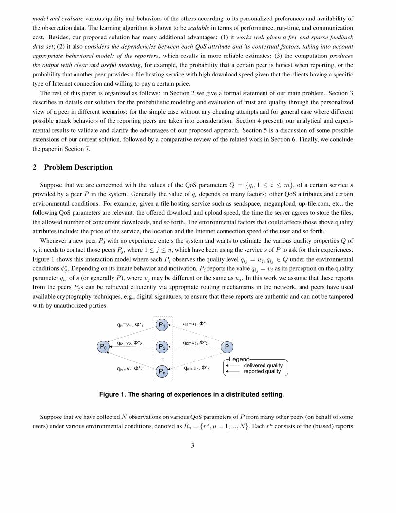
Whenever a new peer P0 with no experience enters the system and wants to estimate the various quality properties Q of

s, it needs to contact those peers Pj , where 1 ≤ j ≤ n, which have been using the service s of P to ask for their experiences.

Figure 1 shows this interaction model where each Pj observes the quality level qij= uj , qij

∈ Q under the environmental

conditions φ∗j . Depending on its innate behavior and motivation, Pj reports the value qij

= vj as its perception on the quality

parameter qijof s (or generally P ), where vj may be different or the same as uj . In this work we assume that these reports

from the peers Pjs can be retrieved efficiently via appropriate routing mechanisms in the network, and peers have used

available cryptography techniques, e.g., digital signatures, to ensure that these reports are authentic and can not be tampered

with by unauthorized parties.

Legend

reported quality qin = vn, Φ*n qin = un, Φ*n

qi2=u2, Φ*2

qi1=u1, Φ*1

qi2=v2, Φ*2

qi1=v1 , Φ*1 P1

P2P0

Pn

P

...

delivered quality

Figure 1. The sharing of experiences in a distributed setting.

Suppose that we have collected N observations on various QoS parameters of P from many other peers (on behalf of some

users) under various environmental conditions, denoted as Rp = {rµ, µ = 1, ..., N}. Each rµ consists of the (biased) reports

3

of some peers on the quality of the peer P under a certain environmental setting. Here we must use a different notation µ

for indexing the observation data set Rp since a peer Pj can submit many reports of various values vj’s to P0. Generally we

have rµ = 〈vµ, hµ〉, where vµ comprises the reported values of some peer(s) Pj on certain QoS parameters under certain

environmental conditions, and hµ represents the unknown (hidden) values of the QoS parameters or environmental factors

which these peers do not report after their usages of the service. Note that vµ and hµ can be different for each observation

rµ. Given the above formalism, P0 basically needs to estimate:

• the probability p(qi = c|φ∗qi

) that the peer P offers qi with quality level c under the environmental condition φ∗qi

(or

more generally the joint probability distribution of some quality parameters qi);

• the probability p(bj) of the real behavioral model of a reporting peer Pj .

The answers to the above questions can be used for several purposes. For example, the output states whether the peer P

performs better than another in terms of its QoS parameter qi and under P0’s environmental settings, so that P0 can select

the more appropriate service to use. Also, given the estimated quality qi’s and based on its own preferences, P0 can build

its personalized trust on P flexibly. The evaluated behavior p(bj) of a peer Pj is also an indication of its trustworthiness

and thus can be utilized by P0 to decide whether to accept future interactions with Pj or not, e.g., for sharing and asking for

experiences.

3 Solution Model

The key idea of our approach is the use of graphical model notations to represent dependencies among QoS parameters,

associated contextual factors, innate behaviors and reported values of the participating peers. In this paper, we only use

directed acyclic graphical models, which is also known as belief or Bayesian networks, since we believe that they are most

appropriate to represent the causality relations among various factors in our scenario: QoS parameters, environmental con-

cepts, and the associated reported values, etc. The use of other types of probabilistic graphical models, for example, Markov

random fields or factor graphs is also an interesting question to be studied, which is beyond the scope of our current research.

The structure of the QoS graphical model of a peer P is to be constructed by the judging peer P subjectively. This modeling

might also be based on certain information provided by the peer P as well, e.g., in the form of a service advertisement or

description. Given an observation data set collected from the other peers in the system (users, rating agents, etc.), P0

firstly learns the parameters of the constructed model that most likely generates these observation data using the variational

Expectation-Maximization (EM) algorithm [21]. Secondly, it uses the Junction Tree Algorithm (JTA) [12] as the main

probabilistic inference procedure on the graphical model with the learnt parameters to compute the required probabilities of

peers’ quality and behaviors.

We choose a solution based on graphical model and EM learning algorithm for several important reasons. First of all,

such an approach would elegantly model the reality: on one hand, the nature of QoS is probabilistic and dependent on various

environmental settings; on the other hand, those dependencies among QoS attributes and associated contextual factors can

be easily obtained in a certain application domain and conveniently described via graphical model notations. Thus the use

of probabilistic graphical models makes it possible to apply the method on any kind of dependencies among QoS parameters

and their related contextual factors in different applications, given that the judging peer spends certain modeling efforts to

build the initial dependency graph. Second, the assumption on the probabilistic behaviors of the participants enables any

peer to describe the actions of related parties flexibly, thus facilitating its subjective evaluation of quality and behaviors of

the others given the prior beliefs and knowledge of the working environment. For instance, the judging peer can describe

its personalized view on the quality of another given its prior beliefs on certain trusted friends and experiences on some

quality dimensions of the peer being evaluated. Third, via the probabilistic inferences on a graphical model, our approach

produces clear outputs with useful meanings, e.g. the probability that a peer provides a high quality service under specific

environmental conditions, or the probability that another peer is honest when sharing its experiences. Forth, the variational

4

EM converges quickly and works well given few and sparse observation data set with many hidden variables. This property

gives us several benefits in term of efficiency and performance since one is likely to get a sparsely populated feedback data

set when collecting reports on many quality dimensions of a service.

3.1 Basic QoS Graphical Model

The basic QoS graphical model is built on the assumption of the judging peer P0 that all peers behave honestly when

giving feedback on QoS of their consumed services. Thus, those values reported by a peer are also its actual observation on

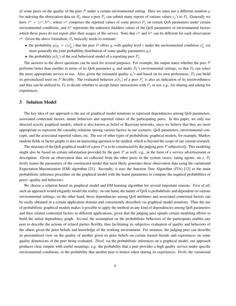
the service quality. In this case, P0 constructs the basic QoS graphical model of a service s provided by P as in Figure 2 (a).

For later references, we also name this model M(1)b . A node el, where 1 ≤ l ≤ t is an environmental (contextual) factor,

and qi, where 1 ≤ i ≤ m denotes the various quality parameters of the service. The rounded square wrapping a variable

represents many similar nodes with the same dependencies with the others. Please note that there may be dependencies

among the different quality attributes qi (and among the nodes els) themselves, which are not shown in the figure for the

clarity of presentation. In this basic model, all nodes are shaded, meaning that their values are observable.

Figure 2 (b) is an example QoS model for the file hosting service provided by the peer P being evaluated by P0. The mean-

ing of each variable is as follows: P =Price, N=Network speed, M=Maximum concurrent downloads, D=Download speed,

and U= Upload speed. Note that this model has been simplified for the clarity of presentation, for instance, we do not con-

sider the dependencies among the quality parameters themselves. In reality, there could be many more QoS parameters and

environmental factors with complicated dependencies.

(a)

D

P

M

N

U

(b)

el

qi

t

m

Download Speed

high ( > 50KB/s)

acceptable ( > 10KB/ s)

low ( < 10KB/s )

Price model

premium ( 10 euros/month)

economic ( 2 euros/month)

free ( 0.0 euro/month)

Network conn. speed

T1/LAN

modems 54.6Kbps

ADSL 2Mbps

Upload Speed

high ( > 20KB/s)


low ( < 5KB/s )

Max conc. downloads

high ( > 10 )

acceptable ( > 2)

low ( =1)

(c)

Figure 2. (a) The basic QoS graphical model M(1)b of the service provided by peer P as viewed by P0;

(b) Example basic QoS graphical model of P providing a file hosting service; (c) Example basic QoS

graphical model with state spaces for each node

Services can be differentiated based on either the absolute value or the conformance of each of their quality parameters.

The latter is actually the compliance of the service’s real performance to its advertised quality and can be measured as the

(normalized) difference between the advertised and the actual quality value offered by the service provider under a specific

environmental setting. Thus, the state space of each node in the QoS graphical model can be modeled as binary (for good or

bad quality conformance) or as discrete values representing different ranges of values for a QoS parameter or environmental

factor depending on the nature of the node and the viewpoint of the judging peer. Figure 2 (c) presents the details of the

model in Figure 2 (b) with a possible assignment of the state spaces for each variable.

Thus, the judging peer P0 who wants to do the quality evaluation of the peer P must establish this dependency graph. The

modeling efforts, in our believes, are negligible since for each application domain, this information can be easily obtained.

For example, these dependencies among nodes and the node’s state spaces can be specified by the domain experts via a QoS

domain ontology, or even from the service description of the peer P who provides the service.

Given the model in Figure 2 (a), the visible nodes are the environmental and QoS parameter variables. The reports of other

peers are their observations Rp on these visible variables, which may contain various missing values. The quality of the peer

5

P through the viewpoint of P0 is the conditional probability table entries p(qi|φqi) whose values maximize the likelihood of

Rp.

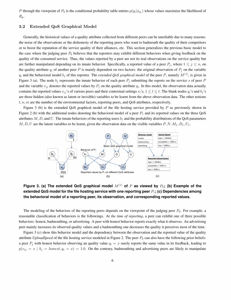
3.2 Extended QoS Graphical Model

Generally, the historical values of a quality attribute collected from different peers can be unreliable due to many reasons:

the noise of the observations or the dishonesty of the reporting peers who want to badmouth the quality of their competitors

or to boost the reputation of the service quality of their alliances, etc. This section generalizes the previous basic model to

the case where the judging peer P0 believes that the reporters may exhibit different behaviors when giving feedback on the

quality of the consumed service. Thus, the values reported by a peer are not its real observations on the service quality but

are further manipulated depending on its innate behavior. Specifically, a reported value of a peer Pj , where 1 ≤ j ≤ n, on

the quality attribute qi of another peer P is mainly dependent on two factors: the original observation of Pj on the variable

qi and the behavioral model bj of this reporter. The extended QoS graphical model of the peer P , namely M (1), is given in

Figure 3 (a). The node bj represents the innate behavior of each peer Pj submitting the reports on the service s of peer P

and the variable vij denotes the reported values by Pj on the quality attribute qi. In this model, the observation data actually

contains the reported values vij’s of various peers and their contextual settings el’s, 1 ≤ l ≤ t. The blank nodes qi’s and bj’s

are those hidden (also known as latent or invisible) variables to be learnt from the above observation data. The other notions

t, n,m are the number of the environmental factors, reporting peers, and QoS attributes, respectively.

Figure 3 (b) is the extended QoS graphical model of the file hosting service provided by P as previously shown in

Figure 2 (b) with the additional nodes denoting the behavioral model of a peer P1 and its reported values on the three QoS

attributes M,D, and U . The innate behaviors of the reporting users b1 and the probability distributions of the QoS parameters

M,D,U are the latent variables to be learnt, given the observation data on the visible variables P,N,M1,D1, U1.

el

qi

vij

bj D

P

M

N

U

M1 D1 U1

Basic QoS graphical model

b1

Behavior of P1

Reported values by P1 on different QoS attributes

(a) (b)

n m

t

mn

Behavior model

honest

badmouthing

advertising

Upload Speed

high ( > 20KB/s)


low ( < 5KB/s )

Reported Upload Speed

high ( > 20KB/s)


low ( < 5KB/s )

(c)

Figure 3. (a) The extended QoS graphical model M (1) of P as viewed by P0; (b) Example of the

extended QoS model for the file hosting service with one reporting peer P1; (c) Dependencies among

the behavioral model of a reporting peer, its observation, and corresponding reported values.

The modeling of the behaviors of the reporting peers depends on the viewpoint of the judging peer P0. For example, a

reasonable classification of behaviors is the followings. At the time of reporting, a peer can exhibit one of three possible

behaviors: honest, badmouthing, or advertising. A peer with honest behavior reports exactly what it observes. An advertising

peer mainly increases its observed quality values and a badmouthing one decreases the quality it perceives most of the time.

Figure 3 (c) show this behavior model and the dependency between the observation and the reported value of the quality

attribute UploadSpeed of the file hosting service modeled in Figure 2. The peer P0 can also have the following prior beliefs:

a peer Pj with honest behavior observing an quality value qi = x surely reports the same value in its feedback, leading to

p(vij = x | bj = honest, qi = x) = 1.0. On the contrary, badmouthing and advertising peers are likely to manipulate

6

the observed values in the most beneficial way for them, therefore p(vij = low | bj = badmouthing, qi = x) = 1.0, and

p(vij = high | bj = advertising, qi = x) = 1.0. Note that this extended QoS model also includes the changes in the

behavior of a peer, since it can alternatively appear as an honest, badmouthing, or advertising peer over different reporting

times.

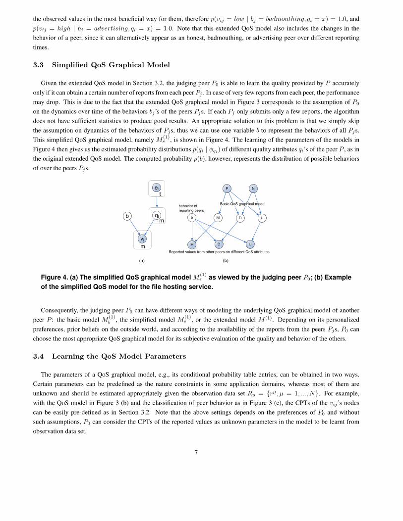
3.3 Simplified QoS Graphical Model

Given the extended QoS model in Section 3.2, the judging peer P0 is able to learn the quality provided by P accurately

only if it can obtain a certain number of reports from each peer Pj . In case of very few reports from each peer, the performance

may drop. This is due to the fact that the extended QoS graphical model in Figure 3 corresponds to the assumption of P0

on the dynamics over time of the behaviors bj’s of the peers Pjs. If each Pj only submits only a few reports, the algorithm

does not have sufficient statistics to produce good results. An appropriate solution to this problem is that we simply skip

the assumption on dynamics of the behaviors of Pjs, thus we can use one variable b to represent the behaviors of all Pjs.

This simplified QoS graphical model, namely M(1)s , is shown in Figure 4. The learning of the parameters of the models in

Figure 4 then gives us the estimated probability distributions p(qi | φqi) of different quality attributes qi’s of the peer P , as in

the original extended QoS model. The computed probability p(b), however, represents the distribution of possible behaviors

of over the peers Pjs.

el

qi

vi

b D

P

M

N

U

M D U

Basic QoS graphical model

b

behavior of

reporting peers

Reported values from other peers on different QoS attributes

(a) (b)

m

t

m

Figure 4. (a) The simplified QoS graphical model M(1)s as viewed by the judging peer P0; (b) Example

of the simplified QoS model for the file hosting service.

Consequently, the judging peer P0 can have different ways of modeling the underlying QoS graphical model of another

peer P : the basic model M(1)b , the simplified model M

(1)s , or the extended model M (1). Depending on its personalized

preferences, prior beliefs on the outside world, and according to the availability of the reports from the peers Pjs, P0 can

choose the most appropriate QoS graphical model for its subjective evaluation of the quality and behavior of the others.

3.4 Learning the QoS Model Parameters

The parameters of a QoS graphical model, e.g., its conditional probability table entries, can be obtained in two ways.

Certain parameters can be predefined as the nature constraints in some application domains, whereas most of them are

unknown and should be estimated appropriately given the observation data set Rp = {rµ, µ = 1, ..., N}. For example,

with the QoS model in Figure 3 (b) and the classification of peer behavior as in Figure 3 (c), the CPTs of the vij’s nodes

can be easily pre-defined as in Section 3.2. Note that the above settings depends on the preferences of P0 and without

such assumptions, P0 can consider the CPTs of the reported values as unknown parameters in the model to be learnt from

observation data set.

7

For brevity, from now on we use the name x, with or without subscripts, to denote a node in the graphical model when

there is no special need to differentiate it with the others. We also name πx as the list of all parent nodes of x. As a result,

the conditional probability that a certain variable x has a value y given the states of all of its parents is p(x = y|π∗x), where

y belongs to the state space of x and π∗x is the realization of all nodes in πx with appropriate values (or evidential states).

Note that if x represents a QoS parameter qi, the term φqidenotes the set of environmental factors that qi depends on, and in

general φqi= φx ⊆ πx.

Given an observation data set Rp on a model, there are two well-known approaches for estimating the model parameters

θ:

• Frequentist-based approach: methods of this category estimate the model parameters such that they approximately

maximize the likelihood of the observation data set Rp, using Maximum Likelihood Estimation, gradient methods,

Expectattion-Maximization (EM) algorithm, etc. In this solution class, the EM algorithm appears to be a potential

candidate since it works well on a general QoS model and is specially useful in case the log likelihood function of the

model is too complex to be optimized directly. This method can deal with incomplete data and is shown to converge

quite rapidly to a (local) maximum of the log likelihood. The main disadvantages of this approach are its possiblity to

reach to a sub-optimal estimate and its sensitivity to the sparseness of observation data.

• Bayesian method: this approach considers the parameters of the model as additional unobserved variables and com-

putes a full posterior distribution over all nodes conditional upon observed data. The next step is to sum (or integrate)

out the unobserved variables to estimate the posterior distributions of the parameters. Unfortunately, this approach is

expensive and may lead to large and intractable Bayesian networks, especially if the original QoS model is complex.

In this paper, we study the use of the EM algorithm in our framework to learn the quality and behavior of peers encoded

as unknown variables in a QoS model. The application of an EM algorithm in our current implementation is mainly due to its

genericity and promising performance. The use of other learning methods in our framework, e.g., an approximate Bayesian

learning algorithm, to compare with an EM-based approach is part of our future work and thus beyond the scope of this paper.

An outline of the EM learning of parameters of a general QoS graphical model with discrete variables is given in Al-

gorithm 1. This algorithm is run by the judging peer P0 in the system to evaluate the quality of the peer P , after P0 has

constructed an appropriate QoS model of P . The difference between the parameter learning for different models, e.g., the

basic, the simplified, and the extended QoS ones is in their corresponding observation data sets Rp. The difference between

the learning of parameters for the basic, the simplified, and the extended QoS models is in their corresponding observation

data sets Rp = {rµ, 1 ≤ µ ≤ N}, where rµ = 〈vµ, hµ〉. In the basic model of Figure 2, P0 assumes that the collected

reports are trustworthy, thus the values of the visible variables in vµ are the observations on the quality properties qi’s of

the service. On the other hand, in the simplified and extended QoS graphical model of Figure 3 and Figure 4, the visible

variables vµ include those in the reports vij’s, and maybe in other quality attributes qi’s that the judging peer P0 has already

had experience on.

The first line of Algorithm 1 initializes the model parameters, which are the unknown CPT entries of the graph. Depending

on its own prior beliefs and preferences, the peer P0 can either initialize the conditional probability p(x|πx) of each QoS

parameter randomly or set them as in the provider advertisement. In case of the extended and the simplified models, the

following settings may be also used:

• According to P0’s confidence on the trustworthiness of a specific peer Pj , the corresponding CPT entries p(bj) should

be defined appropriately. For certain trusted friends Pj , P0 can even set p(bj = honest) = 1.0 and let the corre-

sponding nodes vij’s be equivalent to the associated quality node qi’s to reduce the number of latent variables in the

model.

• The set of visible variables in the underlying QoS graphical model can be changed after each time P0 runs the Algo-

rithm 1, uses the service, and updates the statistics of some quality attributes qi’s with its new experience. Thus the

learning of the model parameters can be seen as an incremental process whose accuracy promisingly increases over

8

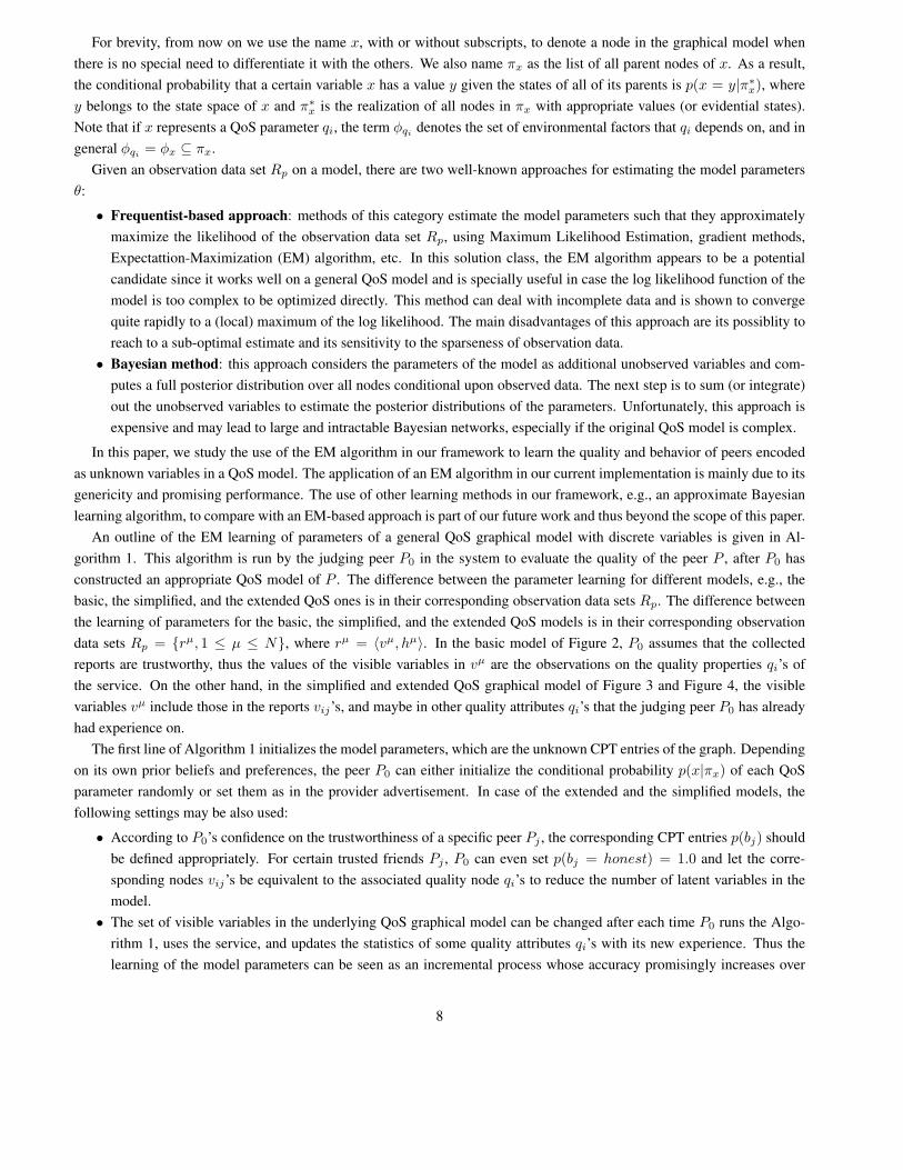
Algorithm 1 QoSGraphicalModelEM(Rp = {rµ = 〈hµ, vµ〉, 1 ≤ µ ≤ N})

1: Initialize the unknown parameters p(x = y|πx = z);

2: /* y, z are possible state values of variables x and πx */

3: repeat

4: for each observation case rµ do

5: for each node x do

6: Compute p(x = y, πx = z|vµ, θ) and p(πx = z|vµ, θ);

7: end for

8: end for

9: Compute Exyz =P

µ p(x = y, πx = z|vµ, θ) and Exz =P

µ p(πx = z|vµ, θ);

10: for each node x do

11: p(x = y|πx = z) = Exyz/Exz ;

12: end for

13: Recompute the log likelihood LL(θ) =P

µ logp(vµ|θ) with current θ;

14: until convergence in LL(θ) or after a maximal number of iterations;

time along with the number of visible variables/observation data that P0 has.

Lines 4 − 9 of Algorithm 1 implement the Expectation step of the EM algorithm, where we compute the expected counts

Exyz and Exz of the events (x = y, πx = z) and (πx = z), given the observed variables vµ in reports and current parameters

θ. We can use any exact or approximate probabilistic inference algorithm in this step to compute the posterior probabilities

p(πx = z|vµ, θ) and p(x = y, πx = z|vµ, θ). Our current implementation uses the Junction Tree Algorithm (JTA) [12] since

it produces exact results, works for all QoS models, and is still scalable in our scenario (see Section 4). The Maximization

step of the EM algorithm is implemented in lines 10 − 12 of Algorithm 1, therein we update the model parameters p(x|πx)

such that they maximize the observation data’s likelihood, assuming that the expected counts computed in lines 4 − 9 are

correct. The two Expectation and Maximization are iterated till the convergence of the log likelihood of the observation data,

which gives us an estimation of all model parameters p(x = y|πx = z).

Once P0 has already learned all parameters of the QoS graphical model of a peer P , it can compute the probability that the

peer P provides a quality level qi = y as follows: it first sets the value of each variable in the set φ∗qi

of the current graphical

model with the values corresponding to its own environment setting, then runs the JTA inference algorithm on the constructed

model to compute the conditional distribution P (qi = y|φ∗qi

) appropriately. The computation of the joint probability of many

quality parameters is done similarly. An illustration of the JTA on the graphical model of Figure 2 (b) is given in Appendix A.

3.5 Subjective Trust Modeling and Evaluation

Our computational framework basically estimates the local perception of the judging peer P0 on the quality level of the

service provided by another peer P in the system. Given the estimated quality qi’s, P0 can evaluate the trust level of P in

different ways depending on its own personalized preferences and objectives. For example, the trust level T that P0 has on

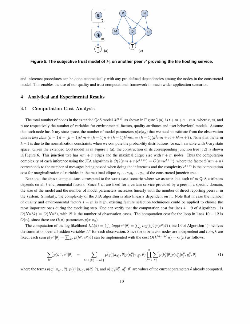
P can be modeled as the joint distribution of the all quality attribute qi’s, as given in Figure 5. Note that the nodes qi’s and

el’s are shaded since their distributions and quality values have already been estimated via the learning of parameters of the

corresponding model (Figure 3). The CPT of the node T is actually defined based on the own preferences and objectives of

the judging peer P0 itself.

Given the model in Figure 5, the judging peer P0 can easily compute the trust value T as the distribution of the node T

conditionally on the values of the quality dimensions qi’s and under its own environmental settings φ∗qi

via the JTA algorithm.

We do not focus on this evaluation of trust in our work since such a computation is trivial but application-oriented and highly

dependent on the judging peer P0. Instead, we are interested in the evaluation of the quality parameters qi’s under various

conditions el’s and a wide variety of reporting behaviors bj’s, from which to provide the judging peer P0 the necessary

inputs for its subjective modeling and evaluation of trust on the other peers. One important aspect is that all above learning

9

l

i

D

P

M

N

U

(a) (b)

m

Figure 5. The subjective trust model of P0 on another peer P providing the file hosting service.

and inference procedures can be done automatically with any pre-defined dependencies among the nodes in the constructed

model. This enables the use of our quality and trust computational framework in much wider application scenarios.

4 Analytical and Experimental Results

4.1 Computation Cost Analysis

The total number of nodes in the extended QoS model M (1), as shown in Figure 3 (a), is t+m+n+mn. where t,m, and

n are respectively the number of variables for environmental factors, quality attributes and user behavioral models. Assume

that each node has k-ary state space, the number of model parameters p(x|πx) that we need to estimate from the observation

data is less than (k − 1)t + (k − 1)ktm + (k − 1)n + (k − 1)k2mn = (k − 1)(k2mn + n + ktm + t). Note that the term

k− 1 is due to the normalization constraints when we compute the probability distributions for each variable with k-ary state

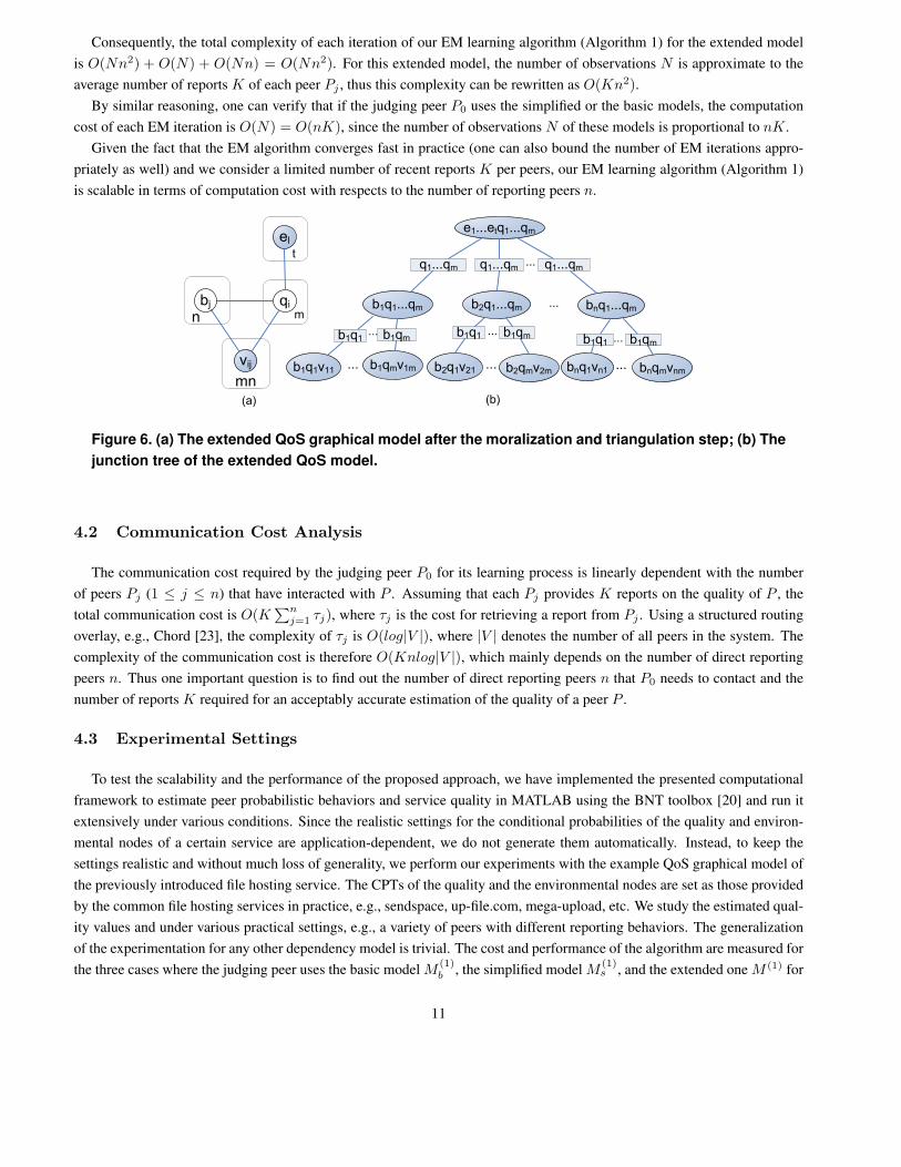
space. Given the extended QoS model as in Figure 3 (a), the construction of its corresponding junction tree [12] is shown

in Figure 6. This junction tree has nm + n edges and the maximal clique size with t + m nodes. Thus the computation

complexity of each inference using the JTA algorithm is O(2(nm + n)et+m) = O(nmet+m), where the factor 2(nm + n)

corresponds to the number of messages being passed when doing the inferences and the complexity et+m is the computation

cost for marginalization of variables in the maximal clique e1 . . . etq1 . . . qm of the constructed junction tree.

Note that the above computations correspond to the worst case scenario where we assume that each of m QoS attributes

depends on all t environmental factors. Since t,m are fixed for a certain service provided by a peer in a specific domain,

the size of the model and the number of model parameters increases linearly with the number of direct reporting peers n in

the system. Similarly, the complexity of the JTA algorithm is also linearly dependent on n. Note that in case the number

of quality and environmental factors t + m is high, existing feature selection techniques could be applied to choose the

most important ones during the modeling step. One can verify that the computation cost for lines 4 − 9 of Algorithm 1 is

O(Nn2k) = O(Nn2), with N is the number of observation cases. The computation cost for the loop in lines 10 − 12 is

O(n), since there are O(n) parameters p(x|πx).

The computation of the log likelihood LL(θ) =∑

µ logp(vµ|θ) =∑

µ log∑µ

h p(vµ|θ) (line 13 of Algorithm 1) involves

the summation over all hidden variables hµ for each observation. Since the n behavior nodes are independent and t,m, k are

fixed, each sum p(vµ|θ) =∑

hµ p(hµ, vµ|θ) can be implemented with the cost O(kt+m+1n) = O(n) as follows:

∑

hµ

p(hµ, vµ|θ) =∑

hµ\{bµ1

,...,bµn}

p(qµi |πq

µi, θ)p(eµ

l |πeµ

l, θ)

n∏

j=1

∑

bµj

p(bµj |θ)p(vµ

ij |bµj , q

µi , θ) (1)

where the terms p(qµi |πq

µi, θ), p(eµ

l |πeµ

l, p(bµ

j |θ), and p(vµij |b

µj , q

µi , θ) are values of the current parameters θ already computed.

10

Consequently, the total complexity of each iteration of our EM learning algorithm (Algorithm 1) for the extended model

is O(Nn2) + O(N) + O(Nn) = O(Nn2). For this extended model, the number of observations N is approximate to the

average number of reports K of each peer Pj , thus this complexity can be rewritten as O(Kn2).

By similar reasoning, one can verify that if the judging peer P0 uses the simplified or the basic models, the computation

cost of each EM iteration is O(N) = O(nK), since the number of observations N of these models is proportional to nK.

Given the fact that the EM algorithm converges fast in practice (one can also bound the number of EM iterations appro-

priately as well) and we consider a limited number of recent reports K per peers, our EM learning algorithm (Algorithm 1)

is scalable in terms of computation cost with respects to the number of reporting peers n.

(b)

b1q1...qm

b1q1v11 b1qmv1m b2q1v21 b2qmv2m bnq1vn1 bnqmvnm... ... ...

b2q1...qm bnq1...qm

e1...etq1...qm

q1...qm q1...qm q1...qm

b1q1 b1qm b1q1 b1qm b1q1 b1qm

el

qi

vij

(a)

n m

t

mn

bj

...

...

.........

Figure 6. (a) The extended QoS graphical model after the moralization and triangulation step; (b) The

junction tree of the extended QoS model.

4.2 Communication Cost Analysis

The communication cost required by the judging peer P0 for its learning process is linearly dependent with the number

of peers Pj (1 ≤ j ≤ n) that have interacted with P . Assuming that each Pj provides K reports on the quality of P , the

total communication cost is O(K∑n

j=1 τj), where τj is the cost for retrieving a report from Pj . Using a structured routing

overlay, e.g., Chord [23], the complexity of τj is O(log|V |), where |V | denotes the number of all peers in the system. The

complexity of the communication cost is therefore O(Knlog|V |), which mainly depends on the number of direct reporting

peers n. Thus one important question is to find out the number of direct reporting peers n that P0 needs to contact and the

number of reports K required for an acceptably accurate estimation of the quality of a peer P .

4.3 Experimental Settings

To test the scalability and the performance of the proposed approach, we have implemented the presented computational

framework to estimate peer probabilistic behaviors and service quality in MATLAB using the BNT toolbox [20] and run it

extensively under various conditions. Since the realistic settings for the conditional probabilities of the quality and environ-

mental nodes of a certain service are application-dependent, we do not generate them automatically. Instead, to keep the

settings realistic and without much loss of generality, we perform our experiments with the example QoS graphical model of

the previously introduced file hosting service. The CPTs of the quality and the environmental nodes are set as those provided

by the common file hosting services in practice, e.g., sendspace, up-file.com, mega-upload, etc. We study the estimated qual-

ity values and under various practical settings, e.g., a variety of peers with different reporting behaviors. The generalization

of the experimentation for any other dependency model is trivial. The cost and performance of the algorithm are measured for

the three cases where the judging peer uses the basic model M(1)b , the simplified model M

(1)s , and the extended one M (1) for

11

its subjective evaluation of quality and trust on the others. In the most complicated setting with the extended QoS graphical

model, the number of nodes in the probabilistic network is 2+3+n+3n, in which the two first visible nodes denote the two

environmental factors, the three next hidden nodes represents the three QoS attributes whose values depend on two previous

environmental variables. There are n latent nodes representing the behaviors of n peers and 3n observable nodes storing the

reported values of those n peers on three invisible QoS parameters. These 3n reported nodes are used to generate the various

reports of several peers on the peer P with the service s being evaluated, which may also contain missing data and whose

values are different to the actual QoS values the peers observed due to either the uncertainty in observation or the dishonesty

of reporters.

We set up the real probabilistic model with various behaviors of peers as specified in the input parameter settings of

each experiment. The conditional probabilities for the QoS parameters are set according to some certain deviations from

the advertised QoS values. This real probabilistic model would be the probabilistic distributions of the service’s QoS and

all peer behaviors which we can only obtain in an ideal world given infinite knowledge. From this established model, we

generate the observation data set as random samples on the visible variables and further hide a fraction of these data items

according to the simulation settings. We initialize the EM algorithm with the following a priori beliefs: the conditional

probability of each QoS parameter is set randomly and behaviors of all peers are set as unknown. This initialization is for

the worst case scenario where the judging peer P0 does not believe in any other peers. The last (3 − 1)323n parameters of

the 3n nodes representing the reported values of peers are initialized as explained in Section 3.2. The other experiments in

case P0 has difference preferences and set of pre-trusted friends are subject to our future work. However, we believe that

we can obtain even better results in those cases. Given the observation data set, we run the EM algorithm to estimate the

CPTs of the extended model and from the learnt model, we compute the distributions of the peers’ behaviors and QoS values

of the service. We measure the accuracy of the approach as the mean and standard deviation of the normalized square root

errors in the estimation of the probability distribution of various QoS parameters and their real probabilities, as well as the

estimated and the actual reporting behaviors of the peers sharing the feedback. The range of the normalized square root errors

is [0.0, 1.0] in which lower values implies higher accuracy and vice versa. Each experiment type consists of 20 individual

experiments with different settings, each of which is run 10 times to get the average result.

4.4 Solution Scalability

To test the scalability of the algorithm in terms of performance and runtime cost, we set up a reasonably vulnerable

environment with 50% honest peers. The other 50% cheating peers includes 5% badmouthing peers, 40% advertising peers,

and 5% uncertain peers, i.e., those with changing behaviors. Note that we set the fraction of advertising users to be much

bigger than that of the badmouthing and the uncertain peers to make the attacks to be more effective (so that the reports of

badmouthing and advertising users do not compensate with each other). We increase the number n of reporting peers Pjs

from 1 to 100 and keep the number of reports by each Pj reasonably low (K = 5).

Figure 7 shows the performance of the algorithm in three cases where a judging peer P0 uses the basic, the simplified

and the extended QoS graphical models for its subjective estimation of the quality of the peer P . The performance of the

algorithm in terms of the estimated behaviors of the reporting peers Pjs is given in Figure 8.

Generally, under the same experimental settings, the number of direct reporting peers n does not have any major influence

in the performance of the algorithm. This experiment shows that a peer only needs to get the reports from a certain number

of other peers (chosen randomly) in the whole system to reduce the total running time and the communication cost of the

algorithm (see Section 4.2) without sacrificing much in the accuracy. Practically, in some other experiments, we only choose

a set of n = 15 reporting peers randomly chosen in the network to reduce the total running time of the learning algorithm.

Figure 7 indicates that the result obtained via the use of the simplified QoS model is the most accurate, which is reasonable

since this model also takes the various cheating behaviors of reporting peers into account appropriately. Using the extended

QoS model gives us less accurate evaluations as the number of observation cases in this case is insufficient (N = K = 5) for

12

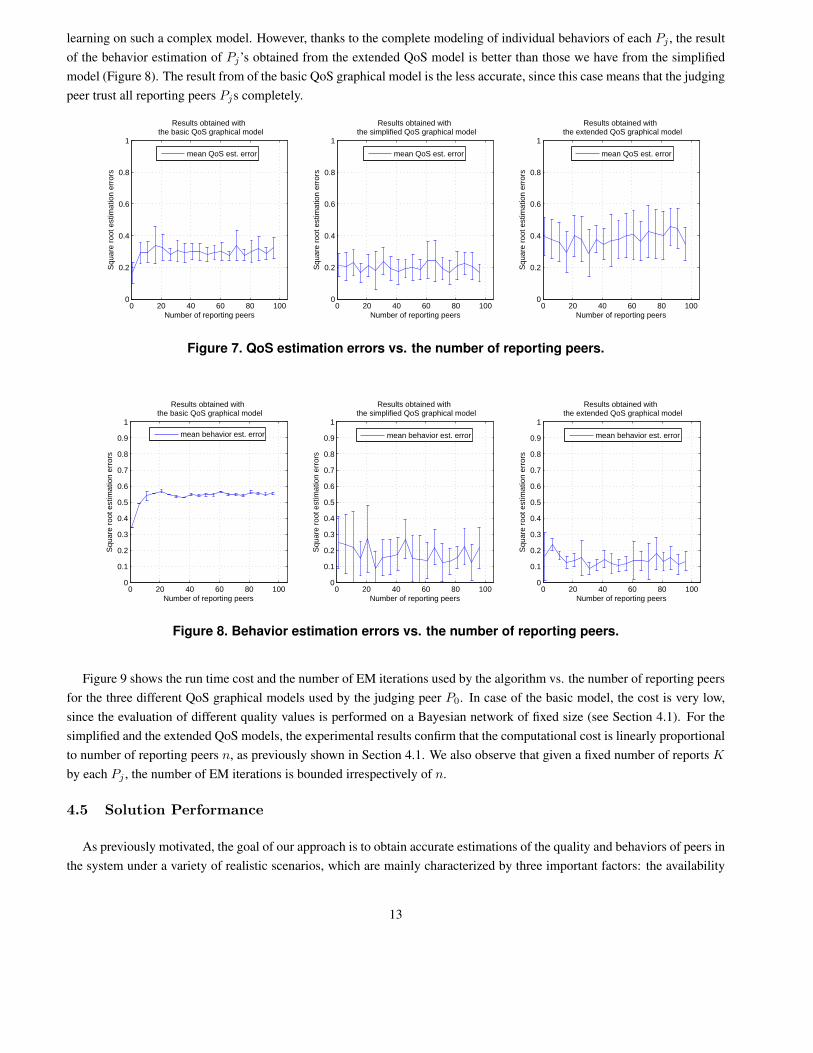
learning on such a complex model. However, thanks to the complete modeling of individual behaviors of each Pj , the result

of the behavior estimation of Pj’s obtained from the extended QoS model is better than those we have from the simplified

model (Figure 8). The result from of the basic QoS graphical model is the less accurate, since this case means that the judging

peer trust all reporting peers Pjs completely.

0 20 40 60 80 1000

0.2

0.4

0.6

0.8

1

Squ

are

root

est

imat

ion

erro

rs

Number of reporting peers

Results obtained with the basic QoS graphical model

mean QoS est. error

0 20 40 60 80 1000

0.2

0.4

0.6

0.8

1

Squ

are

root

est

imat

ion

erro

rsNumber of reporting peers

Results obtained with the simplified QoS graphical model

mean QoS est. error

0 20 40 60 80 1000

0.2

0.4

0.6

0.8

1

Squ

are

root

est

imat

ion

erro

rs


Results obtained with the extended QoS graphical model

mean QoS est. error

Figure 7. QoS estimation errors vs. the number of reporting peers.

0 20 40 60 80 1000

0.1

0.2

0.3

0.4

0.5

0.6

0.7

0.8

0.9

1

Squ

are

root

est

imat

ion

erro

rs



0 20 40 60 80 1000

0.1

0.2

0.3

0.4

0.5

0.6

0.7

0.8

0.9

1

Squ

are

root

est

imat

ion

erro

rs



0 20 40 60 80 1000

0.1

0.2

0.3

0.4

0.5

0.6

0.7

0.8

0.9

1

Squ

are

root

est

imat

ion

erro

rs



mean behavior est. error mean behavior est. error mean behavior est. error

Figure 8. Behavior estimation errors vs. the number of reporting peers.

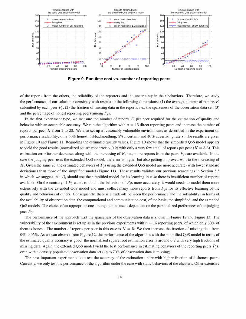
Figure 9 shows the run time cost and the number of EM iterations used by the algorithm vs. the number of reporting peers

for the three different QoS graphical models used by the judging peer P0. In case of the basic model, the cost is very low,

since the evaluation of different quality values is performed on a Bayesian network of fixed size (see Section 4.1). For the

simplified and the extended QoS models, the experimental results confirm that the computational cost is linearly proportional

to number of reporting peers n, as previously shown in Section 4.1. We also observe that given a fixed number of reports K

by each Pj , the number of EM iterations is bounded irrespectively of n.

4.5 Solution Performance

As previously motivated, the goal of our approach is to obtain accurate estimations of the quality and behaviors of peers in

the system under a variety of realistic scenarios, which are mainly characterized by three important factors: the availability

13

0 20 40 60 80 1000

20

40

60

80

100

120

140

160

180

Run

tim

e co

st



0 20 40 60 80 1000

20

40

60

80

100

120

140

160

180

Run

tim

e co

st



0 20 40 60 80 1000

20

40

60

80

100

120

140

160

180

Run

tim

e co

st



mean execution timefitting linemean number of EM iterations



Figure 9. Run time cost vs. number of reporting peers.

of the reports from the others, the reliability of the reporters and the uncertainty in their behaviors. Therefore, we study

the performance of our solution extensively with respect to the following dimensions: (1) the average number of reports K

submitted by each peer Pj ; (2) the fraction of missing data in the reports, i.e., the sparseness of the observation data set; (3)

and the percentage of honest reporting peers among Pjs.

In the first experiment type, we measure the number of reports K per peer required for the estimation of quality and

behavior with an acceptable accuracy. We run the algorithm with n = 15 direct reporting peers and increase the number of

reports per peer K from 1 to 20. We also set up a reasonably vulnerable environments as described in the experiment on

performance scalability: only 50% honest, 5%badmouthing, 5%uncertain, and 40% advertising raters. The results are given

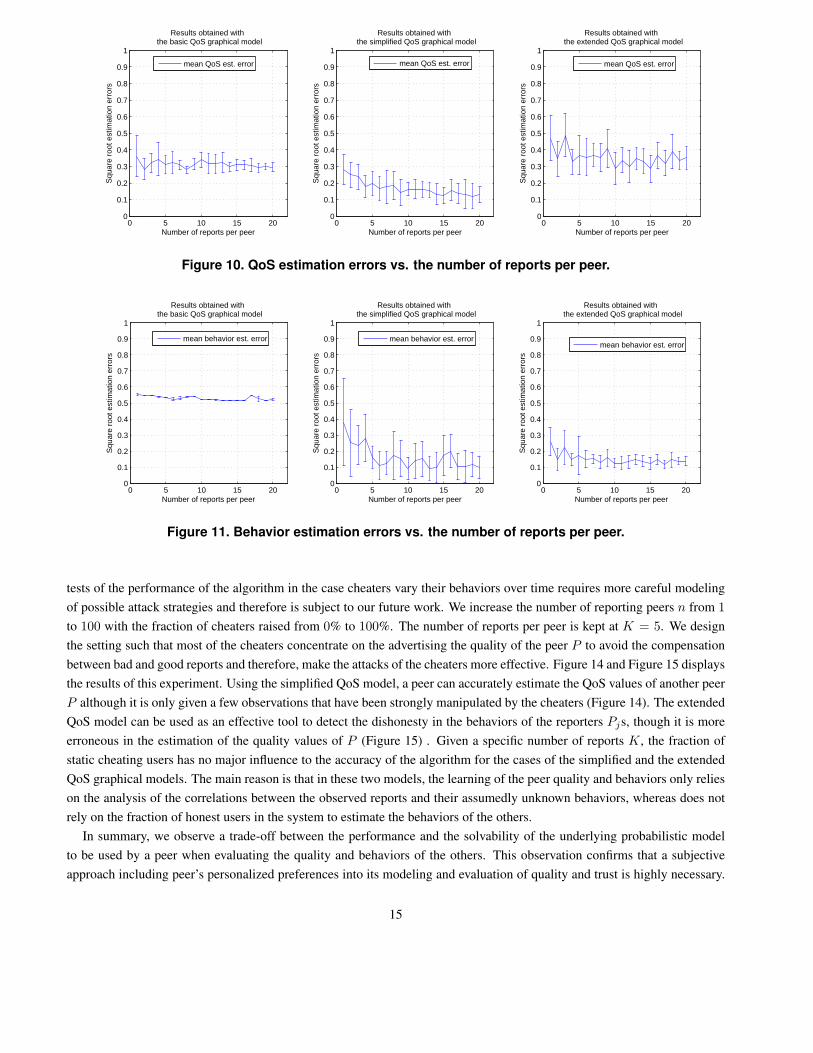
in Figure 10 and Figure 11. Regarding the estimated quality values, Figure 10 shows that the simplified QoS model appears

to yield the good results (normalized square root error ∼ 0.2) with only a very few small of reports per peer (K = 3-5). This

estimation error further decreases along with the increasing of K, i.e., more reports from the peers Pjs are available. In the

case the judging peer uses the extended QoS model, the error is higher but also getting improved w.r.t to the increasing of

K. Given the same K, the estimated behaviors of Pjs using the extended QoS model are more accurate (with lower standard

deviations) than those of the simplified model (Figure 11). These results validate our previous reasonings in Section 3.3

in which we suggest that P0 should use the simplified model for its learning in case there is insufficient number of reports

available. On the contrary, if P0 wants to obtain the behaviors of Pjs more accurately, it would needs to model them more

extensively with the extended QoS model and must collect many more reports from Pjs for its effective learning of the

quality and behaviors of others. Consequently, there is a trade-off between the performance and the solvability (in terms of

the availability of observation data, the computational and communication cost) of the basic, the simplified, and the extended

QoS models. The choice of an appropriate one among them to use is dependent on the personalized preferences of the judging

peer P0.

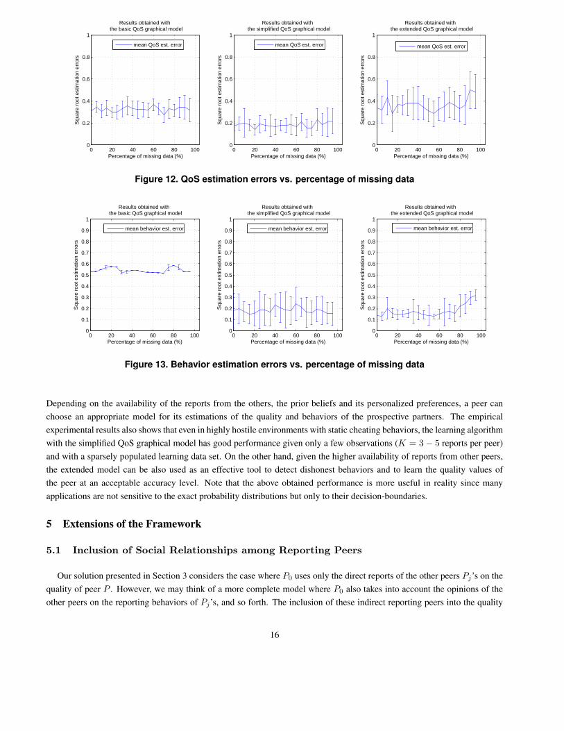
The performance of the approach w.r.t the sparseness of the observation data is shown in Figure 12 and Figure 13. The

vulnerability of the environment is set up as in the previous experiments with n = 15 reporting peers, of which only 50% of

them is honest. The number of reports per peer in this case is K = 5. We then increase the fraction of missing data from

0% to 95%. As we can observe from Figure 12, the performance of the algorithm with the simplified QoS model in terms of

the estimated quality accuracy is good: the normalized square root estimation error is around 0.2 with very high fractions of

missing data. Again, the extended QoS model yield the best performance in estimating behaviors of the reporting peers Pjs,

even with a densely populated observation data set (up to 70% of observation data is missing).

The next important experiments is to test the accuracy of the estimation under with higher fraction of dishonest peers.

Currently, we only test the performance of the algorithm under the case with static behaviors of the cheaters. Other extensive

14

0 5 10 15 200

0.1

0.2

0.3

0.4

0.5

0.6

0.7

0.8

0.9

1

Squ

are

root

est

imat

ion

erro

rs

Number of reports per peer


0 5 10 15 200

0.1

0.2

0.3

0.4

0.5

0.6

0.7

0.8

0.9

1

Squ

are

root

est

imat

ion

erro

rs



0 5 10 15 200

0.1

0.2

0.3

0.4

0.5

0.6

0.7

0.8

0.9

1

Squ

are

root

est

imat

ion

erro

rs



mean QoS est. error mean QoS est. error mean QoS est. error

Figure 10. QoS estimation errors vs. the number of reports per peer.

0 5 10 15 200

0.1

0.2

0.3

0.4

0.5

0.6

0.7

0.8

0.9

1

Squ

are

root

est

imat

ion

erro

rs



mean behavior est. error

0 5 10 15 200

0.1

0.2

0.3

0.4

0.5

0.6

0.7

0.8

0.9

1S

quar

e ro

ot e

stim

atio

n er

rors




0 5 10 15 200

0.1

0.2

0.3

0.4

0.5

0.6

0.7

0.8

0.9

1

Squ

are

root

est

imat

ion

erro

rs




Figure 11. Behavior estimation errors vs. the number of reports per peer.

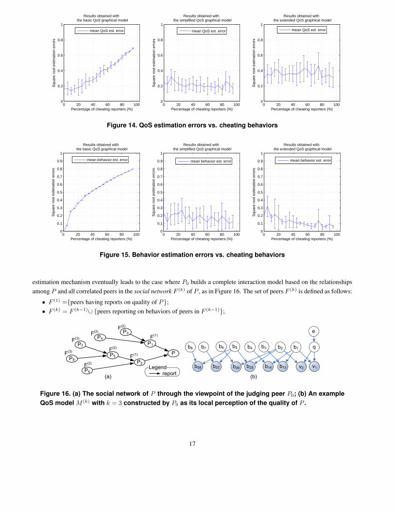
tests of the performance of the algorithm in the case cheaters vary their behaviors over time requires more careful modeling

of possible attack strategies and therefore is subject to our future work. We increase the number of reporting peers n from 1

to 100 with the fraction of cheaters raised from 0% to 100%. The number of reports per peer is kept at K = 5. We design

the setting such that most of the cheaters concentrate on the advertising the quality of the peer P to avoid the compensation

between bad and good reports and therefore, make the attacks of the cheaters more effective. Figure 14 and Figure 15 displays

the results of this experiment. Using the simplified QoS model, a peer can accurately estimate the QoS values of another peer

P although it is only given a few observations that have been strongly manipulated by the cheaters (Figure 14). The extended

QoS model can be used as an effective tool to detect the dishonesty in the behaviors of the reporters Pjs, though it is more

erroneous in the estimation of the quality values of P (Figure 15) . Given a specific number of reports K, the fraction of

static cheating users has no major influence to the accuracy of the algorithm for the cases of the simplified and the extended

QoS graphical models. The main reason is that in these two models, the learning of the peer quality and behaviors only relies

on the analysis of the correlations between the observed reports and their assumedly unknown behaviors, whereas does not

rely on the fraction of honest users in the system to estimate the behaviors of the others.

In summary, we observe a trade-off between the performance and the solvability of the underlying probabilistic model

to be used by a peer when evaluating the quality and behaviors of the others. This observation confirms that a subjective

approach including peer’s personalized preferences into its modeling and evaluation of quality and trust is highly necessary.

15

0 20 40 60 80 1000

0.2

0.4

0.6

0.8

1

Squ

are

root

est

imat

ion

erro

rs

Percentage of missing data (%)


0 20 40 60 80 1000

0.2

0.4

0.6

0.8

1

Squ

are

root

est

imat

ion

erro

rs



0 20 40 60 80 1000

0.2

0.4

0.6

0.8

1

Squ

are

root

est

imat

ion

erro

rs




Figure 12. QoS estimation errors vs. percentage of missing data

0 20 40 60 80 1000

0.1

0.2

0.3

0.4

0.5

0.6

0.7

0.8

0.9

1

Squ

are

root

est

imat

ion

erro

rs



0 20 40 60 80 1000

0.1

0.2

0.3

0.4

0.5

0.6

0.7

0.8

0.9

1S

quar

e ro

ot e

stim

atio

n er

rors



0 20 40 60 80 1000

0.1

0.2

0.3

0.4

0.5

0.6

0.7

0.8

0.9

1

Squ

are

root

est

imat

ion

erro

rs




Figure 13. Behavior estimation errors vs. percentage of missing data

Depending on the availability of the reports from the others, the prior beliefs and its personalized preferences, a peer can

choose an appropriate model for its estimations of the quality and behaviors of the prospective partners. The empirical

experimental results also shows that even in highly hostile environments with static cheating behaviors, the learning algorithm

with the simplified QoS graphical model has good performance given only a few observations (K = 3 − 5 reports per peer)

and with a sparsely populated learning data set. On the other hand, given the higher availability of reports from other peers,

the extended model can be also used as an effective tool to detect dishonest behaviors and to learn the quality values of

the peer at an acceptable accuracy level. Note that the above obtained performance is more useful in reality since many

applications are not sensitive to the exact probability distributions but only to their decision-boundaries.

5 Extensions of the Framework

5.1 Inclusion of Social Relationships among Reporting Peers

Our solution presented in Section 3 considers the case where P0 uses only the direct reports of the other peers Pj’s on the

quality of peer P . However, we may think of a more complete model where P0 also takes into account the opinions of the

other peers on the reporting behaviors of Pj’s, and so forth. The inclusion of these indirect reporting peers into the quality

16

0 20 40 60 80 1000

0.2

0.4

0.6

0.8

1

Squ

are

root

est

imat

ion

erro

rs

Percentage of cheating reporters (%)


0 20 40 60 80 1000

0.2

0.4

0.6

0.8

1

Squ

are

root

est

imat

ion

erro

rs



0 20 40 60 80 1000

0.2

0.4

0.6

0.8

1

Squ

are

root

est

imat

ion

erro

rs




Figure 14. QoS estimation errors vs. cheating behaviors

0 20 40 60 80 1000

0.1

0.2

0.3

0.4

0.5

0.6

0.7

0.8

0.9

1

Squ

are

root

est

imat

ion

erro

rs



0 20 40 60 80 1000

0.1

0.2

0.3

0.4

0.5

0.6

0.7

0.8

0.9

1S

quar

e ro

ot e

stim

atio

n er

rors



0 20 40 60 80 1000

0.1

0.2

0.3

0.4

0.5

0.6

0.7

0.8

0.9

1

Squ

are

root

est

imat

ion

erro

rs




Figure 15. Behavior estimation errors vs. cheating behaviors

estimation mechanism eventually leads to the case where P0 builds a complete interaction model based on the relationships

among P and all correlated peers in the social network F (k) of P , as in Figure 16. The set of peers F (k) is defined as follows:

• F (1) ={peers having reports on quality of P};

• F (k) = F (k−1)∪ {peers reporting on behaviors of peers in F (k−1)};

P

P1

P2

P3P4

P5

P6

P7

P8

Legendreport

F(1)

F(1)

F(2)

F(2)

F(2)

F(2)

F(3)

F(3)q

v1

b1b2

v2b13

b3b4

b14b25b26

b5b6b7b8

b57b58

e

(a) (b)

Figure 16. (a) The social network of P through the viewpoint of the judging peer P0; (b) An example

QoS model M (k) with k = 3 constructed by P0 as its local perception of the quality of P .

17

Given only the local information, the peer P0 can construct its local perception of the QoS model M (k) of P , taking into

account the dependencies in the social network F (k), as in Figure 16 (b). This model is established by the judging peer P0

given its local knowledge of the social network of P previously shown in Figure 16 (a). The values v1, v2 are the reports of

P1, P2 on the quality q of P under environmental condition e, and bjk is the opinion of a peer Pk on the reporting behavior

of another Pj , i.e., bjk reflects the view of Pk on the trustworthiness of Pj in giving recommendations. Depending on how

complete the peer P0 needs to model the behaviors and quality of the others, the list of related peers F (k) can be extended

to contain all paths in the trust multi-graph having the root at P , as considered and evaluated by all existing social network

analysis trust management methods [8]. The parameter learning on the constructed model M (k) of Figure 16 (b) will give P0

its personalized perception of the innate behaviors of those peers in F (k) and the quality of P under various environmental

settings.

With higher values of k, the building of such model M (k) is highly inefficient since the retrievals of reports from other

related peers in the network are highly bandwidth-consuming. Also, the big size of the model M (k) may lead to many

computational difficulties in the probability learning and inferences on it. Thus, there is a trade-off between the complete-

ness/accuracy of the model M (k) vs. the solvability (in terms of the cost of the quality and trust evaluating algorithm) which

P0 needs to consider. An relevant aspect we can observe here is that our computational framework can be easily extended to

integrate the social network relationships among peers into account when doing the learning and estimation of their quality

and behaviors. This leads to a conjecture that our model also subsumes some other social network-based trust and reputation

management approaches, e.g., [13, 28]. In these solutions P0 exploits the relationships among P and other peers in its social

network F (k) to apply various ad hoc aggregation techniques to compute the reputation and trustworthiness of P . Our learn-

ing approach on the model M (k) based on the same principle but relies on a more sound statistical background. We only

use these social relationships to model the influences that the reports of a peer in the social network of P may have on the

reputation of the quality of the peer P . As the result, the algorithm produces outputs with well-defined semantics, e.g., the

probability that P is well-behaved or not through the viewpoint of P0, taking into the opinions of the other related peers in

the network.

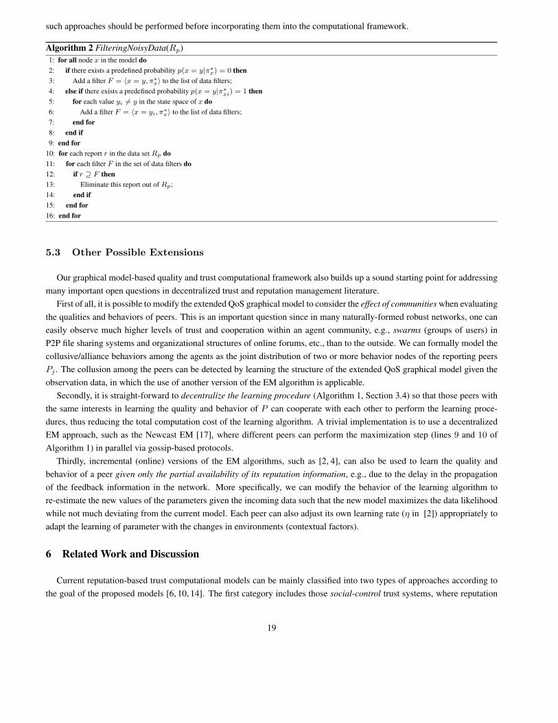
5.2 Rule-based Filtering of Unreliable Data

As aforementioned, one issue with the observation data set is that they may be noisy: either there are cheating peers

trying to boost the QoS performance of their competitors and badmouthing on the others. Even some honest peers can still

have erroneous observation of the perceived QoS levels. A preliminary solution for this problem is to use the pre-defined

constraints (or rules) specified by the domain experts in the graphical model to filter out the unreliable data. Algorithms 2

presents this procedure in details, therein the notion ⊇ represents the matching of the values of the variables in an observation

rµ with the constraint specified in a filter F . The key of the algorithm is based on the following observation. In certain

application domains one can easily define many rules specifying the correlations among the different QoS parameters and

related factors. There rules can be transformed into certain constraints of the conditional probability tables p(x|πx), which

can be used both as the pre-defined settings of the corresponding CPT entries and for the filtering of the erroneous observation

data (which may be intentionally manipulated). For example, given the QoS graphical model in Figure 2, a judging peer P0

with enough expertise in the domain can specify that for a paid service, the maximum concurrent downloads must be greater

than 1, meaning that p(M = Low|P 6= Free) = 0.0. Thus, any report rµ which contains the feedback of the form

〈M = Low,P = Economic〉 or 〈M = Low,P = Premium〉 should be considered as unreliable due to its intrinsic

contradictory and be filtered out of the data set. Thus it is possible to use our framework to perform certain rule-based

filtering of unreliable observation data given the knowledge of the judging peers. More sophisticated dishonesty detection,

can be done, via doing the inferences on parts of the basic QoS model that has been pre-defined by the domain experts, or

learnt from previous experiences. Based on the findings of the maximum a posteriori (MAP) of certain visible variables, we

can also eliminate the unreliable observations. However, more extensive studies on the effectiveness and scalability issues of

18

such approaches should be performed before incorporating them into the computational framework.

Algorithm 2 FilteringNoisyData(Rp)

1: for all node x in the model do

2: if there exists a predefined probability p(x = y|π∗

x) = 0 then

3: Add a filter F = 〈x = y, π∗

x〉 to the list of data filters;

4: else if there exists a predefined probability p(x = y|π∗

xi) = 1 then

5: for each value yi 6= y in the state space of x do

6: Add a filter F = 〈x = yi, π∗

x〉 to the list of data filters;

7: end for

8: end if

9: end for

10: for each report r in the data set Rp do

11: for each filter F in the set of data filters do

12: if r ⊇ F then

13: Eliminate this report out of Rp;

14: end if

15: end for

16: end for

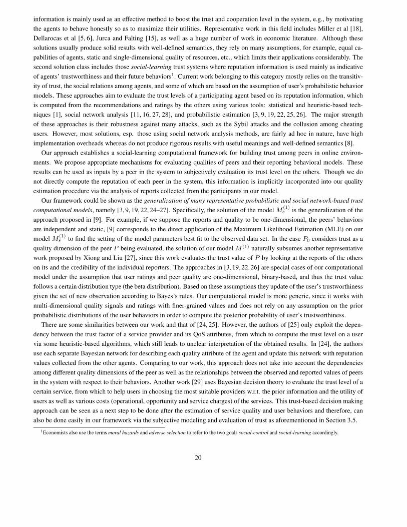
5.3 Other Possible Extensions

Our graphical model-based quality and trust computational framework also builds up a sound starting point for addressing

many important open questions in decentralized trust and reputation management literature.

First of all, it is possible to modify the extended QoS graphical model to consider the effect of communities when evaluating

the qualities and behaviors of peers. This is an important question since in many naturally-formed robust networks, one can

easily observe much higher levels of trust and cooperation within an agent community, e.g., swarms (groups of users) in

P2P file sharing systems and organizational structures of online forums, etc., than to the outside. We can formally model the

collusive/alliance behaviors among the agents as the joint distribution of two or more behavior nodes of the reporting peers

Pj . The collusion among the peers can be detected by learning the structure of the extended QoS graphical model given the

observation data, in which the use of another version of the EM algorithm is applicable.

Secondly, it is straight-forward to decentralize the learning procedure (Algorithm 1, Section 3.4) so that those peers with

the same interests in learning the quality and behavior of P can cooperate with each other to perform the learning proce-

dures, thus reducing the total computation cost of the learning algorithm. A trivial implementation is to use a decentralized

EM approach, such as the Newcast EM [17], where different peers can perform the maximization step (lines 9 and 10 of

Algorithm 1) in parallel via gossip-based protocols.

Thirdly, incremental (online) versions of the EM algorithms, such as [2, 4], can also be used to learn the quality and

behavior of a peer given only the partial availability of its reputation information, e.g., due to the delay in the propagation

of the feedback information in the network. More specifically, we can modify the behavior of the learning algorithm to

re-estimate the new values of the parameters given the incoming data such that the new model maximizes the data likelihood

while not much deviating from the current model. Each peer can also adjust its own learning rate (η in [2]) appropriately to

adapt the learning of parameter with the changes in environments (contextual factors).

6 Related Work and Discussion

Current reputation-based trust computational models can be mainly classified into two types of approaches according to

the goal of the proposed models [6, 10, 14]. The first category includes those social-control trust systems, where reputation

19

information is mainly used as an effective method to boost the trust and cooperation level in the system, e.g., by motivating

the agents to behave honestly so as to maximize their utilities. Representative work in this field includes Miller et al [18],

Dellarocas et al [5, 6], Jurca and Falting [15], as well as a huge number of work in economic literature. Although these

solutions usually produce solid results with well-defined semantics, they rely on many assumptions, for example, equal ca-

pabilities of agents, static and single-dimensional quality of resources, etc., which limits their applications considerably. The

second solution class includes those social-learning trust systems where reputation information is used mainly as indicative

of agents’ trustworthiness and their future behaviors1. Current work belonging to this category mostly relies on the transitiv-

ity of trust, the social relations among agents, and some of which are based on the assumption of user’s probabilistic behavior

models. These approaches aim to evaluate the trust levels of a participating agent based on its reputation information, which

is computed from the recommendations and ratings by the others using various tools: statistical and heuristic-based tech-

niques [1], social network analysis [11, 16, 27, 28], and probabilistic estimation [3, 9, 19, 22, 25, 26]. The major strength

of these approaches is their robustness against many attacks, such as the Sybil attacks and the collusion among cheating

users. However, most solutions, esp. those using social network analysis methods, are fairly ad hoc in nature, have high

implementation overheads whereas do not produce rigorous results with useful meanings and well-defined semantics [8].

Our approach establishes a social-learning computational framework for building trust among peers in online environ-

ments. We propose appropriate mechanisms for evaluating qualities of peers and their reporting behavioral models. These

results can be used as inputs by a peer in the system to subjectively evaluation its trust level on the others. Though we do

not directly compute the reputation of each peer in the system, this information is implicitly incorporated into our quality

estimation procedure via the analysis of reports collected from the participants in our model.

Our framework could be shown as the generalization of many representative probabilistic and social network-based trust

computational models, namely [3, 9, 19, 22, 24–27]. Specifically, the solution of the model M(1)s is the generalization of the

approach proposed in [9]. For example, if we suppose the reports and quality to be one-dimensional, the peers’ behaviors

are independent and static, [9] corresponds to the direct application of the Maximum Likelihood Estimation (MLE) on our

model M(1)s to find the setting of the model parameters best fit to the observed data set. In the case P0 considers trust as a

quality dimension of the peer P being evaluated, the solution of our model M (1) naturally subsumes another representative

work proposed by Xiong and Liu [27], since this work evaluates the trust value of P by looking at the reports of the others

on its and the credibility of the individual reporters. The approaches in [3, 19, 22, 26] are special cases of our computational

model under the assumption that user ratings and peer quality are one-dimensional, binary-based, and thus the trust value

follows a certain distribution type (the beta distribution). Based on these assumptions they update of the user’s trustworthiness

given the set of new observation according to Bayes’s rules. Our computational model is more generic, since it works with

multi-dimensional quality signals and ratings with finer-grained values and does not rely on any assumption on the prior

probabilistic distributions of the user behaviors in order to compute the posterior probability of user’s trustworthiness.

There are some similarities between our work and that of [24, 25]. However, the authors of [25] only exploit the depen-

dency between the trust factor of a service provider and its QoS attributes, from which to compute the trust level on a user

via some heuristic-based algorithms, which still leads to unclear interpretation of the obtained results. In [24], the authors

use each separate Bayesian network for describing each quality attribute of the agent and update this network with reputation

values collected from the other agents. Comparing to our work, this approach does not take into account the dependencies

among different quality dimensions of the peer as well as the relationships between the observed and reported values of peers

in the system with respect to their behaviors. Another work [29] uses Bayesian decision theory to evaluate the trust level of a

certain service, from which to help users in choosing the most suitable providers w.r.t. the prior information and the utility of

users as well as various costs (operational, opportunity and service charges) of the services. This trust-based decision making

approach can be seen as a next step to be done after the estimation of service quality and user behaviors and therefore, can

also be done easily in our framework via the subjective modeling and evaluation of trust as aforementioned in Section 3.5.

1Economists also use the terms moral hazards and adverse selection to refer to the two goals social-control and social-learning accordingly.

20

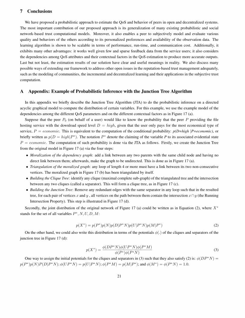
7 Conclusions

We have proposed a probabilistic approach to estimate the QoS and behavior of peers in open and decentralized systems.

The most important contribution of our proposed approach is its generalization of many existing probabilistic and social

network-based trust computational models. Moreover, it also enables a peer to subjectively model and evaluate various

quality and behaviors of the others according to its personalized preferences and availability of the observation data. The

learning algorithm is shown to be scalable in terms of performance, run-time, and communication cost. Additionally, it

exhibits many other advantages: it works well given few and sparse feedback data from the service users; it also considers

the dependencies among QoS attributes and their contextual factors in the QoS estimation to produce more accurate outputs.

Last but not least, the estimation results of our solution have clear and useful meanings in reality. We also discuss many

possible ways of extending our framework to address other open issues in the reputation-based trust management adequately,

such as the modeling of communities, the incremental and decentralized learning and their applications in the subjective trust

computation.

A Appendix: Example of Probabilistic Inference with the Junction Tree Algorithm

In this appendix we briefly describe the Junction Tree Algorithm (JTA) to do the probabilistic inference on a directed

acyclic graphical model to compute the distribution of certain variables. For this example, we use the example model of the

dependencies among the different QoS parameters and on the different contextual factors as in Figure 17 (a).

Suppose that the peer P0 (on behalf of a user) would like to know the probability that the peer P providing the file

hosting service with the download speed level D = high, given that the user only pays for the most economical type of

service, P = economic. This is equivalent to the computation of the conditional probability: p(D=high |P=economic), or

briefly written as p(D = high|P ∗). The notation P ∗ denote the claiming of the variable P to its associated evidential state

P = economic. The computation of such probability is done via the JTA as follows. Firstly, we create the Junction Tree

from the original model in Figure 17 (a) via the four steps:

• Moralization of the dependency graph: add a link between any two parents with the same child node and having no

direct link between them; afterwards, make the graph to be undirected. This is done as in Figure 17 (a).

• Triangulation of the moralized graph: any loop of length 4 or more must have a link between its two non-consecutive

vertices. The moralized graph in Figure 17 (b) has been triangulated by itself.

• Building the Clique Tree: identify any clique (maximal complete sub-graph) of the triangulated tree and the intersection

between any two cliques (called a separator). This will form a clique tree, as in Figure 17 (c).

• Building the Junction Tree: Remove any redundant edges with the same separator in any loop such that in the resulted

tree, for each pair of vertices x and y , all vertices on the path between them contain the intersection x∩y (the Running

Intersection Property). This step is illustrated in Figure 17 (d).

Secondly, the joint distribution of the original network of Figure 17 (a) could be written as in Equation (2), where X∗

stands for the set of all variables P ∗, N, U,D,M :

p(X∗) = p(P ∗)p(N)p(D|P ∗N)p(U |P ∗N)p(M |P ∗) (2)

On the other hand, we could also write this distribution in terms of the potentials φ(.) of the cliques and separators of the

junction tree in Figure 17 (d):

p(X∗) =φ(DP ∗N)φ(UP ∗N)φ(P ∗M)

φ(P ∗)φ(P ∗N)(3)

One way to assign the initial potentials for the cliques and separators in (3) such that they also satisfy (2) is: φ(DP ∗N) =

p(P ∗)p(N)P (D|P ∗N);φ(UP ∗N) = p(U |P ∗N);φ(P ∗M) = p(M |P ∗); and φ(M∗) = φ(P ∗N) = 1.0.

21

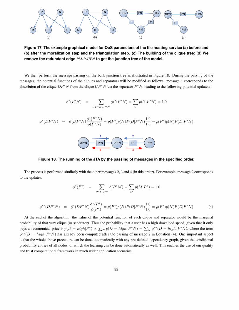
D

P

M

N

U D

P

M

N

U

(a) (b)

DPN UPNPN

PM

P P

(c) (d)

DPN UPNPN

PM

P

Figure 17. The example graphical model for QoS parameters of the file hosting service (a) before and

(b) after the moralization step and the triangulation step. (c) The building of the clique tree; (d) We

remove the redundant edge PM-P-UPN to get the junction tree of the model.

We then perform the message passing on the built junction tree as illustrated in Figure 18. During the passing of the

messages, the potential functions of the cliques and separators will be modified as follows: message 1 corresponds to the

absorbtion of the clique DP ∗N from the clique UP ∗N via the separator P ∗N , leading to the following potential updates:

φ∗(P ∗N) =∑

UP∗N\P∗N

φ(UP ∗N) =∑

U

p(U |P ∗N) = 1.0

φ∗(DP ∗N) = φ(DP ∗N)φ∗(P ∗N)

φ(P ∗N)= p(P ∗)p(N)P (D|P ∗N)

1.0

1.0= p(P ∗)p(N)P (D|P ∗N)

4

2

DP*NUP*N P*N P*MP*

3

1

Figure 18. The running of the JTA by the passing of messages in the specified order.

The process is performed similarly with the other messages 2, 3 and 4 (in this order). For example, message 2 corresponds

to the updates:

φ∗(P ∗) =∑

P∗M\P∗

φ(P ∗M) =∑

M

p(M |P ∗) = 1.0

φ∗∗(DP ∗N) = φ∗(DP ∗N)φ∗(P ∗)

φ(P ∗)= p(P ∗)p(N)P (D|P ∗N)

1.0

1.0= p(P ∗)p(N)P (D|P ∗N) (4)

At the end of the algorithm, the value of the potential function of each clique and separator would be the marginal

probability of that very clique (or separator). Thus the probability that a user has a high download speed, given that it only

pays an economical price is p(D = high|P ∗) ∝∑

N p(D = high, P ∗N) =∑

N φ∗∗(D = high, P ∗N), where the term

φ∗∗(D = high, P ∗N) has already been computed after the passing of message 2 in Equation (4). One important aspect

is that the whole above procedure can be done automatically with any pre-defined dependency graph, given the conditional

probability entries of all nodes, of which the learning can be done automatically as well. This enables the use of our quality

and trust computational framework in much wider application scenarios.

22

References

[1] K. Aberer and Z. Despotovic. Managing trust in a peer-2-peer information system. In CIKM ’01: Proceedings of the tenth interna-

tional conference on Information and knowledge management, pages 310–317, New York, NY, USA, 2001. ACM Press.

[2] E. Bauer, D. Koller, and Y. Singer. Update rules for parameter estimation in bayesian networks. In UAI’97: Proceedings of the

Thirteenth Conference on Uncertainty in Artificial Intelligence, pages 3–13, 1997.

[3] S. Buchegger and J.-Y. L. Boudec. A robust reputation system for P2P and mobile ad-hoc networks. In Proceedings of the Second

Workshop on the Economics of Peer-to-Peer Systems, 2004.

[4] I. Cohen, A. Bronstein, and F. G. Cozman. Online learning of Bayesian network parameters. Technical Report HPL-2001-55R1-

20010615, HP External Technical Report, 2001.

[5] C. Dellarocas. The digitization of word-of-mouth: Promise and challenges of online reputation systems. Management Science,

49(10):1407–1424, 2003.

[6] C. Dellarocas. Reputation mechanism design in online trading environments with pure moral hazard. Information Systems Research,

16(2):209–230, 2005.

[7] C. Dellarocas. Reputation Mechanisms. Handbook on Economics and Information Systems (T. Hendershott, ed.), Elsevier Publishing,

2005.

[8] Z. Despotovic. Building trust-aware P2P systems. PhD thesis, Swiss Federal Institute of Technology Lausanne, Switzerland, 2005.

[9] Z. Despotovic and K. Aberer. A probabilistic approach to predict peers’ performance in P2P networks. In M. Klusch, S. Ossowski,

V. Kashyap, and R. Unland, editors, Cooperative Information Agents VIII: 8th International Workshop, CIA 2004.

[10] Z. Despotovic and K. Aberer. P2P reputation management: Probabilistic estimation vs. social networks. Journal of Computer

Networks, Special Issue on Management in Peer-to-Peer Systems: Trust, Reputation and Security, 2005.

[11] R. Guha, R. Kumar, P. Raghavan, and A. Tomkins. Propagation of trust and distrust. In International World Wide Web Conference

(WWW2004), 2004.

[12] C. Huang and A. Darwiche. Inference in belief networks: A procedural guide. International Journal of Approximate Reasoning,

15(3):225–263, 1996.

[13] A. Jøsang, R. Hayward, and S. Pope. Trust network analysis with subjective logic. In ACSC ’06: Proceedings of the 29th Australasian

Computer Science Conference, pages 85–94, Darlinghurst, Australia, Australia, 2006. Australian Computer Society, Inc.

[14] A. Jøsang, R. Ismail, and C. Boyd. A survey of trust and reputation systems for online service provision. Decision Support Systems,

2005.

[15] R. Jurca and B. Faltings. An incentive compatible reputation mechanism. In Proceedings of the IEEE Conference on E-Commerce,

pages 285–292, Newport Beach, CA, USA, June 24-27 2003.

[16] S. D. Kamvar, M. T. Schlosser, and H. G. Molina. The EigenTrust algorithm for reputation management in P2P networks. In

Proceedings of the Twelfth International World Wide Web Conference, 2003.

[17] W. Kowalczyk and N. A. Vlassis. Newscast em. In Advances in Neural Information Processing Systems 17 [Neural Information

Processing Systems, NIPS 2004, 2004.

[18] N. Miller, P. Resnick, and R. Zeckhauser. Eliciting informative feedback: The peer-prediction method. Management Science,

51(9):1359–1373, 2005.

[19] L. Mui, M. Mohtashemi, and A. Halberstadt. A computational model of trust and reputation. In Proceedings of the 35th Hawaii

International Conference on System Science (HICSS), Hawaii, USA, 2002.

[20] K. Murphy. Bayes Net Toolbox for Matlab. http://bnt.sourceforge.net/, 2006.

[21] R. Neal and G. Hinton. A view of the EM algorithm that justifies incremental, sparse, and other variants. In M. I. Jordan, editor,

Learning in Graphical Models. Kluwer, 1998.

[22] J. Patel, W. T. L. Teacy, N. R. Jennings, and M. Luck. A probabilistic trust model for handling inaccurate reputation sources. In

P. Herrmann, V. Issarny, and S. Shiu, editors, Proceedings of iTrust’05, France, pages 193–209. Springer Berlin Heidelberg, 2005.

[23] I. Stoica, R. Morris, D. Karger, M. F. Kaashoek, and H. Balakrishnan. Chord: A scalable peer-to-peer lookup service for internet

applications. In SIGCOMM ’01: Proceedings of the 2001 conference on Applications, technologies, architectures, and protocols for

computer communications, pages 149–160, New York, NY, USA, 2001. ACM Press.

[24] Y. Wang, V. Cahill, E. Gray, C. Harris, and L. Liao. Bayesian network based trust management. In Internation Conference in

Autonomic and Trusted Computing, pages 246–257, 2006.

23

[25] Y. Wang and J. Vassileva. Bayesian network-based trust model. In WI ’03: Proceedings of the IEEE/WIC International Conference

on Web Intelligence, page 372, Washington, DC, USA, 2003. IEEE Computer Society.

[26] A. Whitby, A. Jøsang, and J. Indulska. Filtering out unfair ratings in Bayesian reputation systems. The Icfain Journal of Management

Research, 4(2):48–64, 2005.

[27] L. Xiong and L. Liu. PeerTrust: Supporting reputation-based trust for peer-to-peer electronic communities. IEEE Trans. Knowl.

Data Eng., 16(7):843–857, 2004.

[28] B. Yu, M. P. Singh, and K. Sycara. Developing trust in large-scale peer-to-peer systems. In Proceedings of First IEEE Symposium

on Multi-Agent Security and Survivability, pages 1–10, 2004.

[29] X. Zheng, H. Chen, Z. Wu, and Y. Zhang. A computational trust model for semantic web based on bayesian decision theory. In

APWeb, pages 745–750, 2006.

24

Documents

Probabilistic Estimation of Peers’ Quality and Behaviors ... · Probabilistic Estimation of Peers’ Quality and Behaviors for Subjective Trust ... [13,16,27 ,28 ... ﬁle hosting