Probabilistic Approximations of SignalingPathway Dynamics

Bing Liu1, P.S. Thiagarajan1,2 and David Hsu1,2

1 NUS Graduate School for Integrative Sciences and Engineering,National University of Singapore

2 Department of Computer Science, National University of Singapore{liubing, dyhsu, thiagu}@comp.nus.edu.sg

Abstract. Systems of ordinary differential equations (ODEs) are oftenused to model the dynamics of complex biological pathways. We con-struct a discrete state model as a probabilistic approximation of the ODEdynamics by discretizing the value space and the time domain. We thensample a representative set of trajectories and exploit the discretizationand the structure of the signaling pathway to encode these trajecto-ries compactly as a dynamic Bayesian network. As a result, many inter-esting pathway properties can be analyzed efficiently through standardBayesian inference techniques. We have tested our method on a modelof EGF-NGF signaling pathway [1] and the results are very promising interms of both accuracy and efficiency.

1 Introduction

Quantitative mathematical models are needed to understand the functioning ofcomplex biological systems. In particular they are needed to capture the dy-namics of various intra (and inter)-cellular processes. Here we focus on signalingpathways which typically sense extra-cellular or internal signals and in response,activate a cascade of intra-cellular reactions. A multitude of signaling pathwaysgovern and coordinate the behavior of cells. As might be expected, many diseaseprocesses arise from defects in signaling pathways. Thus the study of signalingpathways via quantitative dynamic models is of critical importance.

A standard formalism used to model signaling pathways (and other bio-pathways) is a system of Ordinary Differential Equations (ODEs); the equationsdescribe specific bio-chemical reactions while the variables typically representconcentration levels of molecular species (genes, RNAs, proteins). This formalismcan be extended to include discrete aspects [2] and the techniques we develophere can be adapted to such extensions as well.

Signaling pathways usually involve a large number of molecular species andbio-chemical reactions. Hence the corresponding ODEs system will not admitclosed form solutions. Instead, one will have to resort to numerically generatedtrajectories to study the dynamics. A second barrier is that the values of manyof the parameters (rate constants) associated with the ODEs will be unknown.Even assuming all the parameters are known, the observables of the system will

2 Liu et al.

have very limited precision. Specifically, the initial concentration levels of thevarious proteins and rate constants will often be available only as intervals ofvalues. Further, experimental data in the form of the measured concentrationlevels of a few proteins at a small number of time points will also be availableonly in terms of intervals of values. In addition, the data will often be gath-ered using a population of cells. Consequently, when numerically simulating theODEs model, one must resort to Monte Carlo methods to ensure that sufficientlymany point values from the relevant intervals of values are being sampled. As aresult, analysis tasks such as model validation, parameter estimation and sensi-tivity analysis will require the generation of a large number of trajectories. Thismotivates our goal of probabilistically approximating the dynamics of ODEs viadiscretizations.

We start with a system of ODEs and a prior distribution of the initial states.Usually, this prior will consist of a uniform distribution over certain intervalsof values of the variables and the rate constants. We then fix a suitable dis-cretization of the value and time domains. This is followed by sampling theprior distribution of initial states to numerically pre-compute and store a rep-resentative subset of trajectories induced by the ODEs dynamics. The key ideais to exploit the dependencies/independecies in the pathway structure and thediscretization, to compactly encode these trajectories as a time-variant dynamicBayesian network [3]. The resulting approximation is called the Bayesian Dy-namics Model (BDM). Since the trajectories are grouped together through thediscretization, our method bridges the mismatch between the accuracy of theresults obtained by ODE simulation and the limited precision of experimentaldata used for model construction and verification. Secondly, the BDM representsthe global pathway dynamics more explicitly in the graph structure of the under-lying dynamic Bayesian network (DBN). As a result, many interesting pathwayproperties can be analyzed efficiently through standard Bayesian inference tech-niques, instead of resorting to a large number of ODE simulations. There is aone-time computational cost incurred to construct the BDM but this cost canbe amortized by performing multiple analysis tasks such as expected profilesestimation, parameter estimation, sensitivity analysis etc. using the BDM. Wehave tested our method on a model of EGF-NGF signaling pathway [1] and theresults obtained are very promising in terms of both accuracy and efficiency.

In terms of related work, a variety of qualitative and quantitative computa-tional models have been proposed in the recent years to study bio-pathways [2, 4–6]. Among the quantitative models, one usually distinguishes between population-based models driven by stochastic simulations and ODEs based models drivenby -deterministic- numerical simulations. Clearly, both approaches are needed tocover different contexts. Indeed, our work is, in spirit, related to the discretizedapproximations presented in [7–9] that can be applied to high level modelingformalism such as PEPA and PRISM. In these cited works, the dynamics ofa process-algebra-based description of the bio-pathway is given in terms of aContinuous Time Markov Chain (CTMC) which is then discretized (using thenotion of levels) to ease analysis. Apart from the fact that our starting point is

Probabilistic Approximations of Signaling Pathway Dynamics 3

a system of ODEs, a crucial additional step we take is to exploit the structureof the pathway to encode the dynamics more compactly as a dynamic Bayesiannetwork and perform analysis tasks directly on this representation. In a similarvein, we feel that our model is a more compact discrete state model than thanthe graphical model of a network of non-homogenous Markov processes studiedin [10]. We also believe that the techniques proposed in [11], as well as the verifi-cation techniques reported in [12, 13] can be adapted to our setting. Interestingly,there have been recent attempts to synthesize ODEs from PEPA model [14], themotivation being that numerical simulations are faster than stochastic simula-tions. We note however, in our setting, though BDM is a probabilistic graphicalmodel, we do not have to resort to stochastic simulations. The inferencing al-gorithm we use (the so called Factored Frontier Algorithm [15]), in one sweep,gathers information about the statistical properties of the family of trajectoriesencoded by the BDM.

In the next section, we describe our method for constructing our BDM ap-proximation. In section 3, we present a basic inferencing technique and methodsfor performing tasks such as parameter estimation and global sensitivity analysisusing the BDM. We also simultaneously use a realistic signaling pathway modelto evaluate these techniques. In the final section, we summarize the paper anddiscuss future work. The interested reader can find additional technical materialin the form an appendix and relevant supplementary material at [16].

2 The Bayesian Dynamics Model

Conceptually, our approximation technique consists of three steps:

1. We start with a system of ODEs; a discretization of the value space ofeach variable and rate constant into a finite set of intervals; and a digi-talization of the temporal domain of interest into a finite set of time points{t0, t1, . . . , tmax}. We also assume a prior distribution of the initial values(usually, a uniform distribution) over some of the intervals of the value space.These initial values will define an uncountably infinite family of trajectoriesTRAJideal, which in turn, via the discretization, will induce a Markov chainMCideal.

2. It is impossible to compute MCideal explicitly. However, it can be approxi-mated by sampling the set of initial values according to the prior and usingnumerical integration to generate a representative subset TRAJapprox ⊆TRAJideal of trajectories. Then, using the discretization and simple count-ing, we can construct the Markov ChainMCapprox which will be an approx-imation of MCideal.

3. However, MCapprox can be very large since the number of states that thisMarkov chain will be, in the worst case, exponential in the number of vari-ables. To get around this, we exploit the pathway structure (i.e. the waythe variables are coupled to each other in the system of ODEs) to repre-sent MCapprox compactly as time-variant dynamic Bayesian network. Thisrepresentation ofMCapprox is called the Bayesian Dynamics Model (BDM).

4 Liu et al.

We emphasize that this three step procedure is just a conceptual framework;we construct the BDM directly from the given system of ODEs. In what follows,we describe the main technical ideas. The interested reader can find backgroundmaterial and additional details in the appendix portion of the supplementarymaterial.

2.1 ODEs and Flows

We assume a set of ODEs xi(t) = fi(x(t),p) involving the continuous real-valued variables {x1, x2, . . . , xn} and real-valued parameters {p1, p2, . . . , pm}.In our setting, we will often be interested in studying the dynamics for differentcombinations of values for the parameters. Hence it will be convenient to treatthem also as variables. However they will be time-invariant in the sense oncetheir values are fixed at t = 0, these values will not change through the passageof time. Consequently, we will implicitly assume the given system of ODEs to beaugmented with m additional differential equations of the form pj(t) = 0 withj ranging over {1, 2, . . . ,m}. In what follows, we will often let x, v range overIRn

+, the values space of the variables and k range over IRm+ , the values space of

the parameters and z range over IRn+m+ , the combined values space.

In vector form, our system of ODEs may be then represented as Z′ = F (Z).The ODEs will be mainly modeling mass action kinetics or variants such asMichaelis-Menten kinetics. Hence we can assume F : IRn+m

+ → IRn+m+ to be a C1

(continuously differentiable) function. Furthermore, the variables representingthe concentration level of a species within a single cell as well as the parameterscapturing the reaction rates will take values from a bounded interval. Hence thedomain of F can be restricted to a bounded region D of IRn+m

+ .Given z0 = (v0,k) where v0 specifies the initial values of the variables and k

specifies the parameters values, the system of ODEs will have a unique solution(due to F ∈ C1) [17]. We shall denote this solution by Z(t) with Z(0) = z0 andZ′(t) = F (Z(t)).

It will be convenient to define the flow Φ : IR+ × D → D of Z′ = F (Z)for arbitrary initial vectors z. It will be a C0 (continuous) function given by:Φ(t, z) = Z(t) with Φ(0, z) = Z(0) = z and d

dt (Φ(t, z)) = F (Φ(t, z)) for all t.

2.2 The Markov Chain MCideal

Pathways models are usually validated by experimental data available only for afew time points with the concentrations measured at the last time point typicallysignifying the steady state value. Hence we assume the dynamics is of interestonly for discrete time points and that too only up to a maximal time point.Consequently, we fix a time step ∆t > 0 and the time points of interest isassumed to be the set {d ·∆t} with d ranging over {0, 1, . . . , d} where d ·∆t isthe maximal time point of interest.

Next we assume that the values of the variables can be observed with onlyfinite precision and accordingly partition the range of each xi into Li intervals[vmini , v1

i ), [v1i , v

2i ), . . . , [vLi−1

i , vmaxi ]. We denote this set of intervals as Ii. We also

Probabilistic Approximations of Signaling Pathway Dynamics 5

similarly discretize the range of each parameter pj into a set of intervals denotedas In+j . The set I = {Ii}1≤i≤n ∪ {In+j}1≤j≤m is called the discretization.

As pointed out earlier, the initial values vector as well as the rate constants(even when they are known) will be given not as point values but as distributions(usually uniform) over the intervals defined by the discretization. We correspond-ingly assume we are given a prior distribution in the form of a probability densityfunction Υ 0 capturing the distribution of initial values. For example, suppose weare given that the initial values are uniformly distributed within a hypercubeI1 × I2 × . . .× In+m, where Ii ∈ Ii for each i. Let Ii = [li, ui) and wi = ui − li.Then the corresponding prior probability density function Υ 0 will be given by:

Υ 0(z) =

{1

w1·w2·...·wn+mif z ∈ I1 × I2 × . . .× In+m,

0 otherwise.

The associated probability space we have in mind is (D,BD, P 0) where BDis the Borel σ-algebra over D; the minimal σ-algebra containing the open setsof D under the usual topology. P 0 is the probability distribution induced by Υ 0

and is given by:

P 0(B) =∫BΥ 0(z)dz, for every B ∈ BD.

Further, TRAJideal = {Z(t)}t≥0 with Z(0) ∈ I1 × I2 × . . . × In+m is thefamily of trajectories starting from all the possible points in this hypercube.Since the flow is continuous and hence measurable we can associate a probabilitydistribution P t over BD for every t. To define this, let Φ−1

t (B) = {z′ | Φ(t, z′) ∈B} for B ∈ BD. Since Φ(t, ·) is measurable, we have Φ−1

t (B) ∈ BD too. We cannow define P t as:

P t(B) = P 0(Φ−1t (B)), for every B ∈ BD.

Let v be in the range of xi. We define [v] as the interval in which v falls. Inother words, [v] = I iff v ∈ I. Similarly, [k] = J if k ∈ J for a parameter value kof pj with J ∈ In+j .

Lifting this notation to the vector setting, if z = (v1, v2, . . . , vn, k1, k2, . . . , km)∈ IRn+m

+ , we define [z] = ([v1], [v2], . . . , [vn], [k1], . . . , [km]) and refer to it as adiscrete state. An MC-state is a pair (s, d), where s is a discrete state andd ∈ {1, 2, . . . , d}.

We next define Pr(s, d) = P d·∆t({z | z ∈ I1 × I2 × . . . × In+m}), wheres = (I1, I2, . . . , In+m). We term the MC-state M to be feasible iff Pr(M) > 0.

The transition relation denoted as →, between MC-states is defined via:M = (s, d) → M ′ = (s′, d′) iff d′ = d + 1 and both M and M ′ are feasible andthere exist z0, z, and z′ such that Φ(d ·∆t, z0) = z and Φ((d+ 1) ·∆t, z0) = z′.Furthermore, [z] = s and [z′] = s′.

Let E, F denote, respectively, the event that the system is in the discretestate s at time d · ∆t and in the discrete state s′ at time (d + 1) · ∆t for twofeasibleMC-states (s, d ·∆t) and (s′, (d+ 1) ·∆t). Let EF = E ∩F denote jointevent {z0 | Φ(d ·∆t, z0) ∈ s, Φ((d+ 1) ·∆t, z0) ∈ s′}. Consequently, we define the

6 Liu et al.

transition probability Pr((s, d)→ (s′, d′)) = Pr(F |E) = Pr(EF )/Pr(E). SincePr(E) > 0 this transition probability is well-defined.

Let M = {M1,M2, . . . ,Mn} be the set of M-states. We can now definethe Markov chain MCideal = (M, {pij}) with transition probabilities pij =Pr(Mi →Mj) as above.

2.3 The Markov Chain MCapprox

MCideal can not be explicitly computed. Hence we sample z0 a sufficiently largernumber of times, say N , according to the prior distribution P 0 (we say moreabout N below). For each sampled initial z0, we determine through numericalintegration theM-states [Φ(d·∆t, z0)], with d ranging over {0, 1, . . . , d}. We alsodetermine the transitions along this trajectory. Then through a simple countingprocess involving these N trajectories, we compute a Markov chain that we referto as the MCapprox.

Since N is finite, there will be an error between the transition probabilities(also theMC-state probabilities) computed usingMCapprox and the ones definedbyMCideal. By the central limit theorem [18], this error can be probabilisticallybounded. In other words, given an error bound ε and a confidence level c, we cancompute N , the number of samples required to get an error less than or equalto ε with likelihood c (the Appendix gives more details). Further, this error willtend to 0 with probability 1 as N tends to ∞. There will be an additional errorinduced by the pth-order numerical integration method we use to compute theN trajectories. This error will tend to 0 as ∆t tends to 0 or p tends to ∞.

However, the number of states of this Markov chain will be exponential in nand hence for many signaling pathways MCapprox will be too large a structure.Hence we shall construct a time-variant DBN called the BDM to compactlyrepresent MCapprox. We shall however compute the BDM directly from the Nsampled trajectories.

2.4 The BDM Representation

In what follows, we assume the basic background concerning Bayesian networksand dynamic Bayesian networks [3]. The graphical structure of the DBN used forour approximation can be derived from the differential equations. It will have n+m random variables (corresponding to the variables and the parameters) as nodesfor each time slice d ·∆t with d ranging over {0, 1, . . . , d}. For convenience, wewill use the same name to denote a variable (parameter) and the correspondingrandom variable. From the context it should be clear which role is intended.The random variable xi (pj) can assume as values, the finite set of intervals Ii(In+j).

The variable (parameter) xi (pj) in the time slice d ·∆t will be written as xdi(pdj ). Edges connecting a node in the d-th slice to a node in the (d+1)-th slice willbe determined by the dependencies of the variables and the parameters in theODEs. Suppose zdl is a (variable or parameter) node in the d-th time slice and

Probabilistic Approximations of Signaling Pathway Dynamics 7

zd+1q is a node in the next time slice. Then there will be an edge from zdl to zd+1

q

iff zl = zq or zq is a variable node and zl appears in the expression for zq in thesystem of ODEs. As usual, the parents of the node zd+1

q will be the set of nodesof the form zdl from which there is an edge into zd+1

q . Suppose, parents(xd+1i ) =

{zd1 , . . . , zdl }. Then conditional probability table (CPT) associated with the nodexd+1i will have entries of the form Pr(xd+1

i = I | zd1 = I1, . . . , zdl = I l) = h withI ranging over Ii and Ik ranging over Ik and h ∈ [0, 1].

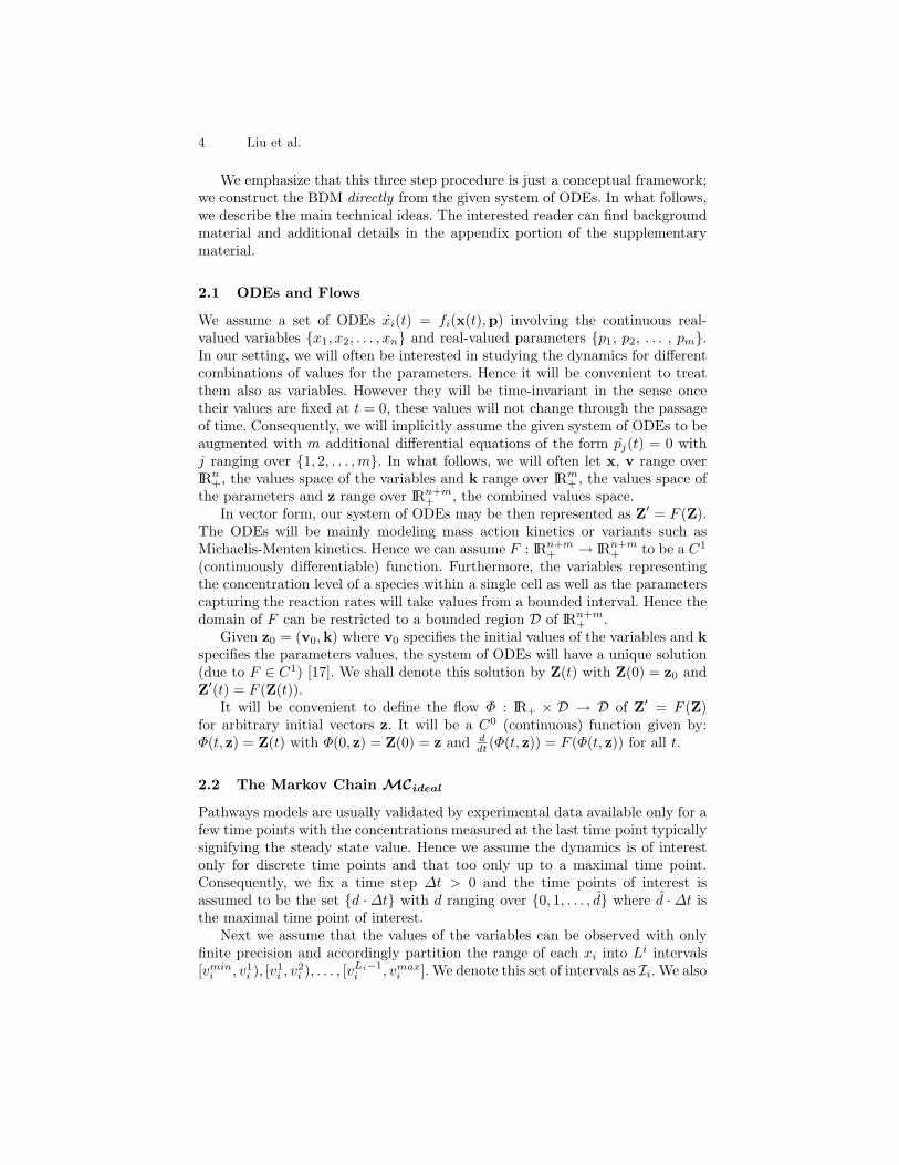
S + Ek1k2ES

k3−−→ E + P

dS

dt= −k1 · S · E + k

′ · ES

dE

dt= −k1 · S · E + (k2 + k3) · ES

dES

dt= k1 · S · E − (k2 + k3) · ES

dP

dt= k3 · ES

E E

ES

Sd

P

ES

S

P

d+1

d

d

d

d

d

d

d+1

d+1

d+1

d+1

d+1

d+1

k1

k2

k3

k1

k2

k3

Pr(P = I |P = I’, ES = I’’, k3= I’’’) = 0.7d+1 d d

I ,I’ Î IPI’’ Î IESI’’’ Î Ik3

M

M

Fig. 1. The ODE model of the enzyme-kinetic system and its BDM.

For instance, Figure 1 shows two adjacent slices of a enzyme-kinetic system.In this BDM, the parent nodes of P d+1 are P d, ESd and kd3 . As mentionedearlier, the parameters are assumed to not change their values during a run andhence we denote kdi as simply ki and there will be no CPTs associated withthese nodes. As illustrated by the example, the connectivity between the nodesin successive slices will remain invariant. However, due to the fact that the CPTsassociated with the nodes capture the transition probabilities ofMC-states, theywill be time variant.MCapprox will have, in the worst case, O(dKn) states and O((d − 1)K2n)

transitions, where K is the maximum of |Ii| with 1 ≤ i ≤ n+m. In contrast, thenumber of nodes in the BDM representation is O(d(n+m)) and the conditionalprobability table associated each node will have at most O(KR+1) entries, whereR is the maximal number of parents a node can have. Usually, the reactants inpathway models will be sparsely coupled to each other and hence R will bemuch smaller than n. For instance, in the case study to be presented, n = 32and R = 5. Even in cases where R is large, due to the nature of the ODEs wedeal with, we can often break up the corresponding node into nodes with smallerfan-in degrees and thus reduce R [16].

To fill up the entries of the CPTs associated with the nodes we randomlychoose N combinations of initial values for the variables and the parametersfrom their prior distribution as before. Note that if we want a coverage of Jsamples per interval in an n+m dimensional vector of intervals we can achieveN = JKR+1 instead of JKn+m by exploiting the network structure. We thenperform numerical integration to generate N trajectories and discretize thosetrajectories by the predefined intervals and compute the conditional probabilities

8 Liu et al.

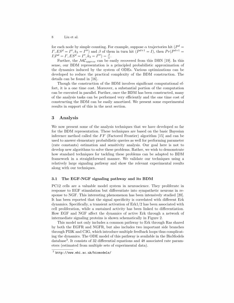
for each node by simple counting. For example, suppose α trajectories hit (P d =I ′, ESd = I ′′, k3 = I ′′′) and β of them in turn hit (P d+1 = I), then Pr(P d+1 =I|P d = I ′, ESd = I ′′, k3 = I ′′′) = β

α .Further, the MCapprox can be easily recovered from this DBN [19]. In this

sense, our BDM representation is a principled probabilistic approximation ofthe dynamics induced by the system of ODEs. Various optimizations can bedeveloped to reduce the practical complexity of the BDM construction. Thedetails can be found in [16].

Though the construction of the BDM involves significant computational ef-fort, it is a one time cost. Moreover, a substantial portion of the computationcan be executed in parallel. Further, once the BDM has been constructed, manyof the analysis tasks can be performed very efficiently and the one time cost ofconstructing the BDM can be easily amortized. We present some experimentalresults in support of this in the next section.

3 Analysis

We now present some of the analysis techniques that we have developed so farfor the BDM representation. These techniques are based on the basic Bayesianinference method called the FF (Factored Frontier) algorithm [15] and can beused to answer elementary probabilistic queries as well for performing parameter(rate constants) estimation and sensitivity analysis. Our goal here is not todevelop new algorithms to solve these problems. Rather, we wish to demonstratehow standard techniques for tackling these problems can be adapted to BDMframework in a straightforward manner. We validate our techniques using arelatively large signaling pathway and show the relevant experimental resultsalong with our techniques.

3.1 The EGF-NGF signaling pathway and its BDM

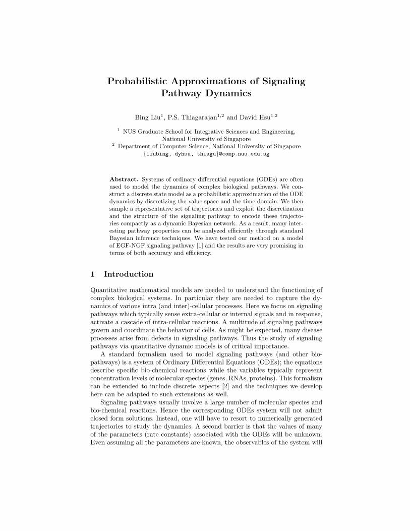
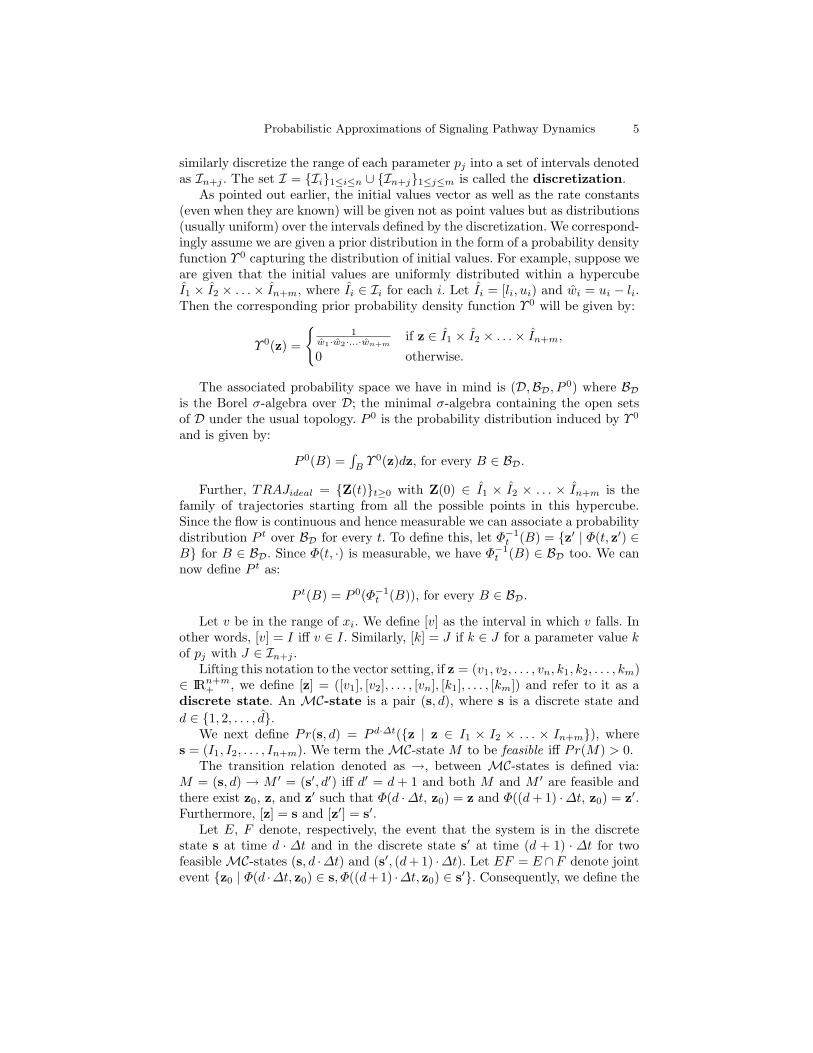
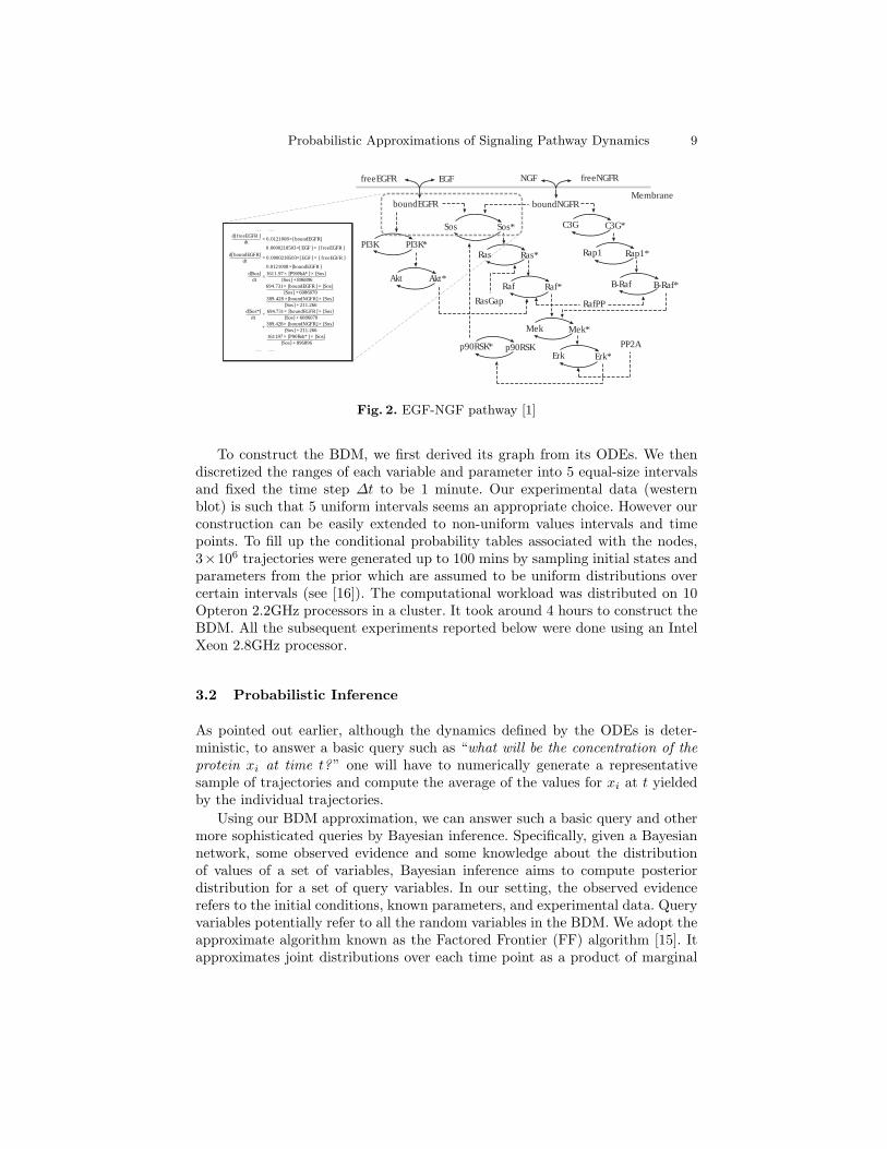
PC12 cells are a valuable model system in neuroscience. They proliferate inresponse to EGF stimulation but differentiate into sympathetic neurons in re-sponse to NGF. This interesting phenomenon has been intensively studied [20].It has been reported that the signal specificity is correlated with different Erkdynamics. Specifically, a transient activation of Erk1/2 has been associated withcell proliferation, while a sustained activity has been linked to differentiation.How EGF and NGF affect the dynamics of active Erk through a network ofintermediate signaling proteins is shown schematically in Figure 2.

This model not only includes a common pathway to Erk through Ras sharedby both the EGFR and NGFR, but also includes two important side branchesthrough PI3K and C3G, which introduce multiple feedback loops thus complicat-ing the dynamics. The ODE model of this pathway is available in the BioModelsdatabase3. It consists of 32 differential equations and 48 associated rate param-eters (estimated from multiple sets of experimental data).3 http://www.ebi.ac.uk/biomodels/

Probabilistic Approximations of Signaling Pathway Dynamics 9

EGFfreeEGFR

boundEGFR

Sos Sos*

Ras Ras*

Raf Raf*

Mek Mek*

Erk Erk*

PI3K PI3K*

Akt Akt*

p90RSK* p90RSK

C3G C3G*

Rap1 Rap1*

B-Raf B-Raf*

NGF freeNGFR

boundNGFR

RasGap RafPP

PP2A

. . . . . .d[ f reeEGF R ]

dt = 0 .0121008× [boundEGF R]

0.0000218503×[ EGF ] × [ f reeEGF R ]d[boundEGF R]

dt = 0 .0000218503×[ EGF ] × [ f reeEGF R ]

0.0121008 ×[boundEGF R ]d[Sos]

dt = 1611.97× [P90Rsk* ] × [Sos][Sos] + 896896

694.731× [boundEGF R ] × [Sos][Sos] + 6086070

389.428 × [boundNGF R ] × [Sos][Sos] + 211.266

d[Sos*]dt = 694.731× [boundEGF R ] × [Sos]

[Sos] + 6086070

+ 389.428× [boundNGF R ] × [Sos][Sos] + 211.266

1611.97× [P90Rsk* ] × [Sos][Sos] + 896896

. . . . . .

Membrane

Fig. 2. EGF-NGF pathway [1]

To construct the BDM, we first derived its graph from its ODEs. We thendiscretized the ranges of each variable and parameter into 5 equal-size intervalsand fixed the time step ∆t to be 1 minute. Our experimental data (westernblot) is such that 5 uniform intervals seems an appropriate choice. However ourconstruction can be easily extended to non-uniform values intervals and timepoints. To fill up the conditional probability tables associated with the nodes,3×106 trajectories were generated up to 100 mins by sampling initial states andparameters from the prior which are assumed to be uniform distributions overcertain intervals (see [16]). The computational workload was distributed on 10Opteron 2.2GHz processors in a cluster. It took around 4 hours to construct theBDM. All the subsequent experiments reported below were done using an IntelXeon 2.8GHz processor.

3.2 Probabilistic Inference

As pointed out earlier, although the dynamics defined by the ODEs is deter-ministic, to answer a basic query such as “what will be the concentration of theprotein xi at time t?” one will have to numerically generate a representativesample of trajectories and compute the average of the values for xi at t yieldedby the individual trajectories.

Using our BDM approximation, we can answer such a basic query and othermore sophisticated queries by Bayesian inference. Specifically, given a Bayesiannetwork, some observed evidence and some knowledge about the distributionof values of a set of variables, Bayesian inference aims to compute posteriordistribution for a set of query variables. In our setting, the observed evidencerefers to the initial conditions, known parameters, and experimental data. Queryvariables potentially refer to all the random variables in the BDM. We adopt theapproximate algorithm known as the Factored Frontier (FF) algorithm [15]. Itapproximates joint distributions over each time point as a product of marginal

10 Liu et al.

0 2 0 4 0 6 0 8 0 1 0 00 . 0 0 0

2 . 6 4 0 x 1 0 4

5 . 2 8 0 x 1 0 4

7 . 9 2 0 x 1 0 4

1 . 0 5 6 x 1 0 5

1 . 3 2 0 x 1 0 5

R a p 1

0 2 0 4 0 6 0 8 0 1 0 00 . 0 0 0

1 . 3 2 0 x 1 0 5

2 . 6 4 0 x 1 0 5

3 . 9 6 0 x 1 0 5

5 . 2 8 0 x 1 0 5

6 . 6 0 0 x 1 0 5

E r k *

0 2 0 4 0 6 0 8 0 1 0 00 . 0 0

2 . 6 0 x 1 0 4

5 . 2 0 x 1 0 4

7 . 8 0 x 1 0 4

1 . 0 4 x 1 0 5

1 . 3 0 x 1 0 5

S o s *

0 2 0 4 0 6 0 8 0 1 0 00

2 4 0 0 0

4 8 0 0 0

7 2 0 0 0

9 6 0 0 0

1 2 0 0 0 0

A K T *

0 2 0 4 0 6 0 8 0 1 0 00 . 0 0

2 . 6 0 x 1 0 4

5 . 2 0 x 1 0 4

7 . 8 0 x 1 0 4

1 . 0 4 x 1 0 5

1 . 3 0 x 1 0 5

R a s *

0 2 0 4 0 6 0 8 0 1 0 00 . 0 0 0

1 . 3 2 0 x 1 0 5

2 . 6 4 0 x 1 0 5

3 . 9 6 0 x 1 0 5

5 . 2 8 0 x 1 0 5

6 . 6 0 0 x 1 0 5

M e k *

0 2 0 4 0 6 0 8 0 1 0 00 . 0 0

2 . 6 0 x 1 0 4

5 . 2 0 x 1 0 4

7 . 8 0 x 1 0 4

1 . 0 4 x 1 0 5

1 . 3 0 x 1 0 5

p 9 0 R S K *

0 2 0 4 0 6 0 8 0 1 0 00 . 0 0 0

2 . 6 4 0 x 1 0 4

5 . 2 8 0 x 1 0 4

7 . 9 2 0 x 1 0 4

1 . 0 5 6 x 1 0 5

1 . 3 2 0 x 1 0 5

C 3 G *

0 2 0 4 0 6 0 8 0 1 0 00

2 6 4 0 0

5 2 8 0 0

7 9 2 0 0

1 0 5 6 0 0

1 3 2 0 0 0

P I 3 K *

0 2 0 4 0 6 0 8 0 1 0 00 . 0 0

2 . 4 0 x 1 0 3

4 . 8 0 x 1 0 3

7 . 2 0 x 1 0 3

9 . 6 0 x 1 0 3

1 . 2 0 x 1 0 4

b o u n d N G F R

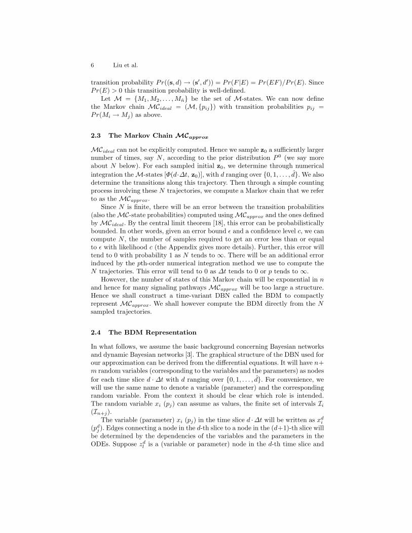
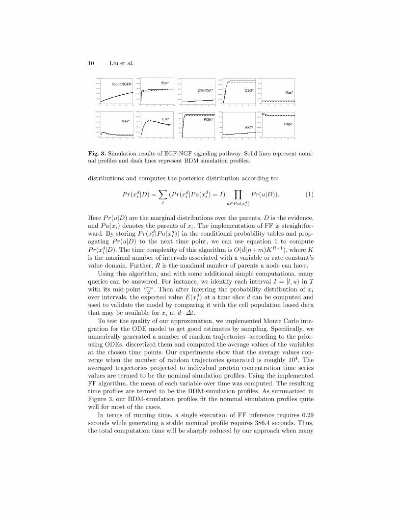
Fig. 3. Simulation results of EGF-NGF signaling pathway. Solid lines represent nomi-nal profiles and dash lines represent BDM simulation profiles.

distributions and computes the posterior distribution according to:

Pr(xdi |D) =∑I

(Pr(xdi |Pa(xdi ) = I)∏

u∈Pa(xdi )

Pr(u|D)). (1)

Here Pr(u|D) are the marginal distributions over the parents, D is the evidence,and Pa(xi) denotes the parents of xi. The implementation of FF is straightfor-ward. By storing Pr(xdi |Pa(xdi )) in the conditional probability tables and prop-agating Pr(u|D) to the next time point, we can use equation 1 to computePr(xdi |D). The time complexity of this algorithm is O(d(n+m)KR+1), where Kis the maximal number of intervals associated with a variable or rate constant’svalue domain. Further, R is the maximal number of parents a node can have.

Using this algorithm, and with some additional simple computations, manyqueries can be answered. For instance, we identify each interval I = [l, u) in Iwith its mid-point l+u

2 . Then after inferring the probability distribution of xiover intervals, the expected value E(xdi ) at a time slice d can be computed andused to validate the model by comparing it with the cell population based datathat may be available for xi at d ·∆t.

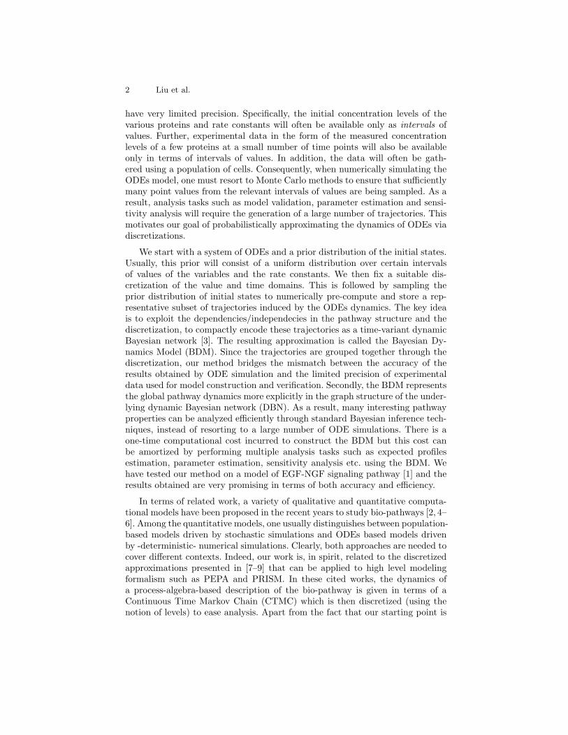
To test the quality of our approximation, we implemented Monte Carlo inte-gration for the ODE model to get good estimates by sampling. Specifically, wenumerically generated a number of random trajectories -according to the prior-using ODEs, discretized them and computed the average values of the variablesat the chosen time points. Our experiments show that the average values con-verge when the number of random trajectories generated is roughly 104. Theaveraged trajectories projected to individual protein concentration time seriesvalues are termed to be the nominal simulation profiles. Using the implementedFF algorithm, the mean of each variable over time was computed. The resultingtime profiles are termed to be the BDM-simulation profiles. As summarized inFigure 3, our BDM-simulation profiles fit the nominal simulation profiles quitewell for most of the cases.

In terms of running time, a single execution of FF inference requires 0.29seconds while generating a stable nominal profile requires 386.4 seconds. Thus,the total computation time will be sharply reduced by our approach when many

Probabilistic Approximations of Signaling Pathway Dynamics 11

such “queries” need to be answered. In the next subsection, we will furtherdemonstrate this advantage by carrying out a simulation-intensive analysis task.

3.3 Parameter estimation.

Lack of knowledge about the parameters and hence the need to perform param-eter estimation using limited data has long been identified as a major bottleneckof pathway modeling. Current approaches to parameter estimation formulateit as a non-linear optimization problem [21]. A typical procedure will involvesearching in a high dimensional solution space, in which each point represents avector of parameter values. Whether a point is good or not is measured by theobjective function, which will capture the difference between experimental dataand prediction generated by simulations using the corresponding parameters.

For a large pathway model, one often needs to evaluate a very large number ofsolution points involving a numerical integration for each evaluation. This makesthe whole process computationally intensive. The BDM representation allows usto carry out the search for good parameter values in a hierarchical manner. Dueto the discretized nature of the BDM, the solution space is transformed to arectilinear grid consisting of a space-filling tessellation by hyperrectangles thatwe call blocks. An important observation is that kinetic parameters are oftenrobust [22]. In other words, the points around the best solution in the searchspace will also have relatively small objective values. Thus, instead of searchingpoint by point in the solution space, we can first search for a few promising blocksand then take a closer look within these small blocks. Therefore, the generalscheme of our “grid search” algorithm will consist of two phases: (1) identifygood blocks, (2) do local search within candidate blocks. We note that phase(2)is necessary only when we aim to estimate parameters with finer granularity thanthe granularity of the BDM’s discretization. Otherwise, one can skip phase(2)and return a probabilistic estimate (typically a Maximal Likelihood Estimate)of a combination of intervals of parameter values. For executing phase(1), wecan apply any standard search algorithms over the discretized search space. Asthe discretized search space is much smaller than the original one, simple directsearch algorithm such as Hooke & Jeeves’s search [23] can be adopted and theoverall search process will only require a small number of executions of the FFalgorithm.

In order to test the performance of the BDM-based parameter estimationmethod, we synthesized experimental time series data for 9 (out of 32) proteins{bounded EGFR, bounded NGFR, active Sos, active C3G, active Akt, activep90RSK, active Erk, active Mek, active PI3K}, measured at the time points{2, 5, 10, 20, 30, 40, 50, 60, 80, 100} (min).This data was synthesized usingprior knowledge about initial conditions and parameters [16]. To mimic westernblot data which is cell population based, we first averaged 104 random trajec-tories generated by sampling initial states and rate constants, and then addedobservation noise with variance 5% to the simulated values. With the assumedmeasurement precision, those values were discretized into 5 intervals, which rep-resent the concentration levels in western blot data. We reserved the data of 7

12 Liu et al.

0 2 0 4 0 6 0 8 0 1 0 00 . 0 0

2 . 6 0 x 1 0 4

5 . 2 0 x 1 0 4

7 . 8 0 x 1 0 4

1 . 0 4 x 1 0 5

1 . 3 0 x 1 0 5

P I 3 K *

0 2 0 4 0 6 0 8 0 1 0 00 . 0 0 0

1 . 3 2 0 x 1 0 5

2 . 6 4 0 x 1 0 5

3 . 9 6 0 x 1 0 5

5 . 2 8 0 x 1 0 5

6 . 6 0 0 x 1 0 5

M e k *

( b )

0 2 0 4 0 6 0 8 0 1 0 0

2 . 6 0 x 1 0 4

5 . 2 0 x 1 0 4

7 . 8 0 x 1 0 4

1 . 0 4 x 1 0 5

1 . 3 0 x 1 0 5

A K T *

( a )

0 2 0 4 0 6 0 8 0 1 0 00 . 0 0

2 . 4 0 x 1 0 3

4 . 8 0 x 1 0 3

7 . 2 0 x 1 0 3

9 . 6 0 x 1 0 3

1 . 2 0 x 1 0 4

b N G F R

0 2 0 4 0 6 0 8 0 1 0 00 . 0 0

2 . 6 0 x 1 0 4

5 . 2 0 x 1 0 4

7 . 8 0 x 1 0 4

1 . 0 4 x 1 0 5

1 . 3 0 x 1 0 5

C 3 G *

0 2 0 4 0 6 0 8 0 1 0 00 . 0 0

2 . 6 0 x 1 0 4

5 . 2 0 x 1 0 4

7 . 8 0 x 1 0 4

1 . 0 4 x 1 0 5

1 . 3 0 x 1 0 5

S o s *

0 2 0 4 0 6 0 8 0 1 0 00 . 0 0

2 . 6 0 x 1 0 4

5 . 2 0 x 1 0 4

7 . 8 0 x 1 0 4

1 . 0 4 x 1 0 5

1 . 3 0 x 1 0 5

p 9 0 R S K *

0 2 0 4 0 6 0 8 0 1 0 00 . 0 0 0

1 . 3 2 0 x 1 0 5

2 . 6 4 0 x 1 0 5

3 . 9 6 0 x 1 0 5

5 . 2 8 0 x 1 0 5

6 . 6 0 0 x 1 0 5

E r k *

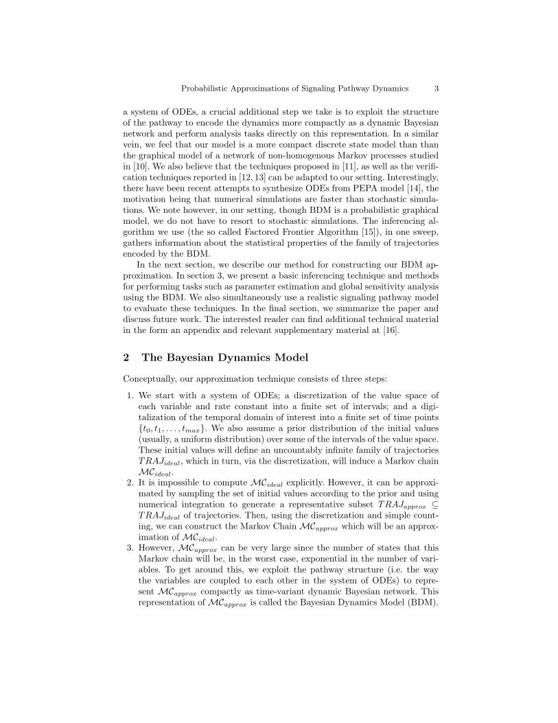
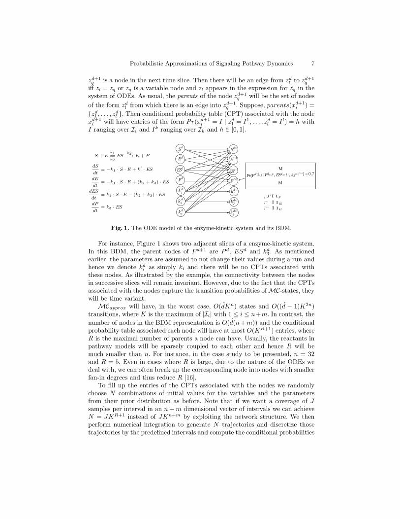
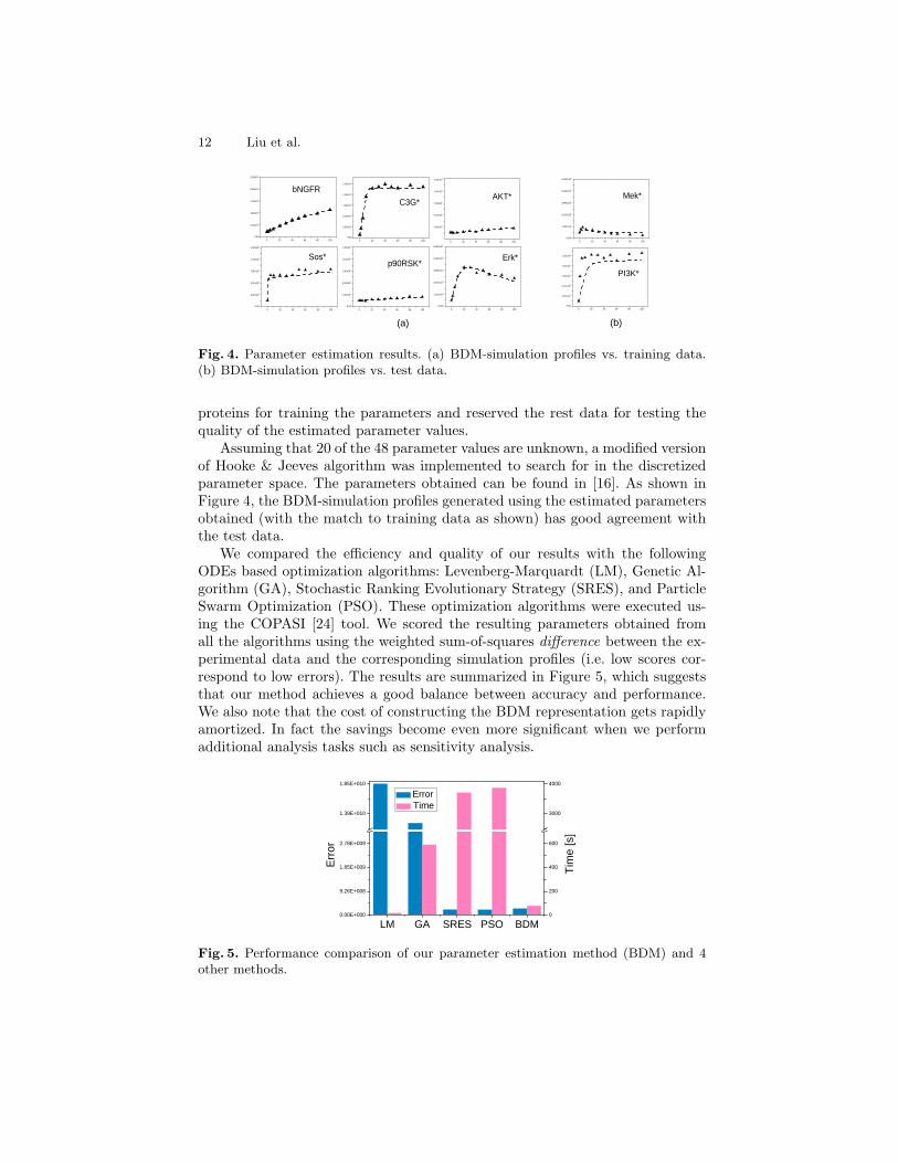
Fig. 4. Parameter estimation results. (a) BDM-simulation profiles vs. training data.(b) BDM-simulation profiles vs. test data.

proteins for training the parameters and reserved the rest data for testing thequality of the estimated parameter values.

Assuming that 20 of the 48 parameter values are unknown, a modified versionof Hooke & Jeeves algorithm was implemented to search for in the discretizedparameter space. The parameters obtained can be found in [16]. As shown inFigure 4, the BDM-simulation profiles generated using the estimated parametersobtained (with the match to training data as shown) has good agreement withthe test data.

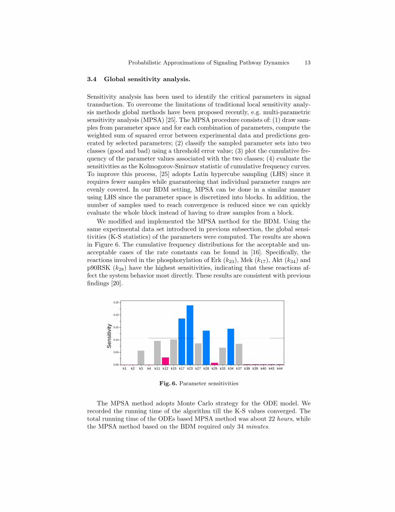
We compared the efficiency and quality of our results with the followingODEs based optimization algorithms: Levenberg-Marquardt (LM), Genetic Al-gorithm (GA), Stochastic Ranking Evolutionary Strategy (SRES), and ParticleSwarm Optimization (PSO). These optimization algorithms were executed us-ing the COPASI [24] tool. We scored the resulting parameters obtained fromall the algorithms using the weighted sum-of-squares difference between the ex-perimental data and the corresponding simulation profiles (i.e. low scores cor-respond to low errors). The results are summarized in Figure 5, which suggeststhat our method achieves a good balance between accuracy and performance.We also note that the cost of constructing the BDM representation gets rapidlyamortized. In fact the savings become even more significant when we performadditional analysis tasks such as sensitivity analysis.

L M G A S R E S P S O B D M0 . 0 0 E + 0 0 0

9 . 2 6 E + 0 0 8

1 . 8 5 E + 0 0 9

2 . 7 8 E + 0 0 9

1 . 3 9 E + 0 1 0

1 . 8 5 E + 0 1 0

0

2 0 0

4 0 0

6 0 0

3 0 0 0

4 0 0 0

Time [

s]

Error

E r r o r T i m e

Fig. 5. Performance comparison of our parameter estimation method (BDM) and 4other methods.

Probabilistic Approximations of Signaling Pathway Dynamics 13

3.4 Global sensitivity analysis.

Sensitivity analysis has been used to identify the critical parameters in signaltransduction. To overcome the limitations of traditional local sensitivity analy-sis methods global methods have been proposed recently, e.g. multi-parametricsensitivity analysis (MPSA) [25]. The MPSA procedure consists of: (1) draw sam-ples from parameter space and for each combination of parameters, compute theweighted sum of squared error between experimental data and predictions gen-erated by selected parameters; (2) classify the sampled parameter sets into twoclasses (good and bad) using a threshold error value; (3) plot the cumulative fre-quency of the parameter values associated with the two classes; (4) evaluate thesensitivities as the Kolmogorov-Smirnov statistic of cumulative frequency curves.To improve this process, [25] adopts Latin hypercube sampling (LHS) since itrequires fewer samples while guaranteeing that individual parameter ranges areevenly covered. In our BDM setting, MPSA can be done in a similar mannerusing LHS since the parameter space is discretized into blocks. In addition, thenumber of samples used to reach convergence is reduced since we can quicklyevaluate the whole block instead of having to draw samples from a block.

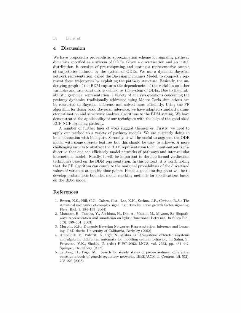
We modified and implemented the MPSA method for the BDM. Using thesame experimental data set introduced in previous subsection, the global sensi-tivities (K-S statistics) of the parameters were computed. The results are shownin Figure 6. The cumulative frequency distributions for the acceptable and un-acceptable cases of the rate constants can be found in [16]. Specifically, thereactions involved in the phosphorylation of Erk (k23), Mek (k17), Akt (k34) andp90RSK (k28) have the highest sensitivities, indicating that these reactions af-fect the system behavior most directly. These results are consistent with previousfindings [20].

k 1 k 2 k 3 k 4 k 1 1 k 1 2 k 1 5 k 1 7 k 2 3 k 2 7 k 2 8 k 2 9 k 3 3 k 3 4 k 3 7 k 3 8 k 3 9 k 4 0 k 4 3 k 4 40 . 0 0

0 . 0 5

0 . 1 0

0 . 1 5

0 . 2 0

0 . 2 5

Sens

itivity

Fig. 6. Parameter sensitivities

The MPSA method adopts Monte Carlo strategy for the ODE model. Werecorded the running time of the algorithm till the K-S values converged. Thetotal running time of the ODEs based MPSA method was about 22 hours, whilethe MPSA method based on the BDM required only 34 minutes.

14 Liu et al.

4 Discussion

We have proposed a probabilistic approximation scheme for signaling pathwaydynamics specified as a system of ODEs. Given a discretization and an initialdistribution, it consists of pre-computing and storing a representative sampleof trajectories induced by the system of ODEs. We use a dynamic Bayesiannetwork representation, called the Bayesian Dynamics Model, to compactly rep-resent these trajectories by exploiting the pathway structure. Basically, the un-derlying graph of the BDM captures the dependencies of the variables on othervariables and rate constants as defined by the system of ODEs. Due to the prob-abilistic graphical representation, a variety of analysis questions concerning thepathway dynamics traditionally addressed using Monte Carlo simulations canbe converted to Bayesian inference and solved more efficiently. Using the FFalgorithm for doing basic Bayesian inference, we have adapted standard param-eter estimation and sensitivity analysis algorithms to the BDM setting. We havedemonstrated the applicability of our techniques with the help of the good sizedEGF-NGF signaling pathway.

A number of further lines of work suggest themselves. Firstly, we need toapply our method to a variety of pathway models. We are currently doing soin collaboration with biologists. Secondly, it will be useful to augment the ODEmodel with some discrete features but this should be easy to achieve. A morechallenging issue is to abstract the BDM representation to an input-output trans-ducer so that one can efficiently model networks of pathways and inter-cellularinteractions models. Finally, it will be important to develop formal verificationtechniques based on the BDM representation. In this context, it is worth notingthat the FF algorithm can compute the marginal probabilities of the discretizedvalues of variables at specific time points. Hence a good starting point will be todevelop probabilistic bounded model checking methods for specifications basedon the BDM model.

References

1. Brown, K.S., Hill, C.C., Calero, G.A., Lee, K.H., Sethna, J.P., Cerione, R.A.: Thestatistical mechanics of complex signaling networks: nerve growth factor signaling.Phys. Biol. 1, 184–195 (2004)

2. Matsuno, H., Tanaka, Y., Aoshima, H., Doi, A., Matsui, M., Miyano, S.: Biopath-ways representation and simulation on hybrid functional Petri net. In Silico Biol.3(3), 389–404 (2003)

3. Murphy, K.P.: Dynamic Bayesian Networks: Representation, Inference and Learn-ing. PhD thesis, University of California, Berkeley (2002)

4. Antoniotti, M., Policriti, A., Ugel, N., Mishra, B.: XS-systems: extended s-systemsand algebraic differential automata for modeling cellular behavior. In Sahni, S.,Prasanna, V.K., Shukla, U. (eds.) HiPC 2002. LNCS, vol. 2552, pp. 431–442.Springer, Heidelberg (2002)

5. de Jong, H., Page, M.: Search for steady states of piecewise-linear differentialequation models of genetic regulatory networks. IEEE/ACM T. Comput. Bi. 5(2),208–223 (2008)

Probabilistic Approximations of Signaling Pathway Dynamics 15

6. Ghosh, R., Tomlin, C.: Symbolic reachable set computation of piecewise affinehybrid automata and its application to biological modelling: Delta-notch proteinsignalling. Systems Biol. 1(1), 170–183 (2004)

7. Calder, M., Gilmore, S., Hillston, J.: Modelling the influence of RKIP on theERK signalling pathway using the stochastic process algebra PEPA. In Trans. onComput. Syst. Biol. VII. LNCS, vol. 4230, pp. 1–23. Springer, Heidelberg (2006)

8. Calder, M., Vyshemirsky, V., Gilbert, D., Orton, R.: Analysis of signalling path-ways using continuous time Markov chains. In Trans. on Comput. Syst. Biol. VI.LNCS, vol. 4220, pp. 44–67. Springer, Heidelberg (2006)

9. Ciocchetta, F., Degasperi, A., Hillston, J., Calder, M.: CTMC with levels modelsfor biochemical systems. Preprint submitted to Elsevier (2009)

10. Nodelman, U., Shelton, C.R., Koller, D.: Continuous time Bayesian networks. In:Proceedings of the 18th Conference in Uncertainty in Artificial Intelligence, pp.378–387. Alberta, Canada (2002)

11. Langmead, C., Jha, S., Clarke, E.: Temporal logics as query languages for dynamicBayesian networks: Application to D. Melanogaster embryo development. Technicalreport, Carnegie Mellon University (2006)

12. Clarke, E.M., Faeder, J.R., Langmead, C.J., Harris, L.A., Jha, S.K., Legay, A.:Statistical model checking in BioLab: Applications to the automated analysis ofT-Cell receptor signaling pathway. In Heiner, M., Uhrmacher, A.M. (eds.) CMSB2008. LNCS, vol. 5307, pp. 231–250. Springer, Heidelberg (2008)

13. Heath, J., Kwiatkowska, M., Norman, G., Parker, D., Tymchyshyn, O.: Probabilis-tic model checking of complex biological pathways. Theor. Comput. Sc. 319(3),239–257 (2008)

14. Geisweiller, N., Hillston, J., Stenico, M.: Relating continuous and discrete PEPAmodels of signalling pathways. Theor. Comput. Sc. 404(2), 97–111 (2008)

15. Murphy, K.P., Weiss, Y.: The factored frontier algorithm for approximate inferencein DBNs. In: Proceedings of the 17th Conference in Uncertainty in ArtificialIntelligence, pp. 378–385. San Francisco, CA, USA (2001)

16. Supplementary Materials: http://www.comp.nus.edu.sg/~rpsysbio/cmsb09.17. Ammann, H.: Ordinary Differential Equations: An Introduction to Nonlinear Anal-

ysis. Walter de Gruyter (1990)18. Durrett, R.: Probability: Theory and Examples. Duxbury Press (2004)19. Nunez, L.M.: On the relationship between temporal Bayes networks and Markov

chains. Master’s thesis, Brown University (1989)20. Kholodenko, B.N.: Untangling the signalling wires. Nat. Cell Biol. 9(3), 247–249

(2007)21. Banga, J.R.: Optimization in computational systems biology. BMC Syst. Biol.

2(47), 1–7 (2008)22. Gutenkunst, R.N., Waterfall, J.J., Casey, F.P., Brown, K.S., Myers, C.R., Sethna,

J.P.: Universally sloppy parameter sensitivities in systems biology. PLoS Comput.Biol. 3(10), 1871–1878 (2007)

23. Hooke, R., Jeeves, T.A.: “Direct search” solution of numerical and statisticalproblems. J. ACM. 8(2), 212–229 (1961)

24. Hoops, S., Sahle, S., Gauges, R., Lee, C., Pahle, J., Simus, N., Singhal, M., Xu,L., Mendes, P., Kummer, U.: COPASI - a COmplex PAthway SImulator. Bioin-formatics 22(24), 3067–3074 (2006)

25. Cho, K.H., Shin, S.Y., Kolch, W., Wolkenhauer, O.: Experimental design in sys-tems biology, based on parameter sensitivity analysis using a monte carlo method:A case study for the TNFα-mediated NF-κB signal transduction pathway. Simu-lation 79(12), 726–739 (2003)