Private Hierarchical Clustering in Federated NetworksAashish Kolluri

National University Of SingaporeSingapore

Teodora BalutaNational University Of Singapore

Singapore

Prateek SaxenaNational University Of Singapore

Singapore

ABSTRACTAnalyzing structural properties of social networks, such as identi-fying their clusters or finding their most central nodes, has manyapplications. However, these applications are not supported by fed-erated social networks that allow users to store their social linkslocally on their end devices. In the federated regime, users wantaccess to personalized services while also keeping their social linksprivate. In this paper, we take a step towards enabling analyticson federated networks with differential privacy guarantees aboutprotecting the user links or contacts in the network. Specifically,we present the first work to compute hierarchical cluster trees us-ing local differential privacy. Our algorithms for computing themare novel and come with theoretical bounds on the quality of thetrees learned. The private hierarchical cluster trees enable a serviceprovider to query the community structure around a user at variousgranularities without the users having to share their raw contactswith the provider. We demonstrate the utility of such queries byredesigning the state-of-the-art social recommendation algorithmsfor the federated setup. Our recommendation algorithms signifi-cantly outperform the baselines which do not use social contactsand are on par with the non-private algorithms that use contacts.

1 INTRODUCTIONMillions of users are moving towards more decentralized or feder-ated services due to trust and privacy concerns of centralized datastorage [3, 34]. Federated social networks are a popular alternativeto the centralized networks as the user’s social connections are keptprivate and stored on user-controlled devices. For instance, Signal, afederated social network, has recently seen tens of millions of usersjoining the platform after WhatsApp announced a controversial pri-vacy policy update [79]. This movement towards decentralizationhas incentivized companies to develop techniques to port conven-tional end applications to the federated setup [2, 11, 70].

Conventional end applications for social and communicationnetworks, such as personalized recommendations and online ad-vertising, require finding similar users on the network that have aninfluence over a target user [38, 89]. For instance, a user’s networkneighbors and other users in their close community are known toinfluence the user’s behavior [30]. Therefore, the ability to probethe close community of a target user is important to analyze. Inthe centralized setup, such queries are trivial because the users’data is stored in the servers of a centralized service provider andthus the whole network is available. However, in the federatedsetup this network structure is not available to the service provider.Moreover, the users of a service often derive value and benefitsfrom conventional end applications, while expecting a reasonableprivacy guarantee on their sensitive data [11]. This new paradigmraises the problem of redesigning conventional applications for the

federated setup, which in turn requires supporting queries such as“Who are the users in the close community of a target user?”

It is useful to think of a federated social network as a graph.Users form vertices of the graph and the outgoing links of a userare only kept locally with it. A starting point for answering queriesover a federated network which preserve privacy of the individuallinks is the local differential privacy (LDP) framework [71]. TheLDP regime eliminates trust in a centralized authority and thusnaturally fits the federated setup [28, 53, 64]. In this setup, eachuser locally adds noise to the query outputs computed on its rawdata to preserve privacy before releasing it. Users communicatewith an untrusted authority which combines the noisy outputs ofthe users, possibly with more than one round of communication,to compute the final result. In the LDP model, the noise added byevery user in multiple rounds of communication adversely affectsthe utility of a query. Consequently, queries in the LDP regimehave largely been restricted to simple statistical queries such ascounts and histograms over categorical, set-valued data, or key-value pairs [20, 24, 31, 36, 92], with only a few exceptions [69]. So,more complex queries that probe the sensitive link or communitystructure around a target user remain a challenge in the LDP regime.

As our first contribution, we propose learning a well-known datastructure called a hierarchical cluster tree (HCT) over a federatednetwork of users in the LDP regime. AnHCT is a tree representationof the network which clusters similar vertices at various levels. Atlower levels, small tightly-connected clusters emerge; and, at higherlevels, larger clusters and structural hubs are captured. Observethat an HCT naturally captures the communities around a user atvarious granularities. In the centralized setup, HCTs are commonlyused in recommender systems [8, 9, 75, 88], intrusion detection [43],link prediction [48] and even in applications beyond computerscience [15, 16, 45, 58]. LearningHCTswith LDP guarantees unlockssuch applications in the federated setup. The only existing approachto privately learn HCTs is for the centralized setup, where thecentral authority is entrusted with the whole network. However,this approach incurs large amounts of noise if it were directlyadapted to fit the LDP regime as it requires multiple queries on thenetwork structure. Therefore, we ask: Can we compute HCTs overfederated networks (graphs) with acceptable privacy and utility?

We present the first algorithm called PrivaCT to learn HCTsover federated graphs in the LDP framework. In the process, wealso design a novel randomized algorithm called GenTree, to com-pute HCTs in the federated setup without differential privacy. Toachieve this, we make the key observation that a recently proposedcost function to measure the quality of HCTs couples well with aknown differentially private construct called degree vectors. Ourdesign choices are principled and guided throughout by theoreticalutility analysis. Specifically, we show that GenTree creates HCTswithin 𝑂 ( log𝑛

𝑛2 ) approximation error of the ideal HCT in expecta-tion, where 𝑛 is the number of vertices in the given federated graph.

1

arX

iv:2

105.

0905

7v1

[cs

.CR

] 1

9 M

ay 2

021

Its differential private version called PrivaCT has an additive ap-proximation error term bounded by a quantity that depends onlyon 𝑛, not on the edge structure of the graph. Therefore, once we fixa graph with 𝑛 vertices, the expected error (or loss in utility) canbe analytically bounded for various choices of the privacy budget𝜖 [22]. Further, PrivaCT requires querying each user just once.

Finally, we show a concrete application that directly benefitsfrom our private HCTs: social recommendation systems. To allevi-ate issues such as lack of data when a new user joins the centralizedrecommendation service, or to increase the recommendation qual-ity, social recommender systems use additional cross-site data suchas users’ social network [19, 62, 65, 74]. The key insight is to usethe private HCTs to identify users in the close communities of atarget user. We show that PrivaCT can be readily integrated intoboth traditional [80] and state-of-the-art [82] algorithms to providerecommendations in a setup where users’ privacy is important andusers do not rely on a trusted central entity. On 3 commonly used so-cial recommendation datasets, we demonstrate that PrivaCT-basedprivate social recommendation algorithms significantly outperformthe algorithms that do not use social information. At the same time,their performance is comparable to the non-private social recom-mendation algorithms. Therefore, PrivaCT can be used to improverecommendation quality by utilizing the users’ social informationfrom federated networks, while providing a strong privacy (𝜖 = 1).

To summarize, we claim the following contributions:

• Conceptual: We propose the first work that learns hierar-chical cluster trees from a federated network in the localdifferential privacy model, to the best of our knowledge.

• Technical: We propose two novel algorithms (Section 4)with utility guarantees: 1) GenTree learns hierarchicalcluster trees which are close to the ideal in expectationand 2) PrivaCT learns private hierarchical cluster treeswhose utility loss can be bounded for various choices of pri-vacy budget. We evaluate the quality of our learned clustertrees by comparing with the state-of-the-art solution devel-oped for differential privacy in a centralized setup, showingempirical improvements in the obtained utility of the hi-erarchical cluster trees (Section 6). Further, the observeddifference in empirical utility of our differentially-privateand non-private versions of our algorithms is small.

• Endapplication: Using PrivaCT-basedHCTs, we redesignthe state-of-the-art social recommendation algorithms suchthat users in the federated setup can be served high-qualityrecommendations without having to share their contactswith the service provider. Our recommendation algorithmsoutperform the baselines which do not use social connec-tions and are on-par with the non-private baselines on 3popular social recommendation datasets (Section 7).

2 MOTIVATION & PROBLEMWe illustrate our problem setup in the context of networks whereedges are private information such as communication and socialnetworks. The structure of social networks captures influence rela-tionships between users which are instrumental in conventionalapplications such as serving recommendations [30] and link pre-diction [49]. At the heart of these applications lies the idea that

Figure 1: To recommend Alice and Bob an artist, we usethe preferences of users in their close communities. There-fore, Alice is recommended Pink Floyd, then Beatles, andvice-versa for Bob. The amount of “closeness” can be set tojust first-degree neighbors or to a higher degree dependingon the scenario. Both of them are not recommended TaylorSwift, a pop artist popular in another community.

users’ preferences are influenced by other users on the network.A user’s influence is projected beyond his immediate neighborsinto the broader community and decreases as the distance on thenetwork increases. Ideally, having the network structure allows usto understand a user’s preferences based on his close communityconsisting of his neighbors, second-degree neighbors, and so on.Therefore, the queries that we are specifically interested in answer-ing are: “Which users are in the close community of a target user?”where closeness dictates the granularity of exploration [19, 62]. Weshow how these queries are useful in social recommendations.

2.1 Motivating ExampleRecommender systems are widely used to help users find interestingproducts, services, or other users from a large set of choices. Thesesystems are crucial for the user experience and user retention [4].Despite their success, recommender systems suffer from the prob-lem of data sparsity. For example, when a new user joins the recom-mendation system there is no history to base the recommendationson (known as the cold start problem). To mitigate this problem,recommender systems benefit from cross-site data such as onlinesocial networks [47, 65, 80]. For example, YouTube recommenderaccuracy was increased using information from Google+ [19], Twit-ter and Amazon were increased with Cheetah Mobile [62, 66]. Infact, this has lead to an area of research called social recommenda-tion [29] which is based on the idea that a user’s preferences aresimilar to or influenced by their friends and other users in the closecommunity. The reason behind this observation can be explainedby social correlation theories [78].

Consider a music streaming service that recommends artiststo users. On the streaming service, each user rates artists from 1to 10 either explicitly or implicitly by the number of times theylistened to that particular artist. Hence, the service stores user’sitem preferences on its centralized servers. The recommendationalgorithm additionally uses social contacts to make recommenda-tions. The social contacts can be obtained by asking users to share

2

their contacts directly while signing up (e.g., Google or Facebookcontacts). In Figure 1, we illustrate such a service where we zoominto the community of users interested in rock music. When newusers Alice and Bob sign up for the streaming service, they connectwith their friends who belong to this broad community. A goodsocial recommendation algorithm recommends Alice the artistsPink Floyd and the Beatles, in that order, and the same artists forBob, but in reverse order. The intuition for this is captured by thecommunity structure around these users. Observe that Alice’s closecommunity consisting of her first- and second-degree neighborshas rated Pink Floyd higher than the Beatles. For example, Sam,her direct neighbor, has rated Pink Floyd 9.0 and the Beatles, 8.0.In the real world, this means that Alice’s friends and friends of herfriends have rated Pink Floyd higher than the Beatles. Alice’s nextclosest community consisting of third-degree neighbors (Eve) ratesthe Beatles higher than Pink Floyd but they still listen to and ratePink Floyd highly > 8.0. However, Taylor Swift, a popular artistin another part of the network, is rated lower in this community.Thus, Taylor Swift does not appear in the top recommendations foreither Alice or Bob.

Currently, centralized streaming services query for close com-munities around a target user. In this work, we take a step towardssupporting such queries in the federated setup. This would enableconventional end applications in the federated setup without theneed for users to share their contacts.

2.2 Problem SetupA federated social network is a graph 𝐺 : (𝑉 , 𝐸) with 𝑛 = |𝑉 |vertices. Each vertex in 𝑉 corresponds (say) to a separate user whostores the list of its neighbors locally. We assume that the graph isstatic thus there is no change in the set of vertices or edges. Thereis an untrusted central authority who knows the registered userson the network. However, the central authority does not know theedges of any user. Users want to keep their edges private. This setupis common in the real-world federated social networks [28, 53]. Weassume that the users are honest and they want good services fromthe central authority. Therefore, the central authority can querythe users on their private edge information and they reply as longas they are given a reasonable privacy guarantee.

In this setup, our goal is to enable the aforementioned querieswithout the central authority knowing the edges of a user. At thesame time, the user should not incur a prohibitive computation orcommunication cost. We turn to a local differential privacy frame-work as it is widely regarded as a strong privacy guarantee that canbe given to a user, while allowing the central authority to extractuseful information from the user.

Differential Privacy. The differential privacy (DP) frameworkhelps to bound the privacy loss incurred by a user by participatingin a computation.

Definition 2.1 (Differential Privacy). For any two datasets, 𝐷 and𝐷 ′ such that (|𝐷−𝐷 ′ | ≤ 1), a randomized query𝑀 : 𝐷 → 𝑆 satisfies𝜖-DP if

𝑃𝑟 (𝑀 (𝐷) ∈ 𝑠) ≤ 𝑒𝜖𝑃𝑟 (𝑀 (𝐷 ′) ∈ 𝑠)

Here, 𝑠 ⊆ 𝑆 is any possible subset of all outputs of𝑀 .

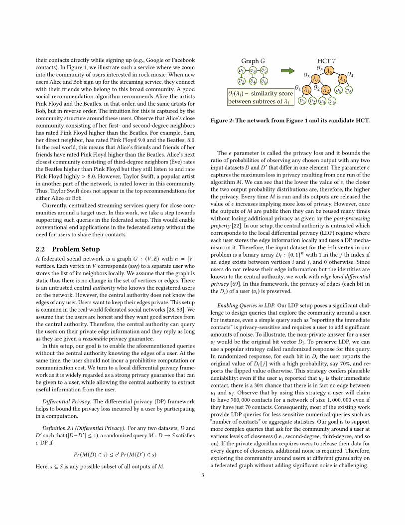
Figure 2: The network from Figure 1 and its candidate HCT.

The 𝜖 parameter is called the privacy loss and it bounds theratio of probabilities of observing any chosen output with any twoinput datasets 𝐷 and 𝐷 ′ that differ in one element. The parameter 𝜖captures the maximum loss in privacy resulting from one run of thealgorithm 𝑀 . We can see that the lower the value of 𝜖 , the closerthe two output probability distributions are, therefore, the higherthe privacy. Every time 𝑀 is run and its outputs are released thevalue of 𝜖 increases implying more loss of privacy. However, oncethe outputs of 𝑀 are public then they can be reused many timeswithout losing additional privacy as given by the post-processingproperty [22]. In our setup, the central authority is untrusted whichcorresponds to the local differential privacy (LDP) regime whereeach user stores the edge information locally and uses a DP mecha-nism on it. Therefore, the input dataset for the 𝑖-th vertex in ourproblem is a binary array 𝐷𝑖 : {0, 1}𝑛 with 1 in the 𝑗-th index ifan edge exists between vertices 𝑖 and 𝑗 , and 0 otherwise. Sinceusers do not release their edge information but the identities areknown to the central authority, we work with edge local differentialprivacy [69]. In this framework, the privacy of edges (each bit inthe 𝐷𝑖 ) of a user (𝑣𝑖 ) is preserved.

Enabling Queries in LDP. Our LDP setup poses a significant chal-lenge to design queries that explore the community around a user.For instance, even a simple query such as “reporting the immediatecontacts” is privacy-sensitive and requires a user to add significantamounts of noise. To illustrate, the non-private answer for a user𝑣𝑖 would be the original bit vector 𝐷𝑖 . To preserve LDP, we canuse a popular strategy called randomized response for this query.In randomized response, for each bit in 𝐷𝑖 the user reports theoriginal value of 𝐷𝑖 [ 𝑗] with a high probability, say 70%, and re-ports the flipped value otherwise. This strategy confers plausibledeniability: even if the user 𝑢𝑖 reported that 𝑢 𝑗 is their immediatecontact, there is a 30% chance that there is in fact no edge between𝑢𝑖 and 𝑢 𝑗 . Observe that by using this strategy a user will claimto have 700, 000 contacts for a network of size 1, 000, 000 even ifthey have just 70 contacts. Consequently, most of the existing workprovide LDP queries for less sensitive numerical queries such as“number of contacts” or aggregate statistics. Our goal is to supportmore complex queries that ask for the community around a user atvarious levels of closeness (i.e., second-degree, third-degree, and soon). If the private algorithm requires users to release their data forevery degree of closeness, additional noise is required. Therefore,exploring the community around users at different granularity ona federated graph without adding significant noise is challenging.

3

3 HIERARCHICAL CLUSTER TREESTo support complex community queries at different granularitieswithout additional noise, we propose to use a well-known datastructure called hierarchical cluster tree (HCT). HCTs are used inmany applications [8, 9, 15, 16, 43, 45, 48, 58, 75, 88]. An HCT cap-tures the idea that the network is a large cluster, which recursivelysplits into smaller clusters of vertices, until only individual verticesremain in each cluster. Thus, one key advantage is that we can learnthe private HCT of the network once and then publicly release it.Any subsequent query on it for various levels of granularity doesnot require additional noise, due to the post-processing property.

To illustrate, in Figure 2 we draw the HCT for the sub-communityfrom our motivating example (Figure 1). Each internal node of theHCT splits the network into two communities, one comprising ofthe leaves in the left subtree and the other from the right subtree.For instance, at the root the whole network is split in to two com-munities with Alice (𝑣2) in the left one and Bob (𝑣6) on the right.Observe that with the increasing depth of the HCT we get users incloser communities. To avoid confusion, we will henceforth referto constituents of the HCT as nodes/links and that of the originalnetwork as vertices/edges.

Let 𝐺 : (𝑉 , 𝐸) be the original network. An HCT for 𝐺 has togroup the vertices in 𝑉 by a measure of similarity/dissimilarity.Different applications can define different similarity notions. Forexample, one natural definition is based on neighbor information—two vertices in 𝑉 are highly similar if they have many commonneighbors in𝐺 . Degree similarity states that two nodes with a largerdifference in degrees are more dissimilar. Modularity measuresthe similarity of two clusters by counting how many more edgesbetween them exist than that predicted in a random graph [60].It is easy to see that members of an isolated clique in 𝐺 will behighly similar to each other by all these definitions. In this work wedesign all our techniques using dissimilarity scores; however, ourtechniques can be extended to the analogous measures of similarity.

Generically, an HCT (𝑇 ) has two components, Λ and \ . Λ is theset of internal nodes and \ is a dissimilarity measure defined asa function that maps internal nodes to a real value. Each internalnode _𝑖 ∈ Λ is associated with two subtrees 𝐿𝑖 and 𝑅𝑖 . Since theleaves of each subtree represent the vertices of the original graph,each internal node represents two sets of clusters, correspondingto the left and right subtrees. Therefore \ (_𝑖 ) can also be thoughtof as the dissimilarity score between two clusters represented by_𝑖 . For instance, in Figure 2 the internal node _3 has two clusters{(𝑣1, 𝑣2), (𝑣3, 𝑣4)}. The \ (_3) represents the dissimilarity betweenthe two clusters at _3. Intuitively, the clusters at lower levels of thehierarchical structure should be more similar to each other thanat the higher levels i.e., closer to the tree root. This can be seenin the graph 𝐺 (sub-community) as well, as 𝑣1, 𝑣2, 𝑣3, 𝑣4 are betterclustered together than the other two vertices 𝑣5, 𝑣6.

Therefore, an HCT is meaningful only if the dissimilarity scoreat an internal node _ is lower than the dissimilarity score at all of itsancestors of _.We call this property as ideal clustering property. Next,we describe traditional algorithms to learn HCTs in the centralizedsetup with and without differential privacy, and the challenges ofextending them to the federated setup with LDP.

3.1 Learning an HCT in the Centralized SetupIn the centralized setup, the authority is trusted and knows theentire graph, i.e., it can query the raw edges in 𝐺 directly. Thecentralized setup offers a reasonable private baseline to compareour eventual solution to learn an HCT in the federated setup.

Even with no DP guarantee, how do we compute𝑇 ? Observe thatthere are combinatorially many (in 𝑛) cluster trees possible for 𝐺 ,since each cluster tree corresponds to a unique way of partitioningthe vertices in the graph. The goal is to find a tree which preservesthe ideal clustering property, and among those which do, find theone which provides the best clustering at each level. Many tradi-tional methods like average linkage [59], which are natural to usein the centralized setup, are ad-hoc and do not provide any quan-titative way of measuring the quality of trees produced. A moresystematic way is the algorithm proposed by Clauset et al. [12, 13]which we refer to as the CMN algorithm. This algorithm is one ofthe most popular for computing hierarchical structures [44, 67, 91],and its DP version is known [86].

The main idea in CMN is to define a cost function, which quanti-fies how good is a cluster tree at clustering similar nodes at eachlevel. For a given graph 𝐺 and a probability assignment function 𝜋 ,the cost of a computed cluster tree 𝑇 is as follows:

CM (𝑇 ) =𝑛−1∏𝑖=1

(𝜋𝑖 )𝐸𝑖 (1 − 𝜋𝑖 )𝐿𝑖𝑅𝑖−𝐸𝑖 , where 𝜋𝑖 = 𝜋 (_𝑖 )

Here, 𝐿𝑖 and 𝑅𝑖 are the number of leaves in the left and rightsub-trees at the 𝑖-th internal node _𝑖 in 𝑇 . 𝐸𝑖 is the number ofedges between the two clusters represented by _𝑖 . The probabilityfunction 𝜋 assigns a probability score at each internal node _𝑖 whichsignifies the probability of an edge existing between a leaf (vertex)in the left subtree at _𝑖 and another vertex in the right. When thegraph is available, 𝜋𝑖 is computed as 𝜋𝑖 = 𝐸𝑖

𝐿𝑖 ·𝑅𝑖 . We will refer toedges that have one node in the left sub-tree and one in the rightsub-tree as edges "crossing the clusters" rooted at _𝑖 . The function𝜋𝑖 gives a probabilistic interpretation to the cost function—it isthe probability of an edge crossing the clusters rooted at _𝑖 , forany graph (not necessarily 𝐺) that can be sampled using 𝑇 and 𝜋 .Therefore, CM is the likelihood of sampling a graph using 𝑇 and 𝜋 .

A tree that optimizes this cost function given the underlyinggraph 𝐺 , will sample 𝐺 that has the maximum likelihood amongall graphs with 𝑛 nodes. Therefore, the CMN algorithms employsthe principle of maximum likelihood estimation to find a 𝑇 and 𝜋conditioned on the given graph 𝐺 as evidence. Maximizing CMby enumeratively evaluating it on the space of all possible clustertrees is intractable. Therefore, the CMN algorithm optimizes forCM using a Markov chain Monte Carlo (MCMC) sampling proce-dure [56]. The MCMC sampling procedure is shown to converge inexpectation to the desired 𝜋 for which 𝐺 maximizes the likelihood.

CMN-DP. The DP version of this algorithm is the state-of-the-artsolution in the computation of differentially private hierarchicalstructures [86]. This is our centralized DP baseline method and wecall itCMN-DP. Specifically, theCMN-DP simulates the exponentialmechanism of differential privacy [22] by following a similarMCMCprocedure to maximize CM , and adds noise to the edge counts 𝐸𝑖after convergence for computing the probabilities 𝜋 . Details of

4

this algorithm are elided here; we refer interested readers to priorwork [86]. The key point is that both the computation of CMN andCMN-DP assume access to the raw edge information of𝐺 . Now weask, can we extend CMN-DP to the LDP setup?

3.2 Challenges: from CMN-DP to LDPThe cost function CM depends on the probability assignment func-tion 𝜋 to measure the “closeness” between two clusters and 𝜋 usesfine-grained private information such as computing the exact num-ber of interconnecting edges between the two clusters. To computethis fine-grained information in the federated setup, the users fromone of the clusters can be asked to report the counts of their neigh-bors in the other cluster after adequately noising them for satisfyingLDP. For instance, in Figure 2, the number of edges (𝐸3) crossing theinternal node _3 can be calculated using the edge counts reported byusers 𝑣1, 𝑣2, 𝑣3, 𝑣4 that cross _3. However, searching for an optimal𝑇 that optimizes for CM requires computing the interconnectingedges for all possible sets of clusters in the worst case. Concretely,CMN-DP implements an iterative search procedure that queriesa user for edge information thousands of times before convergingto the optimal 𝑇 . While this search works in the centralized setupwhere the graph is available, it is not feasible in the federated setupfor two reasons. First, answering every differentially private queryleads to a privacy loss and over many such queries the aggregatedprivacy loss will be high [22]. To exemplify, a thousand querieswith an 𝜖 = 0.1 for each query will lead to an aggregated epsilon𝜖 > 20 with 99% probability, as given by the advanced compositiontheorem [22]. We consider 𝜖 ≤ 2 as reasonable [37] 1, althoughprior works have considered up to 𝜖 = 8 [1]. Second, the searchprocedure for finding the optimal 𝑇 is iterative so the users haveto be available for many iterations of the search to compute thecloseness.

4 OUR SOLUTIONOur key ideas to tackle the aforementioned challenges are two-fold. First, instead of using a fine-grained probability assignmentfunction 𝜋 , we propose a coarse-grained method to compute thecloseness between two clusters such that the users need not bequeried repeatedly for their neighbors. Second, we propose to re-place the cost function CM with another cost function that canwork with any coarse-grained method that captures the closenessbetween two clusters. These two observations enable us to designa novel hierarchical clustering algorithm which only queries theusers once and the rest of the iterative search for an optimal treehappens on the server side. We detail our insights next.

4.1 Key InsightsOur first insight is to use a good coarse-grained approximation forcloseness that can be obtained for a cheap privacy budget. We startfrom a construct called degree vectors, previously proposed in theLDP setup [69]. The degree vectors are a generalized version ofdegree counts, wherein the vertices are randomly partitioned into𝐾 bins (each bin has at least one vertex), and each user is asked toreport how many neighbors it has in each bin. For𝐾 = 1 this degree1Usually, an 𝜖 = 2 allows an attacker to infer a random bit of the training sample (inthis case an edge for each user) with 86% probability.

(a) Close clusters (b) Distant clusters

Figure 3: (a) Two close clusters, high 𝜋 , have more intercon-necting edges than two distant ones. (b) Average dissimilar-ity\ using𝐿1-normof degree vectors also captures closeness.

vector has one element and it yields just the degrees of the verticesin 𝐺 . For 𝐾 = 𝑛, all nodes would have a unique bin, therefore thedegree vectors will encode the original neighbor list for all vertices.For any 1 < 𝐾 < 𝑛 the idea is to preserve more edge informationthan just degrees and less than the exact edges. Then, the degreevector is noised by the user; a random Laplacian noise 𝐿𝑎𝑝 (0, 1

𝜖 ) isadded to each bin count before sending it to the untrusted authority.The 𝐾 is usually a small value compared to the size of the network,typically ≤ log(𝑛) or a small constant [69]. This is intuitively good,since the noise added to the degree vector is proportional to𝐾 . Nowwe ask: What can we compute with degree vectors?

It is not straightforward to compute CM using degree vectors.Nevertheless, observe that if we take two close clusters with respectto 𝜋 , then on average each user in the left cluster has a lot ofneighbors in the right cluster and vice versa. This notion is readilycaptured by degree vectors. Two vertices have very similar degreevectors if they have many common neighbors. Consequently, if wemeasure the dissimilarity as a 𝐿1-norm between their degree vectorsthen the dissimilarity for such vertices should be low. Therefore,the average dissimilarity across vertices of two close clusters willbe lower than for two far clusters. We illustrate our intuition inFigure 3. Figure 3a shows two clusters with high interconnectingedges, hence the 𝜋 associated with the two is high. Consequently,the average 𝐿1-norm distance, will be less. A similar argument canbe made for Figure 3b. Therefore, we propose using the average𝐿1-norm distance using degree vectors as a good coarse-grainedreplacement for 𝜋 to measure closeness between clusters. Observethat the degree vectors can be constructed just once for each userwhich can then be used to compute the average 𝐿1-norm distancefor any two clusters. This key insight allows us to propose a differentcost function that optimizes for the average 𝐿1-norm distance.

We point to a recently introduced cost function by Dasgupta [17].Dasgupta’s cost function takes a dissimilarity matrix and a tree asinputs and measures the quality of the tree for that dissimilaritymatrix. Our first observation is that this cost function does not needthe fine-grained edge counts between clusters (like CM does). Thesecond and even more important observation is that a tree thatoptimizes Dasgupta’s cost has a specific dissimilarity measure \(defined in Section 3). The measure represents the average dissim-ilarity between the vertices of two clusters computed using thedissimilarity matrix. In fact, we formally show that such a treesatisfies the ideal clustering property as well (Section 4.2). Thus, ifwe use the 𝐿1-norm of degree vectors to compute the dissimilar-ity matrix, then by optimizing for the Dasgupta’s cost we get ourdesired coarse-grained average 𝐿1-norm distance as the \ . So, we

5

Algorithm 1: The outline of GenTree.Input :Dissimilarities matrix 𝑆Output :Hierarchical cluster tree 𝑇 ∗

1 Randomly sample a tree 𝑇0;2 𝑖 = 0;3 while not converged do4 Sample an internal node _ from 𝑇𝑖 ;5 Construct two local swap trees 𝑇𝐿

𝑖+1,𝑇𝑅𝑖+1;

6 Pick one of them at random, call it 𝑇𝑖+1;7 Transition to 𝑇𝑖+1 with min(1, 𝑒CD (𝑇𝑖+1)−CD (𝑇𝑖 ) );8 𝑇 ∗=𝑇𝑖 ;9 𝑖 = 𝑖 + 1;

10 end11 return 𝑇 ∗

directly arrive at a tree which minimizes the distance between theclose clusters and maximizes the distance between the far ones.

Using these insights, we design a novel randomized algorithm tosample a differentially private HCT that optimizes Dasgupta’s costfunction after querying a degree vector from each user. To sum-marize, we have shown a way to avoid multiple privacy-violatingqueries in learning an HCT by designing another learning strategythat allows us to replace the fine-grained queries with a coarse-grained one that preserves the ideal clustering property.

4.2 Dasgupta’s Cost FunctionWe now formulate the Dasgupta’s cost function considering onlyfull binary trees, and when a dissimilarity matrix is given as input.

Definition 4.1 (Dasgupta’s Cost Function (CD )). The cost of atree 𝑇 : (Λ, \ ) with respect to a graph 𝐺 with a non-negativedissimilarity matrix 𝑆 is given by

CD (𝑇 ) =∑︁

𝑥 ∈𝑉 ,𝑦∈𝑉𝑆 (𝑥,𝑦) · |leaves(𝑇 [𝑥 ∨ 𝑦]) |

where 𝑇 [𝑥 ∨ 𝑦] is least common ancestor of 𝑥,𝑦.

The expression is a weighted sum of dissimilarities of each pair ofvertices, weighted by the number of leaves in the subtree of the leastcommon ancestor of the pair of vertices. The idea of maximizing CDis intuitive. Any pair of vertices (𝑥,𝑦) which are highly dissimilar toeach other will have a high dissimilarity score 𝑆 (𝑥,𝑦) and therefore,their least common ancestor node (which we denote by 𝑇 [𝑥 ∨𝑦]) should have more leaves in order to maximize the product𝑆 (𝑥,𝑦) · |leaves(𝑇 [𝑥 ∨ 𝑦]) |. It has been shown that, an optimal treewith respect to CD has several nice properties such as: 1) Twodisconnected components in the graph will be separated completelyinto two different clusters; 2) The cost of every tree for a cliqueis the same; and, 3) it represents the clusters well in the plantedpartition model [17]. Property 2) is the most relevant to us, as wewill use it to bound the utility loss.

Originally, the cost function was designed for a non-negativesimilarity matrix with no restriction on the tree space. In the dis-similarity case, if we allow all possible trees then there is always a

Figure 4: The possible swaps of a tree.

trivial tree that maximizes this function, i.e., the star graph withonly one internal root node. Nevertheless, all the above propertieshold in the dissimilarity case when the tree space is restricted tothe full-binary trees [14].

More importantly, notice that the cost function does not requireany edge information of the graph but only a dissimilarity matrix, akey requirement for the design of our algorithm in the decentralizedsetting.As stated previously, we show that the tree𝑇 that maximizesCD also satisfies the ideal clustering property. Further, the \ ofsuch a tree will just be the average dissimilarity between the nodesof two subtrees at each internal node _. Formally, Theorem 4.2captures both these observations.

Theorem 4.2. Given a graph𝐺 : (𝑉 , 𝐸) and a dissimilarity matrix𝑆 , the tree 𝑇𝑂𝑃𝑇 : (Λ, \ ) that maximizes CD preserves the idealclustering property with

\ (_) =∑𝑥 ∈𝐿,𝑦∈𝑅 𝑆 (𝑥,𝑦)

|𝐿 | · |𝑅 |where 𝐿, 𝑅 are the left and right subtrees of _.

The full proof is provided in the Appendix A.1. The theorem isproved by contradiction. Assuming that there exists a CD -optimaltree 𝑇 with two internal nodes _1, _2; _2 = 𝑎𝑛𝑐𝑒𝑠𝑡𝑜𝑟 (_1) such that\ (_1) < \ (_2), we can always construct another tree 𝑇 ′ with ahigher cost than𝑇 . In fact, if𝑇 were the configuration 𝐿 in Figure 4then 𝑇 ′ would be one of the other configurations.

Theorem 4.2 constitutes our first key analytical result. It explainswhy we choose Dasgupta’s cost function and degree vectors to-gether. Next, we describe our algorithm GenTree to learn a treethat maximizes this cost function. GenTree is an independent con-tribution of this work which can be used with any dissimilaritymetric that captures closeness between clusters.

4.3 The GenTree AlgorithmFinding a hierarchical cluster tree that maximizes CD is known tobe NP-hard [17]. Let T be the set of all possible full binary treesthat have 𝑉 as leaves. We want to find the optimal tree 𝑇𝑂𝑃𝑇 ∈ Tthat maximizes CD . The number of possible trees including allthe permutations from internal nodes to leaves is at most 2𝑐𝑛𝑙𝑜𝑔𝑛 ,where 𝑐 = 𝑂 (1) is a small constant.

We propose a randomized algorithmGenTreewhich will samplefrom the distribution of all possible trees such that the sampleprobability is exponential in the cost of the tree. Therefore, if thecost of the tree is high then the sample probability is exponentiallyhigh. This distribution is known as Boltzmann (Gibbs) distributionand we choose it since it enables bounding the utility loss as we

6

Algorithm 2: Outline for PrivaCTInput :Graph 𝐺 , dissimilarities matrix 𝑆Output :Hierarchical cluster tree 𝑇 ∗

1 Aggregator: Randomly partition 𝐺 to 𝐾 = ⌊log𝑛⌋ bins;2 Aggregator: Show the 𝐾 partitions to the user;3 User: Send DP degree vectors with 𝐿𝑎𝑝 (0, 1

𝜖 ) noise;4 Aggregator: Compute dissimilarities 𝑆 using 𝐿1-norm;5 Aggregator: Compute 𝑇 ∗ = GenTree(𝑆) and release 𝑇 ∗

show later. Hence, GenTree samples a tree𝑇 ′ ∈ T with probability

𝑃𝑟 (𝑇 ′ ∈ T) = 𝑒CD (𝑇 ′)∑𝑇 ′′∈T 𝑒CD (𝑇 ′′)

GenTree creates samples from this distribution by using aMetro-polis-Hastings (MH) algorithm based on a Markov chain with statesas trees and state-transition probabilities as ratio of costs betweenthe states. The outline for GenTree is given in Algorithm 1. First, itstarts with a randomly sampled tree𝑇0. In each iteration, it samplesa random internal node _ and does a local swap into one of theconfigurations as shown in Figure 4. Observe that in a local swap, asubtree at the chosen internal node is detached and swapped withthe subtree at the parent internal node leading to two possible localswaps. This state transition (swap) between the trees𝑇𝑖 ,𝑇𝑖+1 is donewith a probability min(1, 𝑒CD (𝑇𝑖+1)−CD (𝑇𝑖 ) ) which is the ratio of thecosts of the two states. This follows the standard MH procedure.

Our chosen stationary distribution ensures that every state has apositive probability of being sampled. Further, every full binary treecan be obtained from another by a sequence of swaps therefore theentire chain is connected. Consequently, a standard analysis [56]leads to the conclusion that the Markov chain induced by GenTreeis ergodic and reversible. Therefore, GenTree will converge to itsstationary distribution, which in our case is the Boltzmann distri-bution, given enough time. We present the differentially privateversion of GenTree next.

4.4 The PrivaCT AlgorithmGenTree only requires a dissimilarity matrix to operate on. Toconstruct a private hierarchical cluster tree using GenTree we canfirst construct private dissimilarity matrix. Recall that any compu-tation on a differentially private output is also differentially privateusing the post-processing property. Using the same property, wecan construct a private dissimilarity matrix from private degreevectors. For that purpose, the central aggregator first sends a ran-dom partition of the users, with each bin having a set of users, toevery user. Using these bins, every user constructs a private de-gree vector by counting their neighbors in each bin and addingLaplacian noise 𝐿𝑎𝑝 (0, 1

𝜖 ) to these counts. Finally, the users sendtheir vectors to the aggregator so that the dissimilarity of everypair of users can be computed as measured by the 𝐿1-norm of theirrespective degree vectors. The outline of PrivaCT is summarizedin the Algorithm 2. Notice that, the aggregator just requires theusers to compute degree vectors privately so that GenTree can berun on the server side to compute a private hierarchical cluster tree.Further, PrivaCT requires a transfer of 𝑂 (𝑛) bits of informationbetween each user and the authority.

5 THEORETICAL BOUND ON UTILITY LOSSGenTree and PrivaCT are randomized algorithms. So, we needto show that they learn trees that are close to the ideal tree thatoptimizes CD given the dissimilarity matrix computed using nondifferentially private degree vectors. The utility loss is given by thecost difference between the ideal tree and the trees sampled by ouralgorithms. Therefore, we bound the following:

(1) GenTree: The utility loss for the tree output by the algo-rithm when dissimilarity matrix is not noised.

(2) PrivaCT: The utility loss for the tree output by the algo-rithm when the dissimilarity matrix is noised.

For ease of analysis, we enforce the dissimilarity between twovertices of the graph to be at least 12, i.e., the 𝐿1-norm betweentwo degree vectors is at least 1 instead of 0. Therefore, a clique willhave a dissimilarity of 1 for all pairs of nodes. Following this, westate a fact that is proved in the original Dasgupta’s work [17].

Theorem 5.1. The cost of a clique with all dissimilarities 1 is samefor all possible trees and is equal to

CD (𝑇𝑐𝑙𝑖𝑞𝑢𝑒 ) =𝑛3 − 𝑛

3This is the least optimal cost tree that can be produced with any

dissimilarity matrix under our assumption, i.e., 𝑆 (𝑣𝑖 , 𝑣 𝑗 ) ≥ 1. Forreal-world graphs, the optimal tree cost can be many times higherthan CD (𝑇𝑐𝑙𝑖𝑞𝑢𝑒 ) depending on the dissimilarity matrix. This isuseful in our proofs later. From here, we represent CD (𝑇𝑐𝑙𝑖𝑞𝑢𝑒 )with 𝜌 for brevity. We now analyze the utility loss for GenTree.

5.1 Utility Loss: GenTreeThere is always an ideal full binary tree that maximizes the Das-gupta cost function given the dissimilarity matrix, say 𝑇𝑂𝑃𝑇 with𝑂𝑃𝑇 = CD (𝑇𝑂𝑃𝑇 ). The GenTree is a randomized algorithm whichsamples different tree 𝑇 at convergence in every run. Therefore,the expected utility loss is the difference between 𝑂𝑃𝑇 and theexpected value of the cost of obtained tree E𝑇 [CD (𝑇 )]. We nowshow that the expected CD cost of the sampled tree at convergenceis close to 𝑂𝑃𝑇 and is concentrated around its expectation.

The expected cost of a sampled tree is less than 𝑂𝑃𝑇 only by atmost a small factor 𝑐 ·𝑙𝑜𝑔 (𝑛)

𝑛2−1 of the 𝜌 , where 𝑐 ≪ 𝑛. The completeproofs for the theorems are provided in the Appendix A.1. Here,we explain the key ideas used in the proofs.

Theorem 5.2. GenTree outputs a tree 𝑇 whose expected costE𝑇 [CD (𝑇 )] is a (1 − 𝑙𝑜𝑔 (𝑛)

𝑛2−1 ) multiplicative factor of 𝑂𝑃𝑇 .

E𝑇 [CD (𝑇 )] ≥ (1 − 𝑐 · 𝑙𝑜𝑔(𝑛)𝑛2 − 1

) ·𝑂𝑃𝑇

To prove this, we first show that the probability of sampling asub-optimal tree is exponentially decreasing.

Lemma 5.2.1. The probability of sampling a tree𝑇 with cost𝑂𝑃𝑇 −𝑐 ′ · 𝑛 · log(𝑛) decreases exponential in 𝑛.

𝑃𝑟 (CD (𝑇 ) ≤ 𝑂𝑃𝑇 − 𝑐 ′ · 𝑛 · log(𝑛)) ≤ 𝑒−𝑛 ·log(𝑛)

2We enforce this in our implementation for correctness.

7

Lemma 5.2.1 implies Theorem 5.2 and it also says that the utilityloss is concentrated around its expectation. This is a consequenceof choosing Boltzman distribution as the stationary distributionfor GenTree. The probability of sampling any sub-optimal treeexponentially reduces with its cost distance from the optimal cost.

5.2 Utility Loss: PrivaCTPrivaCT samples trees based on the probabilities that are expo-nential in the cost of tree computed on the differentially privatedissimilarities. Hence, the probability of sampling a tree 𝑇 willnow depend on the noisy cost, say 𝑔(𝑇 ) = CD (𝑇 ) instead of theactual cost 𝑓 (𝑇 ) = CD (𝑇 ). Let the variables 𝑆 and 𝑆 be the dis-similarity and noisy dissimilarity matrices that store dissimilari-ties between vertices of the network. Recall that the dissimilaritybetween two vertices is computed as 𝐿1-norm of their degree vec-tor counts. The cost computed with original dissimilarity matrixis 𝑓 (𝑇 ) =

∑𝑖 𝑗 𝑆 (𝑣𝑖 , 𝑣 𝑗 ) · leaves(𝑇 [𝑣𝑖 ∨ 𝑣 𝑗 ]) whilst the cost com-

puted by the noisy dissimilarity matrix is 𝑔(𝑇 ) =∑𝑖 𝑗 𝑆 (𝑣𝑖 , 𝑣 𝑗 ) ·

leaves(𝑇 [𝑣𝑖 ∨ 𝑣 𝑗 ]). If 𝑇𝑑𝑝 is the sampled tree at convergence thenthe expected utility loss is computed by taking the difference be-tween 𝑂𝑃𝑇 and E𝑇𝑑𝑝 [𝑓 (𝑇𝑑𝑝 )]. In essence, we are saying that thetree sampled with differentially private dissimilarity matrix shouldnot be away from the optimal tree with respect to the cost computedusing the non-noised or actual dissimilarities. Formally,

Theorem 5.3. Let𝑇𝑑𝑝 be the output of PrivaCT and 𝜌 = CD (𝑇𝑐𝑙𝑖𝑞𝑢𝑒 )be the minimal cost of any hierarchical cluster tree. The expected util-ity loss of PrivaCT is concentrated around its mean with a highprobability and is given by

𝑂𝑃𝑇 − E𝑇𝑑𝑝 [𝑓 (𝑇𝑑𝑝 )] ≤2𝐾𝜖

·(

32+ 6√𝐾

)· 𝜌

In order to prove the bound, we start by first bounding theexpected value of 𝑔(𝑇 ) over the randomness in degree vectors, interms of 𝑓 (𝑇 ). Let 𝑅𝑖 denote the random variable that representsthe Laplacian noise added by 𝑖𝑡ℎ vertex to its degree vectors and𝑅 = (𝑅1, 𝑅2, . . . , 𝑅𝑛).

Lemma 5.3.1. The expectation |E𝑅 [𝑔(𝑇 )] − 𝑓 (𝑇 ) | over randomness𝑅 is bounded by

|E𝑅 [𝑔(𝑇 )] − 𝑓 (𝑇 ) | ≤3𝐾2𝜖

· 𝜌

Then we bound the variance of 𝑔(𝑇 ).

Lemma 5.3.2. The variance of 𝑔(𝑇 ) is bounded by

Var𝑅 [𝑔(𝑇 )] ≤4𝐾𝜖2 · 𝜌2

Finally, we use the Chebyshev’s inequality to bound the valueof 𝑔(𝑇 ) in terms of 𝑓 (𝑇 ).

Lemma 5.3.3. The 𝑔(𝑇 ) is in the interval [𝑓 (𝑇 ) − 𝑃, 𝑓 (𝑇 ) + 𝑃]with a high probability where 𝑃 is,

𝑃 =𝐾

𝜖·(

32+ 6√𝐾

)· 𝜌

Table 1: Dataset graph statistics

Network Domain #Nodes #Edges Densitylastfm social graph 1843 12668 0.0075delicious social graph 1503 6350 0.0056douban social graph 2848 25185 0.0062

Table 2: The quality of HCT evaluated using Dasgupta costfunction. The utility loss is at most 10.87% for a small 𝜖 = 0.5.

Network 𝜖RelativeUtility

EmpiricalUtility Loss (LDP)

lastfm0.5

22.829.57

1.0 4.052.0 1.45

delicious0.5

12.2010.87

1.0 6.612.0 3.29

douban0.5

28.837.09

1.0 3.272.0 1.14

We then use this lemma to prove Theorem 5.3. Note that theutility loss does not depend on the dissimilarity matrix but onlydepends on the parameters 𝐾 and 𝜖 . It can be seen that if 𝜖 is veryhigh then the utility loss converges to that of theGenTree and evenif 𝜖 tends to zero, our artificial bounding of the dissimilarities to begreater than 1 will ensure that the final tree cost never goes below𝜌 . Recall that 𝑂𝑃𝑇 is several times more than 𝜌 for the real-worldgraphs as it depends on the dissimilarity matrix, i.e., the structureof the graph. We empirically observe that the utility loss is smallerthan our bound for all of our evaluated graphs (see Section 6).

6 EVALUATION: QUALITY OF PRIVATE HCTIn this section, our goal is to evaluate the utility of PrivaCT asmeasured by the quality of the HCTs it produces.

First, we want to evaluate the quality of the private HCTs thatPrivaCT generates vs. the non-DP HCTs that GenTree generates.Our algorithms use a different cost function (Dasgupta’s CD ) thanthe centralized baseline that allows us to bound the utility loss the-oretically (Section 5). Here, we measure the utility loss empiricallywith respect to the HCT generated by GenTree as measured byCD . Secondly, we want to evaluate the utility-privacy trade-off ofthe LDP regime vs. the centralized DP setup. Thus, we comparethe quality of the private HCTs that PrivaCT generates with LDPguarantees and the trees generated by the centralized DP algorithmCMN-DP for the same privacy budget. In order to compare thesetrees, we use the cost function CM which measures closeness be-tween two clusters using the fine-grained edge counts as opposedto our coarse-grained degree vectors (see Section 3.1). In summary,we ask the following:

(EQ1) What is the empirical utility loss of the private HCTsproduced by PrivaCT vs. the non-DP HCTs produced by GenTree?

(EQ2) What is the quality of the private HCTs produced byPrivaCT vs. the centralized DP algorithm CMN-DP?

8

0 500 1,000−7.5

−7

−6.5·104

steps/𝑛

logC M

lastfm

0 500 1,000−3.9

−3.8

−3.7

·104

steps/𝑛

logC M

)

delicious

0 500 1,000

−1.5

−1.4

−1.3·105

steps/𝑛

logC M

)

douban

LDP,𝜖 = 0.5 LDP,𝜖 = 1.0 LDP,𝜖 = 2.0 DP,𝜖 = 0.5 DP,𝜖 = 1.0 DP,𝜖 = 2.0

Figure 5: The PrivaCT (marked as LDP) and the CMN-DP (marked as DP) evaluated with log CM at each step of the MCMCprocess for 3 values of 𝜖 ∈ {0.5, 1.0, 2.0}. Higher values of log CM signify smaller loss, so better trees. PrivaCT produces treeswith a better CM cost than the baseline CMN-DP for all values.We also observe that PrivaCT converges within 400 MCMC steps.

Experimental Setup. We use 3 real-world networks which arecommonly used for evaluating recommender systems [52, 69, 75,82] 3. We detail the networks in Table 1. We use privacy budgetvalues of 𝜖 ∈ {0.5, 1.0, 2.0} as they have been used in the priorwork for both centralized as well as the local differential privacysetup [1, 35, 86]. We have two tunable parameters: the number ofbins 𝐾 and the convergence criteria for MCMC in GenTree. The𝐾 is chosen such that it minimizes the noise in the final degreevector as well as it minimizes the number of collisions in the degreevector calculation. A higher 𝐾 minimizes the collisions but incursmore noise on aggregate and vice versa. Previous work has shownthat the value of 𝐾 is usually small and it depends on the graphstructure. We therefore heuristically choose 𝐾 = ⌊log𝑛⌋ as it is nottoo low for not capturing any edge information (see Section 4.1)and not too high so that we might end up adding a lot of noise (seeSection 2.2). If we substitute this 𝐾 value in our utility bound forPrivaCT in Theorem 5.3, we get a loss scaling with log𝑛

𝑛 ·𝜖 . Further,our values of 𝐾 agree with the ones used in the prior work [69]. Weuse a convergence criteria that is similar to the ones used by priorworks in the centralized setting for their MCMC algorithm [13, 86].

Quality of LDP vs. non-DP. We show that the observed cost ofthe differentially private tree generated by PrivaCT, for all valuesof 𝜖 is very close to the cost of the tree generated by the non-DPversion of the algorithm GenTree.

We define the empirical utility loss as |CD (𝑇𝑑𝑝 )−CD (𝑇 ) |CD (𝑇 ) , where

CD (𝑇𝑑𝑝 ) is the cost of the private HCT and CD (𝑇 ) is the costthe non-private tree. Recall that the cost of least optimal tree 𝜌corresponds to that the tree obtained from a clique. Thus, while wecannot compute the optimal tree, we can compute its relative utilitywith respect to the cost 𝜌 as CD (𝑇 )

𝜌 . The higher this value, the betterthe non-private tree is. In Table 2, we observe that the empiricalutility loss is less than 10.87% for all networks and values of 𝜖 weevaluated. The empirical utility loss is approximately 0.08 − 1.67%on average for 𝜖 = 2.0. This confirms that empirically PrivaCTgenerates trees with a small loss of utility. The empirical loss is

3https://grouplens.org/datasets/hetrec-2011/

within the provided conservative theoretical bounds, but, tighteningthe theoretical bounds remains promising future work.

Result 1: The empirical utility loss between the DP and non-DP versionis less than 10.87% for all the graphs and 𝜖 values.

Quality of LDP HCTs vs centralized DP HCTs. Our main resultis that our LDP algorithm produces trees that have a better utilitycost than the ones produced by the centralized DP algorithm asmeasured by the baseline CM cost. Both our non-DP and LDP algo-rithms generate trees while optimizing for a different Dasgupta’scost function. In Figure 5, we show that the log CM of the treesgenerated by PrivaCT have better utility than trees generated byCMN-DP for all values of 𝜖 ∈ {0.5, 1.0, 2.0} across all 3 graphs.

Result 2: The CM cost of the trees generated by our PrivaCT is betterthan the baseline CMN-DP for all evaluated graphs and 𝜖 values.

7 APPLICATION: RECOMMENDER SYSTEMSWe revisit the motivating example of social recommendation fromSection 2 and ask “Can PrivaCT be utilized for providing recom-mendations in the federated setup?” The goal is to accurately predictthe top-𝑘 recommendations for the target users. The target usersshare their preferences/tastes with the recommender system but donot want to share their private contacts. Therefore, this naturallyfalls in the edge-LDP setup.

We consider two scenarios: cold-start and existing users. Re-call that the cold-start scenario occurs when a new user with nohistory of interactions with the service provider has to be servedrecommendations. In contrast, existing users have a history of in-teractions that convey their interests. Specifically, we evaluate theutility of the PrivaCT algorithm for social recommendations byasking the following questions:

(EQ1) For cold-start, are the top-𝑘 recommendationswith PrivaCT-based algorithm better than the non-social baseline?

(EQ2) For existing users, can we improve the top-𝑘 recommenda-tions over the non-social baselines with PrivaCT-based technique?

9

Datasets. We use the same datasets mentioned in Section 6 asthey are commonly used for social recommendations. For lastfmand delicious which are implicit feedback ratings we normalizethe weight of each user-artist and user-bookmark link by dividingthe maximum number of plays/bookmarks of that user across allartists/bookmarks. For douban with explicit feedback ratings wenormalize the ratings by dividing with the maximum rating (5.0).

Experimental Setup. We split the datasets in training and test sets.We perform k-fold cross-validation for 𝑘 = 5 splits of the datasets.For the HCT computation, we use a privacy budget of 𝜖 = 1 andwe average results over HCTs computed for 3 random seeds.

Evaluation Metrics. To evaluate our recommendations we usemean average precision (MAP) and normalized discounted cumula-tive gain (NDCG). These two metrics are widely used to evaluatethe quality of the top-𝑘 recommendations. Higher values of thesemetrics imply better recommendations. Due to space constraints,we explain how these are computed in Appendix A.2.

Next, we describe our baseline and PrivaCT-based algorithm,and then present our results on our social recommendation datasets.

7.1 Collaborative FilteringWe implement a widely used technique for recommender systemscalled collaborative filtering (CF) [72, 73]. In particular, we considermemory-based CF techniques that operate on user-item ratingmatrices tomake top-𝑘 recommendations.We choose this techniquebecause it generally yields good performance, forms the basis of real-world recommender systems such as Netflix [72], Facebook [23].

CF for cold start. In this scenario, the target users have no historyof rated items. We choose two popular strategies, “recommendhighest rated items” (itemAvg) and “recommend highest rated itemsamong your friends” (friendsCF ). Notice that these two methodscorrespond to two different granularities of the “close” community.itemAvg considers the entire network where as the friendsCF takesonly the neighbors.

For friendsCF , if 𝑆 : 𝑈 ×𝑈 → {0, 1} is the social relation functionand 𝑆 (𝑢 ′, 𝑢) = 1 if the users (𝑢,𝑢 ′) are friends and 0 otherwise,then the rating 𝑟𝑢,𝑖 is computed as follows:

𝑟𝑢,𝑖 = 𝑟 𝑖 +∑𝑢′∈U 𝑆 (𝑢 ′, 𝑢) (𝑟𝑢′,𝑖 − 𝑟𝑢′)∑

𝑢′∈U 𝑆 (𝑢 ′, 𝑢)

where 𝑟 𝑖 =∑

𝑢′∈U 𝑟𝑢′,𝑖|U | is the average rating of item 𝑖 , 𝑟𝑢′ =

∑𝑖∈I 𝑟𝑢′,𝑖|I |

represents the average item rating for user 𝑢 ′, I is the set of itemswith a rating from user 𝑢 ′ and U ⊆ 𝑈 is the set of users that havea rating for item 𝑖 . For itemAvg, we just replace 𝑆 (𝑢 ′, 𝑢) with 1 forall 𝑢 ′ ∈ U. Note that itemAvg is a private baseline as no one sharestheir social relations where as friendsCF is a non-private baseline.

CF for existing users. When the user is present in the platform,we can leverage both their ratings and social connections to makebetter recommendations. In this case, we use one of the state-of-the-art social recommendation algorithm called SERec [82]. SERecfirst models the user exposures to the items and then uses these ex-posures to guide the recommendation. The exposures are computedbased on the social information rather than the rating history. Due

to space constraints, we refer the reader to the paper for more de-tails. We use a popular Python implementation4 which follows theoriginal implementation. This represents the non-private baselinefor social recommendations for existing users.

7.2 Collaborative Filtering with PrivaCTThe close community to which a target user belongs can be queriedfrom an HCT which is typically the clusters at the lower levelsof the HCT. We can control the granularity of “closeness” by thepopular query “Who are the𝑚 5 nearest neighbors for user 𝑢𝑖?”.This can be answered with a set 𝑁 (𝑢𝑖 ) : (𝑛1, 𝑛2, ..., 𝑛𝑚) where 𝑛1belongs to the closest community of 𝑢𝑖 , 𝑛2, ..., 𝑛 𝑗<𝑚 in the secondclosest community and so on. This query forms the main insightfor recommendations based on PrivaCT.

We propose a simple strategy to replace the privacy invasivealgorithms that depend on direct social relations into a differentiallyprivate one. Specifically, we query the PrivaCT-based HCT to givethe 𝑚 nearest neighbors to the target user 𝑢𝑖 and use them forrecommendations. We use this strategy to replace our baselineswith and without cold-start.

(1) For friendsCF , we select 𝑚 closest users 𝑁 (𝑢𝑖 ) for eachtarget user 𝑢𝑖 based on HCT and we employ the formulaused by friendsCF with 𝑆 (𝑢 ′, 𝑢) = 1.0 when 𝑢 ′ ∈ 𝑁 (𝑢𝑖 ).

(2) For SERec, we do the same as above i.e., replace the imme-diate social contact with the closest users in HCT and feedit to the algorithm.

For both the above strategies we choose𝑚 as the degree of thetarget user 𝑢𝑖 in order to consider similar number of neighborsto the baseline strategies to be fair. Recall that the degree of auser can be estimated from its degree vector we computed forPrivaCT. However, in the real world𝑚 is application dependentand might require domain expertise or online testing to estimatean ideal value. Note that our insights can be used in any algorithmthat depends on social contacts for recommendations. Furthermore,recommendation algorithms can be designed using the privateHCT with the availability of additional information such as nodeattributes. We leave that for future work.

We are aware of only one prior work that aims to design socialrecommendation algorithms in the LDP setup. LDPGen, whichappeared at CCS 2017, uses differentially private synthetic graphsfor recommendations [69]. It uses the direct graph edge informationin the synthetically generated graphs for recommendations, unlikeour work. The data structure they compute (synthetic graph) isfundamentally different from ours (hierarchical cluster tree) andtherefore, their recommendation algorithm as well. However, adirect comparison to LDPGen is not possible. LDPGen does notaccompany any publicly available implementation. After our severalattempts to implement it faithfully, we were unable to reproducefindings reported therein. Furthermore, the presented theoreticalanalysis in the LDPGen paper has flaws, which were confirmedin private communication with one of the authors of LDPGen.We detail both our experimental effort and observed theoreticalinconsistencies of that work in Appendix A.3.

4https://github.com/Coder-Yu/RecQ5popularly known as 𝑘 nearest neighbors. We use𝑚 because 𝑘 is used elsewhere.

10

Table 3: Results for the two cold start setup. PrivaCT-CF is a1 − 390× better than the itemAvg which shows the utility ofusing community information from the private HCT.

Top-100 itemAvg friendsCF PrivaCT-CF

lastfmNDCG 5.33E-04 1.58E-01 6.21E-02MAP 2.56E-05 4.03E-02 8.63E-03

deliciousNDCG 8.80E-04 6.70E-03 9.00E-04MAP 7.18E-05 8.00E-04 6.59E-05

doubanNDCG 2.00E-04 7.49E-02 7.800E-02MAP 1.46E-05 1.87E-02 2.000E-02

Table 4: PrivaCT-SERec is 2.16 − 17.95× better than the non-social baseline (Basic SERec) and comparable to the non-private baseline SERec.

Top-100 Basic SERec SERec PrivaCT-SERec

lastfmNDCG 0.1223 0.3249 0.3270MAP 0.0240 0.1405 0.1419

deliciousNDCG 0.0058 0.0135 0.0150MAP 0.0021 0.0048 0.0045

doubanNDCG 0.0349 0.2466 0.2469MAP 0.0052 0.0929 0.0930

7.3 Performance of PrivaCT-based CFOur main finding is that in both evaluated scenarios, cold startand existing users, our PrivaCT-based algorithms can be used forsocial recommendations with almost no utility loss for a privacybudget 𝜖 = 1. In both scenarios for all evaluated networks, PrivaCT-based algorithms perform 0.9− 390× better (as per NDCG) than thenon-social recommendation baselines where recommendations arecomputed without social information. Compared to the non-privatebaselines that do use the social links, PrivaCT is either on par withstate-of-the art algorithm (SERec) in the existing users case or noworse than 7.44× for cold start (for NDCG, or 12.1× for MAP).

For cold start CF, PrivaCT-CF outperforms the private baselineitemAvg by 1.1 − 390× across all datasets for NDCG and 0.9 − 1.35 ·103× for MAP (Table 3). The reason is that the close communitiesextracted by PrivaCT through the HCT are a good proxy of simi-larities between users, whereas itemAvg is a simple average overthe items. For lastfm, the non-private friendsCF is 2.54× better inNDCG score than PrivaCT-CF and, respectively, 7.44× better fordelicious. Similarly, for lastfm, the non-private friendsCF is 4.67×better in MAP score than PrivaCT-CF and, respectively, 12.1× bet-ter for delicious. For douban, PrivaCT-CF is 1.1× better than thefriendsCF in NDCG score, and 1.1× in MAP.

Result 3: For cold-start users, PrivaCT-CF’s recommendations arebetter than the non-social baseline for all networks across all metrics.

For existing users, PrivaCT-SERec is performing on par withthe non-private state-of-the-art algorithm SERec for top-100 rec-ommendations for all 3 datasets (see Table 4). These results showthat the similarity between users as captured by the communitiesof our private hierarchical clustering are a good indicator for trustwithin the direct connections in the social network. PrivaCT-SERec

has better 2.67 − 7.08× predictions than the SERec without socialinformation in NDCG score, and, respectively 2.16 − 17.95× betterin MAP. SERec (with social information) has similar performanceto PrivaCT-SERec.

Result 4: For existing users, PrivaCT-SERec has 2.16 − 17.95× betterpredictions than the non-social SERec for all evaluated graphs acrossall metrics. PrivaCT-SERec has similar performance to SERec.

7.4 Why Does PrivaCT-CF Work Well?Recall that a user is influenced by other users based on the distancebetween them on the network [30, 33]. Thus, for our first experi-ment, we measure the correlation between the similarity of users’rating profile and the distance between them on the network. Wefind a negative correlation between these two in all of our datasets,i.e., similar users tend to be closer. We next evaluate if a similar cor-relation can be observed in the top-100 recommendations producedby PrivaCT-CF. Specifically, we ask whether higher NDCG scoresare correlated to shorter distances between the target user and usersin their close community. We observe that for 2 of our datasets,there is, indeed, a negative correlation. This means that for thetop items, the HCT-generated close community mostly consists ofusers that are at a shorter distance on the network. In contrast, thecommunity corresponding to less relevant recommendations, haslarger distances among its users. We next detail how we performthese experiments.

User Interests vs. Distance Correlation. There are two ways tomeasure the similarity between users. First, we consider the partialprofile of users, i.e., we consider only the items that have been ratedby the users. Second, we complete the rating profiles by giving a”0.0” rating to the non-rated ones. This captures the fact that similarusers not only have similar ratings for specific items but also ratethe same items. Finally, we compute the correlation between theshortest path distances and the similarities computed between theusers. All correlations are measured using the Pearson correlation.The results are summarized in the Appendix A.4, Table 5. For partialprofiles, we observe that the correlation between shortest pathdistances and user similarity is negative for 77%, 96% and 95% ofthe users in the three datasets lastfm, delicious and douban. Forfull rating profiles, the correlation is negative for all users. This isan indication that as the distance increases between users, theirsimilarity decreases on all our datasets, confirming our intuitionthat users are influenced based on distance on the network.

NDCG Scores vs. Close Communities. Our goal is to measurewhether relevant items that are ranked higher for a target user arerecommended by other users that are at shorter distances fromthe target user on average. Recall that in the cold start scenario,we choose𝑚 users as the close community, where𝑚 is the degreeof the target user. To measure how the shortest paths vary acrossthe top-100 predictions using PrivaCT-CF, we first compute theshortest path between the target user and other users in their𝑚-sized community who have rated the same items. Thus, for eachtop-100 item of a particular target user, we obtain a correspondingaverage shortest path between userswho have rated it.We constructthe shortest path profile for each user as an array that contains the

11

average shortest paths corresponding top-100 rated items. Finally,we compute the Pearson’s correlation between the NDCG scores ofall users and their corresponding mean of the shortest path profilefor the top-100 recommended items. For lastfm and deliciouswe findthat the correlations for almost all seeds are negative and for doubanthe correlations are positive. For instance, in lastfm we find that thecorrelations range from [−0.31,−0.09]. For delicious, the negativecorrelations range is [−0.21,−0.006] with one positive outlier of0.17. In douban’s case, we observe that the users at distances of 3are as similar to the target user as the users at distances of 1 unlikein the other two networks. This allows many users at distancesof 2 − 3, as suggested by PrivaCT-CF, to contribute more to theNDCG of the target users thus leading to a positive correlation.

8 RELATEDWORKModelling networks as hierarchical clusters has beenwidely-studiedfor more than 70 years [27, 77]. The algorithms to mine hierarchicalclusters can be classified into two groups 1) agglomerative/divisivealgorithms based on node similarities, 2) algorithms optimizingcost functions based on probabilistic modelling of the graph. Thefirst group consists of traditional algorithms such as single, averageand complete linkage, given in the book Pattern Classification [21].Ward’s algorithm optimizes for minimum variance of cluster simi-larities [85]. While these algorithms are simple, they are consideredto be ad-hoc and there is no analytical way to compare them. Werefer the reader to this survey [59].

Unlike the ad-hoc algorithms, more systematic ones been pro-posed that optimize certain cost functions. The examples include,Hierarchical Random Graph model [12, 13] and more recently, theHierarchical Stochastic Block Model (HSBM) [51]. All the afore-mentioned algorithms are not designed with privacy as a concernand require access to the complete graph for functioning.

Consequently, plenty of works try to address the privacy problemin graphs. These works [18, 42, 61, 93] release degree distributions,minimum spanning trees and subgraph counts under edge/nodedifferential privacy. More works generated synthetic graphs pri-vately by using the graph statistics such as degree counts or edgeinformation as inputs [41, 50, 55, 84, 86]. All of them, however, workin the trusted central-aggregator model.

In the LDP setup, many works have been proposed for frequencyestimation and heavy-hitters for categorical or set-valued data [6,20, 24, 26, 31, 36, 68, 87]. Rappor [24] has been used by Googlein the past to collect app statistics. Fanti et al. extends this modelto a situation when the the number of categories is not knownbeforehand [26]. Qin et al. gives a multi round approach like ours tomine heavy hitters from set-valued data [68]. The mechanisms areextended to numerical values and multi-dimensional data in [83].Further, Ye et al. presents the first frequency and mean estimationalgorithms for key-valued data [92]. Bassily has a more generalsetup of estimating linear queries [5]. Our work shares the idea ofusing minimal tools at our disposal with them.

LDP mechanisms for graphs are less explored. Qin et al. [69]proposes a multi round decentralized synthetic graph generationtechnique. They use degree vectors to flat cluster users and thengenerate edges between users based on their cluster assignments.

Our work takes their degree vector insight, however, there are im-portant differences in both problem setup and hence, the techniquesused. Our problem setup is different wherein we mine hierarchicalcluster trees as opposed to flat clustering of nodes. HCT requiresclustering at multiple levels i.e., each node is assigned to many hier-archical clusters, multiple rounds of refining flat clusters cannot bedirectly applied in our setup. The challenges in learning HCT areunique and require a principle design that builds on some existinginsights and many new ones that we talked about in Section 4.1.

GenTree differs from other algorithms that have been proposedafter the introduction of Dasgupta’s cost function. All of them aregreedy approaches and some of them require the edge informationof the graph. For similarity based clustering, Dasgupta proposed agreedy sparsest-cut based algorithm with 𝑂 (𝑐𝑛 log(𝑛)) approxima-tion. Charikar and Chatziafratis have improved it to a 𝑂 (

√︁𝑙𝑜𝑔𝑛)

approximation by using SDP. Addad et al. summarizes the algo-rithms and shows that average linkage achieves a 0.5 approximationdissimilarity setting [14], coinciding with the findings of [57]. Incomparison, although slower than greedy, GenTree achieves betterapproximation 1 −𝑂 ( log(𝑛)

𝑛2−1 ) in the dissimilarity setting due to itsMCMC design. Further, none of the other works have been designedwith a privacy objective and it is not straight-forward to argue abouttheir utility under differential privacy (e.g., using degree vectors).In contrast, we propose a privacy-aware and easy to implementalgorithm that performs better than the existing greedy approaches.Our design also allows for analyzing its utility guarantees underdifferential privacy. In fact, our final algorithm turns out to havecomparable simplicity to the popular algorithm implemented byopen-source libraries, e.g., R packages [46].

Social recommender systems are popular and have been studiedfor over two decades [7, 80]. The correlation between social contactsand their influence on user’s interests has been observed and theo-retically modelled in the real world networks [30, 33, 63, 78]. Whenavailable, the most popular social recommendation algorithms com-bine both item ratings data as well as social data for collaborativefiltering [10, 38]. The collaborative filtering techniques range frommatrix decomposition based [32, 39, 40, 82, 90] to deep learningbased [25]. All of these algorithms however require exact socialgraph. Differential private matrix factorization for recommendersystems is popular in the centralized setup [54, 94]. Recently, thishas been studied in the LDP setup as well [76, 81]. All these tech-niques have a different privacy setup where in they preserve theprivacy of ratings of the user. Further, they do not have any socialcomponent associated with them. Instead, in our work we do so-cial recommendation while preserving the privacy of the inherentsocial network rather than user ratings.

9 CONCLUSION & FUTUREWORKWith millions of users moving towards federated services and socialnetworks, studying how to enable existing analytics applications onthese platforms is a new challenge. In this work, we provide the firstalgorithm to learn a differentially private hierarchical clustering ofin a federated network without a trusted authority. Our approach isprincipled and follows theoretical analysis which explains why ourdesign choices expect to yield good utility. We apply our new algo-rithms in social recommendation for the federated setup, replacing

12

privacy-invasive ones, and show promising results. We hope ourwork encourages future work on supporting richer queries and thefull gamut of conventional analytics for federated networks withno trusted co-ordinators. Enabling queries on graphs with privatenode attributes and on interest graphs are promising next steps.

REFERENCES[1] Martin Abadi, Andy Chu, Ian Goodfellow, H Brendan McMahan, Ilya Mironov,

Kunal Talwar, and Li Zhang. 2016. Deep learning with differential privacy. InConference on Computer and Communications Security (CCS).

[2] Google Research & Ads. 2020. Evaluation of Cohort Algorithms for the FLoCAPI. (2020). https://github.com/google/ads-privacy/blob/master/proposals/FLoC/FLOC-Whitepaper-Google.pdf

[3] Anmol Alphonso. 2019. Twitter has become toxic. Can Mastodon providea saner, safer alternative? Scroll.in (2019). https://scroll.in/article/945163/twitter-has-become-toxic-can-mastodon-provide-a-saner-safer-alternative

[4] Xavier Amatriain and Justin Basilico. 2012. Netflix Recommendations:Beyond the 5 stars (Part 1). (2012). https : / / netflixtechblog . com /netflix-recommendations-beyond-the-5-stars-part-1-55838468f429.

[5] Raef Bassily. 2019. Linear queries estimation with local differential privacy. InConference on Artificial Intelligence and Statistics (AISTATS).

[6] Raef Bassily and Adam Smith. 2015. Local, Private, Efficient Protocols for SuccinctHistograms. In Symposium on Theory of Computing (STOC).

[7] Chumki Basu, Haym Hirsh, William Cohen, et al. 1998. Recommendation asclassification: Using social and content-based information in recommendation.In AAAI Conference on Artificial Intelligence (AAAI).

[8] Hossein Bateni and Kevin Aydin. 2018. Balanced Partitioning and Hierar-chical Clustering at Scale. (2018). https://ai .googleblog.com/2018/03/balanced-partitioning-and-hierarchical.html.

[9] Mohammadhossein Bateni, Soheil Behnezhad, Mahsa Derakhshan, Mohammad-Taghi Hajiaghayi, Raimondas Kiveris, Silvio Lattanzi, and Vahab Mirrokni. 2017.Affinity Clustering: Hierarchical Clustering at Scale. In Neural Information Pro-cessing Systems (NeurIPS).

[10] Izak Benbasat and Weiquan Wang. 2005. Trust in and adoption of online recom-mendation agents. Journal of the Association for Information Systems (JAIS) 6, 3(2005), 4.

[11] Brave. 2020. An Introduction to Brave’s In-Browser Ads. (2020). https://brave.com/intro-to-brave-ads/

[12] Aaron Clauset, Cristopher Moore, and Mark EJ Newman. 2007. Structural In-ference of Hierarchies in Networks. In ICML Workshop on Statistical NetworkAnalysis.

[13] Aaron Clauset, Cristopher Moore, and Mark EJ Newman. 2008. Hierarchicalstructure and the prediction of missing links in networks. Nature (2008).

[14] Vincent Cohen-Addad, Varun Kanade, Frederik Mallmann-Trenn, and ClaireMathieu. 2018. Hierarchical Clustering: Objective Functions and Algorithms. InJournal of the ACM (JACM).

[15] Shaun Cole and Cedric Lacey. 1996. The structure of dark matter haloes inhierarchical clustering models. Monthly Notices of the Royal Astronomical Society(1996).

[16] Florence Corpet. 1988. Multiple sequence alignment with hierarchical clustering.Nucleic Acids Research (1988).

[17] Sanjoy Dasgupta. 2016. A Cost Function for Similarity-Based Hierarchical Clus-tering. In Symposium on Theory of Computing (STOC).

[18] Wei-Yen Day, Ninghui Li, and Min Lyu. 2016. Publishing Graph Degree Distri-bution with Node Differential Privacy. In Conference on Management of Data(SIGMOD).

[19] Zhengyu Deng, Jitao Sang, and Changsheng Xu. 2013. Personalized video recom-mendation based on cross-platform user modeling. In International Conferenceon Multimedia and Expo (ICME).

[20] John C Duchi, Michael I Jordan, and Martin J Wainwright. 2013. Local Privacyand Statistical Minimax Rates. In Symposium on Foundations of Computer Science(FOCS).

[21] Richard O Duda, Peter E Hart, et al. 1973. Pattern classification and scene analysis.Vol. 3. Wiley New York.

[22] Cynthia Dwork, Aaron Roth, et al. 2014. The algorithmic foundations of differen-tial privacy. Foundations and Trends in Theoretical Computer Science 9, 3-4 (2014),211–407.

[23] Facebook Engineering. 2015. Recommending items to more than a bil-lion people. (2015). https://engineering.fb.com/2015/06/02/core-data/recommending-items-to-more-than-a-billion-people/

[24] Úlfar Erlingsson, Vasyl Pihur, and Aleksandra Korolova. 2014. RAPPOR: Ran-domized Aggregatable Privacy-Preserving Ordinal Response. In Conference onComputer and Communications Security (CCS).

[25] Wenqi Fan, Yao Ma, Qing Li, Yuan He, Eric Zhao, Jiliang Tang, and Dawei Yin.2019. Graph neural networks for social recommendation. In International World

Wide Web Conference (WWW).[26] Giulia Fanti, Vasyl Pihur, and Úlfar Erlingsson. 2016. Building a RAPPORwith the

Unknown: Privacy-Preserving Learning of Associations and Data Dictionaries.In Privacy Enhancing Technologies Symposium (PETS).

[27] Kazimierz Florek, Jan Łukaszewicz, Julian Perkal, Hugo Steinhaus, and StefanZubrzycki. 1951. Sur la liaison et la division des points d’un ensemble fini. InColloquium mathematicum, Vol. 2. 282–285.

[28] Diaspora Foundation. 2021. Diaspora. (2021). https://diasporafoundation.org.[29] Jennifer Golbeck. 2006. Generating predictivemovie recommendations from trust

in social networks. In International Conference on Trust Management. Springer.[30] Jennifer Ann Golbeck. 2005. Computing and applying trust in web-based social

networks. Ph.D. Dissertation.[31] Xiaolan Gu, Ming Li, Yang Cao, and Li Xiong. 2019. Supporting Both Range

Queries and Frequency Estimation with Local Differential Privacy. In Conferenceon Communications and Network Security (CNS).

[32] Guibing Guo, Jie Zhang, and Neil Yorke-Smith. 2015. TrustSVD: CollaborativeFiltering with both the explicit and implicit influence of user trust and of itemratings. In AAAI Conference on Artificial Intelligence (AAAI).

[33] Chung-Wei Hang, Yonghong Wang, and Munindar P Singh. 2008. Operators forpropagating trust and their evaluation in social networks. Technical Report. NorthCarolina State University. Dept. of Computer Science.

[34] Alex Hern. 2021. WhatsApp Loses Millions of Users After Terms Update.The Guardian (2021). https://www.theguardian.com/technology/2021/jan/24/whatsapp-loses-millions-of-users-after-terms-update

[35] JustinHsu,MarcoGaboardi, Andreas Haeberlen, Sanjeev Khanna, ArjunNarayan,Benjamin C Pierce, and Aaron Roth. 2014. Differential Privacy: An EconomicMethod for Choosing Epsilon. In Computer Security Foundations Symposium(CSF).

[36] Justin Hsu, Sanjeev Khanna, and Aaron Roth. 2012. Distributed Private HeavyHitters. In International Colloquium on Automata, Languages and Programming(ICALP).

[37] Matthew Jagielski, Jonathan Ullman, and Alina Oprea. 2020. Auditing Differen-tially Private Machine Learning: How Private is Private SGD? arXiv preprintarXiv:2006.07709 (2020).

[38] Mohsen Jamali and Martin Ester. 2009. TrustWalker: A Random Walk Modelfor Combining Trust-based and Item-based Recommendation. In Conference onKnowledge Discovery and Data Mining (KDD).

[39] Mohsen Jamali andMartin Ester. 2010. Amatrix factorization techniquewith trustpropagation for recommendation in social networks. In Recommender SystemsConference (RecSys).

[40] Meng Jiang, Peng Cui, Rui Liu, Qiang Yang, Fei Wang, Wenwu Zhu, and ShiqiangYang. 2012. Social contextual recommendation. In Conference on Information andKnowledge Management (CIKM).

[41] Vishesh Karwa and Aleksandra Slavkovic. 2012. Differentially Private GraphicalDegree Sequences and Synthetic Graphs. Privacy in Statistical Databases.

[42] Shiva Prasad Kasiviswanathan, Kobbi Nissim, Sofya Raskhodnikova, and AdamSmith. 2013. Analyzing Graphs with Node Differential Privacy. In Theory ofCryptography Conference (TCC).

[43] Latifur Khan,MamounAwad, and Bhavani Thuraisingham. 2007. A new intrusiondetection system using support vector machines and hierarchical clustering. TheVLDB Journal (2007).

[44] Ho-Yon Kim and Jin H Kim. 2001. Hierarchical random graph representationof handwritten characters and its application to Hangul recognition. PatternRecognition 34, 2 (2001), 187–201.

[45] David Krackhardt. 1999. The Ties That Torture: Simmelian Tie Analysis inOrganizations. Research in the Sociology of Organizations (1999).

[46] R language. 2021. Hierarchical Random Graph package. (2021). http://search.r-project.org/library/igraph/html/hrg-methods.html.

[47] Chenghao Liu, XinWang, Tao Lu,WenwuZhu, Jianling Sun, and StevenHoi. 2019.Discrete social recommendation. In AAAI Conference on Artificial Intelligence(AAAI).

[48] Linyuan Lü and Tao Zhou. 2011. Link prediction in complex networks: A survey.Physica A: statistical mechanics and its applications (2011).

[49] Linyuan Lü and Tao Zhou. 2011. Link prediction in complex networks: A survey.Physica A: statistical mechanics and its applications 390, 6 (2011), 1150–1170.

[50] Wentian Lu and Gerome Miklau. 2014. Exponential Random Graph Estimationunder Differential Privacy. InConference on Knowledge Discovery and DataMining(KDD).

[51] Vince Lyzinski, Minh Tang, Avanti Athreya, Youngser Park, and Carey Priebe.2015. Community Detection and Classification in Hierarchical Stochastic Block-models. Transactions on Network Science and Engineering (2015).

[52] Hao Ma, Dengyong Zhou, Chao Liu, Michael R Lyu, and Irwin King. 2011. Rec-ommender systems with social regularization. In Conference on Web Search andData Mining (WSDM).

[53] Mastodon. 2021. Mastodon network. (2021). https://joinmastodon.org.[54] Frank McSherry and Ilya Mironov. 2009. Differentially Private Recommender

Systems: Building Privacy into the Netflix Prize Contenders. In Conference on

13

Knowledge Discovery and Data Mining (KDD).[55] Darakhshan Mir and Rebecca N. Wright. 2012. A Differentially Private Estimator

for the Stochastic Kronecker Graph Model. In Joint EDBT/ICDT Workshops.[56] Michael Mitzenmacher and Eli Upfal. 2005. Probability and Computing: Random-

ized Algorithms and Probabilistic Analysis. Cambridge University Press.[57] Benjamin Moseley and Joshua Wang. 2017. Approximation Bounds for Hier-

archical Clustering: Average Linkage, Bisecting K-means, and Local Search. InNeural Information Processing Systems (NeurIPS).

[58] Sara Mostafavi, Debajyoti Ray, David Warde-Farley, Chris Grouios, and QuaidMorris. 2008. GeneMANIA: a real-time multiple association network integrationalgorithm for predicting gene function. Genome biology (2008).

[59] FionnMurtagh and Pedro Contreras. 2012. Algorithms for hierarchical clustering:an overview. Data Mining and Knowledge Discovery (2012).

[60] Mark EJ Newman. 2006. Modularity and community structure in networks.Proceedings of the National Academy of Sciences (2006).

[61] Kobbi Nissim, Sofya Raskhodnikova, and Adam Smith. 2007. Smooth Sensitivityand Sampling in Private Data Analysis. In Symposium on Theory of Computing(STOC).

[62] Miles Osborne, Saša Petrovic, Richard McCreadie, Craig Macdonald, and IadhOunis. 2012. Bieber no more: First story detection using Twitter and Wikipedia.In SIGIR 2013 Workshop on Time Aware Information Access (TAIA).

[63] Rina Panigrahy, Marc Najork, and Yinglian Xie. 2012. How user behavior isrelated to social affinity. In Conference on Web Search and Data Mining (WSDM).

[64] Peepeth. 2021. A blockchain-powered social network. (2021). https://peepeth.com/welcome.

[65] Dilruk Perera and Roger Zimmermann. 2017. Exploring the use of time-dependent cross-network information for personalized recommendations. InInternational Conference on Multimedia (MM).

[66] Dilruk Perera and Roger Zimmermann. 2020. Towards Comprehensive Rec-ommender Systems: Time-Aware Unified Recommendations Based on ListwiseRanking of Implicit Cross-Network Data. In AAAI Conference on Artificial Intelli-gence (AAAI).

[67] Marcin Piekarczyk. 2010. Hierarchical Random Graph Model for Off-line Hand-written Signatures Recognition. In Conference on Complex, Intelligent and Soft-ware Intensive Systems (CISIS).

[68] Zhan Qin, Yin Yang, Ting Yu, Issa Khalil, Xiaokui Xiao, and Kui Ren. 2016.Heavy Hitter Estimation over Set-Valued Data with Local Differential Privacy.In Conference on Computer and Communications Security (CCS).

[69] Zhan Qin, Ting Yu, Yin Yang, Issa Khalil, Xiaokui Xiao, and Kui Ren. 2017. Gen-erating Synthetic Decentralized Social Graphs with Local Differential Privacy.

[70] Daniel Ramage and Stefano Mazzocchi (Google Research). 2020. FederatedAnalytics: Collaborative Data Science without Data Collection. (2020). https://ai.googleblog.com/2020/05/federated-analytics-collaborative-data.html

[71] Sofya Raskhodnikova, Adam Smith, Homin K Lee, Kobbi Nissim, and Shiva PrasadKasiviswanathan. 2008. What Can We Learn Privately?. In Symposium on Foun-dations of Computer Science (FOCS).

[72] Netflix Research. 2021. Recommenders: Figuring out how to bring uniquejoy to each member. (2021). https://research.netflix.com/research-area/recommendations

[73] Paul Resnick, Neophytos Iacovou, Mitesh Suchak, Peter Bergstrom, and JohnRiedl. 1994. GroupLens: An Open Architecture for Collaborative Filtering ofNetnews. In Conference on Computer Supported Cooperative Work.

[74] Suman Deb Roy, Tao Mei, Wenjun Zeng, and Shipeng Li. 2012. SocialTransfer:Cross-Domain Transfer Learning from Social Streams for Media Applications.In International Conference on Multimedia (MM). 649–658.

[75] Andriy Shepitsen, Jonathan Gemmell, Bamshad Mobasher, and Robin Burke.2008. Personalized recommendation in social tagging systems using hierarchicalclustering. In Recommender Systems Conference (RecSys).

[76] Hyejin Shin, Sungwook Kim, Junbum Shin, and Xiaokui Xiao. 2018. PrivacyEnhanced Matrix Factorization for Recommendation with Local DifferentialPrivacy. Transactions on Knowledge and Data Engineering (TKDE) 30, 9 (2018),1770–1782.

[77] Robin Sibson. 1973. SLINK: an optimally efficient algorithm for the single-linkcluster method. The computer journal 16, 1 (1973), 30–34.

[78] Parag Singla and Matthew Richardson. 2008. Yes, there is a correlation - fromsocial networks to personal behavior on the web. In International World WideWeb Conference (WWW).

[79] Nick Statt. 2021. WhatsApp clarifies it’s not giving all yourdata to Facebook after surge in Signal and Telegram users. TheVerge (2021). https : / / www . theverge . com / 2021 / 1 / 12 / 22226792 /whatsapp-privacy-policy-response-signal-telegram-controversy-clarification

[80] Jiliang Tang, Xia Hu, and Huan Liu. 2013. Social recommendation: a review.Social Network Analysis and Mining 3, 4 (2013), 1113–1133.

[81] Stacey Truex, Ling Liu, Ka-Ho Chow, Mehmet Emre Gursoy, andWenqiWei. 2020.LDP-Fed: Federated learning with local differential privacy. In ACM InternationalWorkshop on Edge Systems, Analytics and Networking (EdgeSys).

[82] Menghan Wang, Xiaolin Zheng, Yang Yang, and Kun Zhang. 2018. CollaborativeFiltering with Social Exposure: A Modular Approach to Social Recommendation.In AAAI Conference on Artificial Intelligence (AAAI).

[83] Ning Wang, Xiaokui Xiao, Yin Yang, Jun Zhao, Siu Cheung Hui, Hyejin Shin,Junbum Shin, and Ge Yu. 2019. Collecting and Analyzing Multidimensional Datawith Local Differential Privacy. In International Conference on Data Engineering(ICDE).

[84] Yue Wang, Xintao Wu, and Leting Wu. 2013. Differential Privacy PreservingSpectral Graph Analysis. In Pacific-Asia Conference on Knowledge Discovery andData Mining (PAKDD).

[85] Joe H Ward Jr. 1963. Hierarchical grouping to optimize an objective function.Journal of the American statistical association 58, 301 (1963), 236–244.

[86] Qian Xiao, Rui Chen, and Kian-Lee Tan. 2014. Differentially Private NetworkData Release via Structural Inference. In Conference on Knowledge Discovery andData Mining (KDD).

[87] Sijie Xiong, Anand D Sarwate, and Narayan B Mandayam. 2016. Randomizedrequantization with local differential privacy. In International Conference onAcoustics, Speech and Signal Processing (ICASSP).

[88] Dana Yakoobinsky and Dafang He. 2020. Using machine learning to auto-organize boards. (2020). https : / /medium.com/pinterest-engineering/using-machine-learning-to-auto-organize-boards-13a12b22bf5.

[89] Jun Yan, Ning Liu, Gang Wang, Wen Zhang, Yun Jiang, and Zheng Chen. 2009.How much can behavioral targeting help online advertising?. In InternationalWorld Wide Web Conference (WWW).

[90] Bo Yang, Yu Lei, Jiming Liu, and Wenjie Li. 2016. Social collaborative filteringby trust. Transactions on Pattern Analysis and Machine Intelligence 39, 8 (2016),1633–1647.

[91] Yanli Yang, Hao Guo, Tian Tian, and Haifang Li. 2015. Link prediction in brainnetworks based on a hierarchical random graph model. Tsinghua Science andTechnology 20, 3 (2015), 306–315.

[92] Qingqing Ye, Haibo Hu, Xiaofeng Meng, and Huadi Zheng. 2019. PrivKV: Key-Value Data Collection with Local Differential Privacy. In Symposium on Securityand Privacy (S&P).

[93] Jun Zhang, Graham Cormode, Cecilia M. Procopiuc, Divesh Srivastava, andXiaokui Xiao. 2015. Private Release of Graph Statistics Using Ladder Functions.In Conference on Management of Data (SIGMOD).

[94] Tianqing Zhu, Gang Li, Yongli Ren, Wanlei Zhou, and Ping Xiong. 2013. Dif-ferential privacy for neighborhood-based collaborative filtering. In Advances inSocial Networks Analysis and Mining (ASONAM).

A APPENDIXA.1 ProofsIn this section, we give the detailed proofs for the theorems andlemma presented throughout the paper.

Theorem 4.2. Given a graph𝐺 : (𝑉 , 𝐸) and a dissimilarity matrix𝑆 , the tree 𝑇𝑂𝑃𝑇 : (Λ, \ ) that maximizes CD preserves the idealclustering property with

\ (_) =∑𝑥 ∈𝐿,𝑦∈𝑅 𝑆 (𝑥,𝑦)

|𝐿 | · |𝑅 |where 𝐿, 𝑅 are the left and right subtrees of _.

Proof. We will prove the claim by contradiction.Let 𝑇𝑂𝑃𝑇 maximize CD ; assume _1&_2 be two internal nodes

where _2 ∈ 𝑎𝑛𝑐𝑒𝑠𝑡𝑜𝑟𝑠 (_1) such that the \ (_1) > \ (_2).Then, the three configurations of a tree with _1, _2 are shown

in the Figure 4. If configuration 𝐿 is 𝑇𝑂𝑃𝑇 then one of the othertwo configurations,𝑀 or 𝑁 will have a higher cost than 𝑇𝑂𝑃𝑇 . Let|𝐴| = 𝑎, |𝐵 | = 𝑏 and |𝐶 | = 𝑐 .

14

Given, (1)\ (_2) < \ (_1) (2)

i.e.,∑𝑆 (𝑥, 𝑧) + ∑

𝑆 (𝑦, 𝑧)(𝑎 + 𝑏) · 𝑐 <

∑𝑆 (𝑥,𝑦)𝑎 · 𝑏 (3)

=⇒ (𝑎 · 𝑐∑︁

𝑆 (𝑥,𝑦) − 𝑎 · 𝑏∑︁

𝑆 (𝑥, 𝑧)) (4)

+ (𝑏 · 𝑐∑︁

𝑆 (𝑥,𝑦) − 𝑎 · 𝑏∑︁

𝑆 (𝑦, 𝑧)) > 0 (5)(6)

Next,

CD (𝑀) − CD (𝐿) = (𝑎 + 𝑐) · |∑︁

𝑆 (𝑥, 𝑧) |

+ (𝑎 + 𝑏 + 𝑐) · |∑︁

𝑆 (𝑥,𝑦) +∑︁

𝑆 (𝑦, 𝑧) |

− (𝑎 + 𝑏) · |∑︁

𝑆 (𝑥,𝑦) |

− (𝑎 + 𝑏 + 𝑐) · |∑︁

𝑆 (𝑥, 𝑧) +∑︁

𝑆 (𝑦, 𝑧) |

= 𝑐 ·∑︁

𝑆 (𝑥,𝑦) − 𝑏 ·∑︁

𝑆 (𝑥, 𝑧) (7)Similarly,

CD (𝑁 ) − CD (𝐿) = 𝑐 ·∑︁

𝑆 (𝑥,𝑦) − 𝑎 ·∑︁

𝑆 (𝑦, 𝑧) (8)

Observe that (5) implies at least one of (7) and (8) has to begreater than 0. Hence the contradiction. □

Lemma 5.2.1. The probability of sampling a tree𝑇 with cost𝑂𝑃𝑇 −𝑐 ′ · 𝑛 · log(𝑛) decreases exponential in 𝑛.

𝑃𝑟 (CD (𝑇 ) ≤ 𝑂𝑃𝑇 − 𝑐 ′ · 𝑛 · log(𝑛)) ≤ 𝑒−𝑛 ·log(𝑛)

Proof. Let 𝑛 = |𝑉 |, CD (𝑇 ) represent the cost of the sampledtree𝑇 , from the stationary distribution and let𝑁 be the total numberof possible trees/states. The cost of the optimal tree 𝑇𝑂𝑃𝑇 is 𝑂𝑃𝑇 .

𝑃𝑟 (CD (𝑇 ) ≤ 𝑚) ≤ 𝑃𝑟 (CD (𝑇 ) ≤ 𝑚)𝑃𝑟 (CD (𝑇 ) = 𝑂𝑃𝑇 )

≤𝑁 · 𝑒𝑚∑

𝑒CD (𝑇 )

1 · 𝑒𝑂𝑃𝑇∑𝑒CD (𝑇 )

≤ 𝑁 · 𝑒𝑚−𝑂𝑃𝑇

Since at maximum only 𝑁 states can have less cost than𝑚 andassume only one state has𝑂𝑃𝑇 . If we substitute𝑚 = 𝑂𝑃𝑇−log(𝑁 )−𝑡 , then

𝑃𝑟 (CD (𝑇 ) ≤ 𝑂𝑃𝑇 − log(𝑁 ) − 𝑡) ≤ 𝑁 · 𝑒− log(𝑁 )−𝑡

≤ 𝑒−𝑡

𝑃𝑟 (CD (𝑇 ) ≤ 𝑂𝑃𝑇 − 𝑐 · 𝑛 · log(𝑛) − 𝑡) ≤ 𝑒−𝑡

𝑃𝑟 (CD (𝑇 ) ≤ 𝑂𝑃𝑇 − 𝑐 ′ · 𝑛 · log(𝑛)) ≤ 𝑒−𝑛 ·log(𝑛) (9)

Observe that while CD is a polynomial in 𝑛, the probability ofbeing far from𝑂𝑃𝑇 falls exponentially in 𝑛. Therefore, the expectedloss in utility is 𝑐 ′ · 𝑛 · log(𝑛) and the loss is heavily concentratedaround its expectation. □

Lemma 5.3.1. The expectation |E𝑅 [𝑔(𝑇 )] − 𝑓 (𝑇 ) | over randomness𝑅 is bounded by

|E𝑅 [𝑔(𝑇 )] − 𝑓 (𝑇 ) | ≤3𝐾2𝜖

· 𝜌

Proof. Let the degree vector of vertex 𝑣𝑖 be𝑑𝑣𝑖 = (𝑐1𝑖, 𝑐2𝑖, ·..., 𝑐𝐾

𝑖)

and the noisy degree vector 𝑑𝑣𝑖 = (𝑐1𝑖, 𝑐2𝑖, ·..., 𝑐𝐾

𝑖) such that 𝑐𝑙

𝑖=

𝑐1𝑖+ 𝑅𝑙

𝑖. Similarly, for vertex 𝑣 𝑗 𝑑𝑣 𝑗 = (𝑐1

𝑗, 𝑐2𝑗, ·..., 𝑐𝐾

𝑗) and 𝑑𝑣 𝑗 =

(𝑐1𝑗, 𝑐2𝑗, ·..., 𝑐𝐾

𝑗). Recall that the dissimilarity between two vertices

is computed as 𝐿1-norm of their degree vector counts Let’s boundthe expected difference between original and noisy dissimilaritiesfor two nodes 𝑣𝑖 , 𝑣 𝑗 i.e., E𝑅 [|𝑆 (𝑣𝑖 , 𝑣 𝑗 ) − 𝑆 (𝑣𝑖 , 𝑣 𝑗 ) |].

E𝑅 [|𝑆 (𝑣𝑖 , 𝑣 𝑗 ) − 𝑆 (𝑣𝑖 , 𝑣 𝑗 ) |] =

E𝑅 [���𝑙=𝐾∑︁𝑙=1

|𝑐𝑙𝑖 − 𝑐𝑙𝑗 | −

𝑙=𝐾∑︁𝑙=1

|𝑐𝑙𝑖 − 𝑐𝑙𝑗 |���]

≤E𝑅 [𝑙=𝐾∑︁𝑙=1

|𝑅𝑙𝑖 − 𝑅𝑙𝑗 |]

Note that if 𝑧 = 𝑅𝑙𝑖− 𝑅𝑙

𝑗, then PDF of z, 𝑓

𝑅𝑙𝑖−𝑅𝑙

𝑗(𝑧) is

𝑓𝑅𝑙𝑖−𝑅𝑙

𝑗(𝑧) = 1

4 · 𝜎 [𝑒−|𝑧 |𝜎 + |𝑧 |

𝜎· 𝑒

−|𝑧 |𝜎 ]

∴ E |𝑧 | [𝑓𝑅𝑙𝑖−𝑅𝑙

𝑗(𝑧)] = 3𝜎

2

Finally, we bound the difference between 𝑔(𝑇 ) and 𝑓 (𝑇 )���E𝑅 [𝑔(𝑇 ) − 𝑓 (𝑇 )]��� =���∑︁𝑖, 𝑗

(𝑆 (𝑣𝑖 , 𝑣 𝑗 ) − 𝑆 (𝑣𝑖 , 𝑣 𝑗 )) · 𝑝𝑖, 𝑗���

where 𝑝𝑖, 𝑗 = |leaves(𝑇 [𝑖 ∨ 𝑗]) |

≤∑︁𝑖, 𝑗

���E𝑅 [|𝑆 (𝑣𝑖 , 𝑣 𝑗 ) − 𝑆 (𝑣𝑖 , 𝑣 𝑗 ) |] · 𝑝𝑖, 𝑗 ���≤ 3𝐾

2𝜖·∑︁𝑖, 𝑗

(1 · |leaves(𝑇 [𝑖 ∨ 𝑗]) |)

≤ 3𝐾2𝜖

· 𝜌

□

Lemma 5.3.2. The variance of 𝑔(𝑇 ) is bounded by

Var𝑅 [𝑔(𝑇 )] ≤4𝐾𝜖2 · 𝜌2

15

Proof. Let 𝐿𝑖, 𝑗 denote |leaves(𝑇 [𝑖 ∨ 𝑗]) |. The variance of 𝑔(𝑇 )is given by,

Var[𝑔(𝑇 )] = Var[∑︁𝑖, 𝑗

𝑆 (𝑖, 𝑗) · 𝐿𝑖, 𝑗 ]

= 𝐿2𝑖, 𝑗 ·

∑︁𝑖, 𝑗

Var[𝑆 (𝑖, 𝑗)]

+ 2∑︁𝑖, 𝑗

∑︁𝑖,𝑘 :𝑖≠𝑗≠𝑘

Cov[𝑆 (𝑖, 𝑗), 𝑆 (𝑖, 𝑘)] (10)

First let’s look at Var[𝑆 (𝑖, 𝑗)],

Var[𝑆 (𝑖, 𝑗)] = Var[𝑙=𝐾∑︁𝑙=1

|𝑐𝑙𝑖 − 𝑐𝑙𝑗 |]

If𝑋𝑙 = |𝑐𝑙𝑖−𝑐𝑙

𝑗| then observe that𝑋𝑙∀𝑙 ∈ {1, 2·..., 𝐾} are independent.

Therefore,

Var[𝑆 (𝑖, 𝑗)] = 𝐾 · Var[|𝑐𝑙𝑖 − 𝑐𝑙𝑗 |]

for some 𝑙 ∈ {1, 2 · ..., 𝐾}

= 𝐾 · Var[|𝑐𝑙𝑖 − 𝑐𝑙𝑗 + 𝑅

𝑙𝑖 − 𝑅

𝑙𝑗 |] (11)

Fact, Var[|𝑋 |] = Var[𝑋 ] +E[𝑋 ]2 −E[|𝑋 |]2 for any random variable𝑋 . In our case 𝑋 = |𝑐𝑙

𝑖− 𝑐𝑙

𝑗+ 𝑅𝑙

𝑖− 𝑅𝑙

𝑗| therefore, evaluating each of

the terms in R.H.S

Var[𝑋 ] = Var[𝑐𝑙𝑖 − 𝑐𝑙𝑗 + 𝑅

𝑙𝑖 − 𝑅

𝑙𝑗 ]

= Var[𝑅𝑙𝑖 − 𝑅𝑙𝑗 ]

= Var[𝑅𝑙𝑖 ] + Var[𝑅𝑙𝑖 ]

= 4 · 𝜎2 (𝜎 =1𝜖)

E[𝑋 ]2 = (𝑐𝑙𝑖 − 𝑐𝑗𝑖)2 (E[𝑅𝑙𝑖 ] = 0∀𝑖 ∈ [𝑛])

E[|𝑋 |]2 ≥ E[𝑋 ]2

≥ (𝑐𝑙𝑖 − 𝑐𝑗𝑖)2 ∴

Var[𝑋 ] ≤ 4 · 𝜎2 (12)

From Equations (11),(12),

Var[𝑆 (𝑖, 𝑗)] ≤ 4𝐾𝜎2 (13)

Now let’s bound the covariance term fromEquation 10 i.e.,Cov[𝑆 (𝑖, 𝑗), 𝑆 (𝑖, 𝑘)].Similar to 𝑋𝑙 assume 𝑌𝑙 = |𝑐𝑙

𝑖− 𝑐𝑙

𝑘|

𝑆 (𝑖, 𝑗) =���𝑙=𝐾∑︁𝑙=1

𝑋𝑙

���𝑆 (𝑖, 𝑘) =

���𝑙=𝐾∑︁𝑙=1

𝑌𝑙

���

Observe that 𝑋𝑖 , 𝑌𝑗 when 𝑖 ≠ 𝑗 are independent. Therefore,

Cov[𝑆 (𝑖, 𝑗), 𝑆 (𝑖, 𝑘)] =𝑙=𝐾∑︁𝑙=1

Cov[𝑋𝑙 , 𝑌𝑙 ] (14)

We will investigate Cov[𝑋𝑙 , 𝑌𝑙 ] for some 𝑙 ,

Cov[𝑋𝑙 , 𝑌𝑙 ] = Cov[|𝑐𝑙𝑖 − 𝑐𝑙𝑗 |, |𝑐

𝑙𝑖 − 𝑐

𝑙𝑘|]

= Cov[|𝑐𝑙𝑖 − 𝑐

𝑙𝑗 + 𝑅

𝑙𝑖 − 𝑅

𝑙𝑗 | ,

|𝑐𝑙𝑖 − 𝑐𝑙𝑘+ 𝑅𝑙𝑖 − 𝑅

𝑙𝑘|]

Observe that 𝑅𝑙𝑖− 𝑅𝑙

𝑗, 𝑅𝑙𝑖− 𝑅𝑙

𝑘are identical random variables but

not independent, therefore, we replace both of them with a randomvariable 𝑋𝑖𝑑 .

Cov[𝑋𝑙 , 𝑌𝑙 ] =[|𝑐𝑙𝑖 − 𝑐

𝑙𝑗 + 𝑋𝑖𝑑 |,

|𝑐𝑙𝑖 − 𝑐𝑙𝑘+ 𝑋𝑖𝑑 |

]= [|𝑎 + 𝑋𝑖𝑑 |, |𝑏 + 𝑋𝑖𝑑 |]replacing 𝑎 + 𝑋𝑖𝑑 with 𝑋 ′

𝑖𝑑(15)

=[|𝑋 ′𝑖𝑑|, | (𝑏 − 𝑎) + 𝑋 ′

𝑖𝑑|]

Fact, Cov [|𝑋 |, |𝑎 + 𝑋 |] ≤ Cov [|𝑋 |, |𝑋 |].

∴,Cov[𝑋𝑙 , 𝑌𝑙 ] ≤[|𝑋 ′𝑖𝑑|, |𝑋 ′

𝑖𝑑|]

= Var[|𝑋 ′𝑖𝑑|]

= Var [|𝑎 + 𝑋𝑖𝑑 |] From 15

= Var[|𝑎 + 𝑅𝑙𝑖 − 𝑅

𝑙𝑗 |]

≤ 4 · 𝜎2 From Equation 12 (16)

Similar analysis works for all 𝑙 , therefore, Cov[𝑋𝑙 , 𝑌𝑙 ] ≤ 4 · 𝜎2∀𝑙 ∈{1, 2, ·..., 𝐾}. Therefore, from Equation 14,16

Cov[𝑆 (𝑖, 𝑗), 𝑆 (𝑖, 𝑘) ≤ 4𝐾𝜎2 (17)

From Equations 10,13,17 this follows

Var[𝑔(𝑇 )] ≤ 4𝐾𝜎2 · ©­«∑︁𝑖, 𝑗

𝐿2𝑖, 𝑗 + 2 ·

∑︁𝑖, 𝑗

∑︁𝑖,𝑘

𝐿𝑖, 𝑗𝐿𝑖,𝑘ª®¬

≤ 4𝐾𝜎2 · ©­«∑︁𝑖, 𝑗

1 · 𝐿𝑖, 𝑗ª®¬

2

≤ 4𝐾𝜎2 · 𝜌2

Hence Proved. □

Lemma 5.3.3. The 𝑔(𝑇 ) is in the interval [𝑓 (𝑇 ) − 𝑃, 𝑓 (𝑇 ) + 𝑃]with a high probability where 𝑃 is,

𝑃 =𝐾

𝜖·(

32+ 6√𝐾

)· 𝜌

16

Proof. We know from Theorem 5.3.2,���E𝑅 [𝑔(𝑇 ) − 𝑓 (𝑇 )]��� ≤ 3𝐾2𝜖

· 𝜌

Also, we know a bound on variance of 𝑔(𝑇 ) from theorem 5.3.3.

Var[𝑔(𝑇 )] ≤ 4𝐾𝜎2 · 𝜌2

Applying Chebyshev’s inequality,

𝑃𝑟

(���𝑔(𝑇 ) − E𝑅 [𝑔(𝑇 )]��� ≥ 𝛿) ≤ Var[𝑔(𝑇 )]𝛿2

Substituting, 𝛿 =6√𝐾

𝜖· 𝜌

𝑃𝑟

(���𝑔(𝑇 ) − E𝑅 [𝑔(𝑇 )]��� ≥ 6√𝐾

𝜖· 𝜌

)≤ 1

9

∴ |𝑔(𝑇 ) − 𝑓 (𝑇 ) | ≤ 3𝐾2𝜖

· 𝜌 + 6√𝐾

𝜖· 𝜌 w.h.p (18)

Hence proved. □

Theorem 5.3. Let𝑇𝑑𝑝 be the output of PrivaCT and 𝜌 = CD (𝑇𝑐𝑙𝑖𝑞𝑢𝑒 )be the minimal cost of any hierarchical cluster tree. The expected util-ity loss of PrivaCT is concentrated around its mean with a highprobability and is given by

𝑂𝑃𝑇 − E𝑇𝑑𝑝 [𝑓 (𝑇𝑑𝑝 )] ≤2𝐾𝜖

·(

32+ 6√𝐾

)· 𝜌

Proof. In the PrivaCT, the sampling is done based on the noisyprobabilities 𝑃𝑟 (𝑇𝑑𝑝 ) = 𝑒

𝑔 (𝑇𝑑𝑝 )∑𝑇 ′ 𝑒𝑔 (𝑇 ′) . In order to measure utility loss,

the cost of sampled tree 𝑇𝑑𝑝 is computed using 𝑓 (𝑇𝑑𝑝 ). Let 𝑇 be atree with 𝑓 (𝑇 ) = 𝑚 and the set of trees with cost less than 𝑓 (𝑇 )are 𝑇𝑠𝑒𝑡 and 𝑇 ′′ has the highest probability to be sampled amongthem(Note that, if we sampled using 𝑓 (𝑇𝑑𝑝 ) then 𝑇𝑑𝑝 would havethe least cost and highest probability). If

𝑃 =2𝐾𝜖

·(

32+ 6√𝐾

)· 𝜌

then,

𝑃𝑟 (𝑓 (𝑇𝑑𝑝 ) ≤ 𝑚) ≤𝑃𝑟 (𝑓 (𝑇𝑑𝑝 ) ≤ 𝑚)𝑃𝑟 (𝑓 (𝑇𝑑𝑝 ) = 𝑂𝑃𝑇 )

≤ |𝑇𝑠𝑒𝑡 | · 𝑒𝑔 (𝑇′′)−𝑔 (𝑇𝑂𝑃𝑇 )

≤ 𝑁 · 𝑒 (𝑓 (𝑇′′)+𝑃 )−(𝑓 (𝑇𝑂𝑃𝑇 )−𝑃 )

w.h.p, From lemma 5.3.3

≤ 𝑁 · 𝑒2𝑃 · 𝑒 𝑓 (𝑇 )−𝑂𝑃𝑇 replace T” with T

Now, given lemma 5.3.3 w.h.p, substitute𝑚 = 𝑂𝑃𝑇 − 2𝑃 − 2 · log𝑁

𝑃𝑟 (𝑓 (𝑇𝑑𝑝 ) ≤ 𝑂𝑃𝑇 − 2𝑃 − 2 · log𝑁 ) ≤ 𝑒−𝑛 log𝑛

since, log𝑁 = 𝑐 · 𝑛 log𝑛 (19)∴ Expected Utility Loss = 2𝑃

=2𝐾𝜖

·(

32+ 6√𝐾

)· 𝜌

the log𝑁 is << 𝑃

Hence proved. □

A.2 Evaluation Metrics for SocialRecommendations

We use mean average precision (MAP) and normalized discountedcumulative gain (NDCG) for evaluating the performance of ourrecommendation algorithms. These two metrics give a sense of howrelevant the top-𝑘 recommendations are based on their presence aswell as the order in which they are presented to the user. MAP isthe mean of average precisions that are computed at each cut offpoint in a sequence of recommendations. The precision 𝑝𝑖 at thecut-off point of 𝑖 is defined as the number of true positives in thesequence of 𝑖 recommendations divided by 𝑖 . The relevance 𝑟𝑖 ofan item 𝑖 is an indicator function which equals 1 if the item at rank𝑖 is relevant and 0 otherwise. The average precision 𝐴𝑃𝑘 and themean average precision𝑀𝐴𝑃𝑘 are thus:

𝐴𝑃𝑘 =1𝑁

𝑘∑︁𝑖

𝑝𝑖 · 𝑟𝑖 ;𝑀𝐴𝑃𝑘 =1𝑘

𝑘∑︁𝑖=1

𝐴𝑃𝑖

The normalized discounted gain is the discounted cumulativegain (DCG) normalized by the ideal DCG (IDCG) score. 𝐷𝐶𝐺𝑘 is ametric that evaluates the gain of an item based on its position in thetop-𝑘 recommendation. In𝐷𝐶𝐺𝑘 , we penalize when highly relevantitems appear lower in the recommendation list by reducing theirrelevance 𝑟𝑖 is reduced by the position 𝑖 in the top-𝑘 list. 𝐼𝐷𝐶𝐺𝑘represents the DCG for top-𝑘 sorted items in the ground truth. Weconsider the relevance as binary with 𝑟𝑖 = 1 if the predected top-𝐾item is there in the ground truth.

𝐷𝐶𝐺𝑘 =

𝑘∑︁𝑖=1

𝑟𝑖

log2 (𝑖 + 1) ; 𝑁𝐷𝐶𝐺𝑘 =𝐷𝐶𝐺𝑘

𝐼𝐷𝐶𝐺𝑘

A.3 LDPGen non-reproducibilityWe detail our efforts to reproduce both experiments and theoreticalanalysis of prior work that is closely related to ours [69]. The paperprovides a good insight with regards to using degree vectors tocapture edge information, however, we find some issues with thepaper which might be helpful to the broader community if we pointthem out.

The formula for number of clusters is not valid for their datasets.The paper mentions in Section 4.2 (page 431 in the proceedings)“... Fortunately, by limiting 𝑑𝑥,𝑦 and 𝑘1 to a range (e.g., between 0and 50, which is suitable for most social networks), we get a goodapproximated closed form as follows ...”. However, the networkswhich have been evaluated have a significant number of nodes withdegree more than 50. So, the closed-form expression (20) for thenumber of clusters 𝑘1 does not apply to the evaluated datasets. Inour paper, we heuristically choose to use 𝐾 = log𝑛 which appliesregardless of the degree.

The formula for probability of edge between two nodes u,v does notseem to be correct. The formula given in Section 4.4 is not symmetric,i.e., 𝑝𝑢,𝑣 is not equal to 𝑝𝑣,𝑢 . Therefore, for undirected graphs it isnot clear how to choose the probability. Further, the probabilityformula does not correspond to the Chung-Lu model as mentionedthere. Therefore, we tried to replace the formula with our own

17

Table 5: The correlations between the user-user similaritiesand the shortest path distances between them is given here.The negative values signify that most users are similar toother closer users in thenetwork than the farther ones basedon the shortest path distances between them.

Rating profile % negative corr. corr. range

lastfmPartial 76.8 [-0.25, 0.17]Full 100.0 [-0.23, 0.02]

deliciousPartial 96.6 [-0.26, 0.04]Full 100.0 [-0.23, 0.02]

doubanPartial 95.1 [-0.14, 0.05]Full 100.0 [-0.28, -0.01]

expertise, however, we could not reproduce their results using ourformulas.

We cannot reproduce the recommender system performance. LDP-Gen evaluates recommender system performance on the lastfm andflixster datasets (Section 5.2, page 435). To the best of our ability,we have looked for state-of-the-art social recommendation systemsthat are not private. We cannot reproduce this for the reasons westated above. Moreover, the state-of-the-art non-private baselinesseem to record an NDCG score of 0.3 on lastfm [82]. However, LDP-Gen based differentially private technique records an NDCG scoreof 0.8.

The epsilon values reported are half of what they should be. Inthe LDP setup, the same edge is queried twice, once by each user.Therefore, the privacy loss is double that of the one used by eachuser to answer the query.

One of the authors have confirmed the problems we have men-tioned, however, the code was not given to us. Therefore, afterspending considerable time to figure out the right formulas and met-rics used as per our interpretation we consider it non-reproducible.

A.4 Observations that help PrivaCT-CFThe correlations between user-user similarities and their shortestpath distances on the network are given in Table 5.

18