Embed Size (px)
Citation preview
Privacy Preserving in Serial Data and Social Network Publishing
LIU, Jia
A Thesis Submitted in Partial Fulfillment
of the Requirements for the Degree of
Master of Philosophy
in
Computer Science and Engineering
The Chinese University of Hong Kong
August, 2010
^^ P 2 S AU 2012 i t — : : Y ~ ^
^ KUSRAi;.- mnfAy<^
^ ^ ^ ^ P ^
Abstract
Publishing data with personal-specific information will lead to the risk of com-
promising individual's privacy or revealing the confidential information of or-
ganizations. Thus, privacy preservation has been an important issue in many
data mining applications recently. A typical solution is to anonymize the data
before releasing it to the public.
This thesis presents anonymization approaches for privacy preserving in
serial data and social network publishing.
Serious concerns on privacy protection in social networks have been raised
in recent years; however, research in this area is still in its infancy.We proposed
a framework solution, namely k-isomorphism. The satisfactory performance
on a number of real datasets, including HEP-Th, EUemail and LiveJournal, •
verify the effectiveness and efficiency of our methods.
While previous works on privacy-preserving serial data publishing consider
the scenario where sensitive values may persist over multiple data releases, we
find that no previous work has sufficient protection provided for sensitive values
that can change over time, which should be the more common case. We propose
to study the privacy guarantee for such transient sensitive values, which we
call the global guarantee. We formally define the problem for achieving this
guarantee.
i

Thesis/Assessment Committee
Professor WONG Man Hon (Chair)
Professor FU Wai Chee Ada (Thesis Supervisor)
Professor TAO Yufei (Committee Member)
Professor WANG Ke (External Examiner)

论文评审委员会
王文汉教授(主席)
傅慰慈教授(论文导师)
陶宇飞教授(委员)
王克教授(校外委员)

摘 要
发布具有个人特征的信息将导致影响个人隐私或泄漏机构机密信息。因此’隐私保护已经
成为当今数据挖掘应用中的一个重要问题。典型的解决方案是在数据发布前进行匿名操作。
本文提出对于连续数据发布和社区网络数据发布的匿名算法。
近几年,社区.网络的隐私保护得到了很大的关注,然而,这个领域的研究依然处在起步阶
段。本文提出一个名为“^80巾0「口^113阳”的解决方案,并使用HEP-Th,EUemail以及LiveJournal
数据集运行和分析该方法。
尽管先前的一些基于连续数据发布的隐私保护研究考虑到了敏感数值在多次数据发布中保
持不变的情况,但是我们发现没有针对敏感数数值在不同数据发布中可变的情况的研究,这种情
况在现实中更加普遍。本文提出全保护,这是一种针对这种可变敏感数值隐私保护的研究,并对
问题进行了正式的定义。

Acknowledgments
My deepest gratitude goes first and foremost to Professor Ada Fu , my su-
pervisor, for her constant encouragement and guidance. She has walked me
through all the stages of the writing of this thesis. Without her consistent and
illuminating instruction, this thesis could not have reached its present form.
Second, I would like to express my heartfelt gratitude to Professor J. Cheng
and Professor R. Wong, who helped me a lot in the past two years. I am also
greatly indebted to the professors and teachers at the Department of Computer
Science and Engineering.
Last iny thanks would go to my beloved family for their loving consid-
erations and great confidence in me all through these years. I also owe my
sincere gratitude to my friends and my fellow classmates who gave me their
help and time in listening to me and helping me work out my problems during
the difficult course of the thesis.
ii
Contents
1 Introduction 1
2 Related Work 3
3 Privacy Preserving Network Publication against Structural
Attacks 5
3.1 Background and Motivation 5
3.1.1 Adversary knowledge 6
3.1.2 Targets of Protection 7
3.1.3 Challenges and Contributions 10
3.2 Preliminaries and Problem Definition 11
3.3 Solution:K-Isomorphism 15
3.4 Algorithm 18
3.4.1 Refined Algorithm 21
3.4.2 Locating Vertex Disjoint Embeddings 30
3.4.3 Dynamic Releases 32
3.5 Experimental Evaluation 34
3.5.1 Datasets 34
3.5.2 Data Structure of K-Isomorphism 37
3.5.3 Data Utilities and Runtime 42
3.5.4 Dynamic Releases 47
3.6 Conclusions 47
iii
4 Global Privacy Guarantee in Serial Data Publishing 49
4.1 Background and Motivation 49
4.2 Problem Definition 54
4.3 Breach Probability Analysis 57
4.4 Arioiiymization 58
4.4.1 AG size Ratio 58
4.4.2 Constant-Ratio Strategy 59
4.4.3 Geometric Strategy 61
4.5 Experiment 62
4.5.1 Dataset 62
4.5.2 Anonymization : 63
4.5.3 Evaluation 64
4.6 Conclusion 68
Bibliography 69
iv

List of Figures
3.1 Neighborhood Subgraphs as NAGs 6
3.2 k-anonymity and NAG attacks 9
3.3 NodeInfo Table published along with Gk = G 11
3.4 k-isomorphism and k-security 16
3.5 Given, graph G and partitioning 19
3.6 Baseline Graph Synthesis 20
3.7 Vertex Mapping VM for Gk = {^1,^2,^3,^fc} 21
3.8 Frequency Based Graph Synthesis 23
3.9 Anonymize-PAG 25
3.10 Graph G and Anonymized Graph Gk 26
3.11 i-Graph Formation 29
3.12 Four Embeddings of a subgraph g 31
3.13 an Example of Dataset 35
3.14 PAG and Embeddings 38
3.15 Sturctiire of PAG and VD-Embeddings 39
3.16 Structure of a Graph 40
3.17 Structure of Embedding 40
3.18 Distributions of Degrees (k=10) 43
3.19 Distributions of Shortest Path Lengths (k=10) 44
3.20 Distributions ofCluster Coefficients (Transitivity) (k=10) . . . . 45
3.21 Runtime for different k values 46
3.22 Phantom vertice ID's over multiple releases 48
V

4.1 A motivating example 51
4.2 Anonymization for T\ and T2 51
4.3 Possible worlds for Gi and G2 52
4.4 Anonymization for global guarantee 56
4.5 Use R*-tree to anonymize an individual with transient sensitive
disease ti 64
4.6 Effect of 1 (Constant-Ratio Strategy) where k' = 3 65
4.7 Effect of 1 (Geometric Strategy) where a = 3 66
4.8 Effect of k' (Constant-Ratio Strategy) where 1 — 2 67
4.9 Effect of a (Geometric Strategy) where 1 = 2 68
vi

List of Tables
3.1 Properties of PAGs in Figure 3.10 27
3.2 Parameters of Extraction Function in Our Experiment 36
3.3 Results for 6 different datasets (k=10) 42
4.1 Values of ric with selected values of 1 and k' 61
vii

Chapter 1
Introduct ion
Privacy preservation is an important issue in many data mining application.
Although data mining is quite useful, but the individual privacy must be pro-
tected while the data holder release the data to other parties for data mining.
So, privacy-preserving technique is required to reduce the possibility of iden-
tifying sensitive information. For example, the hospital can release the record
of patient diagnosis, so that other researchers can study the characteristics of
diseases.
There are two groups of attributes of the raw data: The sensitive attributes
and the non-sensitive attributes. The sensitive attributes must not be allowed
to discover by the attackers. Attributes not marked sensitive are non-sensitive
attributes.
There are rnany different ways to preserve the privacy information. In
chapter 2, we will discussed several exist methods.
In chapter 3, we identify two realistic targets of attacks in social network,
namely, NodeInfo and LinkInfo and propose a new method, k-isomorphism,
which is both sufficient and necessary for protection.
Graph is a powerful modeling tool for representing and understanding ob-
jects and their relationships. In recent years, we observe a fast growing popu-
larity in the use of graph data in a wide spectrum of application domains. In
particular, we have seen a dramatic increase in the number, in the size, and
1
Chapter 1 Introduction 2
in the variety of social networks, which can be naturally modeled as graphs.
Popular social networks include collaboration networks, online communities,
telecommunication networks, and many more. Social networking websites such
as Friendster, MySpace, Facebook, Cyworld, and others have become very pop-
ular in recent years. The information in social networks becomes an important
data source, and sometimes it is necessary or beneficial to release such data, to
the public.
There can be different kinds of utility for social network data. Kurnar,
Novak, Tomkins studied the structure and evolution of the network [1]. A
considerable amount of research has been conducted on social network analysis
2, 3, 4]. There are also different kinds of querying or knowledge discovery
processing on social networks [5,6, 7, 8, 9]. [10] is a survey on link mining
for datasets that resemble social networks, while [11] considers topic and role
discovery in social networks.
Many real-world social networks contain sensitive information and serious
privacy concerns on graph data have been raised [12, 13,14]. However, research
on preserving privacy in social networks has just begun to receive attention
recently. To understand the kinds of attack we need to examine some 'of
the potential application data from social networks, how a social network is
translated into a data graph, what kind of sensitive information may be at risk
and how an adversary may launch attack on individual privacy.
In chapter 4, we propose to study the privacy guarantee for such transient
sensitive values, which we call the global guarantee. Most previous works
deal with privacy protection when only one instance of the data is published.
However, in many applications, data is published at regular time intervals. For
example, the medical data from a hospital may be published twice a year. Some
recent papers [15, 16,17] study the privacy protection issues for multiple data
publications of multiple instances of the data. We refer to such data publishing
serial data publishing.

Chapter 2
Related Work
As a pioneer work on privacy in social networks, Backstrom et al [12] discuss
both active a,nd passive attacks using small subgraphs. In active attacks, an
adversary maliciously plants a subgraph in the network before it is published
and uses the knowledge of the planted subgraph to re-identify vertices and
edges in the published network. In passive attacks, an adversary simply uses
a small uniquely identifiable subgraph to infer the identity of vertices in the
published network. However, they do not provide a solution to counter the
attacks. Liu and Terzi [18] propose the guarantee of k-anonymity against
adversary knowledge of vertex degrees, so that for every vertex v, there are
at least {k — 1) other vertices that have the same vertex degrees as v. Zhou
and Pei [19] provide a solution against 1-neighborhood NAGs. Hay et al.
13, 14j propose to protect privacy against subgraph knowledge. A graph is
anonymized by random graph perturbing in [13], while [14] proposes to group
vertices into partitions and publish a graph where vertices are partitions and
edges show the density of edges between the partitions in the original graph.
Campan and Triita [20] protect privacy by forming clusters of vertices and
collapsing each cluster into a single vertex. [21] anonyrnizes the data graph by
edge and vertex additi9n so that the resulting graph is A:-automorphic. They
also propose the use of generalized vertex ID's for handling dynamic data
releases. All the anonymization methods in [14], [20] and [21] do not impose
3

Chapter 2 Related Work 4
any restriction on the neighborhood attack graphs (NAGs) as possessed by the
adversary.
For LinkInfo attacks, Zheleva and Getoor [22] propose to prevent re-identification
of sensitive edges in graph data. Ying and Wu [23] address the problem by
edge addition/deletion and switching. They also analyze the effect of their
method by studying the spectrum of a graph. However, these works do not
have a quantifiable guarantee on their protection.
Most of the above works in privacy preserving publishing of social network
aim at the issue of node reidentification, which means that in the published
data the adversary is not able to link any individual to a node with high
confidence. Most of the solutions target at A:-anonymity. While this target
seems to be reasonable, it does not directly relate to our above targets of
protection.
Then, we summarize the previous works on the problem of privacy preserv-
ing serial data publishing, k-anonymity has been considered in [17] and [24
for serial publication allowing only insertions, but they do not consider the
linkage probabilities to sensitive values. The work in [25] considers sequential
releases for different attribute subsets for the same dataset, which is different
from our definition of serial publishing.
There are some more related works that attempt to avoid the linkage of
individuals to sensitive values. Delayed publishing is proposed in [16] to avoid
problems of insertions, but deletion and updates are not considered. While [26
considers both insertions and deletions, both [16] and [26] make the assumption
that when an individual appears in consecutive data releases, then the sensitive
value for that individual is not changed. As pointed out in [15], this assumption
is not realistic. Also the protection in [26] is record-based and not individual-
based.

Chapter 3
Privacy Preserving Network
Publication against St ructural
Attacks
3.1 Background and Motivation
The first important example of a published social network dataset that has
motivated the study of privacy issues is probably the Enron corpus. In 2001,
Enron Corporation filed for bankruptcy. With the related legal investigation in
the accounting fraud and corruption, the Federal Energy Regulatory Commis-
sion has made public a large set of email messages concerning the corporation.
This dataset is valuable for researchers interested in how emails are used in an
organization and better understanding of organization structure. If we repre-
sent each user as a node, and create an edge between two nodes when there
exists sufficient email correspondence between the two corresponding individ-
uals, then we arrive at a data graph, or a social network. In [23] another real
dataset, consisting of political blogosphere data [27], is considered, this data
graph contains over 1000 vertices and 15000 edges. The structure of the data
graph will be similar to that of the Enron corpus. From such datasets one can
try to understand the nature of privacy attacks.
5

Chapter 3 Privacy Preserving Network Publication against Structural Attacks 6
3.1.1 Adversary knowledge
The first step to anonymization is to know what external information of a
graph may be acquired by an adversary. It has been shown that simply hiding
the identities of the vertices in a graph cannot stop node re-identification [12 .
Recently, several methods [19,18] have been proposed to achieve k-anonymity
28,29’ 30] based on various adversary knowledge. For example, the knowledge
considered in [19] is a neighborhood of unit distance. The c^-neighborhood
subgraph of v is defined in [19] as the induced subgraph of G on the set of
vertices that are the connected to v via paths with at most d edges.
Example 1. In Figure 3.1(a) assume that the identity of the center of the
7-star in G is X. Then X has 7 1-neighbors in G. The 1-neighborhood subgraph
of X is shown in Figure 3.1(h). Since the identities of all vertices in G are
hidden, an adversary does not know which vertex in G is X. However, if the
adversary knows the 1-neighborhood of X, then the vertex of X in G will be
identified. In general, an adversary may have partial informaMon about the
neighborhood ofa vertex, such as a neighborhood ofl as shown in Figure 3.1 (c),
or Figure 3.1(d), because these subgraphs may represent some small groups
whose information can be gathered by the adversaries. Such information also
leads to the re-identification of X. •
S ^ ^ l ^ (a) G (b) (c) (d)
Figure 3.1: Neighborhood Subgraphs as NAGs
We call the subgraph information of an adversary an N A G {Neighborhood
Attack Graph). We do not place any limitation on the NAG, so it can be any
Chapter 3 Privacy Preserving Network Publication against Structural Attacks 7
subgraph of G up to the entire given graph G. Note that in an NAG, one
vertex is always marked (shaded in Figures 3.1(b),(c),(d)) as the vertex under
at t £Lck.
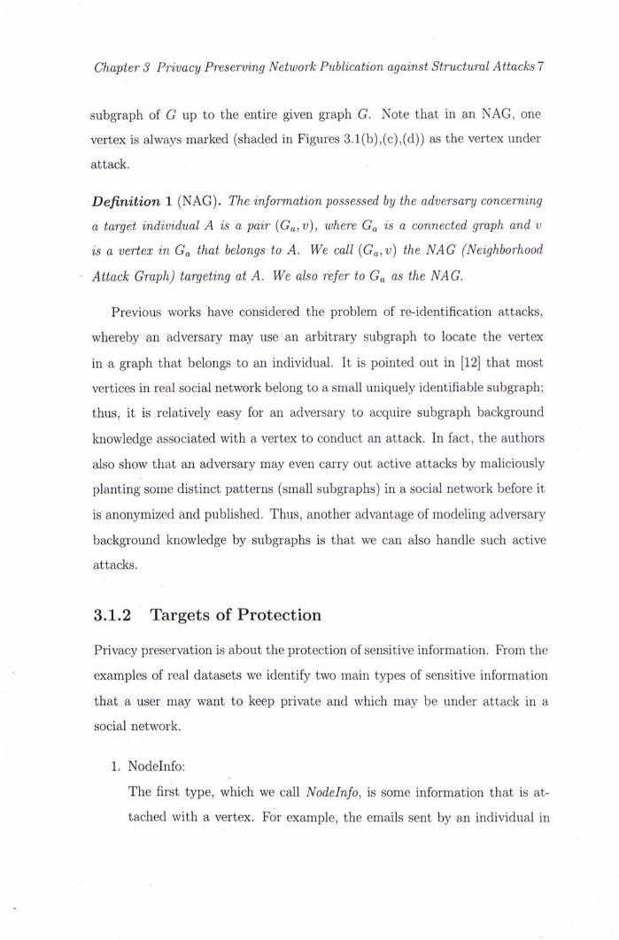
Definition 1 (NAG). The information possessed by the adversary concerning
a target individual A is a pair (Ga, v), where Ga is a connected graph and v
is a vertex in Ga that belongs to A. We call (Ga,v) the NAG (Neighborhood
Attack Graph) targeting at A. We also refer to Ga as the NAG.
Previous works have considered the problem of re-identification attacks,
whereby an adversary may use an arbitrary subgraph to locate the vertex
iri a graph that belongs to aii individual. It is pointed out in [12] that most
vertices in real social network belong to a small uniquely identifiable subgraph;
thus, it is relatively easy for an adversary to acquire subgraph background
knowledge associated with a vertex to conduct an attack. In fact, the authors
also show that an adversary may even carry out active attacks by maliciously
planting some distinct patterns (small subgraphs) in a social network before it
is anonymized and published. Thus, another advantage of modeling adversary
background knowledge by subgraphs is that we can also handle such active
attacks.
3.1.2 Targets of Protection
Privacy preservation is about the protection of sensitive information. From the
examples of real datasets we identify two main types of sensitive information
that a user rnay want to keep private and which may be under attack in a
social network.
1. NodeInfo:
The first type, which we call NodeInfo, is some information that is at-
tached with a vertex. For example, the emails sent by an individual in

Chapter 3 Privacy Preserving Network Publication against Structural Attacks 8
the Enron dataset can be highly sensitive since some of the emails have
been written only for private recipients and should not be allowed to be
linked to any individual. We assume that any identifying information
such as names will first be removed from NodeInfo, so that the content
of NodeInfo does not help the identification of its owner.
2. LinkInfo:
The second type, which we call LinkInfo, is the information about the
relationships among the individuals, which may also be considered sen-
sitive. In this case, the adversary may target at two different individuals
in the network and try to find out if they are connected by some path.
We aim to provide sufficient protection for both NodeInfo and LinkInfo.
We should point out that the linkage of an individual to a node in the published
graph itself does not disclose any sensitive information for the NodeInfo target,
because if we separate the publishing of the NodeInfo from that of the node,
then attacks of the first type will not be possible.
The first shortfall of k-anonymity in addressing our problem comes from
the same issue that has been identified by [31] which proposes the technique
bucketization. The issue is that if the privacy is some sensitive value linked
with some individual, then A:-anonymity is an overkill. The reason is that if the
sensitive values of a set of k records are simply separated from the individual
records and published as a set (bucket), then privacy can be guaranteed and
there is no need to change the raw data related to the other parts of the records.
In the same way, we can publish the original graph structure but publish the
sensitive information as a separate dataset. This is a simple solution with no
distortion to the graph structure. More details are given in Section 3.1.3.
The first shortfall may only be a matter of lower utility. The second short-
fall is more serious because it is a matter of privacy breach. This problem is
similar to that of A>anonymity in relational databases, as has been recognized
Chapter 3 Privacy Preserving Network Publication against Structural Attacks 9
in [32], namely that even with k records with identical quasi-identifiers, so that
110 individual can be linked to any record with a confidence of more than l/fc,
if all the k records contain the same sensitive value, such as AIDS, then the
adversary will be successful in linking an individual to AIDS. The important
point is that even if a graph is A:-anonymous or A:-automorphic, it cannot pro-
tect the data, from LinkInfo attack. The fact that there are k different ways
to map each of 2 individuals in a graph does not protect the linkage of the
2 individuals if all the mappings are identical in terms of the relevant graph
structure. As a simple example, a /c-clique is a graph that is both fc-anonymous
and fc-automoiphic, however, given a A:-clique and that 2 individuals A and B
are in the graph, one can easily decide that the two individuals are connected
by a single edge even though we cannot pinpoint which vertex each individual
corresponds to.
G ^ ^ ^ l M � b = � c
G ^ ¾ ¾ V ^ G a
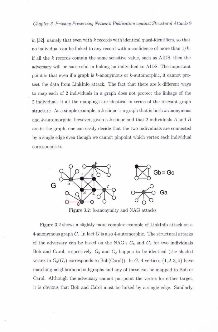
Figure 3.2: k-anonymity and NAG attacks
Figure 3.2 shows a slightly more complex example of LinkInfo attack on a
4-anonymous graph G. In fact G is also 4-automorphic. The structural attacks
of the adversary can be based on the NAG's G^ and Gc for two individuals
Bob and Carol, respectively, Gh and Gc happen to be identical (the shaded
vertex in Gb(Gc) corresponds to Bob(Carol)). In G, 4 vertices {1,2,3,4} have
matching neighborhood subgraphs and any of these can be mapped to Bob or
Carol. Although the adversary cannot pin-point the vertex for either target,
it is obvious that Bob and Carol must be linked by a single edge. Similarly,
Chapter 3 Privacy Preserving Network Publication against Structural Attacks 10
if the adversary has an NAG Ga for Alice, and Gc for Carol, the adversary
can confirm that there must be a path of length 2 linking Alice a,nd Carol.
These examples show that A:-anonymity and A:-automorphism do not guarantee
security for LinkInfo under NAG attacks.
3.1.3 Challenges and Contributions
We model a social network as a simple graph, in which vertices describe entities
(e.g., persons, organizations, etc.) and edges describe the relationships between
entities (e.g., friends, colleagues, business partners). A vertex in the graph has
an identity (e.g., name, SID) and is also associated with some information
such as a set of emails. Our task is to publish the graph in such a way that,
given a specific type of adversary knowledge in terms of NAGs, the NodeInfo or
LinkInfo of any individual can be inferred only with a probability not higher
than a pre-defined threshold, whereas the information loss of the published
graph with respect to the original graph is kept small.
The first half of the problem on NodeInfo security, on its own, has a simple
solution. We can publish the graph structure intact with no distortion on the
edges and vertices. First the content of NodeInfo for each v is screened to
remove the occurrences of names or other user identifying information. The
processed NodeInfo of each v, I(v), is detached from vertex v. We randomly
partition the vertex set V into groups of at least size k. For each group, the
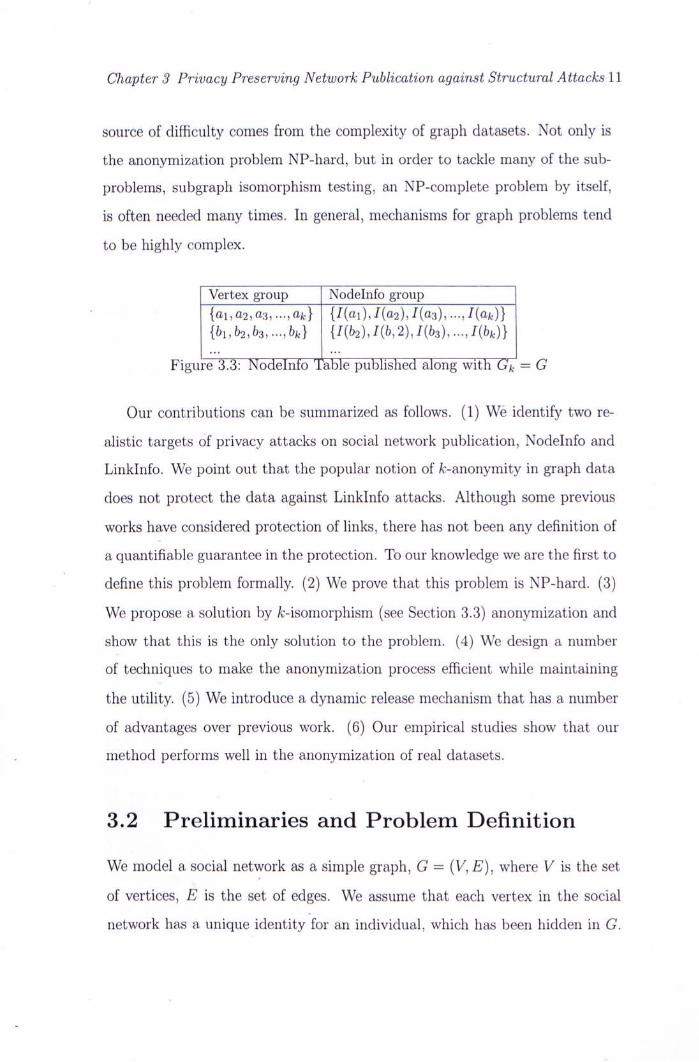
corresponding set of NodeInfo is published as a group. For example, if f i , ...,Vk
form a group, then NodeInfo {/(^;i), ...,I{vk)} will be published as a group,
breaking the linkage of the NodeInfo to each individual. This is illustrated in
Figure 3.3. A similar technique has been proposed in [33] for the anonymization
of bipartite graphs.
The difficulty of our problem therefore lies in the second half of the problem,
where the linkage of two individuals may be under attack. Another major
Chapter 3 Privacy Preserving Network Publication against Structural Attacks 11
source of difficulty comes from the complexity of graph datasets. Not only is
the anonymization problem NP-hard, but in order to tackle many of the sub-
problems, subgraph isomorphism testing, an NP-complete problem by itself,
is often needed many times. In general, mechanisms for graph problems tend
to be highly complex.
Vertex group NodeInfo group {a1,a2,a3,...’ ak} {/(a1),/(a2), /(03),...,/(afc)} { h M M . . . M {/(62),/(6,2),/(63),...,/(6fc)}
Figure 3.3: Nodelnfo T^ble published along with G\ = G
Our contributions can be summarized as follows. (1) We identify two re-
alistic targets of privacy attacks on social network publication, NodeInfo and
LinkInfo. We point out that the popular notion of A:-anonymity in graph data
does not protect the data against LinkInfo attacks. Although some previous
works ha.ve considered protection of links, there has not been any definition of
a quantifiable guarantee in the protection. To our knowledge we are the first to
define this problem formally. (2) We prove that this problem is NP-hard. (3)
We propose a solution by A:-isoinorphism (see Section 3.3) anonymization and
show that this is the only solution to the problem. (4) We design a number
of techniques to make the anonymization process efficient while maintaining
the utility. (5) We introduce a dynamic release mechanism that has a number
of advantages over previous work. (6) Our empirical studies show that our
method performs well in the anonymization of real datasets.
3.2 Preliminaries and Problem Definition
We model a social network as a simple graph, G = (V, E), where V is the set
of vertices, E is the set of edges. We assume that each vertex in the social
network has a unique identity for an individual, which has been hidden in G.

Chapter 3 Privacy Preserving Network Publication against Structural Attacks 12
In addition, we assume that each vertex v in V is associated with some node
information I{v). We also use V{G) and E{G) to refer to the vertex set and
edge set of G.
A graph G' = (K', E') is a subgraph of a graph G = (V, E), denoted by
G' C G, if V' C V and {u,v) G E' only if (u,v) e E. We also say that G is a
supergraph of G', denoted by G D G'.
Definition 2 (Graph Isomorphism). Let G = (V, E) and G' = {V', E') be two
graphs where \V\ = |V|. G and G' are isomorphic if there exists a bijection
h between V and V', h: V{G) ^ V(G'), such that (u, v) E E if and only if
{h{u), h{v)) G E(G'). We say that an isomorphism exists from G to G', and
G = G'. We also say that edge (u,v) is isomorphic to {h(u), h{v)).
Definition 3 (Subgraph Isomorphism). Let G = (V, E) and G' = {V', E') be
two graphs. There exists a subgraph isomorphism from G to G' if G contains
a subgraph that is isomorphic to G'.
We call G a proper subgraph of G', denoted as G C G', if G C G' and
G 2 G'. G is isomorphic to G', or G = G', if G C G' and G' C G.
The decision problem for graph isomorphism is one of a small number of
interesting problems in NP which have neither been proven to be polynomial
time or NP-hard. The decision problem for subgraph isomorphism is NP-
Complete [34 .
Adversary background knowledge refers to the information that an adver-
sary may acquire and use to infer the identify of some vertex in a published
social network. As we motivate in Section 3.1.1, in this paper we study the
privacy preserving publishing problem with the adversary background knowl-
edge being some subgraph that contains the vertex under attack, defined as
N A G (Neighborhood Attack Graph) in Definition 1. As in the recent works of
14], [20] and [21], we do not place any limitation on the NAG, so it can be up
to the entire given graph.

Chapter 3 Privacy Preserving Network Publication against Structural Attacks 13
With the above understanding of the adversary knowledge, our problem
definition is based on the notion of A:-security.
Definition 4 (k-Security). Let G = {V, E) be a given graph with unique node
information I{v) for each node(vertex) v G V. Each vertex v G V is linked to a
unique individual U{v). Let Gk be the anonymized graph ofG. Gk satisfies k-
security, or Gk is k-secuve, with respect to G i f f o r any two target individuals A
and B with corresponding NAGs G^ and Gs that are known by the adversary,
the following two conditions hold
1. (NodeInfo Security) the adversary cannot determine from Gk and GU(Gs)
that A(B) is linked to I(v) for any vertex v with a probability of more
than 1/k
2. (LinkInfo Security) the adversary cannot determine from Gk, GU and Gs
that A and B are linked by a path of a certain length with a probability
of more than 1/k.
While A:-security is our main objective, there is also another important
objective, which is the data utility. We would like the published graph to keep
the main characteristics of the original graph in order that it may be useful for
data analysis. Therefore we must also consider the anonymization cost, which
is a measurement of the information loss due to the anonymization. In our
proposed method, anonymization may involve edge additions and deletions.
One possible measure for the anonymization cost is the edit distance between
G and Gk, which is the total number of edge additions and deletions.
Definition 5 (Edit Distance). The edit distance between G and Gk is given
by ED{G, G,) = \(E{G) U E{Gk)\ - \E{G) n E{Gk)l
However, edit distance is not a sound measure when both edge additions
and deletions are allowed. The anonymization aims to make nodes indistin-
guishable as far as the neighborhood is concerned. A basic step in this process

Chapter 3 Privacy Preserving Network Publication against Structural Attacks 14
is to make sure that for k pairs of vertices, either each is linked by an edge or
none is linked. If the graph is sparse, it is likely that most of the pairs will
not be linked in the original graph, meaning that if edit distance is used as the
utility measure, anonymization will tend to delete edges. Such tendency will
result in poor utility in the published graph. Therefore we follow a principle of
previous works such as [13, 23] which add and delete similar amounts of edges
to maintain about the same number of edges before and after anonymization.
In this way, edge deletions will not become more favorable than edge addi-
tions. To this end, our minimal anonymization cost is given by two conditions:
(1) the difference between the number of edges in G and the nurnber of edges
in Gk is minimized. (2) Under condition (1), the edit distance ED{G, Gk) is
minimized.
Definition 6 (Anonymization Cost). An anonymization from G to Gk has
minimal anonymization cost if
( 1 ) \\E(Gk)\ — ]E{G)W is minimized ;
(2) under condition (1), ED{G,Gk) is minimized
Definition 7 (Problem Definition). The problem of privacy preservation in
graph publication by k-security is defined as follows: given a network graph
G = (V, E) with unique I{v) for each v G V, and a positive integer k, derive
an anonymized graph Gk = (¼, E^) to be published, such that (1) Vk = V
;(2) Gk is A:-secure with respect to G\ and (3) the anonymization from G to
Gk has minimal anonymization cost. We call this problem k-Secure-PPNP (or
k-Secure Privacy Preserving Network Publication).
Theorem 1 (NP-Hardness). The problem ofk-Secure Privacy Preserving Net-
work Publication is NP-hard.

Chapter 3 Privacy Preserving Network Publication against Structural Attacks 15
Corollary 1. The NP-Hardness for K-Secure-PPNP remains to hold if the
minimal anonymization cost requirement is replaced by minimum edit distance
ED[G, Gk) in the problem definition.
Though the problem is NP-hard, typically it is not possible to relax the
privacy requirement. In the next section, we derive a necessary and sufficient
solution for fc-security when we aim at keeping the partitioning of the given
graph to a minimum.
3.3 Solution:K-Isomorphism
In this section, we propose a framework solution for the problem of privacy
preservation in a graph for A;-seciirity. For simplicity we first assume that for
the given graph G = {V, E}, \V\ is a multiple of k. This assumption can be
easily waived by adding no more than k — 1 dummy vertices in the graph. The
solution relies on the concept of graph isomorphism.
Definition 8 (k-isomorphism). A graph G is k-isomorphic ifG consists ofk
disjoint subgraphs gi,...,gk, i.e. G = {gi, ...,gk}, where gi and gj are isomor-
phic for i + j.
The solution is as follows. Given a graph G — {V, E}. Derive a graph Gk 二
{Vfc, Ek} such that Vk = V, and Gk is A:-isomorphic, that is Gk = {gi, ---,9k}
with pairwise isomorphic gi and gj, i + j. Gk is the published graph. For each
V G V, NodeInfo I{v) is attached to v in the published graph.
Theorem 2 (SOUNDNESS). A k-isomorphic graph Gk = {gi, •••,9'fc} is k-
secure.
Proof. Since the graphs gi, ...,Qk are pairwise isomorphic, for any NAG of an
adversary for a target individual Alice, whenever the NAG is contained in any
Qi, there are at least k different vertices vi, ...,Vk that can be mapped to Alice
and they are not distinguishable. Hence NodeInfo security is guaranteed.
Chapter 3 Privacy Preserving Network Publication against Structural Attacks 16
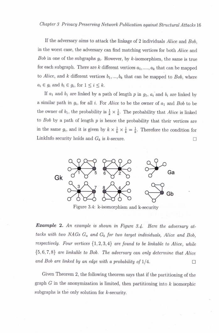
If the adversary aims to attack the linkage of 2 individuals Alice and Bob,
in the worst case, the adversary can find matching vertices for both Alice and
Boh in one of the subgraphs 仿.However, by A:-isomorphism, the same is true
for each subgraph. There are k different vertices ai,....,ak that can be mapped
to Alice, and k different vertices bi,...,bk that can be mapped to Bob, where
cLi e Qi a n d bi e 仿,for 1 < i < k.
If ai and bi are linked by a path of length p in gi, a / and bi are linked by
a similar path in gi, for all i. For Alice to be the owner of ai and Boh to be
the owner of bi, the probability is | x ^. The probability that Alice is linked
to Bob by a path of length p is hence the probability that their vertices are
in the same gi, and it is given by k x 去 x 去=去.Therefore the condition for
LinkInfo security holds and Gk is A;-secure. •
G k ^ ^ ^ ^ « a
給 激 + b -Figure 3.4: k-isomorphism and k-security
Example 2. An example is shown in Figure 34. Here the adversary at-
tacks with two NAGs Ga and Gb for two target individuals, Alice and Bob,
respectively. Four vertices {1,2,3,4} are found to be linkable to Alice, while
{5,6, 7,8} are linkable to Bob. The adversary can only determine that Alice
and Bob are linked by an edge with a probability of 1/4. •
Given Theorem 2,the following theorem says that if the partitioning of the
graph G in the anonymization is limited, then partitioning into k isomorphic
subgraphs is the only solution for A:-security.

Chapter 3 Privacy Preserving Network Publication against Structural Attacks 17
Theorem 3 (NECESSITY). Let a published graph Gk be k-secure, if Gk
is made up of no more than k disjoint connected subgraphs, then Gk is k-
isomorphic.
Proof. For the proof we shall need the notion of graph automorphism: Given
a graph G = {V, E), an automorphism is a function f from V to V, such that
{u,v) e E iff {f{u),f(v)) e E. That is f is a graph isomorphism from G to
itself.
Suppose the graph Gk is a collection of no more than k disjoint subgraphs,
let there be 1 disjoint subgraphs, 1 < k. Let gi be a biggest disjoint subgraph
with a maximum number of vertices. In the worst case the adversary may
identify 2 ta,rgets Alice and Bob by means of two NAGs (G^, VA) and (G^, vs),
where GU = G s = 9i- Then it is possible that the vertices for Alice and Bob
are in gi and therefore they are linked by some path of length p in gi. If there
exist one or more automorphisms in gi , then there will be more than one vertex
that can be mapped to Alice and Bob. However, with each automorphism,
Alice is linked to Bob via a path of the same length p. Hence with or without
aiiy automorphism in gi , if g i is the only disjoint connected subgraph in Gk
that is isomorphic to 6 ^ ^ = ¾ ) , then the adversary can confirm the linkage
between Alice and Bob.
Froni the above, there must be two or more disjoint subgraphs that are
isomorphic to G^(Gs) . Suppose there are m such subgraphs, each containing
a maximum number of vertices. The adversary can confirm that these are
the only disjoint subgraphs where Alice and Bob can be mapped to. The
probability that they are both in one of the m biggest subgraphs is given by
^ X ^ . The probability that Alice and Bob are linked by a path with length
p is given by (m) x ^ x ^ = ^ . In order for the probability to be bounded
by l/k, m > k. Since we are allowed at most k partitioned subgraphs, m = k.
Hence there are exactly k disjoint connected subgraphs that are isomorphic to
each other. •
Chapter 3 Privacy Preserving Network Publication against Structural Attacks 18
Corollary 2. If Gk is k-secure and is made up of more than k disjoint con-
nected subgraphs,let gi be any disjoint connected subgraph in Gk with the
greatest number of vertices, then Gk must contain at least k - 1 other disjoint
connected subgraphs isomorphic to gi.
Proof. The corollary follows readily from arguments similar to that in the proof
of Theorem 3. •
Enforcing A:-isomorphism could mean that we have reduced the information
of the given graph G to l/k the original size. In fact, since all the graphs gi
are isomorphic we may as well publish just one of the subgraphs gi in Gk,
if graph structure is the only interested information. However, if there is
individual information I{v) attached to each vertex v, then the subgraphs are
not totally the same. In considering the utility of Gk, it helps to compare
with conventional data analysis. Many real life applications give rise to very
large graphs in terms of thousands or even millions of vertices. With such
a large population, analysis will typically be based on a statistical study by
sampling. It is noted that each of the k isomorphic subgraphs in Gk can be
seen as a sample of the population and the sample size is very large, consisting
of l/k of the population, where k is very small compared with the graph size.
In fact, the anonymization effort can introduce normalization to the data to
avoid inaccuracies due to overfitting. Hence there is good reason to believe
that the anonymized graph maintains good utilities.
3.4 Algorithm
Our solution as presented in the previous section involves the generation and
publishing of a graph Gk that consists of k isomorphic subgraphs, let us call
these subgraphs i-graphs. Here we consider how to arrive at the i-graphs
from the given graph G. We would preserve the set of vertices by partitioning
Chapter 3 Privacy Preserving Network Publication against Structural Attacks 19
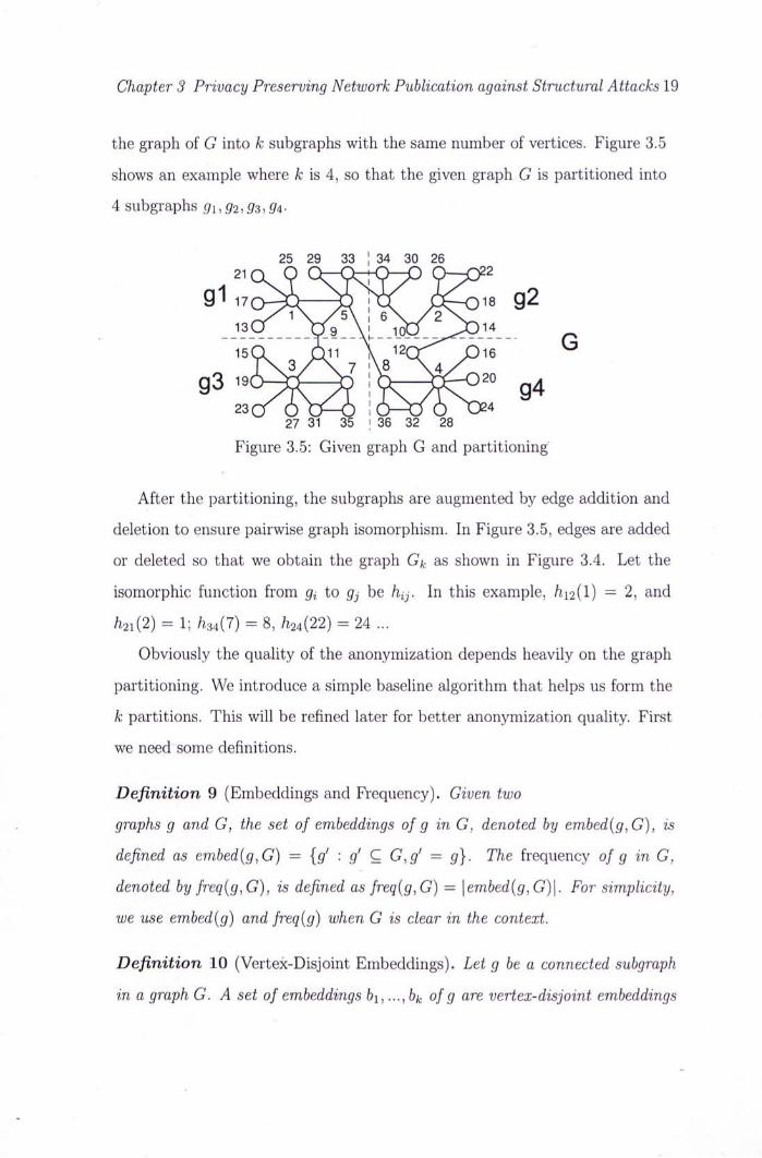
the graph of G into k subgraphs with the same number of vertices. Figure 3.5
shows an example where k is 4, so that the given graph G is partitioned into
4 subgraphs gu92,93,g4-
2 5 2 9 3 3 ! 3 4 3 0 2 6
^ ^ ; : ^ S S ^ ; : % 1 5 J X ^ 7 & - 1 2 Q ^ 1 6 G
g 3 ; 勵 i ^ : g 4 2 7 3 1 3 5 丨 3 6 3 2 2 8
Figure 3.5: Given graph G and partitioning
After the partitioning, the subgraphs are augmented by edge addition and
deletion to ensure pairwise graph isomorphism. In Figure 3.5, edges are added
or deleted so that we obtain the graph Gk as shown in Figure 3.4. Let the
isomorphic function from gi to Qj be /¾. In this example, h12(l) 二 2, and
/i2i(2) = l;/i34(7) = 8, /124(22) = 24 ...
Obviously the quality of the anonymization depends heavily on the graph
partitioning. We introduce a simple baseline algorithm that helps us form the
k partitions. This will be refined later for better anonymization quality. First
we need some definitions.
Definition 9 (Embeddirigs and Frequency). Given two
graphs g and G, the set of embeddings ofg in G, denoted by embed{g, G), is
defined as embed{g, G) = {g' : g' C G,g' = g). The frequency ofg in G,
denoted by freq(g,G), is defined as freq{g, G) = \ embed{g, G)\. For simplicity,
we use embed(g) and freq{g) when G is clear in the context.
Definition 10 (Vertex-Disjoint Embeddings). Let g be a connected subgraph
in a graph G. A set of embeddings bi, ...,bk ofg are vertex-disjoint embeddings
Chapter 3 Privacy Preserving Network Publication against Structural Attacks 20
if^hi,hj,V{hi) n V(bj) = 0. We use “VD-embedding” as a shorthand for
"vertex-disjoint embedding”.
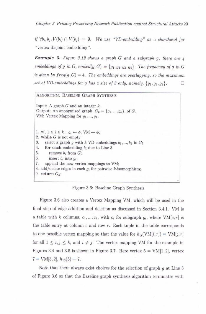
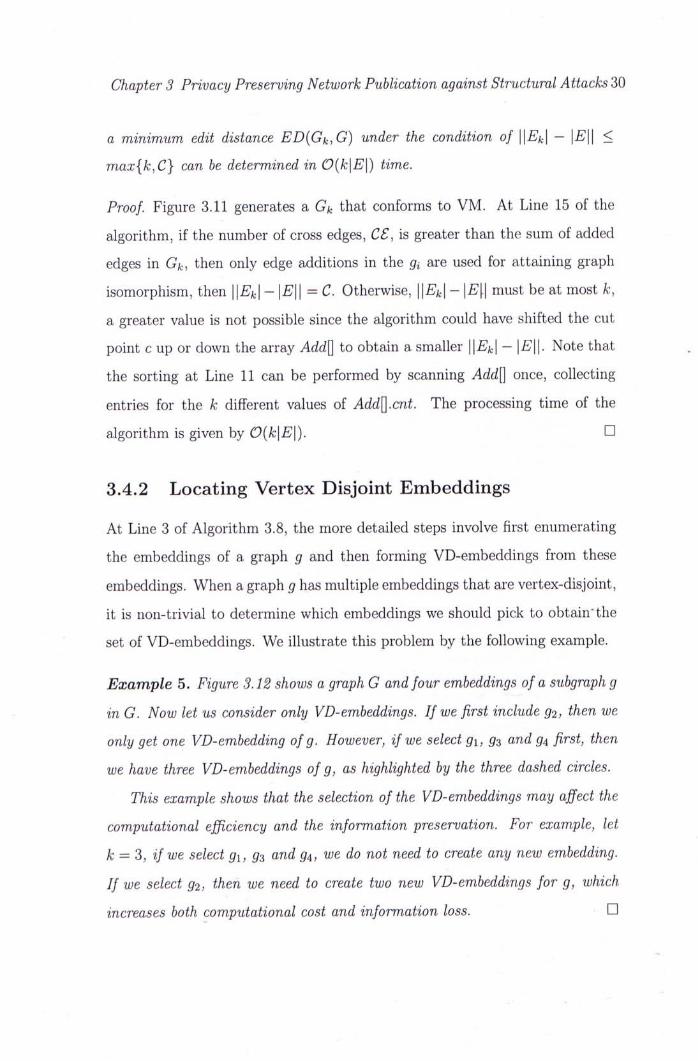
Example 3. Figure 3.12 shows a graph G and a subgraph g, there are 4
emheddings ofg in G, embed{g, G) = {^1,^/2,^3,^4}- The frequency ofg in G
is given by freq{g, G) = 4. The emheddings are overlapping, so the maximum
set of VD-embeddings for g has a size of 3 only, namely, {^1,p4,^3}. •
ALGORITHM: B A S E L I N E G R A P H SYNTHESIS
Input: A graph G and an integer k. Output: An anonymized graph, Gk 二 {ffi,.",ffk}, of G. VM: Vertex Mapping for gi,...,gk-
1. Vz, 1 < i < k : Qi — 0; VM — 0;
2. while G is not empty 3. select a graph g with k VD-embeddings 61,...,6^ in G\ 4. for each embedding bi due to Line 3 5. remove bi from G; 6. insert bi into 讲; 7. append the new vertex mappings to VM; 8. add/delete edges in each gi for pairwise A:-isomorphism; 9. return Gk]
Figure 3.6: Baseline Graph Synthesis
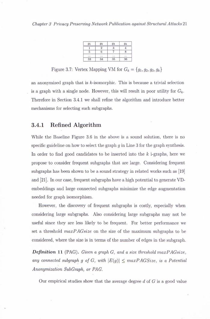
Figure 3.6 also creates a Vertex Mapping VM, which will be used in the
final step of edge addition and deletion as discussed in Section 3.4.1. VM is
a table with k columns, Ci, . . . ,Cfc, with Q for subgraph gi, where VM[c,r] is
the table entry at column c and row r. Each tuple in the table corresponds
to one possible vertex mapping so that the value for /iy(VM[z,r]) = VM[j , r
for all 1 < i,j < k, and i — j. The vertex mapping VM for the example in
Figures 3.4 and 3.5 is shown in Figure 3.7. Here vertex 5 = VM[l,2], vertex
7 = V M [ 3 , 2 ] , ^ ( 5 ) = 7.
Note that there always exist choices for the selection of graph g at Line 3
of Figure 3.6 so that the Baseline graph synthesis algorithm terminates with
Chapter 3 Privacy Preserving Network Publication against Structural Attacks 21
gi 92 ff3 ff4
1 2 3 4 5 ~ ~ 6 ~ 7 — 8
33 — 34 35 36 ~
Figure 3.7: Vertex Mapping VM for Gk = {仍’仍’仍’仇}
an anonymized graph that is A:-isomorphic. This is because a trivial selection
is a graph with a single node. However, this will result in poor utility for Gk,
Therefore in Section 3.4.1 we shall refine the algorithm and introduce better
mechanisms for selecting such subgraphs.
3.4.1 Refined Algorithm
While the Baseline Figure 3.6 in the above is a sound solution, there is no
specific guideline on how to select the graph g in Line 3 for the graph synthesis.
In order to find good candidates to be inserted into the k i-graphs, here we
propose to consider frequent subgraphs that are large. Considering frequent
subgraphs has been shown to be a sound strategy in related works such as [19
and [21]. In oiir case, frequent subgraphs have a high potential to generate VD-
embeddings and large connected subgraphs minimize the edge augmentation
needed for graph isomorphism.
However, the discovery of frequent subgraphs is costly, especially when
considering large subgraphs. Also considering large subgraphs may not be
useful since they are less likely to be frequent. For better performance we
set a threshold maxPAGsize on the size of the maximum subgraphs to be
considered, where the size is in terms of the number of edges in the subgraph.
Definition 11 (PAG). Given a graph G, and a size threshold maxPAGsize,
any connected subgraph g ofG,with \E{g)\ < maxPAGSize, is a Potential
Anonymization SubGraph, or PAG.
Our empirical studies show that the average degree d of G is a good value

Chapter 3 Privacy Preserving Network Publication against Structural Attacks 22
for maxPAGsize. The intuitive explanation for this phenomenon is that many
vertices in G have this degree d and each forms a PAG with their d 1-neighbors.
Using such a threshold would be a good basis for locating frequent subgraphs.
Figure 3.8 outlines the refined algorithm.
At Line 2 of Figure 3.8, we compute a set of PAGs, M^ which is by travers-
ing the given G from each vertex in a depth-first manner and enumerating all
connected subgraphs of size maxPAGsize. If the vertex set of these PAGs can-
not cover all vertices in G, then we also enumerate some PAGs of sizes less
than maxPAGsize, which are in fact those isolated connected components in
G with less than maxPAGsize edges. The graph traversal also determines the
embeddings for each PAG.
For PAGs with at least k VD-embeddirigs, we can extract the vertices of
k such embeddings to be transferred from G to the g:s in Gk (Lines 3-7).
These embeddings ensure that very few or no edge augmentation will be nec-
essary for the anonymization with respect to the embeddings. Since removing
some embeddings from G may affect the formation of VD-embeddings for the
remaining PAGs in G, we select PAGs in a greedy manner. PAGs of bigger
sizes will be considered earlier. Also we give priority to VD-embeddings that
contain vertices with the highest degrees. Such embeddings may incur greater
distortion and there is a better chance to reduce overall distortion if treated
earlier.
We need to anonymize a PAG g G M if g has less than k VD-embeddings.
By anonymizing g, we refer to the process by which k VD-embeddings of g are
formed so that they can be removed from G, their vertex mapping is entered
into VM, and the corresponding vertices inserted into the i-graphs. We discuss
how to anonymize g (Line 10) in Section 3.4.1. When graph G becomes empty,
all vertices have been transferred to Gk. The final step is to add edges to Gk
at Line 11,which will be discussed in Section 3.4.1.
Chapter 3 Privacy Preserving Network Publication against Structural Attacks 23
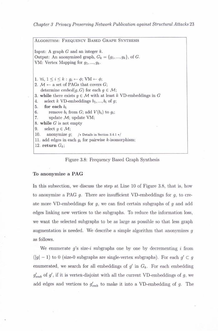
ALGORITHM: F R E Q U E N C Y B A S E D G R A P H SYNTHESIS
Input: A graph G and an integer k. Output: An anonymized graph, Gk = {仍’…,灿},of G. VM: Vertex Mapping for g\, ".,gk.
1. Vz, 1 < i < k : Qi — 0; VM ^ (/);
2. M. <— a set of PAGs that covers G\ determine ernbed{g, G) for each g € M;
. 3. while there exists g G M with at least k VD-embeddings in G 4. select k VD-embeddings 6i, ...,bi of g., 5. for each bi 6. remove b{ from G; add V(bi) to 仍; 7. update M; update VM; 8. while G is not empty 9. select g G M\ 10. anonymize g', / * Details in Section 3.4.1 */
11. add edges in each gi for pairwise fc-isomorphism; 12. return Gk]
Figure 3.8: Frequency Based Graph Synthesis
To anonymize a PAG
In this subsection, we discuss the step at Line 10 of Figure 3.8,that is, how
to anonymize a PAG g. There are insufficient VD-embeddings for g, to cre-
ate rnoi,e VD-embeddings for g, we can find certain subgraphs of g and add
edges linking new vertices to the subgraphs. To reduce the information loss,
we want the selected subgraphs to be as large as possible so that less graph
augmentation is needed. We describe a simple algorithm that anonymizes g
as follows.
We enumerate g's size-i subgraphs one by one by decrementing i from
(1 1 — 1) to 0 (size-0 subgraphs are single-vertex subgraphs). For each g' C g
enumerated, we search for all embeddings of g' in Gk- For each embedding
g'e— of g', if it is vertex-disjoint with all the current VD-embeddings of g, we
add edges and vertices to g'�— to make it into a VD-embedding of g. The
Chapter 3 Privacy Preserving Network Publication against Structural Attacks 24
process continues until the number of VD-embeddings of g in Gk reaches k.
The algorithm described above, however, suffers deficiency in the following
two aspects. First, it requires the searching of all embeddings of the subgraphs
of g in Gk. This process is expensive because it may involve a huge number
of subgraph isomorphism tests. Second, most PAGs actually share with each
other a large number of common subgraphs (as also pointed out in maximal
frequent subgraph mining [35]). Thus, many subgraphs may be repeatedly
processed and much computing resource is wasted.
To address the first deficiency, we take advantage of the fact that the em-
beddings of the PAGs have already been located in G. Thus, we can locate
the embeddings of the subgraphs within each embedding of the PAGs, which
is significantly faster than searching in the big graph G.
To address the second deficiency, we use a hashtable, H, to keep every
subgraph g' that has been processed, along with the embeddings embed(g')
that have been uncovered. Later when we anonymize another PAG g and
enumerate a subgraph g', we can first check if g' is used. If g' is found in
H, then we can readily use the embeddings of g' to anonymize g. The hash
function for H is based on graph properties such as degree distribution.
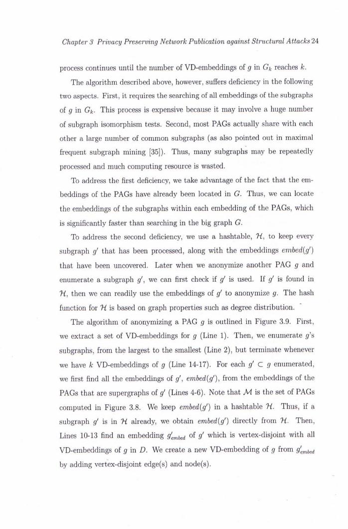
The algorithm of anonymizing a PAG g is outlined in Figure 3.9. First,
we extract a set of VD-embeddings for g (Line 1). Then, we enumerate g,s
subgraphs, from the largest to the smallest (Line 2), but terminate whenever
we have k VD-embeddings of g (Line 14-17). For each g' C g enumerated,
we first find all the embeddings of g\ embed(g'), from the embeddings of the
PAGs that are supergraphs of g' (Lines 4-6). Note that M is the set of PAGs
computed in Figure 3.8. We keep embed(g') in a hashtable H. Thus, if a
subgraph g' is in H already, we obtain emhed[g') directly from H. Then,
Lines 10-13 find an embedding g[^hed of g' which is vertex-disjoint with all
VD-embeddings of g in D. We create a new VD-embedding of g frorn g' rnbed
by adding vertex-disjoint edge(s) and node(s).

Chapter 3 Privacy Preserving Network Publication against Structural Attacks 25
ALGORITHM: A N O N Y M I Z E - P A G
Input: A PAG g to be anonymized, G,Gk, VM, M. Output: Updated Gk = {pi,---,^fc}, G , M , VM. 7i: global hashtable to store processed PAGs and embeddings.
1. V 卜 set of VD-embeddings of g in current G ;
2. for each g' C g in size-descending order 3. if g' is not in H 4. embed{g') <- 0; 5. for each g" e M, where g"�g' and g" * g 6. search in the embeddings of g" for the embeddings of g', and add these embeddings of g' to embed{g')\ 7. insert g' and embed{g') into H\ 8. else 9. obtain emhed{g') from 7i\ 10. for each g'^bed ^ embed(g') 11. if g'embed ^ vertex-disjoint from all graphs in T> 12. create a new VD-embedding b of g from g'embed; 13. delete b from G; insert b into T>-, 14. if \V\ = k 15. insert the vertices of the k graphs in V into gi, ...,gk', 16. update VM; update M; 17 . return
Figure 3.9: Anonymize-PAG
Chapter 3 Privacy Preserving Network Publication against Structural Attacks 26
An Example
The following example illustrates how we partition a graph G for A:-security.
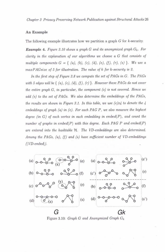
Example 4. Figure 3.10 shows a graph G and its anonymized graph Gk. For
clarity in the explanation of our algorithms we choose a G that consists of
multiple components G = { (a), (h), (c), (d), (e), ( f ) , (r), (s) }. We use a
maxPAGsize of 5 for illustration. The value of k for k-security is 2.
In the first step of Figure 3.8 we compute the set ofPAGs in G. The PAGs
with 5 edges will be { (a), (c), (d), ( f ) , (r) }. However these PAGs do not cover .•
the entire graph G, in particular, the component (s) is not covered. Hence we
add (s) to the set of PAGs. We also determine the embeddings of the PAGs,
the results are shown in Figure 3.1. In this table, we use (e)x4 to denote the 4
embeddings of graph (a) in (e). For each PAG P,we also measure the highest
degree (in G) of each vertex in each embedding in emhed[P), and count the
number of graphs in embed{P) with this degree. Each PAG P and embed{P)
are entered into the hashtable H. The VD-emheddings are also determined.
Among the PAGs, (a), ( f ) and (s) have sufficient number of VD-emheddings
(\ VD-embed\). .
( a ) | o x > V o g > y " ^ ( a ) | o ^ ^ |(e,)
( b ) i c - < A ^ c ^ J ^ I ( f ) (C): c r V S . o 7 ^ |(r)
( c ) | o ^ W ^ & A I i(r) l o ^ _ _ ^ ^ :
( d ) : ^ ^ t a r o A j i(s) ( d ) i ^ ^ " v ^ s N 丨⑷
G Gk Figure 3.10: Graph G and Anonymized Graph Gk

Chapter 3 Privacy Preserving Network Publication against Structural Attacks 27
Table 3.1: Properties ofPAGs in Figure 3.10
PAG embed() #embed | VD-embed\ MaxDeg (count)
(a) (a),(b), (e)x4 6 3 5 (1)
(c) (c) 1 1 2 (1)
(d) (d) 1 1 3 (1)
( f ) (e), ( f ) 2 2 5 (2)
(r) (r) 1 1 3 (1)
(s) (r), (s) 2 2 3 (2)
According to Lines 3 to 7 in Figure 3.8, we select the PAGs (a), ( f ) and (s)
for anonymization. ( f ) will be processed first since it has more VD-embeddings
with a maximum degree of 5 (MaxDeg count of 2). There are exactly 2 VD-
embeddings for ( f ) , namely, (e)-(x) and ( f ) , they are removed from G and
their vertex sets are added to subgraphs gi and g2 of Gk, respectively. Graph
G becomes { (a), (h), (c), (d), (r), (s), (x) }. (x) is added to the PAG set M.
Next we process PAG (a), and remove (a) and (b) from G while adding vertex
set V(a) to Qi and V(b) to g2. For PAG (s), (r)-(y) and (s) are removed from
G and their vertices entered into gi andg2 respectively. G becomes { (c), (d),
M, (y) }•
Since (d) has a higher degree vertex, it is selected as the next g in Line 9 of
Figure 3.8. By Line 2 of Figure 3.9, we select some subgraph of (d) and look
for its embeddings. Suppose the subgraph of (d)-(z) is selected as g'. It is not
in hashtable H. From Line ^-7 in Figure 3.9, we find that g' is a subgraph of
(c) ((c) acts as g" here). Hence we get the embedding (c) and executing Lines
11-12, augment it to (c') to form a VD-emhedding for (d). Vertex sets V(c')
and V(d) are added to gi and g2 respectively, while (c) and (d) are removed
from G. •
Only (x) and (y) remain in G and (x) remains in M, with VD-embeddings
of (x) and (y). They are removed from G to gi and g2, at which point G
Chapter 3 Privacy Preserving Network Publication against Structural Attacks 28
becomes empty and the partitioning of the vertex set is complete. With Line
11 ofFigure 3.8, we add edges to gi andg2, resulting in the graph Gk as shown
in Figure 3.10. •
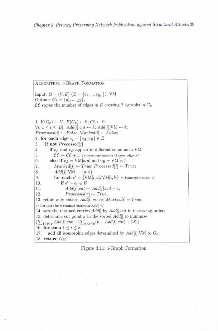
From Vertex Partit ions to i-Graphs
After the vertices of G are partitioned so that the vertices of the i-graphs in
Gk are decided, and VM is formed, we consider the final step of addition of
edges to Gk at Line 11 of Figure 3.8. This step is shown in Figure 3.11, here
the input graph G is the original graph. Intuitively, for each set of k potential
isomorphic edges {VM[i,r1],VM[i,r2]} for 1 < i < k and any pair of n , r 2 , we
have the choice of adding all of them to the QiS or making sure they do not
appear in all gi's. It reduces the edit distance to choose addition when there
are fewer missing edges in G than existing edges, and deletion (not adding)
otherwise. However, we must also keep the number of additions and deletions
similar, so it is necessary to find a balancing point.
With Figure 3.11, for each pair of rows a and b in VM, if ( VM[i, a], VM[z, b
)corresponds to some edge e in E, then the entry of Add[j] for either e or
exactly one of the edges in E isomorphic to e will be filled so that Add[j].vm =
{fl, b} and Add[j].cnt is k minus the number of edges in E isomorphic to e, also
Marked[j] is set to True. Processed[] helps to avoid processing an edge which
has been considered during the processing of some other edge. After the sorting
at Line 14, the Add[e] entries are in increasing order of Add[e].cnt, which is the
number of edges to be added if all edges isomorphic to e should exist in Gk.
The cut point x determines a point in the sorted list where all entries above the
point correspond to edge addition, and those below will involve edge deletion.
Lemma 3.1. In the anonymization of graph G = (V, E), given a vertex map-
ping VM for the graphs Gk = gi, ...,gk in Figure 3.11. Let C = max{{)^CE —
Si<i<n Add{i).cnt} at Line 15. A graph Gk = (V, Ek) conforming to VM with
Chapter 3 Privacy Preserving Network Publication against Structural Attacks 29
ALGORITHM: I - G R A P H FORMATION
Input: G = {V,E) {E = {ei,...,e|js|}), VM. Output: Gk = {gi,---,gkj-CS stores the number of edges in E crossing 2 i-graphs in Gk.
1. V{Gk) — V ; E{Gk) — 0; CS — 0;
Vi, 1 < i < \E\: Add[i].cnt — k; Add[i].YU — 0; Processed[i] <— False, Marked{i] <— False; 2. for each edge ej = {vA^vs] € E 3. if not Processed[j] 4. if VA and VB appear in different columns in VM 5. CS <~ CS + 1; /* increment number of cross edges */
6. else if VA = VM[c, a] and VB = VM[c, b] 7. Marked[j] <— True; Processed[j] <— True\ 8. Add[j],YM^{a,b}-9. for each e' = { V M [ z , a ] , V M [ i , b]} /* isomorphic edges */
10. if e' = er € E 11. Add[j].cnt <— Add[j].cnt — 1; 12. Processed[r] <— True\ 13. retain only entries Add[i] where Marked[i] = True\ /* Let there be n retained entries in Add[] */
14. sort the retained entries AddW by AddW-cnt in increasing order; 15. determine cut point x in the sorted Add[] to minimize I E i < i < . Add{i].cnt - ( E x < i < n ( ^ - Add[i].cnt) + C^:)|
16. for each 1 < i < x 17. add all isomorphic edges determined by Add[i].YM to Gk', 18. return Gfc;
Figure 3.11: i-Graph Formation
Chapter 3 Privacy Preserving Network Publication against Structural Attacks 30
a minimum edit distance ED{Gk, G) under the condition of \\Ek\ — \E\\ <
max{k,C} can be determined in 0{k\E\) time.
Proof. Figure 3.11 generates a Gk that conforms to VM. At Line 15 of the
algorithm, if the number of cross edges, CS, is greater than the sum of added
edges in Gfc, then only edge additions in the 仿 are used for attaining graph
isomorphism, then \ \Ek\-间| = C. Otherwise, \\Ek\ -\E\\ must be at most k,
a greater value is not possible since the algorithm could have shifted the cut
point c up or down the array Add[] to obtain a smaller \\Ek\ - \E\\. Note that ..
the sorting at Line 11 can be performed by scanning Add[] orice, collecting
entries for the k different values of Add[].cnt. The processing time of the
algorithm is given by 0{k\E\). 口
3.4.2 Locating Vertex Disjoint Embeddings
At Line 3 of Algorithm 3.8, the more detailed steps involve first enumerating
the embeddings of a graph g and then forming VD-embeddings from these
embeddings. When a graph g has multiple embeddings that are vertex-disjoint,
it is non-trivial to determine which embeddings we should pick to obtain' the
set of VD-embeddings. We illustrate this problem by the following example.
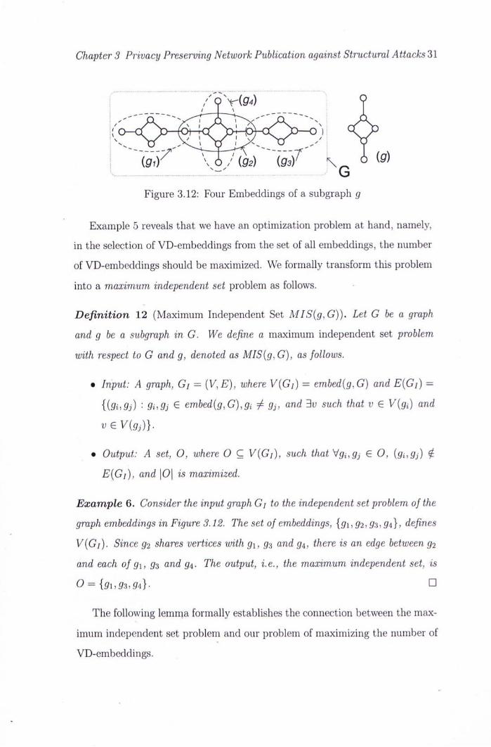
Example 5. Figure 3.12 shows a graph G and four embeddings of a subgraph g
in G. Now let us consider only VD-embeddings. Ifwe first include g2, then we
only get one VD-embedding ofg. However, ifwe select gi, g3 and g4 first, then
we have three VD-embeddings of g, as highlighted by the three dashed circles.
This example shows that the selection of the VD-embeddings may affect the
computational efficiency and the information preservation. For example, let
k = 3, i fwe select gi, g3 and g4, we do not need to create any new embedding.
If we select g2, then we need to create two new VD-embeddings for g, which
increases both computational cost and information loss. •
Chapter 3 Privacy Preserving Network Publication against Structural Attacks 31
>、 / 9 V ( ^ 4 ) 9
_ / \ 一 _
: ( ^ ^ ¾ ^ ^ ^ ^ ^ ^ ¾ ¾ Y \、、二一广7 \ ^ v _ _ _ Y _ _ ^ ^ � � ^-
(9iY \ T / ' {92) {g3)' \ ^ 0 (9) 、 一 : .• G
Figure 3.12: Four Embeddings of a subgraph g
Example 5 reveals that we have an optimization problem at hand, namely,
in the selection of VD-embeddings from the set of all embeddings, the number
of VD-embeddings should be maximized. We formally transform this problem
into a maximum independent set problem as follows. •
Definition 12 (Maximum Independent Set MIS(g,G)). Let G be a graph
and g be a subgraph in G. We define a maximum independent set problem
with respect to G and g, denoted as MIS{g^ G), as follows.
• Input: A graph, Gj = {V,E), where V{Gi) = embed{g,G) and E{Gi)=
{{gi,gj) : gi,gj G embed[g,G),gi 7 gj, and 3v such that v G V(gi) and
veV(g,)}.
• Output: A set, 0, where 0 C V{Gj), such that ^Qi,gj G 0,(gi,gj)孝
E{Gi), and |0| is maximized.
Example 6. Consider the input graph Gj to the independent set problem ofthe
graph embeddings in Figure 3.12. The set of ernbeddings, {gi,Q2^ 93,94}, defines
V{Gi). Since g2 shares vertices with gi, gs and g4, there is an edge between g2
and each of gi, g^ and g4. The output, i.e., the maximum independent set, is
0 = { ^ 1 , 5 - 3 , . ^ 4 } - 口
The following lernma. formally establishes the connection between the max-
imum independent set problem and our problem of maximizing the number of
VD-embeddings.
Chapter 3 Privacy Preserving Network Publication against Structural Attacks 32
Lemma 3.2. Let G be a graph and g be a subgraph in G. Let N be the maxi-
mum number of VD-embeddings ofg in G, and 0 be the output ofMIS(g,G).
Then, N=\0\.
Proof. Let G/ be the input of MIS{g,G). By the construction of Gj, for any
9i,9j € V{Gi), [gi,gj)孝 E(Gi) implies that 仿 and gj are disjoint. Therefore,
the embeddings of g in any independent set for Gj are disjoint, and hence the
maximum independent set defines the largest set of VD-embeddings of g. •
For better efficiency, there are polynomial-time approximation algorithms .
36] which can be used to find a sub-optimal maximum independent set, whose
size is in general greater than�n / (G( + 1)] for an input graph with n vertices
and average degree d, such mechanisms can greatly speed up maximum inde-
pendent set computations.
3.4.3 Dynamic Releases
So far we focus on a single data release for a social network. In general the
data may be evolving and published dynamically. As pointed out in [21],
if we keep the same vertex ID for the node of each individual over multiple
graph releases for better utility, it is possible that the adversary can succeed in
re-identification by intersecting the anonymization vertex groups for a target
individual over the releases.
For example, given 2 releases, R1 and R2. Suppose that in R1, the pub-
lished graph is G[ = {gl,...,gl}. Vertex ID w appears in a partition in Gl.
From the adversary's NAG^,, w is one of k vertices (from different g] 's) that
match a target individual o^j. Let us call this set of k vertex IDs Wi. In
Release R2, the published graph is Gl = {g^,---,9l}- Vertex ID w appears in
a partition in Gl, and from adversary's NAG^, w is one of k vertices (frorn
different gf,s) that match o^. Let us call this set of k vertex IDs W2. All other
vertex IDs in W2, do not appear in Wi. Hence w is the only vertex that maps
Chapter 3 Privacy Preserving Network Publication against Structural Attacks 33
to both NAGj^ and NAG^. This results in node-reidentification of 0 >, and
both NodeInfo and LinkInfo are jeopardized.
Note that vertex ID is different from individual ID in that it only serves the
purpose of tracing the node in multiple releases. [21] is the only work known
to us that deals with dynamic releases of graph data. They propose a method
to generalize certain vertex IDs when necessary.
Our method also makes use of generalized vertex IDs. After we form a
fc-isomorphic graph Gfc, we have a vertex mapping table VM consisting of
tuples of the form VM[r] = {vri,^r2,…’叫&},where Vri is the vertex ID for a
node that is in subgraph 认 and is mapped to the other tVj 's via the isomorphic
functions, hij{vri) = Vrj. With multiple releases, instead of releasing the graph
with vertex IDs of Vri, for each tuple VM[r] in the table VM, we form a
compound vertex ID of {tVi,W2,.",?Vfc},this compound ID will replace each
of the vertex IDs of tvi,Vr2,…,Vrk in Gk, and the resulting graph C^ is
published. We refer to the original vertex IDs of Vri as simple vertex IDs.
There is no need of special handling for vertex addition or deletion. For
vertex deletion, the simple vertex ID of the deleted vertex simply will not
appear in the new data release. For vertex addition, the simple vertex ID of
the new vertex will be part of a compound ID like any other vertex.
With compound vertex IDs, intersecting the anonymization vertex groups
for a target individual over the releases will not identify any node for any
individual since in each release there are k vertices with the same compound
vertex ID.
Theorem 4. Given a series of network graph releases. Assume adversary
knowledge of NAG's for multiple data releases, and also of individuals joining
or leaving the network at each release. If anonymized graphs are published
based on our anonymization by k-isomorphism and the above compound vertex
ID mechanism, then each published graph is k-secure.

Chapter 3 Privacy Preserving Network Publication against Structural Attacks 34
Though the compound vertex method in [21] also solves the above problem,
our method has a number of advantages. Firstly, no record of past releases
need to be maintained and processed in each release. The processing is very
simple. There is no distortion in the way of including vertex IDs of deleted
vertices. Finally, the compound vertex ID size is given by k, where compound
vertex ID size refers to the number of simple vertex IDs in the compound
vertex ID. This compares favorably to a bound of 2k — l + i5 for the generalized
vertex ID size in [21], where < is the number of vertices in the first release
divided by that in the current release.
3.5 Experimental Evaluation
All the programs are coded in C + + . The experiments are performed on a
Linux workstation with a 2.8Ghz CPU and 4 Giga-byte memory.
3.5.1 Datasets
In our experiments, we have used 5 datasets from 3 different applications:
Hep-Th, Enron, EUemail and LiveJournal.
The H E P - T h database presents information on papers in theoretical high-
energy physics. The data in this dataset were derived from the abstract and ci-
tation files provided for the 2003 KDD Cup competition. The original datasets
are from arXiv. We extract a subset of the authors and considered the au-
thors linked if they wrote at least one paper together. There are 5618 ver-
tices and 11786 edges in this data graph. EUemai l is a communication net-
work dataset generated using data from a large European research institution
(http://snap.stanford.edu/data/email-EuAll.html), for a period frorn October
2003 to May 2005. The nodes in the network are email addresses and edges
represent email communication between two nodes. There are 265214 nodes,
from which we randomly extracted 5000 and 10,000 vertices to form 2 datasets,
Chapter 3 Privacy Preserving Network Publication against Structural Attacks 35
4
0 1 1 0
° ? y ? 3 ; 3
i i ^ 2 2 3 3 2
(a) undirected graph (b) dataset
• Figure 3.13: an Example of Dataset
Email-1 and Email-2, respectively. LiveJournal is an online journaling com-
munity^ . T h e nodes are users and edges represent relationship of friend-lists
between users. The entire dataset contains 4847571 nodes, from which we ran-
domly extracted 5000 and then 20,000 vertices to form 2 datasets LiveJ-1 and
LiveJ-2.
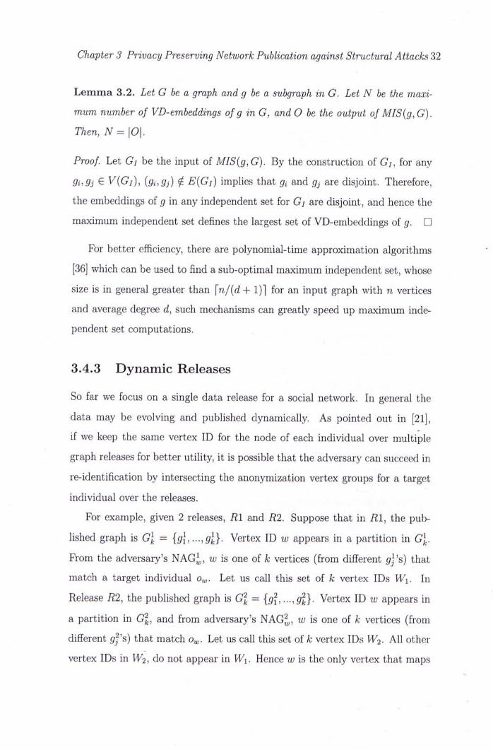
The dataset is an undirected graph. We use \E\ to denote the number
of edges, and use \V\ to denote the number of vertices. In the dataset, each
vertex have a unique ID from 0 to \V\ - 1. Except for the IDs, there is no
other information about the vertices. A single file will be used to describe a
dataset. The first line is an integer |V|. There are 2\E\ lines for \E\ edges in
the following. Each line describes an undirected edge with the format (u v),
where u and v are the IDs of two different vertices. There are two lines for
each edge, (u v) and (v u). The 2\E\ records with the format {u v) are sorted
in the increasing order of the first vertex ID, u. The edges' records with the
same value of u are sorted in the increasing order of the second vertex ID, v.
Figure 3.13 shows an example of dataset. There are 4 vertices and 4 edges
in the dataset. Each vertex has a unique ID fi,oin 0 to 3. In the dataset file,
the first line is |V|,which is 4 in this example. There are 8 (2|E|) lines in the
following, which describe 4 ( |E|) edges. For each edge, there are two records.
For example, record (1 0) and (0 1) describe the edge between vertex 0 and 1.
^http://www.livejournal.com/.

Chapter 3 Privacy Preserving Network Publication against Structural Attacks 36
We use a function to extract a new dataset from the entire dataset. The
inputs of the extraction function are the entire dataset and 4 parameters
(7V, F, I, C). The output is a new dataset with certain vertices. The entire
dataset is a undirected graph, the output dataset is a subgraph of the entire
undirected graph.
The four parameters of the extraction function is shown as:
N: The number of vertices which will be extracted to form the new dataset.
F: In the entire dataset, each vertex has a unique ID and the vertices are
in the increasing order with the IDs. From the vertex whose ID is F , the
extraction function begins to scan and extract the vertices from the original
dataset.
I and C: From the F t h vertex, scan the vertices in the increasing order
with the IDs. For each I vertices, randomly extract C vertices until we get V
extracted vertices.
After choosing the N vertices from the original dataset, we will select the
edges from the original dataset. The edges are chosen in fact form the subgraph
of the original graph induced by the N chosen vertices. Let S be the set of the
N chosen vertices. An edge (x y) in the original data set is chosen if both x
and y are in S. At the end of the extraction function, we will update the IDs
for these N extracted vertices using 0 to N — 1. The extracted edges will be
stored in a new dataset file with the same format of the entire dataset file.
In our experiment, Table 3.2 shown the parameters of the extraction func-
tion to extract two new datasets, Email-1 (5000 vertices) and Email-2 (10000
vertices) from EUemail dataset, and extract another two new datasets, LiveJ-1
(5000 vertices) and LiveJ-2 (20000 vertices) from LiveJournal dataset.
Table 3.2: Parameters of Extraction Function in Our Experiment
Chapter 3 Privacy Preserving Network Publication against Structural Attacks 37
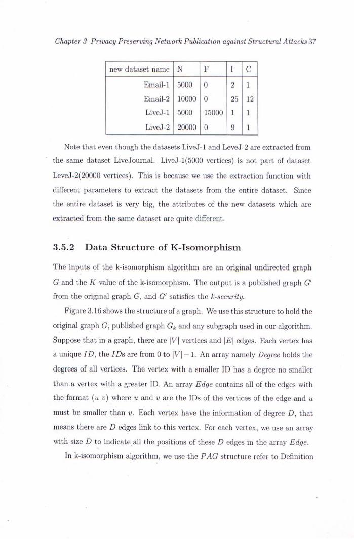
new dataset name N F I C
Email-1 5000 0 2 1
Email-2 10000 0 25 12
LiveJ-1 5000 15000 1 1
LiveJ-2 20000 0 9 1
Note that even though the datasets LiveJ-1 and LeveJ-2 are extracted from
the same dataset LiveJournal. LiveJ-l(5000 vertices) is not part of dataset
LeveJ-2(20000 vertices). This is because we use the extraction function with
different parameters to extract the datasets from the entire dataset. Since
the entire dataset is very big, the attributes of the new datasets which are
extracted froin the same dataset are quite different.
3.5.2 Data Structure of K-Isomorphism
The inputs of the k-isomorphism algorithm are an original undirected graph
G and the K value of the k-isomorphism. The output is a published graph G'
from the original graph G, and G' satisfies the k-security.
Figure 3.16 shows the structure of a graph. We use this structure to hold the
original graph G, published graph Gk and any subgraph used in our algorithm.
Suppose that in a graph, there are | ^ | vertices and \E\ edges. Each vertex has
a unique ID, the IDs are from 0 to |V| - 1. An array namely Degree holds the
degrees of all vertices. The vertex with a smaller ID has a degree no smaller
than a vertex with a greater ID. An array Edge contains all of the edges with
the format (u v) where u and v are the IDs of the vertices of the edge and u
must be smaller than v. Each vertex have the information of degree D, that
means there are D edges link to this vertex. For each vertex, we use an array
with size D to indicate all the positions of these D edges in the array Edge.
In k-isomorphism algorithm, we use the PAG structure refer to Definition

Chapter 3 Privacy Preserving Network Publication against Structural Attacks 38
^ $ ? L J L J ^ g_^2 ^ 5 ^ 3 / ' ' 7 8 ^ % / / " 16
; : ^ ^ C ^ : ^ :¾^ 你
^ m m ^ :丨轮球 (a) G (b) a PAG p (c) embed(p,G)
Figure 3.14: PAG and Embeddings
11. We preset a threshold maxPAGsize. In our experiment, we set max-
PAGsize= 5. Figure 3.14(a) is a undirected graph G. Suppose that we set .
maxPAGsize = 8,Figure 3.14 shows a possible PAG, p. Figure 3.14 shows
all the embed[p,G), refer to Definition 9.
We need to use depth-first search to enumerate all the embed{g^ G) satisfies
that \E{g)\ < maxPAGsize.Figme 3.15 shows the PAG hash table which is
used to hold the PAGs and for each PAG, there is a list of vertex-disjoin
embed(g, G). The hash function is shown as follow.
hash{embed{g, G)) = |V| x \E\ x J J ( ( ^ D + 1) x num)kMask V l—level neighbor
V\ and 1^1 are the numbers of vertices and edges respectively. D is the
degree of a node, num is one of ten prime numbers, between 3 to 37 inclusive.
^i_ieyei neighbor D is the sum of all the 1-level neighborhood's degree. Use a
big integer Mask to apply the binary AND operation.
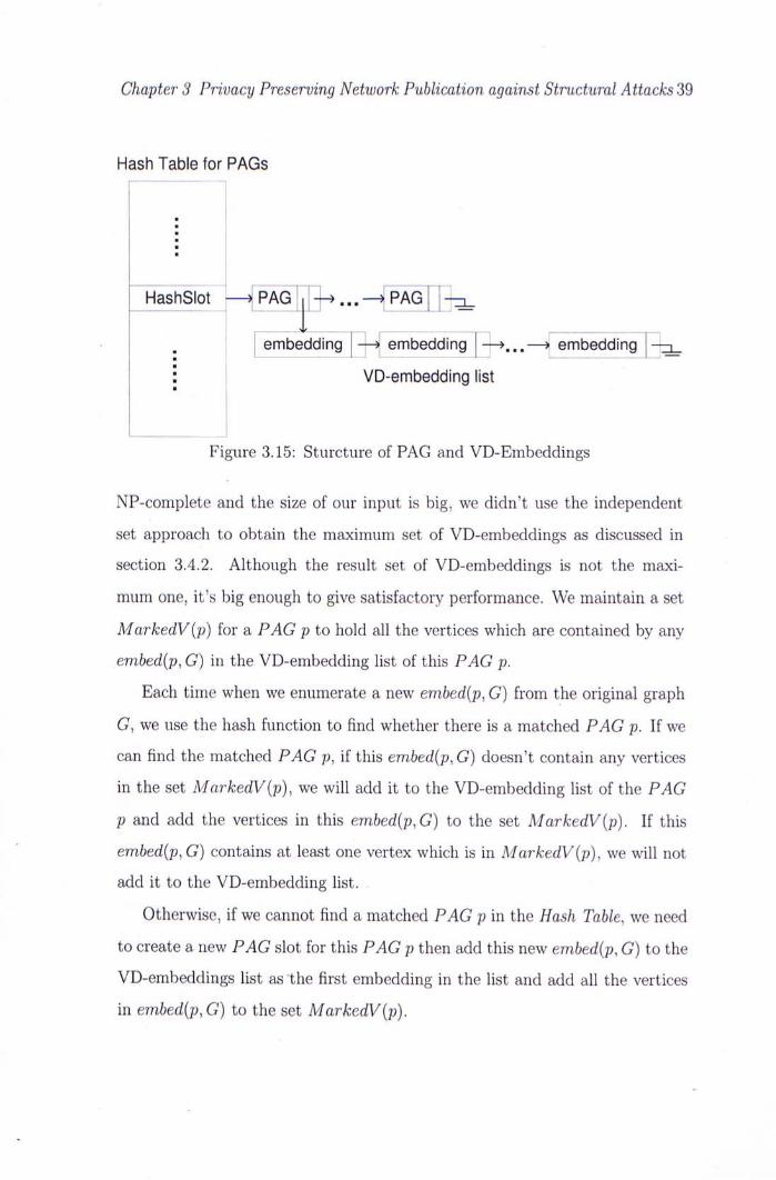
Figure 3.15 show the details of the Hash Table for PAGs. At the begin-
ning, the Hash Table is empty. We do the depth first search to enumerate all
embed(p, G), p is a possible PAG with |E(p)| < mxaPAGsize. A PAG slot
for a PAG p is created the first time we find a matching embed(p, G) frorn the
original graph. For each PAG p, we also maintain a list of VD-embeddings
which is a list of embed[p,G) which are vertex-disjoint embeddings refer to
Definition 10. In our experiments, because the independent set problem is
Chapter 3 Prwacy Preserving Network Publication against Structural Attacks 39
Hash Table for PAGs
~HashSlot ^ P A G T ] ^ . . . ^ " P A G [ 14g^
^ T~~1 embedding -~J embedding ^ , . . ~ — embedding ] ^
: I I L � I — 1——‘ ! j —
: VD-embedding list
Figure 3.15: Sturcture of PAG and VD-Embeddings
NP-complete and the size of our input is big, we didn't use the independent
set approach to obtain the maximum set of VD-embeddings as discussed in
section 3.4.2. Although the result set of VD-embeddings is not the maxi-
mum one, it's big enough to give satisfactory performance. We maintain a set
MarkedV{p) for a PAG p to hold all the vertices which are contained by any
embed{p, G) in the VD-embedding list of this P 4 G p.
Each time when we enumerate a new embed{p, G) from the original graph
G�we use the hash function to find whether there is a matched PAG p. If we
can find the matched PAG p, if this embed(p, G) doesn't contain any vertices
in the set MarkedV{p), we will add it to the VD-embedding list of the PAG
p and add the vertices in this ernbed{p, G) to the set MarkedV{p). If this
embed{p, G) contains at least one vertex which is in MarkedV(p), we will not
add it to the VD-embedding list.
Otherwise, if we cannot find a matched PAG p in the Hash Table, we need
to create a new PAG slot for this PAG p then add this new embed(p, G) to the
VD-embeddings list as 'the first embedding in the list and add all the vertices
in embed(p, G) to the set MarkedV(p).
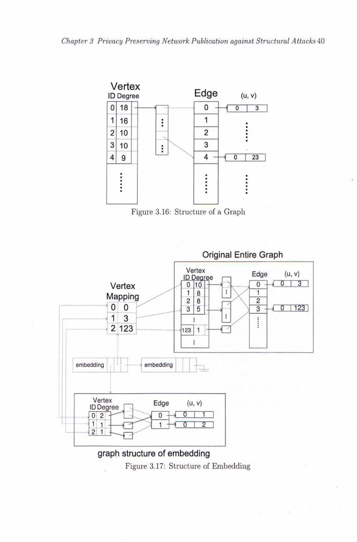
Chapter 3 Privacy Preserving Network Publication against Structural Attacks 40
Vertex _ . ID Degree t d g e (u, v)
0 1 8 ^ — : 0 - ~ " 時 0 I 3 I
1 16 : 1 . 2 10 \ 2 j 3 1 0 ^ ^ \ 3 •
4 9 • \ 4 - ~ i 0 I 23 I • • •
• m • •
• _ • •
Figure 3.16: Structure of a Graph
Original Entire Graph
^ e 口 ^ e (uv) Vertex 伞 两 卜 二 厂 ^ ^ ^ : ^ • I 3 |
Mapping / ^ + + - L y V ^ 1 01 0 r 」 i T : — 」 X - ^ r g - n ^
f' — : • • — 1 一 一 一 — y
I - " l 3 j一-一 — 1 Z '''
i ; J 2 r l 2 3 | 4 ^ r F ^ 3 ^ 三 : ^ : “
I ; I • ::‘ ! _zzzz:z 广 ,!.,._.. ! !. I ] I [ I [ r :! ; ; embedding、; | ‘ I \ embedding | | - ^ I I . _ [..圓」」.._ ; [ . j _ . 丄 . . J I — i r ‘ ! ! 厂
I I ,
I ; .
:I ! ‘ -v
: : ' K e e n . " “ “ E d g e � ’ , ) :i.; (^rifpti::::fT~^~r"gr~r3zi
i - i | i ' — — r r ^ t T ^ 0 I 2 I —一2丨 1i | - ^ ^ Q ^
graph structure of embedding Figure 3.17: Structure of Embedding
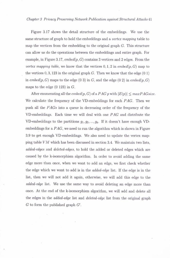
Chapter 3 Privacy Preserving Network Publication against Structural Attacks 41
Figure 3.17 shows the detail structure of the embeddings. We use the
same structure of graph to hold the embeddings and a vertex mapping table to
map the vertices from the embedding to the original graph G. This structure
can allow us do the operations between the embeddings and entire graph. For
example, in Figure 3.17, embed{p, G) contains 3 vertices and 2 edges. From the
vertex mapping table, we know that the vertices 0,1, 2 in embed(p, G) map to
the vertices 0,3’ 123 in the original graph G. Then we know that the edge (0 1)
in embed{p, G) maps to the edge (0 3) in G, and the edge (0 2) in embed(p, G)
maps to the edge (0 123) in G.
After enumerating all the embed(p, G) of a PAG p with \E(p)\ < maxPAGsize.
We calculate the frequency of the VD-embeddings for each PAG. Then we
push all the PAGs into a queue in decreasing order of the frequency of the
VD-embeddings. Each time we will deal with one PAG and distribute the
VD-embeddings to the partitions g1,g2, ---,Qk- If it doesn't have enough VD-
embeddings for a PAG, we need to run the algorithm which is shown in Figure
3.9 to get enough VD-embeddings. We also need to update the vertex map-
ping table VM which has been discussed in section 3.4. We maintain two lists,
added-edges and deleted-edges, to hold the added or deleted edges which are
caused by the k-isomorphism algorithm. In order to avoid adding the same
edge more than once, when we want to add an edge, we first check whether
the edge which we want to add is in the added-edge list. If the edge is in the
list, then we will not add it again, otherwise, we will add this edge to the
added-edge list. We use the same way to avoid deleting an edge more than
once. At the end of the k-isomorphism algorithm, we will add and delete all
the edges in the added-edge list and deleted-edge list from the original graph
G to form the published graph G'.
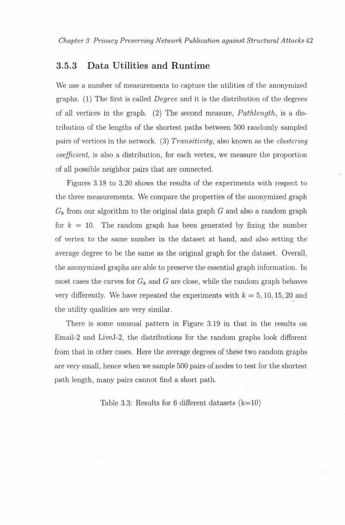
Chapter 3 Privacy Preserving Network Publication against Structural Attacks 42
3.5.3 Data Utilities and Runtime
We use a number of measurements to capture the utilities of the anonymized
graphs. (1) The first is called Degree and it is the distribution of the degrees
of all vertices in the graph. (2) The second measure, Pathlength, is a dis-
tribution of the lengths of the shortest paths between 500 randomly sampled
pairs of vertices in the network. (3) Transitivity, also known as the clustering
coefficient, is also a distribution, for each vertex, we measure the proportion
of all possible neighbor pairs that are connected.
Figures 3.18 to 3.20 shows the results of the experiments with respect to
the three measurements. We compare the properties of the anonymized graph
Gk from our algorithm to the original data graph G and also a random graph
for k = 10. The random graph has been generated by fixing the number
of vertex to the same number in the dataset at hand, and also setting the
average degree to be the same as the original graph for the dataset. Overall,
the anonymized graphs are able to preserve the essential graph information. In
most cases the curves for Gk and G are close, while the random graph behaves
very differently. We have repeated the experiments with k = 5,10,15, 20 and
the utility qualities are very similar.
There is some unusual pattern in Figure 3.19 in that in the results on
Email-2 and LiveJ-2, the distributions for the random graphs look different
from that in other cases. Here the average degrees of these two random graphs
are very small, hence when we sample 500 pairs of nodes to test for the shortest
path length, many pairs cannot find a short path.
Table 3.3: Results for 6 different datasets (k=10)
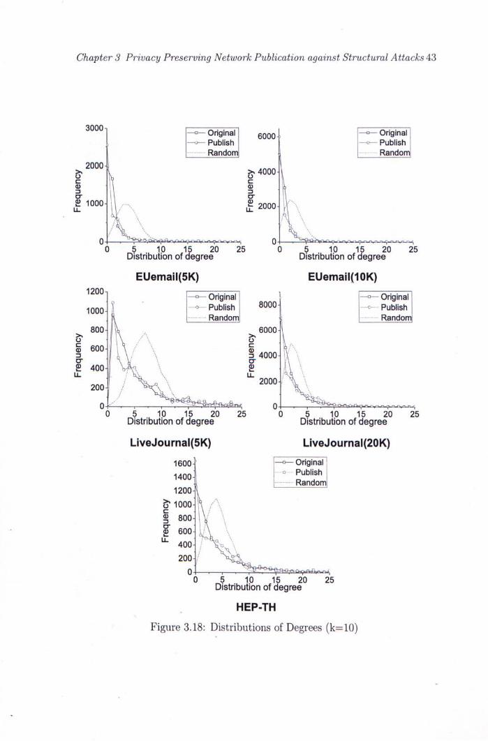
Chapter 3 Privacy Preserving Network Publication against Structural Attacks 43
3000"j —•— Original 6000j -^>~ Original , > Publish - Publish 1 Random| | |- Random
2000-i 一 \
r ^ r � � � - \ 0) • 1 0) i g- 1 i- 1 1 1 _ - |l/--N 1 2000- | ..
A � � . . V . . . . 0 ,~�YOyf>W|fal.Wf '>rtW,w wv i,f:Lj v-wj 0 , *Y*Q"rv rf~W|W�fv�' p~c "Cv 3 “wv -�
0 5 10 15 20 25 0 5 10 15 20 25 Distribution of degree Distribution of degree
EUemail(5K) EUemail(10K) 1200n ;^r^~"n 八 . • ,
“ Original —<>— Original 1000- 1 o Publish 8000-丨 ....”.+。Publish
R Random| '{ Random ^ 800- j l > 6000-1
l - _ , \ Looo.V I 叫 H\ \ I 4 \
200.1 / X A 2 0 0 0 . : \ : :
o J ^ _ _ _ ^ S S 2 5 M s ^ ol . ^ ^ ! % ^ ~ ^ 一 — —
0 5 10 15 20 25 0 5 10 15 20 25 Distribution of degree Distribution of degree
LiveJournal(5K) LiveJournal(20K)
1600| | - ^ ^ Original 1400-丨 o Publ^h
• Random 1200-1
^ 1000-k A.. § 800-丨乂 \ o 600- lA \
“ - . 〜 . \ 200-/ ^ " ^ ^
04~.~,~~Z^2f;2^i^3iii;c;i^wiiii^, 0 5 10 15 20 25
Distribution of degree HEP-TH
Figure 3.18: Distributions of Degrees (k=10)
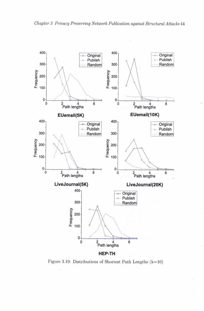
Chapter 3 Privacy Preserving Network Publication against Structural Attacks 44
400n ; ^ ~ - 400n ~ - 7 ^ ~ n + Original . 一 Original
\ 0 Publish c K 0 Publish 300- \ . “ Random| 300- w \ Random
卜 : 警 、 卜 ^ \ ^ 100- ) A \ ^ 100- \ V
oJ 二——, ' ^ ——Q……"….-i -- f. oJ ,——r^^ g ,? f. 0 2 4 6 0 2 4 6
Path lengths Path lengths
EUemail(5K) EUemall(1 OK) 400n ; 400n
+ Original - ^ Original 。Publ ish 0 Publish
300- 。 八 Random| 300- Random
I V \ ^ A s 200- V \ \ § 200- / \
I M I y V \ ^ 100- \ 'A ^ 100- / \ \
\ \ < <s^ 0 j _ , _ , _ _ V - V - r ^ ?丨; 0j__,_;....•.--.---,………〉斤::^ ?:::::~1;^ r,
0 2 4 6 0 2 4 6 Path lengths Path lengths ^
LiveJournal(5K) LiveJournal(20K) 400n :
^ > - Original - P u b l i s h
300- Random
^ ' �A i 2°°. / %,.....•�.., ? / )K \ ^ 100- ^ / \ \
/', \V\ . . 0- -• , � . V ^ r ; : i
0 2 4 6 Path lengths HEP-TH
Figure 3.19: Distributions of Shortest Path Lengths (k=10)
Chapter 3 Privacy Preserving Network Publication against Structural Attacks 45
6000n : ; - < ^ Original i _ n - ^ Original
o Publish - '、 Publish ………Random| 8000 1 丨 Random
4000- t I ^ I ^ 6000. I 0) W, 0) I
| 2 0 0 0 - I I 4000. \ • I 。 2000_ \
0- , W ;> = ^ fe fav j>= ^ 9 ^ >Y V 0- |h""K^ ; ^ H < ^ - ^ ; ^ ^ > ^ _r,Z: 0.0 0.2 0.4 0.6 0.8 1.0 0.0 0.2 0.4 0.6 0.8 1.0
Transitivity Transitivity
EUemail(5K) EUemail(1 OK) 6000n : :
- ^ Original 2OOOO- - ^ ^ Original -...-<、....Publish —o— Publish
Random| % Random 4000- 15000- I r r
1 | 10000- \ 2 2000- g \ S" \ “ ^ / “ 5000. \
V:=5::: ^^^^>o: ^"^=S^^^ j_/''(, ^ L ^ . y- u- .7. ... Q_ y*r*vr^*^|^_r:^|^"*~~~-i".>i~_^|"»~_i(^,. _f;•• „^yf^^^: 0.0 0.2 0:4 0:6 0:8 1:0 0.0 0.2 0.4 0.6 0.8 1.0
Transitivity Transitivity
LiveJournal(5K) LiveJournal(20K) 6000n :
—•— Original . --> Publish
Random 4000-^ c
0) n • g- \ \ 2 2000- U
0- W r > ^ r ^ w ^ 0.0 0.2 0.4 0.6 0.8 1.0
Transitivity
HEP-TH
Figure 3.20: Distributions of Cluster Coefficients (Transitivity) (k=10)
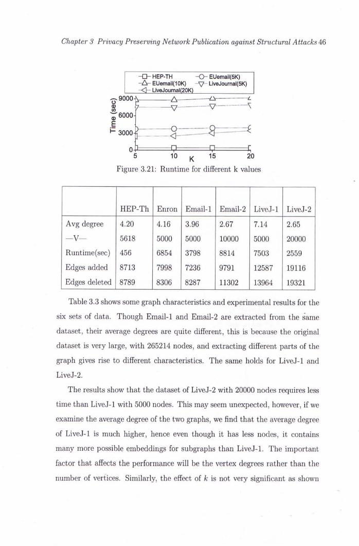
Chapter 3 Privacy Preserving Network Publication against Structural Attacks 46
- n - HEP-TH ~ 0 ~ EUemail(5K) - A - EUemail(10K) • LiveJournal(5K) -<F- LiveJournal(20K)
^ 9 0 0 0 ^ A ^ ^ 0) . j. •...—...... .•—..........—.......• \
^ 6 0 0 0 -
^ 3 0 0 0 - t : : : : : Z : ^ : : = = ^ = = ^
oP ^ n r. 5 10 j 15 20
Figure 3.21: Runtime for different k values
HEP-Th Enron Email-1 Email-2 LiveJ-1 LiveJ-2
Avg degree 4.20 4.16 3.96 2.67 7.14 2.65
—V— 5618 5000 5000 10000 5000 20000
Runtime(sec) 456 6854 3798 8814 7503 2559
Edges added 8713 7998 7236 9791 12587 19116
Edges deleted 8789 8306 8287 11302 13964 19321
Table 3.3 shows some graph characteristics and experimental results for the
six sets of data. Though Email-1 and Email-2 are extracted from the same
dataset, their average degrees are quite different, this is because the original
dataset is very large, with 265214 nodes, and extracting different parts of the
graph gives rise to different characteristics. The same holds for LiveJ-1 and
LiveJ-2.
The results show that the dataset of LiveJ-2 with 20000 nodes requires less
time than LiveJ-1 with 5000 nodes. This may seem unexpected, however, i fwe
examine the average degree of the two graphs, we find that the average degree
of LiveJ-1 is much higher, hence even though it has less nodes, it contains
many more possible embeddings for subgraphs than LiveJ-1. The important
factor that affects the performance will be the vertex degrees rather than the
number of vertices. Similarly, the effect of k is not very significant as shown
Chapter 3 Privacy Preserving Network Publication against Structural Attacks 47
in Figure 3.21,since it does not affect the graph nature related to the costly
operations of subgraph isomorphism or MIS.
3.5.4 Dynamic Releases
Since our multiple release mechanism follows closely the single release method,
the performance is also simila.r. Here we compare the performance of our dy-
• namic release mechanism to that in [21],which we refer to as RDVM (Retaining
Deleted Vertices for Multi-release). The reason is that the mechanism for mul-
tiple release in [21] can also be used in our case. The comparison is shown
in Figure 3.22, this result applies to any dataset under the following assump-
tions: there are 10 data releases, in each data release 10% of the vertices in
the first release are deleted, while the same number of new vertices are added.
Since we do not modify the set of simple vertices from the current dataset, the
distortion is always zero. In the figure our result is labeled CVIM (Compound
Vertex ID's for Multi-release). RDVM suffers from high distortion to the data
in the amount of fictitious vertices. After 10 releases, the proportion of vertex
ID's for deletion vertices^ climbs to almost 50% of all vertex ID's.
3.6 Conclusions
We have identified a new problem of enforcing fc-security for protecting sensi-
tive information concerning the nodes and links in a published network dataset.
Our investigation leads to a solution based on fc-isomorphism. In conclusion,
the selection of anonymization algorithm mainly depends on the adversary
knowledge and the targets of protection. If the target is only NodeInfo protec-
tion against structural attack, a solution as shown in Section 3.1.3 will suffice.
^We clarify that here we have not counted the dummy vertex insertion for graph parti-tioning in [21]. In Algorithm 5 in [21], VD-embeddings are created by introducing a dummy vertex for each overlapping vertex in two embeddings. Here we we only consider dumniy vertex ID's they have used for deleted individuals.
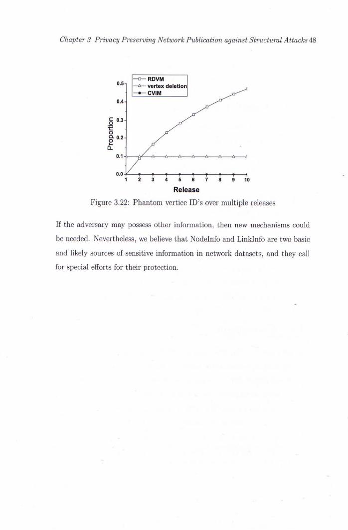
Chapter 3 Privacy Preserving Network Publication against Structural Attacks 48
|-^>- RDVM 0.51 A vertex deletion
• |-*-CVIM J c r ^ 0.4- ^ ^ ^
I。.': X ^ ^ ^ t . X
0.1 -、 ^ y ^ - " A A A JV A-——A A /
o.o4^~t r T T r T T r 1 1 2 3 4 5 6 7 8 9 10
Release Figure 3.22: Phantom vertice ID's over multiple releases
If the adversary may possess other information, then new mechanisms could
be needed. Nevertheless, we believe that NodeInfo and LinkInfo are two basic
and likely sources of sensitive information in network datasets, and they call
for special efforts for their protection.
Chapter 4
Global Privacy Guarantee in
Serial Da ta Publishing
While previous works on privacy-preserving serial data publishing consider the
scenario where sensitive values may persist over multiple data releases, we find
that no previous work has sufficient protection provided for sensitive values
that can change over time, which should be the more common case. In this
chapter, we propose to study the privacy guarantee for such transient sensitive
values, which we call the global guarantee. We formally define the problem
for achieving this guarantee. We show that the data satisfying the global
guarantee also satisfies a privacy guarantee commonly adopted in the privacy
literature called the local guarantee.
4.1 Background and Motivation
Following the settings of previous works, we assume that there is a sensitive
attribute which contains sensitive values that should not be linked to the in-
dividuals in the database. A common example of such a sensitive attribute is
diseases. While some diseases such as flu or stomach virus may not be very sen-
sitive, some diseases such as chlamydia (a sexually transmitted disease (STD))
can be considered highly sensitive. In serial publishing of such a set of data,
49 ..
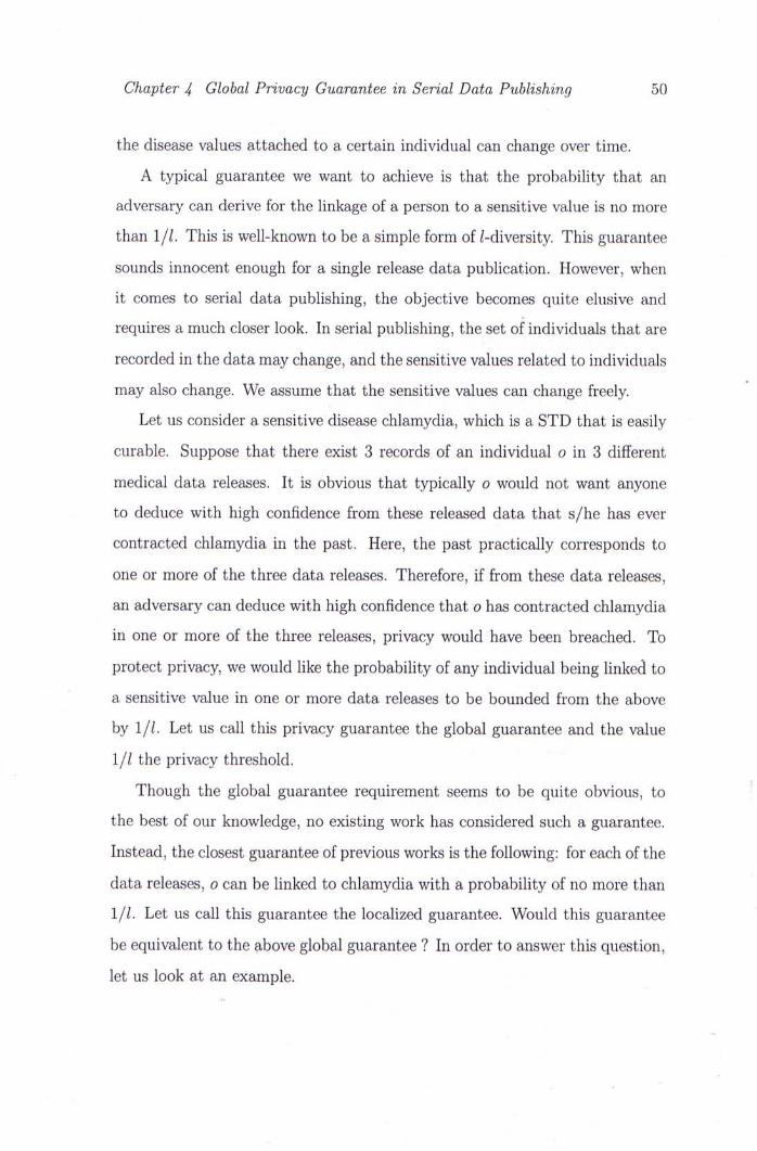
Chapter 4 Global Privacy Guarantee in Serial Data Publishing 50
the disease values attached to a certain individual can change over time.
A typical guarantee we want to achieve is that the probability that an
adversary can derive for the linkage of a person to a sensitive value is no more
than 1//. This is well-known to be a simple form of /-diversity. This guarantee
sounds innocent enough for a single release data publication. However, when
it comes to serial data publishing, the objective becomes quite elusive and
requires a much closer look. In serial publishing, the set of individuals that are
recorded in the data may change, and the sensitive values related to individuals
may also change. We assume that the sensitive values can change freely.
Let us consider a sensitive disease chlamydia, which is a STD that is easily
curable. Suppose that there exist 3 records of an individual o in 3 different
medical data releases. It is obvious that typically o would not want anyone
to deduce with high confidence from these released data that s /he has ever
contracted chlamydia in the past. Here, the past practically corresponds to
one or more of the three data releases. Therefore, if from these data releases,
an adversary can deduce with high confidence that o has contracted chlamydia
in one or more of the three releases, privacy would have been breached. To
protect privacy, we would like the probability of any individual being linked to
a sensitive value in one or more data releases to be bounded from the above
by l/l. Let us call this privacy guarantee the global guarantee and the value
1// the privacy threshold.
Though the global guarantee requirement seems to be quite obvious, to
the best of our knowledge, no existing work has considered such a guarantee.
Instead, the closest guarantee of previous works is the following: for each of the
data releases, o can be linked to chlamydia with a probability of no more than
1//. Let us call this guarantee the localized guarantee. Would this guarantee
be equivalent to the above global guarantee ? In order to answer this question,
let us look at an example.
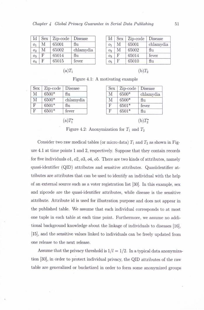
Chapter 4 Global Privacy Guarantee in Serial Data Publishing 51
Id Sex Zip-code Disease Id Sex Zip-code Disease W ~ M "65001 flu ~ ^ M TsOOl chlamydia ~ ^ M T5QQ2 chlamydia ~ ^ M T5002 flu ~ ^ F "65014 flu ~ ^ F ~65Q14 fever
04 F 65015 fever 05 F 65010 flu
(a)Ti (b)T2
Figure 4.1: A motivating example
Sex Zip-code Disease Sex Zip-code Disease M 6500* — flu ~ U r ~ 6500* chlamydia" M 6500* ~ ~ chlamycUT M 6500* SI F 6 5 0 1 *一 flu — " F ~ " 6501* — fever — F 6501* fever ~ ~ F 6501* flu —
(a)Tr (h)T*
Figure 4.2: Anonymization for T\ and T2
Consider two raw medical tables (or micro data) 7] and T2 as shown in Fig-
ure 4.1 at time points 1 and 2’ respectively. Suppose that they contain records
for five individuals ol , o2, o3, o4, o5. There are two kinds of attributes, namely
quasi-identifier (QID) attributes and sensitive attributes. Quasiidentifier at-
tributes are attributes that can be used to identify an individual with the help
of an external source such as a voter registration list [30]. In this example, sex
and zipcode are the quasi-identifier attributes, while disease is the sensitive
attribute. Attribute id is used for illustration purpose and does not appear in
the published table. We assume that each individual corresponds to at most
one tuple in each table at each time point. Furthermore, we assume no addi-
tional background knowledge about the linkage of individuals to diseases [16],
15], and the sensitive values linked to individuals can be freely updated from
one release to the next release.
Assume that the privacy threshold is 1/1 = 1/2. In a typical data anonymiza-
tion [30], in order to protect individual privacy, the QID attributes of the raw
table are generalized or bucketized in order to form some anonymized groups
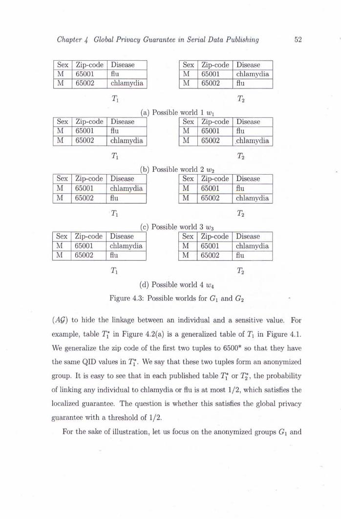
Chapter 4 Global Privacy Guarantee in Serial Data Publishing 52
Sex Zip-code Disease Sex Zip-code Disease M 65001 flu M 65001 chlamydia M 65002 chlamyd¥"] M 65002 flu 一
Ti T2
(a) Possible world 1 Wi Sex Zip-code Disease Sex Zip-code Disease
~ W ~ 65001 — flu — ~ M ~ 65001 一 flu — M 65002 chlamydT^ M 6 5 0 0 2 — ..chlamydia
Ti n
(b) Possible world 2 W2 , Sex Zip-code Disease Sex Zip-code Disease M 65001 ~ ~ ch lamydi r M 65001 — flu ~" M 65002 flu ~ | M 65002 chlamydia
Ti T2
(c) Possible world 3 w^ Sex Zip-code Disease Sex Zip-code Disease M 65001 chlamydia M 65001 c h l a m y ^ M 65002 flu ~~" M 65m2 flu —
T, T2
(d) Possible world 4 w4
Figure 4.3: Possible worlds for Gi and G2 ‘
{AQ) to hide the linkage between an individual and a sensitive value. For
example, table T^ in Figure 4.2(a) is a generalized table of 7] in Figure 4.1.
We generalize the zip code of the first two tuples to 6500* so that they have
the same QID values in Tf. We say that these two tuples form an anonymized
group. It is easy to see that in each published table T^ or TJJ, the probability
of linking any individual to chlamydia or flu is at most 1/2, which satisfies the
localized guarantee. The question is whether this satisfies the global privacy
guarantee with a threshold of 1/2.
For the sake of illustration, let us focus on the anonymized groups Gi and

Chapter 4 Global Privacy Guarantee in Serial Data Publishing 53
G2 containing the first two tuples in tables 7^ and T ; in Figure 4.2, respec-
tively. The probability in serial publishing can be derived by the possible world
analysis. There are four possible worlds for Gi and G2 in these two published
tables, as shown in Figure 4.3. Here each possible world is one possible way to
assign the diseases to the individuals in such a way that is consistent with the
published tables. Therefore, each possible world is a possible assignment of the
sensitive values to the individuals at all the publication time points for groups
Gi and G2. Note that an individual can be assigned to different values at
different data releases, and the assignment in one data release is independent
of the assignment in another release.
Consider individual 02. Among the four possible worlds, three possible
worlds link 02 to “ chlamydia", namely w1,w2 and Wz- In Wi and W2, the linkage
occurs at Ti, and in W2,, the linkage occurs at T2. Thus, the probability that 02
is linked to “chlamydia" in at least one of the tables is equal to 3 /4(= 0.75),
which is greater than 1/2’ the intended privacy threshold. From this example,
we can see that localized guarantee does not imply global guarantee.
The /-scarcity model is introduced in [15] to handle the situations when
some data may be permanent so that once an individual is linked to such a
value, the linkage will remain in subsequent releases whenever the individual
appears (not limited to consecutive releases only). The major focus of [15] is
the privacy protection for permanent sensitive values. However, for transient
sensitive values, [15] and [26] adopt the following principle.
Principle 1 (Localized Guarantee): For each release of the data publication,
the probability that an individual is linked to a sensitive value is bounded by
a threshold.
However, we have seen in the example in the previous section that this can-
not satisfy the expected privacy requirement. Hence, we consider the following
principle.

Chapter 4 Global Privacy Guarantee in Serial Data Publishing 54
Principle 2 (Global Guarantee): Over all the published releases, the prob-
ability that an individual has ever been linked to a sensitive value is bounded
by a threshold.
4.2 Problem Definition
Suppose tables J \ , T2, ...’ Tk are generated at time points, 1,2, ...,k, respec-
tively. Each table Ti has two kinds of attributes, quasi-identifier attributes ‘
and sensitive attributes. For the sake of illustration, we consider one single
sensitive attribute S containing |5*| values, namely si, s2, ..., S|<S|. Assume
that the sensitive values for individuals can freely change from one release to
another release so that the linkage of an individual 0 to a sensitive value s in
one data release has no effect on the linkage of 0 to any other sensitive value
in any other data release. Assume at each time point j, a data, publisher gen-
erates an anonymized version T* of 7} for data publishing so that each record
in Tj will belong to one anonymized group G in Tj. Given an anonymized
group G, we define G.S to be a multi-set containing all sensitive values iii G,
and G.I to be the set of individuals that appear in G.
Definition 13 (Possible World). A series of tables TS = {T�,T�,...,T�} is
a possible world for published tables {T^,T2,---,T|^} ifthe following reqirement
is satisfied. For each i G [1, A:],
1. there is a one-to-one correspondence between individuals in T[ and indi-
viduals in T*
2. for each anonymized group G in T*, the multi-set of the sensitive values
of the corresponding individuals in Tf is equal to G.S.
Chapter 4 Global Privacy Guarantee in Serial Data Publishing 55
Let t.S stand for the sensitive value of tuple t. We say that o is linked to
s in a table Tf if for the tuple t of o in T[, t.S = s. Following previous works,
we define the probability based on the possible worlds as follows.
Definition 14 (Breach Probability). The breach probability is given by
ry(n « k ) - ^iink{o,s,k) P(o’s,fc)— ^�ta,’&
where Wunk(o, s, k) is the total number of possible worlds where o is linked to
s in at least one published table among T f , T f , ..., T�and Wtotai,k ^s the total
number ofpossible worlds for published tables T^, T;,..., T^.
For example, in our running example, for the tables shown in Figure 4.2,
p(02, s, 2) is equal to 3/4 where s is equal to "chlamydia". For the tables shown
in Figure 4.4’ p[02, s, 2) is equal to 7/16. We will describe how a general formula
to calculate p(o, s, k) can be found in Section 4.3. While privacy breach is the
most important concern, the utility of the published data also needs to be
preserved. There are different definitions of utility in the existing literature.
In this chapter, we are studying the following problem.
Problem 1: Given a privacy parameter 1 (a positive integer), a utility mea-
surement, k — 1 published tables, namely 7^, TJ, ..., T: and one raw table
Tk, we want to generate a published table T : from Tk such that the utility is
maximized, and for each individual 0 and each sensitive value s,
p{o,s,k) < l/l
Note that the above problem definition follows Principle 2 for global guarantee.
For example, for the tables shown in Figure 4.3, p{02,s, 2) is equal to 7/16(<
1/2), which satisfies the global guarantee.
Here, we show that protecting individual privacy with Principle 2 (global
guarantee) implies protecting individual privacy with Principle 1 (localized

Chapter 4 Global Privacy Guarantee in Serial Data Publishing 56
Sex Zip-code Disease Sex Zip-code Disease M“F 650**~~ flu ~ ~ W T ~ 6 ^ ~ ~ chlamydi^ M“F 6 5 0 * * ~ chlamydlT M“F ~ 6 ^ ~ ~ flu — M“F 650**~~ flu — M“F " 6 ^ ~ fever ~ ~ M“F 650** fever ~ ~ M“F 650** flu —
(a)Ti* (h)T^
Figure 4.4: Anonymization for global guarantee
guarantee). Under Principle 1, let q(o, s , j , k) be the probability that an in-
dividual 0 is linked to a sensitive value s in the j-th table. Following the
definition of probability adopted in most previous works [26], [15], we have
q(o,s,],k) = L-(o,s,j,k) ^total,k
where Lunk{o, s, k,j) is the total number of possible worlds in which o is
linked to s in the j-th table an Wtotai,k is the total number of possible worlds
for the k published tables.
In our running example, k = 2 and from Figure 4.3, there are four pos-
sible worlds, Wtotai,k = 4. Consider published table T;. There are two pos-
sible worlds where 02 is linked to chlamydia(s), namely wi and w2. Thus,
L i ink (02 ,s , l ,k ) = 2 and g(02,s, l,A:) = | = | . Similarly, when j = 2,
q{02,s,2,k)=全.
In general, it is obvious that Wunk{o,s,k) > L u n k { o , s J , k ) for any j G
1, k]. We derive that
p[o,s,k) > q(o,s,j,k)
Hence we have the following lemma.
Lemma 4.1. Ifp{o,s,k) < l/l (under Principle 2), then for any j e [l,k],
q(o,s,j,k) < l/l (under Principle 1).
Corollary 3. Principle 2 (global guarantee) is a strictly stronger requirement
than Principle 1 (localized guarantee).

Chapter 4 Global Privacy Guarantee in Serial Data Publishing 57
4.3 Breach Probability Analysis
In this section, we give the general formula of the breach probability p{o, s, k).
Consider an anonymized group in Tj for individual o denoted by AQj{o) . Let
rij be the size AQj{o). Let nj’i be the total number of tuples in AQj{o) with
sensitive value Si for i = 1,2,..., |S"|. Without loss of generality, we consider
the privacy protection for an arbitrary sensitive value s = Si. With the above
‘ n o t a t i o n s , we have the following lemma for the general formula of p(o, s, k).
Lemma 4.2 (Closed Form of p(o,Si,k)).
I , . r i j t i ^ j - r i j = i K - ^ j , i ) p ( o , S i , A : ) = ^ ^ •
n_f=i ^3 Prom Lernrna 4.1, p(o ,s i ,k) is defined with a conceptual terms with the
total number of possible worlds. Lernma 4.2 gives a closed form of p(o, Si,k).
Given the information of rij (i.e., the size of the anonymized group in the j-
th table) and rij^i (i.e., the number of tuples iri the anonymized group with
sensitive value Si in the j-th table), we can calculate p(o,Si,k) with its closed
form directly.
Example 7 (Two-Table Illustration). Consider that we want to protect the
linkage between an individual and a sensitive value si. Suppose o appears in
both published tables T^ and T^. Let AQi{o) and AQ2{0) be the anonymized
groups in T: and T; containing 0. Suppose both AQi{o) and AQ2{0) are linked
to Si.
Uk is the size of AQk{o) and n^^i is the total number of tuples in AQk{o)
with sensitive value Si.
By Lemma 4-2, we have
p(o si k)=几1几2 - (ni -n1^1){n2-n2,1) = n2,1n1 +n1,1n2-n1,1n2,1 ‘ ‘ niU2 ri1n2

Chapter 4 Global Privacy Guarantee in Serial Data Publishing 58
Example 8 (Running Example). In our running example as shown in Figure
4-2^ consider the second individual 02 and a sensitive value "chlamydia". We
know that n\ = ri2 = 2.
Suppose si is "chlamydia". Thus, ni,i = n2,1 = 1. With respect to the
published tables as shown in Figure J^.2, according to the formula derived in
Example 1, ( � � 1 X 2 + 1 X 2 - 1 X 1 3
p(02,h ,2) = j ^ = 4
which is greater than 1/2.
However, ifwe publish tables as shown in Figure 4-4> then ni = ri2 = 4 and
ni,i --—- n2,1 = 1.
. � � 1 x 4 + l x 4 - l X 1 7 P(02,si’2) = ^ = I g
which is smaller than 1/2.
In this example, we observe that, since the published tables as shown in
Figure 4-4 have a larger anonymized group size (compared with the published
tables as shown in Figure 4-2), p(02,Si,2) is smaller.
We aim to publish table T : like Figure 4.4 at each time point k such that
p(o, s, k) < 1/1 for each individual 0 and each sensitive value s. ‘
4.4 Anonymization
In this section, we devise a strategy to minimize the maximum anonymized
group size ratio. We also propose another strategy which aims to reduce the
anonymized group size ratio on average.
4.4.1 AG size Ratio
Recall that Let n^ be the size AGk in Tj^. Let rik,i be the total number of tuples
in AQk with sensitive value si. In the following we will derive the minimum
anonymized group size ratio - ^ for privacy protection under global guarantee. fc, 1

Chapter 4 Global Privacy Guarantee in Serial Data Publishing 59
Theorem 5. Let k be an integer greater than 1. Suppose the anonymized group
in Tl containing individual o is linked to Si. p ( o , s i , k ) < l/l if and only if
jn^〉 lU^Zlinj-nja)
"M - /nJ : ! i (w:n, i ) - (^" i )nj :N
For any k > 1, the value of ^ should be lower bounded by the value of
^ . M = m - : i ( ^ . - % l )
m - : l ( n j - n j , 0 - ( l - l ) n ^ : ; n ,
We define n(k) = 1 when k = 1
Example 9 (Running Example). From Example 8, we know that the published
tables shown in Figure 4-4 satisfy the privacy requirement (i.e., p(o, s, k) < l/l
where k = 2 and 1 = 2). At time k = 3, we want to publish a new table T^
from a raw table T3 which contain 02.
Suppose we will put 02 in the anonymized group AQ3(02) in T^ which is
linked to s^ where Si is chlamydia. By Theorem 5, when k = 3,
jii_ � in^Zlinj-n^,i) "M — inj:}(nj-njj)-(l-l)n;i}nj
> __2(4-l)(4-l) — 2 ( 4 - l ) ( 4 - l ) - ( 2 - l ) . 4 - 4
= 9
which is the minimum anonymized group size ratio ^ in the published table
TJ. Suppose AQ3{0) contains only one occurrence ofsi. Then, the size of the
anonymized group AQ3{0) should be at least 9 so that p(o, s i ,3) < 1/2.
4.4.2 Constant-Ratio Strategy
In database related problems, one can typically derive effective mechanisms
based on the characteristics of the data itself. In our problem scenario, a
data publisher has at his/her disposal the statistical information of the data
collections. For example, consider the medical database. The statistics can
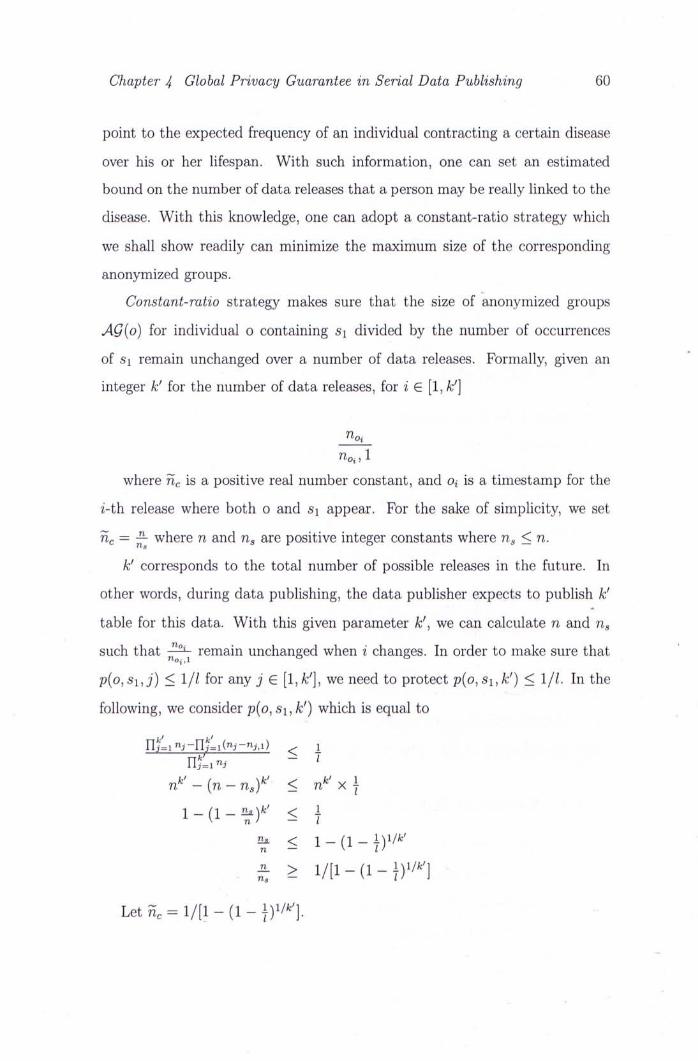
Chapter 4 Global Privacy Guarantee in Serial Data Publishing 60
point to the expected frequency of an individual contracting a certain disease
over his or her lifespan. With such information, one can set an estimated
bound on the number of data releases that a person may be really linked to the
disease. With this knowledge, one can adopt a constant-ratio strategy which
we shall show readily can minimize the maximum size of the corresponding
anonymized groups.
Constant-ratio strategy makes sure that the size of anonymized groups
AG{o) for individual o containing Si divided by the number of occurrences
of si remain unchanged over a number of data releases. Formally, given an '"
integer k' for the number of data releases, for i G [1,k'
npi rioiA
where n � i s a positive real number constant, and Oi is a timestamp for the
2-th release where both o and si appear. For the sake of simplicity, we set
ric = ^ where n and ris are positive integer constants where ris < n.
k' corresponds to the total number of possible releases in the future. In
other words, during data publishing, the data publisher expects to publish k'
table for this data. With this given parameter k\ we can calculate n and n^
such that ^ ^ remain unchanged when i changes. In order to make sure that ‘ "Oj,l
p(o,Si,j) < 1/1 for any j G [1, k'], we need to protect p{o, Si,k') < l/l. In the
following, we consider p{o, si,k') which is equal to
Ylf=inj-Uti(nj-nj,i) i ~ ~ n U ^ j - 了
n^' - {n - risY' < n^' x |
1 - (1 - ^ ) ' ' < 7
^ < 1 - ( 1 ] ) " "
t > l / [ l - ( l ] ) " n
Let 7ic = l / [ l - { l - ] y / ^ ' ] .

Chapter 4 Global Privacy Guarantee in Serial Data Publishing 61
Table 4.1: Values of n � w i t h selected values of 1 and k'
1 2 2 2 5 10 2 5 10
k' 2 5 20 20 20 10 10 10
Uc 3.44 7.75 29.41 90.13 190.33 15.10 45.35 95.42
Table 4.1 shows the values of n � w i t h selected values of 1 and k'. When 1
‘ increases , Uc increases. When k' increases, ric also increases.
The constant-ratio strategy requires the priori knowledge about k' which is
equal to the total number of possible releases in the future. If such information
is unavailable, we can use the geometric strategy proposed in the section 4.4.3
which does not require such statistical information.
4.4.3 Geometric Strategy
We aim to minimize the average group size ratio. In order to achieve this goal,
we examine the probability of occurrences of anonymized groups for linking
individuals o to a certain sensitive value s. From past data, there will be a
distribution of the total number of releases where any given individual has
contracted disease s. For example, if the maximum of such value is 10’ some
individuals rnay be linked to s 10 times in total, but most individuals may
be linked to s less than 10 times in total. Typically, the number of individ-
uals that are linked to s for at least k releases will be greater than that for
k" releases where k < k". Therefore, when choosing the size ratios of the
anonymized groups, it will reduce the average group size if we choose smaller
sizes for the earlier releases where o is linked to s and bigger sizes for the later
such releases. This is the essence of our next proposed strategy, namely, the
geometric strategy.
With the geometric strategy, the anonymized group size ratio will be equal
to the minimum feasible value of n{k) multiplied by a factor, a, at any time
Chapter 4 Global Privacy Guarantee in Serial Data Publishing 62
point k. This will be a growing value since the value of n will grow with k.
Thus, with this strategy, with j > 1, we set
— = a . 5 ( j ) ^j,i
4.5 Experiment
All of our experiments have been performed on a Linux workstation with a
3.2Ghz CPU and 2 Giga-byte memory. ^
4.5.1 Dataset
Similar to [15], we deploy one public available real hospital database CADRMP1.
In the database, there are 8 tables: Reports, Reactions, Drugs, ReportDrug, In-
gredients, Outcome and Druginvolve. Reports consists of some patients' basic
personal information. Therefore, we take it as the voter registration list. Reac-
tions has a foreign key PID referring to the attribute ID in Reports and another
attribute to indicate the person's disease. After removing tuples with missing
values, Reactions has 105,420 tuples while Reports contains 40,478 different
individuals. In the dataset, there are 3 QID attributes [age, weight, height
and a sensitive attribute, disease. We take 10% least frequent sensitive values
as transient sensitive values. There are totally 232 transient sensitive values.
Dynamic microdata table series TSexp = {T1,T2, - . . , ¾ } is created from
Reactions. We divide Reactions into 20 partitions of the same size, namely
P1,P2, -..,^20- Ti is set to Pi. For each i G [2,20], we generate 7\ as follows. T]
is set to Pi initially. Then, we randomly select 20% of tuples in 7\ and insert
them into 7\. Then, in the resulting T“ we randomly select 20% of tuples and
change their values in the sensitive attribute according to the sensitive value
distribution of all tuples in Reaction as follows. For each selected tuple t in the
above step, we randomly pick a tuple t' in the original data Reactions and set
Chapter 4 Global Privacy Guarantee in Serial Data Publishing 63
the sensitive value of t in 7\ to be the sensitive value of t' obtained in Reaction.
4.5.2 Anonymization
For our experiments, we have chosen a bottom-up anonymization algorithm
25] with a variation of involving the individuals that are present in the reg-
istration voter list but absent in the data release. Such individuals can be
• virtually included in an anonymized group and help to dilute the linkage prob-
ability of individuals to sensitive values in the group [15]. This variation helps
to improve the utility since a group can now consist of fewer records that are
actually present in the data. A bottom-up approach is chosen because we
find that typically the anonymized groups can be easily formed based on the
smallest group sizes that satisfy the required group size ratios.
The inputs are the dynamic microdata. table series TSexp = {T1,T2, " . , ¾ }
and the parameters for different strategies (constant-ratio strategy or geometric
strategy). The outputs are the published tables T:,T;, ...,了2*0.
First, we need to calculate the size of anonymized group AQ of each sen-
sitive disease for each release. For constant-ratio strategy, which is shown in
section 4.4.2. We need to use the total number of possible releases in the future
k' and the privacy required parameter 1 to calculate the anonymized group size
ratio by using the formula Uc = 1/[1 - (1 - jY^^']. For geometric strategy refer
to section 4.4.3. The anonymized group size ratio will equal to ^ = a • n(j),
where a is a factor and j is time point. Recall that the anonymized group size
ratio is ^ , where n^ is the anonymized group size at time point k and n ^ j
is the total number of tuples in the anonymized group with sensitive value Si.
Let denote the anonymized group size ratio as r = i , we can get that the ^fc,i
anonymized group size is n^ = r x rik,i.
We adopt R*-tree as the data structure to apply the anonymization algo-
rithm. Figure 4.5 shows how -to use the R*-tree to anonymize an individual
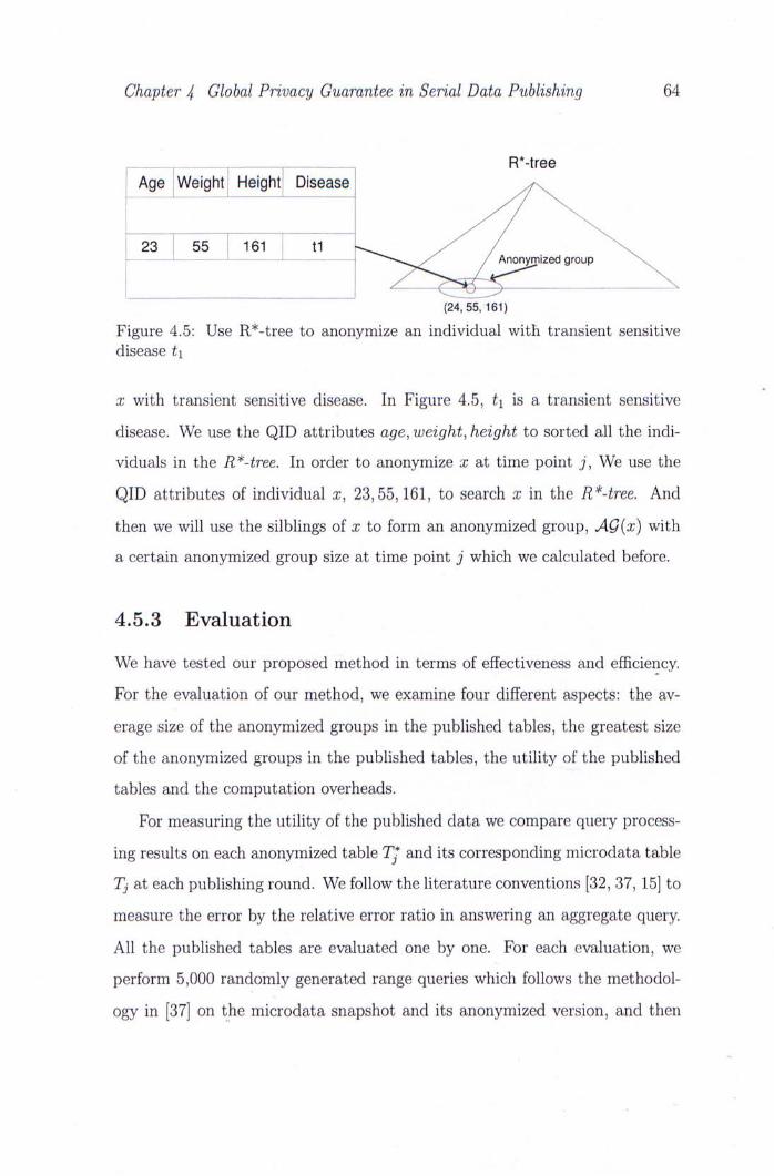
Chapter 4 Global Privacy Guarantee in Serial Data Publishing 64
R*-tree
E ^ 3 y f \ 23 55 161 t1 、-<<^ Z / \
^" - - .N . . . . ^^ / / Anonymized group \ ^
^ ^ ^ ^ ^ \ (24, 55, 161)
Figure 4.5: Use R*-tree to anonymize an individual with transient sensitive disease ti
X with transient sensitive disease. In Figure 4.5, t! is a transient sensitive
disease. We use the QID attributes age, weight, height to sorted all the indi-
viduals in the R*-tree. In order to anonymize x at time point j, We use the
QID attributes of individual x, 23,55,161, to search x in the R*-tree. And
then we will use the silblings of x to form an anonymized group, AG{x) with
a certain anonymized group size at time point j which we calculated before.
4.5.3 Evaluation
We have tested our proposed method in terms of effectiveness and efficiency.
For the evaluation of our method, we examine four different aspects: the av-
erage size of the anonymized groups in the published tables, the greatest size
of the anonymized groups in the published tables, the utility of the published
tables and the computation overheads.
For measuring the utility of the published data we compare query process-
ing results on each anonymized table T* and its corresponding microdata table
Tj at each publishing round. We follow the literature conventions [32, 37, 15] to
measure the error by the relative error ratio in answering an aggregate query.
All the published tables are evaluated one by one. For each evaluation, we
perform 5,000 randomly generated range queries which follows the methodol-
ogy in [37] on the microdata snapshot and its anonymized version, and then
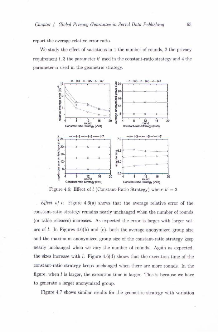
Chapter 4 Global Privacy Guarantee in Serial Data Publishing 65
report the average relative error ratio.
We study the effect of variations in 1 the number of rounds, 2 the privacy
requirement 1, 3 the parameter k' used in the constant-ratio strategy and 4 the
parameter a used in the geometric strategy.
_ • _ 1=3 _ o _ 1=5 _ 6 - 1 = 7 _ o _ | = 3 _ o _ l = 5 _ ^ l = 7 � 6 i ~ . ~ , ~ . • " , ~ . ~ , ~ . ~ .N 2 4 . ~ . ~ , ~ ^ , ~ , ~ ~ . ~ , ~ . ~ ,。\ I . � ) \ 120'i ——A A A , _2 *^^^^ ^ 16- -0) \ \\ .y 0 . \ \2V� p • > 0 0 - o < 1 \ > 存 \ |12-|8- \ �:A . § , 0) o n» „ ._g • o S, 8-1 a o o K I ~ " ^ ‘ ~ . ~ • ~ I ~ • ~ I ~ • ~ 1 e ~ • ~ " i ~ ‘ ^ " i ~ • ~ . ~ • ~ ^ 4 8 12 16 20 ? 4 8 12 16 20
round ® round Constant-ratio Strategy (k_=3) Constant-ratio Strategy (k*=3)
g _ o _ 1=3 _ o _ 1=5 ~ t ^ 1=7 ~ Q ~ 1=3 ~ c > ~ 1=5 ~ ^ 1=7 -¾ 2 4 1 ~ . ~ , ~ ~ , ^ ^ , ~ , ~ , ~ , ~ 7 . 0 1 ~ . ~ , ~ ^ , ~ ~ , ~ . ~ , ~ . ~ a • 2 0 - > A A A ,
T3 26.5- ‘ ^ ^ A A -1 Sl6- - I I - o o o ] B > o � �
§ 12- - 86.0- -ra . g Q D ° ‘ I 8 - 1 • D •
.i 1 1 r~"i 5.5H 1 1 1 ^ 4 8 12 16 20 4 8 12 16 20 E round round
Constant-ratio Strategy (k'=3) Constant-ratio Strategy (k'=3)
Figure 4.6: Effect of 1 (Constant-Ratio Strategy) where k' = 3
Effect of 1: Figure 4.6(a) shows that the average relative error of the
constant-ratio strategy remains nearly unchanged when the number of rounds
(or table releases) increases. As expected the error is larger with larger val-
ues of 1. In Figures 4.6(b) and (c), both the average anonymized group size
and the maximum anonymized group size of the constant-ratio strategy keep
nearly unchanged when we vary the number of rounds. Again as expected,
the sizes increase with 1, Figure 4.6(d) shows that the execution time of the
constant-ratio strategy keeps unchanged when there are more rounds. In the
figure, when 1 is larger, the execution time is larger. This is because we have
to generate a larger anonymized group.
Figure 4.7 shows similar results for the geometric strategy with variation
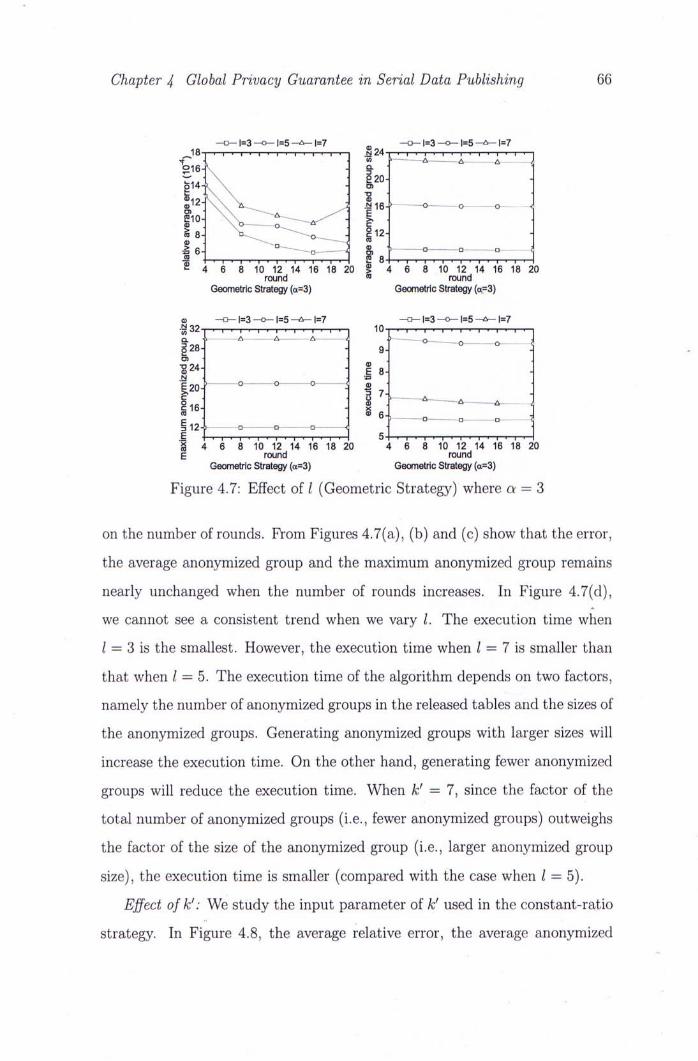
Chapter 4 Global Privacy Guarantee in Serial Data Publishing 66
- o - 1 = 3 ^ 0 ~ 1=5 - ^ 1=7 ① -H>-1=3 - C ^ 1=5 - A - 1 = 7 18n—I—I~~• I <~I—I—I~~I—ri~r~>~"r~~| N 24-r~i~>""i—<~i—<~i~~>~"i"">~~i~>~~i—'~"
节 w k A- --A-- ^ t °16-\ • §• • •^14:\ : e20- • a)^2-V\ \ : 116-> o o o •< iw \ ^ , � � � � Z - I • . ! 8 : 义 ; 。 \ 、 I : 12. -<D � \ � M “
^ 6 - D - 、 、 - o — - - 」 ra ‘ ‘ D -• a ……-o i
^ I ‘ I • I 譬 I I S 8 I I I • 1 • I • " 4 6 8 10 12 14 16 18 20 §J 4 6 8 10 12 14 16 18 20
round “ round Geometric Strategy (a=3) Geometric Strategy (c^=3)
0) ~cH~ 1=3 —o—1=5 ~ ^ 1=7 ~ 3~ 1=3 —o—1=5 ~ ^ 1=7 -¾ 32 I • I 10 I • I ‘ I • ‘ I •
| 2 8 - ' … 各 “ - 9 : ' 。 ° 。 ] ,
^24- • i 8- : N -J3 |20-' � � � ! I / ii6: : | - 1 … 一 丄 -% . . " 6 - , — — — D a 1 § 1 2 - 1 D- o 口….-……< •
.E 5 I § 4 6 8 10 12 14 16 18 20 4 6 8 10 12 14 16 18 20 E round round
Geometric Strategy (a=3) Geometric Strategy (a=3)
Figure 4.7: Effect of 1 (Geometric Strategy) where a = 3
on the number of rounds. From Figures 4.7(a), (b) and (c) show that the error,
the average anonymized group and the maximum anonymized group remains
nearly unchanged when the number of rounds increases. In Figure 4.7(d),
we cannot see a consistent trend when we vary 1. The execution time when
1 = 3 is the smallest. However, the execution time when 1 = 7 is smaller than
that when 1 = 5. The execution time of the algorithm depends on two factors,
namely the number of anonymized groups in the released tables and the sizes of
the anonymized groups. Generating anonymized groups with larger sizes will
increase the execution time. On the other hand, generating fewer anonymized
groups will reduce the execution time. When k' = 7, since the factor of the
total number of anonymized groups (i.e., fewer anonymized groups) outweighs
the factor of the size of the anonymized group (i.e., larger anonymized group
size), the execution time is smaller (compared with the case when 1 = 5).
Effect ofk': We study the input parameter of k' used in the constant-ratio
strategy. In Figure 4.8,the average relative error, the average anonymized
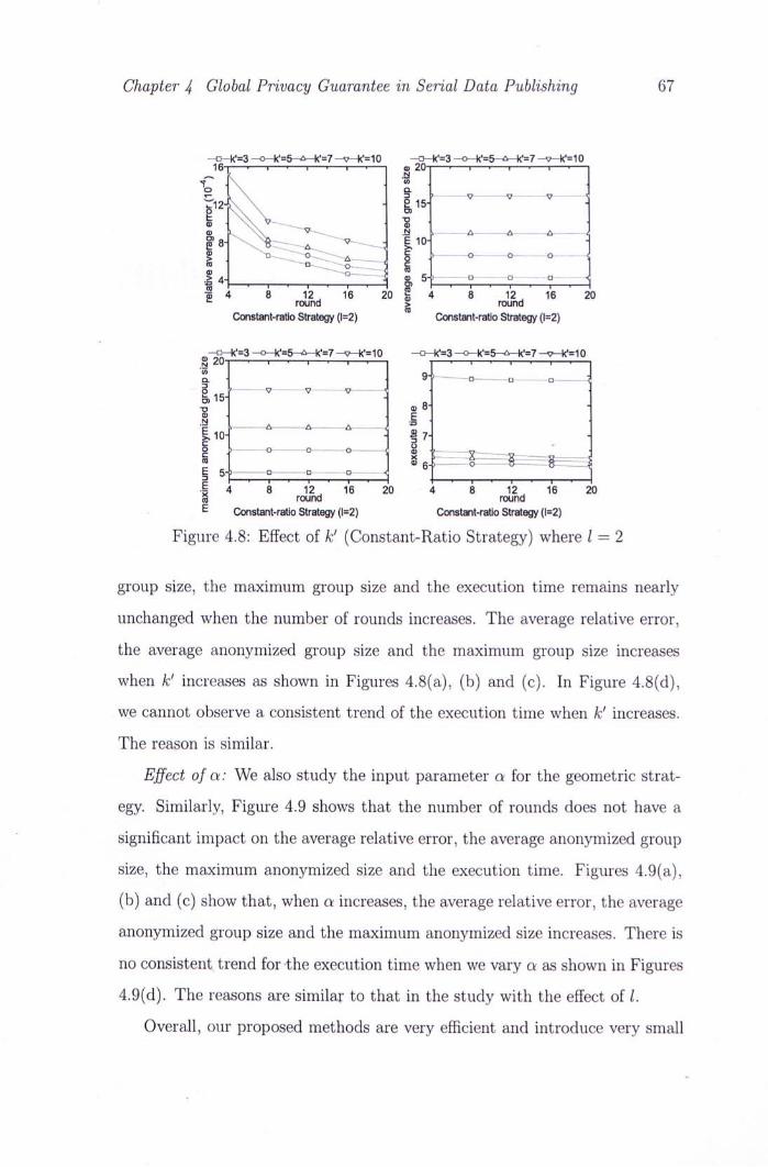
Chapter 4 Global Privacy Guarantee in Serial Data Publishing 67
"CM<.=3 -^k'=5-^k'=7 -vH<'=10 -cM<'=3 -o^=^-^^'=7 -^^=10 16n ‘ 1 ‘ I 1 ‘ 0) 20i ‘ I ‘ 1 ‘ 1
一 K N %= \ . a . r ^ : r ' ' ‘ 0) I� \ \ • .y ^ ^ A A i §'8- \ > - ^ V J E10-? . 力 。 � A- 0 “ � � � W a o i— 2 « .> 4- ��——…1 ® 5” � D a � 运 ^ ~~•~I~• 1~~•~I~~•~~ g' 1~•~I 1~•~~i "55 4 8 12」 16 20 g 4 8 12 16 20 •" round > round
Constant-ratio Strategy (1=2) Constant-ratio Strategy (1=2)
一 "OH<.=3 - o H < ' = 5 - ^ k ' = 7 ^ ^ ' = 1 0 ~oH<"=3 - ^ k ' = 5 - - ^ " = 7 -^7H<'=10 s 20n 1 1 1 1 1 . 1 •<» q., . Q. ® — 0 Q Q- I 2 1«5., • • • j ro 13 o. . ^ . . i® I , A A A , I 1 1 0 . B 7- . 0 ,> - o o o ffl ,— —• „ “ ™ S 6 - ; = : i — fr::--^-:^ E 5" I Q - • • < 1 c 1 I 1 ‘ 1 1 1 I 1 4 8 12」 16 20 4 8 12」 16 20 ro round round E Constant-ratio Strategy (1=2) Constant-ratio Strategy (1=2)
Figui,e 4.8: Effect of k' (Constant-Ratio Strategy) where 1 = 2
group size, the maximum group size and the execution time remains nearly
unchanged when the number of rounds increases. The average relative error,
the average anonymized group size and the maximum group size increases
when k' increases as shown in Figures 4.8(a), (b) and (c). In Figure 4.8(d),
we cannot observe a consistent trend of the execution time when k' increases.
The reason is similar.
Effect of a: We also study the input parameter a for the geometric strat-
egy. Similarly, Figure 4.9 shows that the number of rounds does not have a
significant impact on the average relative error, the average anonymized group
size, the maximum anonymized size and the execution time. Figures 4.9(a),
(b) and (c) show that, when a increases, the average relative error, the average
anonymized group size and the maximum anonymized size increases. There is
no consistent trend for the execution time when we vary a as shown iri Figures
4.9(d). The reasons are similar to that in the study with the effect of 1.
Overall, our proposed methods are very efficient and introduce very small
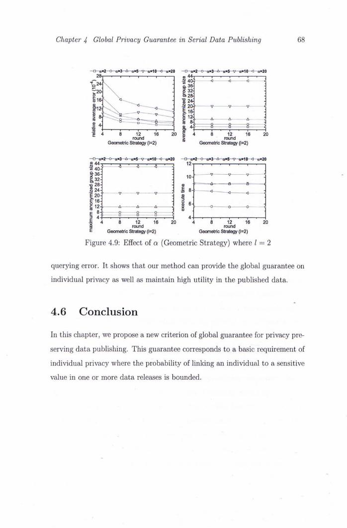
Chapter 4 Global Privacy Guarantee in Serial Data Publishing 68
-Hn—a«2-o-a»3— a"5~-v—a"10-<1-a"20 -HJ-a"2-o~a«3-TiV-a"5~V~a"10-<J-a"20 28-| 1 1 1 • 1 0) 44i r~T 1 1 1 1
-:24^ - ! r " ‘ 一
r \ : ig m1&\ V � - ^24^ ] i l 2 > \ \ \ t - i.: 1 ¾ ' • • • 1 8 t : : V r • • � � | | 3 « ®: : & " ^ - :二6 二 s 1' A A A i ® 4. D S f «8 ^> o o o ^ > 中 0) 4- ‘ � � D ^ ra 1 1 1 2> 1 T • 1 i £ 4 8 12 16 20 I 4 8 12 16 20
rcMjnd > round Geometric Strategy (1=2) Geometric Strategy (1=2)
^ J - a " 2 - o - o " 3 - ^ ^ " 5 - V - a " 1 0 - < - o " 2 0 ^ > - a " 2 - o ^ " 3 - < V - a " 5 - V - a " 1 0 - ^ - a " 2 0
i : ^ i ’ 本 , - 本 , ‘ 丄 1 12j §• 36- - 4^ ‘― • - - • • \ -! 3 2 : - 1。- • •^28� � 0) 卞一--丄《< D B -i N 24 - - M 8 - f < ^ 一 -E 20-' • • • : I — ^ � ‘ |16^ ; “ 6: : C 12-1 A - A A * X > 0 <i o ( ra . • 0) p 8-[ o o o •; £ j, •) D ——a .--O" -- I A i 4 1 1 1 4 1 1 • 1 • 1 I 4 8 12 16 20 4 8 12 16 20 m round round E Geometric Strategy (1=2) Geometric Strategy (1=2)
Figure 4.9: Effect of a (Geometric Strategy) where 1 = 2
querying error. It shows that our method can provide the global guarantee on
individual privacy as well as maintain high utility in the published data.
4.6 Conclusion
In this chapter, we propose a new criterion of global guarantee for privacy pre-
serving data publishing. This guarantee corresponds to a basic requirement of
individual privacy where the probability of linking an individual to a sensitive
value in one or more data releases is bounded.
Bibliography
1] R. Kuinar, J. Novak, and A. Tomkins, Structure and evolution of online
social networks, in KDD, pages 611-617, 2006.
2] L. Backstrom, D. P. Huttenlocher, J. M. Kleiiiberg, and X. Lan, Group
formation in large social networks: membership, growth, and evolution,
in KDD, pages 44—54, 2006.
3] G. Kossinets, J. M. Kleinberg, and D. J. Watts, The structure of in-
formation pathways in a social communication network, in KDD, pages
435-443, 2008.
4] J. Leskovec, L. Backstrom, R. Kumar, and A. Tomkins, Microscopic
evolution of social networks, in KDD, pages 462—470,2008.
5] M. Kuramochi and G. Karypis, Finding frequent patterns in a large sparse
graph, in the SIAM International Conference on Data Mining, 2004.
6] Y. Koren, S. C. North, and C. Volinsky, Measuring and extracting prox-
imity in networks, in KDD, pages 245-255, 2006.
7] H. Tong and C. Faloutsos, Center-piece subgraphs: problem definition
and fast solutions, in KDD, pages 404-413, 2006.
8] J. Cheng, Y. Ke, W. Ng, and J. X. Yu, Context-aware object connection
discovery in large graphs, in Proceedings of the International Conference
on Data Engineering (ICDE), 2009.
69 ..
9] J. Cheng, Y. Ke, A. W.-C. Fu, J. X. Yii, and L. Zhu, Finding maximal
cliques in massive networks by h*-graph, in SIGMOD, 2010.
10] L. Getor and C. Diehl, ACM SIGKDD Explorations Newsletter 7, 3
(2005).
11] A. McCallum, A. Corrada-Emmanuel, and X. Wang, Topic and role dis-
covery in social networks, in Proc. of International Joint Conference on
Artificial Intelligence (IJCAI), 2005.
12] L. Backstrom, C. Dwork, and J. M. Kleinberg, Wherefore art thou
r3579x?: anonymized social networks, hidden patterns, and structural
steganography, in WWW, pages 181-190, 2007.
13] M. Hay, G. Miklau, D. Jensen, P. Weis, and S. Srivastava, Technical report
No. 07-19,Computer Science Department, University of Massachusetts
Amherst (2007).
14] M. Hay, G. Miklau, D. Jensen, D. F. Towsley, and P. Weis, PVLDB 1,
102 (2008).
15] Y. Bii, A. Fu, R. Wong, L. Chen, and J. Li, Privacy preserving serial data,
publishing by role composition, in VLDB, 2008.
16] J. Byun, Y. Sohn, E. Bertino, and N. Li, Secure anonymization for incre-
mental datasets, in Secure Data Management, pages 48-63, 2006.
17] B. Fung, K. Wang, A. Fu, and J. Pei, Anonymity for continuous data
publishing, in EDBT, 2008.
18] K. Liu and E. Terzi, Towards identity anonymization on graphs, in
SIGMOD Conference, pages 93-106, 2008.
19] B. Zhou and J. Pei, Preserving privacy in social networks against neigh-
borhood attacks, in ICDE, pages 506-515, 2008.
70

20] A. Campan and T. M. Truta,A clustering approach for data and struc-
tural anonymity in social networks, in PinKDD, 2008.
[21] L. Zou, L. Chen, and M. T. Ozsu, K-automorphism: A general framework
for privacy preserving network publication, in VLDB, 2009.
22] E. Zheleva and L. Getoor, Preserving the privacy of sensitive relationships
in graph data, in PinKDD, pages 153-171, 2007.
'23] X. Ying and X. Wu, Randomizing social networks: a spectrum preserving
approach, in SDM, pages 739-750, 2008.
24] J. Pei, J. Xu, Z. Wang, W. Wang, and K. Wang, Maintaining k-anonymity
agains incremental updates, in SSEBM, 2007.
25] K.Wang and B. Fung, Anonymizing sequential releases, in SIGKDD,
2006.
26] X. Xiao and Y. Tao, m-invariance: Towards privacy preserving re-
publication of dynamic datasets, in SIGMOD, 2007.
27] L. Adainic and N. Glance, The political blogosphere and the 2004 us
election : divided they blog., in Proceedings of the WWW-2005 Workshop
on the Weblogging Ecosystem, 2005.
28] P. Samarati and L. Sweeney, Protecting privacy when disclosing informa-
tion: k-anonymity and its enforcement through generalization and sup-
pression, Technical report, SRI International, 1998.
29] P. Sainarati, IEEE Transactions on Knowledge and Data Engineering
(TKDE) 13, 1010 (2001).
30] L. Sweeney, International Journal of Uncertainty, Fuzziness and
Knowledge-Based Systems 10’ 557 (2002).
71 ..
31] X. Xiao and Y. Tao, Anatomy: Simple and effective privacy preservation,
in VLDB, 2006.
[32] R. Wong, J. Li, A. Fu, and K. Wang, (alpha, k)-anonymity: An enhanced
k-anonymity model for privacy-preserving data publishing, in KDD, 2006.
33] G. Cormode, D. Srivastava, T. Yu, and Q. Zhang, Anonymizing bipartite
graph data using safe groupings, in PVLDB, 2008.
34] M. R. Garey and D. S. Johnson, Computers and Intractability: A Guide .
to the Theory of NP-Completeness, W. H. Freeman & Co., New York,
NY, USA, 1990.
35] J. Huan, W. Wang, J. Prins, and J. Yang, Spin: mining maximal frequent
subgraphs from graph databases, in KDD, pages 581-586, 2004.
36] A. Dharwadker, http://www.geocities.com/dharwadker/independent_set/
(2006).
37] X. Xiao and Y. Tao, Personalized privacy preservation, in SIGMOD,
2006. ‘
72

i
. ••
‘ ..
'S
•

•• .
• . • -..
.- 〜
- rj
* .' •
- ' •
»
為 • - •
‘ .
V •
‘. •>
C U H K L i b r a r i e s 、
1圓:.. 0 0 4 7 7 9 3 2 0 1 ^
• I