Privacy in Social Networks: identity disclosure

1

1

Privacy in Social Networks:Structural identity disclosure

2

Methods based on k‐anonymityk‐candidatek‐degreek‐neighborhoodk‐automorphism

2

3

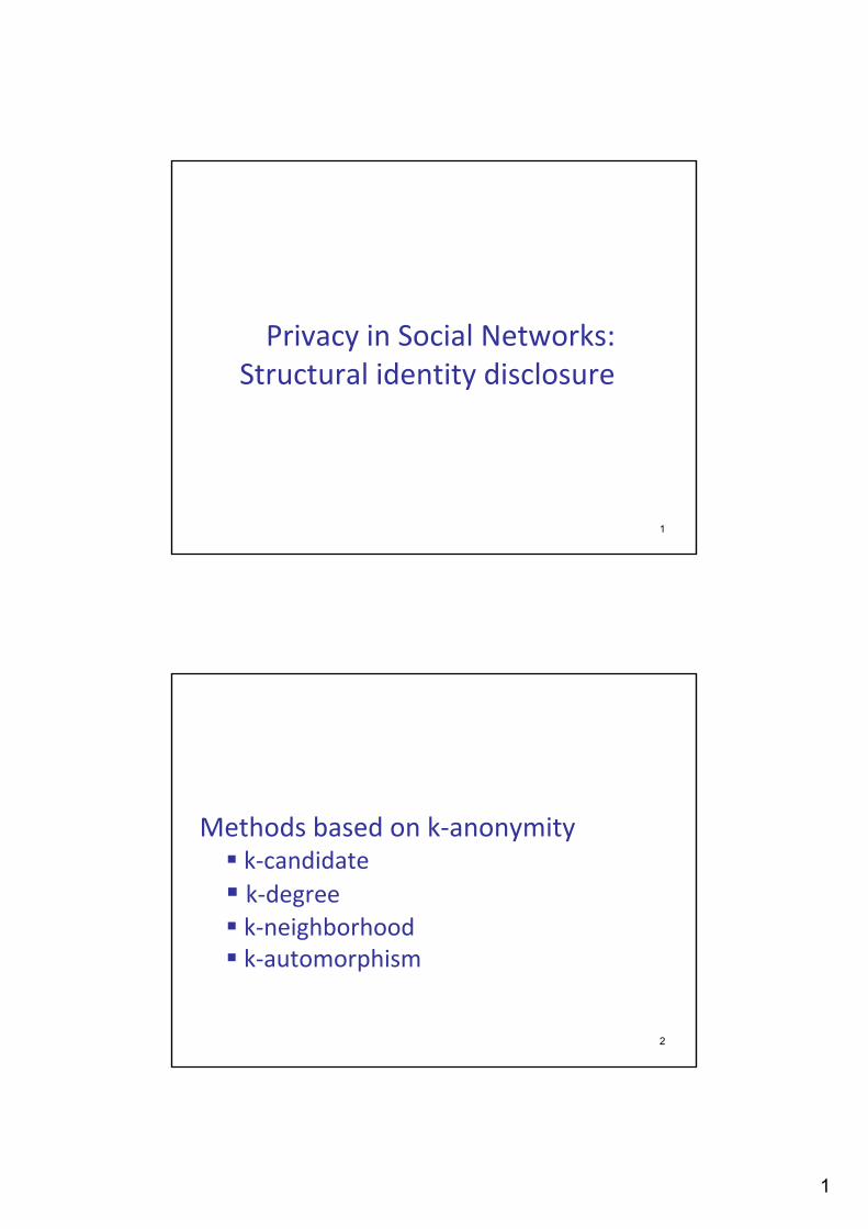
k‐candidate Anonymity

M Hay et al, Resisting Structural Re‐identification in Anonymized Social Networks VLDB 2008

4

An individual x ∈ V called the target has a candidate set, denoted cand(x) which consists of the nodes of Ga that could possibly correspond to x

Ga the naive anonymization of G through an anonymization mapping f

Given an uninformed adversary, each individual has the same risk of re‐identification, cand(x) = Va

In practice, background knowledge, examples:

Bob has three or more neighbors, cand(Bob) =?

Greg is connected to at least two nodes, each with degree 2, cand(Greg) =?

3

5

Focus on

(background knowledge) structural re‐identification where the information of the adversary is about graph structure

(utility) analysis about structural properties: finding communities, fitting power‐law graph models, enumerating motifs, measuring diffusion, accessing resiliency

Two factors

descriptive power of the external information – background knowledge

structural similarity of nodes – graph properties

6

External information may be acquired through

malicious actions by the adversary (active attacks) or

through public information sources

An adversary may be a participant in the network with some innate knowledge of entities and their relationships

Knowledge Acquisition in Practice

Radius ‐ neighborhood

(locality) Adversary knowledge about a targeted individual tends to be local to the targeted nodes

4

7

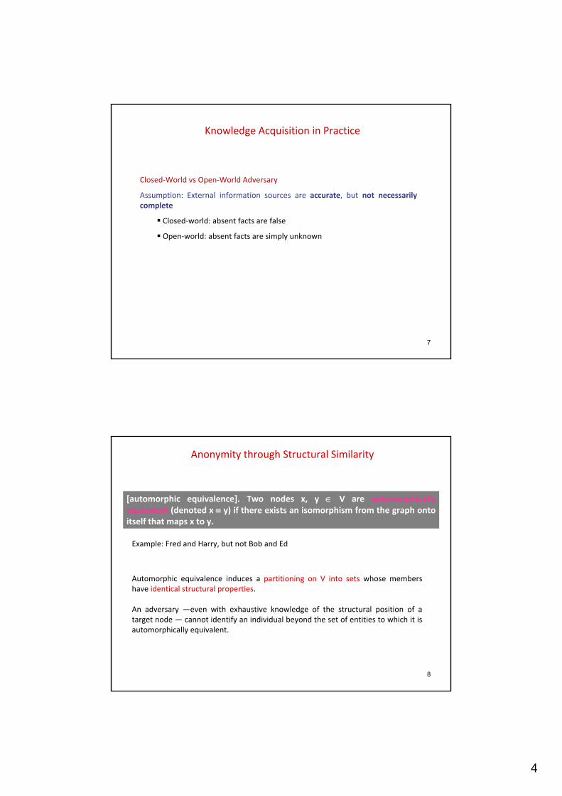
Knowledge Acquisition in Practice

Closed‐World vs Open‐World Adversary

Assumption: External information sources are accurate, but not necessarily complete

Closed‐world: absent facts are false

Open‐world: absent facts are simply unknown

8

Anonymity through Structural Similarity

Example: Fred and Harry, but not Bob and Ed

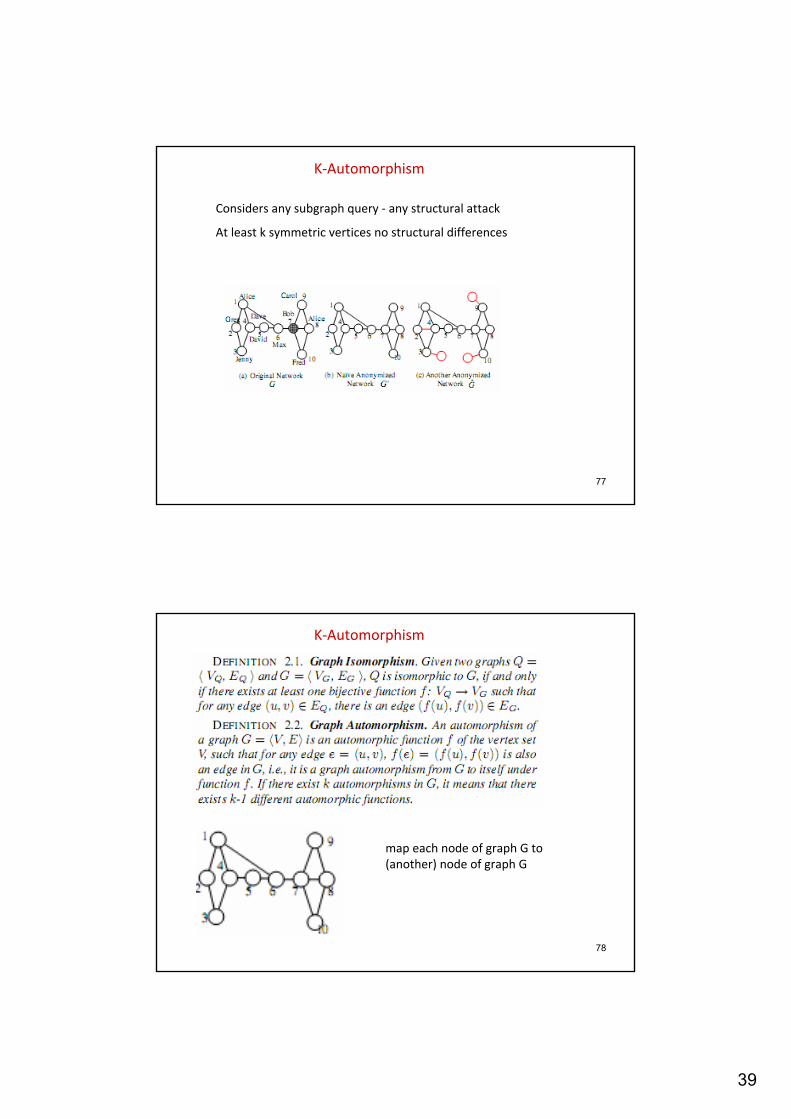
[automorphic equivalence]. Two nodes x, y ∈ V are automorphicallyequivalent (denoted x ≡ y) if there exists an isomorphism from the graph onto itself that maps x to y.

Automorphic equivalence induces a partitioning on V into sets whose members have identical structural properties.

An adversary —even with exhaustive knowledge of the structural position of a target node — cannot identify an individual beyond the set of entities to which it is automorphically equivalent.

5

9

Anonymity through Structural Similarity

Some special graphs have large automorphic equivalence classes.E.g., complete graph, a ring

In general, an extremely strong notion of structural similarity.

10

Adversary Knowledge (model)

An adversary access a source that provides answers to a restricted knowledge query Q evaluated for a single target node of the original graph G.

knowledge gathered by the adversary is accurate.

For target x, use Q(x) to refine the candidate set.

[CANDIDATE SET UNDER Q]. For a query Q over a graph, the candidate set of x w.r.t Q is candQ(x) = {y ∈Va | Q(x) = Q(y)}.

6

11

Adversary Knowledge

1. Vertex Refinement Queries2. Subgraph Queries3. Hub Fingerprint Queries

12

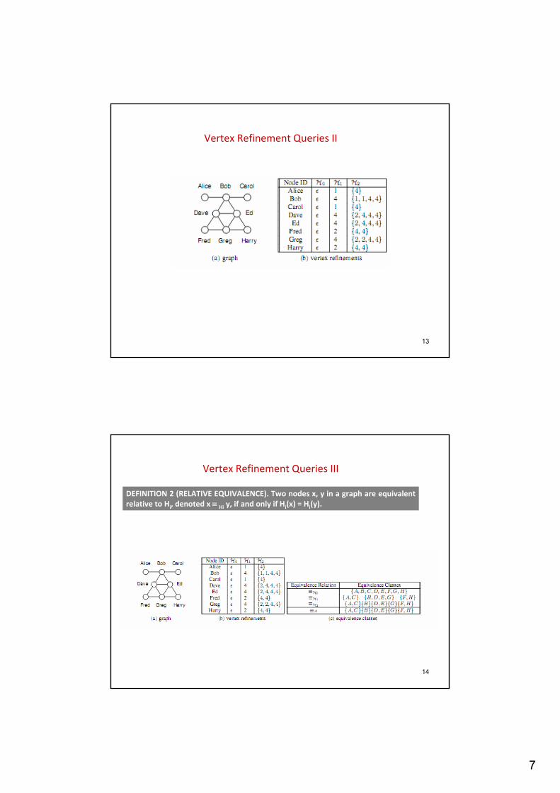
Vertex Refinement Queries

A class of queries of increasing power which report on the local structure of the graph around a node.

The weakest knowledge query, H0, simply returns the label of the node.

H1(x) returns the degree of x,

H2(x) returns the multiset of each neighbors’ degree,

Hi(x) returns the multiset of values which are the result of evaluating Hi‐1 on the nodes adjacent to x

H* Iterative computation of H until no new vertices are distinguished.

7

13

Vertex Refinement Queries II

14

Vertex Refinement Queries III

DEFINITION 2 (RELATIVE EQUIVALENCE). Two nodes x, y in a graph are equivalent relative to Hi, denoted x ≡ Hi y, if and only if Hi(x) = Hi(y).

8

15

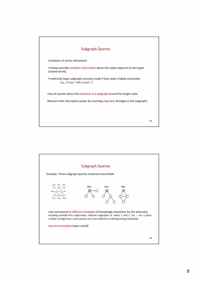
Subgraph Queries

Limitation of vertex refinement:

always provide complete information about the nodes adjacent to the target (closed‐world).

arbitrarily large subgraphs around a node if that node is highly connectedE.g.,, if H1(x) = 100 vs H1(y) = 2

class of queries about the existence of a subgraph around the target node.

Measure their descriptive power by counting edge facts (# edges in the subgraph).

16

Subgraph Queries

Example: Three subgraph queries centered around Bob.

may correspond to different strategies of knowledge acquisition by the adversary. including breadth‐first exploration, induced subgraphs of radius 1 and 2. etc ‐‐ For a given number of edge facts, some queries are more effective at distinguishing individuals.

may be incomplete (open‐world)

9

17

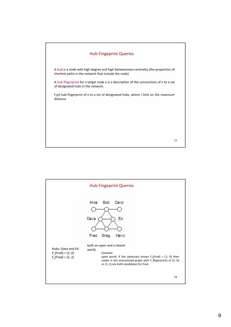
Hub Fingeprint Queries

A hub is a node with high degree and high betweenness centrality (the proportion of shortest paths in the network that include the node)

A hub fingerprint for a target node x is a description of the connections of x to a set of designated hubs in the network.

Fi(x) hub fingerprint of x to a set of designated hubs, where i limit on the maximum distance

18

Hub Fingeprint Queries

Hubs: Dave and Ed F1(Fred) = (1; 0) F2(Fred) = (1; 2)

both an open and a closed world.

Example:open world, if the adversary knows F1(Fred) = (1; 0) then nodes in the anonymized graph with F1 fingerprints of (1; 0) or (1; 1) are both candidates for Fred.

10

19

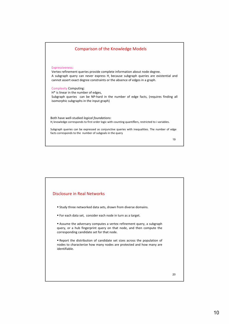
Comparison of the Knowledge Models

Expressiveness:Vertex refinement queries provide complete information about node degree. A subgraph query can never express Hi because subgraph queries are existential and cannot assert exact degree constraints or the absence of edges in a graph.

Complexity Computing: H* is linear in the number of edges,Subgraph queries can be NP‐hard in the number of edge facts, (requires finding all isomorphic subgraphs in the input graph)

Both have well‐studied logical foundations: Hi knowledge corresponds to first order logic with counting quantifiers, restricted to i variables.

Subgraph queries can be expressed as conjunctive queries with inequalities. The number of edge facts corresponds to the number of subgoals in the query

20

Disclosure in Real Networks

Study three networked data sets, drawn from diverse domains.

For each data set, consider each node in turn as a target.

Assume the adversary computes a vertex refinement query, a subgraphquery, or a hub fingerprint query on that node, and then compute the corresponding candidate set for that node.

Report the distribution of candidate set sizes across the population of nodes to characterize how many nodes are protected and how many are identifiable.

11

21

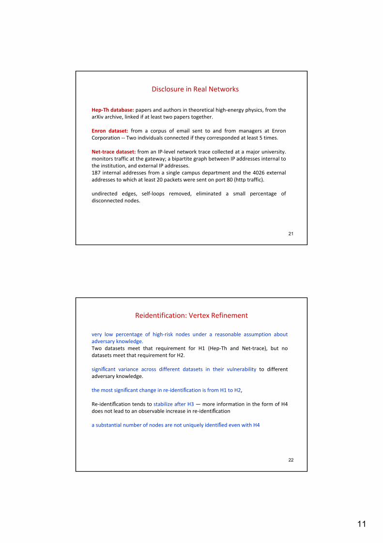
Disclosure in Real Networks

Hep‐Th database: papers and authors in theoretical high‐energy physics, from the arXiv archive, linked if at least two papers together.

Enron dataset: from a corpus of email sent to and from managers at Enron Corporation ‐‐ Two individuals connected if they corresponded at least 5 times.

Net‐trace dataset: from an IP‐level network trace collected at a major university. monitors traffic at the gateway; a bipartite graph between IP addresses internal to the institution, and external IP addresses. 187 internal addresses from a single campus department and the 4026 external addresses to which at least 20 packets were sent on port 80 (http traffic).

undirected edges, self‐loops removed, eliminated a small percentage of disconnected nodes.

22

Reidentification: Vertex Refinement

very low percentage of high‐risk nodes under a reasonable assumption about adversary knowledge.Two datasets meet that requirement for H1 (Hep‐Th and Net‐trace), but no datasets meet that requirement for H2.

significant variance across different datasets in their vulnerability to different adversary knowledge.

the most significant change in re‐identification is from H1 to H2,

Re‐identification tends to stabilize after H3 — more information in the form of H4 does not lead to an observable increase in re‐identification

a substantial number of nodes are not uniquely identified even with H4

12

23

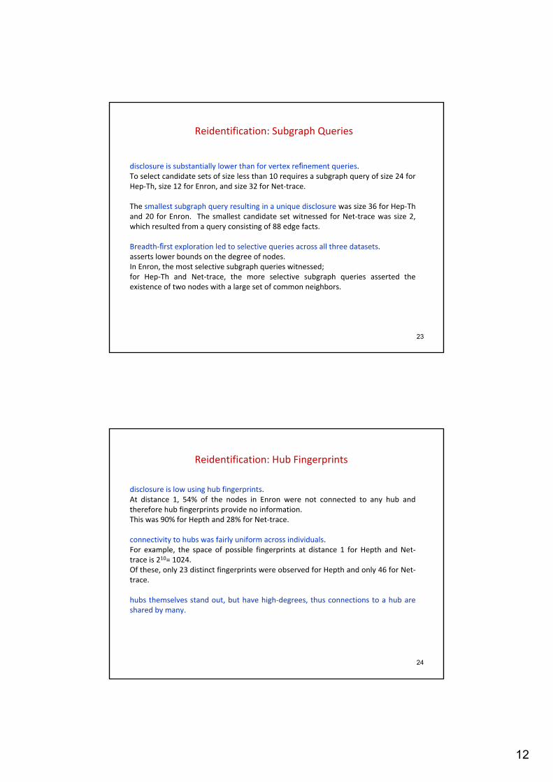
Reidentification: Subgraph Queries

disclosure is substantially lower than for vertex refinement queries. To select candidate sets of size less than 10 requires a subgraph query of size 24 for Hep‐Th, size 12 for Enron, and size 32 for Net‐trace.

The smallest subgraph query resulting in a unique disclosure was size 36 for Hep‐Thand 20 for Enron. The smallest candidate set witnessed for Net‐trace was size 2, which resulted from a query consisting of 88 edge facts.

Breadth‐first exploration led to selective queries across all three datasets. asserts lower bounds on the degree of nodes. In Enron, the most selective subgraph queries witnessed; for Hep‐Th and Net‐trace, the more selective subgraph queries asserted the existence of two nodes with a large set of common neighbors.

24

Reidentification: Hub Fingerprints

disclosure is low using hub fingerprints. At distance 1, 54% of the nodes in Enron were not connected to any hub and therefore hub fingerprints provide no information. This was 90% for Hepth and 28% for Net‐trace.

connectivity to hubs was fairly uniform across individuals. For example, the space of possible fingerprints at distance 1 for Hepth and Net‐trace is 210= 1024. Of these, only 23 distinct fingerprints were observed for Hepth and only 46 for Net‐trace.

hubs themselves stand out, but have high‐degrees, thus connections to a hub are shared by many.

13

25

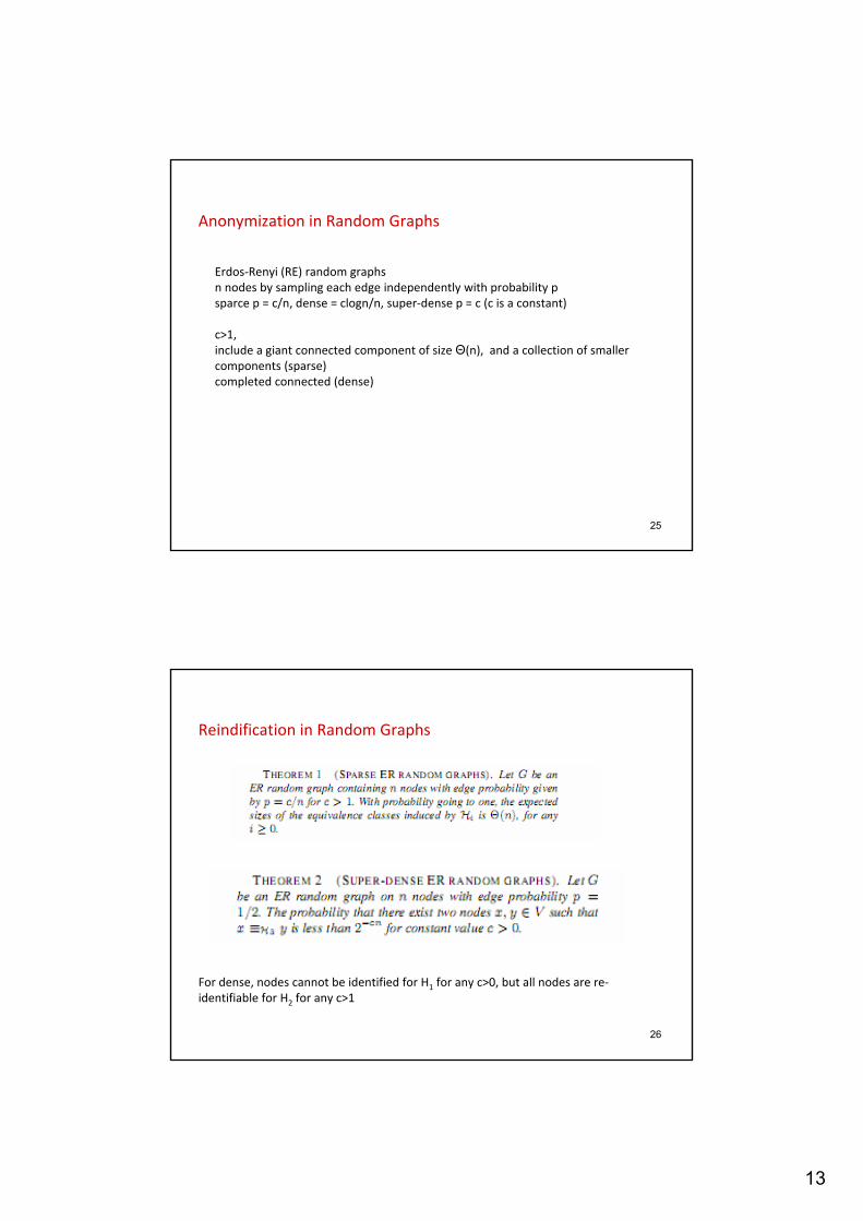
Anonymization in Random Graphs

Erdos‐Renyi (RE) random graphsn nodes by sampling each edge independently with probability psparce p = c/n, dense = clogn/n, super‐dense p = c (c is a constant)

c>1, include a giant connected component of size Θ(n), and a collection of smaller components (sparse)completed connected (dense)

26

Reindification in Random Graphs

For dense, nodes cannot be identified for H1 for any c>0, but all nodes are re‐identifiable for H2 for any c>1

14

27

Reindification in Random Graphs

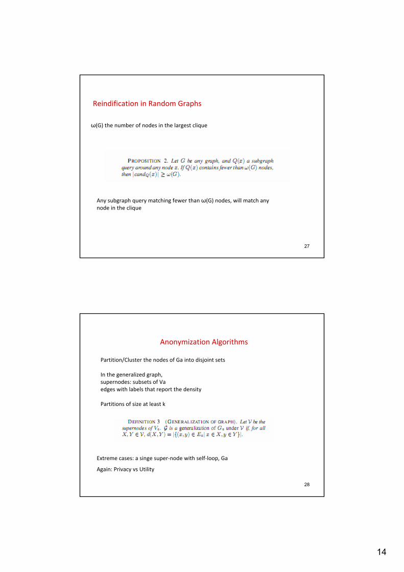
ω(G) the number of nodes in the largest clique

Any subgraph query matching fewer than ω(G) nodes, will match any node in the clique

28

Anonymization Algorithms

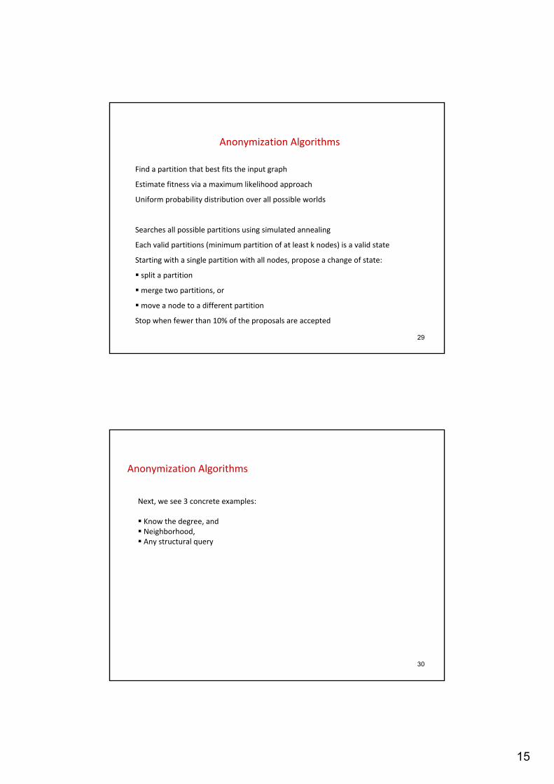
Partition/Cluster the nodes of Ga into disjoint sets

In the generalized graph, supernodes: subsets of Vaedges with labels that report the density

Partitions of size at least k

Extreme cases: a singe super‐node with self‐loop, Ga

Again: Privacy vs Utility

15

29


Find a partition that best fits the input graph

Estimate fitness via a maximum likelihood approach

Uniform probability distribution over all possible worlds

Searches all possible partitions using simulated annealing

Each valid partitions (minimum partition of at least k nodes) is a valid state

Starting with a single partition with all nodes, propose a change of state:

split a partition

merge two partitions, or

move a node to a different partition

Stop when fewer than 10% of the proposals are accepted

30


Next, we see 3 concrete examples:

Know the degree, andNeighborhood,Any structural query

16

31

k‐degree Anonymity

K. Liu and E. Terzi, Towards Identity Anonymization on Graphs, SIGMOD 2008

32

Identity anonymization on graphs

• Question– How to share a network in a manner that permits useful analysis

without disclosing the identity of the individuals involved?

• Observations– Simply removing the identifying information of the nodes before

publishing the actual graph does not guarantee identity anonymization.

L. Backstrom, C. Dwork, and J. Kleinberg, “Wherefore art thou R3579X?: Anonymized social netwoks, hidden patterns, and structural steganography,” In WWW 2007.

J. Kleinberg, “Challenges in Social Network Data: Processes, Privacy and Paradoxes, ” KDD 2007 Keynote Talk.

• Can we borrow ideas from k-anonymity?

17

33

What if you want to prevent the following from happening

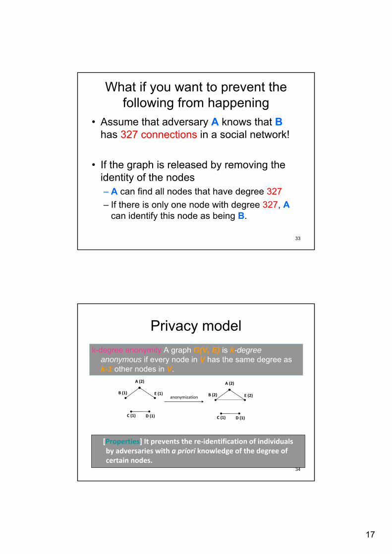
• Assume that adversary A knows that Bhas 327 connections in a social network!

• If the graph is released by removing the identity of the nodes– A can find all nodes that have degree 327– If there is only one node with degree 327, A

can identify this node as being B.

34

Privacy modelk-degree anonymity A graph G(V, E) is k-degree

anonymous if every node in V has the same degree as k-1 other nodes in V.

[Properties] It prevents the re‐identification of individuals by adversaries with a priori knowledge of the degree of certain nodes.

A (2)

B (1) E (1)

C (1) D (1)

A (2)

B (2) E (2)

C (1) D (1)

anonymization

18

35

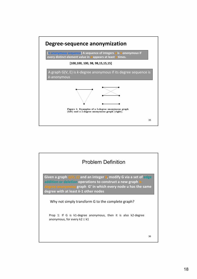
Degree‐sequence anonymization

[k‐anonymous sequence] A sequence of integers d is k‐anonymous if every distinct element value in d appears at least k times.

[100,100, 100, 98, 98,15,15,15]

A graph G(V, E) is k‐degree anonymous if its degree sequence is k‐anonymous

36

Problem Definition

Given a graph G(V, E) and an integer k, modify G via a set of edge addition or deletion operations to construct a new graph k‐degree anonymous graph G’ in which every node u has the same degree with at least k‐1 other nodes

Why not simply transform G to the complete graph?

Prop 1: If G is k1‐degree anonymous, then it is also k2‐degree anonymous, for every k2 ≤ k1

19

37

Problem Definition

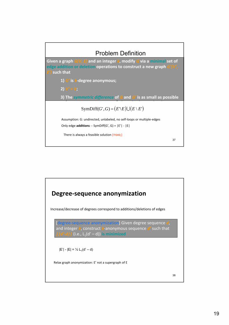
• Symmetric difference between graphs G(V,E) and G’(V,E’) :

Given a graph G(V, E) and an integer k, modify G via a minimal set of edge addition or deletion operations to construct a new graph G’(V’, E’) such that

1) G’ is k‐degree anonymous;

2) V’ = V;

3) The symmetric difference of G and G’ is as small as possible

( ) ( )'\\'),'SymDiff( EEEEGG U=

Assumption: G: undirected, unlabeled, no self‐loops or multiple‐edges

Only edge additions ‐‐ SymDiff(G’, G) = |E’| ‐ |E|

There is always a feasible solution (ποια;)

38

Degree‐sequence anonymization

[degree‐sequence anonymization] Given degree sequence d, and integer k, construct k‐anonymous sequence d’ such that ||d’‐d|| (i.e., L1(d’ – d)) is minimized

Increase/decrease of degrees correspond to additions/deletions of edges

|E’| - |E| = ½ L1(d’ – d)

Relax graph anonymization: E’ not a supergraph of E

20

39

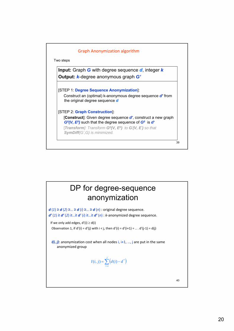
Input: Graph G with degree sequence d, integer kOutput: k-degree anonymous graph G’

[STEP 1: Degree Sequence Anonymization]: Construct an (optimal) k-anonymous degree sequence d’ from the original degree sequence d

[STEP 2: Graph Construction]: [Construct]: Given degree sequence d', construct a new graph G0(V, E0) such that the degree sequence of G0 is d‘[Transform]: Transform G0(V, E0) to G’(V, E’) so that SymDiff(G’,G) is minimized.

Graph Anonymization algorithm

Two steps

40

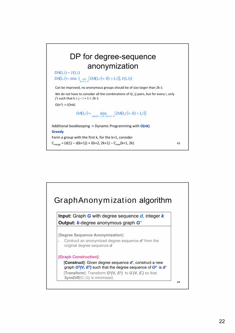
DP for degree-sequence anonymization

d (1) ≥ d (2) ≥… ≥ d (i) ≥… ≥ d (n) : original degree sequence.d’ (1) ≥ d’ (2) ≥…≥ d’ (i) ≥…≥ d’ (n) : k‐anonymized degree sequence.

If we only add edges, d’(i) ≥ d(i)

Observation 1, if d’(i) = d’(j) with i < j, then d’(i) = d’(i+1) = .. . d’(j‐1) = d(j)

( )∑=

−=j

ididjiI

l

*)(),(

I(i, j): anonymization cost when all nodes i, i+1, …, j are put in the same anonymized group

21

41

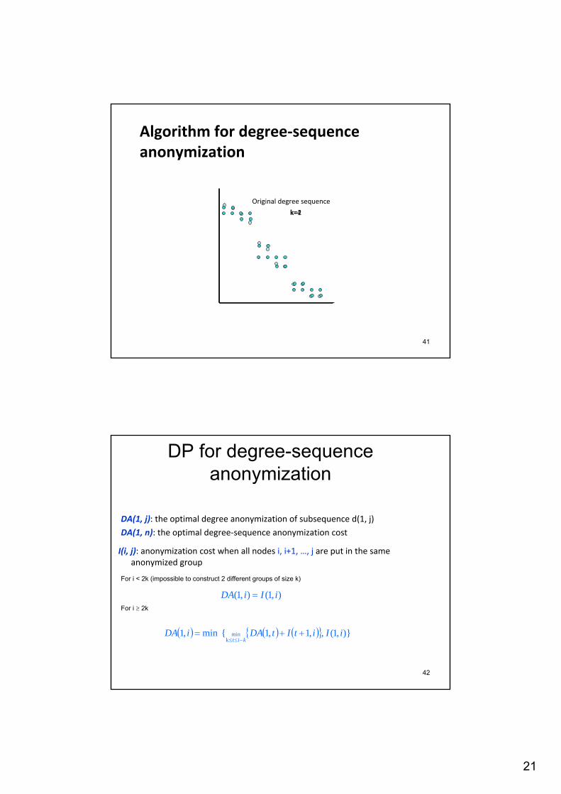
Algorithm for degree‐sequence anonymization

Original degree sequence

k=2k=4

42


DA(1, j): the optimal degree anonymization of subsequence d(1, j)

DA(1, n): the optimal degree‐sequence anonymization cost

I(i, j): anonymization cost when all nodes i, i+1, …, j are put in the same anonymized group

( ) ( ) ( ){ } )},1( ,,1,1{ min,1k

min iIitItDAiDAkit

++=−≤≤

For i < 2k (impossible to construct 2 different groups of size k)

),1(),1( iIiDA =For i ≥ 2k

22

43


Additional bookkeeping ‐> Dynamic Programming with O(nk)Greedy

Form a group with the first k, for the k+1, considerCmerge = (d(1) – d(k+1)) + I(k+2, 2k+1) – Cnew(k+1, 2k)

( ){ }

( ) ( ){ }itItDAiDAkitkik

,1,1min,112,max

++=−≤≤+−

( ) ( ) ( ){ } )},1( ,,1,1{ min,1k

min iIitItDAiDAkit

++=−≤≤

),1(),1( iIiDA =

Can be improved, no anonymous groups should be of size larger than 2k‐1

We do not have to consider all the combinations of I(i, j) pairs, but for every i, only j’s such that k ≤ j – i + 1 ≤ 2k‐1

O(n2) ‐> (Onk)

44

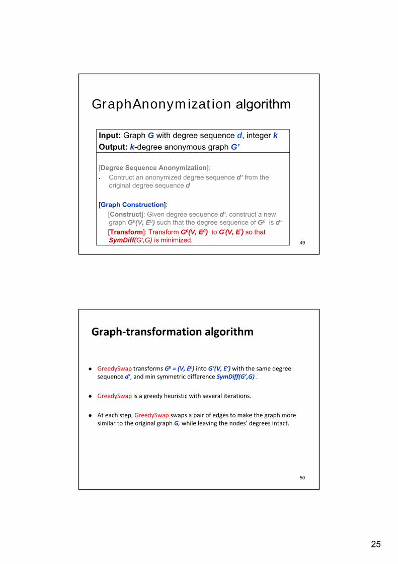
GraphAnonymization algorithm


[Degree Sequence Anonymization]: • Contruct an anonymized degree sequence d’ from the

original degree sequence d

[Graph Construction]: [Construct]: Given degree sequence d', construct a new graph G0(V, E0) such that the degree sequence of G0 is d‘[Transform]: Transform G0(V, E0) to G’(V, E’) so that SymDiff(G’,G) is minimized.

23

45

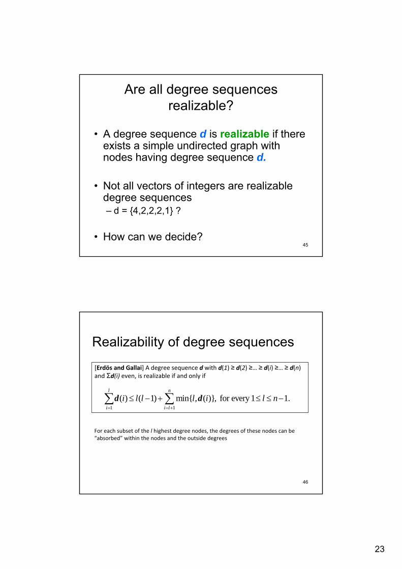
Are all degree sequences realizable?

• A degree sequence d is realizable if there exists a simple undirected graph with nodes having degree sequence d.

• Not all vectors of integers are realizable degree sequences– d = {4,2,2,2,1} ?

• How can we decide?

46

Realizability of degree sequences

[Erdös and Gallai] A degree sequence d with d(1) ≥ d(2) ≥… ≥ d(i) ≥… ≥ d(n) and Σd(i) even, is realizable if and only if

1 1

( ) ( 1) min{ , ( )}, for every 1 1.l n

i i l

i l l l i l n= = +

≤ − + ≤ ≤ −∑ ∑d d

For each subset of the l highest degree nodes, the degrees of these nodes can be “absorbed” within the nodes and the outside degrees

24

47

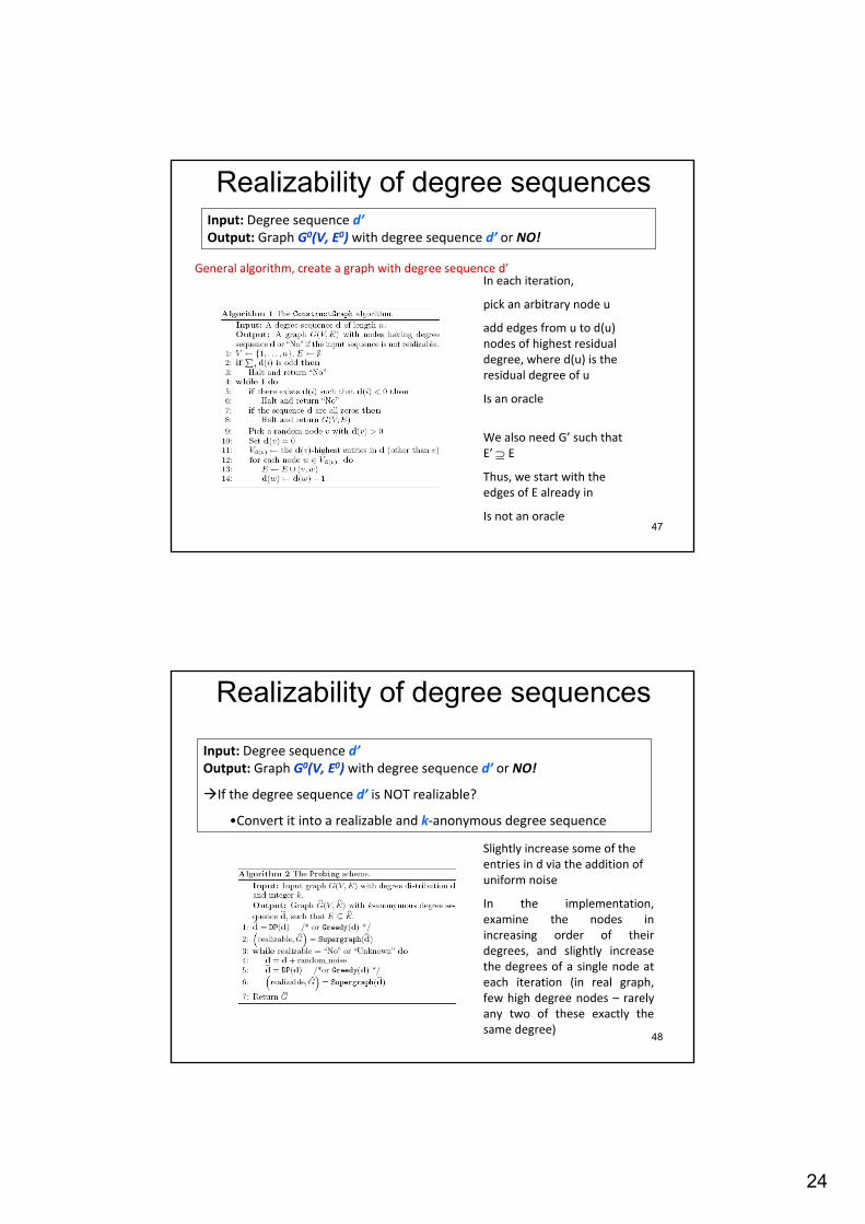
Realizability of degree sequencesInput: Degree sequence d’Output: Graph G0(V, E0) with degree sequence d’ or NO!

In each iteration,

pick an arbitrary node u

add edges from u to d(u) nodes of highest residual degree, where d(u) is the residual degree of u

Is an oracle

We also need G’ such that E’ ⊇ E

Thus, we start with the edges of E already in

Is not an oracle

General algorithm, create a graph with degree sequence d’

48

Realizability of degree sequences

Input: Degree sequence d’Output: Graph G0(V, E0) with degree sequence d’ or NO!

If the degree sequence d’ is NOT realizable?

•Convert it into a realizable and k‐anonymous degree sequence

Slightly increase some of the entries in d via the addition of uniform noise

In the implementation, examine the nodes in increasing order of their degrees, and slightly increase the degrees of a single node at each iteration (in real graph, few high degree nodes – rarely any two of these exactly the same degree)

25

49

GraphAnonymization algorithm


[Degree Sequence Anonymization]: • Contruct an anonymized degree sequence d’ from the

original degree sequence d

[Graph Construction]: [Construct]: Given degree sequence d', construct a new graph G0(V, E0) such that the degree sequence of G0 is d‘[Transform]: Transform G0(V, E0) to G’(V, E’) so that SymDiff(G’,G) is minimized.

50

Graph‐transformation algorithm

GreedySwap transforms G0 = (V, E0) into G’(V, E’) with the same degree sequence d’, and min symmetric difference SymDiff(G’,G) .

GreedySwap is a greedy heuristic with several iterations.

At each step, GreedySwap swaps a pair of edges to make the graph more similar to the original graph G, while leaving the nodes’ degrees intact.

26

51

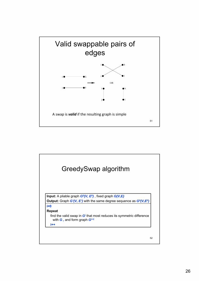
Valid swappable pairs of edges

A swap is valid if the resulting graph is simple

52

GreedySwap algorithm

Input: A pliable graph G0(V, E0) , fixed graph G(V,E)Output: Graph G’(V, E’) with the same degree sequence as G0(V,E0)i=0Repeat

find the valid swap in Gi that most reduces its symmetric difference with G , and form graph Gi+1

i++

27

53

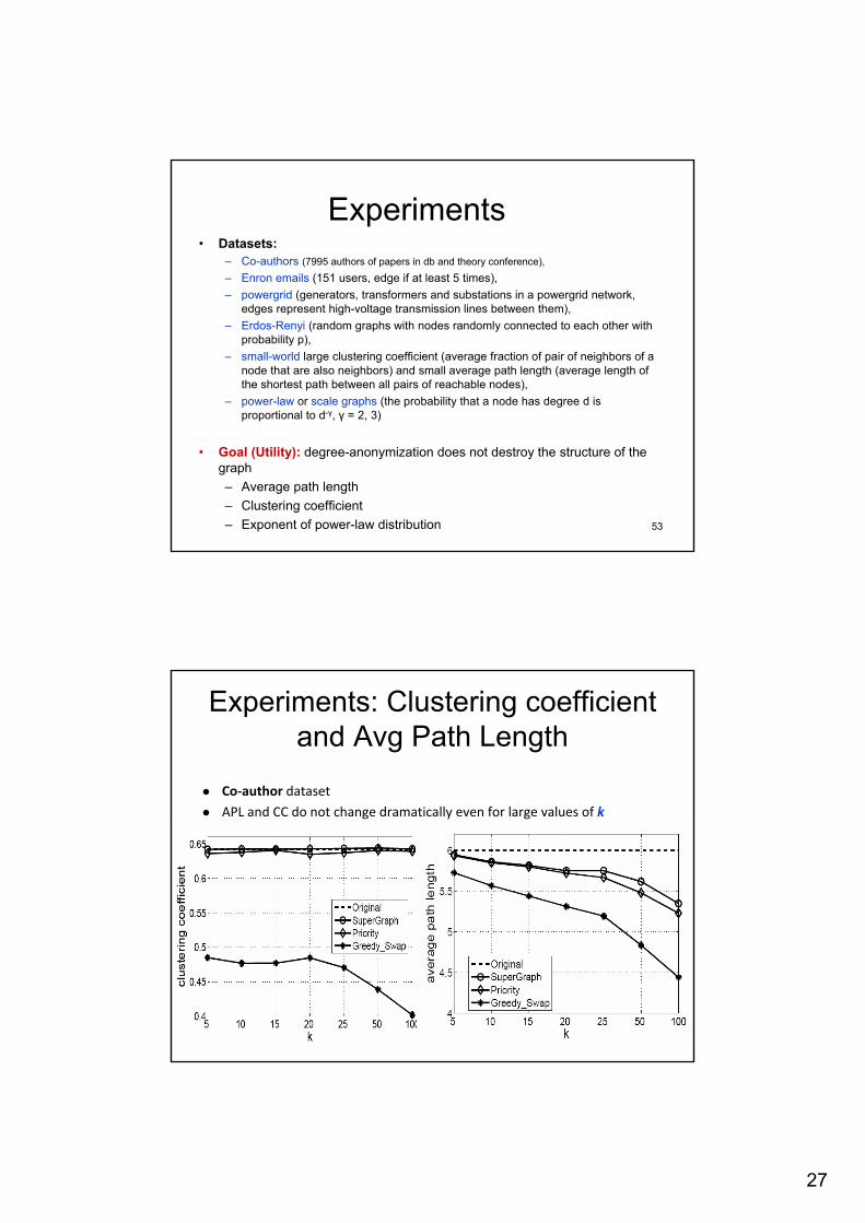
Experiments• Datasets:

– Co-authors (7995 authors of papers in db and theory conference),– Enron emails (151 users, edge if at least 5 times), – powergrid (generators, transformers and substations in a powergrid network,

edges represent high-voltage transmission lines between them), – Erdos-Renyi (random graphs with nodes randomly connected to each other with

probability p), – small-world large clustering coefficient (average fraction of pair of neighbors of a

node that are also neighbors) and small average path length (average length of the shortest path between all pairs of reachable nodes),

– power-law or scale graphs (the probability that a node has degree d is proportional to d-γ, γ = 2, 3)

• Goal (Utility): degree-anonymization does not destroy the structure of the graph– Average path length– Clustering coefficient– Exponent of power-law distribution

54

Experiments: Clustering coefficient and Avg Path Length

Co‐author datasetAPL and CC do not change dramatically even for large values of k

28

55

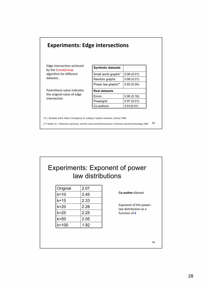
Experiments: Edge intersections

Synthetic datasets

Small world graphs* 0.99 (0.01)Random graphs 0.99 (0.01)

Power law graphs** 0.93 (0.04)

Real datasets

Enron 0.95 (0.16)Powergrid 0.97 (0.01)Co-authors 0.91(0.01)

(*) L. Barabasi and R. Albert: Emergence of scaling in random networks. Science 1999.

(**) Watts, D. J. Networks, dynamics, and the small‐world phenomenon. American Journal of Sociology 1999

Edge intersection achieved by the GreedySwapalgorithm for different datasets.

Parenthesis value indicates the original value of edge intersection

56

Experiments: Exponent of power law distributions

Original 2.07k=10 2.45k=15 2.33k=20 2.28k=25 2.25k=50 2.05k=100 1.92

Co‐author dataset

Exponent of the power‐law distribution as a function of k

29

57

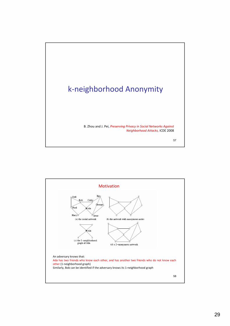
k‐neighborhood Anonymity

B. Zhou and J. Pei, Preserving Privacy in Social Networks Against Neighborhood Attacks, ICDE 2008

58

An adversary knows that:Ada has two friends who know each other, and has another two friends who do not know eachother (1‐neighborhood graph)Similarly, Bob can be identified if the adversary knows its 1‐neighborhood graph

Motivation

30

59

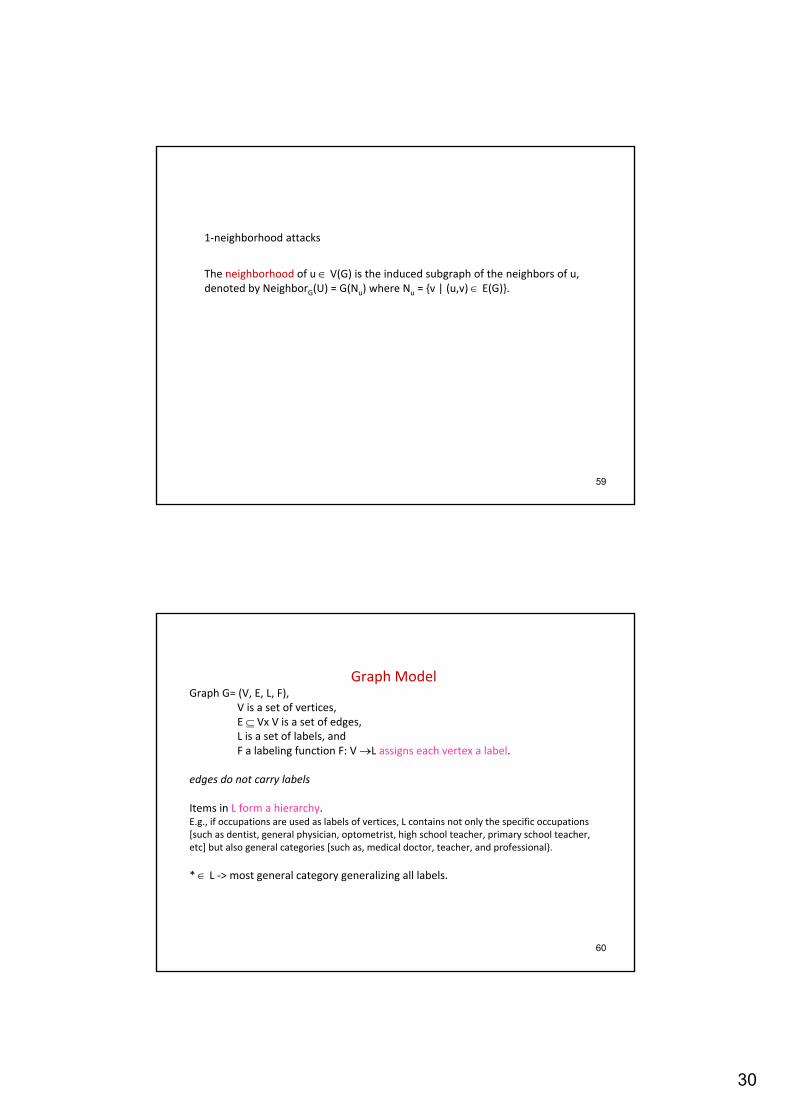
1‐neighborhood attacks

The neighborhood of u ∈ V(G) is the induced subgraph of the neighbors of u, denoted by NeighborG(U) = G(Nu) where Nu = {v | (u,v) ∈ E(G)}.

60

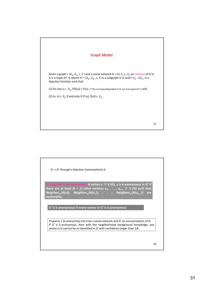
Graph ModelGraph G= (V, E, L, F),

V is a set of vertices, E ⊆ Vx V is a set of edges, L is a set of labels, and F a labeling function F: V →L assigns each vertex a label.

edges do not carry labels

Items in L form a hierarchy. E.g., if occupations are used as labels of vertices, L contains not only the specific occupations [such as dentist, general physician, optometrist, high school teacher, primary school teacher, etc] but also general categories [such as, medical doctor, teacher, and professional}.

* ∈ L ‐> most general category generalizing all labels.

31

61

Graph Model

Given a graph = (VH, EH, L, F ) and a social network G = (V, E, L, L), an instance of H in G is a tuple (H', f) where H' = (VH’ ,EH’ ,L, F) is a subgraph in G and f: VH →VH’, is a bijection function such that

(1) for any u ∈ VH, F(f(u)) ≤ F(u), /* the corresponding labels in H’ are more general */ and

(2) (u, v) ∈ EH if and only if (f (u), f(v)) ∈ EH’.

62

[k‐neighborhood anonymity] A vertex u ∈ V (G), u is k anonymous in G’ ifthere are at least (k − 1) other vertices u1, . . . , uk−1 ∈ V (G) such thatNeighborG′(A(u)), NeighborG′(A(u1)), . . ., NeighborG′(A(uk−1)) areisomorphic.

G′ is k‐anonymous if every vertex in G′ is k‐anonymous.

Property 1 (k‐anonymity) Let G be a social network and G′ an anonymization of G. If G′ is k‐anonymous, then with the neighborhood background knowledge, anyvertex in G cannot be re‐identified in G′ with confidence larger than 1/k .

G ‐> G’ through a bijection (isomorphism) A

32

63

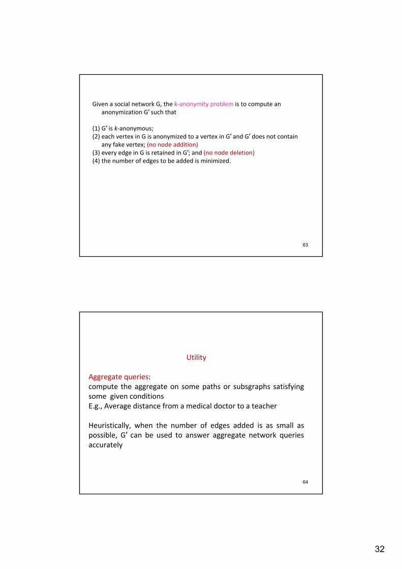
Given a social network G, the k‐anonymity problem is to compute ananonymization G′ such that

(1) G′ is k‐anonymous; (2) each vertex in G is anonymized to a vertex in G′ and G′ does not contain

any fake vertex; (no node addition)(3) every edge in G is retained in G′; and (no node deletion)(4) the number of edges to be added is minimized.

64

Utility

Aggregate queries:compute the aggregate on some paths or subsgraphs satisfying some given conditionsE.g., Average distance from a medical doctor to a teacher

Heuristically, when the number of edges added is as small aspossible, G′ can be used to answer aggregate network queriesaccurately

33

65

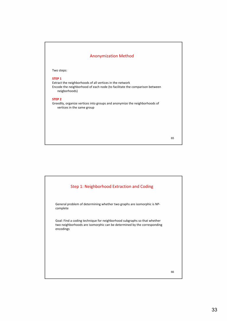
Two steps:

STEP 1Extract the neighborhoods of all vertices in the networkEncode the neighborhood of each node (to facilitate the comparison between

neigborhoods)

STEP 2Greedily, organize vertices into groups and anonymize the neighborhoods of

vertices in the same group

Anonymization Method

66

Step 1: Neighborhood Extraction and Coding

General problem of determining whether two graphs are isomorphic is NP‐complete

Goal: Find a coding technique for neighborhood subgraphs so that whether two neighborhoods are isomorphic can be determined by the corresponding encodings

34

67

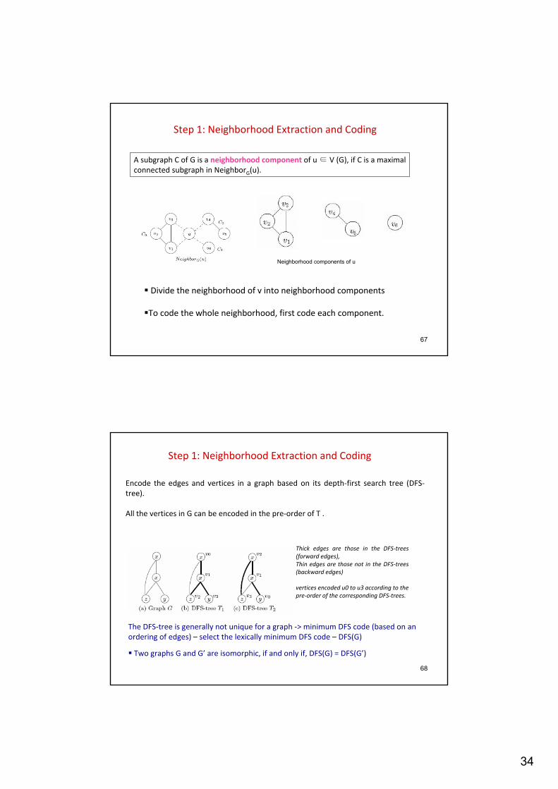
A subgraph C of G is a neighborhood component of u ∈ V (G), if C is a maximalconnected subgraph in NeighborG(u).

Divide the neighborhood of v into neighborhood components

To code the whole neighborhood, first code each component.


Neighborhood components of u

68

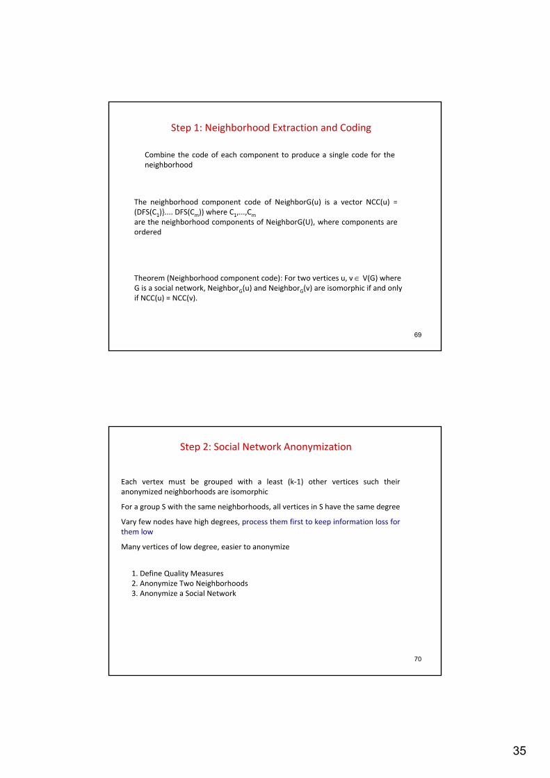
Encode the edges and vertices in a graph based on its depth‐first search tree (DFS‐tree).

All the vertices in G can be encoded in the pre‐order of T .

Thick edges are those in the DFS‐trees(forward edges), Thin edges are those not in the DFS‐trees(backward edges)

vertices encoded u0 to u3 according to thepre‐order of the corresponding DFS‐trees.

The DFS‐tree is generally not unique for a graph ‐> minimum DFS code (based on an ordering of edges) – select the lexically minimum DFS code – DFS(G)


Two graphs G and G’ are isomorphic, if and only if, DFS(G) = DFS(G’)

35

69

Combine the code of each component to produce a single code for the neighborhood

Theorem (Neighborhood component code): For two vertices u, v ∈ V(G) whereG is a social network, NeighborG(u) and NeighborG(v) are isomorphic if and onlyif NCC(u) = NCC(v).


The neighborhood component code of NeighborG(u) is a vector NCC(u) = (DFS(C1)}.... DFS(Cm)) where C1,...,Cmare the neighborhood components of NeighborG(U), where components are ordered

70

Step 2: Social Network Anonymization

Each vertex must be grouped with a least (k‐1) other vertices such their anonymized neighborhoods are isomorphic

For a group S with the same neighborhoods, all vertices in S have the same degree

Vary few nodes have high degrees, process them first to keep information loss for them low

Many vertices of low degree, easier to anonymize

1. Define Quality Measures2. Anonymize Two Neighborhoods3. Anonymize a Social Network

36

71

Step 2: Quality Measures

Generalize vertex labels

l1 (leaf level)‐> more general l2 (penalty or loss as

in relational) size(*)= #leafs

Add Edges

Total number of edges added +

Number of vertices that are not in the neighborhood of the target vertex and are linked for anonymization

72

Step 2: Anonymizing 2 neighborhoodsFirst, find all perfect matches of neighborhood components (perfectly match=same minimum DFS code)

For unmatched, try to pair “similar” components and anonymize them

How: greedily, starting with two vertices with the same degree and label in the two components to be matched (if ties, start from the one with the highest degreeIf there are no such vertices: choose the one with minimum cost

Then a BFS to match vertices one by one, if we need to add a vertex, consider vertices in V(G)

37

73

Step 2: Social Network Anonymization

Maintain a list VertexListof unanonymized vertices in descending order of neighborhood size

74

Co‐authorship data from KDD Cup 2003 (from arXiv, high‐energy physics)Edge – co‐authored at least one paper in the data set. 57,448 vertices120,640 edgesaverage number of vertex degrees about 4.

38

75

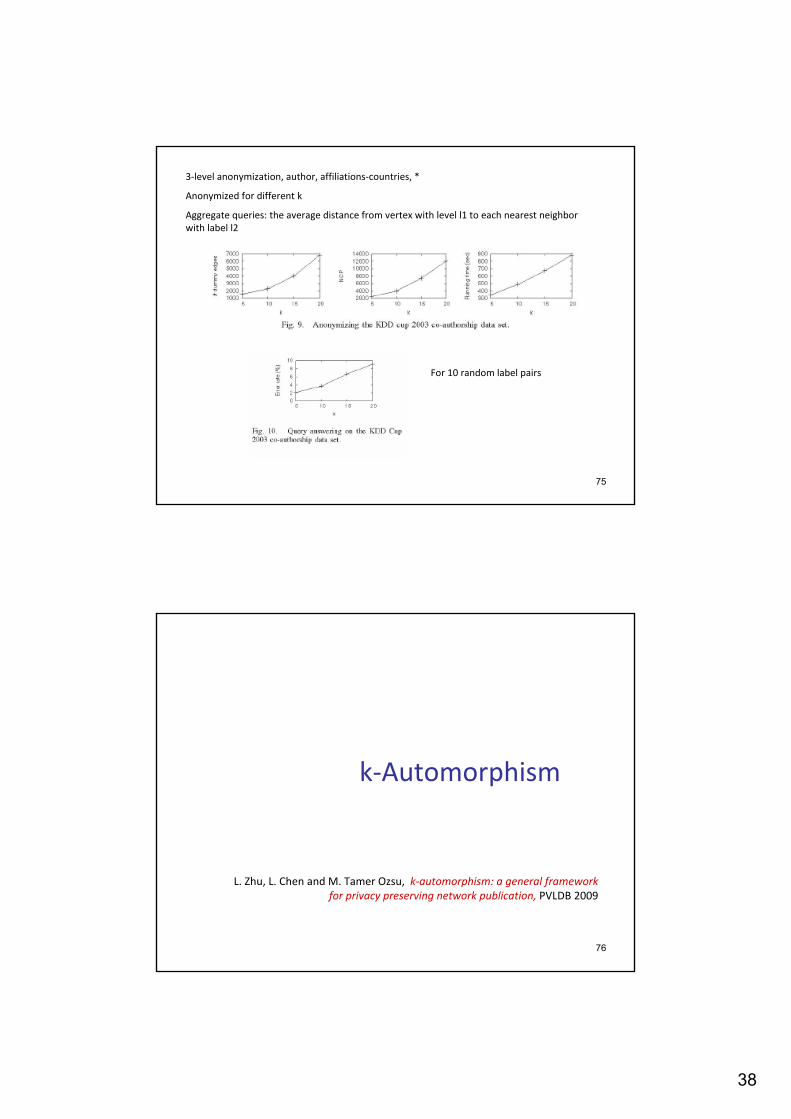
3‐level anonymization, author, affiliations‐countries, *

Anonymized for different k

Aggregate queries: the average distance from vertex with level l1 to each nearest neighbor with label l2

For 10 random label pairs

76

k‐Automorphism

L. Zhu, L. Chen and M. Tamer Ozsu, k‐automorphism: a general framework for privacy preserving network publication, PVLDB 2009

39

77

K‐Automorphism

Considers any subgraph query ‐ any structural attack

At least k symmetric vertices no structural differences

78

K‐Automorphism

map each node of graph G to (another) node of graph G

40

79

K‐Automorphism

any k‐1 automorphic functions?

80

K‐Automorphism

41

81

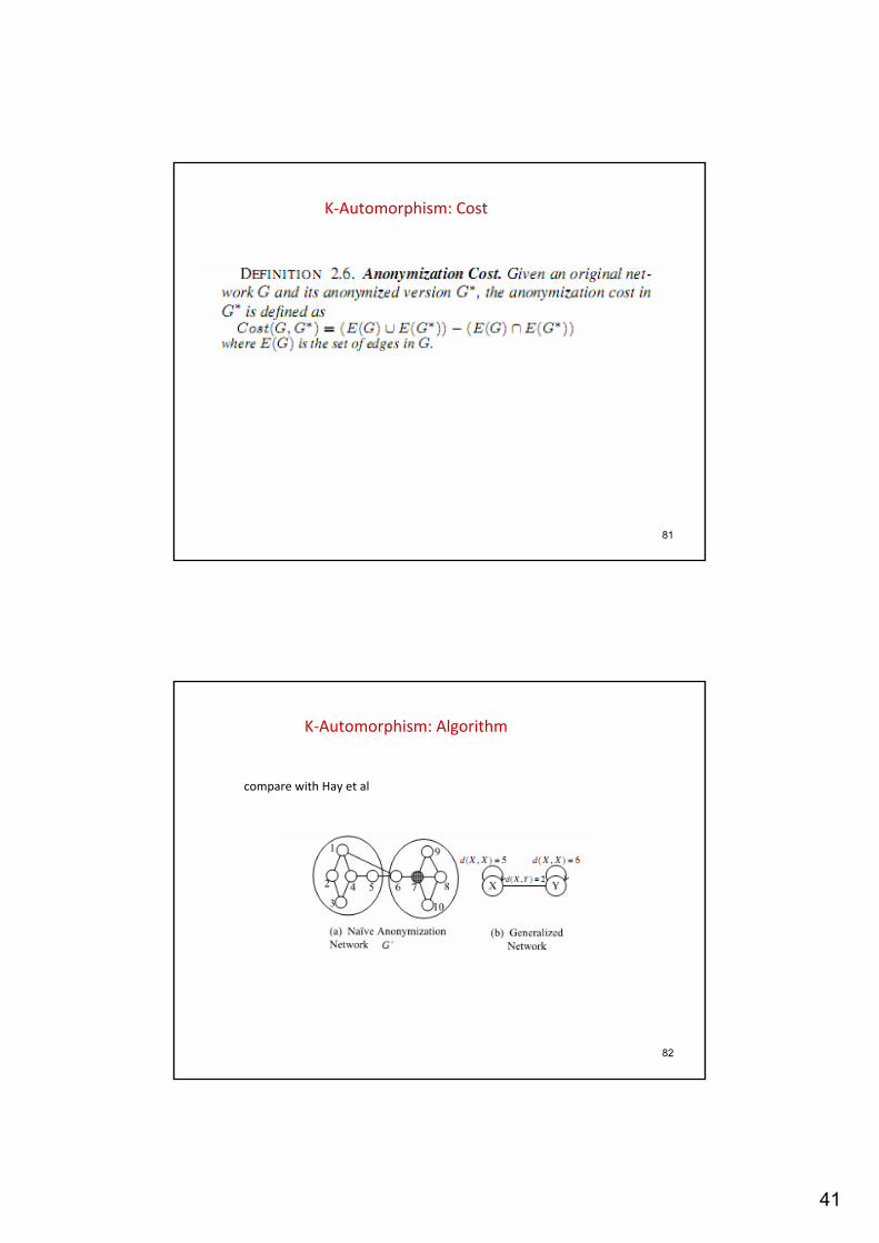
K‐Automorphism: Cost

82

K‐Automorphism: Algorithm

compare with Hay et al

42

83

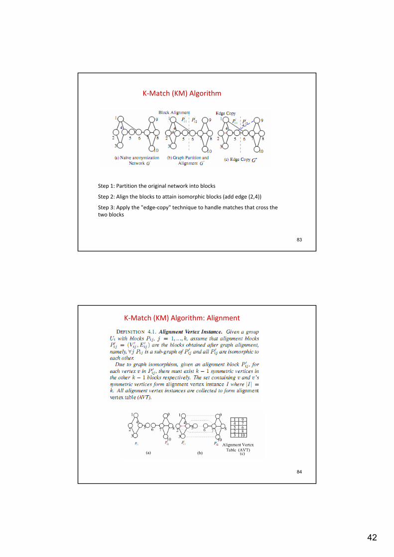
K‐Match (KM) Algorithm

Step 1: Partition the original network into blocks

Step 2: Align the blocks to attain isomorphic blocks (add edge (2,4))

Step 3: Apply the "edge‐copy" technique to handle matches that cross the two blocks

84

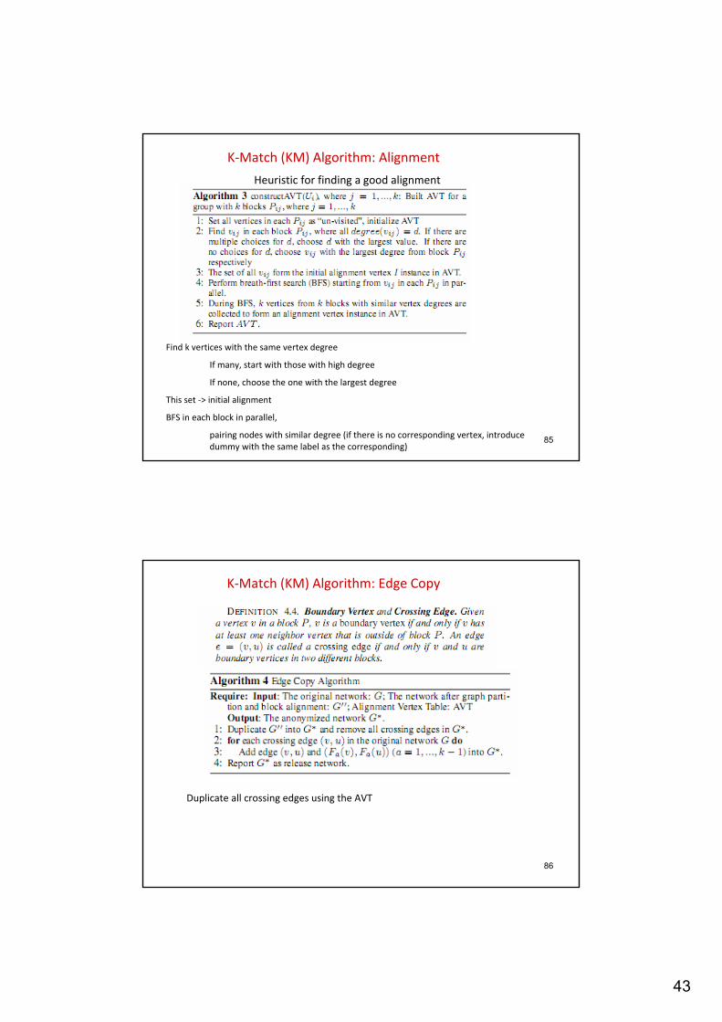
K‐Match (KM) Algorithm: Alignment

43

85

K‐Match (KM) Algorithm: Alignment

Heuristic for finding a good alignment

Find k vertices with the same vertex degree

If many, start with those with high degree

If none, choose the one with the largest degree

This set ‐> initial alignment

BFS in each block in parallel,

pairing nodes with similar degree (if there is no corresponding vertex, introduce dummy with the same label as the corresponding)

86

K‐Match (KM) Algorithm: Edge Copy

Duplicate all crossing edges using the AVT

44

87

K‐Match (KM) Algorithm: Graph Partitioning

How many blocks to add a small number of edges?

Few ‐> fewer crossing edges, but larger groups (more edges for aligning)

NP complete ‐> heuristics

88


45

89


Find all frequent subgraphs (first group!)

Try to expand them until the cost becomes worst, in which case start a new group

90

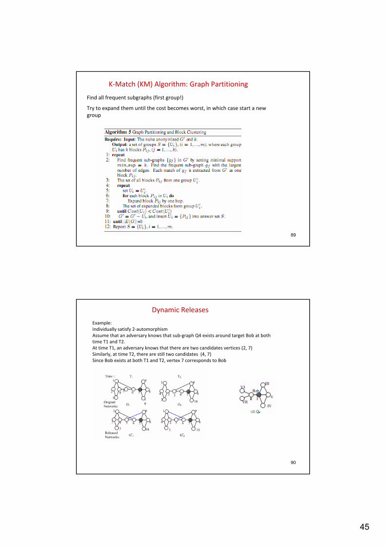
Example:Individually satisfy 2‐automorphismAssume that an adversary knows that sub‐graph Q4 exists around target Bob at both time T1 and T2.At time T1, an adversary knows that there are two candidates vertices (2, 7)Similarly, at time T2, there are still two candidates (4, 7)Since Bob exists at both T1 and T2, vertex 7 corresponds to Bob

Dynamic Releases

46

91

Remove all vertex IDs, or permute vertex IDs randomly (so, a given vertexIDdoes not correspond to the same entity in different publications).Impossible to conduct proper data analysis. Instead, vertex ID generalization

Dynamic Releases

For simplicity, no vertex insertions or deletions in different releases (set of all vertex IDs remains unchanged)

92

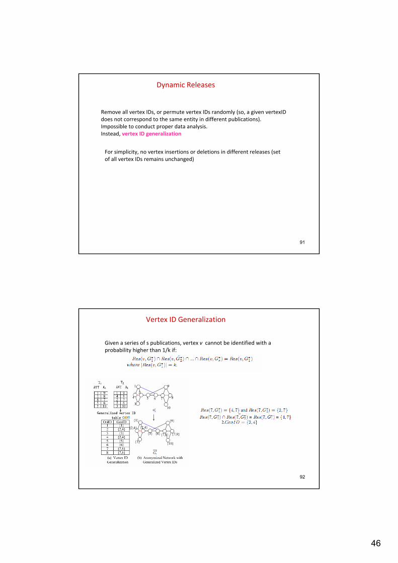
Vertex ID Generalization

Given a series of s publications, vertex v cannot be identified with a probability higher than 1/k if:

47

93

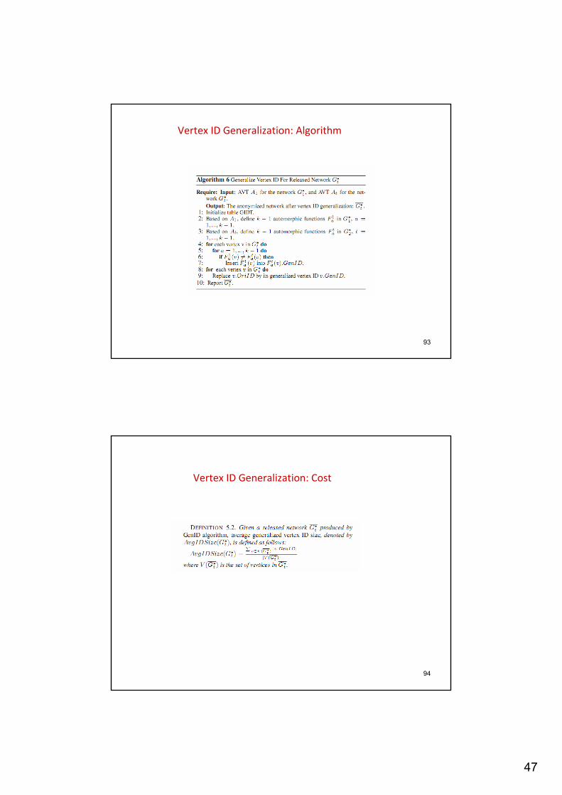
Vertex ID Generalization: Algorithm

94

Vertex ID Generalization: Cost

48

95

Vertex Insertion and Deletion

(Deletion) There is a vertex ID v that exists in G'1 but not in G'tFind an arbitrary vertex ID u that exists in bothInsert v in the generalized vertex ID of u

(Insertion) There is a vertex ID v that exists in G't but not in G'1Assume that instance I contains v in AVT AtFor each vertex u in I, insert v in the generalized vertex ID of u

96

Evaluation

Prefuse (129 nodes, 161 edges)Co‐author graph (7995 authors in database and theory, 10055 edges)

SyntheticErdos Renyi 1000 nodesScale free, 2 < γ < 3

All k = 10 degree anonymous, but no sub‐graph anonymous

49

97

Questions?

Documents

Privacy in Social Networks: identity disclosure