Deutsche Forschungsgemeinschaft

Priority Program 1253

Optimization with Partial Differential Equations

Patrick Penzler, Martin Rumpf and Benedikt Wirth

A Phase-Field Model for Compliance Shape

Optimization in Nonlinear Elasticity

April 2010

Preprint-Number SPP1253-096

http://www.am.uni-erlangen.de/home/spp1253

A PHASE-FIELD MODEL FOR COMPLIANCE SHAPE OPTIMIZATION INNONLINEAR ELASTICITY

Patrick Penzler, Martin Rumpf, Benedikt Wirth1

Abstract. Shape optimization of mechanical devices is investigated in the context of large, geomet-rically strongly nonlinear deformations and nonlinear hyperelastic constitutive laws. A weighted sumof the structure compliance, its weight, and its surface area are minimized. The resulting nonlinearelastic optimization problem differs significantly from classical shape optimization in linearized elas-ticity. Indeed, there exist different definitions for the compliance: the change in potential energy ofthe surface load, the stored elastic deformation energy, and the dissipation associated with the defor-mation. Furthermore, elastically optimal deformations are no longer unique so that one has to choosethe minimizing elastic deformation for which the cost functional should be minimized, and this com-plicates the mathematical analysis. Additionally, along with the non-uniqueness, buckling instabilitiescan appear, and the compliance functional may jump as the global equilibrium deformation switchesbetween different bluckling modes. This is associated with a possible non-existence of optimal shapesin a worst-case scenario.In this paper the sharp-interface description of shapes is relaxed via an Allen–Cahn or Modica–Mortolatype phase-field model, and soft material instead of void is considered outside the actual elastic ob-ject. An existence result for optimal shapes in the phase field as well as in the sharp-interface modelis established, and the model behavior for decreasing phase-field interface width is investigated interms of Γ-convergence. Computational results are based on a nested optimization with a trust-regionmethod as the inner minimization for the equilibrium deformation and a quasi-Newton method as theouter minimization of the actual objective functional. Furthermore, a multi-scale relaxation approachwith respect to the spatial resolution and the phase-field parameter is applied. Various computationalstudies underline the theoretical observations.

1991 Mathematics Subject Classification. 49Q10, 74P05, 49J20.

.

1. Introduction

In this paper we investigate shape optimization in the context of nonlinear elastic constitutive laws forthe underlying objects, where an object is defined as an object domain O ⊂ Ω for some open connected setΩ ⊂ Rd. We are in particular interested in geometrically strongly nonlinear deformations φ : O → R

d whichminimize a certain hyperelastic energy. As hyperelastic energies, we consider polyconvex energy functionals∫

ΩχOW (Dφ) dx, where the integrand W depends on the principal invariants of the Cauchy–Green strain

tensor DφTDφ and its evaluation is restricted to the actual elastic domain O (with characteristic function χO).For these functionals a nowadays already classical existence theory has been established [11, 12, 18] and an

Keywords and phrases: shape optimization, nonlinear elasticity, phase-field model, buckling deformations, Γ-convergence

1 Institute for Numerical Simulation, Bonn University, Endenicher Allee 60, 53115 Bonn

2

effective minimization is also computationally feasible. With respect to the actual shape optimization of theshape O, we aim at minimizing a compliance cost functional J [φ,O], to be evaluated for φ = φ[O] being anequilibrium deformation of O and thus a minimizer of the free energy. This type of compliance optimizationhas applications in engineering, where mechanical devices or structural components have to be developed thatoptimally balance material consumption or component weight with the component stiffness or rigidity. Sincethe compliance is related to the energy absorbed by the mechanical structure, minimizing the compliance is alsorelated to reducing the risk of material failure. Nonlinear elasticity has a strong impact on the behavior of theoptimization problem. Indeed, there exist several possible definitions for the compliance which are all equivalentin linearized elasticity but now in the context of nonlinear elasticity result in significantly different optimizationproblems. We may consider the change in potential energy of the surface load, the stored elastic deformationenergy, or the dissipation associated with the deformation. The deformation induced by the surface load is ingeneral no longer unique, which complicates the mathematical analysis. Buckling instabilities may appear, inwhich structures such as compressed beams can bend to either side, thereby producing non-uniqueness. Sincedifferent buckling deformations generally correspond to different compliance values, one may experience that thecompliance suddenly jumps up during shape optimization as the global equilibrium deformation switches fromone buckling deformation to another one. This phenomenon may result in non-existence of optimal shapes ifwe always pick the worst case from the set of all equilibrium deformations. Furthermore, in nonlinear elasticity,reversing the surface load (changing its sign) in general influences the mechanical response. As a consequence,shape optimization problems that yield symmetric shapes in linearized elasticity now result in asymmetricshapes. Finally, also numerically, the use of nonlinear elasticity poses a challenge. We typically observe ratherlarge, geometrically strongly nonlinear deformations. Their computation requires robust numerical minimizationmethods that reliably detect local rotations and bypass saddle points which frequently appear between twobuckling deformations.

To render the optimization problem analytically tractable and computationally feasible we replace the voidoutside the actual elastic object O by a (some orders of magnitude) softer material. Indeed, we take into accountthe energy functional

∫Ω

((1 − δ)χO + δ)W (Dφ)dx for a small positive constant δ. Furthermore, we propose adouble well phase-field model of Allen–Cahn [8] or Modica–Mortola [27] type for an implicit description of theelastic object with a diffusive interface. Indeed, we describe elastic shapes by a phase-field function v : Ω→ Rand take into account an energy

∫Ωε|∇v|2 + 1

εΨ(v) dx, where Ψ(v) = 916 (v2−1)2 is a double well potential with

minima at v = −1 and v = 1, representing the two material phases O and Ω \ O. For this model, we provethe existence of optimal, shape-encoding phase fields and study the model behavior for decreasing parameterε, which describes the width of the diffusive interface, in terms of Γ-convergence. Furthermore, a variety of 2Dnumerical examples enables a detailed discussion of the impact of the nonlinear elasticity model on the shapeoptimization problem.

The organization of the paper is as follows. Section 2 presents an overview over the related shape optimizationliterature. After presenting the optimization problem and its phase-field approximation in Section 3 we willbriefly examine the nature of nonlinear elasticity in the compliance minimization context in Section 4. Theexistence of minimizers and the sharp-interface limit of the phase-field model are studied in Section 5 beforepresenting the implementation in Section 6 and finally showing a few experiments in Section 7.

2. Related Work

In shape optimization frequently not only the geometry of the shape contour ∂O of an elastic mechanicaldevice O is of interest, but also the topology of O is subject to optimization. Typically, one considers asunderlying state problem the system of equations of linearized elasticity,

divσ = 0

on O, where the Cauchy stress σ is given by C ε[u] = 12C(Du + DuT) for the fourth-order elasticity tensor C

and the displacement u. As boundary conditions, one might impose Dirichlet conditions u = 0 on ΓD ⊂ ∂O,

3

Neumann boundary conditions σ ν = F on ΓN ⊂ ∂O with ΓD ∩ ΓN = ∅ for a prescribed surface load F , andzero surface force boundary conditions σ ν = 0 on the remaining boundary ∂O\ (ΓD ∪ΓN ). With respect to themodeling, ΓD and ΓN are usually a priori fixed parts of the boundary, whereas the remaining boundary is subjectto the actual shape optimization. For the sake of simplicity, we ignore volume forces here. The range of usualobjective functionals J [u,O] is relatively diverse. The mechanical work of the load, the so-called complianceC = 1

2

∫ΓN

F · uda, is very popular [1, 2, 4, 6, 24, 32–35] since it equals the energy to be absorbed by the elasticstructure. A related choice is the L2-norm of the internal stresses [1,4,6],

∫O ‖σ‖

2F dx. If a specific displacement

u0 is to be reproduced, then the L2-distance∫

Ω|u − u0|2 dx serves as the appropriate objective functional [6].

Other possibilities include functionals depending on the shape eigenfrequencies or the compliance for design-dependent loads [7, 13, 30]. Typically, the optimization problem is complemented by a volume constraint for O(otherwise, especially for compliance minimization, O = Ω would be optimal). An equality constraint |O| = Vis either ensured by a Cahn–Hilliard-type H−1-gradient flow [37] or a Lagrange-multiplier ansatz [7, 13, 25].A quadratic penalty term or an augmented Lagrange method is employed in [35]. An inequality constraint|O| ≤ V is implemented in [24,32,33], using a Lagrange multiplier. Chambolle [16] exploits the monotonicity ofthe compliance C (in the sense C(O1) ≥ C(O2) for O1 ⊂ O2) to replace the equality by an inequality constraint.Finally, the volume may just be added as a penalty functional ν|O| for some parameter ν [1].

The above class of shape optimization problems is generically ill-posed since microstructures tend to form,which are associated with a weak but not strong convergence of the characteristic functions χOi along a min-imizing sequence (Oi)i=1,.... In particular, rank-d sequential laminates with the lamination directions alignedwith the stress eigendirections are known to be optimal for compliance minimization [2]. The above ill-posednesscalls for regularization, for which there are several possibilities. A widespread approach is to penalize the shapeperimeter by adding a term ηHd−1(∂O) to the objective functional, which (if the void is replaced by some weakmaterial) also results in existence of optimal shapes as studied in [9] for a scalar problem. An alternative consistsin the relaxation of the problem: The set of admissible shapes can be extended to allow for microstructures, anda quasi–convexification of the integrand in J [u,O] (by taking the infimum over all possible microstructures)then ensures existence of minimizers [2].

There are various approximations and implementations of the elastic shape optimization problem, each ofwhich more or less corresponds to a particular type of regularization. A direct triangulation of O or its boundarywould probably work with all regularizations, but would require remeshing during the optimization and inducetechnical difficulties with topological changes. The so-called evolutionary structural optimization (ESO) is basedon discretizing the computational domain by finite elements and successively removing those elements whichcontribute least to the structural stiffness (or another chosen objective, see for example [10]). This correspondsto a regularization via discretization and thereby introduces a mesh dependence.

The implicit representation of shapes via level sets and corresponding shape optimization approaches areinvestigated by various authors [6, 23, 25, 29]. In particular Allaire and coworkers [2, 3, 5, 6] studied level-setmethods in two- and three-dimensional structural optimization and combined this approach with a homoge-nization method. In [4] they also investigated topological optimization in the context of minimizing the expectedelastic stress. Shape sensitivity analysis as introduced by Sokolowski and Zolesio [31] can be phrased elegantlyin terms of level sets. For the relaxation of the shape functional O 7→ J [u[O],O] gradient-descent schemeshave been investigated, where the actual shape gradient and thus the performance of the relaxation schemesignificantly depend on the underlying metric g. Burger and Stainko [15] provide examples for different g suchas the inner product in H1(∂O) (Laplace–Beltrami flow), H1/2(∂O) (Stefan flow), L2(∂O) (Hadamard flow),H−1/2(∂O) (Mullins–Sekerka flow), and H−1(∂O) (surface diffusion flow). Allaire et al. [7] also propose to useH1-, L2-, or H−1-type inner products. Indeed, during the gradient flow, topology changes can only happenby merging or eliminating holes (whereas in 3D, holes may appear by pinching a thin wall) [1, 7] so that themaximum number of holes is prescribed by the initialization. In order to allow the level-set method to createholes in 2D, the topological derivative is sometimes used to identify and remove rather inactive interior materialparts [20,24].

4

An implicit description of shapes via phase fields—the approach also employed in this paper—is both an-alytically and numerically an attractive alternative. Phase-field models originated in the physical descriptionof multiphase materials: The chemical bulk energy of the material is given by 1

ε

∫Ω

Ψ(v) dx for some chemicalpotential Ψ. The minima of Ψ represent two material phases. This energy is complemented by an interfacialenergy of the form ε

∫Ω|∇v|2 dx. Optimal profiles of v show a diffusive transition region between the two ma-

terial phases whose width scales with the parameter ε. For ε → 0, the above integral forces the phase field vtowards the pure phases, and for appropriate choices of Ψ it Γ-converges to the total interface length. Hence,the approach lends itself for a perimeter regularization. This technique is employed by Wang and Zhou [34]who minimize the compliance of an elastic structure using a triphasic phase field (with one void and two ma-terial phases) for which the potential Ψ is equipped with a periodically repeated sequence of three minima toallow for all three possible types of phase transitions. Furthermore, they replace the term

∫Ω|∇v|2 dx by an

edge-preserving smoothing and perform a multiscale relaxation, starting with large ε and successively decreas-ing it—remarkably beyond the point up to which the grid can still resolve the diffusive interface in a usualfashion. Zhou and Wang [37] compute the Cahn–Hilliard evolution of the shape to be optimized, also using amultiphase material. They solve the elastic equations with finite elements and the resulting fourth-order Cahn–Hilliard-type partial differential equation with a Crank–Nicolson finite–difference scheme in which nonlinearterms are approximated by Taylor series expansion and the resulting linear system is solved by a multigridV-cycle. Burger and Stainko [15] minimize the volume |O| under a stress constraint and show existence of acorresponding minimizer. They use a double obstacle potential Ψ to reformulate the shape optimization as aquadratic programming problem with linear constraints. Finally, Bourdin and Chambolle [13] find minimumcompliance designs for (design-dependent) pressure loads, using a solid, liquid, and void phase, which theydescribe by a scalar phase field allowing for the transitions void–solid–liquid. They also prove existence of min-imizers for the sharp-interface model and implement the optimization as a semi-implicit descent scheme withlinear finite elements on a triangular unstructured mesh.

Guo et al. [24] describe the characteristic function of O by the concatenation of a smoothed Heaviside functionwith a level-set function, where the smoothed Heaviside function acts like a phase-field profile. Wei and Wang [35]encode O in a piecewise constant level set function v, which is also closely related to the phase-field method:They regularize v via total variation, which in conjunction with the penalty

∫Ω

(v − 1)2(v − 2)2 dx for theconstraint v ∈ 1, 2 has a similar effect as the phase-field perimeter term 1

2

∫Ωε|∇v|2 + 1

εΨ(v) dx. Xia andWang [36] compute functionally graded structures, where the shape is described by a level set function andthe smoothly varying material properties by a scalar field (that actually describes the mixture of two materialcomponents from which the physical properties are computed under an isotropy assumption).

3. The nonlinear elastic shape optimization model

In this section, we will briefly recapitulate the mechanical framework of nonlinear elasticity and discuss thedifferent associated compliance cost functionals.

3.1. The hyperelastic constitutive law

Let us assume we are given a sufficiently regular, elastic body O ⊂ Rd which is fixed at part of its boundary,ΓD ⊂ ∂O, and subjected to a sufficiently regular surface load F : ΓN → Rd on ΓN ⊂ ∂O (Figure 1). The bodydeforms under the surface load, and the equilibrium deformation φ : O → Rd minimizes the total free energy

E [O, φ] =W[O, φ]− C[φ]

within a set of admissible deformations φ with trace φ|ΓD = id, where

W[O, φ] =∫OW (Dφ) dx

5

O·x

φ

ΓD

ΓN

F

φ(O)·φ(x)

Figure 1. A surface load F induces a deformation φ of the body O.

describes the elastic energy stored inside the material and

C[φ] =∫

ΓN

F · (φ− id) da

is the (negative) potential of the surface load. Here, we postulated the existence of a Gibbs free energy densitywhich only depends on the Jacobian Dφ of the deformation, also denoted the deformation gradient. Materialsfor which this assumption holds are called hyperelastic. The frame-indifference principle requires that the localelastic energy is independent of the frame of reference, that is, the underlying coordinate system. Hence, acoordinate transformation y = Qx + b for a rotation Q ∈ SO(d) and a shift b ∈ Rd does not change theenergy, so that W (Dφ) = W (QDφ) for all Q ∈ SO(d). We will furthermore assume an isotropic material sothat a rotation of the material before applying a deformation yields the same energy as before, i. e. W (Dφ) =W (DφQ) ∀Q ∈ SO(d). From the above two axiomatic conditions one deduces that the energy density Wonly depends on the singular values, the so-called principal stretches, λ1, λ2, λ3 of the deformation gradientDφ. Instead of the principal stretches, we can equivalently describe the local deformation using the so-calledinvariants of the deformation gradient or the Cauchy–Green strain tensor DφTDφ,

I1 = ‖Dφ‖F =√λ2

1 + λ22 + λ2

3 , I2 = ‖cofDφ‖F =√λ2

1λ22 + λ2

1λ23 + λ2

2λ23 , I3 = detDφ = λ1λ2λ3 ,

where ‖A‖F =√

tr(ATA) for A ∈ Rd×d and the cofactor matrix is given by cofA = detAA−T for A ∈ GL(d),so that overall, for an appropriately chosen W we obtain

W (Dφ) = W (I1, I2, I3) .

I1, I2, and I3 can be interpreted as the locally averaged change of an infinitesimal length, area, and volumeduring the deformation, respectively.

The elastic energy densities have to fulfill further conditions. First, we require the identity, Dφ = 1I, (whichcorresponds to no displacement) to be the global minimizer. Second, the energy density shall converge to infinityas I3, the determinant of the deformation gradient (which describes the volume change), approaches zero orinfinity. Negative values of I3 correspond to local interpenetration of matter and are not allowed at all. Thus,W (Dφ) = W (I1, I2, I3) is strongly nonlinear and can in addition not be convex in the deformation gradient Dφ,since the set of matrices with positive determinant is not even a convex set [18]. This makes the problem ofexistence of minimizers a subtle one, but it can be treated using the direct method of the calculus of variations[11]. Thereto, we require coercivity of E [O, ·] in some convenient topology so that from a minimizing sequence,we can extract a convergent subsequence φi → φ. As a second step, we require E [O, ·] to be sequentially lowersemi-continuous along this sequence with respect to the chosen topology so that lim infi→∞ E [O, φi] ≥ E [O, φ],and hence, φ must be a minimizer. The appropriate topology is the weak topology of a Sobolev space. Hence,we will assume W (Dφ) ≥ C1‖Dφ‖pF − C2 for some p > 1, C1, C2 > 0, as well as F ∈ Lp′

(ΓN ) for 1 = 1p + 1

p′ ,and using in particular the boundedness of the trace operator W 1,p(O) → Lp(ΓN ) we almost directly verify

6

that E [O, φ] ≥ C‖φ‖pW 1,p(O)− C for some C, C > 0. The consistency of the boundary condition φ|ΓD = id withweak convergence implies the desired weak coercivity of E [O, ·]. Obviously, for the weak lower semi-continuityof E [O, ·] we have to require lower semi-continuity of W. This translates (for vector-valued problems) intoquasiconvexity of W [21], which is, however, difficult to examine. Fortunately, a slightly stronger notion canbe applied here. We require W to be polyconvex, that is, W (Dφ) can be rewritten as a convex function of allminors of the deformation gradient Dφ. In that case, by a compensated compactness result due to Ball [11],W[O, ·] is weakly lower semi-continuous on W 1,p(O) for p ≥ d [14], and the variational problem minφ E [O, φ]indeed admits a minimizer in φ ∈ W 1,p(O) : φ|ΓD = id. By imposing growth conditions of the formW (A) ≥ C1(‖A‖pF + ‖cofA‖qF + |detA|r)− C2 one can obtain existence results for smaller p under appropriateconditions on q and r [28]. Typical energy densities of the above type are given by

W (Dφ) = W (I1, I2, I3) = a1‖Dφ‖pF + a2‖cofDφ‖qF + Γ(detDφ)

for a1, a2 > 0, p, q > 1, and a convex function Γ : R→ R with limd→∞ Γ(d) = limd→0 Γ(d) =∞. For example,p = 2 and q = 0 yields a neo-Hookean material law, while p = q = 2 results in a Mooney–Rivlin materiallaw [18]. In our computations, we will employ the particular material law W (Dφ) = µ

2 ‖Dφ‖2F + λ

4 detDφ2 −(µ+ λ

2

)log detDφ − dµ

2 −λ4 for material parameters λ and µ, whose second order Taylor expansion about

Dφ = I (which reveals the small-strain behavior) yields the standard energy from isotropic linearized elasticity,W lin(Dφ) = λ

2 (trε)2 + µtr(ε)2, with ε = 12 ((Dφ− I) + (Dφ− I)T) and the Lame constants λ and µ.

In general linearized elasticity the energy density of the material is a quadratic function

W lin(Dφ) =12C(Dφ− I) : (Dφ− I)

of the strain (Dφ − I), where C denotes a fourth order symmetric positive (semi-)definite (elasticity) tensorand A : B = trATB. Hence, we obtain the equilibrium condition 0 =

∫OC(Dφ − I) : Dθ dx −

∫ΓN

F · θ dafor all test displacements θ. In particular, this holds for θ = φ − id, which implies 2W lin[O, φ] = C[φ] for theequilibrium deformation φ. Here, 2W lin[O, φ] = C[φ] represents a measure of the deformation strength and isdenoted the compliance of the object O, which may be seen as some kind of inverse rigidity. As discussed inSection 2 it is mostly this compliance which has been minimized in elastic shape optimization. Obviously, inlinearized elasticity, it does not matter whether we describe the compliance via 2W lin[O, φ] or C[φ]. However,in the case of a nonlinear hyperelastic constitutive law, this is no longer true as we will see later and it makesa difference which term we choose to minimize.

3.2. The shape optimization problem based on compliance minimization

If we ask for elastic domains O ⊂ Ω ⊂ Rd which minimize the compliance, then, certainly, O ≡ Ω yieldsthe most rigid structure. Hence, we are actually interested in a balance between rigidity, material consumption(weight), and manufacturing simplicity (smoothness of the shape ∂O). The material consumption is expressedby the Lebesgue measure of O, V[O] = |O|. Domains O that minimize just a weighted sum of complianceand volume in general do not exist. Typically, microstructures appear (cf. Section 2), for example higher ranksequential laminates in which material and void rapidly alternate. Hence, as already discussed above, we replacethe void and adjust the elastic energyW[O, φ] accordingly by definingWδ[O, φ] =

∫Ω

((1−δ)χO+δ)W (Dφ) dx.Furthermore, we add the domain perimeter L[∂O] = Hd−1(∂O) as a regularizing prior, which can be interpretedas introducing manufacturing costs for the production and processing of the object surface. Now, the total freeenergy is given by

Eδ[O, φ] =Wδ[O, φ]− C[φ] .

In our computations we choose δ = 10−4. Let us remark that this modification of the free energy in particularallows to properly define the deformation φ outsideO and (combined with suitable Dirichlet boundary conditionson ∂Ω) to prevent self-penetration of matter in form of overlapping material parts. In the case of compliance

7

FF

F

F

φ(x)−x

φ(x)−x

Figure 2. Two possible designs (each shown in the undeformed and the deformed state) tobear a vertical load. The left design exhibits rather low C[φ], but high W[O, φ] whereas theright design (with a hinge) yields the reverse.

minimization via the homogenization method, the shape optimization with real void has been examined as thelimit case when the stiffness of the weak material tends to zero [2].

As already explained earlier, the compliance of an object O may be regarded as a kind of inverse rigidityand can in linearized elasticity be described as 2W lin[O, φ] or equivalently C[φ] for the equilibrium deformationφ. In nonlinear elasticity, however, W[O, φ] and C[φ] are no longer related by a factor of 2, and the questionarises which one appropriately corresponds to the compliance in the linearized setting and which one shouldbe chosen for shape optimization. The stored elastic energy W[O, φ] corresponds to the work transferred tothe body O by the surface load, while the total decrease C[φ] in the potential energy of the surface load F iscomposed of exactly this work plus the energy dissipation during the system dynamics before the equilibrium isreached. Allaire et al. [7], who have already computed a nonlinearly elastic shape optimization example, considerthe minimization of the surface load potential C[φ]. Here, we aim at an analysis of the differences and consider(for parameters η, ν > 0) both cases, the minimization of the total potential energy of the surface load

JC [O, φ] := C[φ] + νV[O] + ηL[∂O] , (1)

or the stored elastic deformation energy

JW [O, φ] := 2Wδ[O, φ] + νV[O] + ηL[∂O] . (2)

However, there is a third possibility which also reduces to the standard notion of compliance in linearizedelasticity. Indeed, we might also choose to minimize the dissipation associated with the transition from theunstressed state to the equilibrium deformation, −2Eδ = 2(C − Wδ). Together with the volume and surfaceregularization we obtain

JD[O, φ] := 2C[φ]− 2Wδ[O, φ] + νV[O] + ηL[∂O] . (3)Independent of the specific cost functional we always consider a minimization for O ∈ O ⊂ Ω : ΓD,ΓN ⊂ ∂Ounder the constraint that φ : Ω → R

d minimizes the free energy Eδ[O, φ] among all deformations in theassociated admissible set of deformations whose trace is the identity on ΓD.

The following toy problem shall illustrate the conceptual differences at least of the first two cases: Considerthe task to design a structure O which is attached to a wall at its left end and has to bear a vertical load Fat its right end (Figure 2). A cantilever-like design (Figure 2, left half) exhibits a rather small displacementφ − id and thus a small value of C[φ], but the strong compression of the lower branch causes a relatively highdeformation energy W[O, φ]. A freely rotating rod, on the other hand, allows a strong displacement with highC[φ] but low W[O, φ] (Figure 2, right half). The former design is more appropriate if the load is supposed tobe sustained without large displacements while the latter design is more related to the material strain and isuseful in systems where the energy dissipation on the way to the final equilibrium configuration is absorbed by

8

a reasonable damping mechanism. With respect to the applications considered in this paper, we have to keep inmind that shape optimization with respect to C[φ] will yield results of the same type as in Figure 2, left, whileoptimization with respect to W[O, φ] generally allows strong deformations and tends to produce shapes as inFigure 2, right. Let us remark, however, that minimizing W[O, φ] does not always result in designs with strongdisplacements. For instance in case of sufficiently low volume costs, O ≡ Ω will yield the optimal design.

3.3. The approximating phase-field model for shape optimization

Shape and topology optimization based on an explicit parametric description of the mechanical devices isalgorithmically very difficult, as already mentioned above. Hence, we consider an approximating phase-fieldrepresentation of the object O via a phase-field function v : Ω → R of Allen–Cahn or Modica–Mortola type.Such phase fields constitute a convenient implicit representation of the objects and their complement andallow for a simple approximation of their boundary length. They originate from the description of biphasicmaterials with a diffusive interface layer, where v might for example represent the local concentration of achemical constituent. The local chemical energy density Ψ(·) has two minima corresponding to the two purephases. The resulting total bulk energy

∫Ω

Ψ(v)dx is then perturbed by an additional interfacial energy of theform

∫Ω|∇v|2dx. In our context of shape modeling, we assume that the two minima of Ψ are −1 and 1 with

Ψ(−1) = Ψ(1) = 0 representing the two phases void (outside of O) and material (inside of O), respectively.Using a proper scaling we obtain the free phase-field energy

LεMM[v] =12

∫Ω

ε|∇v|2 +1ε

Ψ(v) dx ,

where the scale parameter ε describes the width of the interfacial region. In the limit ε → 0, the phase field vis forced towards the pure phases −1 and 1 and Γ-converges to a multiple of the total interface area. In fact,for Ψ ∈ C1(R) with Ψ(−1) = Ψ(1) = 0 being the global minima, the following rigorous result holds [14]: IfLεMM[v] :=∞ for v /∈W 1,2(Ω), then

Γ− limε→0LεMM[·] = cΨPer(·), cΨ =

∫ 1

−1

√Ψ(s) ds,

with respect to the L1(Ω)-topology and for Per(w) := Hd−1(Ω ∩ ∂x ∈ Ω : w(x) = 1) if w : Ω → −1, 1almost everywhere and Per(w) := ∞ else. In (1), (2), and (3) the perimeter term L[∂O] is then replaced byLεMM[v], where we choose the double-well potential

Ψ(v) =916

(v2 − 1)2 ,

which yields cΨ = 1. Furthermore, we introduce an approximation χO(v) to the characteristic function χO,choosing

χO(v) =14

(v + 1)2 . (4)

With this function at hand we approximate the total volume by V[v] =∫

ΩχO(v) dx and the stored elastic

energy by Wδ[v, φ] :=∫

Ω((1− δ)χO(v) + δ)W (Dφ) dx, where we use with a slight misuse of notation the same

symbol for the energy terms in the phase-field model as in the original problem. Overall, based on the phase-fieldapproximation we will now minimize one of the following three functionals

J εW [v, φ] = 2Wδ[v, φ] + νV[v] + ηLεMM[v] , (5)

J εC [v, φ] = C[φ] + νV[v] + ηLεMM[v] , (6)

J εD[v, φ] = 2(C[φ]−Wδ[v, φ]) + νV[v] + ηLεMM[v] (7)

9

for integrable functions v : Ω → R with v|ΓD∪ΓN = 1 under the constraint that φ : Ω → Rd with φ|ΓD = id

minimizes the total free energy for a phase field v, defined (again with a slight misuse of notation) as

Eδ[v, φ] :=Wδ[v, φ]− C[φ] .

4. Effects of nonlinear elasticity and their impact on the shape optimization

The use of a nonlinear instead of a linearized elasticity changes the nature of the compliance minimizationproblem qualitatively. In the following, we will investigate the symmetry-breaking effect of nonlinear elasticityon the optimal shapes and the presence of buckling instabilities which are typical for the nonlinear models. Thisdiscussion is meant as a motivation for the analytical treatment in Section 5 and underpins the specific designof the numerical algorithm presented in Section 6.

4.1. Break of symmetry in nonlinear elastic shape optimization

As a first feature that distinguishes nonlinear from linearized elasticity, let us consider the effect of a signchange of the load F and its nonlinear impact not only on the deformation but also on the optimal geometryO. In linearized elasticity, the (unique) equilibrium deformation is the minimizer of the free energy

E linF [O, φ] =W lin[O, φ]− CF [φ] :=

∫O

12C(Dφ− I) : (Dφ− I) dx−

∫ΓN

F · (φ− id) da

for the symmetric, positive semi-definite elasticity tensor C, where the subscript F indicates the surface load.Obviously, if φF minimizes E lin

F [O, ·], then φ−F := 2 id − φF minimizes E lin−F [O, ·], the total free energy for a

reversed direction of the surface load. Indeed, for deformations φ, ψ with φ + ψ = 2 id we have E linF [O, φ] =

E lin−F [O, ψ], W lin[O, φ] =W lin[O, ψ], and CF [φ] = C−F [ψ]. Hence, the optimal geometry O for a prescribed loadF is the same one as for the load −F . As a consequence, if the sign change of F has the same effect as mirroringthe shape optimization problem (for example, for the cantilever design problem in Figure 3), then the resultingoptimal shapes are symmetric. In contrast, in nonlinear elasticity, the material behavior and geometry changedepend strongly on whether we tear at or push against an object. A sign change of the load F no longer simplyimplies a sign change of the displacement. Consequently, the symmetry property of linearized elasticity is lost:Where the shape optimization with linearized elasticity results in a symmetric shape O, the correspondingoptimal geometry for nonlinear elasticity is generally asymmetric. This phenomenon can already be observedfor quite small displacements as shown in Figure 3 for the design of a cantilever, where the effect of graduallyincreasing the load F is explored.

4.2. Buckling instabilities

A further, even more striking phenomenon of nonlinear elasticity is associated with the non-uniqueness ofequilibrium deformations: While in linearized elasticity the total free energy E [O, φ] is convex and quadratic inthe deformation φ, the energy landscape is much more complicated in nonlinear elasticity and generally admitsmultiple (locally) minimizing deformations φ. Of course, this raises the question which one of the equilibriumdeformations we should actually consider during shape optimization, and this will be investigated theoreticallyin Section 5.2. Often, the existence of multiple, locally minimizing deformations comes along with the bendingof structures. The classical example is given by the compression of straight beams [26], which we recapitulatehere to prepare a later discussion of the non-existence of optimal shapes in a worst-case scenario.

Consider a straight bar of length L which is clamped at one end and subjected to a compression load F at theother end. Let us denote the displacement orthogonal to the bar at position x ∈ [0, L] by u(x), then the bendingmoment M(x) inside the bar at x is given by M(x) = F (u(L)− u(x)). Under the assumption of Bernoulli’sbeam hypothesis and Hooke’s law with Young’s modulus E, this moment can also be expressed as M(x) = EI

ρ ,where I denotes the second moment of the cross-sectional area and ρ is the radius of the osculating circle. Upon

10

F

L

L2

Figure 3. Optimal design of a cantilever according to the sketch top left. The top row showsoptimal designs for loads F = 0.5, 1, 2, 4, 6 (the point load F is approximated by a tent-likesurface load F along a width of 2−3) and η = 25 · 10−5 · F 2, ν = 210 · 10−4 · F 2 (underlyinggrid resolution 2572, λ = µ = 80, L = 1). The bottom row shows the equilibrium deformation.In linearized elasticity, all parameter combinations would yield exactly the same symmetric,optimal shape whereas here, we see strong asymmetries evolving. Computations were performedusing the phase-field model. White indicates full material while black represents the weakmaterial whose stiffness is reduced by the factor δ = 10−4. Note: In the region at the left wallwhere Dirichlet boundary conditions for the deformation are applied, the algorithm realizes thatstiff material in the center of this region does not contribute much to the structural rigidityand hence removes it.

approximating 1ρ ≈ ∂2

xu(x) we obtain the linear ordinary differential equation EI∂2xu(x) = F (u(L)− u(x)),

which together with the boundary conditions u(0) = 0 and ∂xu(0) = 0 can be solved as u(x) = u(L)(1 −cos(

√F/EIx)). Hence, the minimum force allowing for a non-vanishing u(L) is the so-called buckling load

F = EIπ2

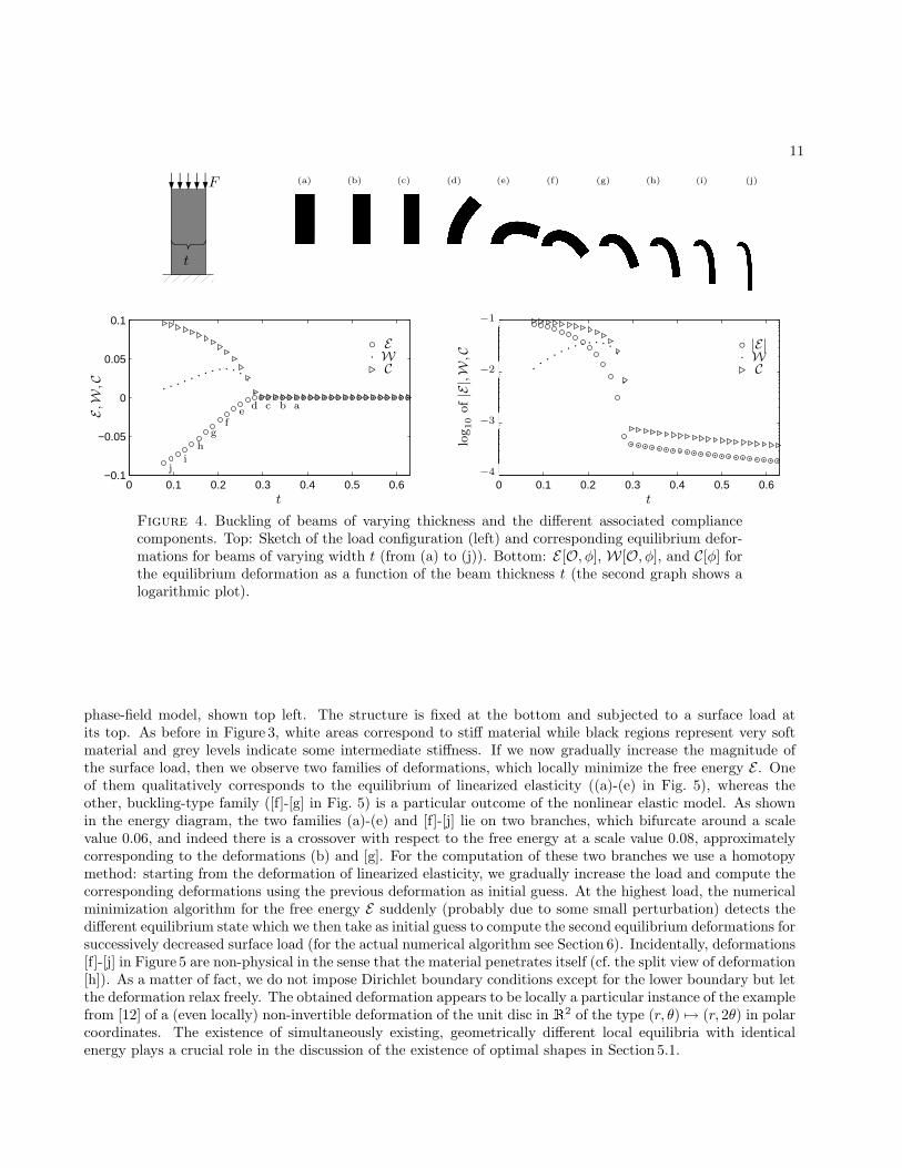
4L2 . It is the smallest load for which we expect a bending of the beam towards one side rather thana symmetric compression. The physical bifurcation associated with this buckling of beams can be reproducedin a nonlinear elasticity model. Figure 4 shows simulation results for the compression of vertical bars withheight one and varying thickness t (actually performed with the approximate phase-field model introducedabove). The top edge of each bar is subjected to a uniformly distributed surface load such that the totalresulting downward force is the same for all bars. The mechanical energy components belonging to the differentconfigurations are shown in Figure 4, bottom, as functions of the bar thickness t. Apparently, down to awidth of t = t ≈ 0.28, we seem to stay in the linearly elastic regime: The deformations φ of the beamsO are symmetric, and W[O, φ] ≈ 1

2C[φ] ≈ −E [O, φ] as in linearized elasticity. For smaller thicknesses t, allenergy components strongly increase, and the beams bend outwards. Indeed, the simulation parameters L = 1,F = 0.05, E = 4µ µ+λ

2µ+λ = 323 (with µ = λ = 4) and the relation I = t3

12 yield t = 3√

48FL2/(π2E) ≈ 0.2836.Note that there is a beam width t below which the stored elastic energyW[O, φ] decreases again. This behavioris linked to the observation in Section 3.2 concerning the difference between W[O, φ] and C[φ]. The thinner abeam the less bending energy is stored, and its base behaves more like a hinge so that the entire configurationresembles just a hanging, dilated rod, which absorbs relatively little elastic energy.

For the example of a compressed beam, the symmetric minimizing state apparently stops existing at t.However, it is not necessarily true that the state which qualitatively corresponds to the equilibrium deformationin linearized elasticity does not persist in parallel to other (local) equilibrium states. Indeed in Figure 5 weconsider a shape which emerged as an intermediate result during the relaxation of our nonlinear elasticity and

11

F

t

(a) (b) (c) (d) (e) (f) (g) (h) (i) (j)

0 0.1 0.2 0.3 0.4 0.5 0.6−0.1

−0.05

0

0.05

0.1

0 0.1 0.2 0.3 0.4 0.5 0.610

−4

10−3

10−2

10−1

abcde

fg

hi

j

t t

E,W,C

log10

of|E|,W,C

−4

−3

−2

−1

E· W. C

|E|· W. C

Figure 4. Buckling of beams of varying thickness and the different associated compliancecomponents. Top: Sketch of the load configuration (left) and corresponding equilibrium defor-mations for beams of varying width t (from (a) to (j)). Bottom: E [O, φ], W[O, φ], and C[φ] forthe equilibrium deformation as a function of the beam thickness t (the second graph shows alogarithmic plot).

phase-field model, shown top left. The structure is fixed at the bottom and subjected to a surface load atits top. As before in Figure 3, white areas correspond to stiff material while black regions represent very softmaterial and grey levels indicate some intermediate stiffness. If we now gradually increase the magnitude ofthe surface load, then we observe two families of deformations, which locally minimize the free energy E . Oneof them qualitatively corresponds to the equilibrium of linearized elasticity ((a)-(e) in Fig. 5), whereas theother, buckling-type family ([f]-[g] in Fig. 5) is a particular outcome of the nonlinear elastic model. As shownin the energy diagram, the two families (a)-(e) and [f]-[j] lie on two branches, which bifurcate around a scalevalue 0.06, and indeed there is a crossover with respect to the free energy at a scale value 0.08, approximatelycorresponding to the deformations (b) and [g]. For the computation of these two branches we use a homotopymethod: starting from the deformation of linearized elasticity, we gradually increase the load and compute thecorresponding deformations using the previous deformation as initial guess. At the highest load, the numericalminimization algorithm for the free energy E suddenly (probably due to some small perturbation) detects thedifferent equilibrium state which we then take as initial guess to compute the second equilibrium deformations forsuccessively decreased surface load (for the actual numerical algorithm see Section 6). Incidentally, deformations[f]-[j] in Figure 5 are non-physical in the sense that the material penetrates itself (cf. the split view of deformation[h]). As a matter of fact, we do not impose Dirichlet boundary conditions except for the lower boundary but letthe deformation relax freely. The obtained deformation appears to be locally a particular instance of the examplefrom [12] of a (even locally) non-invertible deformation of the unit disc in R2 of the type (r, θ) 7→ (r, 2θ) in polarcoordinates. The existence of simultaneously existing, geometrically different local equilibria with identicalenergy plays a crucial role in the discussion of the existence of optimal shapes in Section 5.1.

12

@@R@@R@@R@@RF(a) (b) (c) (d) (e) [f] [g] [h] [i] [j]

-φ[h]

XXzCCW

0 0.05 0.1 0.15−0.1

−0.05

0

0.05

a bc d e

fg

h

i

j

F

E

Figure 5. Top: Sketch of the load carried by the object (left) and the resulting two families (a)-(e) and [f]-[j] of (pairwise simultaneously existing) equilibrium deformations for an increasingload. Bottom: E [O, φ] for the equilibrium deformations as a function of the load magnitude(left). The right figure shows deformation [h] applied to the bottom and the top half of theobject, where the region of material self-penetration is marked by arrows.

5. The existence problem in nonlinear elastic shape optimization

Whether an optimal shape exists or not strongly depends on the objective we aim to minimize. In this sectionwe first prove existence of optimizing phase fields, where in case of multiple global equilibrium deformations wealways choose the one with least compliance. Likewise, we show existence of optimal shapes in a correspondingsharp-interface model. Furthermore, for a worst-case optimization, where we aim at minimizing the compliancewith respect to the deformation that, among all global minimizers of the free energy, yields the largest com-pliance, we show that in general we cannot expect existence of an optimal shape. Finally, the behavior of thephase-field model in the limit for vanishing phase-field parameter ε will be investigated.

5.1. Existence of minimizers for a least compliance optimization

We aim to establish the existence of a phase field v that minimizes J εW [v, φ[v]] or alternatively J εC [v, φ[v]]under the constraint that φ[v] minimizes Eδ[v, ·]. Let us first verify some properties of the functional Eδ. Inwhat follows we will always assume d ∈ 2, 3 and Ω ⊂ Rd to be bounded, open, and connected with Lipschitzboundary.

Theorem 1 (Existence of equilibrium deformations for fixed phase field). Let v ∈ L1(Ω). If W : Rd×d → R

is polyconvex with W (A) ≥ C1‖A‖pF − C2, p > d, and F ∈ L1(ΓN ), then the variational problem minφ Eδ[v, φ]admits a minimizer in φ ∈W 1,p(Ω) : φ|ΓD = id.

Proof. For the proof we refer to [11] or the exposition in [21]. The proof relies on the weak lower semi-continuity of the energy Wδ[v, ·] for fixed phase field v and makes use of the weak continuity of the cofactorand the determinant of the deformation gradient.

In the previous theorem, the phase field v was fixed. However, we are interested in the impact of shapevariations and thus in a variation of the shape-describing phase field. Indeed, we will need a weak lowersemi-continuity result with respect to both the deformation and the phase field, as provided by the followinglemma.

13

Lemma 2. For W : Rd×d → R being polyconvex and bounded from below and for F ∈ L1(ΓN ) the functionalsWδ[v, φ] and Eδ[v, φ] are sequentially lower semi-continuous along sequences (vi, φi)i∈N with vi → v in L1(Ω)and (Dφi, cofDφi,detDφi) (Dφ, cofDφ, detDφ) in Lp(Ω)× Lq(Ω)× Lr(Ω) for p > d, q, r > 1.

Proof. Due to the polyconvexity of W , we may write W (A) = W (A, cofA,detA) for a convex function W .Hence we have to consider the lower semi-continuity of

(vi, φi) 7→∫

Ω

χO(vi)W (Dφi, cofDφi,detDφi) dx

for i→∞, which can be obtained by a straightforward adaptation of the arguments in [11] taking into accountthe continuity of the function χO(·). The lower semi-continuity of C is obvious, as φi → φ strongly in C0(ΓN ),and the integrand is linear in φ.

Lemma 3. Suppose W : Rd×d → R is polyconvex with W (A) ≥ C1‖A‖pF − C2 for p > d and F ∈ L1(ΓN ).Then, for a sequence (vi)i∈N ⊂ L∞(Ω) with ‖vi‖∞ ≤ C and vi → v in L1(Ω) one obtains

Γ− limi→∞

Eδ[vi, ·] = Eδ[v, ·]

with respect to the weak W 1,p(Ω)-topology.

Proof. Since the boundary integral C[·] is just a continuous perturbation, we need to show Γ-convergence ofWδ[vi, ·] only.

Let φi φ in W 1,p(Ω) with lim supi→∞Wδ[vi, φi] < ∞. From the growth conditions on W we deducethe boundedness of (cofDφi,detDφi) in Lp/(d−1)(Ω)×Lp/d(Ω) and thus—due to the reflexivity of the Lebesguespaces—the weak convergence of a subsequence. Then, we can apply Ball’s compensated compactness result [11]to obtain (Dφi, cofDφi,detDφi) (Dφ, cofDφ, detDφ) in Lp(Ω)×Lp/(d−1)(Ω)×Lp/d(Ω). The previous lemmathen yields the lim inf-inequality, that is, lim infi→∞Wδ[vi, φi] ≥ Wδ[v, φ].

For the lim sup-inequality, note that Wδ[vi, φ] → Wδ[v, φ]. Otherwise there would be a ρ > 0 and a subse-quence (vj)j∈J⊂N, such that

∣∣Wδ[vj , φ]−Wδ[v, φ]∣∣ > ρ for all j ∈ J . Since vj → v in L1(Ω), we can furthermore

assume that vj → v pointwise almost everywhere as j →∞ in J . The integrand of Wδ[vj , φ] is bounded fromabove by ((1−δ) 1

4 (C+1)2 +δ)W (Dφ) and converges pointwise to χO(v)W (Dφ). By the dominated convergencetheorem, we obtain Wδ[vj , φ] → Wδ[v, φ] as j → ∞ in J , which is a contradiction. Hence, for the recoverysequence φi = φ for all i ∈ N, we obtain lim supi→∞Wδ[vi, φi] =Wδ[v, φ] which proves the lim sup-inequality.

Based on these preliminaries we are now able to show the existence of minimizing phase fields v for the shapeoptimization problem under the constraint that for fixed phase field v the deformation φ is in the set of globalminimizers of the elastic free energy.

Theorem 4 (Existence of optimal shape-encoding phase fields). Suppose W : Rd×d → R is polyconvex withW (A) ≥ C1‖A‖pF − C2 for p > d and F ∈ L1(ΓN ). Furthermore, consider phase fields v ∈ W 1,2(Ω) with−1 ≤ v ≤ 1. Then the variational problem minv J εG [v, φ] with G being W, C, or D admits a minimizer under theconstraint φ ∈ m[v], where m[v] is the set of minimizing deformations of Eδ[v, ·] in φ ∈W 1,p(Ω) : φ|ΓD = id.Proof. At first, note that for v in v ∈ W 1,2(Ω) : −1 ≤ v ≤ 1 the energy Eδ[v, id] is uniformly boundedfrom above by a constant E < ∞. Consequently, Eδ[v, φ] ≤ E for all φ ∈ m[v]. Also, due to the embeddingW 1,p(Ω) → C0(Ω) we have |C[φ]| ≤ C‖φ‖W 1,p(Ω) for some C > 0. Together with the growth conditions on W

and Eδ[v, φ] ≤ E we deduce that ‖φ‖W 1,p(Ω) is bounded and thus |C[φ]| ≤ C and consequently also |Wδ[v, φ]| ≤ Wfor W, C <∞. Clearly, J εG [v, φ] with φ ∈ m[v] is then uniformly bounded from below by some constant for alladmissible v ∈W 1,2(Ω).

Now, we consider a minimizing sequence (vi)i∈N in v ∈W 1,2(Ω) : −1 ≤ v ≤ 1. Due to the weak W 1,2(Ω)-coercivity of J εG with respect to the phase field (by virtue of the regularization LεMM[v] and the reflexivity of

14

W 1,2(Ω)) there is v ∈W 1,2(Ω) with −1 ≤ v ≤ 1 such that vi v in W 1,2(Ω) (after extraction of a subsequence),and thus vi converges strongly to v in L1(Ω) as i→∞.

Next, let φ[vi] ∈ m[vi] denote one sequence of deformations associated with the minimizing sequence (vi)i∈N.Then, due to the uniform boundedness of φ[vi] in W 1,p(Ω) (by the growth condition on W ) and the reflexivityof W 1,p(Ω), there is a deformation φ ∈W 1,p(Ω) with φ(x) = x for x ∈ ΓD such that φ[vi] φ (after extractinga subsequence). Since for fixed δ > 0 the free energy Eδ[vi, ·] is equi-mildly coercive, Lemma 3 implies φ ∈ m[v].Here, note that the Γ-limit is consistent with the Dirichlet boundary conditions at ΓD.

Finally, J εG [vi, φ[vi]] is sequentially weakly lower semi-continuous as vi v in W 1,2(Ω) and φ[vi] φ inW 1,p(Ω). In fact, the lower semi-continuity of LεMM[vi] and V[vi] is obvious as their integrands are convex in∇v and continuous in v. Furthermore, the Γ-convergence of Eδ stated in Lemma 3 ensures that Eδ[vi, φ[vi]]→Eδ[v, φ]] for i → ∞. Likewise, by the compact embedding of W 1,p(Ω) in L∞(ΓN ), φ[vi] → φ strongly inL∞(ΓN ) so that C[φ[vi]] converges to C[φ]. Finally, as in the proof of the previous lemma, we may assume(Dφ[vi], cofDφ[vi],detDφ[vi]) (Dφ, cofDφ, detDφ) so that Wδ[v, φ] ≤ lim infi→∞Wδ[vi, φ[vi]] follows fromLemma 2. From the above, J εG [v, φ] ≤ lim infi→∞ J εG [vi, φ[vi]] with φ ∈ m[v], and hence v is a minimizer.

Remark 5. In contrast to other phase-field models, the constraint −1 ≤ v ≤ 1 does not follow from a straight-forward comparison argument. Indeed, Eδ[v, φ] ≥ Eδ[max(0,min(1, v)), φ] does not hold in general. Hence, to beable to apply Lemma 3 we have to impose an L∞-bound for the phase field v as a constraint. As an alternative,we might consider a different function χO(·), which is continuous and a priori uniformly bounded on R, forexample

χO(v) := min(

1,14

(v + 1)2

).

In our numerical simulations, however, it was not necessary to cut off χO(v) or to implement an L∞-bound forv.

The above existence result still holds if instead of describing shapes via phase fields v ∈W 1,2(Ω) we considerthe sharp-interface case and represent shapes by functions of bounded variation v ∈ BV (Ω, −1, 1), as shownin the following theorem. In that case, the shape perimeter is expressed via the total variation of v.

Theorem 6 (Existence of optimal shapes). Suppose W : Rd×d → R is polyconvex with W (A) ≥ C1‖A‖pF −C2

for p > d and F ∈ L1(ΓN ). Consider the functional

J 0G [v, φ] := R+ νV[v] +

η

2|v|TV(Ω)

with R being 2Wδ[v, φ], C[φ], or −2Eδ[v, φ] (for G = W, C, or D, respectively) and | · |TV(Ω) denoting thetotal variation. Then the variational problem minv J 0

G [v, φ] admits a minimizer in BV (Ω, −1, 1) under theconstraint φ ∈ m[v], where m[v] is defined as in Theorem 4.

Proof. The proof follows along the same lines as that of Theorem 4. The boundedness of the cost functional frombelow is obtained just as in the phase-field case. We consider a minimizing sequence (vi)i∈N ⊂ BV (Ω, −1, 1),which is bounded due to the total variation regularization in J 0

G . Hence, there is a weak-∗ convergent subse-quence, again denoted (vi)i∈N, with weak-∗ limit v ∈ BV (Ω, −1, 1). We deduce vi → v strongly in L1(Ω),and as in the proof of Theorem 4 we can find a sequence of equilibrium deformations φ[vi] ∈ m[vi] and φ ∈ m[v]such that φ[vi] φ in W 1,p(Ω). The lower semi-continuity of J 0

G [vi, φ[vi]] as vi∗ v in BV (Ω, −1, 1) and

φ[vi] φ in W 1,p(Ω) then follows as before, noting the lower semi-continuity of |vi|TV(Ω).

Remark 7. The growth condition on the elastic deformation energy density W has only been chosen forsimplicity. As already stated earlier, one can just as well impose growth conditions of the form W (A) ≥C1(‖A‖pF +‖cofA‖qF + |detA|r)−C2, where p ≤ d with appropriately chosen q and r [28]. In this case, however,stronger restrictions on the load F ; e.g. F ∈ Lp′

(ΓN ) with 1p′ + 1

p = 1, are needed.

15

erosion p

0 1 2 3 4

B

©

0 1 2 3 4−0.1

0

0.1

0.2

0 1 2 3 40

0.1

0.2

0.3

EW

(—),C

(--)

p

p

Figure 6. Left: Sketch of the shape optimization problem under consideration. Black repre-sents a stiff, grey a very soft material. Middle: Equilibrium deformations for shapes of differentthickness, starting from a reference shape on the left and gradually eroding the stiff material tothe right (the soft material is not displayed). The top and bottom row represent two differentequilibria. Right: Energy components of the different configurations.

5.2. Non-existence of minimizers in a worst case scenario

For the sake of simplicity, the following discussion refers to the phase-field model from Section 3.3. In fact,we underpin our argumentation with numerical results for the phase-field model. However, the same argumentsalso apply to the sharp-interface case from Theorem 6.

The result from the previous section only states that there is a phase field v and one equilibrium deformationφ ∈ m[v] such that J εG [v, φ] is minimal. There are possibly more equilibrium deformations φ ∈ m[v] for whichJ εG [v, φ] > J εG [v, φ] in case G is either W or C. Such worst case deformations are expected to represent strongerstrains (cf. Figure 5). For this reason, it might be more interesting to actually consider the (worst case) objectivefunctional

J εG [v] := supφ∈m[v]

J εG [v, φ] .

However, minimizers for J εG seem not to exist in general as the following example illustrates.We would like to optimize the structure in Figure 6, left. It is composed of two different materials: The

vertical pillar and the crossbeam consist of a stiff material, while the material below the crossbeam, right andleft of the vertical beam, is very soft. The object is clamped at its bottom and subjected to a surface loadfrom the top. Its right-most edge can move freely in vertical direction, but is fixed in horizontal direction.Now, instead of optimizing the structure within the set of all possible shapes, we will only consider a simple,one-dimensional subset which is generated by eroding the vertical and horizontal beam of the original shapedepicted in the sketch. That is, we try to find just the optimal thickness of the stiff components.

The underlying idea of this example is the following: We seek for a configuration with two simultaneouslyexisting equilibrium deformations, which is given by the compressed vertical beam that can buckle to its left orright side. One configuration should be initially preferred (that is, be the global minimizer of E in the case ofrather thick and thus stiff structures), while the other should take over at some point if the structure becomesless stiff and is deformed more strongly. The initial preference for rightward buckling is achieved by addingthe slight upward traction at the top right of the shape. If the pillar buckles so strongly that the soft materialbetween it and the right wall is completely compressed, the structure stiffens (due to the additional supportby the wall), and hence the leftward buckling will at some point yield less free energy and become the globalminimizer of E . Here, the soft material between the pillar and the wall obviously just serves to transmit a

16

p p p

E G J εG

p p p

-deformation

.-deformation

-def.

.-def.

-def.

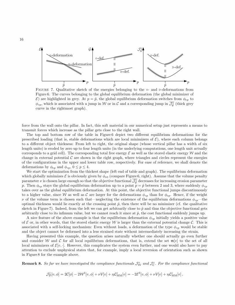
.-def.

Figure 7. Qualitative sketch of the energies belonging to the - and .-deformations fromFigure 6. The curves belonging to the global equilibrium deformation (the global minimizer ofE) are highlighted in grey. At p = p, the global equilibrium deformation switches from φ.p toφp, which is associated with a jump in W or in C and a corresponding jump in J εG (thick greycurve in the rightmost graph).

force from the wall onto the pillar. In fact, this soft material in our numerical setup just represents a means totransmit forces which increase as the pillar gets close to the right wall.

The top and bottom row of the table in Figure 6 depict two different equilibrium deformations for theprescribed loading (that is, stable deformations which are local minimizers of E), where each column belongsto a different object thickness: From left to right, the original shape (whose vertical pillar has a width of sixlength units) is eroded by zero up to four length units (in the underlying computations, one length unit actuallycorresponds to a grid cell). The corresponding total free energy E as well as the stored elastic energyW and thechange in external potential C are shown in the right graph, where triangles and circles represent the energiesof the configurations in the upper and lower table row, respectively. For ease of reference, we shall denote thedeformations by φ.p and φp, 0 ≤ p ≤ 4.

We start the optimization from the thickest shape (left end of table and graph). The equilibrium deformationwhich globally minimizes E is obviously given by φ.0 (compare Figure 6, right). Assume that the volume penaltyparameter ν is chosen large enough so that the objective functional J εG decreases for increasing erosion parameterp. Then φ.p stays the global equilibrium deformation up to a point p = p between 2 and 3, where suddenly φptakes over as the global equilibrium deformation. At this point, the objective functional jumps discontinuouslyto a higher value, since W as well as C are larger for the deformations φp than for φ.p. Hence, if the weightν of the volume term is chosen such that—neglecting the existence of the equilibrium deformations φp—theoptimal thickness would lie exactly at the crossing point p, then there will be no minimizer (cf. the qualitativesketch in Figure 7). Indeed, from the left we can get arbitrarily close to p and thus the objective functional getsarbitrarily close to its infimum value, but we cannot reach it since at p, the cost functional suddenly jumps up.

A nice feature of the above example is that the equilibrium deformation φp initially yields a positive valueof E or, in other words, that the stored elastic energy W is larger than the external potential change C. This isassociated with a self-locking mechanism: Even without loads, a deformation of the type φp would be stableand the object cannot be deformed into a less strained state without intermediately increasing the strain.

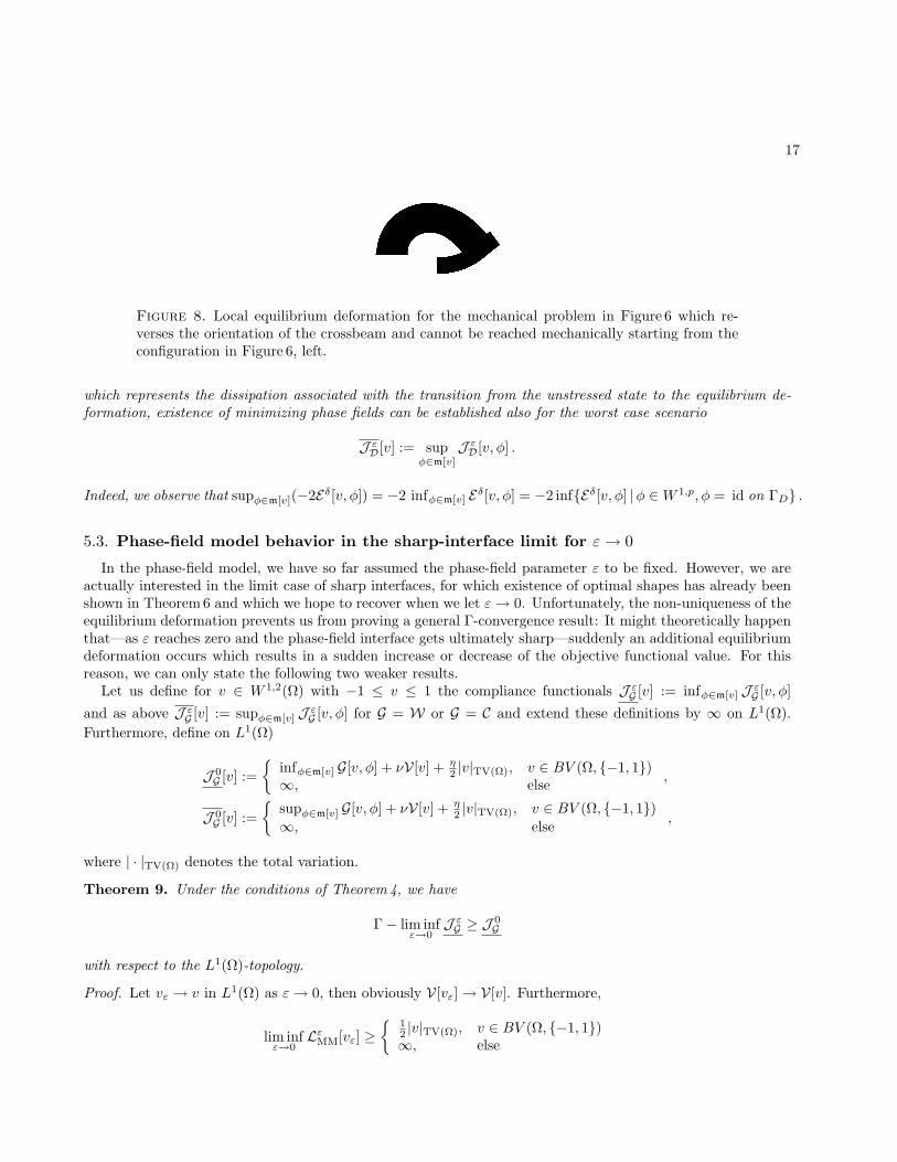
Having presented this example, the question arises naturally whether one should actually go even furtherand consider W and C for all local equilibrium deformations, that is, extend the set m[v] to the set of alllocal minimizers of E [v, ·]. However, this complicates the system even further, and one would also have to payattention to exclude unphysical states that, for example, imply a local reversion of orientation such as shownin Figure 8 for the example above.

Remark 8. So far we have investigated the compliance functionals J εW and J εC . For the compliance functional

J εD[v, φ] = 2C[φ]− 2Wδ[v, φ] + νV[v] + ηLεMM[v] = −2Eδ[v, φ] + νV[v] + ηLεMM[v] ,

17

Figure 8. Local equilibrium deformation for the mechanical problem in Figure 6 which re-verses the orientation of the crossbeam and cannot be reached mechanically starting from theconfiguration in Figure 6, left.

which represents the dissipation associated with the transition from the unstressed state to the equilibrium de-formation, existence of minimizing phase fields can be established also for the worst case scenario

J εD[v] := supφ∈m[v]

J εD[v, φ] .

Indeed, we observe that supφ∈m[v](−2Eδ[v, φ]) = −2 infφ∈m[v] Eδ[v, φ] = −2 infEδ[v, φ] |φ ∈W 1,p, φ = id on ΓD .

5.3. Phase-field model behavior in the sharp-interface limit for ε→ 0

In the phase-field model, we have so far assumed the phase-field parameter ε to be fixed. However, we areactually interested in the limit case of sharp interfaces, for which existence of optimal shapes has already beenshown in Theorem 6 and which we hope to recover when we let ε→ 0. Unfortunately, the non-uniqueness of theequilibrium deformation prevents us from proving a general Γ-convergence result: It might theoretically happenthat—as ε reaches zero and the phase-field interface gets ultimately sharp—suddenly an additional equilibriumdeformation occurs which results in a sudden increase or decrease of the objective functional value. For thisreason, we can only state the following two weaker results.

Let us define for v ∈ W 1,2(Ω) with −1 ≤ v ≤ 1 the compliance functionals J εG [v] := infφ∈m[v] J εG [v, φ]

and as above J εG [v] := supφ∈m[v] J εG [v, φ] for G = W or G = C and extend these definitions by ∞ on L1(Ω).Furthermore, define on L1(Ω)

J 0G [v] :=

infφ∈m[v] G[v, φ] + νV[v] + η

2 |v|TV(Ω), v ∈ BV (Ω, −1, 1)∞, else ,

J 0G [v] :=

supφ∈m[v] G[v, φ] + νV[v] + η

2 |v|TV(Ω), v ∈ BV (Ω, −1, 1)∞, else

,

where | · |TV(Ω) denotes the total variation.

Theorem 9. Under the conditions of Theorem 4, we have

Γ− lim infε→0

J εG ≥ J 0G

with respect to the L1(Ω)-topology.

Proof. Let vε → v in L1(Ω) as ε→ 0, then obviously V[vε]→ V[v]. Furthermore,

lim infε→0

LεMM[vε] ≥

12 |v|TV(Ω), v ∈ BV (Ω, −1, 1)∞, else

18

as already discussed in Section 3.3 (cf. also [14]). Finally, either lim infε→0 infφ∈m[vε] G[vε, φ] = ∞, in whichcase there is nothing left to prove, or there is a sequence (εi)i∈N with εi → 0 as i→∞ and a sequence φi withφi ∈ m[vεi ] such that

limi→∞

G[vεi , φi] = lim infε→0

infφ∈m[vε]

G[vε, φ] <∞ .

From Lemma 3 we deduce thatΓ− lim

i→∞Eδ[vεi , ·] = Eδ[v, ·] .

Furthermore, applying the same arguments as in Theorem 4 we obtain that (φi)i∈N is uniformly bounded inW 1,p(Ω). Hence, for a subsequence we get φi φ in W 1,p(Ω) for some φ ∈ m[v] and Eδ[vεi , φi]→ Eδ[v, φ]. Also,C[φi]→ C[φ] due to the continuity of C and thus alsoWδ[vεi , φi] = Eδ[vεi , φi]+C[φi]→ Eδ[v, φ]+C[φ] =Wδ[v, φ]so that

lim infε→0

infφ∈m[vε]

G[vε, φ] = limi→∞

G[vεi , φi] = G[v, φ] ≥ infφ∈m[v]

G[v, φ] ,

which altogether yields the desired result.

Theorem 10. Under the conditions of Theorem 4, we have

Γ− lim supε→0

J εG ≤ J 0G

with respect to the L1(Ω)-topology.

Proof. Let vε → v be a recovery sequence in L1(Ω) with respect to the Γ-convergence of LεMM [14], for whichwe obtain

lim supε→0

LεMM[vε] ≤

12 |v|TV(Ω), v ∈ BV (Ω, −1, 1)∞, else .

As before, we have V[vε] → V[v]. Finally, as in the previous proof, there are sequences εi and φi with εi → 0,φi ∈ m[vεi ], and φi φ for some φ ∈ m[v] such that

lim supε→0

supφ∈m[vε]

G[vε, φ] = limi→∞

G[vεi , φi] = G[v, φ] ≤ supφ∈m[v]

G[v, φ] ,

which concludes the proof.

If for a given phase field v there is just one single unique equilibrium deformation, then, obviously, J 0G [v] =

J 0G [v], which immediately implies following corollary.

Corollary 11. Let the conditions of Theorem 4 hold, and let v ∈ BV (Ω, −1, 1) be given. If the equilibriumdeformation is unique, that is, m[v] = φ[v] for a unique φ[v] ∈ W 1,p(Ω), then the Γ-limit of J εG and J εG forε→ 0 with respect to the L1(Ω)-topology is defined at v and is given by

J 0G [v] = J 0

G [v] .

As mentioned earlier, since the equilibrium deformation in general is not unique, we cannot state a generalΓ-convergence result. However, note that the above results also hold with the obvious modifications in the caseof linearized elasticity, that is, for

Wδ[v, φ] =Wδ,lin[v, φ] :=∫

Ω

((1− δ)χO(v) + δ)12Cε[φ− id] : ε[φ− id] dx

with a symmetric positive definite elasticity tensor C and ε[u] = 12 (Du+DuT). In this case, where the choices

G =W or D are equivalent to G = C as already discussed, we actually do obtain Γ-convergence of the objectivefunctional.

19

Corollary 12. For Wδ =Wδ,lin and F ∈ L2(ΓN ), we have

Γ− limε→0J εC = Γ− lim

ε→0J εC = J 0

C = J 0C

with respect to the L1(Ω)-topology.

Proof. By Korn’s first inequality, Wδ,lin[v, ·] is coercive on φ ∈ W 1,2(Ω) : φ|ΓD = id; furthermore, it isbounded so that the Lax–Milgram lemma implies the existence of a unique minimizer φ[v] of the associated freeenergy Eδ,lin[v, ·] for which 2Wδ,lin[v, φ[v]] = C[φ[v]]. Hence, in this case we obtain J εC = J εC , J 0

C = J 0C and thus

the desired result applying Theorems 9 and 10.

Finally, let us consider one particular compliance function. If we choose the dissipation associated withthe transition from the unstressed state to the equilibrium deformation as compliance, G = D, instead of theinternal elastic energy, G = W, or the change of external potential, G = C, we also obtain J εD = J εD as well as

J 0D = J 0

D by definition of Eδ[v, φ] and m[v] (cf. also Remark 8). Hence, we again obtain the following.

Corollary 13. Under the conditions of Theorem 4, we have

Γ− limε→0J εD = Γ− lim

ε→0J εD = J 0

D = J 0D

with respect to the L1(Ω)-topology.

6. Numerical Algorithm

In the following paragraphs, we will first state the optimality conditions of the minimization problem andits discretization by finite elements. We then briefly describe the computation of equilibrium deformations viaa trust region method and the optimization for the phase field by a quasi-Newton method, embedded in amultiscale approach.

6.1. Optimality conditions and finite element discretization

A necessary condition for φ to satisfy the constraint of static equilibrium is that it fulfills the Euler–Lagrangecondition

0 = δφEδ(θ) =∫

Ω

((1− δ)χO(v) + δ)W,A(Dφ) : Dθ dx−∫

ΓN

F · θ da

for all test displacements θ : Ω→ Rd with θ|ΓD = 0, where δzF(ζ) denotes the Gateaux derivative of an energyF with respect to z in some test direction ζ. Hence, by the first order optimality conditions, the solution to ourshape optimization problem can be described as a saddle point of the Lagrange functional

L[v, φ, p] = J εG [v, φ] + δφEδ[v, φ](p) ,

where G stands for W, C, or D, p denotes the Lagrange multiplier, and (φ− id)|ΓD = p|ΓD = 0. The associatednecessary conditions are given by 0 = δvL = δφL = δpL with δvL = δvR + νδvV + ηδvLε + δvδφEδ(p) (R here

20

stands for 2Wδ, C, or −2Eδ), δφL = δφR+ δφδφEδ(p), δpL = δφEδ, and

δvV(ϑ) =∫

Ω

∂χO(v)∂v

ϑdx ,

δvLεMM(ϑ) =∫

Ω

ε∇v · ∇ϑ+12ε∂Ψ(v)∂v

ϑ dx ,

δvWδ(ϑ) =∫

Ω

(1− δ)∂χO(v)∂v

ϑW (Dφ) dx ,

δφWδ(θ) =∫

Ω

((1− δ)χO(v) + δ)W,A(Dφ) : Dθ dx ,

δφC(θ) =∫

ΓN

F · θ da ,

δvδφEδ(p)(ϑ) =∫

Ω

(1− δ)∂χO(v)∂v

ϑW,A(Dφ) : Dp dx ,

δφδφEδ(p)(θ) =∫

Ω

((1− δ)χO(v) + δ)W,AA(Dφ)Dθ : Dpdx

for scalar and vector-valued test functions ϑ and θ, respectively, with θ|ΓD = 0.Furthermore, for a sufficiently smooth phase field v and a deformation φ satisfying the equilibrium constraint,

we may locally regard φ as a function φ[v]. Then, by the adjoint method, the derivative of J εG [v] := J εG [v, φ[v]]with respect to v in direction ϑ is given as

δvJ εG (ϑ) = δvJ εG (ϑ) + δvδφEδ(p)(ϑ) ,

where for fixed v, the deformation φ[v] and the Lagrange multiplier p solve 0 = δφL = δpL with the correspondingDirichlet boundary conditions at ΓD. This directional derivative can be used in gradient descent type algorithmsto find the optimal phase field v.

Concerning the discretization, we restrict ourselves to problems in two dimensions (d = 2) and approximatethe phase field v and deformation φ by continuous, piecewise multilinear finite element functions V and Φ on aregular mesh on Ω = [0, 1]2 with 2L + 1 nodes in each space direction. The different energy terms Wδ, V, andLεMM are approximated by third-order Gaussian quadrature on each grid cell. For the ease of presentation, inwhat follows we implicitly assume that the evaluation of every functional on finite element input functions isperformed only approximately using this quadrature. In our applications, for the sake of simplicity we restrictboth ΓD and ΓN to a union of several grid cell faces so that in particular ΓN is discretized in the canonical wayby a regular mesh on which a continuous, piecewise multilinear finite element approximation of the surface loadF can be defined. C is then also computed on this lower dimensional finite element mesh.

6.2. Inner minimization to find equilibrium deformation

We aim at a gradient descent type algorithm for the (discretized) phase field V , where in each step we firstminimize Eδ[V,Φ] to obtain a finite-element approximation Φ[V ] of the equilibrium deformation and then usethis deformation to evaluate the compliance functionals J εW [V,Φ[V ]] or J εC [V,Φ[V ]] and their Gateaux derivativewith respect to V . The inner minimization of Eδ[V,Φ] for Φ has to meet particularly strong requirements. Firstof all, the optimal deformation Φ[V ] has to be accurately found in order to enable a correct evaluation of theobjective energy and to obtain a good approximation of the Gateaux derivative which can then be used tocompute a descent direction. Second, since the minimization has to be performed for each energy evaluation,we need a fast converging method. Finally, the optimization method has to be very robust and should reliablylead to a (local) minimum.

The robustness requirement is particularly related to the use of the nonlinear elastic energy: In the presenceof buckling instabilities, there is typically an unstable or metastable (meaning that small perturbations suffice to

21

0 0.5 1−4.78

−4.76

−4.74

−4.72x 10

−4

0 0.5 14.62

4.64

4.66

4.68

4.7x 10

−4

0 0.5 19.4005

9.401

9.4015

9.402x 10

−4

s s s

Eδ[O,

id+su

1]

Wδ[O,

id+su

1]

C[id

+su

1]

Figure 9. Left: Eigendisplacement of a symmetrically compressed beam (height L = 1, thick-ness t = 0.25, Young’s modulus E = 4) corresponding to the negative eigenvalue of the freeenergy Hessian. Right: Energetic changes for the perturbation of the symmetric compressionin direction of the eigendisplacement. The coordinate s indicates the perturbation strength,and s = 0 corresponds to the symmetric deformation.

abandon the state), non-buckled state of the deformation Φ which more or less corresponds to the deformationin the linearized elastic setting. This state is associated with a saddle point of the energy Eδ[V,Φ], which hasto be robustly bypassed by the minimization method. While simple gradient descent type methods tend toslow down considerably in the vicinity of such points, the basic Newton algorithm is prone to converge exactlyto this saddle point. Indeed, recalling the simulations of buckling rods from Figure 4, for symmetry reasonswe know that the symmetric deformation in between buckling deformations to both sides must be a criticalpoint of Eδ[O, ·]. This deformation is readily obtained by a simple Newton iteration to find the zero of thederivative of Eδ[O, ·]. The corresponding stiffness operator, that is, the Hessian of Eδ[O, ·] at this symmetricdeformation then is indeed indefinite and has a negative eigenvalue, classifying the symmetric deformation asa saddle point of the free energy. For the bar of height L = 1, thickness t = 0.25, and Young’s modulus E = 4the eigendisplacement u1 belonging to the negative eigenvalue λ1 = −2.7 · 10−5 is shown in Figure 9, as well asthe decrease of Eδ[O, id + su1], Wδ[O, id + su1], and C[ id + su1] along this direction for increasing values of s.In fact, the eigendisplacement can easily be recognized as a (linearized) bending deformation.

Due to the above-mentioned problems of simple gradient-descent or Newton methods, we will need a moresophisticated technique. Furthermore, the energy landscape in the nonlinear regime is typically characterizedby long, deep, narrow and bent valleys. These valleys may be interpreted as the paths along which the ma-terial can be deformed, and leaving these valleys will rapidly lead to unphysical states such as local materialinterpenetration and thus the break-down of the minimization.

Trust region methods represent a very reliable minimization technique that satisfies all the above issues.At each step i, the objective functional is approximated by a quadratic model mi which is minimized insidea so-called trust region around Φi to obtain a new guess Φi+1. If the decrease of the objective functionalagrees sufficiently with the decrease of the quadratic model, the step is accepted and the trust region enlarged;otherwise, the trust region is shrunken.

The subtleties of a trust-region method lie in the treatment of the so-called trust region subproblem tominimize the quadratic model within the trust region. In our computations, we chose to implement the algorithmproposed in [19, Algorithm 7.3.4]. At step i, the quadratic model mi is given as the second order Taylorexpansion of the discrete energy Eδ[V, ·] about Φi, which involves the Hessian H(Φi) of Eδ[V, ·]. To minimizethis model within a circular trust region around Φi of radius ∆, the smallest positive scalar ξ is sought such thatHi(ξ) := H(Φi)+ξ id becomes positive definite and the global minimum of the correspondingly modified Taylorexpansions lies within the trust region. The positive definiteness of the quadratic operator is checked via aCholesky factorization Hi(ξ) = LLT, which also serves to find the minimum by solving the corresponding linearsystem of equations that results from the optimality conditions. Additionally, the eigendirection belonging to

22

the smallest eigenvalue of Hi(ξ) is approximated by a technique which aims to find a vector Y such that L−1Yis large. This eigendirection is essentially employed to bypass saddle points. The scalar ξ is itself obtained bya Newton iteration which is safeguarded by a number of sophisticated bounds on ξ (see [19] for details). TheCholesky factorization is performed using the CHOLMOD package from Davis et al. [17, 22], where a matrixreordering ensures a minimum fill-in.

In our setting, the discrete energy gradient and the Hessian matrix H(Φ) are evaluated as

(δφEδ(ϕiej)

)(i,j)∈I0h×1,2

=(∫

Ω

((1− δ)χO(V ) + δ)W,A(DΦ) : D(ϕiej) dx−∫

ΓN

F · (ϕiej) da)

(i,j)∈I0h×1,2

and

H =(δφφEδ(ϕiej , ϕkel)

)(i,j),(k,l)∈I0h×1,2

=(∫

Ω

((1−δ)χO(V )+δ)W,AA(DΦ)D(ϕiej) : D(ϕkel) dx)

(i,j),(k,l)∈I0h×1,2

for the set I0h of node indices in Ω \ΓD, the finite element basis functions ϕii∈I0h , and the canonical Euclidean

basis e1, e2 in R2.

6.3. Optimization for the phase field

Concerning the outer optimization for V , we apply a Davidon–Fletcher–Powell quasi-Newton method, which—expressed for the minimization of a function f : RN → R, x 7→ f(x)—uses the update formula

Bk+1 = Bk +∆xk∆xTkgTk ∆xk

− BkgkgTk B

Tk

gTk Bkgk

to approximate the inverse of the Hessian of f in the (k + 1)th step using the latest update ∆xk = xk+1 − xkand the difference gk = ∇f(xk+1)−∇f(xk) between the gradients. The descent direction pk is then chosen as−Bk∇f(xk), and the step length τk is determined to satisfy the strong Wolfe conditions,

f(xk + τkpk) ≤ f(xk) + c1τk∇fk · pk,|∇f(xk + τkpk) · pk| ≤ c2|∇f(xk) · pk|

for c1 = 0.5, c2 = 0.9. Furthermore, we reset Bk to the identity every tenth step to restrict memory usage andto ensure a descent at least as good as gradient descent.

The gradient of the objective functional J εG [V ] = J εG [V,Φ[V ]] (for G = W or G = C) with respect to V iscomputed via the adjoint method as described in Section 6.1. We first solve

δφδφEδ(Ψ)(P ) = −δφJ εG (Ψ)

for the finite-element Lagrange multiplier P under the constraint P |ΓD = 0, where Ψ runs over all vector-valuedfinite-element functions that are zero on ΓD. In terms of finite-element operators, this can be expressed as thelinear system HP = R, where P denotes the vector of nodal values of P on Ω \ ΓD, the matrix H has beengiven above, and the right-hand side reads

R =(∫

Ω

((1− δ)χO(V ) + δ)W,A(DΦ[V ]) : D(ϕiej) dx)

(i,j)∈I0h×1,2

or R =(∫

ΓN

F · (ϕiej) da)

(i,j)∈I0h×1,2,

23

depending on whether J εW [V,Φ[V ]] or J εC [V,Φ[V ]] is minimized. Then we obtain the gradient of the objectivefunctional with respect to V as (

δvJ εG (ϕi) + δvδφEδ(P )(ϕi))i∈Ih

for all i ∈ Ih, where Ih represents the set of all node indices in Ω except those at which V is fixed by a Dirichletcondition, and where the expressions for the Gateaux derivatives are provided in Section 6.1.

6.4. Embedding the optimization in a multiscale approach

In order to enhance convergence and to avoid local minima, we pursue a multiscale approach, using a hierarchyof dyadic grid resolutions with 2l + 1 nodes in each direction and multilinear interpolation as prolongationtechnique. We first perform the minimization for a coarse spatial discretization and then successively prolongateand refine the result on finer grids. The phase-field scale parameter ε is coupled to the grid size h via ε = hin order to allow a sufficient resolution of the interface. Finally, it is sometimes advantageous to take a smallervalue for ν on coarse grids in order not to penalize the value V = 1 so strongly that intermediate values of Vbetween −1 and 1 are preferred. As the grid gets finer, ν can be increased since the smaller value of ε forcesthe phase-field values towards the pure phases −1 and 1.

A brief overview over the entire algorithm in pseudo code notation reads as follows (bold capital lettersrepresent vectors of nodal values, and G stands for W, C, or D):

EnergyRelaxation initialize Φ = id and V = 0 on grid level l0;for grid level l = l0 to L

do Vold = V;minimize Eδ[V,Φ] for Φ by a trust region method to obtain Φ[V ];evaluate J εG [V,Φ[V ]];compute the dual variable P by solving the linear system

δφδφEδ(Ψ)(P ) = −δφJ εG (Ψ) ∀Ψ;compute the derivative of J εG [V ] := J εG [V,Φ[V ]] with respect to V as

V :=(δvJ εG (ϕi) + δvδφEδ(P )(ϕi)

)i∈Ih

;compute an approximate inverse Hessian B by the Davidon–Fletcher–Powell method;compute a descent direction D := −BV;perform a descent step

V = Vold − τ Dwith Wolfe step size control for τ ;

while(|Vold −V| ≥ Threshold);if (l < L) prolongate V , Φ onto the next grid level;

7. Experiments

The effect of using nonlinear instead of linearized elasticity has already been explored in Figure 3, where wecompared optimal cantilever shapes for loads of different magnitudes, using J εC as objective functional. Whiteand black regions correspond to the phases v = 1 and v = −1, respectively. Of course, increasing the load resultsin stronger deformations and thus higher values of C (andW) so that the shapes would naturally become thickerand more strutted in order to balance the compliance with the volume costs V and the perimeter regularizationLεMM. To make the optimal designs comparable and to reveal the pure influence of introducing geometric andmaterial nonlinearity, the weights ν and η of V and LεMM have to be increased in parallel. Since the compliance

24

LεMM[u] = 9.9525

V[u] = 0.3590

C[φ[u]] = 0.6687

Wδ[v, φ[u]] = 0.3308

E [u, φ[u]] = −0.3380

J εC [u, φ[u]] = 1.3078

J εW [u, φ[u]] = 1.3007

J εD[u, φ[u]] = 1.3150

LεMM[u] = 10.0343

V[u] = 0.3481

C[φ[u]] = 0.6896

Wδ[v, φ[u]] = 0.3383

E [u, φ[u]] = −0.3514

J εC [u, φ[u]] = 1.3113

J εW [u, φ[u]] = 1.2982

J εD[u, φ[u]] = 1.3244

LεMM[u] = 10.0863

V[u] = 0.3648

C[φ[u]] = 0.6599

Wδ[v, φ[u]] = 0.3284

E [u, φ[u]] = −0.3314

J εC [u, φ[u]] = 1.3092

J εW [u, φ[u]] = 1.3062

J εD[u, φ[u]] = 1.3122

Figure 10. Optimal cantilever design for minimizing J εC , J εW , J εD (from left to right), takingthe same parameters as in Figure 3 for the case F = 4 (in these computations, ε was chosen halfthe grid size h in order to obtain acceptable phase fields already for a resolution of 129× 129).Minimization of J εD (right) yields the most symmetric shape, while minimization of J εW (middle)yields the most asymmetric one with the compressed struts being significantly thinner than inthe other cases.

scales quadratically with the load (at least for small deformations in the regime of linearized elasticity), ν andη are chosen such that F 2

ν and F 2

η stay constant.As discussed in Section 4, compared to optimal designs for linearized elasticity, the symmetry of the cantilever

design is broken due to the nonlinear influence of the loading direction. We observe that as the load increases, astructure evolves which exhibits a single thick beam at the top that is supported from below by several thinnerstruts extending from the wall to the point where the load is applied as well as to two or three other pointsalong the beam. These struts are themselves suspended from thread-like structures.

In the beginning, we have stated and discussed the different possibilities to extend the notion of complianceto the setting of nonlinear elasticity. In particular we have considered the change of external potential C andthe internally stored elastic energy W. The compliance minimization yields different results depending on ourchoice: While the use of C will produce rather rigid constructions that allow only small displacements, the useof W does in principle allow for large deformations as long as the final equilibrium state is not heavily strained.As a third possibility we have introduced the energy dissipation −2E = 2C − 2W.

A comparison of the three possibilities reveals a complex interplay between the volume costs and the me-chanical energy (Figure 10). We first observe that the obtained shapes are plausible in the sense that each ofthem indeed has the minimum value of its associated objective function (J εC , J εW , or J εD, respectively) amongall three. However, we also notice that the various energy contributions do not differ significantly betweenthe three designs. Nevertheless, they do look quite different: While the minimizer of JD is almost symmetric,the minimizer of JW is strongly asymmetric. In particular, the bottommost beam, which will be compressedduring the deformation, becomes thinner from JD to JC to JW , thereby allowing stronger displacements. Thisagrees with the simplified model example in Section 3. The internal energy W seems to be not very sensitive to

25

LεMM[u] = 3.9006

V[u] = 0.1385

C[φ[u]] = 4.3841

Wδ[v, φ[u]] = 0.2077

E [u, φ[u]] = −4.1764

J εC [u, φ[u]] = 4.6310

J εW [u, φ[u]] = 0.6623

J ε−E [u, φ[u]] = 8.5997

Figure 11. Initialising the phase field as a single rod, a minimization of J εW retrieves theabove optimal cantilever design with a much lower objective function value than the design inFigure 10, middle.

Figure 12. Optimal designs with respect to J εC for the same load case as in Figure 5 withparameters F = 0.016 ·

√2, λ = µ = 80, η = 2k · 10−8, ν = 25+k · 10−7 for k = 6, . . . , 1 from

left to right (resolution 512× 512). The load is chosen very small so as to stay in the regime oflinearized elasticity such that buckling cannot occur for the fine shapes on the left.

the thickness of the bottommost beam, while the potential change C strongly is. Therefore, it pays off to savevolume at the cost of a slightly increasing W in order to minimize JW . In fact, the model example in Section 3already suggests that the middle design in Figure 10 is only locally optimal. Indeed, if we initialize the shapeas a simple rod similar to Figure 2, then we obtain the design shown in Figure 11 with a much lower objectivefunction value.

Apart from the employed hyperelastic material law, there are two weighting parameters that need to betuned in order to obtain sensible results. Consequently, we have to study the influence of the different energycontributions. The impact of volume penalization and perimeter regularization seems clear; the former prefersthinner structures while the latter tends to reduce the degree of cross-linking. The question arises how thecompliance term affects the optimal shape, whether by thickening its single components or by producing morestrutted shapes. Experiments show that both mechanisms occur until a point at which the different materialparts have grown up to a width that they start to merge and eliminate any fine structure (Figure 12).

To explore the effect of varying the two weight parameters ν and η systematically, let us sample the two-parameter family of (at least locally) optimal shapes which is generated by η and ν. Before doing so, note thatgenerally, the maximally reachable resolution of our optimal designs is restricted due to computation time, whichin turn also fixes the smallest resolvable scale parameter ε. Since the phase field v is only forced towards thepure phases v ∈ −1, 1 for the limit ε→ 0, there will inherently always remain intermediate values (which canalso be observed in some of the previous examples). One particular reason for this lies in the strong interactionbetween the non-convex potential η 9

321ε (v2 − 1)2 with the two energy-minimizing phases v ∈ −1, 1 and the

convex volume costs ν4 (v + 1)2. For too large ε, that is, for ε ≥ η

ν94 , their sum becomes convex so that there

26

-

6

log νη

logη

-

6@

@@

@@

@@

@@

@@

@@Rη →, ν η,ν

η , ν →

Figure 13. Optimal cantilever designs for different parameter values. The middle design isthe same as in Figure 10, left; the top and bottom row as well as the right and left column areobtained by doubling and halving η and ν

η , respectively.

are no longer two preferred phases. Due to the significance of νη in this lower bound, in our parameter study

we shall choose to vary νη and η instead of ν and η.

Figure 13 shows cantilever designs which were obtained by choosing the middle computation as the referencesetting and then doubling or halving ν

η as well as η. Apparently, for fixed ε there is a regime of νη for which

reasonable shapes are obtained, corresponding to the middle column. For larger values, phase-field densitiesbetween −1 and 1 are not sufficiently penalized, and for smaller values we obtain bulky designs without any finestructure. The effect of varying η for a constant volume weight ν can be seen along the descending diagonals;these designs indeed seem to possess similar volumes, but a distinct amount of fine structure. Along thehorizontal direction, just ν changes, and the design volumes can be seen to decrease to the right.

Naturally, the energy landscape associated with J εC , J εW , and J εD is quite complicated and allows for multiplelocal minima. In order to reduce the influence of initialization and to obtain satisfactory results with a sufficientlylow objective function value, in the above examples we pursued a multiscale approach with an initial optimizationon a coarse resolution (to find a good large scale structure) and successive refinement. For initialization on thecoarsest level, each nodal value of the phase field is taken randomly from a uniform distribution on [−0.1, 0.1].Also, we started with a small value of ν on the coarse grid and then doubled it at each prolongation until itsfinal value on the finest grid level. In this way we maintain a constant ratio η

εν over all grid levels so that volumecosts and chemical potential already balance each other on the coarser grid levels and the coarse phase fieldsare already quite close to an optimal design (compare Figure 14).

27

-successive numerical relaxation

h = ε = 2−4 h = ε = 2−5 h = ε = 2−6 h = ε = 2−7

Figure 14. Intermediate results of the optimization for the top left case of Figure 13. The firstthree images in the top row show the results of the multiscale algorithm on grid levels four tosix, where ν has been doubled at each prolongation. The rightmost two images show the shapeafter 300 quasi-Newton iterations on grid level seven as well as the final result. The middle rowshows the same results, only that this time ν is the same on all grid levels. In the bottom row,the optimization was started directly on grid level seven without a multiscale approach. Theintermediate shapes after 300, 600, and 3000 iterations as well as the final result are depicted.The final values of the objective function J εC are 1.3500, 1.3229, 1.3239, respectively.

Alternatively, one could employ the same value of ν on all grid levels or start the optimization directly on thefinest level without a multiscale approach. While all three approaches yield the same result for many parameterconstellations (which is not too surprising especially for the rightmost column in Figure 13, for example, wherewe have reached the regime in which the sum of volume costs and chemical potential are convex), this does nothold for some cases as for example depicted in Figure 14, where the progress of the optimization algorithm isshown. In general, however, the achieved objective function values are very close to each other, and in somecases it seems that at least two of the tree approaches would eventually converge against the same shape if theywere not terminated due to too small progress. Note that for the case in Figure 14, one approach seems not tobe able to create holes inside the bulky shape.

As a final example, we have computed an optimal design for a bridge-like structure with two pointwiseDirichlet boundary conditions and a uniform downward surface load (Figure 15). Apparently, the optimaldesign is to suspend the bottom edge from an arch extending between both fixing points. In order to reducecomputation time for this example (especially during the Cholesky-factorization), we did not use the entire unitsquare [0, 1]2 as the computational domain, but instead updated the computational domain every 100 iterations

28

F

Figure 15. Sketch of the design problem and optimal design for F = 1.2, λ = µ = 80,η = 10−4, ν = 25 · 10−3. The right image shows the final, actual computational domain: Thelight gray background does not belong to the computational domain whereas the foreground(which is cut out of the middle image) does.

as the region x ∈ [0, 1]2 : v(x) > −0.95, dilated by three grid cells. This update does not hamper convergence,and the final, actual computational domain is shown in Figure 15, right.

Acknowledgements

Benedikt Wirth has been funded by the Bonn International Graduate School in Mathematics. The workwas supported by the Deutsche Forschungsgemeinschaft, SPP 1253 (Optimization with Partial DifferentialEquations).

References

[1] G. Allaire. Topology optimization with the homogenization and the level-set method. pages 1–13. Kluwer Academic Pub,

November 2004.[2] G. Allaire, E. Bonnetier, G. Francfort, and F. Jouve. Shape optimization by the homogenization method. Numerische Mathe-

matik, 76:27–68, 1997.

[3] G. Allaire, F. de Gournay, F. Jouve, and A.-M. Toader. Structural optimization using topological and shape sensitivity via alevel set method. Technical Report 555, Ecole Polytechnique, Centre de Mathematiques appliquees, UMR CNRS 7641, 91128

Palaiseau Cedex (France), October 2004.[4] G. Allaire, F. Jouve, and H. Maillot. Topology optimization for minimum stress design with the homogenization method.

Struct Multidisc Optim, 28:87–98, 2004.

[5] Gregoire Allaire. Shape optimization by the homogenization method, volume 146 of Applied Mathematical Sciences. Springer-Verlag, New York, 2002.

[6] Gregoire Allaire, Francois Jouve, and Anca-Maria Toader. A level-set method for shape optimization. C. R. Acad. Sci. Paris,

Serie I, 334:1125–1130, 2002.[7] Gregoire Allaire, Francois Jouve, and Anca-Maria Toader. Structural optimization using sensitivity analysis and a level-set

method. Journal of computational physics, 194:363–393, 2004.

[8] Samuel M. Allen and John W. Cahn. A microscopic theory for antiphase boundary motion and its application to antiphasedomain coarsening. Acta Metallurgica, 27(6):1085–1095, 1979.

[9] Luigi Ambrosio and Giuseppe Buttazzo. An optimal design problem with perimeter penalization. Calculus of Variations and

Partial Differential Equations, 1:55–69, 1993.[10] Ruben Ansola, Estrella Veguerıa, Javier Canales, and Jose A. Tarrago. A simple evolutionary topology optimization procedure

for compliant mechanism design. Finite Elements in Analysis and Design, 44(1–2):53–62, 2007.[11] J. M. Ball. Convexity conditions and existence theorems in nonlinear elasiticity. Archive of Rational Mechanics and Analysis,

63:337–403, 1977.

[12] J.M. Ball. Global invertibility of Sobolev functions and the interpenetration of matter. Proc. Roy. Soc. Edinburgh, 88A:315–328,1981.

[13] B. Bourdin and A. Chambolle. Design-dependent loads in topology optimization. ESAIM Control Optim. Calc. Var., 9:19–48,

2003.[14] Andrea Braides. Γ-convergence for beginners, volume 22 of Oxford Lecture Series in Mathematics and its Applications. Oxford

University Press, Oxford, 2002.

29

[15] Martin Burger and Roman Stainko. Phase-field relaxation of topology optimization with local stress constraints. SIAM Journalon Control and Optimization, 45(4):1447–1466, 2006.

[16] Antonin Chambolle. A density result in two-dimensional linearized elasticity, and applications. Archive for Rational Mechanics

and Analysis, 167(3):211–233, 2003.[17] Y. Chen, T. A. Davis, W. W. Hager, and S. Rajamanickam. Algorithm 887: CHOLMOD, supernodal sparse Cholesky factor-

ization and update/downdate. ACM Transactions on Mathematical Software, 35(3):22:1–22:14, 2009.

[18] P. G. Ciarlet. Three-dimensional elasticity. Elsevier Science Publishers B. V., 1988.[19] A. R. Conn, N. I. M Gould, and P. L. Toint. Trust-Region Methods. SIAM, 2000.

[20] Sergio Conti, Harald Held, Martin Pach, Martin Rumpf, and Rudiger Schultz. Risk averse shape optimization. Siam Journal

on Control and Optimization, 2009. submitted.[21] B. Dacorogna. Direct methods in the calculus of variations. Springer-Verlag, New York, 1989.

[22] T. A. Davis and W. W. Hager. Dynamic supernodes in sparse Cholesky update/downdate and triangular solves. ACM Trans-

actions on Mathematical Software, 35(4):27:1–27:23, 2009.[23] G. P. Dias, J. Herskovits, and F. A. Rochinha. Simultaneous shape optimization and nonlinear analysis of elastic solids.

Computational Mechanics, 1998.[24] Xu Guo, Kang Zhao, and Michael Yu Wang. Simultaneous shape and topology optimization with implicit topology description

functions. Control and Cybernetics, 34(1):255–282, 2005.

[25] Z. Liu, J. G. Korvink, and R. Huang. Structure topology optimization: Fully coupled level set method via femlab. Structuraland Multidisciplinary Optimization, 29:407–417, June 2005.

[26] J. E. Marsden and T. J. R. Hughes. Mathematical foundations of Elasticity. Prentice–Hall, Englewood Cliffs, 1983.

[27] Luciano Modica and Stefano Mortola. Un esempio di Γ−-convergenza. Boll. Un. Mat. Ital. B (5), 14(1):285–299, 1977.[28] Pablo Pedregal. Variational Methods in Nonlinear Elasticity. SIAM, 2000.

[29] J. A. Sethian and A. Wiegmann. Structural boundary design via level set and immersed interface methods. Journal of Com-

putational Physics, 163(2):489–528, 2000.[30] O. Sigmund and P. M. Clausen. Topology optimization using a mixed formulation: An alternative way to solve pressure load

problems. Computer Methods in Applied Mechanics and Engineering, 196(13–16):1874–1889, 2007.

[31] J. Sikolowski and J.-P. Zolesio. Shape sensitivity analysis, chapter Introduction to shape optimization. Springer, 1992.[32] M. Y. Wang, S. Zhou, and H. Ding. Nonlinear diffusions in topology optimization. Structural and Multidisciplinary Optimiza-

tion, 28(4):262–276, 2004.

[33] Michael Yu Wang, Xiaoming Wang, and Dongming Guo. A level set method for structural topology optimization. Computermethods in applied mechanics and engineering, 192:227–246, 2003.

[34] Michael Yu Wang and Shiwei Zhou. Synthesis of shape and topology of multi-material structures with a phase-field method.Journal of Computer-Aided Materials Design, 11(2–3):117–138, 2004.

[35] Peng Wei and Michael Yu Wang. Piecewise constant level set method for structural topology optimization. International

Journal for Numerical Methods in Engineering, 78(4):379–402, 2009.[36] Qi Xia and Michael Yu Wang. Simultaneous optimization of the material properties and the topology of functionally graded

structures. Computer-Aided Design, 40(6):660–675, 2008.

[37] Shiwei Zhou and Michael Yu Wang. Multimaterial structural topology optimization with a generalized Cahn–Hilliard modelof multiphase transition. Structural and Multidisciplinary Optimization, 33:89–111, 2007.