Prioritized Elastic Round Robin:

An Efficient and Low-Latency Packet

Scheduler with Improved Fairness

Salil S. Kanhereand

Harish Sethu

Technical Report DU-CS-03-03Department of Computer Science

Drexel UniversityPhiladelphia, PA 19104

July 2003

Prioritized Elastic Round Robin: An Efficient andLow-Latency Packet Scheduler

with Improved Fairness 1

Salil S. Kanhere and Harish Sethu

Abstract

In emerging high-speed integrated-services packet-switched networks, fair packet schedul-ing algorithms in switches and routers will play a critical role in providing the Quality-of-Service (QoS) guarantees required by real-time applications. Elastic Round Robin (ERR),a recently proposed scheduling discipline, is very efficient with an O(1) work complexity.In addition, it has superior fairness and delay characteristics in comparison to other algo-rithms of equivalent efficiency. However, since ERR is inherently a round robin schedulingalgorithm, it suffers from the limitations of all round robin schedulers such as (i) burstytransmission and (ii) the inability of the flows lagging in service to receive precedenceover the flows that have received excess service. Recently, Tsao and Lin have proposed anew scheme, Pre-order Deficit Round Robin, which tries to eliminate the problems associ-ated with the round robin service order of Deficit Round Robin (DRR). In this report, wepresent a new scheduling discipline called Prioritized Elastic Round Robin (PERR), basedon a similar principle as Pre-order DRR but in a modified and improved form, which over-comes the limitations of ERR. We derive an upper bound on the latency achieved by PERRusing a novel technique based on interpreting the scheduling algorithm as an instance of anested version of ERR. Our analytical results show that PERR has better fairness character-istics and a significantly lower latency bound in comparison to other scheduling disciplinesof equivalent work complexity such as DRR, ERR and Pre-order DRR. We further presentsimulation results, using both synthetic and real traffic traces, which illustrate the improvedperformance characteristics of PERR.

Key words: Fair queueing, Elastic Round Robin, low latency, relative fairness bound,quality of service, Gini index.

Email addresses:salil@ece.drexel.edu (Salil S. Kanhere),sethu@ece.drexel.edu (Harish Sethu).1 This work was supported in part by NSF CAREER Award CCR-9984161 and U.S. AirForce Contract F30602-00-2-0501.

1 Introduction

The Internet traffic today is increasingly dominated by new real-time multimediaapplications such as audio/video-on-demand, IP telephony, and multimedia tele-conferencing, all of which prefer some guarantee of an acceptable quality of service(QoS) in the transmission and delivery of data. These different applications havevarying traffic characteristics with different requirements, and rely on the ability ofthe network to provide QoS guarantees with respect to several quality measures,such as end-to-end delay, bandwidth allocation, delay jitter, and packet loss. Thisrequires a scalable QoS mechanism to efficiently apportion, allocate and managelimited network resources among competing users. Fair, efficient and low-latencypacket scheduling algorithms used at the output links of switches and routers forman important component of such a mechanism [1]. Fair scheduling becomes espe-cially critical in access networks, within metropolitan area networks and in wirelessnetworks where the resource capacity constraints tend to be significantly limitingto high-bandwidth multimedia applications today. Even with the over-provisioningof resources such as is typical in the Internet core, fairness in scheduling is essen-tial to protect flows from other misbehaving flows triggered by deliberate misuseor malfunctioning software on routers or end-systems. Fairness in the managementof resources is also helpful in countering certain kinds of denial-of-service attacks.Fair schedulers have now found widespread implementation in switches and Inter-net routers [2,3].

Given multiple packets awaiting transmission through an output link, the functionof a packet scheduler is to determine the exact sequence in which these packets willbe transmitted through the link. Desirable properties of a packet scheduler include:

• Fairness in bandwidth allocation:This characteristic of a scheduler is most fre-quently judged based on the max-min notion of fairness [1,4].

• Low latency:An appropriate measure of packet schedulers in this regard, espe-cially for schedulers seeking to provide guaranteed services, is the upper boundon the length of time it takes a new flow to begin receiving service at the guar-anteed rate [5].

• Low implementation complexity:A per-packet work complexity ofO(1) withrespect to the number of flows is considered most desirable for ease of imple-mentation, especially in hardware switches.

Often, there is a conflict between a simple and efficient implementation on the onehand and low latency and fairness on the other. In this report, we present a newscheduling discipline calledPrioritized Elastic Round Robin (PERR)with a workcomplexity ofO(1) with respect to the number of flows and with better fairnessand latency characteristics than other known schedulers of equivalent complexity.In addition, these characteristics of PERR are comparable to those of significantlymore complex schedulers such as WFQ. In this report, we present analytical proofs

2

of these characteristics of PERR. Further, using real gateway traffic traces, andbased on a new measure of fairness borrowed from the field of economics, wepresent simulation results that demonstrate the improved fairness characteristics ofPERR.

1.1 Related Work and Motivation

Fair schedulers—those discussed in the research literature as well as those currentlyimplemented in switches and routers—are often based on themax-minnotion offairness [1, 4], a strategy for apportioning a shared resource among multiple re-questing entities. The central idea of the max-min strategy is that no entity receivesa share of the resource larger than its demand and that entities with unsatisfieddemands receive equal shares of the resource. The Generalized Processor Sharing(GPS) [6] is an ideal but unimplementable scheduler that assumes fluid flow trafficto exactly satisfy the above classical notion of fairness.

Over the last several years, a large number of different packet-based schedulingalgorithms have been proposed with an aim to approximate the GPS scheduler.These algorithms can be broadly classified into the following two categories—sorted-priority schedulers and frame-based schedulers. Sorted-priority schedulersmaintain a global variable known as the virtual time or the system potential func-tion. A timestamp corresponding to each packet is computed based on this vari-able, and packets are scheduled in increasing order of their timestamps. Exam-ples of sorted-priority schedulers are Weighted Fair Queueing (WFQ) [6, 7], Self-Clocked Fair Queueing (SCFQ) [8], Start-Time Fair Queueing (SFQ) [9], Frame-based Fair Queueing2 (FFQ) [10] and Worst-Case Fair Weighted Fair Queueing(WF2Q) [11]. The sorted-priority schedulers primarily differ in the manner in whichthey compute the global virtual time function. They generally provide good fairnessand a low latency bound but are not very efficient due to the complexity involved incomputing the virtual time function and in having to maintain a sorted list of pack-ets based on their timestamps. WFQ and WF2Q suffer anO(n) time complexityto compute the virtual time function, wheren is the number of flows sharing thesame output link. Schedulers such as SCFQ, SFQ and FFQ reduce the complexityof computing the virtual time toO(1) by using approximations of the correct vir-tual times. However, they still need to maintain a sorted list of packets based ontheir timestamps incurring a per-packet work complexity ofO(log n).

In frame-based schemes, on the other hand, the scheduler provides service oppor-tunities to the backlogged flows in a particular order and, during each service op-

2 Note that Frame-based Fair Queueing, in spite of its name, is actually a sorted-priorityscheduling discipline. The algorithm uses a framing approach similar to that used in frame-based schedulers to update the state of the system. However, as in sorted-priority sched-ulers, packets are transmitted based on their timestamps.

3

portunity, the intent is to provide the flow an amount of service proportional toits fair share of the bandwidth. Examples of such schedulers are Deficit RoundRobin (DRR) [12], Surplus Round Robin (SRR) [13–15] and Elastic Round Robin(ERR) [16]. The frame-based schedulers do not maintain a global virtual time func-tion and also do not require any sorting among the packets available for trans-mission. This reduces the implementation complexity of frame-based schedulingdisciplines toO(1), making them attractive for implementation in routers and, es-pecially so, in hardware switches. However, these frame-based schedulers sufferthe following disadvantages:

• High Start-Up Latency:The above frame-based schedulers operate in a round-robin fashion, with each active flow receiving exactly one opportunity to transmitin each round. When a new flow becomes active, it has to wait until all otherpreviously active flows receive their service opportunity before it can receiveservice from the scheduler. With large numbers of flows, this time period can bevery large, especially in comparison to sorted-priority schedulers such as WFQand WF2Q.

• Bursty output:Each flow is served over a continuous time interval during itsround robin service opportunity leading to a bursty packet stream at the outputof the scheduler for any given flow. This is not an ideal situation for real-timemultimedia traffic since even smooth flows are rendered bursty as they exit thescheduler.

• Delayed correction of unfairness:If a flow receives very little service in a partic-ular round, it is compensated with proportionately more service in the next round.While this disadvantaged flow waits for its compensation in the next round, otherflows which have already received more service than their fair share in the pre-vious round continue to receive yet more service before the disadvantaged flowreceives its opportunity.

• Compounded Jitter:When a flow’s arrival pattern at the scheduler has high jitter,it can frequently happen that the flow runs out of packets even before it hasreceived its fair share of service during its service opportunity. At this point,the scheduler moves on to serve other currently active flows in a round-robinfashion. Our flow with high jitter will receive its next opportunity only in the nextround after all the other active flows have completed their transmissions. Thisfurther increases the jitter in the output of the scheduler since a delayed packetthat just misses its service opportunity in a certain round ends up experiencingsignificant additional delay because of having to wait for all the other active flowsto complete their transmissions.

These weaknesses of frame-based schedulers discussed above are caused by thesame features that are common to these schedulers:

(1) The round robin nature of the service order.(2) Each flow receives its entire share of service in the round at once in one service

opportunity.

4

Overcoming these weaknesses while preserving theO(1) complexity of frame-based schedulers forms the primary motivation behind this report.

At least a few proposals have been made in the last few years to overcome thelimitations of frame-based schedulers discussed above. The Nested-DRR schedulerproposed in [17] tries to eliminate some of these limitations of the DRR scheduler[12]. For each flowi, the DRR scheduler maintains aquantum, Qi, which representsthe ideal service that the flow should receive in each round of service. If the entirequantum is not used in a given round, the deficit is recorded and used to compensatethe flow in the next round. Nested-DRR splits each DRR round, referred to as anouter round, into one or more smallerinner roundsand executes a modified versionof the DRR algorithm within each of these inner rounds. IfQmin is the quantumassigned to the flow with the lowest reserved rate, the Nested-DRR scheduler triesto serveQmin worth of data from each flow during each inner round. During anouter round, a flow is considered to be eligible for service in as many inner roundsas are required by the scheduler to exhaust its quantum. The Nested-DRR scheduler,just like the DRR scheduler, has a per-packet work complexity ofO(1) as long asthe largest packet that may potentially arrive in flowi is smaller thanQi.

The technique of nesting smaller rounds within a round as in the Nested-DRRscheduler may be adapted for use with otherO(1) schedulers such as ERR andSRR. The Nested-DRR scheduler results in a significant improvement in the la-tency in comparison to DRR, but only in those cases in which there is a significantdifference between the quanta assigned to the flows. If all flows are of the sameweight, the behavior of the Nested-DRR scheduler is identical to that of DRR. Fur-ther, the improvement gained in fairness or latency is again limited by the fact that,within each inner round, the nested scheduler still serves the active flows in a roundrobin manner.

The Pre-order DRR algorithm proposed in [18] combines the nesting techniqueexplained above with a scaled down version of the sorting of packets used in thesorted-priority schedulers and thus, succeeds in overcoming some of the drawbacksof the DRR scheduler. The Pre-order DRR scheduler adds a limited number of pri-ority queues in which packets wait before being actually scheduled for transmis-sion. The packets that are transmitted in a DRR round from each flow are nowclassified into these queues depending on the percentage of the flow’s quantum thateach packet will utilize following its transmission. Thus, the transmission sequenceof the packets in a round in DRR isreorderedallowing certain packets to receivepriority over others, resulting in an improvement in the latency and fairness prop-erties.

5

1.2 Contributions

In this report, we propose a novel packet scheduler,Prioritized Elastic Round Robin(PERR), which exhibits improved fairness and latency characteristics in compari-son to other known schedulers of equivalent complexity, including Pre-order DRRdiscussed earlier. The total service received by a flow in a round in PERR is identi-cal to the service received by the flow in the corresponding round in ERR. However,in PERR, this service received by a flow is split into several parts over the courseof the round. The PERR scheduler, borrowing the principle used in Pre-order DRR,re-orders the transmission sequence within each round of the ERR scheduler. Thetransmission sequence of the packets in a round is reordered to allow the flows thathave received less service in the previous round to gain precedence over the otherflows in the current round. The exact manner in which the transmission sequenceis re-ordered depends on a certain per-flow state that indicates how far ahead orbehind a flow is in consuming its share of bandwidth. As in the Pre-order DRR, thescheduler maintains a limited number,p, of priority queues which serve to imple-ment the re-ordered transmission sequence.

The PERR scheduler achieves a significant improvement in the fairness, latency,and delay jitter characteristics and addresses several of the weaknesses (such asburstiness of output traffic) of round-robin schedulers. In addition to its superiorfairness and latency characteristics, the PERR scheduler holds several advantagesover other schedulers, such as Pre-order DRR, that have attempted to address theseweakness of round-robin schedulers. For example, at the start of a round, the Pre-order DRR scheduler has to classify all the packets that will be transmitted by theactive flows in that round into the priority queues prior to the beginning of thetransmission of the packets. On the contrary, the PERR scheduler simply has toclassify the flows (as opposed to packets) present in theActiveListinto its priorityqueues before the start of the round. This reduces the buffering requirements and thedelay through the finite state machines managing the transmission scheduling, sinceclassifying all the packets in the round into priority queues requires considerablymore time than simply sorting the flow identifiers. In addition, in comparison to Pre-order DRR, this allows a more dynamic re-ordering of the transmission sequencebased on the latest state of the flows, leading to improved fairness at all instants oftime.

As shown in [16, 19], the ERR scheduler has a couple of important advantages incomparison to DRR. Since PERR is based on the ERR scheduler, PERR inheritssome of these advantages as well. For example, unlike DRR or Pre-order DRR, thePERR scheduler does not require the knowledge of the transmission time of eachpacket prior to the scheduling operation. As a result, the scheduler can be used inother networks such as wormhole networks, where the transmission time of a packetdepends not only on the size of the packet but also the downstream congestion. Forthe same reasons, PERR—but not DRR or Pre-order DRR—may be used in ATM

6

networks transmitting IP packets over AAL5, where the end of the packet is notknown until the arrival of the last ATM cell corresponding to the packet.

Further, in this report, we analytically prove the fairness and latency properties ofPERR, using a novel approach based on interpreting the PERR scheduler as aninstance of the Nested Deficit Round Robin (Nested-DRR) discipline discussedin [17]. We prove that the latency bound obtained in this report using this approachis tight. We also show that the per-packet work complexity of the PERR schedulerisO(1) with respect to the number of flows andO(log p) with respect to the numberof priority queues,p. The fairness and latency measures used in this report and inother literature on scheduling algorithms, however, are only bounds and do notaccurately capture the behavior of the scheduler most of the time under normalcircumstances. Therefore, we borrow a measure of inequality used in the field ofeconomics to comparatively judge the instantaneous fairness achieved by PERRwith both synthetic traffic and real gateway traffic traces.

1.3 Organization

The rest of the report is organized as follows. Section 2 presents an overview of theERR algorithm and illustrates some of its disadvantages. In Section 3, we presentour new scheme, Prioritized Elastic Round Robin (PERR), which aims at overcom-ing the drawbacks of ERR. Section 4 discusses the interpretation of PERR band-width allocations as an instance of allocations in a nested version of ERR. Section 5presents analytical results which prove the fairness, latency and efficiency proper-ties of PERR. Section 6 provides a tabulated summary of PERR in comparison toother guaranteed-rate scheduling disciplines. Section 7 presents simulation resultsusing both synthetic traffic and real gateway traffic traces. Finally, Section 8 con-cludes the report.

2 Elastic Round Robin (ERR)

Elastic Round Robin (ERR) [16,19] is a recently proposed fair and efficient schedul-ing discipline for best-effort traffic as well as traffic that requires guaranteed ser-vices. In this section we present a brief overview of ERR, upon which the PERRscheduler is based.

Consider an output link of transmission rater, access to which is controlled by theERR scheduler. Letn be the total number of flows and letρi be the reserved rate forflow i. Let ρmin be the lowest of these reserved rates. Note that since all the flowsshare the same output link, a necessary constraint is that the sum of the reservedrates be no more that the transmission rate of the output link. In order that each

7

flow receives service proportional to its guaranteed rate, the ERR scheduler assignsa weight to each flow. The weight assigned to flowi, wi is given by,

wi =ρi

ρmin

(1)

Note that for any flowi, wi ≥ 1.

A flow is said to beactiveduring an interval of time if it always has packets await-ing service during this interval. A maximal interval of time during which a flow iscontinuously active is called anactive periodof the flow. The ERR scheduler main-tains a linked list of the active flows, called theActiveList. At the start of an activeperiod of a flow, the flow is added to the tail of theActiveList. A roundis defined asone round robin iteration during which the ERR scheduler serves all the flows thatare present in theActiveListat the outset of the round. Each flow receives no morethan one service opportunity during each round. The scheduler selects the flow atthe head of theActiveListfor service and calculates itsAllowance, defined as thenumber of bits that the flow can transmit during the current round. This allowance,however is not a rigid one and is actuallyelastic. In other words, a flow may beallowed to receive more service in the current round than its allowance. LetAi(s)represent the allowance for flowi in some rounds and letSent i(s) represent theactual service received by flowi during this round. The ERR scheduler will beginthe transmission of the next packet in the queue of flowi if and only if Sent i(s)is less thanAi(s). Note that the last packet transmitted by flowi during roundsmay causeSent i(s) to exceedAi(s). In this case, flowi receives more than its fairshare of the bandwidth. This excess usage is recorded in theSurplus Count (SC).Let SC i(s) represent the surplus count of flowi in rounds. Following the serviceof flow i during thes-th round, its surplus count is computed as follows:

SCi(s) = Sent i(s)− Ai(s) (2)

Let MaxSC (s) denote the largest normalized surplus count among all flows servedduring rounds. In other words,

MaxSC(s) =max

∀i served in rounds

SCi(s− 1)

wi

(3)

This quantity is recursively used to compute the allowance of each flow in thesubsequent round, as follows:

Ai(s) = wi(1 + MaxSC (s− 1))− SCi(s− 1) (4)

Note that the allowance of a flow in a certain round depends on the surplus countof the other flows in the previous round. Each flow seeks to catch up with the flowthat has the largest normalized surplus count among all flows served in the previousround.

8

Let m be the size in bits of the largest packet that is actually served during theexecution of a scheduling algorithm. It is proved in [16] that for any flowi androunds,

0≤SCi(s) ≤ m− 1 (5)0≤MaxSC (s) ≤ m− 1 (6)

The above results will be important in our later analysis of PERR in Section 5.

3 Prioritized Elastic Round Robin

The basic principle of the PERR scheduler involves modifying the transmissionsequence of the packets that are scheduled within each round in ERR. This re-ordering is performed upon the transmission of each packet, and is carried out basedon the amount of each active flow’s allowance for the round that is actually con-sumed until the instant that the re-ordering is executed. This allows each flow toutilize its allowance in pieces over the duration of each round. The reordering isimplemented through the use of priority queues, which are nothing but linked listsof flow identifiers. The scheduler transmits packets from the flows in the highestpriority queue first, and begins serving a flow in another priority queue only af-ter all higher priority queues are empty. The core aspect of the PERR algorithm ishow it manages these priority queues and rearranges flows amongst these priorityqueues.

In this section, we present a detailed description of the PERR algorithm. We be-gin our discussion by introducing certain important definitions that are essential tounderstanding the rationale behind the design of the PERR scheduler.

As in ERR, letSent i(s) represent the total service received by flowi in the s-thround of service. Assume that a total ofy packets are transmitted from flowi inround s. The packets are labeled as 1, 2,. . ., y, indicating their position in thetransmission sequence of flowi. Let Sentk

i (s) represent the total data transmittedby flow i after completion of the transmission of the firstk packets of the flowduring thes-th round. Note that the service received by flowi in rounds prior tothe transmission of its first packet in that round is equal to zero, i.e.,Sent0

i (s) = 0.Also, note thatSenty

i (s) = Sent i(s), since both represent the total service receivedby flow i in rounds. In general, of course,

0 ≤ Sentki (s) ≤ Sent i(s), 0 ≤ k ≤ y

The following defines a quantity that tracks the unused portion of a flow’s al-lowance, and thus serves to help in determining the priority queue into which the

9

flow should be placed.

Definition 1 Define theUnserved Allowanceof a flow at any given instant of timeduring a certain round as the flow’s allowance for the round minus the amount oftraffic transmitted by the flow during the round until that instant.

Let UAki (s) represent the unserved allowance of flowi after the transmission of its

k-th packet during thes-th round. In general,UAki (s) is computed as follows:

UAki (s) = Ai(s)− Sentk

i (s) (7)

At the start of rounds, before service for flowi begins,UA0i (s) is exactly equal

to the flow’s allowance for the round,Ai(s). Note that the last packet transmittedfrom flow i in rounds may cause the flow to exceed its allowance. This may resultin a negative value ofUAk

i (s).

Definition 2 DefineUAmaxi (s) as the maximum possible value of the unserved al-

lowance of flowi in round s. At the start of each round, the unserved allowanceof a flow is initialized to its allowance for the round, as defined in Equation (4).Therefore,UAmax

i (s) equals the maximum possible value of the right-hand side ofEquation (4). Using Equation (5), we have,

UAmaxi (s) = wi(1 + MaxSC (s− 1)) (8)

The ratio of the unserved allowance of a flow at a given instant and the allowanceof the flow for the entire round represents the fraction of the allowance of a flowthat is not yet consumed until the given instant. This ratio accurately captures howfar ahead or behind a flow is in comparison to other flows in obtaining its fair shareof service, and may therefore be used in placing flows in specific priority queues.However, an approximation to this quantity is necessary to ensure a per-packetwork complexity ofO(1) for PERR.

Normalizing the unserved allowance of a flow with respect to its maximum pos-sible value (instead of the actual allowance of the flow for the round) representsone measure, though not necessarily the most accurate measure, of the fraction ofits allowance that is not yet consumed. The PERR scheduler uses this approxima-tion which is necessary for the efficient implementation of the scheduler. It will beshown in later sections of this report that, in spite of this approximation, the PERRscheduler achieves better fairness than other knownO(1) schedulers.

Definition 3 TheUnserved Allowance Quotientof a flow at any given instant isdefined as the ratio of the unserved allowance of the flow at that instant and itsmaximum possible unserved allowance,UAmax

i (s). Let Qki (s) represent the un-

served allowance quotient of flowi after the transmission of thek-th packet of flowi during thes-th round.

10

Qki (s) is given by,

Qki (s) =

UAki (s)

UAmaxi (s)

=UAk

i (s)

wi(1 + MaxSC (s− 1))(9)

For purposes of brevity, in the rest of this report, the unserved allowance quotientwill be simply referred to as thequotient.

The quotient of a flow at any given instant during a round represents the approxi-mate fraction of its unserved allowance that can be used by the flow in the remain-der of the round. The ERR scheduler never begins dequeuing the new packet froma flow i if Sentk

i (s) is equal to or more than the allowance,Ai(s). Thus, the nextpacket of a flow is transmitted in the same round as the previous packet if and onlyif UAk

i (s) is positive. This in turn implies that a flowi, after the transmission of itsk-th packet in rounds, is eligible for more service in the same round if and only if,

0 < Qki (s), 0 ≤ k ≤ y (10)

wherey is the number of packets of flowi served during rounds.

The quotient for flowi at the start of rounds is equal toQ0i (s). Using Equations

(4), (7), (8) and (9) we have,

Q0i (s) =

UAmaxi (s)− SCi(s− 1)

UAmaxi (s)

Simplifying further, we get,

SCi(s− 1) = (1−Q0i (s))UAmax

i (s) (11)

This indicates that flowi has already used up(1−Q0i (s))-th fraction of itsUAmax

i (s)in the excess service that it received in the previous round(s − 1). If the quotientfor a flow at the start of a round is equal to unity, it implies that the surplus countof the flow following its service in the previous round is zero, i.e., the flow did notreceive any excess service in the previous round.

In general, the larger the quotient of a flow, the lesser the proportion of itsUn-servedAllowancethat has been expended in the current round.

Definition 4 DefineQmax (s) as the maximum of the quotients among all activeflows at the start of rounds.

Since theUnserved Allowancefor each flow at the start of a round is equal to itsallowance, using Equations (4), (8) and (9), we have,

Q0i (s) =

wi(1 + MaxSC (s− 1))− SCi(s− 1)

wi(1 + MaxSC (s− 1))

11

This implies that the flowi with the least value ofSC i(s−1)wi

, which is the normalizedsurplus count at the end of the previous round(s − 1), will be the one with themaximum value of the quotient among all active flows at the start of rounds.

Ideally the scheduler should serve a packet from the flow with the largest quotientamong all the active flows since it has received the least service in the current round.However, the complexity of maintaining a sorted list of active flows based on theirquotients, and the complexity of computing the maximum in this list prior to eachpacket transmission is high. Givenn flows, the work complexity of the schedulerprior to each packet transmission would beO(log n). The PERR scheduler avoidsthis by grouping the flows into a limited number of priority queues.

Selector

PQ1

PQ p

PQ2

Scheduler

n

2

1

Flow QueuesScheduling Decision Module

(a)

Selected Flow

(b)

Scheduling Decision Module

Priority QueuesFlow State Variables

ActiveList

Organizer

Output Link

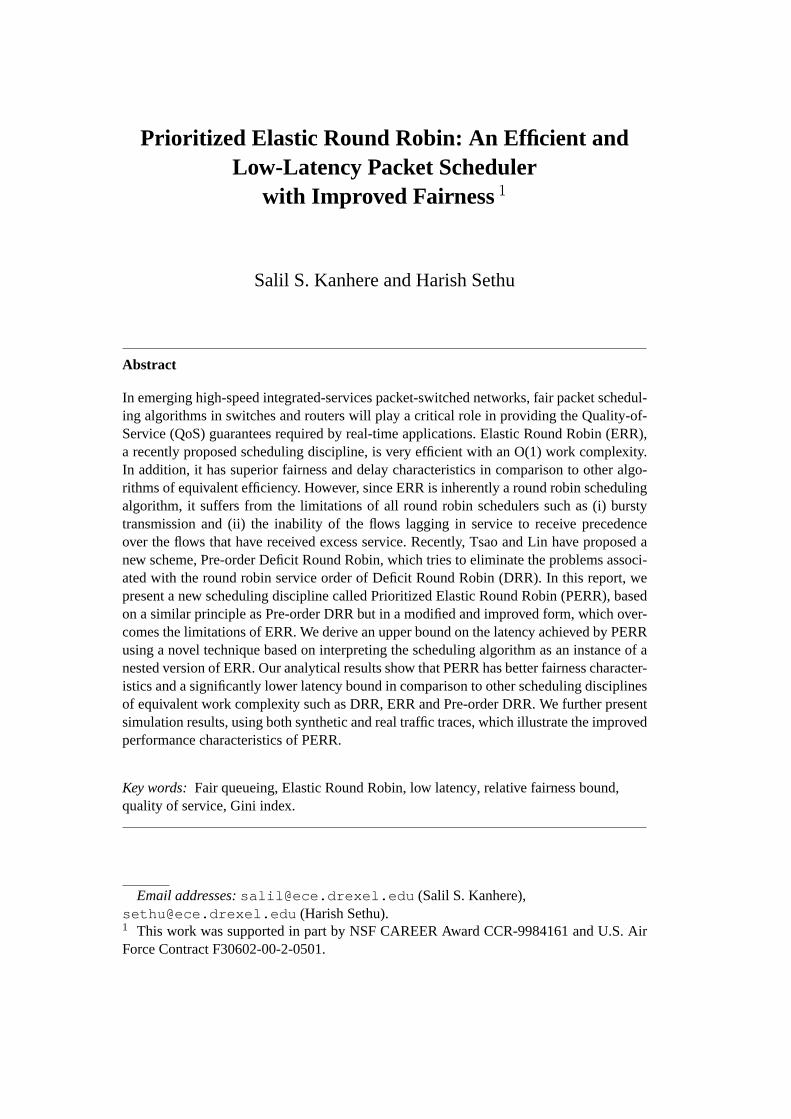
Fig. 1. Block Diagram of (a) PERR Scheduler and (b) Scheduling Decision Module ofPERR

Fig. 1(a) illustrates a block diagram of a generic scheduler. TheScheduling Deci-sion Modulewhich determines the order in which packets are served from the flowqueues is the heart of the scheduler. Fig. 1(b) details the architecture of theSchedul-ing Decision Moduleof the PERR scheduler which is responsible for selecting thenext flow for service. As can be seen from Fig. 1(b), anOrganizer, p priority queuesand aSelectorare appended to the originalScheduling Decision Moduleof ERR.Let PQ1, PQ2, . . . andPQp denote the priority queues in the descending orderof priority with PQ1 representing the queue with the highest priority. Unlike thepriority queues in Pre-order DRR which have to buffer the packets that will betransmitted in the round in progress, these queues in PERR simply contain the flow

12

identifiers. As in ERR, the PERR scheduler maintains a linked list, called theAc-tiveList, of flows which are active. However, the flows in theActiveListare notserved in a round robin manner as in ERR. This is a list of the active flows thathave exhausted their allowance in the current round but, will be eligible for receiv-ing service in the subsequent round. It is the task of theOrganizerto determine theorder in which the flows will receive service in a round. At the start of the round,theOrganizermodule classifies the active flows present in theActiveListinto sev-eral classes according to theirUnserved Allowance Quotientand places them intothe corresponding priority queue. Since there arep priority queues, theOrganizercan classify the flows intop classes. In general, classz of flow i after serving thek-th packet of thes-th round is derived as,

z = (p + 1)−⌈p× Qk

i (s)

Qmax (s)

⌉(12)

Note that at the start of thes-th round,k = 0 for all the flows in the above equation.

Note that the quotient of a flow is a monotonically decreasing function of timeover the duration of a round. Using this fact and the definition ofQmax (s), we canconclude that during rounds, the quotients of all the active flows will always beless than or equal toQmax (s), and thusz is always a non-negative quantity. By theabove method, the flow with the maximum quotient at the start of the rounds isinitially added into the highest priority queue,PQ1.

Note thatQmax (s) is computed only at the start of the round and need not be up-dated as the round progresses. The computation ofQmax (s) simply requires thescheduler to record the least value of the normalized surplus count amongst all theflows in theActiveList. This can be easily accomplished inO(1) time by carryingout a simple comparison operation as the flows are added into theActiveListafterexhausting their allowance in the previous round.

Consider a situation where a flowi becomes active for the first time while somerounds is in progress. It may be possible that the the initial value of the quotientof flow i, Q0

i (s) is greater thanQmax (s). Using Equation (12), it is seen that thepriority class for flowi is less than1, the highest priority class. One possible solu-tion would be to delay the service of flowi until the next round as is done in ERR.However, this would result in an increased latency for flowi since it would thenhave to wait until all the active flows have exhausted their allowance before receiv-ing any service. The PERR scheduler instead simply adds flowi into the highestpriority queuePQ1. This eliminates the increased latency that would be otherwiseexperienced by flowi.

When the scheduler is ready to transmit, theSelectormodule selects the highestnon-empty priority queue, sayPQe and chooses the flow at the head ofPQe, sayflow i, for service. The scheduler serves the packet at the head of the queue corre-sponding to flowi and following the service of this packet recalculates the priority

13

class,z, to which flowi belongs using Equation(12). The scheduler will continueto serve the next packet from the queue of flowi until the occurrence of at least oneof the following events:

(1) A newly active flow is added to a higher priority queue :In this case, thescheduler stops the service of flowi and begins serving the newly active flowsince it belongs to a higher priority class than flowi.

(2) Queue of flowi is empty :In this case, flowi is removed from the head ofpriority queuePQe. Also, theServed flag for flow i is set to indicate that ithas received service in the current round.

(3) The newly computed priority class of flowi, f , does not match its currentpriority class,e : In this case flowi is removed from the head of priorityqueuePQe and is added to the tail of priority queuePQf . Note that the onlyexception is whenf > p. In this case no further packets are to be scheduledfrom flow i during the current round since it has exhausted its allowance. Flowi is instead added to the tail of theActiveList.

At any given instant of time each active flow can either be present in at most oneof the p priority queues or in theActiveList. Over the course of the round, as theflow consumes more and more of its allowance, it will gradually move down fromthe into lower priority queues until it completely exhausts its allowance followingwhich it is added into theActiveList. However during a round it is not necessarythat a flow will pass through each of thep priority queues. In fact it may be possiblethat the only priority queue which a flow visits is the initial queue into which it isclassified at the start of the round. As a result of the categorization brought aboutby the priority queue module in PERR, each flow uses its allowance in pieces overthe course of the round. TheOrganizerreorders the sequence of transmissions toenable the flows that have not utilized a large portion of theirUnservedAllowanceto get precedence over the other flows.

The PERR scheduler also maintains two flags,Servedand Active for each flow.The Active flag indicates whether a flow is active or not. TheServedflag is setwhen the scheduler serves the first packet from a flow in the current round andremains set for the entire duration of the round indicating that the flow has beenserved at least once during the current round. TheServedflags for all the flows arereset at the start of a new round. TheServedflag prevents a flow which frequentlyoscillates between active and inactive periods to receive excessive service. Considera flow which runs out of packets in the middle of a round before utilizing its entireallowance in that round. Since this flow is no longer active itsActiveflag will bereset. Assume that a new packet arrives at the flow at some time before the end ofthe current round. In the absence of theServedflag this flow would be treated as anewly active flow and its per-flow states would be reset. This would allow the flowto receive service in excess of what it would have received if it were active duringthe entire duration of the current round. However in PERR, theServedflag will beset for the flow under consideration indicating that the per-flow states for that flow

14

are still valid for the current round. When the flow becomes active it will be addedinto the appropriate priority queue using Equation (12) depending on how much ofits UnservedAllowancewas utilized when it was last active in the current round,and thus, the flow will not receive any excess service. Note that since theServedflags for all the flows are reset at the end of a round, accumulation of service creditsfrom a previous round is prevented.

Initialize: (Invoked when the scheduler is initialized)MaxSC = 0;CurrentPriority = 0;Qmax = 1;MinNormalizedSC = MAX;for (i = 0; i < n; i = i + 1)

Activei = FALSE;Servedi = FALSE;

Enqueue: (Invoked when a packet arrives)i = QueueInWhichPacketArrives;if ( Activei == FALSE) then

if (Servedi ==FALSE) thenSCi = 0;Senti = 0;

end if;InitializeFlow(i);NewPriority = ComputeNewPriority(i);AddToPriorityQueue(NewPriority, i);if (NewPriority > CurrentPriority) then

ObtainHighestActivePriority == TRUE;end if

end if;

Dequeue:while (TRUE) do

if (AllPriorityQueuesEmpty == TRUE) thenInitializeRound();

end if;if(ObtainHighestActivePriority == TRUE) then

CurrentPriority = GetHighestActivePriorityQueue;end if;i = HeadOfPriorityQueue(CurrentPriority);do

TransmitPacketFromQueue(i);Increase Senti by LengthInFlitsOfTransmittedPacket;Servedi == TRUE;NewPriority == ComputeNewPriority(i);

while ( (NewPriority == CurrentPriority) and(IsEmpty(Queuei ) == FALSE) and(ObtainHighestActivePriority == FALSE) )

if ( (NewPriority > CurrentPriority) or(IsEmpty(Queuei) == TRUE) ) thenRemoveHeadOfPriorityQueue(CurrentPriority);if (IsEmpty(Queuei) == FALSE) then

AddToPriorityQueue(NewPriority, i);end ifif (IsEmpty(CurrentPriority) == TRUE) then

ObtainHighestActivePriority = TRUE;end if

end ifend while

Fig. 2. Pseudo-Code for PERR

15

InitializeRound()for (i = 0; i < n; i = i + 1)

Servedi = FALSE;PreviousMaxSC = MaxSC;MaxSC = 0;MinNormalizedSC = MAX;InitializeFlow(min);Qmax =

Amin

UAmax

min

;

ObtainHighestActivePriority == TRUE;while (IsEmpty(ActiveList) == FALSE) do

flow = HeadOfActiveList;RemoveHeadOfActiveList;Sentflow = 0;InitializeFlow(flow);NewPriority = ComputeNewPriority(flow);AddToPriorityQueue(NewPriority, flow);SCflow = 0;

end while;

Fig. 3.InitializeRound() Routine

InitializeFlow(i)Activei = TRUE;UAmax

i= wi(1+ PreviousMaxSC) ;

Ai = UAmax

i− SCi;

Fig. 4.InitializeFlow() Routine

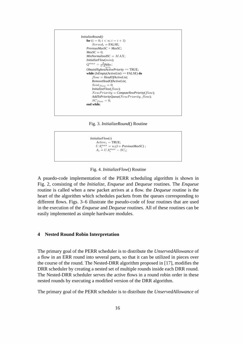
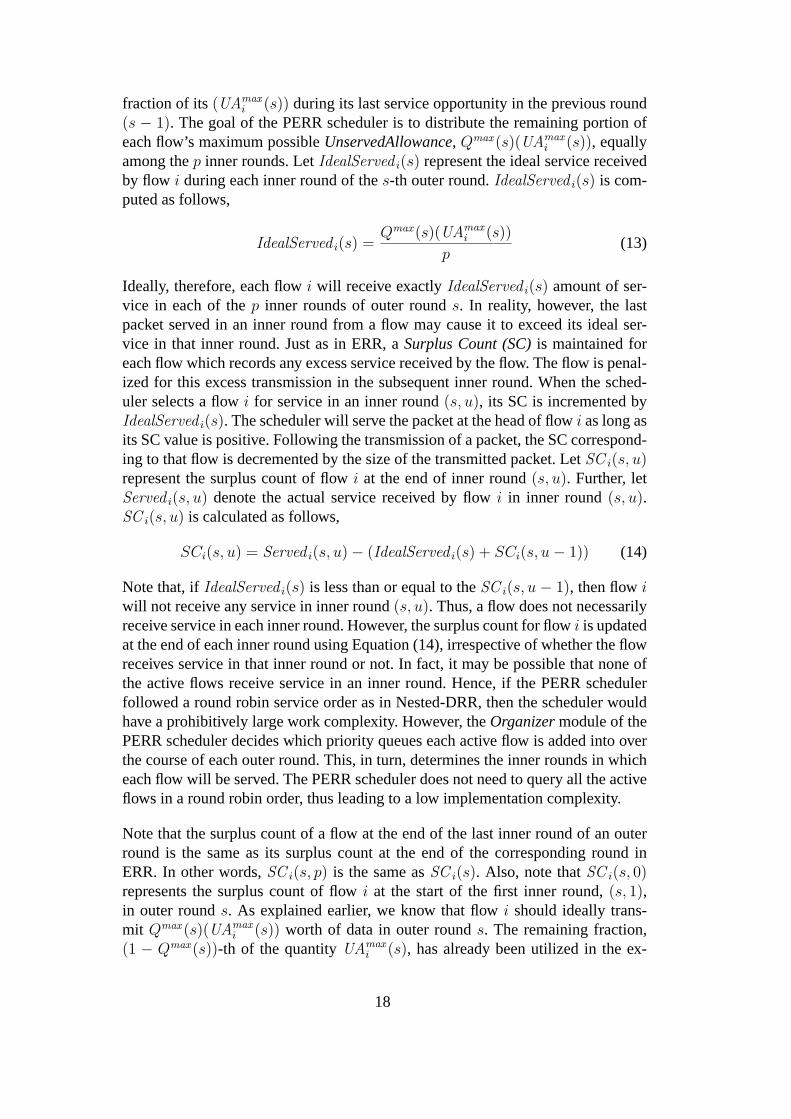
A psuedo-code implementation of the PERR scheduling algorithm is shown inFig. 2, consisting of theInitialize, EnqueueandDequeueroutines. TheEnqueueroutine is called when a new packet arrives at a flow. theDequeueroutine is theheart of the algorithm which schedules packets from the queues corresponding todifferent flows. Figs. 3–6 illustrate the pseudo-code of four routines that are usedin the execution of theEnqueueandDequeueroutines. All of these routines can beeasily implemented as simple hardware modules.

4 Nested Round Robin Interpretation

The primary goal of the PERR scheduler is to distribute theUnservedAllowanceofa flow in an ERR round into several parts, so that it can be utilized in pieces overthe course of the round. The Nested-DRR algorithm proposed in [17], modifies theDRR scheduler by creating a nested set of multiple rounds inside each DRR round.The Nested-DRR scheduler serves the active flows in a round robin order in thesenested rounds by executing a modified version of the DRR algorithm.

The primary goal of the PERR scheduler is to distribute theUnservedAllowanceof

16

AddToPriorityQueue(z, i);if (z > p) then

AddFlowToActiveList(i);SCi = Senti − Ai;if ( SCi

wi

> MaxSC) then

MaxSC =

SCi

wi

;end ifif ( SCi

wi

< MinNormalizedSC ) thenmin = i;MinNormalizedSC =

SCi

wi

;end if

elseAddFlowToPriorityQueue(Pqz , i);

end if

Fig. 5.AddToPriorityQueue() Routine

ComputeNewPriority(i)Qi = Ai−Senti

Amax

i

;

z = (p + 1) −

⌈

Qi×p

Qmax

⌉

;

return z;

Fig. 6.ComputeNewPriority() Routine

a flow in an ERR round into several parts, so that it can be utilized in pieces overthe course of the round. The Nested-DRR algorithm proposed in [17], modifies theDRR scheduler by creating a nested set of multiple rounds inside each DRR round.The Nested-DRR scheduler serves the active flows in a round robin order in thesenested rounds by executing a modified version of the DRR algorithm.

We can hypothetically interpret the operation of the PERR scheduler as anestedversion of ERR which is similar to Nested-DRR. This interpretation proves usefulin the analysis of the latency bound of the PERR scheduler. Each round in ERRcan be referred to as anouter round. The time interval during which the PERRscheduler serves the flows present in priority queuePQu during thes-th outer roundis referred to asinner round(s, u). In effect, each outer round is split into as manyinner rounds as the number of priority queues,p. Since the PERR scheduler servesthe priority queues in a descending order starting at the higher priority queuePQp,the first inner round during outer rounds will be (s, 1), while (s, p) will denote thelast inner round.

From Equation (11), we know that the excess service, if any, received by each flowiin the previous outer round(s−1) is equal to(1−Q0

i (s))UAmaxi (s). SinceQmax (s)

represents the maximum quotient among all the flows at the start of rounds, it isguaranteed that each active flowi has already utilized at least(1 − Qmax (s))-th

17

fraction of its(UAmaxi (s)) during its last service opportunity in the previous round

(s − 1). The goal of the PERR scheduler is to distribute the remaining portion ofeach flow’s maximum possibleUnservedAllowance, Qmax (s)(UAmax

i (s)), equallyamong thep inner rounds. LetIdealServed i(s) represent the ideal service receivedby flow i during each inner round of thes-th outer round.IdealServed i(s) is com-puted as follows,

IdealServed i(s) =Qmax (s)(UAmax

i (s))

p(13)

Ideally, therefore, each flowi will receive exactlyIdealServed i(s) amount of ser-vice in each of thep inner rounds of outer rounds. In reality, however, the lastpacket served in an inner round from a flow may cause it to exceed its ideal ser-vice in that inner round. Just as in ERR, aSurplus Count (SC)is maintained foreach flow which records any excess service received by the flow. The flow is penal-ized for this excess transmission in the subsequent inner round. When the sched-uler selects a flowi for service in an inner round(s, u), its SC is incremented byIdealServed i(s). The scheduler will serve the packet at the head of flowi as long asits SC value is positive. Following the transmission of a packet, the SC correspond-ing to that flow is decremented by the size of the transmitted packet. LetSC i(s, u)represent the surplus count of flowi at the end of inner round(s, u). Further, letServed i(s, u) denote the actual service received by flowi in inner round(s, u).SC i(s, u) is calculated as follows,

SCi(s, u) = Served i(s, u)− (IdealServed i(s) + SCi(s, u− 1)) (14)

Note that, ifIdealServed i(s) is less than or equal to theSC i(s, u − 1), then flowiwill not receive any service in inner round(s, u). Thus, a flow does not necessarilyreceive service in each inner round. However, the surplus count for flowi is updatedat the end of each inner round using Equation (14), irrespective of whether the flowreceives service in that inner round or not. In fact, it may be possible that none ofthe active flows receive service in an inner round. Hence, if the PERR schedulerfollowed a round robin service order as in Nested-DRR, then the scheduler wouldhave a prohibitively large work complexity. However, theOrganizermodule of thePERR scheduler decides which priority queues each active flow is added into overthe course of each outer round. This, in turn, determines the inner rounds in whicheach flow will be served. The PERR scheduler does not need to query all the activeflows in a round robin order, thus leading to a low implementation complexity.

Note that the surplus count of a flow at the end of the last inner round of an outerround is the same as its surplus count at the end of the corresponding round inERR. In other words,SC i(s, p) is the same asSC i(s). Also, note thatSC i(s, 0)represents the surplus count of flowi at the start of the first inner round,(s, 1),in outer rounds. As explained earlier, we know that flowi should ideally trans-mit Qmax (s)(UAmax

i (s)) worth of data in outer rounds. The remaining fraction,(1 − Qmax (s))-th of the quantityUAmax

i (s), has already been utilized in the ex-

18

cess service received by flowi in outer round(s − 1) and, therefore, is a part ofSC i(s− 1). To account for this already utilized portion ofUAmax

i (s), SC i(s, 0) iscomputed as:

SCi(s, 0) = SCi(s− 1)− (1−Qmax (s))(UAmaxi (s)) (15)

It can be easily proved that Equation (5), which expresses the bounds on the surpluscount,SC i(s), also holds true forSC i(s, u). Therefore, for any flowi and innerround(s, u),

0 ≤ SCi(s, u) ≤ m− 1 (16)

Definition 5 LetSent i(s, u) represent the total service received by flowi since thestart of thes-th outer round until the PERR scheduler has finished serving the flowsin the priority queue,PQu.

Note that it is not necessary that flowi was present in priority queuePQu duringouter rounds. From Equation (14), the total data served from flowi in inner round(s, u) is,

Served i(s, u) = IdealServed i(s) + SCi(s, u)− SCi(s, u− 1) (17)

Sent i(s, u) is calculated as follows:

Sent i(s, u) =w=u∑

w=1

Served i(s, w) (18)

Substituting forServed i(s, w) from Equation (17) in Equation (18), we have,

Sent i(s, u) = u(IdealServed i(s)) + SCi(s, u)− SCi(s, 0) (19)

Sent i(s, u) will be positive only if u(IdealServed i(s)) is greater thanSC i(s, 0).Otherwise it indicates that flowi has not received any service until the end of the(s, u)-th inner round. However flowi is guaranteed to receive service in at leastone inner round during thes-th outer round. Using Equations (13), (15) and (19)we have,

Sent i(s, u) =

(u

p

)Qmax (s)UAmax

i (s) + SCi(s, u)− SCi(s− 1) (20)

Definition 6 DefineSent i(s) as the total service received by flowi in outer rounds.

Note thatSent i(s, p) represents the service received by flowi when the schedulerhas finished serving the flows in priority queuePQp which in fact equalsSent i(s).Substitutingu = p in Equation (20) and using Equation(8), we get,

Sent i(s) = wi(1 + MaxSC (s− 1)) + SCi(s)− SCi(s− 1) (21)

19

101010510 10 4

52356554

610

4586

410564101010510235655410586

4564101023510

AD B

8 6 10

C

Flow A, w = 5a

Flow B, w = 3

Flow C, w = 1

Flow D, w = 2d

b

c

AAD BCAAAAABBBB B BBCDDD

ABCDABBBD AAA BBB DA

Round 2

Round 2

Round 1

Round 1

Transmission Sequence of Packets in ERR

Transmission Sequence of Packets in PERR

4 5 10 5 6 5 10 5

pq 1pq 2pq 3pq 4 pq 1pq 4

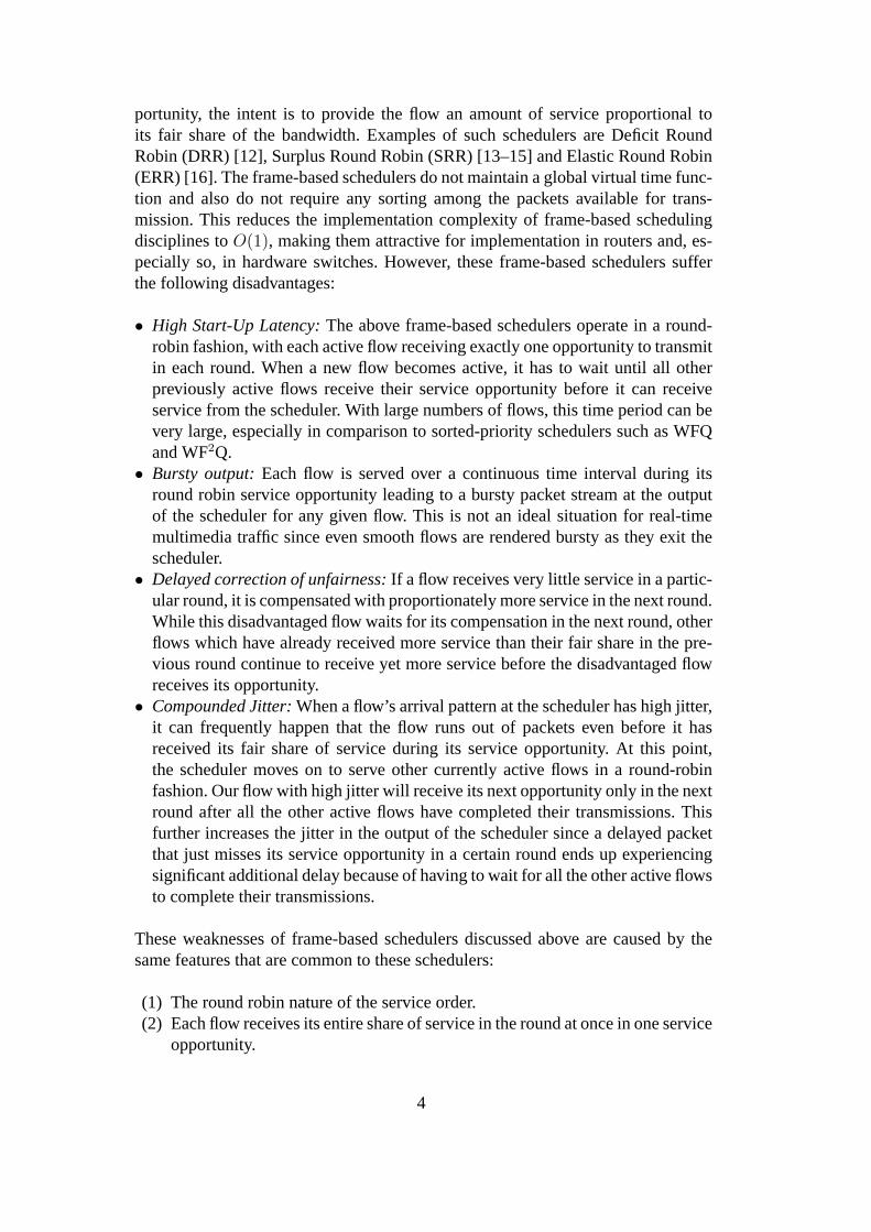
Fig. 7. Comparison of the transmission sequence of packets in ERR and PERR

Hence the total service received by flowi in an outer round in PERR is identical tothe service received by flowi in the corresponding round in ERR.

Ideally, during the normal operation of the PERR scheduler, thep inner rounds inouter rounds follow a strictly sequential order starting at inner round(s, 1) andending at round(s, p). However, in certain situations, it is possible to interrupt thesequential ordering. Let us assume that a flowj becomes active for the first time inouter rounds while the PERR scheduler is serving a flowk at the head of priorityqueuePQd. Since the quotient for flowj is equal to 1, it will be added into prior-ity queuePQ1 which has the highest priority among all the priority queues. Uponfinishing the transmission of the current packet from flowk, the PERR schedulertemporarily suspends the service of flowk and starts serving flowj which is atthe head of queuePQp. The PERR scheduler will keep serving flowj until it isadded either into priority queuePQd or some other queue with lower priority thanPQd. The scheduler will then resume service of thek-th flow. Note that the servicereceived by flowi while it is present in queuePQp is part of the inner round(s, p)even though it is not contiguous with the time interval during which the PERRscheduler served the flows present in queuePQp at the start of the outer rounds.Also, the inner round(s, d) will not extend over a continuous time interval becauseit will be interposed by the entire service received by flowi since the time it be-came active until its addition into priority queuePQd or a lower priority queue. Itis, therefore, not necessary that the inner rounds in an outer round should sequen-tially follow one another and that the flows which receive service in an inner roundshould be served in succession. However, note that this disruption of the otherwisesequential service can only be caused due to a new flow becoming active during theexecution of that outer round.

Fig. 7 compares the transmission sequence in the first two rounds of execution ofthe ERR and PERR schedulers for the given input pattern and flow weights. In

20

the PERR scheduler, the flows are classified into 4 classes corresponding to the4 priority queues. At the start of inner round(1, 1) all the flows are present inpriority queuePQ1. After receiving service in this inner round, flowA is addedinto PQ4. However the other 3 flows exceed their allowance in this inner round andare therefore added into theActiveList. Note that, in the second outer round, unlikethe ERR scheduler where the flowsB, C andD have to wait for their turn in theround robin order to receive service, flowsB andD start receiving service in theinner round(2, 1) whereas flowC is served for the first time in inner round(2, 2).

5 Analytical Results

In this section, we present analytical results on the fairness, latency properties andthe work complexity of PERR.

5.1 Latency Bound of PERR

In deriving an upper bound on the latency of PERR we use the concept of Latency-Rate (LR) servers first proposed in [5]. We now define the notion of a busy period,essential for developing the concept of theLR servers.

Definition 7 A busy period of a flow is defined as the maximal time interval duringwhich the flow is active if it is served at exactly its reserved rate.

Note that the active period of a flow is different from the busy period in the sensethat it reflects the actual behavior of the scheduler where the instantaneous serviceoffered to the flow varies according to the number of active flows.

Definition 8 Let Sent i(t1, t2) represent the amount of service received by flowiduring the time interval(t1, t2).

Note that this notation is identical to the one used in Definition 5, except for the typeof the parameters. Thus,Sent i(β, γ) is to be interpreted according to whetherβ andγ represent two instants of time or(β, γ) denotes an inner round in the executionof the PERR scheduler. In the following, the context will always make clear as tohowSent i(β, γ) should be interpreted.

Let the time instantαi be the start of a busy period for flowi. Let t > αi besuch that flowi is continuously busy during the time interval(αi, t). Let Si(αi, t)be the number of bits belonging to packets in flowi that arrive after timeαi andare scheduled during the time interval(αi, t). Note that, during this time intervalthe scheduler may still be serving packets from a previous busy period, and henceSi(αi, t) is not necessarily the same asSent i(αi, t).

21

Definition 9 The latency of a flow is defined as the minimum non-negative constantΘi that satisfies the following for all possible busy periods of the flow,

Si(αi, t) ≥ max0, ρi(t− αi −Θi) (22)

As defined in [5], a scheduler which satisfies Equation (22) for some non-negativeconstant value ofΘi is said to belong to the class of Latency Rate (LR) servers. Inpractice, however it is easier to analyze scheduling algorithms based on the activeperiod of a flow. Letτi be an instant of time when flowi becomes active. Lett > τi be some time instant such that the flow is continuously active during the timeinterval(τi, t) Let Θ′

i be the smallest non-negative number such that the followingequation is satisfied for allt.

Senti(αi, t) ≥ max0, ρi(t− αi −Θ′i) (23)

Even though(τi, t) may not be a continuously busy period for flowi, it is provedin [5], that the latency as defined by (22) is bounded byΘ′

i.

Theorem 1 The PERR scheduler belongs to the class ofLR servers, with an upperbound on the latencyΘi for flow i given by,

Θi ≤(W−wi)m

p+ (n− 1)(m− 1)

r(24)

wheren is the total number of active flows,p is the number of priority queues,r isthe transmission rate of the output link andW is the sum of the weights of all theflows.

Proof. Since the latency of aLR server can be estimated based on its behaviorin the flow active periods, we will prove the theorem by showing that,

Θ′i ≤

(W−wi)mp

+ (n− 1)(m− 1)

r.

Let τi be the time instant when flowi becomes active. To prove the statement ofthe theorem we consider a time interval(τi, t), wheret > τi, during which flowiis continuously active. We first obtain the lower bound on the total service receivedby flow i during the time interval under consideration. Then we express the lowerbound in the form of Equation (23) to derive the latency bound.

In [19] it has been proved that to obtain a tight upper bound on the latency of theERR scheduler, we must consider an active period(τi, t) such thatτi coincides withthe beginning of the service opportunity of a flow andt belongs to the set of timeinstants at which the scheduler begins serving flowi. We can easily prove that thesame conditions apply for proving the upper bound on the latency of the PERRscheduler. Letτ (e,f)

i be the time instant marking the start of the service of flowi

22

when flowi is at the head of priority queuePQf in rounde. In other words, thistime instant represents the start of the service opportunity of flowi in inner round(e, f). Therefore, in trying to determine the latency bound of the PERR, we needto only consider time interval(τi, τ

(e,f)i ) for all (e, f).

The first step in proving the latency bound involves determining the upper boundon the size of the time interval under consideration. Note that the time instantτi

may or may not coincide with the start of a new round. Letk0 be the round which isin progress at time instantτi or which starts exactly at time instantτi. Let th markthe start of the round(k0 + h). In either case, flowi will be able to transmit at leastAi(k0) worth of data over the course of thek0-th round. If flow i becomes activewhen the roundk0 is in progress, i.e. whenτi < t0 then the service received duringthe interval(t0, τi) will be excluded from the time interval under consideration. Thetime interval(τi, τ

(e,f)i ) will be maximal only if the time instantτi coincides with

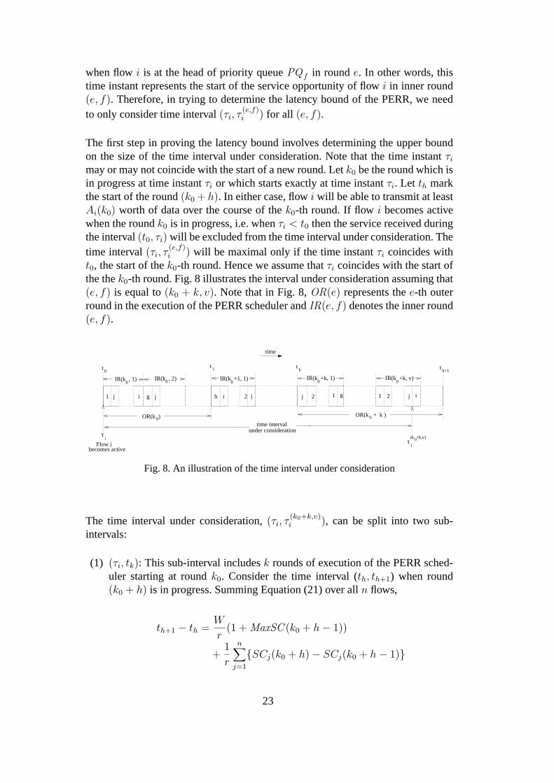
t0, the start of thek0-th round. Hence we assume thatτi coincides with the start ofthe thek0-th round. Fig. 8 illustrates the interval under consideration assuming that(e, f) is equal to(k0 + k, v). Note that in Fig. 8,OR(e) represents thee-th outerround in the execution of the PERR scheduler andIR(e, f) denotes the inner round(e, f).

time

t 0t 1 t k t k+1

0

i

becomes activeFlow i

time intervalunder consideration

OR(k + k )0

g

i

0

1

0 0

OR(k )0

0

j2ihgj j i21 jj 21 i

τ

IR(k , 1) IR(k +k, 1)IR(k , 2) IR(k +k, v)

(k +k,v)0τ

IR(k +1, 1)

Fig. 8. An illustration of the time interval under consideration

The time interval under consideration,(τi, τ(k0+k,v)i ), can be split into two sub-

intervals:

(1) (τi, tk): This sub-interval includesk rounds of execution of the PERR sched-uler starting at roundk0. Consider the time interval (th, th+1) when round(k0 + h) is in progress. Summing Equation (21) over alln flows,

th+1 − th =W

r(1 + MaxSC (k0 + h− 1))

+1

r

n∑

j=1

SCj(k0 + h)− SCj(k0 + h− 1)

23

Summing the above overk rounds beginning with roundk0,

tk − τi =W

r(k) +

W

r

k−1∑

h=0

MaxSC (k0 + h− 1)

+1

r

n∑

j=1

SCj(k0 + k − 1)− SCj(k0 − 1) (25)

(2) (tk, τ(k0+k,v)i ): This sub-interval includes the part of the(k0 + k)-th round

prior to the start of the service of flowi when it is at the head of priorityqueuePQv. In the worst-case flowi will be the the last flow to receive serviceamong all other flows which are present in priority queuePQv. In this case,during the sub-interval under consideration, the service received by flowiequalsSent i(k0+k, v−1) whereas the service received by each flowj amongthe othern−1 flows equalsSent i(k0+k, v). Note that ifv equals1 then flowidoes not receive service in this sub-interval. Hence summingSent i(k0+k, v−1) andSent j(k0 + k, v) for each flowj such that1 ≤ j ≤ n, j 6= i and usingEquation (20), we have,

τ(k0+k,v)i − tk =

1

r

n∑j=1j 6=i

(v

p

)Qmax (k0 + k)UAj(k0 + k)

+1

r

(v − 1

p

)Qmax (k0 + k)UAi(k0 + k)

+1

r

n∑j=1j 6=i

(SCj(k0 + k, v)− SCj(k0 + k − 1))

+1

r(SCi(k0 + k, v − 1)− SCi(k0 + k − 1)) (26)

To simplify the analysis we introduce a new variableΩ, such that,

Ω = Qmax (k0 + k)(1 + MaxSC (k0 + k − 1)) (27)

Using Equation (6) and Corollary 1 in Equation (27), we get,

0 < Ω ≤ m (28)

Combining Equations (25) and (26) and using Equations (5), (8) and (27), we have,

τ(k0+k,v)i −τi ≤ W

rk +

W

r

k−1∑

h=0

MaxSC (k0 + h− 1) +1

r

n∑j=1j 6=i

(v

p

)wjΩ

+1

r

(v − 1

p

)wiΩ +

1

r(n− 1)(m− 1) +

1

rSCi(k0 + k, v − 1) (29)

24

Solving fork and using the fact thatW is the sum of the weights of all then flows,

k ≥ (τ(k0+k,v)i − τi)

r

W−

k−1∑

h=0

MaxSC (k0 + h− 1)− 1

W

(v

p

)(W − wi)Ω

− 1

W

(v − 1

p

)wiΩ− 1

W(n− 1)(m− 1)− 1

WSCi(k0 + k, v − 1) (30)

Note that the total data transmitted by flowi during the time interval under consid-eration can be expressed as the following summation,

Sent i(τi, τ(k0+k,v)i ) = Sent i(τi, tk) + Sent i(tk, τ

(k0+k,v)i ) (31)

As explained, earlierSent i(tk, τ(k0+k,v)i ) is the same asSent i(k, v−1). Sent i(τi, tk)

can be obtained by summing Equation (21) overk rounds starting at roundk0.Substituting the result and Equation (20) in Equation (31) and using Equation (27)and the fact that the surplus count of a newly active flow is equal to 0, we have,

Sent i(τi, τ(k0+k,v)i ) = wik + wi

k−1∑

h=0

MaxSC (k0 + h− 1)

+

(v − 1

p

)wiΩ + SCi(k0 + k, v − 1) (32)

Using (30) to substitute fork in (32), we get,

Sent i(τi, τ(k0+k,v)i ) ≥ wir

W(τ

(k0+k,v)i − τi) +

(v − 1

p

)wiΩ

(W − wi

W

)

− wi

W

(v

p

)(W − wi)Ω− wi

W(n− 1)(m− 1)

− SCi(k0 + k, v − 1)(

wi

W− 1

)

Simplifying further we get,

Sent i(τi, τ(k0+k,v)i ) ≥ wir

W

(τ

(k0+k,v)i − τi)− 1

r

(W − wi

p

)Ω

− 1

r(n− 1)(m− 1)

− SCi(k0 + k, v − 1)

(wi

W− 1

)(33)

Now, since the reserved rates are proportional to the weights assigned to the flowsas given by (1), and since the sum of the reserved rates is no more than the link rater, we have,

ρi ≤ wi

Wr (34)

Using Equation (29) it can be verified that the multiplicand ofwirW

in Equation (33)is always positive. Substituting forwir

Wfrom Equation (34) in Equation (33) we

25

have,

Sent i(τi, τ(k0+k,v)i ) ≥ ρi

(τ

(k0+k,v)i − τi)− 1

r

(W − wi

p

)Ω

− 1

r(n− 1)(m− 1)

− SCi(k0 + k, v − 1)

(wi

W− 1

)(35)

Noting that the latency reaches the upper bound whenSC i(k0 + k, v − 1) equals 0andΩ equalsm, we get,

Sent i(τi, τ(k0+k,v)i ) ≥ max

0, ρi

τ

(k0+k,v)i − τi

−(W−wi

p)m + (n− 1)(m− 1)

r

(36)

As discussed earlier, flowi will experience its worst latency during an interval(τi, τ

(e,f)i ) for some inner round(e, f). Therefore, from Equation (36), the statement

of the theorem is proved.

We now proceed to show that the latency bound given by Theorem 1 is tight byillustrating a case where the bound is actually met. Assume that a flowi becomesactive at time instantτi, which also coincides with the start of a certain roundk0.Assume that for any time instantt, t ≥ τi, a total ofn flows, including flowi,are active. Also, assume that the summation of the reserved rates of all then flowsequals the output link transmission rate,r. Hence,ρi = wi

Wr. Since flowi became

active at timeτi, its surplus count at the start of roundk0 is 0. Let the surplus countof all the other flows at the start of roundk0 be equal to 0. Assume that, a flowlwhich is not active after timeτi and hence is not included in then flows, was activeduring thek0-th round. Assume that flowl exceeded its allowance by(m − 1) inits last service opportunity in round(k0− 1), leading to a value ofMaxSC (k0− 1)equal to(m − 1). Since the surplus counts of all then active flows are equal to 0,the Unserved Allowance Quotientfor all the flows at the start of thek0-th roundwill be equal to unity. HenceQmax (k0) will be equal to 1 and all then flows willbe added into the priority queuePQp at the start of the round. Assume that flowi is the last flow to be added into this queue. From Equations (16), (6) and (17),any given flowj can transmit a maximum ofwj(

mp) + (m − 1) bits during its

service opportunity in an inner round. In the worst case, before flowi is served bythe PERR scheduler, each of the other(n − 1) flows will receive this maximum

26

service. Hence, the cumulative delay until flowi receives service is given by,

D =

(∑

j 6=i

wj)(m

p) + (n− 1)(m− 1)

r

=(W−wi

p)m + (n− 1)(m− 1)

r

Noting thatSi(τi, τi +D) equals zero, it is readily verified that the bound is exactlymet at timet = τi + D.

5.2 Fairness Bound of PERR

In our fairness analysis, we use the popular metric,Relative Fairness Bound (RFB)first proposed in [8]. The RFB is defined as the maximum difference in the normal-ized service received by any two flows over all possible intervals of time.

Definition 10 Given an interval(t1, t2), theRelative Fairness, RF (t1, t2) for thisinterval is defined as the maximum value of|Senti(t1,t2)

wi− Sentj(t1,t2)

wj| over all pairs of

flowsi andj that are active during this time interval. Define theRelative FairnessBound (RFB)as the maximum ofRF (t1, t2) over all possible time intervals(t1, t2).

The Absolute Fairness Bound (AFB)is a related measure of fairness which cap-tures the upper bound on the difference between the normalized service under thecurrent scheduler and that it would receive with the ideal GPS scheduler [1]. It hasbeen shown in [20], that the AFB and RFB are related to each other by a simplerelationship. Hence, we only discuss the RFB in this report.

Theorem 2 For any execution of the PERR scheduling discipline,RFB < 2m+ 2mp

Proof. In [16], while analyzing the fairness properties of ERR, we have provedthat a tight upper bound on the the RFB of ERR can be obtained by considering onlya subset of all possible time intervals. This subset is the set of all time intervalsbounded by time instants that coincide with the start of the service opportunitiesof flows. It can be easily verified that to prove the RFB of the PERR scheduler weneed to consider a time interval(t1, t2) such that both the time instantst1 andt2coincide with the start of a service opportunity of a flow in an inner round.

Consider any two flowsi and j that are active in the time interval between thetime instantst1 andt2. Let (k0, f) and(k0 + k, g) be the inner rounds which are inprogress at time instantst1 andt2 respectively. Let time instantt(h,v) mark the startof inner round(k0 +h, v). In other words,t(k0,f) < t1 < t(k0,f+1) andt(k0,g) < t2 <t(k0,g+1). It may be possible that, if flowj receives service in the inner round(k0, f),then it does so in the time interval(t(k0,f), t1). Unlike the ERR scheduler, in PERR

27

if flow j is served before flowi in a certain inner round then, it is not necessary thatthe same order of service is followed in each of the following inner rounds. Henceon a similar note, it may be possible that if flowj receives service in the innerround(k0 + k, g), then that service is also not included in the time interval underconsideration. HenceSenti(t1, t2) andSentj(t1, t2) can be evaluated as follows:

Sent i(t1, t2) = Sent i(k0)− Sent i(k0, f − 1)

+h=k−1∑

h=1

Sent i(k0 + h) + Sent i(k0 + k, g)

Sent j(t1, t2) = Sent j(k0)− Sent j(k0, f)

+h=k−1∑

h=1

Sent j(k0 + h) + Sent j(k0 + k, g − 1)

Using Equations (8), (20) and (21) in the above and simplifying, we get,

Sent i(t1, t2) =

(f

pQmax (k0)

)UAmax

i (k0) + kh=k−1∑

h=1

UAmaxi (k0 + h)

+

(g

pQmax (k0 + k)

)UAmax

i (k0 + k)

+ SCi(k0 + k, g)− SCi(k0, f − 1) (37)

Sent j(t1, t2) =

(f − 1

pQmax (k0)

)UAmax

j (k0) + kh=k−1∑

h=1

UAmaxj (k0 + h)

+

(g − 1

pQmax (k0 + k)

)UAmax

j (k0 + k)

+ SCj(k0 + k, g − 1)− SCj(k0, f) (38)

Without loss of generality, we can assume that in the interval(t1, t2) flow i receivesmore service as compared to flowj. The normalized service for each of the flowscan be obtained by dividing the above two equations by their respective weights.Subtracting the normalized service of flowj from that of flow i using Equations(37) and (38) we have,

Sent i(t1, t2)

wi

− Sent j(t1, t2)

wj

=UAmax

i (k0)Qmax (k0)

wi p

+UAmax

j (k0 + k)Qmax (k0 + k)

wj p+

SCi(k0 + k, g)

wi

− SCi(k0, f − 1)

wi

+SCj(k0 + k, g − 1)

wj

− SCj(k0, f)

wj

Simplifying the above using Equations (6), (8), (16) and Corollary 1, the statementof the theorem is proved.

28

5.3 Work Complexity

Consider an execution of the PERR scheduler overn flows. The work involvedin processing each packet at the scheduler involves two parts: enqueueing and de-queueing. Hence the work complexity of a scheduler is defined as the order of timecomplexity, with respect ton of enqueueing and then dequeueing a packet for trans-mission [12, 16]. Note thatn, the number of flows competing for a link can be ofthe order of tens of thousands of flows in backbone routers. Hence it is desirablethat the work complexity should be as independent as possible ofn.

Theorem 3 The worst-case work complexity of the PERR scheduler isO(log p).

Proof. The time complexity of enqueueing a packet is the same as the timecomplexity of theEnqueueroutine in Fig. 2, which is executed whenever a newpacket arrives at a flow. Identifying the flow at which the packet arrives is anO(1)operation. If theActiveflag is not set for the flowi, theIdeal Allowance Utilizationfor the flow is calculated which in turn determines the priority queue into whichthe flow should be added. Also, if this priority queue is of a higher priority than thepriority queue which the PERR scheduler is serving, a flag is set to indicate thatafter completing the transmission of the current packet, the scheduler should startserving packets from the newly active flow. The addition of an item to the tail of alinked-list data structure and conditionally setting a flag are bothO(1) operations.

Let us now consider the time complexity of dequeueing a packet. Assume that thePERR scheduler is serving flows from the priority queuePQg. Note that at least onepacket is transmitted from each of the flows that are present inPQg. The operationsinvolved in serving flows in this priority queue include determining the next flowto be served, removing this flow from the head of the priority queue and possiblyadding it into some other priority queue or the ActiveList. All these operations canbe executed inO(1) time. Additionally the PERR scheduler may need to updatecertain per-flow variables which can be easily done in constant time. However oncethe queuePQg is empty the PERR scheduler needs to determine the highest non-empty priority queue. To aid in this, the PERR scheduler maintains a linked listof the identifiers of all the non-empty priority queues. This linked list is sorted indescending order of priority with the head of the list pointing to the highest non-empty priority queue. The complexity of inserting a new identifier into this sortedlinked list is O(log p) wherep represents the total number of priority queues. Toselect the highest non-empty priority queue, the PERR scheduler simply has toread the identifier at the head of this sorted list which can be done inO(1) time.Hence the overall time complexity of this operation isO(log p) A similar situationarises when a flow is added into a priority queue which has a higher priority thanthe current priority queue being served by the PERR scheduler. However if all thepriority queues are empty it is an indication that the current round has come to anend. In this case, prior to the start of the subsequent round, theOrganizermodule

29

has to classify all the flows present in theActiveListinto thep priority queues whichrequiresO(n) time. However since each of then flows is guaranteed to transmit atleast one packet, the overall complexity of this operation isO(1).

Note that the PERR scheduler needs to sort the non-empty priority queues onlyin the two special cases discussed above, unlike the sorted-priority algorithms likeWFQ and SCFQ where these sorting operations need to be executed prior to eachpacket transmission resulting in aO(log n) work complexity wheren is the numberof active flows. Also, sincen À p, the work complexity of the PERR scheduler isalways lower than that of the sorted-priority schedulers. Hence the worst-case workcomplexity of the PERR scheduler isO(log p) resulting in an efficient hardwareimplementation.

6 Comparison with Other Schedulers

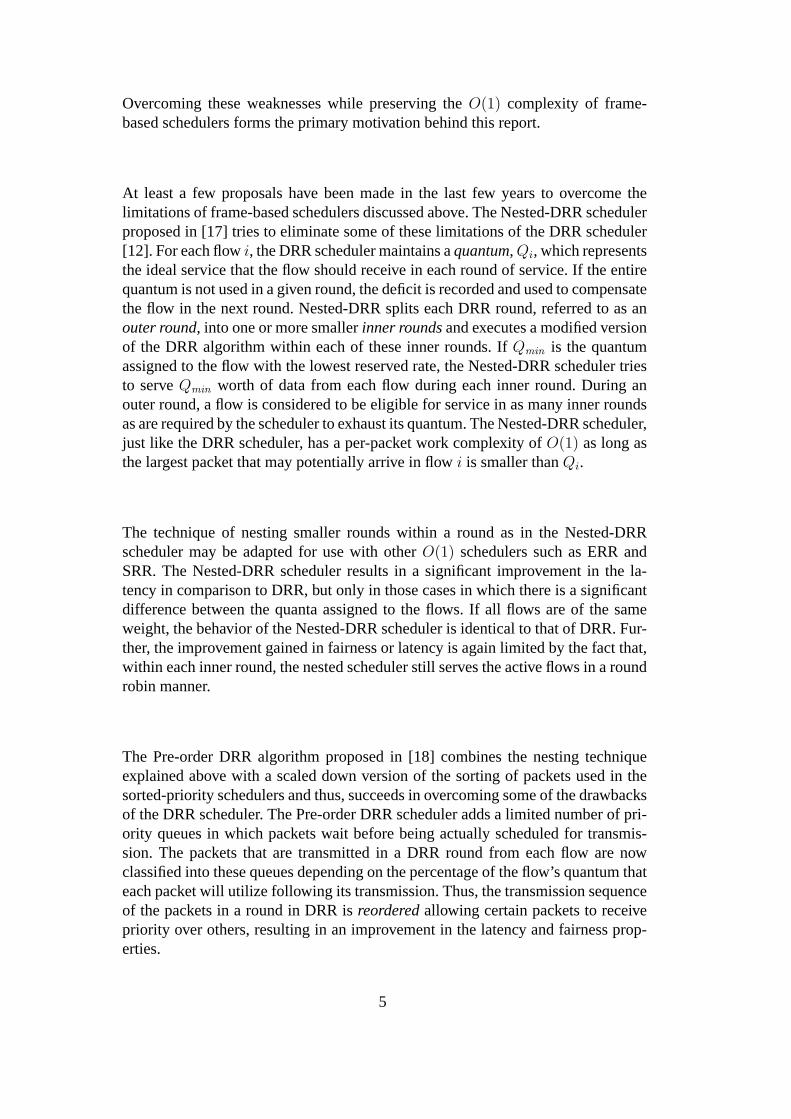
Table 1 summarizes the work complexity, fairness and latency bounds of severalguaranteed-rate scheduling disciplines that belong to the class of (LR) servers. Inthis table,n represents the number of active flows andp represents the number ofpriority queues in Pre-order DRR and PERR. The peak rate of the output link isdenoted byr. M is the size of the largest packet that may potentially arrive duringthe execution of a scheduling algorithm. Recall thatm is the size of the largestpacket thatactuallyarrives during the execution of the scheduler. Usually, in mostnetworks including the Internet,M À m since the majority of packets are muchsmaller than the largest possible packet [21, 22]. The properties of all the frame-based scheduling disciplines are derived in [23]. The latency bounds of DRR andPre-order DRR have been analyzed in [24] and [25]. The RFB and latency boundof ERR have been analyzed in [16, 19]. The expression for the latency bound ofNested-DRR, as proved in [17], is extremely complex and hence does not allow foran easy comparison with the other schedulers under consideration. Hence, in orderto gain a quick understanding of the differences in the latency bounds of Nested-DRR and PERR, in our comparison we include the latency bound of Nested-DRR attwo boundary conditions. In the first case, we consider the latency bound of a flowwhose reserved rate is much lower than that of the other flows sharing the sameoutput link (ρi ¿ ρj, ∀j ∈ n, j 6= i). In the second case, we consider the oppositeend of the spectrum, i.e., the latency bound of a flow whose reserved rate is muchgreater than the other flows multiplexed on the same link (ρi À ρj,∀j ∈ n, j 6= i).In [17], an expression for the latency of a low-rate flow has been derived and it hasalso been shown that the latency of a high-rate flow is marginally lower than thatof the DRR scheduler. For simplicity we assume the latter to be equal to DRR.

30

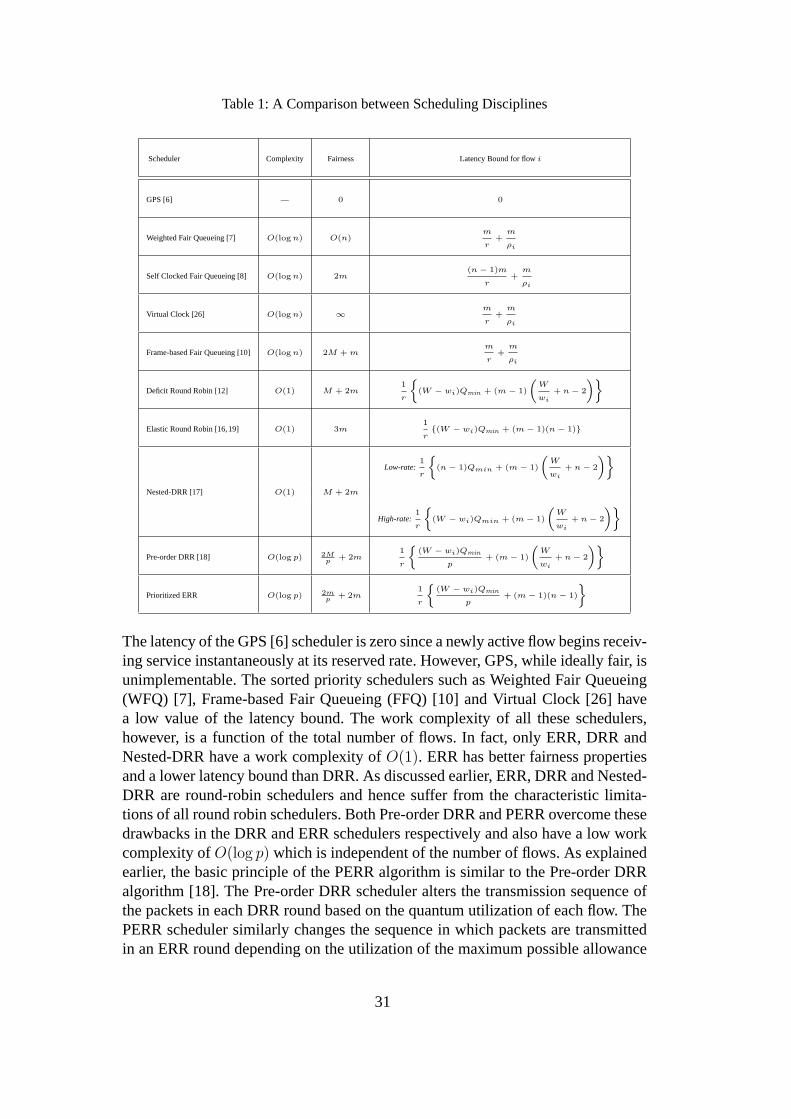
Table 1: A Comparison between Scheduling Disciplines

Scheduler Complexity Fairness Latency Bound for flowi

GPS [6] — 0 0

Weighted Fair Queueing [7] O(log n) O(n)m

r+

m

ρi

Self Clocked Fair Queueing [8] O(log n) 2m(n− 1)m

r+

m

ρi

Virtual Clock [26] O(log n) ∞ m

r+

m

ρi

Frame-based Fair Queueing [10] O(log n) 2M + mm

r+

m

ρi

Deficit Round Robin [12] O(1) M + 2m1

r

(W − wi)Qmin + (m− 1)

(W

wi

+ n− 2

)

Elastic Round Robin [16,19] O(1) 3m1

r(W − wi)Qmin + (m− 1)(n− 1)

Low-rate:1

r

(n− 1)Qmin + (m− 1)

(W

wi

+ n− 2

)

Nested-DRR [17] O(1) M + 2m

High-rate:1

r

(W − wi)Qmin + (m− 1)

(W

wi

+ n− 2

)

Pre-order DRR [18] O(log p) 2Mp

+ 2m1

r

(W − wi)Qmin

p+ (m− 1)

(W

wi

+ n− 2

)

Prioritized ERR O(log p) 2mp

+ 2m1

r

(W − wi)Qmin

p+ (m− 1)(n− 1)

The latency of the GPS [6] scheduler is zero since a newly active flow begins receiv-ing service instantaneously at its reserved rate. However, GPS, while ideally fair, isunimplementable. The sorted priority schedulers such as Weighted Fair Queueing(WFQ) [7], Frame-based Fair Queueing (FFQ) [10] and Virtual Clock [26] havea low value of the latency bound. The work complexity of all these schedulers,however, is a function of the total number of flows. In fact, only ERR, DRR andNested-DRR have a work complexity ofO(1). ERR has better fairness propertiesand a lower latency bound than DRR. As discussed earlier, ERR, DRR and Nested-DRR are round-robin schedulers and hence suffer from the characteristic limita-tions of all round robin schedulers. Both Pre-order DRR and PERR overcome thesedrawbacks in the DRR and ERR schedulers respectively and also have a low workcomplexity ofO(log p) which is independent of the number of flows. As explainedearlier, the basic principle of the PERR algorithm is similar to the Pre-order DRRalgorithm [18]. The Pre-order DRR scheduler alters the transmission sequence ofthe packets in each DRR round based on the quantum utilization of each flow. ThePERR scheduler similarly changes the sequence in which packets are transmittedin an ERR round depending on the utilization of the maximum possible allowance

31

0 20 40 60 805

10

15

20

25

30

35

40

45

50

55

Late

ncy

Bou

nd (

in m

sec)

Reserved Rate of flow i (in Mbps)

(a) m = M

DRRERRNested−DRRPre−order DRRPERR

0 20 40 60 800

5

10

15

20

25

30

35

40

45

50

55

Late

ncy

Bou

nd (

in m

sec)

Reserved Rate of flow i (in Mbps)

(b) m = M/2

DRRERRNested−DRRPre−order DRRPERR

Fig. 9. Comparison of the latency bounds

of each flow in that round.

There is however an important difference between these two schedulers. At the startof a round, the Pre-order DRR scheduler has to classify all the packets that will betransmitted by the active flows in that round into the priority queues prior to startingthe transmission of the packets. On the contrary, the PERR scheduler simply hasto classify the flows present in theActiveList into its priority queues before thestart of the round. It has been shown in [19] that ERR has a couple of importantadvantages over DRR. Now since the PERR and Pre-order DRR algorithms aremodifications of ERR and DRR, respectively, PERR inherits those advantages overPre-order DRR. The following lists these advantages:

• Lower Buffer Requirement :Since the priority queues in PERR simply need tocontain the flow identifiers they can be much smaller in size as compared to thosein Pre-order DRR which have to buffer all the packets that will be transmitted inthe current round.

• Reduced Round Start Delay :Classifying all the packets that are to be transmittedin the round into the priority queues requires considerably more time than simplysorting the flow identifiers. Thus, the delay incurred by the PERR scheduler atthe start of the round is much less in comparison to that incurred by the Pre-orderDRR scheduler.

• Improved Latency and Fairness Characteristics:Table 1 illustrates that PERRhas better fairness properties and a lower latency bound than Pre-order DRR,especially considering thatM is typically much greater thanm.

• Adaptability in other contexts:Unlike DRR and Pre-order DRR, the PERR sched-uler does not require the knowledge of the transmission time of each packet. Asa result the scheduler can be used in other networks such as wormhole networks,

32

where the transmission time of a packet depends not only on the size of thepacket but also the downstream congestion. Similarly, PERR may be used inATM networks transmitting IP packets over AAL5, where the end of the packetis not known until the last ATM cell of the packet arrives.

Note that the latency bound of aLR server is an extremely important QoS param-eter since it has a direct influence of the the size of the playback buffers neededat the receiver for real-time communication applications. In order that the readercan fully appreciate the improvement in the latency characteristics of PERR, wecompare the latency bound of PERR with other efficient scheduling disciplines ofequivalent work complexity such as DRR, ERR, Nested-DRR and Pre-order DRRwithin the context of an example. Note that for this comparison we use the actuallatency bound for Nested-DRR as proved in [17].

Let us assume that a total of 100 flows are multiplexed on an output link with atransmission rate,r of 150 Mbps. Assume thatM is equal to 576 bytes, equal tothe minimum value of the Maximum Transmission Unit (MTU) required of all net-works. Assume thatρmin is equal to 0.1Mbps and that the output link is completelyutilized, i.e.

∑ni=1 ρi = r. Note that this implies that the sum of all the weights,W ,

is equal to150/0.1 = 1500. Let the number of priority queues in the priority queuemodule of Pre-order DRR and PERR be equal to 10, i.e.,p = 10. We comparethe latency bounds of the afore-mentioned schedulers for flowi as a function of itsreserved rate,ρi, for two values ofm : (a)m = M , (b) m = M/2. Fig. 9 illustratesa plot of these latency bounds of flowi for both the values ofm. Note that latencybounds of all the schedulers under consideration depend on the sum of the weightsof all the flows but not on the distribution of the weights among all the flows otherthan flowi. Therefore, the weights of the flows other than flowi are not discussedin the context of this illustration. It can be easily seen that PERR has the lowestlatency bound among all the schedulers under consideration. The improvement inthe latency of PERR is even more apparent whenm < M .

7 Simulation Results

In this section, we first present a brief discussion on a recently proposed new mea-sure of fairness which captures theinstantaneousbehavior of a scheduler. A moredetailed presentation of this measure may be found in [27]. We then present somesimulation results comparing the performance of PERR based on this new metricwith other efficient schedulers.

Table 1 lists the RFBs of the schedulers. However, measures such as the RFBare based on the worst case performance, which is just one aspect of the fairnessachieved by a packet scheduler. For example, a scheduler that rarely reaches theupper bound of the fairness measure will achieve the same measure of fairness

33

as another scheduler that frequently or almost always operates at the same upperbound. Therefore, we also need aninstantaneousmeasure of fairness that capturesthe fairness achieved by the scheduler atanygiven instant of time.

To measure the fairness at any instant of time, we also need to consider situationsin real applications. The RFB is defined under the assumption that queues are con-tinuously backlogged in the interval of interest. Such an assumption is rarely true inreal networks. In networks with real traffic, flow states can change frequently fromactive state to idle state, or vice versa. However, existing measures of fairness havenot taken this factor into account. To effectively guide the design of a fair sched-uler, a fairness measure should also be able to capture the performance under thesituation where flows change their states unpredictably.

A recently proposed measure of fairness described in [27] addresses these issues.There are two components to this measure: one of how to handle real traffic whereflows are not always backlogged and the other of how to measure inequality inservice received by the flows. We review these components briefly in this section;a detailed treatment and a more extensive rationale behind the approach may befound in [27].

7.1 Handling a Newly Backlogged Flow

In order to evaluate the fairness of a scheduler in its treatment of a newly back-logged flow, we need to first define the ideally fair way of doing this. We beginwith an examination of the ideal but unimplementable GPS scheduling discipline.

Let B(t) represent the set of backlogged flows at timet. Assume that the systemstarts at timet = 0.

Definition 11 Let V (t) represent the virtual time function [6, 28] (also known asthe system potential) at timet. The virtual time is used to track the progress of theGPS scheduler and is computed as follows:

V ′(t) =dV (t)

dt=

∑

i∈B(t)

wi

−1

(39)

Hence, the service received by a backlogged flow under the GPS server in the timeinterval (0, t) is given bywiV

′(t). Intuitively, the virtual time represents the idealfair normalized service that each flow should have received by timet.

Let us now consider a set ofn flows served by a scheduling policyP . Consider acase in which then flows have been backlogged since timet1. One of these flows,flow i, changes its status from being backlogged to idle at timet2 > t1 and later

34

becomes backlogged again at timet3 > t2. In order to accurately and meaningfullycompare the service received by all the flows at time instants aftert3, it is necessaryto assign an appropriate value of the normalized service received by flowi untilt3 so that the comparison is over the entire time interval(t1, t3). As mentionedearlier, a newly backlogged flow should neither be favored nor be punished for itsidle period in the interval(t2, t3). Therefore, based on the discussion of the virtualtime, the service received by flowi at timet should bewiV (t). However, if flowi has already received more service than the above amount of service before timet2 while it was backlogged, then the total assumed service should beSent i(0, t2).This is because a flow that receives excess service should not be able to becomeidle and then immediately become backlogged again without being disadvantagedlater for the excess service it received earlier. These concepts and similar argumentshave also been made in [5,8,10,27].

In evaluating the fairness of a specific scheduler it is necessary to keep track ofthe amount of service allocated by the above method. We borrow the method usedin [27] where a per-flow state known as thesession utilityis defined for this purpose.This variable is independent of the scheduling discipline used by the scheduler andis defined as a function of time. Letui(t) represent the session utility for flowi attime instantt. Assume that the system starts at time 0. During the period(t1, t2)that a flow is continuously backlogged, its session utility is updated as follows:

ui(t2) = ui(t1) +Senti(t1, t2)

wi

(40)

We now discuss how to update the session utility of a flow that just becomes back-logged. Let flowi become newly backlogged or backlogged again at timet. LetB(t−) represent the set of flows that are backlogged just prior to the time that flowi becomes backlogged. Our goal in assigning a session utility value to flowi at timet is to ensure that the comparison between session utilities of all the flows is beingmade as though the flows have all been backlogged for the same length of time.Accordingly flowi is assigned the following session utility value:

ui(t) = maxui(t−), V (t) (41)

With the above definition of the session utility, a newly backlogged flow can betreated as if it had been backlogged for the same length of time as all other flows.Therefore, with a measure which is based on session utility, it is possible to capturethe fairness of a scheduler in its treatment of flows that are not always continuouslybacklogged.

35

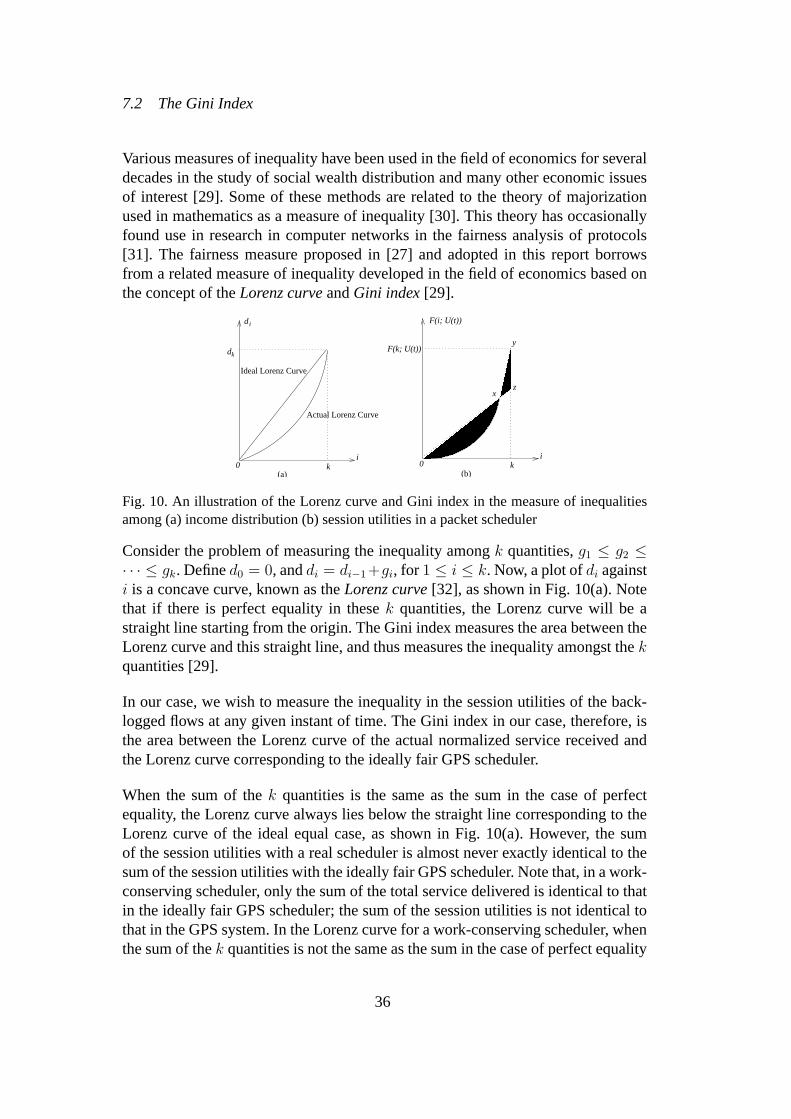
7.2 The Gini Index

Various measures of inequality have been used in the field of economics for severaldecades in the study of social wealth distribution and many other economic issuesof interest [29]. Some of these methods are related to the theory of majorizationused in mathematics as a measure of inequality [30]. This theory has occasionallyfound use in research in computer networks in the fairness analysis of protocols[31]. The fairness measure proposed in [27] and adopted in this report borrowsfrom a related measure of inequality developed in the field of economics based onthe concept of theLorenz curveandGini index[29].

i

F(i; U(t))

F(k; U(t))

k0

x

y

z

dk

d i

ik0

Actual Lorenz Curve

Ideal Lorenz Curve

(a) (b)

Fig. 10. An illustration of the Lorenz curve and Gini index in the measure of inequalitiesamong (a) income distribution (b) session utilities in a packet scheduler

Consider the problem of measuring the inequality amongk quantities,g1 ≤ g2 ≤· · · ≤ gk. Defined0 = 0, anddi = di−1+gi, for 1 ≤ i ≤ k. Now, a plot ofdi againsti is a concave curve, known as theLorenz curve[32], as shown in Fig. 10(a). Notethat if there is perfect equality in thesek quantities, the Lorenz curve will be astraight line starting from the origin. The Gini index measures the area between theLorenz curve and this straight line, and thus measures the inequality amongst thekquantities [29].

In our case, we wish to measure the inequality in the session utilities of the back-logged flows at any given instant of time. The Gini index in our case, therefore, isthe area between the Lorenz curve of the actual normalized service received andthe Lorenz curve corresponding to the ideally fair GPS scheduler.

When the sum of thek quantities is the same as the sum in the case of perfectequality, the Lorenz curve always lies below the straight line corresponding to theLorenz curve of the ideal equal case, as shown in Fig. 10(a). However, the sumof the session utilities with a real scheduler is almost never exactly identical to thesum of the session utilities with the ideally fair GPS scheduler. Note that, in a work-conserving scheduler, only the sum of the total service delivered is identical to thatin the ideally fair GPS scheduler; the sum of the session utilities is not identical tothat in the GPS system. In the Lorenz curve for a work-conserving scheduler, whenthe sum of thek quantities is not the same as the sum in the case of perfect equality

36

as with the GPS scheduler, a portion of the curve for the actual scheduler will liebelow and another portion will lie above the straight line Lorenz curve for the GPSscheduler. This is illustrated in Fig. 10(b). The sum of the shaded areas in the figureis the Gini index.

The computation of the Gini index is described formally as follows:

Definition 12 Let U(t) represent the set of the session utilities of the flows attime instantt when served by a real scheduler and letG(t) denote a similar setwhich is obtained when the flows are served with the ideal GPS scheduler. Letuc1 , uc2 , . . . , uck

be the elements of the setU(t), such thatuc1 ≤ uc2 ≤ · · · ≤ uck.

The Lorenz Curveof the set of session utilitiesU(t) is the functionF (i;U(t)),given by,

F (i;U(t)) =i∑

j=1

ucj, 0 ≤ i ≤ k

The Gini index over thek elements inU(t) is computed as:

k∑

i=1

∣∣∣F (i;U(t))− F (i;G(t))∣∣∣ (42)

As defined above, the closer the Lorenz curve ofU(t) is to the curve of GPS, thesmaller the Gini index is, and thus, the fairer the distribution of the session utilities.From the definition of the virtual time function, we know that the normalized ser-vice received by each flow at timet in the GPS system is equal to the virtual time,V (t). Hence the Gini index can be computed as :

k∑

i=1

∣∣∣F (i;U(t))− F (i; V (t))∣∣∣ (43)

With the Gini index, the fairness of a scheduler can be evaluated at each instantduring the execution of the scheduler. A comparison of schedulers based on theirGini indices allows us to determine which scheduler achieves better fairness thanothers at each instant of time.

7.3 Simulation Results

In our simulation experiments, we compare the Gini index of Pre-order DRR withthose of other efficient and fair schedulers such as DRR, ERR, Nested-DRR andPre-order DRR.

In our first set of experiments, the input queues are fed by backbone router traces.We used the traces provided by the National Laboratory for Applied Network Re-search [33]. Each input is fed by a router trace with a random starting time. Table 2

37

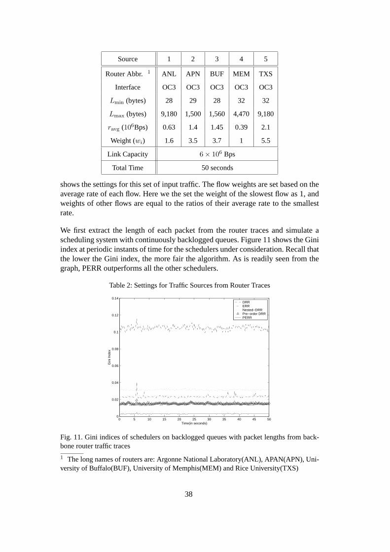
Source 1 2 3 4 5

Router Abbr. 1 ANL APN BUF MEM TXS

Interface OC3 OC3 OC3 OC3 OC3

Lmin (bytes) 28 29 28 32 32

Lmax (bytes) 9,180 1,500 1,560 4,470 9,180

ravg (106Bps) 0.63 1.4 1.45 0.39 2.1

Weight (wi) 1.6 3.5 3.7 1 5.5

Link Capacity 6× 106 Bps

Total Time 50 seconds

shows the settings for this set of input traffic. The flow weights are set based on theaverage rate of each flow. Here we the set the weight of the slowest flow as 1, andweights of other flows are equal to the ratios of their average rate to the smallestrate.

We first extract the length of each packet from the router traces and simulate ascheduling system with continuously backlogged queues. Figure 11 shows the Giniindex at periodic instants of time for the schedulers under consideration. Recall thatthe lower the Gini index, the more fair the algorithm. As is readily seen from thegraph, PERR outperforms all the other schedulers.

Table 2: Settings for Traffic Sources from Router Traces

0 5 10 15 20 25 30 35 40 45 500

0.02

0.04

0.06

0.08

0.1

0.12

0.14

Time(in seconds)

Gin

i Ind

ex

DRR ERR Nested−DRR Pre−order DRRPERR

Fig. 11. Gini indices of schedulers on backlogged queues with packet lengths from back-bone router traffic traces

1 The long names of routers are: Argonne National Laboratory(ANL), APAN(APN), Uni-versity of Buffalo(BUF), University of Memphis(MEM) and Rice University(TXS)

38

In our next set of experiments, we allow that the flows are not always backlogged,while still using real router traces. Since we are more interested in the performancewhen the link is close to fully utilized, we set the link capacity such that the sumof average rates of all the flows is 99% of the link capacity. Figure 12(a) showsthe average length of arriving packets among all sessions during the simulationinterval. Figures 12(b)–(e) show the values of the Gini index observed for the fivedifferent schedulers. For the sake of clarity, we plot each scheduler’s Gini index ona separate graph, with that of the PERR scheduler plotted on each of the graphs.Once again, we find that the PERR scheduler displays a lower Gini index than anyof the other schedulers of equivalent complexity at almost all instants of time.

0 10 20 30 40 50450

500

550

600

650

700

Time(in cycles)

Ave

rage

Len

gth

of

Arr

ivin

g P

acke

ts (

in B

ytes

)

(a)

0 10 20 30 40 500

0.05

0.1

0.15

0.2

Time (in seconds)

Gin

i Ind

ex

(b)

DRRPERR

0 10 20 30 40 500

0.05

0.1

0.15

0.2

Time (in seconds)

Gin

i Ind

ex

(c)

Nested DRRPERR

0 10 20 30 40 500

0.02

0.04

0.06

Time (in seconds)

Gin

i Ind

ex

(d)

ERRPERR

0 10 20 30 40 500

0.02

0.04

0.06

Time (in seconds)

Gin

i Ind

ex

(e)

Pre−order DRRPERR

Fig. 12. Gini indices of schedulers with backbone router traffic traces

8 Conclusion

Elastic Round Robin (ERR), a recently proposed fair scheduler, is very efficientwith anO(1) work complexity. However ERR is a frame-based scheduler and hencesuffers from all the characteristic limitations of these schedulers which arise fromthe round robin nature of their service order. In this report, we have presented anovel scheduling discipline calledPrioritized Elastic Round Robin(PERR), which

39

rearranges the sequence in which packets are transmitted in each round of the ERRscheduler. This is achieved through the addition of a priority queue module con-sisting ofp priority queues. AnOrganizermodule dynamically classifies the activeflows into these priority queues.

We have analytically shown that PERR has a low work complexity ofO(log p)which is independent of the total number of flows, resulting in a simple and ef-ficient hardware implementation. We also prove that PERR belongs to the classof LR servers and also evaluate an upper bound on its latency using a noveltechnique based on interpreting the PERR scheduler as an instance of the NestedDeficit Round Robin algorithm. Our analysis also reveals that PERR has betterfairness characteristics and a significantly lower latency bound in comparison toother scheduling disciplines of equivalent work complexity such as DRR, ERR andPre-order DRR. In addition, we have also presented simulation results, using bothsynthetic and real traces, which corroborate the conclusions of our analysis.

9 Acknowledgments

The authors are grateful to Ms. Hongyuan Shi for her help in the simulation effortsusing the Gini index.

References

[1] S. Keshav, An Engineering Approach to Computer Networks, Addison-WesleyPublishing Company, Reading, MA, 1997.

[2] D. C. Stephens, J. C. R. Bennett, H. Zhang, Implementing scheduling algorithmsin high-speed networks, IEEE Journal on Selected Areas in Communications 17 (6)(1999) 1145–1158.

[3] C. S. Inc., Cisco 12016 Gigabit Switch Router: Application Note (1999).

[4] D. Bertsekas, R. Gallager, Data Networks, 2nd Edition, Prentice Hall, Upper SaddleRiver, NJ, 1991.

[5] D. Stiliadis, A. Verma, Latency-rate servers: A general model for analysis of trafficscheduling algorithms, IEEE Transactions on Networking 6 (3) (1996) 611–624.

[6] A. K. Parekh, R. G. Gallager, A generalized processor sharing approach to flowcontrol—the single node case, in: Proceedings of IEEE INFOCOM, Florence, Italy,1992, pp. 915–924.

[7] A. Demers, S. Keshav, S. Shenker, Design and analysis of a fair queuing algorithm,in: Proceedings of ACM SIGCOMM, Austin, 1989, pp. 1–12.

40

[8] S. J. Golestani, A self-clocked fair queuing scheme for broadband applications, in:Proceedings of IEEE INFOCOM, Toronto, Canada, 1994, pp. 636–646.

[9] P. Goyal, H. M. Vin, H. Cheng, Start-time fair queueing: A scheduling algorithm forintegrated services packet switching networks, IEEE Transactions on Networking 5 (5)(1997) 690–704.

[10] D. Stiliadis, A. Varma, Efficient fair queuing algorithms for packet-switched networks,IEEE Transactions on Networking 6 (2) (1998) 175–185.

[11] J. C. R. Bennett, H. Zhang, WF2Q : Worst-case fair weighted fair queueing, in:Proceedings of IEEE INFOCOM, San Francisco, CA, 1996, pp. 120–128.

[12] M. Shreedhar, G. Varghese, Efficient fair queuing using deficit round-robin, IEEETransactions on Networking 4 (3) (1996) 375–385.

[13] S. Floyd, V. Jacobson, Link-sharing and resource management models for packetnetworks, IEEE Transactions on Networking 3 (4) (1995) 365–386.

[14] S. Floyd, Notes on class-based-queueing and guaranteed service, Unpublished Notes,http://www.aciri.org/floyd/cbq.html .

[15] G. P. H. Adiseshu, G. Varghese, A reliable and scalable striping protocol, in:Proceedings of ACM SIGCOMM, Palo Alto, CA, 1996, pp. 131–141.

[16] S. S. Kanhere, H. Sethu, A. B. Parekh, Fair and efficient packet scheduling usingelastic round robin, IEEE Transactions on Parallel and Distributed Systems 13 (3)(2002) 324–326.

[17] S. S. Kanhere, H. Sethu, Fair, efficient and low-latency packet scheduling using nesteddeficit round robin, in: Proceedings of the IEEE Workshop on High PerformanceSwitching and Routing, Dallas, TX, 2001, pp. 6–10.

[18] S. Tsao, Y. Lin, Pre-order deficit round robin: a new scheduling algorithm for packet-switched networks, Computer Networks 35 (2-3) (2001) 287–305.

[19] S. S. Kanhere, H. Sethu, Low-latency guaranteed-rate scheduling using elastic roundrobin, Computer Communication 25 (14) (2002) 1315–1322.

[20] Y. Zhou, H. Sethu, On the relationship between absolute and relative fairness bounds,IEEE Communication Letters 6 (1) (2002) 37–39.

[21] K. Thompson, G. J. Miller, R. Wilder, Wide-area Internet traffic patterns andcharacteristics, IEEE Network 11 (6) (1997) 10–23.

[22] I. Widjaja, A. I. Elwalid, Performance issues in VC-merge capable switches formultiprotocol label switching, IEEE Journal on Selected Areas in Communications17 (6) (1999) 1178–1189.

[23] D. Stiliadis, Traffic scheduling in packet-switched networks: Analysis, design andimplementation, Ph.D. thesis, University of California, Santa Cruz (1996).

[24] S. S. Kanhere, H. Sethu, On the latency bound of deficit round robin, in: Proceedingsof the International Conference on Computer Communications and Networks, Miami,FL, 2002, pp. 548–553.

41

[25] S. S. Kanhere, H. Sethu, On the latency bound of pre-order deficit round robin, in:Proceedings of the IEEE Conference on Local Computer Networks, Tampa, FL, 2002,pp. 508–517.

[26] L. Zhang, Virtual clock: A new traffic control algorithm for packet switching networks,in: Proceedings of ACM SIGCOMM, Philadelphia, PA, 1990, pp. 19–29.

[27] H. Shi, H. Sethu, An evaluation of timestamp-based packet schedulers usinga novel measure of instantaneous fairness, in: Proceedings of the Int’lPerformance, Computing and Communications Conference, 2003, available athttp://www.ece.drexel.edu/CCL/pubs.html .

[28] D. Stiliadis, Traffic scheduling in packet-switched networks: Analysis, design andimplementation, Ph.D. thesis, University of California, Santa Cruz (1996).

[29] F. A. Cowell, Measuring Inequalities: Techniques for the Social Sciences, John Wileyand Sons, New York, NY, 1977.

[30] A. W. Marshall, I. Olkin, Inequalities: Theory of Majorization and its Applications,Academic Press, New York, NY, 1979.

[31] A. Kumar, J. Kleinberg, Fairness measures for resource allocation, in: Proceedings ofthe Symposium on Foundations of Computer Science, 2000, pp. 75–78.

[32] J. E. Stiglitz, Economics, W. W. Norton and Co, 1993.

[33] National Laboratory for Applied Network Research, ”Passive Measurement andAnalysis”,http://pma.nlanr.net/PMA/ .

42