Principlesofexperimentaldesign 1-FactorAnova Splitplotdesigns · Twoway anova More than two factors Multi-FactorExperiments 1 Twowayanova 2 Morethantwofactors 1/34

Main topics

Principles of experimental design1-Factor AnovaBlock designsFactorial designsFractional factorialsSplit plot designs

Twoway anovaMore than two factors

Multi-Factor Experiments

1 Twoway anova

2 More than two factors

1 / 34


1 Twoway anova


2 / 34


1 Twoway anova


3 / 34


Hypertension: Effect of biofeedback

Biofeedback Biofeedback Medication Control+ Medication

158 188 186 185163 183 191 190173 198 196 195178 178 181 200168 193 176 180

4 / 34


Main effects

Treatment means:Medicationno yes

Biofeedback Totalno 190 186 188yes 188 168 178Total 189 177 183

Main effect of biofeedback: 188− 178 = 10 mmHg

Question: What is the main effect of medication? 12mmHg

5 / 34


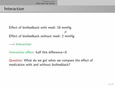
Interaction

Effect of biofeedback with medi: 18 mmHg6=

Effect of biofeedback without medi: 2 mmHg

−→ Interaction

Interaction effect: half this difference=8

Question: What do we get when we compare the effect ofmedication with and without biofeedback?

6 / 34


Interaction plots

165

170

175

180

185

190

Medication

mea

n of

bp

without with

Biofeedback

withoutwith

165

170

175

180

185

190

Biofeedback

mea

n of

bp

without with

Medication

withoutwith

7 / 34


Model for two factors

Yijk = µ+ Ai + Bj + (AB)ij + εijk

i = 1, . . . , I; j = 1, . . . , J; k = 1, . . . , n.∑Ai = 0,

∑Bj = 0,

∑i(AB)ij =

∑j(AB)ij = 0.

Ai : ith effect of factor ABj : jth effect of factor B

µ+ Ai + Bj : overall mean + effect of factor A on level i + effectof factor B on level j

(AB)ij : deviation from additive model

8 / 34


Parameter estimation

µ = y..., Ai = yi .. − y... and Bj = y.j. − y...

AB ij = yij. − (µ+ Ai + Bj) = yij. − yi .. − y.j. + y...

Medication ABiofeedback B no yes Totalno 190 186 y.1. = 188yes 188 168 y.2. = 178Total y1.. = 189 y2.. = 177 y... = 183

µ = 183, A1 = −A2 = 6, B1 = −B2 = 5

9 / 34


Predicted values of the additive model

Predictions: (µ+ Ai + Bj)

Medicationno yes

Biofeedbackno 194 182yes 184 172

y11 = µ+ A1 + B1 = 183+ 6+ 5 = 194

AB11 = AB22 = −AB12 = −AB21 = −4.

10 / 34


Decomposition of Variability

SStot = SSA + SSB + SSAB + SSres

SStot =∑ ∑ ∑

(yijk − y...)2

SSA =∑ ∑ ∑

(yi .. − y...)2

SSB =∑ ∑ ∑

(y.j. − y...)2

SSAB =∑ ∑ ∑

(yij. − yi .. − y.j. + y...)2

SSres =∑ ∑ ∑

(yijk − yij.)2

degrees of freedom: main effect with I levels: I − 1 df,interaction between 2 factors with I and J levels: (I − 1)(J − 1) df.

11 / 34


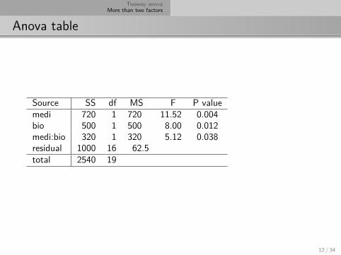
Anova table

Source SS df MS F P valuemedi 720 1 720 11.52 0.004bio 500 1 500 8.00 0.012medi:bio 320 1 320 5.12 0.038residual 1000 16 62.5total 2540 19

12 / 34


Treatment effects

effect size C.I.medi without bio: y21. − y11. = 186− 190 = −4 (−18, 10)medi with bio: y22. − y12. = 168− 188 = −20 (−34,−6)bio without medi: y12. − y11. = 188− 190 = −2 (−16, 12)bio with medi: y22. − y21. = 168− 186 = −18 (−32,−4)

(standard error:√2·MSres/5 = 5)

Question: How are the CI limits calculated?

13 / 34


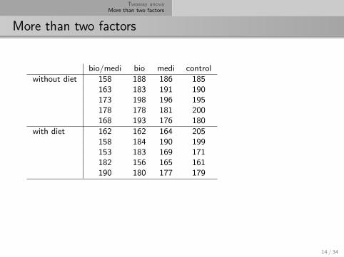
More than two factors

bio/medi bio medi controlwithout diet 158 188 186 185

163 183 191 190173 198 196 195178 178 181 200168 193 176 180

with diet 162 162 164 205158 184 190 199153 183 169 171182 156 165 161190 180 177 179

14 / 34


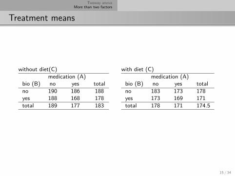
Treatment means

without diet(C)medication (A)

bio (B) no yes totalno 190 186 188yes 188 168 178total 189 177 183

with diet (C)medication (A)

bio (B) no yes totalno 183 173 178yes 173 169 171total 178 171 174.5

15 / 34


Main effects and interactions

Main effects A, B, CDifference of the response on the two levels averaged over all otherfactor levels.medication (A): 183.5 − 174 = 9.5biofeedback (B): 183 − 174.5 = 8.5diet(C): 183 − 174.5 = 8.5

2-way interactions AB, AC, BCAverage over all but two factors.

medi (A)Bio (B) no yes totalno 186.5 179.5 183yes 180.5 168.5 174.5total 183.5 174 178.75

Effect of medi without bio: 7Effect of medi with bio: 12Interaction effect: 2.5

16 / 34


Main effects and interactions cont.

3-way interaction ABCDifference of the 2-way interaction effect between the levels of thethird factor.

Interaction effect AB without diet= 8Interaction effect AB with diet= -3Half this difference=11/2=5.5

17 / 34


Model and Anova table

Yijkl = µ+Ai +Bj +Ck +(AB)ij +(AC)ik +(BC)jk +(ABC)ijk +εijkl

with constraints∑

Ai = 0, . . . ,∑

k(ABC)ijk = 0

Source df MS=SS/df FA I − 1 MSA/MSresB J − 1 MSB/MSresC K − 1 MSC/MSresAB (I − 1)(J − 1) MSAB/MSresAC (I − 1)(K − 1) MSAC/MSresBC (J − 1)(K − 1) MSBC/MSresABC (I − 1)(J − 1)(K − 1) MSABC/MSresResidual «Difference» MSres = σ2

Total IJKn − 1

18 / 34


Anova table

Source SS df MS F P valuemedi 902.5 1 902.5 6.33 0.017bio 722.5 1 722.5 5.06 0.031diet 722.5 1 722.5 5.06 0.031medi:bio 62.5 1 62.5 0.44 0.51medi:diet 62.5 1 62.5 0.44 0.51bio:diet 22.5 1 22.5 0.16 0.69medi:bio:diet 302.5 1 302.5 2.12 0.15Residual 4566.0 32 142.7Total 7363.5 39

19 / 34


Half normal plot

0.0 0.5 1.0 1.5 2.0

05

1015

2025

30

Half−normal quantiles

Sor

ted

Dat

a

+

+medi2

bio2/diet2

20 / 34


Unbalanced Factorials

uncorrelated estimators:

SStot = SSA + SSB + SSAB + SSres︸︷︷︸SSC+...+SSres′

correlated estimators:

SStot = SS ′A + SS ′

B + SS ′AB + SSC + . . .+ SSres′

SS Typ I: SSA ignores all other SSSS Typ II: SSA takes into account all other main effects, ignores

all interactionsSS Typ III: SSA takes into account all other effects

21 / 34


Calculation of SS’s

by model comparison

For SS Typ I:model 1: Yijk = µ+ εijk SSe1 = SSTmodel 2: Yijk = µ+ Ai + εijk SSe2model 3: Yijk = µ+ Ai + Bj + εijk SSe3model 4: Yijk = µ+ Ai + Bj + ABij + εijk SSe4 = SSres

22 / 34


Rat genotype

Litters of rats are separated from their natural mother andgiven to another female to raise.2 factors: mother’s genotype (A, B, I, J) and litter’s genotype(A, B, I, J)response: average weight gain of the litter.

23 / 34


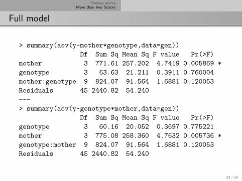
Full model

> summary(aov(y~mother*genotype,data=gen))Df Sum Sq Mean Sq F value Pr(>F)

mother 3 771.61 257.202 4.7419 0.005869 *genotype 3 63.63 21.211 0.3911 0.760004mother:genotype 9 824.07 91.564 1.6881 0.120053Residuals 45 2440.82 54.240---> summary(aov(y~genotype*mother,data=gen))

Df Sum Sq Mean Sq F value Pr(>F)genotype 3 60.16 20.052 0.3697 0.775221mother 3 775.08 258.360 4.7632 0.005736 *genotype:mother 9 824.07 91.564 1.6881 0.120053Residuals 45 2440.82 54.240

24 / 34


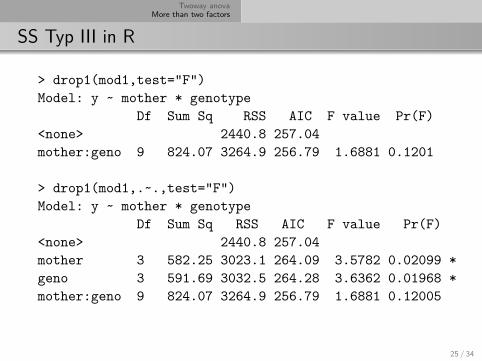
SS Typ III in R

> drop1(mod1,test="F")Model: y ~ mother * genotype

Df Sum Sq RSS AIC F value Pr(F)<none> 2440.8 257.04mother:geno 9 824.07 3264.9 256.79 1.6881 0.1201

> drop1(mod1,.~.,test="F")Model: y ~ mother * genotype

Df Sum Sq RSS AIC F value Pr(F)<none> 2440.8 257.04mother 3 582.25 3023.1 264.09 3.5782 0.02099 *geno 3 591.69 3032.5 264.28 3.6362 0.01968 *mother:geno 9 824.07 3264.9 256.79 1.6881 0.12005

25 / 34


Offer for a 6-year old car

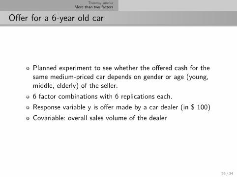
Planned experiment to see whether the offered cash for thesame medium-priced car depends on gender or age (young,middle, elderly) of the seller.6 factor combinations with 6 replications each.Response variable y is offer made by a car dealer (in $ 100)Covariable: overall sales volume of the dealer

26 / 34


Analysis of Covariance

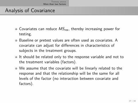
Covariates can reduce MSres , thereby increasing power fortesting.Baseline or pretest values are often used as covariates. Acovariate can adjust for differences in characteristics ofsubjects in the treatment groups.It should be related only to the response variable and not tothe treatment variables (factors).We assume that the covariate will be linearly related to theresponse and that the relationship will be the same for alllevels of the factor (no interaction between covariate andfactors).

27 / 34


Model for two-way ANCOVA

Yijk = µ+ θxijk + Ai + Bj + (AB)ij + εijk

∑Ai =

∑Bj =

∑(AB)ij = 0, εijk ∼ N (0, σ2)

28 / 34


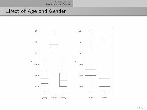
Effect of Age and Gender

young middle elderly

20

22

24

26

28

30y

male female

20

22

24

26

28

30

y

29 / 34


Interaction effect of Age and Gender

2224

2628

cash$age

mea

n of

cas

h$y

young middle elderly

cash$gender

malefemale

2224

2628

cash$gender

mea

n of

cas

h$y

male female

cash$age

middleyoungelderly

30 / 34


Two-way Anova

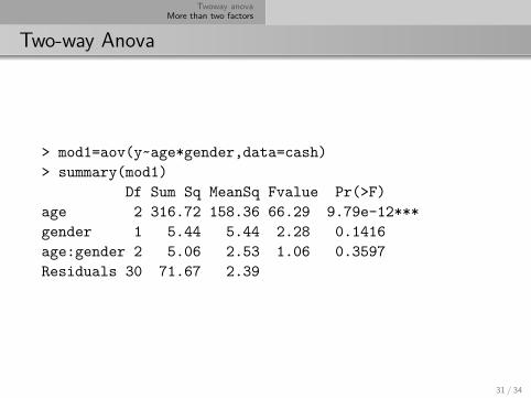
> mod1=aov(y~age*gender,data=cash)> summary(mod1)

Df Sum Sq MeanSq Fvalue Pr(>F)age 2 316.72 158.36 66.29 9.79e-12***gender 1 5.44 5.44 2.28 0.1416age:gender 2 5.06 2.53 1.06 0.3597Residuals 30 71.67 2.39

31 / 34


Sales and Cash Offer

1 2 3 4 5 6

2022

2426

2830

cash$sales

cash

$y

32 / 34


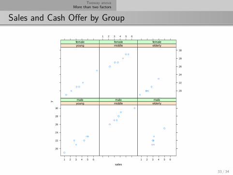
Sales and Cash Offer by Group

sales

y

20

22

24

26

28

30

1 2 3 4 5 6

youngmale

middlemale

1 2 3 4 5 6

elderlymale

youngfemale

1 2 3 4 5 6

middlefemale

20

22

24

26

28

30

elderlyfemale

33 / 34


Two-way Ancova

> mod2=aov(y~sales+age*gender,data=cash)> summary(mod2)

Df SumSq MeanSq Fvalue Pr(>F)sales 1 157.37 157.37 550.22 < 2e-16***age 2 231.52 115.76 404.75 < 2e-16***gender 1 1.51 1.51 5.30 0.02874*age:gender 2 0.19 0.10 0.34 0.71422Residuals 29 8.29 0.29

34 / 34

Documents

Principlesofexperimentaldesign 1-FactorAnova Splitplotdesigns · Twoway anova More than two factors Multi-FactorExperiments 1 Twowayanova 2 Morethantwofactors 1/34