Principles of Pattern Recognition Principles of Pattern Recognition

C. A. Murthy Machine Intelligence Unit Indian Statistical Institute Kolkata e-mail: murthy@isical.ac.in

Pattern RecognitionPattern Recognition

Measurement Space –> Feature Space

–>Decision space

Main Tasks : Feature Selection and

Supervised / Unsupervised Classification

Supervised ClassificationSupervised Classification

ClassificationTwo cases

1. Conditional Probability density functions and prior probabilities are known

2. Training sample points are given

Bayes decision ruleBayes decision rule

M classes class conditional density functions

prior probabilities

Put in class if

Best decision rule Minimizes the prob. of misclassification

)(),.....,(),( 21 xpxpxp M

Nx ℜ∈MPPP ,....., 21

10 << iP Mi ,.....2,1=∀

∑ =M

iP1

1

x

ijxpPxpP jjii ≠∀≥ );()(

i

• We may not know . (Estimation of density functions), Normal distribution

• We may not know

• Error prob. may be difficult to obtain

• Other decision rules are needed

spi '

sPi '

Normal distribution caseNormal distribution case

If and then the

decision boundary is linear.

In general the decision boundary is non-linear

;)()(2

1exp

)2(

1)( 1'

21

−∑−−= −

∑iii

Ni xx

i

xp µµπ

Mi ,.....2,1=

2=M ∑=∑=∑ 21

Suppose we are given n points x1,x2,…xn. Let there be M classes . Let ni of these sample points belong to class i; i=1,2,…M.

K-Nearest Neighbour decision rule

i.e., ∑=

=M

ii nn

1

.

Let x be the point to be classified. Let k be a positiveinteger. Find k nearest neighbors of x among x1,..,xn

Let ki of these nearest neighbors belong to ith class; i=1,2,…M;

Put x in class i if ki > kj ∀j ≠ i

∑=

=M

ii kk

1

.

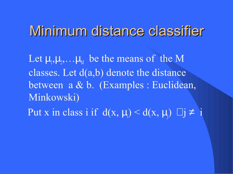
Minimum distance classifierMinimum distance classifier

Let µ1,µ2,…µM be the means of the M classes. Let d(a,b) denote the distance between a & b. (Examples : Euclidean, Minkowski)

Put x in class i if d(x, µi) < d(x, µj) ∀j ≠ i

Some remarksSome remarks

Standardization & normalizationChoosing the appropriate distance functionProbability of misclassificationCost of misclassification

ClusteringClusteringProblem: Finding natural groups in data set

Example 1:

Example 2:

Clustering (contd..)Clustering (contd..)

Let us assume that the given data set

• No. of clusters K may not be known• Choice of similarity/dissimilarity measure• Algorithms

MnxxxS ℜ⊂= },...,,{ 21

Dissimilarity MeasuresDissimilarity Measures

• Metrics

),...,,( 21'

Maaaa =

),...,,( 21'

Mbbbb =

.1;||),(1

1≥

−= ∑

=pbabad

pM

i

piip

2=p Euclidean distance

Similarity MeasuresSimilarity Measures

∑ ∑

∑==

221),(

ii

M

iii

ba

babas

Other such measures are also available

K-Means AlgorithmK-Means Algorithm• Several versions of K-Means algorithm are available. One version is given below Number of clusters = K

d Euclidean distance 1. Partitions of S into K subsets 2. 3. yi = mean of A1i

4. For put xj in A2i if 1. If A1i=A2i for all i=1,2,…k then stop o.w. Rename A2i as A1i and goto step 2.

MnxxxS ℜ⊂= },...,,{ 21

kAAA 11211 ,...,

Φ==== kAAA 22221 ...

.,...2,1 ki =nj ,...,2,1=

iiyxyxd ijij ≠< 1, ),,()(1

ki ,...,2,1=∀

K-Means Algorithm (contd..)K-Means Algorithm (contd..)

• Number of iterations is usually decided by the user

• provides basically convex clusters

• Non convex clusters may not be obtained

• Two different initial partitions may give rise to two different clusterings

Hierarchical Clustering Hierarchical Clustering TechniquesTechniques

• Agglomerative

• Divisive

Agglomerative TechniquesAgglomerative Techniques

1. N clusters level 12. Clusters at the level i Merge two clusters if (one cluster is reduced) Rename the clusters as3. Repeat step 2 till the required no. of clusters is obtained

}{},...{},{ 2211 nn xcxcxc ===121 ,...,, +− inccc

ji cc , 11 ,),,(),(11

jiccDccD jiji ∀<

inccc −,...,, 21

MnxxxS ℜ⊂= },...,,{ 21

d dissimilarity measure

Agglomerative Techniques Agglomerative Techniques (contd..)(contd..)

)),((),( yxdMinBAD

ByAx

∈∈

=

)),((),( yxdMaxBAD

ByAx

∈∈

=

• single linkage. • complete linkage.

• several other such ‘D’s can be considered.• single linkage provides non-convex clustering generally.

Feature selectionFeature selection

Feature X1, X2,…,XN

b no. of features to be selected. b < N

Uses :Reduction in computational complexityRedundant features act as noise. Noise

removalInsight into the classification problem.

Steps of feature selectionSteps of feature selection

Objective function J which attaches a value to every subset of features is to be defined.

Algorithms for feature selection are to be formulated.

Objective functions for feature Objective functions for feature selection (Devijver & Kittler)selection (Devijver & Kittler)

Probabilistic separability (Chernoff, Bhattacharyya, Matusita, Divergence)

Inter class distance

Feature Selection Criteria:Supervised Criterion:

ωi i = 1, …, M : classesni, i = 1, …, M : number of points in class i

Pi : a priori probability of class ixik : kth point of ith class

1. Interclass Distance Measures:

(notations)

∑∑∑∑====

=j

jlik

i

ji

ji

n

l

xxn

knn

1

),(

1

1c

1j

Pc

1i

P2

1 J δ

δ : Euclidean, Minkowski, Manhattan

Reference:Devijver & Kittler, Pattern Recognition: A Statistical Approach, Englewood Cliffs, 1982

2. Probabilistic Separability Measures:

Bhattacharyya Distance:

[ ] dxxx2

1

1B | p() |p(ln - J ∫ )= 2ωω

3. Information Theoretic Measures:

Mutual Information:

dxx

xx i

i

M

ii )p(

) | p(ln ) | p(PJ

1I

ωω∫∑=

=

Difficulty: Computing the probabilities.Empirical estimates are used.

Unsupervised Criterion:

Entropy (E):Similarity between points xi and xj:Sij = e –αδ(xi,xj) i,j = 1, …, l

)S-log(1)S1()log(S

1

S

1ijijij

l

jij

l

i

E −+==

= ∑∑

Other unsupervised indices:

•Fuzzy Feature Evaluation Index•Neuro-fuzzy Feature Evaluation Index

Search Algorithms:

If total number of features = D

Computational complexities:

• Exhaustive search [(DCd)] D =100 and d =10 the no. of computationsis greater than 1013.

• Branch and Bound(gives optimal set for a class of evaluation criteria)

Worst case: (DCd)

Number of features to be selected = d

⇒

Algorithms for feature Algorithms for feature selectionselection

Sequential forward selectionSequential backward selection(l,r) algorithmBranch and bound algorithm

Sequential forward selectionSequential forward selection

Ao = φ .

Ak denotes the k features already selected

Let a1∈ {X1,…XN} – Ak be such that J(AkU{a1}) ≥ J (AkU{a}) ∀a∈{X1,…XN} – Ak then Ak+1=AkU{a1}.

Run the program b times

• Sequential Forward/Backward Search(greedy algorithms, very approximate, gives poor result on most real life data)

• Sequential Floating F/B Search (l-r algorithm)

(relatively better than SFS/SBS)

Non-Monotonicity Property:“Two best features are not always the best two”

KDD ProcessKDD Process

Data Preparation

• Data Condensation

• Dimensionality Reduction

• Noise Removal

MachineLearningPatternRecognition

KnowledgeExtraction/Evaluation

Redu-cedClean

Data

RawData

Data Mining

Knowledge

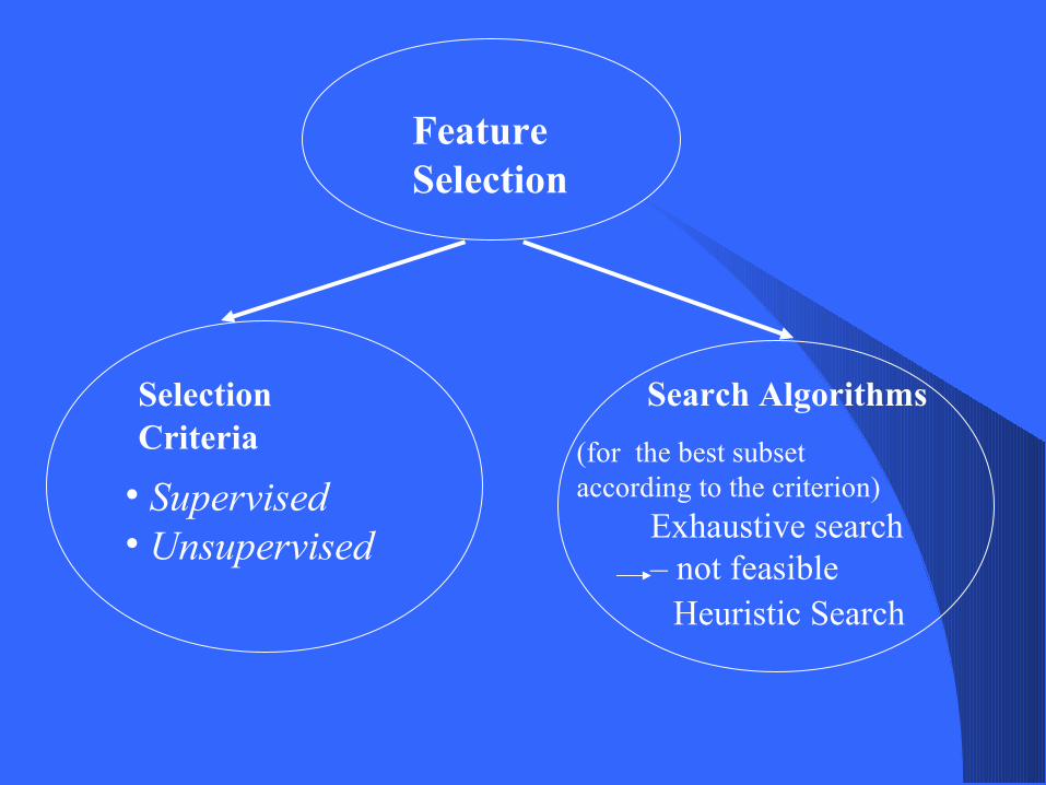
FeatureSelection

Selection Criteria

Search Algorithms

• Supervised• Unsupervised

(for the best subset according to the criterion)

Exhaustive search – not feasible

Heuristic Search

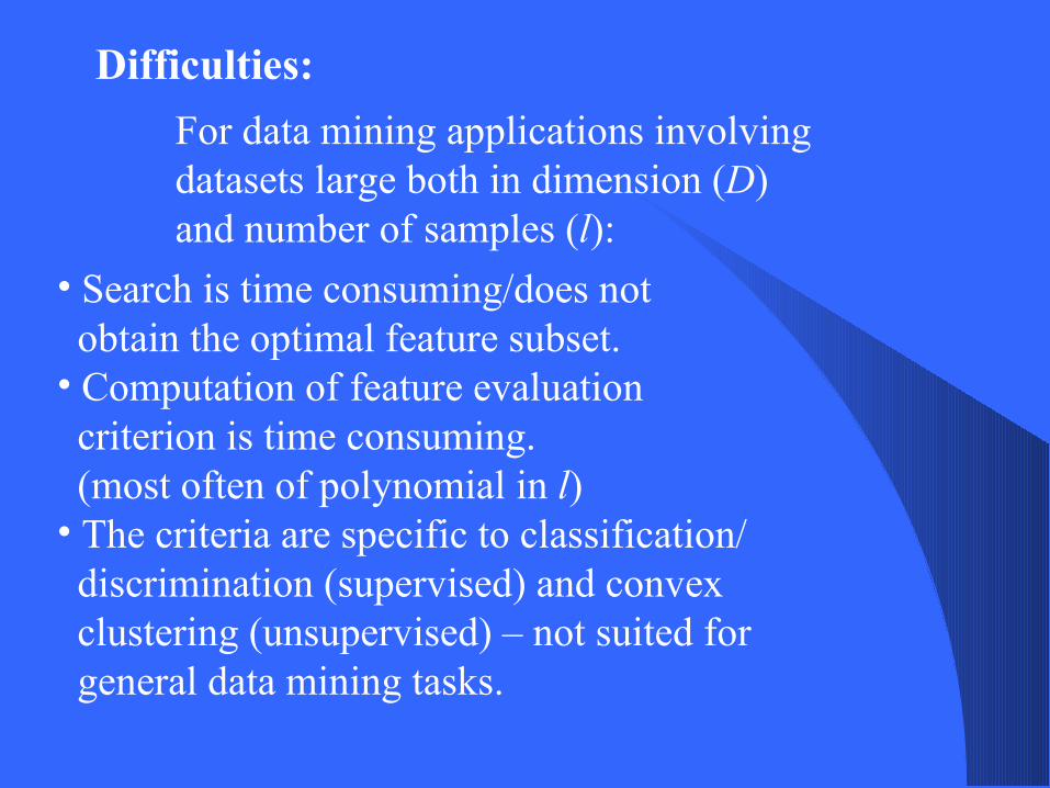
Difficulties:

For data mining applications involvingdatasets large both in dimension (D)and number of samples (l):

• Search is time consuming/does not obtain the optimal feature subset.• Computation of feature evaluation criterion is time consuming. (most often of polynomial in l)• The criteria are specific to classification/ discrimination (supervised) and convex clustering (unsupervised) – not suited for general data mining tasks.

Thank You!!