Embed Size (px)
Citation preview

Principles of Managerial Finance
9th Edition
Chapter 12
Leverage & Capital Structure
Learning Objectives• Discuss the role of breakeven analysis, how to
determine the operating breakeven point, and the
effect of changing costs on the breakeven point.
• Understand operating, financial, and total leverage
and the relationship among them.
• Describe the basic types of capital, external
assessment of capital structure, capital structure of
non-U.S. firms, and capital structure theory.
Learning Objectives• Explain the optimal capital structure using a graphic
view of the firm’s cost of capital functions and a
modified form of zero-growth valuation model.
• Discuss the graphic presentation, risk considerations,
and basic shortcomings of EBIT-EPS approach to
capital structure.
• Review the return and risk of alternative capital
structures and their linkage to market value, and other
important capital structure considerations.
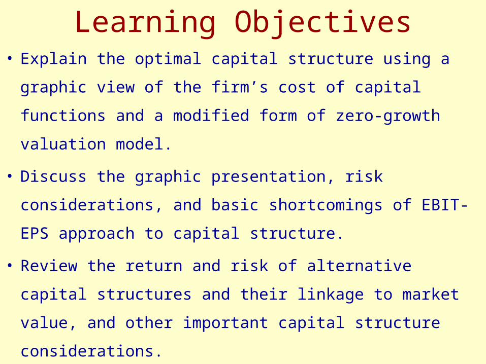
Leverage
Sales revenue 和EPS 之間的關係
Sales revenue 和EBIT 之間的關係
EBIT 和 EPS之間的關係
Breakeven Analysis• Breakeven (cost-volume-profit) Analysis is used to:
– determine the level of operations necessary to
cover all operating costs, and
– evaluate the profitability associated with various
levels of sales.
• The firm’s operating breakeven point (OBP) is the
level of sales necessary to cover all operating
expenses.
• At the OBP, operating profit (EBIT) is equal to zero.
Breakeven Analysis• To calculate the OBP, cost of goods sold and
operating expenses must be categorized as fixed or
variable.
• Variable costs vary directly with the level of sales and
are a function of volume, not time.
• Examples would include direct labor and shipping.
• Fixed costs are a function of time and do not vary with
sales volume.
• Examples would include rent and fixed overhead.
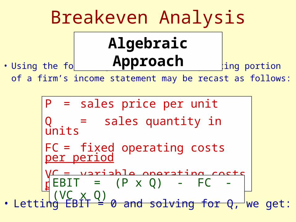
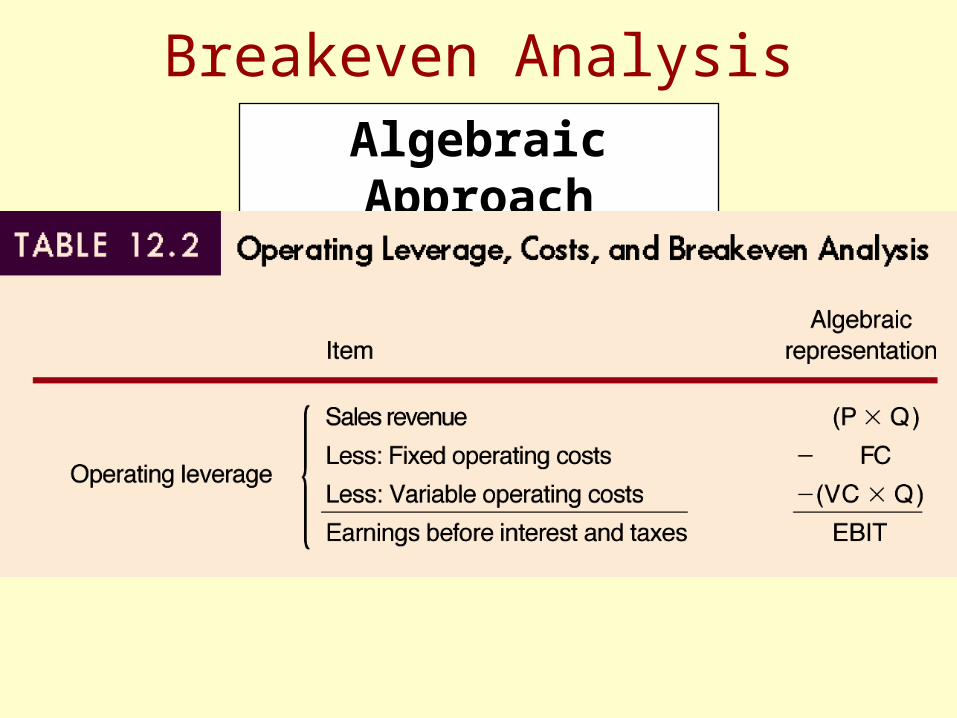
• Using the following variables, the operating portion of
a firm’s income statement may be recast as follows:
Algebraic Approach
P = sales price per unit
Q = sales quantity in units
FC = fixed operating costs per period
VC = variable operating costs per unit
EBIT = (P x Q) - FC - (VC x Q)
• Letting EBIT = 0 and solving for Q, we get:
Breakeven Analysis
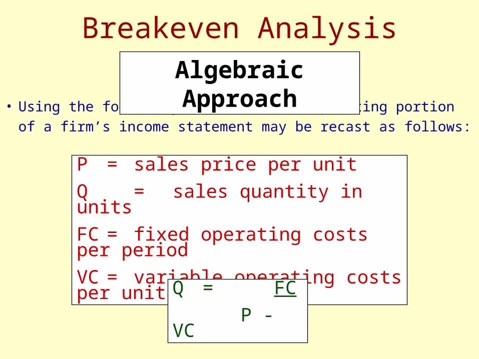
• Using the following variables, the operating portion of
a firm’s income statement may be recast as follows:
Algebraic Approach
P = sales price per unit
Q = sales quantity in units
FC = fixed operating costs per period
VC = variable operating costs per unit
Q = FC
P - VC
Breakeven Analysis
Algebraic Approach
Breakeven Analysis
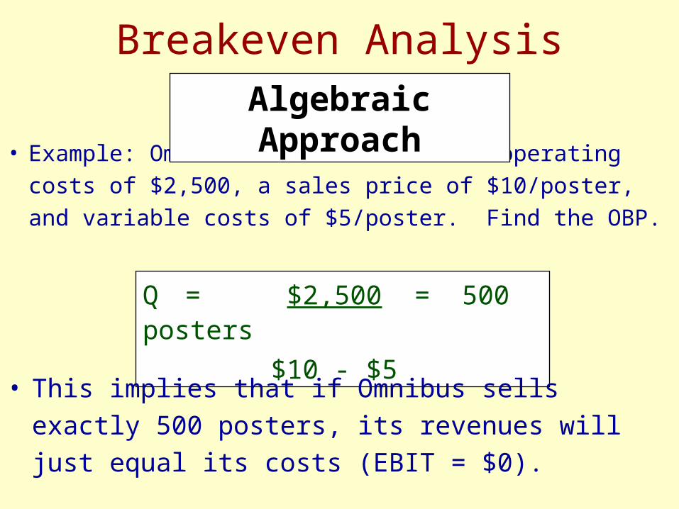
• Example: Omnibus Posters has fixed operating costs
of $2,500, a sales price of $10/poster, and variable
costs of $5/poster. Find the OBP.
Algebraic Approach
Q = $2,500 = 500 posters
$10 - $5
• This implies that if Omnibus sells exactly 500 posters,
its revenues will just equal its costs (EBIT = $0).
Breakeven Analysis
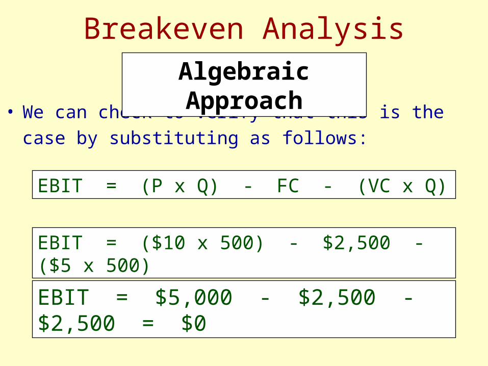
• We can check to verify that this is the case by
substituting as follows:
Algebraic Approach
EBIT = (P x Q) - FC - (VC x Q)
EBIT = ($10 x 500) - $2,500 - ($5 x 500)
EBIT = $5,000 - $2,500 - $2,500 = $0
Breakeven Analysis
Graphic Approach
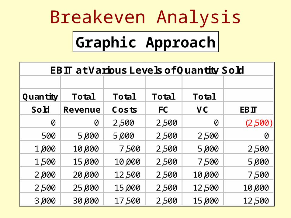
Quantity Total Total Total Total
Sold Revenue Costs FC VC EBIT
0 0 2,500 2,500 0 (2,500)
500 5,000 5,000 2,500 2,500 0
1,000 10,000 7,500 2,500 5,000 2,500
1,500 15,000 10,000 2,500 7,500 5,000
2,000 20,000 12,500 2,500 10,000 7,500
2,500 25,000 15,000 2,500 12,500 10,000
3,000 30,000 17,500 2,500 15,000 12,500
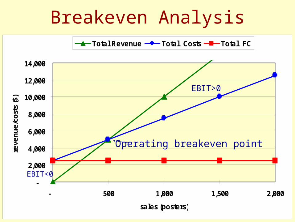
EBIT at Various Levels of Quantity Sold
Breakeven Analysis
-
2,000
4,000
6,000
8,000
10,000
12,000
14,000
- 500 1,000 1,500 2,000
sales (posters)
reve
nu
e/c
ost
s ($
)
Total Revenue Total Costs Total FC
Breakeven Analysis
EBIT>0
EBIT<0
Operating breakeven point
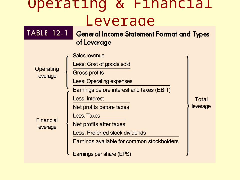
Operating & Financial Leverage
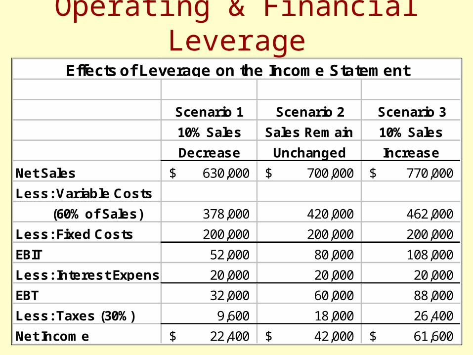
Scenario 1 Scenario 2 Scenario 3
10% Sales Sales Remain 10% Sales
Decrease Unchanged Increase
Net Sales 630,000$ 700,000$ 770,000$
Less: Variable Costs
(60% of Sales) 378,000 420,000 462,000
Less: Fixed Costs 200,000 200,000 200,000
EBIT 52,000 80,000 108,000
Less: Interest Expense 20,000 20,000 20,000
EBT 32,000 60,000 88,000
Less: Taxes (30%) 9,600 18,000 26,400
Net Income 22,400$ 42,000$ 61,600$
Effects of Leverage on the Income Statement
Operating & Financial Leverage
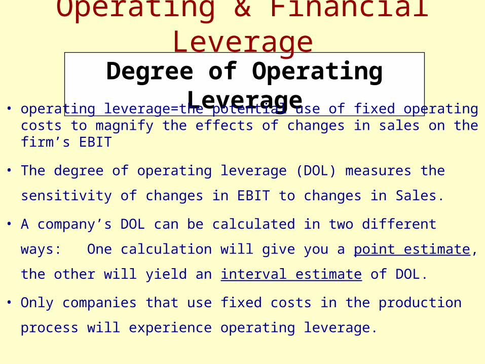
Degree of Operating Leverage
• operating leverage=the potential use of fixed operating costs to magnify the effects of changes in sales on the firm’s EBIT
• The degree of operating leverage (DOL) measures the
sensitivity of changes in EBIT to changes in Sales.
• A company’s DOL can be calculated in two different ways:
One calculation will give you a point estimate, the other will
yield an interval estimate of DOL.
• Only companies that use fixed costs in the production process
will experience operating leverage.
Operating & Financial Leverage
Operating & Financial Leverage
Degree of Operating Leverage
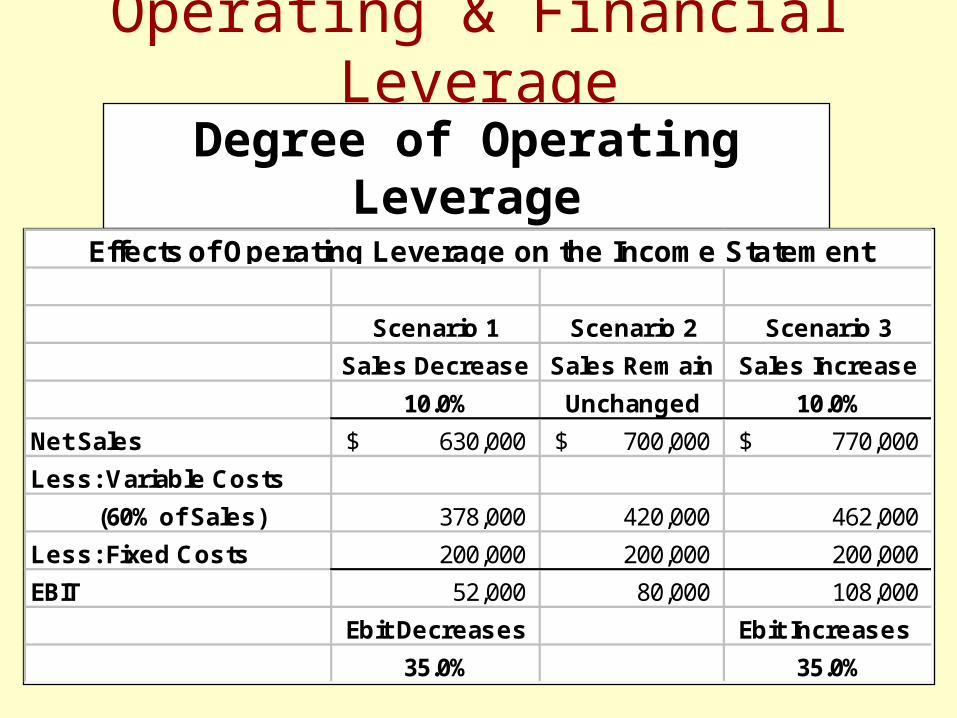
Scenario 1 Scenario 2 Scenario 3
Sales Decrease Sales Remain Sales Increase
10.0% Unchanged 10.0%
Net Sales 630,000$ 700,000$ 770,000$
Less: Variable Costs
(60% of Sales) 378,000 420,000 462,000
Less: Fixed Costs 200,000 200,000 200,000
EBIT 52,000 80,000 108,000
Ebit Decreases Ebit Increases
35.0% 35.0%
Effects of Operating Leverage on the Income Statement
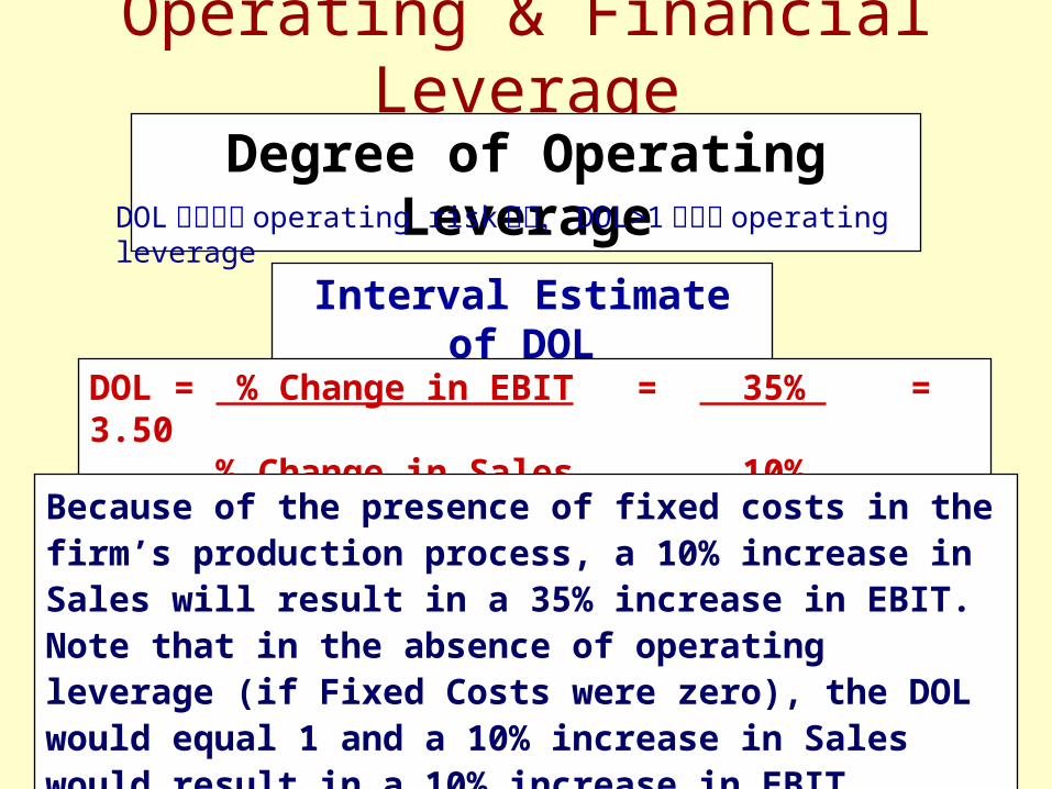
Interval Estimate of DOL
DOL = % Change in EBIT = 35% = 3.50 % Change in Sales 10%
Because of the presence of fixed costs in the firm’s production process, a 10% increase in Sales will result in a 35% increase in EBIT. Note that in the absence of operating leverage (if Fixed Costs were zero), the DOL would equal 1 and a 10% increase in Sales would result in a 10% increase in EBIT.
Operating & Financial Leverage
Degree of Operating LeverageDOL 愈大表示 operating risk 愈大, DOL>1 表示有 operating leverage
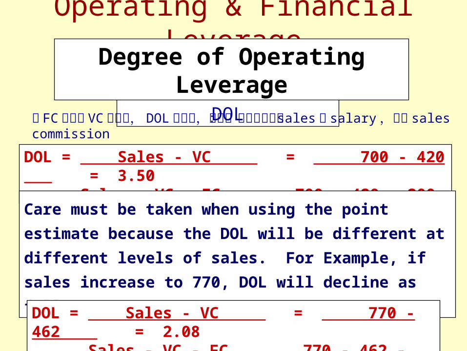
Point Estimate of DOL
DOL = Sales - VC = 700 - 420 = 3.50 Sales - VC - FC 700 - 420 - 200
Care must be taken when using the point estimate
because the DOL will be different at different levels of
sales. For Example, if sales increase to 770, DOL will
decline as follows:
Operating & Financial LeverageDegree of Operating Leverage
DOL = Sales - VC = 770 - 462 = 2.08 Sales - VC - FC 770 - 462 - 200
當 FC 相對於 VC 愈大時, DOL 也愈大,例如:公司決定增加 sales 的salary ,減少 sales commission
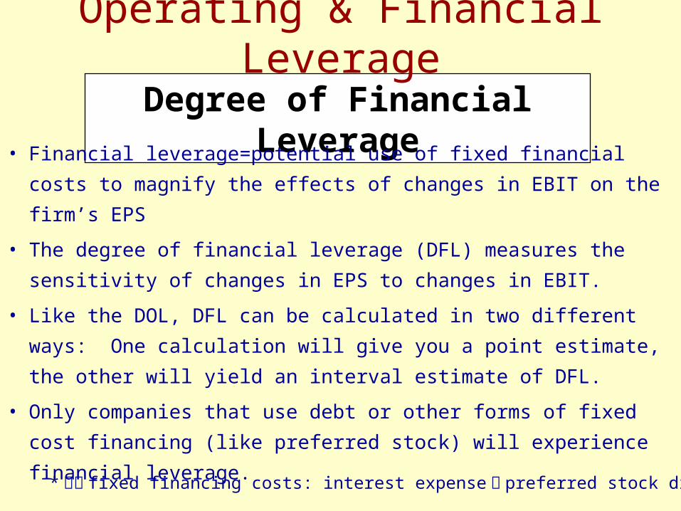
Degree of Financial Leverage
• Financial leverage=potential use of fixed financial costs to
magnify the effects of changes in EBIT on the firm’s EPS
• The degree of financial leverage (DFL) measures the sensitivity
of changes in EPS to changes in EBIT.
• Like the DOL, DFL can be calculated in two different ways:
One calculation will give you a point estimate, the other will
yield an interval estimate of DFL.
• Only companies that use debt or other forms of fixed cost
financing (like preferred stock) will experience financial
leverage.
Operating & Financial Leverage
* 兩種 fixed financing costs: interest expense 與 preferred stock dividend
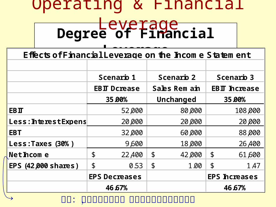
Degree of Financial LeverageOperating & Financial Leverage
Scenario 1 Scenario 2 Scenario 3
EBIT Dcrease Sales Remain EBIT Increase
35.00% Unchanged 35.00%
EBIT 52,000 80,000 108,000
Less: Interest Expense 20,000 20,000 20,000
EBT 32,000 60,000 88,000
Less: Taxes (30%) 9,600 18,000 26,400
Net Income 22,400$ 42,000$ 61,600$
EPS (42,000 shares) 0.53$ 1.00$ 1.47$
EPS Decreases EPS Increases
46.67% 46.67%
Effects of Financial Leverage on the Income Statement
注意:若有特別股存在,則這裡要再減去特別股股利
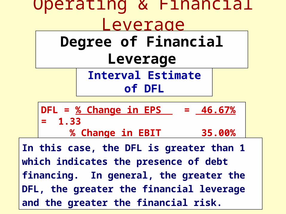
Interval Estimate of DFL
DFL = % Change in EPS = 46.67% = 1.33% Change in EBIT 35.00%
In this case, the DFL is greater than 1 which
indicates the presence of debt financing. In
general, the greater the DFL, the greater the
financial leverage and the greater the financial risk.
Operating & Financial Leverage
Degree of Financial Leverage
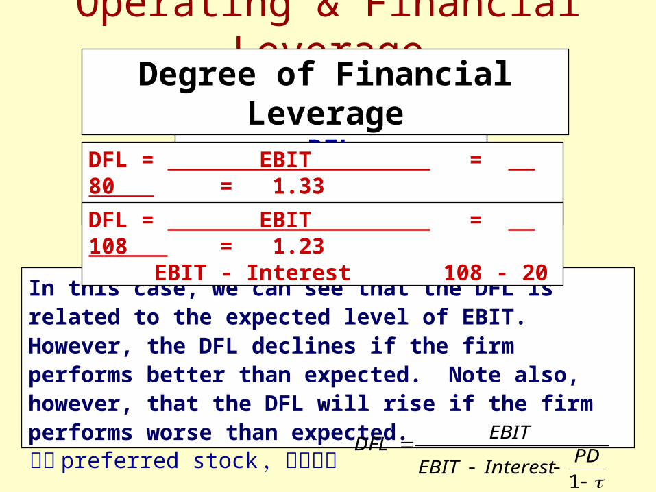
Point Estimate of DFL
DFL = EBIT = 80 = 1.33EBIT - Interest 80 - 20
In this case, we can see that the DFL is related to the expected level of EBIT. However, the DFL declines if the firm performs better than expected. Note also, however, that the DFL will rise if the firm performs worse than expected.
DFL = EBIT = 108 = 1.23EBIT - Interest 108 - 20
Operating & Financial LeverageDegree of Financial Leverage
若有 preferred stock ,則公式為
1PD
InterestEBIT
EBITDFL
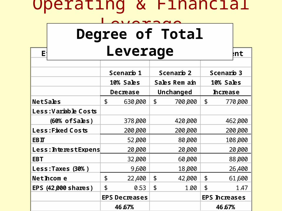
Operating & Financial Leverage
Scenario 1 Scenario 2 Scenario 3
10% Sales Sales Remain 10% Sales
Decrease Unchanged Increase
Net Sales 630,000$ 700,000$ 770,000$
Less: Variable Costs
(60% of Sales) 378,000 420,000 462,000
Less: Fixed Costs 200,000 200,000 200,000
EBIT 52,000 80,000 108,000
Less: Interest Expense 20,000 20,000 20,000
EBT 32,000 60,000 88,000
Less: Taxes (30%) 9,600 18,000 26,400
Net Income 22,400$ 42,000$ 61,600$
EPS (42,000 shares) 0.53$ 1.00$ 1.47$
EPS Decreases EPS Increases
46.67% 46.67%
Effects of Combined Leverage on the Income Statement
Degree of Total Leverage
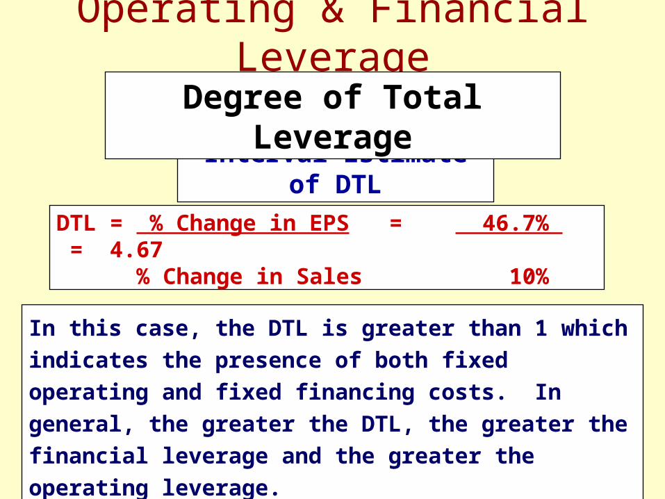
Interval Estimate of DTL
DTL = % Change in EPS = 46.7% = 4.67 % Change in Sales 10%
Operating & Financial Leverage
Degree of Total Leverage
In this case, the DTL is greater than 1 which indicates the
presence of both fixed operating and fixed financing
costs. In general, the greater the DTL, the greater the
financial leverage and the greater the operating leverage.
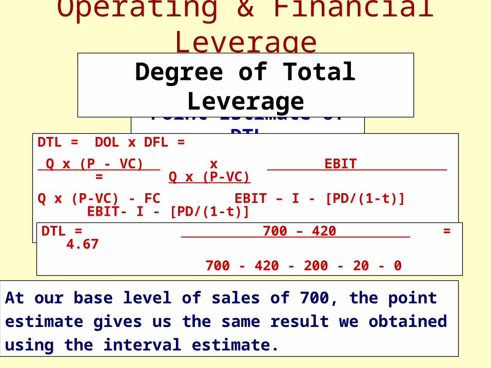
Point Estimate of DTL
DTL = DOL x DFL =
Q x (P - VC) x EBIT = Q x (P-VC)
Q x (P-VC) - FC EBIT – I - [PD/(1-t)] EBIT- I - [PD/(1-t)]
Operating & Financial Leverage
Degree of Total Leverage
At our base level of sales of 700, the point estimate gives
us the same result we obtained using the interval
estimate.
DTL = 700 – 420 = 4.67
700 - 420 - 200 - 20 - 0
DTL = DOL x DFL
Operating & Financial Leverage
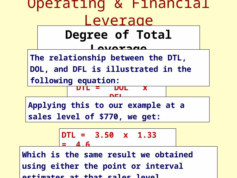
Degree of Total Leverage
The relationship between the DTL, DOL, and
DFL is illustrated in the following equation:
DTL = 3.50 x 1.33 = 4.6
Applying this to our example at a sales level of
$770, we get:
Which is the same result we obtained using either
the point or interval estimates at that sales level.
The Firm’s Capital Structure• Capital structure is one of the most complex areas of
financial decision making due to its interrelationship
with other financial decision variables.
• Poor capital structure decisions can result in a high
cost of capital, thereby lowering project NPVs and
making them more unacceptable.
• Effective decisions can lower the cost of capital,
resulting in higher NPVs and more acceptable
projects, thereby increasing the value of the firm.
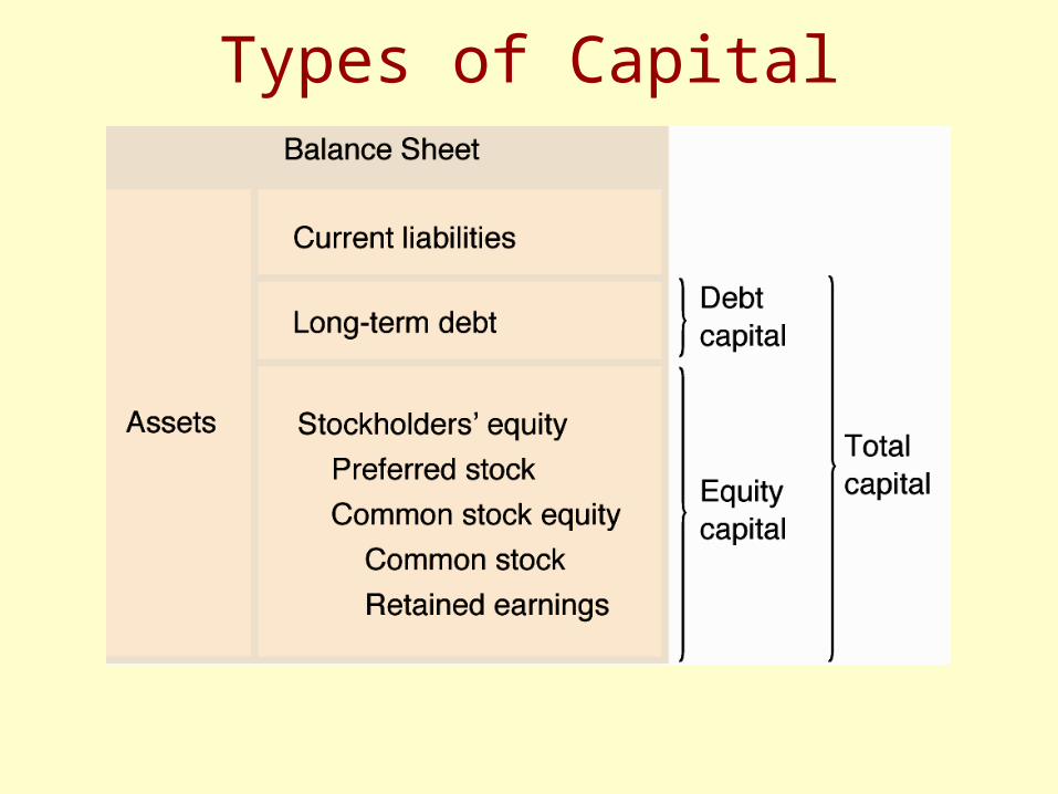
Types of Capital
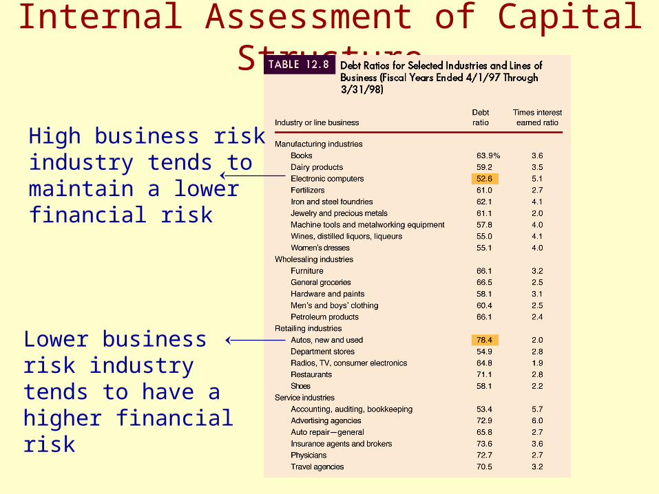
Internal Assessment of Capital Structure
High business risk industry tends to maintain a lower financial risk
Lower business risk industry tends to have a higher financial risk
Capital Structure of Non-U.S. Firms• In recent years, researchers have focused attention
not only on the capital structures of U.S. firms, but on
the capital structures of foreign firms as well.
• In general, non-U.S. companies have much higher
degrees of indebtedness than their U.S. counterparts.
• In most European and Pacific Rim countries, large
commercial banks are more actively involved in the
financing of corporate activity than has been true in
the U.S.
Capital Structure of Non-U.S. Firms• Furthermore, banks in these countries are permitted to
make large equity investments in non-financial
corporations -- a practice forbidden in the U.S.
• However, similarities also exist between U.S. firms
and their foreign counterparts.
• For example, the same industry patterns of capital
structure tend to be found around the world.
• In addition, the capital structures of U.S.-based MNCs
tend to be similar to those of foreign-based MNCs.
Capital Structure Theory• According to finance theory, firms possess a target
capital structure that will minimize its cost of capital.
• Unfortunately, theory can not yet provide financial
mangers with a specific methodology to help them
determine what their firm’s optimal capital structure
might be.
• Theoretically, however, a firm’s optimal capital
structure will just balance the benefits of debt
financing against its costs.
MM [ Modigliani and Miller(1958)]: capital structure irrelevancy
Capital Structure Theory• The major benefit of debt financing is the tax shield
provided by the federal government regarding interest payments.
• The costs of debt financing result from
– the increased probability of bankruptcy caused by debt obligations,
– the agency costs resulting from lenders monitoring the firm’s actions, and
– the costs associated with the firm’s managers having more information about the firm’s prospects than do investors (asymmetric information).
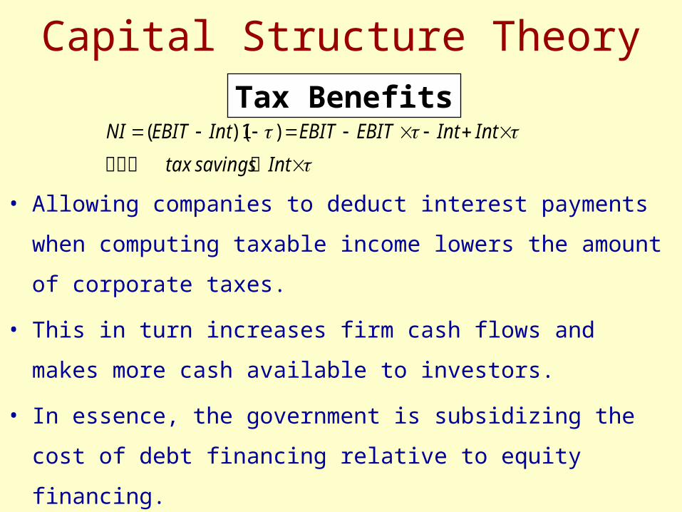
Capital Structure Theory
• Allowing companies to deduct interest payments when
computing taxable income lowers the amount of corporate
taxes.
• This in turn increases firm cash flows and makes more cash
available to investors.
• In essence, the government is subsidizing the cost of debt
financing relative to equity financing.
Tax Benefits
Intsavingstax
IntIntEBITEBITIntEBITNI
為每年的
)1)((
Capital Structure Theory
• The probability that debt obligations will lead to bankruptcy depends on the level of a company’s business risk and financial risk.
• Business risk is the risk to the firm of being unable to
cover operating costs.
• In general, the higher the firm’s fixed costs relative to variable costs, the greater the firm’s operating leverage and business risk.
• Business risk is also affected by revenue and cost
stability.
Probability of Bankruptcy
(1)
(2) (3)
Capital Structure Theory
• The firm’s capital structure - the mix between debt
versus equity - directly impacts financial leverage.
• Financial leverage measures the extent to which a firm
employs fixed cost financing sources such as debt and
preferred stock.
• The greater a firm’s financial leverage, the greater will
be its financial risk - the risk of being unable to meet
its fixed interest and preferred stock dividends.
Probability of Bankruptcy
Capital Structure Theory
• When a firm borrows funds by issuing debt, the
interest rate charged by lenders is based on the
lender’s assessment of the risk of the firm’s
investments.
• After obtaining the loan, the firm (stockholders/managers) could use the funds to invest in riskier assets.
• If these high risk investments pay off, the stockholders
benefit but the firm’s bondholders are locked in and
are unable to share in this success.
Agency Costs Imposed by Lenders
Capital Structure Theory
• To avoid this, lenders impose various monitoring costs
on the firm.
• Examples of these monitoring costs would include:
– raising the rate on future debt issues,
– denying future loan requests,
– imposing restrictive bond provisions.
Agency Costs Imposed by Lenders
Capital Structure Theory
• (1)Retained earnings
• (2)Debt
• (3)Equity
Pecking order
Note: Agency Costs Imposed by Stockholders
• As firms issue more stock, the ownership becomes more diffused and therefore separated from management.
• Manager has incentives to consume more perks and work less.• This will hurt the stockholders.• To avoid this, stockholders impose various monitoring costs
on the firm.
• Examples of these monitoring costs would include:
– establishing a more efficient director board, e.g., outside
director
– pressure from the SEC and CPA to closely monitor the
management,
– asking for more cash dividends.
Capital Structure Theory
• Asymmetric information results when managers of a
firm have more information about operations and
future prospects than do investors.
• Asymmetric information can impact the firm’s capital
structure as follows:
Asymmetric Information
Suppose management has identified an extremely lucrative investment opportunity and needs to raise capital. Based on this opportunity, management believes its stock is undervalued since the investors have no information about the investment.
Capital Structure Theory
• Asymmetric information results when managers of a
firm have more information about operations and
future prospects than do investors.
• Asymmetric information can impact the firm’s capital
structure as follows:
Asymmetric Information
In this case, management will raise the funds using debt since they believe/know the stock is undervalued (underpriced) given this information. In this case, the use of debt is viewed as a positive signal to investors regarding the firm’s prospects.
Capital Structure Theory
• Asymmetric information results when managers of a
firm have more information about operations and
future prospects than do investors.
• Asymmetric information can impact the firm’s capital
structure as follows:
Asymmetric Information
On the other hand, if the outlook for the firm is poor, management will issue equity instead since they believe/know that the price of the firm’s stock is overvalued (overpriced). Issuing equity is therefore generally thought of as a “negative” signal.
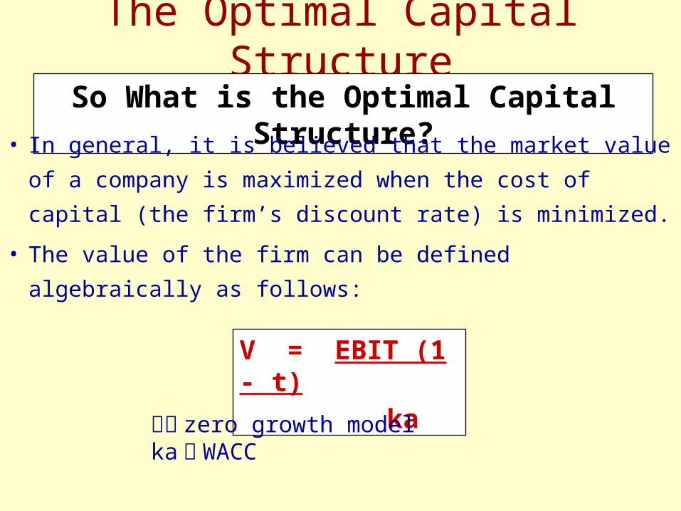
The Optimal Capital StructureSo What is the Optimal Capital Structure?
• In general, it is believed that the market value of a
company is maximized when the cost of capital (the
firm’s discount rate) is minimized.
• The value of the firm can be defined algebraically as
follows:V = EBIT (1 - t)
ka假設 zero growth model ka 為 WACC
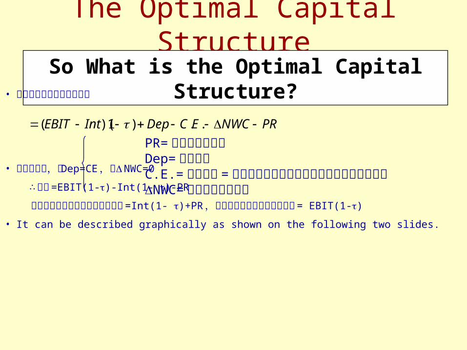
The Optimal Capital StructureSo What is the Optimal Capital Structure?
• 股東每年所享有之現金流量
• 假設不成長,則 Dep=CE ,且NWC=0
∴ 上式 =EBIT(1-)-Int(1- )-PR
至於債權人每年所享有之現金流量 =Int(1- )+PR ,所以整個公司每年的現金流量 = EBIT(1-)
• It can be described graphically as shown on the following two slides.
PRNWCECDepIntEBIT ..)1)(( PR= 本期攤還之本金Dep= 折舊費用C.E.= 資本支出 = 今年的機器廠房等固定資產比去年增加的部份NWC= 淨營運資金之改變
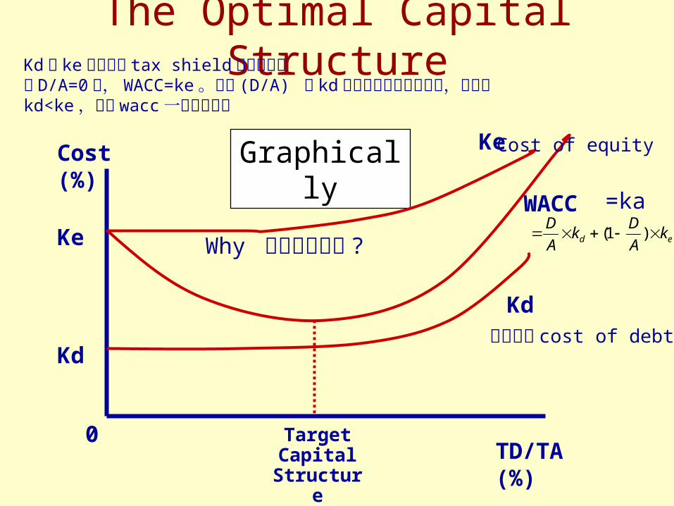
Graphically
Kd
Ke
WACC
Cost (%)
TD/TA (%)0 Target
Capital Structure
Ke
Kd
The Optimal Capital Structure
Cost of equity
=ka
為稅後的 cost of debt
Why 先下降再上升 ?
Kd 比 ke 低是因為 tax shield 以及求償權當 D/A=0 時, WACC=ke 。隨著 (D/A) 時 kd 所佔的比重也愈來愈大,但因為 kd<ke ,所以 wacc 一開始會下降
ed kA
Dk
A
D )1(
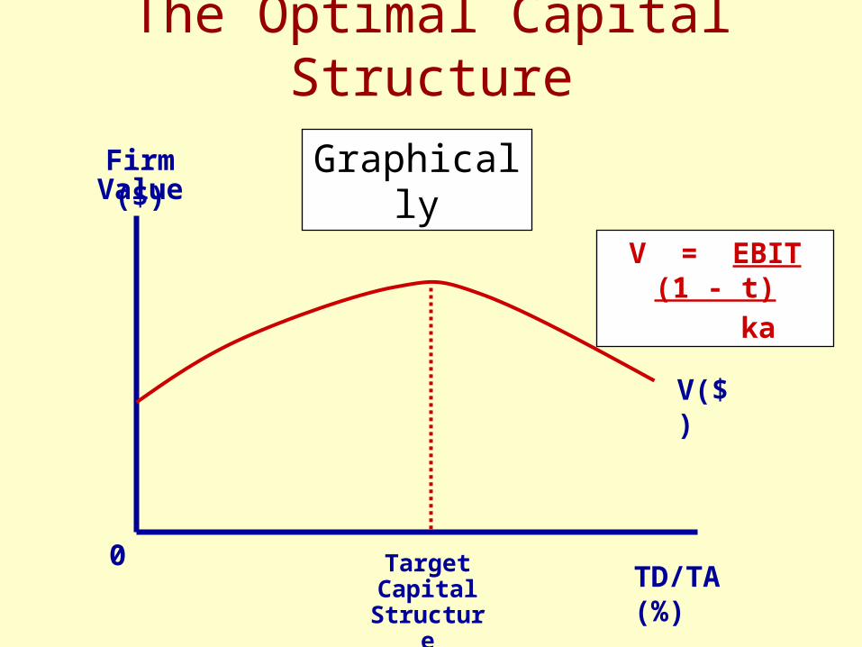
GraphicallyFirmValue ($)
TD/TA (%)0 Target
Capital Structure
V($)
V = EBIT (1 - t)
ka
The Optimal Capital Structure
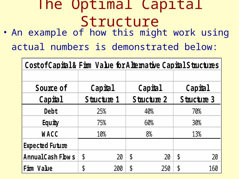
• An example of how this might work using actual
numbers is demonstrated below:
Source of Capital Capital CapitalCapital Structure 1 Structure 2 Structure 3
Debt 25% 40% 70%
Equity 75% 60% 30%
WACC 10% 8% 13%
Expected Future
Annual Cash Flows 20$ 20$ 20$
Firm Value 200$ 250$ 160$
Cost of Capital & Firm Value for Alternative Capital Structures
The Optimal Capital Structure
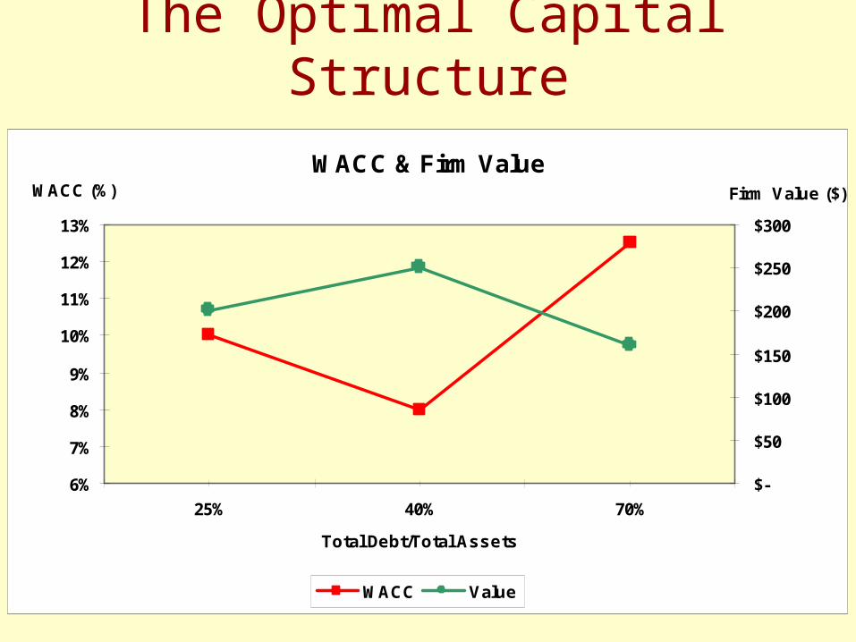
WACC & Firm Value
6%
7%
8%
9%
10%
11%
12%
13%
25% 40% 70%
Total Debt/Total Assets
WACC (%)
$-
$50
$100
$150
$200
$250
$300
Firm Value ($)
WACC Value
The Optimal Capital Structure
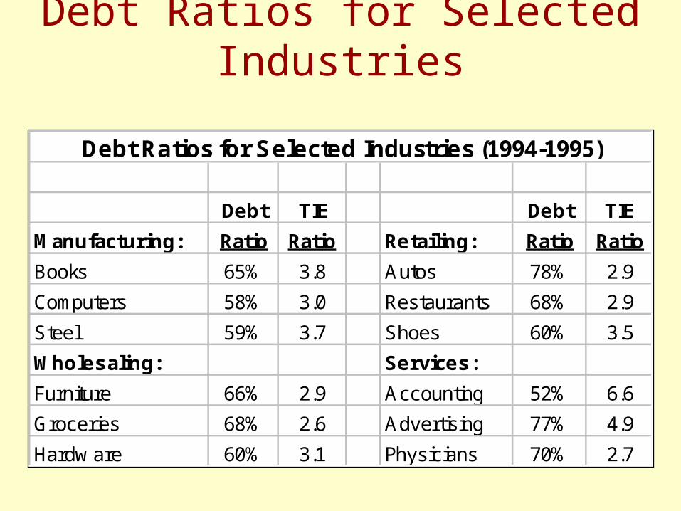
Debt TIE Debt TIE
Manufacturing: Ratio Ratio Retailing: Ratio Ratio
Books 65% 3.8 Autos 78% 2.9
Computers 58% 3.0 Restaurants 68% 2.9
Steel 59% 3.7 Shoes 60% 3.5
Wholesaling: Services:
Furniture 66% 2.9 Accounting 52% 6.6
Groceries 68% 2.6 Advertising 77% 4.9
Hardw are 60% 3.1 Physicians 70% 2.7
Debt Ratios for Selected Industries (1994-1995)
Debt Ratios for Selected Industries
EPS-EBIT Approach to Capital Structure
• The EPS-EBIT approach to capital structure involves
selecting the capital structure that maximizes EPS
over the expected range of EBIT.
• Using this approach, the emphasis is on maximizing
the owners returns (EPS).
• A major shortcoming of this approach is the fact that
earnings are only one of the determinants of
shareholder wealth maximization.
• This method does not explicitly consider the impact of
risk.
EPS-EBIT Approach to Capital Structure
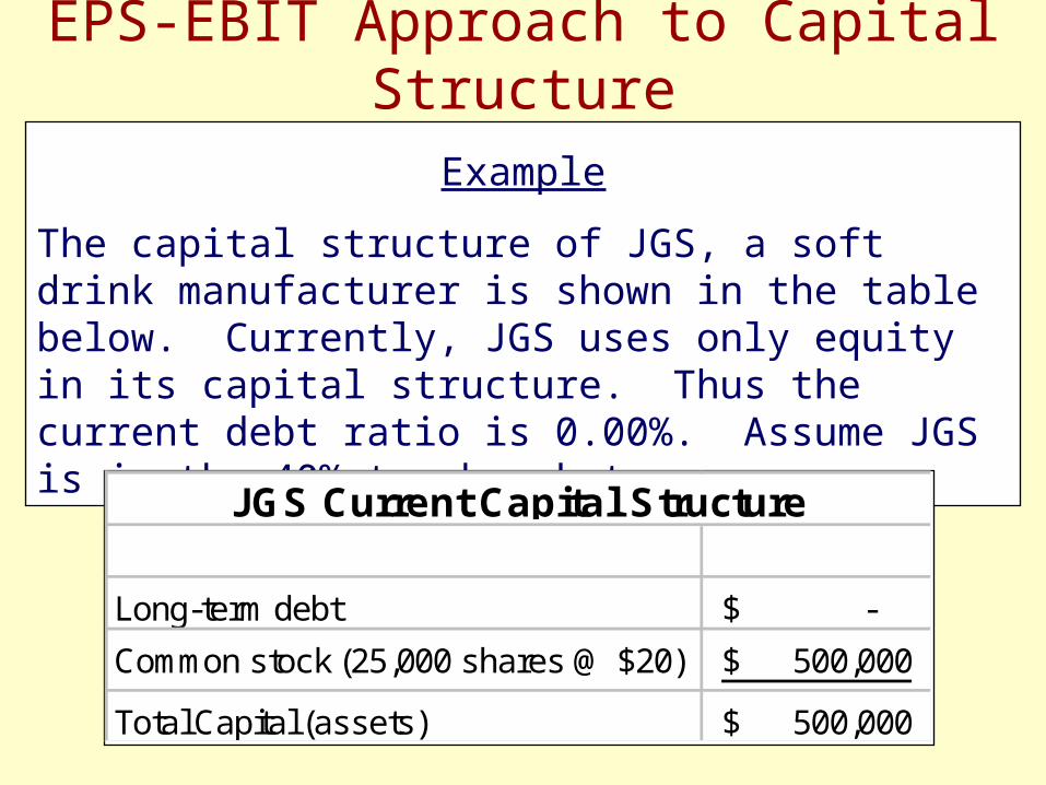
Example
The capital structure of JGS, a soft drink manufacturer is shown in the table below. Currently, JGS uses only equity in its capital structure. Thus the current debt ratio is 0.00%. Assume JGS is in the 40% tax bracket.
Long-term debt -$
Common stock (25,000 shares @ $20) 500,000$
Total Capital (assets) 500,000$
JGS Current Capital Structure
EPS-EBIT Approach to Capital Structure
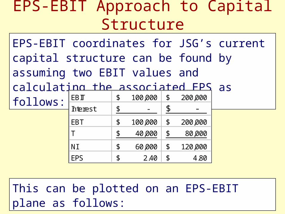
EPS-EBIT coordinates for JSG’s current capital structure can be found by assuming two EBIT values and calculating the associated EPS as follows:
EBIT 100,000$ 200,000$
Interest -$ -$
EBT 100,000$ 200,000$
T 40,000$ 80,000$
NI 60,000$ 120,000$
EPS 2.40$ 4.80$
This can be plotted on an EPS-EBIT plane as follows:
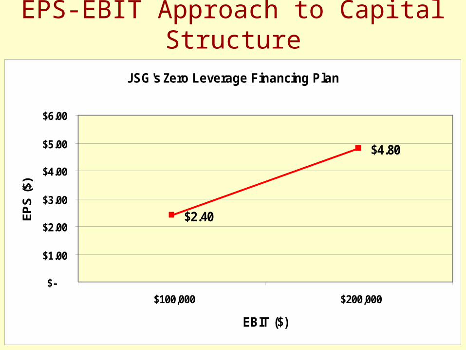
EPS-EBIT Approach to Capital Structure
JSG's Zero Leverage Financing Plan
$2.40
$4.80
$-
$1.00
$2.00
$3.00
$4.00
$5.00
$6.00
$100,000 $200,000
EBIT ($)
EP
S (
$)
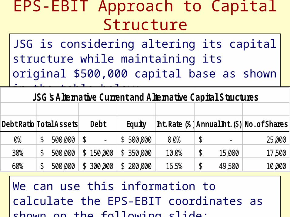
EPS-EBIT Approach to Capital Structure
JSG is considering altering its capital structure while maintaining its original $500,000 capital base as shown in the table below:
Debt Ratio Total Assets Debt Equity Int. Rate (%) Annual Int. ($) No. of Shares
0% 500,000$ -$ 500,000$ 0.0% -$ 25,000
30% 500,000$ 150,000$ 350,000$ 10.0% 15,000$ 17,500
60% 500,000$ 300,000$ 200,000$ 16.5% 49,500$ 10,000
JSG's Alternative Current and Alternative Capital Structures
We can use this information to calculate the EPS-EBIT coordinates as shown on the following slide:
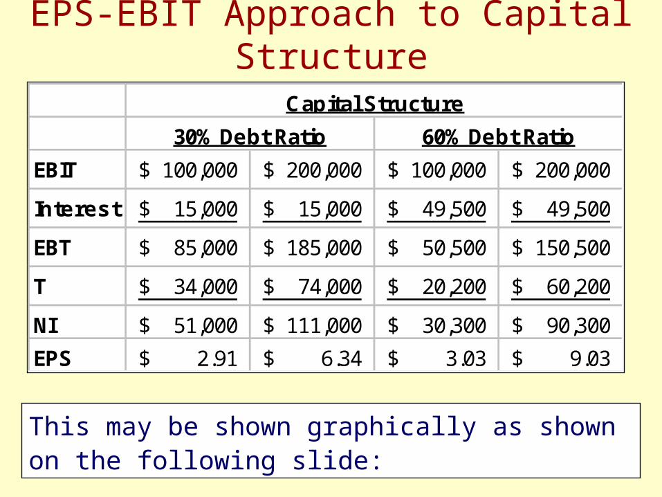
EPS-EBIT Approach to Capital Structure
EBIT 100,000$ 200,000$ 100,000$ 200,000$
Interest 15,000$ 15,000$ 49,500$ 49,500$
EBT 85,000$ 185,000$ 50,500$ 150,500$
T 34,000$ 74,000$ 20,200$ 60,200$
NI 51,000$ 111,000$ 30,300$ 90,300$
EPS 2.91$ 6.34$ 3.03$ 9.03$
30% Debt Ratio 60% Debt Ratio
Capital Structure
This may be shown graphically as shown on the following slide:
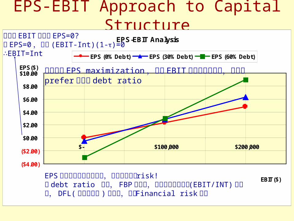
EPS-EBIT Approach to Capital StructureEPS-EBIT Analysis
($4.00)
($2.00)
$0.00
$2.00
$4.00
$6.00
$8.00
$10.00
$- $100,000 $200,000
EBIT($)
EPS($)
EPS (0% Debt) EPS (30% Debt) EPS (60% Debt)
若目標為 EPS maximization ,則當 EBIT 在不同的區間時,公司會 prefer 不同的 debt ratio
EPS 極大化並不是個好目標,因為並未考慮 risk!如 debt ratio 愈大, FBP 就愈大,同時利息保障倍數 (EBIT/INT) 就愈小, DFL( 上圖之斜率 ) 就愈大,所以 Financial risk 愈高
多少的 EBIT 會使得 EPS=0?令 EPS=0 ,所以 (EBIT-Int)(1-)=0∴EBIT=Int
Basic Shortcoming of EPS-EBIT Analysis
• Although EPS maximization is generally good for the
firm’s shareholders, the basic shortcoming of this
method is that it does not necessary maximize
shareholder wealth because it fails to consider risk.
• If shareholders did not require risk premiums
(additional return) as the firm increased its use of debt,
a strategy focusing on EPS maximization would work.
• Unfortunately, this is not the case.
Choosing the Optimal Capital Structure• The following discussion will attempt to create a framework
for making capital budgeting decisions that maximizes
shareholder wealth -- i.e., considers both risk and return.
• Perhaps the best way to demonstrate this is through the
following example:
Assume that JSG is attempting to choose the best of several alternative capital structures -- specifically, debt ratios of 0, 10, 20, 30, 40, 50, and 60 percent. Furthermore, for each of these capital structures, the firm has estimated EPS, the CV of EPS, and required return
Choosing the Optimal Capital Structure
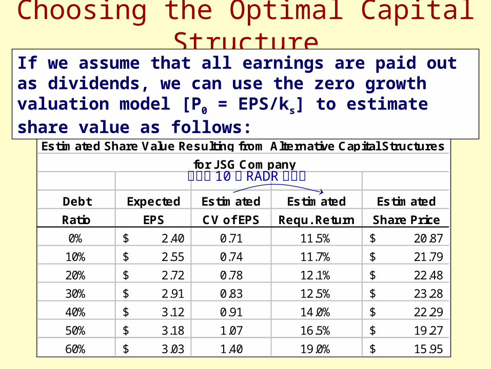
Debt Expected Estimated Estimated Estimated
Ratio EPS CV of EPS Requ. Return Share Price
0% 2.40$ 0.71 11.5% 20.87$
10% 2.55$ 0.74 11.7% 21.79$
20% 2.72$ 0.78 12.1% 22.48$
30% 2.91$ 0.83 12.5% 23.28$
40% 3.12$ 0.91 14.0% 22.29$
50% 3.18$ 1.07 16.5% 19.27$
60% 3.03$ 1.40 19.0% 15.95$
Estimated Share Value Resulting from Alternative Capital Structures
for JSG Company
If we assume that all earnings are paid out as dividends, we can use the zero growth valuation model [P0 = EPS/ks] to estimate share value as follows:
類似第 10 章 RADR 的方式
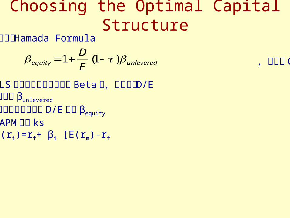
Choosing the Optimal Capital Structure另一個方法為使用 Hamada Formula
,再放入 CAPM
1. 先以 OLS 迴歸估出某公司股票之 Beta 值,並找出其 D/E2. 利用上式估出 βunlevered
3. 再次利用上式找出在不同 D/E 時的 βequity
4. 代入 CAPM 求出 ksE(ri)=rf+ βi [E(rm)-rf
unleveredequity E
D )1(1
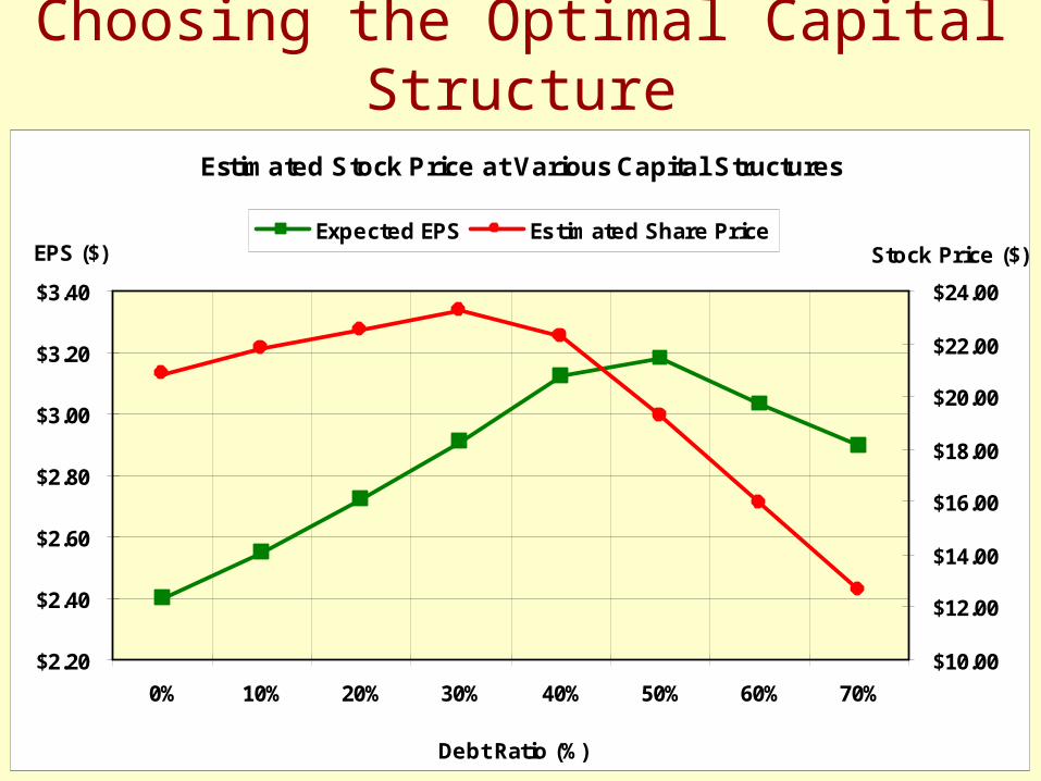
Choosing the Optimal Capital Structure
Estimated Stock Price at Various Capital Structures
$2.20
$2.40
$2.60
$2.80
$3.00
$3.20
$3.40
0% 10% 20% 30% 40% 50% 60% 70%
Debt Ratio (%)
EPS ($)
$10.00
$12.00
$14.00
$16.00
$18.00
$20.00
$22.00
$24.00
Stock Price ($)Expected EPS Estimated Share Price
Flexibility
Maintaining financial flexibility simply means that a
company would like to give itself slack in terms of
being able to raise additional capital to support
working capital requirements if desirable investment
opportunities arise.
Other Influences on Capital Structure Choice
As a result, most firms try to ensure that they have
excess borrowing capacity available by keeping debt
levels at manageable levels.
Timing
The sale of securities by most firms depend not only
on the investment opportunities available but also on
the the cost of capital at a particular point in time.
Successful companies usually try to forecast and
take advantage of changing market conditions to
lower their overall cost of raising funds.
Other Influences on Capital Structure Choice
利率高:發股票
利率低:舉債
Corporate Control
Many firms avoid the issuance of new equity
because it may cause existing controlling
shareholders to lose their ability to influence the
direction of the company.
As a result, most companies are reluctant to issue
new shares of stock and instead issue debt when
additional funds are needed.
Other Influences on Capital Structure Choice
Maturity Matching
Many firms also try to match the maturity of their
source of financing with the maturity of the assets
they are using the funds to finance. As a result, the
capital structure of a firm is determined in part by the
types of investments it makes.
Other Influences on Capital Structure Choice
Management’s Attitude Toward Risk
Management’s perception about the risk of using
debt versus equity to finance assets will also
determine the nature of a company’s capital
structure.
Other Influences on Capital Structure Choice
這些 factors 都會影響 management 決定要舉多少債 ?
External risk assessment: 債權人及信用評等機構對公司的信用風險評估Contractual obligation: 如債權保護條款Business risk