Embed Size (px)
Citation preview


Principles of LaserSpectroscopy andQuantum Optics

This page intentionally left blank
Principles of LaserSpectroscopy andQuantum Optics
Paul R. BermanVladimir S. Malinovsky
PRINCETON UNIVERSITY PRESS . PRINCETON AND OXFORD
Copyright c© 2011 by Princeton University PressPublished by Princeton University Press, 41 William Street,Princeton, New Jersey 08540
In the United Kingdom: Princeton University Press, 6 Oxford Street,Woodstock, Oxfordshire OX20 1TWpress.princeton.edu
All Rights Reserved
Library of Congress Cataloging-in-Publication DataBerman, Paul R., 1945–Principles of laser spectroscopy and quantum optics / Paul R. Berman,Vladimir S. Malinovsky.
p. cm.Includes bibliographical references and index.ISBN 978-0-691-14056-8 (hardback : alk. paper) 1. Quantum optics.2. Laser spectroscopy. I. Malinovsky, Vladimir S., 1962– II. Title.QC446.2.B45 2011535′.15—dc22 2010014005
British Library Cataloging-in-Publication Data is available
This book has been composed in SabonPrinted on acid-free paper. ∞
Typeset by S R Nova Pvt Ltd, Bangalore, IndiaPrinted in the United States of America
10 9 8 7 6 5 4 3 2 1

To the memory of
Belle and Solomon Berman
To the memory of
Antonida Malinovskaya and Sergey Bortkevich

This page intentionally left blank
Contents
Preface xv
1 Preliminaries 11.1 Atoms and Fields 11.2 Important Parameters 21.3 Maxwell’s Equations 41.4 Atom–Field Hamiltonian 71.5 Dirac Notation 81.6 Where Do We Go from Here? 91.7 Appendix: Atom–Field Hamiltonian 10
Problems 13References 14Bibliography 15
2 Two-Level Quantum Systems 172.1 Review of Quantum Mechanics 17
2.1.1 Time-Independent Problems 172.1.2 Time-Dependent Problems 19
2.2 Interaction Representation 212.3 Two-Level Atom 232.4 Rotating-Wave or Resonance Approximation 25
2.4.1 Analytic Solutions 282.5 Field Interaction Representation 322.6 Semiclassical Dressed States 36
2.6.1 Adiabatic Following 392.7 General Remarks on Solution of the Matrix Equation
y(t) = A(t)y(t) 422.7.1 Perturbation Theory 432.7.2 Adiabatic Approximation 432.7.3 Magnus Approximation 43
2.8 Summary 452.9 Appendix A: Representations 45
2.9.1 Relationships between the Representations 462.10 Appendix B: Spin Half Quantum System in a Magnetic Field 47
2.10.1 Analytic Solutions—Magnetic Case 48Problems 50References 54Bibliography 55
viii CONTENTS
3 Density Matrix for a Single Atom 563.1 Density Matrix 563.2 Interaction Representation 623.3 Field Interaction Representation 633.4 Semiclassical Dressed States 663.5 Bloch Vector 67
3.5.1 No Relaxation 703.5.2 Relaxation Included 74
3.6 Summary 753.7 Appendix A: Density Matrix Equations in the Rotating-Wave
Approximation 753.7.1 Schrödinger Representation 753.7.2 Interaction Representation 763.7.3 Field Interaction Representation 763.7.4 Bloch Vector 763.7.5 Semiclassical Dressed-State Representation 77
3.8 Appendix B: Collision Model 78Problems 80References 81Bibliography 82
4 Applications of the Density Matrix Formalism 834.1 Density Matrix for an Ensemble 834.2 Absorption Coefficient—Stationary Atoms 854.3 Simple Inclusion of Atomic Motion 914.4 Rate Equations 954.5 Summary 96
Problems 97References 98Bibliography 98
5 Density Matrix Equations: Atomic Center-of-Mass Motion,Elementary Atom Optics, and Laser Cooling 995.1 Introduction 995.2 Atom in a Single Plane-Wave Field 1005.3 Force on an Atom 101
5.3.1 Plane Wave 1025.3.2 Focused Plane Wave: Atom Trapping 1035.3.3 Standing-Wave Field: Laser Cooling 105
5.4 Summary 1095.5 Appendix: Quantization of the Center-of-Mass Motion 110
5.5.1 Coordinate Representation 1105.5.2 Momentum Representation 1125.5.3 Sum and Difference Representation 1135.5.4 Wigner Representation 113
Problems 115References 118Bibliography 119
CONTENTS ix
6 Maxwell-Bloch Equations 1206.1 Wave Equation 120
6.1.1 Pulse Propagation in a Linear Medium 1216.2 Maxwell-Bloch Equations 123
6.2.1 Slowly Varying Amplitude and Phase Approximation(SVAPA) 124
6.3 Linear Absorption and Dispersion—Stationary Atoms 1256.4 Linear Pulse Propagation 1286.5 Other Problems with the Maxwell-Bloch Equations 1296.6 Summary 1306.7 Appendix: Slowly Varying Amplitude and Phase
Approximation—Part II 130Problems 134Bibliography 135
7 Two-Level Atoms in Two or More Fields: Introduction toSaturation Spectroscopy 1367.1 Two-Level Atoms and N Fields—Third-Order Perturbation
Theory 1367.1.1 Zeroth Order 1387.1.2 First Order 1387.1.3 Second Order 1397.1.4 Third Order 139
7.2 N= 2: Saturation Spectroscopy for Stationary Atoms 1417.3 N= 2: Saturation Spectroscopy for Moving Atoms in
Counterpropagating Fields—Hole Burning 1447.3.1 Hole Burning and Atomic Population Gratings 1447.3.2 Probe Field Absorption 146
7.4 Saturation Spectroscopy in Inhomogeneously Broadened Solids 1497.5 Summary 1517.6 Appendix A: Saturation Spectroscopy—Stationary Atoms in One
Strong and One Weak Field 1517.7 Appendix B: Four-Wave Mixing 153
Problems 155References 157Bibliography 157
8 Three-Level Atoms: Applications to NonlinearSpectroscopy—Open Quantum Systems 1598.1 Hamiltonian for , V, and Cascade Systems 159
8.1.1 Cascade Configuration 1618.1.2 V and Configurations 1628.1.3 All Configurations 163
8.2 Density Matrix Equations in the Field InteractionRepresentation 163
8.3 Steady-State Solutions—Nonlinear Spectroscopy 165
x CONTENTS
8.3.1 Stationary Atoms 1698.3.2 Moving Atoms: Doppler Limit 169
8.4 Autler-Townes Splitting 1728.5 Two-Photon Spectroscopy 1768.6 Open versus Closed Quantum Systems 1788.7 Summary 179
Problems 179References 182Bibliography 182
9 Three-Level Atoms: Dark States, Adiabatic Following,and Slow Light 1849.1 Dark States 1849.2 Adiabatic Following—Stimulated Raman Adiabatic Passage 1889.3 Slow Light 1919.4 Effective Two-State Problem for the Configuration 1969.5 Summary 1989.6 Appendix: Force on an Atom in the Configuration 199
Problems 200References 202Bibliography 203
10 Coherent Transients 20610.1 Coherent Transient Signals 20610.2 Free Polarization Decay 210
10.2.1 Homogeneous Broadening 21010.2.2 Inhomogeneous Broadening 212
10.3 Photon Echo 21410.4 Stimulated Photon Echo 21910.5 Optical Ramsey Fringes 22210.6 Frequency Combs 22510.7 Summary 22810.8 Appendix A: Transfer Matrices in Coherent Transients 22910.9 Appendix B: Optical Ramsey Fringes in Spatially Separated
Fields 231Problems 235References 237Bibliography 240
11 Atom Optics and Atom Interferometry 24211.1 Review of Kirchhoff-Fresnel Diffraction 242
11.1.1 Electromagnetic Diffraction 24211.1.2 Quantum-Mechanical Diffraction 246
11.2 Atom Optics 24811.2.1 Scattering by an Amplitude Grating 25011.2.2 Scattering by Periodic Structures—Talbot Effect 25311.2.3 Scattering by Phase Gratings—Atom Focusing 254

CONTENTS xi
11.3 Atom Interferometry 26311.3.1 Microfabricated Elements 26611.3.2 Counterpropagating Optical Field Elements 267
11.4 Summary 274Problems 275References 277Bibliography 279
12 The Quantized, Free Radiation Field 28012.1 Free-Field Quantization 28012.2 Properties of the Vacuum Field 283
12.2.1 Single-Photon State 28412.2.2 Single-Mode Number State 28512.2.3 Quasiclassical or Coherent States 286
12.3 Quadrature Operators for the Field 29112.3.1 Pure n State 29212.3.2 Coherent State 293
12.4 Two-Photon Coherent States or Squeezed States 29312.4.1 Calculation of UL(z) 296
12.5 Phase Operator 29812.6 Summary 30012.7 Appendix: Field Quantization 300
12.7.1 Reciprocal Space 30212.7.2 Longitudinal and Transverse Vector Fields 30312.7.3 Transverse Electromagnetic Field 30412.7.4 Free Field 308
Problems 308References 310Bibliography 311
13 Coherence Properties of the Electric Field 31213.1 Coherence: Some General Concepts 312
13.1.1 Time versus Ensemble Averages 31213.1.2 Classical Fields 31413.1.3 Quantized Fields 314
13.2 Classical Fields: Correlation Functions 31513.2.1 First-Order Correlation Function 31513.2.2 Young’s Fringes 31913.2.3 Intensity Correlations—Second-Order Correlation
Function 32213.2.4 Hanbury Brown and Twiss Experiment 325
13.3 Quantized Fields: Density Matrix for the Field and PhotonOptics 32613.3.1 Coherent State 32713.3.2 Thermal State 32813.3.3 P(α) Distribution 32913.3.4 Correlation Functions for the Field 330
13.4 Summary 336
xii CONTENTS
Problems 336References 337Bibliography 338
14 Photon Counting and Interferometry 33914.1 Photodetection 339
14.1.1 Photodetection of Classical Fields 34014.1.2 Photodetection of Quantized Fields 343
14.2 Michelson Interferometer 34614.2.1 Classical Fields 34714.2.2 Quantized Fields 349
14.3 Summary 355Problems 355References 357Bibliography 357
15 Atom–Quantized Field Interactions 35815.1 Interaction Hamiltonian and Equations of Motion 358
15.1.1 Schrödinger Representation 35815.1.2 Heisenberg Representation 35915.1.3 Hamiltonian 36015.1.4 Jaynes-Cummings Model 363
15.2 Dressed States 36715.3 Generation of Coherent and Squeezed States 371
15.3.1 Coherent States 37115.3.2 Squeezed States 372
15.4 Summary 372Problems 373References 374Bibliography 374
16 Spontaneous Decay 37516.1 Spontaneous Decay Rate 37516.2 Radiation Pattern and Repopulation of the Ground State 382
16.2.1 Radiation Pattern 38316.2.2 Repopulation of the Ground State 387
16.3 Summary 38916.4 Appendix A: Circular Polarization 38916.5 Appendix B: Radiation Pattern 392
16.5.1 Unpolarized Initial State 39516.5.2 z-Polarized Excitation 39516.5.3 Other than z-Polarized Excitation 397
16.6 Appendix C: Quantum Trajectory Approach to SpontaneousDecay 397
Problems 399References 401Bibliography 401
CONTENTS xiii
17 Optical Pumping and Optical Lattices 40217.1 Optical Pumping 402
17.1.1 Traveling-Wave Fields 40317.1.2 z-Polarized Excitation 40717.1.3 Irreducible Tensor Basis 40917.1.4 Standing-Wave and Multiple-Frequency Fields 411
17.2 Optical Lattice Potentials 41417.3 Summary 41717.4 Appendix: Irreducible Tensor Formalism 417
17.4.1 Coupled Tensors 41717.4.2 Density Matrix Equations 418
Problems 420References 421Bibliography 421
18 Sub-Doppler Laser Cooling 42218.1 Cooling via Field Momenta Exchange and Differential
Scattering 42318.1.1 Counterpropagating Fields 425
18.2 Sisyphus Picture of the Friction Force for a G = 1/2 GroundState and Crossed-Polarized Fields 433
18.3 Coherent Population Trapping 43618.4 Summary 43718.5 Appendix: Fokker-Planck Approach for Obtaining the Friction
Force and Diffusion Coefficients 43718.5.1 Fokker-Planck Equation 43718.5.2 G= 1/2; lin⊥lin Polarization 44118.5.3 G= 1 to H = 2 Transition; σ+ − σ− Polarization 44318.5.4 Equilibrium Energy 445
Problems 449References 451Bibliography 452
19 Operator Approach to Atom–Field Interactions:Source-Field Equation 45319.1 Single Atom 454
19.1.1 Single-Mode Field 45419.1.2 General Problem—n Field Modes 456
19.2 N-Atom Systems 46019.3 Source-Field Equation 46119.4 Source-Field Approach: Examples 465
19.4.1 Average Field and Field Intensity in SpontaneousEmission 466
19.4.2 Frequency Beats in Emission: Quantum Beats 46719.4.3 Four-Wave Mixing 46819.4.4 Linear Absorption 469
19.5 Summary 470
xiv CONTENTS
Problems 470References 472Bibliography 472
20 Light Scattering 47420.1 General Considerations: Perturbation Theory 47520.2 Mollow Triplet 479
20.2.1 Dressed-State Approach to Mollow Triplet 48320.2.2 Source-Field Approach to Mollow Triplet 485
20.3 Second-Order Correlation Function for theRadiated Field 486
20.4 Scattering by a Single Atom in Weak Fields: G = 0 48720.5 Summary 488
Problems 489References 490Bibliography 490
21 Entanglement and Spin Squeezing 49221.1 Entanglement by Absorption 49321.2 Entanglement by Post-Selection—DLCZ Protocol 49821.3 Spin Squeezing 499
21.3.1 General Considerations 50021.3.2 Spin Squeezing Using a Coherent Cavity Field 502
21.4 Summary 505Problems 505References 506Bibliography 507
Index 509
Preface
This book is based on a course that has been given by one of us (PRB) for moreyears than he would like to admit. The basic subject matter of the book is theinteraction of optical fields with atoms. This book is divided roughly into two parts.In the first half of the book, fields are treated classically, while atoms are describedusing quantum mechanics. In the context of this semiclassical theory of matter–fieldinteractions, we establish the basic formalism of the theory and go on to discussseveral applications. Most of the applications can be grouped under the generalheading of laser spectroscopy, although both atom optics and atom interferometryare discussed as well. An emphasis is placed on introducing the physical conceptsone encounters in considering the interaction of radiation with matter. In the secondhalf of this book, the electromagnetic field is quantized, and problems are discussedin which it is necessary to use a fully quantized picture of matter–field interactions.Spontaneous emission is a prototypical problem in which a quantized field approachis needed. We examine in detail the radiation pattern and atomic dynamics thataccompany spontaneous emission. An extension of this work to optical pumping,sub-Doppler laser cooling, and light scattering is also included.
This book is intended to serve a dual purpose. First and foremost, it can be usedas a text in a course that follows an introductory graduate-level quantum mechanicscourse. There is undoubtedly too much material in the book for a one-semestercourse, but the core of a one-semester course could include chapters 1 to 8, 10, 12 to16, and 19. The heart of this book is chapters 2 and 3, where the basic formalism isintroduced for both atomic state amplitudes and density matrix elements. Chapterson slow light, atom optics and interferometry, optical pumping, sub-Doppler lasercooling, light scattering, and entanglement can be added as time permits. The secondpurpose of this book is to provide a reference for graduate students and othersworking in atomic, molecular, and optical physics.
There are many excellent texts available that cover the fields of laser spectroscopyand quantum optics. While presenting topics that are covered in many of these texts,we try to complement the approaches that have been given by other authors. Inparticular, we give a detailed description of different representations that can be usedto analyze problems involving matter–field interactions. A semiclassical dressed-state basis is also defined that allows us to effectively solve problems involvingstrong fields. The chapters on atom optics and interferometry, optical pumping,light scattering, and sub-Doppler laser cooling offer material that may not bereadily available in other introductory texts. The advantages and use of irreducibletensor formalism are explained and encouraged. On the other hand, we discuss
xvi PREFACE
only briefly, or not at all, such topics as superradiance, laser theory, bistability,nonlinear optics, Bose condensates, and pulse propagation. To keep this book toa manageable size, we chose to concentrate on a limited number of fundamentalapplications. Moreover, although references to experimental results are given, thereis no reproduction of experimental data.
Each chapter contains a problems section. The problems are an integral part ofany course based on this book. They extend and illustrate the material presentedin the text. Many of the problems are far from trivial, requiring an intensive effort.Students who work through these problems will be rewarded with an improvedunderstanding of matter–field interactions. Many problems require the students touse computational techniques. We plan to post Mathematica notebooks that containalgorithms for some of the calculations needed in the problems on the websiteassociated with this book (http://press.princeton.edu/titles/9376.html). Moreover,we will use the website to post errata, offer additional problems, and discuss anytopics that have been brought up by readers.
We would like to thank Yvan Castin, Bill Ford, Galina Khitrova, Jean-Louis LeGouët, Rodney Louden, Hal Metcalf, Peter Milonni, Ignacio Sola, and Kelly Youngefor their helpful comments. PRB would especially like to acknowledge the manydiscussions he had with Duncan Steel on topics contained in this book, as well ashis encouragement in the endeavor of writing this text. We would also like to thankBoris Dubetsky for a careful reading and his critique of chapters 10 and 11 andMichael Martin and Jun Ye for their comments on section 10.3.
Last, but not least, we benefited from the continual support of our wives (Debraand Svetlana) and families.
Ann Arbor, MI; Hoboken, NJ Paul BermanJune 2010 Vladimir Malinovsky

Principles of LaserSpectroscopy andQuantum Optics

This page intentionally left blank
1Preliminaries
1.1 Atoms and Fields
As any worker knows, when you come to a job, you have to have the proper toolsto get the job done right. More than that, you must come to the job with the properattitude and a high set of standards. The idea is not simply to get the job done but toachieve an end result of which you can be proud. You must be content with knowingthat you are putting out your best possible effort. Physics is an extraordinarilydifficult “job.” To understand the underlying physical origin of many seeminglysimple processes is sometimes all but impossible. Yet the satisfaction that one gets inarriving at that understanding can be exhilarating. In this book, we hope to provide afoundation on which you can build a working knowledge of atom–field interactions,with specific applications to linear and nonlinear spectroscopy. Among the topics tobe discussed are absorption, emission and scattering of light, the mechanical effectsof light, and quantum properties of the radiation field.
This book is divided roughly into two parts. In the first part, we examine theinteraction of classical electromagnetic fields with quantum-mechanical atoms. Theexternal fields, such as laser fields, can be monochromatic, quasi-monochromatic,or pulsed in nature, and can even contain noise, but any quantum noise effectsassociated with the fields are neglected. Theories in which the fields are treatedclassically and the atoms quantum-mechanically are often referred to as semiclassicaltheories. For virtually all problems in laser spectroscopy, the semiclassical approachis all that is needed. Processes such as the photoelectric effect and Comptonscattering, which are often offered as evidence for photons and the quantum natureof the radiation field can, in fact, be explained rather simply with the use of classicalexternal fields. The price one pays in the semiclassical approach is the use of atime-dependent Hamiltonian for which the energy is no longer a constant of themotion.
Although the semiclassical approach is sufficient for a wide range of problems,it is not always possible to consider optical fields as classical in nature. One mightask when such quantum optics effects begin to play a role. Atoms are remarkabledevices. If you place an atom in an excited state, it radiates a uniquely quantum-type
2 CHAPTER 1
field, the one-photon state. One of the authors (PRB) is a former student ofWillis Lamb, who claimed that it should be necessary for people to apply fora license before they can use the word photon. Lamb was not opposed to theidea of a quantized field mode, but he felt that the word photon was misusedon a regular basis. We will try to explain the distinction between a one-photonfield and a photon when we begin our discussion of the quantized radiationfield.
The field radiated by an atom in an excited state has a uniquely quantumcharacter. In fact, any field in which the average value of the number operatorfor the field (average number of photons in the field) is less than or on the orderof the number of atoms with which the field interacts must usually be treatedusing a quantized field approach. Thus, the second, or quantum optics, part ofthis book incorporates a fully quantized approach, one in which both the atomsand the fields are treated as quantum-mechanical entities. The advantage of usingquantized fields is that one recovers a Hamiltonian that is perfectly Hermitian andindependent of time. The most common quantum optics effects are those associatedwith spontaneous emission, scattering of external fields by atoms, quantum noise,and cavity quantum electrodynamics. There is another class of problems related toquantized field effects involving van der Waals forces and Casimir effects, but we donot discuss these in any detail [1].
1.2 Important Parameters
Why did the invention of the laser cause such a revolution in physics? Laser fieldsdiffer from conventional optical sources in their coherence properties and intensity.In this book, we look at applications that exploit the coherence properties of lasers,although complementary textbooks could be written in which the emphasis is onstrong field–matter interactions. Moreover, we touch only briefly on the currentadvances in atto-second science that have been enabled using nonlinear atom–fieldinteractions. Even if we deal mainly with the coherence properties of the fields, ourplate is quite full. Historically, the coherence properties of optical fields have beenone of the limiting factors in determining the ultimate resolution one can achievein characterizing the transition frequencies of atomic, molecular, and condensedphase systems. It will prove useful to list some of the relevant frequencies that oneencounters in considering such problems.
First and foremost are the transition frequencies themselves. We focus mainlyon optical transitions in this text, for which the transition frequencies are of orderω0/2π 5 × 10¹⁴ Hz. The laser fields needed to probe such transitions must havecomparable frequencies. The first gas and solid-state lasers had a very limited rangeof tunability, but the invention of the dye laser allowed for an expanded rangeof tunability in the visible part of the spectrum. One might even go so far as tosay that it was the dye laser that really launched the field of laser spectroscopy.Since that time, the development of tunable semiconductor-based and titanium-sapphire lasers operating at infrared frequencies, combined with frequency doublers(nonlinear optical crystals) and frequency dividers (optical parametric amplifiers andoscillators), has enabled the creation of tunable coherent sources over a wide rangeof frequencies from the ultraviolet to the far-infrared.
PRELIMINARIES 3
Assuming for the moment that such sources are nearly monochromatic (typicalline widths range from kHz to GHz), there are still underlying processes that limitthe resolution one can achieve using laser sources to probe atoms. In other words,suppose that two transition frequencies in an atom differ by an amount f . Whatis the minimum value of f for which the transitions can be resolved? The ultimatelimiting factor for any transition is the natural width associated with that transition.The natural width arises from interactions of atoms with the vacuum radiationfield, leading to spontaneous emission. Typical natural widths for allowed opticaltransitions are in the range γ2/2π 107 − 108 Hz, where γ2 is a spontaneousemission decay rate. For “forbidden” transitions, such as those envisioned as thebasis for optical frequency standards, natural line widths can be as small as a Hzor so. The fact that an allowed transition has a natural width equal to 108 Hz doesnot imply that the transition frequency can be determined only to this accuracy. Byfitting experimental line shapes to theory, one can hope to reduce this resolution bya factor of 100 or more.
The natural width is referred to as a homogeneous width since it is the same for allatoms in a sample and cannot be circumvented. Another example of a homogeneouswidth in a vapor is the collision line width that arises as a result of energy shifts ofatomic levels that occur during collisions. If the collision duration (typically of order5 ps) is much less than all relevant timescales in the problem, except the opticalperiod, then collisions add a homogeneous width of order 10MHz per Torr ofperturber gas pressure [1Torr = (1/760) atm ≈ 133Pa ≈ 1mmHg]. This width isoften referred to as a pressure broadening width.
Even if there are no collisions in a vapor, linear absorption or emission line shapescan be broadened by an inhomogeneous line broadening mechanism, as was firstappreciated by Maxwell [2]. In a vapor, the moving atoms are characterized by avelocity distribution. As viewed in the laboratory frame, any radiation emitted by anatom is Doppler shifted by an amount (ω0/2π )(v/c) (Hz), where v is the atom’s speedand c is the speed of light. For a typical vapor at room temperature, the velocitywidth is of order 5× 10² m/s, leading to a Doppler width of order 1.0GHz or so. Ina solid, crystal strain and fluctuating fields can give rise to inhomogeneous widthsthat can be factors of 10 to 100 times larger than Doppler widths in vapors. As youwill see, it is possible to eliminate inhomogeneous contributions to line widths usingmethods of nonlinear laser spectroscopy.
Another contribution to absorption or stimulated emission line widths is so-called power broadening. The atom–field interaction strength in frequency units is0/2π µ12E/h, where µ12 is a dipole moment matrix element, E is the amplitudeof the applied field that is driving the transition, h = 2π = 6.63 × 10⁻³⁴ J · s isPlanck’s constant, and 0 is referred to as the Rabi frequency.1 For a 1-mW laserfocused to a 1-mm2 spot size, 0/2π is of the order of several MHz and grows asthe square root of the intensity. Of course, power broadening can be reduced byusing weaker fields.
For vapors, there is an additional cause of line broadening. Owing to theirmotion, atoms may stay in the atom–field interaction region for a finite time τ , which
1 We refer to quantities such as the transition frequency ω0, the optical field frequency ω, the Rabifrequency 0, and the detuning δ as “frequencies,” even though they are actually angular frequencies,having units of s−1. To obtain frequencies in Hz, one must divide these quantities by 2π .
4 CHAPTER 1
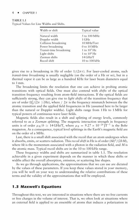
TABLE 1.1Typical Values for Line Widths and Shifts.
Width or shift Typical value
Natural width 5 to 100MHzDoppler width 1GHzCollision broadening 10MHz/TorrPower broadening 0 to 10MHzTransit-time broadening 1 to 105 HzLight shifts 1 to 106 HzZeeman shifts 14GHz/TRecoil shift 10 to 100 kHz
gives rise to a broadening in Hz of order 1/(2πτ ). For laser-cooled atoms, suchtransit-time broadening is usually negligible (on the order of a Hz or so), but in athermal vapor it can be as large as a hundred KHz for laser beam diameters equalto 1mm.
The broadening limits the resolution that one can achieve in probing atomictransitions with optical fields. One must also contend with shifts of the opticaltransition frequency resulting from atom–field interactions. If the optical fields aresufficiently strong, they can give rise to light shifts of the transition frequency thatare of order 2
0/(2πδ) (Hz), where δ/2π is the frequency mismatch between the theatomic transition and the applied field frequencies in Hz (assumed here to be largerthan the natural or Doppler widths). Light shifts range from 1Hz to 1MHz fortypical powers of continuous-wave laser fields.
Magnetic fields also result in a shift and splitting of energy levels, commonlyreferred to as a Zeeman splitting. The magnetic interaction strength in frequencyunits is of order µB/h 14GHz/T, where µB = 9.27 × 10⁻²⁴ JT−1 is the Bohrmagneton. As a consequence, typical level splittings in the Earth’s magnetic field areon the order of a MHz.
Last, there is a small shift associated with the recoil that an atom undergoes whenit absorbs, emits, or scatters radiation. This recoil shift in Hz is of order (k)2/(2hM),where k is the momentum associated with a photon in the radiation field, and M isthe atomic mass. Typical recoil shifts are in the 10 to 100 kHz range.
These frequency widths and shifts are summarized in table 1.1. The resolutionachievable in a given experiment depends on the manner in which these shifts orwidths affect the overall absorption, emission, or scattering line shapes.
As we go through applications, the approximations that we can use are dictatedby the values of these parameters. If you keep these values stored in your memory,you will be well on your way to understanding the relative contributions of theseterms and the validity of the approximations that will be employed.
1.3 Maxwell’s Equations
Throughout this text, we are interested in situations where there are no free currentsor free charges in the volume of interest. That is, we often look at situations wherean external field is applied to an ensemble of atoms that induces a polarization in
PRELIMINARIES 5
the ensemble. We set B = µ0H (neglecting any effects arising from magnetization),but do not take D = ε0E. Rather, we set D = ε0E + P, where the polarization Pis the electric dipole moment per unit volume. We adopt this approach since thepolarization is calculated using a theory in which the atomic medium is treatedquantum-mechanically.
With no free currents or charges and with B = µ0H, Maxwell’s equations can bewritten as
∇· (ε0E + P) = 0, (1.1a)
∇ × E = −∂B∂t, (1.1b)
∇ × B = µ0∂(ε0E + P)
∂t, (1.1c)
∇ · B = 0. (1.1d)
The quantity
µ0 = 4π × 10−7 T · m/A (1.2)
is the permeability of free space, while
ε0 ≈ 8.85 × 10⁻⁷ C2/N · m2 (1.3)
is the permittivity of free space. All field variables are assumed to be functions ofposition R and time t.
From equation (1.1), we find
∇ × (∇ × E) = ∇(∇ · E) − ∇2E
= − ∂
∂t(∇ × B) = −µ0ε0
∂2E∂t2
− µ0∂2P∂t2
(1.4)
or
−∇(∇ · E) + ∇2E − µ0ε0∂2E∂t2
= µ0∂2P∂t2
. (1.5)
In free space, ∇ · E = 0 and P = 0, leading to the wave equation
∇2E − 1v20
∂2E∂t2
= 0, (1.6)
where the wave propagation speed in free space is equal to
v0 = 1√µ0ε0
. (1.7)
Historically, by comparing the electromagnetic (i.e., that based on the force betweenelectrical circuits) and the electrostatic units of electrical charge, Wilhelm Weberhad shown by 1855 that the value of 1/(µ0ε0)1/2 was equal to the speed oflight within experimental error. This led Maxwell to conjecture that light is anelectromagnetic phenomenon [3]. One can only imagine the excitement Maxwellfelt at this discovery.
6 CHAPTER 1
We return to Maxwell’s equations later in this text, but for now, let us considerplane-wave solutions of equations (1.5) and (1.1) for which we can take ∇ · E = 0.We still do not have enough information to solve equation (1.5) since we donot know the relationship between P(R, t) and E(R, t). In general, one can writeP(R, t) = ε0χ e · E(R, t), where χ e is the electric susceptibility tensor, but this doesnot resolve our problem, since χ e is not yet specified. To obtain an expression forχ e, one must model the medium–field interaction in some manner. Ultimately, wecalculate χ e using a quantum-mechanical theory to describe the atomic medium.
For the time being, however, let us the assume that the medium is linear,homogeneous, and isotropic, implying that χ e is a constant times the unit tensorand independent of the electric field intensity. Moreover, if we neglect dispersionand assume that χe is independent of frequency over the range of incident fieldfrequencies, then it is convenient to rewrite χe as
χe = n2 − 1, (1.8)
where n is the index of refraction of the medium. In these limits, equation (1.5)reduces to
∇2E − n2
c2∂2E∂t2
= 0, (1.9)
where c is the speed of light in vacuum. Neglecting dispersion, the fields propagatein the medium with speed v = c/n, as expected.
For a monochromatic or nearly monochromatic field having angular frequencycentered at ω, the magnetic field (or, more precisely, the magnetic induction) B isrelated to the electric field via
B = k × Eω
, (1.10)
where k is the propagation vector having magnitude k = nω/c. It then follows thatthe time average of the Poynting vector, S = E × H = E × B/µ0, is equal to
〈S〉 = |E|2 n2cµ0
k =12nε0c |E|2 k (1.11)
for optical fields having electric field amplitude |E| and propagation directionk = k/k.
By using the Poynting vector, one can calculate the electric field amplitude fromthe field intensity using
E =√
2cµ0 |〈S〉| 27.5√S V/m, (1.12)
where S ≡ |〈S〉| is expressed in W/m2, and we have taken n = 1. At the surfaceof the sun, S ≈ 6.4 × 10⁷ W/m2, giving a value E ≈ 2.2 × 10⁵ V/m. This is to becompared with the value E ≈ 5 × 10¹¹ V/m at the Bohr radius of the hydrogenatom and a value E ≈ 1 × 10⁶ V/m, which is the breakdown voltage of air. Fora He-Ne laser having 1mW of continuous-wave (cw) power focused in 1mm2,S ≈ 103 W/m2, and for an Ar ion laser having 10W of cw power focused in 1mm2,S ≈ 107 W/m2. Semiconductor diode lasers produce tunable cw output in the mWtoW range, having central frequencies that can range from the near-ultraviolet to the
PRELIMINARIES 7
infrared. Ti:sapphire lasers produce several watts of tunable cw radiation centeredin the infrared. Pulsed lasers provide much higher powers (but for short intervalsof time so that the average energy in the pulse rarely exceeds a Joule or so). In1965, Nd:YAG lasers produced 1mJ in 1µs—if focused to 1mm2, S ≈ 109 W/m2,which produces an E field on the order of the breakdown voltage of air. Currently,Ti:sapphire lasers produce pulsed output with average powers as large as a few wattsand pulse lengths as short as a few fs. In 2007, the power output of the Herculeslaser at the University of Michigan was on the order of 100TW = 1014 W, withpower densities greater than 1022 W/cm2.
From the field amplitude E and the dipole moment matrix element µ12 associatedwith the atomic transition that is being driven by the field, one can calculate the Rabifrequency 0 = µ12E/. Typically, µ12 is of order ea0, where e = 1.60 × 10⁻¹⁹ Cis the magnitude of the charge of the electron, and a0 = 5.29 × 10⁻¹¹ m is theBohr radius. A power of 1W/cm2 corresponds to E ≈ 3 × 10³ V/m, which in turncorresponds to a Rabi frequency on the order of0 ≈ 108 s−1 or0/2π ≈ 107 Hz =10MHz.
1.4 Atom–Field Hamiltonian
In dealing with problems involving the interaction of optical fields with atoms, oneoften makes the dipole approximation, based on the fact that the wavelength ofthe optical field is much larger than the size of an atom. You may recall that theleading term in the interaction between a neutral charge distribution and an electricfield that varies slowly on the length scale of the charge distribution is the dipolecoupling, −µ · E, where µ is the dipole moment of the charge distribution, and E isthe electric field evaluated at the center of the charge distribution.
Thus, it is not unreasonable to take as the Hamiltonian for an N-electron atominteracting with an optical field having electric field E(R, t) a Hamiltonian of theform
H = P2CM2M
+ Hatom + VAF , (1.13)
where
Hatom =N∑j=1
p2j2m
+ VC (1.14)
is the atomic Hamiltonian, and
VAF = −µ · E(RCM, t) (1.15)
is the atom–field interaction Hamiltonian. In these equations, RCM is the positionand PCM the momentum operator associated with the center of mass of an atomhaving mass M, p j is the momentum operator of the jth electron in the atom, m isthe electron mass,
µ = −eN∑j=1
r j (1.16)
8 CHAPTER 1
is the electric dipole moment operator of the atom, r j is the coordinate of the jthelectron relative to the nucleus, VC is the Coulomb interaction between the chargesin the atom, and A2 ≡ A · A for any vector A. To a good approximation, RCM
coincides with the position of the nucleus. The Hamiltonian (1.13) provides thestarting point for semiclassical calculations of atom–field interactions in the dipoleapproximation. You are urged to study the appendix in this chapter, where furtherjustification for the choice of this Hamiltonian is given.
1.5 Dirac Notation
It is assumed that anyone reading this text has been exposed to Dirac notation.Dirac developed a powerful formalism for representing state vectors in quantummechanics. Students leaving an introductory course in quantum mechanics oftencan use Dirac notation but may not appreciate its significance. It is not our intentto go into a detailed discussion of Dirac notation. Instead, we would like to remindyou of some of the features that are especially relevant to this text.
It is probably easiest to think of Dirac notation in analogy with a three-dimensional vector space. Any three-dimensional vector can be written as
A = Axi + Ayj + Azk, (1.17)
where Ax, Ay, Az are the components of the vector in this x, y, z basis. We canrepresent the unit vectors as column vectors,
i =⎛⎝100
⎞⎠ , j =
⎛⎝010
⎞⎠ , k =
⎛⎝001
⎞⎠ , (1.18)
such that the vector A can be written as
A =⎛⎝AxAy
Az
⎞⎠ . (1.19)
Of course, the basis vectors i, j,k are not unique; any set of three noncollinearunit vectors would do as well. Let us call one such set u1,u2,u3, such that
A = A1u1 + A2u2 + A3u3. (1.20)
The vector A is absolute in the sense that it is basis-independent. For a given basis,the components of A change in precisely the correct manner to ensure that A remainsunchanged. We are at liberty to represent the basis vectors as⎛
⎝100
⎞⎠ ,
⎛⎝010
⎞⎠ ,
⎛⎝001
⎞⎠ (1.21)
in any one basis, but once we choose this basis, we must express all other unit vectorsin terms of this specific basis. The example in the problems should make this clear.
PRELIMINARIES 9
In quantum mechanics, we express a state vector in a specific basis as
|ψ〉 =N∑n=1
An|n〉, (1.22)
where the sum is over all possible states of the system. In contrast to the case of three-dimensional vectors, this expansion rarely has a simple geometrical interpretation.Rather, the abstract state vector or ket |ψ〉 is expanded in terms of a basis set ofeigenkets. In analogy with the case of vectors, one can take |n〉 as a column matrixin which there is a 1 in the nth row and a zero everywhere else. We are free to chooseonly one set of basis functions with this representation.
In Dirac notation, state vectors are represented by column vectors, and operatorsare represented by matrices. Thus, an operator B can be written as
B =N∑
n,m=1
Bnm |n〉 〈m|, (1.23)
where the bra 〈m| can be represented as a row matrix with a 1 in the mth locationand a zero everywhere else. The basis operator |n〉 〈m| is then an N× Nmatrix witha 1 in the nmth location and zeros everywhere else. Typically, one writes a matrixelement of B as Bnm = 〈n| B |m〉. This tells you nothing about how to calculatethese matrix elements; moreover, the matrix elements depend on the basis that ischosen.
In general, we know only that any Hermitian operator has an associated set ofeigenkets, such that the operator is diagonal in the basis of these eigenkets. Forexample, the states |E〉 are eigenkets of the energy operator H; the fact that His diagonal in the |E〉 basis does not provide any prescription for calculating thediagonal elements (eigenvalues). In essence, one must often revert to the Schrödingerequation in coordinate space to obtain the eigenvalues, although it is sometimespossible to use operator techniques (as in the case of a harmonic oscillator) to deducethe energy spectrum.
1.6 Where Do We Go from Here?
Now that we have reviewed some of the concepts that are needed in the followingchapters, it might prove useful to formulate a strategy for optimizing the benefitsthat you can derive from this text. There are many excellent texts on quantummechanics, laser spectroscopy, lasers, nonlinear optics, and quantum optics on themarket. Several of these are listed in the bibliography at the end of this chapter.Some of the material that we present overlaps with that in other texts, so you mayprefer one treatment to another. You are urged to consult other texts to complementthe material presented herein. In fact, there are many topics that we barely touchon at all, such as collective effects, laser theory, optical bistability, and quantuminformation.
The problems form an integral part of this text. Some of the problems are farfrom trivial and require considerable effort, but the more problems you are able tosolve, the better will be your understanding. Hopefully, the text will provide a useful
10 CHAPTER 1
reference to which you can return as needed. Some of the calculations that woulddisrupt the development are included as appendices in the chapters.
The first few chapters are devoted to a study of a classical electromagnetic fieldinteracting with a “two-level” atom. These chapters are really the heart of thematerial. They provide the fundamental underlying formalism and must be masteredif the various applications are to be appreciated. Let’s get started!
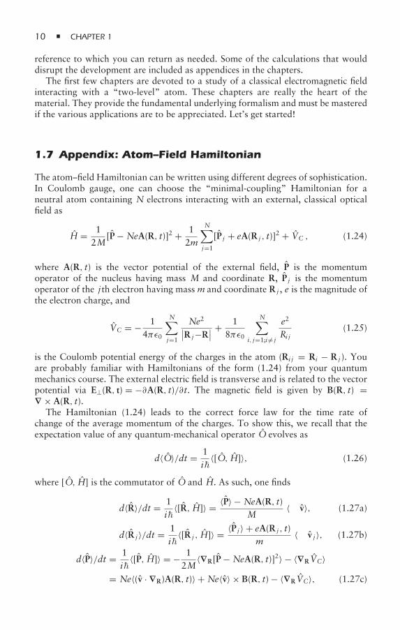
1.7 Appendix: Atom–Field Hamiltonian
The atom–field Hamiltonian can be written using different degrees of sophistication.In Coulomb gauge, one can choose the “minimal-coupling” Hamiltonian for aneutral atom containing N electrons interacting with an external, classical opticalfield as
H = 12M
[P − NeA(R, t)]2 + 12m
N∑j=1
[P j + eA(R j , t)]2 + VC , (1.24)
where A(R, t) is the vector potential of the external field, P is the momentumoperator of the nucleus having mass M and coordinate R, P j is the momentumoperator of the jth electron having mass m and coordinate R j , e is the magnitude ofthe electron charge, and
VC = − 14πε0
N∑j=1
Ne2∣∣R j−R∣∣ + 1
8πε0
N∑i, j=1;i = j
e2
Ri j(1.25)
is the Coulomb potential energy of the charges in the atom (Ri j = Ri − R j ). Youare probably familiar with Hamiltonians of the form (1.24) from your quantummechanics course. The external electric field is transverse and is related to the vectorpotential via E⊥(R, t) = −∂A(R, t)/∂t. The magnetic field is given by B(R, t) =∇ × A(R, t).
The Hamiltonian (1.24) leads to the correct force law for the time rate ofchange of the average momentum of the charges. To show this, we recall that theexpectation value of any quantum-mechanical operator O evolves as
d〈O〉/dt = 1i
〈[O, H]〉, (1.26)
where [O, H] is the commutator of O and H. As such, one finds
d〈R〉/dt = 1i
〈[R, H]〉 = 〈P〉 − NeA(R, t)M
≡ 〈v〉, (1.27a)
d〈R j 〉/dt = 1i
〈[R j , H]〉 = 〈P j 〉 + eA(R j , t)m
≡ 〈v j 〉, (1.27b)
d〈P〉/dt = 1i
〈[P, H]〉 = − 12M
〈∇R[P − NeA(R, t)]2〉 − 〈∇RVC〉= Ne〈(v · ∇R)A(R, t)〉 + Ne〈v〉 × B(R, t) − 〈∇RVC〉, (1.27c)
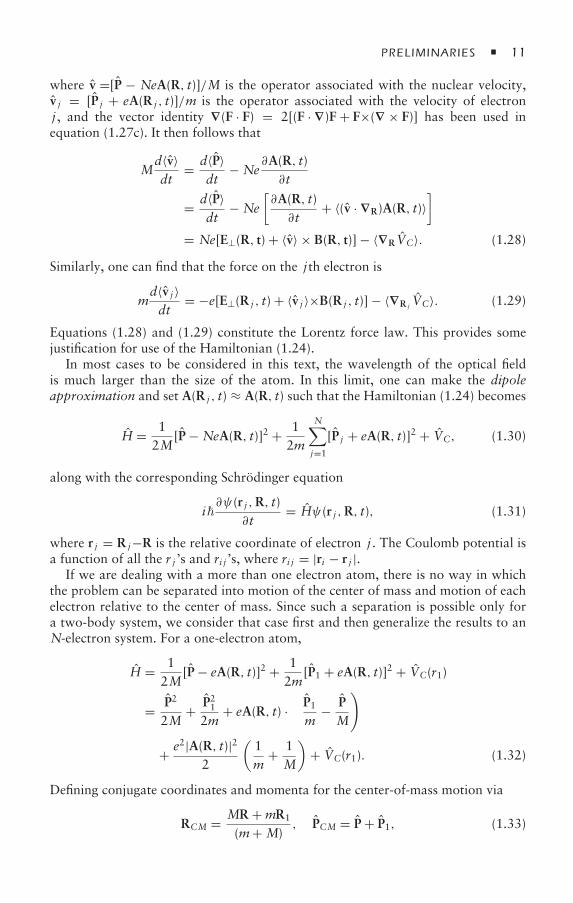
PRELIMINARIES 11
where v =[P − NeA(R, t)]/M is the operator associated with the nuclear velocity,v j = [P j + eA(R j , t)]/m is the operator associated with the velocity of electronj , and the vector identity ∇(F · F) = 2[(F · ∇)F + F×(∇ × F)] has been used inequation (1.27c). It then follows that
Md〈v〉dt
= d〈P〉dt
− Ne∂A(R, t)∂t
= d〈P〉dt
− Ne[∂A(R, t)∂t
+ 〈(v · ∇R)A(R, t)〉]
= Ne[E⊥(R, t) + 〈v〉 × B(R, t)] − 〈∇RVC〉. (1.28)
Similarly, one can find that the force on the jth electron is
md〈v j 〉dt
= −e[E⊥(R j , t) + 〈v j 〉×B(R j , t)] − 〈∇R j VC〉. (1.29)
Equations (1.28) and (1.29) constitute the Lorentz force law. This provides somejustification for use of the Hamiltonian (1.24).
In most cases to be considered in this text, the wavelength of the optical fieldis much larger than the size of the atom. In this limit, one can make the dipoleapproximation and set A(R j , t) ≈ A(R, t) such that the Hamiltonian (1.24) becomes
H = 12M
[P − NeA(R, t)]2 + 12m
N∑j=1
[P j + eA(R, t)]2 + VC, (1.30)
along with the corresponding Schrödinger equation
i∂ψ(r j ,R, t)
∂t= Hψ(r j ,R, t), (1.31)
where r j = R j−R is the relative coordinate of electron j . The Coulomb potential isa function of all the r j ’s and ri j ’s, where ri j = |ri − r j |.
If we are dealing with a more than one electron atom, there is no way in whichthe problem can be separated into motion of the center of mass and motion of eachelectron relative to the center of mass. Since such a separation is possible only fora two-body system, we consider that case first and then generalize the results to anN-electron system. For a one-electron atom,
H = 12M
[P − eA(R, t)]2 + 12m
[P1 + eA(R, t)]2 + VC(r1)
= P2
2M+ P21
2m+ eA(R, t) ·
(P1m
− PM
)
+ e2|A(R, t)|22
(1m
+ 1M
)+ VC(r1). (1.32)
Defining conjugate coordinates and momenta for the center-of-mass motion via
RCM = MR +mR1
(m+ M), PCM = P + P1, (1.33)
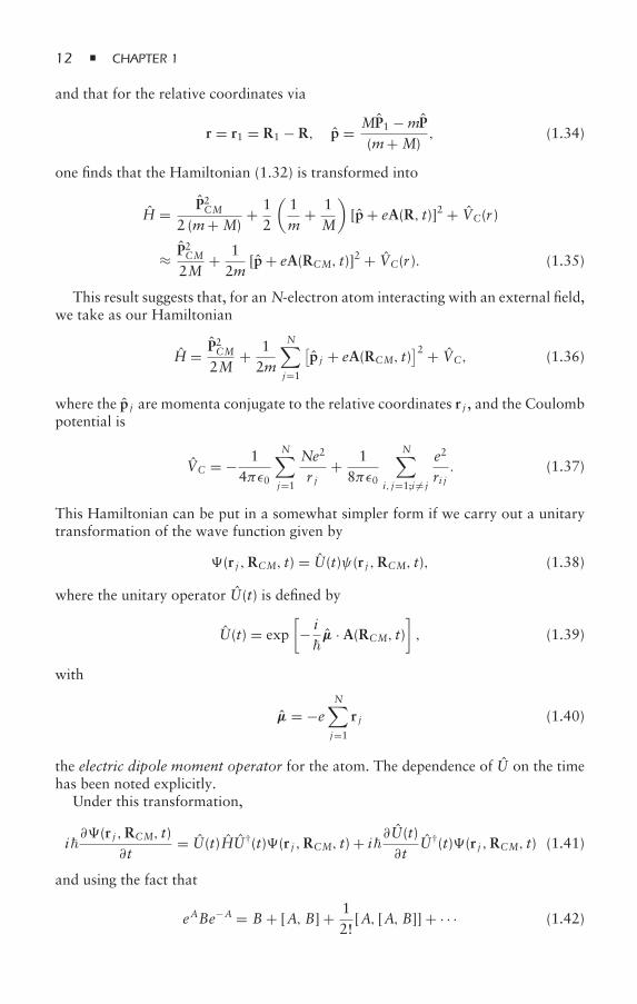
12 CHAPTER 1
and that for the relative coordinates via
r = r1 = R1 − R, p = MP1 −mP(m+ M)
, (1.34)
one finds that the Hamiltonian (1.32) is transformed into
H = P2CM2 (m+ M)
+ 12
(1m
+ 1M
)[p + eA(R, t)]2 + VC(r )
≈ P2CM2M
+ 12m
[p + eA(RCM, t)]2 + VC(r ). (1.35)
This result suggests that, for an N-electron atom interacting with an external field,we take as our Hamiltonian
H = P2CM2M
+ 12m
N∑j=1
[p j + eA(RCM, t)
]2 + VC, (1.36)
where the p j are momenta conjugate to the relative coordinates r j , and the Coulombpotential is
VC = − 14πε0
N∑j=1
Ne2
r j+ 1
8πε0
N∑i, j=1;i = j
e2
ri j. (1.37)
This Hamiltonian can be put in a somewhat simpler form if we carry out a unitarytransformation of the wave function given by
(r j ,RCM, t) = U(t)ψ(r j ,RCM, t), (1.38)
where the unitary operator U(t) is defined by
U(t) = exp[− iµ · A(RCM, t)
], (1.39)
with
µ = −eN∑j=1
r j (1.40)
the electric dipole moment operator for the atom. The dependence of U on the timehas been noted explicitly.
Under this transformation,
i∂(r j ,RCM, t)
∂t= U(t)HU†(t)(r j ,RCM, t) + i
∂U(t)∂t
U†(t)(r j ,RCM, t) (1.41)
and using the fact that
eABe−A = B+ [A, B] + 12!
[A, [A, B]] + · · · (1.42)
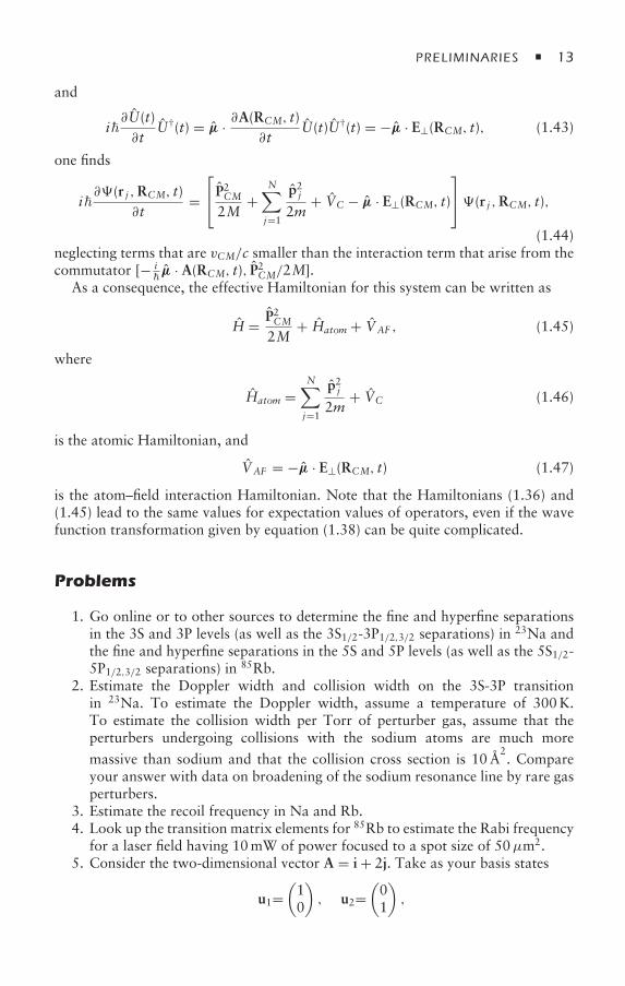
PRELIMINARIES 13
and
i∂U(t)∂t
U†(t) = µ · ∂A(RCM, t)∂t
U(t)U†(t) = −µ · E⊥(RCM, t), (1.43)
one finds
i∂(r j ,RCM, t)
∂t=⎡⎣ P2CM2M
+N∑j=1
p2j2m
+ VC − µ · E⊥(RCM, t)
⎤⎦(r j ,RCM, t),
(1.44)neglecting terms that are vCM/c smaller than the interaction term that arise from thecommutator [− i
µ · A(RCM, t), P2CM/2M].
As a consequence, the effective Hamiltonian for this system can be written as
H = P2CM2M
+ Hatom + VAF , (1.45)
where
Hatom =N∑j=1
p2j2m
+ VC (1.46)
is the atomic Hamiltonian, and
VAF = −µ · E⊥(RCM, t) (1.47)
is the atom–field interaction Hamiltonian. Note that the Hamiltonians (1.36) and(1.45) lead to the same values for expectation values of operators, even if the wavefunction transformation given by equation (1.38) can be quite complicated.
Problems
1. Go online or to other sources to determine the fine and hyperfine separationsin the 3S and 3P levels (as well as the 3S1/2-3P1/2,3/2 separations) in 23Na andthe fine and hyperfine separations in the 5S and 5P levels (as well as the 5S1/2-5P1/2,3/2 separations) in 85Rb.
2. Estimate the Doppler width and collision width on the 3S-3P transitionin 23Na. To estimate the Doppler width, assume a temperature of 300K.To estimate the collision width per Torr of perturber gas, assume that theperturbers undergoing collisions with the sodium atoms are much more
massive than sodium and that the collision cross section is 10Å2. Compare
your answer with data on broadening of the sodium resonance line by rare gasperturbers.
3. Estimate the recoil frequency in Na and Rb.4. Look up the transition matrix elements for 85Rb to estimate the Rabi frequency
for a laser field having 10mW of power focused to a spot size of 50µm2.5. Consider the two-dimensional vector A = i + 2j. Take as your basis states
u1=(10
), u2=
(01
),
14 CHAPTER 1
where
u1,2 = i ± j√2.
Express the unit vectors i and j in this basis, and find the coordinates. Showexplicitly that A1u1 + A2u2 = Axi + Ayj.
6. Derive equation (1.27c).7. Prove that
dA(R, t)dt
= ∂A(R, t)∂t
+ (v · ∇)A(R, t)
for a vector function A(R, t), with v = R.8. Derive equation (1.44) from equation (1.41).9. Show that the analogue of the wave equation (1.5) for the displacement vector
D(R, t) is
∇2D − µ0ε0∂2D∂t2
= −∇×(∇ × P).
10. For an infinite square well potential, show that an arbitrary initial wavepacket will return to its initial state at integral multiples of a revival timeτ = (4ma2)/π, where m is the mass of the particle in the well, and a is thewidth of the well.
11. The radiative reaction rate γ2 for a classical oscillator having charge e, massm, and frequency ω is given by
γ2 = 14πε0
23e2ω2
c3.
Show that
γ2
ω= αF S
ω
mc2, αF S = 1
4πε0
e2
c≈ 1
137,
and estimate this ratio for an electron oscillator having a frequency corre-sponding to an optical frequency.
References
[1] For an introduction to this topic, see, for example, P. W. Milonni and M.-L. Shih,Casimir Forces, Contemporary Physics 33, 313–322 (1992); K. A. Milton, The CasimirEffect (World Scientific, Singapore, 2001). A bibliography can be found at the followingwebsite: http://www.cfa.harvard.edu/~babb/casimir-bib.html.
[2] J. C. Maxwell, Note on a natural limit to the sharpness of spectral lines, Nature VIII,474–475 (1873).
[3] J. C. Maxwell, A Treatise on Electricity and Magnetism, vol. 2 (Dover, New York,1954), chap. XX, article 781.
PRELIMINARIES 15
Bibliography
Listed here is a representative bibliography of some general reference texts, bookson laser spectroscopy, and books on quantum optics.
General Reference Texts
L. Allen and J. H. Eberly, Optical Resonance and Two-Level Atoms (Wiley, New York,1985).
R. Balian, S. Haroche, and S. Liberman, Eds., Frontiers in Laser Spectroscopy, Les HouchesSession XXVII, vols. 1 and 2 (North-Holland, Amsterdam, 1975).
N. Bloembergen, Nonlinear Optics (W. A. Benjamin, New York, 1965).M. Born and E. Wolf, Principles of Optics, 7th ed. (Cambridge University Press, Cambridge,1999).
R. W. Boyd, Nonlinear Optics, 3rd ed. (Academic Press, Burlington, MA, 2008).D. Budker, D. F. Kimball, and D. P. DeMille, Atomic Physics: An Exploration throughProblems and Solutions (Oxford University Press, Oxford, UK, 2006).
C. Cohen-Tannoudji, J. Dupont-Roc, and G. Grynberg, Atom-Photon Interactions (Wiley-Interscience, New York, 1992).
———, Photons and Atoms—Introduction to Quantum Electrodynamics (Wiley-Interscience, New York, 1989).
C. DeWitt, A. Blandin, and C. Cohen-Tannoudji, Eds., Quantum Optics and Electronics(Gordon and Breach, New York, 1964).
C. J. Foot, Atomic Physics (Oxford University Press, Oxford, UK, 2005).H. Haken, Laser Theory (Springer-Verlag, Berlin, 1984).S. Haroche and J.-M. Raimond, Exploring the Quantum: Atoms, Cavities, and Photons(Oxford University Press, Oxford, UK, 2006).
W. Heitler, The Quantum Theory of Radiation, 3rd ed. (Oxford University Press, London,1954).
L. Mandel and E. Wolf, Optical Coherence and Quantum Optics (Cambridge UniversityPress, Cambridge, UK, 1995).
H. J. Metcalf and P. van der Straten, Laser Cooling and Trapping (Springer-Verlag,New York, 1999).
P. Meystre and M. Sargent III, Elements of Quantum Optics, 4th ed. (Springer-Verlag, Berlin,2007).
P. W. Milonni, The Quantum Vacuum: An Introduction to Quantum Electrodynamics(Academic Press, San Diego, CA, 1993).
P. W. Milonni and J. H. Eberly, Lasers (Wiley Series in Pure and Applied Optics): LaserPhysics (Wiley, Hoboken, 2010).
S. Mukamel, Principles of Nonlinear Laser Spectroscopy (Oxford University Press, Oxford,UK, 1955).
E. A. Power, Introductory Quantum Electrodynamics (American Elsevier Publishing,New York, 1965).
M. Sargent III, M. O. Scully, and W. E. Lamb Jr., Laser Physics (Addison-Wesley, Reading,MA, 1974).
Y. R. Shen, The Principles of Nonlinear Optics (Wiley-Interscience, New York, 1984).
16 CHAPTER 1
B. W. Shore, The Theory of Coherent Excitation, vols. 1 and 2 (Wiley-Interscience,New York, 1990). This encyclopedic work contains a wealth of references.
A. E. Siegman, Lasers (University Science Books, Mill Valley, CA, 1986).
Laser Spectroscopy Texts
A. Corney, Atomic and Laser Spectroscopy (Oxford Classics Series, Oxford, UK, 2006).W. Demtröder, Laser Spectroscopy, 4th ed., vol. 1, Basic Principles, and vol. 2, ExperimentalTechniques (Springer-Verlag, Berlin, 2008).
V. S. Letokhov and V. P. Chebotaev,Non-Linear Laser Spectroscopy (Springer-Verlag, Berlin,1977).
M. D. Levenson, Introduction to Nonlinear Laser Spectroscopy (Academic Press, New York,1982).
S. Stenholm, Foundations of Laser Spectroscopy (Wiley, New York, 1984; Dover, Mineola,NY, 2005).
Quantum Optics Texts
S. M. Barnett and P. M. Radmore,Methods in Theoretical QuantumOptics (Clarendon Press,Oxford, UK, 1997).
M. Fox, Quantum Optics: An Introduction (Oxford University Press, Oxford, UK, 2006).J. C. Garrison and R. Y. Chiao, Quantum Optics (Oxford University Press, Oxford, UK,
2006).C. C. Gerry and P. L. Knight, Introductory Quantum Optics (Cambridge University Press,
Cambridge, UK, 2005).J. R. Klauder and E. C. G. Sudarshan, Fundamentals of Quantum Optics (W. A. Benjamin,
New York, 1968; Dover, Mineola, NY, 2006).P. L. Knight and L. Allen, Concepts of Quantum Optics (Pergamon, New York, 1985).R. Loudon, The Quantum Theory of Light, 3rd ed. (Oxford University Press, Oxford, UK,
2003).W. Louisell, Quantum Statistical Properties of Radiation (Wiley, New York, 1973).G. J. Milburn and D. F. Walls, Quantum Optics (Springer-Verlag, Berlin, 1994).H. M. Nussenzweig, Introduction to Quantum Optics (Gordon and Breach, London, 1973).W. P. Schleich, Quantum Optics in Phase Space (Wiley-VCH, Berlin, 2001).M. O. Scully and M. S. Zubairy, Quantum Optics (Cambridge University Press, Cambridge,
UK, 1997).
2Two-Level Quantum Systems
The general subject matter of this text is the interaction of radiation with matter. A“two-level” atom driven by an optical field is considered to be a prototypical system.We examine this problem from several different points of view and use differentanalytical tools to solve the relevant equations. It may seem like a bit of overkill, butthis is a building block problem that must be understood if further progress is to beachieved. Moreover, the problem of a two-level atom interacting with a radiationfield has many more surprises than you might expect. As a result, you will learn someinteresting physics as we go along. Many different mathematical representations areused, and you might ask if this is really necessary. It turns out that each of theserepresentations is well-suited to specific classes of problems involving the interactionof radiation with matter. At first, we consider generic quantum systems, but focuseventually on the two-level atom. Appendix A contains a summary of the variousrepresentations that are introduced.
2.1 Review of Quantum Mechanics
2.1.1 Time-Independent Problems
We are interested in problems that can be termed semiclassical in nature. In suchproblems, the atoms are treated quantum mechanically, but the external fieldswith which they interact are treated classically. Before discussing time-dependentHamiltonians, let us review time-independent Hamiltonians, H = H(r), for aneffective one-electron atom with the electron’s position denoted by r.
For such Hamiltonians, an arbitrary wave function ψ(r, t) can be expanded as
ψ(r, t) =∑n
an(t)ψn(r), (2.1)
18 CHAPTER 2
and an arbitrary state vector |ψ(t)〉 as|ψ(t)〉 =
∑n
an(t)|n〉, (2.2)
where ψn(r) is the eigenfunction, |n〉 is the eigenket, and an(t) is the probabilityamplitude associated with state n. The eigenfunctions and eigenkets are solutions ofthe time-independent Schrödinger equation,
Hψn(r) = Enψn(r), (2.3)
where H is an operator, or
H|n〉 = En|n〉 , (2.4)
where H is a matrix. Recall that the eigenfunctions are related to the eigenkets via
ψn(r) = 〈r|n〉, (2.5)
where |r〉 is the eigenket of the position operator.It follows from the Schrödinger equation
i∂ψ(r, t)∂t
= Hψ(r, t) (2.6)
and equation (2.1) that the probability amplitudes obey the differential equation
ian(t) = Enan(t), (2.7)
where a dot above a symbol indicates differentiation with respect to time. Thesolution of this equation is
an(t) = exp (−i Ent/) an(0). (2.8)
In Dirac notation, H is a matrix whose elements depend on the representationchosen (it is diagonal in the energy representation), and the Schrödinger equationcan be written
i∂|ψ(t)〉∂t
= H|ψ(t)〉. (2.9)
If we try a solution of the type (2.2) in Eq. (2.9), then the an(t), arranged as a columnvector a(t), obey the differential equation
ia(t) = Ha(t), (2.10)
which has as its solution
a(t) = exp (−iHt/) a(0), (2.11)
where exp (−iHt/) is defined by its series expansion,
exp (−iHt/) = 1 − iHt
+ 12!
(−iHt
)2
+ · · · . (2.12)
TWO-LEVEL QUANTUM SYSTEMS 19
Of course, the solutions (2.8) and (2.11) are equivalent, since
〈n| exp (−iHt/) |n′〉 = exp (−i Ent/) δn,n′ , (2.13)
where δn,n′ is the Kronecker delta, equal to 1 if n = n′ and zero otherwise.These results imply that the state populations |an(t)|2 are constant. In other
words, the populations of the eigenstates of a time-independent Hamiltonian do notchange in time. Even though the populations remain constant, this does not implythat the quantum system is just sitting around doing nothing. You already knowthat a free-particle wave packet spreads in time, for example. The dynamics of aquantum system is determined by both the absolute value of the state amplitudes(which are constant) and the relative phases of these amplitudes (which vary linearlywith time). Moreover, the expectation values of Hermitian operators depend onbilinear products of the probability amplitudes and their conjugates, as is discussedin chapter 3. Since physical observables are associated with Hermitian operators,the average values of these quantities can be functions of time. For example, theaverage dipole moment or average momentum of an harmonic oscillator is periodicwith the oscillator period if the oscillator is prepared initially in a superposition ofeigenstates.
If we can solve the Schrödinger equation for the eigenstates and expand the initialstate in terms of the eigenstates, the expansion coefficients totally specify the timeevolution of the state. Unfortunately, it is often difficult to obtain analytic solutions,and one must rely on approximate or numerical solutions. Fortunately, with theavailability of high-speed computers and assorted software, numerical solutions thatwere once a challenge can be obtained with a few keystrokes.
2.1.2 Time-Dependent Problems
Often, we are confronted with problems where we can solve for the eigenstates ofpart of the Hamiltonian. Suppose that we can write
H(r, t) = H0(r) + V(r, t) , (2.14)
H(t) = H0 + V(t) , (2.15)
where V(r, t) represents the interaction of a classical, time-dependent field withthe quantum system, and H0(r) is the Hamiltonian for the quantum system in theabsence of the interaction. For example, H0(r) can be the Hamiltonian of an isolatedatom, and V(r, t) can be the interaction energy associated with an atom driven by aclassical optical field. If H(r, t) depends on time, the energy is no longer a constantof the motion. Let the eigenstates of H0(r) be noted by ψn(r) and the eigenkets of H0
by |n〉, such that
H0(r)ψn(r) = Enψn(r), (2.16)
or, in Dirac notation,
H0|n〉 = En|n〉. (2.17)
20 CHAPTER 2
Again, we expand
ψ(r, t) =∑n
an(t)ψn(r). (2.18)
From the Schrödinger equation
i∂ψ(r, t)∂t
= [H0(r) + V(r, t)]ψ(r, t), (2.19)
it then follows that
i∑n
an(t)ψn(r) = H0(r)∑n
an(t)ψn(r) + V(r, t)∑n
an(t)ψn(r). (2.20)
In Dirac notation, the analogous equations are
|ψ(r, t)〉 =∑n
an(t)|n〉, (2.21)
i∂|ψ(r, t)〉∂t
= [H0 + V(t)] |ψ(r, t)〉, (2.22)
i∑n
an(t)|n〉 = H0
∑n
an(t)|n〉 + V(t)∑n
an(t)|n〉. (2.23)
Using the orthogonality of the eigenfunctions or eigenkets [that is, multiplyingequation (2.20) by ψ∗
n′(r) and integrating over r, or equation (2.23) by 〈n′|], we findthat the state amplitudes evolve as
ian(t) = Enan(t) +∑m
Vnm(t)am(t), (2.24)
where the matrix element Vnm(t) is defined as
Vnm(t) = 〈n|V(t)|m〉=∫
〈n|r〉〈r|V(t)|r′〉〈r′|m〉drdr′
=∫drdr′ψn(r)V(r, t)δ(r − r′)ψm(r′)
=∫ψ∗n (r)V(r, t)ψm(r)dr. (2.25)
We can write equation (2.24) as the matrix equation
ia(t) = Ea(t) + V(t)a(t), (2.26)
where E is a diagonal matrix whose elements are the eigenvalues of H0(r) (E issimply equal toH0 written in the energy representation), and V(t) is a matrix havingelements Vnm(t). The fact that V(t) is not diagonal, in general, implies that there aretransitions between the eigenstates of H0.
It makes sense to talk about transitions between eigenstates of H0 only if theinteraction V(t) has not distorted the original quantum system to a state where it isunrecognizable. Otherwise, it might not be possible to measure a physical quantity
TWO-LEVEL QUANTUM SYSTEMS 21
that corresponds to properties of H0. Consider, for example, the hydrogen atom ina static electric field. There are no stationary states for this system; however, forsufficiently small values of the field, it makes perfect sense to talk about this fieldinducing transitions between states of the hydrogen atom. If the field interactionstrength becomes comparable with the energy separation of populated states of theatom, however, a proper description would involve the use of the eigenstates of thecomposite system of atom plus field.
To obtain the dynamics, one must solve equation (2.26) for the state amplitudes.If V(t) is a finite matrix, the coupled equations can be solved by computer. As withany differential equation, you can obtain an analytic solution only if you alreadyknow the solution. You can guess a solution based on what others have learned inthe past. For example, based on the solution of the scalar equation
ix(t) = f (t)x(t), (2.27)
which is
x(t) = exp[− i
∫ t
0f (t′)dt′
]x(0), (2.28)
you might think (and you would have some company) that a solution toequation (2.26) is
a(t) = exp
− i
[Et +
∫ t
0V(t′)dt′
]a(0), (2.29)
but you would be wrong, as is discussed in section 2.7.3. Only in the limiting casethat V is independent of time is it possible to write the solution as
a(t) = exp[− i(E + V)t
]a(0). (2.30)
In general, however, it is impossible to obtain analytic solutions to equation (2.26)when V is a function of time.
2.2 Interaction Representation
In some sense, we have finished. Either we can solve equation (2.26) or we cannot.That does not prevent us from modifying these equations into what may be moreconvenient forms. Remember, however, that modifying the equations does not makethem solvable, but it may reveal a structure where the solution is more apparent.The first such modification that we use, applicable to any time-dependent quantumproblem, involves an interaction representation. The idea behind the interactionrepresentation is to have the state amplitudes be constant in the absence of theinteraction V(t). To accomplish this, one must remove the rapidly varying phasefactor exp(−i Ent/) from the state amplitudes by writing
|ψ(t)〉 =∑n
cn(t)e−i Ent/ (2.31)
22 CHAPTER 2
or
ψ(r, t) =∑n
cn(t)e−i Ent/ψn(r). (2.32)
It then follows from the Schrödinger equation that the amplitudes cn(t) of theinteraction representation obey the differential equation
icn(t) =∑m
Vnm(t)cm(t)eiωnmt ≡∑m
[VI (t)
]nm cm(t), (2.33)
where
ωnm = (En − Em)/ (2.34)
is a transition frequency, and [VI (t)
]nm = eiωnmtVnm(t) (2.35)
is a matrix element in the interaction representation.From equations (2.21) and (2.31), one sees that the amplitudes an(t) and cn(t) are
related by
an(t) = cn(t)e−i Ent/. (2.36)
In matrix form, equation (2.36) can be written as
a(t) = U0(t)c(t), (2.37)
where
U0(t) = e−iH0t/ = e−iEt/ (2.38)
is an evolution operator associated with H0 that satisfies the differential equation
iU0(t) = H0U0(t) = EU0(t), (2.39)
subject to the initial condition U0(0) = 1. Combining equations (2.26) and (2.37),we find
ia(t) = i[U0(t)c(t) + U0(t)c(t)]
= iU0(t)c(t) + Ea(t) = Ea(t) + V(t)a(t), (2.40)
from which it follows that
ic(t) = U†0(t)V(t)U0(t)c(t) = VI (t)c(t), (2.41)
where
VI (t)= U†0(t)V(t)U0(t) = eiH0t/V(t)e−iH0t/ , (2.42)
and we have used the fact that U†0(t)U0(t) = 1. Equation (2.41) is equivalent to
equation (2.26). The interaction representation does not make the problem easierto solve—it only simplifies the notation. Transitions from state n to m are driveneffectively when Vnm(t) has Fourier components at the frequency separation ωmn.
TWO-LEVEL QUANTUM SYSTEMS 23
J=1
J=0
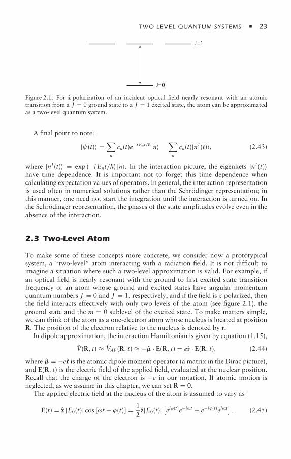
Figure 2.1. For z-polarization of an incident optical field nearly resonant with an atomictransition from a J = 0 ground state to a J = 1 excited state, the atom can be approximatedas a two-level quantum system.
A final point to note:
|ψ(t)〉 =∑n
cn(t)e−i Ent/|n〉 ≡∑n
cn(t)|nI (t)〉, (2.43)
where |nI (t)〉 = exp (−i Ent/) |n〉. In the interaction picture, the eigenkets |nI (t)〉have time dependence. It is important not to forget this time dependence whencalculating expectation values of operators. In general, the interaction representationis used often in numerical solutions rather than the Schrödinger representation; inthis manner, one need not start the integration until the interaction is turned on. Inthe Schrödinger representation, the phases of the state amplitudes evolve even in theabsence of the interaction.
2.3 Two-Level Atom
To make some of these concepts more concrete, we consider now a prototypicalsystem, a “two-level” atom interacting with a radiation field. It is not difficult toimagine a situation where such a two-level approximation is valid. For example, ifan optical field is nearly resonant with the ground to first excited state transitionfrequency of an atom whose ground and excited states have angular momentumquantum numbers J = 0 and J = 1, respectively, and if the field is z-polarized, thenthe field interacts effectively with only two levels of the atom (see figure 2.1), theground state and the m = 0 sublevel of the excited state. To make matters simple,we can think of the atom as a one-electron atom whose nucleus is located at positionR. The position of the electron relative to the nucleus is denoted by r.
In dipole approximation, the interaction Hamiltonian is given by equation (1.15),
V(R, t) ≈ VAF (R, t) ≈ −µ · E(R, t) = er · E(R, t), (2.44)
where µ = −er is the atomic dipole moment operator (a matrix in the Dirac picture),and E(R, t) is the electric field of the applied field, evaluated at the nuclear position.Recall that the charge of the electron is −e in our notation. If atomic motion isneglected, as we assume in this chapter, we can set R = 0.
The applied electric field at the nucleus of the atom is assumed to vary as
E(t) = z |E0(t)| cos [ωt − ϕ(t)] = 12z|E0(t)|
[eiϕ(t)e−iωt + e−iϕ(t)eiωt
], (2.45)
24 CHAPTER 2
where
12E0(t)e−iωt = 1
2|E0(t)| eiϕ(t)e−iωt (2.46)
is the positive frequency component of the field, E0(t) = |E0(t)| eiϕ(t) is the complexamplitude of the field, ω is the carrier frequency of the field, and ϕ(t) is the phase ofthe field. Both the amplitude and the phase can be functions of time. A time-varyingamplitude could correspond to a pulse envelope, while a time-varying phase givesrise to a frequency “chirp” (a frequency that varies in time). With this choice of field,the interaction Hamiltonian becomes
V(r, t) = ez|E0(t)| cos [ωt − ϕ(t)], (2.47)
where z is the z-component of the position operator.For our two-level atom, the energy of the ground state is taken as −ω0/2 and
that of the excited state as ω0/2. Denoting the ground-state eigenket as |1〉 andthe excited-state eigenket as |2〉, we can write the probability amplitudes and matrixelements of the interaction Hamiltonian as
a =(a1a2
)(2.48)
and
V12 = ez12 |E0(t)| cos [ωt − ϕ(t)] , (2.49a)
V21 = ez21 |E0(t)| cos [ωt − ϕ(t)] , (2.49b)
V11 = V22 = 0, (2.49c)
wherez12 = 〈1|z|2〉 = 〈2|z|1〉∗ = z∗21 . (2.50)
The diagonal elements of the interaction Hamiltonian vanish since the operatorz has odd parity. In general, the matrix element z12 is complex, but any singletransition matrix element can be taken as real by an appropriate choice of phase inthe wave function. (However, if z12 is taken to be real, then we are not at liberty totake x12 as real, since the phase of the electronic part of the wave function has beenfixed—the matrix element of one component only of r12 can be taken as real, and thischoice determines whether the other components are real or complex.) Therefore,we can set
ez12 = ez21 = −(µz)12 (real), (2.51)
V12 = V21 = −(µz)12|E0(t)| cos[ωt − φ(t)], (2.52)
and write the Hamiltonian as
H(t) = H0 + V(t) = 2
(−ω0 00 ω0
)
+(
0 |0(t)| cos [ωt − φ(t)]|0(t)| cos [ωt − φ(t)] 0
), (2.53)
TWO-LEVEL QUANTUM SYSTEMS 25
TABLE 2.1Commonly Used Symbols.
E(t) = 12 ε[E0(t)e−iωt + E∗
0(t)eiωt]
Electric fieldE0(t) = |E0(t)| eiφ(t) Complex electric field amplitudeµ Atomic dipole moment operator0(t) = −(µ)21 · εE0(t)/ Rabi frequencyχ (t) = −(µ)21 · εE0(t)/2 Rabi frequency/2ω0 = ω21 Atomic transition frequencyδ = ω0 − ω Atom-field detuning
where
0(t) = −(µz)21E0(t)/ = |0(t)| eiϕ(t) (2.54)
is known as the Rabi frequency and is a measure of the atom–field interactionstrength in frequency units. The Rabi frequency is defined such that it is positivefor positive E0(t) and z12. Equation (2.26) for the probability amplitude a(t) can bewritten as
ia(t) = 2
( −ω0 2 |0(t)| cos [ωt − φ(t)]2 |0(t)| cos [ωt − φ(t)] ω0
)a(t) . (2.55)
This equation can be solved numerically.Note that the Hamiltonian can be recast as
H(t) = −ω0
2σ z + |0(t)| cos [ωt − φ(t)] σ x , (2.56)
where the Pauli spin matrices are defined as
σ x =(0 11 0
), σ y =
(0 −ii 0
), σ z =
(1 00 −1
). (2.57)
This is the same type of Hamiltonian that one encounters for the interaction ofthe spin of the electron with a magnetic field, a problem that is considered inappendix B.
Before we move on, it might be useful to list some of the symbols we introducein this chapter and in chapter 3. You can refer to table 2.1 to remind yourself of thedefinitions of these commonly used symbols.
2.4 Rotating-Wave or Resonance Approximation
Although equation (2.55) can be solved numerically, it is best to gain some physicalinsight into this equation before launching into any solutions. You should not bedeceived by the apparent simplicity of these coupled equations. There are booksdevoted to their solution [1, 2], and even numerical solutions can be difficult toobtain in certain limits [2]. Equation (2.55) characterizes the interaction of an opticalfield with an atom.
26 CHAPTER 2
Without solving the problem, one can ask under what conditions the field iseffective in driving transitions between levels 1 and 2. Let us assume that theamplitude |0(t)| and phase φ(t) of the field are slowly varying on a timescale oforder ω−1 and that |(ω0 − ω) /(ω0 + ω)| 1 and |0(t)/(ω0 + ω)| 1. In that case,the field can be considered to be quasi-monochromatic and is effective in driving the1–2 transition, provided that (ω0 − ω) is small compared with |0(t)|.
The equation for a(t) can be written as
ia(t) = 2
( −ω0 0(t)e−iωt +∗0(t)e
iωt
0(t)e−iωt +∗0(t)e
iωt ω0
)a(t) . (2.58)
In the interaction representation, the corresponding equation for c(t) is
ic(t) = 2
(0 0(t)e−i(ω0+ω)t +∗
0(t)e−iδt
0(t)eiδt +∗0(t)e
i(ω0+ω)t 0
)c(t), (2.59)
where
c(t) =(c1c2
), (2.60)
and
δ = ω0 − ω (2.61)
is the atom–field detuning. In the interaction representation, we see that there areterms that oscillate with frequency ω0 + ω and those that oscillate at frequencyδ. Moreover, we expect that there can also be oscillation at frequency 0(t). Aslong as |0(t)/(ω0 + ω)| 1, |δ/(ω0 + ω)| 1, the rapidly oscillating termsdo not contribute much since they average to zero in a very short time. In otherwords, if we take a coarse-grain time average over a time interval much greater than1/(ω0 + ω), the contribution from these rapidly varying terms would be negligiblysmall compared with the slowly varying terms. The neglect of such terms is calledthe rotating-wave approximation (RWA) or resonance approximation. The reasonfor the nomenclature rotating wave will soon become apparent. In the RWA,equations (2.58) and (2.59) become
ia(t) = 2
( −ω0 ∗0(t)e
iωt
0(t)e−iωt ω0
)a(t), (2.62)
ic(t) = 2
(0 ∗
0(t)e−iδt
0(t)eiδt 0
)c(t) . (2.63)
At this point, it is useful to remind oneself that small is a relative term and, evenmore importantly, that just being relatively small does not mean that a term canautomatically be neglected. (A “small” dog can still give you a serious bite.) As asimple example, consider exp[i(1000 + 1)]. Even though 1 1000, neglecting thesecond term in the exponential produces totally erroneous results. When parametersappear in exponents, their absolute value must be much less than unity before theycan be neglected.
With this reminder, let us estimate the corrections to equations (2.62) and(2.63) produced by the rapidly varying (or counterrotating) terms as follows. The
TWO-LEVEL QUANTUM SYSTEMS 27
amplitude equations in the interaction representation are
c1(t) = [−iχ∗(t)e−iδt − iχ (t)e−i(ω0+ω)t] c2(t), (2.64a)
c2(t) = [−iχ (t)eiδt − iχ∗(t)ei(ω0+ω)t] c1(t), (2.64b)
where
χ (t) = 0(t)/2. (2.65)
Formally integrating equation (2.64b) for c2(t),
c2(t) = c2(0) − i∫ t
0
[χ (t′)eiδt
′ + χ∗(t′)ei(ω0+ω)t′]c1(t′)dt′, (2.66)
and substituting this result into equation (2.64a), we obtain
c1(t) = −iχ∗e−iδtc2(t) − χ (t)∫ t
0e−i(ω0+ω)(t−t′)χ∗(t′)c1(t′)dt′
−χ (t)e−i(ω0+ω)t∫ t
0eiδt
′χ (t′)c1(t′)dt′ − iχ (t)e−i(ω0+ω)tc2(0). (2.67)
If c1,2(t) and χ (t) are slowly varying with respect to e−i(ω0+ω)t, then the thirdand fourth terms are rapidly varying and can be neglected in this order ofapproximation.1 Integrating the second term in equation (2.67) by parts, we find∫ t
0e−i(ω0+ω)(t−t′)χ∗(t′)c1(t′)dt′ ≈ χ∗(t)c1(t) − e−i(ω0+ω)tχ∗(0)c1(0)
i(ω0 + ω)− 1i(ω0 + ω)
∫ t
0e−i(ω0+ω)(t−t′) d
dt
[χ∗(t′)c1(t′)
]dt′. (2.68)
Neglecting the last term in equation (2.68) as well as the rapidly varying termproportional to χ∗(0)c1(0), we obtain∫ t
0e−i(ω0+ω)(t−t′)χ∗(t′)c1(t′)dt′ ≈ χ∗(t)c1(t)
i(ω0 + ω) . (2.69)
Equation (2.67) for c1(t) takes the form
ic1(t) = − |χ (t)|2ω0 + ω c1(t) + χ∗(t)e−iδtc2(t) . (2.70)
Similarly, for c2(t) we find
ic2(t) = |χ (t)|2ω0 + ω c2(t) + χ (t)eiδtc1(t). (2.71)
From equations (2.70) and (2.71), we see that energy of level 1 is shifted downby |χ (t)|2/(ω0 + ω) and energy of level 2 is shifted up by |χ (t)|2/(ω0 + ω). Theselevel shifts are known as Bloch-Siegert shifts [4], which tend to be more important
1 Actually, the third term can contribute a correction of order |χ (t)|/ω; however, this correction woulddepend on the phase of the field and would vanish on averaging over a random distribution of fieldphases—for a good discussion of this problem, see the article by Shirley [3].
28 CHAPTER 2
ω0
δ
1
2
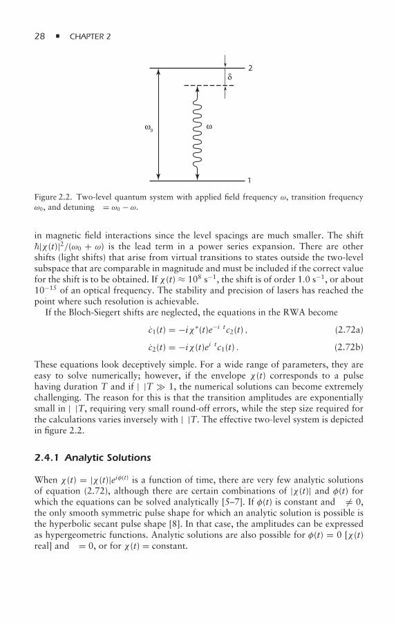
ω
Figure 2.2. Two-level quantum system with applied field frequency ω, transition frequencyω0, and detuning δ = ω0 − ω.
in magnetic field interactions since the level spacings are much smaller. The shift|χ (t)|2/(ω0 + ω) is the lead term in a power series expansion. There are othershifts (light shifts) that arise from virtual transitions to states outside the two-levelsubspace that are comparable in magnitude and must be included if the correct valuefor the shift is to be obtained. If χ (t) ≈ 108 s−1, the shift is of order 1.0 s−1, or about10−15 of an optical frequency. The stability and precision of lasers has reached thepoint where such resolution is achievable.
If the Bloch-Siegert shifts are neglected, the equations in the RWA become
c1(t) = −iχ∗(t)e−iδtc2(t) , (2.72a)
c2(t) = −iχ (t)eiδtc1(t) . (2.72b)
These equations look deceptively simple. For a wide range of parameters, they areeasy to solve numerically; however, if the envelope χ (t) corresponds to a pulsehaving duration T and if |δ|T 1, the numerical solutions can become extremelychallenging. The reason for this is that the transition amplitudes are exponentiallysmall in |δ|T, requiring very small round-off errors, while the step size required forthe calculations varies inversely with |δ|T. The effective two-level system is depictedin figure 2.2.
2.4.1 Analytic Solutions
When χ (t) = |χ (t)|eiφ(t) is a function of time, there are very few analytic solutionsof equation (2.72), although there are certain combinations of |χ (t)| and φ(t) forwhich the equations can be solved analytically [5–7]. If φ(t) is constant and δ = 0,the only smooth symmetric pulse shape for which an analytic solution is possible isthe hyperbolic secant pulse shape [8]. In that case, the amplitudes can be expressedas hypergeometric functions. Analytic solutions are also possible for φ(t) = 0 [χ (t)real] and δ = 0, or for χ (t) = constant.
TWO-LEVEL QUANTUM SYSTEMS 29
2.4.1.1 φ = 0, δ = 0
In this case, the amplitude equations (2.72) become
c1(t) = −iχ (t)c2(t) , (2.73a)
c2(t) = −iχ (t)c1(t) . (2.73b)
Making the transformation
c±(t) = c1(t) ± c2(t), (2.74)
we obtain differential equations of the form
c±(t) = ∓iχ (t)c±(t), (2.75)
which have solutions
c±(t) = e∓i ∫ t0 χ(t′)dt′c±(0), (2.76)
where c±(0) = c1(0)± c2(0) are the initial conditions for the probability amplitudes.In terms of c1(t) and c2(t), the solution is
c1(t) = cos [θ (t)] c1(0) − i sin [θ (t)] c2(0) , (2.77a)
c2(t) = −i sin [θ (t)] c1(0) + cos [θ (t)] c2(0) , (2.77b)
where
θ (t) =∫ t
0χ (t′)dt′. (2.78)
The interpretation of these equations is straightforward. The two levels are degener-ate in the interaction representation, and the driving field couples the states. Thedynamics does not depend on the details of the pulse at any time, only on theintegrated value θ (t).
In the case of an applied pulse such as a Gaussian which “turns on” at t = −∞,the initial conditions should be taken at t = −∞, in which case the solution becomes
c1(t) = cos [θ (t)] c1(−∞) − i sin [θ (t)] c2(−∞) , (2.79a)
c2(t) = −i sin [θ (t)] c1(−∞) + cos [θ (t)] c2(−∞) , (2.79b)
where θ (t) = ∫ t−∞ χ (t
′)dt′. Note that, if at t = −∞, c1(−∞) = 1 and c2(−∞) = 0,then
|c2(∞)|2 = sin2 [θ (∞)] , (2.80)
where
θ (∞) ≡ A/2 =∫ ∞
−∞χ (t′)dt′, (2.81)
and A is the referred to as the pulse area. The pulse area determines how muchpopulation is transferred from the initial to final state. For reasons to be discussedin connection with the Bloch vector in chapter 3, A is defined such that a pulsearea of π corresponds to a complete inversion, |c1(∞)| = 0, |c2(∞)| = 1; a
30 CHAPTER 2
pulse area of π/2 results in an equal superposition of ground and excited states,|c1(∞)| = |c2(∞)| = 1/
√2.
We have arrived at a fairly interesting result. By controlling the pulse area, onecan determine the degree of excitation that is achieved. We will explore applicationsinvolving a series of pulses in the context of optical coherent transients. At this point,however, it might be useful to point out that the use of a π pulse for level inversionis not a “robust” method. One must ensure that the pulse intensity is uniform overthe entire sample and that the pulse area is exactly equal to π to ensure that all theatoms are inverted.
2.4.1.2 χ (t) = 0/2 is constant
In this case, equations (2.72) reduce to
c1(t) = − i2∗
0e−iδtc2(t), (2.82a)
c2(t) = − i20eiδtc1(t). (2.82b)
Taking the derivative of equation (2.82b) and using equation (2.82a), we obtain
c2(t) − iδc2(t) + |0|24
c2(t) = 0. (2.83)
The characteristic equation of Eq. (2.83) has roots
r1,2 = iδ ±2
, (2.84)
where
=√δ2 + |0|2 (2.85)
is known as the generalized Rabi frequency. It then follows that the solution ofequation (2.83) is
c2(t) = eiδt/2[Acos
(t2
)+ B sin
(t2
)]. (2.86)
Similarly, we obtain a solution for c1(t) as
c1(t) = e−iδt/2[Dcos
(t2
)+ E sin
(t2
)]. (2.87)
Only two of the coefficients A, B,D, and E can be independent since we startedwith two, first-order coupled differential equations—the constants are relatedthrough the differential equations. It is convenient to take A and D as independentsince, clearly, A = c2(0) and D = c1(0). Using equations (2.82), (2.83), and (2.86),we can write
c1(0) = −i∗0
2c2(0) = −i
∗0
2A= −i δ
2D+
2E , (2.88)
TWO-LEVEL QUANTUM SYSTEMS 31
which gives
E = iδ
c1(0) − i
∗0
c2(0) . (2.89)
Similarly,
B = −i0
c1(0) − i
δ
c2(0) . (2.90)
Last, the solution of equations (2.82) is
c1(t) = e−iδt/2[
cos(t2
)+ i
δ
sin
(t2
)]c1(0) − i
∗0
sin
(t2
)c2(0)
,
(2.91a)
c2(t) = eiδt/2
−i0
sin
(t2
)c1(0) +
[cos
(t2
)− i
δ
sin
(t2
)]c2(0)
.
(2.91b)
This solution is of fundamental importance since it gives the response of a two-levelatom to a monochromatic field. Note that the amplitudes depend nonlinearly on theapplied amplitude—the atom acts as a nonlinear device, in contrast to a harmonicoscillator.
If c1(0) = 1, c2(0) = 0, then
|c2(t)|2 = |0|22
sin2(
2t). (2.92)
The population oscillates as a function of time. This is known as Rabi flopping. Ontime average,
|c2(t)|2 = 12
|0|22
= 12
|0|2δ2 + |0|2
. (2.93)
Graphs of |c2(t)|2 as a function of time and the time-averaged population |c2(t)|2versus δ are shown in figures 2.3 and 2.4, respectively.
For |δ| |0|, |c2(t)|2 ≈ |0|2 /(2δ2). This is a somewhat surprising result.Even though the field is off resonance, the transition probability falls off inverselyonly as 1/δ2. In fact, we can turn off the field at a time t = T = π/ and findthat |c2(T)|2 ≈ |0|2 /δ2. From the energy-time uncertainty principle (which is nota rigorous result, as are uncertainty relations involving noncommuting operatorsin quantum mechanics), we might expect that the transition probability wouldvanish at least exponentially as |δ|T. (Recall that increasing the light intensity inthe photoelectric experiment does not increase the number of photoelectrons if thefield frequency is not sufficiently high.) What is going on?
Had the field been turned on and off smoothly, one would indeed find that|c2(t)|2 ∼ e− f (|δ|T), where f is some positive function. However, in the calculationthat was carried out, the field is turned on instantaneously at t = 0 and turned offinstantaneously at t = T. Owing to the discontinuities in the derivative of the stepfunction, the Fourier components of a step function vary inversely with δT, ratherthan as an exponentially decaying function of |δ|T.
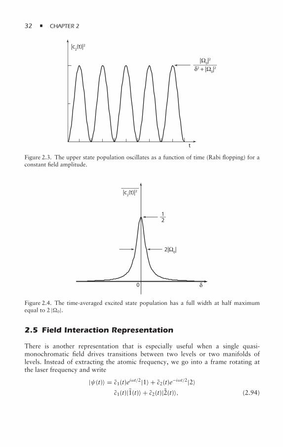
32 CHAPTER 2
|c2(t)|2
________|Ω0|2
δ2 + |Ω0|2
t
Figure 2.3. The upper state population oscillates as a function of time (Rabi flopping) for aconstant field amplitude.
δ
__
______
1 2
0
|c2(t)|2
2|Ω0|
Figure 2.4. The time-averaged excited state population has a full width at half maximumequal to 2 |0|.
2.5 Field Interaction Representation
There is another representation that is especially useful when a single quasi-monochromatic field drives transitions between two levels or two manifolds oflevels. Instead of extracting the atomic frequency, we go into a frame rotating atthe laser frequency and write
|ψ(t)〉 = c1(t)eiωt/2|1〉 + c2(t)e−iωt/2|2〉≡ c1(t)|1(t)〉 + c2(t)|2(t)〉, (2.94)
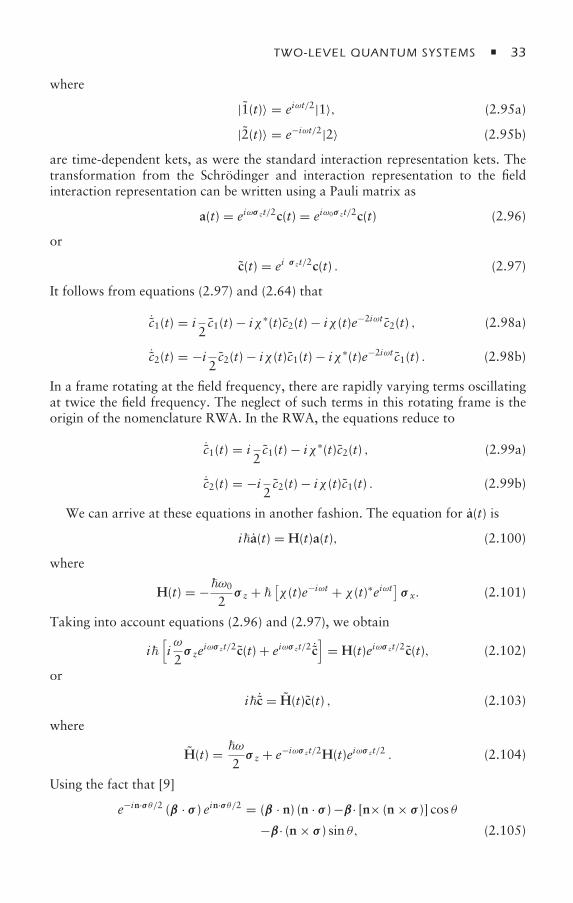
TWO-LEVEL QUANTUM SYSTEMS 33
where
|1(t)〉 = eiωt/2|1〉, (2.95a)
|2(t)〉 = e−iωt/2|2〉 (2.95b)
are time-dependent kets, as were the standard interaction representation kets. Thetransformation from the Schrödinger and interaction representation to the fieldinteraction representation can be written using a Pauli matrix as
a(t) = eiωσ zt/2c(t) = eiω0σ zt/2c(t) (2.96)
or
c(t) = eiδσ zt/2c(t) . (2.97)
It follows from equations (2.97) and (2.64) that
˙c1(t) = iδ
2c1(t) − iχ∗(t)c2(t) − iχ (t)e−2iωt c2(t) , (2.98a)
˙c2(t) = −i δ2c2(t) − iχ (t)c1(t) − iχ∗(t)e−2iωt c1(t) . (2.98b)
In a frame rotating at the field frequency, there are rapidly varying terms oscillatingat twice the field frequency. The neglect of such terms in this rotating frame is theorigin of the nomenclature RWA. In the RWA, the equations reduce to
˙c1(t) = iδ
2c1(t) − iχ∗(t)c2(t) , (2.99a)
˙c2(t) = −i δ2c2(t) − iχ (t)c1(t) . (2.99b)
We can arrive at these equations in another fashion. The equation for a(t) is
ia(t) = H(t)a(t), (2.100)
where
H(t) = −ω0
2σ z + [χ (t)e−iωt + χ (t)∗eiωt] σ x. (2.101)
Taking into account equations (2.96) and (2.97), we obtain
i[iω
2σ zeiωσ zt/2c(t) + eiωσ zt/2 ˙c
]= H(t)eiωσ zt/2c(t), (2.102)
or
i ˙c = H(t)c(t) , (2.103)
where
H(t) = ω2
σ z + e−iωσ zt/2H(t)eiωσ zt/2 . (2.104)
Using the fact that [9]
e−in·σθ/2 (β · σ ) ein·σθ/2 = (β · n) (n · σ )−β· [n× (n × σ )] cos θ
−β· (n × σ ) sin θ, (2.105)
34 CHAPTER 2
where n is a unit vector, β is an arbitrary vector, and σ = σ xx + σ yy + σ zz, one canevaluate the second term in equation (2.104) with n = z, θ = ωt, and
β = − ω0
2z + [χ (t)e−iωt + χ (t)∗eiωt] x , (2.106)
to obtain
e−iωσ zt/2H(t)eiωσ zt/2 = −ω0
2σ z + [χ (t)e−iωt + χ (t)∗eiωt]
× (σ x cosωt + σ y sinωt
). (2.107)
As a result, one finds
H(t) = 2
( −δ 2χ (t)e−2iωt + 2χ (t)∗
2χ (t) + 2χ (t)∗e2iωt δ
), (2.108)
or, in the RWA,
H(t) = ( − δ
2 χ (t)∗
χ (t) δ2
)=
2
( −δ ∗0(t)
0(t) δ
). (2.109)
In terms of the Pauli matrices, the RWA Hamiltonian is
H(t) = 2
−δσ z + Re [0(t)] σ x + Im [0(t)] σ y. (2.110)
The usefulness of the field interaction representation is apparent when 0(t) isconstant. In that limit, H is time-independent, and the solution of equation (2.103)is simply
c(t) = e− iHt c(0) , (2.111)
where
e− iHt = e− i
2 [−δσ z+Re(0)σ x+Im(0)σ y]t = e−i t2 n·σ , (2.112)
and
n = Re (0) x + Im (0) y − δz
. (2.113)
Since [9]
e−i t2 n·σ = I cost2
− in · σ sint2, (2.114)
where I is the identity matrix, one can combine equations (2.111) and (2.112) toobtain
c(t) =[I cos
(t2
)− i
Re (0) σ x + Im (0) σ y − δσ z
sin
(t2
)]c(0), (2.115)
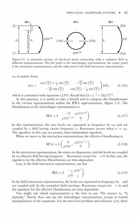
TWO-LEVEL QUANTUM SYSTEMS 35
~
ω0
δ|2
χ(t)e ±iωt
χ(t)e ±iδt
H(t) HI(t)
ω
|1
δ
|2(t) ~
χ(t)
H(t)
|1(t) ~
|1I(t) |2I(t)
Figure 2.5. A schematic picture of two-level atoms interacting with a radiation field indifferent representations. The left panel is the Schrödinger representation, the center panelis the interaction representation, and the right panel is the field interaction representation.
or, in matrix form,
c(t) =(cos
(t2
)+ iδsin
(t2
) − i∗0
sin(t2
)− i0
sin
(t2
)cos
(t2
)− iδsin
(t2
))c(0), (2.116)
which is consistent with equations (2.91). Recall that = [δ2 + |0|2]1/2.At this juncture, it is useful to take a breath and to compare the Hamiltonians
in the various representations within the RWA approximation, (figure 2.5). TheHamiltonian in the Schrödinger representation is
H(t) = (
−ω02 χ (t)∗eiωt
χ (t)e−iωt ω02
). (2.117)
In this representation, the two levels are separated in frequency by ω0 and arecoupled by a field having carrier frequency ω. Resonance occurs when ω = ω0.The eigenkets in this case are proper, time-independent eigenkets.
When we move to the interaction representation, the effective Hamiltonian is
HI (t) = (
0 χ (t)∗e−iδt
χ (t)eiδt 0
). (2.118)
In the interaction representation, the states are degenerate, and the levels are coupledby an effective field having frequency δ. Resonance occurs for δ = 0. In this case, theeigenkets for the effective Hamiltonian are time-dependent.
Last, in the field interaction representation, one has
H(t) = (
− δ2 χ (t)
∗
χ (t) δ2
). (2.119)
In the field interaction representation, the levels are separated in frequency by δ andare coupled only by the (complex) field envelope. Resonance occurs for δ = 0, andthe eigenkets for the effective Hamiltonian are time-dependent.
You might ask which representation is the best to use. The answer is, “Itdepends.” Rarely does one use the Schrödinger representation, except in formalmanipulations of the equations. For the two-level problem and arbitrary χ (t), there
36 CHAPTER 2
is not much difference between the interaction and field interaction representations.Differences between the two representations arise in problems involving more thantwo levels and more than a single field. Generally speaking, the field interactionrepresentation is most useful when a single field drives transitions between twomanifolds of levels, while the interaction representation should be used whenfields having two or more frequencies drive transitions between two levels or twomanifolds of levels. The examples discussed in the remainder of this text help toamplify these ideas.
2.6 Semiclassical Dressed States
The form of the Hamiltonian in the field interaction representation,
H(t) = (
− δ2 χ (t)
∗
χ (t) δ2
), (2.120)
is the springboard for yet another representation. If χ (t) were constant, one wouldnormally solve the equation i ˙c = Hc(t) by diagonalizing H and obtaining theeigenvalues and eigenstates. Some caution is needed since the original eigenketsin the field interaction basis are time-dependent—as a result, the new eigenketsare time-dependent as well. The new basis is called the semiclassical dressed-statebasis since the atomic states are said to be “dressed” by the field [10–12]. A truedressed-state basis with time-independent eigenkets is discussed in chapter 15 afterwe quantize the radiation field. The semiclassical dressed-state representation isparticularly useful when the field amplitude and phase vary slowly compared withdetunings or Rabi frequencies.
The semiclassical dressed states can be given the simplest interpretation if weredefine the field interaction representation slightly using
|ψ(t)〉 = c1(t)ei[ωt−φ(t)]/2|1〉 + c2(t)e−i[ωt−φ(t)]/2|2〉 (2.121)
[recall that 0(t) = |0(t)|eiφ(t)], in which the phase of the complex field amplitudeis included explicitly. With this definition, everything proceeds as before, except thatδ is replaced by
δ(t) = δ + φ(t), (2.122)
and 0(t) by |0(t)|. In other words, one obtains
i ˙c(t) = H(t) c(t) , (2.123)
where
H(t) = 2
( −δ(t) |0(t)||0(t)| δ(t)
). (2.124)
In this picture, the state amplitudes are coupled by the field amplitude, and thedetuning is a function of time that depends on the field phase. If φ(t) = 0, both fieldinteraction representations are equivalent.
For the most part, we will use the original definition (2.94) of the field interactionrepresentation, perhaps with a spatial phase extracted when we consider moving
TWO-LEVEL QUANTUM SYSTEMS 37
atoms. The second definition (2.121) will be reserved for problems involvingadiabatic states and semiclassical dressed states. To distinguish between the twofield interaction representations, we add primes to the amplitudes and state vectorsappearing in equation (2.94). Admittedly, this can be a bit confusing, but we retainthe distinction between the two field interaction representations in this chapterand in chapter 3, since the representation (2.121) is particularly well-suited for adiscussion of adiabatic states and the Bloch vector. From chapter 4 onward, werevert to equation (2.94) and drop all the primes.
With this modified definition, equations (2.95) are replaced by
|1(t)〉 = ei[ωt−φ(t)]/2|1〉 , (2.125a)
|2(t)〉 = e−i[ωt−φ(t)]/2|2〉 . (2.125b)
We introduce a new basis via(|I(t)〉|I I(t)〉
)= T(t)
(|1(t)〉|2(t)〉
), (2.126)
where T(t) is an orthogonal, real matrix of the form
T(t) =(cos θ (t) − sin θ (t)
sin θ (t) cos θ (t)
). (2.127)
The angle θ (t) is chosen such that T(t) diagonalizes H(t) at time t.Before calculating θ (t), we first expand the state vector as
|ψ(t)〉 =2∑
n=1
cn(t)|n(t)〉 =∑i=I,I I
cdi (t)|i(t)〉 = cT(t)|n(t)〉 = cTd (t)|D(t)〉, (2.128)
where the superscript T means transpose,
|n(t)〉 =(
|1(t)〉|2(t)〉
), (2.129)
and
|D(t)〉 =(
|I(t)〉|I I(t)〉
)= T(t)|n(t)〉 . (2.130)
It follows from equations (2.128) and (2.130) that the field interaction and dressed-state amplitudes are related by
cT(t) = cTdT(t) , (2.131)
or, since TT(t) = T†(t),
c(t) = T†(t)cd(t) , cd(t) = T(t)c(t) . (2.132)
It then follows from equation (2.123) that
i[T†(t)cd(t) + T†(t)cd] = H(t)T†(t)cd(t) , (2.133)
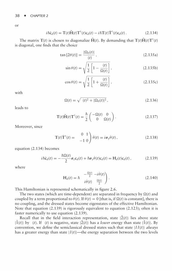
38 CHAPTER 2
or
icd(t) = T(t)H(t)T†(t)cd(t) − iT(t)T†(t)cd(t) . (2.134)
The matrix T(t) is chosen to diagonalize H(t). By demanding that T(t)H(t)T†(t)is diagonal, one finds that the choice
tan [2θ (t)] = |0(t)|δ(t)
, (2.135a)
sin θ (t) =√
12
[1 − δ(t)
(t)
], (2.135b)
cos θ (t) =√
12
[1 + δ(t)
(t)
], (2.135c)
with
(t) =√δ(t)2 + |0(t)|2 , (2.136)
leads to
T(t)H(t)T†(t) = 2
(−(t) 00 (t)
). (2.137)
Moreover, since
T(t)T†(t) =(
0 1
−1 0
)θ(t) = iσyθ (t) , (2.138)
equation (2.134) becomes
icd(t) = −(t)2
σzcd(t) + σyθ(t)cd(t) = Hd(t)cd(t) , (2.139)
where
Hd(t) = (−(t)
2 −i θ (t)i θ (t) (t)
2
). (2.140)
This Hamiltonian is represented schematically in figure 2.6.The two states (which are time-dependent) are separated in frequency by(t) and
coupled by a term proportional to θ (t). If θ (t) = 0 [that is, if(t) is constant], there isno coupling, and the dressed states become eigenstates of the effective Hamiltonian.Note that equation (2.139) is rigorously equivalent to equation (2.123); often it isfaster numerically to use equation (2.139).
Recall that in the field interaction representation, state |2(t)〉 lies above state|1(t)〉 by δ(t). If δ(t) is negative, state |2(t)〉 has a lower energy than state |1(t)〉. Byconvention, we define the semiclassical dressed states such that state |I I(t)〉 alwayshas a greater energy than state |I(t)〉—the energy separation between the two levels
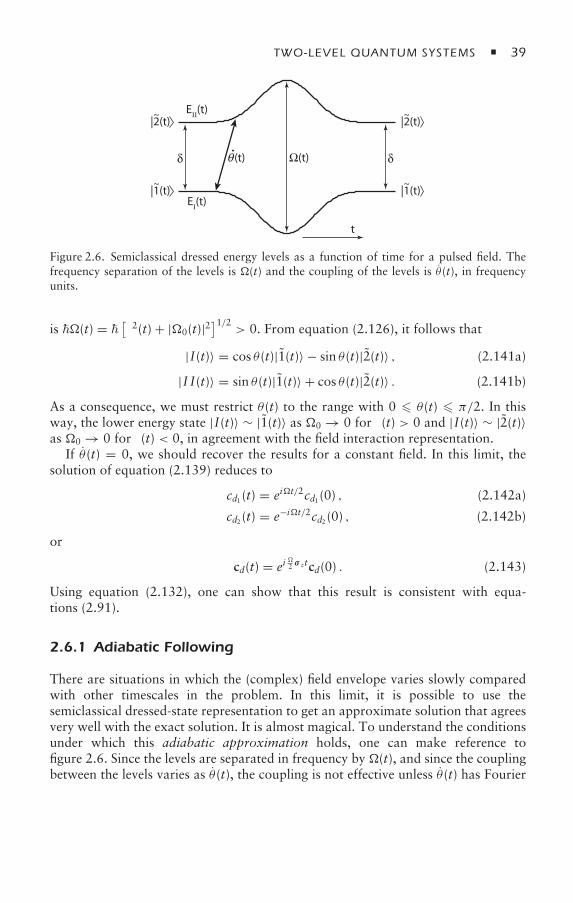
TWO-LEVEL QUANTUM SYSTEMS 39
t
EI(t)
EII(t)
δ δθ Ω(t)(t)•
|2(t) ~
|1(t) ~
|2(t) ~
|1(t) ~
Figure 2.6. Semiclassical dressed energy levels as a function of time for a pulsed field. Thefrequency separation of the levels is (t) and the coupling of the levels is θ (t), in frequencyunits.
is (t) = [δ2(t) + |0(t)|2]1/2
> 0. From equation (2.126), it follows that
|I(t)〉 = cos θ (t)|1(t)〉 − sin θ (t)|2(t)〉 , (2.141a)
|I I(t)〉 = sin θ (t)|1(t)〉 + cos θ (t)|2(t)〉 . (2.141b)
As a consequence, we must restrict θ (t) to the range with 0 θ (t) π/2. In thisway, the lower energy state |I(t)〉 ∼ |1(t)〉 as 0 → 0 for δ(t) > 0 and |I(t)〉 ∼ |2(t)〉as 0 → 0 for δ(t) < 0, in agreement with the field interaction representation.
If θ (t) = 0, we should recover the results for a constant field. In this limit, thesolution of equation (2.139) reduces to
cd1 (t) = eit/2cd1 (0) , (2.142a)
cd2 (t) = e−it/2cd2 (0) , (2.142b)
or
cd(t) = ei2 σ ztcd(0) . (2.143)
Using equation (2.132), one can show that this result is consistent with equa-tions (2.91).
2.6.1 Adiabatic Following
There are situations in which the (complex) field envelope varies slowly comparedwith other timescales in the problem. In this limit, it is possible to use thesemiclassical dressed-state representation to get an approximate solution that agreesvery well with the exact solution. It is almost magical. To understand the conditionsunder which this adiabatic approximation holds, one can make reference tofigure 2.6. Since the levels are separated in frequency by (t), and since the couplingbetween the levels varies as θ(t), the coupling is not effective unless θ(t) has Fourier
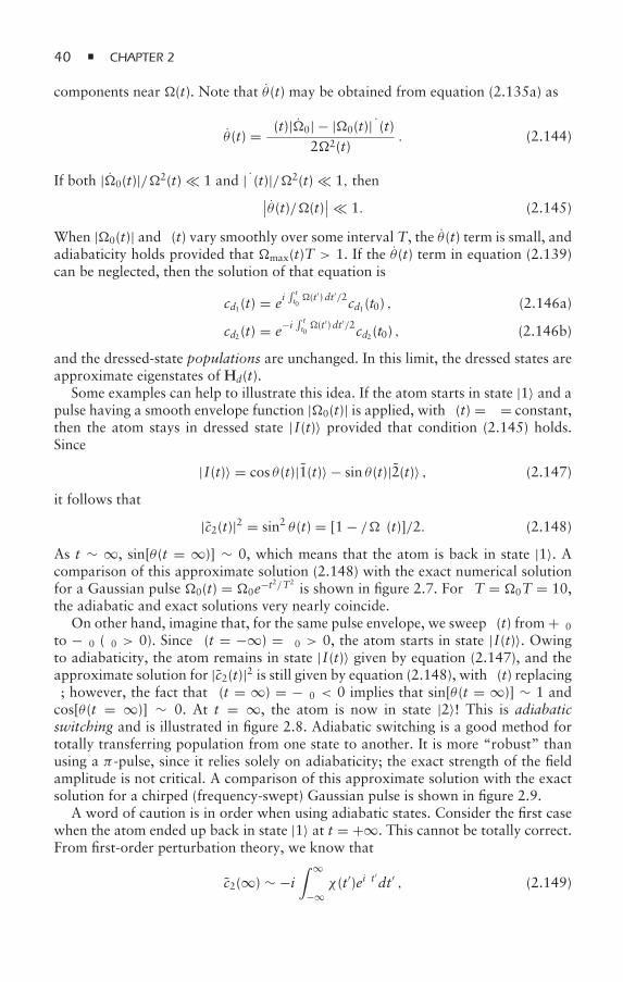
40 CHAPTER 2
components near (t). Note that θ (t) may be obtained from equation (2.135a) as
θ (t) = δ(t)|0| − |0(t)|δ(t)22(t)
. (2.144)
If both |0(t)|/2(t) 1 and |δ(t)|/2(t) 1, then∣∣θ (t)/(t)∣∣ 1. (2.145)
When |0(t)| and δ(t) vary smoothly over some interval T, the θ (t) term is small, andadiabaticity holds provided that max(t)T > 1. If the θ(t) term in equation (2.139)can be neglected, then the solution of that equation is
cd1 (t) = ei∫ tt0(t′)dt′/2cd1 (t0) , (2.146a)
cd2 (t) = e−i ∫ tt0 (t′)dt′/2cd2 (t0) , (2.146b)
and the dressed-state populations are unchanged. In this limit, the dressed states areapproximate eigenstates of Hd(t).
Some examples can help to illustrate this idea. If the atom starts in state |1〉 and apulse having a smooth envelope function |0(t)| is applied, with δ(t) = δ = constant,then the atom stays in dressed state |I(t)〉 provided that condition (2.145) holds.Since
|I(t)〉 = cos θ (t)|1(t)〉 − sin θ (t)|2(t)〉 , (2.147)
it follows that
|c2(t)|2 = sin2 θ (t) = [1 − δ/(t)]/2. (2.148)
As t ∼ ∞, sin[θ (t = ∞)] ∼ 0, which means that the atom is back in state |1〉. Acomparison of this approximate solution (2.148) with the exact numerical solutionfor a Gaussian pulse 0(t) = 0e−t2/T2
is shown in figure 2.7. For δT = 0T = 10,the adiabatic and exact solutions very nearly coincide.
On other hand, imagine that, for the same pulse envelope, we sweep δ(t) from +δ0to −δ0 (δ0 > 0). Since δ(t = −∞) = δ0 > 0, the atom starts in state |I(t)〉. Owingto adiabaticity, the atom remains in state |I(t)〉 given by equation (2.147), and theapproximate solution for |c2(t)|2 is still given by equation (2.148), with δ(t) replacingδ; however, the fact that δ(t = ∞) = −δ0 < 0 implies that sin[θ (t = ∞)] ∼ 1 andcos[θ (t = ∞)] ∼ 0. At t = ∞, the atom is now in state |2〉! This is adiabaticswitching and is illustrated in figure 2.8. Adiabatic switching is a good method fortotally transferring population from one state to another. It is more “robust” thanusing a π -pulse, since it relies solely on adiabaticity; the exact strength of the fieldamplitude is not critical. A comparison of this approximate solution with the exactsolution for a chirped (frequency-swept) Gaussian pulse is shown in figure 2.9.
A word of caution is in order when using adiabatic states. Consider the first casewhen the atom ended up back in state |1〉 at t = +∞. This cannot be totally correct.From first-order perturbation theory, we know that
c2(∞) ∼ −i∫ ∞
−∞χ (t′)eiδt
′dt′ , (2.149)
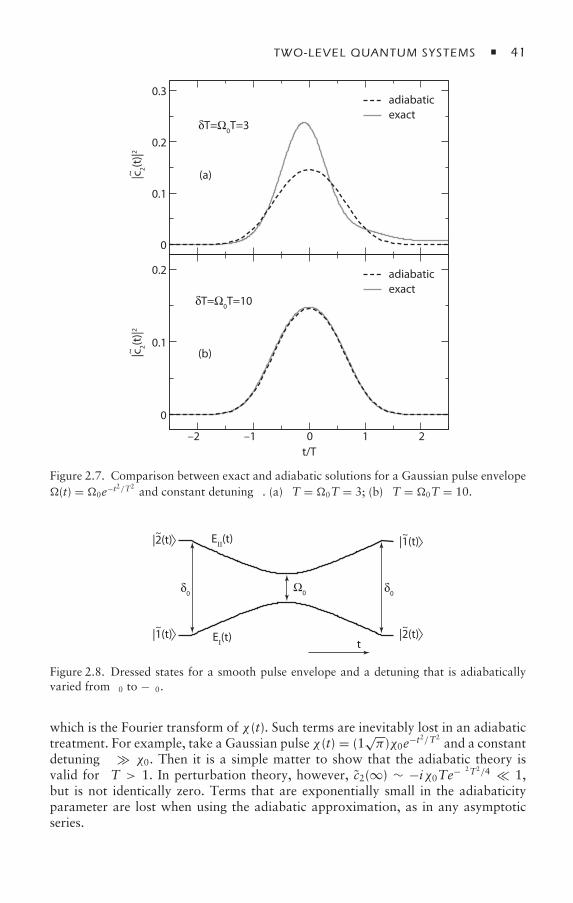
TWO-LEVEL QUANTUM SYSTEMS 41
0
0.1
0.2
0.3
(a)
(b)
adiabaticexact
adiabatic
δT=Ω0T=10
δT=Ω0T=3
exact
–2 –1 0 1 2t/T
0
0.1
0.2
|c2(t
)|2~
|c2(t
)|2~
Figure 2.7. Comparison between exact and adiabatic solutions for a Gaussian pulse envelope(t) = 0e−t2/T2
and constant detuning δ. (a) δT = 0T = 3; (b) δT = 0T = 10.
t
δ0δ0Ω0
EII(t)
EI(t)
|2(t) ~
|1(t) ~
|2(t) ~
|1(t) ~
Figure 2.8. Dressed states for a smooth pulse envelope and a detuning that is adiabaticallyvaried from δ0 to −δ0.
which is the Fourier transform of χ (t). Such terms are inevitably lost in an adiabatictreatment. For example, take a Gaussian pulse χ (t) = (1
√π )χ0e−t2/T2
and a constantdetuning δ χ0. Then it is a simple matter to show that the adiabatic theory isvalid for δT > 1. In perturbation theory, however, c2(∞) ∼ −iχ0Te−δ2T2/4 1,but is not identically zero. Terms that are exponentially small in the adiabaticityparameter are lost when using the adiabatic approximation, as in any asymptoticseries.
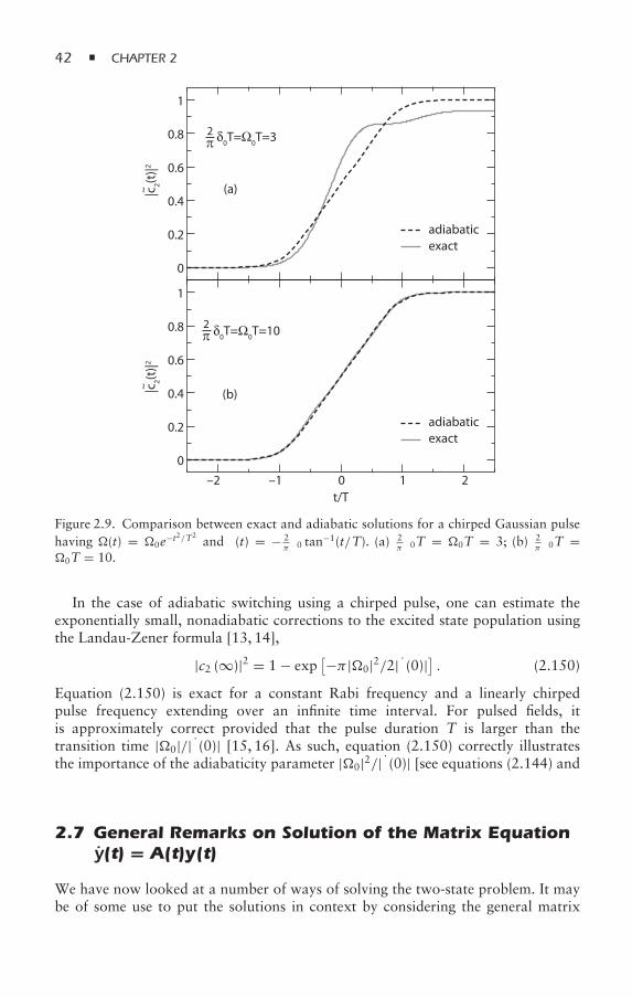
42 CHAPTER 2
0
0.2
0.4
0.6
0.8
1
(a)
(b)
0
0.2
0.4
0.6
0.8
1
adiabaticexact
adiabatic
δ0T=Ω0T=10
δ0T=Ω0T=3
exact
–2 –1 0 1 2t/T
|c2(t
)|2~
|c2(t
)|2~
π
π
2
2
Figure 2.9. Comparison between exact and adiabatic solutions for a chirped Gaussian pulsehaving (t) = 0e−t2/T2
and δ(t) = − 2πδ0 tan−1(t/T). (a) 2
πδ0T = 0T = 3; (b) 2
πδ0T =
0T = 10.
In the case of adiabatic switching using a chirped pulse, one can estimate theexponentially small, nonadiabatic corrections to the excited state population usingthe Landau-Zener formula [13, 14],
|c2 (∞)|2 = 1 − exp[−π |0|2/2|δ(0)|] . (2.150)
Equation (2.150) is exact for a constant Rabi frequency and a linearly chirpedpulse frequency extending over an infinite time interval. For pulsed fields, itis approximately correct provided that the pulse duration T is larger than thetransition time |0|/|δ(0)| [15, 16]. As such, equation (2.150) correctly illustratesthe importance of the adiabaticity parameter |0|2/|δ(0)| [see equations (2.144) and(2.145)] in determining the final state population.
2.7 General Remarks on Solution of the Matrix Equationy(t) = A(t)y(t)
We have now looked at a number of ways of solving the two-state problem. It maybe of some use to put the solutions in context by considering the general matrix
TWO-LEVEL QUANTUM SYSTEMS 43
equation
y(t) = −iA(t)y(t) . (2.151)
For any finite matrix, this equation can be solved numerically. If A(t) is Hermitian,|y(t)|2 is constant. What approximation techniques can be used to solve equation(2.151)?
2.7.1 Perturbation Theory
To first order, a perturbative solution of equation (2.151) is
y(t) ≈ y(0) − i∫ t
0A(t′)dt′y(0), (2.152)
valid only if | ∫ t0 A(t
′)dt′| 1.
2.7.2 Adiabatic Approximation
We set
y(t) = T(t)x(t), (2.153)
where T†(t)A(t)T(t) = (t) is diagonal. Then
x(t) = −i(t)x(t) − T†(t)T(t)x(t) . (2.154)
If matrix elements of T†(t)T(t) are much less than the eigenvalue spacing of (t),then one can neglect the T†(t)T(t) term or treat it in perturbation theory. Note that
1,2(t) = ±√δ(t)2 + |0(t)|2/2 = ±(t)/2
in the two-level problem. This adiabatic approach is useful only if the T†(t)T(t) termcan be neglected. Taking first-order perturbation theory in T†(t)T(t) can be moretime consuming (numerically) than directly integrating the differential equations.
2.7.3 Magnus Approximation
For a single variable, the differential equation
x = −i f (t)x (2.155)
has solution
x(t) = e−i ∫ t0 f (t′)dt′x(0). (2.156)
One might think that the analogous vector solution of equation (2.151) is
y(1)(t) = e−i ∫ t0 A(t′)dt′y(0). (2.157)
44 CHAPTER 2
This expression is called the first Magnus approximation [17]. We can checkwhether it works. Solving equation (2.151) iteratively gives
y(t) =[1 − i
∫ t
0A(t′)dt′ −
∫ t
0dt′
∫ t′
0dt′′A(t′)A(t′′) + · · ·
]y(0) , (2.158)
while the first Magnus approximation is
y(1)(t) = e−i ∫ t0 A(t′)dt′y(0) =1 − i
∫ t
0A(t′)dt′ − 1
2
[∫ t
0A(t′)dt′
]2+ · · ·
y(0) .
(2.159)The two solutions agree to first order in A. Let us compare the second-order terms
by evaluating the third term in equation (2.159) as
12
[∫ t
0A(t′)dt′
]2= 1
2
∫ t
0dt′
∫ t
0dt′′A(t′)A(t′′)
= 12
∫ t
0dt′A(t′)
[∫ t′
0dt′′A(t′′) +
∫ t
t′dt′′A(t′′)
]
= 12
∫ t
0dt′
∫ t′
0dt′′A(t′)A(t′′) + 1
2
∫ t
0dt′′
∫ t′′
0dt′A(t′)A(t′′)
= 12
∫ t
0dt′
∫ t′
0dt′′A(t′)A(t′′) + 1
2
∫ t
0dt′
∫ t′
0dt′′A(t′′)A(t′), (2.160)
where the order of integration was interchanged in going from line 2 to line 3.Equation (2.160) would agree with the third term in equation (2.158) if A(t′′)A(t′) =A(t′)A(t′′), but A(t′′)A(t′) = A(t′)A(t′′), in general. The difference between the twoterms can be obtained by writing A(t′′)A(t′) = A(t′)A(t′′) + [A(t′′),A(t′)]. When thisis substituted into equation (2.160), we find
12
[∫ t
0A(t′)dt′
]2=∫ t
0dt′
∫ t′
0dt′′A(t′)A(t′′)
+12
∫ t
0dt′
∫ t′
0dt′′[A(t′′),A(t′)] . (2.161)
Thus, there is a correction related to the unequal time commutator, and thesolution (2.159) is not correct. Instead, we can try a solution of the form
y(2)(t) = e−i ∫ t0 A(t′)dt′− 12!
∫ t0 dt
′ ∫ t′0 dt′′[A(t′′),A(t′)]y(0), (2.162)
which is guaranteed to be correct to second order in A. The solution (2.162) is theknown as the second Magnus approximation.
We can continue the process. The next correction is
(−i)33!
∫ t
0dt′
∫ t′
0dt′′
∫ t′′
0dt′′′
[A(t′′′),
[A(t′′),A(t′)
]]+ [A(t′′′),A(t′′)],A(t′)
],
and this can be added to the exponential to produce a result that is correct to thirdorder in A. In practice, many people use the first Magnus approximation with no
TWO-LEVEL QUANTUM SYSTEMS 45
TABLE 2.2Different Representations
|ψ(t)〉 Representation
a1(t)|1〉 + a2(t)|2〉 Schrödingerc1(t)eiω0t/2|1〉 + c2(t)e−iω0t/2|2〉 Interactionc′1(t)e
iωt/2|1〉 + c′2(t)e
−iωt/2|2〉 Field interaction 1c1(t)eiωt/2−iφ/2|1〉 + c2(t)e−iωt/2+iφ/2|2〉 Field interaction 2cd1 (t)|I(t)〉 + cd2 (t)|I I(t)〉 Semiclassical dressed state
idea of the errors introduced. It has the advantage that if A(t) is Hermitian, thenthe solution maintains unitarity. As mentioned earlier, the disadvantage is that it isdifficult to estimate the errors.
2.8 Summary
We have introduced several representations for solving the problem of the interac-tion of a classical optical field with a “two-level” atom. The various representationsand their interconnections are summarized in appendix A for easy reference. Asyou become more familiar with the material, you will be able to choose the mostconvenient representation with little difficulty. In very rough terms, however, thefollowing prescription might prove helpful: (1) a single quasi-monochromatic fielddrives transitions between two levels or two manifolds of levels—use the fieldinteraction representation; (2) two or more quasi-monochromatic fields havingdifferent frequencies drive transitions between two levels or two manifolds oflevels—use the interaction representation; and (3) pulsed fields whose envelopesand phases vary slowly compared to their average Rabi frequencies or atom–fielddetunings drive transitions between two levels—use the semiclassical dressed-staterepresentation.
Armed with these representations and your understanding of atom–fielddynamics, you are now ready to attack the important problem of extracting thephysically relevant quantities from the solutions we have obtained so far. Moreover,by defining the density matrix associated with the two-level atom, you will see howone can introduce irreversible decay processes into the atom–field dynamics.
2.9 Appendix A: Representations
The representations are summarized in table 2.2. Here we use primes on the c’s todistinguish the two field interaction representations.
All of the following equations are written in the rotating-wave approximation(RWA), with
E(t) = z2[E0(t)e−iωt + E∗
0(t)eiωt] = z
2[|E0(t)| e−iωt+iφ(t) + |E0(t)| eiωt−iφ(t)], (2.163)
46 CHAPTER 2
and
V(t) = −µz2
[|E0(t)| e−iωt+iφ(t) + |E0(t)| eiωt−iφ(t)]. (2.164)
In the Schrödinger representation,
ia(t) = H(t)a(t),(2.165)
H(t) = (/2)( −ω0 0(t)∗eiωt
0(t)e−iωt ω0
),
where
0(t) = −〈2|µz|1〉E0(t)/ = 2χ (t).
In the interaction representation,
idc(t)/dt = VI (t)c(t), (2.166)
VI (t) = (/2)(
0 0(t)∗e−iδt
0(t)eiδt 0
), (2.167)
where δ = ω0 − ω.In the field interaction representation,
idc′(t)/dt = H′(t) c′(t), H′(t) = (/2)
( −δ 0(t)∗
0(t) δ
), (2.168)
or
idc(t)/dt = H(t)c(t), H(t) = (/2)( −δ(t) |0(t)|
|0(t)| δ(t)
), (2.169)
where
δ(t) = ω0 − ω + dφ/dt.
In the semiclassical dressed-state representation,
idcd(t)/dt = Hd(t)cd(t), Hd(t) = (−(t)
2 −i θ (t)i θ (t) (t)
2
), (2.170)
where (t) = [|0(t)|2 + δ(t)2]1/2 and tan [2θ (t)] = |0(t)| /δ(t).
2.9.1 Relationships between the Representations
Let U0(t) = exp(−iH0t/), where H(t) = H0 + V(t). Then
c(t) = U†0(t)a(t)=eiω0tσ z/2a(t), VI (t) = U†
0(t)V(t)U0(t), (2.171)
TWO-LEVEL QUANTUM SYSTEMS 47
and
c′(t) = e−iωtσ z/2 a(t)=eiδtσ z/2c(t) , (2.172a)
H′(t) = (ω/2)σ z + e−iωtσ z/2H(t)eiωtσ z/2 , (2.172b)
c(t) = e(−iωt/2+iφ/2)σ za(t)=e(iδt/2+iφ/2)σ zc(t) , (2.172c)
H(t) = (ω/2 − φ/2)σ z
+e(−iωt/2+iφ/2)σ zH(t)e(iωt/2−iφ/2)σ z , (2.172d)
cd(t) = T(t)c(t), T(t) =(cos θ (t) − sin θ (t)
sin θ (t) cos θ (t)
), (2.172e)
( |I(t)〉|I I(t)〉
)= T(t)
(ei[ωt−φ(t)]/2|1〉e−i[ωt−φ(t)]/2|2〉
), (2.172f)
Hd(t) = T(t)H(t)T†(t) − iT(t)T†(t). (2.172g)
2.10 Appendix B: Spin Half Quantum System in aMagnetic Field
The Hamiltonian that characterizes the interaction of a magnetic field,
B(t) = B0z + |Bx(t)| cos [ωt − φ(t)] x, (2.173)
with the spin magnetic moment of an electron is
HB = −µmag · B , (2.174)
where
µmag = −eSm
= − e2m
σ = −µBσ (2.175)
is the magnetic moment operator of the electron, m is the electron mass,
µB = e2m
= 9.2740154 × 10⁻²⁴ J T−1 (2.176)
is the Bohr magneton, S = σ/2 is the spin operator, and σ = σ xx + σ yy + σ zz.In terms of the Pauli matrices, the Hamiltonian can be written
HB(t) = µBB0σ z + µB |Bx(t)| cos [ωt − φ(t)] σ x . (2.177)
The connection with equation (2.56) is now apparent if we identify the level spacingas
ω0 = 2µBB0
= emB0 = 1.76 × 10¹¹ B0(Tesla) s−1 = 1.76 × 10⁷ B0(Gauss) s−1 .
(2.178)Note that the sign of the lead terms in the Hamiltonians (2.56) and (2.177) differ,since for the optical case, we have chosen the basis a = (a1, a2), while for themagnetic case, the standard convention for the Pauli matrices requires that we take
48 CHAPTER 2
aB = (a↑, a↓
), where the up (down) arrow refers to the state having spin projection
number 1/2 (−1/2). In frequency units, ω0/2π = 28 GHz/T.Although the equations for the two-level atom interacting with an electric field
and the spin system interacting with a magnetic field look the same, the physicalvalues of the parameters for the two systems differ markedly. Thus, the frequencyseparation of the spin up and spin down states in a constant magnetic field canrange between 0 Hz and 10 GHz, while radio-frequency (rf) coupling strengths[µB |Bx(t)| /h] are typically less than 1.0 MHz. In the optical case, electronictransition frequencies are of order 1014 to 1016 Hz, and coupling strengths vary,but are typically much less than the frequency separation of the levels. Only forintense pulses (>1017 W/cm2) can the coupling strength be comparable to the opticalfrequency separations. For a typical cw laser having a few mW of power, couplingstrengths are typically in the MHz to GHz range. Given this qualitative differencein the magnetic and electric cases, it is not surprising that different approximationschemes are used in the two cases. We have seen that the RWA approximation isusually a good approximation for atom–optical field interactions, but this is notnecessarily so for the magnetic case.
In the interaction representation, the equations for the state amplitudes are
icB(t) = (
0 ωx(t) cos[ωt − φ(t)]eiω0t
ωx(t) cos[ωt − φ(t)]e−iω0t 0
)cB(t) , (2.179)
with cB = (c↑, c↓
), ω0 = ω↑↓ = ω↑ − ω↓, and
ωx(t) = µB |Bx(t)|
. (2.180)
All the solutions that were obtained in the RWA can be taken over to the magneticcase, so we concentrate on situations where the RWA is not applicable.
2.10.1 Analytic Solutions—Magnetic Case
2.10.1.1 ω0 = 0
If there is no longitudinal field [Bz = 0], the energy levels are degenerate, and thestates are coupled by the field oscillating in the x direction. Equations for probabilityamplitudes have the form
c↑(t) = −i f (t)c↓(t), (2.181a)
c↓(t) = −i f (t)c↑(t), (2.181b)
where
f (t) = ωx(t) cos [ωt − φ(t)] . (2.182)
In analogy with equation (2.79), we find a solution
c↑(t) = cos [θ (t)] c↑(0) − i sin [θ (t)] c↓(0), (2.183a)
c↓(t) = −i sin [θ (t)] c↑(0) + cos [θ (t)] c↓(0) , (2.183b)
TWO-LEVEL QUANTUM SYSTEMS 49
where
θ (t) =∫ t
0f (t′)dt. (2.184)
The interpretation of these equations is straightforward. The two levels are degen-erate, and the driving field couples the states.
Although this is a simple solution, it can be used to illustrate some interestingphysical concepts. If we take φ(t) = 0 and ωx(t) = ωx = constant, then∫ t
0f (t′)dt′ = ωx
ωsinωt, (2.185)
which means that the probability amplitudes contain all harmonics of the field. Tosee this more clearly, we can expand cos [(ωx/ω) sinωt] in terms of a series of Besselfunctions Jn using
cos (z sinα) = J0(z) + 2∞∑n=1
J2n(z) cos(2nα) . (2.186)
For example, if the initial state has c↓(0) = 1, c↑(0) = 0, then
∣∣c↑(t)∣∣2 = sin2
(ωxω
sinωt)
=1 − cos
(2ωxω
sinωt)
2
=1 − J0
(2ωxω
)2
+∞∑n=1
J2n
(2ωxω
)cos(2nωt). (2.187)
In contrast to a harmonic oscillator, which is intrinsically a linear device, a two-levelquantum system acts as a nonlinear device—the response does not depend linearlyon the applied field and contains all harmonics of the driving field frequency. Forωx/ω π/2, there are still times when
∣∣c↑(t)∣∣2 = 1.
The time-averaged, spin-up population is
∣∣c↑(t)∣∣2 =
1 − J0(
2ωxω
)2
. (2.188)
The larger the applied frequency, the smaller the time-averaged value of the state uppopulation, provided that ω > 0.522ωx. This is not surprising since the degeneratelevels are resonant with a static field. On the other hand, there are values of
ωx/ω for which∣∣c↑(t)
∣∣2 > 1/2. The maximum value of∣∣c↑(t)
∣∣2 = 0.7 occurs for2ωx/ω = 3.85.
2.10.1.2 ωx(t) = ωx = constant; ω = 0; φ(t) = φ = constant
This corresponds in the magnetic case to a constant field in the x direction and aconstant field in the z direction,
B = B0z + Bxx , (2.189)
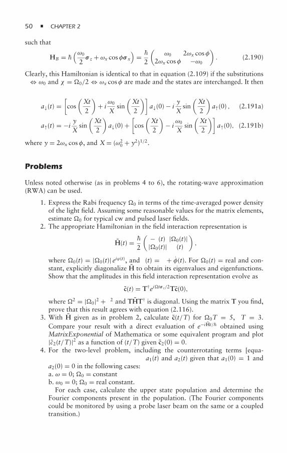
50 CHAPTER 2
such that
HB = (ω0
2σ z + ωx cosφσ x
)=
2
(ω0 2ωx cosφ
2ωx cosφ −ω0
). (2.190)
Clearly, this Hamiltonian is identical to that in equation (2.109) if the substitutionsδ ⇔ ω0 and χ = 0/2 ⇔ ωx cosφ are made and the states are interchanged. It thenfollows that the solution to this problem is [see equation (2.116)]
a↓(t) =[cos
(Xt2
)+ iω0
Xsin
(Xt2
)]a↓(0) − i
yXsin
(Xt2
)a↑(0) , (2.191a)
a↑(t) = −i yX
sin(Xt2
)a↓(0) +
[cos
(Xt2
)− iω0
Xsin
(Xt2
)]a↑(0), (2.191b)
where y = 2ωx cosφ, and X= (ω20 + y2)1/2.
Problems
Unless noted otherwise (as in problems 4 to 6), the rotating-wave approximation(RWA) can be used.
1. Express the Rabi frequency 0 in terms of the time-averaged power densityof the light field. Assuming some reasonable values for the matrix elements,estimate 0 for typical cw and pulsed laser fields.
2. The appropriate Hamiltonian in the field interaction representation is
H(t) = 2
( −δ(t) |0(t)||0(t)| δ(t)
),
where 0(t) = |0(t)| eiϕ(t), and δ(t) = δ + φ(t). For 0(t) = real and con-stant, explicitly diagonalize H to obtain its eigenvalues and eigenfunctions.Show that the amplitudes in this field interaction representation evolve as
c(t) = T†eitσ z/2Tc(0),
where 2 = |0|2 + δ2 and THT† is diagonal. Using the matrix T you find,prove that this result agrees with equation (2.116).
3. With H given as in problem 2, calculate c(t/T) for 0T = 5, δT = 3.Compare your result with a direct evaluation of e−iHt/ obtained usingMatrixExponential of Mathematica or some equivalent program and plot|c2(t/T)|2 as a function of (t/T) given c2(0) = 0.
4. For the two-level problem, including the counterrotating terms [equa-tion (2.55) or (2.179)], solve for a1(t) and a2(t) given that a1(0) = 1 anda2(0) = 0 in the following cases:a. ω = 0; 0 = constantb. ω0 = 0; 0 = real constant.For each case, calculate the upper state population and determine the
Fourier components present in the population. (The Fourier componentscould be monitored by using a probe laser beam on the same or a coupledtransition.)
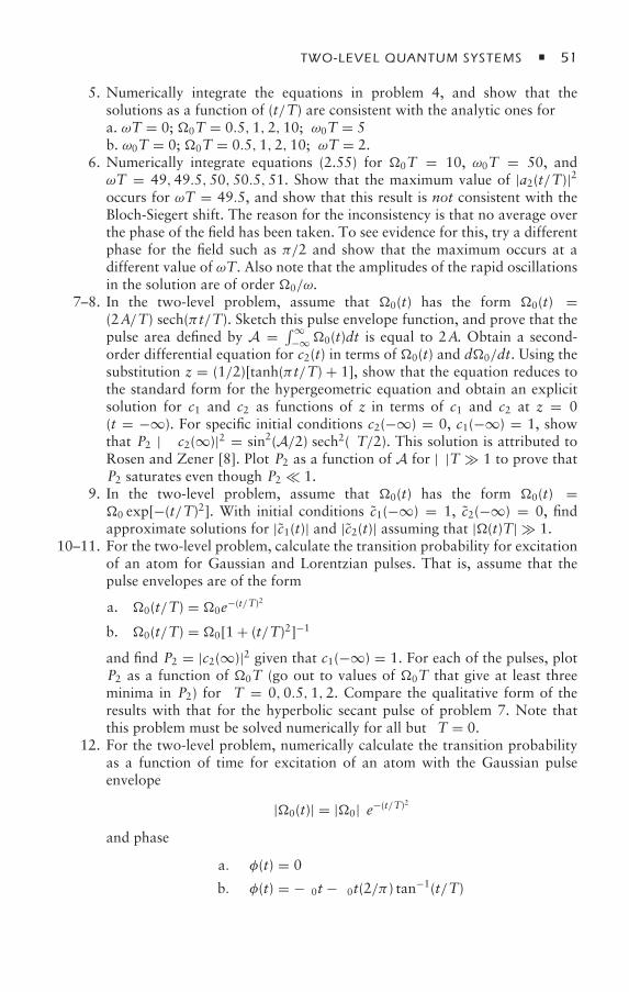
TWO-LEVEL QUANTUM SYSTEMS 51
5. Numerically integrate the equations in problem 4, and show that thesolutions as a function of (t/T) are consistent with the analytic ones fora. ωT = 0; 0T = 0.5,1,2,10; ω0T = 5b. ω0T = 0; 0T = 0.5,1,2,10; ωT = 2.
6. Numerically integrate equations (2.55) for 0T = 10, ω0T = 50, andωT = 49,49.5,50,50.5,51. Show that the maximum value of |a2(t/T)|2occurs for ωT = 49.5, and show that this result is not consistent with theBloch-Siegert shift. The reason for the inconsistency is that no average overthe phase of the field has been taken. To see evidence for this, try a differentphase for the field such as π/2 and show that the maximum occurs at adifferent value of ωT. Also note that the amplitudes of the rapid oscillationsin the solution are of order 0/ω.
7–8. In the two-level problem, assume that 0(t) has the form 0(t) =(2A/T) sech(π t/T). Sketch this pulse envelope function, and prove that thepulse area defined by A = ∫∞
−∞0(t)dt is equal to 2A. Obtain a second-order differential equation for c2(t) in terms of 0(t) and d0/dt. Using thesubstitution z = (1/2)[tanh(π t/T) + 1], show that the equation reduces tothe standard form for the hypergeometric equation and obtain an explicitsolution for c1 and c2 as functions of z in terms of c1 and c2 at z = 0(t = −∞). For specific initial conditions c2(−∞) = 0, c1(−∞) = 1, showthat P2 ≡ |c2(∞)|2 = sin2(A/2) sech2(δT/2). This solution is attributed toRosen and Zener [8]. Plot P2 as a function of A for |δ|T 1 to prove thatP2 saturates even though P2 1.
9. In the two-level problem, assume that 0(t) has the form 0(t) =0 exp[−(t/T)2]. With initial conditions c1(−∞) = 1, c2(−∞) = 0, findapproximate solutions for |c1(t)| and |c2(t)| assuming that |(t)T| 1.
10–11. For the two-level problem, calculate the transition probability for excitationof an atom for Gaussian and Lorentzian pulses. That is, assume that thepulse envelopes are of the form
a. 0(t/T) = 0e−(t/T)2
b. 0(t/T) = 0[1 + (t/T)2]−1
and find P2 = |c2(∞)|2 given that c1(−∞) = 1. For each of the pulses, plotP2 as a function of 0T (go out to values of 0T that give at least threeminima in P2) for δT = 0,0.5,1,2. Compare the qualitative form of theresults with that for the hyperbolic secant pulse of problem 7. Note thatthis problem must be solved numerically for all but δT = 0.
12. For the two-level problem, numerically calculate the transition probabilityas a function of time for excitation of an atom with the Gaussian pulseenvelope
|0(t)| = |0| e−(t/T)2
and phase
a. φ(t) = 0
b. φ(t) = −δ0t − δ0t(2/π) tan−1(t/T)
52 CHAPTER 2
where δ0 is the detuning. Take
(i) δ0T = 3, |0|T = 3
(i i) δ0T = 8, |0|T = 8
to determine whether you are in the adiabatic following limit. Calculateδ(t) = δ0 + φ, and plot ±(t)T/2 = |0(t)|2 + [δ(t)]21/2T/2. Work in thesecond field interaction representation and introduce a dimensionless timeτ = t/T. Assume that c1(−∞) = 1, and calculate |c2|2 as a function of τfor cases a.(i), a.(ii), b.(i), and b.(ii). Show that in case a.(ii), the populationreturns to the first state at the end of the pulse, while in case b.(ii) (adiabaticswitching), the population is transferred to the second state by the pulse.Compare your numerical solutions with the prediction of the dressed-statetheory |c2(t)|2 = sin2[θ (t)] = [1 − δ(t)/(t)] /2.
13. Instead of applying a linearly polarized field, imagine that a circularlypolarized field drives a J = 0 to J = 1 transition. At Z = 0, take thefield to be of the form
E(t) = E0 [x cos(ωt) + y sin(ωt)] ,
where E0 is constant. Show that one can write
E(t) = E0(−ε+e−iωt + ε−eiωt
)/√2 ,
where
ε± = ∓ x±i y√2.
Given that the matrix elements of µ · ε satisfy
〈J = 0;mJ = 0| µ · ε− |J = 1;mJ 〉= − 〈J = 1;mJ | µ · ε+ |J = 0;mJ = 0〉∗ ∝ δmJ ,1,
〈J = 0;mJ = 0| µ · ε+ |J = 1;mJ 〉= − 〈J = 1;mJ | µ · ε− |J = 0;mJ = 0〉∗ ∝ δmJ ,−1,
prove that, if one considers transitions between the J = 0 and J = 1,mJ = 1 levels only, it is not necessary to make any RWA to arriveat equations of the form in equation (2.62). On the other hand, showthat the counterrotating terms drive transitions between the J = 0 andJ = 1,mJ = −1 levels.
14. Consider the differential equation y(t) = Ay(t), where y(t) is a column vectorand A is a constant matrix.(a) Show, by direct substitution, that a solution to this equation isy(t)=eAty(0).In the following parts, take
A = −i(−a b
b a
), y(0) =
(y1(0)y2(0)
), y(t) =
(y1(t)y2(t)
).
TWO-LEVEL QUANTUM SYSTEMS 53
(b) Solve the differential equation directly by assuming a solution of theform y(t) = Beλt.(c) Solve the equations using the identity
e−iθ n·σ = 1 cos θ − i n · σ sin θ ,
where n is a unit vector, and σ is a vector having matrix components
σ x =(0 11 0
), σ y =
(0 −ii 0
), σ z =
(1 00 −1
).
(d) Solve the equation using the MatrixExp[Ia,−Ib, −Ib,−Ia] func-tion of Mathematica or some equivalent program.(e) Find a matrix T such that TAT† = , where
=(1 00 2
)
is a diagonal matrix. Prove that
y(t)= T†etTy(0) = T†
(e1t 00 e2t
)Ty(0),
and evaluate this explicitly.(f) Show that all your results give the same solution. Note that the lastmethod can be used for matrices of any dimension.
15. Suppose that we use the first definition of the field interaction representa-tion. Show that equation (2.134) is unchanged provided that we set
|D(t)〉 = T∗(t)|n′(t)〉, where
|n′(t)〉 =(
|1′(t)〉|2′(t)〉
)=(eiωt/2|1〉e−iωt/2|2〉
).
In this case, T(t) is a unitary matrix, but not real. Find the explicit form forthe matrix T(t) that diagonalizes H
′(t) in terms of the angles θ (t) and φ(t),
where θ (t) is still defined by equation (2.135a) and φ(t) is the argument of0(t)—that is, 0(t) = |0(t)| eiφ(t).
16. Return to problem 7 with equations of the form
c1(τ ) = −i A sech(πτ )e−idτ c2(τ ),
c2(τ ) = −i A sech(πτ )eidτ c1(τ ).
Assuming that c1(−∞) = 1, calculate |c2(∞)|2 using the first Mag-nus approximation, and compare with the exact result, |c2(∞)|2 =sin2(A)sech2(d/2). Under what conditions do the two results agree? What isthe ratio of the results when d 1?
17. For the two-level problem, numerically calculate the transition probabilityas a function of time for excitation of an atom with the Gaussian pulseenvelope
|0(t)| = |0| e−(t/T)2
54 CHAPTER 2
and detuning
δ(t) =δ0[1 − e(t/T)
]3t < 0
0 t > 0.
Take δ0T = 30 and |0|T = 30, and calculate |12 (τ )| = ∣∣c1(τ )c∗2(τ )
∣∣ asa function of τ = t/T, assuming that c1(−∞) = 1. Show that in this case,|12 (∞)| 1/2, the maximum value it can have. This combined detuningand pulse shape maximizes the “coherence” between states 1 and 2.Calculate the result in the adiabatic approximation, and show that it agreeswith the numerical result.
References
[1] See E. E. Nikitin and S. Ya. Umanskii, Theory of Slow Atomic Collisions (Springer-Verlag, Berlin, 1984), for a detailed discussion of this problem, with many references.
[2] For a discussion of some of the problems involved in solving the two-level problemfor an off-resonant field, see P. R. Berman, L. Yan, K.-H. Chiam, and R. Sung,Nonadiabatic transitions in a two-level quantum system: pulse shape dependence of thetransition probability for a two-level atom driven by a pulsed radiation field, PhysicalReview A 57, 79–92 (1998).
[3] J. H. Shirley, Solution of the Schrödinger equation with a Hamiltonian periodic in time,Physical Review 138, B 979–B 987 (1965).
[4] F. Bloch and A. Siegert, Magnetic Resonance for Nonrotating Fields, Physical Review57, 522–527 (1940).
[5] B. W. Shore, The Theory of Coherent Excitation (Wiley-Interscience, New York, 1990),chap. 5.
[6] A. Bambini and P. R. Berman, Analytic solutions to the two-state problem for a classof coupling potentials, Physical Review A 23, 2496–2501 (1981).
[7] F. T. Hioe and C. E. Carroll, Analytic solutions to the two-state problem for chirpedpulses, Journal of the Optical Society B 2, 497–502 (1985).
[8] N. Rosen and C. Zener, Double Stern-Gerlach experiment and related collisionphenomena, Physical Review 40, 502–507 (1932).
[9] See, for example, E. Merzbacher, Quantum Mechanics, 2nd ed. (Wiley, New York,1970), sec. 12.6.
[10] E. Courtens and A. Szoke, Time and spectral resolution in resonance scattering andresonance fluorescence, Physical Review A 15, 1588–1603 (1977).
[11] P. R. Berman and R. Salomaa, Comparison between dressed-atom and bare-atompictures in laser spectroscopy, Physical Review A 25, 2667–2692 (1982).
[12] S. Reynaud and C. Cohen-Tannoudji, Dressed atom approach to collisional redistribu-tion, Journal de Physique (Paris) 43, 1021–1035 (1982).
[13] L. D. Landau, Theory of energy transfer II, Physikalische Zeitschrift der Sowjetunion2, 46–51 (1932).
[14] C. Zener, Non-adiabatic crossing of energy levels, Proceedings of the Royal Society ofLondon, Series A 137, 696–702 (1932).
[15] N. V. Vitanov and B. M. Garraway, Landau-Zener model: effects of finite couplingduration, Physical Review. A 53, 4288–4304 (1996).

TWO-LEVEL QUANTUM SYSTEMS 55
[16] B. M. Garraway and N. V. Vitanov, Population dynamics and phase effects in periodiclevel crossings, Physical Review A 55, 4418–4432 (1997).
[17] W. Magnus, On the exponential solution of differential equations of a linear operator,Communications in Pure and Applied Mathematics 7, 649–673 (1954).
Bibliography
B. W. Shore, The Theory of Coherent Excitation chapters 3 and 5 and section 14.4, (Wiley-Interscience, New York, 1990). In addition, the two-level problem is discussed in most ofthe texts listed in the bibliography in chapter 1.
3Density Matrix for a Single Atom
3.1 Density Matrix
In the previous chapter, we showed in detail how to obtain solutions of thetime-dependent Schrödinger equation for the state amplitudes of a two-level atominteracting with an optical field. To complete the story, we need to understandhow these state amplitudes are related to the possible outcomes of experimentalmeasurements. In quantum mechanics, it is assumed that one can associate aHermitian operator to each physical observable. One can then, in principle, measurethe eigenvalues of the Hermitian operator and the probabilities for a physicalsystem to be in one of the eigenstates of the operator. Of course, any physicalmeasurement yields real results, while the state amplitudes are complex. Therefore,it is to be expected that measured observables depend on bilinear products of thestate amplitudes. As you know already from elementary quantum mechanics, theabsolute value of the state amplitude squared gives the probability for measuringthe eigenvalue associated with that given state. Moreover, if you were to calculatethe expectation value of the electric dipole moment of a two-level atom, you wouldfind that it depends on the bilinear products a∗
1(t)a2(t) and a∗2(t)a1(t), since
〈r〉 = 〈(t)|r|(t)〉= 〈a1(t)ψ1(r) + a2(t)ψ2(r)|r|a1(t)ψ1(r) + a2(t)ψ2( r)〉= a∗
1(t)a2(t)〈1|r|2〉 + c.c., (3.1)
where c.c. stands for complex conjugate, and the fact that r is an odd operator hasbeen used.
Thus, a knowledge of the state amplitudes allows one to calculate the expectationvalues of any operators. Although all the information is contained in the stateamplitudes, we are not necessarily interested in all the information. If we measureonly part of the information content of a system, an amplitude approach is often nolonger satisfactory. This concept can be illustrated with several examples.
First, let us look at spontaneous decay in a two-level atom (figure 3.1). As a resultof spontaneous decay, the upper-state population n2(t) = |a2(t)|2 decreases and the
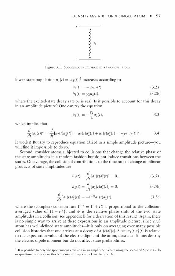
DENSITY MATRIX FOR A SINGLE ATOM 57
γ2
1
2
Figure 3.1. Spontaneous emission in a two-level atom.
lower-state population n1(t) = |a1(t)|2 increases according to
n2(t) = −γ2n2(t), (3.2a)
n1(t) = γ2n2(t), (3.2b)
where the excited-state decay rate γ2 is real. Is it possible to account for this decayin an amplitude picture? One can try the equation
a2(t) = −γ22a2(t), (3.3)
which implies that
ddt
|a2(t)|2 = ddt
[a2(t)a∗2(t)] = a2(t)a∗
2(t) + a2(t)a∗2(t) = −γ2|a2(t)|2. (3.4)
It works! But try to reproduce equation (3.2b) in a simple amplitude picture—youwill find it impossible to do so.1
Second, consider atoms subjected to collisions that change the relative phase ofthe state amplitudes in a random fashion but do not induce transitions between thestates. On average, the collisional contributions to the time rate of change of bilinearproducts of state amplitudes are
n1(t) = ddt
[a1(t)a∗1(t)] = 0, (3.5a)
n2(t) = ddt
[a2(t)a∗2(t)] = 0, (3.5b)
ddt
[a1(t)a∗2(t)] = −(c)a1(t)a∗
2(t), (3.5c)
where the (complex) collision rate (c) = + i S is proportional to the collision-averaged value of
(1 − eiφ
), and φ is the relative phase shift of the two state
amplitudes in a collision (see appendix B for a derivation of this result). Again, thereis no simple way to arrive at these expressions in an amplitude picture, since eachatom has well-defined state amplitudes—it is only on averaging over many possiblecollision histories that one arrives at a decay of a1(t)a∗
2(t). Since a1(t)a∗2(t) is related
to the expectation value of the electric dipole of the atom, elastic collisions destroythe electric dipole moment but do not affect state probabilities.
1 It is possible to describe spontaneous emission in an amplitude picture using the so-called Monte Carloor quantum trajectory methods discussed in appendix C in chapter 16.
58 CHAPTER 3
In problems of this nature, where atoms interact with a bath, such as the vacuumfield for spontaneous emission or perturbers for collisions, it is useful to introducethe density matrix to describe the system’s evolution. The density matrix arisesnaturally even when discussing the quantum mechanics of a single atom—so letus start there.
In making measurements in quantum mechanics, one always measures quantitiesthat are related to the expectation value of a Hermitian operator. An arbitraryHermitian operator, represented by the matrix A in Dirac notation, has itsexpectation value given by
〈(t)|A|(t)〉 =∑n,m
〈m|a∗m(t)Aan(t)|n〉 =
∑n,m
a∗m(t)an(t)〈m|A|n〉 . (3.6)
Let us define a matrix whose elements in the energy basis are equal to an(t)a∗m(t).
A matrix satisfying this criterion is the density matrix
(t) = |(t)〉〈(t)|, (3.7)
since
〈n|(t)|m〉 = 〈n|(t)〉〈(t)|m〉 =∑p,p′
〈n|ap(t)|p〉〈p′|a∗p′ (t)|m〉 = an(t)a∗
m(t). (3.8)
Note that (t) is not a bona fide Schrödinger operator since it is time-dependent,whereas all operators in the Schrödinger picture are taken as time-independent. Withthis definition,
〈(t)|A|(t)〉 =∑nm
nm(t)Amn = Tr [(t)A] , (3.9)
where Tr stands for “trace.”In the energy basis,
(t) = nm(t)|n〉〈m|, (3.10)
where |n〉〈m| is a matrix with a 1 in the nm location and zeros elsewhere. It issometimes more convenient to expand (t) in other bases, such as an irreducibletensor basis, as we do in chapter 16. It is easy to establish some properties for (t)for our single-atom case. First, we note that
(t) = a(t)a†(t), (3.11)
where a is interpreted as a column vector and a† as a row vector,
a =
⎛⎜⎝a1a2...
⎞⎟⎠ , (3.12)
a† = (a∗1 a
∗2 · · · ) , (3.13)
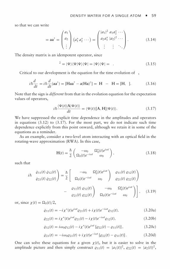
DENSITY MATRIX FOR A SINGLE ATOM 59
so that we can write
= aa† =
⎛⎜⎜⎝a1
a2...
⎞⎟⎟⎠(
a∗1 a
∗2 · · · ) =
⎛⎜⎜⎝
|a1|2 a1a∗2 · · ·
a2a∗1 |a2|2 · · ·
......
. . .
⎞⎟⎟⎠ . (3.14)
The density matrix is an idempotent operator, since
2 = |〉〈|〉〈| = |〉〈| = . (3.15)
Critical to our development is the equation for the time evolution of ,
id
dt= i
ddt
(aa†) = [Haa† − a(Ha)†] = H − H = [H, ]. (3.16)
Note that the sign is different from that in the evolution equation for the expectationvalues of operators,
i〈(t)|A|(t)〉
dt= 〈(t)|[A,H]|(t)〉. (3.17)
We have suppressed the explicit time dependence in the amplitudes and operatorsin equations (3.12) to (3.17). For the most part, we do not indicate such timedependence explicitly from this point onward, although we retain it in some of theequations as a reminder.
As an example, consider a two-level atom interacting with an optical field in therotating-wave approximation (RWA). In this case,
H(t) = 2
( −ω0 ∗0(t)e
iωt
0(t)e−iωt ω0
), (3.18)
such that
i
(11(t) 12(t)
21(t) 22(t)
)=
2
[( −ω0 ∗0(t)e
iωt
0(t)e−iωt ω0
)(11(t) 12(t)
21(t) 22(t)
)
−(11(t) 12(t)
21(t) 22(t)
)( −ω0 ∗0(t)e
iωt
0(t)e−iωt ω0
)], (3.19)
or, since χ (t) = 0(t)/2,
11(t) = −iχ∗(t)eiωt21(t) + iχ (t)e−iωt12(t), (3.20a)
22(t) = iχ∗(t)eiωt21(t) − iχ (t)e−iωt12(t), (3.20b)
12(t) = iω012(t) − iχ∗(t)eiωt [22(t) − 11(t)] , (3.20c)
21(t) = −iω021(t) + iχ (t)e−iωt [22(t) − 11(t)] . (3.20d)
One can solve these equations for a given χ (t), but it is easier to solve in theamplitude picture and then simply construct 11(t) = |a1(t)|2, 22(t) = |a2(t)|2,
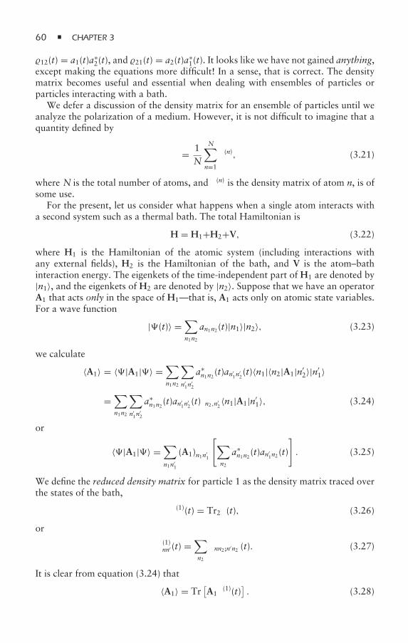
60 CHAPTER 3
12(t) = a1(t)a∗2(t), and 21(t) = a2(t)a∗
1(t). It looks like we have not gained anything,except making the equations more difficult! In a sense, that is correct. The densitymatrix becomes useful and essential when dealing with ensembles of particles orparticles interacting with a bath.
We defer a discussion of the density matrix for an ensemble of particles until weanalyze the polarization of a medium. However, it is not difficult to imagine that aquantity defined by
= 1N
N∑n=1
(n), (3.21)
where N is the total number of atoms, and (n) is the density matrix of atom n, is ofsome use.
For the present, let us consider what happens when a single atom interacts witha second system such as a thermal bath. The total Hamiltonian is
H = H1+H2+V, (3.22)
where H1 is the Hamiltonian of the atomic system (including interactions withany external fields), H2 is the Hamiltonian of the bath, and V is the atom–bathinteraction energy. The eigenkets of the time-independent part of H1 are denoted by|n1〉, and the eigenkets of H2 are denoted by |n2〉. Suppose that we have an operatorA1 that acts only in the space of H1—that is, A1 acts only on atomic state variables.For a wave function
|(t)〉 =∑n1n2
an1n2 (t)|n1〉|n2〉, (3.23)
we calculate
〈A1〉 = 〈|A1|〉 =∑n1n2
∑n′1n
′2
a∗n1n2 (t)an′
1n′2(t)〈n1|〈n2|A1|n′
2〉|n′1〉
=∑n1n2
∑n′1n
′2
a∗n1n2 (t)an′
1n′2(t)δn2,n′
2〈n1|A1|n′
1〉, (3.24)
or
〈|A1|〉 =∑n1n′
1
(A1)n1n′1
[∑n2
a∗n1n2 (t)an′
1n2 (t)
]. (3.25)
We define the reduced density matrix for particle 1 as the density matrix traced overthe states of the bath,
(1)(t) = Tr2(t), (3.26)
or
(1)nn′(t) =
∑n2
nn2;n′n2 (t). (3.27)
It is clear from equation (3.24) that
〈A1〉 = Tr[A1
(1)(t)]. (3.28)
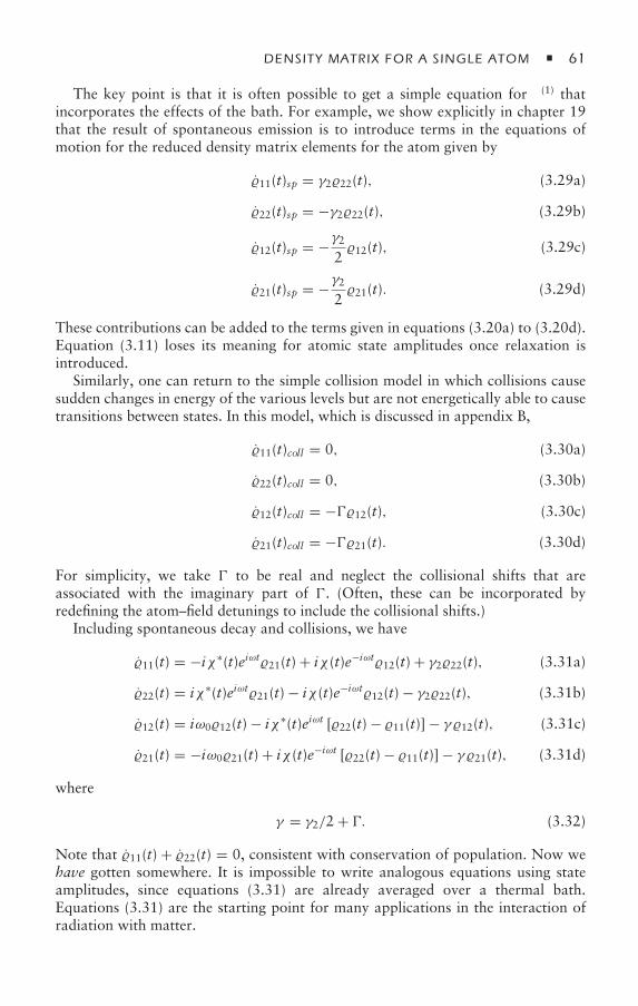
DENSITY MATRIX FOR A SINGLE ATOM 61
The key point is that it is often possible to get a simple equation for (1) thatincorporates the effects of the bath. For example, we show explicitly in chapter 19that the result of spontaneous emission is to introduce terms in the equations ofmotion for the reduced density matrix elements for the atom given by
11(t)sp = γ222(t), (3.29a)
22(t)sp = −γ222(t), (3.29b)
12(t)sp = −γ2212(t), (3.29c)
21(t)sp = −γ2221(t). (3.29d)
These contributions can be added to the terms given in equations (3.20a) to (3.20d).Equation (3.11) loses its meaning for atomic state amplitudes once relaxation isintroduced.
Similarly, one can return to the simple collision model in which collisions causesudden changes in energy of the various levels but are not energetically able to causetransitions between states. In this model, which is discussed in appendix B,
11(t)coll = 0, (3.30a)
22(t)coll = 0, (3.30b)
12(t)coll = −12(t), (3.30c)
21(t)coll = −21(t). (3.30d)
For simplicity, we take to be real and neglect the collisional shifts that areassociated with the imaginary part of . (Often, these can be incorporated byredefining the atom–field detunings to include the collisional shifts.)
Including spontaneous decay and collisions, we have
11(t) = −iχ∗(t)eiωt21(t) + iχ (t)e−iωt12(t) + γ222(t), (3.31a)
22(t) = iχ∗(t)eiωt21(t) − iχ (t)e−iωt12(t) − γ222(t), (3.31b)
12(t) = iω012(t) − iχ∗(t)eiωt [22(t) − 11(t)] − γ 12(t), (3.31c)
21(t) = −iω021(t) + iχ (t)e−iωt [22(t) − 11(t)] − γ 21(t), (3.31d)
where
γ = γ2/2 + . (3.32)
Note that 11(t) + 22(t) = 0, consistent with conservation of population. Now wehave gotten somewhere. It is impossible to write analogous equations using stateamplitudes, since equations (3.31) are already averaged over a thermal bath.Equations (3.31) are the starting point for many applications in the interaction ofradiation with matter.
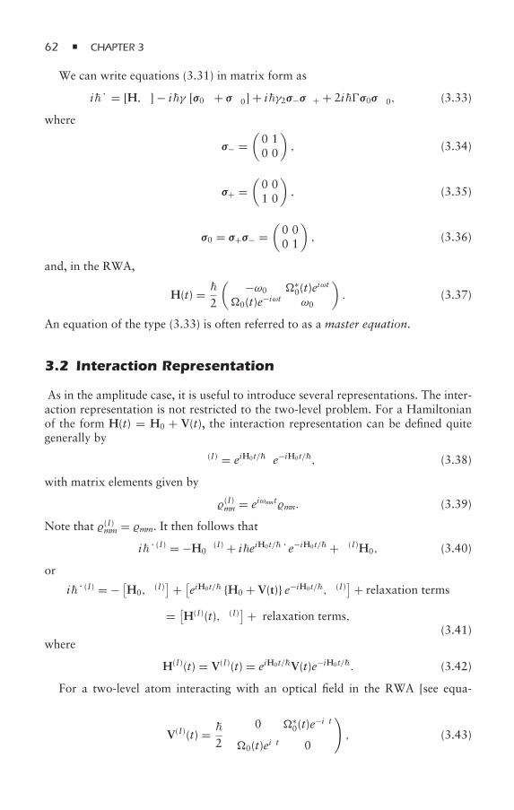
62 CHAPTER 3
We can write equations (3.31) in matrix form as
i = [H, ] − iγ [σ0 + σ 0] + iγ2σ−σ+ + 2iσ0σ 0, (3.33)
where
σ− =(0 10 0
), (3.34)
σ+ =(0 01 0
), (3.35)
σ0 = σ+σ− =(0 00 1
), (3.36)
and, in the RWA,
H(t) = 2
( −ω0 ∗0(t)e
iωt
0(t)e−iωt ω0
). (3.37)
An equation of the type (3.33) is often referred to as a master equation.
3.2 Interaction Representation
As in the amplitude case, it is useful to introduce several representations. The inter-action representation is not restricted to the two-level problem. For a Hamiltonianof the form H(t) = H0 + V(t), the interaction representation can be defined quitegenerally by
(I) = eiH0t/e−iH0t/, (3.38)
with matrix elements given by
(I)mn = eiωmntmn. (3.39)
Note that (I)mm = mm. It then follows that
i(I) = −H0(I) + ieiH0t/e−iH0t/ + (I)H0, (3.40)
or
i(I) = − [H0,
(I)]+ [
eiH0t/ H0 + V(t) e−iH0t/, (I)]+ relaxation terms
= [H(I)(t), (I)
]+ relaxation terms,(3.41)
where
H(I)(t) = V(I)(t) = eiH0t/V(t)e−iH0t/. (3.42)
For a two-level atom interacting with an optical field in the RWA [see equa-tion (2.167)], we have
V(I)(t) = 2
(0 ∗
0(t)e−iδt
0(t)eiδt 0
), (3.43)
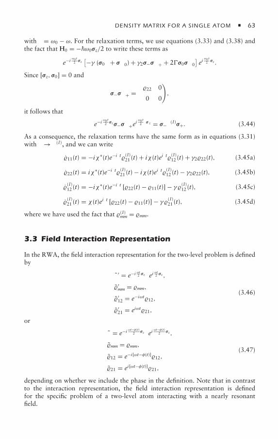
DENSITY MATRIX FOR A SINGLE ATOM 63
with δ = ω0 − ω. For the relaxation terms, we use equations (3.33) and (3.38) andthe fact that H0 = −ω0σz/2 to write these terms as
e−i ω0t2 σz[−γ (σ0 + σ 0) + γ2σ−σ+ + 2σ0σ 0
]ei
ω0 t2 σz .
Since [σz, σ0] = 0 and
σ−σ+ =(22 0
0 0
),
it follows that
e−i ω0t2 σzσ−σ+ei ω0t2 σ z = σ−(I)σ+. (3.44)
As a consequence, the relaxation terms have the same form as in equations (3.31)with → (I), and we can write
11(t) = −iχ∗(t)e−iδt(I)21 (t) + iχ (t)eiδt(I)12 (t) + γ222(t), (3.45a)
22(t) = iχ∗(t)e−iδt(I)21 (t) − iχ (t)eiδt(I)12 (t) − γ222(t), (3.45b)
(I)12 (t) = −iχ∗(t)e−iδt [22(t) − 11(t)] − γ (I)12 (t), (3.45c)
(I)21 (t) = χ (t)eiδt [22(t) − 11(t)] − γ (I)21 (t), (3.45d)
where we have used the fact that (I)mm = mm.
3.3 Field Interaction Representation
In the RWA, the field interaction representation for the two-level problem is definedby
′ = e−i ωt2 σzeiωt2 σz,
′mm = mm,
′12 = e−iωt12,
′21 = eiωt21,
(3.46)
or
= e−i ωt−φ(t)2 σzeiωt−φ(t)
2 σz,
mm = mm,
12 = e−i[ωt−φ(t)]12,
21 = ei[ωt−φ(t)]21,
(3.47)
depending on whether we include the phase in the definition. Note that in contrastto the interaction representation, the field interaction representation is definedfor the specific problem of a two-level atom interacting with a nearly resonantfield.
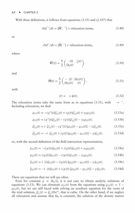
64 CHAPTER 3
With these definitions, it follows from equations (3.33) and (2.107) that
id′/dt = [H′, ′] + relaxation terms, (3.48)
or
id/dt = [H, ] + relaxation terms, (3.49)
where
H′(t) = 2
( −δ ∗0(t)
0(t) δ
), (3.50)
and
H(t) = 2
( −δ(t) |0(t)||0(t)| δ(t)
), (3.51)
with
δ(t) = δ + φ(t). (3.52)
The relaxation terms take the same form as in equations (3.31), with → .Including relaxation, we find
11(t) = −iχ∗(t)′21(t) + iχ (t)′
12(t) + γ222(t), (3.53a)
22(t) = iχ∗(t)′21(t) − iχ (t)′
12(t) − γ222(t), (3.53b)
˙′12(t) = iδ′
12(t) − iχ∗(t) [22(t) − 11(t)] − γ ′12(t), (3.53c)
˙′21(t) = −iδ′
21(t) + iχ (t) [22(t) − 11(t)] − γ ′21(t), (3.53d)
or, with the second definition of the field interaction representation,
11(t) = −i |χ (t)|21(t) + i |χ (t)|12(t) + γ222(t), (3.54a)
22(t) = i |χ (t)|21(t) − i |χ (t)|12(t) − γ222(t), (3.54b)
˙12(t) = iδ(t)12(t) − i |χ (t)| [22(t) − 11(t)] − γ 12(t), (3.54c)
˙21(t) = −iδ(t)21(t) + i |χ (t)| [22(t) − 11(t)] − γ 21(t), (3.54d)
These are equations that we will use often.Even for constant χ = 0/2, it is not easy to obtain analytic solutions of
equations (3.53). We can eliminate 11(t) from the equations using 11(t) = 1 −22(t), but we are still faced with solving an auxiliary equation for the roots ofthe trial solution, ′
i j (t) = ′i j (0)e
rt, that is cubic. On the other hand, if we neglectall relaxation and assume that 0 is constant, the solution of the density matrix
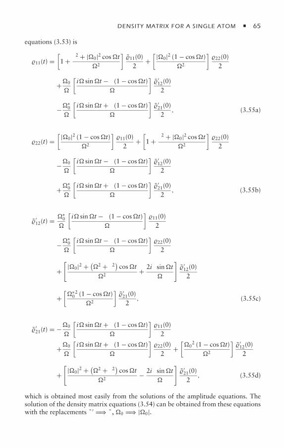
DENSITY MATRIX FOR A SINGLE ATOM 65
equations (3.53) is
11(t) =[1 + δ2 + |0|2 cost
2
]11(0)
2+[ |0|2 (1 − cost)
2
]22(0)
2
+0
[i sint − δ (1 − cost)
]′12(0)2
−∗0
[i sint + δ (1 − cost)
]′21(0)2
, (3.55a)
22(t) =[ |0|2 (1 − cost)
2
]11(0)
2+[1 + δ2 + |0|2 cost
2
]22(0)
2
−0
[i sint − δ (1 − cost)
]′12(0)2
+∗0
[i sint + δ (1 − cost)
]′21(0)2
, (3.55b)
′12(t) = ∗
0
[i sint − δ (1 − cost)
]11(0)
2
−∗0
[i sint − δ (1 − cost)
]22(0)
2
+[
|0|2 + (2 + δ2) cost2
+ 2iδ sint
]′12(0)2
+[∗
02 (1 − cost)
2
]′21(0)2
, (3.55c)
′21(t) = −0
[i sint + δ (1 − cost)
]11(0)
2
+0
[i sint + δ (1 − cost)
]22(0)
2+[0
2 (1 − cost)2
]′12(0)2
+[
|0|2 + (2 + δ2) cost2
− 2iδ sint
]′21(0)2
, (3.55d)
which is obtained most easily from the solutions of the amplitude equations. Thesolution of the density matrix equations (3.54) can be obtained from these equationswith the replacements ′ =⇒ , 0 =⇒ |0|.
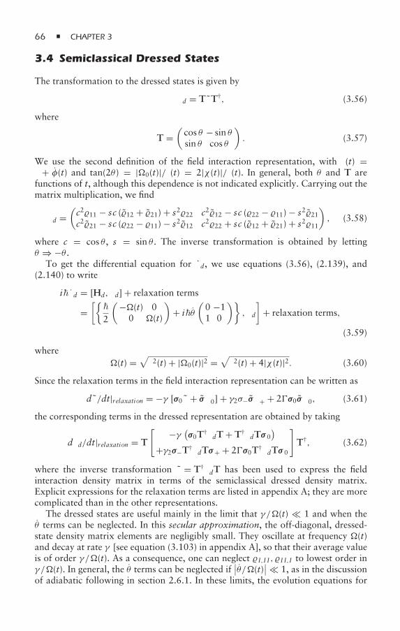
66 CHAPTER 3
3.4 Semiclassical Dressed States
The transformation to the dressed states is given by
d = TT†, (3.56)
where
T =(cos θ − sin θsin θ cos θ
). (3.57)
We use the second definition of the field interaction representation, with δ(t) =δ + φ(t) and tan(2θ ) = |0(t)|/δ(t) = 2|χ (t)|/δ(t). In general, both θ and T arefunctions of t, although this dependence is not indicated explicitly. Carrying out thematrix multiplication, we find
d =(c211 − sc (12 + 21) + s222 c212 − sc (22 − 11) − s221c221 − sc (22 − 11) − s212 c222 + sc (12 + 21) + s211
), (3.58)
where c = cos θ , s = sin θ . The inverse transformation is obtained by lettingθ ⇒ −θ .
To get the differential equation for d, we use equations (3.56), (2.139), and(2.140) to write
id = [Hd, d] + relaxation terms
=[
2
(−(t) 00 (t)
)+ iθ
(0 −11 0
), d
]+ relaxation terms,
(3.59)
where(t) =
√δ2(t) + |0(t)|2 =
√δ2(t) + 4|χ (t)|2. (3.60)
Since the relaxation terms in the field interaction representation can be written as
d/dt|relaxation = −γ [σ0 + σ 0] + γ2σ−σ+ + 2σ0σ 0, (3.61)
the corresponding terms in the dressed representation are obtained by taking
dd/dt|relaxation = T
[ −γ (σ0T†dT + T†dTσ 0)
+γ2σ−T†dTσ+ + 2σ0T†dTσ 0
]T†, (3.62)
where the inverse transformation = T†dT has been used to express the fieldinteraction density matrix in terms of the semiclassical dressed density matrix.Explicit expressions for the relaxation terms are listed in appendix A; they are morecomplicated than in the other representations.
The dressed states are useful mainly in the limit that γ /(t) 1 and when theθ terms can be neglected. In this secular approximation, the off-diagonal, dressed-state density matrix elements are negligibly small. They oscillate at frequency (t)and decay at rate γ [see equation (3.103) in appendix A], so that their average valueis of order γ /(t). As a consequence, one can neglect I,I I , I I,I to lowest order inγ /(t). In general, the θ terms can be neglected if
∣∣θ/(t)∣∣ 1, as in the discussionof adiabatic following in section 2.6.1. In these limits, the evolution equations for
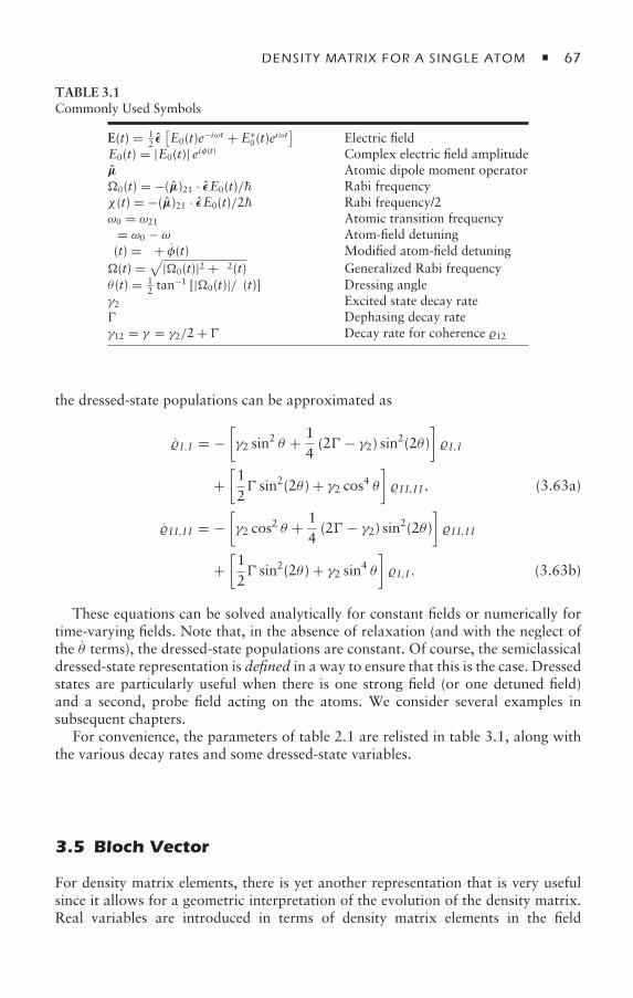
DENSITY MATRIX FOR A SINGLE ATOM 67
TABLE 3.1Commonly Used Symbols
E(t) = 12 ε[E0(t)e−iωt + E∗
0(t)eiωt]
Electric fieldE0(t) = |E0(t)| eiφ(t) Complex electric field amplitudeµ Atomic dipole moment operator0(t) = −(µ)21 · εE0(t)/ Rabi frequencyχ (t) = −(µ)21 · εE0(t)/2 Rabi frequency/2ω0 = ω21 Atomic transition frequencyδ = ω0 − ω Atom-field detuningδ(t) = δ + φ(t) Modified atom-field detuning(t) =
√|0(t)|2 + δ2(t) Generalized Rabi frequency
θ (t) = 12 tan
−1 [|0(t)|/δ(t)] Dressing angleγ2 Excited state decay rate Dephasing decay rateγ12 = γ = γ2/2 + Decay rate for coherence 12
the dressed-state populations can be approximated as
I,I = −[γ2 sin
2 θ + 14(2 − γ2) sin2(2θ )
]I,I
+[12 sin2(2θ ) + γ2 cos4 θ
]I I,I I , (3.63a)
I I,I I = −[γ2 cos2 θ + 1
4(2 − γ2) sin2(2θ )
]I I,I I
+[12 sin2(2θ ) + γ2 sin4 θ
]I,I . (3.63b)
These equations can be solved analytically for constant fields or numerically fortime-varying fields. Note that, in the absence of relaxation (and with the neglect ofthe θ terms), the dressed-state populations are constant. Of course, the semiclassicaldressed-state representation is defined in a way to ensure that this is the case. Dressedstates are particularly useful when there is one strong field (or one detuned field)and a second, probe field acting on the atoms. We consider several examples insubsequent chapters.
For convenience, the parameters of table 2.1 are relisted in table 3.1, along withthe various decay rates and some dressed-state variables.
3.5 Bloch Vector
For density matrix elements, there is yet another representation that is very usefulsince it allows for a geometric interpretation of the evolution of the density matrix.Real variables are introduced in terms of density matrix elements in the field
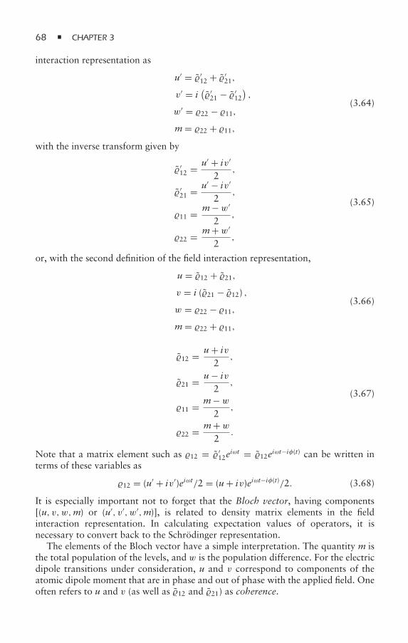
68 CHAPTER 3
interaction representation as
u′ = ′12 + ′
21,
v′ = i(′21 − ′
12
),
w′ = 22 − 11,m= 22 + 11,
(3.64)
with the inverse transform given by
′12 = u′ + iv′
2,
′21 = u′ − iv′
2,
11 = m− w′
2,
22 = m+ w′
2,
(3.65)
or, with the second definition of the field interaction representation,
u = 12 + 21,v = i (21 − 12) ,w = 22 − 11,m= 22 + 11,
(3.66)
12 = u+ iv2
,
21 = u− iv2
,
11 = m− w2
,
22 = m+ w2
.
(3.67)
Note that a matrix element such as 12 = ′12e
iωt = 12eiωt−iφ(t) can be written interms of these variables as
12 = (u′ + iv′)eiωt/2 = (u+ iv)eiωt−iφ(t)/2. (3.68)
It is especially important not to forget that the Bloch vector, having components[(u, v, w,m) or (u′, v′, w′,m)], is related to density matrix elements in the fieldinteraction representation. In calculating expectation values of operators, it isnecessary to convert back to the Schrödinger representation.
The elements of the Bloch vector have a simple interpretation. The quantity m isthe total population of the levels, and w is the population difference. For the electricdipole transitions under consideration, u and v correspond to components of theatomic dipole moment that are in phase and out of phase with the applied field. Oneoften refers to u and v (as well as 12 and 21) as coherence.
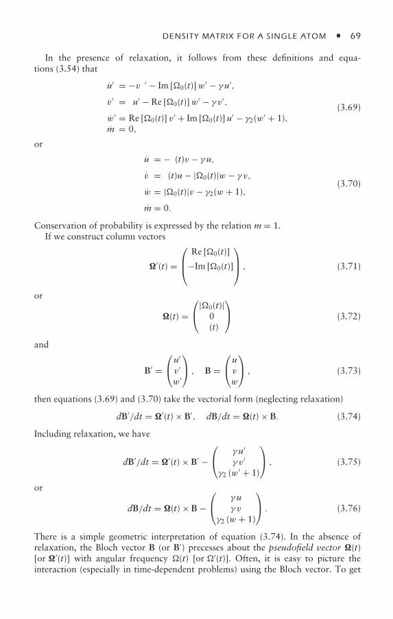
DENSITY MATRIX FOR A SINGLE ATOM 69
In the presence of relaxation, it follows from these definitions and equa-tions (3.54) that
u′ = −δv′ − Im [0(t)]w′ − γu′,
v′ = δu′ − Re [0(t)]w′ − γ v′,
w′ = Re [0(t)] v′ + Im [0(t)]u′ − γ2(w′ + 1),m = 0,
(3.69)
or
u = −δ(t)v − γu,v = δ(t)u− |0(t)|w − γ v,w = |0(t)|v − γ2(w + 1),
m = 0.
(3.70)
Conservation of probability is expressed by the relation m= 1.If we construct column vectors
′(t) =
⎛⎜⎝
Re [0(t)]
−Im [0(t)]
δ
⎞⎟⎠ , (3.71)
or
(t) =⎛⎝|0(t)|
0δ(t)
⎞⎠ (3.72)
and
B′ =⎛⎝u′
v′
w′
⎞⎠ , B =
⎛⎝uv
w
⎞⎠ , (3.73)
then equations (3.69) and (3.70) take the vectorial form (neglecting relaxation)
dB′/dt = ′(t) × B′, dB/dt = (t) × B. (3.74)
Including relaxation, we have
dB′/dt = ′(t) × B′ −⎛⎝ γu′
γ v′
γ2 (w′ + 1)
⎞⎠ , (3.75)
or
dB/dt = (t) × B −⎛⎝ γu
γ v
γ2 (w + 1)
⎞⎠ . (3.76)
There is a simple geometric interpretation of equation (3.74). In the absence ofrelaxation, the Bloch vector B (or B′) precesses about the pseudofield vector (t)[or ′(t)] with angular frequency (t) [or ′(t)]. Often, it is easy to picture theinteraction (especially in time-dependent problems) using the Bloch vector. To get
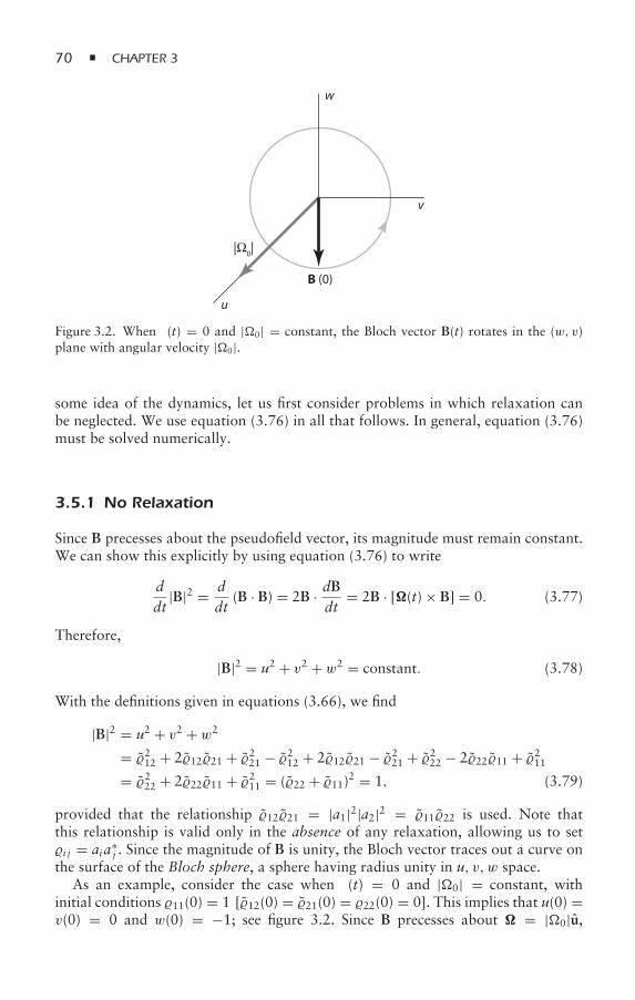
70 CHAPTER 3
|Ω0|
w
v
u
B (0)
Figure 3.2. When δ(t) = 0 and |0| = constant, the Bloch vector B(t) rotates in the (w, v)plane with angular velocity |0|.
some idea of the dynamics, let us first consider problems in which relaxation canbe neglected. We use equation (3.76) in all that follows. In general, equation (3.76)must be solved numerically.
3.5.1 No Relaxation
Since B precesses about the pseudofield vector, its magnitude must remain constant.We can show this explicitly by using equation (3.76) to write
ddt
|B|2 = ddt
(B · B) = 2B · dBdt
= 2B · [(t) × B] = 0. (3.77)
Therefore,
|B|2 = u2 + v2 + w2 = constant. (3.78)
With the definitions given in equations (3.66), we find
|B|2 = u2 + v2 + w2
= 212 + 21221 + 221 − 212 + 21221 − 221 + 222 − 22211 + 211= 222 + 22211 + 211 = (22 + 11)2 = 1, (3.79)
provided that the relationship 1221 = |a1|2|a2|2 = 1122 is used. Note thatthis relationship is valid only in the absence of any relaxation, allowing us to seti j = aia∗
j . Since the magnitude of B is unity, the Bloch vector traces out a curve onthe surface of the Bloch sphere, a sphere having radius unity in u, v, w space.
As an example, consider the case when δ(t) = 0 and |0| = constant, withinitial conditions 11(0) = 1 [12(0) = 21(0) = 22(0) = 0]. This implies that u(0) =v(0) = 0 and w(0) = −1; see figure 3.2. Since B precesses about = |0|u,
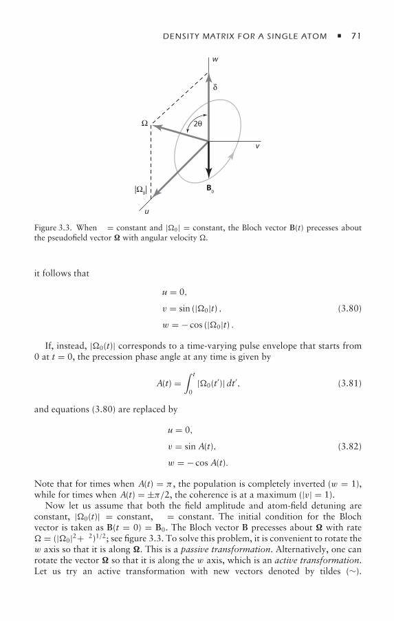
DENSITY MATRIX FOR A SINGLE ATOM 71
u
w
v
B0|Ω0|
Ω
δ
2θ
Figure 3.3. When δ = constant and |0| = constant, the Bloch vector B(t) precesses aboutthe pseudofield vector with angular velocity .
it follows that
u = 0,
v = sin (|0|t) ,w = − cos (|0|t) .
(3.80)
If, instead, |0(t)| corresponds to a time-varying pulse envelope that starts from0 at t = 0, the precession phase angle at any time is given by
A(t) =∫ t
0|0(t′)|dt′, (3.81)
and equations (3.80) are replaced by
u = 0,
v = sin A(t),
w = − cos A(t).
(3.82)
Note that for times when A(t) = π , the population is completely inverted (w = 1),while for times when A(t) = ±π/2, the coherence is at a maximum (|v| = 1).
Now let us assume that both the field amplitude and atom-field detuning areconstant, |0(t)| = constant, δ = constant. The initial condition for the Blochvector is taken as B(t = 0) = B0. The Bloch vector B precesses about with rate = (|0|2+δ2)1/2; see figure 3.3. To solve this problem, it is convenient to rotate thew axis so that it is along . This is a passive transformation. Alternatively, one canrotate the vector so that it is along the w axis, which is an active transformation.Let us try an active transformation with new vectors denoted by tildes (∼).
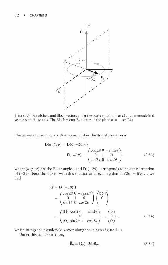
72 CHAPTER 3
w
v~
~
u
B0
Ω
2θ
2θ
Figure 3.4. Pseudofield and Bloch vectors under the active rotation that aligns the pseudofieldvector with the w axis. The Bloch vector B0 rotates in the plane w = − cos(2θ ).
The active rotation matrix that accomplishes this transformation is
D(α, β, γ ) = D(0,−2θ,0)
≡ Dv(−2θ ) =⎛⎝ cos 2θ 0 − sin 2θ
0 1 0sin 2θ 0 cos 2θ
⎞⎠, (3.83)
where (α, β, γ ) are the Euler angles, and Dv(−2θ ) corresponds to an active rotationof (−2θ ) about the v axis. With this rotation and recalling that tan(2θ ) = |0|/δ, wefind
= Dv(−2θ )
=⎛⎝ cos 2θ 0 − sin 2θ
0 1 0sin 2θ 0 cos 2θ
⎞⎠⎛⎝|0|
0δ
⎞⎠
=⎛⎝ |0| cos 2θ − δ sin 2θ
0|0| sin 2θ + δ cos 2θ
⎞⎠ =
⎛⎝00
⎞⎠ , (3.84)
which brings the pseudofield vector along the w axis (figure 3.4).Under this transformation,
B0 = Dv(−2θ )B0. (3.85)
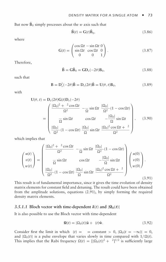
DENSITY MATRIX FOR A SINGLE ATOM 73
But now B0 simply precesses about the w axis such that
B(t) = G(t)B0, (3.86)
where
G(t) =⎛⎝ cost − sint 0
sint cost 00 0 1
⎞⎠ . (3.87)
Therefore,
B = GB0 = GDv(−2θ )B0, (3.88)
such that
B = D†v(−2θ )B = Dv(2θ )B = U(θ, t)B0, (3.89)
with
U(θ, t) = Dv(2θ )G(t)Dv(−2θ )
=
⎛⎜⎜⎜⎜⎜⎜⎜⎝
|0|2 + δ2 cost2
− δ
sint
|0|δ2
(1 − cost)
δ
sint cost −|0|
sint
|0|δ2
(1 − cost)|0|
sint|0|2 cost + δ2
2
⎞⎟⎟⎟⎟⎟⎟⎟⎠, (3.90)
which implies that
⎛⎜⎝u(t)
v(t)
w(t)
⎞⎟⎠ =
⎛⎜⎜⎜⎜⎜⎜⎜⎜⎝
|0|2 + δ2 cost2
− δ
sint
|0|δ2
(1 − cost)
δ
sint cost −|0|
sint
|0|δ2
(1 − cost)|0|
sint|0|2 cost + δ2
2
⎞⎟⎟⎟⎟⎟⎟⎟⎟⎠
⎛⎜⎝u(0)
v(0)
w(0)
⎞⎟⎠ .
(3.91)This result is of fundamental importance, since it gives the time evolution of densitymatrix elements for constant field and detuning. The result could have been obtainedfrom the amplitude solutions, equations (2.91), by simply forming the requireddensity matrix elements.
3.5.1.1 Bloch vector with time-dependent δ(t) and |0(t)|It is also possible to use the Bloch vector with time-dependent
(t) = |0(t)|u + δ(t)w. (3.92)
Consider first the limit in which δ(t) = δ = constant > 0, |0(t = −∞)| = 0,and |0(t)| is a pulse envelope that varies slowly in time compared with 1/(t).This implies that the Rabi frequency (t) = [|0(t)|2 + δ2]1/2 is sufficiently large
74 CHAPTER 3
w
v
u B0
B(t)
Ω(t)2θ
2θ
Figure 3.5. Under adiabatic following conditions, the Bloch vector remains aligned with the(negative of the) pseudofield vector, provided that |0(−∞)| = 0 and δ(−∞) > 0 (assumingthat the atom is in state 1 at t = −∞).
to ensure that the Bloch vector precesses many times around the pseudofield vectorbefore the pseudofield vector changes as a result of changes in |0(t)|. Consider whathappens when w(−∞) = −1 [11(−∞) = 1]. At t = −∞, the pseudofield vector isaligned along the positive w axis and the Bloch vector is aligned along the negativew axis, in a direction opposite to the pseudofield vector. As the field |0(t)| beginsto build, the pseudofield vector rotates sufficiently slowly in the wu plane to ensurethat the amplitude of the precession remains very small. In other words, the Blochvector adiabatically follows the (negative of the) pseudofield vector (figure 3.5).
As a result, the Bloch vector B stays in the wu plane, with
w(t) = − cos [2θ (t)] , v(t) = 0, u(t) = − sin [2θ (t)] , (3.93a)
22(t) = sin2 [θ (t)] , 12(t) = 21(t) = − sin [θ (t)] cos [θ (t)] , (3.93b)
where tan [2θ (t)] = |0(t)| /δ, as in the case of adiabatic following. These are thesame results obtained using dressed states, provided that the angle θ (t) changes ata rate much less than (t). The Bloch vector gives a geometrical perspective to thisresult.
Note that if δ(t) also changes slowly in time and changes sign from δ0 to −δ0,then the Bloch vector adiabatically follows the pseudofield vector and rotates intothe upper half plane (provided the minimum Rabi frequency is sufficiently large toensure adiabaticity). At the end of the pulse, |0(∞)| ∼ 0, the Bloch vector is alignedalong the positive w axis—this implies that 22(∞) = 1 and corresponds to adiabaticswitching.
3.5.2 Relaxation Included
When relaxation is included, as in equations (3.70), the Bloch vector no longerhas constant length, and there is no simple way to find B(t) for a given B0. Withrelaxation, the Bloch vector decreases in length and eventually reaches a steady-state value if the field amplitude and detuning are constant, corresponding to a single
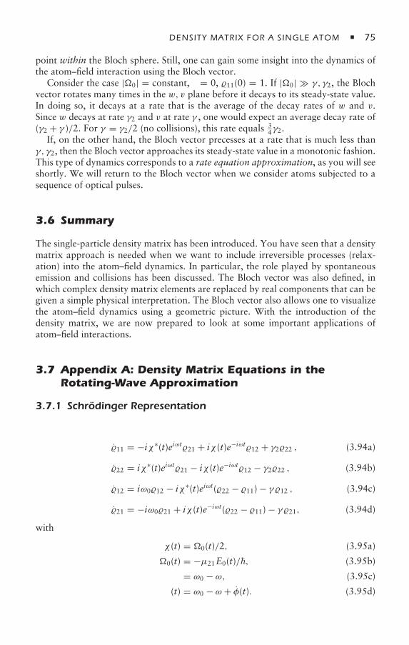
DENSITY MATRIX FOR A SINGLE ATOM 75
point within the Bloch sphere. Still, one can gain some insight into the dynamics ofthe atom–field interaction using the Bloch vector.
Consider the case |0| = constant, δ = 0, 11(0) = 1. If |0| γ, γ2, the Blochvector rotates many times in the w, v plane before it decays to its steady-state value.In doing so, it decays at a rate that is the average of the decay rates of w and v.Since w decays at rate γ2 and v at rate γ , one would expect an average decay rate of(γ2 + γ )/2. For γ = γ2/2 (no collisions), this rate equals 3
4γ2.If, on the other hand, the Bloch vector precesses at a rate that is much less than
γ, γ2, then the Bloch vector approaches its steady-state value in a monotonic fashion.This type of dynamics corresponds to a rate equation approximation, as you will seeshortly. We will return to the Bloch vector when we consider atoms subjected to asequence of optical pulses.
3.6 Summary
The single-particle density matrix has been introduced. You have seen that a densitymatrix approach is needed when we want to include irreversible processes (relax-ation) into the atom–field dynamics. In particular, the role played by spontaneousemission and collisions has been discussed. The Bloch vector was also defined, inwhich complex density matrix elements are replaced by real components that can begiven a simple physical interpretation. The Bloch vector also allows one to visualizethe atom–field dynamics using a geometric picture. With the introduction of thedensity matrix, we are now prepared to look at some important applications ofatom–field interactions.
3.7 Appendix A: Density Matrix Equations in theRotating-Wave Approximation
3.7.1 Schrödinger Representation
11 = −iχ∗(t)eiωt21 + iχ (t)e−iωt12 + γ222 , (3.94a)
22 = iχ∗(t)eiωt21 − iχ (t)e−iωt12 − γ222 , (3.94b)
12 = iω012 − iχ∗(t)eiωt(22 − 11) − γ 12 , (3.94c)
21 = −iω021 + iχ (t)e−iωt(22 − 11) − γ 21, (3.94d)
with
χ (t) = 0(t)/2, (3.95a)
0(t) = −µ21E0(t)/, (3.95b)
δ = ω0 − ω, (3.95c)
δ(t) = ω0 − ω + φ(t). (3.95d)
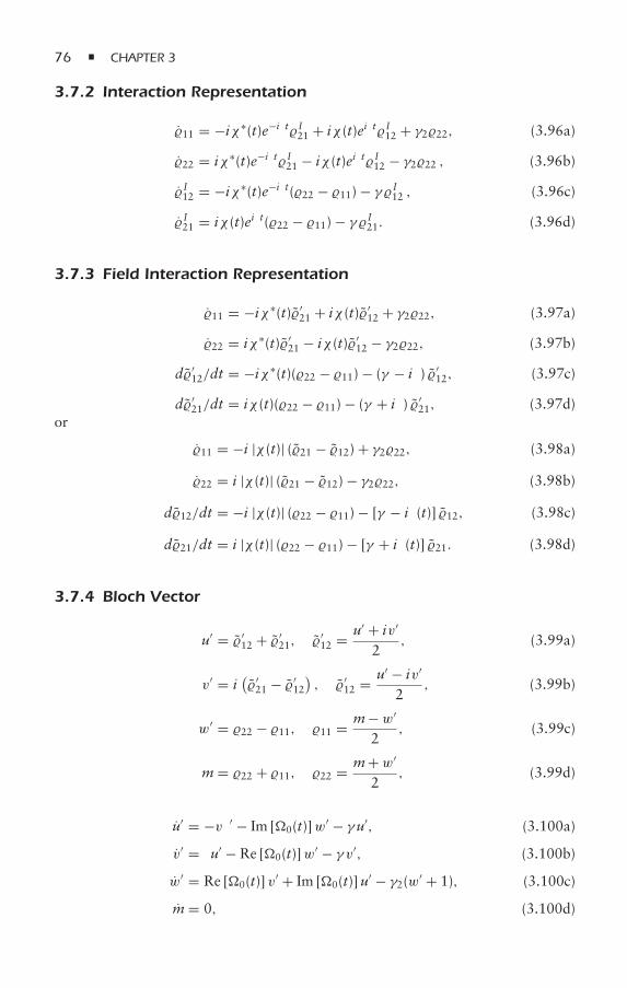
76 CHAPTER 3
3.7.2 Interaction Representation
11 = −iχ∗(t)e−iδtI21 + iχ (t)eiδtI12 + γ222, (3.96a)
22 = iχ∗(t)e−iδtI21 − iχ (t)eiδtI12 − γ222 , (3.96b)
I12 = −iχ∗(t)e−iδt(22 − 11) − γ I12 , (3.96c)
I21 = iχ (t)eiδt(22 − 11) − γ I21. (3.96d)
3.7.3 Field Interaction Representation
11 = −iχ∗(t)′21 + iχ (t)′
12 + γ222, (3.97a)
22 = iχ∗(t)′21 − iχ (t)′
12 − γ222, (3.97b)
d′12/dt = −iχ∗(t)(22 − 11) − (γ − iδ) ′
12, (3.97c)
d′21/dt = iχ (t)(22 − 11) − (γ + iδ) ′
21, (3.97d)or
11 = −i |χ (t)| (21 − 12) + γ222, (3.98a)
22 = i |χ (t)| (21 − 12) − γ222, (3.98b)
d12/dt = −i |χ (t)| (22 − 11) − [γ − iδ(t)] 12, (3.98c)
d21/dt = i |χ (t)| (22 − 11) − [γ + iδ(t)] 21. (3.98d)
3.7.4 Bloch Vector
u′ = ′12 + ′
21, ′12 = u′ + iv′
2, (3.99a)
v′ = i(′21 − ′
12
), ′
12 = u′ − iv′
2, (3.99b)
w′ = 22 − 11, 11 = m− w′
2, (3.99c)
m = 22 + 11, 22 = m+ w′
2, (3.99d)
u′ = −δv′ − Im [0(t)]w′ − γu′, (3.100a)
v′ = δu′ − Re [0(t)]w′ − γ v′, (3.100b)
w′ = Re [0(t)] v′ + Im [0(t)]u′ − γ2(w′ + 1), (3.100c)
m = 0, (3.100d)
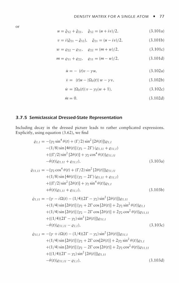
DENSITY MATRIX FOR A SINGLE ATOM 77
oru = 12 + 21, 12 = (u+ iv)/2, (3.101a)
v = i(21 − 12), 21 = (u− iv)/2, (3.101b)
w = 22 − 11, 22 = (m+ w)/2, (3.101c)
m = 11 + 22, 11 = (m− w)/2, (3.101d)
u = −δ(t)v − γu, (3.102a)
v = δ(t)u− |0(t)|w − γ v, (3.102b)
w = |0(t)| v − γ2(w + 1), (3.102c)
m = 0. (3.102d)
3.7.5 Semiclassical Dressed-State Representation
Including decay in the dressed picture leads to rather complicated expressions.Explicitly, using equation (3.62), we find
I,I = −γ2 sin4 θ (t) + (/2) sin2 [2θ (t)]I,I−(1/8) sin [4θ (t)] (γ2 − 2) (I,I I + I I,I )+(/2) sin2 [2θ (t)] + γ2 cos4 θ (t)I I,I I−θ (t)(I,I I + I I,I ), (3.103a)
I I,I I = −γ2 cos4 θ (t) + (/2) sin2 [2θ (t)]I I,I I+(1/8) sin [4θ (t)] (γ2 − 2) (I,I I + I I,I )+(/2) sin2 [2θ (t)] + γ2 sin4 θ (t)I,I+θ (t)(I,I I + I I,I ), (3.103b)
I,I I = −γ − i(t) − (1/4)(2 − γ2) sin2 [2θ (t)]I,I I+(1/4) sin [2θ (t)] γ2 + 2 cos [2θ (t)] + 2γ2 sin
2 θ (t)I,I+(1/4) sin [2θ (t)] γ2 − 2 cos [2θ (t)] + 2γ2 cos2 θ (t)I I,I I+(1/4)(2 − γ2) sin2 [2θ (t)]I I,I−θ (t)(I I,I I − I,I ), (3.103c)
I I,I = −γ + i(t) − (1/4)(2 − γ2) sin2 [2θ (t)]I I,I+(1/4) sin [2θ (t)] γ2 + 2 cos[2θ (t)] + 2γ2 sin
2 θ (t)I,I+(1/4) sin [2θ (t)] γ2 − 2 cos [2θ (t)] + 2γ2 cos2 θ (t)I I,I I+(1/4)(2 − γ2) sin2 [2θ (t)]I,I I−θ (t)(I I,I I − I,I ), (3.103d)
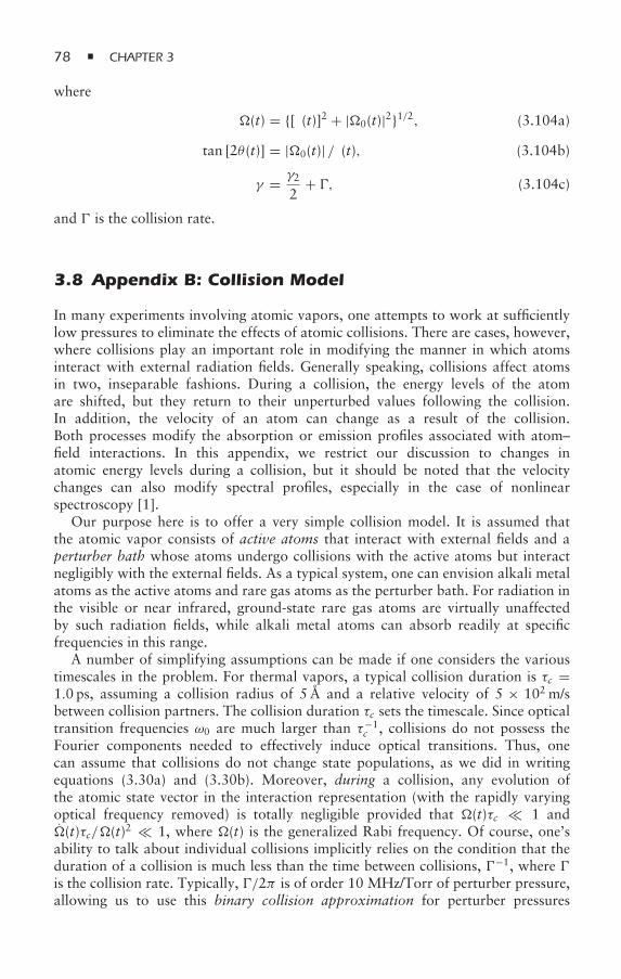
78 CHAPTER 3
where
(t) = [δ(t)]2 + |0(t)|21/2, (3.104a)
tan [2θ (t)] = |0(t)| /δ(t), (3.104b)
γ = γ2
2+ , (3.104c)
and is the collision rate.
3.8 Appendix B: Collision Model
In many experiments involving atomic vapors, one attempts to work at sufficientlylow pressures to eliminate the effects of atomic collisions. There are cases, however,where collisions play an important role in modifying the manner in which atomsinteract with external radiation fields. Generally speaking, collisions affect atomsin two, inseparable fashions. During a collision, the energy levels of the atomare shifted, but they return to their unperturbed values following the collision.In addition, the velocity of an atom can change as a result of the collision.Both processes modify the absorption or emission profiles associated with atom–field interactions. In this appendix, we restrict our discussion to changes inatomic energy levels during a collision, but it should be noted that the velocitychanges can also modify spectral profiles, especially in the case of nonlinearspectroscopy [1].
Our purpose here is to offer a very simple collision model. It is assumed thatthe atomic vapor consists of active atoms that interact with external fields and aperturber bath whose atoms undergo collisions with the active atoms but interactnegligibly with the external fields. As a typical system, one can envision alkali metalatoms as the active atoms and rare gas atoms as the perturber bath. For radiation inthe visible or near infrared, ground-state rare gas atoms are virtually unaffectedby such radiation fields, while alkali metal atoms can absorb readily at specificfrequencies in this range.
A number of simplifying assumptions can be made if one considers the varioustimescales in the problem. For thermal vapors, a typical collision duration is τc =1.0 ps, assuming a collision radius of 5Å and a relative velocity of 5 × 10² m/sbetween collision partners. The collision duration τc sets the timescale. Since opticaltransition frequencies ω0 are much larger than τ−1
c , collisions do not possess theFourier components needed to effectively induce optical transitions. Thus, onecan assume that collisions do not change state populations, as we did in writingequations (3.30a) and (3.30b). Moreover, during a collision, any evolution ofthe atomic state vector in the interaction representation (with the rapidly varyingoptical frequency removed) is totally negligible provided that (t)τc 1 and(t)τc/(t)2 1, where (t) is the generalized Rabi frequency. Of course, one’sability to talk about individual collisions implicitly relies on the condition that theduration of a collision is much less than the time between collisions, −1, where is the collision rate. Typically, /2π is of order 10 MHz/Torr of perturber pressure,allowing us to use this binary collision approximation for perturber pressures
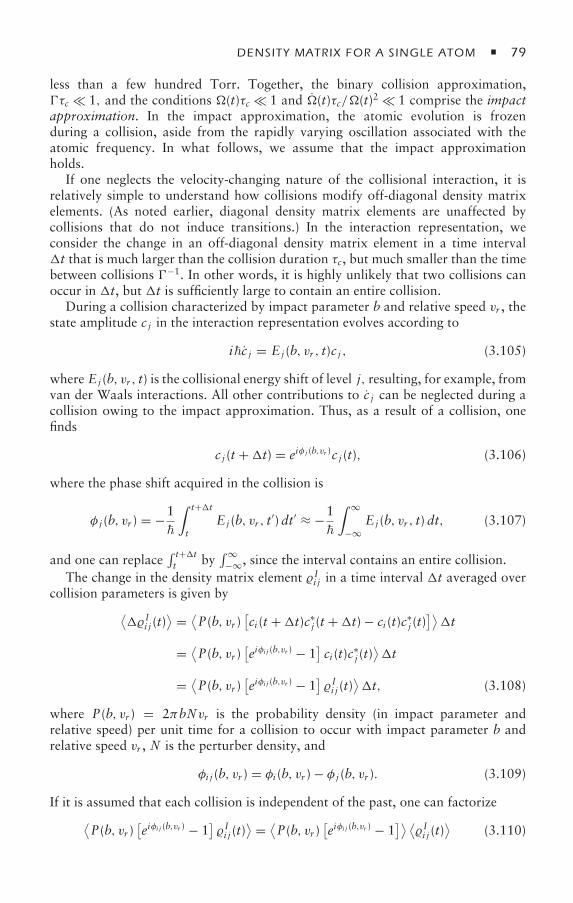
DENSITY MATRIX FOR A SINGLE ATOM 79
less than a few hundred Torr. Together, the binary collision approximation,τc 1, and the conditions (t)τc 1 and (t)τc/(t)2 1 comprise the impactapproximation. In the impact approximation, the atomic evolution is frozenduring a collision, aside from the rapidly varying oscillation associated with theatomic frequency. In what follows, we assume that the impact approximationholds.
If one neglects the velocity-changing nature of the collisional interaction, it isrelatively simple to understand how collisions modify off-diagonal density matrixelements. (As noted earlier, diagonal density matrix elements are unaffected bycollisions that do not induce transitions.) In the interaction representation, weconsider the change in an off-diagonal density matrix element in a time intervalt that is much larger than the collision duration τc, but much smaller than the timebetween collisions −1. In other words, it is highly unlikely that two collisions canoccur in t, but t is sufficiently large to contain an entire collision.
During a collision characterized by impact parameter b and relative speed vr , thestate amplitude c j in the interaction representation evolves according to
ic j = Ej (b, vr , t)c j , (3.105)
where Ej (b, vr , t) is the collisional energy shift of level j, resulting, for example, fromvan der Waals interactions. All other contributions to c j can be neglected during acollision owing to the impact approximation. Thus, as a result of a collision, onefinds
c j (t +t) = eiφ j (b,vr )c j (t), (3.106)
where the phase shift acquired in the collision is
φ j (b, vr ) = −1
∫ t+t
tE j (b, vr , t′)dt′ ≈ −1
∫ ∞
−∞Ej (b, vr , t)dt, (3.107)
and one can replace∫ t+tt by
∫∞−∞, since the interval contains an entire collision.
The change in the density matrix element Ii j in a time interval t averaged overcollision parameters is given by⟨
Ii j (t)⟩ = ⟨
P(b, vr )[ci (t +t)c∗
j (t +t) − ci (t)c∗j (t)
]⟩t
= ⟨P(b, vr )
[eiφi j (b,vr ) − 1
]ci (t)c∗
j (t)⟩t
= ⟨P(b, vr )
[eiφi j (b,vr ) − 1
]Ii j (t)
⟩t, (3.108)
where P(b, vr ) = 2πbN vr is the probability density (in impact parameter andrelative speed) per unit time for a collision to occur with impact parameter b andrelative speed vr , N is the perturber density, and
φi j (b, vr ) = φi (b, vr ) − φ j (b, vr ). (3.109)
If it is assumed that each collision is independent of the past, one can factorize⟨P(b, vr )
[eiφi j (b,vr ) − 1
]Ii j (t)
⟩ = ⟨P(b, vr )
[eiφi j (b,vr ) − 1
]⟩ ⟨Ii j (t)
⟩(3.110)
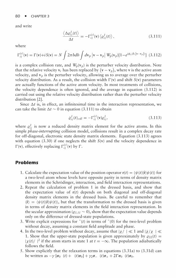
80 CHAPTER 3
and write ⟨Ii j (t)
⟩t
= −(c)i j (v)
⟨Ii j (t)
⟩, (3.111)
where
(c)i j (v) = (v)+i S(v) = N
∫2πbdb
∫dvp
∣∣v − vp∣∣Wp(vp)[1−eiφi j (b,|v−vp|)] (3.112)
is a complex collision rate, and Wp(vp) is the perturber velocity distribution. Notethat the relative velocity vr has been replaced by
(v − vp
), where v is the active atom
velocity, and vp is the perturber velocity, allowing us to average over the perturbervelocity distribution. As a result, the collision width (v) and shift S(v) parametersare actually functions of the active atom velocity. In most treatments of collisions,the velocity dependence is often ignored, and the average in equation (3.112) iscarried out using the relative velocity distribution rather than the perturber velocitydistribution [2].
Since t is, in effect, an infinitesimal time in the interaction representation, wecan take the limit t ∼ 0 in equation (3.111) to obtain
Ii j (t)coll = −(c)i j (v)
Ii j , (3.113)
where Ii j is now a reduced density matrix element for the active atoms. In thissimple phase-interrupting collision model, collisions result in a complex decay ratefor off-diagonal, electronic state density matrix elements. Equation (3.113) agreeswith equation (3.30) if one neglects the shift S(v) and the velocity dependence in(v), effectively replacing (c)
i j (v) by .
Problems
1. Calculate the expectation value of the position operator r(t) = 〈ψ(t)|r|ψ(t)〉 fora two-level atom whose levels have opposite parity in terms of density matrixelements in the Schrödinger, interaction, and field interaction representations.
2. Repeat the calculation of problem 1 in the dressed basis, and show thatthe expectation value of r(t) depends on both diagonal and off-diagonaldensity matrix elements in the dressed basis. Be careful to remember that〈r〉 = 〈ψ(t)|r|ψ(t)〉, but that the transformation to the dressed basis is givenin terms of density matrix elements in the field interaction representation. Inthe secular approximation (I,I I ∼ 0), show that the expectation value dependsonly on the difference of dressed-state populations.
3. Write explicit expressions for (t) in terms of (0) for the two-level problemwithout decay, assuming a constant field amplitude and phase.
4. In the two-level problem without decay, assume that |χ/δ| 1 and |χ/χδ| 1. Show that the upper-state population is given approximately by 22(t) =|χ (t)/δ|2 if the atom starts in state 1 at t = −∞. The population adiabaticallyfollows the field.
5. Show explicitly that the relaxation terms in equations (3.31a) to (3.31d) canbe written as −γ [σ0(t) + (t)σ0] + γ2σ−(t)σ+ + 2σ0(t)σ0.
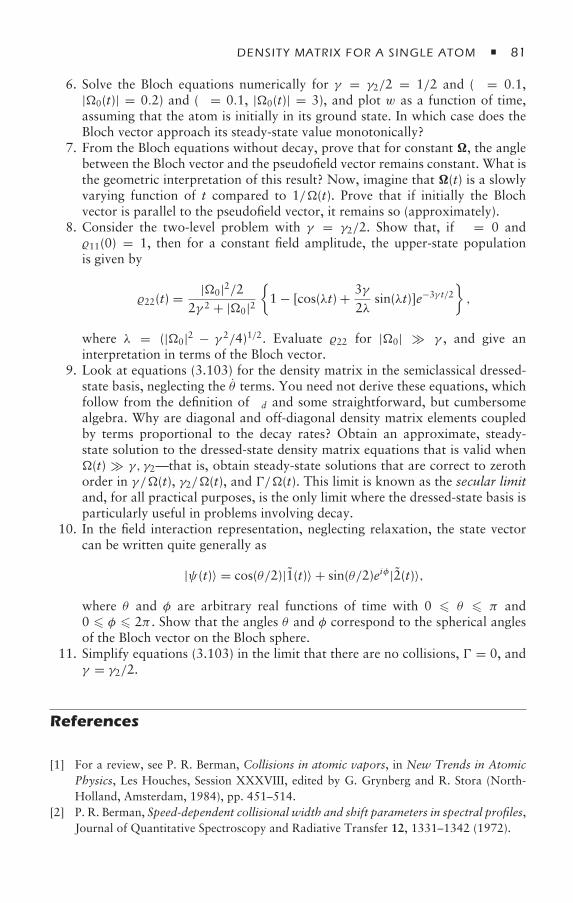
DENSITY MATRIX FOR A SINGLE ATOM 81
6. Solve the Bloch equations numerically for γ = γ2/2 = 1/2 and (δ = 0.1,|0(t)| = 0.2) and (δ = 0.1, |0(t)| = 3), and plot w as a function of time,assuming that the atom is initially in its ground state. In which case does theBloch vector approach its steady-state value monotonically?
7. From the Bloch equations without decay, prove that for constant , the anglebetween the Bloch vector and the pseudofield vector remains constant. What isthe geometric interpretation of this result? Now, imagine that (t) is a slowlyvarying function of t compared to 1/(t). Prove that if initially the Blochvector is parallel to the pseudofield vector, it remains so (approximately).
8. Consider the two-level problem with γ = γ2/2. Show that, if δ = 0 and11(0) = 1, then for a constant field amplitude, the upper-state populationis given by
22(t) = |0|2/22γ 2 + |0|2
1 − [cos(λt) + 3γ
2λsin(λt)]e−3γ t/2
,
where λ = (|0|2 − γ 2/4)1/2. Evaluate 22 for |0| γ , and give aninterpretation in terms of the Bloch vector.
9. Look at equations (3.103) for the density matrix in the semiclassical dressed-state basis, neglecting the θ terms. You need not derive these equations, whichfollow from the definition of d and some straightforward, but cumbersomealgebra. Why are diagonal and off-diagonal density matrix elements coupledby terms proportional to the decay rates? Obtain an approximate, steady-state solution to the dressed-state density matrix equations that is valid when(t) γ, γ2—that is, obtain steady-state solutions that are correct to zerothorder in γ /(t), γ2/(t), and /(t). This limit is known as the secular limitand, for all practical purposes, is the only limit where the dressed-state basis isparticularly useful in problems involving decay.
10. In the field interaction representation, neglecting relaxation, the state vectorcan be written quite generally as
|ψ(t)〉 = cos(θ/2)|1(t)〉 + sin(θ/2)eiφ|2(t)〉,
where θ and φ are arbitrary real functions of time with 0 θ π and0 φ 2π . Show that the angles θ and φ correspond to the spherical anglesof the Bloch vector on the Bloch sphere.
11. Simplify equations (3.103) in the limit that there are no collisions, = 0, andγ = γ2/2.
References
[1] For a review, see P. R. Berman, Collisions in atomic vapors, in New Trends in AtomicPhysics, Les Houches, Session XXXVIII, edited by G. Grynberg and R. Stora (North-Holland, Amsterdam, 1984), pp. 451–514.
[2] P. R. Berman, Speed-dependent collisional width and shift parameters in spectral profiles,Journal of Quantitative Spectroscopy and Radiative Transfer 12, 1331–1342 (1972).

82 CHAPTER 3
Bibliography
The density matrix equations are discussed in most of the books cited in chapter 1.J. Ostmeyer and J. Gea-Banacloche, http://comp.uark.edu/~jgeabana/blochapps/blocheqs2.
html Bloch spheres and Q-functions (2006). This website contains an applet that allowsyou to visualize the evolution of the Bloch vector on the Bloch sphere for arbitrary inputparameters.
4Applications of the DensityMatrix Formalism
4.1 Density Matrix for an Ensemble
We now have the basic tools in place to carry out a number of calculations that areassociated with problems of fundamental importance in matter–field interactions.The topics to be discussed include the absorption coefficient and spectral width,a simple treatment of atomic motion valid in plane-wave fields, and the rateequation approximation (chapter 4); atoms in standing-wave fields—laser cooling(chapter 5); coupling to the radiation field—Maxwell-Bloch equations (chapter 6);atoms in two fields—saturation spectroscopy (chapter 7); three-level atoms in twofields—Autler-Townes splitting (chapter 8); dark states and slow light (chapter 9);and coherent transients—free induction decay, photon echo, Ramsey fringes, andfrequency combs (chapter 10).
Up to this point, we have considered the density matrix of a single atom. At thisstage, we need to introduce an ensemble of atoms that interact with an externalfield. As long as the atoms interact independently with the external fields and do notinteract directly with each other, it is an easy matter to generalize the single-particledensity matrix to a density matrix for the ensemble of atoms. One simply defines
R(R, v, t) = 1N
∑j
∫dR j dv jR( j)(R j , v j , t)δ(R − R j )δ(v − v j ), (4.1)
where δ(R − R j ) is a Dirac delta function,R( j)(R j , v j , t) is the single-particle densitymatrix of atom j , and N is the total number of atoms. We have replaced the symbol with R to indicate that R( j)(R j , v j , t) is a density in both coordinate and velocityspace, whereas is a dimensionless, single-particle density matrix.
Equation (4.1) may seem innocuous, but it hides some problems in electrodynam-ics that have yet to receive a satisfactory solution. For the moment, we consider thatR and v are classical variables—that is, the atomic center-of-mass motion is treatedclassically. If this were not the case, it would be impossible to define a single-particle
84 CHAPTER 4
density matrix that is a function of both position and velocity (momentum), sincethe position and momentum operators do not commute. As is shown in chapter 5,however, this is often not a fundamental problem if one interprets R j and v j as theaverage position and velocity of a wave packet associated with the atomic center-of-mass motion. What remains as a fundamental problem, however, is one related tomacroscopic rather than microscopic descriptions of the atomic medium.
For classical center-of-mass motion, the single-particle density matrix can bewritten as
R( j)(R j , v j , t) = ( j)(R j , v j , t)δ[R j − R j (t)
]δ[v j − v j (t)], (4.2)
where R j (t) and v j (t) are the classical position and velocity of atom j , and( j)(R j , v j , t), the single-particle density matrix of atom j , is dimensionless. Thedensity matrix R(R, v, t) consists of a sum of delta functions. Often, one tries toobtain a continuous distribution for quantities of this nature by averaging over avolume that contains many atoms, assuming that macroscopic quantities (such asphase space density) vary only slightly in such a volume. In electrodynamics, thevolume is typically taken to be smaller than an optical wavelength, but in our case,such a procedure is not valid since we usually consider densities where there are veryfew atoms in a sphere whose radius corresponds to an optical wavelength. Instead,to go over to continuous variables, we choose a volume whose dimensions are muchlarger than a wavelength, but one for which the density N (R) is approximatelyconstant in the absence of the applied fields. In velocity space, the macroscopic“volume” (v)3 is taken to be much smaller than u3, where u is the most probablespeed associated with the velocity distribution W0 (v) that characterizes the atomicensemble in the absence of any applied fields.
In other words, we take as our density matrix
R(R, v, t) = N (R)W0 (v) (R, v, t), (4.3)
where (R, v, t) is the single-particle density matrix of an atom located at positionR having velocity v at time t. It is important to note that, in the presence of theapplied fields, the single-particle density matrix can vary significantly over distancescomparable to a wavelength, as well as in velocity space over velocities whosemagnitudes are small compared with u, whereasN (R) andW0 (v) are approximatelyconstant in these ranges. Conservation of probability in a single atom implies that1∑
α
αα(R, v, t) = 1. (4.4)
Unless noted otherwise, we will assume the density N is constant in the volume ofinterest.
Since each atom interacts independently with the external fields, the results weobtained previously for the single-particle density matrix can be taken over directlyfor the multiple-atom case. The only difference is that we can no longer specify theposition as that of a single atom (previously taken as R = 0) but must allow it tobe a general variable R. Moreover, we must keep track of the manner in which theatomic response depends on the center-of-mass velocity of the atom.
1 If collisions are present that redistribute the velocities, equation (4.4) is replaced by∑α
∫dvW0 (v) αα(R, v, t) = 1.
DENSITY MATRIX APPLICATIONS 85
For the time being, we neglect atomic motion. In that case, for a plane-waveoptical field having electric field vector
E(R, t) = ε |E0(t)| cos [k · R−ωt − ϕ(t)]= 1
2ε|E0(t)|
[eiϕ(t)ei(k·R−ωt) + e−iϕ(t)e−i(k·R−ωt)
], (4.5)
where k is the field propagation vector, and ε is the field polarization, with k · ε = 0and k = ω/c, all the previous equations for the time evolution of the single-particle density matrix elements remain valid, provided one replaces χ (t) withχ (R,t) = χ (t)eik·R or 0(t) with 0(R,t) = 0(t)eik·R in those equations.
4.2 Absorption Coefficient—Stationary Atoms
We first calculate the absorption coefficient for a monochromatic optical fieldincident on an ensemble of stationary two-level atoms. This is as basic as an atom–field interaction gets. The approach we follow in this chapter is a simple one—wecalculate the steady-state density matrix of the atoms in the presence of the field andinfer the loss rate for the field. In chapter 6, we use the density matrix equations,combined with Maxwell’s equations, to arrive at the same result.
The term absorption can be a bit misleading. What does it mean for opticalradiation to be absorbed by a medium? A perfectly reasonable definition wouldbe that the incident energy is transformed into internal energy of the medium, ascan happen in solids and liquids. In this case, the medium would heat as a result ofthe absorption. On the other hand, when light is incident on a low-density atomicvapor, a different type of process occurs. The radiation results in some steady-state excited-state population of the atoms that can be viewed as heating, but thisheating is a transient process. Once the steady-state population is established, thereis no additional heating; nevertheless, the incident field continues to lose energy.The energy loss mechanism involves scattering of the incident field by the atomsinto unoccupied modes of the vacuum field. Neglecting atomic motion, the averagefrequency of this scattered radiation is always the frequency of the incident field andnot the atomic transition frequency, consistent with a scattering interpretation. Wediscuss this interpretation in greater detail in Chapter 20. Thus, when we talk ofabsorption in this section and throughout the text, we actually refer to the loss ofenergy by the incident field and not to an increase in energy of the medium.
You might ask why it is important to study absorption profiles—that is, theabsorption of a field by an ensemble of atoms as a function of the frequency of theapplied fields. Historically, such profiles served as a blueprint for atomic structure.The frequencies giving rise to maximum absorption are related to atomic transitionfrequencies, while the widths of the resonances originate from processes such asspontaneous emission and collisional relaxation. The ability to resolve differentatomic transition frequencies and to fully characterize all the energy levels in anatom depends on the line widths of the transitions.
Let us assume that the atoms are distributed uniformly in a cylindrical volume ofcross-sectional area A and length L (figure 4.1). The axis of the cylinder is taken as
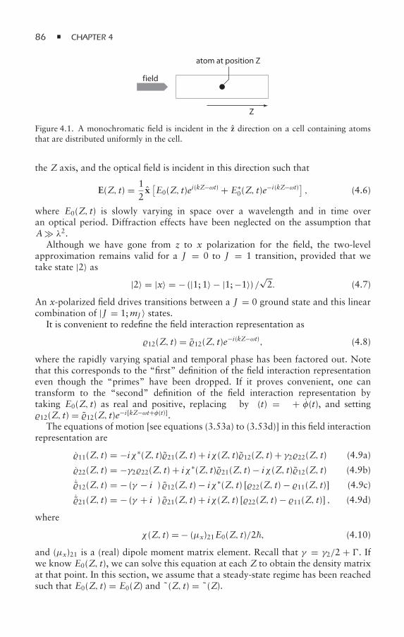
86 CHAPTER 4
atom at position Z
f ield
Z
Figure 4.1. A monochromatic field is incident in the z direction on a cell containing atomsthat are distributed uniformly in the cell.
the Z axis, and the optical field is incident in this direction such that
E(Z, t) = 12x[E0(Z, t)ei(kZ−ωt) + E∗
0(Z, t)e−i(kZ−ωt)] , (4.6)
where E0(Z, t) is slowly varying in space over a wavelength and in time overan optical period. Diffraction effects have been neglected on the assumption thatA λ2.
Although we have gone from z to x polarization for the field, the two-levelapproximation remains valid for a J = 0 to J = 1 transition, provided that wetake state |2〉 as
|2〉 = |x〉 = − (|1; 1〉 − |1;−1〉) /√2. (4.7)
An x-polarized field drives transitions between a J = 0 ground state and this linearcombination of |J = 1;mJ 〉 states.
It is convenient to redefine the field interaction representation as
12(Z, t) = 12(Z, t)e−i(kZ−ωt), (4.8)
where the rapidly varying spatial and temporal phase has been factored out. Notethat this corresponds to the “first” definition of the field interaction representationeven though the “primes” have been dropped. If it proves convenient, one cantransform to the “second” definition of the field interaction representation bytaking E0(Z, t) as real and positive, replacing δ by δ(t) = δ + φ(t), and setting12(Z, t) = 12(Z, t)e−i[kZ−ωt+φ(t)].
The equations of motion [see equations (3.53a) to (3.53d)] in this field interactionrepresentation are
11(Z, t) = −iχ∗(Z, t)21(Z, t) + iχ (Z, t)12(Z, t) + γ222(Z, t) (4.9a)
22(Z, t) = −γ222(Z, t) + iχ∗(Z, t)21(Z, t) − iχ (Z, t)12(Z, t) (4.9b)˙12(Z, t) = − (γ − iδ) 12(Z, t) − iχ∗(Z, t) [22(Z, t) − 11(Z, t)] (4.9c)˙21(Z, t) = − (γ + iδ) 21(Z, t) + iχ (Z, t) [22(Z, t) − 11(Z, t)] , (4.9d)
where
χ (Z, t) = − (µx)21E0(Z, t)/2, (4.10)
and (µx)21 is a (real) dipole moment matrix element. Recall that γ = γ2/2 + . Ifwe know E0(Z, t), we can solve this equation at each Z to obtain the density matrixat that point. In this section, we assume that a steady-state regime has been reachedsuch that E0(Z, t) = E0(Z) and (Z, t) = (Z).
DENSITY MATRIX APPLICATIONS 87
In steady state, all time derivatives are set equal to zero, and we find
12(Z) = −iχ∗(Z) [22(Z) − 11(Z)]γ − iδ
= iχ∗(Z)γ − iδ
γ 2 + δ2γ 2 + δ2 + 4γ
γ2|χ (Z)|2 , (4.11a)
21(Z) = iχ (Z) [22(Z) − 11(Z)]γ + iδ
= −iχ (Z)γ + iδ
γ 2 + δ2γ 2 + δ2 + 4γ
γ2|χ (Z)|2 , (4.11b)
22(Z) =2γγ2
|χ (Z)|2γ 2 + δ2 + 4γ
γ2|χ (Z)|2 , (4.11c)
11(Z) = 1 − 22(Z) =γ 2 + δ2 + 2γ
γ2|χ (Z)|2
γ 2 + δ2 + 4γγ2
|χ (Z)|2 . (4.11d)
For
4γγ2
|χ (Z)|2 γ 2 + δ2, (4.12)
we find that 22(Z) ≈ 11(Z) ≈ 12 , as you might expect, since there is saturation,
resulting in equal ground- and excited-state populations in strong fields. We canrewrite equation (4.11c) as
22(Z) =2γγ2
|χ (Z)|2γ 2B + δ2 , (4.13)
where
γB = γ
√1 + 4|χ (Z)|2
γ γ2(4.14)
is referred to as a power-broadened decay rate, for reasons to be discussed in thissection.
To establish a relationship between 22(Z) and the absorption rate, consider theslab of atoms between Z and Z+dZ shown in figure 4.2. The rate at which energy islost from the field equals that at which it is scattered by the atoms. In other words,each time a scattered photon is produced, one photon of energy is lost from thefield. As a consequence, the rate at which energy E is lost from the field as a resultof scattering by atoms in the slab is given by
d〈E〉dt
= −N ω 22(Z) γ2AdZ, (4.15)
where N is the atom density, A is the cross-sectional area of the slab, and thebrackets indicate a time average over an optical period. We want to convert thistime derivative to a spatial derivative and can do this using the Poynting vector.
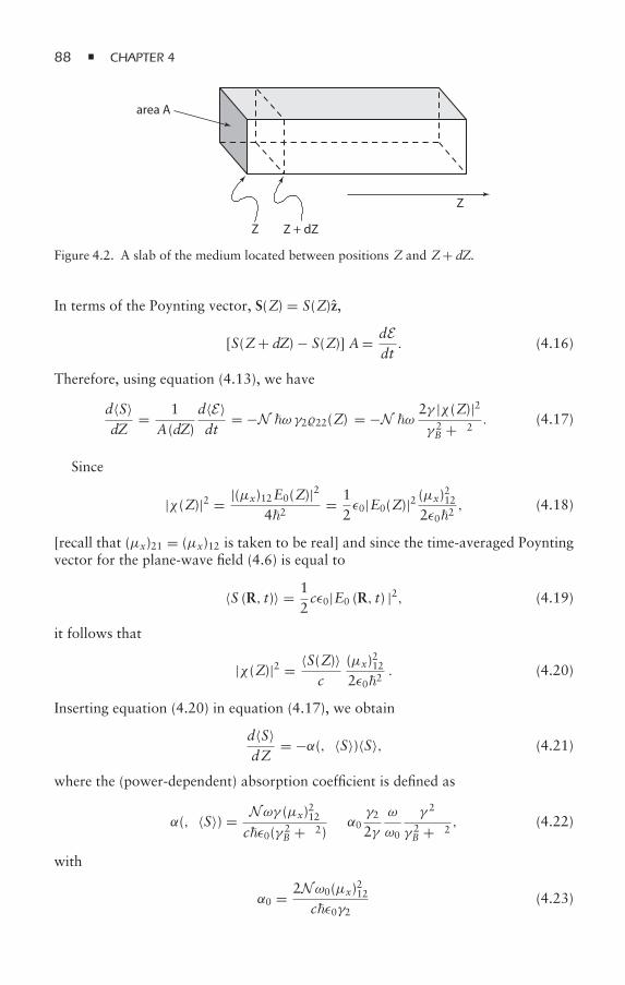
88 CHAPTER 4
Z Z + dZ
area A
Z
Figure 4.2. A slab of the medium located between positions Z and Z+ dZ.
In terms of the Poynting vector, S(Z) = S(Z)z,
[S(Z+ dZ) − S(Z)] A= dEdt. (4.16)
Therefore, using equation (4.13), we have
d〈S〉dZ
= 1A(dZ)
d〈E〉dt
= −N ω γ222(Z) = −N ω 2γ |χ (Z)|2γ 2B + δ2 . (4.17)
Since
|χ (Z)|2 = |(µx)12E0(Z)|242
= 12ε0|E0(Z)|2 (µx)
212
2ε02, (4.18)
[recall that (µx)21 = (µx)12 is taken to be real] and since the time-averaged Poyntingvector for the plane-wave field (4.6) is equal to
〈S (R, t)〉 = 12cε0|E0 (R, t) |2, (4.19)
it follows that
|χ (Z)|2 = 〈S(Z)〉c
(µx)2122ε02
. (4.20)
Inserting equation (4.20) in equation (4.17), we obtain
d〈S〉dZ
= −α(δ, 〈S〉)〈S〉, (4.21)
where the (power-dependent) absorption coefficient is defined as
α(δ, 〈S〉) = Nωγ (µx)212cε0(γ 2
B + δ2) ≡ α0γ2
2γω
ω0
γ 2
γ 2B + δ2 , (4.22)
with
α0 = 2Nω0(µx)212cε0γ2
(4.23)
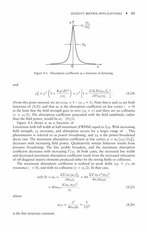
DENSITY MATRIX APPLICATIONS 89
δ
α0
α
0
____
2γB
2γ B
γγ 22
Figure 4.3. Absorption coefficient as a function of detuning.
and
γ 2B = γ 2
(1 + 4|χ (Z)|2
γ γ2
)= γ 2
[1 + 2〈S(Z)〉(µx)212
c2ε0γ γ2
]. (4.24)
(From this point onward, we set ω/ω0 = 1− δ/ω0 ≈ 1). Note that α and γB are bothfunctions of 〈S(Z)〉 and that α0 is the absorption coefficient on line center (δ = 0)in the limit that the field strength goes to zero (γB = γ ) and there are no collisions(γ = γ2/2). The absorption coefficient associated with the field amplitude, ratherthan the field power, would be α(δ, 〈S〉)/2.
Figure 4.3 shows α as a function of δ [see equation (4.22)]. The curve is aLorentzian with full width at half maximum (FWHM) equal to 2γB. With increasingfield strength, γB increases, and absorption occurs for a larger range of δ. Thisphenomenon is referred to as power broadening, and γB is the power-broadeneddecay rate. The maximum absorption coefficient at line center, α = α0
(γ2γ /2γ 2
B
),
decreases with increasing field power. Qualitatively similar behavior results frompressure broadening. The line profile broadens, and the maximum absorptioncoefficient decreases with increasing /γ2. In both cases, the increased line widthand decreased maximum absorption coefficient result from the increased relaxationof off-diagonal matrix elements produced either by the strong fields or collisions.
The maximum absorption coefficient is realized in weak fields (γB ≈ γ ), onresonance (δ = 0), and with no collisions (γ = γ2/2). In that case,
α(0,0) = α0 = 2N ω0 (µx)212cε0γ2
= 4π2N ω0 e2|x12|2
4πcε0γ2
= 8παF SNω0 |x12|2
γ2, (4.25)
where
αF S = e2
4πε0c≈ 1
137(4.26)
is the fine structure constant.
90 CHAPTER 4
We show in chapter 16 that
γ2 = 43αF S|x12|2ω
30
c2, (4.27)
and therefore,
α0 = 348πk20N = 3
2πNλ20 = 6πλ20N , (4.28)
where
k0 = ω0/c = 2π/λ0 = 1/λ0. (4.29)
The resonance absorption cross section σ = α0/N is of order λ20. For λ0 =628 nm, λ0 = 100 nm, giving rise to an absorption coefficient
α0 = [6π × 10−14N (m−3)]m−1 = [6π × 10−10N (cm−3)] cm−1. (4.30)
For N = 1010 atoms/cm3, α0 ≈ 20 cm−1. Thus, under these conditions of maximumabsorption, a substantial part of the field’s energy is lost in a distance of 0.5mm.
We now return to equation (4.21) to see how the Poynting vector dimin-ishes in the medium. If γB ≈ γ (weak field–linear absorption), the solution ofequation (4.21) is
〈S(L)〉 = 〈S(0)〉e−α(δ,0)L, (4.31)where
α(δ,0) = α0γ2
2γγ 2
γ 2 + δ2 . (4.32)
In strong fields, we must express γB in terms of 〈S〉 [equation (4.24)]. We can stillintegrate equation (4.21), which we write in the form
γ 2B + δ2γ 2
d〈S(Z)〉〈S(Z)〉 = −α0 γ22γ dZ. (4.33)
Using equation (4.24), we find
d〈S(Z)〉〈S(Z)〉
γ 2[1 + 2〈S(Z)〉(µx)212
c2ε0γ γ2
]+ δ2
γ 2= −α0 γ22γ dZ, (4.34)
or
d〈S(Z)〉〈S(Z)〉
[1 + 2〈S(Z)〉(µx)212γ
c2ε0γ2(γ 2 + δ2)
]= −α0 γ22γ
γ 2
γ 2 + δ2 dZ. (4.35)
After integration, we obtain
ln〈S(L)〉〈S(0)〉 +
[γ 2B(0)γ 2
− 1] [ 〈S(L)〉
〈S(0)〉 − 1]
γ 2
γ 2 + δ2 = −α0 γ22γγ 2
γ 2 + δ2 L, (4.36)
where
γ 2B(0) = γ 2
[1 + 4|χ (0)|2
γ γ2
]= γ 2
[1 + 2〈S(0)〉(µx)212
c2ε0γ γ2
]. (4.37)
This equation can be solved numerically for 〈S(L)〉/〈S(0)〉.
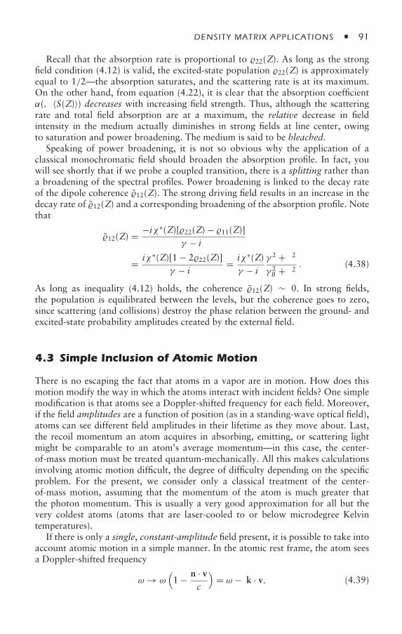
DENSITY MATRIX APPLICATIONS 91
Recall that the absorption rate is proportional to 22(Z). As long as the strongfield condition (4.12) is valid, the excited-state population 22(Z) is approximatelyequal to 1/2—the absorption saturates, and the scattering rate is at its maximum.On the other hand, from equation (4.22), it is clear that the absorption coefficientα(δ, 〈S(Z)〉) decreases with increasing field strength. Thus, although the scatteringrate and total field absorption are at a maximum, the relative decrease in fieldintensity in the medium actually diminishes in strong fields at line center, owingto saturation and power broadening. The medium is said to be bleached.
Speaking of power broadening, it is not so obvious why the application of aclassical monochromatic field should broaden the absorption profile. In fact, youwill see shortly that if we probe a coupled transition, there is a splitting rather thana broadening of the spectral profiles. Power broadening is linked to the decay rateof the dipole coherence 12(Z). The strong driving field results in an increase in thedecay rate of 12(Z) and a corresponding broadening of the absorption profile. Notethat
12(Z) = −iχ∗(Z)[22(Z) − 11(Z)]γ − iδ
= iχ∗(Z)[1 − 222(Z)]γ − iδ
= iχ∗(Z)γ − iδ
γ 2 + δ2γ 2B + δ2 . (4.38)
As long as inequality (4.12) holds, the coherence 12(Z) ∼ 0. In strong fields,the population is equilibrated between the levels, but the coherence goes to zero,since scattering (and collisions) destroy the phase relation between the ground- andexcited-state probability amplitudes created by the external field.
4.3 Simple Inclusion of Atomic Motion
There is no escaping the fact that atoms in a vapor are in motion. How does thismotion modify the way in which the atoms interact with incident fields? One simplemodification is that atoms see a Doppler-shifted frequency for each field. Moreover,if the field amplitudes are a function of position (as in a standing-wave optical field),atoms can see different field amplitudes in their lifetime as they move about. Last,the recoil momentum an atom acquires in absorbing, emitting, or scattering lightmight be comparable to an atom’s average momentum—in this case, the center-of-mass motion must be treated quantum-mechanically. All this makes calculationsinvolving atomic motion difficult, the degree of difficulty depending on the specificproblem. For the present, we consider only a classical treatment of the center-of-mass motion, assuming that the momentum of the atom is much greater thatthe photon momentum. This is usually a very good approximation for all but thevery coldest atoms (atoms that are laser-cooled to or below microdegree Kelvintemperatures).
If there is only a single, constant-amplitude field present, it is possible to take intoaccount atomic motion in a simple manner. In the atomic rest frame, the atom seesa Doppler-shifted frequency
ω → ω(1 − n · v
c
)= ω − k · v, (4.39)
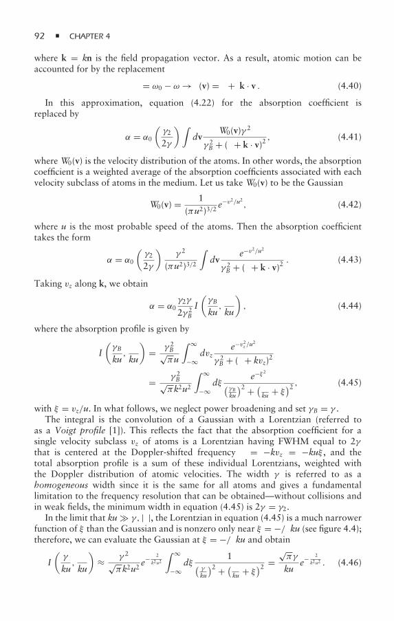
92 CHAPTER 4
where k = kn is the field propagation vector. As a result, atomic motion can beaccounted for by the replacement
δ = ω0 − ω → δ(v) = δ + k · v . (4.40)
In this approximation, equation (4.22) for the absorption coefficient isreplaced by
α = α0
(γ2
2γ
)∫dv
W0(v)γ 2
γ 2B + (δ + k · v)2 , (4.41)
where W0(v) is the velocity distribution of the atoms. In other words, the absorptioncoefficient is a weighted average of the absorption coefficients associated with eachvelocity subclass of atoms in the medium. Let us take W0(v) to be the Gaussian
W0(v) = 1(πu2)3/2
e−v2/u2 , (4.42)
where u is the most probable speed of the atoms. Then the absorption coefficienttakes the form
α = α0
(γ2
2γ
)γ 2
(πu2)3/2
∫dv
e−v2/u2
γ 2B + (δ + k · v)2 . (4.43)
Taking vz along k, we obtain
α = α0γ2γ
2γ 2B
I(γB
ku,δ
ku
), (4.44)
where the absorption profile is given by
I(γB
ku,δ
ku
)= γ 2
B√πu
∫ ∞
−∞dvz
e−v2z /u2
γ 2B + (δ + kvz)2
= γ 2B√
πk2u2
∫ ∞
−∞dξ
e−ξ2(γBku
)2 + (δku + ξ)2 , (4.45)
with ξ = vz/u. In what follows, we neglect power broadening and set γB = γ .The integral is the convolution of a Gaussian with a Lorentzian (referred to
as a Voigt profile [1]). This reflects the fact that the absorption coefficient for asingle velocity subclass vz of atoms is a Lorentzian having FWHM equal to 2γthat is centered at the Doppler-shifted frequency δ = −kvz = −kuξ , and thetotal absorption profile is a sum of these individual Lorentzians, weighted withthe Doppler distribution of atomic velocities. The width γ is referred to as ahomogeneous width since it is the same for all atoms and gives a fundamentallimitation to the frequency resolution that can be obtained—without collisions andin weak fields, the minimum width in equation (4.45) is 2γ = γ2.
In the limit that ku γ, |δ|, the Lorentzian in equation (4.45) is a much narrowerfunction of ξ than the Gaussian and is nonzero only near ξ = −δ/ku (see figure 4.4);therefore, we can evaluate the Gaussian at ξ = −δ/ku and obtain
I(γ
ku,δ
ku
)≈ γ 2
√πk2u2
e− δ2
k2u2
∫ ∞
−∞dξ
1(γ
ku
)2 + (δku + ξ)2 =
√πγ
kue− δ2
k2u2 . (4.46)
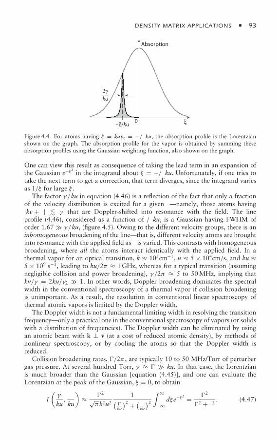
DENSITY MATRIX APPLICATIONS 93
ξ0
__
–δ/ku
2γku
Absorption
Figure 4.4. For atoms having ξ = kuvz = −δ/ku, the absorption profile is the Lorentzianshown on the graph. The absorption profile for the vapor is obtained by summing theseabsorption profiles using the Gaussian weighting function, also shown on the graph.
One can view this result as consequence of taking the lead term in an expansion ofthe Gaussian e−ξ2 in the integrand about ξ = −δ/ku. Unfortunately, if one tries totake the next term to get a correction, that term diverges, since the integrand variesas 1/ξ for large ξ .
The factor γ /ku in equation (4.46) is a reflection of the fact that only a fractionof the velocity distribution is excited for a given δ—namely, those atoms having|kv + δ| γ that are Doppler-shifted into resonance with the field. The lineprofile (4.46), considered as a function of δ/ku, is a Gaussian having FWHM oforder 1.67 γ /ku, (figure 4.5). Owing to the different velocity groups, there is aninhomogeneous broadening of the line—that is, different velocity atoms are broughtinto resonance with the applied field as δ is varied. This contrasts with homogeneousbroadening, where all the atoms interact identically with the applied field. In athermal vapor for an optical transition, k ≈ 105cm−1, u ≈ 5 × 104cm/s, and ku ≈5 × 10⁹ s−1, leading to ku/2π ≈ 1GHz, whereas for a typical transition (assumingnegligible collision and power broadening), γ /2π ≈ 5 to 50MHz, implying thatku/γ = 2ku/γ2 1. In other words, Doppler broadening dominates the spectralwidth in the conventional spectroscopy of a thermal vapor if collision broadeningis unimportant. As a result, the resolution in conventional linear spectroscopy ofthermal atomic vapors is limited by the Doppler width.
The Doppler width is not a fundamental limiting width in resolving the transitionfrequency—only a practical one in the conventional spectroscopy of vapors (or solidswith a distribution of frequencies). The Doppler width can be eliminated by usingan atomic beam with k ⊥ v (at a cost of reduced atomic density), by methods ofnonlinear spectroscopy, or by cooling the atoms so that the Doppler width isreduced.
Collision broadening rates, /2π , are typically 10 to 50 MHz/Torr of perturbergas pressure. At several hundred Torr, γ ≈ ku. In that case, the Lorentzianis much broader than the Gaussian [equation (4.45)], and one can evaluate theLorentzian at the peak of the Gaussian, ξ = 0, to obtain
I(γ
ku,δ
ku
)≈ 2
√πk2u2
1(ku
)2 + (δku
)2∫ ∞
−∞dξe−ξ2 = 2
2 + δ2 . (4.47)
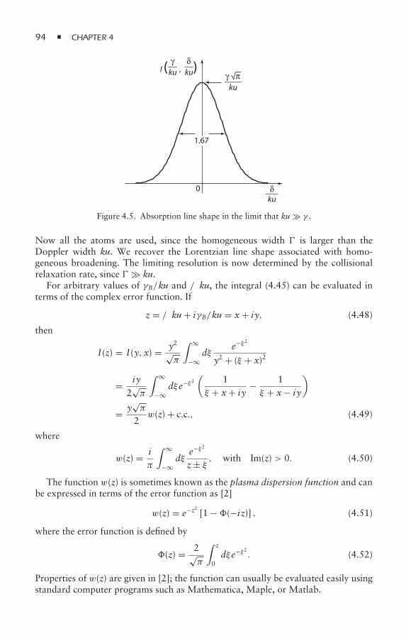
94 CHAPTER 4
1.67
0
I ( , )__γku
____γ √πku
__δku
___δku
Figure 4.5. Absorption line shape in the limit that ku γ .
Now all the atoms are used, since the homogeneous width is larger than theDoppler width ku. We recover the Lorentzian line shape associated with homo-geneous broadening. The limiting resolution is now determined by the collisionalrelaxation rate, since ku.
For arbitrary values of γB/ku and δ/ku, the integral (4.45) can be evaluated interms of the complex error function. If
z = δ/ku+ iγB/ku = x+ iy, (4.48)
then
I(z) = I(y, x) = y2√π
∫ ∞
−∞dξ
e−ξ2
y2 + (ξ + x)2
= iy
2√π
∫ ∞
−∞dξe−ξ2
(1
ξ + x+ iy− 1ξ + x− iy
)
= y√π
2w(z) + c.c., (4.49)
where
w(z) = iπ
∫ ∞
−∞dξ
e−ξ2
z± ξ , with Im(z) > 0. (4.50)
The function w(z) is sometimes known as the plasma dispersion function and canbe expressed in terms of the error function as [2]
w(z) = e−z2 [1 −(−i z)] , (4.51)
where the error function is defined by
(z) = 2√π
∫ z
0dξe−ξ2 . (4.52)
Properties of w(z) are given in [2]; the function can usually be evaluated easily usingstandard computer programs such as Mathematica, Maple, or Matlab.
DENSITY MATRIX APPLICATIONS 95
4.4 Rate Equations
In condensed matter and chemical physics, one often encounters rate equations thatinvolve populations of quantum states only. Coherence (off-diagonal density matrixelements) does not appear, and populations approach their steady-state valuesmonotonically. You might ask how this is possible with all the Rabi oscillationswe have been talking about.
To arrive at rate equations for state populations, one formally integrates theequation for 12(t), equation (4.9c), to obtain
12(t) = 12(0)e−(γ−iδ)t − i∫ t
0dt′e−(γ−iδ)(t−t′)χ∗(t′)
[22(t′) − 11(t′)
]. (4.53)
If χ∗(t) [22(t) − 11(t)] is slowly varying on a timescale |γ − iδ|−1 we can integratethe second term by parts, as in the Bloch-Siegert problem. Keeping only the leadingterm, we find
12(t) = 12(0)e−(γ−iδ)t − iχ∗(t)γ − iδ
[22(t) − 11(t)] . (4.54)
The first term is either small or rapidly varying compared with the second if theapproximation we used is valid. Neglecting the first term, we obtain
12(t) ≈ −i χ∗(t)
γ − iδ[22(t) − 11(t)] . (4.55)
That is, the coherence adiabatically follows the product of the field amplitudeand population difference. The coherence goes to zero in strong fields since thepopulation difference goes to zero as |χ (t)|−2 in this limit. Using equation (4.55)and its complex conjugate in equation (4.9a), (4.9b), we find
11 = −iχ∗(t)21(t) + iχ (t)12(t) + γ222(t)
= 2γ |χ (t)|2γ 2 + δ2 [22(t) − 11(t)] + γ222(t), (4.56a)
22 = iχ∗(t)21(t) − iχ (t)12(t) − γ222(t)
= − 2γ |χ (t)|2γ 2 + δ2 [22(t) − 11(t)] − γ222(t), (4.56b)
or
11 = f (t) [22(t) − 11(t)] + γ222(t), (4.57a)
22 = − f (t) [22(t) − 11(t)] − γ222(t), (4.57b)
where
f (t) = 2γ |χ (t)|2γ 2 + δ2 (4.58)
is the rate at which the field drives the transitions. Equations (4.57a) and (4.57b) arethe rate equations for the populations. Often such equations are used even if theyare not fully justified.
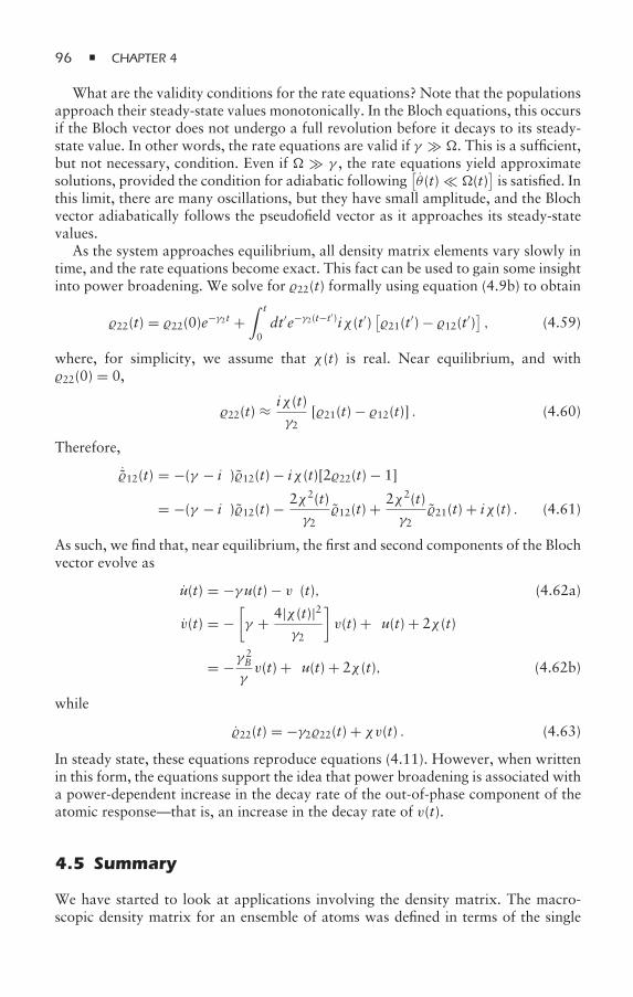
96 CHAPTER 4
What are the validity conditions for the rate equations? Note that the populationsapproach their steady-state values monotonically. In the Bloch equations, this occursif the Bloch vector does not undergo a full revolution before it decays to its steady-state value. In other words, the rate equations are valid if γ . This is a sufficient,but not necessary, condition. Even if γ , the rate equations yield approximatesolutions, provided the condition for adiabatic following
[θ (t) (t)
]is satisfied. In
this limit, there are many oscillations, but they have small amplitude, and the Blochvector adiabatically follows the pseudofield vector as it approaches its steady-statevalues.
As the system approaches equilibrium, all density matrix elements vary slowly intime, and the rate equations become exact. This fact can be used to gain some insightinto power broadening. We solve for 22(t) formally using equation (4.9b) to obtain
22(t) = 22(0)e−γ2t +∫ t
0dt′e−γ2(t−t′)iχ (t′)
[21(t′) − 12(t′)
], (4.59)
where, for simplicity, we assume that χ (t) is real. Near equilibrium, and with22(0) = 0,
22(t) ≈ iχ (t)γ2
[21(t) − 12(t)] . (4.60)
Therefore,
˙12(t) = −(γ − iδ)12(t) − iχ (t)[222(t) − 1]
= −(γ − iδ)12(t) − 2χ2(t)γ2
12(t) + 2χ2(t)γ2
21(t) + iχ (t) . (4.61)
As such, we find that, near equilibrium, the first and second components of the Blochvector evolve as
u(t) = −γu(t) − δv(t), (4.62a)
v(t) = −[γ + 4|χ (t)|2
γ2
]v(t) + δu(t) + 2χ (t)
= −γ2B
γv(t) + δu(t) + 2χ (t), (4.62b)
while
22(t) = −γ222(t) + χv(t) . (4.63)
In steady state, these equations reproduce equations (4.11). However, when writtenin this form, the equations support the idea that power broadening is associated witha power-dependent increase in the decay rate of the out-of-phase component of theatomic response—that is, an increase in the decay rate of v(t).
4.5 Summary
We have started to look at applications involving the density matrix. The macro-scopic density matrix for an ensemble of atoms was defined in terms of the single
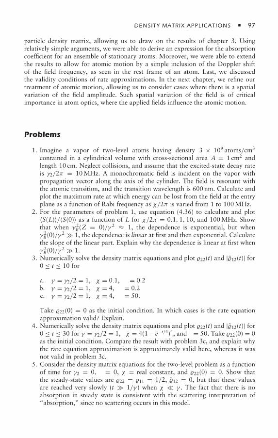
DENSITY MATRIX APPLICATIONS 97
particle density matrix, allowing us to draw on the results of chapter 3. Usingrelatively simple arguments, we were able to derive an expression for the absorptioncoefficient for an ensemble of stationary atoms. Moreover, we were able to extendthe results to allow for atomic motion by a simple inclusion of the Doppler shiftof the field frequency, as seen in the rest frame of an atom. Last, we discussedthe validity conditions of rate approximations. In the next chapter, we refine ourtreatment of atomic motion, allowing us to consider cases where there is a spatialvariation of the field amplitude. Such spatial variation of the field is of criticalimportance in atom optics, where the applied fields influence the atomic motion.
Problems
1. Imagine a vapor of two-level atoms having density 3 × 10⁹ atoms/cm3
contained in a cylindrical volume with cross-sectional area A = 1 cm2 andlength 10 cm. Neglect collisions, and assume that the excited-state decay rateis γ2/2π = 10MHz. A monochromatic field is incident on the vapor withpropagation vector along the axis of the cylinder. The field is resonant withthe atomic transition, and the transition wavelength is 600 nm. Calculate andplot the maximum rate at which energy can be lost from the field at the entryplane as a function of Rabi frequency as χ/2π is varied from 1 to 100MHz.
2. For the parameters of problem 1, use equation (4.36) to calculate and plot〈S(L)〉/〈S(0)〉 as a function of L for χ/2π = 0.1,1,10, and 100MHz. Showthat when γ 2
B(Z = 0)/γ 2 ≈ 1, the dependence is exponential, but whenγ 2B(0)/γ
2 1, the dependence is linear at first and then exponential. Calculatethe slope of the linear part. Explain why the dependence is linear at first whenγ 2B(0)/γ
2 1.3. Numerically solve the density matrix equations and plot 22(t) and |12(t)| for
0 ≤ t ≤ 10 for
a. γ = γ2/2 = 1, χ = 0.1, δ = 0.2b. γ = γ2/2 = 1, χ = 4, δ = 0.2c. γ = γ2/2 = 1, χ = 4, δ = 50.
Take 22(0) = 0 as the initial condition. In which cases is the rate equationapproximation valid? Explain.
4. Numerically solve the density matrix equations and plot 22(t) and |12(t)| for0 ≤ t ≤ 30 for γ = γ2/2 = 1, χ = 4(1− e−t/4)4, and δ = 50. Take 22(0) = 0as the initial condition. Compare the result with problem 3c, and explain whythe rate equation approximation is approximately valid here, whereas it wasnot valid in problem 3c.
5. Consider the density matrix equations for the two-level problem as a functionof time for γ2 = 0, δ = 0, χ = real constant, and 22(0) = 0. Show thatthe steady-state values are 22 = 11 = 1/2, 12 = 0, but that these valuesare reached very slowly (t 1/γ ) when χ γ . The fact that there is noabsorption in steady state is consistent with the scattering interpretation of“absorption,” since no scattering occurs in this model.
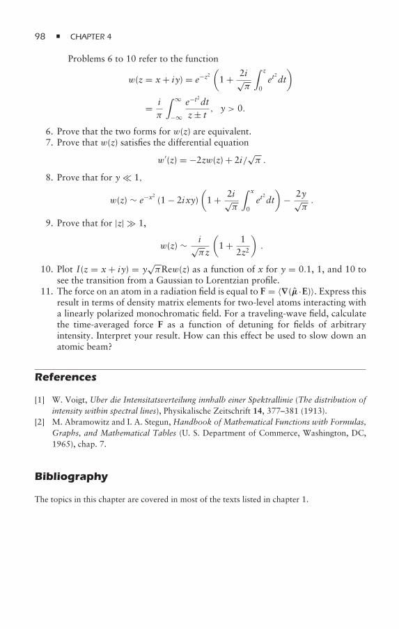
98 CHAPTER 4
Problems 6 to 10 refer to the function
w(z = x+ iy) = e−z2(1 + 2i√
π
∫ z
0et
2dt)
= iπ
∫ ∞
−∞
e−t2dtz± t
, y > 0.
6. Prove that the two forms for w(z) are equivalent.7. Prove that w(z) satisfies the differential equation
w′(z) = −2zw(z) + 2i/√π .
8. Prove that for y 1,
w(z) ∼ e−x2 (1 − 2ixy)(1 + 2i√
π
∫ x
0et
2dt)
− 2y√π.
9. Prove that for |z| 1,
w(z) ∼ i√πz
(1 + 1
2z2
).
10. Plot I(z = x+ iy) = y√πRew(z) as a function of x for y = 0.1, 1, and 10 to
see the transition from a Gaussian to Lorentzian profile.11. The force on an atom in a radiation field is equal to F = 〈∇(µ ·E)〉. Express this
result in terms of density matrix elements for two-level atoms interacting witha linearly polarized monochromatic field. For a traveling-wave field, calculatethe time-averaged force F as a function of detuning for fields of arbitraryintensity. Interpret your result. How can this effect be used to slow down anatomic beam?
References
[1] W. Voigt, Uber die Intensitatsverteilung innhalb einer Spektrallinie (The distribution ofintensity within spectral lines), Physikalische Zeitschrift 14, 377–381 (1913).
[2] M. Abramowitz and I. A. Stegun, Handbook of Mathematical Functions with Formulas,Graphs, and Mathematical Tables (U. S. Department of Commerce, Washington, DC,1965), chap. 7.
Bibliography
The topics in this chapter are covered in most of the texts listed in chapter 1.
5Density Matrix Equations:Atomic Center-of-Mass Motion, Elementary AtomOptics, and Laser Cooling
5.1 Introduction
In the previous chapter, we included the effects of atomic motion for the specificcase of atoms interacting with a single plane-wave field. Moreover, it was assumedthat effects related to quantization of the atomic center-of-mass motion could beneglected. In this chapter, we retain, for the most part, a classical description of thecenter-of-mass motion but provide a general framework that will allow us to dealwith more complicated atom–field geometries. In particular, we calculate the forceon an atom in a standing-wave optical field. To do so, we need a better treatment ofatomic motion.
The appendix in this chapter contains a rigorous derivation of the density matrixequations, including a quantized description of the center-of-mass motion, as wellas a method for taking a classical limit of these equations in which the atomicposition and momentum (or velocity) operators are replaced by classical variables.One can arrive at the same equations by generalizing the results of the previouschapter using a simple heuristic argument. For a moving atom, one can considerthe time derivative in the Schrödinger equation as a total time derivative. Thus,in taking dαα′ (Ri , t)/dt for an atom having classical position Ri and velocityvi = dRi/dt, one sets
dαα′ (Ri , t)/dt = ∂αα′(Ri , t)/∂t + ∇Riαα′ (Ri , t) · dRi/dt
= ∂αα′(Ri , t)/∂t + vi · ∇Riαα′(Ri , t). (5.1)
100 CHAPTER 5
For a single optical field interacting with an ensemble of two-level atoms,equations (4.1) become
∂11(R, v, t)∂t
+ v · ∇11(R, v, t) = −iχ∗(R, t)21(R, v, t) + iχ (R,t)12(R, v, t)
+γ222(R, v, t), (5.2a)
∂22(R, v, t)∂t
+ v · ∇22(R, v, t) = iχ∗(R, t)21(R, v, t) − iχ (R, t)12(R, v, t)
−γ222(R, v, t), (5.2b)
∂12(R, v, t)∂t
+ v · ∇12(R, v, t) = −iχ∗(R, t) [22(R, v, t) − 11(R, v, t)]−(γ − iδ)12(R, v, t), (5.2c)
∂21(R, v, t)∂t
+ v · ∇21(R, v, t) = iχ (R, t) [22(R, v, t) − 11 (R, v, t)]
−(γ + iδ)21(R, v, t), (5.2d)
where
χ (R, t) = − (ε · µ21)E0(R, t)2
, (5.3)
and
E(R, t) = 12
εE0(R, t)e−iωt + c.c. (5.4)
Recall that i j (R, v, t) is a dimensionless, single-atom density matrix element.Equations (5.2) are the basic equations for atom–field interactions involvingtwo-level atoms interacting with a quasi-monochromatic optical field. The totalpopulation
11(R, v, t) + 22(R, v, t) = 1 (5.5)
is conserved, since the effects of velocity-changing collisions are neglected.
5.2 Atom in a Single Plane-Wave Field
For an external field of the form
E(R, t) = 12
εE0ei(k·R−ωt) + c.c., (5.6)
with ε · k = 0, we set χ (R, t) = χeik·R in equations (5.2), with
χ = − (ε · µ21)E0
2. (5.7)
DENSITY MATRIX WITH ATOMIC MOTION 101
If we assume a solution to equations (5.2) of the form
12(R, v, t) = 12(v, t)e−ik·R, (5.8a)
21(R, v, t) = 21(v, t)eik·R, (5.8b)
11(R, v, t) = 11(v, t), (5.8c)
22(R, v, t) = 22(v, t), (5.8d)
we find evolution equations
∂11(v, t)∂t
= −iχ∗21(v, t) + iχ12(v, t) + γ211(v, t), (5.9a)
∂22(v, t)∂t
= iχ∗21(v, t) − iχ12(v, t) − γ222(v, t), (5.9b)
∂12(v, t)∂t
= iχ∗ [11(v, t) − 22(v, t)] − [γ − i(δ + k · v)]12(v, t),(5.9c)
∂21(v, t)∂t
= iχ [22(v, t) − 11(v, t)] − [γ + i(δ + k · v)]21(v, t).(5.9d)
As stated in chapter 4, the net effect is to replace the detuning δ by δ(v) = δ + k · v.
5.3 Force on an Atom
When a radiation field interacts with atoms, it can exert forces on the atoms. Forcesof this nature are responsible for laser cooling, confinement in optical lattices, andthe deflection of atoms. There are times when the atomic center-of-mass motioncan be treated classically (as in this chapter) and times when the motion must bequantized. In chapter 11, we explore these regimes in more detail. The manipulationof atomic motion by optical fields or microfabricated gratings belongs to the generalfield of atom optics. As an elementary application of atom optics, we consider nowthe force on an atom produced by an optical field.
The atom–field interaction energy is −µ · E, so the force on an atom located atposition R having velocity v at time t is
F(R, v, t) = 〈∇(µ · E)〉 = Tr [(R, v, t)∇(µ · E)] . (5.10)
Forces can arise because there is a gradient in the field amplitude or as a result ofscattering of the incident field by the atoms into unoccupied vacuum field modes. Letus consider three cases: a plane wave, a focused plane wave, and a standing-wavefield. In all cases, we take
E(R, t) = 12E0(R)e−iωt + c.c., (5.11)
and
12(R, v, t) = 12(R, v)eiωt. (5.12)
102 CHAPTER 5
As a consequence, the force may be written as
F(R, v) = Tr (R, v, t)∇ [µ · E(R, t)]= 12(R, v, t)∇ [µ21·E(R, t)] + c.c.
≈ 1212(R, v)∇ [µ21·E0(R)] + c.c., (5.13)
where rapidly varying terms—that is, terms varying as exp[±2iωt]—have beenneglected.
5.3.1 Plane Wave
For a plane wave
E0(R) = εE0eik·R, (5.14)
with ε · k = 0, the force is given by
F(v) = 1212(R, v)(µ21 · εE0)ikeik·R + c.c.
= −ikχ12(v) + c.c. = kγ2[iχ∗21(v) − iχ12(v)
γ2
],
(5.15)
where χ = −µ21 · εE0/(2) and 12(R, v) = 12(v)e−ik·R. In steady state, the term inbrackets is just equal to 22(v) [see equation (5.9b)]; therefore,
F(v) = kγ222(v) . (5.16)
This is just what you might have expected. Every time a photon is scattered by anatom, on average, the atom picks up k of momentum from the field, since thescattered dipole radiation has zero average momentum [1]. The scattering rate isjust γ222(v). Note that it is incorrect to say that the atom absorbs radiation at onefrequency and then re-emits via spontaneous emission at another frequency. Thecorrect interpretation is in terms of a scattering process in which the incident field isscattered into modes of the vacuum field that were unoccupied.
The steady-state excited-state population is
22(v) = 2|χ |2γγ2
1γ 2B + (δ + k · v)2 . (5.17)
As a result, the maximum force occurs for atoms having velocity v satisfyingk · v =− δ. For δ = ω0 −ω < 0 (blue detuning), the maximum force occurs for v andk parallel and is in the direction of motion (acceleration), while for δ = ω0 − ω > 0(red detuning), the maximum force occurs for v and k antiparallel and opposes themotion (deceleration) (see figure 5.1). This technique for slowing and cooling atomswas proposed originally by Hänsch and Schawlow in 1975 [2].
DENSITY MATRIX WITH ATOMIC MOTION 103
Fz (arb. units)
0 kvz
δ > 0 δ < 0
δ–δ
Figure 5.1. Dissipative force experienced by an atom in a plane-wave field. For positive(negative) detuning, the field decelerates (accelerates) the atom.
5.3.2 Focused Plane Wave: Atom Trapping
In the previous example, the net force arose from a dissipative process—radiationwas scattered irreversibly into modes of the vacuum field. If instead we let theatoms interact with a field having a spatial intensity gradient, both conservative andnonconservative forces can be experienced by the atoms. To illustrate this point,we assume that the laser field has a Gaussian spatial profile and take E0(R) =εE0(RT)eikZ, where
RT = Xi + Yj (5.18)
is the cylindrical position vector, k · ε ≈ 0, and
E0(RT) = E0e−R2T/a
2, (5.19)
with E0 a real constant. This field does not satisfy Maxwell’s equations, but if ais much greater than λ = 2π/k (allowing one to neglect diffraction of the field), itrepresents an approximate solution.
Since
∇ [µ21 · E0(R)] = µ21 · εeikZ[ikzE0(RT) + ∂E0(RT)
∂RTrT
], (5.20)
where rT = RT/ |RT| is a unit vector, it follows from equation (5.13) that the forceis given by
F(R, v) = −ikzχ (RT)12(R, v)eikZ+ 12
µ21 · ε12(R, v)eikZ∂E0(RT)∂RT
rT + c.c., (5.21)
where
χ (RT) = −(ε · µ21)E0(RT)/(2). (5.22)
It is not so easy to solve equations (5.2) for 12(R, v), since the field is a functionof the cylindrical coordinate RT. Still, the terms in equation (5.21) have an obvious
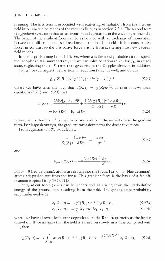
104 CHAPTER 5
meaning. The first term is associated with scattering of radiation from the incidentfield into unoccupied modes of the vacuum field, as in section 5.3.1. The second termis a gradient force term that arises from spatial variations in the envelope of the field.The origin of the gradient force can be associated with an exchange of momentumbetween the different modes (directions) of the incident field—it is a conservativeforce, in contrast to the dissipative force arising from scattering into new vacuumfield modes.
In the large detuning limit, |δ| ku, where u is the most probable atomic speed,the Doppler shift is unimportant, and we can solve equation (5.2c) for 12 in steadystate, neglecting the v · ∇ term that gives rise to the Doppler shift. If, in addition,|δ| γB, we can neglect the 22 term in equation (5.2c) as well, and obtain
12(Z, RT) ≈ iχ∗ (RT) e−ikZ (γ − iδ) /δ2, (5.23)
where we have used the fact that χ (R, t) = χ (RT)eikZ. It then follows fromequations (5.21) and (5.23) that
F(RT) = 2kγ |χ (RT) |2zδ2
+ 1δ
2|χ (RT) |2E0(RT)
∂E0(RT)∂RT
rT,
= Fdis(RT) + Fgrad(RT), (5.24)
where the first term ∼δ−2 is the dissipative term, and the second one is the gradientterm. For large detunings, the gradient force dominates the dissipative force.
From equation (5.19), we calculate
1E0(RT)
∂E0(RT)∂RT
= −2RTa2, (5.25)
and
Fgrad(RT, v) = −4|χ (RT) |2
δ
RTa2
rT . (5.26)
For δ > 0 (red detuning), atoms are drawn into the focus. For δ < 0 (blue detuning),atoms are pushed out from the focus. This gradient force is the basis of a far off-resonance optical trap (FORT) [3].
The gradient force (5.26) can be understood as arising from the Stark-shiftedenergy of the ground state resulting from the field. The ground-state probabilityamplitudes evolve as
c1(RT, t) = −iχ∗(RT, t)e−iδtc2(RT, t), (5.27a)
c2(RT, t) = −iχ (RT, t)eiδtc1(RT, t), (5.27b)
where we have allowed for a time dependence in the Rabi frequencies as the field isturned on. If we imagine that the field is turned on slowly in a time compared withδ−1, then
c2 (RT, t) = −i∫ t
−∞dt′χ (RT, t′)eiδt
′c1(RT, t′) ≈ −χ (RT, t)e
iδt
δc1(RT, t), (5.28)
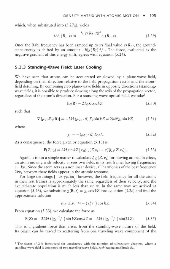
DENSITY MATRIX WITH ATOMIC MOTION 105
which, when substituted into (5.27a), yields
ic1(RT, t) ≈ − |χ (RT, t)|2δ
c1(RT, t). (5.29)
Once the Rabi frequency has been ramped up to its final value χ (RT), the ground-state energy is shifted by an amount −|χ (RT)|2/δ. The force, evaluated as thenegative gradient of this energy shift, agrees with equation (5.26).
5.3.3 Standing-Wave Field: Laser Cooling
We have seen that atoms can be accelerated or slowed by a plane-wave field,depending on their direction relative to the field propagation vector and the atom–field detuning. By combining two plane-wave fields in opposite directions (standing-wave field), it is possible to produce slowing along the axis of the propagation vector,regardless of the atom’s direction. For a standing-wave optical field, we take1
E0(R) = 2E0x cos kZ, (5.30)
such that
∇ [µ21·E0(R)] = −2kz (µ21 · x) E0 sinkZ= 2kzχs sinkZ, (5.31)
where
χs = − (µ21 · x) E0/. (5.32)
As a consequence, the force given by equation (5.13) is
F(Z,vz) = kz sinkZ[χs 12(Z,vz) + χ∗s 21(Z,vz)
]. (5.33)
Again, it is not a simple matter to calculate 12(Z, vz) for moving atoms. In effect,an atom moving with velocity vz sees two fields in its rest frame, having frequenciesω±kvz. Since the atom acts as a nonlinear device, all harmonics of the beat frequency2kvz between these fields appear in the atomic response.
For large detunings [δ γB,ku], however, the field frequency for all the atomsin their rest frames is approximately the same, regardless of their velocity, and theexcited-state population is much less than unity. In the same way we arrived atequation (5.23), we substitute χ (R, t) = χs cos kZ into equation (5.2c) and find theapproximate solution
12(Z,vz) ≈ − (χ∗s /δ
)cos kZ. (5.34)
From equation (5.33), we calculate the force as
F(Z) = −2kz(|χs | 2/δ) sinkZcos kZ= −kz (|χs | 2/δ) sin(2kZ) . (5.35)
This is a gradient force that arises from the standing-wave nature of the field.Its origin can be traced to scattering from one traveling wave component of the
1 The factor of 2 is introduced for consistency with the notation of subsequent chapters, where astanding-wave field is composed of two traveling-wave fields, each having amplitude E0.
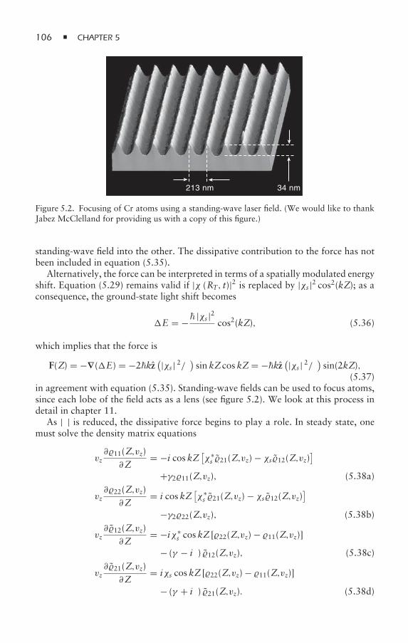
106 CHAPTER 5
213 nm 34 nm
Figure 5.2. Focusing of Cr atoms using a standing-wave laser field. (We would like to thankJabez McClelland for providing us with a copy of this figure.)
standing-wave field into the other. The dissipative contribution to the force has notbeen included in equation (5.35).
Alternatively, the force can be interpreted in terms of a spatially modulated energyshift. Equation (5.29) remains valid if |χ (RT, t)|2 is replaced by |χs |2 cos2(kZ); as aconsequence, the ground-state light shift becomes
E = − |χs |2δ
cos2(kZ), (5.36)
which implies that the force is
F(Z) = −∇(E) = −2kz(|χs | 2/δ) sinkZcos kZ= −kz (|χs | 2/δ) sin(2kZ),
(5.37)in agreement with equation (5.35). Standing-wave fields can be used to focus atoms,since each lobe of the field acts as a lens (see figure 5.2). We look at this process indetail in chapter 11.
As |δ| is reduced, the dissipative force begins to play a role. In steady state, onemust solve the density matrix equations
vz∂11(Z,vz)
∂Z= −i cos kZ[χ∗
s 21(Z,vz) − χs 12(Z,vz)]
+γ211(Z,vz), (5.38a)
vz∂22(Z,vz)
∂Z= i cos kZ
[χ∗s 21(Z,vz) − χs 12(Z,vz)
]−γ222(Z,vz), (5.38b)
vz∂12(Z,vz)
∂Z= −iχ∗
s cos kZ [22(Z,vz) − 11(Z,vz)]− (γ − iδ) 12(Z,vz), (5.38c)
vz∂21(Z,vz)
∂Z= iχs cos kZ [22(Z,vz) − 11(Z,vz)]
− (γ + iδ) 21(Z,vz). (5.38d)
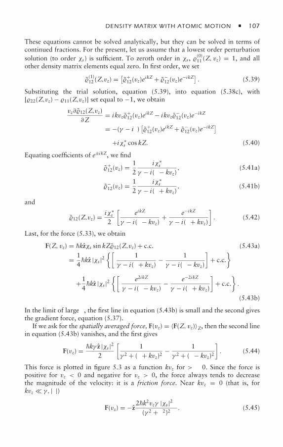
DENSITY MATRIX WITH ATOMIC MOTION 107
These equations cannot be solved analytically, but they can be solved in terms ofcontinued fractions. For the present, let us assume that a lowest order perturbationsolution (to order χs) is sufficient. To zeroth order in χs ,
(0)11 (Z, vz) = 1, and all
other density matrix elements equal zero. In first order, we set
(1)12 (Z,vz) = [
+12(vz)e
ikZ + −12(vz)e
−ikZ] . (5.39)
Substituting the trial solution, equation (5.39), into equation (5.38c), with[22(Z,vz) − 11(Z,vz)] set equal to −1, we obtain
vz∂12(Z,vz)∂Z
= ikvz+12(vz)e
ikZ − ikvz−12(vz)e
−ikZ
= −(γ − iδ)[+12(vz)e
ikZ + −12(vz)e
−ikZ]+iχ∗
s cos kZ. (5.40)
Equating coefficients of e±ikZ, we find
+12(vz) = 1
2iχ∗
s
γ − i(δ − kvz), (5.41a)
−12(vz) = 1
2iχ∗
s
γ − i(δ + kvz), (5.41b)
and
12(Z,vz) = iχ∗s
2
[eikZ
γ − i(δ − kvz)+ e−ikZ
γ − i(δ + kvz)
]. (5.42)
Last, for the force (5.33), we obtain
F(Z, vz) = kzχs sinkZ12(Z,vz) + c.c. (5.43a)
= 14kz |χs |2
[1
γ − i(δ + kvz)− 1γ − i(δ − kvz)
]+ c.c.
+14kz |χs |2
[e2ikZ
γ − i(δ − kvz)− e−2ikZ
γ − i(δ + kvz)
]+ c.c.
.
(5.43b)
In the limit of large δ, the first line in equation (5.43b) is small and the second givesthe gradient force, equation (5.37).
If we ask for the spatially averaged force, F(vz) = 〈F(Z, vz)〉Z, then the second linein equation (5.43b) vanishes, and the first gives
F(vz) = kγ z |χs |22
[1
γ 2 + (δ + kvz)2− 1γ 2 + (δ − kvz)2
]. (5.44)
This force is plotted in figure 5.3 as a function kvz for δ > 0. Since the force ispositive for vz < 0 and negative for vz > 0, the force always tends to decreasethe magnitude of the velocity: it is a friction force. Near kvz = 0 (that is, forkvz γ, |δ|)
F(vz) = −z2k2vzγ |χs |2 δ(γ 2 + δ2)2 . (5.45)
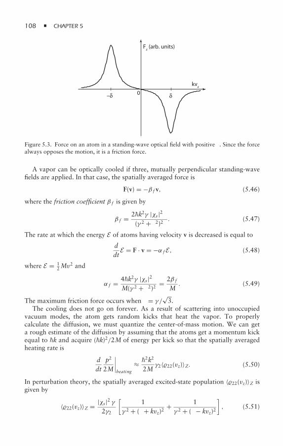
108 CHAPTER 5
Fz (arb. units)
0kvz
δ–δ
Figure 5.3. Force on an atom in a standing-wave optical field with positive δ. Since the forcealways opposes the motion, it is a friction force.
A vapor can be optically cooled if three, mutually perpendicular standing-wavefields are applied. In that case, the spatially averaged force is
F(v) = −β f v, (5.46)
where the friction coefficient β f is given by
β f = 2k2γ |χs |2 δ(γ 2 + δ2)2 . (5.47)
The rate at which the energy E of atoms having velocity v is decreased is equal to
ddtE = F · v = −α fE, (5.48)
where E = 12Mv
2 and
α f = 4k2γ |χs |2 δM(γ 2 + δ2)2 = 2β f
M. (5.49)
The maximum friction force occurs when δ = γ /√3.
The cooling does not go on forever. As a result of scattering into unoccupiedvacuum modes, the atom gets random kicks that heat the vapor. To properlycalculate the diffusion, we must quantize the center-of-mass motion. We can geta rough estimate of the diffusion by assuming that the atoms get a momentum kickequal to k and acquire (k)2/2M of energy per kick so that the spatially averagedheating rate is
ddt
p2
2M
∣∣∣∣heating
≈ 2k2
2Mγ2〈22(vz)〉Z. (5.50)
In perturbation theory, the spatially averaged excited-state population 〈22(vz)〉Z isgiven by
〈22(vz)〉Z = |χs |2 γ2γ2
[1
γ 2 + (δ + kvz)2+ 1γ 2 + (δ − kvz)2
], (5.51)
DENSITY MATRIX WITH ATOMIC MOTION 109
which can be obtained by substituting equation (5.42) into equation (5.38b) andsolving for 22(Z,vz). For kvz γ, |δ|, and with γ2 = 2γ , equation (5.51) reducesto
〈22〉Z ≈ |χs |2 /2γ 2 + δ2 . (5.52)
Therefore, one finds
dEdt
∣∣∣∣heat
= 2k2
4M|χs |2 γ2γ 2 + δ2 = 2D
M, (5.53)
where D is the diffusion coefficient, and
ddtE = −4k2γ |χs |2 δ
M(γ 2 + δ2)2 E + 2k2
4M|χs |2 γ2γ 2 + δ2 . (5.54)
In steady state and for the optimal detuning, δ = γ , we find
E = γ2(γ2 + δ2)
16δγ≈ γ2
8= 1
2kBT, (5.55)
where T is the equilibrium temperature, and kB is Boltzmann’s constant. A morerigorous calculation includes fluctuations arising from the difference in the numberof photons scattered by atoms from each traveling wave component of thestanding-wave field—that is, contributions to diffusion from stimulated as well asspontaneous processes. With the inclusion of such stimulated processes, the finaltemperature increases to TD = 7γ2/20kB, a result that is referred to as the Dopplerlimit of laser cooling [4].2 For Na, one estimates that TD ≈ 170 µK, which corres-ponds to v ≈ 25 cm/s, and kv = 2.7 × 10⁶ s−1 6.3 × 10⁷ s−1 = γ2. When experi-ments were done by Lett et al. [5] and Weiss et al. [6] to test this prediction, theyfound a lower temperature—for reasons we discuss later. For this discovery andthe explanation of the cooling, William Phillips, Steven Chu, and Claude Cohen-Tannoudji shared the Nobel Prize in 1997.
5.4 Summary
In this chapter, we have seen how optical fields can be used to manipulate the center-of-mass motion of atoms. We derived equations that properly account for atomicmotion and calculated the force on atoms produced by various field configurations.For the most part, we have considered large detunings or cold atoms, where Dopplershifts play a minimal role. We now return to a discussion of thermal vapors and seehow saturation spectroscopy can be used to eliminate the Doppler width in spectralprofiles. Before doing so, however, we take a slight detour and derive the so-calledMaxwell-Bloch equations.
2 The correct diffusion coefficient, D = (72k2/20)(|χs |2γ2/(γ 2 + δ2)) can be obtained using theformalism developed in the appendix in chapter 18. Many authors refer to kBT = γ2/2, instead ofkBT = 7γ2/20, as the Doppler limit of laser cooling.
110 CHAPTER 5
5.5 Appendix: Quantization of the Center-of-Mass Motion
As we often tell our students, atoms have never heard about wave packets. Wavepackets are a construction of physicists. In other words, when we consider a vapor oran ensemble of atoms, we usually have a very limited amount of information. Thereis virtually no information about any individual atom’s center-of-mass motion;rather, one has some general thermodynamical variables to describe the vapor.One is then at liberty to choose any wave packets for the atoms’ center-of-massmotion that are consistent with these thermodynamic properties, even if they haveno relation to what you might think would be a “reasonable” atomic wave packet.For example, suppose that a thermal vapor is characterized by a uniform densityand a Maxwellian distribution of velocities. One can carry out calculations usingplane-wave center-of-mass states with a (diagonal) thermal momentum distributionor using highly localized center-of-mass states, randomly distributed in space, inwhich each atom has the entire thermal momentum distribution [7]. Althoughneither of these descriptions seems physical, both models lead to the same resultswhen considering atom–field interactions, since they correspond to the same densitymatrix for the atomic ensemble.
We now proceed to quantize the center-of-mass motion. Let R be the center-of-mass coordinate and r a relative electronic coordinate. The Hamiltonian is assumedto be of the form
H = P2
2M+ H0(r) + V(r,R, t), (5.56)
where P = −i∇R is the momentum conjugate to R. At this stage, all relaxation isneglected. A multitude of representations can be used to label density matrixelements. We consider four possible representations to characterize the center-of-mass motion: coordinate, momentum, sum and difference, and Wigner (coordinate-momentum) representations.
5.5.1 Coordinate Representation
If we expand the wave function as
(r,R, t) =∑α
Aα(R, t)ψα(r), (5.57)
then the state amplitudes obey a Schrödinger-like equation
i∂Aα(R, t)
∂t= −
2
2M∇2RAα(R, t) +
∑α′
Vαα′ (R, t)Aα′ (R, t) + EαAα(R, t), (5.58)
where
Vαα′ (R, t) =∫drψ∗
α (r)V(r,R, t)ψα′ (r), (5.59)
and Eα and ψα(r) are eigenenergies and eigenfunctions of H0(r). Density matrixelements are defined by
αα′(R,R′, t) = Aα(R, t)A∗α′(R′, t). (5.60)
DENSITY MATRIX WITH ATOMIC MOTION 111
Note that we must allow for nondiagonal values of the center-of-mass coordinatesas well as those of the internal states. It then follows directly from equation (5.58)that
i∂αα′(R,R′, t)
∂t= (Eα − Eα′)αα′(R,R′, t)
−(2/2M)[∇2Rαα′(R,R′, t) − ∇2
R′αα′(R,R′, t)]
+∑α′′
[Vαα′′ (R, t)α′′α′ (R,R′, t)
−αα′′ (R,R′, t)Vα′′α′(R′, t)]. (5.61)
This is a very complicated equation. In many problems, the atomic center-of-massmotion can be treated classically. Imagine that the atom can be described by a wavepacket that is much larger than its average de Broglie wavelength λdB (to ensure nospreading), but much smaller than other characteristic lengths in the problem. Thenwe can take
Vαα′ (R, t) ≈ Vαα′ (〈R〉, t),α,α′ (R,R′, t) ≈ α,α′ (〈R〉, 〈R′〉, t),
(5.62)
where 〈R〉 is the average position of the wave packet.The remaining terms in equation (5.61) are
∇Rα,α′ (R,R′, t) and ∇R′α,α′ (R,R′, t). (5.63)
We can write
∇Rαα′ (R,R′, t) = ∇R[Aα(R, t)A∗
α′ (R′, t)]
= 1(2π)3/2
∇R
∫dPα(P, t)e
iP·RA∗
α′ (R′, t)
= (i/)(2π)3/2
∫dPPα(P, t)e
iP·RA∗
α′ (R′, t),
(5.64)
where
α(P, t) = (2π)−3/2∫dR e−iP·R/Aα(R, t) (5.65)
is the wave function in momentum space. Since there is negligible spreading of thewave packet, the momentum of the wave packet is fairly well defined about someaverage value 〈P〉. Setting P = 〈P〉 + (P − 〈P〉) and neglecting the contribution fromthe (P − 〈P〉) term, we obtain
∇Rαα′(R,R′, t) ∼ i〈P〉αα′ (R,R′, t). (5.66)
Similarly,
∇R′αα′ (R,R′, t) ∼ − i〈P〉αα′ (R,R′, t). (5.67)
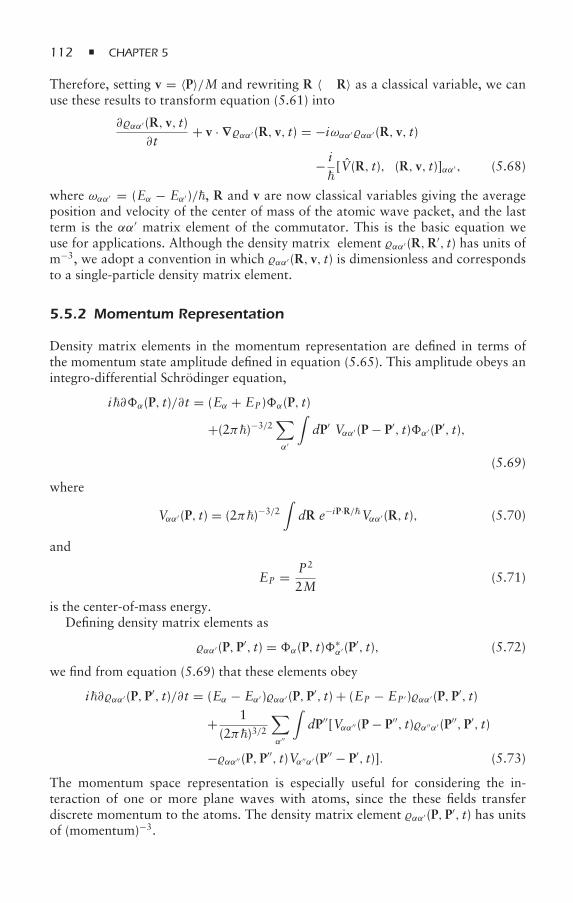
112 CHAPTER 5
Therefore, setting v = 〈P〉/M and rewriting R ≡ 〈R〉 as a classical variable, we canuse these results to transform equation (5.61) into
∂αα′(R, v, t)∂t
+ v · ∇αα′ (R, v, t) = −iωαα′αα′ (R, v, t)
− i[V(R, t), (R, v, t)]αα′ , (5.68)
where ωαα′ = (Eα − Eα′)/, R and v are now classical variables giving the averageposition and velocity of the center of mass of the atomic wave packet, and the lastterm is the αα′ matrix element of the commutator. This is the basic equation weuse for applications. Although the density matrix element αα′ (R,R′, t) has units ofm−3, we adopt a convention in which αα′(R, v, t) is dimensionless and correspondsto a single-particle density matrix element.
5.5.2 Momentum Representation
Density matrix elements in the momentum representation are defined in terms ofthe momentum state amplitude defined in equation (5.65). This amplitude obeys anintegro-differential Schrödinger equation,
i∂α(P, t)/∂t = (Eα + EP )α(P, t)
+(2π)−3/2∑α′
∫dP′ Vαα′ (P − P′, t)α′ (P′, t),
(5.69)
where
Vαα′ (P, t) = (2π)−3/2∫dR e−iP·R/Vαα′ (R, t), (5.70)
and
EP = P2
2M(5.71)
is the center-of-mass energy.Defining density matrix elements as
αα′(P,P′, t) = α(P, t)∗α′ (P′, t), (5.72)
we find from equation (5.69) that these elements obey
i∂αα′ (P,P′, t)/∂t = (Eα − Eα′ )αα′(P,P′, t) + (EP − EP ′)αα′(P,P′, t)
+ 1(2π)3/2
∑α′′
∫dP′′[Vαα′′ (P − P′′, t)α′′α′(P′′,P′, t)
−αα′′ (P,P′′, t)Vα′′α′(P′′ − P′, t)]. (5.73)
The momentum space representation is especially useful for considering the in-teraction of one or more plane waves with atoms, since the these fields transferdiscrete momentum to the atoms. The density matrix element αα′(P,P′, t) has unitsof (momentum)−3.
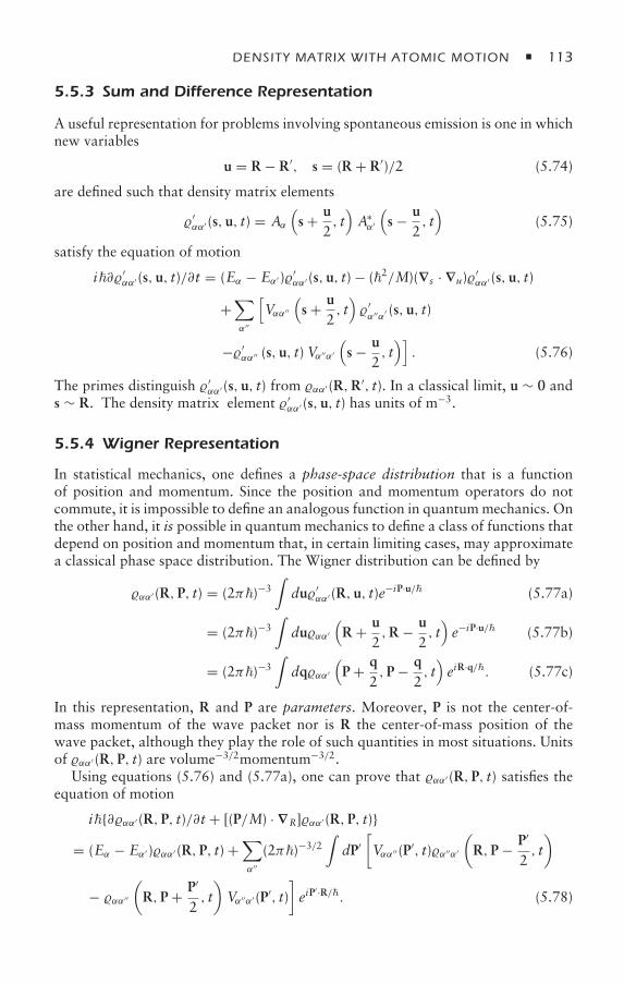
DENSITY MATRIX WITH ATOMIC MOTION 113
5.5.3 Sum and Difference Representation
A useful representation for problems involving spontaneous emission is one in whichnew variables
u = R − R′, s = (R + R′)/2 (5.74)
are defined such that density matrix elements
′αα′ (s,u, t) = Aα
(s + u
2, t)A∗α′
(s − u
2, t)
(5.75)
satisfy the equation of motion
i∂′αα′ (s,u, t)/∂t = (Eα − Eα′)′
αα′ (s,u, t) − (2/M)(∇s · ∇u)′αα′(s,u, t)
+∑α′′
[Vαα′′
(s + u
2, t)′α′′α′ (s,u, t)
−′αα′′ (s,u, t)Vα′′α′
(s − u
2, t)]. (5.76)
The primes distinguish ′αα′ (s,u, t) from αα′(R,R′, t). In a classical limit, u ∼ 0 and
s ∼ R. The density matrix element ′αα′ (s,u, t) has units of m−3.
5.5.4 Wigner Representation
In statistical mechanics, one defines a phase-space distribution that is a functionof position and momentum. Since the position and momentum operators do notcommute, it is impossible to define an analogous function in quantummechanics. Onthe other hand, it is possible in quantum mechanics to define a class of functions thatdepend on position and momentum that, in certain limiting cases, may approximatea classical phase space distribution. The Wigner distribution can be defined by
αα′ (R,P, t) = (2π)−3∫du′
αα′ (R,u, t)e−iP·u/ (5.77a)
= (2π)−3∫duαα′
(R + u
2,R − u
2, t)e−iP·u/ (5.77b)
= (2π)−3∫dqαα′
(P + q
2,P − q
2, t)eiR·q/. (5.77c)
In this representation, R and P are parameters. Moreover, P is not the center-of-mass momentum of the wave packet nor is R the center-of-mass position of thewave packet, although they play the role of such quantities in most situations. Unitsof αα′(R,P, t) are volume−3/2momentum−3/2.
Using equations (5.76) and (5.77a), one can prove that αα′ (R,P, t) satisfies theequation of motion
i∂αα′(R,P, t)/∂t + [(P/M) · ∇R]αα′(R,P, t)= (Eα − Eα′ )αα′(R,P, t) +
∑α′′
(2π)−3/2∫dP′
[Vαα′′ (P′, t)α′′α′
(R,P − P′
2, t)
− αα′′
(R,P + P′
2, t)Vα′′α′ (P′, t)
]eiP
′ ·R/. (5.78)
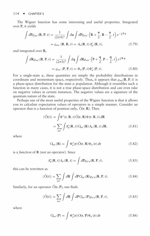
114 CHAPTER 5
The Wigner function has some interesting and useful properties. Integratedover P, it yields∫
dPαα′ (R,P, t) = 1(2π)3
∫du
∫dPαα′
(R + u
2,R − u
2, t)e− i
P·u
= αα′ (R,R, t) = Aα(R, t)A∗α′(R, t), (5.79)
and integrated over R,∫dRαα′ (R,P, t) = 1
(2π)3
∫dq
∫dRαα′
(P + q
2,P − q
2, t)e
iR·q
= αα′ (P,P, t) = α(P, t)∗α′(P, t). (5.80)
For a single-state α, these quantities are simply the probability distributions incoordinate and momentum space, respectively. Thus, it appears that αα(R,P, t) isa phase-space distribution for the state α population. Although it resembles such afunction in many cases, it is not a true phase-space distribution and can even takeon negative values in certain instances. The negative values are a signature of thequantum nature of the state.
Perhaps one of the most useful properties of the Wigner function is that it allowsyou to calculate expectation values of operators in a simple manner. Consider anoperator that is a function of position only, O(r,R). Then
〈O(t)〉 =∫∗(r,R, t)O(r,R)(r,R, t)dR
=∑αα′
∫A∗α(R, t)Oαα′ (R)Aα′(R, t)dR, (5.81)
where
Oαα′(R) =∫∗α(r)O(r,R)α′ (r)dr (5.82)
is a function of R (not an operator). Since
A∗α(R, t)Aα′(R, t) =
∫dPα′α(R,P, t), (5.83)
this can be rewritten as
〈O(t)〉 =∑αα′
∫dR
∫dPOαα′ (R)α′α(R,P, t). (5.84)
Similarly, for an operator O(r,P), one finds
〈O(t)〉 =∑αα′
∫dR
∫dPOαα′ (P)α′α(R,P, t), (5.85)
where
Oαα′ (P) =∫∗α(r)O(r,P)α′(r)dr (5.86)
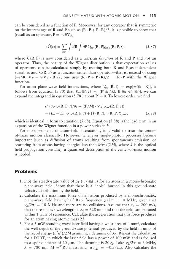
DENSITY MATRIX WITH ATOMIC MOTION 115
can be considered as a function of P. Moreover, for any operator that is symmetricon the interchange of R and P such as (R · P + P · R)/2, it is possible to show that(recall as an operator, P = −i∇R)
〈O(t)〉 =∑αα′
∫dR
∫dPOαα′ (R,P)α′α(R,P, t), (5.87)
where O(R,P) is now considered as a classical function of R and P and not anoperator. Thus, the beauty of the Wigner distribution is that expectation valuesof operators can be calculated simply by treating both R and P as independentvariables and O(R,P) as a function rather than operator—that is, instead of using(−iR · ∇R − i∇R · R)/2, one uses (R · P + P · R)/2 = R · P with the Wignerfunction.
For atom–plane-wave field interactions, where Vαα′ (R, t) ∼ exp[±i(k · R)], itfollows from equation (5.70) that Vαα′ (P′, t) ∼ δ(P′ ± k). If k |〈P〉|, we canexpand the integrand in equation (5.78 ) about P′ = 0. To lowest order, we find
i ∂αα′ (R,P, t)/∂t + [(P/M) · ∇R]αα′(R,P, t)= (Eα − Eα′)αα′(R,P, t) + [V(R, t), (R,P, t)]αα′ , (5.88)
which is identical in form to equation (5.68). Equation (5.88) is the lead term in anexpansion of the Wigner function in a power series in .
For most problems of atom–field interactions, it is valid to treat the center-of-mass motion classically. However, whenever single-photon processes becomeimportant [such as diffusion of atoms resulting from spontaneous emission, orscattering from atoms having energies less than 2k2/(2M), where k is the opticalfield propagation constant], a quantized description of the center-of-mass motionis needed.
Problems
1. Plot the steady-state value of 11(vz)W0(vz) for an atom in a monochromaticplane-wave field. Show that there is a “hole” burned in this ground-statevelocity distribution by the field.
2. Calculate the maximum force on an atom produced by a monochromatic,plane-wave field having half Rabi frequency χ/2π = 10 MHz, given thatγ2/2π = 10 MHz and there are no collisions. Assume that vz = 200 m/s,that the resonance wavelength is λ0 = 628 nm, and that the field can be tunedwithin 1 GHz of resonance. Calculate the acceleration that this force producesfor an atom having atomic mass 23.
3. For a 5-mW standing-wave laser field having a waist area of 4 mm2, calculatethe well depth of the ground-state potential produced by the field in units ofthe recoil energy (2k2)/2M assuming a detuning of 3γ . Repeat the calculationfor a FORT, in which the laser field has a power of 100 mW and is focusedto a spot diameter of 20 µm. The detuning is 20γ2. Take γ2/2π = 6 MHz,λ = 780 nm, M =85Rb mass, and (µx)21 = −0.57ea0. Also calculate the
116 CHAPTER 5
frequency spacing at the bottom of the wells assuming that the potentials canbe approximated as harmonic in that region. Can atoms cooled to the Dopplerlimit of laser cooling be trapped in these potentials? Explain.
4. Consider a transition from a ground state having total angular momentumJ = 0 to an excited state with J = 1. The atom is put in a magnetic fieldthat varies as B = βZz (β =positive constant) near Z = 0. Assume that themagnetic sublevels’ energies vary as Em = E2 + gmZ, where g is a positiveconstant, and m is the magnetic quantum number. If σ+ light is incident inthe +Z direction and σ− light in the −Z direction, show that an atom can betrapped in the Zdirection if the field is detuned below the resonance frequency.Assume that the atoms are moving sufficiently slowly to neglect their Dopplershift. Note that this is the same detuning that will produce cooling for atomslocated near Z = 0. This technique is the basis for the (magneto-opticaltrap)(MOT); see reference [8]. (σ+ radiation drivesm= 1 ground-to excited-state transitions, and σ− radiation drives m = −1 ground-to excited-statetransitions.)
5. In the optical Stern-Gerlach experiment, two plane-wave laser fields intersectat a small angle θ to form a standing-wave field having period d = λ/ sin θ λ.The field amplitude varies as cos (2πZ/d) in the Z direction. An atomic beamhaving diameter much less than d is incident perpendicular to the standing-wave field, and the atoms pass through the laser beam waist, which hasdiameterw0. The longitudinal velocity of the beam is v, and the atoms enter thebeam with 11 = 1. If the field is resonant with the atomic transition, calculatethe energy of the two semiclassical dressed states of the atom–field system andthe maximum angular splitting of these states produced by the field. Assumethat the atom–field interaction can be treated in an impulse approximation,and take v = 1.76 × 10³ m/s, atomic mass = 4, w0 = 39µm, d = 30µm,|χs | /2π = 0.7 GHz; see reference [9].
6. Repeat problem 5, but assume that the detuning δ/2π = 160 MHz issufficiently large that the atom stays adiabatically in the ground dressed stateof the system. In this case, calculate the deflection of the atoms by the field asa function of Z.
7. For an off-resonance standing-wave field, what sign of delta is needed to havethe force on the atoms attract atoms to the antinodes of the field? For thissign of delta, estimate the focal distance of one “lobe” of the field for atomscrossing the field having longitudinal de Broglie wavelength λB, assuming thatthe potential can be approximated as that of a harmonic oscillator. Evaluatethis distance assuming v = 5 × 10² m/s, atomic mass = 85, w0 = 30 µm,λ = 780 nm, |χs | /2π = 300 MHz, and δ/2π = 10GHz.
8–9. Calculate the spatially averaged force for atoms having kv γ2 for two-levelatoms interacting with a standing-wave field. To do this, solve the densitymatrix equations for v = vz = 0, and then calculate a correction term linearin v. Show that in weak fields, your result reduces to equation (5.45). Forstrong fields, show that the sign of the force changes for a given detuning ifone excludes a small region about δ = 0 (i.e., for a given δ, if the force is afriction force for δ < 0 for weak fields, it becomes an accelerating force forstrong fields). Take γ = γ2/2 and χs real.
DENSITY MATRIX WITH ATOMIC MOTION 117
10. Suppose that you want to solve equations (5.38a) to (5.38d) for arbitrary fieldstrengths. For solutions that are periodic in Z, you can set
N= 22 − 11 =∞∑
n=−∞Nne2inkZ,
where N−n = N∗n , and also set
21 =∞∑
n=−∞rnei(2n−1)kZ.
Obtain equations that relate the Fourier coefficients Nn and rn. By truncatingthe series and solving the resulting equations, you can obtain successiveapproximations to the exact solution in terms of continued fractions. Fromyour equations, obtain a value for N to order χ2
s . Take χs to be real.In problems 11 to 22, it is assumed that an atom’s time evolution is
governed by the Hamiltonian
H = P2/(2M) + H0(r) + V(r,R, t),
where M is the atomic mass, H0(r) is the free-atom Hamiltonian havingeigenvalues Eα and eigenfunctions ψα(r), P is the center-of-mass momentumoperator for the atom, and V(r,R, t) is an interaction term describing theatom’s interaction with external fields that can change the atom’s internal stateand center-of-mass momentum.
11. Derive equation (5.58).12. Derive equation (5.61).13. Derive equation (5.69).14. Derive equation (5.73).15. Derive equation (5.76).16. Derive equation (5.78).17. Prove explicitly that equation (5.87) is valid for the operator O(R,P) =
(R · P + P · R)/2 using P = − i∇R.18. Calculate the one-dimensional Wigner function for
ψ1(x) = (2πa2)−1/4 exp(ip0x/) exp[−(x/a)2]
and
ψ2(x) = (2πa2)−1/4
√e18
1 + e18exp[−(x− 3a)2/a2] + exp[−(x+ 3a)2/a2]
.
Use a three-dimensional plot to plot the Wigner function as a function of xand p for a = 1, = 1 and p0 = 2. You will probably want to use acomputer program to evaluate the integrals. Which of these wave functionsis more classical in nature? Explain. The second wave function is referred toas a Schrödinger cat state.
19. For a free particle, use the Wigner distribution function (in one dimension) toevaluate 〈p〉, 〈x〉, 〈p2〉, and 〈x2〉 at time t in terms of their values at t = 0.
118 CHAPTER 5
20. Prove Ehrenfest’s theorem for a particle of mass Mmoving in a potential V(R)using the Wigner distribution function.
21. The total density can be defined as
(R,P, t) =∑α
αα(R,P, t).
Show that (R,P, t) satisfies the equation of motion
i ∂(R,P, t)/∂t + [(P/M) · ∇R](R,P, t) =+∑α,α′
(2π)−3/2∫dP′[Vαα′ (P′, t)α′α
(R,P − P′
2, t)
−αα′
(R,P + P′
2, t)Vα′α(P,′ t)]eiP
′·R/.
Make an expansion of the integrand to first order in P′ to obtain
∂ (R,P, t)/∂t + [(P/M) · ∇R](R,P, t) =+(i/2)
∑α,α′
[∇RVαα′ (R, t) · ∇Pα′α(R,P, t)
+∇Pαα′(R,P, t) · ∇RVα′α(R, t)].
22. Now assume that the external potential is state-independent—that is,
Vαα′ (R, t) = V(R, t)δα,α′ .
Prove that
i ∂(R,P, t)/∂t + [(P/M) · ∇R](R,P, t) =+(2π)−3/2
∫dP′ V(P′, t)
[
(R,P − P′
2, t)
− (R,P + P′
2, t)]
eiP′ ·R/,
where V(P, t) is the Fourier transform of V(R, t). Make an expansion of theintegrand to second order in P′ to obtain
∂(R,P, t)/∂t + [(P/M) · ∇R](R,P, t) + [−∇RV(R, t)] · ∇P(R,P, t) = 0,
and give an interpretation to your result. Note that corrections of order P ′2 donot contribute. In problem 21, the corrections of order P ′2 do not necessarilyvanish and can serve as a source of diffusion for the distribution function.
References
[1] P. R. Berman, Light scattering, Contemporary Physics 49, 313–330 (2008).[2] T. W. Hänsch and A. L. Schawlow, Cooling of gases by laser radiation, Optics
Communications 13, 68–71 (1975).[3] J. D. Miller, R. A. Cline, and D. J. Heinzen, Far-off resonance optical trapping of atoms,
Physical Review A 47, R4567–4570 (1993).[4] D. J. Wineland and W. M. Itano, Laser cooling of atoms, Physical Review A 20, 1521–
1540 (1979).
DENSITY MATRIX WITH ATOMIC MOTION 119
[5] P. D. Lett, W. D. Phillips, S. L. Rolston, C. E. Tanner, R. N. Watts, and C. I. Westbrook,Optical molasses, Journal of the Optical Society of America B 6, 2084–2107 (1989).
[6] D. S. Weiss, E. Riis, Y. Shevy, P. Jeffrey Ungar, and S. Chu, Optical molasses andmultilevel atoms: experiment, Journal of the Optical Society of America B 6, 2072–2083(1989).
[7] R. Beach, S. R. Hartmann, and R. Friedberg, Billiard-ball echo model, Physical ReviewA 25, 2658–2666 (1982).
[8] E. L. Raab, M. Prentiss, A. Cable, S. Chu, and D. E. Pritchard, Trapping of neutralsodium atoms with radiation pressure, Physical Review Letters 59, 2631–2634 (1987).
[9] T. Sleator, T. Pfau, V. Balykin, O. Carnal, and J. Mlynek, Experimental demonstrationof the optical Stern-Gerlach effect, Physical Review Letters 68, 1996–1999 (1992).
Bibliography
A. Ashkin, Applications of laser radiation pressure, Science 210, 1081–1088 (1980).P. R. Berman, Quantum-mechanical transport equation for atomic systems, Physical ReviewA 5, 927–939 (1972).
J. Dalibard and C. Cohen-Tannoudji, Atomic motion in laser light: connection betweensemiclassical and quantum descriptions, Journal of Physics B 18, 1661–1683 (1985).
J. P. Gordon and A. Ashkin, Motion of atoms in a radiation trap, Physical Review A 21,1606–1617 (1980).
H. J. Metcalf and P. van der Straten, Laser Cooling and Trapping (Springer-Verlag, NewYork, 1999).
W. P. Schleich, Quantum Optics in Phase Space (Wiley-VCH, Berlin, 2001), chap. 20.S. Stenholm, Semiclassical expansion for systems with internal degrees of freedom, PhysicalReview A 47, 2523–2531 (1993).
———The semiclassical theory of laser cooling, Reviews of Modern Physics 58, 699–739(1986).
6Maxwell-Bloch Equations
6.1 Wave Equation
Up until this point, we have looked at the modification of the atomic state vectorproduced by an external electromagnetic field; however, for the most part, wehave ignored changes in the external field produced by the atoms. If we quantizethe electromagnetic field, the total energy of the atoms plus field is conserved,guaranteeing that changes in the energy of the incident field are automaticallyincluded. Within the context of the semiclassical theory, however, we are restrictedto a classical description of the incident field. Thus, any changes in the external fieldmust be accounted for using Maxwell’s equations. In thisMaxwell-Bloch approach,the fields are described by Maxwell’s equations, but the polarization that appears inMaxwell’s equations is calculated quantum-mechanically in terms of the expectationvalue of the atomic dipole moment operator.
It is necessary to couple the quantum evolution equation for the atoms toMaxwell’s equations for the fields in order to follow the evolution of the fields.To do this, we write Maxwell’s equations but do not take D = ε0E. Rather, we setD = ε0E + P and calculate P quantum-mechanically as the expectation value of theatomic dipole moment operator. We take B = µ0H and neglect any effects arisingfrom magnetic polarization.
In the absence of free charges and currents, Maxwell’s equations are
∇· (ε0E + P) = 0, (6.1a)
∇ × E = −∂B∂t, (6.1b)
∇ × B = µ0∂(ε0E + P)
∂t, (6.1c)
∇ · B = 0, (6.1d)
MAXWELL-BLOCH EQUATIONS 121
and the wave equation, equation (1.5), is
∇2E − 1c2∂2E∂t2
= ∇(∇ · E) + 1c2ε0
∂2P∂t2
. (6.2)
With no free charges,
∇ · E = ρb/ε0 = −∇ · P/ε0, (6.3)
where ρb is the bound charge density; this term vanishes in vacuum. In a medium,it can give rise to transverse effects such as self-trapping, self-focusing, and ringformation. We neglect any such transverse effects and consider essentially a planewave limit in which the fields propagate in the z direction and have polarization ε inthe XY plane, allowing us to set ∇ · P ≈ 0 and to use
∂2E∂Z2
− 1c2∂2E∂t2
= 1c2ε0
∂2P∂t2
(6.4)
as the wave equation appropriate to our considerations. By setting∇2E ≈−∂2E/∂Z2,we are neglecting any diffraction effects that would accompany a beam having finiteradius a. Diffraction effects are minimal if λ/a 1.
6.1.1 Pulse Propagation in a Linear Medium
To illustrate pulse propagation in a linear medium characterized by a frequency-dependent index of refraction, we first Fourier transform the positive frequencycomponents of the fields using
E+(Z, t) = 1√2π
∫ ∞
0E+(Z, ω′)ei[k
′Z−ω′t]dω′, (6.5a)
P+(Z, t) = 1√2π
∫ ∞
0P+(Z, ω′)ei[k
′Z−ω′t]dω′, (6.5b)
where k′ is a function of ω′ to be determined. In section 6.2, we calculate thepolarization P(Z, t) quantum-mechanically; here, we assume that the polarizationP+(Z, ω) is related to the electric field E+(Z, ω) by
P+(Z, ω) = ε0χ (ω)E+(Z, ω) = ε0[n2(ω) − 1
]E+(Z, ω), (6.6)
where χ (ω) is the electric susceptibility, and n(ω) is the index of refraction, assumedto be both complex and frequency dependent. The total fields are given by
E(Z, t) = [E+(Z, t) + E+(Z, t)∗
], (6.7a)
P(Z, t) = [P+(Z, t) + P+(Z, t)∗
]. (6.7b)
Substituting equations (6.5) into equation (6.4) and using equation (6.6), we findthat equation (6.5a) is a solution of equation (6.4) provided that
k′(ω′) = n(ω′)ω′
c, (6.8)
122 CHAPTER 6
giving rise to a field amplitude
E+(Z, t) = 1√2π
∫ ∞
0E+(Z, ω′)e−iω′[t−n(ω′)Z/c]dω′. (6.9)
It is now assumed that E(Z, ω) is a sharply peaked function about a centralfrequency ω′ = ω. As a result, it is convenient to rewrite equation (6.9) as
E+(Z, t) ≈ ε
2e−iω[t−n(ω)Z/c]E(Z, t), (6.10a)
E+(Z, ω) = 12
ε E(Z, ω), (6.10b)
where the complex pulse amplitude E(Z, t) is given by
E(Z, t) = 1√2π
∫ ∞
0dω′ E(Z, ω′) exp−it + i[ω′n(ω′) − ωn(ω)]Z/c
= 1√2π
∫ ∞
−ωd E(Z, ω +) exp−it + i[(ω +)n(ω +) − ωn(ω)]Z/c
≈ 1√2π
∫ ∞
−∞d E(Z, ω +)
× exp−it + i[(ω +)n(ω +) − ωn(ω)]Z/c. (6.11)
We have set ω′ = ω+ and extended the lower limit of the integral to −∞, sinceE(Z, ω +) is sharply peaked about = 0. Expanding
(ω +)n(ω +) − ωn(ω) ≈ d [ωn(ω)]dω
=[n(ω) + ωdn(ω)
dω
], (6.12)
correct to first order in , we find that
E(Z, t) ≈ 1√2π
∫ ∞
−∞d E(Z, ω +) exp
(−i
t −
[n(ω) + ωdn(ω)
dω
]Zc
)
= E0, t −
[n(ω) + ωdn(ω)
dω
]Zc
, (6.13)
or
E+(Z, t) ≈ ε
2e−iω[t−n(ω) Zc ]E
0, t −
[n(ω) + ωdn(ω)
dω
]Zc
. (6.14)
For real n(ω), equation (6.14) implies that the field propagates without distortionor attenuation with a group velocity
vg = c
n(ω) + ω dn(ω)dω
, (6.15)
and that the phase velocity is vph = c/n(ω). Of course, if we had included higherterms in the expansion (6.12), these terms would have resulted in distortion of thepulse shape as it propagates. These terms become important near resonance. If n(ω)is complex, the leading exponential e−iω[t−n(ω)Z/c] results in attenuation assuming
MAXWELL-BLOCH EQUATIONS 123
that Im[n(ω)] < 0. The group velocity becomes complex, but the pulse propagationspeed is still given by equation (6.15), if Re[n(ω)] is substituted for n(ω).1
6.2 Maxwell-Bloch Equations
Rather than use equation (6.6) to relate the polarization to the field, we would liketo calculate this polarization quantum-mechanically and obtain equations that allowus to find the fields in a self-consistent manner. We have seen already that the atomicresponse to an applied field can result in a nonlinear dependence of density matrixelements on the field amplitude. As a consequence, we expect that, in general, onefinds a polarization that is a nonlinear function of the applied field amplitude.
The macroscopic polarization is defined as the average dipole moment per unitvolume. As such, in quantum mechanics, it becomes the expectation value of theatomic electric dipole moment operator µ, namely,
〈P(Z, t)〉 = N [µ21〈12(Z, t)〉 + µ12〈21(Z, t)〉]= N [
µ21〈12(Z, t)〉e−i(kZ−ωt) + µ12〈21(Z, t)〉]ei(kZ−ωt)
= [P+(Z, t) + P+(Z, t)∗
], (6.16)
where
P+(Z, t) = Nµ12〈21(Z, t)〉ei(kZ−ωt), (6.17)
〈i j (R, t)〉 =∫dvW0(v)i j (R, v, t), (6.18)
N is the density, andW0(v) is the velocity distribution. By combining equation (6.16)for the polarization, equations (5.2) for the evolution of density matrix elements,and the wave equation (6.4), one has a set of coupled partial differential equationsthat can be solved numerically given some initial conditions. Typically, one wouldsuppose that an optical pulse is incident on a medium from vacuum and that theinitial pulse field envelope is specified. The numerical solution of such a problem isfar from trivial, since the integration step sizes must be taken to be much less than anoptical period in time and much less than a wavelength in space. On the other hand,changes in the pulse envelope often occur on much slower time and longer lengthscales. To circumvent this problem, we often make a slowly varying amplitude andphase approximation (SVAPA).
1 For complex n(ω), the point of stationary phase in the integrand of equation (6.11) occurs when
t = cZ
nr (ω) + ω dnr (ω)dω
,
where nr (ω) = Re[n(ω)], implying that the group velocity is
vg = c/[nr (ω) + ω dnr (ω)
dω
].
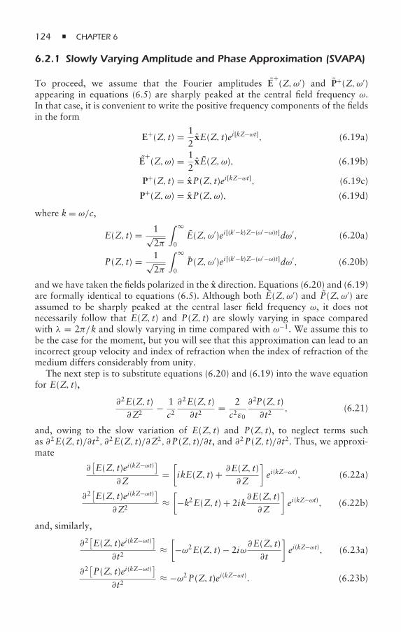
124 CHAPTER 6
6.2.1 Slowly Varying Amplitude and Phase Approximation (SVAPA)
To proceed, we assume that the Fourier amplitudes E+(Z, ω′) and P+(Z, ω′)
appearing in equations (6.5) are sharply peaked at the central field frequency ω.In that case, it is convenient to write the positive frequency components of the fieldsin the form
E+(Z, t) = 12xE(Z, t)ei[kZ−ωt], (6.19a)
E+(Z, ω) = 1
2xE(Z, ω), (6.19b)
P+(Z, t) = xP(Z, t)ei[kZ−ωt], (6.19c)
P+(Z, ω) = xP(Z, ω), (6.19d)
where k= ω/c,
E(Z, t) = 1√2π
∫ ∞
0E(Z, ω′)ei[(k
′−k)Z−(ω′−ω)t]dω′, (6.20a)
P(Z, t) = 1√2π
∫ ∞
0P(Z, ω′)ei[(k
′−k)Z−(ω′−ω)t]dω′, (6.20b)
and we have taken the fields polarized in the x direction. Equations (6.20) and (6.19)are formally identical to equations (6.5). Although both E(Z, ω′) and P(Z, ω′) areassumed to be sharply peaked at the central laser field frequency ω, it does notnecessarily follow that E(Z, t) and P(Z, t) are slowly varying in space comparedwith λ = 2π/k and slowly varying in time compared with ω−1. We assume this tobe the case for the moment, but you will see that this approximation can lead to anincorrect group velocity and index of refraction when the index of refraction of themedium differs considerably from unity.
The next step is to substitute equations (6.20) and (6.19) into the wave equationfor E(Z, t),
∂2E(Z, t)∂Z2
− 1c2∂2E(Z, t)∂t2
= 2c2ε0
∂2P(Z, t)∂t2
, (6.21)
and, owing to the slow variation of E(Z, t) and P(Z, t), to neglect terms suchas ∂2E(Z, t)/∂t2, ∂2E(Z, t)/∂Z2, ∂P(Z, t)/∂t, and ∂2P(Z, t)/∂t2. Thus, we approxi-mate
∂[E(Z, t)ei(kZ−ωt)]
∂Z=[ikE(Z, t) + ∂E(Z, t)
∂Z
]ei(kZ−ωt), (6.22a)
∂2[E(Z, t)ei(kZ−ωt)]
∂Z2≈[−k2E(Z, t) + 2ik
∂E(Z, t)∂Z
]ei(kZ−ωt), (6.22b)
and, similarly,
∂2[E(Z, t)ei(kZ−ωt)]
∂t2≈[−ω2E(Z, t) − 2iω
∂E(Z, t)∂t
]ei(kZ−ωt), (6.23a)
∂2[P(Z, t)ei(kZ−ωt)]
∂t2≈ −ω2P(Z, t)ei(kZ−ωt). (6.23b)
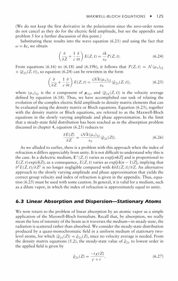
MAXWELL-BLOCH EQUATIONS 125
(We do not keep the first derivative in the polarization since the zero-order termsdo not cancel as they do for the electric field amplitude, but see the appendix andproblem 5 for a further discussion of this point.)
Substituting these results into the wave equation (6.21) and using the fact thatω = kc, we obtain (
∂
∂Z+ 1c∂
∂t
)E(Z, t) = ik
ε0P(Z, t). (6.24)
From equations (6.16) to (6.18) and (6.19b), it follows that P(Z, t) = N (µx)12× 〈21(Z, t)〉, so equation (6.24) can be rewritten in the form(
∂
∂Z+ 1c∂
∂t
)E(Z, t) = iNk (µx)12
ε0〈21(Z, t)〉, (6.25)
where (µx)12 is the x component of µ12, and 〈21(Z, t)〉 is the velocity averagedefined by equation (6.18). Thus, we have accomplished our task of relating theevolution of the complex electric field amplitude to density matrix elements that canbe evaluated using the density matrix or Bloch equations. Equation (6.25), togetherwith the density matrix or Bloch equations, are referred to as the Maxwell-Blochequations in the slowly varying amplitude and phase approximation. In the limitthat a steady-state field distribution has been reached as in the absorption problemdiscussed in chapter 4, equation (6.25) reduces to
∂E(Z)∂Z
= iNk (µx)12ε0
〈21(Z)〉. (6.26)
As we alluded to earlier, there is a problem with this approach when the index ofrefraction n differs appreciably from unity. It is not difficult to understand why this isthe case. In a dielectric medium, E+(Z, t) varies as exp[inkZ] and is proportional toE(Z, t) exp(ikZ); as a consequence, E(Z, t) varies as exp[ik(n− 1)Z], implying that∂2E(Z, t)/∂Z2 is no longer negligible compared with k∂E(Z, t)/∂Z. An alternativeapproach to the slowly varying amplitude and phase approximation that yields thecorrect group velocity and index of refraction is given in the appendix. Thus, equa-tion (6.25) must be used with some caution. In general, it is valid for a medium, suchas a dilute vapor, in which the index of refraction is approximately equal to unity.
6.3 Linear Absorption and Dispersion—Stationary Atoms
We now return to the problem of linear absorption by an atomic vapor as a simpleapplication of the Maxwell-Bloch formalism. Recall that, by absorption, we reallymean the loss of intensity of the beam as it traverses the medium—in steady state, theradiation is scattered rather than absorbed. We consider the steady-state distributionproduced by a quasi-monochromatic field in a uniform medium of stationary two-level atoms, for which 〈21(Z)〉 = 21(Z), since no velocity average is needed. Fromthe density matrix equations (5.2), the steady-state value of 21 to lowest order inthe applied field is given by
21(Z) = −iχ (Z)γ + iδ
, (6.27)
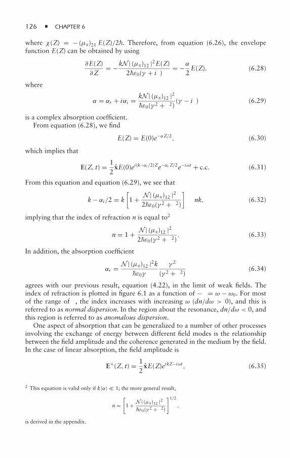
126 CHAPTER 6
where χ (Z) = − (µx)21 E(Z)/2. Therefore, from equation (6.26), the envelopefunction E(Z) can be obtained by using
∂E(Z)∂Z
= −kN | (µx)12 |2E(Z)2ε0(γ + iδ)
= −α2E(Z), (6.28)
where
α = αr + iαi = kN | (µx)12 |2ε0(γ 2 + δ2) (γ − iδ) (6.29)
is a complex absorption coefficient.From equation (6.28), we find
E(Z) = E(0)e−αZ/2, (6.30)
which implies that
E(Z, t) = 12xE(0)ei(k−αi /2)Ze−αr Z/2e−iωt + c.c. (6.31)
From this equation and equation (6.29), we see that
k− αi/2 = k[1 + N | (µx)12 |2δ
2ε0(γ 2 + δ2)]
≡ nk, (6.32)
implying that the index of refraction n is equal to2
n = 1 + N | (µx)12 |2δ2ε0(γ 2 + δ2) . (6.33)
In addition, the absorption coefficient
αr = N | (µx)12 |2kε0γ
γ 2
(γ 2 + δ2) (6.34)
agrees with our previous result, equation (4.22), in the limit of weak fields. Theindex of refraction is plotted in figure 6.1 as a function of −δ = ω − ω0. For mostof the range of δ, the index increases with increasing ω (dn/dω > 0), and this isreferred to as normal dispersion. In the region about the resonance, dn/dω < 0, andthis region is referred to as anomalous dispersion.
One aspect of absorption that can be generalized to a number of other processesinvolving the exchange of energy between different field modes is the relationshipbetween the field amplitude and the coherence generated in the medium by the field.In the case of linear absorption, the field amplitude is
E+(Z, t) = 12xE(Z)eikZ−iωt, (6.35)
2 This equation is valid only if k |α| 1; the more general result,
n =[1 + N | (µx)12 |2δε0(γ 2 + δ2)
]1/2,
is derived in the appendix.
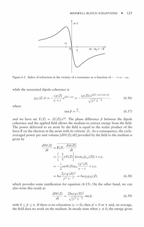
MAXWELL-BLOCH EQUATIONS 127
ω – ω0 = −δγ
n–1
0
–γ
Figure 6.1. Index of refraction in the vicinity of a resonance as a function of −δ = ω − ω0.
while the associated dipole coherence is
21(Z, t) = − iχ (Z)γ + iδ
eikZ−iωt = −|χ (Z)| eikZ−iωt+iφ+iβ√γ 2 + δ2 , (6.36)
where
tanβ = γ
δ, (6.37)
and we have set E(Z) = |E(Z)| eiφ . The phase difference β between the dipolecoherence and the applied field allows the medium to extract energy from the field.The power delivered to an atom by the field is equal to the scalar product of theforce F on the electron in the atom with its velocity 〈r〉. As a consequence, the cycle-averaged power per unit volume [dW(Z)/dt] provided by the field to the medium isgiven by
dW(Z)dt
= F(Z) · d〈r(Z)〉dt
=[−12eE(Z)
][iωx2112(Z)] + c.c.
= − i2ωeE(Z)x21
iχ∗(Z)γ − iδ
+ c.c.
= ω2γ |χ (Z)|2γ 2 + δ2 = ωγ222(Z), (6.38)
which provides some justification for equation (4.15). On the other hand, we canalso write this result as
dW(Z)dt
= 2ω|χ (Z)|2√γ 2 + δ2 sinβ, (6.39)
with 0 ≤ β ≤ π . If there is no relaxation (γ = 0), then β = 0 or π and, on average,the field does no work on the medium. In steady-state when γ = 0, the energy given
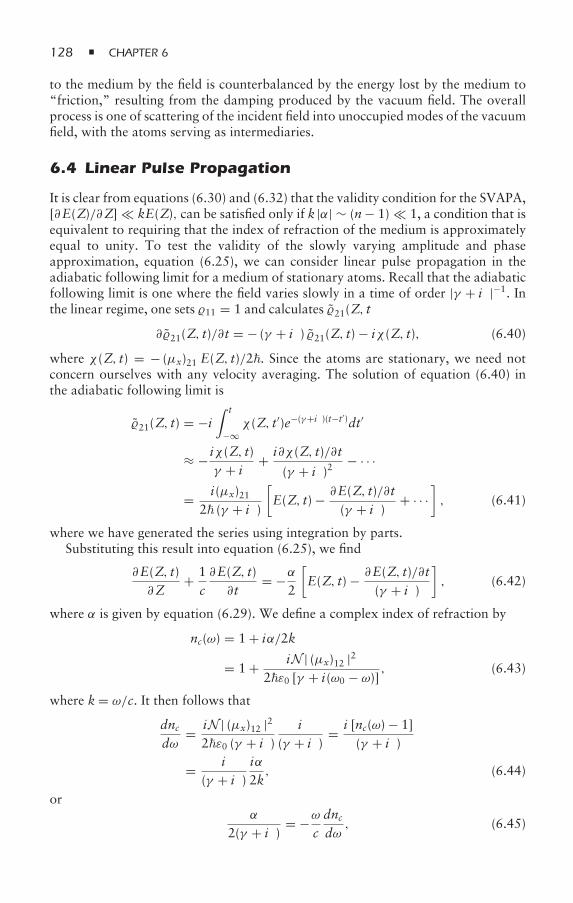
128 CHAPTER 6
to the medium by the field is counterbalanced by the energy lost by the medium to“friction,” resulting from the damping produced by the vacuum field. The overallprocess is one of scattering of the incident field into unoccupied modes of the vacuumfield, with the atoms serving as intermediaries.
6.4 Linear Pulse Propagation
It is clear from equations (6.30) and (6.32) that the validity condition for the SVAPA,[∂E(Z)/∂Z] kE(Z), can be satisfied only if k |α| ∼ (n− 1) 1, a condition that isequivalent to requiring that the index of refraction of the medium is approximatelyequal to unity. To test the validity of the slowly varying amplitude and phaseapproximation, equation (6.25), we can consider linear pulse propagation in theadiabatic following limit for a medium of stationary atoms. Recall that the adiabaticfollowing limit is one where the field varies slowly in a time of order |γ + iδ|−1. Inthe linear regime, one sets 11 = 1 and calculates 21(Z, t) from [see equation (5.9d)]
∂21(Z, t)/∂t = − (γ + iδ) 21(Z, t) − iχ (Z, t), (6.40)
where χ (Z, t) = − (µx)21 E(Z, t)/2. Since the atoms are stationary, we need notconcern ourselves with any velocity averaging. The solution of equation (6.40) inthe adiabatic following limit is
21(Z, t) = −i∫ t
−∞χ (Z, t′)e−(γ+iδ)(t−t′)dt′
≈ − iχ (Z, t)γ + iδ
+ i∂χ (Z, t)/∂t
(γ + iδ)2− · · ·
= i(µx)212 (γ + iδ)
[E(Z, t) − ∂E(Z, t)/∂t
(γ + iδ)+ · · ·
], (6.41)
where we have generated the series using integration by parts.Substituting this result into equation (6.25), we find
∂E(Z, t)∂Z
+ 1c∂E(Z, t)∂t
= −α2
[E(Z, t) − ∂E(Z, t)/∂t
(γ + iδ)
], (6.42)
where α is given by equation (6.29). We define a complex index of refraction by
nc(ω) = 1 + iα/2k
= 1 + iN | (µx)12 |22ε0 [γ + i(ω0 − ω)] , (6.43)
where k= ω/c. It then follows that
dncdω
= iN | (µx)12 |22ε0 (γ + iδ)
i(γ + iδ)
= i [nc(ω) − 1](γ + iδ)
= i(γ + iδ)
iα2k, (6.44)
orα
2(γ + iδ)= −ω
cdncdω, (6.45)
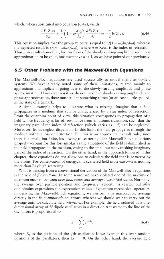
MAXWELL-BLOCH EQUATIONS 129
which, when substituted into equation (6.42), yields
∂E(Z, t)∂Z
+ 1c
(1 + ωdnc
dω
)∂E(Z, t)∂t
= −α2E(Z, t). (6.46)
This equation implies that the group velocity is equal to c/[1 + ω(dn/dω)], whereasthe expected result is c/[n+ ω(dn/dω)], where n = Renc is the index of refraction.Thus, this result shows that, for this form of the slowly varying amplitude and phaseapproximation to be valid, one must have n ≈ 1, as we have pointed out previously.
6.5 Other Problems with the Maxwell-Bloch Equations
The Maxwell-Bloch equations are used successfully to model many atom–fieldsystems. We have already noted some of their limitations, related mainly toapproximations implicit in going over to the slowly varying amplitude and phaseapproximation. However, even if we do not make the slowly varying amplitude andphase approximation, there must still be something rotten (or at least a little spoiled)in the state of Denmark.
A simple example helps to illustrate what is missing. Imagine that a fieldpropagates in a medium that can be characterized by a real index of refraction.From the quantum point of view, this situation corresponds to propagation of afield whose frequency is far off resonance from an atomic transition, such that theimaginary part of the index of refraction (which varies as δ−2) can be neglected.Moreover, let us neglect dispersion. In this limit, the field propagates through themedium without loss or distortion. But this is an approximate result only, sincethere is a small, but finite, loss owing to scattering. The Maxwell-Bloch equationsproperly account for this loss insofar as the amplitude of the field is diminished asthe field propagates in the medium, owing to the small but nonvanishing imaginarypart of the index of refraction. On the other hand, in the approach followed in thischapter, these equations do not allow one to calculate the field that is scattered bythe atoms. For conservation of energy, this scattered field must exist—it is nothingmore than Rayleigh scattering.
What is missing from a conventional derivation of the Maxwell-Bloch equationsis the role of fluctuations. In some sense, we have violated one of the maxims ofquantum mechanics—sum over final states and average over initial states. Normally,the average over particle position and frequency (velocity) is carried out afterone obtains expressions for expectation values of quantum-mechanical operators.In deriving the Maxwell-Bloch equations, we perform this macroscopic averagedirectly in the field amplitude equations, whereas we should wait to carry out theaverage until we calculate field intensities. For example, the field radiated by a one-dimensional array of N dipole oscillators in a direction transverse to the line of theoscillators is proportional to
S =N∑j=1
eikXj , (6.47)
where Xj is the position of the jth oscillator. If we average this over randompositions of the oscillators, then 〈S〉 = 0. On the other hand, the average field
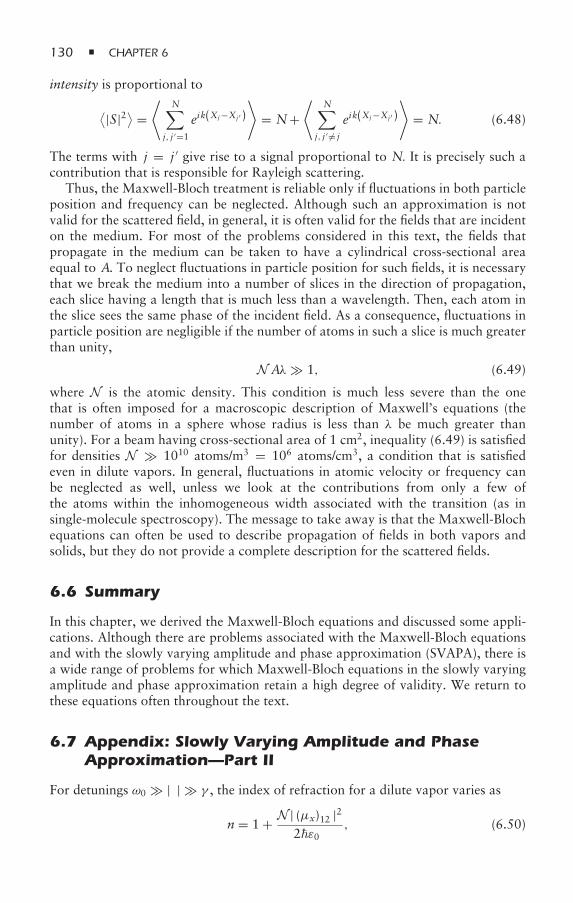
130 CHAPTER 6
intensity is proportional to
⟨|S|2⟩ =⟨
N∑j, j ′=1
eik(Xj−Xj ′ )⟩
= N+⟨
N∑j, j ′ = j
eik(Xj−Xj ′)⟩
= N. (6.48)
The terms with j = j ′ give rise to a signal proportional to N. It is precisely such acontribution that is responsible for Rayleigh scattering.
Thus, the Maxwell-Bloch treatment is reliable only if fluctuations in both particleposition and frequency can be neglected. Although such an approximation is notvalid for the scattered field, in general, it is often valid for the fields that are incidenton the medium. For most of the problems considered in this text, the fields thatpropagate in the medium can be taken to have a cylindrical cross-sectional areaequal to A. To neglect fluctuations in particle position for such fields, it is necessarythat we break the medium into a number of slices in the direction of propagation,each slice having a length that is much less than a wavelength. Then, each atom inthe slice sees the same phase of the incident field. As a consequence, fluctuations inparticle position are negligible if the number of atoms in such a slice is much greaterthan unity,
N Aλ 1, (6.49)
where N is the atomic density. This condition is much less severe than the onethat is often imposed for a macroscopic description of Maxwell’s equations (thenumber of atoms in a sphere whose radius is less than λ be much greater thanunity). For a beam having cross-sectional area of 1 cm2, inequality (6.49) is satisfiedfor densities N 1010 atoms/m3 = 106 atoms/cm3, a condition that is satisfiedeven in dilute vapors. In general, fluctuations in atomic velocity or frequency canbe neglected as well, unless we look at the contributions from only a few ofthe atoms within the inhomogeneous width associated with the transition (as insingle-molecule spectroscopy). The message to take away is that the Maxwell-Blochequations can often be used to describe propagation of fields in both vapors andsolids, but they do not provide a complete description for the scattered fields.
6.6 Summary
In this chapter, we derived the Maxwell-Bloch equations and discussed some appli-cations. Although there are problems associated with the Maxwell-Bloch equationsand with the slowly varying amplitude and phase approximation (SVAPA), there isa wide range of problems for which Maxwell-Bloch equations in the slowly varyingamplitude and phase approximation retain a high degree of validity. We return tothese equations often throughout the text.
6.7 Appendix: Slowly Varying Amplitude and PhaseApproximation—Part II
For detunings ω0 |δ| γ , the index of refraction for a dilute vapor varies as
n = 1 + N | (µx)12 |22ε0δ
, (6.50)
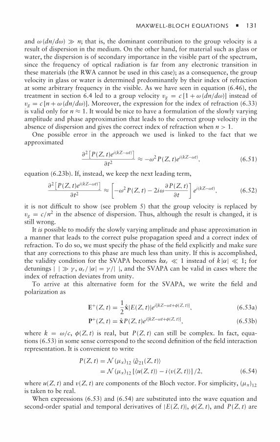
MAXWELL-BLOCH EQUATIONS 131
and ω (dn/dω) n; that is, the dominant contribution to the group velocity is aresult of dispersion in the medium. On the other hand, for material such as glass orwater, the dispersion is of secondary importance in the visible part of the spectrum,since the frequency of optical radiation is far from any electronic transition inthese materials (the RWA cannot be used in this case); as a consequence, the groupvelocity in glass or water is determined predominantly by their index of refractionat some arbitrary frequency in the visible. As we have seen in equation (6.46), thetreatment in section 6.4 led to a group velocity vg = c [1 + ω (dn/dω)] instead ofvg = c [n+ ω (dn/dω)]. Moreover, the expression for the index of refraction (6.33)is valid only for n ≈ 1. It would be nice to have a formulation of the slowly varyingamplitude and phase approximation that leads to the correct group velocity in theabsence of dispersion and gives the correct index of refraction when n > 1.
One possible error in the approach we used is linked to the fact that weapproximated
∂2[P(Z, t)ei(kZ−ωt)]
∂t2≈ −ω2P(Z, t)ei(kZ−ωt), (6.51)
equation (6.23b). If, instead, we keep the next leading term,
∂2[P(Z, t)ei(kZ−ωt)]
∂t2≈[−ω2P(Z, t) − 2iω
∂P(Z, t)∂t
]ei(kZ−ωt), (6.52)
it is not difficult to show (see problem 5) that the group velocity is replaced byvg = c/n2 in the absence of dispersion. Thus, although the result is changed, it isstill wrong.
It is possible to modify the slowly varying amplitude and phase approximation ina manner that leads to the correct pulse propagation speed and a correct index ofrefraction. To do so, we must specify the phase of the field explicitly and make surethat any corrections to this phase are much less than unity. If this is accomplished,the validity condition for the SVAPA becomes kαr 1 instead of k |α| 1; fordetunings |δ| γ , αr/ |α| = γ /|δ|, and the SVAPA can be valid in cases where theindex of refraction deviates from unity.
To arrive at this alternative form for the SVAPA, we write the field andpolarization as
E+(Z, t) = 12x|E(Z, t)|ei[kZ−ωt+φ(Z, t)], (6.53a)
P+(Z, t) = xP(Z, t)ei[kZ−ωt+φ(Z, t)], (6.53b)
where k = ω/c, φ(Z, t) is real, but P(Z, t) can still be complex. In fact, equa-tions (6.53) in some sense correspond to the second definition of the field interactionrepresentation. It is convenient to write
P(Z, t) = N (µx)12 〈21(Z, t)〉= N (µx)12 [〈u(Z, t)〉 − i〈v(Z, t)〉] /2, (6.54)
where u(Z, t) and v(Z, t) are components of the Bloch vector. For simplicity, (µx)12is taken to be real.
When expressions (6.53) and (6.54) are substituted into the wave equation andsecond-order spatial and temporal derivatives of |E(Z, t)|, φ(Z, t), and P(Z, t) are
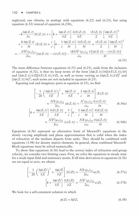
132 CHAPTER 6
neglected, one obtains, in analogy with equations (6.22) and (6.23), but usingequation (6.52) instead of equation (6.23b),
−k∂φ(Z, t)∂z
|E(Z, t)| + i[k+ ∂φ(Z, t)
∂Z
]∂|E(Z, t)|∂Z
− |E(Z, t)|2
[∂φ(Z, t)∂Z
]2
+kc∂φ(Z, t)∂t
|E(Z, t)| + ic
[k− 1
c∂φ(Z, t)∂t
]∂|E(Z, t)|
∂t+ |E(Z, t)|
2
[∂φ(Z, t)∂t
]2
= −Nk2(µx)122ε0
[〈u(Z, t)〉 − i〈v(Z, t)〉] − ikNk2 (µx)12cε0
∂ [〈u(Z, t)〉 − i〈v(Z, t)〉]∂t
.
(6.55)
The main difference between equations (6.55) and (6.25), aside from the inclusionof equation (6.52), is that we keep terms of the form [∂φ(Z, t)/∂t][∂|E(Z, t)|/∂t]and [∂φ(Z, t)/∂Z][∂|E(Z, t)|/∂Z], as well as terms varying as [∂φ(Z, t)/∂Z]2 and[∂φ(Z, t)/∂t]2; such terms are not included in equation (6.25).
Equating real and imaginary parts in equation (6.55), we find
[− 12k
(∂φ(Z, t)∂Z
)2
+ ∂φ(Z, t)∂Z
+ 1c∂φ(Z, t)∂t
]|E(Z, t)|
= Nk (µx)122ε0
〈u(Z, t)〉 + N (µx)12cε0
∂〈v(Z, t)〉∂t
, (6.56a)[k+ ∂φ(Z, t)
∂Z
]∂|E(Z, t)|∂Z
+ 1c
[k− 1
c∂φ(Z, t)∂t
]∂|E(Z, t)|
∂t
= Nk2(µx)122ε0
〈v(Z, t)〉 − Nk (µx)12cε0
∂〈u(Z, t)〉∂t
. (6.56b)
Equations (6.56) represent an alternative form of Maxwell’s equations in theslowly varying amplitude and phase approximation that is valid when the indexof refraction of the medium departs from unity. They should be combined withequations (3.98) for density matrix elements. In general, these combined Maxwell-Bloch equations must be solved numerically.
To show that equations (6.56) lead to the correct index of refraction and groupvelocity, we consider two limiting cases. First, we solve the equations in steady statefor a weak input field and stationary atoms. If all time derivatives in equations (6.56)are set equal to zero, we obtain
[− 12k
(∂φ(Z)∂Z
)2
+ ∂φ(Z)∂Z
]|E(Z)| = Nk (µx)12
2ε0u(Z), (6.57a)
[k+ ∂φ(Z)
∂Z
]∂|E(Z)|∂Z
= Nk2 (µx)122ε0
v(Z). (6.57b)
We look for a self-consistent solution in which
φ(Z) = kβZ, (6.58)
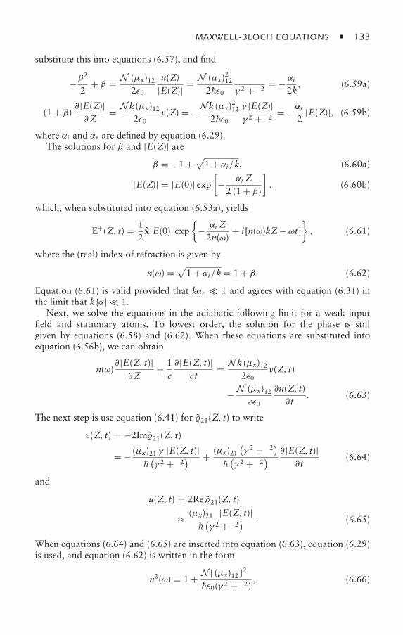
MAXWELL-BLOCH EQUATIONS 133
substitute this into equations (6.57), and find
−β2
2+ β = N (µx)12
2ε0
u(Z)|E(Z)| = N (µx)212
2ε0
δ
γ 2 + δ2 = − αi2k, (6.59a)
(1 + β) ∂|E(Z)|∂Z
= Nk (µx)122ε0
v(Z) = −Nk (µx)212
2ε0
γ |E(Z)|γ 2 + δ2 = −αr
2|E(Z)|, (6.59b)
where αi and αr are defined by equation (6.29).The solutions for β and |E(Z)| are
β = −1 +√
1 + αi/k, (6.60a)
|E(Z)| = |E(0)| exp[− αr Z2 (1 + β)
], (6.60b)
which, when substituted into equation (6.53a), yields
E+(Z, t) = 12x|E(0)| exp
− αr Z2n(ω)
+ i[n(ω)kZ− ωt], (6.61)
where the (real) index of refraction is given by
n(ω) =√
1 + αi/k= 1 + β. (6.62)
Equation (6.61) is valid provided that kαr 1 and agrees with equation (6.31) inthe limit that k |α| 1.
Next, we solve the equations in the adiabatic following limit for a weak inputfield and stationary atoms. To lowest order, the solution for the phase is stillgiven by equations (6.58) and (6.62). When these equations are substituted intoequation (6.56b), we can obtain
n(ω)∂|E(Z, t)|∂Z
+ 1c∂|E(Z, t)|
∂t= Nk (µx)12
2ε0v(Z, t)
− N (µx)12cε0
∂u(Z, t)∂t
. (6.63)
The next step is use equation (6.41) for 21(Z, t) to write
v(Z, t) = −2Im21(Z, t)
= − (µx)21 γ |E(Z, t)|(γ 2 + δ2) + (µx)21
(γ 2 − δ2)
(γ 2 + δ2) ∂|E(Z, t)|
∂t(6.64)
and
u(Z, t) = 2Re 21(Z, t)
≈ (µx)21 δ|E(Z, t)|(γ 2 + δ2) . (6.65)
When equations (6.64) and (6.65) are inserted into equation (6.63), equation (6.29)is used, and equation (6.62) is written in the form
n2(ω) = 1 + N | (µx)12 |2δε0(γ 2 + δ2) , (6.66)
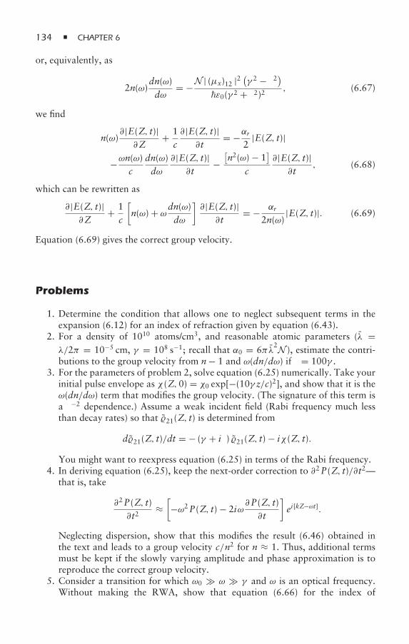
134 CHAPTER 6
or, equivalently, as
2n(ω)dn(ω)dω
= −N | (µx)12 |2 (γ 2 − δ2)ε0(γ 2 + δ2)2 , (6.67)
we find
n(ω)∂|E(Z, t)|∂Z
+ 1c∂|E(Z, t)|
∂t= −αr
2|E(Z, t)|
−ωn(ω)c
dn(ω)dω
∂|E(Z, t)|∂t
−[n2(ω) − 1
]c
∂|E(Z, t)|∂t
, (6.68)
which can be rewritten as
∂|E(Z, t)|∂Z
+ 1c
[n(ω) + ωdn(ω)
dω
]∂|E(Z, t)|
∂t= − αr
2n(ω)|E(Z, t)|. (6.69)
Equation (6.69) gives the correct group velocity.
Problems
1. Determine the condition that allows one to neglect subsequent terms in theexpansion (6.12) for an index of refraction given by equation (6.43).
2. For a density of 1010 atoms/cm3, and reasonable atomic parameters (λ =λ/2π = 10−5 cm, γ = 108 s−1; recall that α0 = 6πλ
2N ), estimate the contri-butions to the group velocity from n− 1 and ω(dn/dω) if δ = 100γ .
3. For the parameters of problem 2, solve equation (6.25) numerically. Take yourinitial pulse envelope as χ (Z,0) = χ0 exp[−(10γ z/c)2], and show that it is theω(dn/dω) term that modifies the group velocity. (The signature of this term isa δ−2 dependence.) Assume a weak incident field (Rabi frequency much lessthan decay rates) so that 21(Z, t) is determined from
d21(Z, t)/dt = − (γ + iδ) 21(Z, t) − iχ (Z, t).
You might want to reexpress equation (6.25) in terms of the Rabi frequency.4. In deriving equation (6.25), keep the next-order correction to ∂2P(Z, t)/∂t2—
that is, take
∂2P(Z, t)∂t2
≈[−ω2P(Z, t) − 2iω
∂P(Z, t)∂t
]ei[kZ−ωt].
Neglecting dispersion, show that this modifies the result (6.46) obtained inthe text and leads to a group velocity c/n2 for n ≈ 1. Thus, additional termsmust be kept if the slowly varying amplitude and phase approximation is toreproduce the correct group velocity.
5. Consider a transition for which ω0 ω γ and ω is an optical frequency.Without making the RWA, show that equation (6.66) for the index of
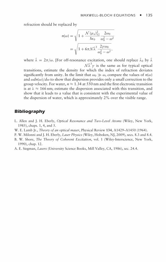
MAXWELL-BLOCH EQUATIONS 135
refraction should be replaced by
n(ω) =√1 + N (µx)212
ε0
2ω0
ω20 − ω2
=√
1 + 6πN λ3 2γω0
ω20 − ω2
,
where λ = 2π/ω. [For off-resonance excitation, one should replace λ0 by λin equation (4.28).] Assuming that N λ3γ is the same as for typical opticaltransitions, estimate the density for which the index of refraction deviatessignificantly from unity. In the limit that ω0 ω, compare the values of n(ω)and ωdn(ω)/dω to show that dispersion provides only a small correction to thegroup velocity. For water, n ≈ 1.34 at 550 nm and the first electronic transitionis at λ ≈ 166nm; estimate the dispersion associated with this transition, andshow that it leads to a value that is consistent with the experimental value ofthe dispersion of water, which is approximately 2% over the visible range.
Bibliography
L. Allen and J. H. Eberly, Optical Resonance and Two-Level Atoms (Wiley, New York,1985), chaps. 1, 4, and 5.
W. E. Lamb Jr., Theory of an optical maser, Physical Review 134, A1429–A1450 (1964).P. W. Milonni and J. H. Eberly, Laser Physics (Wiley, Hoboken, NJ, 2009), secs. 8.3 and 8.4.B. W. Shore, The Theory of Coherent Excitation, vol. 1 (Wiley-Interscience, New York,1990), chap. 12.
A. E. Siegman, Lasers (University Science Books, Mill Valley, CA, 1986), sec. 24.4.
7Two-Level Atoms in Twoor More Fields:Introduction to Saturation Spectroscopy
Shortly after the discovery of the gas laser, it became clear that the principlesunderlying its operation also had important implications for the spectroscopy ofatomic vapors. We have already seen that, for thermal vapors, the factor that limitsthe resolution achievable in linear spectroscopy is the inhomogeneous broadeningproduced by Doppler broadening. We have also noted that this is not an intrinsiclimitation to the resolution, since it could be eliminated by using cold atoms. Withthe development of the gas laser, it became evident that nonlinear or saturationspectroscopy could be used to eliminate the Doppler broadening, even in thermalvapors. The price one pays is that only a small fraction of the atoms in the vaporcell contribute to the observed signals. The use of saturation effects revolutionizedthe spectroscopy of vapors, liquids, and solids and is often referred to as laserspectroscopy since it requires the use of moderately intense, quasi-single-modesources. Aside from its use in providing a probe of matter, laser spectroscopyhas important applications in metrology; laser techniques can be used to stabilizeresonant cavities or “slave” lasers to a narrow atomic or molecular transitionfrequency. In this chapter, we examine the basic concepts needed to understandthe way in which laser spectroscopy can be used to achieve these results.
7.1 Two-Level Atoms and N Fields—Third-OrderPerturbation Theory
We have seen that it is possible to obtain a steady-state solution of the densitymatrix equations in the field interaction representation when a single, plane-wave,monochromatic field interacts with an ensemble of two-level atoms. If we add asecond field having a different frequency (or even a different direction in the case of

TWO-LEVEL ATOMS IN TWO OR MORE FIELDS 137
moving atoms), the problem becomes significantly more difficult to solve. This mayseem surprising at first. For a harmonic oscillator, one simply uses superpositionto account for the presence of a number of fields having different frequencies. Thesuperposition principle applies because the harmonic oscillator is an intrinsicallylinear device. As we have stressed on several occasions, an atom is not a harmonicoscillator; it is intrinsically a nonlinear device. It is just this nonlinearity that weexploit in laser spectroscopy.
Since the atomic response to the field is nonlinear, a superposition approach isdoomed to failure. In fact, it is not difficult to see why. To lowest order in theapplied fields, the atomic dipoles respond at all the frequencies of the applied fields,just as in the linear case. However, to second order in the fields, there are changes instate populations that depend on the beat frequencies of each pair of fields. In higherorder, many different combinations of the field frequencies enter. As a consequence,the only way to solve the problem of a two-level atom interacting with two or morefields of arbitrary intensity having different frequencies is to solve it numerically.Analytic solutions can be obtained using perturbation theory or in the limit thatonly one of the fields is intense. We look first at a perturbative solution and deferthe case of one strong and one weak field to appendix A.
We assume that the total incident field can be written as the sum of N separatefields,
E(R, t) = 12
N∑µ=1
εµEµeikµ·R−iωµt + c.c., (7.1)
where εµ is the polarization of field µ and kµ = ωµ/c. Although not indicatedexplicitly, the complex field amplitudes Eµ can be slowly varying functions of spaceand time. It is of some interest to calculate the total field intensity
⟨|E(R, t)|2⟩ = 12
N∑µ,ν=1
(εµ · εν)|EµEν | cos(kµν · R + δµνt + ϕµν), (7.2)
where
kµν = kµ − kν, (7.3a)
δµ = ω0 − ωµ, (7.3b)
δµν = δµ − δν = ων − ωµ, (7.3c)
ϕµν = ϕµ − ϕν, (7.3d)
Eµ = |Eµ|eiϕµ, (7.3e)
ω0 is the transition frequency, and the brackets refer to a time average over an opticalperiod. We see that the field intensity consists of a constant background from eachfield separately (µ = ν) and standing-wave patterns resulting from the interferenceof the different fields. The standing-wave components are not stationary; they movewith speed δµν/kµν . As we shall see, these external fields give rise to moving atomicpopulation gratings, and the relative phase of the population gratings and the fieldstanding-wave pattern is an important parameter in laser cooling schemes.
To calculate the atomic response to the fields, it is convenient to work in thenormal interaction representation, since there are many field frequencies but only a
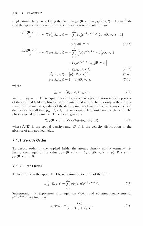
138 CHAPTER 7
single atomic frequency. Using the fact that 11(R, v, t) + 22(R, v, t) = 1, one findsthat the appropriate equations in the interaction representation are
∂I12(R, v, t)∂t
+ v · ∇I12(R, v, t) = −N∑µ=1
iχ∗µe
−ikµ·R−iδµt [222(R, v, t) − 1]
−γ I12(R, v, t), (7.4a)
∂22(R, v, t)∂t
+ v · ∇22(R, v, t) = −N∑µ=1
[iχ∗µe
−ikµ·R−iδµtI21(R, v, t)
− iχµeikµ·R+iδµtI12(R, v, t)]
− γ222(R, v, t), (7.4b)
I21(R, v, t) = [I12(R, v, t)
]∗, (7.4c)
11(R, v, t) = 1 − 22(R, v, t), (7.4d)
where
χµ = − (µ21 · εµ
)Eµ/2, (7.5)
and δµ = ω0 − ωµ. These equations can be solved as a perturbation series in powersof the external field amplitudes. We are interested in this chapter only in the steady-state response—that is, values of the density matrix elements once all transients havedied away. Recall that αα′ (R, v, t) is a single-particle density matrix element. Thephase-space density matrix elements are given by
Rαα′ (R, v, t) = N (R)W0(v)αα′(R, v, t), (7.6)
where N (R) is the spatial density, and W0(v) is the velocity distribution in theabsence of any applied fields.
7.1.1 Zeroth Order
To zeroth order in the applied fields, the atomic density matrix elements re-lax to their equilibrium values, 11(R, v, t) = 1, I21(R, v, t) = I12(R, v, t) =22(R, v, t) = 0.
7.1.2 First Order
To first order in the applied fields, we assume a solution of the form
I(1)12 (R, v, t) =
N∑µ=1
12(v;µ)e−ikµ·R−iδµt. (7.7)
Substituting this expression into equation (7.4a) and equating coefficients ofe−ikµ·R−iδµt, we find that
12(v;µ) = iχ∗µ
γ − i(δµ + kµ· v
) . (7.8)
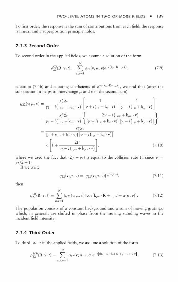
TWO-LEVEL ATOMS IN TWO OR MORE FIELDS 139
To first order, the response is the sum of contributions from each field; the responseis linear, and a superposition principle holds.
7.1.3 Second Order
To second order in the applied fields, we assume a solution of the form
(2)22 (R, v, t) =
N∑µ,ν=1
22(v;µ, ν)e−i(kµν ·R+δµν t). (7.9)
Substituting this expression and the solution [equations (7.8) and (7.7)] intoequation (7.4b) and equating coefficients of e−i(kµν ·R+δµν t), we find that (after thesubstitution, it helps to interchange µ and ν in the second sum)
22(v;µ, ν) = χ∗µχν
γ2 − i(δµν + kµν · v)
[1
γ + i(δν + kν · v) + 1γ − i
(δµ + kµ · v)
]
= χ∗µχν
γ2 − i(δµν + kµν · v)
2γ − i
(δµν + kµν · v)
[γ + i(δν + kν · v)] [γ − i(δµ + kµ · v)]
= χ∗µχν
[γ + i(δν + kν · v)] [γ − i(δµ + kµ · v)]
×[1 + 2
γ2 − i(δµν + kµν · v)
], (7.10)
where we used the fact that (2γ − γ2) is equal to the collision rate , since γ =γ2/2 + .
If we write
22(v;µ, ν) = |22(v;µ, ν)| eiα(µ,ν), (7.11)
then
(2)22 (R, v, t) =
N∑µ,ν=1
|22(v;µ, ν)| cos[kµν · R + δµνt − α(µ, ν)]. (7.12)
The population consists of a constant background and a sum of moving gratings,which, in general, are shifted in phase from the moving standing waves in theincident field intensity.
7.1.4 Third Order
To third order in the applied fields, we assume a solution of the form
I(3)12 (R, v, t) =
N∑µ,ν,σ=1
12(v;µ, ν, σ )e−i[(kµ−kν+kσ )·R+(δµ−δν+δσ )t]. (7.13)
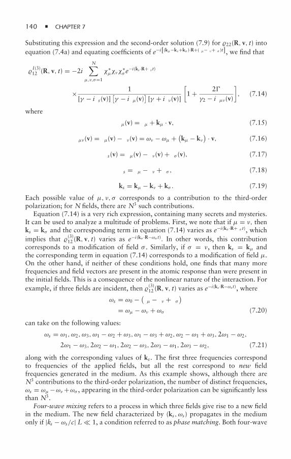
140 CHAPTER 7
Substituting this expression and the second-order solution (7.9) for 22(R, v, t) intoequation (7.4a) and equating coefficients of e−i[(kµ−kν+kσ )·R+(δµ−δν+δσ )t], we find that
I(3)12 (R, v, t) = −2i
N∑µ,ν,σ=1
χ∗µχνχ
∗σ e
−i(ks ·R+δs t)
× 1[γ − iδs(v)]
[γ − iδµ(v)
][γ + iδν(v)]
[1 + 2
γ2 − iδµν(v)
], (7.14)
where
δµ(v) = δµ + kµ · v, (7.15)
δµν(v) = δµ(v) − δν(v) = ων − ωµ + (kµ − kν
) · v, (7.16)
δs(v) = δµ(v) − δν(v) + δσ (v), (7.17)
δs = δµ − δν + δσ , (7.18)
ks = kµ − kν + kσ . (7.19)
Each possible value of µ, ν, σ corresponds to a contribution to the third-orderpolarization; for N fields, there are N3 such contributions.
Equation (7.14) is a very rich expression, containing many secrets and mysteries.It can be used to analyze a multitude of problems. First, we note that if µ = ν, thenks = kσ and the corresponding term in equation (7.14) varies as e−i(kσ ·R+δσ t), whichimplies that (3)12 (R, v, t) varies as e−i(kσ ·R−ωσ t). In other words, this contributioncorresponds to a modification of field σ . Similarly, if σ = ν, then ks = kµ andthe corresponding term in equation (7.14) corresponds to a modification of field µ.On the other hand, if neither of these conditions hold, one finds that many morefrequencies and field vectors are present in the atomic response than were present inthe initial fields. This is a consequence of the nonlinear nature of the interaction. Forexample, if three fields are incident, then (3)12 (R, v, t) varies as e
−i(ks ·R−ωs t), where
ωs = ω0 − (δµ − δν + δσ
)= ωµ − ων + ωσ (7.20)
can take on the following values:
ωs = ω1, ω2, ω3, ω1 − ω2 + ω3, ω1 − ω3 + ω2, ω2 − ω1 + ω3,2ω1 − ω2,
2ω1 − ω3,2ω2 − ω1,2ω2 − ω3,2ω3 − ω1,2ω3 − ω2, (7.21)
along with the corresponding values of ks . The first three frequencies correspondto frequencies of the applied fields, but all the rest correspond to new fieldfrequencies generated in the medium. As this example shows, although there areN3 contributions to the third-order polarization, the number of distinct frequencies,ωs = ωµ−ων +ωσ , appearing in the third-order polarization can be significantly lessthan N3.
Four-wave mixing refers to a process in which three fields give rise to a new fieldin the medium. The new field characterized by (ks, ωs) propagates in the mediumonly if |ks − ωs/c| L 1, a condition referred to as phase matching. Both four-wave
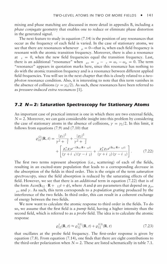
TWO-LEVEL ATOMS IN TWO OR MORE FIELDS 141
mixing and phase matching are discussed in more detail in appendix B, including aphase conjugate geometry that enables one to reduce or eliminate phase distortionin the generated signal.
The next feature to study in equation (7.14) is the position of any resonances thatoccur as the frequency of each field is varied. In the case of stationary atoms, wesee that there are resonances whenever δµ = 0—that is, when each field frequency isresonant with the atomic transition frequency. Moreover, there is also a resonanceat δs = 0, when the new field frequencies equal the transition frequency. Last,there is an additional “resonance” when δµν = δµ − δν = ων − ωµ = 0. The term“resonance” appears in quotation marks here, since this resonance has nothing todo with the atomic transition frequency and is a resonance between different appliedfield frequencies. You will see in the next chapter that this is closely related to a two-photon resonance condition. Also, it is interesting to note that this term vanishes inthe absence of collisions (γ = γ2/2). As such, these resonances have been referred toas pressure-induced extra resonances [1].
7.2 N=2: Saturation Spectroscopy for Stationary Atoms
An important case of practical interest is one in which there are two external fields,N= 2. Moreover, we can gain considerable insight into this problem by consideringthe case of stationary atoms in the absence of collisions, γ = γ2/2. In this limit, itfollows from equations (7.9) and (7.10) that
(2)22 (R, t) = |χ1|2
γ 2 + δ21+ |χ2|2γ 2 + δ22
+[χ∗1χ2e
−i(k12·R+δ12t)
(γ + iδ1) (γ − iδ2)+ χ∗
2χ1ei(k12·R+δ12t)
(γ + iδ2) (γ − iδ1)
]. (7.22)
The first two terms represent absorption (i.e., scattering) of each of the fields,resulting in an excited-state population that leads to a corresponding decrease inthe absorption of the fields in third order. This is the origin of the term saturationspectroscopy, since the field absorption is reduced by the saturating effects of thefield. However, we see that there is an additional term in equation (7.22) that is ofthe form Acos(k12 · R + δ12t + φ), where Aand φ are parameters that depend on χµ,δµ, and γ . As such, this term corresponds to a population grating produced by theinterference of the two fields. In third order, this can result in a coherent exchangeof energy between the two fields.
We now want to calculate the atomic response to third order in the fields. To doso, we assume that the first field is a pump field, having a higher intensity than thesecond field, which is referred to as a probe field. The idea is to calculate the atomicresponse
I12(R, t) ≈ I(1)12 (R, t) + I(3)12 (R, t) (7.23)
that oscillates at the probe field frequency. The first-order response is given byequation (7.8). From equation (7.14), one finds that there are eight contributions tothe third-order polarization when N= 2. These are listed schematically in table 7.1.
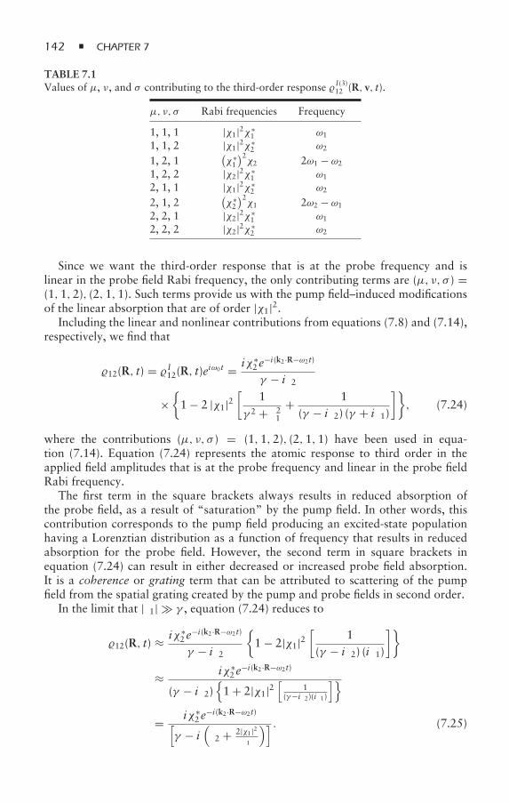
142 CHAPTER 7
TABLE 7.1Values of µ, ν, and σ contributing to the third-order response I(3)12 (R, v, t).
µ, ν, σ Rabi frequencies Frequency
1, 1, 1 |χ1|2χ∗1 ω1
1, 1, 2 |χ1|2χ∗2 ω2
1, 2, 1(χ∗1
)2χ2 2ω1 − ω2
1, 2, 2 |χ2|2χ∗1 ω1
2, 1, 1 |χ1|2χ∗2 ω2
2, 1, 2(χ∗2
)2χ1 2ω2 − ω1
2, 2, 1 |χ2|2χ∗1 ω1
2, 2, 2 |χ2|2χ∗2 ω2
Since we want the third-order response that is at the probe frequency and islinear in the probe field Rabi frequency, the only contributing terms are (µ, ν, σ ) =(1,1,2), (2,1,1). Such terms provide us with the pump field–induced modificationsof the linear absorption that are of order |χ1|2.
Including the linear and nonlinear contributions from equations (7.8) and (7.14),respectively, we find that
12(R, t) = I12(R, t)eiω0t = iχ∗
2e−i(k2·R−ω2t)
γ − iδ2
×1 − 2 |χ1|2
[1
γ 2 + δ21+ 1
(γ − iδ2) (γ + iδ1)
], (7.24)
where the contributions (µ, ν, σ ) = (1,1,2), (2,1,1) have been used in equa-tion (7.14). Equation (7.24) represents the atomic response to third order in theapplied field amplitudes that is at the probe frequency and linear in the probe fieldRabi frequency.
The first term in the square brackets always results in reduced absorption ofthe probe field, as a result of “saturation” by the pump field. In other words, thiscontribution corresponds to the pump field producing an excited-state populationhaving a Lorenztian distribution as a function of frequency that results in reducedabsorption for the probe field. However, the second term in square brackets inequation (7.24) can result in either decreased or increased probe field absorption.It is a coherence or grating term that can be attributed to scattering of the pumpfield from the spatial grating created by the pump and probe fields in second order.
In the limit that |δ1| γ , equation (7.24) reduces to
12(R, t) ≈ iχ∗2e
−i(k2·R−ω2t)
γ − iδ2
1 − 2|χ1|2
[1
(γ − iδ2) (iδ1)
]
≈ iχ∗2e
−i(k2·R−ω2t)
(γ − iδ2)1 + 2|χ1|2
[1
(γ−iδ2)(iδ1)]
= iχ∗2e
−i(k2·R−ω2t)[γ − i
(δ2 + 2|χ1|2
δ1
)] . (7.25)
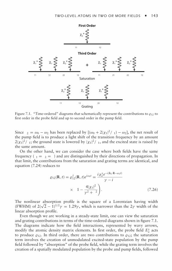
TWO-LEVEL ATOMS IN TWO OR MORE FIELDS 143
First Order
Third Order
+
Saturation
Grating
ρ11 ρ12
χ2*
ρ11 ρ12 ρ22 ρ12
χ1 χ2*χ1*
ρ11 ρ21 ρ22 ρ12
χ1* χ2*χ1
ρ11 ρ12 ρ22 ρ12
χ1 χ1*χ2*
Figure 7.1. “Time-ordered” diagrams that schematically represent the contributions to 12 tofirst order in the probe field and up to second order in the pump field.
Since δ2 = ω0 − ω2 has been replaced by [(ω0 + 2|χ1|2/δ1) − ω2], the net result ofthe pump field is to produce a light shift of the transition frequency by an amount2|χ1|2/δ1; the ground state is lowered by |χ1|2/δ1, and the excited state is raised bythe same amount.
On the other hand, we can consider the case where both fields have the samefrequency (δ1 = δ2 = δ) and are distinguished by their directions of propagation. Inthat limit, the contributions from the saturation and grating terms are identical, andequation (7.24) reduces to
12(R, t) = I12(R, t)eiω0t = iχ∗
2e−i(k2·R−ω2t)
γ − iδ
×(1 − 4|χ1|2
γ 2 + δ2). (7.26)
The nonlinear absorption profile is the square of a Lorentzian having width(FWHM) of 2(
√2 − 1)1/2γ = 1.29γ , which is narrower than the 2γ width of the
linear absorption profile.Even though we are working in a steady-state limit, one can view the saturation
and grating contributions in terms of the time-ordered diagrams shown in figure 7.1.The diagrams indicate how the field interactions, represented by wavy arrows,modify the atomic density matrix elements. In first order, the probe field E∗
2 actsto produce 12. In third order, there are two contributions to 12; the saturationterm involves the creation of unmodulated excited-state population by the pumpfield followed by “absorption” of the probe field, while the grating term involves thecreation of a spatially modulated population by the probe and pump fields, followed
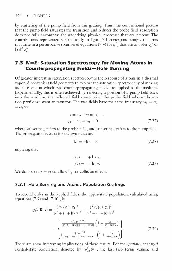
144 CHAPTER 7
by scattering of the pump field from this grating. Thus, the conventional picturethat the pump field saturates the transition and reduces the probe field absorptiondoes not fully encompass the underlying physical processes that are present. Thecontributions represented schematically in figure 7.1 correspond simply to termsthat arise in a perturbative solution of equations (7.4) for I12 that are of order χ
∗2 or
|χ1|2 χ∗2 .
7.3 N=2: Saturation Spectroscopy for Moving Atoms inCounterpropagating Fields—Hole Burning
Of greater interest in saturation spectroscopy is the response of atoms in a thermalvapor. A convenient field geometry to explore the saturation spectroscopy of movingatoms is one in which two counterpropagating fields are applied to the medium.Experimentally, this is often achieved by reflecting a portion of a pump field backinto the medium, the reflected field constituting the probe field whose absorp-tion profile we want to monitor. The two fields have the same frequency ω1 = ω2
= ω, so
δ1 = ω0 − ω = δ2 ≡ δ,
δ21 = ω1 − ω2 = 0, (7.27)
where subscript 2 refers to the probe field, and subscript 1 refers to the pump field.The propagation vectors for the two fields are
k1 = −k2 ≡ k, (7.28)
implying that
δ1(v) = δ + k · v,δ2(v) = δ − k · v. (7.29)
We do not set γ = γ2/2, allowing for collision effects.
7.3.1 Hole Burning and Atomic Population Gratings
To second order in the applied fields, the upper-state population, calculated usingequations (7.9) and (7.10), is
(2)22 (R, v) = (2γ /γ2) |χ1|2
γ 2 + (δ + k · v)2 + (2γ /γ2) |χ2|2γ 2 + (δ − k · v)2
+
⎧⎪⎪⎨⎪⎪⎩
χ∗1χ2e
−2ik·R
[γ+i(δ−k·v)][γ−i(δ+k·v)](1 + 2
γ2−2ik·v)
+ χ∗2χ1e
2ik·R
[γ+i(δ+k·v)][γ−i(δ−k·v)](1 + 2
γ2+2ik·v)⎫⎪⎪⎬⎪⎪⎭. (7.30)
There are some interesting implications of these results. For the spatially averagedexcited-state population, denoted by 〈(2)22 (v)〉, the last two terms vanish, and
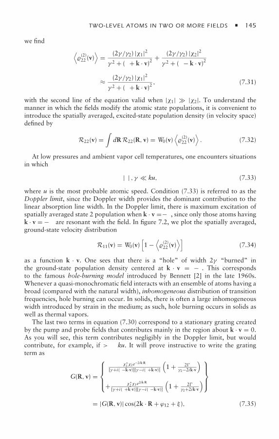
TWO-LEVEL ATOMS IN TWO OR MORE FIELDS 145
we find ⟨(2)22 (v)
⟩= (2γ /γ2) |χ1|2γ 2 + (δ + k · v)2 + (2γ /γ2) |χ2|2
γ 2 + (δ − k · v)2
≈ (2γ /γ2) |χ1|2γ 2 + (δ + k · v)2 , (7.31)
with the second line of the equation valid when |χ1| |χ2|. To understand themanner in which the fields modify the atomic state populations, it is convenient tointroduce the spatially averaged, excited-state population density (in velocity space)defined by
R22(v) =∫dRR22(R, v) = W0(v)
⟨(2)22 (v)
⟩. (7.32)
At low pressures and ambient vapor cell temperatures, one encounters situationsin which
|δ| , γ ku, (7.33)
where u is the most probable atomic speed. Condition (7.33) is referred to as theDoppler limit, since the Doppler width provides the dominant contribution to thelinear absorption line width. In the Doppler limit, there is maximum excitation ofspatially averaged state 2 population when k · v =−δ, since only those atoms havingk · v = − δ are resonant with the field. In figure 7.2, we plot the spatially averaged,ground-state velocity distribution
R11(v) = W0(v)[1 −
⟨(2)22 (v)
⟩](7.34)
as a function k · v. One sees that there is a “hole” of width 2γ “burned” inthe ground-state population density centered at k · v = −δ. This correspondsto the famous hole-burning model introduced by Bennett [2] in the late 1960s.Whenever a quasi-monochromatic field interacts with an ensemble of atoms having abroad (compared with the natural width), inhomogeneous distribution of transitionfrequencies, hole burning can occur. In solids, there is often a large inhomogeneouswidth introduced by strain in the medium; as such, hole burning occurs in solids aswell as thermal vapors.
The last two terms in equation (7.30) correspond to a stationary grating createdby the pump and probe fields that contributes mainly in the region about k · v = 0.As you will see, this term contributes negligibly in the Doppler limit, but wouldcontribute, for example, if δ > ku. It will prove instructive to write the gratingterm as
G(R, v) =
⎧⎪⎪⎨⎪⎪⎩
χ∗1χ2e
−2ik·R
[γ+i(δ−k·v)][γ−i(δ+k·v)](1 + 2
γ2−2ik·v)
+ χ∗2χ1e
2ik·R
[γ+i(δ+k·v)][γ−i(δ−k·v)](1 + 2
γ2+2ik·v)⎫⎪⎪⎬⎪⎪⎭
= |G(R, v)| cos(2k · R + ϕ12 + ξ ), (7.35)
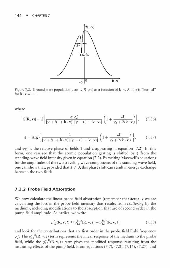
146 CHAPTER 7
2γ
1.67ku
11(v)
0 k • v–δ
R
Figure 7.2. Ground-state population density R11(v) as a function of k · v. A hole is “burned”for k · v = −δ.
where
|G(R, v)| = 2∣∣∣∣ χ1χ
∗2
[γ + i(δ + k · v)] [γ − i(δ − k · v)](1 + 2
γ2 + 2ik · v)∣∣∣∣ , (7.36)
ξ = Arg
1[γ + i(δ + k · v)] [γ − i(δ − k · v)]
(1 + 2
γ2 + 2ik · v), (7.37)
and ϕ12 is the relative phase of fields 1 and 2 appearing in equation (7.2). In thisform, one can see that the atomic population grating is shifted by ξ from thestanding-wave field intensity given in equation (7.2). By writingMaxwell’s equationsfor the amplitudes of the two traveling wave components of the standing-wave field,one can show that, provided that ξ = 0, this phase shift can result in energy exchangebetween the two fields.
7.3.2 Probe Field Absorption
We now calculate the linear probe field absorption (remember that actually we arecalculating the loss in the probe field intensity that results from scattering by themedium), including modifications to the absorption that are of second order in thepump field amplitude. As earlier, we write
I12(R, v, t) ≈ I(1)12 (R, v, t) + I(3)12 (R, v, t) (7.38)
and look for the contributions that are first order in the probe field Rabi frequencyχ∗2 . The
I(1)12 (R, v, t) term represents the linear response of the medium to the probe
field, while the I(3)12 (R, v, t) term gives the modified response resulting from thesaturating effects of the pump field. From equations (7.7), (7.8), (7.14), (7.27), and
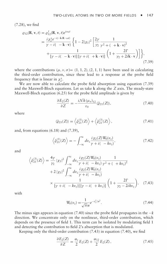
TWO-LEVEL ATOMS IN TWO OR MORE FIELDS 147
(7.28), we find
12(R, v, t) = I12(R, v, t)eiω0t
= iχ∗2e
−i(−k·R−ωt)
γ − i(δ − k · v)1 − 2|χ1|2
[2γγ2
1
γ 2 + (δ + k · v)2
+ 1[γ − i(δ − k · v)] [γ + i(δ + k · v)]
(1 + 2
γ2 + 2ik · v)]
,
(7.39)
where the contributions (µ, ν, σ )= (1,1,2), (2,1,1) have been used in calculatingthe third-order contribution, since these lead to a response at the probe fieldfrequency that is linear in χ∗
2 .We are now able to calculate the probe field absorption using equation (7.39)
and the Maxwell-Bloch equations. Let us take k along the Z axis. The steady-stateMaxwell-Bloch equation (6.25) for the probe field amplitude is given by
∂E2(Z)∂Z
= − iNk (µx)12ε0
〈21(Z)〉, (7.40)
where
〈21(Z)〉 =⟨(1)21 (Z)
⟩+⟨(3)21 (Z)
⟩, (7.41)
and, from equations (6.18) and (7.39),
⟨(1)21 (Z)
⟩= −
∫ ∞
−∞dvz
iχ2(Z)W0(vz)γ + i(δ − kvz)
, (7.42)
and ⟨(3)21 (Z)
⟩= 4γγ2
|χ1|2∫ ∞
−∞dvz
iχ2(Z)W0(vz)γ + i(δ − kvz)
1
γ 2 + (δ + kvz)2
+2 |χ1|2∫ ∞
−∞dvz
iχ2(Z)W0(vz)γ + i(δ − kvz)
× 1[γ + i(δ − kvz)] [γ − i(δ + kvz)]
(1 + 2
γ2 − 2ikvz
), (7.43)
with
W0(vz) = 1√πu
e−v2z /u2 . (7.44)
The minus sign appears in equation (7.40) since the probe field propagates in the −zdirection. We concentrate only on the nonlinear, third-order contribution, whichdepends on the presence of field 1. This term can be isolated by modulating field 1and detecting the contribution to field 2’s absorption that is modulated.
Keeping only the third-order contribution (7.43) in equation (7.40), we find
∂E2(Z)∂Z
= αs
2E2(Z) + α12
2E2(Z) , (7.45)
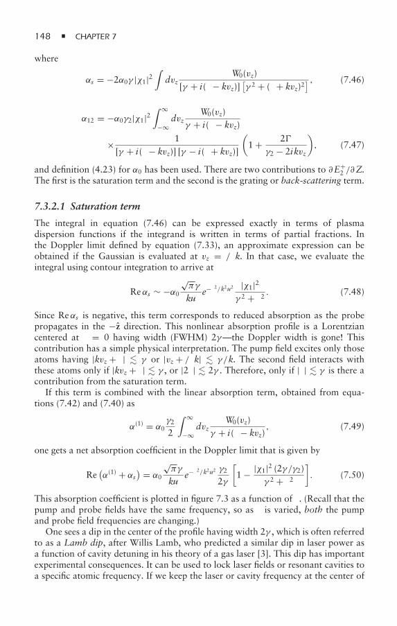
148 CHAPTER 7
where
αs = −2α0γ |χ1|2∫dvz
W0(vz)[γ + i(δ − kvz)]
[γ 2 + (δ + kvz)2
] , (7.46)
α12 = −α0γ2|χ1|2∫ ∞
−∞dvz
W0(vz)γ + i(δ − kvz)
× 1[γ + i(δ − kvz)] [γ − i(δ + kvz)]
(1 + 2
γ2 − 2ikvz
), (7.47)
and definition (4.23) for α0 has been used. There are two contributions to ∂E+2 /∂Z.
The first is the saturation term and the second is the grating or back-scattering term.
7.3.2.1 Saturation term
The integral in equation (7.46) can be expressed exactly in terms of plasmadispersion functions if the integrand is written in terms of partial fractions. Inthe Doppler limit defined by equation (7.33), an approximate expression can beobtained if the Gaussian is evaluated at vz = δ/k. In that case, we evaluate theintegral using contour integration to arrive at
Reαs ∼ −α0√πγ
kue−δ2/k2u2 |χ1|2
γ 2 + δ2 . (7.48)
Since Reαs is negative, this term corresponds to reduced absorption as the probepropagates in the −z direction. This nonlinear absorption profile is a Lorentziancentered at δ = 0 having width (FWHM) 2γ—the Doppler width is gone! Thiscontribution has a simple physical interpretation. The pump field excites only thoseatoms having |kvz + δ| γ or |vz + δ/k| γ /k. The second field interacts withthese atoms only if |kvz + δ| γ , or |2δ| 2γ . Therefore, only if |δ| γ is there acontribution from the saturation term.
If this term is combined with the linear absorption term, obtained from equa-tions (7.42) and (7.40) as
α(1) = α0γ2
2
∫ ∞
−∞dvz
W0(vz)γ + i(δ − kvz)
, (7.49)
one gets a net absorption coefficient in the Doppler limit that is given by
Re(α(1) + αs
) = α0
√πγ
kue−δ2/k2u2 γ2
2γ
[1 − |χ1|2 (2γ /γ2)
γ 2 + δ2]. (7.50)
This absorption coefficient is plotted in figure 7.3 as a function of δ. (Recall that thepump and probe fields have the same frequency, so as δ is varied, both the pumpand probe field frequencies are changing.)
One sees a dip in the center of the profile having width 2γ , which is often referredto as a Lamb dip, after Willis Lamb, who predicted a similar dip in laser power asa function of cavity detuning in his theory of a gas laser [3]. This dip has importantexperimental consequences. It can be used to lock laser fields or resonant cavities toa specific atomic frequency. If we keep the laser or cavity frequency at the center of
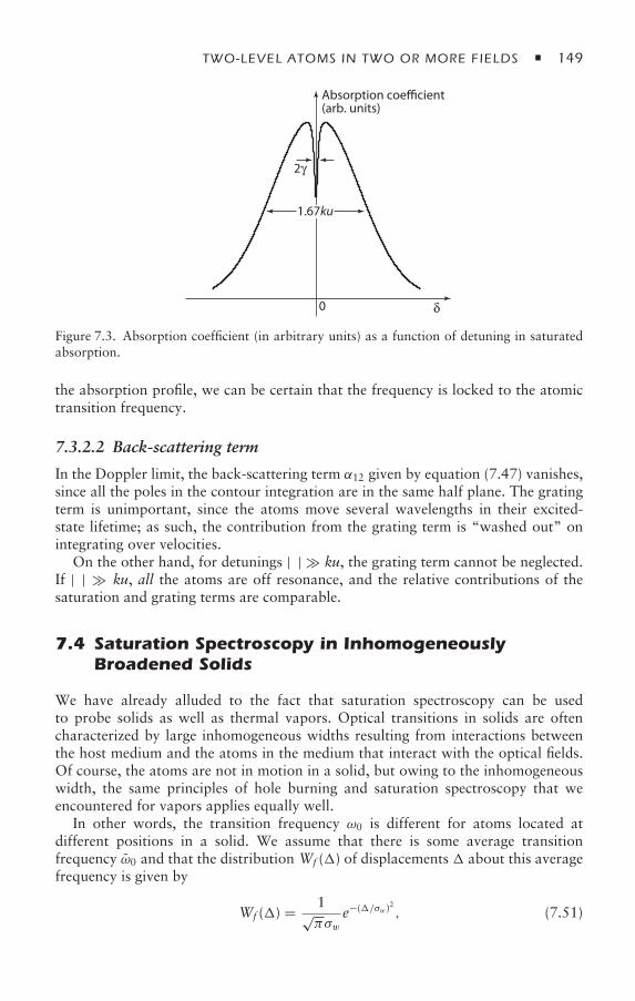
TWO-LEVEL ATOMS IN TWO OR MORE FIELDS 149
δ0
Absorption coefficient(arb. units)
2γ
1.67ku
Figure 7.3. Absorption coefficient (in arbitrary units) as a function of detuning in saturatedabsorption.
the absorption profile, we can be certain that the frequency is locked to the atomictransition frequency.
7.3.2.2 Back-scattering term
In the Doppler limit, the back-scattering term α12 given by equation (7.47) vanishes,since all the poles in the contour integration are in the same half plane. The gratingterm is unimportant, since the atoms move several wavelengths in their excited-state lifetime; as such, the contribution from the grating term is “washed out” onintegrating over velocities.
On the other hand, for detunings |δ| ku, the grating term cannot be neglected.If |δ| ku, all the atoms are off resonance, and the relative contributions of thesaturation and grating terms are comparable.
7.4 Saturation Spectroscopy in InhomogeneouslyBroadened Solids
We have already alluded to the fact that saturation spectroscopy can be usedto probe solids as well as thermal vapors. Optical transitions in solids are oftencharacterized by large inhomogeneous widths resulting from interactions betweenthe host medium and the atoms in the medium that interact with the optical fields.Of course, the atoms are not in motion in a solid, but owing to the inhomogeneouswidth, the same principles of hole burning and saturation spectroscopy that weencountered for vapors applies equally well.
In other words, the transition frequency ω0 is different for atoms located atdifferent positions in a solid. We assume that there is some average transitionfrequency ω0 and that the distribution Wf () of displacements about this averagefrequency is given by
Wf () = 1√πσw
e−(/σw)2 , (7.51)
150 CHAPTER 7
where σw characterizes the width of the inhomogeneous distribution. In some sense,the distribution of detunings δ() replaces the Doppler distribution that is relevantfor vapors. In terms of the transition frequency ω0 and an applied field frequency ω,
δ() = ω0 − ω = δ0 +, (7.52)
where
δ0 = ω0 − ω, = ω0 − ω0. (7.53)
As a consequence, equation (7.14) is replaced by
I(3)12 (R,, t) = −2i
N∑µ,ν,σ=1
χ∗µχνχ
∗σ e
−i[ks ·R+δs t]
× 1[γ − iδs()]
[γ − iδµ()
][γ + iδν()]
(1 + 2
γ2 − iδµν
), (7.54)
where
δµ() = ω0 − ωµ = ω0 − ωµ +, (7.55)
δµν = ων − ωµ, (7.56)
δs() = δµ() − δν() + δσ (). (7.57)
There are a few fundamental differences between equations (7.14) and (7.54).In solids, the directions of the incident fields are irrelevant, since there is noDoppler effect. As a consequence, there is no washing out of the grating term forcounterpropagating fields; the grating and absorption terms contribute on equalfooting, regardless of the directions of the fields. The last factor in equation (7.54)depends only on the field frequencies and not on the atomic frequencies. Asa consequence, this “collision”-induced resonance1 cannot vanish as a result ofaveraging over the inhomogeneous distribution of transition frequencies as it doesfor a thermal vapor and counterpropagating fields [4].
Moreover, it is no longer possible to get a narrow line shape using pumpand probe fields having the same frequency. In the case of a thermal vapor withcounterpropagating fields, each moving atom is exposed to two field frequencies,owing to the Doppler effect. Saturation spectroscopy relied on the fact that bothfields were resonant only for atoms having |k · v| γ—in other words, only thoseatoms in a narrow frequency range interact with both fields. In solids, since thereis no Doppler effect, atoms over the entire inhomogeneous width interact withboth fields if they have the same frequency. To obtain a narrow, homogeneouslybroadened line, one must fix the pump field frequency and vary the probe fieldfrequency. As the probe frequency is tuned, atoms are brought into resonancewith both fields only when the probe frequency equals the pump frequency. In thismanner, one recovers all the features of saturation spectroscopy.
1 Collisions per se are absent in a solid, but a nonvanishing can result from dephasing processesproduced by the host medium.
TWO-LEVEL ATOMS IN TWO OR MORE FIELDS 151
7.5 Summary
Several important concepts were introduced in this chapter. We have seen that it canbe advantageous to use one field to “pump” or prepare atoms and a second field toprobe these atoms. The pump field can modify the velocity distribution associatedwith atomic state populations. In saturation spectroscopy, the pump field excitesa narrow velocity class of excited atoms that are probed by a second field. As aconsequence, it is possible to eliminate the Doppler width in the probe absorptionspectrum by using only these selected atoms. The term saturation spectroscopy canbe somewhat misleading. We have seen that there is another physical process thatenters when one drives atomic ensembles with two or more fields. The fields cancreate population gratings off which any of the fields can scatter. This coherentscattering process can lead to four-wave mixing signals and the coherent exchangeof energy between the fields. In the next chapter, we turn our attention to three-levelatoms to explore new types of phenomena that can arise in such systems.
7.6 Appendix A: Saturation Spectroscopy—StationaryAtoms in One Strong and One Weak Field
Consider a pump–probe experiment in which two fields drive two-level transitions inan ensemble of stationary atoms. The field frequencies are ω1 = ω and ω2 = ω +.We want to calculate the probe field (field 2) absorption to all orders in thepump field (field 1) intensity. The probe field absorption spectrum exhibits manyinteresting features not found in the perturbative solution that was consideredearlier. You are asked to explore some of these features in the problems. In thisappendix, we simply outline the approach needed to solve this problem.
Since the first field is strong, it makes sense to work in the field interactionrepresentation for the first field. In the rotating-wave approximation (RWA), theequations to be solved are
∂12
∂t= −iχ∗
1 (222 − 1) − iχ∗2e
it(222 − 1) − (γ − iδ1) 12, (7.58a)
∂22
∂t= iχ∗
1 21 − iχ112 + iχ∗2e
it21 − iχ2e−it12 − γ222, (7.58b)
21 = [12]∗ , (7.58c)
11 = 1 − 22, (7.58d)
= ω2 − ω1 = δ1 − δ2, (7.58e)
where any spatial phase factors can be included in the χ ′s. We seek a steady-statesolution (i.e., a solution once all transients have died away) that is first order in χ2but all orders in χ1. We have already obtained the solution that is zeroth order in χ2[see equation (4.11)], for which density matrix elements are denoted by (0)i j .
We try a solution
i j = (0)i j + (1)i j , (7.59)
152 CHAPTER 7
where (1)i j is first order in χ2 or χ∗2 , substitute the trial solution in the original
differential equations, and keep only terms linear in the probe field amplitude toobtain
∂(1)12
∂t= −2iχ∗
1(1)22 − iχ∗
2eit
[2(0)22 − 1
]− (γ − iδ1)
(1)12 , (7.60a)
∂(1)22
∂t= iχ∗
1 (1)21 − iχ1
(1)12 + iχ∗
2eit
(0)21 − iχ2e−it(0)12 − γ2(1)22 , (7.60b)
21 = [12]∗ , (7.60c)
(1)11 = −(1)22 . (7.60d)
To solve these equations, we guess a solution of the form
(1)12 = a12 + b12eit + c12e−it, (7.61a)
(1)22 = a22 + b22eit + c22e−it, (7.61b)
substitute it into the differential equations, and equate constant coefficients andcoefficients of e±it to obtain
γ2a22 − iχ∗1a
∗12 + iχ1a12 = 0, (7.62a)
(γ − iδ1) a12 + 2iχ∗1a22 = 0, (7.62b)
(γ2 + i)b22 − iχ∗1c
∗12 + iχ1b12 = iχ∗
2 (0)21 , (7.62c)
[γ + i(− δ1)]b12 + 2iχ∗1b22 = −iχ∗
2
[2(0)22 − 1
], (7.62d)
[γ + i(+ δ1)] c∗12 − 2iχ1c22 = 0. (7.62e)
Before solving these equations, it is useful to note that
(1)12 =
(1)12 e
iω1t = (a12 + b12eit + c12e−it) eiω1t
= a12eiω1t + b12eiω2t + c12ei(2ω1−ω2)t . (7.63)
Thus, the a12 term is a modification of the pump field, the b12 term gives the probefield absorption, which is what is being sought here, and the c12 term is a new fieldgenerated via four-wave mixing.
It is simple to solve equations (7.62) analytically on your own or using acomputer. By either method, one obtains a22 = a12 = 0 and
b12 = −iχ∗2N
(0)
µ′12
[1 − 2|χ1|2
µ′12µ
p21(1 + B)
(1 + 2
µ2
)], (7.64)
TWO-LEVEL ATOMS IN TWO OR MORE FIELDS 153
where
µ2 = γ2 + i, (7.65a)
µ12 = γ + i, (7.65b)
µ′12 = γ − iδ2 = γ + i(− δ1), (7.65c)
µ12 = γ + i(+ δ1), (7.65d)
µp21 = γ + iδ1, (7.65e)
B = 4|χ1|2µ12
µ′12µ12µ2
, (7.65f)
N(0) =[(0)22 − (0)11
]= −
[1 + 4(γ /γ2)|χ1|2
γ 2 + δ21
]−1
. (7.65g)
Although this is a complicated expression, it is easy to program on a computer.The probe absorption is proportional to Im(b12/χ∗
2 ). When δ1 = 0 and |χ1| γ,
the pump field almost totally bleaches the medium, and there is very little probeabsorption or gain, but owing to interesting interference phenomena, there can beeither absorption or gain for the probe field, depending on the value of . For|δ1| γ, |χ1|, there are resonances at = 0,±δ1. The resonance at = −δ1(2ω1 − ω2 = ω0) is a gain term that results, in lowest order, from the absorption oftwo pump photons and the emission of one probe photon. There is a dispersion-likeresonance centered at = 0 that is a little more difficult to explain [5].
Although the probe absorption has been calculated for stationary atoms, it isrelatively simple to generalize equation (7.64) to the case of a thermal vapor excitedby these fields. One need make only the replacements
→ − k21 · v,δ j → + k j · v (7.66)
in equations (7.65). The velocity integration in this case must be carried outnumerically.
7.7 Appendix B: Four-Wave Mixing
Let us consider three fields incident on a vapor, as shown in figure 7.4. Equa-tion (7.14) gives the coherence I(3)12 (R, v, t) to third order in the applied fields. Inthis section, we consider only two terms in the sum, those for which
ks = k1 − k3 + k2. (7.67)
In terms of the summation indices in equation (7.14), this value of ks corresponds to(µ, ν, σ ) = (1,3,2), (2,3,1). For these terms, I(3)21 (R, v, t) is proportional to χ1χ2χ∗
3 .This leads to a polarization contribution
P ∼ 21(R, v)eiks ·R−iωs t, (7.68)
where ks = k1 + k2 − k3, ωs = ω1 + ω2 − ω3.
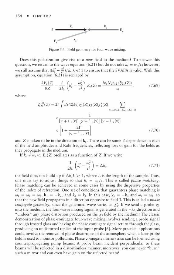
154 CHAPTER 7
E1
k1 k2
k3E3
E2
Figure 7.4. Field geometry for four-wave mixing.
Does this polarization give rise to a new field in the medium? To answer thisquestion, we return to the wave equation (6.21) but do not take ks = ωs/c; however,we still assume that |(k2s − ω2
sc2 )/ks |λ 1 to ensure that the SVAPA is valid. With this
assumption, equation (6.21) is replaced by
∂Es(Z)∂Z
− i2ks
(k2s − ω2
s
c2
)Es(Z) = iksNµ12 〈21(Z)〉
ε0, (7.69)
where
(3)21 (Z) = 2i
∫dvW0(v)χ1(Z)χ2(Z)χ∗
3 (Z)∑
µ,ν,σ=(1,3,2),(2,3,1)
× 1[γ + iδs(v)]
[γ + iδµ(v)
][γ − iδν(v)]
×[1 + 2
γ2 + iδµν(v)
](7.70)
and Z is taken to be in the direction of ks . There can be some Z dependence in eachof the field amplitudes and Rabi frequencies, reflecting loss or gain for the fields asthey propagate in the medium.
If ks = ωs/c, Es(Z) oscillates as a function of Z. If we write
12ks
(k2s − ω2
s
c2
)= ks, (7.71)
the field does not build up if ksL 1, where L is the length of the sample. Thus,one must try to adjust things so that ks = ωs/c. This is called phase matching.Phase matching can be achieved in some cases by using the dispersive propertiesof the index of refraction. One set of conditions that guarantees phase matching isω1 = ω2 = ω3, k1 = −k2, and k3 = k1. In this case, ks = −k3 and ωs = ω3, sothat the new field propagates in a direction opposite to field 3. This is called a phaseconjugate geometry, since the generated wave varies as χ∗
3 . If we send a probe χ3into the medium, the four-wave mixing signal is generated in the −k3 direction and“undoes” any phase distortion produced on the χ3 field by the medium! The classicdemonstration of phase-conjugate four-wave mixing involves sending a probe signalthrough frosted glass and having the phase conjugate signal return through the glass,producing an undistorted replica of the input probe [6]. More practical applicationscould involve the removal of phase distortions of the atmosphere when a laser probefield is used to monitor pollutants. Phase conjugate mirrors also can be formed usingcounterpropagating pump beams. A probe beam incident perpendicular to thesebeams will be reflected in a distortionless manner; moreover, you can never “burn”such a mirror and can even have gain on the reflected beam!
TWO-LEVEL ATOMS IN TWO OR MORE FIELDS 155
If fields 1 and 2 are strong, and if depletion of the pump fields can be neglected,then the coupled equations for the probe and signal field are of the form
∂Es(Z)∂Z
= AE∗3(Z) − α(1)s Es(Z), (7.72a)
∂E∗3(Z)∂Z
= BEs(Z) − α(1)3 E3(Z), (7.72b)
where A and B are proportional to the pump field intensity, and we have addedin terms representing the linear absorption of these fields. These equations can besolved, subject to the conditions E∗
3(Z = 0) = constant and Es(Z = L) = 0 (seereference [7]).
Last, we note that the two contributions in the sum in equation (7.70) can begiven a simple physical interpretation. The term with (µ, ν, σ ) = (1,3,2) corres-ponds to fields 1 and 3, forming a grating off which field 2 scatters in the ksdirection, while the term with (µ, ν, σ ) = (1,3,2) corresponds to fields 2 and 3,forming a grating off which field 1 scatters in the ks direction. In the limit that k1and k3 subtend a small angle, both terms (µ, ν, σ ) = (1,3,2), (2,3,1) contribute forstationary atoms or for δ ku, since the velocity average is unimportant in theselimits. On the other hand, if one is in the Doppler limit, only the “forward grating,”(µ, ν, σ ) = (1,3,2), is nonvanishing when the velocity average is taken.
Problems
1. Kerr effect. Extend the calculation of linear absorption for stationary atomsgiven in the text to include the lowest order nonlinear corrections to thepolarization—that is, include terms in the polarization up to order χ3.Calculate the index of refraction to order χ2, and show that if the incidentbeam has a Gaussian transverse profile, it is possible for the medium to focusthe laser field. This is referred to as self-focusing and occurs if the index effectis sufficiently large to overcome diffraction effects.
2. Derive equations (7.10) and (7.14).3. Consider a pump–probe experiment in which two fields drive a two-level
transition in an atomic beam. The propagation vectors of both fields areperpendicular to the beam such that k1 · v = k2 · v = 0. The field frequenciesare ω1 = ω and ω2 = ω+, and the detuning of the first field is δ1 = ω0 −ω1.Calculate the steady-state value (steady state means that all transients havedied away) of 12 to order |χ1|2χ∗
2 . Consider the limit in which |δ1| γ . Tothis order in |χ1|2χ∗
2 , 12 varies as 12 exp[−ik2 · R + iω2t]. Show that thereis a dispersive-like structure in the probe absorption spectrum [proportionalto Im(12/χ∗
2 )] centered at = 0 and that the linear absorption resonance atδ2 = 0 ( = −δ1) is slightly pulled toward = 0. Moreover, show that if γ =γ2/2 (as it would if the only relaxation was produced by spontaneous decay),the dispersion-like resonance vanishes. The appearance of the resonance at = 0 when collisions are present (so that γ2 = 2γ ) has been referred to aspressure-induced extra resonances (see reference [1]).
4–5. Now repeat the calculation of problem 3 to all orders in χ1 and to first orderin χ∗
2 . To do this, expand each density matrix element as i j = (0)i j +
(1)i j ,
156 CHAPTER 7
where (0)i j is zeroth order in χ∗2 , and
(1)i j is first order in χ∗
2—that is, deriveequation (7.64). Plot Im(b12/χ∗
2 ) as a function of for δ1 = 0, |χ1| γ
and for |δ1| γ, |χ1|. In the latter case, show that there are resonances at = 0,±δ1. The absorption at = −δ1 and gain at = δ1 can be explainedeasily in terms of semiclassical dressed states if you care to try.
6. Consider two counterpropagating fields incident on a vapor. Take bothfields polarized in the x direction so that the total field component in thisdirection is
E = E+ cos(kZ− ωt) + E− cos(kZ+ ωt), E± real.
Show that the time-averaged intensity of this field has a spatially varying partthat varies as E+E− cos(2kZ). These fields interact with an ensemble of two-level atoms. To second order in the field amplitudes, show that the populationdifference 22 − 11 has a spatially varying part that can be written asAcos(2kZ+ ξ ), where A and ξ are real. Calculate A and ξ as a function of kvz,and show that this spatial grating is phase shifted from the incident spatialvariation of the field intensity by an amount ξ that depends on the atomicvelocity.
7–8. For the field of problem 6, the population difference N = 22 − 11 can beexpanded as N= 22−11 = ∑∞
n=−∞ Nn exp(2inkZ), where Nn = N∗−n. Derive
coupled Maxwell-Bloch equations for the field amplitudes E±, and show thatthey depend only on N0 and N±1. Writing N1 = Aei(ξ+φ), where A and ξ arereal and φ = Arg(χ+) − Arg(χ−), determine the conditions on ξ and δ forthere to be an amplification of field E+ at the expense of E−. (Assume that|δ| kv, γ throughout this problem.) To second order in the field amplitudes,show that there can be gain for one of the fields if γ = γ2/2, but not ifγ = γ2/2. Using this result, prove that the atoms are cooled for δ < 0 as aresult of the back-scattering of the fields if γ = γ2/2.
9. Suppose that you have a ground-state density of stationary atoms given by11(Z) = cos2(kZ) in a sample of length L. A plane wave is incident in thepositive Z direction. Show that there is a propagating wave that is generatedin the sample that is directed in the −Z direction. (Hint: Use the Maxwell-Bloch equations.) Neglecting absorption, calculate the amplitude of the wavethat exits the entrance face of the sample, assuming that the density in thesample is equal to N .
10. Evaluate the integrals (7.46) and (7.47) exactly in terms of the plasmadispersion or complex error function. By evaluating these expressions, showthat in the Doppler limit (7.33), the results agree with those derived in thetext. Neglect collisions in the grating term.
11. In the Doppler limit, calculate the contribution to the probe absorption signalthat is first order in the pump field intensity and when the pump field hasfrequency ω1 and the probe field frequency is varied. Assume that the fields arecounterpropagating and that the grating term still vanishes. Show that this con-tribution to the absorption coefficient is a minimum (maximum negative ab-sorption) when ω2 = 2ω0−ω1, but that the width of the resonance is 4γ ratherthan 2γ , as we found in saturated absorption with a standing-wave field of agiven frequency. Interpret the result in terms of a simple hole-burning model.
TWO-LEVEL ATOMS IN TWO OR MORE FIELDS 157
12. Repeat problem 11 for a solid. Take γ = γ2/2, and show that the gratingterm is nonvanishing when an integral over the inhomogeneous frequencydistribution is taken. Moreover, show that the grating term can have a signopposite to that of the saturation term for some detunings.
13. Show that, in the Doppler limit, only one of the terms in equation (7.70)contributes, and explain this result in terms of the gratings that are formed inthe medium. Assume that fields 1 and 3 are nearly copropagating. On the otherhand, show that for either stationary atoms, or for detunings much largerthan the Doppler widths, both terms in the sum contribute. Neglect collisions.
References
[1] For a review, see L. Rothberg, Dephasing-induced coherence phenomena, in Progress inOptics XXIV, edited by E. Wolf (Elsevier Scientific, Amsterdam, 1987), pp. 39–101.
[2] W. R. Bennett Jr., Hole burning effects in a He-Ne optical maser, Physical Review 126,580–593 (1962).
[3] W. E. Lamb Jr., Theory of an optical maser, Physical Review 134, A1429–A1450 (1964).[4] D. G. Steel and S. C. Rand, Ultranarrow nonlinear optical resonances in solids, Physical
Review Letters 55, 2285–2288 (1985).[5] G. Grynberg and C. Cohen-Tannoudji, Central resonance of the Mollow absorption
spectrum: physical origin of gain without population inversion, Optics Communications96, 150–163 (2000); P. R. Berman and G. Khitrova, Theory of pump-probe spectroscopyusing an amplitude approach, Optics Communications 179, 19–27 (2000).
[6] For a review, see D. L. Pepper, in Laser Handbook, vol. 4, edited by M. I. Stich andM. Bass (Elsevier Science, Amsterdam, 1985), pp. 333–485; D. L. Pepper, Applicationsof optical phase conjugation, Scientific American 254, 74–83 (1986); R. L. Abrams,J. F. Lam, R. C. Lind, D. G. Steel, and P. F. Liao, Phase conjugation and high-resolutionspectroscopy by resonant degenerate four-wave mixing, in Optical Phase Conjugation(Academic Press, New York, 1983), pp. 211–284.
[7] R. L. Abrams and R. L. Lind, Degenerate four-wave mixing in absorbing media, OpticsLetters 2, 94–96 (1978); 3, 205, errata (1978).
Bibliography
In addition to the books listed in chapter 1, the following is a nonexhaustive list of some earlyarticles on nonlinear spectroscopy of two-level atoms:
G. S. Agarwal, Absorption spectra of strongly driven two-level atoms, Physical Review A 19,923–924 (1979).
E. V. Baklanov and V. P. Chebotaev, Effects of fields in resonant interaction of opposingwaves in a gas I, Soviet Physics–JETP 33, 300–308 (1971).
———, Resonance interaction of unidirectional waves in gases, Soviet Physics–JETP 34, 490–494 (1972).
R. W. Boyd and S. Mukamel,Origin of spectral holes in pump-probe studies of homogenouslybroadened lines, Physical Review A 29, 1973–1983 (1984).
158 CHAPTER 7
V. P. Chebotaev and V. S. Letokhov, Nonlinear narrow optical resonances induced by laserradiation, Progress in Quantum Electronics 4, 111–206 (1975).
M. Gruneisen, K. Macdonald, and R. W. Boyd, Induced gain and modified absorption ofa weak probe beam in a strongly driven sodium vapor, Journal of the Optical Society ofAmerica B 5, 123–128 (1988).
J. L. Hall, The lineshape problem in laser saturated molecular absorption, in Lectures inTheoretical Physics XII, edited by K. T. Mahahthappa and W. E. Brittin (Gordon andBreach, New York, 1970), pp. 161–210.
S. Haroche and F. Hartmann, Theory of saturated-absorption line shapes, Physical Review A6, 1280–1300 (1972).
L. W. Hillman, R. W. Boyd, J. Krasinski, and C. R. Stroud Jr., Observation of a spectralhole due to population oscillations in a homogenously broadened optical absorption line,Optics Communications 45, 416–419 (1983).
G. Khitrova, P. R. Berman, and M. Sargent III, Theory of pump-probe spectroscopy, Journalof the Optical Society of America B 5, 160–170 (1988).
B. R. Mollow, Stimulated emission and absorption near resonance for driven systems, PhysicalReview A 5, 2217–2222 (1972).
M. Sargent III, Spectroscopic techniques based on Lamb’s laser theory, Physics Reports 43,223–265 (1978).
M. Sargent III and P. E. Toschek, Unidirectional saturation spectroscopy II: general lifetimes,interpretations, and analogies, Applied Physics 11, 107–120 (1976).
J. H. Shirley, Semiclassical theory of saturated absorption in gases, Physical Review A 8,347–368 (1973).
S. Stenholm, Theoretical foundations of laser spectroscopy, Physics Reports 43, 151–221(1978).
Yu. A. Vdovin, V. M. Ermachenko, A. I. Popov, and E. D. Protsenko, Observation of finestructure within the limits of homogenous line width, JETP Letters 15, 282–284 (1972).
F. Y. Wu, S. Ezekiel, M. Ducloy, and B. R. Mollow,Observation of amplification in a stronglydriven two-level atomic system at optical frequencies, Physical Review Letters 38, 1077–1080 (1977).
For discussions of four-wave mixing, including additional references, see:
R. L. Abrams, J. F. Lam, R. C. Lind, D. G. Steel, and P. F. Liao, Phase conjugation andhigh-resolution spectroscopy by resonant degenerate four-wave mixing, in Optical PhaseConjugation (Academic Press, New York, 1983), pp. 211–284.
P. Meystre and M. Sargent III, Elements of Quantum Optics, 3rd ed. (Springer-Verlag, Berlin,1998), chap. 10.
Y. R. Shen, The Principles of Nonlinear Optics (Wiley-Interscience, New York, 1984),chaps. 14 and 15.
8Three-Level Atoms:Applications to Nonlinear Spectroscopy—OpenQuantum Systems
Wenow broaden our horizons and add another level to our atom. As you will see,even for the limited examples presented in this and the next chapter, the addition of athird level opens new vistas. New and important atom–field dynamics appear whena three-level atom interacts with two or more optical fields. Often, one field drives agiven transition in the atom to prepare or dress the atom, while a second field drivesa coupled transition to exploit the state of the atom that has been prepared by thefirst field.
8.1 Hamiltonian for , V, and Cascade Systems
The prototypical system consists of a three-level atom interacting with two travelingwave fields. This system has received a great deal of attention in recent years, owingto applications involving adiabatic transfer of population, lasing without inversion,dark states, coherent population trapping, laser cooling, and slow light. The originalinterest in such systems was for nonlinear spectroscopy—elimination of the Dopplerwidth [1, 2].
There are, in effect, three types of three-level schemes, and these are shown infigure 8.1. We refer to these level schemes as the cascade, V, and configurations,respectively. Two fields,
E(R, t) = 12
ε[E(R, t)ei(k·R−ωt) + E(R, t)∗e−i(k·R−ωt)
], (8.1a)
E′(R, t) = 12
ε′[E′(R, t)ei(k
′ ·R−ω′t) + E′(R, t)∗e−i(k′ ·R−ω′t)
], (8.1b)
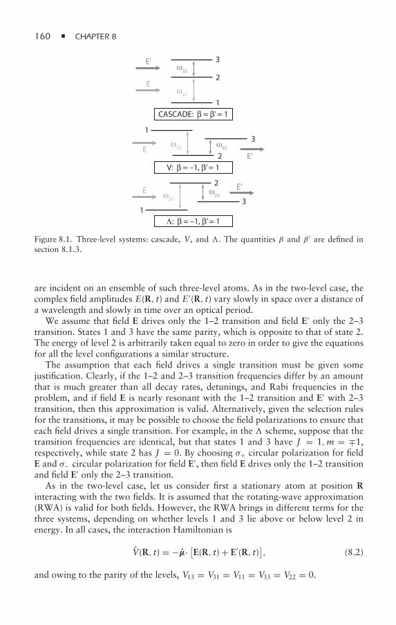
160 CHAPTER 8
E'
E
ω32
ω21
3
3
3
2
2
2
1
1
1
CASCADE: β = β’ = 1
V: β = –1, β’ = 1
Λ: β = –1, β’ = 1
E'
E'
E
E
ω32ω12
ω23ω21
Figure 8.1. Three-level systems: cascade, V, and . The quantities β and β ′ are defined insection 8.1.3.
are incident on an ensemble of such three-level atoms. As in the two-level case, thecomplex field amplitudes E(R, t) and E′(R, t) vary slowly in space over a distance ofa wavelength and slowly in time over an optical period.
We assume that field E drives only the 1–2 transition and field E′ only the 2–3transition. States 1 and 3 have the same parity, which is opposite to that of state 2.The energy of level 2 is arbitrarily taken equal to zero in order to give the equationsfor all the level configurations a similar structure.
The assumption that each field drives a single transition must be given somejustification. Clearly, if the 1–2 and 2–3 transition frequencies differ by an amountthat is much greater than all decay rates, detunings, and Rabi frequencies in theproblem, and if field E is nearly resonant with the 1–2 transition and E′ with 2–3transition, then this approximation is valid. Alternatively, given the selection rulesfor the transitions, it may be possible to choose the field polarizations to ensure thateach field drives a single transition. For example, in the scheme, suppose that thetransition frequencies are identical, but that states 1 and 3 have J = 1,m = ∓1,respectively, while state 2 has J = 0. By choosing σ+ circular polarization for fieldE and σ− circular polarization for field E′, then field E drives only the 1–2 transitionand field E′ only the 2–3 transition.
As in the two-level case, let us consider first a stationary atom at position Rinteracting with the two fields. It is assumed that the rotating-wave approximation(RWA) is valid for both fields. However, the RWA brings in different terms for thethree systems, depending on whether levels 1 and 3 lie above or below level 2 inenergy. In all cases, the interaction Hamiltonian is
V(R, t) = −µ· [E(R, t) + E′(R, t)], (8.2)
and owing to the parity of the levels, V13 = V31 = V11 = V33 = V22 = 0.
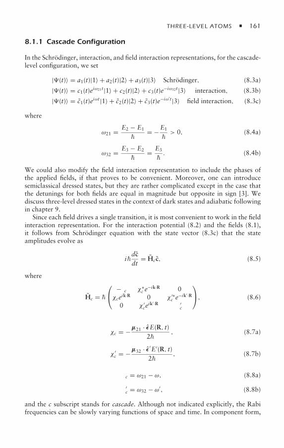
THREE-LEVEL ATOMS 161
8.1.1 Cascade Configuration
In the Schrödinger, interaction, and field interaction representations, for the cascade-level configuration, we set
|(t)〉 = a1(t)|1〉 + a2(t)|2〉 + a3(t)|3〉 Schrödinger, (8.3a)
|(t)〉 = c1(t)eiω21t|1〉 + c2(t)|2〉 + c3(t)e−iω32t|3〉 interaction, (8.3b)
|(t)〉 = c1(t)eiωt|1〉 + c2(t)|2〉 + c3(t)e−iω′t|3〉 field interaction, (8.3c)
where
ω21 = E2 − E1
= −E1
> 0, (8.4a)
ω32 = E3 − E2
= E3
. (8.4b)
We could also modify the field interaction representation to include the phases ofthe applied fields, if that proves to be convenient. Moreover, one can introducesemiclassical dressed states, but they are rather complicated except in the case thatthe detunings for both fields are equal in magnitude but opposite in sign [3]. Wediscuss three-level dressed states in the context of dark states and adiabatic followingin chapter 9.
Since each field drives a single transition, it is most convenient to work in the fieldinteraction representation. For the interaction potential (8.2) and the fields (8.1),it follows from Schrödinger equation with the state vector (8.3c) that the stateamplitudes evolve as
idcdt
= Hcc, (8.5)
where
Hc = ⎛⎝ −δc χ∗
c e−ik·R 0
χceik·R 0 χ ′∗c e
−ik′ ·R
0 χ ′ce
ik′ ·R δ′c
⎞⎠, (8.6)
χc = −µ21 · εE(R, t)2
, (8.7a)
χ ′c = −µ32 · ε′E′(R, t)
2, (8.7b)
δc = ω21 − ω, (8.8a)
δ′c = ω32 − ω′, (8.8b)
and the c subscript stands for cascade. Although not indicated explicitly, the Rabifrequencies can be slowly varying functions of space and time. In component form,
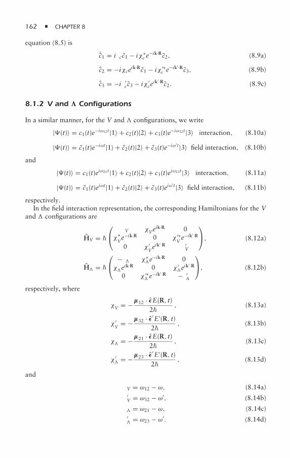
162 CHAPTER 8
equation (8.5) is
˙c1 = iδcc1 − iχ∗c e
−ik·Rc2, (8.9a)
˙c2 = −iχceik·Rc1 − iχ ′∗c e
−ik′ ·Rc3, (8.9b)
˙c3 = −iδ′cc3 − iχ ′ce
ik′ ·Rc2. (8.9c)
8.1.2 V and Configurations
In a similar manner, for the V and configurations, we write
|(t)〉 = c1(t)e−iω12t|1〉 + c2(t)|2〉 + c3(t)e−iω32t|3〉 interaction, (8.10a)
|(t)〉 = c1(t)e−iωt|1〉 + c2(t)|2〉 + c3(t)e−iω′t|3〉 field interaction, (8.10b)
and
|(t)〉 = c1(t)eiω21t|1〉 + c2(t)|2〉 + c3(t)eiω23t|3〉 interaction, (8.11a)
|(t)〉 = c1(t)eiωt|1〉 + c2(t)|2〉 + c3(t)eiω′t|3〉 field interaction, (8.11b)
respectively.In the field interaction representation, the corresponding Hamiltonians for the V
and configurations are
HV = ⎛⎝ δV χVe
ik·R 0χ
∗Ve−ik·R 0 χ ′∗
Ve−ik′ ·R
0 χ ′Veik
′ ·R δ′V
⎞⎠, (8.12a)
H = ⎛⎝ −δ χ∗
e−ik·R 0
χeik·R 0 χ ′
eik′ ·R
0 χ ′∗ e
−ik′ ·R −δ′
⎞⎠, (8.12b)
respectively, where
χV = −µ12 · εE(R, t)2
, (8.13a)
χ ′V
= −µ32 · ε′E′(R, t)2
, (8.13b)
χ = −µ21 · εE(R, t)2
, (8.13c)
χ ′ = −µ23 · ε′E′(R, t)
2, (8.13d)
and
δV = ω12 − ω, (8.14a)
δ′V = ω32 − ω′, (8.14b)
δ = ω21 − ω, (8.14c)
δ′ = ω23 − ω′. (8.14d)
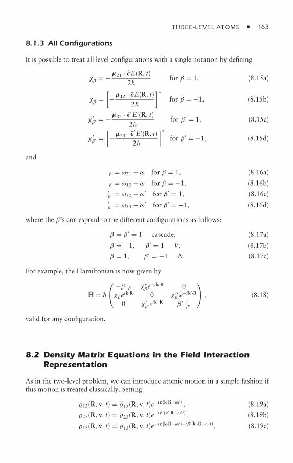
THREE-LEVEL ATOMS 163
8.1.3 All Configurations
It is possible to treat all level configurations with a single notation by defining
χβ = −µ21 · εE(R, t)2
for β = 1, (8.15a)
χβ =[−µ12 · εE(R, t)
2
]∗for β = −1, (8.15b)
χ ′β ′ = −µ32 · ε′E′(R, t)
2for β ′ = 1, (8.15c)
χ ′β ′ =
[−µ23 · ε′E′(R, t)
2
]∗for β ′ = −1, (8.15d)
and
δβ = ω21 − ω for β = 1, (8.16a)
δβ = ω12 − ω for β = −1, (8.16b)
δ′β ′ = ω32 − ω′ for β ′ = 1, (8.16c)
δ′β ′ = ω23 − ω′ for β ′ = −1, (8.16d)
where the β’s correspond to the different configurations as follows:
β = β ′ = 1 cascade, (8.17a)
β = −1, β ′ = 1 V, (8.17b)
β = 1, β ′ = −1 . (8.17c)
For example, the Hamiltonian is now given by
H = ⎛⎝ −βδβ χ∗
βe−ik·R 0
χβeik·R 0 χ ′∗
β ′e−ik′ ·R
0 χ ′β ′eik
′ ·R β ′δ′β ′
⎞⎠ , (8.18)
valid for any configuration.
8.2 Density Matrix Equations in the Field InteractionRepresentation
As in the two-level problem, we can introduce atomic motion in a simple fashion ifthis motion is treated classically. Setting
12(R, v, t) = 12(R, v, t)e−iβ(k·R−ωt) , (8.19a)
23(R, v, t) = 23(R, v, t)e−iβ ′(k′·R−ω′t) , (8.19b)
13(R, v, t) = 13(R, v, t)e−iβ(k·R−ωt)−iβ ′(k′·R−ω′t), (8.19c)
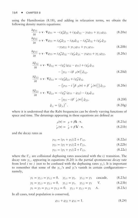
164 CHAPTER 8
using the Hamiltonian (8.18), and adding in relaxation terms, we obtain thefollowing density matrix equations:
∂11
∂t+ v · ∇11 = −iχ∗
β 21 + iχβ12 − γ111 + γ2,122, (8.20a)
∂22
∂t+ v · ∇22 = iχ∗
β 21 − iχβ12 − iχ ′∗β ′ 32 + iχ ′
β ′ 23
−γ222 + γ1,211 + γ3,233, (8.20b)∂33
∂t+ v · ∇33 = iχ ′∗
β ′ 32 − iχ ′β ′ 23 − γ333 + γ2,322, (8.20c)
∂12
∂t+ v · ∇12 = −iχ∗
β (22 − 11) + iχ ′β ′ 13
− [γ12 − iβδβ (v)
]12, (8.20d)
∂13
∂t+ v · ∇13 = −iχ∗
β 23 + iχ ′∗β ′ 12
−γ13 − i
[βδβ(v) + β ′δ′β ′(v)
]13, (8.20e)
∂23
∂t+ v · ∇23 = −iχ ′∗
β ′ (33 − 22) − iχβ13
− [γ23 − iβ ′δ′β ′(v)
]23, (8.20f)
i j = ( j i
)∗, (8.20g)
where it is understood that the Rabi frequencies can be slowly varying functions ofspace and time. The detunings appearing in these equations are defined as
δβ(v) = δβ + βk · v, (8.21a)
δ′β ′(v) = δ′β + β ′k′ · v, (8.21b)
and the decay rates as
γ12 = (γ1 + γ2)/2 + 12, (8.22a)
γ23 = (γ2 + γ3)/2 + 23, (8.22b)
γ13 = (γ1 + γ3)/2 + 13, (8.22c)
where the i j are collisional dephasing rates associated with the i j transition. Thedecay rate γi, j appearing in equations (8.20) is the partial spontaneous decay ratefrom level i to j (not to be confused with the dephasing rates γi j ). It is importantto remember that some of the γi, j ’s and γi ’s vanish in certain configurations—namely,
γ1 = γ2,3 = γ1,2 = 0, γ2,1 = γ2, γ3,2 = γ3 cascade, (8.23a)
γ2 = γ2,3 = γ2,1 = 0, γ1,2 = γ1, γ3,2 = γ3 V, (8.23b)
γ1 = γ3 = γ1,2 = γ3,2 = 0, γ2,1 + γ2,3 = γ2 . (8.23c)
In all cases, total population is conserved,
11 + 22 + 33 = 1. (8.24)
THREE-LEVEL ATOMS 165
It might seem that the collision rates, 12, 23, and 13, are independentparameters, but this is not the case. In fact, putting in arbitrary values for theseparameters can lead to negative populations [4]! The interdependence of the collisionrates can be seen using a simple example. If the collisional interaction is the same forlevels 2 and 3, then 23 = 0 and 13 = 12, since the collision-induced phase shiftsare identical for the state amplitudes 2 and 3.
8.3 Steady-State Solutions—Nonlinear Spectroscopy
Equations (8.20) must be solved numerically when the Rabi frequencies arefunctions of time. In the case of constant Rabi frequencies, however, one can solvethese equations in steady state by setting the entire left-hand side of the equationsequal to zero. One is faced with solving eight linear equations for the density matrixelements since one of the populations can be eliminated using condition (8.24).Symbolic computer programs such as Mathematica have no problem in obtaininganalytic expressions for the steady-state density matrix elements, but they are toolengthy to display here. Moreover, any averaging over the velocity distribution muststill be carried out numerically.
Once solutions are obtained, the field absorption coefficients can be obtainedfrom the steady-state solutions of the Maxwell-Bloch equations (6.25), assumingthat both fields propagate parallel to the Z axis. In that case, for fields propagatingin the z direction, one finds
∂E(Z)∂Z
= iNkµ12
ε0〈21(Z)〉 cascade, , (8.25a)
∂E(Z)∂Z
= iNkµ21
ε0〈12(Z)〉 V, (8.25b)
for field E with µi j = µi j · ε, and
∂E′(Z)∂Z
= iNkµ23
ε0〈32(Z)〉 cascade, V, (8.26a)
∂E′(Z)∂Z
= iNkµ32
ε0〈23(Z)〉 , (8.26b)
for field E′ with µi j = µi j · ε′. For fields propagating in the −z direction, the signsin these equations should be changed. We will refer to field E as the pump field andfield E′ as the probe field, although we have not yet imposed any restrictions on thestrengths of these fields.
In this section, we calculate the probe field E′ absorption coefficient for thecascade configuration in lowest order perturbation theory. The probe field absorp-tion coefficient is proportional to the imaginary part of 32, which, in turn, isproportional to 33 in steady state [see equation (8.20c)]. We leave the case of theV and configurations to the problems, although the configuration is discussedin some detail in chapter 9. Both fields propagate parallel to the Z axis, but thefields can be co- or counterpropagating. As you will see, the resulting excitationprobability offers a new nonlinear spectroscopic tool for obtaining Doppler-freespectra in vapors.
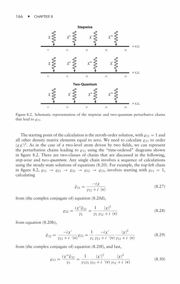
166 CHAPTER 8
ρ11 ρ21 ρ22
Stepwise
+ c.c.ρ32 ρ33
χ* χ’ χ’*χ
ρ11 ρ21 ρ31
Two-Quantum
+ c.c.ρ32 ρ33
χ’ χ* χ’*χ
ρ11 ρ21 ρ22
+ c.c.ρ23 ρ33
χ* χ’* χ’χ
Figure 8.2. Schematic representation of the stepwise and two-quantum perturbative chainsthat lead to 33.
The starting point of the calculation is the zeroth-order solution, with 11 = 1 andall other density matrix elements equal to zero. We need to calculate 33 to order|χχ ′|2. As in the case of a two-level atom driven by two fields, we can representthe perturbation chains leading to 33 using the “time-ordered” diagrams shownin figure 8.2. There are two-classes of chains that are discussed in the following,step-wise and two-quantum. Any single chain involves a sequence of calculationsusing the steady-state solutions of equations (8.20). For example, the top-left chainin figure 8.2, 11 → 21 → 22 → 32 → 33, involves starting with 11 = 1,calculating
21 = −iχγ12 + iδ(v)
(8.27)
from (the complex conjugate of) equation (8.20d),
22 = iχ∗21γ2
= 1γ2
|χ |2γ12 + iδ(v)
(8.28)
from equation (8.20b),
32 = −iχ ′
γ23 + iδ′(v)22 = 1
γ2
−iχ ′
γ23 + iδ′(v)|χ |2
γ12 + iδ(v)(8.29)
from (the complex conjugate of) equation (8.20f), and last,
33 = iχ ′∗32γ3
= 1γ3γ2
|χ ′|2γ23 + iδ′(v)
|χ |2γ12 + iδ(v)
(8.30)
THREE-LEVEL ATOMS 167
from equation (8.20c). In these expressions,
χ = −µ21 · εE(R, t)2
, χ ′ = −µ32 · ε′E′(R, t)2
, (8.31a)
δ(v) = ω21 − ω + k · v, δ′(v) = ω32 − ω′ + k′ · v. (8.31b)
Other chains are calculated in a similar manner. In fact, it is easy to establish “rules”for calculating the contributions from these chains, if one wants. Note that thepopulations 22 and 33 appearing in equations (8.28) and (8.30), respectively, arenot real—they represent the partial contributions to these populations from thisspecific chain. Of course, when one sums the contributions from all the step-wisechains, 22 and 33 will be real and positive.
The step-wise (SW) contribution involves the sequential or step-wise absorptionof each field by the atoms and is characterized by the presence of the intermediate-state population 22. Summing up the contributions from the four chains
11 → 21 → 22 → 32 → 33,
11 → 12 → 22 → 23 → 33,
11 → 21 → 22 → 23 → 33,
11 → 12 → 22 → 32 → 33, (8.32)
of the stepwise contribution represented in figure 8.2, we find
SW33 (v) = −iχγ12 + iδ(v)
iχ∗
γ2
−iχ ′
γ23 + iδ′(v)iχ ′∗
γ3+ c.c.
+ iχ∗
γ12 − iδ(v)−iχγ2
−iχ ′
γ23 + iδ′(v)iχ ′∗
γ3+ c.c.
= 4|χχ ′|2γ2γ3
γ12
γ 212 + (δ + k · v)2
γ23
γ 223 + (δ′ + k′ · v)2 . (8.33)
As might have been expected, this contribution is just the product of the Lorentzianabsorption profile of each field acting on its respective transition. The first two linesof equation (8.33) are written in a manner that illustrates how figure 8.2 can be usedto write the perturbative result by application of some simple rules.
The two-quantum (TQ) chains do not involve the intermediate-state population;rather, the coherence 31 or 13 appears in these chains. We refer to these astwo-quantum chains since they are closely related to the type of contributionone encounters in two-photon transitions (see section 8.4); moreover, this chainis nonvanishing only if both fields are present simultaneously. Of course, wehave assumed both fields to be present simultaneously, but had we used spatiallyseparated pulsed fields, the two-quantum contribution would vanish, whereas thestep-wise terms could contribute.
The left-hand diagram of the two-quantum chain, 11 → 21 → 31 → 32 →33, can be evaluated by starting with 11 = 1, calculating
21 = −iχγ12 + iδ(v)
(8.34)
168 CHAPTER 8
from (the complex conjugate of) equation (8.20d),
31 = −iχ ′21γ13 + i [δ(v) + δ′(v)] (8.35)
from (the complex conjugate) of equation (8.20e),
32 = iχ∗
γ23 + iδ′(v)31 (8.36)
from (the complex conjugate of) equation (8.20f), and last,
33 = iχ ′∗32γ3
(8.37)
from equation (8.20c).Summing the two chains
11 → 21 → 31 → 32 → 33,
11 → 12 → 13 → 23 → 33, (8.38)
of the two-quantum contribution shown in figure 8.2, we obtain
TQ33 (v) = −iχ
γ12 + iδ(v)−iχ ′
γ13 + i [δ(v) + δ′(v)]× iχ∗
γ23 + iδ′(v)iχ ′∗
γ3+ c.c.,
= |χχ ′|2γ3
1γ12 + i(δ + k · v)
1γ23 + i(δ′ + k′ · v)
× 1γ13 + i [δ + δ′ + (k + k′) · v] + c.c. (8.39)
If we look at equations (8.33) and (8.39), it would appear that, for fixed δ, thereare resonances when δ′ = 0 or δ + δ′ = 0 (for v = 0). However, if all the collisionrates vanish, we can combine terms to obtain
33(v) = SW33 (v) + TQ33 (v)
= |χχ ′|2[(γ2/2)2 + (δ + k · v)2] (γ3/2)2 + [δ + δ′ + (k + k′) · v]2
. (8.40)
The resonance at δ′ = 0 has vanished! There is a simple physical interpretationof this result. In lowest order perturbation theory, the transition from state 1 to3 is really a two-photon process, provided that there are no collisions or othermechanism to give energy to or take energy from the system. As such, the widthassociated with this transition depends only on the widths of the initial and finalstates, and not on the width of the intermediate-state 2.
To get the line shape
I =∫dv33(v)W0(v) (8.41)
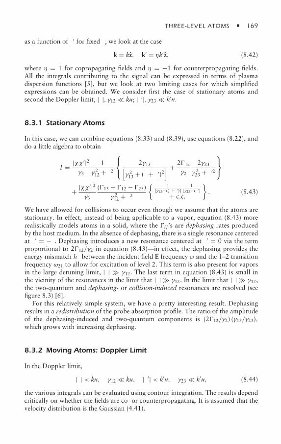
THREE-LEVEL ATOMS 169
as a function of δ′ for fixed δ, we look at the case
k = kz, k′ = ηk′z, (8.42)
where η = 1 for copropagating fields and η = −1 for counterpropagating fields.All the integrals contributing to the signal can be expressed in terms of plasmadispersion functions [5], but we look at two limiting cases for which simplifiedexpressions can be obtained. We consider first the case of stationary atoms andsecond the Doppler limit, |δ|, γ12 ku; |δ′|, γ23 k′u.
8.3.1 Stationary Atoms
In this case, we can combine equations (8.33) and (8.39), use equations (8.22), anddo a little algebra to obtain
I = |χχ ′|2γ3
1γ 212 + δ2
⎧⎨⎩ 2γ13[γ 213 + (δ + δ′)2
] + 212
γ2
2γ23γ 223 + δ′2
⎫⎬⎭
+ |χχ ′|2γ3
(13 + 12 − 23)γ 212 + δ2
1[γ13−i(δ+δ′)]
1(γ23−iδ′)
+ c.c.
. (8.43)
We have allowed for collisions to occur even though we assume that the atoms arestationary. In effect, instead of being applicable to a vapor, equation (8.43) morerealistically models atoms in a solid, where the i j ’s are dephasing rates producedby the host medium. In the absence of dephasing, there is a single resonance centeredat δ′ = −δ. Dephasing introduces a new resonance centered at δ′ = 0 via the termproportional to 212/γ2 in equation (8.43)—in effect, the dephasing provides theenergy mismatch δ between the incident field E frequency ω and the 1–2 transitionfrequency ω21 to allow for excitation of level 2. This term is also present for vaporsin the large detuning limit, |δ| γ12. The last term in equation (8.43) is small inthe vicinity of the resonances in the limit that |δ| γ12. In the limit that |δ| γ12,the two-quantum and dephasing- or collision-induced resonances are resolved (seefigure 8.3) [6].
For this relatively simple system, we have a pretty interesting result. Dephasingresults in a redistribution of the probe absorption profile. The ratio of the amplitudeof the dephasing-induced and two-quantum components is (212/γ2) (γ13/γ23),which grows with increasing dephasing.
8.3.2 Moving Atoms: Doppler Limit
In the Doppler limit,
|δ| < ku, γ12 ku, |δ′| < k′u, γ23 k′u, (8.44)
the various integrals can be evaluated using contour integration. The results dependcritically on whether the fields are co- or counterpropagating. It is assumed that thevelocity distribution is the Gaussian (4.41).
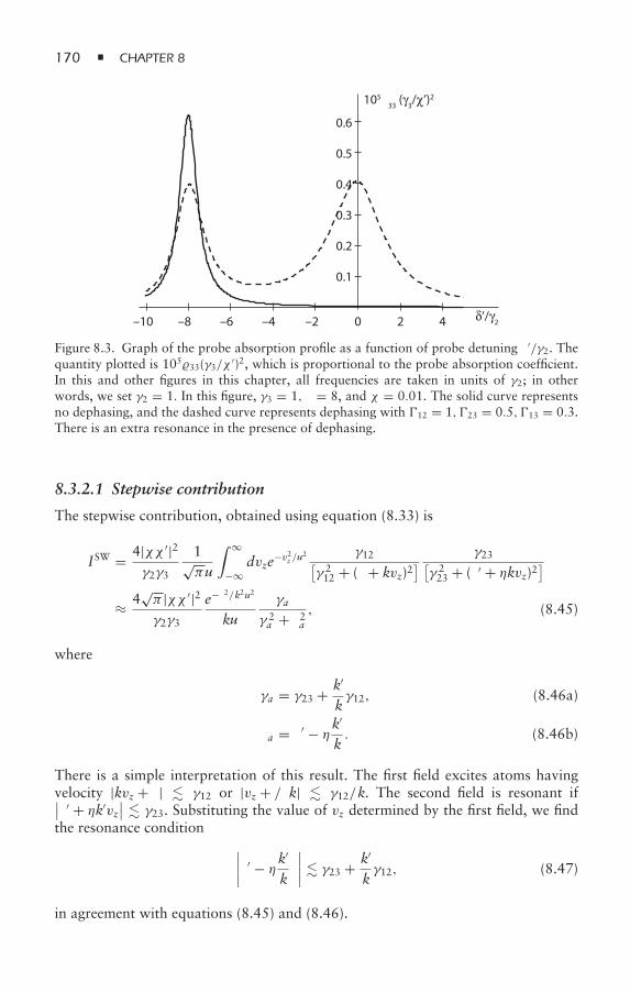
170 CHAPTER 8
0.1
0.2
0.5
0.6
–10 –8 –6 –4 –2 20 4 δ’/γ2
105ρ33 (γ3/χ’)2
0.4
0.3
Figure 8.3. Graph of the probe absorption profile as a function of probe detuning δ′/γ2. Thequantity plotted is 10533(γ3/χ ′)2, which is proportional to the probe absorption coefficient.In this and other figures in this chapter, all frequencies are taken in units of γ2; in otherwords, we set γ2 = 1. In this figure, γ3 = 1, δ = 8, and χ = 0.01. The solid curve representsno dephasing, and the dashed curve represents dephasing with 12 = 1, 23 = 0.5, 13 = 0.3.There is an extra resonance in the presence of dephasing.
8.3.2.1 Stepwise contribution
The stepwise contribution, obtained using equation (8.33) is
ISW = 4|χχ ′|2γ2γ3
1√πu
∫ ∞
−∞dvze−v2z /u2 γ12[
γ 212 + (δ + kvz)2
] γ23[γ 223 + (δ′ + ηkvz)2
]≈ 4
√π |χχ ′|2γ2γ3
e−δ2/k2u2
kuγa
γ 2a + δ2a
, (8.45)
where
γa = γ23 + k′
kγ12, (8.46a)
δa = δ′ − ηk′
kδ. (8.46b)
There is a simple interpretation of this result. The first field excites atoms havingvelocity |kvz + δ| γ12 or |vz + δ/k| γ12/k. The second field is resonant if∣∣δ′ + ηk′vz
∣∣ γ23. Substituting the value of vz determined by the first field, we findthe resonance condition ∣∣∣∣δ′ − ηk′
kδ
∣∣∣∣ γ23 + k′
kγ12, (8.47)
in agreement with equations (8.45) and (8.46).
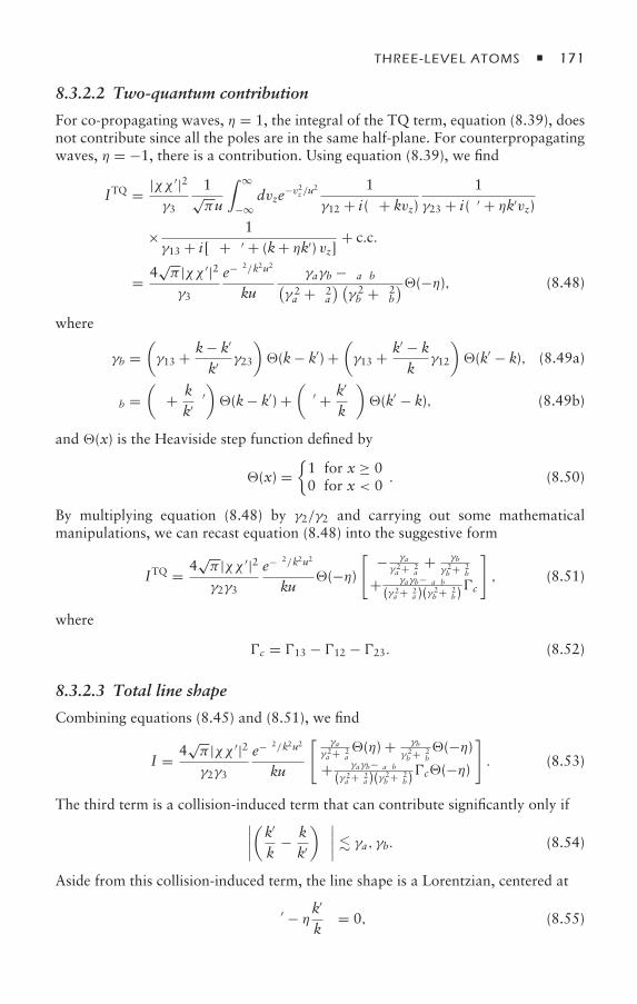
THREE-LEVEL ATOMS 171
8.3.2.2 Two-quantum contribution
For co-propagating waves, η = 1, the integral of the TQ term, equation (8.39), doesnot contribute since all the poles are in the same half-plane. For counterpropagatingwaves, η = −1, there is a contribution. Using equation (8.39), we find
ITQ = |χχ ′|2γ3
1√πu
∫ ∞
−∞dvze−v2z /u2 1
γ12 + i(δ + kvz)1
γ23 + i(δ′ + ηk′vz)
× 1γ13 + i[δ + δ′ + (k+ ηk′) vz]
+ c.c.
= 4√π |χχ ′|2γ3
e−δ2/k2u2
kuγaγb − δaδb(
γ 2a + δ2a
) (γ 2b + δ2b
)(−η), (8.48)
where
γb =(γ13 + k− k′
k′ γ23
)(k− k′) +
(γ13 + k′ − k
kγ12
)(k′ − k), (8.49a)
δb =(δ + k
k′ δ′)(k− k′) +
(δ′ + k′
kδ
)(k′ − k), (8.49b)
and (x) is the Heaviside step function defined by
(x) =1 for x ≥ 00 for x < 0
. (8.50)
By multiplying equation (8.48) by γ2/γ2 and carrying out some mathematicalmanipulations, we can recast equation (8.48) into the suggestive form
ITQ = 4√π |χχ ′|2γ2γ3
e−δ2/k2u2
ku(−η)
[ − γaγ 2a +δ2a + γb
γ 2b +δ2b
+ γaγb−δaδb(γ 2
a +δ2a )(γ 2b +δ2b)
c
], (8.51)
where
c = 13 − 12 − 23. (8.52)
8.3.2.3 Total line shape
Combining equations (8.45) and (8.51), we find
I = 4√π |χχ ′|2γ2γ3
e−δ2/k2u2
ku
[ γaγ 2a +δ2a(η) + γb
γ 2b +δ2b
(−η)+ γaγb−δaδb(γ 2
a +δ2a )(γ 2b +δ2b)
c(−η)
]. (8.53)
The third term is a collision-induced term that can contribute significantly only if∣∣∣∣(k′
k− kk′
)δ
∣∣∣∣ γa, γb. (8.54)
Aside from this collision-induced term, the line shape is a Lorentzian, centered at
δ′ − ηk′
kδ = 0, (8.55)
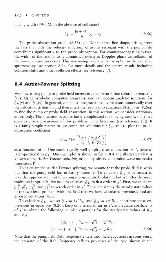
172 CHAPTER 8
having width (FWHM; in the absence of collisions)
2γ = |k+ ηk′|k
γ2 + γ3. (8.56)
The probe absorption profile (8.53) is a Doppler-free line shape, arising fromthe fact that only the velocity subgroup of atoms resonant with the pump fieldcontributes significantly to the probe absorption. For counterpropagating waves,the width of the resonance is diminished owing to Doppler phase cancellation ofthe two-quantum processes. This narrowing is related to two-photon Doppler-freespectroscopy (see section 8.4). For more details and the general result, includingcollision shifts and other collision effects, see reference [7].
8.4 Autler-Townes Splitting
With increasing pump or probe field intensities, the perturbation solution eventuallyfails. Using symbolic computer programs, one can obtain analytic solutions for21(v) and 32(v). In general, one must integrate these expressions numerically overthe velocity distribution and then insert the results into equations (8.25a) or (8.26a)to find the pump or probe field absorption. In this section, we consider stationaryatoms only. The situation becomes fairly complicated for moving atoms, but thereexist extensive discussions of this problem in the literature (see reference [8]). Itis a fairly simple matter to use computer solutions for 32 and to plot the probeabsorption coefficient
α′ = 2 Im[kµ23
ε0
⟨32(Z)E′(Z)
⟩](8.57)
as a function of δ′. One could equally well graph 33 as a function of δ′, since α′
is proportional to 33. One such plot is shown in figure 8.4 and illustrates what isknown as the Autler-Townes splitting, originally observed on microwave moleculartransitions [9].
To calculate the Autler-Townes splitting, we assume that the probe field is weakbut that the pump field has arbitrary intensity. To calculate 32, it is easiest totake the appropriate limit of a computer-generated solution, but we offer the moretraditional approach. We need to calculate 32 to first order in χ ′. First, we calculate(0)11 ,
(0)22 ,
(0)12 , and
(0)21 to zeroth order in χ ′. These are simply the steady-state values
of the two-level problem with one field that we have calculated previously and aregiven in equations (4.11).
To calculate 32, we set 32 = iχ ′R32 and 31 = iχ ′R31, substitute these ex-pressions in equations (8.20), keep only terms linear in χ ′, and equate coefficientsof χ ′ to obtain the following coupled equations for the steady-state values of R32
and R31: [γ23 + iδ′
]R32 = −(0)22 + iχ∗R31,[
γ13 + i(δ + δ′)]R31 = −(0)21 + iχR32. (8.58)
Note that the pump field Rabi frequency enters into these equations; in some sense,the presence of the Rabi frequency reflects processes of the type shown in the
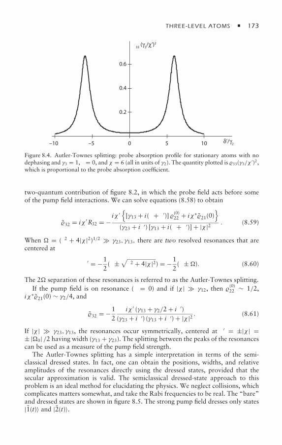
THREE-LEVEL ATOMS 173
–10 –5 50 10
0.2
0.4
0.6
δ’/γ2
ρ33 (γ3/χ’)2
Figure 8.4. Autler-Townes splitting: probe absorption profile for stationary atoms with nodephasing and γ3 = 1, δ = 0, and χ = 6 (all in units of γ2). The quantity plotted is 33(γ3/χ ′)2,which is proportional to the probe absorption coefficient.
two-quantum contribution of figure 8.2, in which the probe field acts before someof the pump field interactions. We can solve equations (8.58) to obtain
32 = iχ ′R32 = −iχ ′
[γ13 + i(δ + δ′)] (0)22 + iχ∗21(0)
(γ23 + iδ′) [γ13 + i(δ + δ′)] + |χ |2 . (8.59)
When = (δ2 + 4|χ |2)1/2 γ23, γ13, there are two resolved resonances that arecentered at
δ′ = −12(δ ±
√δ2 + 4|χ |2) = −1
2(δ ±). (8.60)
The 2 separation of these resonances is referred to as the Autler-Townes splitting.If the pump field is on resonance (δ = 0) and if |χ | γ12, then
(0)22 ∼ 1/2,
iχ∗21(0) ∼ γ2/4, and
32 = −12
iχ ′ (γ13 + γ2/2 + iδ′)(γ23 + iδ′) (γ13 + iδ′) + |χ |2 . (8.61)
If |χ | γ23, γ13, the resonances occur symmetrically, centered at δ′ = ±|χ | =± |0| /2 having width (γ13 + γ23). The splitting between the peaks of the resonancescan be used as a measure of the pump field strength.
The Autler-Townes splitting has a simple interpretation in terms of the semi-classical dressed states. In fact, one can obtain the positions, widths, and relativeamplitudes of the resonances directly using the dressed states, provided that thesecular approximation is valid. The semiclassical dressed-state approach to thisproblem is an ideal method for elucidating the physics. We neglect collisions, whichcomplicates matters somewhat, and take the Rabi frequencies to be real. The “bare”and dressed states are shown in figure 8.5. The strong pump field dresses only states|1(t)〉 and |2(t)〉.
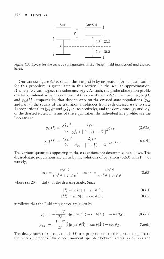
174 CHAPTER 8
Bare Dressed3
2
1
~ 3
II
I
~
~
~ (–δ – Ω)/2
(–δ + Ω)/2
δ’
–δ
Figure 8.5. Levels for the cascade configuration in the “bare” (field-interaction) and dressedbases.
One can use figure 8.5 to obtain the line profile by inspection; formal justificationfor this procedure is given later in this section. In the secular approximation, γ12, we can neglect the coherence I,I I . As such, the probe absorption profilecan be considered as being composed of the sum of two independent profiles, 33(I)and 33(I I), respectively, that depend only on the dressed-state populations (I,Iand I I,I I ), the square of the transition amplitudes from each dressed state to state3 (proportional to |χ ′
3,I |2 and |χ ′3,I I |2, respectively), and the decay rates (γI and γI I )
of the dressed states. In terms of these quantities, the individual line profiles are theLorentzians
33(I) = |χ ′3,I |2γ3
2γI3
γ 2I3 + [
δ′ + 12 (δ +)]2 I,I , (8.62a)
33(I I) = |χ ′3,I I |2γ3
2γI I3
γ 2I I3 + [
δ′ + 12 (δ −)]2 I I,I I . (8.62b)
The various quantities appearing in these equations are determined as follows. Thedressed-state populations are given by the solutions of equations (3.63) with = 0,namely,
I,I = cos4 θ
sin4 θ + cos4 θ, I I,I I = sin4 θ
sin4 θ + cos4 θ, (8.63)
where tan 2θ = |0| /δ is the dressing angle. Since
|I〉 = cos θ |1〉 − sin θ |2〉, (8.64)
|I I〉 = sin θ |1〉 + cos θ |2〉, (8.65)
it follows that the Rabi frequencies are given by
χ ′3,I = − ε′ · E′
2〈3|µ(cos θ |1〉 − sin θ |2〉) = − sin θχ ′, (8.66a)
χ ′3,I I = − ε′ · E′
2〈3|µ(sin θ |1〉 + cos θ |2〉) = cos θχ ′. (8.66b)
The decay rates of states |I〉 and |I I〉 are proportional to the absolute square ofthe matrix element of the dipole moment operator between states |I〉 or |I I〉 and
THREE-LEVEL ATOMS 175
state |1〉, respectively. As such, γI = sin2 θγ2, γI I = cos2 θγ2, and
γI3 = γI + γ32
= γ2 sin2 θ + γ32
, (8.67a)
γI I3 = γI I + γ32
= γ2 cos2 θ + γ32
. (8.67b)
When these values are substituted into equation (8.62), we find
33(I) = 2|χ ′|2γ3
γI3
γ 2I3 + [
δ′ + 12 (δ +)]2
sin2 θ cos4 θ
sin4 θ + cos4 θ, (8.68a)
33(I I) = 2|χ ′|2γ3
γI I3
γ 2I I3 + [
δ′ + 12 (δ −)]2
sin4 θ cos2 θ
sin4 θ + cos4 θ, (8.68b)
from which it follows that the relative amplitude of the two resonances is
33(I I)33(I)
= cos2 θ
sin2 θ
(γ2 sin
2 θ + γ3γ2 cos2 θ + γ3
). (8.69)
For zero pump field detuning, θ = π/4, 33(I I)/33(I) = 1, and the FWHM ofeach resonance is [(γ2/2) + γ3]. The reason that the width has a factor of γ2/2 isthat only half of each dressed state contributes to the decay. Note that the dressed-state approach has greatly simplified the problem. In the secular approximation, theabsorption profile can be written by inspection!
This approach can be justified formally. To do so, we transform the Hamil-tonian (8.6) into the dressed-state basis using
HD = THcT† = ⎛⎝− 1
2 (δ +) 0 χ ′3,I
0 12 (− δ) χ ′
3,I Iχ ′3,I χ ′
3,I I δ′
⎞⎠ , (8.70)
where
T =⎛⎝ cos θ − sin θ 0
sin θ cos θ 00 0 1
⎞⎠ , (8.71)
we have set R = 0 and used equation (8.66). Including decay (see problem 14),the relevant density matrix equations for the Hamiltonian (8.70) in the secularapproximation and to first order in χ ′ are
33 = iχ3,I I(3,I I − I I,3
)γ3
+ iχ ′3,I
(3,I − I,3
)γ3
, (8.72a)
∂I,3
∂t= iχ ′
3,II,I −γI3 − i
[δ′ + 1
2(δ +)
]I,3 , (8.72b)
∂I I,3
∂t= iχ ′
3,I II I,I I −γI I3 − i
[δ′ + 1
2(δ −)
]I I,3. (8.72c)
Solving in steady state using the values (8.63), we obtain the solution (8.68).
176 CHAPTER 8
8.5 Two-Photon Spectroscopy
When the pump field is far off resonance, |δ| γ12,ku, it is still possibleto resonantly drive transitions between levels 1 and 3 in the cascade and
configurations. (It is also possible in the V configuration if one starts in levels 1 or3 and decay is negligible.) In this limit, two-quantum processes are dominant, andone speaks of two-photon transitions. For the sake of definiteness, we consider thecascade configuration. If |δ| γ12,ku, but δ + δ′ ≈ 0, it is possible to adiabaticallyeliminate state |2〉 from the calculation and get an effective two-level probleminvolving levels 1 and 3. Although this limit can be derived from our three-levelequations, it is instructive to rederive the results so that they can be generalized tovery large detunings from a number of intermediate states.
Thus, we consider two fields driving a transition between states 1 and 3 havingthe same parity (see figure 8.6). There are other states m far off-resonance with theincident fields that have parity opposite to states 1 and 3. The states m need notlie between levels 1 and 3 and can even include continuum states. We change thenotation for the fields slightly and take
E(R, t) = 12
ε1
[E1(R, t)ei(k1·R−ω1t) + c.c.
], (8.73a)
E′(R, t) = 12
ε2
[E2(R, t)ei(k2·R−ω2t) + c.c.
], (8.73b)
where ω1 = ω and ω2 = ω′.In the interaction representation, but without making the RWA and allowing
each field to drive each transition, the equations for the probability amplitudes foran atom at the origin, in the absence of relaxation, are
c1 = −i2∑j=1
∑m
[χ( j)1me
−i(ω j−ω1m)t + χ ( j)∗1m ei(ω j+ω1m)t
]cm, (8.74a)
c3 = −i2∑j=1
∑m
[χ( j)3me
−i(ω j−ω3m)t + χ ( j)∗3m ei(ω j+ω3m)t
]cm, (8.74b)
cm = −i2∑j=1
[χ( j)m1e
−i(ω j−ωm1)t + χ ( j)∗m1 e
i(ω j+ωm1)t]c1
+[χ( j)m3e
−i(ω j−ωm3)t + χ ( j)∗m3 e
i(ω j+ωm3)t]c3, (8.74c)
where
χ ( j)mn = − 1
2〈m|µ · ε j |n〉E j, (8.75)
ωmn = (Em − En)/, and Em is the energy of state m. It is assumed that 〈m|µ · ε j |n〉is real. The reason we do not make the RWA and that we allow each field to driveboth transitions is that the frequency detunings may be sufficiently large for bothtransitions to invalidate the assumption that each field drives a single transition.
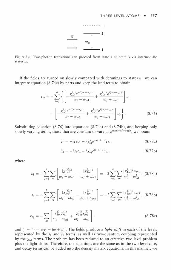
THREE-LEVEL ATOMS 177
E'
Eω31
3
m
1
Figure 8.6. Two-photon transitions can proceed from state 1 to state 3 via intermediatestates m.
If the fields are turned on slowly compared with detunings to states m, we canintegrate equation (8.74c) by parts and keep the lead term to obtain
cm ≈ −2∑j=1
[−χ
( j)m1e
−i(ω j−ωm1)t
ω j − ωm1+ χ
( j)∗m1 e
i(ω j+ωm1)t
ω j + ωm1
]c1
+[−χ
( j)m3e
−i(ω j−ωm3)t
ω j − ωm3+ χ
( j)∗m3 e
i(ω j+ωm3)t
ω j + ωm3
]c3
. (8.76)
Substituting equation (8.76) into equations (8.74a) and (8.74b), and keeping onlyslowly varying terms, those that are constant or vary as e±i(ω+ω′−ω31)t, we obtain
c1 = −is1c1 − iχ∗tqe
−i(δ+δ′)tc3, (8.77a)
c3 = −is3c3 − iχtqei(δ+δ′)tc1, (8.77b)
where
s1 = −2∑j=1
∑m
[|χ ( j)
1m|2ω j − ωm1
− |χ ( j)1m|2
ω j + ωm1
]= −2
2∑j=1
∑m
|χ ( j)1m|2ωm1
ω2j − ω2
m1
, (8.78a)
s3 = −2∑j=1
∑m
[|χ ( j)
3m|2ω j − ωm3
− |χ ( j)3m|2
ω j + ωm3
]= −2
2∑j=1
∑m
|χ ( j)3m|2ωm3
ω2j − ω2
m3
, (8.78b)
χtq = −∑m
[χ(2)3mχ
(1)m1
ω1 − ωm1+ χ
(1)3mχ
(2)m1
ω2 − ωm1
], (8.78c)
and (δ + δ′) = ω31 − (ω + ω′). The fields produce a light shift in each of the levelsrepresented by the s1 and s3 terms, as well as two-quantum coupling representedby the χtq terms. The problem has been reduced to an effective two-level problemplus the light shifts. Therefore, the equations are the same as in the two-level case,and decay terms can be added into the density matrix equations. In this manner, we
178 CHAPTER 8
obtain
∂11
∂t+ v · ∇11 = −iχ∗
tq31 + iχtq13, (8.79a)
∂33
∂t+ v ·∇33 = iχ∗
tq31 − iχtq13 − γ333, (8.79b)
∂13
∂t+ v ·∇13 = −iχ∗
tq(33 − 11) − γ1313
+ i[δ + δ′ + (k + k′) · v − s1 + s3
]13, (8.79c)
31 = (13
)∗. (8.79d)
An in term must also be included in the equation for ∂11/∂t to allow forrepopulation of this state, but it generally involves a cascaded emission throughintermediate states not shown in figure 8.6.
The two-photon absorption line shape has a Doppler width determined by|k+k′|u. If k = −k′, that is, for equal frequencies and oppositely traveling waves, theDoppler effect is totally suppressed, and the resonance width is 2γ13. The resultantline shape is referred to as a two-photon Doppler-free profile [10]. In contrast tosaturation spectroscopy, the entire velocity ensemble contributes to the line shape.The price you pay is that the transition strength is small, since the intermediate stateis far-detuned.1
For cw lasers, if χ/2π ≈ 108 Hz, the light shifts and two-photon couplingstrength is of order 10Hz if (ω j − ωm1)/2π ≈ 1015 Hz, but could be as large as1.0MHz if (ω j − ωm1)/2π ≈ 10GHz (nearly resonant intermediate state).
Some caution must be taken if equations (8.79) are used for a rather thancascade system. The problem is that γ13 is equal to zero for a scheme in whichlevels 1 and 3 are ground-state sublevels. In that case, it is necessary to include higherorder terms in the ∂13/∂t equation that correspond to off-resonant scattering of theincident fields. Such terms are included in chapter 9.
8.6 Open versus Closed Quantum Systems
It is sometimes necessary to consider open quantum systems. For example, in ourthree-level problem in the configuration, imagine that only field E is present.Eventually, all the population decays to state 3. If we take as our quantum systemlevels 1 and 2 only, there is leakage out of the system, and population is no longerconserved for the two-level subsystem. In this case, if the vapor is not replenishedwith new atoms in either states 1 or 2, the only steady state for the system isone in which all density matrix elements are equal to zero. Atoms in gas lasers
1 It was assumed implicitly in this section that the frequency of each field separately was notapproximately equal to ω31/2 so that a single field could not drive two-photon transitions on its own. Thisis no longer the case if we take ω = ω′ ≈ ω31/2, as in the case of two-photon Doppler-free spectroscopy;however, there is a large Doppler width ∼2ku associated with the two-photon transitions from each fieldseparately so that the relative contribution of these terms is small.
THREE-LEVEL ATOMS 179
provide a good example of an open quantum system. The two atomic levels betweenwhich lasing takes place are excited states that must be pumped incoherently via anelectric discharge or collisions with metastable atoms. To achieve a steady statein open quantum systems, there must be some incoherent pumping of the levels.Just as collisions led to new resonances in nonlinear spectroscopy, relaxation ratesin open quantum systems can produce similar effects. For example, in the cascadeconfiguration for stationary atoms, if level 1 has some associated decay rate, thereare always resonances centered at δ′ = −δ and δ′ = 0, even in the absence ofcollisions.
There is another new feature that arises in open quantum systems. For a closedtwo-level system, 11 can be eliminated using the fact that 11 = 1 − 22. In theremaining equations, only the decay rates γ2 and γ12 appear. As a consequence, forrelaxation effects to be discernible, they must occur on a timescale of order γ−1
2 .On the other hand, in open systems, there is a new timescale, γ−1
1 , that enters. Ifγ−11 γ−1
2 , as is often the case, the sensitivity to relaxation effects, such as ground-state velocity-changing collisions, can be increased significantly. Examples are givenin chapter 10.
A qualitatively different type of open quantum system results from atoms leavingthe interaction volume as a consequence of their motion. This loss rate is state-independent; as such, it provides an overall increase in line widths known as transit-time broadening. Transit-time broadening does not lead to additional resonances innonlinear spectroscopic line shapes.
Open quantum systems can be modeled easily by going over to ensemble densitymatrix elements Ri j (R, v, t) and adding incoherent pumping terms i (R, v) andadditional loss terms −iRi i (R, v, t) to the population evolution equations for Ri i .
8.7 Summary
We have introduced some of the basic concepts involved in the interaction of three-level atoms with two fields. The fields drive transitions that share a common level.We have seen how this scheme can be used to eliminate the Doppler width in spectralprofiles. Moreover, we have seen that there are two, qualitatively different processesthat enter, step-wise and two-quantum. In the next chapter, we continue our studyof three-level systems, but concentrate on the configuration. We will see how the configuration differs from the other configurations in one important aspect, andhow this characteristic can be used to generate “slow light.”
Problems
1. Derive equations (8.33) and (8.39).2. Derive equation (8.40).3. Derive equation (8.43).4. The step-wise and two-quantum contributions to probe absorption in pertur-
bation theory are given in equations (8.45) and (8.48). Assume that k = kzand k = ηk′z, with η = ±1. Show that, without taking the Doppler limit, the
180 CHAPTER 8
velocity integrated step-wise contribution can be written in terms of
I1(µ1, µ2, η2/η1) = 1√πu
∫ ∞
−∞dvze−v2z /u2 1
(µ1 + η1vz/u) (µ2 + η2vz/u)and the velocity integrated two-quantum contribution in terms of
I2(µ1, µ2, µ3, η2/η1, η3/η1) = 1√πu
∫ ∞
−∞dvze−v2z /u2
× 1(µ1 + η1vz/u) (µ2 + η2vz/u) (µ3 + η3vz/u) .
5. If the integrals in problem 4 are written such that Imµi > 0, then prove that
I1(µ1, µ2, η) = −M(µ1, µ2, η) [Z(µ1) − ηZ(µ2)],
I2(µ1, µ2, µ3, η, η′) = M(µ1, µ2, η)
[I1(µ1, µ3, η
′) − ηI1(µ1, µ2, η′/η)
],
where
M(µ1, µ2, η) = 1µ2 − ηµ1
,
and
Z(µ) = i√π [w(µ)] = − 1√
πu
∫ ∞
−∞dvze−v2z /u2 1
(µ± vz/u) ,with Imµ > 0.
6. Use a symbolic program to obtain steady-state solutions to equations (8.20)for both the cascade and configurations for stationary atoms in the absenceof collisions. Plot the probe absorption, Im 23/χ
′ as a function of δ′ forδ = 0, γ3 = 1, χ = 4, χ ′ = 0.1, and δ = 0, γ3 = 1, χ = 0.3, χ ′ = 0.1, withall frequencies in terms of γ2, which is arbitrarily set equal to 1. Show that inthe case of the configuration, the probe absorption vanishes identically atδ′ = 0. This is a general result for the configuration—the probe absorptionvanishes in steady state whenever δ′ = δ.
7. Use a symbolic program to obtain a steady-state solution to equations (8.20)for the cascade configuration for stationary atoms. Expand the expressionfor 32 to first order in χ ′, and show that it agrees with equation (8.59).
8. Consider the case of two-photon Doppler-free spectroscopy and calculate thesteady-state excited-state probability to lowest order in the applied fields,including terms that involve absorption of two photons from each fieldseparately. Take δ = δ′ and k = −k′ = −kz. In the Doppler limit, showthat the contribution from these terms is much smaller than the Doppler-freeterms if the fields are tuned to resonance, but that the two-photon absorptionfrom the individual fields provides a broad pedestal to the absorption signal.
9. Compare the “exact” solution 33/|χ ′|2 = −2χ ′∗Im(32)/|χ ′|2 with 32 givenby equation (8.59), with the dressed-state solution
33/|χ ′|2 = [33(I) + 33(I I)] /|χ ′|2,with 33(I) and 33(I I) given by equations (8.68) for δ = 0, γ2 = γ3 = 1,χ = 4 and for δ = 6, γ2 = γ3 = 1, χ = 1. Plot the exact and dressed-statesolutions in these cases. Neglect collisions.
THREE-LEVEL ATOMS 181
10. Consider the V and three-level schemes. In the V scheme, assume thatall the population is in state 2 (the “point” of the V) in the absence ofthe fields, and that both states 1 and 3 decay to state 2. In the scheme,assume that states 1 and 3 each have some equilibrium population inthe absence of the applied fields, and that state 2 decays to both states1 and 3 (γ2,1 +γ2,3 = γ2). Draw perturbation chains similar to those infigure 8.2 that lead to a contribution to probe absorption 32 that isof order |χ |2χ ′ for the V scheme and |χ |2χ ′∗ for the scheme. Nocalculations are required in this problem—just draw the perturbation chains,but be sure to include contributions resulting from spontaneous decay.Suppose that the field χ is detuned by a large amount (δ γ,ku) fromresonance. Which of the perturbation chains will dominate? Why? In thiscase, the nonlinear contribution to the probe absorption can be calculatedas a dispersion curve centered at δ′ = 0. How do you interpret thisresult?
11. Neglecting collisions, show that, to within a factor k/k′, the term in bracketsin equation (8.53) can be written as
γ
γ 2 + δ2,
where
γ =∣∣∣∣k′ + ηk
k
∣∣∣∣ γ22 + γ3
2,
δ = δ′ − ηk′
kδ.
Why is the width less for counterpropagating than for copropagating waves?12. Consider the case of counterpropagating fields and moving atoms in the
cascade configuration. Take the limit that δ ku, but that all the decayrates are less than ku. Show that the probe absorption consists of a singleGaussian in the absence of collisions and two Gaussians when collisions arepresent. Interpret your results.
13. Given that the relaxation of density matrix elements is 11 = 0, d23/dt =− [(γ2 + γ3) /2] 23, d13/dt = − (γ3/2) 13, obtain the corresponding equa-tions for the dressed-state density matrix elements I,3 and I I,3, and showthat the result differs from that used in equation (8.72) since I,3 is coupledto I I,3 and I I,3 is coupled to I,3. Why were these terms ignored?
14. To see the role that an open system can play, reconsider pump–probespectroscopy on a stationary, two-level atom, but add terms −γ111 + 1
to the equation for 11. To zeroth order in the applied fields, the solutionfor 11 is (0)11 = 1/γ1. Calculate the population difference 22 − 11 tosecond order in the applied fields, and show that there is a new, dispersion-like resonance having width 2γ1 centered at ω′ = ω, even in the absenceof dephasing, 12 = 0. Is this a “subnatural” resonance? That is, does thisresonance allow you to determine the transition frequency in the atom witha resolution less than γ12? Explain.
182 CHAPTER 8
References
[1] M. S. Feld and A. Javan, Laser-induced line narrowing effects in coupled Doppler-broadened transitions, Physical Review 177, 540–562 (1969).
[2] Th. Hänsch and P. Toschek, Theory of a three-level gas amplifier, Zeitschrift für Physik236, 213–244 (1970).
[3] P. R. Berman and R. Salomaa, Comparison between dressed-atom and bare-atompictures in laser spectroscopy, Physical Review A 25, 2667–2692 (1982).
[4] P. R. Berman and R. C. O’Connell, Constraints on dephasing widths and shifts in three-level quantum systems, Physical Review A 71, 022501, 1–5 (2005).
[5] P. R. Berman, Study of collisions by laser spectroscopy, in Advances in Atomic,Molecular and Optical Physics, edited by D. R. Bates and B. Bederson, vol. 13(Academic Press, New York, 1977), pp. 57–112.
[6] P. F. Liao, J. E. Bjorkholm, and P. R. Berman, Study of collisional redistribution usingtwo-photon absorption with a nearly resonant intermediate state, Physical Review A20, 1489–1494 (1979).
[7] P. R. Berman, Effects of collisions on linear and nonlinear spectroscopic line shapes,Physics Reports 43, 101–149 (1978).
[8] R. Salomaa and S. Stenholm, Two-photon spectroscopy: effects of a resonant inter-mediate state, Journal of Physics B 8, 1795–1805 (1975); R. Salomaa and S. Stenholm,Two-photon spectroscopy II: effects of residual Doppler broadening, Journal of PhysicsB 9, 1221–1235 (1976); R. Salomaa and S. Stenholm, Two-photon spectroscopy III:general strong-field aspects, Journal of Physics B 10, 3005–3021 (1977); R. Salomaa,Occurrence of split spectra in Doppler-free two-photon spectroscopy, Physica Scripta15, 251–258 (1977).
[9] S. H. Autler and C. H. Townes, Stark effect in rapidly varying fields, Physical Review100, 703–722 (1955).
[10] B. Cagnac, G. Grynberg, and F. Biraben, Spectroscopie d’absorption multiphoniquesans effet Doppler, Journal de Physique 34, 845–858 (1973); F. Biraben, B. Cagnac,and G. Grynberg, Experimental evidence of two-photon transition without Dopplerbroadening, Physical Review Letters 32, 643–645 (1974); T. W. Hänsch, S. A. Lee,R. Wallenstein, and C. Wieman, Doppler-free two photon spectroscopy of hydrogen1S-2S, Physical Review Letters 34, 307–309 (1975).
Bibliography
Three-level saturation spectroscopy is discussed in the books on laser spectroscopy listed inchapter 1. In addition, the following is a representative list of some early articles in this field:
I. M. Beterov, Yu. A. Matyugin, and V. P. Chebotaev, Spectroscopy of two-quantumtransitions in a gas near resonances, Soviet Physics–JETP 37, 756–763 (1973).
M. S. Feld and A. Javan, Laser-induced line narrowing effects in coupled Doppler-broadenedtransitions, Physical Review 177, 540–562 (1969).
Th. Hänsch and P. Toschek, Theory of a three-level gas amplifier, Zeitschrift für Physik 236,213–244 (1970).

THREE-LEVEL ATOMS 183
G. E. Notkin, S. G. Rautian, and A. A. Feoktistov, Contribution to the theory of spontaneousemission from atoms in external fields, Soviet Physics–JETP 25, 1112–1121 (1967).
T. Ya. Popova, A. K. Popov, S. G. Rautian, and R. I. Sokolovskiı, Nonlinear interferenceeffects in emission, absorption, and generation spectra, Soviet Physics–JETP 30, 466–472(1970).
C. Selsart and J.-C. Keller, Absorption line narrowing in a three-level system of neon underinteraction with two quasi-resonant fields, Optics Communications 15, 91–94 (1975).
R. M. Whitley and C. R. Stroud Jr., Double optical resonance, Physical Review A 14, 1498–1513 (1976).
9Three-Level Atoms:Dark States, Adiabatic Following, and Slow Light
In the previous chapter, we concentrated mainly on the cascade three-level systemto illustrate several features of saturation spectroscopy. In this chapter, we examinethe configuration in more detail. A critical feature of a closed configurationoccurs when levels 1 and 3 are stable or metastable. As you will see, this featurecan be exploited to produce such effects as stimulated Raman adiabatic passage andslow light. Moreover, the stability of levels 1 and 3 plays a role in several schemesinvolving the storage of quantum information. In such schemes, one attempts totransfer the quantum information contained in an incoming, quantized optical fieldto a superposition state in the atomic ensemble. A method for achieving this goalis discussed in chapter 21. To simplify matters, we neglect atomic motion and,unless noted otherwise, also neglect any collisional or other dephasing processes.In the appendix, we calculate the force exerted by the fields on atoms in the configuration.
9.1 Dark States
There is a novel feature of three-level systems that can occur when βδβ = −β ′δβ ′ . Ifwe return to the Hamiltonian (8.18) for a single atom located at R = 0, we find thatthe state amplitudes evolve as
˙c1 = iβδβ c1 − iχ∗β (t)c2, (9.1a)
˙c2 = −iχβ(t)c1 − iχ ′∗β ′ (t)c3, (9.1b)
˙c3 = −iβ ′δ′β ′ c3 − iχ ′β ′(t)c2 . (9.1c)
Let us introduce a new state amplitude defined by
cD = χ ′β ′ c1 − χ∗
β c3. (9.2)
THREE-LEVEL ATOMS 185
Provided that
βδβ = −β ′δ′β ′ , (9.3)
it follows immediately that, for constant Rabi frequencies,
cD = χ ′β ′ ˙c1 − χ∗
β˙c3 = iβδβ
(χ ′β ′ c1 − χ∗
β c3) = iβδβcD. (9.4)
The state amplitude cD is completely decoupled from the applied fields! As such, cDis referred to as a dark-state amplitude [1]. For simplicity, we take both χβ and χ ′
β ′
real and positive, unless indicated otherwise.Of course, as a result of relaxation, the dark-state amplitude decays, unless both
states 1 and 3 are stable or metastable and the dephasing or collision rate 13 = 0.In the configuration, it is sometimes possible to choose states 1 and 3 as differentstates of the ground-state manifold of levels. In this case, an atom prepared in thestate
|D〉 = χ ′ |1〉 − χ |3〉√χ2 + χ ′2 (9.5)
at t = 0 stays there forever since it does not interact with the incident fields—it istruly a dark state, provided that
δ = ω21 − ω = δ′ = ω23 − ω′ (9.6)
and 13 = 0. For symmetry purposes, it is convenient to define the Rabi frequenciesχ and χ ′ by
χ = χβ=1 = −µ21 · εE2
, (9.7a)
χ ′ = (χβ ′=−1
)∗ = −µ23 · ε′E′
2, (9.7b)
where E and E′ are the complex field amplitudes.We limit our discussion to the configuration in which states 1 and 3 are stable
ground-state sublevels, since the dark states for the other configurations decay asa result of spontaneous emission. Why is state (9.5) dark when δ = δ′? In effect,the selection rules are such that the “polarization” of the applied fields cannot drivetransitions from state |D〉 to state |2〉. This is most easily seen if we take levels 1 and3 to be the m = ∓1 degenerate magnetic sublevels of a J = 1 ground state, level2 to be a J = 0 excited state, and fields E and E′ to have equal amplitudes and σ+and σ− polarizations, respectively.1 In effect, the incident fields can be considered asa single field that is linearly polarized in the y direction. Instead of using the normalmagnetic state basis |m〉 for the ground-state sublevels, one could define an x, y, zground-state basis in which
|x〉 = −(|1〉 − | − 1〉)/√2, |y〉 = i(|1〉 + | − 1〉)/
√2, |z〉 = |0〉.
1 As discussed in detail in the appendix in chapter 16, σ± polarized fields drive m = ±1 transitionson absorption. The unit vector in the y direction can be written as y = i(ε+ + ε−)/
√2, where
ε± = ∓(x ± i y)/√2 are unit vectors for σ± polarization.
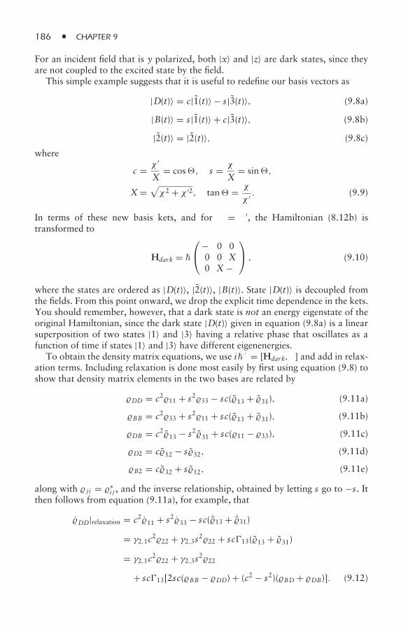
186 CHAPTER 9
For an incident field that is y polarized, both |x〉 and |z〉 are dark states, since theyare not coupled to the excited state by the field.
This simple example suggests that it is useful to redefine our basis vectors as
|D(t)〉 = c|1(t)〉 − s|3(t)〉, (9.8a)
|B(t)〉 = s|1(t)〉 + c|3(t)〉, (9.8b)
|2(t)〉 = |2(t)〉, (9.8c)
where
c = χ ′
X= cos, s = χ
X= sin,
X =√χ2 + χ ′2, tan = χ
χ ′ . (9.9)
In terms of these new basis kets, and for δ = δ′, the Hamiltonian (8.12b) istransformed to
Hdark = ⎛⎝−δ 0 0
0 0 X0 X −δ
⎞⎠ , (9.10)
where the states are ordered as |D(t)〉, |2(t)〉, |B(t)〉. State |D(t)〉 is decoupled fromthe fields. From this point onward, we drop the explicit time dependence in the kets.You should remember, however, that a dark state is not an energy eigenstate of theoriginal Hamiltonian, since the dark state |D(t)〉 given in equation (9.8a) is a linearsuperposition of two states |1〉 and |3〉 having a relative phase that oscillates as afunction of time if states |1〉 and |3〉 have different eigenenergies.
To obtain the density matrix equations, we use i = [Hdark, ] and add in relax-ation terms. Including relaxation is done most easily by first using equation (9.8) toshow that density matrix elements in the two bases are related by
DD = c211 + s233 − sc(13 + 31), (9.11a)
BB = c233 + s211 + sc(13 + 31), (9.11b)
DB = c213 − s231 + sc(11 − 33), (9.11c)
D2 = c12 − s32, (9.11d)
B2 = c32 + s12, (9.11e)
along with j i = ∗i j , and the inverse relationship, obtained by letting s go to −s. It
then follows from equation (9.11a), for example, that
DD|relaxation = c211 + s233 − sc( ˙13 + ˙31)
= γ2,1c222 + γ2,3s222 + sc13(13 + 31)= γ2,1c222 + γ2,3s222
+ sc13[2sc(BB − DD) + (c2 − s2)(BD + DB)]. (9.12)
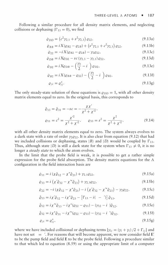
THREE-LEVEL ATOMS 187
Following a similar procedure for all density matrix elements, and neglectingcollisions or dephasing (13 = 0), we find
DD = (c2γ2,1 + s2γ2,3
)22, (9.13a)
BB = i X (B2 − 2B) + (s2γ2,1 + c2γ2,3
)22, (9.13b)
22 = −i X (B2 − 2B) − γ222, (9.13c)
DB = i XD2 − sc (γ2,3 − γ2,1) 22, (9.13d)
D2 = i XDB −(γ22
− iδ)D2, (9.13e)
B2 = i X (BB − 22) −(γ22
− iδ)B2, (9.13f)
j i = ∗i j . (9.13g)
The only steady-state solution of these equations is DD = 1, with all other densitymatrix elements equal to zero. In the original basis, this corresponds to
13 = 31 = −sc = − χχ ′
χ2 + χ ′2 ,
11 = c2 = χ ′2
χ2 + χ ′2 , 33 = s2 = χ2
χ2 + χ ′2 , (9.14)
with all other density matrix elements equal to zero. The system always evolves toa dark state with a rate of order γ222. It is also clear from equation (9.12) that hadwe included collisions or dephasing, states |B〉 and |D〉 would be coupled by 13.Thus, although state |D〉 is still a dark state for the system when 13 = 0, it is nolonger a steady state to which the atom evolves.
In the limit that the probe field is weak, it is possible to get a rather simpleexpression for the probe field absorption. The density matrix equations for the configuration in the field interaction basis are
11 = i (χ12 − χ∗21) + γ2,122, (9.15a)
33 = i(χ ′32 − χ ′∗23
)+ γ2,322, (9.15b)
22 = −i (χ12 − χ∗21) − i(χ ′32 − χ ′∗23
)− γ222, (9.15c)
˙13 = iχ ′12 − iχ∗23 − [13 − i(δ − δ′)] 13, (9.15d)
˙12 = iχ ′∗13 − iχ∗(22 − 11) − (γ12 − iδ)12, (9.15e)
˙32 = iχ∗31 − iχ ′∗(22 − 33) − (γ32 − iδ′)32, (9.15f)
j i = ∗i j , (9.15g)
where we have included collisional or dephasing terms [γi j = (γi + γi ) /2 + i j ] andhave not set δ = δ′. For reasons that will become apparent, we now consider field E′
to be the pump field and field E to be the probe field. Following a procedure similarto that which led to equation (8.59) or using the appropriate limit of a computer
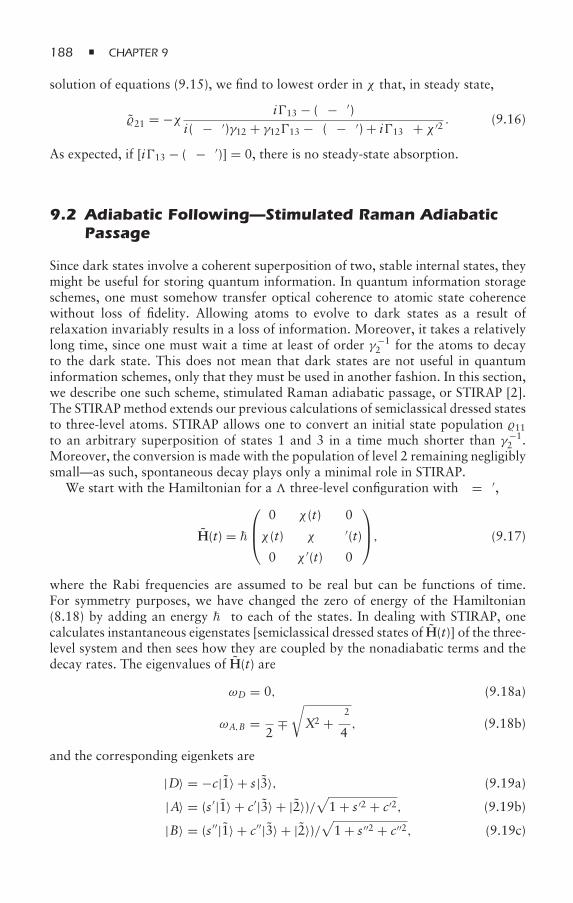
188 CHAPTER 9
solution of equations (9.15), we find to lowest order in χ that, in steady state,
21 = −χ i13 − (δ − δ′)i(δ − δ′)γ12 + γ1213 − δ(δ − δ′) + i13δ + χ ′2 . (9.16)
As expected, if [i13 − (δ − δ′)] = 0, there is no steady-state absorption.
9.2 Adiabatic Following—Stimulated Raman AdiabaticPassage
Since dark states involve a coherent superposition of two, stable internal states, theymight be useful for storing quantum information. In quantum information storageschemes, one must somehow transfer optical coherence to atomic state coherencewithout loss of fidelity. Allowing atoms to evolve to dark states as a result ofrelaxation invariably results in a loss of information. Moreover, it takes a relativelylong time, since one must wait a time at least of order γ−1
2 for the atoms to decayto the dark state. This does not mean that dark states are not useful in quantuminformation schemes, only that they must be used in another fashion. In this section,we describe one such scheme, stimulated Raman adiabatic passage, or STIRAP [2].The STIRAPmethod extends our previous calculations of semiclassical dressed statesto three-level atoms. STIRAP allows one to convert an initial state population 11to an arbitrary superposition of states 1 and 3 in a time much shorter than γ−1
2 .Moreover, the conversion is made with the population of level 2 remaining negligiblysmall—as such, spontaneous decay plays only a minimal role in STIRAP.
We start with the Hamiltonian for a three-level configuration with δ = δ′,
H(t) =
⎛⎜⎝
0 χ (t) 0
χ (t) δ χ ′(t)
0 χ ′(t) 0
⎞⎟⎠, (9.17)
where the Rabi frequencies are assumed to be real but can be functions of time.For symmetry purposes, we have changed the zero of energy of the Hamiltonian(8.18) by adding an energy δ to each of the states. In dealing with STIRAP, onecalculates instantaneous eigenstates [semiclassical dressed states of H(t)] of the three-level system and then sees how they are coupled by the nonadiabatic terms and thedecay rates. The eigenvalues of H(t) are
ωD = 0, (9.18a)
ωA,B = δ
2∓√X2 + δ2
4, (9.18b)
and the corresponding eigenkets are
|D〉 = −c|1〉 + s|3〉, (9.19a)
|A〉 = (s ′|1〉 + c′|3〉 + |2〉)/√
1 + s ′2 + c′2, (9.19b)
|B〉 = (s ′′|1〉 + c′′|3〉 + |2〉)/√
1 + s ′′2 + c′′2, (9.19c)
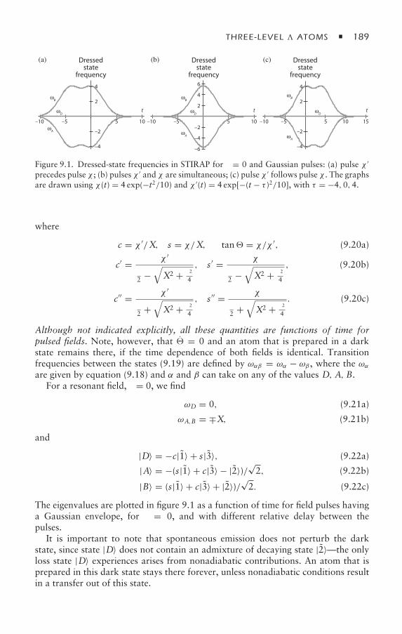
THREE-LEVEL ATOMS 189
–10 –5 10
t
(a) (b) Dressedstate
frequency
Dressedstate
frequency
Dressedstate
frequency
(c)
ωB
ωD
ωA
–4
–2
2
4
5 –10 –5 10
t
ωB
ωD
ωA
ωB
ωD
ωA
5 –10 1510
t
5
–6
–4
–2
2
4
6
–4
–2
2
4
–5
Figure 9.1. Dressed-state frequencies in STIRAP for δ = 0 and Gaussian pulses: (a) pulse χ ′
precedes pulse χ ; (b) pulses χ ′ and χ are simultaneous; (c) pulse χ ′ follows pulse χ . The graphsare drawn using χ (t) = 4 exp(−t2/10) and χ ′(t) = 4 exp[−(t − τ )2/10], with τ = −4, 0, 4.
where
c = χ ′/X, s = χ/X, tan = χ/χ ′, (9.20a)
c′ = χ ′
δ2 −
√X2 + δ2
4
, s ′ = χ
δ2 −
√X2 + δ2
4
, (9.20b)
c′′ = χ ′
δ2 +
√X2 + δ2
4
, s ′′ = χ
δ2 +
√X2 + δ2
4
. (9.20c)
Although not indicated explicitly, all these quantities are functions of time forpulsed fields. Note, however, that = 0 and an atom that is prepared in a darkstate remains there, if the time dependence of both fields is identical. Transitionfrequencies between the states (9.19) are defined by ωαβ = ωα − ωβ , where the ωαare given by equation (9.18) and α and β can take on any of the values D, A, B.
For a resonant field, δ = 0, we find
ωD = 0, (9.21a)
ωA,B = ∓X, (9.21b)
and
|D〉 = −c|1〉 + s|3〉, (9.22a)
|A〉 = −(s|1〉 + c|3〉 − |2〉)/√2, (9.22b)
|B〉 = (s|1〉 + c|3〉 + |2〉)/√2. (9.22c)
The eigenvalues are plotted in figure 9.1 as a function of time for field pulses havinga Gaussian envelope, for δ = 0, and with different relative delay between thepulses.
It is important to note that spontaneous emission does not perturb the darkstate, since state |D〉 does not contain an admixture of decaying state |2〉—the onlyloss state |D〉 experiences arises from nonadiabatic contributions. An atom that isprepared in this dark state stays there forever, unless nonadiabatic conditions resultin a transfer out of this state.
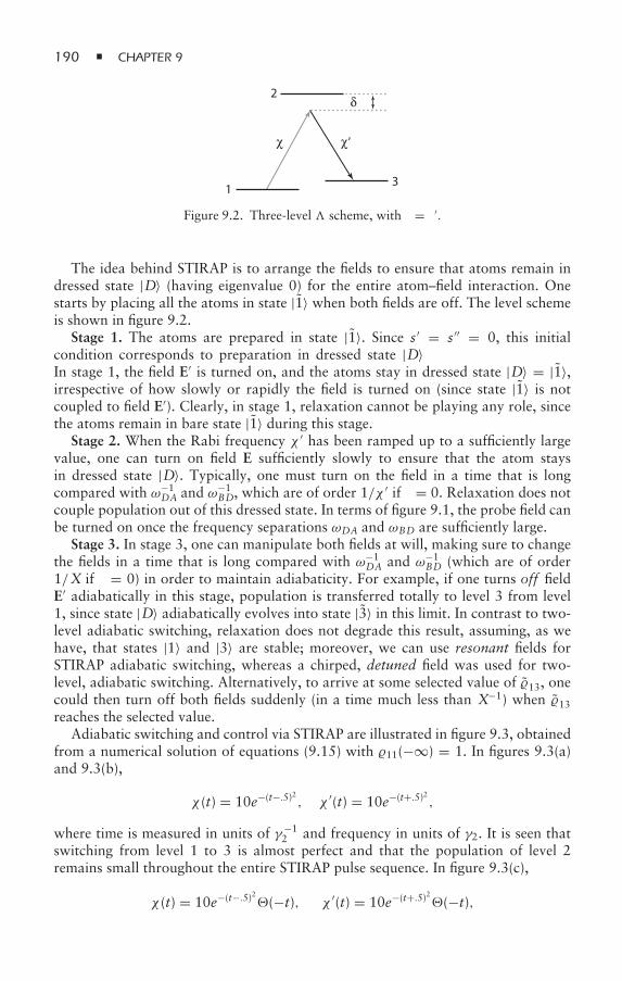
190 CHAPTER 9
2
χ χ‘
δ
13
Figure 9.2. Three-level scheme, with δ = δ′.
The idea behind STIRAP is to arrange the fields to ensure that atoms remain indressed state |D〉 (having eigenvalue 0) for the entire atom–field interaction. Onestarts by placing all the atoms in state |1〉 when both fields are off. The level schemeis shown in figure 9.2.
Stage 1. The atoms are prepared in state |1〉. Since s ′ = s ′′ = 0, this initialcondition corresponds to preparation in dressed state |D〉 [see equations (9.19)].In stage 1, the field E′ is turned on, and the atoms stay in dressed state |D〉 = |1〉,irrespective of how slowly or rapidly the field is turned on (since state |1〉 is notcoupled to field E′). Clearly, in stage 1, relaxation cannot be playing any role, sincethe atoms remain in bare state |1〉 during this stage.
Stage 2. When the Rabi frequency χ ′ has been ramped up to a sufficiently largevalue, one can turn on field E sufficiently slowly to ensure that the atom staysin dressed state |D〉. Typically, one must turn on the field in a time that is longcompared with ω−1
DA and ω−1BD, which are of order 1/χ ′ if δ = 0. Relaxation does not
couple population out of this dressed state. In terms of figure 9.1, the probe field canbe turned on once the frequency separations ωDA and ωBD are sufficiently large.
Stage 3. In stage 3, one can manipulate both fields at will, making sure to changethe fields in a time that is long compared with ω−1
DA and ω−1BD (which are of order
1/X if δ = 0) in order to maintain adiabaticity. For example, if one turns off fieldE′ adiabatically in this stage, population is transferred totally to level 3 from level1, since state |D〉 adiabatically evolves into state |3〉 in this limit. In contrast to two-level adiabatic switching, relaxation does not degrade this result, assuming, as wehave, that states |1〉 and |3〉 are stable; moreover, we can use resonant fields forSTIRAP adiabatic switching, whereas a chirped, detuned field was used for two-level, adiabatic switching. Alternatively, to arrive at some selected value of 13, onecould then turn off both fields suddenly (in a time much less than X−1) when 13reaches the selected value.
Adiabatic switching and control via STIRAP are illustrated in figure 9.3, obtainedfrom a numerical solution of equations (9.15) with 11(−∞) = 1. In figures 9.3(a)and 9.3(b),
χ (t) = 10e−(t−.5)2 , χ ′(t) = 10e−(t+.5)2 ,
where time is measured in units of γ−12 and frequency in units of γ2. It is seen that
switching from level 1 to 3 is almost perfect and that the population of level 2remains small throughout the entire STIRAP pulse sequence. In figure 9.3(c),
χ (t) = 10e−(t−.5)2(−t), χ ′(t) = 10e−(t+.5)2(−t),
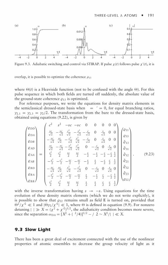
THREE-LEVEL ATOMS 191
(a) (b) (c)
γ2t
ρ33
–4 –2 2 4
γ2t
–4 –2 200 4
0.2
0.4
0.6
0.8
1.0
ρ22
γ2t
–4 –2 20 4
ρ13
0.004
0.008
0.012
0.1
0.2
0.3
0.4
0.5
Figure 9.3. Adiabatic switching and control via STIRAP. If pulse χ (t) follows pulse χ ′(t), it ispossible to adiabatically switch population from level 1 to level 3 [plot (a)] while minimallypopulating level 2 [plot (b)]. With the same sequence but cutting off both pulses when theyoverlap, it is possible to optimize the coherence ρ13 [plot (c)].
where (t) is a Heaviside function (not to be confused with the angle ). For thispulse sequence in which both fields are turned off suddenly, the absolute value ofthe ground-state coherence 13 is optimized.
For reference purposes, we write the equations for density matrix elements inthe semiclassical dressed-state basis when δ = δ′ = 0, for equal branching ratios,γ2,1 = γ2,3 = γ2/2. The transformation from the bare to the dressed-state basis,obtained using equations (9.22), is given by
⎛⎜⎜⎜⎜⎜⎜⎜⎜⎜⎜⎜⎜⎜⎜⎜⎜⎜⎜⎝
DD
DA
DB
AD
AA
AB
BD
BA
BB
⎞⎟⎟⎟⎟⎟⎟⎟⎟⎟⎟⎟⎟⎟⎟⎟⎟⎟⎟⎠
=
⎛⎜⎜⎜⎜⎜⎜⎜⎜⎜⎜⎜⎜⎜⎜⎜⎜⎜⎜⎜⎜⎜⎝
c2 s2 −sc −sc 0 0 0 0 0
sc√2
− sc√2
c2√2
− s2√2
− c√2
0 s√2
0 0
− sc√2
sc√2
− c2√2
s2√2
− c√2
0 s√2
0 0
sc√2
− sc√2
− s2√2
c2√2
0 − c√2
0 s√20
s2
2c2
2sc2
sc2 − s
2 − s2 − c
2 − c2
12
− s2
2 − c2
2 − sc2 − sc
2 − s2
s2 − c
2c2
12
− sc√2
sc√2
s2√2
− c2√2
0 − c√2
0 s√20
− s2
2 − c2
2 − sc2 − sc
2s2 − s
2c2 − c
212
s2
2c2
2sc2
sc2
s2
s2
c2
c2
12
⎞⎟⎟⎟⎟⎟⎟⎟⎟⎟⎟⎟⎟⎟⎟⎟⎟⎟⎟⎟⎟⎟⎠
⎛⎜⎜⎜⎜⎜⎜⎜⎜⎜⎜⎜⎜⎜⎜⎜⎜⎜⎝
11
33
13
31
12
21
32
23
22
⎞⎟⎟⎟⎟⎟⎟⎟⎟⎟⎟⎟⎟⎟⎟⎟⎟⎟⎠
, (9.23)
with the inverse transformation having s → −s. Using equations for the timeevolution of these density matrix elements (which we do not write explicitly), itis possible to show that 22 remains small as field E is turned on, provided that2/χ ′2 1 and |γ2/χ ′2| 1, where is defined in equation (9.9). For nonzerodetuning |δ| X = (χ2 + χ ′2)1/2, the adiabaticity condition becomes more severe,since the separation ωDA = [X2 + (δ2/4)]1/2 − δ/2 ∼ X2/|δ| X.
9.3 Slow Light
There has been a great deal of excitement connected with the use of the nonlinearproperties of atomic ensembles to decrease the group velocity of light as it
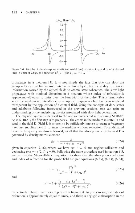
192 CHAPTER 9
–0.4
___
–0.2
0.2
0.4
0.6
γ12
δ
α/α0, 2k(n–1)/α0
0.8
1.0
–20 –10 10 20
Figure 9.4. Graphs of the absorption coefficient (solid line) in units of α0 and (n− 1) (dashedline) in units of 2k/α0 as a function of δ/γ12 for χ ′/γ12 = 10.
propagates in a medium [3]. It is not simply the fact that one can slow thegroup velocity that has aroused interest in this subject, but the ability to transferinformation carried by the optical fields to atomic state coherence. The slow lightpropagates with minimal distortion in a medium whose index of refraction isapproximately equal to unity over the bandwidth of the pulse. This is remarkablesince the medium is optically dense at optical frequencies but has been renderedtransparent by the application of a control field. Using the concepts of dark statesand adiabatic following introduced in the previous sections, one can gain anunderstanding of the underlying physics associated with slow light generation.
The physical system is identical to the one we considered in discussing STIRAP.As in STIRAP, the first step is to prepare all the atoms in the medium in state |1〉 andsend in the field E′. Field E′ is chosen to be sufficiently intense to create a frequencywindow, enabling field E to enter the medium without reflection. To understandhow this frequency window is formed, recall that the absorption of probe field E isgoverned by density matrix element
21 = χδ
−δ2 + iγ12δ + χ ′2 (9.24)
given in equation (9.16), where we have set δ′ = 0 and neglect collisions anddephasing (γ12 = γ2/2, 13 = 0). Following the same procedure used in section 6.3,we can use the Maxwell-Bloch equations to show that the absorption coefficientand index of refraction for the probe field are [see equations (6.25), (6.33), (6.34),(4.23), and (6.66)]
α = α0γ 212δ
2(χ ′2 − δ2)2 + (γ12δ)2
(9.25)
and
n2 = 1 + α0
k
γ12δ(χ ′2 − δ2)(
χ ′2 − δ2)2 + (γ12δ)2, (9.26)
respectively. These quantities are plotted in figure 9.4. As you can see, the index ofrefraction is approximately equal to unity, and there is negligible absorption in the
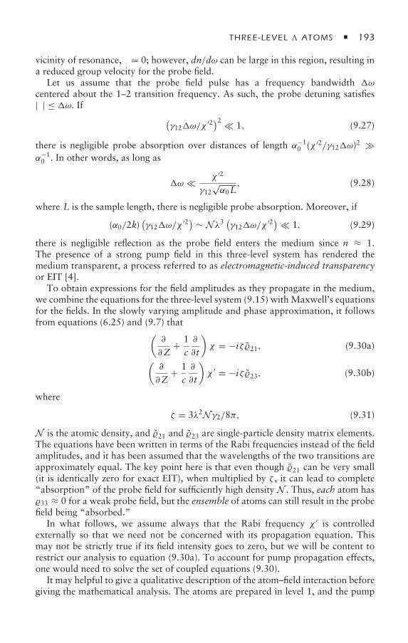
THREE-LEVEL ATOMS 193
vicinity of resonance, δ = 0; however, dn/dω can be large in this region, resulting ina reduced group velocity for the probe field.
Let us assume that the probe field pulse has a frequency bandwidth ω
centered about the 1–2 transition frequency. As such, the probe detuning satisfies|δ| ≤ ω. If (
γ12ω/χ′2)2 1, (9.27)
there is negligible probe absorption over distances of length α−10 (χ ′2/γ12ω)2
α−10 . In other words, as long as
ω χ ′2
γ12√α0L
, (9.28)
where L is the sample length, there is negligible probe absorption. Moreover, if
(α0/2k)(γ12ω/χ
′2) ∼ Nλ3 (γ12ω/χ ′2) 1, (9.29)
there is negligible reflection as the probe field enters the medium since n ≈ 1.The presence of a strong pump field in this three-level system has rendered themedium transparent, a process referred to as electromagnetic-induced transparencyor EIT [4].
To obtain expressions for the field amplitudes as they propagate in the medium,we combine the equations for the three-level system (9.15) with Maxwell’s equationsfor the fields. In the slowly varying amplitude and phase approximation, it followsfrom equations (6.25) and (9.7) that(
∂
∂Z+ 1c∂
∂t
)χ = −iζ 21, (9.30a)(
∂
∂Z+ 1c∂
∂t
)χ ′ = −iζ 23, (9.30b)
where
ζ = 3λ2Nγ2/8π, (9.31)
N is the atomic density, and 21 and 23 are single-particle density matrix elements.The equations have been written in terms of the Rabi frequencies instead of the fieldamplitudes, and it has been assumed that the wavelengths of the two transitions areapproximately equal. The key point here is that even though 21 can be very small(it is identically zero for exact EIT), when multiplied by ζ , it can lead to complete“absorption” of the probe field for sufficiently high density N . Thus, each atom has33 ≈ 0 for a weak probe field, but the ensemble of atoms can still result in the probefield being “absorbed.”
In what follows, we assume always that the Rabi frequency χ ′ is controlledexternally so that we need not be concerned with its propagation equation. Thismay not be strictly true if its field intensity goes to zero, but we will be content torestrict our analysis to equation (9.30a). To account for pump propagation effects,one would need to solve the set of coupled equations (9.30).
It may helpful to give a qualitative description of the atom–field interaction beforegiving the mathematical analysis. The atoms are prepared in level 1, and the pump
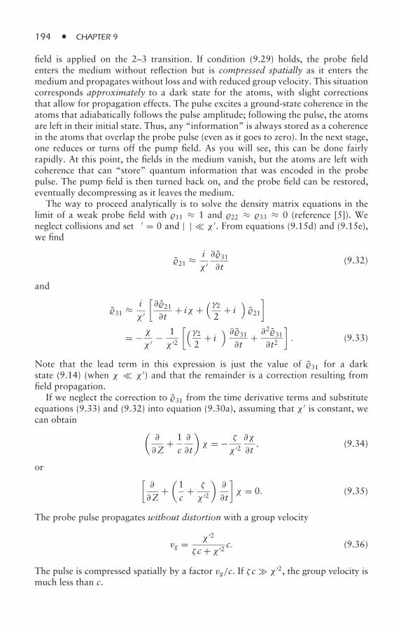
194 CHAPTER 9
field is applied on the 2–3 transition. If condition (9.29) holds, the probe fieldenters the medium without reflection but is compressed spatially as it enters themedium and propagates without loss and with reduced group velocity. This situationcorresponds approximately to a dark state for the atoms, with slight correctionsthat allow for propagation effects. The pulse excites a ground-state coherence in theatoms that adiabatically follows the pulse amplitude; following the pulse, the atomsare left in their initial state. Thus, any “information” is always stored as a coherencein the atoms that overlap the probe pulse (even as it goes to zero). In the next stage,one reduces or turns off the pump field. As you will see, this can be done fairlyrapidly. At this point, the fields in the medium vanish, but the atoms are left withcoherence that can “store” quantum information that was encoded in the probepulse. The pump field is then turned back on, and the probe field can be restored,eventually decompressing as it leaves the medium.
The way to proceed analytically is to solve the density matrix equations in thelimit of a weak probe field with 11 ≈ 1 and 22 ≈ 33 ≈ 0 (reference [5]). Weneglect collisions and set δ′ = 0 and |δ| χ ′. From equations (9.15d) and (9.15e),we find
21 ≈ iχ ′∂31
∂t(9.32)
and
31 ≈ iχ ′
[∂21
∂t+ iχ +
(γ22
+ iδ)21
]
= − χχ ′ − 1
χ ′2
[(γ22
+ iδ) ∂31∂t
+ ∂231
∂t2
]. (9.33)
Note that the lead term in this expression is just the value of 31 for a darkstate (9.14) (when χ χ ′) and that the remainder is a correction resulting fromfield propagation.
If we neglect the correction to 31 from the time derivative terms and substituteequations (9.33) and (9.32) into equation (9.30a), assuming that χ ′ is constant, wecan obtain (
∂
∂Z+ 1c∂
∂t
)χ = − ζ
χ ′2∂χ
∂t, (9.34)
or [∂
∂Z+(1c
+ ζ
χ ′2
)∂
∂t
]χ = 0. (9.35)
The probe pulse propagates without distortion with a group velocity
vg = χ ′2
ζc + χ ′2 c. (9.36)
The pulse is compressed spatially by a factor vg/c. If ζc χ ′2, the group velocity ismuch less than c.
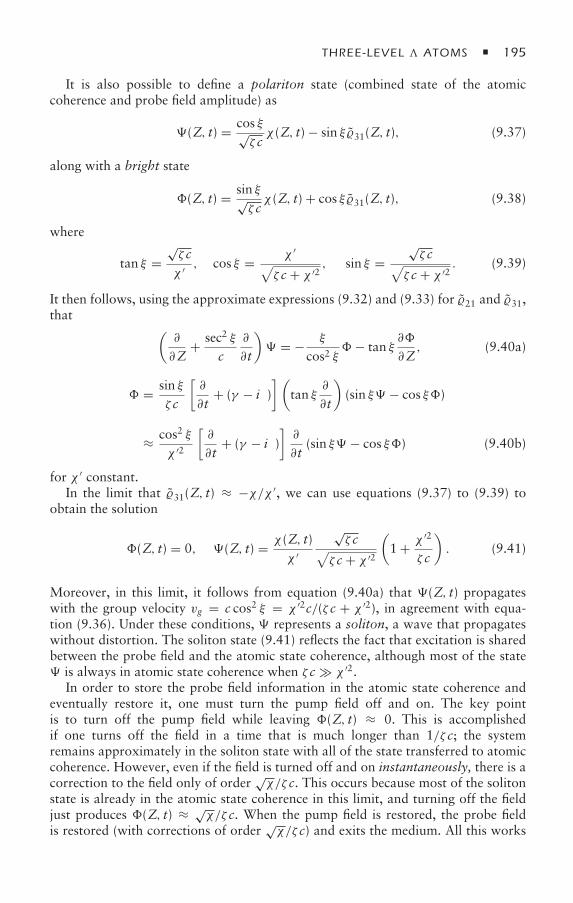
THREE-LEVEL ATOMS 195
It is also possible to define a polariton state (combined state of the atomiccoherence and probe field amplitude) as
(Z, t) = cos ξ√ζcχ (Z, t) − sin ξ 31(Z, t), (9.37)
along with a bright state
(Z, t) = sin ξ√ζcχ (Z, t) + cos ξ 31(Z, t), (9.38)
where
tan ξ =√ζcχ ′ , cos ξ = χ ′√
ζc + χ ′2 , sin ξ =√ζc√
ζc + χ ′2 . (9.39)
It then follows, using the approximate expressions (9.32) and (9.33) for 21 and 31,that (
∂
∂Z+ sec2 ξ
c∂
∂t
) = − ξ
cos2 ξ− tan ξ
∂
∂Z, (9.40a)
= sin ξζc
[∂
∂t+ (γ − iδ)
](tan ξ
∂
∂t
)(sin ξ − cos ξ)
≈ cos2 ξχ ′2
[∂
∂t+ (γ − iδ)
]∂
∂t(sin ξ − cos ξ) (9.40b)
for χ ′ constant.In the limit that 31(Z, t) ≈ −χ/χ ′, we can use equations (9.37) to (9.39) to
obtain the solution
(Z, t) = 0, (Z, t) = χ (Z, t)χ ′
√ζc√
ζc + χ ′2
(1 + χ ′2
ζc
). (9.41)
Moreover, in this limit, it follows from equation (9.40a) that (Z, t) propagateswith the group velocity vg = c cos2 ξ = χ ′2c/(ζc + χ ′2), in agreement with equa-tion (9.36). Under these conditions, represents a soliton, a wave that propagateswithout distortion. The soliton state (9.41) reflects the fact that excitation is sharedbetween the probe field and the atomic state coherence, although most of the state is always in atomic state coherence when ζc χ ′2.
In order to store the probe field information in the atomic state coherence andeventually restore it, one must turn the pump field off and on. The key pointis to turn off the pump field while leaving (Z, t) ≈ 0. This is accomplishedif one turns off the field in a time that is much longer than 1/ζc; the systemremains approximately in the soliton state with all of the state transferred to atomiccoherence. However, even if the field is turned off and on instantaneously, there is acorrection to the field only of order
√χ/ζc. This occurs because most of the soliton
state is already in the atomic state coherence in this limit, and turning off the fieldjust produces (Z, t) ≈ √
χ/ζc. When the pump field is restored, the probe fieldis restored (with corrections of order
√χ/ζc) and exits the medium. All this works
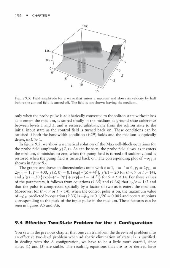
196 CHAPTER 9
t
1.0
0.5
00
5
10
10
15
–5
5
0
χ
Z
Figure 9.5. Field amplitude for a wave that enters a medium and slows its velocity by halfbefore the control field is turned off. The field is not shown leaving the medium.
only when the probe pulse is adiabatically converted to the soliton state without lossas it enters the medium, is stored totally in the medium as ground-state coherencebetween levels 1 and 3, and is restored adiabatically from the soliton state to theinitial input state as the control field is turned back on. These conditions can besatisfied if both the bandwidth condition (9.29) holds and the medium is opticallydense, α0L 1.
In figure 9.5, we show a numerical solution of the Maxwell-Bloch equations forthe probe field amplitude χ (Z, t). As can be seen, the probe field slows as it entersthe medium, diminishes to zero when the pump field is turned off suddenly, and isrestored when the pump field is turned back on. The corresponding plot of −31 isshown in figure 9.6.
The graphs are drawn in dimensionless units with c = 1, δ = δ′ = 0, γ2 = 2γ2,1 =2γ3,1 = 1, ζ = 400, χ (Z,0) = 0.1 exp[−(Z+ 4)2], χ ′(t) = 20 for (t < 9 or t > 14),and χ ′(t) = 20
exp[−(t − 9)2] + exp[−(t − 14)2]
for 9 ≤ t ≤ 14. For these values
of the parameters, it follows from equations (9.35) and (9.36) that vg/c = 1/2 andthat the pulse is compressed spatially by a factor of two as it enters the medium.Moreover, for (t < 9 or t > 14), when the control pulse is on, the maximum valueof −31 predicted by equation (9.33) is −31 ≈ 0.1/20 = 0.005 and occurs at pointscorresponding to the peak of the input pulse in the medium. These features can beseen in figures 9.5 and 9.6.
9.4 Effective Two-State Problem for the Configuration
You saw in the previous chapter that one can transform the three-level problem intoan effective two-level problem when adiabatic elimination of state |2〉 is justified.In dealing with the configuration, we have to be a little more careful, sincestates |1〉 and |3〉 are stable. The resulting equations that are to be derived have
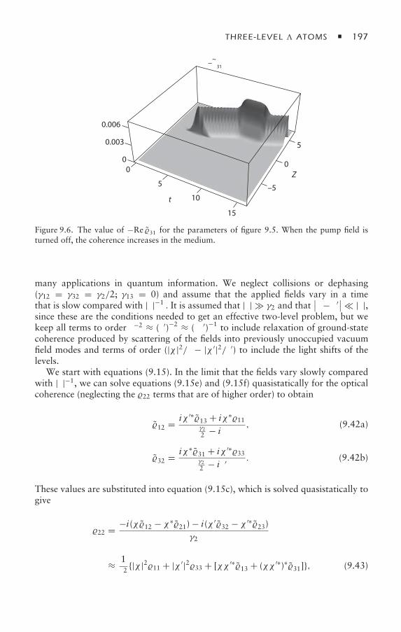
THREE-LEVEL ATOMS 197
t
0.006
0.003
00
5
10
15
–5
5
–ρ31
0Z
~
Figure 9.6. The value of −Re 31 for the parameters of figure 9.5. When the pump field isturned off, the coherence increases in the medium.
many applications in quantum information. We neglect collisions or dephasing(γ12 = γ32 = γ2/2; γ13 = 0) and assume that the applied fields vary in a timethat is slow compared with |δ|−1 . It is assumed that |δ| γ2 and that
∣∣δ − δ′∣∣ |δ|,since these are the conditions needed to get an effective two-level problem, but wekeep all terms to order δ−2 ≈ (δ′)−2 ≈ (δδ′)−1 to include relaxation of ground-statecoherence produced by scattering of the fields into previously unoccupied vacuumfield modes and terms of order (|χ |2/δ − |χ ′|2/δ′) to include the light shifts of thelevels.
We start with equations (9.15). In the limit that the fields vary slowly comparedwith |δ|−1, we can solve equations (9.15e) and (9.15f) quasistatically for the opticalcoherence (neglecting the 22 terms that are of higher order) to obtain
12 = iχ ′∗13 + iχ∗11γ22 − iδ
, (9.42a)
32 = iχ∗31 + iχ ′∗33γ22 − iδ′
. (9.42b)
These values are substituted into equation (9.15c), which is solved quasistatically togive
22 = −i(χ12 − χ∗21) − i(χ ′32 − χ ′∗23)γ2
≈ 1δ2
|χ |211 + |χ ′|233 + [χχ ′∗13 + (χχ ′∗)∗31], (9.43)
198 CHAPTER 9
where we have used the fact that δ−2 ≈ (δ′)−2 ≈ (δδ′)−1. Last, equations (9.42) and(9.43) are substituted into equations (9.15a) and (9.15d) to arrive at
11 ≈ −γ2,3|χ |2δ2
11 + γ2,1|χ ′|2δ2
33 + i(χtq13 − χ∗tq31)
+ (γ2,3 − γ2,1)2δ
(χtq13 + χ∗tq31), (9.44a)
˙13 = i(δ − δ′)13 − iχ∗tq(33 − 11) + γ2χ
∗tq
2δ(33 + 11)
− γ2(|χ |2 + |χ ′|2)2δ2
13 + i( |χ |2δ′
− |χ ′|2δ
)13, (9.44b)
33 = 1 − 11, (9.44c)
where
χtq = −χχ′∗
δ, (9.45)
the relationship (γ2,1 + γ2,3) = γ2 has been used, and terms of order (γ2/δ)2 and|δ− δ′|/|δ| have been neglected. These equations differ from equations (8.79) for thecascade system in that the entire contribution to the decay of the 1–3 state coherenceresults from off-resonant scattering of the input fields.
Since (11 + 33) ≈ 1, there is a driving term proportional to γ2χ∗tq/2δ for the
ground-state coherence. This term actually corresponds to a coherent pumping of13 by the fields. Note the difference between the dark-state basis and the originalstate basis pictures. In the dark-state picture, spontaneous emission populates thedark state that is decoupled from the field—the dark state is a linear combinationof states |1〉 and |3〉, resulting in a coherence between these states. On the otherhand, in the bare-state picture, the steady-state ground-state coherence results froman equilibrium that is reached between the coherent pumping of that coherence bythe input fields and the decay of the coherence resulting from spontaneous emission(scattering of the fields into unoccupied vacuum field modes).
The term i[(|χ |2/δ′) − (|χ ′|2/δ)]13 in equation (9.44c) corresponds to a lightshift. You might have expected that the light shift term would be i[(|χ |2/δ) −(|χ ′|2/δ′)]13, reflecting the light shifts from each field separately, but you can verifythat equation (9.44c) gives the correct result by solving the full, three-state problem.Had we neglected terms of order |δ|−2, there would not be a steady-state solution.In that limit, the adiabatic elimination procedure has to be modified somewhat, andthe light shifts are as expected. Details are relegated to the problems.
9.5 Summary
We have seen that the configuration brings into play new features not foundin the cascade configuration. It is the stability of levels 1 and 3 that leads to newpossibilities for slow light production and the storage of optical signal in atomicstate coherence. We now turn our attention toward coherent transient spectroscopy.
THREE-LEVEL ATOMS 199
9.6 Appendix: Force on an Atom in the Configuration
We can generalize our result on the force on a two-level atom to the three-level atomwith minimal difficulty. In doing so, we gain additional insight into the friction force.The obvious generalization of equation (5.15) for the time-averaged friction force toa three-level atom is
F = −[iχk(12 − 21) + iχ ′k′(32 − 23)]. (9.46)
It then follows from equations (9.15a) and (9.15b) that
F = [(kγ2,1 + k′γ2,3)22 − (k11 + k′33)]. (9.47)
In steady state, the averaged friction force vanishes regardless of the detunings δ, δ′,and regardless of the ratio of the Rabi frequencies associated with the coupledtransitions provided that
kγ2,1 + k′γ2,3 = 0. (9.48)
For counterpropagating fields and k ≈ −k′, the friction force vanishes for equalbranching ratios, γ2,1 = γ2,3 (see reference [6]). Even if condition (9.48) is notsatisfied, the steady-state, averaged friction force vanishes provided that δ = δ′,since there is a dark state in this limit and 22 = 0 in steady state.
Equation (9.47) can be given a simple physical interpretation. In steady state,the second term vanishes, and the force arises solely from scattered radiation. Eachphoton scattered on the 2–1 transition involves a loss of one photon from fieldE, and each photon scattered on the 3–2 transition involves a loss of one photonfrom field E′, with a corresponding force on the atoms that is proportional tothe scattering rates kγ2,1 and k′γ3,2, respectively. In the transient regime, thereis an additional contribution to the force, represented by the second term inequation (9.46). This term corresponds to a stimulated exchange of momentumbetween the fields resulting in a corresponding change in momentum of the atoms.
The result (9.47) is valid for all atom–field detunings. In the adiabatic limit ofsection 9.4, we can show that the vanishing of the friction force results from thecancellation of two contributions. From equations (9.46) and (9.42), it follows thatin steady state and for real Rabi frequencies,
F = γ2(kχ211γ 224 + δ2
+ k′χ ′233γ 224 + δ′2
)
+ χχ ′[k(
13γ22 − iδ
+ 31γ22 + iδ
)+ k′
(31
γ22 − iδ′
+ 13γ22 + iδ′
)]. (9.49)
Under dark-state conditions (9.14), this force vanishes. When condition (9.48)holds, the force also vanishes as a result of the cancellation of population andcoherence terms, each of which separately is nonvanishing.
200 CHAPTER 9
Problems
1–2. Consider the three-level problem, neglecting decay and for resonant fields.In dimensionless variables, the equations for the state amplitudes in theinteraction picture are
dc1/dτ = −iac2,dc2/dτ = −iac1 − ibc3,
dc3/dτ = −ibc2,where a = χT, b = χ ′T, and time is measured in units of τ = t/T. Take a andb to be Gaussian functions of time:
a = (1/√π )a0 exp(−τ 2),
b = (1/√π )b0 exp[−(τ − τ0)2],
where τ0 is a delay that can be positive or negative. Consider the limit in whicha0 1 and b0 1. Use computer solutions to show that if at t = −∞, c1 = 1,it is possible to maximize the state 3 population at τ = ∞ by choosing τ0 tobe negative (counterintuitive pulse sequence).
To be specific, look at a0 = b0 = 9.5,10,11 for τ0 = 0.75,0,−0.75. Showthat if τ0 = −0.75, one maximizes the state 3 population at τ = ∞ in a fairlyrobust manner.
3. Derive the equivalent of equations (9.13), including collision or dephasingterms, and without the assumption that δ = δ′. Show that they are given by
DD = (γ2,1c2 + γ2,3s2)22 − 2s2c213(DD − BB)+ sc[13(c2 − s2)(DB + BD) − i(δ − δ′)(DB − BD)],
BB = i X(B2 − 2B) + (γ2,1s2 + γ2,3c2)22 − 2s2c213(BB − DD)+ sc[−13(c2 − s2)(DB + BD) + i(δ − δ′)(DB − BD)],
22 = −i X(B2 − 2B) − γ222,DB = i XD2 + sc[13(c2 − s2)(DD − BB) − i(δ − δ′)(DD − BB)]
− [13(c4 + s4) + i(δ − δ′)(c2 − s2)]DB
+2s2c213BB − sc(γ2,3 − γ2,1)22,D2 = i XDB − [γ32s2 + γ12c2 − i(δc2 + δ′s2)]D2
− sc[(γ12 − γ32) − i(δ − δ′)]B2,B2 = i X(BB − 22) − [γ32c2 + γ12s2 − i(δs2 + δ′c2)]B2
− sc[(γ12 − γ32) + i(δ − δ′)]D2, j i = ∗
i j .
THREE-LEVEL ATOMS 201
Show that if 13 = 0, the dark state is no longer a stationary state of thesystem.
4. Solve equations (9.15) numerically in dimensionless units, where γ2 = 1,χ = 4, χ ′ = 2, γ2,1 = γ2,3 = 1/2, and δ = δ′ = 5, for 11(0) = 33(0) = 1/2and all other i j (0) = 0. In particular, plot 22 and 33 as a function of time,and show that they evolve to their appropriate dark-state values.
5. Repeat problem 4, but take 13 = 0.2. Show that in this case, the systemevolves to a steady state that is not a dark state. Repeat problem 4, but takeδ = 2δ′ = 10. Show that in this case, the system evolves to a steady state thatis not a dark state.
6. With |δ − δ′|/|δ| 1, derive equations (9.44). Show that all time derivativesvanish when the steady-state values of density matrix elements correspondingto a dark state, equations (9.14), are used.
7. Consider pump–probe spectroscopy of a two-level atom (see appendix A inchapter 7). For a detuning |δ| γ , to order χ2, there is a dispersion-likestructure centered near δ′ = δ. Prove that there is no absorption at δ′ = δ,but that the index of refraction of the medium is enhanced at this detuning.Calculate the enhancement factor for a medium having density N .
8. Show that the light shifts predicted in equation (9.44) are correct by consider-ing the steady-state solution of the three-level problem (obtained by computer)with χ = 20, δ = 100, and χ ′ = 0.1 in some dimensionless units. Showthat the maximum of | Im 23| occurs at δ′ ≈ δ + 3.85, which corresponds toδ + χ2/δ′ = 103.85 and not δ + χ2/δ = 104.0.
9. Solve the amplitude equations for the three-level problem in the normalinteraction representation by adiabatically eliminating state 2, assuming largedetunings, and neglecting all decay. Show that the corresponding densitymatrix equations are
11 = −i(χ∗χ ′
δ13 − χχ ′∗
δ′31
),
˙13 = i(δ − δ′)13 − i( |χ |2δ
− |χ ′|2δ′
)13 + i
(χ∗χ ′
δ33 − χ∗χ ′
δ′11
),
33 = 1 − 11.The light shifts are now at their expected values, but there is no steady-state solution to the equations. As such, the procedure used to arrive atequations (9.42) is not quite correct. The first term in equation (9.42a) arisesfrom
12 = iχ ′∗∫ t
−∞dt′13(t
′)e−(γ12−iδ)(t−t′).
When decay of 13(t′) resulting from spontaneous emission was included,
13 reaches a constant value and can be removed from the integral. In thiscase, however, no steady state is reached, and we must write 13(t
′) ≈13(t)e
−i(δ−δ′)(t−t′)—with this substitution, the light shift resulting from thisterm varies as |χ |2/δ and not |χ |2 /δ′.
10. Using the steady-state solution of equations (9.44), prove that the force (9.49)vanishes when condition (9.48) holds.
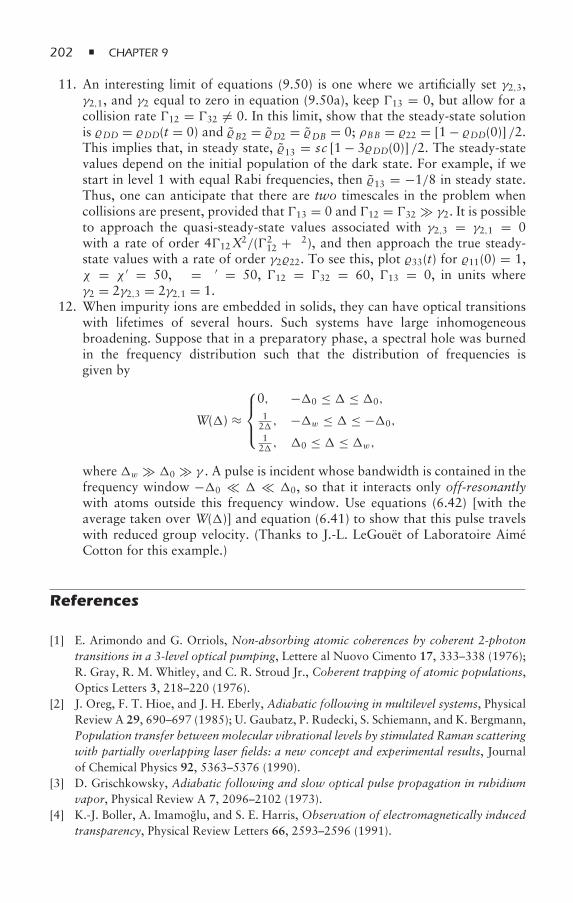
202 CHAPTER 9
11. An interesting limit of equations (9.50) is one where we artificially set γ2,3,γ2,1, and γ2 equal to zero in equation (9.50a), keep 13 = 0, but allow for acollision rate 12 = 32 = 0. In this limit, show that the steady-state solutionis DD = DD(t = 0) and B2 = D2 = DB = 0; ρBB = 22 = [1 − DD(0)] /2.This implies that, in steady state, 13 = sc [1 − 3DD(0)] /2. The steady-statevalues depend on the initial population of the dark state. For example, if westart in level 1 with equal Rabi frequencies, then 13 = −1/8 in steady state.Thus, one can anticipate that there are two timescales in the problem whencollisions are present, provided that 13 = 0 and 12 = 32 γ2. It is possibleto approach the quasi-steady-state values associated with γ2,3 = γ2,1 = 0with a rate of order 412X2/(2
12 + δ2), and then approach the true steady-state values with a rate of order γ222. To see this, plot 33(t) for 11(0) = 1,χ = χ ′ = 50, δ = δ′ = 50, 12 = 32 = 60, 13 = 0, in units whereγ2 = 2γ2,3 = 2γ2,1 = 1.
12. When impurity ions are embedded in solids, they can have optical transitionswith lifetimes of several hours. Such systems have large inhomogeneousbroadening. Suppose that in a preparatory phase, a spectral hole was burnedin the frequency distribution such that the distribution of frequencies isgiven by
W() ≈
⎧⎪⎨⎪⎩0, −0 ≤ ≤ 0,
12, −w ≤ ≤ −0,
12, 0 ≤ ≤ w,
where w 0 γ . A pulse is incident whose bandwidth is contained in thefrequency window −0 0, so that it interacts only off-resonantlywith atoms outside this frequency window. Use equations (6.42) [with theaverage taken over W()] and equation (6.41) to show that this pulse travelswith reduced group velocity. (Thanks to J.-L. LeGouët of Laboratoire AiméCotton for this example.)
References
[1] E. Arimondo and G. Orriols, Non-absorbing atomic coherences by coherent 2-photontransitions in a 3-level optical pumping, Lettere al Nuovo Cimento 17, 333–338 (1976);R. Gray, R. M. Whitley, and C. R. Stroud Jr., Coherent trapping of atomic populations,Optics Letters 3, 218–220 (1976).
[2] J. Oreg, F. T. Hioe, and J. H. Eberly, Adiabatic following in multilevel systems, PhysicalReview A 29, 690–697 (1985); U. Gaubatz, P. Rudecki, S. Schiemann, and K. Bergmann,Population transfer between molecular vibrational levels by stimulated Raman scatteringwith partially overlapping laser fields: a new concept and experimental results, Journalof Chemical Physics 92, 5363–5376 (1990).
[3] D. Grischkowsky, Adiabatic following and slow optical pulse propagation in rubidiumvapor, Physical Review A 7, 2096–2102 (1973).
[4] K.-J. Boller, A. Imamoglu, and S. E. Harris, Observation of electromagnetically inducedtransparency, Physical Review Letters 66, 2593–2596 (1991).
THREE-LEVEL ATOMS 203
[5] M. Fleischhauer and M. D. Lukin,Quantum memory for photons: dark-state polaritons,Physical Review A 65, 022314, 1–12 (2002).
[6] F. Papoff, F. Mauri, and E. Arimondo, Transient velocity-selective coherent populationtrapping in one dimension, Journal of the Optical Society of America B 9, 321–331(1992).
Bibliography
There are probably more than a thousand articles on the subject matter in this chapter. Welist only a few articles and reviews for each topic.
Three-Level Systems
E. Arimondo, Coherent population trapping in laser spectroscopy, in Progress in Optics,edited by E. Wolf, vol. 35 (Elsevier, Amsterdam, 1996), pp. 257–354. This is a reviewarticle.
E. Arimondo and G. Orriols, Non-absorbing atomic coherences by coherent 2-photontransitions in a 3-level optical pumping, Lettere al Nuovo Cimento 17, 333–338 (1976).
J. H. Eberly and V. V. Kozlov, Wave equation for dark coherence in three-level media,Physical Review Letters 88, 243604, 1–4 (2002).
H. Friedmann and A. D. Wilson-Gordon, Nonlinear refractive index near points of zeroabsorption and in the dead zone, Physical Review A 52, 4070–4077 (1995).
H. R. Gray, R. M. Whitley, and C. R. Stroud Jr., Coherent trapping of atomic populations,Optics Letters 3, 218–220 (1978).
M. Löffler, D. E. Nikinov, O. A. Kocharovskaya, and M. O. Scully, Strong field indexenhancement via selective population of dressed states, Physical Review A 56, 5014–5021(1997).
U. Rathe, M. Fleishhauer, S.-Y. Zhu, T. W. Hänsch, and M. O. Scully, Nonlinear theory ofindex enhancement via quantum coherence and interference, Physical Review A 47, 4994–5002 (1993).
M. O. Scully, Enhancement of the index of refraction via quantum coherence, Physical ReviewLetters 67, 1855–1858 (1991).
D. D. Yavuz, Refractive index enhancement in a far-off resonant atomic system, PhysicalReview Letters 95, 223601, 1–4 (2005).
A. S. Zibrov, M. D. Lukin, L. Hollberg, D. E. Nikonov, M. O. Scully, H. G. Robinson,and V. L. Velichansky, Experimental demonstration of enhanced index of refraction viaquantum coherence in Rb, Physical Review Letters 76, 3935–3938 (1996).
STIRAP
U. Gaubatz, P. Rudecki, S. Schiemann, and K. Bergmann, Population transfer betweenmolecular vibrational levels by stimulated Raman scattering with partially overlapping laserfields: a new concept and experimental results, Journal of Chemical Physics 92, 5363–5376(1990).
204 CHAPTER 9
J. Oreg, F. T. Hioe, and J. H. Eberly, Adiabatic following in multilevel systems, PhysicalReview A 29, 690–697 (1985).
B. W. Shore, K. Bergmann, J. Oreg, and S. Rosenwaks, Multilevel adiabatic populationtransfer, Physical Review A 44, 7442–7447 (1991).
N. V. Vitanov, M. Fleischhauer, B. W. Shore, and K. Bergmann, Coherent manipulationof atoms and molecules by sequential laser pulses, in Advances in Atomic, Molecular,and Optical Physics, edited by B. Bederson and H. Walther, vol. 46 (Academic Press,New York, 2001), pp. 55–190. This is a comprehensive review article with extensivereferences.
EIT
K.-J. Boller, A. Imamoglu, and S. E. Harris, Observation of electromagnetically inducedtransparency, Physical Review Letters 66, 2593–2596 (1991).
M. Fleischauer, A. Imamoglu, and J. Marangos, Electromagnetically induced transparency:optics in coherent media, Reviews of Modern Physics 77, 633–673 (2003). This is a reviewarticle with extensive references.
M. D. Lukin, Trapping and manipulating photon states in atomic ensembles, Reviews ofModern Physics 75, 457–472 (2003). This is a “colloquium” review.
Slow Light
R. W. Boyd and D. J. Gauthier, “Slow” and “fast” light, in Progress in Optics, edited by E.Wolf, vol. 43 (Elsevier, Amsterdam, 2002), pp. 497–530. This is a review article.
D. Budker, D. F. Kimball, S. M. Rochester, and V. V. Yashchuk, Nonlinear magneto-opticsreduced group velocity of light in atomic vapor with slow ground state relaxation, PhysicalReview Letters 83, 1767–1770 (1999).
M. Fleischhauer and M. D. Lukin, Quantum memory for photons: dark-state polaritons,Physical Review A 65, 022314, 1–12 (2002).
D. Grischkowsky, Adiabatic following and slow optical pulse propagation in rubidium vapor,Physical Review A 7, 2096–2102 (1973).
L. V. Hau, S. E. Harris, Z. Dutton, and C. H. Behroozi, Light speed reduction to 17 metresper second in an ultracold atomic gas, Nature 397, 594–598 (1999).
M. M. Kash, V. A. Sautenkov, A. S. Zibrov, L. Hollberg, G. W. Welch, M. D. Lukin, Y.Rostovtsev, E. S. Fry, and M. O. Scully, Ultraslow group velocity and enhanced nonlinearoptical effects in a coherently driven hot atomic gas, Physical Review Letters 82, 5229–5332 (1999).
C. Liu, Z. Dutton, C. H. Behroozi, and L. V. Hau, Observation of coherent opticalinformation storage in an atomic medium using halted light pulses, Nature 409, 490–493(2001).
J. J. Longdell, E. Fraval, M. J. Sellars, and N. B. Manson, Stopped light with storage timesgreater than one second using electromagnetically induced transparency in a solid, PhysicalReview Letters 95, 063601, 1–4 (2005).
P. W. Milonni, Controlling the speed of light pulses, Journal of Physics B 35, R31–R56(2002). This is a review article.
———, Fast Light, Slow Light, and Left-Handed Light (Taylor and Francis Group,New York, 2005).

THREE-LEVEL ATOMS 205
D. F. Phillips, A. Fleischhauer, A. Mair, R. L. Walsworth, and M. D. Lukin, Storage of lightin atomic vapor, Physical Review Letters 86, 783–786 (2001).
O. Schmidt, R. Wynands, Z. Hussein, and D. Meschede, Steep dispersion and group velocitybelow c/3000 in coherent population trapping, Physical Review A 53, R27–R30 (1996).
A. V. Turukhin, V. S. Sudarshanan, M. S. Shahriar, J. A. Musser, B. S. Ham, and P. R.Hemmer, Observation of ultraslow and stored light pulses in a solid, Physical ReviewLetters 88, 023602, 1–4 (2002).
R. G. Ulbrich and G. W. Fehrenbach, Polariton wave packet propagation in the excitonresonance of a semiconductor, Physical Review Letters 43, 963–966 (1979).
10Coherent Transients
Optical spectroscopic methods fall into two broad categories: continuous-wave (cw)or stationary spectroscopy, and time-dependent or transient spectroscopy. To thispoint, we have considered cw spectroscopy, in which the absorption or emissionline shapes are measured as a function of the frequency of a probe field. In coherenttransient optical spectroscopy, pulsed optical fields are used to create atomic statepopulations or coherence between atomic states. Following the excitation, thetime evolution of the atoms is monitored. By using different pulse sequences, it ispossible to extract both transition frequencies and relaxation rates from the coherenttransient signals. Whether transient spectroscopy offers distinct advantages overcw spectroscopy depends on a number of factors, such as signal to noise and thereliability of line shape formulas [1].
In describing the coherent transient spectroscopy of two-level quantum systems,one often uses new labels for the relaxation rates that were already encounteredin cw spectroscopy. The quantity γ2 is referred to as the longitudinal relaxationrate and T1 = γ−1
2 as the longitudinal relaxation time. The rate γ at which12 decays is referred to as the transverse relaxation rate and T2 = γ−1 as thetransverse relaxation time. If there is inhomogeneous broadening in the system,one often associates a relaxation time T∗
2 = (ω0)−1 with the inhomogeneousbroadening, where ω0 is the inhomogeneous frequency width characterizing theatomic ensemble. In the case of purely radiative broadening (spontaneous emission),γ2 = 2γ and T1 = T2/2. For open quantum systems, an additional relaxation rate,related to ground-state decay, must also be specified.
10.1 Coherent Transient Signals
The underlying principle of coherent transient spectroscopy is quite simple. Opticalfields are used to create a phased array of atomic dipoles that then radiate a coherentsignal. In a typical experiment, one applies one or more “short” radiation pulses toan atomic sample and monitors the radiation field emitted by the atoms following
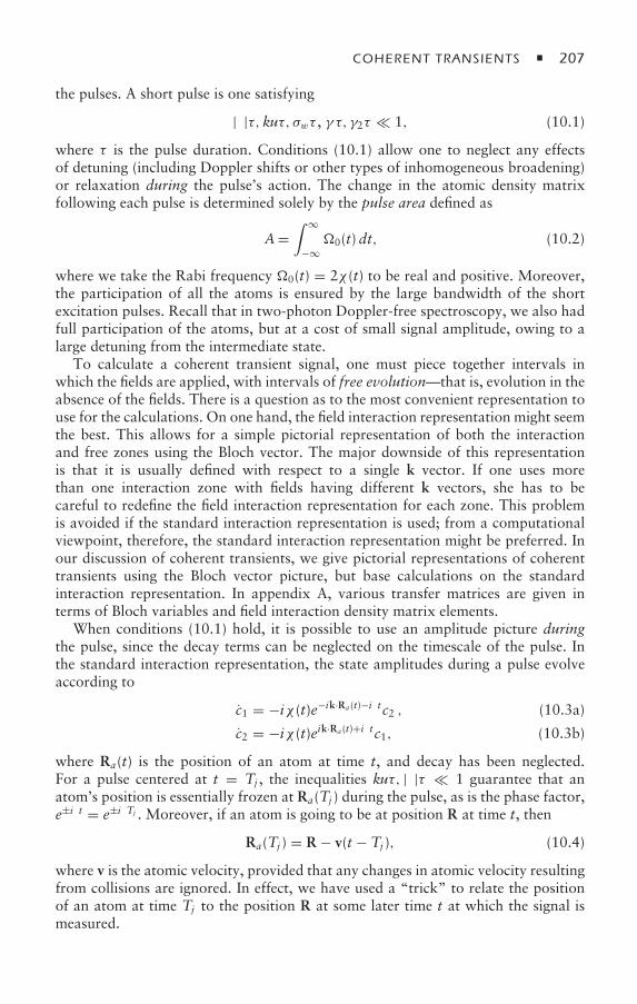
COHERENT TRANSIENTS 207
the pulses. A short pulse is one satisfying
|δ|τ,kuτ, σwτ , γ τ, γ2τ 1, (10.1)
where τ is the pulse duration. Conditions (10.1) allow one to neglect any effectsof detuning (including Doppler shifts or other types of inhomogeneous broadening)or relaxation during the pulse’s action. The change in the atomic density matrixfollowing each pulse is determined solely by the pulse area defined as
A=∫ ∞
−∞0(t)dt, (10.2)
where we take the Rabi frequency 0(t) = 2χ (t) to be real and positive. Moreover,the participation of all the atoms is ensured by the large bandwidth of the shortexcitation pulses. Recall that in two-photon Doppler-free spectroscopy, we also hadfull participation of the atoms, but at a cost of small signal amplitude, owing to alarge detuning from the intermediate state.
To calculate a coherent transient signal, one must piece together intervals inwhich the fields are applied, with intervals of free evolution—that is, evolution in theabsence of the fields. There is a question as to the most convenient representation touse for the calculations. On one hand, the field interaction representation might seemthe best. This allows for a simple pictorial representation of both the interactionand free zones using the Bloch vector. The major downside of this representationis that it is usually defined with respect to a single k vector. If one uses morethan one interaction zone with fields having different k vectors, she has to becareful to redefine the field interaction representation for each zone. This problemis avoided if the standard interaction representation is used; from a computationalviewpoint, therefore, the standard interaction representation might be preferred. Inour discussion of coherent transients, we give pictorial representations of coherenttransients using the Bloch vector picture, but base calculations on the standardinteraction representation. In appendix A, various transfer matrices are given interms of Bloch variables and field interaction density matrix elements.
When conditions (10.1) hold, it is possible to use an amplitude picture duringthe pulse, since the decay terms can be neglected on the timescale of the pulse. Inthe standard interaction representation, the state amplitudes during a pulse evolveaccording to
c1 = −iχ (t)e−ik·Ra (t)−iδtc2 , (10.3a)
c2 = −iχ (t)eik·Ra (t)+iδtc1, (10.3b)
where Ra(t) is the position of an atom at time t, and decay has been neglected.For a pulse centered at t = Tj , the inequalities kuτ, |δ|τ 1 guarantee that anatom’s position is essentially frozen at Ra(Tj ) during the pulse, as is the phase factor,e±iδt = e±iδTj . Moreover, if an atom is going to be at position R at time t, then
Ra(Tj ) = R − v(t − Tj ), (10.4)
where v is the atomic velocity, provided that any changes in atomic velocity resultingfrom collisions are ignored. In effect, we have used a “trick” to relate the positionof an atom at time Tj to the position R at some later time t at which the signal ismeasured.
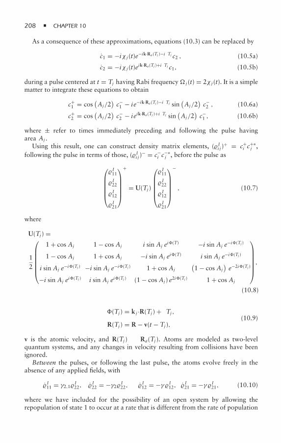
208 CHAPTER 10
As a consequence of these approximations, equations (10.3) can be replaced by
c1 = −iχ j (t)e−ik·Ra (Tj )−iδTj c2 , (10.5a)
c2 = −iχ j (t)eik·Ra (Tj )+iδTj c1, (10.5b)
during a pulse centered at t = Tj having Rabi frequency j (t) = 2χ j (t). It is a simplematter to integrate these equations to obtain
c+1 = cos
(Aj/2
)c−1 − ie−ik·Ra (Tj )−iδTj sin
(Aj/2
)c−2 , (10.6a)
c+2 = cos
(Aj/2
)c−2 − ieik·Ra (Tj )+iδTj sin
(Aj/2
)c−1 , (10.6b)
where ± refer to times immediately preceding and following the pulse havingarea Aj .
Using this result, one can construct density matrix elements, (Ii j )+ = c+
i c+∗j ,
following the pulse in terms of those, (Ii j )− = c−
i c−∗j , before the pulse as
⎛⎜⎜⎜⎜⎝I11
I22
I12
I21
⎞⎟⎟⎟⎟⎠
+
= U(Tj )
⎛⎜⎜⎜⎜⎝I11
I22
I12
I21
⎞⎟⎟⎟⎟⎠
−
, (10.7)
where
U(Tj ) =
12
⎛⎜⎜⎜⎜⎜⎝
1 + cos Aj 1 − cos Aj i sin Aj ei(T) −i sin Aj e−i(Tj )
1 − cos Aj 1 + cos Aj −i sin Aj ei(T) i sin Aj e−i(Tj )
i sin Aj e−i(Tj ) −i sin Aj e−i(Tj ) 1 + cos Aj(1 − cos Aj
)e−2i(Tj )
−i sin Aj ei(Tj ) i sin Aj ei(Tj ) (1 − cos Aj ) e2i(Tj ) 1 + cos Aj
⎞⎟⎟⎟⎟⎟⎠,
(10.8)
(Tj ) = k j ·R(Tj ) + δTj ,(10.9)
R(Tj ) = R − v(t − Tj ),
v is the atomic velocity, and R(Tj ) ≡ Ra(Tj ). Atoms are modeled as two-levelquantum systems, and any changes in velocity resulting from collisions have beenignored.
Between the pulses, or following the last pulse, the atoms evolve freely in theabsence of any applied fields, with
I11 = γ2,1I22, I22 = −γ2I22, I12 = −γ I12, I21 = −γ I21, (10.10)
where we have included for the possibility of an open system by allowing therepopulation of state 1 to occur at a rate that is different from the rate of population
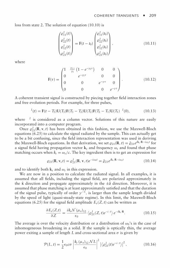
COHERENT TRANSIENTS 209
loss from state 2. The solution of equation (10.10) is⎛⎜⎜⎜⎜⎝I11(t)
I22(t)
I12(t)
I21(t)
⎞⎟⎟⎟⎟⎠ = F(t − t0)
⎛⎜⎜⎜⎜⎝I11(t0)
I22(t0)
I12(t0)
I21(t0)
⎞⎟⎟⎟⎟⎠ , (10.11)
where
F(τ ) =
⎛⎜⎜⎜⎜⎝1 γ2,1
γ2
(1 − e−γ2τ) 0 0
0 e−γ2τ 0 0
0 0 e−γ τ 0
0 0 0 e−γ τ
⎞⎟⎟⎟⎟⎠ . (10.12)
A coherent transient signal is constructed by piecing together field interaction zonesand free evolution periods. For example, for three pulses,
I (t) = F(t − T3)U(T3)F(T3 − T2)U(T2)F(T2 − T1)U(T1)I (0), (10.13)
where I is considered as a column vector. Solutions of this nature are easilyincorporated into a computer program.
Once I21(R, v, t) has been obtained in this fashion, we use the Maxwell-Blochequations (6.25) to calculate the signal radiated by the sample. This can actually getto be a bit confusing, since the field interaction representation was used in derivingthe Maxwell-Bloch equations. In that derivation, we set 21(R, t) = 21eiks ·R−iωs t fora signal field having propagation vector ks and frequency ωs and found that phasematching occurs when ks = ωs/c. The key ingredient then is to get an expression for
21(R, v, t) = I21(R, v, t)e−iω0t = 21eiks ·R−iωs t (10.14)
and to identify both ks and ωs in this expression.We are now in a position to calculate the radiated signal. In all examples, it is
assumed that all fields, including the signal field, are polarized approximately inthe x direction and propagate approximately in the ±z direction. Moreover, it isassumed that phase matching is at least approximately satisfied and that the durationof the signal pulse, typically of order γ−1, is larger than the sample length dividedby the speed of light (quasi-steady-state regime). In this limit, the Maxwell-Blochequations (6.25) for the signal field amplitude Es(Z, t) can be written as
∂Es(Z,t)∂Z
= iksN (µx)12ε0
⟨I21(Z, t)e
−iδt⟩ e−iks ·R. (10.15)
The average is over the velocity distribution or a distribution of ω0’s in the case ofinhomogeneous broadening in a solid. If the sample is optically thin, the averagepower exiting a sample of length L and cross-sectional area σ is given by
P(L, t) = 12ε0cσ
∣∣∣∣ks (µx)12N Lε0
∣∣∣∣2 ∣∣⟨I21(t)e−iδt⟩∣∣2 , (10.16)
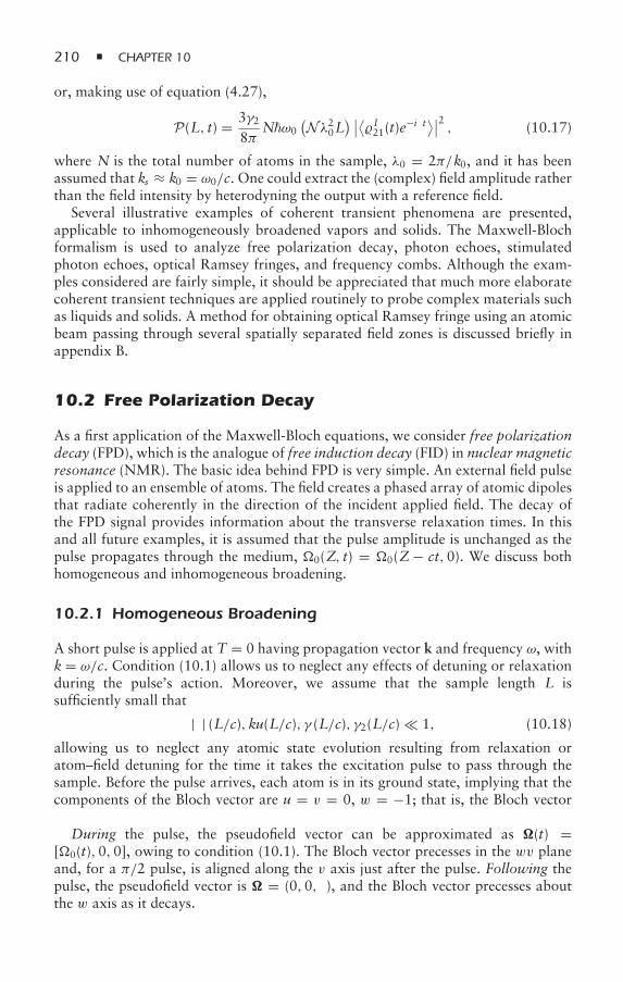
210 CHAPTER 10
or, making use of equation (4.27),
P(L, t) = 3γ28π
Nω0(Nλ20L
) ∣∣⟨I21(t)e−iδt⟩∣∣2 , (10.17)
where N is the total number of atoms in the sample, λ0 = 2π/k0, and it has beenassumed that ks ≈ k0 = ω0/c. One could extract the (complex) field amplitude ratherthan the field intensity by heterodyning the output with a reference field.
Several illustrative examples of coherent transient phenomena are presented,applicable to inhomogeneously broadened vapors and solids. The Maxwell-Blochformalism is used to analyze free polarization decay, photon echoes, stimulatedphoton echoes, optical Ramsey fringes, and frequency combs. Although the exam-ples considered are fairly simple, it should be appreciated that much more elaboratecoherent transient techniques are applied routinely to probe complex materials suchas liquids and solids. A method for obtaining optical Ramsey fringe using an atomicbeam passing through several spatially separated field zones is discussed briefly inappendix B.
10.2 Free Polarization Decay
As a first application of the Maxwell-Bloch equations, we consider free polarizationdecay (FPD), which is the analogue of free induction decay (FID) in nuclear magneticresonance (NMR). The basic idea behind FPD is very simple. An external field pulseis applied to an ensemble of atoms. The field creates a phased array of atomic dipolesthat radiate coherently in the direction of the incident applied field. The decay ofthe FPD signal provides information about the transverse relaxation times. In thisand all future examples, it is assumed that the pulse amplitude is unchanged as thepulse propagates through the medium, 0(Z, t) = 0(Z− ct,0). We discuss bothhomogeneous and inhomogeneous broadening.
10.2.1 Homogeneous Broadening
A short pulse is applied at T = 0 having propagation vector k and frequency ω, withk= ω/c. Condition (10.1) allows us to neglect any effects of detuning or relaxationduring the pulse’s action. Moreover, we assume that the sample length L issufficiently small that
|δ| (L/c),ku(L/c), γ (L/c), γ2(L/c) 1, (10.18)
allowing us to neglect any atomic state evolution resulting from relaxation oratom–field detuning for the time it takes the excitation pulse to pass through thesample. Before the pulse arrives, each atom is in its ground state, implying that thecomponents of the Bloch vector are u = v = 0, w = −1; that is, the Bloch vectorpoints down [see figure 10.1(a)].
During the pulse, the pseudofield vector can be approximated as (t) =[0(t),0,0], owing to condition (10.1). The Bloch vector precesses in the wv planeand, for a π/2 pulse, is aligned along the v axis just after the pulse. Following thepulse, the pseudofield vector is = (0,0, δ), and the Bloch vector precesses aboutthe w axis as it decays.
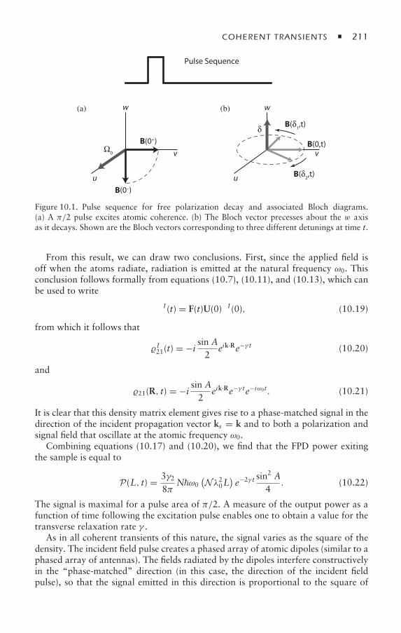
COHERENT TRANSIENTS 211
u
vv
w(a)
B(0+)
B(0–)
Ω0
Pulse Sequence
u
w(b)
B(0,t)
B(δ1,t)
B(δ2,t)
δ
Figure 10.1. Pulse sequence for free polarization decay and associated Bloch diagrams.(a) A π/2 pulse excites atomic coherence. (b) The Bloch vector precesses about the w axisas it decays. Shown are the Bloch vectors corresponding to three different detunings at time t.
From this result, we can draw two conclusions. First, since the applied field isoff when the atoms radiate, radiation is emitted at the natural frequency ω0. Thisconclusion follows formally from equations (10.7), (10.11), and (10.13), which canbe used to write
I (t) = F(t)U(0)I (0), (10.19)
from which it follows that
I21(t) = −i sin A2
eik·Re−γ t (10.20)
and
21(R, t) = −i sin A2
eik·Re−γ te−iω0t. (10.21)
It is clear that this density matrix element gives rise to a phase-matched signal in thedirection of the incident propagation vector ks = k and to both a polarization andsignal field that oscillate at the atomic frequency ω0.
Combining equations (10.17) and (10.20), we find that the FPD power exitingthe sample is equal to
P(L, t) = 3γ28π
Nω0(Nλ20L
)e−2γ t sin
2 A4
. (10.22)
The signal is maximal for a pulse area of π/2. A measure of the output power as afunction of time following the excitation pulse enables one to obtain a value for thetransverse relaxation rate γ .
As in all coherent transients of this nature, the signal varies as the square of thedensity. The incident field pulse creates a phased array of atomic dipoles (similar to aphased array of antennas). The fields radiated by the dipoles interfere constructivelyin the “phase-matched” direction (in this case, the direction of the incident fieldpulse), so that the signal emitted in this direction is proportional to the square of
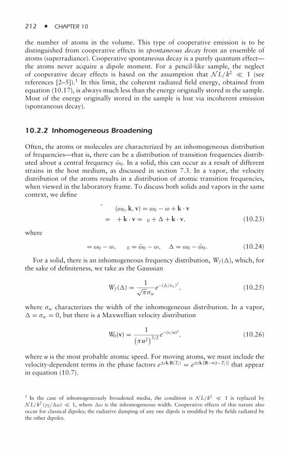
212 CHAPTER 10
the number of atoms in the volume. This type of cooperative emission is to bedistinguished from cooperative effects in spontaneous decay from an ensemble ofatoms (superradiance). Cooperative spontaneous decay is a purely quantum effect—the atoms never acquire a dipole moment. For a pencil-like sample, the neglectof cooperative decay effects is based on the assumption that N L/k2 1 (seereferences [2–5]).1 In this limit, the coherent radiated field energy, obtained fromequation (10.17), is always much less than the energy originally stored in the sample.Most of the energy originally stored in the sample is lost via incoherent emission(spontaneous decay).
10.2.2 Inhomogeneous Broadening
Often, the atoms or molecules are characterized by an inhomogeneous distributionof frequencies—that is, there can be a distribution of transition frequencies distrib-uted about a central frequency ω0. In a solid, this can occur as a result of differentstrains in the host medium, as discussed in section 7.3. In a vapor, the velocitydistribution of the atoms results in a distribution of atomic transition frequencies,when viewed in the laboratory frame. To discuss both solids and vapors in the samecontext, we define
δ ≡ δ(ω0,k, v) = ω0 − ω + k · v= δ + k · v = δ0 ++ k · v, (10.23)
where
δ = ω0 − ω, δ0 = ω0 − ω, = ω0 − ω0. (10.24)
For a solid, there is an inhomogeneous frequency distribution, Wf (), which, forthe sake of definiteness, we take as the Gaussian
Wf () = 1√πσw
e−(/σw)2 , (10.25)
where σw characterizes the width of the inhomogeneous distribution. In a vapor, = σw = 0, but there is a Maxwellian velocity distribution
W0(v) = 1(πu2
)3/2 e−(v/u)2 , (10.26)
where u is the most probable atomic speed. For moving atoms, we must include thevelocity-dependent terms in the phase factors e±ik·R(Tj ) = e±ik·[R−v(t−Tj )] that appearin equation (10.7).
1 In the case of inhomogeneously broadened media, the condition is N L/k2 1 is replaced byN L/k2 (γ2/ω) 1, where ω is the inhomogeneous width. Cooperative effects of this nature alsooccur for classical dipoles; the radiative damping of any one dipole is modified by the fields radiated bythe other dipoles.
COHERENT TRANSIENTS 213
0.50 1.0 1.5 2.0 2.5 3.0γ t
P(L,t)/P0
0.05
0
0.10
0.15
0.20
0.25
P P
Figure 10.2. Free polarization decay signal for stationary (dashed curve) and inhomoge-neously broadened (solid curve) atoms.
The net effect of including inhomogeneous broadening is that equation (10.22)must be replaced by
P(L, t) = P0∣∣⟨I21(t)e−iδt⟩∣∣2
= P0sin2 A
4
∣∣∣∣∫dvW0(v)
∫dWf ()e−[γ+i(+k·v)]t
∣∣∣∣2
= P0sin2 A
4e−2γ te−(σwt)2/2e−(kut)2/2, (10.27)
whereP0 = 3γ2
8πNω0(N λ20L), (10.28)
λ0 = 2πc/ω0, and we used the fact that
I21(t)e−iδt = −i sin A
2eik·R(0)e−γ te−i(δ0+)t
= −i sin A2
eik·(R−vt)e−γ te−i(δ0+)t. (10.29)
In a solid, u ∼ 0; in a vapor, σw ∼ 0.If σw γ (solids) or ku γ (vapors), the signal decays mainly as a result
of inhomogeneous broadening. To use a Bloch vector picture to model FPD inan inhomogeneously broadened system, we must remember that between pulses,the effective detuning appearing in the field interaction representation is δ(ω0,k, v).Bloch vectors corresponding to different frequencies precess about the w axis atdifferent rates, implying that the optical dipoles created by the pulse lose theirrelative phase in a time of order T∗
2 = σ−1w (solids) or (ku)−1 (vapors) [see
figure 10.1(b)]. The FPD signal can be used to measure T∗2 , which can be viewed as
an inhomogeneous, transverse relaxation time. In a room temperature vapor, ku/γis typically of order of 100. In a solid, σw/γ can be orders of magnitude larger. Infigure 10.2, the FPD signal P(L, t)/P0 is plotted as a function of γ t for a pulse areaA= π/2, σw = 0, and k1u/γ = 0 (dashed curve—stationary atoms) and k1u/γ = 10(solid curve—inhomogeneously broadened sample).
214 CHAPTER 10
The rapid decay of the FPD signal in inhomogeneously broadened media has asimple physical explanation. The pulse excites a phased array of atomic dipoles thatbegins to radiate coherently. However, these atoms radiate at different frequenciesas seen in the laboratory frame. After a time on the order of the inverse of the widthof the inhomogeneous frequency distribution, the dipoles are out of phase, and whileeach atom radiates coherently, there is no longer any constructive interference fromthe ensemble of atoms.
10.3 Photon Echo
Although the FPD signal produced by short excitation pulses decays in a time oforder T∗
2 , the coherence of individual atoms decays in a much longer time, T2. Thequestion arises as to whether it is possible to bring all the atomic dipoles back intophase so that they can radiate a coherent signal. The photon echo accomplishes thisgoal, although it has very little to do with either photons or echoes, but it doessound good. The photon echo, first observed in ruby by Kurnit et al. [6], is theoptical analogue of the spin echo in NMR [7]. A pulse having propagation vector k1and frequency ω is applied at t = 0, and a second pulse having propagation vectork2 = k1 is applied at t = T21. The echo is radiated at time t = 2T21 in a directionks = k1. There are many ways to explain echo formation and some of these areindicated in the following.
In the Bloch vector picture, a π/2 pulse excites the optical dipoles at t = 0,bringing the Bloch vector along the v axis [figure 10.3(a)]. The Bloch vector thenbegins to precess in the uv plane at a rate equal to the atom–field detuning. In aninhomogeneously broadened medium, the Bloch vectors associated with differentatoms precess at different rates and dephase relative to each other in a time T∗
2[figure 10.3(b)]. The dipole coherence is not lost, however. If at time T21 a π pulseis applied, the net effect of the pulse is to cause a reflection about the uw plane[figure 10.3(c)]. As the atoms continue to precess at different rates [figure 10.3(d)],the rates are such that the Bloch vectors for all the atoms become aligned withthe −v axis at time t = 2T21 and the “echo” signal is emitted [figure 10.3(e)].
It is not necessary that the pulse areas be equal to π/2 and π , although theseareas lead to a maximal signal. What is necessary is that the second pulse produceat least a partial reflection about the uw plane. This reflection takes the Bloch vectorcomponents u + iv into u − iv or, equivalently, takes density matrix element 12into 21. Since 12 and 21 are related to the real and imaginary parts of the averagedipole moment operator, the second pulse must couple these real and imaginaryparts. Such coupling is impossible for a linear atom–field interaction. Thus, by itsvery nature, the photon echo can occur only when a nonlinear atomic response ispresent.
An alternative way to picture echo formation is to use phase or double-sidedFeynman diagrams [8] that keep track of the relative phase of the different dipoles.Diagrams similar to those indicated in figure 10.4 were introduced by Beach,Hartmann, and Friedberg in the context of a “billiard ball echo model” [9] andhave been used extensively in theories of atom interferometry. Each line representsa field amplitude. The abscissa is time, and the ordinate is the phase associated withthe amplitude. As in the Bloch vector picture, the phases represented in this diagram
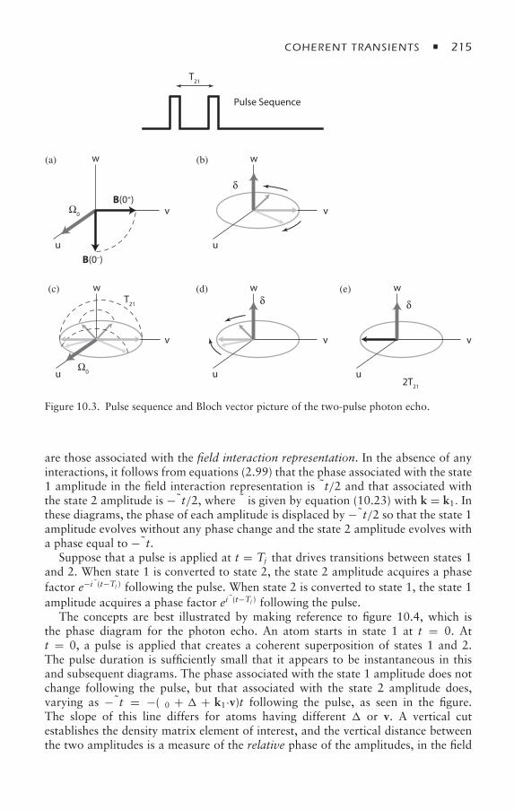
COHERENT TRANSIENTS 215
u
w(b)
δ
u
v v
u
w(e)
δ
v
u
w(d)δ
v
u
w(c)
v
w(a)
B(0+)
B(0–)
Ω0
Ω0
Pulse Sequence
T21
T21
2T21
Figure 10.3. Pulse sequence and Bloch vector picture of the two-pulse photon echo.
are those associated with the field interaction representation. In the absence of anyinteractions, it follows from equations (2.99) that the phase associated with the state1 amplitude in the field interaction representation is δt/2 and that associated withthe state 2 amplitude is −δt/2, where δ is given by equation (10.23) with k = k1. Inthese diagrams, the phase of each amplitude is displaced by −δt/2 so that the state 1amplitude evolves without any phase change and the state 2 amplitude evolves witha phase equal to −δt.
Suppose that a pulse is applied at t = Tj that drives transitions between states 1and 2. When state 1 is converted to state 2, the state 2 amplitude acquires a phasefactor e−i δ(t−Tj ) following the pulse. When state 2 is converted to state 1, the state 1amplitude acquires a phase factor ei δ(t−Tj ) following the pulse.
The concepts are best illustrated by making reference to figure 10.4, which isthe phase diagram for the photon echo. An atom starts in state 1 at t = 0. Att = 0, a pulse is applied that creates a coherent superposition of states 1 and 2.The pulse duration is sufficiently small that it appears to be instantaneous in thisand subsequent diagrams. The phase associated with the state 1 amplitude does notchange following the pulse, but that associated with the state 2 amplitude does,varying as −δt = −(δ0 + + k1·v)t following the pulse, as seen in the figure.The slope of this line differs for atoms having different or v. A vertical cutestablishes the density matrix element of interest, and the vertical distance betweenthe two amplitudes is a measure of the relative phase of the amplitudes, in the field
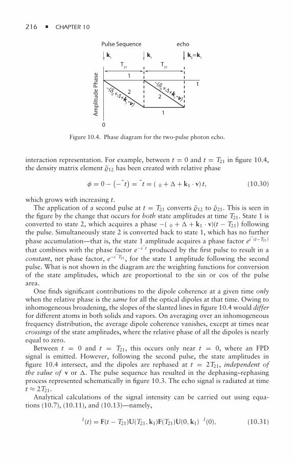
216 CHAPTER 10
Pulse Sequence
Am
plitu
de P
hase
echo
0
1
22
t
1
–(δ0 +∆+k
1 •v)
–(δ0 +∆+k
1 •v)
k1 k1
T21 T21
kS=k1
Figure 10.4. Phase diagram for the two-pulse photon echo.
interaction representation. For example, between t = 0 and t = T21 in figure 10.4,the density matrix element 12 has been created with relative phase
φ = 0 − (−δt) = δt = (δ0 ++ k1 · v) t, (10.30)
which grows with increasing t.The application of a second pulse at t = T21 converts 12 to 21. This is seen in
the figure by the change that occurs for both state amplitudes at time T21. State 1 isconverted to state 2, which acquires a phase −(δ0 + + k1 · v)(t − T21) followingthe pulse. Simultaneously state 2 is converted back to state 1, which has no furtherphase accumulation—that is, the state 1 amplitude acquires a phase factor ei δ(t−T21)
that combines with the phase factor e−i δt produced by the first pulse to result in aconstant, net phase factor, e−i δT21 , for the state 1 amplitude following the secondpulse. What is not shown in the diagram are the weighting functions for conversionof the state amplitudes, which are proportional to the sin or cos of the pulsearea.
One finds significant contributions to the dipole coherence at a given time onlywhen the relative phase is the same for all the optical dipoles at that time. Owing toinhomogeneous broadening, the slopes of the slanted lines in figure 10.4 would differfor different atoms in both solids and vapors. On averaging over an inhomogeneousfrequency distribution, the average dipole coherence vanishes, except at times nearcrossings of the state amplitudes, where the relative phase of all the dipoles is nearlyequal to zero.
Between t = 0 and t = T21, this occurs only near t = 0, where an FPDsignal is emitted. However, following the second pulse, the state amplitudes infigure 10.4 intersect, and the dipoles are rephased at t = 2T21, independent ofthe value of v or . The pulse sequence has resulted in the dephasing–rephasingprocess represented schematically in figure 10.3. The echo signal is radiated at timet ≈ 2T21.
Analytical calculations of the signal intensity can be carried out using equa-tions (10.7), (10.11), and (10.13)—namely,
I (t) = F(t − T21)U(T21,k1)F(T21)U(0,k1)I (0), (10.31)
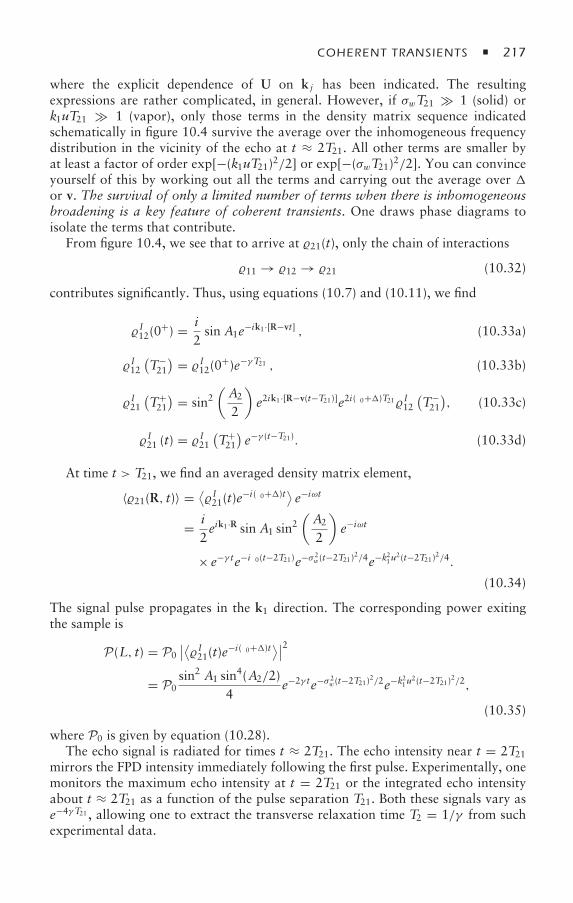
COHERENT TRANSIENTS 217
where the explicit dependence of U on k j has been indicated. The resultingexpressions are rather complicated, in general. However, if σwT21 1 (solid) ork1uT21 1 (vapor), only those terms in the density matrix sequence indicatedschematically in figure 10.4 survive the average over the inhomogeneous frequencydistribution in the vicinity of the echo at t ≈ 2T21. All other terms are smaller byat least a factor of order exp[−(k1uT21)2/2] or exp[−(σwT21)2/2]. You can convinceyourself of this by working out all the terms and carrying out the average over or v. The survival of only a limited number of terms when there is inhomogeneousbroadening is a key feature of coherent transients. One draws phase diagrams toisolate the terms that contribute.
From figure 10.4, we see that to arrive at 21(t), only the chain of interactions
11 → 12 → 21 (10.32)
contributes significantly. Thus, using equations (10.7) and (10.11), we find
I12(0+) = i
2sin A1e−ik1·[R−vt] , (10.33a)
I12(T−21
) = I12(0+)e−γT21 , (10.33b)
I21(T+21
) = sin2(A2
2
)e2ik1·[R−v(t−T21)]e2i(δ0+)T21I12
(T−21
), (10.33c)
I21 (t) = I21(T+21
)e−γ (t−T21). (10.33d)
At time t > T21, we find an averaged density matrix element,
〈21(R, t)〉 = ⟨I21(t)e
−i(δ0+)t⟩ e−iωt
= i2eik1·R sin A1 sin
2(A2
2
)e−iωt
× e−γ te−iδ0(t−2T21)e−σ 2w(t−2T21)2/4e−k21u2(t−2T21)2/4.
(10.34)
The signal pulse propagates in the k1 direction. The corresponding power exitingthe sample is
P(L, t) = P0∣∣⟨I21(t)e−i(δ0+)t⟩∣∣2
= P0sin2 A1 sin
4(A2/2)4
e−2γ te−σ 2w(t−2T21)2/2e−k21u2(t−2T21)2/2,
(10.35)
where P0 is given by equation (10.28).The echo signal is radiated for times t ≈ 2T21. The echo intensity near t = 2T21
mirrors the FPD intensity immediately following the first pulse. Experimentally, onemonitors the maximum echo intensity at t = 2T21 or the integrated echo intensityabout t ≈ 2T21 as a function of the pulse separation T21. Both these signals vary ase−4γT21 , allowing one to extract the transverse relaxation time T2 = 1/γ from suchexperimental data.
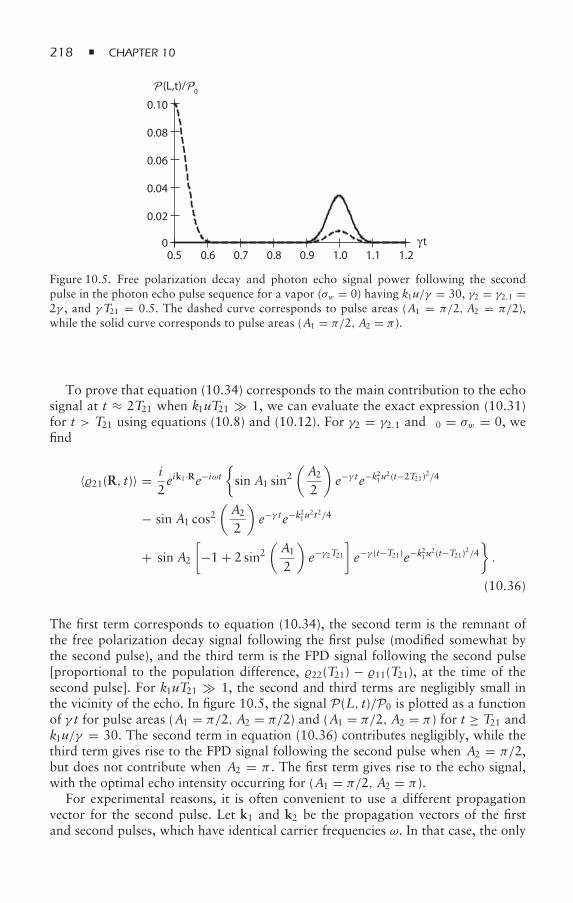
218 CHAPTER 10
0.60.5 0.7 0.8 0.9 1.0 1.21.1γ t
P(L,t)/P0
0.02
0
0.04
0.06
0.08
0.10P P
Figure 10.5. Free polarization decay and photon echo signal power following the secondpulse in the photon echo pulse sequence for a vapor (σw = 0) having k1u/γ = 30, γ2 = γ2,1 =2γ , and γT21 = 0.5. The dashed curve corresponds to pulse areas (A1 = π/2, A2 = π/2),while the solid curve corresponds to pulse areas (A1 = π/2, A2 = π ).
To prove that equation (10.34) corresponds to the main contribution to the echosignal at t ≈ 2T21 when k1uT21 1, we can evaluate the exact expression (10.31)for t > T21 using equations (10.8) and (10.12). For γ2 = γ2,1 and δ0 = σw = 0, wefind
〈21(R, t)〉 = i2eik1·Re−iωt
sin A1 sin
2(A2
2
)e−γ te−k21u2(t−2T21)2/4
− sin A1 cos2(A2
2
)e−γ te−k21u2t2/4
+ sin A2
[−1 + 2 sin2
(A1
2
)e−γ2T21
]e−γ (t−T21)e−k21u2(t−T21)2/4
.
(10.36)
The first term corresponds to equation (10.34), the second term is the remnant ofthe free polarization decay signal following the first pulse (modified somewhat bythe second pulse), and the third term is the FPD signal following the second pulse[proportional to the population difference, 22(T21) − 11(T21), at the time of thesecond pulse]. For k1uT21 1, the second and third terms are negligibly small inthe vicinity of the echo. In figure 10.5, the signal P(L, t)/P0 is plotted as a functionof γ t for pulse areas (A1 = π/2, A2 = π/2) and (A1 = π/2, A2 = π ) for t ≥ T21 andk1u/γ = 30. The second term in equation (10.36) contributes negligibly, while thethird term gives rise to the FPD signal following the second pulse when A2 = π/2,but does not contribute when A2 = π . The first term gives rise to the echo signal,with the optimal echo intensity occurring for (A1 = π/2, A2 = π ).
For experimental reasons, it is often convenient to use a different propagationvector for the second pulse. Let k1 and k2 be the propagation vectors of the firstand second pulses, which have identical carrier frequencies ω. In that case, the only
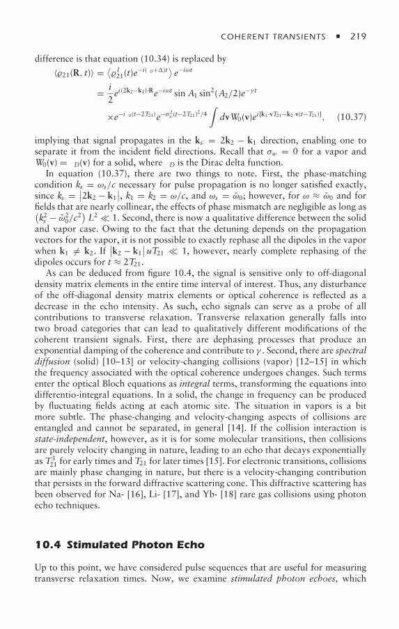
COHERENT TRANSIENTS 219
difference is that equation (10.34) is replaced by
〈21(R, t)〉 = ⟨I21(t)e
−i(δ0+)t⟩ e−iωt
= i2ei(2k2−k1)·Re−iωt sin A1 sin
2(A2/2)e−γ t
×e−iδ0(t−2T21)e−σ 2w(t−2T21)2/4
∫dvW0(v)ei[k1·vT21−k2·v(t−T21)], (10.37)
implying that signal propagates in the ks = 2k2 − k1 direction, enabling one toseparate it from the incident field directions. Recall that σw = 0 for a vapor andW0(v) = δD(v) for a solid, where δD is the Dirac delta function.
In equation (10.37), there are two things to note. First, the phase-matchingcondition ks = ωs/c necessary for pulse propagation is no longer satisfied exactly,since ks = ∣∣2k2 − k1
∣∣, k1 = k2 = ω/c, and ωs = ω0; however, for ω ≈ ω0 and forfields that are nearly collinear, the effects of phase mismatch are negligible as long as(k2s − ω2
0/c2)L2 1. Second, there is now a qualitative difference between the solid
and vapor case. Owing to the fact that the detuning depends on the propagationvectors for the vapor, it is not possible to exactly rephase all the dipoles in the vaporwhen k1 = k2. If
∣∣k2 − k1∣∣ uT21 1, however, nearly complete rephasing of the
dipoles occurs for t ≈ 2T21.As can be deduced from figure 10.4, the signal is sensitive only to off-diagonal
density matrix elements in the entire time interval of interest. Thus, any disturbanceof the off-diagonal density matrix elements or optical coherence is reflected as adecrease in the echo intensity. As such, echo signals can serve as a probe of allcontributions to transverse relaxation. Transverse relaxation generally falls intotwo broad categories that can lead to qualitatively different modifications of thecoherent transient signals. First, there are dephasing processes that produce anexponential damping of the coherence and contribute to γ . Second, there are spectraldiffusion (solid) [10–13] or velocity-changing collisions (vapor) [12–15] in whichthe frequency associated with the optical coherence undergoes changes. Such termsenter the optical Bloch equations as integral terms, transforming the equations intodifferentio-integral equations. In a solid, the change in frequency can be producedby fluctuating fields acting at each atomic site. The situation in vapors is a bitmore subtle. The phase-changing and velocity-changing aspects of collisions areentangled and cannot be separated, in general [14]. If the collision interaction isstate-independent, however, as it is for some molecular transitions, then collisionsare purely velocity changing in nature, leading to an echo that decays exponentiallyas T3
21 for early times and T21 for later times [15]. For electronic transitions, collisionsare mainly phase changing in nature, but there is a velocity-changing contributionthat persists in the forward diffractive scattering cone. This diffractive scattering hasbeen observed for Na- [16], Li- [17], and Yb- [18] rare gas collisions using photonecho techniques.
10.4 Stimulated Photon Echo
Up to this point, we have considered pulse sequences that are useful for measuringtransverse relaxation times. Now, we examine stimulated photon echoes, which
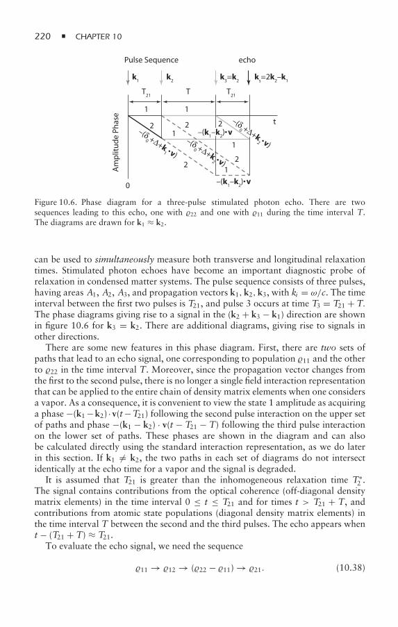
220 CHAPTER 10
Pulse Sequence
Am
plitu
de P
hase
echo
0
1 1
2
2 2 2
2
t
1
11–(δ
0 +∆+k1 •v)
–(δ0 +∆+k
2 •v)
k1 k2
T21 T T21
k3=k2 ks=2k2–k1
–(k1–k2)•v
–(δ0 +∆+k
2 •v)–(k1–k2)•v
Figure 10.6. Phase diagram for a three-pulse stimulated photon echo. There are twosequences leading to this echo, one with 22 and one with 11 during the time interval T.The diagrams are drawn for k1 ≈ k2.
can be used to simultaneously measure both transverse and longitudinal relaxationtimes. Stimulated photon echoes have become an important diagnostic probe ofrelaxation in condensed matter systems. The pulse sequence consists of three pulses,having areas A1, A2, A3, and propagation vectors k1,k2,k3, with ki = ω/c. The timeinterval between the first two pulses is T21, and pulse 3 occurs at time T3 = T21 + T.The phase diagrams giving rise to a signal in the (k2 + k3 − k1) direction are shownin figure 10.6 for k3 = k2. There are additional diagrams, giving rise to signals inother directions.
There are some new features in this phase diagram. First, there are two sets ofpaths that lead to an echo signal, one corresponding to population 11 and the otherto 22 in the time interval T. Moreover, since the propagation vector changes fromthe first to the second pulse, there is no longer a single field interaction representationthat can be applied to the entire chain of density matrix elements when one considersa vapor. As a consequence, it is convenient to view the state 1 amplitude as acquiringa phase −(k1 −k2) ·v(t−T21) following the second pulse interaction on the upper setof paths and phase −(k1 − k2) · v(t − T21 − T) following the third pulse interactionon the lower set of paths. These phases are shown in the diagram and can alsobe calculated directly using the standard interaction representation, as we do laterin this section. If k1 = k2, the two paths in each set of diagrams do not intersectidentically at the echo time for a vapor and the signal is degraded.
It is assumed that T21 is greater than the inhomogeneous relaxation time T∗2 .
The signal contains contributions from the optical coherence (off-diagonal densitymatrix elements) in the time interval 0 ≤ t ≤ T21 and for times t > T21 + T, andcontributions from atomic state populations (diagonal density matrix elements) inthe time interval T between the second and the third pulses. The echo appears whent − (T21 + T) ≈ T21.
To evaluate the echo signal, we need the sequence
11 → 12 → (22 − 11) → 21. (10.38)
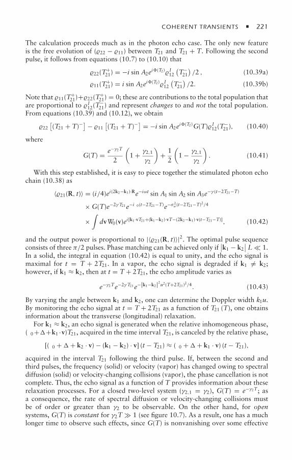
COHERENT TRANSIENTS 221
The calculation proceeds much as in the photon echo case. The only new featureis the free evolution of (22 − 11) between T21 and T21 + T. Following the secondpulse, it follows from equations (10.7) to (10.10) that
22(T+21) = −i sin A2ei(T2)I12
(T−21
)/2 , (10.39a)
11(T+21) = i sin A2ei(T2)I12
(T−21
)/2. (10.39b)
Note that 11(T+21)+22(T+
21) = 0; these are contributions to the total population thatare proportional to I12(T
−21) and represent changes to and not the total population.
From equations (10.39) and (10.12), we obtain
22[(T21 + T)−
]− 11[(T21 + T)−
] = −i sin A2ei(T2)G(T)I12(T−21), (10.40)
where
G(T) = e−γ2T
2
(1 + γ2,1
γ2
)+ 1
2
(1 − γ2,1
γ2
). (10.41)
With this step established, it is easy to piece together the stimulated photon echochain (10.38) as
〈21(R, t)〉 = (i/4)ei(2k2−k1)·Re−iωt sin A1 sin A2 sin A3e−γ (t−2T21−T)
× G(T)e−2γT21e−iδ0(t−2T21−T)e−σ 2w(t−2T21−T)2/4
×∫dvW0(v)ei[k1·vT21+(k1−k2)·vT−(2k2−k1)·v(t−T21−T)], (10.42)
and the output power is proportional to |〈21(R, t)〉|2. The optimal pulse sequenceconsists of three π/2 pulses. Phase matching can be achieved only if
∣∣k1 − k2∣∣ L 1.
In a solid, the integral in equation (10.42) is equal to unity, and the echo signal ismaximal for t = T + 2T21. In a vapor, the echo signal is degraded if k1 = k2;however, if k1 ≈ k2, then at t = T + 2T21, the echo amplitude varies as
e−γ2Te−2γT21e−|k1−k2|2u2(T+2T21)2/4. (10.43)
By varying the angle between k1 and k2, one can determine the Doppler width k1u.By monitoring the echo signal at t = T + 2T21 as a function of T21 (T), one obtainsinformation about the transverse (longitudinal) relaxation.
For k1 ≈ k2, an echo signal is generated when the relative inhomogeneous phase,(δ0++k1 ·v)T21, acquired in the time interval T21, is canceled by the relative phase,
[(δ0 ++ k2 · v) − (k1 − k2) · v] (t − T21) ≈ (δ0 ++ k1 · v) (t − T21),
acquired in the interval T21 following the third pulse. If, between the second andthird pulses, the frequency (solid) or velocity (vapor) has changed owing to spectraldiffusion (solid) or velocity-changing collisions (vapor), the phase cancellation is notcomplete. Thus, the echo signal as a function of T provides information about theserelaxation processes. For a closed two-level system (γ2,1 = γ2), G(T) = e−γ2T; asa consequence, the rate of spectral diffusion or velocity-changing collisions mustbe of order or greater than γ2 to be observable. On the other hand, for opensystems, G(T) is constant for γ2T 1 (see figure 10.7). As a result, one has a muchlonger time to observe such effects, since G(T) is nonvanishing over some effective
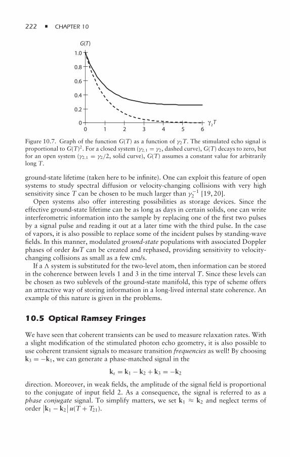
222 CHAPTER 10
10 2 3 4 5 6γ 2T
G(T)
0.2
0
0.4
0.6
0.8
1.0
Figure 10.7. Graph of the function G(T) as a function of γ2T. The stimulated echo signal isproportional to G(T)2. For a closed system (γ2,1 = γ2, dashed curve), G(T) decays to zero, butfor an open system (γ2,1 = γ2/2, solid curve), G(T) assumes a constant value for arbitrarilylong T.
ground-state lifetime (taken here to be infinite). One can exploit this feature of opensystems to study spectral diffusion or velocity-changing collisions with very highsensitivity since T can be chosen to be much larger than γ−1
2 [19, 20].Open systems also offer interesting possibilities as storage devices. Since the
effective ground-state lifetime can be as long as days in certain solids, one can writeinterferometric information into the sample by replacing one of the first two pulsesby a signal pulse and reading it out at a later time with the third pulse. In the caseof vapors, it is also possible to replace some of the incident pulses by standing-wavefields. In this manner, modulated ground-state populations with associated Dopplerphases of order kuT can be created and rephased, providing sensitivity to velocity-changing collisions as small as a few cm/s.
If a system is substituted for the two-level atom, then information can be storedin the coherence between levels 1 and 3 in the time interval T. Since these levels canbe chosen as two sublevels of the ground-state manifold, this type of scheme offersan attractive way of storing information in a long-lived internal state coherence. Anexample of this nature is given in the problems.
10.5 Optical Ramsey Fringes
We have seen that coherent transients can be used to measure relaxation rates. Witha slight modification of the stimulated photon echo geometry, it is also possible touse coherent transient signals to measure transition frequencies as well! By choosingk3 = −k1, we can generate a phase-matched signal in the
ks = k1 − k2 + k3 = −k2
direction. Moreover, in weak fields, the amplitude of the signal field is proportionalto the conjugate of input field 2. As a consequence, the signal is referred to as aphase conjugate signal. To simplify matters, we set k1 ≈ k2 and neglect terms oforder
∣∣k1 − k2∣∣ u(T + T21).
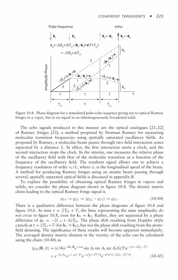
COHERENT TRANSIENTS 223
Pulse Sequence
Am
plitu
de P
hase
echo
t1
1
1
1
1
2 22
2
–(δ 0+∆+k 1
• v)
k1 k2
T21 T T21
k3=–k1 ks=–k2
–(k1–k2)•v
–(k 2+k 1
)• vφd
φd
φd=–2(δ0+∆)T21–(k1–k2)•v(T+T21)
≈ –2(δ0+∆)T21
–(δ0+∆–k
2 •v)
–(δ 0+∆+k 2
• v)
Figure 10.8. Phase diagram for a stimulated pulse echo sequence giving rise to optical Ramseyfringes in a vapor, but to no signal in an inhomogeneously broadened solid.
The echo signals produced in this manner are the optical analogues [21, 22]of Ramsey fringes [23], a method proposed by Norman Ramsey for measuringmolecular transition frequencies using spatially separated oscillatory fields. Asproposed by Ramsey, a molecular beam passes through two field interaction zonesseparated by a distance L. In effect, the first interaction starts a clock, and thesecond interaction stops the clock. In the interim, one measures the relative phaseof the oscillatory field with that of the molecular transition as a function of thefrequency of the oscillatory field. The resultant signal allows one to achieve afrequency resolution of order v/L, where v is the longitudinal speed of the beam.A method for producing Ramsey fringes using an atomic beam passing throughseveral, spatially separated optical fields is discussed in appendix B.
To explore the possibility of obtaining optical Ramsey fringes in vapors andsolids, we consider the phase diagram shown in figure 10.8. The density matrixchain leading to the optical Ramsey fringe signal is
11 → 21 → (22 − 11) → 21. (10.44)
There is a qualitative difference between the phase diagrams of figure 10.8 andfigure 10.6. At time t = 2T21 + T, the lines representing the state amplitudes donot cross in figure 10.8, even for k1 = k2. Rather, they are separated by a phasedifference of φd = −2(δ0 + )T21. The phase shift resulting from Doppler shiftscancels at t = 2T21+T (for k1 ≈ k2), but not the phase shift resulting from the atom–field detuning. The significance of these results will become apparent immediately.The averaged density matrix element in the vicinity of the echo can be calculatedusing the chain (10.44) as
〈21(R, t)〉 = (i/4)e−ik2·Re−iωt sin A1 sin A2 sin A3G(T)e−γ (t−2T21−T)
× e−2γT21e−iδ0(t−T)e−σ 2w(t−T)2/4e−k2u2(t−2T21−T)2/4. (10.45)
224 CHAPTER 10
In a solid, the signal is negligibly small near t = 2T21 + T since σwT21 1. (Thereare no optical Ramsey fringes in an inhomogeneously broadened solid owing to theaverage over .)
In a vapor, however, an echo is formed at time t ≈ T + 2T21. Although the linescorresponding to state amplitudes 1 and 2 do not cross at this time, the relativephase is the same for all the atoms. (Recall that = 0 in a vapor, so there isno average over to kill the signal, as in solids.) At t = T + 2T21, the averageddensity matrix element 〈21〉 varies as e−2iδ0T21 , a factor that was absent when allfields are nearly copropagating. This phase factor is the optical analogue of the phasefactor that is responsible for the generation of Ramsey fringes. One can measure thephase factor directly by heterodyning the signal field with a reference field, or byconverting the off-diagonal density matrix element to a population by the additionof a fourth pulse in the −k2 direction at time t = T + 2T21. The population canbe detected, for example, by the spontaneous emission signal emitted by the excitedatoms. In either case, the signal varies as cos(2δ0T21). In itself, this dependence isuseless for determining the optical frequency, since one cannot identify the fringecorresponding to δ0 = 0. It is necessary to take data as a function of δ0 for severalvalues of T21, and then average the data over T21; in this manner, the central fringecan be identified [24]. Using a four-pulse sequence of this type on an ensemble ofultracold, laser-cooled atoms, Degenhardt et al. achieved a relative uncertainty ofone part in 1014 on the Ca intercombination line [25].
A typical Ramsey fringe pattern, proportional to
H (δ0) =∫ ∞
0dT21 cos(2δ0T21)e−2γT21W(T21) (10.46)
for fixed T, is shown in figure 10.9 as a function of a = δ0T21 for γ T21 = 0.2 andT21/T21 = 0.3, assuming a distribution function
W(T21) =⎧⎨⎩
1T21
−T212 ≤ T21 − T21 ≤ T21
2
0 otherwise. (10.47)
For δ0 = 0, all phases cancel, and the signal is a maximum. As δ0T21 increases, theaveraged signal begins to wash out. Experiments of this type allow one to measureoptical frequencies with accuracy of order T−1
21 . While this would appear to be“subnatural” resolution for T21 > γ−1
2 , such a designation is somewhat misleading.The Ramsey fringe signal in this case diminishes as e−2γ2T21 , so the ability to measurea signal always boils down to a question of signal to noise.
The optical Ramsey fringe geometry has been reinterpreted as an atom inter-ferometer [26, 27]. It is not difficult to see how such an interpretation is possiblefor any coherent transient signal that leads to echo formation. As is evidentfrom figures 10.4 to 10.8, there are two paths that combine to produce the echosignal. One can interpret each path as representing one arm of an interferometer,although the analogue with optical interferometers is somewhat misleading. Opticalinterferometers rely on the wave nature of light for their operation, but as discussedin this chapter, the wave nature of the atoms’ center-of-mass motion plays no rolein echo formation. On the other hand, the interpretation becomes cogent whenthe atomic motion is quantized, since there are frequency shifts associated with
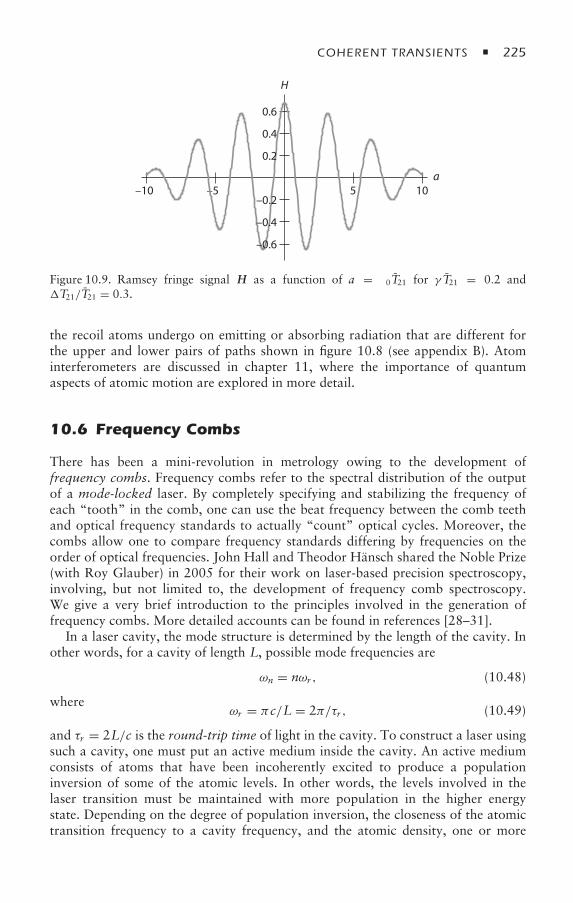
COHERENT TRANSIENTS 225
H
a–10 –5 5 10
–0.2
0.2
0.4
0.6
–0.6
–0.4
Figure 10.9. Ramsey fringe signal H as a function of a = δ0T21 for γ T21 = 0.2 andT21/T21 = 0.3.
the recoil atoms undergo on emitting or absorbing radiation that are different forthe upper and lower pairs of paths shown in figure 10.8 (see appendix B). Atominterferometers are discussed in chapter 11, where the importance of quantumaspects of atomic motion are explored in more detail.
10.6 Frequency Combs
There has been a mini-revolution in metrology owing to the development offrequency combs. Frequency combs refer to the spectral distribution of the outputof a mode-locked laser. By completely specifying and stabilizing the frequency ofeach “tooth” in the comb, one can use the beat frequency between the comb teethand optical frequency standards to actually “count” optical cycles. Moreover, thecombs allow one to compare frequency standards differing by frequencies on theorder of optical frequencies. John Hall and Theodor Hänsch shared the Noble Prize(with Roy Glauber) in 2005 for their work on laser-based precision spectroscopy,involving, but not limited to, the development of frequency comb spectroscopy.We give a very brief introduction to the principles involved in the generation offrequency combs. More detailed accounts can be found in references [28–31].
In a laser cavity, the mode structure is determined by the length of the cavity. Inother words, for a cavity of length L, possible mode frequencies are
ωn = nωr , (10.48)
whereωr = πc/L = 2π/τr , (10.49)
and τr = 2L/c is the round-trip time of light in the cavity. To construct a laser usingsuch a cavity, one must put an active medium inside the cavity. An active mediumconsists of atoms that have been incoherently excited to produce a populationinversion of some of the atomic levels. In other words, the levels involved in thelaser transition must be maintained with more population in the higher energystate. Depending on the degree of population inversion, the closeness of the atomictransition frequency to a cavity frequency, and the atomic density, one or more
226 CHAPTER 10
modes may be above threshold for lasing. The actual frequency of the modes will bechanged somewhat from the cavity mode frequencies owing to the presence of themedium, but the spacing between modes remains an integer multiple of ωr .
When a large number of modes are above threshold, they normally have randomphases, resulting in a laser output that is quasi-continuous. To produce the shortpulses needed to generate frequency combs, it is necessary to phase lock the variousmodes [32]. Mode locking can be accomplished actively by placing an acousto-opticor electro-optic modulator in the laser cavity that modulates the light in the cavitywith a frequency ωr . Such active mode locking can produce pulse widths on theorder of picoseconds. To achieve the femtosecond pulses used in frequency combs,passive mode locking is employed. In one approach to passive mode locking, asaturable absorber is placed inside the laser cavity. As was shown in chapter 5,once a transition is saturated or bleached, the relative absorption of an incident fieldincreases very slowly with increasing field strength. As such, a saturable absorberfavors the passage of intense fields. When placed in a cavity, a saturable absorbercan result in a nonlinear absorption coefficient that is modulated at frequency ωr .The mode coupling in the presence of a saturable absorber is modified in such amanner that results in phase locking of the modes. The field inside the cavity thenconsists of a narrow, intense pulse that propagates between the cavity mirrors, asmall part of which is coupled out of the cavity, resulting in a train of equally spacedpulses. An alternative method for achieving passive mode locking that is used in thetitanium-sapphire laser is based on lensing produced by the Kerr effect [33]. TheKerr effect is the change in the index of refraction of a medium produced by intensefields (see problem 1 in chapter 7).
Let us imagine that N+1 modes are above threshold. We set the central frequencyequal to
ωcentral = ωc + ωph, (10.50)
where ωc = n0ωr corresponds to one of the cavity modes in the absence of themedium, and ωph is the offset resulting from the presence of the medium. Thus, theoutput frequencies are given by
ωn = ωc + nωr + ωph, (10.51)
and n runs from −N/2 to N/2 (assuming N to be even).The Fourier transform of the positive frequency component of the field is assumed
to be of the form of a comb of frequencies,
E+(ω) = g (ω − ωc)N/2∑
n=−N/2
δ(ω − ωc − nωr − ωph
), (10.52)
where g(ω) is a smooth function (think Gaussian) that is centered at ω = 0 andhas a width that corresponds to anywhere between several thousand and a millionmodes. Since this spectral function cuts off the modes that are below threshold, wecan extend the sum as
E+(ω) = g(ω − ωc)∞∑
n=−∞δ(ω − ωc − nωr − ωph) (10.53)
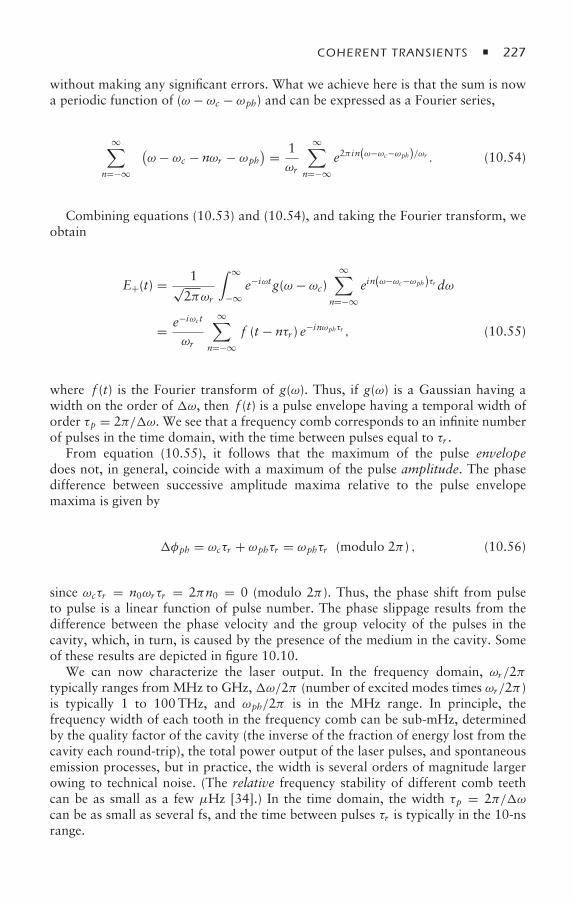
COHERENT TRANSIENTS 227
without making any significant errors. What we achieve here is that the sum is nowa periodic function of (ω − ωc − ωph) and can be expressed as a Fourier series,
∞∑n=−∞
δ(ω − ωc − nωr − ωph
) = 1ωr
∞∑n=−∞
e2π in(ω−ωc−ωph)/ωr . (10.54)
Combining equations (10.53) and (10.54), and taking the Fourier transform, weobtain
E+(t) = 1√2πωr
∫ ∞
−∞e−iωtg(ω − ωc)
∞∑n=−∞
ein(ω−ωc−ωph)τr dω
= e−iωct
ωr
∞∑n=−∞
f (t − nτr ) e−inωphτr , (10.55)
where f (t) is the Fourier transform of g(ω). Thus, if g(ω) is a Gaussian having awidth on the order of ω, then f (t) is a pulse envelope having a temporal width oforder τp = 2π/ω. We see that a frequency comb corresponds to an infinite numberof pulses in the time domain, with the time between pulses equal to τr .
From equation (10.55), it follows that the maximum of the pulse envelopedoes not, in general, coincide with a maximum of the pulse amplitude. The phasedifference between successive amplitude maxima relative to the pulse envelopemaxima is given by
φph = ωcτr + ωphτr = ωphτr (modulo 2π ) , (10.56)
since ωcτr = n0ωrτr = 2πn0 = 0 (modulo 2π ). Thus, the phase shift from pulseto pulse is a linear function of pulse number. The phase slippage results from thedifference between the phase velocity and the group velocity of the pulses in thecavity, which, in turn, is caused by the presence of the medium in the cavity. Someof these results are depicted in figure 10.10.
We can now characterize the laser output. In the frequency domain, ωr/2πtypically ranges fromMHz to GHz, ω/2π (number of excited modes times ωr/2π )is typically 1 to 100THz, and ωph/2π is in the MHz range. In principle, thefrequency width of each tooth in the frequency comb can be sub-mHz, determinedby the quality factor of the cavity (the inverse of the fraction of energy lost from thecavity each round-trip), the total power output of the laser pulses, and spontaneousemission processes, but in practice, the width is several orders of magnitude largerowing to technical noise. (The relative frequency stability of different comb teethcan be as small as a few µHz [34].) In the time domain, the width τp = 2π/ωcan be as small as several fs, and the time between pulses τr is typically in the 10-nsrange.
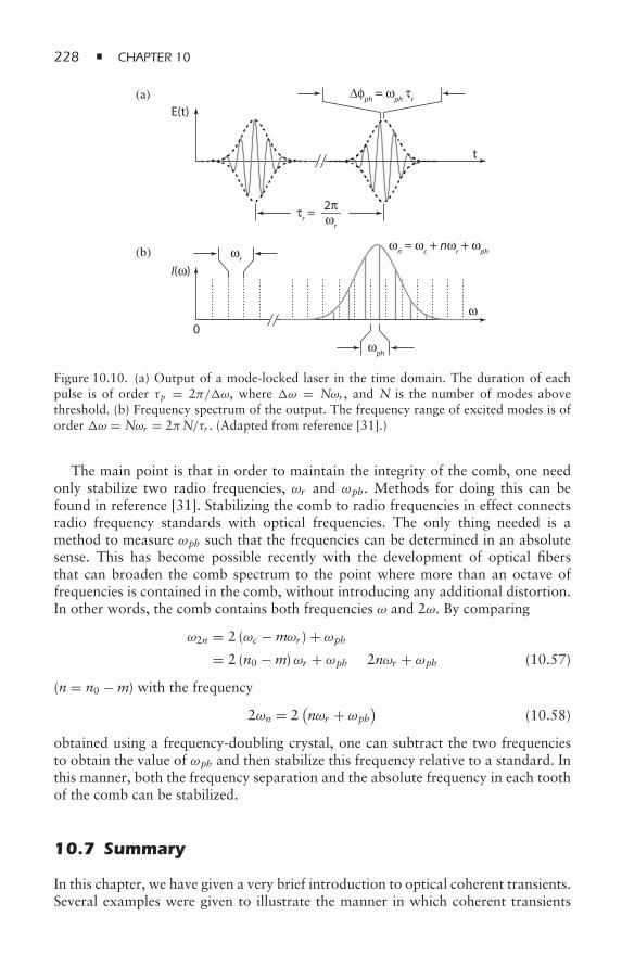
228 CHAPTER 10
E(t)(a)
(b)
t
0
I(ω)
ω
∆φph = ωph τr
ωn = ωc + nωr + ωph
τr =___2πωr
ωr
ωph
Figure 10.10. (a) Output of a mode-locked laser in the time domain. The duration of eachpulse is of order τp = 2π/ω, where ω = Nωr , and N is the number of modes abovethreshold. (b) Frequency spectrum of the output. The frequency range of excited modes is oforder ω = Nωr = 2πN/τr . (Adapted from reference [31].)
The main point is that in order to maintain the integrity of the comb, one needonly stabilize two radio frequencies, ωr and ωph. Methods for doing this can befound in reference [31]. Stabilizing the comb to radio frequencies in effect connectsradio frequency standards with optical frequencies. The only thing needed is amethod to measure ωph such that the frequencies can be determined in an absolutesense. This has become possible recently with the development of optical fibersthat can broaden the comb spectrum to the point where more than an octave offrequencies is contained in the comb, without introducing any additional distortion.In other words, the comb contains both frequencies ω and 2ω. By comparing
ω2n = 2 (ωc −mωr ) + ωph
= 2 (n0 −m)ωr + ωph ≡ 2nωr + ωph (10.57)
(n = n0 −m) with the frequency
2ωn = 2(nωr + ωph
)(10.58)
obtained using a frequency-doubling crystal, one can subtract the two frequenciesto obtain the value of ωph and then stabilize this frequency relative to a standard. Inthis manner, both the frequency separation and the absolute frequency in each toothof the comb can be stabilized.
10.7 Summary
In this chapter, we have given a very brief introduction to optical coherent transients.Several examples were given to illustrate the manner in which coherent transients
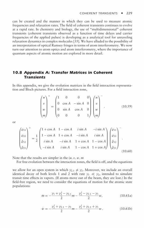
COHERENT TRANSIENTS 229
can be created and the manner in which they can be used to measure atomicfrequencies and relaxation rates. The field of coherent transients continues to evolveat a rapid rate. In chemistry and biology, the use of “multidimensional” coherenttransients (coherent transients observed as a function of time delays and carrierfrequencies of the applied pulses) is developing as a analytical tool for unravelingrelaxation dynamics in complex molecules [35]. We have alluded to the possibility ofan interpretation of optical Ramsey fringes in terms of atom interferometry. We nowturn our attention to atom optics and atom interferometry, where the importance ofquantum aspects of atomic motion are explored in more detail.
10.8 Appendix A: Transfer Matrices in CoherentTransients
In this appendix, we give the evolution matrices in the field interaction representa-tion and Bloch pictures. For a field interaction zone,
⎛⎜⎜⎜⎜⎜⎝
u
v
w
m
⎞⎟⎟⎟⎟⎟⎠
+
=
⎛⎜⎜⎜⎜⎜⎝
1 0 0 0
0 cos A − sin A 0
0 sin A cos A 0
0 0 0 1
⎞⎟⎟⎟⎟⎟⎠
⎛⎜⎜⎜⎜⎜⎝
u
v
w
m
⎞⎟⎟⎟⎟⎟⎠
−
, (10.59)
or ⎛⎜⎜⎜⎜⎜⎝
11
22
12
21
⎞⎟⎟⎟⎟⎟⎠
+
= 12
⎛⎜⎜⎜⎜⎜⎝
1 + cos A 1 − cos A i sin A −i sin A1 − cos A 1 + cos A −i sin A i sin A
i sin A −i sin A 1 + cos A 1 − cos A
−i sin A i sin A 1 − cos A 1 + cos A
⎞⎟⎟⎟⎟⎟⎠
⎛⎜⎜⎜⎜⎜⎝
11
22
12
21
⎞⎟⎟⎟⎟⎟⎠
−
.
(10.60)
Note that the results are simpler in the (u, v, w,m) basis [equation (10.59)].For free evolution between the interaction zones, the field is off, and the equations
are simpler in the density matrix basis [equation (10.60)]. To be a little more general,we allow for an open system in which γ2,1 = γ2. Moreover, we include an overallidentical decay of both levels 1 and 2 with rate γ1 γ2, intended to simulatetransit time effects in vapors. (If atoms move out of the beam, they are lost.) In thefield-free region, we need to consider the equations of motion for the atomic statepopulations:
m = −γ1 + γ t2 − γ2,12
m− γ t2 − γ2,1 − γ12
w, (10.61a)
w = −γt2 + γ2,1 − γ1
2m− γ t2 + γ2,1 + γ1
2w , (10.61b)
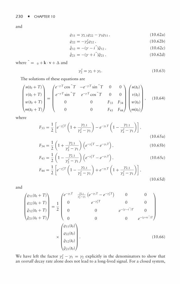
230 CHAPTER 10
and
11 = γ2,122 − γ111 , (10.62a)
22 = −γ t222 , (10.62b)˙12 = −(γ − i δ)12 , (10.62c)˙21 = −(γ + i δ)21 , (10.62d)
where δ = δ0 + k · v + and
γ t2 = γ2 + γ1. (10.63)
The solutions of these equations are⎛⎜⎜⎜⎜⎜⎝
u(t0 + T)
v(t0 + T)
w(t0 + T)
m(t0 + T)
⎞⎟⎟⎟⎟⎟⎠ =
⎛⎜⎜⎜⎜⎜⎝
e−γT cos δT −e−γT sin δT 0 0
e−γT sin δT e−γT cos δT 0 0
0 0 F33 F34
0 0 F43 F44
⎞⎟⎟⎟⎟⎟⎠
⎛⎜⎜⎜⎜⎜⎝
u(t0)
v(t0)
w(t0)
m(t0)
⎞⎟⎟⎟⎟⎟⎠ , (10.64)
where
F33 = 12
[e−γ t2T
(1 + γ2,1
γ t2 − γ1
)− e−γ1T
(1 − γ2,1
γ t2 − γ1
)],
(10.65a)
F34 = 12
(1 + γ2,1
γ t2 − γ1
)(e−γ t2T − e−γ1T
), (10.65b)
F43 = 12
(1 − γ2,1
γ t2 − γ1
)(e−γ t2T − e−γ1T
), (10.65c)
F44 = 12
[e−γ t2T
(1 − γ2,1
γ t2 − γ1
)+ e−γ1T
(1 + γ2,1
γ t2 − γ1
)],
(10.65d)
and ⎛⎜⎜⎜⎜⎜⎝
11(t0 + T)
22(t0 + T)
12(t0 + T)
21(t0 + T)
⎞⎟⎟⎟⎟⎟⎠ = 1
2
⎛⎜⎜⎜⎜⎜⎝
e−γ1T γ2,1γ t2−γ1
(e−γ1T − e−γ t2T
)0 0
0 e−γ t2T 0 0
0 0 e−(γ−i δ)T 0
0 0 0 e−(γ+i δ)T
⎞⎟⎟⎟⎟⎟⎠
×
⎛⎜⎜⎜⎜⎜⎝
11(t0)
22(t0)
12(t0)
21(t0)
⎞⎟⎟⎟⎟⎟⎠ . (10.66)
We have left the factor γ t2 − γ1 = γ2 explicitly in the denominators to show thatan overall decay rate alone does not lead to a long-lived signal. For a closed system,
COHERENT TRANSIENTS 231
except for overall decay, i.e. γ2,1 = γ t2−γ1, F33 ∼ e−γ t2T, F34 ∼ e−γ t2T−e−γ1T, F43 ∼ 0,F44 ∼ e−γ1T—that is, F33 has no slowly decaying part, and as a consequence, thereis no long-lived signal in the stimulated photon echo.
To calculate a coherent transient signal, one multiplies the appropriate transfermatrices together; however, it is efficient to use the diagrammatic technique to isolateonly those terms that are needed.
10.9 Appendix B: Optical Ramsey Fringes in SpatiallySeparated Fields
An alternative means for observing coherent transient signals is to use an atomicbeam that traverses a field interaction zone. A standard geometry involves a well-collimated atomic beam propagating in the Z direction that passes through one ormore field interaction zones. The fields propagate in the ±Xdirection and have beamwidth equal to w (see figure 11.4 in chapter 11) in the Z direction. As such, if anatom is moving with longitudinal velocity v, it “sees” a radiation pulse havingduration w/v in its rest frame. The velocity density distribution of an effusivethermal beam can be approximated as [36, 37]
W(vT, v) = 4π1/2u3
v2 e−v2 /u2WT(vT) , (10.67)
where θb is the beam divergence,WT(vT) is the transverse velocity distribution (whichcan also depend on v) having width of order uT ≈ uθb, and u is the most probablelongitudinal speed of atoms in the beam. For a typical thermal, collimated effusivebeam having θb ≈ 1 mrad, u is of order 600m/s, and uT is of order 6.0m/s. Assuch, the transverse Doppler width is of order kuT/2π ≈ 1 − 10 MHz. Supersonicbeams have narrower longitudinal velocity spreads. Although kuT is comparableto the excited-state decay rates considered throughout this text, optical Ramseyfringe experiments are often carried out on “forbidden” (e.g., intercombination)transitions or two-photon transitions between ground-state hyperfine levels (such asthe Cs “clock” transition). In both these metrological applications, the decay timesof the relevant levels is all but negligible, with line widths limited by other factors.In any event, the transverse Doppler width is much larger than all relaxation rates insuch situations, so we can apply the same formalism that we have been using. Alsoimportant for a beam is the beam intensity or current density distribution given by
WJ (vT, v) = 2u4v3 e
−v2 /u2WT(vT), (10.68)
for which
v = 3√πu/4 . (10.69)
There are several differences between coherent transients involving pulsed fieldsacting on atoms in a vapor cell and those with atoms moving through spatiallyseparated fields. Consider first the FPD signal radiated by a monoenergetic atomicbeam a distance L from the scattering zone. If the atoms have longitudinal velocityv, then the FPD signal, measured at a distance L from the field interaction zone,
232 CHAPTER 10
arises from atoms that were excited at time te = t− L/v. This implies that ρ I21(te) isproportional to
ρ I21(te) = −iN sin A2
eiδte ∝ eiδ(t−L/c). (10.70)
As a consequence, ρ21(t, L) varies as
eiδ(t−L/c)e−iω0te−γ (t−te) = e−iωte−γ L/c.
The emitted field is radiated at the incident field frequency ω rather than the atomicfrequency ω0. Emission at the laser frequency rather than the atomic frequency ischaracteristic of the radiated signals associated with experiments involving spatiallyseparated fields.
A second difference is that owing to a distribution of longitudinal velocities inthe beam, the pulse area is different for different atoms, since the pulse duration inan atom’s rest frame varies inversely with its longitudinal velocity. Moreover, forslowly moving atoms in the beam, the approximation of negligibly short interactiontimes [conditions (10.1)] is bound to be violated. In what follows, however, we willassume that conditions (10.1) hold for most of the atoms in the beam.
Without a doubt, the most important experiments involving atoms movingthrough spatially separated fields are those in which optical Ramsey fringes areproduced [21, 22, 26, 38] (at least before the development of frequency combs). Wecan analyze this case using the results of section 10.2.2, with the time intervalsbetween pulses replaced by the spatial separation of the field zones, divided bythe longitudinal velocity of the atoms. The geometry we choose has three fieldzones, located at Z = 0, Z = L21, and Z = L21 + L, in which the fields havepropagation vectors k1 = k, k2 = k, and k3 = −k, respectively. As was mentionedin section 10.2.2, one has the option of transforming the optical coherence to apopulation using a fourth pulse at position Z = L + 2L21 (t = T + 2T21) andmeasuring the population 22 immediately following this fourth pulse, or one canmonitor the field radiated at that position. In the case of atoms moving throughspatially separated fields with different longitudinal velocities, one must first averageequation (10.45) over longitudinal velocities before taking the absolute square tocalculate the radiated field. As a result of this averaging, the radiated signal intensityis maximum for δ0 = 0. Consequently, for spatially separated fields, heterodynedetection or a fourth field is not necessary, since the radiated field intensity, as afunction of δ0, allows us to determine the line center.
Let us now calculate the Ramsey fringe signal for the case when a fourth fieldinteraction zone, located at Z= L+2L21 is used to convert coherence to population.The field propagation vector for this fourth field is k4 = −k. Thus, we need toevaluate the density matrix chain
11 → 21 → (22 − 11) → 21 → 22 + c.c. (10.71)
We have already calculated the first three steps of this chain to arrive at equa-tion (10.45), which can be written in the interaction representation before the
COHERENT TRANSIENTS 233
average over velocity is taken as
I21(R, v, t) = −(1/4)e−ik·Reiδ0t sin A1 sin A2 sin A3G(T)e−γ (t−2T21−T)
× e−2γT21e−iδ0(t−T)eikvx(t−2T21−T), (10.72)
where
T21 = L21/v, T = L/v. (10.73)
Using equation (10.8) to calculate the transformation of 21 → 22 produced by thefourth pulse, we find
22(R, v, t) = −(1/4) sin A1 sin A2 sin A3 sin A4
× G(T)e−γ2(t−2T21−T)e−2γT21e−2iδ0T21 + c.c.
= −(1/2) sin A1 sin A2 sin A3 sin A4
× G(T)e−γ2(t−2T21−T)e−2γT21 cos (2δ0T21) , (10.74)
exhibiting Ramsey fringe structure; there is no longer any dependence on thetransverse velocity, since the fourth pulse is applied at the echo time. If thepopulation is measured shortly after the fourth interaction zone, we find
22(v, t ≈ 2T21 + T) = −(1/2)4∏j=1
sin(Aj v/v
)×G(L/v)e−2γ L21/v cos (2δ0L21/v) , (10.75)
where equation (10.73) was used and we have assumed that pulse j has area Aj
if v = v. The fact that 22 is negative should not be of concern, since this isonly that part of 22 exhibiting Ramsey fringe structure. There is an additionalbackground term that ensures that the total excited-state population is positive, orelse we would be in serious trouble. The background term, which does not exhibitRamsey fringe structure, consists of contributions to 22 that add to those given inthe chain (10.71). They contain terms that represent the contributions to 22 fromeach field acting separately, as well as the non-Ramsey-like population produced bymultiple fields.
For a closed system with γ2 = 2γ , G(L/v) = e−2γ L/v , and the Ramsey fringesignal is determined by the function
H(δ0) =∫ ∞
0dv cos(2δ0L21/v)e−2γ L/ve−2γ L21/vWJ (v)
4∏j=1
sin(Aj v/v
),
(10.76)where WJ is given by equation (10.68). For δ0 = 0, all phases cancel and the signalis a maximum. As δ0L21 increases, small changes in v produce larger phase changesand the signal diminishes. You are asked to plot this result in the problems.
Often, instead of using three traveling wave fields, standing-wave fields areused for one or more of the interactions regions [26, 39–41]. For example, ifk1 = k2 = −k3 = k, one can collapse the second and third interaction zones (L ∼ 0).In this manner, one has effectively replaced the second and third fields by a single,standing-wave field. In fact, in many of the original proposals for obtaining optical
234 CHAPTER 10
Ramsey fringes, standing-wave fields were used for each field interaction zone. Whilethis complicates the analysis somewhat, since all spatial harmonics of the opticalcoherence are created by standing-wave fields, the underlying physics remains thesame.
The accuracy and precision of optical Ramsey fringe experiments is extra-ordinary. The recoil that atoms acquire when they absorb or emit radiationfrom oppositely propagating optical fields can be resolved using optical Ramseyfringes [42]. (The recoil shift, of order 23 kHz for Ca, results from recoil shifts ofopposite sign for the two pairs of interferometric paths shown in figure 10.8.) It isnot difficult to understand the origin of the recoil splitting by incorporating recoilinto the phase diagram. We have seen that the excited-state amplitude for a vaporacquires a phase factor exp[−i δ(t − Tj )] following absorption, and the ground-stateamplitude acquires a phase factor exp[i δ(t − Tj )] following emission, where
δ = δ0 + k j · v = E2 − E1
− ωL + k j · v, (10.77)
where Ej is the energy of state j . To include both the Doppler phase factor and therecoil energy, we replace this equation by
δ = E2(P + k j ) − E1(P)
− ωL
= E2 − E1
+ (P + k j )2
2M− P2
2M− ωL
= δ0 + k j · v + ωkj , (10.78)
where ωkj = k2j /2M is a recoil frequency, and P = Mv is the center-of-massmomentum before pulse j is applied.
In the interval between t = 0 and t = T + 2T21 in figure 10.8, 21 for the lowerpair of paths acquires a phase
−[δ0 + (P + k1)2
2M− P2
2M
]T21 −
[(P + k1 − k2)2
2M− P2
2M
]T
−[δ0 + (P + k3)2
2M− P2
2M
][t − (T − 2T21)]
= −2 (δ0 + ωk)T21,
since k1 = k2 = −k3 = k. However, 21 for the upper pair of paths acquires a phase
−[δ0 + (P + k1)2
2M− P2
2M
]T21 −
[(P + k1)2
2M− (P + k2)2
2M
]T
−[δ0 + (P + k1)2
2M
]−[(P + k2 − k3)2
2M
][t − (T − 2T21)]
= −2 (δ0 − ωk)T21.
Thus, the net Ramsey signal is a maximum for δ0 = −ωk for the lower pair ofpaths and δ0 = ωk for the upper pair of paths, resulting in a recoil splitting ωsplit
COHERENT TRANSIENTS 235
given by
ωsplit = 2ωk = k2
M. (10.79)
The sensitivity of optical Ramsey fringe experiments is also sufficient to resolvethe second-order Doppler shift associated with the motion of the atoms relativeto the sources of the optical fields [43]. By detecting optical Ramsey fringes usingthermal atomic beams passing through spatially separated fields, precisions havebeen achieved of 2.5 × 10⁻¹² for the 657-nm Ca transition [44] and 2.5 × 10⁻¹²
for the 457-nm Mg transition [45], both of which are 1S0 to 3P1 intercombinationtransitions.
Problems
1. Derive equations (10.6) and (10.8).2. For the two-pulse echo with copropagating pulses having areas π/2 and π ,
estimate the peak power exiting a sample of length L. Assume that the mediumconsists of an optically thin vapor having k1u/2π = 1.0GHz, γ2/2π =10MHz, L = 1 cm, ω0 = 3 × 10¹⁵ s−1, T21 = 10 ns, σ (pulse cross-sectionalarea) = 10mm2, and N = 108 atoms/cm3. Estimate the number of photons inthe echo signal.
3. Consider a “vapor” of stationary atoms that undergoes FPD following theapplication of a short π/2 pulse. Take the sample to be confined in a cylindricalvolume of cross-sectional area A and length L. Calculate the power exiting thesample, assuming that the sample is optically thin. Show that for a sufficientlyhigh density, the power exiting the sample exceeds the maximum energy thatthe initial pulse could have deposited in the sample. What is wrong here?
4. Consider FPD for an ensemble of two-level atoms having a Maxwelliandistribution of velocities with most probable speed u. The atoms are subjectedto a monochromatic field having constant amplitude for the time period(−∞,0). At t = 0, the field is suddenly turned off. Calculate the FPD signalemitted for times t (1/ku), assuming that |δ| < ku, γ ku. Calculate thesignal only to lowest nonvanishing order in the preparation field, and showthat the lead term in 〈12〉 varies as the field amplitude cubed. On physicalgrounds, explain why the signal, which decays in a time of order (1/γ ), hasthis field dependence.
5. Use the U and F matrices to calculate I21(t) for t > T for the two-pulse echo,including all contributions. Show that in the region t ≈ 2T, the only term thatcontributes significantly to the signal is given by equation (10.34), assumingkuT 1.
6. Go through the details of the stimulated photon echo calculation ofsection 10.2.1 for k1 = k2 = k3 = k and the following decay scheme:
11 = −111 + γ222, 22 = −(2 + γ2)22, 12 = −γ 12.Draw a Doppler phase diagram to show that an echo is produced at time T21following the third pulse. Calculate 21(R, t) in the vicinity of the echo time.
236 CHAPTER 10
Show that if 1 γ2 and 1 = 2, one can have a photon echo for very longT = T32 (times as long as one hour have been observed), but if 1 = 2, thereis no long-lived echo. How do you explain this?
7. Integrate equation (10.76) numerically in the limit that γ L/v 1 andneglecting the dependence of pulse area on v, that is, numerically integrate,
H(δ0) =∫ ∞
0dv cos(2δ0L21/v)e−2γ L21/vWJ (v),
and plot the signal as a function of a = δ0L21/v for b = γ L21/v = 0,0.5, 1.5 to display a typical Ramsey fringe pattern. The distribution WJ (v) isgiven by equation (10.68). Does the decay affect the resolution of the signalsignificantly? See how the dependence of pulse area on v modifies the signalby plotting
H′(δ0) =∫ ∞
0dv cos(2δ0L21/v)e−2γ L21/vWJ (v) sin
4(π
2v
v
)
for the same parameters.8. Imagine a collimated atomic beam passing through two field zones that
drive radio-frequency transitions between two ground-state hyperfine levels.Consider the k vector of the field to be in the X direction and the atomicbeam to propagate in the Z direction. If the atoms are prepared in one ofthe hyperfine levels, show that the population of the other level, consideredas a function of the detuning between the applied fields and the hyperfinetransition frequency, exhibits Ramsey fringes. Why does this two-zone methodnot work for optical fields, in which an atomic beam propagating in the Zdirection passes through two field regions in which the fields propagate in theX direction? Since the hyperfine levels have essentially infinite lifetimes, whatwill ultimately determine the resolution of the Ramsey fringes?
9. Derive equation (10.45).10. Consider a three-pulse “echo” in an homogeneously broadened systems. Draw
a phase diagram in which field 1 acts first that leads to a signal in the k =k1 − k2 + k3 = 2k1 − k2 direction (with k1 = k3). We have not considered thiscontribution for inhomogeneously broadened systems, since such a diagramleads to an overall phase of φd = 2(δ0 +− 2k1 · v)T21 at time t = T + 2T21.On averaging over either or v in an inhomogeneously broadened sample, thiscontribution would vanish. In a homogeneously broadened sample, however, = 0 and v = 0, giving an identical relative phase φd to all the atoms. Fort > T + T21, calculate 〈21(R, t)〉. Show that the signal does not constitutean “echo” in the usual sense, since there is no dephasing–rephasing cycle.The signal appears promptly (it is actually an FPD signal) following the thirdpulse. If one measures the time-integrated intensity in the signal followingthe third pulse, however (as is often the case with ultrafast pulses in whichtime resolution of the echo is not possible), it is impossible to tell directlywhether an “echo” has occurred. For such measurements, a signal emittedin the k = 2k1 − k2 direction when pulse 1 acts first is a clear signatureof an homogeneously broadened system, since such a signal vanishes forinhomogeneously broadened samples.
COHERENT TRANSIENTS 237
11. Calculate the overall phase of 21 using figure 10.6, and also calculate thephase of I21 using equation (10.7) for the three field zones. Show that they arein agreement, given the fact that 21 = I21e
−i(δ0+)t.12. Consider a three-pulse echo in which the three fields have wave vectors k1,
k2,−k2, with k1 ≈ k2. Show that there is a Ramsey-fringe-type signal forvapors in the ks = k1 − 2k2 direction and a stimulated echo signal ininhomogeneously broadened solids in the ks = −k1 direction. To do this,consider the two sequences
11 → 21 → (22 − 11) → 21
and
11 → 12 → (22 − 11) → 21.
You need not calculate the signal explicitly. Just find the overall phase factorresulting from these two sequences.
13. Consider a tri-level echo for the level scheme of chapter 9. This is astimulated photon echo in which the first and third pulses have propagationvectors k = kz and are resonant with the 1–2 transition, while the secondpulse has k′ = ηk′z (η = ±1) and is resonant with the 2–3 transition. Thefirst two pulses are separated by T21, and the second and third pulses by T.For an inhomogeneously broadened vapor, use a Doppler phase diagram toshow that, for η = 1, there is a contribution to an echo on the 2–3 transitioninvolving 13 as an intermediate state. Show that there is no such contributionfor η = −1, which is analogous to the result in the steady-state three-levelsystem result (although you can convince yourself that there are no step-wisecontributions to the echo in this scheme). Give an interpretation of this resultin terms of Doppler phase cancellation. Use the phase diagram to calculatethe time at which the echo occurs. This allows one to store information in the1–3 coherence for a relatively long time. It differs from the slow light case,however, in that only a small portion of the input fields are “absorbed” in themedia. Note that no density matrix calculations are needed in this problem; allresults can be read off the phase diagrams (see reference [46]).
14. Prove equation (10.54).
References
[1] H. Metcalf and W. D. Phillips, Time-resolved subnatural-width spectroscopy, OpticsLetters 5, 540–542 (1980); W. D. Phillips and H. J. Metcalf, Time resolved subnaturalwidth spectroscopy, in Precision Measurements and Fundamental Constants II, editedby B. N. Taylor and W. D. Phillips, National Bureau of Standards Special Publication617 (U.S. Government Printing Office, Washington, DC, 1984) pp. 177–180.
[2] A. I. Lvovsky and S. R. Hartmann, Superradiant self-diffraction, Physical Review A 59,4052–4057 (1999).
[3] R. H. Dicke, Coherence in spontaneous radiation processes, Physical Review 93,99–110 (1954).
238 CHAPTER 10
[4] See, for example, I. P. Herman, J. C. MacGillivray, N. Skribanowitz, and M. S. Feld,Self-induced emission in optically pumped HF gas: the rise and fall of the superradiantstate, in Laser Spectroscopy, edited by R. G. Brewer and A. Mooradian (Plenum,New York, 1974), 379–412.
[5] D. Polder, M. F. H. Schuurmans, and Q. H. F. Vrehen, Superfluorescence: quantum-mechanical derivation of Maxwell-Bloch description with fluctuating field source,Physical Review A 19, 1192–1203 (1979).
[6] N. A. Kurnit, I. D. Abella, and S. R. Hartmann,Observation of a photon echo, PhysicalReview Letters 13, 567–568 (1964).
[7] E. L. Hahn, Spin echoes, Physical Review 80, 580–594 (1950).[8] P. R. Berman, Theory of collision effects on line shapes using a quantum-mechanical
description of the atomic center-of-mass motion—Application to lasers, PhysicalReview A 2, 2435–2454 (1970).
[9] R. Beach, S. R. Hartmann, and R. Friedberg, Billiard ball echo model, Physical ReviewA 25, 2658–2666 (1982); R. Friedberg and S. R. Hartmann, Billiard balls and matter-wave interferometry, Physical Review A 48, 1446–1472 (1993); R. Friedberg andS. Hartmann, Echoes and billiard balls, Laser Physics 3, 1128–1137 (1993).
[10] P. W. Anderson, B. I. Halperin, and C. M. Varma, Anomalous low-temperature thermalproperties of glasses and spin glasses, Philosophical Magazine 25, 1–9 (1972).
[11] P. M. Selzer, General techniques and experimental methods in laser spectroscopyof solids, in Laser Spectroscopy of Solids, edited by W. M. Yen and P. M. Silzer,Springer Series in Topics in Applied Physics, vol. 49 (Springer-Verlag, Berlin, 1986),pp. 115–140.
[12] P. R. Berman,Validity conditions for the optical Bloch equations, Journal of the OpticalSociety of America B 3, 564–571 (1986), and references therein.
[13] P. R. Berman, Markovian relaxation processes for atoms in vapors and in solids:calculation of free-induction decay in the weak external-field limit, Journal of theOptical Society of America B 3, 572–586 (1986), and references therein.
[14] P. R. Berman, Collisional effects in laser spectroscopy, in New Trends in AtomicPhysics, edited by G. Grynberg and R. Stora Les Houches Session XXXVIII, vol. 1(North-Holland, Amsterdam, 1984), pp. 451–514.
[15] P. R. Berman, J. M. Levy, and R. G. Brewer, Coherent optical transient study ofmolecular collisions: theory and observations, Physical Review A 11, 1668–1688(1975).
[16] T. W. Mossberg, R. Kachru, and S. R. Hartmann, Observation of collisional velocitychanges associated with atoms in a superposition of dissimilar electronic states, PhysicalReview Letters 44, 73–77 (1980).
[17] R. Kachru, T. J. Chen, S. R. Hartmann, T. W. Mossberg, and P. R. Berman,Measurement of a total atomic-radiator-perturber scattering cross section, PhysicalReview Letters 47, 902–905 (1981).
[18] R. A. Forber, L. Spinelli, J. E. Thomas, and M. S. Feld, Observation of quantumdiffractive velocity-changing collisions by use of two-level heavy optical radiators,Physical Review Letters 50, 331–335 (1982).
[19] R. Kachru, T. W. Mossberg, and S. R. Hartmann, Stimulated photon echo studyof Na(32S1/2)-CO velocity-changing collisions, Optics Communications 30, 57–62(1979).
COHERENT TRANSIENTS 239
[20] T. Mossberg, A. Flusberg, R. Kachru, and S. R. Hartmann, Total scattering crosssection for Na on He measured by stimulated photon echoes, Physical Review Letters42, 1665–1669 (1979).
[21] J. C. Bergquist, S. A. Lee, and J. L. Hall, Saturated absorption with spatially separatedlaser fields: observation of optical Ramsey fringes, Physical Review Letters 38, 159–162(1977).
[22] Ch. J. Bordé, Ch. Salomon, S. Avrillier, A. Van Lerberghe, Ch. Bréant, D. Bassi, andG. Scoles, Optical Ramsey fringes with traveling waves, Physical Review A 30, 1836–1848 (1984).
[23] N. Ramsey, A molecular beam resonance method with separated oscillating fields,Physical Review 78, 695–699 (1950).
[24] See, for example, L. S. Vasilenko, I. D. Matveyenko, and N. N. Rubtsova, Studyof narrow resonances of coherent radiation in time separated fields in SF6, OpticsCommunications 53, 371–374 (1985).
[25] C. Degenhardt, H. Stoehr, C. Lisdat, G. Wilpers, H. Schnatz, B. Lipphardt, T.Nazarova, P.-E. Pottie, U. Sterr, J. Helmcke, and F. Riehle, Calcium optical frequencystandard with ultracold atoms: approaching 10−15 relative uncertainty, PhysicalReview A 72, 062111, 1–17 (2005).
[26] B. Ya. Dubetsky, A. P. Kazantsev, V. P. Chebotaev, and V. P. Yakolev, Interference ofatoms in separated optical fields, Soviet Physics 62, 685–693 (1985); V. P. Chebotaev,B. Ya. Dubetsky, A. P. Kazantsev, and V. P. Yakolev, Interference of atoms in separatedoptical fields, Journal of the Optical Society of America B 2, 1791–1798 (1985).
[27] Ch. J. Bordé, Atomic interferometry with internal state labeling, Physics Letters A 140,10–12 (1989).
[28] Th. Udem, J. Reichert, R. Holzwarth, and T. W. Hänsch, Absolute optical frequencymeasurement of the cesium D1 line with a mode-locked laser, Physical Review Letters82, 3568–3571 (1999).
[29] D. J. Jones, S. A. Diddams, J. K. Ranka, A. Stentz, R. S. Windeler, J. L. Hall, andS. T. Cundiff, Carrier-envelope phase control of femtosecond mode-locked lasers anddirect optical frequency synthesis, Science 288, 635–639 (2000).
[30] S. A. Diddams, D. J. Jones, J. Ye, S. T. Cundiff, J. L. Hall, J. K. Ranka, R. S. Windeler,R. Holzwarth, Th. Udem, and T. W. Hänsch, Direct link between microwave andoptical frequencies with a 300-THz femtosecond laser comb, Physical Review Letters84, 5102–5105 (2000).
[31] For a review with many references, see M. C. Stowe, M. J. Thorpe, A. Pe’er, J. Ye,J. E. Stalnaker, V. Gerginov, and S. A. Diddams, Direct frequency comb spectroscopy,in Advances in Atomic, Molecular, and Optical Physics, edited by E. Arimondo,P. R. Berman, and C. C. Lin, vol. 55 (Elsevier, Amsterdam, 2008), pp. 1–60. Also, seeS. T. Cundiff and J. Ye, Colloquium: femtosecond optical frequency combs, Reviews ofModern Physics 75, 325–342 (2003).
[32] A. E. Siegman, Lasers (University Science Books, Mill Valley, CA, 1986), chap. 28;P. W. Milonni and J. H. Eberly, Lasers (Wiley, New York, 2009), chap. 12.
[33] U. Siegner and U. Keller, Nonlinear optical processes for ultrashort pulse generation,in Handbook of Optics, edited by M. Bass, J. M. Enoch, E. Van Stryland, andW. L. Wolf, Vol. IV (McGraw-Hill, New York, 2001), chap. 25, and referencestherein.
[34] J. K. Wahlstrand, J. T. Willis, C. R. Menyuk, and S. T. Cundiff, The quantum-limitedcomb lineshape of a mode-locked laser: fundamental limits on frequency uncertainty,
240 CHAPTER 10
Optics Express 16, 18624–18630 (2008); M. J. Martin, S. M. Foreman, T. R. Schibli,and J. Ye, Testing ultrafast mode-locking at microhertz relative optical linewidth,Optics Express 17, 558–568 (2009).
[35] For a review with many references, see J. P. Ogilvie and K. J. Kubarych, Multidi-mensional electronic and vibrational spectroscopy: an ultrafast probe of molecularrelaxation and reaction dynamics, in Advances in Atomic, Molecular, and OpticalPhysics, edited by E. Arimondo, P. R. Berman, and C. C. Lin, vol. 57 (Elsevier,Amsterdam, 2009), pp. 249–321.
[36] N. F. Ramsey, Molecular Beams (Oxford University Press, London, 1956) chap. II;E. A. Kennard, Kinetic Theory of Gases (McGraw-Hill, New York, 1938),section 37.
[37] P. T. Greenland, M. A. Lauder, and D. J. H. Wort, Atomic beam velocity distributions,Journal of Physics D 18, 1223–1232 (1985).
[38] For a review with many references, see U. Sterr, K. Sengstock, W. Ertmer, F.Riehle, and W. Ertmer, Atom interferometry based on separated light fields, in AtomInterferometry, edited by P. R. Berman (Academic Press, San Diego, CA, 1997),pp. 293–362.
[39] Ye. V. Baklanov, B. Ya. Dubetsky, and V. P. Chebotaev, Nonlinear Ramsey resonancein the optical region, Applied Physics 11, 171–173 (1976).
[40] V. P. Chebotaev, Method of separated fields in optics, Soviet Journal of QuantumElectronics 8, 935–941 (1978).
[41] N. Hata and K. Shimoda, Theory of optical Ramsey resonance in three separated fieldsproduced by a corner reflector, Applied Physics 22, 1–9 (1980).
[42] R. L. Barger, J. C. Bergquist, T. C. English, and D. J. Glaze, Resolution of photon-recoilstructure of the 6573-Å calcium line in an atomic beam with optical Ramsey fringes,Applied Physics Letters 34, 850–852 (1979).
[43] R. L. Barger, Influence of second-order Doppler effect on optical Ramsey fringe profiles,Optics Letters 6, 145–147 (1981).
[44] A. Morinaga, F. Riehle, J. Ishikawa, and J. Helmcke, A Ca optical frequency standard:frequency stabilization by means of nonlinear Ramsey resonances, Applied Physics B48, 165–171 (1989).
[45] J. Friebe, A. Pape, M. Riedmann, K. Moldenhauer, T. Mehlstäubler, N. Rehbein,C. Lisdat, E. M. Rasel, W. Ertmer, H. Schnatz, B. Lipphardt, and G. Grosche, Absolutefrequency measurement of the magnesium intercombination transition 1S0 → 3P1,Physical Review A 78, 033830-1–7 (2008).
[46] T. W. Mossberg, R. Kachru, S. R. Hartmann, and A. M. Flusberg, Echoes in gaseousmedia: a generalized theory of rephasing phenomena, Physical Review A 20, 1976–1996 (1979).
Bibliography
Many of the general references listed in chapter 1 have one or more chapters oncoherent transients. There are thousands of articles in this field. Some review articlesand books are listed here:
A. Abragam, The Principles of Nuclear Magnetism (Oxford University Press, New York,1961).
COHERENT TRANSIENTS 241
P. R. Berman and R. G. Brewer, Coherent transient spectroscopy in atomic and molecularvapors, in Encyclopedia of Modern Optics, edited by B. D. Guenther and D. G. Steel(Elsevier, Amsterdam, 2004) pp. 154–163.
P. R. Berman and D. G. Steel, Coherent optical transients, in Handbook of Op-tics, edited by M. Bass, J. M. Enoch, E. Van Stryland, and W. L. Wolf,Vol. IV, (McGraw-Hill, New York, 2001), chap. 24.
R. G. Brewer, Coherent optical spectroscopy, in Frontiers in Laser Spectroscopy,Les Houches Session XXVII, edited by R. Balian, S. Haroche, and S. Liberman,vol. 1 (North-Holland, Amsterdam, 1977), pp. 341–396.
———, Coherent optical spectroscopy, in Nonlinear Spectroscopy, Proceedingsof the International School of Physics, Enrico Fermi, Course 64, edited byN. Bloembergen (North-Holland, Amsterdam, 1977) pp. 87–137.
R. L. Shoemaker, Coherent transient infrared spectroscopy, in Laser and Co-herence Spectroscopy, edited by J. L. Steinfeld (Plenum, New York, 1978),pp. 197–371.
C. P. Slichter, Principles of Magnetic Resonance (Harper and Row, New York, 1963).W. Zinth and W. Kaiser, Ultrafast coherent spectroscopy, in Ultrashort Laser Pulses andApplications, edited by W. Kaiser, vol. 60 (Springer-Verlag, Berlin, 1978), pp. 235–277.
11Atom Optics and Atom Interferometry
In chapter 5, we introduced a number of concepts related to atom optics. Inparticular, we examined the manner in which electromagnetic fields can exert forceson atoms. Moreover, in the previous chapter, we indicated that some coherenttransient signals could be interpreted within the context of atom interferometry. Inthis chapter, we examine both atom optics and atom interferometry in more detail.Before doing so, however, it will prove useful to review some aspects of classicaldiffraction theory.
11.1 Review of Kirchhoff-Fresnel Diffraction
Diffraction plays an important role in both electromagnetism and quantum me-chanics, since both are wave theories. Diffraction in quantum mechanics is actuallya much easier problem than diffraction in electromagnetism, due to the fact thatlight is a vector field, whereas the quantum-mechanical wave function is a scalar. Inreality, diffraction in electromagnetism is basically an unsolved problem, because ofthe difficulty of specifying the exact boundary conditions for the fields. Nevertheless,it is possible to get a good idea of diffraction phenomena that agrees well withexperiment by using a theory in which the electric field is considered as a scalar field.This can be a good approximation if one limits the discussion to distances fromthe scatterer that are large compared with a wavelength, since in that region, thefields can be approximated as plane-wave fields. We present an approach to scalardiffraction based on wave-packet propagation that works for both electromagneticand matter waves. In the end, we arrive at equations that coincide with those ofKirchhoff-Fresnel diffraction theory.
11.1.1 Electromagnetic Diffraction
Let us first consider the propagation of a wave in free space. Imagine that a pulsepropagating in the Z direction strikes a diffracting screen at Z = 0. The screen is
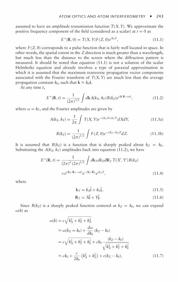
ATOM OPTICS AND ATOM INTERFEROMETRY 243
assumed to have an amplitude transmission function T(X,Y). We approximate thepositive frequency component of the field (considered as a scalar) at t = 0 as
E+(R,0) = T(X,Y)F (Z,0)eik0Z, (11.1)
where F (Z,0) corresponds to a pulse function that is fairly well located in space. Inother words, the spatial extent in the Z direction is much greater than a wavelength,but much less than the distance to the screen where the diffraction pattern ismeasured. It should be noted that equation (11.1) is not a solution of the scalarHelmholtz equation and already involves a type of paraxial approximation inwhich it is assumed that the maximum transverse propagation vector componentsassociated with the Fourier transform of T(X,Y) are much less than the averagepropagation constant k0, such that k ≈ k0z.
At any time t,
E+(R, t) = 1
(2π )3/2
∫dkA(kX,kY)B(kZ)ei(k·R−ωt), (11.2)
where ω = kc, and the Fourier amplitudes are given by
A(kX,kY) = 12π
∫T(X,Y)e−i(kXX+kYY)dXdY, (11.3a)
B(kZ) = 1
(2π )1/2
∫F (Z,0)e−i(kZ−k0)ZdZ. (11.3b)
It is assumed that B(kZ) is a function that is sharply peaked about kZ = k0.Substituting the A(kX,kY) amplitudes back into equation (11.2), we have
E+(R, t) = 1
(2π )2 (2π )1/2
∫dkTdkZdR′
T T(X′,Y′)B(kZ)
×ei(kT ·RT−ωt)e−ikT ·R′T eikZZ, (11.4)
where
kT = kXi + kY j , (11.5)
RT = Xi + Yj. (11.6)
Since B(kZ) is a sharply peaked function centered at kZ = k0, we can expandω(k) as
ω(k) = c√k2X + k2Y + k2Z
≈ ω(kZ = k0) + dωdk0
(kZ − k0)
= c√k2X + k2Y + k20 + ck0
(kZ − k0)√k2X + k2Y + k20
≈ ck0 + c2k0
(k2X + k2Y
)+ c(kZ − k0), (11.7)
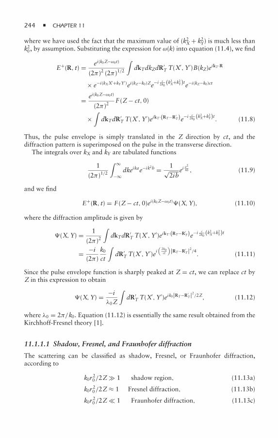
244 CHAPTER 11
where we have used the fact that the maximum value of (k2X + k2Y) is much less thank20, by assumption. Substituting the expression for ω(k) into equation (11.4), we find
E+(R, t) = ei(k0Z−ω0t)
(2π )2 (2π )1/2
∫dkTdkZdR′
T T(X′,Y′)B(kZ)eikT ·R
× e−i(kXX′+kYY′)ei(kZ−k0)Ze−i c2k0(k2X+k2Y)te−i(kZ−k0)ct
= ei(k0Z−ω0t)
(2π )2F (Z− ct,0)
×∫dkTdR′
T T(X′,Y′)eikT ·(RT−R′
T)e−i c2k0(k2X+k2Y)t. (11.8)
Thus, the pulse envelope is simply translated in the Z direction by ct, and thediffraction pattern is superimposed on the pulse in the transverse direction.
The integrals over kX and kY are tabulated functions
1
(2π )1/2
∫ ∞
−∞dkeikae−ik2b = 1√
2ibei
a24b , (11.9)
and we find
E+(R, t) = F (Z− ct,0)ei(k0Z−ω0t)(X,Y), (11.10)
where the diffraction amplitude is given by
(X,Y) = 1
(2π )2
∫dkTdR′
T T(X′,Y′)eikT ·(RT−R′
T)e−i c2k0(k2X+k2Y)t
= −i(2π )
k0ct
∫dR′
T T(X′,Y′)ei
(2k0ct
)|RT−R′T|2/4. (11.11)
Since the pulse envelope function is sharply peaked at Z = ct, we can replace ct byZ in this expression to obtain
(X,Y) = −iλ0Z
∫dR′
T T(X′,Y′)eik0|RT−R′
T|2/2Z, (11.12)
where λ0 = 2π/k0. Equation (11.12) is essentially the same result obtained from theKirchhoff-Fresnel theory [1].
11.1.1.1 Shadow, Fresnel, and Fraunhofer diffraction
The scattering can be classified as shadow, Fresnel, or Fraunhofer diffraction,according to
k0r20/2Z 1 shadow region, (11.13a)
k0r20/2Z≈ 1 Fresnel diffraction, (11.13b)
k0r20/2Z 1 Fraunhofer diffraction, (11.13c)
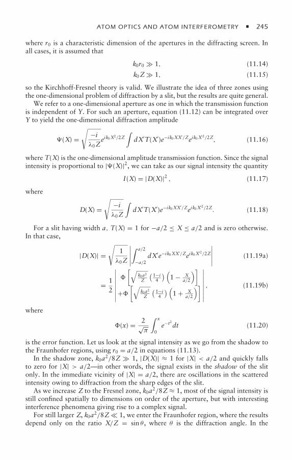
ATOM OPTICS AND ATOM INTERFEROMETRY 245
where r0 is a characteristic dimension of the apertures in the diffracting screen. Inall cases, it is assumed that
k0r0 1, (11.14)
k0Z 1, (11.15)
so the Kirchhoff-Fresnel theory is valid. We illustrate the idea of three zones usingthe one-dimensional problem of diffraction by a slit, but the results are quite general.
We refer to a one-dimensional aperture as one in which the transmission functionis independent of Y. For such an aperture, equation (11.12) can be integrated overY to yield the one-dimensional diffraction amplitude
(X) =√
−iλ0Z
eik0X2/2Z
∫dX′T(X′)e−ik0XX′/Zeik0X
′2/2Z, (11.16)
where T(X) is the one-dimensional amplitude transmission function. Since the signalintensity is proportional to |(X)|2, we can take as our signal intensity the quantity
I(X) = |D(X)|2 , (11.17)
where
D(X) =√
−iλ0Z
∫dX′T(X′)e−ik0XX′/Zeik0X
′2/2Z. (11.18)
For a slit having width a, T(X) = 1 for −a/2 ≤ X ≤ a/2 and is zero otherwise.In that case,
|D(X)| =√
1λ0Z
∣∣∣∣∣∫ a/2
−a/2dX′e−ik0XX′/Zeik0X
′2/2Z
∣∣∣∣∣ (11.19a)
= 12
∣∣∣∣∣∣∣∣
[√k0a2Z
( 1−i4
) (1 − X
a/2
)]
+[√
k0a2Z
( 1−i4
) (1 + X
a/2
)]∣∣∣∣∣∣∣∣, (11.19b)
where
(x) = 2√π
∫ x
0e−t2dt (11.20)
is the error function. Let us look at the signal intensity as we go from the shadow tothe Fraunhofer regions, using r0 = a/2 in equations (11.13).
In the shadow zone, k0a2/8Z 1, |D(X)| ≈ 1 for |X| < a/2 and quickly fallsto zero for |X| > a/2—in other words, the signal exists in the shadow of the slitonly. In the immediate vicinity of |X| = a/2, there are oscillations in the scatteredintensity owing to diffraction from the sharp edges of the slit.
As we increase Z to the Fresnel zone, k0a2/8Z≈ 1, most of the signal intensity isstill confined spatially to dimensions on order of the aperture, but with interestinginterference phenomena giving rise to a complex signal.
For still larger Z, k0a2/8Z 1, we enter the Fraunhofer region, where the resultsdepend only on the ratio X/Z = sin θ , where θ is the diffraction angle. In the
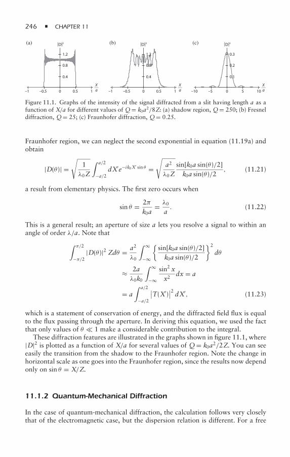
246 CHAPTER 11
Xa
__–1 –0.5 1
(a) (b) (c)| |2 | |2 | |2
0.4
0.8
1.2
0.50Xa
__–1 –0.5 10.50
Xa
__–10 –5 1050
0.4
0.8
1.2
0.1
0.2
0.3
D D D
Figure 11.1. Graphs of the intensity of the signal diffracted from a slit having length a as afunction of X/a for different values of Q= k0a2/8Z: (a) shadow region, Q= 250; (b) Fresneldiffraction, Q= 25; (c) Fraunhofer diffraction, Q= 0.25.
Fraunhofer region, we can neglect the second exponential in equation (11.19a) andobtain
|D(θ )| =√
1λ0Z
∫ a/2
−a/2dX′e−ik0X′ sin θ =
√a2
λ0Zsin[k0a sin(θ )/2]k0a sin(θ )/2
, (11.21)
a result from elementary physics. The first zero occurs when
sin θ = 2πk0a
= λ0
a. (11.22)
This is a general result; an aperture of size a lets you resolve a signal to within anangle of order λ/a. Note that
∫ π/2
−π/2|D(θ )|2 Zdθ = a2
λ0
∫ ∞
−∞
sin[k0a sin(θ )/2]k0a sin(θ )/2
2
dθ
≈ 2aλ0k0
∫ ∞
−∞
sin2 xx2
dx = a
= a∫ a/2
−a/2
∣∣T(X′)∣∣2 dX′, (11.23)
which is a statement of conservation of energy, and the diffracted field flux is equalto the flux passing through the aperture. In deriving this equation, we used the factthat only values of θ 1 make a considerable contribution to the integral.
These diffraction features are illustrated in the graphs shown in figure 11.1, where|D|2 is plotted as a function of X/a for several values of Q= k0a2/2Z. You can seeeasily the transition from the shadow to the Fraunhofer region. Note the change inhorizontal scale as one goes into the Fraunhofer region, since the results now dependonly on sin θ = X/Z.
11.1.2 Quantum-Mechanical Diffraction
In the case of quantum-mechanical diffraction, the calculation follows very closelythat of the electromagnetic case, but the dispersion relation is different. For a free
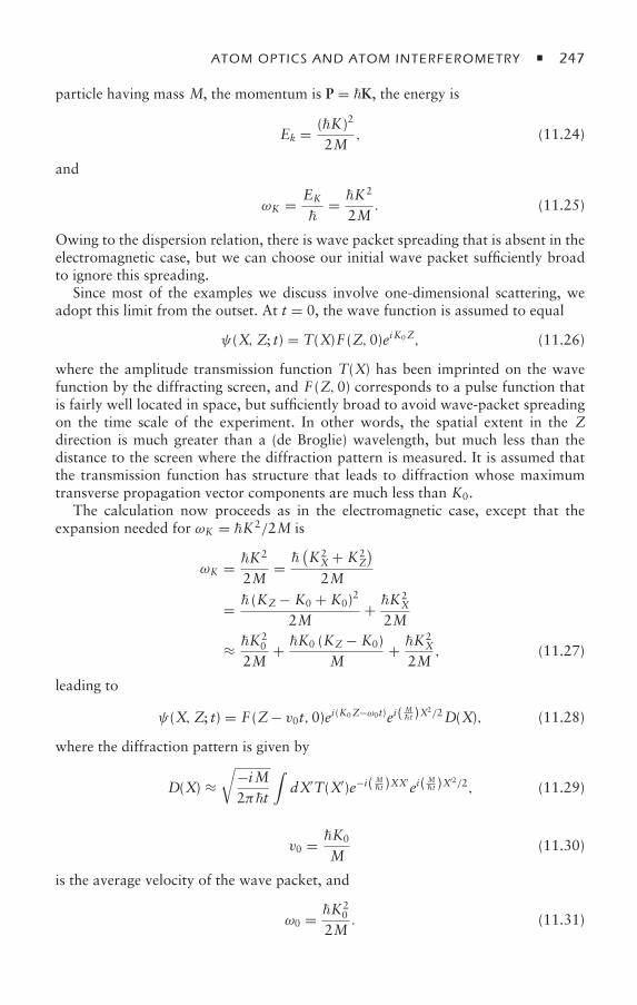
ATOM OPTICS AND ATOM INTERFEROMETRY 247
particle having mass M, the momentum is P = K, the energy is
Ek = (K)2
2M, (11.24)
and
ωK = EK
= K
2
2M. (11.25)
Owing to the dispersion relation, there is wave packet spreading that is absent in theelectromagnetic case, but we can choose our initial wave packet sufficiently broadto ignore this spreading.
Since most of the examples we discuss involve one-dimensional scattering, weadopt this limit from the outset. At t = 0, the wave function is assumed to equal
ψ(X, Z; t) = T(X)F (Z,0)eiK0Z, (11.26)
where the amplitude transmission function T(X) has been imprinted on the wavefunction by the diffracting screen, and F (Z,0) corresponds to a pulse function thatis fairly well located in space, but sufficiently broad to avoid wave-packet spreadingon the time scale of the experiment. In other words, the spatial extent in the Zdirection is much greater than a (de Broglie) wavelength, but much less than thedistance to the screen where the diffraction pattern is measured. It is assumed thatthe transmission function has structure that leads to diffraction whose maximumtransverse propagation vector components are much less than K0.
The calculation now proceeds as in the electromagnetic case, except that theexpansion needed for ωK = K2/2M is
ωK = K2
2M=
(K2X + K2
Z
)2M
= (KZ − K0 + K0)2
2M+ K
2X
2M
≈ K20
2M+ K0 (KZ − K0)
M+ K
2X
2M, (11.27)
leading to
ψ(X, Z; t) = F (Z− v0t,0)ei(K0Z−ω0t)ei(Mt )X2/2D(X), (11.28)
where the diffraction pattern is given by
D(X) ≈√
−iM2πt
∫dX′T(X′)e−i( M
t )XX′ei(
Mt )X′2/2, (11.29)
v0 = K0
M(11.30)
is the average velocity of the wave packet, and
ω0 = K20
2M. (11.31)
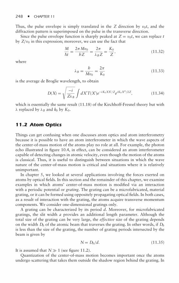
248 CHAPTER 11
Thus, the pulse envelope is simply translated in the Z direction by v0t, and thediffraction pattern is superimposed on the pulse in the transverse direction.
Since the pulse envelope function is sharply peaked at Z = v0t, we can replace tby Z/v0 in this expression; moreover, we can use the fact that
Mt
= 2πMv0hZ
= 2πλBZ
= K0
Z, (11.32)
where
λB = hMv0
= 2πK0
(11.33)
is the average de Broglie wavelength, to obtain
D(X) =√
−iZλB
∫dX′T(X′)e−i K0XX′/ZeiK0X′2/2Z, (11.34)
which is essentially the same result (11.18) of the Kirchhoff-Fresnel theory but withλ replaced by λB and k0 by K0.
11.2 Atom Optics
Things can get confusing when one discusses atom optics and atom interferometrybecause it is possible to have an atom interferometer in which the wave aspects ofthe center-of-mass motion of the atoms play no role at all. For example, the photonecho illustrated in figure 10.4, in effect, can be considered an atom interferometercapable of detecting changes in atomic velocity, even though the motion of the atomsis classical. Thus, it is useful to distinguish between situations in which the wavenature of the center-of-mass motion is critical and situations where it is relativelyunimportant.
In chapter 5, we looked at several applications involving the forces exerted onatoms by optical fields. In this section and the remainder of this chapter, we examineexamples in which atoms’ center-of-mass motion is modified via an interactionwith a periodic potential or grating. The grating can be a microfabricated, materialgrating, or it can be formed using oppositely propagating optical fields. In both cases,as a result of interaction with the grating, the atoms acquire transverse momentumcomponents. We consider one-dimensional gratings only.
A grating can be characterized by its period d. Moreover, for microfabricatedgratings, the slit width a provides an additional length parameter. Although thetotal size of the grating can be very large, the effective size of the grating dependson the width Db of the atomic beam that traverses the grating. In other words, if Db
is less than the size of the grating, the number of grating periods intersected by thebeam is given by
N= Db/d. (11.35)
It is assumed that N 1 (see figure 11.2).Quantization of the center-of-mass motion becomes important once the atoms
undergo scattering that takes them outside the shadow region behind the grating. In
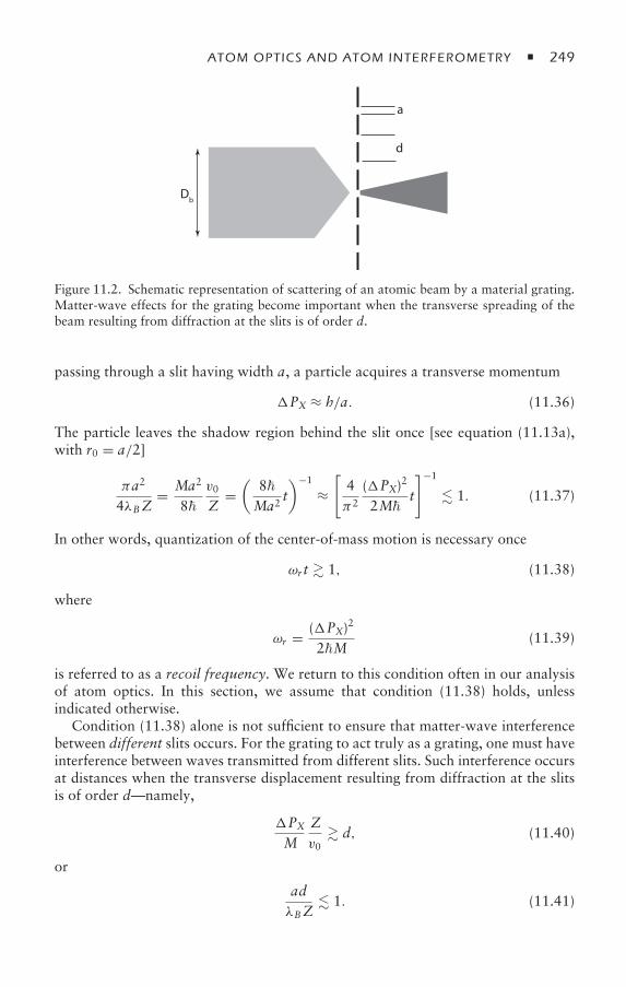
ATOM OPTICS AND ATOM INTERFEROMETRY 249
a
d
Db
Figure 11.2. Schematic representation of scattering of an atomic beam by a material grating.Matter-wave effects for the grating become important when the transverse spreading of thebeam resulting from diffraction at the slits is of order d.
passing through a slit having width a, a particle acquires a transverse momentum
PX ≈ h/a. (11.36)
The particle leaves the shadow region behind the slit once [see equation (11.13a),with r0 = a/2]
πa2
4λBZ= Ma2
8v0
Z=(
8Ma2
t)−1
≈[4π2
(PX)2
2Mt
]−1
1. (11.37)
In other words, quantization of the center-of-mass motion is necessary once
ωr t 1, (11.38)
where
ωr = (PX)2
2M(11.39)
is referred to as a recoil frequency. We return to this condition often in our analysisof atom optics. In this section, we assume that condition (11.38) holds, unlessindicated otherwise.
Condition (11.38) alone is not sufficient to ensure that matter-wave interferencebetween different slits occurs. For the grating to act truly as a grating, one must haveinterference between waves transmitted from different slits. Such interference occursat distances when the transverse displacement resulting from diffraction at the slitsis of order d—namely,
PXM
Zv0 d, (11.40)
or
adλBZ
1. (11.41)

250 CHAPTER 11
Last, by imposing the condition
aDb
λBZ 1, (11.42)
we guarantee that diffraction by a single slit does not lead to transverse displace-ments that are larger than Db, a limit we want to avoid in this discussion. In practice,we take a and d to be comparable.
Rather than deal with the conditions for shadow, Fresnel, and Fraunhoferdiffraction in the abstract, we consider scattering by an amplitude grating to seehow the various length scales determine the nature of the scattering.
11.2.1 Scattering by an Amplitude Grating
We consider first scattering by a microfabricated grating having period d and slitwidth a. The transmission function for a beam having diameter Db is
T(X′) = F (X′)(|X′| − Db/2), (11.43)
where is the Heaviside step function,
F (X′) =1 jd − αd/2 ≤ X′ ≤ jd + αd/20 jd + αd/2 ≤ X′ ≤ ( j + 1)d − αd/2,
(11.44)
α = a/d (11.45)
is the ratio of the slit width to the period (duty cycle), and j is an integer that variesfrom −∞ to ∞. In other words, the transmission function is that of an infinitegrating multiplied by the beam width Db (see figure 11.2).
Since F (X′) is a periodic function with period d, we can expand it as the Fourierseries
F (X′) =∞∑
n=−∞ane2π inX
′/d, (11.46)
where
an = 1d
∫ d/2
−d/2F (X′)e−2π inX′/ddX′
= 1d
∫ αd/2
−αd/2e−2π inX′/ddX′ = sin(nπα)
nπ. (11.47)
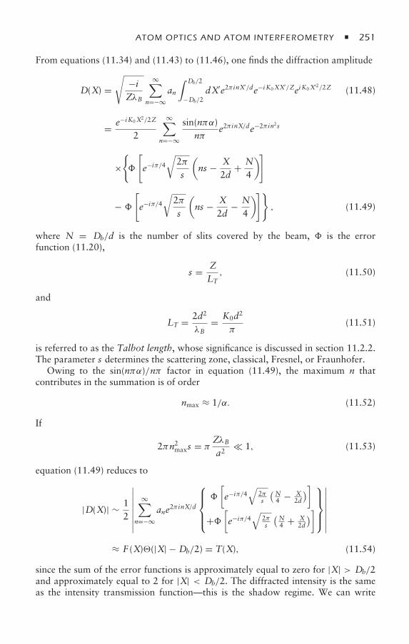
ATOM OPTICS AND ATOM INTERFEROMETRY 251
From equations (11.34) and (11.43) to (11.46), one finds the diffraction amplitude
D(X) =√
−iZλB
∞∑n=−∞
an
∫ Db/2
−Db/2dX′e2π inX
′/de−i K0XX′/ZeiK0X′2/2Z (11.48)
= e−i K0X2/2Z
2
∞∑n=−∞
sin(nπα)nπ
e2π inX/de−2π in2s
×
[e−iπ/4
√2πs
(ns − X
2d+ N
4
)]
−
[e−iπ/4
√2πs
(ns − X
2d− N
4
)], (11.49)
where N = Db/d is the number of slits covered by the beam, is the errorfunction (11.20),
s = ZLT, (11.50)
and
LT = 2d2
λB= K0d2
π(11.51)
is referred to as the Talbot length, whose significance is discussed in section 11.2.2.The parameter s determines the scattering zone, classical, Fresnel, or Fraunhofer.
Owing to the sin(nπα)/nπ factor in equation (11.49), the maximum n thatcontributes in the summation is of order
nmax ≈ 1/α. (11.52)
If
2πn2maxs = πZλBa2
1, (11.53)
equation (11.49) reduces to
|D(X)| ∼ 12
∣∣∣∣∣∣∣∣∞∑
n=−∞ane2π inX/d
⎧⎪⎪⎨⎪⎪⎩
[e−iπ/4
√2πs
(N4 − X
2d
)]
+[e−iπ/4
√2πs
(N4 + X
2d
)]⎫⎪⎪⎬⎪⎪⎭
∣∣∣∣∣∣∣∣≈ F (X)(|X| − Db/2) = T(X), (11.54)
since the sum of the error functions is approximately equal to zero for |X| > Db/2and approximately equal to 2 for |X| < Db/2. The diffracted intensity is the sameas the intensity transmission function—this is the shadow regime. We can write
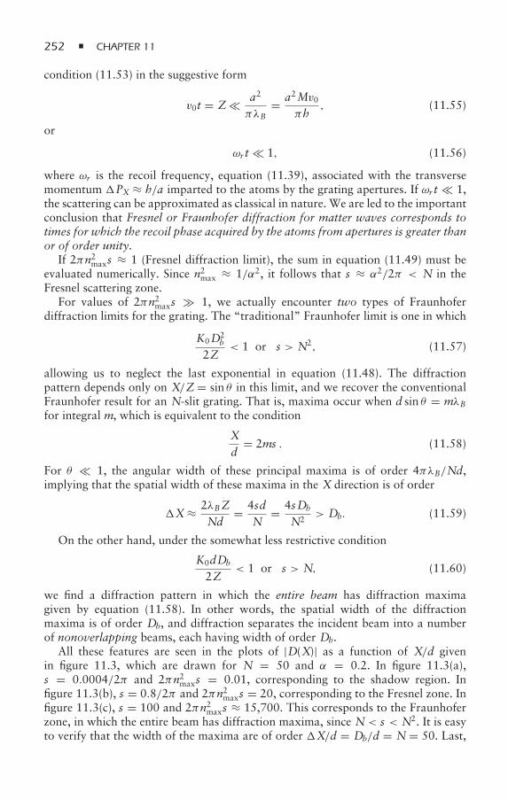
252 CHAPTER 11
condition (11.53) in the suggestive form
v0t = Z a2
πλB= a2Mv0
πh, (11.55)
or
ωr t 1, (11.56)
where ωr is the recoil frequency, equation (11.39), associated with the transversemomentum PX ≈ h/a imparted to the atoms by the grating apertures. If ωr t 1,the scattering can be approximated as classical in nature. We are led to the importantconclusion that Fresnel or Fraunhofer diffraction for matter waves corresponds totimes for which the recoil phase acquired by the atoms from apertures is greater thanor of order unity.
If 2πn2maxs ≈ 1 (Fresnel diffraction limit), the sum in equation (11.49) must beevaluated numerically. Since n2max ≈ 1/α2, it follows that s ≈ α2/2π < N in theFresnel scattering zone.
For values of 2πn2maxs 1, we actually encounter two types of Fraunhoferdiffraction limits for the grating. The “traditional” Fraunhofer limit is one in which
K0D2b
2Z< 1 or s > N2, (11.57)
allowing us to neglect the last exponential in equation (11.48). The diffractionpattern depends only on X/Z = sin θ in this limit, and we recover the conventionalFraunhofer result for an N-slit grating. That is, maxima occur when d sin θ = mλBfor integral m, which is equivalent to the condition
Xd
= 2ms . (11.58)
For θ 1, the angular width of these principal maxima is of order 4πλB/Nd,implying that the spatial width of these maxima in the X direction is of order
X≈ 2λBZNd
= 4sdN
= 4sDb
N2> Db. (11.59)
On the other hand, under the somewhat less restrictive condition
K0dDb
2Z< 1 or s > N, (11.60)
we find a diffraction pattern in which the entire beam has diffraction maximagiven by equation (11.58). In other words, the spatial width of the diffractionmaxima is of order Db, and diffraction separates the incident beam into a numberof nonoverlapping beams, each having width of order Db.
All these features are seen in the plots of |D(X)| as a function of X/d givenin figure 11.3, which are drawn for N = 50 and α = 0.2. In figure 11.3(a),s = 0.0004/2π and 2πn2maxs = 0.01, corresponding to the shadow region. Infigure 11.3(b), s = 0.8/2π and 2πn2maxs = 20, corresponding to the Fresnel zone. Infigure 11.3(c), s = 100 and 2πn2maxs ≈ 15,700. This corresponds to the Fraunhoferzone, in which the entire beam has diffraction maxima, since N< s < N2. It is easyto verify that the width of the maxima are of order X/d = Db/d = N = 50. Last,
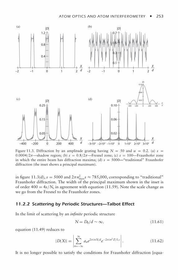
ATOM OPTICS AND ATOM INTERFEROMETRY 253
Xd
__–2 –1 2
(a) |D|
0.4
0.8
1.2
10 0
Xd
__–2 –1 2
(b) |D|
0.3
0.5
0.1
0.7
1
Xd
__–400 –200 4000
(c) |D|
0.05
0.15
0.25
200
Xd
__–3•104 –2•104 –1•104 3•1042•104
(d) |D|
0.06
0.02
0.10
1•1040
Xd
__–400 –200 400
|D|
2000
0.02
0.06
0.10
Figure 11.3. Diffraction by an amplitude grating having N = 50 and α = 0.2. (a) s =0.0004/2π—shadow region; (b) s = 0.8/2π—Fresnel zone; (c) s = 100—Fraunhofer zonein which the entire beam has diffraction maxima; (d) s = 5000—“traditional” Fraunhoferdiffraction (the inset shows a principal maximum).
in figure 11.3(d), s = 5000 and 2πn2maxs ≈ 785,000, corresponding to “traditional”Fraunhofer diffraction. The width of the principal maximum shown in the inset isof order 400 = 4s/N, in agreement with equation (11.59). Note the scale change aswe go from the Fresnel to the Fraunhofer zones.
11.2.2 Scattering by Periodic Structures—Talbot Effect
In the limit of scattering by an infinite periodic structure
N= Db/d ∼ ∞, (11.61)
equation (11.49) reduces to
|D(X)| =∣∣∣∣∣
∞∑n=−∞
ane2π inX/de−2π in2Z/LT
∣∣∣∣∣ . (11.62)
It is no longer possible to satisfy the conditions for Fraunhofer diffraction [equa-tions (11.57) and (11.60)] in this limit; scattering is in either the classical or Fresnel
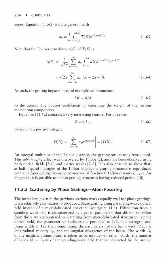
254 CHAPTER 11
zones. Equation (11.62) is quite general, with
an = 1d
∫ d/2
−d/2T(X′)e−2π inX′/d. (11.63)
Note that the Fourier transform A(K) of T(X) is
A(K) = 1√2π
∞∑n=−∞
an
∫ ∞
−∞dX′e2π inX
′/de−i KX′
=√2π
∞∑n=−∞
anδ(K − 2πn/d). (11.64)
As such, the grating imparts integral multiples of momentum
K = h/d (11.65)
to the atoms. The Fourier coefficients an determine the weight of the variousmomentum components.
Equation (11.62) contains a very interesting feature. For distances
Z= mLT, (11.66)
where m is a positive integer,
|D(X)| =∣∣∣∣∣
∞∑n=−∞
ane2π inX/d∣∣∣∣∣ = |T(X)| . (11.67)
An integral multiples of the Talbot distance, the grating structure is reproduced!This self-imaging effect was discovered by Talbot [2], and has been observed usingboth optical fields [3–6] and matter waves [7–9]. It is also possible to show that,at half-integral multiples of the Talbot length, the grating structure is reproducedwith a half-period displacement. Moreover, at fractional Talbot distances, LT/r , forintegral r , it is possible to obtain grating structures having reduced period [10].
11.2.3 Scattering by Phase Gratings—Atom Focusing
The formalism given in the previous sections works equally well for phase gratings.It is a relatively easy matter to produce a phase grating using a standing-wave opticalfield instead of a microfabricated structure (see figure 11.4). Diffraction from astanding-wave field is characterized by a set of parameters that differs somewhatfrom those we encountered in scattering from microfabricated structures. For theoptical field, the parameter set includes the period d = λ/2, field strength, andbeam width w. For the atomic beam, the parameters are the beam width Db, thelongitudinal velocity v0, and the angular divergence of the beam. The width Db
of the incident atomic beam is taken to be infinite—in other words, the numberof lobes N = Db/d of the standing-wave field that is intersected by the atomic
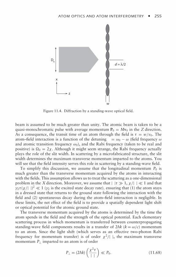
ATOM OPTICS AND ATOM INTERFEROMETRY 255
z
w
d = λ/2
x
Db
Figure 11.4. Diffraction by a standing-wave optical field.
beam is assumed to be much greater than unity. The atomic beam is taken to be aquasi-monochromatic pulse with average momentum P0 = Mv0 in the Z direction.As a consequence, the transit time of an atom through the field is τ = w/v0. Theatom–field interaction is a function of the detuning δ = ω0 − ω (field frequency ωand atomic transition frequency ω0), and the Rabi frequency (taken to be real andpositive) is 0 = 2χ . Although it might seem strange, the Rabi frequency actuallyplays the role of the slit width. In scattering by a microfabricated structure, the slitwidth determines the maximum transverse momentum imparted to the atoms. Youwill see that the field intensity serves this role in scattering by a standing-wave field.
To simplify this discussion, we assume that the longitudinal momentum P0 ismuch greater than the transverse momentum acquired by the atoms in interactingwith the fields. This assumption allows us to treat the scattering as a one-dimensionalproblem in the X direction. Moreover, we assume that |δ|τ 1, χ/|δ| 1 and thatγ2τ (χ/|δ|)2 1 (γ2 is the excited state decay rate), ensuring that (1) the atom staysin a dressed state that returns to the ground state following the interaction with thefield and (2) spontaneous decay during the atom–field interaction is negligible. Inthese limits, the net effect of the field is to provide a spatially dependent light shiftor optical potential for the atomic ground state.
The transverse momentum acquired by the atoms is determined by the time theatom spends in the field and the strength of the optical potential. Each elementaryscattering process in which momentum is transferred between counterpropagatingstanding-wave field components results in a transfer of 2k (k= ω/c) momentumto an atom. Since the light shift (which serves as an effective two-photon Rabifrequency for momentum transfer) is of order χ2/|δ|, the maximum transversemomentum P⊥ imparted to an atom is of order
P⊥ = (2k)(χ2τ
|δ|)
P0. (11.68)
256 CHAPTER 11
It is in this sense that a strong field corresponds to a narrow slit, since equa-tion (11.68) can be written as P⊥ = h/aef f , with
aef f = π |δ|kχ2τ
. (11.69)
A dimensionless parameter that helps to characterize the atom–field interaction isthe transverse Doppler phase φD acquired during the atom–field interaction. Thisphase is of order
φD = kv⊥τ = k(P⊥/M)τ =(χ2τ
|δ|)ω2kτ, (11.70)
where
ωq = q2
2M(11.71)
is the recoil frequency associated with a scattering process in which q of momentumis transferred to the atom. In the examples considered in this chapter,
q = 2k. (11.72)
For arbitrary values of φD, the atom–field dynamics can be solved numerically.There are two limits, however, for which analytic solutions can be obtained. Thelimit φD 1 corresponds to the Raman-Nath approximation [11, 12], in which alltransverse motion of the atoms can be neglected during the atom–field interaction.The limit in which ωqτ 1 is referred to as the Bragg limit, for reasons that willbecome apparent in the following section. In this section, we discuss the Raman-Nath limit. Scattering of atoms from a standing-wave optical field is often referredto as Kapitza-Dirac scattering [13], since they proposed that standing-wave opticalfields could be used to produce Bragg scattering of electrons.
11.2.3.1 Raman-Nath limit
In the Raman-Nath approximation, and with |δ|τ 1, χ/|δ| 1, andγ2τ (χ/|δ|)2 1, the only effect of the atom–field interaction on the atoms is tomodify the phase of the ground-state amplitude. In other words, the field resultssimply in a spatially modulated light shift of the ground-state energy. The positivefrequency component of the field amplitude is given by
E+(X, Z, t) = 12E0(Z)e−iωt(eikX + e−ikX), (11.73)
where E0(Z) is the field envelope in the Z direction, having characteristic widthw (see figure 11.4). After eliminating the excited-state amplitude, we find that theground-state amplitude evolves as
ia1 = −4χ2(t) cos2(kX)δ
a1, (11.74)
where
χ (t) = −µ21E0(t)2
(11.75)
ATOM OPTICS AND ATOM INTERFEROMETRY 257
is one-half the Rabi frequency associated with each traveling-wave component ofthe field as seen in an atom’s rest frame, and µ21 is the matrix element of the dipolemoment operator along the direction of the field polarization. The Z dependenceof the field envelope function in the laboratory frame is transformed into a timedependence in an atom’s rest frame. Aside from an overall constant phase factor, itfollows that the amplitude transmission function in the Raman-Nath approximationis simply
T(X) = ei Acos (2kX), (11.76)
where
A= 2∫ ∞
−∞
χ2(t)δ
dt (11.77)
is an effective pulse area. From the form of T(X), it is clear that this off-resonantstanding-wave field acts as a phase grating. We take δ > 0 (red detuning).
It is instructive to calculate the Fourier transform of the transmission function,
(PX) = 1√2π
∫ ∞
−∞dXei A cos(2kX)e−i PXX/
=√2π
∞∑n=−∞
(i)n Jn(A)δ(PX − 2nk), (11.78)
where Jn is a Bessel function. To arrive at this equation, we used the expansion
ei A cos(2kX) =∞∑
n=−∞(i)n Jn(A)e2inkX. (11.79)
The grating imparts integral multiples of momentum 2k to the atoms, with Besselfunction weighting factors. The larger the pulse area, the larger the amount oftransverse momentum given to the atoms. The different momentum componentscan be detected experimentally [14].
We now want to calculate the diffraction pattern. The transmission function is aperiodic function of X having period d = π/k, and the Talbot length is
LT = 2d2
λB= πMv0k2
. (11.80)
As a consequence,
2πZ/LT = 2πv0t/LT = ωqt, (11.81)
where the recoil frequency ωq, with q = 2k, is defined by equation (11.71). Withthese results, we find that the diffraction amplitude, as given by equation (11.62), is
|D(X)| =∣∣∣∣∣
∞∑n=−∞
aneinqXe−in2ωqt∣∣∣∣∣ , (11.82)
258 CHAPTER 11
with
an = kπ
∫ π/2k
−π/2kdXei A cos(2kX)e−2iknX
= (i)n Jn(A). (11.83)
The diffraction intensity is proportional to
|D(X)|2 =∞∑
n,n′=−∞(i)n (−i)n′
Jn(A)Jn′(A)ei(n−n′)qXe−i(n2−n′2)ωqt
=∞∑
m=−∞(i)m e−im2ωqteimqX
×∞∑
n′=−∞Jn′+m(A)Jn′ (A)e−2imn′ωqt. (11.84)
In this form, we can use an addition theorem for Bessel functions [15],
∞∑k=−∞
Jk+m(A)Jk(A)e−ikα = Jm [2Asin(α/2)] e−im( π2 − α2 ), (11.85)
to rewrite equation (11.84) as
I(X) = |D(X)|2 = 1 + 2∞∑n=1
Jn[2Asin(ωqt)] cos(nqX) (11.86)
= 1 + 2∞∑n=1
Jn [2Asin(2πZ/LT)] cos(2knX). (11.87)
Although written in compact form, equation (11.87) displays a rich structure.At both integral and half-integral multiples of the Talbot distance, I(X) = 1,reproducing the original density pattern. At other distances, however, the phasegrating is converted to a spatially varying atomic density containing all even spatialharmonics of the field. Although not apparent in equation (11.87), the standing-wave lobes act as lenses to focus the atoms at a distance Zf = LT/ (4πA) from thefield for A 1. This focal length can be obtained by a simple argument.
We approximate the optical potential near a lobe maximum as
U(X, t) = −2χ2(t) [1 + cos(2kX)]
δ≈ −4χ
2(t)(1 − k2X2
)δ
, (11.88)
which implies that the momentum impulse imparted to the atoms by the field as afunction of X is
PX = −∫dt∂U(X, t)∂X
= −4k2XA. (11.89)
As a consequence, the atoms will be brought to a focus at
Zf = v0t = v0MX|PX| = v0M
4k2A= LT
4πA. (11.90)
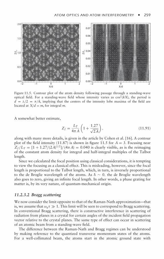
ATOM OPTICS AND ATOM INTERFEROMETRY 259
–2 –1 0 1 20.0
0.5
1.0
1.5
2.0
X/d–2 –1 0 1 2
X/d
Z/L T
Z/L T
0.00
0.01
0.02
0.03
0.04
0.05
0.06
0.07
Figure 11.5. Contour plot of the atom density following passage through a standing-waveoptical field. For a standing-wave field whose intensity varies as cos2(kX), the period isd = λ/2 = π/k, implying that the centers of the intensity lobe maxima of the field arelocated at X/d = m, for integral m.
A somewhat better estimate,
Zf = LT4πA
(1 + 1.27√
2A
), (11.91)
along with many more details, is given in the article by Cohen et al. [16]. A contourplot of the field intensity (11.87) is shown in figure 11.5 for A = 3. Focusing nearZf /LT = [1 + 1.27/(2A)1/2]/ (4πA) = 0.040 is clearly visible, as is the reimagingof the constant atom density for integral and half-integral multiples of the Talbotlength.
Since we calculated the focal position using classical considerations, it is temptingto view the focusing as a classical effect. This is misleading, however, since the focallength is proportional to the Talbot length, which, in turn, is inversely proportionalto the de Broglie wavelength of the atoms. As ∼ 0, the de Broglie wavelengthalso goes to zero, giving an infinite focal length. In other words, a phase grating formatter is, by its very nature, of quantum-mechanical origin.
11.2.3.2 Bragg scattering
We now consider the limit opposite to that of the Raman-Nath approximation—thatis, we assume that ωqτ 1. This limit will be seen to correspond to Bragg scattering.In conventional Bragg scattering, there is constructive interference in scattering ofradiation from planes in a crystal for certain angles of the incident field propagationvector relative to the crystal planes. The same type of effect can occur in scatteringof an atomic beam from a standing-wave field.
The difference between the Raman-Nath and Bragg regimes can be understoodby making reference to the quantized transverse momentum states of the atoms.For a well-collimated beam, the atoms start in the atomic ground state with
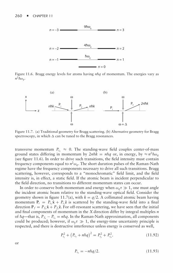
260 CHAPTER 11
n = –39hωq-
4hωq-
hωq-
n = –2
n = –1
n = 3
n = 2
n = 1
n = 0
Figure 11.6. Bragg energy levels for atoms having nq of momentum. The energies vary asn2ωq.
z
x ω
ω
Pfnhk- nhk-Pi
(a) (b)ω
ω + ∆
Pf 2nhk-
Pi
Figure 11.7. (a) Traditional geometry for Bragg scattering. (b) Alternative geometry for Braggspectroscopy, in which can be tuned to the Bragg resonances.
transverse momentum Pix ≈ 0. The standing-wave field couples center-of-massground states differing in momentum by 2nk = nq or, in energy, by ≈ n2ωq(see figure 11.6). In order to drive such transitions, the field intensity must containfrequency components equal to n2ωq. The short duration pulses of the Raman-Nathregime have the frequency components necessary to drive all such transitions. Braggscattering, however, corresponds to a “monochromatic” field limit, and the fieldintensity is, in effect, a static field. If the atomic beam is incident perpendicular tothe field direction, no transitions to different momentum states can occur.
In order to conserve both momentum and energy when ωqτ 1, one must anglethe incident atomic beam relative to the standing-wave optical field. Consider thegeometry shown in figure 11.7(a), with k = q/2. A collimated atomic beam havingmomentum Pi = Pix x + Piz z is scattered by the standing-wave field into a finaldirection P f = Pfx x+ Pfz z. For off-resonant scattering, we have seen that the initialand final components of momentum in the X direction differ by integral multiples nof q—that is, Pfx − Pix = nq. In the Raman-Nath approximation, all componentscould be produced; however, if ωqτ 1, the energy-time uncertainty principle isrespected, and there is destructive interference unless energy is conserved as well,
P2iz + (
Pix + nq)2 = P2
iz + P2ix, (11.92)
or
Pix = −nq/2. (11.93)
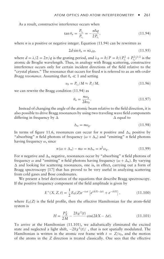
ATOM OPTICS AND ATOM INTERFEROMETRY 261
As a result, constructive interference occurs when
tan θn = PixPiz
= −nq2Piz
, (11.94)
where n is a positive or negative integer. Equation (11.94) can be rewritten as
2d sin θn = nλdB, (11.95)
where d = λ/2 = 2π/q is the grating period, and λB = h/P = h/(P2iz + P2
ix)1/2 is the
atomic de Broglie wavelength. Thus, in analogy with Bragg scattering, constructiveinterference occurs only for certain incident directions of the field relative to the“crystal planes.” The resonance that occurs for fixed n is referred to as an nth-orderBragg resonance. Assuming that θn 1 and setting
v0 = Piz/M ≈ Pi/M, (11.96)
we can rewrite the Bragg condition (11.94) as
θn = nωq2kv0
. (11.97)
Instead of changing the angle of the atomic beam relative to the field direction, it isalso possible to drive Bragg resonances by using two traveling wave field componentsdiffering in frequency by [figure 11.7(b)] and by choosing equal to
n = nωq. (11.98)
In terms of figure 11.6, resonances can occur for n positive and n positive by“absorbing” n field photons of frequency (ω +n) and “emitting” n field photonshaving frequency ω, since
n (ω +n) − nω = nn = n2ωq. (11.99)
For n negative and n negative, resonances occur by “absorbing” n field photons offrequency ω and “emitting” n field photons having frequency (ω +n). By varying and looking for scattering resonances, one is, in effect, carrying out a form ofBragg spectroscopy [17] that has proved to be very useful in analyzing scatteringfrom cold gases and Bose condensates.
We present a brief derivation of the equations that describe Bragg spectroscopy.If the positive frequency component of the field amplitude is given by
E+(X, Z, t) = 12E0(Z)e−iωt [ei(kX−t) + e−ikX] , (11.100)
where E0(Z) is the field profile, then the effective Hamiltonian for the atom–fieldsystem is
H = P2X
2M− 2χ2(t)
δcos(2kX−t). (11.101)
To arrive at the Hamiltonian (11.101), we adiabatically eliminated the excitedstate and neglected a light shift, −2χ2(t)/δ, that is not spatially modulated. TheHamiltonian is written in the atomic rest frame with t = Z/v0, and the motionof the atoms in the Z direction is treated classically. One sees that the effective
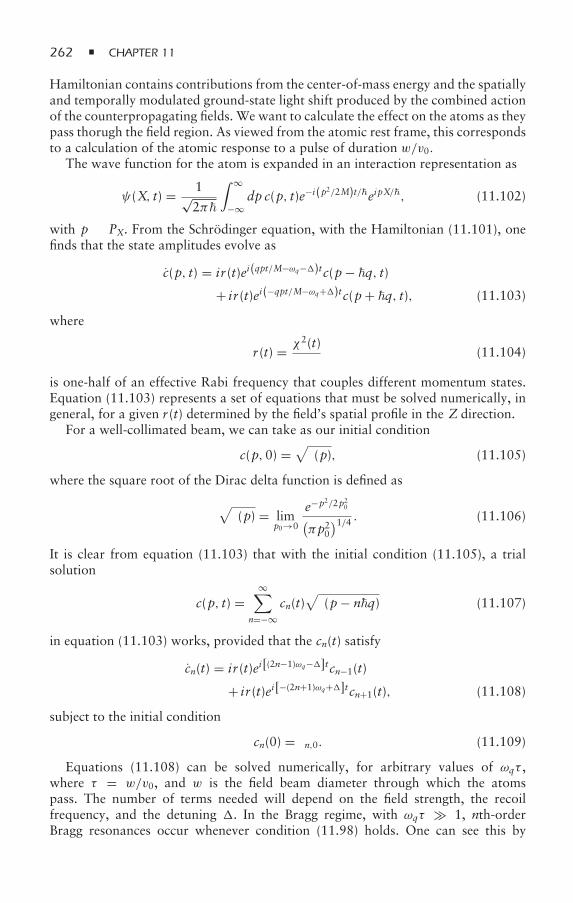
262 CHAPTER 11
Hamiltonian contains contributions from the center-of-mass energy and the spatiallyand temporally modulated ground-state light shift produced by the combined actionof the counterpropagating fields. We want to calculate the effect on the atoms as theypass thorugh the field region. As viewed from the atomic rest frame, this correspondsto a calculation of the atomic response to a pulse of duration w/v0.
The wave function for the atom is expanded in an interaction representation as
ψ(X, t) = 1√2π
∫ ∞
−∞dpc(p, t)e−i(p2/2M)t/eipX/, (11.102)
with p ≡ PX. From the Schrödinger equation, with the Hamiltonian (11.101), onefinds that the state amplitudes evolve as
c(p, t) = ir (t)ei(qpt/M−ωq−)tc(p− q, t)+ ir (t)ei(−qpt/M−ωq+)tc(p+ q, t), (11.103)
where
r (t) = χ2(t)δ
(11.104)
is one-half of an effective Rabi frequency that couples different momentum states.Equation (11.103) represents a set of equations that must be solved numerically, ingeneral, for a given r (t) determined by the field’s spatial profile in the Z direction.
For a well-collimated beam, we can take as our initial condition
c(p,0) =√δ(p), (11.105)
where the square root of the Dirac delta function is defined as
√δ(p) = lim
p0→0
e−p2/2p20(πp20
)1/4 . (11.106)
It is clear from equation (11.103) that with the initial condition (11.105), a trialsolution
c(p, t) =∞∑
n=−∞cn(t)
√δ(p− nq) (11.107)
in equation (11.103) works, provided that the cn(t) satisfy
cn(t) = ir (t)ei[(2n−1)ωq−]tcn−1(t)
+ ir (t)ei[−(2n+1)ωq+]tcn+1(t), (11.108)
subject to the initial condition
cn(0) = δn,0. (11.109)
Equations (11.108) can be solved numerically, for arbitrary values of ωqτ ,where τ = w/v0, and w is the field beam diameter through which the atomspass. The number of terms needed will depend on the field strength, the recoilfrequency, and the detuning . In the Bragg regime, with ωqτ 1, nth-orderBragg resonances occur whenever condition (11.98) holds. One can see this by
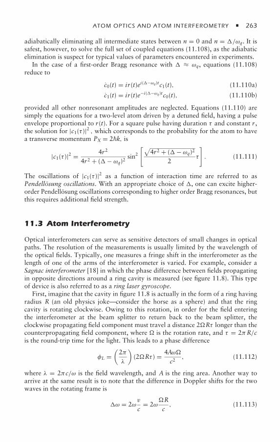
ATOM OPTICS AND ATOM INTERFEROMETRY 263
adiabatically eliminating all intermediate states between n = 0 and n = /ωq. It issafest, however, to solve the full set of coupled equations (11.108), as the adiabaticelimination is suspect for typical values of parameters encountered in experiments.
In the case of a first-order Bragg resonance with ≈ ωq, equations (11.108)reduce to
c0(t) = ir (t)ei(−ωq)tc1(t), (11.110a)
c1(t) = ir (t)e−i(−ωq)tc0(t), (11.110b)
provided all other nonresonant amplitudes are neglected. Equations (11.110) aresimply the equations for a two-level atom driven by a detuned field, having a pulseenvelope proportional to r (t). For a square pulse having duration τ and constant r ,the solution for |c1(τ )|2 , which corresponds to the probability for the atom to havea transverse momentum PX = 2k, is
|c1(τ )|2 = 4r2
4r2 + (− ωq)2 sin2[√
4r2 + (− ωq)22
τ
]. (11.111)
The oscillations of |c1(τ )|2 as a function of interaction time are referred to asPendellösung oscillations. With an appropriate choice of , one can excite higher-order Pendellösung oscillations corresponding to higher order Bragg resonances, butthis requires additional field strength.
11.3 Atom Interferometry
Optical interferometers can serve as sensitive detectors of small changes in opticalpaths. The resolution of the measurements is usually limited by the wavelength ofthe optical fields. Typically, one measures a fringe shift in the interferometer as thelength of one of the arms of the interferometer is varied. For example, consider aSagnac interferometer [18] in which the phase difference between fields propagatingin opposite directions around a ring cavity is measured (see figure 11.8). This typeof device is also referred to as a ring laser gyroscope.
First, imagine that the cavity in figure 11.8 is actually in the form of a ring havingradius R (an old physics joke—consider the horse as a sphere) and that the ringcavity is rotating clockwise. Owing to this rotation, in order for the field enteringthe interferometer at the beam splitter to return back to the beam splitter, theclockwise propagating field component must travel a distance 2Rτ longer than thecounterpropagating field component, where is the rotation rate, and τ = 2πR/cis the round-trip time for the light. This leads to a phase difference
φL =(2πλ
)(2Rτ ) = 4Aω
c2, (11.112)
where λ = 2πc/ω is the field wavelength, and A is the ring area. Another way toarrive at the same result is to note that the difference in Doppler shifts for the twowaves in the rotating frame is
ω = 2ωv
c= 2ω
Rc, (11.113)
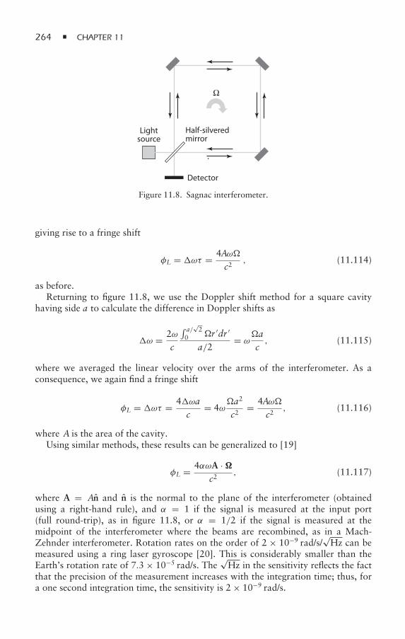
264 CHAPTER 11
Lightsource
Half-silveredmirror
Detector
Ω
Figure 11.8. Sagnac interferometer.
giving rise to a fringe shift
φL = ωτ = 4Aωc2
, (11.114)
as before.Returning to figure 11.8, we use the Doppler shift method for a square cavity
having side a to calculate the difference in Doppler shifts as
ω = 2ωc
∫ a/√2
0 r ′dr ′
a/2= ω
ac, (11.115)
where we averaged the linear velocity over the arms of the interferometer. As aconsequence, we again find a fringe shift
φL = ωτ = 4ωac
= 4ωa2
c2= 4Aω
c2, (11.116)
where A is the area of the cavity.Using similar methods, these results can be generalized to [19]
φL = 4αωA ·
c2, (11.117)
where A = An and n is the normal to the plane of the interferometer (obtainedusing a right-hand rule), and α = 1 if the signal is measured at the input port(full round-trip), as in figure 11.8, or α = 1/2 if the signal is measured at themidpoint of the interferometer where the beams are recombined, as in a Mach-Zehnder interferometer. Rotation rates on the order of 2 × 10⁻⁹ rad/s/
√Hz can be
measured using a ring laser gyroscope [20]. This is considerably smaller than theEarth’s rotation rate of 7.3 × 10⁻⁵ rad/s. The
√Hz in the sensitivity reflects the fact
that the precision of the measurement increases with the integration time; thus, fora one second integration time, the sensitivity is 2 × 10⁻⁹ rad/s.
ATOM OPTICS AND ATOM INTERFEROMETRY 265
It is intriguing to consider the possibility of replacing the optical waves by matterwaves in this device [21–23]. Then, equation (11.112) is replaced by
φM =(2πλB
)(2αRτ ) =
(2πλB
)(2αR
2πRv0
)= 4αMA
, (11.118)
where v0 is the average speed of the matter wave. For all things equal, the ratio
φM
φL= Mc2
ω, (11.119)
which can represent a 1010 increase in sensitivity! Of course, the big catch hereis “for all things equal.” While it is possible to get large-angle beam splitters foroptical fields, the beam splitters for matter waves usually produce relatively smallmomentum kicks (typically, several k = π/d, where d is the grating period).Moreover, laser field intensities are considerably larger than the equivalent atomfluxes. As a consequence, the factor of 1010 is reduced dramatically. Still, rotationrates with sensitivities approaching 6 × 10⁻¹⁰ rad/s/
√Hz have been achieved using
matter-wave interferometers [24].There is another advantage of matter wave over optical interferometers. Since
matter waves carry mass, an atom interferometer is sensitive to inertial effects suchas gravity, to the recoil that atoms undergo in scattering radiation, and to thechanges in velocity or phase produced by collisions with atoms in the paths of theinterferometers. The measurement of the recoil frequency, along with a sensitivemeasurement of the atom’s mass, has the potential for yielding the most sensitivemeasurement of the fine structure constant. Thus, there are many reasons to pursuethe concept of atom interferometry.
A generic interferometer contains a beam splitter that separates an incomingbeam along different paths (which may be overlapping). A second element ofthe interferometer recombines the separated beams so that they can interfere ata detector. In the Michelson interferometer, for example, a half-reflecting, half-transmitting mirror serves as both the beam splitter and recombiner. The atominterferometers we discuss are assumed to work in the Raman-Nath regime—that is, the interactions of the atoms with the elements of the interferometer(microfabricated slits, standing-wave optical fields) occur sufficiently fast that anymotion of the atoms during the interaction can be neglected.
In a typical atom interferometer, a collimated atomic beam passes through twosets of slits (or two standing-wave optical fields) separated in distance by L. The firstset of slits serves as a beam splitter, and the second as a beam recombiner. Followingpassage through both sets of slits, the transverse atomic density is detected at adistance Z from the second slits. (In practice, one often uses a third set of slits asthe detector, observing the atom flux as the slits are moved transverse to the atomicbeam.) We discussed the first stage of this process in the section 11.2, where it wasassumed that the incoming beam was mono-energetic.
Actually, for a perfectly mono-energetic beam, the recombiner is not necessaryif the atom paths overlap. In fact, the diffraction pattern itself arises from atomsmoving along different paths. However, the collimation requirements (transversemomentum k = π/d, where d is the grating period) are severe in this case(typically, the beam angular divergence must be less than 10−4), and it useful to use a
266 CHAPTER 11
scheme, similar to that of a photon echo, where the destructive interference resultingfrom the transverse momentum distribution can be canceled in certain echo planes.A device operating in this fashion is referred to as a Talbot-Lau interferometer[2, 25–27].
In a Talbot-Lau interferometer, the angular divergence of the incoming beamsatisfies
θb d/L, (11.120)
ensuring that any structure in the transverse density following the interaction withthe beam splitter washes out in a distance Z L. For a longitudinal velocity v0 anda transverse velocity u⊥ = v0θb, this condition may be rewritten as
θb = v0θb
dLv0
= u⊥dT = ku⊥T
π 1 (11.121)
and is reminiscent of that needed for a photon echo, kuT 1, to ensure thatthe optical coherence is washed out before the second pulse. However, just as ina photon echo, the second grating can restore the signal at certain echo times orplanes. Also, as in a photon echo, such points are determined by the conditionthat a Doppler phase cancels for all atoms, regardless of their transverse velocity.Since the Doppler phase does not contain , the location of the echo points can bedetermined from classical considerations, even if matter-wave effects are importantin determining the actual density distribution at such points. The angular divergenceof the beam cannot be arbitrarily large; we must require that θb d/w, where w isthe grating thickness or beam diameter of the standing-wave optical field, in orderto ensure that the atoms interact effectively with the beam splitter. This requirementis analogous to the one we used in coherent transients, where the condition kuτ 1was needed to guarantee that all atoms were in the bandwith of the pulse.
As we mentioned earlier, there are so many different types of atom interfero-meters that things can get confusing. Let us give a brief classification. In all cases, werestrict the discussion to Talbot-Lau–type interferometers—that is, those in whichthere is a transverse velocity distribution satisfying condition (11.120).
11.3.1 Microfabricated Elements
If the beam splitters and recombiners consist of microfabricated slits, the interfero-meters operate in basically two regimes, the moiré or classical limit, and the matter-wave limit. A moiré interferometer relies on the shadow effect for its operation—the motion of the particles is treated classically. Moiré is a French word referringto the patterns one sees in insect wings. In a moiré interferometer, particles passthrough two sets of slits separated by some distance L LT. By tracing the classicalpaths in such a geometry, one arrives at patterns following the second set of slitscharacteristic of a Talbot-Lau interferometer. This interferometer is sensitive to anychanges in the atomic velocity, since they destroy the moiré pattern.
The matter-wave limit, on the other hand, corresponds to separation of the slitsL LT, where wave features can be seen. A detailed discussion of the theory ofatom interferometers using microfabricated gratings can be found in the article byDubetsky and Berman [10]. Here, we consider only atom interferometers in which
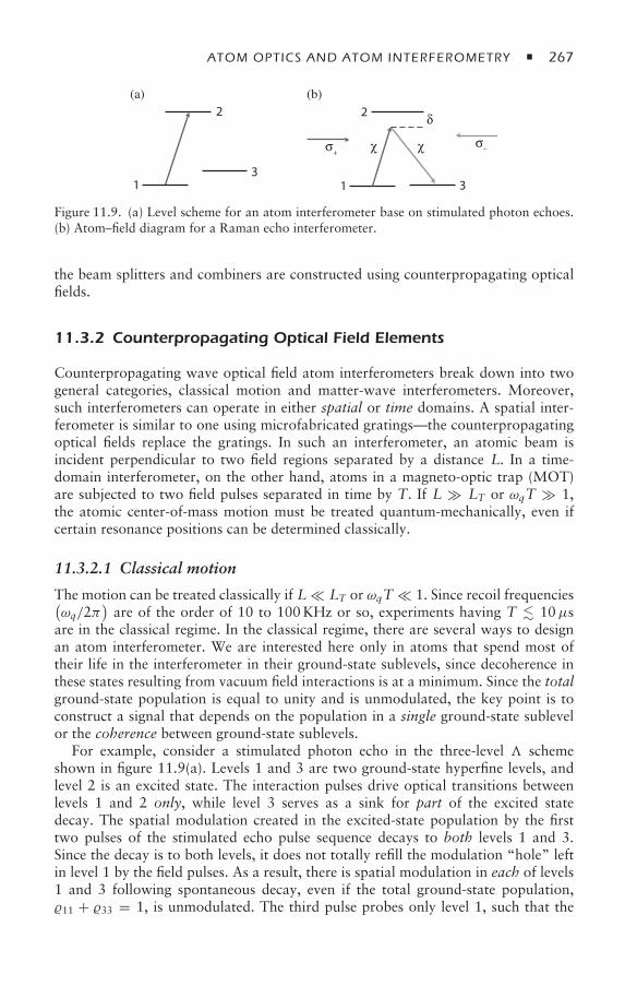
ATOM OPTICS AND ATOM INTERFEROMETRY 267
1
2(a) (b)
3
2 δ
σ+σ–χχ
31
Figure 11.9. (a) Level scheme for an atom interferometer base on stimulated photon echoes.(b) Atom–field diagram for a Raman echo interferometer.
the beam splitters and combiners are constructed using counterpropagating opticalfields.
11.3.2 Counterpropagating Optical Field Elements
Counterpropagating wave optical field atom interferometers break down into twogeneral categories, classical motion and matter-wave interferometers. Moreover,such interferometers can operate in either spatial or time domains. A spatial inter-ferometer is similar to one using microfabricated gratings—the counterpropagatingoptical fields replace the gratings. In such an interferometer, an atomic beam isincident perpendicular to two field regions separated by a distance L. In a time-domain interferometer, on the other hand, atoms in a magneto-optic trap (MOT)are subjected to two field pulses separated in time by T. If L LT or ωqT 1,the atomic center-of-mass motion must be treated quantum-mechanically, even ifcertain resonance positions can be determined classically.
11.3.2.1 Classical motion
The motion can be treated classically if L LT or ωqT 1. Since recoil frequencies(ωq/2π
)are of the order of 10 to 100KHz or so, experiments having T 10µs
are in the classical regime. In the classical regime, there are several ways to designan atom interferometer. We are interested here only in atoms that spend most oftheir life in the interferometer in their ground-state sublevels, since decoherence inthese states resulting from vacuum field interactions is at a minimum. Since the totalground-state population is equal to unity and is unmodulated, the key point is toconstruct a signal that depends on the population in a single ground-state sublevelor the coherence between ground-state sublevels.
For example, consider a stimulated photon echo in the three-level schemeshown in figure 11.9(a). Levels 1 and 3 are two ground-state hyperfine levels, andlevel 2 is an excited state. The interaction pulses drive optical transitions betweenlevels 1 and 2 only, while level 3 serves as a sink for part of the excited statedecay. The spatial modulation created in the excited-state population by the firsttwo pulses of the stimulated echo pulse sequence decays to both levels 1 and 3.Since the decay is to both levels, it does not totally refill the modulation “hole” leftin level 1 by the field pulses. As a result, there is spatial modulation in each of levels1 and 3 following spontaneous decay, even if the total ground-state population,11 + 33 = 1, is unmodulated. The third pulse probes only level 1, such that the
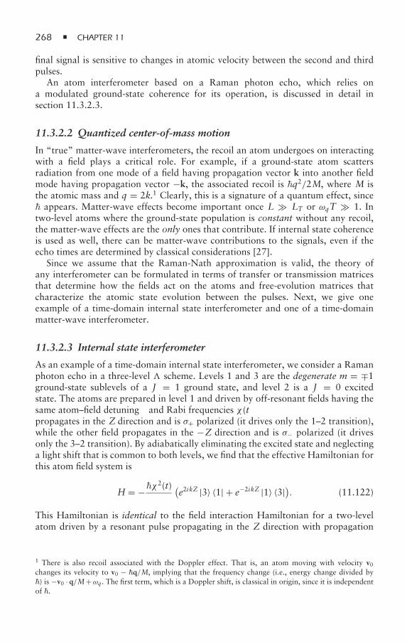
268 CHAPTER 11
final signal is sensitive to changes in atomic velocity between the second and thirdpulses.
An atom interferometer based on a Raman photon echo, which relies ona modulated ground-state coherence for its operation, is discussed in detail insection 11.3.2.3.
11.3.2.2 Quantized center-of-mass motion
In “true” matter-wave interferometers, the recoil an atom undergoes on interactingwith a field plays a critical role. For example, if a ground-state atom scattersradiation from one mode of a field having propagation vector k into another fieldmode having propagation vector −k, the associated recoil is q2/2M, where M isthe atomic mass and q = 2k.1 Clearly, this is a signature of a quantum effect, since appears. Matter-wave effects become important once L LT or ωqT 1. Intwo-level atoms where the ground-state population is constant without any recoil,the matter-wave effects are the only ones that contribute. If internal state coherenceis used as well, there can be matter-wave contributions to the signals, even if theecho times are determined by classical considerations [27].
Since we assume that the Raman-Nath approximation is valid, the theory ofany interferometer can be formulated in terms of transfer or transmission matricesthat determine how the fields act on the atoms and free-evolution matrices thatcharacterize the atomic state evolution between the pulses. Next, we give oneexample of a time-domain internal state interferometer and one of a time-domainmatter-wave interferometer.
11.3.2.3 Internal state interferometer
As an example of a time-domain internal state interferometer, we consider a Ramanphoton echo in a three-level scheme. Levels 1 and 3 are the degenerate m = ∓1ground-state sublevels of a J = 1 ground state, and level 2 is a J = 0 excitedstate. The atoms are prepared in level 1 and driven by off-resonant fields having thesame atom–field detuning δ and Rabi frequencies χ (t) [see figure 11.9(b)]. One fieldpropagates in the Z direction and is σ+ polarized (it drives only the 1–2 transition),while the other field propagates in the −Z direction and is σ− polarized (it drivesonly the 3–2 transition). By adiabatically eliminating the excited state and neglectinga light shift that is common to both levels, we find that the effective Hamiltonian forthis atom field system is
H = −χ2(t)δ
(e2ikZ |3〉 〈1| + e−2ikZ |1〉 〈3|). (11.122)
This Hamiltonian is identical to the field interaction Hamiltonian for a two-levelatom driven by a resonant pulse propagating in the Z direction with propagation
1 There is also recoil associated with the Doppler effect. That is, an atom moving with velocity v0changes its velocity to v0 − q/M, implying that the frequency change (i.e., energy change divided by) is −v0 · q/M+ωq. The first term, which is a Doppler shift, is classical in origin, since it is independentof .
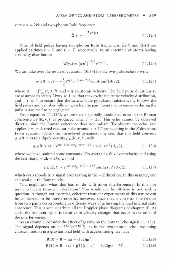
ATOM OPTICS AND ATOM INTERFEROMETRY 269
vector q = 2kz and two-photon Rabi frequency
(t) = −2χ2(t)δ
. (11.123)
Pairs of field pulses having two-photon Rabi frequencies 1(t) and 2(t) areapplied at times t = 0 and t = T, respectively, to an ensemble of atoms havinga velocity distribution
W(v0) = (πu2
)−3/2e−v20/u2 . (11.124)
We can take over the result of equation (10.34) for the two-pulse echo to write
31(R, v, t) = − i2eiq·Re−iq·v(t−2T) sin A1 sin
2(A2/2), (11.125)
where Aj = ∫∞−∞ j (t)dt, and v is an atomic velocity. The field pulse durations τ j
are assumed to satisfy 2kuτ j 1, so that they excite the entire velocity distribution,and |δ|τ 1 to ensure that the excited-state population adiabatically follows thefield pulses and vanishes following each pulse pair. Spontaneous emission during thepulse is assumed to be negligible.
From equation (11.125), we see that a spatially modulated echo in the Ramancoherence 31(R, v, t) is produced when t = 2T. This echo cannot be observeddirectly, since the Raman coherence does not radiate. To observe the echo, oneapplies a σ+ polarized readout pulse around t ≈ 2T propagating in the Z direction.From equation (9.15f) for three-level dynamics, one sees that this field converts31(R, v, t) to a dipole density 32(R, v, t), with
32(R, v, t) ∼ ei(q−k)·R+iωte−iq·v(t−2T) sin A1 sin2 (A2/2), (11.126)
where we have omitted some constants. On averaging this over velocity and usingthe fact that q = 2k = 2kz, we find
32(Z, t) ∼ eikZ+iωte−k2u2(t−2T)2 sin A1 sin2 (A2/2), (11.127)
which corresponds to a signal propagating in the −Z direction. In this manner, onecan read out the Raman echo.
You might ask what this has to do with atom interferometry. Is this notjust a coherent transient calculation? You would not be off-base to ask such aquestion. Although not essential, coherent transient experiments of this nature canbe considered to be interferometric, however, since they involve an interferencefrom two paths corresponding to different ways of achieving the final internal statecoherence. This is seen clearly in all the Doppler phase diagrams of chapter 10. Assuch, the resultant signal is sensitive to velocity changes that occur in the arms ofthe interferometer.
As an example, consider the effect of gravity on the Raman echo signal (11.126).The signal depends on 〈e−iq·R(0)e2iq·R(T)〉, as in the two-photon echo. Assumingclassical motion in a gravitational field with acceleration g, we have
R(0) = R − v0t − (1/2)gt2, (11.128)
R(T) = R− (v0 + gT) (t − T) − (1/2)g(t − T)2, (11.129)
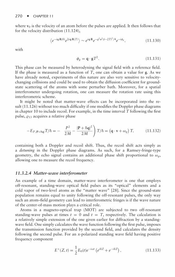
270 CHAPTER 11
where v0 is the velocity of an atom before the pulses are applied. It then follows thatfor the velocity distribution (11.124),
⟨e−iq·R(0)e2iq·R(T)⟩ ∼ eiq·Re−q2u2(t−2T)2/4e−iφg , (11.130)
with
φg = q · gT2. (11.131)
This phase can be measured by heterodyning the signal field with a reference field.If the phase is measured as a function of T, one can obtain a value for g. As wehave already noted, experiments of this nature are also very sensitive to velocity-changing collisions and could be used to obtain the diffusion coefficient for ground-state scattering of the atoms with some perturber bath. Moreover, for a spatialinterferometer undergoing rotation, one can measure the rotation rate using thisinterferometric scheme.
It might be noted that matter-wave effects can be incorporated into the re-sult (11.126) without too much difficulty if one modifies the Doppler phase diagramsin chapter 10 to include recoil. For example, in the time interval T following the firstpulse, 13 acquires a relative phase
−EP,|P+q|T/ = −(P2
2M− |P + q|2
2M
)T/ = (
q · v + ωq)T, (11.132)
containing both a Doppler and recoil shift. Thus, the recoil shift acts simply asa detuning in the Doppler phase diagrams. As such, for a Ramsey-fringe-typegeometry, the echo signal contains an additional phase shift proportional to ωq,allowing one to measure the recoil frequency.
11.3.2.4 Matter-wave interferometer
An example of a time domain, matter-wave interferometer is one that employsoff-resonant, standing-wave optical field pulses as its “optical” elements and acold vapor of two-level atoms as the “matter wave” [28]. Since the ground-statepopulation remains equal to unity following the off-resonant pulses, the only waysuch an atom–field geometry can lead to interferometric fringes is if the wave natureof the center-of-mass motion plays a critical role.
Atoms in a magneto-optical trap (MOT) are subjected to two off-resonantstanding-wave pulses at times t = 0 and t = T, respectively. The calculation isa relatively simple extension of the one given earlier for diffraction by a standing-wave field. One simply calculates the wave function following the first pulse, imposesthe transmission function provided by the second field, and calculates the densityfollowing the second pulse. For an x-polarized standing wave field having positivefrequency component
E+(Z, t) = 12E0(t)e−iωt (eikZ + e−ikZ) , (11.133)
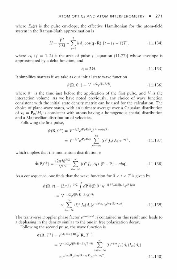
ATOM OPTICS AND ATOM INTERFEROMETRY 271
where E0(t) is the pulse envelope, the effective Hamiltonian for the atom–fieldsystem in the Raman-Nath approximation is
H = P2
2M−
2∑j=1
Aj cos(q · R)δ[t − ( j − 1)T], (11.134)
where Aj ( j = 1,2) is the area of pulse j [equation (11.77)] whose envelope isapproximated by a delta function, and
q = 2kz. (11.135)
It simplifies matters if we take as our initial state wave function
ψ(R,0−) = V−1/2eiP0·R/, (11.136)
where 0− is the time just before the application of the first pulse, and V is theinteraction volume. As we have noted previously, any choice of wave functionconsistent with the initial state density matrix can be used for the calculation. Thechoice of plane-wave states, with an ultimate average over a Gaussian distributionof v0 = P0/M, is consistent with atoms having a homogenous spatial distributionand a Maxwellian distribution of velocities.
Following the first pulse,
ψ(R,0+) = V−1/2eiP0·R/ei A1 cos(q·R)
= V−1/2eiP0·R/∞∑
n=−∞(i)n Jn(A1)einq·R, (11.137)
which implies that the momentum distribution is
(P,0+) = (2π)3/2
V1/2
∞∑n=−∞
(i)n Jn(A1)δ(P − P0 − nq). (11.138)
As a consequence, one finds that the wave function for 0 < t < T is given by
ψ(R, t) = (2π)−3/2∫dP (P,0+)e−i(P2/2M)t/eiP·R/
= V−1/2ei(P0·R−EP0 t)/
×∞∑
n=−∞(i)n Jn(A1)e−in2ωqteinq·(R−v0t). (11.139)
The transverse Doppler phase factor e−inq·v0t is contained in this result and leads toa dephasing in the density similar to the one in free polarization decay.
Following the second pulse, the wave function is
ψ(R,T+) = ei A2 cos(q·R)ψ(R,T−)
= V−1/2ei(P0·R−EP0T)/∞∑
n,m=−∞(i)n+m Jn(A1)Jm(A2)
× eimq·Reinq·(R−v0T)e−in2ωqT. (11.140)
272 CHAPTER 11
One can recalculate the momentum distribution as
(P,T+) = (2π)−3/2∫dRψ(R,T+)ei(P
2/2M)T/eiP·R/
= (2π)3/2
V1/2
∞∑n,m=−∞
(i)n+mJn(A1)Jm(A2)ei(m+n)q·v0Tei(n+m)2ωqT
× e−inq·v0Te−in2ωqTδ[P − P0 − (n+m) q]. (11.141)
As a consequence, the wave function for t > T is
ψ(R, t) = (2π)−3/2∫dP (P,T+)e−i(P2/2M)t/eiP·R/
= ei(P0·R−EP0 t)/
×∞∑
n,m=−∞(i)n+m Jn(A1)Jm(A2)e−inq·v0Te−in2ωqT
× ei(n+m)q·[R−v0(t−T)]e−i(n+m)2ωq(t−T). (11.142)
We are interested in the atomic density ρ(R, t) = |ψ(R, t)|2 following thesecond pulse, averaged over the velocity distribution. Using equations (11.142) and(11.124), we find that the velocity averaged density is
〈ρ(R, t)〉 = V−1∞∑
n,m,n′m′=−∞(i)n+m−n′−m′
Jn(A1)Jm(A2)Jn′(A1)Jm′(A2)
× e−i(n2−n′2)ωqTe−i[(n+m)2−(n′+m′)2]ωq(t−T)ei(n+m−n′−m′)qZ
× e−[(n+m−n′−m′)(t−T)+(n−n′)T]2q2u2/4. (11.143)
If we set n = n− n′, m= m−m′, and use the sum rule (11.85) in the form
i n∑n′
Jn+n′ (A1)Jn′ (A1)e−iα(n+2n′) = Jn [2A1 sinα], (11.144)
we can transform equation (11.143) into the simpler form
〈ρ(R, t)〉 = V−1∞∑
n,m=−∞ei(n+m)qZe−[(n+m)(t−T)+nT]2q2u2/4
×Jn2A1 sin[(n+ m)ωq (t − T) + nωqT]
×Jm
2A2 sin[(n+ m)ωq(t − T)]
. (11.145)
Although somewhat complicated, equation (11.145) displays an extraordinarilyrich structure. If ωqt 1 (classical motion limit), ρ(R, t) ∼ V−1; there is no structurein the classical motion limit. In other words, the diffraction pattern must arise fromeffects related to the quantized nature of the center-of-mass motion. If we assumethat
quT = 2ωqT (Mu/q) 1, (11.146)
ATOM OPTICS AND ATOM INTERFEROMETRY 273
which is typical for atoms in a MOT (momentum greater than recoil momentum),then the interference pattern washes out except in the vicinity of echo times
te =(1 − n
n+ m
)T > T. (11.147)
At such times, the spatial density is constant, but there is spatial modulationhaving period λ/[2|n + m|] in the transverse direction that occurs during a timeinterval t ≈ 1/qu about these points. This result shows that while the structuresobserved are products of matter-wave interferometry, the positions of the matter-wave gratings are determined by classical echo considerations, i.e., where a Dopplerphase cancels, as in any Talbot-Lau interferometer.
Near the echo times t = te + t = [1 − n/(n + m)]T + t, equation (11.145)reduces to
〈ρ(R, t)〉 = V−1∞∑
n,m=−∞ei(n+m)qZe−[(n+m)qut]2/4 Jn
2A1 sin[ωqt(n+ m)]
×Jm
2A2 sin[−nωqT + ωqt(n+ m)]
, (11.148)
provided that |t| 1/qu. For pulse areas of order unity and for (Mu/q) 1,equation (11.148) becomes
〈ρ(R, t)〉 ∼ V−1∞∑
n,m=−∞(−1)m (−1)(|n|−n)/2 (|n|!)−1 ei(n+m)qZe−[(n+m)qut]2/4
× [A1ωqt(n+ m)
]|n|Jm
[2A2 sin(nωqT)
]. (11.149)
All harmonics in the signal vanish at the echo times, but they exist in the vicinity ofthese points.
A contour plot of the signal is shown in figure 11.10, illustrating these features.The large amplitude near t = T (n = 0, m = ±1) corresponds to a freepolarization decay signal following the second pulse, with the density [obtained fromequation (11.148)] varying as
V〈ρ(R, t)〉 ∼ 1 + 2(A2ωqt)e−(qut)2/4 cos(qZ) (11.150)
for t T. Near the echo plane at t = 2T (n = ∓1, m= ±2), the density varies as
V〈ρ(R, t)〉 ∼ 1 − 2(A1ωqt)J2[2A2 sin(ωqT)]e−(qut)2/4 cos(qZ), (11.151)
with modulation period 2π/q, and near the echo plane at t = 3T/2 (n = ∓1,m= ±3), as
V〈ρ(R, t)〉 ∼ 1 − 2(A1ωqt)J3[2A2 sin(ωqT)]e−(qut)2/4 cos(2qZ), (11.152)
with modulation period π/q. You can also see the modulation with period 2π/3qnear the echo plane at t = 4T/3 (n = ∓1, m= ±4), and the modulation with period2π/q near the echo plane at t = 3T (n = ∓2, m= ±3), where the density varies as
V〈ρ(R, t)〉 ∼ 1 + (A1ωqt
)2J2[2A2 sin(2ωqT)]e−(qut)2/4 cos(qZ). (11.153)
The density in the echo planes is constant.
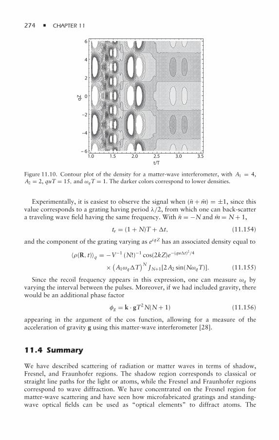
274 CHAPTER 11
1.0 1.5 2.0 2.5 3.0 3.5– 6
–4
–2
0
2
4
6
t/T
qZ
Figure 11.10. Contour plot of the density for a matter-wave interferometer, with A1 = 4,A2 = 2, quT = 15, and ωqT = 1. The darker colors correspond to lower densities.
Experimentally, it is easiest to observe the signal when (n+ m) = ±1, since thisvalue corresponds to a grating having period λ/2, from which one can back-scattera traveling wave field having the same frequency. With n = −N and m= N+ 1,
te = (1 + N)T +t, (11.154)
and the component of the grating varying as eiqZ has an associated density equal to
〈ρ(R, t)〉q = −V−1 (N!)−1 cos(2kZ)e−(qut)2/4
× (A1ωqT
)NJN+1[2A2 sin(NωqT)]. (11.155)
Since the recoil frequency appears in this expression, one can measure ωq byvarying the interval between the pulses. Moreover, if we had included gravity, therewould be an additional phase factor
φg = k · gT2N(N+ 1) (11.156)
appearing in the argument of the cos function, allowing for a measure of theacceleration of gravity g using this matter-wave interferometer [28].
11.4 Summary
We have described scattering of radiation or matter waves in terms of shadow,Fresnel, and Fraunhofer regions. The shadow region corresponds to classical orstraight line paths for the light or atoms, while the Fresnel and Fraunhofer regionscorrespond to wave diffraction. We have concentrated on the Fresnel region formatter-wave scattering and have seen how microfabricated gratings and standing-wave optical fields can be used as “optical elements” to diffract atoms. The
ATOM OPTICS AND ATOM INTERFEROMETRY 275
Talbot effect, or self-imaging of a periodic structure, was derived, as was thediffraction pattern for amplitude and phase gratings. The Raman-Nath and Braggscattering limits were distinguished. Following a discussion of atom optics, weshowed how atoms can be used in atom interferometric schemes to provide sensitivemeasurements of inertial effects and the recoil frequency. Interferometers in whichthe atomic motion could be taken to be classical were distinguished from thosein which the center-of-mass motion had to be quantized. All calculations for atominterferometry were carried out in the Talbot-Lau regime, analogous to photon echoschemes in which there is a rephasing for different velocity groups at certain echopoints or planes. We now switch gears and move on to the second part of this book,involving quantization of the radiation field.
Problems
1. Estimate the spreading of a Gaussian laser beam by using a transmissionfunction
T(X,Y) = 1√πa2
e−(X2+Y2)/2a2
and calculating
(X,Y) ∼ 1λ0Z
∫dR′
TT(X′,Y′)e−ik0RT ·R′
T/Z,
valid in the Fraunhofer regime.2. A lens can be modeled as having a transmission function
T(X,Y) = eikαa[1−(
RTa
)2]
across the area of the lens, where a is the lens radius and kα is a constant that isproportional to n−1 , where n is the index of refraction of the lens. Neglectingthe transmission from beyond the lens border, show that focusing occurs at adistance
Z= k0a2kα
behind the lens. Moreover, prove that in the focal plane, the Fresnel (quadratic)contribution to the diffraction amplitude vanishes and that one is left witha Fraunhofer scattering result, even though the signal appears in the Fresnelzone. Estimate the spot size.
3. Assume that there is an angular divergence θb in the incident atomic beamresulting from a distribution of transverse velocities in the beam. Determinethe maximum value of θb for which the Talbot effect is not “washed out” as aresult of the beam divergence.
4. Use equation (11.48) or (11.49) to estimate the positions and widths ofthe intensity maxima for an N-slit grating in the traditional Fraunhoferlimit, equation (11.57), when α is sufficiently small to neglect the diffraction
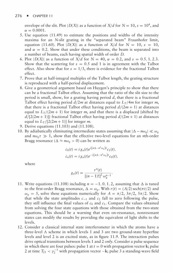
276 CHAPTER 11
envelope of the slit. Plot |D(X)| as a function of X/d for N= 10, s = 104, andα = 0.0001.
5. Use equation (11.49) to estimate the positions and widths of the intensitymaxima for an N-slit grating in the “separated beam” Fraunhofer limit,equation (11.60). Plot |D(X)| as a function of X/d for N = 10, s = 10,and α = 0.2. Show that under these conditions, the beam is separated intoa number of beams, each having spatial width of order D.
6. Plot |D(X)| as a function of X/d for N = 40, α = 0.2, and s = 0.5,1,2.3.Show that the scattering for s = 0.5 and 1 is in agreement with the Talboteffect. Also show that for s = 1/3, there is evidence for the fractional Talboteffect.
7. Prove that at half-integral multiples of the Talbot length, the grating structureis reproduced with a half-period displacement.
8. Give a geometrical argument based on Huygen’s principle to show that therecan be a fractional Talbot effect. Assuming that the ratio of the slit size to theperiod is small, show, for a grating having period d, that there is a fractionalTalbot effect having period d/2m at distances equal to LT/4m for integer m,that there is a fractional Talbot effect having period d/(2m+ 1) at distancesequal to LT/(2m+ 1) for integer m, and that there is a displaced shifted byd/[2(2m+ 1)] fractional Talbot effect having period d/(2m+ 1) at distancesequal to LT/[2(2m+ 1)] for integer m.
9. Derive equations (11.103) and (11.108).10. By adiabatically eliminating intermediate states assuming that |− nωq| ωq
and nωqτ 1, show that the effective two-level equations for an nth-orderBragg resonance ( ≈ nωq > 0) can be written as
c0(t) = iχn(t)ei(n−n2ωq)tc1(t),
cn(t) = iχn(t)e−i(n−n2ωq)tc0(t),
where
χn(t) = rn(t)
[(n− 1)!]2 ωn−1q
.
11. Write equations (11.108) including n = −1,0,1,2, assuming that is tunedto the first-order Bragg resonance, = ωq. With r (t) = (A/2) sech(π t/2) andωq = 5, solve these equations numerically for A = π/2, 3π/2, 5π/2. Showthat while the state amplitudes c−1 and c2 fall to zero following the pulse,they still influence the final values of c0 and c1. Compare the values obtainedfrom solving the four state equations with those obtained from the two-stateequations. This should be a warning that even on-resonance, nonresonantstates can modify the results by providing the equivalent of light shifts to thelevels.
12. Consider a classical internal state interferometer in which the atoms have athree-level scheme in which levels 1 and 3 are two ground-state hyperfinelevels and level 2 is an excited state, as in figure 11.9. The interaction pulsesdrive optical transitions between levels 1 and 2 only. Consider a pulse sequencein which there are four pulses: pulse 1 at t = 0 with propagation vector k; pulse2 at time T21 < γ−1
2 with propagation vector −k; pulse 3 a standing-wave field
ATOM OPTICS AND ATOM INTERFEROMETRY 277
in the ±k direction at time T21+T; and pulse 4 at time T21+2T in direction −k.Draw a Doppler phase diagram for this pulse sequence, and show that an echocan be produced at te = 2T21 +2T in the k direction. What is the advantage ofthis grating-stimulated echo [29] over the conventional stimulated echo withregard to sensitivity to velocity-changing collisions?
13. Derive equation (11.145) starting from equation (11.143).14. Draw a Doppler phase diagram analogous to that of figure 10.8 for resonant
Raman transitions rather than optical transitions, including the effects ofrecoil. That is, take the difference of the propagation vectors equal to q, q,−q for the three field interaction zones. This can be done using the methodoutlined at the end of appendix B in chapter 10. Show that at the echo pointt = 2T21 + T, 31 varies as cos(2ωqT21).
15. Draw Doppler phase diagrams to show how the phase shifts (11.131) and(11.156) arise.
16. Using arguments similar to those in arriving at equation (11.131), derive anexpression for the fringe shift that occurs in the Raman echo for an atomicbeam having velocity v0 = v0z + vT passing through two field zones separatedby L as a result of the fact that the entire experiment is being carried out in arotating frame (such as the Earth). To do this, assume that the acceleration ofthe atom in the interferometer is simply 2v0z × , the “fictitious” Coriolisacceleration. Show that your result agrees with equation (11.118). Thus,even if the entire apparatus is rotating, including the source, one can use aninterferometer to measure the rotation rate. Assume that the transverse velocityvT v0, but that 2kvTL/v0 = qvTL/v0 1.
17. Estimate the fringe shift per radian of rotation rate when a supersonicsodium atomic beam passes though two microfabricated gratings separatedby 0.66m [22]. Assume that the beam velocity is 1.03×10³ m/s and that thegrating period is 200 nm. Consider only the matter-wave grating having thelowest order (that is, the largest) period.
References
[1] J. D. Jackson, Classical Electrodynamics, 3rd ed. (Wiley, New York, 1999), sec. 10.5.[2] H. F. Talbot, Facts relating to optical science, No. IV, Philosophical Magazine 9,
401–407 (1836).[3] J. M. Cowley and A. F. Moodie, Fourier images I. the point source; II. the out-of-
focus patterns; III. finite sources, Proceedings of the Physical Society of London B 70,486–496; 497–504; 505–513 (1957).
[4] G. L. Rogers, Diffraction theory of insect vision II. theory and experiments witha simple model eye, Proceedings of the Royal Society of London B 157, 83–98(1962).
[5] J. T. Winthrop and C. R. Worthington, Theory of Fresnel images I. plane periodicobjects in monochromatic light, Journal of the Optical Society of America 55, 373–381(1965).
[6] For a review, see K. Patorski, The self-imaging phenomenon and its application, inProgress in Optics XXVII, edited by E. Wolf (North-Holland, Amsterdam, 1989),pp. 1–108.
278 CHAPTER 11
[7] M. S. Chapman, C. R. Ekstrom, T. D. Hammond, J. Schmiedmayer, B. E. Tannian,S. Wehinger, and D. E. Pritchard, Near-field imaging of atomic diffraction gratings: theatomic Talbot effect, Physical Review A 51, R14–R17 (1995).
[8] S. Nowak, Ch. Kurtsiefer, T. Pfau, and C. David, High-order Talbot fringes for atomicmatter waves, Optics Letters 22, 1430–1432 (1997).
[9] L. Deng, E. W. Hagley, J. Denschlag, J. E. Simsarian, M. Edwards, C. W. Clark,K. Helmerson, S. L. Rolston, and W. D. Phillips, Temporal, matter-wave-dispersionTalbot effect, Physical Review Letters 83, 5407–5411 (1999).
[10] B. Dubetsky and P. R. Berman, Atom interference using microfabricated structures, inAtom Interferometry, edited by P. R. Berman (Academic Press, San Diego, CA, 1997),pp. 407–468.
[11] C. V. Raman and N. S. N. Nath, Diffraction of light by H. F. sound waves. parts I andII, Proceedings of the Indian Academy of Science, Section A 2, 406–420 (1935).
[12] R. J. Cook and A. F. Bernhardt, Deflection of atoms by a resonant standing wave field,Physical Review A 18, 2533–2537 (1978).
[13] P. L. Kapitza and P. A. M. Dirac, The reflection of electrons from standing light waves,Mathematical Proceedings of the Cambridge Philosophical Society 29, 297–300 (1933).
[14] P. E. Moskowitz, P. L. Gould, S. R. Atlas, and D. E. Pritchard,Diffraction of an atomicbeam by standing wave radiation, Physical Review Letters 51, 370–373 (1983).
[15] M. Abramowitz and I. A. Stegun, Handbook of Mathematical Functions with Formu-las, Graphs, and Mathematical Tables (U.S. Department of Commerce, Washington,DC, 1965), chap. 9.
[16] J. L. Cohen, B. Dubetsky, and P. R. Berman, Atom focusing by far-detuned andresonant standing wave fields: thin-lens regime, Physical Review A 60, 4886–4901(1999).
[17] P. R. Berman and B. Bian, Pump-probe spectroscopy approach to Bragg scattering,Physical Review A 55, 4382–4385 (1997).
[18] G. Sagnac, Luminous ether demonstrated by the effect of relative wind of ether in auniform rotation of an interferometer, Comptes Rendus Hebdomadaires des Seancesde l’Academie des Sciences 157, 708–710 (1913).
[19] For a review, see G. Rizzi and M. L. Ruggiero, The relativistic Sagnac effect: twoderivations, in Relativity in Rotating Frames, edited by G. Rizzi and M. L. Ruggiero(Kluwer Academic Publishers, Dordrecht, The Netherlands, 2003), pp. 179–220, plusother chapters in this book.
[20] C. H. Rowe, U. K. Schreiber, S. J. Cooper, B. T. King, M. Poulton, and G. E. Stedman,Design and operation of a very large ring laser gyroscope, Applied Optics 38, 2516–2523 (1999).
[21] F. Riehle, Th. Kisters, A. Witte, J. Helmcke, and Ch. J. Bordé, Optical Ramseyspectroscopy in a rotating frame: Sagnac effect in a matter wave interferometer, PhysicalReview Letters 67, 177–180 (1991).
[22] A. Lenef, T. D. Hammond, E. T. Smith, M. S. Chapman, R. A. Rubenstein, and D. E.Pritchard, Rotation sensing with an atom interferometer, Physical Review Letters 78,760–763 (1997).
[23] T. L. Gustavson, P. Bouyer, and M. A. Kasevich, Precision rotation measurements withan atom interferometer gyroscope, Physical Review Letters 78, 2046–2049 (1997).
[24] T. L. Gustavson, A. Landragin, and M. A. Kasevich, Rotation sensing with a dualatom-interferometer Sagnac gyroscope, Classical and Quantum Gravity 17, 2385–2397(2000).
ATOM OPTICS AND ATOM INTERFEROMETRY 279
[25] E. Lau, Beugungserscheinungen an Doppelrastern (Diffraction phenomena from twoparallel gratings), Annalen der Physik 6, 417–423 (1948).
[26] J. L. Clauser and S. Li, Talbot-vonLau atom interferometer with cold potassium,Physical Review A 49, R2213–R2216 (1994).
[27] A. V. Turlapov, A. Tonyushkin, and T. Sleator, Talbot-Lau effect for atomic de Brogliewaves manipulated with light, Physical Review A 71, 043612, 1–5 (2005).
[28] S. B. Cahn, A. Kumarakrishnan, U. Shim, T. Sleator, P. R. Berman, and B. Dubetsky,Time domain de Broglie wave interferometer, Physical Review Letters 79, 784–787(1997).
[29] B. Dubetsky, P. R. Berman, and T. Sleator, Grating stimulated echo, Physical ReviewA 46, R2213–R2216 (1992).
Bibliography
There are more than one thousand references appropriate to this chapter. The following threereviews contain extensive lists of references:
C. S. Adams, M. Sigel, and J. Mlynek, Atom Optics, Physics Reports 240, 143–210 (1994).P. R. Berman, Ed. Atom Interferometry (Academic Press, San Diego,CA, 1997).A. D. Cronin, J. Schmiedmayer, and D. E. Pritchard, Optics and interferometry with atomsand molecules, Reviews of Modern Physics 81, 1051–1129 (2009).
12The Quantized, Free Radiation Field
We now move on to problems in which it is necessary to quantize the electro-magnetic field. As was mentioned in chapter 1, such problems fall into a number ofcategories, including cavity fields, spontaneous emission, and light scattering. Thereare many ways to quantize the radiation field. In the appendix, one such approachis given, following the treatment in Cohen-Tannoudji et al. [1]. More generally,however, the most foolproof way to quantize the field is to calculate the classicalfield modes associated with a given boundary value problem and then assign creationand annihilation operators that give rise to each of these distinct field modes.
There are many excellent texts on quantum optics that offer detailed discussionson quantum aspects of the radiation field. Some of these texts are listed in thebibliography of chapter 1. We provide a very limited introduction to quantumproperties of the radiation field and photodetection in this and the following twochapters. In subsequent chapters, we concentrate on applications involving theinteraction of the quantized radiation field with atoms.
12.1 Free-Field Quantization
We first consider fields in free space with no sources. Of course, there have tobe sources present somewhere to produce these fields. To quantize the free fieldusing a simplified approach, one can start with the spatial modes of a free, classicalfield satisfying periodic boundary conditions. Such spatial modes are plane waves,varying as exp(ik · R), where
k = kxx + kyy + kzz, (12.1)
kx = 2πnxL
, ky = 2πnyL
, kz = 2πnzL, (12.2)
and L3 = V is the quantization volume. The quantities nx, ny, and nz can take on allinteger values.
THE QUANTIZED, FREE RADIATION FIELD 281
The quantized electric field operator is written as
E(R) = i∑j
E j [a jε j eik j ·R − a†j ε j e
−ik j ·R]
≡ E+(R) + E−(R) , (12.3)
where ε j is the polarization of mode j ,1 Ej is a (real) normalization constant, a j (a†j )
is the destruction (creation) operator for a mode having propagation vector k j andpolarization ε j , and
E+(R) = [E−(R)
]† = i∑j
E ja jε j eik j ·R (12.4)
is the positive frequency component of the field. The free-field modes are transverse,with k j · ε j = 0. There are two independent polarization vectors and creation anddestruction operators associated with a given k j , and the subscript j is a shorthandnotation for a set of quantum numbers
(nx,ny,nz
). The destruction and creation
operators satisfy the commutation relations
[ai , a j ] = [a†i , a
†j ] = 0, [ai , a
†j ] = δi, j . (12.5)
In calculating any physically relevant quantities, the final answers must be indepen-dent of the choice of quantization volume V.
Although ai and a†i are operators, we do not write them as ai and a†
i , nor dowe include a “hat” (ˆ) on the field operator. In fact, from this point onward, exceptwhere there is cause for confusion, we suppress the hat symbol on all operators.
For the free field, the total energy in the field is twice the integral of theenergy density associated with the electric field integrated over the volume. As aconsequence, the energy operator corresponding to the field (12.3) is
H = ε0∑j, j ′
∫d3REj Ej ′ (a j eik j ·R − a†
j e−ik j ·R)(a†
j ′e−ik j ′ ·R − a j ′eik j ′ ·R)
= ε0V∑j
E2j (a ja
†j + a†
j a j ) = 2ε0V∑j
E2j
(a†j a j + 1
2
), (12.6)
where ε0 is the vacuum permittivity. If we choose
Ej =√ω j
2ε0V, (12.7)
where ω j = kjc, then
H =∑j
ω j
(n j + 1
2
), (12.8)
where the number operator n j is defined by
n j = a†j a j . (12.9)
1 We adopt a notation in which the polarization vector for the quantized field is written without aˆ (“hat”), although we continue to include the ˆ in the polarization vectors of classical fields.
282 CHAPTER 12
The Hamiltonian is the same as that for an ensemble of harmonic oscillators hav-ing frequency ω j . We will assume that equation (12.8) is the free-field Hamiltonian.For reference purposes, we list the momentum of the field
P =∑j
k j
(a†j a j + 1
2
)=∑j
k j a†j a j , (12.10)
the vector potential
A(R) =∑j
Aj (a jε j eik j ·R + a†j ε j e
−ik j ·R), (12.11)
the electric field
E(R) = i∑j
E j (a jε j eik j ·R − a†j ε j e
−ik j ·R), (12.12)
and the magnetic field
B(R) = i∑j
Bj (a jκ j × ε j eik j ·R − a†jκ j × ε j e−ik j ·R). (12.13)
In these equations,
Ej =√ω j
2ε0V, Bj = Ej
c, Aj = Ej
ω j, (12.14)
and
κ j = k j
kj. (12.15)
is a unit vector. For a single-mode field with ω j = ω, the Hamiltonian is
H = ω(a†a + 1
2
)= ω
(n+ 1
2
), (12.16)
where n = a†a. Since the Hamiltonian is the same as that of a harmonic oscillator,the eigenenergies are given by
En = ω(n+ 1
2
), (12.17)
where n = 0,1, . . . . The eigenkets are denoted by |n〉, which are called photonstates of the field. They are also referred to as number states or Fock states. Theyare not localized states, extending over the quantization volume. As in the case ofthe harmonic oscillator, the destruction operator a is a lowering operator,
a|n〉 = √n|n− 1〉, (12.18)
while the creation operator a† is a raising operator,
a†|n〉 = √n+ 1|n+ 1〉, (12.19)
THE QUANTIZED, FREE RADIATION FIELD 283
and the number operator leaves the ket unchanged,
n |n〉 = a†a |n〉 = n|n〉. (12.20)
It follows from equation (12.19) that the ket |n〉 can be written as
|n〉 =(a†)n
√n!
|0〉, (12.21)
where the state |0〉 is referred to as the vacuum state of the field. For a multimodefield,
|n1n2 . . . ni 〉 =(a†1
)n1√n1!
(a†2
)n2√n2!
. . .
(a†i
)ni√ni !
|0〉 . (12.22)
We have not said anything about how one can construct such number states. Ingeneral, this is a difficult task. The most common way to create a number state is tosend a single atom in an excited state into a cavity and allow the atom to transfer itsexcitation to a single-cavity mode.
12.2 Properties of the Vacuum Field
The expectation value of the electric field in the vacuum state vanishes, since
〈0|E|0〉 = i∑j
E j 〈0|(a jε j e jk j ·R − a†j ε j e
−ik j ·R)|0〉 = 0. (12.23)
This is the type of result one would expect for the vacuum field. However, the factthat the average field vanishes does not imply that the energy density in the field,proportional to 〈0|E2|0〉, also vanishes. In fact, one finds that the energy density
ε0〈0|E2|0〉 = −ε0∑j, j ′
√ω jω j ′
2ε0Vε j · ε j ′[〈0|a†
j a†j ′ |0〉e−i(k j+k j ′ )·R
+〈0|a ja j ′ |0〉ei(k j+k j ′ )·R − 〈0|a ja†j ′ |0〉ei(k j−k j ′ )·R − 〈0|a†
j a j ′ |0〉ei(k j+k j ′ )·R]
=∑j
ω j
2V =∑j
kjc2V . (12.24)
Going from a discrete sum to a continuum using the prescription∑j
= V(2π )3
∫dk, (12.25)
one obtains
ε0〈0|E2|0〉 = c2
4π(2π )3
∫ ∞
0dkk3, (12.26)
which diverges. The energy density of the vacuum field at each point in spaceis infinite. Depending on your point of view, this can be viewed as either anembarrassment or a simple inconvenience. The fact that the vacuum energy is infinite
284 CHAPTER 12
does not seem to have any physical consequence (apart from the cosmologicalconstant). Nevertheless, vacuum fluctuations (e.g., the possibility to emit a photonwhile exciting an atom to a higher energy state) have measurable consequences suchas the Lamb shift of atomic levels and the Casimir effect (e.g., attraction of two metalplates in vacuum). The field of quantum electrodynamics was developed in largepart to deal with infinities associated with these vacuum fluctuations. When pointcharges and masses are renormalized to their measured values, vacuum fluctuationsare found to lead to finite rather than infinite corrections to energy levels andinteractions.
In expanding any state in the Schrödinger representation, it is useful to use arepresentation in which the (infinite) energy of the vacuum field is eliminated. Thisis the convention that we adopt such that, for the most part, we take as our effectiveHamiltonian
H =∑j
ω j a†j a j . (12.27)
Moreover, any Lamb shifts of atomic energy levels resulting from the interactionwith the vacuum field are assumed to be incorporated into the energies of the atomicstates.
12.2.1 Single-Photon State
A multimode, one-photon state for the free field can be defined by
|(t)〉 =∑j
c j (t)a†j |0〉 . (12.28)
In effect, this state represents a superposition of single-photon states of the type|1 j 〉—that is, a state where there is a single photon in mode j . From the Schrödingerequation with the Hamiltonian (12.27), it follows that the state amplitudes c j (t)evolve according to
c j (t) = −iω j c j (t) . (12.29)
Therefore, we find
|(t)〉 =∑j
c j (0)a†j |0〉e−iω j t =
∑j
e−iω j tc j (0)|1 j 〉 . (12.30)
For this one-photon state, the expectation value of the positive frequencycomponent of the field vanishes, since
〈E+〉 = i∑j
(ω j
2ε0V
)1/2
eik j ·Rε j 〈(t)|a j |(t)〉 = 0. (12.31)
This is not a surprising result—a one-photon state of the field cannot possess a well-defined phase, implying that a quantum-mechanical average of the field operatormust vanish. On the other hand, the average value of 〈E−·E+〉, which is proportionalto the average field intensity measured by a detector (since E+ “destroys” a photon
THE QUANTIZED, FREE RADIATION FIELD 285
at the detector), is
〈E− · E+〉 = 〈|∑j, j ′
2ε0Vε j · ε j ′
√ω jω j ′a
†j a j ′e
−i(k j−k j ′ )·R|〉
=∑j, j ′,l,l ′
〈1l |a†j
2ε0Vε j · ε j ′
√ω jω j ′e−i(k j−k j ′ )·Re−iωll′ ta j ′ |1l ′ 〉c∗
l (0)cl ′(0) .
(12.32)
In the sum in equation (12.32), only terms with j = l and j ′ = l ′ contribute, leadingto
〈E− · E+〉 =
2ε0V
∣∣∣∣∣∣∑j
√ω j ei(k j ·R−ω j t)ε j c j (0)
∣∣∣∣∣∣2
. (12.33)
This expression is similar to that for the propagation of a classical electric fieldpulse. If all k j are along the x direction (plane wave), then the solution is a functionof (X− ct) only.
The result (12.33) is somewhat paradoxical. Recall that although the energydensity at each point in space for the vacuum field is infinite, the average vacuumfield intensity measured by a detector, proportional to 〈0|E− · E+|0〉, vanishes. Onthe other hand, the average value of E− · E+ given in equation (12.33) for a single-photon state is proportional to the quantization volume when the sums over j areconverted to integrals using the prescription (12.25). Since the quantization volumegoes to infinity in free space, it would appear that the energy in a single-photon pulsemeasured by a detector is infinite. Clearly, something is wrong with this result.
Where did we go wrong? Well, we really didn’t go wrong yet. In converting thesums to integrals in equation (12.33), we must also convert the state amplitudes c j (0)corresponding to discrete field modes to continuum-mode variables c(k, t = 0). Toaccomplish this conversion, we set
c j (t) →√
(2π )3
V c(k, t),
with the normalization such that∫dk
∣∣c(k,0)∣∣2 = 1. With this substitution, equation(12.33) goes over into
〈E− · E+〉 =
2ε0
∣∣∣∣∫dk
√kcei(k·R−kct)εkc(k,0)
∣∣∣∣2
, (12.34)
which is independent of the quantization volume.
12.2.2 Single-Mode Number State
For a single mode of the field in a pure number or Fock state |n〉,n2 = 〈n2〉 − 〈n〉2 = 0, (12.35)
286 CHAPTER 12
and
〈E+〉 = 0, (12.36a)
〈E− · E+〉 = ωn2ε0V
, (12.36b)
〈(E− · E+)2〉 =(ω
2ε0V
)2 ⟨a†aa†a
⟩ =(ω
2ε0V
)2 (n2 + n
), (12.36c)
(E− · E+) =
(ω
2ε0V
) √n, (12.36d)
where represents the standard deviation. Provided that n 1, there is a relativelysmall uncertainty in the field intensity, since
(E− · E+) /〈E− · E+〉 = 1/
√n. On the
other hand, a pure n state is not an eigenstate of field intensity. The fact that 〈E+〉 = 0is related to an uncertainty in the phase of the field. Phase is discussed in section 12.5,but for now, we note that a pure n state has a phase that can be considered to betotally random. In some sense, a pure n state is similar to a field having amplitudeE0 = √
2[ω/(ε0V)]1/2√n and random phase φ such that E = E0 cos(kz− t + φ),
〈E+〉φ = 0, and 〈E−E+〉φ = E20/4 = ωn/2ε0V. The analogy is not complete,
however, since there are no fluctuations in the intensity of this classical field.
12.2.3 Quasiclassical or Coherent States
In the early 1960s, the advent of the laser led Roy Glauber to consider a special classof states of the quantized radiation field that are known as quasiclassical or coherentstates [2]. These states are chosen in such a fashion that their properties mirror thoseof classical radiation fields. More precisely, the coherent states are defined in a waythat they reproduce the corresponding classical field results if quantum fluctuationsof the field can be neglected. For his work, Glauber shared the Nobel Prize in 2005.Glauber has stated that his work aroused a great deal of skepticism at first, owingto some unusual properties of the coherent states.
In order to discuss coherent states, it will prove useful to introduce the Heisenbergrepresentation. To this point, we have used the Schrödinger representation in whichoperators are time-independent and the state vector is a function of time. We willgive a somewhat more detailed description of the Heisenberg representation inchapters 15 and 19. At this time, you need remember only that an operator OH(t) inthe Heisenberg representation is a function of time, obeying an evolution equation
idOH(t)dt
= [OH(t), H], (12.37)
and that the state vector for the system in the Heisenberg representation, |〉H,is constant in time, equal to the state vector for the system in the Schrödingerrepresentation at time t = 0. The Heisenberg representation is especially usefulwhen one is interested in obtaining equations for operators rather than the statevector of a system, since the Heisenberg operators usually obey time-evolutionequations that closely resemble those of the corresponding classical system. In the
THE QUANTIZED, FREE RADIATION FIELD 287
remainder of this chapter, Heisenberg operators will always be written with anexplicit time dependence. The Heisenberg and Schrödinger operators are definedin such a manner that they coincide at t = 0. If the Hamiltonian is time-independentin the Schrödinger representation, it is also time-independent in the Heisenbergrepresentation; moreover, the commutation relations of operators is the same inthe Heisenberg and Schrödinger representation.
From equations (12.37), (12.27), and (12.5), it follows that, for free fields, theevolution equation for the annihilation operator a j (t) is
a j (t) = −iω j a j (t), (12.38)
with solution
a j (t) = e−iω j ta j , (12.39)
where a j = a j (0) is a Schrödinger operator. Similarly,
a†j (t) = eiω j ta†
j . (12.40)
As a consequence, the electric field operator E(R, t) (now written as a Heisenbergoperator) for the free field is
E(R, t) = i∑j
E j (a jε j eik j ·R−iω j t − a†j ε j e
−ik j ·R+iω j t). (12.41)
Assume for the moment that there exists a single-mode quantum state of the field|α〉 that is an eigenket of the annihilation operator a—that is,
〈α|a|α〉 = α, (12.42a)
〈α|a†|α〉 = α∗, (12.42b)
where α is a complex number. If such a state existed, then the expectation value ofthe electric field operator E(R, t) for this single-mode field having frequency ω = kcand polarization ε is
〈E(R, t)〉 = i Eωε(αeik·R−iωt − α∗eik·R−iωt), (12.43)
where Eω = (ω/2ε0V)1/2. In other words, the expectation value of the field isidentical to that of a monochromatic plane-wave field having (complex) amplitudeEωα. Moreover, the expectation values of the field energy and momentum equalthose of the corresponding classical fields.
Thus, as long as quantum fluctuations of the fields are unimportant, the states|α〉 can be associated with classical fields. Fluctuations tend to be unimportant if〈n(t)〉 = ⟨
a†(t)a(t)⟩ 1, although this proves to be a necessary, but not sufficient,
condition. We have not yet indicated the manner in which one can create suchquantum states of the field, but it is not unreasonable to believe that most ofthe radiation fields we encounter can be represented in first approximation bycoherent states of the field. In fact, we will show in chapter 15 that a classicalcurrent distribution gives rise to a quantized coherent state of the radiationfield.
288 CHAPTER 12
In general, several coherent-state field modes can be excited. A multimodecoherent state can be written as |α1, α2, . . . α j . . .〉, for which
〈E(R, t)〉 = i∑j
E j [α jε j eik j ·R−iω j t − α∗j (t)ε j e
−ik j ·R+iω j t]. (12.44)
For the remainder of this chapter, we deal mainly with single-mode fields.The equation
a|α〉 = α|α〉 (12.45)
defines a coherent state. It is a fairly amazing equation, since the application of thedestruction operator results in a state with the same value of 〈n〉. It is precisely thisproperty of coherent states that Glauber claims was disturbing to some people whoread his articles. The fact that equation (12.45) leads to coherent states of the fielddoes not guarantee the existence of such states, since the non-Hermitian operator amay not possess a set of normalizable eigenkets. However, we can try to constructsuch a state by writing
|α〉 =∞∑n=0
〈n|α〉|n〉 (12.46)
and see whether we can find the expansion coefficients 〈n|α〉.We start by using equations (12.45), (12.46), and (12.18) to write
a|α〉 =∑n
√n|n− 1〉〈n|α〉 = α|α〉. (12.47)
Multiplying by 〈m− 1|, we obtain√m〈m|α〉 = α〈m− 1|α〉. (12.48)
Therefore,
〈n|α〉 = α√n〈n− 1|α〉 = α2√
n(n− 1)〈n− 2|α〉 = αn√
n!〈0|α〉, (12.49)
and it follows from equation (12.46) that
|α〉 =∑n
αn√n!
〈0|α〉|n〉. (12.50)
To fix the value of 〈0|α〉, we assume that the |α〉 states are normalized, such that
〈α|α〉 =∑n
|α|2nn!
|〈0|α〉|2 = |〈0|α〉|2e|α|2 = 1. (12.51)
Taking 〈0|α〉 to be real and positive, we obtain
〈0|α〉 = e−|α|2/2 (12.52)
THE QUANTIZED, FREE RADIATION FIELD 289
and
|α〉 =∑n
αn√n!
〈0|α〉|n〉 =∑n
αn√n!e−|α|2/2|n〉
=∑n
(αa†)n
n!e−|α|2/2|0〉 = eαa
†e−|α|2/2|0〉. (12.53)
Although there was no guarantee that eigenkets of a exist, it has been possible toconstruct them. The coherent state with α = 0 is the vacuum state of the field.
12.2.3.1 Properties of coherent states
The probability distribution of photon number n in a coherent state obeys a Poissondistribution
|〈n|α〉|2 = |α|2nn!
e−|α|2 . (12.54)
The mean, mean square, and variance of the photon number are
〈n〉 = 〈a†a〉 = 〈α|a†a|α〉 = |α|2, (12.55a)
〈n2〉 = 〈a†aa†a〉 = 〈α|a†(a†a + 1)a|α〉 = |α|2(|α|2 + 1), (12.55b)
〈n2〉 = 〈n2〉 − 〈n〉2 = |α|2, (12.55c)
such that
〈n〉〈n〉 = 1√〈n〉 = 1
|α| . (12.56)
For large values of |α|, the relative fluctuations of the intensity of a coherent stateare minimal. These equations are valid only for α = 0. The state with α = 0 corre-sponds to the vacuum state |0〉, which is an eigenstate of the number operator havingeigenvalue zero.
Since a is not a Hermitian operator, there is no guarantee that the eigenkets of aare orthogonal and complete. In fact, the coherent states are not orthogonal, since
〈α|β〉 =∑n,m
(α∗)n√n!
βm√m!
e−(|α|2+|β|2)/2〈n|m〉 = e−(|α|2+|β|2)/2∑n
(α∗β)n
n!
= e− 12 (|α|2+|β|2)+α∗β = e− 1
2 |α−β|2 e12 (α
∗β−αβ∗), (12.57a)
|〈α|β〉|2 = e−|α−β|2 . (12.57b)
On the other hand, the coherent-state eigenkets form an overcomplete set. That is,although they obey a completeness-type relationship
1π
∫d2α|α〉〈α| = 1, (12.58)
290 CHAPTER 12
owing to the lack of orthogonality, any coherent state can be expressed as a linearcombination of other coherent states,
|α〉 = 1π
∫d2β|β〉〈β|α〉 . (12.59)
Since α and β are complex, the integrals in equation (12.58) and (12.59) are over thecomplex plane, d2α = dRe(α)dIm(α), d2β = dRe(β)dIm(β). The overcompletenessof the eigenkets will be exploited when we consider the density matrix for the field.
12.2.3.2 Representation of a coherent state as a translation of thevacuum state
It turns out to be very useful to seek an alternative representation for coherentstates. In particular, we want to show that a coherent state can be represented asa translation of the vacuum state. Recall that the vacuum state is a coherent statewith α = 0, for which 〈α|a|α〉 = 〈α|a†|α〉 = 0.
We seek unitary operators D(β, β∗) and D†(β, β∗) that act as a translationoperators for the field creation and annihilation operators—namely,
D†(β, β∗)aD(β, β∗) = a + β, (12.60a)
D†(β, β∗)a†D(β, β∗) = a† + β∗. (12.60b)
Since β is complex, it is completely determined if we specify its real and imaginaryparts or, alternatively, if we consider β and β∗ as independent variables, whichproves more convenient at the moment. Using equations (12.60a) and (12.47), wefind
a[D†(β, β∗)|α〉] = [
D†(β, β∗)aD(β, β∗) − β]D†(β, β∗)|α〉= (α − β)D†(β, β∗)|α〉. (12.61)
In other words, D†(β, β∗)|α〉 is an eigenket of a with eigenvalue (α − β). It followsthat D†(α, α∗)|α〉 = c|0〉, where c is a constant that must have a magnitude of unityif D(β, β∗) is unitary. Taking c = 1 leads to
|α〉 = D(α, α∗)|0〉, (12.62)
which implies that D(α, α∗) generates coherent states from the vacuum state.To arrive at a specific form for D(α, α∗), we consider first infinitesimal transla-
tions ε in the complex plane given by
D†(ε, ε∗)aD(ε, ε∗) = a + ε. (12.63)
To first order in ε and ε∗, we can write
D(ε, ε∗) = 1 + εA+ ε∗B, (12.64)
which implies that, to this order,
D†(ε, ε∗) = 1 − εA− ε∗B, (12.65)
THE QUANTIZED, FREE RADIATION FIELD 291
and
(1 − εA− ε∗B)a(1 + εA+ ε∗B) = a + ε [a, A] + ε∗ [a, B] . (12.66)
If we compare equations (12.63) and (12.66), we find that A = a† and that B is afunction of a only. Using a similar procedure starting with
D†(ε, ε∗)a†D(ε, ε∗) = a† + ε∗, (12.67)
we obtain B = −a. As a consequence, equation (12.64) becomes
D(ε, ε∗) = 1 + εa† − ε∗a. (12.68)
To get D(α, α∗) for finite translations, we use a standard “trick” and write
|α(λ+ dλ)〉 = D[α(λ+ dλ), α∗(λ+ dλ)] |0〉= D(αdλ, α∗dλ)D(αλ, α∗λ) |0〉, (12.69)
where λ is real. It then follows that
∂D(αλ, α∗λ)∂λ
dλ = (a†αdλ− aα∗dλ)D(αλ, α∗λ). (12.70)
Integrating this equation from λ= 0 to λ= 1, using the fact that D(0,0)= 1, we find
D(α, α∗) = eαa†−aα∗ = e− 1
2 |α|2eαa†e−α∗a . (12.71)
The coherent state (12.62) can be written as
|α〉 = D(α, α∗)|0〉 = e− 12 |α|2eαa
† |0〉, (12.72)
since e−α∗a|0〉 = |0〉.We have accomplished our goal of obtaining a displacement operator that acts on
the vacuum state |0〉 to produce the coherent state |α〉. Expressing a coherent state interms of the displacement operator often simplifies calculations involving coherentstates. Using the fact that eA+B = eAeBe−[A,B]/2, provided that both A and Bcommute with [A, B], you can easily prove the “addition theorem” for translations,
D(α1 + α2, α∗
1 + α∗2
) = D(α1, α
∗1
)D(α2, α
∗2
)e(α1α
∗2−α∗
1α2). (12.73)
12.3 Quadrature Operators for the Field
The operators a and a† are not Hermitian and do not correspond to physical ob-servables. So far, the only operators that we have discussed that could correspond tophysical observables are a†a and the field operators. Actually, in most experiments,it is a field intensity that is measured, so it is important to connect that intensitymeasurement with quantum-mechanical operators that characterize the field.
For a single-mode field,
E(R, t) = i E(aeik·R−iωt − a†e−ik·R+iωt)ε. (12.74)
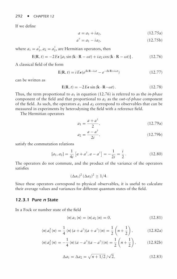
292 CHAPTER 12
If we define
a = a1 + ia2, (12.75a)
a† = a1 − ia2, (12.75b)
where a1 = a†1, a2 = a†
2, are Hermitian operators, then
E(R, t) = −2Eε [a1 sin (k · R − ωt) + ia2 cos (k · R − ωt)] . (12.76)
A classical field of the form
E(R, t) = i Eε(eik·R−iωt − e−ik·R+iωt) (12.77)
can be written as
E(R, t) = −2Eε sin (k · R−ωt) . (12.78)
Thus, the term proportional to a1 in equation (12.76) is referred to as the in-phasecomponent of the field and that proportional to a2 as the out-of-phase componentof the field. As such, the operators a1 and a2 correspond to observables that can bemeasured in experiments by heterodyning the field with a reference field.
The Hermitian operators
a1 = a + a†
2, (12.79a)
a2 = a − a†
2i, (12.79b)
satisfy the commutation relations
[a1, a2] = 14i
[a + a†, a − a†
] = − 12i
= i2. (12.80)
The operators do not commute, and the product of the variance of the operatorssatisfies
(a1)2 (a2)2 ≥ 1/4.
Since these operators correspond to physical observables, it is useful to calculatetheir average values and variances for different quantum states of the field.
12.3.1 Pure n State
In a Fock or number state of the field
〈n| a1 |n〉 = 〈n| a2 |n〉 = 0, (12.81)
〈n| a21 |n〉 = 14
〈n| (a + a†)(a + a†) |n〉 = 12
(n+ 1
2
), (12.82a)
〈n| a22 |n〉 = −14
〈n| (a − a†)(a − a†) |n〉 = 12
(n+ 1
2
), (12.82b)
a1 = a2 =√n+ 1/2 /
√2, (12.83)
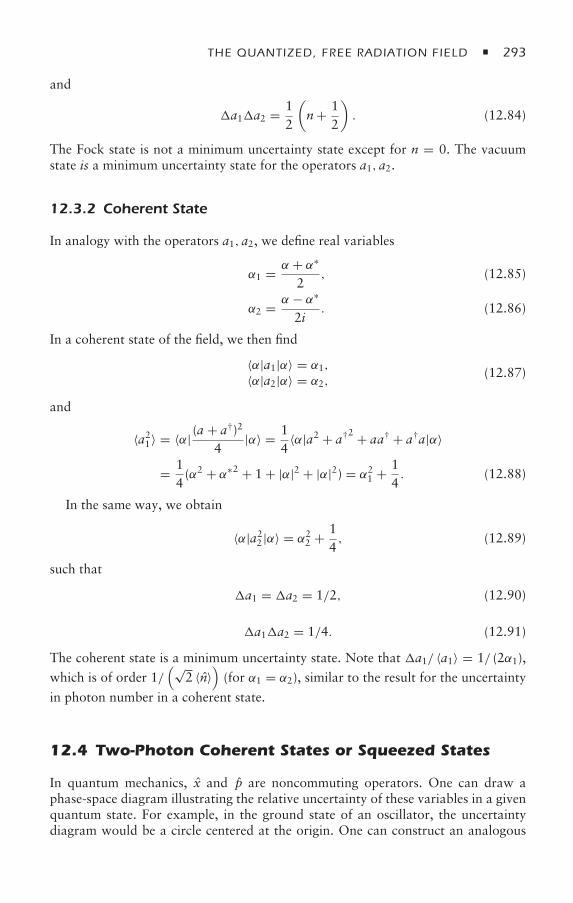
THE QUANTIZED, FREE RADIATION FIELD 293
and
a1a2 = 12
(n+ 1
2
). (12.84)
The Fock state is not a minimum uncertainty state except for n = 0. The vacuumstate is a minimum uncertainty state for the operators a1, a2.
12.3.2 Coherent State
In analogy with the operators a1, a2, we define real variables
α1 = α + α∗
2, (12.85)
α2 = α − α∗
2i. (12.86)
In a coherent state of the field, we then find
〈α|a1|α〉 = α1,
〈α|a2|α〉 = α2,(12.87)
and
〈a21〉 = 〈α| (a + a†)2
4|α〉 = 1
4〈α|a2 + a†2 + aa† + a†a|α〉
= 14(α2 + α∗2 + 1 + |α|2 + |α|2) = α21 + 1
4. (12.88)
In the same way, we obtain
〈α|a22 |α〉 = α22 + 14, (12.89)
such that
a1 = a2 = 1/2, (12.90)
a1a2 = 1/4. (12.91)
The coherent state is a minimum uncertainty state. Note that a1/ 〈a1〉 = 1/ (2α1),
which is of order 1/(√
2 〈n〉)(for α1 = α2), similar to the result for the uncertainty
in photon number in a coherent state.
12.4 Two-Photon Coherent States or Squeezed States
In quantum mechanics, x and p are noncommuting operators. One can draw aphase-space diagram illustrating the relative uncertainty of these variables in a givenquantum state. For example, in the ground state of an oscillator, the uncertaintydiagram would be a circle centered at the origin. One can construct an analogous
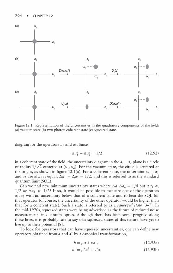
294 CHAPTER 12
(a) a2
a1
D(α,α*)
(b) a2
a1
a2
α2
α1
a1
a2
a1
UL(z)α2
α1
D(α,α*)
(c) a2
a1
a2
a1
a2
a1
UL(z)α2
α1
Figure 12.1. Representation of the uncertainties in the quadrature components of the field:(a) vacuum state (b) two-photon coherent state (c) squeezed state.
diagram for the operators a1 and a2. Since
a21 +a22 = 1/2 (12.92)
in a coherent state of the field, the uncertainty diagram in the a1 −a2 plane is a circleof radius 1/
√2 centered at (α1, α2). For the vacuum state, the circle is centered at
the origin, as shown in figure 12.1(a). For a coherent state, the uncertainties in a1and a2 are always equal, a1 = a2 = 1/2, and this is referred to as the standardquantum limit (SQL).
Can we find new minimum uncertainty states where a1a2 = 1/4 but a1 1/2 or a2 1/2? If so, it would be possible to measure one of the operatorsa1, a2 with an uncertainty below that of a coherent state and to beat the SQL forthat operator (of course, the uncertainty of the other operator would be higher thanthat for a coherent state). Such a state is referred to as a squeezed state [3–7]. Inthe mid-1970s, squeezed states were being advertised as the future of reduced noisemeasurements in quantum optics. Although there has been some progress alongthese lines, it is probably safe to say that squeezed states of this nature have yet tolive up to their potential [8].
To look for operators that can have squeezed uncertainties, one can define newoperators obtained from a and a† by a canonical transformation,
b = µa + νa†, (12.93a)
b† = µ∗a† + ν∗a, (12.93b)
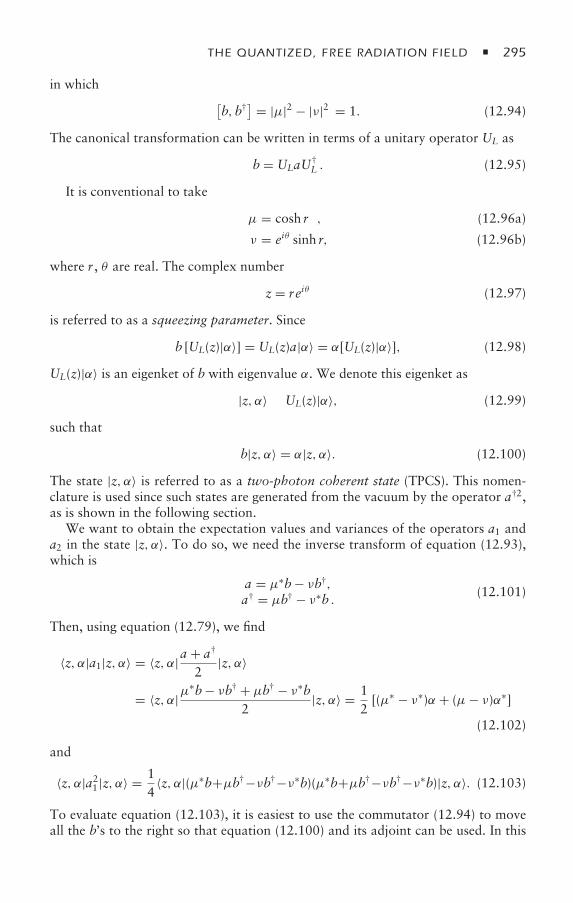
THE QUANTIZED, FREE RADIATION FIELD 295
in which [b,b†
] = |µ|2 − |ν|2 = 1. (12.94)
The canonical transformation can be written in terms of a unitary operator UL as
b = ULaU†L . (12.95)
It is conventional to take
µ = cosh r , (12.96a)
ν = eiθ sinh r, (12.96b)
where r , θ are real. The complex number
z = reiθ (12.97)
is referred to as a squeezing parameter. Since
b [UL(z)|α〉] = UL(z)a|α〉 = α[UL(z)|α〉], (12.98)
UL(z)|α〉 is an eigenket of b with eigenvalue α. We denote this eigenket as
|z, α〉 ≡ UL(z)|α〉, (12.99)
such that
b|z, α〉 = α|z, α〉. (12.100)
The state |z, α〉 is referred to as a two-photon coherent state (TPCS). This nomen-clature is used since such states are generated from the vacuum by the operator a†2,as is shown in the following section.
We want to obtain the expectation values and variances of the operators a1 anda2 in the state |z, α〉. To do so, we need the inverse transform of equation (12.93),which is
a = µ∗b− νb†,
a† = µb† − ν∗b . (12.101)
Then, using equation (12.79), we find
〈z, α|a1|z, α〉 = 〈z, α|a + a†
2|z, α〉
= 〈z, α|µ∗b− νb† + µb† − ν∗b
2|z, α〉 = 1
2[(µ∗ − ν∗)α + (µ− ν)α∗]
(12.102)
and
〈z, α|a21 |z, α〉 = 14
〈z, α|(µ∗b+µb†−νb†−ν∗b)(µ∗b+µb†−νb†−ν∗b)|z, α〉. (12.103)
To evaluate equation (12.103), it is easiest to use the commutator (12.94) to moveall the b’s to the right so that equation (12.100) and its adjoint can be used. In this
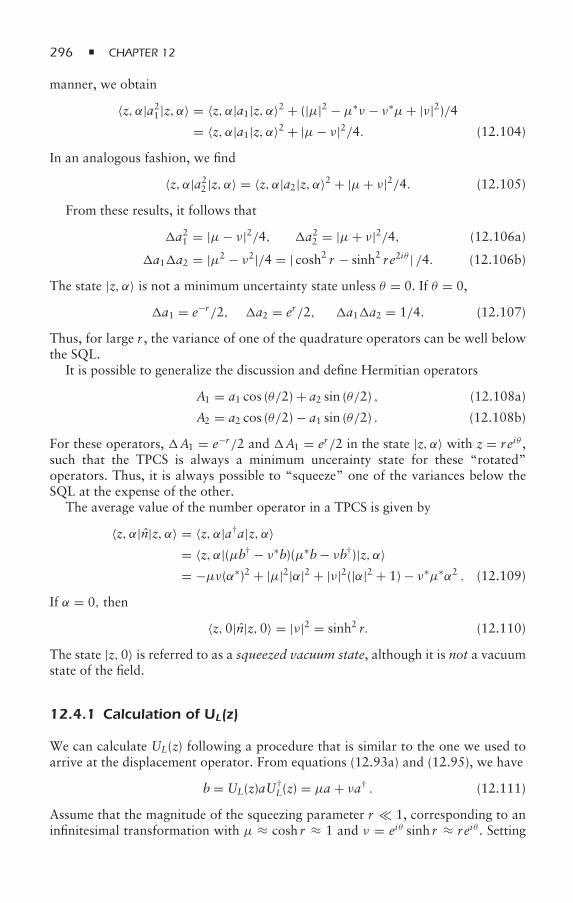
296 CHAPTER 12
manner, we obtain
〈z, α|a21 |z, α〉 = 〈z, α|a1|z, α〉2 + (|µ|2 − µ∗ν − ν∗µ+ |ν|2)/4= 〈z, α|a1|z, α〉2 + |µ− ν|2/4. (12.104)
In an analogous fashion, we find
〈z, α|a22 |z, α〉 = 〈z, α|a2|z, α〉2 + |µ+ ν|2/4. (12.105)
From these results, it follows that
a21 = |µ− ν|2/4, a22 = |µ+ ν|2/4, (12.106a)
a1a2 = |µ2 − ν2|/4 = | cosh2 r − sinh2 re2iθ | /4. (12.106b)
The state |z, α〉 is not a minimum uncertainty state unless θ = 0. If θ = 0,
a1 = e−r/2, a2 = er/2, a1a2 = 1/4. (12.107)
Thus, for large r , the variance of one of the quadrature operators can be well belowthe SQL.
It is possible to generalize the discussion and define Hermitian operators
A1 = a1 cos (θ/2) + a2 sin (θ/2) , (12.108a)
A2 = a2 cos (θ/2) − a1 sin (θ/2) . (12.108b)
For these operators, A1 = e−r/2 and A1 = er/2 in the state |z, α〉 with z = reiθ ,such that the TPCS is always a minimum uncerainty state for these “rotated”operators. Thus, it is always possible to “squeeze” one of the variances below theSQL at the expense of the other.
The average value of the number operator in a TPCS is given by
〈z, α|n|z, α〉 = 〈z, α|a†a|z, α〉= 〈z, α|(µb† − ν∗b)(µ∗b− νb†)|z, α〉= −µν(α∗)2 + |µ|2|α|2 + |ν|2(|α|2 + 1) − ν∗µ∗α2 . (12.109)
If α = 0, then
〈z,0|n|z,0〉 = |ν|2 = sinh2 r. (12.110)
The state |z,0〉 is referred to as a squeezed vacuum state, although it is not a vacuumstate of the field.
12.4.1 Calculation of UL(z)
We can calculate UL(z) following a procedure that is similar to the one we used toarrive at the displacement operator. From equations (12.93a) and (12.95), we have
b = UL(z)aU†L(z) = µa + νa† . (12.111)
Assume that the magnitude of the squeezing parameter r 1, corresponding to aninfinitesimal transformation with µ ≈ cosh r ≈ 1 and ν = eiθ sinh r ≈ reiθ . Setting
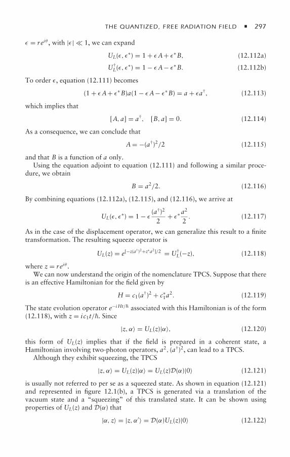
THE QUANTIZED, FREE RADIATION FIELD 297
ε = reiθ , with |ε| 1, we can expand
UL(ε, ε∗) = 1 + εA+ ε∗B, (12.112a)
U†L(ε, ε
∗) = 1 − εA− ε∗B. (12.112b)
To order ε, equation (12.111) becomes
(1 + εA+ ε∗B)a(1 − εA− ε∗B) = a + εa†, (12.113)
which implies that
[A, a] = a†, [B, a] = 0. (12.114)
As a consequence, we can conclude that
A= −(a†)2/2 (12.115)
and that B is a function of a only.Using the equation adjoint to equation (12.111) and following a similar proce-
dure, we obtain
B = a2/2. (12.116)
By combining equations (12.112a), (12.115), and (12.116), we arrive at
UL(ε, ε∗) = 1 − ε (a†)2
2+ ε∗ a
2
2. (12.117)
As in the case of the displacement operator, we can generalize this result to a finitetransformation. The resulting squeeze operator is
UL(z) = e[−z(a†)2+z∗a2]/2 = U†
L(−z), (12.118)
where z = reiθ .We can now understand the origin of the nomenclature TPCS. Suppose that there
is an effective Hamiltonian for the field given by
H = c1(a†)2 + c∗1a
2. (12.119)
The state evolution operator e−i Ht/ associated with this Hamiltonian is of the form(12.118), with z = ic1t/. Since
|z, α〉 = UL(z)|α〉, (12.120)
this form of UL(z) implies that if the field is prepared in a coherent state, aHamiltonian involving two-photon operators, a2, (a†)2, can lead to a TPCS.
Although they exhibit squeezing, the TPCS
|z, α〉 = UL(z)|α〉 = UL(z)D(α)|0〉 (12.121)
is usually not referred to per se as a squeezed state. As shown in equation (12.121)and represented in figure 12.1(b), a TPCS is generated via a translation of thevacuum state and a “squeezing” of this translated state. It can be shown usingproperties of UL(z) and D(α) that
|α, z〉 = |z, α′〉 = D(α)UL(z)|0〉 (12.122)
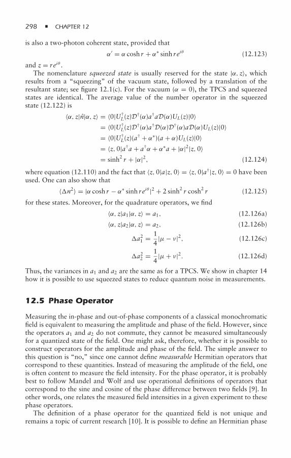
298 CHAPTER 12
is also a two-photon coherent state, provided that
α′ = α cosh r + α∗ sinh reiθ (12.123)
and z = reiθ .The nomenclature squeezed state is usually reserved for the state |α, z〉, which
results from a “squeezing” of the vacuum state, followed by a translation of theresultant state; see figure 12.1(c). For the vacuum (α = 0), the TPCS and squeezedstates are identical. The average value of the number operator in the squeezedstate (12.122) is
〈α, z|n|α, z〉 = 〈0|U†L(z)D†(α)a†aD(α)UL(z)|0〉
= 〈0|U†L(z)D†(α)a†D(α)D†(α)aD(α)UL(z)|0〉
= 〈0|U†L(z)(a
† + α∗)(a + α)UL(z)|0〉= 〈z,0|a†a + a†α + α∗a + |α|2|z,0〉= sinh2 r + |α|2, (12.124)
where equation (12.110) and the fact that 〈z,0|a|z,0〉 = 〈z,0|a†|z,0〉 = 0 have beenused. One can also show that
〈n2〉 = |α cosh r − α∗ sinh reiθ |2 + 2 sinh2 r cosh2 r (12.125)
for these states. Moreover, for the quadrature operators, we find
〈α, z|a1|α, z〉 = a1, (12.126a)
〈α, z|a2|α, z〉 = a2, (12.126b)
a21 = 14
|µ− ν|2, (12.126c)
a22 = 14
|µ+ ν|2. (12.126d)
Thus, the variances in a1 and a2 are the same as for a TPCS. We show in chapter 14how it is possible to use squeezed states to reduce quantum noise in measurements.
12.5 Phase Operator
Measuring the in-phase and out-of-phase components of a classical monochromaticfield is equivalent to measuring the amplitude and phase of the field. However, sincethe operators a1 and a2 do not commute, they cannot be measured simultaneouslyfor a quantized state of the field. One might ask, therefore, whether it is possible toconstruct operators for the amplitude and phase of the field. The simple answer tothis question is “no,” since one cannot define measurable Hermitian operators thatcorrespond to these quantities. Instead of measuring the amplitude of the field, oneis often content to measure the field intensity. For the phase operator, it is probablybest to follow Mandel and Wolf and use operational definitions of operators thatcorrespond to the sine and cosine of the phase difference between two fields [9]. Inother words, one relates the measured field intensities in a given experiment to thesephase operators.
The definition of a phase operator for the quantized field is not unique andremains a topic of current research [10]. It is possible to define an Hermitian phase
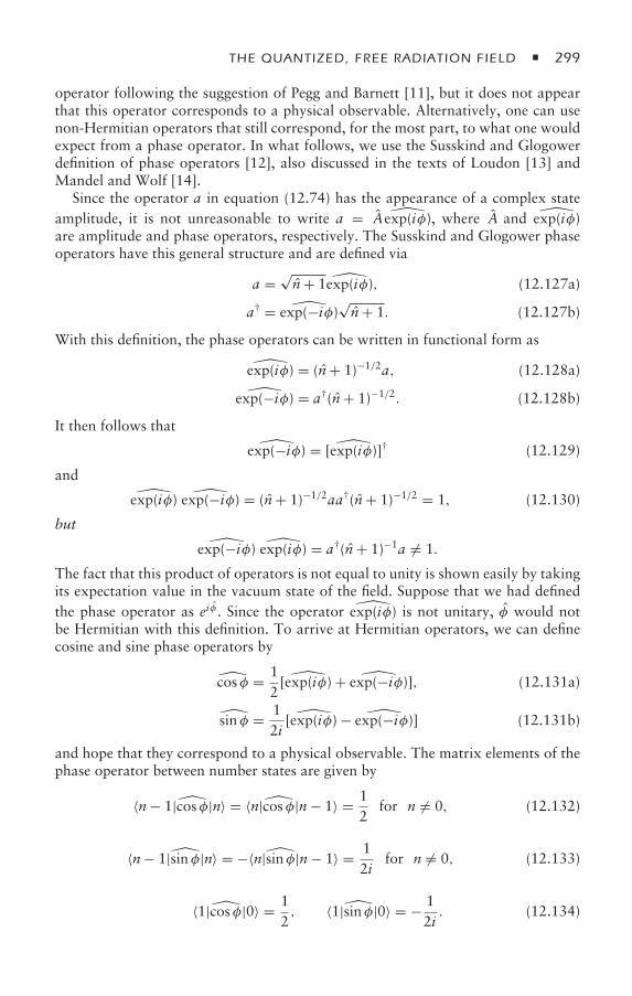
THE QUANTIZED, FREE RADIATION FIELD 299
operator following the suggestion of Pegg and Barnett [11], but it does not appearthat this operator corresponds to a physical observable. Alternatively, one can usenon-Hermitian operators that still correspond, for the most part, to what one wouldexpect from a phase operator. In what follows, we use the Susskind and Glogowerdefinition of phase operators [12], also discussed in the texts of Loudon [13] andMandel and Wolf [14].
Since the operator a in equation (12.74) has the appearance of a complex stateamplitude, it is not unreasonable to write a = A exp(iφ), where A and exp(iφ)are amplitude and phase operators, respectively. The Susskind and Glogower phaseoperators have this general structure and are defined via
a =√n+ 1 exp(iφ), (12.127a)
a† = exp(−iφ)√n+ 1. (12.127b)
With this definition, the phase operators can be written in functional form as
exp(iφ) = (n+ 1)−1/2a, (12.128a)
exp(−iφ) = a†(n+ 1)−1/2. (12.128b)
It then follows thatexp(−iφ) = [ exp(iφ)]† (12.129)
andexp(iφ) exp(−iφ) = (n+ 1)−1/2aa†(n+ 1)−1/2 = 1, (12.130)
butexp(−iφ) exp(iφ) = a†(n+ 1)−1a = 1.
The fact that this product of operators is not equal to unity is shown easily by takingits expectation value in the vacuum state of the field. Suppose that we had definedthe phase operator as ei φ . Since the operator exp(iφ) is not unitary, φ would notbe Hermitian with this definition. To arrive at Hermitian operators, we can definecosine and sine phase operators by
cosφ = 12[ exp(iφ) + exp(−iφ)], (12.131a)
sinφ = 12i
[ exp(iφ) − exp(−iφ)] (12.131b)
and hope that they correspond to a physical observable. The matrix elements of thephase operator between number states are given by
〈n− 1|cosφ|n〉 = 〈n|cosφ|n− 1〉 = 12
for n = 0, (12.132)
〈n− 1|sinφ|n〉 = −〈n|sinφ|n− 1〉 = 12i
for n = 0, (12.133)
〈1|cosφ|0〉 = 12, 〈1|sinφ|0〉 = − 1
2i. (12.134)
300 CHAPTER 12
All other matrix elements vanish. We also find
〈n|cosφ|n〉 = 〈n|sinφ|n〉 = 0, (12.135a)
〈n|cos2 φ|n〉 = 〈n|sin2 φ|n〉 = 12
for n = 0, (12.135b)
〈n|cos2 φ|n〉 = 〈n|sin2 φ|n〉 = 14
for n = 0. (12.135c)
Other properties of the phase operators are left to the problems.We would like to think of a number state as one for which the phase is random.
The expectation values given in equations (12.135a) and (12.135b) are consistent
with this idea. The fact that the average value of cos2 φ or sin2 φ equals 1/4 in thevacuum state is somewhat troubling and throws into doubt the reliability of theseoperators.
For a coherent state with α = |α|eiθ , one would expect to find 〈cosφ〉α ≈ cos θand a minimum value of n (cosφ). In other words, a coherent state is one inwhich both the amplitude and phase of the field are fairly well-defined. Calculationsof these expectation values are left to the problems.
12.6 Summary
We have given a brief introduction to properties of the free, quantized radiationfield. Various possible states of the field were discussed, including number states,coherent states, and squeezed states. Methods for generating such states is still anactive research area. Generally speaking, one generates number states in a cavity bypassing an excited-state atom through the cavity and verifying that the atom left thecavity in its ground state, transferring one photon to the cavity field [15]. Coherentstates can be generated from classical current sources, as is discussed in chapter 15.Moreover, the output of laser resonators, while not a coherent state of the field,closely resembles one. Squeezed states are generated in two-photon processes, suchas those encountered in parametric down conversion of a single “source” photoninto a “signal” and “idler” photon, four-wave mixing, and resonance fluorescence.The quantum properties of the field are invariably linked to the quantum propertiesof the oscillating charges that produce the fields. We now proceed to discuss andcompare coherence properties of classical and quantized fields.
12.7 Appendix: Field Quantization
In this appendix, we indicate a possible path for field quantization, following theapproach given in reference [1]. In the presence of charge density ρ and currentdensity J, Maxwell’s equations are
∇ · E = ρ/ε0, (12.136a)
∇ × E = −∂B∂t, (12.136b)
∇ × B = µ0
(J + ε0 ∂E
∂t
), (12.136c)
∇ · B = 0, (12.136d)
THE QUANTIZED, FREE RADIATION FIELD 301
and the Lorentz force on a charge qα having mass mα located at position Rα is
mαRα = qα (E + vα × B) , (12.137)
where vα = Rα.The equation of continuity is
∂ρ
∂t+ ∇ · J = 0, (12.138)
where
ρ =∑α
qαδ [R − Rα(t) ] , (12.139)
J =∑α
qαvα(t)δ [R − Rα(t) ] , (12.140)
and the sum is over all charges. The Hamiltonian or total energy for the system ofcharges and fields is
H =∑α
12mαv2α + ε0
2
∫d3R
(E2 + c2B2) , (12.141)
while the total momentum is
P =∑α
mαvα + ε0∫d3RE × B . (12.142)
The electric E and magnetic B field are related to the vector potential A and scalarpotential φ by
B = ∇ × A, (12.143a)
E = −∂A∂t
− ∇φ. (12.143b)
Substituting equation (12.143) into Maxwell equations, we obtain
∇2φ = −∂ (∇ · A)∂t
− ρ/ε0, (12.144a)(1c2∂2
∂t− ∇2
)A = µ0J − ∇
(∇·A + 1
c2∂φ
∂t
). (12.144b)
The electric and magnetic fields, equation (12.143), are invariant with respect to thegauge transformation
A → A − ∇ , (12.145a)
φ → φ + ∂
∂t, (12.145b)
where the gauge function is an arbitrary function of position and time.One can impose various conditions on A and φ. In Lorentz gauge, we choose
such that
∇·A + 1c∂φ
∂t= 0 . (12.146)
302 CHAPTER 12
This condition simplifies the field equations, equation (12.144), which become
φ = ρ/ε0, (12.147a)
A = µ0J, (12.147b)
where
= 1c2∂2
∂t2− ∇2 . (12.148)
In Coulomb gauge, we choose
∇·A = 0, (12.149)
so that equations (12.144) become
∇2φ = −ρ/ε0, (12.150a)
A = µ0J + 1c2
∇ ∂φ∂t. (12.150b)
12.7.1 Reciprocal Space
It proves convenient to introduce reciprocal space in which
E(k, t) = 1(2π )3/2
∫d3RE(R, t)e−ik·R ≡ E. (12.151)
It is easy to see that
E(−k, t) = E∗(k, t) . (12.152)
In reciprocal space, Maxwell equations become
ik · E = ρ/ε0, (12.153a)
ik · B = 0, (12.153b)
ik × E = −∂B∂t, (12.153c)
ik × B = 1c2∂E∂t
+ µ0J, (12.153d)
where
f ≡ f (k, t) = 1(2π )3/2
∫d3R f (R, t)e−ik·R. (12.154)
The equation of continuity is
∂ρ
∂t+ ik · J = 0, (12.155)
and the scalar and vector potentials are described via
B = ik × A, (12.156)
E = −∂A∂t
− ikφ. (12.157)
THE QUANTIZED, FREE RADIATION FIELD 303
Gauge transformations are defined by
A → A + ik , (12.158a)
φ → φ − ∂
∂t, (12.158b)
leading to the equations
1c2
A + k2A = µ0J − ik(ik · A + 1
c2∂φ
∂t
), (12.159a)
k2φ = ρ/ε0 + ik·∂A∂t. (12.159b)
The Lorentz gauge condition is
ik · A + 1c2∂φ
∂t= 0, (12.160)
and Coulomb gauge is defined by
k · A = 0 . (12.161)
12.7.2 Longitudinal and Transverse Vector Fields
It is always possible to write a vector field F as
F = FL + FT,
where
∇ × FL = 0; ∇ · FT = 0 . (12.162)
In reciprocal space, the corresponding equations are
F = FT + FL
and
ik × FL = 0, ik · FT = 0, (12.163)
where
FL = κ(κ · F), (FT)i =∑j
(δi, j − kikj
k2
)(F) j , (12.164)
with
κ = k/|k| . (12.165)
Taking a Fourier transform of the transverse field and using the convolutiontheorem, we obtain
(FT)i =∑j
∫d3R ′δTi j (R − R ′)
[F(R ′)
]j , (12.166)
304 CHAPTER 12
where
δTi j (R) = 1(2π )3/2
∫d3k eik·R
(δi, j − kikj
k2
)= δi, jδ(R) − ∂2
∂Ri∂R j
1R
(12.167)
is a transverse Dirac delta function. Although this decomposition is not relativisti-cally invariant, it is still useful for quantization.
12.7.3 Transverse Electromagnetic Field
Since ∇ · B = 0, the magnetic field is purely transverse
BL = 0, B = BT . (12.168)
In decomposing the electric field, one associates the longitudinal component of thefield with the free charges,
EL(R) = 14πε0
∫d3R′ρ(R ′, t)
R − R ′
|R − R ′|3 ∼ 14πε0
∑α
qαR − Rα
|R − Rα|3 , (12.169)
which, in reciprocal space, is
EL = κ(κ · E) = −i ρ
ε0k2k . (12.170)
In terms of the scalar and vector potentials, the electric field components are
ET = −∂AT
∂t, (12.171)
EL = −∂AL
∂t− ∇φ, (12.172)
since ∇φ is purely longitudinal.From this point onward, it will be convenient to work in Coulomb gauge,
∇·A = 0. In Coulomb gauge, A = AT is purely transverse, and
EL = −∇φ, (12.173)
φ(R, t) = 14πε0
∫d3R′ ρ(R
′, t)|R − R ′| ∼ 1
4πε0
∑α
qα|R − Rα| . (12.174)
In terms of these quantities, Maxwell equations become
∇ · EL = ρ/ε0, (12.175a)
∇ × ET = −∂B∂t, (12.175b)
∇ · B = 0, (12.175c)
∇ × B = 1
c2∂
∂t(EL + ET) + 1
ε0c2(JL + JT), (12.175d)
THE QUANTIZED, FREE RADIATION FIELD 305
ik · EL = ρ/ε0, (12.176a)
ik × ET = −∂B∂t, (12.176b)
BL = 0, (12.176c)
ik × B = 1
c2∂ET∂t
+ 1ε0c2
JT, (12.176d)
and the energy is
Hfield = HL + HT, (12.177)
where
HL = 12ε0
∫d3k|EL|2 = 1
2ε0
∫d3R|EL|2 = Vcoul , (12.178)
and
HT = 12ε0
∫d3k
(|ET|2 + c2B|2
)= 1
2ε0
∫d3R
(|ET|2 + c2|B|2) . (12.179)
[The longitudinal part of equation (12.175d) simply reproduces the equation ofcontinuity.] The total energy of the charges plus fields is
Htot = 12
∑α
mα R2α + VC + HT, (12.180)
where the Coulomb potential for an ensemble of point charges is given by
VC = 18πε0
∑α,β =α
qαqβ|Rα − Rβ | , (12.181)
neglecting the self-energy of each charge.Similarly, for the momentum,
PL = ε0
∫d3REL × B = ε0
∫d3k E∗
L × B. (12.182)
Taking into account equation (12.156) and equation (12.170), we obtain
PL =∫d3RρA =
∑α
qαA(Rα), (12.183)
PT = ε0
∫d3RET × B, (12.184)
Ptot =∑α
mαRα + qαA(Rα) + PT, (12.185)
Htot =∑α
12mα
[pα − qαA(Rα)]2 + VC + HT . (12.186)
306 CHAPTER 12
We now define
α(k, t) = − i2N(k)
(ET − cκ × B
)(12.187)
and
β(k, t) = − i2N(k)
(ET + cκ × B
)= −α∗(−k, t), (12.188)
where N(k) is a normalization factor that will be fixed at a later time. Usingequations (12.187) and (12.188), we find
ET = iN(k) [α(k, t) − α∗(−k, t)] , (12.189)
B = icN(k) [κ × α(k, t) + κ × α∗(−k, t)] , (12.190)
∂α(k, t)∂t
+ iωα(k, t) = i2ε0N(k)
JT, (12.191)
where ω = ck.Including two polarizations εk for each k, we write
α(k, t) =∑εk
εkαε(k, t), (12.192)
∂αε(k, t)∂t
+ iωαε(k, t) = i2ε0N(k)
εk · J . (12.193)
If we introduce
α = α(k, t),α− = α(−k, t), (12.194)
then the transverse field energy can be written as
HT = 12ε0
∫d3k
(|ET|2 + c2B|2)= ε0
∫d3kN2(k)[α∗
εk· αεk + (α−)ε−k
(α−)∗ε−k]
= ε0∑εk
∫d3kN2(k)
(α∗
εkαεk + αεkα
∗εk
). (12.195)
Even though everything is classical to this point, we now choose the normaliza-tion constant in such a way that it leads to an energy of ω in each mode of the field(you can think of as some undefined constant)—that is, we set
N(k) =(ω
2ε0
)1/2( L2π
)3/2
, (12.196)
THE QUANTIZED, FREE RADIATION FIELD 307
where L3 = V is the quantization volume in space. Then,
HT =(
L2π
)3 ∫d3k
∑εk
12ω
(α∗
εkαεk + αεkα
∗εk
), (12.197)
PT =(
L2π
)3 ∫d3k
∑εk
12k
(α∗
εkαεk + αεkα
∗εk
), (12.198)
ET = i∫d3k
∑εk
Eω(αεkεkeik·R − α∗
εkεke−ik·R), (12.199)
B = i∫d3k
∑εk
Bω(αεkκ × εkeik·R − α∗εk
κ × εke−ik·R); (12.200)
A = i∫d3k
∑εk
Aω(αεkεkeik·R + α∗
εkεke−ik·R), (12.201)
where
Eω =√
ωV2ε0(2π )3
, Bω = Eωc, Aω = Eω
ω. (12.202)
We can go over to discrete variables by using the prescription (12.25) with k j
defined by equations (12.1) and, (12.2). In this manner, we obtain
HT =∑j
12ω j
(α∗jα j + α jα∗
j
), (12.203)
PT =∑j
12k j
(α∗jα j + α jα∗
j
), (12.204)
A =∑j
Aj (α jε j eik j ·R + α∗j ε j e
−ik j ·R), (12.205)
ET = i∑j
E j (α jε j eik jR − α∗j ε j e
−ik jR), (12.206)
B = i∑j
Bj (α jκ j × ε j eik j ·R − α∗jκ j × ε j e−ik j ·R), (12.207)
where α j ≡ αk j ,εk j, and
Ej =√ω j
2ε0V, Bj = Ej
c, Aj = Ej
ω j, κ j = k j/|k j |. (12.208)
308 CHAPTER 12
The α j obey the equation of motion
α j + iω jα j = i√2ε0ω j
J j , (12.209)
with
J j = 1√V
∫dR e−ik j ·Rε j ·J(R, t). (12.210)
12.7.4 Free Field
In the absence of sources, equation (12.209) becomes
α j + iω jα j = 0. (12.211)
Therefore,
α j = α j (0)e−iω j t, (12.212a)
α∗j = α∗
j (0)eiω j t . (12.212b)
Using equation (12.203), we then find
∂HT
∂α j= ω jα
∗j = −iα∗
j , (12.213a)
1i∂HT
∂α∗j
= − i
∂HT
∂α∗j
= −iω jα j = α j . (12.213b)
Therefore, α j and iα∗j are canonical variables. Quantization of the free field is then
carried out using the prescription αi → ai , α∗i → a†
i , with
[ai , a j ] = [a†i , a
†j
] = 0,[ai , a
†j
] = δi, j . (12.214)
In this manner, we arrive at equations (12.8) to (12.13) of the text. The samequantization procedure in the presence of sources leads to the correct equationsof motion for both the charges and the fields.
Problems
1. Given the Hamiltonian H = ∑i (1/2)ωi (α
∗i αi + αiα
∗i ), where αi satisfies
αi + iωiαi = 0, show that two sets of canonical variables are (αi and iα∗i )
and [qi = (/2ωi )1/2(αi + α∗i ) and pi = i(ωi/2)1/2(α∗
i − αi )]. Use these resultsto write H in two distinct quantized forms.
2. Prove that [Ex(R), By(R′)] = −(i/ε0)∂/∂z[δ(R−R′)]—that is, the fields do notcommute.
3. Evaluate 〈E(R, t)〉 and 〈E(R, t)2〉 for a single-mode coherent state and a pure nstate, using the Heisenberg operators for the fields. Also calculateE for thesestates.
THE QUANTIZED, FREE RADIATION FIELD 309
4. Prove that for the operators
A1 = a1 cos (θ/2) + a2 sin(θ/2),
A2 = a2 cos (θ/2) − a1 sin(θ/2),
A1 = e−r/2, A1 = er/2 in a single-mode TPCS.5. Derive equations (12.126).6. Prove that a† has no normalizable eigenstates.7. Prove that [n, exp(iφ)] = − exp(iφ); [n, exp(−iφ)] = exp(−iφ); [n, cos(φ)] =
−i sinφ; [n, sinφ] = i cos(φ), and that
exp(iφ)|n〉 =√n
(n+ 1)1/2|n− 1〉, exp(−iφ)|n〉 = |n+ 1〉.
8. Prove that, in a single-mode coherent state with |α| 1,
〈cosφ〉α = cos θ(1 − 1
8|α|2),
〈cos2 φ〉α = cos2 θ − cos 2θ4|α|2 ,
〈 (cosφ)n〉 ≈ 12sin θ ≈ 1
2〈sinφ〉,
where α = |α|eiθ . In other words, show that both the intensity and phase arefairly well-defined in a coherent state whose average energy is much greaterthan ω. You will need to use the following asymptotic expansions:
∞∑n=0
|α|2n√n+ 1n!
= e|α|2
|α|(1 − 1
8|α|2),
∞∑n=0
|α|2n√(n+ 1) (n+ 2)n!
= e|α|2
|α|2(1 − 1
2|α|2),
valid for |α| 1.9. Prove that
|n〉〈n| = π−2∫d2α d2β e−[|a|2+|β|2]/2(n!)−1(α∗β)n|α〉〈β|
and
|n〉〈n| =∫
P(α)|α〉〈α|d2α, with P(α) = n!er2
2πr (2n)!
(− ∂
∂r
)2n
δ(r ),
where α = |r |eiθ . How can this operator be either diagonal or nondiagonal inthe α basis?A two-photon coherent state (TPCS) is defined by
b|z, β〉 = β|z, β〉,
310 CHAPTER 12
where
b = U(z)a[U(z)]† = a cosh(r ) + a†eiθ sinh(r ),
U(z) = e(z∗a2−za†2)/2
and z = reiθ .In the text, it is shown that |z, β〉 = U(z)|β〉, where |β〉 is now the normal
coherent state defined through a|β〉 = β|β〉, |β〉 = D(β)|0〉, D(β) = eβa†−β∗a ,
and [D(β)]†aD(β) = a + β.10. Using the facts that
D(β)D(α) = e(βα∗−αβ∗)/2D(α + β),
[UL(z)]†D(β)UL(z) = D(β ′),
where
β ′ = β cosh(r ) + β∗ sinh(r )eiθ ,
prove that ∣∣z, α + β ′⟩ = e−(β ′α∗−β ′∗α)D(β)|z, α〉.In other words, D(β) |z, α〉 is also a TPCS. In particular, show that
|α, z〉 ≡ |z, α′〉 = D(α)|z,0〉 = D(α)UL(z)|0〉,where
α′ = α cosh(r ) + α∗ sinh(r )eiθ .
11. For the states |z, α′〉 defined in problem 10, prove that
n2 = |α′′|2 + 2 sinh2(r ) cosh2(r ), α′′ = α cosh(r ) − α∗ sinh(r )eiθ .
Hint: Use of the relationship [D(α)]†aD(α) = a + α and the fact thatUL(−z)aUL(z) = b′ = b(−z) = µa − νa† may save you some time.
12. Calculate 〈E(R, t)〉, 〈E(R, t)2〉, and E for the single-mode states defined inproblem 10, using the Heisenberg operators for the fields. Compare the resultswith those of problem 3.
References
[1] C. Cohen-Tannoudji, J. Dupont-Roc, and G. Grynberg, Photons and Atoms—Introduction to Quantum Electrodynamics (Wiley-Interscience, New York, 1989),chaps. 1 and 2.
[2] R. G. Glauber, The Quantum Theory of Optical Coherence, Physical Review 130,2529–2539 (1963); R. G. Glauber Coherent and incoherent states of the radiation field,Physical Review 131, 2766–2788 (1963).
[3] D. Stoler, Equivalence classes of minimum uncertainty packets, Physical Review D 1,3217–3219 (1970); D 4, 1925–1926 (1971).
THE QUANTIZED, FREE RADIATION FIELD 311
[4] H. P. Yuen, Two-photon coherent state of the radiation field, Physical Review A 13,2226–2243 (1976).
[5] D. F. Walls, Squeezed states of light, Nature 206, 141–146 (1983).[6] H. J. Kimble and D. F. Walls, Eds., Squeezed States of the Electromagnetic Field, Special
Issue of Journal of the Optical Society of America B 4, 1449–1741 (1987); R. Loudonand P. L. Knight, Eds., Special Issue of the Journal of Modern Optics on SqueezedLight, 34, 707–1020 (1987).
[7] S. Reynaud, A Heidmann, E. Giacobino, and C. Fabre, Quantum fluctuations inoptical systems, in Progress in Optics, edited by E. Wolf vol. XXX, (North-Holland,Amsterdam, 1992) 3–85.
[8] For a more recent article with promising applications to detection of gravitationalwaves, see H. Vahlbruch, M. Mehmet, S. Chelkowski, B. Hage, A. Franzen, N. Lastzka,S. Goßler, K. Danzmann, and R. Schnabel, Observation of squeezed light with 10-dBquantum-noise reduction, Physical Review Letters 100, 033602, 1–4 (2008).
[9] L. Mandel and E. Wolf, Optical Coherence and Quantum Optics (Cambridge Univer-sity Press, Cambridge, UK, 1995), sec. 10.7.4.
[10] S. M. Barnett and J. A. Vaccarro Eds., The Quantum Phase Operator: A Review (CRCPress, Taylor and Francis Group, Boca Raton, FL, 2007).
[11] D. T. Pegg and S. M. Barnett, Phase properties of the quantized single-mode electro-magnetic field, Physical Review A 39, 1665–1675 (1989).
[12] L. Susskind and J. Glogower, Quantum mechanical phase and time operator, Physics(Long Island City, NY) 1, 49–61 (1964).
[13] R. Loudon, The Quantum Theory of Light, 2nd ed. (Oxford University Press, Oxford,UK, 1983), sec. 4.8.
[14] L. Mandel and E. Wolf, Optical Coherence and Quantum Optics (Cambridge Univer-sity Press, Cambridge, UK, 1995), sec. 10.7.
[15] See, for example, S. Haroche and J. M. Raimond, Manipulation of nonclassical fieldstates in a cavity by atom interferometry, in Advances in Atomic, Molecular, andOptical Physics, Supplement I, edited by P. Berman (Academic Press, New York, 1994),pp. 123–170.
Bibliography
See the books on quantum optics listed in chapter 1.
13Coherence Properties of the ElectricField
13.1 Coherence: Some General Concepts
Now that we have discussed quantized states of the radiation field, it is probablya good time to consider ways in which it is possible to characterize optical fields.The coherence properties of fields are discussed extensively in Mandel and Wolf [1].Here, we adopt a simplified approach but still attempt to touch upon many of theessential components needed to piece together a theory of coherence.
13.1.1 Time versus Ensemble Averages
The coherence properties of any time-dependent process, denoted here in somegeneric fashion by the function f (t), are often described in terms of a quantity F (t, τ )defined by
F (t, τ ) = 〈 f (t) f (t + τ )〉 / ⟨ f 2(t)⟩ . (13.1)
This type of definition of coherence is appealing, since it compares the function withitself at different times; clearly, if the function f (t) is constant, then F (t, τ ) = 1, andthe function is perfectly coherent according to this definition.
The confusion associated with equation (13.1) is hidden in the brackets 〈. . .〉.Exactly what do these brackets mean? For the time being, let us restrict thediscussion to classical rather than quantum-mechanical systems. Most likely, youhave heard it told that a monkey typing at random would eventually produce allthe works of literature, given an infinite time. (Alas, if only we all had an infiniteamount of time.) On the other hand, you could also achieve the same result withan infinite number of monkeys typing for a much shorter time. The two processesillustrate the difference between a time average and an ensemble average. Often,the ergodic theorem is invoked to guarantee the equivalence of both averages. Ifa system has enough time to experience all possible random configurations of its
ELECTRIC FIELD COHERENCE PROPERTIES 313
components, there is no difference between a time and an ensemble average. Forfinite times, and experiments are usually carried out over a finite time, there canbe a fundamental difference between time and ensemble averages. We illustrate thisconcept by considering a simple physical system.
Imagine that a two-level atom, whose transition frequency is ω0 in the absenceof interactions, is placed in a bath of stationary perturber atoms located at randompositions in space. The net effect of each perturber atom is to alter the transitionfrequency of the two-level atom by an amount that depends on its separationfrom the atom (e.g., shifts resulting from van der Waals interactions). The atom isprepared in a superposition of its ground and excited states at t = 0 and allowed toradiate. To simplify matters, we neglect any effects of spontaneous decay—the atomacts as an undamped oscillator. The question is, “What is the line width associatedwith the oscillator?”
Since the perturber atoms are stationary, the only effect of the bath, in this limit,is to change the transition frequency of the atom. It still radiates as an undampedoscillator—in other words, the radiation is perfectly coherent with “zero” line width.On the other hand, if we place a large number of these oscillators in the sampleand excite them all at t = 0, the situation is similar to the one we encounteredin free polarization decay—owing to the inhomogeneous broadening of the sample(different atoms have their frequencies shifted by a different amount by the bath),the coherent signal decays very rapidly, and the line width is the inhomogeneousline width of the sample. In this instance, the difference between a time average fora single atom and an ensemble average is dramatic. The research field of single-molecule spectroscopy [2] depends critically on the fact that the response of asingle molecule is totally different from the response of an ensemble of such atomsembedded in a host material.
The situation changes somewhat if we allow the bath atoms to move. Now ifwe wait for a sufficiently long time, all possible bath configurations will have beenexperienced by the (stationary) single two-level atom. In this case, a time averagetaken over a sufficiently long time reproduces the same result as an ensemble averageof a large number of these atoms placed in the bath at random.
The output field of a laser cavity is another case in point. The laser field is closeto that of a coherent state with a fairly well-defined phase. But this phase must bea global phase, since the laser starts from spontaneous emission. In other words,if one turns on the laser at different times, the global phase of the output wouldbe different. An ensemble average over different realizations of the laser outputyields an average field amplitude at any time that vanishes, whereas the output fieldamplitude for a laser can be considered almost as a classical field.
It should be clear from this discussion that the results of a given experiment mustbe examined on a case-by-case basis to see what type of average enters. In most cases,such as atoms in a vapor cell, one encounters ensemble rather than time averages;however, if one is truly following a single realization of a stochastic process, such asin single-molecule spectroscopy or the output of a laser cavity, it is a time averagethat is needed.
The lesson to be learned here is that some care must be taken in evaluating the〈. . .〉 in equation (13.1). Even in quantum mechanics, where you might think that the〈. . .〉 refers to a quantum-mechanical average in the usual sense, the situation is notso simple. The reason for this is that it is usually all but impossible to carry out the
314 CHAPTER 13
average over a complicated atom–bath system, and some types of approximations,corresponding to ensemble averages, are often invoked. With this warning in mind,let us now turn our attention to optical fields. We are interested in determining whatparameters are needed to characterize these fields.
13.1.2 Classical Fields
For monochromatic fields in vacuum, it is necessary to specify only the frequencyand amplitude of the field. One could also specify a phase, but this assignment isequivalent to choosing a time origin. It is natural to think of a monochromatic fieldas a coherent field, since its amplitude and phase are well-defined. But what happensif the field consists of a sum of two monochromatic fields? Of course, we must nowspecify not only the amplitude and frequency of each field, but also the relative phaseof the two fields. Is this superposition state of two fields coherent? The answer tothis question depends on whether we consider an ensemble or a time average. In thiscase, as for any complex wave form, an ensemble average has no meaning, since weare not considering fluctuations in the sources of the field. In this sense, the field isstill a coherent field, since it is totally deterministic. On the other hand, you will seethat the field is not coherent, according to the standard definition (13.1), when thebrackets in that equation represent a time average.
The situation can change if we take into account any fluctuations in the sourcesgiving rise to the field. Imagine that the field is produced by an ensemble ofoscillators having the same natural frequency but random, constant phases. Sincethe phases are constant, if one uses the time-averaged definition, the field radiatedby these oscillators would be purely coherent. That is, for a specific realization of thephases, the output is perfectly coherent. If one takes an ensemble average, however,corresponding to repeating the experiment many times with different sets of phases,the coherence properties of the radiation field are altered. Examples are given in thefollowing section. For phases that are fluctuating functions of time, the time- andensemble-averaged results are identical for sufficiently long sampling times.
13.1.3 Quantized Fields
In some sense, the description of quantized fields is more straightforward thanclassical fields. As in any quantum system, the state vector provides a completedescription of the system. However, the quantum state of a field that fluctuatesas a result of its interactions with its environment is an extremely complex entity.The radiation field can become entangled with the environment owing to theseinteractions. If we do not observe the environment, we are, in effect, tracing overthe environment states. In this limit, it is the reduced density matrix of the field thatprovides a complete description of our knowledge of the field. Thus, in discussingquantized fields, we concentrate on the density matrix or photon statistics (densitymatrix elements of the field in the number representation) of the field. You willsee that there are properties of the quantized field that can distinguish it in anunambiguous way from classical fields. You have already seen this for atomic states,where negative values of the density matrix elements in the Wigner representationare a signature of quantum effects.
ELECTRIC FIELD COHERENCE PROPERTIES 315
13.2 Classical Fields: Correlation Functions
13.2.1 First-Order Correlation Function
We limit our discussion to one polarization component of an electric field. For themoment, we neglect the position dependence and look at the field as a function oftime at R = 0, setting E(R, t) = E(0, t). It is convenient to expand E(0, t) in terms ofpositive and negative frequency components as
E(0, t) = ε[E+(t) + E−(t)
], (13.2)
where ε is the field polarization
E+(t) = 1√2π
∫ ∞
−∞dωE(ω)e−iωt , (13.3)
and E− = (E+)∗. The separation into positive and negative frequency componentsmakes sense only for ω > 0, but we can formally allow for negative values of ωby setting E(ω) = 0 for ω < 0. The quantity E(ω) is the Fourier transform of thepositive frequency component of the field.
The power spectrum of the field is proportional to the absolute square of thisquantity,
|E(ω)|2 = 12π
∫ ∞
−∞dt′E+(t′)eiωt
′∫ ∞
−∞dtE−(t)e−iωt
= 12π
∫ ∞
−∞dτ
∫ ∞
−∞dtE−(t)E+(t + τ )eiωτ . (13.4)
If we define
h(τ ) ≡ 〈E−(t)E+(t + τ )〉 = limT→∞
1T
∫ T/2
−T/2dtE−(t)E+(t + τ ) , (13.5)
then
|E(ω)|2 = T2π
∫ ∞
−∞dτh(τ )eiωτ . (13.6)
Note that, at this point, h(τ ) represents a time average.The power spectrum F (ω) is defined as
F (ω) ≡ |E(ω)|2∫ ∞
−∞dω|E(ω)|2
= |E(ω)|2∫ ∞
−∞dt|E+(t)|2
= |E(ω)|2T〈E−(t)E+(t)〉 , (13.7)
such that
F (ω) = 12π
∫ ∞
−∞dτg(1)(τ )eiωτ , (13.8)
where
g(1)(τ ) = 〈E−(t)E+(t + τ )〉〈E−(t)E+(t)〉 (13.9)
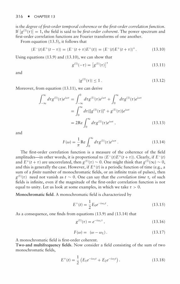
316 CHAPTER 13
is the degree of first-order temporal coherence or the first-order correlation function.If∣∣g(1)(τ )∣∣ = 1, the field is said to be first-order coherent. The power spectrum and
first-order correlation functions are Fourier transforms of one another.From equation (13.5), it follows that
〈E−(t)E+(t − τ )〉 = 〈E−(t + τ )E+(t)〉 = 〈E−(t)E+(t + τ )〉∗ . (13.10)
Using equations (13.9) and (13.10), we can show that
g(1)(−τ ) = [g(1)(τ )
]∗(13.11)
and
|g(1)(τ )| ≤ 1 . (13.12)
Moreover, from equation (13.11), we can derive∫ ∞
−∞dτg(1)(τ )eiωτ =
∫ 0
−∞dτg(1)(τ )eiωτ +
∫ ∞
0dτg(1)(τ )eiωτ
=∫ ∞
0dτ [g(1)(τ )]∗ + g(1)(τ )eiωτ
= 2Re∫ ∞
0dτg(1)(τ )eiωτ , (13.13)
and
F (ω) = 1πRe
∫ ∞
0dτg(1)(τ )eiωτ . (13.14)
The first-order correlation function is a measure of the coherence of the fieldamplitudes—in other words, it is proportional to 〈E−(t)E+(t+ τ )〉. Clearly, if E−(t)and E+(t + τ ) are uncorrelated, then g(1)(τ ) ∼ 0. One might think that g(1)(∞) ∼ 0,and this is generally the case. However, if E+(t) is a periodic function of time (e.g., asum of a finite number of monochromatic fields, or an infinite train of pulses), theng(1)(τ ) need not vanish as t ∼ 0. One can say that the correlation time τc of suchfields is infinite, even if the magnitude of the first-order correlation function is notequal to unity. Let us look at some examples, in which we take τ > 0.
Monochromatic field. A monochromatic field is characterized by
E+(t) = 12E0e−iωLt . (13.15)
As a consequence, one finds from equations (13.9) and (13.14) that
g(1)(τ ) = e−iωLτ , (13.16)
F (ω) = δ(ω − ωL) . (13.17)
A monochromatic field is first-order coherent.Two-and multifrequency fields. Now consider a field consisting of the sum of twomonochromatic fields,
E+(t) = 12
(E1e−iω1t + E2e−iω2t
). (13.18)
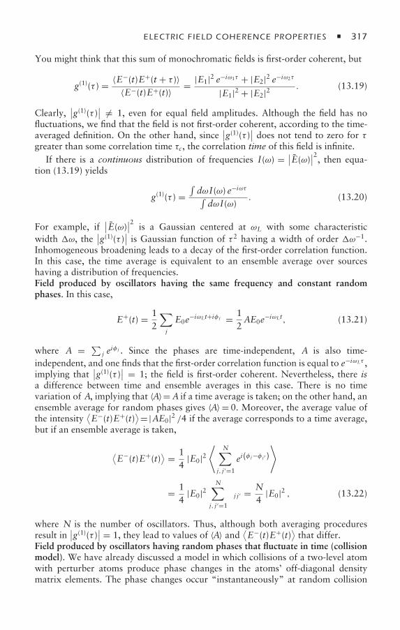
ELECTRIC FIELD COHERENCE PROPERTIES 317
You might think that this sum of monochromatic fields is first-order coherent, but
g(1)(τ ) = 〈E−(t)E+(t + τ )〉〈E−(t)E+(t)〉 = |E1|2 e−iω1τ + |E2|2 e−iω2τ
|E1|2 + |E2|2. (13.19)
Clearly,∣∣g(1)(τ )∣∣ = 1, even for equal field amplitudes. Although the field has no
fluctuations, we find that the field is not first-order coherent, according to the time-averaged definition. On the other hand, since
∣∣g(1)(τ )∣∣ does not tend to zero for τgreater than some correlation time τc, the correlation time of this field is infinite.
If there is a continuous distribution of frequencies I(ω) = ∣∣E(ω)∣∣2, then equa-tion (13.19) yields
g(1)(τ ) =∫dωI(ω) e−iωτ∫dωI(ω)
. (13.20)
For example, if∣∣E(ω)∣∣2 is a Gaussian centered at ωL with some characteristic
width ω, the∣∣g(1)(τ )∣∣ is Gaussian function of τ 2 having a width of order ω−1.
Inhomogeneous broadening leads to a decay of the first-order correlation function.In this case, the time average is equivalent to an ensemble average over sourceshaving a distribution of frequencies.Field produced by oscillators having the same frequency and constant randomphases. In this case,
E+(t) = 12
∑j
E0e−iωLt+iφ j = 12AE0e−iωLt, (13.21)
where A = ∑j e
iφ j . Since the phases are time-independent, A is also time-independent, and one finds that the first-order correlation function is equal to e−iωLτ ,implying that
∣∣g(1)(τ )∣∣ = 1; the field is first-order coherent. Nevertheless, there isa difference between time and ensemble averages in this case. There is no timevariation of A, implying that 〈A〉=A if a time average is taken; on the other hand, anensemble average for random phases gives 〈A〉 = 0. Moreover, the average value ofthe intensity
⟨E−(t)E+(t)
⟩=|AE0|2 /4 if the average corresponds to a time average,but if an ensemble average is taken,
⟨E−(t)E+(t)
⟩ = 14
|E0|2⟨
N∑j, j ′=1
ei(φ j−φ j ′ )⟩
= 14
|E0|2N∑
j, j ′=1
δ j j ′ = N4
|E0|2 , (13.22)
where N is the number of oscillators. Thus, although both averaging proceduresresult in
∣∣g(1)(τ )∣∣ = 1, they lead to values of 〈A〉 and ⟨E−(t)E+(t)⟩that differ.
Field produced by oscillators having random phases that fluctuate in time (collisionmodel). We have already discussed a model in which collisions of a two-level atomwith perturber atoms produce phase changes in the atoms’ off-diagonal densitymatrix elements. The phase changes occur “instantaneously” at random collision
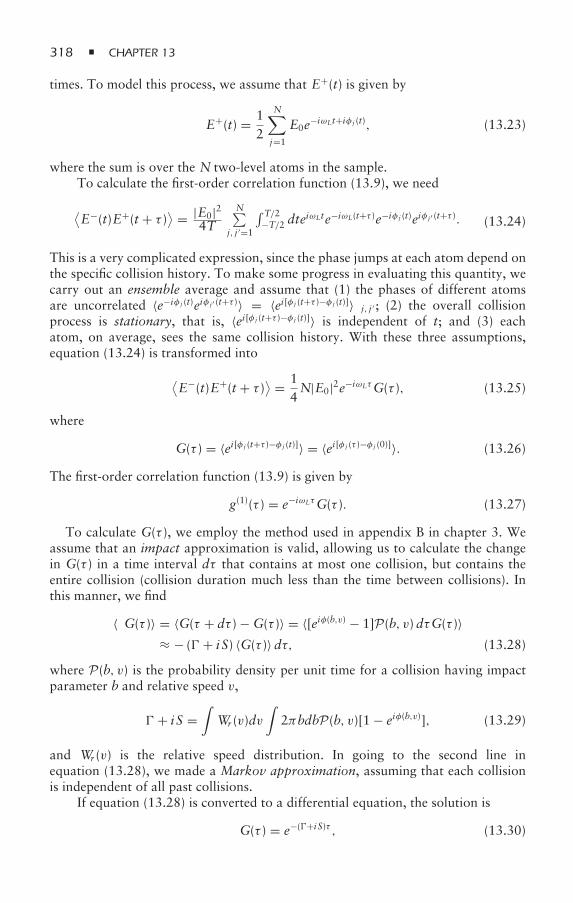
318 CHAPTER 13
times. To model this process, we assume that E+(t) is given by
E+(t) = 12
N∑j=1
E0e−iωLt+iφ j (t), (13.23)
where the sum is over the N two-level atoms in the sample.To calculate the first-order correlation function (13.9), we need
⟨E−(t)E+(t + τ )⟩ = |E0|2
4T
N∑j, j ′=1
∫ T/2−T/2 dte
iωLte−iωL(t+τ )e−iφ j (t)eiφ j ′ (t+τ ). (13.24)
This is a very complicated expression, since the phase jumps at each atom depend onthe specific collision history. To make some progress in evaluating this quantity, wecarry out an ensemble average and assume that (1) the phases of different atomsare uncorrelated 〈e−iφ j (t)eiφ j ′ (t+τ )〉 = 〈ei[φ j (t+τ )−φ j (t)]〉δ j, j ′ ; (2) the overall collisionprocess is stationary, that is, 〈ei[φ j (t+τ )−φ j (t)]〉 is independent of t; and (3) eachatom, on average, sees the same collision history. With these three assumptions,equation (13.24) is transformed into
⟨E−(t)E+(t + τ )⟩ = 1
4N|E0|2e−iωLτG(τ ), (13.25)
where
G(τ ) = 〈ei[φ j (t+τ )−φ j (t)]〉 = 〈ei[φ j (τ )−φ j (0)]〉. (13.26)
The first-order correlation function (13.9) is given by
g(1)(τ ) = e−iωLτG(τ ). (13.27)
To calculate G(τ ), we employ the method used in appendix B in chapter 3. Weassume that an impact approximation is valid, allowing us to calculate the changein G(τ ) in a time interval dτ that contains at most one collision, but contains theentire collision (collision duration much less than the time between collisions). Inthis manner, we find
〈δG(τ )〉 = 〈G(τ + dτ ) − G(τ )〉 = 〈[eiφ(b,v) − 1]P(b, v)dτG(τ )〉≈ − ( + i S) 〈G(τ )〉dτ, (13.28)
where P(b, v) is the probability density per unit time for a collision having impactparameter b and relative speed v,
+ i S =∫
Wr (v)dv∫
2πbdbP(b, v)[1 − eiφ(b,v)], (13.29)
and Wr (v) is the relative speed distribution. In going to the second line inequation (13.28), we made a Markov approximation, assuming that each collisionis independent of all past collisions.
If equation (13.28) is converted to a differential equation, the solution is
G(τ ) = e−(+i S)τ , (13.30)
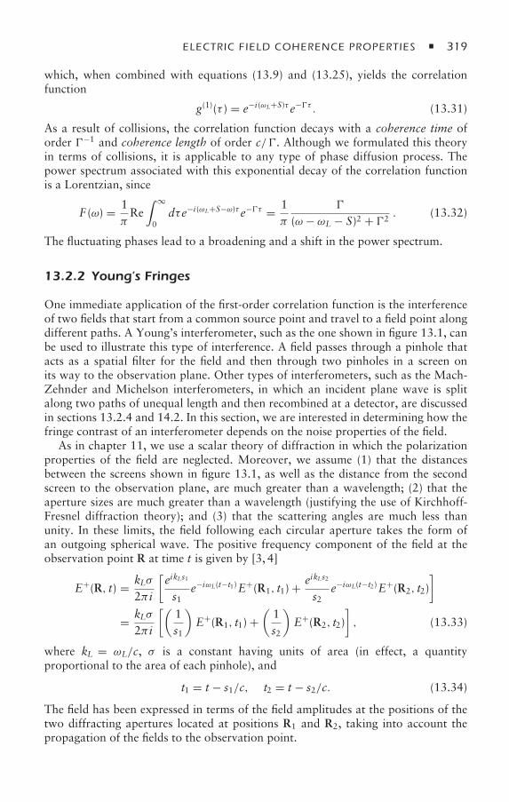
ELECTRIC FIELD COHERENCE PROPERTIES 319
which, when combined with equations (13.9) and (13.25), yields the correlationfunction
g(1)(τ ) = e−i(ωL+S)τ e−τ . (13.31)
As a result of collisions, the correlation function decays with a coherence time oforder −1 and coherence length of order c/. Although we formulated this theoryin terms of collisions, it is applicable to any type of phase diffusion process. Thepower spectrum associated with this exponential decay of the correlation functionis a Lorentzian, since
F (ω) = 1πRe
∫ ∞
0dτe−i(ωL+S−ω)τ e−τ = 1
π
(ω − ωL − S)2 + 2. (13.32)
The fluctuating phases lead to a broadening and a shift in the power spectrum.
13.2.2 Young’s Fringes
One immediate application of the first-order correlation function is the interferenceof two fields that start from a common source point and travel to a field point alongdifferent paths. A Young’s interferometer, such as the one shown in figure 13.1, canbe used to illustrate this type of interference. A field passes through a pinhole thatacts as a spatial filter for the field and then through two pinholes in a screen onits way to the observation plane. Other types of interferometers, such as the Mach-Zehnder and Michelson interferometers, in which an incident plane wave is splitalong two paths of unequal length and then recombined at a detector, are discussedin sections 13.2.4 and 14.2. In this section, we are interested in determining how thefringe contrast of an interferometer depends on the noise properties of the field.
As in chapter 11, we use a scalar theory of diffraction in which the polarizationproperties of the field are neglected. Moreover, we assume (1) that the distancesbetween the screens shown in figure 13.1, as well as the distance from the secondscreen to the observation plane, are much greater than a wavelength; (2) that theaperture sizes are much greater than a wavelength (justifying the use of Kirchhoff-Fresnel diffraction theory); and (3) that the scattering angles are much less thanunity. In these limits, the field following each circular aperture takes the form ofan outgoing spherical wave. The positive frequency component of the field at theobservation point R at time t is given by [3, 4]
E+(R, t) = kLσ2π i
[eikLs1
s1e−iωL(t−t1)E+(R1, t1) + eikLs2
s2e−iωL(t−t2)E+(R2, t2)
]
= kLσ2π i
[(1s1
)E+(R1, t1) +
(1s2
)E+(R2, t2)
], (13.33)
where kL = ωL/c, σ is a constant having units of area (in effect, a quantityproportional to the area of each pinhole), and
t1 = t − s1/c, t2 = t − s2/c. (13.34)
The field has been expressed in terms of the field amplitudes at the positions of thetwo diffracting apertures located at positions R1 and R2, taking into account thepropagation of the fields to the observation point.
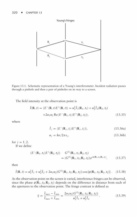
320 CHAPTER 13
Young’s fringes
R1
R2
s1
s2
Figure 13.1. Schematic representation of a Young’s interferometer. Incident radiation passesthrough a pinhole and then a pair of pinholes on its way to a screen.
The field intensity at the observation point is
I(R, t) = 〈E−(R, t)E+(R, t)〉 = u21 I1(R1, t1) + u22 I2(R2, t2)
+2u1u2 Re〈E−(R1, t1)E+(R2, t2)〉, (13.35)
where
I j = 〈E−(R j , tj )E+(R j , tj )〉, (13.36a)
uj = kσ/2πs j , (13.36b)
for j = 1,2.If we define
〈E−(R1, t1)E+(R2, t2)〉 ≡ G(1)(R1, t1;R2, t2)
= |G(1)(R1, t1;R2, t2)|eiφ(R1,t1;R2,t2), (13.37)
then
I(R, t) = u21 I1 + u22 I2 + 2u1u2|G(1)(R1, t1;R2, t2)| cos [φ(R1, t1;R2, t2)] . (13.38)
As the observation point on the screen is varied, interference fringes can be observed,since the phase φ(R1, t1;R2, t2) depends on the difference in distance from each ofthe apertures to the observation point. The fringe contrast is defined as
ξ = Imax − IminImax + Imin
= 2u1u2|G(1)(R1, t1;R2, t2)|u21 I1 + u22 I2
. (13.39)
ELECTRIC FIELD COHERENCE PROPERTIES 321
This expression can be recast in a suggestive form if the definition of the first-order correlation function is generalized as
g(1)(R1, t1;R2, t2) = G(1)(R1, t1;R2, t2)√I1 I2
= 〈E−(R1, t1)E+(R2, t2)〉√I1 I2
. (13.40)
In terms of g(1)(R1, t1;R2, t2), equation (13.39) becomes
ξ = 2u1u2√I1 I2
u21 I1 + u22 I2|g(1)(R1, t1;R2, t2)| . (13.41)
The maximum fringe contrast occurs if |g(1)(R1, t1;R2, t2)| = 1, that is, if thefields are first-order coherent. In what follows, we assume that R1 = R2, such thatI1 = I2 = I, and also assume that u1 ≈ u2 ≡ u. As a consequence, the fieldintensity (13.38) and fringe contrast (13.41) are given by
I(R, t) = 2uI1 + |g(1)(R1, t1;R2, t2)| cos [φ(R1, t1;R2, t2)]
(13.42)
and
ξ = |g(1)(R1, t1;R2, t2)|, (13.43)
respectively.For coherent fields with
E+(R, t) = 12E0ei(k·R−ωLt), (13.44)
(k is the field propagation vector before the first screen), the first-order correlationfunction is
g(1)(R1, t1;R2, t2) = expi [k·(R2 − R1) + k(s2 − s1)]
, (13.45)
where the fact that
t2 − t1 = (s1 − s2) /c (13.46)
has been used. The field intensity (13.42) is
I(R, t) = 2uI1 + cos [k·(R2 − R1) + k(s2 − s1)]
, (13.47)
and fringes are observed as (s2 − s1) is varied. The fringe contrast (13.43) is unity.Since the correlation length for a coherent field is infinite, the fringe contrast doesnot change as (s2 − s1) is varied (neglecting changes in the uj ’s).
In the phase diffusion or collision model, it follows from equations (13.40) and(13.31) that
g(1)(R1, t1;R2, t2) = expi [k·(R2 − R1) + k(s2 − s1) − Sτ ]
e−τ , (13.48)
where τ = |s2 − s1| /c. In this case, the fringe contrast (13.43) is
ξ = e−|s2−s1|/c . (13.49)
Owing to the fact that the field is not first-order coherent, the fringes wash outif |s2 − s1|/c > 1 or |s2 − s1| > λcoh, where λcoh = c/ is the coherence length.

322 CHAPTER 13
Thus, when phase noise is present in the fields, the difference in arm lengths of aninterferometer is limited by the coherence length of the source. For stabilized laserfields, the coherence length can be on the order of kilometers or more.
13.2.3 Intensity Correlations—Second-Order Correlation Function
The first-order correlation function provides us with some information about thestatistical properties of the field, but as with any statistical distribution, higherorder moments are needed to fully characterize the distribution. We are content tolimit ourselves to the second-order correlation function, but note that higher ordercorrelation functions have been studied experimentally [5].
Our discussion of the second-order correlation function begins with the definition
I(t) ≡ E−(t)E+(t). (13.50)
The quantity I(t) is proportional to the field intensity measured at a detector. Therecan be fluctuations in the field intensity, so it is appropriate to introduce the variousmoments:
I = 〈I(t)〉, I2 = 〈I2(t)〉, I =√I2 − I
2. (13.51)
As was the case for the field amplitudes, we can compare the field intensity atdifferent times. This leads to a definition of the second-order correlation function:
g(2)(τ ) ≡ 〈I(t)I(t + τ )〉I2
= 〈E−(t)E−(t + τ )E+(t + τ )E+(t)〉〈E−(t)E+(t)〉2 . (13.52)
The quantities E±(t) are classical functions of time, but we write the expression ina way that will allow us to make a connection with the analogous equation forquantized fields. It is relatively easy to prove that g(2)(t) satisfies
g(2)(−τ ) = g(2)(τ ), (13.53a)
g(2)(0) ≥ 1, (13.53b)
g(2)(τ ) ≤ g(2)(0). (13.53c)
Ifg(2)(τ ) = 1, (13.54)
the field is said to be second-order coherent. Whereas the time-average definitionof g(1)(τ ) yields consistent results even for pulses of finite temporal extent, it leadsto g(2)(0) = ∞ and ill-defined values of g(2)(τ ) for pulses of finite extent (seeproblem 5).
The second-order correlation function is a measure of the coherence of the fieldintensity—that is, it represents a comparison of the field intensity at two timesseparated by τ . Clearly, if I(t) and I(t + τ ) are uncorrelated, then g(2)(τ ) ∼ 1. Ingeneral, g(2)(τ ) decays in a smooth fashion from its maximum value at τ = 0 toa value of unity for τ τc, unless I(t) is a periodic function of time. As with thefirst-order correlation function, a periodic field can have an infinite correlation time,even if the field is not second-order coherent.
ELECTRIC FIELD COHERENCE PROPERTIES 323
Monochromatic field. With E+(t) = 12E0e−iωLt, I(t) = I = 1
4 |E0|2, 〈I(t)I(t + τ )〉 =116 |E0|4, and g(2)(τ ) = 1. A monochromatic field is second-order coherent.Two- and multifrequency fields. The field amplitude is given by equation (13.18),implying that
I(t) = 14
[|E1|2 + |E2|2 + E1E∗2e
−i(ω1−ω2)t + E2E∗1e
i(ω1−ω2)t], (13.55)
I = 14
(|E1|2 + |E2|2), (13.56)
〈I(t)I(t + τ )〉 = I2 + 1
8|E1|2 |E2|2 cos [(ω2 − ω1) τ ] , (13.57)
and
g(2)(τ ) = 1 + 2 |E1|2 |E2|2 cos [(ω2 − ω1) τ ](|E1|2 + |E2|2)2 . (13.58)
The field is not second-order coherent, but the correlation time is infinite, sinceg(2)(τ ) does not tend to unity as τ ∼ ∞. For equal field intensities, g(2)(τ )oscillates between values of 3/2 and 1/2. If there is a continuous distribution offrequencies having characteristic width ω, g(2)(τ ) decays in a smooth fashion fromits maximum value at τ = 0 to a value of unity for τ τc ≈ ω−1.Field produced by oscillators having constant random phases. For the field amplitudegiven in equation (13.21),
I(t) = I = 14
|E0|2N∑
j, j ′=1
ei(φ j−φ j ′ ), (13.59)
where N is the number of oscillators. Clearly, since there is no time dependence inI, g(2) = 1, if we use the time-average definition for the correlation function.
On the other hand, if we use the ensemble-average definition, then
g(2) =
⟨N∑
j, j ′,k,k′=1ei(φ j+φ j ′ −φk−φk′)
⟩⟨
N∑j, j ′=1
ei(φ j−φ j ′ )⟩2 , (13.60)
which is also time-independent. The phases φ j are random numbers between 0 and2π . As a consequence,⟨
N∑j, j ′=1
ei(φ j−φ j ′ )⟩
=⟨
N∑j, j ′=1
ei(φ j−φ j ′ )δ j, j ′
⟩=
N∑j=1
1 = N. (13.61)
The average of the sum in the numerator in equation (13.60) is nonvanish-ing only if ( j = k and j ′ = k′) or ( j = k′ and j ′ = k). We consider first the term
324 CHAPTER 13
with j = k= j ′ = k′,
⟨N∑j
1
⟩= N. (13.62)
Next, we look at the terms with ( j = k and j ′ = k′). We can choose j in any of Nways; however, once we choose j , there are only (N− 1) choices left for j ′ sincewe must exclude terms with j = j ′. As a result, this contribution, as well as theremaining contribution from terms with ( j = k′ and j ′ = k), is
⎛⎝ N∑
j=1
1N−1∑j ′=1
1
⎞⎠ = N2 − N, (13.63)
such that the numerator in equation (13.60) is given by
⟨N∑
j, j ′,k,k′=1
ei(φ j+φ j ′ −φk−φk′)⟩
= N+ 2(N2 − N) = 2N2 − N, (13.64)
implying that
g(2) = 2N2 − NN2
. (13.65)
The field is not second-order coherent if one employs the ensemble-averagedefinition, with g(2) ≈ 2 for N 1. For a single realization of the phases, theoutput is that of a coherent source; however, the output averaged over ensemblesof oscillators having different sets of initial phases results in different statisticalproperties of the field. One would expect the output of a laser cavity or a field thathas been sent through a narrow-band spectral filter, such as a Fabry-Pérot cavity, tocorrespond to the time-average definition.Field produced by oscillators having random phases that fluctuate in time (collisionmodel). The field amplitude is given by equation (13.23), from which one obtains
I = 14
|E0|2N∑
j, j ′=1
ei[φ j (t)−φ j ′ (t)] = 14N |E0|2 (13.66)
and
〈E−(t)E−(t + τ )E+(t + τ )E+(t)〉
= |E0|416
⟨N∑
j, j ′,k,k′=1
ei[φ j (t)+φ j ′ (t+τ )−φk(t+τ )−φk′ (t)]⟩. (13.67)
As in the case of constant phases, the sum is nonvanishing only if ( j = k and j ′ = k′)or ( j = k′ and j ′ = k), and using the same method that we used to arrive at

ELECTRIC FIELD COHERENCE PROPERTIES 325
–2 –1 0 1 2
g(2) (τ)
2Γτ
1
2
Figure 13.2. Second-order correlation function for the collision or phase diffusion model ofthe field sources.
equation (13.64) and the fact that |〈ei(φ j (t)−φ j (t+τ ))〉|2 is independent of j , we find⟨N∑
j, j ′,k,k′=1
ei[φ j (t)+φ j ′ (t+τ )−φk(t+τ )−φk′ (t)]⟩
= N+ N(N− 1) + N(N− 1)|〈ei[φ j (t)−φ j (t+τ )]〉|2. (13.68)
As a consequence, the second-order correlation function is
g(2)(τ ) = N+ N(N− 1)[1 + |〈ei[φ j (t)−φ j (t+τ )]〉|2]/N2
= 1N
+(1 − 1
N
)[1 + |g(1)(τ )|2], (13.69)
where the fact that |〈ei[φ j (t)−φ j (t+τ )]〉| = |g(1)(τ )| [see equations (13.26) and (13.27)]has been used. In the limit that N 1 and with |g(1)(τ )| = e−τ , one finds thatg(2)(τ ) ∼ 1 + e−2τ (see figure 13.2). Equation (13.53a) is used to extend the resultsto negative τ .
Often, the fact that the correlation function is a maximum at τ=0 and falls offwith increasing τ is associated with photon bunching, a process that is connectedwith the fact that photons are bosons. Clearly, our discussion has made no mentionof the quantum properties of the field. The maximum in the second-order correlationfunction at τ=0 is simply a consequence of the fact that
⟨I2(t)
⟩ ≥ 〈I(t)〉2.
13.2.4 Hanbury Brown and Twiss Experiment
As in the case of the first-order correlation function, the definition of the second-order correlation function associated with light at space-time points (R1, t1) and(R2, t2) can be generalized as
g(2)(R1, t1;R2, t2) = 〈E−(R1, t1)E−(R2, t2)E+(R2, t2)E+(R1, t1)〉I1 I2
, (13.70)
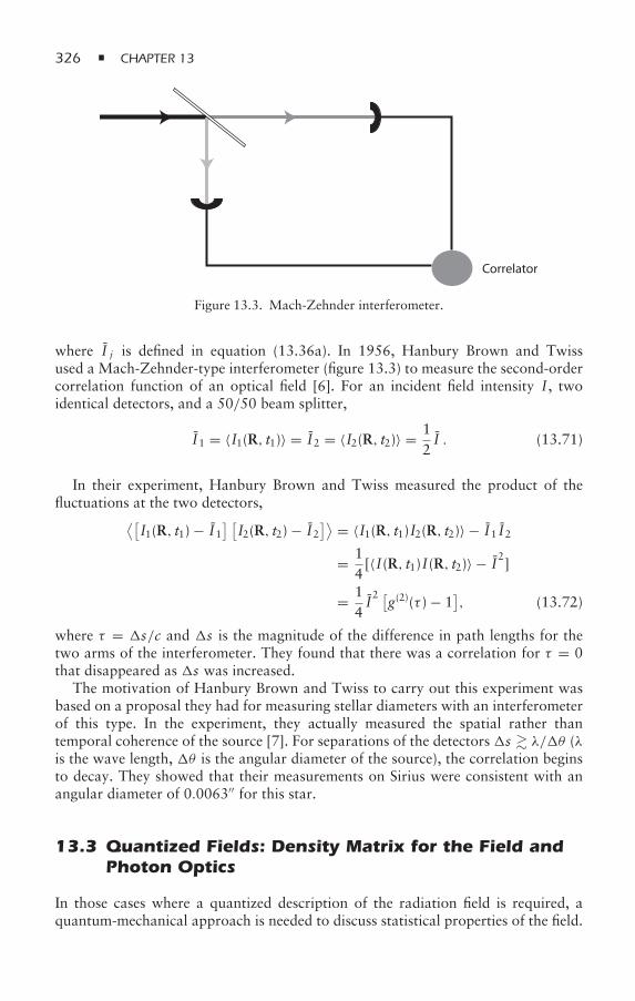
326 CHAPTER 13
Correlator
Figure 13.3. Mach-Zehnder interferometer.
where I j is defined in equation (13.36a). In 1956, Hanbury Brown and Twissused a Mach-Zehnder-type interferometer (figure 13.3) to measure the second-ordercorrelation function of an optical field [6]. For an incident field intensity I, twoidentical detectors, and a 50/50 beam splitter,
I1 = 〈I1(R, t1)〉 = I2 = 〈I2(R, t2)〉 = 12I . (13.71)
In their experiment, Hanbury Brown and Twiss measured the product of thefluctuations at the two detectors,⟨[
I1(R, t1) − I1] [I2(R, t2) − I2
]⟩ = 〈I1(R, t1)I2(R, t2)〉 − I1 I2
= 14[〈I(R, t1)I(R, t2)〉 − I
2]
= 14I2 [g(2)(τ ) − 1
], (13.72)
where τ = s/c and s is the magnitude of the difference in path lengths for thetwo arms of the interferometer. They found that there was a correlation for τ = 0that disappeared as s was increased.
The motivation of Hanbury Brown and Twiss to carry out this experiment wasbased on a proposal they had for measuring stellar diameters with an interferometerof this type. In the experiment, they actually measured the spatial rather thantemporal coherence of the source [7]. For separations of the detectors s λ/θ (λis the wave length, θ is the angular diameter of the source), the correlation beginsto decay. They showed that their measurements on Sirius were consistent with anangular diameter of 0.0063′′ for this star.
13.3 Quantized Fields: Density Matrix for the Field andPhoton Optics
In those cases where a quantized description of the radiation field is required, aquantum-mechanical approach is needed to discuss statistical properties of the field.
ELECTRIC FIELD COHERENCE PROPERTIES 327
Just as for atomic states, we can define a density matrix for field states. That is, wecan write
=∑
nm|n〉〈m|, (13.73)
in the n basis. Let us consider some possible quantized field states.
13.3.1 Coherent State
If the field is in a single-mode coherent state
|α〉 =∞∑n=0
αn√n!e− 1
2 |α|2 |n〉, (13.74)
density matrix elements are given by
nm = αnα∗m√n!m!
e−|α|2 , (13.75)
and the density matrix is not diagonal in the number basis. Of course, we couldequally well express the density matrix as a diagonal matrix in the coherent-statebasis,
= |α〉〈α|. (13.76)
Note that in the number-state basis,
Pn = nn = |α|2nn!
e−|α|2 (13.77)
represents a Poisson distribution, with
〈n〉 =∞∑n=0
nPn = |α|2 (13.78)
and
〈n2〉 =∞∑n=0
n2Pn = |α|4 + |α|2 . (13.79)
For a multimode coherent state,
= |α1α2 . . .〉〈α1α2 . . . |, (13.80)
or, in the number-state basis,
=N∏j=1
∞∑nj ,mj=0
αnjj
(αmj
j
)∗√nj !mj !
e−|α j |2 |nj 〉⟨mj
∣∣, (13.81)
where N is the number of modes.
328 CHAPTER 13
13.3.2 Thermal State
For a field in thermal equilibrium with some reservoir at temperature T,
= e−βH
Tr(e−βH), (13.82)
where β = 1/(kBT), and kB is Boltzmann’s constant. For a single-mode free field,H = ωLa†a, and
nm = 〈n|e−qa†a|m〉∑∞n=0〈n|e−qa†a|n〉
= e−nq∑∞n=0 e−nq δn,m = (1 − e−q)e−nqδn,m, (13.83)
where
q = ωLkBT
. (13.84)
The density matrix of a thermal state is diagonal in the number-state basis and canbe written as
=∑
Pn|n〉〈n|, (13.85)
where
Pn = (1 − e−q)e−nq (13.86)
is the probability for being in a state of n photons.The average number of photons in the thermal state is
n = 〈n〉 =∑n
nPn =∑n
n(1 − e−q)e−nq = −(1 − e−q)ddq
∑n
e−nq
= −(1 − e−q)ddq
11 − e−q = e−q
1 − e−q . (13.87)
Therefore,
e−q = n1 + n
, (13.88)
1 − e−q = 11 + n
, (13.89)
and
Pn = nn = 11 + n
(n
1 + n
)n
. (13.90)
ELECTRIC FIELD COHERENCE PROPERTIES 329
For a multimode thermal field,
=(∑
n1
Pn1 |n1〉〈n1|)(∑
n2
Pn2 |n2〉〈n2|). . .
(∑nk
Pnk|nk〉〈nk|)
=∑
n1n2...nk
|n1n2 . . .〉〈n1n2 . . . |∏k
Pnk . (13.91)
13.3.3 P(α) Distribution
Sometimes, it is convenient to expand the field density matrix in the coherent-statebasis rather than the number-state basis. The density matrix can be expanded interms of coherent states as
=∫
〈α||β〉|α〉〈β|d2αd2β, (13.92)
where d2α = dRe (α)d Im (α). Since the |α〉 are overcomplete, this expansion is notunique. On the other hand, owing to this property, it may be possible to find adiagonal representation in which
=∫
P(α′)|α′〉〈α′|d2α′, (13.93)
where P(α′) ≡ P(α′, α′∗). The distribution P(α) is not necessarily positive definite; ingeneral, it cannot be interpreted as the probability of being in state α. The usefulnessof this representation is that it becomes trivial to calculate the expectation value ofany operator that can be written in “normal” order with all a’s to right and a†’s toleft.
As a first step to obtain P(α), we write
(α) ≡ 〈α||α〉 =∫d2α′P(α′)|〈α′|α〉|2 =
∫d2α′P(α′)e−|α−α′ |2 , (13.94)
where is the density matrix in some arbitrary representation, and equation (12.57)was used. The problem is to find P(α), given and 〈α||α〉. With the substitutions
α = q + ip√2, (13.95a)
α′ = q′ + ip′√2
, (13.95b)
we can rewrite equation (13.94) as the integral equation
(q, p) =∫dq′dp′P(q′, p′)K(q − q′, p− p′), (13.96)
where the kernel K(q, p) is given by
K(q, p) = 12e− 1
2q2e− 1
2 p2. (13.97)
Since the kernel of this integral equation is a function of (q−q′) and (p− p′) only,it can be solved by integral transform techniques. Taking Fourier transforms of each
330 CHAPTER 13
side, we obtain a solution
(x,k) = 2π K(x,k)P(x,k), (13.98)
where the Fourier transforms are defined by
A(x,k) = 12π
∫ei(xp−kq)A(q, p)dqdp . (13.99)
Since the Fourier transform of the Gaussian function is also a Gaussian, we find
(x,k) = πe− 12 (x
2+k2) P(x,k), (13.100)
or
P(x,k) = 1πe
12 (x
2+k2)(x,k) . (13.101)
We can get P(α, α∗) by taking the inverse transform, if it exists [8]. Using thismethod, we can show that, for a thermal state,
P(α, α∗) = 1π n
e− |α|2n . (13.102)
13.3.4 Correlation Functions for the Field
We are now in a position to calculate the correlation functions analogous to thosecalculated for classical fields. It is convenient to use the Heisenberg representationfor operators.
13.3.4.1 First-order correlation function
The first-order correlation function is defined by
g(1)(R1, t1;R2, t2) ≡ 〈E−1 E
+2 〉√
〈E−1 E
+1 〉〈E−
2 E+2 〉, (13.103)
where 〈A〉 ≡ Tr (A), and
E±1 ≡ E±(R1, t1), E±
2 ≡ E±(R2, t2). (13.104)
13.3.4.1.1 Single-mode field: For a single-mode field having frequency ωL andpropagation vector k, the positive frequency component of the field operator is
E+ (R, t) = i√Ceiσ (R,t)a, (13.105)
where
σ (R, t) = k · R − ωLt (13.106)
and
C = ωL/(2ε0V). (13.107)
ELECTRIC FIELD COHERENCE PROPERTIES 331
It follows that
〈E−1 E
+1 〉 = CTr
(a†a
) = C∑n
nnn (13.108)
and
〈E−1 E
+2 〉 = Ceiσ21Tr
(a†a
) = Ceiσ21∑n
nnn, (13.109)
where
σ21 = k· (R2 − R1) − ωL (t2 − t1) . (13.110)
From the definition (13.103), we then find
g(1)(R1, t1;R2, t2) = eiσ21 , (13.111)
|g(1)(R1, t1;R2, t2)| = 1, (13.112)
and
g(1)(τ ) ≡ g(1)(R1, t1;R1, t1 + τ ) = e−iωLτ . (13.113)
Any single-mode field is first-order coherent since only a single frequency is present.That is, even a thermal single-mode field does not correspond to a field whose phasesfluctuate in time. It is closer to a filtered field or a field produced by oscillators withconstant random phases.
13.3.4.1.2 Multimode fields: In all cases, we take the modes to have the samepolarization and to propagate in the z direction.
13.3.4.1.2.1 Two-Photon State: The state vector is denoted by |〉 = |11〉, a singlephoton in each of two modes. The positive frequency component of the two-modefield is
E+ (Z, t) = i√C1a1eiσ1(Z,t) + i
√C2a2eiσ2(Z,t), (13.114)
where
σ j (Z, t) = kj Z− ω j t, Cj = ω j/(2ε0V) (13.115)
( j = 1,2). Reminiscent of equations (13.108) and (13.109), we find
〈E−1 E
+1 〉 = C1 + C2 (13.116)
and
〈E−1 E
+2 〉 = C1e−iω1τ + C1e−iω2τ , (13.117)
with τ = t2 − t1 − (Z2 − Z1)/c. Therefore,
g(1)(τ ) = C1e−iω1τ + C1e−iω2τ
C1 + C2, |g(1)(τ )| = 1 . (13.118)
As was the case for a superposition of two classical monochromatic fields, thetotal field is not first-order coherent. In the quantum case considered, however,
332 CHAPTER 13
the reason that |g(1)(τ )| = 1 is different than in the classical case. In the classicalcase, the fact that |g(1)(τ )| = 1 is a consequence of the definition of g(1)(τ ) in termsof a time average. In the quantum case, g(1)(τ ) is defined in terms of a quantum-mechanical average, not a time average. The fact that |g(1)(τ )| = 1 in the quantumcase can be traced to a state of the field in which the two modes are in pure numberstates, such that the relative phase of the two field modes is not well-defined, e.g.,〈11| a†
2a1|11〉 = 0.
13.3.4.1.2.2 Multimode coherent state: The positive frequency component of thefield is
E+ (Z, t) = i∑j
√Cja j eiσ j (Z,t), (13.119)
and the state vector for the field is
|〉 = |αk〉 = |α1α2 . . .〉. (13.120)
we find that
〈E−1 E
+1 〉 =
∑j j ′
√CjCj ′ei[σ j (1)−σ j ′ (1)]〈a†
j ′a j 〉 = |A1|2, (13.121)
where
A1 =∑j
√Cjα j eiσ j (1), (13.122)
and
σ j (n) = kj Zn − ω j tn, (13.123)
having used the fact that 〈a†j ′a j 〉 = α jα
∗j ′ . Moreover, it is a simple matter to show
that
〈E−1 E
+2 〉 = A∗
1A2, (13.124)
and therefore,
g(1)(τ ) = A∗1A2
|A1A2| ,∣∣g(1)(τ )∣∣ = 1 (13.125)
and the field is first-order coherent. This result differs from that for a classicalmultifrequency field. As noted earlier, the difference can be traced to the timeaverage taken in the classical case. In the quantum case, we are taking an ensembleaverage. Note that 〈E−
1 E+1 〉 = |A1|2 is a function of time for a multifrequency
quantized field.
13.3.4.1.2.3 Multimode thermal state: The density matrix for a multimode thermalstate is
=∑
n1,n2,...
|n1,n2, . . .〉〈n1,n2, . . . |∏k
P(nk), (13.126)
ELECTRIC FIELD COHERENCE PROPERTIES 333
where
P(nk) = (nk)nk
(1 + nk)1+nk . (13.127)
The average field intensity 〈E−1 E
+1 〉 = Tr
(E−
1 E+1
)can be calculated as
〈E−1 E
+1 〉 =
∑n1,n2,...
〈n1,n2, . . . |∏k
P(nk)√CjCj ′ei[σ j (1)−σ j ′ (1)]
×a†j ′a j |n1,n2, . . .〉, (13.128)
where σ j (1) is defined by equation (13.123). The terms in equation (13.128)contribute only if j = j ′; therefore,
〈E−1 E
+1 〉 =
∑n1,n2,...
∏k
P(nk)∑j
Cjn j
=∑
n1,n2,...
P(n1)P(n2) . . . (C1n1 + C2n2 + · · · )
=∑j
Cj n j . (13.129)
In a similar manner, we obtain
〈E−1 E
+2 〉 =
∑j
Cj n j ei[σ j (2)−σ j (1)], (13.130)
such that the first-order correlation function is
g(1)(τ ) =∑
j Cj n j e−iω j τ∑j Cj n j
=∑
j ω j n j e−iω j τ∑j ω j n j
, (13.131)
where τ = t2 − t1 − (Z2 − Z1)/c.In essence, ω j n j , properly normalized, gives the frequency distribution of the
modes. For example, if we set
ω j n j = N(ω)π
(ω − ωL)2 + 2, (13.132)
in which N(ω) is a slowly varying normalization factor that can be evaluated atω = ωL, treat ω j → ω as a continuous variable, and replace
∑j ⇒ 2πL/c
∫dω for
our one-dimensional modes, we obtain (for τ > 0)
g(1)(τ ) = e−iωLτ e−τ , (13.133)
in agreement with the classical phase diffusion or collision model in which the shiftS is neglected.
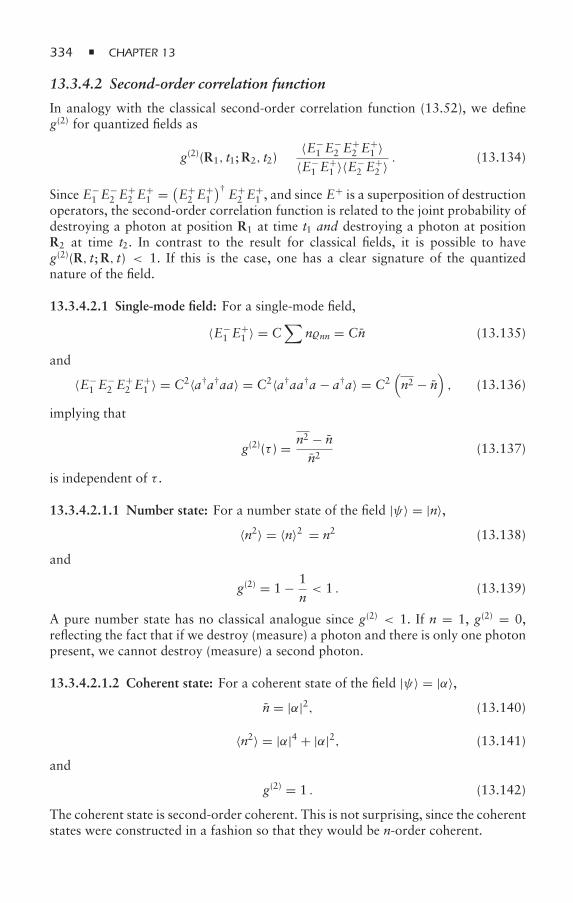
334 CHAPTER 13
13.3.4.2 Second-order correlation function
In analogy with the classical second-order correlation function (13.52), we defineg(2) for quantized fields as
g(2)(R1, t1;R2, t2) ≡ 〈E−1 E
−2 E
+2 E
+1 〉
〈E−1 E
+1 〉〈E−
2 E+2 〉 . (13.134)
Since E−1 E
−2 E
+2 E
+1 = (
E+2 E
+1
)†E+2 E
+1 , and since E+ is a superposition of destruction
operators, the second-order correlation function is related to the joint probability ofdestroying a photon at position R1 at time t1 and destroying a photon at positionR2 at time t2. In contrast to the result for classical fields, it is possible to haveg(2)(R, t;R, t) < 1. If this is the case, one has a clear signature of the quantizednature of the field.
13.3.4.2.1 Single-mode field: For a single-mode field,
〈E−1 E
+1 〉 = C
∑nnn = Cn (13.135)
and
〈E−1 E
−2 E
+2 E
+1 〉 = C2〈a†a†aa〉 = C2〈a†aa†a − a†a〉 = C2
(n2 − n
), (13.136)
implying that
g(2)(τ ) = n2 − nn2
(13.137)
is independent of τ .
13.3.4.2.1.1 Number state: For a number state of the field |ψ〉 = |n〉,〈n2〉 = 〈n〉2 = n2 (13.138)
and
g(2) = 1 − 1n< 1 . (13.139)
A pure number state has no classical analogue since g(2) < 1. If n = 1, g(2) = 0,reflecting the fact that if we destroy (measure) a photon and there is only one photonpresent, we cannot destroy (measure) a second photon.
13.3.4.2.1.2 Coherent state: For a coherent state of the field |ψ〉 = |α〉,n = |α|2, (13.140)
〈n2〉 = |α|4 + |α|2, (13.141)
and
g(2) = 1 . (13.142)
The coherent state is second-order coherent. This is not surprising, since the coherentstates were constructed in a fashion so that they would be n-order coherent.
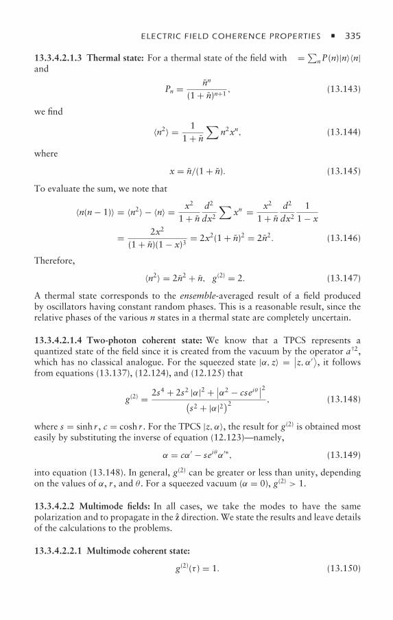
ELECTRIC FIELD COHERENCE PROPERTIES 335
13.3.4.2.1.3 Thermal state: For a thermal state of the field with = ∑nP(n)|n〉〈n|
and
Pn = nn
(1 + n)n+1, (13.143)
we find
〈n2〉 = 11 + n
∑n2xn, (13.144)
where
x = n/(1 + n). (13.145)
To evaluate the sum, we note that
〈n(n− 1)〉 = 〈n2〉 − 〈n〉 = x2
1 + nd2
dx2∑
xn = x2
1 + nd2
dx21
1 − x
= 2x2
(1 + n)(1 − x)3= 2x2(1 + n)2 = 2n2. (13.146)
Therefore,
〈n2〉 = 2n2 + n, g(2) = 2. (13.147)
A thermal state corresponds to the ensemble-averaged result of a field producedby oscillators having constant random phases. This is a reasonable result, since therelative phases of the various n states in a thermal state are completely uncertain.
13.3.4.2.1.4 Two-photon coherent state: We know that a TPCS represents aquantized state of the field since it is created from the vacuum by the operator a†2,which has no classical analogue. For the squeezed state |α, z〉 = ∣∣z, α′⟩, it followsfrom equations (13.137), (12.124), and (12.125) that
g(2) = 2s4 + 2s2 |α|2 + ∣∣α2 − cseiθ∣∣2(
s2 + |α|2)2 , (13.148)
where s = sinh r , c = cosh r . For the TPCS |z, α〉, the result for g(2) is obtained mosteasily by substituting the inverse of equation (12.123)—namely,
α = cα′ − seiθα′∗, (13.149)
into equation (13.148). In general, g(2) can be greater or less than unity, dependingon the values of α, r , and θ . For a squeezed vacuum (α = 0), g(2) > 1.
13.3.4.2.2 Multimode fields: In all cases, we take the modes to have the samepolarization and to propagate in the z direction. We state the results and leave detailsof the calculations to the problems.
13.3.4.2.2.1 Multimode coherent state:
g(2)(τ ) = 1. (13.150)
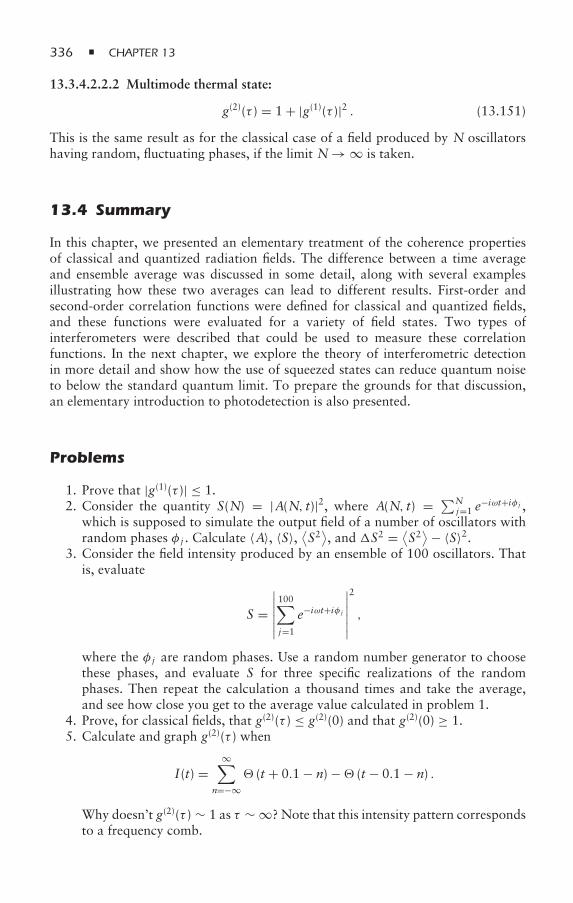
336 CHAPTER 13
13.3.4.2.2.2 Multimode thermal state:
g(2)(τ ) = 1 + |g(1)(τ )|2 . (13.151)
This is the same result as for the classical case of a field produced by N oscillatorshaving random, fluctuating phases, if the limit N→ ∞ is taken.
13.4 Summary
In this chapter, we presented an elementary treatment of the coherence propertiesof classical and quantized radiation fields. The difference between a time averageand ensemble average was discussed in some detail, along with several examplesillustrating how these two averages can lead to different results. First-order andsecond-order correlation functions were defined for classical and quantized fields,and these functions were evaluated for a variety of field states. Two types ofinterferometers were described that could be used to measure these correlationfunctions. In the next chapter, we explore the theory of interferometric detectionin more detail and show how the use of squeezed states can reduce quantum noiseto below the standard quantum limit. To prepare the grounds for that discussion,an elementary introduction to photodetection is also presented.
Problems
1. Prove that |g(1)(τ )| ≤ 1.2. Consider the quantity S(N) = |A(N, t)|2, where A(N, t) = ∑N
j=1 e−iωt+iφ j ,
which is supposed to simulate the output field of a number of oscillators withrandom phases φ j . Calculate 〈A〉, 〈S〉, ⟨S2⟩, and S2 = ⟨
S2⟩− 〈S〉2.
3. Consider the field intensity produced by an ensemble of 100 oscillators. Thatis, evaluate
S =∣∣∣∣∣∣100∑j=1
e−iωt+iφ j
∣∣∣∣∣∣2
,
where the φ j are random phases. Use a random number generator to choosethese phases, and evaluate S for three specific realizations of the randomphases. Then repeat the calculation a thousand times and take the average,and see how close you get to the average value calculated in problem 1.
4. Prove, for classical fields, that g(2)(τ ) ≤ g(2)(0) and that g(2)(0) ≥ 1.5. Calculate and graph g(2)(τ ) when
I(t) =∞∑
n=−∞ (t + 0.1 − n) − (t − 0.1 − n) .
Why doesn’t g(2)(τ ) ∼ 1 as τ ∼ ∞? Note that this intensity pattern correspondsto a frequency comb.
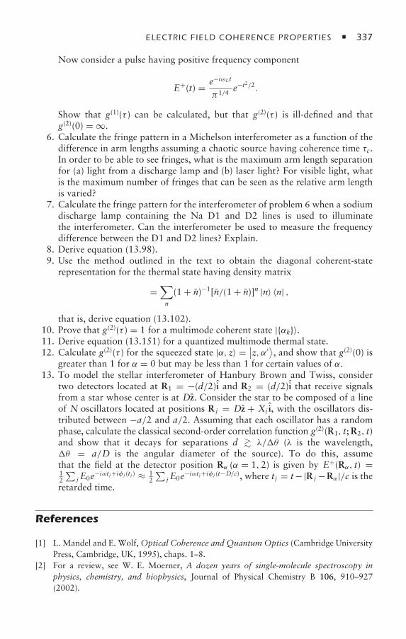
ELECTRIC FIELD COHERENCE PROPERTIES 337
Now consider a pulse having positive frequency component
E+(t) = e−iωLt
π1/4e−t2/2.
Show that g(1)(τ ) can be calculated, but that g(2)(τ ) is ill-defined and thatg(2)(0) = ∞.
6. Calculate the fringe pattern in a Michelson interferometer as a function of thedifference in arm lengths assuming a chaotic source having coherence time τc.In order to be able to see fringes, what is the maximum arm length separationfor (a) light from a discharge lamp and (b) laser light? For visible light, whatis the maximum number of fringes that can be seen as the relative arm lengthis varied?
7. Calculate the fringe pattern for the interferometer of problem 6 when a sodiumdischarge lamp containing the Na D1 and D2 lines is used to illuminatethe interferometer. Can the interferometer be used to measure the frequencydifference between the D1 and D2 lines? Explain.
8. Derive equation (13.98).9. Use the method outlined in the text to obtain the diagonal coherent-state
representation for the thermal state having density matrix
=∑n
(1 + n)−1[n/(1 + n)]n |n〉 〈n| ,
that is, derive equation (13.102).10. Prove that g(2)(τ ) = 1 for a multimode coherent state |αk〉.11. Derive equation (13.151) for a quantized multimode thermal state.12. Calculate g(2)(τ ) for the squeezed state |α, z〉 = ∣∣z, α′⟩, and show that g(2)(0) is
greater than 1 for α = 0 but may be less than 1 for certain values of α.13. To model the stellar interferometer of Hanbury Brown and Twiss, consider
two detectors located at R1 = −(d/2)i and R2 = (d/2)i that receive signalsfrom a star whose center is at Dz. Consider the star to be composed of a lineof N oscillators located at positions R j = Dz + Xj i, with the oscillators dis-tributed between −a/2 and a/2. Assuming that each oscillator has a randomphase, calculate the classical second-order correlation function g(2)(R1, t;R2, t)and show that it decays for separations d λ/θ (λ is the wavelength,θ = a/D is the angular diameter of the source). To do this, assumethat the field at the detector position Rα (α = 1,2) is given by E+(Rα, t) =12
∑j E0e−iωtj+iφ j (tj ) ≈ 1
2
∑j E0e−iωtj+iφ j (t−D/c), where tj = t−|R j −Rα|/c is the
retarded time.
References
[1] L. Mandel and E. Wolf,Optical Coherence and Quantum Optics (Cambridge UniversityPress, Cambridge, UK, 1995), chaps. 1–8.
[2] For a review, see W. E. Moerner, A dozen years of single-molecule spectroscopy inphysics, chemistry, and biophysics, Journal of Physical Chemistry B 106, 910–927(2002).

338 CHAPTER 13
[3] J. D. Jackson, Classical Electrodynamics, 3rd ed. (Wiley, New York, 1999), sec. 10.5.[4] A. Sommerfeld, Optics (Academic Press, New York, 1964), chaps. V and VI.[5] See, for example, S. Chopra and L. Mandel, Higher-order correlation properties of a
laser beam, Physical Review Lettters 30, 60–63 (1973).[6] R. Hanbury Brown and R. Q. Twiss, Correlation between photons in two coherent
beams of light, Nature 177, 27–29 (1956).[7] R. Hanbury Brown and R. Q. Twiss, A test of a new type of stellar interferometer,
Nature 178, 1046–1048 (1956).[8] H. Nussenzveig, Introduction to Quantum Optics (Gordon and Breach, London, 1973),
secs. 3.3 and 3.4.
Bibliography
See the books on quantum optics listed in chapter 1.
14Photon Counting and Interferometry
14.1 Photodetection
In quantum mechanics, there is no way to avoid the measurement problem. Thatis, although quantum mechanics represents an incredibly successful theory of matterand of matter–field interactions, it does not provide a prescription for coupling thequantum-mechanical system of interest to a classical measuring apparatus. Quantummechanics enables one to make predictions for the outcome of measurements buthas very little to say about the measurements themselves. In this chapter, we givea very elementary discussion of photodetection and discuss some applications tointerferometry. There are chapters in most quantum optics textbooks on this topic,and you are urged to consult these texts for more details. Suffice it to say, however,that the theory of photodetection and photodetectors is far from complete.
One simple model for a photodetector is an optically thick medium consistingof inhomogeneously broadened two-level atoms. If we consider a time that issufficiently short, any radiation incident on such a medium is absorbed by the atomsand is not scattered into other modes of the vacuum field. In contrast to the scatteringprocess that we have been discussing throughout this text, this is true absorption.If the inhomogeneous width is sufficiently large, the medium acts as a broadbanddetector. The excited-state population can be used as a measure of the “numberof photons” absorbed in the medium. Of course, we need to specify some way inwhich this excited-state population is measured. Let us not worry about this. Inmost theories of photodetection, the “excited state” of the atoms is actually thecontinuum, and the ejected electron is assumed to produce a measurable signal.
You can appreciate why the theory of photodetection is complicated. Imaginethat we have some initial field pulse that is heading toward the detector. If we knowthe quantum state of this field, we have a well-defined quantum-mechanical problemin which the atoms in the detector are all in their ground states and the field stateis specified. In principle, we can calculate the state of the system at any future timeand obtain the probability to have n atoms excited in the detector. The problem isthat, in an ideal photodetector, each time an atom is excited, it leads to a measurablesignal, which implies that the quantum state of the system is modified. Somehow,
340 CHAPTER 14
this measurement must be fed back into the system and the quantum state of thesystem updated. Although there are theories of continuous measurement [1] thataddress questions of this nature, quantum mechanics runs into problems once themeasuring apparatus is included in the system being studied.
14.1.1 Photodetection of Classical Fields
Let us assume that the probability of photo-emission in the detector is proportionalto the intensity I(t) = |E+(t)|2 of an incident classical field, integrated over thesurface of the detector. Since a photodetector is a quantum device, there are alwaysquantum fluctuations in the number of “counts” registered by a photodetector. Thatis, if we prepare the same classical pulse and send it into a detector several times,the number of photo-counts recorded each time will differ. For a given incident fieldintensity, we can define Pm(t, τ ) as the probability of registering m counts in a timebetween t and (t + τ ). We assume that τ > 0.
We can calculate Pm(t, τ ) in much the same way that we calculated the correlationfunction for collisions—that is, we assume that we can choose a δτ sufficiently shortto guarantee that at most one photo-count occurs in δτ , but sufficiently long toensure that a “complete” photo-count occurs (in other words, δτ is much greaterthan the response time of the photodetector). This is reminiscent of the impactapproximation used to examine the role of collisions on line shapes.
With these approximations, we can write
Pm(t, τ + δτ ) = P0(t + τ, δτ )Pm(t, τ ) + P1(t, δτ )Pm−1(t, τ ), (14.1)
where P0(t, δτ ) is the probability for no counts in a time between t and (t + δτ ), andP1(t, δτ ) is the probability of one count in that interval. Let p(t) be the probabilityper unit time that a photo-count occurs at time t. We assume that p(t) is proportionalto the field intensity,
p(t) = µI(t), (14.2)
where µ is related to the detector efficiency. As a consequence,
P1(t, δτ ) = p(t)δτ = µI(t)δτ. (14.3)
Equation (14.1) can be rewritten as
Pm(t, τ ) + dPm(t, τ )dτ
dτ = [1 − p(t + τ )dτ ] Pm(t, τ ) + p(t + τ )dτ Pm−1(t, τ ), (14.4)
or
dPm(t, τ )dτ
= −p(t + τ )Pm(t, τ ) + p(t + τ )Pm−1(t, τ ). (14.5)
For m= 0,
dP0(t, τ )dτ
= −p(t + τ )P0(t, τ ), (14.6)
and P0(t,0) = 1. Therefore,
P0(t, τ ) = e− ∫ τ0 p(t+τ ′)dτ ′ = e−µ ∫ t+τt I(t′)dt′ ≡ e−µI(t,T)T, (14.7)
PHOTON COUNTING AND INTERFEROMETRY 341
where
I(t, τ ) ≡ 1τ
∫ t+τ
tI(t′)dt′. (14.8)
If we try a solution to equation (14.5) of the form
Pm(t, τ ) = Pm(t, τ )e− ∫ τ0 p(t+τ ′)dτ ′, (14.9)
with Pm(t,0) = 1, then [see equation (14.7)]
P0(t, τ ) = 1, (14.10)
and, for m> 0, Pm(t, τ ), satisfies the differential equation
dPm(t, τ )dτ
= p(t + τ )Pm−1(t, τ ). (14.11)
Therefore,
P1(t, τ ) =∫ τ
0p(t + τ ′)dτ ′ =
∫ t+τ
tp(t′)dt′, (14.12)
P2(t, τ ) =∫ t+τ
tdt′
∫ t+t′
tdt′′p(t′)p(t′′), (14.13)
and so on.Recall that, for functions f (t), the time-ordered exponential T e
∫ t0 f (t′)dt′ and the
exponential e∫ t0 f (t′)dt′ are identical, as we have already noted in chapter 2. Since each
of the Pm(t, τ ) represent terms in the expansion of the time-ordered exponentialT e∫ t+τt p(t′)dt′′ = e
∫ t+τt p(t′)dt′′ , we conclude that
Pm(t, τ ) = 1m!
[∫ t+τ
tp(t′)dt′
]m= 1m!
[µI(t, τ )τ ]m , (14.14)
where I(t, τ ) is defined by equation (14.8). Combining this result with equa-tion (14.9), we obtain
Pm(t, τ ) = 1m!
[µI(t, τ )τ ]m e−µI(t,τ )τ. (14.15)
If a radiation pulse is incident on the detector, then it is clear that Pm(t, τ ) dependson t, insofar as the pulse envelope is a function of t. For continuous fields that can beconsidered to be stationary (that is, their noise properties do not change in time), it iscustomary to define a photo-count distribution that is averaged over time—namely,
Pm(τ ) = 〈Pm(t, τ )〉t . (14.16)
Unless noted otherwise, we limit our discussions to stationary fields.If I(t, τ ) = I is constant, as would be the case for a monochromatic field, then
Pm(τ ) = Xm
m!e−X , (14.17)
342 CHAPTER 14
where
X= µIτ. (14.18)
Even for a constant field intensity, there is a distribution of photo-counts, owingto the statistical nature of the quantum-mechanical detection mechanism. Thedistribution (14.17) is a Poisson distribution, with m = X, m2 = m2 + m,m2 = m, and m/m ∼ 1/
√m. The unavoidable noise that is associated with
the photodetection process is referred to as shot noise.When the field itself has noise properties, the signal recorded by a photodetector
reflects both the noise properties of the field and that of the detector. If the responsetime of the detector is longer than the correlation time of the field, the detectionprocess tends to average out the noise properties of the field. We consider only theopposite limit, in which the integral in equation (14.8) is carried out for a time τ thatis short compared with the correlation time of the field intensity, but sufficiently longto contain a large number of counts. In this limit, I(t, τ ) given by equation (14.8), isequal to I(t).
The noise properties of the field can be attributed to the noise properties of thesources of the field. If a sufficiently large number of successive measurements istaken at the photodetector, the time average of these measurements is equivalent toan ensemble average over the sources, such that the photo-count distribution, givenby equations (14.15) and (14.16), is
Pm(τ ) = 1m!
⟨(µIτ )m e−µIτ⟩ , (14.19)
where the average now corresponds to an ensemble average over the sources of thefield.
We can characterize the signal by the number of photo-counts m(τ ) in a timeinterval τ and the variance of this quantity. The average number of counts isgiven by
m(τ ) =⟨∑
m
mPm(t, τ )
⟩= µ 〈I〉 τ (14.20)
and the second moment by
m2(τ ) = µ2 ⟨I2⟩ τ 2 + µ 〈I〉 τ, (14.21)
such that
m2(τ ) = µ 〈I〉 τ + µ2τ 2[〈I2〉 − 〈I〉2] . (14.22)
Thus, fluctuations in number count have a contribution from shot noise, µ 〈I〉 τ ,and one from field fluctuations, µ2τ 2[〈I2〉 − 〈I〉2]. The shot noise can be reduced byincreasing the counting statistics.
For constant field intensity,
m2(τ ) = µ 〈I〉 τ = m(τ ), (14.23)
PHOTON COUNTING AND INTERFEROMETRY 343
as was found earlier. For a field produced by sources having fluctuating phases,
E+(t) = 12
|E0|N∑j=1
e−iωLt+iφ j (t), (14.24)
〈I〉 = 14N |E0|2 , (14.25)
〈I2〉 = 116
(2N2 − N
) |E0|4 , (14.26)
such that
m2(τ ) = [4µNτ |E0|2 + µ2τ 2
(N2 − N
) |E0|4]/16. (14.27)
The shot noise and source noise fluctuations can be distinguished by their τdependence.
In the limit of large N, the moments for the phase diffusion model areapproximately given by 〈In〉 = n!(N |E0|2/4)n, which is consistent with a Poissonintensity distribution
P(I) = 1
Ie−I/ I , (14.28)
where I = N |E0|2/4. In this approximation, the photo-count distribution (14.19)can be evaluated as
Pm(τ ) =∫ ∞
0dI
1m!
P(I) (µIτ )m e−µIτ
= [m(τ )]m
[m(τ )] + 1m+1 , (14.29)
where m(τ ) = µ Iτ . This is a scaled version of the photon number distribution fora thermal source. You will see that this result is typical when the sampling time ismuch shorter than the correlation time of the field—the photon counting statistics isa scaled version of the photon number distribution, the scaling factor depending onthe detector efficiency µ and counting time τ .
14.1.2 Photodetection of Quantized Fields
As we mentioned, the problem of photodetection of quantized fields is a complexone, since the measurement process itself modifies the field. We shall neglect suchcomplications for the most part and assume that the signal at the detectors isproportional to ⟨
E−(Rd, t)E+(Rd, t)⟩ = Tr[E−(Rd, t)E+(Rd, t)], (14.30)
where is the density matrix for the field, and the bar indicates an average over thesurface Rd of the detector. In other words, the signal is assumed to be proportionalto the average value of the intensity operator, averaged over the surface of thedetector. Moreover, we assume that the field is uniform over the detector andsuppress the field label Rd. Of course, this procedure is oversimplified, since no
344 CHAPTER 14
detector has an instantaneous response. In actual cases involving rapid changes inE−(Rd, t)E+(Rd, t), the correlation time of the detector must be taken into account.
For a quantized radiation field, one must destroy m photons in the field to get mphoto-counts. The probability for m photo-counts depends on averages of the form⟨|E+(tm)E+(tm−1) . . . |2
⟩ = ⟨E−(t1)E−(t2) . . . E−(tm)E+(tm) . . . E+(t2)E+(t1)
⟩.
That is, all E+’s appear to the right, in what is called normal order. The calculationproceeds much as in the classical field case, except that one must now account forthe fact that the intensity is an operator and that the photo-count distribution mustinvolve the field operators taken in normal order.
A formal expression for the photo-count probability distribution can be takenas [2]
Pm(t, τ ) = Tr
N
[µ I(t, τ )τ ]m
m!e−µ I(t,τ )τ
, (14.31)
where
I(t, τ ) ≡ 1τ
∫ t+τ
tE−(t′)E+(t′)dt′ , (14.32)
and N is a “normal order” operator that moves all E+’s in the expansion to theright. As in any operator equation, the exponential function is defined by its seriesexpansion. The fields are to be evaluated at the detector surface. At this point, weconsider single-mode fields only, for which
E+(R, t) ∼ i(ω
2ε0V
)1/2
aei(k·R−ωt) (14.33)
and
Pm(τ ) = Tr[N
(ξa†a)m
m!e−ξa†a
], (14.34)
where
ξ = µ
(ω
2ε0V
)τ (14.35)
is known as the quantum efficiency of the detector.If we expand the exponential and orders the resulting operators in normal order,
we find
Pm(τ ) = Tr
⎡⎣
∞∑q=0
(−ξ )qξm(a†)m+qam+q
m!q!
⎤⎦ . (14.36)
In the n-representation, where
=∑n,n′nn′ |n〉 〈n′|, (14.37)
it is easy to show that only diagonal terms enter into the expression (14.36) forPm(τ ), since matrix elements of the form 〈n′|(a†)m+qam+q |n〉 are needed. Moreover,
PHOTON COUNTING AND INTERFEROMETRY 345
it is obvious that one must have m+ q < n, which is satisfied for n > m, q < n−m.Since
am+q|n〉 =√n(n− 1) . . . [n− (m+ q)]|0〉, (14.38)
it follows from equations (14.36) to (14.38) that
Pm(τ ) =∞∑n=m
n−m∑q=0
Pn(−ξ )qξmm!q!
n!(n−m− q)!
=∞∑n=m
Pn
(nm
)ξm(1 − ξ )n−m , (14.39)
where
Pn = nn, (14.40)
(nm
)= n!m! (n−m)!
(14.41)
is a binomial coefficient, and we used the fact that
p∑q=0
(−a)qq!(p− q)!
=p∑
q=0
(pq
)(−a)qp!
= (1 − a)p
p!. (14.42)
We can now evaluate Pm(τ ) for various quantized states of the field.
14.1.2.1 Coherent state
For a coherent state |α〉, is not diagonal, but only diagonal elements,
Pn = nn
n!e−n = |α|2n
n!e−|α|2 , (14.43)
are of importance in the photo-count distribution. From equation (14.39), we find
Pm(τ ) = (ξ n)m
m!e−ξm . (14.44)
The photo-count distribution is just a scaled version of the photon numberdistribution.
14.1.2.2 Thermal state
For a thermal state with
Pn = nn
(1 + n)1+n , (14.45)
we find
Pm(τ ) = (ξ n)m
(1 + ξ n)1+m . (14.46)
Again, the photo-count distribution is just a scaled version of the photon numberdistribution.
346 CHAPTER 14
14.1.2.3 Number state
For the number state |q〉,Pn = δq,n, (14.47)
and
Pm(τ ) =(p
q
)ξm(1 − ξ )q−m , if m≤ q,
0, if m> q.(14.48)
In this case, the photo-count distribution, which is simply a binomial distribution form≤ q, is no longer a scaled version of the photon number distribution. Of course, itis clear that our assumption that the measurement does not affect the quantum stateof the field cannot remain valid here; if q photons are detected, there cannot be anyfield left.
One can also relate the photo-count distribution to the second-order correlationfunction for a single-mode field. (The magnitude of the first-order correlationfunction is unity.) From equations (13.137) and (14.39), we find
∑m
m(m− 1)Pm(τ )m2
=∑n
n(n− 1)Pnn2
= g(2)(τ ). (14.49)
Moreover, for the photo-count distribution (14.39), it is straightforward to calculate
m= ξ n , (14.50a)
m2 = ξ n+ ξ2(n2 − n
), (14.50b)
m2 = ξ2n2 + ξ n (1 − ξ ) =(mn
)2
n2 + m(1 − m
n
). (14.50c)
For an ideal detector, ξ = 1 and m2 = n2.
14.2 Michelson Interferometer
Photodetectors are often used as the measuring devices in optical interferometers.The general configuration of an interferometer involves a beam splitter that dividesan incoming field along two paths. After traversing different paths, the beams arerecombined on a detector. The interference pattern is measured as the optical pathlength between the two arms of the interferometer is varied. Phase changes betweenthe two arms translate into fringe shifts at the detector. The optical path lengthbetween the two arms can result in a number of ways. One can physically changethe path length by using a micrometer screw or a piezoelectric transducer. Moreoften, one uses the interferometer to monitor changes in optical paths resulting fromsome transitory effect such as a gravitational wave (not so easy to measure), theintroduction of a transparent test body into one of the arms, or a difference in thevelocity of light in the two arms owing to an “ether drift” (as in the Michelson-Morley experiment).
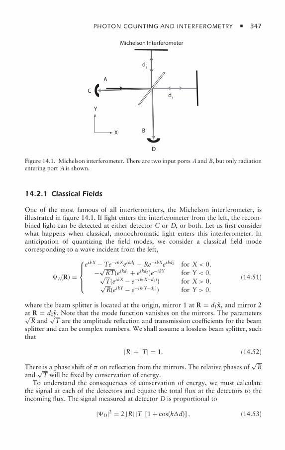
PHOTON COUNTING AND INTERFEROMETRY 347
Y
X
C
A
D
B
d1
d2
Michelson Interferometer
Figure 14.1. Michelson interferometer. There are two input ports Aand B, but only radiationentering port A is shown.
14.2.1 Classical Fields
One of the most famous of all interferometers, the Michelson interferometer, isillustrated in figure 14.1. If light enters the interferometer from the left, the recom-bined light can be detected at either detector C or D, or both. Let us first considerwhat happens when classical, monochromatic light enters this interferometer. Inanticipation of quantizing the field modes, we consider a classical field modecorresponding to a wave incident from the left,
A(R) =
⎧⎪⎪⎨⎪⎪⎩eikX − Te−ikXeikd1 − Re−ikXeikd2 for X< 0,
−√RT(eikd1 + eikd2 )e−ikY for Y < 0,√T(eikX − e−ik(X−d1)) for X> 0,√R(eikY − e−ik(Y−d2)) for Y > 0,
(14.51)
where the beam splitter is located at the origin, mirror 1 at R = d1x, and mirror 2at R = d2y. Note that the mode function vanishes on the mirrors. The parameters√R and
√T are the amplitude reflection and transmission coefficients for the beam
splitter and can be complex numbers. We shall assume a lossless beam splitter, suchthat
|R| + |T| = 1. (14.52)
There is a phase shift of π on reflection from the mirrors. The relative phases of√R
and√T will be fixed by conservation of energy.
To understand the consequences of conservation of energy, we must calculatethe signal at each of the detectors and equate the total flux at the detectors to theincoming flux. The signal measured at detector D is proportional to
|D|2 = 2 |R| |T| [1 + cos(kd)] , (14.53)
348 CHAPTER 14
where
d = d2 − d1, (14.54)
and the signal at detector C is proportional to
|C|2 = |R|2 + |T|2 + RT∗eikd + R∗Te−ikd. (14.55)
Since (|R| + |T|)2 = 1, this equation can be transformed into
|C|2 = 1 − 2 |R| |T| + RT∗eikd + R∗Te−ikd. (14.56)
By equating the total flux striking the detectors to the incident flux, |D|2+|C|2=1,we obtain the condition
eikd(|R| |T| + RT∗) + e−ikd(|R| |T| + R∗T) = 0. (14.57)
If we set
R= |R| e2iφR, (14.58a)
T = |T| e2iφT , (14.58b)
condition (14.57) implies that
φT − φR = ±π/2 . (14.59)
This is a general result for any lossless beam splitter; the relative phase ofthe (amplitude) transmission and reflection coefficients is π/2. Without loss ofgenerality, we take φT = 0, φR = π/2, such that
√R= i
√|R| ,
√T =
√|T|. (14.60)
If
φ ≡ 2kd (14.61)
is defined as the optical path difference for the two arms of the interferometer andif equation (14.60) is used, it follows that equations (14.53) and (14.56) can berewritten in the form
|D|2 = 4 |R| |T| cos2(φ
4
), (14.62a)
|C|2 = 1 − 4 |R| |T| cos2(φ
4
). (14.62b)
The asymmetry in the signals at the two detectors arises from the fact that the signalreaching detector C is the sum of two field components, one of which is reflectedtwice at the beam splitter and the other is transmitted twice at the beam splitter,while the signal at detector D is the sum of two field components, both of which arereflected once at the beam splitter and transmitted once at the beam splitter.
Fringe maxima and minima occur when φ = 2nπ , for integer n. To achievemaximum sensitivity to small phase shifts, one needs to choose a region where theslope of the signal is a maximum with respect to changes in φ. Moreover, to helpreduce the effects of any fluctuations in the incident fields on the signals, one can
PHOTON COUNTING AND INTERFEROMETRY 349
subtract the signals at the two detectors. The difference signal is proportional to aquantity S defined by
S = |E+A|2 (|D|2 − |C|2)
= |E+A|2 [4 |R| |T| cos(φ/2) + 4 |R| |T| − 1], (14.63)
where |E+A|2 is proportional to the incident field intensity. In the examples to follow,
we will always assume a 50/50 beam splitter with |R| = |T| = 1/2; in this limit,
S = |E+A|2 cos(φ/2) . (14.64)
The signal vanishes when φ/2 = (n + 1/2)π , which also corresponds to themaximum slope of the signal as a function of φ. If one adjusts the arm lengthsof the interferometer such that φ/2 = (n+ 1/2)π + δφ with |δφ| 1,
S ≈ ±|E+A|2δφ, (14.65)
the signal is linearly proportional to δφ. For a classical coherent field, the sensitivityis limited only by shot noise.
14.2.2 Quantized Fields
It is not difficult to go over to the quantized field case if we use the prescriptionmentioned in chapter 12—that is, we write the Hamiltonian for a single-modefield as
H = ω|A(R)|2a†AaA , (14.66)
where aA is a destruction operator for this mode. This method is especially good forconsidering an infinite number of modes (as is needed for the vacuum field), but welimit the discussion to a single mode.
Several new features enter when we consider quantized rather than classicalfields. First, there is the annoying but persistent problem that measurement ofthe field invariably modifies the quantum state of the field. Thus, if one wantsto start with quantum states of the field corresponding to single- or two-photonpulses, some care in modeling the photodetectors is needed. Second, there areinvariably number-state fluctuations for a quantum field, except for those preparedin a pure number state. This can translate into scaled photo-count distributions,as was discussed earlier. However, there can be an additional contribution to thesignal noise resulting from fluctuations in the difference in “photon number” ineach arm of the interferometer—this contribution is absent for classical fields. Weconcentrate on formulating a theory that can be used to illustrate the manner inwhich squeezed light can be used to reduce signal noise, but the formalism is alsouseful for understanding the contributions to the signal at a given detector.
The starting point of the calculation is the expression for the positive frequencycomponent of the electric field amplitude,
E+ = i(ω
2ε0V
) 12
A(R)aA . (14.67)
350 CHAPTER 14
Most of the results for the classical field can be taken over directly to the quantizedfield case. In all cases, we assume a 50/50 beam splitter.
14.2.2.1 Signal at detector D
The generalization of equation (14.62a) for the field intensity operator at detectorD is
ID = E−(RD, t)E+(RD, t) cos2(φ/4). (14.68)
Assuming stationary fields, we can calculate the photo-count distribution in the samemanner as we did in going from equations (14.31) to (14.50). The only differenceis that the detector efficiency ξ is replaced by ξ cos2(φ/4). That is, equations (14.50)remain valid provided that ξ is replaced by ξ cos2(φ/4).
As a consequence,
m2 =(mn
)2
n2 + m(1 − m
n
), (14.69)
with
m= ξ n cos2 (φ/4) . (14.70)
For different incident field states, we find
m2 =
⎧⎪⎪⎨⎪⎪⎩m(1 − m
n
)number state,
m coherent state,
m (1 + m) thermal state.
(14.71)
The fluctuations for a pure number state are lower than that for a coherent state;this is sometimes referred to as number-state squeezing.
Notice that both the signal and the fluctuations vanish at the minima for a 50/50beam splitter, since there is total interference at the detector. (Of course, when thesignal vanishes at detector D, it is a maximum at detector C.) The absence of anyfluctuations at these points can be traced to the fact that we are dealing with a single-mode field. For a multimode field, there is a distribution of k’s, and it is impossible tosatisfy the condition for signal maxima or minima simultaneously for all modes. Thefirst term in equation (14.69) represents scaled fluctuations. For an ideal detector,m = n cos2(φ/4), and the second term can be interpreted as a fluctuation due toa difference in “photon number” in each arm of the interferometer [2]; this termvanishes at both signal maxima and minima (recall that a maximum at one detectoris a minimum at the other) since there is total interference at such points.
14.2.2.2 Correlated signals at both detectors: difference photo-countsignal
In this section, we want to illustrate the concept of correlated measurements andto calculate the probability of observing a photo-count at both detectors C andD. Moreover, to prepare for calculations involving more than one input field, weobtain expressions for the average number of photo-counts and their fluctuations
PHOTON COUNTING AND INTERFEROMETRY 351
in terms of the field operators at each detector. To simplify matters, we assumethat the detector efficiency is equal to unity. For an ideal detector (ξ = 1), theaverage number of counts at detector D and its variance can be obtained fromequations (14.70) and (14.69) as
mD = cos2(φ/4)n = cos2(φ/4)⟨a†a
⟩, (14.72a)
m2D = cos2(φ/4)n+ cos4 (φ/4)
(n2 − n
)= cos2(φ/4)
⟨a†a
⟩+ cos4(φ/4)⟨a†a†aa
⟩. (14.72b)
We can re-express these quantities in terms of the field operators acting at detectorD by
mD = 1K
⟨E−DE
+D
⟩, (14.73a)
m2D = 1
K
⟨E−DE
+D
⟩+ 1K2
⟨E−DE
−DE
+DE
+D
⟩, (14.73b)
where K = ω/(2ε0V). In an analogous manner, the corresponding expressions fordetector C are
mC = 1K
⟨E−C E
+C
⟩, (14.74a)
m2C = 1
K
⟨E−C E
+C
⟩+ 1K2
⟨E−C E
−C E
+C E
+C
⟩. (14.74b)
There is one additional quantity we need to calculate, the joint probability ofmeasuringmC counts at detector C and mD counts at detector D—that is,mCmD [3].Since this corresponds to the simultaneous destruction of mC photons at detector Cand mD photons at detector D, the joint probability distribution must correspond toa time-ordered expression involving
(E+C E
+D
)†E+C E
+D. We will assume that [3]
mCmD = mDmC = sin2(φ/4) cos2(φ/4)⟨a†a†aa
⟩ = 1K2
⟨E−DE
−C E
+C E
+D
⟩. (14.75)
To show that these definitions are reasonable, let us calculate the expectationvalues of these operators for a single-photon state of the field, having the spatialmode defined by equation (14.51), such that
E+C = −
√Ke2ie−ikX sin(φ/4) a, (14.76a)
E+D =
√Ke2ie−ikY cos(φ/4) a, (14.76b)
where
= k(d1 + d2)/4. (14.77)
Although there are problems with measurement of a one-photon state since themeasurement destroys the state, the probabilities for photodetection of such statescan be calculated using standard procedures. In practice, one requires a multimodefield to get a one-photon pulse, but we neglect such complications.
352 CHAPTER 14
For a one-photon state |1〉 having field mode (14.51), we can use equa-tions (14.74a), (14.73a), (14.75), and (14.76) to obtain
mC = sin2(φ/4), mD = cos2(φ/4), (14.78)
and
mCmD = sin2(φ/4) cos2(φ/4)⟨a†a†aa
⟩ = 0. (14.79)
The one photon can be detected in either detector, but it is (obviously) impossible tomeasure a count at both detectors C and D for a one-photon field.
As in the case of classical fields, one can maximize the detection sensitivity tosmall phase changes by measuring the difference signal from the two detectors. Wewill assume that the photo-current distributions are proportional to the photo-countdistributions. Let S = MD − MC, where Mα is the photo-count operator at detectorα, defined in such a manner that 〈Mα〉 = mα and 〈MCMD〉 = mCmD. Then, theaverage difference signal and its variance are given by
〈S〉 = mD − mC = 1K
(⟨E−DE
+D
⟩− ⟨E−C E
+C
⟩), (14.80a)
〈S2〉 = m2D +m2
C − 2mCmD
= 1K
(⟨E−DE
+D
⟩+ ⟨E−C E
+C
⟩)+ 1K2
(⟨E−DE
−DE
+DE
+D
⟩+ ⟨E−C E
−C E
+C E
+C
⟩)− 2K2
⟨E−DE
−C E
+C E
+D
⟩. (14.80b)
14.2.2.3 Coherent state
We now want to study the difference signal between detectors D and C, and thefluctuations in this signal when the incident field is in a coherent state |α〉, assumingideal detectors and a 50/50 beam splitter. The average signal and its variance,obtained using equations (14.80) and (14.76), are
〈S〉 = cos(φ/2) |α|2, (14.81a)
〈S2〉 = |α|2 + cos2(φ/2) |α|4 . (14.81b)
Note that
S2 = 〈S2〉 − 〈S〉2 = |α|2 (14.82)
independent of φ.Suppose that the interferometer is adjusted such that
φ = π − 2ε, (14.83)
where |ε| 1. In this limit,
〈S〉 = ε |α|2 , (14.84)
and the signal is a linear function of ε. Since 〈S〉 = ε |α|2 and S = |α|, we aresensitive to phase shifts
ε ≈ |α|−1 = 〈nA〉−1/2, (14.85)
PHOTON COUNTING AND INTERFEROMETRY 353
where nA is the number operator for the incoming field mode. For smaller values ofε, the noise begins to dominate the signal. The value ε = |α|−1 corresponds to thestandard quantum limit (SQL) for this interferometer.
14.2.2.4 Entrance port B: reduction of noise below the SQL
The Michelson interferometer shown in figure 14.1 actually has two input ports.The field mode we have discussed up to now is one associated with a field enteringfrom X< 0 into port A. There is, in addition, a field mode entering from Y < 0 intoport B. The mode function for this field mode is
B(R) =
⎧⎪⎪⎪⎨⎪⎪⎪⎩
eikY − Te−ikYeikd2 − Re−ikYeikd1 for Y < 0,
−√RT(eikd1 + eikd2 )e−ikX for X< 0,√R[eikX − e−ik(X−d1)] for X> 0,√T[eikY − e−ik(Y−d2)] for Y > 0.
(14.86)
The question arises as to whether we can reduce the noise below the SQL byreplacing the vacuum field, which has been assumed implicitly to enter port B, witha field of our choosing.
Although one should allow for an infinite number of modes into port B inconsidering the vacuum field, we consider only the limit in which single-mode fieldshaving the same frequency and polarization enter ports A and B. In this limit, theHamiltonian is
H = ω[|A(R)|2 a†
AaA + |B(R)|2 a†BaB
], (14.87)
where aα is an annihilation operator for mode α. For a 50/50 beam splitter withR= −1/2, T = 1/2, it follows from equations (14.51) and (14.86) that the positivefrequency components of the fields at detectors C and D are given by
E+C = i(
√K/2)e−ikX [(eikd2 − eikd1
)aA − i(eikd2 + eikd1 )aB
]=
√Ke2ie−ikX [cos(φ/4)aB − sin(φ/4)aA] (14.88)
and
E+D = i(
√K/2)e−ikY [−i (eikd2 + eikd1
)aA − (
eikd2 − eikd1)aB]
=√Ke2ie−ikY [cos(φ/4) aA + sin(φ/4) aB], (14.89)
respectively.One can use equations (14.74a), (14.73a), (14.88), and (14.89) to show that
mC + mD = 〈a†AaA〉 + 〈a†
BaB〉, (14.90)
which is consistent with the conservation of probability. We are interested incalculating 〈S〉 and 〈S2〉 given in equations (14.80). From equations (14.80a),(14.88), and (14.89), we find
〈S〉 =[cos(φ/2)〈a†
AaA − a†BaB〉 − sin(φ/2)〈a†
AaB − a†BaA〉
]. (14.91)
354 CHAPTER 14
In what follows, let us assume that a coherent state |α〉 enters port A and that α isreal. Then,
〈S〉 = cos(φ/2)(α2 − nB) + α sin(φ/2) 〈a†B + aB〉, (14.92)
where nB = 〈a†BaB〉. If the vacuum field enters port B, nB = 0, 〈a†
B + aB〉 = 0, andequation (14.92) reduces to (14.81a).
There is now a lot of algebra involved in calculating 〈S2〉 and S. Usingequations (14.80b), (14.88), and (14.89), one can obtain a very complicatedexpression for 〈S2〉. However, we are interested only in fluctuations about the pointφ = π − 2ε where the signal is most sensitive to changes in φ. Since we knowfrom equation (14.82) that S has a contribution of order ε0 at φ = π , to zerothorder in ε, we need only calculate the fluctuations at the point φ = π . Usingequations (14.80b), (14.88), and (14.89) with φ = π and a coherent state in port A,we find [using the fact that all operators in equation (14.80b) are normal-ordered,allowing us to replace a by α and a† by α∗ = α in that equation]
〈S2〉 = nA + nB + 14
〈(α + a†B)(α + a†
B)(α + aB)(α + aB)〉
+14
〈(a†B − α)(a†
B − α)(aB − α)(aB − α)〉
−12
〈(α + a†B)(a
†B − α)(aB − α)(α + aB)〉
= nA + nB + 12
〈α4 + α2[a2B + (a†B)
2 + 4a†BaB] + (a†
BaB)2〉
−12
〈α4 − α2[a2B + (a†B)
2] + (a†BaB)
2〉= nA + nB + α2〈(a†
B)2 + a2B + 2a†
BaB〉= nA + nB + α2〈(a†
B + aB)2 + (a†BaB − aBa
†B)〉
= α2 + nB + α2〈(a†B + aB)2〉 − α2 = nB + α2〈(aB + a†
B)2〉
= nB + 4α2〈a2B1〉 , (14.93)
where aB1 = 2(aB + a†B) is one of the field quadrature operators for the field entering
port B.Therefore, at φ = π ,
S2 = 〈S2〉 − 〈S〉2 = 4α2a2B1+ nB. (14.94)
For the vacuum field entering port B, a2B1= 1/4, nB = 0, and we recover
equation (14.82). However, for a squeezed vacuum entering port B, a2B1∼ 1
4e−r
and nB = sinh2 r , where r is the squeezing parameter. Thus, if√4α2a2B1
+ nB < α, (14.95)
the noise is reduced below the SQL. This will be the case if α2 > er sinh2 r . Thus,by replacing the vacuum field with a squeezed field, one can reduce the sensitivity ofthe measurement to below the SQL.
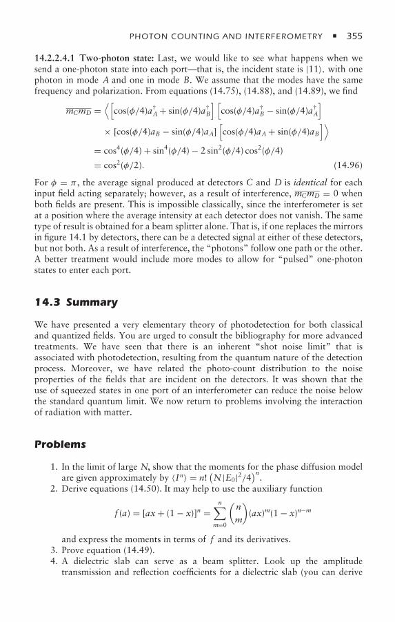
PHOTON COUNTING AND INTERFEROMETRY 355
14.2.2.4.1 Two-photon state: Last, we would like to see what happens when wesend a one-photon state into each port—that is, the incident state is |11〉, with onephoton in mode A and one in mode B. We assume that the modes have the samefrequency and polarization. From equations (14.75), (14.88), and (14.89), we find
mCmD =⟨[
cos(φ/4)a†A + sin(φ/4)a†
B
] [cos(φ/4)a†
B − sin(φ/4)a†A
]× [cos(φ/4)aB − sin(φ/4)aA]
[cos(φ/4)aA + sin(φ/4)aB
]⟩= cos4(φ/4) + sin4(φ/4) − 2 sin2(φ/4) cos2(φ/4)
= cos2(φ/2). (14.96)
For φ = π , the average signal produced at detectors C and D is identical for eachinput field acting separately; however, as a result of interference, mCmD = 0 whenboth fields are present. This is impossible classically, since the interferometer is setat a position where the average intensity at each detector does not vanish. The sametype of result is obtained for a beam splitter alone. That is, if one replaces the mirrorsin figure 14.1 by detectors, there can be a detected signal at either of these detectors,but not both. As a result of interference, the “photons” follow one path or the other.A better treatment would include more modes to allow for “pulsed” one-photonstates to enter each port.
14.3 Summary
We have presented a very elementary theory of photodetection for both classicaland quantized fields. You are urged to consult the bibliography for more advancedtreatments. We have seen that there is an inherent “shot noise limit” that isassociated with photodetection, resulting from the quantum nature of the detectionprocess. Moreover, we have related the photo-count distribution to the noiseproperties of the fields that are incident on the detectors. It was shown that theuse of squeezed states in one port of an interferometer can reduce the noise belowthe standard quantum limit. We now return to problems involving the interactionof radiation with matter.
Problems
1. In the limit of large N, show that the moments for the phase diffusion modelare given approximately by 〈In〉 = n!
(N |E0|2/4
)n.
2. Derive equations (14.50). It may help to use the auxiliary function
f (a) = [ax+ (1 − x)]n =n∑
m=0
(nm
)(ax)m(1 − x)n−m
and express the moments in terms of f and its derivatives.3. Prove equation (14.49).4. A dielectric slab can serve as a beam splitter. Look up the amplitude
transmission and reflection coefficients for a dielectric slab (you can derive
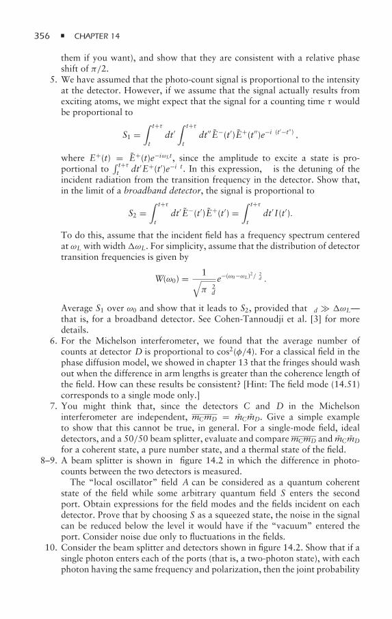
356 CHAPTER 14
them if you want), and show that they are consistent with a relative phaseshift of π/2.
5. We have assumed that the photo-count signal is proportional to the intensityat the detector. However, if we assume that the signal actually results fromexciting atoms, we might expect that the signal for a counting time τ wouldbe proportional to
S1 =∫ t+τ
tdt′
∫ t+τ
tdt′′ E−(t′)E+(t′′)e−iδ(t′−t′′) ,
where E+(t) = E+(t)e−iωLt, since the amplitude to excite a state is pro-portional to
∫ t+τt dt′E+(t′)e−iδt. In this expression, δ is the detuning of the
incident radiation from the transition frequency in the detector. Show that,in the limit of a broadband detector, the signal is proportional to
S2 =∫ t+τ
tdt′ E−(t′)E+(t′) =
∫ t+τ
tdt′ I(t′).
To do this, assume that the incident field has a frequency spectrum centeredat ωL with widthωL. For simplicity, assume that the distribution of detectortransition frequencies is given by
W(ω0) = 1√πδ2d
e−(ω0−ωL)2/δ2d .
Average S1 over ω0 and show that it leads to S2, provided that δd ωL—that is, for a broadband detector. See Cohen-Tannoudji et al. [3] for moredetails.
6. For the Michelson interferometer, we found that the average number ofcounts at detector D is proportional to cos2(φ/4). For a classical field in thephase diffusion model, we showed in chapter 13 that the fringes should washout when the difference in arm lengths is greater than the coherence length ofthe field. How can these results be consistent? [Hint: The field mode (14.51)corresponds to a single mode only.]
7. You might think that, since the detectors C and D in the Michelsoninterferometer are independent, mCmD = mCmD. Give a simple exampleto show that this cannot be true, in general. For a single-mode field, idealdetectors, and a 50/50 beam splitter, evaluate and comparemCmD and mCmD
for a coherent state, a pure number state, and a thermal state of the field.8–9. A beam splitter is shown in figure 14.2 in which the difference in photo-
counts between the two detectors is measured.The “local oscillator” field A can be considered as a quantum coherent
state of the field while some arbitrary quantum field S enters the secondport. Obtain expressions for the field modes and the fields incident on eachdetector. Prove that by choosing S as a squeezed state, the noise in the signalcan be reduced below the level it would have if the “vacuum” entered theport. Consider noise due only to fluctuations in the fields.
10. Consider the beam splitter and detectors shown in figure 14.2. Show that if asingle photon enters each of the ports (that is, a two-photon state), with eachphoton having the same frequency and polarization, then the joint probability
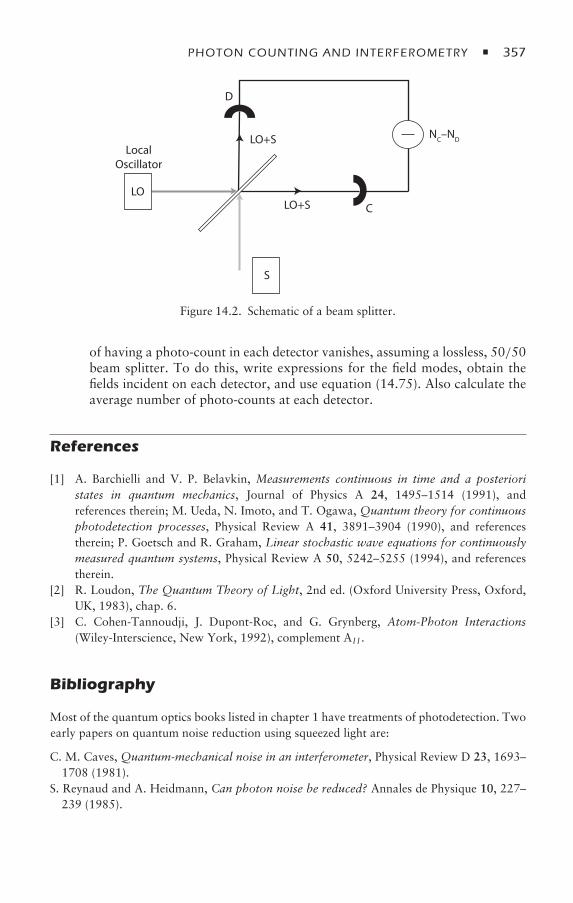
PHOTON COUNTING AND INTERFEROMETRY 357
D
C
S
LO
NC–ND
LocalOscillator
LO+S
LO+S
Figure 14.2. Schematic of a beam splitter.
of having a photo-count in each detector vanishes, assuming a lossless, 50/50beam splitter. To do this, write expressions for the field modes, obtain thefields incident on each detector, and use equation (14.75). Also calculate theaverage number of photo-counts at each detector.
References
[1] A. Barchielli and V. P. Belavkin, Measurements continuous in time and a posterioristates in quantum mechanics, Journal of Physics A 24, 1495–1514 (1991), andreferences therein; M. Ueda, N. Imoto, and T. Ogawa, Quantum theory for continuousphotodetection processes, Physical Review A 41, 3891–3904 (1990), and referencestherein; P. Goetsch and R. Graham, Linear stochastic wave equations for continuouslymeasured quantum systems, Physical Review A 50, 5242–5255 (1994), and referencestherein.
[2] R. Loudon, The Quantum Theory of Light, 2nd ed. (Oxford University Press, Oxford,UK, 1983), chap. 6.
[3] C. Cohen-Tannoudji, J. Dupont-Roc, and G. Grynberg, Atom-Photon Interactions(Wiley-Interscience, New York, 1992), complement AI I .
Bibliography
Most of the quantum optics books listed in chapter 1 have treatments of photodetection. Twoearly papers on quantum noise reduction using squeezed light are:
C. M. Caves, Quantum-mechanical noise in an interferometer, Physical Review D 23, 1693–1708 (1981).
S. Reynaud and A. Heidmann, Can photon noise be reduced? Annales de Physique 10, 227–239 (1985).
15Atom–Quantized Field Interactions
In the previous chapters, we considered quantized radiation fields, but not theirinteraction with matter. In this chapter, we introduce a Hamiltonian that can beused to model the interaction of quantized radiation fields with atoms. We firstgive a brief review of the Heisenberg picture and then obtain an expression forthe atom–field Hamiltonian in dipole approximation. To explore a relatively simpleapplication of the formalism, we look at the interaction of a monochromatic cavityfield with a single two-level atom that is stationary within the cavity—this problemis referred to as the Jaynes-Cummings problem [1]. As a second application of theformalism, we discuss dressed states of the atom–field system for a monochromaticfield interacting with a two-level atom. These quantized dressed states differ in afundamental manner from the semiclassical dressed states that we have been usingup to this point. The quantized dressed states are true stationary states of the atom–field Hamiltonian in the rotating-wave approximation (RWA). Last, we indicate amethod for creating coherent and squeezed states of the radiation field.
15.1 Interaction Hamiltonian and Equations of Motion
We have seen that there are times that the Heisenberg representation offersadvantages over the Schrödinger representation. The Heisenberg state vector |ψ〉His related to the Schrödinger state vector |ψ(t)〉 via
|ψ〉H = eiHt|ψ(t)〉, (15.1)
where H is the total Hamiltonian for the system.
15.1.1 Schrödinger Representation
In the Schrödinger representation, the state vector, |ψ(t)〉, is time-dependent, as isthe density matrix
S(t) = |ψ(t)〉〈ψ(t)|. (15.2)
ATOM–QUANTIZED FIELD INTERACTIONS 359
Operators are time-independent, but their expectation values are time-dependent,owing to the time dependence of the state vector. The equation of motion for theexpectation value of an operator O is
iddt
〈ψ(t)|O|ψ(t)〉 = 〈ψ(t)|[O,H]|ψ(t)〉, (15.3)
where
〈O〉 = 〈ψ(t)|O|ψ(t)〉 =∑E,E′
〈ψ(t)|E〉〈E|O|E′〉〈E′|ψ(t)〉
=∑E,E′
〈E′|ψ(t)〉〈ψ(t)|E〉〈E|O|E′〉
=∑E,E′
〈E′|S(t)|E〉〈E|O|E′〉 = Tr[S(t)O] . (15.4)
15.1.2 Heisenberg Representation
In the Heisenberg representation, the state vector is time-independent, as is thedensity matrix of the system, but the operators themselves are generally functions oftime. We have
|ψ〉H = eiHt|ψ(t)〉 = e
iHte− i
Ht|ψ(0)〉 = |ψ(0)〉, (15.5)
H = eiHtS(t)e− i
Ht = S(0), (15.6)
and
OH(t) = eiHtOe− i
Ht. (15.7)
The expectation values of operators are still time time-dependent, but the timedependence originates from the operator rather than the state vector—namely,
〈O〉 = Tr[HOH(t)]. (15.8)
Using the definition (15.7), it is easy to show that OH(t) satisfies the equation ofmotion
idOH(t)dt
= [OH(t),H]. (15.9)
The advantage of the Heisenberg representation is that the operators often obeyequations of motion that are identical to their classical counterparts. It is importantto note that commutation laws such as [x(t), p(t)] = i remain valid in theHeisenberg representation, but that [x(t), p(t′)] = i in general, if t = t′.
Things can get a bit confusing. The operator |E〉〈E| is constant in the Heisenbergrepresentation since e
iHt|E〉〈E|e− i
Ht = |E〉〈E|. On the other hand, if atoms
interact with a field via a Hamiltonian H = HA + HF + VAF , where HA|A〉 =EA|A〉, HF |F 〉 = EF |F 〉, then A ≡ |A〉〈A| is a time-independent operator, butAH(t) = e
iHt|A〉〈A|e− i
Ht is a function of time. In other words, if one considers
a two-level atom interacting with a quantized radiation field, the raising operator
360 CHAPTER 15
σ+ = |2〉〈1| is time-independent, but the corresponding Heisenberg operator σ+(t) =e
iHt|2〉〈1|e− i
Ht is a function of time.
15.1.3 Hamiltonian
The Hamiltonian in Coulomb gauge derived in the appendix in chapter 12,appropriate to an N-electron atom interacting with a quantized radiation field, isgiven by
H =N∑α=1
12m
[pα + eA(rα)]2 + HT + VC , (15.10)
where m is the electron mass,
VC = − 14πε0
N∑α=1
Ne2
rα+ 1
8πε0
N∑α,β=1;α =β
e2∣∣rα − rβ∣∣ (15.11)
is the electrostatic Coulomb potential, assuming that the nucleus is fixed at R = 0and has charge Ne, rα is the coordinate of electron α,
HT =∑k,εk
ωka†k,εk
ak,εk (15.12)
is the Hamiltonian associated with the transverse field modes,
A(R) =∑k,εk
(
2ε0ωkV
)1/2 (ak,εkεke
ik·R + a†k,εk
εke−ik·R)
(15.13)
is the vector potential (transverse in Coulomb gauge),
εk · k = 0, (15.14)
and the sum over εk is over two independent free-field polarizations for each fieldmode having propagation vector k. The quantity pα is the momentum canonical torα for particle α having charge −e.
If we quantize as in the free atom and free-field case using[(rα)i , (pα′ ) j
] = iδα,α′δi, j , (15.15)[ai , a
†j
]= iδi, j , (15.16)
and work in the Heisenberg representation, we regain Newton’s equations for theatomic operators (with the Lorentz force law) andMaxwell’s equations for the fields,i.e.,
a j + iω j a j =(
i2ε0ω j
)JTj , (15.17)
where JTj is the transverse current defined by equation (12.210). Note that a j (t) =a j (0)e−iω j t if JTj = 0 at any time.
ATOM–QUANTIZED FIELD INTERACTIONS 361
When one deals with atom–classical field interactions, one often makes the dipoleapproximation, assuming that ka 1, where k is the propagation constant for thefield, and a is a characteristic atomic dimension on the order of the Bohr radius a0.For a quantized field, however, the approximation ka 1 cannot be true for all thefield modes. Thus, if we run into any infinities involving summations over quantizedfield modes, some of those infinities can be removed by imposing a cutoff at k≈ a−1
0 .For the time being, let us suppose that the dipole approximation is valid for the fieldmodes of interest.
In the dipole approximation, it is useful to carry out a unitary transformation onthe state vector of the form
|ψ(t)〉 = T|ψ(t)〉, (15.18)
where
T = e− i
µ·A(R=0), (15.19)
and µ = −∑Nα=1 erα is the electric dipole moment operator. Under this unitary
transformation (15.19), the Hamiltonian (15.10) becomes
H = THT† =N∑α=1
(TpαT†
)22m
+ VC + T∑j
ω j a†j a j T
†, (15.20)
where the sum over j is a sum over all field modes.Using the fact that
eABe−A = B+ [A, B] + 12!
[A, [A, B]] + · · · , (15.21)
we find that
TpαT† = pα − eA(0). (15.22)
Moreover, since
T = e∑
j λ∗j a j−λ j a†
j =∏j
D†(λ j , λ∗j ) (15.23)
is just a product of field displacement operators (12.71), with
λ j = i ε j · µ√2ε0Vω j
, (15.24)
it follows that
Ta jT† = D†(λ j , λ∗j )a jD(λ j , λ∗
j ) = a j + λ j (15.25)
and
Ta†j T
† = a†j + λ∗
j . (15.26)
362 CHAPTER 15
As a result, H can be written as
HT =N∑α=1
p2α2m
+ VC +∑j
ω j a†j a j
+∑j
ω j (λ∗j a j + λ j a†
j ) +∑j
ω j |λ j |2. (15.27)
The∑
j ω j (λ∗j a j + λ j a†
j ) term is simply equal to −µ · ET(0), where
ET(R) = i∑k,εk
(ωk
2ε0V
)1/2 (ak,εkεke
ik·R − a†k,εk
εke−ik·R)
(15.28)
is the quantum operator for the transverse electric field. The∑
j ω j |λ j |2 term isinfinite, but independent of the field—it represents a self-energy term that can betaken into account by a renormalization of the atomic state energies. Consequently,we subtract out this term (the zero point field energy has already been excluded) andtake as our Hamiltonian in dipole approximation
H =N∑α=1
p2α2m
+ VC(rα) − µ · ET(0) +∑j
ω j a†j a j . (15.29)
Any expectation values of operators calculated with the new Hamiltonian are thesame as those for the original one, although technically speaking, in a dielectricmedium the correct operator in this equation should be DT(0) rather than ET(0), ifwe use our original basis states to take expectation values [2, 3].
This Hamiltonian can be generalized to include the center-of-mass motion of theatom. In that case, we take
H = P2
2M+ HAtom + HField + VAF , (15.30)
HAtom =N∑α=1
p2α2m
+ VC(rα), (15.31)
HField =∑j
ω j a†j a j , (15.32)
VAF = −µ · ET(R), (15.33)
where R is the center-of-mass coordinate of the atom, P is the center-of-massmomentum of the atom, M is the atomic mass, m is the reduced mass of anelectron located at position rα relative to the nucleus having canonical momentumpα, and ET(R) is given by equation (15.28). We will usually use the Schrödingerrepresentation when working with probability amplitudes and the Heisenbergrepresentation when working with density matrix and operator equations. TheHamiltonian (15.30) is the starting point for many of the calculations in theremainder of this book.
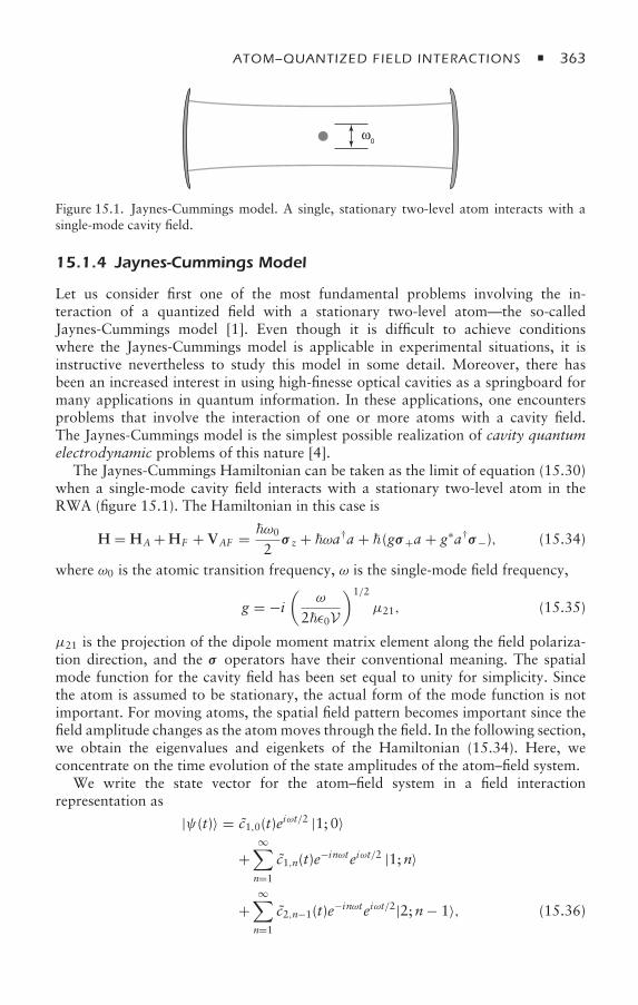
ATOM–QUANTIZED FIELD INTERACTIONS 363
ω0
Figure 15.1. Jaynes-Cummings model. A single, stationary two-level atom interacts with asingle-mode cavity field.
15.1.4 Jaynes-Cummings Model
Let us consider first one of the most fundamental problems involving the in-teraction of a quantized field with a stationary two-level atom—the so-calledJaynes-Cummings model [1]. Even though it is difficult to achieve conditionswhere the Jaynes-Cummings model is applicable in experimental situations, it isinstructive nevertheless to study this model in some detail. Moreover, there hasbeen an increased interest in using high-finesse optical cavities as a springboard formany applications in quantum information. In these applications, one encountersproblems that involve the interaction of one or more atoms with a cavity field.The Jaynes-Cummings model is the simplest possible realization of cavity quantumelectrodynamic problems of this nature [4].
The Jaynes-Cummings Hamiltonian can be taken as the limit of equation (15.30)when a single-mode cavity field interacts with a stationary two-level atom in theRWA (figure 15.1). The Hamiltonian in this case is
H = HA + HF + VAF = ω0
2σ z + ωa†a + (gσ+a + g∗a†σ−), (15.34)
where ω0 is the atomic transition frequency, ω is the single-mode field frequency,
g = −i(
ω
2ε0V
)1/2
µ21, (15.35)
µ21 is the projection of the dipole moment matrix element along the field polariza-tion direction, and the σ operators have their conventional meaning. The spatialmode function for the cavity field has been set equal to unity for simplicity. Sincethe atom is assumed to be stationary, the actual form of the mode function is notimportant. For moving atoms, the spatial field pattern becomes important since thefield amplitude changes as the atommoves through the field. In the following section,we obtain the eigenvalues and eigenkets of the Hamiltonian (15.34). Here, weconcentrate on the time evolution of the state amplitudes of the atom–field system.
We write the state vector for the atom–field system in a field interactionrepresentation as
|ψ(t)〉 = c1,0(t)eiωt/2 |1; 0〉
+∞∑n=1
c1,n(t)e−inωteiωt/2 |1;n〉
+∞∑n=1
c2,n−1(t)e−inωteiωt/2|2;n− 1〉, (15.36)
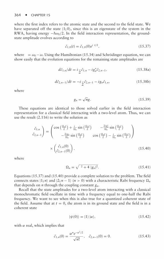
364 CHAPTER 15
where the first index refers to the atomic state and the second to the field state. Wehave separated off the state |1; 0〉, since this is an eigenstate of the system in theRWA, having energy −ω0/2. In the field interaction representation, the ground-state amplitude evolves according to
c1,0(t) = c1,0(0)eiδt/2, (15.37)
where δ = ω0 −ω. Using the Hamiltonian (15.34) and Schrödinger equation, we canshow easily that the evolution equations for the remaining state amplitudes are
dc1,n/dt = iδ
2c1,n − ig∗
nc2,n−1, (15.38a)
dc2,n−1/dt = −i δ2c2,n−1 − ignc1,n, (15.38b)
where
gn = √ng. (15.39)
These equations are identical to those solved earlier in the field interactionrepresentation for a classical field interacting with a two-level atom. Thus, we canuse the result (2.116) to write the solution as
(c1,nc2,n−1
)=⎛⎝ cos
(nt2
)+ iδn
sin(nt2
) − 2ig∗n
nsin
(nt2
)− 2ign
nsin
(nt2
)cos
(nt2
)− iδn
sin(nt2
)⎞⎠
×(
c1,n(0)c2,n−1(0)
), (15.40)
where
n =√δ2 + 4 |gn|2. (15.41)
Equations (15.37) and (15.40) provide a complete solution to the problem. The fieldconnects states |1;n〉 and |2;n− 1〉 (n > 0) with a characteristic Rabi frequency n
that depends on n through the coupling constant gn.Recall that the state amplitudes for a two-level atom interacting with a classical
monochromatic field oscillate in time with a frequency equal to one-half the Rabifrequency. We want to see when this is also true for a quantized coherent state ofthe field. Assume that at t = 0, the atom is in its ground state and the field is in acoherent state
|ψ(0)〉 = |1〉 |α〉, (15.42)
with α real, which implies that
c1,n(0) = αne−α2/2√n!
, c2,n−1(0) = 0. (15.43)
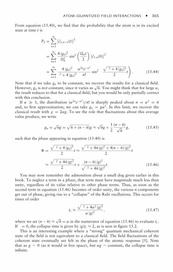
ATOM–QUANTIZED FIELD INTERACTIONS 365
From equation (15.40), we find that the probability that the atom is in its excitedstate at time t is
P2 =∞∑n=1
∣∣c2,n−1(t)∣∣2
=∞∑n=1
4 |gn|22n
sin2(nt2
) ∣∣c1,n(0)∣∣2
=∞∑n=1
4 |gn|2δ2 + 4 |gn|2
α2ne−α2
n!sin2
(√δ2 + 4 |gn|2
2t
). (15.44)
Note that if we take gn to be constant, we recover the results for a classical field.However, gn is not constant, since it varies as
√n. You might think that for large α,
the result reduces to that for a classical field, but you would be only partially correctwith this conclusion.
If α 1, the distribution (α2ne−α2 )/n! is sharply peaked about n = α2 = nand, to first approximation, we can take gn = gα2. In this limit, we recover theclassical result with χ = 2αg. To see the role that fluctuations about this averagevalue produce, we write
gn = √ng =
√n+ (n− n)g ≈
√ng + 1
2(n− n)√
ng, (15.45)
such that the phase appearing in equation (15.40) is
=√δ2 + 4 |gn|2
2t ≈
√δ2 + 4n |g|2 + 4(n− n) |g|2
2t
≈√δ2 + 4n |g|2
2t + (n− n) |g|2√
δ2 + 4n |g|2t. (15.46)
You may now remember the admonition about a small dog given earlier in thisbook. To neglect a term in a phase, that term must have magnitude much less thanunity, regardless of its value relative to other phase terms. Thus, as soon as thesecond term in equation (15.46) becomes of order unity, the various n componentsget out of phase, giving rise to a “collapse” of the Rabi oscillations. This occurs fortimes of order
tc ≈√δ2 + 4α2 |g|2α |g|2 , (15.47)
where we set (n− n) ≈ √n = α in the numerator of equation (15.46) to evaluate tc.
If δ = 0, the collapse time is given by |g|tc ≈ 2, as is seen in figure 15.2.This is an interesting example where a “strong” quantum mechanical coherent
state of the field is not equivalent to a classical field. The field fluctuations of thecoherent state eventually are felt in the phase of the atomic response [5]. Notethat as g ∼ 0 (as it would in free space), but αg ∼ constant, the collapse time isinfinite.
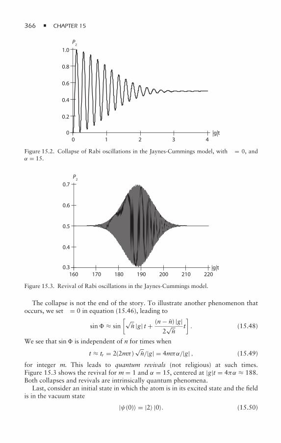
366 CHAPTER 15
10 2 3 4g t
0.2
0
0.4
0.6
0.8
1.0P2
Figure 15.2. Collapse of Rabi oscillations in the Jaynes-Cummings model, with δ = 0, andα = 15.
170 180 190 200 210 220160g t
0.4
0.3
0.5
0.6
0.7P2
Figure 15.3. Revival of Rabi oscillations in the Jaynes-Cummings model.
The collapse is not the end of the story. To illustrate another phenomenon thatoccurs, we set δ = 0 in equation (15.46), leading to
sin ≈ sin[√
n |g| t + (n− n) |g|2√n
t]. (15.48)
We see that sin is independent of n for times when
t ≈ tr = 2(2mπ )√n/|g| = 4mπα/|g| , (15.49)
for integer m. This leads to quantum revivals (not religious) at such times.Figure 15.3 shows the revival for m= 1 and α = 15, centered at |g|t = 4πα ≈ 188.Both collapses and revivals are intrinsically quantum phenomena.
Last, consider an initial state in which the atom is in its excited state and the fieldis in the vacuum state
|ψ(0)〉 = |2〉 |0〉. (15.50)
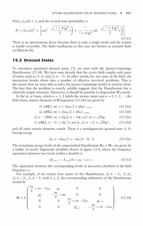
ATOM–QUANTIZED FIELD INTERACTIONS 367
Now, c2,0(0) = 1, and the excited state probability is
P2 = ∣∣c2,0(t)∣∣2 =[cos2
(√δ2 + 4 |g|2
2t
)+ δ2
δ2 + 4 |g|2 sin
(√δ2 + 4 |g|2
2t
)].
(15.51)There is no spontaneous decay because there is only a single mode and the systemis totally reversible. The Rabi oscillations in this case are known as vacuum Rabioscillations [6].
15.2 Dressed States
To introduce quantized dressed states [7], we start with the Jaynes-CummingsHamiltonian (15.34). We have seen already that the cavity field couples only pairsof states such as |1,n〉 and |2,n − 1〉. In other words, for any state of the field, theinteraction breaks down into a number of effective two-level problems. This isthe reason that we were able to solve the Jaynes-Cummings model in analytic form.The fact that the problem is exactly soluble suggests that the Hamiltonian has arelatively simple structure. Moreover, it should be possible to diagonalizeH exactly.
In the |α,n〉 basis, where α = 1,2 labels the atomic states and n = 0,1,2, . . . thefield states, matrix elements of H [equation (15.34)] are given by
〈1,n|H|1,m〉 = (−ω0/2 + nω) δn,m, (15.52a)
〈2,n|H|2,m〉 = (ω0/2 + nω) δn,m, (15.52b)
〈2,n− 1|H|1,n〉 = g〈2,n− 1|σ+a|1,n〉 = √ng, (15.52c)
〈1,n|H|2,n− 1〉 = g∗〈1,n|a†σ−|2,n− 1〉 = √ng∗, (15.52d)
and all other matrix elements vanish. There is a nondegenerate ground state |1,0〉having energy
E0 = −ω0/2 = −ω/2 − δ/2. (15.52e)
The remaining energy levels of the unperturbed Hamiltonian HA + HF are given bya ladder of nearly degenerate doublets shown in figure 15.4, where the frequencyseparation between two levels within a doublet is
(E2,n−1 − E1,n)/ = ω0 − ω = δ. (15.53)
The separation between the corresponding levels in successive doublets is the fieldfrequency ω.
For example, if we isolate four states of the Hamiltonian, |2,n − 1〉, |1,n〉,|2,n − 2〉, |1,n − 1〉 with n ≥ 2, the corresponding submatrix of the Hamiltonianwould be
H =
⎛⎜⎜⎜⎜⎜⎜⎝
ω0
2+ (n− 1)ω gn 0 0
g∗n −ω0
2+ nω 0 0
0 0ω0
2+ (n− 2)ω gn−1
0 0 g∗n−1 −ω0
2+ (n− 1)ω
⎞⎟⎟⎟⎟⎟⎟⎠, (15.54)
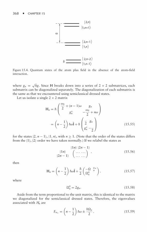
368 CHAPTER 15
2,n
ω
δ
1,n
1,n+1
1,n–1
2,n–1
2,n–2
Figure 15.4. Quantum states of the atom plus field in the absence of the atom–fieldinteraction.
where gn = √ng. Since H breaks down into a series of 2 × 2 submatrices, each
submatrix can be diagonalized separately. The diagonalization of each submatrix isthe same as that we encountered using semiclassical dressed states.
Let us isolate a single 2 × 2 matrix
Hn = ⎛⎝ ω0
2+ (n− 1)ω gn
g∗n −ω0
2+ nω
⎞⎠
=(n− 1
2
)ωI +
⎛⎜⎝δ
2gn
g∗n − δ
2
⎞⎟⎠ (15.55)
for the states |2,n− 1〉, |1,n〉, with n ≥ 1. (Note that the order of the states differsfrom the |1〉, |2〉 order we have taken normally.) If we relabel the states as
|1n〉 |2n− 1〉|1n〉
|2n− 1〉(. . . . . .
. . . . . .
), (15.56)
then
Hn =(n− 1
2
)ωI +
2
(−δ 0 ∗n
0n δ
), (15.57)
where
0n = 2gn. (15.58)
Aside from the term proportional to the unit matrix, this is identical to the matrixwe diagonalized for the semiclassical dressed states. Therefore, the eigenvaluesassociated with Hn are
En± =(n− 1
2
)ω ± n
2, (15.59)
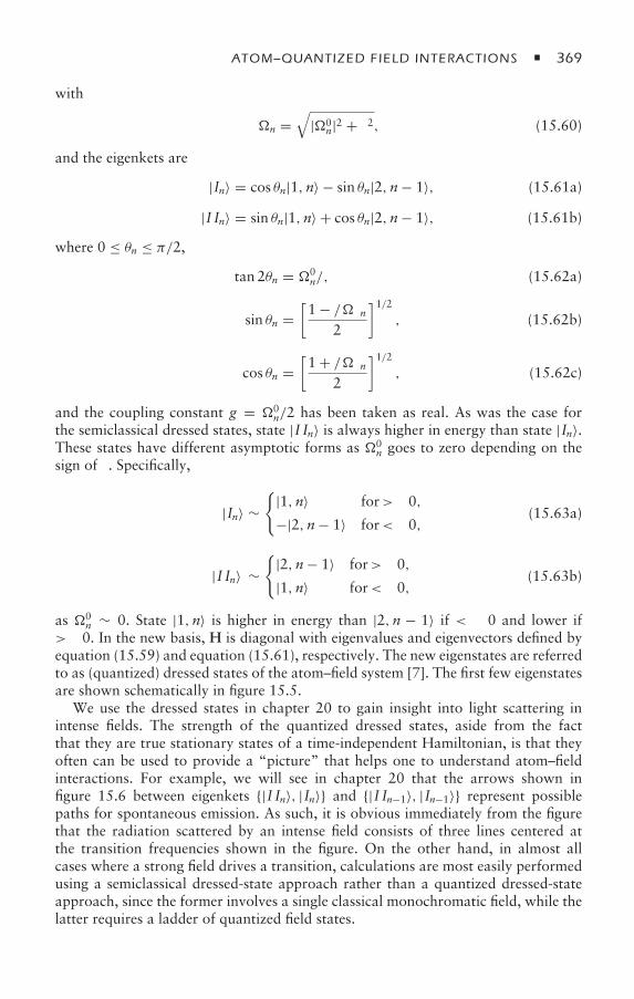
ATOM–QUANTIZED FIELD INTERACTIONS 369
with
n =√
|0n|2 + δ2, (15.60)
and the eigenkets are
|In〉 = cos θn|1,n〉 − sin θn|2,n− 1〉, (15.61a)
|I In〉 = sin θn|1,n〉 + cos θn|2,n− 1〉, (15.61b)
where 0 ≤ θn ≤ π/2,tan 2θn = 0
n/δ, (15.62a)
sin θn =[1 − δ/n
2
]1/2, (15.62b)
cos θn =[1 + δ/n
2
]1/2, (15.62c)
and the coupling constant g = 0n/2 has been taken as real. As was the case for
the semiclassical dressed states, state |I In〉 is always higher in energy than state |In〉.These states have different asymptotic forms as 0
n goes to zero depending on thesign of δ. Specifically,
|In〉 ∼
|1,n〉 for δ > 0,
−|2,n− 1〉 for δ < 0,(15.63a)
|I In〉 ∼
|2,n− 1〉 for δ > 0,
|1,n〉 for δ < 0,(15.63b)
as 0n ∼ 0. State |1,n〉 is higher in energy than |2,n − 1〉 if δ < 0 and lower if
δ > 0. In the new basis, H is diagonal with eigenvalues and eigenvectors defined byequation (15.59) and equation (15.61), respectively. The new eigenstates are referredto as (quantized) dressed states of the atom–field system [7]. The first few eigenstatesare shown schematically in figure 15.5.
We use the dressed states in chapter 20 to gain insight into light scattering inintense fields. The strength of the quantized dressed states, aside from the factthat they are true stationary states of a time-independent Hamiltonian, is that theyoften can be used to provide a “picture” that helps one to understand atom–fieldinteractions. For example, we will see in chapter 20 that the arrows shown infigure 15.6 between eigenkets |I In〉, |In〉 and |I In−1〉, |In−1〉 represent possiblepaths for spontaneous emission. As such, it is obvious immediately from the figurethat the radiation scattered by an intense field consists of three lines centered atthe transition frequencies shown in the figure. On the other hand, in almost allcases where a strong field drives a transition, calculations are most easily performedusing a semiclassical dressed-state approach rather than a quantized dressed-stateapproach, since the former involves a single classical monochromatic field, while thelatter requires a ladder of quantized field states.
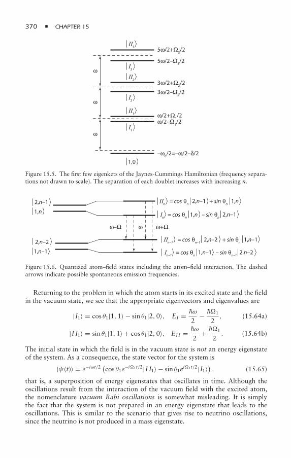
370 CHAPTER 15
ω
ω
ω
1,0
5ω/2+Ω3/2
5ω/2–Ω3/2
3ω/2+Ω2/2
3ω/2–Ω2/2
ω/2+Ω1/2
ω/2–Ω1/2
–ω0/2=–ω/2–δ/2
I1
I2
II1
II2
I3
II3
Figure 15.5. The first few eigenkets of the Jaynes-Cummings Hamiltonian (frequency separa-tions not drawn to scale). The separation of each doublet increases with increasing n.
ωω–Ω ω+Ω
1,n
1,n–1
2,n–1
2,n–2
1,n
1,n–1
2,n–1
2,n–2
1,n
2,n–1
2,n–2
1,n–1
In
IIn
= cos θn
+ sin θn
= cos θn
– sin θn
In–1
IIn–1
= cos θn–1
+ sin θn
= cos θn
– sin θn–1
Figure 15.6. Quantized atom–field states including the atom–field interaction. The dashedarrows indicate possible spontaneous emission frequencies.
Returning to the problem in which the atom starts in its excited state and the fieldin the vacuum state, we see that the appropriate eigenvectors and eigenvalues are
|I1〉 = cos θ1|1,1〉 − sin θ1|2,0〉, EI = ω2
− 1
2, (15.64a)
|I I1〉 = sin θ1|1,1〉 + cos θ1|2,0〉, EII = ω2
+ 1
2. (15.64b)
The initial state in which the field is in the vacuum state is not an energy eigenstateof the system. As a consequence, the state vector for the system is
|ψ(t)〉 = e−iωt/2 (cos θ1e−i1t/2|I I1〉 − sin θ1ei1t/2|I1〉), (15.65)
that is, a superposition of energy eigenstates that oscillates in time. Although theoscillations result from the interaction of the vacuum field with the excited atom,the nomenclature vacuum Rabi oscillations is somewhat misleading. It is simplythe fact that the system is not prepared in an energy eigenstate that leads to theoscillations. This is similar to the scenario that gives rise to neutrino oscillations,since the neutrino is not produced in a mass eigenstate.
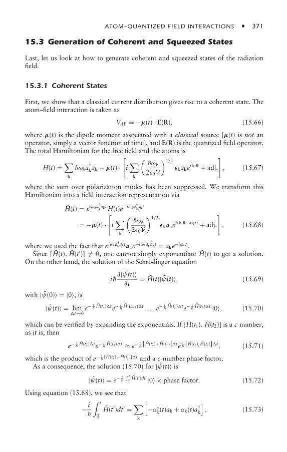
ATOM–QUANTIZED FIELD INTERACTIONS 371
15.3 Generation of Coherent and Squeezed States
Last, let us look at how to generate coherent and squeezed states of the radiationfield.
15.3.1 Coherent States
First, we show that a classical current distribution gives rise to a coherent state. Theatom–field interaction is taken as
VAF = −µ(t) · E(R), (15.66)
where µ(t) is the dipole moment associated with a classical source [µ(t) is not anoperator, simply a vector function of time], and E(R) is the quantized field operator.The total Hamiltonian for the free field and the atoms is
H(t) =∑k
ωka†kak − µ(t) ·
[i∑k
(ωk
2ε0V
)1/2
εkakeik·R + adj.
], (15.67)
where the sum over polarization modes has been suppressed. We transform thisHamiltonian into a field interaction representation via
H(t) = eiωka†kaktH(t)e−iωka†
kakt
= −µ(t) ·[i∑k
(ωk
2ε0V
)1/2
εkakei(k·R−ωkt) + adj.
], (15.68)
where we used the fact that eiωka†kaktake−iωka†
kakt = ake−iωkt.Since [H(t), H(t′)] = 0, one cannot simply exponentiate H(t) to get a solution.
On the other hand, the solution of the Schrödinger equation
i∂|ψ(t)〉∂t
= H(t)|ψ(t)〉, (15.69)
with |ψ(0)〉 = |0〉, is|ψ(t)〉 = lim
t→0e− i
H(tn)te− i
H(tn−1)t . . . e− i
H(t2)te− i
H(t1)t |0〉, (15.70)
which can be verified by expanding the exponentials. If [H(t1), H(t2)] is a c-number,as it is, then
e− iH(t2)te− i
H(t1)t ≈ e− i
[H(t2)+H(t1)]tei [H(t1),H(t2)]t, (15.71)
which is the product of e− i[H(t2)+H(t1)]t and a c-number phase factor.
As a consequence, the solution (15.70) for |ψ(t)〉 is|ψ(t)〉 = e− i
∫ t0 H(t′)dt′ |0〉 × phase factor. (15.72)
Using equation (15.68), we see that
− i
∫ t
0H(t′)dt′ =
∑k
[−α∗
k(t)ak + αk(t)a†k
], (15.73)
372 CHAPTER 15
where
α∗k(t) = 1
(ωk
2ε0V
)1/2 ∫ t
0dt′µ(t′) · εkei(k·R−ωkt′) . (15.74)
Thus, to within a constant phase factor,
|ψ(t)〉 = e∑
k(−α∗kak+αka†
k)|0〉 =∏k
e(−α∗kak+αka†
k)|0〉. (15.75)
In other words, a classical current source creates a multimode coherent state of thefield.
15.3.2 Squeezed States
To generate a squeezed state, it is necessary to produce two photons that arecorrelated. This can be done in four-wave mixing by converting two pump photonsto two correlated signal photons or in parametric down conversion, where a singlephoton is converted to two photons. A prototype Hamiltonian in a field interactionrepresentation is taken to be of the form
H = a2 + ∗a† 2, (15.76)
where can represent either the second-order susceptibility (parametric downconversion) or third-order susceptibility (four-wave mixing). There are very fewtreatments, if any, in which is calculated from first principles. The solution ofthe Schrödinger equation for this Hamiltonian is
|ψ(t)〉 = eξa2−ξ∗(a†)2 |0〉, (15.77)
where
ξ = −it. (15.78)
We recognize that the state (15.77) is just the squeezed vacuum.
15.4 Summary
The atom–field Hamiltonian has been obtained in dipole approximation. This is theHamiltonian we use for the rest of this book. The simple, but important, Jaynes-Cummings model was studied. It was found that a coherent, quantized state ofthe field can lead to atom–field dynamics that differs from that of a classical field,even if the field strength is large. The Jaynes-Cummings model was also the startingpoint for a discussion of dressed states of a quantized field interacting with a two-level atom. In contrast to semiclassical dressed states, these quantized field dressedstates are stationary states of the atom–field Hamiltonian. Last, we showed how thespecific atom–field Hamiltonians can give rise to coherent and squeezed states of theradiation field. Now, we turn our attention to multimode quantized field states tosee how the vacuum field can lead to spontaneous decay.
ATOM–QUANTIZED FIELD INTERACTIONS 373
Problems
1–2. For the Hamiltonian
H =∑α
[pα − qαA(rα)]2/(2mα) + VC + HT,
prove that
mrα = qαE(rα) + qα[rα × B(rα) − B(rα) × rα]/2
and that
a j + iω j a j = i(2ε0ω j )−1/2 J j ,
where the operators are written in the Heisenberg representation, VC is theelectrostatic Coulomb interaction potential, and
HT =∑j
ω j
(a†j a j + 1/2
),
J j = (1/√V)
∫dr e−ik j ·rε j · J(r),
J(r) = (1/2)∑α
qα[rαδ(r − rα) + δ(r − rα)rα],
A(r) =∑j
(
2ε0ω jV
)1/2 (a jε j eik j ·r + a†
j ε j e−ik j ·r).
In other words, the operators satisfy the Lorentz force equation for the chargesand Maxwell’s equations for the fields, properly symmetrized.
3. For the Hamiltonian given by equation (15.30), introduce the unitary trans-formation H′ = T(t)H[T(t)]†, with
T(t) = !i exp(λ∗i ai − λi a†
i ), λi = αi e−ii t .
Show that, under this transformation, the electric field operator transforms as
E′(R, t) = TET† = Ecl(αi ,R, t) + E(R),
and if the initial state function was the coherent state |αi 〉, the new trans-formed state function is just the vacuum. Consequently, the true quantizedcoherent state field can be approximated by a classical field, provided thatthe effects of vacuum fluctuations are not important relative to those of theclassical field.
4. Consider a three-level cascade atom interacting with two single-mode quan-tized radiation fields. The first field drives the 1–2 transition, and the secondfield the 2–3 transition. The second field is weak and can be treated inperturbation theory, while the first field is of arbitrary intensity and is besttreated using a dressed-atom basis. Using a dressed-atom energy-level diagram,explain why one would expect two resonance peaks (Autler-Townes doublet)
374 CHAPTER 15
in the absorption spectrum for the second field, and calculate the positions ofthese resonances.
5. Draw an energy-level diagram for the first four dressed-state manifolds.6. Imagine that the initial state of the system in the Jaynes-Cummings problem
is |ψ(0)〉 = 1√2|1〉(|1〉 + |2〉)—that is, the atom in state 1 and the field in a
superposition of one- and two-photon states. Assume that δ = 0. Find andplot the probability that the atom is in its excited state as a function of time.Show that there can never be a complete revival of the system, nor can theexcited-state population be exactly equal to unity.
7. Choose your own set of parameters to illustrate collapse and revival in theJaynes-Cummings model.
8. Prove that [H(t1), H(t2)] is a c-number, for H(t) given in equation (15.68).
References
[1] E. T. Jaynes and F. W. Cummings, Comparison of quantum and semiclassical radiationtheories with application to the beam maser, Proceedings of the IEEE 51, 89–109 (1963).
[2] J. R. Ackerhalt and P. Milonni, Interaction Hamiltonian of quantum optics, Journal ofthe Optical Society of America B 1, 116–120 (1984).
[3] C. Cohen-Tannoudji, J. Dupont-Roc, and G. Grynberg, Atom-Photon Interactions(Wiley-Interscience, New York, 1992), app. 5.
[4] P. R. Berman, Ed., Cavity Quantum Electrodynamics (Academic Press, New York,1994).
[5] T. von Foerster, A comparison of quantum and semiclassical theories of the interactionbetween a two-level atom and the radiation field, Journal of Physics A 8, 95–103 (1975).
[6] M. Brune, F. Schmidt-Kaler, A. Maali, J. Dreyer, E. Hagley, J. M. Raimond, and S.Haroche, Quantum Rabi oscillation: a direct test of field quantization in a cavity,Physical Review Letters 76, 1800–1803 (1996).
[7] C. Cohen-Tannoudji, Atoms in Strong Resonant Fields, in Frontiers in Laser Spec-troscopy, Les Houches Session XXVII, vol. 1, edited by R. Balian, S. Haroche, andS. Liberman (North Holland, Amsterdam, 1975), pp. 3–103; C. Cohen-Tannoudji,J. Dupont-Roc, and G. Grynberg, Atom-Photon Interactions (Wiley-Interscience,New York, 1992), chap. VI.
Bibliography
See the references in chapter 1. In particular, additional coverage and references for thematerial in this chapter is given in
B. W. Shore, The Theory of Coherent Excitation, vols. 1 and 2 (Wiley-Interscience, NewYork, 1990), secs. 9.15–10.6.
16Spontaneous Decay
When you first learn quantum mechanics, you spend a lot of time studyingstationary states of the hydrogen atom, as you should. However, a little later in life,you find out that these states are not stationary at all. In fact, some of the low-lyingstates decay back to the ground state in times of the order of nanoseconds. Clearly,something was left out in the treatment of the stationary states of the hydrogen atom.That “something” was the vacuum field. Even though the ether has disappeared, thevacuum field has remained an essential component of modern physics.
In this chapter, we look at the interaction of the vacuum field with an atomprepared in an excited state. This is one of the most basic atom–field interactions,and one of practical importance. We calculate the rate at which the excited statedecays and the properties of the field emitted by the atom.
Suffice it to say that spontaneous emission leads to some interesting problems thathave yet to be resolved. One starts with a perfectly unitary Hamiltonian and endsup with irreversible behavior. How can this happen? The irreversibility is linkedto the assumption that any radiation emitted by an atom as a result of the atom–vacuum field interaction cannot come back and excite the atom at some later time. Interms of field quantization, the equivalent assumption is that the spacing of the fieldmodes approaches zero or the quantization volume approaches infinity. Even withthis approximation, there are problems with unitarity. Some additional assumptions,sometimes not rigorously justified, are needed to save the day.
16.1 Spontaneous Decay Rate
Despite the apparent simplicity of spontaneous emission—put an atom in an excitedstate and watch it decay—spontaneous emission poses all sorts of mathematicaldifficulties. Before considering spontaneous emission, let us first look at the problemof an atom in its ground state and no photons present in the field. It is apparentfrom the Hamiltonian (15.29) that this state is not an eigenstate of the system. Theatom can “emit” a photon while going to an excited state. Of course, such a process
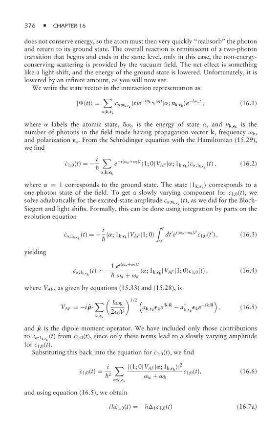
376 CHAPTER 16
does not conserve energy, so the atom must then very quickly “reabsorb” the photonand return to its ground state. The overall reaction is reminiscent of a two-photontransition that begins and ends in the same level, only in this case, the non-energy-conserving scattering is provided by the vacuum field. The net effect is somethinglike a light shift, and the energy of the ground state is lowered. Unfortunately, it islowered by an infinite amount, as you will now see.
We write the state vector in the interaction representation as
|(t)〉 =∑α;k,εk
cα;nk,εk (t)e−ink,εkωkt|α;nk,εk〉e−iωα t , (16.1)
where α labels the atomic state, ωα is the energy of state α, and nk,εk is thenumber of photons in the field mode having propagation vector k, frequency ωk,and polarization εk. From the Schrödinger equation with the Hamiltonian (15.29),we find
c1;0(t) = − i
∑α,k,εk
e−i(ωα+ωk)t〈1; 0|VAF |α; 1k,εk〉cα;1k,εk (t) , (16.2)
where α = 1 corresponds to the ground state. The state |1k,εk〉 corresponds to aone-photon state of the field. To get a slowly varying component for c1;0(t), wesolve adiabatically for the excited-state amplitude cα;nk,εk (t), as we did for the Bloch-Siegert and light shifts. Formally, this can be done using integration by parts on theevolution equation
cα;1k,εk (t) = − i〈α; 1k,εk |VAF |1; 0〉
∫ t
0dt′ei(ωα+ωk)t
′c1;0(t′), (16.3)
yielding
cα;1k,εk (t) ∼ −1
ei(ωα+ωk)t
ωα + ωk 〈α; 1k,εk |VAF |1; 0〉c1;0(t) , (16.4)
where VAF , as given by equations (15.33) and (15.28), is
VAF = −iµ·∑k,εk
(ωk
2ε0V
)1/2 (ak,εkεke
ik·R − a†k,εk
εke−ik·R), (16.5)
and µ is the dipole moment operator. We have included only those contributionsto cα;1k,εk (t) from c1;0(t), since only these terms lead to a slowly varying amplitudefor c1;0(t).
Substituting this back into the equation for c1;0(t), we find
c1;0(t) = i2
∑α;k,εk
|〈1; 0|VAF |α; 1k,εk〉|2ωα + ωk c1;0(t), (16.6)
and using equation (16.5), we obtain
ic1;0(t) = −1c1;0(t) (16.7a)
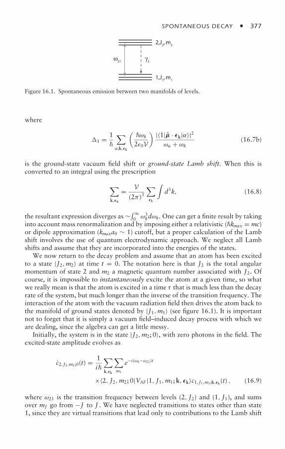
SPONTANEOUS DECAY 377
ω21
γ2
2,J2, m
2
1,J1, m
1
Figure 16.1. Spontaneous emission between two manifolds of levels.
where
1 = 1
∑α;k,εk
(ωk
2ε0V
) |〈1|µ · εk|α〉|2ωα + ωk (16.7b)
is the ground-state vacuum field shift or ground-state Lamb shift. When this isconverted to an integral using the prescription
∑k,εk
= V(2π )3
∑εk
∫d3k, (16.8)
the resultant expression diverges as ∼∫∞0 ω3
kdωk. One can get a finite result by takinginto account mass renormalization and by imposing either a relativistic (kmax = mc)or dipole approximation (kmaxa0 ∼ 1) cutoff, but a proper calculation of the Lambshift involves the use of quantum electrodynamic approach. We neglect all Lambshifts and assume that they are incorporated into the energies of the states.
We now return to the decay problem and assume that an atom has been excitedto a state |J2,m2〉 at time t = 0. The notation here is that J2 is the total angularmomentum of state 2 and m2 a magnetic quantum number associated with J2. Ofcourse, it is impossible to instantaneously excite the atom at a given time, so whatwe really mean is that the atom is excited in a time τ that is much less than the decayrate of the system, but much longer than the inverse of the transition frequency. Theinteraction of the atom with the vacuum radiation field then drives the atom back tothe manifold of ground states denoted by |J1,m1〉 (see figure 16.1). It is importantnot to forget that it is simply a vacuum field–induced decay process with which weare dealing, since the algebra can get a little messy.
Initially, the system is in the state |J2,m2; 0〉, with zero photons in the field. Theexcited-state amplitude evolves as
c2,J2,m2;0(t) = 1i
∑k,εk
∑m1
e−i(ωk−ω21)t
×〈2, J2,m2; 0|VAF |1, J1,m1;k, εk〉c1,J1,m1;k,εk(t) , (16.9)
where ω21 is the transition frequency between levels (2, J2) and (1, J1), and sumsover mJ go from −J to J . We have neglected transitions to states other than state1, since they are virtual transitions that lead only to contributions to the Lamb shift
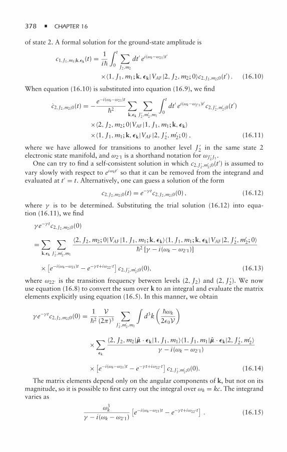
378 CHAPTER 16
of state 2. A formal solution for the ground-state amplitude is
c1,J1,m1;k,εk(t) = 1i
∫ t
0
∑J2,m2
dt′ ei(ωk−ω21)t′
×〈1, J1,m1;k, εk|VAF |2, J2,m2; 0〉c2,J2,m2;0(t′) . (16.10)
When equation (16.10) is substituted into equation (16.9), we find
c2,J2,m2;0(t) = −e−i(ωk−ω21)t
2
∑k,εk
∑J ′2,m
′2,m1
∫ t
0dt′ ei(ωk−ω2′1)t′c2,J ′
2,m′2;0(t
′)
×〈2, J2,m2; 0|VAF |1, J1,m1;k, εk〉×〈1, J1,m1;k, εk|VAF |2, J ′
2,m′2; 0〉 , (16.11)
where we have allowed for transitions to another level J ′2 in the same state 2
electronic state manifold, and ω2′1 is a shorthand notation for ωJ ′2 J1 .
One can try to find a self-consistent solution in which c2,J ′2,m
′2;0(t
′) is assumed tovary slowly with respect to eiωkt
′so that it can be removed from the integrand and
evaluated at t′ = t. Alternatively, one can guess a solution of the form
c2,J2,m2;0(t) = e−γ tc2,J2,m2;0(0) , (16.12)
where γ is to be determined. Substituting the trial solution (16.12) into equa-tion (16.11), we find
γ e−γ tc2,J2,m2;0(0)
=∑k,εk
∑J ′2,m
′2,m1
〈2, J2,m2; 0|VAF |1, J1,m1;k, εk〉〈1, J1,m1;k, εk|VAF |2, J ′2,m
′2; 0〉
2 [γ − i(ωk − ω2′1)]
× [e−i(ωk−ω21)t − e−γ t+iω22′ t] c2,J ′
2,m′2;0(0), (16.13)
where ω22′ is the transition frequency between levels (2, J2) and (2, J ′2). We now
use equation (16.8) to convert the sum over k to an integral and evaluate the matrixelements explicitly using equation (16.5). In this manner, we obtain
γ e−γ tc2,J2,m2;0(0) = 12
V(2π )3
∑J ′2,m
′2,m1
∫d3k
(ωk
2ε0V
)
×∑εk
〈2, J2,m2|µ · εk|1, J1,m1〉〈1, J1,m1|µ · εk|2, J ′2,m
′2〉
γ − i(ωk − ω2′1)
× [e−i(ωk−ω21)t − e−γ t+iω22′ t] c2,J ′
2,m′2;0(0). (16.14)
The matrix elements depend only on the angular components of k, but not on itsmagnitude, so it is possible to first carry out the integral over ωk = kc. The integrandvaries as
ω3k
γ − i(ωk − ω2′1)
[e−i(ωk−ω21)t − e−γ t+iω22′ t] . (16.15)
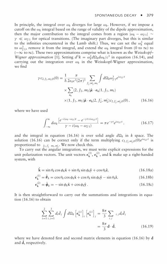
SPONTANEOUS DECAY 379
In principle, the integral over ωk diverges for large ωk. However, if we impose acutoff on the ωk integral based on the range of validity of the dipole approximation,then the major contribution to the integral comes from a region |ωk − ω2′1| ∼γ ω2′1 for optical transitions. (The imaginary part diverges, but this is similarto the infinities encountered in the Lamb shift.) Thus, we can set the ω3
k equalto ω3
2′1, remove it from the integral, and extend the ωk integral from (0 to ∞) to(−∞ to∞). These two approximations comprise what is known as the Weisskopf–Wigner approximation [1]. Setting d3k = ω2
kdkdωk/c3 in equation (16.14), andcarrying out the integration over ωk in the Weisskopf-Wigner approximation,we find
γ c2,J2,m2;0(0) = 1
π
2ε0c3(2π )3∑
J ′2,m
′2,m1
∫dkω
32′1e
iω22′ t
×∑εk
〈2, J2,m2|µ · εk|1, J1,m1〉
×〈1, J1,m1|µ · εk|2, J ′2,m
′2〉c2,J ′
2,m′2;0(0) , (16.16)
where we have used
∫ ∞
−∞dωk
[e−i(ωk−ω21)t − e−γ t+iω22′ t
]γ − i(ωk − ω2′1)
= πe−γ teiω22′ t , (16.17)
and the integral in equation (16.16) is over solid angle dk in k space. Thesolution (16.16) can be correct only if the term multiplying c2,J ′
2,m′2;0(0)e
iω22′ t isproportional to δJ2,J ′
2δm2,m′
2. We now check this.
To carry out the angular integration, we must write explicit expressions for theunit polarization vectors. The unit vectors ε
(1)k , ε
(2)k , and k make up a right-handed
system, with
k = sin θk cosφkx + sin θk sinφky + cos θkz, (16.18a)
ε(1)k = θk = cos θk cosφkx + cos θk sinφky − sin θkz, (16.18b)
ε(2)k = φk = − sinφkx + cosφky . (16.18c)
It is then straightforward to carry out the summations and integrations in equa-tion (16.16) to obtain
2∑λ=1
3∑i, j=1
di d j
∫dk
[ε(λ)k
]i
[ε(λ)k
]j= 8π
3
∑i, j
δi, j di d j
= 8π3
d · d, (16.19)
where we have denoted first and second matrix elements in equation (16.16) by dand d, respectively.
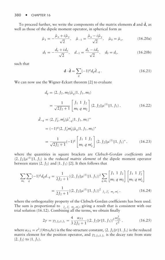
380 CHAPTER 16
To proceed further, we write the components of the matrix elements d and d, aswell as those of the dipole moment operator, in spherical form as
µ1 = − µx + iµy√2
, µ−1 = µx − iµy√2
, µ0 = µz, (16.20a)
d1 = −dx + idy√2
, d−1 = dx − idy√2
, d0 = dz, (16.20b)
such that
d · d =∑q
(−1)qdqd−q . (16.21)
We can now use the Wigner-Eckart theorem [2] to evaluate
dq = 〈2, J2,m2|µq|1, J1,m1〉
= 1√2J2 + 1
[J1 1 J2
m1 q m2
]〈2, J2‖µ(1)‖1, J1〉 , (16.22)
d−q = 〈2, J ′2,m
′2|µ†
−q|1, J1,m1〉∗
= (−1)q〈2, J ′2m
′2|µq|1, J1,m1〉∗
= 1√2J2 + 1
(−1)q[J1 1 J2
m1 q m′2
]〈2, J2‖µ(1)‖1, J1〉∗ , (16.23)
where the quantities in square brackets are Clebsch-Gordan coefficients and〈2, J2‖µ(1)‖1, J1〉 is the reduced matrix element of the dipole moment operatorbetween states |2, J2〉 and |1, J1〉 [2]. It then follows that
∑m1
∑q
(−1)qdqd−q = 12J2 + 1
|〈2, J2‖µ(1)‖1, J1〉|2∑q,m1
[J1 1 J2
m1 q m2
][J1 1 J ′
2
m1 q m′2
]
= 12J2 + 1
|〈2, J2‖µ(1)‖1, J1〉|2δJ2 ,J ′2δm2 ,m
′2, (16.24)
where the orthogonality property of the Clebsch-Gordan coefficients has been used.The sum is proportional to δJ2 ,J ′
2δm2 ,m
′2, giving a result that is consistent with our
trial solution (16.12). Combining all the terms, we obtain finally
2γ = γ2,J2;1,J1 = 43
αF S
2J2 + 1|〈2, J2‖r‖1, J1〉|2ω
321
c2, (16.25)
where αF S = e2/(4πε0c) is the fine-structure constant, 〈2, J2‖r‖1, J1〉 is the reducedmatrix element for the position operator, and γ2,J2;1,J1 is the decay rate from state|2, J2〉 to |1, J1〉.
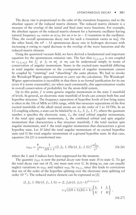
SPONTANEOUS DECAY 381
The decay rate is proportional to the cube of the transition frequency and to theabsolute square of the reduced matrix element. The reduced matrix element is ameasure of the overlap of the initial and final state wave functions. For example,the absolute square of the reduced matrix element for a harmonic oscillator havingnatural frequency ω0 varies as n/ω0 for an n to (n − 1) transition in the oscillator.Thus, the overall spontaneous decay rate for such a transition varies as nω2
0. Onthe other hand, the nP − 1S spontaneous decay rate in hydrogen decreases withincreasing n owing to rapid decrease in the overlap of the wave functions and thereduced matrix element.
Using the quantized vacuum field, we have derived a fundamental and importantequation for the spontaneous emission rate. The fact that c2,J2,m2;0 is not coupledto c2,J ′
2,m′2;0 for J ′
2 = J2 or m′2 = m2 can be understood simply in terms of
conservation of angular momentum. States in the excited-state manifold differingin total angular momentum or the z-component of angular momentum cannotbe coupled by “emitting” and “absorbing” the same photon. We had to invokethe Weisskopf-Wigner approximation to carry out the calculation. The Weisskopf-Wigner approximation is incredible in that there is no formal justification for its use(even if it seems reasonable), yet when used consistently, this approximation resultsin overall conservation of probability for the atom–field system.
Up to this point, J is some generic angular momentum in the state 2 manifoldof levels. In general, an electronic state manifold of levels can contain both fine andhyperfine structure. The frequency separation of hyperfine levels of low-lying statesis often in the 10s of MHz to GHz range, while fine-structure separations of the firstexcited manifolds of the alkali metal atoms are on the order of 1 to 10THz. In anLS coupling scheme, a state can be labeled by |n, Ln, S, Jn, I, F 〉, where the quantumnumber n specifies the electronic state, Ln the total orbital angular momentum,S the total spin angular momentum, Jn the combined orbital and spin angularmomentum that characterizes a fine structure manifold, I the total nuclear spinangular momentum, and F the total angular momentum that characterizes a givenhyperfine state. Let H label the total angular momentum of an excited hyperfinestate and G the total angular momentum of a ground hyperfine state. In that case,equation (16.25) is transformed into
γH;G = 43αF S
12H+ 1
|〈2, J2, I,H‖r‖1, J1, I,G〉|2ω3HG
c2, (16.26)
where the L and S indices have been suppressed for the moment.The quantity γH;G is now the partial decay rate from state H to state G. To get
the total decay rate out of H, one must sum over G. In doing so, one can usuallyneglect variations in ωHG and replace ωHG by ωJ2 J1 , since this leads to correctionsthat are of the order of the hyperfine splitting over the electronic state splitting (oforder 10−6). The reduced matrix element can be expressed as [2]
〈2, J2, I,H‖r‖1, J1, I,G〉 = 〈2, J2‖r‖1, J1〉(−1)G+I+J2+1
×√(2H+ 1)(2G+ 1)
J2 1 J1G I H
,
(16.27)
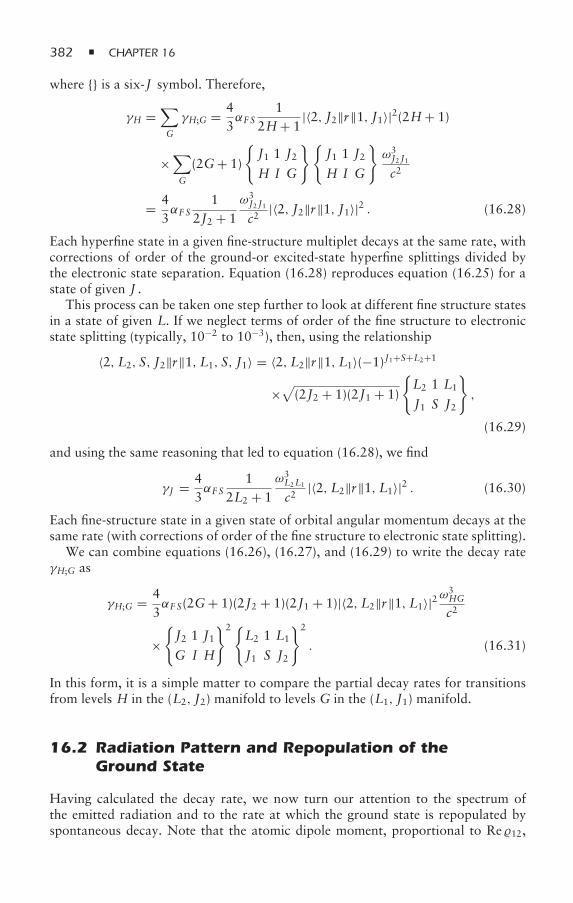
382 CHAPTER 16
where is a six-J symbol. Therefore,
γH =∑G
γH;G = 43αF S
12H+ 1
|〈2, J2‖r‖1, J1〉|2(2H+ 1)
×∑G
(2G+ 1)
J1 1 J2H I G
J1 1 J2H I G
ω3J2 J1
c2
= 43αF S
12J2 + 1
ω3J2 J1
c2|〈2, J2‖r‖1, J1〉|2 . (16.28)
Each hyperfine state in a given fine-structure multiplet decays at the same rate, withcorrections of order of the ground-or excited-state hyperfine splittings divided bythe electronic state separation. Equation (16.28) reproduces equation (16.25) for astate of given J .
This process can be taken one step further to look at different fine structure statesin a state of given L. If we neglect terms of order of the fine structure to electronicstate splitting (typically, 10−2 to 10−3), then, using the relationship
〈2, L2, S, J2‖r‖1, L1, S, J1〉 = 〈2, L2‖r‖1, L1〉(−1)J1+S+L2+1
×√
(2J2 + 1)(2J1 + 1)
L2 1 L1
J1 S J2
,
(16.29)
and using the same reasoning that led to equation (16.28), we find
γJ = 43αF S
12L2 + 1
ω3L2L1
c2|〈2, L2‖r‖1, L1〉|2 . (16.30)
Each fine-structure state in a given state of orbital angular momentum decays at thesame rate (with corrections of order of the fine structure to electronic state splitting).
We can combine equations (16.26), (16.27), and (16.29) to write the decay rateγH;G as
γH;G = 43αF S(2G+ 1)(2J2 + 1)(2J1 + 1)|〈2, L2‖r‖1, L1〉|2ω
3HG
c2
×J2 1 J1G I H
2L2 1 L1
J1 S J2
2
. (16.31)
In this form, it is a simple matter to compare the partial decay rates for transitionsfrom levels H in the (L2, J2) manifold to levels G in the (L1, J1) manifold.
16.2 Radiation Pattern and Repopulation of theGround State
Having calculated the decay rate, we now turn our attention to the spectrum ofthe emitted radiation and to the rate at which the ground state is repopulated byspontaneous decay. Note that the atomic dipole moment, proportional to Re 12,
SPONTANEOUS DECAY 383
equals zero at all times in this problem, since the atom is in a superposition of states|1, J1,m1;k, εk〉 and |2, J2,m2; 0〉, for which 12 = 0. The fact that the atomic dipolemoment vanishes implies that the average field emitted by the atom also vanishes,where the average is a quantum-mechanical average over a number of identicallyprepared systems. Since we start in an excited state with no well-defined phase, it isnot surprising that the average field vanishes. As you will see, however, even thoughthe average field vanishes, the radiation pattern of the field intensity can be the sameas that of a classical dipole oscillator, in certain limits.
16.2.1 Radiation Pattern
The calculation of the radiation spectrum begins with the expression for theamplitude to be in the ground state with a photon of type k, εk in the field. Thisamplitude is equal to [see equations (16.10) and (16.12)]
c1,J1,m1;k,εk(t) = 1i
〈1, J1,m1;k, εk|VAF |2, J2,m2; 0〉
×∑m2
∫ t
0dt′ei(ωk−ω21)t′e−γ2t′/2c2,J2,m2;0(0). (16.32)
In this expression, J can be considered to be a generic angular momentum; thecalculation is valid equally for transitions between manifolds of hyperfine-or fine-structure states. However, we restrict the discussion to transitions between a singleexcited-state and a single ground-state manifold, with ω21 the transition frequencybetween these manifolds of levels.
The radiation emitted by the atom is characterized by the frequency spectrum,angular distribution, and polarization of the radiated field. Information about allthese quantities is contained in the probability |c1,J1,m1;k,εk(∞)|2, since this quantityrepresents the probability that the radiation is found in mode k, εk after the excitedstate has decayed. Thus, |c1,J1,m1;k,εk(∞)|2 (ω2
k/c3)dωkdk is the probability that
the photon has frequency between ωk and ωk + dωk and is emitted with polarizationεk in an element of solid angle dk around the direction k. The normalization issuch that
V(2π )3
∫ ∞
0
(ω2k/c
3) dωk∫dk
∑εk
∑m1
|c1,J1,m1;k,εk (∞)|2 = 1. (16.33)
We define the spectral density dIk,εk (2, J2; 1, J1)/dωkdk for the J2; J1 transitionas
dIk,εk (2, J2; 1, J1)/dωkdk = (ω2k/c
3)∑m1
|c1,J1,m1;k,εk (∞)|2 = Vω2k
8π32c3
×∑
m1,m2,m′2
〈2, J2,m′2; 0|VAF |1, J1,m1;k, εk〉〈1, J1,m1;k, εk|VAF |2, J2,m2; 0〉
(ωk − ω21)2 + (γ2/2)2
×2,J2,m2;2,J2,m′2(0). (16.34)
The spectrum is Lorentzian if the ωk’s appearing in the matrix elements and the ω2k
multiplicative factor are evaluated at ωk = ω21. In fact, the normalization given
384 CHAPTER 16
by equation (16.33) is valid only if all multiplicative values of ωk appearing inequation (16.33) are evaluated at ωk = ω21 and if the integral is extended to −∞. Insome sense, one maintains unitarity only if a Weisskopf-Wigner-like approximationis also used for the radiated field intensity.
The product of matrix elements and the initial density matrix determines theangular distribution of radiation, on which we now concentrate. We evaluate thematrix elements explicitly using equation (16.5), integrate over ωk, and use equation(16.25) to define the angular distribution as
dIk,εk (2, J2; 1, J1)/dk =∫ ∞
0dωk dIk,εk(2, J2; 1, J1)/dωkdk
= 38π
(2J2 + 1)∑m2,m′
2
Am2,m′2J2,m2;J2,m′
2(0), (16.35)
where
Am2,m′2=
∑m1(εk · 〈J1,m1|µ|J2,m2〉)
(εk · 〈J1,m1|µ|J2,m′
2〉)∗
|〈J1‖µ‖J2〉|2 , (16.36)
and some indices have been suppressed. This definition is consistent with anormalization in which
∑εk
∫dk
[dIk,εk (2, J2; 1, J1)/dk
] = 1. (16.37)
To evaluate the matrix elements, we write
ε · µ =1∑
q=−1
(−1)qε−qµq , (16.38)
where
ε1 = −εx + iεy√2
, (16.39a)
ε−1 = εx − iεy√2
, (16.39b)
ε0 = εz , (16.39c)
with similar equations for the spherical tensor operators µq.Writing ε · µ in this form allows us to use the Wigner-Eckart theorem to obtain
Am2,m′2
=∑
q,q′,m1
(−1)q+q′ε−q
(εq′)∗
2J1 + 1
[J2 1 J1m2 q m1
][J2 1 J1m′
2 q′ m1
]
=∑
q,q′,m1
εq(εq′)∗
2J2 + 1
[J1 1 J2m1 q m2
][J1 1 J2m1 q′ m′
2
]. (16.40)
SPONTANEOUS DECAY 385
By combining this equation with equations (16.35), we find
dIk,εk (2, J2; 1, J1)/dk = 38π
∑m1,q,q′,m2,m′
2
εqε∗q′
[J1 1 J2m1 q m2
]
×[J1 1 J2m1 q′ m′
2
]J2,m2;J2,m′
2(0) . (16.41)
In effect, this equation determines how the initial excited-state polarization,represented by density matrix elements J2,m2;J2,m′
2(0), is transferred to the radiated
field. Consider first the limit where the initial state is unpolarized
J2,m2;J2,m′2(0) = 1
2J2 + 1δm2,m′
2. (16.42)
In this case,
dIk,εk(2, J2; 1, J1)/dk =∑
m1,q,q′,m2
38π
εq(εq′)∗
(2J2 + 1)
[J1 1 J2m1 q m2
][J1 1 J2m1 q′ m2
]
= 18π
∑m1,q,q′,m2
εq(εq′)∗[
J1 J2 1
−m1 m2 q
][J1 J2 1
−m1 m2 q′
]
= 18π
∑q,q′εq(εq′)∗δq,q′ = 1
8π
∑q
|εq|2 = 18π. (16.43)
As expected, the emitted radiation is unpolarized and isotropic in this limit, since theinitial atomic state is unpolarized. The integral of (1/8π ) over solid angle, summedover the two independent polarizations, equals unity.
Next, consider a polarized initial atomic state and a J1 = 0, J2 = 1 transition.From equation (16.41), we find
dIk,εk (2,1; 1,0)/dk = εm2ε∗m′
2J2,m2;J2,m′
2(0). (16.44)
Not surprisingly, the angular distribution and polarization of the emitted radiationdepends on how the initial state was prepared. If a z-polarized field is used to preparethe atom in the m2 = 0 sublevel, then
J2,m2;J2,m′2(0) = δm2,0δm′
2,0, (16.45a)
and
dIk,εk(2,1; 1,0)/dk = 38π
[(εk)0]2 = 3
8π[(εk)z]
2 . (16.45b)
For a given direction k, there are two independent polarization directions given byequations (16.18b) and (16.18c). For these polarization components, we find
(ε(1)k )z = (θk)z = − sin θk , (16.46a)
(ε(2)k )z = (φk)z = 0 . (16.46b)
386 CHAPTER 16
Therefore,
dIk,θk(2,1; 1,0)/dk = 3
8πsin2 θk (16.47)
polarized in the ε(1)k or θk direction. The angular distribution and polarization is
identical to that of a classical radiating dipole aligned along the z axis, even thoughthe dipole moment of the atom vanishes identically. It turns out that this result isunique to a J = 0 − 1 transition.
Suppose, instead, that the atom is prepared in the m2 = 1 state using a circularlypolarized field, J2,m2;J2,m′
2(0) = δm2,1δm′
2,1. The radiation pattern is given by
dIk,εk(2,1; 1,0)/dk = 38π
|(εk)1|2 = 38π
[(εk)x]2 + [
(εk)y]2
2. (16.48)
Therefore, the intensity of the θk polarization component is
dIk,θk(2,1; 1,0)/dk =
[ε(1)x
]2 + [ε(1)y
]22
= cos2 θk2
, (16.49a)
and that of the φk component is
dIk,φk(2,1; 1,0)/dk =
[ε(2)x
]2 + [ε(2)y
]22
= 12. (16.49b)
For θk = 0 or π , the intensity in both components is the same, a result consistentwith circularly polarized radiation.
To prove that the field is circularly polarized, we need an alternative expansionfor the vacuum field. In the decomposition of the free quantized electric field, wetook ε
(1)k = θk and ε
(2)k = φk to be real, corresponding to two independent linear
polarizations (θk×φk = k). We could just as well have used complex ε’s defined by
ε±k = ε
(1)k ± iε(2)k√
2= θk ± i φk√
2. (16.50)
The field is then written as
ET(R) = i∑k,λ=±
(ωk
2ε0V
)1/2 [akλε
(λ)k eik·R − a†
kλ
(ε(λ)k
)∗e−ik·R
], (16.51)
where ak± is a destruction operator for photons having polarization ε±k . As is
shown in appendix A, for field propagation in the k direction, ε±k correspond to the
polarization of left and right circularly polarized photons, respectively. In calculatingthe emitted field (as we do in chapter 19), one finds that, for radiation emittedparallel to the z axis, one circular polarization component only of the field is createdif the atom is prepared in either sublevel m= 1 or m= −1.
For a somewhat more detailed discussion of the manner in which the radiationpattern is linked to the fields that create the initial density matrix and for transitionsother than J1 = 0, J2 = 1, see the discussion in appendix B.
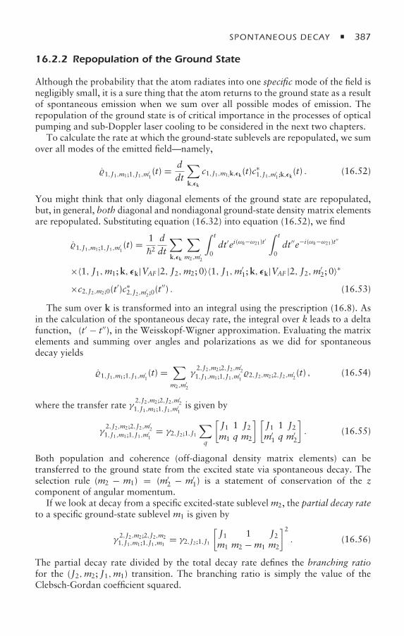
SPONTANEOUS DECAY 387
16.2.2 Repopulation of the Ground State
Although the probability that the atom radiates into one specific mode of the field isnegligibly small, it is a sure thing that the atom returns to the ground state as a resultof spontaneous emission when we sum over all possible modes of emission. Therepopulation of the ground state is of critical importance in the processes of opticalpumping and sub-Doppler laser cooling to be considered in the next two chapters.
To calculate the rate at which the ground-state sublevels are repopulated, we sumover all modes of the emitted field—namely,
1,J1,m1;1,J1,m′1(t) = d
dt
∑k,εk
c1,J1,m1;k,εk(t)c∗1,J1,m′
1;k,εk(t) . (16.52)
You might think that only diagonal elements of the ground state are repopulated,but, in general, both diagonal and nondiagonal ground-state density matrix elementsare repopulated. Substituting equation (16.32) into equation (16.52), we find
1,J1,m1;1,J1,m′1(t) = 1
2
ddt
∑k,εk
∑m2,m′
2
∫ t
0dt′ei(ωk−ω21)t′
∫ t
0dt′′e−i(ωk−ω21)t′′
×〈1, J1,m1;k, εk|VAF |2, J2,m2; 0〉〈1, J1,m′1;k, εk|VAF |2, J2,m′
2; 0〉∗
×c2,J2,m2;0(t′)c∗
2,J2,m′2;0(t′′) . (16.53)
The sum over k is transformed into an integral using the prescription (16.8). Asin the calculation of the spontaneous decay rate, the integral over k leads to a deltafunction, δ(t′ − t′′), in the Weisskopf-Wigner approximation. Evaluating the matrixelements and summing over angles and polarizations as we did for spontaneousdecay yields
1,J1,m1;1,J1,m′1(t) =
∑m2,m′
2
γ2,J2,m2;2,J2,m′
21,J1,m1;1,J1,m′
12,J2,m2;2,J2,m′
2(t) , (16.54)
where the transfer rate γ2,J2,m2;2,J2,m′
21,J1,m1;1,J1,m′
1is given by
γ2,J2,m2;2,J2,m′
21,J1,m1;1,J1,m′
1= γ2,J2;1,J1
∑q
[J1 1 J2m1 q m2
] [J1 1 J2m′
1 q m′2
]. (16.55)
Both population and coherence (off-diagonal density matrix elements) can betransferred to the ground state from the excited state via spontaneous decay. Theselection rule (m2 − m1) = (m′
2 − m′1) is a statement of conservation of the z
component of angular momentum.If we look at decay from a specific excited-state sublevelm2, the partial decay rate
to a specific ground-state sublevel m1 is given by
γ2,J2,m2;2,J2,m21,J1,m1;1,J1,m1
= γ2,J2;1,J1
[J1 1 J2m1 m2 −m1 m2
]2. (16.56)
The partial decay rate divided by the total decay rate defines the branching ratiofor the (J2,m2; J1,m1) transition. The branching ratio is simply the value of theClebsch-Gordan coefficient squared.
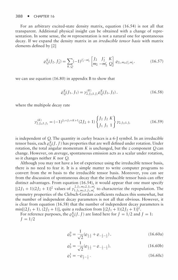
388 CHAPTER 16
For an arbitrary excited-state density matrix, equation (16.54) is not all thattransparent. Additional physical insight can be obtained with a change of repre-sentation. In some sense, the m representation is not a natural one for spontaneousdecay. If we expand the density matrix in an irreducible tensor basis with matrixelements defined by [2]
KQ(J2, J′2) =
∑K,Q
(−1)J′2−m′
2
[J2 J ′
2 Km2 −m′
2 Q
]J2,m2;J ′
2,m′2, (16.57)
we can use equation (16.80) in appendix B to show that
KQ(J1, J1) = γ(K)2,J2;1,J1
KQ(J2, J2) , (16.58)
where the multipole decay rate
γ(K)2,J2;1,J1 = (−1)J2+J1+K+1(2J2 + 1)
J2 J2 K
J1 J1 1
γ2,J2;1,J1 (16.59)
is independent of Q. The quantity in curley braces is a 6-J symbol. In an irreducibletensor basis, each KQ(J , J ) has properties that are well defined under rotation. Underrotation, the total angular momentum K is unchanged, but the z component Q canchange. However, on average, spontaneous emission acts as a scalar under rotation,so it changes neither K nor Q.
Although you may not have a lot of experience using the irreducible tensor basis,there is no need to fear it. It is a simple matter to write computer programs toconvert from the m basis to the irreducible tensor basis. Moreover, you can seefrom the discussion of spontaneous decay that the irreducible tensor basis can offerdistinct advantages. From equation (16.54), it would appear that one must specify[(2J1 + 1)(2J2 + 1)]2 values of γ
2,J2,m2;2,J2,m′2
1,J1,m1;1,J1,m′1to characterize the repopulation. The
symmetry properties of the Clebsch-Gordan coefficients reduces this somewhat, butthe number of independent decay parameters is not all that obvious. However, itis clear from equation (16.58) that the number of independent decay parameters ismin[(2J1 + 1), (2J2 + 1)], quite a reduction from [(2J1 + 1)(2J2 + 1)]2.
For reference purposes, the KQ(J , J ) are listed here for J = 1/2 and J = 1:J = 1/2
00 = 1√2( 1
212
+ − 12− 1
2) , (16.60a)
10 = 1√2( 1
212
− − 12− 1
2), (16.60b)
11 = − 12− 1
2. (16.60c)
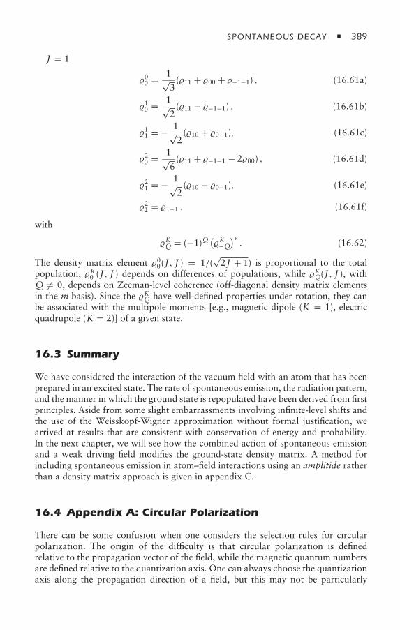
SPONTANEOUS DECAY 389
J = 1
00 = 1√3(11 + 00 + −1−1) , (16.61a)
10 = 1√2(11 − −1−1) , (16.61b)
11 = − 1√2(10 + 0−1), (16.61c)
20 = 1√6(11 + −1−1 − 200) , (16.61d)
21 = − 1√2(10 − 0−1), (16.61e)
22 = 1−1 , (16.61f)
with
KQ = (−1)Q(K−Q
)∗. (16.62)
The density matrix element 00(J , J ) = 1/(√2J + 1) is proportional to the total
population, K0 (J , J ) depends on differences of populations, while KQ(J , J ), withQ = 0, depends on Zeeman-level coherence (off-diagonal density matrix elementsin the m basis). Since the KQ have well-defined properties under rotation, they canbe associated with the multipole moments [e.g., magnetic dipole (K = 1), electricquadrupole (K = 2)] of a given state.
16.3 Summary
We have considered the interaction of the vacuum field with an atom that has beenprepared in an excited state. The rate of spontaneous emission, the radiation pattern,and the manner in which the ground state is repopulated have been derived from firstprinciples. Aside from some slight embarrassments involving infinite-level shifts andthe use of the Weisskopf-Wigner approximation without formal justification, wearrived at results that are consistent with conservation of energy and probability.In the next chapter, we will see how the combined action of spontaneous emissionand a weak driving field modifies the ground-state density matrix. A method forincluding spontaneous emission in atom–field interactions using an amplitide ratherthan a density matrix approach is given in appendix C.
16.4 Appendix A: Circular Polarization
There can be some confusion when one considers the selection rules for circularpolarization. The origin of the difficulty is that circular polarization is definedrelative to the propagation vector of the field, while the magnetic quantum numbersare defined relative to the quantization axis. One can always choose the quantizationaxis along the propagation direction of a field, but this may not be particularly
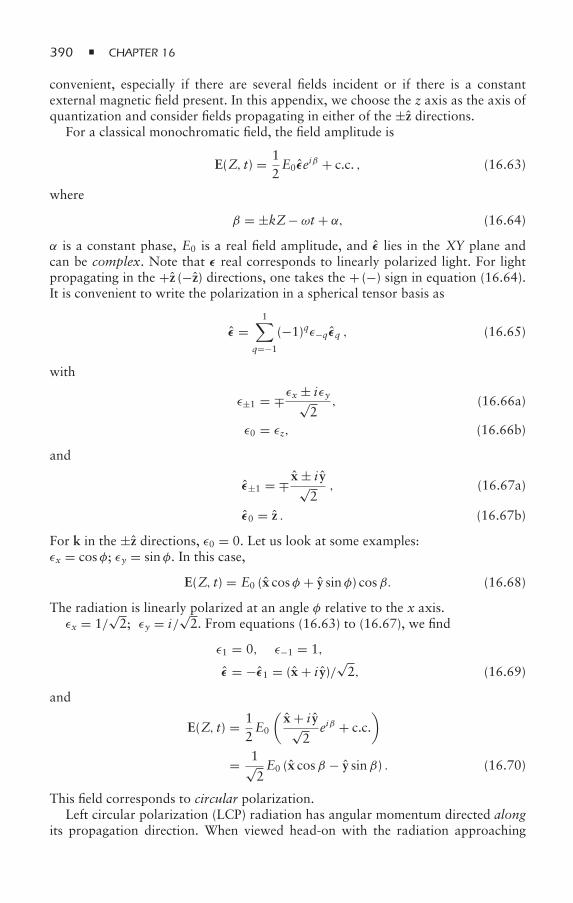
390 CHAPTER 16
convenient, especially if there are several fields incident or if there is a constantexternal magnetic field present. In this appendix, we choose the z axis as the axis ofquantization and consider fields propagating in either of the ±z directions.
For a classical monochromatic field, the field amplitude is
E(Z, t) = 12E0εeiβ + c.c. , (16.63)
where
β = ±kZ− ωt + α, (16.64)
α is a constant phase, E0 is a real field amplitude, and ε lies in the XY plane andcan be complex. Note that ε real corresponds to linearly polarized light. For lightpropagating in the +z (−z) directions, one takes the + (−) sign in equation (16.64).It is convenient to write the polarization in a spherical tensor basis as
ε =1∑
q=−1
(−1)qε−qεq , (16.65)
with
ε±1 = ∓εx ± iεy√2
, (16.66a)
ε0 = εz, (16.66b)
and
ε±1 = ∓ x ± i y√2, (16.67a)
ε0 = z . (16.67b)
For k in the ±z directions, ε0 = 0. Let us look at some examples:εx = cosφ; εy = sinφ. In this case,
E(Z, t) = E0 (x cosφ + y sinφ) cosβ. (16.68)
The radiation is linearly polarized at an angle φ relative to the x axis.εx = 1/
√2; εy = i/
√2. From equations (16.63) to (16.67), we find
ε1 = 0, ε−1 = 1,
ε = −ε1 = (x + i y)/√2, (16.69)
and
E(Z, t) = 12E0
(x + i y√
2eiβ + c.c.
)
= 1√2E0 (x cosβ − y sinβ) . (16.70)
This field corresponds to circular polarization.Left circular polarization (LCP) radiation has angular momentum directed along
its propagation direction. When viewed head-on with the radiation approaching
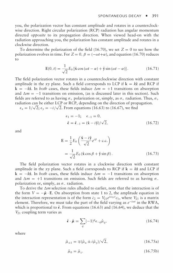
SPONTANEOUS DECAY 391
you, the polarization vector has constant amplitude and rotates in a counterclock-wise direction. Right circular polarization (RCP) radiation has angular momentumdirected opposite to its propagation direction. When viewed head-on with theradiation approaching you, the polarization has constant amplitude and rotates in aclockwise direction.
To determine the polarization of the field (16.70), we set Z = 0 to see how thepolarization evolves in time. For Z= 0, β = (−ωt+α), and equation (16.70) reducesto
E(0, t) = 1√2E0 [x cos (ωt − α) + y sin (ωt − α)] . (16.71)
The field polarization vector rotates in a counterclockwise direction with constantamplitude in the xy plane. Such a field corresponds to LCP if k = kz and RCP ifk = −kz. In both cases, these fields induce m = +1 transitions on absorptionand m = −1 transitions on emission, (as is discussed later in this section). Suchfields are referred to as having σ+ polarization or, simply, as σ+ radiation. Thus, σ+radiation can be either LCP or RCP, depending on the direction of propagation.εx = 1/
√2; εy = −i/√2. From equations (16.63) to (16.67), we find
ε1 = −1; ε−1 = 0,
ε = ε−1 = (x − i y)/√2, (16.72)
and
E = 12E0
(x − i y√
2eiβ + c.c.
)
= 1√2E0 (x cosβ + y sinβ) . (16.73)
The field polarization vector rotates in a clockwise direction with constantamplitude in the xy plane. Such a field corresponds to RCP if k = kz and LCP ifk = −kz. In both cases, these fields induce m = −1 transitions on absorptionand m = +1 transitions on emission. Such fields are referred to as having σ−polarization or, simply, as σ− radiation.
To derive the m selection rules alluded to earlier, note that the interaction is ofthe form V = −µ · E. On absorption from state 1 to 2, the amplitude equation inthe interaction representation is of the form c2 = V21eiω21tc1, where V21 is a matrixelement. Therefore, we must take the part of the field varying as e−iωt in the RWA,which is proportional to ε. From equations (16.63) and (16.64), we deduce that theV21 coupling term varies as
ε · µ =∑q
(−1)qε−qµq, (16.74)
where
µ±1 = ∓(µx ± iµy)/√2, (16.75a)
µ0 = µz. (16.75b)
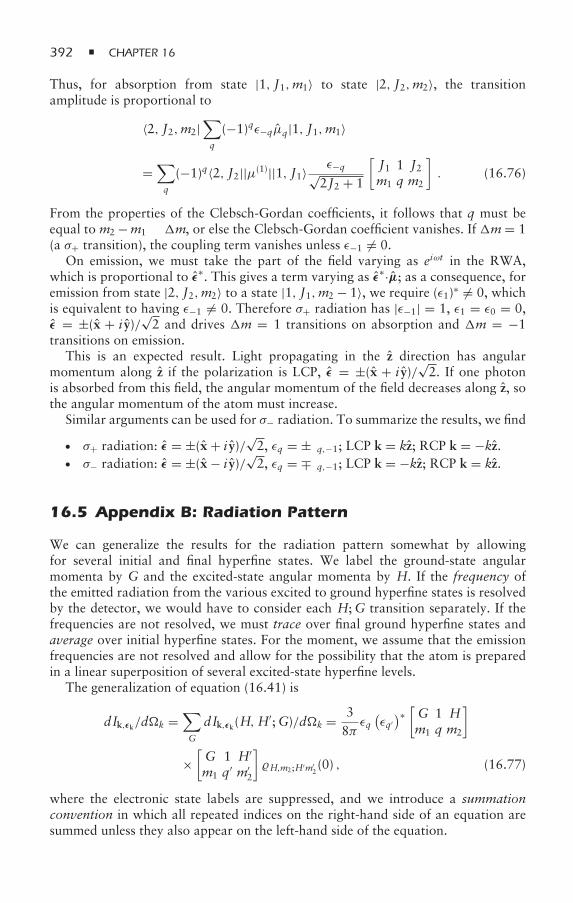
392 CHAPTER 16
Thus, for absorption from state |1, J1,m1〉 to state |2, J2,m2〉, the transitionamplitude is proportional to
〈2, J2,m2|∑q
(−1)qε−qµq|1, J1,m1〉
=∑q
(−1)q〈2, J2||µ(1)||1, J1〉 ε−q√2J2 + 1
[J1 1 J2m1 q m2
]. (16.76)
From the properties of the Clebsch-Gordan coefficients, it follows that q must beequal to m2 −m1 ≡ m, or else the Clebsch-Gordan coefficient vanishes. If m= 1(a σ+ transition), the coupling term vanishes unless ε−1 = 0.
On emission, we must take the part of the field varying as eiωt in the RWA,which is proportional to ε∗. This gives a term varying as ε∗·µ; as a consequence, foremission from state |2, J2,m2〉 to a state |1, J1,m2 − 1〉, we require (ε1)∗ = 0, whichis equivalent to having ε−1 = 0. Therefore σ+ radiation has |ε−1| = 1, ε1 = ε0 = 0,ε = ±(x + i y)/
√2 and drives m = 1 transitions on absorption and m = −1
transitions on emission.This is an expected result. Light propagating in the z direction has angular
momentum along z if the polarization is LCP, ε = ±(x + i y)/√2. If one photon
is absorbed from this field, the angular momentum of the field decreases along z, sothe angular momentum of the atom must increase.
Similar arguments can be used for σ− radiation. To summarize the results, we find
• σ+ radiation: ε = ±(x + i y)/√2, εq = ±δq,−1; LCP k = kz; RCP k = −kz.
• σ− radiation: ε = ±(x − i y)/√2, εq = ∓δq,−1; LCP k = −kz; RCP k = kz.
16.5 Appendix B: Radiation Pattern
We can generalize the results for the radiation pattern somewhat by allowingfor several initial and final hyperfine states. We label the ground-state angularmomenta by G and the excited-state angular momenta by H. If the frequency ofthe emitted radiation from the various excited to ground hyperfine states is resolvedby the detector, we would have to consider each H;G transition separately. If thefrequencies are not resolved, we must trace over final ground hyperfine states andaverage over initial hyperfine states. For the moment, we assume that the emissionfrequencies are not resolved and allow for the possibility that the atom is preparedin a linear superposition of several excited-state hyperfine levels.
The generalization of equation (16.41) is
dIk,εk/dk =∑G
dIk,εk(H,H′;G)/dk = 3
8πεq(εq′)∗[G 1 Hm1 q m2
]
×[G 1 H′
m1 q′ m′2
]H,m2;H′m′
2(0) , (16.77)
where the electronic state labels are suppressed, and we introduce a summationconvention in which all repeated indices on the right-hand side of an equation aresummed unless they also appear on the left-hand side of the equation.
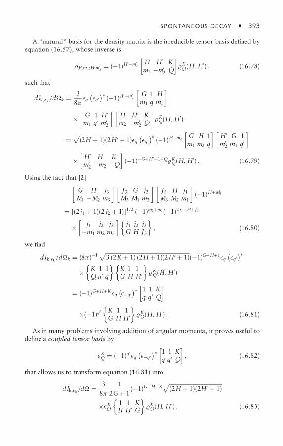
SPONTANEOUS DECAY 393
A “natural” basis for the density matrix is the irreducible tensor basis defined byequation (16.57), whose inverse is
H,m2;H′m′2= (−1)H
′−m′2
[H H′ Km2 −m′
2 Q
]KQ(H,H
′) , (16.78)
such that
dIk,εk/dk = 38πεq(εq′)∗ (−1)H
′−m′2
[G 1 Hm1 q m2
]
×[G 1 H′
m1 q′ m′2
] [H H′ Km2 −m′
2 Q
]KQ(H,H
′)
=√(2H+ 1)(2H′ + 1)εq
(εq′)∗ (−1)H−m2
[G H 1m1 m2 q
] [H′ G 1m′
2 m1 q′
]
×[H′ H Km′
2 −m2 −Q
](−1)−G+H′+1+QKQ(H,H
′) . (16.79)
Using the fact that [2][G H j3M1 −M2 m3
] [J3 G j2M3 M1 m2
] [J3 H j1M3 M2 m1
](−1)H+M2
= [(2 j1 + 1)(2 j2 + 1)]1/2 (−1)m2+m3 (−1)2 j1+H+J3
×[
j1 j2 j3−m1 m2 m3
]j1 j2 j3G H J3
, (16.80)
we find
dIk,εk/dk = (8π )−1√
3 (2K + 1) (2H+ 1)(2H′ + 1)(−1)G+H+1εq(εq′)∗
×K 1 1Qq′ q
K 1 1G H H′
KQ(H,H
′)
= (−1)G+H+Kεq(ε−q′
)∗[1 1 Kq q′ Q
]
×(−1)q′K 1 1G H H′
KQ(H,H
′) . (16.81)
As in many problems involving addition of angular momenta, it proves useful todefine a coupled tensor basis by
εKQ = (−1)q′εq(ε−q′
)∗[1 1 Kq q′ Q
], (16.82)
that allows us to transform equation (16.81) into
dIk,εk/d = 38π
12G+ 1
(−1)G+H+K√
(2H+ 1)(2H′ + 1)
×εKQ1 1 KH H′ G
KQ(H,H
′) . (16.83)
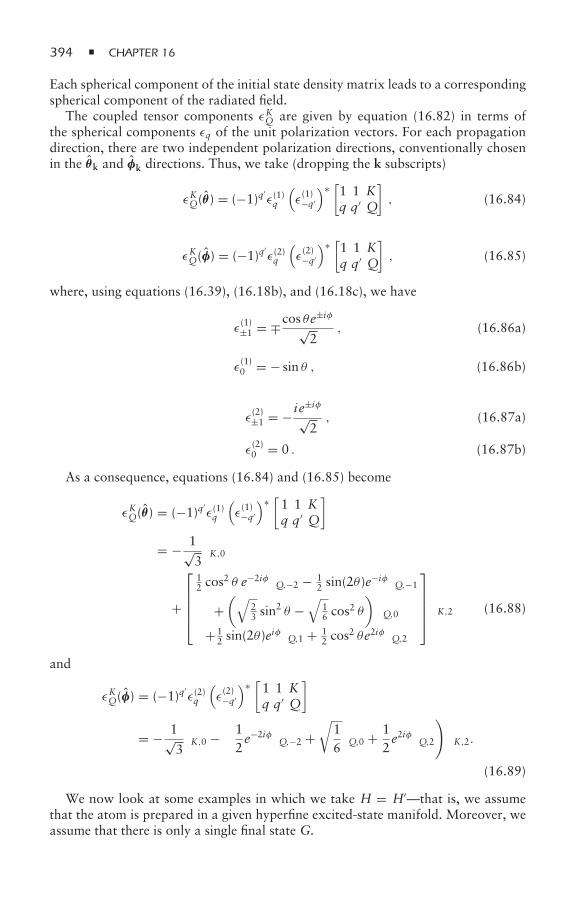
394 CHAPTER 16
Each spherical component of the initial state density matrix leads to a correspondingspherical component of the radiated field.
The coupled tensor components εKQ are given by equation (16.82) in terms ofthe spherical components εq of the unit polarization vectors. For each propagationdirection, there are two independent polarization directions, conventionally chosenin the θk and φk directions. Thus, we take (dropping the k subscripts)
εKQ(θ ) = (−1)q′ε(1)q
(ε(1)−q′
)∗ [1 1 Kq q′ Q
], (16.84)
εKQ(φ) = (−1)q′ε(2)q
(ε(2)−q′
)∗ [1 1 Kq q′ Q
], (16.85)
where, using equations (16.39), (16.18b), and (16.18c), we have
ε(1)±1 = ∓cos θe±iφ
√2
, (16.86a)
ε(1)0 = − sin θ , (16.86b)
ε(2)±1 = − ie±iφ
√2, (16.87a)
ε(2)0 = 0 . (16.87b)
As a consequence, equations (16.84) and (16.85) become
εKQ(θ ) = (−1)q′ε(1)q
(ε(1)−q′
)∗ [1 1 Kq q′ Q
]
= − 1√3δK,0
+
⎡⎢⎢⎢⎣
12 cos
2 θ e−2iφδQ,−2 − 12 sin(2θ )e
−iφδQ,−1
+(√
23 sin
2 θ −√
16 cos
2 θ
)δQ,0
+ 12 sin(2θ )e
iφδQ,1 + 12 cos
2 θe2iφδQ,2
⎤⎥⎥⎥⎦ δK,2 (16.88)
and
εKQ(φ) = (−1)q′ε(2)q
(ε(2)−q′
)∗ [1 1 Kq q′ Q
]
= − 1√3δK,0 −
(12e−2iφδQ,−2 +
√16δQ,0 + 1
2e2iφδQ,2
)δK,2.
(16.89)
We now look at some examples in which we take H = H′—that is, we assumethat the atom is prepared in a given hyperfine excited-state manifold. Moreover, weassume that there is only a single final state G.
SPONTANEOUS DECAY 395
16.5.1 Unpolarized Initial State
If the atom is prepared in an unpolarized initial state,
KQ(H,H) = 1√2H+ 1
δK,0δQ,0 , (16.90)
one can use the fact that 1 1 0H H G
= (−1)H+G√
3 (2H+ 1)(16.91)
to obtain
dIk,εk/d = 38π
(−1)G+H√
(2H+ 1)ε00(−1)H+G√3 (2H+ 1)
= (−1)q′√3
8πεq(ε−q′
)∗[1 1 0q q′ 0
]
= 18π
∑q
|εq|2 = 18π
. (16.92)
The radiation is unpolarized and isotropic, as expected.
16.5.2 z-Polarized Excitation
To examine other initial conditions, we need to specify KQ(H,H). The initial statedensity matrix elements KQ(H,H) are created by the external excitation fields. Inperturbation theory, one can show that the values of KQ(H,H) are determined bythe coupled tensor εKQ(i) of the excitation field according to
KQ(H,H) ∝ εK−Q(i)1 1 KH H G
. (16.93)
This result can be derived using the formalism presented in the following chapter.Combining equation (16.93) with equation (16.83), we find an (unnormalized)radiation pattern given by
dIk,εk/dk = (−1)KεKQεK−Q(i)
1 1 KH H G
2
. (16.94)
For a z-polarized light field (εq = δq,0), we can use equation (16.82) to calculate
εKQ(i) ∝(
− 1√3δK,0 + 2√
6δK,2
)δQ,0 , (16.95)
which implies that
dIk,εk/dk = εK0
(− 1√
3δK,0 + 2√
6δK,2
)1 1 KH H G
2
. (16.96)
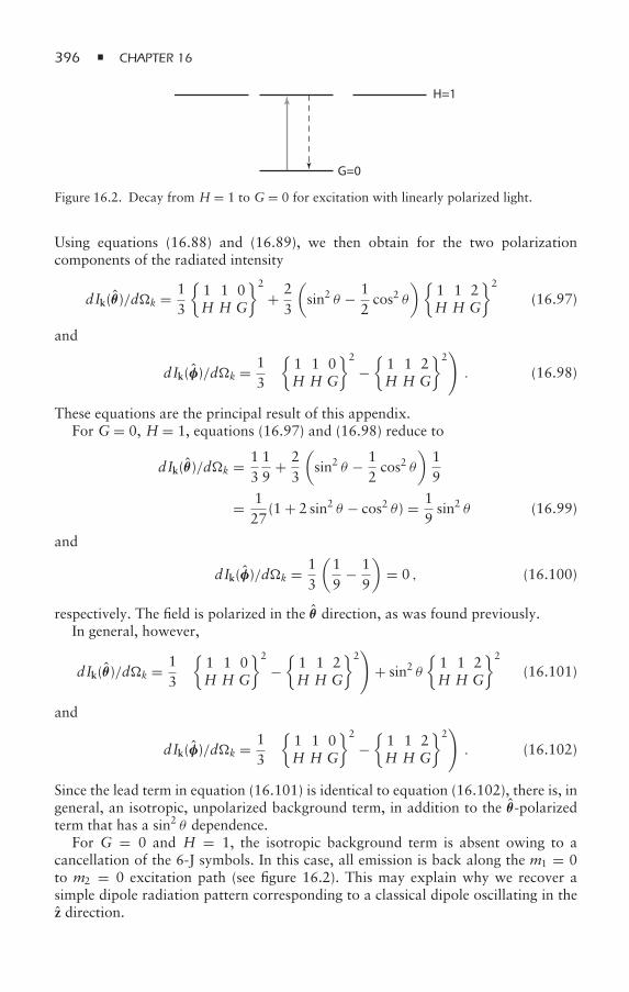
396 CHAPTER 16
G=0
H=1
Figure 16.2. Decay from H = 1 to G = 0 for excitation with linearly polarized light.
Using equations (16.88) and (16.89), we then obtain for the two polarizationcomponents of the radiated intensity
dIk(θ )/dk = 13
1 1 0H H G
2
+ 23
(sin2 θ − 1
2cos2 θ
)1 1 2H H G
2
(16.97)
and
dIk(φ)/dk = 13
(1 1 0H H G
2
−1 1 2H H G
2). (16.98)
These equations are the principal result of this appendix.For G = 0, H = 1, equations (16.97) and (16.98) reduce to
dIk(θ)/dk = 1319
+ 23
(sin2 θ − 1
2cos2 θ
)19
= 127
(1 + 2 sin2 θ − cos2 θ ) = 19sin2 θ (16.99)
and
dIk(φ)/dk = 13
(19
− 19
)= 0 , (16.100)
respectively. The field is polarized in the θ direction, as was found previously.In general, however,
dIk(θ )/dk = 13
(1 1 0H H G
2
−1 1 2H H G
2)
+ sin2 θ1 1 2H H G
2
(16.101)
and
dIk(φ)/dk = 13
(1 1 0H H G
2
−1 1 2H H G
2). (16.102)
Since the lead term in equation (16.101) is identical to equation (16.102), there is, ingeneral, an isotropic, unpolarized background term, in addition to the θ -polarizedterm that has a sin2 θ dependence.
For G = 0 and H = 1, the isotropic background term is absent owing to acancellation of the 6-J symbols. In this case, all emission is back along the m1 = 0to m2 = 0 excitation path (see figure 16.2). This may explain why we recover asimple dipole radiation pattern corresponding to a classical dipole oscillating in thez direction.
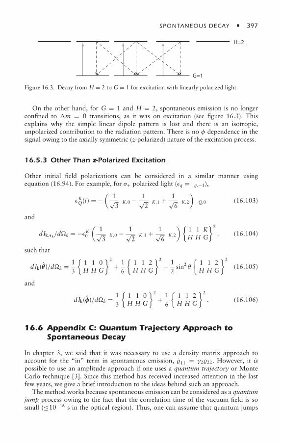
SPONTANEOUS DECAY 397
G=1
H=2
Figure 16.3. Decay from H = 2 to G = 1 for excitation with linearly polarized light.
On the other hand, for G = 1 and H = 2, spontaneous emission is no longerconfined to m = 0 transitions, as it was on excitation (see figure 16.3). Thisexplains why the simple linear dipole pattern is lost and there is an isotropic,unpolarized contribution to the radiation pattern. There is no φ dependence in thesignal owing to the axially symmetric (z-polarized) nature of the excitation process.
16.5.3 Other Than z-Polarized Excitation
Other initial field polarizations can be considered in a similar manner usingequation (16.94). For example, for σ+ polarized light (εq = δq,−1),
εKQ(i) = −(
1√3δK,0 − 1√
2δK,1 + 1√
6δK,2
)δQ,0 (16.103)
and
dIk,εk/dk = −εK0(
1√3δK,0 − 1√
2δK,1 + 1√
6δK,2
)1 1 KH H G
2
, (16.104)
such that
dIk(θ)/dk = 13
1 1 0H H G
2
+ 16
1 1 2H H G
2
− 12sin2 θ
1 1 2H H G
2
(16.105)
and
dIk(φ)/dk = 13
1 1 0H H G
2
+ 16
1 1 2H H G
2
. (16.106)
16.6 Appendix C: Quantum Trajectory Approach toSpontaneous Decay
In chapter 3, we said that it was necessary to use a density matrix approach toaccount for the “in” term in spontaneous emission, 11 = γ222. However, it ispossible to use an amplitude approach if one uses a quantum trajectory or MonteCarlo technique [3]. Since this method has received increased attention in the lastfew years, we give a brief introduction to the ideas behind such an approach.
The method works because spontaneous emission can be considered as a quantumjump process owing to the fact that the correlation time of the vacuum field is sosmall (≤10−16 s in the optical region). Thus, one can assume that quantum jumps

398 CHAPTER 16
occur according to some random algorithm and then average over a large numberof possible histories.
The basic idea is to look at the wave function and density matrix at time intervalsseparated by δt. We consider only a two-level atom. At a given time, the wavefunction is of the form
|(t)〉 = a1(t)|1〉 + a2(t)|2〉 (16.107)
and is assumed to evolve under the non-Hermitian Hamiltonian
H = H0 +(0 00 −iγ
), (16.108)
where γ = γ2/2.In a time interval δt small compared with (Rabi frequencies)−1, (detunings)−1,
and γ−12 , the probability dP for spontaneous emission is
dP = γ2|a2(t)|2δt . (16.109)
We now choose a random variable ε uniformly distributed between 0 and 1. Ifε < dP, no emission occurs, and we set
|(t + δt)〉 =
(1 − iHδt
)|(t)〉
〈(t + δt)|(t + δt)〉1/2 . (16.110)
In other words, we allow the system to evolve according to the Hamiltonian H, butrenormalize the state vector for the system. On the other hand, if ε > dP, emissionoccurs, and we set
|(t + δt)〉 = |1〉, (16.111)
that is, we restart the atom in its ground state. Note that
〈(t + δt)|(t + δt)〉 = 〈(t)|(1 + iH†δt
)(1 − iHδt
)|(t)〉
≈ 〈(t)|(t)〉 − γ2〈(t)|(0 00 1
)|(t)〉δt
= 1 − γ2δt|a2(t)|2 = 1 − dP . (16.112)
Now we construct the density matrix at time (t + δt) using
(t + δt) = P0(δt)
(1 − i
Hδt
) |(t)〉〈(t)| (1 + iH†δt
)1 − dP
+ dP|1〉〈1| , (16.113)
where P0(δt) = (1 − dP) is the probability of no emission in time δt and the “line”denotes averaging over different histories. From equations (16.108) and (16.113),we obtain, to order δt,
(t + δt) =
(t) + 1i
[H0, (t)
]δt − γ2
2
[(t)
(0 00 1
)+(0 00 1
)(t)
]δt
+γ2|a2(t)|2δt|1〉〈1| , (16.114)
SPONTANEOUS DECAY 399
or
˙(t) = 1i
[H0, (t)] − γ2
2[12(t)|1〉〈2| + 21(t)|2〉〈1|]
−γ222(t)|2〉〈2| + γ222(t)|1〉〈1| , (16.115)
which is identical to the optical Bloch equations.Thus, one can use amplitude equations for a number of histories and then form
density matrix elements. The advantage is that for n coupled amplitude equations,one need solve only n equations (for a number of histories) rather than n2 equationsfor a single history. This method is especially useful if one has to use a quantizeddescription of the center-of-mass motion, since the number of quantized motionstates that must be included can become very large.
Problems
1. Estimate the 2P–1S decay rate in hydrogen and also the 2S–2P decay rate.You will need to look up the wave functions and frequency spacings of theselevels.
2. Use equations (16.28) and (16.29) to estimate the ratio of the decay rates forthe D1 and D2 transitions in Na.
3. Consider spontaneous emission from state |2, J2〉 to state |1, J1〉 in an ensembleof independently decaying atoms. Calculate the radiation pattern as a functionof k and the polarization defined by ε = cos(ψ)θ +sin(ψ)φ, assuming an initialdensity matrix 〈J2,m2||J2,m′
2〉 for the atoms. The unit vectors θ and φ aredefined relative to the direction of emission k. For an unpolarized initial state,〈J2,m2||J2,m′
2〉 = (2J2 + 1)−1δm2,m′2, show that the radiation in any direction
is unpolarized (that is, the radiated intensity is independent of ψ for any θand φ). For J1 = 0 and J2 = 1, show that the radiation emitted in the zdirection is consistent with circularly polarized radiation if 〈J2,m2||J2,m′
2〉 =δm2,1δm′
2,1.4. Prove that
2∑λ=1
∫dk
∑i
[ε(λ)k
]idi∑j
[ε(λ)k
]jd j = 8π
3
∑i
di di .
5. Prove that ∑m1
〈2, J2,m2|d|1, J1,m1〉 · 〈1, J1,m1|d|2, J ′2,m
′2〉
= |〈2, J2‖d‖1, J1〉|22J2 + 1
δm2 ,m′2δJ2,J ′
2.
6. Derive equation (16.54).7. Use equation (16.80) to derive equation (16.57) from equation (16.54).8. Use perturbation theory and equation (16.80) to derive equation (16.93).9. Write a program to calculate density matrix elements in the irreducible tensor
basis, given the density matrix elements in the m basis. Use your program toverify equations (16.60) and (16.61).
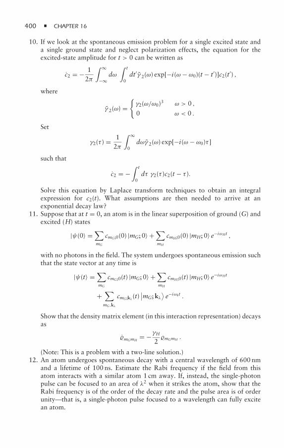
400 CHAPTER 16
10. If we look at the spontaneous emission problem for a single excited state anda single ground state and neglect polarization effects, the equation for theexcited-state amplitude for t > 0 can be written as
c2 = − 12π
∫ ∞
−∞dω
∫ t
0dt′γ 2(ω) exp[−i(ω − ω0)(t − t′)]c2(t′) ,
where
γ 2(ω) =γ2(ω/ω0)3 ω > 0 ,
0 ω < 0 .
Set
γ2(τ ) = 12π
∫ ∞
0dωγ 2(ω) exp[−i(ω − ω0)τ ]
such that
c2 = −∫ t
0dτ γ2(τ )c2(t − τ ).
Solve this equation by Laplace transform techniques to obtain an integralexpression for c2(t). What assumptions are then needed to arrive at anexponential decay law?
11. Suppose that at t = 0, an atom is in the linear superposition of ground (G) andexcited (H) states
|ψ(0〉 =∑mG
cmG;0(0) |mG; 0〉 +∑mH
cmH;0(0) |mH; 0〉 e−iωHt ,
with no photons in the field. The system undergoes spontaneous emission suchthat the state vector at any time is
|ψ(t〉 =∑mG
cmG;0(t) |mG; 0〉 +∑mH
cmH;0(t) |mH; 0〉 e−iωHt
+∑mG,kλ
cmG;kλ (t)∣∣mG;kλ
⟩e−iωkt .
Show that the density matrix element (in this interaction representation) decaysas
mGmH= −γH
2mGmH .
(Note: This is a problem with a two-line solution.)12. An atom undergoes spontaneous decay with a central wavelength of 600 nm
and a lifetime of 100 ns. Estimate the Rabi frequency if the field from thisatom interacts with a similar atom 1 cm away. If, instead, the single-photonpulse can be focused to an area of λ2 when it strikes the atom, show that theRabi frequency is of the order of the decay rate and the pulse area is of orderunity—that is, a single-photon pulse focused to a wavelength can fully excitean atom.
SPONTANEOUS DECAY 401
References
[1] V. Weisskopf and E. Wigner, Berechnung der natürlichen Linienbreite auf Grundder Diracschen Lichttheorie, Zeitschrift für Physik 63, 54–73 (1930); a translation isavailable, Calculation of the natural line width on the basis of Dirac’s theory of light, inW. R. Hindmarsh, Atomic Spectra (Pergamon Press, London, 1967), pp. 304–327.
[2] We follow the phase conventions given in vol. II, app. C, of A. Messiah, QuantumMechanics (North Holland, Amsterdam, 1966). Properties of the Clebsch-Gordan, 3-J,6-J, and 9-J symbols are discussed in this appendix, as well as irreducible tensor operatorsand rotation matrices.
[3] See, for example, J. Dalibard, Y. Castin, and K. Mølmer, Wave-function approach todissipative processes in quantum optics, Physical Review Letters 68, 580–583 (1992);R. Dum, A. S. Parkins, P. Zoller, and C. W. Gardiner,Monte Carlo simulation of masterequations in quantum optics for vacuum, thermal, and squeezed reservoirs, PhysicalReview A 46, 4382–4396 (1992); K. Mølmer, Y. Castin, and J. Dalibard, Monte Carlowave-function method in quantum optics, Journal of the Optical Society of America B10, 524–538 (1993); H. J. Carmichael, Quantum trajectory theory for cascaded opensystems, Physical Review Letters 70, 2273–2276 (1993); Y. Castin and K. Mølmer,Monte Carlo wave functions and nonlinear master equations, Physical Review A 54,5275–5290 (1996).
Bibliography
W. Heitler, The Quantum Theory of Radiation, 3rd ed. (Oxford University Press, Lon-don,1954), chaps. IV and V.
Some books on angular momentum and irreducible tensor operators are listed here:K. Blum, Density Matrix Theory and Applications (Plenum Press, New York, 1981).D. M. Brink and G. R. Satchler, Angular Momentum, 3rd ed. (Clarendon Press, Oxford, UK,1994).
A. R. Edmonds, Angular Momentum in Quantum Mechanics (Princeton University Press,Princeton, NJ, 1996).
U. Fano and G. Racah, Irreducible Tensorial Sets (Academic Press, New York, 1959).M. E. Rose, Elementary Theory of Angular Momentum (Dover, New York, 1995).W. J. Thompson, Angular Momentum (Wiley, New York, 1994).
For quantum trajectory theory, seeH. J. Carmichael, An Open Systems Approach to Quantum Optics, Lecture Notes in Physics,New Series M—Monographs, vol. M18 (Springer-Verlag, Berlin, 1993).
17Optical Pumping and Optical Lattices
17.1 Optical Pumping
In 1950, Alfred Kastler proposed optical pumping [1] as a means for using opticalfields to transfer internal state angular momentum to atoms. For his discoveries,Kastler was awarded the Nobel Prize in 1966. Optical pumping refers to a processin which the combined action of (1) stimulated absorption and emission producedby optical fields and (2) spontaneous decay results in a polarized ground state.[A polarized ground state is one in which J,m;J,m′ = δm,m′/(2J +1); in irreducibletensor language, KQ =δK,0δQ,0/(2J+1)1/2.] Actually, as has been stressed throughoutthis book, one cannot really represent the scattering of a cw field by atoms asabsorption followed by spontaneous emission. The entire process is one in whichthe incident field is scattered into previously unoccupied modes of the vacuum field,resulting also in a modification of the ground-state density matrix of the atoms.This should be kept in mind, even if we use the terms absorption and spontaneousemission in this chapter.
Although the density matrix equations can get algebraically complicated, the ideais simple. As an example, consider transitions between a G=1 ground state and anH= 0 excited state driven by a z-polarized field (figure 17.1). (In all examples andcalculations, we limit the discussion to a single ground-state hyperfine level havingtotal angular momentum G and excited state having total angular momentum H.)The dipole selection rules are m = ±1,0, with m = 0 forbidden if G=H and Gis integral. For the level scheme of figure 17.1, optical pumping results ultimately insteady-state populations
0,0 = 0, −1−1 = 11 = 12, (17.1)
and moreover, the atom is decoupled from the field. In this case, the groundstate becomes polarized, but the expectation value of the z component of angularmomentum is equal to zero. A linearly polarized field has no intrinsic or spin angularmomentum associated with it [2]. It can transfer linear momentum to the atom’s
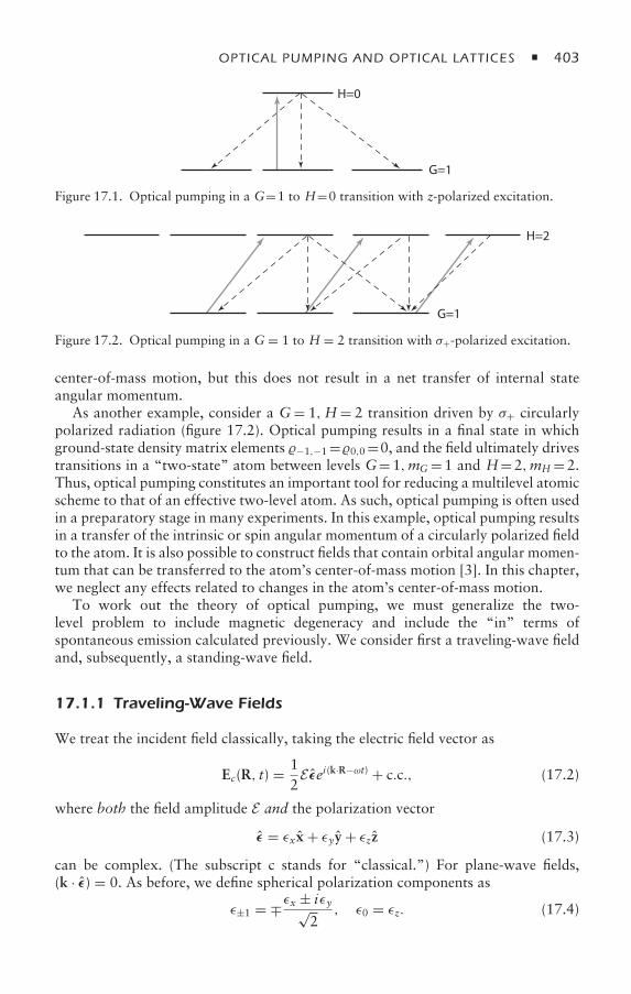
OPTICAL PUMPING AND OPTICAL LATTICES 403
G=1
H=0
Figure 17.1. Optical pumping in a G=1 to H=0 transition with z-polarized excitation.
G=1
H=2
Figure 17.2. Optical pumping in a G= 1 to H = 2 transition with σ+-polarized excitation.
center-of-mass motion, but this does not result in a net transfer of internal stateangular momentum.
As another example, consider a G= 1,H= 2 transition driven by σ+ circularlypolarized radiation (figure 17.2). Optical pumping results in a final state in whichground-state density matrix elements −1,−1=0,0=0, and the field ultimately drivestransitions in a “two-state” atom between levels G=1,mG=1 and H=2,mH =2.Thus, optical pumping constitutes an important tool for reducing a multilevel atomicscheme to that of an effective two-level atom. As such, optical pumping is often usedin a preparatory stage in many experiments. In this example, optical pumping resultsin a transfer of the intrinsic or spin angular momentum of a circularly polarized fieldto the atom. It is also possible to construct fields that contain orbital angular momen-tum that can be transferred to the atom’s center-of-mass motion [3]. In this chapter,we neglect any effects related to changes in the atom’s center-of-mass motion.
To work out the theory of optical pumping, we must generalize the two-level problem to include magnetic degeneracy and include the “in” terms ofspontaneous emission calculated previously. We consider first a traveling-wave fieldand, subsequently, a standing-wave field.
17.1.1 Traveling-Wave Fields
We treat the incident field classically, taking the electric field vector as
Ec(R, t) = 12E εei(k·R−ωt) + c.c., (17.2)
where both the field amplitude E and the polarization vector
ε = εxx + εyy + εzz (17.3)
can be complex. (The subscript c stands for “classical.”) For plane-wave fields,(k · ε) = 0. As before, we define spherical polarization components as
ε±1 = ∓εx ± iεy√2
, ε0 = εz. (17.4)
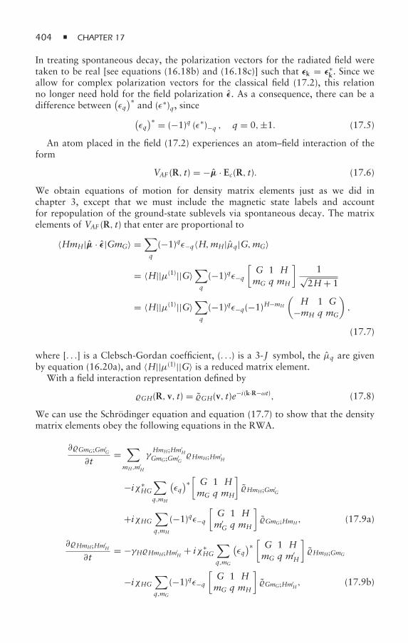
404 CHAPTER 17
In treating spontaneous decay, the polarization vectors for the radiated field weretaken to be real [see equations (16.18b) and (16.18c)] such that εk = ε∗
k. Since weallow for complex polarization vectors for the classical field (17.2), this relationno longer need hold for the field polarization ε. As a consequence, there can be adifference between
(εq)∗ and (ε∗)q, since(εq)∗ = (−1)q (ε∗)−q , q = 0,±1. (17.5)
An atom placed in the field (17.2) experiences an atom–field interaction of theform
VAF (R, t) = −µ · Ec(R, t). (17.6)
We obtain equations of motion for density matrix elements just as we did inchapter 3, except that we must include the magnetic state labels and accountfor repopulation of the ground-state sublevels via spontaneous decay. The matrixelements of VAF (R, t) that enter are proportional to
〈HmH|µ · ε|GmG〉 =∑q
(−1)qε−q〈H,mH|µq|G,mG〉
= 〈H||µ(1)||G〉∑q
(−1)qε−q
[G 1 HmG q mH
]1√
2H+ 1
= 〈H||µ(1)||G〉∑q
(−1)qε−q(−1)H−mH
(H 1 G
−mH q mG
),
(17.7)
where [. . .] is a Clebsch-Gordan coefficient, (. . .) is a 3-J symbol, the µq are givenby equation (16.20a), and 〈H||µ(1)||G〉 is a reduced matrix element.
With a field interaction representation defined by
GH(R, v, t) = GH(v, t)e−i(k·R−ωt), (17.8)
We can use the Schrödinger equation and equation (17.7) to show that the densitymatrix elements obey the following equations in the RWA.
∂GmG;Gm′G
∂t=
∑mH,m′
H
γHmH;Hm′
HGmG;Gm′
GHmH;Hm′
H
−iχ∗HG
∑q,mH
(εq)∗[G 1 HmG q mH
]HmH;Gm′
G
+iχHG∑q,mH
(−1)qε−q
[G 1 Hm′G q mH
]GmG;HmH , (17.9a)
∂HmH;Hm′H
∂t= −γHHmH;Hm′
H+ iχ∗
HG
∑q,mG
(εq)∗[G 1 HmG q m′
H
]HmH;GmG
−iχHG∑q,mG
(−1)qε−q
[G 1 HmG q mH
]GmG;Hm′
H, (17.9b)
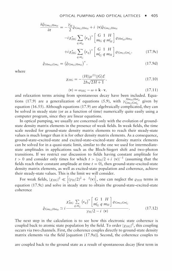
OPTICAL PUMPING AND OPTICAL LATTICES 405
∂GmG;HmH
∂t= −γH
2GmG;HmH + iδ(v)GmG;HmH
−iχ∗HG
∑q,m′
H
(εq)∗[G 1 HmG q m′
H
]Hm′
H;HmH
+iχ∗HG
∑q,m′
G
(εq)∗[G 1 Hm′G q mH
]GmG;Gm′
G, (17.9c)
HmH;GmG = (GmG;HmH
)∗, (17.9d)
where
χHG = −〈H||µ(1)||G〉E2
√2H+ 1
, (17.10)
δ (v) = ωHG − ω + k · v, (17.11)and relaxation terms arising from spontaneous decay have been included. Equa-tions (17.9) are a generalization of equations (5.9), with γ
HmH;Hm′H
GmG;Gm′G
given byequation (16.55). Although equations (17.9) are algebraically complicated, they canbe solved in steady state (or as a function of time) numerically quite easily using acomputer program, since they are linear equations.
In optical pumping, we usually are concerned only with the evolution of ground-state density matrix elements in the presence of weak fields. In weak fields, the timescale needed for ground-state density matrix elements to reach their steady-statevalues is much longer than it is for other density matrix elements. As a consequence,ground-state–excited-state and excited-state–excited-state density matrix elementscan be solved for in a quasi-static limit, similar to the one we used for intermediate-state amplitudes in applications such as the Bloch-Siegert shift and two-photontransitions. If we restrict our discussion to fields having constant amplitude fort > 0 and consider only times for which t > |γH/2 + iδ(v)|−1 (assuming that thefields reach their constant amplitude at time t = 0), then ground-state–excited-statedensity matrix elements, as well as excited-state population and coherence, achievetheir steady-state values. This is the limit we will consider.
For weak fields, |χHG|2 [(γH/2)
2 + δ2(v)], one can neglect the HH terms in
equation (17.9c) and solve in steady state to obtain the ground-state–excited-statecoherence
GmG;HmH i
χ∗HG
∑q,m′
G
(εq)∗[G 1 Hm′G q mH
]GmG;Gm′
G
γH/2 − iδ(v). (17.12)
The next step in the calculation is to see how this electronic state coherence iscoupled back to atomic state population by the field. To order |χHG|2, this couplingoccurs via two channels. First, the coherence couples directly to ground-state densitymatrix elements via the field [equation (17.9a)]. Second, the coherence couples toexcited-state density matrix elements via the field [equation (17.9b)], which, in turn,are coupled back to the ground state as a result of spontaneous decay [first term inequation (17.9a)].
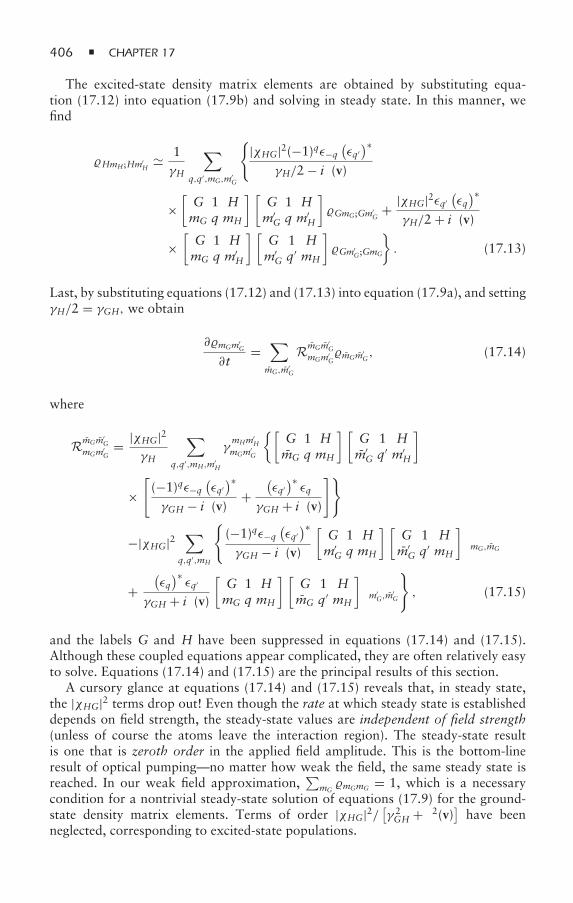
406 CHAPTER 17
The excited-state density matrix elements are obtained by substituting equa-tion (17.12) into equation (17.9b) and solving in steady state. In this manner, wefind
HmH;Hm′H
1γH
∑q,q′,mG,m′
G
|χHG|2(−1)qε−q
(εq′)∗
γH/2 − iδ(v)
×[G 1 HmG q mH
] [G 1 Hm′G q m′
H
]GmG;Gm′
G+ |χHG|2εq′
(εq)∗
γH/2 + iδ(v)
×[G 1 HmG q m′
H
] [G 1 Hm′G q′ mH
]Gm′
G;GmG
. (17.13)
Last, by substituting equations (17.12) and (17.13) into equation (17.9a), and settingγH/2 = γGH, we obtain
∂mGm′G
∂t=
∑mG,m′
G
RmGm′G
mGm′GmGm′
G, (17.14)
where
RmGm′G
mGm′G
= |χHG|2γH
∑q,q′,mH,m′
H
γmHm′
HmGm′
G
[G 1 HmG q mH
] [G 1 Hm′G q′ m′
H
]
×[(−1)qε−q
(εq′)∗
γGH − iδ(v)+
(εq′)∗εq
γGH + iδ(v)
]
−|χHG|2∑
q,q′,mH
(−1)qε−q
(εq′)∗
γGH − iδ(v)
[G 1 Hm′G q mH
] [G 1 Hm′G q′ mH
]δmG,mG
+(εq)∗εq′
γGH + iδ(v)
[G 1 HmG q mH
] [G 1 HmG q′ mH
]δm′
G,m′G
, (17.15)
and the labels G and H have been suppressed in equations (17.14) and (17.15).Although these coupled equations appear complicated, they are often relatively easyto solve. Equations (17.14) and (17.15) are the principal results of this section.
A cursory glance at equations (17.14) and (17.15) reveals that, in steady state,the |χHG|2 terms drop out! Even though the rate at which steady state is establisheddepends on field strength, the steady-state values are independent of field strength(unless of course the atoms leave the interaction region). The steady-state resultis one that is zeroth order in the applied field amplitude. This is the bottom-lineresult of optical pumping—no matter how weak the field, the same steady state isreached. In our weak field approximation,
∑mGmGmG = 1, which is a necessary
condition for a nontrivial steady-state solution of equations (17.9) for the ground-state density matrix elements. Terms of order |χHG|2/ [γ 2
GH + δ2(v)] have beenneglected, corresponding to excited-state populations.
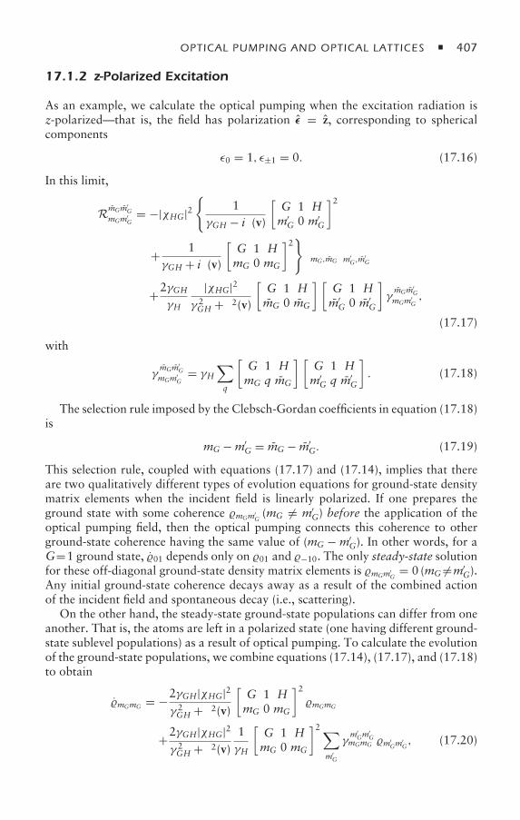
OPTICAL PUMPING AND OPTICAL LATTICES 407
17.1.2 z-Polarized Excitation
As an example, we calculate the optical pumping when the excitation radiation isz-polarized—that is, the field has polarization ε = z, corresponding to sphericalcomponents
ε0 = 1, ε±1 = 0. (17.16)
In this limit,
RmGm′G
mGm′G
= −|χHG|2
1γGH − iδ(v)
[G 1 Hm′G 0 m′
G
]2
+ 1γGH + iδ(v)
[G 1 HmG 0 mG
]2δmG,mGδm′
G,m′G
+2γGHγH
|χHG|2γ 2GH + δ2(v)
[G 1 HmG 0 mG
] [G 1 Hm′G 0 m′
G
]γmGm′
GmGm′
G,
(17.17)
with
γmGm′
GmGm′
G= γH
∑q
[G 1 HmG q mG
] [G 1 Hm′G q m′
G
]. (17.18)
The selection rule imposed by the Clebsch-Gordan coefficients in equation (17.18)is
mG −m′G = mG − m′
G. (17.19)
This selection rule, coupled with equations (17.17) and (17.14), implies that thereare two qualitatively different types of evolution equations for ground-state densitymatrix elements when the incident field is linearly polarized. If one prepares theground state with some coherence mGm′
G(mG = m′
G) before the application of theoptical pumping field, then the optical pumping connects this coherence to otherground-state coherence having the same value of (mG − m′
G). In other words, for aG=1 ground state, 01 depends only on 01 and −10. The only steady-state solutionfor these off-diagonal ground-state density matrix elements is mGm′
G= 0 (mG =m′
G).Any initial ground-state coherence decays away as a result of the combined actionof the incident field and spontaneous decay (i.e., scattering).
On the other hand, the steady-state ground-state populations can differ from oneanother. That is, the atoms are left in a polarized state (one having different ground-state sublevel populations) as a result of optical pumping. To calculate the evolutionof the ground-state populations, we combine equations (17.14), (17.17), and (17.18)to obtain
mGmG = −2γGH|χHG|2γ 2GH + δ2(v)
[G 1 HmG 0 mG
]2mGmG
+2γGH|χHG|2γ 2GH + δ2(v)
1γH
[G 1 HmG 0 mG
]2∑m′G
γm′Gm
′G
mGmG m′Gm
′G, (17.20)
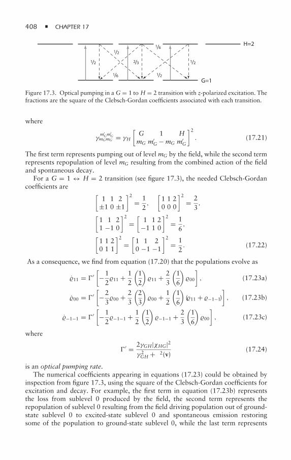
408 CHAPTER 17
G=1
1/2 1/22/3
1/2
1/21/6
1/6H=2
Figure 17.3. Optical pumping in aG = 1 to H = 2 transition with z-polarized excitation. Thefractions are the square of the Clebsch-Gordan coefficients associated with each transition.
where
γm′Gm
′G
mGmG = γH
[G 1 HmG m′
G −mG m′G
]2. (17.21)
The first term represents pumping out of levelmG by the field, while the second termrepresents repopulation of level mG resulting from the combined action of the fieldand spontaneous decay.
For a G = 1 ↔ H = 2 transition (see figure 17.3), the needed Clebsch-Gordancoefficients are [
1 1 2±1 0 ±1
]2= 1
2,
[1 1 20 0 0
]2= 2
3,
[1 1 21 −1 0
]2=[
1 1 2−1 1 0
]2= 1
6,
[1 1 20 1 1
]2=[1 1 20 −1 −1
]2= 1
2. (17.22)
As a consequence, we find from equation (17.20) that the populations evolve as
11 = ′[−1211 + 1
2
(12
)11 + 2
3
(16
)00
], (17.23a)
00 = ′[−2300 + 2
3
(23
)00 + 1
2
(16
)(11 + −1−1)
], (17.23b)
−1−1 = ′[−12−1−1 + 1
2
(12
)−1−1 + 2
3
(16
)00
], (17.23c)
where
′ = 2γGH|χHG|2γ 2GH + δ2(v) (17.24)
is an optical pumping rate.The numerical coefficients appearing in equations (17.23) could be obtained by
inspection from figure 17.3, using the square of the Clebsch-Gordan coefficients forexcitation and decay. For example, the first term in equation (17.23b) representsthe loss from sublevel 0 produced by the field, the second term represents therepopulation of sublevel 0 resulting from the field driving population out of ground-state sublevel 0 to excited-state sublevel 0 and spontaneous emission restoringsome of the population to ground-state sublevel 0, while the last term represents
OPTICAL PUMPING AND OPTICAL LATTICES 409
the repopulation of sublevel 0 resulting from the field driving population out ofground-state sublevels ±1 to excited-state sublevels ±1 and spontaneous emissiontransferring some of the population back to ground-state sublevel 0. The steady-statesolution of equations (17.23) is
11 = −1−1 = 417, (17.25a)
00 = 917, (17.25b)
with all other density matrix elements equal to zero. As discussed earlier, althoughthe ground state is polarized, no net internal state angular momentum has beentransferred to the atoms by the z-polarized optical field.
17.1.3 Irreducible Tensor Basis
For other than z-polarized fields, there can be off-diagonal density matrix elementsin steady state. If we use linearly polarized light in the x rather than the z direction,for example, drawing simple diagrams is not too much help, since the field createscoherence in the excited state that is maintained in the decay. The final densitymatrix elements can be obtained by “rotating” the z-polarized results using angularmomentum rotation matrices (see problems 1–2), giving steady-state values
11 = −1−1 = 13/34, (17.26a)
00 = 4/17, (17.26b)
1−1 = −11 = −5/34, (17.26c)
with all other density matrix elements equal to zero. There is now a nonvanishingground-state coherence (off-diagonal density matrix element), but the average valueof the z component of angular momentum remains equal to zero, since the excitationis via a linearly polarized field. This result also indicates that what looks like unequalpopulations and zero coherence in one basis can appear as both unequal populationsand nonvanishing coherence in a rotated basis. The only ground-state density matrixthat is invariant under rotation is an unpolarized state.
In this and more complicated cases, it is easier to use an irreducible tensor basissince decay is diagonal in that basis. As was mentioned in the previous chapter,many people get very nervous when irreducible tensors are mentioned, but thereis no need to panic. The irreducible tensor basis represents simply an alternativebasis to the usual angular momentum basis. Moreover, it often leads to simplifiedequations when systems have simple properties under rotation.
To transform equation (17.14) into an irreducible tensor basis requires a lot ofalgebra, which we do not reproduce here [4]. We simply give the result; the ground-state density matrix elements evolve as
KQ(G) =∑
K,K ′,K,Q′
A(K, K ′, K;Q,Q′;G,H)P(G,H; K, K ′, K)K′
Q′(G), (17.27)
410 CHAPTER 17
where
A(K, K ′, K;Q,Q′;G,H) = (−1)Q′ ∑
Q
(K ′ K K
−Q′ Q Q
)|χGH|2ε KQ
×[
1γGH − iδ(v)
+ (−1)K+K ′+K
γGH + iδ(v)
], (17.28)
P(G,H; K, K ′, K) = −3(−1)K+K ′+H−G√(2K + 1)(2K ′ + 1)(2K + 1)
×
⎡⎢⎢⎢⎢⎣
K K ′ KG G G
1 1 KG G H
−(−1)2G(2H+ 1)H H KG G 1
⎧⎨⎩K K ′ KH G 1H G 1
⎫⎬⎭
⎤⎥⎥⎥⎥⎦ , (17.29)
εKQ =∑q,q′
(−1)q′εq(ε−q′
)∗[1 1 Kq q′ Q
], (17.30)
χHG = −〈H||µ(1)||G〉E2
√2H+ 1
, (17.31)
and the last in equation (17.29) is a 9-J symbol. It is a simple matter toprogram equation (17.27). Clebsch-Gordan, 3-J, 6-J, and 9-J symbols are standardsubroutines in most symbolic math programs.
To get some idea of the power of the irreducible tensor basis, we consider opticalpumping on a G = 1 to H = 2 transition by an x-polarized field, starting withan unpolarized initial state KQ = (1/
√3)δK,0δQ,0. For an x-polarized field (see the
appendix),
ε(x)q = (δq,−1 − δq,−1
)/√2 (17.32)
and
εKQ = − 1√3δK,0δQ,0 + δK,2
[− 1√
6δQ,0 + 1
2
(δQ,2 + δQ,−2
)]. (17.33)
Substituting equation (17.33) into equation (17.27), setting G= 1 and H= 2, andusing the fact that 00 = 1/
√3, we obtain the evolution equations
20 = ′
120
(−2220 + 4
√622 + 5
√23
), (17.34a)
22 = ′
120
(−3022 + 2
√620 − 5
), (17.34b)
where ′ is given by equation (17.24), and 2−2 = 22. The steady-state solution is
20 = 517
1√6, 2±2 = − 5
34, (17.35)
OPTICAL PUMPING AND OPTICAL LATTICES 411
which is consistent with equation (17.26). There are only two density matrixelements that need to be calculated using an irreducible tensor basis.
Equation (17.27) actually has a very simple structure, although you might besomewhat skeptical about this conclusion. The dynamics is governed by two factors,A(K, K ′, K;Q,Q′;G,H) and P(G,H; K, K ′, K). The quantity P(G,H; K, K ′, K)is a “geometric” factor that is independent of field polarization, whileA(K, K ′, K;Q,Q′;G,H) reflects the polarization of the driving field, written interms of the coupled polarization tensor εKQ. The coupled tensor description isespecially useful for determining the manner in which population and coherenceis transferred from the ground-state to the excited-state and back to the ground-state manifolds. For reference purposes, values of εKQ for various field polarizationsare given in the appendix.
17.1.4 Standing-Wave and Multiple-Frequency Fields
The results can be generalized to any number of incident fields. This generalizationis especially important since it will allow us to consider the standard geometries forsub-Doppler cooling that are discussed in the next chapter. The total electric field istaken to be of the form
Ec(R, t) = 12
∑j
E ( j)ε( j)ei(k·R−ω j t) + c.c., (17.36)
that is, a sum of a number of monochromatic fields. Density matrix equations arenow written in the standard interaction representation, since the field frequenciesand wave vectors of the various fields need not be equal. In general, the equationscannot be solved analytically, since there are several frequencies present in theatomic rest frame. Let us assume, however, that the adiabatic elimination of the GHand HH density matrix elements remains valid [4], allowing us to arrive at the sametype of evolution equation for KQ(G) that was found earlier—namely [4],
∂KQ(G)
∂t+ v · ∇KQ(G) =
∑K,K ′,K,Q′
A(K, K ′, K;Q,Q ′;G,H;R, t)
×P(G,H; K, K ′, K)K′
Q′(G), (17.37)
where the factor A(K, K ′, K;Q,Q′;G,H;R, t) now contains all combinationseiφ j j ′ (R,t) of spatial and temporal beats between the different fields with
φ j j ′(R, t) = (k j − k j ′ ) · R − (ω j − ω j ′ )t. (17.38)
Explicitly, we find [4]
A(K, K ′, K;Q,Q′;G,H;R, t) = (−1)Q′ ∑j, j ′,Q
(K ′ K K
−Q′ Q Q
)
×χ ( j)HG
(χ( j ′)HG
)∗ε KQ( j, j
′)eiφ j j ′ (R,t)[
1γGH − iδ( j ′)(v)
+ (−1)K+K ′+K
γGH + iδ( j)(v)
], (17.39)
412 CHAPTER 17
where
χ( j)HG = −〈H||µ(1)||G〉E ( j)
2√3
, (17.40)
εKQ( j, j′) =
∑q,q′
(−1)q′ε( j)q
[ε( j ′)q′
]∗ [1 1 Kq q′ Q
], (17.41)
and
δ( j)(v) = ωHG − ω j + k j · v. (17.42)
Of course, these equations look complicated, but the basic physical content issimple. Each pair of fields i, j (including i = j) drives population and coherencefrom the ground-state manifold to the excited-state manifold of levels in a mannerdependent on the spherical tensor components εKQ( j, j
′). Spontaneous emissionreturns some of this population and coherence to the ground state. Since thereis a spatial and temporal phase given by equation (17.38) that occurs for fieldshaving different k vectors and frequencies, respectively, it is possible for the fieldsto create both spatial modulation and temporal beats in the ground-state densitymatrix elements. However, for our “closed” G–H transition, the total ground-statepopulation is constant,
ddt00(G) = 0, (17.43)
and
00(G) = 1√2G+ 1
(17.44)
to zeroth order in the optical pumping rate ′. On the other hand, ground-statedensity matrix elements, KQ(G) for K = 0,Q = 0, can be modulated in space andtime. We refer to this as modulated atomic state polarization. As you will see, thisfeature is critical for sub-Doppler cooling.
17.1.4.1 Counterpropagating fields
Let us look at some limiting cases to see what happens to the ground-state sublevelsfor two counterpropagating fields. We set k1=−k2=k, E1=E2, and ω1=ω2=ω=kc.
17.1.4.1.1 ‖ polarization: If both fields have the same polarization, εKQ( j, j′) is
independent of j or j ′; therefore,
A(K, K ′, K;Q,Q′;G,H;R, t) ∝(1 + e2ik·R + e−2ik·R
), (17.45)
and
KQ = ∂KQ
∂t+ v · ∇KQ =
∑K ′,Q′
TK ′Q′KQ K
′Q′
(1 + e2ik·R + e−2ik·R
), (17.46)
OPTICAL PUMPING AND OPTICAL LATTICES 413
where TK ′Q′KQ is some coupling coefficient. Let us assume a steady-state solution of
the form
KQ(G) = KQ(G,0) + KQ(G,+)e2ik·R + KQ(G,−)e−2ik·R. (17.47)
The second two terms constitute the modulated atomic state polarization.Substituting this trial solution into equation (17.46), we find, in steady state,∑
K ′,Q′TK ′Q′KQ K
′Q′(G,0) = 0, (17.48a)
±2ik · vKQ(G,±) =∑K ′,Q′
TK ′Q′KQ K
′Q′(G,±). (17.48b)
Equations (17.48a) and (17.48b) each correspond to a set of (2G+ 1)2 linearequations. Equation (17.48a) has a nontrivial solution owing to the fact that00(G) = 1/(2G+ 1)1/2; that is, the K
′Q′(G,0) are not linearly independent. On the
other hand, in equation (17.48b), the KQ(G,±) are linearly independent, and theonly solution of these equations is
KQ(G,±) = 0. (17.49)
For parallel polarization, it then follows from equation (17.47) that there is nomodulated atomic state polarization. It is easy to understand why this is thecase. No matter where in the sample an atom finds itself, it experiences the samefield polarization, implying that the steady state cannot be a function of position,provided that an atom does not remain in a node of the field. Each atom is opticallypumped to the same steady state.
17.1.4.1.2 lin⊥lin polarization: For crossed, linearly polarized fields ε1 = x; ε2 = y,the spherical polarization tensor components that are needed are (see the appendix)
εKQ (x, x) = − 1√3δK,0δQ,0 + δK,2
[− 1√
6δQ,0 + 1
2
(δQ,2 + δQ,−2
)],
εKQ (y, y) = − 1√3δK,0δQ,0 − δK,2
[1√6δQ,0 + 1
2
(δQ,2 + δQ,−2
)],
εKQ (x, y) = [εK−Q (y, x)
]∗ = i√2
[δK,1δQ,0 + 1√
2δK,2
(δQ,2 − δQ,−2
)].
(17.50)
In contrast to the case of parallel polarization, the polarization of the totalfield (17.36) is now a function of position, implying that the atomic response can bemodulated as well.
If the counterpropagating, crossed-polarized fields are incident on atoms that areinitially in an unpolarized ground state, the resulting ground-state dynamics can bequite complicated. However, for a G=1/2 ground state, the only values of KQ thatcan enter are 00 = 1/
√2 and 1Q, since K = 0,1 when one couples two spin 1/2
systems. Moreover, for the values of εKQ given in equation (17.50), and for K=0,1,it is clear that only Q=0 can enter. Thus, the only density matrix element that needbe evaluated is 10 when G=1/2 for crossed-polarized fields.
414 CHAPTER 17
Using equations (17.37) and (17.50) and the fact that 00 = 1/√2, we find that,
for a G = 1/2 ground state and with χ ( j)HG ≡ χHG,
∂10
∂t+ v · ∇10 = −′(1/2,1/2)10 − 1√
2′(1/2,1/2) sin 2kZ (17.51)
if H = 1/2 and
∂10
∂t+ v · ∇10 = −′(1/2,3/2)10 − 1√
2′(1/2,3/2) sin 2kZ (17.52)
if H = 3/2, where
′(1/2,1/2) = 2′(3/2,1/2) = 23
|χHG|2γHγ 2GH + δ2 , (17.53)
the appropriate values of G and H are to be inserted in χHG, and γH = 2γGH. Since
10 = (1/2,1/2 − −1/2,−1/2
)/√2,
it is clear from these equations that the population difference,(1/2,1/2 − −1/2,−1/2
),
is spatially modulated. In the next chapter, we show that this leads to polarizationgradient, sub-Doppler cooling.
17.1.4.1.3 σ+ – σ− polarization: For σ+–σ− radiation, ε1 = (x+i y)/√2 [εq = δq,−1],ε2 = −(x − i y)/
√2 [εq = δq,1], and (see the appendix)
εKQ (σ+, σ+) = −(
1√3δK,0 − 1√
2δK,1 + 1√
6δK,2
)δQ,0,
εKQ (σ−, σ−) = −(
1√3δK,0 + 1√
2δK,1 + 1√
6δK,2
)δQ,0,
εKQ (σ+, σ−) = −δK,2δQ,−2, εKQ (σ−, σ+) = −δK,2δQ,2. (17.54)
In the next chapter, we will see that, for a G = 1 ground state, 22 = 1−1 ismodulated as e2ikz and 2−2 = −11 as e−2ikz, but the population differences arenot spatially modulated. This leads to a “corkscrew” type of sub-Doppler cooling.
17.2 Optical Lattice Potentials
If the incident fields are detuned by a sufficiently large amount, one can infirst approximation neglect the repopulation of the ground state as a result ofspontaneous emission. In other words, one neglects the “in” terms of spontaneousemission and works with an effective Hamiltonian for the system that is obtainedby adiabatically eliminating the excited-state amplitudes. An amplitude approachis possible, since the repopulation of the ground state is neglected. One can evenretain the decay parameters in the equations for the ground-state–excited-statecoherence. In doing so, one arrives at an effective non-Hermitian Hamiltonian forthe ground-state sublevels. Since the ground-state polarization can be modulated, theHamiltonian is also spatially modulated. In other words, the atoms find themselves
OPTICAL PUMPING AND OPTICAL LATTICES 415
in a modulated potential or optical lattice that can actually serve as a networkof traps for the atoms. For a review of this subject area, see the article by Jessenand Deutsch [5]. Optical lattices provide a controllable environment for simulatingcondensed matter systems.
We use the same formalism as for optical pumping, but work with stateamplitudes rather than density matrix elements. We assume that all the fields havethe same frequency and neglect any Doppler shifts of the atoms, assuming thatthey have been cooled to very low temperatures, such that
∣∣k j · v∣∣ γH. In a fieldinteraction representation, the excited-state amplitudes evolve as
dcHmH/dt = −(γH
2+ iδ
)cHmH + i
2
∑j,mG
〈H,mH|µ · ε( j)|G,mG〉eik j ·RE ( j)cGmG.
(17.55)Assuming that the optical pumping rate ′ is much less than |γH/2+ iδ|, the excited-state amplitude becomes approximately constant on a time scale much less than1/′. Thus, we can adiabatically eliminate the upper-state amplitude by takingdcH,mH/dt ≈ 0, or
cHmH ≈ i2 (γH/2 + iδ)
∑j,m′
G
〈H,mH|µ · ε( j)|G,m′G〉eik j ·RE ( j)cGm′
G. (17.56)
The ground-state amplitudes evolve as
dcGmG/dt = i2
∑j ′,mH
〈G,mG|µ·[ε( j
′)]∗
|H,mH〉e−ik j ′ ·RE ( j ′)∗cHmH
= i2
∑j ′,mH
[ε( j
′)]∗
· 〈H,mH|µ|G,mG〉∗e−ik j ′ ·RE ( j ′)∗cHmH .
(17.57)
Combining equations (17.56) and (17.57), and using
µ · ε =1∑
q=−1
(−1)q µqε−q (17.58)
and the Wigner-Eckart theorem to evaluate matrix elements of µ, we find
idcGmG/dt =∑m′G
HmGm′GcGm′
G,
where
HmGm′G
= − 12H+ 1
3δ − iγH/2
∑q,q′,mH, j, j ′
(−1)q+q′[G 1 Hm′G q mH
]
×[G 1 HmG −q′ mH
]χ( j)HG
[χ( j ′)HG
]∗ε( j)−q[ε( j ′)q′
]∗eik j j ′ ·R. (17.59)
The matrix elements HmGm′Gform a non-Hermitian, effective Hamiltonian for the
ground-state manifold.For any given field polarizations, we calculate these matrix elements and
diagonalizeH to get the optical lattice potentials. It is possible to getH into a simple
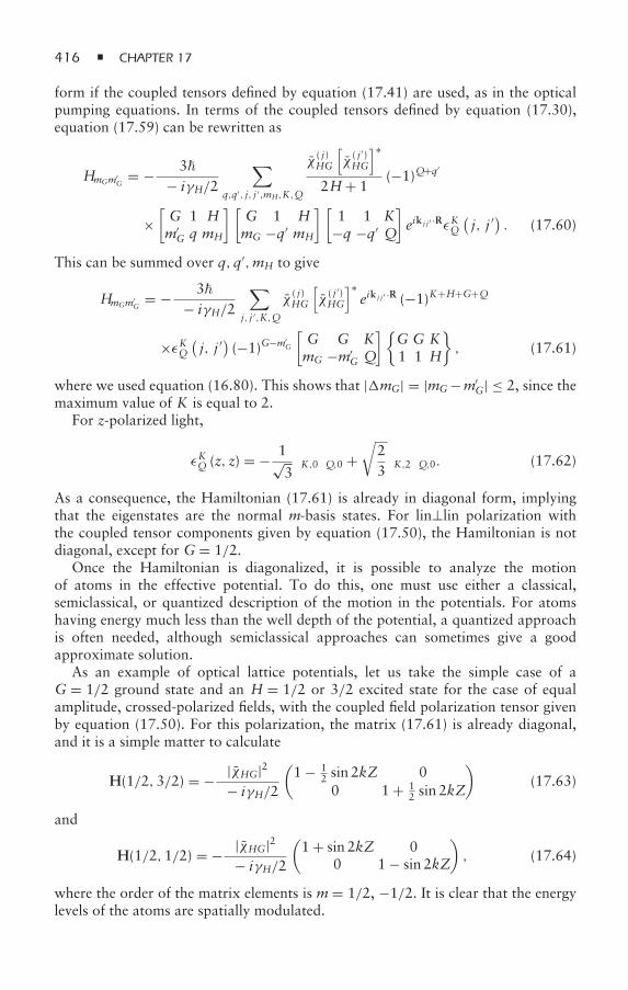
416 CHAPTER 17
form if the coupled tensors defined by equation (17.41) are used, as in the opticalpumping equations. In terms of the coupled tensors defined by equation (17.30),equation (17.59) can be rewritten as
HmGm′G
= − 3δ − iγH/2
∑q,q′, j, j ′,mH,K,Q
χ( j)HG
[χ( j ′)HG
]∗
2H+ 1(−1)Q+q′
×[G 1 Hm′G q mH
] [G 1 HmG −q′ mH
] [1 1 K
−q −q′ Q
]eik j j ′ ·RεKQ
(j, j ′
). (17.60)
This can be summed over q,q′,mH to give
HmGm′G
= − 3δ − iγH/2
∑j, j ′,K,Q
χ( j)HG
[χ( j ′)HG
]∗eik j j ′ ·R (−1)K+H+G+Q
×εKQ(j, j ′
)(−1)G−m′
G
[G G KmG −m′
G Q
]G G K1 1 H
, (17.61)
where we used equation (16.80). This shows that |mG| = |mG−m′G| ≤ 2, since the
maximum value of K is equal to 2.For z-polarized light,
εKQ (z, z) = − 1√3δK,0δQ,0 +
√23δK,2δQ,0. (17.62)
As a consequence, the Hamiltonian (17.61) is already in diagonal form, implyingthat the eigenstates are the normal m-basis states. For lin⊥lin polarization withthe coupled tensor components given by equation (17.50), the Hamiltonian is notdiagonal, except for G = 1/2.
Once the Hamiltonian is diagonalized, it is possible to analyze the motionof atoms in the effective potential. To do this, one must use either a classical,semiclassical, or quantized description of the motion in the potentials. For atomshaving energy much less than the well depth of the potential, a quantized approachis often needed, although semiclassical approaches can sometimes give a goodapproximate solution.
As an example of optical lattice potentials, let us take the simple case of aG = 1/2 ground state and an H = 1/2 or 3/2 excited state for the case of equalamplitude, crossed-polarized fields, with the coupled field polarization tensor givenby equation (17.50). For this polarization, the matrix (17.61) is already diagonal,and it is a simple matter to calculate
H(1/2,3/2) = − |χHG|2δ − iγH/2
(1 − 1
2 sin 2kZ 00 1 + 1
2 sin 2kZ
)(17.63)
and
H(1/2,1/2) = − |χHG|2δ − iγH/2
(1 + sin 2kZ 0
0 1 − sin 2kZ
), (17.64)
where the order of the matrix elements is m = 1/2, −1/2. It is clear that the energylevels of the atoms are spatially modulated.
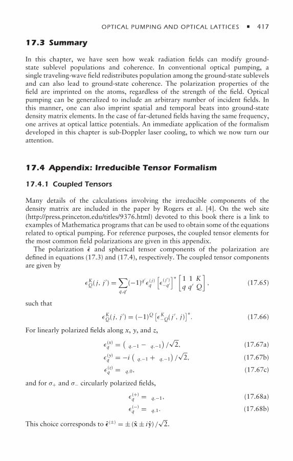
OPTICAL PUMPING AND OPTICAL LATTICES 417
17.3 Summary
In this chapter, we have seen how weak radiation fields can modify ground-state sublevel populations and coherence. In conventional optical pumping, asingle traveling-wave field redistributes population among the ground-state sublevelsand can also lead to ground-state coherence. The polarization properties of thefield are imprinted on the atoms, regardless of the strength of the field. Opticalpumping can be generalized to include an arbitrary number of incident fields. Inthis manner, one can also imprint spatial and temporal beats into ground-statedensity matrix elements. In the case of far-detuned fields having the same frequency,one arrives at optical lattice potentials. An immediate application of the formalismdeveloped in this chapter is sub-Doppler laser cooling, to which we now turn ourattention.
17.4 Appendix: Irreducible Tensor Formalism
17.4.1 Coupled Tensors
Many details of the calculations involving the irreducible components of thedensity matrix are included in the paper by Rogers et al. [4]. On the web site(http://press.princeton.edu/titles/9376.html) devoted to this book there is a link toexamples of Mathematica programs that can be used to obtain some of the equationsrelated to optical pumping. For reference purposes, the coupled tensor elements forthe most common field polarizations are given in this appendix.
The polarization ε and spherical tensor components of the polarization aredefined in equations (17.3) and (17.4), respectively. The coupled tensor componentsare given by
εKQ( j, j′) =
∑q,q′
(−1)q′ε( j)q
[ε( j ′)−q′
]∗ [1 1 Kq q′ Q
], (17.65)
such that
εKQ( j, j′) = (−1)Q
[εK−Q( j
′, j)]∗. (17.66)
For linearly polarized fields along x, y, and z,
ε(x)q = (δq,−1 − δq,−1
)/√2, (17.67a)
ε(y)q = −i (δq,−1 + δq,−1)/√2, (17.67b)
ε(z)q = δq,0, (17.67c)
and for σ+ and σ− circularly polarized fields,
ε(+)q = δq,−1, (17.68a)
ε(−)q = δq,1. (17.68b)
This choice corresponds to ε(±) = ± (x ± i y) /√2.
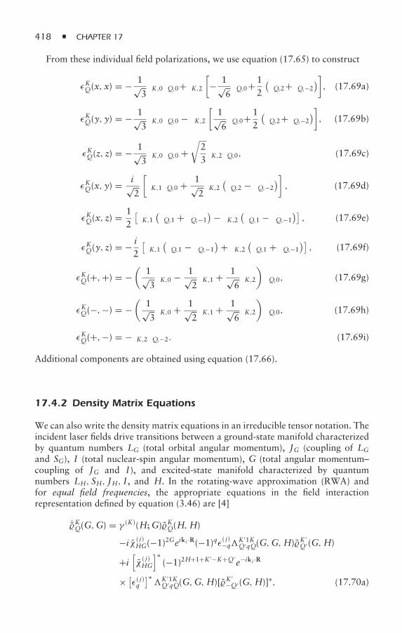
418 CHAPTER 17
From these individual field polarizations, we use equation (17.65) to construct
εKQ(x, x) = − 1√3δK,0δQ,0+δK,2
[− 1√
6δQ,0+ 1
2
(δQ,2+δQ,−2
)], (17.69a)
εKQ(y, y) = − 1√3δK,0δQ,0 − δK,2
[1√6δQ,0+ 1
2
(δQ,2+δQ,−2
)], (17.69b)
εKQ(z, z) = − 1√3δK,0δQ,0 +
√23δK,2δQ,0, (17.69c)
εKQ(x, y) = i√2
[δK,1δQ,0 + 1√
2δK,2
(δQ,2 − δQ,−2
)], (17.69d)
εKQ(x, z) = 12
[δK,1
(δQ,1 + δQ,−1
)− δK,2(δQ,1 − δQ,−1
)], (17.69e)
εKQ(y, z) = − i2
[δK,1
(δQ,1 − δQ,−1
)+ δK,2(δQ,1 + δQ,−1
)], (17.69f)
εKQ(+,+) = −(
1√3δK,0 − 1√
2δK,1 + 1√
6δK,2
)δQ,0, (17.69g)
εKQ(−,−) = −(
1√3δK,0 + 1√
2δK,1 + 1√
6δK,2
)δQ,0, (17.69h)
εKQ(+,−) = −δK,2δQ,−2. (17.69i)
Additional components are obtained using equation (17.66).
17.4.2 Density Matrix Equations
We can also write the density matrix equations in an irreducible tensor notation. Theincident laser fields drive transitions between a ground-state manifold characterizedby quantum numbers LG (total orbital angular momentum), JG (coupling of LGand SG), I (total nuclear-spin angular momentum), G (total angular momentum–coupling of JG and I), and excited-state manifold characterized by quantumnumbers LH, SH, JH, I, and H. In the rotating-wave approximation (RWA) andfor equal field frequencies, the appropriate equations in the field interactionrepresentation defined by equation (3.46) are [4]
˙KQ(G,G) = γ (K)(H;G)KQ(H,H)
−i χ ( j)HG(−1)2Geik j ·R(−1)qε( j)−q
K ′1KQ′qQ(G,G,H)K
′Q′ (G,H)
+i[χ( j)HG
]∗(−1)2H+1+K ′−K+Q′
e−ik j ·R
× [ε( j)q
]∗K ′1K
Q′qQ(G,G,H)[K′
−Q′(G,H)]∗, (17.70a)
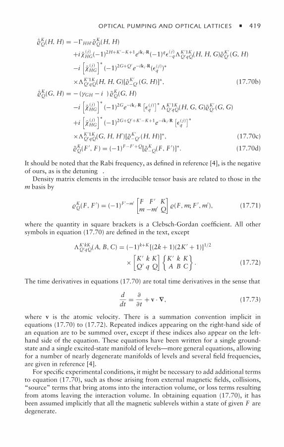
OPTICAL PUMPING AND OPTICAL LATTICES 419
˙KQ(H,H) = −HH′ KQ(H,H)
+i χ ( j)HG(−1)2H+K ′−K+1eik j ·R(−1)qε( j)−qK ′1K
Q′qQ(H,H,G)K′
Q′ (G,H)
−i[χ( j)HG
]∗(−1)2G+Q′
e−ik j ·R(ε( j)q )∗
×K ′1KQ′qQ(H,H,G)[K
′−Q′ (G,H)]∗, (17.70b)
˙KQ(G,H) = − (γGH − iδ) KQ(G,H)
−i[χ( j)HG
]∗(−1)2Ge−ik j ·R [ε( j)q
]∗K ′1K
Q′qQ(H,G,G)K′
Q′ (G,G)
+i[χ( j)HG
]∗(−1)2G+Q′+K ′−K+1e−ik j ·R [ε( j)q
]∗×K ′1K
Q′qQ(G,H,H′)[K
′−Q′(H,H)]∗, (17.70c)
KQ(F′, F ) = (−1)F−F ′+Q[K−Q(F, F
′)]∗. (17.70d)
It should be noted that the Rabi frequency, as defined in reference [4], is the negativeof ours, as is the detuning δ.
Density matrix elements in the irreducible tensor basis are related to those in them basis by
KQ(F, F′) = (−1)F
′−m′[F F ′ Km −m′ Q
](F,m; F ′,m′), (17.71)
where the quantity in square brackets is a Clebsch-Gordan coefficient. All othersymbols in equation (17.70) are defined in the text, except
K ′kKQ′qQ(A, B,C) = (−1)k+K [(2k+ 1)(2K ′ + 1)]1/2
×[K ′ k KQ′ q Q
]K ′ k KA B C
. (17.72)
The time derivatives in equations (17.70) are total time derivatives in the sense that
ddt
= ∂
∂t+ v · ∇, (17.73)
where v is the atomic velocity. There is a summation convention implicit inequations (17.70) to (17.72). Repeated indices appearing on the right-hand side ofan equation are to be summed over, except if these indices also appear on the left-hand side of the equation. These equations have been written for a single ground-state and a single excited-state manifold of levels—more general equations, allowingfor a number of nearly degenerate manifolds of levels and several field frequencies,are given in reference [4].
For specific experimental conditions, it might be necessary to add additional termsto equation (17.70), such as those arising from external magnetic fields, collisions,“source” terms that bring atoms into the interaction volume, or loss terms resultingfrom atoms leaving the interaction volume. In obtaining equation (17.70), it hasbeen assumed implicitly that all the magnetic sublevels within a state of given F aredegenerate.
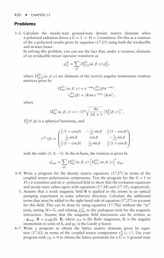
420 CHAPTER 17
Problems
1–2. Calculate the steady-state ground-state density matrix elements whenx-polarized radiation drives aG = 1 → H = 2 transition. Do this as a rotationof the z-polarized results given by equation (17.25) using both the irreducibleand m-state bases.In solving this problem, you can use the fact that, under a rotation, elementsof an irreducible tensor operator transform as
′KQ =
∑Q′
D(K)Q′Q (α, β, γ ) KQ′ ,
where D(K)Q′Q (α, β, γ ) are elements of the (active) angular momentum rotation
matrices given by
D(K)mm′ (α, β, γ ) = e−imαr (K)
mm′(β)e−im′γ ,
r (K)mm′(β) = 〈Km| e−iβ Jy ∣∣Km′⟩ ,
where
D(K)0m (α, β, γ ) = (−1)m
√4π
2K + 1
[YKQ (β, γ )
]∗,
YKQ (θ, φ) is a spherical harmonic, and
r (1) (β) =
⎛⎜⎜⎝
12 (1 + cosβ) − 1√
2sinβ 1
2 (1 − cosβ)1√2sinβ cosβ − 1√
2sinβ
12 (1 − cosβ) 1√
2sinβ 1
2 (1 + cosβ)
⎞⎟⎟⎠ ,
with the order (1,0,−1). In the m basis, the rotation is given by
′mm′ =
∑qq′
D(G)mq (α, β, γ )
[D(G)m′q′ (α, β, γ )
]∗qq′ .
3–4. Write a program for the density matrix equations (17.27) in terms of thecoupled tensor polarization components. Test the program for the G= 1 toH=2 transition and an x−polarized field to show that the evolution equationsand steady-state values agree with equations (17.34) and (17.35), respectively.
5. Assume that a weak magnetic field B is applied to the atoms in an opticalpumping experiment in some arbitrary direction. Calculate the additionalterms that must be added to the right-hand side of equation (17.27) to accountfor this field. This can be done by using equation (17.70a) without the “in”term, setting H=G, and relating χ ( j)
HG to the analogous term for the magneticinteraction. Assume that the magnetic field interaction can be written as−µmag · B = µBgGG · B, where µB is the Bohr magneton, G is the angularmomentum in units of , and gG is the Landé g factor.
6–7. Write a program to obtain the lattice matrix elements given by equa-tion (17.61) in terms of the coupled tensor components εKQ ( j, j ′). Use yourprogram with γH = 0 to obtain the lattice potentials for a G = 1 ground state
OPTICAL PUMPING AND OPTICAL LATTICES 421
with H = 2 for both lin⊥lin and σ+ − σ− field polarizations. Show that thereis no modulation in the σ+ − σ− case.
8. Derive any one of equations (17.9) without the decay terms for the interactionpotential given by equation (17.9).
References
[1] A. Kastler, Quelques suggestions concernant la production optique et la détectionoptique d’une inégalité de population des niveaux de quantification spatiale des atomes—application à l’experience de Stern et Gerlach et à resonance magnetique (Some ideasabout the production and detection by optical means of an inequality in magneticsublevels—application to the Stern-Gerlach experiment and magnetic resonance), Jour-nal de Physique et le Radium 11, 255–265 (1950); J. Brossel, A. Kastler, and J. Winter,Création optique d’une inégalité de population entre les sous-niveaux Zeeman de l’étatfondamental des atoms (Creation of an inequality in ground-state magnetic sublevels),Journal de Physique et le Radium 13, 668 (1952).
[2] L. Mandel and E. Wolf,Optical Coherence and Quantum Optics (Cambridge UniversityPress, Cambridge, UK, 1995), sec. 10.6.
[3] L. Allen, M. J. Padgett, and M. Babiker, The orbital angular momentum of light, inProgress in Optics, edited by E. Wolf, vol. XXXIX (Elsevier Science, Amsterdam, 1999),pp. 291–372; M. F. Andersen, C. Ryu, P. Cladé, V. Natarajan, A. Vaziri, K. Helmerson,and W. D. Phillips, Quantized rotation of atoms from photons with orbital angularmomentum, Physical Review Letters 97, 170406, 1–4 (2006).
[4] G. Rogers, P. R. Berman, and B. Dubetsky, Rate equations between electronic-statemanifolds, Physical Review A 48, 1506–1513 (1993).
[5] P. S. Jessen and I. H. Deutsch, Optical lattices, in Advances in Atomic, Molecular, andOptical Physics, edited by B. Bederson and H. Walther, vol. 37 (Academic Press, NewYork, 1996), pp. 95–138.
Bibliography
W. Happer, Optical pumping, Reviews of Modern Physics 44, 169–249 (1972). This reviewarticle contains a comprehensive list of references.
A. Omont, Irreducible components of the density matrix. Application to optical pumping,Progress in Quantum Electronics 5, 69–138 (1977).
See also the references in chapter 16.
18Sub-Doppler Laser Cooling
In chapter 5, we found a limit of kBT ≈ γ2/2 for laser cooling. One of themost dramatic violations of Murphy’s law (if something can go wrong, it will)occurred in the late 1980s, when several research groups tried to verify this limit ofDoppler cooling. The temperature they obtained was lower than that predicted bytheory. This discovery and the subsequent explanation of the sub-Doppler coolingmechanismwas rewarded with a Nobel Prize in 1997 for Steven Chu, Claude Cohen-Tannoudji, and William Phillips. The work also paved the way for experiments thatultimately resulted in a Bose condensate of neutral atoms.
It was not that the theory of Doppler cooling was wrong, it was only that itdid not quite go far enough. In theories of laser cooling, the atoms were modeledas two-level quantum systems. This is a useful model in many cases, but for lasercooling, it missed the boat. We have already seen in the previous chapter how opticalpumping using standing-wave optical fields can result in a spatial modulation ofthe ground-state polarization. Moreover, this steady-state modulation is achievedon a time scale that is related to the optical pumping rate ′ rather than theexcited-state decay rate γH. Thus, optical pumping introduces a new timescaleinto the problem. Since, for sufficiently weak fields, ′ γH, it is possible thata relationship such as kBT = γ2/2 could be replaced by kBT = ′/2 /2.Even if this expression does not provide the correct limit, it is clear that one mustreevaluate the limits of laser cooling, taking into account the effects of opticalpumping.
There are essentially three mechanisms by which optical pumping using counter-propagating fields can result in cooling:
(1) Optical pumping results in a spatially modulated ground-state polarization(that is, a spatially modulated population difference or coherence betweendifferent ground-state sublevels), allowing for an exchange of momentumbetween counterpropagating fields.
(2) Optical pumping results in an unmodulated imbalance in ground-statepopulations, leading to different scattering rates for each of the counter-propagating waves.
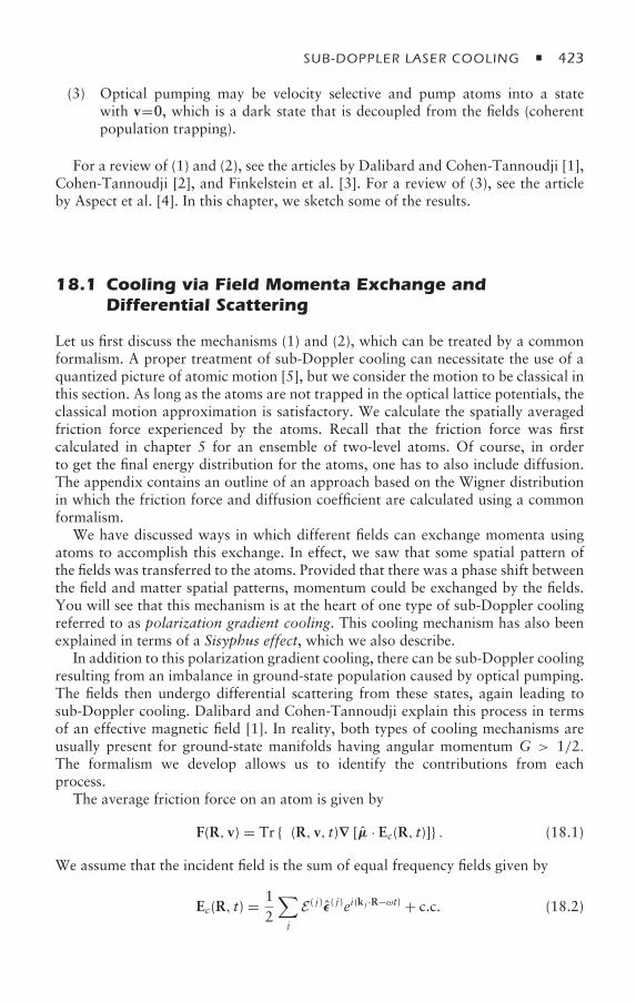
SUB-DOPPLER LASER COOLING 423
(3) Optical pumping may be velocity selective and pump atoms into a statewith v=0, which is a dark state that is decoupled from the fields (coherentpopulation trapping).
For a review of (1) and (2), see the articles by Dalibard and Cohen-Tannoudji [1],Cohen-Tannoudji [2], and Finkelstein et al. [3]. For a review of (3), see the articleby Aspect et al. [4]. In this chapter, we sketch some of the results.
18.1 Cooling via Field Momenta Exchange andDifferential Scattering
Let us first discuss the mechanisms (1) and (2), which can be treated by a commonformalism. A proper treatment of sub-Doppler cooling can necessitate the use of aquantized picture of atomic motion [5], but we consider the motion to be classical inthis section. As long as the atoms are not trapped in the optical lattice potentials, theclassical motion approximation is satisfactory. We calculate the spatially averagedfriction force experienced by the atoms. Recall that the friction force was firstcalculated in chapter 5 for an ensemble of two-level atoms. Of course, in orderto get the final energy distribution for the atoms, one has to also include diffusion.The appendix contains an outline of an approach based on the Wigner distributionin which the friction force and diffusion coefficient are calculated using a commonformalism.
We have discussed ways in which different fields can exchange momenta usingatoms to accomplish this exchange. In effect, we saw that some spatial pattern ofthe fields was transferred to the atoms. Provided that there was a phase shift betweenthe field and matter spatial patterns, momentum could be exchanged by the fields.You will see that this mechanism is at the heart of one type of sub-Doppler coolingreferred to as polarization gradient cooling. This cooling mechanism has also beenexplained in terms of a Sisyphus effect, which we also describe.
In addition to this polarization gradient cooling, there can be sub-Doppler coolingresulting from an imbalance in ground-state population caused by optical pumping.The fields then undergo differential scattering from these states, again leading tosub-Doppler cooling. Dalibard and Cohen-Tannoudji explain this process in termsof an effective magnetic field [1]. In reality, both types of cooling mechanisms areusually present for ground-state manifolds having angular momentum G > 1/2.The formalism we develop allows us to identify the contributions from eachprocess.
The average friction force on an atom is given by
F(R, v) = Tr (R, v, t)∇ [µ · Ec(R, t)] . (18.1)
We assume that the incident field is the sum of equal frequency fields given by
Ec(R, t) = 12
∑j
E ( j)ε( j)ei(k j ·R−ωt) + c.c. (18.2)
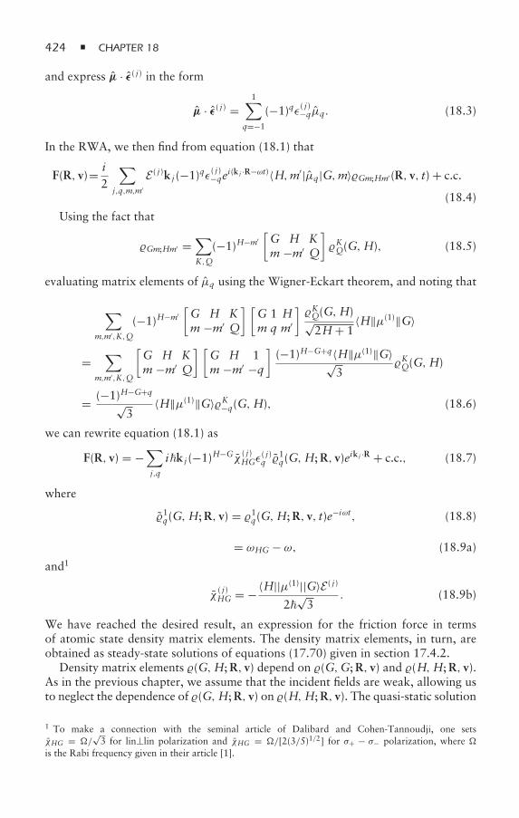
424 CHAPTER 18
and express µ · ε( j) in the form
µ · ε( j) =1∑
q=−1
(−1)qε( j)−qµq. (18.3)
In the RWA, we then find from equation (18.1) that
F(R, v)= i2
∑j,q,m,m′
E ( j)k j (−1)qε( j)−qei(k j ·R−ωt)〈H,m′|µq|G,m〉Gm;Hm′(R, v, t) + c.c.
(18.4)
Using the fact that
Gm;Hm′ =∑K,Q
(−1)H−m′[G H Km −m′ Q
]KQ(G,H), (18.5)
evaluating matrix elements of µq using the Wigner-Eckart theorem, and noting that
∑m,m′,K,Q
(−1)H−m′[G H Km −m′ Q
] [G 1 Hm q m′
]KQ(G,H)√2H+ 1
〈H‖µ(1)‖G〉
=∑
m,m′,K,Q
[G H Km −m′ Q
] [G H 1m −m′ −q
](−1)H−G+q〈H‖µ(1)‖G〉√
3KQ(G,H)
= (−1)H−G+q√3
〈H‖µ(1)‖G〉K−q(G,H), (18.6)
we can rewrite equation (18.1) as
F(R, v) = −∑j,q
ik j (−1)H−Gχ ( j)HGε
( j)q
1q(G,H;R, v)eik j ·R + c.c., (18.7)
where
1q(G,H;R, v) = 1q(G,H;R, v, t)e−iωt, (18.8)
δ = ωHG − ω, (18.9a)
and1
χ( j)HG = −〈H||µ(1)||G〉E ( j)
2√3
. (18.9b)
We have reached the desired result, an expression for the friction force in termsof atomic state density matrix elements. The density matrix elements, in turn, areobtained as steady-state solutions of equations (17.70) given in section 17.4.2.
Density matrix elements (G,H;R, v) depend on (G,G;R, v) and (H,H;R, v).As in the previous chapter, we assume that the incident fields are weak, allowing usto neglect the dependence of (G,H;R, v) on (H,H;R, v). The quasi-static solution
1 To make a connection with the seminal article of Dalibard and Cohen-Tannoudji, one setsχHG = /
√3 for lin⊥lin polarization and χHG = /[2(3/5)1/2] for σ+ − σ− polarization, where
is the Rabi frequency given in their article [1].
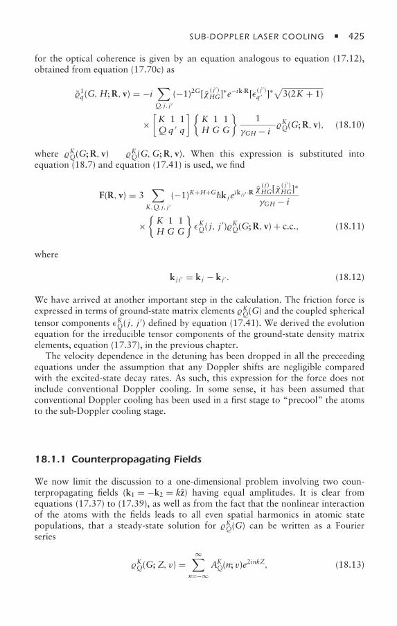
SUB-DOPPLER LASER COOLING 425
for the optical coherence is given by an equation analogous to equation (17.12),obtained from equation (17.70c) as
1q(G,H;R, v) = −i∑Q, j, j ′
(−1)2G[χ ( j ′)HG]
∗e−ik·R[ε( j′)
q ′ ]∗√
3(2K + 1)
×[K 1 1Qq ′ q
]K 1 1H G G
1
γGH − iδKQ(G;R, v), (18.10)
where KQ(G;R, v) ≡ KQ(G,G;R, v). When this expression is substituted intoequation (18.7) and equation (17.41) is used, we find
F(R, v) = 3∑
K,Q, j, j ′(−1)K+H+Gk j eik j j ′ ·R χ
( j)HG[χ
( j ′)HG]
∗
γGH − iδ
×K 1 1H G G
εKQ( j, j
′)KQ(G;R, v) + c.c., (18.11)
where
k j j ′ = k j − k j ′ . (18.12)
We have arrived at another important step in the calculation. The friction force isexpressed in terms of ground-state matrix elements KQ(G) and the coupled sphericaltensor components εKQ( j, j
′) defined by equation (17.41). We derived the evolutionequation for the irreducible tensor components of the ground-state density matrixelements, equation (17.37), in the previous chapter.
The velocity dependence in the detuning has been dropped in all the preceedingequations under the assumption that any Doppler shifts are negligible comparedwith the excited-state decay rates. As such, this expression for the force does notinclude conventional Doppler cooling. In some sense, it has been assumed thatconventional Doppler cooling has been used in a first stage to “precool” the atomsto the sub-Doppler cooling stage.
18.1.1 Counterpropagating Fields
We now limit the discussion to a one-dimensional problem involving two coun-terpropagating fields (k1 = −k2 = kz) having equal amplitudes. It is clear fromequations (17.37) to (17.39), as well as from the fact that the nonlinear interactionof the atoms with the fields leads to all even spatial harmonics in atomic statepopulations, that a steady-state solution for KQ(G) can be written as a Fourierseries
KQ(G; Z, v) =∞∑
n=−∞AKQ(n; v)e
2inkZ, (18.13)
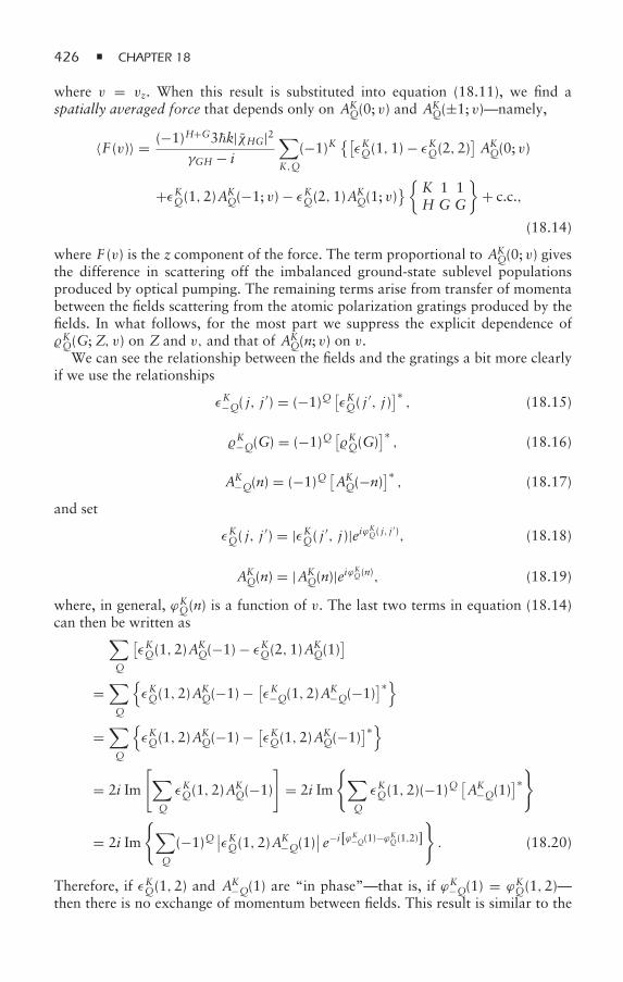
426 CHAPTER 18
where v = vz. When this result is substituted into equation (18.11), we find aspatially averaged force that depends only on AK
Q(0; v) and AKQ(±1; v)—namely,
〈F (v)〉 = (−1)H+G3k|χHG|2γGH − iδ
∑K,Q
(−1)K[εKQ(1,1) − εKQ(2,2)
]AKQ(0; v)
+εKQ(1,2)AKQ(−1; v) − εKQ(2,1)AK
Q(1; v) K 1 1
H G G
+ c.c.,
(18.14)
where F (v) is the z component of the force. The term proportional to AKQ(0; v) gives
the difference in scattering off the imbalanced ground-state sublevel populationsproduced by optical pumping. The remaining terms arise from transfer of momentabetween the fields scattering from the atomic polarization gratings produced by thefields. In what follows, for the most part we suppress the explicit dependence ofKQ(G; Z, v) on Z and v, and that of AK
Q(n; v) on v.We can see the relationship between the fields and the gratings a bit more clearly
if we use the relationships
εK−Q( j, j′) = (−1)Q
[εKQ( j
′, j)]∗, (18.15)
K−Q(G) = (−1)Q[KQ(G)
]∗, (18.16)
AK−Q(n) = (−1)Q
[AKQ(−n)
]∗, (18.17)
and set
εKQ( j, j′) = |εKQ( j ′, j)|eiϕ
KQ( j, j
′), (18.18)
AKQ(n) = |AK
Q(n)|eiϕKQ(n), (18.19)
where, in general, ϕKQ(n) is a function of v. The last two terms in equation (18.14)can then be written as∑
Q
[εKQ(1,2)A
KQ(−1) − εKQ(2,1)AK
Q(1)]
=∑Q
εKQ(1,2)A
KQ(−1) − [
εK−Q(1,2)AK−Q(−1)
]∗
=∑Q
εKQ(1,2)A
KQ(−1) − [
εKQ(1,2)AKQ(−1)
]∗
= 2i Im
[∑Q
εKQ(1,2)AKQ(−1)
]= 2i Im
∑Q
εKQ(1,2)(−1)Q[AK
−Q(1)]∗
= 2i Im
∑Q
(−1)Q∣∣εKQ(1,2)AK
−Q(1)∣∣ e−i[ϕK−Q(1)−ϕKQ(1,2)]
. (18.20)
Therefore, if εKQ(1,2) and AK−Q(1) are “in phase”—that is, if ϕK−Q(1) = ϕKQ(1,2)—
then there is no exchange of momentum between fields. This result is similar to the
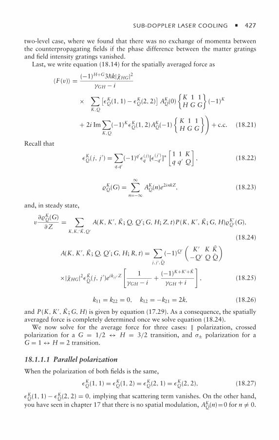
SUB-DOPPLER LASER COOLING 427
two-level case, where we found that there was no exchange of momenta betweenthe counterpropagating fields if the phase difference between the matter gratingsand field intensity gratings vanished.
Last, we write equation (18.14) for the spatially averaged force as
〈F (v)〉 = (−1)H+G3k|χHG|2γGH − iδ
×(∑
K,Q
[εKQ(1,1) − εKQ(2,2)
]AKQ(0)
K 1 1H G G
(−1)K
+ 2i Im∑K,Q
(−1)KεKQ(1,2)AKQ(−1)
K 1 1H G G
)+ c.c. (18.21)
Recall that
εKQ( j, j′) =
∑q,q′
(−1)q′ε( j)q [ε( j
′)−q′]∗
[1 1 Kq q′ Q
], (18.22)
KQ(G) =∞∑
n=−∞AKQ(n)e
2inkZ, (18.23)
and, in steady state,
v∂KQ(G)
∂Z=
∑K,K,′ K,Q′
A(K, K ′, K;Q,Q′;G,H; Z, t)P(K, K ′, K;G,H)K′
Q′(G),
(18.24)
A(K, K ′, K;Q,Q′;G,H; R, t) =∑j, j ′,Q
(−1)Q′(
K ′ K K−Q′ Q Q
)
×|χHG|2ε KQ( j, j ′)eikj j ′ Z[
1γGH − iδ
+ (−1)K+K ′+K
γGH + iδ
], (18.25)
k11 = k22 = 0, k12 = −k21 = 2k, (18.26)
and P(K, K ′, K;G,H) is given by equation (17.29). As a consequence, the spatiallyaveraged force is completely determined once we solve equation (18.24).
We now solve for the average force for three cases: ‖ polarization, crossedpolarization for a G = 1/2 ↔ H = 3/2 transition, and σ± polarization for aG = 1 ↔ H = 2 transition.
18.1.1.1 Parallel polarization
When the polarization of both fields is the same,
εKQ(1,1) = εKQ(1,2) = εKQ(2,1) = εKQ(2,2), (18.27)
εKQ(1,1) − εKQ(2,2) = 0, implying that scattering term vanishes. On the other hand,you have seen in chapter 17 that there is no spatial modulation, AK
Q(n)=0 for n = 0.
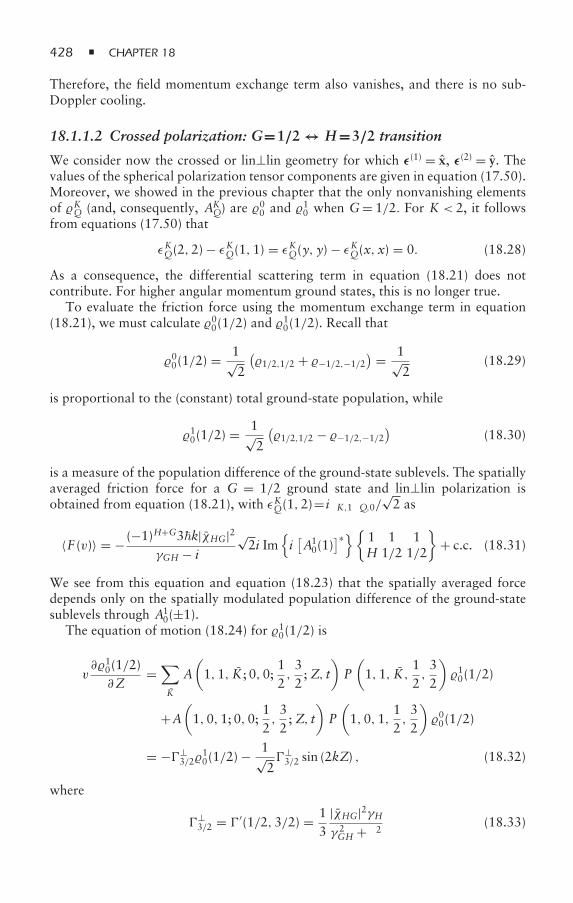
428 CHAPTER 18
Therefore, the field momentum exchange term also vanishes, and there is no sub-Doppler cooling.
18.1.1.2 Crossed polarization: G=1/2 ↔ H=3/2 transition
We consider now the crossed or lin⊥lin geometry for which ε(1) = x, ε(2) = y. Thevalues of the spherical polarization tensor components are given in equation (17.50).Moreover, we showed in the previous chapter that the only nonvanishing elementsof KQ (and, consequently, AK
Q) are 00 and 10 when G= 1/2. For K < 2, it follows
from equations (17.50) that
εKQ(2,2) − εKQ(1,1) = εKQ(y, y) − εKQ(x, x) = 0. (18.28)
As a consequence, the differential scattering term in equation (18.21) does notcontribute. For higher angular momentum ground states, this is no longer true.
To evaluate the friction force using the momentum exchange term in equation(18.21), we must calculate 00(1/2) and
10(1/2). Recall that
00(1/2) = 1√2
(1/2,1/2 + −1/2,−1/2
) = 1√2
(18.29)
is proportional to the (constant) total ground-state population, while
10(1/2) = 1√2
(1/2,1/2 − −1/2,−1/2
)(18.30)
is a measure of the population difference of the ground-state sublevels. The spatiallyaveraged friction force for a G = 1/2 ground state and lin⊥lin polarization isobtained from equation (18.21), with εKQ(1,2)= iδK,1δQ,0/
√2 as
〈F (v)〉 = − (−1)H+G3k|χHG|2γGH − iδ
√2i Im
i[A10(1)
]∗ 1 1 1H 1/2 1/2
+ c.c. (18.31)
We see from this equation and equation (18.23) that the spatially averaged forcedepends only on the spatially modulated population difference of the ground-statesublevels through A1
0(±1).The equation of motion (18.24) for 10(1/2) is
v∂10(1/2)∂Z
=∑K
A(1,1, K ; 0,0;
12,32; Z, t
)P(1,1, K,
12,32
)10(1/2)
+A(1,0,1; 0,0;
12,32; Z, t
)P(1,0,1,
12,32
)00(1/2)
= −⊥3/2
10(1/2) − 1√
2⊥3/2 sin (2kZ) , (18.32)
where
⊥3/2 = ′(1/2,3/2) = 1
3|χHG|2γHγ 2GH + δ2 (18.33)
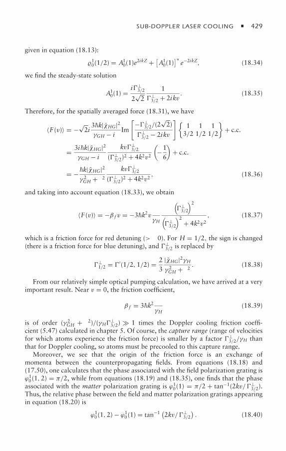
SUB-DOPPLER LASER COOLING 429
is an optical pumping rate [see equation (17.53)]. With a trial solution of the formgiven in equation (18.13):
10(1/2) = A10(1)e
2ikZ + [A10(1)
]∗e−2ikZ, (18.34)
we find the steady-state solution
A10(1) = i⊥
3/2
2√2
1⊥3/2 + 2ikv
. (18.35)
Therefore, for the spatially averaged force (18.31), we have
〈F (v)〉 = −√2i
3k|χHG|2γGH − iδ
Im
[−⊥
3/2/(2√2)
⊥3/2 − 2ikv
]1 1 1
3/2 1/2 1/2
+ c.c.
= 3ik|χHG|2γGH − iδ
kv⊥3/2
(⊥3/2)2 + 4k2v2
(−16
)+ c.c.
= −k|χHG|2γ 2GH + δ2
δkv⊥3/2
(⊥3/2)2 + 4k2v2
, (18.36)
and taking into account equation (18.33), we obtain
〈F (v)〉 = −β f v = −3k2vδ
γH
(⊥3/2
)2
(⊥3/2
)2+ 4k2v2
, (18.37)
which is a friction force for red detuning (δ > 0). For H = 1/2, the sign is changed(there is a friction force for blue detuning), and ⊥
3/2 is replaced by
⊥1/2 = ′(1/2,1/2) = 2
3|χHG|2γHγ 2GH + δ2 . (18.38)
From our relatively simple optical pumping calculation, we have arrived at a veryimportant result. Near v = 0, the friction coefficient,
β f = 3k2δ
γH(18.39)
is of order (γ 2GH + δ2)/(γH⊥
3/2) 1 times the Doppler cooling friction coeffi-cient (5.47) calculated in chapter 5. Of course, the capture range (range of velocitiesfor which atoms experience the friction force) is smaller by a factor ⊥
3/2/γH thanthat for Doppler cooling, so atoms must be precooled to this capture range.
Moreover, we see that the origin of the friction force is an exchange ofmomenta between the counterpropagating fields. From equations (18.18) and(17.50), one calculates that the phase associated with the field polarization grating isϕ10(1,2) = π/2, while from equations (18.19) and (18.35), one finds that the phaseassociated with the matter polarization grating is ϕ10(1) = π/2 + tan−1(2kv/⊥
3/2).Thus, the relative phase between the field and matter polarization gratings appearingin equation (18.20) is
ϕ10(1,2) − ϕ10(1) = tan−1 (2kv/⊥3/2
). (18.40)
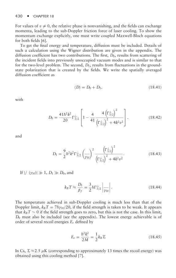
430 CHAPTER 18
For values of v = 0, the relative phase is nonvanishing, and the fields can exchangemomenta, leading to the sub-Doppler friction force of laser cooling. To show themomentum exchange explicitly, one must write coupled Maxwell-Bloch equationsfor both fields [6].
To get the final energy and temperature, diffusion must be included. Details ofsuch a calculation using the Wigner distribution are given in the appendix. Thediffusion coefficient has two contributions. The first, D0, results from scattering ofthe incident fields into previously unoccupied vacuum modes and is similar to thatfor the two-level problem. The second, D1, results from fluctuations in the ground-state polarization that is created by the fields. We write the spatially averageddiffusion coefficient as
〈D〉 = D0 + D1, (18.41)
with
D0 = 412k2
20⊥3/2
⎡⎢⎣1 − 4
41
4(⊥3/2
)2
(⊥3/2
)2+ 4k2v2
⎤⎥⎦ , (18.42)
and
D1 = 922k2⊥
3/2
(δ
γH
)2(⊥3/2
)2
(⊥3/2
)2+ 4k2v2
. (18.43)
If |δ/(γH)| 1, D1 D0, and
kBT ≈ D1
β f= 3
2⊥
3/2
∣∣∣∣ δγH∣∣∣∣ . (18.44)
The temperature achieved in sub-Doppler cooling is much less than that of theDoppler limit, kBT = 7γH/20, if the field strength is taken to be weak. It appearsthat kBT ∼ 0 if the field strength goes to zero, but this is not the case. In this limit,D0 must also be included (see the appendix). The lowest energy achievable is oforder of several recoil energies Er defined by
Er = 2k2
2M= 1
2kBTr (18.45)
In Cs, Tr ≈2.5 µK (corresponding to approximately 13 times the recoil energy) wasobtained using this cooling method [7].
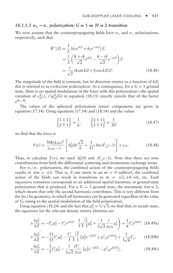
SUB-DOPPLER LASER COOLING 431
18.1.1.3 σ+ − σ− polarization: G = 1 ⇒ H = 2 transition
We now assume that the counterpropagating fields have σ+ and σ− polarizations,respectively, such that
E+(Z) = 12
(ε1eikZ + ε2e−ikZ) E,
= 12
(x + i y√
2eikZ − x − i y√
2e−ikZ
)E
= i√2(x sinkZ+ y cos kZ) E . (18.46)
The magnitude of the field is constant, but its direction rotates as a function of kZ;this is referred to as corkscrew polarization. As a consequence, for a G = 1 groundstate, there is no spatial modulation of the force with this polarization—the spatialvariation of εKQ( j, j
′)KQ(G) in equation (18.11) exactly cancels that of the factoreik j j ′ ·R.
The values of the spherical polarization tensor components are given inequation (17.54). Using equations (17.54) and (18.14) and the values
1 1 12 1 1
= 1
6,
2 1 12 1 1
= 1
30, (18.47)
we find that the force is
F (v) = 3k|χHG|2γGH − iδ
[A10(0)
√26
+ 115
i ImA2−2(−1)
]+ c.c. (18.48)
Thus, to calculate F (v), we need A10(0) and A2
−2(−1). Note that there are nowcontributions from both the differential scattering and momentum exchange terms.
For σ+–σ− polarization, the combined action of the counterpropagating fieldsresults in m = ±2. That is, if one starts in an m = 0 sublevel, the combinedaction of the fields can result in transitions to m = ±2,±4,±6, etc. Eachsuccessive transition corresponds to an additional spatial harmonic in ground-statepolarization that is produced. For a G = 1 ground state, the maximum m is 2,which means that only the second harmonic contributes. This is very different fromthe lin⊥lin geometry, in which all harmonics can be generated regardless of the valueof G, owing to the spatial modulation of the field polarization.
Using equation (18.24) and the fact that 00 = 1/√3, we find that, in steady state,
the equations for the relevant density matrix elements are
v∂22
∂Z= −′
c22 − ′
ce2ikZ
(15
√2320 + 1
5√2
iδγGH
10
)+ 1
6′ce
2ikZ, (18.49a)
v∂20
∂Z= −11
15′c
20 − ′
c
5
√23
(22e
−2ikZ + 2−2e2ikZ)+ 1
3√6′c, (18.49b)
v∂10
∂Z= −1
5′c
10 − 1
5√2
i′cδ
γGH
(22e
−2ikZ − 2−2e2ikZ) , (18.49c)
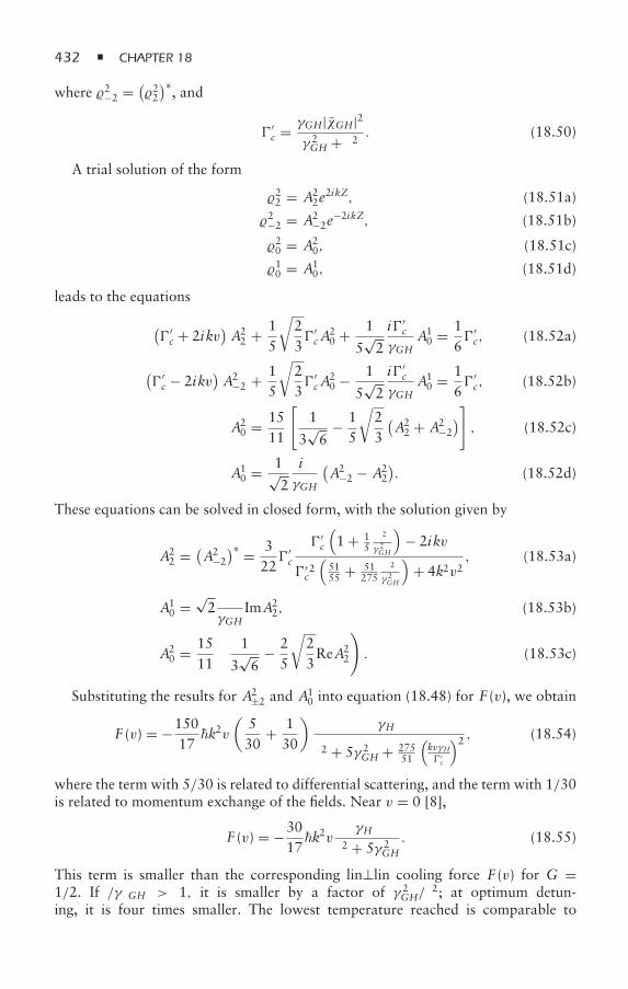
432 CHAPTER 18
where 2−2 = (22)∗, and
′c = γGH|χGH|2
γ 2GH + δ2 . (18.50)
A trial solution of the form
22 = A22e
2ikZ, (18.51a)
2−2 = A2−2e
−2ikZ, (18.51b)
20 = A20, (18.51c)
10 = A10, (18.51d)
leads to the equations
(′c + 2ikv
)A22 + 1
5
√23′c A
20 + 1
5√2
i′cδ
γGHA10 = 1
6′c, (18.52a)
(′c − 2ikv
)A2
−2 + 15
√23′c A
20 − 1
5√2
i′cδ
γGHA10 = 1
6′c, (18.52b)
A20 = 15
11
[1
3√6
− 15
√23
(A22 + A2
−2
)], (18.52c)
A10 = 1√
2
iδγGH
(A2
−2 − A22
). (18.52d)
These equations can be solved in closed form, with the solution given by
A22 = (
A2−2
)∗ = 322′c
′c
(1 + 1
5δ2
γ 2GH
)− 2ikv
′2c
(5155 + 51
275δ2
γ 2GH
)+ 4k2v2
, (18.53a)
A10 =
√2δ
γGHImA2
2, (18.53b)
A20 = 15
11
(1
3√6
− 25
√23ReA2
2
). (18.53c)
Substituting the results for A2±2 and A1
0 into equation (18.48) for F (v), we obtain
F (v) = −15017k2v
(530
+ 130
)γHδ
δ2 + 5γ 2GH + 275
51
(kvγH′c
)2 , (18.54)
where the term with 5/30 is related to differential scattering, and the term with 1/30is related to momentum exchange of the fields. Near v = 0 [8],
F (v) = −3017k2v
γHδ
δ2 + 5γ 2GH
. (18.55)
This term is smaller than the corresponding lin⊥lin cooling force F (v) for G =1/2. If δ/γGH > 1, it is smaller by a factor of γ 2
GH/δ2; at optimum detun-
ing, it is four times smaller. The lowest temperature reached is comparable to
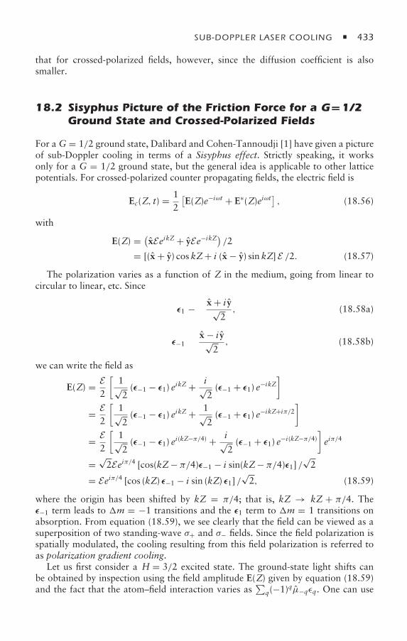
SUB-DOPPLER LASER COOLING 433
that for crossed-polarized fields, however, since the diffusion coefficient is alsosmaller.
18.2 Sisyphus Picture of the Friction Force for a G=1/2Ground State and Crossed-Polarized Fields
For aG = 1/2 ground state, Dalibard and Cohen-Tannoudji [1] have given a pictureof sub-Doppler cooling in terms of a Sisyphus effect. Strictly speaking, it worksonly for a G = 1/2 ground state, but the general idea is applicable to other latticepotentials. For crossed-polarized counter propagating fields, the electric field is
Ec(Z, t) = 12
[E(Z)e−iωt + E∗(Z)eiωt
], (18.56)
with
E(Z) = (xEeikZ + yEe−ikZ) /2
= [(x + y) cos kZ+ i (x − y) sinkZ] E /2. (18.57)
The polarization varies as a function of Z in the medium, going from linear tocircular to linear, etc. Since
ε1 ≡ − x + i y√2, (18.58a)
ε−1 ≡ x − i y√2, (18.58b)
we can write the field as
E(Z) = E2
[1√2(ε−1 − ε1) eikZ + i√
2(ε−1 + ε1) e−ikZ
]
= E2
[1√2(ε−1 − ε1) eikZ + 1√
2(ε−1 + ε1) e−ikZ+iπ/2
]
= E2
[1√2(ε−1 − ε1) ei(kZ−π/4) + i√
2(ε−1 + ε1) e−i(kZ−π/4)
]eiπ/4
=√2Eeiπ/4 [cos(kZ− π/4)ε−1 − i sin(kZ− π/4)ε1] /
√2
= Eeiπ/4 [cos (kZ) ε−1 − i sin (kZ) ε1] /√2, (18.59)
where the origin has been shifted by kZ = π/4; that is, kZ → kZ + π/4. Theε−1 term leads to m = −1 transitions and the ε1 term to m = 1 transitions onabsorption. From equation (18.59), we see clearly that the field can be viewed as asuperposition of two standing-wave σ+ and σ− fields. Since the field polarization isspatially modulated, the cooling resulting from this field polarization is referred toas polarization gradient cooling.
Let us first consider a H = 3/2 excited state. The ground-state light shifts canbe obtained by inspection using the field amplitude E(Z) given by equation (18.59)and the fact that the atom–field interaction varies as
∑q(−1)qµ−qεq. One can use
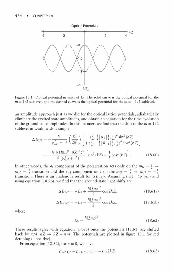
434 CHAPTER 18
–4 –2 2 4kZ
–2.0E/E0
Optical Potentials
–1.5
–1.0
–0.5
Figure 18.1. Optical potential in units of E0. The solid curve is the optical potential for them= 1/2 sublevel, and the dashed curve is the optical potential for the m= −1/2 sublevel.
an amplitude approach just as we did for the optical lattice potentials, adiabaticallyeliminate the excited state amplitudes, and obtain an equation for the time evolutionof the ground-state amplitudes. In this manner, we find that the shift of the m= 1/2sublevel in weak fields is simply
E1/2 = − δ
γ 2GH + δ2
( E222
)[ ⟨ 32 ,
32
∣∣ µ1∣∣ 12 ,
12
⟩2sin2 (kZ)
+ ⟨ 32 ,− 1
2
∣∣ µ−1∣∣ 12 ,
12
⟩2cos2 (kZ)
]
= −δ|〈H||µ(1)||G〉|2E28(γ 2GH + δ2)
[sin2 (kZ) + 1
3cos2 (kZ)
]. (18.60)
In other words, the ε1 component of the polarization acts only on the mG = 12 →
mH = 32 transition and the ε−1 component only on the mG = 1
2 → mH = − 12
transition. There is an analogous result for E−1/2. Assuming that δ γGH andusing equation (18.9b), we find that the ground-state light shifts are
E1/2 = −E0 + |χHG|22δ
cos 2kZ, (18.61a)
E−1/2 = −E0 − |χHG|22δ
cos 2kZ, (18.61b)
where
E0 = |χHG|2δ
. (18.62)
These results agree with equation (17.63) once the potentials (18.61) are shiftedback by π/4, kZ → kZ − π/4. The potentials are plotted in figure 18.1 for reddetuning (δ positive).
From equation (18.32), for v = 0, we have
1/2,1/2 − −1/2,−1/2 = − sin 2kZ (18.63)
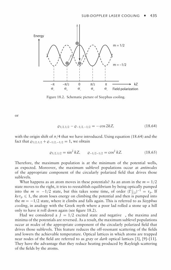
SUB-DOPPLER LASER COOLING 435
Energy
Field polarization
m = –1/2
m = 1/2
kZ–πσ–
–π/2
σ+
0σ–
π/2
σ+
πσ–
Figure 18.2. Schematic picture of Sisyphus cooling.
or
1/2,1/2 − −1/2,−1/2 = − cos 2kZ, (18.64)
with the origin shift of π/4 that we have introduced. Using equation (18.64) and thefact that 1/2,1/2 + −1/2,−1/2 = 1, we obtain
1/2,1/2 = sin2 kZ, −1/2−1/2 = cos2 kZ. (18.65)
Therefore, the maximum population is at the minimum of the potential wells,as expected. Moreover, the maximum sublevel populations occur at antinodesof the appropriate component of the circularly polarized field that drives thosesublevels.
What happens as an atom moves in these potentials? As an atom in the m = 1/2state moves to the right, it tries to reestablish equilibrium by being optically pumpedinto the m = −1/2 state, but this takes some time, of order (⊥
3/2)−1 = τp. If
kvτp 1, the atom loses energy on climbing the potential and then is pumped intothe m = −1/2 state, where it climbs and falls again. This is referred to as Sisyphuscooling, in analogy with the Greek myth where a poor lad rolled a stone up a hillonly to have it roll down again (see figure 18.2).
Had we considered a J = 1/2 excited state and negative δ, the maxima andminima of the potentials are reversed. As a result, the maximum sublevel populationsoccur at nodes of the appropriate component of the circularly polarized field thatdrives those sublevels. This feature reduces the off-resonant scattering of the fieldsand lowers the achievable temperature. Optical lattices in which atoms are trappednear nodes of the field are referred to as gray or dark optical lattices [3], [9]–[11].They have the advantage that they reduce heating produced by Rayleigh scatteringof the fields by the atoms.
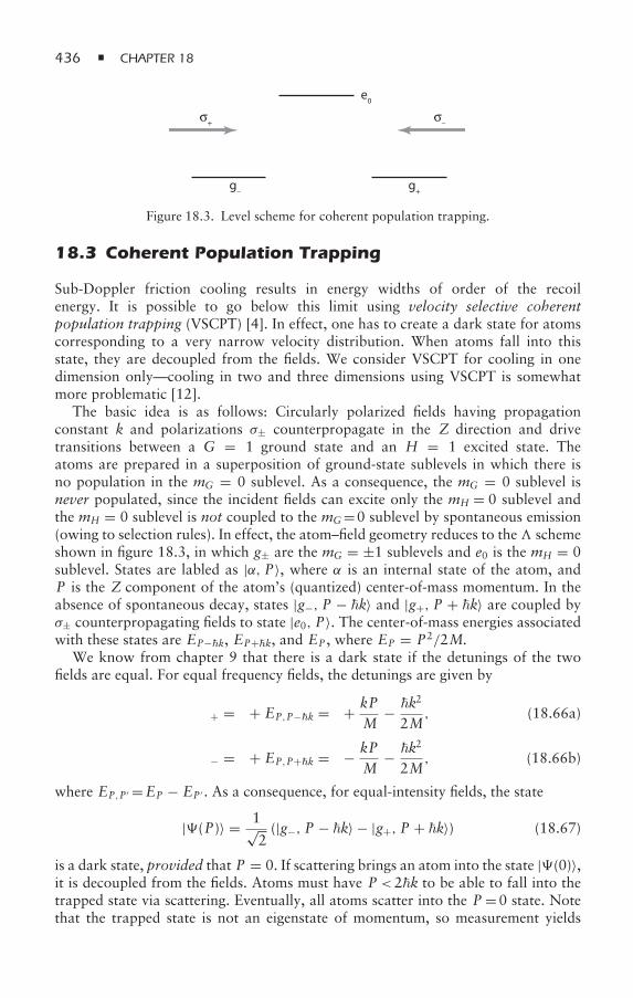
436 CHAPTER 18
e0
g–
g+
σ–
σ+
Figure 18.3. Level scheme for coherent population trapping.
18.3 Coherent Population Trapping
Sub-Doppler friction cooling results in energy widths of order of the recoilenergy. It is possible to go below this limit using velocity selective coherentpopulation trapping (VSCPT) [4]. In effect, one has to create a dark state for atomscorresponding to a very narrow velocity distribution. When atoms fall into thisstate, they are decoupled from the fields. We consider VSCPT for cooling in onedimension only—cooling in two and three dimensions using VSCPT is somewhatmore problematic [12].
The basic idea is as follows: Circularly polarized fields having propagationconstant k and polarizations σ± counterpropagate in the Z direction and drivetransitions between a G = 1 ground state and an H = 1 excited state. Theatoms are prepared in a superposition of ground-state sublevels in which there isno population in the mG = 0 sublevel. As a consequence, the mG = 0 sublevel isnever populated, since the incident fields can excite only the mH = 0 sublevel andthe mH = 0 sublevel is not coupled to the mG=0 sublevel by spontaneous emission(owing to selection rules). In effect, the atom–field geometry reduces to the schemeshown in figure 18.3, in which g± are the mG = ±1 sublevels and e0 is the mH = 0sublevel. States are labled as |α, P〉, where α is an internal state of the atom, andP is the Z component of the atom’s (quantized) center-of-mass momentum. In theabsence of spontaneous decay, states |g−, P − k〉 and |g+, P + k〉 are coupled byσ± counterpropagating fields to state |e0, P〉. The center-of-mass energies associatedwith these states are EP−k, EP+k, and EP , where EP = P2/2M.
We know from chapter 9 that there is a dark state if the detunings of the twofields are equal. For equal frequency fields, the detunings are given by
δ+ = δ + EP,P−k = δ + kPM
− k2
2M, (18.66a)
δ− = δ + EP,P+k = δ − kPM
− k2
2M, (18.66b)
where EP,P ′ =EP − EP ′ . As a consequence, for equal-intensity fields, the state
|(P)〉 = 1√2(|g−, P − k〉 − |g+, P + k〉) (18.67)
is a dark state, provided that P = 0. If scattering brings an atom into the state |(0)〉,it is decoupled from the fields. Atoms must have P <2k to be able to fall into thetrapped state via scattering. Eventually, all atoms scatter into the P =0 state. Notethat the trapped state is not an eigenstate of momentum, so measurement yields
SUB-DOPPLER LASER COOLING 437
two peaks, centered at ±k, provided that P = 0. The widths of each ofthese peaks decreases the longer the field interacts with the atoms, a processthat is governed by Lévy statistics. For some limits on this type of cooling, seeBardou et al. [13].
18.4 Summary
We have shown that optical pumping gives rise to two distinct sub-Doppler coolingmechanisms. The first involves an exchange of momentum between the fieldsresulting from scattering of the fields from a matter-state polarization grating thatis created by the fields. The second mechanism involves a differential scattering ofthe fields from a ground-state sublevel imbalance produced by optical pumping.Both of these mechanisms require ground states having magnetically degeneratesubstates. A third type of sub-Doppler cooling, coherent population trapping,involves optical pumping of zero-velocity atoms into a dark state. In the nextchapter, we return to our discussion of atom-quantized field interactions. Insteadof using the Schrödinger representation, however, we obtain equations of motionfor operators in the Heisenberg representation and derive a source-field expressionfor the electric field operator in terms of atomic state operators.
18.5 Appendix: Fokker-Planck Approach for Obtainingthe Friction Force and Diffusion Coefficients
18.5.1 Fokker-Planck Equation
This appendix contains a calculation of the diffusion coefficient and the final energydistribution for sub-Doppler cooling. There is quite a bit of algebra needed for thederivation of these quantities, so the calculation may appear somewhat complicated.You should keep in mind that we are trying to find the Wigner function for theground-state population density. To do this, we obtain a Fokker-Planck equationfor the ground-state density matrix elements.
We have seen that the modifications of ground-state populations and coherencegive rise to two contributions to the sub-Doppler friction force, one producedby differential scattering from any unmodulated population imbalance and oneby momentum exchange of the fields via a spatially modulated ground-statepolarization. Optical pumping also results in momentum diffusion for the atoms.This spontaneous contribution to diffusion results from the recoil an atom undergoeswhen a field is scattered into a previously unoccupied vacuum field mode. Wehave already encountered this contribution to diffusion in conventional Dopplercooling—the additional degenerate sublevels simply complicate the algebra. Thereis, in addition, a stimulated contribution to diffusion resulting from fluctuations inthe spatially modulated ground-state polarization.
We assume that the atomic momentum is much greater than the recoil momentumand that the energy of the atoms is greater that the ground-state light shifts. If
438 CHAPTER 18
this is not the case, one must solve the full quantum dynamics for the atom–fieldsystem using the eigenstates of the atoms in the periodic light shift potentials. If themomentum is much less than the atomic momentum, changes in atomic velocity canbe treated in a diffusion or Brownian motion approximation. In statistical physics,the Fokker-Planck equation for the phase-space distribution function describes suchdiffusive motion. The Fokker-Planck equation can be derived as an appropriate limitof the transport equation. A general form of the Fokker-Planck equation is [14]
∂ f (Z, P, t)∂t
+ v ∂ f (Z, P, t)∂Z
= ∂
∂P[βP f (Z, P, t)] + D
∂2 f (Z, P, t)∂P2
, (18.68)
where f (Z, P, t) is the distribution function, β is a friction coefficient, D is adiffusion constant, and v = P/M. We consider one-dimensional motion only. It isassumed that the transverse velocity distribution undergoes negligible cooling whenthe incident fields are directed along the Z axis.
The goal in this appendix is to derive the analogue of the Fokker-Planck equationfor the Wigner function associated with the ground-state population. You may recallthat the Wigner function was discussed in chapter 5 and is the quantum analogue ofthe distribution function. The starting point for the calculation is the generalizationof equation (17.27) to include the center-of-mass motion of the atoms, starting fromequation (5.73). There is considerable algebra needed to derive such an equation,and we do not give the details; however, the final equation simply reflects the recoilprocesses described earlier. Explicitly, we find [15]
∂KQ(P, P′, t;G)
∂t+ iωP,P ′KQ(P, P
′;G) = (−1)Q′(K K ′ KQ−Q′ Q
)
×ε KQ( j, j
′)S+(K, K ′, K,G,H, j, j ′)K′
Q′(P, P ′ + kj j ′ , t;G
)+ε KQ( j, j ′)S−(K, K ′, K,G,H, j, j ′)K
′Q′(P − kj j ′ , P ′, t;G
)+T(K, K ′, K, K, K ′
,G,H, j, j ′)∫dλ(K, K
′, K, Q, j, j ′;)
× K′
Q′[P + (q − kj ), P ′ + (q − kj ′), t;G)
], (18.69)
where
ωP,P ′ =(P2 − P ′2)2M
, (18.70)
T(K, K ′, K, K, K ′,G,H, j, j ′) = 3(−1)1+K+K ′
(2H+ 1) BK
×[(2K + 1)(2K ′ + 1
) (2K + 1
) (2K + 1
)(2K
′ + 1)]1/2
×|χHG|2 (γ 2GH + δ2)−1
A(K, K ′, K, K, K ′,G,H), (18.71)
A(K, K ′, K, K, K ′,G,H) = (2X+ 1)
K K ′ KK
′K X
⎧⎨⎩K X KG H 1G H 1
⎫⎬⎭⎧⎨⎩X K ′ K ′
H G 1H G 1
⎫⎬⎭ ,(18.72)
SUB-DOPPLER LASER COOLING 439
S+(K, K ′, K,G,H, j, j ′) = −3(−1)H−G+K [(2K + 1)(2K ′ + 1
)]1/2×(2K + 1)1/2|χHG|2 (γGH − iδ)−1
K K ′ KG G G
1 1 KG G H
, (18.73)
S−(K, K ′, K,G,H, j, j ′) = (−1)K+K ′−K [S+(K, K ′, K,G,H, j, j ′)]∗, (18.74)
λ(K, K′, K, Q, j, j ′;)= 3
8π(−1)K+K
′+Q√
2K+1(K K
′K
Q−Q′ Q
)YKQ()ε
K′
Q′ ( j, j ′),
(18.75)
BK =√
16π/3δK,0 +√
8π/15δK,2, (18.76)
q = kcos θ, (18.77)
k1 = −k2 = k, kj j ′ = kj − kj ′ , (18.78)
YKQ() is a spherical harmonic, and all other symbols have been defined in the text.A summation convention is used in equation (17.9), and all subsequent equationsin this appendix in which any repeated indices appearing on the right-hand sideof an equation are summed over, unless they also appear on the left-hand side ofthe equation. There is no sum over G or H, since only one value for each of theseparameters is considered.
Admittedly, this is an algebraically complicated equation, containing an integralover the projection, q cos θ , onto the z axis of the recoil momentum associated withscattering of the field into the vacuum mode. Nevertheless, it is a relatively simplematter to program this equation; a link to a Mathematica notebook that accom-plishes this task is posted at http://press.princeton.edu/titles/9376.html. The nextstep is to convert equation (18.69) to the Wigner function using equation (5.77c),
KQ(Z, P, t;G) = (2π)−1∫ ∞
−∞duKQ(P + u/2, P − u/2, t;G)eiuZ/. (18.79)
From equations (18.69) and (18.79), and using the fact that
(2π)−1∫ ∞
−∞duuKQ(P + u/2, P − u/2, t;G)eiuZ/ = (/ i) ∂KQ(Z, P, t;G)/∂Z,
(18.80)we can obtain(
∂
∂t+ v ∂
∂Z
)KQ(Z, P, t;G) = (−1)Q
′(K K ′ KQ−Q′ Q
)eikj j ′ Z
×T(K, K ′, K, K, K ′
,G,H, j, j ′)
×∫dλ(K, K
′, K, Q, j, j ′;)K
′Q′[Z, P + (q − kj/2 − kj ′/2), t;G
]+ε KQ( j, j ′)S+(K, K ′, K,G,H, j, j ′)K
′Q′(Z, P + kj j ′/2, t;G
)+ ε KQ( j, j
′)S−(K, K ′, K,G,H, j, j ′)K′
Q′(Z, P − kj j ′/2, t;G
). (18.81)
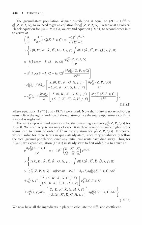
440 CHAPTER 18
The ground-state population Wigner distribution is equal to (2G + 1)1/2 ×00(Z, P, t;G), so we need to get an equation for 00(Z, P, t;G). To arrive at a Fokker-Planck equation for 00(Z, P, t;G), we expand equation (18.81) to second order in to arrive at(
∂
∂t+ v ∂
∂Z
)00(Z, P, t;G) = (−1)K
′eikj j ′ Z√
2K ′ + 1
×T(0, K ′, K ′, K, K ′
,G,H, j, j ′)∫dλ(K, K
′, K ′,Q′, j, j ′;)
×[(kcos θ − kj/2 − kj ′/2)
∂K′
Q′ (Z, P, t;G)
∂P
+ 2(kcos θ − kj/2 − kj ′/2)2∂2K
′Q′ (Z, P, t;G)
∂P2
]
+εK ′Q′ ( j, j ′)kj j ′
[S+(0, K ′, K ′,G,H, j, j ′)
−S−(0, K ′, K ′,G,H, j, j ′)
]∂K
′Q′ (Z, P, t;G)
∂P
+ εK′
Q′( j, j ′)2k2j j ′2
[S+(0, K ′, K ′,G,H, j, j ′)
+S−(0, K ′, K ′,G,H, j, j ′)
]∂2K
′Q′ (Z, P, t;G)
∂P2
,
(18.82)
where equations (18.71) and (18.72) were used. Note that there is no zeroth-orderterm in on the right-hand side of the equation, since the total population is constantif recoil is neglected.
The next step is to find equations for the remaining elements KQ(Z, P, t;G) forK = 0. We need keep terms only of order in these equations, since higher orderterms lead to terms of order 3k3 in the equation for 00(Z, P, t;G). Moreover,we can solve for these terms in quasi-steady-state, since they adiabatically followthe total ground population, once any initial transients have died away. Thus, forK = 0, we expand equation (18.81) in steady state to first order in to arrive at
v∂KQ(Z, P, t;G)
∂Z= (−1)Q
′(K K ′ KQ−Q′ Q
)eikj j ′ Z
×T(K, K ′, K, K, K ′
,G,H, j, j ′)∫dλ(K, K
′, K, Q, j, j ′;)
×[K
′Q′(Z, P, t;G) + (kcos θ − kj/2 − kj ′/2)∂K
′Q′(Z, P, t;G)/∂P
]
+ε KQ( j, j ′)[S+(K, K ′, K,G,H, j, j ′)
+S−(K, K ′, K,G,H, j, j ′)
]K
′Q′(Z, P, t;G)
+ ε KQ( j, j′)kj j ′
[S+(K, K ′, K,G,H, j, j ′)
−S−(K, K ′, K,G,H, j, j ′)
]∂K
′Q′(Z, P, t;G)/∂P
.
(18.83)
We now have all the ingredients in place to calculate the diffusion coefficient.
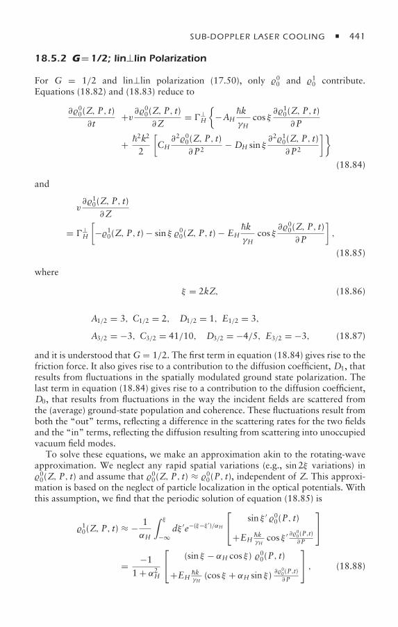
SUB-DOPPLER LASER COOLING 441
18.5.2 G=1/2; lin⊥lin Polarization
For G = 1/2 and lin⊥lin polarization (17.50), only 00 and 10 contribute.Equations (18.82) and (18.83) reduce to
∂00(Z, P, t)∂t
+v ∂00(Z, P, t)∂Z
= ⊥H
−AH
kδγH
cos ξ∂10(Z, P, t)
∂P
+ 2k2
2
[CH∂200(Z, P, t)
∂P2− DH sin ξ
∂210(Z, P, t)∂P2
](18.84)
and
v∂10(Z, P, t)
∂Z
= ⊥H
[−10(Z, P, t) − sin ξ 00(Z, P, t) − EH
kδγH
cos ξ∂00(Z, P, t)
∂P
],
(18.85)
where
ξ = 2kZ, (18.86)
A1/2 = 3, C1/2 = 2, D1/2 = 1, E1/2 = 3,
A3/2 = −3, C3/2 = 41/10, D3/2 = −4/5, E3/2 = −3, (18.87)
and it is understood that G = 1/2. The first term in equation (18.84) gives rise to thefriction force. It also gives rise to a contribution to the diffusion coefficient, D1, thatresults from fluctuations in the spatially modulated ground state polarization. Thelast term in equation (18.84) gives rise to a contribution to the diffusion coefficient,D0, that results from fluctuations in the way the incident fields are scattered fromthe (average) ground-state population and coherence. These fluctuations result fromboth the “out” terms, reflecting a difference in the scattering rates for the two fieldsand the “in” terms, reflecting the diffusion resulting from scattering into unoccupiedvacuum field modes.
To solve these equations, we make an approximation akin to the rotating-waveapproximation. We neglect any rapid spatial variations (e.g., sin 2ξ variations) in00(Z, P, t) and assume that 00(Z, P, t) ≈ 00(P, t), independent of Z. This approxi-mation is based on the neglect of particle localization in the optical potentials. Withthis assumption, we find that the periodic solution of equation (18.85) is
10(Z, P, t) ≈ − 1αH
∫ ξ
−∞dξ ′e−(ξ−ξ ′)/αH
⎡⎣ sin ξ ′ 00(P, t)
+EHkδγH
cos ξ ′ ∂00(P,t)∂P
⎤⎦
= −11 + α2H
⎡⎣ (sin ξ − αH cos ξ ) 00(P, t)
+EHkδγH
(cos ξ + αH sin ξ ) ∂00(P,t)∂P
⎤⎦ , (18.88)
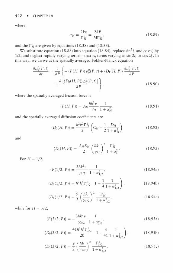
442 CHAPTER 18
where
αH = 2kv⊥H
= 2kPM⊥
H, (18.89)
and the ⊥H are given by equations (18.38) and (18.33).
We substitute equation (18.88) into equation (18.84), replace sin2 ξ and cos2 ξ by1/2, and neglect rapidly varying terms—that is, terms varying as sin 2ξ or cos 2ξ . Inthis way, we arrive at the spatially averaged Fokker-Planck equation
∂00(P, t)∂t
= ∂
∂P
−〈F (H, P)〉 00(P, t) + 〈D1(H, P)〉 ∂
00(P, t)∂P
+ ∂[〈D0(H, P)〉 00(P, t)
]∂P
, (18.90)
where the spatially averaged friction force is
〈F (H, P)〉 = AHk2vδγH
11 + α2H
, (18.91)
and the spatially averaged diffusion coefficients are
〈D0(H, P)〉 = 2k2⊥
H
2
(CH + 1
2DH
1 + α2H
)(18.92)
and
〈D1(H, P)〉 = AHEH
2
(kδγH
)2⊥H
1 + α2H. (18.93)
For H = 1/2,
〈F (1/2, P)〉 = 3k2vδγ1/2
11 + α21/2
, (18.94a)
〈D0(1/2, P)〉 = 2k2⊥1/2
(1 + 1
41
1 + α21/2
), (18.94b)
〈D1(1/2, P)〉 = 92
(kδγ1/2
)2⊥H
1 + α21/2, (18.94c)
while for H = 3/2,
〈F (3/2, P)〉 = −3k2vδγ3/2
11 + α23/2
, (18.95a)
〈D0(3/2, P)〉 = 412k2⊥3/2
20
(1 − 4
411
1 + α23/2
), (18.95b)
〈D1(3/2, P)〉 = 92
(kδγ3/2
)2 ⊥3/2
1 + α23/2. (18.95c)
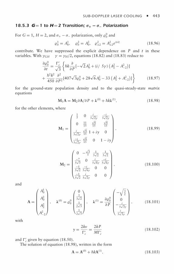
SUB-DOPPLER LASER COOLING 443
18.5.3 G=1 to H=2 Transition; σ+ − σ− Polarization
For G = 1, H = 2, and σ+ − σ− polarization, only 00 and
10 = A10, 20 = A2
0, 2±2 = A2±2e
±iξ (18.96)
contribute. We have suppressed the explicit dependence on P and t in thesevariables. With γGH ≡ γ = γH/2, equations (18.82) and (18.83) reduce to
∂00
∂t= ′
c√3
k
∂
∂P[−
√2A1
0 + (iδ/5γ )(A22 − A2
−2
)]
+ 2k2
450∂2
∂P2[407
√300 + 28
√6A2
0 − 33(A22 + A2
−2
)]
(18.97)
for the ground-state population density and to the quasi-steady-state matrixequations
M1A = M2∂A/∂P + λ(0) + kλ(1), (18.98)
for the other elements, where
M1 =
⎛⎜⎜⎜⎜⎜⎜⎝
15 0 iδ
5√2γ
−iδ5√2γ
0 1115
√6
15
√6
15
iδ5√2γ
√6
15 1 + iy 0
−iδ5√2γ
√6
15 0 1 − iy
⎞⎟⎟⎟⎟⎟⎟⎠, (18.99)
M2 =
⎛⎜⎜⎜⎜⎜⎜⎝
0 −√35
15√2
15√2
−75√3
0 iδ5√6γ
−iδ5√6γ
−15√2
−iδ5√6γ
0 0−15√2
iδ5√2γ
0 0
⎞⎟⎟⎟⎟⎟⎟⎠, (18.100)
and
A =
⎛⎜⎜⎜⎜⎜⎝
A10
A20
A22
A2−2
⎞⎟⎟⎟⎟⎟⎠ , λ(0) = 00
⎛⎜⎜⎜⎜⎝
01
3√2
12√3
12√3
⎞⎟⎟⎟⎟⎠ , λ(1) = ∂00
∂P
⎛⎜⎜⎜⎜⎜⎝
−√
32
0− iδ
5√3γ
iδ5√3γ
⎞⎟⎟⎟⎟⎟⎠ , (18.101)
with
y = 2kv′c
= 2kPM′
c(18.102)
and ′c given by equation (18.50).
The solution of equation (18.98), written in the form
A = A(0) + kA(1), (18.103)
444 CHAPTER 18
is
A(0) ≡ A[0] = M−11 λ(0) (18.104)
and
A(1) = M−11 λ(1) + M−1
1 M2M−11∂λ(0)
∂P+ M−1
1 M2∂M−1
1
∂Pλ(0). (18.105)
The solution for A(0) is given by equations (18.53), multiplied by√300(Z, P, t). The
three terms in equation (18.105) are designated as
A[1] = M−11 λ(1), (18.106a)
A[2] = M−11 M2M−1
1∂λ(0)
∂P, (18.106b)
A[3] = M−11 M2
∂M−11
∂Pλ(0). (18.106c)
There is considerable algebra required to evaluate equations (18.104) and(18.105), but they are handled easily by a computer program. After solving for A(0)
and A(1), we substitute these values into equation (18.97) and write that equation inthe form (18.90). The friction force is given by
F (y) = −k′c√
3[−
√2A1
0[0] + (iδ/5γ )(A22[0] − A2
−2[0])]
= −3017k2v
γHδ
δ2 + 5γ 2 + c1y2γ 2, (18.107)
where y is defined in equation (18.102),
c1 = 275/51, (18.108)
and γ =γGH=γH/2. This result agrees with equation (18.54). There is an additionalcontribution to the force arising from the last term in equation (18.105) that canbe included; however, this term is small for the range of parameters for which thetheory is valid (see problem 10). The diffusion coefficients are given by
D0(y) = 2k2′
c
450
[407
√3 + 28
√2A2
0[0]/00 − 11
√3(A22[0] + A2
−2[0])/00
]
= 3834252k2′
cδ2 + 5γ 2 + c2y2γ 2
δ2 + 5γ 2 + c1y2γ 2, (18.109)
with
c2 = 4275/766, (18.110)
and
D1(y) = Da(y) + Db(y), (18.111)
SUB-DOPPLER LASER COOLING 445
with
Da(y) = 2k2′
c√3
[−√2A1
0[1] + (iδ/5γ )(A22[1] − A2
−2[1])](∂00
∂P
)−1
= 2k2′
c
525
(5γ 2 + c1y2γ 2
)− δ2δ2 + 5γ 2 + c1y2γ 2
; (18.112a)
Db(y) = 2k2′
c√3
[−√2A1
0[2] + (iδ/5γ )A22[2] − A2
−2[2]](∂00
∂P
)−1
= 2k2′
c
260134375y4γ 4 + 75y2γ 2
(425γ 2 − 13δ2
)+ 306δ2(δ2 + 5γ 2
)(δ2 + 5γ 2 + c1y2γ 2
)2 .
(18.112b)
Near zero velocity (y = 0), we can write a single diffusion coefficient [1, 8],
D= D0 + D1 = 2k2′c
(348425
+ 43217
γ 2
δ2 + 5γ 2
). (18.113)
18.5.4 Equilibrium Energy
Having calculated the friction and diffusion coefficients, we can estimate theequilibrium energy starting from the Fokker-Planck equation (18.90). In steadystate, the solution of that equation for the ground-state population density ψ(P) =(2G+ 1)1/200(P;G) is
−〈F (P)〉ψ(P) + 〈D1(P)〉 ∂ψ(P)∂P
+ ∂ [〈D0(P)〉ψ(P)]∂P
= constant = 0, (18.114)
where we take the constant equal to zero to insure that ψ(0) is finite. Once wecalculate ψ(P), we can find the equilibrium energy by evaluating the average valueof P2/2M. In terms of dimensionless variables, equation (18.114) can be written as
[−δβ F (β) +
′
2∂ D0(β)∂β
]ψ(β) +
′
2D(β)
∂ψ(β)∂β
= 0, (18.115)
where
F (β) = M 〈F (β)〉2k3δβ
, (18.116a)
D0(β) = 〈D0(β)〉2k2′ , (18.116b)
D(β) = [〈D1(β)〉 + 〈D0(β)〉]2k2′ , (18.116c)
446 CHAPTER 18
β = Pk
= Mvk, β2 = Mv2/2
2k2/2M= E
ER, (18.117)
δ = δ/γH, (18.118)
′ = ′
k2/2M, (18.119)
and ′ is the optical pumping rate appropriate to a given level scheme (⊥H or c).
The (′/2)(∂ D0/∂β) term in equation (18.115) acts as an effective force, but usually
can be neglected (see problem 9). The solution of equation (18.115) with the neglectof this term is
ψ(β) = ψ(0) exp2δ/
′∫ β
0β ′dβ ′ [F (β ′) /D(
β ′)] . (18.120)
To proceed further, we must put in the specific forms for the friction and diffusioncoefficients.
18.5.4.1 lin⊥lin polarizationIn this case, from equations (18.116), (18.91), (18.93), and (18.92), we have
F (β) = F H(β) = AH
1 + 16β2/⊥2H
, (18.121)
D(β) = CH
2+ DH/2 + AHEHδ
2
2(1 + 16β2/
⊥2H
) . (18.122)
Setting
x = 4β/⊥H, (18.123)
we can write equation (18.120) as
ψ(x) = ψ(0) exp
[−aH
∫ x
0x′dx′ AH
JH + (1 + x′2)GH
](18.124a)
= ψ(0) exp
[− aHAH
2GHln(1 + GHx2
GH + JH
)]
= ψ(0)(1 + GHx2
GH + JH
)− aHAH
2GH
, (18.124b)
where
GH = CH/2, (18.125)
JH = (DH/2 + AHEHδ
2) /2, (18.126)
aH = −δ⊥H/8, (18.127)
and AH, CH, DH, and EH are defined in equation (8.87). (Note that aHAH > 0. IfH = 1/2, AH = 3, but δ < 0 for cooling; if H = 3/2, AH = −3, and δ > 0 forcooling.)
SUB-DOPPLER LASER COOLING 447
___
50
0
100
150
|a3/2|
200
250
<E>ER
50 10 2015 25
Figure 18.4. Graph of 〈E〉/ER as a function of∣∣a3/2∣∣ when H = 3/2 and δ = 5 (solid line)
and δ = 1 (dashed line).
The average equilibrium energy, in units of the recoil energy ER = 2k2/2M, isgiven by
〈E〉ER
=∫∞
−∞ ψ(β)β2dβ∫∞
−∞ ψ(β)dβ=
⊥2H
16
∫∞−∞ ψ(x)x
2dx∫∞−∞ ψ(x)dx
. (18.128)
The integrals are tabulated, enabling us to obtain
〈E〉ER
= ⊥2H
16GH + JH
AHaH − 3GH
= 4a2Hδ2
GH + JHAHaH − 3GH
. (18.129)
Since aH is proportional to the field intensity, the average energy decreases linearlywith decreasing intensity for AHaH 3GH, reaches a minimum, and then increasesas the field intensity is lowered even more, owing to spontaneous contributions to thediffusion coefficient that dominate at these low field intensities. A graph of 〈E〉 /ER
as a function of∣∣a3/2∣∣ is shown in figure 18.4 for δ = 1 and 5.
The average energy actually diverges when AHaH = 3GH, but the calculation isnot valid for such field intensities. The minimum energy occurs for aHAH = 6GH,such that
〈E〉ER
)min
= 48GHGH + JHA2Hδ
2
= 12CHCH + (
DH/2 + AHEHδ2)
A2Hδ
2. (18.130)
For H = 1/2,
〈E〉ER
)min
= 24[1 + 5/
(18δ2
)], (18.131)
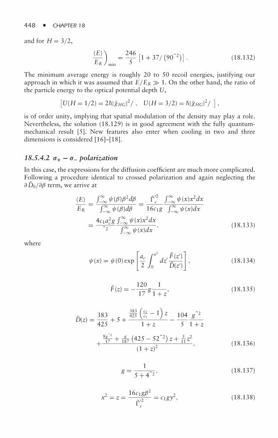
448 CHAPTER 18
and for H = 3/2,
〈E〉ER
)min
= 2465
[1 + 37/
(90δ2
)]. (18.132)
The minimum average energy is roughly 20 to 50 recoil energies, justifying ourapproach in which it was assumed that E/ER 1. On the other hand, the ratio ofthe particle energy to the optical potential depth U,[
U(H = 1/2) = 2|χHG|2/δ , U(H = 3/2) = |χHG|2/δ] ,is of order unity, implying that spatial modulation of the density may play a role.Nevertheless, the solution (18.129) is in good agreement with the fully quantum-mechanical result [5]. New features also enter when cooling in two and threedimensions is considered [16]–[18].
18.5.4.2 σ+ − σ− polarization
In this case, the expressions for the diffusion coefficient are much more complicated.Following a procedure identical to crossed polarization and again neglecting the∂ D0/∂β term, we arrive at
〈E〉ER
=∫∞
−∞ ψ(β)β2dβ∫∞
−∞ ψ(β)dβ=
′2c
16c1g
∫∞−∞ ψ(x)x
2dx∫∞−∞ ψ(x)dx
= 4c1a2c gδ2
∫∞−∞ ψ(x)x
2dx∫∞−∞ ψ(x)dx
, (18.133)
where
ψ(x) = ψ(0) exp
[ac2
∫ x2
0dz′
F (z′)D(z′)
], (18.134)
F (z) = −12017
g1
1 + z, (18.135)
D(z) = 383425
+ 5 +383425
(c2c1
− 1)z
1 + z− 104
5gδ2
1 + z
+8gδ2
17 + g187
(425 − 52δ2
)z+ 5
11 z2
(1 + z)2, (18.136)
g = 15 + 4δ2
, (18.137)
x2 = z = 16c1gβ2
′2c
= c1gy2, (18.138)
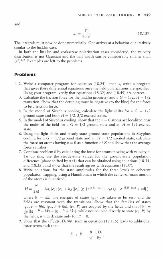
SUB-DOPPLER LASER COOLING 449
and
ac = δ′c
8c1g. (18.139)
The integrals must now be done numerically. One arrives at a behavior qualitativelysimilar to the lin⊥lin case.
In both the lin⊥lin and corkscrew polarization cases considered, the velocitydistribution is not Gaussian and the half width can be considerably smaller than〈v2〉1/2. Examples are left to the problems.
Problems
1–2. Write a computer program for equation (18.24)—that is, write a programthat gives these differential equations once the field polarizations are specified.Using your program, verify that equations (18.32) and (18.49) are correct.
3. Calculate the friction force for the lin⊥lin geometry and a G = 1/2, H = 1/2transition. Show that the detuning must be negative (to the blue) for the forceto be a friction force.
4. In the model of Sisyphus cooling, calculate the light shifts for a G = 1/2ground state and both H = 1/2,3/2 excited states.
5. In the model of Sisyphus cooling, show that the v = 0 atoms are localized nearthe nodes of the field for a G = 1/2 ground state and an H = 1/2 excitedstate.
6. Using the light shifts and steady-state ground-state populations in Sisyphuscooling for a G = 1/2 ground state and an H = 1/2 excited state, calculatethe force on atoms having v = 0 as a function of Z and show that the averageforce vanishes.
7. Continue problem 6 by calculating the force for atoms moving with velocity v.To do this, use the steady-state values for the ground-state populationdifference (phase shifted by π/4) that can be obtained using equations (18.34)and (18.35), and show that the result agrees with equation (18.37).
8. Write equations for the state amplitudes for the three levels in coherentpopulation trapping, using a Hamiltonian in which the center-of-mass motionof the atoms is quantized,
H = P2
2M+ ω0 |e0〉 〈e0| + χ (|e0〉 〈g−| eik·R−iω0t + |e0〉 〈g+| e−ik·R−iω0t + adj.),
where k = kz. The energies of states |g±〉 are taken to be zero and thefields are resonant with the transitions. Show that the families of states|g−, P − k〉, |g+, P + k〉, |e0, P〉 are coupled by the fields and that |〉 =1√2(|g−, P − k〉 − |g+, P + k〉), while not coupled directly to state |e0, P〉 by
the fields, is a dark state only for P = 0.9. Show that the (
′/2)(∂ D0/∂β) term in equation (18.115) leads to additional
force terms such that
F → F − 8
δy′∂ D0
∂y,
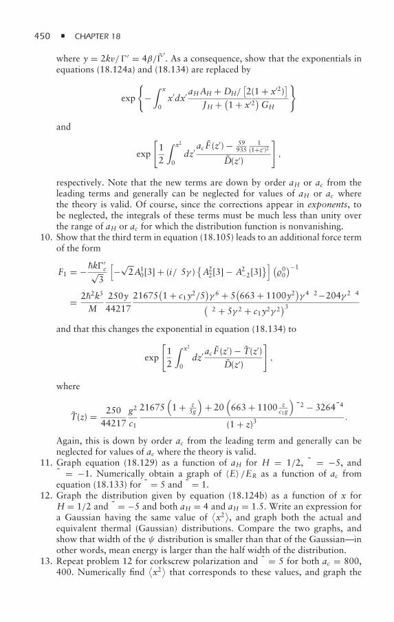
450 CHAPTER 18
where y = 2kv/′ = 4β/′. As a consequence, show that the exponentials in
equations (18.124a) and (18.134) are replaced by
exp
−∫ x
0x′dx′ aHAH + DH/
[2(1 + x′2)
]JH + (
1 + x′2)GH
and
exp
[12
∫ x2
0dz′
ac F (z′) − 59935
1(1+z′)2
D(z′)
],
respectively. Note that the new terms are down by order aH or ac from theleading terms and generally can be neglected for values of aH or ac wherethe theory is valid. Of course, since the corrections appear in exponents, tobe neglected, the integrals of these terms must be much less than unity overthe range of aH or ac for which the distribution function is nonvanishing.
10. Show that the third term in equation (18.105) leads to an additional force termof the form
F1 = −k′c√
3
[−
√2A1
0[3] + (iδ/5γ )A22[3] − A2
−2[3]] (
00)−1
= 22k3
M250y44217
21675(1 + c1y2/5
)γ 6 + 5
(663 + 1100y2
)γ 4δ2−204γ 2δ4(
δ2 + 5γ 2 + c1y2γ 2)3
and that this changes the exponential in equation (18.134) to
exp
[12
∫ x2
0dz′
ac F (z′) − T(z′)D(z′)
],
where
T(z) = 25044217
g2
c1
21675(1 + z
5g
)+ 20
(663 + 1100 z
c1g
)δ2 − 3264δ4
(1 + z)3.
Again, this is down by order ac from the leading term and generally can beneglected for values of ac where the theory is valid.
11. Graph equation (18.129) as a function of aH for H = 1/2, δ = −5, andδ = −1. Numerically obtain a graph of 〈E〉 /ER as a function of ac fromequation (18.133) for δ = 5 and δ = 1.
12. Graph the distribution given by equation (18.124b) as a function of x forH = 1/2 and δ = −5 and both aH = 4 and aH = 1.5. Write an expression fora Gaussian having the same value of
⟨x2⟩, and graph both the actual and
equivalent thermal (Gaussian) distributions. Compare the two graphs, andshow that width of the ψ distribution is smaller than that of the Gaussian—inother words, mean energy is larger than the half width of the distribution.
13. Repeat problem 12 for corkscrew polarization and δ = 5 for both ac = 800,400. Numerically find
⟨x2⟩that corresponds to these values, and graph the
SUB-DOPPLER LASER COOLING 451
actual distribution and the (unnormalized) Gaussian distribution having amean square width equal to
⟨x2⟩. Compare the two graphs, and show that
width of the ψ distribution is smaller than that of the Gaussian—in otherwords, mean energy is larger than the half width of the distribution.
References
[1] J. Dalibard and C. Cohen-Tannoudji, Laser cooling below the Doppler limit bypolarization gradients: simple theoretical models, Journal of the Optical Society B 6,2023–2045 (1989).
[2] C. Cohen-Tannoudji, New laser cooling mechanisms, in Laser Manipulation of Atomsand Ions, Enrico Fermi Summer School Course CXVIII, edited by E. Arimondo,W. D. Phillips, and S. Strumia (North-Holland, Amsterdam, 1992), pp. 99–169.
[3] V. Finkelstein, P. R. Berman, and J. Guo, One-dimensional laser cooling below theDoppler limit, Physical Review A 45, 1829–1842 (1992).
[4] A. Aspect, E. Arimondo, R. Kaiser, N. Vansteenkiste, and C. Cohen-Tannoudji, Lasercooling below the one-photon recoil energy by velocity selective coherent populationtrapping: theoretical analysis, Journal of the Optical Society B 6, 2112–2124 (1989).
[5] Y. Castin, J. Dalibard, and C. Cohen-Tannoudji, The limits of Sisyphus cooling,in Light-Induced Kinetic Effects on Atoms, Ions, and Molecules, edited by L. Moi,S. Gozzini, C. Gabbanini, E. Arimondo, and F. Strumia (ETS Editrice, Pisa, 1991),pp. 5–24; J. Dalibard and Y. Castin, Laser cooling from the semi-classical to thequantum regime, in Frontiers in Laser Spectroscopy, Enrico Fermi Summer SchoolCourse CXX, edited by T. W. Hänsch and M. Inguscio (North-Holland, Amsterdam,1994) pp. 445–476.
[6] P. R. Berman, Nonlinear spectroscopy and laser cooling, in Laser Spectroscopy,edited by L. Ducloy, E. Giacobino, and G. Gamy (World Scientific, Singapore, 1992),pp. 15–20.
[7] C. Salomon, J. Dalibard, W. D. Phillips, A. Clairon, and S. Guellati, Laser cooling ofcesium atoms below 3 microkelvins, Europhysics Letters 12, 683–688 (1990).
[8] Y. Castin and K. Mølmer, Atomic momentum diffusion in a σ+−σ− laser configuration:influence of internal level structure, Journal of Physics B 23, 4101–4110 (1990).
[9] G. Grynberg and J.-Y. Courtois, Proposal for a magneto-optic lattice for trappingatoms in nearly dark states, Europhysics Letters 27, 41–46 (1994).
[10] A. Hemmerich, M. Weidemüller, T. Esslinger, G. Zimmermann, and T. Hänsch,Trapping atoms in dark optical lattices, Physical Review Letters 75, 37–40 (1995).
[11] K. I. Petsas, J.-Y. Courtois, and G. Grynberg, Temperature and magnetism of grayoptical lattices, Physical Review A 53, 2533–2538 (1996).
[12] F. Mauri and E. Arimondo, Coherent trapping subrecoil cooling in two dimensionsaided by a force, Europhysics Letters 16, 717–722 (1991); M. A. Ol’shanii and V. G.Minogin, Three-dimensional velocity selective coherent population trapping in resonantlight fields, in Light-Induced Kinetic Effects on Atoms, Ions, and Molecules, edited byL. Moi, S. Gozzini, C. Gabbanini, E. Arimondo, and F. Strumia (ETS Editrice, Pisa,1991), pp. 99–110; J. Lawall, S. Kulin, B. Saubamea, N. Bigelow, M. Leduc, andC. Cohen-Tannoudji, Three-dimensional laser cooling of helium beyond the singlephoton recoil limit, Physical Review Letters 75, 4194–4197 (1995).
452 CHAPTER 18
[13] F. Bardou, J.-P. Bouchaud, A. Aspect, and C. Cohen-Tannoudji, Levy Statistics andLaser Cooling (Cambridge University Press, Cambridge, UK, 2001).
[14] H. Risken, The Fokker-Planck Equation: Methods of Solutions and Applications, 2nded. (Springer-Verlag, Berlin, 1989).
[15] B. Dubetsky and P. R. Berman, Atom-field interactions: density matrix equationsincluding quantization of the center-of-mass motion, Physical Review A 53, 390–399(1996).
[16] V. Finkelstein, J. Guo, and P. R. Berman, Two-dimensional forces and atomic motionin a sub-Doppler limit, Physical Review A 46, 7108–7122 (1992).
[17] K. Mølmer, Friction and diffusion coefficients for cooling of atoms in laser fields withmultidimensional periodicity, Physical Review A 44, 5820–5832 (1991); Y. Castinand K. Mølmer, Monte-Carlo wave function analysis of 3D optical molasses, PhysicalReview Letters 74, 3772–3775 (1995).
[18] J. Javanainen, Numerical experiments in semi-classical laser cooling theory of multi-state atoms, Physical Review A 46, 5819–5835 (1992).
Bibliography
H. J. Metcalf and P. van der Straten, Laser Cooling and Trapping, (Springer-Verlag, NewYork, 1999). This book is an excellent reference, covering many topics on laser cooling notdiscussed in this chapter. In addition, it contains an extensive list of references.
See also:C. Cohen-Tannoudji, Laser Manipulation of Atoms and Ions, in Enrico Fermi Summer School
Course CXVIII, edited by E. Arimondo, W. D. Phillips, and S. Strumia (North-Holland,Amsterdam, 1992), pp. 99–169.
J. Javanainen, Cooling and trapping, in Springer Handbook of Atomic, Molecular, andOptical Physics, edited by G. Drake (Springer, Würzburg, Germany, 2006), pp. 1091–1106.
Journal of the Optical Society B 6 (1989). Special issue on laser cooling.K. Mølmer, The optimum Fokker-Planck equation for laser cooling, Journal of Physics B 27,
1889–1898 (1994).S. Stenholm, The semiclassical theory of laser cooling, Reviews of Modern Physics 58,
699–739 (1986).
19Operator Approach to Atom–FieldInteractions: Source-Field Equation
For the most part, we have used the Schrödinger representation to this point. Inthis chapter, we consider the equations of motion for atomic and field operatorsin the Heisenberg representation. The atomic and field operators already containan implicit trace over other state variables. For example, the atomic populationdifference operator σz contains a trace over field variables, while the numberoperator n = a†a involves a trace over all atomic variables. Thus, use of theHeisenberg representation can greatly simplify calculations when we are interested infield or atomic variables only. On the other hand, if one is interested in correlationsbetween field and atomic states, the Schrödinger representation is often moreuseful, but computationally more cumbersome. As an application of the Heisenbergoperator approach, we derive a source-field expression for the electric field operatorthat relates the properties of the field to those of the atomic sources that create thefield. In this fashion, one arrives at an equation that closely mirrors its classicalcounterpart.
The Heisenberg representation was discussed in chapter 15. Of particularrelevance to this chapter are the equations for the time development for theexpectation values of operators. Recall that in the Schrödinger representation, thedensity matrix S(t) is a function of time, while operators such as AS are time-independent. On the other hand, in the Heisenberg representation, the densitymatrix H = S(0) is time-independent, while operators such as AH(t) are functionsof time. The expectation values of operators in the two repesentations are related by
⟨AS⟩ = Tr
[S(t)AS] = ⟨
AH(t)⟩ = Tr
[S(0)AH(t)
]. (19.1)
454 CHAPTER 19
19.1 Single Atom
19.1.1 Single-Mode Field
We consider first a single-mode field interacting with a single, stationary, two-level atom located at the origin. In the RWA, the Hamiltonian is given byequation (15.34),
H = ω0
2σz + ωa†a + (gσ+a + g∗a†σ−
), (19.2)
with
g = −iµ21
(ω
2ε0V
)1/2
. (19.3)
We have dropped the boldface notation here for Heisenberg matrices since alloperators in this chapter are matrices. The operators appearing in equation (19.2)can be taken to be either Schrödinger or Heisenberg operators. In this chapter, unlessindicated otherwise, all operators are assumed to be time-dependent, Heisenbergoperators, except for the density matrix, S(t). At time t = 0,
σ+(0) = |2〉〈1|, (19.4a)
σ−(0) = |1〉〈2|, (19.4b)
σ1(0) = |1〉〈1|, σ2(0) = |2〉〈2|, (19.4c)
σi j (0) = |i〉〈 j |, (19.4d)
that is, the operators coincide with the Schrödinger operators. It is important toremember that these equations hold only at t = 0; in general, σi j (t) = |i〉〈 j |. On theother hand, equal time products of any Heisenberg operators are the same as theirSchrödinger counterparts since
A(t)B(t) = eiHt Ae−i HteiHt Be−i Ht = eiHt ABe−i Ht. (19.5)
Thus, σi j (t)σkl(t) = σil (t)δ j,k.The equal time commutators for the atomic and field operators are
[σ1, σz] = [σ2, σz] = 0, (19.6a)
[σ1, σ+] = −σ+, [σ1, σ−] = σ−, (19.6b)
[σ2, σ+] = σ+, [σ2, σ−] = −σ−, (19.6c)
[σ+, σz] = −2σ+, [σ−, σz] = 2σ−, (19.6d)
[σ+, σ−] = σz, (19.6e)
[a, a] = [a†, a†
] = 0,[a, a†
] = 1, (19.6f)[σi j , a
] = [σi j , a†
] = 0. (19.6g)
The time evolution of the operators, obtained from
σ = 1i
[σ,H], (19.7)
OPERATOR APPROACH 455
is given by
σ1 = igσ+a − ig∗a†σ−, (19.8a)
σ2 = −igσ+a + ig∗a†σ−, (19.8b)
σz = −2igσ+a + 2ig∗a†σ−, (19.8c)
σ+ = iω0σ+a − ig∗a†σz, (19.8d)
σ− = −iω0σ− + igσza, (19.8e)
a = −iωa − ig∗σ−. (19.8f)
These are operator equations. Moreover, they are nonlinear equations, since theycontain products of atomic and field operators. Thus, it would seem that theprospect of obtaining solutions of these equations is not good. However, theHamiltonian (19.2) is just the Jaynes-Cummings Hamiltonian for which we havealready obtained exact solutions in the n basis. Thus, while it appears thatequations (19.8) have no obvious solutions, it must be true that it is possible tosolve exactly for the expectation values of these operators using the n basis. Recall,however, that while σ+(0)a(0) |1,n〉 = √
n |2,n− 1〉, since σ+(0) and a(0) coincidewith the Schrödinger operators, σ+(t)a(t) |1,n〉 = √
n |2,n− 1〉 for t = 0. As aresult, the solution in the n basis for the operators is not as transparent as it wasin the Schrödinger representation for the state amplitudes. So far, the Heisenbergrepresentation does not appear to have simplified our lives.
On the other hand, if we start in the state
S(0) = |α〉〈α|Satom(0), (19.9)
where |α〉 is a coherent state for the field, and Satom(0) is the initial state atomic
density matrix operator, we can examine under what conditions the atoms evolveas if they were subject to a classical monochromatic field. To do so, we need to takeexpectation values of equations (19.8a) to (19.8e). It is simple to evaluate
〈σ1〉 = 11(t), 〈σ2〉 = 22(t), 〈σ+〉 = 12(t), 〈σ−〉 = 21(t). (19.10)
In addition, however, we must evaluate terms such as
〈σ+ a〉 = Tr[S(0)σ+ a
] = Trσ+ a(t)
[|α〉〈α|Satom(0)
], (19.11)
where, as a reminder, the explicit dependence of the Heisenberg operator a on thetime has been indicated.
In order to be able use
a(0)|α〉 = α|α〉, (19.12)
we integrate equation (19.8f) formally to obtain
a(t) = a(0)e−iωt − ig∗∫ t
0e−iω(t−t′)σ−(t′)dt′ (19.13)
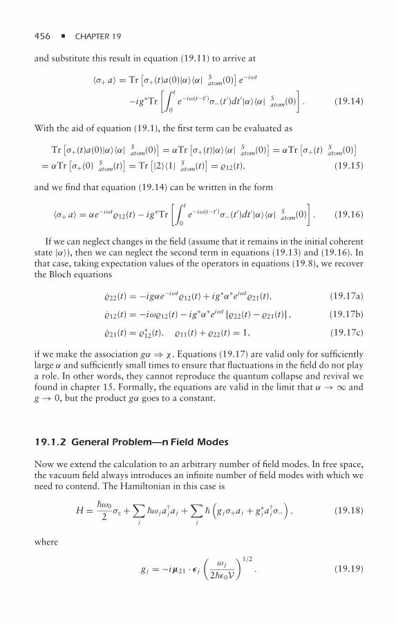
456 CHAPTER 19
and substitute this result in equation (19.11) to arrive at
〈σ+ a〉 = Tr[σ+(t)a(0)|α〉〈α|S
atom(0)]e−iωt
−ig∗Tr[∫ t
0e−iω(t−t′)σ−(t′)dt′|α〉〈α|S
atom(0)]. (19.14)
With the aid of equation (19.1), the first term can be evaluated as
Tr[σ+(t)a(0)|α〉〈α|S
atom(0)] = αTr
[σ+(t)|α〉〈α|S
atom(0)] = αTr
[σ+(t)S
atom(0)]
= αTr[σ+(0)S
atom(t)] = Tr
[|2〉〈1|Satom(t)
] = 12(t), (19.15)
and we find that equation (19.14) can be written in the form
〈σ+ a〉 = αe−iωt12(t) − ig∗Tr[∫ t
0e−iω(t−t′)σ−(t′)dt′|α〉〈α|S
atom(0)]. (19.16)
If we can neglect changes in the field (assume that it remains in the initial coherentstate |α〉), then we can neglect the second term in equations (19.13) and (19.16). Inthat case, taking expectation values of the operators in equations (19.8), we recoverthe Bloch equations
22(t) = −igαe−iωt12(t) + ig∗α∗eiωt21(t), (19.17a)
12(t) = −iω12(t) − ig∗α∗eiωt [22(t) − 21(t)] , (19.17b)
21(t) = ∗12(t), 11(t) + 22(t) = 1, (19.17c)
if we make the association gα ⇒ χ . Equations (19.17) are valid only for sufficientlylarge α and sufficiently small times to ensure that fluctuations in the field do not playa role. In other words, they cannot reproduce the quantum collapse and revival wefound in chapter 15. Formally, the equations are valid in the limit that α → ∞ andg → 0, but the product gα goes to a constant.
19.1.2 General Problem—n Field Modes
Now we extend the calculation to an arbitrary number of field modes. In free space,the vacuum field always introduces an infinite number of field modes with which weneed to contend. The Hamiltonian in this case is
H = ω0
2σz +
∑j
ω j a†j a j +
∑j
(g jσ+a j + g∗
j a†jσ−
), (19.18)
where
g j = −iµ21 · ε j
(ω j
2ε0V
)1/2
. (19.19)
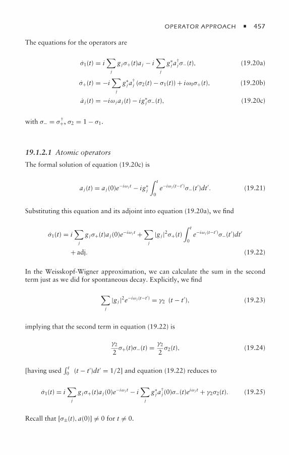
OPERATOR APPROACH 457
The equations for the operators are
σ1(t) = i∑j
g jσ+(t)a j − i∑j
g∗j a
†jσ−(t), (19.20a)
σ+(t) = −i∑j
g∗j a
†j (σ2(t) − σ1(t)) + iω0σ+(t), (19.20b)
a j (t) = −iω j a j (t) − ig∗jσ−(t), (19.20c)
with σ− = σ†+, σ2 = 1 − σ1.
19.1.2.1 Atomic operators
The formal solution of equation (19.20c) is
a j (t) = a j (0)e−iω j t − ig∗j
∫ t
0e−iω j (t−t′)σ−(t′)dt′. (19.21)
Substituting this equation and its adjoint into equation (19.20a), we find
σ1(t) = i∑j
g jσ+(t)a j (0)e−iω j t +∑j
|g j |2σ+(t)∫ t
0e−iω j (t−t′)σ−(t′)dt′
+ adj. (19.22)
In the Weisskopf-Wigner approximation, we can calculate the sum in the secondterm just as we did for spontaneous decay. Explicitly, we find
∑j
|g j |2e−iω j (t−t′) = γ2δ(t − t′), (19.23)
implying that the second term in equation (19.22) is
γ2
2σ+(t)σ−(t) = γ2
2σ2(t), (19.24)
[having used∫ t0 δ(t − t′)dt′ = 1/2] and equation (19.22) reduces to
σ1(t) = i∑j
g jσ+(t)a j (0)e−iω j t − i∑j
g∗j a
†j (0)σ−(t)eiω j t + γ2σ2(t). (19.25)
Recall that [σ±(t), a(0)] = 0 for t = 0.
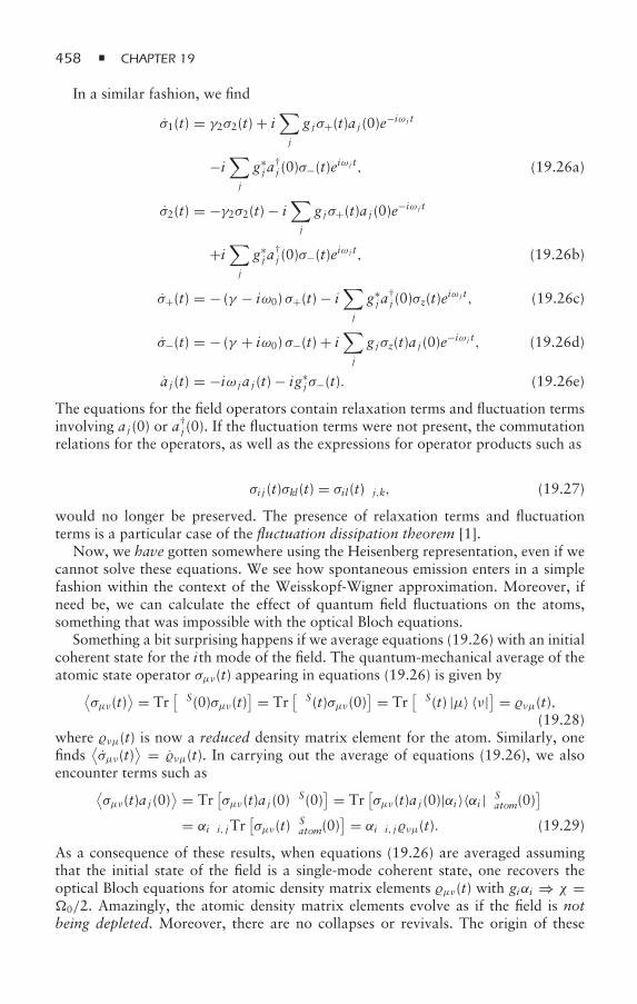
458 CHAPTER 19
In a similar fashion, we find
σ1(t) = γ2σ2(t) + i∑j
g jσ+(t)a j (0)e−iω j t
−i∑j
g∗j a
†j (0)σ−(t)eiω j t, (19.26a)
σ2(t) = −γ2σ2(t) − i∑j
g jσ+(t)a j (0)e−iω j t
+i∑j
g∗j a
†j (0)σ−(t)eiω j t, (19.26b)
σ+(t) = − (γ − iω0) σ+(t) − i∑j
g∗j a
†j (0)σz(t)e
iω j t, (19.26c)
σ−(t) = − (γ + iω0) σ−(t) + i∑j
g jσz(t)a j (0)e−iω j t, (19.26d)
a j (t) = −iω j a j (t) − ig∗jσ−(t). (19.26e)
The equations for the field operators contain relaxation terms and fluctuation termsinvolving a j (0) or a
†j (0). If the fluctuation terms were not present, the commutation
relations for the operators, as well as the expressions for operator products such as
σi j (t)σkl(t) = σil(t)δ j,k, (19.27)
would no longer be preserved. The presence of relaxation terms and fluctuationterms is a particular case of the fluctuation dissipation theorem [1].
Now, we have gotten somewhere using the Heisenberg representation, even if wecannot solve these equations. We see how spontaneous emission enters in a simplefashion within the context of the Weisskopf-Wigner approximation. Moreover, ifneed be, we can calculate the effect of quantum field fluctuations on the atoms,something that was impossible with the optical Bloch equations.
Something a bit surprising happens if we average equations (19.26) with an initialcoherent state for the ith mode of the field. The quantum-mechanical average of theatomic state operator σµν(t) appearing in equations (19.26) is given by⟨
σµν(t)⟩ = Tr
[S(0)σµν(t)
] = Tr[S(t)σµν(0)
] = Tr[S(t) |µ〉 〈ν|] = νµ(t),
(19.28)where νµ(t) is now a reduced density matrix element for the atom. Similarly, onefinds
⟨σµν(t)
⟩ = νµ(t). In carrying out the average of equations (19.26), we alsoencounter terms such as⟨
σµν(t)a j (0)⟩ = Tr
[σµν(t)a j (0)S(0)
] = Tr[σµν(t)a j (0)|αi 〉〈αi |S
atom(0)]
= αiδi, jTr[σµν(t)S
atom(0)] = αiδi, jνµ(t). (19.29)
As a consequence of these results, when equations (19.26) are averaged assumingthat the initial state of the field is a single-mode coherent state, one recovers theoptical Bloch equations for atomic density matrix elements µν(t) with giαi ⇒ χ =0/2. Amazingly, the atomic density matrix elements evolve as if the field is notbeing depleted. Moreover, there are no collapses or revivals. The origin of these
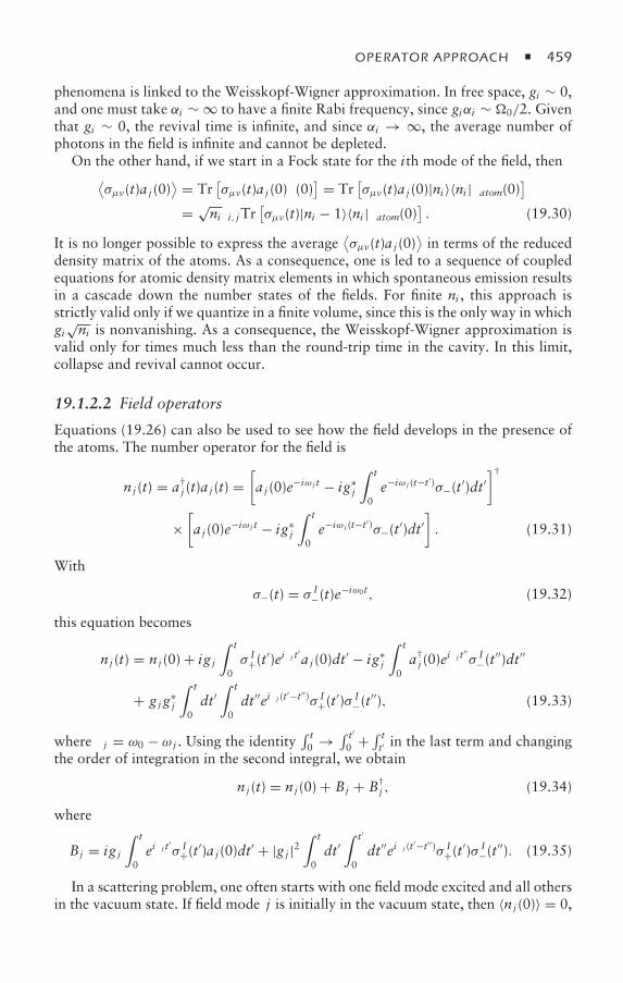
OPERATOR APPROACH 459
phenomena is linked to the Weisskopf-Wigner approximation. In free space, gi ∼ 0,and one must take αi ∼ ∞ to have a finite Rabi frequency, since giαi ∼ 0/2. Giventhat gi ∼ 0, the revival time is infinite, and since αi → ∞, the average number ofphotons in the field is infinite and cannot be depleted.
On the other hand, if we start in a Fock state for the ith mode of the field, then⟨σµν(t)a j (0)
⟩ = Tr[σµν(t)a j (0)(0)
] = Tr[σµν(t)a j (0)|ni 〉〈ni |atom(0)
]= √
niδi, jTr[σµν(t)|ni − 1〉〈ni |atom(0)
]. (19.30)
It is no longer possible to express the average⟨σµν(t)a j (0)
⟩in terms of the reduced
density matrix of the atoms. As a consequence, one is led to a sequence of coupledequations for atomic density matrix elements in which spontaneous emission resultsin a cascade down the number states of the fields. For finite ni , this approach isstrictly valid only if we quantize in a finite volume, since this is the only way in whichgi
√ni is nonvanishing. As a consequence, the Weisskopf-Wigner approximation is
valid only for times much less than the round-trip time in the cavity. In this limit,collapse and revival cannot occur.
19.1.2.2 Field operators
Equations (19.26) can also be used to see how the field develops in the presence ofthe atoms. The number operator for the field is
nj (t) = a†j (t)a j (t) =
[a j (0)e−iω j t − ig∗
j
∫ t
0e−iω j (t−t′)σ−(t′)dt′
]†
×[a j (0)e−iω j t − ig∗
j
∫ t
0e−iω j (t−t′)σ−(t′)dt′
]. (19.31)
With
σ−(t) = σ I−(t)e
−iω0t, (19.32)
this equation becomes
nj (t) = nj (0) + ig j
∫ t
0σ I
+(t′)eiδ j t
′a j (0)dt′ − ig∗
j
∫ t
0a†j (0)e
iδ j t′′σ I−(t
′′)dt′′
+ g j g∗j
∫ t
0dt′
∫ t
0dt′′eiδ j (t
′−t′′)σ I+(t
′)σ I−(t
′′), (19.33)
where δ j = ω0 − ω j . Using the identity∫ t0 → ∫ t′
0 + ∫ tt′ in the last term and changing
the order of integration in the second integral, we obtain
nj (t) = nj (0) + Bj + B†j , (19.34)
where
Bj = ig j
∫ t
0eiδ j t
′σ I
+(t′)a j (0)dt′ + |g j |2
∫ t
0dt′
∫ t′
0dt′′eiδ j (t
′−t′′)σ I+(t
′)σ I−(t
′′). (19.35)
In a scattering problem, one often starts with one field mode excited and all othersin the vacuum state. If field mode j is initially in the vacuum state, then 〈nj (0)〉 = 0,
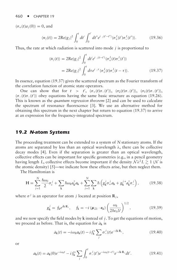
460 CHAPTER 19
〈σ+(t)a j (0)〉 = 0, and
〈nj (t)〉 = 2Re|g j |2∫ t
0dt′
∫ t′
0dt′′eiδ j (t
′−t′′)〈σ I+(t
′)σ I−(t
′′)〉. (19.36)
Thus, the rate at which radiation is scattered into mode j is proportional to
〈n j (t)〉 = 2Re|g j |2∫ t
0dt′eiδ j (t−t
′)〈σ I+(t)σ
I−(t
′)〉
= 2Re|g j |2∫ t
0dτeiδ j τ 〈σ I
+(t)σI−(t − τ )〉. (19.37)
In essence, equation (19.37) gives the scattered spectrum as the Fourier transform ofthe correlation function of atomic state operators.
One can show that for t > t′, 〈σ+(t)σ−(t′)〉, 〈σ2(t)σ−(t′)〉, 〈σ1(t)σ−(t′)〉,〈σ−(t)σ−(t′)〉 obey equations having the same basic structure as equation (19.26).This is known as the quantum regression theorem [2] and can be used to calculatethe spectrum of resonance fluorescence [3]. We use an alternative method forobtaining this spectrum in the next chapter but return to equation (19.37) to arriveat an expression for the frequency-integrated spectrum.
19.2 N-atom Systems
The proceeding treatment can be extended to a system of N stationary atoms. If theatoms are separated by less than an optical wavelength λ, there can be collectivedecay modes [4]. Even if the separation is greater than an optical wavelength,collective effects can be important for specific geometries (e.g., in a pencil geometryhaving length L, collective effects become important if the density Nλ2L 1 (N isthe atomic density) [5]—we indicate how these effects arise, but then neglect them.
The Hamiltonian is
H =N∑j=1
ω0
2σ jz +
∑k
ωka†kak +
N∑j=1
∑k
(g jkσ
j+ak + g j ∗k a†
kσj
−), (19.38)
where σ j is an operator for atom j located at position R j ,
g jk = fkeik·R j , fk = −i (µ21 · εk)(
ωk
2ε0V
)1/2
, (19.39)
and we now specify the field modes by k instead of j . To get the equations of motion,we proceed as before. That is, the equation for ak is
ak(t) = −iωkak(t) − i f ∗k
∑j
σj
−(t)e−ik·R j , (19.40)
or
ak(t) = ak(0)e−iωkt − i f ∗k
∑j
∫ t
0σj
−(t′)e−iωk(t−t′)e−ik·R j dt′. (19.41)
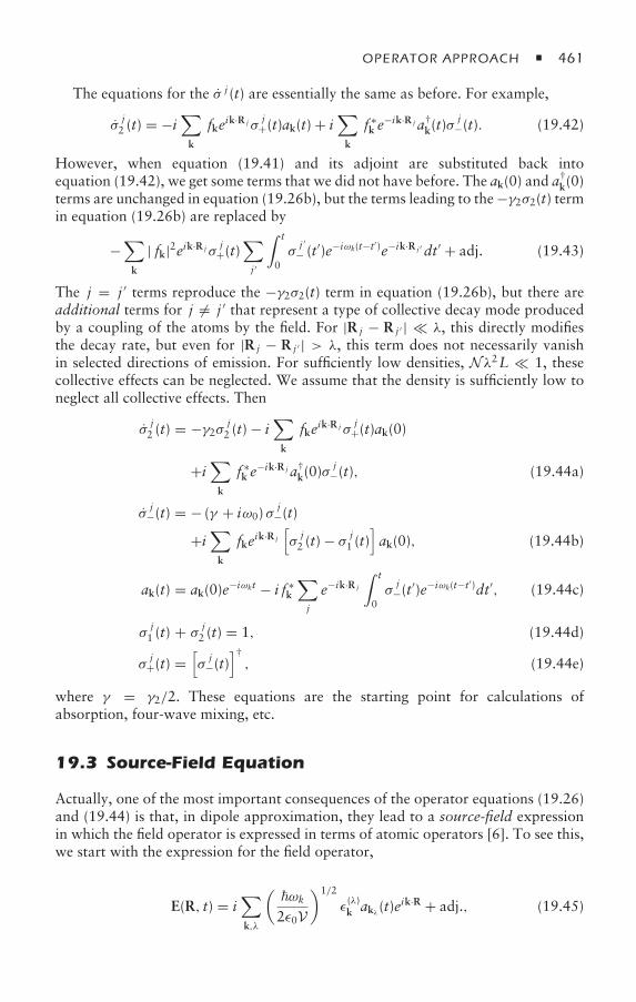
OPERATOR APPROACH 461
The equations for the σ j (t) are essentially the same as before. For example,
σj2 (t) = −i
∑k
fkeik·R jσj
+(t)ak(t) + i∑k
f ∗k e
−ik·R j a†k(t)σ
j−(t). (19.42)
However, when equation (19.41) and its adjoint are substituted back intoequation (19.42), we get some terms that we did not have before. The ak(0) and a
†k(0)
terms are unchanged in equation (19.26b), but the terms leading to the−γ2σ2(t) termin equation (19.26b) are replaced by
−∑k
| fk|2eik·R jσj
+(t)∑j ′
∫ t
0σj ′
− (t′)e−iωk(t−t′)e−ik·R j ′dt′ + adj. (19.43)
The j = j ′ terms reproduce the −γ2σ2(t) term in equation (19.26b), but there areadditional terms for j = j ′ that represent a type of collective decay mode producedby a coupling of the atoms by the field. For |R j − R j ′ | λ, this directly modifiesthe decay rate, but even for |R j − R j ′ | > λ, this term does not necessarily vanishin selected directions of emission. For sufficiently low densities, Nλ2L 1, thesecollective effects can be neglected. We assume that the density is sufficiently low toneglect all collective effects. Then
σj2 (t) = −γ2σ j
2 (t) − i∑k
fkeik·R jσj
+(t)ak(0)
+i∑k
f ∗k e
−ik·R j a†k(0)σ
j−(t), (19.44a)
σj
−(t) = − (γ + iω0) σj
−(t)
+i∑k
fkeik·R j
[σj2 (t) − σ j
1 (t)]ak(0), (19.44b)
ak(t) = ak(0)e−iωkt − i f ∗k
∑j
e−ik·R j
∫ t
0σj
−(t′)e−iωk(t−t′)dt′, (19.44c)
σj1 (t) + σ
j2 (t) = 1, (19.44d)
σj
+(t) =[σj
−(t)]†, (19.44e)
where γ = γ2/2. These equations are the starting point for calculations ofabsorption, four-wave mixing, etc.
19.3 Source-Field Equation
Actually, one of the most important consequences of the operator equations (19.26)and (19.44) is that, in dipole approximation, they lead to a source-field expressionin which the field operator is expressed in terms of atomic operators [6]. To see this,we start with the expression for the field operator,
E(R, t) = i∑k,λ
(ωk
2ε0V
)1/2
ε(λ)k akλ (t)e
ik·R + adj., (19.45)
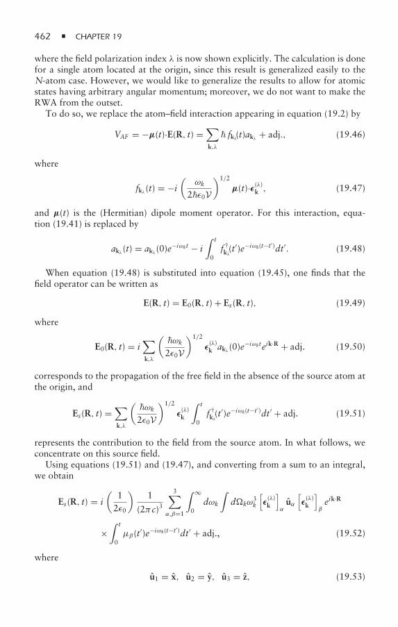
462 CHAPTER 19
where the field polarization index λ is now shown explicitly. The calculation is donefor a single atom located at the origin, since this result is generalized easily to theN-atom case. However, we would like to generalize the results to allow for atomicstates having arbitrary angular momentum; moreover, we do not want to make theRWA from the outset.
To do so, we replace the atom–field interaction appearing in equation (19.2) by
VAF = −µ(t)·E(R, t) =∑k,λ
fkλ(t)akλ + adj., (19.46)
where
fkλ (t) = −i(
ωk
2ε0V
)1/2
µ(t)·ε(λ)k , (19.47)
and µ(t) is the (Hermitian) dipole moment operator. For this interaction, equa-tion (19.41) is replaced by
akλ(t) = akλ (0)e−iωkt − i
∫ t
0f †kλ(t′)e−iωk(t−t′)dt′. (19.48)
When equation (19.48) is substituted into equation (19.45), one finds that thefield operator can be written as
E(R, t) = E0(R, t) + Es(R, t), (19.49)
where
E0(R, t) = i∑k,λ
(ωk
2ε0V
)1/2
ε(λ)k akλ (0)e
−iωkteik·R + adj. (19.50)
corresponds to the propagation of the free field in the absence of the source atom atthe origin, and
Es(R, t) =∑k,λ
(ωk
2ε0V
)1/2
ε(λ)k
∫ t
0f †kλ(t′)e−iωk(t−t′)dt′ + adj. (19.51)
represents the contribution to the field from the source atom. In what follows, weconcentrate on this source field.
Using equations (19.51) and (19.47), and converting from a sum to an integral,we obtain
Es(R, t) = i(
12ε0
)1
(2πc)3
3∑α,β=1
∫ ∞
0dωk
∫dkω
3k
[ε(λ)k
]αuα
[ε(λ)k
]βeik·R
×∫ t
0µβ(t′)e−iωk(t−t′)dt′ + adj., (19.52)
where
u1 = x, u2 = y, u3 = z, (19.53)
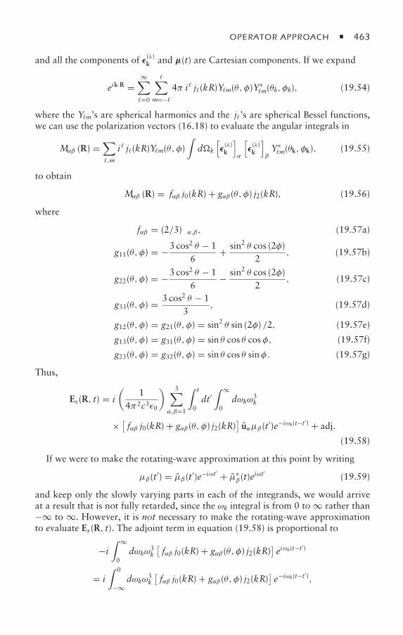
OPERATOR APPROACH 463
and all the components of ε(λ)k and µ(t) are Cartesian components. If we expand
eik·R =∞∑=0
∑m=−
4π i j(kR)Ym(θ, φ)Y∗m(θk, φk), (19.54)
where the Ym’s are spherical harmonics and the j’s are spherical Bessel functions,we can use the polarization vectors (16.18) to evaluate the angular integrals in
Mαβ (R) =∑,m
i j(kR)Ym(θ, φ)∫dk
[ε(λ)k
]α
[ε(λ)k
]βY∗m(θk, φk), (19.55)
to obtain
Mαβ (R) = fαβ j0(kR) + gαβ(θ, φ) j2(kR), (19.56)
where
fαβ = (2/3) δα,β, (19.57a)
g11(θ, φ) = −3 cos2 θ − 16
+ sin2 θ cos (2φ)2
, (19.57b)
g22(θ, φ) = −3 cos2 θ − 16
− sin2 θ cos (2φ)2
, (19.57c)
g33(θ, φ) = 3 cos2 θ − 13
, (19.57d)
g12(θ, φ) = g21(θ, φ) = sin2 θ sin (2φ) /2, (19.57e)
g13(θ, φ) = g31(θ, φ) = sin θ cos θ cosφ, (19.57f)
g23(θ, φ) = g32(θ, φ) = sin θ cos θ sinφ. (19.57g)
Thus,
Es(R, t) = i(
14π2c3ε0
) 3∑α,β=1
∫ t
0dt′
∫ ∞
0dωkω3
k
× [fαβ j0(kR) + gαβ(θ, φ) j2(kR)
]uαµβ(t′)e−iωk(t−t′) + adj.
(19.58)
If we were to make the rotating-wave approximation at this point by writing
µβ(t′) = µβ(t′)e−iωt′ + µ∗β(t)e
iωt′ (19.59)
and keep only the slowly varying parts in each of the integrands, we would arriveat a result that is not fully retarded, since the ωk integral is from 0 to ∞ rather than−∞ to ∞. However, it is not necessary to make the rotating-wave approximationto evaluate Es(R, t). The adjoint term in equation (19.58) is proportional to
−i∫ ∞
0dωkω3
k
[fαβ j0(kR) + gαβ(θ, φ) j2(kR)
]eiωk(t−t
′)
= i∫ 0
−∞dωkω3
k
[fαβ j0(kR) + gαβ(θ, φ) j2(kR)
]e−iωk(t−t′),
464 CHAPTER 19
which implies that
Es(R, t) = i(
14π2c3ε0
) 3∑α,β=1
∫ t
0dt′
∫ ∞
−∞dωkω3
k
× [fαβ j0(kR) + gαβ(θ, φ) j2(kR)
]uαµβ(t′)e−iωk(t−t′). (19.60)
To proceed, we write
j(x) = h(1) (x) + h(2) (x)2
= c(x)eix + d(x)e−ix
2, (19.61)
where the h’s are spherical Hankel functions, and c0 and c2 are given by [7]
c0(x) = − ix, c2(x) = i
x− 3x2
− 3ix3, (19.62)
substitute this result into equation (19.60), and use the fact that ωnke−iωk(t−t′) =
indn[e−iωk(t−t′)] /dtn. The integration over ωk leads to delta functions having
argument (t′ − t + R/c) for the c terms and (t′ − t − R/c) for the d terms. Sincet′ ≤ t, only the c terms are nonvanishing. In this manner, we can obtain
Es(R, t) =(
14πε0
) 3∑α,β=1
uα
− fαβ − gαβ(θ, φ)
c2Rµβ(t − R/c)
+ gαβ(θ, φ)[
3cR2
µβ(t − R/c)+ 3R3µβ(t − R/c)
]. (19.63)
In dipole approximation, the quantum properties of the field are determinedtotally by the quantum properties of the atom, evaluated at the retarded time. Theresult is purely retarded and has the same form as the field radiated by a classicaldipole [8]. The Weisskopf-Wigner approximation was not needed for its derivation.This is a fairly remarkable result, and one that is not used all that often. Theadvantage of using Heisenberg operators is evident since the quantum field mirrorsthat of the corresponding classical field. The extension to a system of N atoms is
Es(R, t) =(
14πε0
) 3∑α,β=1
N∑j=1
uα
− fαβ − gαβ(θ j , φ j )
c2Rµ( j)β (t − ∣∣R − R j
∣∣ /c)
+ gαβ(θ j , φ j )
[3cR2 µ
( j)β (t − ∣∣R − R j
∣∣ /c)+ 3
R3µ( j)β (t − ∣∣R − R j
∣∣ /c)]
, (19.64)
where (θ j , φ j ) are angles measured from atom j to the observation point.We want to emphasize that equation (19.64) is exact, in dipole approximation.
Neither the Weisskopf-Wigner nor the RWA has been used in its derivation. Foroptical fields driving atomic transitions, some simplifications are possible. If weassume that the source atoms have a G–H transition that provides the majorcontribution to the field, then
µ( j)β (t) =
∑mG,mH
〈GmG|µβ |HmH〉 σ ( j)− (GmG,HmH; t) + adj., (19.65)
OPERATOR APPROACH 465
where G and H are the angular momenta of the lower- and upper-state manifolds,respectively, and σ− (GmG,HmH; 0) = |GmG〉 〈HmH| is a lowering operator. Inthe RWA, σ ( j)
− (GmG,HmH; t) oscillates as e−iωs t, where ωs is some characteristicfrequency (natural frequency, laser field frequency, etc.) in the problem that is muchlarger than any decay rates, detunings, or Rabi frequencies. With these assumptions,in the RWA, the positive frequency component of the field (19.64) can be written as
E+s (R, t) =
(1
4πε0
) ∑mG,mH
3∑α,β=1
N∑j=1
〈GmG|µβ |HmH〉 uα
×ω2s
[fαβ − gαβ(θ j , φ j )
]c2R
+ gαβ(θ j , φ j )(
−3iωscR2
+ 3R3
)
×σ ( j)−
(GmG,HmH; t − ∣∣R − R j
∣∣ /c) . (19.66)
In what follows, we will limit our discussion to the radiation zone, where
(θ j , φ j ) ≈ (θ, φ) (19.67)
for a sample of finite size. Physically, this implies that we make observations so farfrom the sample that the angle to the observation point from any point in the sampleis essentially the same. In the radiation zone, equation (19.66) reduces to
E+s (R, t) =
(ω2s
4πε0
) ∑mG,mH
3∑α,β=1
N∑j=1
〈GmG|µβ |HmH〉
× fαβ − gαβ(θ, φ)c2R
uασ( j)−
(GmG,HmH; t − ∣∣R − R j
∣∣ /c) .(19.68)
To see that this equation reduces to something familiar, imagine that G = 0,H = 1, and the field polarizations are such that only σ ( j)
− (00,10; t) ≡ σ( j)− (t) is
of importance for the problem. Making use of equations (19.57) and (16.18b),we find that equation (19.68) can be written as
E+s (R, t) = −
(ω2s
4πε0c2R
)µ12 sin θ
N∑j=1
σ( j)− (t − ∣∣R − R j
∣∣ /c)θ , (19.69)
with
µ12 ≡ 〈00|µz |10〉 . (19.70)
This equation is recognized as the radiation field associated with dipoles oscillatingin the z direction.
19.4 Source-Field Approach: Examples
The source-field approach is versatile and simple, as is illustrated in the followingexamples.
466 CHAPTER 19
19.4.1 Average Field and Field Intensity in Spontaneous Emission
We calculated the spectrum and angular distribution of radiation emitted inspontaneous emission in chapter 16. Here, we are interested primarily in thetemporal dependence of the emitted signal from a single atom located at the origin.We assume that the atom is prepared at t = 0 into some arbitrary superposition ofZeeman sublevels mH in excited level H and undergoes spontaneous emission to thesublevels mG in level G.
From equation (19.68), we see that the average field amplitude⟨E+s (R, t)
⟩depends on 〈σ−(GmG,HmH; t − R/c)〉. Using equation (19.26d), generalized toinclude magnetic state sublevels, we find that
〈σ− (GmG,HmH; t)〉 = 〈σ− (GmG,HmH; 0)〉 e−γHt/2(t)
= Tr[S(0) |GmG〉 〈HmH|] e−γHt/2(t) = 0,
(19.71)
where (t) is the Heaviside step function. The trace vanishes, since
S(0) = HmH,Hm′H(0) |HmH〉 ⟨Hm′
H
∣∣ . (19.72)
If the atom is prepared without any ground-state–excited-state coherence, theaverage field vanishes, since the phase of the field is random.
On the other hand, the average field intensity, given by⟨E−(R, t) · E+(R, t)
⟩, is
nonvanishing. In the RWA, the positive frequency component of the field in theradiation zone is
E+s (R, t) ≈
(ω20
4πε0
) 3∑α,β=1
fαβ − gαβ(θ, φ)c2R
×∑
mG,mH
〈GmG|µβ |HmH〉
×σ− (GmG,HmH; t − R/c) uα. (19.73)
Using equation (19.68), with ωs = ω0 = ωHG, the fact that uα · uα′ = δα,α′ and[σ−
(Gm′
G,Hm′H; t
)]†σ− (GmG,HmH; t)
= ∣∣Hm′H
⟩ 〈HmH| δmG,m′Ge−γHt(t), (19.74)
we find ⟨E−(R, t) · E+(R, t)
⟩=(
ω20
4πε0c2R
)2
e−γH(t−R/c)(t − R/c)∑α,β,β ′
(fαβ − gαβ
) (fαβ ′ − gαβ ′
)
×∑
mG,mH,mH′
〈GmG|µβ |HmH〉∗ 〈GmG|µβ ′∣∣Hm′
H
⟩HmH;Hm′
H(0).
(19.75)
OPERATOR APPROACH 467
This is the intensity associated with the one-photon wave packet emitted by theatom. The wave front is located a distance ct from the atom, and the pulse durationis of order γ−1
H . The angular distribution and polarization of the emitted radiationdepends on the state preparation through the factor HmH;Hm′
H(0). Specific examples
are left to the problems.Equation (19.75) contains an interesting and even perplexing result. Nowhere
in its derivation did we make any assumption regarding the ground-state–excited-state coherence produced by the excitation field. In other words, imagine that theatom is excited with a π/2 pulse. As a result of the excitation, both dipole (ground–excited state) and excited-state Zeeman coherence is produced. In this case, theaverage field emitted by the atom does not vanish; however, the radiated intensitydepends in no direct way on the dipole coherence. The average intensity dependsonly on the excited-state density matrix elements created by the field. You mightthink that the spectrum of the radiation would provide a signature of the dipolecoherence, but alas, this is not the case. Recall that the spectrum is proportionalto
∑mG
|bGmG;kεk(∞)|2, the probability to find the atom in its ground state with a
photon emitted in direction k having polarization εk. You have seen in chapter 16that this quantity depends only on excited-state density matrix elements. Thus, weare led to a somewhat paradoxical conclusion that the field intensity radiated by asingle atom that has been prepared by an excitation pulse depends in no direct wayon its dipole coherence. To prove that the dipole coherence is nonvanishing, one caninterfere the radiated signal with a reference field. A nonvanishing dipole coherencebecomes much more important when we consider the field emitted bymore than oneatom. A simple example to illustrate this is given in the problems, and an exampleinvolving coherent transients is given in section 19.4.3.
19.4.2 Frequency Beats in Emission: Quantum Beats
As a second example involving emission from a single atom, we consider frequencybeats in emission [9]. Qualitatively, it is usually possible to distinguish two typesof situations in which beats occur. The first corresponds to a beat frequency inthe intensity radiated by two classical dipoles having different natural frequencies.This could be referred to as “classical” beats. However, as you saw earlier, dipolecoherence can play no role in the intensity radiated by a single atom. Thus, evenif a single atom is excited into a superposition of states giving rise to a dipolecoherence that oscillates at two distinct frequencies, there can be no classical beatsin the emitted intensity. One could detect the presence of the two field frequenciesby heterodyning (beating) the radiated field with a reference field.
Thus, any beat in the field radiated by a single atom that has been preparedby an excitation pulse must originate from excited-state coherence between twoexcited-state manifolds differing in frequency (or between Zeeman sublevels in asingle manifold that have been split in energy by an external magnetic field). Theresultant quantum beats are a purely quantum phenomena.
The calculation given earlier for the field intensity in spontaneous emission isgeneralized easily to the case of two excited-state manifolds H and H′, separated infrequency by ωHH′ . One simply replaces∑
mG,mH,mH′
〈GmG|µβ |HmH〉∗ 〈GmG|µβ ′∣∣Hm′
H
⟩HmH;Hm′
H(0)
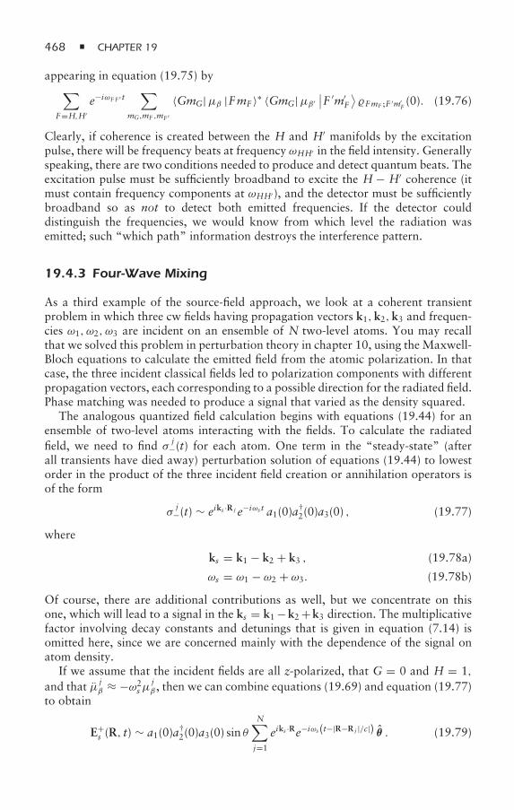
468 CHAPTER 19
appearing in equation (19.75) by∑F=H,H′
e−iωF F ′ t∑
mG,mF ,mF ′
〈GmG|µβ |FmF 〉∗ 〈GmG|µβ ′∣∣F ′m′
F
⟩FmF ;F ′m′
F(0). (19.76)
Clearly, if coherence is created between the H and H′ manifolds by the excitationpulse, there will be frequency beats at frequency ωHH′ in the field intensity. Generallyspeaking, there are two conditions needed to produce and detect quantum beats. Theexcitation pulse must be sufficiently broadband to excite the H − H′ coherence (itmust contain frequency components at ωHH′), and the detector must be sufficientlybroadband so as not to detect both emitted frequencies. If the detector coulddistinguish the frequencies, we would know from which level the radiation wasemitted; such “which path” information destroys the interference pattern.
19.4.3 Four-Wave Mixing
As a third example of the source-field approach, we look at a coherent transientproblem in which three cw fields having propagation vectors k1,k2,k3 and frequen-cies ω1, ω2, ω3 are incident on an ensemble of N two-level atoms. You may recallthat we solved this problem in perturbation theory in chapter 10, using the Maxwell-Bloch equations to calculate the emitted field from the atomic polarization. In thatcase, the three incident classical fields led to polarization components with differentpropagation vectors, each corresponding to a possible direction for the radiated field.Phase matching was needed to produce a signal that varied as the density squared.
The analogous quantized field calculation begins with equations (19.44) for anensemble of two-level atoms interacting with the fields. To calculate the radiatedfield, we need to find σ j
−(t) for each atom. One term in the “steady-state” (afterall transients have died away) perturbation solution of equations (19.44) to lowestorder in the product of the three incident field creation or annihilation operators isof the form
σj
−(t) ∼ eiks ·R j e−iωs t a1(0)a†2(0)a3(0) , (19.77)
where
ks = k1 − k2 + k3 , (19.78a)
ωs = ω1 − ω2 + ω3. (19.78b)
Of course, there are additional contributions as well, but we concentrate on thisone, which will lead to a signal in the ks = k1 −k2 +k3 direction. The multiplicativefactor involving decay constants and detunings that is given in equation (7.14) isomitted here, since we are concerned mainly with the dependence of the signal onatom density.
If we assume that the incident fields are all z-polarized, that G = 0 and H = 1,and that µ j
β ≈ −ω2sµ
jβ , then we can combine equations (19.69) and equation (19.77)
to obtain
E+s (R, t) ∼ a1(0)a
†2(0)a3(0) sin θ
N∑j=1
eiks ·Re−iωs(t−|R−R j |/c|) θ . (19.79)
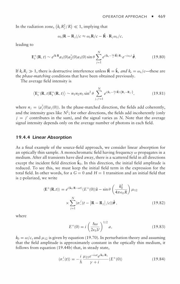
OPERATOR APPROACH 469
In the radiation zone,(ks R2
j /R) 1, implying that
ωs |R − R j |/c ≈ ωsR/c − R · R jωs/c,
leading to
E+s (R, t) ∼ eik·Ra1(0)a
†2(0)a3(0) sin θ
N∑j=1
ei(ks−ωsc R)·R j e−iωs t θ . (19.80)
If ks Rj 1, there is destructive interference unless R = ks and ks = ωs/c—these arethe phase-matching conditions that have been obtained previously.
The average field intensity is
⟨E−s (R, t)E
+s (R, t)
⟩ ∼ n1n2n3 sin2 θ
N∑j, j ′=1
ei(ks−ωsc R)·(R j−R j ′ ), (19.81)
where nj = 〈a†j (0)a j (0)〉. In the phase-matched direction, the fields add coherently,
and the intensity goes like N2; for other directions, the fields add incoherently (onlyj = j ′ contributes in the sum), and the signal varies as N. Note that the averagesignal intensity depends only on the average number of photons in each field.
19.4.4 Linear Absorption
As a final example of the source-field approach, we consider linear absorption foran optically thin sample. A monochromatic field having frequency ω propagates in amedium. After all transients have died away, there is a scattered field in all directionsexcept the incident field direction k0. In this direction, the initial field amplitude isreduced. To see this, we must keep the initial field term in the expression for thetotal field. In other words, for a G= 0 and H = 1 transition and an initial field thatis z-polarized, we write
〈E+(R,t)〉 = ei(k0·R−ωt)〈E+(0)〉z − sin θ(
k204πε0R
)µ12
×N∑j=1
〈σ j−(t − ∣∣R − R j
∣∣ /c)〉θ , (19.82)
where
E+(0) = i(ω
2ε0V
)1/2
a, (19.83)
k0 = ω/c, and µ12 is given by equation (19.70). In perturbation theory and assumingthat the field amplitude is approximately constant in the optically thin medium, itfollows from equation (19.44b) that, in steady state,
〈σ j−(t)〉 = − i
µ21e−iωteik0·R j
γ + iδ〈E+(0)〉 (19.84)
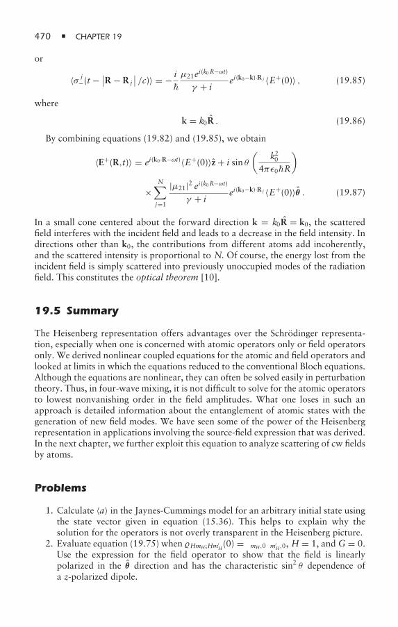
470 CHAPTER 19
or
〈σ j−(t − ∣∣R − R j
∣∣ /c)〉 = − i
µ21ei(k0R−ωt)
γ + iδei(k0−k)·R j 〈E+(0)〉 , (19.85)
where
k = k0R . (19.86)
By combining equations (19.82) and (19.85), we obtain
〈E+(R,t)〉 = ei(k0·R−ωt)〈E+(0)〉z + i sin θ(
k204πε0R
)
×N∑j=1
|µ21|2 ei(k0R−ωt)
γ + iδei(k0−k)·R j 〈E+(0)〉θ . (19.87)
In a small cone centered about the forward direction k = k0R = k0, the scatteredfield interferes with the incident field and leads to a decrease in the field intensity. Indirections other than k0, the contributions from different atoms add incoherently,and the scattered intensity is proportional to N. Of course, the energy lost from theincident field is simply scattered into previously unoccupied modes of the radiationfield. This constitutes the optical theorem [10].
19.5 Summary
The Heisenberg representation offers advantages over the Schrödinger representa-tion, especially when one is concerned with atomic operators only or field operatorsonly. We derived nonlinear coupled equations for the atomic and field operators andlooked at limits in which the equations reduced to the conventional Bloch equations.Although the equations are nonlinear, they can often be solved easily in perturbationtheory. Thus, in four-wave mixing, it is not difficult to solve for the atomic operatorsto lowest nonvanishing order in the field amplitudes. What one loses in such anapproach is detailed information about the entanglement of atomic states with thegeneration of new field modes. We have seen some of the power of the Heisenbergrepresentation in applications involving the source-field expression that was derived.In the next chapter, we further exploit this equation to analyze scattering of cw fieldsby atoms.
Problems
1. Calculate 〈a〉 in the Jaynes-Cummings model for an arbitrary initial state usingthe state vector given in equation (15.36). This helps to explain why thesolution for the operators is not overly transparent in the Heisenberg picture.
2. Evaluate equation (19.75) when HmH;Hm′H(0) = δmH,0δm′
H,0, H = 1, andG = 0.Use the expression for the field operator to show that the field is linearlypolarized in the θ direction and has the characteristic sin2 θ dependence ofa z-polarized dipole.
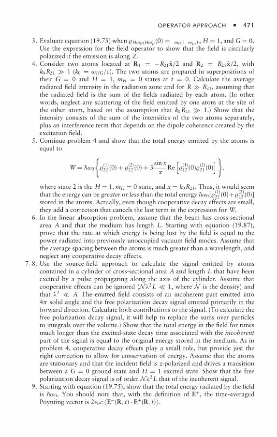
OPERATOR APPROACH 471
3. Evaluate equation (19.75) when HmH;Hm′H(0) = δmH,1δm′
H,1, H = 1, andG= 0.Use the expression for the field operator to show that the field is circularlypolarized if the emission is along Z.
4. Consider two atoms located at R1 = −R21x/2 and R2 = R21x/2, withk0R21 1 (k0 = ωHG/c). The two atoms are prepared in superpositions oftheir G = 0 and H = 1, mH = 0 states at t = 0. Calculate the averageradiated field intensity in the radiation zone and for R R21, assuming thatthe radiated field is the sum of the fields radiated by each atom. (In otherwords, neglect any scattering of the field emitted by one atom at the site ofthe other atom, based on the assumption that k0R21 1.) Show that theintensity consists of the sum of the intensities of the two atoms separately,plus an interference term that depends on the dipole coherence created by theexcitation field.
5. Continue problem 4 and show that the total energy emitted by the atoms isequal to
W = ω0
(1)22 (0) + (2)22 (0) + 3
sin xx
Re[(1)12 (0)
(2)21 (0)
],
where state 2 is the H = 1,mH = 0 state, and x = k0R21. Thus, it would seemthat the energy can be greater or less than the total energy ω0[
(1)22 (0)+(2)22 (0)]
stored in the atoms. Actually, even though cooperative decay effects are small,they add a correction that cancels the last term in the expression for W.
6. In the linear absorption problem, assume that the beam has cross-sectionalarea A and that the medium has length L. Starting with equation (19.87),prove that the rate at which energy is being lost by the field is equal to thepower radiated into previously unoccupied vacuum field modes. Assume thatthe average spacing between the atoms is much greater than a wavelength, andneglect any cooperative decay effects.
7–8. Use the source-field approach to calculate the signal emitted by atomscontained in a cylinder of cross-sectional area A and length L that have beenexcited by a pulse propagating along the axis of the cylinder. Assume thatcooperative effects can be ignored (Nλ2L 1, where N is the density) andthat λ2 A. The emitted field consists of an incoherent part emitted into4π solid angle and the free polarization decay signal emitted primarily in theforward direction. Calculate both contributions to the signal. (To calculate thefree polarization decay signal, it will help to replace the sums over particlesto integrals over the volume.) Show that the total energy in the field for timesmuch longer than the excited-state decay time associated with the incoherentpart of the signal is equal to the original energy stored in the medium. As inproblem 4, cooperative decay effects play a small role, but provide just theright correction to allow for conservation of energy. Assume that the atomsare stationary and that the incident field is z-polarized and drives a transitionbetween a G = 0 ground state and H = 1 excited state. Show that the freepolarization decay signal is of order Nλ2L that of the incoherent signal.
9. Starting with equation (19.75), show that the total energy radiated by the fieldis ω0. You should note that, with the definition of E+, the time-averagedPoynting vector is 2ε0c
⟨E−(R, t) · E+(R, t)
⟩.

472 CHAPTER 19
References
[1] H.B. Callen and T.A. Welton, Irreversibility and generalized noise, Physical Review 83,34–40 (1951).
[2] M. Lax,Quantum noise. XI. Multitime correspondence between quantum and classicalstochastic processes, Physical Review 172, 350–361 (1968).
[3] C. Cohen-Tannoudji, Atoms in strong resonant fields, in Frontiers in Laser Spec-troscopy, Les Houches, Session XXVII, vol. 1, edited by R. Balian, S. Haroche, andS. Liberman, (North Holland, Amsterdam, 1975) pp. 88–98; C. Cohen-Tannoudji, J.Dupont-Roc, and G. Grynberg, Atom-Photon Interactions (Wiley-Interscience, NewYork, 1992), complement AV.
[4] R.H. Dicke, Coherence in spontaneous radiation processes, Physical Review 93, 99–110 (1954).
[5] D. Polder, M.F.H. Schuurmans, and Q.H.F. Vrehen, Superfluorescence: quantum-mechanical derivation of Maxwell-Bloch description with fluctuating field source,Physical Review A 19, 1192–1203 (1979).
[6] R. Loudon, The Quantum Theory of Light, 3rd ed., (Oxford University Press, Oxford,UK, 2003), sec. 7.8, and references therein.
[7] M. Abramowitz and I.A. Stegun,Handbook of Mathematical Functions with Formulas,Graphs, and Mathematical Tables (U.S. Department of Commerce, Washington, DC,1965), chap. 10.
[8] J.D. Jackson, Classical Electrodynamics, 3rd ed., (Wiley, New York, 1999) sec. 9.2.[9] A. Corney and G.W. Series, Theory of resonance fluorescence excited by modulated
or pulsed light, Proceedings of the Physical Society 83, 207–216 (1964); S. Haroche,J.A. Paisner, and A.L. Schawlow,Hyperfine quantum beats observed in Cs vapor underpulsed dye laser excitation, Physical Review Letters 30, 948–951 (1973).
[10] See, for example, R. Newton, Scattering Theory of Waves and Particles, 2nd ed.(Springer-Verlag, New York, 1982; Dover, New York, 2002), sec. 1.3.9.
Bibliography
For an excellent review of the Heisenberg approach to atom-field dynamics, see
P. Milonni, Semiclassical and quantum electrodynamical approaches in nonrelativistic radia-tion theory, Physics Reports 25, 1–81 (1976), and references therein. Milonni is a strongproponent of the use of the Heisenberg equations of motion.
Some early papers on superradiance are listed here:C.M. Bowden and D.W. Howgate, Eds., Cooperative Effects in Matter and Radiation
(Plenum Press, New York, 1977).R. Friedberg and S.R. Hartmann, Frequency shifts in emission and absorption by resonantsystems of two-level atoms, Physics Reports 7, 101–179 (1973).
I.P. Herman, J.C. MacGillivray, N. Skribanowitz, and M.S. Feld, Self-induced emission inoptically pumped HF gas: the rise and fall of the superradiant state, in Laser Spectrocopy,edited by R. G. Brewer and A. Mooradian (Plenum Press, New York, 1974), 379–412.
N.E. Rehler and J.H. Eberly, Superradiance, Physical Review A 3, 1735–1751 (1979).

OPERATOR APPROACH 473
In addition to the quantum optics texts listed in chapter 1, some additional references fornoise properties of the field are:
H. Haken, Laser Theory (Springer-Verlag, Berlin, 1984).M. Lax, Fluctuation and coherence phenomena in Classical and Quantum Physics, BrandeisUniversity Summer Institute in Theoretical Physics, 1966, Statistical Physics, PhaseTransitions and Superfluidity, edited by M. Chrétien, E. P. Gross, and S. Deser, vol. II(Gordon and Breach, New York, 1968), pp. 270–478.
W.H. Louisell, Quantum Statistical Properties of Radiation (Wiley, New York, 1973).L. Mandel and E. Wolf, Optical Coherence and Quantum Optics (Cambridge UniversityPress, Cambridge, UK, 1995), chap. 17.
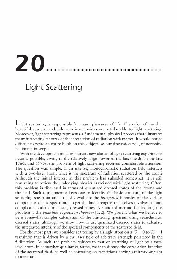
20Light Scattering
Light scattering is responsible for many pleasures of life. The color of the sky,beautiful sunsets, and colors in insect wings are attributable to light scattering.Moreover, light scattering represents a fundamental physical process that illustratesmany interesting features of the interaction of radiation with matter. It would not bedifficult to write an entire book on this subject, so our discussion will, of necessity,be limited in scope.
With the development of laser sources, new classes of light scattering experimentsbecame possible, owing to the relatively large power of the laser fields. In the late1960s and 1970s, the problem of light scattering received considerable attention.The question was simple. If an intense, monochromatic radiation field interactswith a two-level atom, what is the spectrum of radiation scattered by the atom?Although the initial interest in this problem has subsided somewhat, it is stillrewarding to review the underlying physics associated with light scattering. Often,this problem is discussed in terms of quantized dressed states of the atoms andthe field. Such a treatment allows one to identify the basic structure of the lightscattering spectrum and to easily evaluate the integrated intensity of the variouscomponents of the spectrum. To get the line strengths themselves involves a morecomplicated calculation using dressed states. A standard method for treating thisproblem is the quantum regression theorem [1, 2]. We present what we believe tobe a somewhat simpler calculation of the scattering spectrum using semiclassicaldressed states, although we show how to use quantized dressed states to calculatethe integrated intensity of the spectral components of the scattered field.
For the most part, we consider scattering by a single atom on a G = 0 to H = 1transition that is driven by a cw laser field of arbitrary strength polarized in thez direction. As such, the problem reduces to that of scattering of light by a two-level atom. In somewhat qualitative terms, we then discuss the correlation functionof the scattered field, as well as scattering on transitions having arbitrary angularmomentum.
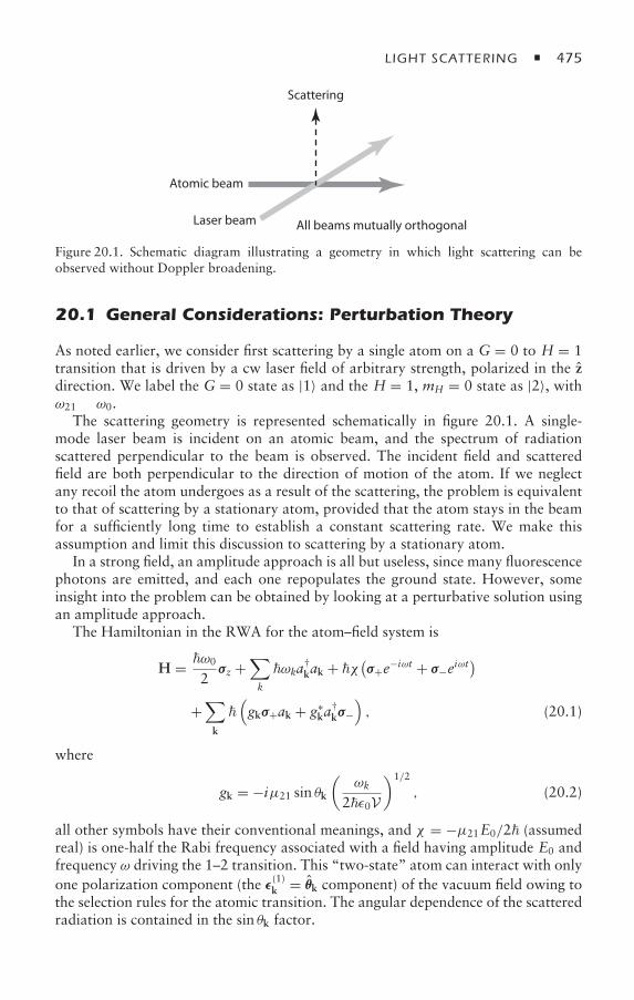
LIGHT SCATTERING 475
Scattering
All beams mutually orthogonal
Atomic beam
Laser beam
Figure 20.1. Schematic diagram illustrating a geometry in which light scattering can beobserved without Doppler broadening.
20.1 General Considerations: Perturbation Theory
As noted earlier, we consider first scattering by a single atom on a G = 0 to H = 1transition that is driven by a cw laser field of arbitrary strength, polarized in the zdirection. We label the G = 0 state as |1〉 and the H = 1, mH = 0 state as |2〉, withω21 ≡ ω0.
The scattering geometry is represented schematically in figure 20.1. A single-mode laser beam is incident on an atomic beam, and the spectrum of radiationscattered perpendicular to the beam is observed. The incident field and scatteredfield are both perpendicular to the direction of motion of the atom. If we neglectany recoil the atom undergoes as a result of the scattering, the problem is equivalentto that of scattering by a stationary atom, provided that the atom stays in the beamfor a sufficiently long time to establish a constant scattering rate. We make thisassumption and limit this discussion to scattering by a stationary atom.
In a strong field, an amplitude approach is all but useless, since many fluorescencephotons are emitted, and each one repopulates the ground state. However, someinsight into the problem can be obtained by looking at a perturbative solution usingan amplitude approach.
The Hamiltonian in the RWA for the atom–field system is
H = ω0
2σz +
∑k
ωka†kak + χ(σ+e−iωt + σ−eiωt
)+∑k
(gkσ+ak + g∗
ka†kσ−
), (20.1)
where
gk = −iµ21 sin θk
(ωk
2ε0V
)1/2
, (20.2)
all other symbols have their conventional meanings, and χ = −µ21E0/2 (assumedreal) is one-half the Rabi frequency associated with a field having amplitude E0 andfrequency ω driving the 1–2 transition. This “two-state” atom can interact with onlyone polarization component (the ε
(1)k = θk component) of the vacuum field owing to
the selection rules for the atomic transition. The angular dependence of the scatteredradiation is contained in the sin θk factor.
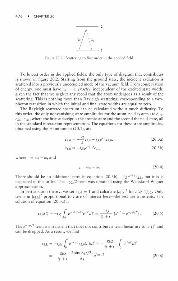
476 CHAPTER 20
2
1
ωk
ω
Figure 20.2. Scattering to first order in the applied field.
To lowest order in the applied fields, the only type of diagram that contributesis shown in figure 20.2. Starting from the ground state, the incident radiation isscattered into a previously unoccupied mode of the vacuum field. From conservationof energy, one must have ωk = ω exactly, independent of the excited state width,given the fact that we neglect any recoil that the atom undergoes as a result of thescattering. This is nothing more than Rayleigh scattering, corresponding to a two-photon transition in which the initial and final state widths are equal to zero.
The Rayleigh scattered spectrum can be calculated without much difficulty. Tothis order, the only nonvanishing state amplitudes for the atom–field system are c1;0,c2;0, c1;k, where the first subscript is the atomic state and the second the field state, allin the standard interaction representation. The equations for these state amplitudes,obtained using the Hamiltonian (20.1), are
c2;0 = −γ22c2;0 − iχeiδtc1,0, (20.3a)
c1,k ≈ −igke−iδktc2,0, (20.3b)
where δ = ω0 − ω, and
δk = ω0 − ωk. (20.4)
There should be an additional term in equation (20.3b), −iχe−iδtc2,k, but it is isneglected in this order. The −γ2/2 term was obtained using the Weisskopf-Wignerapproximation.
In perturbation theory, we set c1, 0 = 1 and calculate |c1,k|2 for t 1/γ2. Onlyterms in |c1,k|2 proportional to t are of interest here—the rest are transients. Thesolution of equation (20.3a) is
c2,0(t) ∼ −iχ∫ t
0e− γ2
2 (t−t′)eiδt′dt′ = −iχ
γ22 + iδ
(eiδt − e−γ2t/2) . (20.5)
The e−γ2t/2 term is a transient that does not contribute a term linear in t to |c1k|2 andcan be dropped. As a result, we find
c1,k = −igk∫ t
0e−iδkt′c2,0(t′)dt′ ≈ − gkχ
γ22 + iδ
∫ t
0eikt′dt′
= − gkχγ22 + iδ
2 sin(kt/2)k
eikt/2 (20.6)
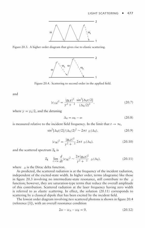
LIGHT SCATTERING 477
2
1
ωk
ω
Figure 20.3. A higher order diagram that gives rise to elastic scattering.
2
1
ωB
ωA
ωω
Figure 20.4. Scattering to second order in the applied field.
and
|c1,k|2 = |gkχ |2γ 2 + δ2
sin2[kt/2]
(k/2)2 , (20.7)
where γ = γ2/2, and the detuning
k = ωk − ω (20.8)
is measured relative to the incident field frequency. In the limit that t → ∞,
sin2[kt/2]/(k/2)2 ∼ 2π tδD (k), (20.9)
|c1k|2 = |gkχ |2γ 2 + δ2 2π tδD (k), (20.10)
and the scattered spectrum Ik is
Ik ≡ limt→∞
ddt
|c1k|2 ∼ 2π |gkχ |2γ 2 + δ2 δD (k), (20.11)
where δD is the Dirac delta function.As predicted, the scattered radiation is at the frequency of the incident radiation,
independent of the excited-state width. In higher order, terms (diagrams) like thosein figure 20.3 involving no intermediate-state resonance, still contribute to the δDfunction; however, they are saturation-type terms that reduce the overall amplitudeof this contribution. Scattered radiation at the laser frequency having zero widthis referred to as elastic scattering. In effect, the solution (20.11) corresponds toscattering by a classical dipole that has been excited by the incident field.
The lowest order diagram involving two scattered photons is shown in figure 20.4(reference [3]), with an overall resonance condition
2ω − ωA − ωB = 0, (20.12)
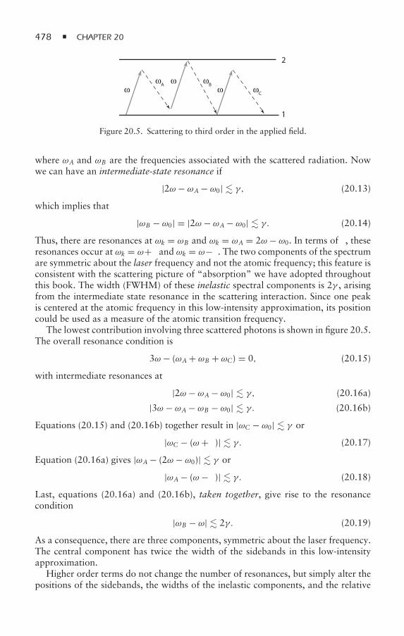
478 CHAPTER 20
2
1
ωB
ωC
ωA
ωω
ω
Figure 20.5. Scattering to third order in the applied field.
where ωA and ωB are the frequencies associated with the scattered radiation. Nowwe can have an intermediate-state resonance if
|2ω − ωA − ω0| γ, (20.13)
which implies that
|ωB − ω0| = |2ω − ωA − ω0| γ. (20.14)
Thus, there are resonances at ωk = ωB and ωk = ωA = 2ω − ω0. In terms of δ, theseresonances occur at ωk = ω+δ and ωk = ω−δ. The two components of the spectrumare symmetric about the laser frequency and not the atomic frequency; this feature isconsistent with the scattering picture of “absorption” we have adopted throughoutthis book. The width (FWHM) of these inelastic spectral components is 2γ , arisingfrom the intermediate state resonance in the scattering interaction. Since one peakis centered at the atomic frequency in this low-intensity approximation, its positioncould be used as a measure of the atomic transition frequency.
The lowest contribution involving three scattered photons is shown in figure 20.5.The overall resonance condition is
3ω − (ωA + ωB + ωC) = 0, (20.15)
with intermediate resonances at
|2ω − ωA − ω0| γ, (20.16a)
|3ω − ωA − ωB − ω0| γ. (20.16b)
Equations (20.15) and (20.16b) together result in |ωC − ω0| γ or
|ωC − (ω + δ)| γ. (20.17)
Equation (20.16a) gives |ωA − (2ω − ω0)| γ or
|ωA − (ω − δ)| γ. (20.18)
Last, equations (20.16a) and (20.16b), taken together, give rise to the resonancecondition
|ωB − ω| 2γ. (20.19)
As a consequence, there are three components, symmetric about the laser frequency.The central component has twice the width of the sidebands in this low-intensityapproximation.
Higher order terms do not change the number of resonances, but simply alter thepositions of the sidebands, the widths of the inelastic components, and the relative
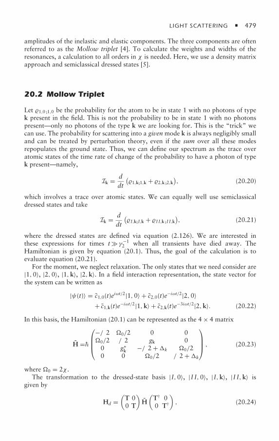
LIGHT SCATTERING 479
amplitudes of the inelastic and elastic components. The three components are oftenreferred to as the Mollow triplet [4]. To calculate the weights and widths of theresonances, a calculation to all orders in χ is needed. Here, we use a density matrixapproach and semiclassical dressed states [5].
20.2 Mollow Triplet
Let 1,0 ;1,0 be the probability for the atom to be in state 1 with no photons of typek present in the field. This is not the probability to be in state 1 with no photonspresent—only no photons of the type k we are looking for. This is the “trick” wecan use. The probability for scattering into a givenmode k is always negligibly smalland can be treated by perturbation theory, even if the sum over all these modesrepopulates the ground state. Thus, we can define our spectrum as the trace overatomic states of the time rate of change of the probability to have a photon of typek present—namely,
Ik = ddt
(1,k;1,k + 2,k ;2,k
), (20.20)
which involves a trace over atomic states. We can equally well use semiclassicaldressed states and take
Ik = ddt
(I,k;I,k + I I,k ;I I,k
), (20.21)
where the dressed states are defined via equation (2.126). We are interested inthese expressions for times t γ−1
2 when all transients have died away. TheHamiltonian is given by equation (20.1). Thus, the goal of the calculation is toevaluate equation (20.21).
For the moment, we neglect relaxation. The only states that we need consider are|1,0〉, |2,0〉, |1,k〉, |2,k〉. In a field interaction representation, the state vector forthe system can be written as
|ψ(t)〉 = c1,0(t)eiωt/2|1,0〉 + c2,0(t)e−iωt/2|2,0〉+ c1,k(t)e−iωt/2|1,k〉 + c2,k(t)e−3iωt/2|2,k〉. (20.22)
In this basis, the Hamiltonian (20.1) can be represented as the 4 × 4 matrix
H =
⎛⎜⎜⎝
−δ/2 0/2 0 00/2 δ/2 gk 00 g∗
k −δ/2 +k 0/20 0 0/2 δ/2 +k
⎞⎟⎟⎠ , (20.23)
where 0 = 2χ .The transformation to the dressed-state basis |I,0〉, |I I,0〉, |I,k〉, |I I,k〉 is
given by
Hd =(T 00 T
)H(T† 00 T†
), (20.24)
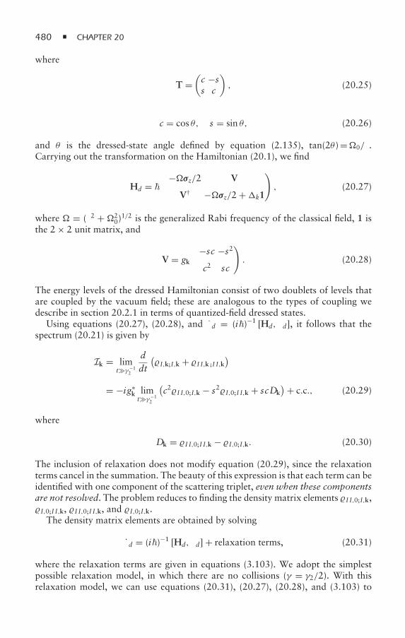
480 CHAPTER 20
where
T =(c −ss c
), (20.25)
c = cos θ, s = sin θ, (20.26)
and θ is the dressed-state angle defined by equation (2.135), tan(2θ )=0/δ.Carrying out the transformation on the Hamiltonian (20.1), we find
Hd = (−σz/2 V
V† −σz/2 +k1
), (20.27)
where = (δ2 + 20)
1/2 is the generalized Rabi frequency of the classical field, 1 isthe 2 × 2 unit matrix, and
V = gk
(−sc −s2c2 sc
). (20.28)
The energy levels of the dressed Hamiltonian consist of two doublets of levels thatare coupled by the vacuum field; these are analogous to the types of coupling wedescribe in section 20.2.1 in terms of quantized-field dressed states.
Using equations (20.27), (20.28), and d = (i)−1 [Hd, d], it follows that thespectrum (20.21) is given by
Ik = limt γ−1
2
ddt
(I,k;I,k + I I,k ;I I,k
)
= −ig∗k limt γ−1
2
(c2I I,0;I,k − s2I,0;I I,k + scDk
)+ c.c., (20.29)
where
Dk = I I,0;I I,k − I,0;I,k. (20.30)
The inclusion of relaxation does not modify equation (20.29), since the relaxationterms cancel in the summation. The beauty of this expression is that each term can beidentified with one component of the scattering triplet, even when these componentsare not resolved. The problem reduces to finding the density matrix elements I I,0;I,k,I,0;I I,k, I I,0;I I,k, and I,0;I,k.
The density matrix elements are obtained by solving
d = (i)−1 [Hd, d] + relaxation terms, (20.31)
where the relaxation terms are given in equations (3.103). We adopt the simplestpossible relaxation model, in which there are no collisions (γ = γ2/2). With thisrelaxation model, we can use equations (20.31), (20.27), (20.28), and (3.103) to
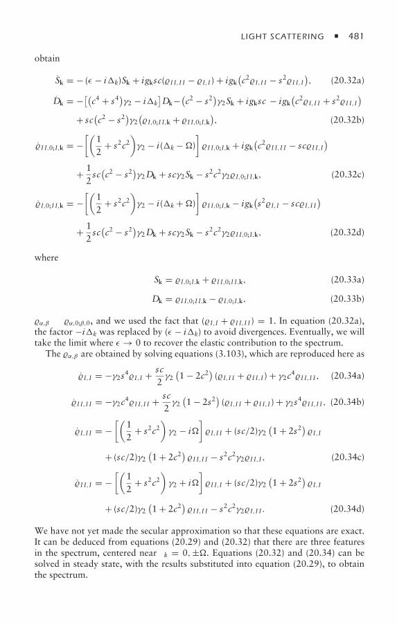
LIGHT SCATTERING 481
obtain
Sk = − (ε − ik)Sk + igksc(I I,I I − I,I ) + igk(c2I,I I − s2I I,I
), (20.32a)
Dk = −[(c4 + s4)γ2 − ik
]Dk−
(c2 − s2
)γ2Sk + igksc − igk
(c2I,I I + s2I I,I
)+ sc
(c2 − s2
)γ2(I,0;I I,k + I I,0;I,k
), (20.32b)
I I,0;I,k = −[(
12
+ s2c2)γ2 − i(k −)
]I I,0;I,k + igk
(c2I I,I I − scI I,I
)
+ 12sc(c2 − s2
)γ2Dk + scγ2Sk − s2c2γ2I,0;I I,k, (20.32c)
I,0;I I,k = −[(
12
+ s2c2)γ2 − i(k +)
]I I,0;I,k − igk
(s2I,I − scI,I I
)
+ 12sc(c2 − s2
)γ2Dk + scγ2Sk − s2c2γ2I I,0;I,k, (20.32d)
where
Sk = I,0;I,k + I I,0;I I,k, (20.33a)
Dk = I I,0;I I,k − I,0;I,k, (20.33b)
α,β ≡ α,0;β,0, and we used the fact that (I,I + I I,I I ) = 1. In equation (20.32a),the factor −ik was replaced by (ε − ik) to avoid divergences. Eventually, we willtake the limit where ε → 0 to recover the elastic contribution to the spectrum.
The α,β are obtained by solving equations (3.103), which are reproduced here as
I,I = −γ2s4I,I + sc2γ2(1 − 2c2
)(I,I I + I I,I ) + γ2c4I I,I I , (20.34a)
I I,I I = −γ2c4I I,I I + sc2γ2(1 − 2s2
)(I,I I + I I,I ) + γ2s4I I,I I , (20.34b)
I,I I = −[(
12
+ s2c2)γ2 − i
]I,I I + (sc/2)γ2
(1 + 2s2
)I,I
+ (sc/2)γ2(1 + 2c2
)I I,I I − s2c2γ2I I,I , (20.34c)
I I,I = −[(
12
+ s2c2)γ2 + i
]I I,I + (sc/2)γ2
(1 + 2s2
)I,I
+ (sc/2)γ2(1 + 2c2
)I I,I I − s2c2γ2I,I I . (20.34d)
We have not yet made the secular approximation so that these equations are exact.It can be deduced from equations (20.29) and (20.32) that there are three featuresin the spectrum, centered near δk = 0,±. Equations (20.32) and (20.34) can besolved in steady state, with the results substituted into equation (20.29), to obtainthe spectrum.
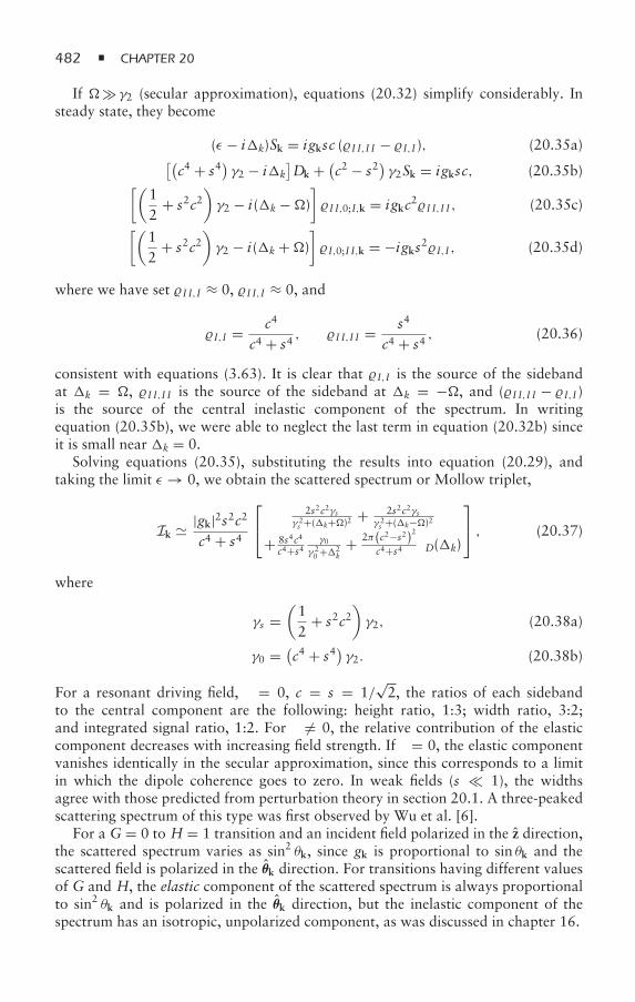
482 CHAPTER 20
If γ2 (secular approximation), equations (20.32) simplify considerably. Insteady state, they become
(ε − ik)Sk = igksc (I I,I I − I,I ), (20.35a)[(c4 + s4
)γ2 − ik
]Dk + (
c2 − s2)γ2Sk = igksc, (20.35b)[(
12
+ s2c2)γ2 − i(k −)
]I I,0;I,k = igkc2I I,I I , (20.35c)[(
12
+ s2c2)γ2 − i(k +)
]I,0;I I,k = −igks2I,I , (20.35d)
where we have set I I,I ≈ 0, I I,I ≈ 0, and
I,I = c4
c4 + s4, I I,I I = s4
c4 + s4, (20.36)
consistent with equations (3.63). It is clear that I,I is the source of the sidebandat k = , I I,I I is the source of the sideband at k = −, and (I I,I I − I,I )is the source of the central inelastic component of the spectrum. In writingequation (20.35b), we were able to neglect the last term in equation (20.32b) sinceit is small near k = 0.
Solving equations (20.35), substituting the results into equation (20.29), andtaking the limit ε → 0, we obtain the scattered spectrum or Mollow triplet,
Ik |gk|2s2c2c4 + s4
⎡⎣ 2s2c2γs
γ 2s +(k+)2 + 2s2c2γs
γ 2s +(k−)2
+ 8s4c4c4+s4
γ0γ 20 +2
k+ 2π(c2−s2)2
c4+s4 δD(k)
⎤⎦ , (20.37)
where
γs =(12
+ s2c2)γ2, (20.38a)
γ0 = (c4 + s4
)γ2. (20.38b)
For a resonant driving field, δ = 0, c = s = 1/√2, the ratios of each sideband
to the central component are the following: height ratio, 1:3; width ratio, 3:2;and integrated signal ratio, 1:2. For δ = 0, the relative contribution of the elasticcomponent decreases with increasing field strength. If δ = 0, the elastic componentvanishes identically in the secular approximation, since this corresponds to a limitin which the dipole coherence goes to zero. In weak fields (s 1), the widthsagree with those predicted from perturbation theory in section 20.1. A three-peakedscattering spectrum of this type was first observed by Wu et al. [6].
For a G = 0 to H = 1 transition and an incident field polarized in the z direction,the scattered spectrum varies as sin2 θk, since gk is proportional to sin θk and thescattered field is polarized in the θk direction. For transitions having different valuesof G and H, the elastic component of the scattered spectrum is always proportionalto sin2 θk and is polarized in the θk direction, but the inelastic component of thespectrum has an isotropic, unpolarized component, as was discussed in chapter 16.
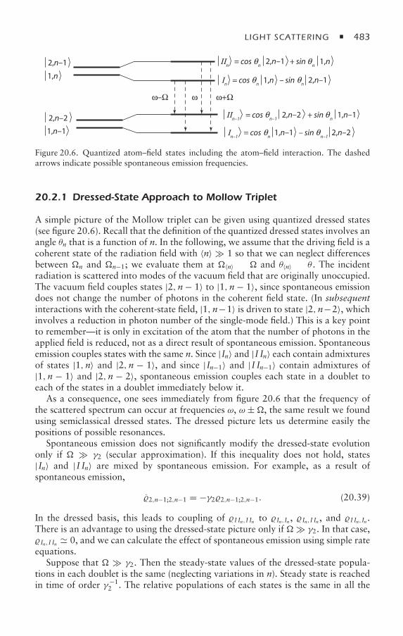
LIGHT SCATTERING 483
ωω–Ω ω+Ω
1,n
1,n–1
2,n–1
2,n–2
1,n
1,n–1
2,n–1
2,n–2
1,n
2,n–1
2,n–2
1,n–1
In
IIn
= cos θn
+ sin θn
= cos θn
– sin θn
In–1
IIn–1
= cos θn–1
+ sin θn
= cos θn
– sin θn–1
θ θ
θθ
θ θ
θ θ
Figure 20.6. Quantized atom–field states including the atom–field interaction. The dashedarrows indicate possible spontaneous emission frequencies.
20.2.1 Dressed-State Approach to Mollow Triplet
A simple picture of the Mollow triplet can be given using quantized dressed states(see figure 20.6). Recall that the definition of the quantized dressed states involves anangle θn that is a function of n. In the following, we assume that the driving field is acoherent state of the radiation field with 〈n〉 1 so that we can neglect differencesbetween n and n−1; we evaluate them at 〈n〉 ≡ and θ〈n〉 ≡ θ . The incidentradiation is scattered into modes of the vacuum field that are originally unoccupied.The vacuum field couples states |2,n− 1〉 to |1,n− 1〉, since spontaneous emissiondoes not change the number of photons in the coherent field state. (In subsequentinteractions with the coherent-state field, |1,n−1〉 is driven to state |2,n−2〉, whichinvolves a reduction in photon number of the single-mode field.) This is a key pointto remember—it is only in excitation of the atom that the number of photons in theapplied field is reduced, not as a direct result of spontaneous emission. Spontaneousemission couples states with the same n. Since |In〉 and |I In〉 each contain admixturesof states |1,n〉 and |2,n − 1〉, and since |In−1〉 and |I In−1〉 contain admixtures of|1,n − 1〉 and |2,n − 2〉, spontaneous emission couples each state in a doublet toeach of the states in a doublet immediately below it.
As a consequence, one sees immediately from figure 20.6 that the frequency ofthe scattered spectrum can occur at frequencies ω, ω ±, the same result we foundusing semiclassical dressed states. The dressed picture lets us determine easily thepositions of possible resonances.
Spontaneous emission does not significantly modify the dressed-state evolutiononly if γ2 (secular approximation). If this inequality does not hold, states|In〉 and |I In〉 are mixed by spontaneous emission. For example, as a result ofspontaneous emission,
2,n−1;2,n−1 = −γ22,n−1;2,n−1. (20.39)
In the dressed basis, this leads to coupling of I In,I In to In,In , In,I In , and I In,In .There is an advantage to using the dressed-state picture only if γ2. In that case,In,I In 0, and we can calculate the effect of spontaneous emission using simple rateequations.
Suppose that γ2. Then the steady-state values of the dressed-state popula-tions in each doublet is the same (neglecting variations in n). Steady state is reachedin time of order γ−1
2 . The relative populations of each states is the same in all the
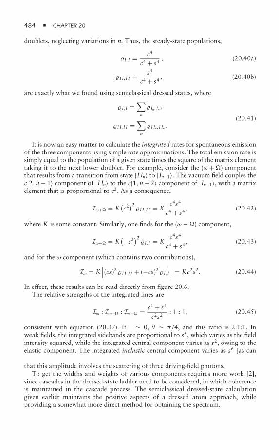
484 CHAPTER 20
doublets, neglecting variations in n. Thus, the steady-state populations,
I,I = c4
c4 + s4, (20.40a)
I I,I I = s4
c4 + s4, (20.40b)
are exactly what we found using semiclassical dressed states, where
I,I =∑n
In,In,
I I,I I =∑n
I In,I In .(20.41)
It is now an easy matter to calculate the integrated rates for spontaneous emissionof the three components using simple rate approximations. The total emission rate issimply equal to the population of a given state times the square of the matrix elementtaking it to the next lower doublet. For example, consider the (ω +) componentthat results from a transition from state |I In〉 to |In−1〉. The vacuum field couples thec|2,n− 1〉 component of |I In〉 to the c|1,n− 2〉 component of |In−1〉, with a matrixelement that is proportional to c2. As a consequence,
Iω+ = K(c2)2I I,I I = K
c4s4
c4 + s4, (20.42)
where K is some constant. Similarly, one finds for the (ω −) component,
Iω− = K(−s2)2 I,I = K
c4s4
c4 + s4, (20.43)
and for the ω component (which contains two contributions),
Iω = K[(cs)2 I I,I I + (−cs)2 I,I
]= Kc2s2. (20.44)
In effect, these results can be read directly from figure 20.6.The relative strengths of the integrated lines are
Iω : Iω+ : Iω− = c4 + s4
c2s2: 1 : 1, (20.45)
consistent with equation (20.37). If δ ∼ 0, θ ∼ π/4, and this ratio is 2:1:1. Inweak fields, the integrated sidebands are proportional to s4, which varies as the fieldintensity squared, while the integrated central component varies as s2, owing to theelastic component. The integrated inelastic central component varies as s6 [as canbe calculated from equation (20.37)], consistent with the perturbation theory resultthat this amplitude involves the scattering of three driving-field photons.
To get the widths and weights of various components requires more work [2],since cascades in the dressed-state ladder need to be considered, in which coherenceis maintained in the cascade process. The semiclassical dressed-state calculationgiven earlier maintains the positive aspects of a dressed atom approach, whileproviding a somewhat more direct method for obtaining the spectrum.
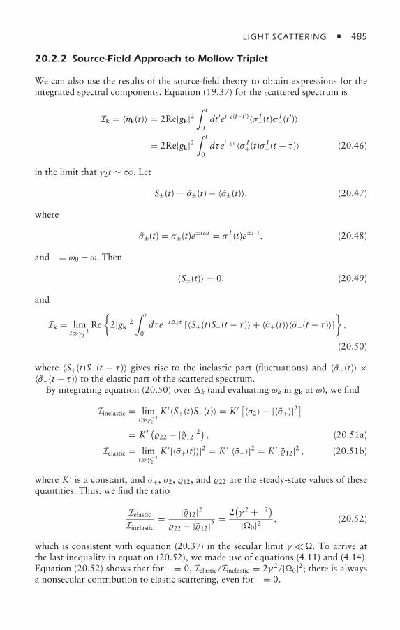
LIGHT SCATTERING 485
20.2.2 Source-Field Approach to Mollow Triplet
We can also use the results of the source-field theory to obtain expressions for theintegrated spectral components. Equation (19.37) for the scattered spectrum is
Ik = 〈nk(t)〉 = 2Re|gk|2∫ t
0dt′eiδk(t−t
′)〈σ I+(t)σ
I−(t
′)〉
= 2Re|gk|2∫ t
0dτeiδkτ 〈σ I
+(t)σI−(t − τ )〉 (20.46)
in the limit that γ2t ∼ ∞. Let
S±(t) = σ±(t) − 〈σ±(t)〉, (20.47)
where
σ±(t) = σ±(t)e±iωt = σ I±(t)e
±iδt, (20.48)
and δ = ω0 − ω. Then
〈S±(t)〉 = 0, (20.49)
and
Ik = limt γ−1
2
Re2|gk|2
∫ t
0dτe−ikτ [〈S+(t)S−(t − τ )〉 + 〈σ+(t)〉〈σ−(t − τ )〉]
,
(20.50)
where 〈S+(t)S−(t − τ )〉 gives rise to the inelastic part (fluctuations) and 〈σ+(t)〉 ×〈σ−(t − τ )〉 to the elastic part of the scattered spectrum.
By integrating equation (20.50) over k (and evaluating ωk in gk at ω), we find
Iinelastic = limt γ−1
2
K ′〈S+(t)S−(t)〉 = K ′ [〈σ2〉 − |〈σ+〉|2]= K ′ (22 − |12|2
), (20.51a)
Ielastic = limt γ−1
2
K ′|〈σ+(t)〉|2 = K ′|〈σ+〉|2 = K ′|12|2 , (20.51b)
where K ′ is a constant, and σ+, σ2, 12, and 22 are the steady-state values of thesequantities. Thus, we find the ratio
IelasticIinelastic
= |12|222 − |12|2
= 2(γ 2 + δ2)|0|2 , (20.52)
which is consistent with equation (20.37) in the secular limit γ . To arrive atthe last inequality in equation (20.52), we made use of equations (4.11) and (4.14).Equation (20.52) shows that for δ = 0, Ielastic/Iinelastic = 2γ 2/|0|2; there is alwaysa nonsecular contribution to elastic scattering, even for δ = 0.
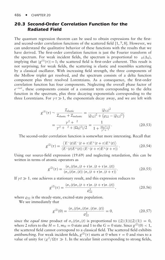
486 CHAPTER 20
20.3 Second-Order Correlation Function for theRadiated Field
The quantum regression theorem can be used to obtain expressions for the first-and second-order correlation functions of the scattered field [1, 7, 8]. However, wecan understand the qualitative behavior of these functions with the results that wehave derived. The first-order correlation function is just the Fourier transform ofthe spectrum. For weak incident fields, the spectrum is proportional to δD(k),implying that |g(1)(τ )| =1; the scattered field is first-order coherent. This result isnot surprising; for weak fields, the scattering is elastic and resembles scatteringby a classical oscillator. With increasing field strength, the three components ofthe Mollow triplet get resolved, and the spectrum consists of a delta functioncomponent plus three resolved Lorentzians. As a consequence, the first-ordercorrelation function has four components. Neglecting the overall phase factor ofe−iωτ , these components consist of a constant term corresponding to the deltafunction in the spectrum, plus three decaying exponentials corresponding to thethree Lorentzians. For γ τ 1, the exponentials decay away, and we are left with[see equations (20.51)]
g(1)(τ ) ∼ IelasticIelastic + Iinelastic = |12|2
|12|2 + (22 − |12|2
)= γ 2 + δ2γ 2 + δ2 + |0|2|/2 = 1
1 + |0|2|/2γ 2+δ2
. (20.53)
The second-order correlation function is somewhat more interesting. Recall that
g(2)(τ ) =⟨E−(t)E−(t + τ )E+(t + τ )E+(t)
⟩〈E−(t)E+(t)〉 〈E−(t + τ )E+(t + τ )〉 . (20.54)
Using our source-field expression (19.69) and neglecting retardation, this can bewritten in terms of atomic operators as
g(2)(τ ) = 〈σ+(t)σ+(t + τ )σ−(t + τ )σ−(t)〉〈σ+(t)σ−(t)〉 〈σ+(t + τ )σ−(t + τ )〉 . (20.55)
If γ t 1, one achieves a stationary result, and this expression reduces to
g(2)(τ ) = 〈σ+(t)σ+(t + τ )σ−(t + τ )σ−(t)〉222
, (20.56)
where 22 is the steady-state, excited-state population.We see immediately that
g(2)(0) = 〈σ+(t)σ+(t)σ−(t)σ−(t)〉222
= 0, (20.57)
since the equal time product of σ+(t)σ+(t) is proportional to (|2〉〈1|)(|2〉〈1|) = 0,where 2 refers to the H = 1,mH = 0 state and 1 to theG = 0 state. Since g(2)(0) < 1,the scattered field cannot correspond to a classical field. The scattered field exhibitsantibunching. For weak incident fields, g(2)(τ ) starts at 0 when τ = 0 and rises to avalue of unity for (χ2/)τ 1. In the secular limit corresponding to strong fields,
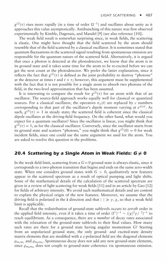
LIGHT SCATTERING 487
g(2)(τ ) rises more rapidly (in a time of order −1) and oscillates about unity as itapproaches this value asymptotically. Antibunching of this nature was first observedexperimentally by Kimble, Dagenais, and Mandel [9] (see also reference [10]).
The weak field result is somewhat surprising since, in weak fields, the scatteringis elastic. One might have thought that the field scattered by the atom shouldresemble that of the field scattered by a classical oscillator. It is sometimes stated thatquantum fluctuations in the scattered signal resulting from spontaneous emission areresponsible for the quantum nature of the scattered field. Alternatively, it is arguedthat once a photon is detected at the photodetector, we know that the atom is inits ground state and it takes some time for the atom to be re-excited before we canget the next count at the photodetector. We prefer the latter explanation, since itreflects the fact that g(2)(τ ) is defined as the joint probability to destroy “photons”at the detector at times t and t + τ ; however, this argument must be supplementedwith the fact that it is not possible for a single atom to absorb two photons of thefield, in the two-level approximation that has been assumed.
It is interesting to compare the result for g(2)(τ ) for an atom with that of anoscillator. The source-field approach works equally well for classical or quantizedsources. For a classical oscillator, the operators σ±(t) are replaced by c numberscorresponding to that part of the oscillator’s dipole moment varying at e∓iωt. Assuch, g(2)(τ ) = 1 in steady state; the scattered field is coherent since the classicaldipole oscillates at the driving-field frequency. On the other hand, what would youexpect for a quantum oscillator? Since the oscillator is linear, you might think thatg(2)(τ ) = 1, as for the classical oscillator. Conversely, since the oscillator starts fromits ground state and scatters “photons,” you might think that g(2)(0) = 0 for weakincident fields, since one could use the same argument we used for the atom. Youare asked to resolve this question in the problems.
20.4 Scattering by a Single Atom in Weak Fields: G = 0
In the weak field limit, scattering from a G=0 ground state is always elastic, since itcorresponds to a two-photon transition that begins and ends on the same zero-widthstate. When one considers ground states with G > 0, qualitatively new featuresappear in the scattered spectrum as a result of optical pumping and light shifts.Some of the mathematical details of the calculation of the scattered spectrum aregiven in a review of light scattering for weak fields [11] and in an article by Gao [12]for fields of arbitrary intensity. We avoid such mathematical details and are contentto explain the physical origin of the new features. Moreover, we assume that thedriving field is polarized in the z direction and that |δ| γ, χ , so that a weak fieldlimit is applicable.
Recall that the redistribution of ground-state sublevels occurs to zeroth order inthe applied field intensity, even if it takes a time of order (′)−1 ∼ (|χ |2γ /δ2)−1 toreach equilibrium. As a consequence, there are a number of decay rates associatedwith the relaxation of the ground-state sublevels to their final values. How manysuch rates are there for a ground state having angular momentum G? Startingfrom an unpolarized ground state, the only ground- and excited-state densitymatrix elements that are modified with a z-polarized field are the diagonal elementsmGmG and mHmH . Spontaneous decay does not add any new ground-state elements,since mHmH does not couple to ground-state coherence via spontaneous emission.
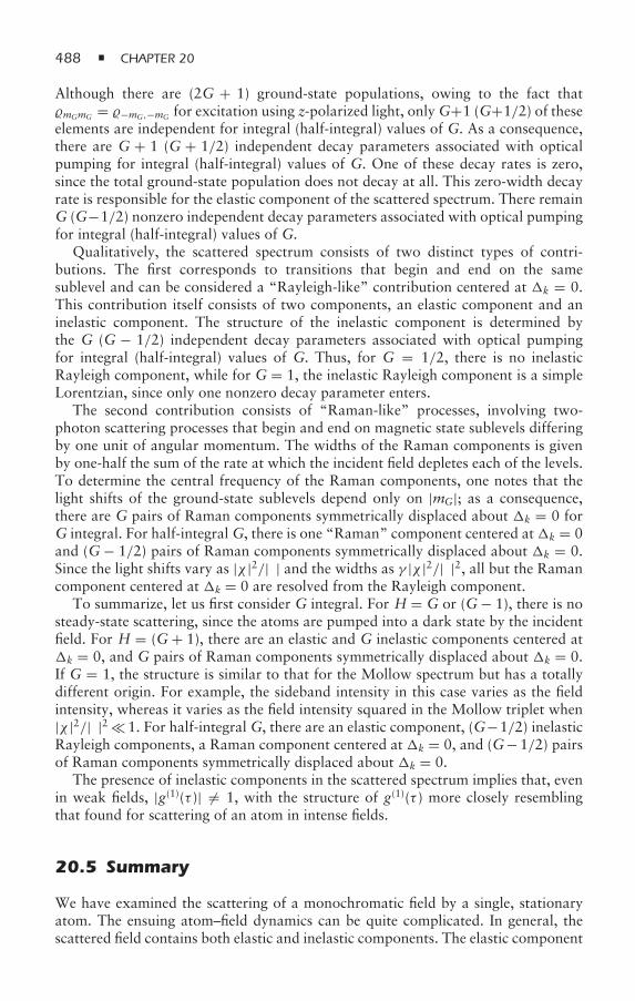
488 CHAPTER 20
Although there are (2G + 1) ground-state populations, owing to the fact thatmGmG = −mG,−mG for excitation using z-polarized light, onlyG+1 (G+1/2) of theseelements are independent for integral (half-integral) values of G. As a consequence,there are G + 1 (G + 1/2) independent decay parameters associated with opticalpumping for integral (half-integral) values of G. One of these decay rates is zero,since the total ground-state population does not decay at all. This zero-width decayrate is responsible for the elastic component of the scattered spectrum. There remainG (G−1/2) nonzero independent decay parameters associated with optical pumpingfor integral (half-integral) values of G.
Qualitatively, the scattered spectrum consists of two distinct types of contri-butions. The first corresponds to transitions that begin and end on the samesublevel and can be considered a “Rayleigh-like” contribution centered at k = 0.This contribution itself consists of two components, an elastic component and aninelastic component. The structure of the inelastic component is determined bythe G (G − 1/2) independent decay parameters associated with optical pumpingfor integral (half-integral) values of G. Thus, for G = 1/2, there is no inelasticRayleigh component, while for G = 1, the inelastic Rayleigh component is a simpleLorentzian, since only one nonzero decay parameter enters.
The second contribution consists of “Raman-like” processes, involving two-photon scattering processes that begin and end on magnetic state sublevels differingby one unit of angular momentum. The widths of the Raman components is givenby one-half the sum of the rate at which the incident field depletes each of the levels.To determine the central frequency of the Raman components, one notes that thelight shifts of the ground-state sublevels depend only on |mG|; as a consequence,there are G pairs of Raman components symmetrically displaced about k = 0 forG integral. For half-integral G, there is one “Raman” component centered atk = 0and (G− 1/2) pairs of Raman components symmetrically displaced about k = 0.Since the light shifts vary as |χ |2/|δ| and the widths as γ |χ |2/|δ|2, all but the Ramancomponent centered at k = 0 are resolved from the Rayleigh component.
To summarize, let us first consider G integral. For H = G or (G− 1), there is nosteady-state scattering, since the atoms are pumped into a dark state by the incidentfield. For H = (G+ 1), there are an elastic and G inelastic components centered atk = 0, and G pairs of Raman components symmetrically displaced about k = 0.If G = 1, the structure is similar to that for the Mollow spectrum but has a totallydifferent origin. For example, the sideband intensity in this case varies as the fieldintensity, whereas it varies as the field intensity squared in the Mollow triplet when|χ |2/|δ|2 1. For half-integral G, there are an elastic component, (G−1/2) inelasticRayleigh components, a Raman component centered at k = 0, and (G−1/2) pairsof Raman components symmetrically displaced about k = 0.
The presence of inelastic components in the scattered spectrum implies that, evenin weak fields, |g(1)(τ )| = 1, with the structure of g(1)(τ ) more closely resemblingthat found for scattering of an atom in intense fields.
20.5 Summary
We have examined the scattering of a monochromatic field by a single, stationaryatom. The ensuing atom–field dynamics can be quite complicated. In general, thescattered field contains both elastic and inelastic components. The elastic component
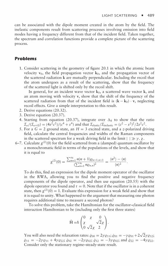
LIGHT SCATTERING 489
can be associated with the dipole moment created in the atom by the field. Theinelastic components result from scattering processes involving emission into fieldmodes having a frequency different from that of the incident field. Taken together,the spectrum and correlation functions provide a complete picture of the scatteringprocess.
Problems
1. Consider scattering in the geometry of figure 20.1 in which the atomic beamvelocity v0, the field propagation vector k0, and the propagation vector ofthe scattered radiation k are mutually perpendicular. Including the recoil thatthe atom undergoes as a result of the scattering, show that the frequencyof the scattered light is shifted only by the recoil shift.
In general, for an incident wave vector k0, a scattered wave vector k, andan atom moving with velocity v, show that the shift of the frequency of thescattered radiation from that of the incident field is (k − k0) · v, neglectingrecoil effects. Give a simple interpretation to this result.
2. Derive equations (20.32).3. Derive equation (20.37).4. Starting from equation (20.37), integrate over k to show that the ratioIω/(Iω+) = (4s2c2)/(c4 + s4) and that Ielastic/Iinelastic = (c2 − s2)2/2s2c2.
5. For a G = 2 ground state, an H = 3 excited state, and a z-polarized drivingfield, calculate the central frequencies and widths of the Raman componentsin the scattered spectrum for a weak driving field in the limit |δ| γ, χ .
6–7. Calculate g(2)(0) for the field scattered from a (damped) quantum oscillator bya monochromatic field in terms of the populations of the levels, and show thatit is equal to
g(2)(0) =∑∞
n=1 n(n+ 1)n+1,n+1
(∑∞
n=1 nn,n)2= 〈n2〉 − 〈n〉
〈n〉2 .
To do this, find an expression for the dipole moment operator of the oscillatorin the RWA, allowing you to find the positive and negative frequencycomponents of the dipole operator, and then use equation (20.55) with thedipole operator you found and τ = 0. Note that if the oscillator is in a coherentstate, then g(2)(0) = 1. Evaluate this expression for a weak field and show thatit is equal to unity. What happened to the argument that measuring one photonrequires additional time to measure a second photon?
To solve this problem, take the Hamiltonian for the oscillator–classical fieldinteraction Hamiltonian to be (including only the first three states)
H =⎛⎝0 χ 0χ δ
√2χ
0√2χ 2δ
⎞⎠.
You will also need the relaxation rates: 00 = 2γ 11; 01 = −γ 01+2√2γ 12;
11 = −2γ 11 + 4γ 22; 02 = −2γ 02; 12 = −3γ 02; and 22 = −4γ 22.Consider only the stationary regime–steady-state result.
490 CHAPTER 20
References
[1] B. R. Mollow, Pure-state analysis of resonant light scattering: radiative damp-ing, saturation, and multiphoton effects, Physical Review A 12, 1919–1943(1975).
[2] C. Cohen-Tannoudji, Atoms in Strong Resonant Fields, in Frontiers in Laser Spec-troscopy, Les Houches Session XXVII, vol. 1, edited by R. Balian, S. Haroche, andS. Liberman (North Holland, Amsterdam, 1975), pp. 88–98; C. Cohen-Tannoudji,J. Dupont-Roc, and G. Grynberg, Atom-Photon Interactions (Wiley-Interscience,New York, 1992), complement AV.
[3] C. Cohen-Tannoudji, Atoms in Strong Resonant Fields: Spectral Distribution ofthe Fluorescence Light, in Laser Spectroscopy, edited by S. Haroche, J. C. Pebay-Peyroula, T. W. Hänsch, and S. E. Harris (Springer-Verlag, Berlin, 1975), pp. 324–339; S. Reynaud, La fluorescence de résonance: étude par la méthode de l’atome habillé(Resonance fluorescence: study by the dressed atom method), Annales de Physique 8,315–370 (1983).
[4] B. R. Mollow, Power spectrum of light scattered by two-level systems, Physical Review188, 1969–1975 (1969).
[5] P. R. Berman, Theory of fluorescence and probe absorption in the presence of a drivingfield using semiclassical dressed states, Physical Review A 53, 2627–2632 (1996).
[6] F. Y. Wu, R. E. Grove, and S. Ezekiel, Investigation of the spectrum of resonancefluorescence induced by a monochromatic field, Physical Review Letters 35, 1426–1429 (1975); R. E. Grove, F. Y. Wu, and S. Ezekiel, Measurement of the spectrumof resonance fluorescence from a two-level atom in an intense monochromatic field,Physical Review A 15, 227–233 (1977).
[7] H. J. Kimball and L. Mandel, Theory of resonance fluorescence, Physical Review A 13,2123–2144 (1976).
[8] H. J. Carmichael and D. F. Walls, Proposal for the measurement of the resonantStark effect by photon correlation techniques, Journal of Physics B 9, L43–L46 (1976);H. J. Carmichael and D. F. Walls, A quantum-mechanical master equation treatmentof the dynamical Stark effect, Journal of Physics B 9, 1199–1219 (1976).
[9] H. J. Kimball, M. Dagenais, and L. Mandel, Photon antibunching in resonancefluorescence, Physical Review Letters 39, 691–695 (1977).
[10] M. Dagenais and L. Mandel, Investigation of two-time correlations in photon emissionsfrom a single atom, Physical Review A 18, 2217–2228 (1978).
[11] P. R. Berman, Light scattering, Contemporary Physics 49, 313–330 (2008).[12] B. Gao, Effects of Zeeman degeneracy on the steady-state properties of an atom
interacting with a near-resonant laser field: resonance fluorescence, Physical ReviewA 50, 4139–4156 (1994).
Bibliography
W. Heitler, The Quantum Theory of Radiation, 3rd ed. (Oxford University Press, Oxford,UK, 1954), sec. 20.
R. Loudon, The Quantum Theory of Light, 3rd ed. (Oxford University Press, Oxford, UK,2003), chap. 8.
LIGHT SCATTERING 491
L. Mandel and E. Wolf, Optical Coherence and Quantum Optics (Cambridge UniversityPress, Cambridge, UK, 1995), sec. 15.6.
B. R. Mollow, Theory of intensity dependence resonance light scattering and resonance fluo-rescence, in Progress in Optics, edited by E. Wolf, vol. XIX (North-Holland, Amsterdam,1981), pp. 1–43.
R. G. Newton, Scattering Theory of Waves and Particles, 2nd ed. (Dover, New York,2002).
Lord Rayleigh,On the transmission of light through an atmosphere containing small particlesin suspension, and on the origin of the blue of the sky, Philosophical Magazine XLVII,375–384 (1899).
21Entanglement and Spin Squeezing
We have just about come to the end of the road. Our trip has taken us to manydestinations, but there are many others that were given just a glance or not seenat all. Topics such as optical bistability, applied nonlinear optics, superradiance,pulse propagation, and the theory of laser operation were excluded. Moreover,many-atom systems in which correlations play a dominant role, such as Bose-Einstein condensates, were not discussed. Many of these topics are included in thebibliography entries that have been given throughout this book.
We would like to think that we have given the reader an introduction to thetheory of atom–field interactions that will prove helpful. The techniques that weredeveloped are quite general and can be applied to a wide range of problems. By thistime, it is hoped that you are comfortable with the various representations that wereused and that the choice of which representation to use has become “natural” foryou.
One topic that was not discussed is entanglement. Entangled or correlated statesof a multiple-atom system are states that cannot be factorized into a product of statevectors for the individual atoms. For example, the state function for a two-atomsystem
|ψ〉 = 12(|1〉1 + |2〉1)(|1〉2 + |2〉2) = 1
2(|11〉 + |12〉 + |21〉 + |22〉),
in which |α〉 j corresponds to the state vector for atom j to be in state α and |αα′〉corresponds to the state vector for atom one to be in state α and atom two to be instate α′, is not an entangled state since it can be factorized. On the other hand,
|ψ〉 = 1√2(|12〉 + |21〉)
is an entangled state since it cannot be factorized. Entangled states have becomeincreasingly important with the development of quantum information and the questfor a quantum computer.
Of course, entanglement and correlated states are at the heart of quantummechanics. In the spirit of this book, we finish this chapter by considering three cases
ENTANGLEMENT AND SPIN SQUEEZING 493
in which a quantized field state becomes entangled with a many-atom state. Directinteractions between the atoms, such as those produced by electrostatic forces, areneglected; any entanglement of the atoms is produced by the field(s).
21.1 Entanglement by Absorption
The first case we look at involves the complete absorption of a single-photon pulsein an optically dense medium [1, 2]. As the pulse is absorbed in the medium, anentangled state of the atoms and the field is produced; once the pulse is totallyabsorbed, the atoms are left in an entangled state involving a single excitation [3].
To simplify the problem, we restrict the discussion to an effective one-dimensionalproblem. That is, we neglect all modes of the radiation field having propagationvectors in other than the x direction; we do not consider scattering of the incidentfield into transverse field modes. The neglect of scattering into transverse modes isvalid provided that the calculation is limited to times for which γ2t 1, where γ2is the excited-state decay rate. The process we consider is truly absorption by theatoms, and not the scattering process with which we have been dealing throughoutmost of this book. The energy lost by the field at any time is converted to excitationenergy of the atoms.
It is assumed that the atomic medium is inhomogeneously broadened. It turnsout that inhomogeneous broadening of the atomic transition frequencies providesan important simplification in this problem, provided that the inhomogeneous widthis much larger than the single-photon pulse bandwidth. In that limit, all frequencycomponents of the incident pulse are absorbed in an identical manner, resulting ina pulse that propagates without distortion. In the case of homogeneous broadening,there could be significant reshaping of the radiation pulse as it propagates in themedium.
The two-level atoms are uniformly distributed in the half-space X > 0, with theposition of atom m denoted by Rm. Owing to inhomogeneous broadening, theseatoms have a distribution of atomic transition frequencies centered about somecentral frequency ω0. That is, atom m has frequency ωm, which is detuned fromthe central transition frequency by an amount
m = ωm − ω0. (21.1)
The inhomogeneous frequency distribution is denoted by W(m).The positive frequency component of the electric field is
E+(X) = i z∞∑
j=−∞
(ω j
2ε0AL
)1/2
eikj Xa j , (21.2)
where
ω j = ∣∣kj ∣∣ /c, (21.3)
A is the cross-sectional area of the field pulse, and a j is a destruction operator forfield mode j . As noted earlier, we consider an effective one-dimensional problem inwhich the field propagates in the x direction with polarization z. The quantization
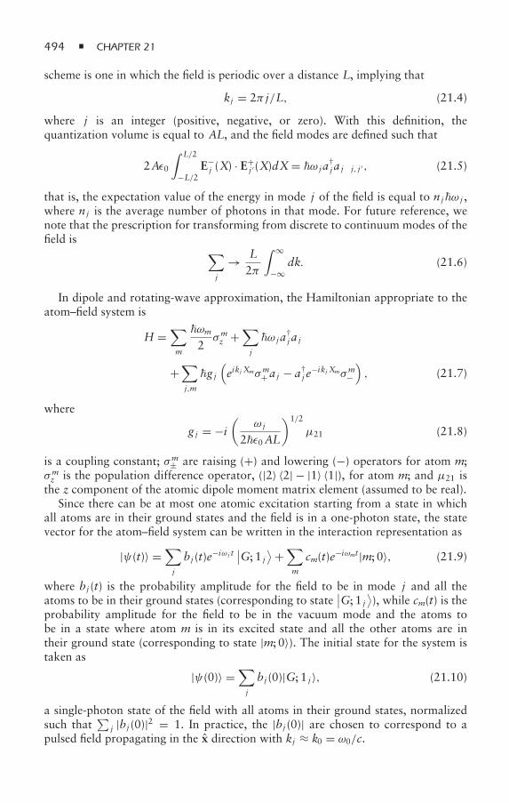
494 CHAPTER 21
scheme is one in which the field is periodic over a distance L, implying that
kj = 2π j/L, (21.4)
where j is an integer (positive, negative, or zero). With this definition, thequantization volume is equal to AL, and the field modes are defined such that
2Aε0
∫ L/2
−L/2E−j (X) · E+
j ′ (X)dX= ω j a†j a jδ j, j ′ , (21.5)
that is, the expectation value of the energy in mode j of the field is equal to njω j ,where nj is the average number of photons in that mode. For future reference, wenote that the prescription for transforming from discrete to continuum modes of thefield is ∑
j
→ L2π
∫ ∞
−∞dk. (21.6)
In dipole and rotating-wave approximation, the Hamiltonian appropriate to theatom–field system is
H =∑m
ωm
2σmz +
∑j
ω j a†j a j
+∑j,m
g j(eikj Xmσm+ a j − a†
j e−ikj Xmσm−
), (21.7)
where
g j = −i(
ω j
2ε0AL
)1/2
µ21 (21.8)
is a coupling constant; σm± are raising (+) and lowering (−) operators for atom m;σmz is the population difference operator, (|2〉 〈2| − |1〉 〈1|), for atom m; and µ21 isthe z component of the atomic dipole moment matrix element (assumed to be real).
Since there can be at most one atomic excitation starting from a state in whichall atoms are in their ground states and the field is in a one-photon state, the statevector for the atom–field system can be written in the interaction representation as
|ψ(t)〉 =∑j
bj (t)e−iω j t∣∣G; 1 j
⟩+∑m
cm(t)e−iωmt|m; 0〉, (21.9)
where bj (t) is the probability amplitude for the field to be in mode j and all theatoms to be in their ground states (corresponding to state
∣∣G; 1 j⟩), while cm(t) is the
probability amplitude for the field to be in the vacuum mode and the atoms tobe in a state where atom m is in its excited state and all the other atoms are intheir ground state (corresponding to state |m; 0〉). The initial state for the system istaken as
|ψ(0)〉 =∑j
bj (0)|G; 1 j 〉, (21.10)
a single-photon state of the field with all atoms in their ground states, normalizedsuch that
∑j |bj (0)|2 = 1. In practice, the |bj (0)| are chosen to correspond to a
pulsed field propagating in the x direction with kj ≈ k0 = ω0/c.
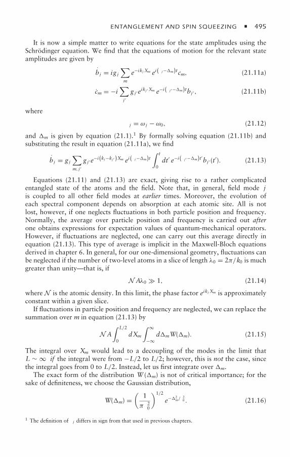
ENTANGLEMENT AND SPIN SQUEEZING 495
It is now a simple matter to write equations for the state amplitudes using theSchrödinger equation. We find that the equations of motion for the relevant stateamplitudes are given by
b j = ig j∑m
e−ikj Xm ei(δ j−m)tcm, (21.11a)
cm = −i∑j ′g j ′eikj ′ Xm e−i(δ j ′ −m)tbj ′ , (21.11b)
where
δ j = ω j − ω0, (21.12)
and m is given by equation (21.1).1 By formally solving equation (21.11b) andsubstituting the result in equation (21.11a), we find
b j = g j∑m, j ′
g j ′e−i(kj−kj ′)Xm ei(δ j−m)t∫ t
0dt′ e−i(δ j ′−m)t′bj ′ (t′). (21.13)
Equations (21.11) and (21.13) are exact, giving rise to a rather complicatedentangled state of the atoms and the field. Note that, in general, field mode jis coupled to all other field modes at earlier times. Moreover, the evolution ofeach spectral component depends on absorption at each atomic site. All is notlost, however, if one neglects fluctuations in both particle position and frequency.Normally, the average over particle position and frequency is carried out afterone obtains expressions for expectation values of quantum-mechanical operators.However, if fluctuations are neglected, one can carry out this average directly inequation (21.13). This type of average is implicit in the Maxwell-Bloch equationsderived in chapter 6. In general, for our one-dimensional geometry, fluctuations canbe neglected if the number of two-level atoms in a slice of length λ0 = 2π/k0 is muchgreater than unity—that is, if
N Aλ0 1, (21.14)
where N is the atomic density. In this limit, the phase factor eikj Xm is approximatelyconstant within a given slice.
If fluctuations in particle position and frequency are neglected, we can replace thesummation over m in equation (21.13) by
N A∫ L/2
0dXm
∫ ∞
−∞dmW(m). (21.15)
The integral over Xm would lead to a decoupling of the modes in the limit thatL ∼ ∞ if the integral were from −L/2 to L/2; however, this is not the case, sincethe integral goes from 0 to L/2. Instead, let us first integrate over m.
The exact form of the distribution W (m) is not of critical importance; for thesake of definiteness, we choose the Gaussian distribution,
W(m) =(
1πδ20
)1/2
e−2m/δ
20 . (21.16)
1 The definition of δ j differs in sign from that used in previous chapters.
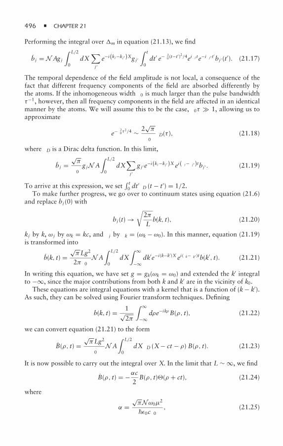
496 CHAPTER 21
Performing the integral over m in equation (21.13), we find
b j = N Agj
∫ L/2
0dX
∑j ′e−i(kj−kj ′)Xg j ′
∫ t
0dt′ e−δ20 (t−t′)2/4eiδ j te−iδ j ′ t′bj ′ (t′). (21.17)
The temporal dependence of the field amplitude is not local, a consequence of thefact that different frequency components of the field are absorbed differently bythe atoms. If the inhomogeneous width δ0 is much larger than the pulse bandwidthτ−1, however, then all frequency components in the field are affected in an identicalmanner by the atoms. We will assume this to be the case, δ0τ 1, allowing us toapproximate
e−δ20τ 2/4 ∼ 2√π
δ0δD(τ ), (21.18)
where δD is a Dirac delta function. In this limit,
b j =√π
δ0g jN A
∫ L/2
0dX
∑j ′g j ′e−i(kj−kj ′)X ei(δ j−δ j ′)tbj ′ . (21.19)
To arrive at this expression, we set∫ t0 dt
′δD (t − t′) = 1/2.To make further progress, we go over to continuum states using equation (21.6)
and replace bj (0) with
bj (t) →√
2πLb(k, t), (21.20)
kj by k, ω j by ωk = kc, and δ j by δk = (ωk − ω0). In this manner, equation (21.19)is transformed into
b(k, t) =√πLg2
2πδ0N A
∫ L/2
0dX
∫ ∞
−∞dk′e−i(k−k′)X ei(δk−δk′ )tb(k′, t). (21.21)
In writing this equation, we have set g = gk(ωk = ω0) and extended the k′ integralto −∞, since the major contributions from both k and k′ are in the vicinity of k0.
These equations are integral equations with a kernel that is a function of (k− k′).As such, they can be solved using Fourier transform techniques. Defining
b(k, t) = 1√2π
∫ ∞
−∞dρe−ikρB(ρ, t), (21.22)
we can convert equation (21.21) to the form
B(ρ, t) =√πLg2
δ0N A
∫ L/2
0dXδD (X− ct − ρ) B(ρ, t). (21.23)
It is now possible to carry out the integral over X. In the limit that L ∼ ∞, we find
B(ρ, t) = −αc2B(ρ, t)(ρ + ct), (21.24)
where
α =√πNω0µ
2
ε0cδ0, (21.25)
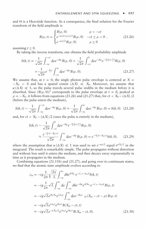
ENTANGLEMENT AND SPIN SQUEEZING 497
and is a Heaviside function. As a consequence, the final solution for the Fouriertransform of the field amplitude is
B(ρ, t) =
⎧⎪⎨⎪⎩B(ρ,0) ρ < −cte−αc(t+ρ/c)/2B(ρ,0) −ct ≤ ρ < 0
e−αct/2B(ρ,0) ρ ≥ 0
, (21.26)
assuming t ≥ 0.By taking the inverse transform, one obtains the field probability amplitude
b(k, t) = 1√2π
∫ −ct
−∞dρe−ikρB(ρ,0) + 1√
2π
∫ 0
−ctdρe−ikρe− αc
2 (t+ ρ
c )B(ρ,0)
+ 1√2π
e− αc2 t∫ ∞
−ctdρe−ikρB(ρ,0). (21.27)
We assume that, at t = 0, the single photon pulse envelope is centered at X =−X0 < 0 and has a spatial extent (X) X0. Moreover, we assume thatα (X) 1, so the pulse travels several pulse widths in the medium before it isabsorbed. Since |B(ρ,0)|2 corresponds to the pulse envelope at t = 0, peaked atρ = −X0, it follows from equations (21.26) and (21.27) that, for ct < X0 − (X) /2(before the pulse enters the medium),
b(k, t) ∼ 1√2π
∫ −ct
−∞dρe−ikρB(ρ,0) ≈ 1√
2π
∫ ∞
−∞dρe−ikρB(ρ,0) = b(k,0) (21.28)
and, for ct > X0 − (X) /2 (once the pulse is entirely in the medium),
b(k, t) ∼ 1√2π
∫ 0
−ctdρe−ikρe− αc
2 (t+ ρ
c )B(ρ,0)
≈ e− αc2 (t−X0/c)
√2π
∫ ∞
−∞dρe−ikρB(ρ,0) = e− αc
2 (t−X0/c)b(k,0), (21.29)
where the assumption that α (X) 1 was used to set e−αρ/2 equal eαX0/2 in theintegrand. The result is remarkably simple. The pulse propagates without distortionand without loss until it enters the medium, and then decays away exponentially intime as it propagates in the medium.
Combining equations (21.11b) and (21.27), and going over to continuum states,we find that the atomic state amplitude evolves according to
cm = −ig L2π
√2πL
∫ ∞
−∞dkeikXm e−i(δk−m)tb(k, t)
= −ig 12π
√L∫ ∞
−∞dρ
∫ ∞
−∞dke−ikρeikXm e−i(δk−m)t B(ρ, t)
= −ig√Leik0Xmeimt
∫ ∞
−∞dρe−ik0ρδD (Xm − ct − ρ) B(ρ, t)
= −ig√Leimteik0ct B(Xm − ct, t)
≈ −ig√Le−αXm/2eimteik0ct B(Xm − ct,0), (21.30)
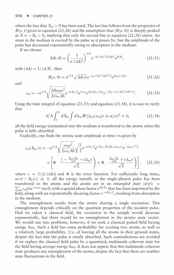
498 CHAPTER 21
where the fact that Xm > 0 has been used. The last line follows from the properties ofB(ρ, t) given in equation (21.26) and the assumption that |B(ρ,0)| is sharply peakedat X = −X0 < 0, implying that only the second line in equation (21.26) enters. Anatom in the medium is excited by the pulse as it passes by, but the amplitude of thepulse has decreased exponentially owing to absorption in the medium.
If we choose
b(k,0) =(
1
π (k)2
)1/4
e−(k−k0)2/2(k)2eikX0 , (21.31)
with (k) = 1/ (X) , then
B(ρ,0) = π1/4√k/πe−(ρ+X0)2(k)2/2eik0(ρ+X0) (21.32)
and
cm = −π1/4
√kω0µ2
2πε0Ae−αXm/2eimteik0(Xm+X0)e−(Xm−ct+X0)2(k)2/2. (21.33)
Using the time integral of equation (21.33) and equation (21.18), it is easy to verifythat
N A∫ ∞
0dXm
∫dmW (m) |cm(t α/c)|2 = 1; (21.34)
all the field energy transmitted into the medium is transferred to the atoms when thepulse is fully absorbed.
Explicitly, one finds the atomic state amplitude at time t is given by
cm(Xm, t) = −π1/4
√ω0µ
2
2cε0A
√τ
2e−αXm/2ei(Xm+X0)(k0+m/c)e−(mτ )2/2
×[
(tτ
− Xm+X0X − imτ√
2
)+
(Xm+X0X + imτ√
2
)], (21.35)
where τ = 1/ [c (k)] and is the error function. For sufficiently long times,αc (t − X0/c) 1, all the energy initially in the single-photon pulse has beentransferred to the atoms and the atoms are in an entangled state |ψ(t)〉 =∑
m cm(t)e−iωmt |m; 0〉 with a spatial phase factor eik0Xm that has been imprinted by the
field, along with an exponentially decaying factor e−αXm/2, resulting from absorptionin the medium.
The entanglement results from the atoms sharing a single excitation. Thisentanglement depends critically on the quantum properties of the incident pulse.Had we taken a classical field, the excitation in the sample would decreaseexponentially, but there would be no entanglement in the atomic state vector.We would run into problems, however, if we took a classical pulsed field havingenergy ω0. Such a field has some probability for exciting two atoms, as well asa relatively large probability, 1/e, of leaving all the atoms in their ground states,despite the fact that the pulse is totally absorbed. Such contradictions are avoidedif we replace the classical field pulse by a quantized, multimode coherent state forthe field having average energy ω0. It does not appear that this multimode coherentstate produces any entanglement of the atoms, despite the fact that there are numberstate fluctuations in the field.
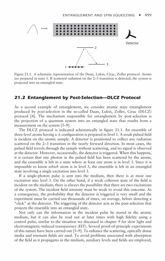
ENTANGLEMENT AND SPIN SQUEEZING 499
3
2Detector
1
Figure 21.1. A schematic representation of the Duan, Lukin, Cirac, Zoller protocol. Atomsare prepared in state 1. If scattered radiation on the 2–3 transition is detected, the system isprojected into an entangled state.
21.2 Entanglement by Post-Selection—DLCZ Protocol
As a second example of entanglement, we consider atomic state entanglementproduced by post-selection in the so-called Duan, Lukin, Zoller, Cirac (DLCZ)protocol [4]. The mechanism responsible for entanglement by post-selection isthe projection of a quantum system into an entangled state that results from ameasurement on the system [5–9].
The DLCZ protocol is indicated schematically in figure 21.1. An ensemble ofthree-level atoms having a configuration is prepared in level 1. Aweak pulsed fieldis incident on the atomic sample. A detector is positioned to collect any radiationscattered on the 2–3 transition in the nearly forward direction. In most cases, thepulsed field travels through the sample without scattering, and no signal is observedat the detector. However, occasionally, the detector is triggered. When this happens,it is certain that one photon in the pulsed field has been scattered by the atoms,and the ensemble is left in a state where at least one atom is in level 3. Since it isimpossible to know which atom is in level 3, the ensemble is left in an entangledstate involving a single excitation into level 3.
If a single-photon pulse is sent into the medium, then there is at most oneexcitation into level 3. On the other hand, if a weak coherent state of the field isincident on the medium, there is always the possibility that there are two excitationsof the system. The incident field intensity must be weak to avoid this outcome. Asa consequence, the probability that the detector is triggered is very small and theexperiment must be carried out thousands of times, on average, before detecting a“click” at the detector. The triggering of the detector acts as the post-selection thatprojects the ensemble into an entangled state.
Not only can the information in the incident pulse be stored in the atomicmedium, but it can also be read out at later times with high fidelity using acontrol pulse, similar to the situation we discussed in chapter 9 for slow light andelectromagnetic-induced transparency (EIT). Several proof-of-principle experimentsof this nature have been carried out [5–9]. To enhance the scattering, optically densemedia and resonant fields are used. To avoid problems associated with absorptionof the field as it propagates in the medium, auxiliary levels and fields are employed,
500 CHAPTER 21
allowing the signal field to propagate without loss owing to an EIT window that iscreated for the fields [10–12].
21.3 Spin Squeezing
As a third example of entanglement, we consider the transfer of entanglement froma quantized cavity field state to the quantum state of a pair of atoms [13].
21.3.1 General Considerations
In a Ramsey fringe experiment, one measures the upper-state population as afunction of atom–field detuning. This is the basic type of measurement needed foroptical clocks to determine the frequency of a transition. The precision of sucha measurement, as well as its accuracy, is of critical importance in metrology.Quantum fluctuations evidently play a role in the precision that can be achieved.
For a single atom, a quantum measurement of the excited-state population yieldseither a 1 (if the atom is measured in its excited state |2〉) or a 0 (if the atom isnot measured in its excited state |2〉). In an ensemble of N atoms, excited in thesame manner by the fields giving rise to the Ramsey fringe signal, one measures anexcited-state population equal to N22, on average. However, owing to quantumfluctuations in the measurement process, there is usually an uncertainty of order(N22)1/2 associated with the measurement referred to as the standard quantum limit(SQL). Since the precision of clock measurements is limited by this factor, there hasbeen considerable interest is determining whether these fluctuations can be reducedby spin squeezing [14–18], the matter analogue of optical squeezing. An excellentintroduction to this topic is given in an article by Wineland et al. [19]. Here, we givea very brief discussion of spin squeezing.
We have seen already that the state of a two-level quantum system can berepresented in terms of the Pauli matrices. That is, the operator for a two-level atom,in the field interaction representation, can be written as
s = sxi + syj+szk, (21.36)
where the operators
sz = (|2〉〈2| − |1〉〈1|)/2, (21.37a)
s+ = |2〉 〈1|, s− = |1〉 〈2|, (21.37b)
sx = (s+ + s−)/2, sy = (s+ − s−)/2i, (21.37c)
are closely related to the Pauli spin matrices. Suppose that we choose our coordinatesystem with 〈s〉 along the z axis, such that 〈sx〉 = 〈sy〉 = 0. In that case, the quantumfluctuations in the measurement of 〈s〉 occur in the xy plane, with⟨
s2x⟩ = ⟨
s2y⟩ = 1/4. (21.38)
There can be no spin squeezing for a single atom, since both the 〈s2x〉 and 〈s2y〉variances are constant.
ENTANGLEMENT AND SPIN SQUEEZING 501
If we now consider N atoms interacting uniformly with the external fields, wecan define collective operators
Sα =N∑j=1
s jα, α = x, y, z,+,−. (21.39)
It is an easy matter to show that these collective operators obey the same com-mutation relations as the single-atom operators,[
Sx, Sy] = i Sz,
[Sy, Sz
] = i Sx, [Sz, Sx] = i Sy, (21.40)
but that the product of collective operators does not obey the same type ofrelationship that holds for the single-atom operators. That is, while s2x = 1/4,
S2x =N∑
i, j=1
sixsjx =
N∑i=1
(six)2 +
N∑i, j =i
sixsjx
= N/4 +N∑
i, j =isixs
jx. (21.41)
Imagine that the atoms have been prepared with all the spins “down.” Thisrepresents a product state for all the atoms with 〈Sz〉 = −N/2, 〈Sx〉 = 〈Sy〉 = 0,and
|〈S〉| =√
〈Sx〉2 + 〈Sy〉2+〈Sz〉2 = N/2. (21.42)
Such a state is referred to as a coherent spin state [20]. It is convenient to use angularmomentum notation to label the N-atom states. The states can be labeled by thetotal angular momentum S and the z component of angular momentum Sz quantumnumbers. In coupling N spins, one finds that S can vary from 0 (or 1/2 if N is odd)to N/2. Clearly, the coherent state has maximal S = N/2, since all the spins arealigned.
In a coherent state, 〈Sx〉 = 〈Sy〉 = 0, and the variance of Sx is
⟨S2x⟩ = 1
4
⟨(S+ + S−)2
⟩
= 14
⟨N2,−N
2
∣∣∣∣ (S2+)+ (S2−)+ S+S− + S−S+
∣∣∣∣N2 ,−N2
⟩
= 14
⟨N2,−N
2
∣∣∣∣ S−S+
∣∣∣∣N2 ,−N2
⟩= N/4, (21.43)
where we have used the relation
S± |S,m〉 =√
(S ∓m) (S ±m+ 1) |S,m± 1〉 . (21.44)
Similarly, 〈S2y〉 = N/4. We can define a parameter
ξx =√N√⟨
S2x⟩
|〈S〉| , (21.45)
502 CHAPTER 21
which is a measure of the precision. A value of ξx = 1 corresponds to the SQL. If wecan find a spin component perpendicular to the direction of 〈S〉 that is less than thisvalue, the state is said to be spin-squeezed.
To determine the conditions needed to generate spin squeezing, we start from anaverage spin aligned along the z axis, and use the fact that SxSy ≥ |〈Sz〉| /2 towrite equation (21.45) as
ξx =√NSx/| 〈Sz〉 | ≥
√N/
(2Sy
) =⎡⎣1 + 4
N
N∑j, j ′ = j
⟨S( j)y S( j
′)y
⟩⎤⎦−1/2
. (21.46)
For correlated states, the sum can be positive and one cannot rule out the possibilitythat ξx < 1. On the other hand, for uncorrelated states, using the fact that 〈Sy〉2 = 0,it follows that
1 + 4N
N∑j, j ′ = j
⟨S( j)y S( j
′)y
⟩= 1 − 4
N
N∑j
⟨S( j)y
⟩2. (21.47)
As a consequence, ξx ≥ 1, and there is no spin squeezing for unentangled states.We are led to the important conclusion that entanglement is necessary for spinsqueezing. An entangled state does not necessarily lead to spin squeezing, but spinsqueezing cannot occur unless there is entanglement.
You might think that, just as in the optical case, it is possible to squeeze onecomponent of the spin to an arbitrarily small value. However, this is not the case.Since Sy ≤ N/2, it follows from equation (21.46) that the minimum value of ξxthat can be reached is 1/
√N, a value referred to as the Heisenberg limit, since it is a
limit imposed by the Heisenberg uncertainty relation.For N= 3 (S = 3/2), an example of a squeezed state is
|ψ〉 = 0.935 |3/2,3/2〉 + 0.354|3/2,−1/2〉, (21.48)
for which ξx = 0.76, not quite at the Heisenberg limit of ξx = 1/√3 = 0.577. For
N= 2 (S = 1), the state
|ψ〉 = 1√2 cosh(2θ )
(e−θ |1,1〉 + eθ |1,−1〉), (21.49)
approaches the Heisenberg limit as θ ∼ 0 [21].To construct spin-squeezed states, one has essentially two options to produce
the needed entanglement. One can use interactions between atoms to provide theentanglement, or couple the atoms to a quantized state of the radiation field andtransfer the quantum properties of the field to the atoms. We look at the latter ofthese possibilities [13].
21.3.2 Spin Squeezing Using a Coherent Cavity Field
In dipole approximation and RWA, the Hamiltonian for an ensemble of two-levelatoms (lower state |1〉, upper state |2〉, transition frequency ω0) interacting with aresonant cavity field having frequency ω = ω0 is
H = ωSz + ωa†a + g(S+a + S−a†), (21.50)
ENTANGLEMENT AND SPIN SQUEEZING 503
where a and a† are annihilation and creation operators for the field, and g isa coupling constant (assumed to be real). Constants of the motion are S2 =S2x + S2y + S2z and
(Sz + a†a
). The Hamiltonian (21.50) is referred to as the Tavis-
Cummings Hamiltonian [22]. If, initially, all spins are in their lower energy state,then 〈Sz + a†a〉 = S(S + 1) + n0, where S = N/2, and n0 is the average photonnumber in the initial field. Since S = N/2, states of the atom plus field can belabeled by |Sz,n〉, with −S ≤ Sz ≤ S.
We note two general conclusions that are valid for arbitrary N. First, if we wereto replace the cavity field by a classical field, the Hamiltonian would be transformedinto
Hclass =∑j
ωS( j)z + g′[S( j)+ e−iωt + S( j)− eiωt]
, (21.51)
where g′ is a constant. Since the Hamiltonian is now a sum of Hamiltonians for theindividual atoms, the wave function is a direct product of the wave functions of theindividual atoms. As a consequence, there is no entanglement and no spin squeezingfor a classical field. Second, if the initial state of the field is a Fock state, althoughthere is entanglement between the atoms and the field, there is no spin squeezing.There is no spin squeezing unless the initial state of the field has coherence betweenat least two states differing in n by 2.
It is convenient to carry out the calculations in an interaction representation withthe wave function expressed as
|ψ(t)〉 =N/2∑
m=−N/2
∞∑k=0
cmk(t) e−iω(m+k)t|m,k〉, (21.52)
where m labels the value of Sz and k labels the number of photons in the cavity field.In this representation, the Hamiltonian governing the time evolution of the cmk(t) isgiven by
H = g(S+a + S−a†). (21.53)
We consider only the two-atom case, N = 2, S = 1. For other N, seereference [13]. If the spins are all in their lower energy state at t = 0, the initialwave function is
|ψ(0)〉 =∞∑k=0
ck| − 1,k〉, (21.54)
where the ck are the initial state amplitudes for the field. Solving the time-dependentSchrödinger equation with initial condition (21.54), we find
c−1,k(t) = 1(2k− 1)
[k− 1 + kcos(
√4k− 2gt)
]ck, (21.55a)
c0,k(t) = −i√
k+ 12k+ 1
sin(√4k+ 2gt)ck+1, (21.55b)
c1,k(t) =√
(k+ 1) (k+ 1)2k+ 3
[−1 + cos(
√4k+ 6gt)
]ck+2. (21.55c)
These state amplitudes can be used to calculate all expectation values of the spinoperators.
504 CHAPTER 21
If the initial state of the cavity field is a coherent state, then
ck = αke−|α|2/2/√k!, (21.56)
and the average number, n0, of photons in the field is given by n0 = |α|2. Forsimplicity, we take α to be real. We limit our discussion to a weak coherent state ofthe field, |α|2 1.
Keeping terms to order α2, we find from equations (21.55) and (21.56) that theonly state amplitudes of importance are
c−1,0(t) = (1 − α2/2), (21.57a)
c−1,1(t) = α cos(√2gt), (21.57b)
c−1,2(t) = α2
3√2
[1 + 2 cos(
√6gt)
], (21.57c)
c0,0(t) = −iα sin(√2gt), (21.57d)
c0,1(t) = − iα2√3sin(
√6gt), (21.57e)
c1,0(t) = −α2
3
[1 − cos(
√6gt)
]. (21.57f)
Using equations (21.52) and (21.44), with S = 1 (N = 2), and the fact thatSz |S,m〉 = m |S,m〉, we find that the spin components’ expectation values are
〈Sx〉 = 0,⟨Sy⟩ =
√2α sin(
√2gt), (21.58a)
〈Sz〉 = −[1 − α2 sin2(
√2gt)
]. (21.58b)
We need to calculate the spin variances in a plane perpendicular to 〈S〉. Themotion of the average value for the spin vector operator is in the yz plane, withthe length of the vector always equal to unity, to order α2. Since 〈Sx〉 = 0, theplane in which we look for spin squeezing is the one defined by the x axis and anaxis orthogonal to both x and the instantaneous direction of the spin. Making anappropriate rotation in the yz plane to define a y′ axis perpendicular to 〈S〉 andx, and afterward choosing an arbitrary direction defined by an angle φ in this plane(see figure 21.2), we find that ξφ minξx, ξy′ , which implies that the best squeezingis to be found in either the x or y′ directions. The analytic expressions for ξx, ξy′ ,obtained using equations (21.45) and (21.57) are
ξx =√2Sx|〈S〉| 1 + α2
[12sin2(
√2gt) − 2
3sin2(
√6gt/2)
], (21.59a)
ξy′ =√2Sy′
|〈S〉| 1 + α2[−12sin2(
√2gt) + 2
3sin2(
√6gt/2)
]. (21.59b)
The lowest possible value for the squeezing occurs in the x direction and is equal to
ξmin = 1 − 23α2 (21.60)
at a time when sin(√2gt) = 0 and cos(
√6gt) = −1.
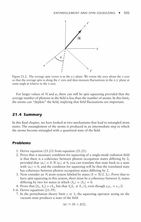
ENTANGLEMENT AND SPIN SQUEEZING 505
zz’
y’
φ
y
x
S
Figure 21.2. The average spin vector is in the y-z plane. We rotate the axes about the x axisso that the average spin is along the z′ axis and then measure fluctuations in the x-y′ plane atsome angle φ relative to the x axis.
For larger values of N and α, there can still be spin squeezing provided that theaverage number of photons in the field is less than the number of atoms. In this limit,the atoms can “deplete” the field, implying that field fluctuations are important.
21.4 Summary
In this final chapter, we have looked at two mechanisms that lead to entangled atomstates. The entanglement of the atoms is produced in an intermediate step in whichthe atoms become entangled with a quantized state of the field.
Problems
1. Derive equation (21.23) from equation (21.21).2. Prove that a necessary condition for squeezing of a single-mode radiation field
is that there is a coherence between photon occupation states differing by 2,provided that 〈a1〉 = 0. If 〈a1〉 = 0, you can translate that state back to a statewith 〈a1〉 = 0, and the condition for squeezing will be that the translated statehas coherence between photon occupation states differing by 2.
3. Now consider an N atom system labeled by states |S = N/2, Sz〉. Prove that tohave spin squeezing in this system, there must be a coherence between Sz statesdiffering by two for states in which 〈Sx〉 = 〈Sy〉 = 0.
4. Prove that [Sx, Sy] = i Sz, but that SzS+ = S+/2, even though szs+ = s+/2.5–6. Derive equations (21.59).
7. In the perturbation theory limit z 1, the squeezing operator acting on thevacuum state produces a state of the field
|ψ〉 ≈ |0〉 + β|2〉,

506 CHAPTER 21
where β = −z/√2. Assuming this to be the cavity field with z real, calculate thespin squeezing that this cavity field produces in a two-atom system. Althoughspin-squeezed fields transfer squeezing to the atoms, they cannot produce statesat the Heisenberg limit [13].
8. Consider two, noninteracting, two-level atoms driven by the same atom–fieldinteraction. The atoms start in state |11〉, and the field only couples states |11〉,(|12〉 + |21〉)/√2, and |22〉, since
〈11|V(|12〉 − |21〉)/√2 = (〈11|V|12〉 − 〈11|V|21〉)/
√2 = 0,
because the interaction is the same for both atoms. Thus, it would appear thata weak incident field pulse that is resonant with the 1–2 transition in eachatom excites only the entangled state (|12〉 + |21〉)/√2. Prove that this is thewrong conclusion—there is no entanglement following the pulse.
9. Now consider an additional atom–atom interaction term in problem 8 thatshifts level |22〉 by frequency . Show that in this case, it is possible to createentanglement, since the atom can be blockaded in state (|12〉+|21〉)/√2. Whatare the conditions on the pulse width to produce this entanglement?
References
[1] A. E. Kozhekin, K. Mølmer, and E. S. Polzik, Quantum memory for light, PhysicalReview A 62, 033809, 1–5 (2000).
[2] S. A. Moiseev and S. Kröll, Complete reconstruction of the quantum state of a single-photon wave packet absorbed by a Doppler-broadenened transition, Physical ReviewLetters 87, 173601, 1–4 (2001).
[3] P. R. Berman and J.-L. Legouët,Quantum information storage: a Schrödinger equationapproach, Physical Review A 79, 042314, 1–13 (2009).
[4] L.-M. Duan, M. D. Lukin, J. I. Cirac, and P. Zoller, Long-distance quantum commu-nication with atomic ensembles and linear optics, Nature 414, 413–418 (2001).
[5] A. Kuzmich, W. P. Bowen, A. D. Boozer, A. Boca, C. W. Chou, L.-M. Duan, and H. J.Kimble, Generation of nonclassical photon pairs for scalable quantum communicationwith atomic ensembles, Nature 423, 731–734 (2003).
[6] B. Julsgaard, J. Sherson, J. I. Cirac, J. Fiurášek, and E. S. Polzik, Experimentaldemonstration of quantum memory for light, Nature 432, 482–486 (2004).
[7] C. W. Chou, S. Polyakov, A. Kuzmich, and H. J. Kimble, Single photon generationfrom stored excitation in an atomic ensemble, Physical Review Letters 92, 213601, 1–4(2004).
[8] C. W. Chou, H. de Riedmatten, D. Felinto, S. V. Polyakov, S. J. van Enk, andH. J. Kimble, Measurement-induced entanglement for excitation stored in remoteatomic ensembles, Nature 438, 828–832 (2005).
[9] R. Zhao, Y. O. Dudin, C. J. Campbell, D. N. Matsukevich, T.A.B. Kennedy, A.Kuzmich, and S. D. Jenkins, Long-lived quantum memory, Nature Physics 5, 100–104(2008).
[10] D. A. Braje, V. Balic, S. Goda, G. Y. Yin, and S. E. Harris, Frequency mixing usingelectromagnetically induced transparency in cold atoms, Physical Review Letters 93,183601, 1–4 (2004).
ENTANGLEMENT AND SPIN SQUEEZING 507
[11] T. Chanelière, D. N. Matsukevich, S. D. Jenkins, S.-Y. Lan, T.A.B. Kennedy, andA. Kuzmich, Storage and retrieval of single photons transmitted between remotequantum memories, Nature 438, 833–836 (2005).
[12] D. N. Matsukevich, T. Chanelière, M. Bhattacharya, S.-Y. Lan, S. D. Jenkins,T.A.B. Kennedy, and A. Kuzmich, Entanglement of a photon and a collective excitation,Physical Review Letters 95, 040405, 1–4 (2005).
[13] C. Genes, P. R. Berman, and A. Rojo, Spin squeezing via atom-cavity field coupling,Physical Review A 68, 043809, 1–10 (2003).
[14] J. M. Radcliffe, Some properties of coherent spin states, Journal of Physics A 4,313–323 (1971).
[15] B. Yurke, S. L. McCall, and J. R. Klauder, SU(2) and SU(3) interferometers, PhysicalReview A 33, 4033–4054 (1986).
[16] D. J. Wineland, J. J. Bollinger, W. M. Itano, F. L. Moore, and D. J. Heinzen,Spin squeezing and reduced quantum noise in spectroscopy, Physical Review A 46,R6797–R6800 (1992).
[17] M. Kitagawa and M. Ueda, Squeezed spin states, Physical Review A 47, 5138–5143(1993).
[18] G. S. Agarwal and R. R. Puri, Atomic states with spectroscopic squeezing, PhysicalReview A 49, 4968–4971 (1994).
[19] D. J. Wineland, J. J. Bollinger, W. M. Itano, and D. J. Heinzen, Squeezed atomic statesand projection noise in spectroscopy, Physical Review A 50, 67–88 (1994).
[20] F. T. Arecchi, E. Courtens, R. Gilmore, and H. Thomas, Atomic coherent states inquantum optics, Physical Review A 6, 2211–2237 (1994).
[21] M. A. Rashid, The intelligent states. I. Group-theoretic study and the computation ofmatrix elements; The intelligent states. II. The computation of the Clebsch–Gordancoefficients, Journal of Mathematical Physics 19, 1391–1396; 1397–1402 (1978).
[22] M. Tavis and F. W. Cummings, Exact solution for an N-molecule–radiation-fieldHamiltonian, Physical Review 170, 379–384 (1968).
Bibliography
Some general references on quantum information, including discussions of entanglement, arelisted here:
I. Bengtsson and K. Zyczkowski,Geometry of Quantum States: An Introduction to QuantumEntanglement (Cambridge University Press, Cambridge, UK, 2006).
D. Bouwmeester, A. K. Ekert, and A. Zeilinger, Eds., The Physics of Quantum Information:Quantum Cryptography, Quantum Teleportation, Quantum Computation (Springer-Verlag, Berlin, 2000).
D. Esteve, J.-M. Raimond, and J. Dalibard, Eds., Quantum Entanglement and InformationProcessing, vol. LXXIX Les Houches Summer School 2003 (Elsevier, Amsterdam, 2004).
Z. Ficek and R. Tanas, Entangled states and collective nonclassical effects in two-atomsystems, Physics Reports 372, 369–443 (2002).
R. Horodecki, P. Horodecki, M. Horodecki, and K. Horodecki, Quantum entanglement,Reviews of Modern Physics 81, 865–942 (2009).
M. A. Nielsen and L. Chuang, Quantum Computation and Quantum Information(Cambridge University Press, Cambridge, UK, 2000).

508 CHAPTER 21
Some early experiments on spin squeezing are listed here:
J. Hald, J. L. Sørensen, C. Schori, and E. S. Polzik, Spin squeezed atoms: a macroscopicentangled ensemble created by light, Physical Review Letters 83, 1319–1322 (1999).
A. Kuzmich, N. P. Bigelow, and L. Mandel, Atomic quantum nondemolition measurementsand squeezing, Europhysics Letters 42, 481–486 (1998).
A. Kuzmich and L. Mandel,Quantum nondemolition measurements of collective atomic spin,Physical Review A 60, 2346–2350 (1999).
A. Kuzmich, L. Mandel, and N. P. Bigelow, Generation of spin squeezing via continuousquantum nondemolition measurement, Physical Review Letters 85, 1594–1597 (1999).
A. Kuzmich, K. Mølmer, and E. S. Polzik, Spin squeezing in an ensemble of atoms illuminatedwith squeezed light, Phyical Review Letters 79, 4782–4785 (1997).
V. Meyer, M. A. Rowe, D. Kielpinski, C. A. Sackett, W. M. Itano, C. Monroe, andD. J. Wineland, Experimental demonstration of entanglement-enhanced rotation angleestimation using trapped ions, Physical Review Letters 86, 5870–5873 (2001).
J. L. Sørensen, J. Hald, and E. S. Polzik, Quantum noise of an atomic spin polarizationmeasurement, Physical Review Letters 80, 3487–3490 (1997).
Index
absorption: entanglement by, 493–498;linear, by stationary atoms, 125–128,469–470; in photodetector, 339; asscattering into field modes, 85, 87, 128,469–470; as true absorption, 339, 493.See also scattering into vacuum field
absorption coefficient, 85–87; complex, 126;for moving atoms, 91–92; probe field,148–149, 165, 192; for stationary atoms,85–91, 126
absorption profiles: atomic motion and,91–94; atomic structure and, 85; collisionsand, 78; two-photon, 178. See alsohomogeneous widths; inhomogeneousbroadening; Lorentzian absorption profile
adiabatic approximation, 39–42; for generalmatrix differential equation, 43
adiabatic following, 39–42; Bloch vector in,74; linear pulse propagation and, 128;Maxwell-Bloch equations and, 133; rateequations and, 95, 96; in stimulatedRaman adiabatic passage, 188–191
adiabatic states, and field interactionrepresentation, 37
adiabatic switching, 40, 42; Bloch vector in,74; in stimulated Raman adiabaticpassage, 190
amplitude gratings, 250–254angular momentum: of circularly polarizedradiation, 390–391, 392; coupled tensorbasis and, 393–394; optical pumping and,402; in spontaneous decay, 387, 388, 392
annihilation and creation operators, 280,281–283; coherent states and, 287, 288,289, 290; evolution equation for, 287;phase operators and, 299; quadratureoperators and, 291–293; squeezed statesand, 294–295
anomalous dispersion, 126antibunching of scattered field, 486–487
atom–field Hamiltonian, 7–8, 10–13,360–363
atom–field interaction energy, 101atom focusing, 106, 258–259atomic beams. See atom interferometry;
atom optics; light scattering by stationaryatoms
atomic motion: absorption profile and,91–94; criterion for quantized descriptionof, 115, 248–249; density matrixequations with, 99–101, 163–165;Hamiltonian including, 362; quantizationof, 110–115; in three-level system,163–165. See also classical atomic motion;collisions; inhomogeneous broadening
atom interferometry, 263–274; with classicalatomic motion, 248, 266, 267–268, 272;coherent transients and, 269; withcounterpropagating optical fields,267–274; with microfabricated elements,266; optical analog of, 263–265; opticalRamsey fringes and, 224–225; summaryof, 275. See also interferometers
atom optics, 101–109, 248–263; amplitudegratings in, 250–254; introduction to,101, 248–250; phase gratings in, 254–263
atom trapping, 103–105. See alsomagneto-optical trap (MOT)
Autler-Townes splitting, 172–175
back-scattering term. See grating term, insaturation spectroscopy
basis operator, 9basis vectors, 8–9bath. See perturber bath; thermal bathbeam splitter, 263, 265–266billiard ball echo model, 214binary collision approximation, 78–79bleached medium, 91, 153Bloch equations. See optical Bloch equations
510 INDEX
Bloch-Siegert shifts, 27–28Bloch sphere, 70, 75Bloch vector, 67–75; for constant field and
detuning, 71–73; defined, 67–68; fieldinteraction representation and, 37, 67–68;in free polarization decay, 210, 213;geometric interpretation of, 69–75;interpretation of components, 68; with norelaxation, 70–74; photon echo and, 214;rate equations and, 96; with relaxationincluded, 74–75; summary of, 76–77;with time-dependent detuning, 74; withtime-dependent pseudofield vector, 73–74
bra, 9Bragg limit, 256, 259Bragg resonances, 261, 262–263Bragg scattering, 256, 259–263Bragg spectroscopy, 261–263branching ratio, for spontaneous decay, 387bright state, 195
cascade configuration, 159, 160, 161–162,163; open quantum systems in, 179;probe field absorption for, 165–172, 174;two-photon transitions in, 176–178
Casimir effect, 2, 284cavity field: coherent, spin squeezing with,
502–504; generating number states of,300; in Jaynes-Cummings model, 358,363–370
cavity quantum electrodynamics, 363center-of-mass motion. See atomic motionchirped pulse, adiabatic approximation
with, 40, 42circularly polarized radiation, 386,
389–392; optical pumping with, 403; insub-Doppler cooling, 433, 435, 436
classical atomic motion: atominterferometry in limit of, 248, 266,267–268, 272; criterion for use of, 115
classical field coherence properties, 314;first-order correlation functions, 315–322;second-order correlation functions,322–326
Clebsch-Gordan coefficients, 380, 387, 388,392, 410
closed two-level system, 179coherence (off-diagonal density matrix
element), 68; decay rate of, 67; electricdipole, 126–127; optical pumping and,407, 409; photon echo and, 219; rateequations and, 95
coherence, excited-state, 467–468coherence length, 319, 321–322coherence properties of fields, 312–314.See also correlation functions
coherence term. See grating term, insaturation spectroscopy
coherence time, 319coherent cavity field, with spin squeezing,502–504
coherent population trapping, 436–437coherent spin state, 501coherent-state basis, 289–290, 327,329–330
coherent states of quantized field, 286–291;classical current distribution and,371–372; defining equation for, 288;density matrix of, 327; generation of, 300,371–372; Jaynes-Cummings model and,364–366; with Michelson interferometer,350, 352–353, 354; as minimumuncertainty states, 293; multimode, 332,335; phase operator for, 300; photo-countdistribution, 345; photon number in, 289;properties of, 289–290; quadratureoperators for, 293; second-order coherent,334; as translations of vacuum state,290–291; two-photon, 293–298
coherent transient optical spectroscopy, 206coherent transient phenomena, 206–235;atom interferometry and, 269; basicprinciples of signals in, 206–210; freepolarization decay in, 210–214; frequencycombs and, 225–228; multidimensional,229; optical Ramsey fringes in, 222–225,231–235; photon echo in, 214–219, 248;source-field approach to, 468–469;stimulated photon echo in, 219–222,267–268; transfer matrices in, 229–231
collective decay modes, 460, 461collision dephasing rates, 164, 165, 169collision (pressure) broadening, 3, 89, 93–94collision model, 61–62, 78–80; correlationfunctions for, 317–319, 321, 324–325,333
collisions: amplitude approach and, 57;density matrix and, 58, 61–62, 79–80;photon echo signal and, 219; stimulatedphoton echo signal and, 221–222; inthree-level system, 164, 165
continuity equation, 301; in reciprocalspace, 302
continuous-wave (cw) spectroscopy, 206
INDEX 511
coordinate representation, of center-of-massmotion, 110–112
corkscrew polarization, 414, 431–433;Fokker-Planck equation and, 443–445,448–449
correlation functions for classical fields:first-order, 315–319, 321; higher order,322; second-order, 322–326
correlation functions for quantized fields:first-order, 330–333; second-order,334–336, 346
correlation functions of scattered field,486–487
correlation time: of classical fields, 316, 317,322, 323; of vacuum field, 397
Coulomb gauge, 302, 304; in reciprocalspace, 303
counterpropagating fields: atominterferometry with, 267–274; opticalpumping with, 412–414, 422–423;saturation spectroscopy and, 144–149;sub-Doppler cooling with, 425–433,436–437. See also standing-wave fields
coupled tensor basis, 393–394, 411, 413,414, 417–418
creation operator. See annihilation andcreation operators
current density, 300, 301, 302, 304–305,308
current distribution, and coherent states,371–372
dark optical lattices, 435dark states, 184–188; coherent populationtrapping and, 436; compared to bare-statepicture, 198; friction force and, 199; slowlight and, 192, 194; STIRAP method and,188–191
de Broglie wavelength: atom focusing and,259; Bragg scattering and, 261
density matrix: basic properties of, 58–59;center-of-mass motion and, 110–115;collisions and, 58, 61–62, 79–80; defined,58; for ensemble of atoms, 60, 83–85;field interaction representation and,63–65, 76; for field states, 314, 326–330,332–333, 335; in Heisenbergrepresentation, 359; interactionrepresentation and, 62–63; in irreducibletensor basis, 388–389, 393, 402,409–411, 417–419; irreversible processesand, 75; photodetection and, 343–345;
rationale for, 56–58; reduced, 60–61, 80,314, 458, 459; in rotating-waveapproximation, 59–60, 62–63, 75–78; inSchrödinger representation, 358–359;semiclassical dressed states and, 66–67;for single atom, 56–62; thermal bath and,58, 60–61; time evolution of, 59. See alsoBloch vector
density matrix equations: with atomicmotion, 99–100, 110–115; in irreducibletensor basis, 418–419; for three-levelatom, 163–164, 187; for two-level atom,61–65, 75–76
dephasing decay rate, 67destruction and creation operators. See
annihilation and creation operatorsdetuning, atom-field, 26; absorption
coefficient as function of, 88–89; withatomic motion, 92, 101; time-dependent,36
differential scattering, in sub-Doppler lasercooling, 422, 423–433
diffraction: electromagnetic, 121, 242–246;of matter waves, 251, 252, 253–254;quantum-mechanical, 242, 246–248;summary of, 274–275. See also atomoptics; scattering
diffractive scattering, with photon echotechniques, 219
diffusion, in laser cooling, 108–109,437–438
diffusion coefficient: in Fokker-Planckequation, 438; interferometricmeasurement of, 270; for laser cooling,109; for sub-Doppler cooling, 423, 430,433, 437, 440–442, 444–448
dipole, classical: radiation pattern of, 386,396, 464, 465; scattering by, 477,487
dipole approximation, 7, 11, 361–362;source-field equation and, 461, 464;spontaneous decay and, 377, 379
dipole coherence: power broadening and,91; spontaneous emission field intensityand, 467
dipole moment, vanishing, in spontaneousemission, 382–383, 386
dipole moment matrix element, and Rabifrequency, 7
dipole moment operator, 7–8, 12;macroscopic polarization and,123
512 INDEX
Dirac notation, 8–9dispersion, 126, 130–131; phase matching
and, 154. See also index of refractiondisplacement operator, producing coherent
state, 290–291, 297–298Doppler broadening, 3, 91–94; eliminated in
saturation spectroscopy, 136, 148, 159,165, 172; methods for elimination orreduction of, 93, 178; of stimulatedphoton echo signal, 221; two-photonspectroscopy and, 172, 178. See alsoinhomogeneous broadening
Doppler limit: of laser cooling, 109; insaturation spectroscopy, 145, 148, 149,169–172
Doppler phase, transverse, 256Doppler shifts: in Sagnac interferometer,
263–264; second-order, optical Ramseyfringes and, 235
dressed states. See quantized dressed states;semiclassical dressed states
dressing angle, 67Duan, Lukin, Cirac, Zoller (DLCZ)
protocol, 498–499duty cycle, of amplitude grating, 250
eigenkets, 9, 18; time-dependent, 23, 36elastic scattering, 477, 479, 481, 482, 485,
486, 487, 488electric dipole moment operator. See dipole
moment operatorelectric field amplitude, from Poynting
vector, 6–7electric susceptibility, 121electric susceptibility tensor, 6electromagnetic diffraction, 121,
242–246electromagnetic-induced transparency (EIT),
193, 499energy density, in vacuum field, 281,
283–284, 285ensemble averages, 312–314; of classical
fields, 317, 318, 323–324; of quantizedfields, 332, 335
ensemble of atoms, density matrix for, 60,83–85
entanglement: by absorption, 493–498;introduction to, 492–493; bypost-selection, 498–499; spin squeezingand, 502, 503
ergodic theorem, 312error function, 94
evolution equation: for annihilation andcreation operators, 287; for densitymatrix, 59; for expectation value, 10, 59,359; in Heisenberg representation, 286,359
expectation values: evolution of, 10, 59,359; in Heisenberg representation, 359,453; measurements and, 56, 57, 58; inSchrödinger representation, 453; Wignerfunction and, 114–115
far off-resonance optical trap (FORT),104
field interaction representation, 32–36;Bloch vector and, 37, 67–68; densitymatrix and, 63–65, 76; second definitionof, 36–37, 63, 64; semiclassical dressedstates and, 36–39; summary of, 45–47
field quantization, 280–283, 300–308fine structure constant: atom interferometryand, 265; maximum absorptioncoefficient and, 89–90; spontaneous decayrate and, 380
fine structure states, decay rates of, 382first-order coherent field: classical, 316, 317;quantized, 331, 332; scattered, 486; inYoung’s interferometer, 321
fluctuation dissipation theorem, 458fluctuations: coherent states and, 286, 287,289; Maxwell-Bloch equations and,129–130; Michelson interferometer and,349, 350–355; in photodetection,342–343; in sources of classical fields,314; spin squeezing and, 500; in vacuumfield, 284. See also correlation functions;diffusion, in laser cooling; noise
Fock states. See number states (Fock states)focusing. See atom focusing; self-focusingFokker-Planck equation, 437–440;corkscrew polarization and, 443–445,448–449; crossed-polarized fields and,441–442, 446–448; equilibrium energyand, 445–449
force on atom in optical field, 101–109; offocused plane wave, 101, 103–105; ofplane wave, 101, 102; standing-wave,101, 105–109. See also friction force
four-wave mixing, 140–141, 152, 153–155;source-field approach to, 468–469;squeezed state in, 372
Fraunhofer diffraction, 244, 245–246; ofmatter waves, 251, 252
INDEX 513
free polarization decay (FPD), 210–214,216, 217, 218, 271, 273, 313, 471
free radiation field. See quantized, freeradiation field
frequency: units of, 3. See also transitionfrequencies
frequency beats, 467–468frequency combs, 225–228frequency locking, 148–149frequency window, 192–193Fresnel diffraction, 244, 245, 246; of matterwaves, 251, 252, 253–254
friction coefficient, 108, 429; inFokker-Planck equation, 438
friction force: capture range for, 429; instanding-wave field, 107–108; insub-Doppler cooling, 423–433, 437, 442,444, 445–446, 448; on three-level atom,199
fringe contrast, with Young’s interferometer,320–322
gauge transformation, 301; in reciprocalspace, 303
Gaussian absorption profile, 92–93Gaussian pulse, adiabatic approximationwith, 40, 41
generalized Rabi frequency, 30–31gratings: amplitude, 250–254;microfabricated, 248–253, 266; phase,254–263; polarization, 426–427,429–430; population, 137, 139, 141–146,155
grating term, in saturation spectroscopy,142, 145–146, 148, 149; with solids, 150
gravitational acceleration measurement:with matter-wave interferometer, 274;with Raman echo interferometer,269–270
gray optical lattices, 435ground state repopulation, 387–389
Hamiltonian: atom–field, 7–8, 10–13,360–363; time-dependent, 19–21;time-independent, 17–19
Hanbury Brown and Twiss experiment,325–326
Heisenberg limit, 502Heisenberg representation, 286–287, 358,359–360, 453; atom–field interactions in,454–461; correlation functions and, 330.See also source-field approach
Hermitian operator, 9, 58hole burning, 144–146; with solids, 149homogeneous widths, 3, 92, 94; in free
polarization decay, 210–212. See alsopressure (collision) broadening
hyperbolic secant pulse, 28hyperfine states: decay rates of, 381–382;
radiation pattern and, 392, 394
impact approximation, 79, 318incoherent pumping, 179index of refraction, 6, 26; complex, 121,
128; Kerr effect and, 155, 226; linearabsorption and, 126; Maxwell-Blochequations and, 124, 125, 130–134; pulsepropagation in linear medium and,121–123, 128–129; slow light and,192–193
inelastic spectral components, 478–479,482, 484, 485, 486, 488
inhomogeneous broadening, 3–4; inabsorption by optically dense medium,339, 493; in coherent transientspectroscopy, 206, 217; Dopplerbroadening as (see Doppler broadening);in free polarization decay, 212–214;optical Ramsey fringes and, 224; inperturber bath, 313; in photodetector,339; photon echo and, 216–217; powerbroadening as, 3, 89, 91, 96; transit-timebroadening as, 4, 179
intensity correlations, 322–326interaction representation, 21–23; compared
to other representations, 35–36; densitymatrix and, 62–63, 76; summary of,45–47
interferometers: internal state, 268–270;Mach-Zehnder, 326; Michelson,346–355; moiré, 266; Raman photonecho, 267, 268–270; Sagnac, 263;Talbot-Lau, 266, 273, 275; Young’s,319–322
interferometry. See atom interferometry;optical interferometry
internal state interferometer, 268–270irreducible tensor basis, 388–389, 417–419;
density matrix equations in, 418–419;inverse of, 393; optical pumping and, 402,409–411; polarization and, 417–418
Jaynes-Cummings model, 358, 363–3703-J symbols, 404, 410
514 INDEX
6-J symbols, 388, 4109-J symbols, 410
Kapitza-Dirac scattering, 256Kerr effect, 155, 226ket, 9Kirchhoff-Fresnel diffraction, 319. See also
diffraction
lambda () configuration, 184–199; basicdescription of, 159, 160, 162–163; darkstates of, 184–191, 192, 194, 198, 199,436; effective two-state problem for,196–198; force on an atom in, 199;information storage in, 222, 499;interferometers using, 267–270; openquantum system in, 178; slow light in,191–196; STIRAP method and,188–191; two-photon transitions in,176, 178
Lamb dip, 148–149Lamb shift, 284, 377Landau-Zener formula, 42laser cooling, 105–109. See also
sub-Doppler laser coolinglasers: output field of, 313; power outputs
of, 6–7; tunable types of, 2, 6–7laser spectroscopy, 136, 137. See also
saturation (nonlinear) spectroscopylevel inversion using π pulses, 29–30, 71.See also adiabatic switching
Lévy statistics, 437light scattering by stationary atoms,
474–489; correlation functions for,486–487; dressed states and, 369, 474,483–484; Mollow triplet in, 479–485,486; perturbation theory of, 475–479; inweak fields, 487–488. See also scattering
light shifts, 4; in Bragg spectroscopy,261–262; by cross-polarized fields,433–434; in effective two-state problem,197, 198; by pump field, 143, 433–434,437–438; by standing-wave optical field,106, 255, 256, 261–262; in two-levelsystem, 28; in two-photon spectroscopy,177, 178; in weak field scattering,488
line shifts, 4. See also light shifts; recoil shiftsline widths. See absorption profiles;
homogeneous widths; inhomogeneousbroadening
longitudinal relaxation rate, 206
longitudinal relaxation time, 206; stimulatedphoton echo and, 220, 221
longitudinal vector fields, 303Lorentz force law, 11, 301Lorentz gauge, 301–302; in reciprocal space,303
Lorentzian absorption profile: for movingatoms, 92, 93–94; in saturationspectroscopy, 148; square of, in saturationspectroscopy, 143; for stationary atoms,89; for three-level atoms, 171–172, 174
Lorentzian power spectrum, 319Lorentzian radiation spectrum, 383–384lowering operator, 282
Mach-Zehnder interferometer, 326magneto-optical trap (MOT), 267,270–271, 273
Magnus approximation, 43–45Markov approximation, 318master equation, 62matrix differential equation, 42–45matrix elements, 9; reduced, 380–382matter-wave interferometers, 265–267, 268,270–274
Maxwell-Bloch equations, 123–125;approach to, 120–121; coherent transientsand, 209–210; for index of refractiongreater than unity, 132–134; limitationsof, 129–130; linear absorption and,125–128; probe field absorption and,147–148; slow light and, 192, 196;three-level system and, 165. See alsooptical Bloch equations
Maxwell’s equations: condition formacroscopic description by, 130; with nofree currents or charges, 4–6, 120;plane-wave solutions of, 6; in reciprocalspace, 302, 305; with sources, 300, 302,304–305
measurement: entanglement resulting from,498–499; expectation values and, 56, 57,58; quantum-mechanical problem of,339–340. See also metrology;photodetection; standard quantum limit(SQL)
metrology: frequency combs in, 225; opticalRamsey fringes in, 231, 500
Michelson interferometer, 346–355; classicalfields in, 347–349; correlated signalswith, 350–352; quantized fields in,349–355
INDEX 515
microfabricated gratings: atominterferometers using, 266; scatteringfrom, 248–253
mode-locked laser, frequency combs of,225–228
modulated atomic state polarization, 412,413, 414
moiré interferometer, 266Mollow triplet, 479–482, 486; quantizeddressed-state approach to, 483–484;source-field approach to, 485
momentum exchange, in sub-Doppler lasercooling, 422, 423–433
momentum of field, 282, 301, 305, 307momentum representation, ofcenter-of-mass motion, 112
monochromatic fields, coherence propertiesof, 316–317, 323–324
Monte Carlo technique, for spontaneousemission, 397–399
moving atoms. See atomic motionmultipole decay rate, 388
natural line width, 3, 313noise: in photodetection, 342–343; Young’sinterferometer and, 319, 322. See alsofluctuations
nonlinear spectroscopy. See saturation(nonlinear) spectroscopy
normal dispersion, 126nuclear magnetic resonance (NMR), 210,214; of spin half quantum system, 47–50
number operator, 281, 282, 283; inHeisenberg representation, 459–460; insqueezed state, 298; in two-photoncoherent state, 296
number states (Fock states), 282–283;density matrix and, 327, 328;experimental generation of, 300;Michelson interferometer and, 350; phaseoperators and, 299–300; photo-countdistribution for, 346; quadratureoperators and, 292–293; second-ordercorrelation function for, 334;single-mode, 285–286
number-state squeezing, 350
one-photon state, 2, 284–285open quantum systems, 178–179; coherenttransient signals in, 206, 208–209,229–230; stimulated photon echo signaland, 221–222
operators, 9; in Heisenberg representation,286–287
optical Bloch equations, 69, 76–77;Heisenberg representation and, 456, 458;Maxwell-Bloch equations and, 125;photon echo and, 219; quantum trajectoryapproach and, 399; rate equations and, 96
optical interferometry, 263–265optical lattice potentials, 414–416;
sub-Doppler cooling and, 433, 434, 435optical pumping, 402–414; with
counterpropagating fields, 412–414;introduction to, 402–403; irreducibletensor basis used for, 402, 409–411; lasercooling and, 422–423, 435, 437 (see alsosub-Doppler laser cooling); with multiplefields, 411–414; with single-frequencyfields, 403–411; with weak fields,scattered spectrum in, 487–488; withz-polarized excitation, 407–409
optical pumping rate, 408; for circularlypolarized fields, 432; for crossed-polarizedfields, 414, 428–429
optical Ramsey fringes, 222–225; inspatially separated fields, 231–235
optical theorem, 470overcompleteness of coherent-state
eigenkets, 289–290, 329
parametric down conversion, 372partial decay rates, 164, 381, 382, 387passive mode locking, 226Pauli spin matrices, 25, 47, 500Pendellösung oscillations, 263permeability of free space, 5permittivity of free space, 5perturber bath: coherence and, 313;
collision model with, 78–80phase conjugate geometry, 141, 154phase conjugate signal, 222phase diagram: optical Ramsey fringes and,
223–224, 234–235; for photon echo,214–217; Raman echo interferometerand, 270; with recoil splitting, 234–235;for stimulated photon echo, 220,223–224
phase diffusion model, 319, 321–322,324–325, 333; photon counting and, 343.See also collision model
phase gratings, 254–263phase-interrupting collision model, 80phase locking, 226
516 INDEX
phase matching: coherent transients and,209, 211, 219, 221, 222, 469; four-wavemixing and, 140–141, 154
phase operators, 298–300phase-space distribution function:
Fokker-Planck equation for, 438; Wignerfunction and, 113, 114
photodetection, 339–346; of classical fields,340–343; of quantized fields, 343–346
photon, 2. See also one-photon state; photonstates
photon bunching, 325photon echo, 214–219; as atom
interferometer, 248; stimulated, 219–222photon states, 282–283. See also number
states (Fock states)photon statistics, 314, 327–329plasma dispersion function, 94, 148, 169Poisson distribution of photon number, 289,
327; photodetection and, 342, 343polariton state, 195polarization, circular. See circularly
polarized radiationpolarization, macroscopic: in
Maxwell-Bloch equations, 123–125, 131;in Maxwell’s equations, 5, 6
polarization gradient cooling, 423, 433–435polarization grating, 426–427, 429–430polarization tensor. See coupled tensor basispolarized ground state, 402, 409, 412population gratings, 137, 139; in four-wave
mixing, 155; in two-field case, movingatoms, 144–146; in two-field case,stationary atoms, 141–144
population trapping, coherent, 436–437post-selection, 498–499power-broadened decay rate, 87, 89power broadening, 3, 89, 91; rate equations
and, 96power delivered to medium, 127–128power of coherent transient signal,
209–210; in free polarization decay, 211,213; with photon echo, 217, 218; withstimulated photon echo, 221
power spectrum, of classical field, 315–316,319
Poynting vector, 6–7; absorption coefficientand, 87–89, 90–91
pressure (collision) broadening, 3, 89, 93–94pressure-induced extra resonances, 141probe field. See saturation (nonlinear)
spectroscopy
propagation vector, 6pseudofield vector, 69; active transformationof, 71–72; in free polarization decay, 210;rate equations and, 96
pulse area, 29–30; Bloch vector and, 71; incoherent transient spectroscopy, 207, 208;with phase grating, 257
pulsed fields, and semiclassical dressedstates, 40, 42, 45, 188–191
pulse propagation in linear medium,121–123, 128–129
pump field. See saturation (nonlinear)spectroscopy
quadrature operators, 291–294; variancesof, 295–296, 298
quantization of radiation field: in free space,280–283, 308; with sources, 300–308
quantized, free radiation field: effectiveHamiltonian of, 284; energy density of,281, 283–284, 285; in-phase andout-of-phase components of, 292; phaseoperator for, 298–300; properties of,283–291; quadrature operators for,291–293; single-mode number state of,285–286; single-photon state of, 2,284–285. See also coherent states ofquantized field; quantized fields
quantized dressed states, 358, 367–370; lightscattering spectrum and, 474, 483–484
quantized fields: characterization of, 314;density matrix for, 314, 326–330, 332,335; Hamiltonian for interaction withmatter, 360–362; Jaynes-Cummingsmodel for interaction with matter,363–367. See also quantized, freeradiation field
quantum beats, 467–468quantum collapse and revival, 365–366quantum efficiency of detector, 344, 350,351
quantum electrodynamics, 284; cavity, 363;Lamb shift and, 377
quantum information: dark states and, 184,188; entangled states and, 492, 499;Jaynes-Cummings model and, 363; slowlight and, 194; stimulated photon echosignals and, 222
quantum jump, 397quantum-mechanical diffraction, 242,246–248
quantum optics, 1–2
INDEX 517
quantum regression theorem, 460, 474, 486quasiclassical states. See coherent states ofquantized field
quasi-monochromatic fields, representationsfor, 45. See also specific representations
Rabi flopping, 31Rabi frequency, 3, 7, 25; generalized, 30–31;with quantized coherent state, 364–365
Rabi oscillations, 365–366, 367, 370radiation field. See quantized, free radiationfield
radiation pattern, 382–386, 392–397raising operator, 282Raman-like scattering processes, 488Raman-Nath approximation, 256–259, 260;interferometers using, 265, 268, 271
Raman photon echo interferometer, 267,268–270
Ramsey fringes, 222–225; in spatiallyseparated fields, 231–235
rate equation approximation, 75, 96rate equations, 95–96Rayleigh scattering, 476–477, 488; grayoptical lattices and, 435; Maxwell-Blochequations and, 129–130
reciprocal space, 302–303, 304, 306recoil, in sub-Doppler cooling, 437, 438,439, 447–448
recoil frequency: with amplitude grating,252; defined, 249; interferometry and,267, 270, 274; with phase grating, 256,257, 259, 262–263
recoil shifts, 4; optical Ramsey fringes and,234; Raman echo interferometry and, 270
reduced density matrix, 60–61, 80, 314,458, 459
reduced matrix elements, 380–382relaxation: Bloch vector and, 74–75; withcoherent transient signals (see longitudinalrelaxation time; transverse relaxationtime); in open systems, 179; single-atomdensity matrix and, 61, 63, 64, 66
renormalization, 284, 362, 377repopulation of ground state, 387–389resolution of transition frequencies, 2–4. Seealso homogeneous widths;inhomogeneous broadening
resonance approximation. See rotating-waveapproximation (RWA)
resonance fluorescence spectrum, 460ring laser gyroscope, 263, 264
rotating-wave approximation (RWA),25–28; comparison of representations in,35–36, 45–46; density matrix and, 59–60,62–63, 75–78; in field interactionrepresentation, 33, 34, 35;Jaynes-Cummings model and, 363, 364;for magnetic case, 48; quantized dressedstates in, 358; source-field applicationsand, 466; source-field equation and, 462,463, 464–465; for three-level systems, 160
Sagnac interferometer, 263saturation of two-level atoms: probe
absorption profile and, 148–149; bypump field, 142; by strong field, 87, 91
saturation (nonlinear) spectroscopy, 136,137; collisional energy shifts and, 78; ininhomogeneously broadened solids,149–150; for moving atoms incounterpropagating fields, 144–149; withone strong and one weak field, 151–153;for stationary atoms, 141–144, 151–153;terminology issues with, 141, 151; withthree-level atoms, 159, 165–172;two-photon spectroscopy compared to,178
scalar potential, 301–303, 304; in reciprocalspace, 302–303
scattering: by amplitude gratings, 250–254;entangled state resulting from, 499; byinfinite periodic structure, 253–254; byphase gratings, 254–263; of pump fieldfrom spatial grating, 142, 144; Rayleigh,129–130, 435, 476–477, 488; betweenstanding-wave field components,105–106. See also diffraction; lightscattering by stationary atom
scattering into vacuum field: absorption bystationary atoms as, 85, 87, 91, 128,469–470; diffusion coefficient and, 430,437; in effective two-state problem, 197,198; force on atom resulting from, 101,102, 104; during laser cooling, 108;operator approach to spectrum, 460;optical pumping and, 402, 437; probefield absorption as, 146, 148, 149;Rayleigh, 476; recoil in, 437, 438, 439,447; source-field approach and, 469–470;spontaneous emission and, 483; inthree-level systems, 197, 198, 199; vs. trueabsorption, 339, 493
Schrödinger cat state, 117
518 INDEX
Schrödinger equation, 9, 18, 19Schrödinger representation, 358–359, 362,
453; of density matrix equations, 75; fortwo-level atom, 35, 45, 46–47; vacuumenergy and, 284
second-order coherent field, 322, 323, 334secular approximation: for dressed-state
density matrix elements, 66; Mollowtriplet spectrum and, 481–482, 483, 485
self-energy term, 362self-focusing, 155semiclassical dressed states, 36–39, 45, 46,
47; adiabatic approximation and, 39–42;appropriate applications for, 67;Autler-Townes splitting and, 173–175;density matrix and, 66–67; density matrixequations and, 77; light scatteringspectrum and, 474, 479–482; STIRAPmethod and, 188–191; three-level, 161
semiclassical theories: atom-field Hamil-tonian in, 8; polarization vector in, 120
shadow (classical) region, 244, 245, 246; formatter waves, 251–252, 253
shot noise: Michelson interferometer and,349; in photodetection, 342, 343
single-molecule spectroscopy, 313Sisyphus effect, 423, 433–435slow light, 191–196slowly varying amplitude and phase
approximation (SVAPA), 123–125, 128,130–134
solids: free polarization decay in, 212–214;optical Ramsey fringes in, 223–224;photon echo and, 219; saturationspectroscopy in, 149–150; stimulatedphoton echo in, 221–222
soliton state, 195–196source-field approach, 465–470; to
four-wave mixing, 468–469; to frequencybeats in emission, 467–468; to linearabsorption, 469–470; to Mollow triplet,485; to spontaneous emission, 466–467
source-field equation, 453, 461–465spectral diffusion: photon echo and, 219;
stimulated photon echo and, 221–222spherical polarization components, 394,
403–404, 417, 431. See also coupledtensor basis
spin half quantum system, in magnetic field,47–50
spin matrices, 25, 47, 500spin operator, 47
spin squeezing, 499–505spontaneous emission: average field in, 466;average field intensity in, 466–467;circular polarization and, 386, 389–392;cooperative, 212; decay rate in, 375–382;frequency beats in, 467–468; ground staterepopulation in, 387–389; Mollow tripletand, 483–484; quantum trajectoryapproach to, 397–399; radiation patternin, 382–386, 392–397; sum and differencerepresentation for, 113; in two-level atom,56–57, 61–62
squeezed states, 293–298; defined, 298;experimental generation of, 300;second-order correlation function of, 335;spin-squeezed, 499–505
squeezed vacuum state, 296, 298; generationof, 372; in Michelson interferometer, 354
squeeze operator, 296–298squeezing parameter, 295, 296standard quantum limit (SQL), 294, 296; forMichelson interferometer, 353–354; spinsqueezing and, 500, 501
standing-wave fields: of atom interferometer,265, 266, 270; force on atom in, 101,105–109; optical pumping with, 412–413;optical Ramsey fringes with, 233–234; asphase grating, 254–263. See alsocounterpropagating fields
standing-wave patterns, in sum of N fields,137, 139, 146
state vectors, 9; in Heisenbergrepresentation, 286, 358, 359; inSchrödinger representation, 358–359
stepwise perturbative chain, 166, 167, 168,170
Stern-Gerlach experiment, optical, 116stimulated photon echo, 219–222; atominterferometer based on, 267–268
stimulated Raman adiabatic passage(STIRAP), 188–191
sub-Doppler laser cooling: introduction to,422–423; by momentum exchange anddifferential scattering, 422, 423–433; bySisyphus effect, 423, 433–435. See alsoFokker-Planck equation
sum and difference representation, 113summation convention, 392superradiance, 212SVAPA (slowly varying amplitude and phaseapproximation), 123–125, 128, 130–134
symbols, commonly used, 25, 67
INDEX 519
Talbot effect, 253–254Talbot-Lau interferometers, 266, 273, 275Talbot length, 251; interferometry and, 266,267; with phase grating, 257, 258, 259
Tavis-Cummings Hamiltonian, 502temperature of laser cooling, 109;sub-Doppler, 430, 433, 435
thermal bath, and density matrix, 58, 60–61thermal states: Michelson interferometerand, 350; photo-count distribution, 345,350; of quantized field, 328, 330, 331,332–333, 335, 336
three-level systems: Autler-Townes splittingwith, 172–175; configurations of,159–163; density matrix equations for,163–165; with moving atoms in Dopplerlimit, 169–172; probe field absorptionwith, 165–172; with stationary atoms,169. See also cascade configuration; darkstates; lambda () configuration
time averages, 312–313; of classical fields,314, 315, 317, 323, 324
time-dependent Hamiltonians, 19–21time-dependent spectroscopy, 206time-independent Hamiltonians, 17–19transfer matrices for coherent transients,229–231
transient spectroscopy, 206transition frequencies, 2–4; inelasticscattering and, 478; interactionrepresentation and, 22; optical Ramseyfringes and, 222, 224, 235. See alsoabsorption profiles; homogeneous widths;inhomogeneous broadening
transitions between eigenstates, 20–21, 22transitions in two-level system, 45transit-time broadening, 4, 179transverse Dirac delta function, 304transverse electromagnetic field, 304–308transverse relaxation rate, 206transverse relaxation time, 206; in freepolarization decay, 210, 211, 213; photonecho and, 217, 219; stimulated photonecho and, 220, 221
transverse vector fields, 303–304two-level atom, 23–25; density matrix for,59–60; in N fields, 136–141; as nonlineardevice, 31, 49, 105, 137; spontaneous
decay in, 56–57, 61–62; summary ofrepresentations for, 35–36, 45–47.See also rotating-wave approximation(RWA); saturation of two-level atoms
two-photon spectroscopy, 172, 176–178two-photon state, 331–332; coherent,
295–296, 297–298, 335; in Michelsoninterferometer, 355
two-quantum perturbative chain, 166,167–168, 171
uncertainty diagrams for quadratureoperators, 293–294
unitarity, 375, 384
vacuum field. See quantized, free radiationfield; scattering into vacuum field
vacuum fluctuations, 284vacuum Rabi oscillations, 367, 370vacuum state, 283; coherent, 289;
quadrature operators and, 293, 294;squeezed, 296, 298, 354, 372; translationsof, 290–291, 297
van der Waals forces, 2, 313V configuration, 159, 160, 162–163;
two-photon transitions in, 176vector fields, longitudinal and transverse,
303–304vector potential, 301–308; of free field, 282;
in reciprocal space, 302–303velocity selective coherent population
trapping, 436–437Voigt profile, 92
wave equation, 5, 6, 121wave packets, 110, 111–112, 113;
one-photon, field intensity of, 467Weisskopf-Wigner approximation, 379,
381; ground state repopulation and, 387;Heisenberg representation and, 457, 458,459, 464; light scattering and, 476
Wigner representation, 113–115, 314;sub-Doppler cooling and, 437, 438,439–440
Young’s interferometer, 319–322
Zeeman splitting, 4