Embed Size (px)
Citation preview

1
Principles of Kinetic Analysis for
Condensed-Phase Thermal
Decomposition
Alan K. Burnham
PhD, Physical Chemistry
November, 2011
Revised October, 2014

2
Outline of Presentation
General background on kinetics (pp. 3-15)
Approaches to kinetic analysis (p.16)
• How not to do kinetic analysis (pp. 17-22)
• Simple kinetic analyses and how to pick a reaction
model (pp. 23-34)
• Model fitting by non-linear regression (pp. 35-45)
Examples of Kinetics by Model Fitting (pp. 46-62)

3
Chemical Reactions
All life and many manufacturing processes involve
chemical reactions
• Reactants Products
Chemical reactions proceed at a finite rate
The rate of virtually all chemical reactions varies with
time and temperature
Chemical kinetics describe how chemical reaction rates
vary with time and temperature

4
Why Study Chemical Kinetics?
Understanding reaction characteristics
• Acceleratory
• Deceleratory
Interpolation within the range of experience
• Optimization of chemical and material processes
Extrapolation outside the range of experience
• Lifetime predictions
• Petroleum formation
• Explosions

5
Unimolecular Decomposition
The products can be either more stable or less stable
than the reactants
If the products are more stable, heat is given off
If the products are less stable, heat is absorbed
k
reactant products
k is the reaction rate constant
k has units of reciprocal time
The reaction rate has units of quantity per unit time

6
The Energy Barrier
Ef is the activation energy for the forward reaction
Er is the activation energy for the reverse reaction
Ef - Er is the energy change of the reaction, E
reactants
products reactants
products
Endothermic reactions Exothermic reactions
E positive E negative
Ef
Ef Er Er

7
Unimolecular Reactions
The reaction rate is proportional to how much reactant is present
where dx/dt is the limit when t becomes infinitesimally small (from differential calculus)
x is the amount of the reactant
t is time
k is the rate constant
k has units of reciprocal time for unimolecular reactions
The negative sign means that x decreases with time
kxdt
dx

8
The Arrhenius Law
Empirical relationship from 1889 describing the
temperature dependence of chemical reactions
k = Ae-E/RT
k is the rate constant
A is the pre-exponential factor or frequency factor
(units are reciprocal time for unimolecular reactions)
E is the activation energy
R is the universal gas constant (1.987 cal/molK)
T is the absolute temperature (Kelvins)

9
The Arrhenius Law is Approximate
Gas phase reactions typically have a power temperature
dependence in addition to the exponential dependence to
account for collision frequency
• k = ATbe-E/RT, where b is ranges from 1/2 to 3/2
Transition state theory provides a linear temperature term
• k = (kBT/h)e-E/RT
• kB is Boltzmann’s constant and h is Planck’s constant
The power temperature dependence can be absorbed into
the apparent activation energy with negligible error
[See Burnham and Braun, Energy & Fuels 13, p. 3,1999, for specific examples]

10
Transition State Theory
A hypothetical transition state exists at the maximum
energy in the reaction trajectory
The pre-exponential factor is related to the molecular
vibration frequency of the dissociating bond ~ 1014 Hz
Transition state theory is often invoked under conditions
far beyond its legitimate applicability
Transition state theory has been only marginally useful
for most reactions of practical interest
• An exception is gas phase combustion modeling
• Advances in computation methods are making it useful for
probing mechanisms of complex reactions

11
The Effect of Pressure is Variable
Pressure can either increase or decrease reaction rates,
depending upon circumstances
Increasing pressure for unimolecular decomposition
• can increase rate for simple molecules by increasing energy
redistribution
• can decrease rate for complex molecules by inhibiting dissociation
Increasing pressure for bimolecular reactions
• can increase rate by increasing collision frequency at low densities
• can decrease rate by increasing viscosity and decreasing freedom
to move around at high densities
Reversible reactions in which a gaseous product is formed
from solid decomposition depend upon product pressure

12
The Effect of Pressure Can Reverse
The decomposition of energetic material HMX is
one example of pressure reversal
Increase at
lower pressures
probably due to
autocatalysis
Decrease at
higher pressures
due to some type
of hindrance
Pressure-dependent decomposition kinetics of the energetic material HMX up to 3.6 GPa, E. Glascoe, et al., J. Phys. Chem. A, 113, 13548-55, 2009.

13
Separation of Functional Dependences
It is commonly assumed that the dependences on
conversion, temperature, and pressure can be separated
Functions for f() are commonly tabulated in the thermal
analysis literature
For solid solid + gas, h(P)=1-P/Peq , where P is the
gaseous product partial pressure and Peq is the
equilibrium vapor pressure
)()1()( PhxfTkdt
dx
ICTAC Kinetics Committee recommendations for performing kinetic computations on
thermal analysis data, S. Vyazovkin, et al., Thermochimica Acta 520, 1-19, 2011.
)()()( PhfTkdt
d
where x is the fraction remaining
where α is the fraction reacted

14
Reaction Models Can Be Integrated
Many models can be integrated exactly for isothermal conditions
Models can be integrated approximately for a constant heating rate
• Depends on the well-known temperature integral:
where x = E/RT
• Several hundred papers have addressed the temperature integral and its solution by various approximations
[see, for example, J. H. Flynn, Thermochimica Acta 300, 83-92, 1997]
)(/)(0
fdg
dxxxx
]/)[exp( 2

15
Tabulations Exist For Isothermal Models
S. Vyazovkin and C. A. Wight, Annual Rev. Phys. Chem. 48, 125-49, 1997

16
Two basic approaches to kinetic analysis
Model fitting
• Do some type of numerical comparison of selected
models to determine the best model
Isoconversional fitting
• Assume that the reaction is infinitely sequential, i.e.,
that the same reactions occur at a given extent of
conversion independent of temperature
Both approaches can be used to make predictions
for other thermal histories, including with Kinetics05

17
Model Fitting is Often Done Poorly
Many people have derived kinetics from a single
heating rate experiment
• Most common is to assume a first-order reaction
• Others fitted all the reactions in the previous table
with some approximation to the temperature integral
and assumed that the fit with the lowest regression
residuals was the correct model
These approaches usually give the wrong kinetic
parameters, and sometimes absurdly wrong, so
predictions with the parameters are unreliable

18
One Example of Why Fitting to a Single
Heating Rate Doesn’t Work
Nonlinear regression fits of a first-order
reaction to simulated data at a constant
heating rate for a Gaussian distribution
of activation energies
Apparent activation energy as a
function of the magnitude of the
reactivity distribution—it can be
qualitatively wrong!
R. L. Braun and A. K. Burnham, Energy & Fuels 1, 153-161, 1987

19
Another Example of Why Fitting to a Single
Heating Rate Doesn’t Work
Derived using a generalized Coats-Redfern
Equation:
The correlation coefficient is absolutely useless
for model discernment
RTEERTEARTg /)]/21)(/ln[(]/)(ln[ 2
S. Vyazovkin and C. A. Wight, Annual
Rev. Phys. Chem. 48, 125-49, 1997
20
A and E are Correlated for Various Models
A and Ea compensate for each other at the measurement temperature,
but predictions diverge outside the measurement range
0
10
20
30
0 100 200 300
Activation Energy, kJ/mol
Fre
qu
en
cy
Fa
cto
r, ln
(A/m
in-1
)

21
Data at Different Temperatures Constrain
Possible A-E Pairs and Extrapolations
For a single rate measurement, possible A-E pairs are defined by a
line of infinite length
For measurements at 3 or more temperatures, the range of possible
A-E pairs is defined by an error ellipsoid (narrow in shape)
A-E pairs at the extremes of the error ellipsoid define the plausible
range of the extrapolation
The example at the
right shows the range of
kinetic extrapolations
for natural petroleum
formation based on a
data set measuring the
rate over a time-scale of
up to a few hours
From A. Burnham, presentation at the
AAPG annual meeting, Calgary, June 1992

22
What have we learned?
Single heating-rate kinetic methods don’t work except by
luck—don’t do it!
Improperly derived activation energies can be high or low
from the true value by as much as a factor of five
Even with the wrong model, A and E compensate for
each other to get the average rate constant approximately
right at the measurement temperature
Most compensation law observations are due to
imprecision and bad methodology, and most mechanistic
interpretations are nonsense

23
Back to basics to get it right
First, get accurate data over a range of thermal histories
Next, look at the reaction profile to understand its
characteristics—you can narrow the choices considerably
Reactions can be (1) accelerating, (2) decelerating, or
(3) sigmoidal
Decelerating reactions are the
most common type for fossil fuel
kinetics
Sigmoidal reactions are the
most common type for
decomposition of energetic
materials and crystalline solids

24
Data requirements
The data should cover as wide a temperature range as possible, as that helps constrain the model parameters
• Enough temperature change to cause a tenfold change in reaction rate for isothermal experiments (~40 oC)
• At least a factor of 10 change for constant heating rates
Multiple heating schedules can include constant heating rate, isothermal, and arbitrary thermal histories
• Having both nonisothermal and isothermal histories is advantageous, because they are sensitive to different aspects of the reaction
• Having methods that can analyze arbitrary heating rates are advantageous, because ideal limits are hard to achieve in practice
• Using sinusoidal ramped thermal histories is a promising but untapped approach

AKB 8/99
Create synthetic data for a reaction with
A = 1e13 s-1
E = 40 kcal/mol
Gaussian s = 4%
reaction order = 2
reacting over this thermal history
200
250
300
350
400
450
0 5 10 15 20
Time, min
Te
mp
era
ture
, C
0
5
10
15
20
30 32 34 36 38 40 42 44 46 48 50 52 54 56
Pe
rce
nt
Activation Energy, kcal/mol
C:\Kinetics\MEBrown\oscillint.otd
A = 9.2074E+12
0.0
0.2
0.4
0.6
0.8
1.0
2 4 6 8 10 12 14 16 18 20
No
rma
lize
d r
ea
ctio
n r
ate
Time, min
C:\Kinetics\MEBrown\oscillint.otd
25
Sidebar: Example of using a single sinusoidal
ramped heating rate
This approach was mentioned by J. Flynn, Thermochimica Acta 300, 83-92, 1997
It is different from modulated DSC, which is designed to separate reversible and non-reversible contributions to the heat flow in DSC
Presented by A. Burnham at UC Davis, Oct 11,1999
Derived kinetics using
the discrete E model

26
Comparing Reaction Profiles to First-Order
Behavior is Instructive
A. K. Burnham and R. L.
Braun, Energy & Fuels
13, 1-39, 1999
• nth-order and
distributed reactivity
models are both
deceleratory • Is the rate of
deceleration greater
or less than a first-
order reaction?
• Nucleation-growth
models are sigmoidal • m is a model growth
parameter, which is
zero for a first-order
reaction
0.0001
0.001
0.01
0.1
0 25 50 75 100 125
Time, s
Re
actio
n r
ate
, s
-1
Nth-order
n = 1
n = 2
n = 0.67
n = 0.5
0.0001
0.001
0.01
0.1
0 25 50 75 100 125
Time, s
Re
actio
n r
ate
, s
-1
Modified Prout-Thomkins
m = 0.0
m = 0.15
m = 0.30
m = 0.45
0.0001
0.001
0.01
0.1
0 25 50 75 100 125
Time, s
Re
actio
n r
ate
, s-1
Gaussian Distribution of E
sigma = 0%
sigma = 2%
sigma = 4%
0.0001
0.001
0.01
0.1
0 25 50 75 100 125
Time, s
Re
actio
n r
ate
, s
-1
Nth-order
n = 1
n = 2
n = 0.67
n = 0.5
0.0001
0.001
0.01
0.1
0 25 50 75 100 125
Time, s
Re
actio
n r
ate
, s
-1
Modified Prout-Thomkins
m = 0.0
m = 0.15
m = 0.30
m = 0.45
0.0001
0.001
0.01
0.1
0 25 50 75 100 125
Time, s
Re
actio
n r
ate
, s-1
Gaussian Distribution of E
sigma = 0%
sigma = 2%
sigma = 4%
Nucleation-growth
Gaussian Distribution in E
nth-order
375 425 475 525 575
Temperature, C
Re
actio
n r
ate
n = 0.5
n = 1.5
n = 1.0
n = 2.0
375 425 475 525 575
Temperature, C
Re
actio
n r
ate
m = 0.30m = 0.45
m = 0.15m = 0.0
375 425 475 525 575
Temperature, C
Re
actio
n r
ate
sigma = 4%
sigma = 2%
sigma = 0%GaussianGaussian
nth-order
Nucleation-growth

27
The Model Selection Process Can Be
Formalized
Preliminary analysis
-inspect reaction profiles for multiple reactions
-check constancy of E by isoconversional analysis
-examine profile shape for acceleratory,
deceleratory, or auto-catalytic character
Single
Reaction
Complex
reaction
Choose one or more
probable models
Linear model fitting
Nonlinear model fitting
Nonlinear model fitting

28
Model Optimization in Kinetics05
Friedman’s method is used to check the variation of Ea
as a function of conversion
Kissinger’s method is used to estimate the mean values
of A and E for multiple constant heating rate experiments
The nonisothermal profile width and asymmetry are used
to select a model and initial guesses for nonlinear
regression analysis
Nonlinear regression refines the program-supplied or
user-supplied model parameters

29
Kissinger’s method
)/ln(/)/ln( max
2
max EARTERTH r
Hr is the heating rate
A plot of Hr /RTmax versus 1/Tmax gives
a slope of E/R, and the value of E can
then extract A from the intercept
As written, it is rigorously correct for
first-order reactions
A more complete formulation has a
term f’() in the “intercept” term—if it
is not constant, the value of E is
shifted
As a practical matter, the shift is
negligible for nth-order, nucleation-
growth, and distributed reactivity
models
0.0
0.2
0.4
0.6
0.8
1.0
300 320 340 360 380 400 420 440 460 480 500 520
No
rma
lize
d r
ea
cti
on
ra
te
Temperature, C
oC/min 1.0 10 0.1
-20
-18
-16
-14
1.35 1.4 1.45 1.5 1.55
1000/T, K-1
ln(H
r/R
T)
slope is -E/R ln
(Hr/R
T2)
2

30
Shapes of nonisothermal reaction profiles
The left-hand plot is for rate data, and the right-hand plot
is for fraction-reacted data
Finding where the sample in question is located on one of
these plots helps define the correct model
0.0
0.4
0.8
1.2
1.6
2.0
0.5 1.0 1.5 2.0 2.5
T80%-T20%A
sym
me
try nth-order
Gaussiannucleation
Weibull
1st-order
0.0
0.5
1.0
1.5
2.0
2.5
0.5 1.0 1.5 2.0 2.5
FWHH
As
ym
me
try nth-order
Gaussian
nucleation
Weibull
1st-order
0.0
0.4
0.8
1.2
1.6
2.0
0.5 1.0 1.5 2.0 2.5
T80%-T20%A
sym
me
try nth-order
Gaussiannucleation
Weibull
1st-order
0.0
0.5
1.0
1.5
2.0
2.5
0.5 1.0 1.5 2.0 2.5
FWHH
As
ym
me
try nth-order
Gaussian
nucleation
Weibull
1st-order
nth-order nucleation

31
Another Way to Estimate Reaction Order is to
Plot Rate Versus Conversion
Fractional order reactions are skewed to high conversion
Higher order reactions are skewed to low conversion
The three linear polymers shown all have profiles narrower than a first-order reaction
Consequently, an nth-order nucleation-growth model is appropriate (Avrami-Erofeev or Prout-Tompkins —more on that later)
Vyazovkin et al., Thermochim. Acta 520, 1-19 (2011)
0.0
0.2
0.4
0.6
0.8
1.0
0.0 0.2 0.4 0.6 0.8 1.0
d
/dt (n
orm
aliz
ed)
0.5 order
1st order2nd order
polystyreneLD polyethylene
HD polyethylene

32
Isoconversional Kinetics are Instructive and
Useful for Predictions, Also
Assumes simply that an Arrhenius
plot of the ith extent of conversion
gives a true value of E and Af() at
that extent of conversion
Many formalisms exist, but the two
simplest, accurate methods are due
to Friedman and Starink
Friedman differential method
Starink integral method
Friedman’s method works for any
thermal history, while Starink’s works
only for constant heating rates
)](ln[/)/ln( ,, fARTEtdd ii
constRTETH iiir ,,
92.1
, /0008.1)/ln(
)](ln[/)/ln( ,, fARTEdtd ii
Vyazovkin et al., Thermochimica Acta 520, 1-19 (2011)

33
Two additional methods used in Kinetics05
Multi-heating-rate Coats-Redfern integral method
• Iterative solution required because E is on both sides
• Although no quantitative comparison has been done to
Starink’s formula, this method recovers simple model
parameters accurately
Miura’s formula
• Designed to take activation energy distributions into account
to derive more fundamental A and E pairs
• For Friedman-like analysis:
• For integral isoconversional analysis:
)1ln(/)58.0ln( AAMiura
)/()58.0ln( /2 RTE
rMiura eRTEHA
)]1ln(/ln[/))]/21(/(ln[ ,,
2
, EARRTEERTTH iiir

34
Review: Things to look for when picking a model
Is the reaction deceleratory or sigmoidal for isothermal conditions? • If sigmoidal, use a nucleation-growth model
Do A and E change with conversion for isoconversional analysis?
• If an increase, use an E distribution model
• If a decrease, the reaction is probably autocatalytic
For constant heating rates, are their multiple peaks or inflection points that suggest multiple reactions? • If so, use parallel reactions or independent analyses
For constant heating rates, is the reaction • Narrower or broader than a first order reaction? (see p.30)
• Is it skewed more to high or low temperature compared to a first-order reaction? (see p.30)

35
Model fitting by nonlinear regression
Involves minimizing the residuals between measured and calculated curves
• The minimization can be accomplished by a variety of mathematical methods
The function to be minimized, hence the answer, will be slightly different for analyzing rate or fraction-reacted data
• Minimizing to the actual function (rate for EGA and DSC and fraction reacted for TGA) has some advantages
• It is possible and even desirable to minimize both simultaneously
Minimizing to measured values is preferable to mathematically linearizing f() or g() and using linear regression, which usually weights the error-prone small values too heavily

36
Models available in Kinetics05
Nth-order (up to 3 parallel reactions)
Alternate pathway (including sequential reactions)
Gaussian and Weibull E Distributions
Discrete E Distributions (constant and variable A)
Nucleation-growth (up to 3 parallel extended Prout-
Tompkins reactions)
Equilibrium-limited nucleation-growth
Sequential Gaussian and nucleation-growth model
• Contains numerous limits of above models
All these models are either deceleratory or sigmoidal in nature

37
Nth-order models
Reaction order has a completely different interpretation for decomposition of materials than in solution and gas kinetics
Reaction orders of 2/3 and 1/2 apply to shrinking spheres and cylinders, respectfully
Zero-order kinetics have been observed for a moving planar interface
Reaction orders greater than 1 generally reflect a reactivity distribution, as a gamma distribution in frequency factor is equivalent to an nth-order reaction
nkxdt
dx
nkdt
d)1(
0E+00
2E-02
4E-02
6E-02
8E-02
100 150 200
Temperature, C
Re
actio
n r
ate
n = 0.5
n = 1.0
n=1.5
n=2.0

38
nth-order Gaussian distribution
The model originated in the coal literature in the 1970s
Although the model is often described in continuous mathematical
distributions, the implementation is actually as a discrete distribution
with weighting factors approximating a Gaussian distribution
wi are Gaussian distribution weighting factors for reaction channels
having evenly spaced energies, and iwi=1
n is the reaction order, which can be 1 if desired
• Having n greater than one enables one to fit a reaction profile skewed to
high temperature, which is common for distributed reactivity reactions
Up to three parallel nth-order Gaussian reactions are allowed to fit
multiple peaks
n
iiii xkwdtdx /
]2/)(exp[)2()( 22
0
12/1
EE EEED ss

39
Alternate pathway reactions
The primary motivation of this model was to enable oil to be formed directly from kerogen or via a bitumen intermediate
One limit (k1=0) is the serial reaction model, which is useful as an alternative to a nucleation-growth model for narrow reaction profiles
The three reactions all have independent reaction orders and Gaussian energy distributions, but the A values can be tied together if desired
A B
C k1
k2
k3
40
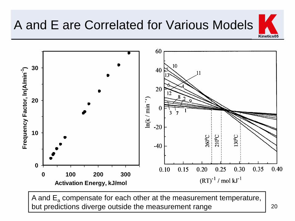
Weibull distribution of E
is a width parameter, is a shape parameter, and is the
activation energy threshold
The Weibull distribution is very flexible and can approximate
Gaussian and nth-order distributions
Up to three parallel Weibull reactions are allowed
A Weibull distribution in E is completely different from a Weibull
distribution in temperature advocated by some
• the later is useful only for smoothing data, not deriving kinetics
Although the model is described as a continuous mathematical
distribution, the implementation is actually as a discrete distribution
with weighting factors approximating a Weibull distribution
}]/)[(exp{]/))[(/()( 1 EEED

41
Discrete E distribution
This is the most powerful model for materials having reactivity distributions without distinct multiple reactions
• It has its roots in the German coal literature in 1967
It assumes a set of equally spaced reaction channels separated by a constant E spacing selected by the user
A and the weighting factors for each energy channel are optimized by iterative linear and nonlinear regression
The frequency factor can depend on activation energy in the form A = a + bE if desired
It can be used to calculate the shift in Rock-Eval Tmax as a function of maturity for petroleum source rocks

42
Nucleation-Growth Models
These were developed for solid-state reactions and linear polymer decomposition more than 50 years ago
• Don’t be a Luddite and ignore them
Different variations emerged from the Prout-Tompkins and Avrami-Erofeev (or JMA) approaches for solid-state reactions
They are equally applicable to organic pyrolysis reactions
• Initiation is analogous to nucleation
• Propagation is analogous to growth
• It is an approximation to the autocatalytic reaction A B; B + A 2B
We use the extended Prout-Tompkins formalism
• x (=1-) is the fraction remaining
• q is a user selectable initiation parameter (default in Kinetics05 is 0.99)
• m is a growth parameter
• n is still the reaction order
mn qxkxdtdx )1(/

43
Equilibrium-Limited Nucleation-Growth
This is an extension of the nucleation-growth model to
account for equilibrium inhibition
Examples are
• the distance away from a phase transition in solid-state
transformations
• The effect of a product gas inhibition in solid-state
decomposition (e.g., CO2 for calcite decomposition)
where Keq is the equilibrium constant
)/11()1(/ eq
mn Kqxkxdtdx
For an example ( phase transformation of HMX), see Burnham et al.,
J. Phys. Chem. B 108, 19432-19441, 2004
44
Sequential Gaussian and Nucleation-
Growth Model
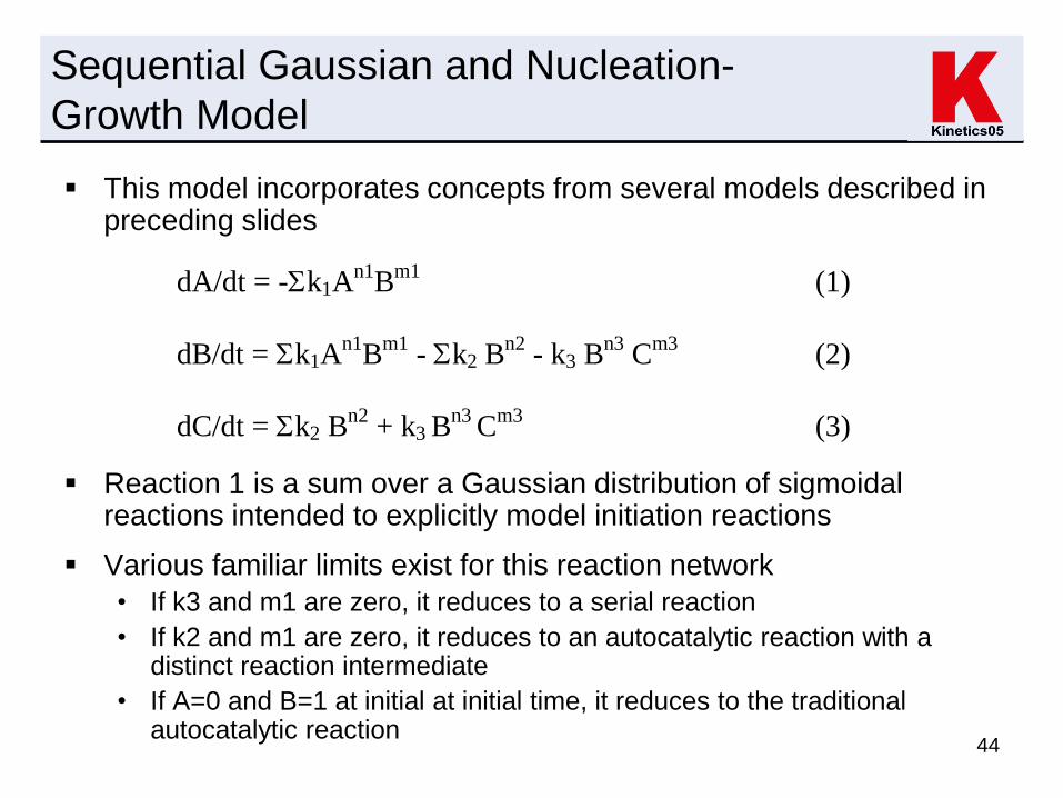
This model incorporates concepts from several models described in preceding slides
Reaction 1 is a sum over a Gaussian distribution of sigmoidal reactions intended to explicitly model initiation reactions
Various familiar limits exist for this reaction network
• If k3 and m1 are zero, it reduces to a serial reaction
• If k2 and m1 are zero, it reduces to an autocatalytic reaction with a distinct reaction intermediate
• If A=0 and B=1 at initial at initial time, it reduces to the traditional autocatalytic reaction
dA/dt = -k1An1
Bm1
(1)
dB/dt = k1An1
Bm1
- k2 Bn2
- k3 Bn3
Cm3
(2)
dC/dt = k2 Bn2
+ k3 Bn3
Cm3
(3)

45
10-parameter Radical Reaction Model
This model was intended to do more rigorous modeling of organic
decomposition, but it has not been explored much
It is available only in the DOS emulation mode
Reaction Rate Law Mass Balance
(1) Initiation P 2R P R
(2) Recombination/disproportionation R + R P + 2E R P + E
(3) Hydrogen transfer/scission R + P 2E + R P E
(4) Volatile product formation R + E V + R E V
P = crosslinked polymer, R = radical, E = non-radical end group, V = volatile product

46
Examples of Model Fitting
Nucleation-Growth (autocatalytic) Reactions
• Cellulose
• PEEK
• Frejus Boghead Coal
Surface Desorption
Distributed Reactivity Reactions
• Pittsburgh #8 coal
• Farsund Formation Marine Shale
• Hydroxyapatite Sintering
Multiple Reactions
• Estane
• Poly (vinyl acetate)
• Ammonium Perchlorate

47
Cellulose has a narrow pyrolysis profile
characteristic of an autocatalytic reaction
Kinetic parameters
Isoconversional analysis:
E ~ 42 kcal/mol; A ~ 1012 s-1
approximately independent of conversion
Extended Kissinger analysis:
E, kcal/mol 43.3
A, s-1 4.0 1012
rel. width 0.71
asym. 0.64
approx. m 0.48
Nonlinear regression analysis
E, kcal/mol 42.27
A, s-1 1.36x10⁷
m 0.41
dx/dt = -kx(1-x)m
0.0
0.4
0.8
1.2
1.6
2.0
0.5 1.0 1.5 2.0 2.5
T80%-T20%
As
ym
me
try nth-order
Gaussiannucleation
Weibull
1st-order
0.0
0.5
1.0
1.5
2.0
2.5
0.5 1.0 1.5 2.0 2.5
FWHH
As
ym
me
try nth-order
Gaussian
nucleation
Weibull
1st-order
0.0
0.4
0.8
1.2
1.6
2.0
0.5 1.0 1.5 2.0 2.5
T80%-T20%
As
ym
me
try nth-order
Gaussiannucleation
Weibull
1st-order
0.0
0.5
1.0
1.5
2.0
2.5
0.5 1.0 1.5 2.0 2.5
FWHH
As
ym
me
try nth-order
Gaussian
nucleation
Weibull
1st-order
0.0
0.2
0.4
0.6
0.8
1.0
300 350 400 450
No
rma
lize
d r
ea
ctio
n r
ate
Temperature, C
C:\Kinetics\Biomass\fibcell.otm
0.94 6.7 48 oC/min
}
Reynolds and Burnham,
Energy & Fuels 11, 88-97, 1997

48
Polyether-ether-ketone (PEEK) has classic
sigmoidal (autocatalytic) reaction characteristics
0.0
0.2
0.4
0.6
0.8
0 200 400 600 800 1000 1200 1400
Fra
ctio
n r
ea
cte
d
Time, min
C:\Kinetics\PEEK\peekall-iso.otmn
0.0
0.2
0.4
0.6
0.8
1.0
500 550 600
Fra
ctio
n r
ea
cte
d
Temperature, C
C:\Kinetics\PEEK\peekall-hr.otmnIsothermal reaction 460 to 500 oC Constant heating rate 0.67 to 19.5 oC/min
dx/dt = -kx0.9(1-0.99x)0.9
Nonlinear regression k = 7.9x10¹²exp(-28940/T) s-1 [57.5 kcal/mol]
• Simultaneous Friedman analysis of both data sets gave a
roughly constant activation energy of about 58 kcal/mol
• Extended Kissinger analysis of the constant heating rate data
gave E of 56.6 kcal/mol and m=1 for the growth parameter
Note
sigmoidal
shape!
A. K. Burnham, J. Thermal Anal. Cal. 60, 895-908, 2000
49
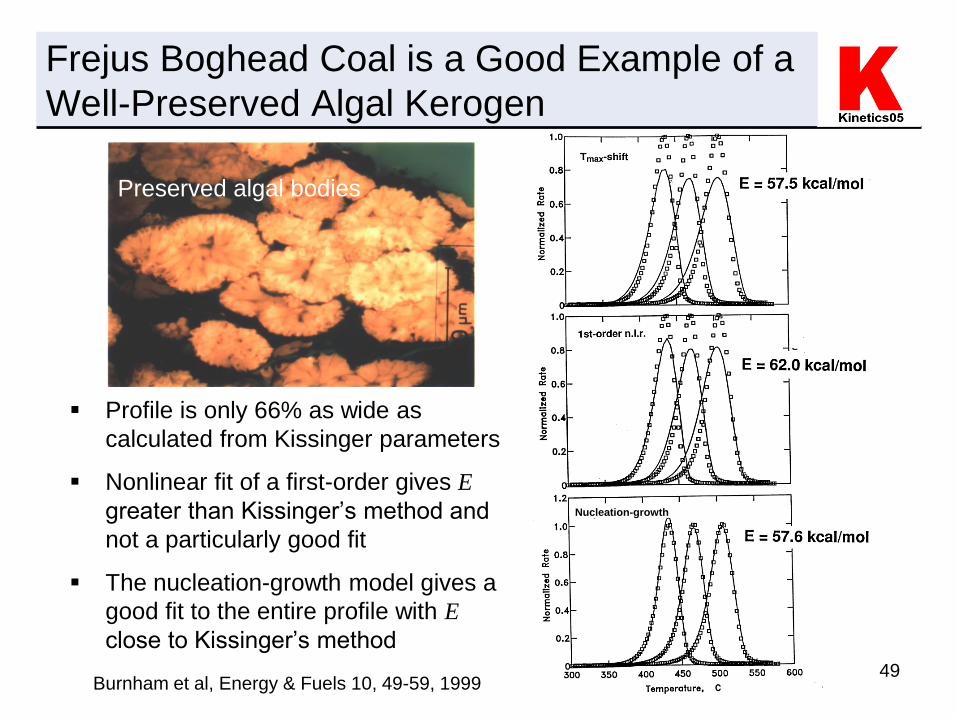
Frejus Boghead Coal is a Good Example of a
Well-Preserved Algal Kerogen
Profile is only 66% as wide as
calculated from Kissinger parameters
Nonlinear fit of a first-order gives E
greater than Kissinger’s method and
not a particularly good fit
The nucleation-growth model gives a
good fit to the entire profile with E
close to Kissinger’s method
Preserved algal bodies
Nucleation-growth
Burnham et al, Energy & Fuels 10, 49-59, 1999

50
A 1st-Order Reaction Also Fails to Fit Isothermal
Data From Fluidized Bed Pyrolysis
Dashed line:
Kissinger 1st-order
parameters from
Pyromat data
Solid line:
Nonlinear 1st-order
fit to fluidized bed
data
The slow rise time
at constant T is
characteristic of
an autocatalytic
reaction

51
The Nucleation-Growth model Fits the Frejus
Fluidized-Bed Data Very Well, Also
All the fluidized-
bed calculations
take advantage of
the unique ability
of Kinetics05 to
account for
dispersion of the
gas signal
between the
reactor and
detector. This is
accomplished by
using a tracer
signal in a fourth
column of the
data file.

52
Surface desorption can follow different
kinetic laws

53
Pittsburgh #8 Coal Pyrolysis Requires a
Distributed Reactivity Model
40
60
80
100
120
0 0.2 0.4 0.6 0.8
Fraction reacted
Ac
tiv
ati
on
en
erg
y, k
ca
l/m
ol
Friedman
Modified Coats-
Redfern
Approximate kinetic
parameters
E50% 57 kcal/mol
A50% 4.1x10¹⁴ s-1
Width relative
to 1st-order rxn 3.6
Asymmetry 2.4
(skewed to high T)
n from width 5.1
Gaussian s 9.8%
Isoconversion analysis
A. K. Burnham and R. L. Braun, Energy & Fuels 13, 1-39, 1999

54
The Discrete E Model Easily Provides the
Best Fit to Pittsburgh #8 Volatiles
0.0
0.2
0.4
0.6
0.8
300 400 500 600 700 800
Fra
cti
on
re
ac
ted
Temperature, C
C:\Kinetics\Miura coal kinetics\miurapitt8.otn
0.0
0.2
0.4
0.6
0.8
1.0
300 400 500 600 700 800
Fra
cti
on
re
ac
ted
Temperature, C
C:\Kinetics\Miura coal kinetics\MiuraPitt8.otg
0.0
0.2
0.4
0.6
0.8
300 400 500 600 700 800
Fra
cti
on
re
ac
ted
Temperature, C
C:\Kinetics\Miura coal kinetics\miurapitt8.otd
0
10
20
30
43
49
55
61
67
73
79
85
91
A ctiva tion ene rgy, kca l/m o l
Pe
rce
nt
of
rea
cti
on A = 4 .38E +14 s
- 1
Gaussian
rss =0.799 Discrete
rss =0.011
nth-order
rss =0.195

55
The Extended Discrete Model Fits Slightly Better
and Agrees Better With Isoconversional Analysis
0.000
0.200
0.400
0.600
0.800
1.000
425 525 625 725Temperature
Re
ac
tio
n r
ate
Model
Discrete
CR-Miura
lnA=a+bE
1000 K/s
0.000
0.200
0.400
0.600
0.800
1.000
50 75 100 125 150 175 200Temperature
Re
ac
tio
n r
ate
ModelDiscreteCR-MiuralnA=a+bE
3 K/m.y.
1.E+09
1.E+12
1.E+15
1.E+18
1.E+21
1.E+24
1.E+27
30 50 70 90 110
Activation energy, kcal/mol
Fre
qu
en
cy
fa
cto
r
Miura isoconversion
LLNL isoconversion
extended discrete
ln(A) = 21.68 + 2.33E-04*E
0
10
20
30
40
36926
49482
62038
74594
87149
99705
112261
124816
137372
Activation energy, cal/mol
% o
f to
tal re
ac
tio
n

56
The Ability of the Discrete Model to Model
Residual Activity Has Been Tested
Measure Pyromat kinetics
for an immature sample
from the Danish North Sea
Calculate Pyromat reaction
profiles for residues from
hydrous pyrolysis (72 h at
various temperatures)
The comparison uses the
Apply feature with a thermal
history combining the
hydrous pyrolysis and
Pyromat thermal histories
0.0
0.2
0.4
0.6
0.8
1.0
300 350 400 450 500 550
No
rma
lize
d r
ea
ctio
n r
ate
Temperature, C
1 7 50 oC/min
Temperature, oC
Reacti
on
rate
Residues
heated at
7 oC/min
Pyromat
kinetics
Burnham et al, Org. Geochem.
23, 931-939, 1995

57
The Original Sparse Distribution Did Poorly
at High Conversions
Distributed E kinetics
should be able to
predict the reactivity of
the residue if the model
is rigorously correct
The model qualitatively
predicts the increase in
Tmax with maturation
The model does not do
well for T above 550 oC,
because the original
signal was low and
possibly because the
baseline was clipped
too much

58
Agreement is Improved by Fitting All Samples
Simultaneously
All thermal histories include
both the hydrous pyrolysis
and Pyromat heating phases
The fit to the unreacted
sample is not quite as good
as when it is fitted by itself
The frequency factor and
principal activation energy
shifted up slightly, with a net
increase of about 5 oC in the
predicted T of petroleum
formation
The parallel reaction model is
verified within the accuracy of
the data
Temperature, oC

59
The Distributed Reactivity Approach Can Also
Model Sintering
Sintering is a highly deceleratory process, with an apparent limit that superficially increases with temperature
Sintering is commonly modeled by a power law or nth-order model
Mathematically, the exponent of the power law is related to reaction order: n=1+1/
Conceptually, reaction order can be interpreted as a distribution of diffusion lengths
Adding a Gaussian E distribution can account for the spectrum of defects leading to mobile material Fraction sintered = 1-S/S0 where S is surface area
Burnham, Chem. Eng. J. 108, 47-50, 2005
Sintering of 2 forms of hydroxyapatite

60
Kinetics05 can fit reactions with distinct
individual components
The 1st order, nth order,
nucleation-growth, Gaussian,
and Weibull models can fit up
to three independent peaks,
but simultaneous regression on
all parameters is not reliable
With strongly overlapping
peaks, guidance from the
isoconversional analysis and a
manual Kissinger analysis can
help pick good initial guesses
A multiple step refinement of
subsets of the parameters can
give a good model
Burnham and Weese, Thermochimica
Acta 426, 85-92, 2005
Fit to 2 independent nucleation-growth reactions
Comparison of
isothermal
measurement
and prediction

61
0.0
0.2
0.4
0.6
0.8
1.0
1.2
400 500 600 700
No
rma
lize
d r
ea
ctio
n r
ate
Temperature, C
C:\Users\akburnham\Desktop\Sample 3 3PT H3 of 4.out
400 500 600 700
0.0
0.2
0.4
0.6
0.8
1.0
1.2
400 500 600 700
No
rma
lize
d r
ea
ctio
n r
ate
Temperature, C
C:\Users\akburnham\Desktop\Sample 3 3PT H3 of 4.out
400 500 600 700
Kerogen and
mineral weight
losses from oil
shale
Sometimes reaction profiles have better
separated multiple peaks
With minimally overlapping
peaks, splitting the data and
doing an initial separate
analysis is a useful first step
Subsequent fitting of the entire
profile using the separate
results as initial guesses
improves the likelihood of a
robust convergence
Poly (vinyl
acetate)
PVAc
1st peak: nth-order nucleation-growth reaction
2nd peak: nth-order reaction
A. K. Burnham and R. L. Braun, Energy & Fuels
13, 1-39, 1999

62
Two-Step Ammonium Perchlorate Kinetics From
TGA Mass Loss Can Predict DSC Heat Flow
0.0
0.2
0.4
0.6
0.8
1.0
1.2
0.0 0.1 0.2 0.3 0.4 0.5 0.6 0.7 0.8 0.9
No
rma
lize
d r
ea
ctio
n r
ate
Fraction reacted
C:\Kinetics\MEBrown\amonpalls.ot2
0.0
0.2
0.4
0.6
0.8
100 200 300
Fra
ctio
n r
ea
cte
d
Time, min
C:\Kinetics\MEBrown\amonpalls.ot2
-11
-9
-7
-5
-3
-1
200 250 300 350 400 450
Temperature, C
Heat
flow
experiment
nonisothermal kinetics
isothermal kinetics
Kinetic parameters
Rxn 1 27% of total Rxn 2 73% of total
A 1.36x10⁷ s-1 A 4.19x10⁶ s-1
E 22.8 kcal/mol E 26.6 kcal/mol
m 1.00 m 0.00
n 1.96 n 0.28
Decomposition
is exothermic
Sublimation is
endothermic
Decomposition:
nucleation-growth
Sublimation:
receding interface
62