Principles of Interferometry - Science Website · • This is the basic concept of interferometry. ... 14th Synthesis Imaging School 14 •Antenna 1 Voltage ... Principles of Interferometry

Fourteenth NRAO Synthesis Imaging Summer School

Socorro, NM

Fundamentals of Radio Interferometry Rick Perley, NRAO/Socorro

Topics

• Why Interferometry?

• The Single Dish … as an interferometer

• The Basic Interferometer

– Response to a Point Source

– Response to an Extended Source

– The Complex Correlator

– The Visibility and its relation to the Intensity

– Picturing the Visibility

3 14th Synthesis Imaging School

Why Interferometry?

• Because of Diffraction: For an aperture of diameter D, and at

wavelength l, the image resolution is

• In ‘practical’ units:

• To obtain 1 arcsecond resolution at a wavelength of 21 cm, we

require an aperture of ~42 km!

• The (currently) largest single, fully-steerable apertures are the

100 meter antennas near Bonn, and at Green Bank.

• So we must develop a method of synthesizing an equivalent

aperture.

• The methodology of synthesizing a continuous aperture through

summations of separated pairs of antennas is called ‘aperture

synthesis’.

The Single Dish – as in Interferometer

• A parabolic reflector has a power response (vs angle) roughly as shown below.

• The formation of this response follows the same laws of physics as an interferometer.

• A basic understanding of the origin of the focal response will aid in understanding how an interferometer works.

Illustrated here is the

approximate power response of

a 25-meter antenna, at n = 1

GHz.

The Parabolic Reflector

• The parabola has the remarkable property of directing

all rays from in incoming wave front to a single point

(the focus), all with the same distance.

• Hence, all rays arrive at the focus with the same phase.

• Key Point: Distance from incoming phase front to focal point is the

same for all rays.

• The E-fields will thus all be in phase at the focus – the place for the

receiver.

Beam Pattern Origin (1-Dimensional Example)

• An antenna’s

response is a

result of coherent

vector summation

of the electric field

at the focus.

• First null will

occur at the angle

where one extra

wavelength of path

is added across

the full width of the

aperture:

q ~ l/D

(Why?)

On-axis

incidence

Off-axis

incidence

Specifics: First Null, and First Sidelobe

• When the phase differential across the aperture is 1, 2, 3, … wavelengths,

we get a null in the total received power.

– The nulls appear at (approximately): q = l/D, 2l/D, 3l/D, … radians.

• When the phase differential across the full aperture is ~1.5, 2.5, 3.5, …

wavelengths, we get a maximum in total received power.

– These are the ‘sidelobes’ of the antenna response.

– But, each successive maximum is weaker than the last.

– These maxima appear at (approximately): q = 3l/2D, 5l/2D, 7l/2D, … radians.

14th Synthesis Imaging School 7

• We don’t need a single

parabolic structure.

• We can consider a series

of small antennas, whose

individual signals are

summed in a network.

• This is the basic concept

of interferometry.

• Aperture Synthesis is an

extension of this concept.

Interferometry – Basic Concept


Quasi-Monochromatic Radiation

• Analysis is simplest if the fields are perfectly monochromatic.

• This is not possible – a perfectly monochromatic electric field

would both have no power (Dn = 0), and would last forever.

• So we consider instead ‘quasi-monochromatic’ radiation, where

the bandwidth dn is very small.

• For a time dt ~1/dn, the electric fields will be sinusoidal.

• Consider then the electric fields from a small sold angle dW about

some direction s, within some small bandwidth dn, at frequency n.

• We can write the temporal dependence of this field as:

• The amplitude and phase remains unchanged to a time duration

of order dt ~1/dn, after which new values of A and f are needed.

Simplifying Assumptions

• We now consider the most basic interferometer, and seek a relation between the characteristics of the product of the voltages from two separated antennas and the distribution of the brightness of the originating source emission.

• To establish the basic relations, the following simplifications are introduced:

– Fixed in space – no rotation or motion

– Quasi-monochromatic (signals are sinusoidal)

– No frequency conversions (an ‘RF interferometer’)

– Single polarization

– No propagation distortions (no ionosphere, atmosphere …)

– Idealized electronics (perfectly linear, no amplitude or phase perturbations, perfectly identical for both elements, no added noise, …)

Symbols Used, and their Meanings

• We consider:

– two identical sensors, separated by vector distance b

– receiving signals from vector direction s

– at frequency n (angular frequency w = 2pn)

• From these, the key quantity

is formed. This is the ‘geometric time delay’ – the extra time

taken for the signal to reach the more distant sensor.

• Finally, the phase corresponding to this extra distance is defined:


The Stationary, Quasi-Monochromatic

Radio-Frequency Interferometer

X

s s

b

multiply

average

The path lengths

from sensors

to multiplier are

assumed equal!

Geometric

Time Delay

Rapidly varying,

with zero mean

Unchanging


Pictorial Example: Signals In Phase


•Antenna 1

Voltage

•Antenna 2

Voltage

•Product

Voltage

•Average

2 GHz Frequency, with voltages in phase:

b.s = nl, or tg = n/n

Pictorial Example: Signals in Quad Phase


•Antenna 1

Voltage

•Antenna 2

Voltage

•Product

Voltage

•Average

2 GHz Frequency, with voltages in quadrature phase:

b.s=(n +/- ¼)l, tg = (4n +/- 1)/4n

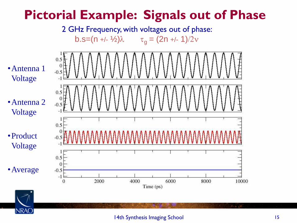
Pictorial Example: Signals out of Phase


•Antenna 1

Voltage

•Antenna 2

Voltage

•Product

Voltage

•Average

2 GHz Frequency, with voltages out of phase:

b.s=(n +/- ½)l tg = (2n +/- 1)/2n


Some General Comments

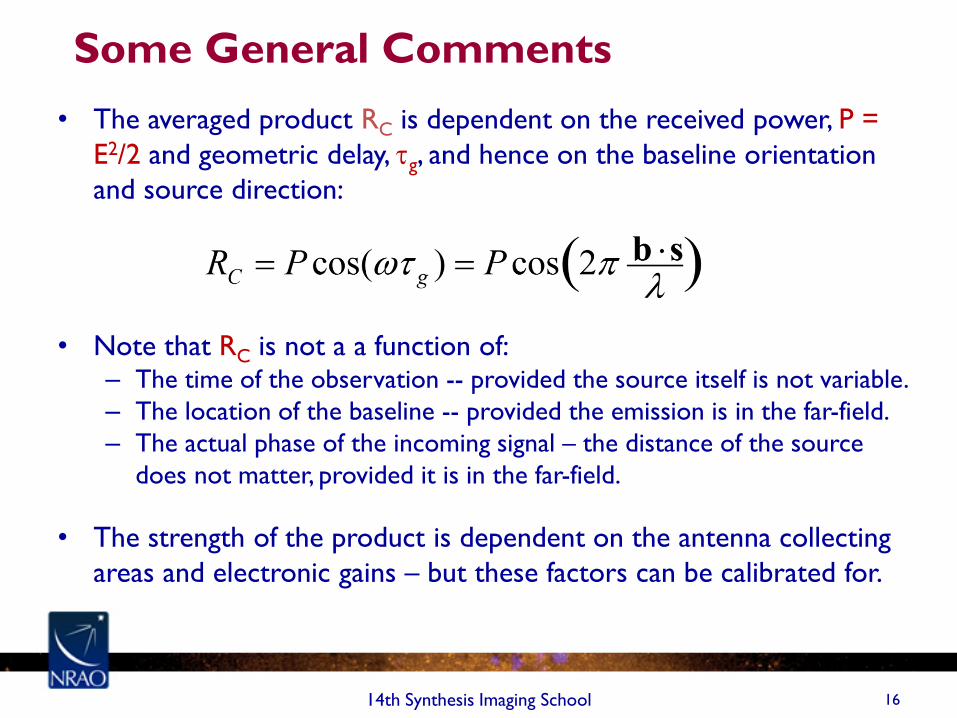
• The averaged product RC is dependent on the received power, P =

E2/2 and geometric delay, tg, and hence on the baseline orientation

and source direction:

• Note that RC is not a a function of: – The time of the observation -- provided the source itself is not variable.

– The location of the baseline -- provided the emission is in the far-field.

– The actual phase of the incoming signal – the distance of the source

does not matter, provided it is in the far-field.

• The strength of the product is dependent on the antenna collecting

areas and electronic gains – but these factors can be calibrated for.


Pictorial Illustrations

• To illustrate the response, expand the dot product in one dimension:

• Here, u = b/l is the baseline length in wavelengths, and q is the

angle w.r.t. the plane perpendicular to the baseline.

• is the direction cosine

• Consider the response Rc, as a function of angle, for two different

baselines with u = 10, and u = 25 wavelengths:

a

b

s

q

)20cos( lRC

p=

qa sincos ==l

Whole-Sky Response

• Top: u = 10

There are 20 whole

fringes over the

hemisphere.

Peak separation 1/10

radians

• Bottom: u = 25

There are 50 whole

fringes over the

hemisphere.

Peak separation 1/25

radians.

0 2 5 7 9 10 -10 -5 -3 -8

-25 25

)20cos( lRC

p=

)50cos( lRC

p=

From an Angular Perspective

Top Panel:

The absolute value of the

response for u = 10, as a

function of angle.

The ‘lobes’ of the response

pattern alternate in sign.

Bottom Panel:

The same, but for u = 25.

Angular separation between

lobes (of the same sign) is

dq ~ 1/u = l/b radians.

0

5

10

3

9

7

q

+

+

+

-

-

Hemispheric Pattern

• The preceding plot is a meridional cut

through the hemisphere, oriented along

the baseline vector.

• In the two-dimensional space, the fringe

pattern consists of a series of coaxial

cones, oriented along the baseline vector.

• The figure is a two-dimensional

representation when u = 4.

• As viewed along the baseline vector, the

fringes show a ‘bulls-eye’ pattern –

concentric circles.


The Effect of the Sensor

• The patterns shown presume the sensor (antenna) has

isotropic response.

• This is a convenient assumption, but doesn’t represent reality.

• Real sensors impose their own patterns, which modulate the

amplitude and phase, of the output.

• Large antennas have very high directivity -- very useful for

some applications.

The Effect of Sensor Patterns

• Sensors (or antennas)

are not isotropic, and

have their own

responses.

• Top Panel: The

interferometer pattern

with a cos(q)-like

sensor response.

• Bottom Panel: A

multiple-wavelength

aperture antenna has a

narrow beam, but also

sidelobes.


The Response from an Extended Source

• The response from an extended source is obtained by summing the

responses at each antenna to all the emission over the sky, multiplying

the two, and averaging:

• The averaging and integrals can be interchanged and, providing the

emission is spatially incoherent, we get

• This expression links what we want – the source brightness on the

sky, In(s), – to something we can measure - RC, the interferometer

response.

• Can we recover In(s) from observations of RC?

A Schematic Illustration in 2-D • The correlator can be thought of ‘casting’ a cosinusoidal coherence pattern, of

angular scale ~l/b radians, onto the sky.

• The correlator multiplies the source brightness by this coherence pattern, and integrates (sums) the result over the sky.

• Orientation set by baseline

geometry.

• Fringe separation set by

(projected) baseline length and

wavelength. • Long baseline gives close-packed

fringes

• Short baseline gives widely-

separated fringes

• Physical location of baseline

unimportant, provided source is in

the far field. - + - + - + -

Fringe Sign

l/b rad.

Source

brightness

l/b


A Short Mathematics Digression –

Odd and Even Functions

• Any real function, I(x,y), can be expressed as the sum of two real

functions which have specific symmetries:

An even part:

An odd part:

= + I

IE IO I IE IO


Why One Correlator is Not Enough

• The correlator response, Rc:

is not enough to recover the correct brightness. Why?

• Only the even part of the distribution is seen.

• Suppose that the source of emission has a component with odd symmetry:

Io(s) = -Io(-s)

• Since the cosine fringe pattern is even, the response of our interferometer to the odd brightness distribution is 0.

• Hence, we need more information if we are to completely recover the source brightness.

Why Two Correlations are Needed

• The integration of the cosine response, Rc, over the source

brightness is sensitive to only the even part of the brightness:

since the integral of an odd function (IO) with an even function

(cos x) is zero.

• To recover the ‘odd’ part of the brightness, IO, we need an ‘odd’

fringe pattern. Let us replace the ‘cos’ with ‘sin’ in the integral

since the integral of an even times an odd function is zero.

• To obtain this necessary component, we must make a ‘sine’

pattern. How?

Making a SIN Correlator

• We generate the ‘sine’ pattern by inserting a 90 degree phase shift

in one of the signal paths.

X

s s

A Sensor b

multiply

average

90o

Define the Complex Visibility • We now DEFINE a complex function, the complex visibility, V, from the

two independent (real) correlator outputs RC and RS:

where

• This gives us a beautiful and useful relationship between the source

brightness, and the response of an interferometer:

• With the right geometry, this is a 2-D Fourier transform, giving us a well

established way to recover I(s) from V(b).

The Complex Correlator and Complex

Notation

• A correlator which produces both ‘Real’ and ‘Imaginary’ parts – or the

Cosine and Sine fringes, is called a ‘Complex Correlator’

– For a complex correlator, think of two independent sets of projected

sinusoids, 90 degrees apart on the sky.

– In our scenario, both components are necessary, because we have assumed

there is no motion – the ‘fringes’ are fixed on the source emission, which is

itself stationary.

• The complex output of the complex correlator also means we can use

complex analysis throughout: Let:

• Then:

(

( )/(

2

1

Re)]/(cos[

Re)cos(

csbti

ti

AectAV

AetAV

--

-

=-=

==

w

w

w

w

sb

ci

correAVVP

/2*

21

sb -

==w

Wideband Phase Shifters – Hilbert Transform

• For a quasi-monochromatic signal, forming a the 90 degree

phase shift to the signal path is easy --- add a piece of cable

l/4 wavelengths long.

• For a wideband system, this obviously won’t work.

• In general, a wideband device which phase shifts each spectral

component by 90 degrees, while leaving the amplitude intact,

is a Hilbert Transform.

• For real interferometers, such an operation can be performed

by analog devices.

• Far more commonly, this is done using digital techniques.

• The complex function formed by a real function and its

Hilbert transform is termed the ‘analytic signal’.


Picturing the Visibility • The source brightness is Gaussian, shown in black.

• The interferometer ‘fringes’ are in red.

• The visibility is the integral of the product – the net dark green area.

RS

Long

Baseline

Short

Baseline

Long Baseline

Short Baseline

RC


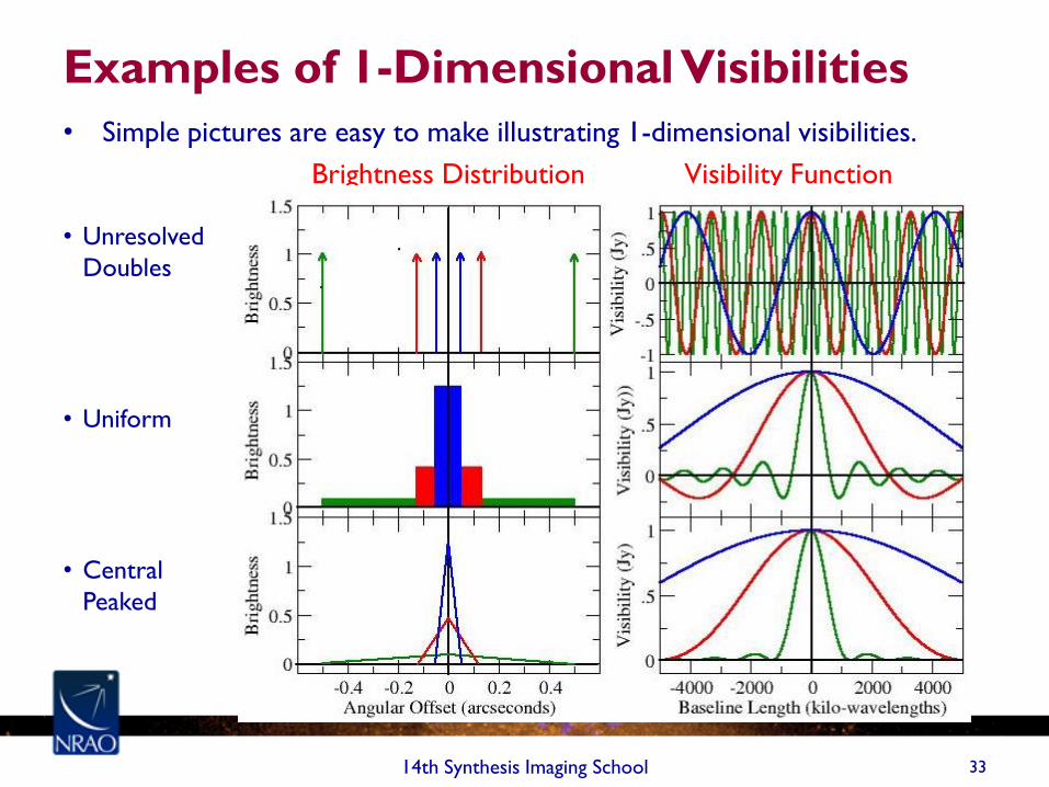
Examples of 1-Dimensional Visibilities


• Simple pictures are easy to make illustrating 1-dimensional visibilities.

Brightness Distribution Visibility Function

• Unresolved

Doubles

• Uniform

• Central

Peaked

More Examples


• Simple pictures are easy to make illustrating 1-dimensional visibilities.

Brightness Distribution Visibility Function

• Resolved

Double

• Resolved

Double

• Central

Peaked

Double

Another Way to Conceptualize …

• For those of you adept in thinking in terms of complex

functions, another way to picture the effect of the

interferometer may be attractive …

• The interferometer casts a *phase slope* across the (real)

brightness distribution.

– The phase slope becomes steeper for longer baselines, or

higher frequencies, and is zero for zero baseline.

– The phase is zero at the phase origin.

– The amplitude response is unity (ignoring the primary

beam) throughout.

• The Visibility is the complex integral of the brightness times

the phase ramp.


The Complex Integral

2p

l = sin q 1/u

Amplitude

Basic Characteristics of the Visibility

• For a zero-spacing interferometer, we get the ‘single-dish’ (total-power) response.

• As the baseline gets longer, the visibility amplitude will in general decline.

• When the visibility is close to zero, the source is said to be ‘resolved out’.

• Interchanging antennas in a baseline causes the phase to be negated – the visibility of the ‘reversed baseline’ is the complex conjugate of the original. (Why?)

• Mathematically, the visibility is Hermitian. (V(u) = V*(-u)).

• The Visibility is a unique function of the source brightness.

• The two functions are related through a Fourier

transform.

• An interferometer, at any one time, makes one measure of

the visibility, at baseline coordinate (u,v).

• `Sufficient knowledge’ of the visibility function (as derived

from an interferometer) will provide us a `reasonable

estimate’ of the source brightness.

• How many is ‘sufficient’, and how good is ‘reasonable’?

• These simple questions do not have easy answers…

Some Comments on Visibilities

),(),( mlIvuV

Documents

Principles of Interferometry - Science Website · • This is the basic concept of interferometry. ... 14th Synthesis Imaging School 14 •Antenna 1 Voltage ... Principles of Interferometry