Principles of Inheritance: Mendel's Laws and Genetic Models

Chapter 2Principles of Inheritance: Mendel’s Lawsand Genetic Models

It is difficult to overstate the impact of Mendel’s research on the history of genetics;indeed, his research in genetics has been credited as one of the great experimen-tal advances in biology (Fisher, 1965). Prior to the publication of his results onexperimental hybridization in plants, the concept of inheritance of physical ‘units’(later called genes) was accepted, and scientists had reported on many hybridizationexperiments in both animals and plants. Yet no one had set forth principles of inher-itance which could be used as a universal theory to explain how traits in offspringcan be predicted from traits in the parents. Mendel provided an explicit rule forhow the genotypes of the offspring can be predicted from the genotypes of theirparents, and he also established models for how genotypes were related to traits.This is nothing short of astonishing in view of the fact that genes and genotypeswere not observed; rather their existence was inferred from the phenotypes that wereobserved. Needless to say, the underlying biology of cell division and the process offormation of sperm and egg cells was not then known; otherwise the derivation ofMendel’s laws would be more straightforward.

Part of Mendel’s success was due to his implicit introduction of the concept ofa genetic model. A genetic model specifies a probability distribution for the trait,conditional on the underlying genotype at the hypothesized disease locus. Mendel’sgenetic models were very simple forms for dichotomous traits that lead to determin-istic outcomes. Genetic models underlie most analyses used in statistical genetics.In order to formalize the process of localizing disease mutations and measuring theireffect sizes, we often translate the problem to the framework of statistical hypothesistesting and estimation of parameters in the genetic model.

2.1 Mendel’s Experiments

Mendel’s work is known largely through a single research paper, ‘Experiments inPlant Hybridization’ published in 1865. It reported on eight years of experimen-tation with the garden pea. Mendel made several deliberate choices for his exper-iments which were crucial in enabling one to infer the laws of inheritance in hisseries of experiments, essentially examining very simple, now called Mendelian,

N.M. Laird, C. Lange, The Fundamentals of Modern Statistical Genetics,Statistics for Biology and Health, DOI 10.1007/978-1-4419-7338-2_2,C© Springer Science+Business Media, LLC 2011

15

16 2 Mendel’s Laws

forms of inheritance. In describing Mendel’s experiments we use the terms geneand genotype to refer to the genetic locus underlying the traits, although the wordgene came into use only after Mendel; following Mendel, we refer to the two allelesof a gene as A and a.

Mendel laid out several principles of good experimentation: using large enoughsamples of crosses, avoiding unintended cross fertilization, choosing hybrids withno reduction in fertility, etc. Here we focus only on those features of Mendel’s exper-iments bearing on genetics. First is the importance of choosing simple, dichotomoustraits for study which are easily recognizable and reproducible. (Mendel studiedseven different dichotomous traits.) He called these ‘constant differentiating char-acteristics’, meaning that two forms of the trait, e.g., green or yellow pods, couldbe differentiated in plants, and that the same two forms appeared unchanged in off-spring. Mendel excluded traits which produced ‘transitional or blended’ results inoffspring, or quantitative traits generally. Using dichotomous traits enabled him touse simple genetic models to demonstrate laws of inheritance. It took many decadesfor scientists to develop models which allowed them to apply Mendel’s laws tocontinuous traits.

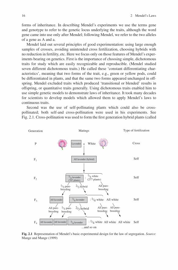
Second was the use of self-pollinating plants which could also be cross-pollinated; both self-and cross-pollination were used in his experiments. SeeFig. 2.1. Cross-pollination was used to form the first generation hybrid plants (called

All lavender (hybrid)

Type of fertilization

Cross

Matings

Lavender White

Generation

P

Self

Self

Self:

:

:

SelfAll white

All white

All white

...and so on

All lavender

2/3 hybrid

2/3 hybrid1/3 pure-breeding

3/4 lavender(787 plants)

1/4 white

1/4 white3/4 lavender

1/4 white3/4 lavender

1/3 pure-breeding

All pure-breeding

All pure-breeding

All pure-breeding

All pure-breeding

F4

F3

F2

F1

All lavender All lavender

(277 plants)

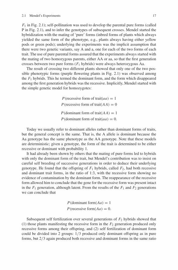
Fig. 2.1 Representation of Mendel’s basic experimental design for the law of segregation. Source:Mange and Mange (1999)

2.1 Mendel’s Experiments 17

F1 in Fig. 2.1); self-pollination was used to develop the parental pure forms (calledP in Fig. 2.1), and to infer the genotypes of subsequent crosses. Mendel started thehybridization with the mating of ‘pure’ forms (inbred forms of plants which alwaysyielded the same form of the phenotype, e.g., plants always having either yellowpods or green pods); underlying the experiments was the implicit assumption thatthere were two genetic variants, say A and a, one for each of the two forms of eachtrait. The use of pure parental forms assured that the experiments always started withthe mating of two homozygous parents, either AA or aa, so that the first generationcrosses between two pure forms (F1 hybrids) were always heterozygous Aa.

The result of crossing two different plants showed that only one of the two pos-sible phenotypic forms (purple flowering plants in Fig. 2.1) was observed amongthe F1 hybrids. This he termed the dominant form, and the form which disappearedamong the first generation hybrids was the recessive. Implicitly, Mendel started withthe simple genetic model for homozygotes:

P(recessive form of trait|aa) = 1

P(recessive form of trait|AA) = 0

P(dominant form of trait|AA) = 1

P(dominant form of trait|aa) = 0.

Today we usually refer to dominant alleles rather than dominant forms of traits,but the general concept is the same. That is, the A allele is dominant because theAa genotype has the same phenotype as the AA genotype. Note that these modelsare deterministic; given a genotype, the form of the trait is determined to be eitherrecessive or dominant with probability 1.

It had already been shown by others that the mating of pure forms led to hybridswith only the dominant form of the trait, but Mendel’s contribution was to insist oncareful self breeding of successive generations in order to deduce their underlyinggenotype. He found that the offspring of F1 hybrids, called F2, had both recessiveand dominant trait forms, in the ratio of 1:3, with the recessive form showing noevidence of contamination by the dominant form. The reappearance of the recessiveform allowed him to conclude that the gene for the recessive form was present intactin the F1 generation, although latent. From the results of the F1 and F2 generationswe can conclude that

P(dominant form|Aa) = 1

P(recessive form|Aa) = 0.

Subsequent self fertilization over several generations of F2 hybrids showed that(1) those plants manifesting the recessive form in the F2 generation produced onlyrecessive forms among their offspring, and (2) self fertilization of dominant formcould be divided into 2 groups: 1/3 produced only dominant offspring as in pureforms, but 2/3 again produced both recessive and dominant forms in the same ratio


seen in the F2 generation of 1:3. These phenotypic ratios are idealized in Fig. 2.1.This led Mendel to deduce the following about the genotypes: 1/4 of the F2 hybridswere of the parental recessive form (aa), 1/4 = 3/4 × 1/3 were of the parentaldominant form (AA), and 1/2 = 3/4 × 2/3 were the same as the F1 generation.From this it follows that the genotypes AA, Aa, aa are in the ratio 1:2:1 in the F2generation. This allows us to infer Mendel’s first law:

Mendel’s First Law (Segregation): One allele of each parent is randomly andindependently selected, with probability 1

2 , for transmission to the offspring; thealleles unite randomly to form the offspring’s genotype.

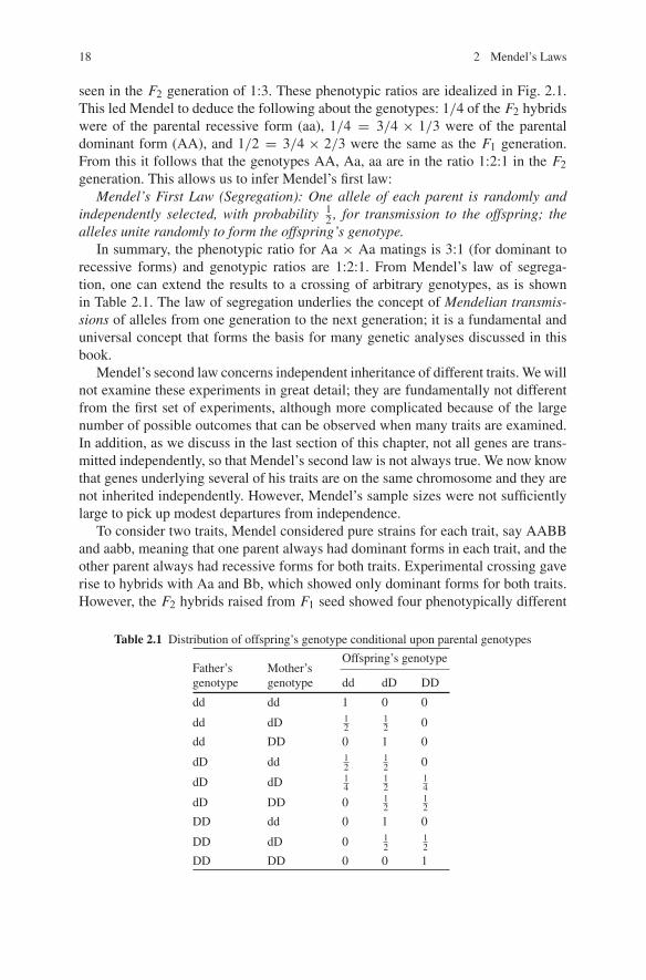
In summary, the phenotypic ratio for Aa × Aa matings is 3:1 (for dominant torecessive forms) and genotypic ratios are 1:2:1. From Mendel’s law of segrega-tion, one can extend the results to a crossing of arbitrary genotypes, as is shownin Table 2.1. The law of segregation underlies the concept of Mendelian transmis-sions of alleles from one generation to the next generation; it is a fundamental anduniversal concept that forms the basis for many genetic analyses discussed in thisbook.

Mendel’s second law concerns independent inheritance of different traits. We willnot examine these experiments in great detail; they are fundamentally not differentfrom the first set of experiments, although more complicated because of the largenumber of possible outcomes that can be observed when many traits are examined.In addition, as we discuss in the last section of this chapter, not all genes are trans-mitted independently, so that Mendel’s second law is not always true. We now knowthat genes underlying several of his traits are on the same chromosome and they arenot inherited independently. However, Mendel’s sample sizes were not sufficientlylarge to pick up modest departures from independence.

To consider two traits, Mendel considered pure strains for each trait, say AABBand aabb, meaning that one parent always had dominant forms in each trait, and theother parent always had recessive forms for both traits. Experimental crossing gaverise to hybrids with Aa and Bb, which showed only dominant forms for both traits.However, the F2 hybrids raised from F1 seed showed four phenotypically different

Table 2.1 Distribution of offspring’s genotype conditional upon parental genotypes

Offspring’s genotypeFather’sgenotype

Mother’sgenotype dd dD DD

dd dd 1 0 0

dd dD 12

12 0

dd DD 0 1 0

dD dd 12

12 0

dD dD 14

12

14

dD DD 0 12

12

DD dd 0 1 0

DD dD 0 12

12

DD DD 0 0 1

2.2 A Framework for Genetic Models 19

plants: those with both dominant forms, plants with one dominant and one recessiveform (2 kinds) and plants with two recessive forms, in the approximate ratio of9:3:3:1 (see exercise 2 of Section 2.4). Subsequent self-pollination of the F2 gener-ation allowed him to deduce 9 genetic forms among the F2 hybrids: AABB, AABb,AAbb, AaBB, AaBb, Aabb aaBB, aaBb and aabb in the ratio 1:2:1:2:4:2:1:2:1.These ratios exactly coincide with what one would expect if inheritance of the twotraits is independent, for then, with F2 hybrids,

P(AA and B B) = P(AA)P(B B)

= (1/4)2 = 1/16 = 1/(1 + 2 + 1 + 2 + 4 + 2 + 1 + 2 + 1),

P(AA and Bb) = P(AA)P(Bb) = (1/4)(1/2) = 1/8 = 2/16 etc.,

when describing the result of a double heterozygote mating.Mendel’s Second Law (Independent Assortment): The alleles underlying two or

more different traits are transmitted to offspring independently of each other; thetransmission of each trait separately follows the first law of segregation.

Fisher (1936) noted that many of Mendel’s statistics were generally too close totheir expectations, thus χ2 statistics comparing observed numbers offspring with agiven phenotype to those expected assuming his laws of segregation were true, wereoften too small, suggesting some data manipulation. This, and the lack of gener-ality of his law of independent assortment (see exercise 3 of Section 2.4), has notdiminished the value of his contributions. The lack of independent transmission ofdifferent genes is, in fact, fortuitous, as it provides the basis for mapping diseasegenes by linkage analysis, as will be described in Section 2.3, and in Chapter 11.

2.2 A Framework for Genetic Models

A genetic model describes the relationship, usually probabilistic, between an indi-vidual’s genotype and their phenotype or trait. In Genetic Epidemiology, phenotypeswill typically be affection status and we distinguish only between affected and unaf-fected subjects in the statistical analysis. Such binary traits can be coded by Y , whereY = 1 denotes affected and Y = 0 denotes unaffected. For other dichotomous traitssuch as those that Mendel used, this labeling is arbitrary. For complex diseases, e.g.,Asthma, Chronic obstructive pulmonary disease (COPD), Obesity, etc., affectionstatus is often defined by a set of intermediate phenotypes or endophenotypes whichare quantitative measurements that can be more reproducible assessments of thedisease features. They can also provide additional insight into the nature and sever-ity of the disease. Standard intermediate phenotypes are body mass index (BMI)as an assessment of obesity, forced expiratory volume in one second (FEV1) forasthma, etc. In some cases, e.g., Alzheimer’s disease, the phenotype affection statuscan be refined by selecting age-of-onset as the target phenotype in the statisticalanalysis. In general, the selection of the target phenotype is a key question in theplanning of the study and the statistical analysis. The phenotype choice will depend


on the disease, the possible study designs, statistical power considerations and thenecessary adjustments for confounding factors. We will use the variable Y as thevariable that describes the phenotype or trait of interest, whether dichotomous ormeasured.

An individual’s genotype at a marker is given by the combination of their twoalleles at that locus; we use the notation G to denote an individual’s genotype. Inthe majority of scenarios that we will consider, the marker locus will have only twodistinct alleles, e.g., alleles ‘A’ and ‘a’. In the literature such genetic loci are calleddi-allelic or bi-allelic. Typically, the “small-letter” allele ‘a’ is assumed to be themore frequent allele of the two and is referred to as the wild type or normal allele.The less frequent allele is labeled with the capital-letter ‘A’ and referred to as theminor allele. This differs from Mendel’s designation of the capital allele as repre-senting the allele associated with the dominant form, because most of the geneticloci we study do not have any known associated dominant or recessive phenotypes,hence today the capital letter usually refers to the less common allele. Under theassumption that the genetic locus is bi-allelic, each of the two chromosomes has tocarry either an ‘a’ or ‘A’ allele, and, consequently, only three different genotypesare possible: the two homozygous genotypes, AA and aa, and the heterozygousgenotype Aa. Order does not matter, so Aa is the same as aA. Thus G can takeon only three values in a di-allelic system. With three alleles, there are 6 possiblegenotypes, etc. Genotypes are inherently categorical but can always be recoded inthe form of numerical or indicator variables, as we will discuss at the end of thissection.

If the genetic locus is a Disease Susceptibility Locus (DSL), it is conventional touse the D/d designation, as opposed to A/a or B/b; the D-allele is then sometimesreferred to as the Disease Variant or Disease Susceptibility Allele. In formulatinggenetic models for disease outcomes, we assume the DSL has a direct effect onthe phenotype through some biological mechanism. Genetic models can either bedeterministic, i.e., the genotype determines the phenotype exactly (Mendelian Dis-ease, or, in most cases, probabilistic, i.e., the genotype influences the probabilityof disease. Conditional upon the individual’s genotype G, the probabilistic effect ofthe locus on the phenotype Y is described by the penetrance function which is a setof conditional probabilities, or density functions for continuous phenotypes, whichmodel the distribution of the phenotype/trait, i.e., P(Y |G). If the genetic locus underconsideration has no effect on the phenotype of interest, the penetrance probabilitiesfor all three genotypes will be equal regardless of the individual’s genotype, i.e.,P(Y |G = dd) = P(Y |G = d D) = P(Y |G = DD).

The specification of penetrance probabilities will depend on the type of the dis-ease phenotype. If the phenotype of interest is dichotomous, the penetrance func-tion specifies simple probabilities between zero and one for each genotype, withP(Y = 1|G) + P(Y = 0|G) = 1, for each G. When Y denotes disease status, thepenetrance probability for Y = 1 defines the probability of disease conditional onthe genotype of the individual. Mendel considered only two simple genetic modelsfor dichotomous traits: recessive and dominant. The dominant model is

P(Y = 1|DD) = P(Y = 1|Dd) = 1 and P(Y = 1|dd) = 0, (2.1)


and the recessive is

P(Y = 1|DD) = 1 and P(Y = 1|Dd) = P(Y = 1|dd) = 0. (2.2)

Note that here D is the disease allele (the variant), and Y = 1 refers to disease,so that the two models are different. If disease is recessive, it requires two variants,but a dominant disease requires only one. However, if the dominant model holds forthe disease outcome, then the recessive model holds for the non-disease outcome,Y = 0. This is why Mendel used the terms dominant and recessive to describepossible trait outcomes.

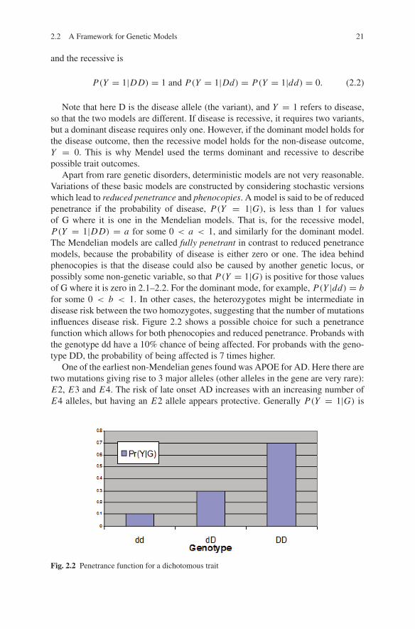
Apart from rare genetic disorders, deterministic models are not very reasonable.Variations of these basic models are constructed by considering stochastic versionswhich lead to reduced penetrance and phenocopies. A model is said to be of reducedpenetrance if the probability of disease, P(Y = 1|G), is less than 1 for valuesof G where it is one in the Mendelian models. That is, for the recessive model,P(Y = 1|DD) = a for some 0 < a < 1, and similarly for the dominant model.The Mendelian models are called fully penetrant in contrast to reduced penetrancemodels, because the probability of disease is either zero or one. The idea behindphenocopies is that the disease could also be caused by another genetic locus, orpossibly some non-genetic variable, so that P(Y = 1|G) is positive for those valuesof G where it is zero in 2.1–2.2. For the dominant mode, for example, P(Y |dd) = bfor some 0 < b < 1. In other cases, the heterozygotes might be intermediate indisease risk between the two homozygotes, suggesting that the number of mutationsinfluences disease risk. Figure 2.2 shows a possible choice for such a penetrancefunction which allows for both phenocopies and reduced penetrance. Probands withthe genotype dd have a 10% chance of being affected. For probands with the geno-type DD, the probability of being affected is 7 times higher.

One of the earliest non-Mendelian genes found was APOE for AD. Here there aretwo mutations giving rise to 3 major alleles (other alleles in the gene are very rare):E2, E3 and E4. The risk of late onset AD increases with an increasing number ofE4 alleles, but having an E2 allele appears protective. Generally P(Y = 1|G) is

Fig. 2.2 Penetrance function for a dichotomous trait


a complex function of G, but never reaches 1 or 0 for any genotype at the APOElocus.

One publication from the popular press (Pamela McDonald, The APOE GeneDiet: A Breakthrough in Changing, Cholesterol, Weight, Heart and Alzheimer’sUsing the Body’s Own Genes) lists the risk for AD as a function of selected APOEgenotypes: 20% for 33, 50% for 24, 60% for 34 and 92% for 44. In reality, pen-etrance functions for AD as a function of APOE genotype are difficult to quan-tify because they also depend on sex and age. With six possible genotypes, largeprospective samples will be required to quantify risk as a function of age and sexwith much precision.

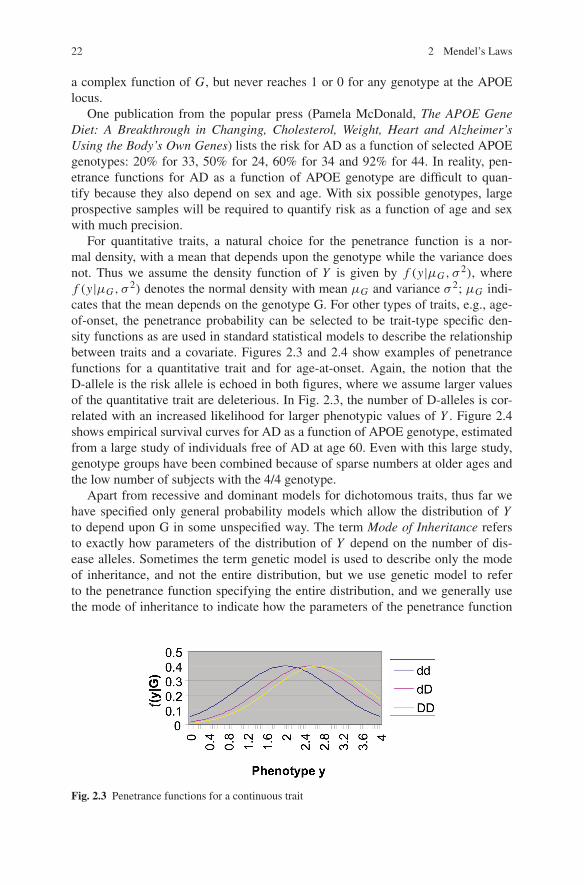
For quantitative traits, a natural choice for the penetrance function is a nor-mal density, with a mean that depends upon the genotype while the variance doesnot. Thus we assume the density function of Y is given by f (y|μG , σ

2), wheref (y|μG , σ

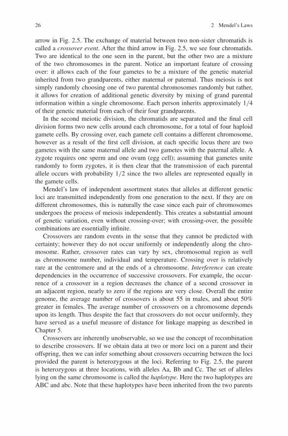
2) denotes the normal density with mean μG and variance σ 2; μG indi-cates that the mean depends on the genotype G. For other types of traits, e.g., age-of-onset, the penetrance probability can be selected to be trait-type specific den-sity functions as are used in standard statistical models to describe the relationshipbetween traits and a covariate. Figures 2.3 and 2.4 show examples of penetrancefunctions for a quantitative trait and for age-at-onset. Again, the notion that theD-allele is the risk allele is echoed in both figures, where we assume larger valuesof the quantitative trait are deleterious. In Fig. 2.3, the number of D-alleles is cor-related with an increased likelihood for larger phenotypic values of Y . Figure 2.4shows empirical survival curves for AD as a function of APOE genotype, estimatedfrom a large study of individuals free of AD at age 60. Even with this large study,genotype groups have been combined because of sparse numbers at older ages andthe low number of subjects with the 4/4 genotype.

Apart from recessive and dominant models for dichotomous traits, thus far wehave specified only general probability models which allow the distribution of Yto depend upon G in some unspecified way. The term Mode of Inheritance refersto exactly how parameters of the distribution of Y depend on the number of dis-ease alleles. Sometimes the term genetic model is used to describe only the modeof inheritance, and not the entire distribution, but we use genetic model to referto the penetrance function specifying the entire distribution, and we generally usethe mode of inheritance to indicate how the parameters of the penetrance function

Fig. 2.3 Penetrance functions for a continuous trait


Fig. 2.4 Empirical survival curves for AD as a function of APOE genotype in the NIMH GeneticsInitiative Alzheimer’s Disease (AD) Sample. The genotype variable x counts the number of ε4-alleles at the locus

depend on the number of disease alleles. There are four modes of inheritance thatare commonly used: recessive, dominant, additive and codominant. When only onecopy of the disease allele is required to induce an effect on the disease phenotype,Pr(Y = 1|d D) = Pr(Y = 1|DD), the mode of inheritance is called dominant.However, if 2 copies of the disease allele are required to elevate the disease risk,we speak of a recessive model or recessive mode of inheritance. Depending on the‘scale’, with an additive mode of inheritance the penetrance probability of heterozy-gous genotype is mid-way between the penetrance probabilities of both homozygousgenotypes, e.g., P(Y = 1|Dd) = 0.5 ∗ (P(Y = 1|DD) + P(Y = 1|dd)) on thelinear scale, or P(Y = 1|Dd) = √

P(Y = 1|DD) ∗ P(Y = 1|dd) on the log (mul-tiplicative) scale. The codominant mode of inheritance makes no assumptions aboutthe relationship among the three penetrance functions, only that they are different.The heterozygote advantage model specifies that heterozygotes have the lowest (orhighest for a heterozygote disadvantage model) risk of disease; it is occasionallyused, especially in plant breeding. We do not use it since it is a special case of themore general codominant model.

Note that with dichotomous traits, P(Y = 1|G) can be equivalently expressed asE(Y |G), and likewise for the continuous trait, μG = E(Y |G). Generalized LinearModels (GLM) provide a convenient way to express the dependence of the trait meanon G without specifying the entire distribution of Y . A generalized linear model issimilar to an ordinary linear regression model, except it allows the mean of Y todepend on covariates, X , in a non-linear way as:

g(E(Y |X)) = β0 + X ′β1. (2.3)

The link function, g(·), depends on the type of trait. For affection status out-comes, the logistic link:


log[E(Y |X)/(1 − E(Y |X))] = β0 + X ′β1, (2.4)

or log(relative risk) link:

log[E(Y |X)] = β0 + X ′β1, (2.5)

models are commonly used in epidemiological work; in genetics, linear models inthe probabilities themselves are also commonly used.

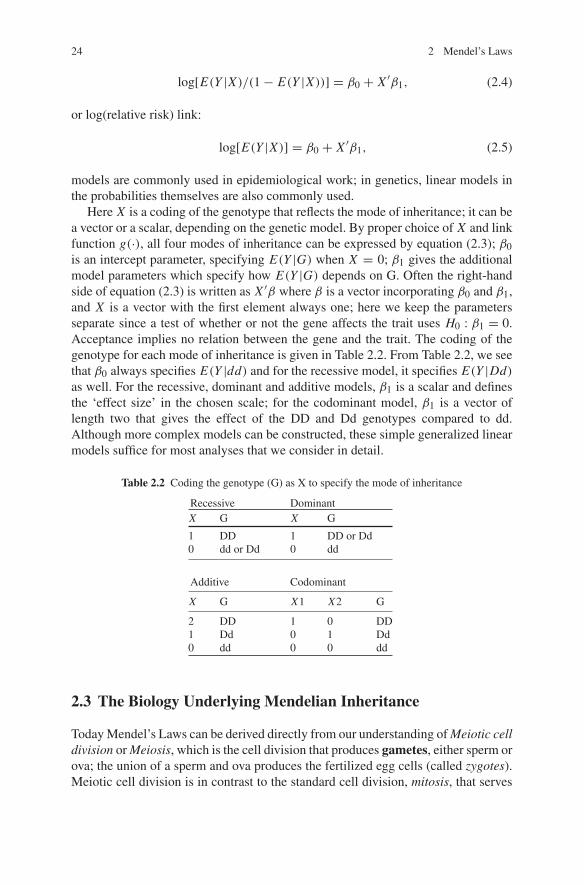
Here X is a coding of the genotype that reflects the mode of inheritance; it can bea vector or a scalar, depending on the genetic model. By proper choice of X and linkfunction g(·), all four modes of inheritance can be expressed by equation (2.3); β0is an intercept parameter, specifying E(Y |G) when X = 0; β1 gives the additionalmodel parameters which specify how E(Y |G) depends on G. Often the right-handside of equation (2.3) is written as X ′β where β is a vector incorporating β0 and β1,and X is a vector with the first element always one; here we keep the parametersseparate since a test of whether or not the gene affects the trait uses H0 : β1 = 0.Acceptance implies no relation between the gene and the trait. The coding of thegenotype for each mode of inheritance is given in Table 2.2. From Table 2.2, we seethat β0 always specifies E(Y |dd) and for the recessive model, it specifies E(Y |Dd)as well. For the recessive, dominant and additive models, β1 is a scalar and definesthe ‘effect size’ in the chosen scale; for the codominant model, β1 is a vector oflength two that gives the effect of the DD and Dd genotypes compared to dd.Although more complex models can be constructed, these simple generalized linearmodels suffice for most analyses that we consider in detail.

Table 2.2 Coding the genotype (G) as X to specify the mode of inheritance

Recessive DominantX G X G

1 DD 1 DD or Dd0 dd or Dd 0 dd

Additive Codominant

X G X1 X2 G

2 DD 1 0 DD1 Dd 0 1 Dd0 dd 0 0 dd

2.3 The Biology Underlying Mendelian Inheritance

Today Mendel’s Laws can be derived directly from our understanding of Meiotic celldivision or Meiosis, which is the cell division that produces gametes, either sperm orova; the union of a sperm and ova produces the fertilized egg cells (called zygotes).Meiotic cell division is in contrast to the standard cell division, mitosis, that serves

2.3 The Biology Underlying Mendelian Inheritance 25

the purpose of cell growth, development, repair and replacement of worn-out cells.While mitosis results in cells that are genetically identical (or clones), the purposeof meiosis is to introduce further genetic diversity by creating gametes, either eggcells or sperm cells, that are genetically different from the parent cells.

The nucleus of every cell contains two copies of each chromosome inheritedfrom the parents, one maternal copy and one paternal copy. Such cells are calleddiploid because they have two copies of each chromosome (except for males whohave one X and one Y for the sex chromosomes). Meiosis consists of two rounds ofcell divisions, each following a meiotic division (Fig. 2.5) ending with four haploidcells containing only one copy of each chromosome.

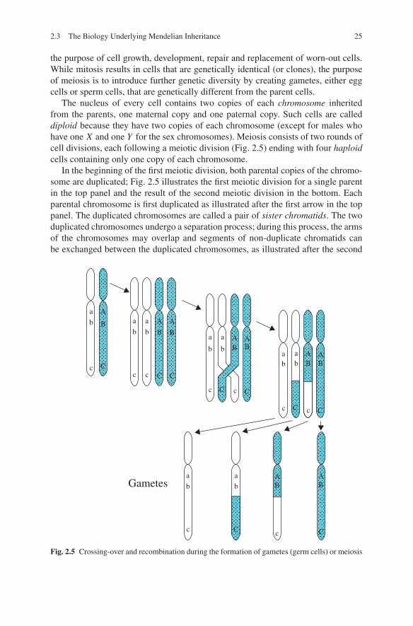
In the beginning of the first meiotic division, both parental copies of the chromo-some are duplicated; Fig. 2.5 illustrates the first meiotic division for a single parentin the top panel and the result of the second meiotic division in the bottom. Eachparental chromosome is first duplicated as illustrated after the first arrow in the toppanel. The duplicated chromosomes are called a pair of sister chromatids. The twoduplicated chromosomes undergo a separation process; during this process, the armsof the chromosomes may overlap and segments of non-duplicate chromatids canbe exchanged between the duplicated chromosomes, as illustrated after the second

a

b

c

a

b

c

a

b

c

a

b

c

a

b

c c

a

b

C C

a

b

C

ab

c c

ab

C C

A

B

C

A

B

C

A

B

C

C

A AB B

AB

AB

AB

AB

c

Gametes

Fig. 2.5 Crossing-over and recombination during the formation of gametes (germ cells) or meiosis


arrow in Fig. 2.5. The exchange of material between two non-sister chromatids iscalled a crossover event. After the third arrow in Fig. 2.5, we see four chromatids.Two are identical to the one seen in the parent, but the other two are a mixtureof the two chromosomes in the parent. Notice an important feature of crossingover: it allows each of the four gametes to be a mixture of the genetic materialinherited from two grandparents, either maternal or paternal. Thus meiosis is notsimply randomly choosing one of two parental chromosomes randomly but rather,it allows for creation of additional genetic diversity by mixing of grand parentalinformation within a single chromosome. Each person inherits approximately 1/4of their genetic material from each of their four grandparents.

In the second meiotic division, the chromatids are separated and the final celldivision forms two new cells around each chromosome, for a total of four haploidgamete cells. By crossing over, each gamete cell contains a different chromosome,however as a result of the first cell division, at each specific locus there are twogametes with the same maternal allele and two gametes with the paternal allele. Azygote requires one sperm and one ovum (egg cell); assuming that gametes uniterandomly to form zygotes, it is then clear that the transmission of each parentalallele occurs with probability 1/2 since the two alleles are represented equally inthe gamete cells.

Mendel’s law of independent assortment states that alleles at different geneticloci are transmitted independently from one generation to the next. If they are ondifferent chromosomes, this is naturally the case since each pair of chromosomesundergoes the process of meiosis independently. This creates a substantial amountof genetic variation, even without crossing-over; with crossing-over, the possiblecombinations are essentially infinite.

Crossovers are random events in the sense that they cannot be predicted withcertainty; however they do not occur uniformly or independently along the chro-mosome. Rather, crossover rates can vary by sex, chromosomal region as wellas chromosome number, individual and temperature. Crossing over is relativelyrare at the centromere and at the ends of a chromosome. Interference can createdependencies in the occurrence of successive crossovers. For example, the occur-rence of a crossover in a region decreases the chance of a second crossover inan adjacent region, nearly to zero if the regions are very close. Overall the entiregenome, the average number of crossovers is about 55 in males, and about 50%greater in females. The average number of crossovers on a chromosome dependsupon its length. Thus despite the fact that crossovers do not occur uniformly, theyhave served as a useful measure of distance for linkage mapping as described inChapter 5.

Crossovers are inherently unobservable, so we use the concept of recombinationto describe crossovers. If we obtain data at two or more loci on a parent and theiroffspring, then we can infer something about crossovers occurring between the lociprovided the parent is heterozygous at the loci. Referring to Fig. 2.5, the parentis heterozygous at three locations, with alleles Aa, Bb and Cc. The set of alleleslying on the same chromosome is called the haplotype. Here the two haplotypes areABC and abc. Note that these haplotypes have been inherited from the two parents

2.3 The Biology Underlying Mendelian Inheritance 27

of the parent, i.e., the grandparents of the offspring whose gametes are displayed.Suppose that the first gamete, abc, is inherited from the parent. There is no evidenceof crossing over here because one parental chromosome is identical abc, and theother parental chromosome shares none of these alleles. In this case we say thereis no recombination between either the A to B locus, or the B to C locus (or A toC either). Suppose the offspring inherits the second gamete, abC. In this case, theoffspring’s haplotype differs from either of the parent’s haplotypes, thus a crossovermust have occurred between the B and C locus, but not the A and B. Thus we sayno recombination has occurred between A and B, but a recombination occurredbetween B and C.

There is not a one-to-one relationship between recombination events and crossingover because recombination refers only to what can be observed between the twospecific loci, whereas crossing over refers to events that can occur anywhere in theinterval. If no crossover has occurred between two loci (as between the A and B lociin Fig. 2.5) then we will not see a recombination. However, it is possible for twocrossovers to occur in an interval; in this case, we may see no recombinant betweentwo markers flanking the interval, i.e., there may be segments of grand-maternalmaterial at the ends of the interval, with grand-paternal material in the middle. Theformal definition of the recombination fraction θ is given by P(recombination occursbetween two loci).

Crossovers between two loci very close to one another are rare. In this case, theprobability of a recombination between the two loci is very small. For example inFig. 2.5, considering loci A and B, among the four gametes, we observe two abgametes and two AB gametes: thus among these gametes, the probability of A ora (or B or b) is always 1

2 by Mendel’s law of segregation, but P(A allele and Ballele) = P(a allele and b allele) = 1

2 and P(A allele and b allele) = P(a alleleand B allele)= 0. This is contrary to what we would expect by Mendel’s law ofindependent assortment, which would specify a probability of 1

4 for each of the fourpossible gametes.

Between loci B and C, the situation is different because we observe a recombina-tion. Again, among the four gametes, P(B) = P(b) and likewise for C and c, but nowP(b and c) = P(B and c) = P(b and C) = P(B and C) = 1

4 , which corresponds toindependent assortment. In general, the distribution of gametes over many meioseswill depend upon the number of crossovers between them. If the two loci are close,θ is small, and the alleles at two loci tend to be inherited together, so that the law ofindependent assortment does not hold.

The relationship between θ and the distribution of crossovers is given byMather’s law:

θ = (1 − P0)/2,

where P0 is the probability of zero crossovers. Mather’s law can be argued as fol-lows. If there are no crossovers, P0 = 1, and there can be no recombination. Withprobability (1 − P0), at least one crossover occurs. If at least one crossover occurs,then the probability of a recombination is 1

2 , regardless of the number of crossovers.


To see why, recall that crossovers cannot occur between sister chromatids, but onlybetween non-sister chromatids. It is easy to see from Fig. 2.5 that one crossoverwill create two recombinant gametes and two non-recombinant gametes. With twocrossovers, the same two non-sister chromatids can be involved in both crossovers(and the number of recombinant gametes is zero) or both sister chromatids of eachpair cross over once with their non-sister chromatids, in which case all four gametesare recombinants. Since these two possibilities are equally likely, the average pro-portion of recombinants is 1

2 . The last possibility, that one sister chromatid crossesover twice with two different non-sister chromatids, gives 2 recombinant and 2 non-recombinant gametes. It is straightforward to argue the probability of a recombinantis also 1

2 for three crossovers, and so on.If two loci are very far apart, there are likely many crossovers between them; P0

approaches one in the limit and the recombination fraction approaches 12 . The upper

limit of θ corresponds to what we might expect if two loci are on different chromo-somes, since by the law of independent assortment, if the parent is heterozygous atboth loci, the four gametes will carry the four possible combinations, AB, Ab. aB,and ab with equal probability.

2.4 Exercises

1. Verify lines 1–3 of Table 2.1 using Mendel’s first law.2. Assume two genes with alleles A/a and B/b, controlling two different traits.

Assuming that Mendel’s second law holds (the alleles underlying the two dif-ferent traits are inherited independently), and starting with the pure strains as inMendel’s experiments:

(a) Verify the 1:2:1:2:4:2:1:2:1 ratios for the 9 possible genotypes inferred inthe F2 generation.

(b) Verify the 9:3:3:1 ratio for 4 possible traits observed in the F2 generation.

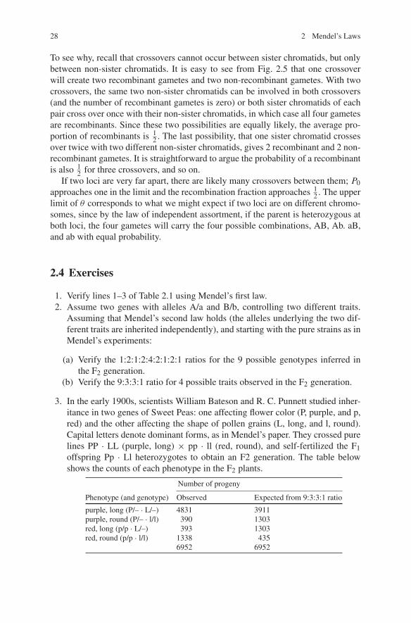
3. In the early 1900s, scientists William Bateson and R. C. Punnett studied inher-itance in two genes of Sweet Peas: one affecting flower color (P, purple, and p,red) and the other affecting the shape of pollen grains (L, long, and l, round).Capital letters denote dominant forms, as in Mendel’s paper. They crossed purelines PP · LL (purple, long) × pp · ll (red, round), and self-fertilized the F1offspring Pp · Ll heterozygotes to obtain an F2 generation. The table belowshows the counts of each phenotype in the F2 plants.

Number of progeny

Phenotype (and genotype) Observed Expected from 9:3:3:1 ratio

purple, long (P/– · L/–) 4831 3911purple, round (P/– · l/l) 390 1303red, long (p/p · L/–) 393 1303red, round (p/p · l/l) 1338 435

6952 6952

2.4 Exercises 29

(a) Verify the Expected column for testing goodness of fit to the 9:3:3:1 ratio.(b) Show that the chi-square goodness of fit test exceeds significance.

Note: As a possible explanation for the lack of fit, Bateson and Punnett pro-posed that the F1 had actually produced more P × L and p × l gametes thanwould be produced by Mendelian independent assortment. Because thesegenotypes were the gametic types in the original pure lines, the researchersthought that physical coupling between the dominant alleles P and L andbetween the recessive alleles p and l might have prevented their independentassortment in the F1. However, they did not know what the nature of thiscoupling could be.

(c) What is another possible explanation for lack of fit?

4. How many genotypes are possible with a 3-allele marker? With K alleles?5. Early onset Alzheimer’s disease is very rare; for illustrative purpose, assume it

is 0.1% among adults aged 30-60. Rare variants in 3 genes, APP, PSEN1 andPSEN2 have been identified as causing early onset AD in a dominant fashion,with P(AD | any of the three variants) = 1. Early onset AD can also be causedby head injury; many other non-genetic factors have been suggested. In a seriesof 101 cases of early onset AD, only 7 (or approximately 7%) were found tohave these variants in APP, PSEN1 or PSEN2; that is, the attributable risk dueto the three rare variants is low. For simplicity, assume that the probability ofvariants in these 3 genes is so rare that we can assume P(no variant in anygene) ≈ 1. Let the disease allele D symbolize a variant in any one of the threegenes, d is no variant, and Y = 1 means AD present.Estimate the probability of a phenocopy, P(Y = 1|dd) (also known as pheno-copy rate) for these genes combined, using the data given and Bayes Rule.

6. Consider a recessive Mendelian disease, where in the population, P(an individ-ual has 2 disease variants) = 0.000001.

(a) What is the probability that a randomly selected person is affected? Supposethat the randomly selected person is affected. What does that imply aboutthe probability that their sibling is also affected (you can assume that havingeither one or two parents with two variants is so rare that you can ignorethem)?

(b) Now answer both of these questions assuming the penetrance is only 12 , i.e.,

P(disease | 2 variants) = 12 , but the phenocopy rate is still zero.

7. Suppose we are dealing with a quantitative recessive trait, which is distributedas N (μ, 1) when there are two variants, and N (0, 1) otherwise. Calculate theprobability that a randomly selected person with two variants has a trait higherthan a person with one or no variants, when μ = 0.5, and when μ = 2.

8. Suppose we observe a quantitative trait which seems to show variation in boththe mean and the variance as a function of genotype. Give one example of agenetic model which allows for this.

9. One of the dichotomous traits that Mendel studied, length of plant stem, wasactually dichotomized from the measured length. He selected plants with a 6–7’


long axis to have the dominant trait and plants with a 3/4′ to 1.5′ long axis tohave the recessive trait. Mendel commented that in fact, “. . .the longer of thetwo parental stems is usually exceeded by the hybrid. . . Thus for instance, inrepeated experiments, stems of 1′ and 6′ in length yielded without exceptionhybrids which varied in length between 6′ and 7.5′.” What would be an appro-priate (non-deterministic) Gaussian penetrance function model for axis lengthas a continuous trait? Mendel also noted that there is very little variation instem height within genotype class. What does that imply about your Gaussianmodel?

10. Consider the Generalized Linear Model given in equation (2.3) Suppose youwish to include covariates, such as sex or age. Suggest how you might do thatin the context of the GLM.

11. Verify the statement concerning two crossovers: If one paternal chromatidcrosses over twice with two different maternal chromatids, this gives 2 recom-binant and 2 non-recombinant gametes.

http://www.springer.com/978-1-4419-7337-5

Documents

Principles of Inheritance: Mendel's Laws and Genetic Models