Embed Size (px)
Citation preview


Principles ofBroadband
Switching andNetworking
Tony T. Lee and Soung C. Liew

Principles ofBroadband
Switching andNetworking

WILEY SERIES IN TELECOMMUNICATIONSAND SIGNAL PROCESSINGJohn G. Proakis, EditorNortheastern University
A complete list of the titles in this series appears at the end of this volume.
telecommun.qxd 12/17/2009 1:47 PM Page 1

Principles ofBroadband
Switching andNetworking
Tony T. Lee and Soung C. Liew

Copyright © 2010 by John Wiley & Sons, Inc. All rights reserved.
Published by John Wiley & Sons, Inc., Hoboken, New JerseyPublished simultaneously in Canada
No part of this publication may be reproduced, stored in a retrieval system, or transmitted in any form orby any means, electronic, mechanical, photocopying, recording, scanning, or otherwise, except aspermitted under Section 107 or 108 of the 1976 United States Copyright Act, without either the priorwritten permission of the Publisher, or authorization through payment of the appropriate per-copy fee tothe Copyright Clearance Center, Inc., 222 Rosewood Drive, Danvers, MA 01923, (978) 750-8400, fax(978)-750-4470, or on the web at www.copyright.com. Requests to the Publisher for permission shouldbe addressed to the Permissions Department, John Wiley & Sons, Inc., 111 River Street, Hoboken, NJ07030, (201) 748-6011, fax (201) 748-6008, or online at http://www.wiley.com/go/ permissions.
Limit of Liability/Disclaimer of Warranty: While the publisher and author have used their best efforts inpreparing this book, they make no representations or warranties with respect to the accuracy orcompleteness of the contents of this book and specifically disclaim any implied warranties ofmerchantability or fitness for a particular purpose. No warranty may be created or extended by salesrepresentatives or written sales materials. The advice and strategies contained herein may not be suitablefor your situation. You should consult with a professional where appropriate. Neither the publisher norauthor shall be liable for any loss of profit or any other commercial damages, including but not limited tospecial, incidental, consequential, or other damages.
For general information on our other products and services or technical support, please contact ourCustomer Care Department within the United States at (800) 762-2974, outside the United States at (317)572-3993 or fax (317) 572-4002.
Wiley also publishes its books in a variety of electronic formats. Some content that appears in print maynot be available in electronic books. For more information about Wiley products, visit our web site atwww.wiley.com
ISBN: 978-0-471-13901-0
Library of Congress Cataloging-in-Publication Data is available.
Printed in the United States of America
10 9 8 7 6 5 4 3 2 1

Dedicated to Professor Charles K. Kao for his guidance,and to our wives, Alice and So Kuen, for their unwavering support.


CONTENTS
Preface xiii
About the Authors xvii
1 Introduction and Overview 11.1 Switching and Transmission 2
1.1.1 Roles of Switching and Transmission 2
1.1.2 Telephone Network Switching and Transmission Hierarchy 4
1.2 Multiplexing and Concentration 5
1.3 Timescales of Information Transfer 8
1.3.1 Sessions and Circuits 9
1.3.2 Messages 9
1.3.3 Packets and Cells 9
1.4 Broadband Integrated Services Network 10
Problems 12
2 Circuit Switch Design Principles 152.1 Space-Domain Circuit Switching 16
2.1.1 Nonblocking Properties 16
2.1.2 Complexity of Nonblocking Switches 18
2.1.3 Clos Switching Network 20
2.1.4 Benes Switching Network 28
2.1.5 Baseline and Reverse Baseline Networks 31
2.1.6 Cantor Switching Network 32
2.2 Time-Domain and Time–Space–Time Circuit Switching 35
2.2.1 Time-Domain Switching 35
2.2.2 Time–Space–Time Switching 37
Problems 39
vii

viii CONTENTS
3 Fundamental Principles of Packet Switch Design 433.1 Packet Contention in Switches 45
3.2 Fundamental Properties of Interconnection Networks 48
3.2.1 Definition of Banyan Networks 49
3.2.2 Simple Switches Based on Banyan Networks 51
3.2.3 Combinatoric Properties of Banyan Networks 54
3.2.4 Nonblocking Conditions for the Banyan Network 54
3.3 Sorting Networks 59
3.3.1 Basic Concepts of Comparison Networks 61
3.3.2 Sorting Networks Based on Bitonic Sort 64
3.3.3 The Odd–Even Sorting Network 70
3.3.4 Switching and Contention Resolution in Sort-Banyan Network 71
3.4 Nonblocking and Self-Routing Properties of Clos Networks 75
3.4.1 Nonblocking Route Assignment 76
3.4.2 Recursiveness Property 79
3.4.3 Basic Properties of Half-Clos Networks 81
3.4.4 Sort-Clos Principle 89
Problems 90
4 Switch Performance Analysis and Design Improvements 954.1 Performance of Simple Switch Designs 95
4.1.1 Throughput of an Internally Nonblocking Loss System 96
4.1.2 Throughput of an Input-Buffered Switch 96
4.1.3 Delay of an Input-Buffered Switch 103
4.1.4 Delay of an Output-Buffered Switch 112
4.2 Design Improvements for Input Queueing Switches 113
4.2.1 Look-Ahead Contention Resolution 113
4.2.2 Parallel Iterative Matching 115
4.3 Design Improvements Based on Output Capacity Expansion 119
4.3.1 Speedup Principle 119
4.3.2 Channel-Grouping Principle 121
4.3.3 Knockout Principle 131
4.3.4 Replication Principle 137
4.3.5 Dilation Principle 138
Problems 144
5 Advanced Switch Design Principles 1515.1 Switch Design Principles Based on Deflection Routing 151
5.1.1 Tandem-Banyan Network 151
5.1.2 Shuffle-Exchange Network 154

CONTENTS ix
5.1.3 Feedback Shuffle-Exchange Network 158
5.1.4 Feedback Bidirectional Shuffle-Exchange Network 166
5.1.5 Dual Shuffle-Exchange Network 175
5.2 Switching by Memory I/O 184
5.3 Design Principles for Scalable Switches 187
5.3.1 Generalized Knockout Principle 187
5.3.2 Modular Architecture 191
Problems 198
6 Switching Principles for Multicast, Multirate,and Multimedia Services 2056.1 Multicast Switching 205
6.1.1 Multicasting Based on Nonblocking Copy Networks 208
6.1.2 Performance Improvement of Copy Networks 213
6.1.3 Multicasting Algorithm for Arbitrary NetworkTopologies 220
6.1.4 Nonblocking Copy Networks Based on Broadcast ClosNetworks 228
6.2 Path Switching 235
6.2.1 Basic Concept of Path Switching 237
6.2.2 Capacity and Route Assignments for Multirate Traffic 242
6.2.3 Trade-Off Between Performance and Complexity 249
6.2.4 Multicasting in Path Switching 254
6.A Appendix 268
6.A.1 A Formulation of Effective Bandwidth 268
6.A.2 Approximations of Effective Bandwidth Based on On–OffSource Model 269
Problems 270
7 Basic Concepts of Broadband Communication Networks 2757.1 Synchronous Transfer Mode 275
7.2 Delays in ATM Network 280
7.3 Cell Size Consideration 283
7.4 Cell Networking, Virtual Channels, and Virtual Paths 285
7.4.1 No Data Link Layer 285
7.4.2 Cell Sequence Preservation 286
7.4.3 Virtual-Circuit Hop-by-Hop Routing 286
7.4.4 Virtual Channels and Virtual Paths 287
7.4.5 Routing Using VCI and VPI 289
7.4.6 Motivations for VP/VC Two-Tier Hierarchy 293

x CONTENTS
7.5 ATM Layer, Adaptation Layer, and Service Class 295
7.6 Transmission Interface 300
7.7 Approaches Toward IP over ATM 300
7.7.1 Classical IP over ATM 301
7.7.2 Next Hop Resolution Protocol 302
7.7.3 IP Switch and Cell Switch Router 303
7.7.4 ARIS and Tag Switching 306
7.7.5 Multiprotocol Label Switching 308
Appendix 7.A ATM Cell Format 311
7.A.1 ATM Layer 311
7.A.2 Adaptation Layer 314
Problems 319
8 Network Traffic Control and Bandwidth Allocation 3238.1 Fluid-Flow Model: Deterministic Discussion 326
8.2 Fluid-Flow On–Off Source Model: Stochastic Treatment 332
8.3 Traffic Shaping and Policing 348
8.4 Open-Loop Flow Control and Scheduling 354
8.4.1 First-Come-First-Serve Scheduling 355
8.4.2 Fixed-Capacity Assignment 357
8.4.3 Round-Robin Scheduling 358
8.4.4 Weighted Fair Queueing 364
8.4.5 Delay Bound in Weighted Fair Queueing with Leaky-BucketAccess Control 373
8.5 Closed-Loop Flow Control 380
Problems 381
9 Packet Switching and Information Transmission 3859.1 Duality of Switching and Transmission 386
9.2 Parallel Characteristics of Contention and Noise 390
9.2.1 Pseudo Signal-to-Noise Ratio of Packet Switch 390
9.2.2 Clos Network with Random Routing as a Noisy Channel 393
9.3 Clos Network with Deflection Routing 396
9.3.1 Cascaded Clos Network 397
9.3.2 Analysis of Deflection Clos Network 397
9.4 Route Assignments and Error-Correcting Codes 402
9.4.1 Complete Matching in Bipartite Graphs 402
9.4.2 Graphical Codes 405
9.4.3 Route Assignments of Benes Network 407
CONTENTS xi
9.5 Clos Network as Noiseless Channel-Path Switching 410
9.5.1 Capacity Allocation 411
9.5.2 Capacity Matrix Decomposition 414
9.6 Scheduling and Source Coding 416
9.6.1 Smoothness of Scheduling 417
9.6.2 Comparison of Scheduling Algorithms 420
9.6.3 Two-Dimensional Scheduling 424
9.7 Conclusion 430
Bibliography 433


PREFACE
The past few decades have seen the merging of many computer and communica-tion applications. Enabled by the advancement of optical fiber, wireless communi-cation, and very-large-scale integration (VLSI) technologies, modern telecommuni-cation networks can be regarded as one of the most important inventions of the pastcentury.
Before the emergence of Broadband Integrated Services Digital Network(B-ISDN), several separate communication networks already existed. They includethe telephone network for voice communication, the computer network for data com-munication, and the television network for TV program broadcasting. These net-works are designed with a specific application in mind and are typically not wellsuited for other applications. For example, the conventional telephone network can-not carry high-speed multimedia services, which require diverse quality-of-service(QoS) guarantees to support multirate and multicast connections. In addition, theseheterogeneous networks often require expensive gateways equipped with differentaccess interfaces running different protocols.
Meanwhile, the appeal of interactive video communication is on the rise in a soci-ety that is increasingly information-oriented. Images and facial expressions are morevivid and informative than text and audio for many types of human interactions. Forexample, video conferencing has made distant learning, medicine, and surgery pos-sible, while 3D Internet games give rise to real-time interactions between remoteplayers. All these applications are based on high-resolution video with large band-width demands. These developments led to the emergence of B-ISDN—the conceptof an integrated network to support communication services of all kinds to achievethe most cost-effective sharing of resources was conceived in the late 1980s.
This book focuses on the design and analysis of switch architectures that aresuitable for broadband integrated networks. In particular, the emphasis is on packet-switched interconnection networks with distributed routing algorithms. The focus ison the mathematical properties of these networks rather than specific implementationtechnologies. As such, although the pedagogical explanations in this book are inthe context of switches, many of the fundamental principles are relevant to othercommunication networks with regular topologies. For example, the terminals in amulti-hop ad hoc wireless network could conceivably be interconnected together toform a logical topology that is regular. This could be enabled by the use of directional
xiii

xiv PREFACE
antennas, inexpensive multi-radio, and cognitive-radio technologies that can identifyunused spectra. These technologies allow links to be formed among the terminals ina more flexible way, not necessarily based on proximity alone. There are two mainadvantages to regular network topologies: (1) very simple routing and scheduling arepossible with their well-understood mathematical properties; and (2) performanceand behavior are well understood and predictable. The performance and robustnessof these ad hoc networks are by no means ad hoc.
The original content of this book was an outgrowth of an evening course offered atthe Electrical Engineering Department of Columbia University, New York, in 1989.Since then, this course has been taught at Polytechnic Institute of New York Univer-sity, Brooklyn, NY and the Chinese University of Hong Kong, Hong Kong. The targetaudience is senior undergraduate and first-year postgraduate students with solid back-ground in probability theory. We found that many of our former students acquiredan appreciation of the beauty of the mathematics associated with telecommunicationnetworks after taking courses based on this book.
A general introduction and an overview of the entire book are given in Chapter 1,in which the roles of switching and transmission in the computer networks and tele-phone networks are discussed. The concept of the modern broadband integrated ser-vices network is explained and the reasons why this concept is necessary in modernsociety are also given in this chapter. The focus of Chapter 2 is on circuit switch designprinciples. Two types of the circuit switch design—space domain and time domain—are introduced in this chapter. Several classical nonblocking networks, including Closnetwork, Benes network, and Cantor network, are discussed.
Chapter 3 is devoted to fundamental principles of packet switch design, andChapter 4 focuses on the throughput and delay analyses of both waiting and lossswitching systems. The nonblocking and self-routing properties of packet switchesare elaborated by the combination of sorting and Banyan networks. Throughput im-provements are illustrated by some switch design variations such as speedup principle,channel-grouping principle, knockout principle, and dilation principle.
Chapter 5, following the previous chapter, explains some advanced switch designprinciples to alleviate the packet contention problem. Several networks based onthe deflection routing principle such as tandem-banyan, shuffle-exchange, feedbackshuffle-exchange, feedback bidirectional shuffle-exchange, and dual shuffle-exchangeare introduced. Switch scalability is discussed, which provides some key principlesto the construction of large switches out of modest-size switches, without sacrificingoverall switch performance. Chapter 6, on switch design principles for broadbandservices, first presents several fundamental switch design principles for multicasting.Then we end the chapter by introducing the concept of path switching, which is acompromise of the dynamic and the static routing schemes.
Chapter 7 departs from switch designs and the focus moves to broadband commu-nication networks that make use of such switches. The asynchronous transfer mode(ATM) being standardized worldwide is the technology that meets the requirementsof the broadband communication networks. ATM is a switching technology that di-vides data into fixed-length packets called cells. Chapter 8, on network traffic controland bandwidth allocation, gives an introduction on how to allocate network resources

PREFACE xv
and control the traffic to satisfy the quality-of-service (QoS) requirements of networkusers and to maximize network usage.
The content of Chapter 9 is an article “The mathematical parallels be-tween packet switching and information transmission” originally posted athttp://arxiv.org/abs/cs/0610050, which is included here as an epilogue. It is clear fromthe title that this is a philosophical discussion of analogies between switching andtransmission. We show that transmission noise and packet contention actually havesimilar characteristics and can be tamed by comparable means to achieve reliable com-munication. From various comparisons, we conclude that packet switching systemsare governed by mathematical laws that are similar to those of digital transmissionsystems as envisioned by Shannon in his seminal 1948 BSTJ paper “A MathematicalTheory of Communication.”
We would like to thank many former students of Broadband Communication Lab-oratory at the Chinese University of Hong Kong, including Cheuk H. Lam, Philip To,Man Chi Chan, Cathy Chan, Soung-Yue Liew, Yun Deng, Manting Choy, JianmingLiu, Sichao Ruan, Li Pu, Dongjie Yin, and Pui King Wong, who participated in thediscussions of the content of the book over the years. We are especially grateful for thedelicate latex editing and figure drawing of the entire book by our student assistantsJiawei Chen and Yulin Deng. Our “family networks,” though small, have given us theconnectivity to many joys of life. We can never repay the debt of gratitude we owe toour families—our wives, Alice and So Kuen, and our children, Wynne and EdwardLee, and Vincent and Austin Liew—for their understanding, support, and patiencewhile we wrote this book.
Tony T. LeeSoung C. Liew


ABOUT THE AUTHORS
Professor Tony T. Lee received his BSEE degree from the National Cheng KungUniversity, Taiwan, in 1971, and his MS and PhD degrees in electrical engineeringfrom the Polytechnic University in New York in 1976 and 1977, respectively. Cur-rently, he is a Professor of Information Engineering at the Chinese University ofHong Kong and an Adjunct Professor at the Institute of Applied Mathematics of theChinese Academy of Sciences. From 1991 to 1993, he was a Professor of ElectricalEngineering at the Polytechnic Institute of University of New York, Brooklyn, NY.He was with AT&T Bell Laboratories, Holmdel, NJ, from 1977 to 1983, and Bell-core, currently Telcordia Technologies, Morristown, NJ, from 1983 to 1993. He isnow serving as an Editor of the IEEE Transactions on Communications, and an AreaEditor of Journal of Communication Network. He is a fellow of IEEE and HKIE. Heis the recipient of many awards including the National Natural Science Award fromChina, the Leonard G. Abraham Prize Paper Award from the IEEE CommunicationSociety, and the Outstanding Paper Award from IEICE.
Professor Soung Chang Liew received his SB, SM, EE, and PhD degrees fromthe Massachusetts Institute of Technology. From 1984 to 1988, he was at the MITLaboratory for Information and Decision Systems, where he investigated fiber-opticcommunication networks. From March 1988 to July 1993, Professor Liew was atBellcore (now Telcordia), New Jersey, where he was engaged in broadband networkresearch. He is currently Professor and Chairman of the Department of InformationEngineering, the Chinese University of Hong Kong. He is also an Adjunct Professorat the Southeast University, China. His current research interests include wirelessnetworks, Internet protocols, multimedia communications, and packet switch design.Professor Liew and his students won the best paper awards at the 1st IEEE Interna-tional Conference on Mobile Ad-Hoc and Sensor Systems (IEEE MASS 2004) andthe 4th IEEE International Workshop on Wireless Local Network (IEEE WLN 2004).Separately, TCP Veno, a version of TCP to improve its performance over wirelessnetworks proposed by Professor Liew and his students, has been incorporated into arecent release of Linux OS. In addition, Professor Liew initiated and built the firstinteruniversity ATM network testbed in Hong Kong in 1993.
Besides academic activities, Professor Liew is active in the industry. He cofoundedtwo technology start-ups in Internet software and has been serving as consultantto many companies and industrial organizations. He is currently consultant for the
xvii

xviii ABOUT THE AUTHORS
Hong Kong Applied Science and Technology Research Institute (ASTRI), providingtechnical advice as well as helping to formulate R&D directions and strategies in theareas of wireless internetworking, applications, and services. Professor Liew holdsthree U.S. patents and is a Fellow of IEE and HKIE. He is listed in Marquis Who’sWho in Science and Engineering. He is the recipient of the first Vice-ChancellorExemplary Teaching Award at the Chinese University of Hong Kong.
1
INTRODUCTION AND OVERVIEW
The past few decades have seen the merging of computer and communication tech-nologies. Wide-area and local-area computer networks have been deployed to inter-connect computers distributed throughout the world. This has led to a proliferation ofmany useful data communication services, such as electronic mail, remote file transfer,remote login, and web pages. Most of these services do not have very stringent “real-time” requirements in the sense that there is no urgency for the data to reach the re-ceiver within a very short time, say, below 1s. At the other spectrum, the telephone net-work has been with us for a long time, and the information carried by the network hasbeen primarily real-time telephone conversations. It is important for voice to reach thelistener almost immediately for an intelligible and coherent conversation to take place.
With the emergence of multimedia services, real-time traffic will include not justvoice, but also video, image, and computer data files. This has given rise to the visionof an integrated broadband network that is capable of carrying all kinds of information,real-time or non-real-time.
Many wide-area computer networks are implemented on top of telephone net-works: transmission lines are leased from the telephone companies, and each of theselines interconnects two routers that perform data switching. Home computers are alsolinked to a gateway via telephone lines using modems. The gateway is in turn con-nected via telephone lines to other gateways or routers over the wide-area network.Thus, present-day computer networks are mostly networks overlaid on telephone net-works. Strictly speaking, the telephone networks that are being used to carry computerdata cannot be said to be integrated. The networks are designed with the intentionthat voice traffic will be carried, and their designs are optimized according to this as-sumption. A transmission line optimized for voice traffic is not necessarily optimal forother traffic types. The computer data are just “guests” to the telephone networks, andmany components of the telephone network may not be optimized for the transportof non-voice services.
Principles of Broadband Switching and Networking, by Tony T. Lee and Soung C. LiewCopyright © 2010 John Wiley & Sons, Inc.
1

2 INTRODUCTION AND OVERVIEW
The focus of this book is on future broadband integrated networks. Loosely, theterms “broadband” and “integration” imply that services with rates from below onekbps to hundreds of Mbps can be supported. Some of these services, such as videoconferencing, are widely known and anticipated, whereas others may be unforeseenand created only when the broadband network becomes available. The broadbandnetwork must be flexible enough to accommodate these unanticipated services aswell.
1.1 SWITCHING AND TRANSMISSION
At the fundamental level, a communication network is composed of switching andtransmission resources that make it possible to transport information from one userto another. On top of the switching and transmission resources, we have the controlfunctions, which could be implemented by either software or hardware, or both.Among other things, the control functions make it possible to automate the settingup of a connection between two users. At another level, they also ensure efficientusage of the switching and transmission resources. In a real network, the switching,transmission, and control facilities are typically distributed across many locations.
1.1.1 Roles of Switching and Transmission
When there are only two users, as shown in Fig. 1.1, information created by one useris always targeted to the other user: switching is not needed and only transmissionis required. In essence, the transmission facilities serve to carry information directlyfrom one end of the transmission medium, which could be a coaxial cable, an opticalfiber, or the air space, to the other end.
As soon as we have a third user in our network, the question of who wants tocommunicate with whom, and at what time, arises. With reference to Fig. 1.2, userA may want to talk to user B at one time but to user C later. The switching functionmakes it possible to change the connectivity among users in a dynamic way. In thisway, a user can communicate with different users at different times.
BA
Transmission medium
When there are only two users, information from A is
by default destined for B, and vice versa
FIGURE 1.1 A two-user network; switching is not required.

SWITCHING AND TRANSMISSION 3
A
Switching
B
C
Information from A may be destined for B or C
FIGURE 1.2 A three-user network; switching is required.
It turns out that the locations of the switching facilities in a network have asignificant impact on the amount of transmission facilities required in a network.Figure 1.3(a) depicts a telephone network in which the switching facilities are dis-tributed and positioned at the N users’ locations, and a user is connected to each ofthe other users via a unique line. Switching is performed when the user decides whichof the N lines to use. When N is large, there will be many transmission lines and thetransmission cost will be rather prohibitive.
In contrast, Fig. 1.3(b) shows a network in which each user has only one accessline through which it can be connected to the other users. Switching is performed at
Switching is performed
by a central switchCentral
Switch
1
2
3
N ...
1
N
2
3
...
Switching is performed at
user’s location by selecting
one of the links for reception
# of bidirectional links
= N(N–1)/2
(a)
(b)
FIGURE 1.3 N -user networks with switching performed (a) at user’s locations (b) by a centralswitch.
4 INTRODUCTION AND OVERVIEW
a central location. To the extent that a user does not need to speak to all the otherusers at the same time, this is a better solution because of the reduced number oftransmission lines. Of course, if a user wants to be able to connect to more than oneuser simultaneously, multiple lines must still be installed between the user and thecentral switch.
In practice, a network typically consists of multiple switching centers at variouslocations that are interconnected via transmission lines. By locating the switchingcenters judiciously, transmission cost can be reduced.
1.1.2 Telephone Network Switching and Transmission Hierarchy
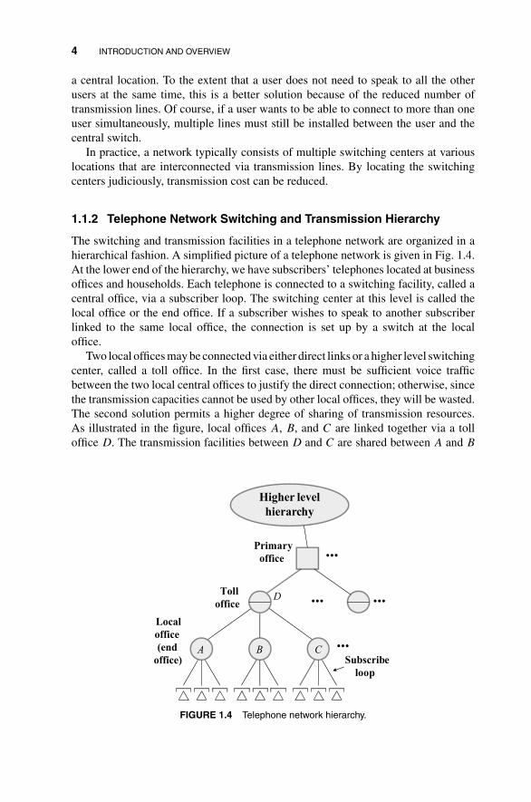
The switching and transmission facilities in a telephone network are organized in ahierarchical fashion. A simplified picture of a telephone network is given in Fig. 1.4.At the lower end of the hierarchy, we have subscribers’ telephones located at businessoffices and households. Each telephone is connected to a switching facility, called acentral office, via a subscriber loop. The switching center at this level is called thelocal office or the end office. If a subscriber wishes to speak to another subscriberlinked to the same local office, the connection is set up by a switch at the localoffice.
Two local offices may be connected via either direct links or a higher level switchingcenter, called a toll office. In the first case, there must be sufficient voice trafficbetween the two local central offices to justify the direct connection; otherwise, sincethe transmission capacities cannot be used by other local offices, they will be wasted.The second solution permits a higher degree of sharing of transmission resources.As illustrated in the figure, local offices A, B, and C are linked together via a tolloffice D. The transmission facilities between D and C are shared between A and B
A B C
Higher level
hierarchy
...
...
...
...
Primary
office
Toll
office
Local
office
(end
office)
D
Subscribe
loop
FIGURE 1.4 Telephone network hierarchy.

MULTIPLEXING AND CONCENTRATION 5
in the sense that both traffic between A and C and between B and C travel overthem.
The toll offices are interconnected via an even higher level office, called the primaryoffice. The primary offices are in turn connected by a yet even higher level office.Each level may move up to a higher level. In this way, a network hierarchy is formed.
The total amount of traffic reduces as we move up the hierarchy because of the so-called community-of-interest phenomenon. For instance, it is generally more likelyfor a user to make local phone calls than long-distance phone calls. The former mayinvolve only a local switching office while the latter involves a series of switchingoffices at successive levels.
In short, an important objective achieved with the hierarchical network is thesharing of resources. The resources at the higher level are shared by a larger populationof subscribers. The amount of resources can be reduced because it is statisticallyunlikely that all the subscribers will want to use the higher level resources at the sametime.
Another advantage that comes with the hierarchical structure is the simplicity infinding a “route” for a connection between two subscribers. When subscriber i wantsto connect to subscriber j, the local office of i first checks if j also belongs to thesame office. If yes, switching is completed at the office. Otherwise, a connection ismade between the local office and the next level toll office (assuming there are nodirect links between the central offices of i and j). This procedure is repeated until anoffice with branches leading to both i and j is found.
1.2 MULTIPLEXING AND CONCENTRATION
Multiplexing and concentration are important concepts in reducing transmission cost.In both, a number of users share an underlying transmission medium (e.g., an opticalfiber, a coaxial cable, or the air space).
As a multiplexing example, frequency-division multiplexing (FDM) is used tobroadcast radio and TV programs on the air medium. In FDM, the capacity, or band-width, of the transmission medium is divided into different frequency bands, andeach band is a logical channel for carrying information from a unique source. FDMcan be used to subdivide the capacity of air medium, a coaxial cable, or any othertransmission medium. Figure 1.5 depicts the transmission of digital information froma number of sources using FDM. Different carrier frequencies are used to transportdifferent information streams. Receivers at the other end use bandpass filters to selectthe desired information stream.
Multiplexing can also be performed in the time domain. This is a more widelyused multiplexing technique than FDM in telephone networks. Figure 1.6 illustratesa simple time-division multiplexing (TDM) scheme. The N sources take turns in around-robin fashion to transmit on the transmission medium. Time is divided intoframes, each having N time slots. Each source has a time slot dedicated to it in eachframe. Thus, time slot 1 is assigned to source 1, time slot 2 to source 2, and so on.The slot positions i in successive frames all belong to the source i.

6 INTRODUCTION AND OVERVIEW
FIGURE 1.5 Frequency-division multiplexing.
In this book, we define switching as changing the connectivity between end usersor equipments. The goal of a multiplexing system (consisting of the multiplexer, thetransmission medium, and the demultiplexer) is not to perform switching; the goal isto partition a transmission medium into a number of logical channels, each of whichcan be used to interconnect a transmitter and a receiver. In the two scenarios above,each of the N multiplexed channels is dedicated exclusively to a transmitter–receiverpair, and which transmitter is connected to which receiver does not change over time.As an overall system, an input of the multiplexer is always connected to the sameoutput of the demultiplexer. Thus, functionally, no switching occurs. Such is not thecase with a concentrator.
Concentration achieves cost saving by making use of the fact that it is unlikelyfor all users to be active simultaneously at any given time. Therefore, transmissionfacilities need only be allocated to the active users. In the telephone network, forinstance, it is unlikely that all the subscribers of the same local office want to use theirphones at the same time. An N × M concentrator, as shown in Fig. 1.7, concentratestraffic from N sources onto M (M < N) outputs. A number of concentrators areusually placed at the “front end” of the local switching center to reduce the number
Source 1
Source 2
Source N
Receiver 1
Receiver 2
Receiver N
M
U
X
D
E
M
U
X
. . .. . .
Time
slot
Frame
NB bps
B bps
FIGURE 1.6 Time-division multiplexing.

MULTIPLEXING AND CONCENTRATION 7
N Mconcentrator
(N > M )
.
.
.
.
.
.
Input 1
Input 2
Input N
Output 1
Output 2
Output N
An active input is assigned to one of the outputs. It does
not matter which output is assigned.
FIGURE 1.7 An N × M concentrator.
of ports of the switch. An output of a concentrator, hence an input to the switch, isallocated to the subscriber only when he picks up the phone. The connectivity (i.e.,which input is connected to which output) of the concentrator changes in a dynamicmanner over time. If more than M sources are active at the same time, then someof the sources may be “blocked.” For telephone networks, M can usually be madeconsiderably smaller than N to save cost without incurring a high likelihood forblocking.
Both multiplexers and concentrators achieve resource sharing, but in differentways. Let us refer to the sums of the capacities (bit rates) of the transmission linesconnected to the inputs and outputs as the total input and output capacities, respec-tively. For a multiplexer, the total output capacity is equal to the total input capacity,whereas for a concentrator, the total output capacity is smaller than the total inputcapacity. The output capacity or bandwidth of the concentrator is said to be sharedamong the inputs, and that of the multiplexer is not. The concentrator outputs are al-located dynamically to the inputs based on need, and the allocation cannot be foretoldin advance. In contrast, although a multiplexer allows the same transmission mediumto be shared among several transmitter–receiver pairs, this is achieved by subdividingthe capacity of the transmission medium and dedicating the resulting subchannels inan exclusive manner to individual pairs.
Statistical multiplexing is a packet-switching technique that can be considered ascombining TDM with concentration. Consider a TDM scheme in which there are M
(M < N) time slots in a frame. The output capacity is then smaller than the maximumpossible total capacities of the inputs. A time slot is not always dedicated to a particularsource. Slot 1 of frame 1 may be used by user 1, but user 1 may be idle in the nextframe and slot 1 of frame 2 may be used by another user. The same slot positions ofdifferent frames can be used by different users, and therefore they can be targeted fordifferent destinations in the overall communication network. To route the informationin a slot to its final destination, we therefore need to encode the routing informationin a “header” and attach the header to the information bits before putting both into
8 INTRODUCTION AND OVERVIEW
Statistical
multiplexer
12
3123
Input 1
Input 2
Input N
.
.
.
Arriving packets
B bps
Less than NB bps
Transmission capacity is shared
dynamically among the input
according to packet arrivals
FIGURE 1.8 A statistical multiplexer.
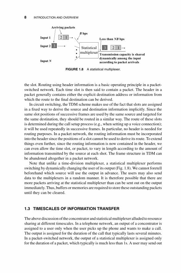
the slot. Routing using header information is a basic operating principle in a packet-switched network. Each time slot is then said to contain a packet. The header in apacket generally contains either the explicit destination address or information fromwhich the route to the final destination can be derived.
In circuit switching, the TDM scheme makes use of the fact that slots are assignedin a fixed way to derive the source and destination information implicitly. Since thesame slot positions of successive frames are used by the same source and targeted forthe same destination, they should be routed in a similar way. The route of these slotsis determined during the call setup process (e.g., when setting up a voice connection);it will be used repeatedly in successive frames. In particular, no header is needed forrouting purposes. In a packet network, the routing information must be incorporatedinto the header since the positions of a slot cannot be used to derive its route. To extendthings even further, since the routing information is now contained in the header, wecan even allow the time slot, or packet, to vary in length according to the amount ofinformation transmitted by the source at each shot. The frame structure in TDM canbe abandoned altogether in a packet network.
Note that unlike a time-division multiplexer, a statistical multiplexer performsswitching by dynamically changing the user of its output (Fig. 1.8). We cannot foretellbeforehand which source will use the output in advance. The users may also senddata to the multiplexers in a random manner. It is therefore possible that there aremore packets arriving at the statistical multiplexer than can be sent out on the outputimmediately. Thus, buffers or memories are required to store these outstanding packetsuntil they can be cleared.
1.3 TIMESCALES OF INFORMATION TRANSFER
The above discussion of the concentrator and statistical multiplexer alluded to resourcesharing at different timescales. In a telephone network, an output of a concentrator isassigned to a user only when the user picks up the phone and wants to make a call.The output is assigned for the duration of the call that typically lasts several minutes.In a packet-switched network, the output of a statistical multiplexer is assigned onlyfor the duration of a packet, which typically is much less than 1s. A user may send out
TIMESCALES OF INFORMATION TRANSFER 9
packets sporadically during a communication session. It is important to have a clearconcept of the timescales of information transfer to appreciate the fact that resourcesharing and network control can be achieved at different timescales.
1.3.1 Sessions and Circuits
Before two end users can send information to each other, a communication sessionneeds to be established. A telephone call is a communication session. As anotherexample, when we log onto a computer remotely, we establish a session between thelocal terminal and the remote computer.
Network resources are assigned to set up a circuit or connection for this session.Some of these resources, such as an output of a concentrator in a circuit-switchednetwork, may be dedicated exclusively to this connection while it remains active.Some of these resources, such as the output of a statistical multiplexer in a packetnetwork, may be used by other sessions concurrently. In the latter, the transmissionbandwidth is not dedicated exclusively to the session and is shared among activesessions, and the associated circuit is sometimes called a virtual circuit.
Some packet networks are not connection-oriented. It is not necessary to preestab-lish a connection (hence a route from the source to the destination) before data are sentby a session. In fact, successive packets of the session may traverse different routesto reach the destination. Although the concept of a connection is absent within thenetwork, the end users still need to set up a session before they start to communicate.The setup time, however, can be much shorter than in a connection-oriented networkbecause the control functions inside the network need not be involved for connectionsetup.
1.3.2 Messages
Once a session is set up, the users can then send information in the form of messagesin an on–off manner. For a remote login session, the typing of the carriage-return keyby the end user may result in the sending of a line of text as a message. Files mayalso be sent as a message. So, messages tend to vary in length.
For a two-party telephone session, for example, it is known that a user speaks only40% of the time. The activity of the user is said to alternate between idle period andbusy period. The busy period is called a talkspurt, which can be viewed as a messagein a voice session. A scheme called time assigned speech interpolation (TASI) is oftenused to statistically multiplex several voice sources onto the same satellite link on atalkspurt basis.
1.3.3 Packets and Cells
Messages are data units that have meaning to the end users and have a logical rela-tionship with the associated service. It could be a talkspurt, a line of text, a file, andso on. Packets, on the other hand, are transport data units within the network.
10 INTRODUCTION AND OVERVIEW
In a packet network, a long message is often fragmented into smaller packets beforeit is transported across the network. One possible reason for fragmentation could bethat the communication network does not support packets beyond a certain length.For instance, the Internet has a maximum packet size of 64 Kbytes.
Another reason for message fragmentation is that most computer networks arestore-and-forward networks in which a switching node must receive the entire packetbefore it is forwarded to the next node. By fragmenting a long message into manysmaller packets, the end-to-end delay of the message can be made smaller, especiallywhen the network is lightly loaded (see Problem 1.4).
Yet another motivation for fragmentation is to prevent a long packet from hogginga communication channel. Consider the output of a statistical multiplexer. While along packet is being transmitted, newly arriving packets from other sources must waituntil the completion of its transmission, which may take an excessively long time ifthere were no limit on its length. On the other hand, if the long packet has been cut intomany smaller packets, the newly arriving packets from other sources have a chanceto jump ahead and access the output channel after a short wait for the transmission ofthe current packet to complete.
Packet length can be variable or fixed. One advantage of the fixed packet-lengthscheme is that more efficient packet switches can be implemented. For instance, bytime aligning the boundaries of the packets across the inputs of a packet switch, higherthroughput can be achieved with the fixed packet-length scheme than with the variablepacket-length scheme.
The fixed packet-length scheme has a disadvantage when the messages to be sentare much shorter than the packet length. In this case, only a small part of each packetcontains the useful message, and the rest is stuffed with dummy bits to make up thewhole packet. The observation suggests that small packets are preferable. However,the length of the packet header is largely independent of the overall packet length(e.g., the destination address length in the header is independent of the packet length).Hence, the header overhead (ratio of header length to packet length) tends to be largerfor smaller packets. Thus, too small a packet can lead to high inefficiency as well.
In general, the determination of packet size is a complicated issue involving consid-erations from many different angles, not the least the characteristics of the underlyingnetwork traffic. The ITU (International Telecommunication Union), an internationalstandard body, has chosen the asynchronous transfer mode (ATM) to be the informa-tion transport mechanism for the future broadband integrated network. An essenceof the ATM scheme is that the basic information data unit is a 53-byte fixed-lengthpacket called cells. The details of ATM and the motivations for the small-size cellwill be covered in the later chapters.
1.4 BROADBAND INTEGRATED SERVICES NETWORK
The discussion up to this point forms the backdrop of the focus of this book—broadband integrated services networks. As the name suggests, an integrated networkmust be capable of supporting many different kinds of services.

BROADBAND INTEGRATED SERVICES NETWORK 11
Traditionally, services are segregated and each communication network supportsonly one type of service. Some examples of these networks are the telephone, televi-sion, airline reservation, and computer data networks. There are many advantages tohaving a single integrated network for the support of all these services. For instance,efficient resource sharing may be achievable. Take the telephone service. More phonecalls are made during business hours than during the evening. The television service,on the other hand, is in high demand during the evening. By integrating these ser-vices on the same network, the same resources can be assigned to different servicesat different times.
Traditionally, whenever a new service is introduced, a new communication networkmay need to be designed and set up. Carrying the information traffic of this serviceon a network designed for another service may not be very efficient because of thedissimilar characteristics of the traffic. If an integrated network is designed with theforethought that some unknown services may need to be introduced in the future, thenthese services can be accommodated more easily.
The design of an integrated network taking into account the above concern is byno means easy. Figure 1.9 shows some services with widely varying traffic character-istics; the holding times (durations of sessions) and bit rate requirements of differentservices may differ by several orders of magnitude. Furthermore, some services, suchas computer data transfer, tend to generate traffic in a bursty manner during a session(Fig. 1.10). Other services such as telephony and video conferencing generate trafficin a more continuous fashion.
The delay requirements may also be different. Real-time services are highly sensi-tive to network delay. For example, if real-time video data do not arrive at the displaymonitor at the receiver within certain time, they might as well be considered as lost.
Duration of session (second)
Bit rate
(bps)
107
106
105
104
103
102
10
1
0107 108 109 101010610510410310 1021
Voice
Low-speed
data
Telemetry
Conference
video
High-quality
entertainment
video
High-speed data
information retrieval
FIGURE 1.9 Holding times and bit rates of various services.
12 INTRODUCTION AND OVERVIEW
Less-bursty traffic
Bit rate
Time
Bursty traffic
Bit rate
Time
Continuous traffic
Bit rate
Time
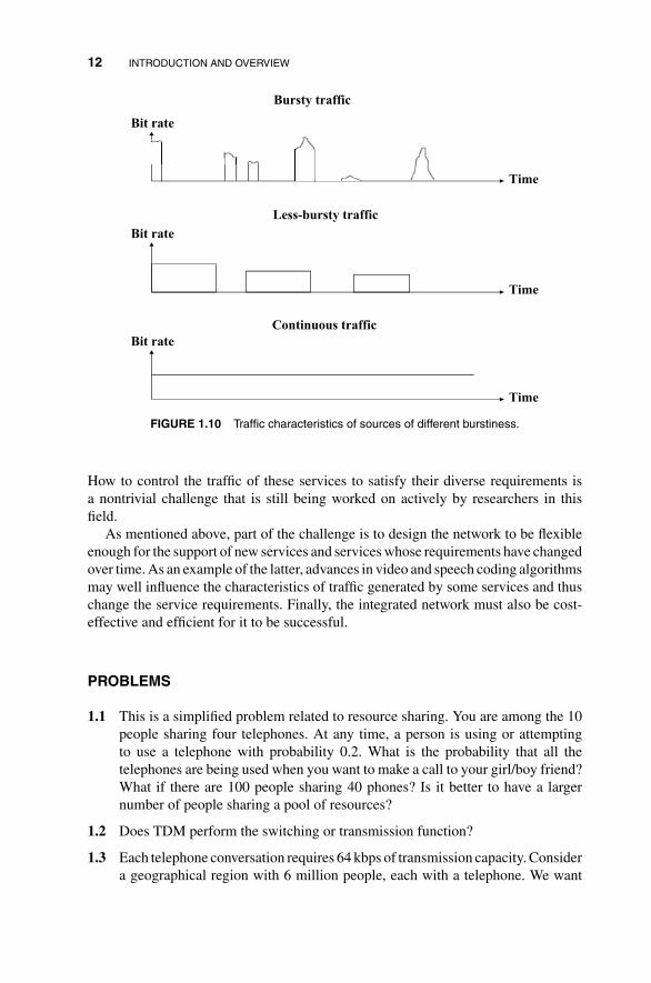
FIGURE 1.10 Traffic characteristics of sources of different burstiness.
How to control the traffic of these services to satisfy their diverse requirements isa nontrivial challenge that is still being worked on actively by researchers in thisfield.
As mentioned above, part of the challenge is to design the network to be flexibleenough for the support of new services and services whose requirements have changedover time. As an example of the latter, advances in video and speech coding algorithmsmay well influence the characteristics of traffic generated by some services and thuschange the service requirements. Finally, the integrated network must also be cost-effective and efficient for it to be successful.
PROBLEMS
1.1 This is a simplified problem related to resource sharing. You are among the 10people sharing four telephones. At any time, a person is using or attemptingto use a telephone with probability 0.2. What is the probability that all thetelephones are being used when you want to make a call to your girl/boy friend?What if there are 100 people sharing 40 phones? Is it better to have a largernumber of people sharing a pool of resources?
1.2 Does TDM perform the switching or transmission function?
1.3 Each telephone conversation requires 64 kbps of transmission capacity. Considera geographical region with 6 million people, each with a telephone. We want
PROBLEMS 13
to multiplex all the telephone traffic onto a number of optical fibers, each withcapacity of 2.4 Gbps. How many fibers are needed?
1.4 Consider the problem of fragmenting a message of 1000 bytes into packets ofx bytes each. Each packet has a header (overhead) of 10 bytes. The messagepasses through five links of the same transmission rate in a store-and-forwardnetwork on its way to destination. There is no other traffic in the network. Whatis the optimal packet size x in order to minimize end-to-end delay?
1.5 Consider 100 active phone conversations being multiplexed onto 60 lines byTASI. Assume a person speaks only 40% of the time when using a telephone.Talkspurts are clipped when all 60 lines have been used. What is the probabilityof a talkspurt being clipped?


2
CIRCUIT SWITCH DESIGNPRINCIPLES
The telephone network is the most widespread and far-reaching among all commu-nication networks. It is difficult to imagine a modern society without it. In fact, thetelephone network is one of the largest and most complex engineering systems cre-ated by mankind. A large portion of the Internet is built upon the telephone networkinfrastructure. Much thought and work have gone into the design of the telephonenetwork.
The telephone network is largely a circuit-switched network in which resourcesharing is achieved at the session level. Transmission and switching facilities arededicated to a session only when a telephone call is initiated. Using these resources,a circuit, or a connection, is formed between two end users. These facilities will bereleased upon the termination of the call so that other sessions may use them. Whilethe session is ongoing, however, the resources assigned to the circuit are not sharedby other circuits and can be used to carry the traffic of the circuit only. In otherwords, once the resources are assigned to a circuit, they are guaranteed. Of course,there is a no guarantee that a newly initiated session will get the resources that itrequests. In this case, the call is said to be “blocked.” One important design issue ofthe circuit-switched network is how to minimize the blocking probability in a low-costand efficient manner.
An example of this problem is the determination of the minimum number of“trunks” or transmission lines between two switching centers in order to meet acertain blocking probability requirement. In general, more trunks will be needed forsmaller blocking probability. One of the exercises of this chapter goes over this inmore detail. A call can also be blocked because of the design of the switch even ifthere are enough trunks. This chapter focuses on the fundamental design principlesof circuit switches; in particular, how switches can be designed to be nonblocking,
Principles of Broadband Switching and Networking, by Tony T. Lee and Soung C. LiewCopyright © 2010 John Wiley & Sons, Inc.
15

16 CIRCUIT SWITCH DESIGN PRINCIPLES
1
2
N
1
2
N
......
Inputs Outputs
FIGURE 2.1 An N × N switch used to interconnect N inputs and N outputs.
in which case blocking will be due entirely to number of calls exceeding number oftrunks.
2.1 SPACE-DOMAIN CIRCUIT SWITCHING
An N × N space-division switch can be used to connect N incoming links to N
outgoing links, as illustrated in Fig. 2.1. Switches are often constructed using 2 × 2switching elements, called crosspoints, shown in Fig. 2.2. Each crosspoint has twostates. In the bar state, the upper input is connected to the upper output and the lowerinput is connected to the lower output. In the cross state, the upper input is connectedto the lower output and the lower input connected to the upper output.
Figure 2.3 shows two ways of constructing 4 × 4 switches out of the 2 × 2 ele-ments. For the crossbar switch, the elements are arranged in a square grid, and bysetting the individual elements in bar and cross states, any input can be connected toany output without internal blocking. The baseline switch, although requires fewernumber of switch elements, is blocking. As illustrated, if input 1 is already connectedto output 1, then input 2 cannot be connected to output 2. In general, there is a trade-offbetween the number of crosspoints needed and the blocking level of the switch.
2.1.1 Nonblocking Properties
Circuit switches are often classified according to their nonblocking properties.
Definition 2.1 (Strictly Nonblocking). A switch is strictly nonblocking if a connec-tion can always be set up between any idle (or free) input and output without the needto rearrange the paths of the existing connections.
Bar state Cross state
FIGURE 2.2 Bar and cross states of 2 × 2 switching elements.

SPACE-DOMAIN CIRCUIT SWITCHING 17
1
2
3
4
21 43
Inputs
Outputs
(a)
Connections:
Input 1 to output 3
Input 2 to output 4
Blocking: Input 2 cannot be connected to output 2
if input 1 is already connected to output 1
1
2
3
4
1
2
3
4
(b)
FIGURE 2.3 (a) Crossbar switch; (b) baseline switch.
The reader can verify that the crossbar switch shown in Fig. 2.3(a) is strictlynonblocking. By setting selected switch elements to bar or cross states, you canalways find a path from an idle input to an idle output without the need to rearrangethe paths taken by the existing connections. The number of switch elements requiredin a crossbar switch is N2, where N is the number of input or output ports.
Definition 2.2 (Rearrangeably Nonblocking). A switch is rearrangeably non-blocking if a connection can always be set up between any idle input and output,although it may be necessary to rearrange the existing connections.
A 4 × 4 rearrangeably nonblocking switch is shown in Fig. 2.4(a). Figure 2.4(b)depicts a situation where input 2 is connected to output 2 and input 3 to output 3with all the switch elements in the bar states. If a new connection arrives requestingconnection from input 4 to output 1, it will be blocked by the two current connections.However, if we rearrange the connection between input 2 and output 2 as in Fig. 2.4(c),we find that the new request can now be accommodated.
Definition 2.3 (Wide-Sense Nonblocking). A switch is wide-sense nonblocking ifa route selection policy exists for setting connections in such a way that a new con-nection can always be set up between any idle input and output without the need torearrange the paths of the existing connections.

18 CIRCUIT SWITCH DESIGN PRINCIPLES
12
34
12
34
1
2
34
12
34
Connection cannot be set up
between input 4 and output 1
Connection can now be set up
between input 4 and output 112
34
1
2
34
(a)
(b)
(c)
FIGURE 2.4 (a) A 4 × 4 rearrangeably nonblocking switch; (b) a connection request from input4 to output 1 is blocked; (c) same connection request can be satisfied by rearranging the existingconnection from input 2 to output 2.
Thus, associated with the wide-sense nonblocking is an algorithm for setting theinternal paths of the switch. The study and the proof of wide-sense nonblockingproperty is generally not easy, since not only the arrivals of connection requests mustbe considered, but the departures (terminations) of existing connections must also beconsidered.
From the above definitions, it is easily seen that the strictly nonblocking propertyposes the most stringent requirements, followed by wide-sense nonblocking propertyand then rearrangeably nonblocking. A switch that is strictly nonblocking is alsononblocking by the other two definitions, but not vice versa. If a switch is wide-sensenonblocking, it is also rearrangeably nonblocking. To see this, consider a new requestarriving at a wide-sense nonblocking switch. Suppose we have not been followingthe connection setup algorithm required for it to be nonblocking and the new requestis blocked. But we can rearrange the existing connections! In the worst case, we candisconnect all the existing connections and then reconnect them one by one followingthe wide-sense nonblocking algorithm. The new request is guaranteed to be satisfiableafter the rearrangement. Note that a rearrangeably nonblocking switch, however, isnot necessarily wide-sense nonblocking.
2.1.2 Complexity of Nonblocking Switches
An interesting question is what is the minimum number of crosspoints needed to buildan N × N nonblocking switch. It turns out that an order of N log N crosspoints are
SPACE-DOMAIN CIRCUIT SWITCHING 19
1
2
3
4
1
2
3
4
(a)
1
2
N
1
2
(b)
N
.
.
.
.
.
.
N! mappings
M crosspoints
N log2 N
for large N
M ≥ log2 N!
2m ≥ N!
# states ≥ # mappings
≈
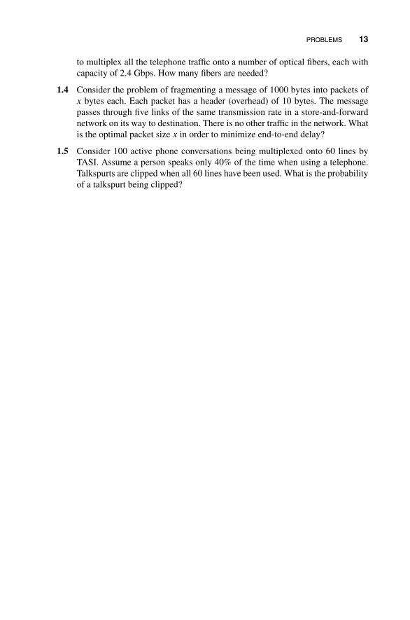
FIGURE 2.5 (a) An example of one-to-one mapping from input to output; (b) number of cross-points needed for nonblocking switch.
needed. This can be seen by relating the number of possible input–output mappingsto the number of states of the switch.
A one-to-one mapping from inputs to outputs is a unique connection of inputs tooutputs in a one-to-one fashion, an example of which is given in Fig. 2.5(a). Clearly,there are N! possible mappings if all inputs and outputs are busy. In practice, there maybe some idle inputs and outputs at any given time. However, since there is no signal(or information flow) on these idle ports, it does not matter how they are connectedas long as they are not connected to a busy port. Thus, the mappings with idle inputsand outputs can be subsumed under one of the N! one-to-one mappings. That is, therealization of one of the N! mappings can also be used to realize a mapping with idleports, and we need only be concerned about the N! mappings.
We must set the states of the individual crosspoints within the switch to realize theN! mappings. Let there be M crosspoints in the overall switch. Since each crosspointhas two states and the state of the overall switch is defined by the combination ofthe states of the crosspoints, there are 2M states for the overall switch. Each of thesestates can realize one and only one of the N! mapping. Thus, to realize all the N!mappings, we must have
2M ≥ N! (2.1)
The inequality is due to the fact that two states may realize the same mapping. Thereader can easily verify this by experimenting with the switch in Fig. 2.4.

20 CIRCUIT SWITCH DESIGN PRINCIPLES
The Stirling’s formula is
N! = NNe−N√
2πN(1 + ε(N)),
where ε > 0 is a decreasing function of N. Substituting this into Eq. (2.1) and takingthe log on both sides, we have
M ≥ N log2 N − N log2 e + 0.5 log2(2πN) + log2(1 + ε(N)). (2.2)
The dominant term on the right-hand side of inequality (2.2) is N log N for large N.Thus, asymptotically, the number of crosspoints required must be at least N log2 N.
Note that the bound applies to all three nonblocking properties defined previously.The derivation is nonconstructive in that it does not tell us how to construct a switchthat achieves the N log2 N bound. It only tells us that if such a switch exists, its orderof complexity cannot be lower than N log2 N. Thus, the question of whether thereare switches satisfying this bound arises. We now turn our attention to some specificswitch constructions.
2.1.3 Clos Switching Network
An important issue in switch design is the construction of a large switch out of smallerswitch modules. A three-stage Clos switching network is shown in Fig. 2.6. Switchmodules are arranged in three stages and any module is interconnected with anymodule in the adjacent stage via a unique link. The modules are nonblocking andcould be, for example, the crossbar switches described previously. To motivate thestudy of a three-stage network rather than a two-stage network, Problem 2.11 arguesthat two-stage networks are not suitable for constructing nonblocking switches.
n1 r2
n1 r2
n1 r2
r1 r3
r1 r3
r1 r3
r2 n3
r2 n3
r2 n3
...
...
...
...
...
...
(1)
(2)
(r1)
(1)
(2)
(r2)
(1)
(2)
(r3)
......
n1r1 = n3r3 = N for N N switch
ri — # switchmodules incolumn i
n1 — # inputs incolumn 1module
n3 — # outputs incolumn 3module
Necessary condition for nonblocking:
312 ,nnr ≥
...
... ...
...
...
...
...
......
... ... ... ...
FIGURE 2.6 A three-stage Clos switch architecture.

SPACE-DOMAIN CIRCUIT SWITCHING 21
Key:Find a commonly
accessible middle
node from both
input and output
nodes
A
G B
1
2
3
4
5
6
7
8
9
1
2
3
4
5
6
7
8
9
A request for connection from input 9 to output 4 is blocked
SA = set of middle-stage nodes used by A= { F, G }
SB = set of middle-stage nodes used by B= { H }
H
F
FIGURE 2.7 An example of blocking in a three-stage switch.
There are five independent parameters in the Clos architecture. We have r1, r2,and r3 modules in stages 1, 2, and 3, respectively. The dimensions of the modulesin the stages 1, 2, and 3 are n1 × r2, r1 × r3, and r2 × n3, respectively. If the overallswitch has equal number of inputs and outputs, then the number of inputs or outputsis N = n1r1 = n3r3, and there are only four independent parameters.
Figure 2.7 shows a Clos switch with n1 = r1 = r2 = r3 = n3 = 3. This particu-lar switch structure is not strictly nonblocking. We want to derive the relationshipamong the parameters that will guarantee nonblocking operation. A crucial point isthe number of middle-stage modules r2. By making r2 larger, there are more alter-native paths between stage-1 and stage-3 modules, and therefore we should expectthe likelihood of blocking to be smaller. In fact, if r2 is made large enough, blockingcan be eliminated altogether. On the other hand, the switch becomes more complexin terms of both the number of stage-2 modules and the dimensions of stage-1 andstage-3 modules.
It is easy to see that for the switch to be nonblocking, we must have
r2 ≥ n1, n3. (2.3)
Otherwise, if all of the inputs (outputs) of a stage-1 (stage-2) module are active, someof the connections cannot be set up. Inequalities (2.3) are necessary conditions. Weshall see that they are also sufficient for achieving the rearrangeably nonblockingproperty but not the strictly nonblocking property.
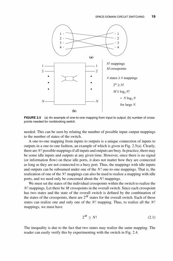
We need to develop some notational tools before we proceed. Figure 2.8 showsthat the connection state of the switch can be represented in the form of a connectionmatrix. Row i corresponds to first-stage module i and column j corresponds to third-stage module j. Entry (i, j) is associated with the middle-stage modules. As shown,if there are connections between module A and module B through modules F, G, and
22 CIRCUIT SWITCH DESIGN PRINCIPLES
AB
F
G
H
F,G,H
2
1
A
r1
21 rB 2
Stage-1
module
Stage-3 module
FIGURE 2.8 The connection matrix of the three-stage network.
H , then entry (A, B) = {F, G, H}. In other words, entry (i, j) contains the symbolsor labels of the middle-stage modules that are used to connect calls from module i instage 1 to module j in stage 3.
Let SA and SB be the sets of symbols in any row A and column B, respectively.There are three conditions that must be satisfied by a legitimate connection matrix:
1. Each row can have at most n1 symbols:
|SA| ≤ n1. (2.4)
This is because each first-stage module has n1 inputs and can have at most n1connections. Each connection needs to go through one and only one middle-stage module.
2. Each column can have at most n3 symbols:
|SB| ≤ n3. (2.5)
3. The symbols in each row or each column must be distinct: this is because eachfirst- or third- stage module is connected to each middle-stage module by oneand only one link. There can be at most r2 symbols in each row or column.Thus,
|SA|, |SB| ≤ r2. (2.6)

SPACE-DOMAIN CIRCUIT SWITCHING 23
Theorem 2.1. Assuming the underlying switch modules are individually strictly non-blocking, a three-stage N × N Clos network is strictly nonblocking if and only if
r2 ≥ min{n1 + n3 − 1, N}. (2.7)
Proof. The trivial case when N ≤ n1 + n3 − 1 is easy to see: since there can be nomore than N calls in progress at the same time in the overall switch, r2 need not bemore than N. For n1 + n3 − 1 < N, suppose there is a new connection request froman input in module A to an output in module B. Consider the worst-case situation inwhich all other inputs and outputs of A and B are busy. Then,
|SA| = n1 − 1,
|SB| = n3 − 1. (2.8)
Furthermore,
|SA ∪ SB| = |SA| + |SB| − |SA ∩ SB|≤ |SA| + |SB| = n1 + n3 − 2. (2.9)
The above inequality is satisfied with equality if |SA ∩ SB| = 0; that is, the middle-stage modules used by connections from A and B are disjoint. If r2 ≥ n1 + n3 − 1,there must be at least one symbol not in either SA or SB. This is a symbol correspondingto a middle-stage module as yet unused by the existing connections of A and B, andit can be used to set up the new connection request. �
The value of r2 can be made smaller if we only require the switch to be rearrangeablynonblocking. In fact, r2 needs only be no less than max(n1, n3). Certainly, by the pre-vious theorem, the switch is not strictly nonblocking with this value of r2. Therefore,we must find a way to rearrange the existing circuits to accommodate a new requestwhenever it is blocked.
Substituting a symbol of an entry in the connection matrix with another symbolcorresponds physically to rearranging an existing connection. Specifically, the con-nection is disconnected and reestablished over the middle-stage module representedby the new symbol. Certainly, we cannot simply substitute the old symbol with anyarbitrary symbol. The new symbol must not have already occurred in the row andcolumn of the entry in order not to violate the legitimacy of the matrix.
With reference to Fig. 2.9, suppose we want to establish a new connection betweenfirst-stage module A and third-stage module B. Suppose that all symbols except D
occur in row A and all symbols except C occur in column B. Then, the connection isblocked because we could not find a symbol that have neither occurred in row A norin column B for entry (A, B).
Since C is not currently in column B, we might try to change the symbol D incolumn B to symbol C so that we can put D in entry (A, B). But if there were a C
already in the row occupied by the D in column B (see Fig. 2.9), we could not changethe D to C without violating the matrix constraint.
24 CIRCUIT SWITCH DESIGN PRINCIPLES
C
D
D
D
C
CA
AAA
BB B |SA SB| = r2
Connection between
A and B is blocked
D ∉ SA
C ∉ SB
Chain terminates
at A″ because
C ∉ SA′′
(a)
A
A
A
A
..
..
..
..
..
B
B
B
..
..
..
..
C
D
..
..
..
A is already
connected to
all middle-
stage nodes
except D
B is already
connected to
all middle-
stage nodes
except C
(b)
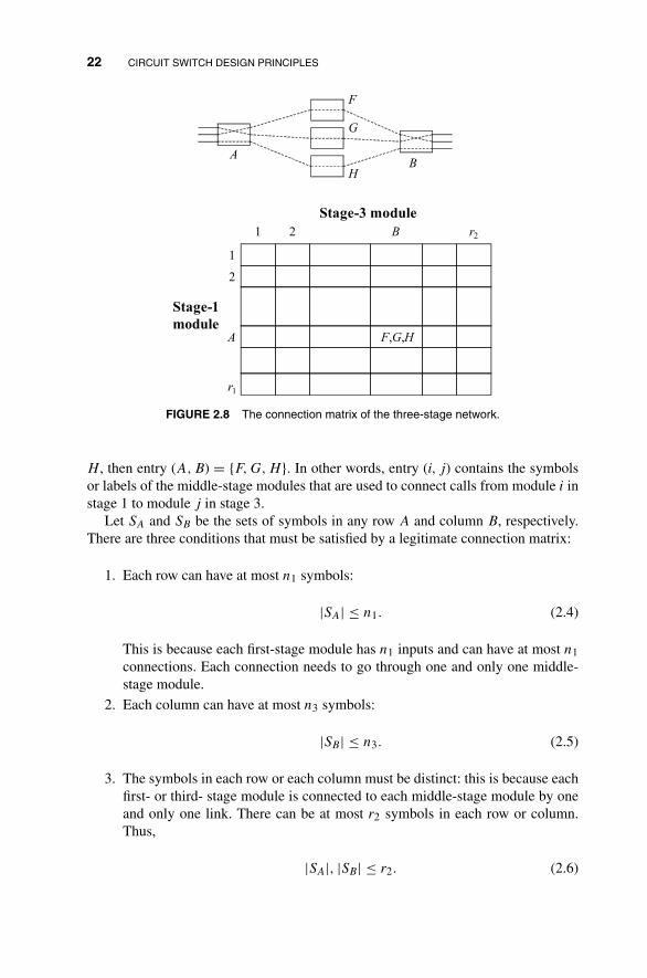
FIGURE 2.9 (a) A chain of C and D originating from B; (b) physical connections correspondingto the chain.
In other words, we may need to rearrange more than just one existing connection.To see which connections need to be rearranged, let us introduce the concept of therearrangement chain. A chain of two symbols, C and D, with end points at columnB and row A′′ is shown in Fig. 2.9(a). An end point must lie in a row or columncontaining either C or D but not both. For example, column B contains the endpoint with symbol D and it does not have a symbol C. The row and column of anintermediate point each contains one C and one D. To identify the chain, we searchacross the rows and columns alternatively for C and D. Thus, if we find a C duringa row search, we then search for D across the column containing C, and so on. Theprocess stops when a row search fails to find a C or a column search fails to find a D.The current C or D then forms the other end point of the chain. Note that the chainhas a finite number of points and a loop is impossible if we start with an end point;otherwise, C or D will occur more than once in some row or column, as illustrated inFig. 2.10.
The physical interpretation of the chain is shown in Fig. 2.9(b). Specifically, thechain corresponds to a set of first-stage and third-stage modules with connectionsacross middle-stage modules C and D.
The chain is said to be rearranged if we switch the symbols C and D in the chain.This corresponds to rearranging the associated connections, as illustrated in Fig. 2.11.Connections that used to be established across C are now established across D, andvice versa. Note that rearranging the chain as such will not lead to a violation ofthe rule that a symbol can occur at most once in each row or column. As shown, byrearranging the chain starting in B as in Fig. 2.11, we can put D in entry (A, B).
Now, a problem could arise if the chain from column B ends in the symbol C inrow A, as indicated in Fig. 2.12(b), since the rearrangement would have switched the

SPACE-DOMAIN CIRCUIT SWITCHING 25
DC
DC
CD
A loop in the chain
D occurs twice in this column,
making the matrix illegitimate
(i.e., physically impossible in
associated switch)
* There should betwo end points ina chain
FIGURE 2.10 Illustration showing loops in chains are not permitted in legitimate connectionmatrix.
C in row A to D and we cannot then put D in the entry (A, B) for the new connectionwithout violating the constraint that a symbol can occur at most once in each row.Fortunately, as indicated in Fig. 2.12(b), it is impossible for the chain from columnB to end in row A. To see this, note that for the search starting from column B, eachrow search always attempts to find a C and each column search always attempts tofind a D: having the chain connected to the C in row A leads to the contradiction thata column search finds the C in row A.
C
C
C
C
D
DA
AAA
BB B
D can now be put into entry (A, B)
(a)
A
A
A
A
..
..
..
..
..
B
B
B
..
..
..
..
C
D
..
..
..(b)
FIGURE 2.11 (a) Rearrangement of the chain in Fig. 2.9; (b) the corresponding rearrangementof connections.

26 CIRCUIT SWITCH DESIGN PRINCIPLES
D
D
C
C D
D C
D
C
.. ... .
A
B
(a)
D
D
C
C DC
. ..
A
BThis column search ends in C, which is not possible
Start searching from B. Column search always looks for D
(b)
FIGURE 2.12 (a) Two chains, one originates from B and one from A; (b) illustration that the twochains in (a) cannot be connected.
The example assumes that originally there was a symbol C in SA but not in SB anda symbol D in SB but not in SA. The following theorem states that this is always truegiven that r2 ≥ max(n1, n3).
Theorem 2.2. Assuming the underlying switch modules are individually rearrange-ably nonblocking, a three-stage N × N Clos network is rearrangeably nonblockingif and only if
r2 ≥ max(n1, n3). (2.10)
Proof. We first consider the more specific case where the underlying modules arestrictly nonblocking. The “only if” part is a trivial corollary of condition (2.3). For the“if” part, suppose r2 ≥ max(n1, n3), and we want to set up a new connection betweenA and B. For the existing connections, we have
|SA| ≤ n1 − 1,
|SB| ≤ n3 − 1. (2.11)
There are two cases: (i) |SA ∪ SB| < r2 and (ii) |SA ∪ SB| = r2. In case (i), there isa symbol not in A and B and the corresponding middle-stage module can be used to
SPACE-DOMAIN CIRCUIT SWITCHING 27
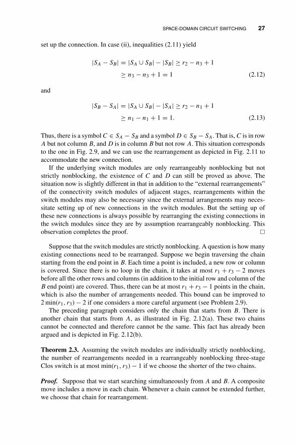
set up the connection. In case (ii), inequalities (2.11) yield
|SA − SB| = |SA ∪ SB| − |SB| ≥ r2 − n3 + 1
≥ n3 − n3 + 1 = 1 (2.12)
and
|SB − SA| = |SA ∪ SB| − |SA| ≥ r2 − n1 + 1
≥ n1 − n1 + 1 = 1. (2.13)
Thus, there is a symbol C ∈ SA − SB and a symbol D ∈ SB − SA. That is, C is in rowA but not column B, and D is in column B but not row A. This situation correspondsto the one in Fig. 2.9, and we can use the rearrangement as depicted in Fig. 2.11 toaccommodate the new connection.
If the underlying switch modules are only rearrangeably nonblocking but notstrictly nonblocking, the existence of C and D can still be proved as above. Thesituation now is slightly different in that in addition to the “external rearrangements”of the connectivity switch modules of adjacent stages, rearrangements within theswitch modules may also be necessary since the external arrangements may neces-sitate setting up of new connections in the switch modules. But the setting up ofthese new connections is always possible by rearranging the existing connections inthe switch modules since they are by assumption rearrangeably nonblocking. Thisobservation completes the proof. �
Suppose that the switch modules are strictly nonblocking. A question is how manyexisting connections need to be rearranged. Suppose we begin traversing the chainstarting from the end point in B. Each time a point is included, a new row or columnis covered. Since there is no loop in the chain, it takes at most r1 + r3 − 2 movesbefore all the other rows and columns (in addition to the initial row and column of theB end point) are covered. Thus, there can be at most r1 + r3 − 1 points in the chain,which is also the number of arrangements needed. This bound can be improved to2 min(r1, r3) − 2 if one considers a more careful argument (see Problem 2.9).
The preceding paragraph considers only the chain that starts from B. There isanother chain that starts from A, as illustrated in Fig. 2.12(a). These two chainscannot be connected and therefore cannot be the same. This fact has already beenargued and is depicted in Fig. 2.12(b).
Theorem 2.3. Assuming the switch modules are individually strictly nonblocking,the number of rearrangements needed in a rearrangeably nonblocking three-stageClos switch is at most min(r1, r3) − 1 if we choose the shorter of the two chains.
Proof. Suppose that we start searching simultaneously from A and B. A compositemove includes a move in each chain. Whenever a chain cannot be extended further,we choose that chain for rearrangement.

28 CIRCUIT SWITCH DESIGN PRINCIPLES
In each composite move, a new row will be traversed by one of the chains whilea new column will be traversed by the other chain. Since the chains are disjoint, thesame row or column cannot be covered by both chains. There can be at most r1 − 2composite moves before all rows are included (2 is subtracted from r1 because theinitial two end points occupy two rows). Therefore, the number of points in the shorterchain is no more than r1 − 1. Similarly, by considering the columns, the number ofpoints in the shorter chain is no more than r3 − 1. Thus, the number of points in theshorter chain is at most min(r1, r3) − 1. �
2.1.4 Benes Switching Network
The modules in the Clos switch architecture are usually relatively large switchescompared to the 2 × 2 crosspoints. However, this does not preclude the useof the theory developed above for 2 × 2 switch elements. Figure 2.13 showsa symmetric three-stage network in which n1 = n3 = 2. Each of the first- andthird-stage modules are 2 × 2 switching elements. It can be seen that the prob-lem of constructing an N × N switch has been broken down to the problem ofconstructing two N/2 × N/2 switches in the middle. By Theorem 2.2, the N × N
switch is rearrangeably nonblocking if the N/2 × N/2 switches are rearrangeablynonblocking.
To construct the N/2 × N/2 rearrangeably nonblocking modules, we can use thesame decomposition in a recursive manner. That is, each N/2 × N/2 module can bebroken down into three stages consisting of 2 × 2 elements in the first and third stagesand two N/4 × N/4 modules in the middle. Repeating this, recursively, only 2 × 2elements will remain in the end. An 8 × 8 switch constructed this way is shown inFig. 2.14. This architecture is called the Benes network.
A question is how many crosspoints are there in an N × N Benes network. Let usassume that N = 2n; that is, it is a power of 2. Let the number of stages in a k × k
2 2
2 2
2 2
N/2 N/2
N/2 N/2
2 2
2 2
2 2
.
.
.
.
....
.
.
.
.
.
.
12
34
N–1 N–1
N N
12
3
4
The N N network is rearrangeably nonblocking if
the N/2 N/2 networks are rearrangeably nonblocking.
FIGURE 2.13 Recursive decomposition of a rearrangeably nonblocking network.

SPACE-DOMAIN CIRCUIT SWITCHING 29
1
2
3
4
5
6
7
8
1
2
3
4
5
6
7
8
Baseline
network Reverse
baseline
network
FIGURE 2.14 An 8 × 8 Benes network.
Benes switch be denoted by f (k). By the recursive construction, we have
f (N) = f
(N
2
)+ 2. (2.14)
Applying the above as below yields a closed-form expression of f (N):
f (2n) = f (2n−1) + 2
= f (2n−2) + 4
...
= f (2n−j) + 2j
...
= f (2) + 2(n − 1)
= 1 + 2(n − 1)
= 2n − 1. (2.15)
Since each stage has N/2 crosspoints, the total number of crosspoints is
N
2(2n − 1) = N log2 N − N
2. (2.16)
Notice that asymptotically (i.e., for large N), the Benes network satisfies the N log N
lower bound on the number of crosspoints required in a nonblocking switch.Although the number of crosspoints in the Benes network is of order N log N,
lacking is a fast control algorithm that can set up paths between the inputs and outputs.

30 CIRCUIT SWITCH DESIGN PRINCIPLES
This makes it less appealing for fast- packet switching in which the paths taken bypackets must be determined in a very short time.
Let us consider a looping algorithm. As illustrated in Fig. 2.13, the Benes networkconsists of two subnetworks sandwiched between the first and last columns of 2 × 2switch elements. Therefore, one way to set up the path for an input–output pair isto first determine whether it should go through the upper or lower subnetwork. Theconstraints that must be satisfied are that the paths of the inputs (outputs) sharingthe same 2 × 2 elements (e.g., inputs (outputs) 1 and 2) must go through differentsubnetworks since there is only one link from a 2 × 2 element to a subnetwork.Once the set of disjoint paths has been determined at this level, we can then go downto the next level of setting up paths within each of the two N/2 × N/2 subnetworks.The same algorithm can be applied in a recursive manner until the complete paths aredetermined for all input–output pairs.
Let us illustrate the algorithm with an example. With reference to Fig. 2.15, inwhich we wish to set up paths for the following input–output pairs: (1,4), (2,5), (3,6),(4,3), (5,7), (6,8), (7,1), (8,2), we start out by routing the first path (the one frominput 1) through the upper subnetwork. This path reaches output 4. We next satisfythe constraint generated at the output (i.e., the path to output 3, which shares the sameswitch element as output 4) by routing the path from input 4 to output 3 through thelower subnetwork. This generates the constraint that the path from input 3 must gothrough the upper subnetwork. Performing this iteratively by satisfying the constraintscreated at the output and input alternatively, eventually, we will close the “loop” byestablishing a path from input 2, which shares an element with input 1, through thelower subnetwork. This is the situation as depicted in Fig. 2.15. Notice that since thisis a Clos network, we can use the connection matrix already discussed to represent the
1
2
3
4
5
6
7
8
1
2
3
4
5
6
7
8
Set up paths for input–output pairs:
(1, 4), (2, 5), (3, 6), (4, 3)
(5, 7), (6, 8), (7, 1), (8, 2)
Central algorithm: # steps = N log N⎟⎟⎠
⎞⎜⎜⎝
⎛
45637812
12345678
output
input
FIGURE 2.15 Illustration of a looping connection setup algorithm; we want to set up paths forinput–output pairs: (1, 4), (2, 5), (3, 6), (4, 3), (5, 7), (6, 8), (7, 1), (8, 2).
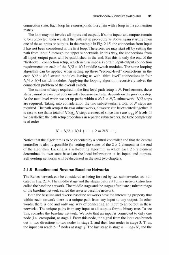
SPACE-DOMAIN CIRCUIT SWITCHING 31
connection state. Each loop here corresponds to a chain with a loop in the connectionmatrix.
The loop may not involve all inputs and outputs. If some inputs and outputs remainto be connected, then we start the path setup procedure as above again starting fromone of these inputs or outputs. In the example in Fig. 2.15, the connection from input5 has not been considered in the first loop. Therefore, we may start off by setting thepath from input 5 through the upper subnetwork. In this way, the connections fromall input–output pairs will be established in the end. But this is only the end of the“first-level” connection setup, which in turn imposes certain input-output connectionrequirements on each of the N/2 × N/2 middle switch modules. The same loopingalgorithm can be applied when setting up these “second-level” connections in theeach N/2 × N/2 switch modules, leaving us with “third-level” connections in fourN/4 × N/4 switch modules. Applying the looping algorithm recursively solves theconnection problem of the overall switch.
The number of steps required in the first-level path setup is N. Furthermore, thesesteps cannot be executed concurrently because each step depends on the previous step.At the next level when we set up paths within a N/2 × N/2 subnetwork, N/2 stepsare required. Taking into consideration the two subnetworks, a total of N steps arerequired. The path setup at the two subnetworks, however, can be executed together. Itis easy to see that a total of N log2 N steps are needed since there are log2 N levels. Ifwe parallelize the path setup procedures in separate subnetworks, the time complexityis of order
N + N/2 + N/4 + · · · + 2 = 2(N − 1).
Notice that the algorithm is to be executed by a central controller and that the centralcontroller is also responsible for setting the states of the 2 × 2 elements at the endof the algorithm. Lacking is a self-routing algorithm in which each 2 × 2 elementdetermines its own state based on the local information at its inputs and outputs.Self-routing networks will be discussed in the next two chapters.
2.1.5 Baseline and Reverse Baseline Networks
The Benes network can be considered as being formed by two subnetworks, as indi-cated in Fig. 2.14. The middle stage and the stages before it form a network structurecalled the baseline network. The middle stage and the stages after it are a mirror imageof the baseline network called the reverse baseline network.
Both the baseline and reverse baseline networks have the interesting property thatwithin each network there is a unique path from any input to any output. In otherwords, there is one and only one way of connecting an input to an output in thesenetworks. The unique paths from any input to all outputs form a binary tree. To seethis, consider the baseline network. We note that an input is connected to only onenode (i.e., crosspoint) at stage 1. From this node, the signal from the input can branchout in two directions to two nodes in stage 2, and then four nodes in stage 3. Thus,the input can reach 2j−1 nodes at stage j. The last stage is stage n = log2 N, and the

32 CIRCUIT SWITCH DESIGN PRINCIPLES
input can reach all the N/2 nodes in the last stage, from which it can reach all theN outputs. An input can only reach a subset of the nodes in the stages before stagen, and the path to each of the node in the subset is clearly unique from the aboveexplanation. In general, we observe the following:
Reachability of nodes in baseline/reverse baseline networks: A node in stage i can bereached by 2i inputs and can reach 2n−i+1 outputs.
2.1.6 Cantor Switching Network
The Benes network is only rearrangeably nonblocking. However, the above obser-vations about the two subnetworks of the Benes network can be used to constructa parallel Benes network, called the Cantor network, which is strictly nonblocking.Figure 2.16 shows a Cantor network. It is made up of log2 N Benes networks arrangedin a parallel fashion. Input i of the overall switch is connected to inputs i of all thelog2 N Benes switches via a front-end 1 × log2 N switch. Similarly, output j of theoverall switch is connected to outputs j of all the log2 N Benes switch via a back-endlog2 N × 1 switch. Basically, the function of the front-end and back-end switches isto increase the number of alternative paths for any input–output pair so as to increasethe chance of a successful connection. It just turns out that log2 N Benes networksare sufficient to always allow connection between any idle input–output pair.
Theorem 2.4. The Cantor network is strictly nonblocking.
..1
2
N
m = (1)
m = (log2N)
.
.
.
..
..
..
..
..
.
.
.
1
2
N
..
1 x log2N switch log2N x 1 switch
FIGURE 2.16 The Cantor network.

SPACE-DOMAIN CIRCUIT SWITCHING 33
Proof. For each Benes network, an input can be connected to any of the middle-stagenodes if there are no existing connections. However, if there are already some existingconnections in the network, it may not be possible to connect the input to some of themiddle-stage nodes. We say that an input can access a node at or before the middlestage only if none of the links in the unique path from the input to that node is alreadyused by an existing connection. For example, with respect to Fig. 2.4(b), which showsthe connection state of a 4 × 4 Benes Switch made up of 2 × 2 nodes, the lower nodein the middle stage cannot be accessed by input 1. We define accessibility from anoutput to those nodes at or after the middle stage in a similar fashion.
The essence of our argument is to show that there is a node in the middle stage inone of the Benes networks that can be accessed by both the input and the output ofthe new request. The 1 × log2 N and log2 N × 1 switches can then be used to connectthe input and output to that Benes switch and the connection is established thereof.
Let m be the number of Benes networks required to make the Cantor networkstrictly nonblocking. Suppose we want to set up a new connection between input a
and output b. We shall first examine accessibility from input a. In each Benes network,the paths leading from input a to the N/2 middle-stage nodes form a binary tree, asillustrated in the example of Fig. 2.17, in which a = 3. There are altogether m binarytrees, one in each Benes network, and they contain the paths from input a to the Nm/2middle-stage nodes in the Cantor network.
Consider the worst-case situation in which all the other N − 1 inputs and outputare currently busy. Each of the N − 1 connections has an associated path from itsinput to its output. Each path must intersect or meet with one of the m binary trees atsome node at or before the middle stage. We say that the path meets the binary treesat stage i if the path intersects with one of the trees for the first time at stage i. Notethat the rest of the path must also intersect with the tree thereof.
1
2
3
4
5
6
7
8
1
2
3
4
5
6
7
8
Connection paths from inputs 1 and 2 intersect
with binary tree for the first time in stage 2
If input 4 is connected to this link,
a subtree is formed by the three
subsequent nodes
Therefore, the two lower middle-
stage nodes are eliminated from
connection by input 3
FIGURE 2.17 Binary tree extended from an input to all middle-stage nodes.

34 CIRCUIT SWITCH DESIGN PRINCIPLES
By the construction of the Benes network, we can verify that out of the N − 1paths, one path meets the binary trees at stage 1. Consider Fig. 2.16 and suppose thatinput a is input 3. Then, the path of the existing connection from input 4 meets abinary tree of input 3 at a stage-1 node. Next, two paths meet the binary trees at stage2, four paths meet the binary trees at stage 3, and so on. In general, the number ofpaths meeting the binary trees at stage i is
Ai = 2i−1.
For verification, the reader can check that
log2 N∑i=1
Ai = N − 1.
For each of the paths meeting with the trees before the middle stage, say at stage i,the path will exit on one of the outgoing links of the intersecting node. The subtreeextending out of this link cannot be used by input a for connection (see the examplein Fig. 2.16). This subtree has
Bi = N
2i+1
nodes in the middle stage, and they are not accessible by input a.A total of
C ≤log2 N−1∑
i=1
AiBi (2.17)
middle-stage nodes will be eliminated from accessibility by input a. The inequalityis satisfied with equality only in the worst case when all the subtrees generated by theN − 1 paths are disjoint and therefore the middle-stage nodes eliminated are disjoint.For the strictly nonblocking property, what is important is the worst-case situation.Notice, however, that in general some of the subtrees may overlap: for instance, bythe rearrangeably nonblocking property of the Benes network, it is possible for allthe N − 1 paths to concentrate on one of the m Benes networks, eliminating onlyN/2 − 1 middle-stage nodes.
Substituting Ai and Bi into the above yields
C ≤ (log2 N − 1)N/4. (2.18)
Thus, the number of middle-stage nodes that can be accessed by input a is
|I| = Nm/2 − C ≥ Nm/2 − (log2 N − 1)N/4, (2.19)
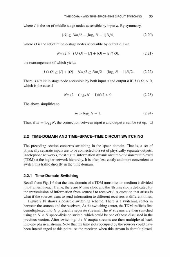
TIME-DOMAIN AND TIME–SPACE–TIME CIRCUIT SWITCHING 35
where I is the set of middle-stage nodes accessible by input a. By symmetry,
|O| ≥ Nm/2 − (log2 N − 1)N/4, (2.20)
where O is the set of middle-stage nodes accessible by output b. But
Nm/2 ≥ |I ∪ O| = |I| + |O| − |I ∩ O|, (2.21)
the rearrangement of which yields
|I ∩ O| ≥ |I| + |O| − Nm/2 ≥ Nm/2 − (log2 N − 1)N/2. (2.22)
There is a middle-stage node accessible by both input a and output b if |I ∩ O| > 0,which is the case if
Nm/2 − (log2 N − 1)N/2 > 0. (2.23)
The above simplifies to
m > log2 N − 1. (2.24)
Thus, if m = log2 N, the connection between input a and output b can be set up. �
2.2 TIME-DOMAIN AND TIME–SPACE–TIME CIRCUIT SWITCHING
The preceding section concerns switching in the space domain. That is, a set ofphysically separate inputs are to be connected to a set of physically separate outputs.In telephone networks, most digital information streams are time-division multiplexed(TDM) at the higher network hierarchy. It is often less costly and more convenient toswitch this traffic directly in the time domain.
2.2.1 Time-Domain Switching
Recall from Fig. 1.6 that the time domain of a TDM transmission medium is dividedinto frames. In each frame, there are N time slots, and the ith time slot is dedicated forthe transmission of information from source i to receiver i. A question that arises iswhat if the sources want to send information to different receivers at different times.
Figure 2.18 shows a possible switching scheme. There is a switching center inbetween the sources and the receivers. At the switching center, the TDM traffic is firstdemultiplexed into N physically separate streams. The N streams are then switchedusing an N × N space-division switch, which could be one of those discussed in theprevious section. After switching, the N output streams are then multiplexed backinto one physical stream. Note that the time slots occupied by the sources could havebeen interchanged at this point. At the receiver, when this stream is demultiplexed,

36 CIRCUIT SWITCH DESIGN PRINCIPLES
FIGURE 2.18 Performing time-slot interchange using space-division switch.
the information received by receiver i depends on switching performed by the space-division switch.
A more direct way to achieve the same function is to use a time-slot interchanger(TSI) in the middle, as shown in Fig. 2.19. As the name suggests, a TSI interchangesthe time slots occupied by the logical channels within a TDM stream. The TSI isusually implemented using random access memory (RAM). After a whole frame iswritten into the RAM, the time slots in the frame can then be read out in an orderdictated by the switching (or time-slot interchange) to be performed. Thus, if the dataon time slot N are to be switched to time slot 1, these data will be read out first onthe output frame. In this way, switching is performed directly in the time domain.Logically, the TSI is equivalent to an N × N space-division switch.
Notice that there must be a delay equal to one frame time in the TSI. After a wholeframe is written, it is read. Meanwhile the next frame is being written. Two dataframes of memory are needed.
FIGURE 2.19 Direct time-slot interchange using random access memory (switching in the timedomain).
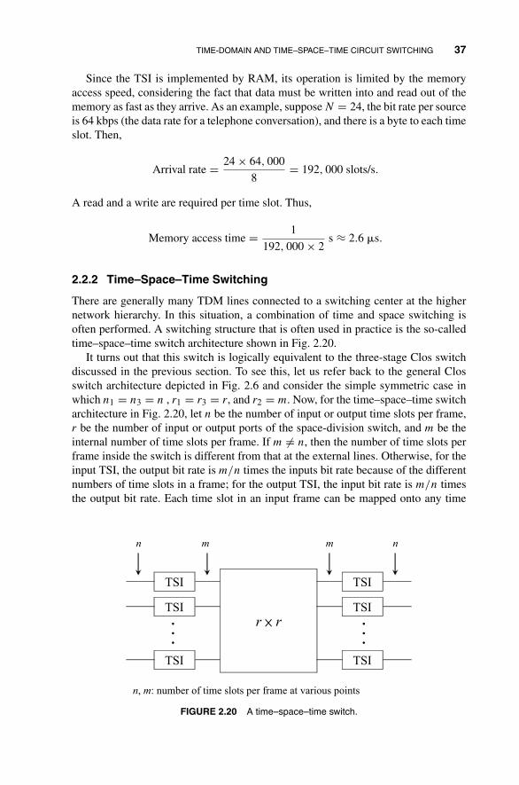
TIME-DOMAIN AND TIME–SPACE–TIME CIRCUIT SWITCHING 37
Since the TSI is implemented by RAM, its operation is limited by the memoryaccess speed, considering the fact that data must be written into and read out of thememory as fast as they arrive. As an example, suppose N = 24, the bit rate per sourceis 64 kbps (the data rate for a telephone conversation), and there is a byte to each timeslot. Then,
Arrival rate = 24 × 64, 000
8= 192, 000 slots/s.
A read and a write are required per time slot. Thus,
Memory access time = 1
192, 000 × 2s ≈ 2.6 �s.
2.2.2 Time–Space–Time Switching
There are generally many TDM lines connected to a switching center at the highernetwork hierarchy. In this situation, a combination of time and space switching isoften performed. A switching structure that is often used in practice is the so-calledtime–space–time switch architecture shown in Fig. 2.20.
It turns out that this switch is logically equivalent to the three-stage Clos switchdiscussed in the previous section. To see this, let us refer back to the general Closswitch architecture depicted in Fig. 2.6 and consider the simple symmetric case inwhich n1 = n3 = n , r1 = r3 = r, and r2 = m. Now, for the time–space–time switcharchitecture in Fig. 2.20, let n be the number of input or output time slots per frame,r be the number of input or output ports of the space-division switch, and m be theinternal number of time slots per frame. If m = n, then the number of time slots perframe inside the switch is different from that at the external lines. Otherwise, for theinput TSI, the output bit rate is m/n times the inputs bit rate because of the differentnumbers of time slots in a frame; for the output TSI, the input bit rate is m/n timesthe output bit rate. Each time slot in an input frame can be mapped onto any time
TSI
TSI
TSI
r r
TSI
TSI
TSI
.
.
....
mn nm
n, m: number of time slots per frame at various points
FIGURE 2.20 A time–space–time switch.
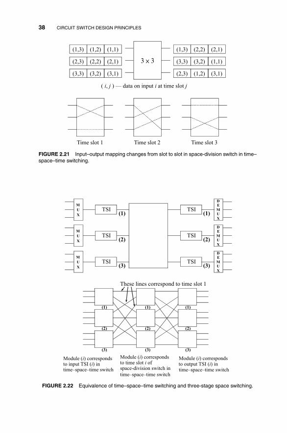
38 CIRCUIT SWITCH DESIGN PRINCIPLES
(1,3) (1,2) (1,1)
(2,3) (2,2) (2,1)
(3,3) (3,2) (3,1)
3 3
(1,3) (2,2) (2,1)
(3,3) (3,2) (1,1)
(2,3) (1,2) (3,1)
( i, j ) — data on input i at time slot j
Time slot 1 Time slot 2 Time slot 3
FIGURE 2.21 Input–output mapping changes from slot to slot in space-division switch in time–space–time switching.
M
U
X
M
U
X
M
U
X
TSI
TSI
TSI
TSI
TSI
TSI
DE
MU
X
DE
MU
X
DE
MU
X
(1)
(2)
(3)
(1)
(2)
(3)
These lines correspond to time slot 1
(1) (1) (1)
(2) (2) (2)
(3) (3) (3)
Module (i) correspondsto input TSI (i) intime–space–time switch
Module (i) corresponds Module (i) correspondsto time slot i ofspace-division switch in
time–space–time switchtime–space–time switchto output TSI (i) in
FIGURE 2.22 Equivalence of time–space–time switching and three-stage space switching.

PROBLEMS 39
slot in an output frame. Thus, logically, the input TSI is like an n × m switch and theoutput TSI is like an m × n switch.
The operation of the center space-division switch can be considered as beingdivided into m time slots. In the first time slot, it switches the information fromtime slot 1 of the inputs to time slot 1 of the outputs. In the second time slot, adifferent input–output mapping is used to switch information from time slot 2 ofinputs to time slot 2 of outputs. Thus, the input–output mapping realized by theswitch changes very dynamically from time slot to time slot, and as illustrated inFig. 2.21, it is as if there were m copies of space-division switches, one for each timeslot. In fact, if we were to put a time-division multiplexer before each input TSI, anda time-division demultiplexer after each output, as in Fig. 2.22, the switch will befunctionally identical to the three-stage Clos architecture. Thus, all the nonblockingconditions we derived previously for the Clos switch also apply here. For instance,if m = 2n − 1, the switch will be strictly nonblocking, and if m = n, the switch willbe rearrangeably nonblocking. Of course, in the latter case the way time slots areinterchanged in the TSI may need to be rearranged.
PROBLEMS
2.1 A formula that is often used to engineer the trunk facilities between two switch-ing centers is the Erlang B formula given by
B = an/n!∑ni=0 ai/i!
,
where B is the blocking probability, n is the number of trunks, and a = λ/μ
is the product of the arrival rate of new connections λ and the average holdingtime of a connection 1/μ. Suppose new connections arrive at the rate of 20calls /min and the average holding time of a call is 5 min. Find the minimumnumber of trunks needed to make the blocking probability 10−3.
2.2 Explain why a rearrangeably nonblocking circuit switch is not necessary wide-sense nonblocking.
2.3 True or false? Constructing a wide-sense nonblocking switch requires a largernumber of crosspoints than constructing a strictly nonblocking switch. Explain.
2.4 Section 2.1.2 mentions that two different switch states may realize the sameinput–output mappings. Give an example illustrating this.
2.5 In Section 2.1.2, we examined the lower bound on the number of crosspointsrequired by a nonblocking switch. Derive a lower bound for an N × N ′ asym-metric switch where N ′ = N/2 using the same method.
2.6 Consider a strictly nonblocking symmetric Clos switch with n1 = n3 = n andr1 = r3 = r made up of three stages of crossbar switch modules. Express the
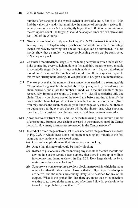
40 CIRCUIT SWITCH DESIGN PRINCIPLES
number of crosspoints in the overall switch in terms of n and r. For N = 1000,find the values of n and r that minimize the number of crosspoints. (Note: If itis necessary to have an N that is slightly larger than 1000 in order to minimizethe crosspoint count, the larger N should be adopted since we can always usejust 1000 of the N ports.)
2.7 Give an example of a strictly nonblocking N × N Clos network in which r2 =N < n1 + n3 − 1. Explain why in practice no one would construct a three-stageswitch this way by showing that one of the stages can be eliminated. In otherwords, show that a simpler two-stage nonblocking switch can be constructedif N < n1 + n3 − 1.
2.8 Consider a modified three-stage Clos switching network in which there are twolinks connecting every switch module in first and third stages to every modulein the middle stage. Each first-stage switch module is n × 2n, each third-stagemodule is 2n × n, and the numbers of modules in all the stages are equal. Isthis switch strictly nonblocking? If yes, prove it. If no, give a counterexample.
2.9 The text proves that the number of rearrangements needed in a rearrangeablyClos nonblocking switch is bounded above by r1 + r3 − 1 by considering onechain, where r1 and r3 are the number of modules in the first and third stages,respectively. Improve the bound to 2 min(r1, r3) − 2, still considering only onechain. That is, you choose one of the two chains before starting to identify thepoints in the chain, but you do not know which chain is the shorter one. (Hint:You may choose the chain based on your knowledge of r1 and r3, but there isno guarantee that the one you choose will be the shorter one. After choosingthe chain, first consider the columns covered and then the rows covered.)
2.10 Show how to construct N × 1 and 1 × N switches using the minimum numberof crosspoints. Suppose your designs are used in the construction of the Cantornetwork. How many crosspoints are needed in the Cantor network?
2.11 Instead of a three-stage network, let us consider a two-stage network as shownin Fig. 2.23, in which there is one link interconnecting any module at the firststage and any module at the second stage.(a) Give an example showing that this network is blocking.
(b) Argue that this network could be highly blocking.
(c) Instead of just one link interconnecting any module at the first module andany module at the second stage, suppose that there is a group of m linksinterconnecting them, as shown in Fig. 2.24. How large should m be tomake this network nonblocking?
(d) Suppose we want to explore a seldom blocking network in which the valueof m is less than the above value. Assume that n = 8, all inputs and outputsare active, and the inputs are equally likely to be destined for any of theoutputs. What is the probability that there are more than m connectionswanting to go through the same group of m links? How large should m beto make this probability less than 10−3.
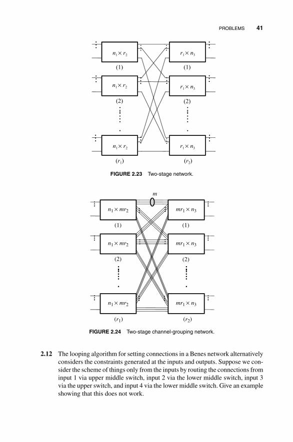
PROBLEMS 41
n1 × r2
n1 × r2
r1 × n3
r1 × n3
r1 × n3n1 × r2
… …
…
…
… …
…
.…….
.…….
(1) (1)
(2) (2)
(r1) (r2)
… …
…
… …
FIGURE 2.23 Two-stage network.
n1 × mr2 mr1 × n3
mr1 × n3
mr1 × n3n1 × mr2
n1 × mr2…
……
…
…
…
…
…
.…….
.…….
(1)(1)
(2) (2)
(r1) (r2)
m
…
…
…
…
FIGURE 2.24 Two-stage channel-grouping network.
2.12 The looping algorithm for setting connections in a Benes network alternativelyconsiders the constraints generated at the inputs and outputs. Suppose we con-sider the scheme of things only from the inputs by routing the connections frominput 1 via upper middle switch, input 2 via the lower middle switch, input 3via the upper switch, and input 4 via the lower middle switch. Give an exampleshowing that this does not work.

42 CIRCUIT SWITCH DESIGN PRINCIPLES
(1,3) (1,2) (1,1)
(2,3) (2,2) (2,1)
(3,3) (3,2) (3,1)
3 3
TSI
TSI
TSI
TSI
TSI
TSI
2
2
2
13
13
31
Frame
Targeted outputs
FIGURE 2.25 A time–space–time switch.
2.13 Benes network is a rearrangeably nonblocking network with a recursive struc-ture. Suppose we want to construct a strictly nonblocking structure usinga similar recursion, but with 2 × 3 switch modules at the first stage, 3 × 2switch modules at the third stage, and three N/2 × N/2 modules in the middlestage.(a) Constructing the switch recursively this way, how many 2 × 3, 3 × 2, and
2 × 2 switch modules are needed altogether, assuming N is a power of 2?
(b) The ratio of the number of internal links at each stage to the number ofinputs is called the bandwidth expansion factor. What is the maximumbandwidth expansion factor for this switch?
(c) Compare this switch with the Cantor network.
2.14 Consider an 8 × 8 Cantor network. The number of Benes networks neededto make it strictly nonblocking is log2 8 = 3. Give an example showing thatif the number of Benes networks is only 2, the Cantor network is not strictlynonblocking.
2.15 The text explains time–space–time switching in terms of the Clos switch ar-chitecture. This problem attempts to look at time–space–time switching froma different viewpoint. With reference to Fig. 2.25, let (i, j) denote the datain time slot j of input 1. In the example the data on different inputs may bedestined for the same output in the same time slot. Show how the input TSIscan be used to interchange the time slots occupied by the data to avoid outputconflict. Explain why the output TSIs are needed after the data arrive at theoutputs.
3
FUNDAMENTAL PRINCIPLESOF PACKET SWITCH DESIGN
The next few chapters focus primarily on fixed-length packet (or cell) switching. Toswitch variable-length packets using a fixed-length switch, one could first fragmentthe variable-length packets at the inputs into small fixed-length packets, switch thepackets, and then reassemble the packets back into the original variable-length packetsat the outputs. Generally, it is possible for the packet boundaries of different inputs tobe unaligned (see Fig. 3.1). Because of the fixed packet length, we can deliberatelydelay the early arriving packets (e.g., store them into a buffer) in order to align theboundaries. Thus, as far as the operation of the switch is concerned, we may assumethat time is divided into fixed slots of one-packet duration. In the beginning of eachtime slot, new packets arrive at all the inputs simultaneously.
One of the exercises in the preceding chapter examines time–space–time circuitswitching from the viewpoint of contention resolution. Specifically, the informationon different inputs may be destined for the same output of the space-division switchat any given time slot (see Fig. 2.23). The input TSI rearranges the time slots occupiedby the information so that output conflicts do not occur.
In circuit switching, the time slots occupying the same relative position in succes-sive frames of an input are assigned to the same circuit, and they contain informationdestined for the same output. In other words, the output link to which the informationshould be forwarded is known implicitly a priori. In packet switching, the outputlinks to which a packet should be forwarded is not known before their arrivals. Unlikein time-division multiplexing, there is no telling exactly how many packets from aninput will be destined for each output over a given period of time. Transmission ca-pacity may not be dedicated to each communication session in an exclusive manner.This and the lack of a transmission frame structure make it impossible to use a TSI to
Principles of Broadband Switching and Networking, by Tony T. Lee and Soung C. LiewCopyright © 2010 John Wiley & Sons, Inc.
43

44 FUNDAMENTAL PRINCIPLES OF PACKET SWITCH DESIGN
3 1 1
4 2 4
1 1
4 2
…
…
…
…
4 4
Switch
1
2
3
4
Output destinations
are random
Idle slots
(no active packets)
Arrival boundaries
may be unaligned
FIGURE 3.1 Packet arrivals in a 4 × 4 packet switch.
eliminate blocking the way it is done in circuit switching.1 Other methods are neededto deal with the contention problem.
The output destination of a packet must be contained in a header or derivable fromit. In virtual-circuit networks, a virtual circuit is set up for each session and the routeof the virtual circuit is determined during the call setup time. Once the route is setup, all packets of the virtual circuit will follow the same route while traveling to thedestination. The packet header does not contain the final output destination explicitly.Instead, it contains a number called the virtual-circuit identifier (VCI). At the switchinput, this number is translated into a local address associated with an output of theswitch. In addition, the input VCI is also mapped onto an output VCI. The input VCIin the header will be replaced by the output VCI, and the packet will be switched to theoutput. The output is in turn connected to an outgoing link that may be connected toan input of a subsequent switch. In this case, the output VCI becomes the input VCI ofthe subsequent switch, and it will be used to identify the output and output VCI of thepacket at the subsequent switch. In general, the switch output to which an input VCIon an input should be mapped forms part of the end-to-end route that was determinedduring the setting up of the virtual circuit. Once the mapping is determined, it is storedin a memory.
Figure 3.2 shows a schematic diagram of the header translation process. An in-coming packet is first disassembled into the information part and the header part.The header contains the input VCI of the packet. The header processor, in addition toperforming other functions, uses the input VCI as an index to locate from the memorythe switch output to which the packet should be forwarded. The output address, alongwith the bits of the original header, is then attached to the packet by the assembler.
1The reader should be aware that the point here is not to argue that circuit switching is superior to packetswitching. It is to indicate that because of the different ways in which transmission resources are used inthese two schemes, the switching requirements are different.
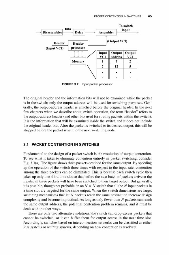
PACKET CONTENTION IN SWITCHES 45
Disassembler Delay Assembler
Header
processor
Info
Header
Memory
Input
VCI
Output
address
Output
VCI
1 5 2
2 12 5
.
.
.
.
.
.
To switch
input
(Input VCI)
(Output VCI)
FIGURE 3.2 Input packet processor.
The original header and the information bits will not be examined while the packetis in the switch; only the output address will be used for switching purposes. Gen-erally, the output-address header is attached before the original header. In the nextfew chapters when we describe about switch operation, the term “header” refers tothe output-address header (and other bits used for routing packets within the switch).It is the information that will be examined inside the switch and it does not includethe original header bits. After the packet is switched to its desired output, this will bestripped before the packet is sent to the next switching node.
3.1 PACKET CONTENTION IN SWITCHES
Fundamental to the design of a packet switch is the resolution of output contention.To see what it takes to eliminate contention entirely in packet switching, considerFig. 3.3(a). The figure shows three packets destined for the same output. By speedingup the operation of the switch three times with respect to the input rate, contentionamong the three packets can be eliminated. This is because each switch cycle thentakes up only one-third time slot so that before the next batch of packets arrive at theinputs, all three packets will have been switched to their target output. But generally,it is possible, though not probable, in an N × N switch that all the N input packets ina time slot are targeted for the same output. When the switch dimensions are large,switching mechanisms that let N packets reach the same destination increase designcomplexity and become impractical. As long as only fewer than N packets can reachthe same output address, the potential contention problem remains, and it must bedealt with in other ways.
There are only two alternative solutions: the switch can drop excess packets thatcannot be switched, or it can buffer them for output access in the next time slot.Accordingly, switches based on interconnection networks can be classified as eitherloss systems or waiting systems, depending on how contention is resolved.

46 FUNDAMENTAL PRINCIPLES OF PACKET SWITCH DESIGN
1
1
1
2
(a)
4 4
1
2
3
4
Packets may be switched one by one to outputs if speedup
is N times, not viable for large N
One of these
packets must
be dropped if
group size = 2
1
1
1
2
4 × 4
1
2
3
4
(b)
Two of these
packets must
be buffered if
group size = 1
1
1
1
2
(c)
1
2
3
4
4 × 4
FIGURE 3.3 Packet contention dealt with by (a) speeding up switch operation by N times;(b) dropping packets that cannot be switched; (c) queueing packets that cannot be switched.
In a loss system, packets are either dropped or switched to their outputs immedi-ately. By providing sufficient paths from inputs to outputs, packet loss probability canbe made as small as desired. The maximum number of packets that can be receivedby an output in one time slot will be called the group size. Since switch complexitygenerally increases with group size, one would look for the minimum group size tomeet the packet loss probability requirement in practice. In addition, if the group size
PACKET CONTENTION IN SWITCHES 47
is more than 1, packet buffers are needed at outputs, since the output port may not beable to transmit all arriving packets at once.
As an example, Fig. 3.3(b) shows a 4 × 4 switch that has a group size of 2. If threepackets arrive for the same output, one of them will be dropped. As long as the groupsize is less than N, there is the likelihood that a packet will be dropped. There is atrade-off between switch complexity and packet-loss probability. In some switches,even though there is no output contention, it is possible that there is internal contentiondue to their blocking structures. An example is the baseline switch discussed in thepreceding chapter. If these switches are designed as a loss system, packets may bedropped internally.
For waiting systems, excess packets are buffered whenever contention arises so thatattempts can be made to switch them in subsequent switch cycles. These packets maybe buffered at the inputs or internally in the switch. Figure 3.3(c) shows a scenarioin which two of the three packets destined for the same output are buffered at theinputs. We shall see that the throughput of a waiting-system switch is generally lessthan 100%. This limitation can be relaxed by increasing the group size so that morepackets can access their destination outputs simultaneously.
To summarize, switches can be classified into two classes with the following char-acteristics:
� Loss system
– The switch fabric has no input or internal buffers; packets already reachingtheir outputs may be queued at outputs waiting to be transmitted if the groupsize is more than 1.
– Packets may be dropped internally or at outputs due to contention. The lossprobability can be made arbitrarily small by adjusting the group size or somerelated switch design parameters.
� Waiting system
– Output conflicts are resolved by some contention-resolution mechanism toselect the packets that will be switched. Packets that have lost contentionwill be buffered so that they can be switched in one of the later time slots.Packets already reaching their outputs may be queued at outputs waiting tobe transmitted if the group size is more than 1.
– The throughput of the switch can be made arbitrarily close to 100% by in-creasing the group size or other design parameters.
In the switching literature, the term “input-buffered switch” is often used to refer to awaiting system with a group size of one that buffers packets only at the inputs. Packetsare not queued at the outputs because no more than one packet may arrive at an outputin a time slot, and by the time the next packet arrives, the current packet at the output,if any, would have been transmitted. The term “output-buffered switch” is often usedto refer to an ideal switch with a group size of N. Since all packets can be switchedto their desired outputs in the same time slot, there is no contention and buffers atthe inputs are then not needed. However, buffers are needed at the outputs since the
48 FUNDAMENTAL PRINCIPLES OF PACKET SWITCH DESIGN
output link may not be able to transmit all simultaneously arriving packets due to itslimited transmission rate. In the output-buffered switch, there is neither throughputlimitation nor packet loss in the switch. Although the names “input-buffered switch”and “output-buffered switch” are rather descriptive, they could also be misleading inthat the superior performance of the output-buffered switch improvement is often at-tributed either explicitly or implicitly to buffering packets at the outputs. In actuality,the performance improvement of the output-buffered switch over the input-bufferedswitch is really an outcome of having a large group size. As we shall see in the nextchapter, this is not without cost and the switch necessarily becomes more complex.That buffers are needed at the outputs is really a consequence of this switch de-sign principle rather than the cause of the performance improvement: simply puttingbuffers at the outputs without increasing the group size will not lead to any throughputimprovement.
3.2 FUNDAMENTAL PROPERTIES OF INTERCONNECTIONNETWORKS
Many packet switches proposed to date are based on interconnection networks, orig-inally intended for multiprocessor interconnect in highly parallel computer systems.These switches make use of many small switch elements in their overall architectures.An attractive feature of these switches is their regular topological interconnection pat-tern, that can be easily implemented by VLSI technology.
Some of the circuit switches discussed in the preceding chapter are also made upof small switch elements. However, the control algorithms used for establishing thecircuits are central algorithms. One can imagine that there is a central controller thatis fully aware of which inputs are to be mapped onto which outputs. It then sets theswitch elements into bar or cross state to establish the connections in a nonconflictingmanner.
A packet switch is said to be internally nonblocking if packets with non-overlapping targeted outputs can be routed through it in a nonconflicting manner.Centrally controlled switches that are rearrangeably nonblocking in the circuit switch-ing sense are also internally nonblocking in the packet-switching sense. To see theequivalence, consider a set of packets arriving to a rearrangeably nonblocking switchat the beginning of a time slot. Before they can be launched into the switch, a setof nonconflicting paths within the switch must be determined by the central con-troller. The controller can decide the paths in a one-by-one manner and “rearrange”the paths decided earlier should conflicts arise during the computation. Notice thatthese rearrangements do not change the paths already used by packets. Rather, therearrangements change the paths tentatively assigned to packets earlier in the compu-tation: after all, no packet has been launched into the switch yet. By the definition ofrearrangeability, if all packets have non-overlapping outputs, a set of nonconflictingpaths can be determined in the end. Of course, there may be algorithms that are moreclever than others that require less computation time.

FUNDAMENTAL PROPERTIES OF INTERCONNECTION NETWORKS 49
The practical difference between rearrangeably nonblocking circuit switches andinternally nonblocking packet switch is the speed at which the path setup algorithmmust be executed. In packet switching, to avoid large overhead, the execution must becompleted within a small fraction of a time slot. When the switch size N is large, thisbecomes difficult with a central algorithm. An advantage of switches constructed usinginterconnection networks is their distributed routing algorithm that can be scaled moreeasily. These networks to be discussed in this chapter are sometimes called self-routingnetworks in the sense that the switch elements make use of only the destination labelsin the packets to perform switching and that they do not need to know the states of theother switch elements. There is no direct coordination or communication among theswitch elements and a central controller is not needed. This is an important property,especially for a large switch with packets of small size, since many packets need tobe switched within a short time.
It is also important to point out that unlike a store-and-forward packet communica-tion network in which packets are received in their entirety before they are forwarded,the switch elements in an interconnection network need to process only the header inorder to set their states. Thus, a switch element may start to forward a packet beforethe rest of it has arrived. Generally, there are at most a few bits of delay at each switchelement; in many designs, there is only one bit of delay.
3.2.1 Definition of Banyan Networks
Let us first consider a fundamental class of interconnection networks that are notinternally nonblocking called the Banyan networks. Figure 3.4 shows four networks
Networks (a) and (c) are isomorphic: one can be obtained
from the other by interchanging the shaded elements
(a) (b)
(d)(c)
FIGURE 3.4 Four different Banyan networks: (a) shuffle-exchange (omega) network; (b) reverseshuffle-exchange network; (c) banyan network; (d) baseline network.

50 FUNDAMENTAL PRINCIPLES OF PACKET SWITCH DESIGN
belonging to this class: the shuffle-exchange network (also called the omega network),the inverse shuffle-exchange network, the banyan network, and the baseline network.A point of confusion is that the term “banyan network” is sometimes also used to referto the network in (c) and sometimes used to refer to any of the networks. To avoidconfusion and to accommodate the common usage, when referring to the specificnetwork in (c), we shall use the term “banyan network” with a lowercase “b”, andwhen referring to any network in the class, we shall use the term “Banyan network”with an uppercase “B”. Thus, a banyan network and a baseline network are bothBanyan networks, but the baseline network is not a banyan network. For our purposea network is considered a Banyan network if it has these two properties:
1. There is a unique path from any input to any output.
2. There are log2 N columns, each with N/2 2 × 2 switch elements.
These networks may have different properties besides the two common propertiesabove and it is important to distinguish them. On the other hand, characteristics thatdepend only on the two properties above are common to all networks within theclass.
Different Banyan networks may be isomorphic with each other—that is there aredifferent ways of drawing the same network. For example, by interchanging the posi-tions of the two shaded switch elements of network (a) (without changing the adjacentswitch elements to which they are connected), we get network (c). If we enclose eachof these two networks in a black box, there is no way of telling them apart just bytheir properties. Network (b) is not isomorphic to network (a), because one networkcannot be obtained from the other by just rearranging the drawing. In fact, the input–output mappings that can be realized in one network may not be realizable in the othernetwork, and vice versa.2
Let us now examine how a packet can be routed from an input to its desired outputdestination. Suppose the output destination is labeled as a string of n = log2 N bits,b1 · · · bn. This output address is encoded into the header of the packet. In the firstcolumn (or stage), the most significant bit b1 is examined. If it is 0, the packet will beforwarded to the upper outgoing link; if it is 1, the packet will be forwarded to the loweroutgoing link. In the next stage, the next most significant bit b2 will be examined andthe routing performed likewise. The example in Fig. 3.5 illustrates that after log2 N
stages when all the destination bits have been used, the packet reaches the desireddestination. It is easy to understand why this strategy works. After each stage, thepacket enters a smaller subnetwork, and the number of outputs that can be reachedis halved. The subsets of reachable outputs as the packet progresses through thestages always include the desired output. After log2 N stages, only the desired output
2The four networks, however, are “internally isomorphic” in the sense that if we ignore the externalconnections of inputs and outputs to the switch elements at the first and last stages, we may obtain onenetwork from the other by rearranging the positions of switch elements. This means that by rearranging theconnections of inputs and outputs to the first and last stages, all the four networks can be made isomorphicto each other, and as a result they realize the same input–output mappings.

FUNDAMENTAL PROPERTIES OF INTERCONNECTION NETWORKS 51
0
1
0
1
0
1
0
1
0
1
0
1
0
1
0
1
0
1
0
1
0
1
0
1
101
100
101
101
100
100
000
001
010
011
100
101
110
111
Destination addresses are in binary form. The log2 N-bit address
is used as the routing bits for the packet: bit i is used in stage i
FIGURE 3.5 Routing in the banyan network.
remains. Notice that the routing algorithm is distributed. Each switching elementmakes its decision based on only one bit, and a central controller is not needed.
Since the shuffle-exchange network in (a) is isomorphic to this network, the samerouting strategy will also work for the shuffle-exchange network. We shall explain whythe same routing network works for the shuffle-exchange network from a differentviewpoint in one of the subsequent chapters. This routing strategy, however, will notwork for the reverse shuffle-exchange network in (c). The reverse shuffle-exchangenetwork is a mirror image of the shuffle-exchange network. In this network, oneshould route a packet starting from the least significant bit of the output address andproceeding to the most significant bit.
3.2.2 Simple Switches Based on Banyan Networks
So far we have examined the routing of one packet without considering contentionamong packets while they are being routed. As discussed before, packets may contendfor the same output. For Banyan networks, packets with different output addressesmay also contend with each other internally for the same outgoing link of a switchelement, as illustrated in Fig. 3.6.
Let us consider the throughput and the loss probability of the Banyan networkwhen it is operated as a loss system. Assume a uniform-traffic situation in whicheach packet is equally likely to be destined for any of the outputs. Because of theunique-path property, a packet is also equally likely to be destined for either of thetwo outgoing links at each switch element. Let
Pm = Pr[there is a packet at an input link at stage m + 1].
The input load of the network is P0 = ρo. Note that Pm decreases as m increasesas more and more packets are dropped. To express Pm+1 in terms of Pm, consider
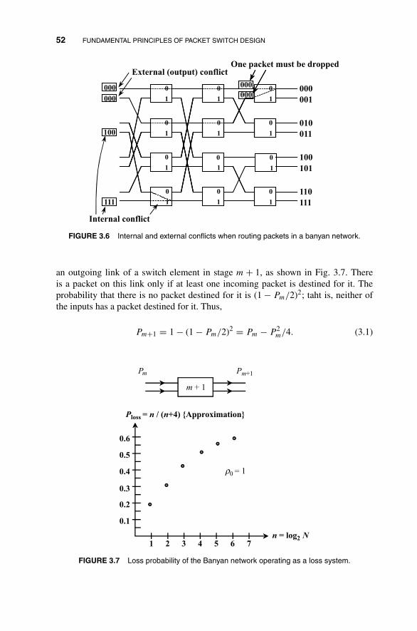
52 FUNDAMENTAL PRINCIPLES OF PACKET SWITCH DESIGN
0
1
000
111
000
001
010
011
100
101
110
111
000
100
000
000
One packet must be dropped
Internal conflict
1
0
1
0
1
0
0
1
0
1
0
0
1
1
1
0
1
0
1
0
0
1
External (output) conflict
FIGURE 3.6 Internal and external conflicts when routing packets in a banyan network.
an outgoing link of a switch element in stage m + 1, as shown in Fig. 3.7. Thereis a packet on this link only if at least one incoming packet is destined for it. Theprobability that there is no packet destined for it is (1 − Pm/2)2; taht is, neither ofthe inputs has a packet destined for it. Thus,
Pm+1 = 1 − (1 − Pm/2)2 = Pm − P2m/4. (3.1)
m + 1
Pm Pm+1
654321 7n = log2 N
0.1
0.2
0.3
0.4
0.5
0.6
Ploss = n / (n+4) {Approximation}
ρ0 = 1
FIGURE 3.7 Loss probability of the Banyan network operating as a loss system.

FUNDAMENTAL PROPERTIES OF INTERCONNECTION NETWORKS 53
From the above, we can calculate Plog2 N in a recursive manner and obtain the lossprobability from
Ploss = P0 − Plog2 N
P0. (3.2)
However, a closed-form expression for Ploss cannot be obtained this way, since Plog2 N
is not in closed form. As an approximation, suppose we treat m as a “continuous”variable and expand Pm+1 as a Taylor series:
Pm+1 = Pm + dPm
dm+ 1
2!
d2Pm
dm2 + · · ·
If dnPm/dmn is small for n ≥ 2, then (3.1) can be viewed as the recursion relationfor the following differential equation:
dPm
dm= −P2
m
4. (3.3)
From this, we have
dPm
P2m
= −dm
4.
Integrating from m = 0 and substituting P0 = ρo yields
Pm = 4ρo
mρo + 4. (3.4)
The overall packet loss probability is then given by
Ploss = ρo − Pn
ρo= nρo
nρo + 4, (3.5)
where n = log2 N. The maximum throughput is obtained when ρo = 1, and it is
ρ∗ = 1 − Ploss = 4
n + 4. (3.6)
Figure 3.7 plots the loss probability as a function of n for ρo = 1. The loss probabil-ity increases quite rapidly with n. Even for a small 4 × 4 switch, the loss probability isalready greater than 0.5. Thus, this switch is not suitable for a communication networkthat must provide good quality of service. The problem with the Banyan network isthat there is one and only one path from an input to an output. One must provide morepaths from inputs to outputs in order to reduce the loss probability. We shall examinein the next chapter how switch parameters, such as the group size, can be engineeredto improve performance.
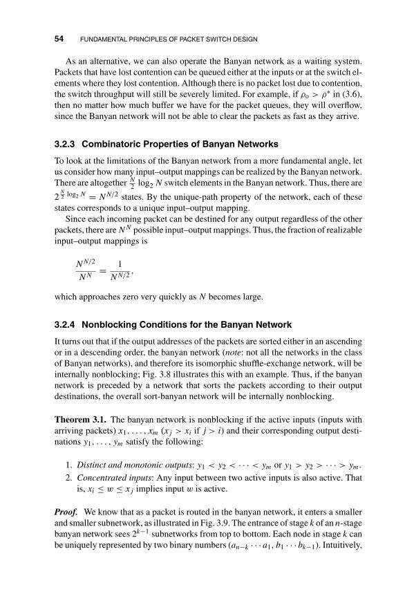
54 FUNDAMENTAL PRINCIPLES OF PACKET SWITCH DESIGN
As an alternative, we can also operate the Banyan network as a waiting system.Packets that have lost contention can be queued either at the inputs or at the switch el-ements where they lost contention. Although there is no packet lost due to contention,the switch throughput will still be severely limited. For example, if ρo > ρ∗ in (3.6),then no matter how much buffer we have for the packet queues, they will overflow,since the Banyan network will not be able to clear the packets as fast as they arrive.
3.2.3 Combinatoric Properties of Banyan Networks
To look at the limitations of the Banyan network from a more fundamental angle, letus consider how many input–output mappings can be realized by the Banyan network.There are altogether N
2 log2 N switch elements in the Banyan network. Thus, there are
2N2 log2 N = NN/2 states. By the unique-path property of the network, each of these
states corresponds to a unique input–output mapping.Since each incoming packet can be destined for any output regardless of the other
packets, there are NN possible input–output mappings. Thus, the fraction of realizableinput–output mappings is
NN/2
NN= 1
NN/2 ,
which approaches zero very quickly as N becomes large.
3.2.4 Nonblocking Conditions for the Banyan Network
It turns out that if the output addresses of the packets are sorted either in an ascendingor in a descending order, the banyan network (note: not all the networks in the classof Banyan networks), and therefore its isomorphic shuffle-exchange network, will beinternally nonblocking; Fig. 3.8 illustrates this with an example. Thus, if the banyannetwork is preceded by a network that sorts the packets according to their outputdestinations, the overall sort-banyan network will be internally nonblocking.
Theorem 3.1. The banyan network is nonblocking if the active inputs (inputs witharriving packets) x1, . . . , xm (xj > xi if j > i) and their corresponding output desti-nations y1, . . . , ym satisfy the following:
1. Distinct and monotonic outputs: y1 < y2 < · · · < ym or y1 > y2 > · · · > ym.
2. Concentrated inputs: Any input between two active inputs is also active. Thatis, xi ≤ w ≤ xj implies input w is active.
Proof. We know that as a packet is routed in the banyan network, it enters a smallerand smaller subnetwork, as illustrated in Fig. 3.9. The entrance of stage k of an n-stagebanyan network sees 2k−1 subnetworks from top to bottom. Each node in stage k canbe uniquely represented by two binary numbers (an−k · · · a1, b1 · · · bk−1). Intuitively,

FUNDAMENTAL PROPERTIES OF INTERCONNECTION NETWORKS 55
000
001
010
011
100
101
110
111(a)
001
010
011
110
000
001
010
011
100101
110111
001
010
011
110 Sorting
network
(b)
FIGURE 3.8 (a) An example showing the banyan network is nonblocking for sorted inputs; (b)nonblocking sort-banyan network.
b1 · · · bk−1 is the subnetwork label and an−k · · · a1 is the relative position of the nodenumbered from the top within the subnetwork.
Node (an−k · · · a1, b1 · · · bk−1) in stage k is connected by output link bk (0 or 1) tonode (an−k−1 · · · a1, b1 · · · bk−1bk). Thus, the path from an input x = an · · · a1 to anoutput y = b1 · · · bn, denoted by 〈x, y〉, consists of the following sequence of nodes:
(an−1 · · · a1, ∅)b1→ (an−2 · · · a1, b1) · · · (an−k · · · a1, b1 · · · bk−1) · · · bn−1→
(∅, b1 · · · bn−1).
Suppose that two packets, one from input x = an · · · a1 to output y = b1 · · · bn andthe other from input x′ = a′
n · · · a′1 to output y′ = b′
1 · · · b′n, collide in stage k. That is,
the two paths 〈x, y〉 and 〈x′, y′〉 merge at the same node (an−k · · · a1, b1 · · · bk−1) =(a′
n−k · · · a′1, b
′1 · · · b′
k−1) and share the same outgoing link bk = b′k. Then, we have
an−k · · · a1 = a′n−k · · · a′
1 (3.7)
and
b1 · · · bk = b′1 · · · b′
k. (3.8)
Since the packets are concentrated, the total number of packets between inputs x andx′, inclusively, is
|x′ − x| + 1. (3.9)

56 FUNDAMENTAL PRINCIPLES OF PACKET SWITCH DESIGN
000,∅
001,∅
010,∅
011,∅
100,∅
101,∅
110,∅
111,∅
00,0
01,0
10,0
11,0
00,1
01,1
10,1
11,1
0,00
1,00
0,01
1,01
0,10
1,10
0,11
1,11
∅, 000
∅, 001
∅, 010
∅, 011
∅, 100
∅, 101
∅, 110
∅, 111
Subnetwork 0
Subnetwork 00
Subnetwork 1
00000001
0010
001101000101
0110
0111
10001001
1010
101111001101
1110
1111
00000001
0010
001101000101
0110
0111
10001001
1010
101111001101
1110
1111
(a)
an …a1 (an–1…a1 ,∅) (an–2…a1 ,b1 (∅, b) 1 …bn–1 (b) 1 …bn)
Input
Stage-1
node
Stage-2
node
Stage-n
node Output…
…b1 bn
(b)
FIGURE 3.9 (a) Labeling of nodes in the banyan network; (b) sequence of nodes traversed bya packet from input an · · · a1 to output b1 · · · bn .
By condition 1, all these packets are destined for different outputs, and therefore theremust be |x′ − x| + 1 distinct output addresses among them. Considering the monotonecondition, the largest and the smallest addresses must be y and y′, respectively, ory′ and y, respectively. Hence, |y − y′| + 1 ≥ number of distinct output addresses =|x′ − x| + 1, or
|x′ − x| ≤ |y′ − y|. (3.10)
According to (3.7) and (3.8),
|x′ − x| = |a′n · · · a′
1 − an · · · a1|= |a′
n · · · a′n−k+10 · · · 0 − an · · · an−k+10 · · · 0|
= 2n−k|a′n · · · a′
n−k+1 − an · · · an−k+1|≥ 2n−k (3.11)
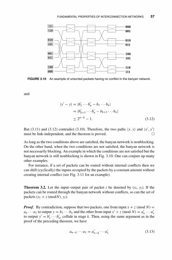
FUNDAMENTAL PROPERTIES OF INTERCONNECTION NETWORKS 57
111 000
001
010
011
100
101
110
111
110
010
101
001
011
100
000
FIGURE 3.10 An example of unsorted packets having no conflict in the banyan network.
and
|y′ − y| = |b′1 · · · b′
n − b1 · · · bn|= |b′
k+1 · · · b′n − bk+1 · · · bn|
≤ 2n−k − 1. (3.12)
But (3.11) and (3.12) contradict (3.10). Therefore, the two paths 〈x, y〉 and 〈x′, y′〉must be link-independent, and the theorem is proved. �
As long as the two conditions above are satisfied, the banyan network is nonblocking.On the other hand, when the two conditions are not satisfied, the banyan network isnot necessarily blocking. An example in which the conditions are not satisfied but thebanyan network is still nonblocking is shown in Fig. 3.10. One can conjure up manyother examples.
For instance, if a set of packets can be routed without internal conflicts then wecan shift (cyclically) the inputs occupied by the packets by a constant amount withoutcreating internal conflict (see Fig. 3.11 for an example).
Theorem 3.2. Let the input–output pair of packet i be denoted by (xi, yi). If thepackets can be routed through the banyan network without conflicts, so can the set ofpackets (xi + z (modN), yi).
Proof. By contradiction, suppose that two packets, one from input x + z (mod N) =an · · · a1 to output y = b1 · · · bn and the other from input x′ + z (mod N) = a′
n · · · a′1
to output y′ = b′1 · · · b′
n, collide in stage k. Then, using the same argument as in theproof of the preceding theorem, we have
an−k · · · a1 = a′n−k · · · a′
1 (3.13)

58 FUNDAMENTAL PRINCIPLES OF PACKET SWITCH DESIGN
011 000
001
010
011
100
101
110
111
110
001
010
(x1, y1)
(xm, ym)
.. nonblocking(x1 + Z mod N, y1)
(xm + Z mod N, ym)
..
FIGURE 3.11 Sorted packets in Fig. 3.8(a) remain unblocked after their inputs are shifted(mod 8) by 6.
and
b1 · · · bk = b′1 · · · b′
k. (3.14)
Also,
x = (x + z) − z = (x + z) + (N − z) (mod N),
x′ = (x′ + z) − z = (x′ + z) + (N − z) (mod N). (3.15)
Let N − z = cn · · · c1. Then,
x = an · · · a1 + cn · · · c1 (mod N),
x′ = a′n · · · a′
1 + cn · · · c1 (mod N). (3.16)
In other words, x and x′ are the addition of cn · · · c1 to an · · · a1 and a′n · · · a′
1, re-spectively, with only the n least significant bits retained. If an−k · · · a1 = a′
n−k · · · a′1,
then
an−k · · · a1 + cn−k · · · c1 = a′n−k · · · a′
1 + cn−k · · · c1. (3.17)
The above expressions may have more than n − k bits. The n − k least significant bitsmust be equal for the whole expressions to be equal. Thus, the n − k least significantbits of x and x′ are equal. Therefore, if the two packets with input–output pairs(x + z (mod N), y) and (x′ + z (mod N), y′) collide in stage k, so will the two packetswith input–output pairs (x, y) and (x′, y′). �
SORTING NETWORKS 59
The properties summarized in the two theorems let us implement many usefulfunctions using the banyan and reverse banyan networks. We already see that aninternally nonblocking network can be constructed by cascading a sorting networkand a banyan network. We can also build a packet concentrator using a reverse banyannetwork. That is, suppose not all N inputs are always active and we want to concentratethe incoming packets to M < N links. Unlike for switching, it is not necessary forthe concentrator to route a packet to a specific output—any one of the M outputswould do. To concentrate packets using the reverse banyan network in a nonblockingfashion, we can assign the first packet (from top to bottom) the output address 0, thesecond packet the output address 1, and so on. By routing from the least significantbit of the address to the most significant bit, Theorem 3.1 says that the packets wouldnot have internal conflict—of course, we have to interpret the inputs as outputs andoutputs as inputs.
We can also build a shifter using a reverse banyan network. Suppose that we want todistribute the incoming packets in a cyclic fashion to the outputs. Say, in the previoustime slot, a batch of packets arrive and they are assigned to adjacent outputs withoutput i being the last (from top to bottom) having a packet assignment. In the currenttime slots, the batch of incoming packets is to be distributed to outputs i + 1 (mod N),i + 2 (mod N), and so on. Instead of assigning the output addresses starting from 0,as in the ordinary concentrator, we offset the assignment by i + 1 (mod N). Thus,the first packet is assigned to output i + 1 (mod N), the second packet to outputi + 2 (mod N), and so on. By keeping track of the next output to be assigned, wecan distribute packets to the outputs in a cyclic and evenly manner. Theorem 3.1together with Theorem 3.2 says that assigning output addresses this way does notcause internal conflict.
One can implement the concentration and shifting functions together in a reversebanyan network. Suppose that the number of outputs is M < N, with M a power of2. Then, instead of offsetting output addresses using mod N arithmetic, we can usemod M arithmetic. The reader can easily check that the shifting property in Theorem3.2 is still valid. Both the concentrator and the shifter are useful building blocks forconstructing other switching and computation architectures, as will be seen in thenext chapter.
3.3 SORTING NETWORKS
A sorting network is a nonblocking network by itself if
1. All inputs are active.
2. No two packets are destined for the same output.
This is illustrated in Fig. 3.12(a). Let us first examine condition 1 assuming condition2 is satisfied. When some of the inputs are inactive, the packets may arrive at thewrong destination, as illustrated in Fig. 3.12(b). This is the reason why we need to
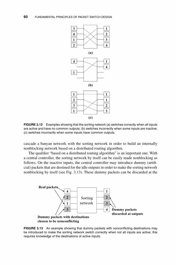
60 FUNDAMENTAL PRINCIPLES OF PACKET SWITCH DESIGN
3
4
1
2
1
2
3
4
4
1
1
4
1
2
3
1
1
1
2
3
(a)
(b)
(c)
FIGURE 3.12 Examples showing that the sorting network (a) switches correctly when all inputsare active and have no common outputs; (b) switches incorrectly when some inputs are inactive;(c) switches incorrectly when some inputs have common outputs.
cascade a banyan network with the sorting network in order to build an internallynonblocking network based on a distributed routing algorithm.
The qualifier “based on a distributed routing algorithm” is an important one. Witha central controller, the sorting network by itself can be easily made nonblocking asfollows. On the inactive inputs, the central controller may introduce dummy (artifi-cial) packets that are destined for the idle outputs in order to make the sorting networknonblocking by itself (see Fig. 3.13). These dummy packets can be discarded at the
Sorting
network
4
2
1
3
1
2
3
4
Real packets
Dummy packets with destinations
chosen to be nonconflicting
Dummy packets
discarded at outputs
FIGURE 3.13 An example showing that dummy packets with nonconflicting destinations maybe introduced to make the sorting network switch correctly when not all inputs are active; thisrequires knowledge of the destinations of active inputs.
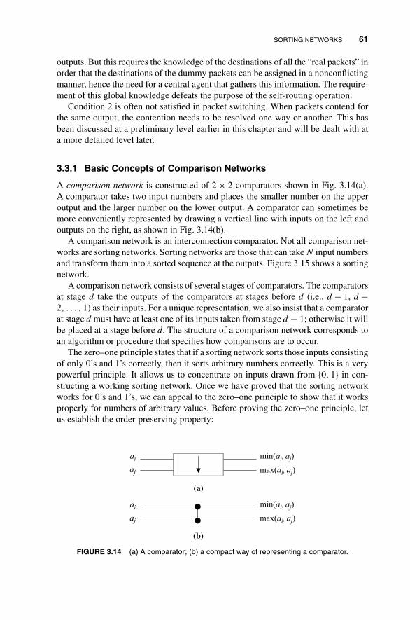
SORTING NETWORKS 61
outputs. But this requires the knowledge of the destinations of all the “real packets” inorder that the destinations of the dummy packets can be assigned in a nonconflictingmanner, hence the need for a central agent that gathers this information. The require-ment of this global knowledge defeats the purpose of the self-routing operation.
Condition 2 is often not satisfied in packet switching. When packets contend forthe same output, the contention needs to be resolved one way or another. This hasbeen discussed at a preliminary level earlier in this chapter and will be dealt with ata more detailed level later.
3.3.1 Basic Concepts of Comparison Networks
A comparison network is constructed of 2 × 2 comparators shown in Fig. 3.14(a).A comparator takes two input numbers and places the smaller number on the upperoutput and the larger number on the lower output. A comparator can sometimes bemore conveniently represented by drawing a vertical line with inputs on the left andoutputs on the right, as shown in Fig. 3.14(b).
A comparison network is an interconnection comparator. Not all comparison net-works are sorting networks. Sorting networks are those that can take N input numbersand transform them into a sorted sequence at the outputs. Figure 3.15 shows a sortingnetwork.
A comparison network consists of several stages of comparators. The comparatorsat stage d take the outputs of the comparators at stages before d (i.e., d − 1, d −2, . . . , 1) as their inputs. For a unique representation, we also insist that a comparatorat stage d must have at least one of its inputs taken from stage d − 1; otherwise it willbe placed at a stage before d. The structure of a comparison network corresponds toan algorithm or procedure that specifies how comparisons are to occur.
The zero–one principle states that if a sorting network sorts those inputs consistingof only 0’s and 1’s correctly, then it sorts arbitrary numbers correctly. This is a verypowerful principle. It allows us to concentrate on inputs drawn from {0, 1} in con-structing a working sorting network. Once we have proved that the sorting networkworks for 0’s and 1’s, we can appeal to the zero–one principle to show that it worksproperly for numbers of arbitrary values. Before proving the zero–one principle, letus establish the order-preserving property:
ai
ai
aj
aj
min(ai, aj)
max(ai, aj)
min(ai, aj)
max(ai, aj)
(a)
(b)
FIGURE 3.14 (a) A comparator; (b) a compact way of representing a comparator.

62 FUNDAMENTAL PRINCIPLES OF PACKET SWITCH DESIGN
a1
a2
a3
a4
b1
b2
b3
b4
Stage
1
Stage
2
Stage
3
a1
a2
a3
a4
b1
b2
b3
b4
(a)
(b)
FIGURE 3.15 A 4 × 4 sorting network (a) is the compact representation; (b) is the fullrepresentation.
Order-Preserving Property. Suppose a comparison network transforms the in-put sequence a = 〈a1, a2, . . . , aN〉 into the output sequence b = 〈b1, b2, . . . , bN〉,then for any monotonically increasing function f , the network transforms the in-puts sequence f (a) = 〈f (a1), f (a2), . . . , f (aN )〉 into the output sequence f (b) =〈f (b1), f (b2), . . . , f (bN )〉.
Proof. With reference to Fig. 3.16, consider a comparator with inputs x and y andupper output min(x, y) and lower output max(x, y). Without loss of generality, letx ≤ y. Since f is monotonically increasing, this implies f (x) ≤ f (y). Thus, if the
xy
min(x, y)
max(x, y)
yfxfyxyfxfyx
for any monotonic function f
)()(and)()( >⇒>≤⇒≤
f (x)
f (y)
min( f (x), f ( y))
max( f (x), f (y))⎩⎨⎧
>=≤=
=yxyxfyf
yxyxfxf
if)),(min()(
if)),(min()(
⎩⎨⎧
>=≤=
=yxyxfxf
yxyxfyf
if)),(max()(
if)),(max()(
FIGURE 3.16 Illustration that a comparator has the order-preserving property.

SORTING NETWORKS 63
aiaj
ci = min(ai, aj)
cj= max(ai, aj)
f (ai)
f(aj)
min( f (ai), f (aj))= f (min(ai, aj)) = f(ci)
f (cj)
Outputs of stages before stage d
Comparison network
Comparison network
By assumption of induction, they must be f (ai) and f (aj)
A comparator at stage d
a
f(a)
(a)
(b)
FIGURE 3.17 (a) The inputs and outputs of a comparator at stage d when input sequence isa; (b) the inputs and outputs of the same comparator when input sequence is f (a).
inputs were f (x) and f (y), the upper and lower outputs would be, respectively,
min(f (x), f (y)) = f (x) = f (min(x, y)),
max(f (x), f (y)) = f (y) = f (max(x, y)). (3.18)
Thus, a comparator has the order-preserving property. For a general comparison net-work, we can show by induction the correctness of this statement: If an output of acomparator at stage d assumes the value of ci when the input sequence to the overallnetwork is a, it assumes a value of f (ci) when the input sequence is f (a). Note thatsince stage d can be any stage, including the last stage, the correctness of the abovestatement implies the order-preserving property.
By (3.18), the statement is true for d = 1, since numbers at the outputs of stage 1have passed through at most one comparator. By induction, assume that the statementis true for stages d − 1 and below, we want to show that it is also true for stage d. Theinputs to a comparator at stage d are outputs from the stages d − 1 and below. Thus, ifthe inputs assume the value of ai and aj when the input sequence is a, they must assumethe values f (ai) and f (aj) (see Fig. 3.17) when the input sequence is f (a). When theinput sequence is a, the upper and lower outputs of the comparator are ci = min(ai, aj)and cj = max(ai, aj), respectively. Therefore, by (3.18), the upper and lower outputsare f (min(ai, aj)) = f (ci) and f (max(ai, aj)) = f (cj), respectively, when the inputsequence is f (a). �
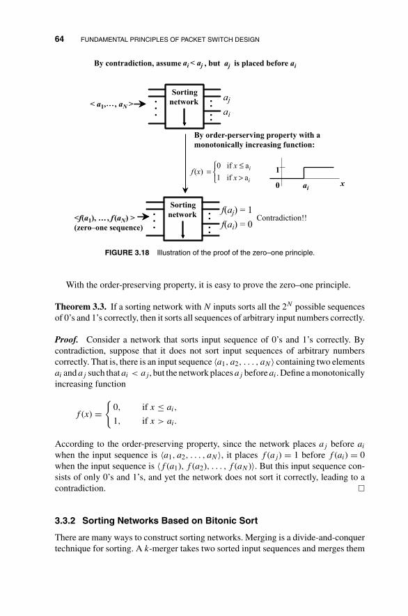
64 FUNDAMENTAL PRINCIPLES OF PACKET SWITCH DESIGN
⎩⎨⎧
>≤
=f (x)ai1 if xai0 if x
0
1
ai x
Contradiction!!
By contradiction, assume , but aj is placed before aiai < aj
Sorting
network ....
...< a1, , aN >
ajai
By order-perserving property with a
monotonically increasing function:
Sorting
network ....
...<f(a1), …, f (aN) >
(zero–one sequence)
f(aj) = 1
f(ai) = 0
FIGURE 3.18 Illustration of the proof of the zero–one principle.
With the order-preserving property, it is easy to prove the zero–one principle.
Theorem 3.3. If a sorting network with N inputs sorts all the 2N possible sequencesof 0’s and 1’s correctly, then it sorts all sequences of arbitrary input numbers correctly.
Proof. Consider a network that sorts input sequence of 0’s and 1’s correctly. Bycontradiction, suppose that it does not sort input sequences of arbitrary numberscorrectly. That is, there is an input sequence 〈a1, a2, . . . , aN〉 containing two elementsai and aj such that ai < aj , but the network places aj before ai. Define a monotonicallyincreasing function
f (x) ={
0, if x ≤ ai,
1, if x > ai.
According to the order-preserving property, since the network places aj before ai
when the input sequence is 〈a1, a2, . . . , aN〉, it places f (aj) = 1 before f (ai) = 0when the input sequence is 〈f (a1), f (a2), . . . , f (aN )〉. But this input sequence con-sists of only 0’s and 1’s, and yet the network does not sort it correctly, leading to acontradiction. �
3.3.2 Sorting Networks Based on Bitonic Sort
There are many ways to construct sorting networks. Merging is a divide-and-conquertechnique for sorting. A k-merger takes two sorted input sequences and merges them
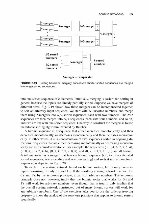
SORTING NETWORKS 65
2-merger
2-merger4-merger
2-merger
2-merger4-merger
... …
N/2-merger
N/2-merger
...
...
N-merger
.
.
.
N-merger...
.
.
.
k/2 sorted
numbers
k/2 sorted
numbers
k sorted
numbers
2-merger = comparator
FIGURE 3.19 Sorting based on merging; successive shorter sorted sequences are mergedinto longer sorted sequences.
into one sorted sequence of k elements. Intuitively, merging is easier than sorting ingeneral because the inputs are already partially sorted. Suppose we have mergers ofdifferent sizes; Fig. 3.19 shows how these mergers can be interconnected togetherto sort an arbitrary input sequence. We start with N unsorted numbers, and mergethem using 2-mergers into N/2 sorted sequences, each with two numbers. The N/2sequences are then merged into N/4 sequences, each with four numbers, and so on,until we are left with one sorted sequence. One way to construct the mergers is to usethe bitonic sorting algorithm invented by Batcher.
A bitonic sequence is a sequence that either increases monotonically and thendecreases monotonically, or decreases monotonically and then increases monotoni-cally. In other words, it is a concatenation of two sequences sorted in opposing di-rections. Sequences that are either increasing monotonically or decreasing monoton-ically are also considered bitonic. For example, the sequences 〈0, 1, 4, 6, 7, 7, 5, 4〉,〈9, 8, 7, 3, 3, 2, 4, 6〉, 〈0, 1, 4, 7, 7, 7, 8, 8〉, and 〈8, 7, 3, 3, 2, 1, 1, 0〉 are all bitonic.A bitonic sorter is a merger that takes a bitonic sequence (i.e., two concatenatedsorted sequences, one ascending and one descending) and sorts it into a monotonicsequence, as depicted in Fig. 3.20.
To explain the sorting network based on bitonic sorters, let us only considerinputs consisting of only 0’s and 1’s. If the resulting sorting network can sort the0’s and 1’s, by the zero–one principle, it can sort arbitrary numbers. The zero–oneprinciple does not, however, imply that the bitonic sorter that works for 0’s and1’s will work for arbitrary numbers, even though that is true. It only implies thatthe overall sorting network constructed out of many bitonic sorters will work forany arbitrary numbers. One of the exercises asks you to use the order-preservingproperty to show the analog of the zero–one principle that applies to bitonic sortersspecifically.

66 FUNDAMENTAL PRINCIPLES OF PACKET SWITCH DESIGN
or
k-bitonic
sorter
...
...
...
Ascending
sequence
Descending
sequence
Ascending
sequence
k-bitonic
sorter
...
...
...Ascending
sequence
Descending
sequenceAscending
sequence
*The two input sequences do not have to be of the same length
*The two input sequences are of opposing directions
FIGURE 3.20 Bitonic Sorters.
A bitonic sequence consisting of only 0’s and 1’s is either of the form 0i1j0k orof the form 1i0j1k, for some i, j, k ≥ 0, where the notation xi means i successivex values. A bitonic sequence a is said to be no less (greater) than another bitonicsequence if none of the element in a is less (greater) than any of the elements in b;symbolically, we write a ≥ b if a is not less than b and a ≤ b if a is not greater thanb. For example,
〈001100〉 ≥ 〈000000〉,〈111100〉 ≤ 〈111111〉.
Two sequences do not necessarily have an ordering relationship. For example,〈001100〉 is neither not less than nor not greater than 〈111100〉. Two zero–one se-quences have an ordering relationship if and only if at least one of them is consistingof all 0’s or all 1’s. This is one reason why it is easier to focus on zero–one sequencesin constructing a comparison network.
The following theorem shows how a bitonic sequence a can be decomposed intotwo bitonic subsequences a′ and a′′ with a′ ≤ a′′ using only one stage of comparators.The same decomposition method can then be applied to a′ and a′′ to produce fourbitonic subsequences with each subsequence not greater than the next. Applyingthis decomposition in a recursive manner allows us to sort the original bitonicsequence into a monotonic sequence (when all the subsequences have only oneelement).
Theorem 3.4. If a zero–one sequence of 2n elements a = 〈a1, a2, . . . , a2n〉 is bitonic,then the two n-element sequences
a′ = 〈min(a1, an+1), min(a2, an+2), . . . , min(an, a2n)〉

SORTING NETWORKS 67
a1
a2
an
an+1
an+2
a2n
min(a1, an+1)
min(a2, an+2)
min(an, a2n)
max(a1, an+1)
max(a2, an+2)
max(an, a2n)
...
...
...
...
a′bitonic
≥
a″bitonic
If ais a zero–one sequence, either a′ is all 0’s or a″ is all 1’s, or both
abitonic
FIGURE 3.21 A half-cleaner.
and
a′′ = 〈max(a1, an+1), max(a2, an+2), . . . , max(an, a2n)〉
have two properties:
1. They are both bitonic.
2. a′ ≤ a′′.
Comment. The above decomposition can be implemented by a single stage of n
comparators, called a half-cleaner, as depicted in Fig. 3.21. As shown, elements inthe first half and the second half of the input sequence are paired and compared. Thelarger elements and smaller elements of the comparisons form two subsequences withthe above properties. Since a′ and a′′ have an ordering relationship and they consist ofonly 0’s and 1’s, at least one of them must be all 0’s or all 1’s. A sequence consistingof all 0’s or all 1’s is said to be clean, hence the name half-cleaner for the comparisonnetwork.
Proof. Without loss of generality, suppose that the bitonic sequence is of the form0i1j0k. Proving the case 1i0j1k is similar to the argument presented here. There areonly four possible cases depending on where the midpoint falls, as shown in Fig. 3.22.Cases (i) and (ii) have midpoints falling on a block of 0’s. From the figure, it can beseen that the theorem holds for both cases. Cases (iii) and (iv) have midpoints fallingon the block of 1’s. In case (iii), there are more 0’s than 1’s in the sequence a, andin case (iv), there are at least as many 1’s as 0’s. Again, as shown in the figure, thetheorem holds for both cases. �

68 FUNDAMENTAL PRINCIPLES OF PACKET SWITCH DESIGN
FIGURE 3.22 Operations performed by a half-cleaner for different cases.
Figure 3.23 shows the decomposition of a k-bitonic sorter (one that sorts k elements)into a k-half cleaner followed by two k/2-bitonic sorters. The above theorem states thatthe inputs to the lower k/2-bitonic sorter are not less than the inputs to the upper k/2-bitonic sorter. Furthermore, each of the input sequences is bitonic. The k/2-bitonic
k-half
cleaner
k/2-bitonic
cleaner
k/2-bitonic
cleaner
.
.
.
...
...
...
...
FIGURE 3.23 Recursive construction of a k -bitonic sorter.

SORTING NETWORKS 69
2-bitonic
sorter
2-bitonic
sorter
2-bitonic
sorter
2-bitonic
sorter
4-bitonic
sorter
4-bitonic
sorter
(a)
8-bitonic
sorter
Four 2-bitonic
sorters
Two 4-bitonic
sorters
One 8-bitonic
sorter
(b)
FIGURE 3.24 (a) A sorting network based on merging using bitonic sorters; (b) the samenetwork broken down into comparators.
sorters can be further broken down into two k/2-half cleaners and four k/4-bitonicsorters using the same decomposition. Applying the decomposition recursively, only2-bitonic sorters are left in the end, and 2-bitonic sorters are simply comparators.Notice that the structure of the bitonic sorter is the same as that of the banyan network,and it consists of log2 N stages of comparators.
Now that we know how to build bitonic sorters, we can use them as the mergers inFig. 3.19 to build an overall sorting network that sorts arbitrary zero–one sequences(i.e., sequences that are not necessarily bitonic). Figure 3.24 shows the constructionof an 8 × 8 Batcher sorting network based on the bitonic sort.
To compute the number of comparators in a Batcher sorting network, note that thenumber of stages in a k-bitonic sorter is
f (k) = log2 k. (3.19)
Figure 3.24(a) shows that an input element passes through one 2-bitonic sorter,one 22-bitonic sorter, one 23-bitonic sorter, and so on, on its way to the output ofthe overall sorting network. Therefore, the total number of stages in the Batchernetwork is
log2 N∑i=1
f (2i) =log2 N∑i=1
i = log2 N(log2 N + 1)
2. (3.20)

70 FUNDAMENTAL PRINCIPLES OF PACKET SWITCH DESIGN
Odd
merge
d1
d2
d3
d4
dn
...
Even
merge
e1
e2
e3
e4
en
...
a1
a2
a3
a4
an
...
b1
b2
b3
b4
bn
...
c1
c2
c3
c4
c5
c6
c7
c2n
..
....
FIGURE 3.25 Recursion for odd–even merging networks.
Since each stage in the sorting network has N/2 comparators, the total number ofcomparator is
N log2 N(log2 N + 1)
4. (3.21)
The number of elements in the sorting network is therefore of order N log22 N.
3.3.3 The Odd–Even Sorting Network
Batcher also invented another order N log22 N sorting network. As in the bitonic
sorting algorithm, sorting by merging is used. Instead of using bitonic sorters formerging, odd–even mergers are used. The basic idea of the recursive odd–even mergeris illustrated in Fig. 3.25. The essence is contained in the following theorem.
Theorem 3.5. Consider two sorted input sequences a = 〈a1, . . . , an〉 and b =〈b1, . . . , bn〉. The odd-indexed elements of a and b, a′ = 〈a1, a3, . . .〉 and b′ =〈b1, b3, . . .〉, and the even-indexed elements,a′′ = 〈a2, a4, . . .〉 and b′′ = 〈b2, b4, . . .〉,are all sorted subsequences. Suppose that the odd-indexed subsequences a′ and b′ aremerged into a sorted sequence d = 〈d1, d2, . . .〉, and the even-indexed subsequencesa′′ and b′′ are merged into e = 〈e1, e2〉. Then, it can be shown that
ei−2 ≤ di ≤ ei. (3.22)
Comment. The above merging of a′ and b′, and a′′ and b′′, is depicted in Fig. 3.25.The theorem implies that c = 〈d1, min(d2, e1), max(d2, e1), . . . , min(di, ei−1),max(di, ei−1), . . . , 〉 must be a sorted sequence: that each element is at least as large asthe preceding element can be easily verified using (3.22). The sequence c is produced

SORTING NETWORKS 71
at the last stage of the odd–even merger in Fig. 3.25. The smaller mergers in the mid-dle are implemented by the same algorithm in a recursive manner. Note the differencebetween the bitonic recursion and the odd–even recursion: the smaller mergers in theformer are positioned after the one-stage comparison whereas the latter is the otherway round.
Proof. Let us assume n is even. The proof for odd n is similar. We appeal to thezero–one principle and shall assume a and b to consist of only 0’s and 1’s. Letf (x) = (nx, mx) be a tuple denoting the number of 0’s, nx, and the number of 1’s,mx, in the sequence x. Then, for even n, it can be easily seen that
f (a′) =(⌈na
2
⌉,⌊ma
2
⌋),
f (a′′) =(⌊na
2
⌋,⌈ma
2
⌉),
f (b′) =(⌈nb
2
⌉,⌊mb
2
⌋),
f (b′′) =(⌊nb
2
⌋,⌈mb
2
⌉).
Therefore, since d and e are sorted sequences resulting from merging a′ and b′,and a′′ and b′′, respectively, we have
f (d) =(⌈na
2
⌉+
⌈nb
2
⌉,⌊ma
2
⌋+
⌊mb
2
⌋),
f (e) =(⌊na
2
⌋+
⌊nb
2
⌋,⌈ma
2
⌉+
⌈mb
2
⌉).
The number of elements in d and e is the same. The number of 0’s in d is no smallerthan that in e, implying di ≤ ei. The number of 0’s in d can be more than that in e
by at most 2, implying ei−2 ≤ di for i = 3, 4, . . .. These observations complete theproof. �
3.3.4 Switching and Contention Resolution in Sort-Banyan Network
Recall that in packet switching, the output address of a packet is contained inthe header. When using the Batcher sorting network for switching, the compara-tor only looks at the header and passes on the information bits without examiningthem. Only a delay of one-bit duration is experienced by packets passing through acomparator.
Figure 3.26 illustrates the operation of a comparator used for packet switching.Suppose that the output address of the upper packet is 0010 and that of the lowerpacket is 0001, and suppose that the comparator is in the bar state initially. Eachtime a bit of the output address has arrived on both inputs, the comparator does acomparison. If both bits are 0’s or 1’s, as in the first and second bits in our example,
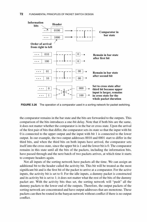
72 FUNDAMENTAL PRINCIPLES OF PACKET SWITCH DESIGN
0100…
1000…
HeaderInformation
bits
Order of arrival from right to left
Comparator in bar state
010…
100…Remain in bar state after first bit
0
0
01…
10…Remain in bar state after second bit
00
00
0…
1…
Set to cross state after third bit because upper input is larger, remains in cross state for the whole packet duration
000
100
FIGURE 3.26 The operation of a comparator used in a sorting network for packet switching.
the comparator remains in the bar state and the bits are forwarded to the outputs. Thiscomparison of the bits introduces a one-bit delay. Note that if both bits are the same,it does not matter whether the comparator is in the bar or cross state. Upon the arrivalof the first pair of bits that differ, the comparator sets its state so that the input with bit0 is connected to the upper output and the input with bit 1 is connected to the loweroutput. In our example, the two output addresses 0010 and 0001 start to differ in thethird bits, and when the third bits on both inputs have arrived, the comparator setsitself into the cross state, since the upper bit is 1 and the lower bit is 0. The comparatorremains in this state until all the bits of the packets, including the information bits,have passed through and the next batch of two packets arrives, at which time it startsto compare headers again.
Not all inputs of the sorting network have packets all the time. We can assign anadditional bit to the header called the activity bit. This bit will be treated as the mostsignificant bit and is the first bit of the packet to arrive at a comparator. For the activeinputs, the activity bit is set to 0. For the idle inputs, a dummy packet is constructedand its activity bit is set to 1; it does not matter what the rest of the bits of the dummypacket are. With the activity bits thus set, the sorting network will “push” all thedummy packets to the lower end of the outputs. Therefore, the output packets of thesorting network are concentrated and have output addresses that are monotone. Thesepackets can then be routed in the banyan network without conflict if there is no outputconflict.
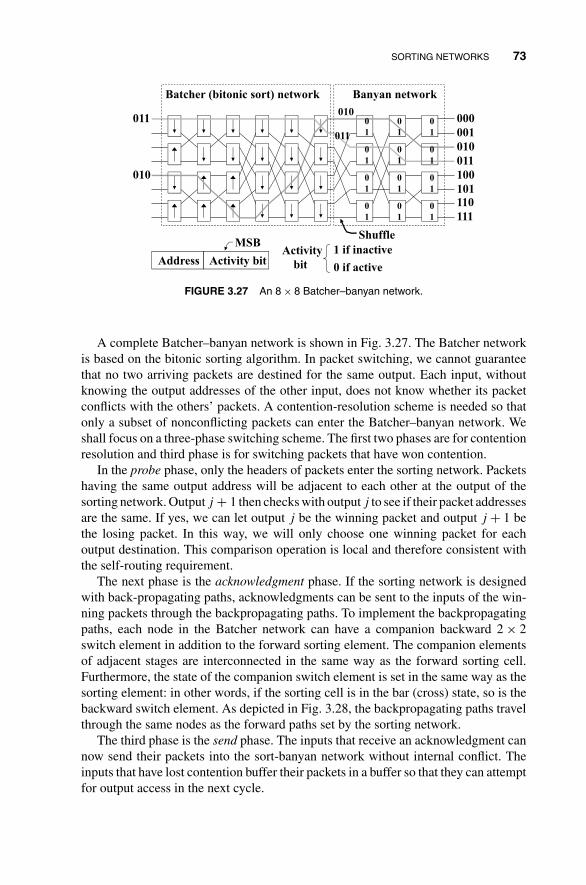
SORTING NETWORKS 73
0
1
0
1
0
1
0
1
0
1
0
1
0
1
0
1
0
1
0
1
0
1
0
1
011
010
000
001
010
011
100
101
110
111
010
011
Shuffle
Batcher (bitonic sort) network Banyan network
Address Activity bit
MSBActivity
bit
1 if inactive
0 if active
FIGURE 3.27 An 8 × 8 Batcher–banyan network.
A complete Batcher–banyan network is shown in Fig. 3.27. The Batcher networkis based on the bitonic sorting algorithm. In packet switching, we cannot guaranteethat no two arriving packets are destined for the same output. Each input, withoutknowing the output addresses of the other input, does not know whether its packetconflicts with the others’ packets. A contention-resolution scheme is needed so thatonly a subset of nonconflicting packets can enter the Batcher–banyan network. Weshall focus on a three-phase switching scheme. The first two phases are for contentionresolution and third phase is for switching packets that have won contention.
In the probe phase, only the headers of packets enter the sorting network. Packetshaving the same output address will be adjacent to each other at the output of thesorting network. Output j + 1 then checks with output j to see if their packet addressesare the same. If yes, we can let output j be the winning packet and output j + 1 bethe losing packet. In this way, we will only choose one winning packet for eachoutput destination. This comparison operation is local and therefore consistent withthe self-routing requirement.
The next phase is the acknowledgment phase. If the sorting network is designedwith back-propagating paths, acknowledgments can be sent to the inputs of the win-ning packets through the backpropagating paths. To implement the backpropagatingpaths, each node in the Batcher network can have a companion backward 2 × 2switch element in addition to the forward sorting element. The companion elementsof adjacent stages are interconnected in the same way as the forward sorting cell.Furthermore, the state of the companion switch element is set in the same way as thesorting element: in other words, if the sorting cell is in the bar (cross) state, so is thebackward switch element. As depicted in Fig. 3.28, the backpropagating paths travelthrough the same nodes as the forward paths set by the sorting network.
The third phase is the send phase. The inputs that receive an acknowledgment cannow send their packets into the sort-banyan network without internal conflict. Theinputs that have lost contention buffer their packets in a buffer so that they can attemptfor output access in the next cycle.

74 FUNDAMENTAL PRINCIPLES OF PACKET SWITCH DESIGN
Banyan
network
(a)
4
5
i4
i
2
4
i
2
4
4
5
i
i
4
i
Sorting
network
Output
destinations
i = idle outputs
Sorted header. Each output
examines the output above
for possible conflict
Banyan
network
2
4
4
5
ii
4
i
Acknowledgment
path is reverse of
forward sorting path
(b)
2
5
4
Concentrated and monotonic
output addresses
4
2
5
(c)
FIGURE 3.28 Three-phase scheme for sort-banyan network (a) is for probing for conflict; (b) isfor acknowledgment of winning packets; (c) is for routing winning packets.
There are many possible variations to the above basic scheme. The main idea,however, is to use the sort-banyan network as the contention arbiter as well as theswitching network. The initial two phases are for contention resolution. While thefirst two phases are ongoing, no packets are being routed to their outputs, and this in-troduces a certain amount of contention-resolution overhead, reducing the throughputof the switch to below 100%.

NONBLOCKING AND SELF-ROUTING PROPERTIES OF CLOS NETWORKS 75
Internally
nonblocking
switch
13
2 1
4
3
1
2
3
4
Input queues
Winning packet
Losing packet
Cannot access
output 2 because
it is blocked by
the first packet
Outputs
FIGURE 3.29 Illustration of head-of-line blocking.
The so-called head-of-line (HOL) blocking further reduces the throughput of theswitch. Since the packets losing contention are buffered at their inputs, the sort-banyan network as described above is a waiting system. While the packets are beingbuffered, new packets may arrive, forming queues at the inputs. As illustrated inFig. 3.29, the second packet of an input queue whose first packet has lost contentionmay be destined for an idle output. If the packets at the inputs access their outputsin a first-in-first-out fashion, the second packet cannot access its output until the firstpacket has accessed its own output. It is said to be blocked by the first (or HOL)packet. The throughput limitation due to HOL blocking will be derived in the nextchapter.
3.4 NONBLOCKING AND SELF-ROUTING PROPERTIESOF CLOS NETWORKS
In the previous sections, we have introduced the fundamental properties of Banyannetworks and demonstrated the way to construct a nonblocking packet switch basedon them. Here, we turn our concern to the Clos networks. We shall focus on theirnonblocking conditions and self-routing properties.
Before proceeding, we need to present a scheme to assign addresses to the inputsand outputs of Clos networks. Let us consider a three-stage Clos network as shown inFig. 3.30, which is characterized by two integer parameters p and q. Here, the numberof inputs and outputs N is given by N = pq. There are two ways to address the inputsand outputs. One is to number them in a consecutive top-to-bottom manner from 0 toN − 1. The other is to use a 2-tuple addressing scheme. An input is numbered (ai, bi)if it is the (bi + 1)th input port on switch module ai. Similarly, an output is numbered(xi, yi) if it is the (yi + 1)th output port on switch module xi. The 2-tuple addressess̃i and d̃i can be obtained from their corresponding consecutive addresses si and di by
s̃i =(⌊
si
q
⌋, [si]q
)and d̃i =
(⌊di
q
⌋, [di]q
), (3.23)

76 FUNDAMENTAL PRINCIPLES OF PACKET SWITCH DESIGN
0
0
1
q–1
...
0
1
q–1
...
1
0
1
q–1
...
qq+1
2q–1
...
p–1
0
1
q–1
...
(p–1)q(p–1)q+1
pq–1
...
...
0
q–1
...
0
q–1
...
0
q–1
...
0
1
q–1
...
0
p–1
...
0
p–1
...
0
p–1
...
0
p–1
...
0
p–1
...
0
p–1
...
0
0
1
q–1
...
1
0
1
q–1
...
p–1
0
1
q–1
...
...
0
q–1
...
0
q–1
...
0
q–1
...
0
1
q–1
...
qq+1
2q–1
...
(p–1)q(p–1)q+1
pq–1
...
...–..
[s]s q q p q p d[d]qq q⎦⎣s/q ⎦⎣d/q
⎦⎣ ),[s]s/q(s~ q= ⎦⎣ ),[d]d/q(d~ q=
ba
FIGURE 3.30 A three-stage Clos network with address numbering scheme.
where � ab� is the largest integer smaller than a/b and [a]b is the reminder of a/b. For
simplicity, we will denote the address (ai, bi) by aibi whenever there is no ambiguity.Actually, the 2-tuple addressing scheme can be used for routing. For instance, to go
from any middle-stage module to an output xiyi, a packet should go to the (xi + 1)thoutput in the middle-stage module and to the (yi + 1)th output in the output-stagemodule. Since each middle-stage module here is of size p × p and each output-stagemodule is q × q, xi is of base p (0 ≤ xi ≤ p − 1) and yi is of base q (0 ≤ yi ≤ q − 1).
3.4.1 Nonblocking Route Assignment
For nonblocking routing of packets across a Clos network, we need a route assignmentalgorithm to assign a middle-stage module for each connection request. An assignmentis nonblocking if none of the internal links is shared by two paths. Consider a three-stage Clos network with parameters p and q. There are q middle-stage modules, whichprovide totally q alternate paths for each input–output pair. Let C = {0, 1, . . . , q − 1}be the set of middle-stage modules and π = {(s0, d0), . . . , (sn−1, dn−1)} the input–output permutation (which may be partial). A sufficient condition for an assignmentf : π → C to be nonblocking is
f (si, di) = f (sj, dj) ⇒ | si − sj |≥ q and | di − dj |≥ q, (3.24)
where di = π(si) and dj = π(sj). That is, if two connections (si, di) and (sj, dj) gothrough the same middle-stage module, the condition | si − sj |≥ q guarantees that

NONBLOCKING AND SELF-ROUTING PROPERTIES OF CLOS NETWORKS 77
the inputs are on different switch modules and the condition | di − dj |≥ q guaranteesthat the outputs are on different switch modules. With this, no more than one inputor output on the same module will be assigned to the same middle-stage module andhence the assignment is nonblocking. Note that (3.24) is a strong condition in thesense that we only require si and sj to be on different input-stage modules and di
and dj to be on different output-stage modules for the assignment to be nonblocking.They do not need to be differed by q.
For an assignment f , the routing tag for the connection (si, di) is given by
(f (si, di),
⌊di
q
⌋, [di]q
). (3.25)
The first component in the routing tag is the middle-stage module to which theconnection request is assigned. The second and third components are derived fromthe address of the output destination. Thus, once the first component is determinedby the route assignment algorithm, the routing tag can be determined immediately.
Consider the reverse path from output di to input si. In order that si and di to beconnected, they must be assigned the same middle-stage module. Therefore, to gofrom di to si, the routing tag for the reverse path is
(f (si, di),
⌊si
q
⌋, [si]q
). (3.26)
The set of connection requests π is monotonic if the active inputs s0, s1, . . . , sn−1and their corresponding outputs d0, d1, . . . , dn−1 satisfy either one of the followingconditions:
si < sj ⇒ di < dj for all i, j; or (3.27)
si < sj ⇒ di > dj for all i, j.
Equivalently, the set of output destinations corresponding to the set of active inputsis either strictly increasing or strictly decreasing. The reason why we consider mono-tonic connection requests is because they exhibit a simple nonblocking self-routingscheme due to the following fundamental lemma.
Lemma 3.1. Let x0, x1, ..., xn−1 be a strict monotonic sequence of integers and defineg(xi) as follows:
g(xi) = [m + i]q for all i,
where m and q are constant integers. Then g(xi) = g(xj) implies | xi − xj |≥ q fori = j.

78 FUNDAMENTAL PRINCIPLES OF PACKET SWITCH DESIGN
Proof. Without loss of generality, assume that the sequence is increasing and leti < j. It follows that g(xi) = g(xj), which implies i + lq = j, where l ≥ 1. Thus,
xj − xi = (xj − xj−1) + (xj−1 − xj−2) + · · · + (xi+1 − xi)
≥ 1 + · · · + 1︸ ︷︷ ︸j−i
= j − i = lq ≥ q.
�
Based on this lemma, we obtain a route assignment algorithm for ordered connec-tion requests, which routes the calls according to their “ranks” and is the so-calledthe rank-based assignment algorithm.
Theorem 3.6 (Rank-Based Assignment Algorithm). Let the set of connectionrequests π = {(s0, d0), . . . , (sn−1, dn−1)} be monotonic. The assignment
f (si, di) = [m + i]q, (3.28)
where m is a constant integer and i is the rank of the connection request (si, di = π(si)),is nonblocking.
Proof. Since the set of connection requests π = {(s0, d0), . . . , (sn−1, dn−1)}is a monotonic input–output permutation, both sequences (s0, . . . , sn−1) and(d0, . . . , dn−1) are monotonic. Let
g1(si) = f (si, π(si)) = f (si, di) = [m + i]q and
g2(di) = f (π−1(di), di) = f (si, di) = [m + i]q
for all i. Thus, f (si, di) = f (sj, dj) implies g1(si) = g1(sj) and g2(di) = g2(dj). Itfollows from Lemma 3.1 that
| si − sj |≥ q and | di − dj |≥ q.
Hence, the assignment is nonblocking according to the condition given in (3.24). �
As an example, consider a three-stage Clos network with q = 3 and p = 4 and aset of monotonic connection requests given by
π =(
1 3 5 6 9 11
2 4 7 8 9 11
).
Using the rank-based assignment algorithm, we obtain a nonblocking route as-signment as shown in Table 3.1. In this case, m = 0. The resulting route assignmentis shown graphically in Fig. 3.31.
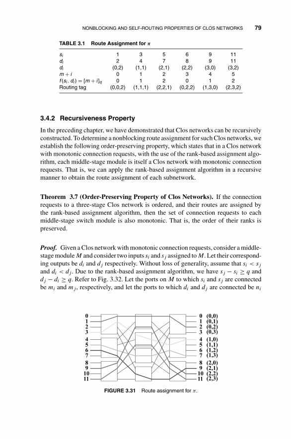
NONBLOCKING AND SELF-ROUTING PROPERTIES OF CLOS NETWORKS 79
TABLE 3.1 Route Assignment for �
si 1 3 5 6 9 11di 2 4 7 8 9 11di (0,2) (1,1) (2,1) (2,2) (3,0) (3,2)m + i 0 1 2 3 4 5f (si , di ) = [m + i ]q 0 1 2 0 1 2Routing tag (0,0,2) (1,1,1) (2,2,1) (0,2,2) (1,3,0) (2,3,2)
3.4.2 Recursiveness Property
In the preceding chapter, we have demonstrated that Clos networks can be recursivelyconstructed. To determine a nonblocking route assignment for such Clos networks, weestablish the following order-preserving property, which states that in a Clos networkwith monotonic connection requests, with the use of the rank-based assignment algo-rithm, each middle-stage module is itself a Clos network with monotonic connectionrequests. That is, we can apply the rank-based assignment algorithm in a recursivemanner to obtain the route assignment of each subnetwork.
Theorem 3.7 (Order-Preserving Property of Clos Networks). If the connectionrequests to a three-stage Clos network is ordered, and their routes are assigned bythe rank-based assignment algorithm, then the set of connection requests to eachmiddle-stage switch module is also monotonic. That is, the order of their ranks ispreserved.
Proof. Given a Clos network with monotonic connection requests, consider a middle-stage module M and consider two inputs si and sj assigned to M. Let their correspond-ing outputs be di and dj respectively. Without loss of generality, assume that si < sjand di < dj . Due to the rank-based assignment algorithm, we have sj − si ≥ q anddj − di ≥ q. Refer to Fig. 3.32. Let the ports on M to which si and sj are connectedbe mi and mj , respectively, and let the ports to which di and dj are connected be ni
0123
4567
89
1011
0123
4567
89
1011
(0,0)(0,1)(0,2)(0,3)
(1,0)(1,1)(1,2)(1,3)
(2,0)(2,1)(2,2)(2,3)
FIGURE 3.31 Route assignment for �.

80 FUNDAMENTAL PRINCIPLES OF PACKET SWITCH DESIGN
si
sj
M
mi
mj
......
ni
nj
... ...
di
dj
si < sj di < dj
FIGURE 3.32 Order is preserved in a middle-stage module M .
and nj , respectively. Now, from (3.25) and (3.26), we have
mj =⌊
sj
q
⌋≥
⌊si + q
q
⌋=
⌊si
q
⌋+ 1 = mi + 1 > mi,
nj =⌊
dj
q
⌋≥
⌊di + q
q
⌋=
⌊di
q
⌋+ 1 = ni + 1 > ni.
(3.29)
The rank order is preserved in each middle-stage module. The active inputs and theircorresponding outputs on M are therefore monotonic. �
As an example, suppose we have an N × N Clos network with monotonic connec-tion requests. Assume that N can be factorized into N = pqr. As shown in Fig. 3.33,
000 0 0
r-1 p-1 r-1
r-1 p-1 r-1
00 0
pr-1 pr-1
× p p
× pp
r × r
r × r
× p p
× p p
q × q
q × q
q × q
q × q
. . .. . .
. . .
. . .
. . .. . .
. . .. . .
. . .
. . .
. . .. . .
. . .
. . .
. . .. . .
. . .. . .
... ...
. . .. . .
. . .. . .
......
......
. . .
. . .
. . .. . .
•••
•••
. . .
Subnetwork 0
Subnetwork q
FIGURE 3.33 Recursive construction of Clos network.

NONBLOCKING AND SELF-ROUTING PROPERTIES OF CLOS NETWORKS 81
each switch module in the input stage and in the output stage is of size q × q. Thereare q middle-stage modules, each of size pr × pr. By Theorem 3.7, each middle-stage module is a Clos network with monotonic connection requests and can befurther decomposed. Suppose a connection request (si, di) is assigned to a middle-stage module M. The rank of the corresponding connection request on M is given by�i/q�. To see this, recall that a connection request (si, di) is assigned to a middle-stagemodule M if f (si, di) = [m + i]q = M. Without loss of generality, suppose m = 0and f (si, di) = [i]q. Those connection requests with rank M, M + q, M + 2q, ... areassigned to M. Taking the integer division of their ranks by q therefore gives the rankof their corresponding connections on M. In this example, there are p middle-stagemodules in each smaller Clos network. The route assignment within each smaller Closnetwork can then be determined recursively and the routing tag for this five-stage Closnetwork is ⎛
⎝[r(si)]q ,
[⌊r(si)
q
⌋]p
,
⎢⎢⎢⎣⌊
di
q
⌋p
⎥⎥⎥⎦ ,
[⌊di
q
⌋]p
, [di]q
⎞⎠ . (3.30)
The first two components in this routing tag are due to the rank-based assignmentand indicate which middle-stage module a call should be routed to. The last threecomponents are used to route the packet correctly to destination starting from themiddle-stage module.
3.4.3 Basic Properties of Half-Clos Networks
A Clos network can be considered as the cascade combination of two symmetric sub-networks, referred to as half-Clos networks. One well-known example is the formationof the Benes network by combining the baseline network and the reverse baseline net-work. In these half-Clos networks, there is a unique path from any input to any outputthat can be completely determined by the output destination address. Thus, we cansee that the half-Clos networks possess the nonblocking self-routing property and allthe multistage interconnection networks (MINs) previously described belong to thisclass. When two half-Clos networks are combined to form a Clos network, multiplealternative paths exist for each input–output pair. These paths are the products of theunique paths in the half-Clos networks.
Figure 3.34 shows that when a Clos network is divided into two parts, the omeganetwork and the reverse omega network are formed. Without loss of generality, weshall study the properties of half-Clos networks based on them and explain the fun-damental principle behind the rank-based assignment algorithm by combining themtogether. This leads us to the observation that any MIN can be combined with itsreverse network to form a general Clos-type network taht also possesses the samenonblocking self-routing property as that of the classical Clos networks.
3.4.3.1 Omega Network An omega network is the right half of a Clos network.An example of omega network, together with the address numbering scheme, is shown

82 FUNDAMENTAL PRINCIPLES OF PACKET SWITCH DESIGN
Reverse omega network Omega network
Clos network
FIGURE 3.34 Dividing a Clos network into two half-Clos networks.
in Fig. 3.35. There are three modules in the input stage and four in the output stage.Using the numbering scheme introduced earlier, we can number each input port andeach output port by a 2-tuple address. The shuffle stage at the inputs is required toensure that the same numbering scheme is used in the input and the output ports.Suppose there is no shuffle stage. Denote an input address by aibi and an output
0
00010203
0123
1
10111213
0123
2
20212223
0123
0000102
012
1101112
012
2202122
012
3303132
012
000102
101112
202122
303132
012
345
678
91011
012
345
678
91011
si bi ai aibi xi ai diq = 3 p = 4 xiyi
Nonblocking if and only if ai = aj → xi ≠ xjRouting tag for output xiyi : (xi, yi)
⎤⎡ qii
ii
sa
qsb
=
⎥⎦
⎥⎢⎣
⎢=
⎤⎡ qii
ii
dy
qdx
=
⎥⎦
⎥⎢⎣
⎢=
FIGURE 3.35 An omega network.

NONBLOCKING AND SELF-ROUTING PROPERTIES OF CLOS NETWORKS 83
address by xiyi. It is easy to see that ai is of base q = 3 and bi is of base p = 4 whilexi is of base p = 4 and yi is of base q = 3. The numbering of inputs and outputs istherefore inconsistent. With the shuffle stage, the input addresses become biai. Eachtuple in the input address then has the same base as the corresponding tuple in theoutput address.
Denote an input si by biai and an output di by xiyi. For the omega network to beexternally nonblocking (i.e., no output port conflict) we must have
xi = xj ⇒ yi = yj, (3.31)
and it is internally nonblocking if and only if the active inputs satisfy
ai = aj ⇒ xi = xj. (3.32)
The following theorem gives the sufficient conditions for an omega network to beinternally nonblocking.
Theorem 3.8 (Nonblocking Conditions for Omega Networks). The omega net-work is internally nonblocking if the active inputs s0, . . . , sn−1 (sj > si if j > i) andtheir corresponding output destinations d0, . . . , dn−1 satisfy the following:
1. Concentrated inputs: Any input between two active inputs is also active. Thatis, if si and sj are active and si ≤ w ≤ sj , then w is active.
2. Monotonic outputs: d0 < d1 < · · · < dn−1 or d0 > d1 > · · · > dn−1.
Proof. Using the same 2-tuple numbering scheme, denote two active inputs si and sj(si < sj) by biai and bjaj , respectively. Similarly denote their corresponding outputsdi and dj by xiyi and xjyj , respectively. Without loss of generality, assume thatdi < dj . By the concentrated inputs and monotonic outputs conditions, we have
xjyj − xiyi ≥ bjaj − biai.
We are going to show that the omega network is nonblocking by contradiction. Ifai = aj , we have
xjyj − xiyi ≥ bjaj − biai = (bj − bi) · q ≥ q (3.33)
because ai is of base q. However, xi = xj implies
xjyj − xiyi = yj − yi ≤ q − 1. (3.34)
Since (3.33) and (3.34) cannot hold simultaneously, the omega network must beinternally nonblocking with concentrated and ordered connection requests accordingto condition (3.32). �
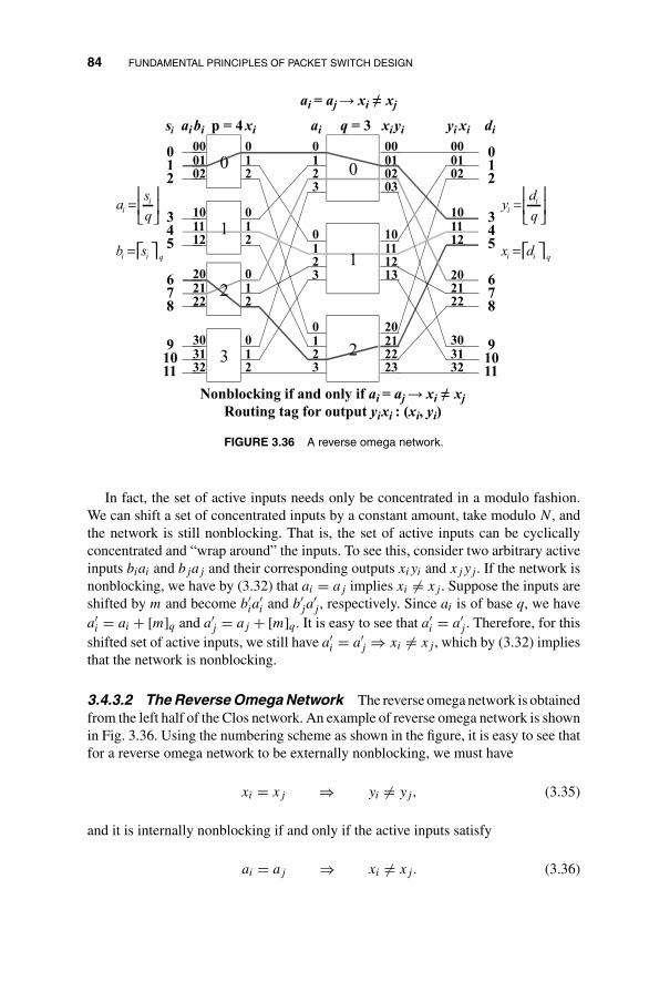
84 FUNDAMENTAL PRINCIPLES OF PACKET SWITCH DESIGN
⎤⎡ qii
ii
sb
qsa
=
⎥⎦
⎥⎢⎣
⎢=
⎤⎡ qii
ii
dx
qdy
=
⎥⎦
⎥⎢⎣
⎢=
0
00010203
0123
1
10111213
0123
2
20212223
0123
0000102
012
1101112
012
2202122
012
3303132
012
000102
101112
202122
303132
012
345
678
91011
012
345
678
91011
si yi xixiyiaixiaibi diq = 3p = 4
Nonblocking if and only if ai = aj → xi ≠ xjRouting tag for output yixi : (xi, yi)
ai = aj → xi ≠ xj
FIGURE 3.36 A reverse omega network.
In fact, the set of active inputs needs only be concentrated in a modulo fashion.We can shift a set of concentrated inputs by a constant amount, take modulo N, andthe network is still nonblocking. That is, the set of active inputs can be cyclicallyconcentrated and “wrap around” the inputs. To see this, consider two arbitrary activeinputs biai and bjaj and their corresponding outputs xiyi and xjyj . If the network isnonblocking, we have by (3.32) that ai = aj implies xi = xj . Suppose the inputs areshifted by m and become b′
ia′i and b′
ja′j , respectively. Since ai is of base q, we have
a′i = ai + [m]q and a′
j = aj + [m]q. It is easy to see that a′i = a′
j . Therefore, for thisshifted set of active inputs, we still have a′
i = a′j ⇒ xi = xj , which by (3.32) implies
that the network is nonblocking.
3.4.3.2 The Reverse Omega Network The reverse omega network is obtainedfrom the left half of the Clos network. An example of reverse omega network is shownin Fig. 3.36. Using the numbering scheme as shown in the figure, it is easy to see thatfor a reverse omega network to be externally nonblocking, we must have
xi = xj ⇒ yi = yj, (3.35)
and it is internally nonblocking if and only if the active inputs satisfy
ai = aj ⇒ xi = xj. (3.36)
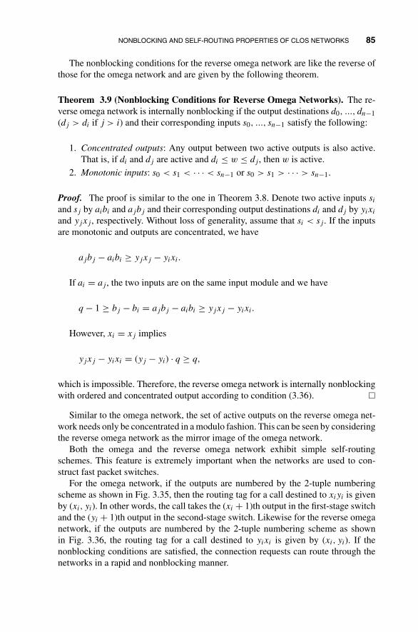
NONBLOCKING AND SELF-ROUTING PROPERTIES OF CLOS NETWORKS 85
The nonblocking conditions for the reverse omega network are like the reverse ofthose for the omega network and are given by the following theorem.
Theorem 3.9 (Nonblocking Conditions for Reverse Omega Networks). The re-verse omega network is internally nonblocking if the output destinations d0, ..., dn−1(dj > di if j > i) and their corresponding inputs s0, ..., sn−1 satisfy the following:
1. Concentrated outputs: Any output between two active outputs is also active.That is, if di and dj are active and di ≤ w ≤ dj , then w is active.
2. Monotonic inputs: s0 < s1 < · · · < sn−1 or s0 > s1 > · · · > sn−1.
Proof. The proof is similar to the one in Theorem 3.8. Denote two active inputs siand sj by aibi and ajbj and their corresponding output destinations di and dj by yixi
and yjxj , respectively. Without loss of generality, assume that si < sj . If the inputsare monotonic and outputs are concentrated, we have
ajbj − aibi ≥ yjxj − yixi.
If ai = aj , the two inputs are on the same input module and we have
q − 1 ≥ bj − bi = ajbj − aibi ≥ yjxj − yixi.
However, xi = xj implies
yjxj − yixi = (yj − yi) · q ≥ q,
which is impossible. Therefore, the reverse omega network is internally nonblockingwith ordered and concentrated output according to condition (3.36). �
Similar to the omega network, the set of active outputs on the reverse omega net-work needs only be concentrated in a modulo fashion. This can be seen by consideringthe reverse omega network as the mirror image of the omega network.
Both the omega and the reverse omega network exhibit simple self-routingschemes. This feature is extremely important when the networks are used to con-struct fast packet switches.
For the omega network, if the outputs are numbered by the 2-tuple numberingscheme as shown in Fig. 3.35, then the routing tag for a call destined to xiyi is givenby (xi, yi). In other words, the call takes the (xi + 1)th output in the first-stage switchand the (yi + 1)th output in the second-stage switch. Likewise for the reverse omeganetwork, if the outputs are numbered by the 2-tuple numbering scheme as shownin Fig. 3.36, the routing tag for a call destined to yixi is given by (xi, yi). If thenonblocking conditions are satisfied, the connection requests can route through thenetworks in a rapid and nonblocking manner.

86 FUNDAMENTAL PRINCIPLES OF PACKET SWITCH DESIGN
0
00010203
0123
1
10111213
0123
2
20212223
0123
0
012
1
012
2
012
3
012
000102
101112
202122
303132
012
345
678
91011
0
00010203
0123
1
10111213
0123
2
20212223
0123
0
000102
012
1
101112
012
2
202122
012
3
303132
012
000102
101112
202122
303132
012
345
678
91011
Reverse omega network Omega network
Stage 1 2 43 5
000102
101112
202122
303132
FIGURE 3.37 Combining a reverse omega network and an omega network.
3.4.3.3 Cascade Combination of Half-Clos Networks Consider the net-work formed by combining a reverse omega network and an omega network. Anexample is shown in Fig. 3.37. The network has five stages but the central stage(stage 3) is dummy and no switching is performed in that stage. Input packets are firstrouted through the reverse omega network and then fed into the omega network forrouting to route to their final destinations. This network is nonblocking if the inputsand their corresponding outputs are monotonic. This is because given monotonic in-puts, we can always route the packets to a set of concentrated ports in stage 3 so asto avoid blocking in the reverse omega network. Afterward, when the packets enterthe omega network, no blocking will occur because the inputs are concentrated andtheir outputs are monotonic. Any sets of concentrated ports in stage 3 can be used,including cyclically concentrated sets. It is observed that due to the shuffle stage atthe output of the reverse omega network, routing the packets to a set of concentratedports in stage 3 is equivalent to routing them to consecutive modules in stage 2. Thiscan be done with the help of the rank of each connection request.
Since stage 3 is dummy, we can eliminate it and stage 2 and stage 4 are combinedinto a single stage. The resulting network is a three-stage Clos network. A nonblockingroute assignment can therefore be obtained by assigning the connection requestshaving consecutive ranks to consecutive middle-stage modules in a modulo fashion.This is the basis of the rank-based assignment algorithm.
In general, any multistage interconnection network can be combined with its re-verse network to form a general Clos-type network. The scenario is similar to com-bining the omega with the reverse omega network. In an MIN, there is a unique path

NONBLOCKING AND SELF-ROUTING PROPERTIES OF CLOS NETWORKS 87
for each input–output pair. If the MIN is N × N and is composed of 2 × 2 switchelements, the number of alternative paths for each input–output pair in the combinednetwork will be equal to N/2. These alternative paths are the product of the paths inthe MINs.
3.4.3.4 Recursiveness Properties Both the omega and the reverse omeganetwork can be recursively constructed and share the same order-preserving property.The following is a proof of the order-preserving property of the omega network. Thisproof can be similarly applied to the reverse omega network.
Theorem 3.10 (Order-Preserving Property of Omega Network). If the connec-tion requests to an omega network satisfy the concentrated inputs and monotonicoutputs conditions, then the set of connection requests to each switch module in thenetwork also satisfy the concentrated inputs and monotonic outputs conditions. Thatis, the order of their ranks is preserved.
Proof. Without loss of generality assume that the inputs to an omega network areconcentrated and their corresponding outputs are monotonically increasing. The proofis divided into two parts.
(1) First-stage modules: We first show that the inputs to a switch module in thefirst stage are concentrated and their corresponding outputs on that module aremonotonic. Consider two active ports bi and bj on a first-stage module M, withbi < bj . They are numbered by the 2-tuple addresses Mbi and Mbj . Supposethere exists a port bk, where bi < bk < bj , which is inactive. Due to the shufflestage, the corresponding input addresses of these ports are biM, bkM, and bjM,respectively (see Fig. 3.38(a)). We have
bkM − biM = (bk − bi) · q ≥ q and
bjM − bkM = (bj − bk) · q ≥ q.
Therefore, biM < bkM < bjM. In other words, between two active inputs,there is an inactive port and this contradicts with the concentrated inputs as-sumption. Therefore, the active inputs on M are concentrated.
Suppose the destinations of inputs biM and bjM (biM < bjM) are xiyi andxjyj , respectively. On module M, the two connection requests will take outputsxi and xj , respectively, due to the self-routing property. We want to show thatgiven bi < bj we have xi < xj . In other words, the active outputs on M aremonotonically increasing.
With the concentrated inputs and monotonic outputs assumptions, we have
biM < bjM ⇒ xiyi < xjyj. (3.37)

88 FUNDAMENTAL PRINCIPLES OF PACKET SWITCH DESIGN
(a)
(b)
FIGURE 3.38 (a) A banyan network; (b) a reverse banyan network.
This implies that xi ≤ xj . But since the omega network is nonblocking andai = aj , by (3.32) we have xi = xj . Therefore, we have xi < xj and the outputson M are monotonically increasing.
(2) Second-stage modules: Consider a second-stage switch module M ′ in an omeganetwork. Since the active outputs of the omega network are monotonicallyincreasing, the active outputs on M are obviously monotonically increasing.
Denote the active outputs on M ′ by x1y1, x2y2, . . . , xkyk (x1y1 < x2y2 <
· · · < xkyk) and suppose that they originate from inputs b1a1, b2a2, . . . , bkak,respectively (see Fig. 3.38(b)). Obviously, b1a1 < b2a2 < · · · < bkak and theyare concentrated. In other words, their least significant digit ai’s are consecutive(modulo q) because ai’s are of base q. Let m1, m2, . . . , mk be the active inputson M corresponding to x1y1, x2y2, . . . , xkyk. If we imagine routing from theoutputs to the inputs instead, the network becomes a reverse omega network

NONBLOCKING AND SELF-ROUTING PROPERTIES OF CLOS NETWORKS 89
Concentration required
No concentration required
(a) Sorting network + omega network
(b) Sorting network + Clos network
FIGURE 3.39 Construction of nonblocking self-routing switches.
and it is easy to see that the m1 = a1, m2 = a2, ..., mk = ak. Therefore, the setof active inputs on M is concentrated (modulo q). �
3.4.4 Sort-Clos Principle
A nonblocking self-routing point-to-point switch can be constructed with an omeganetwork or a Clos network. As illustrated in Fig. 3.39(a), we can cascade a sortingnetwork and an omega network to form a nonblocking self-routing switch. The sortingnetwork sorts the input packets based on their output destinations and concentratesthem so that the set of input packets to the omega network is concentrated and theircorresponding output destinations are monotonic. The omega network then routes thepackets to their destinations in a nonblocking manner. This is the basic sort-banyanprinciple. In a similar manner, a nonblocking self-routing switch can be constructedby cascading a sorting network and a Clos network, as shown in Fig. 3.39(b). Thesorting network, however, is only required to provide a set of monotonic connectionrequests to the Clos network. No concentration is required. Thus, the contention res-olution consists only of two phases. By using the rank-based assignment algorithm, anonblocking route assignment can be easily found and the packets can be self-routedto their destinations. We denote this as the sort-Clos principle. It is the generaliza-tion of the sort-banyan principle. With this switching principle, the construction ofnonblocking self-routing switch is no longer limited to 2 × 2 switch elements.

90 FUNDAMENTAL PRINCIPLES OF PACKET SWITCH DESIGN
PROBLEMS
3.1 Consider an 8 × 8 reverse shuffle-exchange network.(a) Show how the bits in the output address are used to route a packet from
input 001 to output 110. Show how a packet is routed from input 110 tooutput 010.
(b) If this network is used as a loss system, do you think its loss probabilitywould be higher or lower than a shuffle-exchange network?
3.2 For the class of Banyan networks, suppose a central controller knowing thedestinations of all the input packets is used to perform the routing and settingthe states of the switch elements. Can the loss probability be improved withrespect to that in the self-routing Banyan networks? If your answer is no,explain why. If your answer is yes, give an example in which a centralizedrouting decision leads to fewer packets being dropped.
3.3 Consider an 8 × 8 Banyan network. Suppose with probability 0.75 a packetis destined for outputs 000, 001, 010, or 011, and with probability 0.25 it isdestined for the other four outputs. Within each group of outputs, the packet isequally likely to be destined for any of the four outputs. Is the loss probabilityhigher in this case than when a packet is equally likely to be destined for anyof the eight outputs? Modify the analysis in the text to answer this question.
3.4 In Section 3.2.3, it is mentioned that each of the NN/2 states of the Banyannetwork corresponds to a unique input–output mapping by the unique-pathproperty. Explain why. In Section 3.2.2, it is mentioned that the uniform-trafficassumption also means that a packet is equally likely to be destined for eitherof the two outgoing links of a switch element. Explain why.
3.5 Show how to use the reverse banyan (reverse shuffle-exchange) network asa concentrator. That is, we want to concentrate packets from N inputs to M
outputs where M < N. It does not matter which output a packet goes to as longas the packet gets to an output. As long as there are no more than M incomingpackets, none of them will be dropped or buffered at the input.
3.6 Use the order-preserving property to show that a bitonic sorter that works forzero–one sequence also works for sequences of arbitrary numbers.
3.7 A circular bitonic sequence is a sequence that can be made bitonic byshifting the sequence in a circular fashion. For example, the sequence〈3, 1, 1, 2, 3, 4, 5, 4〉 is circular bitonic because after two circular left shiftit becomes the bitonic sequence 〈1, 2, 3, 4, 4, 5, 3, 1〉. The bitonic sequencesare a subset of circular bitonic sequences.(a) Show that a bitonic sorter also sorts circular bitonic sequences of arbitrary
numbers correctly. (Hint: Use a proof similar to that of the zero–one prin-ciple, but first argue that if the numbers are limited to 0’s and 1’s, there isno difference between circular bitonic and bitonic sequences.)

PROBLEMS 91
8×8
Sorting
network
8×8
Banyan
network
001100
i100000
ii
101
000001010011100101110111
Output address of a packet
Idle input
Output
FIGURE 3.40 A set of input packets for a sort-banyan network.
(b) Theorem 3.4 concerns the decomposition of a zero–one bitonic sequenceinto two zero–one bitonic sequences. For a bitonic sequence of arbitrarynumbers, the decomposition does not necessarily yield two bitonic se-quences; one of the sequences could be circular bitonic but not bitonic.Give an example to illustrate this.
3.8 Prove the bitonic sorting algorithm without relying on the zero–one principle.
3.9 The proof of the odd–even merging algorithm in the text assumes that n iseven. Repeat the proof for odd n.
3.10 For n a power of 2, compute the number of 2 × 2 comparators in an overallsorting network based on the odd–even merging algorithm.
3.11 Show that the odd-even merging algorithm can merge two sorted input se-quences of different sizes. That is, the input sequences are 〈a1, . . . , as〉 and〈b1, . . . , bt〉 where s t.
Internally
nonblocking
switch
0
1
0
0
Output destination of packet
Circulating tokens for output access
5
2
1
FIGURE 3.41 Ring contention-resolution scheme.

92 FUNDAMENTAL PRINCIPLES OF PACKET SWITCH DESIGN
3.12 Consider an N × N banyan network with n = log2 N stages, where n is even.Suppose that there are N input packets, all destined for different outputs. Showthat in the worst case, there may be
√N packets wanting to cross the same link
inside the network in order to reach their outputs. That is, the same link is in√N input–output paths of the packets.
3.13 Consider a Batcher–banyan network that uses the three-phase contention-resolution scheme.(a) How many bits of delays (in terms of N) are needed before the completion
of the first two phases, assuming the acknowledgments take only one-bitdelay?
(b) Suppose that the information payload of the packets is 53-byte long.Express the overhead in terms of the ratio of the contention-resolutiondelay to the amount of time needed to route one batch of packets to theirdestinations. For what N does the ratio become 50%?
3.14 Consider an 8 × 8 Batcher–banyan switch with input packets as depicted inFig. 3.40.(a) Draw the 8 × 8 Batcher bitonic sorting network and show how the paths
taken by the input packets.
(b) Which packets will win contention in the three-phase switching scheme?
(c) Show the paths taken by the winning packets in the banyan network.
3.15 When the sorting network is used for contention resolution, an unlucky packetmay end up at a sorting-network output lower than other packets destined forthe same switch output repeatedly in successive time slots. For fairness, wecan add several priority bits to the header so that the priority level of a packetwill be raised in the next time slot each time a packet loses contention. Explainhow these bits should be used in the sorting network so that the packet that haslost contention the most number of times will be the winner among all packetsdestined for the same switch output in each time slot.
3.16 We can use a ring contention–resolution scheme for a sort-banyan network. Thering contention-resolution scheme is very much like the medium access control(MAC) of the token-ring local-area network, except that there are N tokens,one for each output. The tokens circulate around the inputs, as illustrated inFig. 3.41. Each token has only one bit that is set to 0 initially. The token foroutput i is positioned at input i at the beginning. If input i has a packet thatis destined for output i, it sets the token to 1, capturing the right to send tooutput i. The tokens then undergo a circular shift so that the token for output i
is now positioned at input i + 1 (mod N). If input i + 1 (mod N) has a packetdestined for output i, it first must make sure that the token is not already setto 1. If yes, it has lost the contention to another input. Otherwise, it sets tokento 1 and captures the right to send a packet to output i. After N steps andeach token has the chance to visit each token once, the contention-resolution

PROBLEMS 93
process is completed. The winning inputs can then send their packets to theoutputs.(a) How does this scheme compare with the three-phase scheme in terms of
contention-resolution overhead?
(b) Describe how the basic scheme can be modified to obviate the needfor the banyan network by letting the tokens circulate around the inputstwice.

4
SWITCH PERFORMANCE ANALYSISAND DESIGN IMPROVEMENTS
This chapter first focuses on the performance analysis of some simple switch designs.From the analysis, we shall see that head-of-line (HOL) blocking as well as outputcontention among packets may severely limit the switch throughput. This chapter willthen present several fundamental switch design principles to alleviate these problemsand achieve performance improvement. Each switch design principle will be illus-trated using specific implementations. Note, however, that many implementations arepossible based on each switch design concept, and one should not confuse implemen-tations with concepts.
4.1 PERFORMANCE OF SIMPLE SWITCH DESIGNS
This section analyzes the delay and throughput performance of some simple switchdesigns with an internally nonblocking structure. Since the packets are fixed-length,the arrivals can be aligned (as discussed at the beginning of the preceding chapter)with a maximum alignment delay of one-packet duration. With the alignment, we mayassume in our analysis that time is slotted and that the packets arrive to the inputs atthe beginning of each time slot.
For simplicity, we shall also assume a uniform-traffic distribution. Packet arrivals atthe inputs are described by a simple Bernoulli process: in any time slot, the probabilitythat a packet will arrive on a particular input is ρo. The parameter ρo is also referred toas the offered load. Each packet is destined for any given output with equal probability1/N and the output destinations of successive packets are independent.
We shall engage much of the analysis in the domain of generating functions.The generating function of any random variable R, E[zR], will be denoted by
Principles of Broadband Switching and Networking, by Tony T. Lee and Soung C. LiewCopyright © 2010 John Wiley & Sons, Inc.
95
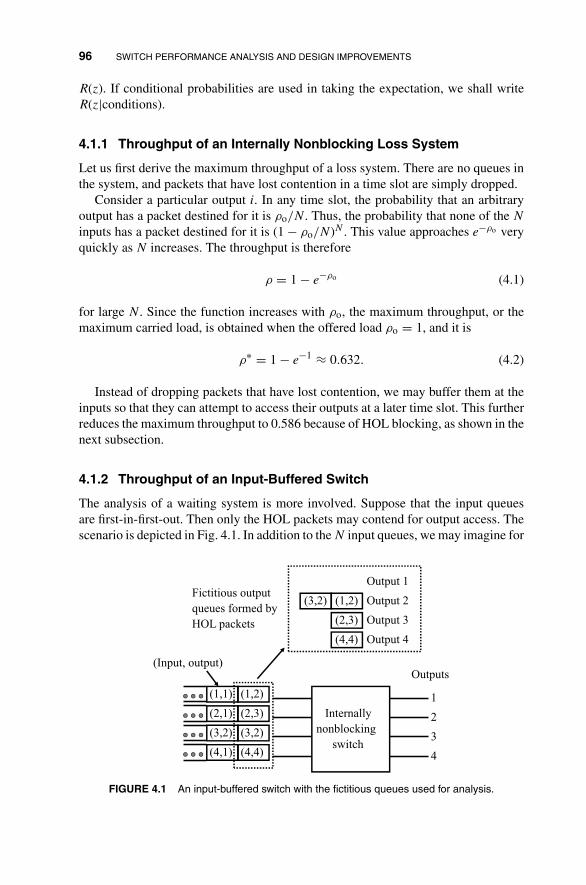
96 SWITCH PERFORMANCE ANALYSIS AND DESIGN IMPROVEMENTS
R(z). If conditional probabilities are used in taking the expectation, we shall writeR(z|conditions).
4.1.1 Throughput of an Internally Nonblocking Loss System
Let us first derive the maximum throughput of a loss system. There are no queues inthe system, and packets that have lost contention in a time slot are simply dropped.
Consider a particular output i. In any time slot, the probability that an arbitraryoutput has a packet destined for it is ρo/N. Thus, the probability that none of the N
inputs has a packet destined for it is (1 − ρo/N)N . This value approaches e−ρo veryquickly as N increases. The throughput is therefore
ρ = 1 − e−ρo (4.1)
for large N. Since the function increases with ρo, the maximum throughput, or themaximum carried load, is obtained when the offered load ρo = 1, and it is
ρ∗ = 1 − e−1 ≈ 0.632. (4.2)
Instead of dropping packets that have lost contention, we may buffer them at theinputs so that they can attempt to access their outputs at a later time slot. This furtherreduces the maximum throughput to 0.586 because of HOL blocking, as shown in thenext subsection.
4.1.2 Throughput of an Input-Buffered Switch
The analysis of a waiting system is more involved. Suppose that the input queuesare first-in-first-out. Then only the HOL packets may contend for output access. Thescenario is depicted in Fig. 4.1. In addition to the N input queues, we may imagine for
1
2
3
4
Outputs
Internally
nonblocking
switch
(Input, output)
Fictitious output
queues formed by
HOL packets
(1,2)(1,1)
(2,3)(2,1)
(3,2)(3,2)
(4,4)(4,1)
(1,2)(3,2)
(2,3)
(4,4) Output 4
Output 3
Output 2
Output 1
FIGURE 4.1 An input-buffered switch with the fictitious queues used for analysis.
PERFORMANCE OF SIMPLE SWITCH DESIGNS 97
analytical purposes that there are also N fictitious queues, one for each output, whoseelements consist of the HOL packets destined for the N outputs. Thus, a packet joinsa fictitious queue only after it has proceeded to the front of its input queue.
Let us consider the fictitious queue associated with a particular output i. Let Cim
be the number of packets in it at the start of time slot m. Let Aim be the number of
packets entering the fictitious queue at the start of time slot m. The system evolvesaccording to the equation
Cim = max(0, Ci
m−1 − 1) + Aim
= Bim−1 + Ai
m, (4.3)
where Bim−1 = max(0, Ci
m−1 − 1) is the number of packets remaining in the fictitiousqueue at the end of time slot m − 1. To interpret the equation, note that if the queuewas not empty at the beginning of time slot m − 1, then one packet would be clearedby the end of it, hence the term Ci
m−1 − 1. On the other hand, if the queue was empty(Ci
m−1 = 0), no packet would be cleared, and the queue remained empty at the end ofthe time slot, hence the term max(0, Ci
m−1 − 1). To this we add the number of newlyarriving packets at the beginning of time slot m, Ai
m, to obtain Cim.
To study the system dynamic, we need to know Aim. For the calculation of the
maximum allowable throughput, let us assume that all the input queues are saturatedso that as soon as a HOL packet is cleared, its position is taken by a subsequent packetin the next time slot. In this way, the system is loaded at its maximum capacity. Atthe beginning of time slot m, the inputs can be divided into two groups:
1. Those that won contention in the previous time slot.
2. Those that lost contention in the previous time slot.
Let Fm−1 be the number of inputs that won contention in time slot m − 1. This isalso the number of new HOL packets in time slot m under the saturation condition.The total number of backlogged packets at the HOL at the end of time slot m − 1 is∑N
i=1 Bim−1. By conservation,
Fm−1 +N∑
i=1
Bim−1 = N.
The probability that a new HOL packet is destined for output i is 1/N. Thus, consid-ering all the Fm−1 new HOL packets, the probability that k of them are destined foroutput i is
Pr{Aim = k | Fm−1} =
(Fm−1
k
)(1
N
)k (1 − 1
N
)Fm−1−k
. (4.4)

98 SWITCH PERFORMANCE ANALYSIS AND DESIGN IMPROVEMENTS
The above packet arrival process is difficult to deal with analytically because Fm−1(and therefore Ai
m) depends on Bim−1. It is known in queueing theory that whenever
the arrival process depends on the system state, the analysis becomes complicated.Fortunately, the concern goes away when N is very large so that we can at least getan analytical result for that case.
To see this, let us first look at the effect of Bim−1 on Fm−1. Recall that Fm−1 is
the number of cleared packets in time slot m − 1. Certainly, given Bim−1, the range
of values that Fm−1 can adopt is 1, . . . , N − Bim−1, since we know that at least Bi
m−1HOL packets addressed for output i did not get cleared. When N is small (e.g.,N = 2), the effect of Bi
m−1 on Fm−1 is rather significant. However, when N is large,since Bi
m−1 is the backlogged packets of one output among many outputs, Bim−1 is
typically much smaller than N and N − Bim−1 ≈ N. The dependence between Bi
m−1and Fm−1 is negligible for large N. In the limit N → ∞, Bi
m−1 and Aim become
independent. Therefore, for simplicity, we shall assume that N is very large in thefollowing analysis.
Intuitively, the binomial arrival process in (4.4) approaches a Poisson process asN → ∞. However, Fm−1 changes from time slot to time slot. As a result, the binomialarrival process as described in (4.4) is a modulated binomial process in which thenumber of packet sources Fm−1 changes with time. We now argue that to the extentthat N → ∞, Ai
m approaches an “unmodulated” Poisson process with rate ρ, whereρ is the maximum load yet to be determined.
To avoid cluttered notation, we shall drop the superscript i in Aim, Bi
m, and Cim
in the following with the implicit understanding that they all refer to the particularoutput i. The generating function of Am given Fm−1 is
Am(z | Fm−1)def= E[zAm | Fm−1] =
Fm−1∑k=0
zk Pr{Am = k | Fm−1}
=Fm−1∑k=0
zk
(Fm−1
k
)(1
N
)k (1 − 1
N
)Fm−1−k
=[
1 + (z − 1)
N
]Fm−1
. (4.5)
Now, let
Gm−1 = Fm−1
N. (4.6)
The knowledge of Gm−1 is equivalent to the knowledge of Fm−1, so thatAm(z | Fm−1) = Am(z | Gm−1). Since the value of Gm−1 is finite (between 0 and 1),
PERFORMANCE OF SIMPLE SWITCH DESIGNS 99
we may take the following limit for large N:
Am(z | Gm−1) =[
1 + (z − 1)
N
]NGm−1
→ e(z−1)Gm−1
= 1 + (z − 1)Gm−1 + (z − 1)
2!G2
m−1 + · · · (4.7)
We want to uncondition Am(z | Gm−1) on Gm−1. Define
Xjm
def={
1, if the HOL packet on input j is cleared in time slot m,
0, otherwise.(4.8)
Thus, by definition,
Fm =N∑
j=1
Xjm.
Suppose that all inputs are treated equally in the contention-resolution process. Then,by symmetricity, for all j, E[Xj
m] = Pr{Xjm = 1} = ρ in the steady state as m → ∞,
where ρ is the maximum carried load. In general,
E[(Xjm)k] = 0k Pr{Xj
m = 0} + 1k Pr{Xjm = 1} = ρ
for all k ≥ 1. Thus, we can write
E[Gm−1] = E
[Fm−1
N
]= 1
N
∑j
E[Xjm−1] = ρ
and
E[G2m−1] = 1
N2
∑j
∑k
E[X
jm−1X
km−1
]
= 1
N2
⎛⎝∑
j
E
[(X
jm−1
)2]
+∑
j
∑k =j
E[X
jm−1X
km−1
]⎞⎠ .

100 SWITCH PERFORMANCE ANALYSIS AND DESIGN IMPROVEMENTS
When N is large, the dependence between the clearance of packets at inputs j and k
can be neglected, and Xjm−1 and Xk
m−1 are independent as N〉∞. We have
E[G2m−1] ≈ 1
N2
⎛⎝∑
j
E[(
Xjm−1
)2]
+∑
j
∑k =j
E[X
jm−1
]E[Xk
m−1
]⎞⎠= 1
N2 [Nρ + N(N − 1)ρ2]
→ ρ2.
In general, we can show that
E[Gkm−1] → ρk. (4.9)
Thus,
Am(z) = EGm−1 [Ajm(z | Gm−1)]
= 1 + (z − 1)E[Gm−1] + (z − 1)2
2!E[G2
m−1] + · · ·
→ 1 + (z − 1)ρ + (z − 1)2
2!ρ2 + · · ·
= e(z−1)ρ. (4.10)
Note that in the steady state, the arrival process Am is independent of m and thereforewe can replace Am(z) with A(z). It can be easily verified that A(z) is the generatingfunction of a Poisson process:
Pr{A = k} = ρk
k!e−ρ. (4.11)
In the steady state, the subscript m in Bm and Cm can also be dropped. The generatingfunction of B = max(0, C − 1) is
B(z) =∞∑
k=0
zk Pr{B = k}
= Pr{B = 0} + z Pr{B = 1} + z2 Pr{B = 2} + · · ·= Pr{C = 0} + Pr{C = 1} + z Pr{C = 2} + z2 Pr{C = 3} + · · ·= Pr{C = 0} + z−1(z Pr{C = 1} + z2 Pr{C = 2} + z3 Pr{C = 3} + · · ·= (1 − z−1) Pr{C = 0} + z−1(Pr{C = 0} + z Pr{C = 1} + z2 Pr{C = 2} + · · ·= (1 − z−1)(1 − ρ) + z−1C(z), (4.12)
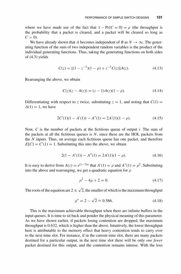
PERFORMANCE OF SIMPLE SWITCH DESIGNS 101
where we have made use of the fact that 1 − Pr{C = 0} = ρ (the throughput isthe probability that a packet is cleared, and a packet will be cleared so long asC > 0).
We have already shown that A becomes independent of B as N → ∞. The gener-ating function of the sum of two independent random variables is the product of theindividual generating functions. Thus, taking the generating functions on both sidesof (4.3) yields
C(z) = [(1 − z−1)(1 − ρ) + z−1C(z)]A(z). (4.13)
Rearranging the above, we obtain
C(z)(z − A(z)) = (z − 1)A(z)(1 − ρ). (4.14)
Differentiating with respect to z twice, substituting z = 1, and noting that C(1) =A(1) = 1, we have
2C′(1)(1 − A′(1)) − A′′(1) = 2A′(1)(1 − ρ). (4.15)
Now, C is the number of packets at the fictitious queue of output i. The sum ofthe packets at all the fictitious queues is N, since these are the HOL packets fromthe N inputs. Thus, on average each fictitious queue has one packet, and thereforeE[C] = C′(1) = 1. Substituting this into the above, we obtain
2(1 − A′(1)) − A′′(1) = 2A′(1)(1 − ρ). (4.16)
It is easy to derive from A(z) = e(z−1)ρ that A′(1) = ρ and A′′(1) = ρ2. Substitutinginto the above and rearranging, we get a quadratic equation for ρ
ρ2 − 4ρ + 2 = 0. (4.17)
The roots of the equation are 2 ± √2, the smaller of which is the maximum throughput
ρ∗ = 2 −√
2 ≈ 0.586. (4.18)
This is the maximum achievable throughput when there are infinite buffers in theinput queues. It is time to sit back and ponder the physical meaning of this parameter.As we have shown earlier, if packets losing contention are dropped, the maximumthroughput is 0.632, which is higher than the above. Intuitively, the lower throughputhere is attributable to the memory effect that heavy contention tends to carry overto the next time slot. For instance, if in the current time slot, there are many packetsdestined for a particular output, in the next time slot there will be only one fewerpacket destined for this output, and the contention remains intense. With the loss

102 SWITCH PERFORMANCE ANALYSIS AND DESIGN IMPROVEMENTS
TABLE 4.1 MaximumThroughput for Input-BufferedSwitches of Different Sizes
N �∗
2 0.753 0.684 0.665 0.646 0.637 0.628 0.62∞ 0.59
system, all these packets would have been dropped and the next time slot is a wholenew ball game.
The carried load ρ is ρo(1 − Pdrop), where ρo is the offered load and Pdrop is theprobability that a packet is dropped. When ρo < ρ∗, Pdrop can be made arbitrarilysmall with sufficiently large buffer size, making it possible to carry all the offeredload (i.e., ρ ≈ ρo). In contrast, when ρo ≥ ρ∗, no matter how large the buffer size is,the carried load cannot be larger than ρ∗. This is because the throughput limitation isdue to switch design, not the buffer size.
The analysis presented applies only for large N. When N is small, we can use aMarkov chain analysis to find the maximum throughput. One of the exercises asks youto do that for a 2 × 2 switch. Unfortunately, the number of states in the Markov chaingrows exponentially with N and the analysis becomes very complicated. Thus, theanalysis is simple when N is small or very large, but not somewhere in between. Thatthe performance analysis can be made simpler by letting certain system parameterapproach infinity is also observed in many other systems. One example is the classof multiple-access communication networks, which is often analyzed assuming thenumber of users is infinite. Fortunately for the input-buffered switch, the maximumthroughput approaches 0.586 very quickly as N increases, as shown in Table 4.1. Theanalysis of many cases with finite N is therefore unnecessary.
It should be noticed that our analysis did not assume any particular contention-resolution discipline. It does not matter whether the packets at the fictitious queueare served in a first-in-first-out (FIFO) fashion, random fashion, or any other manner.As long as the queue is a work-conserving system in which a packet is cleared ineach time slot when the queue is not empty, the same maximum throughput will beobserved. The delay experienced by a packet, on the other hand, does depend on thecontention-resolution discipline. What this means is that the delay will go to infinityas the offered load approaches the maximum throughput, but for offered load belowthe maximum throughput different contention-resolution disciplines yield differentdelays.
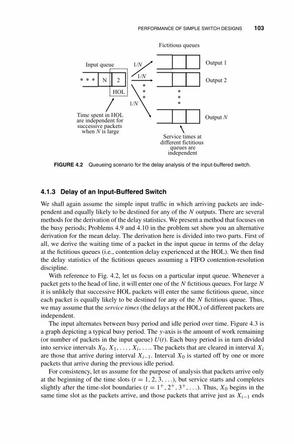
PERFORMANCE OF SIMPLE SWITCH DESIGNS 103
Output 1
Fictitious queues
Output 2
Output N
Input queue
Time spent in HOL are independent for successive packets
when N is largeService times at
different fictitious queues are
independent
2N
HOL
1/N
1/N
1/N
FIGURE 4.2 Queueing scenario for the delay analysis of the input-buffered switch.
4.1.3 Delay of an Input-Buffered Switch
We shall again assume the simple input traffic in which arriving packets are inde-pendent and equally likely to be destined for any of the N outputs. There are severalmethods for the derivation of the delay statistics. We present a method that focuses onthe busy periods; Problems 4.9 and 4.10 in the problem set show you an alternativederivation for the mean delay. The derivation here is divided into two parts. First ofall, we derive the waiting time of a packet in the input queue in terms of the delayat the fictitious queues (i.e., contention delay experienced at the HOL). We then findthe delay statistics of the fictitious queues assuming a FIFO contention-resolutiondiscipline.
With reference to Fig. 4.2, let us focus on a particular input queue. Whenever apacket gets to the head of line, it will enter one of the N fictitious queues. For large N
it is unlikely that successive HOL packets will enter the same fictitious queue, sinceeach packet is equally likely to be destined for any of the N fictitious queue. Thus,we may assume that the service times (the delays at the HOL) of different packets areindependent.
The input alternates between busy period and idle period over time. Figure 4.3 isa graph depicting a typical busy period. The y-axis is the amount of work remaining(or number of packets in the input queue) U(t). Each busy period is in turn dividedinto service intervals X0, X1, . . . , Xi, . . .. The packets that are cleared in interval Xi
are those that arrive during interval Xi−1. Interval X0 is started off by one or morepackets that arrive during the previous idle period.
For consistency, let us assume for the purpose of analysis that packets arrive onlyat the beginning of the time slots (t = 1, 2, 3, . . .), but service starts and completesslightly after the time-slot boundaries (t = 1+, 2+, 3+, . . .). Thus, X0 begins in thesame time slot as the packets arrive, and those packets that arrive just as Xi−1 ends

104 SWITCH PERFORMANCE ANALYSIS AND DESIGN IMPROVEMENTS
X0X3X2X1 X0
Busy periodIdle
periodBusy periodY
t
U(t)
Arrivals here are
considered as
arrivals in
intervals i-2
Arrivals here are considered as
arrivals in intervals i-1
Xi-1 Xi
FIGURE 4.3 The busy periods and interpretations for delay analysis of an input queue.
and Xi starts will be considered as having arrived in Xi−1 and therefore will be servedin Xi (see Fig. 4.3). Define
Ydef= length of busy period = X0 + X1 + · · · ,
Nidef= number of arrivals during interval Xi,
Sdef= service time at the HOL.
Suppose that Ni−1 = n packets arrive during interval i − 1 with Xi−1 = x. ThenXi is the sum of the service times of the n packets. The service times of the packets areindependent and identically distributed. Thus, the generating function of their sumsis the product of their generating functions. We can write
Xi(z | Xi−1 = x, Ni−1 = n) = Sn(z).
Unconditioning on Ni−1, we have
Xi(z | Xi−1 = x) =∞∑
n=0
Sn(z) Pr{Ni−1 = n | Xi−1 = x}.
Notice that we allow the possibility of n = 0 and Xi = 0. We note that the abovesummation is similar to the computation of the conditional generating function of
PERFORMANCE OF SIMPLE SWITCH DESIGNS 105
Ni−1 except that z has been replaced by S(z). Therefore,
Xi(z | Xi−1 = x) = Ni−1[S(z) | Xi−1 = x].
Unconditioning on Xi−1 gives
Xi(z) =∞∑
x=0
Ni−1[S(z) | Xi−1 = x] Pr{Xi−1 = x}.
Let
Kdef= number of arrivals in an arbitrary time slot .
We shall assume that arrivals at different time slots are independent and iden-tically distributed. The total number of arrivals over x time slots therefore hasthe generating function Kx(z). Noting that Ni−1(z | Xi−1 = x) = Kx(z), we canwrite
Xi(z) =∞∑
x=0
Kx[S(z)] Pr{Xi−1 = x} = Xi−1{K[S(z)]}. (4.19)
The physical meaning of the above relationship can be unveiled by expanding thegenerating functions in terms of the power of z. Intuitively, since Xi is the sum of theservice durations of those packets arriving in interval i − 1, we can expect Xi−1 tocorrelate positively with Xi. Each time slot in interval i − 1 produces a random of K
packets to be served in interval i, and each of these packets has a random service timeof S. Equation (4.19) is simply a succinct way of summarizing this dependency. Weshall come back to use the above relationship later. Let us now focus on one particularpacket that arrives in service interval i. Define
Wdef= waiting time of the packet before joining HOL,
Ridef= the residual time of interval i upon the arrival of the packet,
Midef= the number of arrivals in the same interval but in time slots
prior to the one in which the packet of focus arrives,
Ldef= the number of arrivals in the same time slot as the packet of focus
that will be served before it.
In queueing theory, the waiting time customarily refers to the time from the arrivalto the start of service, and the delay is the waiting time plus the service time. Thus,defining the “start of service” as the time the packet proceeds to the HOL, the delayhere is the waiting time plus time spent at the HOL. The definitions of the other

106 SWITCH PERFORMANCE ANALYSIS AND DESIGN IMPROVEMENTS
mi =2
prior
arrivals
Arrival of the packet of focus. One simultaneous arrival to be served before the packet; L=1
Departure of packet of focus
Xi Xi+1
Ri
W
Packet arrival in interval i
Packet departure in interval i+1
Number of arrivals(n)
(1) (1) (2)
FIGURE 4.4 Illustration of the meanings of the random variables used in the delay analysis ofan input queue.
random variables are illustrated in Fig. 4.4. Note also that for a Bernoulli arrivalprocess at most one packet can arrive in any given time slot, and so L = 0. However,such is not the case for the fictitious queue. In order that we can borrow the resultshere for the analysis of the fictitious queue later, the general dependency of W on L
is retained intentionally in the following.Suppose Mi = m, L = l, and Ri = r are given. Then the waiting time is the sum
of the residual time of interval i and service times of the m + l packets. We have
W(z | i, Xi = x, Ri = r, Mi = m, L = l) = zrSm+l(z).
We assume the arrivals on different time slots are independent and therefore L andMi are independent. Unconditioning on Mi and L, we have
W(z | i, Xi = x, Ri = r) = zr∞∑l=0
∞∑m=0
Sm+l(z) Pr{Mi = m | i, Xi = x, Ri = r}
× Pr{L = l | i, Xi = x, Ri = r}= zrL[S(z) | i, Xi = x, Ri = r]
× Mi[S(z) | i, Xi = x, Ri = r]
= zrL[S(z)] Mi[S(z) | i, Xi = x, Ri = r], (4.20)
where we note in the last line that the L relates to the arrivals in one particular timeslot and therefore is independent of the lengths of Xi and Ri. To uncondition on Xi

PERFORMANCE OF SIMPLE SWITCH DESIGNS 107
and Ri, we first find
Pr{Xi = x, Ri = r | i} = Pr{Ri = r | i, Xi = x} Pr{Xi = x | i}
= 1
x× x
E[Xi]Pr{Xi = x}. (4.21)
In the above, given that the packet arrives in a service interval of length x, it is equallylikely for the residual time Ri to be 0, 1, 2, . . . , or x − 1. Also, it is more likely forthe packet to fall into a larger interval than a smaller one. Therefore, the interval sizeobserved by the packet is not identically distributed as Xi. To see this, let us considera very long stretch of time with a large number of busy periods. Let N be the numberof busy periods we observe. For large N, the number of busy periods with Xi = x isN Pr{Xi = x}. The expected number of arrivals in these intervals is ρxN Pr{Xi = x}.The expected number of arrivals in intervals i of all N busy periods, regardless ofXi, is
∑∞x=0 ρxN Pr{Xi = x}. Thus, the probability that a packet entering in an ith
interval will find the interval to be of length x is
Pr{Xi = x | i} = limN→∞
N Pr{Xi = x}xρ∑∞x=0 NPr{Xi = x}xρ = x Pr{Xi = x}
E[Xi].
We now use (4.21) to uncondition (4.20)
W(z | i) =∞∑
x=1
x−1∑r=0
zrL[S(z)] Mi[S(z) | i, Xi = x, Ri = r] × Pr{Xi = x}E[Xi]
= L[S(z)]
E[Xi]
∞∑x=1
Pr{Xi = x}zx−1x−1∑r=0
Mi[S(z) | i, Xi = x, Ri = r]
zx−1−r. (4.22)
Recall that K is the random variable for the number of arrivals in one time slot.Given Xi = x and R = r, there are x − r − 1 earlier time slots in which the Mi
packets can arrive. Therefore, Mi[z | i, Xi = x, Ri = r] = Kx−r−1(z). Substitutinginto (4.22) and simplifying, we have
W(z | i) = L[S(z)]
E[Xi]
∞∑x=1
Pr{Xi = x}{Kx[S(z)] − zx}K[S(z)] − z
= L[S(z)]
E[Xi]
(Xi{K[S(z)]} − Xi(z))
K[S(z)] − z
= L[S(z)]
E[Xi]
(Xi+1(z) − Xi(z))
K[S(z)] − z, (4.23)
where in the last line we have made use of the relationship (4.19). Given that thepacket enters in a busy period, the probability that it falls into interval i is E[Xi]/E[Y ].
108 SWITCH PERFORMANCE ANALYSIS AND DESIGN IMPROVEMENTS
Unconditioning on i, we have
W(z | enter in busy period) =∞∑i=0
W(z | i)E[Xi]
E[Y ]
= L[S(z)]
E[Y ]{K[S(z)] − z}∞∑i=0
[Xi+1(z) − Xi(z)]
= L[S(z)]
E[Y ]{K[S(z)] − z} [1 − X0(z)], (4.24)
where we have made use of the fact that limi→∞ Xi(z) = 1 (since with probabilityone a busy period eventually will terminate and therefore limi→∞ Pr{Xi = 0} = 1).For the input queue, X0 is the service time of one packet because at most one packetcan arrive in a time slot. If multiple packets can arrive simultaneously, such as thecase with the fictitious queue, things are more complicated. To analyze the generalsituation, let N−1 be the number of simultaneous arrivals that start off a new busyperiod. Given that N−1 = n, the subsequent X0 consists of the service times of n
packets. Thus,
X0(z | N−1 = n) = Sn(z).
Now N−1 is the number of arrivals in a time slot given that there is at least one arrival.Therefore,
Pr{N−1 = n} =⎧⎨⎩
0, if n = 0,
Pr{K = n}1 − Pr{K = 0} , if n ≥ 1.
This gives
X0(z) =∞∑
n=1
X0(z | N−1 = n)Pr{K = n}
1 − Pr{K = 0}
=∞∑
n=1
Sn(z)Pr{K = n}
1 − Pr{K = 0}
= K[S(z)] − Pr{K = 0}1 − Pr{K = 0} . (4.25)
Substituting the above into (4.24), we get
W(z | enter in busy period) = L[S(z)]
E[Y ]{K[S(z)] − z}{
1 − K[S(z)]
1 − Pr{K = 0}}
. (4.26)

PERFORMANCE OF SIMPLE SWITCH DESIGNS 109
There are several ways to find E[Y ]. One of the exercises asks you to derive it based ona direct probabilistic argument. If our derivation W(z | enter in busy period) is correctup to this point, we can use a normalization method. Specifically, any generatingfunction substituted with z = 1 is equal to 1. The normalization method should alwaysbe used with care because the mistakes in the derivation ofW(z | enter in busy period),if any, will not be uncovered; whereas if we use both the direct and normalizationmethods, we can verify that the two results are the same. Knowing that this checkingis done in the exercise, we now normalize W(z | enter in busy period), giving
E[Y ] = S′(1)K′(1)
[1 − S′(1)K′(1)](1 − Pr{K = 0}) = Sρ
(1 − Sρ)(1 − Pr{K = 0}) . (4.27)
Substituting the above into (4.24) gives
W(z | enter in busy period) = 1 − Sρ
Sρ
{L[S(z)]{1 − K[S(z)]}
K[S(z)] − z
}.
Over a long stretch of time t, ρt packets arrive, and each of them contributes an averageof S to the busy periods. Thus, the fraction of time the system is in busy periods islimt→∞ ρtS/t = ρS. Therefore, with probability ρS a packet will enter during a busyperiod and with probability 1 − ρS it will enter during an idle period, in which casethe generating function of the waiting time is L[S(z)]. We have
W(z) = (1 − ρS)L[S(z)] + ρSW(z | enter in busy period)
= (1 − ρS)L[S(z)]
{1 − z
K[S(z)] − z
}. (4.28)
For the input queue with Bernoulli arrival process,
L(z) = 1, (4.29)
K(z) = 1 + (z − 1)ρ. (4.30)
Substituting into (4.28), we get
W(z) = (1 − ρS)1 − z
(1 − z) + [S(z) − 1]ρ. (4.31)
The mean waiting time W can be obtained by differentiating (4.31). This yields
W = ρS(S − 1)
2(1 − ρS). (4.32)
Equations (4.28) and (4.31) are only valid when the input queue is FIFO (the fictitiousqueue does not have to be). Equation (4.32), on the other hand, applies even when the
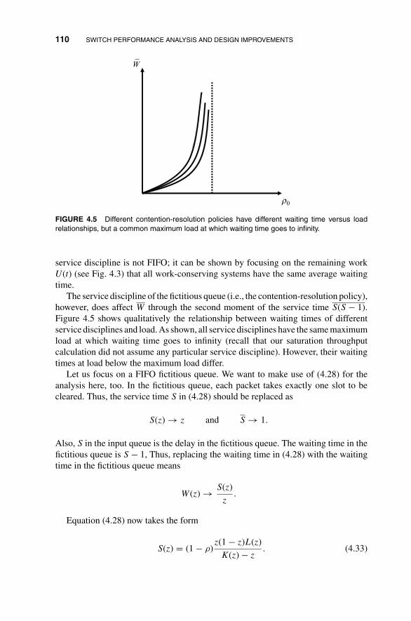
110 SWITCH PERFORMANCE ANALYSIS AND DESIGN IMPROVEMENTS
W
ρ0
FIGURE 4.5 Different contention-resolution policies have different waiting time versus loadrelationships, but a common maximum load at which waiting time goes to infinity.
service discipline is not FIFO; it can be shown by focusing on the remaining workU(t) (see Fig. 4.3) that all work-conserving systems have the same average waitingtime.
The service discipline of the fictitious queue (i.e., the contention-resolution policy),however, does affect W through the second moment of the service time S(S − 1).Figure 4.5 shows qualitatively the relationship between waiting times of differentservice disciplines and load. As shown, all service disciplines have the same maximumload at which waiting time goes to infinity (recall that our saturation throughputcalculation did not assume any particular service discipline). However, their waitingtimes at load below the maximum load differ.
Let us focus on a FIFO fictitious queue. We want to make use of (4.28) for theanalysis here, too. In the fictitious queue, each packet takes exactly one slot to becleared. Thus, the service time S in (4.28) should be replaced as
S(z) → z and S → 1.
Also, S in the input queue is the delay in the fictitious queue. The waiting time in thefictitious queue is S − 1, Thus, replacing the waiting time in (4.28) with the waitingtime in the fictitious queue means
W(z) → S(z)
z.
Equation (4.28) now takes the form
S(z) = (1 − ρ)z(1 − z)L(z)
K(z) − z. (4.33)
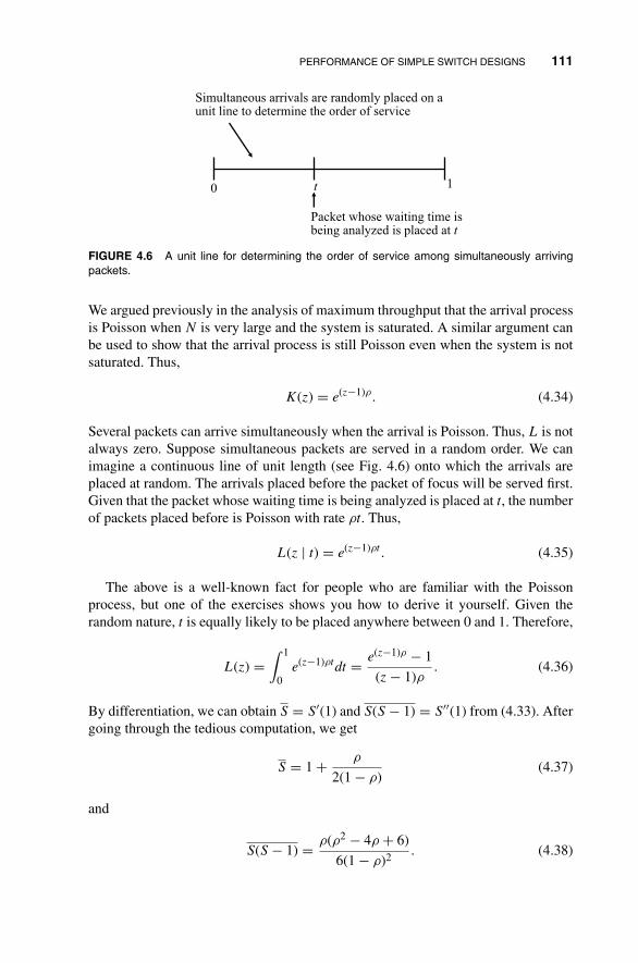
PERFORMANCE OF SIMPLE SWITCH DESIGNS 111
t 10
Simultaneous arrivals are randomly placed on a unit line to determine the order of service
Packet whose waiting time is being analyzed is placed at t
FIGURE 4.6 A unit line for determining the order of service among simultaneously arrivingpackets.
We argued previously in the analysis of maximum throughput that the arrival processis Poisson when N is very large and the system is saturated. A similar argument canbe used to show that the arrival process is still Poisson even when the system is notsaturated. Thus,
K(z) = e(z−1)ρ. (4.34)
Several packets can arrive simultaneously when the arrival is Poisson. Thus, L is notalways zero. Suppose simultaneous packets are served in a random order. We canimagine a continuous line of unit length (see Fig. 4.6) onto which the arrivals areplaced at random. The arrivals placed before the packet of focus will be served first.Given that the packet whose waiting time is being analyzed is placed at t, the numberof packets placed before is Poisson with rate ρt. Thus,
L(z | t) = e(z−1)ρt. (4.35)
The above is a well-known fact for people who are familiar with the Poissonprocess, but one of the exercises shows you how to derive it yourself. Given therandom nature, t is equally likely to be placed anywhere between 0 and 1. Therefore,
L(z) =∫ 1
0e(z−1)ρtdt = e(z−1)ρ − 1
(z − 1)ρ. (4.36)
By differentiation, we can obtain S = S′(1) and S(S − 1) = S′′(1) from (4.33). Aftergoing through the tedious computation, we get
S = 1 + ρ
2(1 − ρ)(4.37)
and
S(S − 1) = ρ(ρ2 − 4ρ + 6)
6(1 − ρ)2 . (4.38)

112 SWITCH PERFORMANCE ANALYSIS AND DESIGN IMPROVEMENTS
Substituting the above into (4.32) and solving, we obtain
W = ρ2(ρ2 − 4ρ + 6)
6(1 − ρ)(ρ2 − 4ρ + 2). (4.39)
The average delay experienced by a packet from arrival to departure is
D = W + S = ρ2(ρ2 − 4ρ + 6)
6(1 − ρ)(ρ2 − 4ρ + 2)+ 2 − ρ
2(1 − ρ). (4.40)
As an example, for offered load ρo = ρ = 0.5, S = 1.5 and W ≈ 1.41. The averagedelay D ≈ 3. That is, a packet experiences an average delay of three packet durationsin the input queue. We see that the delay is rather small if the offered load is slightlybelow the maximum throughput. The variance of delay is also an important parameter,especially for real-time communication services. The variance can be obtained fromthe higher derivatives of W(z) and S(z).
4.1.4 Delay of an Output-Buffered Switch
As mentioned earlier in the chapter, the throughput of a switch can be improved byincreasing the group size, which is the number of packets that can access a commonoutput in a given time slot. The throughput as a function of the group size will bestudied in the next chapter.
Let us now examine the ideal case in which all N packets (where N is the numberof input ports) can access the same output in the same time slot if they so desire.All packets are switched to their destined outputs immediately upon their arrivalsand none of them are dropped at the inputs. Therefore, there is no throughput limi-tation like that in the input-buffered switch. This ideal switch also obviates the needfor input buffers. In addition, instead of the fictitious output queues discussed pre-viously, we have real output queues here. These output queues are needed becausethe output link may not be able to transmit all the simultaneously arriving packetsimmediately.
The study of the output queues is similar to that of the the fictitious queue. In fact,the justification for the Poisson arrival process is more straightforward for the outputqueues because its packet sources are the inputs, whose number does not change withtime; the packet sources of the fictitious queue are those inputs whose HOL packetswere cleared in the previous time slot, and their number may change from time slotto time slot.
Given that the arrival process to each input is Bernoulli with rate ρo, the arrivalprocess to an output is binomial: Pr{A = k} = (
Nk
) (ρoN
)k (1 − ρoN
)N−k, which ap-proaches the Poisson distribution with rate ρo as N → ∞. We can therefore imme-diately use the result obtained for the fictitious queue, replacing ρ with ρo. Note thatfor the fictitious queue, the carried load ρ may not be the same as the offered load ρobecause of input queueing; but for the output queue, since all packets are immediately

DESIGN IMPROVEMENTS FOR INPUT QUEUEING SWITCHES 113
switched to the output with no loss, the offered load is the same as the carried loadso long as the output buffer does not overflow.
Let us consider a particular output and assume that it has infinite buffering space.From (4.14), the number of backlogged packets at the beginning of each time slot isgiven by
C(z) = (z − 1)A(z)(1 − ρo)
(z − A(z)), (4.41)
where A(z) = e(z−1)ρo . Unlike for the fictitious queue in which C ≤ 1 because of theconstraint imposed by the input queues, the value of C for the output queue dependson ρo, and it can be obtained from (4.41) by differentiation:
C = C′(1) = ρo + ρ2o
2(1 − ρo). (4.42)
The average delay in the output queue is given by the Little’s law:
S = C
ρo= 1 + ρo
2(1 − ρo). (4.43)
The delay can also be obtained directly by considering the waiting time. Replacing ρ
with ρo in (4.33), (4.34), and (4.36), we get
S(z) = z(1 − ρo)(1 − e(z−1)ρo )
ρo(e(z−1)ρo − z). (4.44)
From (4.44), we can derive (4.43) and other higher moments of S.
4.2 DESIGN IMPROVEMENTS FOR INPUT QUEUEING SWITCHES
The preceding section showed that input-buffered switch with single FIFO queues,on the contrary, is good for its simplicity but is constrained by its low throughput of58.6%. It is the result of head-of-line (HOL) blocking at an input queue, forbiddingpackets other than the HOL one to be transmitted when more than one HOL packetfrom different inputs contends at the same output (see Fig. 3.28). For throughputimprovement, we need to remove the FIFO constraint on the input queues to relievethe HOL blocking.
4.2.1 Look-Ahead Contention Resolution
An earlier scheme for improving the performance of an input-buffered switches islook-ahead selection of packets in FIFO input queues. In the look-ahead scheme,the first w packets of each input will be examined during the contention-resolution

114 SWITCH PERFORMANCE ANALYSIS AND DESIGN IMPROVEMENTS
TABLE 4.2 Maximum Throughput of a 32 × 32Input-Buffered Switch for Various ContentionWindow Sizes
w �∗
1 0.592 0.703 0.764 0.805 0.836 0.857 0.878 0.88∞ 1 (by analytical argument)
phase. The contention-resolution procedure is divided into w cycles. The first cycleis like the original scheme and at the end of it a set of winning packets out of theHOL packets are determined. In the second cycle, the scheme looks at the second setof packets of the inputs that have lost contention in the first cycle to see if they aredestined for any outputs that are as yet unclaimed. A second set of winning packetsis then determined. In this way, each cycle looks one packet deeper into the queuethan the previous cycle. After w cycles, the w sets of winning packets are then sent totheir outputs. Each input still sends at most one packet, and each output still receivesat most one packet, in a time slot. Certainly, as w increases, we expect the maximumthroughput to increase accordingly.
There is no known exact analytical method for deriving the maximum throughputfor w > 1. Table 4.2 lists the simulation results for various values of w for a 32 × 32switch. In general, it can be easily shown (see Problem 4.12) that as w → ∞, ρ∗ → 1,assuming the input queues have infinite amounts of buffers (note that this is anotherexample that the analysis is simple when a relevant system parameter is either smallor very large; but it becomes difficult when the parameter is somewhere in between).Table 4.2 shows, however, that ρ∗ approaches 1 very slowly.
It should be pointed out the throughput improvement does not come without cost.If the three-phase sort-banyan network switch is used, the first two phases must beperformed w times, resulting in higher contention-resolution overhead. Let ε be theoverhead associated with one round of contention resolution measured in time slot.The actual throughput is then ρ∗/(1 + wε). As w is increased, a point may be reachedat which the throughput improvement is more than offset by the contention-resolutionoverhead, bringing about a lower actual throughput.
A second factor that may decrease the throughput improvement is the input trafficcharacteristics. We have assumed that successive packets on an input are indepen-dently and equally likely to be destined for any output. In many situations, successivepackets may not be independent and are destined for only a small subset of the out-puts. The input look-ahead scheme will yield smaller throughput improvement in

DESIGN IMPROVEMENTS FOR INPUT QUEUEING SWITCHES 115
VOQ1, 1
VOQ 1, N
VOQ N, 1
VOQN , N
Input 1
Input N
. . .
. . .
. . . . . . . . . . . .
Internally
nonblocking
switch fabric
Output 1
Output N
. . . . . . . . . . . .
FIGURE 4.7 Virtual output queueing scheme.
such situations because looking deeper into the queue may often find packets withthe same destination.
4.2.2 Parallel Iterative Matching
In order to get rid of HOL blocking in an input-buffered switch, we can modifythe above buffer organization in such a way that every input port maintains N logicalqueues, named virtual output queues (VOQs), instead of keeping a single FIFO queue.This is illustrated in Fig. 4.7. In this setup, each of these N logical queues is dedicatedfor one of the N output ports so that packets with different destinations can take partin the contention resolution simultaneously, thus entirely eliminating HOL blockingat input ports. This technique is known as virtual output queueing because the switchbehaves as if it is an output queueing switch. In order to further increase the switchthroughput, a scheduler is needed for resolving input and output conflicts with theexisting connection requests. The arbitration of the scheduler is then passed to theswitching fabrics, and connection among input and outputs will be set up accordingly.
The question that arises now is how we can schedule the transmission of the queuedpackets so as to achieve a high throughput. In actuality, choosing a set of packets fortransmission in an input-buffered switch can be formulated as a matching problemin a bipartite graph as shown in Fig. 4.8, where inputs and outputs of the switch canbe considered as the two sets of nodes for matching. It is obvious that if we couldalways maximize the number of matches for the matching requests given in the graph,then we can achieve an optimum throughput performance for the switch. However,owing to the fact that finding a maximum matching is computationally complex, an
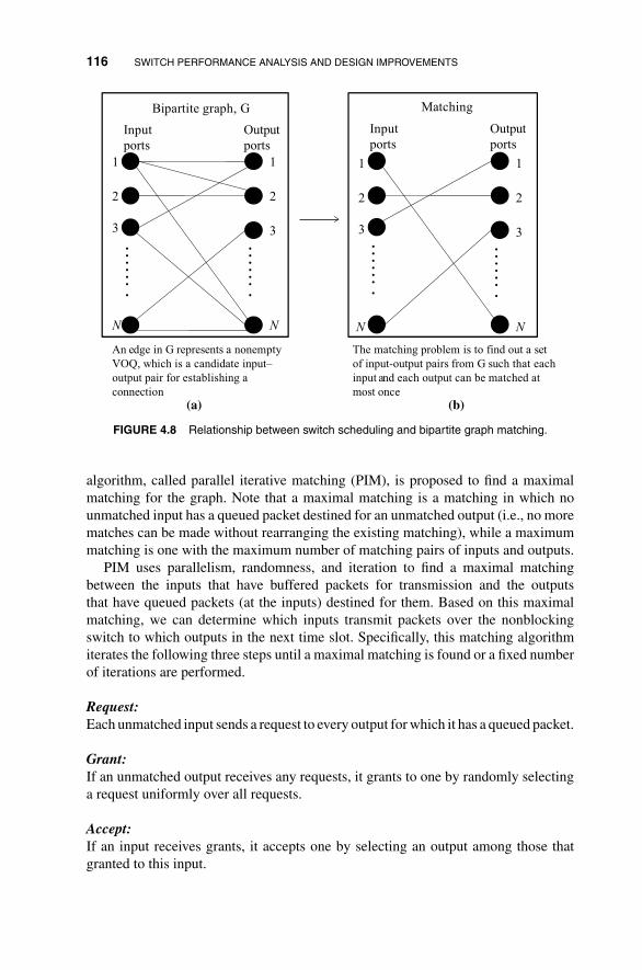
116 SWITCH PERFORMANCE ANALYSIS AND DESIGN IMPROVEMENTS
Input
ports
Output
ports
1
2
3
N
1
2
3
N
. . . . . . .
. . . . . . .
Bipartite graph, G
Input
ports
Output
ports
1
2
3
N
1
2
3
N
Matching
. . . . . . .
. . . . . . .
An edge in G represents a nonempty
VOQ, which is a candidate input–
output pair for establishing a
connection
(a)
The matching problem is to find out a set
of input-output pairs from G such that each
input and each output can be matched at
most once
(b)
FIGURE 4.8 Relationship between switch scheduling and bipartite graph matching.
algorithm, called parallel iterative matching (PIM), is proposed to find a maximalmatching for the graph. Note that a maximal matching is a matching in which nounmatched input has a queued packet destined for an unmatched output (i.e., no morematches can be made without rearranging the existing matching), while a maximummatching is one with the maximum number of matching pairs of inputs and outputs.
PIM uses parallelism, randomness, and iteration to find a maximal matchingbetween the inputs that have buffered packets for transmission and the outputsthat have queued packets (at the inputs) destined for them. Based on this maximalmatching, we can determine which inputs transmit packets over the nonblockingswitch to which outputs in the next time slot. Specifically, this matching algorithmiterates the following three steps until a maximal matching is found or a fixed numberof iterations are performed.
Request:Each unmatched input sends a request to every output for which it has a queued packet.
Grant:If an unmatched output receives any requests, it grants to one by randomly selectinga request uniformly over all requests.
Accept:If an input receives grants, it accepts one by selecting an output among those thatgranted to this input.

DESIGN IMPROVEMENTS FOR INPUT QUEUEING SWITCHES 117
1
2
3
1
2
3
1
2
3
111
2 2
3 3
Request
1
2
3
1
2
3
1
2
3
111
22
3
Accept
12
3
1
2
1
2
3
11
2
33
Grant
(a)
12
3
1
2
1
2
3
1
1
2
33
Request
(b)
FIGURE 4.9 (a) PIM: first iteration; (b) PIM: second iteration, request phase only.
Figure 4.9(a) illustrates how PIM works in one iteration. First, in the request phase,every unmatched input port sends a request to every output port whenever there isbacklogged packet for it. As depicted in Fig. 4.9, input port 1 sends requests to outputports 1, 2, and 3 simultaneously. Then, in the grant phase, if an unmatched output
118 SWITCH PERFORMANCE ANALYSIS AND DESIGN IMPROVEMENTS
receives multiple requests, it grants one randomly. For example, output 2 grants input1 in the grant phase below. Finally, in the accept phase, an unmatched input will acceptone grant randomly on receiving multiple grants. In this case, input 1 accepts the grantfrom output 1 and input 2 accepts that from output 3. After the first iteration, input3 remains unmatched, and therefore, it will send requests to output ports 1, 2, and 3in the request phase of the second iteration (see Fig. 4.9(b)). Since outputs 1 and 3have already been matched, they will neglect those requests and postpone schedulingof the corresponding packets to the next time slot. Only output 2 will consider therequest sent by input 3 in this iteration. Thus, two iterations are required for PIM tofind a maximal matching in this example.
In the following, we analyze the maximum throughput of an input-buffered switchwith respect to the number of iterations of PIM invoked. Let us assume that the switchis very large in size and all the logical queues are saturated so that as soon as a HOLpacket is cleared, its position is taken by a subsequent packet in the next time slot. Inthis way, the switch is loaded at its maximum capacity and each output port receivesa request from every unmatched input port during the request phase.
Consider that in the first iteration, the output port receive a request from each ofN input ports and will select one of them randomly to grant. The probability that aparticular input port does not receive any grant is
Pr{no grant received} =(
1 − 1
N
)N
. (4.45)
Thus, the probability that an input port will receive at least one grant for matching inthe first iteration is given by
ρ̂ = 1 − Pr{no grant received} = 1 −(
1 − 1
N
)N
. (4.46)
When N is large,
ρ̂ ≈ 1 − e−1 = 0.632. (4.47)
This is the maximum throughput of an input-buffered switch with invoking only oneiteration of PIM.
After the first iteration, there are totally N̂ = (1 − ρ̂)N input–output pairs not yetto be matched. We can use the same approach to find the number of pairs that couldbe matched up in the second iteration. That is,
[1 −
(1 − 1
N̂
)N̂]
· N̂ = ρ̂ · N̂ = ρ̂ · (1 − ρ̂)N. (4.48)

DESIGN IMPROVEMENTS BASED ON OUTPUT CAPACITY EXPANSION 119
TABLE 4.3 Maximum Throughput for Input-Buffered Switches Invoking DifferentNumber of Iterations of PIM
Number of iterations 1 2 3 4 5
Maximum throughput 0.632 0.865 0.950 0.981 0.993
In other words, the proportion of pairs that can be matched up, or the maximumthroughput that can be achieved in the first two iterations of PIM, is
max. throughput2 = ρ̂ + ρ̂(1 − ρ̂), (4.49)
where ρ̂ = 0.632.Similarly, for K ≥ 2 iterations, it is easy to show that the maximum throughput is
max. throughputK = ρ̂
K∑k=1
(1 − ρ̂)k−1, (4.50)
when N is sufficiently large. The analytical results of the maximum throughput areshown in Table 4.3 for different number of iterations of PIM invoked.
4.3 DESIGN IMPROVEMENTS BASED ON OUTPUT CAPACITYEXPANSION
Output capacity expansion refers to a class of design strategies that alleviate thecontention problem by allowing more than one packet to reach the same output in thesame time slot. Therefore, the throughput of a switch can be much increased.
4.3.1 Speedup Principle
Perhaps the most straightforward output capacity expansion strategy is to speed upthe operation of the switch so that each switch cycle is equal to a fraction of a timeslot. For example, by operating an internally nonblocking switch at twice the externallink rate, each switch cycle is equal to half a time slot. In the first half of a time slot,a contention-resolution scheme elects the winning packets for output access. In thesecond half, the losing packets, together with the new HOL packets, attempt to accesstheir outputs. It is easily seen that the maximum throughput is now 2 × 0.586, andsince the offered load by definition cannot be more than 1, the input queues will notsaturate.
For such a switch, a packet incurs delays at an input queue and an output queue(see Fig. 4.10). The output queue is needed because two packets may arrive at anoutput in a time slot, during which only one packet can be transmitted on the outputlink. The input queue is still required because there remains the chance that more thantwo HOL input packets are destined for the same output.
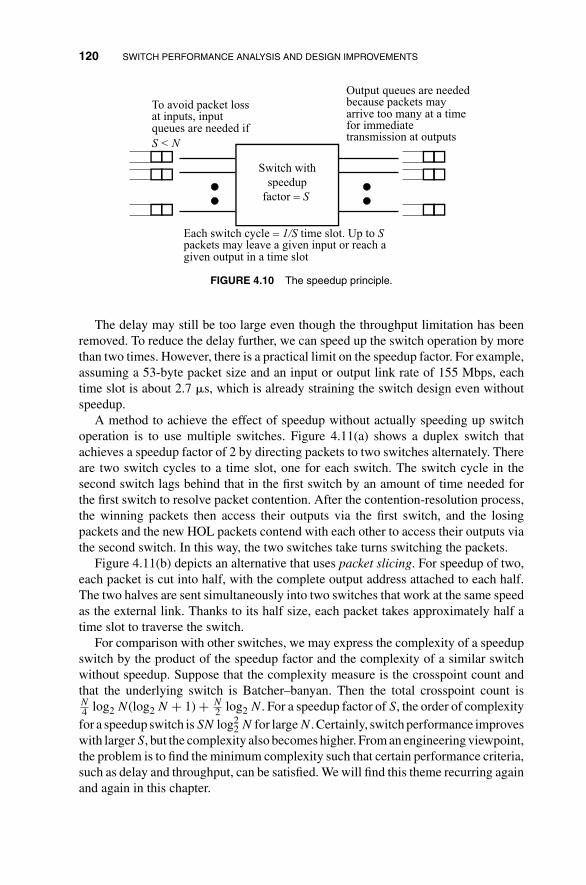
120 SWITCH PERFORMANCE ANALYSIS AND DESIGN IMPROVEMENTS
Switch with
speedup
factor = S
To avoid packet loss at inputs, input queues are needed if
S < N
Output queues are needed because packets may arrive too many at a time for immediate transmission at outputs
Each switch cycle = 1/S time slot. Up to S packets may leave a given input or reach a given output in a time slot
FIGURE 4.10 The speedup principle.
The delay may still be too large even though the throughput limitation has beenremoved. To reduce the delay further, we can speed up the switch operation by morethan two times. However, there is a practical limit on the speedup factor. For example,assuming a 53-byte packet size and an input or output link rate of 155 Mbps, eachtime slot is about 2.7 �s, which is already straining the switch design even withoutspeedup.
A method to achieve the effect of speedup without actually speeding up switchoperation is to use multiple switches. Figure 4.11(a) shows a duplex switch thatachieves a speedup factor of 2 by directing packets to two switches alternately. Thereare two switch cycles to a time slot, one for each switch. The switch cycle in thesecond switch lags behind that in the first switch by an amount of time needed forthe first switch to resolve packet contention. After the contention-resolution process,the winning packets then access their outputs via the first switch, and the losingpackets and the new HOL packets contend with each other to access their outputs viathe second switch. In this way, the two switches take turns switching the packets.
Figure 4.11(b) depicts an alternative that uses packet slicing. For speedup of two,each packet is cut into half, with the complete output address attached to each half.The two halves are sent simultaneously into two switches that work at the same speedas the external link. Thanks to its half size, each packet takes approximately half atime slot to traverse the switch.
For comparison with other switches, we may express the complexity of a speedupswitch by the product of the speedup factor and the complexity of a similar switchwithout speedup. Suppose that the complexity measure is the crosspoint count andthat the underlying switch is Batcher–banyan. Then the total crosspoint count isN4 log2 N(log2 N + 1) + N
2 log2 N. For a speedup factor of S, the order of complexityfor a speedup switch isSN log2
2 N for largeN. Certainly, switch performance improveswith larger S, but the complexity also becomes higher. From an engineering viewpoint,the problem is to find the minimum complexity such that certain performance criteria,such as delay and throughput, can be satisfied. We will find this theme recurring againand again in this chapter.
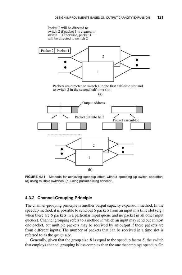
DESIGN IMPROVEMENTS BASED ON OUTPUT CAPACITY EXPANSION 121
2
1
Packet 2 will be directed to switch 2 if packet 1 is cleared in switch 1. Otherwise, packet 1 will be directed to switch 2
Packet 2 Packet 1
Packets are directed to switch 1 in the first half-time slot and to switch 2 in the second half-time slot
(a)
2
1
(b)
Output address
Packet cut into halfPacket assembled
FIGURE 4.11 Methods for achieving speedup effect without speeding up switch operation:(a) using multiple switches; (b) using packet-slicing concept.
4.3.2 Channel-Grouping Principle
The channel-grouping principle is another output capacity expansion method. In thespeedup method, it is possible to send out S packets from an input in a time slot (e.g.,when there are S packets in a particular input queue and no packet in all other inputqueues). Channel grouping refers to a method in which an input may send out at mostone packet, but multiple packets may be received by an output if these packets arefrom different inputs. The number of packets that can be received in a time slot isreferred to as the group size.
Generally, given that the group size R is equal to the speedup factor S, the switchthat employs channel grouping is less complex than the one that employs speedup. On

122 SWITCH PERFORMANCE ANALYSIS AND DESIGN IMPROVEMENTS
Banyan network 0
Banyan network
R-1
R–2
Batcher network
MUX
MUX
Output
0
N–1
0
0
0
N–1
N–1
N–1
Output i (i=0, …, N–1) connected to input ⎣ i/R ⎦ of banyan network i mod R
FIGURE 4.12 A Batcher–R-banyan network that implements the channel-grouping principle.
the other hand, the speedup switch has better performance because of its capabilityto switch multiple packets of an input within the same time slot.
4.3.2.1 Channel Grouping Using Batcher–banyan Networks A Batcher–R-banyan network that utilizes the channel-grouping concept is shown in Fig. 4.12.As shown, the structure consists of a Batcher network connected to R parallel banyannetworks. The outputs of the Batcher network are connected to the inputs of the R
banyan network in an interleaving fashion as shown in the figure: the first output ofthe Batcher network is connected to the first input of the first banyan network, thesecond output to the first input of the second banyan network, and so on. In general,the output i (i = 0, 1, 2, . . . , N − 1) of the Batcher network is connected to input�i/R� (the integer part of i/R) of banyan network i mod R.
If at most R input packets are addressed to the same destination (output of theoverall switch), then the Batcher network and the interleaving connections betweenit and the banyan networks ensure that the input packets to each banyan network aresorted, concentrated, and have nonconflicting output addresses. The banyan networksare therefore nonblocking. Outputs i (i = 0, . . . , N − 1) of different banyan networkscorrespond to the same logical address and they are collected and fed into a multiplexerfor transmission on the output port.
To ensure that no more than R packets are addressed to the same output, theunderlying contention-resolution scheme must be modified. Consider for examplethe three-phase scheme in which the Batcher network is used to resolve contention.At the end of the first phase, output i of the Batcher network examines output i − R
(as opposed to output i − 1 without channel grouping) for possible conflict. If thedestination addresses of these two packets are the same, then at least R + 1 packetshave the same destination address, thanks to the sorting performed by the Batchernetwork. That is, packets at outputs i − R to i all have the same destination addresses.
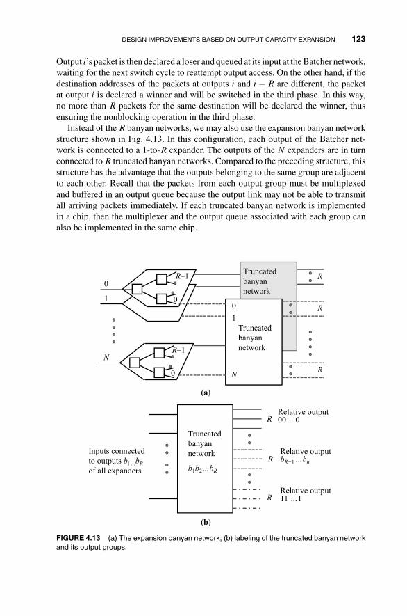
DESIGN IMPROVEMENTS BASED ON OUTPUT CAPACITY EXPANSION 123
Output i’s packet is then declared a loser and queued at its input at the Batcher network,waiting for the next switch cycle to reattempt output access. On the other hand, if thedestination addresses of the packets at outputs i and i − R are different, the packetat output i is declared a winner and will be switched in the third phase. In this way,no more than R packets for the same destination will be declared the winner, thusensuring the nonblocking operation in the third phase.
Instead of the R banyan networks, we may also use the expansion banyan networkstructure shown in Fig. 4.13. In this configuration, each output of the Batcher net-work is connected to a 1-to-R expander. The outputs of the N expanders are in turnconnected to R truncated banyan networks. Compared to the preceding structure, thisstructure has the advantage that the outputs belonging to the same group are adjacentto each other. Recall that the packets from each output group must be multiplexedand buffered in an output queue because the output link may not be able to transmitall arriving packets immediately. If each truncated banyan network is implementedin a chip, then the multiplexer and the output queue associated with each group canalso be implemented in the same chip.
R
R
R
Truncated
banyan
network
(a)
Truncated
banyan
network
0
1
N
0
R–1
R–1
0
0
1
N
Truncated
banyan
network
b1b2…bR
R
R
Relative output 00 …0
RRelative output bR+1 …bn
Relative output 11 …1
Inputs connected
to outputs b1 ...bRof all expanders
(b)
FIGURE 4.13 (a) The expansion banyan network; (b) labeling of the truncated banyan networkand its output groups.
124 SWITCH PERFORMANCE ANALYSIS AND DESIGN IMPROVEMENTS
The expander has the structure of a binary tree. Routing in the expander is similarto that in an ordinary banyan network. Assuming R is a power of 2, a 1-to-R expanderhas r = log2 R stages and it uses the r most significant bits of the output addressfor routing. A truncated banyan network is a banyan network with the last r stagesremoved and it uses the remaining s = log2 N/R bits for routing. Recall that as apacket travels through a banyan network, it sees a smaller and smaller subnetwork,and the outputs it can reach are restricted to a smaller and smaller subset. If it is notnecessary to reach any particular output of an output group (i.e., any output withina group will do), then there is no need to travel farther through the banyan networkbeyond the stages needed to distinguish between the different groups, hence the ideabehind truncation.
To see why the expander truncated banyan network is nonblocking, first note thatno conflict occurs in the expanders since at most one packet travels through each ofthem. Packets that exit from expander outputs b1b2 · · · br (labeled in a binary fashion)are for destinations b1b2 · · · br00 · · · 0, b1b2 · · · br00 · · · 1, . . ., or b1b2 · · · br11 · · · 1.These packets are routed to a particular truncated banyan network labeled b1b2 · · · br,as shown in Fig. 4.13(b). The input packets to any particular truncated banyan networkare monotone and concentrated, thanks to the preceding Batcher network. The proofof the following theorem completes our argument.
Theorem 4.1. The R-truncated-banyan network is nonblocking if the active inputsx1, . . . , xn (xj > xi if j > i) and their corresponding output addresses y1, . . . , ym
satisfy the following:
1. Limited output conflict: At most R packets are destined for any given output.
2. Monotonic outputs: y1 ≤ y2 ≤ · · · ≤ ym or y1 ≥ y2 ≥ · · · ≥ ym.
3. Concentrated inputs: Any input between two active inputs is also active. Thatis, xi ≤ w ≤ xj implies input w is active.
Proof. The output address of a packet has only s = n − r remaining bits for rout-ing. The relative output address of an output group is therefore labeled br+1 · · · bn,where n = log2 N. The complete address of the output group, b1 · · · brbr+1 · · · bn, isobtained by concatenating the truncated banyan network label b1b2 · · · br with therelative output address br+1 · · · bn. To show that conflict does not occur in any of thes stages of the truncated banyan network, let us assume the contrary: two packets ata node in stage k, 1 ≤ k ≤ s, want to access the same outgoing link. Let the inputand relative output addresses of the packet 1 be x = an · · · a1 and y = br+1 · · · bn,respectively, and those of packet 2 be x′ = a′
n · · · a′1 and y′ = b′
r+1 · · · b′n. As in the
proof of Theorem 3.1, their conflict in stage k implies
an−k · · · a1 = a′n−k · · · a′
1 (4.51)
and
br+1 · · · br+k = b′r+1 · · · b′
r+k. (4.52)
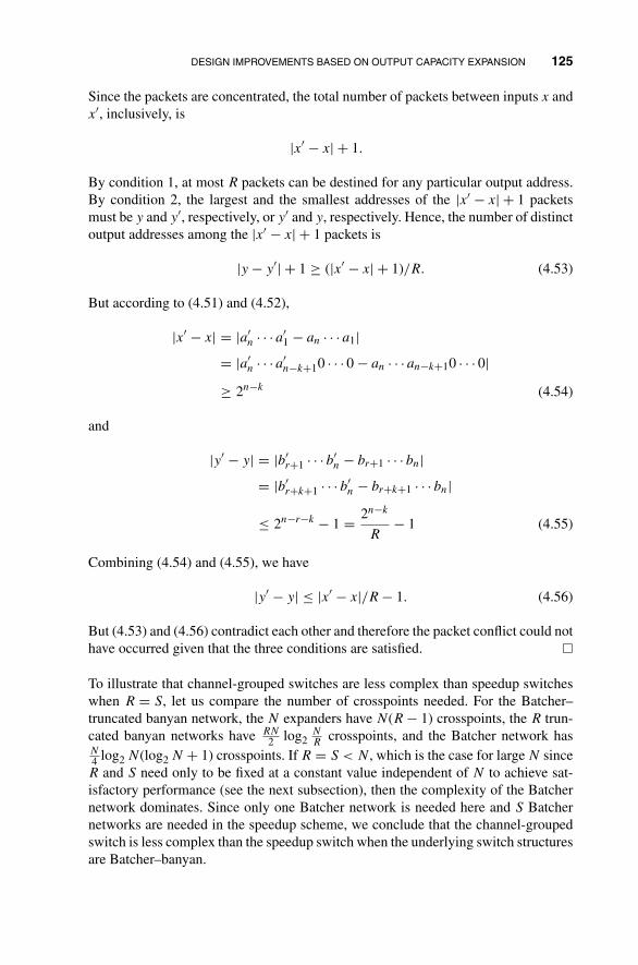
DESIGN IMPROVEMENTS BASED ON OUTPUT CAPACITY EXPANSION 125
Since the packets are concentrated, the total number of packets between inputs x andx′, inclusively, is
|x′ − x| + 1.
By condition 1, at most R packets can be destined for any particular output address.By condition 2, the largest and the smallest addresses of the |x′ − x| + 1 packetsmust be y and y′, respectively, or y′ and y, respectively. Hence, the number of distinctoutput addresses among the |x′ − x| + 1 packets is
|y − y′| + 1 ≥ (|x′ − x| + 1)/R. (4.53)
But according to (4.51) and (4.52),
|x′ − x| = |a′n · · · a′
1 − an · · · a1|= |a′
n · · · a′n−k+10 · · · 0 − an · · · an−k+10 · · · 0|
≥ 2n−k (4.54)
and
|y′ − y| = |b′r+1 · · · b′
n − br+1 · · · bn|= |b′
r+k+1 · · · b′n − br+k+1 · · · bn|
≤ 2n−r−k − 1 = 2n−k
R− 1 (4.55)
Combining (4.54) and (4.55), we have
|y′ − y| ≤ |x′ − x|/R − 1. (4.56)
But (4.53) and (4.56) contradict each other and therefore the packet conflict could nothave occurred given that the three conditions are satisfied. �
To illustrate that channel-grouped switches are less complex than speedup switcheswhen R = S, let us compare the number of crosspoints needed. For the Batcher–truncated banyan network, the N expanders have N(R − 1) crosspoints, the R trun-cated banyan networks have RN
2 log2NR
crosspoints, and the Batcher network hasN4 log2 N(log2 N + 1) crosspoints. If R = S < N, which is the case for large N sinceR and S need only to be fixed at a constant value independent of N to achieve sat-isfactory performance (see the next subsection), then the complexity of the Batchernetwork dominates. Since only one Batcher network is needed here and S Batchernetworks are needed in the speedup scheme, we conclude that the channel-groupedswitch is less complex than the speedup switch when the underlying switch structuresare Batcher–banyan.

126 SWITCH PERFORMANCE ANALYSIS AND DESIGN IMPROVEMENTS
mux
Output queue
Rx1switch working at R = 4times the links rate
1
R(a)
Shifting
concentrator
1Rmux
R
Rx1switch working at same
speed as link rate
Packets are loaded into
queues in round-robin
fashion
Packets are read out from
queues in round-robin
fashion
(b)
FIGURE 4.14 (a) Multiplexer and output queue at an output of a channel-grouped switch. Toaccommodate simultaneous packet arrivals, the multiplexer must work R times faster than linkrate. (b) An implementation of a logical FIFO queue such that the multiplexer only have to workat same speed as link rate.
Both speedup and channel-grouping schemes require a multiplexer and an outputqueue in each output. Figure 4.14(a) shows an implementation that employs an R × 1switch that runs at R times the link speed. In each time slot, the multiplexer scansacross all the inputs and switches the packets, if any, one by one to the output queue.The access speed of the memory that implements the queue must also be fast enoughto keep up with the scanning.
Figure 4.14(b) is an alternative scheme that achieves the same function with-out employing speedup. It consists of an R × R shifting concentrator (described inSection 3.2.4) followed by R queues and a multiplexer. For explanation, let us pre-tend that the structure does not have the shifting concentrator for the time being. Themultiplexer works at the same speed as the output link. It scans the queues in a round-robin fashion and in each time slot and selects a packet from one of the queues fortransmission on the output link. In R time slots, each queue has at least one chanceto send a packet. It is possible for successive packets of a communication session toarrive at different output queues due to the interference of packets from other inputs:the number of other packets contending with the session’s packets, and their inputs,may change from time slot to time slot. If by chance a packet of the session reaches aqueue that is shorter than the one reached by an earlier packet, it will be transmittedfirst, causing the packets to be received out of order at the destination.
The purpose of the shifting concentrator is to maintain the sequence order of thepackets. It concentrates and loads the arriving packets in a round-robin fashion intothe queues. In the very first time slot of the switch operation, the shifting concentratorloads the arriving packets into queues 1, 2, and so on. Similarly, packets will be

DESIGN IMPROVEMENTS BASED ON OUTPUT CAPACITY EXPANSION 127
read out from the queues by the multiplexer starting from queue 1 in a round-robinmanner. Suppose that queue i is the last queue to which a packet is loaded and thatK ≤ R packets arrive in the next time slot. Then the shifting concentrator sends thenewly arriving packets to queues i + 1, . . . , i + K (mod R). In the subsequent timeslot, packets will be loaded into the queues starting from queue i + K + 1 (mod R).Meanwhile the multiplexer reads packets out of the queues in a round-robin fashion,and if it finds the queue to be read empty in a time slot, it simply waits until the shiftingconcentrator loads a packet into the queue—in this situation, the other queues are alsoempty, and the queue is the one to be loaded next. It can be easily seen that the R
queues are logically equivalent to a FIFO queue, because it is impossible for a packetof a session to depart from the switch before an earlier packet does. As for the shiftingconcentrator, it has already been shown in Section 3.2.4 that it can be implementedusing a reverse banyan network.
4.3.2.2 Performance of Switches Based on Channel Grouping Let usconsider a waiting system in which if more than R packets are destined for the sameoutput, the excess packets are buffered at the inputs. The special case R = 1 has beenconsidered in the preceding chapter. The basic steps are the same in the general case.Therefore, we will go through the derivations rather briefly.
We made the same assumption that each packet is equally likely to be destinedfor any of the N outputs and packet destinations are independent. To derive themaximum throughput, as before, consider the fictitious queue that consists of HOLpackets destined for a particular output. Let Cm be the number of packets in the queueand Am be the number of arriving packets at the start of time slot m. The systemevolves according to the equation
Cm = max(0, Cm−1 − R) + Am. (4.57)
As before, we can argue that for large N, Am is Poisson and independent of m in thesteady state. For the steady-state analysis, the subscript m is dropped. Its generatingfunction is
A(z) = e(z−1)ρ, (4.58)
where ρ is the throughput of the system. Using the same steps, we can show that
C(z) =A(z)
[∑R−1k=0 (zR − zk) Pr{C = k}
]zR − A(z)
. (4.59)
We have expressed C(z) in terms of Pr{C = 0}, Pr{C = 1}, . . . , Pr{C = R − 1}.These probabilities cannot be found so easily, and they can only be derived indi-rectly numerically.
The term∑R−1
k=0 (zR − zk) Pr{C = k} in the numerator of C(z) is a polynomialof degree R in z. We can therefore alternatively express it as K(z − 1)(z − z1) . . .
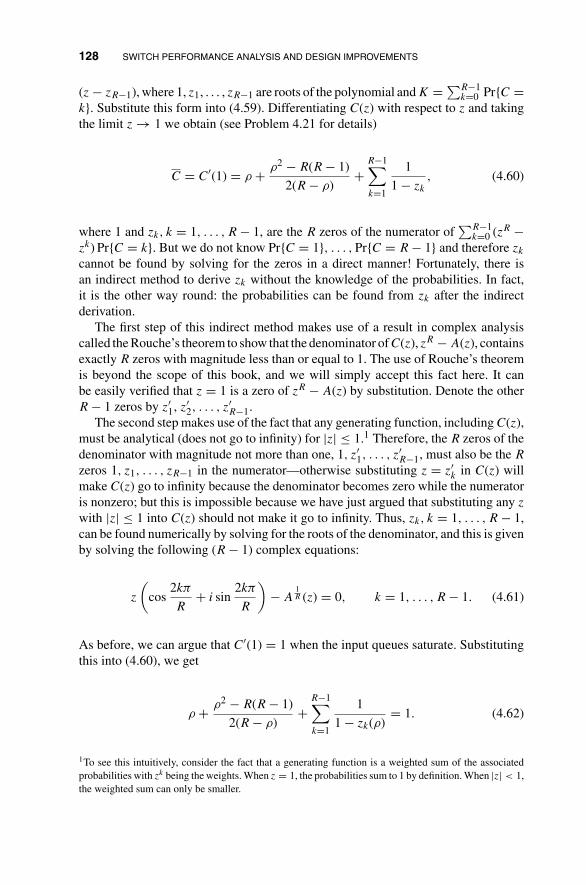
128 SWITCH PERFORMANCE ANALYSIS AND DESIGN IMPROVEMENTS
(z − zR−1), where 1, z1, . . . , zR−1 are roots of the polynomial and K = ∑R−1k=0 Pr{C =
k}. Substitute this form into (4.59). Differentiating C(z) with respect to z and takingthe limit z → 1 we obtain (see Problem 4.21 for details)
C = C′(1) = ρ + ρ2 − R(R − 1)
2(R − ρ)+
R−1∑k=1
1
1 − zk
, (4.60)
where 1 and zk, k = 1, . . . , R − 1, are the R zeros of the numerator of∑R−1
k=0 (zR −zk) Pr{C = k}. But we do not know Pr{C = 1}, . . . , Pr{C = R − 1} and therefore zk
cannot be found by solving for the zeros in a direct manner! Fortunately, there isan indirect method to derive zk without the knowledge of the probabilities. In fact,it is the other way round: the probabilities can be found from zk after the indirectderivation.
The first step of this indirect method makes use of a result in complex analysiscalled the Rouche’s theorem to show that the denominator ofC(z), zR − A(z), containsexactly R zeros with magnitude less than or equal to 1. The use of Rouche’s theoremis beyond the scope of this book, and we will simply accept this fact here. It canbe easily verified that z = 1 is a zero of zR − A(z) by substitution. Denote the otherR − 1 zeros by z′
1, z′2, . . . , z
′R−1.
The second step makes use of the fact that any generating function, including C(z),must be analytical (does not go to infinity) for |z| ≤ 1.1 Therefore, the R zeros of thedenominator with magnitude not more than one, 1, z′
1, . . . , z′R−1, must also be the R
zeros 1, z1, . . . , zR−1 in the numerator—otherwise substituting z = z′k in C(z) will
make C(z) go to infinity because the denominator becomes zero while the numeratoris nonzero; but this is impossible because we have just argued that substituting any z
with |z| ≤ 1 into C(z) should not make it go to infinity. Thus, zk, k = 1, . . . , R − 1,can be found numerically by solving for the roots of the denominator, and this is givenby solving the following (R − 1) complex equations:
z
(cos
2kπ
R+ i sin
2kπ
R
)− A
1R (z) = 0, k = 1, . . . , R − 1. (4.61)
As before, we can argue that C′(1) = 1 when the input queues saturate. Substitutingthis into (4.60), we get
ρ + ρ2 − R(R − 1)
2(R − ρ)+
R−1∑k=1
1
1 − zk(ρ)= 1. (4.62)
1To see this intuitively, consider the fact that a generating function is a weighted sum of the associatedprobabilities with zk being the weights. When z = 1, the probabilities sum to 1 by definition. When |z| < 1,the weighted sum can only be smaller.

DESIGN IMPROVEMENTS BASED ON OUTPUT CAPACITY EXPANSION 129
TABLE 4.4 MaximumThroughput for Input-BufferedSwitches with Group Size R
R �∗
1 0.5862 0.8853 0.9754 0.9968 1.000
Note that we have explicitly put in the dependence of zk found from (4.61) on ρ
through the notation zk(ρ). Equation (4.62) relates the throughput ρ and the groupsize R. To find the saturation throughput ρ numerically, we start with an initial guessof ρ and find the corresponding roots zk(ρ) using (4.61). The roots are then substitutedinto (4.62) to get a quadratic equation of ρ, from which we obtain a new ρ. This newρ is then substituted into (4.61) for a new set of roots zk(ρ). This process is iterateduntil the required accuracy of ρ is obtained. The resulting throughput is the saturationor maximum achievable throughput ρ∗. Table 4.4 lists the values of ρ∗ for various R
and shows that it indeed approaches to 1 very quickly with R.The derivation of the waiting time can largely be proceeded as before. In particular,
the general form of (4.31) still applies:
W(z) = (1 − ρS)1 − z
(1 − z) + [S(z) − 1]ρ, (4.63)
where W(z) and S(z) are, respectively, the generating functions of the waiting timeand the service time at the HOL. The mean waiting time is
W = ρS(S − 1)
2(1 − ρS). (4.64)
These equations are expressed in terms of S, the service time at HOL. But as forC(z), there is no known way of finding S(z) or Pr{S} in closed form. To find S(z)numerically, let the number of packets at the end of a time slot in the steady state beB. Then,
B(z) = C(z)
A(z)=
[∑R−1k=0 (zR − zk) Pr{C = k}
]zR − A(z)
. (4.65)
As for C(z), we can argue that for B(z) the R roots of the numerator are the sameas the R roots of the denominator that are less than or equal to 1. For a given ρ <
ρ∗, therefore, we can use (4.61) to find the roots zk(ρ), k = 1, . . . , R − 1, and then
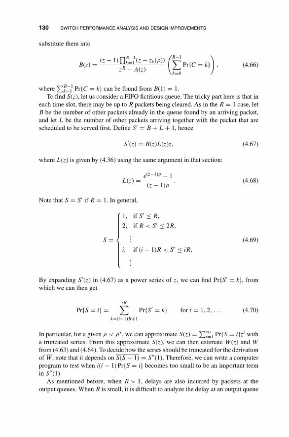
130 SWITCH PERFORMANCE ANALYSIS AND DESIGN IMPROVEMENTS
substitute them into
B(z) = (z − 1)∏R−1
k=1 (z − zk(ρ))
zR − A(z)
(R−1∑k=0
Pr{C = k})
, (4.66)
where∑R−1
k=1 Pr{C = k} can be found from B(1) = 1.To find S(z), let us consider a FIFO fictitious queue. The tricky part here is that in
each time slot, there may be up to R packets being cleared. As in the R = 1 case, letB be the number of other packets already in the queue found by an arriving packet,and let L be the number of other packets arriving together with the packet that arescheduled to be served first. Define S′ = B + L + 1, hence
S′(z) = B(z)L(z)z, (4.67)
where L(z) is given by (4.36) using the same argument in that section:
L(z) = e(z−1)ρ − 1
(z − 1)ρ. (4.68)
Note that S = S′ if R = 1. In general,
S =
⎧⎪⎪⎪⎪⎪⎪⎪⎪⎨⎪⎪⎪⎪⎪⎪⎪⎪⎩
1, if S′ ≤ R,
2, if R < S′ ≤ 2R,
...
i, if (i − 1)R < S′ ≤ iR,
...
(4.69)
By expanding S′(z) in (4.67) as a power series of z, we can find Pr{S′ = k}, fromwhich we can then get
Pr{S = i} =iR∑
k=(i−1)R+1
Pr{S′ = k} for i = 1, 2, . . . (4.70)
In particular, for a given ρ < ρ∗, we can approximate S(z) = ∑∞i=1 Pr{S = i}zi with
a truncated series. From this approximate S(z), we can then estimate W(z) and W
from (4.63) and (4.64). To decide how the series should be truncated for the derivationof W , note that it depends on S(S − 1) = S′′(1), Therefore, we can write a computerprogram to test when i(i − 1) Pr{S = i} becomes too small to be an important termin S′′(1).
As mentioned before, when R > 1, delays are also incurred by packets at theoutput queues. When R is small, it is difficult to analyze the delay at an output queue
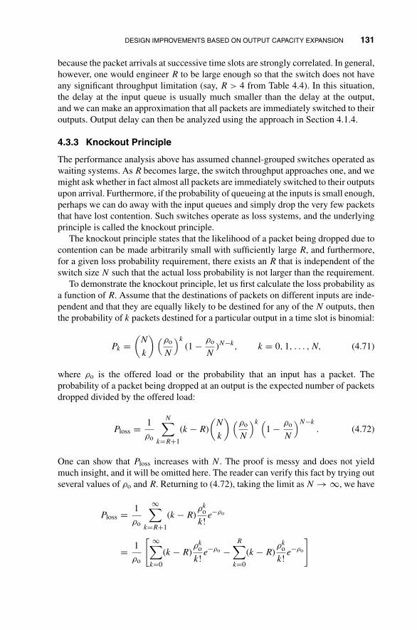
DESIGN IMPROVEMENTS BASED ON OUTPUT CAPACITY EXPANSION 131
because the packet arrivals at successive time slots are strongly correlated. In general,however, one would engineer R to be large enough so that the switch does not haveany significant throughput limitation (say, R > 4 from Table 4.4). In this situation,the delay at the input queue is usually much smaller than the delay at the output,and we can make an approximation that all packets are immediately switched to theiroutputs. Output delay can then be analyzed using the approach in Section 4.1.4.
4.3.3 Knockout Principle
The performance analysis above has assumed channel-grouped switches operated aswaiting systems. As R becomes large, the switch throughput approaches one, and wemight ask whether in fact almost all packets are immediately switched to their outputsupon arrival. Furthermore, if the probability of queueing at the inputs is small enough,perhaps we can do away with the input queues and simply drop the very few packetsthat have lost contention. Such switches operate as loss systems, and the underlyingprinciple is called the knockout principle.
The knockout principle states that the likelihood of a packet being dropped due tocontention can be made arbitrarily small with sufficiently large R, and furthermore,for a given loss probability requirement, there exists an R that is independent of theswitch size N such that the actual loss probability is not larger than the requirement.
To demonstrate the knockout principle, let us first calculate the loss probability asa function of R. Assume that the destinations of packets on different inputs are inde-pendent and that they are equally likely to be destined for any of the N outputs, thenthe probability of k packets destined for a particular output in a time slot is binomial:
Pk =(
N
k
)(ρo
N
)k
(1 − ρo
N)N−k, k = 0, 1, . . . , N, (4.71)
where ρo is the offered load or the probability that an input has a packet. Theprobability of a packet being dropped at an output is the expected number of packetsdropped divided by the offered load:
Ploss = 1
ρo
N∑k=R+1
(k − R)
(N
k
)(ρo
N
)k (1 − ρo
N
)N−k
. (4.72)
One can show that Ploss increases with N. The proof is messy and does not yieldmuch insight, and it will be omitted here. The reader can verify this fact by trying outseveral values of ρo and R. Returning to (4.72), taking the limit as N → ∞, we have
Ploss = 1
ρo
∞∑k=R+1
(k − R)ρk
o
k!e−ρo
= 1
ρo
[ ∞∑k=0
(k − R)ρk
o
k!e−ρo −
R∑k=0
(k − R)ρk
o
k!e−ρo
]

132 SWITCH PERFORMANCE ANALYSIS AND DESIGN IMPROVEMENTS
= 1
ρo
[(ρo − R) −
R∑k=0
kρk
o
k!e−ρo + R
R∑k=0
ρko
k!e−ρo
]
= 1
ρo
[(ρo − R) − ρo
R−1∑k=0
ρko
k!e−ρo + R
R∑k=0
ρko
k!e−ρo
]
= 1
ρo
[(ρo − R) − (ρo − R)
R∑k=0
ρko
k!e−ρo + ρo
ρRo
R!e−ρo
]
=(
1 − R
ρo
)(1 −
R∑k=0
ρko
k!e−ρo
)+ ρR
o
R!e−ρo .
(4.73)
It can be easily shown from the above expression that Ploss decreases as R increases.That is, Ploss decreases monotonically as R → N, and when R = N, Ploss = 0 (it isphysically obvious that if up to N packets can access the same output simultaneously,the loss probability must be zero). This means that for any given loss probabilityrequirement, we can always find a sufficiently large R to achieve a loss probabilitythat is not larger than the requirement. To illustrate that a finite R would do for allN, consider a loss probability requirement of 10−6. We can compute from (4.73)that R = 8 is enough. Furthermore, this R applies for all N, since (4.73) is an upperbound on the loss probability for finite N.
The channel-grouped Batcher–banyan networks described in the previous subsec-tion can adopt the knockout principle and operate as a loss system. As in the waitingsystem, a contention-resolution scheme (e.g., the three-phase scheme) is used to selectup to R packets for each output for switching. The excess packets, instead of beingqueued, are dropped at the inputs.
An alternative to separating the contention-resolution phase and the switchingphase is to deal with the contention on-the-fly while the packets are being routed. Thiseliminates the overhead associated with a dedicated contention-resolution phase. Fig-ure 4.15 shows a Batcher–banyan switch design in which a reverse banyan concentra-tor is inserted between the Batcher and the banyan networks. In this network, packetsare launched in their entireties into the Batcher network at the beginning of each timeslot (as opposed to only the headers in the three-phase scheme). As discussed before,winning and losing packets are determined at the outputs of the Batcher network byaddress comparison. The losing packets are dropped. This means that the remain-ing winning packets may not be concentrated anymore. Internal conflict may arise ifthey are launched into the banyan networks directly. To avoid such conflict, a reversebanyan network is a used as a concentrator to remove the gaps between the packets.
The outputs of the reverse banyan concentrator are connected in an interleavingfashion to R N × N banyan networks (as in the connection from the Batcher networkto the banyan networks in Fig. 4.12): output i (i = 0, . . . , N − 1) of the concentrator isconnected to input �i/R� of banyan network i mod R. It is easily seen that no conflictoccurs in any of the N × N banyan network because the packets are concentrated and

DESIGN IMPROVEMENTS BASED ON OUTPUT CAPACITY EXPANSION 133
?=
?=
?=
0
1
0
1
RBatcher
network
Reverse-
banyan
concentratorR+1
0
1
R
NxN banyan
(1)
NxN banyan
(2)
NxN banyan
(R)
MUX
MUX
0
1
N–1
N–1
MUX
a
b?=
Packet 1
Packet 2
Output
address
Let packet 2 go
through if and only if
a≠b
FIGURE 4.15 A Batcher–banyan knockout switch.
have distinct monotonic addresses. Outputs i (i = 0, . . . , N − 1) of different banyannetworks correspond to the same output address and they are collected and fed intoa multiplexer with a logical FIFO (see Fig. 4.14(b)) to maintain packet sequenceintegrity.
The Batcher–banyan knockout switch is a good example of how the basic buildingblocks that we have learned so far can be used to construct a sophisticated packetswitch. A number of parallel distributed algorithms—sorting in the Batcher network,concentration in the reverse banyan network, routing in the banyan networks, andmultiplexing in the logical FIFO queues at the outputs—are executed simultaneously.Every essential step seems to have been parallelized except for one thing. In thediscussion of the reverse banyan concentrator in Section 3.2.4, we have ignored acritical problem that surfaces when N is large, namely, how does a packet at an inputfind out the number of arriving packets at other inputs so that its output address atthe shifting concentrator can be determined accordingly? After all, the concentratoroutput assigned to a packet corresponds to the number of active packets above it:from top to bottom, the first active packet is assigned output 0, second, output 1,third, output 2, and so on. When the number of inputs N is small, a central controllerthat polls the inputs and returns the assigned output addresses at the beginning ofeach time slot can be incorporated (see Fig. 4.16(a)). But this takes up an amount oftime proportional to the number of inputs. When the number of inputs N is large, thisapproach is not viable. Hence, a parallel architecture that performs such polling andaddress assignment in a distributed fashion is needed.
For each input, the task is to compute the number (or the running sum) of packetsabove it. Figure 4.16(b) shows an 8 × 8 running-adder address generator for suchcomputation. An N × N running-adder address generator comprises log2 N stages ofN adders each. At the inputs, a log2 N-bit header is attached to each packet for the
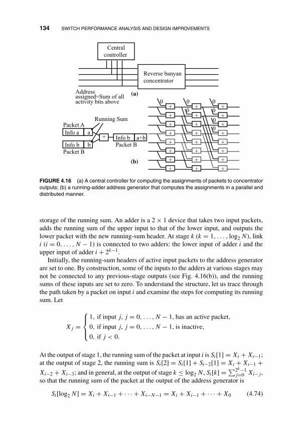
134 SWITCH PERFORMANCE ANALYSIS AND DESIGN IMPROVEMENTS
Central
controller
Reverse banyan
concentrator
(a)
+
+
+
+
+
+
+
+
+
+
+
+
+
+
+
+
+
+
+
+
+
+
+
+
Address assigned=Sum of all activity bits above
Running Sum
Info b b
Info a aInfo b a+b+
(b)
00
0
0
0
0
0
Packet B
Packet A
Packet B
FIGURE 4.16 (a) A central controller for computing the assignments of packets to concentratoroutputs; (b) a running-adder address generator that computes the assignments in a parallel anddistributed manner.
storage of the running sum. An adder is a 2 × 1 device that takes two input packets,adds the running sum of the upper input to that of the lower input, and outputs thelower packet with the new running-sum header. At stage k (k = 1, . . . , log2 N), linki (i = 0, . . . , N − 1) is connected to two adders: the lower input of adder i and theupper input of adder i + 2k−1.
Initially, the running-sum headers of active input packets to the address generatorare set to one. By construction, some of the inputs to the adders at various stages maynot be connected to any previous-stage outputs (see Fig. 4.16(b)), and the runningsums of these inputs are set to zero. To understand the structure, let us trace throughthe path taken by a packet on input i and examine the steps for computing its runningsum. Let
Xj =
⎧⎪⎨⎪⎩
1, if input j, j = 0, . . . , N − 1, has an active packet,
0, if input j, j = 0, . . . , N − 1, is inactive,
0, if j < 0.
At the output of stage 1, the running sum of the packet at input i is Si[1] = Xi + Xi−1;at the output of stage 2, the running sum is Si[2] = Si[1] + Si−2[1] = Xi + Xi−1 +Xi−2 + Xi−3; and in general, at the output of stage k ≤ log2 N, Si[k] = ∑2k−1
j=0 Xi−j ,so that the running sum of the packet at the output of the address generator is
Si[log2 N] = Xi + Xi−1 + · · · + Xi−N−1 = Xi + Xi−1 + · · · + X0 (4.74)

DESIGN IMPROVEMENTS BASED ON OUTPUT CAPACITY EXPANSION 135
Since the running sum Si[·] includes packet i, one is subtracted from Si[log2 N] atthe output of the address generator to obtain the concentrator-output assignment ofthe packet.
Let us consider the order of complexity of the overall Batcher–banyan knockoutswitch. The complexity of the address generator is of order N log2 N because it hasN log2 N adders. Considering its crosspoint count, the reverse banyan concentratoralso has a complexity of order N log2 N. The crosspoint count of the R N log2 N
banyan networks is RN2 log2 N. Since R can be fixed at a constant independent of
N to satisfy any loss probability requirement, the order of complexity is N log2 N
for large N. By the same token, the N logical FIFO queues are of complexity orderN. For large N, therefore, the order of complexity of the Batcher network N log2
2 N
dominates. Thus, overall, this is still a N log22 N network.
Figure 4.17 shows yet another realization of the knockout concept. This is thedesign proposed by the original proponents of the knockout principle. It uses N
buses to broadcast all input packets to all outputs. At each output, filters are used toselect the packets addressed to it. Contention resolution is performed by a “knockout”concentrator at the output that selects R packets to feed into a logical FIFO queue.The excess packets are dropped (knocked out) in the knockout concentrator. Anadvantage of this structure is that multicast capability (sending copies of a packetto several outputs simultaneously) is inbuilt: the same packet can be selected byfilters at different outputs concurrently. A disadvantage is that the implementationcomplexity is higher than that of the Batcher–banyan design.
The knockout concentrator is implemented as shown in Fig. 4.18. It is divided intoR sections, each corresponding to a tournament that selects one winning packet. TheN inputs of the concentrator are connected to the first section on the left. The losingpackets at each section are fed into the next section so that after R sections, R or fewer
Knockout
concentrator
Shifter
21 R
Output 1
21 N
12
NInput
Output
Output N
21 N
FIGURE 4.17 A knockout switch based on broadcast buses and knockout concentrators.

136 SWITCH PERFORMANCE ANALYSIS AND DESIGN IMPROVEMENTS
Losing
packets
D
D
D
D
D
Packet filters
Input
D
D
D
D
D
D
D
D
D
Knockout
element Delay element
1 32 4Output
Number of switch elements = (N–1)+(N–2)+ … (N–R) = NR–R(R+1)/2 ≈ NR
Packet
a
Packet
b
Packet
a
Inactive Inactive Packet
b
FIGURE 4.18 An 8 × 4 knockout concentrator and operation of its component 2 × 2 switchelements.
packets (if there are fewer than R input packets) are selected as winners. As shownin the figure, each section is a binary-tree interconnection of 2 × 2 switch elements.The delay elements are used to synchronize packet arrivals at the switch elements andat the concentrator outputs.
At each switch element, if there is only one packet at the inputs, it is declared thewinner and sent out on the left output. If there are two packets at the inputs, the switchelement is set to the bar state to make the left packet winner and right packet loser.The switch element can also be designed so that it alternates between favoring the leftand right inputs in successive switch cycles to achieve a certain degree of fairness.
The number of switch elements in the kth section is N − k. The total number ofswitch elements is (N − 1) + (N − 2) + · · · + (N − R) ≈ NR for N � R. There-fore, considering all outputs, the total number of switch elements in all N knockoutconcentrators is N2R. Hence, the complexity of this design is of order N2.
That the knockout concept can be implemented using very different switch archi-tectures points out that it is important to separate principles from realizations so thatwe have a clear idea of what the realizations aim to achieve. The same switchingprinciple can be implemented in different ways, each with its own advantages and

DESIGN IMPROVEMENTS BASED ON OUTPUT CAPACITY EXPANSION 137
disadvantages. When comparing switch architectures, better insight can be obtained ifwe have a clear idea of whether the differences are due to different implementationsof the same switching principle or different underlying switching principles (e.g.,waiting system versus loss system).
4.3.4 Replication Principle
Switches that employ the channel-grouped and knockout principles are internally non-blocking. In fact, they are more than internally nonblocking in that multiple packetscan be routed to the same output destination simultaneously. Many other switchingnetworks, such as the Banyan networks, are internally blocking. It turns out that we cantackle the problems of internal and external conflicts concurrently in these networksusing two techniques that are similar to channel grouping. The first technique employsthe replication principle and is discussed in this subsection. The second technique isbased on the dilation principle and will be discussed in the next subsection.
To explain the replication principle, let us apply it to the class of Banyan networks.Figure 4.19 depicts a parallel Banyan network. The basic idea is to have multiplecopies of Banyan networks so that a packet has several alternative routes, one in eachBanyan network, to its destination. There are two ways to operate the parallel network.
The first alternative is based on random routing. Suppose that there are K parallelnetworks. An incoming packet is routed randomly to one of the K networks. The loadto each Banyan network is reduced by a factor of K, giving rise to a correspondinglylower Ploss. Using (3.5), with the load set to ρo/K, we find that
Ploss = nρo
nρo + 4K. (4.75)
1st banyan
network
Kth banyan
network
1
2
N
1
2
N
Random router or
broadcaster
Statistical
multiplexer
FIGURE 4.19 A parallel banyan network.

138 SWITCH PERFORMANCE ANALYSIS AND DESIGN IMPROVEMENTS
Suppose we fix the loss probability requirement and ask what is the value of K thatis needed to satisfy that requirement. From (4.75), we have
K = (P−1loss − 1)nλ
4≈ λ
4
log N
Ploss(4.76)
for small Ploss. Each Banyan network has N2 log N switch elements. In terms of N,
therefore, the parallel Banyan network has a complexity order of N log2 N.Instead of random routing, we can use broadcast routing. An incoming packet is
broadcast to all the K parallel Banyan networks. Since multiple copies of the packetmay be received at the output, filters are needed to remove redundant packets. Withbroadcast routing, the load to each Banyan network is still ρo, but a packet is lost onlyif all its replicas fail to reach its destination output. For this strategy to work properly,we must adopt a random contention-resolution scheme in each of the parallel Banyannetworks so that when two packets attempt to access the same output of a 2 × 2 switchelement, the winning packet will be chosen at random. Otherwise, with all the Banyannetworks using the same fixed contention-resolution scheme (e.g., always choose thepacket from the upper input port), packets that are dropped in one Banyan networkwill also be dropped in other Banyan networks.
Even with the random contention-resolution scheme, the event of a packet beingdropped in one Banyan network is not independent of the events of its replicas beingdropped in the other Banyan networks, because all Banyan networks have the sameset of input packets. Given a packet is dropped in one Banyan network, for instance, itis more likely that the packet will be dropped in another Banyan network because theknowledge that it is dropped in the first network implies that there is at least one otherpacket contending with it. For simplicity, if we further make the assumption that thecontention-resolution processes in different Banyan networks are independent, then
Ploss =(
nρo
nρo + 4
)K
. (4.77)
From this, we get
K = log Ploss
log(
1 − 4nρo+4
) ≈ (4 + ρo log N)
4(− ln Ploss). (4.78)
The number of parallel Banyan networks needed for broadcast routing is lessthan the number needed for random routing. In either case, however, the order ofcomplexity is not less than that of the Batcher–banyan network.
4.3.5 Dilation Principle
We shall focus on dilated Banyan networks operated as loss systems. The basic ideaof the dilated Banyan network is to expand the internal link bandwidth in order
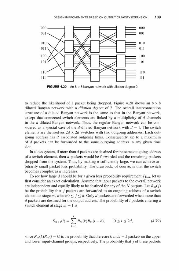
DESIGN IMPROVEMENTS BASED ON OUTPUT CAPACITY EXPANSION 139
010
001
100
011
000
111
110
101
010
001
100
011
000
111
110
101
FIGURE 4.20 An 8 × 8 banyan network with dilation degree 2.
to reduce the likelihood of a packet being dropped. Figure 4.20 shows an 8 × 8dilated Banyan network with a dilation degree of 2. The overall interconnectionstructure of a dilated-Banyan network is the same as that in the Banyan network,except that connected switch elements are linked by a multiplicity of d channelsin the d-dilated-Banyan network. Thus, the regular Banyan network can be con-sidered as a special case of the d-dilated-Banyan network with d = 1. The switchelements are themselves 2d × 2d switches with two outgoing addresses. Each out-going address has d associated outgoing links. Consequently, up to a maximumof d packets can be forwarded to the same outgoing address in any given timeslot.
In a loss system, if more than d packets are destined for the same outgoing addressof a switch element, then d packets would be forwarded and the remaining packetsdropped from the system. Thus, by making d sufficiently large, we can achieve ar-bitrarily small packet loss probability. The drawback, of course, is that the switchbecomes complex as d increases.
To see how large d should be for a given loss probability requirement Ploss, let usfirst consider an exact calculation. Assume that input packets to the overall networkare independent and equally likely to be destined for any of the N outputs. Let Rm(j)be the probability that j packets are forwarded to an outgoing address of a switchelement at stage m, where 0 ≤ j ≤ d. Only d packets are forwarded when more thand packets are destined for the output address. The probability of i packets entering aswitch element at stage m + 1 is
Sm+1(i) =i∑
k=0
Rm(k)Rm(i − k), 0 ≤ i ≤ 2d, (4.79)
since Rm(k)Rm(i − k) is the probability that there are k and i − k packets on the upperand lower input-channel groups, respectively. The probability that j of these packets

140 SWITCH PERFORMANCE ANALYSIS AND DESIGN IMPROVEMENTS
are destined for a particular output address is(
ij
)2−i. Thus,
Rm+1(j) ={∑2d
i=j Sm+1(i)(
ij
)2−i, if j < d,∑2d
i=d Sm+1(i)∑i
k=d
(ik
)2−i, if j = d.
(4.80)
With the initial condition
R0(j) =
⎧⎪⎨⎪⎩
1 − ρo, if j = 0,
ρo, if j = 1,
0, if j > 1,
where ρo is the offered load, Rn(j) can be found recursively. The packet loss proba-bility for the overall switch is simply
Ploss = 1 −∑d
j=0 jRn(j)
ρo, (4.81)
where n = log2 N.The above is not a closed-form result and it does not relate Ploss to n, d, and ρo
explicitly. The approximate analysis below will be used to study how dilation degreed is related to n for given Ploss and ρo.
There are two groups of d incoming links for each switch element. Strictly speak-ing, the links belonging to the same group are not independent in the sense that findinga packet on one link is correlated with finding packets on other links. For analyticaltractability, however, we will make the simplifying assumption that the input ports areindependent. Let Pm denote the probability that there is a packet at an input channel ofa switch element at stage m + 1. With the independence assumption, the probabilityof finding a packet at an arbitrary outgoing link of this switch element (or an incominglink of a switch element in the m + 2 stage ) is
Pm+1 = 1
d
{d∑
k=1
k
(2d
k
)(Pm
2
)k (1 − Pm
2
)2d−k
+ d
2d∑k=d+1
(2d
k
)(Pm
2
)k (1 − Pm
2
)2d−k}
= Pm − 1
d
2d∑k=d+1
(k − d)
(2d
k
)(Pm
2
)k (1 − Pm
2
)2d−k
. (4.82)

DESIGN IMPROVEMENTS BASED ON OUTPUT CAPACITY EXPANSION 141
The complexity of the dilated Banyan network can be estimated from the packet lossprobability for a switch element at stage m given by
Qm = 1 − Pm
Pm−1
= 1
Pm−1d
2d∑k=d+1
(k − d)
(2d
k
)(Pm−1
2
)k (1 − Pm−1
2
)2d−k
, m > log2 d.
(4.83)
We limit the application of the above formula to m > log2 d because it can be seenfrom the structure of the switch that Qm = 0 for m ≤ log d: there can be no morethan d/2 packets at each input group of switch elements at stages 1 through log d;that is, even under full loading conditions, when all input ports of the overall networkhave a packet, it takes at least log d + 1 stages before contentions between packetsmay occur.
It is easy to see from (4.82) that Pm decreases monotonically with m. Intuitively,the loss probability Qm also decreases monotonically with m:
Q1 ≥ · · · ≥ Qn. (4.84)
The above monotonic sequence is easy to interpret: As we progress through the stagesof the network and as packets are dropped due to contention, fewer and fewer packetsare left. This means the contention level is lighter in the later stages and therefore Qm
decreases as m increases. Problem 4.24 derives (4.84) formally.In the following, all logarithms are taken to the base two unless otherwise noted:
log = log2. The loss probability Ploss can be bounded from above as follows:
Ploss = P0 − Pn
P0
= (P0 − P1) + (P1 − P2) + · · · + (Pn−1 − Pn)
P0
= Q1 + Q2P1
P0+ · · · + Qlog d
Plog d−1
P0+ Qlog d+1
Plog d
P0+ · · · + Qn
Pn−1
P0
≤ (n − log d) Qlog d+1, (4.85)
where the last line is obtained by observing that Q1 = Q2 = · · · = Qlogd= 0 and
that Qm and Pm decrease monotonically with m. This is basically a union bound(i.e., the overall loss probability is upper-bounded by the sum of loss probabilities atdifferent stages), which is likely to be very good when Ploss (and therefore Qm) is

142 SWITCH PERFORMANCE ANALYSIS AND DESIGN IMPROVEMENTS
small. To find a bound for Qlog d+1, substituting Plog d = ρo/d into (4.83) gives
Qlog d+1 = 1
ρo
2d∑j=d+1
(j − d)
(2d
j
)(ρo
2d
)j (1 − ρo
2d
)2d−j
= (ρo/2d)d
ρo
d∑i=1
i
(2d
i + d
)(ρo
2d
)i (1 − ρo
2d
)d−i
, (4.86)
where we have made the index change i = j − d. Now,
(2d
i + d
)=
(2d
d
)(d
i
)× d! i!
(i + d)!=
(2d
d
)(d
i
)× i
i + d
i − 1
i − 1 + d× · · ·
× 1
1 + d≤
(2d
d
)(d
i
)2−i for i ≤ d.
Substituting the above into (4.86) and simplifying by Stirling’s formula
n! = nne−n√
2πn(1 + ε(n)), (4.87)
where ε(n) > 0 is a decreasing function of n, we get
Qlog d+1 ≤ 1
4
(ρo
d
)d (1 − ρo
4d
)d−1 2d
√πd
.
Thus,
Ploss ≤ (n − log d)1
4
(ρo
d
)d (1 − ρo
4d
)d−1 2d
√πd
. (4.88)
To get a lower bound for Ploss, continuing from the first line of (4.85), we have
Ploss ≥ Pn
P0(Qlog d+1 + Qlog d+2 + · · · + Qn)
≥ (1 − Ploss)(n − log d)Qn. (4.89)
From (4.83) and with the index change i = k − d, we obtain
Qn = (Pn−1/2)d
Pn−1d
d∑i=1
i
(2d
i + d
)(Pn−1
2
)i (1 − Pn−1
2
)d−i
. (4.90)
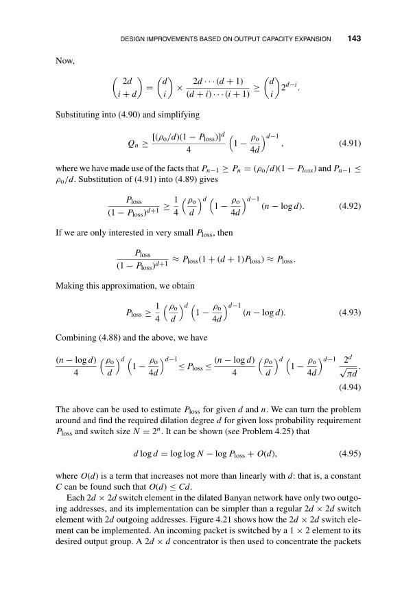
DESIGN IMPROVEMENTS BASED ON OUTPUT CAPACITY EXPANSION 143
Now, (2d
i + d
)=
(d
i
)× 2d · · · (d + 1)
(d + i) · · · (i + 1)≥
(d
i
)2d−i.
Substituting into (4.90) and simplifying
Qn ≥ [(ρo/d)(1 − Ploss)]d
4
(1 − ρo
4d
)d−1, (4.91)
where we have made use of the facts that Pn−1 ≥ Pn = (ρo/d)(1 − Ploss) and Pn−1 ≤ρo/d. Substitution of (4.91) into (4.89) gives
Ploss
(1 − Ploss)d+1 ≥ 1
4
(ρo
d
)d (1 − ρo
4d
)d−1(n − log d). (4.92)
If we are only interested in very small Ploss, then
Ploss
(1 − Ploss)d+1 ≈ Ploss(1 + (d + 1)Ploss) ≈ Ploss.
Making this approximation, we obtain
Ploss ≥ 1
4
(ρo
d
)d (1 − ρo
4d
)d−1(n − log d). (4.93)
Combining (4.88) and the above, we have
(n − log d)
4
(ρo
d
)d (1 − ρo
4d
)d−1≤ Ploss ≤ (n − log d)
4
(ρo
d
)d (1 − ρo
4d
)d−1 2d
√πd
.
(4.94)
The above can be used to estimate Ploss for given d and n. We can turn the problemaround and find the required dilation degree d for given loss probability requirementPloss and switch size N = 2n. It can be shown (see Problem 4.25) that
d log d = log log N − log Ploss + O(d), (4.95)
where O(d) is a term that increases not more than linearly with d: that is, a constantC can be found such that O(d) ≤ Cd.
Each 2d × 2d switch element in the dilated Banyan network have only two outgo-ing addresses, and its implementation can be simpler than a regular 2d × 2d switchelement with 2d outgoing addresses. Figure 4.21 shows how the 2d × 2d switch ele-ment can be implemented. An incoming packet is switched by a 1 × 2 element to itsdesired output group. A 2d × d concentrator is then used to concentrate the packets

144 SWITCH PERFORMANCE ANALYSIS AND DESIGN IMPROVEMENTS
2 d×d concentrator
2 d×d concentrator
Complexity~ O(d log d)
FIGURE 4.21 An implementation of 2d × 2d switch element with order of complexity d log d .
destined for the same group to d outgoing links. Excess packets are dropped if morethan d packets arrive for the same output group.
We have learned earlier in this chapter that the concentrator can be realized usinga running-adder address generator and a reverse Banyan network. The order of com-plexity is d log d. The order of complexity of each switch element is therefore d log d.Since there are altogether N
2 log N such switch elements, the overall dilated networkis of order N
2 log N × d log d. For large N, d log d is of order log log N, in terms of N.The dilated network is therefore of order N log N log log N. This order of complexityis less than those of the parallel Banyan network and Batcher–banyan network. How-ever, since order-of-complexity measure is meaningful only for large N, it cannot beargued that this network is simpler to implement in practice, especially if one consid-ers that for small d, it may not be worthwhile to use the running-adder-and-reversebanyan approach to build the 2d × 2d switch.
PROBLEMS
4.1 Consider a 2 × 2 switch operating as a waiting system. Each input has a queue.If the two packets at the heads of the queues are destined for the same output,one of them is chosen at random to be routed and the other will remain in thequeue. Consider the saturation situation in which there are always packets inthe queues. Draw a four-state Markov chain in which state (i, j) means that thepacket at the head of queue 1 is destined for output i and the packet at the headof queue 2 is destined for output j. Each transition corresponds to the passingof a time slot. Derive the maximum switch throughput.
4.2 Explain intuitively why input-buffered switches of smaller dimensions havehigher maximum throughput than those of larger dimensions when the packetson each input are equally likely to be destined for any of the outputs.
PROBLEMS 145
4.3 Consider two N × N internally nonblocking packet switches where N is verylarge. One is operated as a waiting system with very large input buffers andthe other is operated as a loss system without input buffers. For the former,packets are dropped when the input buffers overflow, and for the latter, packetsthat lost contention are dropped.(a) When the load is 0.5, which system has a lower packet loss probability?
How about when the load is 1?
(b) Roughly, what is the “transition point” for the load at which the relativeloss performance of the systems is reversed?
4.4 Consider an 8 × 8 input-buffered switch with nonuniform traffic distributions:Packets from inputs 1 to 4 are equally likely to be destined for outputs 1 to 4but none of them is destined for outputs 5 to 8. Similarly, packets from inputs5 to 8 are equally likely to be destined for outputs 5 to 8 but none of themis destined for outputs 1 to 4. Do you expect the maximum throughput to behigher or lower than the case in which packets from all inputs are equally likelyto be destined for all outputs. Explain.
4.5 Explain qualitatively why a switch operated as a loss system generally has ahigher maximum throughput than the same switch operated as a waiting system.For example, for an internally nonblocking switch, the maximum throughputis 0.632 for the former and 0.586 for the latter. Should we then operate allswitches as loss systems?
4.6 For a large input-buffered switch, we derived in the text that the average backlogin a fictitious queue is
C′(1) = 2ρ(1 − ρ) + ρ2
2(1 − ρ),
where ρ is the throughput.(a) Explain why C′(1) is between 0 and 1 in general.
(b) Show that the maximum throughput is indeed achieved when the inputqueue is saturated (i.e., when C′(1) = 1).
(c) Plot qualitatively the throughput ρ as a function of the offered load ρo forρo between 0 and 1. That is, ρo is the probability that a packet arrives atan input queue in a given time slot.
4.7 The text uses the normalization method to derive the expected length of a busyperiod equation (4.27). We now wish to derive it directly. Consider a longstretch of time from 0 to t.(a) Argue that the total amount of time the system is in busy periods is approx-
imately ρtS, and therefore, the total amount of idle time is approximatelyt − ρtS.
146 SWITCH PERFORMANCE ANALYSIS AND DESIGN IMPROVEMENTS
(b) Show that the average duration of idle periods is 11−Pr{K=0} , and there-
fore the total number of idle periods is approximately (t − ρtS)(1 −Pr{K = 0}).
(c) From (a) and (b) show that E[Y ] = Sρ
(1−Sρ)(1−Pr{K=0}).4.8 Prove the argument that gives rise to Eq. (4.35):
(a) Consider a Poisson process with rate ρ. Show that given that at least onepacket arrives, the probability that there are N other arrivals is still Poissonwith rate ρ (i.e., the arrivals of other packets are not affected by the arrivalof the packet of focus).
(b) Given that N is Poisson with rate ρ, show that if the N arrivals are randomlyplaced on a unit line, the number of arrivals placed before point t is Poissonwith rate ρt. (Hint: Find the conditional probability that L packets areplaced before t given that N packets arrive. Then uncondition on N.)
4.9 The text uses the busy-period method to arrive at the waiting time at an inputqueue of an input-buffered switch (Eqs. (4.31) and (4.32)). This problemconsiders the number of packets in the input queue upon the arrival of a newpacket. The mean waiting time W in (4.32) can then be obtained by Little’slaw.(a) Argue that the number of packets H found by an arriving packet (not
including the arriving packet) has the same probability distribution as thenumber of packets D left behind by a departing packet (not including thedeparting packet).
(b) Show that Dm+1 = max(0, Dm − 1) + Am+1, where Dm is the numberof packets left behind by the mth packet that departs from the system andAm is the number packets that arrive during its service time.
(c) Derive D(z) from the above and obtain D from it.
(d) Argue that the number of packets found by an arriving packet has the sameprobability distribution as the number of packets found by an arbitraryobserver at arbitrary time. Use Little’s law to obtain the average waitingtime from D (i.e., derive (4.32)).
4.10 Let us consider an alternative derivation of the first and second moments ofthe service time of an input queue (Eqs. (4.37) and (4.38)). Let B be thenumber of packets found by an arriving packet to the fictitious queue and L bethe number of simultaneously arriving packets scheduled to be served beforethe arriving packet.(a) Show that S = B + L + 1.
(b) Express S and S(S − 1) in terms of the moments of B and L.
(c) Find B(z) in terms of A(z) = e(z−1)ρ, the moment-generating function ofthe arrival process. (Hint: See Eqs. (4.12) and (4.13).)
(d) Find the moments of B and L, and express S and S(S − 1) in terms ofonly ρ.

PROBLEMS 147
4.11 True or false? The look-ahead contention-resolution scheme in the input-buffered switch cannot maintain the sequence order of the cells of apoint-to-point VC because the packets in the input queues may not be servedin a first-in-first-out fashion.
4.12 For the input-buffered switch operated with a look-ahead scheme with windowsize w (see the last few paragraphs of Section 4.1.2):(a) Argue that if the input queues have infinite amounts of buffer, as w → ∞,
the maximum throughput approaches 1.
(b) Show that the average delay of the input-window scheme can never besmaller than that in the ideal output-buffered switch of Section 4.1.4.(Hint: Consider the packet backlog and use Little’s law.)
4.13 Consider the following analytical derivation of the maximum throughput ofan input-buffered switch with a look-ahead window size of w = 2. Undersaturation, since we are considering the first two packets from each inputqueue, the average number of packets in the fictitious queue of a particularoutput is C′(1) = 2. Substituting this into the formula that relates C′(1) to
the throughput from the analysis of the fictitious queue, C′(1) = (2ρ−ρ2)2(1−ρ) ,
and solving for ρ, we get ρ = 3 − √(5) = 0.76, which is different from the
simulation result of 0.70. Give an example showing how the above argumentfails to reflect the real situation in the look-ahead scheme.
4.14 Consider a three-phase Batcher–banyan switch with a look-ahead contention-resolution scheme. With reference to the maximum throughputs given in Table4.2 (these throughputs do not take into account the contention-resolutionoverhead), for what value of w is the throughput maximized for a 32 × 32switch if the contention-resolution overhead is taken into consideration.Assume a packet size of 53 bytes plus 6 bits (5 bits for output address and 1bit for activity bit), and assume that checking of conflict at the outputs of thesorting network takes one-bit time and the backpropagating acknowledgmentstake one-bit time.
4.15 Consider an improved input look-ahead scheme. For an input queue, if the firstpacket loses contention in the first round, the second packet will be examinedin the second round. However, if its output address is the same as that of thefirst packet, we proceed immediately to the third packet (since the output hasbeen taken by a packet at another input during the first-round contention), andso on until a packet with a different output address is found. Thus, we canbe sure that the packets presented by an input for contention in the w roundshave distinct addresses.(a) Describe qualitatively why you expect to see improvement over the look-
ahead scheme described in the text. Do you expect much improvement ifsuccessive packets are independent and the switch size N is large? Whatif the output addresses of successive packets are strongly correlated andlikely to be the same?
148 SWITCH PERFORMANCE ANALYSIS AND DESIGN IMPROVEMENTS
(b) What is wrong with the following analysis? Assume N is very large andall packets are independent. Let ρ∗ = 0.586 be the maximum throughputwhen w = 1. When w = 2, after the first round, a set of outputs have beenassigned to a set of inputs, and the fraction of remaining inputs and outputsis approximately 1 − ρ∗. It is as if we have a smaller N(1 − ρ∗) × N(1 −ρ∗) switch in the second round. Therefore, the additional throughput ob-tained with the second-round contention is (1 − ρ∗)ρ∗. Arguing this way,the total throughput in general is ρ∗ + (1 − ρ∗)ρ∗ + · · · + (1 − ρ∗)w−1ρ∗.
4.16 Which switch has the better delay performance when the input offered loadis 0.2?
1. The generic nonblocking input-buffered (with no speedup, no look-ahead,etc.) where queueing delay is incurred only at the inputs.
2. The generic nonblocking output-buffered switch in which all incomingpackets are immediately forwarded to their desired outputs and queuedthere.
4.17 Consider the packet-slicing switch design (see Fig. 4.11(b)). Suppose thatthe switch is 256 × 256 and the packet size is 53 bytes not including theoutput-address header. If a speedup factor of 8 is to be achieved, what is theratio of switch cycle to time slot?
4.18 Consider an 8 × 8 channel-grouped Batcher–banyan switch with R = 2.Suppose that the three-phase contention-resolution scheme is adopted. Drawdiagrams showing how the following set of packets will be routed through theswitch: (0, 1), (2, 4), (4, 2), (5, 1), (6, 2), (7, 1), where (i, j) means a packetat input i destined for output j. Do not show the inside of the Batcher andbanyan networks. Only show the positions of the packets at the inputs andoutputs of the networks.
4.19 Show how to build an N × M expansion Batcher–banyan switch, whereM = NK > N, K an integer, using an N × N Batcher network and anexpansion banyan structure similar to that of Fig. 4.13. There is no channelgrouping and each of the M outputs corresponds to a distinct address. Showhow the routing is done and argue that the switch is internally nonblocking.
4.20 Consider an N × MR switch operating as a channel-grouped waiting system.There are M output addresses, and a group of R output ports belong to thesame address. Rank these switches according to their maximum through-puts per input: (i) N = 16, M = 16, R = 2; (ii) N = 16, M = 16, R = 1;(iii) N = 16, M = 8, R = 2; (iv) N = 8, M = 8, R = 2.
4.21 This problem shows how to derive Eq. (4.60) from Eq. (4.59) in the text. FromEq. (4.59), we have C(z) = N(z)/D(z), where D(z) = zRA−1(z) − 1 andN(z) = ∑R−1
k=0 (zR − zk) Pr{C = k}. The text argues that N(z) can be writtenalternatively as N(z) = K(z − 1)(z − z1(ρ)) · · · (z − zR−1(ρ)), where zk(ρ) isthe (R − 1) complex roots of zR − A(z) with modulus less than 1.

PROBLEMS 149
(a) Show that D(1) = N(1) = 0.
(b) By differentiating the left and right sides of D(z)C(z) = N(z) once, showthat D′(1) = N ′(1). From this, show that K = (R − ρ)/
∏R−1i=1 (1 − zi(ρ)).
(c) By differentiating D(z)C(z) = N(z), show that C′(1) = (N ′′(1) −D′′(1))/2D′(1).
(d) Find N ′′(1), D′′(1), and D′(1) to substitute into the above to deriveEq. (4.60).
4.22 Find the mean delay at an input queue of a channel-grouped waiting systemin which R = 2 and ρ = 0.8.
4.23 For an 8 × 8 Batcher–banyan knockout switch with R = 2 (as the one depictedin Fig. 4.15), draw diagrams showing how the following set of packets willbe routed through the switch: (0, 1), (2, 4), (4, 2), (5, 1), (6, 2), (7, 1), where(i, j) means a packet at input i destined for output j. Do not show the insideof the Batcher and banyan networks, but show how the running-adder addressgenerator, including its internal operations, and the reverse banyan networkare used to concentrate the packets.
4.24 We want to derive (4.84). First, rewrite (4.82) in the form Pm+1 =Pm − 1
df (Pm), where f (x) = ∑2d
k=d+1(k − d)(2d
k
)( x
2 )k(1 − x2 )2d−k.
(a) Show that f (x) increases monotonically with x for 0 ≤ x ≤ 1.
(b) Show that Qm+1 − Qm = (P2m − Pm+1Pm−1)/Pm−1Pm ≤ 0.
4.25 Derive (4.95) as follows:(a) Taking logarithms on both sides of (4.88), show that
log n − log Ploss ≥ d log d + f (d),
where
f (d) = 2 − d log ρo − d − 1
2log π + 1
2log d.
(b) Taking logarithms on both sides of (4.93), show that
log Ploss − (d + 1) log(1 − Ploss) ≥ log n + log
(1 − log d
n
)− 2
+ d log ρo − d log d + (d − 1) log(
1 − ρo
4d
)+ d.
From
(d − 1) log(
1 − ρo
4d
)≥ (d − 1) log
(1 − ρo
4
)
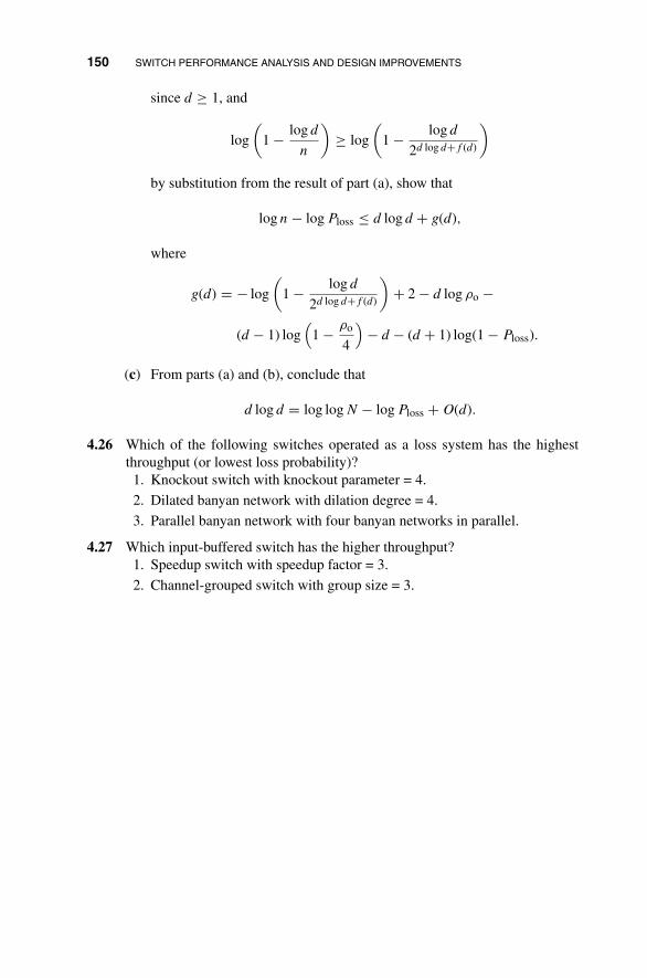
150 SWITCH PERFORMANCE ANALYSIS AND DESIGN IMPROVEMENTS
since d ≥ 1, and
log
(1 − log d
n
)≥ log
(1 − log d
2d log d+f (d)
)
by substitution from the result of part (a), show that
log n − log Ploss ≤ d log d + g(d),
where
g(d) = − log
(1 − log d
2d log d+f (d)
)+ 2 − d log ρo −
(d − 1) log(
1 − ρo
4
)− d − (d + 1) log(1 − Ploss).
(c) From parts (a) and (b), conclude that
d log d = log log N − log Ploss + O(d).
4.26 Which of the following switches operated as a loss system has the highestthroughput (or lowest loss probability)?
1. Knockout switch with knockout parameter = 4.
2. Dilated banyan network with dilation degree = 4.
3. Parallel banyan network with four banyan networks in parallel.
4.27 Which input-buffered switch has the higher throughput?1. Speedup switch with speedup factor = 3.
2. Channel-grouped switch with group size = 3.

5
ADVANCED SWITCH DESIGNPRINCIPLES
The preceding chapter has introduced various basic switch design principles to solvepacket contention problem. In this chapters, we shall first present some advanceswitch design principles to further alleviate this problem. We shall see that despitethese advanced switch designs, switch dimensions continue to be severely limitedby both technological and physical constraints. We close this chapter by providingsome key principles to construct large switches out of modest-size switches, withoutsacrificing overall switch performance.
5.1 SWITCH DESIGN PRINCIPLES BASED ONDEFLECTION ROUTING
One way to solve the packet contention problem without having to buffer the losingpackets is to use deflection routing. The basic idea is to route (deflect) the losingpackets to “wrong” outgoing links rather than drop them. Redundancy is built intothe switch design so that deflected packets can be routed in later switching stages ina way that corrects the earlier mistakes.
5.1.1 Tandem-Banyan Network
The tandem-Banyan switching network consists of K Banyan networks connected inseries (see Fig. 5.1). Except for the last Banyan network, each output of a Banyannetwork is connected to both an input of the subsequent Banyan network and a con-centrator (statistical multiplexer). With this setup, a packet would be routed to theconcentrator if it reaches the correct output, and to the subsequent Banyan networkotherwise. Thus, each packet can have up to K attempts to reach its destined output.
Principles of Broadband Switching and Networking, by Tony T. Lee and Soung C. LiewCopyright © 2010 John Wiley & Sons, Inc.
151
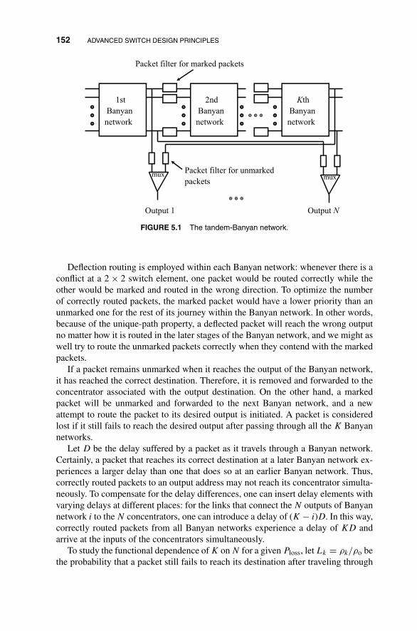
152 ADVANCED SWITCH DESIGN PRINCIPLES
mux mux
1st
Banyan
network
2nd
Banyan
network
Kth
Banyan
network
Packet filter for marked packets
Packet filter for unmarked
packets
Output 1 Output N
FIGURE 5.1 The tandem-Banyan network.
Deflection routing is employed within each Banyan network: whenever there is aconflict at a 2 × 2 switch element, one packet would be routed correctly while theother would be marked and routed in the wrong direction. To optimize the numberof correctly routed packets, the marked packet would have a lower priority than anunmarked one for the rest of its journey within the Banyan network. In other words,because of the unique-path property, a deflected packet will reach the wrong outputno matter how it is routed in the later stages of the Banyan network, and we might aswell try to route the unmarked packets correctly when they contend with the markedpackets.
If a packet remains unmarked when it reaches the output of the Banyan network,it has reached the correct destination. Therefore, it is removed and forwarded to theconcentrator associated with the output destination. On the other hand, a markedpacket will be unmarked and forwarded to the next Banyan network, and a newattempt to route the packet to its desired output is initiated. A packet is consideredlost if it still fails to reach the desired output after passing through all the K Banyannetworks.
Let D be the delay suffered by a packet as it travels through a Banyan network.Certainly, a packet that reaches its correct destination at a later Banyan network ex-periences a larger delay than one that does so at an earlier Banyan network. Thus,correctly routed packets to an output address may not reach its concentrator simulta-neously. To compensate for the delay differences, one can insert delay elements withvarying delays at different places: for the links that connect the N outputs of Banyannetwork i to the N concentrators, one can introduce a delay of (K − i)D. In this way,correctly routed packets from all Banyan networks experience a delay of KD andarrive at the inputs of the concentrators simultaneously.
To study the functional dependence of K on N for a given Ploss, let Lk = ρk/ρo bethe probability that a packet still fails to reach its destination after traveling through

SWITCH DESIGN PRINCIPLES BASED ON DEFLECTION ROUTING 153
(k+1)th
Banyan
network
(k+2)th
Banyan
network
MUX
ρkρk+1
ρk = ρk+1 + ρck+1
ρck+1
FIGURE 5.2 Relationship between the offered load �k , carried load �ck+1, and rejected load
�k+1 of the (k + 1) Banyan network in a tandem-Banyan network.
k Banyan networks, where ρo is the initial offered load and ρk is the offered load tothe input of (k + 1)th Banyan network, and let ρc
k be the carried load on each outputof the kth Banyan network (see Fig. 5.2). It follows that
ρk+1 = ρk − ρck+1 ≈ ρk − 4ρk
nρk + 4= nρk
2
nρk + 4. (5.1)
We then immediately have the recursive formula for the loss probability of a tandem-Banyan switch with k + 1 Banyan networks:
Lk+1 = (ρk+1/ρo) = nρo(ρk/ρo)2
nρo(ρk/ρo) + 4= aL2
k
aLk + 4, (5.2)
where a = ρon = ρo log N. From the above,
Lk+1 − Lk = −4Lk
aLk + 4. (5.3)
Using the Taylor series approximation technique introduced earlier, we can transformthe above difference equation into the following differential equation:
dLk
dk= −4Lk
aLk + 4.
Integration and matching of the boundary conditions, L0 = 1 and LK = Ploss,gives
K = ρo log N
4(1 − Ploss) − ln Ploss. (5.4)
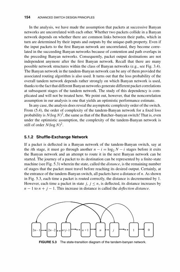
154 ADVANCED SWITCH DESIGN PRINCIPLES
In the analysis, we have made the assumption that packets at successive Banyannetworks are uncorrelated with each other. Whether two packets collide in a Banyannetwork depends on whether there are common links between their paths, which inturn are determined by their inputs and outputs by the unique-path property. Even ifthe input packets to the first Banyan network are uncorrelated, they become corre-lated in the succeeding Banyan networks because of contention and path overlaps inthe preceding Banyan networks. Consequently, packet output destinations are notindependent anymore after the first Banyan network. Recall that there are manypossible network structures within the class of Banyan networks (e.g., see Fig. 3.4).The Banyan network in the tandem-Banyan network can be any of them provided theassociated routing algorithm is also used. It turns out that the loss probability of theoverall tandem network depends rather strongly on which Banyan network is used,thanks to the fact that different Banyan networks generate different packet correlationsat subsequent stages of the tandem network. The study of this dependency is com-plicated and will not be treated here. We point out, however, that the noncorrelationassumption in our analysis is one that yields an optimistic performance estimate.
In any case, the analysis does reveal the asymptotic complexity order of the switch.From (5.4), the order of complexity of the tandem-Banyan network for a fixed lossprobability is N(log N)2, the same as that of the Batcher–banyan switch! That is, evenunder the optimistic assumption, the complexity of the tandem-Banyan network isstill of order N(log N)2.
5.1.2 Shuffle-Exchange Network
If a packet is deflected in a Banyan network of the tandem-Banyan switch, say atthe ith stage, it must go through another n − i = log2 N − i stages before it exitsthe Banyan network and an attempt to route it in the next Banyan network can bestarted. The journey of a packet to its destination can be represented by a finite-statemachine (see Fig. 5.3) wherein the state, called the distance, is the remaining numberof stages that the packet must travel before reaching its desired output. Certainly, atthe entrance of the tandem-Banyan switch, all packets have a distance of n. As shownin Fig. 5.3, each time a packet is routed correctly, the distance is decremented by 1.However, each time a packet in state j, j ≤ n, is deflected, its distance increases byn − 1 to n + j − 1. This increase in distance is called the deflection distance.
2n – 1 2n –2 n+j–1 n +1 jn 1 0
FIGURE 5.3 The state-transition diagram of the tandem-banyan network.

SWITCH DESIGN PRINCIPLES BASED ON DEFLECTION ROUTING 155
n–1n 1j 0
FIGURE 5.4 The state-transition diagram of the shuffle-exchange network.
The number of Banyan networks required to meet a Ploss requirement, hence theswitch complexity, is closely related to the number of steps required for a packetto reach its destinations in the finite-state machine model. The number of steps is arandom variable depending on the number of deflections and the deflection penalties.With K Banyan networks in the tandem structure, a packet must reach its destinationwithin Kn steps, or else it will be dropped. Thus, minimizing deflection distance hasthe effect of decreasing the packet loss probability. By the same token, for a fixedloss probability requirement, minimizing deflection distance reduces the number ofBanyan networks required, hence the switch complexity.
A question one might raise is whether attempts can be made immediately upondeflections to route packets to their destinations rather than having to waste j − 1more steps in the current Banyan network. In other words, can one realize a finite-state machine model depicted in Fig. 4.18 wherein each deflection sets the distanceof the packet back to n rather than n + j − 1? This requires the stages in the Banyannetwork to be homogeneous and leads us to the shuffle-exchange network introducedin Chapter 3 (see Fig. 3.4).
We mentioned in Chapter 3 that the regular shuffle-exchange network with n stagesis isomorphic to the banyan network without a formal proof. To show that the samerouting mechanism applies and to introduce some key concepts and notation, let usfirst consider the structure of a single stage, shown in Fig. 5.5.
000
001
010
011
100
101
110
111
000
001
010
011
100
101
110
111
Perfect shuffle Perfect shuffle + exchange
Packet on link x x3 2 x1 x2 x1 x3Packet on link x x3 2 x1 x2 x1 d3
d3 = routing bit
FIGURE 5.5 Algebraic operations of shuffle and exchange.

156 ADVANCED SWITCH DESIGN PRINCIPLES
The term “shuffle” refers to the way adjacent switch stages are interconnected: itis analogous to the shuffling of a deck of cards. Suppose we take the top and bottomhalves of a deck of cards and merge them by taking cards one by one alternately fromthe two halves from top to bottom. We are said to have performed a “perfect shuffle.”Imagine a deck of N cards riding on the outgoing links of a switch stage, one oneach link. These cards “travel” to the incoming links of the next stage through theinterconnection. It can be easily seen from Fig. 5.5 that the interconnection performsa perfect shuffle on the cards.
What is interesting from the switching viewpoint is that perfect shuffle achieves acyclic left shift of the link label. Let us label the links from top to bottom in a binaryfashion. Thus, the top link is 00 · · · 0 and the bottom link is 11 · · · 1. It can be shownthat (or verified from the example in Fig. 5.5) outgoing link xnxn−1 · · · x1 of a stage isconnected to incoming link xn−1 · · · x1xn of the next stage. In other words, a packeton link xnxn−1 · · · x1 occupies link xn−1 · · · x1xn after the shuffle.
The term “exchange” refers to the operation performed by 2 × 2 switch elements.Let us label the 2 × 2 switch elements in any stage with (n − 1)-bit binary numbers.The two incoming, as well as the two outgoing, links connected to switch elementxn−1 · · · x1 are labeled xn−1 · · · x10 and xn−1 · · · x11. The 2 × 2 switch element for-wards an input packet to output link xn−1 · · · x10 if the routing bit is 0 and to linkxn−1 · · · x11 if the routing bit is 1. In other words, the switch element exchangesthe least significant bit of the link label with the routing bit. Thus, if the incom-ing link occupied by a packet is xn−1 · · · x1xn at a switching stage and dn is therouting bit, then the packet will occupy link xn−1 · · · x1dn at the output of the stage(see Fig. 5.5).
The algebraic operations of the shuffling and switching stages provide us witha way to understand why the overall routing mechanism works. Let the source anddestination addresses of a packet be S = sn · · · s1 and D = dn · · · d1, respectively.The destination address will be used for routing starting from the most significant bitto the least significant bit. Initially, the packet occupies link sn · · · s1 at the entranceto the shuffle-exchange network. After the first shuffle, its link label is sn−1 · · · s1snat the input to the first-stage switching node. Bit dn is used to switch this packetto outgoing link sn−1 · · · s1dn. We see that sn has been replaced by dn. By anothershuffle and exchange, the packet then occupies link sn−2 · · · s1dndn−1 at the output ofthe next stage. Repeating this process, we see that the output links of the successiveswitching stages traversed by a packet are
S = sn · · · s1 → sn−1 · · · s1dn → · · · (5.5)
→ sn−i · · · s1dn · · · dn−i+1 → · · · (5.6)
→ dn · · · d1 = D. (5.7)
In other words, the sequence of links is embedded in the binary string sn · · · s1dn · · · d1and can be revealed by an n-bit window moving one bit per stage from left to right.After the last step, the packet reaches link dn · · · d1, which is the desired destination.In this way, bit by bit, the packet is routed to its targeted output. Figure 5.6 gives anexample of how a packet is routed in an 8 × 8 regular shuffle-exchange network.

SWITCH DESIGN PRINCIPLES BASED ON DEFLECTION ROUTING 157
00
01
10
11
00
01
10
11
00
01
10
11
101
101
101
101
ith bit of destination address used for routing at
ith stage
Sliding window routing: packet with source–destination
label sn…sn–i…s1dn…dn–i+1…d1 occupies
link sn–i…s1dn…dn–i+1…d1 after stage i
FIGURE 5.6 Routing in shuffle-exchange network.
The above describes the route traversed by a packet when there is no contentionfrom other packets. When deflection routing is used to tackle the contention problem,instead of a regular shuffle-exchange network with n stages, we have an elongatedshuffle-exchange network with L ≥ n stages, as depicted in Fig. 5.7. As discussed
00
01
10
11
00
01
10
11
00
01
10
11
00
01
10
11
00
01
10
11
000
001
010
011
100
101
110
111
000
001
010
011
100
101
110
111
101
101
101
101
100
100
100
100
100
100
101Packet A Packet B 100 Bypass
B deflectedA reaches
destination
100 100 100 100 100
Routing bit used by B at each stage
FIGURE 5.7 A shuffle-exchange network with n = 3 and L = 5.
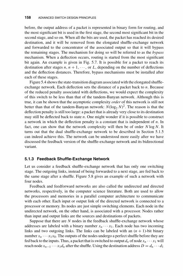
158 ADVANCED SWITCH DESIGN PRINCIPLES
before, the output address of a packet is represented in binary form for routing, andthe most significant bit is used in the first stage, the second most significant bit in thesecond stage, and so on. When all the bits are used, the packet has reached its desireddestination, and it will be removed from the elongated shuffle-exchange networkand forwarded to the concentrator of the associated output so that it will bypassthe remaining stages. The mechanism for doing so will be referred to as the bypassmechanism. When a deflection occurs, routing is started from the most significantbit again. An example is given in Fig. 5.7. It is possible for a packet to reach itsdestination after stages n, n + 1, · · · , or L, depending on the number of deflectionsand the deflection distances. Therefore, bypass mechanisms must be installed aftereach of these stages.
Figure 5.4 shows the state-transition diagram associated with the elongated shuffle-exchange network. Each deflection sets the distance of a packet back to n. Becauseof the reduced penalty associated with deflections, we would expect the complexityof this switch to be less than that of the tandem-Banyan network. Although this istrue, it can be shown that the asymptotic complexity order of this network is still notbetter than that of the tandem-Banyan network: N(log2 N)2. The reason is that thedeflection penalty is still too large: a packet that is already very close to its destinationmay still be deflected back to state n. One might wonder if it is possible to constructa network in which the deflection penalty is a constant that is independent of n. Infact, one can show that the network complexity will then be of order N log N. Itturns out that the dual shuffle-exchange network to be described in Section 5.1.5can indeed achieve this. The network can be understood more easily after we havediscussed the feedback version of the shuffle-exchange network and its bidirectionalvariant.
5.1.3 Feedback Shuffle-Exchange Network
Let us consider a feedback shuffle-exchange network that has only one switchingstage. The outgoing links, instead of being forwarded to a next stage, are fed back tothe same stage after a shuffle. Figure 5.8 gives an example of such a network withfour nodes.
Feedback and feedforward networks are also called the undirected and directednetworks, respectively, in the computer science literature. Both are used to allowthe processors and memories in a parallel computer architecture to communicatewith each other. Each input or output link of the directed network is connected to aprocessor or memory. Its nodes are just simple switching elements. Each node in theundirected network, on the other hand, is associated with a processor. Nodes ratherthan input and output links are the sources and destinations of packets.
Suppose that there are N nodes in the feedback shuffle-exchange network whoseaddresses are labeled with a binary number xn · · · x1. Each node has two incominglinks and two outgoing links. The links can be labeled with an (n + 1)-bit binarynumber xn · · · x1x0. The outputs of the nodes undergo a perfect shuffle before they arefed back to the inputs. Thus, a packet that is switched to output dn of node xn · · · x1 willreach node xn−1 · · · x1dn after the shuffle. Using the destination address D = dn · · · d1

SWITCH DESIGN PRINCIPLES BASED ON DEFLECTION ROUTING 159
00
01
10
11
0
1
0
1
0
1
0
1
FIGURE 5.8 A four-node feedback shuffle network.
as the routing tag, a packet will reach its destination node after n undeflected steps.From this, we see that the operation of the feedback network is similar to that in thefeedforward network.
Notice, however, that whereas the design issue in the feedforward network is thenumber of stages L required to meet a loss probability requirement, the situationhere is slightly different in that a packet can be routed indefinitely until it reachesits destination node: packet loss probability due to contention is zero! Moreover, thenumber of stage is fixed at one. Is there some magic going on here? The answer iswe have not gained something for nothing. It turns out that the performance issue inthe feedback network is throughput rather than packet loss. Whereas the maximumthroughput per input or output of the feedforward network is close to one when theloss probability is small, which can be achieved by having a sufficient number ofstages, the fact that there is only one stage in the feedback network severely limitsthe network throughput when N is large. We shall derive this throughput limitationanalytically later in this subsection.
Recall that with the multistage feedforward shuffle-exchange network, a nodeforwards a packet to the next stage as soon as it has received enough bits of the headerfor it to make the switching decision. It is not necessary to wait for the arrival of theentire packet.1 With the feedback version of the network, because of the feedbackloop, the information bits of the previous packets are still being transmitted at theoutputs when their headers arrive at the inputs of the nodes. Therefore, the arrivingpackets must wait until all the bits of the previous packets have been transmittedbefore they can be forwarded to the outputs. As shown in Fig. 5.9, a one-packet bufferis located at each input link of a node to buffer the arriving packet while it waits for
1This is sometimes called virtual cut-through routing.
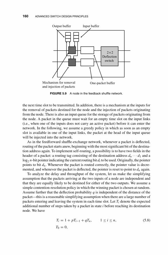
160 ADVANCED SWITCH DESIGN PRINCIPLES
Output buffer Input buffer
2× 2
Deflection
switch
Mechanism for removal
and injection of packetsOne-packet buffer
FIGURE 5.9 A node in the feedback shuffle network.
the next time slot to be transmitted. In addition, there is a mechanism at the inputs forthe removal of packets destined for the node and the injection of packets originatingfrom the node. There is also an input queue for the storage of packets originating fromthe node. A packet in the queue must wait for an empty time slot on the input links(i.e., when one of the inputs does not carry an active packet) before it can enter thenetwork. In the following, we assume a greedy policy in which as soon as an emptyslot is available in one of the input links, the packet at the head of the input queuewill be injected into the network.
As in the feedforward shuffle-exchange network, whenever a packet is deflected,routing of the packet starts anew, beginning with the most significant bit of the destina-tion address again. To implement self-routing, a possibility is to have two fields in theheader of a packet: a routing tag consisting of the destination address dn · · · d1 and alog2 n-bit pointer indicating the current routing bit di to be used. Originally, the pointerpoints to bit dn. Whenever the packet is routed correctly, the pointer value is decre-mented, and whenever the packet is deflected, the pointer is reset to point to dn again.
To analyze the delay and throughput of the system, let us make the simplifyingassumption that the packets arriving at the two inputs of a node are independent andthat they are equally likely to be destined for either of the two outputs. We assume asimple contention-resolution policy in which the winning packet is chosen at random.Assume further that the deflection probability q is independent of the distance of thepacket—this is a reasonable simplifying assumption when there are a large number ofpackets entering and leaving the system in each time slot. Let Ti denote the expectedadditional number of steps taken by a packet in state i before reaching its destinationnode. We have
Ti = 1 + pTi−1 + qTn, 1 ≤ i ≤ n, (5.8)
T0 = 0,
SWITCH DESIGN PRINCIPLES BASED ON DEFLECTION ROUTING 161
where p = (1 − q) is the probability of not being deflected. Equation (5.8) is a lineardifference equation in i. It is a well-established result that the general solution of a lin-ear difference equation is a constant times the homogeneous solution plus a particularsolution. The homogeneous solution to Ti − pTi−1 = 0 is Ti = pi and a particularsolution to Ti − pTi−1 = 1 + qTn is Ti = (1 + qTn)/(1 − p) = (1 + qTn)/q. There-fore, we have
Ti = cpi + 1 + qTn
q, (5.9)
where c is a constant to be found by matching the boundary condition. The boundarycondition T0 = 0 yields c = −(1 + qTn)/q. Thus,
Ti = (1 + Tn)(1 − pi)
q, 0 ≤ i ≤ n. (5.10)
Substituting i = n in the above, we get
Tn = 1 − pn
pnq. (5.11)
Substituting this into (5.9), we have
Ti = 1 − pi
pnq, 0 ≤ i ≤ n. (5.12)
Let ρ be the probability of finding a packet at an input link at the beginning ofa time slot; this is the link loading. Then, with probability ρ/2 an input packet willencounter a packet at the other input of the same node that desires the same output.Thus, with the random contention-resolution scheme, the packet will be deflectedwith probability q = ρ/4. The total throughput of the network � is given by Little’slaw:
� = Expected number of packets in the whole network
Expected packet delay
= 2Nρ
Tn
= 8Nq2pn
1 − pn
= 8N(ρ/4)2(1 − ρ/4)n
1 − (1 − ρ/4)n. (5.13)
It can be shown from the above equation that for n ≤ 4, � is maximum when ρ = 1.This is achieved when the input queues at the nodes are saturated so that as soon as apacket reaches its destination, a new packet is injected into the network. In this case,the maximum throughput of the system �max is equal to its saturation throughput
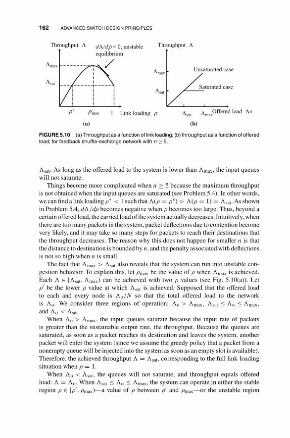
162 ADVANCED SWITCH DESIGN PRINCIPLES
Throughput Λ
Λmax
Λsat
Link loading ρ
(a)
dΛ/dρ < 0, unstable
equilibrium
ρ ′ ρmax 1
Throughput Λ
Λmax
Λsat
Offered load Λ0
(b)
Λsat Λmax
Unsaturated case
Saturated case
FIGURE 5.10 (a) Throughput as a function of link loading; (b) throughput as a function of offeredload; for feedback shuffle-exchange network with n ≥ 5.
�sat. As long as the offered load to the system is lower than �max, the input queueswill not saturate.
Things become more complicated when n ≥ 5 because the maximum throughputis not obtained when the input queues are saturated (see Problem 5.4). In other words,we can find a link loading ρ∗ < 1 such that �(ρ = ρ∗) > �(ρ = 1) = �sat. As shownin Problem 5.4, d�/dρ becomes negative when ρ becomes too large. Thus, beyond acertain offered load, the carried load of the system actually decreases. Intuitively, whenthere are too many packets in the system, packet deflections due to contention becomevery likely, and it may take so many steps for packets to reach their destinations thatthe throughput decreases. The reason why this does not happen for smaller n is thatthe distance to destination is bounded by n, and the penalty associated with deflectionsis not so high when n is small.
The fact that �max > �sat also reveals that the system can run into unstable con-gestion behavior. To explain this, let ρmax be the value of ρ when �max is achieved.Each � ∈ [�sat, �max) can be achieved with two ρ values (see Fig. 5.10(a)). Letρ′ be the lower ρ value at which �sat is achieved. Supposed that the offered loadto each and every node is �o/N so that the total offered load to the networkis �o. We consider three regions of operation: �o > �max, �sat ≤ �o ≤ �max,and �o < �sat.
When �o > �max, the input queues saturate because the input rate of packetsis greater than the sustainable output rate, the throughput. Because the queues aresaturated, as soon as a packet reaches its destination and leaves the system, anotherpacket will enter the system (since we assume the greedy policy that a packet from anonempty queue will be injected into the system as soon as an empty slot is available).Therefore, the achieved throughput � = �sat, corresponding to the full link-loadingsituation when ρ = 1.
When �o < �sat, the queues will not saturate, and throughput equals offeredload: � = �o. When �sat ≤ �o ≤ �max, the system can operate in either the stableregion ρ ∈ [ρ′, ρmax)—a value of ρ between ρ′ and ρmax—or the unstable region

SWITCH DESIGN PRINCIPLES BASED ON DEFLECTION ROUTING 163
ρ ∈ [ρmax, 1]. In the stable region, throughput equals offered load: � = �o. In theunstable region, as reasoned in the next paragraph, the system quickly evolves awayfrom the region, ending up either at ρ = 1 and � = �sat, the saturated case, or atρ ∈ [ρ′, ρmax) and � = �o, the unsaturated case.
The offered load is the average packet arrival rate to the input queues over a longtime period. Because of the statistical nature of packet arrivals and departures, thenumber of backlogged packets in the input queues varies over time. These backloggedpackets in turn determine the instantaneous or near-term offered load to the network.Therefore, the instantaneous offered load fluctuates over time in accordance to thebacklogged packets. Any increase in the number of nonempty input queues results inan increase in instantaneous offered load, which in turn raises the instantaneous linkloading ρ of the network. By the same token, decreasing instantaneous offered loadalso decreases instantaneous ρ. In the unstable region, since d�/dρ is negative, thethroughput decreases as a result of even a small increase in the instantaneous offeredload. Therefore, the throughput � becomes smaller than the offered load �o, andthe negative balance between packet arrival and departure rates further increases theinput-queue backlogs, resulting in an even higher instantaneous offered load. Thiscreates a positive feedback effect that eventually brings � down to �sat and the inputqueues are saturated. By the same token, in the unstable region any decrease in theinstantaneous offered load will quickly bring the system back to the stable pointat which � = �o through a positive feedback effect. Figure 5.10(b) shows � as afunction of �o. There is a bifurcation point at �o = �sat, and there are two operatingregions between �o = �sat and �o = �max.
If the system is unsaturated with �o ≥ �sat (hence ρ′ ≤ ρ < ρmax), there is still thedanger that the system will evolve to the unstable region and then become saturated.This can be caused by (1) a sudden increase in the number of packets arriving at theinput queues, or (2) a series of bad luck in which packets already in the network aredeflected more than the usual number of times so that there is a sudden increase in linkloading ρ to beyond ρmax. Once that happens, the system may become saturated veryquickly, making it impossible for the system to return to the original operating point.On the other hand, if �o < �sat (hence ρ < ρ′), the system will eventually evolveback to the stable region even when there is a temporary increase in the number ofpackets in the system. This is because the saturation throughput �sat can sustain theoffered load over the long term. Such is not the case, however, when �o ≥ �sat.In general, the system can only be safely operated at offered load below �sat eventhough the maximum throughput �max is higher. One can easily write a simulationcomputer program to verify this: when �o ∈ [�sat, �max], even if the throughput andthe offered load are balanced to begin with (� = �o), the system eventually evolvesto the saturation point � = �sat < �o.
In the unstable region, we have a typical network congestion scenario in whichhigher offered load brings about lower throughput and higher delay at the same time.Figure 5.10 also suggests that if some congestion control mechanism is exercised overthe system, offered load of up to �max may be sustainable without instability. Forinstance, we could introduce 2Nρmax tokens in the network. A packet is not allowedto enter the network until it has acquired a token from one of the input links, and
164 ADVANCED SWITCH DESIGN PRINCIPLES
the token will be released back to the network only when the packet has reached itsdestination. In this way, ρ is kept to be not more than ρmax. As with all networksoperated with token access, one has to deal with the possibility of lost tokens due totransmission errors or malfunctioning nodes.
Another strategy is to use a contention-resolution policy that is more efficientthan the random contention-resolution policy and it is hoped that it will reduce thedeflection penalty enough to stabilize the system. It turns out that an arbitration policythat favors packets closer to their destinations will stabilize the system. When a packetin state i is deflected back to state n, n − i + 1 previous routing steps are wasted. Theidea of favoring packets closer to their destinations is to minimize the amount ofrouting effort that is wasted given that deflection is inevitable.
The analysis of this strategy is more complicated because the deflection probabilityis state dependent. Instead of the uniform deflection probability q, we have qi for thedeflection probability at state i, 1 ≤ i ≤ n. Although tokens are not used in reality,we can still imagine for analytical purposes that there are 2N fictitious tokens, one oneach link, circulating around the network. A packet at an input queue must acquirean unused token before it can enter the network. A token is said to be active and instate i, 1 ≤ i ≤ n, if the packet it carries is in state i. A token is said to be inactive orin state 0 if it is unused.
We trace the evolution of the state of a particular token. Let P(i) be the probabilitythat the token is in state i at the beginning of a time slot. We have
P(i − 1) = P(i)(1 − qi), 2 ≤ i ≤ n. (5.14)
Define
π(i) = P(1) + · · · + P(i), 1 ≤ i ≤ n,
to be the probability of the token either in state 1, 2, · · ·, or i. By definition, theprobability of the token being active is π(n). An active token implies the link itoccupies is active. Since every link has a token on it at all time, the probability of anactive token must also be the probability of an active link. Thus,
π(n) = ρ.
Assume that when two packets of the same state contend with each other, the winningpacket will be chosen at random. The probability of a packet in state i being deflectedis given by the sum of the probability of being deflected by a packet in state i and theprobability of being deflected by a packet in state below i:
qi = P(i)
4+ P(1) + · · · + P(i − 1)
2= P(i)
4+ π(i)
2, 1 ≤ i ≤ n.
(5.15)

SWITCH DESIGN PRINCIPLES BASED ON DEFLECTION ROUTING 165
Substituting the above into (5.14) for each i, summing equations, and after somemanipulation, we obtain
π(i − 1) = [π(i) − π(1)]
{1 − π(1)
2−
[π(i) − π(1)
4
]}, 2 ≤ i ≤ n, (5.16)
π(n) = ρ. (5.17)
Equation (5.16) is subject to this interpretation: the probability that the token is activeand in state i − 1 or lower is equal to the probability that it was in the previous timeslot an active token in state between 2 and i and that the packet it carries was notdeflected. The above can be simplified to
π(i − 1) = π(i) − π2(i)
4− π(1) + π2(1)
4, 2 ≤ i ≤ n,
π(n) = ρ. (5.18)
The throughput is related to π(1) as follows. The probability of a token in state 1 notbeing deflected is (1 − π/4), and if it is not deflected the packet carried by it willreach the final destination. Therefore,
� = 2Nπ(1)
(1 − π(1)
4
). (5.19)
Unfortunately, (5.18) does not allow π(1) to be solved in closed form in terms of ρ.Therefore, numerical method is needed for an exact solution. Equation (5.18) doeslet us show that the kind of instability associated with random contention-resolutionpolicy does not occur here. The key is to show that d�/dρ > 0 for all 0 ≤ ρ ≤ 1.From (5.19),
d�
dπ(1)= 2N
[1 − π(1)
2
]> 0. (5.20)
From (5.18),
dπ(i)
dπ(i − 1)=
{1 +
[1 − π(1)
2
]dπ(1)
dπ(i−1)
}[1 − π(i)
2 ], 2 ≤ i ≤ n. (5.21)
Substituting i = 2, we find that dπ(2)/dπ(1) > 0. It can be easily shown by inductionusing (5.21) that dπ(i)/dπ(1) > 0 for all 1 ≤ i ≤ n. Thus,
d�
dρ= d�
dπ(n)= d�
dπ(1)
dπ(1)
dπ(n)> 0. (5.22)

166 ADVANCED SWITCH DESIGN PRINCIPLES
00
01
10
11
00100111
00100111
00100111
00100111
FIGURE 5.11 A feedback bidirectional shuffle-exchange network.
Although instability does not occur with shortest-distance priority contention res-olution, the deflection penalty is still rather significant for large n. The next subsectionconsiders a shuffle-exchange network in which the shuffle links are bidirectional. Itis shown that the deflection distance can be reduced to 1.
5.1.4 Feedback Bidirectional Shuffle-Exchange Network
Let us consider a bidirectional shuffle-exchange network in which the shuffle links arebidirectional so that packets can travel in the reverse direction. In actual implementa-tion, each node is 4 × 4 in dimensions, and there is a set of unshuffle links laying sideby side with the set of shuffle links, as shown in Fig. 5.11. When a packet is deflectedfrom node i to node j, thanks to the link in the reverse direction connecting node j
to node i, the packet can travel back to node j from node i, correcting the deflectionin one step. Implementation of self-routing is more complicated here, since a packetcan be deflected a number of times in succession. We need to encode systematicallyin the packet header the routing steps required to correct deflections.
Since each node has four outputs, two routing bits are needed to indicate theoutgoing link desired by a packet. In the original shuffle-exchange network, the twooutputs of a node are labeled 0 and 1. Here, the four outputs are labeled 00, 01, 10,and 11: the most significant bit indicates whether the link is a shuffle or unshufflelink. Without loss of generality, let outputs 00 and 01 be unshuffle links 0 and 1,
SWITCH DESIGN PRINCIPLES BASED ON DEFLECTION ROUTING 167
respectively, and outputs 10 and 11 be the shuffle links 0 and 1, respectively. Thecollections of shuffle and unshuffle links connected to all nodes are said to be in theshuffle and unshuffle planes, respectively.
Consider a packet at nodes xn · · · x1. If it is routed to a shuffle link 1r (r = 0 or1), by the cyclic left shift operation, the next node visited is xn−1 · · · x1r. That is,the combination of switching and shuffling removes bit xn from the left and attachesbit r to the right of the node label. If, on the other hand, the packet is routed toan unshuffle link 0r, by the cyclic right shift operation, the next node visited isrxn · · · x2: bit x1 is removed from the right and bit r attaches to the left of the nodelabel.
Let us first look at the routing of a packet from source S = sn · · · s1 to destinationD = dn · · · d1 through the network without deflections. There are two possible waysof setting the initial routing tags of the packet. We can set it to 1dn1dn−1 · · · 1d1, inwhich case the packet will travel to its destination via the shuffle plane. After eachhop, the next two bits will be used for routing in the next node. The sequence of nodestraversed is then the same as that in the unidirectional shuffle-exchange network givenby (5.7). Alternatively, we can set the routing tag to 0d10d2 · · · 0dn, in which case thepacket will travel through the unshuffle links (note: in the unshuffle network, the orderin which the destination address bits are used is reverse, hence the way the routingtag is set). The sequence of nodes traversed is then
S = sn · · · s1 → d1sn · · · s2 → · · · (5.23)
→ di · · · d1sn · · · si+1 → · · · (5.24)
→ dn · · · d1 = D. (5.25)
We now consider what happens when a packet is deflected. For illustration, letus assume that the routing tag of the packet is set to 1dn1dn−1 · · · 1d1. The ba-sic idea is to remove two routing bits from the routing tag whenever routing issuccessful in each stage, and add two error-correction routing bits whenever a de-flection is encountered. After i hops without deflections, the packet arrives at aninput of node sn−isn−i−1 · · · s1dndn−1 · · · dn−i+1 with routing tag 1dn−i · · · 1d1. Sup-pose it is deflected at this node to the wrong shuffle output link. Instead of arrivingsubsequently at the correct node sn−i−1 · · · s1dn · · · dn−i, the packet will arrive atnode sn−i−1 · · · s1dn...d̄n−i, where d̄n−i is the complement of dn−i, as illustrated inFig. 5.12.
In order to correct this deflection, we add two routing bits 0sn−i; this indicatesthat the packet wants to go back to the previous node where the deflection occurred.Thus, the routing tag at this point is 0sn−i1dn−i1dn−i−1 · · · d1. Suppose routing atthe node sn−i−1 · · · s1dn · · · d̄n−i is successful. Then the next node visited will besn−i · · · s1dndn−1dn−i+1, the node at which the deflection occurred. At this point therouting tag will be 1dn−i · · · 1d1. We see that the packet returns to the original state,and the packet can proceed as before to its destination.
In general, a packet can be deflected to any of the three incorrect outputs at a node,and the basic idea is to add two routing bits to indicate the reverse link on which the

168 ADVANCED SWITCH DESIGN PRINCIPLES
Nodesn–i–1… s1dn … dn–i
Nodesn–i… s1dn … dn–i+1
Nodesn–i–1… s1dn … dn–i
_
1dn–1
1dn-1
_
Packets deflected to node sn–i–1… s1dn … dn–i can return
to node sn–i… s1dn … dn–i+1 via this link
_
FIGURE 5.12 Illustration showing how a routing error can be corrected via a reverse link.
packet can return to the node where the deflection occurred. Figure 5.13 summarizesthe algorithm performed at the output of a node. Consider a packet at node xn · · · x1with routing tag ckrk · · · c1r1. If it is switched to the correct output indicated by therouting bits ckrk, then these two bits will be removed from its routing tag and it will
Packet at node xn…x1 with
routing tag =ckrk…c1r1
Switched to output cr
cr=ckrk? (undeflected)
Yes
Yes No
No
k=n?
Remove two routing
bits. New routing tag
= ck–1rk–1… c1r1
Reset routing tag to
0d1…0dn or
1dn…1d1
Add two routing bits:
ck+1rk+1= 0xn if c = 11x1 if c = 0
New routing tag = ck+1rk+1ckrk…c1r1
{
Forward packet to next
node
FIGURE 5.13 The algorithm for correcting deflection errors.

SWITCH DESIGN PRINCIPLES BASED ON DEFLECTION ROUTING 169
be forwarded to the next node with routing tag ck−1rk−1 · · · c1r1. If it is switched toan incorrect output cr, the routing bits ckrk will not be removed and two routing bitsck+1rk+1 will be added to the routing tag:
ck+1rk+1 ={
0xn, if c = 1,
1x1, if c = 0.
The following explains why ck+1rk+1 are set in this manner. If c = 1, the packethas been deflected to the shuffle plane and will visit node xn−1 · · · x1r next. Thetwo routing bits added, 0xn, will return the packet back to node xn · · · x1 from nodexn−1 · · · x1r. If c = 0, the packet has been deflected to the unshuffle plane and willvisit node rxn · · · x2 next. The two routing bits, 1x1, will return the packet back tonode xn · · · x1 from node rxn · · · x2.
Note that because of the addition of routing bits, the routing tag may grow inan unbounded fashion if the packet is deflected many times in successive nodes. Toprevent this, whenever the distance is n and the packet is deflected, the routing tagis reset to either 1dn · · · 1d1 or 0d1 · · · 0dn so that the distance is always no morethan n.
To see that successive deflections can be corrected with the algorithm in Fig. 5.13,refer to the finite-state machine representation in Fig. 5.14. The state of a packetis represented by a 2-tuple (routing tag, node). Since there is only a finite numberof different combinations of routing tags and node labels, there is only a finite numberof states. Suppose that a packet is deflected from the current state, say, state a, to one ofthe three possible states, say, state b. The error-correction algorithm guarantees thatthere is a transition through which the packet can return to state a later. But suppose
ck–1rk–1… c1r1
xn–1… x1rk
0xnckrk … c1r1
xn-1… x1rk
ckrk … c1r1 xn … x1
1x1ckrk … c1r1
rk xn … x2
1x1ckrk … c1r1
rkxn … x2
_
_
0xn 1rk
1rk 0xn
0rk
1x10rk
1x1
__
Regular transition
Deflection Assume ck= 1
FIGURE 5.14 A state and its four adjacent states in the finite-state machine representation ofpacket state.

170 ADVANCED SWITCH DESIGN PRINCIPLES
Pointer Routing tag Destination address
log n bits 2n bits n bits
(a)
Regular
pointer Regular
routing tagError-correction
pointerError-correction
routing tagMode
log n bits 2n bits log n bits 2n bits1 bits
(b)
FIGURE 5.15 Two possible packet-header implementations.
that another deflection occurs immediately after the current deflection so that thepacket reaches state c subsequently. By attaching two additional error-correction bitsto the routing tag, we provide a return transition from state c to state b, from whichthe packet can eventually return to state a. The error-correction bits are added andused in a last-in-first-out fashion, and they guarantee a transition path back to statea no matter how many times the packet has been deflected. Thus, the algorithm isrecursive and capable of correcting multiple deflections.
An alternative way to look at the problem that may appeal to readers who arefamiliar with Markov chain is as follows. Except for the absorption state that corre-sponds to packet reaching its destination, there is a transition path from each state tothe other states. If at each state, the “correct” transition occurs with finite probability,then the packet will eventually reach the absorption state.
Figure 5.15 shows two possible implementations of the packet header. In (a), theheader consists of a copy of the complete destination address, a routing tag, a pointer,and a destination indicator. The complete destination address is for the purpose ofresetting the routing tag as described above. The routing tag contains the currentremaining routing bits. The pointer points to the two routing bits to be used next.The removal of two routing bits upon successful switching can be implemented bydecreasing the pointer value by 1 (note: pointer points to a pair of bits rather than onebit). When a deflection occurs, two routing bits are inserted at locations just beyondthe position to which the pointer refers, and the pointer value increases by 1. Note thatthe pointer value is equal to packet distance minus 1, and it ranges from 0 to n − 1.The one-bit destination indicator is initially set to 0. After the last step in switching,it is set to 1 so that the next node recognizes the packet as being destined for it.
At any time, a packet in the bidirectional shuffle-exchange network is in oneof two possible modes: it is either in the regular mode (when the packet isin its regular path to its destination), or in the error mode. In Fig. 5.15(b), aone-bit field is used to indicate the packet mode. There are two routing tags:the regular routing tag is used when the packet is in the regular mode and theerror-correction routing tag is used when the packet is in the error mode. The regularrouting tag is set to either 1dn · · · 1d1 or 0d1 · · · 0dn initially and is never modified.The regular pointer points to the two routing bits in the regular routing tag that will

SWITCH DESIGN PRINCIPLES BASED ON DEFLECTION ROUTING 171
n n –1 1i 0p
q
p
q
p
q
p
q
q
q = deflection probability
FIGURE 5.16 The state-transition diagram of a packet in the bidirectional shuffle-exchangenetwork in which the distance is the state.
be used next. The error-correction routing tag consists of the error-correction routingbits. Whenever there is a deflection, two bits are added to this tag, and the error-correction pointer increases by 1. This field operates like a stack. When the bits inthis tag are exhausted, the packet returns to the regular mode, and the regular routingtag will then be used for subsequent stages.
Let us now consider the performance of the network. As far as the distance todestination is concerned, the packet is performing a random walk associated withthe state-transition diagram in Fig. 5.16. In actuality, the knowledge of distance isnot enough for a complete analysis. A packet in general is not equally likely tobe destined for the outputs in different planes. Therefore, for a fixed distance, thedeflection probability for cross-plane switching is different from that for in-planeswitching. The complete analysis is rather lengthy and involved.
We shall explore an approximate analysis that assumes that each packet is equallylikely to be destined for any of the four outputs of a node regardless of whetherthe packet is in the error or regular mode. We shall also assume the randomcontention-resolution scheme.2 As before, let Ti be the expected number of addi-tional hops a packet in state i will experience before reaching the destination node.Then,
T0 = 0, (5.26)
Ti = 1 + pTi−1 + qTi+1, 1 ≤ i ≤ n − 1, (5.27)
Tn = 1 + pTn−1 + qTn. (5.28)
Let us define Mi = Ti − Ti−1. From (5.27) and (5.28), we have
pMi = qMi+1 + 1, 1 ≤ i ≤ n − 1, (5.29)
pMn = 1. (5.30)
2Since deflection distances are equal for all states (except stage n), favoring packets closer to their des-tinations in contention resolution will not yield as significant an improvement as in the shuffle-exchangenetwork.
172 ADVANCED SWITCH DESIGN PRINCIPLES
A particular solution to the linear difference equation (5.29) is Mi = 1/(p − q), andthe homogeneous solution to pMi − qMi+1 = 0 is (p/q)i. Therefore,
Mi = Ti − Ti−1 = 1
(p − q)+ c
(p
q
)i
, (5.31)
where c is a constant that can be found from the boundary condition (5.30). Doing soyields
c = −(
q
p
)n ( 1
p − q− 1
p
).
Now,
Ti = Ti − T0
=i∑
j=1
Mj
= i
p − q+ c
p
q
[1 − (p
q)i
1 − pq
]
= i
p − q−
(1
p−q− 1
p
)[(pq
)i − 1
](
pq
)n−1 (pq
− 1) . (5.32)
To interpret the above equation, let us refer to the state-transition diagram in Fig. 5.16.In each step, with probability p, state i (i < n) will drift to the right (direction towardstate 0) and with probability q, it will drift to the left. Therefore, (p − q) is the expecteddrift toward state 0 at state i. Suppose that the state transitions were homogeneouswithout the reflection boundary at state n. That is, suppose that deflection distancesin all states were equal to one, and a packet in state n would be deflected to staten + 1, a packet in state n + 1 would be deflected to state n + 2, and so on. It can beshown that i/(p − q) would be the expected number of steps required to reach state0 starting from any state i if p > q. In our case, thanks to the reflection boundary,the expected number of steps is reduced by the second term in (5.32). This reduction,however, is not significant for large n, and the system dynamics can be understoodmore readily by simply examining the first term.
To find p in terms of link loading ρ, consider the probability of at least one inputpacket desiring a particular outgoing link, which is 1 − (1 − ρ/4)4. If there is at leastone input packet targeted for the output, there is an undeflected packet on it afterthe routing at the node. Thus, this is also the probability of finding an undeflectedpacket on an output link. By conservation, the probability must equal the probability

SWITCH DESIGN PRINCIPLES BASED ON DEFLECTION ROUTING 173
of finding a packet on an input link and that it will not be deflected, ρp. Thus,
p = 1 − (1 − ρ/4)4
ρ. (5.33)
Let us examine Tn for large n. Substituting i = n into (5.32) and after some minorsimplification, we obtain
Tn = n
p − q−
(1
p − q− 1
p
)[1 − (q/p)n
1 − q/p
]≤ n
p − q. (5.34)
In particular, Tn is dominated by the term np−q
for large n, and we can write
Tn ≈ n
p − q. (5.35)
Comparing the above with (5.11), the expected delay in the unidirectional shuffle-exchange network, we notice a very significant improvement: whereas the expecteddelay in (5.11) grows exponentially with n, the expected delay here grows only linearlywith n. Since the expected delay is related to throughput, we should expect a markedimprovement in throughput also.
Let us consider the system throughput � as a function of link loading ρ. There arefour links to a node. By Little’s law,
� = 4Nρ
Tn
. (5.36)
It can be shown that d�/dρ < 0 for ρ close to 1, and therefore the instability problemexists in this network. However, it can be shown that the instability problem is muchless severe than the unidirectional shuffle-exchange network and that the maximumthroughput �max is very close to the saturation throughput �sat. Problem 4.7 exploresthis issue in detail. With ρ = 1 in (5.33), (5.35), and (5.36), we get
�sat ≈ 1.469N
n. (5.37)
Instead of using a nonblocking 4 × 4 switch at each node, we could also usethe simpler reverse banyan network shown in Fig. 5.17 (or any network within theBanyan class provided the associated routing algorithm is used) to perform switchingat each node. The deflection probability will be higher since there is the possibility ofinternal conflict. For instance, as shown in the figure, although packet A and packet Bare destined for different outputs, one of them will be deflected to the wrong output. Inthe reverse banyan network, bit x1 of the routing bits x2x1 is used at the first column,and bit x2 is used at the second column. Once a packet has been deflected in column1, it does not matter how it is routed in the column 2 because it will reach the wrong
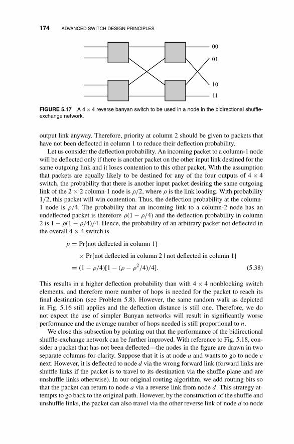
174 ADVANCED SWITCH DESIGN PRINCIPLES
00
01
10
11
FIGURE 5.17 A 4 × 4 reverse banyan switch to be used in a node in the bidirectional shuffle-exchange network.
output link anyway. Therefore, priority at column 2 should be given to packets thathave not been deflected in column 1 to reduce their deflection probability.
Let us consider the deflection probability. An incoming packet to a column-1 nodewill be deflected only if there is another packet on the other input link destined for thesame outgoing link and it loses contention to this other packet. With the assumptionthat packets are equally likely to be destined for any of the four outputs of 4 × 4switch, the probability that there is another input packet desiring the same outgoinglink of the 2 × 2 column-1 node is ρ/2, where ρ is the link loading. With probability1/2, this packet will win contention. Thus, the deflection probability at the column-1 node is ρ/4. The probability that an incoming link to a column-2 node has anundeflected packet is therefore ρ(1 − ρ/4) and the deflection probability in column2 is 1 − ρ(1 − ρ/4)/4. Hence, the probability of an arbitrary packet not deflected inthe overall 4 × 4 switch is
p = Pr{not deflected in column 1}× Pr{not deflected in column 2 | not deflected in column 1}
= (1 − ρ/4)[1 − (ρ − ρ2/4)/4]. (5.38)
This results in a higher deflection probability than with 4 × 4 nonblocking switchelements, and therefore more number of hops is needed for the packet to reach itsfinal destination (see Problem 5.8). However, the same random walk as depictedin Fig. 5.16 still applies and the deflection distance is still one. Therefore, we donot expect the use of simpler Banyan networks will result in significantly worseperformance and the average number of hops needed is still proportional to n.
We close this subsection by pointing out that the performance of the bidirectionalshuffle-exchange network can be further improved. With reference to Fig. 5.18, con-sider a packet that has not been deflected—the nodes in the figure are drawn in twoseparate columns for clarity. Suppose that it is at node a and wants to go to node c
next. However, it is deflected to node d via the wrong forward link (forward links areshuffle links if the packet is to travel to its destination via the shuffle plane and areunshuffle links otherwise). In our original routing algorithm, we add routing bits sothat the packet can return to node a via a reverse link from node d. This strategy at-tempts to go back to the original path. However, by the construction of the shuffle andunshuffle links, the packet can also travel via the other reverse link of node d to node

SWITCH DESIGN PRINCIPLES BASED ON DEFLECTION ROUTING 175
ca
db
Bidirectional links
In bidirectional shuffle-exchange network, nodes a and bconnected to node d implies they are also connected to another
common node c
FIGURE 5.18 Illustration showing that both reverse links can be used to correct a deflectionerror.
b and then via a forward link in node b to node c; going back to node a is not strictlynecessary. This is a simple observation of the shuffle and unshuffle interconnections:if nodes a and b are connected by shuffle (unshuffle) links to a common node d, thenboth nodes a and b are also connected by shuffle (unshuffle) links to another commonnode c.
By letting the packet use either of the reverse links, we reduce the deflectionprobability of the packet while its previous deflection is being corrected. In otherwords, we have a “don’t care” situation in which the packet does not care whichreverse link it acquires as long as one is available. In general, however, we do notalways have a “don’t care” situation when performing error correction. For example,if the packet were to be deflected to a reverse link instead of a forward link at node a,then it would be necessary for it to go back to node a to get to node c. When correctingsuccessive deflections, it is also possible that some steps have a “don’t care” situationwhile some do not. The general treatment is beyond the scope of this book. Sufficeit to say that by considering the routing tags of packets and the nodes they occupyat each step, one can derive systematically the general “don’t care” conditions andmodify the routing strategy for further performance improvement. Further discussioncan be found in Problem 5.10.
5.1.5 Dual Shuffle-Exchange Network
The idea of the feedback bidirectional shuffle-exchange network can be used in afeedforward dual shuffle-exchange network. Instead of feeding the outputs of thenodes back to the inputs of the same nodes through a set of shuffle links and a set ofunshuffle links, the outputs are fed forward to a set of “new” nodes at the next stage.In this way, a packet traverses physically different nodes on route to its destination.
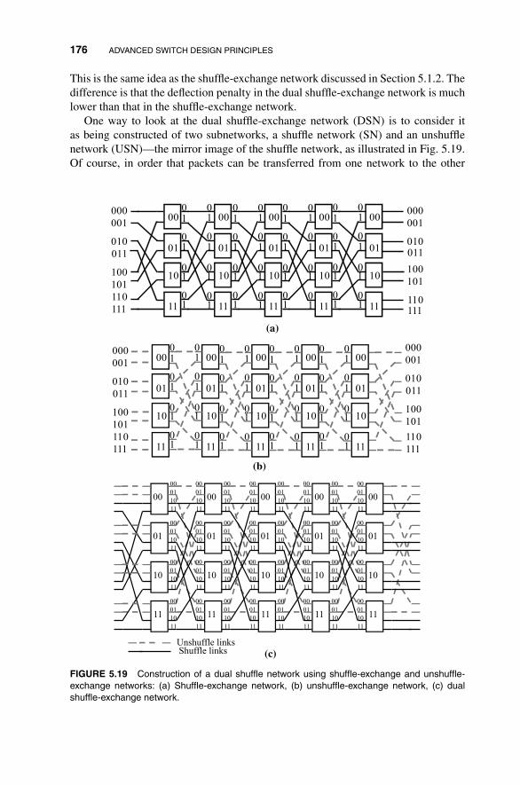
176 ADVANCED SWITCH DESIGN PRINCIPLES
This is the same idea as the shuffle-exchange network discussed in Section 5.1.2. Thedifference is that the deflection penalty in the dual shuffle-exchange network is muchlower than that in the shuffle-exchange network.
One way to look at the dual shuffle-exchange network (DSN) is to consider itas being constructed of two subnetworks, a shuffle network (SN) and an unshufflenetwork (USN)—the mirror image of the shuffle network, as illustrated in Fig. 5.19.Of course, in order that packets can be transferred from one network to the other
000
01
10
11
00
01
10
11
00
01
10
11
00
01
10
11
00
01
10
11
000
001
010
011
100
101
110
111
000
001
010011
100
101
110111
1
01
01
01
01
01
01
01
01
01
01
01
01
01
01
01
01
01
01
01
01
01
01
01
01
01
01
01
01
01
01
01
(a)
(b)
000
01
10
11
00
01
10
11
00
01
10
11
00
01
10
11
00
01
10
11
000
001
010
011
100
101
110
111
000
001
010
011
100
101
110
111
1
01
01
01
01
01
01
01
01
01
01
01
01
01
01
01
01
01
01
01
01
01
01
01
01
01
01
01
01
01
01
01
00
01
10
11
00
01
10
11
00
01
10
11
00
01
10
11
00
01
10
11
00
01
10
11
00
01
10
11
00
01
10
11
00
01
10
11
00
01
10
11
00
01
10
11
00
01
10
11
00
01
10
11
00
01
10
11
00
01
10
11
00
01
10
11
00
01
10
11
00
01
10
11
00
01
10
11
00
01
10
11
00
01
10
11
Unshuffle linksShuffle links (c)
00
01
10
11
00
01
10
11
00
01
10
11
00
01
10
11
00
01
10
11
00
01
10
11
00
01
10
11
00
01
10
11
00
01
10
11
00
01
10
11
00
01
10
11
00
01
10
11
00
01
10
11
00
01
10
11
00
01
10
11
00
01
10
11
FIGURE 5.19 Construction of a dual shuffle network using shuffle-exchange and unshuffle-exchange networks: (a) Shuffle-exchange network, (b) unshuffle-exchange network, (c) dualshuffle-exchange network.

SWITCH DESIGN PRINCIPLES BASED ON DEFLECTION ROUTING 177
for correcting deflections, we need 4 × 4 nodes rather than 2 × 2 nodes. Conceptu-ally, the routing and error-correction mechanisms of the DSN are the same as thosein the feedback bidirectional shuffle-exchange network. There are, however, somedifferences relating to implementation and performance issues, and this subsectionconcentrates on these areas.
In the bidirectional shuffle-exchange network, the nodes are the packet sources anddestinations; in the DSN, the input and output links are the sources and destinations.Consider a network with N/2 nodes at each stage. Since each node is 4 × 4, thereare altogether 2N links connecting adjacent stages. We label the N/2 nodes at eachstage with an (n − 1)-bit number xn · · · x2 (as opposed to xn · · · x1 in the feedbacknetwork with N nodes). The four output shuffle and unshuffle links connecting to aparticular node xn · · · x2 are labeled as (1, xn · · · x1) and (0, xn · · · x1), respectively.The four input links are also similarly labeled. Routing of a packet in the DSN consistsof first directing it to the node to which the desired output is attached—which issimilar to routing in the feedback network—in the first log2 n − 1 steps, and thenfrom the node to the destination output link in the last step. Therefore, the same error-correcting routing algorithm as depicted in Figs. 5.13 and 5.14 can be used, with theunderstanding that x1 in the figures must be replaced by x2 to take into account thenew situation that x2 is the least significant bit of the node label.
The DSN can be configured as an N × N switch or a 2N × 2N switch, as shownin Fig. 5.20. Figure 5.20(a) depicts the N × N version. Both the SN and USN inthe DSN are used for routing packets. In the N × N DSN, links (1, dn · · · d1) and(0, dn · · · d1) are associated with the same logical address dn · · · d1. Packets reachingthese two links as their final destinations will be multiplexed onto the same outputlink of the overall switch. Therefore, a packet with destination address dn · · · d1 can
N N SN
N N USN
Multiplexer
Output address space:
dndn–1... d1; di ∈{0,1}
4 4 node interconnecting SN and USN
1 2 router
(a)
N N SN
N N USN
Output address space: 1dndn–1… d1
2N outputs2N inputs
Output address space: 0dndn–1… d1
(b)
FIGURE 5.20 (a) DSN configured as N × N switch; (b) DSN configured as 2N × 2N switch.

178 ADVANCED SWITCH DESIGN PRINCIPLES
have either of them as its destination. An incoming packet to the switch is routedeither to an SN input or an USN input, and accordingly, its routing tag is set to either1dn · · · 1d1 or 0d1 · · · 0dn. In the first case, the packet’s primary route is in the SN, andin the second case, the primary route is in the USN. Any excursion to the companionnetwork is for error-correction purposes only.
Figure 5.20(b) shows the 2N × 2N version. Here, links (1, dn · · · d1) and(0, dn · · · d1) belong to two different logical addresses, 1dn · · · d1 and 0dn · · · d1, re-spectively. An incoming packet with destination 1d1d2 · · · dn is assigned the routingtag 1dn1dn−1 · · · 1d1, and a packet with destination 0dndn−1 · · · d1 is assigned therouting tag 0d10d2 · · · 0dn. This setup has the advantage that the switch size is doublethat of Fig. 5.20(a) with essentially the same amount of hardware. For explanationpurposes, however, we shall focus mainly on the design in Fig. 5.20(a) for the rest ofthis subsection.
Figure 5.21 shows an example of the routing of two packets A and B whoseprimary routes are both in the shuffle plane. The shuffle and unshuffle planes in theDSN are drawn separately for clarity, with the understanding that the two nodes withthe same label at the same stage of the two planes are actually the same node in theDSN. As shown, the deflection of packet A to an incorrect shuffle link is correctedby forwarding it to an unshuffle link that returns it back to the previous node wherethe deflection occurred (node with the same label two stages later). In general, asin the bidirectional networks, deflections to shuffle links are corrected by routing tounshuffle links, and vice versa.
For further design simplification, let us reexamine the SN and USN shown inFig. 5.19. We note that the first shuffle of the inputs to the SN is unnecessary and can
00
01
10
11
00
01
10
11
00
01
10
11
00
01
10
11
00
01
10
11
000001
010011
000001
010011
000001
010011
000001
010011
00
01
10
11
00
01
10
11
000001
010011
000001
010011
000001
010011
000001
010011
00
01
10
11
00
01
10
11
00
01
10
11
Destination of A: 101 Destination of B: 100
B reaches destination
A reaches destination
Correcting error of A
Packet A Packet B
FIGURE 5.21 An example of deflection error in the shuffle plane being corrected in the unshuffleplane.
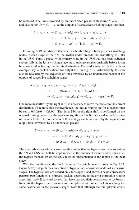
SWITCH DESIGN PRINCIPLES BASED ON DEFLECTION ROUTING 179
be removed. The links traversed by an undeflected packet with source S = sn · · · s1and destination D = dn · · · d1 at the outputs of successive switching stages are then
S = sn · · · s1 → (1, sn · · · s2dn) → (1, sn−1 · · · s2dndn−1)
→ · · · → (1, sn−i+1 · · · s2dn · · · dn−i+1) → · · ·→ (1, s2dn · · · d2) → (1, dn · · · d1) = D.
From Fig. 5.19, we also see that whereas the shuffling of links precedes switchingnodes in each stage of the SN, the switch nodes precede the unshuffling of linksin the USN. Thus, a packet with primary route in the USN that has been switchedsuccessfully at the last switching stage must undergo another unshuffle before it canbe considered as having reached its destination. The reader may verify this with anexample, say, a packet destined for output 101, in Fig. 5.19. Alternatively, this canalso be revealed by the sequence of links traversed by an undeflected packet at theoutputs of successive switching stages:
S = sn · · · s1 → (0, sn · · · s2d1) → (0, d1sn · · · s3d2)
→ · · · → (0, di−1 · · · d1sn · · · si+1di) → · · ·→ (0, dn−2 · · · d1sndn−1) → (0, dn−1 · · · d1dn) = D.
One more unshuffle (cyclic right shift) is necessary to move the packet to the correctdestination. To remove this inconvenience, the initial routing tag for a packet mustbe set to 0d20d30 · · · 0dn0d1. That is, a 2-bit cyclic right shift is performed on theoriginal routing tag so that the two least significant bits 0d1 are used at the last stageof the new USN. The correctness of this strategy can be revealed by the sequence ofoutput links traversed by an undeflected packet:
S = sn · · · s1 → (0, sn · · · s2d2) → (0, d2sn · · · s3d3)
→ · · · → (0, di · · · d2sn · · · si+1di+1) → · · ·→ (0, dn−1 · · · d1sndn) → (0, dn · · · d1) = D.
The main advantage of the above modification is that the bypass mechanisms withinthe SN and USN can both be implemented at the outputs of switch nodes; otherwise,the bypass mechanism of the USN must be implemented at the inputs of the nextstage.
With the modification, the block diagram of a switch node is shown in Fig. 5.22.Figure 5.22(b) depicts the connection of bypass lines across two nodes of successivestages. The bypass lines are needed only for stages n and above. The postprocessorsperform two functions: (1) process packets according to the error-correction routingalgorithm; and (2) forward packets that have reached their destinations to the bypasslines. At the bypass lines, packets are multiplexed with other packets reaching thesame destination in the previous stages. Note that although the multiplexers create

180 ADVANCED SWITCH DESIGN PRINCIPLES
Postprocessor
Postprocessor
Postprocessor
Postprocessor
00
01
10
11
00
01
10
11
4 × 4
Deflection
switch
xn … x21
Bypass line xn … x20
Bypass line xn … x21
(a)
xn … x2 xn … x2
Bypass lines(b)
FIGURE 5.22 (a) Block diagram of a switch node; (b) interconnection of bypass lines betweenadjacent switch nodes of same labels.
physical queues internal to the network, the switch is logically an output-queuedswitch; the physical buffers for the output queues are distributed across many switchnodes. Instead of the above, we may also have lines leading out of the switch fromthe bypass locations and use a “large” multiplexer to multiplex packets for the samedestination (see the configuration of the tandem-Banyan switch). In this case, thereis only one physical queue for each output.
We now show that the complexity of the DSN is N log N using an approximateanalysis. The validity of the analysis and the correctness of the routing algorithm havebeen verified with simulation.
Since routing requires at least n = log N stages, clearly the lower bound on thecomplexity of the DSN is N log N. We shall now show that N log N is also an upperbound on the order of complexity for a given packet loss probability requirementPloss. As a simplifying approximation, we assume that the input packets to a switchnode are uncorrelated with each other and that they are equally likely to be destinedfor any of the four outputs. We further assume that the 4 × 4 switch elements areinternally nonblocking. Let ρt be the load of an input at switch stage t, that is, ρt is theprobability that there is an incoming packet on an input link. Let pt be the probabilitythat a packet is successfully routed at stage t. We have
pt =1 −
(1 − 1
4ρt
)4
ρt
. (5.39)
It is easy to show that dpt/dρt ≤ 0 for 0 ≤ ρt ≤ 1. Since the load cannot increase ast increases (number of packets cannot increase), ρt is a nonincreasing function of t.

SWITCH DESIGN PRINCIPLES BASED ON DEFLECTION ROUTING 181
Therefore, pt ≥ pt−1 ≥ · · · ≥ p1. This agrees with our intuition that the probabilityof success increases as more and more packets are removed from the network. Toobtain an upper bound on L, the number of stages required to meet a given Ploss, weperform a worst-case analysis in which pt , for all t, is replaced by p1 = p. That is,the L required by our system is bounded above by the L required in a corresponding“time-invariant” random walk depicted by the Markov chain in Fig. 4.30, in whichthe state is the packet distance, and q = 1 − p is the deflection probability.
For analytical convenience, let us adopt a version of the DSN similar to the one inFig. 5.20(a), but in which each of the N incoming packets is randomly routed to oneof the 2N input ports of the SN and USN, with at most one packet assigned to thesame input port. The input load on each input is ρ1 = 0.5. This gives
p = p1 = 1 − (1 − 0.5/4)4
0.5≈ 0.828. (5.40)
Let gi(k) be the conditional probability that a packet will reach its destination (orstate 0) in k more steps given that its current state is i.
g0(k) ={
1, if k = 0,
0, otherwise,(5.41)
gi(k) = pgi−1(k − 1) + qgi+1(k − 1), 0 < i < n, (5.42)
gn(k) = pgn−1(k − 1) + qgn(k − 1). (5.43)
The generating function Gi(z) = ∑∞k=0 gi(k)zk is given by
G0(z) = 1, (5.44)
Gi(z) = pzGi−1(z) + qzGi+1(z), 0 < i < n, (5.45)
Gn(z) = pzGn−1(z) + qzGn(z). (5.46)
Equation (5.45) is a homogeneous linear difference equation in terms of i; (5.44) and(5.46) are the boundary conditions. The general technique for solving the differenceequation (5.45) is to substitute Gi(z) = Si(z). This gives
S2(z) − 1
qzS(z) + p
q= 0. (5.47)
The roots of the quadratic equation are
S1(z), S2(z) = 1
2qz
(1 ±
√1 − 4pqz2
). (5.48)
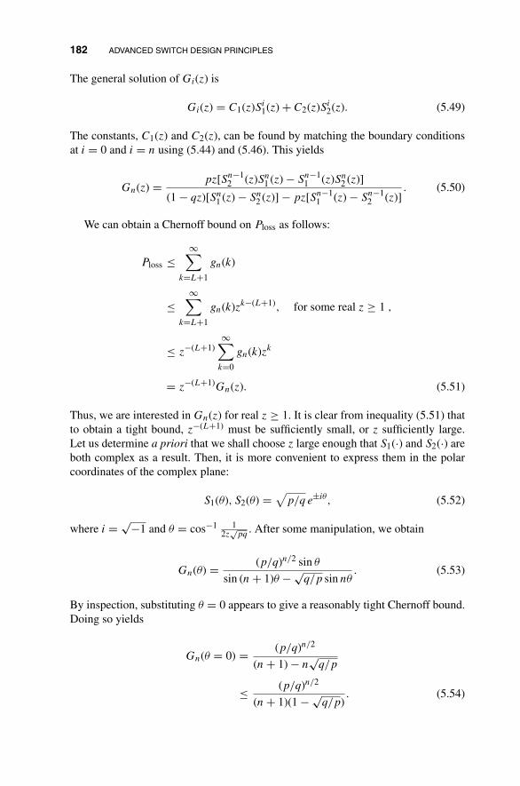
182 ADVANCED SWITCH DESIGN PRINCIPLES
The general solution of Gi(z) is
Gi(z) = C1(z)Si1(z) + C2(z)Si
2(z). (5.49)
The constants, C1(z) and C2(z), can be found by matching the boundary conditionsat i = 0 and i = n using (5.44) and (5.46). This yields
Gn(z) = pz[Sn−12 (z)Sn
1 (z) − Sn−11 (z)Sn
2 (z)]
(1 − qz)[Sn1 (z) − Sn
2 (z)] − pz[Sn−11 (z) − Sn−1
2 (z)]. (5.50)
We can obtain a Chernoff bound on Ploss as follows:
Ploss ≤∞∑
k=L+1
gn(k)
≤∞∑
k=L+1
gn(k)zk−(L+1), for some real z ≥ 1 ,
≤ z−(L+1)∞∑
k=0
gn(k)zk
= z−(L+1)Gn(z). (5.51)
Thus, we are interested in Gn(z) for real z ≥ 1. It is clear from inequality (5.51) thatto obtain a tight bound, z−(L+1) must be sufficiently small, or z sufficiently large.Let us determine a priori that we shall choose z large enough that S1(·) and S2(·) areboth complex as a result. Then, it is more convenient to express them in the polarcoordinates of the complex plane:
S1(θ), S2(θ) =√
p/q e±iθ, (5.52)
where i = √−1 and θ = cos−1 12z
√pq
. After some manipulation, we obtain
Gn(θ) = (p/q)n/2 sin θ
sin (n + 1)θ − √q/p sin nθ
. (5.53)
By inspection, substituting θ = 0 appears to give a reasonably tight Chernoff bound.Doing so yields
Gn(θ = 0) = (p/q)n/2
(n + 1) − n√
q/p
≤ (p/q)n/2
(n + 1)(1 − √q/p)
. (5.54)

SWITCH DESIGN PRINCIPLES BASED ON DEFLECTION ROUTING 183
Now, θ = 0 implies z = 1/2√
pq. Substituting the above Gn(·) and z into inequality(5.51) and taking logarithms on both sides yields an upper bound for L:
L ≤ 2.793n − 3.554 ln(n + 1) + 3.554 ln P−1loss + 1.162. (5.55)
Since each stage consists of N/2 switch elements, the complexity of the DSN for agiven Ploss is therefore of order N log N.
Theoretically, this is the lowest complexity that can be achieved. We saw in Chapter2 that the complexity order of a nonblocking switch must be at least N log N. In acertain sense, this is also the least complexity order of any “reasonable” switch, notnecessarily nonblocking. For example, the Banyan networks are the least complexswitches that guarantee that there is at least one path from any input to any output,and they are also of order N log N. Of course, the Banyan networks operated as losssystems would have very high loss probability, as has been demonstrated in Chapter 3.What we have shown for the DSN is that it can achieve the same order of complexityas the Banyan network while attaining arbitrarily small loss probability.
We close this subsection by observing that the complexity of the bypass mech-anisms can be also reduced using a simple trick. The DSN operation assumed sofar is associated with the random-walk model in Fig. 5.16. State n is different fromother states because error in this state does not increment the distance further: therouting tag is simply reset to the original routing tag. Suppose that this state is treatedno differently than other states. The corresponding random-walk model is shown inFig. 5.23(a), in which there is no reflecting barrier.
The advantage of removing the boundary is that the number of bypass locationsin the DSN can be decreased. With this new random walk, regardless of the stateof a packet, each deflection means the packet will need two more steps to reach itsdestination. In other words, a packet that experiences a total of k deflections willexit at stage n + 2k of the DSN. Therefore, only stages n + 2k, k = 0, 1, 2, · · ·, needto have the bypass mechanisms installed. The disadvantage is that the length of therouting tag may in principle grow in an unbounded fashion.
n+2 n+1 n i 1 0
Bypass location: n + 2k; k = 0,1,2, ...(a)
n+1 n i 1 0
Transition probability
from n + 1 to n = 1By-pass locations: n + 2k; k = 0,1,2...
(b)
FIGURE 5.23 Two random-walk models realizable with DSN: (a) random walk without boundary;(b) boundary with one-step reflection to the right.

184 ADVANCED SWITCH DESIGN PRINCIPLES
Partition 1
Partition N
RAM
Inputs Outputs
Writes Reads
NB bits/s NB bits/s B bits/sB bits/s
Select inputs
one by one
11
NN
FIGURE 5.24 Switching by loading packets from N inputs into RAM locations based on theirtargeted outputs and outputting packets into the N outputs in a round-robin fashion.
The random walk in Fig. 5.23(b) also only needs bypass mechanisms at stagesn + 2k, k = 0, 1, 2, · · ·, but bounds the routing tag to at most 2(n + 1) bits. Torealize this random walk, if an error is made in state n, the routing tag is re-set to the original destination address plus two dummy bits: x1x20d10d2 · · · 0dn orx1x21dn1dn−1 · · · 1d1, where x1x2 are the dummy routing bits.3 This moves the packetto state n + 1. In state n + 1, routing will be considered successful regardless of theoutcome and the two dummy routing bits removed. Consequently, a packet in staten + 1 will move to state n in one step with probability 1. Thus, we have a boundaryin the random walk that reflects the walk one step to the right. Again, each deflectionresults in two additional steps before the packet can reach its destination.
5.2 SWITCHING BY MEMORY I/O
So far we have been mainly concentrating on packet switching in the space domain. InChapter 2, it was shown that circuit switching in the time domain can be implementedusing random access memory (RAM). Recall that in TDM, time is divided into frames,each of which consists of a number of time slots. The information on different timeslots are associated with different circuits and are read into a RAM in the order oftheir arrival. By changing the order in which the information are read onto the output,the time slots occupied by the information can be interchanged.
A similar idea can be used in packet switching. Consider the N × N packet switchdepicted in Fig. 5.24. An N × 1 switch multiplexes the packets from the N inputs ontoone channel connected to a RAM. The buffer space in the memory is divided into N
partitions, one for each output. Packets are loaded into the partitions associated withtheir targeted outputs, and the N outputs take turns reading out their packets fromthe memory via a 1 × N switch. In practice, small switches based on variants of this
3Alternatively, state n + 1 can be indicated using another extra bit in the header and the routing tag keptto length 2n bits.
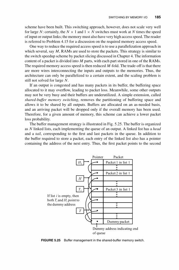
SWITCHING BY MEMORY I/O 185
scheme have been built. This switching approach, however, does not scale very wellfor large N: certainly, the N × 1 and 1 × N switches must work at N times the speedof input or output links; the memory must also have very high access speed. The readeris referred to Problem 4.15 for a discussion on the required memory access speed.
One way to reduce the required access speed is to use a parallelization approach inwhich several, say M, RAMs are used to store the packets. This strategy is similar tothe switch speedup scheme by packet slicing discussed in Chapter 4. The informationcontent of a packet is divided into M parts, with each part stored in one of the RAMs.The required memory access speed is then reduced M-fold. The trade-off is that thereare more wires interconnecting the inputs and outputs to the memories. Thus, thearchitecture can only be parallelized to a certain extent, and the scaling problem isstill not solved for large N.
If an output is congested and has many packets in its buffer, the buffering spaceallocated to it may overflow, leading to packet loss. Meanwhile, some other outputsmay not be very busy and their buffers are underutilized. A simple extension, calledshared-buffer memory switching, removes the partitioning of buffering space andallows it to be shared by all outputs. Buffers are allocated on an as-needed basis,and an arriving packet will be dropped only if the overall memory has been used.Therefore, for a given amount of memory, this scheme can achieve a lower packetloss probability.
The buffer management strategy is illustrated in Fig. 5.25. The buffer is organizedas N linked lists, each implementing the queue of an output. A linked list has a headand a tail, corresponding to the first and last packets in the queue. In addition tothe buffer required to store a packet, each entry of the linked list also has a pointercontaining the address of the next entry. Thus, the first packet points to the second
Packet 1 in list 1
Packet 2 in list 1
PacketPointer
Packet 3 in list 1
Dummy packet
Dummy address indicating end
of queue
If list i is empty, then
both Ti and Hi point to
the dummy address
H1
H
T1
T
FIGURE 5.25 Buffer management in the shared-buffer memory switch.

186 ADVANCED SWITCH DESIGN PRINCIPLES
packet, the second points to the third, and so on. The last entry, the tail, points toa specially designated dummy address (could be address 0, for example) to indicatethe end of the linked list. The addresses of the head and tail of queue i are stored inbuffers (or registers) Hi and Ti, respectively.
The N linked lists consist of all the used buffer locations. There is another linkedlist, called the free list, whose entries are the free buffer locations that could beallocated to the newly arriving packets. The addresses of the head and tail of this listare stored in buffers (or registers) H and T . An incoming packet destined for output i
must first acquire a free location from this list. The operations on the linked lists areas follows, where we assume for the sake of brevity that the free list and list i are notempty (a few steps must be added if this is not the case):
(H ) ← PACKET load packet into location pointed to by H ,
(Ti ).NEXT ← H add packet to tail of list i ,
Ti ← H update the tail of list i ,
H ← (H ).NEXT update H to point to the next free location,
(Ti ).NEXT ← DUMMY last entry of list i points to dummy address.
The N outputs take turns reading packets from the memory via the 1 × N switch.After output i has successfully read out a packet, the free list and list i are updated asfollows, where we assume for brevity that the free list is not empty before the updateand list i is not empty after the update:
(T ).NEXT ← Hi return buffer to free list,
T ← Hi
Hi ← (Hi ).NEXT update list i ,
(T ).NEXT ← DUMMY last entry of free list points to dummy address.
Although it can be seen intuitively and shown quantitatively that the packet lossprobability can indeed be reduced by the buffer-sharing approach, one must be care-ful in drawing the conclusion that the shared-buffer switch is therefore superior tounshared-buffer switch. There are several arguments against the shared-buffer switchthat must also be considered.
In the unshared-buffer switch, output queues do not interfere with each other. Inthe shared-buffer switch, a misbehaving output (due to traffic congestion, networkmanagement errors, or hardware failures) can easily use up a large amount of theshared memory, to the detriment of the other outputs. The shared-buffer switch hasan advantage over the unshared-buffer switch only to the extent that memory is anexpensive resources. With the rapid advances in memory technology, this is fastbecoming a weak argument. One might contend that in a real network, potential fortraffic congestion always exists, and no matter how much buffer there is, there is achance that it will fill up; therefore, having more buffer always helps. The problemwith this argument is that more buffer does not help solve traffic congestion; in fact,it may delay the discovery of congestion. The shared-buffer switch allows an outputqueue to grow very large because of the sharing. If the carried traffic is real-time

DESIGN PRINCIPLES FOR SCALABLE SWITCHES 187
(e.g., video conference traffic) and must reach the receiver within certain time limit,excessive delay may have been incurred: the packets may as well be dropped at theswitch. Furthermore, many network traffic management schemes use buffer overflowas an indication of congestion. For these schemes to be effective, the buffer cannotbe too large. Overall, in designing a switch, we want it to have enough buffer toprevent excessive packet loss under normal traffic conditions; using more buffer thannecessary, however, does not solve the congestion in heavy-traffic situations.
5.3 DESIGN PRINCIPLES FOR SCALABLE SWITCHES
Although various switches can theoretically be designed to large dimensions, techno-logical and physical constraints often impose a practical limit on their maximum size,N ′ × N ′. If we want to construct a large switch system, say 2N ′ × 2N ′, then two ormore N ′ × N ′ switches have to be interconnected. Straightforward interconnectionsof these small switches create several stages of queueing delay. This may also result insevere performance degradation if congestion occurs at intermediate switches. Thus,increasing performance penalty for larger switch sizes seems unavoidable.
In this section we shall focus on switch scalability; we shall provide some keyprinciples to construct large switches out of modest-size switches, without sacrificingoverall switch performance.
5.3.1 Generalized Knockout Principle
As mentioned before, the knockout switch takes advantage of the fact that, withuncorrelated traffic among input ports and uniformly directed to all output ports, theprobability of more than R packets destined for any particular output port in eachtime slot is very low. In this way, we can do away with the input queues and operatethe switch as a loss system by simply dropping the very few packets that have lostcontention.
The knockout principle can be implemented using very different switch architec-tures. In Chapter 4, we have presented two possible ways for its implementation. Oneis a design based on Batcher–banyan networks and the other is an implementationusing broadcast buses and knockout concentrators. Although the complexity of theBatcher-banyan knockout switch is of order N log2
2 N, which is much lower than thatof the second implementation for large N, the growing complexity of interconnectionwiring between stages in this design makes it impossible to scale well. The knockoutswitch based on broadcast buses and concentrators has a uniform and regular structureand thus has the advantages of easy expansion and high integration density for VLSIimplementation. It is one of the representative approaches to construct large-scaleswitches.
For large N (e.g., a few thousands), the complexity of a knockout concentrator atthe output is still very high; the total number of switch elements in all N knockout con-centrator is N2R. Although we can design VLSI chips to contain such large amountsof switch elements, it is still desirable to reduce the number of switch elements to

188 ADVANCED SWITCH DESIGN PRINCIPLES
Knockout concentrator
Knockout concentrator
N × R to n distribution
network
N × R to n distribution
network
Group 1 Group (N/n)
1
2
N21 1N 2 N
1 2
21
1
1
2
2
n × R
n
n × R
n
Grouping network
FIGURE 5.26 Partitioning outputs into multiple groups.
some extent by reducing the value of R. There are two ways to reduce the R value.One is to provide an input buffer at each input port, and an output buffer at eachoutput port. Suppose that an eight-packet buffer is added at each input port; R can bereduced from 8 to 3 at the same packet loss probability of 10−6 for any switch size N
with ρo = 0.9 (i.e., 90% load). Because the input buffer scheme is used, contentionresolution must be performed among packets destined for the same output port. Thiswill increase its complexity to the same extent as the pure input buffer scheme, whichis the extreme case of R = 1.
The second way to reduce the value of R is to put a number of output ports intoa group so that the routing links belonging to the same group can be shared by thepackets that are destined for any outputs in this group. For example, as shown inFig. 5.26, every n output ports are put together in one group, and R × n routing linksare shared in this group. The center network, as shown in Fig. 5.26, used to partitionoutput ports into a number of groups is thus called a “grouping network.” If thereare more than R × n packets in one time slot destined for the same output group,the excess packets will be discarded and lost while they are competing with othersfor available paths. Once packets are sent onto the R × n vertical routing links at theoutput of the knockout concentrator, they are routed to proper output ports througha distribution network, which can be implemented by any modest-size switch. Thismethod generalizes the knockout principle from a single output to a group of outputsand is so-called generalized knockout principle. It is the combination of the knockoutprinciple and channel grouping and provides a promising way to construct largeswitches out of small-scale switches.
Assuming the packets have independent, uniform destination address distributions,then the probability an input packet is destined to this group of outputs is simplyn/N. If we only allow up to R × n packets to pass through to the group outputs, the

DESIGN PRINCIPLES FOR SCALABLE SWITCHES 189
TABLE 5.1 Value of R for Different Group Sizes n and Loss Probability Ploss with�o = 0.9
Ploss n = 1 n = 2 n = 4 n = 8 n = 16 n = 32 n = 64 n = 128 n = 256
10−6 8 5.30 3.70 2.70 2.10 1.70 1.45 1.25 1.1510−8 10 6.45 4.40 3.15 2.40 1.90 1.55 1.35 1.2010−10 12 7.50 5.05 3.60 2.65 2.00 1.70 1.45 1.25
probability for a packet to be dropped is
Ploss = 1
nρo
N∑k=Rn+1
(k − Rn)
(N
k
)(nρo
N
)k (1 − nρo
N
)N−k
, (5.56)
where ρo is the offered load of each input port. As N → ∞, we have
Ploss =(
1 − R
ρo
)(1 −
Rn∑k=0
(nρo)ke−nρo
k!
)+ (nρo)Rne−nρo
(Rn)!. (5.57)
The practical R and n combinations for three different packet loss probabilities aredetermined from (5.57) and listed in Table 5.1. For a given acceptable packet lossprobability, for example, 10−10, the required value of R decreases from 12 to 8 asthe number n of output ports in each group increases from 1 to 2. The larger the sizeof the output group, the smaller the R value required. It is interesting to notice thatas the R value increases from 1.25 to 1.45, the size n of the output group reducesconsiderably from 256 to 128 at 10−10 loss probability. Because it is practical to routepackets to different groups based on some portion of the routing information carriedin the packet header, the group size is therefore chosen as 2i, where i = 0, 1, 2, · · ·. Inactuality, it is always desirable to choose a smaller R for a large group size n to keepthe hardware complexity smaller. However, to avoid the implementation difficultyresulting from the requirement of preserving correct packet sequence, every group islimited to a reasonable size.
We can also apply the generalized knockout principle to the distribution networksand further reduce the size n of the output groups by increasing the R value. Forexample, as the R value is increased from 1.25 to 2, the group size is reduced from256 to 32 for the loss probability of 10−10. This principle can be applied recursivelyuntil the n value becomes 1, where input packets are routed to an output port properly.In this way, many stages of the grouping network can be constructed recursively, whichresults in smaller hardware complexity and packet delay. Figure 5.27 illustrates onepossible way to construct a switch with three stages of grouping network. In this switchdesign, the first stage grouping network has K groups (K = N/n), and each grouphas R × n fanouts. They are then fed to another grouping network at the second stage,which hasR × n input lines andK′ output (K′ = n/n′), with each group’s fanout equalto R′ × n′. At the third stage, the R′ × n′ input lines are then routed to n′ groups with

190 ADVANCED SWITCH DESIGN PRINCIPLES
Group 1
Grouping network
(GN)
Group K
Group 1
GN
Group K′
Group 1
GN
Group K′
Group 1
GN
Group n′
Group 1
GN
Group n′
Output
buffer
Output
buffer
Output buffer
Output buffer
Stage 1 Stage 2 Stage 3
R × nR′ × n′
R′′1
n′
(N–n′+1)
N
….
….
…
…
Small module
Large module
….
K = N/n K′ = n/n′
FIGURE 5.27 A switch with three stages of grouping networks.
R′′ fanouts for each group. Packets on these R′′ lines are statistically multiplexed andstored in a multiplexer with a logical FIFO to maintain packet sequence integrity.
As shown in Fig. 5.27, there are N/n knockout concentrators in the groupingnetwork at the first stage. Thus, the total number of switch elements in the first stageis equal to
N/n × (number of input lines) × (number of output lines per concentrator)
= N/n × N × Rn
= N2R. (5.58)
Similarly, we obtain the number of switch elements used in the second stage andthe third stage; they are N × n × R × R′ and N × n′ × R′ × R′′, respectively. Thetotal number of switch elements in the switch fabric is, therefore, equal to the sumof them, or N2R + N × n × R × R′ + N × n′ × R′ × R′′. If we choose n = 256,R = 1.25, n′ = 32, R′ = 2, and R′′ = 12 for the packet loss probability of 10−10,the total number of switch elements will be equal to 1.25N2 + 1048N ≈ 1.25N2 forvery large N. It is close to one order of magnitude reduction from 12N2, which isthe number of switch elements required for building an N × N knockout switch withR = 12 and n = 1.

DESIGN PRINCIPLES FOR SCALABLE SWITCHES 191
MUX
MUX
....
....
Module 1
Module K
111
N1
1
N
1
M
M(K – 1) + 1
MK
KN
K….……
…………
MUX....Module 2
2
N
M + 1
2MK
….……
11
……….
…….……….
FIGURE 5.28 The decomposition of a large switch into modules.
5.3.2 Modular Architecture
The generalized knockout principle provides the flexibility and efficiency for increas-ing the switch size by equally partitioning all outputs into multiple groups and doingrouting according to these groups. Here, we shall present a modular architecture,which does so by equally partitioning all inputs into multiple subsets and performingswitching based on them.
Figure 5.28 illustrates the basic idea of the modular approach to construct a switchfabric with a large number of ports. The set of all inputs is equally partitioned into K
subsets. Each subset of the inputs is then interconnected to all N outputs, forming thebasic building block of the system called the switch module. The number of inputsof a switch module, M = N/K, is called the base dimension of the switch. In thisarchitecture, each module is an autonomous nonblocking, self-routing packet switch.The outputs with the same index, one from each switch module, are multiplexedtogether and then fed to the output queue bearing that index as its port address.
Physically, as shown in Fig. 5.29, the modular architecture can be realized as anarray of three-dimensional parallel processors. Each processor is a switch module con-sisting of a Batcher sorting network and an expansion routing network. The expansionnetwork is a set of binary trees cross interconnected with a set of banyan networks.The set of concurrent modules is interconnected at the outputs by multiplexers. Thus,no interference between switch modules is possible, which is the key to simplifying

192 ADVANCED SWITCH DESIGN PRINCIPLES
Bas
e dim
ensi
on
Number of stages
(b)
Num
ber
of
stag
es
FIGURE 5.29 The 3D modular architecture of Batcher-binary-banyan packet switch.
the operation and maintenance of the whole system. This architecture also allowsindependent clocking of modules, which simplifies timing substantially. Within eachmodule, the small physical size makes it fairly straightforward to synchronize, andthe simpler hardware makes higher speed implementation possible.
5.3.2.1 Modular Batcher–Binary–Banyan Switch With reference to theprevious discussion, each of the K modules of an N × N switch is a cascade ofan M × M Batcher network, a stack of M binary trees and a group of K banyan

DESIGN PRINCIPLES FOR SCALABLE SWITCHES 193
OutputsInputs
1
2
12
K
K
12
K
12
M × MBatcher
sorting
networks
1 × K
Binary
trees
M × MBanyan
routing
networks
……
……
……
………
K
FIGURE 5.30 The divide-and-conquer modular approach.
networks where M = N/K. We will use σ(M, N, K) to represent such a switch mod-ule. The Batcher network sorts the input packets based on their destination addresses.The succeeding binary trees and banyan networks then route the packets to the correctoutputs.
The principle of this modular architecture is based on a common approachcalled divide-and-conquer, which has been used extensively in designing efficientalgorithms. A well-known example is the fast Fourier transform. It simply splitsa large problem into small parts, solves them, and then combines the solutionsfor the parts into a solution for the whole. This point is illustrated in Fig. 5.30.The set of inputs is first partitioned into K subsets. Each subset is sorted by aBatcher network. The sorted subset is then partitioned again by the binary treesinto finer subsubsets. In each module, the ordered packets of these subsubsetsare routed concurrently to their destinations by K parallel banyan subnetworks.Finally, these packets are buffered in respective output queues, waiting fortransmission.
The combination of binary trees and banyan networks forms an expansion network,a network has larger fan-out than fan-in. As such, the output space of an expansionnetwork can be arbitrarily enlarged by adding more banyan networks. Thus, eachmodule may even have more outlets than the number of outputs. The structure andproperty of the switch modules are detailed below.

194 ADVANCED SWITCH DESIGN PRINCIPLES
00
01
10
11
00,0
00,1
01,0
01,1
10,0
10,1
11,0
11,1
0,00
0,01
0,10
0,11
1,00
1,01
1,10
1,11
000
001
010
011
100
101
110
111
M inputs N outputs
Banyan networksBinary trees
log Mlog N-log Mstages stages
FIGURE 5.31 A 4 × 8 expansion network.
Binary–Banyan Expansion Network An n-stage expansion network with M =2m inputs and N = 2n outputs is a combination of a set of M binary trees and aset of K = N/M banyan networks. Figure 5.31 illustrates a three-stage expansionnetwork with four inputs and eight outputs. Each 1 × K binary tree has k = log K =log N − log M = n − m stages and each M × M banyan network has m stages. Everynode of the network is either a 1 × 2 or a 2 × 2 switch element capable of performingthe binary routing algorithm based on the n-bit destination address in the header ofthe packet. That is, a node at stage j sends the packet on link 0 (up) or link 1 (down)according to the jth bit of the header.
The cross interconnection of M binary trees and K banyan networks is similarto the link system of a multistage crossbar switch. The outputs of a binary tree canbe labeled by two binary numbers (x1 · · · xm, y1 · · · yn−m=k), where x1 · · · xm is thetop-down numbering of the binary tree and y1 · · · yk is the local address of eachinput within the binary tree. Similarly, the inputs of the banyan network can alsobe identified by two binary numbers (a1 · · · an−m=k, b1 · · · bm) where a1 · · · an−m
is the top-down numbering of the banyan network and b1 · · · bm is the local ad-dress of the input. The binary trees and banyan networks are transpose intercon-nected according to this numbering scheme; the two ports are interconnected if(x1 · · · xm, y1 · · · yn−m) = (b1 · · · bm, a1 · · · an−m). This transpose cross interconnec-tion results in a three-dimensional realization of switch modules as portrayed inFig. 5.29.
The binary trees of the expansion network consist of 1 × 2 elements, which onlyallow one input packet at any instant of time. Packets will never collide in this stageof the network, but this may occur in the subsequent banyan subnetworks. In thefollowing, we will discuss the condition on inputs that prevents any possible packetcollisions in an expansion network.
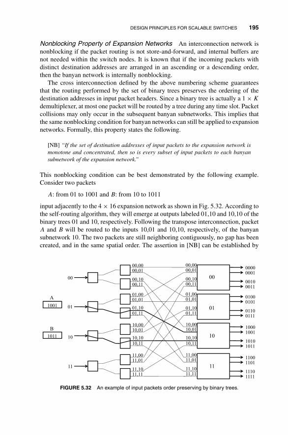
DESIGN PRINCIPLES FOR SCALABLE SWITCHES 195
Nonblocking Property of Expansion Networks An interconnection network isnonblocking if the packet routing is not store-and-forward, and internal buffers arenot needed within the switch nodes. It is known that if the incoming packets withdistinct destination addresses are arranged in an ascending or a descending order,then the banyan network is internally nonblocking.
The cross interconnection defined by the above numbering scheme guaranteesthat the routing performed by the set of binary trees preserves the ordering of thedestination addresses in input packet headers. Since a binary tree is actually a 1 × K
demultiplexer, at most one packet will be routed by a tree during any time slot. Packetcollisions may only occur in the subsequent banyan subnetworks. This implies thatthe same nonblocking condition for banyan networks can still be applied to expansionnetworks. Formally, this property states the following.
[NB] “If the set of destination addresses of input packets to the expansion network ismonotone and concentrated, then so is every subset of input packets to each banyansubnetwork of the expansion network.”
This nonblocking condition can be best demonstrated by the following example.Consider two packets
A: from 01 to 1001 and B: from 10 to 1011
input adjacently to the 4 × 16 expansion network as shown in Fig. 5.32. According tothe self-routing algorithm, they will emerge at outputs labeled 01,10 and 10,10 of thebinary trees 01 and 10, respectively. Following the transpose interconnection, packetA and B will be routed to the inputs 10,01 and 10,10, respectively, of the banyansubnetwork 10. The two packets are still neighboring contiguously, no gap has beencreated, and in the same spatial order. The assertion in [NB] can be established by
00,0000,01
00,1000,11
01,0001,01
01,1001,11
10,0010,01
10,1010,11
11,0011,01
11,1011,11
00,0000,01
00,1000,11
01,0001,01
01,1001,11
10,0010,01
10,1010,11
11,0011,01
11,1011,11
00000001
00100011
01000101
01100111
10001001
10101011
11001101
11101111
00
01
10
11
00
01
10
11
1001
1011
A
B
FIGURE 5.32 An example of input packets order preserving by binary trees.
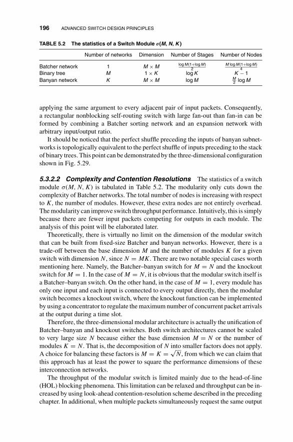
196 ADVANCED SWITCH DESIGN PRINCIPLES
TABLE 5.2 The statistics of a Switch Module �(M, N, K )
Number of networks Dimension Number of Stages Number of Nodes
Batcher network 1 M × Mlog M (1+log M )
2M log M (1+log M )
4Binary tree M 1 × K log K K − 1Banyan network K M × M log M M
2 log M
applying the same argument to every adjacent pair of input packets. Consequently,a rectangular nonblocking self-routing switch with large fan-out than fan-in can beformed by combining a Batcher sorting network and an expansion network witharbitrary input/output ratio.
It should be noticed that the perfect shuffle preceding the inputs of banyan subnet-works is topologically equivalent to the perfect shuffle of inputs preceding to the stackof binary trees. This point can be demonstrated by the three-dimensional configurationshown in Fig. 5.29.
5.3.2.2 Complexity and Contention Resolutions The statistics of a switchmodule σ(M, N, K) is tabulated in Table 5.2. The modularity only cuts down thecomplexity of Batcher networks. The total number of nodes is increasing with respectto K, the number of modules. However, these extra nodes are not entirely overhead.The modularity can improve switch throughput performance. Intuitively, this is simplybecause there are fewer input packets competing for outputs in each module. Theanalysis of this point will be elaborated later.
Theoretically, there is virtually no limit on the dimension of the modular switchthat can be built from fixed-size Batcher and banyan networks. However, there is atrade-off between the base dimension M and the number of modules K for a givenswitch with dimension N, since N = MK. There are two notable special cases worthmentioning here. Namely, the Batcher–banyan switch for M = N and the knockoutswitch for M = 1. In the case of M = N, it is obvious that the modular switch itself isa Batcher–banyan switch. On the other hand, in the case of M = 1, every module hasonly one input and each input is connected to every output directly, then the modularswitch becomes a knockout switch, where the knockout function can be implementedby using a concentrator to regulate the maximum number of concurrent packet arrivalsat the output during a time slot.
Therefore, the three-dimensional modular architecture is actually the unification ofBatcher–banyan and knockout switches. Both switch architectures cannot be scaledto very large size N because either the base dimension M = N or the number ofmodules K = N. That is, the decomposition of N into smaller factors does not apply.A choice for balancing these factors is M = K = √
N, from which we can claim thatthis approach has at least the power to square the performance dimensions of theseinterconnection networks.
The throughput of the modular switch is limited mainly due to the head-of-line(HOL) blocking phenomena. This limitation can be relaxed and throughput can be in-creased by using look-ahead contention-resolution scheme described in the precedingchapter. In additional, when multiple packets simultaneously request the same output

DESIGN PRINCIPLES FOR SCALABLE SWITCHES 197
port of the same switch module, output conflict occurs. To resolve these conflicts,we can directly apply the contention-resolution algorithms developed for Batcher–banyan switches (see Chapter 4) without any modification. Also, we can engineer theswitch throughput to meet any desired requirement. This can be achieved by adjustingthe number of modules K and the maximum number R of packets that can be receivedby an output port simultaneously.
5.3.2.3 Performance Analysis In the following, we analyze the throughput ofa switch module σR(M, N, K), which allows at most R packet arrivals at the outputin a time slot. We assume that if there are S(>R) packets waiting at the heads of inputqueues addressed to the same output, the selection of R to pass through the switch isdone at random, and the S − R that loses the contention will be ignored. Under theseassumptions, the switch throughput is defined to be the carried load on an output linewhen all input lines are fully loaded.
Suppose the input line loading, or the probability that a slot contains a packet, isλ. Let Mi be the number of packets addressed to output i, we have
Pr{Mi = j} =(
M
j
)(λ
N
)j (1 − λ
N
)M−j
,
j = 0, · · · , M. (5.59)
Suppose Ai = min(Mi, R) is the number of packets that actually arrived at outputi in a time slot. For sufficiently large N, we can use Poisson approximation withparameter Mλ/N = λ/K to obtain
aj = Pr{Ai = j} =(
λ
K
)je−λ/K
j!,
j = 0, · · · , R − 1. (5.60)
and
aR = 1 − a0 − · · · − aR−1. (5.61)
The carried load on an output line, denoted by λ′, can be intuitively interpreted as theprobability that a time slot on the output line is occupied by a packet. Because of thesymmetricity of the K modules, we immediately obtain
λ′ = K · E[Ai] = K ·⎡⎣R −
R−1∑j=0
(R − j)aj
⎤⎦
= K ·⎡⎣R − e−λ/K
R−1∑j=0
(λ
K
)jR − j
j!
⎤⎦ . (5.62)

198 ADVANCED SWITCH DESIGN PRINCIPLES
TABLE 5.3 Maximum Throughput of Modular Switches �R (M, N, K )
L K = 1 K = 2 K = 4 K = 8 K = 16 K = 32
1 0.6321 0.7869 0.8848 0.9400 0.9694 0.98452 0.8964 0.9673 0.9908 0.9976 0.9994 0.99983 0.9767 0.9961 0.9994 0.9999 1.0000 1.0000
The maximum throughput of the switch is the carried load when all input lines aresaturated, which can be obtained by substituting λ = 1 into (5.62). Table 5.3 liststhe maximum throughput versus number of modules K for different values of R. ForK ≥ 2, maximum throughput λ = 0.95 can be achieved with R = 2. So, we can seethat we can improve the switch throughput by increasing the value of K only.
PROBLEMS
5.1 Show formally that the shuffle link interconnection pattern corresponds to acyclic left shift of the link label.
5.2 Consider a feedback shuffle-exchange network with nodes 00, 01, 10, and 11.Suppose that there is a packet at each of the nodes and the source–destinationmapping is 00 → 01, 01 → 10, 10 → 11, and 11 → 00.(a) Show the sequence of nodes traversed by each of the packets on route to
its destination node. Is there contention among packets?
(b) Give an example in which there is contention among packets even thoughthey are destined for different destinations. (Hint: Can there be contentionif there is only one packet at each source?)
5.3 In the analysis of the feedback shuffle-exchange network in Section 5.1.3, wemade the assumption that the packets on the incoming link are independentlyand equally likely to be destined for either of the output link. Do you ex-pect the independence assumption to give rise to an optimistic or pessimisticperformance estimate? Write a simulation program to verify your conjecture.
5.4 We want to study the relationship between the saturation throughput �sat andthe maximum throughput �max of a feedback shuffle-exchange network withN = 2n nodes. From (5.13),(a) Show that d�/dρ ≥ 0 when n ≤ 4.
(b) Show that for each n ≥ 5, there is a ρ < 1 beyond which d�/dρ < 0.
(c) Argue that �max > �sat for n ≥ 5 from parts (a) and (b).
5.5 Consider the input queue at a node in a feedback shuffle-exchange networkwith the random deflection scheme in which the winning packet is chosenat random under contention. This problem explores how the queueing delayincurred by a packet can in principle be derived, given an offered load to the
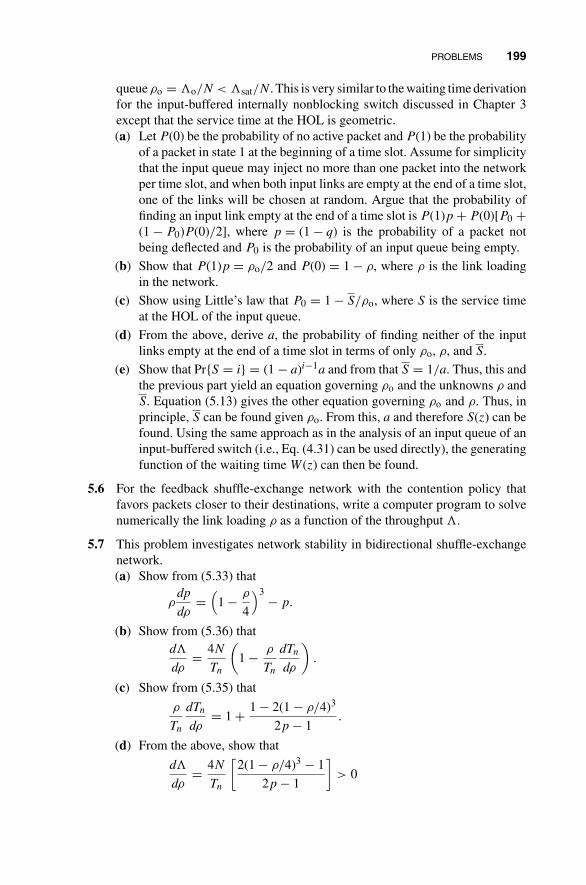
PROBLEMS 199
queue ρo = �o/N < �sat/N. This is very similar to the waiting time derivationfor the input-buffered internally nonblocking switch discussed in Chapter 3except that the service time at the HOL is geometric.(a) Let P(0) be the probability of no active packet and P(1) be the probability
of a packet in state 1 at the beginning of a time slot. Assume for simplicitythat the input queue may inject no more than one packet into the networkper time slot, and when both input links are empty at the end of a time slot,one of the links will be chosen at random. Argue that the probability offinding an input link empty at the end of a time slot is P(1)p + P(0)[P0 +(1 − P0)P(0)/2], where p = (1 − q) is the probability of a packet notbeing deflected and P0 is the probability of an input queue being empty.
(b) Show that P(1)p = ρo/2 and P(0) = 1 − ρ, where ρ is the link loadingin the network.
(c) Show using Little’s law that P0 = 1 − S/ρo, where S is the service timeat the HOL of the input queue.
(d) From the above, derive a, the probability of finding neither of the inputlinks empty at the end of a time slot in terms of only ρo, ρ, and S.
(e) Show that Pr{S = i} = (1 − a)i−1a and from that S = 1/a. Thus, this andthe previous part yield an equation governing ρo and the unknowns ρ andS. Equation (5.13) gives the other equation governing ρo and ρ. Thus, inprinciple, S can be found given ρo. From this, a and therefore S(z) can befound. Using the same approach as in the analysis of an input queue of aninput-buffered switch (i.e., Eq. (4.31) can be used directly), the generatingfunction of the waiting time W(z) can then be found.
5.6 For the feedback shuffle-exchange network with the contention policy thatfavors packets closer to their destinations, write a computer program to solvenumerically the link loading ρ as a function of the throughput �.
5.7 This problem investigates network stability in bidirectional shuffle-exchangenetwork.(a) Show from (5.33) that
ρdp
dρ=
(1 − ρ
4
)3 − p.
(b) Show from (5.36) thatd�
dρ= 4N
Tn
(1 − ρ
Tn
dTn
dρ
).
(c) Show from (5.35) that
ρ
Tn
dTn
dρ= 1 + 1 − 2(1 − ρ/4)3
2p − 1.
(d) From the above, show that
d�
dρ= 4N
Tn
[2(1 − ρ/4)3 − 1
2p − 1
]> 0

200 ADVANCED SWITCH DESIGN PRINCIPLES
and that if ρ < 0.825, regardless of n, d�/dρ > 0. Find the differencebetween �max and �sat.
(e) Write a computer program based on the more accurate formula for Tn,Eq. (5.34), and Eq. (5.36). By plotting graphs, show that �sat and �maxare very close to each other for n up to 30 (3 billion nodes!). Argue thereforethat the stability problem is not severe and can be ignored in this network.
5.8 Consider the feedback bidirectional shuffle-exchange network with the 4 × 4switching nodes implemented using Banyan networks.(a) From (5.33) and (5.38), show that the deflection probability is higher with
the Banyan network than with a nonblocking switching network.
(b) Derive the mean delay and the saturation throughput of the bidirectionalnetwork when the Banyan networks are used.
5.9 Consider a network with four nodes 00, 01, 10, and 11 arranged as a square.There are eight links in the network interconnecting nodes whose labels differin one bit only in both directions (e.g., there are two links between nodes 01and 00 and no links between nodes 00 and 11). This is the two-dimensionalhypercube network. Consider using deflection routing in this network. Thenodes are the sources and destinations of packets. The distance of a packetinside the network at any time is either 2 or 1. There is zero probability ofdeflection when the distance is 2, since routing to either of the adjacent nodedecreases the distance by 1. A packet with distance 1 cannot be deflectedby a packet with distance 2—priority is given to the packet with distance1, since the packet with distance 2 is guaranteed not to be deflected. For thisquestion, assume random contention resolution when two packets with distance1 contend with each other. Furthermore, assume that a new packet just arrivingto the network externally is equally likely to be destined for any of the threeother nodes.(a) Draw the state-transition diagram of a packet being routed in the network.
(b) Express T1 and T2, the mean delay given a packet is in states 1 and 2,respectively, in terms of the success probability at state 1, p = 1 − q,where q is the deflection probability. What is the mean delay for an arbitrarypacket?
(c) Consider the saturation situation in which a packet leaving the network isimmediately replaced by a new packet so that the link loading ρ is always1. Express the saturation throughput �sat of the overall network in termsof p.
(d) Let N1 be the expected number of packets in state 1 at the beginning of atime slot under saturation condition. Express N1 in terms of p and �sat.
(e) Find p, hence the saturation throughput in terms of a real number.
5.10 Toward the end of Section 5.1.4, we discussed a strategy for reducing the de-flection probability in bidirectional shuffle-exchange networks by considering
PROBLEMS 201
certain “don’t care” situation in routing. Let us examine the problem in moredetail. Consider a packet in transit to its destination.(a) Argue that in general, after a series of successes and deflections, the node
at which the packet is currently residing has label dn−k · · · di+1y′i · · · y1,
x′k · · · x1dn−k · · · di+1, or x′
k · · · x1dn−k · · · di+1y′i · · · y1, where dn · · · d1 is
the destination address, and xj’s, yj’s, i, i′ k, and k′ are unknowns thatdepend on previous packet deflections. What are the physical meanings ofi, i′ k, and k′? Show that i + k = i′ + k′.
(b) Consider the general case with node label x′k · · · x1dn−k · · · di+1y
′i · · · y1,
what should the next few routing steps be in order to send the packetto the node dn−k · · · di+1y
′i · · · y1 · · ·? Do we have a “don’t care” situ-
ation in these routing steps? What if we want to send the packet tonode · · · x′
k · · · x1dn−k · · · di+1 instead?
(c) Consider sending the packet to node dn−k · · · di+1y′i · · · y1 · · ·, and then
to node dn · · · di+1y′i · · · y1, then to node · · · dn · · · di+1, and then to the
destination node dn · · · d1. How many undeflected steps are needed alto-gether? How many steps have “don’t care” situations and how many donot, which steps involve routing to the shuffle plane and which steps tounshuffle plane?
(d) Answer the same questions for the other alternative: sending the packetto node · · · x′
k · · · x1dn−k
· · · di+1, then to node x′k · · · x1dn−k · · · d1, and then to node
dn−k · · · di+1 · · ·, and then to the destination node dn · · · di+1. Whichalternative is more efficient?
(e) Show that by keeping the four parameters i, i′, k, and k′ and the destinationdn · · · d1 in the packet header, we have sufficient information for routingdecision at each node.
5.11 Consider a variant of feedback shuffle-exchange network called the stay-or-shuffle network. Each node, in addition to the two regular input and two regularoutput links, has a third link that feeds back to the same node so that the nodehas three inputs and three outputs. The third link will be called a stationarylink and the regular links, shuffle links.(a) Suppose that at a node, only two of the input links have an incoming
packet and both packets want to access the same shuffle output link. Is itbetter to deflect the losing packet to the other shuffle link or the stationarylink? Why? Do you expect this network to perform better than the regularfeedback shuffle-exchange network? Why?
(b) When all three inputs have an incoming packet, each output (stationaryor shuffle link) will have a packet forwarded to it. When only two of theinputs have an incoming packet, assuming that they are equally likely tobe destined for any of the two shuffle output links, what is the probabilitythat the stationary output link will have a packet forwarded to it?

202 ADVANCED SWITCH DESIGN PRINCIPLES
(c) Let the link loading of the stationary link be ρ′ and the link loading of eachof the shuffle link be ρ. Derive the relationship between ρ′ and ρ drawingfrom clues in the previous part.
(d) Represent the state of a packet by a 2-tuple (i, j). State (i, 0) means thedistance of the packet is i and it is currently on a shuffle link, and state(i, 1) means the distance of the packet is i and it is currently on a stationarylink. Draw the state-transition diagram. Use pi, qi, and ri to denote theprobabilities of success, deflection to the wrong shuffle link, and deflectionto the stationary link, respectively, at state (i, 0). Use p′
i, q′i, and r′
i to denotethe corresponding probabilities at state (i, 1).
(e) Consider the random contention-resolution scheme in which contendingpackets are equally likely to be chosen as the winner. Derive p = pi, r = ri,q = qi, p′ = p′
i, r′ = r′i, and q′ = q′
i, in terms of ρ and ρ′.(f) Let T (i, j) denote the expected number of steps needed to reach the des-
tination from state (i, j). Write down the dynamic equations of T (i, j).Describe how you would solve for the throughput of the system.
5.12 This problem compares the configuration of a DSN as a 2N × 2N switch andas an N × N switch.(a) Given a fixed load per input, argue that a DSN configured as a 2N × 2N
switch has higher packet loss probability than the same DSN configured asan N × N switch. How would you modify the 2N × 2N switch to achievethe same loss probability with the same load? Which switch has highercomplexity now?
(b) Let us consider two DSNs, one with N/2 nodes and other with N/4nodes in each stage. Both are configured as an N × N switch. For a givenfixed input load and a fixed loss probability, intuitively, which networkwould have a higher number of nodes? Can you argue for your conclusionanalytically?
5.13 Consider a log2 N-stage reverse shuffle-exchange network with the last un-shuffling of links removed. The text explained that the routing tag of a packetshould be set to d2d3 · · · dnd1 in order to route the packet to its destinationdn · · · d1 in this network. True or false? A set of input packets that can berouted through the original shuffle-exchange network (the one without the lastunshuffling of links removed) without conflict can also be routed through thisnetwork without conflict.
5.14 In the text, contention is resolved in a random manner at the switch nodes ofthe DSN. This problem shows that deadlocks could occur when contention isresolved in a deterministic manner. Deadlock occurs when a group of pack-ets contend with other in a periodic fashion and they take turns winning thecontention.(a) Give an example in which two packets keep contending with other, re-
sulting in a deadlock situation in which the distance of neither packetprogresses to 0.

PROBLEMS 203
(b) Argue that deadlocks could not occur if packets with the shorter distanceare favored under contention.
5.15 Consider an unshared-buffer memory switch. Suppose that packets are 60 bytesin length and that the transmission rate of input and output ports is 150 Mbps.Assume that four bytes can be written into and read out of the RAM togethereach time and that the access times for read and write are the same. What isthe required access time for the RAM for a 64 × 64 switch?


6
SWITCHING PRINCIPLES FORMULTICAST, MULTIRATE, AND
MULTIMEDIA SERVICES
A challenge of modern broadband digital networks is to efficiently support multirateand multicast connections for providing high-speed multimedia services. These ser-vices often have diverse quality-of-service (QoS) requirements. A key to the successof the future broadband network deployments, therefore, lies in the design of a high-speed packet switch to cope with these three m’s. In this chapter, we first presentseveral fundamental switch design principles for multicasting. Then, we introducethe concept of path switching, which combines the advantageous elements of bothdynamic and static routing. A cross-path switch is a Clos network operated under theprinciple of path switching. We shall show how cross-path switches can integrate var-ious switch design principles together to support multirate, multicast, and multimediatraffic efficiently.
6.1 MULTICAST SWITCHING
So far we have been focusing on point-to-point switching in which an input packet istargeted for one and only one output. Many communication services, such as telephonecalls, are point-to-point in nature and involve only two parties. At the other end of thespectrum, we have services such as television broadcast in which the same programsare received by all network users. The most general form of network connectivity ispoint-to-multipoint, in which information from one source is sent to a selected groupof destinations. A three-party video conference call, for example, may be set upusing three point-to-multipoint simplex (one-direction) connections, one from eachsource. Sending the same information from one source to a number of destinations
Principles of Broadband Switching and Networking, by Tony T. Lee and Soung C. LiewCopyright © 2010 John Wiley & Sons, Inc.
205

206 SWITCHING PRINCIPLES FOR MULTICAST, MULTIRATE, AND MULTIMEDIA SERVICES
FIGURE 6.1 (a) Multicasting by separate point-to-point connections from source to destinations;(b) multicasting using multicast switches in network.
is called multicasting, and unicasting and broadcasting are the two extreme forms ofmulticasting.
While it is possible to perform multicasting by having the source establish a sepa-rate connection for each destination (see Fig. 6.1), this is usually not the most efficientway and is not viable when the number of destinations is large. Consider, for example,a video program vendor that wants to send its programs to hundreds of subscribers.This strategy would require very costly access facilities from the video source tothe network. A better way is to set up just one connection from the source to somenode (or nodes) in the communication network wherein the information is replicatedand forwarded to the destinations. The node then requires a switch that can sendinformation from one input to a number of selected outputs.
One version of the knockout switch architectures in the previous chapter uses N
buses, one for each input, to broadcast input packets to the outputs. Filters at the outputsthen select the packets destined for them. The multicast capability is inbuilt to suchbus-based switch architectures. We may introduce, say, m bits in the packet header toindicate the multicast group. During connection setup, the filters of the outputs thatbelong to the multicast group are informed of the m-bit group identification. It is thenpossible for the filters to recognize and select the packets belonging to the group. Thecomplexity of this switch architecture, as has been seen, is of order N2, indicatingthat it does not scale well for large N.
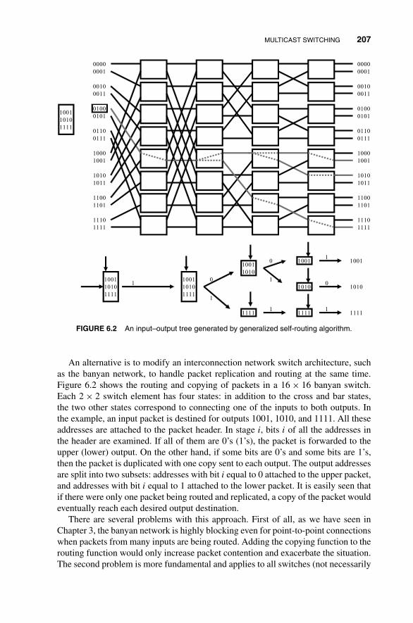
MULTICAST SWITCHING 207
1000
1001
1010
1011
1100
1101
1111
1110
0000
0001
0010
0011
0100
0101
0111
0110
1000
1001
1010
1011
1100
1101
1111
1110
0000
0001
0010
0011
0100
0101
0111
0110
1010
1001
1111
1010
1001
1111
1010
1001
1111
1010
1001
1111
1001
1010
1111
1
1
0
1
1
0
1
0
11001
1010
1111
FIGURE 6.2 An input–output tree generated by generalized self-routing algorithm.
An alternative is to modify an interconnection network switch architecture, suchas the banyan network, to handle packet replication and routing at the same time.Figure 6.2 shows the routing and copying of packets in a 16 × 16 banyan switch.Each 2 × 2 switch element has four states: in addition to the cross and bar states,the two other states correspond to connecting one of the inputs to both outputs. Inthe example, an input packet is destined for outputs 1001, 1010, and 1111. All theseaddresses are attached to the packet header. In stage i, bits i of all the addresses inthe header are examined. If all of them are 0’s (1’s), the packet is forwarded to theupper (lower) output. On the other hand, if some bits are 0’s and some bits are 1’s,then the packet is duplicated with one copy sent to each output. The output addressesare split into two subsets: addresses with bit i equal to 0 attached to the upper packet,and addresses with bit i equal to 1 attached to the lower packet. It is easily seen thatif there were only one packet being routed and replicated, a copy of the packet wouldeventually reach each desired output destination.
There are several problems with this approach. First of all, as we have seen inChapter 3, the banyan network is highly blocking even for point-to-point connectionswhen packets from many inputs are being routed. Adding the copying function to therouting function would only increase packet contention and exacerbate the situation.The second problem is more fundamental and applies to all switches (not necessarily
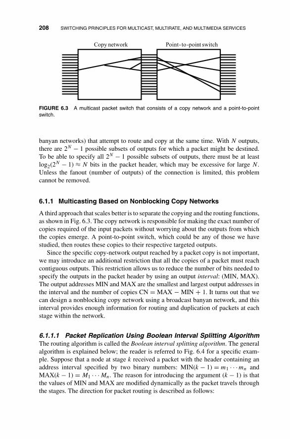
208 SWITCHING PRINCIPLES FOR MULTICAST, MULTIRATE, AND MULTIMEDIA SERVICES
Copy network Point- to-point switch
FIGURE 6.3 A multicast packet switch that consists of a copy network and a point-to-pointswitch.
banyan networks) that attempt to route and copy at the same time. With N outputs,there are 2N − 1 possible subsets of outputs for which a packet might be destined.To be able to specify all 2N − 1 possible subsets of outputs, there must be at leastlog2(2N − 1) ≈ N bits in the packet header, which may be excessive for large N.Unless the fanout (number of outputs) of the connection is limited, this problemcannot be removed.
6.1.1 Multicasting Based on Nonblocking Copy Networks
A third approach that scales better is to separate the copying and the routing functions,as shown in Fig. 6.3. The copy network is responsible for making the exact number ofcopies required of the input packets without worrying about the outputs from whichthe copies emerge. A point-to-point switch, which could be any of those we havestudied, then routes these copies to their respective targeted outputs.
Since the specific copy-network output reached by a packet copy is not important,we may introduce an additional restriction that all the copies of a packet must reachcontiguous outputs. This restriction allows us to reduce the number of bits needed tospecify the outputs in the packet header by using an output interval: (MIN, MAX).The output addresses MIN and MAX are the smallest and largest output addresses inthe interval and the number of copies CN = MAX − MIN + 1. It turns out that wecan design a nonblocking copy network using a broadcast banyan network, and thisinterval provides enough information for routing and duplication of packets at eachstage within the network.
6.1.1.1 Packet Replication Using Boolean Interval Splitting AlgorithmThe routing algorithm is called the Boolean interval splitting algorithm. The generalalgorithm is explained below; the reader is referred to Fig. 6.4 for a specific exam-ple. Suppose that a node at stage k received a packet with the header containing anaddress interval specified by two binary numbers: MIN(k − 1) = m1 · · · mn andMAX(k − 1) = M1 · · · Mn. The reason for introducing the argument (k − 1) is thatthe values of MIN and MAX are modified dynamically as the packet travels throughthe stages. The direction for packet routing is described as follows:
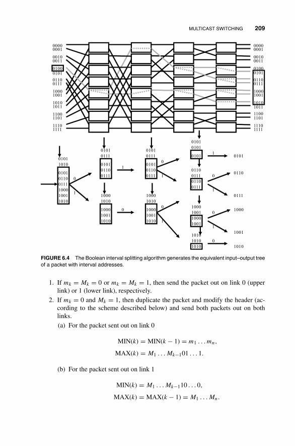
MULTICAST SWITCHING 209
0110
0101
0111
10001001
10101011
11001101
11111110
00000001
00100011
01000101
01110110
10001001
10101011
11001101
11111110
00000001
00100011
01000101
01110110
1001
1000
1010
0101
1010
1
0
0110
0101
0111
1001
1000
1010
0101
0111
1000
1010
1
0
0110
0101
0111
1001
1000
1010
0101
0111
1000
1010
1
0
1
0
0110
0101
0111
0101
0101
0110
0111
1010
1000
1000
1001
1010
1010
1001
1
0
1
0
0
10101
0110
0111
1000
1001
1010
FIGURE 6.4 The Boolean interval splitting algorithm generates the equivalent input–output treeof a packet with interval addresses.
1. If mk = Mk = 0 or mk = Mk = 1, then send the packet out on link 0 (upperlink) or 1 (lower link), respectively.
2. If mk = 0 and Mk = 1, then duplicate the packet and modify the header (ac-cording to the scheme described below) and send both packets out on bothlinks.
(a) For the packet sent out on link 0
MIN(k) = MIN(k − 1) = m1 . . . mn,
MAX(k) = M1 . . . Mk−101 . . . 1.
(b) For the packet sent out on link 1
MIN(k) = M1 . . . Mk−110 . . . 0,
MAX(k) = MAX(k − 1) = M1 . . . Mn.
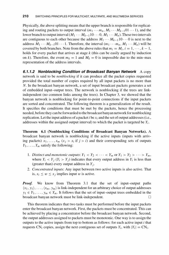
210 SWITCHING PRINCIPLES FOR MULTICAST, MULTIRATE, AND MULTIMEDIA SERVICES
Physically, the above splitting means that the upper branch is responsible for replicat-ing and routing packets to output interval (m1 · · · mn, M1 · · · Mk−101 · · · 1), and thelower branch to output interval (M1 · · · Mk−110 · · · 0, M1 · · · Mn). These two intervalsare contiguous to each other because the address M1 · · · Mk−110 · · · 0 is next to theaddress M1 · · · Mk−101 · · · 1. Therefore, the interval (m1 · · · mn, M1 · · · Mn) will becovered by both branches. Note from the above rules that mi = Mi, i = 1, · · · , k − 1,holds for every packet that arrives at stage k (this can be easily argued by inductionon k). Therefore, the event mk = 1 and Mk = 0 is impossible due to the min–maxrepresentation of the address intervals.
6.1.1.2 Nonblocking Condition of Broadcast Banyan Network A copynetwork is said to be nonblocking if it can produce all the packet copies requestedprovided the total number of copies required by all input packets is no more thanN. In the broadcast banyan network, a set of input broadcast packets generates a setof embedded input–output trees. The network is nonblocking if the trees are link-independent (no common links among the trees). In Chapter 3, we showed that thebanyan network is nonblocking for point-to-point connections if the input packetsare sorted and concentrated. The following theorem is a generalization of the result.It specifies the conditions that must be met by the packets, hence the processingneeded, before they can be forwarded to the broadcast banyan network for nonblockingreplication. Let the input address of a packet i be xi and the set of output addresses (i.e.,addresses within the assigned output interval) to which the packet is targeted be Yi.
Theorem 6.1 (Nonblocking Conditions of Broadcast Banyan Networks). Abroadcast banyan network is nonblocking if the active inputs (inputs with arriv-ing packets) x1, . . . , xm (xj > xi if j > i) and their corresponding sets of outputsY1, . . . , Ym satisfy the following:
1. Distinct and monotonic outputs: Y1 < Y2 < · · · < Ym or Y1 > Y2 > · · · > Ym,where Yi < Yj (Yi > Yj) indicates that every output address in Yi is less than(greater than) every output address in Yj .
2. Concentrated inputs: Any input between two active inputs is also active. Thatis, xi ≤ w ≤ xj implies input w is active.
Proof. We know from Theorem 3.1 that the set of input–output paths〈x1, y1〉, . . . , 〈xm, ym〉 is link-independent for an arbitrary choice of output addressesy1 ∈ Y1, . . . , ym ∈ Ym. It follows that the set of input–output trees embedded in thebroadcast banyan network must be link-independent. �
This theorem indicates that two tasks must be performed before the input packetsenter the broadcast banyan network. First, the packets must be concentrated. This canbe achieved by placing a concentrator before the broadcast banyan network. Second,the output addresses assigned to packets must be monotonic. One way is to assign theoutputs to the active inputs from top to bottom as follows: for each active input i thatrequests CNi copies, assign the next contiguous set of outputs Yi, with |Yi| = CNi.

MULTICAST SWITCHING 211
Three active packets, A, B, and C, and their copy numbers
Copy-number running sums
Address intervals
Copy indices of packets
Outputs
0
1
2
3
4
5
6
7
0
0
2
2
3
7
7
7
A:0
A:1
B:0
C:0
C:1
C:2
C:3
A: 2
B: 1
C: 4
A:(0,1)
B:(2,2)
C:(3,6)
Running- adder network
Dummy address encoder
Reverse Banyan network
Broadcast Banyan network
Trunk- number translator
Packets order unchanged
Concentrated
BCN CN BCN IR MIN, MAX BCN CI TN
FIGURE 6.5 The structure of a nonblocking copy network.
Recall that a concentrator may be built by a running-adder network and a reversebanyan network. The running-adder network assigns a set of concentrated reversebanyan network’s output addresses to the input packets by computing the runningsums of their activity bits. It turns out that the running-adder address network canalso be used to assign the broadcast banyan network’s output intervals to the inputpackets, as will be described after the following overview.
The overall structure of the copy network is depicted in Fig. 6.5. As shown, it con-sists of a cascade of five components: a running-adder network, a set of N dummyaddress encoders, a reverse banyan network, a broadcast banyan network, and a setof N trunk-number translators. There are two additional fields in the header of eachincoming packet: the broadcast channel number (BCN) identifies the multicast con-nection, and the copy number (CN) specifies the number of copies required. The BCNand CN are associated with a virtual connection and are determined during the callsetup time. The different copies of a packet must reach different output destinations ofthe point-to-point switch that follows the copy network and they are distinguished bytheir copy indices (CIs). The CIs are generated inside the copy network after packetreplication. The output addresses are referred to as the trunk numbers (TNs), and atrunk-number translator uses the packet’s BCN and CI to look up its trunk number.
Packet replications are accomplished by two fundamental processes, an encodingprocess and a decoding process. The encoding process is performed by the running-adder network and dummy address encoders. The decoding process is performed bythe concentrator, broadcast banyan network, and the trunk-number translator.
6.1.1.3 Encoding Process Two pieces of information must be generated forevery packet during the encoding process: (1) its reverse banyan network output

212 SWITCHING PRINCIPLES FOR MULTICAST, MULTIRATE, AND MULTIMEDIA SERVICES
Running sum of
activity bits
Info B d
Info A cInfo B c+d+
+
+
+
+
+
+
+
+
+
+
+
+
+
+
+
+
+
+
+
+
+
+
+
+0 0
0
0
0
0
0
Address assigned =Sum of all activity bits above= Running sum - 1
a
b
a+b
Packet B
Packet A
Packet B
Running sum of copy numbers
FIGURE 6.6 An adder in the running-adder network of the copy network: adding both therunning sums of the activity bits and the copy numbers.
address and (2) its broadcast banyan network output intervals. The use of a running-adder network to compute the former has been described earlier in this chapter. Toproduce the latter, in addition to the running sums of the activity bits of packets,the running-adder network also computes the running sums of CNs, as depicted inFig. 6.6. Similar to the computation of the activity bit running sums, it can be shownthat the running sum
RSj =j∑
i=0
CNi
is produced at output j, 0 ≤ j ≤ N − 1, of the network. Based on adjacent runningsums, the dummy address encoders then generate the following sequence of addressintervals:
(0, RS0 − 1), (RS0, RS1 − 1), . . . , (RSN−2, RSN−1 − 1).
If the packet on output j is active, then RSj − 1 ≥ RSj−1 and (RSj−1, RSj − 1) is alegitimate interval and the output interval assigned to the packet is (MIN, MAX) =(RSj−1, RSj − 1). If the packet is inactive, RSj = RSj−1 and the interval is illegiti-mate, which is of no adverse consequence anyway.
6.1.1.4 Decoding Process First of all, the reverse banyan network concen-trates the input packets based on the running sums of their activity bits. The header ofa packet as it enters the broadcast banyan network contains three fields important tothe copying process: the BCN, address interval (MIN, MAX), and an index reference

MULTICAST SWITCHING 213
(IR) that is set to MIN. The IR field is not used or modified in the broadcast banyannetwork, and all copies of the same master packet have the same IR value. Its purposeis the computation of copy indices (CI), which identifies the different copies at theoutputs of the banyan network, as will be explained shortly.
We have already seen that packets can be replicated and routed in a nonblockingmanner in the broadcast banyan network based on the Boolean routing algorithm.Some finer implementation details are described here. An activity bit must be postedin front of the address field to indicate whether the packet is active. At a switch node,if one of the input packets is active and one is inactive, routing will be performedbased on the active packet header. Depending on the header, the switch element couldbe set to cross, bar, or the branching state. If both packets are inactive, we have a“don’t care” situation and it does not matter to which state the switch is set. If bothpackets are active, neither packet needs to be duplicated. The switch element must beset to either the bar or cross state, and either packet header can be used to achieve thesame setting.
When packets emerge from the broadcast banyan network, the address intervalin their header contains only one address. That is, according to the Boolean intervalsplitting algorithm, we have
MIN(n) = MAX(n) = output address
and the copy index is computed by
CI = output address − IR.
In this way, the CN copies of a packet would have distinct CI, ranging from 0 toCN − 1. Based on BCN and CI, the trunk-number translator retrieves the trunk number(output address of the subsequent point-to-point switch) for which the packet copyis destined from a table. The trunk number corresponding to a BCN and a CI isdetermined during the setup of the multicast connection and is stored in the tablethroughout the duration of the session. Note that successive packets of the same BCNand CI may emerge from different broadcast banyan network outputs in different timeslots. Therefore, it is important that the trunk number associated with the BCN andCI be stored in all the trunk-number translators.
6.1.2 Performance Improvement of Copy Networks
In the copy network discussed thus far, if the total number of copies requested byall input ports is not more than the network capacity N, all the requests are granted;otherwise, overflow of the copy requests occurs and some requests must be queuedat the inputs for the next time slot.1 The overflow problem gives rise to two issues:
1One may also design a loss system in which the overflow packets are dropped. As in the point-to-pointswitch, the issue then is how to design and engineer the copy network to have small packet loss probability.

214 SWITCHING PRINCIPLES FOR MULTICAST, MULTIRATE, AND MULTIMEDIA SERVICES
1. How to remove the inherent bias of the running-adder network against the lowerports?
2. How to perform partial service of a copy request?
The first issue is related to input fairness. Since the address intervals of the broadcastbanyan network are assigned to the copy requests by the running-adder networkstarting from top to bottom, lower input ports suffer when the available addresses runout. As a result, packets from lower input ports must be buffered much more oftenthan those from upper ports under heavy-traffic situations. The solution is to allowcomputation of the running sums starting from any arbitrary input i so that port i
is effectively the top port and port (i − 1) mod N the bottom port. Changing i fromtime slot to time slot based on the overflow condition allows input fairness to beachieved.
The second issue is related to the efficiency of the copy network. The utilizationof the copy network would be improved if partial service of copy requests, called callsplitting, can be implemented when overflow occurs. For argument’s sake, supposethat the packet from the first input requests one copy and the packet from the secondinput requests N copies. If no partial service is allowed, the copy network wouldproduce only one packet copy in the current time slot, resulting in much wastefulness.The solution is to allow N − 1 copies to be made of the second packet in the currenttime slot, leaving a residual copy to be made in the next time slot. Call splittingallows the maximum number of packet copies (N) to be made whenever overflowoccurs.
Before providing the solution, let us illustrate what we want to achieve with the4 × 4 copy network example given in Fig. 6.7. In the current time slot, the totalnumber of copies requested is seven, exceeding the capacity of the network. We note
Current time slot
Packet A : 2Packet B : 1Packet C : 3Packet D : 1
Packet E : 2
CN
Copy network
Next time slot
Packet E : 2
Packet C : 2Packet D : 1
Copy network
(New starting point)
FIGURE 6.7 Illustration showing the principle for achieving input fairness by shifting the servicepriority order and the principle of achieving efficiency by call splitting in a copy network.

MULTICAST SWITCHING 215
that although packet C requests three copies, the request cannot be satisfied due tooverflow. However, call splitting allows one copy to be made in the current time slot.In the next time slot, the starting point for service will be packet C, because this iswhere overflow occurs in the current time slot.
6.1.2.1 Cyclic Running-Adder Network To achieve the above, we intro-duce a modified running-adder network called the cyclic running-adder network.Figure 6.8 shows the basic structure and operation of the cyclic running-adder net-work. The structure is totally symmetrical across all ports. Recall that in the originalrunning-adder network, partially computed running sums from the upper links arefed to the lower links, but not the other way round. In the cyclic structure, partiallycomputed running sums from the lower links are also fed to the upper links, asshown in the figure, where the interconnections are indicated by letters a, b, . . . , g.Wrapping the top of the figure to the bottom results in a cylindrically symmetricalstructure.
In each time slot, a starting point for the computation of the running sums isdefined. In Fig. 6.8, for example, running sums are computed starting from the fourthport. For explanation, we shall refer to the starting point as port 0, the next as port 1,and so on (see Fig. 6.8), with the understanding that the labeling changes from timeslot to time slot. The partially computed running sums that cross the starting point areignored by the adders to which they are fed: with reference to Fig. 6.8, the darkened
+
+
+
+
+
+
+
+
+
+
+
+
+
+
+
+
+
+
+
+
+
+
+
+0 1 1
0 2 1
0 4 1
1 2 1
0 1 1
0 2 1
0 0 0
0 1 1
5 0 2 2
0 3 2
0 6 2
1 2 1
1 3 2
0 3 2
0 2 1
0 1 1
0 4 3
0 4 3
0 8 4
1 2 1
1 3 2
1 5 3
1 5 3
0 4 3
1 7 5
1 9 6
1 13 7
1 2 1
1 3 2
1 5 3
1 5 3
1 6 4
6
7
0
1
2
3
4
Starting indicator
Running sum of copy numbersRunning sum of activity bits
a
a b c
b c
d e f g
d e f g
+Packet A SIA RSA RAA
RSAPacket B SIB RSB RAB
SIC RSC RAC
If SIB = 0SIC = SIARSC = RSA + RSBRAC = RAA + RAB
If SIB = 1SIC = SIBRSC = RSBRAC =RAB
FIGURE 6.8 The architecture and operation of a cyclic running-adder network.

216 SWITCHING PRINCIPLES FOR MULTICAST, MULTIRATE, AND MULTIMEDIA SERVICES
links that cross the dashed horizontal line are ignored by the shaded adders. In otherwords, the partial running sums on the darkened links are treated as having values ofzero, effectively making port 0 the top port, port 1, the second port, and so on, in therunning-sum computation (cf. Fig. 6.6).
The next question is how to inform the shaded adders to ignore their upper inputs,considering that the set of shaded adders changes from time slot to time slot with thestarting point. We note that the paths from the starting input port to the shaded addersform a binary tree. Therefore, we introduce a one-bit starting indicator (SI) field, asshown in Fig. 6.8. Initially, only the starting port has this field set to 1; the other portshave it set to 0. The adders in the network simply add the SI fields on their two inputs.Notice that only the shaded adders have the SI field on their lower inputs set to 1.Therefore, this can be used as an indication that they must ignore their upper inputsin running-sum computation.
The starting point remains the same until overflow occurs, in which case the newstarting point in the next time slot will be the first port that encounters overflow inthe current time slot. By the end of each time slot, every input port must be informedof the effective starting point for the next time slot and the number of copies pro-duced for its request in the current time slot—this is needed for implementing callsplitting.
For this purpose, at the outputs of the running-adder network, the SI for the nexttime slot and the served copy number (SCN) for the current time slot are determinedfor every port based on its running sum and the one above. This information is thenfed back to the corresponding input port via a backpropagating path. Let RSi be therunning sum computed at output i. The SI bit indicates whether the input port is thenext starting point and is computed as follows:
SI0 ={
1, if RSN−1 ≤ N ,
0, otherwise ,
SIi ={
1, if RSi−1 ≤ N and RSi > N ,
0, otherwise ,(6.1)
for port i = 1, 2, . . . , N − 1. In Fig. 6.8, the next starting point is port 6 (the secondport from the top) and its SI bit for the next time slot is set to 1 according to the aboverule.
The SCN represents the number of copies allowed for the packet in the currenttime slot. It is computed as follows:
SCN0 = RS0,
SCNi ={
min(N, RSi) − RSi−1, if RSi−1 < N ,
0, otherwise ,(6.2)
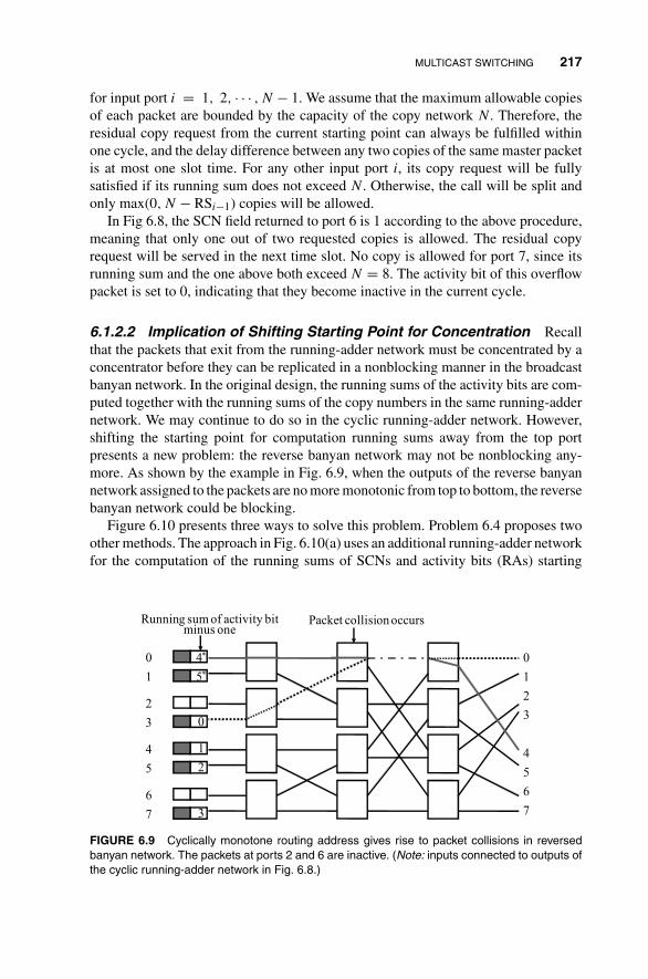
MULTICAST SWITCHING 217
for input port i = 1, 2, · · · , N − 1. We assume that the maximum allowable copiesof each packet are bounded by the capacity of the copy network N. Therefore, theresidual copy request from the current starting point can always be fulfilled withinone cycle, and the delay difference between any two copies of the same master packetis at most one slot time. For any other input port i, its copy request will be fullysatisfied if its running sum does not exceed N. Otherwise, the call will be split andonly max(0, N − RSi−1) copies will be allowed.
In Fig 6.8, the SCN field returned to port 6 is 1 according to the above procedure,meaning that only one out of two requested copies is allowed. The residual copyrequest will be served in the next time slot. No copy is allowed for port 7, since itsrunning sum and the one above both exceed N = 8. The activity bit of this overflowpacket is set to 0, indicating that they become inactive in the current cycle.
6.1.2.2 Implication of Shifting Starting Point for Concentration Recallthat the packets that exit from the running-adder network must be concentrated by aconcentrator before they can be replicated in a nonblocking manner in the broadcastbanyan network. In the original design, the running sums of the activity bits are com-puted together with the running sums of the copy numbers in the same running-addernetwork. We may continue to do so in the cyclic running-adder network. However,shifting the starting point for computation running sums away from the top portpresents a new problem: the reverse banyan network may not be nonblocking any-more. As shown by the example in Fig. 6.9, when the outputs of the reverse banyannetwork assigned to the packets are no more monotonic from top to bottom, the reversebanyan network could be blocking.
Figure 6.10 presents three ways to solve this problem. Problem 6.4 proposes twoother methods. The approach in Fig. 6.10(a) uses an additional running-adder networkfor the computation of the running sums of SCNs and activity bits (RAs) starting
4*
5*
0
1
2
3
0
1
2
3
4
5
6
7
0
1
2
3
4
5
6
7
Running sum of activity bit minus one
Packet collision occurs
FIGURE 6.9 Cyclically monotone routing address gives rise to packet collisions in reversedbanyan network. The packets at ports 2 and 6 are inactive. (Note: inputs connected to outputs ofthe cyclic running-adder network in Fig. 6.8.)
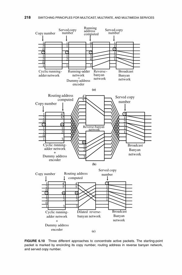
218 SWITCHING PRINCIPLES FOR MULTICAST, MULTIRATE, AND MULTIMEDIA SERVICES
12021201
11
212
1
01
234
5
112121
Copy numberServed copy
number
Running address computed
Served copy number
Cyclic running-adder network
Running-adder network
+ Dummy address
encoder
Reverse -banyan network
Broadcast Banyan network
(a)
12021201
Copy number
Cyclic running-adder network
+Dummy address
encoder
Served copynumber
Reverse-banyan network
BroadcastBanyan network
(b)
11
212
1
4*
5*
012
3
4*
5*
012
3
Routing address computed
12021201
Copy number
Cyclic running-adder network
+Dummy address
encoder
Served copynumber
Dilated reverse-banyan network
BroadcastBanyan network
(c)
11
212
1
4*
5*
012
3
4*
5*
012
3
Routing addresscomputed
FIGURE 6.10 Three different approaches to concentrate active packets. The starting-pointpacket is marked by encircling its copy number, routing address in reverse banyan network,and served copy number.
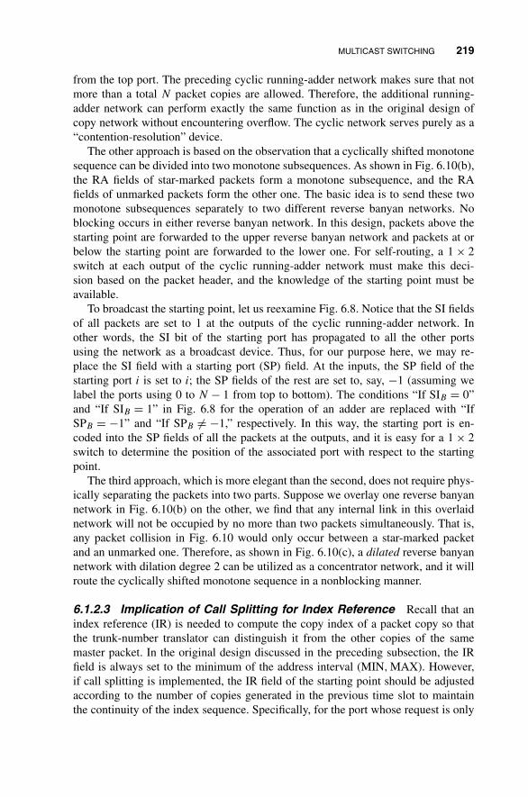
MULTICAST SWITCHING 219
from the top port. The preceding cyclic running-adder network makes sure that notmore than a total N packet copies are allowed. Therefore, the additional running-adder network can perform exactly the same function as in the original design ofcopy network without encountering overflow. The cyclic network serves purely as a“contention-resolution” device.
The other approach is based on the observation that a cyclically shifted monotonesequence can be divided into two monotone subsequences. As shown in Fig. 6.10(b),the RA fields of star-marked packets form a monotone subsequence, and the RAfields of unmarked packets form the other one. The basic idea is to send these twomonotone subsequences separately to two different reverse banyan networks. Noblocking occurs in either reverse banyan network. In this design, packets above thestarting point are forwarded to the upper reverse banyan network and packets at orbelow the starting point are forwarded to the lower one. For self-routing, a 1 × 2switch at each output of the cyclic running-adder network must make this deci-sion based on the packet header, and the knowledge of the starting point must beavailable.
To broadcast the starting point, let us reexamine Fig. 6.8. Notice that the SI fieldsof all packets are set to 1 at the outputs of the cyclic running-adder network. Inother words, the SI bit of the starting port has propagated to all the other portsusing the network as a broadcast device. Thus, for our purpose here, we may re-place the SI field with a starting port (SP) field. At the inputs, the SP field of thestarting port i is set to i; the SP fields of the rest are set to, say, −1 (assuming welabel the ports using 0 to N − 1 from top to bottom). The conditions “If SIB = 0”and “If SIB = 1” in Fig. 6.8 for the operation of an adder are replaced with “IfSPB = −1” and “If SPB = −1,” respectively. In this way, the starting port is en-coded into the SP fields of all the packets at the outputs, and it is easy for a 1 × 2switch to determine the position of the associated port with respect to the startingpoint.
The third approach, which is more elegant than the second, does not require phys-ically separating the packets into two parts. Suppose we overlay one reverse banyannetwork in Fig. 6.10(b) on the other, we find that any internal link in this overlaidnetwork will not be occupied by no more than two packets simultaneously. That is,any packet collision in Fig. 6.10 would only occur between a star-marked packetand an unmarked one. Therefore, as shown in Fig. 6.10(c), a dilated reverse banyannetwork with dilation degree 2 can be utilized as a concentrator network, and it willroute the cyclically shifted monotone sequence in a nonblocking manner.
6.1.2.3 Implication of Call Splitting for Index Reference Recall that anindex reference (IR) is needed to compute the copy index of a packet copy so thatthe trunk-number translator can distinguish it from the other copies of the samemaster packet. In the original design discussed in the preceding subsection, the IRfield is always set to the minimum of the address interval (MIN, MAX). However,if call splitting is implemented, the IR field of the starting point should be adjustedaccording to the number of copies generated in the previous time slot to maintainthe continuity of the index sequence. Specifically, for the port whose request is only

220 SWITCHING PRINCIPLES FOR MULTICAST, MULTIRATE, AND MULTIMEDIA SERVICES
partially fulfilled in the previous time slot,
IR = MIN − previous SCN. (6.3)
It follows that the copy index (CI) of a packet that exits at output i of the broadcastbanyan network would be
CI = i − IR = i − MIN + previous SCN. (6.4)
In this way, the trunk-number translator can then assign the correct output address tothe packet for routing in the subsequent point-to-point switch.
6.1.3 Multicasting Algorithm for Arbitrary Network Topologies
In the copy networks of the preceding subsections, the routes traversed by a packetare predetermined before they enter the copy networks. There is another category ofcopy networks that operate in an analogous way as deflection routing in that the routesare determined on the fly as packet traverses the networks.
In the previous approach, much preprocessing is performed before packets arelaunched into the broadcast banyan network for replication. The goal of the prepro-cessing is to avoid the conflict of packets inside the network. It can be easily seenthat the complexity of the preprocessing hardware is actually more than that of thebroadcast banyan network itself.
An alternative approach is to make no attempt to avoid packet conflict in thebroadcast banyan network. Arriving packets are immediately launched into it. At any2 × 2 node in the network, an input packet desiring replication will be duplicated andforwarded to both outputs provided there is no packet arriving on the other input. Oth-erwise, each of the input packets will simply be forwarded to one of the two outputs.In other words, a packet desiring replication will be duplicated when possible. Other-wise, the replication process will be delayed until a later stage. This strategy is rathergeneral and does not depend on the nonblocking condition of the broadcast banyannetwork, since no attempt is made to avoid conflict in the network anyway. Therefore,it can be applied to arbitrary network topologies, including directed networks.
Let us first focus on the shuffle-exchange network before relating the replicationalgorithm to general network topologies. Instead of a log2 N-stage network, we havean L-stage network in which L ≥ log2 N. In general, the larger the L value, the morelikely that all the copy requests can be satisfied, since larger L implies more chancesfor packet replication attempts.
We shall generalize the Boolean splitting interval algorithm (Problem 6.5 considersan approach in which the copy number is encoded in the packet header rather than thesplitting interval). Instead of using the interval to code the exact output addresses ofthe packet, we use it to code the fanout or the number of copies desired by the packet.For instance, the interval (0, F − 1) can be assigned to every packet, where F is itsfanout number. On which output a particular packet copy will end up depends on its in-teractions with other packets within the network and is not predetermined beforehand.
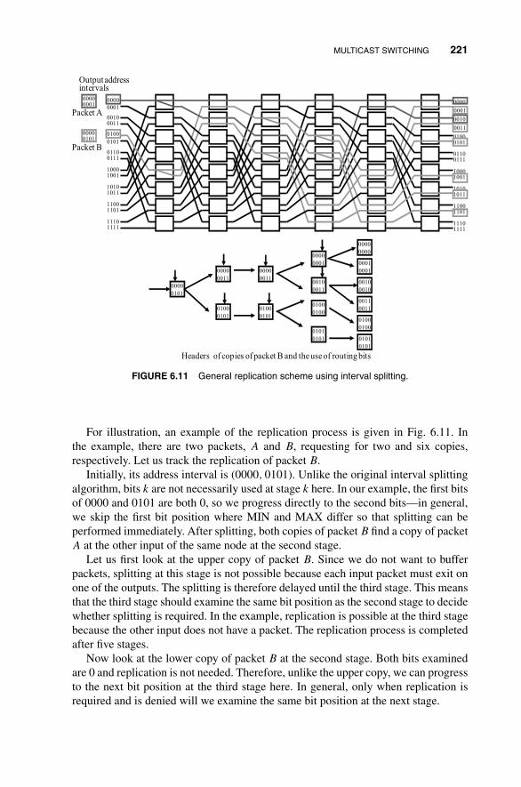
MULTICAST SWITCHING 221
10001001
10101011
11001101
11111110
0000
0001
00100011
0100
0101
01110110
10001001
10101011
11001101
11111110
0000
0001
0010
0011
01000101
01110110
00000001
Output address intervals
00000101
Packet A
Packet B
0000
0101
0000
0011
0100
0101
0000
0011
0100
0101
0000
0001
0010
0011
0100
0100
0101
0101
0000
0000
0001
0001
0010
0010
0011
0011
0100
0100
0101
0101
Headers of copies of packet B and the use of routing bits
FIGURE 6.11 General replication scheme using interval splitting.
For illustration, an example of the replication process is given in Fig. 6.11. Inthe example, there are two packets, A and B, requesting for two and six copies,respectively. Let us track the replication of packet B.
Initially, its address interval is (0000, 0101). Unlike the original interval splittingalgorithm, bits k are not necessarily used at stage k here. In our example, the first bitsof 0000 and 0101 are both 0, so we progress directly to the second bits—in general,we skip the first bit position where MIN and MAX differ so that splitting can beperformed immediately. After splitting, both copies of packet B find a copy of packetA at the other input of the same node at the second stage.
Let us first look at the upper copy of packet B. Since we do not want to bufferpackets, splitting at this stage is not possible because each input packet must exit onone of the outputs. The splitting is therefore delayed until the third stage. This meansthat the third stage should examine the same bit position as the second stage to decidewhether splitting is required. In the example, replication is possible at the third stagebecause the other input does not have a packet. The replication process is completedafter five stages.
Now look at the lower copy of packet B at the second stage. Both bits examinedare 0 and replication is not needed. Therefore, unlike the upper copy, we can progressto the next bit position at the third stage here. In general, only when replication isrequired and is denied will we examine the same bit position at the next stage.

222 SWITCHING PRINCIPLES FOR MULTICAST, MULTIRATE, AND MULTIMEDIA SERVICES
The general algorithm can be described as follows:
Generalized Interval Splitting Algorithm
1. Initially, skip directly to the first bit position where MIN and MAX differ.
2. At any stage, examine the two routing bits.
(a) If the bits are different and the other input of the switch node does nothave a packet, perform splitting according to the original interval splittingalgorithm.
(b) If the bits are different and the other input of the switch node has a packet,do not perform splitting. At the next stage, the same two bits will still beexamined.
(c) If the bits are the same, progress to the next bits at the next stage.
Since the bits to be examined at stage k are not necessarily bits k, a way to indicatethe effective routing bits is needed. This can be solved rather easily by positioning theeffective routing bits at the front of the packet header at all times so that they are bydefault the first two bits, and this can be achieved by a logic design involving six-bitdelays at each stage. The details of bit manipulation and logic implementation arebeyond the scope of this book, which focuses only on the principles.
Several issues that must be addressed are discussed below.
6.1.3.1 Distinguishing Packet Copies As discussed before, at the outputs ofa copy network, packets of different multicast connections are distinguished usingBCN and an IR. All copies of the same master packet have the same BCN, so theBCN can be incorporated into the header of the packet. For generation of distinct IRs,suppose that the interval (0, F − 1) is assigned to all master packets. After successfulreplication, there will be F copies, all with MIN equal to MAX in their interval fields.Furthermore, the MIN (MAX) of the different copies are distinct and range from 0 toF − 1. Therefore, the MIN (or MAX) value can be used as the IR and no explicit IRfield is needed in the header. If the replication process is not completed yet for a copyat an output of the copy network, then its MIN < MAX, and (MAX − MIN) copieswill be considered as lost. The copy chosen to be the successful one can have an IRanywhere between MIN and MAX, inclusively.
6.1.3.2 Deadlock Prevention Although larger L implies lower packet lossprobability, there are two phenomena, however, that may prevent the completionof the replication process, no matter how large L is.
This first is obvious, and it is request overflow, which occurs when the sum of thefanouts of input packets exceeds N, the capacity of the network. The ways for dealingwith overflow will be discussed later. The second phenomenon is deadlock, whichoccurs even when the total copies requested is less than N if certain deterministicrouting policies are used.

MULTICAST SWITCHING 223
Idle input
F= 2
1000
1001
1010
1011
1100
1101
1111
1110
0000
0001
0010
0011
0100
0101
0111
0110
F =1
F =1
F =1
F =1
F =1
F =1
F =1
F =1
F =1
F =1
F =1
F =1
F =1
F =1
FIGURE 6.12 A deadlock example with a deterministic routing policy: set switch elements intobar state under “don’t care” situations. A packet fails to be duplicated regardless of the numberof stages while the bottom link is idle at each stage.
Figure 6.12 shows an example of a deadlock with the following policy: at a 2 × 2node, if there are two input packets, set the switch element to bar state (i.e., forwardthe upper input packet to the upper output and the lower input packet to the lower);also set the switch element to bar state under the “don’t care” situation when one inputhas a packet that does not need to be replicated while the other input does not havean active packet. In the example, the top input has a packet with F = 2, the bottominput does not have an active packet, and each of the rest of the inputs has a packetwith F = 1. It is easily seen that with the above policy, no matter how large L is, thetop packet will stay at the top link while the bottom link remains idle throughout allthe stages. This is not a contrived example, and one can come up with many differentdeadlock scenarios.
There are two ways to prevent deadlocks. One is to use random routing policy.Whenever we have a “don’t care” situation, set the switch element randomly eitherto bar or to cross state. One disadvantage with this approach is the need for imple-menting a random-number generator at each switch node. The alternative is to devisedeterministic routing policies that are deadlock-free. We explain below a very simpledeadlock-free policy.
For simple explanation, one can picture a token on each idle link. In order for apacket to be duplicated at a node, it must acquire and “consume” a token on the otherinput. Thus, the problem becomes that of devising a routing policy that will ensurethe meeting of a token and the packet desiring replication. There are two “don’t care”

224 SWITCHING PRINCIPLES FOR MULTICAST, MULTIRATE, AND MULTIMEDIA SERVICES
situations that must be made into “care” conditions: (1) whenever there is a tokenat one input and the other input does not have a packet that desires duplication, weforward the token to the upper output; (2) whenever the two inputs are occupied andat least one packet desires duplication, we forward that packet to the upper output.
To see why this strategy works, suppose we label the nodes in each stage from top tobottom in a binary fashion. As we have already learned, the construction of the shuffle-exchange network is such that a packet or a token residing at node xnxn−1 · · · x2 willbe forwarded via the upper outgoing link to node 0xnxn−1 · · · x3 at the next stage.Therefore, the above policy can be viewed as attempting to route tokens and packetsdesiring replication to the top node 00 · · · 0. Thus, if there is a token and a packet thatdesires replication in the network, they will eventually meet at node 00 · · · 0, if notearlier. Consequently, deadlocks cannot occur.
In the worst case, a packet can be duplicated at node 00 · · · 0 every log2 N stages.In actuality, packets desiring replication and tokens meet much more often. Thisbecomes evident when we view the routing policy as attempting to concentrate tokensand packets desiring replications at nodes with many 0’s (but not necessarily all 0’s)in their labels. Packets whose replication has been completed are “pushed” to nodeswith many 1’s in their labels.
6.1.3.3 Overflow Problem Overflow occurs when the sum of the fanouts ofinput packets exceeds N. There are two classes of approaches to this problem. Thefirst, such as that discussed in the preceding subsection, is to incorporate a reserva-tion (contention-resolution) mechanism so that the packets allowed to enter the copynetwork desire at most a total of N copies. The overflow requests are buffered at theinputs so that replication can be attempted in the next time slot. One of the goals ofthe copy network in this subsection, however, is to eliminate this kind of preprocess-ing. Therefore, we examine the second approach, which is to increase the bandwidth(capacity) inside the network with respect to the external bandwidth.
One possibility is to employ expansion. An M × M (M > N) shuffle-exchangecopy network could be used in such a way that only the upper N of its M input portsare connected to input links. Because only N of the input links are used, some switchelements at the initial stages are guaranteed not to be traversed by packets. An N × M
expansion network results when these switch elements are removed. In this way, thecapacity of the network is expanded to M and the internal load to the copy networkis reduced, making the occurrence of overflow less likely.
Another possibility is to speed up the internal link with respect to the externallink. With a speedup factor of 2, for example, each external time slot corresponds totwo internal time slots, and by dividing the copy requests into two batches, one foreach internal time slot, the overflow probability can be reduced. With this approach,if the point-to-point switch that follows the copy network does not employ speedup,buffers are needed in between them, since multiple copies may be delivered to thesame link interconnecting them in the same time slot. In this sense, this scheme iscompatible with point-to-point switches that employ input buffering. This schemeis also compatible with those point-to-point output-buffered switches that employinternal speedup with the same or higher speedup factor. The overall multicast switchwill then be output-buffered.
MULTICAST SWITCHING 225
6.1.3.4 Performance We consider a brief approximate analysis of the loss prob-ability of packet copies. The analysis here applies to arbitrary network topologies.Consider an input packet requesting F = 2f copies in a large-size copy network. Wecan picture the input packet as having F embedded copies and focus on one of thecopies. Each time splitting occurs, the copy becomes embedded in one of the outputpackets. The loss probability of the copy can be approximated by the probability thatthe copy experiences fewer than f splittings after traversing the L stages of the copynetwork.
For simplicity, we assume that a splitting attempt will be made as long as thereplication process is not completed. Furthermore, we assume the probabilities ofsuccessful splitting at different stages to be independent. In reality, the probabilitiesof success at the earlier stages are higher than those at later stages because there aremore packet copies at later stages. However, for analytical tractability, we assume thatthe probabilities are all equal to p, which will be set to the worst-case value later.2
The situation is then the same as that in Bernoulli trials with success probability p
and failure probability q = 1 − p. Denote the number of successes in L trials by SL.The loss probability can be approximated by the probability that SL is less than f ,which can in turn be approximated by the error function when f is large:
Ploss ≈ Pr{SL < f } ≈ 1√2π
∫ −y
−∞e−x2/2dx, (6.5)
where
y = Lp − f√pqL
=√
L(p − f/L)√pq
. (6.6)
The inequality
1√2π
∫ −y
−∞e−x2/2dx ≤ 1
2e−y2/2 (6.7)
can be used to obtain a simpler bound. For L large enough that (p − f/L) ≈ p, it canbe seen that Ploss decreases exponentially with L.
Let us now take another viewpoint: what L is required to meet a given loss prob-ability requirement? We note from (6.5) and (6.6) that f/L is an important quantity.Specifically, for a given constant f/L < p the upper bound on Ploss approaches zeroas f (and therefore L increases), whereas if f/L > p the upper bound approachesone. Therefore, in general, the required L for a given loss probability requirementshould be a constant times f ′ = f/p:
L = kf ′ = kf/p, (6.8)
where k > 1. For large f , L needs only be slightly more than f/p.
2This analysis has also ignored the overflow effect, which causes the success probabilities at differentstages to be dependent. Thus, strictly speaking, our approximation is valid only if the overflow probabilityhas been made very small by design.
226 SWITCHING PRINCIPLES FOR MULTICAST, MULTIRATE, AND MULTIMEDIA SERVICES
Consider the following fact: when there is no contention and p = 1, f stagesare needed to complete the replication process; but when p < 1, roughly f ′ = f/p
stages are required according to the above analysis. Therefore, f ′ can be interpretedas the effective fanout parameter when there is contention from other packets. Forthe worst possible fanout, f = n, the required L is proportional to n/p, wheren = log2 N.3
To see how L relates to a given Ploss more specifically, write k = 1 + ε whereε > 0. It is easy to derive from (6.5) and (6.7) that
ε2 ≤ −2q
fln(2Ploss) − ε < −2q
fln(2Ploss). (6.9)
Thus, the ε required to achieve a given loss probability goes to zero as f tends toinfinity given a fixed q. This indicates that for large copy networks, in the worst case,the required L needs only be slightly more than n/p.
We now relate p to the network load. Let ρ denote the output offered load of thenetwork. It is related to the input offered load ρo (probability of finding a packet at aninput) by ρ = fρo, where f is the average fanout. Inside the network, the probabilityof a packet finding another packet at the same switch node, and therefore splitting isnot possible, is bounded by ρ. In other words, p = 1 − ρ and q = ρ. For a networkthat adopts expansion or speedup (see Section 6.1.3.3) with an expansion or speedupfactor of S, p = 1 − ρ/S and q = ρ/S.
Let us consider an example in which ρ = 0.8, S = 2, and F = 32. Suppose thata loss probability of 10−8 is required. It can be derived from (6.9) that the requiredε < 1.7, and the required L < 23. For a 256 × 256 copy network, n = log2 N = 8,this means L < 2.8n.
In reality, the required L should be much smaller, thanks to our generous simpli-fying assumptions in the analysis. The interested readers are referred to Ref. [Lie95]for simulated performance results.
6.1.3.5 Application to Arbitrary Topologies Let us now illustrate the gen-erality of the replication scheme by considering an entirely different network topol-ogy. The main observation is that the correctness of the algorithm does not dependon the shuffle-exchange pattern. The adjacent stages can be interconnected in anyfashion.4
The same scheme also applies to undirected networks. An example is the shuffle-exchange network consisting of only one stage in which the output links of the stageare connected back to the inputs of the same stage via a shuffle pattern. For undi-
3In practice, the fanouts of multicast connections depend on the underlying services and applications, andthey may not simply grow with the switch size. One would therefore expect the required L to be less thanproportional to n/p as n increases.4The performance, however, may be dependent on the interconnection pattern regularly or irregularly. Forexample, we can have an interconnection in which the N × N copy network is actually two unconnectedN/2 × N/2 shuffle-exchange networks in parallel. The performance will not be as good as a single N × N
shuffle-exchange network.
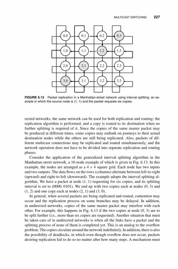
MULTICAST SWITCHING 227
0,0
1,0
2,0
3,0
0,1
1,1
2,1
3,1
0,2
1,2
2,2
3,2
0,3
1,3
2,3
3,3
FIGURE 6.13 Packet replication in a Manhattan-street network using interval splitting: an ex-ample in which the source node is (1, 1) and the packet requests six copies.
rected networks, the same network can be used for both replication and routing: thereplication algorithm is performed, and a copy is routed to its destination when nofurther splitting is required of it. Since the copies of the same master packet maybe produced at different times, some copies may embark on journeys to their actualdestination nodes while the others are still being replicated. Also, packets of dif-ferent multicast connections may be replicated and routed simultaneously, and thenetwork operation does not have to be divided into separate replication and routingphases.
Consider the application of the generalized interval splitting algorithm in theManhattan-street network, a 16-node example of which is given in Fig. 6.13. In thisexample, the nodes are arranged as a 4 × 4 square grid. Each node has two inputsand two outputs. The data flows on the rows (columns) alternate between left-to-right(upward) and right-to-left (downward). The example adopts the interval splitting al-gorithm. We have a packet at node (1, 1) requesting for six copies, and its splittinginterval is set to (0000, 0101). We end up with two copies each at nodes (0, 3) and(1, 2) and one copy each at nodes (2, 1) and (3, 0).
In general, when several packets are being replicated and routed, contention mayoccur and the replication process on some branches may be delayed. In addition,in undirected networks, copies of the same master packet may interfere with eachother. For example, this happens in Fig. 6.13 if the two copies at node (0, 3) are tobe split further (i.e., more than six copies are requested). Another situation that mustbe taken care of in undirected networks is when all the links have a packet and thesplitting process of none of them is completed yet. This is an analog to the overflowproblem. The copies circulate around the network indefinitely. In addition, there is alsothe possibility of deadlocks, in which even though overflow does not occur, packetsdesiring replication fail to do so no matter after how many steps. A mechanism must
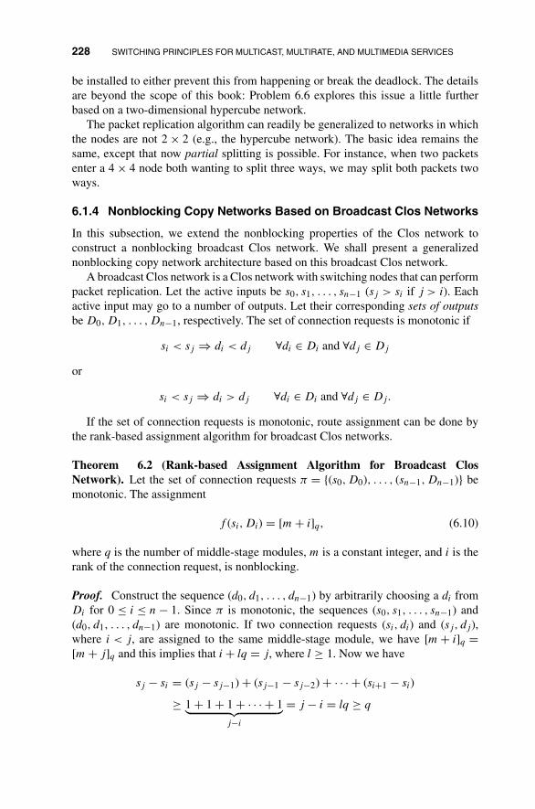
228 SWITCHING PRINCIPLES FOR MULTICAST, MULTIRATE, AND MULTIMEDIA SERVICES
be installed to either prevent this from happening or break the deadlock. The detailsare beyond the scope of this book: Problem 6.6 explores this issue a little furtherbased on a two-dimensional hypercube network.
The packet replication algorithm can readily be generalized to networks in whichthe nodes are not 2 × 2 (e.g., the hypercube network). The basic idea remains thesame, except that now partial splitting is possible. For instance, when two packetsenter a 4 × 4 node both wanting to split three ways, we may split both packets twoways.
6.1.4 Nonblocking Copy Networks Based on Broadcast Clos Networks
In this subsection, we extend the nonblocking properties of the Clos network toconstruct a nonblocking broadcast Clos network. We shall present a generalizednonblocking copy network architecture based on this broadcast Clos network.
A broadcast Clos network is a Clos network with switching nodes that can performpacket replication. Let the active inputs be s0, s1, . . . , sn−1 (sj > si if j > i). Eachactive input may go to a number of outputs. Let their corresponding sets of outputsbe D0, D1, . . . , Dn−1, respectively. The set of connection requests is monotonic if
si < sj ⇒ di < dj ∀di ∈ Di and ∀dj ∈ Dj
or
si < sj ⇒ di > dj ∀di ∈ Di and ∀dj ∈ Dj.
If the set of connection requests is monotonic, route assignment can be done bythe rank-based assignment algorithm for broadcast Clos networks.
Theorem 6.2 (Rank-based Assignment Algorithm for Broadcast ClosNetwork). Let the set of connection requests π = {(s0, D0), . . . , (sn−1, Dn−1)} bemonotonic. The assignment
f (si, Di) = [m + i]q, (6.10)
where q is the number of middle-stage modules, m is a constant integer, and i is therank of the connection request, is nonblocking.
Proof. Construct the sequence (d0, d1, . . . , dn−1) by arbitrarily choosing a di fromDi for 0 ≤ i ≤ n − 1. Since π is monotonic, the sequences (s0, s1, . . . , sn−1) and(d0, d1, . . . , dn−1) are monotonic. If two connection requests (si, di) and (sj, dj),where i < j, are assigned to the same middle-stage module, we have [m + i]q =[m + j]q and this implies that i + lq = j, where l ≥ 1. Now we have
sj − si = (sj − sj−1) + (sj−1 − sj−2) + · · · + (si+1 − si)
≥ 1 + 1 + 1 + · · · + 1︸ ︷︷ ︸j−i
= j − i = lq ≥ q
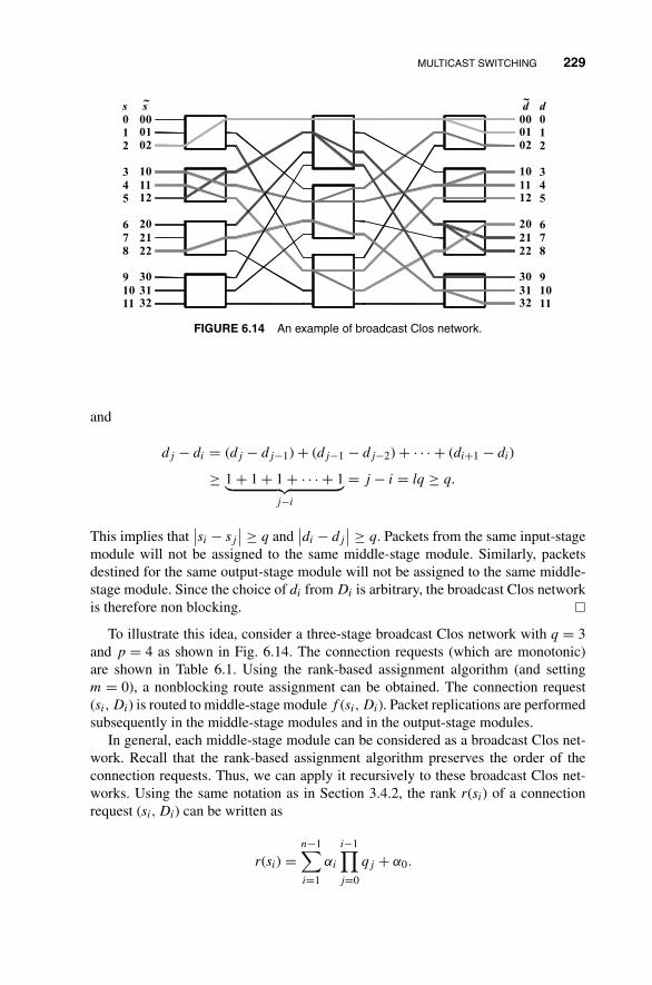
MULTICAST SWITCHING 229
000102
101112
202122
303132
012
345
678
91011
000102
101112
202122
303132
012
345
678
91011
ss d d~ ~
FIGURE 6.14 An example of broadcast Clos network.
and
dj − di = (dj − dj−1) + (dj−1 − dj−2) + · · · + (di+1 − di)
≥ 1 + 1 + 1 + · · · + 1︸ ︷︷ ︸j−i
= j − i = lq ≥ q.
This implies that∣∣si − sj
∣∣ ≥ q and∣∣di − dj
∣∣ ≥ q. Packets from the same input-stagemodule will not be assigned to the same middle-stage module. Similarly, packetsdestined for the same output-stage module will not be assigned to the same middle-stage module. Since the choice of di from Di is arbitrary, the broadcast Clos networkis therefore non blocking. �
To illustrate this idea, consider a three-stage broadcast Clos network with q = 3and p = 4 as shown in Fig. 6.14. The connection requests (which are monotonic)are shown in Table 6.1. Using the rank-based assignment algorithm (and settingm = 0), a nonblocking route assignment can be obtained. The connection request(si, Di) is routed to middle-stage module f (si, Di). Packet replications are performedsubsequently in the middle-stage modules and in the output-stage modules.
In general, each middle-stage module can be considered as a broadcast Clos net-work. Recall that the rank-based assignment algorithm preserves the order of theconnection requests. Thus, we can apply it recursively to these broadcast Clos net-works. Using the same notation as in Section 3.4.2, the rank r(si) of a connectionrequest (si, Di) can be written as
r(si) =n−1∑i=1
αi
i−1∏j=0
qj + α0.

230 SWITCHING PRINCIPLES FOR MULTICAST, MULTIRATE, AND MULTIMEDIA SERVICES
TABLE 6.1 Connection Requests to the Broadcast Clos Network
si 2 3 4 5 8
s̃i 02 10 11 12 22Di 0,1 2,3,4 5,6 7,8,9 10,11D̃i 00,01 02,10,11 12,20 21,22,30 31,32
m + i 0 1 2 3 4f (si , Di ) = [m + i ]q 0 1 2 0 1
The routing tag for the packet to go from input to the middle-stage module assignedto it is given by (α0, α1, α2, . . . , αn−2). Once the packets reach the middle-stagemodules, packet replications and routing are controlled by the generalized intervalsplitting algorithm that is discussed in the following.
6.1.4.1 Generalized Interval Splitting Algorithm for Broadcast Clos Net-work We denote the switch modules from the middle stage to the output stage asbroadcast switch modules due to their capability in performing replication. A packetarriving at a broadcast switch module can be routed to any one of the output links, orit can be replicated if necessary and sent out to a subset of the output links. For thenonblocking operation of the broadcast Clos network, assume that the set of connec-tion requests is monotonic and the set of output destinations assigned to each inputpacket is consecutive. This assumption is justified because in a copy network, thereplicated packets do not need to be routed to some specific output ports. Routingis done by a point-to-point switching network that is cascaded behind the copy net-work. We can therefore deliberately assign the sets of output destinations to the inputpackets such that the connection requests are monotonic. Under such assumption, theset of output destinations of each packet consists of an address interval that can berepresented by two numbers, the minimum and maximum.
Let N = q0 · q1 · · · · · qn−1. The broadcast Clos network consists of 2n − 1 stagesnumbered 0, 1, . . . , 2n − 2. An address interval is a set of contiguous n-tuple. Sup-pose a node at stage i (n − 1 ≤ i ≤ 2n − 2) receives a packet containing an address in-terval specified by min(i − 1) = mn−1 · · · m2n−2 and max(i − 1) = Mn−1 · · · M2n−2,where the argument (i − 1) indicates that the packet comes from a node in stage(i − 1). Since the size of the modules in different stages may be different, each tuplein an address can be of different bases. As discussed in Section 3.4.2, mj and Mj ,where n − 1 ≤ j ≤ 2n − 2, are of base q2n−2−j . When a node in stage i receives apacket, the following procedure is performed:
1. If mi = Mi, then send the packet out on link mi.
2. If mi = Mi, then (Mi − mi + 1) copies of the packet are required. Replicatethe packet, modify the headers and send the packets out on links mi to Mi.
The purpose of header modification is to split the original address interval intoseveral subintervals, each contained in a replicated packet. It is easy to see that

MULTICAST SWITCHING 231
mj = Mj for j = n − 1, . . . , i − 1 holds for every packet that arrives at stage i, wheren − 1 ≤ i ≤ 2n − 2. The event mi > Mi is impossible. For the packet sent out on linkmi, the header becomes
min(i) = min(i − 1) = (mn−1, . . . , mi, mi+1, . . . , m2n−2),
max(i) = (mn−1, . . . , mi, q(2n−2)−(i+1) − 1, . . . , q0 − 1). (6.11)
This is due to the fact that the bases of mi+1, mi+2, . . . , m2n−2 are q(2n−2)−(i+1),q(2n−2)−(i+2), . . . , q0, respectively. For the packet sent out on link Mi, the headerbecomes
min(i) = (Mn−1, . . . , Mi, 0, . . . , 0),
max(i) = max(i − 1) = (Mn−1, . . . , Mi, Mi+1, . . . , M2n−2). (6.12)
For those packets going to output j where mi < j < Mi, the header becomes
min(i) = (mn−1, . . . , mi−1, j, 0, . . . , 0),
max(i) = (mn−1, . . . , mi−1, j, q(2n−2)−(i+1) − 1, . . . , q0 − 1). (6.13)
Figure 6.15 shows the operations of the generalized interval splitting algorithm ona five-stage broadcast Clos network. An input or output address is represented by a3-tuple. The first and the second components are of base 2 while the third one is of base3. By recursively applying the rank-based assignment algorithm, the packet is routedto one of the middle-stage modules. The packets are then subsequently replicatedand routed to the destinations using the generalized interval splitting algorithm. Theaddress intervals contained in the header of each packet are shown in the shadedboxes.
6.1.4.2 Decomposition and Degeneration The broadcast Clos network is infact the cascade combination of a reverse omega network and a broadcast omega net-work. As mentioned in Chapter 3, the omega network belongs to a class of multistageinterconnection networks (MINs) and possesses the nonblocking and self-routingproperties. A broadcast omega network is an omega network with switching nodesthat can perform packet replications. The sufficient conditions for the broadcast omeganetwork to be nonblocking are exactly the same as that for broadcast banyan network.They are given as follows.
Theorem 6.3 (Nonblocking Conditions of Broadcast Omega Networks). A broad-cast omega network is nonblocking if the active inputs s0, s1, · · · , sn−1 (sj > si ifj > i) and their corresponding sets of outputs D0, D1, . . . , Dn−1 satisfy the fol-lowing:
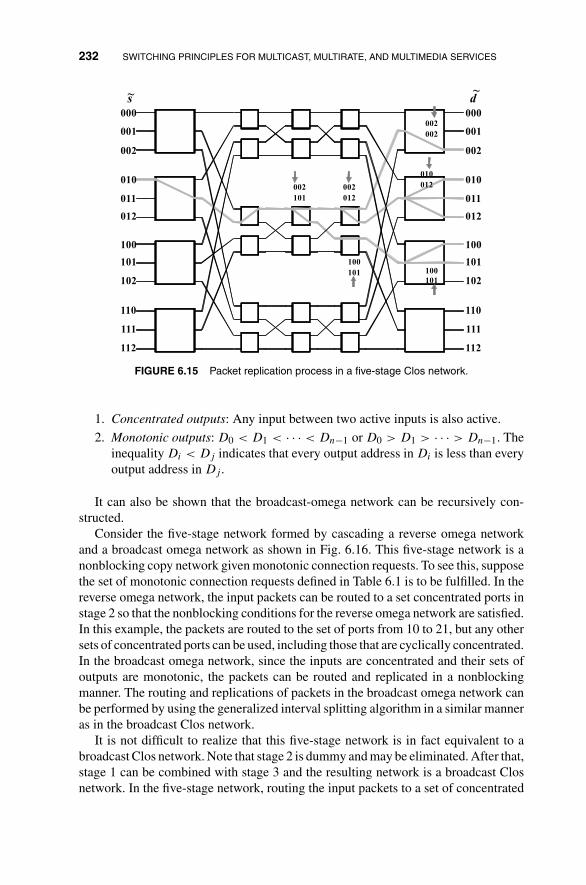
232 SWITCHING PRINCIPLES FOR MULTICAST, MULTIRATE, AND MULTIMEDIA SERVICES
000
001
002
010
011
012
100
101
102
110
111
112
000
001
002
010
011
012
100
101
102
110
111
112
s~ ~d
101
002
012
002
101
100
002
002
012
010
101
100
FIGURE 6.15 Packet replication process in a five-stage Clos network.
1. Concentrated outputs: Any input between two active inputs is also active.
2. Monotonic outputs: D0 < D1 < · · · < Dn−1 or D0 > D1 > · · · > Dn−1. Theinequality Di < Dj indicates that every output address in Di is less than everyoutput address in Dj .
It can also be shown that the broadcast-omega network can be recursively con-structed.
Consider the five-stage network formed by cascading a reverse omega networkand a broadcast omega network as shown in Fig. 6.16. This five-stage network is anonblocking copy network given monotonic connection requests. To see this, supposethe set of monotonic connection requests defined in Table 6.1 is to be fulfilled. In thereverse omega network, the input packets can be routed to a set concentrated ports instage 2 so that the nonblocking conditions for the reverse omega network are satisfied.In this example, the packets are routed to the set of ports from 10 to 21, but any othersets of concentrated ports can be used, including those that are cyclically concentrated.In the broadcast omega network, since the inputs are concentrated and their sets ofoutputs are monotonic, the packets can be routed and replicated in a nonblockingmanner. The routing and replications of packets in the broadcast omega network canbe performed by using the generalized interval splitting algorithm in a similar manneras in the broadcast Clos network.
It is not difficult to realize that this five-stage network is in fact equivalent to abroadcast Clos network. Note that stage 2 is dummy and may be eliminated. After that,stage 1 can be combined with stage 3 and the resulting network is a broadcast Closnetwork. In the five-stage network, routing the input packets to a set of concentrated

MULTICAST SWITCHING 233
000102
101112
202122
303132
012
0123
00010203
10111213
20212223
00010203
10111213
20212223
0123
0123
0123
0123
0123
012
012
012
012
012
012
012
000102
101112
202122
303132
000102
101112
202122
303132
000102
101112
202122
303132
Stage 0 1 2 3 4
0
1
2
3
0
1
2
0
1
2
0
1
2
3
Reverse omega network Omega network
FIGURE 6.16 Broadcast Clos network decomposed into a reverse omega network and a broad-cast omega network.
ports in stage 2 is equivalent to routing consecutive input packets to consecutivemodules in stage 1 in a modulo fashion. In our example, the first input packet isrouted to module 0, the second routed to module 1, and so on. In fact, this is the basisof the rank-based assignment algorithm used in the broadcast Clos network, whichperforms route assignment based on the rank of each connection request.
When the reverse omega network and the broadcast omega network in this five-stage network are recursively constructed using 2 × 2 switching elements, we obtaina cascade combination of the reverse banyan network and the broadcast-banyan net-work, which is the structure of the copy network presented in Section 6.1.1. Thereverse banyan network, together with a running-adder network, performs the func-tion of packet concentration and the broadcast banyan network is responsible forpacket replication and routing. Therefore, we can see that the copy network based onbroadcast Clos network is in fact the generalization of the structure based on broadcastbanyan network.
6.1.4.3 Generalized Connection Networks A generalized connection net-work (GCN) is a switching network with N inputs and N outputs in which each outputmay be connected to any one of the inputs for a total of NN different connection pat-terns. In other words, a mapping π = {(s0, π(s0)), . . . , (sn−1, π(sn−1))}, where π(i)is a set of output destinations (not necessarily continuous), can be realized if
π(i) ∩ π(j) = ∅ for i = j and 0 ≤ i, j ≤ n − 1.

234 SWITCHING PRINCIPLES FOR MULTICAST, MULTIRATE, AND MULTIMEDIA SERVICES
012
345
678
91011
012
345
678
91011
S i d j
FIGURE 6.17 A five-stage GCN.
Let |π(si)| denote the number of elements in π(si). Here, we show by an examplethat a five-stage GCN can be constructed using a broadcast Clos network and theconcepts discussed in this subsection. Consider the network formed by cascading a12 × 12 broadcast Clos network and a 12 × 12 Clos network. Let q = 3 and p = 4in both networks. The resulting five-stage network is a GCN. Suppose the followingset of connection requests is to be satisfied:
π =(
0 2 5 10
{6, 9} {0, 4, 7} {1, 5, 10} {3}
).
Using the previous notations, we have π(0) = {6, 9}, π(2) = {0, 4, 7}, π(5) ={1, 5, 10}, and π(10) = {3}. The broadcast Clos network is responsible for broad-casting the inputs based on the number of output destinations of each input. Given π,the number of output destinations of each input is determined and π is transformedto a set of connection requests for the broadcast Clos network. In this example,input si is assigned a set of consecutive outputs Di in stage 2 based on | π(si) |(Table 6.2). By using the rank-based assignment algorithm and the generalized in-terval splitting algorithm, the inputs are broadcasted to the outputs in stage 2 in anonblocking manner.
When the calls emerge from the broadcast Clos network, they subsequently enterthe Clos network. Since the calls appear consecutively at the output of stage 2, the setof connection requests for the Clos network can be easily determined. In our example,let πj(si) denote the jth element of the set π(si) and let π′ be the set of connection

PATH SWITCHING 235
TABLE 6.2 Connection Requests to the Broadcast-Clos Network.
si 0 2 5 10
Di 0,1 2,3,4 5,6,7 8m + i 0 1 2 3
f (si , Di ) = [m + i ]q 0 1 2 0
requests in the Clos network. We can obtain π′ as follows:
π′ =(
0 1 2 3 4 5 6 7 8
π0(0) π1(0) π0(2) π1(2) π2(2) π0(5) π1(5) π2(5) π0(10)
)
=(
0 1 2 3 4 5 6 7 8
6 9 0 4 7 1 5 10 3
).
This is because there are two output destinations from input 0, three from inputs2 and 5, and one from input 10, respectively. Based on π′, a nonblocking routeassignment can be determined and the connection requests can be established in anonblocking manner.
Obviously, no switching is performed between modules in stage 2 and modules instage 3. We can therefore combine them together to form a five-stage rearrangeablynonblocking multiconnection network. Note, however, that this network is only suit-able for circuit switching applications since centralized route assignment is requiredin the Clos network.
6.2 PATH SWITCHING
Large packet switch architectures can be built based on the modular Clos network. Asdiscussed in Chapter 2, the original Clos network was proposed for circuit switchingsystems, in which a path from an input to an output is established and dedicated toa connection during its whole lifetime. In contrast to these systems, packet switchescarry information in multiplexed format. Often, each connection only requires a por-tion of the capacity of the internal link carrying it, and the bandwidth needed for theconnection may be time varying. One way to operate such systems is to use staticroute assignment, called multirate circuit switching, where a path is established foreach connection such that a portion of the path capacity is allocated to the connectionduring its lifetime. The capacity allocated along the path can be the peak bandwidthrequirement of the connection in order to ensure low delay and packet loss probability.Static routing, however, may result in low utilization of the system, because it doesnot exploit the full advantage of the statistical multiplexing gain offered by packetswitching. The other extreme is the dynamic routing scheme, called cell switching,where the connection pattern of the Clos network is rearranged in every time slotaccording to the targeted outputs of the arrived packets. Since paths for incoming

236 SWITCHING PRINCIPLES FOR MULTICAST, MULTIRATE, AND MULTIMEDIA SERVICES
packets must be assigned on a slot-by-slot basis, the collecting and processing ofglobal traffic information for path hunting on the fly would become a bottleneckseverely limiting the growth of the switch size and speed. Unlike multirate circuitswitching, the dynamic routing scheme usually does not guarantee the bandwidthfor each individual connection, thus only desired overall system performance, suchas total packet loss probability or throughput, is attainable. In general, the systemutilization of the dynamic scheme is expected to be higher than the static scheme, butthe latter provides better guarantee of QoS for each connection.
In this section, we shall present a novel quasi-static routing scheme called pathswitching. It is a unification of circuit switching and packet switching and is a com-promise of the dynamic and the static routing schemes. In actuality, static switchingis similar to the railway system, where path scheduling and reservation for trains aresuch that the railway is idle most of time, resulting in low utilization. On the otherhand, although dynamic routing i packet switching can raise utilization, its complex-ity places a limit on the size of the switch. Path switching is an analog to the trafficsignals governing the routing of cars at the crossroad. It does not require any compli-cated or special hardware, but still yields high utilization. Because of its simplicityand its flexibility, this quasi-static routing scheme provides distributed control in theClos network.
The routing of path switching is based on the concept of virtual path within theClos network. We consider that there is a virtual path between an input module andan output module, which comprises all virtual circuits interconnecting any incomingport and any outgoing port on this pair of modules. The scheduling of path switchingconsists of two parts. First, the capacity required for each virtual path is determined bythe traffic statistics among all pairs of input and output modules so that the path-levelQoS of the traffic on each pair can be satisfied. Then, a finite number of regular bipartitemultigraphs are generated according to the capacity assignment matrix. If the switchis operated repeatedly according to a set of connection patterns, predetermined bythe edge coloring of the bipartite graph, then the capacity requirement on each virtualpath can be satisfied in the long run, and the computation of route assignment onthe fly can be avoided. Path switching is a quasi-static routing scheme, and it is acompromise of the static scheme and the dynamic scheme.
The path-switched Clos network will be called cross-path switch, a statistical Closnetwork. Instead of using a central controller to process, schedule, and route all incom-ing packets simultaneously. The cross-path switch makes use of a routing algorithmthat is distributed over the three stages of the Clos network. The route assignment incentral modules, predetermined by the bipartite multigraphs, will be used repeatedly.Storing the routing table in the local memory of every input module, the connectionpattern of the central stage is known in every time slot. Each connection pattern speci-fies exactly how many packets can be delivered to a particular output module throughwhich central modules in that time slot. Based on this routing specification, each inputmodule will select those packets waiting in the local input buffers according to theirdestinations and priorities. The selection process will match the destination addresseswith the desired output modules only, such that each output module would have tohandle the output port contentions.

PATH SWITCHING 237
To construct the cross-path switch, any nonblocking, self-routing interconnect fab-rics can be used as the building blocks of the first two stages. The switch modulesof the third stage must be capable of resolving the output port contentions; eitherthe Batcher–banyan network with extended outputs or the knockout switch can beemployed to perform this task. The implementation of path switching is completelydistributed. Although the computation of the capacity assignment and route assign-ment by the central controller still requires global information, it is not a slot-by-slottask. The routing tables stored in the local memory of input modules would be updatedonly if the traffic matrix changes significantly and the switch performance becomesunacceptable.
6.2.1 Basic Concept of Path Switching
A three-stage Clos network is shown in Fig. 6.18. The first stage consists of k inputmodules, each of dimensions n × m. The dimensions of each central module in themiddle stage are k × k. As illustrated in Fig. 6.19, the routing constraints of Closnetwork are briefly stated as follows:
1. Any central module can only be assigned to one input of each input module,and one output of each output module.
2. Input i and output j can be connected through any central module.
3. The number of alternate paths between input i and output j is equal to thenumber of central modules.
n×m k ×k m×n
n×m m×n
n×m m×n
Input stage Output stageMiddle stage
0
1
k−1
0
1
k−1
0
1
m−1
k input modules
m central modules
k output modules
01
n−1
01
n-1
nn +1
2n−1
nn+1
2n-1
n(k−1)n(k−1)+1
nk−1
n(k-1)n(k-1)+1
nk-1k ×k
k ×k
FIGURE 6.18 Three-stage Clos network.

238 SWITCHING PRINCIPLES FOR MULTICAST, MULTIRATE, AND MULTIMEDIA SERVICES
0
1
2
3
0
1
2
0
1
2
FIGURE 6.19 Routing in Clos network.
If we consider each input module and each output module as a node, a particularconnection pattern in the middle stage of the Clos network can be represented by aregular bipartite multigraph with node degree m as illustrated in Fig. 6.20, where eachcentral module corresponds to a group of k edges, each connecting one distinct pairof input–output nodes (modules). Suppose the routing algorithm of the Clos networkis based on dynamic cell switching, and the amount of traffic from input module Ii
to output module Oj is λij cells per time slot. The connection pattern will change inevery time slot according to arrived packets, and the routes will be computed on aslot-by-slot basis. Let eij(t) be the number of edges from Ii to Oj of the correspondingbipartite multigraph in time slot t. Then the capacity Cij of the virtual path between
Input modules
Output modules
0
1
2
3
0
1
2
3
Central module 1Central module 2Central module 3
0
1
2
3
0
1
2
0
1
2
3
3×3 3×3 4×4
(a)(b)
FIGURE 6.20 Correspondence between the middle-stage route scheduling in a Clos networkand the edge coloring of the regular bipartite multigraph: (a) three-stage Clos network; (b) theequivalent regular bipartite graph.

PATH SWITCHING 239
Ii and Oj must satisfy
Cij = limT→∞
∑Tt=1 eij(t)
T> λij. (6.14)
On the other hand, the routes of circuit-switched Clos network are fixed, and theconnection pattern will be the same in every time slot. The capacity must satisfy
Cij = eij(t) = eij > λij, (6.15)
which implies that the peak bandwidth Cij is provided for each virtual circuit at callsetup time, and it does not take statistical multiplexing into consideration at all. Weimplement the idea of quasi-static routing, called path switching, using finite numberof different connection patterns in the middle stage repeatedly, as a compromise ofthe above two extreme schemes. For any given λij , if
∑i λij < n ≤ m, and
∑j λij <
n ≤ m, we can always find a finite number f of regular bipartite multigraphs suchthat ∑f
t=1 eij(t)
f> λij, (6.16)
where eij(t) is the number of edges from node i to node j in the tth bipartite multi-graph. A cross-path switch is said to be statistically stable if and only if the capacityrequirement (6.14) can be satisfied by providing connections repeatedly according tothe coloring of these F bipartite multigraphs. These finite amounts of routing informa-tion can be stored in the local memory of each input module to avoid the slot-by-slotcomputation of route assignments. Path switching becomes circuit switching if f = 1,and it is equivalent to cell switching if f → ∞.
The scheduling of path switching consists of two steps, the capacity assignmentand the route assignment. The capacity assignment is to find the capacity Cij > λij
for each virtual path between input module Ii and output module Oj; it can be carriedout by optimizing some objective functions subject to
∑i Cij = ∑
j Cij = m. Thechoice of the objective function depends on the stochastic characteristic of the trafficon virtual paths and the quality of service requirements of connections.
The next step is to convert the capacity matrix [Cij] into edge coloring of afinite number f of regular bipartite multigraphs; each of them represents a parti-cular connection pattern of central modules in the Clos network. An edge coloring ofa bipartite multigraph is to assign m distinct colors to m edges of each node such thatno two adjacent edges have the same color. It is well known that a regular bipartitemultigraph with degree m is m-colorable. Each color corresponds to a central module,and the color assigned to an edge from input module i to output module j representsa connection between them through the corresponding central module.
Suppose that we choose a sufficient large integer f such that fCij are integersfor all i, j and form a regular bipartite multigraph, called capacity graph, in whichthe number of edges between node i and node j is fCij . Since the capacity graph is

240 SWITCHING PRINCIPLES FOR MULTICAST, MULTIRATE, AND MULTIMEDIA SERVICES
regular with degree fm, it can be edge colored by fm different colors. Furthermore,it is easy to show that any edge coloring of the capacity graph with degree fm is thesuperposition of the edge coloring of f regular bipartite multigraphs of degree m.Consider a particular color assignment a ∈ {0, 1, . . . , fm − 1} of an edge betweeninput node Ii and output node Oj of the capacity graph. Let
a = r · f + t, (6.17)
where r ∈ {0, 1, . . . , m − 1} and t ∈ {0, 1, . . . , f − 1} are the quotient and theremainder of dividing a by f , respectively. The mapping g(a) = (t, r) from theset {0, 1, . . . , fm − 1} → {0, 1, . . . , f − 1} × {0, 1, . . . , m − 1} is one-to-one andonto, that is,
a = a′ ⇐⇒ t = t′ and r = r′.
That is, the color assignment a, or equivalently the assignment pair (t, r), of theedge between Ii and Oj indicates that the central module r has been assigned toa route from Ii to Oj in the tth time slot of every cycle. Adopting the conventionin TDMA system, each cycle will be called a frame and the period f frame size.As illustrated by the example shown in Fig. 6.21(a)–(c), where m = 3 and framesize f = 2, the decomposition of the edge coloring into assignment pairs guaranteesthat route assignments are either space interleaved or time interleaved. Thus, relation(6.17) will be called the time–space interleaving principle.
For uniform traffic, where the distribution of traffic loading between input modulesand output modules is homogeneous, the fm edges of each node can be evenly dividedinto k groups, where k is the total number of input (output) modules. Each groupcontains g = fm/k edges between any I/O pair, where the frame size f should bechosen properly to make the group size g an integer. The edges of this capacity graphcan be easily colored by the Latin square given in Fig. 6.22, where each Ai, 0 ≤ i ≤k − 1, represents a set of distinct colors, for example,
A0 = {0, 1, . . . , g − 1}; A1 = {g, g + 1, . . . , 2g − 1}; . . . ; Ak−1
= {(k − 1)g, (k − 1)g + 1, . . . , kg − 1}.
Since each number in the set {0, 1, . . . , fm − 1} appears only once in any rowor column in the table, it is a legitimate edge coloring of the capacity graph. Theassignment a = (t, r) of an edge between the Ii/Oj pair indicates that the centralmodule r will connect the input module i to output module j in the tth slot of everyframe. As an example, for m = 3 and k = 2, we can choose f = 2 and thus g = 3.Then, the groups of colors are A0 = {0, 1, 2} and A1 = {3, 4, 5}, respectively.The procedure described above is illustrated in Fig. 6.22, and the correspondencebetween the route assignments and the connection patterns in the middle stage isshown in Fig. 6.23.

PATH SWITCHING 241
Input modules
Output modules
0
1
2
0
1
2
0 01 12 23
3
4
4
5
5
0 0
1 12
2
3
3
44 55
0
4
0
1 1
2
2
3 3
4
4 5
5
a r t
0 0
2 1
4 2
1 0
3 1
5 2
0
1
0
1
2
0
1
2
0 01 1
2
2
0 0
1
1
22
0 0
1
12
2
0
(a)
(b)
(c)
12
012
0012
012
1012
012
2
t = 0
0
1
2
0
1
2
0 01
1
2
2
0 0
1
1
22
0 0
11
2
2
012
012
0012
012
1012
012
2
t = 1
FIGURE 6.21 Illustration of time–space interleaving principle.
A 0…A 3A 2A 1Ik−1
.
.
...
.
.
.
.
.
...
.
.
.
Ak−2…A 1A 0Ak−1I1
Ak−1…A 2A 1A 0I0
Ok−1…O2O1O0
FIGURE 6.22 Latin square assignment.
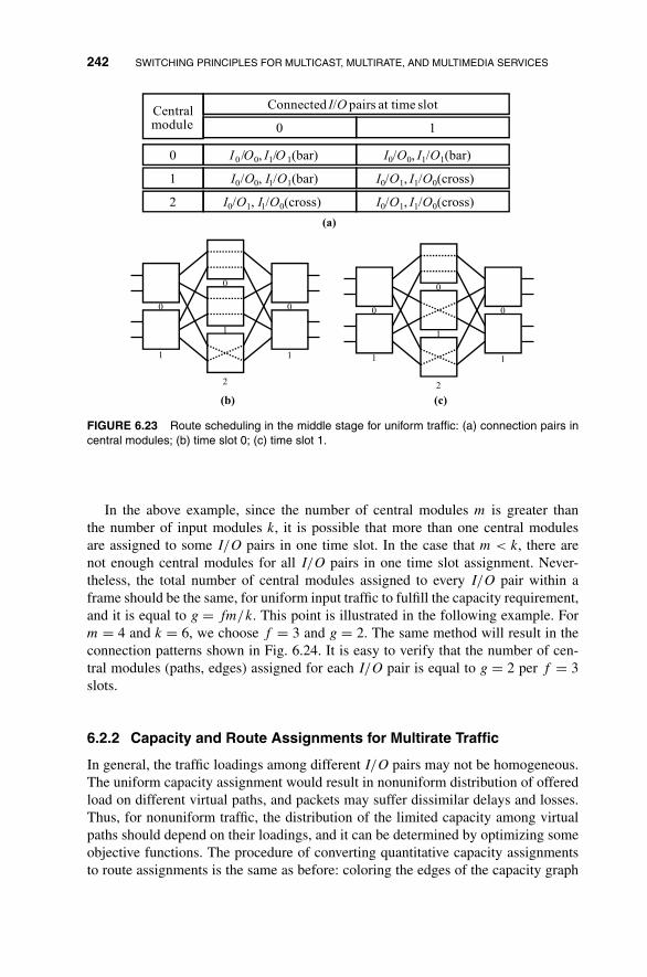
242 SWITCHING PRINCIPLES FOR MULTICAST, MULTIRATE, AND MULTIMEDIA SERVICES
Central module
Connected I/O pairs at time slot
I0 /O0, I1/O 1(bar)0
10
I0/O0, I1/O1(bar)
I0/O0, I1/O1(bar)1 I0/O1, I1/O0(cross)
I0/O1, I1/O0(cross)2 I0/O1, I1/O0(cross)
0
1
0
1
0
1
2
0
1
0
1
0
1
2
(a)
(b) (c)
FIGURE 6.23 Route scheduling in the middle stage for uniform traffic: (a) connection pairs incentral modules; (b) time slot 0; (c) time slot 1.
In the above example, since the number of central modules m is greater thanthe number of input modules k, it is possible that more than one central modulesare assigned to some I/O pairs in one time slot. In the case that m < k, there arenot enough central modules for all I/O pairs in one time slot assignment. Never-theless, the total number of central modules assigned to every I/O pair within aframe should be the same, for uniform input traffic to fulfill the capacity requirement,and it is equal to g = fm/k. This point is illustrated in the following example. Form = 4 and k = 6, we choose f = 3 and g = 2. The same method will result in theconnection patterns shown in Fig. 6.24. It is easy to verify that the number of cen-tral modules (paths, edges) assigned for each I/O pair is equal to g = 2 per f = 3slots.
6.2.2 Capacity and Route Assignments for Multirate Traffic
In general, the traffic loadings among different I/O pairs may not be homogeneous.The uniform capacity assignment would result in nonuniform distribution of offeredload on different virtual paths, and packets may suffer dissimilar delays and losses.Thus, for nonuniform traffic, the distribution of the limited capacity among virtualpaths should depend on their loadings, and it can be determined by optimizing someobjective functions. The procedure of converting quantitative capacity assignmentsto route assignments is the same as before: coloring the edges of the capacity graph

PATH SWITCHING 243
(a)
(b)
(c)
FIGURE 6.24 Route scheduling in central modules for the second example of uniform traffic:(a) time slot 0; (b) time slot 1; (c) time slot 2.

244 SWITCHING PRINCIPLES FOR MULTICAST, MULTIRATE, AND MULTIMEDIA SERVICES
first and then decomposing them into assignment pairs according to the time–spaceinterleaving principle.
6.2.2.1 Capacity Allocation In this part, we shall discuss the allocation ofthe limited capacity in the cross-path switch to meet diverse QoS requirements forindividual calls. The capacity in the cross-path switch can be classified into threelevels, namely, the switch level, the call level, and the packet level. The capacityof switch level can be viewed as the overall switching resources in the cross-pathswitch. It is defined to be the number of packets that can be routed from the inputstage to the output stage in one slot time. The switch-level capacity is fixed anddetermined by the number of central modules. The call-level capacity allocation isconstrained by the capacity of the switch level. At the call level, the cross-path switchwill allocate a certain amount of capacity, called effective bandwidth, to individualcalls such that their statistical QoS constraints in terms of delay or loss at the packetlevel can be satisfied. The effective bandwidths can be estimated through the directapproach, model fitting, or the virtual-buffer approach. An example of calculatingeffective bandwidths based on–off source model is provided in the appendix.
Let αuv, in unit of cells/slot, be the effective bandwidth required to accommodatethe aggregate traffic between an input link u and an output link v. We assume that thefollowing link capacity constraints are observed by call admission procedure:{∑
u αuv ≤ 1, ∀ 0 ≤ v ≤ N − 1,∑v αuv ≤ 1, ∀ 0 ≤ u ≤ N − 1.
(6.18)
The capacity of each link may not be fully utilized, and its remaining capacity canbe distributed to available bit rate (ABR) traffic, which is not bounded by any delayconstraints, as specified in the following chapter. The ABR service can be supportedby feedback flow control mechanisms to provide rapid access to unused networkbandwidth whenever available. Let ρuv be the mean rate of the admitted ABR trafficbetween input link u and output link v, satisfying the following constraint of remaininglink capacity: {∑
u ρuv ≤ 1 − ∑u αuv, ∀ v,∑
v ρuv ≤ 1 − ∑v αuv, ∀ u.
(6.19)
As shown in Fig. 6.25, let λij = ∑(u,v)|u∈Ii,v∈Oj
ρuv be the total rate of ABR trafficon the virtual path between input module Ii and output module Oj , and we assumethat the following k × k ABR traffic matrix is given:
T =
⎡⎢⎢⎢⎢⎣
λ0,0 λ0,1 · · · λ0,k−1
λ1,0 λ1,1 · · · λ1,k−1
......
. . ....
λk−1,0 λk−1,1 · · · λk−1,k−1
⎤⎥⎥⎥⎥⎦ .

PATH SWITCHING 245
0
1
n−2
n−1
Input buffers
Aggregate arrival rate λ ij Capacity Cij
Virtual path
0
1
n-2
n−1
Outputs buffers
Input module i Output module j
FIGURE 6.25 Virtual path between input module i and output module j .
Then, the capacity allocation is to find a matrix
C =
⎡⎢⎢⎢⎢⎣
c0,0 c0,1 · · · c0,k−1
c1,0 c1,1 · · · c1,k−1
......
. . ....
ck−1,0 ck−1,1 · · · ck−1,k−1
⎤⎥⎥⎥⎥⎦ ,
subject to the following constraints:
⎧⎪⎪⎨⎪⎪⎩
cij ≥ λij, ∀i, j,∑j cij = m − ∑
u∈Ii,vαuv, ∀i,∑
i cij = m − ∑v∈Oj,u
αuv, ∀j.
(6.20)
The goal of capacity allocation is to distribute limited resources fairly among allABR calls. In the one-dimensional case, a fair allocation is to distribute the capacityproportional to individual arrival rates as follows:
ci = λi · c∑j λj
, ∀i, (6.21)
where c is the total bandwidth. This is equivalent to minimizing the total weightedoffered load λi/ci function
z =∑
i
λ2i
ci
,
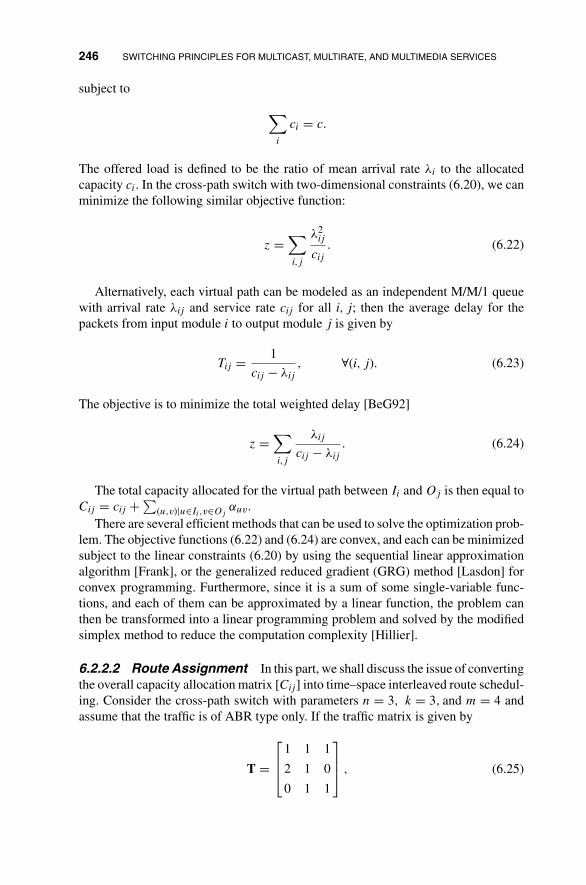
246 SWITCHING PRINCIPLES FOR MULTICAST, MULTIRATE, AND MULTIMEDIA SERVICES
subject to
∑i
ci = c.
The offered load is defined to be the ratio of mean arrival rate λi to the allocatedcapacity ci. In the cross-path switch with two-dimensional constraints (6.20), we canminimize the following similar objective function:
z =∑i,j
λ2ij
cij
. (6.22)
Alternatively, each virtual path can be modeled as an independent M/M/1 queuewith arrival rate λij and service rate cij for all i, j; then the average delay for thepackets from input module i to output module j is given by
Tij = 1
cij − λij
, ∀(i, j). (6.23)
The objective is to minimize the total weighted delay [BeG92]
z =∑i,j
λij
cij − λij
. (6.24)
The total capacity allocated for the virtual path between Ii and Oj is then equal toCij = cij + ∑
(u,v)|u∈Ii,v∈Ojαuv.
There are several efficient methods that can be used to solve the optimization prob-lem. The objective functions (6.22) and (6.24) are convex, and each can be minimizedsubject to the linear constraints (6.20) by using the sequential linear approximationalgorithm [Frank], or the generalized reduced gradient (GRG) method [Lasdon] forconvex programming. Furthermore, since it is a sum of some single-variable func-tions, and each of them can be approximated by a linear function, the problem canthen be transformed into a linear programming problem and solved by the modifiedsimplex method to reduce the computation complexity [Hillier].
6.2.2.2 Route Assignment In this part, we shall discuss the issue of convertingthe overall capacity allocation matrix [Cij] into time–space interleaved route schedul-ing. Consider the cross-path switch with parameters n = 3, k = 3, and m = 4 andassume that the traffic is of ABR type only. If the traffic matrix is given by
T =
⎡⎢⎣ 1 1 1
2 1 0
0 1 1
⎤⎥⎦ , (6.25)
PATH SWITCHING 247
the capacity assignment matrix calculated by the minimization of the total weighteddelay (6.24) is
C =
⎡⎢⎣ 1.3366 1.2774 1.3859
2.6564 1.3366 0
0 1.3859 2.6044
⎤⎥⎦ ≈
⎡⎢⎣
43
43
43
83
43 0
0 43
83
⎤⎥⎦ . (6.26)
In general, the resulting capacity assignment matrix is non-integer such as the exampleshown above. However, the capacity assignments in a frame of size f , f · C, can berounded off into integers, and the round-off error is inversely proportional to f . Thatis, the error can be arbitrarily small if the frame size is sufficiently large. However,since the amount of routing information stored in the memory is linearly proportionalto f , the frame size is limited by the access speed and the memory space of inputmodules. In practice, the choice of frame size f is a compromise between the round-off error and the memory requirement. We assume, without loss of generality, thateij = f · cij are all integers for a sufficiently large f . Then,
∑j
eij =∑
i
eij = f · m (6.27)
and
E = f · C =
⎡⎢⎢⎢⎢⎣
e0,0 e0,1 · · · e0,k−1
e1,0 e1,1 · · · e1,k−1
......
. . ....
ek−1,0 ek−1,1 · · · ek−1,k−1
⎤⎥⎥⎥⎥⎦ .
In the above matrix E, each element eij represents the number of the edges betweenthe Ii/Oj pair in the k × k capacity graph, in which each node has degree of fm. Asmentioned in Section II, this capacity graph can be colored by fm colors, and eachcolor represents one distinct time–space slot based on the time–space interleavingprinciple (6.17). Coloring can be found by complete matching, which is repeatedrecursively to reduce the degree of every node one by one. One general method tosearch for a complete matching is the so-called Hungarian algorithm or alternatingpath algorithm [Leighton, McEliece]. It is a sequential algorithm with the worst timecomplexity O(k2), or totally O(fm × k2) because there are fm matchings. For theabove example, the route scheduling is shown in Fig. 6.26. If each of fm and k is apower of 2, an efficient parallel algorithm proposed in Ref. [LeLi02] for conflict-freeroute scheduling in a three-stage Clos network with time complexity of O(log2(fmk))can be used.
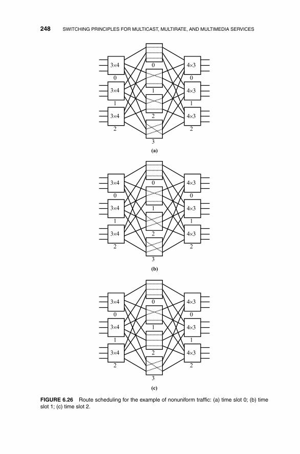
248 SWITCHING PRINCIPLES FOR MULTICAST, MULTIRATE, AND MULTIMEDIA SERVICES
0
1
2
3
3×4 4×3
4×3
4×3
3×4
3×4
3×4 4×3
4×3
4×3
3×4
3×4
3×4 4×3
4×3
4×3
3×4
3×4
0
1
2
0
1
2
0
1
2
3
0
1
2
0
1
2
0
1
2
3
0
1
2
0
1
2
(a)
(b)
(c)
FIGURE 6.26 Route scheduling for the example of nonuniform traffic: (a) time slot 0; (b) timeslot 1; (c) time slot 2.

PATH SWITCHING 249
6.2.3 Trade-Off Between Performance and Complexity
Although the core issue of the cross-path switch is to incorporate the concept ofvirtual path in the switch architecture and provide a coherent network managementparadigm, we still need to investigate the trade-off between its cell-level performanceand switch complexity to provide information for switch design. First, we shall studyvarious trade-offs between performance and complexity in terms of the parametersn, m, and k of an N × N Clos Network. Since a packet arriving at its destined outputmodule of m × n still needs to be routed to one of the n output ports, the complexityof output modules will grow with respect to n. On the other hand, a large value ofn means a small value of k for fixed switch size N = nk, and the traffic stream oneach virtual path would be much smoother, resulting in better statistical multiplexinggain. This is because the superposition of n point processes will approach a Poissonprocess for large n. Also, the capacity assignment and route assignment will be simplerfor a smaller value of k, since both the optimization procedure and edge-coloringalgorithm are based on the k × k traffic matrix. In practice, the determination of theprecise module size n should take the overall loss probability and the throughput intoconsideration.
A fair comparison of systems with different values of n and m/n must be basedon the same amount of overhead. There are three types of overhead in implementingthe cross-path switch.
1. Input arbitration: For better throughput performance, the look-aheadcontention-resolution scheme described in Section 4.2.1 is implemented atthe input modules. Recall that the depth of search in each queue is calledwindow size. The larger the window size, the better the throughput, but theprocessing of look-ahead selection is limited by the transmission time of onepacket. For window size w and module size n, the maximum number of pack-ets that can be examined is wn. This product reflects the processing time re-quired by the look-ahead scheme, and therefore we assume that it is fixedin making the throughput comparison. For example, the throughput of the1024 × 1024 switch with module size n = 8 and window size w = 8 will becompared with that of n = 16 and w = 4, because they have the same productwn = 64. Notice that the module size n should not be too large, otherwise theinternal processing speed may not be fast enough to support the look-aheadscheme.
2. Input memory: In a cross-path switch, the predetermined central-stage connec-tion patterns are stored in the memory of each input module. The total numberof memory space needed to store the addresses of all central modules is ex-actly m, and the overall memory requirement is mkf = m/n · (Nf ) for k inputmodules with frame size f . We assume that the frame size f is a constant in allcases, and use the expansion factor m/n to represent this memory requirement.This point is illustrated by the example shown in Fig. 6.27.
3. Expansion factor: The expansion factor m/n represents the overall capac-ity expansion, and it is the most critical parameter in the performance of
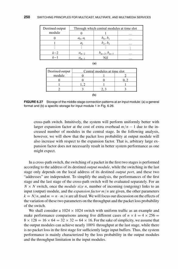
250 SWITCHING PRINCIPLES FOR MULTICAST, MULTIRATE, AND MULTIMEDIA SERVICES
…Nilam−1
…bm−2, bm−1am−2k−2
k−1
......
......
…b2 , b3a21
…b0 , b1a0 , a10
…10
Through which central modules at time slotDestined output
module
32, 332
111, 21
0, 2000
210
Central modules at time slotDestined output
module
(a)
(b)
FIGURE 6.27 Storage of the middle-stage connection patterns at an input module: (a) a generalformat and (b) a specific storage for input module 1 in Fig. 6.26.
cross-path switch. Intuitively, the system will perform uniformly better withlarger expansion factor at the cost of extra overhead m/n − 1 due to the in-creased number of modules in the central stage. In the following analysis,however, we will show that the packet loss probability at output module willalso increase with respect to the expansion factor. That is, arbitrary large ex-pansion factor does not necessarily result in better system performance as onemight expect.
In a cross-path switch, the switching of a packet in the first two stages is performedaccording to the address of its destined output module, while the switching in the laststage only depends on the local address of its destined output port, and these two“addresses” are independent. To simplify the analysis, the performances of the firststage and the last stage of the cross-path switch will be evaluated separately. For anN × N switch, once the module size n, number of incoming (outgoing) links to aninput (output) module, and the expansion factor m/n are given, the other parametersk = N/n, and m = n · m/n are all fixed. We will focus our discussion on the effects ofthe variation of these two parameters on the throughput and the packet loss probabilityof the switch.
We shall consider a 1024 × 1024 switch with uniform traffic as an example andmake performance comparisons among five different cases of n × k = 4 × 256 =8 × 128 = 16 × 64 = 32 × 32 = 64 × 16. For the sake of simplicity, we assume thatthe output modules can achieve nearly 100% throughput at the last stage, while thereis no packet loss in the first stage for sufficiently large input buffers. Thus, the systemperformance is mainly characterized by the loss probability in the output modulesand the throughput limitation in the input modules.
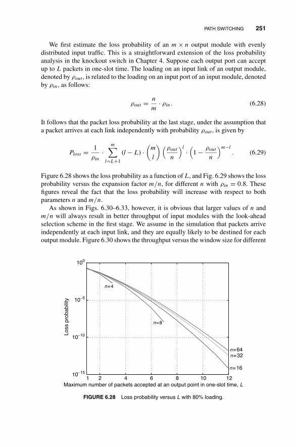
PATH SWITCHING 251
We first estimate the loss probability of an m × n output module with evenlydistributed input traffic. This is a straightforward extension of the loss probabilityanalysis in the knockout switch in Chapter 4. Suppose each output port can acceptup to L packets in one-slot time. The loading on an input link of an output module,denoted by ρout , is related to the loading on an input port of an input module, denotedby ρin, as follows:
ρout = n
m· ρin. (6.28)
It follows that the packet loss probability at the last stage, under the assumption thata packet arrives at each link independently with probability ρout , is given by
Ploss = 1
ρin
·m∑
l=L+1
(l − L) ·(
m
l
)(ρout
n
)l ·(
1 − ρout
n
)m−l
. (6.29)
Figure 6.28 shows the loss probability as a function of L, and Fig. 6.29 shows the lossprobability versus the expansion factor m/n, for different n with ρin = 0.8. Thesefigures reveal the fact that the loss probability will increase with respect to bothparameters n and m/n.
As shown in Figs. 6.30–6.33, however, it is obvious that larger values of n andm/n will always result in better throughput of input modules with the look-aheadselection scheme in the first stage. We assume in the simulation that packets arriveindependently at each input link, and they are equally likely to be destined for eachoutput module. Figure 6.30 shows the throughput versus the window size for different
21 4 6 8 10 1210−15
10−10
10−5
100
Maximum number of packets accepted at an output point in one-slot time, L
Loss
pro
babi
lity
n=4
n=8
n=16
n=64n=32
FIGURE 6.28 Loss probability versus L with 80% loading.

252 SWITCHING PRINCIPLES FOR MULTICAST, MULTIRATE, AND MULTIMEDIA SERVICES
0 0.5 1 1.5 2 2.5 3 3.5 410−10
10−9
10−8
10−7
10−6
Expansion factor, m/n
Loss
pro
babi
lity
n = 64
n = 32
n =16
n = 8
n = 4
FIGURE 6.29 Loss probability versus expansion factor (m/n) with fixed L = 8 and 80% inputloading.
1 2 3 4 5 6 7 80
0.1
0.2
0.3
0.4
0.5
0.6
0.7
0.8
0.9
1
Window size, w
Thr
ough
put
n =64
n =32
n =16
n =8
n=4
FIGURE 6.30 Throughput versus window size w with fixed expansion factor (m/n) = 1.5.

PATH SWITCHING 253
0.5 1 1.5 20
0.1
0.2
0.3
0.4
0.5
0.6
0.7
0.8
0.9
1
Expansion factor, m/n
Thr
ough
put
m =64
n=32
n =16
n=8
n =4
FIGURE 6.31 Throughput versus expansion factor (m/n) with fixed window size w = 4.
1
n =64
n =32
n =16
n =8
n =4
0.9
0.8
0.7
0.6
0.5
Thr
ough
put
0.4
0.3
0.2
0.10.5 1 1.5
Expansion factor, m /n2
FIGURE 6.32 Throughput versus expansion factor (m/n) with fixed product of window size andmodule size wn = 64.

254 SWITCHING PRINCIPLES FOR MULTICAST, MULTIRATE, AND MULTIMEDIA SERVICES
100 101 1020
2
4
6
8
10
12
Module size n
Exp
ansi
on fa
ctor
, m/n
wn = 32
wn = 64
wn = 128
FIGURE 6.33 Expansion factor (m/n) versus module size n to achieve 80% throughput forseveral fixed products of window size and module size.
module sizes n with constant expansion factor m/n = 1.5. Figure 6.31 illustratesthat the throughput is increasing with respect to the expansion factor m/n. However,larger values of m/n and w will increase the complexity of the central stage and theprocessing time at the input stage, respectively. To have a fair comparison, we fixthe input-arbitration overhead wn = 64 in Fig. 6.32 when plotting the throughput fordifferent module sizes n. It shows again that the larger the module size, the higher thethroughput.
Figure 6.33 shows how large the expansion factor m/n should be for some particu-lar module size n to achieve 80% throughput with several fixed products of the windowsize and the module size. Again, the larger modules behave better. The trade-off be-tween the loss probability of output modules and the throughput of input modulesis summarized in Table 6.3. It shows that a proper choice of the module size andthe expansion factor should be n = 16 and m/n = 2, respectively, for switch sizeN = 1024. With window size w = 4, the maximal throughput that can be achieved isabove 80%, while the loss probability at the output modules is kept below 10−7 withL = 8.
6.2.4 Multicasting in Path Switching
In this subsection, we shall study two multicast schemes to enhance the cross-pathswitch to support multicasting. The first scheme, namely scheme 1, performs replica-tion in both input and output modules. As shown in Fig. 6.34(a), a packet in this case is

PATH SWITCHING 255
TABLE 6.3 Summary of Trade-Off in Module Size n
Module Expansion Factor m/n = 1, Expansion Factor m/n = 2,
Size n Ploss(L = 8, Load = 80%) Throughput Ploss(L = 8, Load = 80%) Throughput
4 0 0.29 0 0.478 0 0.41 O(10−8) 0.6416 O(10−8) 0.56 O(10−7) 0.8432 O(10−7) 0.72 O(10−7) 0.9764 O(10−7) 0.78 O(10−7) 0.99
first replicated at the input stage. The number of copies replicated at this stage is equalto the number of destined output modules of the packet. These copies will be routedby the central modules to their destined output modules. Each copy arriving at the laststage will be further replicated if it is destined for more than one output port withinthat output module. In contrast to the scheme 1, the second scheme, namely scheme2, only performs packet replication in input modules. In this scheme, a packet that hasdifferent destined output ports within the same output module needs to be replicatedin the first stage and the resulting copies will be routed independently through differ-ent central modules (see Fig. 6.34(b)). We do not consider multicasting at the middlestage, because the capacity provided by some point-to-multipoint connection patternin the central modules will be affected by the time-varying replication requests andit is not appropriate for the capacity assignment of the cross-path switch.
With the same number of central modules, one would intuitively expect higherthroughput in the first scheme. However, as it requires packet replication at the laststage, the complexity of output modules will be higher. On the contrary, by usingmore central modules in the second multicast scheme, the same throughput can alsobe attained. Since both schemes have their own advantages, it is necessary to evaluatethe trade-off between the performance and the complexity.
Replicating cells in both input and output stage
Replicating cells only in the input stage
(a) (b)
FIGURE 6.34 Two multicast schemes in cross-path switch.

256 SWITCHING PRINCIPLES FOR MULTICAST, MULTIRATE, AND MULTIMEDIA SERVICES
6.2.4.1 Capacity Allocation for Multicast Traffic In the original unicastcross-path switch, the capacity allocation is based on the traffic load and the effectivebandwidth of each virtual path at the middle stage to guarantee the QoS require-ment. For multicast traffic, the middle-stage traffic load will be affected by the packetfanout distribution and the multicast schemes used. The modified capacity assignmentprocedure is described below.
Let Su, Sv, SIi , and SOj be the sets of the call requests on input link u, output linkv, input module Ii, and output module Oj , respectively. We assume that the trafficload (before replication) ρr, in unit of packet/slot, the effective bandwidth (beforereplication) αr, and the packet fanout number yr of call request r are given at thecall setup, and they satisfy the following constraints to fulfill the packet-level QoSrequirement:
1. Input link load constraint: ∑r∈Su
ρr ≤ 1, ∀u. (6.30)
2. Output link capacity constraint:∑r∈Sv
αr ≤ 1, ∀v. (6.31)
We say that r ∈ Su when the call request r comes from input link u, and r ∈ Sv
when one of the destinations of r is output link v.Define λij to be the total traffic load of the virtual path connecting input module
Ii and output module Oj . For scheme 1, in which a call request has only one copyrouted in the middle stage for each destined output module,
λ(1)ij =
∑r∈SIi
, r∈SOj
ρr. (6.32)
In contrast, the traffic load of call request r at the middle stage of scheme 2 is expandedyr times, and yr(i, j) of them will be routed through the virtual path from Ii to Oj .Then the total traffic load of this virtual path is given by
λ(2)ij =
∑r∈SIi
, r∈SOj
ρr · yr(i, j). (6.33)
Similarly, the aggregate effective bandwidths βij of a virtual path connecting Ii andOj in two multicast schemes are given, respectively, as follows:
β(1)ij =
∑r∈SIi
, r∈SOj
αr, β(2)ij =
∑r∈SIi
, r∈SOj
αr · yr(i, j). (6.34)

PATH SWITCHING 257
The capacity assignment is to find the capacity Cij for the virtual path connectingIi and Oj such that the following constraints are satisfied:
⎧⎪⎨⎪⎩
Cij ≥ βij, ∀i, j,∑i Cij = m, ∀j,∑j Cij = m, ∀i,
(6.35)
where m is the number of central modules.Like the case of unicast traffic, an optimal assignment requires establishing an
objective function such as minimizing total weighted delay z after each virtual pathis modeled as an M/M/1 queue:
z =∑i,j
λij
Cij − λij
. (6.36)
6.2.4.2 Performance Evaluations In the following, we shall study how themulticast traffic affects the throughput and the packet loss probability in a 1024 ×1024 cross-path switch. The performance analysis is based on two assumptions. First,the traffic distribution among input ports and output ports is homogeneous, and apacket is equally likely to be destined for any output port. Second, the arrival processat each input link is Bernoulli, that is, the probability that there is a packet arriving ineach time slot is identical and independent.
Fanout Distribution and Middle-Stage Traffic Load To characterize the effect ofthe multicast traffic on the cross-path switch, we consider three fanout distributionsto make comparisons. Let Y be the random variable of the fanout number, and M beits maximum.
1. Constant distribution:
Pr{Y = M} = 1. (6.37)
Mean E[Y ] = M and variance Var[Y ] = 0.
2. Uniform distribution: Suppose the requested fanout is uniformly distributedfrom 1 to M, which is the maximum. In other words,
Pr{Y = y} = 1/M, 1 ≤ y ≤ M. (6.38)
Thus, E[Y ] = M + 1/2 and Var[Y ] = M(M + 1)/6.
3. Truncated geometric distribution:
Pr{Y = y} = (1 − q)qy−1
1 − qM, 1 ≤ y ≤ M, (6.39)

258 SWITCHING PRINCIPLES FOR MULTICAST, MULTIRATE, AND MULTIMEDIA SERVICES
where q is used to control the shape of the distribution. The mean is given by
E[Y ] = 1
1 − q− MqM
1 − qM. (6.40)
This distribution is often used in the literature for modeling the fanout distri-bution. By fixing M equal to the switch size N = 1024, the parameter q can becalculated for a given mean fanout E[Y ].
Multicast traffic load in input stage is different from that in the output stage becausepackets are replicated inside the switch. Let ρin and ρout denote the traffic load ofeach input link at input stage and the traffic load of each output link at output stage,respectively. The traffic in output stage is more than that in input stage, and the ratiois given by
ρout
ρin= E[Y ], (6.41)
which is the mean packet fanout number.Here, we define the middle-stage traffic load ρmid such that ρmid/ρin is equal to the
ratio of the amount of traffic in middle stage to that in input stage. It can be viewedas a reference load of the switch and reflects some difference between two multicastschemes when comparing their throughput and loss performance.
To calculate the middle-stage traffic load ρmid, we let X be the number of copiesthat are replicated from a packet at input stage, that is, the number of distinct outputmodules that the packet is destined for, then ρmid = ρin · E[X].
For scheme 1 in which there is packet replication at both the input and the outputstages, E[X] varies for different fanout distributions. To evaluate E[X], we first noticethat the probability that a packet has no copy destined for a specific output module isgiven by
p0 =M∑
y=1
(n0
)(N−n
y
)(Ny
) · Pr{Y = y}. (6.42)
Then the average of the total number of copies replicated from a packet at the inputstage is k · (1 − p0) = E[X]. For scheme 2 where there is no replication in outputmodules, E[X] = E[Y ]; thus, ρmid = ρout .
To facilitate the comparison of the two schemes in the following, we provide somenumerical figures of ρmid by fixing ρout = 1 in Table 6.4.
Throughput Since output queueing implemented in output modules ensures 100%throughput at the last stage, the throughput of the whole switch is limited only bythe head-of-line blocking in input modules with look-ahead selection. Here, we shallonly focus on the throughput at the input stage.
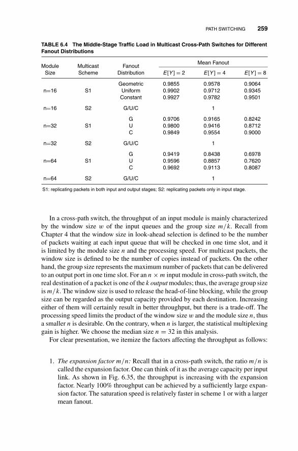
PATH SWITCHING 259
TABLE 6.4 The Middle-Stage Traffic Load in Multicast Cross-Path Switches for DifferentFanout Distributions
Mean FanoutModule Multicast Fanout
Size Scheme Distribution E [Y ] = 2 E [Y ] = 4 E [Y ] = 8
Geometric 0.9855 0.9578 0.9064n=16 S1 Uniform 0.9902 0.9712 0.9345
Constant 0.9927 0.9782 0.9501
n=16 S2 G/U/C 1
G 0.9706 0.9165 0.8242n=32 S1 U 0.9800 0.9416 0.8712
C 0.9849 0.9554 0.9000
n=32 S2 G/U/C 1
G 0.9419 0.8438 0.6978n=64 S1 U 0.9596 0.8857 0.7620
C 0.9692 0.9113 0.8087
n=64 S2 G/U/C 1
S1: replicating packets in both input and output stages; S2: replicating packets only in input stage.
In a cross-path switch, the throughput of an input module is mainly characterizedby the window size w of the input queues and the group size m/k. Recall fromChapter 4 that the window size in look-ahead selection is defined to be the numberof packets waiting at each input queue that will be checked in one time slot, and itis limited by the module size n and the processing speed. For multicast packets, thewindow size is defined to be the number of copies instead of packets. On the otherhand, the group size represents the maximum number of packets that can be deliveredto an output port in one time slot. For an n × m input module in cross-path switch, thereal destination of a packet is one of the k output modules; thus, the average group sizeis m/k. The window size is used to release the head-of-line blocking, while the groupsize can be regarded as the output capacity provided by each destination. Increasingeither of them will certainly result in better throughput, but there is a trade-off. Theprocessing speed limits the product of the window size w and the module size n, thusa smaller n is desirable. On the contrary, when n is larger, the statistical multiplexinggain is higher. We choose the median size n = 32 in this analysis.
For clear presentation, we itemize the factors affecting the throughput as follows:
1. The expansion factor m/n: Recall that in a cross-path switch, the ratio m/n iscalled the expansion factor. One can think of it as the average capacity per inputlink. As shown in Fig. 6.35, the throughput is increasing with the expansionfactor. Nearly 100% throughput can be achieved by a sufficiently large expan-sion factor. The saturation speed is relatively faster in scheme 1 or with a largermean fanout.

260 SWITCHING PRINCIPLES FOR MULTICAST, MULTIRATE, AND MULTIMEDIA SERVICES
1 1.2 1.4 1.6 1.8 20. 8
0.82
0.84
0.86
0.88
0. 9
0.92
0.94
0.96
0.98
1
Expansion factor, m/n
Thr
ough
put
Scheme 1 Scheme 2 Geo E [Y ]=2
Geo E [Y ]=8 Geo E [Y ]=4*
+
FIGURE 6.35 Throughput increase with expansion factor m/n.
2. The mean fanout E[Y ]: To see the multicast effect, we first focus on the firstmoment of multicast traffic, that is, the mean fanout. The throughput versusE[Y ] curve is plotted in Fig. 6.36. It can be observed that the throughput ishigher when the mean fanout is larger. The reason is that the copies from thesame packet have distinct destinations, thus the output contention at the headof line is reduced, compared with the case of having the same total number ofunicast packets waiting. In conclusion, the look-ahead throughput performanceis more favored to multicast traffic.
3. The fanout distribution: Even with the same mean fanout number, the through-put still varies for different fanout distributions as shown in Figs. 6.37 and 6.38.The throughput discrepancy is larger in scheme 1 because the middle-stagetraffic load ρmid is different for different fanout distributions, as shown in Table6.4. The larger the ρmid , the more congested the switch and the smaller thethroughput. It helps to explain why the highest throughput is attained when thepacket fanout is geometrically distributed.
Conversely, the throughput discrepancy in scheme 2 is smaller because themiddle-stage traffic load ρmid is the same as ρout for all fanout distributions.However, since the geometric fanout distribution has the largest variance, itsperformance is the worst. This is similar to other switching systems that theperformance is probably better in handling traffic with less fluctuations.
Loss Probability The overall loss probability of the switch can be well approxi-mated by the knockout loss at the output stage, provided the buffer size of each inputlink is sufficiently large and thus the packet loss at the input stage is negligible.
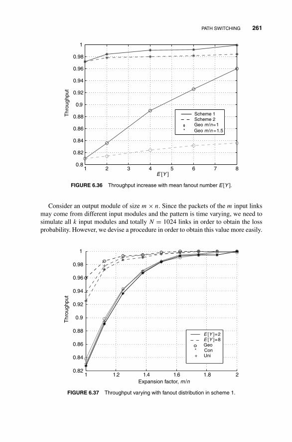
PATH SWITCHING 261
1 2 3 4 5 6 7 80.8
0.82
0.84
0.86
0.88
0.9
0.92
0.94
0.96
0.98
1
E [Y ]
Thr
ough
put
Scheme 1 Scheme 2 Geo m /n=1 * Geo m /n =1.5
FIGURE 6.36 Throughput increase with mean fanout number E [Y ].
Consider an output module of size m × n. Since the packets of the m input linksmay come from different input modules and the pattern is time varying, we need tosimulate all k input modules and totally N = 1024 links in order to obtain the lossprobability. However, we devise a procedure in order to obtain this value more easily.
1 1.2 1.4 1.6 1.8 20.82
0.84
0.86
0.88
0.9
0.92
0.94
0.96
0.98
1
Expansion factor, m /n
Thr
ough
put
E [Y ]=2 E [Y ]=8 Geo * Con + Uni
FIGURE 6.37 Throughput varying with fanout distribution in scheme 1.
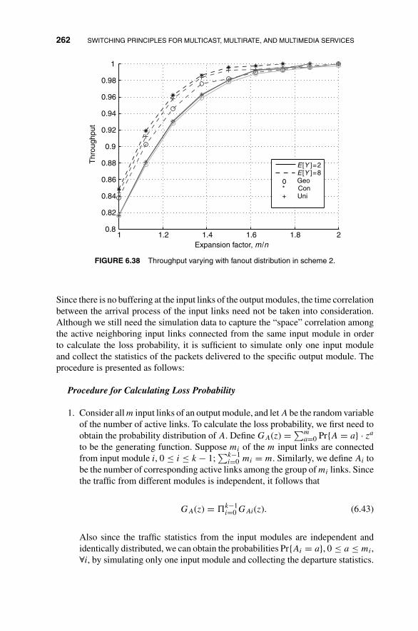
262 SWITCHING PRINCIPLES FOR MULTICAST, MULTIRATE, AND MULTIMEDIA SERVICES
1 1.2 1.4 1.6 1.8 20.8
0.82
0.84
0.86
0.88
0.9
0.92
0.94
0.96
0.98
1
Expansion factor, m/n
Thr
ough
put
E [Y ]=2 E [Y ]=8 Geo * Con + Uni
FIGURE 6.38 Throughput varying with fanout distribution in scheme 2.
Since there is no buffering at the input links of the output modules, the time correlationbetween the arrival process of the input links need not be taken into consideration.Although we still need the simulation data to capture the “space” correlation amongthe active neighboring input links connected from the same input module in orderto calculate the loss probability, it is sufficient to simulate only one input moduleand collect the statistics of the packets delivered to the specific output module. Theprocedure is presented as follows:
Procedure for Calculating Loss Probability
1. Consider all m input links of an output module, and let A be the random variableof the number of active links. To calculate the loss probability, we first need toobtain the probability distribution of A. Define GA(z) = ∑m
a=0 Pr{A = a} · za
to be the generating function. Suppose mi of the m input links are connectedfrom input module i, 0 ≤ i ≤ k − 1;
∑k−1i=0 mi = m. Similarly, we define Ai to
be the number of corresponding active links among the group of mi links. Sincethe traffic from different modules is independent, it follows that
GA(z) = �k−1i=0 GAi(z). (6.43)
Also since the traffic statistics from the input modules are independent andidentically distributed, we can obtain the probabilities Pr{Ai = a}, 0 ≤ a ≤ mi,∀i, by simulating only one input module and collecting the departure statistics.
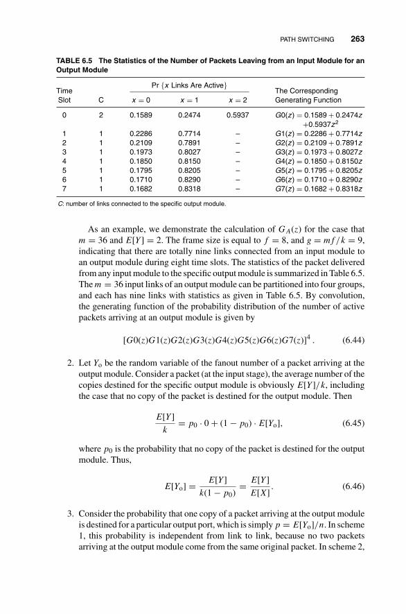
PATH SWITCHING 263
TABLE 6.5 The Statistics of the Number of Packets Leaving from an Input Module for anOutput Module
Pr {x Links Are Active}Time The CorrespondingSlot C x = 0 x = 1 x = 2 Generating Function
0 2 0.1589 0.2474 0.5937 G0(z ) = 0.1589 + 0.2474z
+0.5937z2
1 1 0.2286 0.7714 – G1(z ) = 0.2286 + 0.7714z
2 1 0.2109 0.7891 – G2(z ) = 0.2109 + 0.7891z
3 1 0.1973 0.8027 – G3(z ) = 0.1973 + 0.8027z
4 1 0.1850 0.8150 – G4(z ) = 0.1850 + 0.8150z
5 1 0.1795 0.8205 – G5(z ) = 0.1795 + 0.8205z
6 1 0.1710 0.8290 – G6(z ) = 0.1710 + 0.8290z
7 1 0.1682 0.8318 – G7(z ) = 0.1682 + 0.8318z
C: number of links connected to the specific output module.
As an example, we demonstrate the calculation of GA(z) for the case thatm = 36 and E[Y ] = 2. The frame size is equal to f = 8, and g = mf/k = 9,indicating that there are totally nine links connected from an input module toan output module during eight time slots. The statistics of the packet deliveredfrom any input module to the specific output module is summarized in Table 6.5.The m = 36 input links of an output module can be partitioned into four groups,and each has nine links with statistics as given in Table 6.5. By convolution,the generating function of the probability distribution of the number of activepackets arriving at an output module is given by
[G0(z)G1(z)G2(z)G3(z)G4(z)G5(z)G6(z)G7(z)]4 . (6.44)
2. Let Yo be the random variable of the fanout number of a packet arriving at theoutput module. Consider a packet (at the input stage), the average number of thecopies destined for the specific output module is obviously E[Y ]/k, includingthe case that no copy of the packet is destined for the output module. Then
E[Y ]
k= p0 · 0 + (1 − p0) · E[Yo], (6.45)
where p0 is the probability that no copy of the packet is destined for the outputmodule. Thus,
E[Yo] = E[Y ]
k(1 − p0)= E[Y ]
E[X]. (6.46)
3. Consider the probability that one copy of a packet arriving at the output moduleis destined for a particular output port, which is simply p = E[Yo]/n. In scheme1, this probability is independent from link to link, because no two packetsarriving at the output module come from the same original packet. In scheme 2,
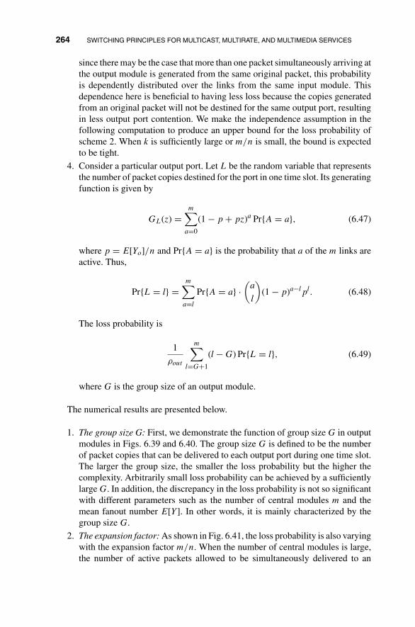
264 SWITCHING PRINCIPLES FOR MULTICAST, MULTIRATE, AND MULTIMEDIA SERVICES
since there may be the case that more than one packet simultaneously arriving atthe output module is generated from the same original packet, this probabilityis dependently distributed over the links from the same input module. Thisdependence here is beneficial to having less loss because the copies generatedfrom an original packet will not be destined for the same output port, resultingin less output port contention. We make the independence assumption in thefollowing computation to produce an upper bound for the loss probability ofscheme 2. When k is sufficiently large or m/n is small, the bound is expectedto be tight.
4. Consider a particular output port. Let L be the random variable that representsthe number of packet copies destined for the port in one time slot. Its generatingfunction is given by
GL(z) =m∑
a=0
(1 − p + pz)a Pr{A = a}, (6.47)
where p = E[Yo]/n and Pr{A = a} is the probability that a of the m links areactive. Thus,
Pr{L = l} =m∑
a=l
Pr{A = a} ·(
a
l
)(1 − p)a−lpl. (6.48)
The loss probability is
1
ρout
m∑l=G+1
(l − G) Pr{L = l}, (6.49)
where G is the group size of an output module.
The numerical results are presented below.
1. The group size G: First, we demonstrate the function of group size G in outputmodules in Figs. 6.39 and 6.40. The group size G is defined to be the numberof packet copies that can be delivered to each output port during one time slot.The larger the group size, the smaller the loss probability but the higher thecomplexity. Arbitrarily small loss probability can be achieved by a sufficientlylarge G. In addition, the discrepancy in the loss probability is not so significantwith different parameters such as the number of central modules m and themean fanout number E[Y ]. In other words, it is mainly characterized by thegroup size G.
2. The expansion factor: As shown in Fig. 6.41, the loss probability is also varyingwith the expansion factor m/n. When the number of central modules is large,the number of active packets allowed to be simultaneously delivered to an
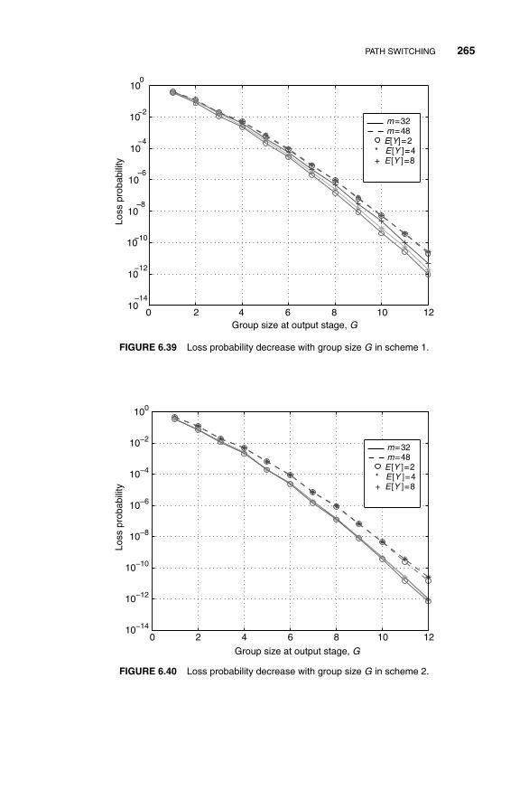
PATH SWITCHING 265
0 2 4 6 8 10 1210
10
10
10
10
10
10
10
Group size at output stage, G
Loss
pro
babi
lity
−14
−12
−10
−8
−6
−4
−2
0
m=32 m=48 E[Y]=2 * E [Y ]=4 + E [Y ]=8
FIGURE 6.39 Loss probability decrease with group size G in scheme 1.
0 2 4 6 8 10 1210−14
10−12
10−10
10−8
10−6
10−4
10−2
100
Group size at output stage, G
Loss
pro
babi
lity
m=32 m=48 E [Y ]=2 * E [Y ]=4 + E [Y ]=8
FIGURE 6.40 Loss probability decrease with group size G in scheme 2.

266 SWITCHING PRINCIPLES FOR MULTICAST, MULTIRATE, AND MULTIMEDIA SERVICES
1 1.2 1.4 1.6 1.8 210−7
10−6
10−5
Expansion factor, m/n
Loss
Pro
babi
lity
Scheme 1 Scheme 2 E [Y ]=2 G=8 * E [Y ]=4 G=8 + E [Y]=8 G=8
FIGURE 6.41 Loss probability increase with expansion factor m/n.
output module tends to be more uniformly distributed, and thus a higher lossprobability is expected.
3. The mean fanout number: The effect of multicast traffic on the loss probabilityis not so significant. As shown in Fig. 6.42 with fixed group size G = 8, theexpansion factor m/n dominates the trend of the loss probability. It changesonly a little when the mean fanout number E[Y ] increases, except when theexpansion factor is small (m/n = 1) in scheme 1 due to the dramatic increasein throughput. Please refer to Fig. 6.36.
6.2.4.3 Overall Complexity Measurements and Comparisons We haveconsidered feasible designs for each multicast schemes to implement the multi-cast cross-path switch. In the following, we shall estimate their complexity interms of the number of switching nodes used under certain performance require-ment.
The input modules and the central modules in both schemes will be the same.Since the central modules are required to be rearrangeably nonblocking only, so thatevery connection pattern of the route assignment can be realized, Benes networks aresuitable and sufficient. Its complexity is given by
Ccm = k
(log2 k − 1
2
), (6.50)

PATH SWITCHING 267
2 3 4 5 6 7 81
2
3
4
5
6
7
8x 10⁻⁷
E [Y ]
Loss
pro
babi
lity
Scheme 1 Scheme 2 m=32 G=8 * m=48 G=8
FIGURE 6.42 The little change of loss probability with mean fanout E [Y ].
where k is the size of a central module, that is, the number of input modules. Thenthe complexity of the middle stage consisting m central modules is
Cmid = mk
(log2 k − 1
2
). (6.51)
Since packet replications are necessary at the input stage, a copy network cascadedwith a point-to-point switch is sufficient. As mentioned in the previous section, thecopy network is estimated as two banyan interconnection fabrics, each with complex-ity Ccn = m
2 log2 m, while the point-to-point switch consists of a Batcher–banyan andits complexity is given by
Cpp = m
4log2 m(log2 m + 1) + m
2log2 m. (6.52)
Thus, the overall complexity of the input stage is Cin = k(Ccn + Cpp).At the last stage, two different switches are used. For scheme 1 where packet
replications are still needed in the output modules, a knockout switch with broadcastbuses can be used. Since each concentrator with group size G has the complexity
m + (m − 1) + (m − 2) + · · · + (m − G) = mG − G(G + 1)
2,

268 SWITCHING PRINCIPLES FOR MULTICAST, MULTIRATE, AND MULTIMEDIA SERVICES
0.8 0.85 0.9 0.95 10.5
1
1.5
2
2.5
3
3.5
4
4.5x 10⁵
Througput
No.
of 2
x2
switc
hing
nod
es
Scheme 1 Scheme 2 E [Y ]=2 G=8 * E [Y ]=4 G=8 + E [Y ]=8 G=8
FIGURE 6.43 The complexity comparison between two multicast schemes for different through-put requirement.
we need Cknock = n[mG − G(G + 1)/2] switching nodes to build up one knock-out switch and totally Cout1 = kCknock for the whole output stage. For scheme 2,a Batcher–banyan switch with channel grouping can be used in the output module.Recall from Chapter 4 that this switch contains an m × m Batcher sorting network,an m × m concentrator, and G parallel banyan networks. The total complexity of theoutput stage for scheme 2 is given by
Cout2 = k ·[m
4log2 m(log2 m + 1) + m
2log2 m + G · n
2log2 n
]. (6.53)
The complexity measures of the switch architectures are shown in Figs. 6.43 and6.44, respectively. The trade-off between performance and complexity of scheme 2is superior to scheme 1 because of the huge complexity in establishing the broadcastknockout switches. Therefore, it might not be worth implementing multicast switchingat the output stage of the cross-path switch.
6.A APPENDIX
6.A.1 A Formulation of Effective Bandwidth
The basis of call-level capacity allocation is the QoS requirement at the packet level.In general, the QoS requirement could be the loss rate, the mean delay, the delay jitter,
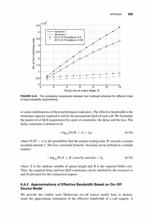
APPENDIX 269
0 2 4 6 8 10 120
0.5
1
1.5
2
2.5
3
3.5
4
4.5x 10
5
Group size at output stage, G
No.
of 2
x2
switc
hing
nod
e Scheme 1 Scheme 2 E [Y ]=8 Throughput=0.9 * E [Y ]=8 Throughput=0.99
FIGURE 6.44 The complexity comparison between two multicast schemes for different orderof loss probability requirements.
or some combinations of these performance indicators. The effective bandwidth is theminimum capacity required to satisfy the prerequisite QoS of each call. We formulatethe packet-level QoS requirement by a pair of constraints: the delay and the loss. Thedelay constraint is defined to be
− log10 Pr{W > τ} > δD, (6.54)
where Pr{W > τ} is the probability that the packet waiting time W exceeds a certainaccepted amount τ. The loss constraint [Guerin, Veciana] can be defined in a similarmanner:
− log10 Pr{X ≥ B | seen by arrivals} > δL, (6.55)
where X is the random variable of queue length and B is the required buffer size.Thus, the required delay and loss QoS constraints can be satisfied by the resources α
and B allocated for the connection request.
6.A.2 Approximations of Effective Bandwidth Based on On–OffSource Model
We provide the widely used Markovian on–off source model here to demon-strate the approximate estimation of the effective bandwidth of a call request. A

270 SWITCHING PRINCIPLES FOR MULTICAST, MULTIRATE, AND MULTIMEDIA SERVICES
two-state Markovian process can be fully characterized by the following three pa-rameters [AMS81]:
⎧⎪⎨⎪⎩
mean arrival rate, λ cell/slot,
peak arrival rate, λp cell/slot,
average“on”period, Ton slot.
With service rate (capacity) μ, the queue length distribution given in Ref.[Anick] isas follows:
Pr{X > x} = λ
μe− λp(μ−λ)x
μTon(λp−μ)(λp−λ) . (6.56)
The overflow probability seen by arrivals is given by
Pr{X > x | seen by arrivals} = e− λp(μ−λ)x
μTon(λp−μ)(λp−λ) . (6.57)
The waiting time distribution Pr{W > τ} is just a scaled version of (6.57) due to therelation x = μτ, and given as follows:
Pr{W > τ} = e− λp(μ−λ)τ
Ton(λp−μ)(λp−λ) . (6.58)
The effective bandwidth α can be calculated from the delay constraint (6.54), and itis given by
α = λ + Ton(δD + log10 e)(λp − λ)2
λpτ + Ton(δD + log10 e)(λp − λ). (6.59)
Similarly, the required buffer size B given below can be obtained from (6.55) through(6.57).
B = αTon(λp − α)(λp − λ)(δL + log10 e)
λp(α − λ). (6.60)
PROBLEMS
6.1 For the broadcast banyan network, argue that two bits are the minimum numberof bits required to perform routing at each switch element, and therefore, theBoolean interval splitting algorithm is a “minimal” algorithm.
6.2 Consider the following broadcast banyan network that attempts to perform copy-ing and routing at the same time with a 2n-bit routing tag. Two bits are used

PROBLEMS 271
in each stage. Bits 00 and 11 mean the packet is to be forwarded to upper andlower outgoing links, respectively. Bits 01 mean the packet is to be duplicatedand forwarded to both outgoing links. Not all the 2N − 1 subsets of outputs canbe reached this way. Describe the subsets of outputs that can be reached.
6.3 Consider an 8 × 8 copy network based on the Boolean interval splitting algo-rithm in the broadcast banyan network operated as a waiting system such thatoverflow requests that cannot be fulfilled will be queued at inputs.
(a) Show the encoding and decoding processes for the following copy requests:two copies for input 0, one copy for input 3, and three copies for input 5;the other inputs are inactive. Show the values adopted by the various fieldsin the packet headers as they travel through the five components of the copynetwork. Assume the running-adder network is not cyclic.
(b) Now, do the same assuming a cyclic running-adder network and a dilatedreverse banyan concentrator, with input 5 being the starting point.
(c) Give an example showing that fewer than N packet copies are allowedeven though there are more requests still waiting at the input queues (Hint:consider HOL blocking).
(d) Show how the efficiency of the copy network can be improved by placing ashifting concentrator before the copy network so as to implement a logicalFIFO queue out of the N input queues.
(e) Consider an input–output pair of a multicast communication session of theoverall multicast switch. Show that packets arriving at successive time slotsto the input to the shifting concentrator may have their copies deliveredsimultaneously to the output of the point-to-point switch, assuming that theswitch is an output-buffered switch. However, it is not possible for a laterarriving packet to have its copy delivered to the output before an earlierarriving packet.
(f) Part (e) means that the switch output must be able to uncover the underlyingsequence of the simultaneously delivered packets in order to avoid out-of-sequence packet transmission on its transmission links. Propose a schemethat enables the output to do so.
6.4 The text explained how a reverse–banyan network fails to concentrate the packetsbetween the cyclic running-adder network and the broadcast–banyan networkin a copy network. Three approaches to solving this problem were proposed.This question considers two other approaches.
(a) Show that a Benes network can be used to concentrate the packets. In par-ticular, show how you would set the 2n − 1 bits for routing in the Benesnetwork.
(b) A three-phase scheme analogous to the sort-banyan point-to-point switchcould be used. In the first two phases, only the headers of packets enter thecyclic running-adder network. The first phase calculates the running sumsand determines the served copy numbers. The second phase acknowledges

272 SWITCHING PRINCIPLES FOR MULTICAST, MULTIRATE, AND MULTIMEDIA SERVICES
00 01
10 11
FIGURE 6.45 Hypercube network.
the inputs of the served copy numbers and the current starting port. The thirdphase performs a cyclic shift on all the winning input packets so that thestarting-port packet appears on the uppermost output of the adder network.In this way, a reverse–banyan network can then be used to concentratethe packets in a nonblocking manner. Show how to use the adder-networkstructure to perform the cyclic shift.
6.5 For the probabilistic copy algorithm for arbitrary network topologies, the textconsidered the splitting interval to keep track of the replication process. Analternative is to directly encode the copy number, CN, into the header.(a) Explain how you would modify CN at each stage whenever it is possible to
duplicate a packet.
(b) An index reference (IR) field is also needed in the packet header. How wouldyou modify the IR field whenever duplication occurs so that the IR fields ofpacket copies of the same master packet are distinct?
6.6 Consider applying the probabilistic copy algorithm on a two-dimensional hy-percube network with four nodes, labeled as 00, 01, 10, and 11, as shown inFig. 6.45. The links are bidirectional and simultaneously carry one packet ineach direction.(a) Suppose that there is a packet at node 00 desiring four copies and there are
no other packets. Show the packet replication process.
(b) Show that a deadlock occurs if the packet desires eight copies.
(c) Suppose that there is a buffer that can hold just one packet at each node. Inother words, when there are no incoming packets to a node, both desiringreplication, we can hold one of the packets in the buffer while duplicatethe other packets on the two outgoing links. Show that this eliminates thedeadlock in part (b).
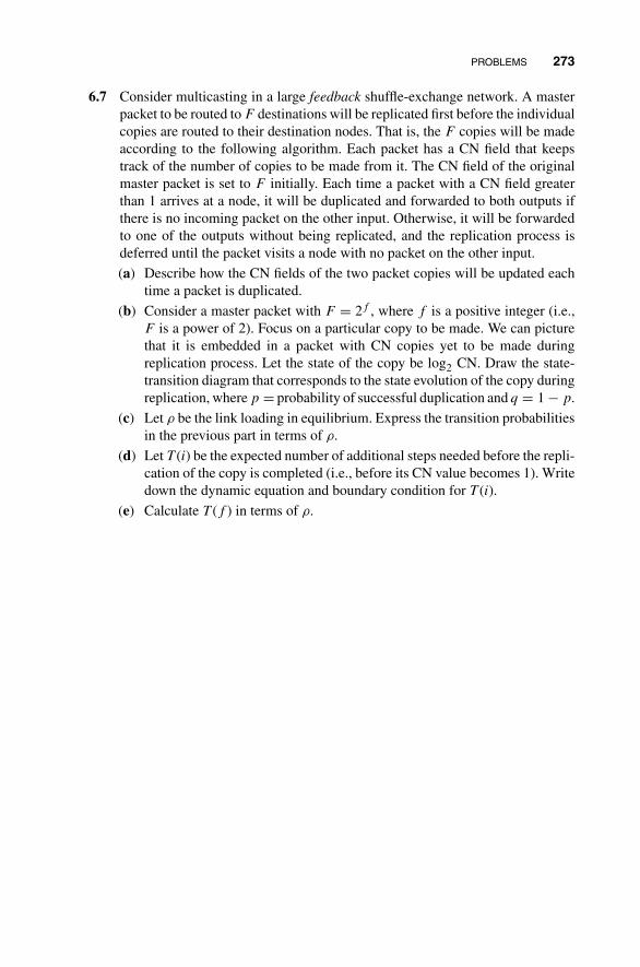
PROBLEMS 273
6.7 Consider multicasting in a large feedback shuffle-exchange network. A masterpacket to be routed to F destinations will be replicated first before the individualcopies are routed to their destination nodes. That is, the F copies will be madeaccording to the following algorithm. Each packet has a CN field that keepstrack of the number of copies to be made from it. The CN field of the originalmaster packet is set to F initially. Each time a packet with a CN field greaterthan 1 arrives at a node, it will be duplicated and forwarded to both outputs ifthere is no incoming packet on the other input. Otherwise, it will be forwardedto one of the outputs without being replicated, and the replication process isdeferred until the packet visits a node with no packet on the other input.
(a) Describe how the CN fields of the two packet copies will be updated eachtime a packet is duplicated.
(b) Consider a master packet with F = 2f , where f is a positive integer (i.e.,F is a power of 2). Focus on a particular copy to be made. We can picturethat it is embedded in a packet with CN copies yet to be made duringreplication process. Let the state of the copy be log2 CN. Draw the state-transition diagram that corresponds to the state evolution of the copy duringreplication, where p = probability of successful duplication and q = 1 − p.
(c) Let ρ be the link loading in equilibrium. Express the transition probabilitiesin the previous part in terms of ρ.
(d) Let T (i) be the expected number of additional steps needed before the repli-cation of the copy is completed (i.e., before its CN value becomes 1). Writedown the dynamic equation and boundary condition for T (i).
(e) Calculate T (f ) in terms of ρ.


7
BASIC CONCEPTS OF BROADBANDCOMMUNICATION NETWORKS
This chapter discusses various elementary concepts of broadband communicationnetworks. The focus is on networks in which information is transported in fixed-length packets called cells. The asynchronous transfer mode (ATM) standardizedworldwide, for example, assumes such a transport mechanism. The coverage is briefbut should provide enough background information for the more detailed study inChapter 8.
7.1 SYNCHRONOUS TRANSFER MODE
To understand the motivations behind ATM, let us consider the limitations of the syn-chronous transfer mode (STM) that lead to the proposal of ATM in the first place. Sim-ply put, STM is time-division multiplexing (TDM) and ATM is fixed-length packetswitching.
Recall from Chapter 1 that in TDM, information from several sources is multi-plexed onto one physical transmission medium in which the time is slotted. Time slotsare grouped into frames. Each time-slot position in a frame is dedicated exclusively toa particular source. Thus, time slot i of frames 1, 2, 3, . . . can carry information fromone and only one source once the connection has been set up. There is no sharing oftime slots among different connections.
While this exclusive dedication of bandwidth works well for sources that producetraffic in a continuous fashion (e.g., voice and video), it is wasteful for sources withbursty traffic (e.g., computer data): when the sources are idle, their associated timeslots do not carry any information. This limitation of STM is rather obvious and haslong been recognized as one of the disadvantages of circuit switching when compared
Principles of Broadband Switching and Networking, by Tony T. Lee and Soung C. LiewCopyright © 2010 John Wiley & Sons, Inc.
275
276 BASIC CONCEPTS OF BROADBAND COMMUNICATION NETWORKS
with packet switching. It turns out that this efficiency consideration, although valid,was not the main motivation for ATM when it was first proposed. ATM is advantageousin many respects even if all sources had more or less constant-rate traffic. In fact,some people view the bandwidth efficiency of ATM for bursty traffic as icing on thecake.
The ATM transport mechanism was originally proposed by the telephone networkcommunity, although the technology is also aggressively being adopted by the com-puter communication community. To understand the original motivation for ATM, letus briefly review the STM technology the way it is adopted in telephone networks.There are several fixed transport rates in the telephone networks. A voice conver-sation, after digitization, requires 64 kbps of bandwidth, and this forms the basictransport rate. The Digital Signal Level 0 (DS-0) of the TDM hierarchy carries infor-mation at this rate. The next higher rate is the DS-1 rate, which is about 1.5 Mbps.Thus, 24 telephone conversations, or DS-0 channels, can be multiplexed onto a DS-1channel. Each time slot is 1 byte and each frame consists of 24 bytes, one for eachDS-0 channel.
Instead of subscribing communication channels from the network operator at thebasic 64 kbps rate, a customer may also lease a T-1 line that carries a 1.5 Mbps DS-1data signal. Note that the term “DS-1” refers to the data signal whereas the term “T-1”refers to the carrier system, that includes the transmitter, the transmission medium,and the receiver for the DS-1 data signal. The T-1 line can be used to send either voiceor computer data, and the choice is up to the subscriber. If it is used to carry data, thewhole 1.5 Mbps can be used as an entire chunk of bandwidth without the need for apreliminary stage of multiplexing DS-0 signals.
A number of DS-1 signals can be multiplexed onto a high-speed data-signal level.The DS-2 signal consists of 4 DS-1 signals and the DS-3 signal consists of 28 DS-1signals. The DS-3 rate is about 45 Mbps. For the purpose of TDM, instead of multi-plexing from DS-1 to DS-2 and then to DS-3, it is a common practice to multiplexdirectly from DS-1 to DS-3. In this case, each time slot in a DS-3 is dedicated to datafrom a particular DS-1 signal.
With this transport-rate hierarchy, the next question is how to switch these channels.The STM switches are typically designed to switch at one of the basic rates (i.e., at 64kbps, 1.5 Mbps, or 45 Mbps). Switching at rate r means that all the data in an inputchannel of rate r will be switched to an output channel of rate r; that is, one cannotswitch some of the data within the input channel across different output channels. Forinstance, a switch that switches at DS-1 rate does not take apart the underlying DS-0signals before switching is being performed, and the whole input DS-1 is switched toan output DS-1.
The switching rate may not be the same as the data rate of the input lines. Forexample, as illustrated in Fig. 7.1, a switch that switches at the 64 kbps DS-0 ratemay have input lines at the DS-1 rate. It is more complicated to switch at the lowerrate for two reasons. First, the switch must be able to take apart the data at the higherrate to obtain the data at the lower rate: this is essentially the demultiplexing function.Second, there are more data channels at the lower rate and their switching is morecomplicated simply because of their large number.
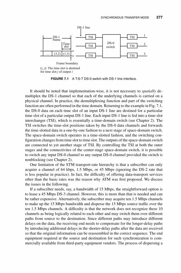
SYNCHRONOUS TRANSFER MODE 277
DS-0
switch
TSI
TSI
TSI
1
2
3
TSI
TSI
TSI
DS-1 line
(1,3)(3,2)…
Time slot
DS-1 frame
Frame boundary
(i, j): The time slot is destined for time slot j of output i
FIGURE 7.1 A T-S-T DS-0 switch with DS-1 line interface.
It should be noted that implementation-wise, it is not necessary to spatially de-multiplex the DS-1 channel so that each of the underlying channels is carried on aphysical channel. In practice, the demultiplexing function and part of the switchingfunction are often performed in the time domain. Returning to the example in Fig. 7.1,the DS-0 data on each time slot of an input DS-1 line are destined for a particulartime slot of a particular output DS-1 line. Each input DS-1 line is fed into a time-slotinterchanger (TSI), which is essentially a time-domain switch (see Chapter 2). TheTSI switches the time-slot positions taken by the DS-0 data channels and forwardsthe time-slotted data in a one-by-one fashion to a next stage of space-domain switch.The space-domain switch operates in a time-slotted fashion, and the switching con-figuration changes from time slot to time slot. The outputs of the space-domain switchare connected to yet another stage of TSI. By controlling the TSI at both the outerstages and the connectivites of the center-stage space-domain switch, it is possibleto switch any input DS-0 channel to any output DS-0 channel provided the switch isnonblocking (see Chapter 2).
One limitation of the STM transport-rate hierarchy is that a subscriber can onlyacquire a channel of 64 kbps, 1.5 Mbps, or 45 Mbps (ignoring the DS-2 rate thatis less popular in practice). In fact, the difficulty of offering data-transport servicesother than the basic rates was the reason why ATM was first proposed. We discussthe issues in the following.
If a subscriber needs, say, a bandwidth of 15 Mbps, the straightforward option isto lease a 45 Mbps DS-3 channel. However, this is more than that is needed and canbe rather expensive. Alternatively, the subscriber may acquire ten 1.5 Mbps channelsto make up the 15 Mbps bandwidth and disperse the 15 Mbps source traffic over theten 1.5 Mbps channels. A difficulty is that the network does not recognize these 10channels as being logically related to each other and may switch them over differentpaths from source to the destination. Since different paths may introduce differentdelays on the data, the receiving end needs to compensate for the longer-delay pathsby introducing additional delays in the shorter-delay paths after the data are receivedso that the original information can be reassembled in the correct sequence. The endequipment required at the source and destination for such synchronization is com-mercially available from third-party equipment vendors. The process of dispersing a

278 BASIC CONCEPTS OF BROADBAND COMMUNICATION NETWORKS
channel over several parallel subchannels is called inverse multiplexing for obviousreason. The network operator is unaware of (and has no need to be aware of) theuse of inverse multiplexing by the subscriber. The inverse-multiplexing equipment,however, introduces additional cost to the subscriber.
Instead of inverse multiplexing, one may also modify the switches so that they canperform multirate switching so that channels of rate n× basic rate, n an integer, canbe supported. For example, if a switch has input and output lines of DS-3 rate andcan switch at the DS-1 rate, we can modify it so that it can switch a channel of n×DS-1 rate, where n = 1, 2, . . . , 28. The switch must recognize the n DS-1 channels aslogical subchannels of the actual channel during both call setup and switching of timeslots. There are two ways to go about this and both introduce additional complexityto the switch design.
The first method is to simply perform some sort of inverse multiplexing at theswitch. A subscriber sends to the network a channel of 1.5 × n Mbps bandwidth.After being multiplexed with data from other subscribers, the channel occupies n
time slots of a DS-3 input line to a switch. During call setup, the switch controllermust be informed of the n time-slot positions taken by the input channel. One byone, the controller sets up n DS-1 connections over the switch. Although these con-nections have the same input and output, they may be switched over different pathswithin the switch. This is illustrated in Fig. 7.2(a), which shows many T-S-T switchmodules (each T-S-T module is like that in Fig. 7.1) connected in three stages. Thesen time slots, if switched over different internal paths, may suffer different processingand switching delays. Consequently, it is possible that the n time slots within a frameperiod at the input may arrive at the output in different frame periods. Hence, it is nec-essary to introduce artificial delays at the output (as in inverse multiplexing) to thesetime slots so that the time slots of the frame period at the input can be realigned backinto the same frame period at the output. In addition, within the same frame period, theorder of the time slots may not be preserved and a time-slot interchanger is needed toreorder the time slots (although the controller can integrate this consideration easilyinto the call setup procedure).
The second method for multirate switching is to design the switch such that onecan specify not only the desired output of a connection, but also the internal path tobe taken. By insisting that the switch sets up n subchannels over the same internalpath, there will be no need for time-slot realignment at the output. This is illustratedin Fig. 7.2(b). Although there is no need for time-slot realignment at the output, somenew complexities are introduced as a result.
First, the call setup is more complicated because the overall switch must recognizethe logical relationship of all the time slots and must then attempt to switch them overthe same path, maintaining the sequence. In addition, there is also the performancepenalty in terms of the increased blocking probability as compared to the first method.This is due to the phenomenon of bandwidth fragmentation: one may not find n idletime slots in any particular path (especially when n is large) although there are morethan n idle time slots in total over different paths, in which case the call is not blockedin the first method, but is blocked in the second method. For the same blockingperformance, the second method generally requires the number of alternative paths

SYNCHRONOUS TRANSFER MODE 279
(a)
T-S-T
T-S-T
T-S-T
T-S-T
T-S-T
T-S-T
T-S-T
T-S-T
T-S-T
An interconnection of T-S-T switch modules
Resequencing necessary
Framealignmentdelay
Three slots of the same connection in a frame
T-S-T
T-S-T
T-S-T
T-S-T
T-S-T
T-S-T
T-S-T
T-S-T
T-S-T
Switch the time slots of the same connection as a bundle along the same path
(b)
Resequencing unnecessary
FIGURE 7.2 (a) Using basic rate switch to switch multirate connections; (b) using multirateswitch to switch multirate connections.
to be increased. For the switching network in Fig. 7.2, this means that the number ofmiddle-stage switch modules must be increased.
To summarize, the first limitation of STM is that the present-day network canonly offer the basic rate transport because most network equipments are not designedto handle multirate switching. The second limitation is that although multirateswitching is possible by modifying the switches, additional complexity will beincurred at both the software (managing the connections) and hardware levels. Evenif multirate switching were available, there would still be the third limitation thatthe channel rate must be an integral multiple of the basic rate of the switch. Forexample, a DS-1 switch modified to handle multirate switching will not be able toaccommodate channels at 100 kbps, 1 Mbps, or 2 Mbps.
280 BASIC CONCEPTS OF BROADBAND COMMUNICATION NETWORKS
To deal with these limitations, the proponents of ATM argued that the concept offrames should be removed so that time slots can be assigned independently to chan-nels: time slots are not assigned in a periodic fashion to channels and they are given tothe channels only when there is information to be transported on that channel. In otherwords, time slots are not dedicated to channels in a synchronous fashion. Without theframes, the output (destinations) of a time slot is not implicitly derivable from itsposition anymore. Therefore, a header that specifies the output must be attached tothe time slot so that the switch can use it to route the time slot to the correct output.With this, what we have is basically the framework for fixed-length packet switchingwhere each time slot carries a fixed-length packet! With the additional introductionof virtual-circuit routing (to be discussed in Section 7.4) so that information from asource is routed through a single path over the network, there is no need for inversemultiplexing. Also, without the frame structure, there is no need to limit the band-width assignment to an integral multiple of the basic rate. This new framework alsogives rise to new issues and considerations, and they will be discussed in the next fewsections.
In addition to regular user data, network equipment also needs to coordinate witheach other to achieve certain functions. For instance, to set up an end-to-end connec-tion from source to destination, several switches will be involved. The traffic statusat different parts of the network may also need to be disseminated. In STM, controlchannels can be defined for the purpose of transporting control information. However,the bandwidth of the control channels will typically need to be overengineered so asto accommodate control functions needed in future services. Also, control informa-tion, unlike continuous traffic like voice and video, may arrive in a bursty fashion.For efficiency, one can send the control information in packet form in the controlchannel.
One advantage of ATM is that the transport mechanism is already packet-based,and only as much bandwidth as is required by the control channels needs to be as-signed. Among the five-byte headers, only certain bits need to be predefined forthe indication of whether the cell is a control or a regular data cell. If 5 bytes arenot enough to distinguish the different levels or shades of control functionalitiesneeded, one may further define different types of control cells using some of thebytes of the 48-byte payload. To draw an analogy, control information is like in-structions in a computer in that they both achieve certain functions by invoking op-erations of the underlying systems. ATM cells are a very simple mechanism thatallows a rich set of “instructions” to be defined: each 53-byte cell is like a 53-byteinstruction.
7.2 DELAYS IN ATM NETWORK
Let us consider the delays incurred by packets in an ATM network. With the aidof Fig. 7.3, we shall trace the delays of a packet as it travels from its source to thereceiver. At the source, the information must be packetized into fixed-length packetscalled cells. In the ATM standard, each cell is 53 bytes of which 48 bytes are dedicated
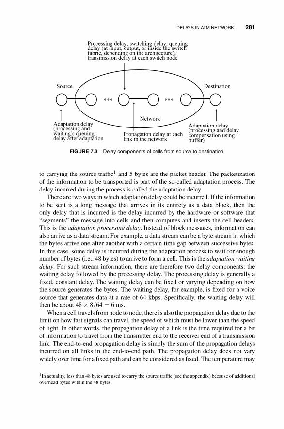
DELAYS IN ATM NETWORK 281
Processing delay; switching delay; queuing delay (at input, output, or inside the switch fabric, depending on the architecture); transmission delay at each switch node
Network
Source Destination
Adaptation delay (processing and waiting); queuing delay after adaptation
Propagation delay at each link in the network
Adaptation delay (processing and delay compensation using buffer)
FIGURE 7.3 Delay components of cells from source to destination.
to carrying the source traffic1 and 5 bytes are the packet header. The packetizationof the information to be transported is part of the so-called adaptation process. Thedelay incurred during the process is called the adaptation delay.
There are two ways in which adaptation delay could be incurred. If the informationto be sent is a long message that arrives in its entirety as a data block, then theonly delay that is incurred is the delay incurred by the hardware or software that“segments” the message into cells and then computes and inserts the cell headers.This is the adaptation processing delay. Instead of block messages, information canalso arrive as a data stream. For example, a data stream can be a byte stream in whichthe bytes arrive one after another with a certain time gap between successive bytes.In this case, some delay is incurred during the adaptation process to wait for enoughnumber of bytes (i.e., 48 bytes) to arrive to form a cell. This is the adaptation waitingdelay. For such stream information, there are therefore two delay components: thewaiting delay followed by the processing delay. The processing delay is generally afixed, constant delay. The waiting delay can be fixed or varying depending on howthe source generates the bytes. The waiting delay, for example, is fixed for a voicesource that generates data at a rate of 64 kbps. Specifically, the waiting delay willthen be about 48 × 8/64 = 6 ms.
When a cell travels from node to node, there is also the propagation delay due to thelimit on how fast signals can travel, the speed of which must be lower than the speedof light. In other words, the propagation delay of a link is the time required for a bitof information to travel from the transmitter end to the receiver end of a transmissionlink. The end-to-end propagation delay is simply the sum of the propagation delaysincurred on all links in the end-to-end path. The propagation delay does not varywidely over time for a fixed path and can be considered as fixed. The temperature may
1In actuality, less than 48 bytes are used to carry the source traffic (see the appendix) because of additionaloverhead bytes within the 48 bytes.

282 BASIC CONCEPTS OF BROADBAND COMMUNICATION NETWORKS
have an effect on the propagation delay of, say, a fiber link, because the temperatureexpansion and contraction of the glass may affect the fiber length, but the effect isgenerally insignificant.
As a cell travels from node to node, it may also incur processing delay and waitingdelay at each node. First, consider the source node again. After adaptation, the cellwill be forwarded to the transmitter end of the transmission link. Because there couldbe a number of cells already waiting to be transmitted, the cell concerned will incur aqueueing delay while waiting for its turn to be transmitted. For example, after a longmessage has been adapted, the resulting cells may be put into a buffer waiting to betransmitted. The cells at the later part of the message would wait for a longer timethan cells at the earlier part of the message.
As the cell travels through nodes in the network, within each node, the cell willbe processed (e.g., VCI translation, switching, etc.) upon arriving at each node. Theswitching part of the processing delay can be varying or fixed, depending on the switchimplementation. Recall that the arrivals of packets to a switch are not scheduled inan ATM network, and several cells may be targeted for the same output at the sametime. This leads to the contention problem that we have already covered in Chapters3 and 4. As has been seen, some solutions to the contention problem (e.g., using inputbuffers to store packets that have lost contention) may cause random and variabledelays. In short, some input delay is incurred at the input. Part of the input delay is theprocessing delay for VCI translation and so on. Depending on the switch architecture,part of the delay can be random and variable delay due to waiting at an input queuefor output access.
In addition, cells may also incur delay at an output after they have arrived at theoutputs. There are two possible delay components at an output, the queueing delayand the transmission delay. The queueing delay is incurred when more cells arriveat the output than can be transmitted immediately. Some of the cells must then bebuffered for transmission some time in the future. This can happen in switches thatare capable of forwarding more than one cell to an output in each time slot. Thetransmission delay is simply the amount of time needed to transmit one cell. For anideal output-buffered switch, the output queueing delay is the only delay componentthat is random and varying.
The random and varying queueing delays at the nodes in turn cause the end-to-enddelay from source to destination to be random and time varying. The variation in theend-to-end delay from cell to cell is often referred to as the delay jitter. For manyapplications, it is desirable to remove this delay jitter so that data can be forwarded tothe user (or end application) in a continuous and periodic fashion. For example, forvoice conversation, data are injected into the network in a continuous and periodicfashion. While traveling through the network, the cells may incur varying delays andthe time gap between adjacent cells may be variable by the time they arrive at thereceiver because of network delay jitter. It is necessary to remove the jitter before theaudio is played out.
A smoothing buffer is generally used to remove the delay jitter. The principle ofthe smoothing buffer works like that of a water dam. Water may arrive to the damin a bursty manner that depends on the rainfall. However, the water flows out of the

CELL SIZE CONSIDERATION 283
dam at a constant rate. At the receiver, instead of immediately presenting the arriveddata to the user, the receiver buffers it in the smoothing buffer first. By introducinga sufficiently large delay at the buffer, it is possible to deliver the data to the user ina continuous fashion. This additional delay is the adaptation delay incurred at thereceiver end. The idea is that cells that have suffered a large delay within the networkwill incur a small receiver adaptation delay, and vice versa. Specifically, let Tn beall other delays and Ta be the adaptation delay introduced by the smoothing buffer.The idea is to make Tn + Ta a constant: when Tn is large and Ta is small, and viceversa.
7.3 CELL SIZE CONSIDERATION
We have already covered the motivations for fixed-length cell switching from theviewpoint of traditional circuit switching. These were the considerations that gaverise to the ATM proposal originally. In that context, cells are basically time slots of 53bytes. Instead of motivating cell switching from the shortcomings of circuit switch-ing, let us examine fixed-length cell switching in the context of packet switching.Specifically, we now consider fixed-length versus variable-length packet switchingand the issue of setting packet size.
Transport using fixed-length cells may incur more overhead than using variable-length packet because of the segmentation process. Consider the sending of a message.As shown in Fig. 7.4, if the underlying network transports information in the form offixed-length cells, it is then necessary to partition the packet into many cells beforetransmission. The header of each cell must contain enough information for the nodes inthe network to be able route it to the desired destination, and this information must berepeated for successive cells. This incurs much overhead as compared to transportingthe long message as a long packet. In a variable-length packet, the packet can be aslong as the message to be transmitted.
Let Lm be the length of the message, and let Lo be the header size. For the sake ofargument, suppose that Lo in the cell network and the variable-length packet networkare the same. Then, the number of bytes needed to transmit the message as a packet
Lm
Lo Lc
FIGURE 7.4 Segmentation of a message into cells during the adaptation process.
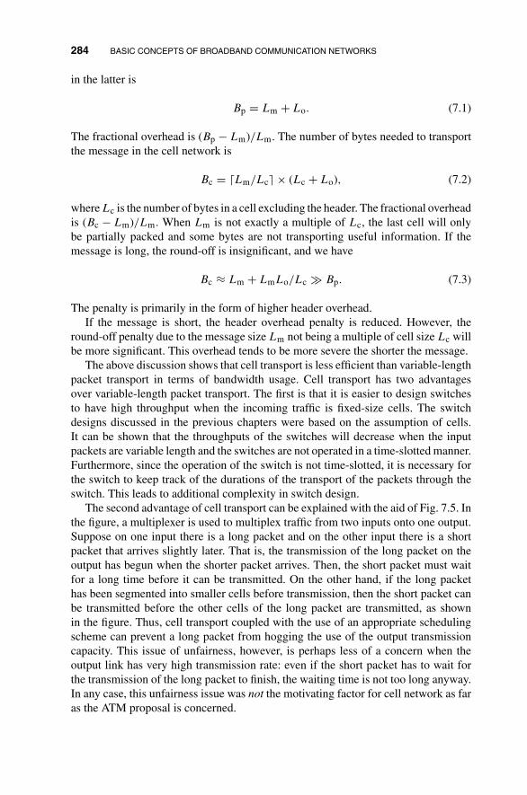
284 BASIC CONCEPTS OF BROADBAND COMMUNICATION NETWORKS
in the latter is
Bp = Lm + Lo. (7.1)
The fractional overhead is (Bp − Lm)/Lm. The number of bytes needed to transportthe message in the cell network is
Bc = �Lm/Lc� × (Lc + Lo), (7.2)
where Lc is the number of bytes in a cell excluding the header. The fractional overheadis (Bc − Lm)/Lm. When Lm is not exactly a multiple of Lc, the last cell will onlybe partially packed and some bytes are not transporting useful information. If themessage is long, the round-off is insignificant, and we have
Bc ≈ Lm + LmLo/Lc � Bp. (7.3)
The penalty is primarily in the form of higher header overhead.If the message is short, the header overhead penalty is reduced. However, the
round-off penalty due to the message size Lm not being a multiple of cell size Lc willbe more significant. This overhead tends to be more severe the shorter the message.
The above discussion shows that cell transport is less efficient than variable-lengthpacket transport in terms of bandwidth usage. Cell transport has two advantagesover variable-length packet transport. The first is that it is easier to design switchesto have high throughput when the incoming traffic is fixed-size cells. The switchdesigns discussed in the previous chapters were based on the assumption of cells.It can be shown that the throughputs of the switches will decrease when the inputpackets are variable length and the switches are not operated in a time-slotted manner.Furthermore, since the operation of the switch is not time-slotted, it is necessary forthe switch to keep track of the durations of the transport of the packets through theswitch. This leads to additional complexity in switch design.
The second advantage of cell transport can be explained with the aid of Fig. 7.5. Inthe figure, a multiplexer is used to multiplex traffic from two inputs onto one output.Suppose on one input there is a long packet and on the other input there is a shortpacket that arrives slightly later. That is, the transmission of the long packet on theoutput has begun when the shorter packet arrives. Then, the short packet must waitfor a long time before it can be transmitted. On the other hand, if the long packethas been segmented into smaller cells before transmission, then the short packet canbe transmitted before the other cells of the long packet are transmitted, as shownin the figure. Thus, cell transport coupled with the use of an appropriate schedulingscheme can prevent a long packet from hogging the use of the output transmissioncapacity. This issue of unfairness, however, is perhaps less of a concern when theoutput link has very high transmission rate: even if the short packet has to wait forthe transmission of the long packet to finish, the waiting time is not too long anyway.In any case, this unfairness issue was not the motivating factor for cell network as faras the ATM proposal is concerned.

CELL NETWORKING, VIRTUAL CHANNELS, AND VIRTUAL PATHS 285
M
U
X
(a)
M
U
X
(b)
FIGURE 7.5 (a) Multiplexing variable-length packets; (b) multiplexing cells.
Given that we want to adopt cell transport, there is then the consideration of thecell size. If the cell size is small, the header overhead will then be large. If the cellsize is too large, on the other hand, the adaptation waiting delay of low-rate real-timeservices, such as voice, may be too large. Recall that ATM was originally initiated bypeople in the telephone network community. The decision to set the cell size to 53bytes is mainly motivated from the consideration of the transport of voice. Smallercell size may be inefficient. Cell size much larger than this (say 100 bytes) may resultin echo problems. The voice transmitted by the source, through the headset of thereceiver, may be fed back to the source through the reverse path of a duplex voiceconnection. Recall that the bit rate of digital voice is 64 kbps. Each sample is one bytein length. Therefore, the sampling rate is 8000 samples per second. The adaptationdelay both ways, assuming 100-byte cell, is already 2 × 100/8 = 25 ms. This itselfresults in noticeable echoes even in the absence of all other delays.
7.4 CELL NETWORKING, VIRTUAL CHANNELS, AND VIRTUAL PATHS
There are many options and alternatives for the operation and architecture design ofa cell network. This book by and large assumes those options adopted by the ATMstandard. This section explains the principles and rationale behind them.
7.4.1 No Data Link Layer
In traditional packet-switched networks, the links between nodes are not reliable andthe bit error rate is high. Therefore, the data link layer (more specifically, automaticrepeat request (ARQ) in the data link layer) is introduced to coordinate and auto-mate the retransmission of data in case of data corruption. The advent of fiber-optictechnology brings along very reliable transmission. An important assumption in theATM standard is the use of reliable links. With reliable links, the ATM proponents

286 BASIC CONCEPTS OF BROADBAND COMMUNICATION NETWORKS
argue that there is no need of a data link layer, which only makes networking morecomplicated and less efficient. Thus, for ATM networks, there is no data link layer.The recent development of wireless ATM may challenge the assumption of reliablelinks, since the transmission medium may not be as reliable as is assumed. Neverthe-less, the ATM standard has been defined, and other ways must be sought for reliablecommunication. A possibility is to introduce ARQ at a layer higher than the ATMlayer.
7.4.2 Cell Sequence Preservation
To simplify the implementation of network services and applications over ATM net-works, the standard specifies that ATM networks must deliver cells in the correctsequence from source to destination. In other words, if you write an application pro-gram that sends data from a source workstation to a destination workstation over anATM network, the communication “pipe” is expected to be FIFO so that the order inwhich cells are sent at the source is also the order in which they are received at thedestination. This makes it easier for the users to develop network applications andservices over the ATM network.
7.4.3 Virtual-Circuit Hop-by-Hop Routing
An implication of the sequence-preservation requirement is that the ATM networkmust be a virtual-circuit (or connection-oriented) network. A connection must be setup a priori before data can be sent over the network. If the network were to be adatagram (connectionless) network, cells might then travel over different physicalroutes to their destinations, and the different delays of these routes might introduceout-of-sequence arrivals at the receiver.
There are two possible routing mechanisms in a virtual-circuit network: sourcerouting and hop-by-hop routing. In source routing, the sequence of nodes to be tra-versed by a packet is encoded in the packet header. In a cell network, the cells havea fixed-length header, and therefore there is an upper bound on the number of bytesthat can be used to encode the sequence of nodes. In other words, there is a limit onthe maximum number hops if source routing were to be adopted.
The ATM standard adopted hop-by-hop routing. The nodes traversed are not ex-plicitly encoded in the header. Rather, there is a fixed-length virtual-circuit identifierin the header that is used to identify cells belonging to a particular virtual circuit.Upon the arrival of a cell to a node, its virtual-circuit identifier is used to retrieve froma lookup table the output link of the node to which the cell must be forwarded. Thecell is then switched and transported on this output link, that connects to the node nextin sequence in the path. In this way, the sequence of nodes to be traveled is derivedon a hop-by-hop basis, and there is no limit on the maximum number of nodes thatcan be in the route. The virtual-circuit identifiers of different virtual circuits on thesame physical link must be distinct; otherwise, there will be confusion during thetable lookup.
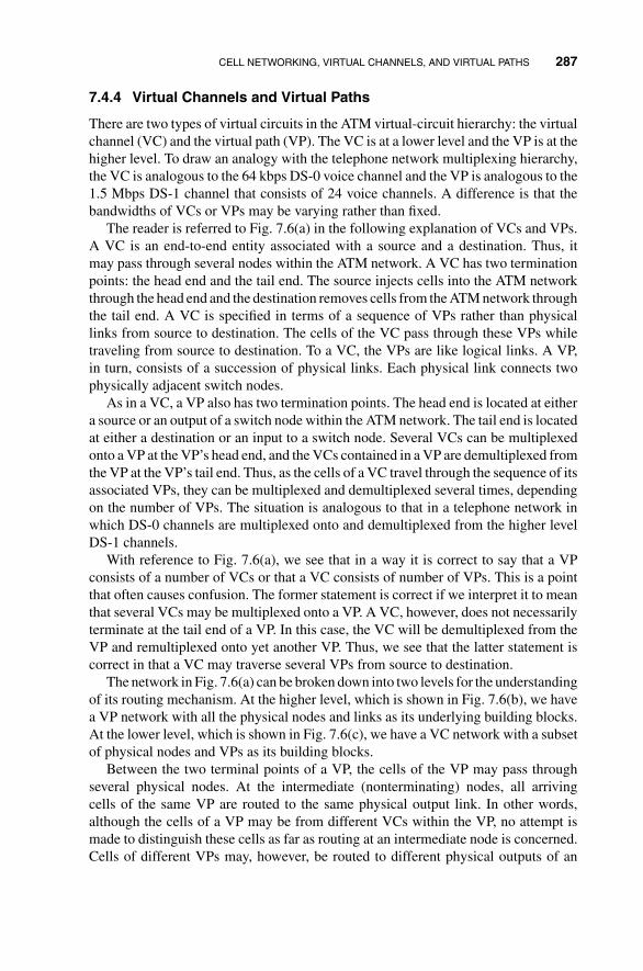
CELL NETWORKING, VIRTUAL CHANNELS, AND VIRTUAL PATHS 287
7.4.4 Virtual Channels and Virtual Paths
There are two types of virtual circuits in the ATM virtual-circuit hierarchy: the virtualchannel (VC) and the virtual path (VP). The VC is at a lower level and the VP is at thehigher level. To draw an analogy with the telephone network multiplexing hierarchy,the VC is analogous to the 64 kbps DS-0 voice channel and the VP is analogous to the1.5 Mbps DS-1 channel that consists of 24 voice channels. A difference is that thebandwidths of VCs or VPs may be varying rather than fixed.
The reader is referred to Fig. 7.6(a) in the following explanation of VCs and VPs.A VC is an end-to-end entity associated with a source and a destination. Thus, itmay pass through several nodes within the ATM network. A VC has two terminationpoints: the head end and the tail end. The source injects cells into the ATM networkthrough the head end and the destination removes cells from the ATM network throughthe tail end. A VC is specified in terms of a sequence of VPs rather than physicallinks from source to destination. The cells of the VC pass through these VPs whiletraveling from source to destination. To a VC, the VPs are like logical links. A VP,in turn, consists of a succession of physical links. Each physical link connects twophysically adjacent switch nodes.
As in a VC, a VP also has two termination points. The head end is located at eithera source or an output of a switch node within the ATM network. The tail end is locatedat either a destination or an input to a switch node. Several VCs can be multiplexedonto a VP at the VP’s head end, and the VCs contained in a VP are demultiplexed fromthe VP at the VP’s tail end. Thus, as the cells of a VC travel through the sequence of itsassociated VPs, they can be multiplexed and demultiplexed several times, dependingon the number of VPs. The situation is analogous to that in a telephone network inwhich DS-0 channels are multiplexed onto and demultiplexed from the higher levelDS-1 channels.
With reference to Fig. 7.6(a), we see that in a way it is correct to say that a VPconsists of a number of VCs or that a VC consists of number of VPs. This is a pointthat often causes confusion. The former statement is correct if we interpret it to meanthat several VCs may be multiplexed onto a VP. A VC, however, does not necessarilyterminate at the tail end of a VP. In this case, the VC will be demultiplexed from theVP and remultiplexed onto yet another VP. Thus, we see that the latter statement iscorrect in that a VC may traverse several VPs from source to destination.
The network in Fig. 7.6(a) can be broken down into two levels for the understandingof its routing mechanism. At the higher level, which is shown in Fig. 7.6(b), we havea VP network with all the physical nodes and links as its underlying building blocks.At the lower level, which is shown in Fig. 7.6(c), we have a VC network with a subsetof physical nodes and VPs as its building blocks.
Between the two terminal points of a VP, the cells of the VP may pass throughseveral physical nodes. At the intermediate (nonterminating) nodes, all arrivingcells of the same VP are routed to the same physical output link. In other words,although the cells of a VP may be from different VCs within the VP, no attempt ismade to distinguish these cells as far as routing at an intermediate node is concerned.Cells of different VPs may, however, be routed to different physical outputs of an

288 BASIC CONCEPTS OF BROADBAND COMMUNICATION NETWORKS
(a)
VP head end: VCs are
multiplexed here
VP tail end: VCs are
demultiplexed here
(b)
(c)
Two VPs on the same physical link that terminate at different VC switches
VC
VP
Physical link
VC switch
VP switch
VC/VP switch
FIGURE 7.6 (a) A VC/VP network; (b) the VP logical network; (c) the VC logical network.

CELL NETWORKING, VIRTUAL CHANNELS, AND VIRTUAL PATHS 289
intermediate node when the VPs do not traverse the same sequence of physical links.These intermediate nodes are sometimes called VP switches, since they distinguishcells based on their VPs rather than VCs in the routing process.
The nodes to which the termination points of a VP are attached are called VCswitches, and they form the nodes of the lower level VC network shown in Fig. 7.6(c).The network in the figure is a logical network rather than a physical network. The VPswitches are transparent in the logical network, since VCs do not terminate there. Toa VC, a VP is like a link between two nodes. At the input of a VC switch, the cellsfrom a terminating VP are distinguished based on their VCs, and cells from differentVCs may be routed to different output VPs at the VC switch. Note that we say outputVPs rather than output physical links because each output physical link may containseveral VPs that, to the VCs, are different logical entities. Different output VPs at theVC switch, even if they were on the same physical output links, could lead to differentVC switches at their tail ends, as shown by the example in Fig. 7.6(c).
In general, a switch can be a VC, VP, or VC/VP switch. As explained above, a VPswitch is not a terminating node for VPs or VCs, and a VC switch is a terminating nodefor VPs but not VCs. (Note: VCs terminate at their destinations outside the network.)A VC/VP switch is simply one in which some VPs terminate and some VPs donot (see Fig. 7.6(a) for an example). In this switch, the cells of nonterminating VPsare not distinguished based on their VCs, and the cells of terminating VPs must bedistinguished based on their VCs for further routing.
We can draw an analogy between VP/VC networking and transportation by bus.Cells of a VC are like people who are from a common origin wanting to go to acommon destination. If there is no direct bus from the origin to the destination, thenthese people must take several bus routes in succession to reach the destination. Thedifferent bus routes are like VPs. Each bus route goes through several streets or roads,which are analogous to physical links. At the beginning of each bus route, people(possibly from different origins and to different destinations) board the bus, and atthe end of the bus route, they either reach their destinations or continue on to anotherbus route. This is analogous to multiplexing VCs onto and demultiplexing VCs froma VP. A VP switch is like a nonterminal road junction where nobody is allowed toboard or leave the bus. A VC switch, on the other hand, is like a bus station wheremany bus routes end and begin.
7.4.5 Routing Using VCI and VPI
With hop-by-hop routing, virtual-circuit identifiers must be encoded in the cell headersso that a switch may use them to decide how to route cells. The identifiers are used asan index to retrieve routing information from a routing table. Each input of a switchtypically has a routing table. The routing information associated with a virtual circuitis added to the table during the setting up of the virtual circuit, and it is removed fromthe table when the virtual circuit is torn down.
With the two-level hierarchy in which there are two types of virtual circuits, VCsand VPs, each cell has two identifiers in its header: the virtual-channel identifier (VCI)and the virtual-path identifier (VPI). Figure 7.7 illustrates how routing is performed

1
2 3
1 2
2
3
1
VP
I=2
, V
CI=
2
VP
I=6
, V
CI=
3
VP
I=2
, V
CI=
2
VP
I=6
, V
CI=
4
VP
I=5
, V
CI=
4
VP
I=5
, V
CI=
6
…
VP
I=5
VC
I=2
VP
I=1
V
CI=
2
VP
I=1
,VC
I=1
1
VP
I=3
VC
I=3
42
6
52
2
Outp
ut
VP
I
Outp
ut
VP
I
11
5
32
4
Outp
ut
VP
I
Outp
ut
VP
I
1
Outp
ut
VP
I
1
Outp
ut
3
VP
I
3
VC
I
1
Outp
ut
VC
I
36
14
5
22
26
5
2
Outp
ut
VP
I
1
Outp
ut
6
VP
I
4
VC
I
2
Outp
ut
VC
I
VP
sw
itch
VC
sw
itch
Physi
cal
link w
ith l
abel
i
Thre
e dif
fere
nt
VC
s
i
FIG
UR
E7.
7V
P/V
Cro
utin
g;ill
ustr
atio
nof
the
rout
esof
thre
eV
Cs
and
thei
rre
latio
nshi
psto
the
rout
ing
tabl
es.
290

CELL NETWORKING, VIRTUAL CHANNELS, AND VIRTUAL PATHS 291
at the VC and VP switches and the corresponding routing tables. Each input link(physical link) of a VP switch has a routing table that is used to determine how toroute cells arriving on the input. The VPI of a cell is used as the index to look up anentry in the table, and the entry contains two elements (output link and output VPI),which indicates the output link to which the cell must be switched and the new VPIvalue it should adopt at the output link.
The cells of a VP may change its VPI value as they travel from a physical linkto another physical link within the VP. The reasons for allowing the VPI to changefrom link to link, even though the VP has not terminated, are to simplify networkoperation and to reduce blocking probability due to insufficient VPIs. These are alsothe reasons for allowing the VCI of a VC to change, the details of which will beelaborated shortly. A point also to be noted is that the cells with the same VPI valuebut on different physical links may actually belong to different VPs.
While a VP switch uses only the VPI for routing, a VC switch uses both VPI andVCI. As shown in Fig. 7.7, the VPI–VCI combination is the index for reference toan entry in the routing table. This is because the cells of a VC can only be identifiedby the combination of VPI and VCI: cells with different VPIs but the same VCIs, orwith different VCIs but the same VPIs, are cells of different VCs. An entry of therouting tables at a VC switch consists of three elements: output link, output VPI, andoutput VCI).
The VCI of a VC is allowed to change as its cells travel from source to destination.While the VPI of the cells can change from physical link to physical link, the VCI canchange only when the cells pass through a VC switch; the VCI does not change whencells pass through a VP switch. The changing of VPI and VCI does not cause confusionas long as the VPI–VCI combinations of different VCs on a link are different. Ananalogy is to compare the situation to that of a person wearing shirts of different colorsor adopting different names on different occasions: as long as the color or name isunique on each occasion (i.e., no other person wears the same color or uses the samename), we can use it to identify the person.
There are two reasons why the VCI of a VC and the VPI of a VP are allowed tochange: simpler operation and lower blocking probability during call setup. Considerthe alternative of requiring the VPI and VCI to remain the same. Let us focus on thesetting up of a new VC over the lower level VC network. Suppose that a sequenceof VPs for the VC has been identified. Each VP in the sequence may have someVCI values already used by existing VCs within the VP. To set up the new VC, thesequence of VC switches at the termination points of the VPs must coordinate witheach other to come up with a commonly available VCI not already used in any ofthe VPs. For instance, if VCI = 11 is already used in the first VP, and VPI = 10 isalready used in the second VP, then neither VCI = 10 nor VPI = 11 can be assignedto the new VC.
The coordination of the VC switches to come up with a unique VCI assignmentthroughout the path required a complicated distributed control algorithm and a lot ofcontrol information to be sent around among the VC switches (see Problem 7.7). Thealternative of allowing the VCI to change from VP to VP is much more desirable.Each VC switch simply keeps track of the unused VCIs on each of its output virtual
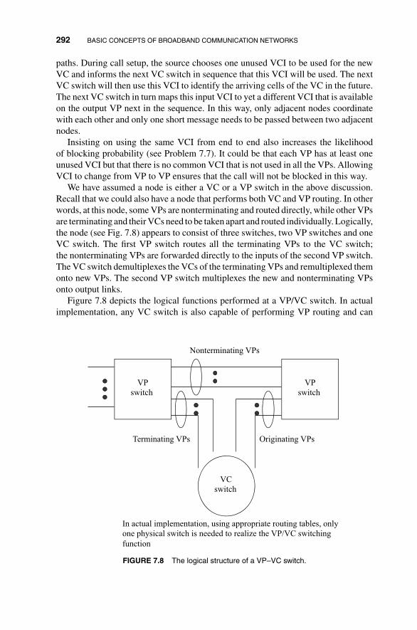
292 BASIC CONCEPTS OF BROADBAND COMMUNICATION NETWORKS
paths. During call setup, the source chooses one unused VCI to be used for the newVC and informs the next VC switch in sequence that this VCI will be used. The nextVC switch will then use this VCI to identify the arriving cells of the VC in the future.The next VC switch in turn maps this input VCI to yet a different VCI that is availableon the output VP next in the sequence. In this way, only adjacent nodes coordinatewith each other and only one short message needs to be passed between two adjacentnodes.
Insisting on using the same VCI from end to end also increases the likelihoodof blocking probability (see Problem 7.7). It could be that each VP has at least oneunused VCI but that there is no common VCI that is not used in all the VPs. AllowingVCI to change from VP to VP ensures that the call will not be blocked in this way.
We have assumed a node is either a VC or a VP switch in the above discussion.Recall that we could also have a node that performs both VC and VP routing. In otherwords, at this node, some VPs are nonterminating and routed directly, while other VPsare terminating and their VCs need to be taken apart and routed individually. Logically,the node (see Fig. 7.8) appears to consist of three switches, two VP switches and oneVC switch. The first VP switch routes all the terminating VPs to the VC switch;the nonterminating VPs are forwarded directly to the inputs of the second VP switch.The VC switch demultiplexes the VCs of the terminating VPs and remultiplexed themonto new VPs. The second VP switch multiplexes the new and nonterminating VPsonto output links.
Figure 7.8 depicts the logical functions performed at a VP/VC switch. In actualimplementation, any VC switch is also capable of performing VP routing and can
Nonterminating VPs
Terminating VPs Originating VPs
VC
switch
VP
switch
VP
switch
In actual implementation, using appropriate routing tables, only
one physical switch is needed to realize the VP/VC switching
function
FIGURE 7.8 The logical structure of a VP–VC switch.
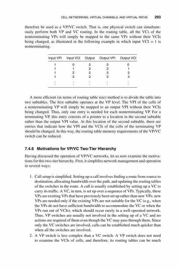
CELL NETWORKING, VIRTUAL CHANNELS, AND VIRTUAL PATHS 293
therefore be used as a VP/VC switch. That is, one physical switch can simultane-ously perform both VP and VC routing. In the routing table, all the VCs of thenonterminating VPs will simply be mapped to the same VPs without their VCIsbeing changed, as illustrated in the following example in which input VCI = 1 isnonterminating.
Input VPI Input VCI Output Output VPI Output VCI
1 0 2 3 01 1 2 3 11 2 2 3 21 3 2 3 3...
......
......
A more efficient (in terms of routing table size) method is to divide the table intotwo subtables. The first subtable operates at the VP level. The VPI of the cells ofa nonterminating VP will simply be mapped to an output VPI without their VCIsbeing changed. Thus, only one entry is needed for each nonterminating VP. For aterminating VP, this entry consists of a pointer to a location in the second subtablerather than the output VPI value. At this location of the second subtable, there areentries that indicate how the VPI and the VCIs of the cells of the terminating VPshould be changed. In this way, the routing table memory requirements of the VP/VCswitch can be reduced.
7.4.6 Motivations for VP/VC Two-Tier Hierarchy
Having discussed the operation of VP/VC networks, let us now examine the motiva-tions for this two-tier hierarchy. First, it simplifies network management and operationin several ways:
1. Call setup is simplified. Setting up a call involves finding a route from source todestination, allocating bandwidth over the path, and updating the routing tablesof the switches in the route. A call is usually established by setting up a VC tocarry its traffic. A VC, in turn, is set up over a sequence of VPs. Typically, theseVPs are existing VPs that have previously been set up rather than new VPs: newVPs are needed only if the existing VPs are not suitable for the VC (e.g., whenthe VPs do not have sufficient bandwidth to accommodate the VC or when theVPs run out of VCIs), which should occur rarely in a well-operated network.Thus, VP switches are usually not involved in the setting up of a VC and noactions are required of them even though the VC may pass through them. Sinceonly the VC switches are involved, calls can be established much quicker thanwhen all the switches are involved.
2. A VP switch is less complex than a VC switch. A VP switch does not needto examine the VCIs of cells, and therefore, its routing tables can be much
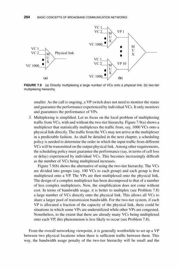
294 BASIC CONCEPTS OF BROADBAND COMMUNICATION NETWORKS
(a)
MUX
VC 1
VC 2
VC 1000
Physical link
MUX
VC 1
VC 2
VC 1000
VP 1
MUX
VC 1
VC 2
VC 1000
VP 10
MUX
(b)
FIGURE 7.9 (a) Directly multiplexing a large number of VCs onto a physical link; (b) two-tiermultiplexing hierarchy.
smaller. As the call is ongoing, a VP switch does not need to monitor the statusand guarantee the performance experienced by individual VCs. It only monitorsand guarantees the performance of VPs.
3. Multiplexing is simplified. Let us focus on the local problem of multiplexingtraffic from VCs, with and without the two-tier hierarchy. Figure 7.9(a) shows amultiplexer that statistically multiplexes the traffic from, say, 1000 VCs onto aphysical link directly. The traffic from the VCs may not arrive at the multiplexerin a predictable fashion. As shall be detailed in the next chapter, a schedulingpolicy is needed to determine the order in which the input traffic from differentVCs will be transmitted on the output physical link. Among other requirements,the scheduling policy must guarantee the performance (say, in terms of cell lossor delay) experienced by individual VCs. This becomes increasingly difficultas the number of VCs being multiplexed increases.
Figure 7.9(b) shows the alternative of using the two-tier hierarchy. The VCsare divided into groups (say, 100 VCs to each group) and each group is firstmultiplexed onto a VP. The VPs are then multiplexed onto the physical link.The design of a complex multiplexer has been decomposed to that of a numberof less complex multiplexers. Now, the simplification does not come withoutcost. In terms of bandwidth usage, it is better to multiplex (see Problem 7.8)a large number of VCs directly onto the physical link. This allows all VCs toshare a larger pool of transmission bandwidth. For the two-tier system, if eachVP is allocated a fraction of the capacity of the physical link, there could besituations in which some VPs are underutilized while other VPs are congested.Nonetheless, to the extent that there are already many VCs being multiplexedonto each VP, this phenomenon is less likely to occur (see Problem 7.8).
From the overall networking viewpoint, it is generally worthwhile to set up a VPbetween two physical locations when there is sufficient traffic between them. Thisway, the bandwidth usage penalty of the two-tier hierarchy will be small and the
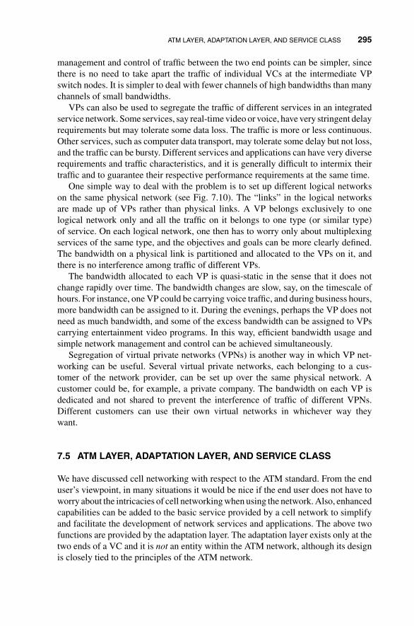
ATM LAYER, ADAPTATION LAYER, AND SERVICE CLASS 295
management and control of traffic between the two end points can be simpler, sincethere is no need to take apart the traffic of individual VCs at the intermediate VPswitch nodes. It is simpler to deal with fewer channels of high bandwidths than manychannels of small bandwidths.
VPs can also be used to segregate the traffic of different services in an integratedservice network. Some services, say real-time video or voice, have very stringent delayrequirements but may tolerate some data loss. The traffic is more or less continuous.Other services, such as computer data transport, may tolerate some delay but not loss,and the traffic can be bursty. Different services and applications can have very diverserequirements and traffic characteristics, and it is generally difficult to intermix theirtraffic and to guarantee their respective performance requirements at the same time.
One simple way to deal with the problem is to set up different logical networkson the same physical network (see Fig. 7.10). The “links” in the logical networksare made up of VPs rather than physical links. A VP belongs exclusively to onelogical network only and all the traffic on it belongs to one type (or similar type)of service. On each logical network, one then has to worry only about multiplexingservices of the same type, and the objectives and goals can be more clearly defined.The bandwidth on a physical link is partitioned and allocated to the VPs on it, andthere is no interference among traffic of different VPs.
The bandwidth allocated to each VP is quasi-static in the sense that it does notchange rapidly over time. The bandwidth changes are slow, say, on the timescale ofhours. For instance, one VP could be carrying voice traffic, and during business hours,more bandwidth can be assigned to it. During the evenings, perhaps the VP does notneed as much bandwidth, and some of the excess bandwidth can be assigned to VPscarrying entertainment video programs. In this way, efficient bandwidth usage andsimple network management and control can be achieved simultaneously.
Segregation of virtual private networks (VPNs) is another way in which VP net-working can be useful. Several virtual private networks, each belonging to a cus-tomer of the network provider, can be set up over the same physical network. Acustomer could be, for example, a private company. The bandwidth on each VP isdedicated and not shared to prevent the interference of traffic of different VPNs.Different customers can use their own virtual networks in whichever way theywant.
7.5 ATM LAYER, ADAPTATION LAYER, AND SERVICE CLASS
We have discussed cell networking with respect to the ATM standard. From the enduser’s viewpoint, in many situations it would be nice if the end user does not have toworry about the intricacies of cell networking when using the network. Also, enhancedcapabilities can be added to the basic service provided by a cell network to simplifyand facilitate the development of network services and applications. The above twofunctions are provided by the adaptation layer. The adaptation layer exists only at thetwo ends of a VC and it is not an entity within the ATM network, although its designis closely tied to the principles of the ATM network.
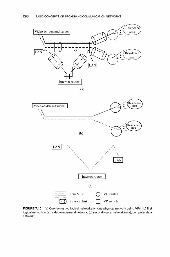
296 BASIC CONCEPTS OF BROADBAND COMMUNICATION NETWORKS
LAN
LAN
Internet router
Video-on-demand server
(a)
Residence
area
Residence
area
Residence area
Residence area
Video-on-demand server
(b)
LAN
LAN
Internet router
(c)
Four VPs
Physical link
VC switch
VP switch
FIGURE 7.10 (a) Overlaying two logical networks on one physical network using VPs; (b) firstlogical network in (a), video-on-demand network; (c) second logical network in (a), computer datanetwork.

ATM LAYER, ADAPTATION LAYER, AND SERVICE CLASS 297
One task performed by the adaptation layer is to convert the data to be sent at thesource into cells before transmission and to reassemble the cells reaching the receiverback into the original form. In addition, certain services may have particular require-ments. For example, for services that require the end-to-end delay to be constant, theadaptation layer may handle cell delay variation introduced by the network via the useof an elastic buffer (see Section 7.2). For services that deliver data to the adaptationlayer in stream mode (see Section 7.2) but require the delay to be not too large, theadaptation layer may limit the maximum adaptation waiting delay at the source andsend out partially filled cells if necessary. Given that there is no data link layer in theATM network, end-to-end error protection will be required for services that demandhigh integrity in data delivery if the network links are unreliable (e.g., wireless datalinks). This protection can be applied at the adaptation layer through forward errorcontrol and ARQ. In addition to the above functions, the adaptation layer at the re-ceiver may also be responsible for the recovery of source clock. In short, the purposeof the adaptation layer is to make the underlying network easier to use from the user’sperspective. What functions are implemented at the adaptation layer depends on theservices to be supported.
In the ATM standard, the adaptation layer is divided into two sublayers. Each ofthe sublayers may add overhead information to the data to be transmitted in orderto perform its job. The lower sublayer is the segmentation and reassembly (SAR)sublayer. It is responsible for segmenting source data into cells and reassembling re-ceived data from cells at the receiver. The higher sublayer is the convergence sublayer(CS). It is responsible for managing the flow of data to and from the SAR sublayer.Depending on the services, the CS performs functions like synchronizing the receiverand sender’s clock, handling delay variations, and so on, as described in the previousparagraph.
The ATM standard divides the services to be supported by the ATM network intofour classes, and different ATM adaptation layers (AALs) are defined accordingly tofacilitate their support. As shown in the following table, each class is associated withcertain characteristics. The appendix goes into the details of AAL headers adoptedby the standard committee. Here, we confine ourselves to a brief discussion of thebasic principles.
Class A Class B Class C Class D
Constant bit-rate traffic Variable bit-rate traffic
Connection-oriented Connectionless
Fixed delay required Fixed delay not required
With reference to the above table, there are two important aspects to a service. Thefirst is the characteristics of the traffic generated by the source and the second isthe required support and performance to be guaranteed by the network. For the firstconsideration, the traffic can be generated by the source either in a continuous or abursty fashion. The former presents a constant-rate data stream to the network and thelatter a variable-rate data stream. The sources are commonly referred to as constant

298 BASIC CONCEPTS OF BROADBAND COMMUNICATION NETWORKS
bit-rate (CBR) and variable bit-rate (VBR) services, respectively. An example ofa continuous bit-rate traffic source is the telephone, in which traffic is generatedcontinuously at a rate of 64 kbps. An example of a variable bit-rate traffic sourceis the computer, in which traffic is generated only when the user has something tosend.
For the second consideration, there are two aspects. First, a user can demand eitherconnection-oriented services or connectionless services. The ATM network itself isconnection-oriented and therefore offering connection-oriented services is relativelystraightforward. However, it is sometimes desirable to overlay a connectionless net-work on top of the ATM network. One can define a set of VPs within the ATM networkfor the exclusive use of the traffic generated connectionless services, as illustrated bythe Internet example in Fig. 7.10(c). The Internet Protocol (IP) is connectionless andthe Internet router in the figure is an example of a connectionless server. Basically,this server performs connectionless routing. In the later section, we shall discuss thesupport of IP services over ATM in detail. The two ends of a VP of the connection-less network are connected to connectionless servers, end users of the connectionlesscommunication service, or LANs connected to the end users. The interface of theATM network with the overlaid connectionless network is through the adaptationlayer between the VP termination points and the connectionless servers, users, orLANs. In other words, the offering of connectionless services is made possible by theadaptation layer and the connectionless servers outside the ATM network. Considerthe delivery of an IP packet. At the source, the adaptation layer divides the packet intomany cells and routes them through the ATM network to a connectionless server. Theadaptation layer at the connection server reassembles the IP packet from the cells.The server examines the IP address in the packet and decides how to further routethe packet. The packet is then forwarded to the VP associated with the route to betaken. Of course, before the data enter the VP, they must go through the segmentationprocess at the adaptation layer.
A service may also have certain performance requirements. Some services, suchas telephone voice, may require a fixed delay from end to end. As already discussedin Section 7.2, the ATM network may introduce time-varying delay. The adapta-tion layer is responsible for handling this delay variations by introducing additionalcompensating delay at the receiver. In addition, for services that have very stringentrequirements on the integrity of data delivered, the adaptation layer is responsible forproviding error protection at the receiving end.
To deal with the diverse traffic characteristics and the requirements of services,several types adaptation layers can be defined. Exactly how many different types arerequired is a controversial issue and some people argue that one universal adaptationwill suffice. Currently, there are five different AALs in the ATM standard.
AAL1 is for the adaptation of constant bit-rate, connection-oriented services thatrequire fixed end-to-end delay. That is, the end-to-end delay must be constant andthe introduction of delay compensation at the receiver adaptation layer is necessary.Examples of these services are voice, constant bit-rate video, and circuit emulation.Circuit emulation basically emulates the circuit-switched environment in which a usercan lease a circuit from the telephone company. For these services, within the ATM

ATM LAYER, ADAPTATION LAYER, AND SERVICE CLASS 299
network, an amount of bandwidth equal to the bit rate of the service must be dedicatedexclusively for the associated connection.
AAL2 is for variable bit-rate, connection-oriented services with fixed delay re-quirement. An example is the delivery of video data that have been compressed witha variable-rate compression algorithm: compression reduces the data amount by re-moving redundant information in the data, and depending on the scene contents, thecompression ratio may vary over time, giving rise to variable bit-rate compressedoutput. Bandwidth allocation is especially difficult (relative to other service classes)within the ATM network for this class of services. If no exclusive bandwidth is allo-cated, then it is difficult to bound end-to-end delay tightly. If bandwidth equivalentto the peak rate is allocated, then bandwidth usage will be very inefficient and itsomewhat defeats the original purpose of data compression. If a bandwidth belowthe peak rate is allocated, then the delay may be large when the source generatesdata at close to the peak rate because the network is not ready to deal with it. Manyissues remain to be investigated further, and perhaps for this reason, AAL2 is the leastwell-standardized among all the AALs.
AAL3 and AAL4 are for connection-oriented and connectionless variable bit-rateservices, respectively. There is no strict delay requirement and the end-to-enddelay can be varying. The standard committee has found the specifications ofAAL3 and AAL4 to be so similar that there is no strong reason to distinguishbetween the connection-oriented and connectionless services at the adaptationlayer. Consequently, AAL3 and AAL4 have been combined into one adaptationlayer type, AAL3/4. AAL3/4 does not perform all functions required by connec-tionless services. For instance, functions like routing and network addressing arehandled at a higher layer (through a connectionless server, for example). Thus,for a source with multiple ongoing sessions simultaneously, the data of sessionsdestined for different destinations must be separated by the higher layer before theyenter the adaptation layer. The data of separate sessions are handled by separateadaptation-layer processes, and each adaptation-layer process is associated witha VC or VP. For multiple sessions with a common destination, AAL3/4 allowstheir data to be multiplexed at the adaptation layer so that they can be handled byone adaptation-layer process and they will use only one VC or VP to reach thedestination.
AAL3/4 is primarily for datadelivery services. After the standardization ofAAL3/4, it was found that it is very inefficient (the header overhead in the AAL3/4SAR sublayer is rather high) for such services and does not provide sufficient dataprotection. Subsequently, AAL5 was developed to replace it. The reader can find moredetails in the appendix.
For services with no stringent delay requirements, no exclusive bandwidth needsto be dedicated in the ATM network. The traffic of this service class, for instance,may use the leftover bandwidth on a link. The kind of network service provided tothe users that does not have hard bandwidth guarantee is called the available bit-rate(ABR) service. The ABR service matches well with the AAL5 protocol.
The above has briefly discussed the different AALs in the ATM standard. A moredetailed discussion requires us to look into the AAL cell headers and explains the
300 BASIC CONCEPTS OF BROADBAND COMMUNICATION NETWORKS
motivations for each field in the headers and how they are used. This discussion canbe found in the appendix.
7.6 TRANSMISSION INTERFACE
ATM switches and equipment are connected by physical links. Bits of the cells arecoded and transmitted on these physical links according to some specifications, whichare sometimes referred to as the transmission interfaces, and they belong to the phys-ical layer of the network protocol stack. Examples of the common transmission in-terfaces are the 100 Mbps 4B/5B2 TAXI interface, the 45 Mbps DS-3 interface, theSONET/OC-3c, and so on. The specifications include the way bits are encoded, over-head bytes used for synchronizing the transmitter and receiver, error protection, andso on. Each of these interfaces can be used to transmit data other than ATM cells,and additional specifications on how cells are packed and transported are generallyneeded when used for ATM purposes.
It is possible to have an ATM switch that has input/output ports with differenttransmission interfaces. However, the transmitter end and the receiver end of a phys-ical link must be of the same interface for compatibility. Some of the standards(e.g., TAXI) are purely for transmission purposes only (i.e., they transmit bits orbytes with no regard to the applications) and they cause no confusion. Other stan-dards, such as DS-3 and SONET/OC-3, are also commonly used to transport STMdata, and they were originally designed by the telephone community to have a fixed-size frame for such a purpose. The use of these interfaces on ATM equipment maybe wrongly perceived as combining the ATM and STM multiplexing techniques.It turns out that DS-3 or OC-3 frames can also be used to transport cells with theunderstanding that the data in them are not TDM data. If the two pieces of ATMequipment connected to the two ends of a DS-3 or OC-3 line conform to the samecell-packing standard, cells can be extracted from the frames at the receiving endwithout any problem. If the equipment is an ATM switch, the extracted cells fromthe physical/transmission layer are then forwarded to inputs of the switch for furtherrouting.
7.7 APPROACHES TOWARD IP OVER ATM
Although ATM is suitable for wide-area networks (WANs) as well as for local-area networks (LANs), the deployment of an end-to-end ATM infrastructure may beexpensive compared to the other competing technologies such as Fast Ethernet andGigabit Ethernet in LANs. Also, there is a lack of applications deployed directlyon an ATM network infrastructure. Typically application developers concentrated
2A standard block code that transforms 4 bits into 5 bits for error protection and synchronization purposesat the physical layer.

APPROACHES TOWARD IP OVER ATM 301
on IP stack for end-to-end data communications, and ATM is therefore mainlyused as a lower layer technology for WANs, which in most cases carries IP-relatedtraffic.
IP is a connectionless network layer protocol capable of supporting point-to-pointand multicast communication. Each IP datagram is routed from its source to its des-tination in a hop-by-hop manner via a number of IP routers. The delivery service iscalled best-effort as no quality-of-service (QoS) guarantee is provided. However, witha surge of business activities on the Internet, users are demanding more bandwidthand QoS support for multimedia applications. These applications generally requirethe underlying network to provide predictable and bounded packet delay, loss rate,and minimum bandwidth. The best-effort service of Internet can no longer satisfythese requirements. Owing to its QoS support as well as the ability to provide highbit rate, ATM seems to be the most promising candidate as an underlying link-layermechanism for carrying IP packets.
There are many challenges and problems in transmitting IP traffic over ATM net-works. Recall that ATM is connection-oriented. It is fast, but could be expensiveand ineffective for short-lived applications. On the other hand, IP traffic is connec-tionless, and there are no overhead and delay associated with connection set-up in aconnection-oriented network. However, it is in general more difficult to provide QoSguarantee on a differentiated basis (i.e., different QoS for different applications) ina connectionless network. ATM technology provides an evolutionary path for IP forQoS support.
7.7.1 Classical IP over ATM
Recently, various methodologies have been proposed for supporting IP traffic on topof ATM backbone infrastructure. Classical IP over ATM (RFC1577) is one of theearly attempts. The term “classical” here grew out of a need to make no changesin the internetworking paradigm when deploying ATM. The prime concern of thismodel is not on how to take full advantage of ATM for efficient data forwarding. Incontrast, it largely negates the potential benefits of ATM in exchange for preservingthe connectionless nature of IP for facilitating easy migration to ATM. For example,in classical IP over ATM, an ATM network is separated into logical IP subnets (LISs)interconnected by IP routers. In this environment, direct ATM connections betweenIP hosts in separate LISs are prohibited even if the underlying ATM topology iscapable of supporting them. An ATM virtual connection (VC) originating within agiven LIS can only extend as far as a router at the LIS boundary where the contentsof the received ATM cells will be reassembled into IP packets, each of which is thensubjected to an IP forwarding decision. These IP packets will be resegmented intoATM cells at the next intra-LIS router along the journey and sent along a default VCwithin this LIS (see Fig. 7.11).
In actuality, the reassembly and resegmentation of IP packets at each router alongthe path severely restrict the potential benefits of ATM. Also, the necessity for anaddress resolution mechanism for this approach to map a next hop’s IP address to its

302 BASIC CONCEPTS OF BROADBAND COMMUNICATION NETWORKS
IP layer
ATM layer
ATM cells send
over a default VCATM cells arrive over
a default VC
Reassemblepacket
Reassemblepacket intocells
FIGURE 7.11 Overhead of IP layer forwarding with classical models.
ATM address greatly limits the overall size of the ATM network. In addition, becausethe end-to-end path is forced to traverse certain LIS boundary routers, a convolutedpath may result, which depends on the physical positioning of those boundary routers.Furthermore, to accommodate certain IP protocols, each LIS must provide intra-LISbroadcast, which is typically implemented using a point-to-point VC from every nodein the LIS to a multicast server and a single point-to-multipoint VC from the multicastserver to every node in the LIS it serves. This implementation imposes a limit on thenumber of nodes in each LIS, which depends on the number of VCs the multicastserver can support.
7.7.2 Next Hop Resolution Protocol
The Next Hop Resolution Protocol (NHRP) was developed to utilize the potentialbenefits of ATM, which are lost with the classical IP over ATM. NHRP is an inter-LISaddress resolution mechanism that maps a destination’s IP address to the destination’sATM address if the destination resides within the same ATM cloud as the sources.In cases where the destination resides outside the ATM cloud containing the source,NHRP returns the ATM address of the source ATM cloud’s egress router that isclosest to the destination. Once the source receives the NHRP response, it can thenset up a direct cut-through VC to the destination or to the closest egress router to thedestination in cases where the destination is outside the ATM cloud, using standardATM signaling/routing protocols (Fig. 7.12).
Although NHRP overcomes some of the weaknesses of the classical IP over ATMmodel, it has its own restrictions. First, setting up a separate VC for every singledata flow is unlikely to yield optimal results, especially in large ATM clouds withinthe Internet. This is because in such an environment the number of IP flows travers-ing the cloud may be very large. Using a separate VC for each flow in this casemay result in an unmanageable number of VCs at switches within the cloud. Sec-ond, providing such a cut-through VC may be unnecessary and even undesirable forcertain short-lived flows. In these cases, it would be hard to justify the associated

APPROACHES TOWARD IP OVER ATM 303
FIGURE 7.12 Classical service path and cut-through service path.
overhead of the end-to-end connection and its setup, especially for flows that makeno assumptions about QoS anyway. Also, NHRP cannot directly support multicast,although certain elements of NHRP may be used to facilitate shortcuts within cer-tain multicast scenarios. Moreover, an NHRP solution necessitates routing/signalingfunctionality in both the ATM and IP layers, which further increases the overallcomplexity.
7.7.3 IP Switch and Cell Switch Router
There have been a number of schemes proposed based on similar hybrid ATMswitch/IP router designs, which allow coexistence of hop-by-hop IP forwarding withdirect VC cut-through mode of service in order to provide each data flow with themost suitable mode of service while maintaining desirable network conditions suchas a manageable number of VCs at each switch. Amongst these schemes, IP switchand cell switch router (CSR) are the most well known and established, and thus theyare the focus of our discussion in this subsection.
The IP switch and CSR hybrid switch/routers contain all the usual functionality ofconventional IP routers and thus can support connectionless IP forwarding services.However, their usage depends on the topological configurations. The IP switch doesnot support the ATM user–network interface (UNI) standards, so it is incapable ofinterfacing with conventional ATM switch in existing ATM networks. For example,it can work for the topology shown in Fig. 7.13 but not for that in Fig. 7.14. TheCSR, on the other hand, is UNI compatible and therefore capable of interconnectingATM subnets in a similar way to the LIS border routers in the classical IP over ATMmodel. The difference is that unlike the classical model, the CSR is also capable ofproviding direct VC cut-through between the adjacent subnets for selected data flows.Consequently, the valid configurations for it include that of Figs. 7.13 and 7.14.
In IP switch and CSR, a dedicated cut-through VC for a data flow can be setup by associating an incoming VC with an outgoing VC for switching cells of thatflow directly in hardware without IP forwarding (see Fig. 7.15). This cut-through

304 BASIC CONCEPTS OF BROADBAND COMMUNICATION NETWORKS
FIGURE 7.13 Topology for IP switch or CSR.
service differs from that offered by NHRP and traditional ATM signaling in thatthe switching table associations are no longer made on an end-to-end basis. Instead,each hybrid switch router makes a decision independently on whether to implementlocal cut-through. The rules for making such decisions can be configured by networkmanagement and will typically result in cut-through for flows of any suitable higherlayer protocol. For example, TCP FTP flows are suitable since they are of sufficientduration to justify the overhead associated with cut-through setup. User Datagram
FIGURE 7.14 Topology for CSR.

APPROACHES TOWARD IP OVER ATM 305
IP layer
ATM layer
ATM cells sent
over flow-specific
VC
ATM cells arrive
over flow-specific
VC
IP layer is
bypassed
ATM layer
cut-through
FIGURE 7.15 Cut-through service of a hybrid switch/router.
Protocol (UDP) flows carrying Network Time Protocol (NTP) traffic, on the otherhand, are not suitable since each UDP flow typically consists of a single packet. Thehigher layer protocol can be determined by inspecting the packet headers during IPprocessing of the first packet of a flow. Once the cut-through decision has been madeand the switching table associations installed, all further packets of the flow willreceive local cut-through service at each hybrid switch/router along the path. Theend-to-end service received by the flow is essentially the same as that obtained usingthe end-to-end signaling approach of NHRP.
Using a concatenation of local cut-throughs is advantageous in a number of aspects.One of the advantages is that with the hybrid switch/routers, the end-to-end routeis determined entirely, using the underlying IP routing protocols. This means thatthe ATM routing/signaling and address resolution protocols are no longer required,which leads to a reduction in complexity. Note that CSRs must still support ATMUNI signaling in order to connect to adjacent CSRs that are reachable across ATMsubnets. Also, hybrid switch/routers are well suited for use with Resource ReservationProtocol (RSVP), which is the protocol of choice for setting up QoS over IP networksand will be discussed in the next chapter. RSVP control messages would travel overthe default VCs and would receive full IP processing at each hybrid switch/router,where they could initiate setup of flow-specific VC cut-throughs according to the QoSinformation contained within the RSVP messages. In addition, any VC associationsset up by the hybrid switch/routers are soft-state, which means that they need tobe continually refreshed in order to avoid timeout. The use of soft-state rather thanhard-state helps to maintain much of the connectionless nature of IP. Another keyadvantage of hybrid switch/routers over NHRP is that they offer full support for cut-through multicast trees by accommodating branch points at the ATM layer. In spite ofits point-to-point nature, NHRP could be used to emulate multicast through a number

306 BASIC CONCEPTS OF BROADBAND COMMUNICATION NETWORKS
of point-to-point VCs, although this would be bandwidth-inefficient since many ofthe multicast VCs may share common links that consequently carry the same datamore than once.
7.7.4 ARIS and Tag Switching
In the hybrid switch/router approaches, setup of VCs is either topology-driven fordefault VCs in ATM subnets or traffic-driven for flow-specific VCs. The traffic-drivenapproach requires cooperation between edge devices and hybrid switch/routers inorder to make a decision on whether to establish a “cut-through” path across thehybrid switch/router. The topology-driven approach, on the other hand, requires aprotocol to distribute the routing information, as well as a way to label the cells withshort headers used by the ATM switches for forwarding. The fundamental differencesin the two approaches are that the amount of control traffic in a traffic-driven scheme isequal to the number of individual flows (which may grow very high), while the amountof control traffic in a topology-driven approach is constant, based on the number of IPdestinations. IBM’s Aggregated Route-Based IP Switching (ARIS) and Cisco’s TagSwitching architecture are approaches to IP over ATM in which VC association iscompletely topology-driven. Both ARIS and Tag Switching use VC cut-through for alltraffic, including best-effort. They can do this without causing “VC explosion” sincethey are able to offer a choice of granularities according to the network environment.In this way, the cut-through VCs of both ARIS and Tag Switching can have a coarsergranularity than the per-flow cut-through VCs of the hybrid switch/routers.
ARIS introduces the concept of “egress identifier” type to define granularity. Foreach value of “egress identifier,” the ARIS protocol establishes a multipoint-to-pointtree that originates at routing domain ingress integrated switch routers (ISRs) andterminates at the router domain egress ISR for that particular egress identifier. Themultipoint-to-point tree will also be a multipoint-to-point VC if VC merging is used,as described later. Here, ISR is the name used to refer to an ARIS-compatible switch.The identification of the egress ISR for a particular egress identifier is obtained fromthe routing protocols. Thus, if the egress identifier represents IP destination prefixes,a separate multipoint-to-point tree is set up per IP destination prefix. This is illustratedin Fig. 7.16, which shows a multipoint-to-point tree that is set up from ingress ISRsA, B, C, and D to egress ISR E. When a packet arrives at one of these ingress ISRs,the forwarding table is consulted to determine which outgoing interface as well asvirtual-path identifier/VC identifier (VPI/VCI) label to be used. Cells from the packetare then switched along the tree completely at the ATM layer until they reach egressISR E, where they are again reassembled.
The ARIS protocol mechanisms for setting up the tree vary depending on whetherVC merging is used. VC merging is when cells arriving on separate incoming links ofan ISR are routed onto the same VC of an outgoing link of the ISR. With AAL5, whichhas no intra-VC multiplexing identifier, VC merging is only possible provided nointerleaving of cells from different AAL5 frames occurs. Otherwise, it is not possibleto reconstruct each AAL5 frame at the destination since it is difficult to determinewhich cells belong to which frames. To support VC merging, switches need to buffer

APPROACHES TOWARD IP OVER ATM 307
FIGURE 7.16 ARIS multipoint-to-point tree.
cells of each incoming AAL5 frame until the full frame has arrived, store the fullframe for a period of time determined by the scheduler, and then transmit the frameso that it occupies a contiguous sequence of cells on the output link, as shown inFig. 7.17. VC merging reduces the number of consumed VCs but introduces latencydue to buffering of AAL5 frames. However, this increase in latency will still be lessthan that for the case of IP forwarding, while the switching speed will be close to thatattainable without VC merging. If VC merging is not used by the ISRs, buffering ofAAL5 frames is unnecessary since mapping each input VC to a separate output VCallows us to reconstruct each AAL5 frame at the destination while cells of frames
1
Input
VCI
Output
VCI
5
62
23
5 2 6 5 6 62
Output cell stream
Without VC merging
Input cell stream
1 1
2 22
33
1
Input
VCI
Output
VCI
4
42
43
4 4 4 4 4 44
Output cell stream
With VC merging
Input cell stream
1 1
2 22
33
FIGURE 7.17 VC merging versus non-VC merging.

308 BASIC CONCEPTS OF BROADBAND COMMUNICATION NETWORKS
from different input VCs are interleaved on the output link. The interleaving processis illustrated in Fig. 7.17.
Tag Switching uses a tag information base (TIB) in each tag switch router (TSR) inorder to provide the mapping between an incoming interface and tag (VPI/VCI value)of an incoming cell to the outgoing interface and the outgoing tag of the cell. TheTIB entries can be generated either explicitly or using the Tag Distribution Protocol.In the latter case, a separate TIB entry is created for each route in the forwardinginformation base (FIB). The FIB is the information base in IP routers that is used toforward IP packets. In addition, the FIB is extended to include a tag entry for eachroute. That is, when a packet first arrives at the ingress TSR for the tag switchingnetwork, the FIB forwards the packet to the next hop while labeling the outgoingcells with the indicated tag value. In this case, each TSR will switch the cells directlyat the ATM layer using the TIBs of each subsequent TSR traversed.
There are a lot of similarities between ARIS and Tag Switching mechanisms. First,both mechanisms can provide support for multicast and explicit routes. Second, bothuse default VCs between the hybrid switch/routers in order to implement hop-by-hop forwarding for their control protocols as well as for the IP routing protocols.Third, the ARIS and Tag Switching architectures include protocol mechanisms toavoid setup of switched path loops. Also, they are both able to correctly implementtime-to-live (TTL) decrement for cut-throughs. That is, when a packet is reassembledat the egress router following VC cut-through, its TTL value will be the same asif it had undergone hop-by-hop IP forwarding instead. Furthermore, apart from thethroughput improvement obtained by ARIS and Tag Switching through bypassing theIP layer, the use of underlying ATM technology also makes them very suitable foroffering QoS support.
7.7.5 Multiprotocol Label Switching
The works of ARIS and Tag Switching are currently receiving much attention withinthe networking community, and this has resulted in the Internet Engineering TaskForce (IETF) setting up the Multiprotocol Label Switching (MPLS) Working Groupin order to standardize these schemes. The MPLS Working Group of the IETF isconcerned with the label switching concept of ARIS and Tag Switching in generaland not just with the special case of label switching in an ATM environment.
MPLS is designed to incorporate many elements of ARIS and Tag Switching,including label distribution protocols and mechanisms, topology-based assignment,support for VC merging, as well as multicast, QoS, and traffic engineering. It has awide range of usage; some of the examples include IP-over-ATM, high-performanceforwarding, QoS, and traffic differentiation.
In MPLS, labels are assigned to packets for transport across packet- or cell-basednetworks, which is just similar to ATM networks and frame relay networks. LikeARIS, the forwarding mechanism throughout the network is label swapping, in whichunits of data carry a short, fixed-length label that tells switching nodes along thepackets path how to process and forward the data. The label may correspond to anATM VPI/VCI.

APPROACHES TOWARD IP OVER ATM 309
IP routing protocols
MPLS IP routing controlContr
ol
pla
ne
in a
node
Routing information exchange
with other routers
Label binding exchange
with other routers
Outgoing labeled
packets
IP routing table
Label forwarding table X
Data plane in a node
Incoming labeled
packets
FIGURE 7.18 Basic architecture of an MPLS node.
The MPLS architecture is divided into two separate components: the control com-ponent and the forwarding component. The control component is responsible forintercepting the information from the IP routing protocols and creating and main-taining label-forwarding information, which is called bindings, among a group ofinterconnected label switches. In addition, it is responsible for signaling and topol-ogy discovery. The forwarding component is responsible for maintaining the label-forwarding database and using the label switch to perform the forwarding of datapackets based on labels carried by packets. Figure 7.18 shows the basic architectureof an MPLS node that performs IP routing.
MPLS requires the IP routing protocols to operate together. Every MPLS nodemust rely on the IP routing protocols to exchange IP routing information with otherMPLS nodes. Similar to traditional routers, the IP routing protocols populate the IProuting table, but it is not directly used. Instead, it is now used for determining thelabel binding exchange, where adjacent MPLS nodes exchange labels for individualsubnets that are contained within the IP routing table.
The concept of MPLS architecture network is very similar to the differentiatedservices (discussed in the next chapter). Any router or switch that is capable of im-plementing label distribution procedures and forwarding packets based on labels iscalled label switch router (LSR), which is similar to that in ARSI. A group of LSRforms a domain called MPLS domain. When a packet enters a particular MPLS do-main from the non-MPLS domain, a label is being added for the incoming packets,which is called label imposition, at the ingress point of the MPLS domain, and thelabel is removed when it leaves the MPLS domain, which is called label disposition,at the egress point of MPLS domain. Both of the actions are done by the edge-LSR,which is located at the boundary of the MPLS domain. The edge-LSR keeps both the

310 BASIC CONCEPTS OF BROADBAND COMMUNICATION NETWORKS
•Perform match on
incoming label
•Look for the outgoing
interface and label•Swap labels and forward
to appropriate interface
Forwarding based
on label
•Perform layer lookup
•Map to FEC
•Attach label and forward
out appropriate interface
according to FEC
•Pop off label
•Perform layer 3 lookup
•Forward according to
layer 3 lookup
LabelIP packet
Label
IP packet
Ingress
point
Egress
point
Forward using
IP address
LSR
Edge LSR
FIGURE 7.19 Basic operation of MPLS.
IP routing table and label routing table. When the non-boundary LSR encounters alabeled packet, it will only use the label-forwarding table to determine the next hopaddress for the packet.
To perform label imposition, the edge-LSR needs to understand where the packetis headed and which label should be assigned to the packet. This actually involvestwo steps. The first step is to divide the entire set of possible packets into a set ofIP destination prefixes. In MPLS architecture, the result of the first step is calledforwarding equivalence classes (FEC), which describes a group of IP packets thatare forwarded in the same manner. The criteria for FEC can be fields in IP packet,such as destination IP subnet and the IP precedence value. The second step is tomap the IP destination prefix to an IP next hop address. In MPLS, it is possiblebased on other criteria, rather than the shortest path, to determine the next hop. Thisfeature is very desirable as the shortest path may not necessarily be the best path withQoS. In addition, this feature is a must for the implementation of per-hop QoS. Therelationship between different components of MPLS is shown in Fig. 7.19.
Each LSR keeps two tables for holding the relevant information for MPLS forward-ing component. The first one, known as label information base (LIB), holds all labelsassigned by the LSR and the mappings of the labels from other neighbors in differentMPLS domains. This information is distributed by using label distribution protocol(LDP). The second table, known as label-forwarding information base (LFIB), storesonly the labels that are currently used by the forwarding component of MPLS.

ATM CELL FORMAT 311
As previously mentioned, each packet enters an MPLS network at an ingress LSRand exits the MPLS network at an egress LSR. Here, LDP is used to create the unidi-rectional path from ingress to egress point for each FEC in the MPLS domain, which isreferred to as label switched path (LSP). It is necessary because the forwarding tablesat each LSR must be populated with the mappings from the incoming interface/labelvalue to outgoing interface/label value. The creation of LSP is connection-orientedas the path needs to be set up before any traffic flow.
The MPLS architecture document does not assign a single protocol for the distri-bution of labels between LSRs. Several approaches to label distribution can be useddepending on the requirements of the hardware and the administrative policies usedon the network. Only the approaches related to traffic engineering are covered.
From the previously mentioned architecture of MPLS, if the LSP can be controlledin such a way that it will only be set up as long as certain QoS requirements can besatisfied for that path, then MPLS can be easily used for traffic engineering, whichis referred to as the process where data are routed through the network accordingto a management view of the availability of resources and the current and expectedtraffic. The MPLS domain uses LSPs to provide tunnel-like topological isolation, andtemporal isolation if the LSPs have associated QoS guarantees. Hence, one of themain uses of MPLS is for building virtual private network (VPN).
Traffic-engineered and/or QoS-enabled LSPs are conventionally referred to asconstraint-routed LSPs (CR-LSPs). Two solutions exist for the explicit signalingof CR-LSPs. One solution are borrows from existing RSVP called M-RSVP, andthe other solution requires adding new functionality to the base LDP, referred to asCR-LDP. At abstract level, both the protocols have a lot of similarity between theirfunctions. Both of them can form strict or loose specification of the route to be taken bythe LSP that is initialized by edge-LSR and specify QoS parameters to be associatedwith the LSP. The details of the protocol will not be covered here.
APPENDIX 7.A ATM CELL FORMAT
This appendix describes the ATM cell formats and the function of each field in theheader. The overhead at the AAL is also described.
7.A.1 ATM Layer
An ATM cell is 53 bytes in length. Out of the 53 bytes, 5 bytes are overhead and48 bytes are payload for carrying information from and to the layer above the ATMlayer. There are two formats for the 5 bytes of overhead, as shown in Fig. 7.20(a)and (b).
A function of any standard is to allow equipment of different vendors to inter-operate. As such, conformation to the cell formats is important at the “interface”between equipment. The header format in Fig. 7.20(a) applies to the UNI (user–network interface), and the header format in Fig. 7.20(b) applies to the NNI (network–node interface). As the names suggest, the former refers to the interface between the

312 BASIC CONCEPTS OF BROADBAND COMMUNICATION NETWORKS
VCI
VCI
HEC
PTIVCI
VCI
VPI
GFC
CLP
12345678
1
2
3
4
5
(a)
Bit
ByteVCI
VCI
HEC
PTIVCI
VCI
VPI
GFC
CLP
2345678 1
1
2
3
4
5
(b)
Bit
Byte
FIGURE 7.20 (a) The cell header format for the UNI; (b) the cell header format for the NNI.
user’s equipment and the network, and the latter refers to the interface between twoATM nodes. The only difference between these two formats is that the UNI formathas a 4-bit GFC (generic flow control) field whereas the NNI format does not.
The GFC is not carried from end to end and has local significance only for flowcontrol on the customer site. The user’s terminal equipment may not be directlyconnected to an input port of a public ATM switch. In fact, a number of users maybe connected to a multiaccess local-area or metropolitan-area network (such as, e.g.,a DQDB (distributed queue dual bus) network), which is in turn connected to theATM network. The GFC field provides a mechanism for the flow control of trafficof multiple user terminals on the multiaccess network. Alternatively, traffic from anumber of users may be multiplexed onto a shared trunk that is connected to the ATMnetwork. The GFC field also allows the multiplexer to regulate the transmission ofthe users’ traffic to the multiplexer.
The GFC field is absent in the NNI header. The 4 bits of GFC and 8 bits of VPI inthe UNI header become the 12 bits of VPI in the NNI header. This means that therecan be 16 times more VPs on a physical link in the ATM network of the networkprovider, which is reasonable since VPs are expected to be more widely used in thehigher network hierarchy. The rest of the header formats are the same for the UNIand the NNI.
There are two bytes for VCI. After that, three bits are reserved for PTI (payloadtype). In the ATM network, both the traffic of the user and the control traffic pertainingto operations, administration, and management (OAM) are carried in cells. The PTIfield is used to distinguish among different traffic types. The values of the PTI aredefined as follows:
PTI Cell Type
000 and 001 User cell, no congestion010 and 011 User cell, congestion100 Segment OAM cell for a VC101 End-to-end OAM cell for a VC110 Resource management cell111 Reserved for future functions

ATM CELL FORMAT 313
The first bit is used to differentiate between user and OAM cells. If it is 0 thenthe cell is a user cell, and if it is 1 then the cell is an OAM cell. For the user cell,the second bit is set if the cell encounters congestion in the network. The third bitis available to the users for end-to-end indication purposes. The ATM network doesnot examine this bit and will not modify it. For instance, in AAL 5, the bit is usedto indicate whether the cell is the last cell of a packet, that has been segmented intoseveral cells during adaptation.
For the OAM cell, PTI = 100 or 101 means that the cell is related to the OAMfunction of a VC. The VPI and VCI of the cell will be set to be same as that of theuser cells of the same VC. If PTI = 100, then the cell is related to the OAM functionof the segment of a VC across the UNI. Segment OAM cells will be removed andexamined at the end of the segment (i.e., at the first public network node throughwhich the VC traverses). If PTI = 101, then the cell is related to the end-to-end OAMfunction of a VC. End-to-end OAM cells are passed unmodified by all intermediatenodes, although the contents may be monitored by any node in the path. These cellsare removed and examined at the end point of the VC. Finally, if PTI = 110, then thecell is a resource management cell, and at the moment PTI = 111 is undefined andreserved for future use.
After PTI, there is one CLP (cell loss priority) bit for indicating the priority of thecell when it is necessary to discard cells in the network during congestion. Cells withlower priority are dropped first before the cells with higher priority.
One byte of HEC (header error control) is used to store the CRC (cyclic redundancycode) computed over the five-byte header using the CRC polynomial x8 + x2 + x + 1.Since the header of a cell may change from node to node (consider, for instance, thatthe VPI and VCI may change), the CRC needs to be checked and recomputed at everynode. With the CRC polynomial, the header has a minimum distance of 4, meaningtwo headers must differ in at least four bits. A point to emphasize is that this HEC isfor the protection of the header only, and the 48-byte payload is not protected in theATM network.
The CRC is used for both error detection and correction. The normal or defaultmode is the single-bit error-correction mode. In this mode, if a single-bit error isdetected, it is corrected and the cell is forwarded, and the receiver goes into thedetection mode. Note that with a minimum distance of 4, it is possible to treat a three-bit error as a single-bit error and “correct” the header the wrong way. More generally,odd number of errors will be treated as single-bit errors and even number of errors willbe treated as multiple-bit errors. If multiple-bit errors are detected during the normalmode, the cell will be discarded and the receiver goes into the detection mode. In thedetection mode, no attempt is made to correct errors, and all cells with errors detectedwill be discarded: this, for instance, prevents odd bit errors from being treated assingle-bit errors, which occurs during the correction mode. As soon as a header withno error is encountered, the receiver goes back to the correction mode. This operationis devised with very high-quality links (e.g., fiber-optic link) in mind. Random biterrors in the link and the detector are rare and independent, and encountering morethan a bit error in the header due to noise in the physical channel is even rarer. Thedetection mode is used to guard against burst errors, that may occur when there is an
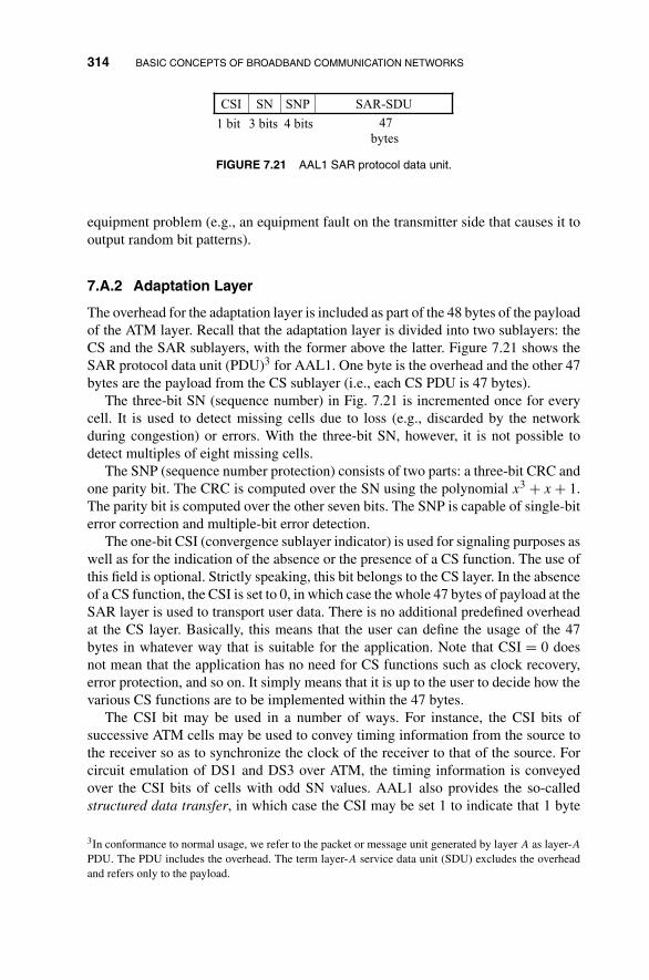
314 BASIC CONCEPTS OF BROADBAND COMMUNICATION NETWORKS
SAR-SDUSNPSNCSI
1 bit 3 bits 4 bits 47
bytes
FIGURE 7.21 AAL1 SAR protocol data unit.
equipment problem (e.g., an equipment fault on the transmitter side that causes it tooutput random bit patterns).
7.A.2 Adaptation Layer
The overhead for the adaptation layer is included as part of the 48 bytes of the payloadof the ATM layer. Recall that the adaptation layer is divided into two sublayers: theCS and the SAR sublayers, with the former above the latter. Figure 7.21 shows theSAR protocol data unit (PDU)3 for AAL1. One byte is the overhead and the other 47bytes are the payload from the CS sublayer (i.e., each CS PDU is 47 bytes).
The three-bit SN (sequence number) in Fig. 7.21 is incremented once for everycell. It is used to detect missing cells due to loss (e.g., discarded by the networkduring congestion) or errors. With the three-bit SN, however, it is not possible todetect multiples of eight missing cells.
The SNP (sequence number protection) consists of two parts: a three-bit CRC andone parity bit. The CRC is computed over the SN using the polynomial x3 + x + 1.The parity bit is computed over the other seven bits. The SNP is capable of single-biterror correction and multiple-bit error detection.
The one-bit CSI (convergence sublayer indicator) is used for signaling purposes aswell as for the indication of the absence or the presence of a CS function. The use ofthis field is optional. Strictly speaking, this bit belongs to the CS layer. In the absenceof a CS function, the CSI is set to 0, in which case the whole 47 bytes of payload at theSAR layer is used to transport user data. There is no additional predefined overheadat the CS layer. Basically, this means that the user can define the usage of the 47bytes in whatever way that is suitable for the application. Note that CSI = 0 doesnot mean that the application has no need for CS functions such as clock recovery,error protection, and so on. It simply means that it is up to the user to decide how thevarious CS functions are to be implemented within the 47 bytes.
The CSI bit may be used in a number of ways. For instance, the CSI bits ofsuccessive ATM cells may be used to convey timing information from the source tothe receiver so as to synchronize the clock of the receiver to that of the source. Forcircuit emulation of DS1 and DS3 over ATM, the timing information is conveyedover the CSI bits of cells with odd SN values. AAL1 also provides the so-calledstructured data transfer, in which case the CSI may be set 1 to indicate that 1 byte
3In conformance to normal usage, we refer to the packet or message unit generated by layer A as layer-APDU. The PDU includes the overhead. The term layer-A service data unit (SDU) excludes the overheadand refers only to the payload.

ATM CELL FORMAT 315
Cell 47 bytes
1
2
3
125
126
127
128
124
… …Video data
Reed–Solomen
codes
Bytes i of codes computed over bytes i of video data
FIGURE 7.22 AAL1 CS forward error correction for transporting video data.
in the SAR payload is reserved for CS usage and only 46 bytes are for the userdata.
Another function that can be performed by the CS is forward error correction. Theexample in Fig. 7.22 shows the CS for the transport of video data with forward errorcorrection. The video data is arranged in 124 rows of 47 bytes each, and each row ispacked into one cell. Additional four cells are used for error-protection purposes. Anerror-correction code (e.g., the Reed–Solomen code) is computed over the ith bytesof all rows and it forms the four ith bytes in the four error-protection cells. After thecodes are computed, they are put into cells separated from the data cell. Up to fourlost cells can be recovered at the receiver.
Figure 7.23 shows the SAR PDU for AAL2. The SN field contains the sequencenumber of the cell. The source generates traffic at variable rate and some cells couldbe partially filled only. A message may be contained in one or more cells. The IT (in-formation type) field is two bits in length, and it indicates whether the cell contains theBOM (begin of message), COM (continuation of message), or EOM (end of message):10 for BOM, 00 for COM, 01 for EOM, and 11 for a message equal to or shorter thanone cell in length (i.e., the cell contains the whole message). The LI (length indicator)at the trailer of the cell indicates the number of bytes used in partially filled cells. Atpresent, AAL2 is not well defined and the length of each field requires further study.
CRCLISAR-SDUITSN
2 bits
FIGURE 7.23 AAL2 SAR protocol data unit.

316 BASIC CONCEPTS OF BROADBAND COMMUNICATION NETWORKS
SAR-SDU CRCLIRES/MIDITSN
2 bits 4 bits 10 bits 44 bytes 6 bits 10 bits
FIGURE 7.24 AAL3/4 SAR protocol data unit.
There are two modes for AAL3/4:
� Message mode: In this mode, the layer above the AAL passes data to the AALas messages that could be fixed or variable in length. Each message is passed inits entirety at one time. At the receiver end, data are also passed from the AALto the layer above in discrete messages.
� Streaming Mode: This service provides the transport of long variable-lengthdata units. In this mode, the layer above the AAL may pass data to the AAL inseparate chunks. Each pass may contain only part of the whole data unit, andseveral passes may occur at separate times. A reason for not passing a data unitas a whole could be that the data unit has not been created by the applicationentirely. The AAL may send out cells associated with a data unit before all thedata have arrived. In this way, the adaptation delay could be reduced.
Figure 7.24 shows the SAR-PDU format of AAL3/4. Four bytes in each cell are used asthe overhead. The two-bit ST (segment type) field is the same as the IT field in AAL2,and it is used to indicate BOM, COM, EOM, or SSM (single segment message). Thefour-bit SN is used for detection of lost and inserted cells. The LI field is six bits inlength: an EOM or SSM cell may be only partially filled (i.e., less than 44 bytes) andthe LI indicates the number of bytes used. The 10 CRC bits are computed over thewhole SAR PDU using the generating polynomial x10 + x9 + x5 + x4 + x + 1.
The 10-bit MID (multiplexing identifier) field is used in AAL4 (i.e., connectionlessservice) only; the bits are reserved for future usage in AAL3. In AAL4, this meansthat up to 210 connectionless packets (messages) can be transmitted on the same ATMconnection simultaneously. For instance, there could be two connectionless servers(e.g., IP routers) connected to the two ends of the ATM connection sitting on top ofthe adaptation layer. At the transmitter end, the connectionless server aggregates allthe connectionless traffic to be routed to the other connectionless server and forwardsit via the ATM connection. Each IP packet can be assigned an MID, and the cells ofthe packet will have the same MID. At the receiving end, the connectionless serverin turn examines the MID field of each incoming cell and reassembles the cells withthe same MID back to the packet before deciding how to further route it.
The multiplexing/demultiplexing mechanism is needed only if the cells of dif-ferent messages are interleaved during the transmission over one ATM connection.In this case, successive cells arriving at the receiving end may belong to differentmessages and the MID field is needed to distinguish them apart. For illustration, asituation where this may arise is shown in Fig. 7.25. There are several connectionlessservers connecting to the same ATM switch via different inputs of the switch. Theconnectionless servers may have traffic to be routed to a remote connection server,

ATM CELL FORMAT 317
Connectionless server
Connectionless server
Connectionless server
Connectionless server
One VP
FIGURE 7.25 Multiplexing the cells from several connectionless servers onto one VP.
that is connected to a remote ATM switch. To improve efficiency, the traffic from allthe transmitting connection servers may be statistically multiplexed onto the sameATM connection (say, a VC) for transport to the remote ATM switch.
In situations where the cells of different messages are not interleaved over anATM connection, there is no need for the MID, since any particular message will betransmitted as successive cells. The ST field will be sufficient for reassembling themessage at the receiver end. In the above example, instead of one VC, separate VCscan be used to transport the cells from different connectionless servers to the remoteconnectionless server. There will then be no need for the use of MID. Of course,there will be several AAL processes, one for each VC, interfacing with the receivingconnectionless server.
In the situation where cells of different messages are interleaved, instead of theMID, one could in principle encode the routing information in all cells of a mes-sage. Each message forwarded by the connectionless server to the AAL must containthe explicit routing information (e.g., IP address for IP routing) for the receivingconnectionless server to further route the message. The problem is that the routinginformation may be much lengthier than the MID (e.g., the IP address is 32 bits) andwill therefore create larger overhead if it is incorporated in all cells of the message.
The overhead in the CS of AAL3/4 consists of four bytes of header and fourbytes of trailer, as illustrated in Fig. 7.26. The one-byte CPI (common part indicator)signals how the rest of the overhead fields are to be interpreted. Until further studiesby the standard committee, this field is always set to 0. The zero value indicates thatthe counting units in the two-byte BASize (buffer allocation size) and the one-byteLength fields are bytes.
The BASize indicates the maximum number of bytes needed to store the CS PDUat the receiver. It is used to reserve buffer at the receiver for the reception of the PDU.It is possible for the cells associated with the CS PDU to arrive at the peer convergence
LengthETagALPADCS-SDUBASizeBTagCPI
2 bytes
1 byte
1 byte
0–3 bytes1–216 bytes2 bytes1
byte1
byte
FIGURE 7.26 AAL3/4 CS protocol data unit.

318 BASIC CONCEPTS OF BROADBAND COMMUNICATION NETWORKS
sublayer at the receiver separated in time. This could be the case, for instance, whenthe interface between the CS and AAL3/4 at the sender is in the streaming mode.With 16 bits, the maximum size of the CS PDU is 216 bytes. When the message modeis used, the BASize corresponds to the payload of the CS PDU (or SDU), and thecontents of the BASize and Length fields are the same. The BASize and Length fieldsmay be different when the streaming mode is used. In this case, the BASize is set tobe equal to or greater than the actual CS SDU length. Typically, this is set to be themaximum possible CS SDU length, since in the streaming mode the sender itself maynot know the exact length of the data unit when it sends out the cell containing theBASize field (because the data unit may not have arrived in its entirety). The exactlength of the SDU is indicated in the Length field, that is contained in the last cell ofthe data unit.
The one-byte BTag (beginning tag) and the one-byte ETag (end tag) fields are setto the same value, which changes for each successive CS PDU. They are for errordetection purposes. If the BTag and ETag of a received CS PDU do not match, thensome cells must have been lost. Although the four-bit SN of the AAL3/4 SAR sublayeris also meant for detecting missing cells, the mechanism at the SAR sublayer maynot be strong enough and in many situations, lost cells may not be detected. Thus, theBTag and ETag can be viewed as an enhancement to the cell loss detection capability.
The one-byte AL (alignment) field serves no other purpose than to make the trailer32-bit long. The reason is that many computers are 32-bit machines that work on 32bits in each cycle. Between the CS PDU payload and the trailer, there will be 0–3unused bytes for padding purposes. The reason is again to make sure that the wholeCS PDU is a multiple of 32 bits in length.
The overhead in the AAL3/4 SAR layer is rather high: 4 bytes out of every 44bytes. Also, the 10-bit CRC may not offer enough protection at the cell level, andthere is no CRC at the CS PDU level; generally, the longer the block length of the data,the better the efficiency achieved in error protection (i.e., for a given data corruptionprobability, the longer the block length, the smaller the ratio of CRC bits to the databits), and this would have argued for putting the CRC in the CS. For these and otherreasons, the computing industry initiated the AAL5.
There is no overhead in the AAL5 SAR sublayer. All 48 bytes of the payload ofthe ATM layer are used to carry the CS PDU. Figure 7.27 shows the format of theAAL5 CS PDU and how it is being segmented into cells at the SAR sublayer. One bitof the PTI (payload type) field of the ATM-layer header is used to indicate the end ofthe PDU. That is, if the cell is user cell (first bit of the PTI is set to 0) and if the last bitof the PTI is set to 1, then the cell contains the last segment of the PDU. If this is thecase, then the last eight bytes of the payload of the cell are the overhead associatedwith the convergence sublayer of AAL5. The one-byte UU (user-to-user indication)field is intended for signaling between two end users and it is carried transparently byAAL5. The usage of the one-byte CPI is currently not defined. The two-byte Lengthfield is the number of bytes in the CS SDU, not including the padding in the last cell.The 32-bit CRC is computed over the entire CS PDU, including the padding and thetrailer. Notice that strictly speaking, AAL5 has violated the layering principle in thata bit of the overhead of the ATM layer has been “stolen” for use in the AAL layer.

PROBLEMS 319
CRCLengthCPIUUPADCS-SDU
4 bytes2 bytes1 byte1 byte0–47 bytes1–216 bytes
SAR-PDU CRCLengthCPIUUPADData
SAR-PDU SAR-PDU
ATM header, PTI = 000 ATM header, PTI = 011
48 bytes 40 bytes
CS-PDU
SAR-PDU
ATM-PDU
FIGURE 7.27 AAL5 CS protocol data unit and its segmentation.
This, however, does not cause any confusion as long as the designers of the AAL5and ATM hardware or software have taken it into account.
PROBLEMS
7.1 Consider the second method of multirate switching depicted in Fig. 7.2(b). Themain idea is that all the n channels of the same input connection must be routedover the same internal path. Each input/output link is DS-1, which consists of24 DS-0s. Suppose that each connection consists of either one or two DS-0channels (i.e., n is either 1 or 2). How many middle-stage modules are neededfor the overall switch to be strictly nonblocking, assuming the switch modulesin all stages are nonblocking?
7.2 Does ATM switching solve the problem of bandwidth fragmentation in a switchconsisting of multiple stages of switch modules? Has the problem of increasedblocking probability during call setup of a connection due to bandwidth frag-mentation been solved?
7.3 Consider sending the cells from a voice source over an ATM network. Supposethat the delay suffered by each cell in the network ranges from 2 to 10 ms. Howmuch time after the arrival of the first cell can the receiver start to play out theaudio? How should the buffer be dimensioned to avoid data overflow?
7.4 What is the worst message length for a cell network in terms of the overhead?
7.5 Suppose that each cell has a fixed header size of 5 bytes. The packet to befragmented into cells has a fixed size of 100 bytes. What is the overhead ifthe cell size is fixed to be 32 bytes (excluding the 5-byte header)? What is theoverhead if the cell size is 48 bytes instead? Which cell size is more efficientfor these fixed-length packets?

320 BASIC CONCEPTS OF BROADBAND COMMUNICATION NETWORKS
7.6 The network shown in Fig. 7.7 consists of a number of VC and VP switches.(a) Identify the end-to-end path of the VC from user A to user B with VPI =
2 and VCI = 3 at the source.
(b) Write down the VPI/VCI entry in the VPI/VCI table needed for routingthe VC traffic at the last node just before the traffic reaches user B. (Note:the answer is not unique.)
(c) Indicate the VP termination points (if any) in the path.
(d) Indicate the VC termination points (if any) in the path.
7.7 Consider the problem of setting up a new VC over a sequence of n VPs.Suppose that the VCI of the VC is not allowed to change from VP to VP andthat we want to use the same VCI throughout. Suppose that on each of theVPs, a fraction p of the VCI values has already been used, and a fraction 1 − p
has not been used. Assume that there are altogether m possible VCI values oneach VP.(a) The source node first randomly chooses a VCI not already used in the first
VP, it then asks the next VC switch whether this VCI has been used in thenext VP. If no, the next VC switch asks the VC switch further downstreamwhether the VCI has been used; if yes, the source is asked to choose anotherVCI and repeat the process. This is repeated until a unique VCI throughoutthe path can be found. For small p, how many attempts by the source willbe needed before a unique VCI can be found? Can you think of a betterway to reduce the number of attempts?
(b) Estimate the probability of not having a unique VCI throughout in termsof p, n, and m, assuming the VCIs already used in different VPs are un-correlated? For p = 0.75, n = 4, and m = 256, what is the blocking prob-ability?
7.8 This problem examines the shortcoming of the VP/VC two-tier multiplexinghierarchy depicted in Fig. 7.8 and the extent to which the shortcoming is impor-tant. Suppose that all the VCs behave the same way. For each VC, half of thetime, data are arriving at the rate of r bits per second and half of the time there isno data arriving. Suppose that there are n VCs being multiplexed directly ontoa physical link of 0.6rn bits per second. Define the probability of congestionas the probability that the arrival rate of the data into the multiplexer is higherthan the departure rate, 0.6rn. Suppose we use the two-tier hierarchy with 10VPs, each of which have a bandwidth of 0.06rn bits per second, and there are0.1n VCs being multiplexed onto each VP. What is probability of congestionfor each of the first-level multiplexers? How do the two cases differ when n issmall, say, n = 20, and when n is large, say, n = 1000.
7.9 The text discussed the mapping of input VPI–VCI pair to an output VPI–VCIpair at an input of a VC switch. This works for point-to-point connections.For a multicast connection in a multicast switch, there are several outputs, andtherefore, several output VPI–VCI pairs must be mapped to the input VPI–VCIpair. Consider a 256 × 256 switch in the following.

PROBLEMS 321
(a) Suppose the switch supports only point-to-point connections. Assume thatthe VPI is 12 bits and VCI is 16 bits. Estimate the routing table size at aninput.
(b) For a switch that supports multicast connections, suggest a structure forthe routing table at an input, assuming that the number of outputs for ageneral connection (point-to-point or multicast) can range from 1 to 256.Based on this routing table, estimate the memory required at an input.
(c) For the multicast switch that is made up of a cascade of a copy networkand a point-to-point switch, what is the problem (other than the largememory requirement) of doing the mapping at the input? (Hint: Beforepacket replication, the master packet represents many packets that will bereplicated, what output VPI–VCI should it have?)
(d) Consider the cascade multicast network again. Suppose that for point-to-point connections, the mapping will be the same as before. But formulticast connections, the BCN mechanism will be used at the outputs ofthe copy network to retrieve both the output and the output VPI–VCI pairof a packet. Estimate the memory requirement of the lookup table at anoutput of the copy network.
(e) Consider a bus-based multicast switch such as the knockout switch. In thiscase, the outputs of a multicast cell pick up the cell from the bus. Discussthe design of the routing tables and their locations in such a switch.
7.10 With respect to the discussion of the use of MID in AAL4 in the appendix,can AAL5 be used to transport messages from different connectionless serversover the same ATM connection? How?
7.11 Suppose we want to send a short message of 1000 bytes, is AAL3/4 moreefficient or AAL5? Is there any situation under which AAL3/4 is more effi-cient than AAL5? Do you think AAL3/4 will be used in practice to transportconnectionless data?


8
NETWORK TRAFFIC CONTROLAND BANDWIDTH ALLOCATION
A broadband integrated network carries a large volume of traffic, and the traffic may befrom many different types of sources and have diverse characteristics. It is necessaryto allocate network resources and control this traffic to achieve two fundamentalgoals:
� Satisfy the QoS (quality of service) requirements of network users.� Maximize network usage.
Controls at different timescales are exercised to achieve these two goals. Recall thatmany logical networks can be set up on the same physical network by VP networking.Control can be exercised on the VPs in logical networks. Each logical network canbe used by many end users who establish VCs over it, so we also have control at theVC connection level. Finally, the delivery of cells over a VC must also be controlledto meet certain QoS objectives, such as delay and cell loss probability.
In a virtual-path (VP) network, the virtual paths and the bandwidths on them maybe reconfigured dynamically over time. For instance, if VPs are used to segregateservices, different services may demand different amount of network resources atdifferent times of the day. To maximize network usage and service quality, bandwidthscan be reallocated once in a while (say, every half hour or so) among the differentlogical networks according to their usage. In addition, new VPs may be set up andold VPs may be torn down in a logical network dynamically to reflect the change intraffic demands within it. The control timescale at the VP level is large compared tothat in cell-level control.
At the VC connection level, we have the control functions of call admission,routing, and bandwidth allocation. Since each VP may contain many VCs, the amount
Principles of Broadband Switching and Networking, by Tony T. Lee and Soung C. LiewCopyright © 2010 John Wiley & Sons, Inc.
323

324 NETWORK TRAFFIC CONTROL AND BANDWIDTH ALLOCATION
of control actions is larger at the VC level than at the VP level: VC-level control occursmore frequently in the network. Depending on the service, a VC may last for a long orshort time. A telephone call will probably last a few minutes, and the control timescaleof the associated VC will be smaller than that at the VP-level control. A movie, onthe other hand, may last up to 2 h, and the control timescale is not necessarily smallerthan that at the VP level.
For an overview, let us briefly walk through the process of call admission controlat the VC connection level. The purpose of call admission is basically to determinewhether to admit or reject a connection request based on a projection of the conse-quences of admitting the call. If accepting the call will degrade the QoS (say, thedelay or the cell loss probability) of the existing connections to an unsatisfactorylevel, then the call should be rejected. At the same time, if the QoS demanded bythe call cannot be satisfied, then the call should either be rejected or negotiationshould be initiated to see if a lower QoS is acceptable to the end user requesting thecall.
Closely tied to call admission is the issue of routing. There may be several al-ternative routes in the network from the source to the destination of a new con-nection request. Whether the call is admitted depends on whether an acceptableroute can be found. Some paths may not satisfy the QOS criteria and some may.Among the latter, the “optimal” route should be chosen such that the network re-sources are used in the most efficient way. The definition of the optimal route is notas trivial as it might first appear. For instance, if by optimality, we mean the routethat can maximize the number of accepted calls in the future (or minimize the callblocking probability), then some statistics of the future call arrivals must be avail-able. In addition to routing, bandwidth allocation (i.e., how much bandwidth is to beallocated to the connection) should also be considered as part of the call admissionprocess. In short, the issues of call admission, routing, and bandwidth allocation areinterrelated.
Once a call is accepted, control at the cell level will be exercised throughoutthe call’s duration. Since each VC may have many cells, cell-level control is verymuch more frequent than connection-level control. Also, each cell lasts for a veryshort time, and therefore the control timescale is very small. For this reason, cell-level control is often performed by specialized hardware rather than software. Forexample, the switches we have discussed in the previous chapters are specializedhardware for routing cells. This is in contrast to VC- and VP- level control that isoften implemented in software for flexibility.
Cell-level control can occur at several places in the network. Control may be appliedat the boundary of the network to make sure that the connection is not pumping cellsinto the network at a rate higher than some pre-agreed rate. This is sometimes called thepolicing function. The end user may also perform “traffic shaping” (e.g., intentionallydelay some cells at the edge or space out their transmission in time) at the source sothat the traffic presented to the network conforms to the pre-agreed rate.
Once the cells enter the network, their flow may also be monitored and controlled.Consider a connection traversing several nodes in a given direction. A node is saidto be upstream (downstream) of another node if cells of the connection traverse the

NETWORK TRAFFIC CONTROL AND BANDWIDTH ALLOCATION 325
node before (after) passing through the other node. In feedback flow control (alsocalled closed-loop control), the downstream traffic conditions are fed back upstreamto regulate the traffic flow. In feedforward flow control (also called open-loop control),there is no feedback signal.
There are several possibilities for closed-loop control: among them are link-to-link flow control and end-to-end flow control. In link-to-link flow control, the trafficcondition at a node is fed back to the immediate upstream node. If the downstreamlink is congested, then the upstream node will slow down the transmission of cells tothe downstream node. This in turn may cause cells to back up at the upstream node,and through feedback, the node further upstream will be informed to cut down therate of its traffic flow. Through a chain of this “back-pressure” mechanism, eventuallythe source will be told to reduce its transmission of traffic.
In end-to-end feedback flow control, the feedback to the source comes from thedestination rather than through the back-pressure mechanism in link-to-link control.There are many possibilities for end-to-end feedback. In ATM network, recall thatthere is a bit in the PTI (see the appendix of Chapter 7) field in the ATM cell headerthat is used for congestion indication. In ABR service, the source sets this bit tozero. As a cell travels through the nodes in the network, this bit will be set to one atcongestion points. The destination, upon receiving this cell, can then inform the sourceof the occurrence of congestion (or the absence of it) through a path in the reversedirection.
In open-loop control, since there is no feedback on the downstream traffic con-ditions, the rate at which the source pumps traffic into the network must be tightlycontrolled so that it conforms to some pre-agreed rate. Otherwise, if many sourcestransmit large amounts of traffic simultaneously, congestion in the network may occur,giving rise to large cell loss rates when switch buffers start to overflow. If all trafficsources conform to their pre-agreed rates, the transport of their cells in the network canbe scheduled such that their desired QoS can be satisfied. Feedforward flow controleliminates a problem with feedback flow control in a high-speed network in whichthe propagation delay is large compared to how fast the statistics of cell traffic canchange: by the time the feedback signal arrives at the source, the traffic conditions atthe downstream nodes may have already changed; it is also possible that by the timea traffic congestion signal reaches the source, the source may have already pumpedout a large number of cells, making the congestion even worse.
Feedforward flow control, on the other hand, may not be able to achieve a statisticalmultiplexing gain as high as that in feedback flow control. In case of light traffic at thedownstream node, the source may not be able to take advantage of that by pumpingin more traffic, since there is no feedback telling it so.
The current ATM standard reflects the following as far as feedback and feedfor-ward flow control is concerned. For services that have stringent delay requirements,feedforward flow control can better meet the requirement. This will be the case forAAL1 and AAL2 traffic, and the targeted network services are CBR and VBR. Fordata services such as those supported by AAL3/4 and AAL5, delay requirement isless stringent. The targeted network services are either ABR (available bit rate) orUBR (unspecified bit rate). In the ABR service, for instance, the available capacity

326 NETWORK TRAFFIC CONTROL AND BANDWIDTH ALLOCATION
for the transmission of the traffic from a source may change over time in a way thatdepends on network usage by other users. The network capacity available at anytime is reflected in the feedback signal. Having overviewed the general issues andmethods of traffic control, the remaining sections of this chapter will treat them ata more fundamental level. As a start, we will first introduce a traffic model for celltraffic that will be useful for the study of flow control.
8.1 FLUID-FLOW MODEL: DETERMINISTIC DISCUSSION
A fluid-flow model can be used to describe the flow of cell traffic in the network. Thismodel treats traffic as fluid flow. The fluid-flow model is a powerful and intuitivetool for visualizing the flow traffic in the network without the need for complicatedqueueing analysis. This is especially true when we have a deterministic descriptionof the “worst-case” input traffic pattern that a source can pump into the network. Thisis the case, for example, when traffic policing is applied at the edge of the network.When the input traffic is stochastic and not known deterministically, the model canalso be subjected to rigorous mathematical analysis, as shall be seen in Section 8.2. Byadopting the fluid-flow model, closed-form analytical solutions can often be obtainedwhere they are not so readily available otherwise. In other words, the analysis canoften be carried out further with the fluid-flow model than by using the cell-trafficmodel.
To explain the fluid-flow model, let us focus on the traffic of a simple “on–offsource.” Figure 8.1(a) shows the cell-traffic model. During on time a cell is generatedevery T seconds, and during off time no cell is generated. Packetized voice trafficexhibits this kind of behavior. The on time is the duration of a talkspurt when the
T T T
…
On timeOff time
(a)
(b)
…
T T T
…
On timeOff time
… Peak
Fluid flow on time
FIGURE 8.1 (a) On–off cell-traffic source; (b) approximating on–off cell traffic with fluid-flowtraffic.

FLUID-FLOW MODEL: DETERMINISTIC DISCUSSION 327
speaker speaks, and the off time is simply when the speaker idles. The average datarate during on time is therefore 1/T cells/s or
ron-time = 53 × 8
Tbits/s. (8.1)
The on and off times are in general not fixed and may vary over time. Let the averageoff time be denoted by 1/λ and the average on time be denoted by 1/μ. Then theaverage rate of the traffic is
rave =1μron-time
1λ
+ 1μ
= λron-time
λ + μbits/s. (8.2)
Figure 8.1(b) shows the approximation of the cell-traffic model with the fluid-flowmodel. During on time, instead of cells being separated by intervals of T , we makethe approximation that the arrivals are continuous in time at rate ron. Thus, instead ofcell arrivals, we have “fluid” arrivals. The peak rate of the on–off fluid-flow source isrpeak = ron. Both models have the same total number of bits arrived in each on period,but the bit arrivals are distributed evenly over time in the fluid-flow model.
Consider the statistical multiplexing of traffic from several on–off sources, asillustrated in Fig. 8.2. Suppose that the buffer capacity is B bits and the transmissionbandwidth is C bits/s. Then, as far as the buffer occupancy is concerned, the mul-tiplexer is analogous to a leaky bucket of size B with a hole at the bottom. Fluid ispoured into the bucket at a rate corresponding to the traffic generated by the sources,and fluid leaks out of the bucket at rate C.
Figure 8.3 shows the simple case in which there is only one traffic source andrpeak > C. Both the rate-versus-time and cumulative traffic-versus-time curves aredrawn. By drawing the cumulative arrived and departed traffic, we can find out thedelay of a bit i (or a drop of fluid) and the buffer occupancy at time t. As shown in
Source
1
Source
2 Source
N…
C bits/s
Leaky
bucket
Source
1
Source
2 Source
N…
C bits/s
Buffer
size
= B bits
(Statistical multiplexing)
FIGURE 8.2 An analogy between a transmission buffer of output rate C and a leaky bucket.

328 NETWORK TRAFFIC CONTROL AND BANDWIDTH ALLOCATION
b1
b2
tt 1 t2
Slope = c
Departurebit iSlope = rpeak
Arrival
t1−t2 = delay of bit i
Time (s)
Cumulative traffic (bits)
b2− b1
= buffer
occupancy
at time t
Single
source
C
rpeak >C
Arrival curve
Departure curve
(a)
Arrival curve
Departure curve
Time (s)
Traffic rate (bits/s)
C
(b)
rpeak
FIGURE 8.3 A leaky bucket with a single source; (a) cumulative traffic-versus-time arrival anddeparture curves; (b) traffic rate-versus-time arrival and departure curves.
Fig. 8.3, the delay of a bit i corresponds to the horizontal difference between the arrivaland departure curves at bit position i. The buffer occupancy at time t corresponds tothe vertical difference between the two curves at time t.
Figure 8.4 shows the case in which there are multiple sources. The cumulativearrived traffic is a piecewise linear curve whose slope changes according to howmany sources are on: specifically, when m sources are on, the slope is mrpeak. In thefigure, we assume that the traffic is normalized so that rpeak = 1. The departure curvehas a maximum slope of C. When the departure curve is below the arrival curve, thebacklog in the buffer starts to build up. If we assume that the system works as hardas possible to clear up the backlog, the slope of the departure curve is C wheneverthe backlog is nonzero. That is, with the leaky-bucket analogy, fluid will continue toleak out at the maximum rate C so long as there is fluid in the bucket.
When there is no backlog and the total arrival rate from all sources is less thanor equal to C, then the fluid that goes into the bucket immediately flows out. In this

FLUID-FLOW MODEL: DETERMINISTIC DISCUSSION 329
Arrival curve
Departure curve
Time
Arrival traffic rate
123
Two sources on
Three sources on
Source 1
Source 2 Source
N…
1 < C < 2
rpeak = 1
Time
Cumulative traffic
Slope = 1
2
1
2
1
3
Slope = c
c
(Slope = m rpeak if m sources have arrivals)
FIGURE 8.4 The arrival and departure curves of a fluid-flow multiplexer.
situation, the cumulative departed traffic equals the cumulative arrived traffic, and thedeparture rate equals the arrival rate. When there is no backlog and the arrival rate islarger than C, then backlog immediately builds up, and the departure rate will be C.
The curves in Fig. 8.4 only show the “global” view of a multiplexer. The QoSas perceived by individual traffic streams cannot be seen from the curves. The QoSperceived by a traffic stream depends to a large extent on the scheduling algorithmused by the multiplexer. When several streams have backlog in the multiplexer, themultiplexer has a choice of whose data to send out first, and the order in which the dataare sent out is determined by a scheduling algorithm. Different scheduling schemesmay give rise to different QoS.
Let us assume that the traffic of each stream must be served in a first-come-first-serve (FCFS) manner. That is, for a particular stream, the bit that arrives beforeanother bit from the same stream must also depart before this other bit. Interpretingeach stream as one VC in the ATM network, the FCFS requirement makes sure thatthe data will be delivered to the end destination in the correct order. For sequencepreservation of the data of a VC, however, it is not necessary that the bits from differentstreams to be served in any particular order: for example, sending out a bit of a streambefore a bit of another stream that arrives earlier would not compromise the sequenceorder of either stream.
Let us first return to the cell-traffic model. The round-robin scheduling schemetreats all streams as equal and serves them in a round-robin fashion. Conceptually,there is one buffer for each traffic stream. The multiplexer selects cells from thenonempty buffers in a round-robin fashion. That is, the head-of-line cells of thenonempty buffers are served in a cyclic fashion.

330 NETWORK TRAFFIC CONTROL AND BANDWIDTH ALLOCATION
We would like to approximate the round-robin service discipline with a fluid-flowservice model that is compatible with the fluid-flow source traffic model. That is,instead of serving data in a cell-by-cell manner, we assume that data are infinitelydivisible (i.e., like fluid) and can be served in infinitesimal amount by infinitesimalamount fashion. A more detailed discussion of the relationship between the round-robin service discipline and the fluid-flow service discipline will be presented inSection 8.4.
Roughly, the round-robin service discipline with cell traffic can be approximatedby the fluid-flow service discipline with fluid traffic as follows: instead of scanningthrough the streams with backlog, all streams with backlog will be served simultane-ously in the fluid-flow service discipline. Specifically, the output capacity C will bedivided evenly among the traffic streams with backlog: if there are m backlog streams,then the departure rate of each stream will be C/m.
Figure 8.5 gives an example in which there are two traffic streams: for traffic streami, Ai(t) and Di(t) are the cumulative arrived traffic and cumulative departed traffic;
Arrival traffic rate
(Sources 1)1
Timet 0 t 2
Arrival traffic rate
(Sources 2)1
Timet 1 t 4
Arrival traffic rate
(Sources 1 and 2)
1
Timet 0 t 4
2
t 1 t 2
Source 1
Source 2
1 < C < 2
rpeak = 1
Equal-service discipline
Cumulative traffic (Sources 1 and 2)
Cumulative traffic (Sources 1 and 2)
Time
Time
Slope = 1
2
1
12
1 < C < 2
1
1 C/2Slope = 1
t 0 t 4t 1 t 2 t 3
When both sources busy, divide capacity evenly
Arrival curve
Departure curve
FIGURE 8.5 A multiplexer with two sources: the cumulative arrival and departure curves for thetotal traffic and the traffic of stream 1.

FLUID-FLOW MODEL: DETERMINISTIC DISCUSSION 331
the rpeak of each source is 1 and 1 < C < 2. From time t0 to t1, there are arrivalsfrom stream 1 but not from stream 2, so the arrived traffic departs immediately, sincethe whole capacity C is dedicated to stream 1 and C > 1 = rpeak. From time t1 tot2, there are arrivals from both streams 1 and 2, the total arrival rate, 2, is morethan C; C is divided evenly among the two streams and each of them is served atthe rate of C/2; backlog starts to build up for both streams. From time t2 to t4,only stream 2 has arrivals. But at time t2, there is still backlog for stream 1 andtherefore the service rates for both streams remain at C/2. At time t3(t2 < t3 < t4),the backlog of stream 1 is cleared, and therefore from time t3 to t4, stream 2 is served atrate C.
Strictly speaking, the preceding discussion was overly simplified and it neglected asubtle difference between the cell-traffic and the fluid-flow models. In the cell-trafficmodel, as far as the service discipline is concerned, each stream is in one of the twopossible states: when its buffer is empty, it is in the idle state. An idle stream willnot receive any service, and a busy stream will wait for its turn to receive service.At any one time, only one of the busy streams is served, and during its service thewhole capacity C is dedicated to it to transmit a cell. In the fluid-flow service model,we assume that the capacity C can be divided and allocated to the busy streams sothat they can be served simultaneously, each at a lower rate than C. In the discussionin the preceding paragraph, we attempted to divide the capacity evenly among thebusy streams. But such even distribution of capacity cannot always be achieved in thefluid-flow model, as described below!
Consider an example. Suppose that there are m = 2 streams with backlog. How-ever, there is another stream with no backlog, which is in the on state and therefore hastraffic arriving at the rate of 1. Suppose that C = 4. Then, how should C be dividedamong the three streams? Dividing it evenly means each stream should be served atrate C/3 = 4/3, but this is more than the arrival rate of the third stream, and we arecertainly not making full use of the capacity C. If we divide C only among the firsttwo streams, then backlog immediately builds up in the third stream, making it alsoa busy stream and therefore C must be divided among three streams again. In otherwords, the service rate of the third stream alternates between 0 and C/3 within aninfinitesimal amount of time.
A problem is with the previous definition of “busy streams.” As far as the servicediscipline is concerned, for the fluid-flow model, it is more appropriate to treat thestreams as having three possible states: (1) idle state: the buffer is empty and the arrivalrate is zero; (2) busy state: the buffer is nonempty; and (3) partially busy state: thebuffer is empty but the arrival rate is nonzero. In the above example, the third stream,which is partially busy, will be served at its input rate 1, and the two busy streamswill be served at rate (C − 1)/2 = 3/2. Of course, in situations where rpeak > C, itis not possible to have the partially busy state.
In general, the fluid-flow service discipline that attempts to approximate the round-robin discipline will first see if it is possible to serve each non-idle stream at rateC/(m + n), where m is number of busy streams and n is the number of partially busystreams. Among the partially busy streams, those with arrival rate ri < C/(m + n)will be served at rate ri. If none of the partially busy streams has arrival rate less than
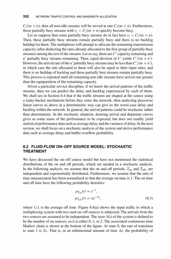
332 NETWORK TRAFFIC CONTROL AND BANDWIDTH ALLOCATION
C/(m + n), then all non-idle streams will be served at rate C/(m + n). Furthermore,those partially busy streams with ri > C/(m + n) quickly become busy.
Let us suppose that some partially busy streams do in fact have ri < C/(m + n).Then, these partially busy streams remain partially busy and there is no backlogbuildup for them. The multiplexer will attempt to allocate the remaining transmissioncapacity (after deducting the rates already allocated to the first group of partially busystreams) among the rest of the streams. Let us say, there are C′ capacity remaining andn′ partially busy streams remaining. Then, equal division of C′ yields C′/(m + n′).However, the arrival rate of the n′ partially busy streams may be less than C′/(m + n′),in which case the rate allocated to them will also be equal to their input rates, andthere is no buildup of backlog and these partially bust streams remain partially busy.This process is repeated until all remaining non-idle streams have arrival rate greaterthan the equipartition of the remaining capacity.
Given a particular service discipline, if we know the arrival patterns of the trafficstreams, then we can predict the delay and backlog experienced by each of them.We shall see in Section 8.4 that if the traffic streams are shaped at the source usinga leaky-bucket mechanism before they enter the network, then analyzing piecewiselinear curves as above in a deterministic way can give us the worst-case delay andbacklog within the network. In general, the arrival patterns could be stochastic ratherthan deterministic. In the stochastic situation, drawing arrival and departure curvesgives us some sense of the performance to be expected, but does not readily yieldstatistical performance data such as average delay and the variance of delay. In the nextsection, we shall focus on a stochastic analysis of the system and derive performancedata such as average delay and buffer-overflow probability.
8.2 FLUID-FLOW ON–OFF SOURCE MODEL: STOCHASTICTREATMENT
We have discussed the on–off source model but have not mentioned the statisticaldistributions of the on and off periods, which are needed in a stochastic analysis.In the following analysis, we assume that the on and off periods, Ton and Toff , areindependent and exponentially distributed. Furthermore, we assume that the unit oftime measurement has been normalized so that the average on time is 1. The on timeand off time have the following probability densities:
pTon (t) = e−t ,
pToff (t) = λe−λt, (8.3)
where 1/λ is the average off time. Figure 8.6(a) shows the input traffic to which amultiplexing system with two such on–off sources is subjected. The arrivals from thetwo sources are assumed to be independent. The state S(t) of the system is defined tobe the number of on sources, so it is either 0, 1, or 2. The associated continuous-timeMarkov chain is shown at the bottom of the figure. At state 0, the rate of transitionto state 1 is 2λ. That is, in an infinitesimal amount of time �t, the probability of
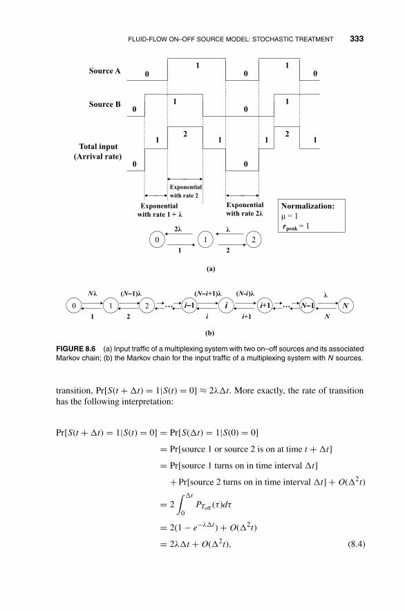
FLUID-FLOW ON–OFF SOURCE MODEL: STOCHASTIC TREATMENT 333
Source A
Source B
Total input
(Arrival rate)
Exponential
with rate 2
Exponential
with rate 1 + λ
Exponential
with rate 2λ
0 00
00
00
11 1122
11
11
0 1 2
2λ λ
21
Normalization:
μ = 1
rpeak = 1
(a)
0 1 2
Nλ (N−1)λ
21
i−1 i i+1
(N−i+1)λ (N-i)λ
i+1iN−1 N
λ
N……
(b)
FIGURE 8.6 (a) Input traffic of a multiplexing system with two on–off sources and its associatedMarkov chain; (b) the Markov chain for the input traffic of a multiplexing system with N sources.
transition, Pr[S(t + �t) = 1|S(t) = 0] ≈ 2λ�t. More exactly, the rate of transitionhas the following interpretation:
Pr[S(t + �t) = 1|S(t) = 0] = Pr[S(�t) = 1|S(0) = 0]
= Pr[source 1 or source 2 is on at time t + �t]
= Pr[source 1 turns on in time interval �t]
+ Pr[source 2 turns on in time interval �t] + O(�2t)
= 2∫ �t
0PToff (τ)dτ
= 2(1 − e−λ�t) + O(�2t)
= 2λ�t + O(�2t), (8.4)

334 NETWORK TRAFFIC CONTROL AND BANDWIDTH ALLOCATION
where O(�2t) represents all terms of order �2t or higher: this includes, for example,the probability of multiple transitions, such as both sources turn on in time interval�t. By the same argument, we can show that
Pr[S(t + �t) = 0|S(t) = 0] = 1 − 2λ�t + O(�2t),
Pr[S(t + �t) = 2|S(t) = 0] = O(�2t),
Pr[S(t + �t) = 0|S(t) = 1] = �t + O(�2t),
Pr[S(t + �t) = 1|S(t) = 1] = 1 − (1 + λ)�t + O(�2t),
Pr[S(t + �t) = 2|S(t) = 1] = λ�t + O(�2t),
Pr[S(t + �t) = 0|S(t) = 2] = O(�2t),
Pr[S(t + �t) = 1|S(t) = 2] = 2�t + O(�2t),
Pr[S(t + �t) = 2|S(t) = 2] = 1 − 2�t + O(�2t). (8.5)
Let Pi(t) be the probability of state i at time t. We can write
Pi(t + �t) =∑
j
Pj(t)Pr[S(t + �t) = i|S(t) = j], i = 0, 1, 2. (8.6)
From (8.5) and (8.6), we can get
dP0
dt= lim
�t→0
P0(t + �t) − P0(t)
�t= −2λP0(t) + P1(t). (8.7)
Note that the terms O(�2t) get canceled out in the limit �t → 0. Also, note that thecoefficients in (8.7) are associated with the transition rates: 2λ is the transition rateout of state 0 and 1 is the transition rate into state 0 from state 1. In a similar fashion,the following can be derived from (8.5) and (8.6), yielding the same interpretation ofthe transition rates:
dP1
dt= −(1 + λ)P1(t) + 2λP0(t) + 2P2(t),
dP2
dt= −2P2(t) + λP1(t). (8.8)
At equilibrium (as t → ∞), dPi/dt → 0. Substituting this into (8.7) and (8.8), weget
P1 = 2λP0,
P2 = λ
2P1 = λ2P0, (8.9)
FLUID-FLOW ON–OFF SOURCE MODEL: STOCHASTIC TREATMENT 335
where Pi denotes the equilibrium probability Pi(t → ∞). Using the fact that P0 +P1 + P2 = 1 in (8.9), we can get
P0 = 1/(1 + 2λ + λ2) = 1/(1 + λ)2. (8.10)
In general, we note that
Pi =(
2
i
)(1
1 + 1/λ
)i ( 1/λ
1 + 1/λ
)2−i
, i = 0, 1, 2. (8.11)
This could have been obtained using the following more straightforward argumentthan the Markov chain analysis. At any arbitrary time, the probability of a sourcebeing on, denoted by q, is the ratio of the average on time divided by the sum of theaverage on and off times (i.e., a “cycle” of on and off times). This is q = 1/(1 + 1/λ).Given that the sources are independent, the number of on sources is then given by thebinomial distribution with parameter q, which yields (8.11).
Equation (8.11) does not tell us much about the multiplexing system. It onlydescribes the source behavior. To study a multiplexer in more detail, we have to definethe state to include the buffer occupancy in addition to the number of on sources. Inthis case, straightforward argument as in the previous paragraph does not work. Thisis the motivation for the more roundabout Markov chain approach: we can modifythe argument to study the buffer occupancy.
Before moving onto the study of buffer occupancy, Fig. 8.6(b) shows the Markovchain of the general case with N sources. From state i, 1 < i < N, the system canonly evolve to state i − 1 or i + 1 in the next transition. At the boundary states, 0 andN, the transition can go only one way. The equilibrium probability is given by
Pi =(
N
i
)(1
1 + 1/λ
)i ( 1/λ
1 + 1/λ
)N−i
=(
N
i
)λi
(1
1 + λ
)N
, i = 0, . . . , N. (8.12)
We now consider a multiplexer system with infinite buffering space. Let X(t) be therandom variable for the buffer occupancy level and S(t), as discussed before, be therandom number denoting the number of on sources at time t. For a stable system inwhich X(t) does not grow to infinity, the output capacity C must be larger than theaverage arrival rate from the N sources,
r = N
1 + 1/λ. (8.13)
In the fluid-flow model, X(t) is a continuous variable. Let the probability density thatS(t) = i and X(t) = x be denoted by pi(t, x). We want to find the dynamic equationgoverning the evolution of pi(t, x). For i = 1, 2, . . . , N − 1, pi(t + �t, x) can be

336 NETWORK TRAFFIC CONTROL AND BANDWIDTH ALLOCATION
expressed in terms of the probability densities at time t as the sum of three terms,corresponding to the events of no transition and transitions from two neighboringstates i − 1 and i + 1. Let Enone, Eon, and Eoff , be the events of no transition, an offsource turns on, and an on source turns off in time �t, respectively. The events ofmultiple transitions have probability densities of order �2t. We have
pi(t + �t, x) = Ai + Ai−1 + Ai+1 + O(�2t),
where
Ai = p(S(t) = i, Enone, X(t) = x − (i − C)�t),
Ai−1 = p(S(t) = i − 1, Eon, X(t) = f (x)),
Ai+1 = p(S(t) = i + 1, Eoff , X(t) = g(x)), (8.14)
where p(·) are probability densities, and we leave f (x) and g(x) undefined for thetime being.
The term Ai is associated with no transition in the time interval �t. Given thatthere is no transition, away from the boundary where X(t) = 0, the departure ratefrom the buffer is C and the arrival rate to the buffer is i. This means that the netincrease in buffer occupancy from time t to time �t is (i − c). Therefore, in order thatX(t + �t) = x, we must have X(t) = x − (i − C)�t. We can write
Ai = Pr[Enone|S(t) = i, X(t) = x − (i − C)�t] pi(t, x − (i − C)�t)
= [1 − {(N − i)λ + i}�t] pi(t, x − (i − C)�t) + O(�2t)
= [1 − {(N − i)λ + i}�t]
{pi(t, x) − (i − C)�t
∂pi
∂x+ O(�2t)
}+ O(�2t)
= [1 − {(N − i)λ + i}�t]pi(t, x) − (i − C)�t∂pi
∂x+ O(�2t), (8.15)
where we have used the Taylor’s series expansion in the second last line.The term Ai−1 in (8.14) is associated with an off source turning on in time interval
�t. The question is what should f (t) be. Depending on when the source turns onwithin the time interval �t, f (t) may differ. Let t + �t′ (0 < �t′ ≤ �t) be the timethe source turns on. We can write
Ai−1 =∫ �t
0d(�t′) p(S(t) = i − 1, Eon, on transition at t
+ �t′, X(t) = x − (i − C)�t + �t′), (8.16)
where we have made use of the fact that the on transition is at time t + �t′ to de-rive that X(t) = x − (i − C)�t + �t′. Note that (8.16) makes use of the marginalprobability-density formula: p(A = a) = ∫
all bdb p(A = a, B = b). Continuing

FLUID-FLOW ON–OFF SOURCE MODEL: STOCHASTIC TREATMENT 337
from (8.16),
Ai−1 =∫ �t
0d(�t′) p(S(t) = i − 1, Eon, X(t) = x − (i − C)�t + �t′)
×p(on transition at t + �t′|S(t) = i − 1, Eon, X(t)
= x − (i − C)�t + �t′). (8.17)
Now, the conditional probability density p(on transition at t + �t′|S(t) = i − 1,Eon, X(t) = x − (i − C)�t + �t′) does not depend on X(t) given Eon and S(t). Wehave
p(on transition at t + �t′|S(t) = i − 1, Eon, X(t) = x − (i − C)�t + �t′)
= p(on transition at t + �t′|Eon, S(t) = i − 1)
= {N − (i − 1)}λe−{N−(i−1)}λ�t′
1 − e−{N−(i−1)}λ�t, (8.18)
where, in the last line, the numerator is the unconditional probability density thatone of the {N − (i − 1)} off sources turns on at time �t′, and the denominator is theprobability that one of the off sources turns on within the time interval �t. Now,
p(S(t) = i − 1, Eon, X(t) = x − (i − C)�t + �t′)
= Pr[Eon|S(t) = i − 1, X(t) = x − (i − C)�t + �t′]
pi−1(t, x − (i − C)�t + �t′)
= {N − (i − 1}λ�t × pi−1(t, x − (i − C)�t + �t′) + O(�2t)
= {N − (i − 1)}λ�t ×[pi−1(t, x) − {(i − C)�t + �t′}∂pi−1
∂x+ O(�2t)
]+ O(�2t).
(8.19)
Substituting (8.18) and (8.19) into (8.17) and integrating, we can get
Ai−1 = {N − (i − 1)}λ�tpi−1(t, x) + O(�2t). (8.20)
Note that the term associated with ∂pi−1/∂x after integration has a coefficient of orderO(�2t). It will disappear when we take the limit �t → 0 later. So, although we havetaken the exact time of transition t + �t′ into consideration and the term ∂pi−1/∂x
arises from this consideration, the term turns out to be not important after all. Wecould have ignored at the outset the ∂pi−1/∂x term and just consider the transitionfrom state i − 1 to state i without taking into account the change in x. The abovederivation, however, shows exactly how this can be justified.
338 NETWORK TRAFFIC CONTROL AND BANDWIDTH ALLOCATION
Using a similar argument, it is routine to show that
Ai+1 = (i + 1)�tpi+1(t, x) + O(�2t). (8.21)
From (8.14), (8.15), (8.20), and (8.21), we can get
∂pi
∂t= lim
�t→0
pi(t + �t, x) − pi(t, x)
�t
= lim�t→0
Ai + Ai−1 + Ai+1 − pi(t, x)
�t
= − {(N − i)λ + i}pi(t, x) − (i − C)∂pi
∂x
+ {N − (i − 1)}λpi−1(t, x) + (i + 1)pi+1(t, x), (8.22)
which is the dynamic equation governing the evolution of the probability densitiespi(t, x). Solving this equation completely will give us the transient as well as equi-librium probability densities. For a stable system ∂pi/∂x → 0 as t → ∞, and theresulting pi(t = ∞, x) is the equilibrium probability density. Let us now study theequilibrium probability density. Define
fi(x) = limt→∞ pi(t, x).
From (8.22) we have
(i − C)dfi
dx= −{(N − i)λ + i}fi(x) + {N − (i − 1)}λfi−1(x) + (i + 1)fi+1(x).
Notice that instead of ∂fi/∂x, we wrote dfi/dx to signify the fact that there is nodependence on t. Instead of probability density, we can focus on the probability dis-tribution that turns out to be more convenient when matching the boundary conditionslater on. Define
Fi(x) = Pr[X(t) ≤ x] =∫ x
0fi(x
′)dx′.
In the above, we need to know fi(x) at x = 0. Equation (8.23), however, is valid onlyfor x ≥ 0+: in the derivation of Ai in (8.15), we have assumed that x > 0 so thatx − (i − C)�t is not negative. Note also that there may be a finite probability thatthe buffer size is 0 that translates to fi(0) being an impulse. Integrating (8.23) fromx = 0+, we have
(i − C){fi(x) − fi(0+)}= −{(N − i)λ + i}(Fi(x) − Fi(0)) + {N − (i − 1)}λ(Fi−1(x) − Fi−1(0))
+ (i + 1)(Fi+1(x) − Fi+1(0)). (8.23)

FLUID-FLOW ON–OFF SOURCE MODEL: STOCHASTIC TREATMENT 339
It turns out that the above can be further reduced to
(i − C)dFi(x)
dx= − {(N − i)λ + i}Fi(x) + {N − (i − 1)}λFi−1(x)
+ (i + 1)Fi+1(x). (8.24)
which is of the same form as (8.23) with fi replaced by Fi, because
(i − C)dFi(x)
dx
∣∣∣∣x=0+
= −{(N − i)λ + i}Fi(0) + {N − (i − 1)}λFi−1(0)
+ (i + 1)Fi+1(0). (8.25)
Equation (8.25) can be derived using a similar argument as the derivation (8.23),but instead of probability density, probability distribution is examined. Briefly, as in(8.14) we start out by observing
Pr[S(t + �t) = i, X(t + �t) = 0] = Ai + Ai−1 + Ai+1 + O(�2t),
where
Ai = Pr[S(t) = i, Enone, X(t) ≤ −(i − c)�t],
Ai−1 = Pr[S(t) = i − 1, Eon, X(t) ≤ f ],
Ai+1 = Pr[S(t) = i + 1, Eoff , X(t) ≤ g], (8.26)
where, as mentioned before, f and g depend on the analysis of the transition timebut turn out to be not important when the limit �t → 0 is taken: that is, both f
and g can be treated as 0. Using the same argument as before, it can be shownthat
Ai = [1 − {(N − i)λ + i}�t]Pr{S(t) = i, X(t) = 0}−(i − c)�tpi(t, 0+) + O(�2t),
Ai−1 = {N − (i − 1)}λ�tPr{S(t) = i − 1, X(t) = 0} + O(�2t),
Ai+1 = (i + 1)�tPr{S(t) = i + 1, X(t) = 0} + O(�2t). (8.27)
From the above, (8.25) can be derived by considering the equilibrium probabilitydistribution in exactly the same way as discussed before. Note that in (8.27), Ai = 0for all i > C because Pr{S(t) = i, X(t) = 0} = 0 for all i > C due to the fact that anyempty buffer fills up in no time at all in the fluid-flow model when the input rate isgreater than the output rate. Equation (8.25) remains valid, however, so long as wehave this understanding: indeed, this fact will be used later to match the boundaryconditions.

340 NETWORK TRAFFIC CONTROL AND BANDWIDTH ALLOCATION
We now move to the second part of the derivation: solving the dynamic equation(8.24). Define an (N + 1)-dimensional vector
F(x) = [F0(x) F1(x) F2(x) · · · FN (x)]T . (8.28)
Then (8.24) can be written in vector form as
Dd
dxF(x) = MF(x), x ≥ 0, ) (8.29)
where D is an (N + 1) × (N + 1) diagonal matrix:
D = diag{−c, 1 − c, 2 − c, . . . , N − c} (8.30)
and M is an (N + 1) × (N + 1) tridiagonal matrix:
M =
⎡⎢⎢⎢⎢⎢⎢⎢⎢⎢⎣
−Nλ 1 0 · · · 0 0
Nλ −((N − 1)λ + 1) 2 · · · 0 0
0 (N − 1)λ −((N − 2)λ + 2) · · · 0 0...
......
......
...
0 0 0 · · · −(λ + (N − 1)) N
0 0 0 · · · λ −N
⎤⎥⎥⎥⎥⎥⎥⎥⎥⎥⎦
.
(8.31)
Equation (8.29) is a system of linear differential equations. The standard way ofsolving it is as follows. Let us assume that F has the form
F = esx�, (8.32)
where
� = [φ0 φ1 · · · φN ]T .
We want to find s and �, which are referred to as the eigenvalue and eigenvector,respectively. Substituting (8.32) into (8.29), we get
Dsesx� = Mesx�, (8.33)
which gives
(D−1M − sI)� = 0, (8.34)
where D−1 is the inverse of D and I is the (N + 1) × (N + 1) identity matrix. In orderthat the solution to � is not the trivial solution (i.e., � = 0), the matrix (D−1M − sI)
FLUID-FLOW ON–OFF SOURCE MODEL: STOCHASTIC TREATMENT 341
must not have an inverse: otherwise, multiplying the LHS and RHS of (8.34) by theinverse will yield the trivial solution. To have no inverse,
det(D−1M − sI) = 0. (8.35)
This translates to solving for the roots of an (N + 1)-order polynomial equation in s.The (N + 1) roots, s0, s1, . . . , sN are the eigenvalues. Corresponding to each root siis an eigenvector �i that can be solved by substituting si into (8.34).
After solving for all the eigenvalues and eigenvectors, the general solution of (8.29)is given by
F(x) =∑
i
aiesix�i, (8.36)
where the coefficients {ai} are determined by boundary conditions. Although in prin-ciple the above general method can be used, numerical instability may result if we relyon numerical computation by a computer. Also, the special structures of the matricesD and M allow us to carry the analysis further to yield further insights.
Because of the diagonal structure of D and tridiagonal structure of M, we can writefrom (8.29) and (8.32) the following:
s(i − C)φi = λ(N + 1 − i)φi−1 − {(N − i)λ + i}φi + (i + 1)φi+1,
0 ≤ i ≤ N. (8.37)
Define the generating function of φi as
�̃(z) =N∑
i=0
φizi. (8.38)
It is straightforward to verify that
�̃′(z)
�̃(z)= sC − Nλ + Nλz
λz2 + (s + 1 − λ)z − 1, (8.39)
where �̃′(z) = d�̃/dz. Let z1 and z2 denote the roots of the denominator λz2 + (s +1 − λ)z − 1:
z1, z2 = −(s + 1 − λ) ±√
(s + 1 − λ)2 + 4λ
2λ. (8.40)
We can write
�̃′(z)
�̃(z)= sC − Nλ + Nλz
λ(z − z1)(z − z2)= C1
z − z1+ C2
z − z2, (8.41)

342 NETWORK TRAFFIC CONTROL AND BANDWIDTH ALLOCATION
where
C1 = sC − Nλ + Nλz1
λ(z1 − z2), (8.42)
C2 = N − C1. (8.43)
From (8.41), we have the following indefinite integration:
∫d�̃
�̃=
∫dz
(C1
z − z1+ C2
z − z2
), (8.44)
the solution of which is ln �̃ = C1 ln(z − z1) + C2 ln(z − z2) + constant, or
�̃(z) = K(z − z1)C1 (z − z2)C2 = K(z − z1)C1 (z − z2)N−C1 , (8.45)
where K is a constant. The eigenvector of an eigenvalue is unique modulus, a constant.That is, if �i is an eigenvector of si, so is K�i, where K is a constant. At this point,only the relative magnitudes of the components of an eigenvector are important. Whenall the eigenvectors and eigenvalues are found, boundary conditions will be matchedusing (8.36), at which point, the constant ai will be adjusted. And so we may ignoreK in (8.45) and write
�̃(z) = (z − z1)C1 (z − z2)N−C1 . (8.46)
In (8.42), C1 is expressed in terms of the eigenvalue s, but s is not derived yet. Wemay turn the problem around and take a different standpoint: if C1 is known, then theassociated eigenvalue s can be found. There are two important observations on �̃(z)that narrow down the possibilities for C1:
1. By definition in (8.38), �(z) is a polynomial of z of degree N.
2. From (8.40), it can be seen that z1 = z2.
The two observations, applied on (8.46), imply that C1 must be an integer in [0, N].That is,
�̃(z) = (z − z1)k(z − z2)N−k, k = 0, 1, . . . , N. (8.47)
As shown below, each k corresponds to two eigenvalues. Substituting C1 = k as wellas z1 and z2 from (8.40) into (8.42), we can get the following second-order polynomialof s:
A(k)s2 + B(k)s + C(k) = 0, k = 0, 1, . . . , N, (8.48)

FLUID-FLOW ON–OFF SOURCE MODEL: STOCHASTIC TREATMENT 343
where
A(k) = (N/2 − k)2 − (N/2 − C)2, (8.49)
B(k) = 2(1 − λ)(N/2 − k)2 − N(1 + λ)(N/2 − C), (8.50)
C(k) = −(1 + λ)2{(N/2)2 − (N/2 − k)2}. (8.51)
Note from the above that A(k) = A(N − k), B(k) = B(N − k), and C(k) = C(N −k). Therefore, substituting k and (N − k) in (8.48) yields the same eigenvalues. Itis easily seen that the number of eigenvalues for k = 0, . . . , �N� is (N + 1) for N
odd. For N even, k = N/2 yields a repeated real root in (8.48), and so the numberof distinct eigenvalues is also (N + 1). It can also be shown that among the (N + 1)eigenvalues, N − �C� are negative, one is 0, and �C� are positive. Furthermore, theyare all distinct. Label the negative eigenvalues s0, s1, . . . , sN−�C�−1, the 0 eigenvaluesN , and the positive eigenvalue sN−�C�, . . . , sN−1. The positive eigenvalues corre-spond to unstable solutions in (8.36) because esix → ∞ as x → ∞, and thereforethey can be eliminated from consideration (i.e., the associated ai = 0 in (8.36)), sincethey do not make physical sense. The negative and zero eigenvalues correspond tostable solutions.
Associated with k = 0 is the zero eigenvalue and the largest negative eigenvalue.Label this largest negative eigenvalue by s0. It is
s0 = −(1 + λ − Nλ/C)
(1 − c/N)= − (1 + λ)(1 − ρ)
(1 − c/N), (8.52)
where ρ = Nλ/C(1 + λ) is the traffic load. Now, as x → ∞, esix → 0 if si < 0.Therefore, only the term corresponding to the zero eigenvalue is left in (8.36). Thatis,
F(∞) = aN�N. (8.53)
Thus, we can write
F(x) = F(∞) +N−�C�−1∑
i=0
aiesix�i. (8.54)
The value of F(∞) can be derived either by substituting s = 0 into (8.34) and solvingfor the eigenvector or by the direct observation that
Fj(∞) = Pr[i sources are on] =(
N
j
)(1
1 + 1/λ
)j ( 1/λ
1 + 1/λ
)N−j
=(
N
j
)λj
(1
1 + λ
)N
. (8.55)
344 NETWORK TRAFFIC CONTROL AND BANDWIDTH ALLOCATION
Now that we know how to solve for the eigenvalues s0, . . . , sN−�C�−1, the next stepis to solve for the corresponding eigenvectors. Given a k and an associated eigenvaluesi, we can use (8.40) to solve for z1 and z2. All these are then substituted into (8.47)and the coefficients of the resulting polynomial are the eigenvector components.Specifically, the ith component of the eigenvector is
φi = (−1)N−ik∑
i=0
(k
j
)(N − k
i − j
)zk−j1 z
N−k−i+j2 , 0 ≤ i ≤ N. (8.56)
The rest is to solve for the coefficientsai in (8.52) by matching boundary conditions.Consider the boundary at x = 0 (i.e., buffer is empty). If the number of on sources j >
C, the capacity of the output channel, then Pr[x = 0] = 0, since the buffer occupancyis always increasing. Using this fact on (8.54), we have
Fj(0) = 0 = Fj(∞) +N−�C�−1∑
i=0
ai(�i)j, �C� + 1 ≤ j ≤ N, (8.57)
where (�i)j is the jth component of the eigenvector �i. The above equation givesus N − �C� equations that can be used to determine the N − �C� coefficients ai.However, it is difficult to get a closed-form solution for large N. A closed-formsolution can be obtained by a different method that is beyond the scope of this book.1
It is given by
ai = −(
λ
1 + λ
)N N−�C�−1∏j=0j =i
sj
sj − si, 0 ≤ i ≤ N − �C� − 1. (8.58)
Several performance measures of interest can be derived. Let us first examine theprobability that the buffer content exceeds x, denoted by G(x). In the above analysis,the buffer size is assumed to be infinite. In a real system, the buffer size is limitedby the physical constraint. The probability G(x) gives us a rough idea on how likelythat a real system with a buffer size of x will overflow. In general, G(x) is an upperbound on the overflow probability (see Problem 8.2), which is the proportion of timethe finite buffer will overflow in a long stretch of time. The derivation of G(x) is asfollows:
G(x) = Pr{Queue length > x }
= 1 −N∑
i=0
Fi(x) = 1 − (11 · · · 1)F(x)
1See Ref. [AMS82] for details.

FLUID-FLOW ON–OFF SOURCE MODEL: STOCHASTIC TREATMENT 345
= 1 − 1 − (11 · · · 1)F(∞) − (11 · · · 1)N−�C�−1∑
i=0
aiesix�i
= −N−�C�−1∑
i=0
aiesix(11 · · · 1)�i. (8.59)
To approximate a finite-buffer system with a large buffer size, we are interested inlarge x. As x → ∞, the asymptotic behavior of G(x) will be dominated by the termwith the largest eigenvalue s0, which is given by (8.52). Therefore, for large x
G(x) ∼ −a0es0x(11 · · · 1)�0. (8.60)
For eigenvalue s0, we have
z1 = 1 − N
C, z2 = 1
λ
1
N/C − 1, k = 0, (8.61)
and
�̃0(z) = {z + (N/C − 1)}N . (8.62)
Now,
(11 · · · 1)�0 = �̃0(z = 0) = (N/C)N. (8.63)
Substituting the above and (8.58) into (8.60), we get
G(x) ∼ ρN
⎧⎨⎩
N−�C�−1∏j=0
sj
sj − s0
⎫⎬⎭ es0x. (8.64)
Recall that the traffic intensity ρ = Nλ/C(1 + λ). Thus, the probability G(x) varieswith three parameters: the average off period 1/λ for a source, the output capacityC, and the total number of sources N. Figure 8.7 plots G(x) versus buffer size x. Wehave the following observations from (8.64) and the graph:
1. G(x) is asymptotically linear in log scale with x, and the slope is s0. The asymp-totical approximation is less accurate for small x. This can be seen directly from(8.64).
2. For fixed C and λ, G(x) becomes larger as the number of sources N increases(see Fig. 8.7(a)). This is expected because the system is then subjected to highertraffic load.
3. For fixed traffic intensity ρ and C, G(x) increases as N increases. The expla-nation is that although the input traffic intensity ρ remains the same, the trafficis more bursty than before with a larger number of sources.

346 NETWORK TRAFFIC CONTROL AND BANDWIDTH ALLOCATION
4. For fixed ρ and λ, G(x) becomes smaller as N increases (see Fig. 8.7(b)). Toexplain this, observe that C varies in a way that is proportional to N when ρ andλ are fixed. That is, doubling N also doubles the output capacity C. Resourcesharing is achieved at a higher level because more sources are sharing a largerpool of bandwidth with bandwidth per source being constant.
Instead of using G(x) to approximate the overflow probability in a finite-buffersystem, one may also derive the solution for the finite-buffer system directly. Theeigenvalues and eigenvectors derived remain valid, and the difference is in matchingthe boundary conditions to find out ai’s. This is considered in Problem 8.3. Also, theoverflow probability is not the probability of data loss due to overflow. The former isrelated to the proportion of time the system overflows and the latter is related to theproportion of input traffic that is discarded due to buffer overflow. This is consideredin more detail in Problem 8.4.
Continuing on the infinite-buffer system, we now consider the delay. The averagedelay can be derived easily using the Little’s law. Let f (x) = ∑N
j=0 fj(x) and F (x) =∑Nj=0 Fj(x). The average buffer occupancy is given by
E[X] =∫ ∞
0xf (x)dx =
∫ ∞
01 − F (x)dx. (8.65)
The second equality is a standard probability result and is derived in Problem 8.5.The average delay is given by E[X]/r, where r is the average traffic arrival rate,Nλ/(1 + λ).
To derive the delay distribution, a subtle point to note is that Fj(x) is the probabilitydistribution observed at an arbitrary point in time, which is not the same as theprobability distribution observed by an arbitrary arrival. This is because the arrivalrate during larger j is higher than during lower j, and therefore more arrivals seelarger j than indicated by Fj(x). Let
Hj(x) = Pr[an arrival sees state j and X ≤ x] (8.66)
Consider an infinitely long stretch of time T , the fraction of time the system is in statej is TFj(x). Therefore, the total amount of traffic arrivals seeing state j and X ≤ x isjTFj(x). The total amount of arrived traffic is T r. Therefore,
Hj(x) = jTFj(x)
T r= jFj(x)
Nλ/(1 + λ). (8.67)
We have
Pr[an arbitrary arrival sees X ≤ x] =N∑
j=0
Hj(x). (8.68)

FLUID-FLOW ON–OFF SOURCE MODEL: STOCHASTIC TREATMENT 347
0 2 4 6 8 10 12 14 16 18 20
100
10−1
10−2
10−3
10−4
10−5
10−6
10−7
10−8
10−9
10−10
Buffer size
Pro
babi
lity
of o
verf
low
N=60 N =70
N =80
λ = 0.4C = 33.333
Asymptotic
(a)
0 5 10 15 20Buffer size
Pro
babi
lity
of o
verf
low
N=60
N=70
N=80
ρ = 0.75λ = 0.4
100
10−1
10−2
10−3
10−4
10−5
10−6
10−7
10−8
10−9
10−10
(b)
FIGURE 8.7 Probability of overflow versus buffer size for (a) fixed � and C , and (b) fixed �
and �.

348 NETWORK TRAFFIC CONTROL AND BANDWIDTH ALLOCATION
An arbitrary arrival seeing X ≤ x has a waiting time or delay of W ≤ x/C. Thus, thedelay distribution
Pr[delay ≤ t] =N∑
j=0
Hj(Ct). (8.69)
8.3 TRAFFIC SHAPING AND POLICING
Traffic shaping and policing are functions performed at the boundary of the networkat the user–network interface (UNI). The idea is that there is some sort of a contractbetween the user and the network that specifies the traffic that the user can inject intothe network. From the user’s viewpoint, the network is required to provide certainperformance guarantee: for instance, the network may guarantee the user that themaximum delay experienced by a packet in the network will not exceed a certainbound. However, without any constraint on the user traffic, the network will not beable to offer performance guarantee to individual users, especially when many usersstart to pump excessive amount of data into the network. In such a situation, well-behaved users may experience bad performance because of greedy users. Thus, itis essential that each user be constrained somewhat. As part of the user–networkcontract, the allowable traffic from each user is specified in terms of a set of trafficparameters.
Traffic policing is performed by the network to ensure that the parameters specifiedby the user are being complied. Traffic in excess of the specification may be discardedat the UNI or transmitted as low-priority traffic that may be discarded in the networkwhen congestion arises.
The source traffic (e.g., the traffic output from a video encoder) can have char-acteristics that do not conform to the specification in the contract. For instance, thesource traffic may be very bursty in nature while the contract specifies that the inputrate of the traffic into the network must be constant. Traffic shaping can be performedby the user on the source traffic in order to conform to the specification. Instead ofinjecting the source traffic into the network immediately when a burst occurs, the usermay buffer the excess data outside the network so that they can be sent out later. Inthis way, traffic injected into the network is smoother than the traffic generated by thesource.
The simplest form of a traffic-shaping device is perhaps the simple leaky bucketshown in Fig. 8.8(a). Here, the contract between the user and the network is specifiedin terms of a parameter: the channel capacity ρ. The user cannot inject bursty trafficinto the network and only CBR traffic is allowed. Any data in excess of those allowedare temporarily stored in a buffer of size β.
We now use the fluid-flow model to discuss several traffic-shaping mechanisms.First, in the simple leaky bucket of Fig. 8.8(a), the buffer is analogous to a bucket witha hole at the bottom through which fluid can flow out at the rate of ρ. Figure 8.8(b)
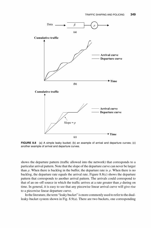
TRAFFIC SHAPING AND POLICING 349
β ρData
Time
Cumulative traffic
Arrival curve
Departure curve
(a)
(b)
Time
Cumulative traffic
Arrival curve
Departure curve
Slope = p
(c)
FIGURE 8.8 (a) A simple leaky bucket; (b) an example of arrival and departure curves; (c)another example of arrival and departure curves.
shows the departure pattern (traffic allowed into the network) that corresponds to aparticular arrival pattern. Note that the slope of the departure curve can never be largerthan ρ. When there is backlog in the buffer, the departure rate is ρ. When there is nobacklog, the departure rate equals the arrival rate. Figure 8.8(c) shows the departurepattern that corresponds to another arrival pattern. The arrivals could correspond tothat of an on–off source in which the traffic arrives at a rate greater than ρ during ontime. In general, it is easy to see that any piecewise linear arrival curve will give riseto a piecewise linear departure curve.
In the literature, the term “leaky bucket” is more commonly used to refer to the dual-leaky-bucket system shown in Fig. 8.9(a). There are two buckets, one corresponding
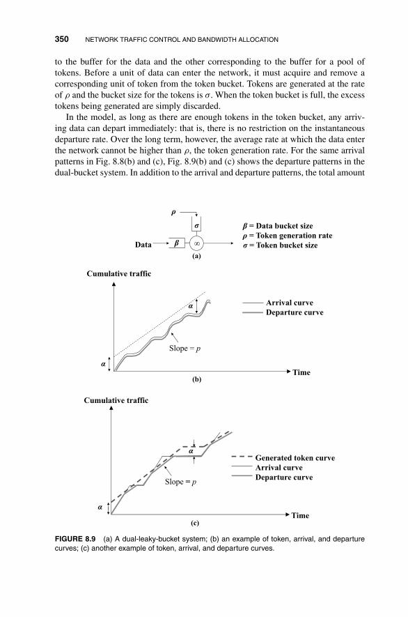
350 NETWORK TRAFFIC CONTROL AND BANDWIDTH ALLOCATION
to the buffer for the data and the other corresponding to the buffer for a pool oftokens. Before a unit of data can enter the network, it must acquire and remove acorresponding unit of token from the token bucket. Tokens are generated at the rateof ρ and the bucket size for the tokens is σ. When the token bucket is full, the excesstokens being generated are simply discarded.
In the model, as long as there are enough tokens in the token bucket, any arriv-ing data can depart immediately: that is, there is no restriction on the instantaneousdeparture rate. Over the long term, however, the average rate at which the data enterthe network cannot be higher than ρ, the token generation rate. For the same arrivalpatterns in Fig. 8.8(b) and (c), Fig. 8.9(b) and (c) shows the departure patterns in thedual-bucket system. In addition to the arrival and departure patterns, the total amount
σ
∞βData
ρ
β = Data bucket size
ρ = Token generation rate
σ = Token bucket size
Time
Cumulative traffic
Arrival curve
Departure curve
Slope = p
α
α
(a)
(b)
Time
Cumulative traffic
Slope = p
Generated token curve
Arrival curve
Departure curve
α
α
(c)
FIGURE 8.9 (a) A dual-leaky-bucket system; (b) an example of token, arrival, and departurecurves; (c) another example of token, arrival, and departure curves.

TRAFFIC SHAPING AND POLICING 351
of tokens that have been generated is also shown, assuming initially the token bucketis full.
Note that the data that arrive when the token bucket is nonempty can depart im-mediately. Comparing Figs. 8.8(b) and 8.9(b), we see that in Fig. 8.9(b), all arrivalsdepart immediately because the token bucket is never empty. Also note that it is notpossible for both the token bucket and the data bucket to be nonempty at the sametime: the data backlog would have used the tokens to depart the system. Becauseof this, with the fluid-flow model, the departure curve tracks either the token curve(when the data bucket is nonempty) or the arrival curve (when the token bucket isnonempty). Problem 8.6 makes use of this fact to perform a stochastic analysis of thesystem.
Compared with the simple leaky bucket, the dual leaky bucket allows a certaindegree of burstiness in the traffic that enters the network. In the simple leaky-bucketsystem, the maximum amount of data allowed into the network in a duration of T
is ρT . Assuming a full token bucket initially, the dual-bucket system can allow amaximum amount of data equal to ρT + σ. For small T , we see that the data canenter the network as a large burst. But over a long period (i.e., ρT � σ), the datadeparture rate averages out to be approximately ρ in the worst case.
In actual implementation, the tokens and token bucket need not be implementedas actual physical entities. We only need a counter to keep track of the amount oftokens in the token bucket. For discrete cell traffic (as opposed to the fluid-flowtraffic), each time a cell departs, the counter is decremented, and each time a token isgenerated (assuming the tokens are also generated in a discrete manner), the counteris incremented.
Figure 8.10(a) shows a more sophisticated three-bucket system. In addition to thetwo buckets in the dual-bucket system, an additional data bucket is added to the outputof the dual-bucket system. This additional bucket has a bucket size of σ and a servicerate of C. There are two reasons for this model. The first is that it models the physicalsituation more realistically. For instance, the link between the UNI and the networkmay have only a finite capacity C rather than ∞, which is assumed in the dual-bucketsystem. The second applies to the situation where the physical link has capacity morethan C: the additional constraint is introduced so as to reduce the burstiness of trafficentering the network. The maximum amount of traffic that can enter the network inthis system in a period of time T is min(ρT + σ, CT ).
Note that it does not make sense in the three-bucket system to have a ρ > C.Otherwise, the traffic entering the third bucket may saturate the buffer when thearrivals are bursty, resulting in lost data; meanwhile, the traffic cannot depart ata rate higher than C anyway: that is, increasing ρ beyond C does not relax theburstiness constraint on the data entering the network. If ρ = C, then the systemis equivalent to a simple leaky-bucket system (see Problem 8.8). Thus, only whenC > ρ does it make sense to have a three-leaky-bucket system. When C > ρ, giventhat the token bucket size is σ, the backlog in the third bucket can never be morethan σ (why?), and therefore as shown in the figure, the size of the third bucketis also σ. Figure 8.10(b) and (c) shows the departure curves for the same arrivalpatterns as discussed before. In general, with C > ρ, the departure curve of the
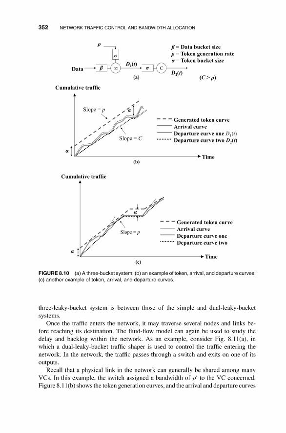
352 NETWORK TRAFFIC CONTROL AND BANDWIDTH ALLOCATION
Time
Cumulative traffic
Slope = C
α
αSlope = p
Generated token curve
Arrival curve
Departure curve one D1(t) Departure curve two D2(t)
ρ
σ
∞βData
β = Data bucket size
ρ = Token generation rate
σ = Token bucket sizeD1(t) σ CD2(t)
(C > ρ)(a)
(b)
Generated token curve
Arrival curve
Departure curve one
Departure curve two
Time
Cumulative traffic
Slope = p
α
α
(c)
FIGURE 8.10 (a) A three-bucket system; (b) an example of token, arrival, and departure curves;(c) another example of token, arrival, and departure curves.
three-leaky-bucket system is between those of the simple and dual-leaky-bucketsystems.
Once the traffic enters the network, it may traverse several nodes and links be-fore reaching its destination. The fluid-flow model can again be used to study thedelay and backlog within the network. As an example, consider Fig. 8.11(a), inwhich a dual-leaky-bucket traffic shaper is used to control the traffic entering thenetwork. In the network, the traffic passes through a switch and exits on one of itsoutputs.
Recall that a physical link in the network can generally be shared among manyVCs. In this example, the switch assigned a bandwidth of ρ′ to the VC concerned.Figure 8.11(b) shows the token generation curves, and the arrival and departure curves

TRAFFIC SHAPING AND POLICING 353
Switch
Leaky bucket type 2 (σ , ρ)
D1Infinite
bandwidth
Leaky bucket type 1 (ρ′ )UNI
A1 D2
ρ′ < ρ
Time
Cumulative traffic
α
α
Generated token curve
Arrival curve
D1
A 1
D2
slope = p
Fixed
delay = d
(a)
(b)
time
Cumulative traffic
Slope = p′α
Worst case D1
Worst case A1
D2
Fixed
delay = d
D2 when p′ < p
D2 when p′ > p
(c)
FIGURE 8.11 (a) A cascade curve of a dual leaky bucket and a simple leaky bucket; (b) anexample of cumulative curves; (c) worst-case arrival curve and its associated departure curves.
at various locations. Note that the traffic leaving the leaky bucket will suffer a fixedamount of propagation delay from the output of the leaky bucket to the switch andthen a fixed amount of processing delay in the switch before arriving at the targetedswitch output (we assume that the switch is an output-buffered switch so that the onlyqueueing point, where delay can be variable, is at the switch output).
With an amount of bandwidth ρ′ assigned to it, it is as if there is a simple leakybucket at the switch output controlling the traffic of the source that leaves the switch.So, we can again use the fluid-flow diagram to study the delay at the output. First,suppose that ρ′ > ρ. A question is what is the worst-case delay. The corresponding

354 NETWORK TRAFFIC CONTROL AND BANDWIDTH ALLOCATION
fluid-flow diagram is depicted in Fig. 8.11(c). We shall not provide a rigorous prooffor the following results, as they are pretty obvious intuitively.
The worst-case delay is incurred whenever the source pumps in as much traffic asis allowed by the dual leaky bucket, and this corresponds to the linear curve shownin the diagram. Note that at time 0, the traffic entering the network is an impulseof σ, and since we assume the link between the source and the switch has infi-nite bandwidth, this impulse arrives at the switch output after a fixed delay d. Themore realistic situation in which the link has a limited capacity C is explored inProblem 8.9.
As shown in Fig. 8.11(c), since ρ′ > ρ, the maximum backlog occurs at time d,where d is the fixed delay between the output of the dual leaky bucket and the outputof the switch. The maximum delay is suffered by the first bit of the data that entersthe switch output, and this is σ/ρ′. Also illustrated in Fig. 8.11(c) is the fact that thedelay and backlog will be unfounded if ρ′ < ρ, since the slope of the departure curvewill then be smaller than the slope of the arrival curve.
The above discussion concerns static assignment of bandwidth ρ′ to the VC con-cerned. More generally, to use the output capacity more efficiently, ρ′ could be afunction varying with time t. For instance, when there is little traffic arriving fromthe other VCs sharing the same output link, we could increase ρ′(t) if there is a lot oftraffic from the VC concerned. This is related to the flow control issues that will bediscussed in the next Section.
8.4 OPEN-LOOP FLOW CONTROL AND SCHEDULING
Open-loop control, or feedforward flow control, deals with the issue of regulating theflow of the traffic of a session through the network without feedback. The issues inopen-loop flow control are listed as follows:
1. Service guarantee: During call setup, a session may have been guaranteed acertain amount of end-to-end transport capacity. An issue is how to ensure eachsession receives its proper amount of transmission capacity as its packets passfrom node to node. For instance, a greedy session that pumps a lot of data intothe network should not jeopardize the service of other sessions.
2. Efficient use of link capacity: Another issue is how to make use of the linkcapacity in an efficient manner. Ideally, if there are packets waiting to use thelink, a packet should be transmitted. Also, it could turn out that the sum total ofthe guaranteed capacities to all the sessions passing through the link is less thanthe link transmission capacity. This extra capacity, if not used, will be wasted.An issue is how to allocate the extra capacity to the sessions in a fair mannerso that their packets can be delivered as soon as possible.
The two issues above are addressed by how multiplexing is performed at the outputlinks of a node. Multiplexing has been discussed very briefly in Sections 8.1 and 8.2.

OPEN-LOOP FLOW CONTROL AND SCHEDULING 355
The discussion in Section 8.2, in particular, dwelled on the multiplexing of homoge-neous fluid-flow on–off sources. The focus was on the overall performance rather thanon the performance of individual data streams. That is, not much has been said aboutthe allocation of transmission capacity to a particular session. The performance asperceived by individual sessions was not discussed, although some simple exampleswere given in Section 8.1 to familiarize the reader with the use of the fluid-flow modelas an intuitive tool to aid understanding.
This section is devoted to a more detailed study of the multiplexing issue. Inparticular, we shall investigate how to schedule the transmission of input traffic on theoutput channel of a multiplexer in order to guarantee the performance of individualsessions. As shown in Fig. 8.12, the situation at a particular output of an output-buffered switch is the same as that in the multiplexer. Scheduling is a form of open-loop flow control on individual sessions. At the multiplexer, the backlog consists ofdata from different sources. It is up to the multiplexer to schedule the order in whichdata will be transmitted.
8.4.1 First-Come-First-Serve Scheduling
The simplest scheduling scheme is perhaps the first-come-first-serve (FCFS) scheme.With FCFS scheduling, the data from different sessions are put into a common bufferand transmitted in a first-come-first-serve manner. This scheduling scheme is “fair”to the extent that the sources are homogeneous and there are no misbehaving sources.However, it cannot guarantee the performance of individual sessions in case there aresome “greedy” sessions that pump an excessive amount of data into the multiplexer.A well-behaved session will then suffer a large delay because of the greedy sessions.This is illustrated in Fig. 8.17 using the fluid-flow model.
In Fig. 8.13, there are three sessions. The cumulative curves A1(t), A2(t), and A3(t)are the amount of traffic arrived from sessions 1, 2, and 3, respectively. The capacityof the output channel is C. The arrival rates of both sessions 1 and 2 are C from time
Switch
VC1
VC2
VCn
C
Issues:
•Strong guarantee of QoS of
individual VC firewalls to
avoid adverse interference
among VCs
•Efficient use of capacity C
FIGURE 8.12 Multiplexing at the output of a switch.

356 NETWORK TRAFFIC CONTROL AND BANDWIDTH ALLOCATION
A1(1)
A2(1)
A3(1)
CD1(1), D2(1), D3(1)
Time
Cumulative
traffic
Slope = c
2T
A1(1) or A2(1)
Time
Cumulative
traffic
Slope = c
T
A3(1)
3T
Time
Cumulative
traffic
Slope = c
T
A1(1)+A2(1)+A3(1)
3T2T 6T
D1(1)+D2(1)+D3(1)
Slope = 2c
Slope = 3c
Slope = c
Time
Cumulative
traffic
Slope = c
T
A3(1)
3T2T 6T
slope = c
5T
Session 3’s traffic
suffers because of
the greediness of
the traffic of
sessions 1 and 2
Cannot
guarantee the
performance
of individual
sessions
FIGURE 8.13 FCFS service discipline.
0 to 2T . The arrival rate of session 3 is C from time T to 3T . Between time 0 and T ,the total amount of traffic arriving from sessions 1 and 2 is 2CT , while the amount oftraffic exiting the multiplexer is CT . This leaves a backlog of CT by the time the firstbit of session 3 arrives. Therefore, with the FCFS service discipline, session 3’s trafficmust wait for another T time unit before its first bit will go out of the multiplexer. Thisservice discipline is unfair to session 3 because it is being penalized by the arrivalsof other sessions.
An alternative is to maintain a separate queue for each session. Within the queueof a session, data are still served in a FCFS fashion. However, the data from separatequeues may not be served in the FCFS manner. An issue then is the order in which
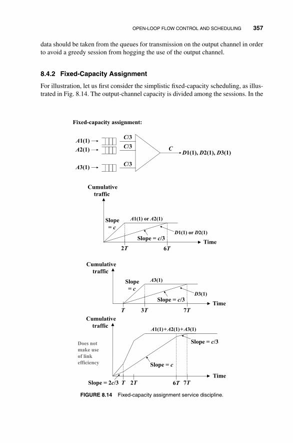
OPEN-LOOP FLOW CONTROL AND SCHEDULING 357
data should be taken from the queues for transmission on the output channel in orderto avoid a greedy session from hogging the use of the output channel.
8.4.2 Fixed-Capacity Assignment
For illustration, let us first consider the simplistic fixed-capacity scheduling, as illus-trated in Fig. 8.14. The output-channel capacity is divided among the sessions. In the
A1(1)
Fixed-capacity assignment:
A2(1)
A3(1)
CD1(1), D2(1), D3(1)
C/3
C/3
C/3
Time
Cumulative
traffic
Slope = c/3
A1(1) or A2(1)
2T 6T
Slope
= cD1(1) or D2(1)
Time
Cumulative
traffic
Slope = c/3
A3(1)
3T 7T
Slope
= cD3(1)
T
Time
Cumulative
traffic
Slope = c
T
A1(1)+A2(1)+A3(1)
2T 6T 7T
Slope = c/3
Slope = 2c/3
Does not
make use
of link
efficiency
FIGURE 8.14 Fixed-capacity assignment service discipline.

358 NETWORK TRAFFIC CONTROL AND BANDWIDTH ALLOCATION
figure, a fixed capacity of C/3 is allocated exclusively to each of the three sessions.A session’s traffic cannot make use of the capacity already assigned to another ses-sion. Conceptually, it is as if the traffic of each session enters a simple leaky bucket(i.e., the one in Fig. 8.8(a)) with a drain rate of C/3. There is no interference amongthe sessions. This is the same situation as in that of Fig. 8.11. With the same arrivalpatterns as in Fig. 8.13, we see from Fig. 8.14 that session 3’s traffic is not penalizedbecause of other sessions’ traffic.
If the capacity guaranteed to each session is less than or equal to C/3, then theabove fixed-capacity scheduling can meet the commitment. More generally, it is notnecessary that the sessions be allocated equal amount of capacities. The only constraintis that the sum total of the allocated capacities should not exceed C.
Unfortunately, the output channel cannot be used in an efficient manner with ex-clusive allocation of capacities. For example, in Fig. 8.14 the sum of the arrival ratesof sessions 1 and 2 is 2C from time 0 to T . The output rate in the same time win-dow is only 2C/3, which is below the transmission capacity C of the output channel.Meanwhile, the backlogs of sessions 1 and 2 build up. A better scheduling scheme isas follows: when there is no arrival from a particular session and there is no backlogfor that session, the capacity allocated to that session should be reallocated and usedby other sessions with backlogs. With our example, the capacity of C/3 originallyassigned to session 3 could have been redistributed to sessions 1 and 2 from time 0 toT . This will reduce the backlogs and delays of both these sessions. At time T , whenthe traffic of session 3 begins to arrive, this capacity can be returned to session 3. Inthis way, the capacity already guaranteed to session 4 can still be maintained.
There are many ways in which unused capacities of idle sessions can be redis-tributed to the active sessions. A multiplexer is said to be work conserving if the output-channel capacity is fully used (i.e., data are being transmitted at rate C) when thereis backlog (of any session) in the multiplexer. Loosely speaking, a work-conservingmultiplexer is “efficient” in the sense that it tries to use the capacity of the outputchannel whenever it is possible; the only time the output capacity is not fully used iswhen there is no backlog, and data arrive at a rate smaller than C.
FCFS scheduling is work conserving, while fixed-capacity assignment is not. TheFCFS scheduling scheme suffers from the lack of guarantees to individual sessions,while the fixed-capacity assignment scheme is not efficient because it is not workconserving. There are many scheduling schemes that can maintain the capacity guar-anteed to each session while being efficient. We shall discuss two general schemeshere.
8.4.3 Round-Robin Scheduling
We have used the fluid-flow model to simplify the discussion in the above. In practice,traffic must be transmitted at the output channel in a packet-by-packet manner. Thus,the above discussion, particularly the discussion of the fixed-capacity assignmentscheme, is only an approximation to what happens in reality. In the example of thefixed-assignment scheme, what happens in reality is that the queues of the sessions

OPEN-LOOP FLOW CONTROL AND SCHEDULING 359
FIGURE 8.15 Round-robin scheduler.
are scanned in a one-by-one fashion. One packet is taken out of each nonempty queuewhenever it is scanned. If the queue is empty, no packet is transmitted on the outputand the capacity is wasted. A more efficient scheme is to skip directly to a nonemptyqueue whenever an empty queue is encountered in order to save the time slot. This isthe idea underpinning the round-robin scheduling scheme.
The round-robin service discipline is illustrated in Fig. 8.15. The scheduler scansthe queues in a round-robin fashion: whenever it encounters a nonempty queue, itoutputs the head-of-line packet from the queue and moves on to the next queue; ifa queue is empty, it simply moves on to the next queue without wasting a time slotdoing nothing. Therefore, it is a work-conserving service discipline.
With N sessions, the worst-case service time for a head-of-line packet, TS, definedas the maximum amount of time it can spend at the head of its queue in the worst case,is N packet times, and this occurs when the queues of all N sessions are nonempty.To see this, consider a packet that moves into the head of its queue immediately afterthe transmission of the previous head-of-line packet. If all the other sessions havepackets, it will take N − 1 packet times before the scheduler visits its queue again.Another unit of time is needed to transmit the packet itself. In the round-robin scheme,TS is also the worst-case cycle time TC, which is the maximum amount of time beforethe scanning pattern repeats itself.
There is a minimum performance guarantee to each session in that each sessiongets a capacity of at least C/N, and the negative effect of a greedy session on othersessions is restrained. It is also possible to construct a more sophisticated round-robinscheduler that takes into account the varying service requirements and priorities ofdifferent sessions. For instance, a scheduler may serve more than one packet froma high-priority queue in each cycle of service when it scans through all queues.Specifically, for each queue i, we may assign a number ni (ni ≥ 1) that represents themaximum number of packets that will be served each time the scheduler serves thequeue. One shortcoming is that TS would then be larger because TC is. Specifically,
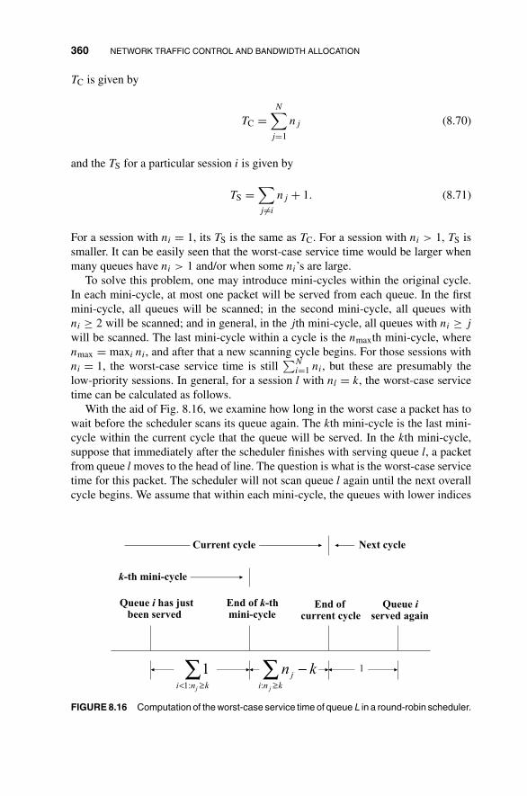
360 NETWORK TRAFFIC CONTROL AND BANDWIDTH ALLOCATION
TC is given by
TC =N∑
j=1
nj (8.70)
and the TS for a particular session i is given by
TS =∑j =i
nj + 1. (8.71)
For a session with ni = 1, its TS is the same as TC. For a session with ni > 1, TS issmaller. It can be easily seen that the worst-case service time would be larger whenmany queues have ni > 1 and/or when some ni’s are large.
To solve this problem, one may introduce mini-cycles within the original cycle.In each mini-cycle, at most one packet will be served from each queue. In the firstmini-cycle, all queues will be scanned; in the second mini-cycle, all queues withni ≥ 2 will be scanned; and in general, in the jth mini-cycle, all queues with ni ≥ j
will be scanned. The last mini-cycle within a cycle is the nmaxth mini-cycle, wherenmax = maxi ni, and after that a new scanning cycle begins. For those sessions withni = 1, the worst-case service time is still
∑Ni=1 ni, but these are presumably the
low-priority sessions. In general, for a session l with nl = k, the worst-case servicetime can be calculated as follows.
With the aid of Fig. 8.16, we examine how long in the worst case a packet has towait before the scheduler scans its queue again. The kth mini-cycle is the last mini-cycle within the current cycle that the queue will be served. In the kth mini-cycle,suppose that immediately after the scheduler finishes with serving queue l, a packetfrom queue l moves to the head of line. The question is what is the worst-case servicetime for this packet. The scheduler will not scan queue l again until the next overallcycle begins. We assume that within each mini-cycle, the queues with lower indices
Queue i has just been served
End of k-th mini-cycle
End of current cycle
Queue i served again
∑≥< ki j1:n1 ∑
≥
−ki:n
jj
kn l
k-th mini-cycle
Current cycle Next cycle
FIGURE 8.16 Computation of the worst-case service time of queue L in a round-robin scheduler.

OPEN-LOOP FLOW CONTROL AND SCHEDULING 361
are scanned before the higher one. The time till the end of the kth mini-cycle after apacket from queue l is served is
∑i>l:ni≥k 1, or the number of sessions with ni ≥ k
and i > l. The time from the end of the kth mini-cycle till the end of the current cycleis
∑i:ni>k(ni − k). Thus, the time from the end of the service of the packet from
queue l till the end of the current cycle is
∑i>l:ni≥k
1 +∑
i:ni>k
(ni − k). (8.72)
From the beginning of the next cycle until the completion of the service of the nextpacket from queue l is l (i.e., there are (l − 1) queues that will be scanned before queuel and it takes one packet time to transmit the packet of queue l). Thus, for session l,the worst-case service time is
TS =∑
i>l:ni≥k
1 +∑
i:ni>k
(ni − k) + l. (8.73)
It can be seen that the introduction of the mini-cycles reduces the worst-case servicetime (see Problem 8.10). However, the mini-cycle scheme can be further improved.For illustration, consider a session l with nl = 2, and suppose that there are manysessions with ni > 2. The worst-case service time is incurred by a packet that movesto the front of the queue l immediately after the scheduler serves the queue in thesecond mini-cycle. The packet must wait for a long time before the next cycle begins.Certainly, the worst-case service time can be reduced if instead of the second mini-cycle, we serve queue l at a later time within the overall cycle. In particular, if thescheduler can make sure that the intervals between scanning times of queue l areequally separated, then the worst-case service time can be reduced.
For simplicity, let us first examine the problem of scheduling the service of aqueue with approximately equal scanning intervals when all the sessions always havepackets to send. We will retain the concept of a repeating scanning pattern in everycycle but do away with the mini-cycles. When all sessions always have packets tosend, the cycle time is TC = ∑N
i=1 ni, and a queue l with nl = k must be servedapproximately every TC/k time slots to minimize the TS.
There are two ways in which it is not possible to schedule the service interval tobe exactly TC/k. The first is due to the discrete nature of time slots: the scanninginterval cannot be exactly TC/k if TC/k is not an integer. To approximate, we may letthe interval be �TC/k� sometimes and �TC/k� at other times. The second scenario ismore subtle and it occurs even when TC/k is an integer for all sessions. Consider anexample in which the number of sessions N = 3, and n1 = 1, n2 = 2, and n3 = 3.The cycle time is 6, and session 3 is to be served once every other time slot. It canbe easily seen that if we serve session 3 every other slots and session 1 once everysix slots, it is then not possible to serve session 2 once every three slots. In general,the scheduler must perform some computation to approximate the periodic serviceof once every TC/k slots for each session, and with a large N, the task would not besimple.
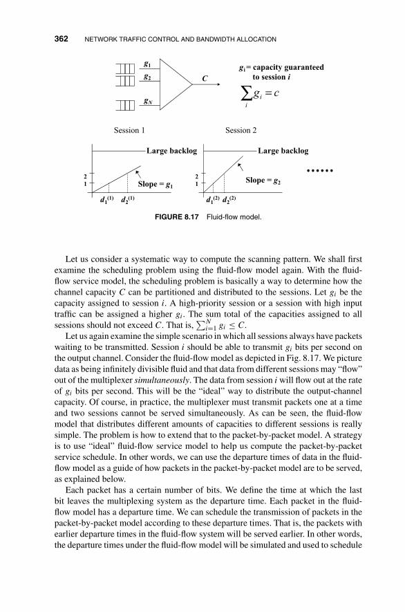
362 NETWORK TRAFFIC CONTROL AND BANDWIDTH ALLOCATION
C
g1
g2
gN
gi = capacity guaranteed
to session i
ci
=∑ ig
Session 1
Large backlog
1
2
d1(1) d2
(1)
Session 2
Slope = g2 Slope = g1
Large backlog
1
2
d1(2) d2
(2)
FIGURE 8.17 Fluid-flow model.
Let us consider a systematic way to compute the scanning pattern. We shall firstexamine the scheduling problem using the fluid-flow model again. With the fluid-flow service model, the scheduling problem is basically a way to determine how thechannel capacity C can be partitioned and distributed to the sessions. Let gi be thecapacity assigned to session i. A high-priority session or a session with high inputtraffic can be assigned a higher gi. The sum total of the capacities assigned to allsessions should not exceed C. That is,
∑Ni=1 gi ≤ C.
Let us again examine the simple scenario in which all sessions always have packetswaiting to be transmitted. Session i should be able to transmit gi bits per second onthe output channel. Consider the fluid-flow model as depicted in Fig. 8.17. We picturedata as being infinitely divisible fluid and that data from different sessions may “flow”out of the multiplexer simultaneously. The data from session i will flow out at the rateof gi bits per second. This will be the “ideal” way to distribute the output-channelcapacity. Of course, in practice, the multiplexer must transmit packets one at a timeand two sessions cannot be served simultaneously. As can be seen, the fluid-flowmodel that distributes different amounts of capacities to different sessions is reallysimple. The problem is how to extend that to the packet-by-packet model. A strategyis to use “ideal” fluid-flow service model to help us compute the packet-by-packetservice schedule. In other words, we can use the departure times of data in the fluid-flow model as a guide of how packets in the packet-by-packet model are to be served,as explained below.
Each packet has a certain number of bits. We define the time at which the lastbit leaves the multiplexing system as the departure time. Each packet in the fluid-flow model has a departure time. We can schedule the transmission of packets in thepacket-by-packet model according to these departure times. That is, the packets withearlier departure times in the fluid-flow system will be served earlier. In other words,the departure times under the fluid-flow model will be simulated and used to schedule

OPEN-LOOP FLOW CONTROL AND SCHEDULING 363
Departure time: time at which the last bit leaves,
example: g1 = 1, g2 = 2, g3 = 3
Session 1
g1 = 1
Large backlog
1
t11
Session 2
g2 = 2
1
t22t21
2
Large backlog
Session 3
g2 = 3
1
t32t31
2
Large backlog
3
t33
t31 < t21 < t32 < t33 = t22 = t11
FIGURE 8.18 Departure time: time at which the last bit leaves.
the transmission of packets in the actual system. This is illustrated in Fig. 8.18. Thereare three sessions in the examples, with g1 = 1, g2 = 2, and g3 = 3. The jth packet ofsession i is denoted by (i, j), and the departure times of the packet under the fluid-flowmodel are denoted by tij . As shown, the transmission schedule should accordingly be
(3, 1), (2, 1), (3, 2), (3, 3), (2, 2), (1, 1), . . . (8.74)
Note that t11 = t22 = t33 and we have a tie for three packets, in which case the actualordering can be determined in an arbitrary fashion. Also, the departure time of apacket in the “real” schedule is different from its departure time in the “simulated”schedule in the fluid-flow model. Let us assume gi and C are expressed in terms ofpackets per second. Then t31 = 1/3 s. However, its actual departure time in the “real”multiplexer is t = 1/6 s, ahead of t31. The departure time of a packet in the actualpacket-by-packet system is therefore different from that in the simulated fluid-flowmodel.
The above schedule determines the order of transmission in a cycle of the round-robin scheduling scheme. Corresponding to (8.74) is the order of transmission: session3, session 2, session 3, session 3, session 2, and session 1. The scanning pattern keepsrepeating itself. Note that the transmission times of session 3’s packets are sometimesseparated by zero time slots, sometimes by one time slot, and sometimes by two timeslots. This is somewhat different from the ideal of one time slot, and it is due to thearbitrary tie breaking of simultaneous departures.
Now, in practice some of the queues may not have packets to send when they arescanned. In this case, as mentioned before, the multiplexer simply looks to the nextqueue in the scanning pattern for a packet to transmit. In this way, the busy sessions

364 NETWORK TRAFFIC CONTROL AND BANDWIDTH ALLOCATION
are being served more often when some of the other sessions are idling. In fact, a busysession i receives more than its allocated share of capacity gi when there are someidle sessions.
8.4.4 Weighted Fair Queueing
The fluid-flow model is used to construct the scanning pattern in a cycle in the above.Weighted fair queueing is another work-conserving service discipline. It also usesthe departure times of packets under the fluid-flow service model to schedule theactual transmission of the packets. The concept of a repetitive scanning cycle isdropped altogether. The system chooses the packet with the smallest departure timefor transmission rather than relying on the scanning-cycle pattern to decide whom toserve next.
For explanation, we first consider the scenario in which all sessions have backlogpackets in the multiplexer. With reference to the example in Fig. 8.19, we now explainthe calculation of the departure time of a packet. Let a(i)
n be the arrival time of thenth packet from session i. The arrival time is defined to be the time by which the lastbit of the packet has arrived. Let d(i)
n be the departure time of this packet under thefluid-flow model. Suppose that the capacity gi is expressed in terms of packets persecond. Then
d(i)n = max[a(i)
n , d(i)n−1] + 1/gi. (8.75)
Note that d(i)n = a(i)
n + 1/gi if the (n − 1)th packet has already departed by the time
the nth packet has arrived, and d(i)n = d
(i)n−1 + 1/gi if the (n − 1)th packet is still in
the multiplexer by the time the nth packet has arrived.This scheme and the round-robin scheme differ when not all sessions are active and
some sessions do not have backlogs in the multiplexer. In the round-robin scheme, thescanning cycle is retained and the scheduler will simply skip over the inactive queuesto an active queue. The weighted fair queueing does not use a repetitive scanningpattern. Instead, the departure times are adjusted when some queues are inactive. Inother words, the departure times are calculated in a different manner from (8.75) whensome queues are empty. Let B(t) denote the set of busy sessions (i.e., sessions withbacklog in the fluid-flow multiplexer) at time t. In the weighted fair queueing scheme,the service rate of queue i at time t is
g′i(t) = gi × g∑
i∈B(t) gi
, (8.76)
where g = ∑Ni=1 gi. For our purpose, we may assume that g = C. If g < C, we can
introduce for conceptual purposes a dummy session that is assigned a capacity C − g
so that all the capacity C will be used.Consider the nth arriving packet from session i again. Let Th = (max[a(i)
n , d(i)n−1],
d(i)n ] be the time interval during which this nth packet is at the head of the queue.

OPEN-LOOP FLOW CONTROL AND SCHEDULING 365
Weighted fair queueing
4321
1
2
3
Time
Session 1
4321
1
2
3
Time
Session 2
arrivals
Departures
4321
1
2
3
Time5 6 7 4321
1
2
3
Time5 6 7
(a)
• dj(1) are sorted. Service performed according to the order
• d1(1), d1
(2), d2(1), d2
(2), d3(1)
4321Time
5 6
Session 1
321 4Time
5 6
Session 2
(1)d1ˆ (1)d2
ˆ (1)d3ˆ (2)d1
ˆ (2)d2ˆ
cdd (i)j
(i)j
(i)j
(i)j
1ˆ dˆUsually, d ≤−≤ ,
(b)
FIGURE 8.19 (a) Fluid-flow service: packet-by-packet arrivals; (b) packet-by-packet servicearrival.
Suppose that B(t) does not change during Th. Then
d(i)n = max[a(i)
n , d(i)n−1] + 1/g′
i(t), (8.77)
where t ∈ Th. Equation (8.77), however, is valid only when B(t) does not changeduring Th. If B(t) changes during this time (either due to the arrival of new packets
366 NETWORK TRAFFIC CONTROL AND BANDWIDTH ALLOCATION
to some empty queues or due to the emptying of some backlogged queues), g′i(t)
will change accordingly. But we know that the packet must accumulate the serviceequivalent to one packet before it can depart. The time needed to accumulate thisservice is
Th such that∫
t∈Th
g′i(t)dt = 1, (8.78)
where we have assumed that g′(t) has been normalized to have unit in packet per unittime. One way to interpret the above result is the following. At any time, the departuretime of a head-of-line packet in a queue will be calculated assuming B(t) does notchange during its stay at the head of the queue. However, if B(t) changes before itdeparts, then the departure time is recalculated, taking into account the amount ofservice that has already been accumulated so far and the amount of remaining servicethat is required before the packet can depart. The computation complexity can bequite formidable because it is possible that the departure time of a packet has to berecomputed again and again.
The computation complexity can be solved somewhat by making the observationthat the departure times in the fluid-flow system are used to order the transmissionof packets in the actual packet-by-packet system. As indicated earlier, they are notthe actual departure times of the packets in the real system. In the real system, thescheduler will simply serve the packet with the earliest departure time. It is quitepossible that while transmitting this packet (say packet A), another packet (say packetB) has arrived into the empty queue of another session and that this packet shouldhave an earlier departure time under the fluid-flow model (see Problem 8.11). In thiscase, there is a discrepancy between the departure order in fluid-flow weighted fairqueueing and that in packet-by-packet fair queueing, which corresponds to the actualsystem. But given that packet B has not arrived when the scheduler serves packetA, in order not to waste the output-channel capacity, the scheduler must go aheadand serve packet A anyway. The actual system does its best to “track” the simulatedsystem. We shall come back to examine the maximum “extra” delay suffered by apacket under the packet-by-packet model relative to the fluid-flow model.
Returning to the issue of computation complexity of the departure times of thefluid-flow model. The observation that the actual departure times of packets are notimportant and that only the order of departure times is important for scheduling theservice of packets in the real system allows us to simplify the computation somewhat.Let dA, dB, . . . be the departure times of packets A, B, . . . calculated using the methodas described previously. Without loss of generality, suppose that
dA ≤ dB ≤ · · · (8.79)
Suppose we have another way of calculating another set of departure times d′A, d′
B, . . .
for the packets such that the order is preserved:
d′A ≤ d′
B ≤ · · · (8.80)

OPEN-LOOP FLOW CONTROL AND SCHEDULING 367
As far as ordering the service of packets in the real packet-by-packet system is con-cerned, the new way of calculating the departure times is equivalent to the old waybecause the order of service remains the same. In particular, the departure times donot need to be the time as measured by a real clock. We now describe a method inwhich the departure time of a packet needs to be calculated only once. Instead ofadjusting its departure time whenever B(t) changes, we adjust the rate at which a“virtual” clock ticks.
Consider a real clock and a virtual clock. The real clock advances at a constantrate; the rate at which the virtual clock advances, however, may change with time.For the time being, let us say the advancement rate of the virtual clock changes inan arbitrary manner, except that it must be positive (i.e., the reading of the virtualclock cannot become smaller and smaller). Now, instead of labeling the departuretimes dA, dB, . . . of packets A, B, . . . with the readings of the real clock, suppose thatwe label them with the readings of the virtual clock at real times dA, dB, . . .. Let thereadings of the virtual clock be V (dA), V (dB), . . .. Certainly
V (dA) ≤ V (dB) ≤ · · · (8.81)
In other words, the readings of the virtual clock are just as good as far as orderingpackets is concerned.
We now specify the advancement rate of the virtual clock. Let V (t) be the read-ing of the virtual clock at real time t. Then, the rate at which the virtual clockadvances is
dV (t)
dt= g∑
i∈B(t) gi
(8.82)
Note that the virtual time advances faster (slower) when there are fewer (more) busysessions. This corresponds to the fact that the service rate received by a busy sessionis higher (lower) when there are fewer (more) busy sessions, and therefore, the virtualdeparture time of a packet will be reached earlier (later).
Recall that each packet needs to receive a unit of service before it can depart in theoriginal method. Let us see how much virtual time is needed before a unit of serviceis accumulated. From (8.76) and (8.78),
∫ d(i)n
max[a(i)n ,d
(i)n−1]
gi × g∑i∈B(t) gi
dt = 1. (8.83)
The above and (8.82) imply that
∫ V (d(i)n )
V (max[a(i)n ,d
(i)n−1])
gidV = 1. (8.84)

368 NETWORK TRAFFIC CONTROL AND BANDWIDTH ALLOCATION
This gives us
V (d(i)n ) = max[V (a(i)
n ), V (d(i)n−1)] + 1/gi, (8.85)
which is the formula for the virtual departure time calculation. Note that this formulais similar to (8.75), with the difference that both the arrival times and the departuretimes of packets are now virtual times with reference to a virtual clock. In particular,the service rate gi in the new method is constant.
In the original method, the service rate varies with time according to g′i(t) and time
advances at a constant rate. In the virtual-time method, the service rate is fixed but thetime advancement rate varies. The advantage of the virtual-time method is that thevirtual departure time of a packet can be immediately computed according to (8.85);this is not possible in the real-time method, because the real departure time needs tobe adjusted according to the number of busy sessions in the future. Once the virtualdeparture time of the packet is computed, it can then be sorted together with otherexisting packets and their transmission ordered; there is no need to recompute thedeparture time of a packet again and again.
We have thus reduced the problem to that of constructing or simulating a virtualclock with the advancement rate given by (8.82). Since the advancement rate dependson B(t), the set of busy sessions must be tracked. A subtlety is that B(t) is still afunction of the real time, and therefore, we still need to know when B changes in realtime, (as opposed to in virtual time). The overall updating of the virtual time and thecomputation are given as follows.
Define the busy period of the system as the time during which there is backlog inthe fluid-flow multiplexer. Whenever the system is idle with no packets in any queue,both the real time and virtual time are set to be zero. Therefore, the beginning of anybusy period is always time 0. We will see how virtual time is to be updated during thebusy period. Since the set B may change only when there is an arrival or when thereis a departure, we only need to update the virtual times at this instance. An arrivalinstant is always known since it is marked by an input packet to the system. (Note:Arrival instants in the simulated fluid-flow model are the same as those in the actualpacket-by-packet system and therefore the arrival instants in the actual system can beused for updating purposes in the simulated model.)
When the nth packet of session i arrives at real time a(i)n , the following computation
is performed.
Computation of Virtual Departure Time
1. The virtual time is updated:
V (a(i)n ) = dV
dt× (a(i)
n − tlast) + V (tlast), (8.86)
where tlast is the last time (real time) when the virtual time was updated anddV/dt was the effective virtual clock advancement rate between tlast and a(i)
n .

OPEN-LOOP FLOW CONTROL AND SCHEDULING 369
2. The parameter tlast is updated:
tlast = a(i)n . (8.87)
3. Equation (8.85) is used to compute the virtual departure time of the packet. Thevirtual departure time is used to schedule the transmission of the packet andwill be stored.
4. If the queue of session i is empty when the packet arrives, then B will changeafter the arrival. In this case, update B and the virtual clock advancement rateaccording to (8.82).
The update of the virtual clock advancement rate due to a departure is more prob-lematic compared to that due to an arrival. Unlike the arrival instant, the departureinstant of a packet in the simulated fluid-flow model may not be the same as the actualdeparture instant of the packet in the actual packet-by-packet system, and therefore,we cannot use the actual departure time as the time to perform the update. In otherwords, the departure time under the fluid-flow model must be used for the purposeof updating. However, the stored virtual departure time of the packet does not tell uswhen to update the virtual clock advancement rate; it is only used to order packetsfor transmission purposes; the real time must be used. This means that, at any time,we must know the real time at which the next departure will occur in the fluid-flowmodel in order that we can adjust B should it change at this instant. Let tnext be thereal time at which the next packet will depart if there are no more packet arrivals fromnow to tnext. The value of tnext can be computed from the virtual time V (tnext) of thepacket scheduled to depart next, by the following relationship:
V (tnext) = V (tlast) + (tnext − tlast)dV
dt. (8.88)
Or equivalently,
tnext = tlast + [V (tnext) − V (tlast)]
dV/dt. (8.89)
If indeed that there is no arrival between tlast and tnext, then at tnext the following willbe performed.
Update of Virtual Clock Rate Due to Departures
1. Check and see if the departure of the packet at tnext will leave its associatedqueue empty. If so, B will change after the departure, and so update B and thevirtual clock advancement rate according to (8.82).
2. Update the virtual time: V (tlast) = V (tnext).
3. Update the last update time for the virtual time: tlast = tnext.
370 NETWORK TRAFFIC CONTROL AND BANDWIDTH ALLOCATION
4. If the system still has backlog packets after the departure of the above packet,compute the real departure time tnext of the next packet according to (8.89).
If there is an arrival between tlast and tnext, there are two possibilities that must betaken into account: (1) this new packet may have a smaller virtual departure time thanthe packet originally scheduled to depart next, especially if the service rate assignedto the session of the new packet is high; (2) the value of B may change (hence dV/dt)due to this arrival. In either case, after computing the virtual departure time of thisnew packet according to the procedure “Computation of Virtual Departure Time,”recompute tnext with virtual departure time of the packet scheduled to depart next(whether it is the original or the new packet) according to (8.89).
To summarize, we have described in the above a way of computing the virtualdeparture times of packets for the purpose of ordering the packets for transmission.The method obviates the need to recompute the departure times of a packet againand again. Implementation-wise, with the virtual departure times, arriving packetsfrom all sessions can be inserted into a common queue according to the values oftheir departure times. Of course, simultaneous arrivals and simultaneous departuresare still possible in the fluid-flow model. For simultaneous departures, arbitrary tiebreaking can be performed to schedule the packet to transmit next in the actual packet-by-packet system.
There is another subtlety. As described above, in the fluid-flow model, a new arrivalmay have a departure time earlier than all those packets already in the system. In thiscase, the new packet will still depart earlier than the previous head-of-line packet inthe fluid-flow model. In the packet-by-packet model, however, the previous head-of-line packet is already under service when the new packet arrives and the new packetmust wait until the previous packet has been totally transmitted before it can depart.This means that it is possible for the departure time of a packet in the packet-by-packetsystem to be later than its departure time in the fluid-flow system. Nevertheless, weshall see in the following that the worst-case increase in departure time is still quiteminimal when packet lengths are small.
Consider an arbitrary packet k. Let its departure time (real) in the fluid-flow systembe dk and its departure time in the packet-by-packet system be d̂k. It can be shownthat
d̂k − dk ≤ 1
g. (8.90)
In other words, the departure time “penalty” for the packet-by-packet system is atmost 1/g. Before explaining the result, let us consider an example shown in Fig. 8.20.There are two sessions, and g1 = g2 = 0.5. The system is not busy until the arrivalof a packet from session 1 at time a
(1)1 = 0. Another packet arrives from session 2
almost immediately after that at time a(2)1 = ε, where ε is an arbitrarily small positive
number. In the fluid-flow system, the departure times of both the first and secondpackets are approximately 2. In the packet-by-packet model, however, the departuretime of the first packet is 1 and the departure time of the second packet is 2. It can be
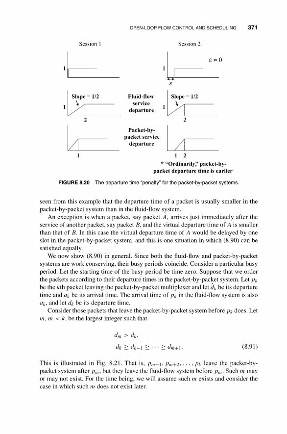
OPEN-LOOP FLOW CONTROL AND SCHEDULING 371
1
Session 1 Session 2
1
ε
ε ≈ 0
1
2
Slope = 1/2
1
2
Slope = 1/2Fluid-flow
service
departure
1
Packet-by-
packet service
departure
21
* “Ordinarily”, packet-by-
packet departure time is earlier
FIGURE 8.20 The departure time “penalty” for the packet-by-packet systems.
seen from this example that the departure time of a packet is usually smaller in thepacket-by-packet system than in the fluid-flow system.
An exception is when a packet, say packet A, arrives just immediately after theservice of another packet, say packet B, and the virtual departure time of A is smallerthan that of B. In this case the virtual departure time of A would be delayed by oneslot in the packet-by-packet system, and this is one situation in which (8.90) can besatisfied equally.
We now show (8.90) in general. Since both the fluid-flow and packet-by-packetsystems are work conserving, their busy periods coincide. Consider a particular busyperiod. Let the starting time of the busy period be time zero. Suppose that we orderthe packets according to their departure times in the packet-by-packet system. Let pk
be the kth packet leaving the packet-by-packet multiplexer and let d̂k be its departuretime and ak be its arrival time. The arrival time of pk in the fluid-flow system is alsoak, and let dk be its departure time.
Consider those packets that leave the packet-by-packet system before pk does. Letm, m < k, be the largest integer such that
dm > dk,
dk ≥ dk−1 ≥ · · · ≥ dm+1. (8.91)
This is illustrated in Fig. 8.21. That is, pm+1, pm+2, . . . , pk leave the packet-by-packet system after pm, but they leave the fluid-flow system before pm. Such m mayor may not exist. For the time being, we will assume such m exists and consider thecase in which such m does not exist later.

372 NETWORK TRAFFIC CONTROL AND BANDWIDTH ALLOCATION
11 ... +− ≥≥≥>
mkk
km
ddddd
Departure times in packet-
by-packet system
Departure times in
fluid-flow system
md̂ 1ˆ
+md 1ˆ
−kd kd̂
1/g 1/g
1ˆ
+md 2ˆ
+md 1ˆ
−kd kd̂
mp 1+mp 1−kp kp
md̂
Assume such m exists first, when is this possible?
Assigned service rate of pm is very small. However, when the service
starts in the packet-by-packet model, pm, pm, …, pm have not arrived
FIGURE 8.21 Departure times in (a) fluid-flow systems, (b) packet-by-packet systems.
In the packet-by-packet system, pm starts getting served at time d̂m − 1/g. Now,the arrival times of pm+1, pm+2, . . . , pk must be after d̂m − 1/g; otherwise, by (8.91),they would have been served in the packet-by-packet system before pm, which con-tradicts our assumption.
Let us now look at the fluid-flow system. Packets pm+1, pm+2, . . . , pk also arriveat the same time. In particular, these (k − m) packets must also arrive during the timeinterval (d̂m − 1/g, dk). Since they also depart during this time interval, we musthave
{dk −
(d̂m − 1
g
)}× g ≥ k − m. (8.92)
The left-hand side is the amount of service performed during this interval, and theright-hand side is the minimum amount of service needed so that these (k − m) packetscan arrive and leave the system within this time interval.
Let us now examine the packet-by-packet system. With reference to Fig. 8.22, wemust have
(d̂k − d̂m) = (k − m)
g, (8.93)
since the interdeparture times of successive leaving packets are always 1/g. From(8.92) and (8.93), we get the result we want: (8.90).
Now, suppose that pm does not exist such that (8.91) is satisfied. Then, none ofp1, . . . , pk−1 leaves the fluid-flow system after pk does. In the fluid-flow system, the

OPEN-LOOP FLOW CONTROL AND SCHEDULING 373
amount of work performed in the interval (0, dk] is
dkg ≥ k, (8.94)
since by time dk (including time dk), k packets would have left the fluid-flow system.In the packet-by-packet system, the number of packets that have left the system bytime d̂k is also k, and we have
d̂k = k
g. (8.95)
From (8.94) and (8.95), we therefore have
d̂k ≤ dk. (8.96)
8.4.5 Delay Bound in Weighted Fair Queueing with Leaky-BucketAccess Control
In the subsequent discussion, we shall see how the packet delay in the weightedfair queueing system can be bounded if the arrivals from sessions are regulated byleaky buckets. These delay bounds are necessary for us to provide deterministic delayguarantees for each data session in the system.
A leaky-bucket scheme is shown in Fig. 8.9(a). Tokens here are generated at afixed rate, ρ, and packets can be released into the network only after removing therequired number of tokens from the token bucket that contains at most σ bits worth oftokens. There is no bound on the number of packets that can be buffered. The trafficis constrained to leave the bucket at a maximum rate of C > ρ.
Let Ai(τ, t) denote the amount of traffic from session i that leaves the leaky bucketand enters the network in time interval (τ, t]. Then,
Ai(τ, t) ≤ min{(t − τ)Ci, σi + ρi(t − τ)}, for all t ≥ τ ≥ 0, (8.97)
for every session i.We say that the arrival function Ai conforms to (σi, ρi, Ci), or A ∼ (σi, ρi, Ci).
This arrival constraint is attractive because it restricts the traffic in terms ofthree simple parameters: average sustainable rate (ρi), burstiness (σi), and peakrate (Ci).
Ai(0, t) is plotted in Fig. 8.22. Let li(t) be the amount of tokens in the sessioni token bucket at time t. Assuming that the session starts out with a full bucket oftokens, if Li(t) is the total number of tokens accepted at the session i bucket in theinterval (0, t] (it does not include the full bucket of tokens that session i starts outwith, and does not include arriving tokens that find the bucket full), then
Li(t) = min0≤τ≤t
{Ai(0, τ) + ρi(t − τ)}. (8.98)
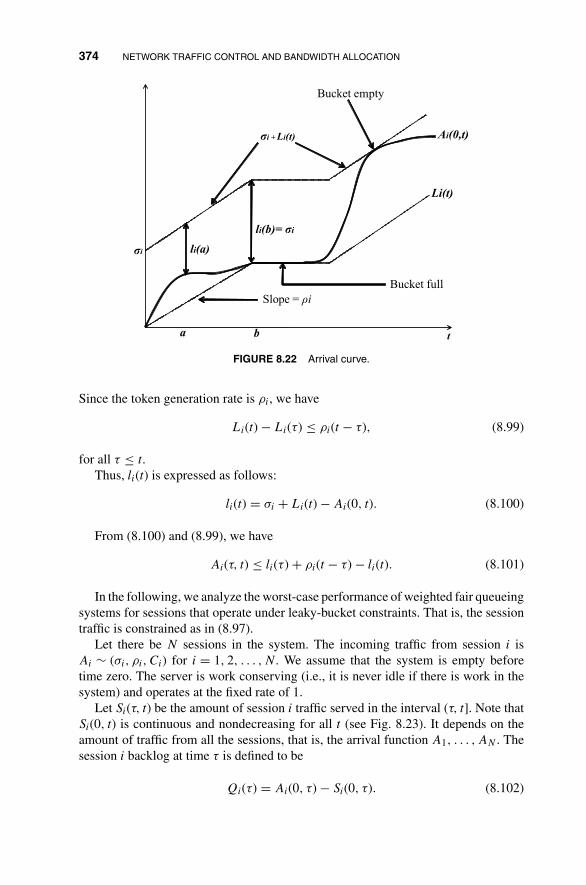
374 NETWORK TRAFFIC CONTROL AND BANDWIDTH ALLOCATION
Bucket empty
σ + i Li(t)
σi
li(b)= σi
li(a)
Li(t)
Slope = ρiBucket full
Ai(0,t)
a b t
FIGURE 8.22 Arrival curve.
Since the token generation rate is ρi, we have
Li(t) − Li(τ) ≤ ρi(t − τ), (8.99)
for all τ ≤ t.Thus, li(t) is expressed as follows:
li(t) = σi + Li(t) − Ai(0, t). (8.100)
From (8.100) and (8.99), we have
Ai(τ, t) ≤ li(τ) + ρi(t − τ) − li(t). (8.101)
In the following, we analyze the worst-case performance of weighted fair queueingsystems for sessions that operate under leaky-bucket constraints. That is, the sessiontraffic is constrained as in (8.97).
Let there be N sessions in the system. The incoming traffic from session i isAi ∼ (σi, ρi, Ci) for i = 1, 2, . . . , N. We assume that the system is empty beforetime zero. The server is work conserving (i.e., it is never idle if there is work in thesystem) and operates at the fixed rate of 1.
Let Si(τ, t) be the amount of session i traffic served in the interval (τ, t]. Note thatSi(0, t) is continuous and nondecreasing for all t (see Fig. 8.23). It depends on theamount of traffic from all the sessions, that is, the arrival function A1, . . . , AN . Thesession i backlog at time τ is defined to be
Qi(τ) = Ai(0, τ) − Si(0, τ). (8.102)
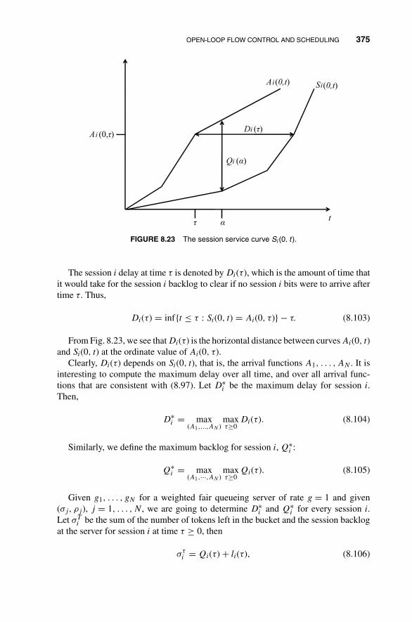
OPEN-LOOP FLOW CONTROL AND SCHEDULING 375
Ai (0,τ)
Ai(0,t) (0,t)Si
Di (τ)
Qi (α)
ατ t
FIGURE 8.23 The session service curve Si (0, t ).
The session i delay at time τ is denoted by Di(τ), which is the amount of time thatit would take for the session i backlog to clear if no session i bits were to arrive aftertime τ. Thus,
Di(τ) = inf{t ≤ τ : Si(0, t) = Ai(0, τ)} − τ. (8.103)
From Fig. 8.23, we see that Di(τ) is the horizontal distance between curves Ai(0, t)and Si(0, t) at the ordinate value of Ai(0, τ).
Clearly, Di(τ) depends on Si(0, t), that is, the arrival functions A1, . . . , AN . It isinteresting to compute the maximum delay over all time, and over all arrival func-tions that are consistent with (8.97). Let D∗
i be the maximum delay for session i.Then,
D∗i = max
(A1,...,AN )maxτ≥0
Di(τ). (8.104)
Similarly, we define the maximum backlog for session i, Q∗i :
Q∗i = max
(A1,···,AN )maxτ≥0
Qi(τ). (8.105)
Given g1, . . . , gN for a weighted fair queueing server of rate g = 1 and given(σj, ρj), j = 1, . . . , N, we are going to determine D∗
i and Q∗i for every session i.
Let σTi be the sum of the number of tokens left in the bucket and the session backlog
at the server for session i at time τ ≥ 0, then
στi = Qi(τ) + li(τ), (8.106)
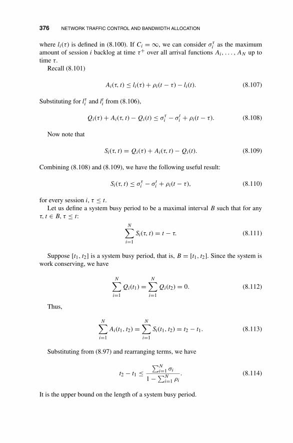
376 NETWORK TRAFFIC CONTROL AND BANDWIDTH ALLOCATION
where li(τ) is defined in (8.100). If Ci = ∞, we can consider στi as the maximum
amount of session i backlog at time τ+ over all arrival functions Ai, . . . , AN up totime τ.
Recall (8.101)
Ai(τ, t) ≤ li(τ) + ρi(t − τ) − li(t). (8.107)
Substituting for lτi and lti from (8.106),
Qi(τ) + Ai(τ, t) − Qi(t) ≤ στi − σt
i + ρi(t − τ). (8.108)
Now note that
Si(τ, t) = Qi(τ) + Ai(τ, t) − Qi(t). (8.109)
Combining (8.108) and (8.109), we have the following useful result:
Si(τ, t) ≤ στi − σt
i + ρi(t − τ), (8.110)
for every session i, τ ≤ t.Let us define a system busy period to be a maximal interval B such that for any
τ, t ∈ B, τ ≤ t:N∑
i=1
Si(τ, t) = t − τ. (8.111)
Suppose [t1, t2] is a system busy period, that is, B = [t1, t2]. Since the system iswork conserving, we have
N∑i=1
Qi(t1) =N∑
i=1
Qi(t2) = 0. (8.112)
Thus,
N∑i=1
Ai(t1, t2) =N∑
i=1
Si(t1, t2) = t2 − t1. (8.113)
Substituting from (8.97) and rearranging terms, we have
t2 − t1 ≤∑N
i=1 σi
1 − ∑Ni=1 ρi
. (8.114)
It is the upper bound on the length of a system busy period.
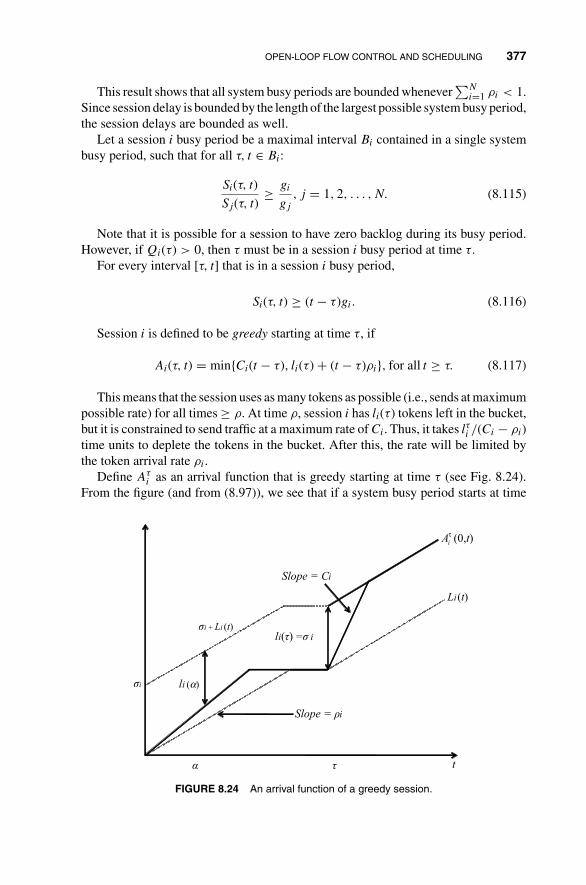
OPEN-LOOP FLOW CONTROL AND SCHEDULING 377
This result shows that all system busy periods are bounded whenever∑N
i=1 ρi < 1.Since session delay is bounded by the length of the largest possible system busy period,the session delays are bounded as well.
Let a session i busy period be a maximal interval Bi contained in a single systembusy period, such that for all τ, t ∈ Bi:
Si(τ, t)
Sj(τ, t)≥ gi
gj
, j = 1, 2, . . . , N. (8.115)
Note that it is possible for a session to have zero backlog during its busy period.However, if Qi(τ) > 0, then τ must be in a session i busy period at time τ.
For every interval [τ, t] that is in a session i busy period,
Si(τ, t) ≥ (t − τ)gi. (8.116)
Session i is defined to be greedy starting at time τ, if
Ai(τ, t) = min{Ci(t − τ), li(τ) + (t − τ)ρi}, for all t ≥ τ. (8.117)
This means that the session uses as many tokens as possible (i.e., sends at maximumpossible rate) for all times ≥ ρ. At time ρ, session i has li(τ) tokens left in the bucket,but it is constrained to send traffic at a maximum rate of Ci. Thus, it takes lτi /(Ci − ρi)time units to deplete the tokens in the bucket. After this, the rate will be limited bythe token arrival rate ρi.
Define Aτi as an arrival function that is greedy starting at time τ (see Fig. 8.24).
From the figure (and from (8.97)), we see that if a system busy period starts at time
Slope = Ci
Slope = ρi
li (α)
li(τ) =σ iσ + i Li (t)
σi
Li(t)
τα t
(0,t)Aiτ
FIGURE 8.24 An arrival function of a greedy session.

378 NETWORK TRAFFIC CONTROL AND BANDWIDTH ALLOCATION
zero, then
A0i (0, t) ≥ A(0, t), for all A ∼ (σi, ρi, Ci), t ≥ 0. (8.118)
Suppose that Cj ≥ g for every session j, where g is the rate of a server. Then,for every session i, D∗
i and Q∗i are achieved (not necessarily at the same time)
when every session is greedy starting at time zero, the beginning of a system busyperiod.
This means that the all-greedy regime can maximize the delay as well as thebacklog for every session in the weighted fair queueing system. In actuality, it seemsreasonable that if a session sends as much traffic as possible at all times, it is going toimpede the progress of packets arriving from the other sessions. This gives a simplescenario for investigating the worst-case behavior. To prove this result, the easiestway is to show it is true for the case when Ci = ∞ for all i first and then based on thisanalysis to yield the results for the cases with finite link capacities. Since the proofis very complicated and cannot provide any insight to the readers, we do not includeit here.
Define e1 as the first time at which one of the sessions, say L(1), ends its busyperiod in an all-greedy system. That is, in the interval [0, e1], each session i is in abusy period and is served at rate gi/
∑Nk=1 gk, assuming that σ − i > 0 for all i. Since
session L(1) is greedy after 0, it follows that
ρL(1) <gi∑Nk=1gk
, (8.119)
where i = L(1). Now each session j still in a busy period will be served at rate
(1 − ρL(1))gj∑Nk=1 gk − gL(1)
(8.120)
until a time e2 when another session, say L(2), ends its busy period.Similarly, for each k, we have
ρL(k) <(1 − ρL(j))gi∑N
j=1 gj − ∑k−1j=1 gL(j)
, k = 1, 2, . . . , N, i = L(k). (8.121)
As shown in Fig. 8.25, the slopes of the various segments that comprise Si(0, t)are si1, s
i2, . . .. From (8.121), we get
sik =(
1 − ∑k−1j=1 ρL(j)
)gi∑N
j=1 gj − ∑k−1j=1 gL(j)
, k = 1, 2, . . . , L(i). (8.122)
It can be seen that sik, k = 1, 2, . . . , L(i), forms an increasing sequence. Anyordering of sessions that meets (8.121) is known as a feasible ordering.

OPEN-LOOP FLOW CONTROL AND SCHEDULING 379
Ai(0,t)
σi
0 e1e e2 e3 e4 e5t
Si(0,t)
Traffic
iS1
iS2
iS3
iS4
iS5
FIGURE 8.25 The departure curve of session i .
Note that we only require that 0 ≤ e1 ≤ e2 ≤ · · · ≤ eN , allowing for several ei tobe equal. Session L(i) in this case has exactly one busy period, the interval [0, ei].Also, we are only interested in t ≤ eL(i), since the session i buffer is always emptyafter this time.
In the following, we shall determine bounds for the maximum delay D∗i and the
maximum backlog Q∗i . Suppose Q∗
i is achieved at time t, and let τ be the first timebefore t when there are no session i bits backlogged in the server. Then by (8.116),we have
Q∗i ≤ (σi + ρi(t − τ)) − gi(t − τ)
≤ (σi + ρi(t − τ)) − gi(t − τ)
= σi. (8.123)
An arriving session i bit will be after at most Q∗i session i bits have been served.
Since these backlogged bits are served at a rate of at least gi,
D∗i ≤ Q∗
i
gi
≤ σi
gi
. (8.124)
However, the bounds obtained above are quite loose since the assumption is thatthe session i is served with a constant rate gi till its backlog is cleared. In reality, theservice rates of backlogged sessions increase as more and more sessions completetheir backlogged periods, where a backlogged period for session i is any periodof time during which packets belonging to that session are continuously queued inthe system. This is because as each session completes its backlog, the bandwidth

380 NETWORK TRAFFIC CONTROL AND BANDWIDTH ALLOCATION
released is distributed among the still backlogged sessions in proportion to theirweights.
8.5 CLOSED-LOOP FLOW CONTROL
One problem with open-loop flow control is that network bandwidth may not be usedefficiently. Access control is needed to prevent a session from injecting excessiveamount of data into the network. The data rate allowed by each session is prenegotiatedupfront and it does not take into account that the available network bandwidth aswell as the desirable bandwidth by the user sessions may vary dynamically withtime.
If the “natural” data rates of all sessions are more or less constant (e.g., such asthat for digitized voice), open loop will work well because there is no need to give thesessions more bandwidth, even when there is unused bandwidth in the network. Bycontrast, if each session would like to pump in as much data as possible by makinguse of unused bandwidth in the network, open-loop control does not work well. Twoexample scenarios are as follows: (1) file transfer in which it is desirable to transfera large file to the destination as fast as possible; and (2) a VBR (variable bit-rate)coded video in which it is desirable to exploit any unused bandwidth in the networkto increase image quality.
A reasonable way to provision the network bandwidth is to divide sessions intodifferent service types. For services that do not have highly varying data rates thatrequire strong guarantee for bandwidth availability during transmission, the open-loop control can be used. In this situation, the services would not attempt to usemore than their allocated share of bandwidth and the network would not assign morebandwidth than preallocated to the services.
For services that do not require strong guarantee on bandwidth availability butthat may desire extra bandwidth in a time-varying way (e.g., file transfers that areinitiated in a sporadic fashion), we may use closed-loop control to provision band-width. This kind of service is sometimes referred to as the available bit-rate service(ABR).
For the ABR service, there must be a way to inform the sessions if extra bandwidthis available in the network and if so how much of it is available. In other words, thenetwork traffic conditions must be fed back to the sessions so that they know howmuch traffic to inject into the network. And this is the reason why closed-loop controlis needed so that excess unused bandwidth can be utilized.
For simplicity, let us begin by looking at the interactions between two successivelinks of an ABR VC. Consider Fig. 6.23 in which we show the source node connectingto a switch in the network. When the output link of the VC on the switch does notsuffer congestion, its buffer is relatively empty. The source should not be preventedfrom pumping in data to make off the unused bandwidth on the output link. Thisoutput link, however, may be shared by several ABR VCs, and when many of themstart to pump in data, it is possible that the input rate to the output link is higher thanits output rate. The buffer occupancy starts to build up, and unless something is done

PROBLEMS 381
to limit the data from the sources, the buffer may eventually overflow, resulting in dataloss. If the higher level protocol at the sources attempts to retransmit data because ofthis data loss, the congestion will tend to become even worse. Therefore, it is betterto prevent the data loss to begin with and take actions before the buffer begins tooverflow.
We can set a threshold on the buffer occupancy. When the threshold is exceeded,the sources of the ABR VCs that pass through the link will be instructed to cut downtheir rates. Two issues that must be resolved are
� What should be the value of the threshold in order to prevent data loss.� How should the source data rates be reduced when congestion occurs.
PROBLEMS
8.1 Use the fluid-flow model in this question. Suppose you want to multiplextwo on–off sources using a statistical multiplexer with output capacity C = 3.Suppose that the peak rate of one of the sources is 1 and that of the other sourceis 3.(a) For the arrival rates shown in Fig. 8.1 for the two sources, plot the amount
of total traffic that has arrived at and departed from the multiplexer.
(b) When there is backlog for one source, the whole capacity c will be dedi-cated to the transmission of its traffic. When both sources have backlogs,the multiplexer will serve source A with rate 1 and source B with rate 2.Plot the arrived and departed traffic for each source.
(c) Suppose the average “on” time for both sources is 1 and the average “off”time for both sources is λ. Both the on and off times are exponentiallydistributed. Draw a four-state Markov chain to represent the state transitionof the system. State 00 means both sources are off, state 01 means sourceA is off and source B is on, and so on. What is the expected number of onsources at any time?
(d) With the service discipline in part (b) and the arrival processes in part (c),what is the expected amount of time needed to completely clear the trafficof source B that arrives during a single on period?
8.2 Explain why G(x) derived in (8.59) in the text is an upper bound on the over-flow probability of a finite buffer of size x. Use a simple example and draw afluid-flow diagram in your explanation. (Hint: Consider two systems, one withinfinite buffer and one with finite buffer, and both systems are subjected to thesame arrival traffic pattern. Argue that at any time, the system with infinitebuffer has a higher buffer occupancy than the one with finite buffer. Arguethat if the buffer occupancy in the infinite-buffer system is more than x, thefinite-buffer system does not necessarily overflow; when the finite-buffer sys-tem overflows, however, the buffer occupancy in the infinite-buffer system isgreater than x.)

382 NETWORK TRAFFIC CONTROL AND BANDWIDTH ALLOCATION
8.3 Section 8.2 analyzes an infinite-buffer multiplexing system with on–off fluidflow sources. This problem explores the solution when the buffer size B is finite.The eigenvalues and eigenvectors are the same as before, but the coefficientsai’s must be matched to different boundary conditions.(a) Explain why the terms with positive eigenvalues cannot be ignored any-
more. Argue that
Fj(0) = 0 =N∑
i=0
ai(�i)j, �C� + 1 ≤ j ≤ N.
(b) Explain why Fj(x) at boundary x = B may have a discontinuity (i.e.,Fj(B−) = Fj(B)). For what j’s are there discontinuities?
(c) Argue that
Fj(B−) =(
N
j
)λj
(1
1 + λ
)N
=N∑
i=0
ai(�i)j, 0 ≤ j ≤ �C� − 1.
(d) Parts (a) and (b) give N + 1 equations for N + 1 unknowns ai, 0 ≤ i ≤ N,when C is not an integer. For C an integer, there are only N equations. Foran additional equation, argue that
{(N − C)λ + C}FC(0) = {N − (C − 1)}λFC−1(0),
which gives
N∑i=0
ai[{(N − C)λ + C}(�i)C − {N − (C − 1)}λ(�i)C−1] = 0.
(e) Express the overflow probability in terms Fj(B−), 0 ≤ j ≤ N, when C isnot an integer as well as when C is an integer.
8.4 Continuing from the previous problem, this problem examines the loss prob-ability in a finite-buffer system. Consider an infinitely long stretch of time T .The total amount of traffic arriving at the system is approximately rT , wherer = Nλ/(1 + λ) is the average arrival rate.(a) Argue that amount of loss traffic is approximately
N∑j>C
(Fj(B) − Fj(B−))(j − C)T.
(b) Express Fj(B) in terms of N and λ.
(c) Express the loss probability in terms of Fj(B−), λ, and N.
PROBLEMS 383
8.5 This problem derives the standard probability result in the second equality of(8.65). Express
∫ ∞0 xf (x)dx as limb→∞
∫ b
0 xf (x)dx.(a) By integration by parts, show that∫ b
0xf (x)dx =
∫ b
0F (b) − F (x)dx.
(b) Argue that
limb→∞
∫ b
0F (b) − F (x)dx =
∫ ∞
01 − F (x)dx.
8.6 Using the fluid-flow traffic model, this problem considers the stochastic analy-sis of a dual-leaky-bucket system with input traffic from an on–off source. Weshall use the same traffic model as described in Section 8.2 and assume thatthe data buffer in the dual-leaky-bucket size is infinite. A similar analysis as inSection 8.2 can be used to study the buffer occupancy in the data buffer of theleaky bucket. Let QD(t) be the buffer occupancy of the data bucket and QT(t)be the buffer occupancy of the token bucket at time t. The state of the systemis defined by three parameters: whether source is on or off, QD(t), and QT(t).(a) Argue that both QD(t) and QT(t) cannot be nonzero at the same time.
(b) Argue that because of the above, we can define a parameter Q(t) such thatQ(t) = σ + QD(t) when QD(t) = 0 and Q(t) = σ − QT(t) when QT(t) =0, and describe the state with just two parameters: whether the source ison or off, and Q(t). Argue that QD(t) and QT(t) can be derived from Q(t)if it is known.
(c) Interpret Q(t) as the buffer occupancy of a fictitious queue with a serverserving at the rate of ρ. Argue that the same analysis as in Section 8.2 canthen be used to study Q(t). (Note: It is actually simpler here since we haveonly one source.)
8.7 In the three-leaky-bucket system, argue that if the arrival rate is never morethan C, then the third leaky bucket is redundant. That is, the departure curvewould have been the same in the dual-bucket system.
8.8 In the three-leaky-bucket system, argue that if ρ = C, we can replace the systemwith a simple leaky-bucket system with bucket size β + σ as far as the departedtraffic is concerned. What is the service rate of the simple leaky bucket? (Hint:Argue that it is not possible for the third leaky bucket to be empty while thefirst leaky bucket is not empty.)
8.9 Consider the situation in Fig. 8.11 in the text. Instead of a dual-leaky-buckettraffic shaper, we have a three-leaky-bucket traffic shaper. Assuming that C >
ρ′ > ρ, draw a diagram similar to that in Fig. 8.11(c). What is the worst-casebacklog and delay suffered by the traffic at the output of the switch.
384 NETWORK TRAFFIC CONTROL AND BANDWIDTH ALLOCATION
8.10 For the round-robin scheduling scheme that serves ni packets from session i ina continuous fashion before moving on to the next queue (i.e., the one withoutmini-cycles), derive the worst-case service time for a session l with nl = k.How does this compare with the worst-case service time in the scheduler withmini-cycles?
8.11 Give an example in which the order of service in the simulated fluid-flowweighted fair queueing is different from that in the real packet-by-packetweighted fair queueing. (Hint: Consider the arrival of a packet into an emptyqueue of session i with a very high ρi.)
9
PACKET SWITCHING ANDINFORMATION TRANSMISSION
All communication networks comprise transmission systems and switching systems,even though their designs are usually treated as two separate issues. Communicationchannels are generally disturbed by noise from various sources. In circuit-switchednetworks, reliable communication requires error-tolerant transmission of bits overnoisy channels. In packet-switched networks, however, not only can bits be corruptedwith noise, but resources along connection paths are also subject to contention. Thus,quality of service (QoS) is determined by buffer delays and packet losses. The themeof this chapter is to show that transmission noise and packet contention actually havesimilar characteristics and can be tamed by comparable means to achieve reliablecommunication. The following analogies between switching and transmission areidentified:
1. Buffering against contention is a process that is similar to the error correctionof noise corrupted signals. A signal-to-noise ratio that represents the carriedload of packet switches can be deduced from the Boltzmann model of packetdistribution.
2. When deflection routing is applied to Clos networks, the loss probability de-creases exponentially, which is similar to the exponential behavior of the errorprobability of binary symmetric channels with random channel coding. In in-formation theory, this result is stated as the noisy channel coding theorem.
3. The similarity between Hall’s condition of bipartite matching and expandergraph manifests the resemblance between nonblocking route assignments anderror-correcting codes. An extension of the Sipser–Speilman decoding algo-rithm of expander codes to route assignments of Benes networks is given toillustrate their correspondence.
Principles of Broadband Switching and Networking, by Tony T. Lee and Soung C. LiewCopyright © 2010 John Wiley & Sons, Inc.
385
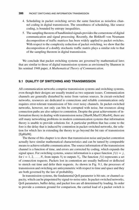
386 PACKET SWITCHING AND INFORMATION TRANSMISSION
4. Scheduling in packet switching serves the same function as noiseless chan-nel coding in digital transmission. The smoothness of scheduling, like sourcecoding, is bounded by entropy inequalities.
5. The sampling theorem of bandlimited signals provides the cornerstone of digitalcommunication and signal processing. Recently, the Birkhoff–von Neumanndecomposition of traffic matrices has been widely applied to packet switches.With respect to the complexity reduction of packet switching, we show that thedecomposition of a doubly stochastic traffic matrix plays a similar role to thatof the sampling theorem in digital transmission.
We conclude that packet switching systems are governed by mathematical lawsthat are similar to those of digital transmission systems as envisioned by Shannon inhis seminal 1948 paper, A Mathematical Theory of Communication.
9.1 DUALITY OF SWITCHING AND TRANSMISSION
All communication networks comprise transmission systems and switching systems,even though their designs are usually treated as two separate issues. Communicationchannels are generally disturbed by noise from various sources. In circuit-switchednetworks, resources are dedicated to connections and reliable communication onlyrequires error-tolerant transmission of bits over noisy channels. In packet-switchednetworks, however, not only can bits be corrupted with noise, but resources alongconnection paths are also subject to contention. Despite the great achievements of in-formation theory in dealing with transmission noise [Sha48,Mac03,Mas84], there arestill many networking problems in modern communication systems that informationtheory is unable to provide solutions for. A particular problem that has come to thefore is the delay that is induced by contention in packet-switched networks, the solu-tion for which lies in extending the theory to go beyond the bit rate of transmission[EpHa98].
The theme of this chapter is to show that transmission noise and packet contentionactually have similar mathematical characteristics and can be tamed by comparablemeans to achieve reliable communication. The source information of the transmissionchannel is a function of time, and errors are corrected by coding, which expands thesignal space. For switching systems, source information is a space function f (i) = j,for i = 1, 2, . . . , N, from inputs VI to outputs Vo. The function f (i) represents a setof connection requests. Packets lost in contention are usually buffered or deflectedto stretch out time and defer their requests. As shown in Fig. 9.1, the processes oftransmission and switching are antisymmetric with respect to time and space and theyare both governed by the law of probability.
In transmission systems, the fundamental QoS parameter is bit rate, or channel ca-pacity, which can be pinpointed by signal-to-noise ratio. In packet-switched networks,QoS parameters, buffer delay, and packet loss are all determined by loading. In orderto provide a common ground for comparison, the carried load of a packet switch is

DUALITY OF SWITCHING AND TRANSMISSION 387
Time
Delay due to contention
(a)
Connection request f (i) = j
0101
0111
0100
(b)
0001
1111
Message = 0101
FIGURE 9.1 The parallel characteristics between packet switching and digital transmission.
converted into a pseudo signal-to-noise ratio (PSNR) induced by Boltzmann’s modelof packet distribution. Based on this correspondence between carried load and PSNR,we show that a packet-switched Clos network with random routing can be modeledas an abstract channel with additive Gaussian noise.
The schematic diagrams of a transmission channel and a three-stage Clos network[Clo53] are shown in Fig. 9.2. The input modules in the first stage and output modulesin the third stage of the Clos network correspond to transmitters and receivers, respec-tively, of the transmission system. The number of central modules is the bandwidthof the Clos network. The disturbances due to internal contentions in the middle stageof a packet-switched Clos network mimic the noise of a channel. In this chapter, wedemonstrate that various routing schemes applied to a packet-switched Clos networkto cope with contentions are comparable to coding schemes of a transmission channel.The routing schemes of packet switching and their counterparts in digital transmis-sion are listed in Fig. 9.3. Depending on the implementation of routing schemes, andsimilar to the separation of channel coding and source coding in information theory,the Clos network can be modeled as either a noisy channel with nonblocking routing,analogous to channel coding, or a noiseless channel with route scheduling, analogousto source coding, as explained below.
The noisy channel model of the Clos network. We first compare the deflection rout-ing of packet switching with the random coding over noisy channel. Errors introducedby noises in transmission are subdued by redundant bits, while packet contentionscan be relieved by redundant links in switching. When deflection routing is applied
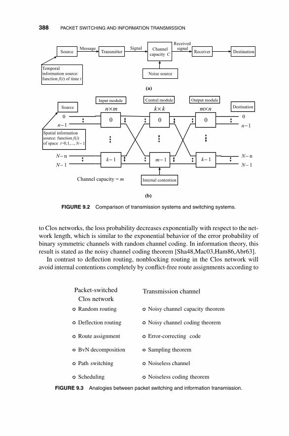
388 PACKET SWITCHING AND INFORMATION TRANSMISSION
TransmitterChannel
capacity C Receiver DestinationSource
Noise source
Temporalinformation source:function f(t) of time t
Message SignalReceived signal
(a)
DestinationSource
Spatial information
source: function f(i)of space i=0,1,...,
0 0 0
Internal contention
0
n−1 n−1
N− 1k− 1m− 1k− 1
N− n
N− 1
N− 1
N− n
0
Input module
n×m m×nk× kCentral module Output module
Channel capacity = m
(b)
FIGURE 9.2 Comparison of transmission systems and switching systems.
to Clos networks, the loss probability decreases exponentially with respect to the net-work length, which is similar to the exponential behavior of the error probability ofbinary symmetric channels with random channel coding. In information theory, thisresult is stated as the noisy channel coding theorem [Sha48,Mac03,Ham86,Abr63].
In contrast to deflection routing, nonblocking routing in the Clos network willavoid internal contentions completely by conflict-free route assignments according to
Packet-switchedClos network
Random routing
Deflection routing
Route assignment
BvN decomposition
Path switching
Scheduling
Noisy channel capacity theorem
Noisy channel coding theorem
Error-correcting code
Sampling theorem
Noiseless channel
Noiseless coding theorem
Transmission channel
FIGURE 9.3 Analogies between packet switching and information transmission.
DUALITY OF SWITCHING AND TRANSMISSION 389
input requests [Ben65,ChJi03,Jaj03]. The route assignment algorithms are based onthe matching of bipartite graphs. In the error-correcting code, the low-density paritycheck (LDPC) code developed by Gallager can also be represented by a bipartite graph[Gal62,Tan81], and a subclass called the expander code was constructed by Sipserand Speilman [SiSp96]. The condition on the expander graph is a generalizationof Hall’s condition on complete matching, which suggests the resemblance betweennonblocking route assignments and error-correcting codes. An extension of the Sipserand Speilman decoding algorithm of expander codes to route assignments of Benesnetworks is given to illustrate their correspondence.
The noiseless channel model of the Clos network. A drastically different approach,called path switching (see Chapter 7), to deal with contention in a Clos networkis proposed in Ref. [LeLa97]. A set of connection patterns of central modules isdetermined by the traffic matrix decomposition for this purpose. Path switching pe-riodically uses this finite set of predetermined connections in the central stage of theClos network to avoid online computation of route assignments. Once the connectionpatterns of central modules are fixed in each time slot, incoming packets can be sched-uled accordingly in the input buffer. Regarding the predetermined connections as acode book, scheduling is a process similar to source coding in digital transmission[Sha48,Mac03,Ham86,Abr63]. The smoothness of scheduling, like noiseless coding,is bounded by entropy inequalities.
The decomposition of traffic matrices, sometimes called the Birkhoff–von Neu-mann decomposition, has been widely used in SS/TDMA satellite communications[Inu79,BBB87]. Path switching adopts this scheduling scheme in packet switchingsystems to guarantee the capacity of virtual paths in Clos networks. The same approachcan be applied to the crossbar switch, also called the Birkhoff–von Neumann switch,in Ref. [CCH00]. Mathematically, the series expansion and reconstruction of doublystochastic capacity matrices are similar to the Fourier series expansion and interpola-tion of sampling theorem of bandlimited signals [Nyq28,Sha49,Whi15,Kot33]. Theyalso serve the same function in terms of complexity reduction of communication sys-tems. The capacity matrix decomposition employed in path switching will reduce thedimension of permutation space of a Clos network from N! to O(N2) or even lower,while the sampling theorem in transmission reduces the infinite-dimensional signalspace of any duration T to a finite number of samples.
The remainder of the chapter is organized as follows. In Section 9.2, we proposethe definition of pseudo signal-to-noise ratio of packet switch and prove that thetrade-off between the bandwidth and PSNR of a Clos network is the same as thatgiven by noisy channel capacity theorem in transmission. In Section 9.3, we showthat the loss probability of the Clos network with deflection routing is similar to theexponential error probability of binary symmetric channels with random coding. InSection 9.4, we demonstrate the correspondence between nonblocking route assign-ments and error-correcting codes. In Section 9.5, we address the capacity allocationand capacity matrix decomposition issues related to the path switching implementedon a Clos network. In Section 9.6, the entropy inequalities of smoothness of schedul-ing are derived, and comparisons of scheduling algorithms are discussed. Finally, theconclusion and future research are summarized in Section 9.7.

390 PACKET SWITCHING AND INFORMATION TRANSMISSION
0ρ ′ρ
ρ /Ν
ρ /Ν
1
N−1
01
N−1
FIGURE 9.4 The carried load of an N × N crossbar switch.
9.2 PARALLEL CHARACTERISTICS OF CONTENTION AND NOISE
The apparent causes of contention and noise are quite different, but they both limitthe performance of communication systems. In transmission, the trade-off betweenbandwidth and signal-to-noise ratio is given by Shannon–Hartley’s noisy channelcapacity theorem [Sha49]. In packet switching, the difference between offered loadand carried load reflects the degree of contention. In order to provide a commonground to compare contention and noise, a pseudo signal-to-noise ratio is defined torepresent the carried load of a packet switch. We show that the packet-switched Closnetwork with random routing can be mathematically modeled as a noisy channel.
9.2.1 Pseudo Signal-to-Noise Ratio of Packet Switch
Output port contention occurs in a crossbar switch when several packets are destinedfor the same output in a time slot. Packets lost in contention will be dropped as shownin Fig. 9.4. Consider an N × N crossbar switch, without any prior knowledge ofinput traffic. We assume that input loading ρ is homogeneous and output address isuniformly distributed, then the carried load ρ′ is the probability that an output is busyin any given time slot:
ρ′ = 1 −(
1 − ρ
N
)N N→+∞−→ 1 − e−ρ. (9.1)
The difference between offered load and carried load is caused by packet droppingdue to contention at the outputs. Benes considered the number of calls in progressas the energy of the connecting network in the thermodynamics theory of traffic in atelephone system [Ben63]. A similar traffic model was also explored in the broadbandnetwork [HuKa95]. If we regard packets as energy quantum, this proposition can beadopted in packet switching and stated as follows.
Proposition 9.1 (Benes). The signal power Sp of an N × N crossbar switch is thenumber of packets carried by the system, and the noise power is equal toNp = N − Sp.Furthermore, both the signal power and noise power are Gaussian random variableswhen N is large.
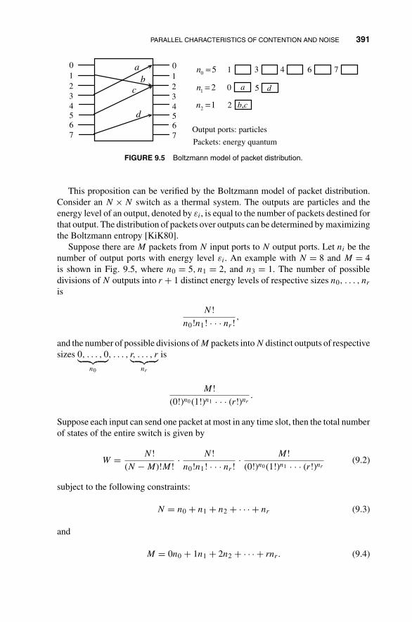
PARALLEL CHARACTERISTICS OF CONTENTION AND NOISE 391
0123
0 5n =
1 2n =
2 1n =
1
0 5
b,c2
a d
ab
c
d
Output ports: particles
Packets: energy quantum
4567
01234567
3 4 6 7
FIGURE 9.5 Boltzmann model of packet distribution.
This proposition can be verified by the Boltzmann model of packet distribution.Consider an N × N switch as a thermal system. The outputs are particles and theenergy level of an output, denoted by εi, is equal to the number of packets destined forthat output. The distribution of packets over outputs can be determined by maximizingthe Boltzmann entropy [KiK80].
Suppose there are M packets from N input ports to N output ports. Let ni be thenumber of output ports with energy level εi. An example with N = 8 and M = 4is shown in Fig. 9.5, where n0 = 5, n1 = 2, and n3 = 1. The number of possibledivisions of N outputs into r + 1 distinct energy levels of respective sizes n0, . . . , nr
is
N!
n0!n1! · · · nr!,
and the number of possible divisions of M packets into N distinct outputs of respectivesizes 0, . . . , 0︸ ︷︷ ︸
n0
, . . . , r, . . . , r︸ ︷︷ ︸nr
is
M!
(0!)n0 (1!)n1 · · · (r!)nr.
Suppose each input can send one packet at most in any time slot, then the total numberof states of the entire switch is given by
W = N!
(N − M)!M!· N!
n0!n1! · · · nr!· M!
(0!)n0 (1!)n1 · · · (r!)nr(9.2)
subject to the following constraints:
N = n0 + n1 + n2 + · · · + nr (9.3)
and
M = 0n0 + 1n1 + 2n2 + · · · + rnr. (9.4)
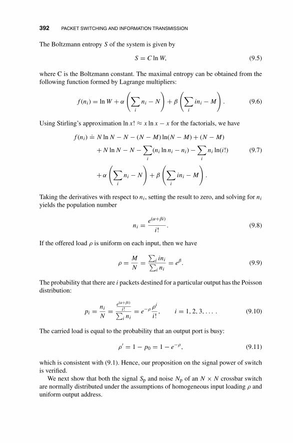
392 PACKET SWITCHING AND INFORMATION TRANSMISSION
The Boltzmann entropy S of the system is given by
S = C ln W, (9.5)
where C is the Boltzmann constant. The maximal entropy can be obtained from thefollowing function formed by Lagrange multipliers:
f (ni) = ln W + α
(∑i
ni − N
)+ β
(∑i
ini − M
). (9.6)
Using Stirling’s approximation ln x! ≈ x ln x − x for the factorials, we have
f (ni).= N ln N − N − (N − M) ln(N − M) + (N − M)
+ N ln N − N −∑
i
(ni ln ni − ni) −∑
i
ni ln(i!) (9.7)
+ α
(∑i
ni − N
)+ β
(∑i
ini − M
).
Taking the derivatives with respect to ni, setting the result to zero, and solving for ni
yields the population number
ni = e(α+βi)
i!. (9.8)
If the offered load ρ is uniform on each input, then we have
ρ = M
N=
∑i ini∑i ni
= eβ. (9.9)
The probability that there are i packets destined for a particular output has the Poissondistribution:
pi = ni
N=
e(α+βi)
i!∑i ni
= e−ρ ρi
i!, i = 1, 2, 3, . . . . (9.10)
The carried load is equal to the probability that an output port is busy:
ρ′ = 1 − p0 = 1 − e−ρ, (9.11)
which is consistent with (9.1). Hence, our proposition on the signal power of switchis verified.
We next show that both the signal Sp and noise Np of an N × N crossbar switchare normally distributed under the assumptions of homogeneous input loading ρ anduniform output address.
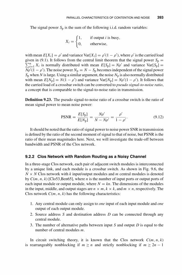
PARALLEL CHARACTERISTICS OF CONTENTION AND NOISE 393
The signal power Sp is the sum of the following i.i.d. random variables:
Xi ={
1, if output i is busy,
0, otherwise,
with mean E[Xi] = ρ′ and variance Var[Xi] = ρ′(1 − ρ′), where ρ′ is the carried loadgiven in (9.1). It follows from the central limit theorem that the signal power Sp =∑n
i=1 Xi is normally distributed with mean E[Sp] = Nρ′ and variance Var[Sp] =Nρ′(1 − ρ′). The noise power Np = N − Sp becomes independent of the signal powerSp when N is large. Using a similar argument, the noise Np is also normally distributedwith mean E[Np] = N(1 − ρ′) and variance Var[Np] = Nρ′(1 − ρ′). It follows thatthe carried load of a crossbar switch can be converted to pseudo signal-to-noise ratio,a concept that is comparable to the signal-to-noise ratio in transmission.
Definition 9.23. The pseudo signal-to-noise ratio of a crossbar switch is the ratio ofmean signal power to mean noise power:
PSNR = E[Sp]
E[Np]= Nρ′
N − Nρ′ = ρ′
1 − ρ′ . (9.12)
It should be noted that the ratio of signal power to noise power SNR in transmissionis defined by the ratio of the second moment of signal to that of noise, but PSNR is theratio of their mean magnitudes here. Next, we will investigate the trade-off betweenbandwidth and PSNR of the Clos network.
9.2.2 Clos Network with Random Routing as a Noisy Channel
In a three-stage Clos network, each pair of adjacent switch modules is interconnectedby a unique link, and each module is a crossbar switch. As shown in Fig. 9.6, theN × N Clos network with k input/output modules and m central modules is denotedby C(m, n, k) [Clo53,Ben65], where n is the number of input ports or output ports ofeach input module or output module, where N = kn. The dimensions of the modulesin the input, middle, and output stages are n × m, k × k, and m × n, respectively. TheClos network C(m, n, k) has the following characteristics:
1. Any central module can only assign to one input of each input module and oneoutput of each output module.
2. Source address S and destination address D can be connected through anycentral module.
3. The number of alternative paths between input S and output D is equal to thenumber of central modules m.
In circuit switching theory, it is known that the Clos network C(m, n, k)is rearrangeably nonblocking if m ≥ n and strictly nonblocking if m ≥ 2n − 1
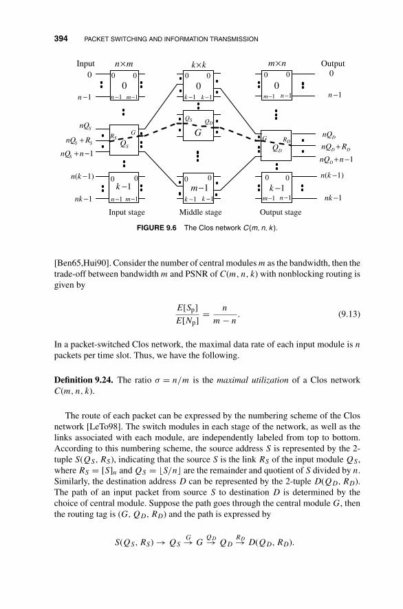
394 PACKET SWITCHING AND INFORMATION TRANSMISSION
0 00
1k − 1m− 1k −
1m−
1m−
OutputInput0
1n −
0
1n−
n×m0
0
k×k m×n
Input stage Middle stage Output stage
SQDQ
0
1n −
SnQ
1SnQ n −+SSnQ R+
GG
1k −
1k −
0
1k −
0
1k −
0
0
0
1n −
1)n(k −
1nk −
1)n(k −
1nk −
RS
QS QD
G RD
DDnQ R+DnQ
1DnQ n −+
1m−
1m−
0
0
0
1n−
0
1n −
FIGURE 9.6 The Clos network C(m, n, k ).
[Ben65,Hui90]. Consider the number of central modules m as the bandwidth, then thetrade-off between bandwidth m and PSNR of C(m, n, k) with nonblocking routing isgiven by
E[Sp]
E[Np]= n
m − n. (9.13)
In a packet-switched Clos network, the maximal data rate of each input module is n
packets per time slot. Thus, we have the following.
Definition 9.24. The ratio σ = n/m is the maximal utilization of a Clos networkC(m, n, k).
The route of each packet can be expressed by the numbering scheme of the Closnetwork [LeTo98]. The switch modules in each stage of the network, as well as thelinks associated with each module, are independently labeled from top to bottom.According to this numbering scheme, the source address S is represented by the 2-tuple S(QS, RS), indicating that the source S is the link RS of the input module QS ,where RS = [S]n and QS = �S/n� are the remainder and quotient of S divided by n.Similarly, the destination address D can be represented by the 2-tuple D(QD, RD).The path of an input packet from source S to destination D is determined by thechoice of central module. Suppose the path goes through the central module G, thenthe routing tag is (G, QD, RD) and the path is expressed by
S(QS, RS) → QSG→ G
QD→ QDRD→ D(QD, RD).

PARALLEL CHARACTERISTICS OF CONTENTION AND NOISE 395
In a packet-switched Clos network C(m, n, k), contentions may occur in the middlestage even if destination addresses of input packets are all different. With randomrouting scheme, the trade-off between bandwidth m and PSNR is given as follows.
Theorem 9.1. The maximum data rate of each input module of the packet-switchedClos network C(m, n, k) with random routing is given by
n = m ln
(1 + E[Sp]
E[Np]
). (9.14)
Proof. The maximum data rate is achieved when the input loading ρ = 1 and des-tination addresses of input packets are all different in every time slot, in which caseinput modules and output modules are contention-free. If the central module is se-lected randomly for each input packet, then the loading on each input link of a centralmodule is given by
σ = n/m.
Since each switch module of the Clos network is a crossbar switch, the carried loadon each output link of a central module is
σ′ = 1 −(
1 − n/m
k
)kk→+∞−→ = 1 − e−n/m. (9.15)
Substituting the following PSNR for the carried load σ′ in (9.15),
E[Sp]
E[Np]= kmσ′
km − kmσ′ = σ′
1 − σ′ ,
and taking logarithm, we obtain (9.14). �
The trade-offs given in (9.13) and (9.14) for constant data rate n packets per timeslot of each input/output module are plotted in Fig. 9.7, which shows the improvementof PSNR that can be achieved by nonblocking routing. The same kind of trade-offbetween bandwidth and SNR in the transmission channel is stated in the Shannon–Hartley theorem [Sha49] on noisy cannel capacity as follows.
Noisy Channel Capacity Theorem. The channel capacity of a bandlimited Gaussianchannel in the presence of additive Gaussian noise is given by
C = W log
(1 + S
N
), (9.16)

396 PACKET SWITCHING AND INFORMATION TRANSMISSION
3
2.5
2
1.5
1
0.5
0n 2n−1 m
E[Sp]
E[Np]
1.11
0.69
Rearrangeably nonblocking Strictly nonblocking
Circuit switchingwith nonblocking routing
Packet switchingwith random routing
FIGURE 9.7 Trade-off between bandwidth m and PSNR of C(m, n, k ).
where C is the capacity in bits per second, W is the bandwidth of the channel in Hertz,and S/N is the signal-to-noise ratio.
With the understanding that the contention is mathematically analogous to noise,the rest of the chapter seeks to investigate the connections between the various routingschemes of the Clos network and the corresponding coding schemes of the trans-mission channel. We first demonstrate the similarity between deflection routing andrandom coding in the next section.
9.3 CLOS NETWORK WITH DEFLECTION ROUTING
Packet contention is inevitable in packet switching. One way of solving this problemwithout having to buffer the losing packet is to use deflection routing. In contrast to“store-and-forward” routing where the network allows buffering, deflection routing,also known as hot potato routing, is a routing scheme without buffering and canonly be implemented for packet-switched networks [Tan81]. In case the individualcommunication links cannot support more than one packet at a time, excessive packetswill be transferred to other available links. Conceptually, deflection routing utilizesidle or redundant links of the network as temporary storages. Redundancy is built intothe switch design so that deflected packets can use extra stages to correct the deviatedroutes.

CLOS NETWORK WITH DEFLECTION ROUTING 397
012
345
01
2345
1
1
2
012
012
012
012
01 1
01
01
1
1
2 2
Deflection Output
1
C(3,3,2)C(2,2,3)
Destination Q1 R1
0 0 0
1 0 1
2 0 2
3 1 0
4 1 1
5 1 2
Routing coding in C(3,3,2)Destination Q2 R2
0 0 0
1 0 1
2 1 0
3 1 1
4 2 0
5 2 1
Routing coding in C(2,2,3)
D = 3Q1 + R1 D = 2Q2 + R2
Output
1
FIGURE 9.8 Cascaded Clos network with deflection routing.
9.3.1 Cascaded Clos Network
A cascaded Clos network is constructed by a sequence of alternate three-stageC(n, n, k) and C(k, k, n) networks, as illustrated in Fig. 9.8. Each output link of aswitch module is connected to a module in the next stage and an output concentrator(not shown in Fig. 9.8). A packet will be sent to the concentrator if its destinationaddress matches the output numbering, otherwise it will continue with the remain-ing journey. The loss probability can be made arbitrarily small by providing a largeenough number of stages.
In the cascaded Clos network, the destination address D of a packet can be ex-pressed by either D = nQ1 + R1 in the C(n, n, k) network or D = kQ2 + R2 in theC(k, k, n) network, as shown in the example given in Fig. 9.8, and therefore, therouting tag in the packet header comprises a 4-tuple (Q1, R1, Q2, R2). A packet canreach its destination D in any two consecutively successful steps, either (Q1, R1) or(Q2, R2). The Markov chain shown in Fig. 9.9 describes the complete journey of apacket, where pi and qi = 1 − pi are respective probabilities of success and deflectionin C(n, n, k) and C(k, k, n).
9.3.2 Analysis of Deflection Clos Network
For the sake of simplicity, we assume that the cascaded Clos network is formedby C(n, n, n) network uniformly. Since we will consider the worst-case deflection

398 PACKET SWITCHING AND INFORMATION TRANSMISSION
2q1Q
2Q
O
1R
2R
1p
2p
1p1q
2p
2q 1q Output
Input
FIGURE 9.9 The Markov chain of deflection routing.
probability when both n and k are sufficiently large, the assumption that n = k doesnot lose the generality of analysis, and the packet loss probability will be a conservativeestimate. Under this presumption, a simplified Markov chain is depicted in Fig. 9.10.
The probability of success p in an n × n switch module is a function of inputloading ρ. Under the homogeneous traffic assumption, we have
1 − pρ =(
1 − ρ
n
)n n→∞−→ e−ρ.
Thus, the worst probability of success is given by
p = 1 − e−ρ
ρ.
The probabilities of success p and deflection q = 1 − p versus the loading ρ areplotted in Fig. 9.11(a). Let Gi(k) be the probability that the packet in state i will reachthe output state O in exactly k steps. The following equations can be derived fromthe Markov chain shown in Fig. 9.10:
GO(k) ={
1, if k = 0,
0, otherwise,
GR(k) = pG0(k − 1) + qGQ(k − 1), k = 1, 2, . . . ,
GQ(k) = pGR(k − 1) + qGQ(k − 1), k = 1, 2, . . . . (9.17)
Input
Q R O
q
q
pp
Output
FIGURE 9.10 The simplified Markov chain of deflection routing.
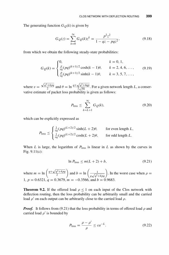
CLOS NETWORK WITH DEFLECTION ROUTING 399
The generating function GQ(k) is given by
GQ(z) =∞∑
k=0
GQ(k)zk = p2z2
1 − qz − pqz2 , (9.18)
from which we obtain the following steady-state probabilities:
GQ(k) =
⎧⎪⎨⎪⎩
0, k = 0, 1,pvq
(pq)(k+1)/2 cosh(k − 1)θ, k = 2, 4, 6, . . . ,
pvq
(pq)(k+1)/2 sinh(k − 1)θ, k = 3, 5, 7, . . . ,
(9.19)
where v =√
q2+4pq
2 and θ = ln q+√
q2+4qp
2√
pq. For a given network length L, a conser-
vative estimate of packet loss probability is given as follows:
Ploss ≤∞∑
k=L+1
GQ(k), (9.20)
which can be explicitly expressed as
Ploss ≤⎧⎨⎩
1vq
(pq)(L+2)/2 sinh(L + 2)θ, for even length L,
1vq
(pq)(L+2)/2 cosh(L + 2)θ, for odd length L.
When L is large, the logarithm of Ploss is linear in L as shown by the curves inFig. 9.11(c):
ln Ploss ≤ m(L + 2) + b, (9.21)
where m = ln
(q+
√q2+4pq
2
)and b = ln
(1
q√
q2+4pq
). In the worst case when ρ =
1, p = 0.6321, q = 0.3679, m = −0.3566, and b = 0.9683.
Theorem 9.2. If the offered load ρ ≤ 1 on each input of the Clos network withdeflection routing, then the loss probability can be arbitrarily small and the carriedload ρ′ on each output can be arbitrarily close to the carried load ρ.
Proof. It follows from (9.21) that the loss probability in terms of offered load ρ andcarried load ρ′ is bounded by
Ploss = ρ − ρ′
ρ≤ ca−L. (9.22)
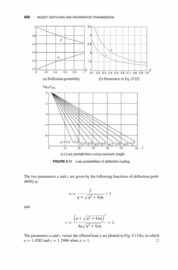
400 PACKET SWITCHING AND INFORMATION TRANSMISSION
FIGURE 9.11 Loss probabilities of deflection routing.
The two parameters a and c are given by the following functions of deflection prob-ability q:
a = 2
q +√
q2 + 4pq> 1
and
c =(q +
√q2 + 4pq
)2
4q√
q2 + 4pq> 1.
The parameters a and c versus the offered load ρ are plotted in Fig. 9.11(b), in whicha = 1.4285 and c = 1.2906 when ρ = 1. �

CLOS NETWORK WITH DEFLECTION ROUTING 401
p0
1
0
1p
q
q
FIGURE 9.12 Binary symmetric channel.
Conversely, if the offered load ρ > 1, then the loss probability is unbounded,because the number of packets input to a switch module could be more than the totalnumber of outputs and there is not enough space to deflect packets, which can be losthalfway through.
Compare the deflection Clos network with the binary symmetric channel (BSC)with random coding, as illustrated in Fig. 9.12. Table 9.1 provides the parallels be-tween the above theorem and Shannon’s main theorem [Sha48,Mac03,Ham86,Abr63]stated as follows.
Noisy Channel Coding Theorem. Given a noisy channel with capacity C and in-formation transmitted at a rate R, then if R ≤ C, there exists a coding technique thatallows the probability of error at the receiver to be made arbitrarily small. This meansit is possible to transmit information without error up to a limit C. However, if R > C,the probability of error at the receiver increases without bound.
The capacity of BSC with cross probability q = 1 − p is given by
C = 1 + p log p + (1 − p) log(1 − p). (9.23)
The noisy channel coding theorem states that there exist an encoding functionE : {0, 1}k → {0, 1}n and a decoding function D : {0, 1}n → {0, 1}k, such that the
TABLE 9.1 Comparison of Deflection Clos Network and Binary Symmetric Channel
Deflection Clos Network Binary Symmetric Channel
Deflection probability q < 1/2 Cross probability q < 1/2Deflection routing Random coding� ≤ 1 R ≤ C
Exponential loss probability Exponential error probabilityPloss ≤ ca−L Pe ≤ a−n + c−n
Complexity increases Complexity increaseswith network length L with code length n
Equivalent set of outputs Typical set decoding
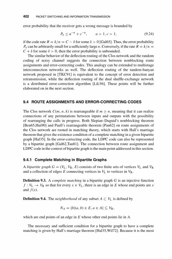
402 PACKET SWITCHING AND INFORMATION TRANSMISSION
error probability that the receiver gets a wrong message is bounded by
Pe ≤ a−n + c−n, a > 1, c > 1, (9.24)
if the code rate R = k/n = C − δ for some δ > 0 [Gal65]. Thus, the error probabilityPe can be arbitrarily small for a sufficiently large n. Conversely, if the rate R = k/n =C + δ for some δ > 0, then the error probability is unbounded.
The similar behavior of the deflection routing of the Clos network and the randomcoding of noisy channel suggests the connection between nonblocking routeassignments and error-correcting codes. This analogy can be extended to multistageinterconnection networks as well. The deflection routing of the tandem-banyannetwork proposed in [TKC91] is equivalent to the concept of error detection andretransmission, while the deflection routing of the dual shuffle-exchange networkis a distributed error-correction algorithm [LiL94]. These points will be furtherelaborated on in the next section.
9.4 ROUTE ASSIGNMENTS AND ERROR-CORRECTING CODES
The Clos network C(m, n, k) is rearrangeable if m ≥ n, meaning that it can realizeconnections of any permutations between inputs and outputs with the possibilityof rearranging the calls in progress. Both Slepian–Duguid’s nonblocking theorem[Ben65,Hui90] and Paull’s rearrangeable theorem [Pau62] on route assignments ofthe Clos network are rooted in matching theory, which starts with Hall’s marriagetheorem that gives the existence condition of a complete matching in a given bipartitegraph [Hal35]. In the error-correcting code, the LDPC code can also be representedby a bipartite graph [Gal62,Tan81]. The connection between route assignment andLDPC code in the context of bipartite graph is the main point addressed in this section.
9.4.1 Complete Matching in Bipartite Graphs
A bipartite graph G = (VL, VR, E) consists of two finite sets of vertices VL and VRand a collection of edges E connecting vertices in VL to vertices in VR.
Definition 9.3. A complete matching in a bipartite graph G is an injective functionf : VL → VR so that for every x ∈ VL, there is an edge in E whose end points are x
and f (x).
Definition 9.4. The neighborhood of any subset A ⊂ VL is defined by
NA = {b|(a, b) ∈ E, a ∈ A} ⊆ VR,
which are end points of an edge in E whose other end points lie in A.
The necessary and sufficient condition for a bipartite graph to have a completematching is given by Hall’s marriage theorem [Hal35,Wil72]. Because it is the most

ROUTE ASSIGNMENTS AND ERROR-CORRECTING CODES 403
fundamental theorem in switching theory, we state the theorem and give Rado’selegant proof [Rad67] below.
Theorem 9.3 (Hall). Let G = (VL, VR, E) be a bipartite graph, then there exists acomplete matching for G if and only if
|NA| ≥ |A| (9.25)
for any subset A ⊆ VL.
Proof. It is clear that the condition is essential for the existence of a completematching, but it remains to show that it is sufficient. Let VL = {1, 2, . . . , n} andF = {N1, N2, . . . , Nn}; by contradiction, suppose N1 contains x, y, then the removalof either x or y violates Hall’s condition. There exist A, B ⊆ {2, . . . , n} with theproperty
RA = NA ∪ (N1 − {x}), |RA| ≤ |A|,RB = NB ∪ (N1 − {y}), |RB| ≤ |B|.
Then, |RA ∪ RB| = |NA∪B ∪ N1| and |RA ∩ RB| ≥ |NA∩B|. It follows that
|A| + |B| ≥ |RA| + |RB| = |RA ∪ RB| + |RA ∩ RB|≥ |NA∪B ∪ N1| + |NA∩B|. (9.26)
On the other hand, from Hall’s condition, we have
|NA∪B ∪ N1| + |NA∩B| ≥ |A ∪ B| + 1 + |A ∩ B| = |A| + |B| + 1. (9.27)
Combining (9.26) and (9.27) will lead to
|A| + |B| ≥ |A| + |B| + 1,
a contradiction. Hence, the removal of either x or y does not violate Hall’s condition,and a complete matching can be obtained by repeating this procedure until each Ni
contains only one element. �
The nonblocking route assignment of the Clos network and the edge coloring ofthe bipartite graph stated in the following theorem are equivalent consequences ofHall’s marriage theorem.
Theorem 9.4. The following statements are equivalent:
1. A regular bipartite graph G with degree n can be edge colored by m colors ifm ≥ n.

404 PACKET SWITCHING AND INFORMATION TRANSMISSION
0
1
2
3
0
1
2
3
11 10
11 01
11 10
00 12
1 000 1000 10 00
10 00 1 000 100 0
1000 10 00 1 000
100 0 100 0 1000
= + +
FIGURE 9.13 An edge-colored regular bipartite graph and decomposition of integer doublystochastic matrix.
2. Slepian–Duguid: The Clos network C(m, n, k) is rearrangeably nonblocking ifm ≥ n.
Proof. 1. For any subset A ⊆ VL, the edges terminating on vertices in A must beterminated on vertices in its neighborhood set NA at the other end; Hall’s conditionholds because
n|NA| ≥ n|A| ⇒ |NA| ≥ |A|.
The bipartite graph G can be reduced to n complete matching by repeatedly ap-plying Hall’s theorem. It is clear that edge-coloring can be satisfied if m ≥ n. Theedge-colored bipartite graph is equivalent to the decomposition of an integer doublystochastic matrix into permutation matrices. An example to illustrate this point isshown in Fig. 9.13.
2. Consider a set of call requests {(S0, D0), . . . , (SN−1, DN−1)}, in which thedestination addresses are all different, and suppose the central module Gi is assignedto the request (Si, Di) for i = 0, . . . , N − 1. This set of assignments is nonblocking,or contention-free, if and only if
�Si/n� = �Sj/n� ⇒ Gi = Gj
and
�Di/n� = �Dj/n� ⇒ Gi = Gj
for all i = j. It simply means that if either of the two sources Si and Sj are on the sameinput modules, or the two destinations Di and Dj are on the same output module,then the central modules assigned to (Si, Di) and (Sj, Dj) must be different.
The route assignments can be formulated as the edge coloring of a bipartite graphG(VL, VR, E), in which vertices of VL represent input modules and vertices of VRrepresent output modules, and each connection request (Si, Di) is represented by anedge (�Si/n�, �Di/n�) in E. This bipartite graph is regular with degree n and can be

ROUTE ASSIGNMENTS AND ERROR-CORRECTING CODES 405
0
1
2
3
0
1
2
3
0
1
2
01
23
45
67
01
23
45
67
Inputmodules
Outputmodules
Centralmodules
Inputmodules
Outputmodules
0
1
2
3
0
1
2
3
(a) Three-stage Clos network (b) Equivalent regular bipartite graph
FIGURE 9.14 Correspondence between Clos network and bipartite graph.
colored by m colors if m ≥ n, such that each color represents a central module andthe edge coloring is the set of route assignments. �
An example to show the equivalence between route assignment of the Clos networkand edge coloring of the bipartite graph is given in Fig. 9.14. The resulting routeassignments of the call request are listed in Table 9.2. The connection between routeassignment and error-correcting code will be addressed in the sequel.
9.4.2 Graphical Codes
The LDPC code is a class of linear block code that can be represented by bipartitegraphs G(VL, VR, E), called Tanner graph [Tan81], in which VL is the set of variablevertices and VR the set of constraint vertices. The parity matrix specifies the edge setE. Each variable can assume the value of 0 or 1, and a constraint is satisfied if thesum of all the variables adjacent to it is 0 mod 2. Figure 9.15 illustrates an exampleof such a bipartite graph that represents the following matrix:
⎡⎢⎢⎢⎣
0 1 0 1 1 0 0 1
1 1 1 0 0 1 0 0
0 0 1 0 0 1 1 1
1 0 0 1 1 0 1 0
⎤⎥⎥⎥⎦ . (9.28)
TABLE 9.2 The Set of Routing Tags (G, Q, R)
S 0 1 2 3 4 5 6 7D 1 3 2 0 6 4 7 5G 0 2 0 2 2 1 0 2Q 0 1 1 0 3 2 3 2R 1 1 0 0 0 0 1 1
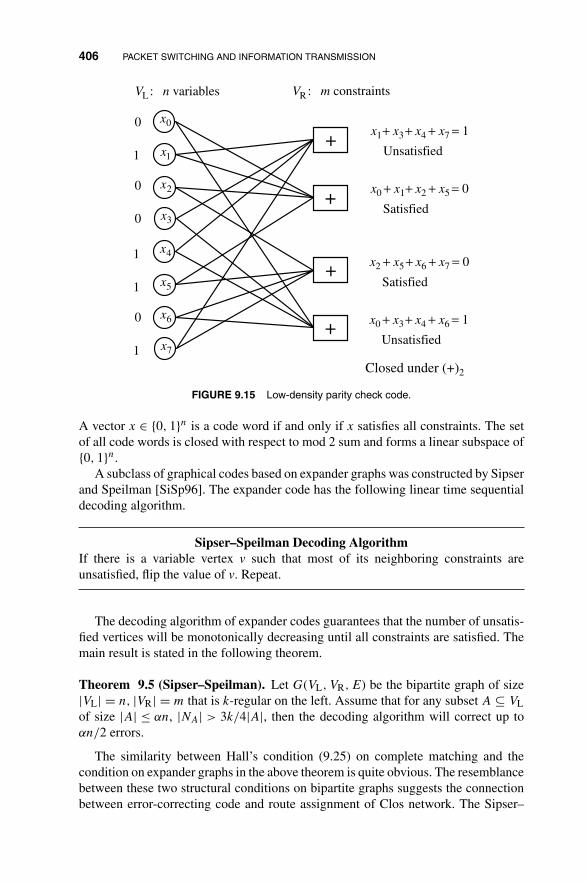
406 PACKET SWITCHING AND INFORMATION TRANSMISSION
0x
1x
2x
3x
+
+
0
0
0
1
:L n variablesV :R m constraintsV
Unsatisfied
x3x1 x7x4++ = 1+
Satisfied
x1x0 x5x2+ = 0++
Closed under (+)2
4x
5x
6x
7x
+
+
1
0
1
1 Satisfied
x5x2 x7x6++ = 0+
Unsatisfied
x3x0 x6x4++ = 1+
FIGURE 9.15 Low-density parity check code.
A vector x ∈ {0, 1}n is a code word if and only if x satisfies all constraints. The setof all code words is closed with respect to mod 2 sum and forms a linear subspace of{0, 1}n.
A subclass of graphical codes based on expander graphs was constructed by Sipserand Speilman [SiSp96]. The expander code has the following linear time sequentialdecoding algorithm.
Sipser–Speilman Decoding AlgorithmIf there is a variable vertex v such that most of its neighboring constraints areunsatisfied, flip the value of v. Repeat.
The decoding algorithm of expander codes guarantees that the number of unsatis-fied vertices will be monotonically decreasing until all constraints are satisfied. Themain result is stated in the following theorem.
Theorem 9.5 (Sipser–Speilman). Let G(VL, VR, E) be the bipartite graph of size|VL| = n, |VR| = m that is k-regular on the left. Assume that for any subset A ⊆ VLof size |A| ≤ αn, |NA| > 3k/4|A|, then the decoding algorithm will correct up toαn/2 errors.
The similarity between Hall’s condition (9.25) on complete matching and thecondition on expander graphs in the above theorem is quite obvious. The resemblancebetween these two structural conditions on bipartite graphs suggests the connectionbetween error-correcting code and route assignment of Clos network. The Sipser–

ROUTE ASSIGNMENTS AND ERROR-CORRECTING CODES 407
Speilman decoding algorithm is extended to the nonblocking route assignment ofBenes network to illustrate their correspondence.
9.4.3 Route Assignments of Benes Network
A Benes network is a multistage connecting network that can be recursively con-structed from Clos network C(2, 2, k) [Ben65,Hui90]. A set of call requests is amapping from inputs to outputs. An example is given in (9.29), which displays a setof connection requests in an 8 × 8 Benes network. The upper row of the matrix is theordered inputs from 0 to 7, and the lower row consists of the respective outputs.
π =(
0 1 2 3 4 5 6 7
1 6 0 5 7 2 4 3
). (9.29)
The two central modules in C(2, 2, N/2), as shown in Fig. 9.19(a), are labeled,respectively, by 0 and 1. Let xi be the binary variable associated with the request(i, π(i)), for i = 0, . . . , N − 1. The value of xi ∈ {0, 1} defines the following routeassignment:
xi ={
0, if module 0 is assigned to (i, π(i)),
1, otherwise.(9.30)
Since the same central module cannot be assigned to two inputs or two outputs on thesame module, the necessary and sufficient condition on nonblocking route assignmentcan be simply formulated as a set of linear constraints
xi + xj = 1 (9.31)
for all i = j such that either two inputs i and j are on the same input module or twooutputs π(i) and π(j) are on the same output module.
As shown in Fig. 9.16, let VL = {x0, . . . , xN−1} be the set of variables and VR be theset of constraints (9.31); a bipartite graph G(VL, VR, E) similar to that of LDPC canbe constructed to solve for the values of x′
i’s, which determine the nonblocking routesof the set of call requests in π. It should be noted that the set of solutions to (9.31) is notclosed with respect to mod 2 sum. In fact, two solutions in each connected componentof the bipartite graph G(VL, VR, E) are complementary to each other, and the totalnumber of solutions of (9.31) should be 2g, where g is the number of connectedcomponents of G. The following route assignment algorithm is a modification ofSipser–Speilman decoding algorithm.
The flip algorithm for nonblocking route assignments:
Step 1 Initially assign x0 = 0, x1 = 1, x2 = 0, x3 = 1, . . . to satisfy all input moduleconstraints.
Step 2 In each cycle of the bipartite graph, unsatisfied vertices divide the cycle intoline segments. Label them α and β alternately and flip the values of all variableslocated in α segments.

408 PACKET SWITCHING AND INFORMATION TRANSMISSION
0
1
01
23
45
67
01
23
5
67
4
Bipartite graph of call requests
10 432 65 7
61 50 427 3
0
1
2
3
0
1
2
3
+
10
32
54
76
1
1
1
1
xx
xx
xx
xx
=+
=+
=+
=+
+
+
+
+
+
+
+
Input moduleconstraints
20
75
63
41
1
1
1
1
xx
xx
xx
xx
=+
=+
=+
=+
Output moduleconstraints
0 unsatisfiedModule 2 sum =
satisfied1
Not closed under +
0x
2x
3x
4x
5x
6x
7x
1x
FIGURE 9.16 Nonblocking constraints of Benes network.
The initial values of all variables can be arbitrarily assigned. Compared to theSipser–Speilman decoding algorithm, the initial assignment can be considered as thereceived signal, and errors are systematically removed by the flip algorithm to satisfyall constraints.
Theorem 9.6. All constraints are satisfied when the flip algorithm terminates.
Proof. The proof of this theorem is illustrated by the example displayed in Fig. 9.17.First, we want to show that every cycle has an even number of unsatisfied vertices. Itis clear that the total number of constraints is even because there is an equal numberof input modules and output modules in each cycle. Assume by contradiction thatthe number of unsatisfied vertices is odd, then the number of satisfied vertices mustalso be odd. Let u0 and u1 be the number of unsatisfied vertices whose neighboringvariables both equal 0 and 1, respectively, and let s be the number of satisfied vertices.Then, the number of variables equal to 0 and 1, respectively, should be u0 + s/2 andu1 + s/2, which is impossible if s is odd.
Next, we want to show that all constraints are satisfied when the flip algorithm ter-minates as shown in Fig. 9.17. For an arbitrary constraint vertexv ∈ VR, let xi, xj ∈ VL

ROUTE ASSIGNMENTS AND ERROR-CORRECTING CODES 409
0x
1x
2x
3x
+
+
+
+
4x
5x
6x
7x+
+
+
+
0
1
0
1
0
1
0
1
10 1xx =+
32 1xx =+
54 1xx =+
76 1xx =+
20 0xx =+
75 0xx =+
63 1xx =+
41 1xx =+
Input moduleconstraints
Output moduleconstraintsVariables
FIGURE 9.17 The flip algorithm for nonblocking route assignments.
be the two neighboring variables of v. If v is unsatisfied, the two variables xi and xj
should have the same value but are located in segments bearing different labels. Onlyone located in the α segment will flip the value, and the vertex v should be satisfiedwhen the algorithm terminates.
On the other hand, if the constraint v is initially satisfied, then xi and xj flipsimultaneously if they are both in an α segment, or else they keep the same value ifthey are located in a β segment. Hence, the constraint v remains satisfied in eithercase when the algorithm terminates. �
The route assignments of the set of call requests (9.29) resulting from the flipalgorithm are displayed in Fig. 9.18, and the complete assignments shown in Fig.9.19 can be determined iteratively. If both N and n are of the power of 2, the set ofequations (9.31) can also be solved by the parallel algorithm proposed in Ref. [LeLi02]with time complexity on the order of O(log2(N)).
01
23
45
67
01
23
5
67
4
10 32 54 76Call requests
5061 427 3
Assignment 0= 10011 01
0
1
2
3
0
1
2
3
FIGURE 9.18 The connection requests and route assignments.

410 PACKET SWITCHING AND INFORMATION TRANSMISSION
01
23
45
6
7
01
23
45
6
7
FIGURE 9.19 The complete route assignments of Benes network.
9.5 CLOS NETWORK AS NOISELESS CHANNEL-PATH SWITCHING
Path switching proposed in Ref. [LeLa97] is a compromise of static routing anddynamic routing schemes for a Clos network. A set of connection patterns of thecentral modules is predetermined according to the traffic between pairs of input andoutput modules. This set of connection patterns is repeatedly used in a cyclic mannersuch that online path hunting can be avoided and bandwidth requirements can besatisfied in the long run.
The scheduling of path switching is based on the following relationships betweenthe edge-colored bipartite graph and the connection pattern in the middle stage of theClos network as depicted in Fig. 9.14 earlier:
1. The number of edges eij represents the number of packets that can be sentfrom input module Ii to output module Oj , the virtual path Vij , in one timeslot.
2. Each color of the bipartite graph corresponds to a central module of the Closnetwork.
This correspondence suggests the scheduling of switch according to predeterminedconnection patterns if traffic matrix is expressed as weighted sum of a finite numberof permutation matrices as shown in Fig. 9.20.
For any given traffic matrix T = [λij], where λij is the number of packets pertime slot from input module Ii to output module Oj , such that
∑i λij < n ≤ m and∑
j λij < n ≤ m, there exist a finite number F of regular bipartite graphs such thatthe capacity cij of the virtual path Vij between Ii and Oj satisfies
cij =∑F−1
t=0 eij(t)
F> λij, (9.32)
where eij(t) is the number of edges from node i to node j in the tth bipartite graph. Thebandwidth requirement T = [λij] can be satisfied if the system periodically providesconnections according to the edge coloring of these F bipartite graphs. Adoptingconvention in the TDMA system, each cycle is called a frame and the period F frame

CLOS NETWORK AS NOISELESS CHANNEL-PATH SWITCHING 411
FIGURE 9.20 Capacity of virtual path as average number of edges.
size. The routing information can be stored in the local memory of each input moduleto avoid the slot-by-slot computation of route assignments [EHY,MeT89].
Since the connection patterns of switch modules in the middle stage are fixed, thevirtual path between any pair of input module and output module is contention-free. Asshown in Fig. 9.21, input/output modules are scaled to a much smaller size and routingdecisions in these modules become independent. Each input module is an independentinput-queued switch, and arrival packets can be scheduled in the input buffer accordingto predetermined routes in every time slot by some matching algorithm similar to thescheduling algorithm for input-queued crossbar switch [McK99], while each outputmodule could be an output-queued switch similar to a knockout switch [YHA87].Consider the scheduled Clos network as a noiseless channel, then the scheduling ofpath switching maps central modules and time slots into incoming packets, a processsimilar to the source coding of transmission [Sha48,Mac03,Ham86,Abr63] if the setof predetermined connection patterns is regarded as a code book. In this section,we address the capacity allocation and traffic matrix decomposition issues, and thesmoothness of scheduling will be discussed in the next section.
9.5.1 Capacity Allocation
The capacity allocation problem seeks to find the capacity cij > λij for each virtualpath Vij between Ii andOj such that non-overbooking condition
∑i cij = ∑
j cij = m
for each input/output module is observed. The problem can be formulated as con-strained optimization of some objective function [Str86]. The choice of the objectivefunction depends on the stochastic characteristic of the traffic on virtual paths and thequality-of-service requirements of connections. Following Kleinrock’s independencyassumption [Klei75,BeG92], each virtual path can be modeled as an M/M/1 queue

412 PACKET SWITCHING AND INFORMATION TRANSMISSION
0
k−1
0
m−1
0
k−1
Predetermined
connection pattern
in every time slot
0
n−1
0
n−1
N−nN−1
N−nN−1
Input module
(input-queued
switch)
n×m k×k m×n
Central module
(nonblocking
switch)
Output module
(output-queued
switch)
Output bufferInput buffer
Buffer
and
scheduler
Input
module i
Buffer
and
scheduler
Output
module jVirtual path
Destination λij Source
Scheduling to combat
channel noise
Buffering to combat
source noise
FIGURE 9.21 Noiseless virtual path of Clos network.
with arrival rate λij and service rate cij for all i, j, then the average delay for thepackets from input module Ii to output module Oj is given by
Dij = 1
cij − λij
(9.33)
and the objective is to minimize the total weighted delay [Klei75]∑i,j
λij
cij − λij
(9.34)
subject to cij > λij and∑
i cij = ∑j cij = m. The computation of the optimal allo-
cation is quite involved in general. Nevertheless, the following heuristic algorithmbased on Kleinrock’s square root rule [Klei75] can always yield suboptimal capacityallocation that is close to the optimal solution.
Theorem 9.7. For any given traffic matrix T = [λij] with nonzero entries, λij > 0for all i and j, then
n∑j=1
λij ≤n∑
j=1
cij = m (9.35)
CLOS NETWORK AS NOISELESS CHANNEL-PATH SWITCHING 413
and
n∑i=1
λij ≤n∑
i=1
cij = m (9.36)
when the capacity allocation algorithm terminates.
Capacity Allocation Algorithm
Step 1 Initialization: Set k = 1 and c(0)ij = λij.
Step 2 Calculate slack capacity of each input module (row) and output module (col-umn). ⎧⎨
⎩A(k−1)i = m − ∑n
j=1 c(k−1)ij
B(k−1)j = m − ∑n
i=1 c(k−1)ij
Step 3 Remove any saturated row i if A(k−1)i = 0 and column j if B
(k−1)j = 0. The
algorithm terminates if there is no slack capacity left, otherwise do
c(k)ij = c
(k−1)ij + min
(A
(k−1)i
√λij∑n
j=1
√λij
,B
(k−1)j
√λij∑n
i=1
√λij
),
and set k = k + 1, go to step 2.
Proof. Since λij > 0, it is obvious that
c(k)ij > c
(k−1)ij (9.37)
in kth iteration of the algorithm for all k. Also, we have
n∑j=1
c(k)ij ≤
n∑j=1
c(k−1)ij +
n∑j=1
A(k−1)i
√λij∑n
j=1
√λij
= m. (9.38)
The combination of (9.37) and (9.38) assures that∑n
j=1 cij = m, and similarly, that∑ni=1 cij = m, when the algorithm terminates. �
Notice that if some entries λij are zero, then the strict inequality (9.37) does nothold in general, and there is no guarantee that the algorithm will halt. It is also truefor any capacity allocation algorithm that if λij = 0 implies cij = 0, then the doublystochastic matrix C = [cij] that satisfies (9.35) and (9.36) may not exist. Nevertheless,this problem can be eliminated in practice if a small amount of capacity cij = ε
allocated to a virtual path with λij = 0 is allowed.

414 PACKET SWITCHING AND INFORMATION TRANSMISSION
9.5.2 Capacity Matrix Decomposition
The time axis is divided into frames of time slots, and the frame size is denoted byF . Within each frame, the rate requirement will be satisfied by a set of connectionpatterns, which are predetermined by the decomposition of the capacity matrix [cij]. Ina time-slotted system, it is reasonable to assume that all entries cij are rational numberswith a least common denominator F . Then [F · cij] is an integer doubly stochasticmatrix with constant mF row sum and column sum. According to Theorem 2, thebipartite graph corresponding to the matrix [F · cij] can be colored by mF colors.The colored bipartite graph can also be expressed by the generalized Birkhoff–vonNeumann decomposition [Bir46,LLL83,LLL86] stated in the following theorem.
Theorem 9.8 (Generalized Birkhoff–von Neumann Decomposition). The capac-ity matrix C has the following expansions:
C = 1
F
mF∑i=1
Mi = 1
F
F∑i=1
Gi =K∑
i=1
φiPi, (9.39)
such that Gi = ∑mij=m(i−1)+1 Mj, i = 1, . . . , F , and
∑Ki=1 φi = 1.
With respect to the scheduling of path switching, the correspondence betweenconnection patterns in the Clos network C(m, n, k) and these matrices in the seriesexpansions (9.39) is given as follows:
1. Each Mi is a permutation matrix, or complete matching.
2. Each matrix Gi is a sum of m permutation matrices, Mm(i−1)+1, . . . , Mmi,which represent connection patterns of those m central modules of C(m, n, k)in time slot i of every frame. That is, the matrix Gi is an edge-colored regularbipartite graph with degree m. The combination of permutation matrices in Gi
can be arbitrary.
3. Each matrix Pi is a state of the switch such that Pi = Pj for all i = j, and{P1, . . . , PK} = {G1, . . . , GF }. The coefficient φi is the frequency of the statePi within each time frame. Since the total number of constraints in the doublystochastic matrix C is equal to (N − 1)2 + 1, the number of states is boundedby K ≤ min{F, N2 − 2N + 2}.
The scheduling information stored in the memory is linearly proportional to F ,and the frame size is limited by the access speed and the memory space of inputmodules. In the capacity matrix decomposition (9.39), both K and F could be toolarge in practice, because the number of states K is on the order of O(N2) and theframe size F is determined by the least common denominator of cij . The followinglimitations compromise between complexity and QoS:
1. If the capacity matrix C is bandlimited such that cij ≤ B/F , then it is easy toshow that K ≤ F ≤ BN/m.

CLOS NETWORK AS NOISELESS CHANNEL-PATH SWITCHING 415
1.4 0.5 1.1
0.6 1.8 0.6
1.0 0.7 1.3ijc =
Capacity matrix(per slot)
425
72 2
524ije =
11 84
144 4
58 10ije =
F 4=
RMS error = 0.104
F 8=
RMS error = 0.0608
FIGURE 9.22 Round-off errors with different frame size F .
2. The frame size F can be a constant independent of switch size N if [F · cij]is rounded off into an integer matrix, and the round-off error on the order ofO(1/F ) is acceptable. The error can be arbitrarily small if the frame size F issufficiently large, as shown in the examples given in Fig. 9.22.
Consider the traffic matrix as the aggregate of signals input to the packet switch,then the series expansion of doubly stochastic capacity matrix into permutation ma-trices (9.39) and the reconstruction of capacity by weighted running sum of scheduledconnections are mathematically similar to those of the Nyquist–Shannon samplingtheorem of bandlimited signals [Nyq28,Sha49,Whi15,Kot33] input to the transmis-sion channel.
Sampling Theorem of bandlimited signal. If a function f (t) contains no frequencieshigher than W cps, it is completely determined by its ordinates at a series of equallyspaced sampling intervals of 1/2W s, called Nyquist intervals. If |F (ω)| = 0, for|ω| ≥ 2πW , then
f (t) =+∞∑−∞
fn
sin π(2Wt − n)
π(2Wt − n)
where fn = f(
n2W
)is the nth sample of f (t).
An important common characteristic of both series expansions is the reductionof complexity. Without scheduling, the total number of possible permutations of apacket switch for a given capacity matrix is N!. The complexity reduction is achievedby limiting the space to those permutations only involved in the expansion (9.39).Hence, the dimension of permutation space is reduced to O(N2) by the traffic matrixdecomposition. It can further be reduced to O(N) if each connection is bandwidthlimited. The complexity of packet-level problems can be significantly reduced if the

416 PACKET SWITCHING AND INFORMATION TRANSMISSION
TABLE 9.3 Comparison of Traffic Matrix Decomposition and Sampling Theorem
Packet Switching Digital Transmission
Network environment Time-slotted switching system Time-slotted transmission system
Bandwidth limitation Capacity-limited traffic matrix Bandwidth-limited signal function
N∑i=1
�ij ≤N∑
i=1
cij = m f (t ) = 12�
∫ 2�w
−2�w
F (ω)dω
N∑j=1
�ij ≤N∑
i=1
cij = m F (ω) = 0, |ω| ≥ 2�w
�ij ≤ cij
Samples (0, 1) Permutation matrices (0, 1) Binary sequences
BvN decomposition (Hall’s marriagetheorem)
Fourier series
Expansion C =Fm∑i=1
Mi
F=
K∑i=1
�i Pi f (t ) =+∞∑−∞
fnsin�(2Wt − n)
�(2Wt − n)
Frame size = F = lcm ofdenominators of cij
Nyquist interval = T = 1/2W
Inversion Reconstruct the capacity by runningsum
Reconstruct the signal byinterpolation
Complexity reduction • Reduce number of permutationsfrom N ! to O(N2)
• Reduce infinite-dimensional signalspace to finite number 2tW in anyduration t• Reduce to O(N ) if bandwidth is
limited• Reduce to constant F if truncation
error of orderO(1/F ) is acceptable
QoS Capacity guarantee, scheduling,delay bound
Error-correcting code, datacompression, DSP
switch fabric is limited to this set of predetermined permutations only, operating ina much smaller subspace, yet the capacity of each connection is still guaranteed.In general, the minimal number of permutations required is determined by the edgecoloring of the corresponding bipartite graphs as stated in Theorem 9.4.
In digital transmission, the sampling theorem reduces the infinite-dimensionalsignal space in any time interval T to a finite number 2TW of samples, and the minimalnumber of samples is determined by the Nyquist sampling rate for limited bandwidthW of the input signal function. The comparisons of the these two expansions and theirrespective roles in packet switching and digital transmission are listed in Table 9.3.
9.6 SCHEDULING AND SOURCE CODING
The process and function of a scheduling algorithm are similar to those of sourcecoding in transmission. If we regard the set of predetermined connection patterns as
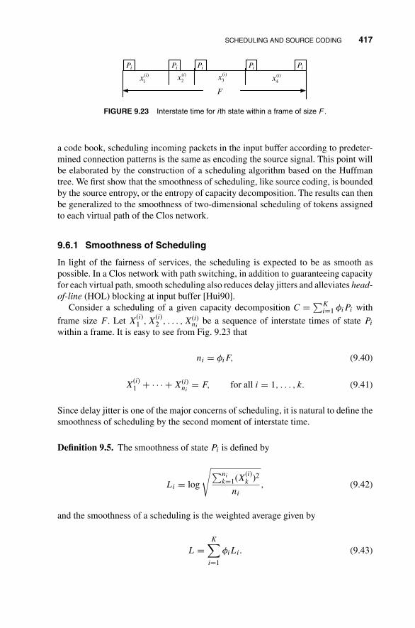
SCHEDULING AND SOURCE CODING 417
Pi Pi Pi Pi Pi(i)1x (i)
2x (i)3x (i)
4x
F
FIGURE 9.23 Interstate time for i th state within a frame of size F .
a code book, scheduling incoming packets in the input buffer according to predeter-mined connection patterns is the same as encoding the source signal. This point willbe elaborated by the construction of a scheduling algorithm based on the Huffmantree. We first show that the smoothness of scheduling, like source coding, is boundedby the source entropy, or the entropy of capacity decomposition. The results can thenbe generalized to the smoothness of two-dimensional scheduling of tokens assignedto each virtual path of the Clos network.
9.6.1 Smoothness of Scheduling
In light of the fairness of services, the scheduling is expected to be as smooth aspossible. In a Clos network with path switching, in addition to guaranteeing capacityfor each virtual path, smooth scheduling also reduces delay jitters and alleviates head-of-line (HOL) blocking at input buffer [Hui90].
Consider a scheduling of a given capacity decomposition C = ∑Ki=1 φiPi with
frame size F . Let X(i)1 , X
(i)2 , . . . , X(i)
nibe a sequence of interstate times of state Pi
within a frame. It is easy to see from Fig. 9.23 that
ni = φiF, (9.40)
X(i)1 + · · · + X(i)
ni= F, for all i = 1, . . . , k. (9.41)
Since delay jitter is one of the major concerns of scheduling, it is natural to define thesmoothness of scheduling by the second moment of interstate time.
Definition 9.5. The smoothness of state Pi is defined by
Li = log
√∑ni
k=1(X(i)k )2
ni
, (9.42)
and the smoothness of a scheduling is the weighted average given by
L =K∑
i=1
φiLi. (9.43)
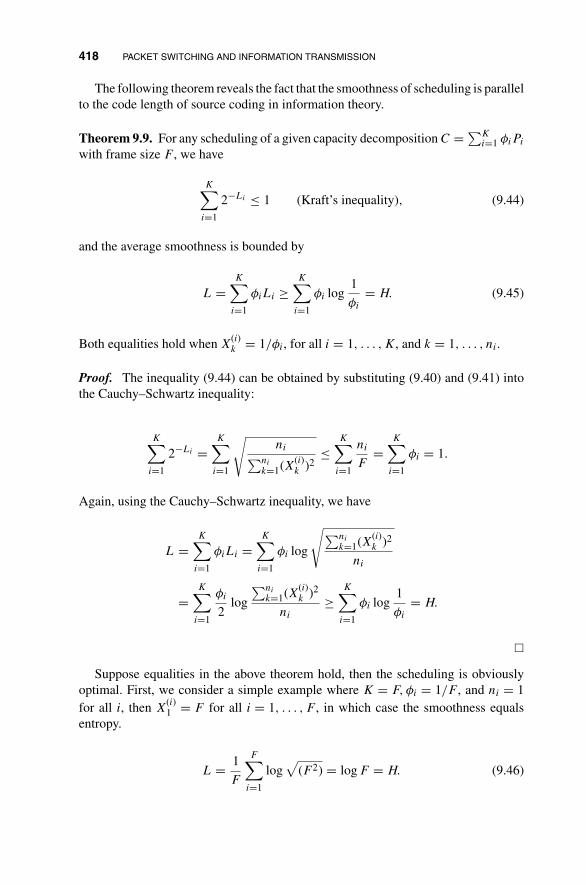
418 PACKET SWITCHING AND INFORMATION TRANSMISSION
The following theorem reveals the fact that the smoothness of scheduling is parallelto the code length of source coding in information theory.
Theorem 9.9. For any scheduling of a given capacity decomposition C = ∑Ki=1 φiPi
with frame size F , we have
K∑i=1
2−Li ≤ 1 (Kraft’s inequality), (9.44)
and the average smoothness is bounded by
L =K∑
i=1
φiLi ≥K∑
i=1
φi log1
φi
= H. (9.45)
Both equalities hold when X(i)k = 1/φi, for all i = 1, . . . , K, and k = 1, . . . , ni.
Proof. The inequality (9.44) can be obtained by substituting (9.40) and (9.41) intothe Cauchy–Schwartz inequality:
K∑i=1
2−Li =K∑
i=1
√ni∑ni
k=1(X(i)k )2
≤K∑
i=1
ni
F=
K∑i=1
φi = 1.
Again, using the Cauchy–Schwartz inequality, we have
L =K∑
i=1
φiLi =K∑
i=1
φi log
√∑ni
k=1(X(i)k )2
ni
=K∑
i=1
φi
2log
∑ni
k=1(X(i)k )2
ni
≥K∑
i=1
φi log1
φi
= H.
�
Suppose equalities in the above theorem hold, then the scheduling is obviouslyoptimal. First, we consider a simple example where K = F, φi = 1/F , and ni = 1for all i, then X
(i)1 = F for all i = 1, . . . , F , in which case the smoothness equals
entropy.
L = 1
F
F∑i=1
log√
(F2) = log F = H. (9.46)

SCHEDULING AND SOURCE CODING 419
P1 P2 P1 P3 P1 P2 P1 P4 P1 P1 P2 P1 P1 P2 P3 P4
(a) Optimal scheduling (b) WFQ scheduling
FIGURE 9.24 Examples of Scheduling.
When all weights are reciprocals of the power of 2, for example φi =1/2, 1/4, 1/8, 1/8, an optimal scheduling can be easily found. An example is shownin Fig. 9.24(a), where F = 8, K = 4, and ni = 4, 2, 1, 1 with respect to state Pi fori = 1, . . . , 4. The scheduling with constant interstate time X(i) = 2, 4, 8, 8 satisfiesboth equalities of Theorem 10.9:
H = L = 1
2· +1
4· 2 + 1
8· 3 + 1
8· 3 = 1.75. (9.47)
Another scheduling based on weighted fair queueing (WFQ) for the same decom-position is shown in Fig. 9.24(b). The smoothness L = 1.8758 is greater than thedecomposition entropy H = 1.75, and the superiority of the optimal scheduling isquite obvious by comparing Fig. 9.24(a) and (b). An upper bound of smoothness isgiven in the following theorem.
Theorem 9.10. For any capacity decomposition C = ∑Ki=1 φiPi, it is always possible
to devise a scheduling whose smoothness L is within 1/2 of decomposition entropy:
H ≤ L < H + 1
2. (9.48)
Proof. Consider a random scheduling without frame structure such that the state Pi ofeach time slot is randomly selected with probability φi. The interstate time X(i) of statePi is a geometric random variable with E[X(i)] = 1/φi and Var[X(i)] = (1 − φi)/φ2
i .The second moment of X(i) and the smoothness of state Pi are given, respectively, asfollows:
E[(X(i))2] = Var[X(i)] + (E[X(i)])2 = 2 − φi
φ2i
(9.49)
and
Li = log√
E[(X(i))2] = 1
2log (2 − φi) + log φi. (9.50)
It is counterintuitive that the smoothness L of random scheduling is not equal to thedecomposition entropy H ; in fact, we have
L =K∑
i=1
φiLi = 1
2
K∑i=1
φi log (2 − φi) + H. (9.51)

420 PACKET SWITCHING AND INFORMATION TRANSMISSION
It is easy to show that the Kullback–Leibler distance L − H reaches the maximumvalue when φ1 = φ2 = · · · = φK = 1
K, in which case we have
L − H = 1
2
K∑i=1
φi log (2 − φi) ≤ 1
2log
(2 − 1
K
)<
1
2. (9.52)
The random scheduling is actually no scheduling at all. Hence, a scheduling algorithm,with or without frame, should exist that satisfies the bound given in (9.48). �
It is obvious that Theorems 9.9 and 9.10 are counterparts of the source codingtheorem stated as follows.
Noiseless Coding Theorem. Let random variable X take the possible valuesx1, . . . , xK with respective probabilities p(x1), . . . , p(xK). Then, the necessary andsufficient condition to encode the values of X in binary prefix code (none of which isan extension of another) of respective lengths L1, . . . , LK is
K∑i=1
2−Li ≤ 1 (Kraft’s inequality). (9.53)
The average code length is bounded by
L =K∑
i=1
p(xi)Li ≥ H(X) =K∑
i=1
p(xi) log1
p(xi)(9.54)
and it is always possible to devise an optimal prefix code for X whose average codelength L is within 1 of entropy:
H(X) ≤ L < H(X) + 1. (9.55)
9.6.2 Comparison of Scheduling Algorithms
The scheduling algorithm for an arbitrary set of decomposition weights φi achievesoptimal smoothness if L = H , which requires the constant interstate time that is equalto the inverse of weight X(i)
k = F/ni = 1/φi for all state Pi. Most proposed schedulingalgorithms are indeed constructed from the reciprocal of the normalized weights. Acomparison of several stereotype algorithms is given below.
9.6.2.1 Weighted Fair Queueing (WFQ) Scheduling Algorithm TheWFQ scheduling algorithm [DKS89] is constructed from the sequence of virtualfinish times 1/φi, 2/φi, . . . of each state Pi with the initial finish time 1/φi. Thealgorithm is given as follows.

SCHEDULING AND SOURCE CODING 421
The WFQ Scheduling Algorithm
Select the state with the smallest finish time and increase its finish time by the inverseof its weight. Repeat this process until the frame size is reached.
We will use the running example of a set of five states P1, P2, P3, P4, and P5with respective weights φ1 = 0.5 and φ2 = φ3 = φ4 = φ5 = 0.125 to illustrate theperformance of the scheduling algorithms presented in this section. The sequencegenerated by WFQ in each time slot τ within a frame is given in Table 9.4, and thefinal sequence is P1P1P1P1P2P3P4P5.
Although the WFQ algorithm properly utilizes the inverse weights in constructingthe scheduling, the above example shows that the sequence generated by WFQ isstill far from the achievable optimal smoothness. Possible amendments to WFQ arediscussed below.
9.6.2.2 WF 2Q Scheduling Algorithm WF2Q is a scheduling algorithm[Zha95] that incorporates the stringent rate requirement of generalized processorsharing (GPS)[PaGa93] in WFQ. Let Ti(τ) be the number of time slots assigned tostate Pi up to time τ, then the WF2Q will select the state Pi that satisfies
Ti(τ − 1) < τ · φi (9.56)
in every time slot τ = 1, 2, . . .. That is, only the states that have started its service inthe corresponding GPS system will be selected. The set of states qualified for selectionin time slot τ is defined by
Qτ = {Pi | Ti(τ − 1) < τ · φi}. (9.57)
Hence, all states are qualified in the first time slot (see Table 9.4), because Ti(0) = 0for all i. The set of qualified states Q1 = {P1P2P3P4P5} is then ordered by their finishtime and the state P1 is selected. In the second time slot, however, T1(1) = 1 and2 · φ1 = 1, so the state P1 cannot be selected and Q2 = {P2P3P4P5}. In each timeslot, whenever a state is selected, like in WFQ, its finish time will be increased by theinverse of its weight.
TABLE 9.4 An Example of WFQ Algorithm
� P1 P2 P3 P4 P5 Selection
1 2 8 8 8 8 P1
2 4 8 8 8 8 P1
3 6 8 8 8 8 P1
4 8 8 8 8 8 P1
5 10 8 8 8 8 P2
6 10 16 8 8 8 P3
7 10 16 16 8 8 P4
8 10 16 16 16 8 P5
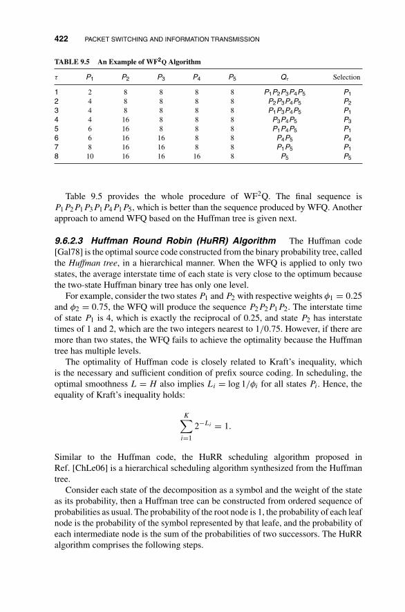
422 PACKET SWITCHING AND INFORMATION TRANSMISSION
TABLE 9.5 An Example of WF2Q Algorithm
� P1 P2 P3 P4 P5 Q� Selection
1 2 8 8 8 8 P1P2P3P4P5 P1
2 4 8 8 8 8 P2P3P4P5 P2
3 4 8 8 8 8 P1P3P4P5 P1
4 4 16 8 8 8 P3P4P5 P3
5 6 16 8 8 8 P1P4P5 P1
6 6 16 16 8 8 P4P5 P4
7 8 16 16 8 8 P1P5 P1
8 10 16 16 16 8 P5 P5
Table 9.5 provides the whole procedure of WF2Q. The final sequence isP1P2P1P3P1P4P1P5, which is better than the sequence produced by WFQ. Anotherapproach to amend WFQ based on the Huffman tree is given next.
9.6.2.3 Huffman Round Robin (HuRR) Algorithm The Huffman code[Gal78] is the optimal source code constructed from the binary probability tree, calledthe Huffman tree, in a hierarchical manner. When the WFQ is applied to only twostates, the average interstate time of each state is very close to the optimum becausethe two-state Huffman binary tree has only one level.
For example, consider the two states P1 and P2 with respective weights φ1 = 0.25and φ2 = 0.75, the WFQ will produce the sequence P2P2P1P2. The interstate timeof state P1 is 4, which is exactly the reciprocal of 0.25, and state P2 has interstatetimes of 1 and 2, which are the two integers nearest to 1/0.75. However, if there aremore than two states, the WFQ fails to achieve the optimality because the Huffmantree has multiple levels.
The optimality of Huffman code is closely related to Kraft’s inequality, whichis the necessary and sufficient condition of prefix source coding. In scheduling, theoptimal smoothness L = H also implies Li = log 1/φi for all states Pi. Hence, theequality of Kraft’s inequality holds:
K∑i=1
2−Li = 1.
Similar to the Huffman code, the HuRR scheduling algorithm proposed inRef. [ChLe06] is a hierarchical scheduling algorithm synthesized from the Huffmantree.
Consider each state of the decomposition as a symbol and the weight of the stateas its probability, then a Huffman tree can be constructed from ordered sequence ofprobabilities as usual. The probability of the root node is 1, the probability of each leafnode is the probability of the symbol represented by that leafe, and the probability ofeach intermediate node is the sum of the probabilities of two successors. The HuRRalgorithm comprises the following steps.

SCHEDULING AND SOURCE CODING 423
The HuRR Scheduling Algorithm
Step 1 Initially set the root to be temporary node PX and S = PX · · · PX to be atemporary sequence.
Step 2 Apply the WFQ to the two successors of PX to produce a sequence T andsubstitute T for the subsequence PX · · · PX of S.
Step 3 If there is no intermediate node in the sequence S, then terminate the algorithm.Otherwise, select an intermediate node PX appearing in S and goto step 2.
The Huffman tree of the previous example is shown in Fig. 9.25; the HuRR schedul-ing algorithm will generate the following sequences:
P1PZP1PZP1PZP1PZ → P1PXP1PYP1PXP1PY
→ P1P2P1P4P1P3P1P5.
In this particular example, the following Huffman code can be generated from thetree depicted in Fig. 9.25:
P1 ←− 0, P2 ←− 100, P3 ←− 101, P4 ←− 110, P5 ←− 111
and the logarithm of interstate time of each state is equal to the length of its Huffmancode. The smoothness of the sequence of this example is the same as that generatedby WF2Q earlier. However, the HuRR outperforms WF2Q in general as demonstratedby the comparison given next.
PY PX 0.25 0.25
P1
0.5
P2
0.125
P3
0.125
P4
0.125 0.125
P5
PZ 0.5
1
FIGURE 9.25 A Huffman tree of HuRR Algorithm.

424 PACKET SWITCHING AND INFORMATION TRANSMISSION
TABLE 9.6 The Smoothness Comparison of Scheduling Algorithms
P1 P2 P3 P4 Random WFQ WF2Q HuRR Entropy
0.1 0.1 0.1 0.7 1.628 1.575 1.414 1.414 1.3570.1 0.1 0.2 0.6 1.894 1.734 1.626 1.604 1.5710.1 0.1 0.3 0.5 2.040 1.784 1.724 1.702 1.6860.1 0.2 0.2 0.5 2.123 1.882 1.801 1.772 1.7610.1 0.1 0.4 0.4 2.086 1.787 1.745 1.745 1.7220.1 0.2 0.3 0.4 2.229 1.903 1.903 1.884 1.8470.2 0.2 0.2 0.4 2.312 2.011 1.980 1.933 1.9220.1 0.3 0.3 0.3 2.286 1.908 1.908 1.908 1.8960.2 0.2 0.3 0.3 2.370 2.016 2.016 1.980 1.971
9.6.2.4 Comparison of Smoothness of Scheduling Algorithms Thesmoothness of preceding scheduling algorithms is compared with random schedul-ing in Table 9.6 to show its progressive improvement. It is clear that the sequencesgenerated by HuRR are, in general, closer to the entropy than the other two. The per-formance of WF2Q is comparable to HuRR, while WFQ is not satisfactory in somecases.
The significance of the Huffman coding scheme lies in the structure of the Huffmantree. By the same token, HuRR, which is also implemented with the Huffman tree, canprovide the best performance in terms of smoothness among the scheduling algorithmsdiscussed in this section. However, HuRR has not yet been proven to be the optimalscheduling algorithm. It is clear that the key to construct optimal scheduling is toexplore the structure of the smoothness Li of each state Pi in a frame of size F andKraft’s inequality that is satisfied by Li, which is mathematically equivalent to thecodeword length in the source coding theorem.
9.6.3 Two-Dimensional Scheduling
The smoothness of scheduling described in the preceding section is for a single-serversystem. However, the capacity matrix decomposition of the packet switch system isa two-dimensional scheduling aimed at multiple inputs and outputs [LiLe00]. Thegeneralization of the smoothness to two-dimensional scheduling is discussed in thissection.
Recall that the capacity matrix C = [cij] of a C(m, n, k) Clos network is a k × k
matrix, where cij is the average number of tokens assigned to the virtual path Vij
between input module i and output module j. If the frame size is F , then the matrixF · C is integer doubly stochastic, such that
∑ki cij = m,
∑kj cij = m.
In the following discussion of two-dimensional smoothness, we will consider,without loss of generality, capacity matrix C = [cij] and
∑Ni cij = 1,
∑Nj cij = 1 of
a crossbar switch for the sake of simplicity. The two-dimensional entropies of thecapacity matrix C are defined as follows.

SCHEDULING AND SOURCE CODING 425
Definition 9.6. Let C = [cij] be a doubly stochastic capacity matrix; the entropy ofinput module i is defined by
Hi = −N∑
j=1
cij log cij, (9.58)
and the set of entropies of input modules is represented by the column vector
H =
⎡⎢⎢⎢⎢⎣
H1
H2
...
HN
⎤⎥⎥⎥⎥⎦ = [
H1, H2, . . . , HN
]T. (9.59)
Similarly, the entropy of output module j is defined by
Hj = −N∑
i=1
cij log cij, (9.60)
and the set of entropies of output modules is represented by the row vector
H = [H1, H2, . . . , HN
]. (9.61)
The entropy of the capacity matrix C is defined by
H(C) =N∑
i=1
Hi =N∑
j=1
Hj = −N∑
j=1
N∑i=1
cij log cij. (9.62)
The smoothness of a two-dimensional scheduling is defined by the intertokentime in the same manner as the interstate time of single-server scheduling. Let nij
be the number of tokens assigned to the virtual path Vij within a frame F , and
y(ij)1 , y
(ij)2 , . . . , y
(ij)nij be the sequence of the intertoken times. We have
nij = cijF, (9.63)
y(ij)1 + y
(ij)2 + · · · + y(ij)
nij= F (9.64)
for all i, j = 1, . . . , N. It should be noted that the number of tokens assigned to avirtual path Vij in a time slot can be more than one if the number of central modules
m > 1, in which case the degenerate intertoken time y(ij)k = 0 will be allowed. The
smoothness of two-dimensional scheduling is defined as follows.

426 PACKET SWITCHING AND INFORMATION TRANSMISSION
Definition 9.7. For a given scheduling of the capacity matrix decomposition C =∑Ki=1 φiPi, the smoothness of the virtual path Vij is defined by
dij = log
√√√√√∑nij
k=1
(y
(ij)k
)2
nij
. (9.65)
The smoothness of input module i is defined by
Di =N∑
j=1
cijdij =N∑
j=1
cij log
√∑nij
k=1(y(ij)k )2
nij
, (9.66)
and the input smoothness is the column vector
D =
⎡⎢⎢⎢⎢⎣
D1
D2
...
DN
⎤⎥⎥⎥⎥⎦ = [
D1, D2, . . . , DN
]T. (9.67)
Similarly, the smoothness of output module j is defined by
Dj =N∑
i=1
cijdij =N∑
i=1
cij log
√∑nij
k=1(y(ij)k )2
nij
, (9.68)
and the output smoothness is the row vector
D = [D1, D2, . . . , DN
](9.69)
The smoothness of the two-dimensional scheduling is defined by
D =N∑
i=1
Di =N∑
j=1
Dj =N∑
j=1
N∑i=1
cijdij. (9.70)
The properties of two-dimensional smoothness are similar to that of single-serverscheduling. The proof of the following theorem is the same as that of Theorem 9.9.
Theorem 9.11. For capacity matrix decomposition C = ∑Ki=1 φiPi with frame size
F , any scheduling satisfies the following smoothness inequalities:
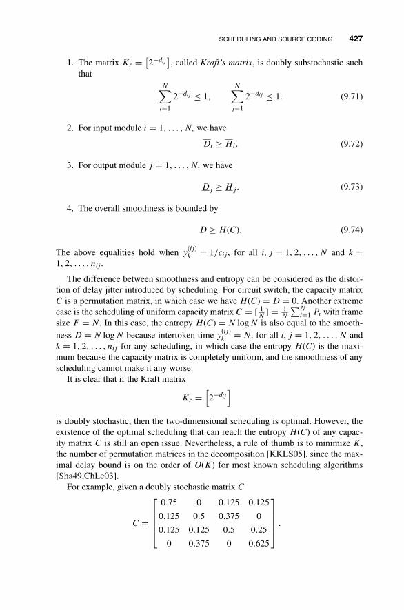
SCHEDULING AND SOURCE CODING 427
1. The matrix Kr = [2−dij
], called Kraft’s matrix, is doubly substochastic such
thatN∑
i=1
2−dij ≤ 1,
N∑j=1
2−dij ≤ 1. (9.71)
2. For input module i = 1, . . . , N, we have
Di ≥ Hi. (9.72)
3. For output module j = 1, . . . , N, we have
Dj ≥ Hj. (9.73)
4. The overall smoothness is bounded by
D ≥ H(C). (9.74)
The above equalities hold when y(ij)k = 1/cij , for all i, j = 1, 2, . . . , N and k =
1, 2, . . . , nij .
The difference between smoothness and entropy can be considered as the distor-tion of delay jitter introduced by scheduling. For circuit switch, the capacity matrixC is a permutation matrix, in which case we have H(C) = D = 0. Another extremecase is the scheduling of uniform capacity matrix C = [ 1
N] = 1
N
∑Ni=1 Pi with frame
size F = N. In this case, the entropy H(C) = N log N is also equal to the smooth-ness D = N log N because intertoken time y
(ij)k = N, for all i, j = 1, 2, . . . , N and
k = 1, 2, . . . , nij for any scheduling, in which case the entropy H(C) is the maxi-mum because the capacity matrix is completely uniform, and the smoothness of anyscheduling cannot make it any worse.
It is clear that if the Kraft matrix
Kr =[2−dij
]is doubly stochastic, then the two-dimensional scheduling is optimal. However, theexistence of the optimal scheduling that can reach the entropy H(C) of any capac-ity matrix C is still an open issue. Nevertheless, a rule of thumb is to minimize K,the number of permutation matrices in the decomposition [KKLS05], since the max-imal delay bound is on the order of O(K) for most known scheduling algorithms[Sha49,ChLe03].
For example, given a doubly stochastic matrix C
C =
⎡⎢⎢⎢⎣
0.75 0 0.125 0.125
0.125 0.5 0.375 0
0.125 0.125 0.5 0.25
0 0.375 0 0.625
⎤⎥⎥⎥⎦ .

428 PACKET SWITCHING AND INFORMATION TRANSMISSION
The input entropy H and output entropy H of matrix C are given, respectively, by
H = [1.0613 1.4056 1.7500 0.9544
]Tand
H = [1.0613 1.4056 1.4056 1.2988
].
The entropy of the capacity matrix C is H(C) = 5.1714. One possible decompositionis given by
8 · C =
⎡⎢⎢⎢⎣
6 0 1 1
1 4 3 0
1 1 4 2
0 3 0 5
⎤⎥⎥⎥⎦ = 4
⎡⎢⎢⎢⎣
1 0 0 0
0 1 0 0
0 0 1 0
0 0 0 1
⎤⎥⎥⎥⎦
+
⎡⎢⎢⎢⎣
1 0 0 0
0 0 1 0
0 1 0 0
0 0 0 1
⎤⎥⎥⎥⎦ +
⎡⎢⎢⎢⎣
1 0 0 0
0 0 1 0
0 0 0 1
0 1 0 0
⎤⎥⎥⎥⎦
+
⎡⎢⎢⎢⎣
0 0 1 0
1 0 0 0
0 0 0 1
0 1 0 0
⎤⎥⎥⎥⎦ +
⎡⎢⎢⎢⎣
0 0 0 1
0 0 1 0
1 0 0 0
0 1 0 0
⎤⎥⎥⎥⎦
in which K = 5 and the permutation matrices are denoted by {P1, P2, . . . , P5}, re-spectively. If the WFQ scheduling algorithm is applied to this set of permutationmatrices, the resulting sequence is
P1P1P1P1P2P3P4P5,
which gives rise to the following two-dimensional scheduled tokens:
a a a a a a b c
b b b b c d d d
c c c c b b a b
d d d d d c c a
where each row corresponds to an output module and the symbols a, b, c, and d
represent the respective tokens assigned to input modules 1–4. The input smoothness

SCHEDULING AND SOURCE CODING 429
of this scheduling is given by
D = [1.2084 1.6997 2.0323 1.3118]
]T,
and the output smoothness is
D = [1.2084 1.7636 1.6997 1.5805
],
which sum up to D = 6.2522. When the HuRR scheduling algorithm is applied tothe same set of permutation matrices, the resulting sequence is
P1P2P1P4P1P3P1P5,
which gives rise to the following two-dimensional scheduled tokens:
a a a b a a a c
b c b d b d b d
c b c a c b c b
d d d c d c d a
This result is obviously smoother than the previous one as evident by the followingsmoothness measures:
D = [1.1250 1.4375 1.7902 1.0267
]Tand
D = [1.1250 1.4375 1.4375 1.3794
],
which sum up to D = 5.3794, an improvement consistent with the comparison ofsingle-server scheduling described in the preceding section.
Suppose we consider another capacity matrix decomposition
8 · C =
⎡⎢⎢⎢⎣
0 0 1 0
1 0 0 0
0 1 0 0
0 0 0 1
⎤⎥⎥⎥⎦ +
⎡⎢⎢⎢⎣
0 0 0 1
0 0 1 0
1 0 0 0
0 1 0 0
⎤⎥⎥⎥⎦
+2
⎡⎢⎢⎢⎣
1 0 0 0
0 0 1 0
0 0 0 1
0 1 0 0
⎤⎥⎥⎥⎦ + 4
⎡⎢⎢⎢⎣
1 0 0 0
0 1 0 0
0 0 1 0
0 0 0 1
⎤⎥⎥⎥⎦
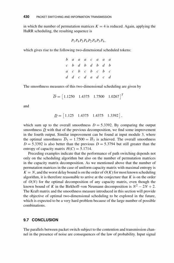
430 PACKET SWITCHING AND INFORMATION TRANSMISSION
in which the number of permutation matrices K = 4 is reduced. Again, applying theHuRR scheduling, the resulting sequence is
P1P4P3P4P2P4P3P4,
which gives rise to the following two-dimensional scheduled tokens:
b a a a c a a a
c b d b d b d b
a c b c b c b c
d d c d a d c d
The smoothness measures of this two-dimensional scheduling are given by
D = [1.1250 1.4375 1.7500 1.0267
]Tand
D = [1.125 1.4375 1.4375 1.3392
],
which sum up to the overall smoothness D = 5.3392. By comparing the outputsmoothness D with that of the previous decomposition, we find some improvementin the fourth output. Similar improvement can be found at input module 3, wherethe optimal smoothness D3 = 1.7500 = H3 is achieved. The overall smoothnessD = 5.3392 is also better than the previous D = 5.3794 but still greater than theentropy of capacity matrix H(C) = 5.1714.
Preceding examples indicate that the performance of path switching depends notonly on the scheduling algorithm but also on the number of permutation matricesin the capacity matrix decomposition. As we mentioned above that the number ofpermutation matrices in the case of uniform capacity matrix with maximal entropy isK = N, and the worst delay bound is on the order of O(K) for most known schedulingalgorithm, it is therefore reasonable to arrive at the conjecture that K is on the orderof O(N) for the optimal decomposition of any capacity matrix, even though theknown bound of K in the Birkhoff–von Neumann decomposition is N2 − 2N + 2.The Kraft matrix and the smoothness measure introduced in this section will providethe objective of optimal two-dimensional scheduling to be explored in the future,which is expected to be a very hard problem because of the large number of possiblecombinations.
9.7 CONCLUSION
The parallels between packet switch subject to the contention and transmission chan-nel in the presence of noise are consequences of the law of probability. Input signal

CONCLUSION 431
to transmission is a function of time, the main theorem on noisy channel coding be-ing based on the law of large number. On the other hand, the input signal to switchis a function of space, and both theorems on deflection routing and smoothness ofscheduling are proved on the ground of randomness. In both systems, the randomdisturbances are tamed by means of similar mathematical tools aimed for reliablecommunication.
The communication network has gone through two phases of quantization in thepast century. The first phase was the quantization of transmission channels, fromanalog to digital, based on the sampling theorem of bandlimited signal. The secondphase is the quantization of the switching system, from circuit switching to packetswitching. The comparisons provided in this chapter demonstrate that the schedulingbased on capacity matrix decomposition serves the same function as the samplingtheorem to reduce the complexity of communication.
The concept of path switching can be further extended to the network level to copewith resource contentions. A connection-oriented subnetwork with predeterminedtopology and bandwidth can be embedded in the current IP network for supportingQoS of real-time services such as voice or video over IP. The scheduling of pathswitching in conjunction with the routing scheme of multiprotocol label switching(MPLS) will provide a platform to support different traffic classes of differentiatedservices (DiffServ) [Law01,TAPF01]. The predetermined paths of label switchedsubnetwork are similar to the subway system embedded in the public transportationnetwork. It will provide a coherent end-to-end QoS solution to the multilevel resourceallocation [LeLa97] issues arising from real-time services. First, the predeterminedconnection patterns at each router are contention-free at the packet level. Next, theperiodic connection patterns are frame based, and the bandwidth assigned to eachsession is fixed at burst level within each frame. Finally, the stable capacity of eachsession is guaranteed at call level. The traffic engineering of this Internet subwaysystem could be a challenging networking research area in the future.


Bibliography
[Abr63] N. Abramson, Information Theory and Coding, New York: McGraw-Hill, 1963.
[ABF01] M. Allman, H. Balakrishnan, and S. Floyd, “Enhancing TCPs Loss Recovery UsingLimited Transmit,” RFC 3042, 2001.
[ADL95] J. S. Ahn, P. B. Danzig, Z. Liu, and L. Yan, “Evaluation with TCP Vegas: Emulationand Experiment,” ACM SIGCOMM Comput. Commun. Rev., Vol. 25, No. 4, 1995,pp. 185–195.
[AhD89] H. Ahmadi and W. Denzel, “A Survey of Modern High-Performance Switch Fabricfor Integrated Circuit and Packet Switching,” IEEE J. Select. Areas Commun.,Vol. 7, No. 7, 1989.
[AKS83] M. Ajtai, J. Komlos, and E. Szemeredi, “An O(n log n) Sorting Network,” Proceed-ings of the 15th ACM Symposium on Theory of Computation, 1983, pp. 1–9.
A significant theoretical breakthrough: the firstO(n log n) sorting network. The constant in front of then log n, however, is rather large, rendering this net-work impractical.
[AMS81] D. Anick, D. Mitra, and M. M. Sondhi, “Stochastic Theory of a Data-HandlingSystem with Multiple Sources,” Bell Syst. Tech. J., Vol. 61, No. 8, 1982, pp. 1871–1894.
The original work on the application of the fluid-flow model that led to much subsequent work by others.This book attempts to simplify the presentation in thepaper to make the theory more accessible to undergrad-uate students. Some details have been omitted.
[Bar64] P. Baran, “On Distributed Communications Networks,” IEEE Trans. Commun.,Vol. 12, 1964, pp. 1–9.
The first paper on deflection routing (called hot-potato routing in the paper) in the context of wide-area communications networks.
Principles of Broadband Switching and Networking, by Tony T. Lee and Soung C. LiewCopyright © 2010 John Wiley & Sons, Inc.
433
434 BIBLIOGRAPHY
[Bat68] K. E. Batcher, “Sorting Networks and Their Applications,” AFIPS Proceeding ofthe Spring Joint Computer Conference, 1968, pp. 307–314.
The seminal work by Batcher on the bitonic and odd–even sorting networks. Although both networks areO(n log2 n), they remain perhaps the most implementablenetworks in practice throughout all these yearsbecause of their simple structures.
[Bat76] K. E. Batcher, “The Flip Network in STARAN,” Proceedings of the 1976 Interna-tional Conference on Parallel Processing, 1976, pp. 65–71.
[BBB87] A. Bertossi, G. Bongiovanni, and M. Bonuccelli, “Time Slot Assignment inSS/TDMA Systems with Intersatellite Links,” IEEE Trans. Commun., Vol. 35,No. 6, 1987, pp. 602–608.
[BeG92] D. Bertsekas and R. Gallager, Data Networks, 2nd edition, Prentice-Hall, 1992.
A widely used graduate-level course book. Highlyanalytical compared to other books in the same area.Mostly about traditional data networks, althoughmany of the issues remain valid even for broadbandnetworks.
[Bel81] J. Bellamy, Digital Telephony, Wiley, 1982.
An excellent reference book for modern telephonesystems.
[Ben63] V. E. Benes, “A Thermodynamics Theory of Traffic in Telephone Systems,” BellSyst. Tech. J., Vol. 42, 1963, pp. 567–607.
[Ben65] V. E. Benes, Mathematical Theory of Connecting Networks and Telephone Traffic,Academic Press, 1965.
The first book on switching theory. Highly mathemati-cal.
[BiB88] B. Bingham and H. Bussey, “Reservation-Based Contention Resolution Mechanismfor Batcher–Banyan Packet Switches,” Electron. Lett., Vol. 24, No. 13, 1988, pp.772–773.
On using a ring contention-resolution scheme for aninput-buffered switch.
[Bir46] G. Birkhoff, “Tres observaciones sobre el algebra lineal,” Universidad Nacionalde Tucuman Revista (Serie A), Vol. 5, 1946, pp. 147–151.
[BOP94] L. S. Brakmo, S. W. O’Malley, and L. L. Peterson, “TCP Vegas: New Techniquesfor Congestion Detection and Avoidance,” Proceedings of ACM SIGCOMM94,No. 4, October 1994, pp. 24–35.
[BP95] L. S. Brakmo and L. L. Peterson, “TCP Vegas: End to End Congestion Avoidanceon a Global Internet,” IEEE J. Select. Areas Commun., Vol. 13, No. 8, 1995, pp.1465–1480.
[ByL94] J. W. Byun and T. T. Lee, “The Design and Analysis of an ATM Multicast Switchwith Adaptive Traffic Controller,” IEEE/ACM Trans. Networking, Vol. 2, No. 3,1994, pp. 288–298.
Much of the discussion in Section 6.1.2 is based onthis work.

BIBLIOGRAPHY 435
[Can71] D. Cantor, “On Non-Blocking Switching Networks,” Networks, Vol. 1, 1971.
The original paper on Cantor Networks.
[CCH00] C. S. Chang, W. J. Chen, and H. Y. Huang, “Birkhoff–von Neumann input bufferedcrossbar switches,” INFOCOM 2000: Proceedings of the 19th Annual JointConference of the IEEE Computer and Communications Societies, Vol. 3, IEEE,2000, pp. 1614–1623.
[Cha91] H. J. Chao, “A Recursive Modular Terabit/Second ATM Switch,” IEEE J. Select.Area Commun., Vol. 9, No. 8, 1991, p. 1161.
[ChJi03] H. Chao, Z. Jing, and S. Liew, “Matching Algorithms for Three-Stage BufferlessClos Network Switches,” IEEE Commun. Mag., Vol. 41, No. 10, 2003, pp. 46–54.
[ChL91] C. J. Chang and C. J. Ling, “Overflow Controller in Copy Network of BroadbandPacket Switch,” Electron. Lett., Vol. 27, No. 11, 1991, pp. 937–939.
[ChLe03] M. C. Chan and T. Lee, “Statistical Performance Guarantees in Large-Scale Cross-Path Packet Switch,” IEEE/ACM Trans. Networking, Vol. 11, 2003, pp. 325–337.
[ChLe06] M. T. Choy and T. T. Lee, “Huffman Fair Queueing: A Scheduling AlgorithmProviding Smooth Output Traffic,” ICC 06, IEEE, June 2006.
[ChLi91] H. J. Chao and S. C. Liew, “Architecture Design for ATM Statistical Multiplexers,”Int. J. Digital Analog Commun. Syst., Vol. 4, No. 4, 1991, pp. 239–248.
[ChLi95] T. M. Chen and S S. Liu, ATM Switching Systems, Artech House, 1995.
A book that attempts to include control and manage-ment functions in the examination of the ATM switchingsystem. It contains useful information on the SONETand ATM standards for interested readers. Its focusis more about how rather than why things are done in acertain way.
[Cho91] C.-H. Chow, “On Multicast Path Finding Algorithm,” Conference Record, IEEEInfocom’91, pp. 1274–1283.
On finding a multicast tree for a multicast connectionover wide-area networks.
[ChS91] J.S.-C. Chen and T. E. Stern, “Throughput Analysis, Optimal Buffer Allocation,and Traffic Imbalance Study of a Generic Nonblocking Packet Switch,” IEEE J.Select. Areas Commun., Vol. 9, No. 3, 1991, pp. 439–449.
[CJ89] D. M. Chiu and R. Jain, “Analysis of Increase and Decrease Algorithms for Con-gestion Avoidance in Computer Network,” Comput. Networks ISDN Syst., Vol. 17,1989.
[Clo53] C. Clos, “A Study of Non-Blocking Switch Network,” Bell Syst. Tech. J., Vol. 32,1953, pp. 406–424.
The seminal paper by Clos on Clos networks.
[DeD87] M. De Prycker and M. Desomer, “Performance of a Service Independent SwitchingNetwork with Distributed Control,” IEEE J. Select. Areas Commun., Vol. 5, 1987,pp. 1293–1301.
[DeP93] M. De Prycker, Asynchronous Transfer Mode: Solution for Broadband ISDN, 2ndedition, Ellis Horwood, 1993.
A good reference book on details of the ATM standardand reasons why ATM was originally proposed.

436 BIBLIOGRAPHY
[Des88] A. Descloux, “Contention Probabilities in Packet Switching Networks with StrungInput Processes,” Proceedings of the ITC 12, 1988.
[DGH87] C. Day, J. Giacopelli, and J. Hickey, “Applications of Self-Routing Switches toLATA Fiber Optic Networks,” Proceedings of ISS ’87, March 1987.
[DiJ81] D. M. Dias and J. R. Jump, “Analysis and Simulation of Buffered Delta Network,”IEEE Trans. Comput., Vol. C-30, 1981, pp. 273–282.
[DKS89] A. Demers, S. Keshav, and S. Shenker, “Analysis and Simulation of a Fair QueueingAlgorithm,” Proceedings of the ACM Sigcomm, 1989, pp. 3–12.
[DyS95] D. E. McDysan and D. L. Spohn, ATM: Theory and Application, McGraw-Hill,1995.
A reference book that is suitable for network managersand engineers who want to have an overall but not nec-essary in-depth (i.e., research-level) understandingof ATM networking.
[EcH88] A. E. Eckberg and T. C. Hou, “Effects of Output Buffer Sharing on Buffer Require-ments in an ATDM Packet Switch,” Proceedings of INFOCOM’88.
An analysis of the advantage of having the outputs ofthe switch share a common buffer.
[EHY] K. Eng, M. Hluchyj, and Y. Yeh, “A Knockout Switch for Variable-Length Packets,”IEEE J. Select. Areas Commun., Vol. 5, No. 9, 1987.
The original paper on the Knockout switch.
[EKY] K. Y. Eng, M. J. Karol, and Y. S. Yeh, “A Growable Packet (ATM) Switch Archi-tecture: Design Principles and Applications,” Conference Record, Globecom ’89,pp. 32.2.1–32.2.7.
[EpHa98] A. Ephremides and B. Hajek, “Information Theory and Communication Networks:An Unconsummated Union,” IEEE Trans. Inform. Theory, Vol. 44, 1998, pp. 2416–2434.
[FH99] S. Floyd, and T. Henderson, “The NewReno Modification to TCP¡¯s Fast RecoveryAlgorithm,” RFC 2582, April 1999.
[Fu01] C. P. Fu, “TCP Veno: End-to-End Congestion Control over Heterogeneous Net-works,” Ph.D. Dissertation, The Chinese University of Hong Kong, August2001.
[Gal62] R. Gallager, “Low-Density Parity-Check Codes,” IEEE Trans. Inform. Theory, Vol.8, No. 1, 1962, pp. 21–28.
[Gal65] R. Gallager, “A Simple Derivation of the Coding Theorem and Some Applications,”IEEE Trans. Inform. Theory , Vol. 11, No. 1, 1965, pp. 3–18.
[Gal78] R. Gallager, “Variations on a Theme by Huffman,” IEEE Trans. Inform. Theory,Vol. 24, No. 6, 1978, pp. 668–674.
[Ger98] M. Gerla, E. Leonardo, F. Neri, and P. Panalti, “Minimum Distance Routing inBidirectional Shufflenet,” IEEE INFOCOM ’98.
[GHM91] J. N. Giacopelli, J. J. Hickley, W. S. Marcus, W. D. Sincoskie, and M. Littlewood,“Sunshine: A High Performance Self-Routing Broadband Packet Switch Architec-ture,” IEEE J. Select. Areas Commun., Vol. 9, No. 8, 1991, p. 1289.
On a Batcher–banyan switch architecture.

BIBLIOGRAPHY 437
[GAC86] P. Gonet, P. Adams, and J. P. Courdreuse, “Asynchronous Time-Division Switch-ing: The Way to Flexible Broadband Communication Networks,” Proceedings ofthe IEEE 1986 International Zurich Seminar on Digital Communications, Zurich,Switzerland, March 1986.
The people who first proposed ATM.
[Haj88] K. Hajikano, K. Murakami, E. Iwabuchi, O. Isono, and T. Kobayashi, “Asyn-chronous Transfer Mode Switching Architecture for Broadband ISDN,” ConferenceRecord, IEEE ICC’88, pp. 911–915.
[Haj89] B. Hajek, “Bounds on Evacuation Time for Deflection Routing,” Distributed Com-puting, Springer-Verlag, Vol. 5, 1991, pp. 1–6.
[Hal35] P. Hall, “On Representatives of Subsets,” J. London Math. Soc., Vol. 10, 1935, pp.26–30.
[Ham86] R. W. Hamming, Coding and Information Theory, Englewood Cliffs, NJ: Prentice-Hall, 1986.
[HBM91] J. F. Hayes, R. Breault, and M. K. Mehmet-Ali, “Performance Analysis ofa Multicast Switch,” IEEE Trans. Commun., Vol. 39, No. 4, 1991, pp. 581–587.
[HlK88] M. G. Hluchyj and M. J. Karol, “Queueing in High-Performance Packet Switching,”IEEE J. Select. Areas Commun., Vol. 6, No. 9, 1988, pp. 1587–1597.
Analysis on output-buffered and input-bufferedswitches.
[HuA87] Y. N. J. Hui and E. Arthurs, “A Broadband Packet Switch for Integrated Transport,”IEEE J. Select. Areas Commun., Vol. 5, No. 8, 1987, pp. 1264–1273.
The original paper on the three-phase algorithmapplied on a Batcher–banyan input-buffered switch.
[Hui88] J. Hui, “Resource Allocation for Broadband Networks,” IEEE J. Select. AreasCommun., Vol. 6, No. 9, 1988.
[Hui90] J. Hui, Switching and Traffic Theory for Integrated Broadband Networks, KluwerAcademic Publishers, 1990.
A good reference book for circuit and fast-packetswitching as well as the mathematical tools used toanalyze broadband network performance. Requires thereaders to have a certain level of mathematical matu-rity. Suitable textbook for a graduate-level course.
[HuK84] A. Huang and S. Knauer, “Starlite: A Wideband Digital Switch,” Proceeding ofGlobecom ’84, pp. 121–125.
The Batcher–banyan switch structure was originallyproposed here.
[HuKa95] J. Y. Hui and E. Karasan, “A Thermodynamic Theory of Broadband Networks withApplication to Dynamic Routing,” IEEE J. Select. Areas Commun., Vol. 13, 1995,pp. 991–1003.
[Ino79] H. Hiroshi, Digital Integrated Communications Systems, University of Tokyo Press,1979.
[Inu79] T. Inukai, “An Efficient SS/TDMA Time Slot Assignment Algorithm,” IEEE Trans.Commun., Vol. 27, No. 10, 1979, pp. 1449–1455.

438 BIBLIOGRAPHY
[Jac88] V. Jacobson, “Congestion Avoidance and Control,” ACM SIGCOMM 88, August1988.
[Jaj03] A. Jajszczyk, “Nonblocking, Repackable, and Rearrangeable Clos Networks: FiftyYears of the Theory Evolution,” IEEE Commun. Mag. , Vol. 41, No. 10, 2003, pp.28–33.
[JaG93] A. Jajszczyk and G. Jekel “A New Concept—Repackable Networks,” IEEE Trans.Commun., Vol. 41, No. 8, 1993, pp. 1232–1237.
[Jain89] R. Jain, “A Delay-Based Approach for Congestion Avoidance in InterconnectedHeterogeneous Computer Networks,” ACM Comput. Commun. Rev., Vol. 19, No.5, 1989.
[KaJ91] M. Kawarasaki and B. Jabbari, “B-ISDN Architecture and Protocol,” IEEE J. Select.Areas Commun., Vol. 9, 1991, pp. 1405–1415.
[KeK79] P. Kermani and L. Kleinrock, “Virtual Cut-Through: A New Computer Communi-cation Switching Technique,” Comput. Networks, Vol. 3, 1979, pp. 167–286.
[Kes91] S. Keshav, “A Control-Theoretic Approach to Flow Control,” SIGCOMM91,September 1991.
[KHM87] M. J. Karol, M. G. Hluchyj, and S. P. Morgan, “Input vs. Output Queuing on aSpace Division Packet Switch,” IEEE Trans. Commun., Vol. 35, No. 12, 1987, pp.1347–1356.
[KiK80] C. Kittel and H. Kroemer, Thermal Physics, New York: W. H. Freeman, 1980.
[KiL88] H. S. Kim and A. Leon-Garcia, “Performance of Buffered Banyan Networks UnderNonuniform Traffic Patterns,” INFOCOM ’88, New Orleans, March 1988.
[KKLS05] I. Keslassy, M. Kodialam, T. V. Lakshman, and D. Stiliadis, “On GuaranteedSmooth Scheduling for Input-Queued Switches,” IEEE/ACM Trans. Networking,Vol. 13, No. 6, 2005, pp. 1364–1375.
[Kle75] L. Kleinrock, Queueing Systems Theory, Vol. 1, Wiley, 1975.
[Klei75] L. Kleinrock, Queueing Systems, Computer Applications, Vol. 2, New York: Wiley,1975.
[Knu81] D. E. Knuth, The Art of Computer Programming, Sorting and Searching, Addison-Wesley, Vol. III, 1981.
[Kot33] V. A. Kotelnikov, “On the Carrying Capacity of the Ether and Wire in Telecom-munications,” Material for the First All-Union Conference on Questions of Com-munication, Izd. Red. Upr. Svyazi RKKA, Moscow (Russian), 1933.
[KrH90] A. Krishna and B. Hajek, “Performance of Shuffle-Like Switching Networks withDeflection,” Proceedings of IEEE INFOCOM’90 , San Francisco, CA, pp. 473–480.
[KrS83] C. P. Kruskal and M. Snir, “The Performance of Multistage Interconnection Net-works for Multiprocessors” IEEE Trans. Comput., Vol. 32, No. 12, 1983.
[KuJ86] M. Kumar and J. R. Jump, “Performance of Unbuffered Shuffle-Exchange Net-works” IEEE Trans. Comput., Vol. 35, No. 6, 1986, pp. 573–577.
[Kuw89] H. Kuwahara, et al., “A shared buffer memory switch for an ATM exchange,”Conference Record, ICC’89, Vol. 1, pp. 118–122.
[Lai95] C. W. Lai and S. C. Liew, “A Framework for Statistical Multiplexing onto a Variable-Bit Rate Output Channel,” IEEE INFOCOM ’95, pp. 394–401.

BIBLIOGRAPHY 439
[LaP80] D. H. Lawrie and D. A. Padua, “Analysis of Message Switching with Shuffle-Exchanges in Multiprocessors,” Proceedings of the Workshop on InterconnectionNetworks for Parallel and Distributed Processing, 1980, pp. 116 – 123. Alsoreprinted in Ref. [WuF84].
[Law01] J. Lawrence, “Designing Multiprotocol Label Switching Networks,” IEEE Com-mun. Mag., Vol. 39, No 7, 2001, pp. 134–142.
[Law75] D. Lawrie, “Access and Alignment of Data in an Array Processor,” IEEE Trans.Comput., Vol. C-24, No. 12, 1975, pp. 1145–55.
[Lea86] C. T. Lea, “The Load-Sharing Banyan Network,” IEEE Trans. Comput., Vol. 35,1986, pp. 1025–1034.
[Lee88] T. T. Lee, “Non-Blocking Copy Networks for Multicast Packet Switching,” IEEEJ. Select. Areas Commun., Vol. 6, No. 9, 1988, pp. 1455–1467.
[Lee90] T. T. Lee, “A Modular Architecture for Very Large Packet Switches,” IEEE Trans.Commun., Vol. 6, No. 9, 1990, pp. 1455–1467.
[Lee93] T. T. Lee, “Parallel Communications for ATM Network Control and Management,”IEEE Globecom ’93.
[LeL94] T. T. Lee and S. C. Liew, “Broadband Packet Switches based on Dilated Intercon-nected Networks,” IEEE Trans. Commun., Part I of 3 parts, Vol. 42, No. 2/3/4,1994, pp. 732–744.
[LeLa97] T. T. Lee and C. H. Lam, “Path Switching: A Quasi-Static Route Scheme forLarge-Scale ATM Switches,” IEEE J. Select. Areas Commun., Vol. 15, No. 5, 1997,pp. 914–924.
[LeLi02] T. T. Lee and S. Y. Liew, “Parallel Routing Algorithms in Benes–Clos Networks,”IEEE Trans. Commun., Vol. 50, No 11, 2002, pp. 1841–1847.
[LeTo98] T. T. Lee and P. P. To, “Non-Blocking Routing Properties of Clos Networks,”DIMACS: Series in Discrete Mathematics and Theoretical Computer Science,American Mathematical Society, 1998, pp. 181–195.
[LeWi00] A. Leon-Garcia and I. Widjaja, Communication Networks, McGraw-Hill, 2000.
[Lie89] S. C. Liew, “Comments on ‘Fundamental Conditions Governing TDM SwitchingAssignments in Terrestrial and Satellite Networks’,” IEEE Trans. Commun., Vol.37, No. 2, 1989, pp. 187–189.
[Lie94a] S. C. Liew, “Performance of Various Input-Buffered and Output-Buffered ATMSwitch Design Principles Under Bursty Traffic: Simulation Study,” IEEE Trans.Commun., part II of 3 parts, Vol. 42, No. 2/3/4, 1994, pp. 1371–1379.
[Lie94b] S. C. Liew, “Multicast Routing in 3-Stage Clos ATM Switching Networks,” IEEETrans. Commun., part II of 3 parts, Vol. 42, No. 2/3/4, 1994, pp. 1380–1390.
[Lie95] S. C. Liew, “A General Packet Replication Scheme for Multicast in InterconnectionNetworks,” IEEE INFOCOM ’95, pp. 394–401.
[Liew99] S. Y. Liew, “Real Time Scheduling in Large Scale ATM Cross-Path Switch,” Ph.D.Dissertation, The Chinese University of Hong Kong, July 1999.
[LiL89] S. C. Liew and K. W. Lu, “A 3-Stage Interconnection Structure for Very LargePacket Switches,” Int. J. Digital Analog Cabled Syst., Vol. 2, 1989, pp. 303–316.
[LiL91] S. C. Liew and K. W. Lu, “Comparison of Buffering Strategies for AsymmetricPacket Switch Modules,” IEEE J. Select. Areas Commun., 1991, pp. 428–438.

440 BIBLIOGRAPHY
[LiL94] S. C. Liew and T. T. Lee, “N log N Dual Shuffle-Exchange Network with Error-Correcting Routing,” IEEE Trans. Commun., part I of 3 parts, Vol. 42, No. 2/3/4,1994, pp. 754–766.
[LiL95] S. C. Liew and T. T. Lee, “SKEL: A Fundamental Property desirable in ATMSwitches for Simple Traffic Management: Illustration with Generic Output-Buffered and Input-Buffered Switches,” Perform. Evaluation, Vol. 25, No. 4, 1996,pp. 247–266.
[LiLe89] S.-Q. Li and M. J. Lee, “A Study of Traffic Imbalances in a Fast Packet Switch,”Conference Record, ICC’89, pp. 538–545.
[LiLe00] S. Y. Liew and T. T. Lee, “Bandwidth Assignment with QoS Guarantee in a Classof Scalable ATM Switches,” IEEE Trans. Commun., Vol. 483, 2000, pp. 377–380.
[LLL83] J. Lewandowski, J. Liu, and C. Liu, “SS/TDMA Time Slot Assignment withRestricted Switching Modes,” IEEE Trans. Commun., Vol. 31, No. 1, 1983, pp.149–154.
[LLL86] J. L. Lewandowski, C. L. Liu, and J. W. S. Liu, “An Algorithmic Proof of a Gen-eralization of the Birkhoff–von Neumann Theorem”, J. Algorithms, Vol. 7, 1986,pp. 323–330.
[Mac03] D. J. C. MacKay, Information Theory, Inference, and Learning Algorithms,Cambridge: Cambridge University Press, 2003.
[Mas84] J. Massey, “Information Theory: The Copernican System of Communications,”IEEE Commun. Mag., Vol. 22, No. 12, 1984, pp. 26–28.
[Max87] N. F. Maxemchuk, “Routing in the Manhattan Street Network,” IEEE Trans. Com-mun., Vol. 35, No. 5, 1987, pp. 503–512.
[Max89] N. F. Maxemchuk, “Comparison of Deflection and Store and Forward Techniquesin the Manhattan Street Network and Shuffle Exchange Networks.” Proceedingsof INFOCOM’89, April 1989, pp. 800-809.
[McK99] N. McKeown, “The iSLIP Scheduling Algorithm for Input-Queued Switches,”IEEE/ACM Trans. Networking, Vol. 7, No. 2, 1999, pp. 188–201.
[MeT89] R. Melen and J. S. Turner, “Nonblocking Networks for Fast Packet Switching,”Proceedings of IEEE INFOCOM’89, April 1989, pp. 548–557.
[MeT93] R. Melen and J. S. Turner, “Nonblocking Multirate Distribution Networks,” IEEETrans. Commun., Vol. 41, No. 2, 1993.
[MM96] M. Mathis and J. Mahdavi, “Forward Acknowledgment: Refining TCP CongestionControl,” Proceedings of SIGCOMM96, August 1996.
[MMFR96]M. Mathis, J. Mahdavi, S. Floyd, and A. Romanow “TCP Selective Acknowledge-ment Options,” RFC 2018, October 1996.
[New88] P. Newman, “A Fast Packet Switch for the Integrated Services Backbone Network,”IEEE J. Select. Areas Commun., Vol. 6, No. 9, 1988, pp. 1468–1479.
[Nyq28] H. Nyquist, “Certain Topics in Telegraph Transmission Theory”, Trans. AIEE, Vol.47, 1928, pp. 617–644.
[Oie89] Y. Oie, M. Murata, K. Kubota, and H. Miyahara, “Effect of Speedup in NonblockingPacket Switch,” Conference Record, ICC’89, Vol. 1, pp. 410–415.
[OpT71] D. C. Opferman and N. T. Tsao-Wu, “On a Class of Rearrangeable SwitchingNetworks,” Bell Syst. Tech. J., Vol. 50, 1971, pp. 1579–1618.

BIBLIOGRAPHY 441
[PaGa93] A. Parekh and R. Gallager, “A Generalized Processor Sharing Approach to FlowControl in Integrated Services Networks: The Single-Node Case,” IEEE/ACMTrans. Networking, Vol. 1, No. 3, 1993, pp. 344–357.
[Pau62] M. C. Paull, “Reswitching of Connection Networks,” Bell Syst. Tech. J., Vol. 41,1962, pp. 833–855.
[Par94] C. Partridge, Gigabit Networking, Addison-Wesley, 1994.
[Pat81] J. H. Patel, “Performance of Processor–Memory Interconnections for Multiproces-sors,” IEEE Trans. Comput., Vol. 30, 1981, pp. 771–780.
[Pat88] A. Pattavina, “Multichannel Bandwidth Allocation in a Broadband Packet Switch,”IEEE J. Select. Areas Commun., Vol. 6, No. 9, 1988, pp. 1489–1499.
[Pea77] M. C. Pease, “The Indirect Binary n-Cube Microprocessor Array,” IEEE Trans.Comput., Vol. C-26, 1977, pp. 458–473.
[PG99] C. Parsa and J.J. Garcia-Luna-Aceves, “Improving TCP Congestion Control overInternet with Heterogeneous Transmission Media,” Proceeding of IEEE ICNP99.
[Rad67] R. Rado, “On the Number of Systems of Distinct Representatives of Sets,”J. London Math. Soc., Vol. 42, 1967, pp. 107–109.
[Rob93] T. G. Robertazzi (Ed.), Performance Evaluation of High Speed Switching Fabricsand Networks: ATM, Broadband ISDN, and MAN Technology, Collection of Papers,IEEE Press, 1993.
[Sak90] Y. Sakurai, N. Ido, S. Gohara, and N. Endo, “Large-Scale ATM Multi-Stage Switch-ing Network with Shared Buffer Memory Switches, ” Proceedings of ISS ’90, Vol. 4,pp. 121–126.
[SaZ95] S. Sibal and J. Zhang “On a Class of Banyan Networks and Tandem Banyan Switch-ing Fabrics,” IEEE Trans. Commun., Vol 43, No. 7, 1995, pp. 2231–2240.
[Sch87] M. Schwartz, Telecommunication Networks, Protocols, Modeling, and Analysis,Addison-Wesley, 1987.
[Sha48] C. E. Shannon, “A Mathematical Theory of Communication,” Bell Syst. Tech. J.,Vol. 27, 1948, pp. 379–423 (Part I), pp. 623–656 (Part II).
[Sha49] C. E. Shannon, “Communication in the Presence of Noise,” Proceedings of Instituteof Radio Engineers, Vol. 37, January 1949, pp. 10–21.
[Sha50] C. E. Shannon, “Memory Requirements in a Telephone Exchange,” Bell Syst. Tech.J., Vol. 29, 1950, pp. 343–349.
[Sch87] M. Schwartz, Telecommunication Networks Protocols, Modeling and Analysis,Addison-Wesley, 1987.
[Sie85] H. J. Siegel, Interconnection Networks for Large-Scale Parallel Processing, Lex-ington Books, 1985.
[SiSp96] M. Sipser and D. Spielman, “Expander Codes,” IEEE Trans. Inform. Theory, Vol.42, No. 6, 1996, pp. 1710–1722.
[Sta95] W. Stallings, ISDN and Broadband ISDN with Frame Relay and ATM, Prentice-Hall, 1995.
[Sto71] H. S. Stone, “Parallel Processing with the Perfect Shuffle,” IEEE Trans. Comput.,Vol. C-20, 1971, pp. 153–161.
[Str86] G. Strang, Introduction to Applied Mathematics, Wellesley, MA: Wellesley-Cambridge Press, 1986.

442 BIBLIOGRAPHY
[Suz89] H. Suzuki, H. Nagano, T. Suzuki, T. Takeuchi, and S. Iwasaki, “Output-BufferSwitch Architecture for Asynchronous Transfer Mode,” Conference Record, IEEEICC’89, pp. 99–103.
[Tan81] A. S. Tanenbaum, Computer Networks, Englewood Cliffs, NJ: Prentice-Hall,1981.
[Tan81] R. M. Tanner, “A Recursive Approach to Low Complexity Codes,” IEEE Trans.Inform. Theory, Vol. 27, No. 5, 1981, pp. 533–547.
[TAPF01] P. Trimintzios, I. Andrikopoulos, G. Pavlou, P. Flegkas, D. Griffin, P. Georgatsos,D. Goderis, Y. T. Joens, L. Georgiadis, C. Jacquenet, and R. Egan, “A Managementand Control Architecture for Providing IP Differentiated Services in MPLS-BasedNetworks,” IEEE Commun. Mag., Vol. 39, No 5, 2001, pp. 80–88.
[TKC91] F. Tobagi, T. Kwok, and F. Chiussi, “Architecture, Performance, and Implementa-tion of the Tandem Banyan Fast Packet Switch,” IEEE J. Select. Areas Commun.,Vol. 9, No. 8, 1991, pp. 1173–1193.
[ToK91] F. A. Tobagi and T. Kwok, “The Tandem Banyan Switching Fabric: A SimpleHigh-Performance Fast Packet Switch,” Proceedings of IEEE INFOCOM ’91.
[Tur86a] J. S. Turner, “New Directions in Communications (or Which Way to the InformationAge),” IEEE Commun. Mag., Vol. 4, No. 10, 1986, pp. 8–15.
[Tur86b] J. S. Turner, “Design of a Broadcast Switching Network,” Proceedings of IEEEINFOCOM ’86, pp. 667–675.
[Tur86c] J. S. Turner, “Design of an Integrated Service Packet Network,” IEEE J. Select.Areas Commun., 1986.
[Tur88] J. Turner, “Design of a Broadband Packet Switching Network,” IEEE Trans. Com-mun., Vol. 36, No. 6, 1988.
[Tur93] J. Turner, “A Practical Version of Lee’s Multicast Switch Architecture,” IEEE Trans.Commun., Vol. 41, No. 8, 1993, pp. 1166–1169.
[WC91] Z. Wang and J. Crowcroft, “A New Congestion Control Scheme: Slow Start andSearch (Tri-S),” ACM Comput. Commun. Rev., 1991.
[WFL80] C. L. Wu and T. Y. Feng, “On a Class of Multistage Interconnection Networks,”IEEE Trans. Comput., Vol. C-29, 1980, pp. 694–702.
[Whi15] E. T. Whittaker, “On the Functions Which are Represented by the Expansions ofthe Interpolation Theory,” Proc. R. Soc. Edinburgh, Vol. 35, 1915, pp. 181–194.
[Wil72] R. J. Wilson, Introduction to Graph Theory, New York: Academic Press, 1972.
[WuF84] C. L. Wu and T. Y. Feng, Tutorial: Interconnection Networks for Parallel andDistributed Processing, IEEE Computer Society Press, 1984.
[YHA87] Y. S. Yeh, M. G. Hluchyj, and A. S. Acampora, “The Knockout Switch: A Simple,Modular Architecture for High-Performance Packet Switching,” IEEE J. Select.Areas Commun., Vol. 5, No. 8, 1987, pp. 1274–1283.
[Zha95] H. Zhang, “Service Disciplines for Guaranteed Performance Service in Packet-Switching Networks,” Proc. IEEE, Vol. 83, No. 10, 1995, pp. 1374–1399.
[ZOK93] W. De Zhong, Y. Onozata, and J. Kaniyil, “A Copy Network with Shared Buffersfor Large-Scale Multicast ATM Switching,” IEEE/ACM Trans. Networking, Vol. 1,No. 2, 1993, pp. 157–165.

INDEX
1-to-R expander, 123, 1242-tuple numbering scheme, 83, 85ABR service, 244, 299, 325, 380Absorption state, 170Accept phase, 117, 118Acknowledgement phase, 73, 74Active link, 164, 262Active token, 164, 165Activity bit(s), 71, 72, 212Adaptation delay, 281, 283, 285Adaptation layer, 295, 297–299, 314Adaptation process, 281Adaptation processing delay, 281Adaptation waiting delay, 281Additive Gaussian noise, 387, 395Address assignment, 133Address comparison, 132Address generator, 133, 134, 135, 144Address interval, 208, 210, 212–214, 219,
221, 230, 231Aggregated route-base IP switching
(ARIS), 306Air medium, 5Air space, 2, 5Allocation, 7, 244, 245–246, 256, 299,
323–324, 355, 358, 389, 411–413,431
Alternating path algorithm, 247Alternative routes, 137, 324Arrival rate, 37, 39, 163, 245, 246, 270,
329–336, 346, 349, 355–358, 377,412
Asymptotic complexity order, 154, 158Asynchronous transfer mode(ATM), 10,
275ATM adaptation layers (AALs), 297cell header, 325network, 280, 286–287, 295, 297–303,
312, 313,325, 329
Automatic repeat request (ARQ), 285Available bit rate (ABR), 244, 299, 325Average data rate, 327
Backlogged packet(s), 97, 98, 113, 163Back-pressure mechanism, 325Bandlimited signal(s), 386, 389, 415, 431Bandpass filter, 5Bandwidth, 5, 7, 9, 138, 224, 235, 236, 239,
244, 245, 256, 268–270, 276–280,287, 293–295, 299, 301, 324, 327,346, 352–354, 380
allocation, 299, 324effective, 244, 256, 268–270external, 224fragmentation, 278
Banyan network(s), 49–60, 69, 71–75, 88,89, 122–127, 132, 133, 135, 137,138–139, 141, 143–144, 151–155,158, 173, 174, 183, 187, 191,193–196, 207–208, 210–214,217–220, 231, 233, 268
baseline network, 29, 31, 32, 49, 50, 81baseline switch, 16, 17, 47
Principles of Broadband Switching and Networking, by Tony T. Lee and Soung C. LiewCopyright © 2010 John Wiley & Sons, Inc.
443
444 INDEX
Banyan network(s) (continued)dilated banyan network, 138, 139, 141,
143dilated reverse banyan network, 219feedback bidirectional shuffle-exchange
network, 166, 175, 177feedback shuffle-exchange network, 156,
158, 162feedforward shuffle-exchange
network, 159, 160parallel banyan network(s), 122, 137,
138, 144, 193, 268reverse banyan concentrator, 132–135reverse banyan network(s), 59, 211reverse baseline network, 29, 31, 32, 81reverse omega network(s), 81, 84–86,
231–233reverse shuffle-exchange network, 49, 50shuffle-exchange network, 49–51, 54,
154–158, 220, 226tandem-banyan network, 151–154, 158,
180Bar state, 16, 17, 71–72, 136,
207, 223Batcher network
Batcher–banyan knockout switch, 133,135, 187
Batcher–banyan network, 73, 122, 132,138, 144, 187, 237
Batcher–banyan switch, 132, 154, 187,192, 193, 196, 197, 268
Batcher–R-banyan network, 122Batcher sorting network, 69, 71, 191,
193, 196, 268Batcher–truncated banyan network, 125dual shuffle-exchange network, 156, 158,
175, 176modular Batcher–binary–banyan
switch, 192Benes network, 28–34, 81, 266Bernoulli process, 95Bernoulli trials, 225Best-effort, 301, 306Binary–banyan expansion network, 194Binary numbers, 54, 156, 194, 208Binary symmetric channel(s), 385, 388,
389, 401Binary tree(s), 31, 33, 34, 191–196, 124,
136, 216
Binomial distribution, 335Bipartite graph, 115, 116, 236Bipartite matching, 385Bipartite multigraph(s), 236, 239–240Birkhoff-von Neumann
decomposition, 386, 389, 414, 430Bitonic sequence, 65–67Bitonic sorter, 65–69, 70Blocking probability, 15, 39, 278, 291–292,
324Boltzmann entropy, 391Boltzmann model, 385, 391Boolean interval splitting algorithm, 208,
213Buffer, 43, 45–48, 54, 73, 75, 96, 101–103,
112–115, 118, 123, 151, 159, 160,180, 184–190, 195, 221, 224, 250,260, 282–283, 297, 317
buffer delay(s), 385, 386buffer occupancy, 327, 335–336, 344,
346, 380buffer size, 102, 260, 269–270, 338,
344–347, 382buffer-sharing approach, 186infinite buffer(s), 101, 113, 335, 346input buffering, 47, 48, 224input queue(s), 75, 96, 97, 101, 104, 106,
108–110, 112–114, 119–121, 128,131, 160–164, 187, 197, 259, 282,411, 412
internal buffer(s), 47, 195output-buffered switch, 47, 48, 112, 224,
282, 353Bursty traffic, 12, 27, 52, 76, 348Bus-based switch, 206Busy period, 9, 103, 104, 107–109, 368,
371, 376–379Busy state, 331Busy stream, 331–332Bypass, 156–158, 179–184, 308Bypass mechanism(s), 158, 179,
183, 184
Call admission control, 324Call admission process, 324Call level, 244, 268Call’s duration, 324Call splitting, 214–216, 219Cantor Switching Network, 32, 33
INDEX 445
Capacity(s), 5, 7, 35, 43, 58, 97, 118, 119,121, 213, 214, 217, 222, 224,235–242, 244–249, 255–259,268–270, 294, 362, 378
capacity allocation, 27, 244–246, 256,268
capacity assignment matrix, 236, 247capacity graph, 239, 240, 242, 247capacity matrix decomposition, 389, 414,
424, 426, 429–431Carried load, 96, 99, 102, 112, 113, 153,
162, 197, 198Carrier frequencies, 5Cascaded Clos network, 397Cauchy–Schwartz inequality, 418CBR traffic, 348Cells, 9, 238, 244, 255, 280–289, 291–293,
297–308cell-level control, 323–324cell loss priority (CLP), 313cell size, 283–285cell switching, 43, 235, 238, 239, 283cell switch router (CSR), 303cell-traffic model, 326–331
Central controller, 48, 49, 51, 60, 133, 236,237
Centralized route assignment, 235Central limit theorem, 393Central switch, 3, 4Channel coding theorem, 385, 388,
401Channel-grouping principle, 121, 122Channel-path switching, 410Circuit-switched network(s), 9, 15, 35Circuit switching, 8, 43, 44, 48, 184,
235–236, 239, 275, 283Clos networks, 20–23, 26–30, 37, 39, 75,
79, 81, 205, 228, 229three-stage network, 20–23, 26–28,
37–39Closed-form, 29, 53, 129, 140, 326, 344Closed-loop control, 325, 380Coaxial cable, 2, 5Combinatoric property(s), 54Communication channel(s), 10, 276Communication session, 9, 126Community-of-interest phenomenon, 5Comparator, 61–67, 69–72Comparison network, 61–63, 66, 67
Complexity, 18, 20, 31, 45–47, 120, 125,135, 136, 138, 141, 144, 366, 154,155, 158, 180, 183, 187, 188, 196,206, 220, 236, 246–247, 249,254–255, 264, 266–269, 278–279,301, 303–305
Concentrated inputs, 54, 83, 84, 87, 124,210
Concentration, 5, 6, 7, 54, 55, 59, 61, 72,83–87, 89, 133, 217, 233
Concentrator, 6–9, 59, 126, 127, 132–136,143, 144, 151, 152, 158, 187–190,196, 210, 211, 217, 219, 267–268
Conectivity, 6, 27Conflict-free route assignment(s), 388Conflicts, 43, 47–49, 51, 57, 59, 72–74, 83,
115, 137, 197Connection-level control, 324Connection matrix, 21, 22, 23, 25, 30, 31Connection-oriented, 9, 286, 298–301,
311Congestion points, 325Consecutive, 75, 86, 230, 233, 234Constant bit-rate (CBR), 298Contention, 44–47, 51, 54, 61, 71, 73–75,
89, 96, 97, 101–103, 113–115,119–120, 122, 131, 132, 135, 141,151, 154, 157, 159–162, 164–166,171, 174, 187–188, 196, 197, 207,219, 224, 226–227, 236, 237, 260,264, 282
contention problem, 44, 45, 119, 151,157, 282
contention-resolution, 47, 73, 74, 99,102, 103, 110, 113, 114, 119, 120,122, 132, 138, 219, 224, 249
mechanism, 224policy, 110, 160, 164, 165process, 99, 120, 138
shortest-distance priority contentionresolution, 166
Contiguous outputs, 208Continuous-time Markov chain, 332Convergence sublayer (CS), 297Convergence sublayer indicator (CSI),
314Copy network, 208, 213, 220, 228
copy index (CI), 220copying function, 207

446 INDEX
Copy network (continued)copy number (CN), 211cyclic running-adder network, 215, 217,
219Cost saving, 6Cross and bar states, 207Cross state, 16, 48, 72, 213, 223Crossbar switch, 16, 17, 20, 194Cross-path switch(es), 205, 236, 237, 239,
244, 246, 249, 250, 254–259, 266Cross-plane switching, 171Crosspoint(s), 16, 18, 19, 20, 28,
29, 31Cyclically shifted monotone sequence, 219Cyclic redundancy code (CRC), 313Cyclic running-adder network, 215, 217,
219
Datagram network, 286Data link layer, 285–286, 297Data loss, 295, 381d-dilated-Banyan network, 139Deadlock, 222–224, 227, 228
deadlock-free, 223deadlock prevention, 222
Decoding process, 211Decomposition, 28, 66–69, 191, 196, 231,
240Deflection
deflection Clos network, 397, 401deflection distance, 154, 155, 158, 166,
171, 172, 174deflection penalty(s), 155, 158, 164, 166,
176deflection probability, 160, 164, 171,
173–175, 181deflection routing, 151–184, 220
Degeneration, 231Delay, 10–11, 36, 49, 71–72, 95, 102–106,
110, 112, 113, 119–120, 130–131,152, 160–163, 173, 186–189, 217,222, 247, 244, 246, 247, 268–270,277–286, 294–301
delay at the fictitious queues, 103delay jitter, 268, 282delay of an input-buffered switch, 103delay of an output-buffered switch, 112input delay, 282queueing delay, 187
Demultiplexer, 6, 39, 195Departure curve, 327–332, 349–354, 379Departure rate, 163, 329, 330, 336, 349–351Destination address, 8, 10, 81, 122, 123,
156–158, 160, 167, 170, 177, 184,188, 193–195, 236
Deterministic routing policy, 223Diagonal structure, 341Dilated banyan network, 138, 139, 141, 143Dilated reverse banyan network, 219Dilation degree, 139, 140, 143, 219Dilation principle, 138Direct connection, 4Direction for packet routing, 208Distance, 154, 155, 158, 160, 162, 166,
169–174, 181, 183, 313Distinct and monotonic, 54, 210Distributed control, 236, 291Distributed queue dual bus (DQDB), 312Distribution network(s), 188, 189Divide-and-conquer, 64, 193Downstream, 324–325DS-1, 276–278, 287DS-3, 276–278Dual shuffle-exchange network, 156, 158,
175, 176Dual-bucket system, 351Dual-leaky-bucket system, 352Dummy address encoder, 211, 212, 218Dummy packets, 60, 61, 72Dummy routing bit(s), 184Duplication, 208, 224, 301Dynamic routing, 205, 235, 236
Edge coloring, 236, 238–240, 249Edge-colored bipartite graph, 404, 410Effective bandwidth, 244, 256, 268–270Effective fanout, 226Efficient use of link capacity, 354Eigenvalue, 340–346Eigenvector, 340–346Elastic buffer, 297Encoding process, 211End office, 4End-to-end delay, 10, 282, 297–299End-to-end flow control, 325Energy quantum, 390Entropy, 386, 389–392, 417–420, 424–430
entropy inequality(s), 386, 389
INDEX 447
Equilibrium probability densities, 338Error correction, 167, 169, 170, 171, 175,
177–179, 313–315Error-correction routing bit(s), 167, 169,
170, 171, 177–179Error function, 225Error mode, 170Error-tolerant transmission, 385, 386Even distribution, 331Even-indexed, 70Expander graph(s), 385, 389, 406Expansion
expansion factor, 249–255, 259–262,264, 266
expansion network, 191, 193–196External bandwidth, 224External link, 119, 120, 224
external link rate, 119Externally nonblocking, 83, 84External rearrangement(s), 27External time slot, 224
Failure probability, 225Feasible ordering, 378Feedback bidirectional shuffle-exchange
network, 166, 175, 177Feedback flow control, 325Feedback shuffle-exchange network, 156,
158, 162Feedback network
feedback bidirectional shuffle-exchangenetwork, 166, 175, 177
feedback shuffle-exchange network, 156,158, 162
Feedforward flow control, 325, 354Feedforward shuffle-exchange
network, 159, 160Feedforward network
feedforward shuffle-exchangenetwork, 159, 160
Fictitious queue(s), 96, 97, 101–103, 106,108–110, 112, 113, 127, 130
Filter(s), 5, 135, 136, 138, 152, 206Finite-state machine, 154, 155, 169First-come-first-serve(FCFS), 329, 355First-in-first-out, 96, 102Fixed-capacity scheduling, 357, 358Fixed-length, 43, 95, 275, 280, 283, 286,
308
Fixed-length packet switching, 275, 280Fixed traffic intensity, 345Fluid-flow
fluid-flow model, 326, 327, 331, 335,339, 348, 351, 352, 355, 358,362–364, 366, 368–370
fluid-flow service, 330, 362, 364, 365fluid-flow weighted fair queueing, 366
Forwarding equivalence classes (FEC), 310Forwarding information base (FIB), 308,
310Fourier series expansion, 389, 416Frame(s), 5–8, 35–37, 39, 43, 184, 240,
242, 247, 249, 263, 275–280, 300,306–308, 410, 414–421, 424–431
Frequency band(s), 5Frequency-division multiplexing(FDM), 5, 6Fundamental design principle(s), 15, 95
Gaussian channel, 395Gaussian noise, 387, 395Generalized connection networks
(GCN), 233Generalized interval splitting
algorithm, 222, 227, 230–232, 234Generalized knockout principle, 187–189,
191Generalized processor sharing, 421Generalized reduced gradient method
(GRG), 246Generating function, 95, 98, 100, 101, 104,
105, 109, 127–129, 181, 262–264,341, 399
Generic flow control (GFC), 312Grant phase, 117, 118Group identification, 206Grouping network, 188–190Group size, 46–48, 53, 112, 121, 129, 189,
240, 259, 264–266, 269
Half-cleaner, 67, 68Half-Clos networks, 81, 82, 86Hall’s condition, 385, 389, 403, 404, 406Header(s), 7, 8, 44, 45, 50, 71–74, 132–134,
159, 160, 166, 170, 184, 189, 194,195, 206–209, 211–213, 219–222,230, 231, 280, 281, 283–286, 289,297, 299, 300, 305, 306, 311–313,317–319, 325, 397
448 INDEX
Header error control (HEC), 313Header translation process, 44Head-of-line (HOL), 75, 95–104, 112–115,
127, 129, 196, 258, 259, 329, 359,366, 370
head-of-line (HOL) blocking, 196, 258,259
Heavy-traffic, 187, 214Hierarchical structure, 5Hierarchy, 4, 5, 8, 276, 277, 287, 289, 293,
294, 312Highly blocking, 207High-speed network, 325High-speed packet switch, 205Hop-by-hop routing, 286, 289Huffman round rabin
algorithm(HURR), 422Huffman tree, 417, 422–424Hungarian algorithm, 247
Identity matrix, 340Idle period, 9, 103, 109Idle state, 331Idle stream, 331, 332Independent, 10, 21, 95, 98, 100–106, 114,
125, 127, 131, 154, 158, 160, 188,192, 210, 225, 246, 250, 251, 255,257, 262, 263, 280, 304, 313, 332,335, 393, 394, 411, 415
independent random variable(s), 101link-independent, 57, 210
Index reference (IR), 212, 219Individual data streams, 355Infinite buffer(s), 101, 113, 335, 346Information stream, 5, 35Information theory, 385–388, 418In-plane switching, 171Input broadcast packet(s), 210Input-buffered switch, 47, 48, 96, 102, 103,
112–115, 118, 119Input buffering, 47, 48, 224Input capacity(s), 7Input-channel group(s), 139Input delay, 282Input faireness, 214Input offered load, 226Input-output mapping(s), 19, 38, 39, 50–54Input-output path, 210Input-output tree(s), 207, 209, 210
Input queue(s), 75, 96, 97, 101, 104, 106,108–110, 112–114, 119–121, 128,131, 160–164, 187, 197, 259, 282,411, 412
Input-stage module, 77, 229, 237, 244, 254,255, 258–260, 263, 267
Input traffic intensity, 345Integrated broadband network, 1Integrated network, 2, 10–12, 323Integrated switch routers (ISRs), 306Interconnection network(s), 45, 48, 49, 81,
86, 195, 196, 207, 231Internal buffer(s), 47, 195Internal contention(s), 47, 387, 388Internal link, 76, 138, 219Internally nonblocking, 48, 49, 54, 59, 60,
83–85, 91, 95, 96, 115, 119, 137,180, 195
Internal time slot, 224Inverse multiplexing, 278, 280Isomorphic, 49–51, 54, 155
Kleinrock’s independency assumption, 411Knockout concentrator(s), 187, 188, 190Knockout principle, 131, 132, 135, 137,
187–189, 191Knockout switch, 133, 135, 149, 187, 190,
196, 206, 237, 251, 267, 268, 411Kraft’s inequality, 418, 420, 422, 424Kraft’s matrix, 427Kullback–Leibler distance, 420
Label distribution prptocol (LDP), 310Label-forwarding information base
(LFIB), 310Label information base (LIB), 310Label switch router (LSR), 309Label switched path (LSP), 311Lagrange multiplier(s), 392Latin square, 240, 241Leaky-bucket analogy, 328Leaky-bucket constraint(s), 374Least significant bit(s), 51, 58, 59, 88, 156,
177, 179Linear difference equation, 161, 172, 181Linear differential equation, 340Link-independent, 57, 210Link-to-link flow control, 325Little’s law, 113, 161, 173, 346

INDEX 449
Local address, 44, 194, 250Local-area computer networks, 1Local-area networks (LANs), 300, 312Local office, 4, 5Logical channel(s), 5, 6, 36Logical IP subnets (LISs), 301Look-ahead, 113, 114, 196, 249, 251,
258–260Look-ahead contention resolution, 113,
114, 196, 249Looping algorithm, 30, 31Losing packet, 73, 119, 120, 132, 135, 136,
151, 396Loss probability, 46, 47, 51–53, 131, 132,
135, 138–141, 143, 151–154, 159,180, 183, 185, 186, 188–190, 213,222, 225, 226, 236, 249–252, 254,257, 260–262, 264–267, 269, 323,324, 385, 388, 389, 397–399, 401
Loss system(s), 45–47, 50, 51, 96, 131, 132,137–139, 183, 187, 213
Lost contention, 47, 54, 73, 75, 96, 97, 114,131, 187, 282
Low-density parity check (LDPC)code, 389
Lower branch, 210Low-priority session(s), 360Low-priority traffic, 348
Manhattan-street network, 227Marked packet, 151, 152, 219Markov chain, 102, 170, 181, 332, 333,
335, 397, 398Markovian on-off source model, 269Master packet, 213, 217, 219, 222, 227Matching problem, 115,116Maximal utilization, 394Maximum capacity(s), 97, 118Maximum data rate, 395Maximum throughput, 53, 96, 101, 102,
111, 112, 114, 118, 119, 127, 129,159, 161–163, 173, 198
m-colorable, 239Memory I/O, 184, 185Merger, 64, 65, 69–71Message mode, 316, 318Middle-stage module, 21–24, 31–35,
76–77, 79–81, 86, 228–231Mini-cycle, 360, 361
Modest-size switch(es), 151, 187, 188Modular architecture, 191–193, 196Modular Batcher–binary–banyan
switch, 192Modulated binomial process, 98Monotonic, 54, 55, 62–66, 74, 77–89, 124,
132, 133, 141, 210, 217, 228–230,232, 406
Multicast capability, 135, 206Multicast group, 206Multicasting algorithm, 220Multicast network
branching state, 213broadband integrated network, 2, 10, 323broadband network, 1, 2, 205broadcast banyan network, 208,
210–214, 217, 220, 231, 233broadcast channel number (BCN), 211broadcast clos network, 228–235broadcast knockout switch, 268broadcast omega network, 231–233broadcast routing, 138broadcast switch, 230served copy number (SCN), 216truck number (TNs) translators, 211truncated banyan network, 123, 124
Multicast switching, 205, 268multicast capability, 135, 206multicast group, 206multicasting algorithm, 220
Multimedia service(s)(QoS), 1, 205Multiple-access communication
network(s), 102Multiplexed channel, 6Multiplexer(s), 6–10, 39, 122, 123, 126,
127, 133, 137, 151, 177, 179, 180,190, 191, 195, 284, 294, 312, 327,329, 330, 332, 335, 355, 356, 358,362–364, 368, 371
Multiplexing indentifier (MID), 316Multiprotocol label switching (MPLS), 308,
431Multirate, 205, 235, 236, 242, 278, 279
multirate circuit switching, 235, 236multirate switching, 278, 279multirate traffic, 242
Multirate circuit switching, 235, 236Multirate switching, 278, 279Multirate traffic, 242
450 INDEX
Multistage crossbar switch, 194Multistage interconnection networks
(MINs), 81, 86, 87, 231, 402Multistage network
multistage crossbar switch, 194multistage interconnection networks
(MINs), 81, 86, 87, 231, 402
Network resource(s), 9, 323, 324Network time protocol (NTP), 305Next hop resolution protocol (NHRP), 302Noiseless channel model, 389Noiseless coding theorem, 388, 420Noise power, 390, 393Noisy channel capacity theorem, 388–390,
395Noisy channel coding theorem, 385, 388, 401Nonblocking condition, 39, 54, 75, 83, 85,
195, 210, 220, 231, 232Nonblocking property(s), 16, 21, 34, 195,
228Nonconflicting, 48, 61, 73, 122Numbering scheme, 76, 81–85, 194, 195,
394Nyquist–Shannon sampling theorem, 415
Occurrence of congestion, 325Odd–even merger, 70, 71Odd–even sorting network, 70
odd–even merger, 70, 71odd-indexed, 70
Offered load, 95, 96, 102, 112, 119, 131,140, 153, 162, 163, 189, 226, 242,245, 246, 390, 392, 399–401
Omega network, 49, 50, 81–89, 231–233One-packet buffer, 159, 160On-off source, 9, 244, 269, 326, 327, 332,
333, 349, 355Open-loop control, 325, 354, 380Operations, administration, and
management (OAM), 312Optical fiber, 2, 5Order-preserving property, 61–65, 79, 87Out-of-sequence, 286Output address, 44, 45, 50, 51, 54, 56, 59,
71–74, 83, 120–122, 124, 125, 133,139, 140, 152, 158, 177, 207, 208,210, 211, 213, 220, 221, 231, 232,390, 392
Output-buffered switch, 47, 48, 112, 224,282, 353
Output capacity(s), 7, 119, 121, 259, 330,335, 345, 346, 354, 358
Output capacity expansion, 119, 121Output contention, 45, 47, 95, 260Output interval, 208, 210–212Output link, 43, 48, 55, 112, 119, 120, 123,
126, 156, 158, 167, 172, 174, 177,179, 185, 226, 230, 244, 256, 258,284, 286, 287, 289, 291, 292, 307,308, 354, 380, 395, 397
Output offered load, 226Output-stage module, 76, 77, 229Overflow, 54, 113, 185, 187, 213–217, 219,
222, 224–227, 270, 325, 332, 344,346, 381
Overhead penalty, 284
Packet collision, 194, 195, 217, 219Packet conflict, 73, 125, 220Packet contention, 45, 120, 151, 207,
385–387, 396Packet level, 244, 256, 268, 269, 415, 431Packet loss(es), 46–48, 53, 120, 139, 140,
141, 155, 159, 180, 185–190, 213,222, 236, 250, 251, 257, 260, 385,386, 398, 399
Packet replication, 207, 208, 211, 222,227–233, 255, 258, 267
Packet routing, 195, 208Packet slicing, 180, 120, 121Packet switching, 7, 30, 43–45, 48, 49, 61,
71–73, 184, 235, 236, 275, 276, 280,283, 386–392, 396, 416, 431
Packet-based, 280Packet-by-packet fair queueing, 366Packet-loss probability, 46, 47, 53,
131–133, 139, 140, 141, 155, 159,180, 185, 186, 188–190
Packet-switched network(s), 8, 285, 385,386, 396
Parallel algorithm, 247, 409Parallel banyan network(s), 122, 137, 138,
144, 193, 268Parallel iterative matching(PIM),
115, 116Parallel network(s), 137
parallel algorithm, 247, 409

INDEX 451
parallel banyan network(s), 122, 137,138, 144, 193, 268
parallel iterative matching(PIM), 115,116parallelization approach, 185
Partially busy state, 331Partial service, 214Partial splitting, 228Path switching, 205, 235–237, 239, 254,
388, 389, 410, 411, 414, 417, 430,431
Paull’s rearrangeable theorem,402
Penalty, 158, 164, 166, 176, 187, 278, 284,370
Perfect shuffle, 155, 156, 158, 196Performance, 48, 95, 102, 113, 120, 125,
151, 154, 159, 171, 174, 175, 177,187, 196, 197, 225
Performance of simple switch design, 95Point-to-multipoint, 205, 255Point-to-point, 89, 205–210, 224,
230, 267Poisson approximation, 197Poisson process, 98, 100, 111, 249Policing function, 324Polling, 133Pre-agreed rate, 324, 325Preprocessing, 220, 224Primary office, 5Primary route, 178, 179Probe phase, 73Projection, 324Propagation delay, 281, 282Pseudo signal-to-noise ratio (PSNR), 387
Quality of service(QoS), 53, 323Quasi-static, 236, 239, 295Quasi-static routing, 236Queueing delay, 187Queueing theory, 98, 105
Random access memory (RAM), 36, 184,185
Random channel coding, 385, 388Random number generator, 223Random routing, 137, 138, 223
random routing policy, 223Random-walk model, 183Rank-based assignment algorithm, 78, 228
Rate-versus-time, 327Real-time communication services,
112Real-time service, 11Rearrange, 16–18, 23, 24, 43, 48, 49Rearrangeably nonblocking, 17, 18, 21, 23,
26–28, 32, 39, 48Recursiveness properties, 87Redundancy, 151Redundant packets, 138Regular mode, 170, 171Reliable communication, 385, 386, 431Replicating, 210Replication principle, 137Replication process, 220–225,
227, 232Request phase, 117, 118Reservation mechanism, 224Residual time, 106, 107Resource reservation protocol (RSVP), 305Resource sharing, 7–12, 15Restriction, 208Reverse banyan concentrator,
132–135Reverse banyan network(s), 59, 211Reverse baseline network, 29, 31, 32, 81Reverse omega network(s), 81, 84–86,
231–233Reverse shuffle-exchange network, 49, 50Rouche’s theorem, 128Round-off penalty, 284Round-robin, 5, 126Round-robin fashion, 5, 126, 127, 184Route assignment, 76–81, 228, 233–239,
249, 266, 389, 402–407Routing algorithm, 49, 51, 60Routing bits, 51, 166–174, 222Routing cells, 324Routing function, 207Routing tag, 159, 160, 167–171, 175, 179,
183, 184, 230, 394, 397Running-adder address generator, 133, 144Running-adder network, 211–219, 233Running sum(s), 133–135, 415, 416Running-sum header, 134
Sampling theorem, 386, 389, 415, 416, 431Saturated, 97, 111, 118, 161–163, 413Saturation throughput, 161, 163, 173
452 INDEX
Scheduling algorithm, 329, 416–424,428–430
Segmentation and reassembly, 297Self-routing, 31, 49, 61, 73, 75, 77, 81, 85,
87, 89, 160, 166, 191, 195, 196, 207,231
Sequence number (SN), 314, 315Sequence number protection (SNP), 314Sequence-preservation, 286Sequential linear approximation
algorithm, 246Served copy number (SCN), 216Service guarantee, 354Service quality, 323Service times, 103, 104, 106, 108Shaded adders, 216Shannon–Hartley theorem, 395Shannon’s main theorem, 401Shared-buffer memory switching,
185Sharing of resourses, 5Shifter, 59Shifting concentrator, 126, 127, 133Shifting starting point, 217Shortest-distance priority contention
resolution, 166Shuffle-exchange network, 49–51, 54,
154–158, 220, 226Shuffle link, 166, 167, 174–178Shuffle plane(s), 167, 169, 174, 178Signal power, 390–393Signal-to-noise ratio, 385–390, 393, 396Simple leaky bucket, 348–353Sipser–Speilman, 385, 406Sipser–Speilman decoding
algorithm, 406–408Slot-by-slot, 236Smoothing buffer, 282, 283Smoothness, 386, 389, 417–431Sorting network, 60–73, 89
sort-banyan network, 54, 55, 71–74sorted and concentrated, 210
Source data rates, 381Source routing, 286Space-division switch, 16, 35–39, 43Space-domain, 277Space domain circuit switching, 16Speedup, 120–125, 224
speedup principle, 119
speedup scheme, 185Splitting, 209–232Sporadic fashion, 380SS/TDMA satellite communications, 389Starting point (SP) field, 219State-transition diagram, 154, 155, 158,
171, 172Static
static routing, 205, 236statistical multiplexing, 7statistical multiplexing gain, 235, 249,
259statistically stable, 239
Stirling’s approximation, 392Stirling’s formula, 20, 142Stochastic capacity matrix(s),
415, 425Stochastic situation, 332Store-and-forward networks, 10Store-and-forward routing, 396Stream mode, 297Strictly nonblocking, 16, 18, 21, 23, 26, 27,
32–34, 39, 319Subchannel, 7Subnetwork, 30, 31, 51, 54–56, 79–81, 124,
431Subscriber loop, 4Subsequent switch, 44, 47Sustainable output rate, 162Switch
switch dimensions, 45switching, 2switching centre, 4switching facilities, 3, 15switching system(s), 416, 431switch level, 244
Synchronous transfer mode (STM), 275
Tag information base (TIB), 308Tag switching, 306Tag switch router (TSR), 308Talkspur, 9Tandem-banyan network, 151–154, 158,
180Tanner graph, 405Taylor series, 53
approximation, 153TDM, 6, 35–37, 184TDMA, 410

INDEX 453
Telephone network(s), 1, 3, 4, 6, 8, 15, 35,276, 285, 287
Telephone session, 9Thermal system, 391Thermodynamics theory, 390Three-leaky-bucket system, 351, 352Three-phase scheme, 73, 74, 122, 132Three-phase sort-banyan network, 114Three-stage expansion network, 194Three-stage network, 20–23, 26–28, 37–39Threshold, 381Throughput, 10, 47, 48, 51–54, 74, 75, 96,
101, 110–120, 127, 159–165,236–260, 284
throughput of an input-bufferedswitch, 96
throughput of an internally nonblockingloss system, 96
Time assigned speechinterpolation(TASI), 9
Time slot(s), 5, 35–39, 43, 47, 59, 103, 105,106, 126, 131, 275–282, 284, 361,363
time-slot interchanger (TSI), 277Time-divisoin multiplexing (TDM), 5, 43,
275Time-domain switching, 35–37Timescales, 323
timescales of information transfer, 9Time-space interleaving priciple, 240Time space time circuit switching, 35–38Time-to-live (TTL), 308Token(s), 155, 163–165, 223, 350–353, 373Toll office, 4, 5Trade-off, 16, 47, 249, 389, 390, 393–395Traffic
traffic demands, 323traffic flow, 325traffic load, 256–260, 343traffic matrix(s), 386, 410, 415traffic matrix decomposition, 389, 411,
415traffic policing, 326, 348traffic shaping, 324, 348traffic-versus-time, 327
Transmissiontransmission capacity, 43, 332, 354, 355,
358transmission delay, 282
transmission facilities, 2–6transmission hierarchy, 4transmission interface, 200transmission medium, 2transmission noise, 385, 386transmission system(s), 387transmitter-receiver, 6, 7
Truck number (TNs), 211Truck-number translators, 211Truncated banyan network, 123, 124Truncated geometric distribution,
257Truncated series, 130Trunk(s), 15T-S-T switch modules, 278
Unicasting, 206Unidirectional shuffle-exchange
network, 161, 173Uniform-traffic distribution, 95Unique-path, 31, 33, 51, 54, 152, 154Unmarked packet, 151, 152Unshared-buffer switch, 186Unshuffle link, 166, 167, 174–178Unshuffle plane(s), 167, 169, 174, 178Unspecified bit rate(UBR), 325Upper branch, 210Upstream, 324, 325User datagram protocol (UDP), 305User-network interface (UNI),
303, 348
Variable bit-rate (VBR), 298, 299Variable-length, 43, 283VBR (variable bit-rate), 325, 380VCI translation, 282VCs, 287–295, 302–308, 323, 352Video and speech coding algorithms, 12Video conferencing, 2, 11Virtual channel (VC), 287
level, 324Virtual circuit, 9
virtual-circuit identifier (VCI), 44, 289virtual-circuit networks, 44virtual-circuit routing, 280
Virtual output queues (VOQs), 115Virtual path (VP), 236, 287
virtual-path identifier (VPI), 289virtual-path networking, 323

454 INDEX
Virtual private networks (VPNs), 295VLSI, 187VP level, 323, 324
Waiting systems, 45, 47, 131Waiting time, 105, 106, 109–113, 129Weighted fair queueing (WFQ), 364, 419WFQ scheduling algorithm, 420, 428WF2Q scheduling algorithm, 421
Wide-area computer networks, 1Wide-area networks (WANs), 300Wide-sense nonblocking, 17, 18Window size, 249–254, 259Winning packet, 73–75, 114, 120, 124, 135,
138, 160, 164Work-conserving system, 102, 110
Zero–one principle, 61, 64, 71
WILEY SERIES IN TELECOMMUNICATIONSAND SIGNAL PROCESSINGJohn G. Proakis, EditorNortheastern University
Introduction to Digital Mobile CommunicationsYoshihiko Akaiwa
Digital Telephony, 3rd EditionJohn Bellamy
ADSL, VDSL, and Multicarrier ModulationJohn A. C. Bingham
Biomedical Signal Processing and Signal ModelingEugene N. Bruce
Policy-Driven Mobile Ad hoc Network Management Ritu Chadha and Latha Kant
Elements of Information Theory, 2nd EditionThomas M. Cover and Joy A. Thomas
Erbium-Doped Fiber Amplifiers: Device and System DevelopmentsEmmanuel Desurvire
Fiber-Optic Systems for TelecommunicationsRoger L. Freeman
Fundamentals of Telecommunications, 2nd EditionRoger L. Freeman
Practical Data Communications, 2nd EditionRoger L. Freeman
Radio System Design for Telecommunications, 3rd EditionRoger L. Freeman
Telecommunication System Engineering, 4th EditionRoger L. Freeman
Telecommunications Transmission Handbook, 4th EditionRoger L. Freeman
Introduction to Communications Engineering, 2nd EditionRobert M. Gagliardi
Optical Communications, 2nd EditionRobert M. Gagliardi and Sherman Karp
Efficient Algorithms for MPEG Video CompressionDzung Tien Hoang and Jeffrey Scott Vitter
Advances in Multiuser DetectionMichael L. Honig, Editor
telecommun.qxd 12/17/2009 1:47 PM Page 2

FTTX Concepts and ApplicationsGerd Keiser
Active Noise Control Systems: Algorithms and DSP ImplementationsSen M. Kuo and Dennis R. Morgan
Mobile Communications Design Fundamentals, 2nd EditionWilliam C. Y. Lee
Robust Adaptive BeamformingJian Li and Petre Stoica, Editors
Expert System Applications for TelecommunicationsJay Liebowitz
Principles of Broadband Switching and NetworkingSoung C. Liew and Tony Lee
Polynomial Signal ProcessingV. John Mathews and Giovanni L. Sicuranza
Digital Signal EstimationRobert J. Mammone, Editor
Digital Communication Receivers: Synchronization, Channel Estimation, and Signal ProcessingHeinrich Meyr, Marc Moeneclaey, and Stefan A. Fechtel
Synchronization in Digital Communications, Volume IHeinrich Meyr and Gerd Ascheid
Business Earth Stations for TelecommunicationsWalter L. Morgan and Denis Rouffet
Wireless Information Networks, 2nd EditionKaveh Pahlavan and Allen H. Levesque
Satellite Communications: The First Quarter Century of ServiceDavid W. E. Rees
Fundamentals of Telecommunication NetworksTarek N. Saadawi, Mostafa Ammar, with Ahmed El Hakeem
Analogue and Digital Microwave Links: Theory and DesignCarlos Salema
Microwave Radio Links: From Theory to DesignCarlos Salema
Meteor Burst Communications: Theory and PracticeDonald L. Schilling, Editor
Digital Communication over Fading Channels, 2nd EditionMarvin K. Simon and Mohamed-Slim Alouini
Ultra-Wideband Communications Systems: Multiband OFDM ApproachW. Pam Siriwongpairat and K. J. Ray Liu
Digital Signal Processing: A Computer Science PerspectiveJonathan (Y) Stein
telecommun.qxd 12/17/2009 1:47 PM Page 3
Vector Space Projections: A Numerical Approach to Signal and Image Processing, Neural Nets, and OpticsHenry Stark and Yongyi Yang
Signaling in Telecommunication Networks, 2nd EditionJohn G. van Bosse and Fabrizio Devetak
Telecommunication Circuit Design, 2nd EditionPatrick D. van der Puije
Worldwide Telecommunications Guide for the Business ManagerWalter H. Vignault
telecommun.qxd 12/17/2009 1:47 PM Page 4