Embed Size (px)
Citation preview


Principles ofAdaptive Optics
Third Edit ion

SERIES IN OPTICS AND OPTOELECTRONICSSeries Editors: E. Roy Pike, Kings College, London, UK Robert G. W. Brown, University of California, Irvine Recent titles in the series
Thin-Film Optical Filters, Fourth EditionH Angus Macleod
Optical Tweezers: Methods and ApplicationsMiles J Padgett, Justin Molloy, David McGloin (Eds.)
Principles of NanophotonicsMotoichi Ohtsu, Kiyoshi Kobayashi, Tadashi KawazoeTadashi Yatsui, Makoto Naruse
The Quantum Phase Operator: A ReviewStephen M Barnett, John A Vaccaro (Eds.)
An Introduction to Biomedical OpticsR Splinter, B A Hooper
High-Speed Photonic DevicesNadir Dagli
Lasers in the Preservation of Cultural Heritage:Principles and ApplicationsC Fotakis, D Anglos, V Zafiropulos, S Georgiou, V Tornari
Modeling Fluctuations in Scattered WavesE Jakeman, K D Ridley
Fast Light, Slow Light and Left-Handed LightP W Milonni
Diode LasersD Sands
Diffractional Optics of Millimetre WavesI V Minin, O V Minin
Handbook of Electroluminescent MaterialsD R Vij
Handbook of Moire MeasurementC A Walker
Next Generation PhotovoltaicsA Martí, A Luque
Stimulated Brillouin ScatteringM J Damzen, V Vlad, A Mocofanescu, V Babin

A TAYLOR & FRANC IS BOOK
CRC Press is an imprint of theTaylor & Francis Group, an informa business
Boca Raton London New York
Robert TysonUniversity of North Carolina
Charlotte, USA

CRC PressTaylor & Francis Group6000 Broken Sound Parkway NW, Suite 300Boca Raton, FL 33487-2742
© 2011 by Taylor and Francis Group, LLCCRC Press is an imprint of Taylor & Francis Group, an Informa business
No claim to original U.S. Government works
Printed in the United States of America on acid-free paper10 9 8 7 6 5 4 3 2 1
International Standard Book Number-13: 978-1-4398-0859-7 (Ebook-PDF)
This book contains information obtained from authentic and highly regarded sources. Reasonable efforts have been made to publish reliable data and information, but the author and publisher cannot assume responsibility for the validity of all materials or the consequences of their use. The authors and publishers have attempted to trace the copyright holders of all material reproduced in this publication and apologize to copyright holders if permission to publish in this form has not been obtained. If any copyright material has not been acknowledged please write and let us know so we may rectify in any future reprint.
Except as permitted under U.S. Copyright Law, no part of this book may be reprinted, reproduced, transmitted, or utilized in any form by any electronic, mechanical, or other means, now known or hereafter invented, including photocopying, microfilming, and recording, or in any information stor-age or retrieval system, without written permission from the publishers.
For permission to photocopy or use material electronically from this work, please access www.copy-right.com (http://www.copyright.com/) or contact the Copyright Clearance Center, Inc. (CCC), 222 Rosewood Drive, Danvers, MA 01923, 978-750-8400. CCC is a not-for-profit organization that pro-vides licenses and registration for a variety of users. For organizations that have been granted a pho-tocopy license by the CCC, a separate system of payment has been arranged.
Trademark Notice: Product or corporate names may be trademarks or registered trademarks, and are used only for identification and explanation without intent to infringe.
Visit the Taylor & Francis Web site athttp://www.taylorandfrancis.com
and the CRC Press Web site athttp://www.crcpress.com

To Peggy, Andy, Chip, Kia, and Chase

vii
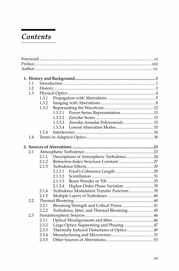
Contents
Foreword xiPreface xiiiAuthor xv
1. History and Background ...............................................................................111 Introduction 112 History 313 Physical Optics 4
131 Propagation with Aberrations 5132 Imaging with Aberrations 8133 Representing the Wavefront 12
1331 Power-Series Representation 131332 Zernike Series 131333 Zernike Annular Polynomials 151334 Lowest Aberration Modes 15
134 Interference 1614 Terms in Adaptive Optics 18
2. Sources of Aberrations ................................................................................2321 Atmospheric Turbulence 23
211 Descriptions of Atmospheric Turbulence 24212 Refractive-Index Structure Constant 27213 Turbulence Effects 29
2131 Fried’s Coherence Length 292132 Scintillation 312133 Beam Wander or Tilt 332134 Higher-Order Phase Variation 35
214 Turbulence Modulation Transfer Function 39215 Multiple Layers of Turbulence 40
22 Thermal Blooming 40221 Blooming Strength and Critical Power 41222 Turbulence, Jitter, and Thermal Blooming 45
23 Nonatmospheric Sources 46231 Optical Misalignments and Jitter 46232 Large Optics: Segmenting and Phasing 47233 Thermally Induced Distortions of Optics 49234 Manufacturing and Microerrors 51235 Other Sources of Aberrations 53

viii Contents
236 Aberrations due to Aircraft Boundary Layer Turbulence 53237 Aberrations in Laser Resonators and Lasing Media 54
3. Adaptive Optics Compensation ................................................................5531 Phase Conjugation 5532 Limitations of Phase Conjugation 60
321 Turbulence Tilt or Jitter Error 60322 Turbulence Higher-Order Spatial Error 61
3221 Modal Analysis 613222 Zonal Analysis: Corrector Fitting Error 62
323 Turbulence Temporal Error 63324 Sensor Noise Limitations 65325 Thermal Blooming Compensation 66326 Anisoplanatism 66327 Postprocessing 69
33 Artificial Guide Stars 70331 Rayleigh Guide Star 72332 Sodium Guide Stars 76
34 Lasers for Guide Stars 7835 Combining the Limitations 7836 Linear Analysis 79
361 Random Wavefronts 79362 Deterministic Wavefronts 81
37 Partial Phase Conjugation 83
4. Adaptive Optics Systems ............................................................................8541 Adaptive Optics Imaging Systems 85
411 Astronomical Imaging Systems 85412 Retinal Imaging 87
42 Beam Propagation Systems 88421 Local-Loop Beam Cleanup Systems 90422 Alternative Concepts 91423 Pros and Cons of Various Approaches 94424 Free-Space Laser Communications Systems 94
43 Unconventional Adaptive Optics 95431 Nonlinear Optics 95432 Elastic Photon Scattering: Degenerate
Four- Wave Mixing 96433 Inelastic Photon Scattering 98
4331 Raman and Brillouin Scattering 9844 System Engineering 103
441 System Performance Requirements 107442 Compensated Beam Properties 107443 Wavefront Reference Beam Properties 108444 Optical System Integration 108

Contents ix
5. Wavefront Sensing .....................................................................................11151 Directly Measuring Phase 112
511 Nonuniqueness of the Diffraction Pattern 112512 Determining Phase Information from Intensity 113513 Modal and Zonal Sensing 116
5131 Dynamic Range of Tilt and Wavefront Measurement 118
52 Direct Wavefront Sensing—Modal 119521 Importance of Wavefront Tilt 119522 Measurement of Tilt 122523 Focus Sensing 126524 Modal Sensing of Higher-Order Aberrations 128
53 Zonal Direct Wavefront Sensing 129531 Interferometric Wavefront Sensing 129
5311 Methods of Interference 1305312 Principle of a Shearing Interferometer 1385313 Practical Operation of a Shearing
Interferometer 1405314 Lateral Shearing Interferometers 1405315 Rotation and Radial Shear Interferometers 145
532 Shack–Hartmann Wavefront Sensors 147533 Curvature Sensing 150534 Pyramid Wavefront Sensor 151535 Selecting a Method 152536 Correlation Tracker 152
54 Indirect Wavefront Sensing Methods 153541 Multidither Adaptive Optics 154542 Image Sharpening 159
55 Wavefront Sampling 161551 Beam Splitters 161552 Hole Gratings 163553 Temporal Duplexing 163554 Reflective Wedges 165555 Diffraction Gratings 166556 Hybrids 167557 Sensitivities of Sampler Concepts 170
56 Detectors and Noise 172
6. Wavefront Correction ................................................................................17761 Modal-Tilt Correction 17962 Modal Higher-Order Correction 18063 Segmented Mirrors 18164 Deformable Mirrors 183
641 Actuation Techniques 184642 Actuator Influence Functions 185

x Contents
65 Bimorph Corrector Mirrors 18966 Membranes and Micromachined Mirrors 19167 Edge-Actuated Mirrors 19368 Large Correcting Optics 19469 Special Correction Devices 194
691 Liquid-Crystal Phase Modulators 195692 Spatial Light Modulators 195693 Ferrofluid Deformable Mirrors 196
7. Reconstruction and Controls ....................................................................19771 Introduction 19772 Single-Channel Linear Control 199
721 Fundamental Control Tools 200722 Transfer Functions 201723 Proportional Control 206724 First- and Second-Order Lag 207725 Feedback 208726 Frequency Response of Control Systems 209727 Digital Controls 216
73 Multivariate Adaptive Optics Controls 218731 Solution of Linear Equations 218
74 Direct Wavefront Reconstruction 222741 Phase from Wavefront Slopes 222742 Modes from Wavefront Slopes 228743 Phase from Wavefront Modes 230744 Modes from Wavefront Modes 231745 Zonal Corrector from Continuous Phase 231746 Modal Corrector from Continuous Phase 232747 Zonal Corrector from Modal Phase 233748 Modal Corrector from Modal Phase 233749 Indirect Reconstructions 2347410 Modal Corrector from Wavefront Modes 2347411 Zonal Corrector from Wavefront Slopes 235
75 Beyond Linear Control 236
8. Summary of Important Equations ..........................................................23981 Atmospheric Turbulence Wavefront Expressions 23982 Atmospheric Turbulence Amplitude Expressions 24283 Adaptive Optics Compensation Expressions 24284 Laser Guide Star Expressions 245
Bibliography 247
Index 293

xi
Foreword
Adaptive optics (AO) is one of the most exciting advances in optical imaging in the past twenty years Conceived in 1953 by Horace Babcock, the subject remained a scientific curiosity until it was developed, at enormous expense, for military purposes A rebirth of the subject occurred in the late 1980s, when astronomers built the first 19-actuator AO system, “COME-ON,” for the European Southern Observatory’s 36-meter telescope at La Silla, Chile Now, all of the world’s large telescopes have sophisticated AO systems, and there is an alphabet-soup of acronyms—laser guide star adaptive optics (LGSAO), multi-conjugate adaptive optics system (MCAO), laser tomography adaptive optics (LTAO), ground layer adaptive optics (GLAO), extreme adaptive optics (XAO), and multi-object adaptive optics (MOAO)—for the different variet-ies of AO being developed for astronomy The next generation of ground-based telescopes, with diameters upward of 30 meters, will have AO systems whose deformable mirrors will have more than 5,000 actuators
Concurrent with the development of top-end AO for astronomy, there has been a growing list of applications for “low-cost” AO Until a decade ago, AO had a big-science mentality: teams of dedicated engineers were required to build successful AO systems In fact, AO is not rocket science, and any competent graduate student can build his or her own AO system in a few months for a cost as low as $10,000 (and a copy of this book) The lowest-cost AO system, using a 14-actuator spatial light modulator and costing less than $1, is used in one manufacturer’s DVD players
When Bob Tyson’s Principles of Adaptive Optics was first published in 1991, it immediately became the reference text for everyone working in the field The comprehensive coverage of all aspects of the field, clear explanations, and extensive reference to the original literature ensured its success This completely revised and updated third edition retains the strengths of the original text Everyone involved in AO should have a copy on the shelf, and like the original, the extensive list of references (more than 900) provides an excellent pointer to the original literature
Christopher DaintyNational University of Ireland, Galway


xiii
Preface
Since the publication of the second edition of Principles of Adaptive Optics in 1997, there has been a virtual explosion in the developments and applica-tions of adaptive optics Observatories are now producing outstanding sci-ence with adaptive optics technology rather than developing first-generation adaptive optics systems, as was the case in the 1990s Many components, such as micromachined deformable mirrors and very low noise detectors, have revolutionized the field While the principles remain essentially the same, the application and complexity of those principles has increased dramatically
There also has been a rapid rise in industrial and medical applications of adaptive optics, including improvements in laser propagation for free-space laser communications, beam control in laser-induced fusion, and medical retinal imaging This edition, similar to the last, is intended to compile recent developments and add a fresh supply of new references Well over 10,000 publications in books, journals, and conference proceedings now document this multidisciplinary field I have tried to cite recent papers, major contribu-tions, or seminal papers along the way I sincerely apologize to those who have not received recognition in the bibliography If you care to help fund my research over the next few years, you will be prominently mentioned in the fourth edition
Robert K. TysonCharlotte, North Carolina


xv
Author
Robert K. Tyson is an associate professor of physics and optical science at the University of North Carolina (UNC) at Charlotte He has a bachelor’s degree in physics from Pennsylvania State University and MS and PhD degrees in physics from West Virginia University He has been working in the field of adaptive optics for over thirty years and has taught many courses on the topic, in addition to writing numerous books, this being the seventh Before joining UNC-Charlotte in 1999, he worked in the aerospace industry design-ing systems and supporting technology for strategic-defense high-energy laser weapons systems


1
1History and Background
1.1 Introduction
Adaptive optics is a scientific and engineering discipline whereby the per-formance of an optical signal is improved by using information about the environment through which it passes The optical signal can be a laser beam or a light that eventually forms an image The principles used to extract that information and apply the correction in a controlled manner make up the content of this book
Various deviations from this simple definition make innovation a desired and necessary quality of the field Extracting the optical information from beams of light coming from galaxies light-years away is a challenge [47,524] Applying a correction to a beam that has the power to melt most man-made objects pushes the state of technology Adaptive optics is changing; it is growing It has become a necessary technology in optical systems that are constrained by dynamic aberrations
Developments in adaptive optics have been evolutionary There is no single inventor of adaptive optics Hundreds of researchers and technologists have contributed to the development of adaptive optics, primarily over the past thirty-five years There have been great strides and many, many small steps The desire to both propagate an undistorted beam of light, or to receive an undistorted image [71], has made the field of adaptive optics a scientific and engineering discipline in its own right
Adaptive optics has clearly evolved from the understanding of wave prop-agation Basic knowledge of physical optics is aided by the development of new materials, electronics, and methods for controlling light Adaptive optics encompasses many engineering disciplines This book will focus on the prin-ciples that are employed by the technological community that requires the use of adaptive optics methods That community is large, and the field could encompass many of the topics normally found in texts dealing with optics, electronic controls, and material sciences This book is intended to condense the vast array of literature and provide a means to apply the principles that have been developed over the years

2 Principles of Adaptive Optics
If everything concerned with actively controlling a beam of light is con-sidered adaptive optics, then the field is indeed very broad However, the most commonly used restriction of this definition leads to the approach that adaptive optics deals with the control of light in a real-time closed-loop fashion Therefore, adaptive optics is a subset of the much broader discipline, active optics The literature often confuses and interchanges the usage of these terms,* and examples in this book show that discussion of open-loop approaches to some problems often should be considered [672]
Other restrictions on the definition of adaptive optics have been observed For the purposes of this book, adaptive optics includes more than coherent, phase-only correction There are a number of techniques that use intensity correction for the control of light, and other techniques that make multiple corrections over various pupil conjugates Incoherent imaging is definitely within the realm of adaptive optics
The existence of the animal visual system is an example of adaptive optics having been in use for much longer than recorded history The eye is capa-ble of adapting to various environmental conditions to improve its imaging quality The active focus “system” of the eye–brain combination is a per-fect example of adaptive optics The brain interprets an image, determines the correction, either voluntary or involuntary, and applies that correction through biomechanical movement of parts of the eye, such as the lens or cor-nea When the lens is compressed, the focus is corrected The eye–brain sys-tem can also track an object’s direction This is a form of a tilt-mode adaptive optics system The iris can open or close in response to light levels, which demonstrates adaptive optics in an intensity-control mode; and the muscles around the eye can force a “squint” that, as an aperture stop, is an effective spatial filter and phase-controlling mechanism This is both closed-loop and phase-only correction
The easiest answer to the layman’s question, “What is adaptive optics?” is straightforward, albeit not completely accurate: “It’s a method of automati-cally keeping the light focused when it gets out of focus” Every sighted per-son understands when something is not in focus The image is not clear and sharp; it is fuzzy If we observe light that is not in focus, we can either move to a position where the light is in focus or, alternately, apply a correction without any movement to bring the beam into focus This is a principle that our eyes apply constantly The adaptive process of focus sensing is a learned process, and the correction (called an accommodation) is a learned response When the correction reaches its biophysical limit, we require outside help, that is, corrective lenses The constant adjustment of our eyes is a closed-loop adaptive process performed using optics It is therefore called adaptive optics
* Wilson et al [869] differentiate them by bandwidth They refer to systems operating below 1/10 Hz as active and those operating above 1/10 Hz as adaptive This definition is used widely in the astronomy community

History and Background 3
1.2 History
Many review authors [320,603] cite Archimedes’s destruction of the Roman fleet in 215 bc as an early use of adaptive optics As the attacking Roman fleet approached the army defending Syracuse, the soldiers lined up so that they could focus sunlight on the sides of the ships By polishing their shields or some other “burning glass” and properly positioning each one, hundreds of beams were directed toward a small area on the side of a ship The resultant intensity was apparently enough to ignite the ship and defeat the attackers The “burn-ing glass” approach by Archimedes was clearly innovative; however, details of the scientific method are scarce [144,743] Whether a feedback loop or phase control was used was never reported, but the survival of Syracuse was
The use of adaptive optics has been limited by the technology available Even the greatest minds of physical science failed to see its utility Isaac Newton, writing in Opticks in 1730, saw no solution to the problem of limita-tions imposed by atmospheric turbulence in astronomy [559]
If the Theory of making Telescopes could at length be fully brought into Practice, yet there would be certain Bounds beyond which Telescopes could not perform For the Air through which we look upon the Stars, is in perpet-ual Tremor; as may be seen by the tremulous Motion of Shadows cast from high Towers, and by the twinkling of the fix’d Stars But these Stars do not twinkle when viewed through Telescopes which have large apertures For the Rays of Light which pass through diverse parts of the aperture, tremble each of them apart, and by means of their various and sometimes contrary Tremors, fall at one and the same time upon different points in the bottom of the Eye, and their trembling Motions are too quick and confused to be per-ceived severally And all these illuminated Points constitute one broad lucid Point, composed of those many trembling Points confusedly and insensi-bly mixed with one another by very short and swift Tremors, and thereby cause the Star to appear broader than it is, and without any trembling of the whole Long Telescopes may cause Objects to appear brighter and larger than short ones can do, but they cannot be so formed as to take away that confusion of the Rays which arises from the Tremors of the Atmosphere The only Remedy is a most serene and quiet Air, such as may perhaps be found on the tops of the highest Mountains above the grosser Clouds
In 1953, Babcock [45] proposed the use of a deformable optical element, driven by a wavefront sensor, to compensate for atmospheric distortions that affected telescope images This appears to be the earliest reference to use of adaptive optics as we define the field today Linnik described how a beacon placed in the atmosphere could be used to probe the disturbances [466] Although Linnik’s paper is the first reference to what we now refer to as “guide stars,” his concept precedes the invention of the laser and was, until the early 1990s, unknown to Western scientists developing laser guide stars

4 Principles of Adaptive Optics
Development of the engineering disciplines involved in adaptive optics has taken a course common to technology development As problems arose, solu-tions were sought Directed research within the field was often aided by inno-vations and inventions on the periphery The need to measure the extent of the optical problem and to control the outcome was often dependent upon the electronics or computer capability of the day, the proverbial “state-of-the-art”
Other methods that do not employ real-time wavefront compensation, such as speckle interferometry [441,662] or hybrid techniques combining adaptive optics and image postprocessing, have been successful These are described by Roggemann and Welsh [672]
A review article by Hardy [320] gives an excellent account of the history of active and adaptive optics, describing the state-of-the-art as it was in 1978 The developments of the first three decades are described in detail through this book and reviewed by Babcock [46], Hardy [322], Greenwood and Primmerman [309], Benedict et al [77], and others [794] In 1991, much of the military work in adaptive optics in the United States was declassified [257,632] Research involving laser guide stars [210] was published and discussed to enhance the research work that was developing in the astronomical community [229]
Scientific journals and technical societies continually publish new tech-niques and results In addition to technology development and field dem-onstrations, the first results for an infrared adaptive optics system on an astronomical telescope were presented in 1991 [526] Results from other systems around the world continue to be presented One example of the exciting improvements in astronomical imaging is shown in Figure 11 The history of adaptive optics continues to be written
1.3 Physical Optics
The principles of adaptive optics are based on the premise that one can change the effects of an optical system by adding, removing, or altering optical elements For most optical systems of interest, diffraction effects are harmful In other words, they make the propagation of a beam of light or the image of an object different When a beam is propagated, either collimated or focused, we normally want all of the light to reach the receiver in the best condition Similarly, for an imaging system, we want the image to be the best reproduction of the object that we can get Diffractive effects degrade the image because they degrade the propagation process We cannot get rid of diffractive effects; they are inherent in Maxwell’s laws The best that we can do is reach the limit of diffraction When mechanical or thermal defects degrade the image or propagation process beyond the diffraction limit, we can try to alter the optical system to compensate for the defects even though we cannot get rid of them

History and Background 5
1.3.1 Propagation with Aberrations
One way to describe the propagation of light as it applies to adaptive optics is through mathematical formalism Literally hundreds of volumes have been written describing optical propagation The classic text by Born and Wolf [89] describes it in a manner that clearly shows the effects of the phase of an opti-cal field in a pupil plane on the resultant field in an “image” plane
For a beam of coherent light at wavelength λ, the intensity of light at a point P on the image, or focal, plane at a distance of z is given by
I PAaR
i k u( ) [ cos( ) ]=
− − −2
2
212
2
λρυρ θ ψ ρe Φ dρρ θ
π
d0
2
0
12
∫∫ (11)
where the circular pupil has radius a and coordinates (ρ, θ); the image plane has polar coordinates (r, ψ); the coordinate z is normal to the pupil plane; R is the slant range from the center of the pupil* to point P; k = 2π/ λ; and kΦ is the deviation in phase from a perfect sphere about the origin of the focal
* R is also the radius of the wavefront sphere that would perfectly focus at P
8
6
2
0
−2
6 4 2x (arc sec)
y (a
rc se
c)
0 −2 −4
4
Figure 1.1Image of the irregular dwarf galaxy IC-10 in the constellation Cassiopeia, taken using the W M Keck Observatory adaptive optics system (Photo courtesy of SOFIA-USRA, NASA Ames Research Center, Moffett Field, CA Vacca, W D, C D Sheehy, and J R Graham 2007 Ap J 662, 272–83 With permission)

6 Principles of Adaptive Optics
plane (Figure 12) To simplify the presentation, normalized coordinates in the focal plane are used as follows:
uaR
z=
22
πλ
(12)
υ πλ
=
2 aR
r (13)
The amplitude of a uniform electric field in the pupil plane is A/R; and there-fore, the intensity in the pupil plane, Iz=0, is A2/R2
From the viewpoint of adaptive optics, the most important quantity in the above expressions is Φ, which is often mistakenly called simply phase It is more commonly referred to as the wavefront The symbol Φ represents all the aberrations that are present in the optical system before its propagation to point P If no aberrations are present, the intensity is a maximum on-axis (r = 0) intensity, which is called the Gaussian image point
I PAaR
aR
Ir zΦ= = =
=
0 0
22
2
22 4
2 2( ) π
λπλ ==0 (14)
The Strehl ratio (S), also called the normalized intensity, is the ratio between the on-axis intensity of an aberrated beam and that of an unaberrated beam If the tilt (distortion) aberration is not removed, the axis of this definition would be normal to the plane of that tilt, rather than parallel to the z-axis Static tilt should be removed when the Strehl ratio is used as a figure of merit for the quality of beam propagation
z
R
r
aP
Ψθρ
Figure 1.2The coordinate system for the calculation of the diffraction with an aberration Φ

History and Background 7
Combining Equations 11 and 14, the Strehl ratio becomes
SI PI
i k u= ==
− − −( ) [ cos( ) ]
Φ
Φ
02
0
1 12
2
πρ ρ θυρ θ ψ ρe d d
22
0
12
π
∫∫ (15)
For small aberrations, when tilt* is removed and the focal plane is displaced to its Gaussian focus, the linear and quadratic terms in the exponential of Equation 15 disappear If the remaining aberrations, which are now cen-tered about a sphere with reference to point P, are represented by ΦP, the Strehl ratio simplifies to
S eik= ∫∫1
20
2
0
12
πρ ρ θ
πΦP d d (16)
which shows how the wavefront affects the degradation of the propagation If the beam at the pupil is unaberrated, ΦP = 0, and the Strehl ratio reduces to unity, S = 1; that is, the intensity at the focus is diffraction-limited Equation 14 shows that the absolute intensity is enhanced by a factor proportional to the square of the Fresnel number, a2/λR A larger aperture, a smaller wavelength, or a shorter propagation distance will increase the maximum intensity in the focal plane All systems with any aberration at all, that is, ΦP > 0, will have a Strehl ratio less than 1 If the wavefront aberration is small, its variance can be directly related to the Strehl ratio The wavefront variance (ΔΦP)2 can be found from the expression
( )
( )
∆ΦΦ Φ
P
P P
2
2
0
2
0
1
0
2
0
1=
−∫∫
∫∫
ρ ρ θ
ρ ρ θ
π
π
d d
d d
(17)
where ΦP is the average wavefront It can be shown [89] that the Strehl ratio for ΔΦP < λ/2π is as follows:
S = −
≅ −
1
2 22
2
2
2πλ
πλ
( ) exp ( )∆Φ ∆ΦP P
(18)
which gives a simple method of evaluating the propagation quality of a sys-tem by considering only the small variance in the wavefront The square root of the variance, formally, the standard deviation of the wavefront, ΔΦP, is often called the root-mean-square phase error, the rms phase error, phase error, or
* For the purposes of this text, tilt is a component of Φ linear in the coordinates ρ cos θ or ρ sin θ in the pupil plane

8 Principles of Adaptive Optics
wavefront error These terms are used interchangeably in the literature The fact that the quality of beam propagation can be directly related to the rms phase error is a very powerful result
1.3.2 imaging with Aberrations
The physical processes behind imaging combine the process of propagation with the effects of lenses, mirrors, and other imaging optics The process that combines these effects results from an examination of Kirchoff’s formula for propagation, which is a more generalized form of Equation 11 The field at point P, in the x–y plane U(P), is given by [89]
U x yiA
rsn r n s S
ik r s
( , ) [cos( , ) cos( , )]( )
= − −+
2λe
dAAp∫∫ (19)
where the coordinates are defined in Figure 13 and the integral is over the aperture Here, A is the amplitude of the field with a plane wave, represented by U(z)plane = Ae±ikz, and a spherical wave, represented by U(z)sph = A/re±ikr The source is in the x0–y0 plane with a distance z0 to the x′–y′ pupil plane The distance z represents the distance from the pupil to the image plane
For large propagation distances, that is, z > the largest of x, y, x′, y′, x0, or y0, Equation 19 reduces to the Fresnel integral as follows:
U x y C x yikf x y
A
( , ) ( , )= ′ ′ ′′ ′∫∫ e d dp
(110)
where the term C′ is not a function of the pupil coordinates and can be rep-resented as follows:
′ ≡ − −+
CA
n r n szz
ikik z z
2
0
0λ[cos( , ) cos( , )] exp
( )e22 20
02
02 2 2
zx y
ikz
x y+( )
+
exp ( ) (111)
Aperturearea A
Sources
P
(n, s)(n, r) n→
r→
Figure 1.3The geometry of the Kirchoff formula

History and Background 9
and the function in the exponent is
f x y x y z z xxz
xz
( , ) ( ) ( )′ ′ = ′ + ′ + − ′ +
− −12
2 20
1 1 0
0
− ′ +
yyz
yz
0
0
(112)
In many beam-propagation or astronomical-imaging applications, the prop-agation distances are quite large Applying the following approximations,
zx y
zx y
0
2 2 2 2
( )
;( )max max′ + ′
>′ + ′
λ λand (113)
the Kirchoff integral reduces to the Fraunhofer integral as follows:
U x y C ikxz
xz
xyz
yz
( , ) exp= ′ − +
′ + +
0
0
0
0 ′
′ ′∫∫ y x y
A
d dp
(114)
Combining the terms in C′ and the terms in the kernel that relate to the source in the x0–y0 plane, the integral takes the form of a Fourier transform:
U x y C U x yikz
xx yy x yA( , ) ( , ) exp ( )= ′ ′ ′ ′ + ′ ′ ′−
p d d∞∞∫∫ (115)
Equation 115 can be written in a shortened notation as follows:
U x y F U x y( , ) [ ( , )]∝ ′ ′ (116)
In the preceding equation, F represents the Fourier transform operation and U(x′, y′) is the pupil function or aperture function When the optical system con-tains aberrations Φ, the pupil function can be written as
U x y A x y eik x y x y( , ) ( , ) ( , , , )′ ′ = ′ ′ ′ ′Φ 0 0 (117)
which uses the fact that aberrations are derived from all elements of the opti-cal system, including the physical pupil in the (x′, y′) plane
When no aberrations are present and the aperture is a simple geometrical shape, Equation 115 can be solved exactly For a rectangular aperture of sides 2a and 2b, after a propagation distance L, the normalized field that results from Fraunhofer diffraction is
U x yL
kaxL
kbyL
k xy( , )
sin sin=
4 2
2 (118)

10 Principles of Adaptive Optics
An important result is the Fraunhofer diffraction from a circular aperture In polar coordinates, the normalized field becomes
U rLar
JarL
( , )θ λπ
πλ
=
1
2 (119)
where J1 is the first-order Bessel function of the first kind The intensity of light from the diffracted field is the square of the magnitude of these fields, that is, I = |U|2
The pupil function of an imaging system is modified by the effect of lenses and other focusing optics A lens transmission function is given in one form by Gaskill [265]:
Tif
x ylens = − +
exp ( )
πλ
2 2 (120)
where f is the focal length of the lens The process of adding lens trans-mission functions and intermediate propagations to the integral equations reduces Equation 115 to
U x y C U x y ikz f
xx yy( , ) ( , )exp ( )= ′ ′ ′ − −
′ + ′1 1
′ ′∫∫ d dx y (121)
which shows the retention of the Fourier transform properties of the imag-ing system with f as its effective focal length By introducing a coordinate change in the image plane,
ξ = kxf
(122)
and
η =kyf
(123)
the Fraunhofer diffraction becomes
U C U x y x yi x y( , ) ( , ) ( )ξ η ξ η= ′ ′ ′ ′ ′− ′+ ′∫∫ e d d (124)
which shows that the Fraunhofer diffraction pattern, at focal distance f, is the Fourier transform of the pupil function
For pupils with and without aberrations, this diffraction pattern is called the point spread function, or PSF The new coordinates (ξ, η) have the units of inverse distance and are called spatial frequencies This is analogous to the

History and Background 11
spectra calculated in the time domain, where frequency is the inverse of time In imaging applications, spatial frequencies are usually two dimensional
Some important physical results can be derived from Equation 124 If the pupil function is spatially limited, such as that with a finite aperture, the Fourier transform operation cuts out the high spatial frequencies of the objects, which contain the fine detail of the object Therefore, an imaging system that can pass these high frequencies, such as one with a large aperture, is “better” because it can produce images with high resolution In addition, an aberration-free pupil will not produce an image where the high-frequency characteristics of the aber-rations screen the high-frequency content of the object This is the principal need for adaptive optics in imaging systems The fact that image-forming qual-ity can be specified by a function that describes how much spatial frequency content is passed to the image is an important result of Equation 124
The field of the image for a coherent imaging system* can be expressed [265] as the convolution of the geometrical image with the PSF as follows:
U W Uim geom im PSF= ∗∗[( ) ] (125)
The geometrical image is the distribution of the object that has been adjusted for imaging system magnification, shifting along the plane, and geometri-cal (ray trace) shadows and differences of intensity In many discussions of imaging in literature [299], the terms geometrical image and object are used interchangeably This is not a problem until exact calculations are performed, because the principles of imaging are the same The constant W takes into account the radiance of the object and the constant transmission or absorp-tion of elements within the system The two-dimensional (2-D) convolution process, represented by ∗∗ in Equation 125, accounts for the diffraction effects of the optics The convolution operation can be Fourier-transformed on both sides [299] as follows:
F U W F U F( ) [ ( ) ( )]im geom im PSF= i (126)
The Fourier transform of the PSF is itself a measure of the imaging quality of a system The optical transfer function, or OTF, represents how each spatial frequency in an object field is transferred to the image [351,352] as follows:
OTF (PSF)= F (127)
One definition of the resolution of a system is the spatial frequency at which the OTF vanishes In many circumstances, this is more descriptive of the optical system than the simple Rayleigh criterion of resolution [89]†
* Incoherent and white light imaging systems are treated in a similar manner, but the exact form of the expression is different
† Lord Rayleigh proposed that two equal, but displaced, objects are “resolved” when the princi-pal intensity maximum of one coincides with the first intensity minimum of the other [639]

12 Principles of Adaptive Optics
Because one observes the intensity distribution of images rather than the electric fields, the magnitudes of the fields are important The objects and images are formed from the Fourier components of the intensity Considering one frequency component, ξ for instance, the intensity of the object, Iobj, can be represented by a constant and a frequency component as follows:
I b b xobj = +0 1 2cos πξ (128)
Similarly, the intensity of the image can be written as
I c c xim = +0 1 2cos πξ (129)
The modulation, or contrast, M, is the relationship between the peaks and valleys of the intensity at the designated frequency
MI II I
=−+
max min
max min
(130)
When substituting the expressions for the individual intensities, the modula-tion M becomes normalized to the constant level of intensity The results are
Mbb
Mccobj imand( )
( )( )
( )( )( )
ξξξ
ξξξ
= =1
0
1
0
(131)
It can be shown as follows [265] that the ratio of these modulations is the magnitude of the OTF:
| ( )|OTF im
obj
ξ =MM
(132)
The magnitude of the OTF is the ratio of how much modulation in the object was transferred to modulation in the image This function, called the modula-tion transfer function (MTF), is a very useful measure of the ability of an imag-ing system to transfer spatial detail The MTF contains no phase information because it is only the magnitude of the OTF A perfect system has an MTF equal to 1 at all frequencies, which requires an infinitely large aperture The MTF of realistic systems is less than 1 for all spatial frequencies greater than zero
1.3.3 representing the Wavefront
A number of mathematical constructs are used to describe the phase of a beam The deviation of phase from a reference sphere [89] is the wavefront In adaptive optics, the wavefront is usually the quantity that is changed to alter the propagation characteristics of the beam
The wavefront is a 2-D map of the phase at an aperture or any other plane of concern that is normal to the line of sight between the origin of the beam and the target In an imaging system, the plane of concern would be normal to

History and Background 13
the line of sight between the object and the image By this definition, the tilt of the beam would be considered part of the wavefront In many instances, the tilt and the piston* are of interest for adaptive optics and are included The wavefront is positive in the direction of propagation
1.3.3.1 Power-Series Representation
One way to represent the 2-D wavefront map is using a power series in polar (ρ, θ) coordinates:
Φ( , ) cos sin, ,,
ρ θ ρ θ ρ θ= +=
∞
∑ S Sn mn m
n mn m
n m1 2
0
(133)
In this series, the primary, or Seidel, aberrations [89] are explicit A coordi-nate transformation to Cartesian coordinates is easily made (x = ρ cos θ, y = ρ sin θ) Table 11 shows the first few Seidel terms
1.3.3.2 Zernike Series
The commonality of circular apertures, telescopes, and lenses make treat-ment in polar coordinates very attractive The power-series representation is, unfortunately, not an orthonormal set over a circle One set of polynomi-als that are orthonormal over a circle, introduced by Zernike [903], has some very useful properties The series, called a Zernike series, is composed of sums of power series terms with the appropriate normalizing factors A detailed description of the Zernike series is given by Born and Wolf [89], and an analysis of Zernike polynomials and atmospheric turbulence, including their Fourier transforms, was done by Noll [570]† Roddier [665] shows how
* Piston is the constant retardation or advancement of the phase over the entire beam† There is a difference in the normalization between the series described by Born and Wolf
and that of Noll Each of Noll’s polynomials should be multiplied by the factor (2(n + l))−1/2 to obtain the Born and Wolf normalization
TAble 1.1
Representation of the First Few Seidel Terms
n m Representation Description
0 0 1 Piston1 1 ρ cos θ Tilt, distortion2 0 ρ2 Focus, field curvature, “sphere”2 2 ρ2 cos2 θ Astigmatism, cylinder3 1 ρ3 cos θ Coma4 0 ρ4 Spherical aberration
14 Principles of Adaptive Optics
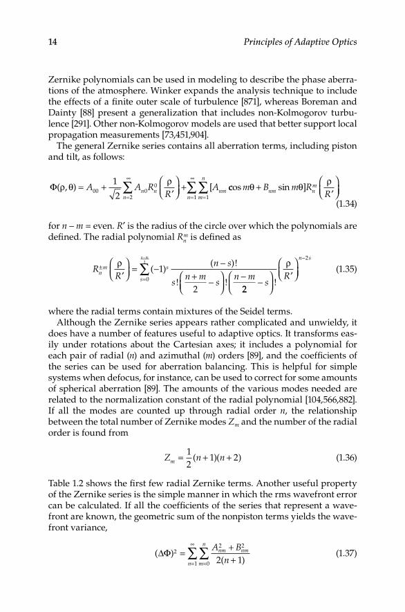
Zernike polynomials can be used in modeling to describe the phase aberra-tions of the atmosphere Winker expands the analysis technique to include the effects of a finite outer scale of turbulence [871], whereas Boreman and Dainty [88] present a generalization that includes non-Kolmogorov turbu-lence [291] Other non-Kolmogorov models are used that better support local propagation measurements [73,451,904]
The general Zernike series contains all aberration terms, including piston and tilt, as follows:
Φ( , ) [ρ θ ρ= +′
+=
∞
=∑ ∑A A R
RAn n
n m
n
nm00 00
2 1
1
2ccos sin ]m B m R
Rnm nm
n
θ θ ρ+′
=
∞
∑1
(134)
for n – m = even R′ is the radius of the circle over which the polynomials are defined The radial polynomial Rn
m is defined as
RR
n s
sn m
sn mn
m s±
′
= − −+ −
−ρ
( )( )!
! !1
2 22
2
0
2
−
′
−
=
−
∑s
R
n s
s
n m
!
ρ (135)
where the radial terms contain mixtures of the Seidel termsAlthough the Zernike series appears rather complicated and unwieldy, it
does have a number of features useful to adaptive optics It transforms eas-ily under rotations about the Cartesian axes; it includes a polynomial for each pair of radial (n) and azimuthal (m) orders [89], and the coefficients of the series can be used for aberration balancing This is helpful for simple systems when defocus, for instance, can be used to correct for some amounts of spherical aberration [89] The amounts of the various modes needed are related to the normalization constant of the radial polynomial [104,566,882] If all the modes are counted up through radial order n, the relationship between the total number of Zernike modes Zm and the number of the radial order is found from
Z n nm = + +12
1 2( )( ) (136)
Table 12 shows the first few radial Zernike terms Another useful property of the Zernike series is the simple manner in which the rms wavefront error can be calculated If all the coefficients of the series that represent a wave-front are known, the geometric sum of the nonpiston terms yields the wave-front variance,
( )( )
∆Φ 22 2
01 2 1= +
+==
∞
∑∑ A Bn
nm nm
m
n
n
(137)
History and Background 15
This variance can be used to calculate the Strehl ratio directly In the spe-cial case where the wavefront is symmetric about the meridional plane (Bnm = 0), the power-series expansion coefficients can be calculated from the Zernike coefficients [787] Similarly, the Zernike coefficients can be calcu-lated from the power-series coefficients [151] Because we can calculate the Zernike coefficients Anm and Bnm using simple integrals, the Zernike series provides a manageable representation of the wavefront for computational purposes or for determining the effects of primary aberrations on circular beams
1.3.3.3 Zernike Annular Polynomials
Some optical systems (Cassegrain and Newtonian telescopes for instance) have a centrally obscured beam A wavefront for these systems is not eas-ily represented using a power series or Zernike polynomials, because the obscuration is represented by very high spatial frequencies in the radial direction A large number of terms of the series are required to repre-sent even primary aberrations Mahajan [496] discusses a series that is orthonormal over an annulus By using the Gram–Schmidt orthogonaliza-tion process, a series of polynomials based on the Zernike polynomials is obtained This series includes the quantity representing the inner radius of the optical wavefront and uses terms similar to the radial Zernike polynomials
1.3.3.4 Lowest Aberration Modes
In addition to the piston, which is only a uniform shift in the entire wave-front, tilt and focus are the primary aberrations that mostly affect propagation or an image According to the rigorous theory, these are not even “aberra-tions” [89] They have a fundamental geometrical significance Repeating Equation 11 for the intensity of light at a point P in a focal plane
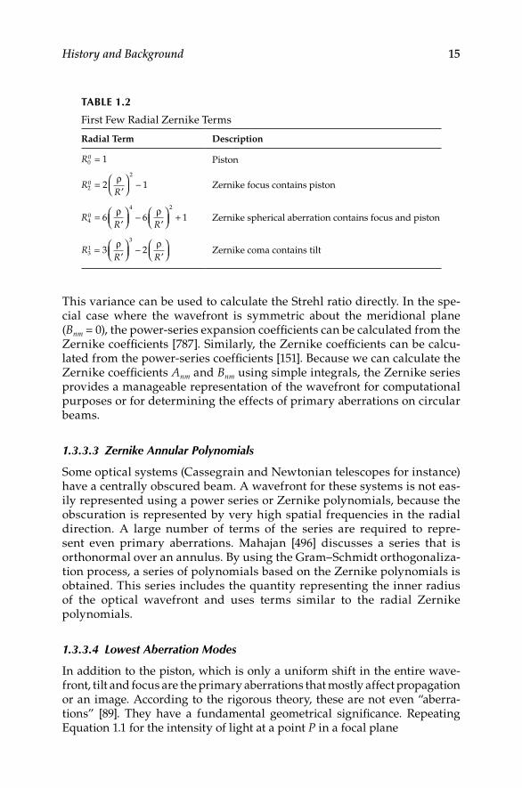
TAble 1.2
First Few Radial Zernike Terms
Radial Term Description
R00 1= Piston
RR2
02
2 1=′
−
ρZernike focus contains piston
RR R4
04 2
6 6 1=′
−
′
+
ρ ρZernike spherical aberration contains focus and piston
RR R3
13
3 2=′
−
′
ρ ρZernike coma contains tilt
16 Principles of Adaptive Optics
I PAaR
i k u( ) [ cos( ) ]=
− − −2
2
212
2
λρυρ θ ψ ρe dΦ ρρ θ
π
d0
2
0
1 2
∫∫ (138)
one can see that the exponent contains three basic terms, the wavefront con-tribution kΦ, the tilt contribution υρ cos(θ−ψ), and the focus contribution uρ2 If we determine that the wavefront Φ contains tilt of a magnitude Kx in the x direction, we can perform a coordinate transformation Φ = Φ′ + Kxρ sin θ With the tilt term separated into its x–y components, the focal length repre-sented by f, and the aperture radius, a, the exponent becomes
k kKkaf
rkaf
rx′ + − − −Φ ρ θ ρ ψ θ ρ ψ θsin sin sin cos cos12
kkzaf
2
2ρ (139)
Removing the tilt from the higher-order wavefront term Φ′ and transform-ing according to ′ = − ′ = ′ =x x R a K y y z zx( / ) , , , the exponent becomes
kkaf
kzaf
Φ − ′ − ′ −
ρ θ ψ ρcos( )12
2
2 (140)
which is the same form as Equation 11 The distribution of light in the image plane will be the same as the original untilted wavefront The centroid of the image will shift, however, by an amount equal to f Kx/a
A similar transformation can be made for a focal shift If the wavefront contains the term Kzρ2, then the distribution of light will not change in the focal plane, but the focal distance f will shift an amount proportional to Kz This very important result is fundamental to the measurement of the focus or the tilt in a beam and will be discussed in detail in Chapter 5
1.3.4 interference
Interference occurs when two or more coherent light beams are superim-posed White light interference can occur because (incoherent) white light can be thought of as the sum of coherent components that interfere Basic principles of optical interference can be used for practical applications such as measuring wavefronts in adaptive optics [424]
The intensity is the time-averaged squared magnitude of the electric field We can begin by expressing the electric field vector of a plane wave as
E A r A r= +− ∗12
[ ( ) ( ) ]e i t i tω ωe (141)
where the vector components of the amplitude are
A ax xikr x= −e δ (142)

History and Background 17
A ay yikr y= −e δ (143)
A az zikr z= −e δ (144)
and the phases of the components are the δ′s The magnitude of the field |E|2 takes the form
| | ( )E i t i t2 2 2 2 214
2= + +− ∗ ∗A A A Ae eω ω i (145)
Averaging the magnitude of the field over a large time interval becomes the intensity, as follows:
I a a ax y z= = = + +( )∗E A A2 2 2 212
12
i (146)
If two such fields are superimposed, the vectors add as follows:
E E E= +1 2 (147)
The magnitude of the sum of the two fields becomes
E E E E E212
1 22= + +22 i (148)
and the intensity of the two superimposed fields is
I I I I I a a a a a ax x y y z z= + + = + + + +1 2 1 1 2 1 2 1 2 1 22 E Ei 2 ( )ccosδ (149)
where δ is the phase difference between the two fields Without loss of generality, but for simplifying the presentation, the light can be treated as transverse and linearly polarized, that is, ayi = azi = 0 The intensities of the individual beams are, from Equation 141,
I ax1 121
2+ (150)
I ax2 221
2= (151)
and the intensity of the superimposed beams is
I I I I I= + +1 2 1 22 cos δ (152)
The maximum intensity occurs when cos δ = 1, that is, δ = 0, 2π, 4π, …, and the minimum occurs when the cosine term is zero, that is, δ = π, 3π, 5π, …

18 Principles of Adaptive Optics
For the special, but not so uncommon, case I1 = I2, the intensity of the super-imposed beams is
I I= 4 212cos ( / )δ (153)
with the maximum intensity Imax = 4I1 and the minimum intensity Imin = 0Measuring the interference pattern is equivalent to measuring the spatial
coherence function of an optical field The Van Cittert–Zernike theorem [672] states that the spatial coherence properties of an optical field are a Fourier transform of the irradiance distribution of the source The fields of optical and radio interferometry are based on this theorem The application of these principles of interference is also fundamental to the development of wave-front control Adaptive optics is, if nothing more, an engineering field, where controlling the phase δ at one place leads to managing the optical intensity I at another place
1.4 Terms in Adaptive Optics
A number of terms are commonly used throughout the adaptive optics community Some of the terms have evolved from electrical or mechani-cal engineering Some are derived from the terminology of special military applications [806], and others uniquely apply to adaptive optics
Many authors use various definitions for the same or similar terms This is not unusual in a growing international field To maintain consistency in this book, some terms are defined as they are generally applied in the adaptive optics–engineering community involved with both astronomy and propaga-tion Other definitions will be found in the context in which they are used
The difference between active and adaptive optics was discussed in Section 11 It requires a rather broad definition of open and closed loops If an optical system or an electro-optical system employs feedback in any fashion, it can be deemed a closed loop This applies to both positive and negative feed-back, and to optical, electrical, mechanical, or any other method of closing the loop between information and compensation
If the optical information is gathered at the receiver or the target end (in beam propagation) or the image plane (in an imaging application), the sys-tem is considered a target loop If the information is intercepted before the target or the image plane or before the application of some correction, the short-circuited loop is called a local loop
If optical information is received by the adaptive optics system before a propagating beam reaches the target, it is considered an outgoing wave If information about the propagation is conveyed from the target back to the correction system, it is called a return wave Rough, extended objects that

History and Background 19
are targets of a propagating beam present special problems with speckled return These speckles can be mitigated with a process called “speckle- average phase conjugation” [834]
If the compensation requires the movement of a macroscopic mass, it is deemed inertial If the compensation alters the state of matter, rather than grossly moving it, it is called noninertial If the compensation is carried out by spatially dividing the region of correction and treating each region indepen-dently (possibly with crosscoupling), it is called zonal correction Conversely, if the compensation is carried out by dividing the region of correction in another manner, such as mathematically decomposing the correction into normal modes, it is called modal correction
Understandably, some of these definitions have gray areas For instance, acousto-optic variance of the index of refraction moves mass on a molecular level, but because it is not a gross macroscopic application, it is noninertial Similarly, there might be no “target” defined in the case of adaptive optics inside a laser resonator This target loop might then be called simply the out-put loop
When a beam strikes an opaque surface, the spot of light can take on almost any shape depending on the apertures and the wavefront of the beam If the beam is circular and has a sharp edge, it is easy to specify the spot radius or diameter Gaussian intensity profiles do not have sharp cutoffs at the edge The edge is usually specified as the point where the intensity reaches 135% of the maximum This is the 1/e2 point of the beam intensity, also called the beam waist A beam shape that has an easily defined edge is the Fraunhofer diffraction pattern of a circular aperture (Equation 119) Because the Bessel function reaches its first zero at a well-known value, J1(38) = 00, the “edge of the circular spot” is defined as the first dark ring, a region of destructive interference The “spot” in this case contains 84% of the energy (Figure 14)
1.0
ba
0.5
0.135
Spot radius Spot radius
Nor
mal
ized
inte
nsity
First darkring
“Edge” ofGaussian
Figure 1.4The spot size is defined differently for various intensity profiles: (a) Gaussian profile and (b) the far-field spot of a uniform beam diffracted by a circular aperture

20 Principles of Adaptive Optics
Other beam spots may be asymmetric, greatly distorted, or have numer-ous pockets of high and low intensity (similar to the speckle pattern on a rough diffuse surface) By taking the area of the smallest spot that has 84% of the energy and computing the diameter of its equivalent circle, an approxi-mation for the spot size is achieved
Using Huygens’ wavelet concept [80,89], we can see that a plane wave passing through an aperture will begin to diverge from its collimated form as soon as it leaves the aperture The amount of divergence is dependent on the amplitude and the phase of the initial beam, the distribution over the aperture, the propa-gation medium that scatters and diffracts the beam, and one’s definition of the “edge” of the beam The beam divergence is usually expressed in terms of an angle between the axis of propagation and the line joining the edge of the beam at different points of the beam path The solid angle defined by the beam edge over the path of the beam is occasionally used to express beam divergence
The use of the Strehl ratio is a fundamental description of the amount of intensity reduction due to aberrations Another quantity, the beam quality, is used in a similar manner A number of definitions for beam quality are used in the optics community The most common definition states that the beam quality is the square root of the inverse of the Strehl ratio
BQ S= 1/ (154)
For a Gaussian beam, the beam quality is equivalent to the linear increase in beam waist due to beam divergence In general, the linear size growth of the diffraction spot is the beam quality Some investigators have redefined the diffraction limit of a beam to better describe a particular system For instance, the Strehl ratio relates the intensity of the aberrated beam to that of the unaber-rated beam If a beam is not uniform when it is unaberrated, such as an annu-lar beam or any other obscured beam, the intensity of the unaberrated beam will not be as high as a similar, equal-area unobscured beam The addition of phase aberrations would normally reduce the on-axis intensity of the beam However, in some cases, the addition of phase aberrations could increase the on-axis intensity of a strangely obscured beam This results in a Strehl ratio greater than one, and a subsequent beam quality less than one By replacing the on-axis intensity of the obscured but unaberrated beam in the definition of Strehl ratio, the beam quality can be viewed as a single number relating only the phase aberrations to the propagated intensity Beam quality should always be related to the unaberrated beam of the same size and shape
Jitter is the dynamic tilt of a beam It is usually expressed in terms of angular variance or its square root, the rms deviation of an angle The dynamics are often expressed in terms of a power spectral density, similar to any mechani-cal vibration If the jitter is very slow, usually slower than the response of the system under consideration, it is called drift Because tilt alters the direc-tion and not the shape of a propagated beam, it does not have any effect on the Strehl ratio according to its formal definition However, if a system is

History and Background 21
constructed to maintain a beam on a receiver, a physical spot in space, jitter will cause the beam to sweep across the spot The time-averaged intensity on the target is reduced by an amount related to the jitter
The on-axis far-field intensity Iff for a circular aperture with reductions due to diffraction, expressed as variance of the wavefront σ = Φ2 2( )k∆ , jitter, and transmission losses for m optical elements is given by [715]
I
I TK
Dff
jit
≅−
+
02
2
12 22
exp[ ].
σαλ
(155)
where
T Ti
m
i==Π
1 (156)
is the transmission of m optics, K is an aperture-shape correction described in reference [349], D is the aperture diameter, λ is the wavelength, and αjit is the one-axis rms jitter The intensity without aberrations or jitter is found by substitution in Equation 14,
ID P
L0
2
22= π
λ( ) (157)
where L is the propagation distance and P is the uniformly distributed input power into a circular aperture
According to Babinet’s principle, the intensity of a circular aperture with an obscuration ratio ε becomes [89]
ID P
L0
2
22
21obsc = −π
λε
( )( ) (158)
Knowing the on-axis intensity is sufficient to describe the far-field effects when the beam has a relatively simple analytical form for the intensity distri-bution For greatly aberrated beams or those with complicated apertures, the on-axis intensity is insufficient to describe the far-field effects A measure-ment of the total power in the focal or the target plane or over a portion of the focal plane is needed Integrating the power deposited in a circle on the focal plane results in a quantity called the total integrated power If one places a “bucket” of a specified radius in the focal plane, the “bucket” would catch that amount of power; thus the term power-in-the-bucket For the perfect cir-cular aperture, the power-in-the-bucket is expressed as [89]
PB = −
−
12 2
02
12J
abL
JabL
πλ
πλ
(159)
where a is the aperture radius and b is the bucket radius

22 Principles of Adaptive Optics
It is often necessary to express the propagation capability of a system in terms that are independent of the propagation distance The expression for far-field intensity Iff, Equation 155, when multiplied by the square of the propagation distance, L2, results in a quantity expressed in units of power per solid angle This term, called brightness, is a description of the propagat-ing system, rather than the effect of the propagation itself
Brightness
jit
≈−
+
π σ
λαλ
D PTK
D
2 2
24 12 22
exp[ ]
.
2 (160)
Astronomical brightness, the number of photons reaching the Earth’s surface, in a given area in unit time, depends on the magnitude of the star It is defined for a visible passband by the expression
B mastro
v photons cm= × −( ) / s/ .4 10 106 2 5 2 i (161)
where mv is the visual magnitude of the observed star The limit of vision of an unaided human eye in a dark location is roughly equal to a visual mag-nitude of 6 A visual magnitude of 14 is roughly the brightness of a sunlit geosynchronous satellite
Astronomers use the term “seeing” to describe the condition of turbulence in the atmosphere It is based on the ability to resolve two point objects when observed through the atmosphere It is essentially the same as the Rayleigh criterion [89,639] for resolving two point objects That is, the full-width-half-maximum of the PSF stated as an angle is the “seeing” It is normally expressed in arc seconds (or arc minutes), recognizing that 1 arc sec = 48 μ radians Uncompensated atmospheric seeing can be as low as 045 arc sec [27] or, sometimes, as high as 20 arc sec [664] For surveillance of low Earth orbit space objects, the seeing should be less than 002 arc sec [509] For astronomy, good seeing is 01–05 arc sec Adaptive optics is used to improve the seeing
23
2Sources of Aberrations
Unwanted variations in the intensity during an image capture or beam propagation create the need for adaptive optics Chapter 1 showed that it is the deviation of the phase from the reference sphere (the wavefront), that is, the principal cause of the intensity variations, that can be treated by adaptive optics There are many sources of wavefront errors
Astronomers are mostly concerned with the turbulence in the atmosphere that degrades an image Engineers working to propagate a beam and to max-imize its useful energy into a receiver must be concerned with errors intro-duced by lasers themselves, the optics that direct them, and the propagation medium that they encounter This chapter will discuss the many sources of phase aberrations addressed by adaptive optics systems These include lin-ear effects due to turbulence, optical manufacturing, and misalignments, as well as errors that result from nonlinear thermal effects and fluid properties The minimization of these effects is always a consideration while developing any optical system from the ground up Real-time compensation for these disturbances is the realm of adaptive optics
2.1 Atmospheric Turbulence
Naturally occurring small variations in temperature (<1°C) cause random changes in wind velocity (eddies), which we view as turbulent motion in the atmosphere The changes in temperature give rise to small changes in the atmospheric density and, hence, in the index of refraction These index changes, on the order of 10−6, can accumulate, and the cumulative effect can cause significant inhomogeneities in the index profile of the atmosphere The wavefront of a beam will change in the course of propagation This can lead to beam wander, intensity fluctuations (scintillations), and beam spreading
These small changes in the index of refraction act as small lenses in the atmosphere They focus and redirect waves and eventually, through interfer-ence, cause intensity variations Each of these “lenses” is roughly the size of the turbulence eddy that caused it The thin lens model is a useful approxi-mation, but it is not completely accurate because there are few discontinuities in the atmosphere

24 Principles of Adaptive Optics
The most common effects of turbulence can be seen manifested in the twinkling and quivering of stars Twinkling is the random intensity varia-tion of light from a star because of the random interference between waves from the same star passing through slightly different atmospheric paths The average position of the star also shows a random quiver because the aver-age angle-of-arrival of light from the star is affected by the changing index of refraction along its path through the atmosphere A third effect, known a long time ago to astronomers, is the apparent spreading of a star’s image due to turbulence The aberrations introduced by optics do not account for the large spot image of the star, a point object Turbulence produces random higher-order aberrations that cause the spreading
These three primary effects of turbulence will be examined here because they are subject to compensation by adaptive optics Other atmospheric effects, such as aerosol scattering and molecular absorption, will only be introduced when they affect the performance of the adaptive optics The control of large spatial and temporal changes of a wavefront can reduce the phase changes caused by the random temperature fluctuations This is the principal reason for using adaptive optics
Several volumes [130,374,746,755] and hundreds of papers have been writ-ten on this topic, examining the theoretical basis for describing the effects of turbulence and the experimental verification of those theories [209] A 1986 book by Lukin, recently updated and translated from Russian [488], is a com-prehensive theoretical examination of adaptive optics–related turbulence phenomena
Turbulence, as it applies to adaptive optics, can be summarized using basic principles that relate the physical turbulence phenomena with optical prop-agation and phase effects Propagation through atmospheric turbulence is not completely understood, especially in terms of small-scale phenomena The theories of turbulence are based on statistical analyses, because the com-plexity of the real atmosphere is beyond the capabilities of deterministic pre-diction or numerical analysis The emphasis on a statistical description of atmospheric turbulence has resulted in a number of very useful theories and scaling laws that describe the average effects on gross properties, such as total beam wander, beam spread, and scintillation [208]
2.1.1 Descriptions of Atmospheric Turbulence
Areas of high- and low-density air are moved around by random winds This process can be described by statistical quantities Kolmogorov [425] studied the mean-square velocity difference between two points in space separated by a displacement vector r The structure tensor Dij is defined as
Dij i i j j= + − + −[ ( ) ( )][ ( ) ( )]υ υ υ υr r r r r r1 1 1 1 (21)

Sources of Aberrations 25
where υi and υj are the different components of the velocity and the brackets represent an ensemble average It is not a simple equation to evaluate with real velocity descriptors; however, if three assumptions about the atmosphere are made, the structure tensor can be simplified First, the atmosphere is locally homogeneous (velocity depends on vector r); second, the atmosphere is locally isotropic (velocity depends only on the magnitude of r); and third, the turbulence is incompressible (∇ • v = 0) The tensor now becomes a single structure function [65] as follows:
D r rυ υ υ= + −[ ( ) ( )]r r r1 12 (22)
If the separation r is small (within the inertial subrange of turbulence), the structure function takes on a 2/3 law dependence on r:
D C rυ υ= 2 2 3/ (23)
The constant Cυ2 is the velocity structure constant, which is a measure of the
energy in the turbulence This form of the structure function is valid when the value of r is above the smallest eddy size l0 and below the largest eddy size L0 The small eddy, called the inner scale or the microscale, is the size below which viscous effects are important and energy is dissipated as heat The inner scale is related to the rate of dissipation of the turbulent kinetic energy ε and the kinematic viscosity ν by the following equation [577]:
l0
3 1 4
7 4=
.
/νε
(24)
The large eddy, called the outer scale, is the size above which isotropic behav-ior is violated One can approximate l0 as being a few millimeters near the Earth’s surface to a few centimeters or more in the troposphere The outer scale L0 ranges from a few meters to hundreds of meters Near the ground, below 1 km, L0 ≈ 04h, where h is the height above the ground [755] In the free atmosphere, the outer scale is normally on the order of tens of meters, but it can reach hundreds of meters [52]
Through the concept of passive additives, Tatarskii [755] and Corrsin [152] related the velocity structure to the index-of-refraction structure This quan-tity Dn is much more important when we deal with propagation issues
D r C r l r Ln n( ) ;/= < <2 2 30 0 (25)
where Cn2 is the refractive-index structure constant, a measure of the strength
of the turbulence The effects of a finite inner scale and the behavior of the structure function when r is close to l0 are discussed by Whitman and Beran [858]

26 Principles of Adaptive Optics
The atmosphere can be assumed to be made up of a mean index of refraction, n r( ) , and a fluctuating index part, n1(r) The covariance of the refractive-index field Bn becomes
B n nn = +1 1 1 1( ) ( )r r r (26)
The power spectral density (PSD) is the Fourier transform of the covariance,
Φn ni rrB r( )
( )( )K K= −∫
12 3
3
πd e (27)
where K is the three-dimensional spatial wave number Using Kolmogorov’s inertial subrange expression (Equation 25), changing the coordinates to spherical terms, K = (K, θ, ϕ), and carrying out the ensemble averaging [746], the PSD becomes
Φn nl
L
K C K r Kr r( ) sin( ) /= − −∫5
182 3 1 3
0
0
πd (28)
If we let the integral limits diverge, l0 → 0 and L0 → ∞, the integral results in the Kolmogorov spectrum:
Φn nK C K( ) . /= −0 033 2 11 3 (29)
A zero inner scale and an infinite outer scale were convenient for performing the integration Tatarskii [756] described a spectrum that could be used for finite inner scales [488], given by
Φn nK C KK
l( ) . exp
( . / )/= −
−0 0335 92
2 11 32
02
(210)
The Von Karman spectrum [755] is useful for cases with finite outer scales and is expressed as follows:
Φ ΓΓn K L K K( )
( / )( / )
( / )/
= +−
−11 61 3 8
19 2
203 2
02 11π δ //6 (211)
In this expression, the constant term is evaluated to yield the following value:
Γ
Γ( / )
( / ).
/11 61 3 8
2 54 109 2
4π−−≅ × (212)
Sources of Aberrations 27
K0 = 2π/L0, and the variance of the refractivity fluctuations is given by
δ22
02 31 9
= CK
n
. / (213)
Each of these spectra is valid only for regions in the following inertial subrange:
2 2
0 0
π πL
Kl
≤ ≤ (214)
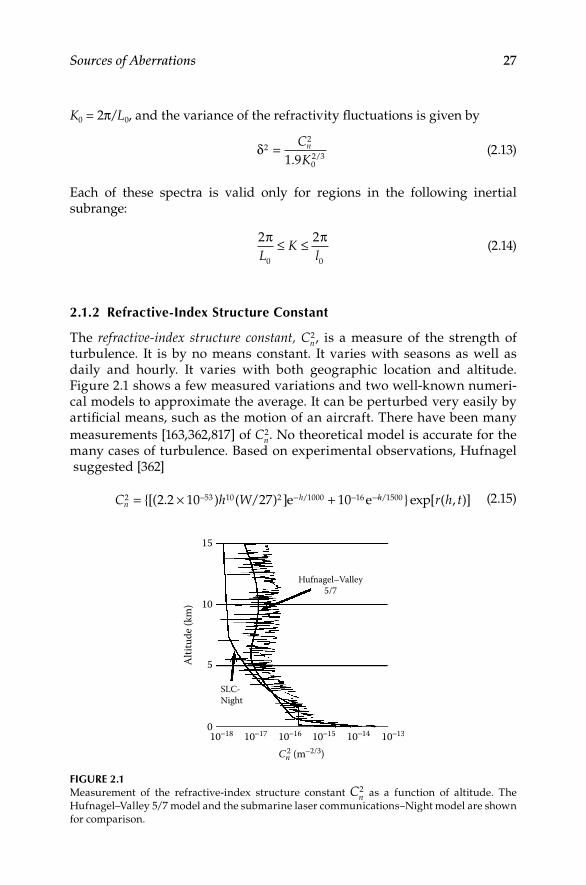
2.1.2 refractive-index Structure Constant
The refractive-index structure constant, Cn2, is a measure of the strength of
turbulence It is by no means constant It varies with seasons as well as daily and hourly It varies with both geographic location and altitude Figure 21 shows a few measured variations and two well-known numeri-cal models to approximate the average It can be perturbed very easily by artificial means, such as the motion of an aircraft There have been many measurements [163,362,817] of Cn
2 No theoretical model is accurate for the many cases of turbulence Based on experimental observations, Hufnagel suggested [362]
C h Wnh2 53 10 2 1000 162 2 10 27 10= [( . ) ( / ) ] /× +− − −e e−−h r h t/ exp[ ( , )]1500 (215)
15
Hufnagel–Valley5/7
10
Alti
tude
(km
)
5
SLC-Night
010−18 10−17 10−16 10−15
Cn2 (m−2/3)
10−14 10−13
Figure 2.1Measurement of the refractive-index structure constant Cn
2 as a function of altitude The Hufnagel–Valley 5/7 model and the submarine laser communications–Night model are shown for comparison

28 Principles of Adaptive Optics
where h is the height above sea level in meters, W is the wind correlating factor that is defined as
W h h=
∫
115
2
5
201 2
kmd
km
km
υ ( )
/
(216)
and r(h, t) is a zero-mean homogeneous Gaussian random variable The term υ(h) is the wind speed at height h The unit of Cn
2 is m−2/3The dependence of wind speed on altitude is required for a rigorous appli-
cation of Equation 215 A wind model that is commonly used and is appli-cable to calculations throughout this book was developed by Bufton [106], as follows:
υ( ) exp ..
z z= + − −
5 30 9 44 8
2
(217)
where z is in kilometers and the wind velocity υ is in meters per secondValley [808] altered the wind model slightly in his study of anisoplanatism,
which is discussed in Chapter 3 Ulrich added a term to account for the boundary layer, resulting in the Hufnagel–Valley boundary (HVB) model [800], which is expressed as follows:
C z eW
nz2 23 10
2
16 25 94 1027
2 7 10= ×
+ ×− − − −. . e zz hA/3 10+ −e (218)
where z is the height above mean sea level in kilometers, h is the height above the surface of the site in kilometers, and Cn
2 is in m−2/3 W is an adjustable parameter related to the upper-atmosphere wind velocity, and A is a scaling constant [800,808] If the site is at sea level, both W and A can be adjusted so that they correspond to specific integrated values of the coherence length r0 and the isoplanatic angle θ0* For the case of r0 = 5 cm, θ0 = 7 μrad, and λ = 05 μm (the so-called Hufnagel–Valley 5/7 model), the parameters are A = 17 × 10−14 and W = 21 With the wavelength λ in micrometers, the coher-ence length r0 in centimeters, and the isoplanatic angle θ0 in microradians, the HVB parameters can be found for any site conditions [791] using
W = −−27 75 0 1405 3 2 1 2( . )/ /θ λ (219)
and
A r= × − × −− − −1 29 10 1 61 10 3 89120
5 3 2 130
5 3 2. . ./ /λ θ λ ×× −10 15 (220)
* The coherence length and isoplanatic angle are formally described in Section 213

Sources of Aberrations 29
Another model commonly used to calculate the parameters associated with atmospheric turbulence is the submarine laser communications (SLC)–Night model, named after the SLC program for which it was developed, where h is the altitude above ground (in meters) The model is described as follows:
Altitude Cn2
h ≤ 185 840 × 10−15
185 < h ≤ 110 287 × 10−12h−2
110 < h ≤ 1500 25 × 10−16
1500 < h ≤ 7200 887 × 10−7h−3
7200 < h < 20,000 200 × 10−16h−05
2.1.3 Turbulence effects
Turbulence will cause high spatial frequency beam spreading, low spatial frequency beam wander, and intensity variations Beam spread is produced by eddies that are smaller than the beam size Wander is produced by eddies that are larger than the beam size [746] The Kolmogorov spectrum suggests that intensity variations are produced by eddies with sizes on the order of
λL , where L is the propagation distance
2.1.3.1 Fried’s Coherence Length
In a study of an optical heterodyne communications receiver, Fried [237] found that the maximum allowable diameter of a collector before atmo-spheric distortion seriously limits performance is r0, where the “coherence length”* is
r k C z zn
L
02 2
0
3 5
0 423=
∫
−
. sec( ) ( )/
β d (221)
In this expression, L is the path length, β is the zenith angle, and Cn2 can vary
with altitude z The phase structure function for the Kolmogorov turbulence can be found for a number of cases in terms of this parameter [238] For plane waves
Drrφ =
6 880
5 3
./
(222)
* This is often called the “seeing-cell size” [239]
30 Principles of Adaptive Optics
The radial variable r is normal to the propagation direction For spherical waves, the coherence length is slightly modified as follows:
r k C zzL
zn
L
0sph d=
∫0 423 2 2
5 3
0
. sec( ) ( )/
β
−3 5/
(223)
Equation 222 can be generalized for non-Kolmogorov turbulence Nicholls et al [563] discuss a generalized model for the structure function that takes the form
D rr
Rn( ) =
−
γ η
η
0
2
(224)
When η = 11/3, R0 = r0, and γη = 688, Kolmogorov turbulence is assumed If η is less than 11/3, some of the energy for phase aberrations shifts from lower- to higher-order modes, requiring modifications to adaptive optics
For a constant Cn2 (ie, for a horizontal path length), the coherence length
for plane waves reduces to
r C Lkn02 2 3 51 68| . ( ) /
pl = − (225)
For spherical waves, the coherence length is
r C Lkn02 2 3 53 0| . ( ) /
sph = − (226)
In astronomy, starlight is a plane wave when it enters the atmosphere; hence, the plane-wave description is assumed Typical nighttime median r0 at wave-length λ can be approximated by [246]
[ ] ..
(sec )/
/r0 7
6 530 114
5 5 10median =×
−
−λ β 55 (227)
where λ is in metersFried’s coherence length has been used to describe various atmospheric turbu-
lence phenomena The coherence length can be measured [40,700] indirectly By using a two-channel Shack–Hartmann sensor (Section 532) as a differential image motion monitor [227,690], atmospheric seeing can be measured Because r0 incorporates the turbulence strength Cn
2, the wavelength, and the propagation path into one parameter, it is widely used for scaling laws and descriptions of atmospheric phenomena For instance, the spectrum of turbulence in the spatial domain (with spatial frequency ξ expressed in inverse meters) is expressed in terms of coherence length [570] With r0 in meters, the spectrum is
Φ( ).
//ξ ξ=
−0 023
05 3
11 3
r (228)

Sources of Aberrations 31
This spatial frequency spectrum can be used to describe all the aberration modes of atmospheric turbulence in terms of Zernike coefficients and other polynomials [665] In addition, the spectrum can be integrated to give an overall wavefront variance as follows:
σ ξ ξ2 2= ∫ Φ( )d (229)
2.1.3.2 Scintillation
Intensity variations are usually expressed as fluctuations of the log of the amplitude (log-amplitude fluctuations) The Kolmogorov spectrum suggests that log-amplitude fluctuations are produced by eddies with sizes on the order of λL, where L is the propagation distance Assuming the Von Karman spectrum and l L0 << λ , the log-amplitude variance σχ
2 is given by [755]
σχ2 7 6 11 6 20 307= . / /k L Cn (230)
for a plane wave and
σχ2 7 6 11 6 20 124= . / /k L Cn (231)
for a spherical wave These formulae break down for long paths and strong turbulence [633], because perturbation theory was used to derive them Tatarskii [755] used a technique derived by Rytov [681] to develop this the-ory Because of the limitations of the Rytov approximation, these equations hold only for σχ
2 0 3< . Using the simple multiple-lens model for the atmosphere, one can calcu-
late the amplitude variance Because each eddy of diameter l acts as a lens, it will have a focal length of f l n≈ ∆ In the geometric optics regime, l L> λ and l L0 < λ ; then, the log-amplitude variance is [145]
σχ2 7 6 11 6 2≈ k L Cn
/ / (232)
which is within a multiplicative constant of the more rigorous Tatarskii method
The scintillation effects are most prominent when a small or point receiv-ing aperture, like an optical communications receiver, a small optical tracker, or the human eye, is used In some cases, scintillation can be interpreted in a centroid tracker as a tilt or jitter error when no phase tilt actually exists [350] For larger apertures, the scintillation effects are averaged over the extent of

32 Principles of Adaptive Optics
the aperture, and the focused irradiance varies less Scintillation is observed as a variation in the irradiance, σ I
2, and is expressed as
σ σI2 24 1= −A X[exp( ) ] (233)
where A is an aperture-averaging factor [20,139]Churnside [139] presents a number of expressions for the aperture-
averaging factor under various conditions For weak turbulence conditions and a small l0, the aperture-averaging factor is
AkD
L= +
−
1 1 074
27 6 1
./
(234)
For other conditions, see [19,790]Because atmospheric turbulence is dynamic, scintillation is dynamic
Tatarskii [755] gives the temporal power spectrum of scintillation in terms of the frequency f, and the zenith angle β:
P f kC z z
zz
x
nL
( ) . sec( )
( )/ /
/
=
×
∫8 27 7 3 2 32 4 3
0
2
βυw
d
++
+
−f
f zx
ff z
x2
02
11 6
22
02( )
sin( )
/
d00
∞
∫ (235)
The frequency f0(z) is a function of the wind velocity υw(z):
f zk
zz0
1 22
( )sec
( )/
=
β
υw (236)
The integral over the dummy variable x in Equation 235 can be approxi-mated by [791]
[ ] exp . ..
d forxff
ff
= − −
1 8 0 50
1 9
0
≥≥∫ 0 5. (237)
[ ] . d forxff
= <∫ 1 0 50
(238)

Sources of Aberrations 33
2.1.3.3 Beam Wander or Tilt
The turbulent atmosphere will cause a beam to wander as it propagates When the wander is fast, it is often called beam jitter When the wander is slow, it is called drift It is caused by the dynamic tilt of the wavefront Sasiela [693] gives a general description of the wavefront variance as follows:
σ κκWF d d2 2 2
0
11 3 20 2073=−∞
∞−∫∫. ( ) cos/k zC zn
L κκ κ
2
02( )
( , )z Lk
F zi
N
i−
=
Π
(239)
where the z integral is over the atmospheric path, κ is a two-dimensional
spatial frequency, N is the number of Zernike modes included, and k = 2π/λ The filters Fi for the Zernike modes [695] are given by the following equations:
F nJ D
Dm nn
even , ( ) ( )( / )/
coκκ
κ= +
+2 1
2 22
1
2
ss ( )2 mφ (240)
F nJ D
Dm nn
odd , ( ) ( )( / )/
sinκκ
κ= +
+2 1
2 22
1
2
22( )mφ (241)
F nJ D
Dm nn
=+= +
0
1
2
12 2
2, ( ) ( )( / )/
κκ
κ (242)
Using the relations n = 1 and m = 1 from Equation 241 in the filters, Sasiela derives the following expression for wavefront tilt variance σ tilt
2 :
σ κ κtilt d d2 2 2
0
2 2 11 60 20731= +∫ −. ( ) [ ] /k zC z kn
L 66 22
22
2
kDJ D
D
−∞
∞
−∞
∞
∫∫( / )
/κ
κ (243)
where J2 is the second-order Bessel function of the first kind, κ is the spatial
frequency, and D is the aperture diameter A similar expression was derived for the tilt variance for an annular aperture with a centered obscuration of diameter ε D, as shown in Equation 244:
σ ε
κ κ
tilt d
d
2 2 2
0
2 2
0 2073( ) . ( )
[ ]
D k zC z
k
n
L
=
× +
∫
− 11164
2 3 2161
22
/
( )( / )
/(
−∞
∞
∫ −
−kD
J kDkD
Jε
εkk D
k Dε
ε/ )
/2
2
2
−∞
∞
∫ (244)

34 Principles of Adaptive Optics
Using Equation 243 and evaluating the coherence length, the variance of the tilt angle α2 can be found for two uncorrelated axes or a single axis using the expression
α λ αtwo-axis oneor2
0
5 3 2
0 364=
./
Dr D --axis
2
0
5 3 2
0 182=
./
Dr D
λ (245)
The dynamics of the tilt are manifested in their power spectra For a gradi-ent tilt (G-tilt), such as that measured by quadrant detectors, the one-axis tilt power spectrum assumes the following form [781]:
P f D f Ff
C zG n( ) . sec ( )/ /=
− −0 155 1 3 8 3 2βυ
υw
wwd5 3
0
/ zL
∫ (246)
where the function FG is given by
F y xx
xJ y xG( ) ( / )
/
=−∫ d5 3
2 12
0
1
1π (247)
For low frequencies, this reduces to a −2/3 power law expression
P f D f C z zn
L
( ) . sec ( )/ / /low w d→ − − −0 804 1 3 2 3 2 1 3
0
β υ∫∫ (248)
and for high frequencies, it follows a −11/3 power law expression
P f D f C z zn( ) . sec ( )/ / /high w d→ − −0 110 1 3 11 3 2 8 3
0
β υLL
∫ (249)
Similar expressions follow for the Zernike tilt (Z-tilt)*
P f D f Ff
C zZ n( ) . sec ( )/ /=
− −0 251 1 3 14 3 2βυ
υw
ww d11 3
0
/ zL
∫ (250)
where the function FZ is
F y xx
xJ y xZ( ) ( / )
/
=−∫ d11 3
2 22
0
1
1π (251)
* Z-tilt is the direction that is normal to a best-fit plane with reference to the wavefront

Sources of Aberrations 35
For low frequencies, this reduces to the same −2/3 power law expression that was found for the G-tilt
P f D f C z zn( ) . sec ( )/ / /low w d→ − − −0 804 1 3 2 3 2 1 3
0
β υLL
∫ (252)
For high frequencies, the Z-tilt power spectrum follows a −17/3 power law
P f D f C zn( ) . sec ( )/ / /high w d→ − −0 014 1 3 17 3 2 14 3β υ zz
L
0∫ (253)
A single parameter can represent the entire spectrum for adaptive optics compensation analysis The characteristic frequency of the tilt of atmospheric turbulence, often called the tilt Greenwood frequency, is expressed by Tyler [781] For G-tilt, the expression is
f D C z zG n
L
T wd=
− − ∫0 331 1 6 1 1 2 2 2
0
. sec ( )/ /λ β υ
1 2/
(254)
For Z-tilt, the constant in Equation 254 becomes 0368
2.1.3.4 Higher-Order Phase Variation
Turbulent eddies that are smaller than the beam size break up the beam and spread out the energy The wavefront variations arise because the refrac-tive index is a random function of space and time The phase difference δϕ between two parallel paths through the atmosphere separated by distance ρ is δφ ρ ρ k n[ ( )]∆ , where the difference in index is Δn By averaging over many statistical realizations and assuming a path length L, the phase structure func-tion can be determined as follows:
D k C L l Lnφ ρ ρ= < <1 46 2 2 5 30 0. ,/ (255)
When propagation occurs over long paths and many eddies, the wave can lose coherence If the wavefront is strongly aberrated before it encounters an eddy, the plane-wave approximations used thus far are no longer valid If the phase difference ( )δφ π2 2< , the beam becomes coherent If ρ0 is the largest eddy for which a plane wave is considered coherent, from Equation 255, the coherence distance is calculated as follows:
ρ ππ0
2
2 2
3 5
≈
C Ln
/
(256)

36 Principles of Adaptive Optics
This coherence limitation can be used to derive the total beam spread Lutomirski and Yura [493] used the extended Huygens–Fresnel principle to show that the angular spread θ of a collimated uniform beam of radius α in uniform turbulence* is
θρ
22 2 2
02
1 1≈ +k a k (257)
For the specific case of a Gaussian beam [384],
Iww w
= −
02
2
2
2
2
b b
expρ
(258)
For short propagation distances (z w<< π λ02/ ), the beam waist wb increases
from its initial size w0 according to the following expression:
w w C k L wnb2
02 2 1 3 8 3
01 32 86= + . / / / (259)
For long distances (z w>> π λ02/ ), it increases according to the relation
wz
k wC L wnb
22
202
2 30
1 343 58= + −. / (260)
The Strehl ratio and the imaging system’s spatial resolution can be computed from the phase variance Noll [570] shows that the uncompensated turbu-lence wavefront variance is
σuncomp2 =
1 020
5 3
./
Dr (261)
Because we are concerned with beam spread and not the wander of the beam centroid, the wavefront variance after removal of the two-axis tilt becomes
σ tiltcomp2
0
5 3
0 134=
./
Dr (262)
The Strehl ratio S can be calculated using Equation 160, disregarding the terms that do not contribute to beam spreading In addition to the beam spread from small turbulent eddies, large eddies also jitter the beam Over
* When Cn2 is assumed to be independent of altitude, the turbulence is said to be uniform

Sources of Aberrations 37
a long exposure, a beam that is spread due to high-order turbulence effects will be spread to a greater extent by high-frequency jitter The long-exposure Strehl ratio is [268]
SD
=+
−e comp
jit
σ
αλ
2
12 22 2.
(263)
where σcomp2 is the wavefront variance with tilt removed and αjit is the one-axis
tilt jitter The image of a star captured with an astronomical telescope, that is, using the optical system’s point spread function (PSF), will have a bright cen-tral core and a wider background halo similar to that shown in Figure 22 Parenti [598] shows a modified Strehl ratio expression that accounts for the background halo:
SD D
=+
+− −e 1 ecomp comp
jit
σ σ
αλ
2 2
12 22
12.
−
+rr0
2
(264)
The full-width-half-maximum (FWHM) of the central PSF core can be approximated by
FWHMcore jit=
+1 22 2 7
22. ( . )λ α
D (265)
The halo has an FWHM equal to 122λ/r0 (see Figure 22)The resolution R of an optical system imaging through the atmosphere
(using Rayleigh’s criterion [639]) becomes slightly complicated by the halo being superimposed upon the image core [598] The resolution is given by
RD
QS
=
1 22.
λ (266)
Imagecore
Imagehalo
∼λ/D
∼λ/r0
Figure 2.2Point spread function through the atmosphere, which exhibits a diffraction-limited central core and a halo

38 Principles of Adaptive Optics
where S is the Strehl ratio from Equation 264 and
QD
=
+
+ −
+
− −e ecomp comp
jit
2
2
2 2
12 22
1
1
σ σ
αλ
. DDr0
2
(267)
Turbulence is a random process that has temporal statistics as well as spatial statistics From an adaptive optics viewpoint, these statistics are important If turbulence moves very slowly, then an adaptive optics system can view the disturbance as static Correction would only be required in the spatial domain However, if the turbulence is very fast, an adaptive optics system would only see the time-averaged disturbance Fortunately, the actual tur-bulence is driven by winds and local eddies, which can be tracked by elec-tronic means A beam will pass through a different part of the air every time the wind moves it one beam diameter, t ≈ D/υw (D is the beam diameter, and υw is the wind velocity) When a beam is much larger than the coherence length, the time of interest is the time τ the wind takes to transport the beam one coherence length [907], and is calculated as follows:
τυ
≈
0 53 0
0
1 6
./
r Drw
(268)
When the wind velocity is high, the movement of eddies across the beam edges becomes very fast The result is high-frequency fluctuations of ampli-tude and phase The power frequency spectrum for higher-order wavefront variations Pϕ (ƒ ) shows the ƒ −8/3 power law dependence as follows:
P f k f C z z zf n
L
φ υ( ) . ( ) ( )/ /→∞
−= ∫0 0326 2 8 3 2 5 3
0w d (269)
An adaptive optics system with a closed-loop servo response should reject most of the phase fluctuations Greenwood [307] calculated the characteristic frequency fG (often called the Greenwood frequency) as follows:
f C z z zn
L
G w d=
− ∫2 31 6 5 2 5 3
0
. sec ( ) ( )/ /λ β υ33 5/
(270)
In the case of a constant wind, the Greenwood frequency can be approxi-mated by
frG
w
0
= 0 43.υ
(271)

Sources of Aberrations 39
For most cases of interest, the Greenwood frequency of the atmosphere is in the range of tens to hundreds of Hertz Beland and Krause-Polstorff [72] present measurements that show how the Greenwood frequency can vary between sites Mt Haleakala in Maui, Hawaii, has an average Greenwood frequency of 20 Hz For strong winds (jet stream, etc) and ultraviolet wave-lengths, the Greenwood frequency can reach 600 Hz
2.1.4 Turbulence Modulation Transfer Function
The distortion due to optics, turbulence, atmospheric absorption, and scat-tering were combined into a simple formulation by Lutomirski [492] The modulation transfer function (MTF) of the system is the product of the MTF of turbulence and the MTF of optics, with an attenuation by the atmospheric extinction ε, and is found using the following expression:
M M Mzsys opt turbe= −ε (272)
where z is the propagation path length The MTF for a diffraction-limited circular aperture of diameter D is
MFD
FD
FDopt =
−
−
−211
πξ λ ξ λ ξ λ
cos
2 1 2/
(273)
where F is the focal length of the optical system, ξ is the spatial frequency, and the turbulence MTF [300] is given by the following equations:
M z k C Lnturb = << −1 0 4 2 205 3 1, ( . )/ (274)
MF
rzturb = −
>>exp.
, ( ./
2 010
0
5 3ξ λ
442 205 3 1k C Ln/ )− (275)
Belen’kii [74] derived the MTF for turbulence when a finite inner scale l0 is assumed:
M lF l l
rturb( ) exp[( ) ]
/
/ /
/0
202 5 6
05 3
05
2= − + −
( )ξ λ
33
(276)

40 Principles of Adaptive Optics
2.1.5 Multiple layers of Turbulence
Although turbulence is continuous throughout the atmosphere, some regions have stronger turbulence and will greatly affect astronomical images When phase conjugation is described in Section 31, it will be assumed that all the wavefront errors are concentrated in a single horizon-tal layer The optical conjugate of the adaptive optics sensors and correctors is placed at the position of this layer The strongest turbulence is typically found at low altitudes, often only a few meters above the ground and the telescope The optical system is then designed to conjugate this layer of turbulence, assuming that all the integrated turbulence above it is included in the ground layer, or, more simply, completely ignoring the turbulence at other altitudes
Because atmospheric conditions change, the distance to the strongest tur-bulent layer may change; therefore, the optical system conjugate pupils must be adaptable in themselves
The next-strongest turbulent layer is typically at the altitude of the jet stream, near 10 km The jet stream turbulence is very high, in spite of the low density of air, because large wind differences occur over only a few hundred meters and strong eddies form The jet stream appears in the Cn
2 models at an altitude specified by an average position As any weather report tells us, the jet stream is highly variable in its strength, location, and duration An adaptive optics system that has conjugate pupils at the jet stream must also be adaptable to the varying conditions The statistics of the Strehl ratio can be determined by measuring a few relevant turbulence parameters, such as r f0
2, ,G Ior σ , at various sites of interest [785]Because the strength of turbulence is variable and continuous along a
vertical path, it is not important for objects exactly on the optical axis The combined integrated index of refraction is indifferent to the vertical position of the turbulence which caused it On the other hand, for objects or optical paths that are off-axis, the total integrated index is strongly geometrically dependent on the altitude of the disturbance To compensate for multiple lay-ers of different degrees of turbulence, multiple pupil phase conjugates must be present in the system, greatly complicating the design and the construc-tion of such systems The system design consequences of multiconjugate sys-tems are discussed in detail in Chapter 4
2.2 Thermal Blooming
Atmospheric turbulence occurs whenever any amount of thermal agita-tion is present, whereas thermal blooming occurs whenever the atmo-sphere absorbs enough energy from a beam to alter the local index of
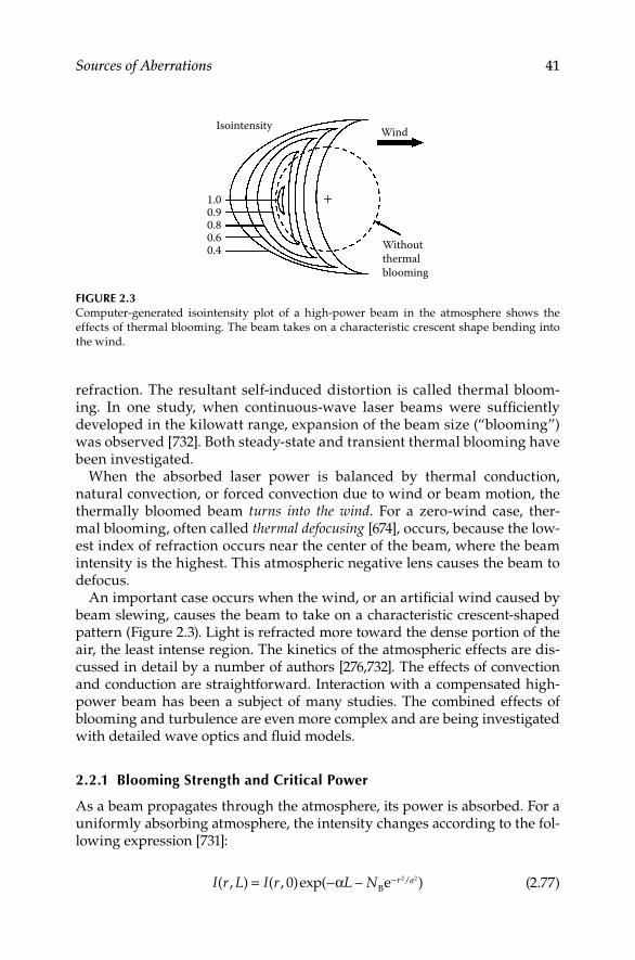
Sources of Aberrations 41
refraction The resultant self-induced distortion is called thermal bloom-ing In one study, when continuous-wave laser beams were sufficiently developed in the kilowatt range, expansion of the beam size (“blooming”) was observed [732] Both steady-state and transient thermal blooming have been investigated
When the absorbed laser power is balanced by thermal conduction, natural convection, or forced convection due to wind or beam motion, the thermally bloomed beam turns into the wind For a zero-wind case, ther-mal blooming, often called thermal defocusing [674], occurs, because the low-est index of refraction occurs near the center of the beam, where the beam intensity is the highest This atmospheric negative lens causes the beam to defocus
An important case occurs when the wind, or an artificial wind caused by beam slewing, causes the beam to take on a characteristic crescent-shaped pattern (Figure 23) Light is refracted more toward the dense portion of the air, the least intense region The kinetics of the atmospheric effects are dis-cussed in detail by a number of authors [276,732] The effects of convection and conduction are straightforward Interaction with a compensated high-power beam has been a subject of many studies The combined effects of blooming and turbulence are even more complex and are being investigated with detailed wave optics and fluid models
2.2.1 blooming Strength and Critical Power
As a beam propagates through the atmosphere, its power is absorbed For a uniformly absorbing atmosphere, the intensity changes according to the fol-lowing expression [731]:
I r L I r L N r a( , ) ( , )exp( )/= − − −0 2 2α Be (277)
Isointensity
1.0
Wind
+
Withoutthermalblooming
0.90.80.60.4
Figure 2.3Computer-generated isointensity plot of a high-power beam in the atmosphere shows the effects of thermal blooming The beam takes on a characteristic crescent shape bending into the wind

42 Principles of Adaptive Optics
where the linear absorption coefficient is α, the beam radius is a, the propa-gation path is L, and the dimensionless parameter NB is the magnitude of the blooming distortion [92]
For a case when a wind (or the beam is being slewed through the air), the distortion is not symmetric The blooming strength then becomes a func-tion of the wind velocity υw, the beam radius a, the specific heat at constant pressure Cp, and the density of the air ρ The Bradley–Herrmann blooming distortion number NB is [87,92]
NP n T k LC aB
p w
d d= −4 22
( / ) αρ υ
(278)
where P is the beam power, ρ is the mass density, and dn/dT is the change of index of refraction with temperature The index of refraction of air at tem-perature T is given by [608]
( ) ( ) ( )..
n T nT0 151 1
1 05491 0 00366air = + −
+
(279)
where T is in degrees Celsius The index for air at 15°C is given by Edlen [186] as
( ) ..
n158
21 10 8342 1
2406030130
1599638 9
− × = +−
+−λ −− −λ 2
(280)
where λ is in microns For example, (n0)air = 1000276 at 15°C and λ = 06328 μm For a focused beam, the radius a is replaced by an effective radius aeff over the propagation length L as follows:
aLa
eff =
λπ
1 3/
(281)
where the absorption coefficient is not constant along the propagation path and physical slewing of the beam occurs, Karr [403] presents a more general expression for the distortion number as follows:
Nn TC
Pa
zz zD
p w
= ∂ ∂
+
∞
∫8 22 0
πρ λ
αυ θ
/ ( )( )
e xxp [ ( ) ( )]− ′ + ′ ′
∫ α αz z z zz
s d d0
(282)
where α(z) is the path-dependent absorption coefficient, αs(z) is the path- dependent scattering coefficient, and θ is the angular slew rate
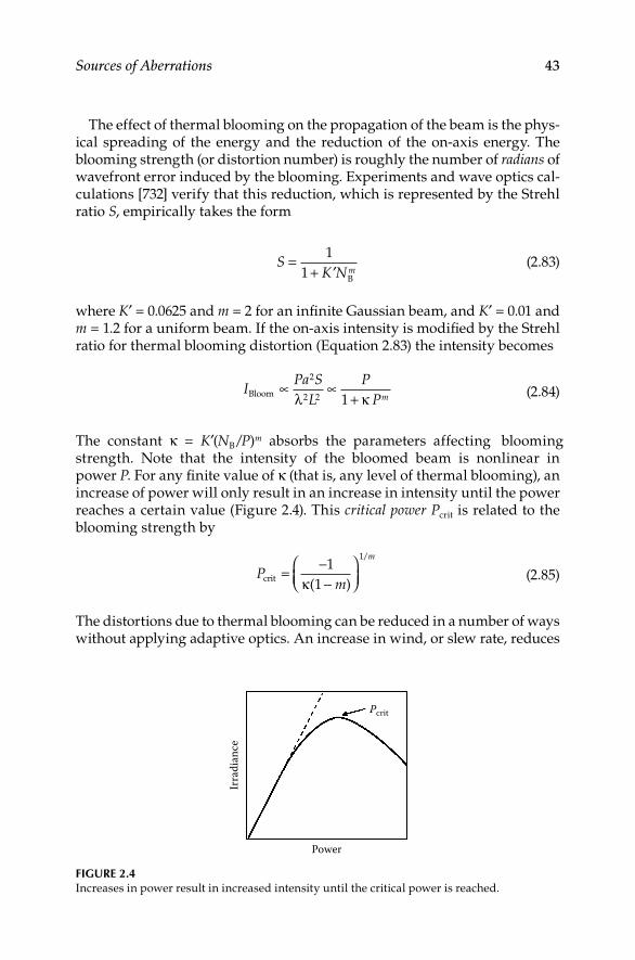
Sources of Aberrations 43
The effect of thermal blooming on the propagation of the beam is the phys-ical spreading of the energy and the reduction of the on-axis energy The blooming strength (or distortion number) is roughly the number of radians of wavefront error induced by the blooming Experiments and wave optics cal-culations [732] verify that this reduction, which is represented by the Strehl ratio S, empirically takes the form
SK Nm
=+ ′
11 B
(283)
where K′ = 00625 and m = 2 for an infinite Gaussian beam, and K′ = 001 and m = 12 for a uniform beam If the on-axis intensity is modified by the Strehl ratio for thermal blooming distortion (Equation 283) the intensity becomes
IPa S
LP
PmBloom ∝ ∝+
2
2 2 1λ κ (284)
The constant κ = K′(NB /P)m absorbs the parameters affecting blooming strength Note that the intensity of the bloomed beam is nonlinear in power P For any finite value of κ (that is, any level of thermal blooming), an increase of power will only result in an increase in intensity until the power reaches a certain value (Figure 24) This critical power Pcrit is related to the blooming strength by
Pm
m
crit = −−
11
1
κ( )
/
(285)
The distortions due to thermal blooming can be reduced in a number of ways without applying adaptive optics An increase in wind, or slew rate, reduces
Power
Pcrit
Irra
dian
ce
Figure 2.4Increases in power result in increased intensity until the critical power is reached

44 Principles of Adaptive Optics
the blooming strength and increases the Strehl ratio directly [426] Although this is simple, it is often impractical because the wind on a specific day in a specific place is unpredictable and the beam-propagation scenario might not allow slewing the beam in an arbitrary manner
If the power in the beam is applied for a duration that is too short for the atmosphere to develop a thermal lens, blooming could be avoided This prin-ciple can be applied by using pulse lasers Blooming will occur whenever density changes are propagated transverse to the beam by acoustic waves By properly controlling the pulse length and the pulse repetition frequency, thermal blooming often can be reduced
Pulsing a laser to avoid thermal blooming is not possible in all cases Reducing the pulse length without simultaneously reducing power can cause other phenomena worse than blooming Gas breakdown is the ioniza-tion of the air path that results from intense radiation in the gas The result is often total laser beam absorption [733]
When the pulse is long compared to the time a/υs, where a is the beam radius and υs is the velocity of sound, the long-time thermal blooming strength is given by
Nn T I tL
C altp
d d=
−2 02
2
( / )αρ
(286)
where αL << 1 Although the expression for long-time blooming strength shows a linear increase in time, there is a limiting factor Ulrich [799] showed that there exists a time when the on-axis intensity drops because of ther-mal blooming, such that the blooming can no longer continue This point is achieved when the intensity is about one-tenth of its initial value The time taken for this saturation to occur is given by
tn C
n TL
a Es
p
sd d=
0 048 0
2
1 22
.( / )
/ρ
υ αλ
(287)
where E is the pulse energyWhen the pulse length tp is short compared to the hydrodynamic lens-
forming time th, the pulse thermal blooming strength Np becomes [732]
Nn T E L t
C t as
pp p
d d=
−83
2 2 3
6
( / )υ απρ
(288)
where E is the pulse energy and the quantity αL is assumed to be small, that is, αL << 1 Equation 288 shows a cubic dependence on the time t after the onset of the pulse Short-term transient thermal blooming is often called t-cubed blooming

Sources of Aberrations 45
When a number of pulses are strung together, a condition called multiple- pulse thermal blooming occurs [183,588] The parameters that describe the effects of blooming for this case are the blooming strength Nmp and the num-ber of pulses per flow time (NP), so that
Nn T ELC amp
p
d d= −2 2
4
( / )αρ π
(289)
and
NP PRF= [ ]2aυ
(290)
These basic expressions can be used in Equation 283 to evaluate the effects of thermal blooming in the atmosphere The application of adaptive optics to correct for thermal blooming phenomena will require knowledge of the tem-poral and spatial effects of blooming distortion [602] Other than the pulse and multiple-pulse effects described earlier, the overall frequency for atmo-spheric response fb under blooming conditions [562] is fb = υ/(2a), where the wind velocity υ can be caused by slewing or actual wind or a combination of both, and the beam radius a must be evaluated for each case For a collimated beam, the aperture radius is a suitable approximation, and for a focused beam, the beam radius at 075L can be used for an approximation [7]
The historical summary and the simple expressions given here can be used for order-of-magnitude analyses The nonlinear behavior of the high-power beam in the atmosphere requires both extensive analysis and supporting experimentation [489]
2.2.2 Turbulence, Jitter, and Thermal blooming
The combined and often closely coupled effects of atmospheric turbulence, beam jitter, and thermal blooming are the topics of much investigation Although we can show simple rules for estimating the three effects indepen-dently, the response of the atmosphere for the three competing phenomena is extremely complicated For example, thermal blooming strength is a func-tion of the beam radius a and the wind velocity υ Beam jitter has the effect of a false wind, which would alter the degree of blooming If the jitter is of high frequency, the beam intensity is smeared before the atmosphere has time to respond, giving the appearance of a larger effective radius For inter-mediate frequencies, the beam’s own jitter might follow the bending into the wind phenomenon or even counteract it All of these phenomena might occur simultaneously [276]
Atmospheric turbulence has the effect of inducing dynamic tilt, which has the same characteristics as complicated beam jitter Turbulence can also

46 Principles of Adaptive Optics
induce beam spreading because of its high spatial frequency content This can increase the apparent beam radius, thus reducing the local intensity and the magnitude of the turbulence
Another phenomenon occurs when adaptive optics is used to try to correct for the combined effects of thermal blooming and turbulence The errors in the wavefront that occur in the propagation path tend to defocus or spread the beam Compensation for the negative atmospheric lens involves the application of the conjugate positive lens in beam-transmitting optics This effectively increases the intensity, which, on one hand, is the desired effect, but on the other hand, increases the strength of the thermal blooming and forces the atmosphere into a more negative lens This instability [404] along the beam path has been observed in a number of experiments [391] and is observed as small spatial scale (high spatial frequency) phase-conjugate instabilities [57,392,705,706]
Many investigators have studied the complexities of turbulence and thermal blooming [200,277,572,844] They have investigated simple scal-ing relationships [94], the detailed physics of the distortion process [97,337], and the applications of adaptive optics [540,706,842] They have used four- dimensional wave-optics models [154,540,551] supported by experimental verification [89,390,631] The limitations of adaptive optics compensation for thermal blooming, especially the requirement for full-field* compensation, generate the most interest [402] The complex interaction of diffraction, tur-bulence, and the high-power thermal blooming phenomenon at small scales limits the applicability of phase-only corrections [550]
2.3 Nonatmospheric Sources
Although turbulence is the major source of concern for astronomers using adaptive optics, and thermal blooming is a limiting factor for high-power beam propagation, adaptive optics are often used to correct for aberrations that enter a system in other ways
2.3.1 Optical Misalignments and Jitter
The inadvertent introduction of tilt or dynamic tilt (jitter) into a system can reduce its performance In some cases, this performance is only slightly reduced, as in the case of an imaging system where tilt simply moves the
* Full-field compensation applies a correction to both the amplitude and the phase This differs from the conventional phase-conjugate approach, discussed in Section 31, where correction is applied to the phase only

Sources of Aberrations 47
position of the image without affecting its quality These problems often can be accepted On the other hand, slight misalignments in optics inside a laser resonator can greatly reduce its performance and, in many cases, can elimi-nate the possibility of lasing altogether Errors in setting up or mounting, external error sources (such as mechanical (acoustic) vibration [599]), and thermal problems can all contribute negatively to a poorly performing sys-tem Defects such as tilt [898] and decenter [515] can be studied using ABCD matrices (see Section 31)
Adaptive optics in a tilt-correction mode can be used to correct for these errors [100] The problem of maintaining alignment or beam pointing has evolved from early electromechanical telescope- and radar-control systems to the present-day scanning and control systems that operate in the mega-hertz range This book treats tilt as a fundamental low-order wavefront aberration A tilted component in a system can induce other higher-order aberrations A tilted mirror or beam splitter intercepting a converging beam will introduce the next higher-order aberration, astigmatism A tilted spherical optical element in a telescope will introduce coma Severe tilts in complicated optical configurations can introduce many high-order aberrations
The elimination of tilt, or pointing error, is the first business of adaptive optics Control of fast tilt (jitter) or slow tilt (drift) is often all that is needed in an adaptive optics system
2.3.2 large Optics: Segmenting and Phasing
Striving for ever-better means of collecting faint starlight or focusing laser beams to extremely small spots requires larger and larger optical elements, the manufacture of which presents new problems for investigators and new challenges for adaptive optics Extending technology from the Keck tele-scopes’ alignment and phasing of the thirty-six 18-m segments into a 10-m diameter aperture has evolved into the phasing of 8-m segments into behe-moths as large as the 42-m diameter European Extremely Large Telescope
In large optics, small local deviations from perfect curvature are mani-fested as high spatial frequency aberrations that require correction Casting large mirrors requires extreme care [182] Even after a perfect casting, figur-ing, and coating, large optics (mostly mirrors) are placed in relatively hos-tile environments One operation that often produces aberrations is simply placing the mirror The effects of gravity on massive objects (weighing thou-sands of pounds and stretching many feet across) cause the mirror to sag and deform [23] If this mirror is placed on a movable mount, the direction of the deformation will change with the motion The sag can neither be calibrated out nor be polished away, because it will change during operation
The gravitational sag of a large mirror can be calculated The deflection ωz, normal to the surface, of a circular plate of radius a, which is placed horizon-tally is [58]

48 Principles of Adaptive Optics
ωρ ν ν
νν
νz =− +
+− +
++
3 116
51
2 31
2
24 2 2 4g
Eha a r r
( ) ( )
(291)
where ρ is material density, E is Young’s modulus, ν is Poisson’s ratio, h is disk thickness, and g is gravitational acceleration The aberrations for a mirror or large lens under the influence of gravity are a constant piston, a sphere term proportional to r2, and a spherical aberration proportional to r4 For a 24-m fused-silica mirror (the Hubble Space Telescope), for instance, there can be a total deflection of 3 μm and a spherical aberration compo-nent of 07 μm on the ground during polishing that would not be present in orbit
Adaptive optics can be used to correct for gravity effects and other effects of large size Large mirrors present interesting problems and interesting solutions Large mirrors can be self-correcting; that is, they can contain the necessary physical elements that adjust their figure and correct aberrations in other parts of the system as well [446]
Large optics can be subdivided into smaller segments These segments can then be coaligned or phased to act as a larger mirror The aberrations induced in large mirrors and the systems that are used to phase segments have been studied for a number of years [212,728] For the purpose of the study of adap-tive optics, aberrations due to gravity (low spatial frequency), local defects, or deformation (high spatial frequency) can be treated in the same manner as similar aberrations in smaller optics, with only the magnification of spa-tial frequency taken into account
Large mirror jitter is the same as small mirror jitter in terms of temporal frequency* The spatial frequency of the aberration is usually expressed in cycles/diameter (cyc/diam) Thus, a defect in a large 1-m mirror that is 1 cm across has much higher spatial frequency content (100 cyc/diam) than the same defect in a 20-cm mirror (20 cyc/diam)
The aberrations that occur at mismatched edges have very high spatial frequency content These almost-infinite spatial frequencies must be treated separately The correction over the edges (which is usually a very small por-tion of the area of the aperture) can be simply disregarded, or the light that impinges on these edges can be masked out The appearance of a sharp edge in a wavefront can disrupt an adaptive optics system If the wavefront is measured at two points on either side of the edge and it senses a difference in phase, the control system may perceive this to be a local tilt, whereas it is actually a piston error on one or both sides of the edge If the error is greater than one wavelength, the adaptive optics system may become unstable These difficulties are addressed in Chapter 5
* Even though it is difficult to get a large mirror jittering quickly, it is generally treated the same by an adaptive optics system
Sources of Aberrations 49
2.3.3 Thermally induced Distortions of Optics
When a beam of light strikes an optical surface, some of the energy is absorbed For low-power beams, imaging systems, and transparent glasses, the absorption is rarely noticed High-power beams (>10 kW/cm2) can induce a temperature rise in the optics that is proportional to the absorbed incident intensity Passive or uncooled mirrors and actively cooled mirrors exhibit distortions under high-power illumination
For a mirror modeled as a flat plate, the strain ε induced is proportional to the temperature rise T,
ε α= T (292)
where α is the coefficient of linear thermal expansion of the material For a plate in the x–y plane, the in-plane stresses σxx and σyy are given by
σν
ε νε α νxx xx yyE
T=−
+ − +1
12
[( ) ( ) ] (293)
σν
ε νε α νyy yy xxE
T=−
+ − +1
12
[( ) ( ) ] (294)
where the strain tensors are ε, Young’s modulus is E, and ν is Poisson’s ratio Myers and Allen [550] show as follows how the in-plane stresses result in the strain:
ε ν σ σ αxx xx yyET= + +( ) (295)
With uniform incident intensity, a flat circular plate of thickness h shows an out-of-plane displacement ω(r, θ)
ω θ θ( , ) [ ] [ ]exp( )r C C r C r C r i= + + +0 22
1 33 (296)
This is a solution of Poisson’s equation ∇ = −2ω mt, where mt is the thermal moment density, calculated as follows:
mE
T x y z z zh
h
t d= −− −
∫α
ν1 2
2
( , , )/
/
(297)
The constants Ci are computed from the specific boundary conditions For a plate uniformly constrained at the edges (ie, C1 = C3 = 0), the distortion is a constant plus a function of the radial distance from the center Thus,
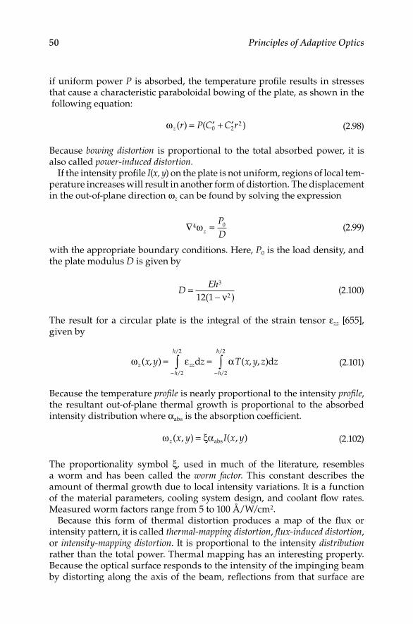
50 Principles of Adaptive Optics
if uniform power P is absorbed, the temperature profile results in stresses that cause a characteristic paraboloidal bowing of the plate, as shown in the following equation:
ωz r P C C r( ) ( )= ′ + ′0 22 (298)
Because bowing distortion is proportional to the total absorbed power, it is also called power-induced distortion
If the intensity profile I(x, y) on the plate is not uniform, regions of local tem-perature increases will result in another form of distortion The displacement in the out-of-plane direction ωz can be found by solving the expression
∇ =4 0ωz
PD
(299)
with the appropriate boundary conditions Here, P0 is the load density, and the plate modulus D is given by
DEh=
−
3
212 1( )ν (2100)
The result for a circular plate is the integral of the strain tensor εzz [655], given by
ω ε αz zzh
h
h
h
x y z T x y z z( , ) ( , , )/
/
/
/
= =− −∫ ∫d d
2
2
2
2
(2101)
Because the temperature profile is nearly proportional to the intensity profile, the resultant out-of-plane thermal growth is proportional to the absorbed intensity distribution where αabs is the absorption coefficient
ω ξαz x y I x y( , ) ( , )= abs (2102)
The proportionality symbol ξ, used in much of the literature, resembles a worm and has been called the worm factor This constant describes the amount of thermal growth due to local intensity variations It is a function of the material parameters, cooling system design, and coolant flow rates Measured worm factors range from 5 to 100 Å/W/cm2
Because this form of thermal distortion produces a map of the flux or intensity pattern, it is called thermal-mapping distortion, flux-induced distortion, or intensity-mapping distortion It is proportional to the intensity distribution rather than the total power Thermal mapping has an interesting property Because the optical surface responds to the intensity of the impinging beam by distorting along the axis of the beam, reflections from that surface are

Sources of Aberrations 51
advanced or retarded by the surface map Thermal mapping translates inten-sity information from a beam into the phase (wavefront) Nonuniformity in the intensity results in reduction of the Strehl ratio and more severe beam-propagation limitations
The thermomechanical response of a plate cannot always follow the inten-sity pattern exactly Thermal diffusion tends to smooth the temperature dis-tribution, and the mechanical response of the plate tends to smooth it more A more exact treatment of thermal mapping would show these effects as convolutions (represented by ∗) among the responses of the material to ther-mal load RT, mechanical stress RM, and absorbed intensity forcing function αI(x, y, t), as follows:
ω ξz t R t R t I x y t( ) ( ) ( ) ( , , )= ∗ ∗T M α (2103)
These responses can often be calculated numerically for different conditions Both steady-state and transient solutions are often needed For instance, a continuous beam impinging on a mirror with active cooling reaches steady-state distortion in a few seconds or less The temperature profile, used in Equation 297, for the surface of a mirror when it is illuminated by a pulsed beam is a function of the thermal diffusivity ζ and thermal conductivity kt:
T x y T x yI x y
k( , , ) ( , , )
( , )τ ζτ
π= +0 0
4
t
(2104)
where τ is the pulse length and T0 is the surface temperature before the pulse [114]
2.3.4 Manufacturing and Microerrors
Manufacturing of optics has always been limited by the available technol-ogy The choice of glass or metal substrates is dependent on their ultimate performance In 1730, Isaac Newton wrote [559]:
But because Metal is more difficult to polish than Glass, and is afterwards very apt to be spoiled by tarnishing, and reflects not so much Light as Glass quick-silver’d over does: I would propound to use instead of the Metal, a Glass ground concave on the foreside, and as much convex on the back-side, and quick-silver’d over on the convex side The Glass must be every where of the same thickness exactly
The manufacturing technology of the optical surfaces limits the overall per-formance of the optical system With adaptive optics technology, many of the defects that arise from manufacturing can be corrected The materials chosen for refractive or reflective optics may have surface errors that figuring and polishing cannot remove Generally, they are of such low magnitude or high
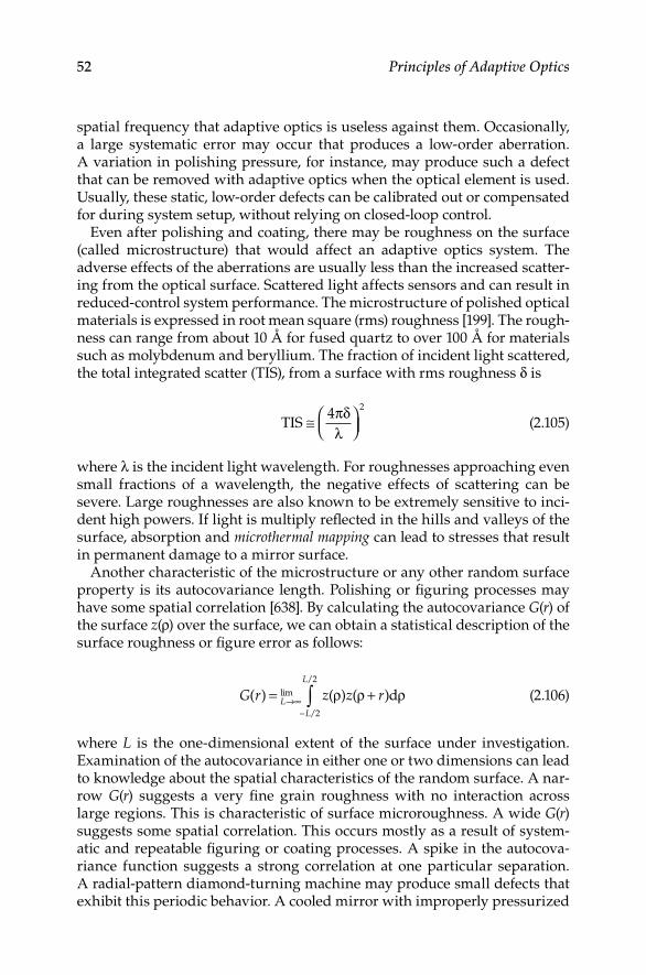
52 Principles of Adaptive Optics
spatial frequency that adaptive optics is useless against them Occasionally, a large systematic error may occur that produces a low-order aberration A variation in polishing pressure, for instance, may produce such a defect that can be removed with adaptive optics when the optical element is used Usually, these static, low-order defects can be calibrated out or compensated for during system setup, without relying on closed-loop control
Even after polishing and coating, there may be roughness on the surface (called microstructure) that would affect an adaptive optics system The adverse effects of the aberrations are usually less than the increased scatter-ing from the optical surface Scattered light affects sensors and can result in reduced-control system performance The microstructure of polished optical materials is expressed in root mean square (rms) roughness [199] The rough-ness can range from about 10 Å for fused quartz to over 100 Å for materials such as molybdenum and beryllium The fraction of incident light scattered, the total integrated scatter (TIS), from a surface with rms roughness δ is
TIS ≅
4 2πδλ
(2105)
where λ is the incident light wavelength For roughnesses approaching even small fractions of a wavelength, the negative effects of scattering can be severe Large roughnesses are also known to be extremely sensitive to inci-dent high powers If light is multiply reflected in the hills and valleys of the surface, absorption and microthermal mapping can lead to stresses that result in permanent damage to a mirror surface
Another characteristic of the microstructure or any other random surface property is its autocovariance length Polishing or figuring processes may have some spatial correlation [638] By calculating the autocovariance G(r) of the surface z(ρ) over the surface, we can obtain a statistical description of the surface roughness or figure error as follows:
G r z z rLL
L
( ) ( ) ( )lim
/
/
= +→∞−∫ ρ ρ ρd
2
2
(2106)
where L is the one-dimensional extent of the surface under investigation Examination of the autocovariance in either one or two dimensions can lead to knowledge about the spatial characteristics of the random surface A nar-row G(r) suggests a very fine grain roughness with no interaction across large regions This is characteristic of surface microroughness A wide G(r) suggests some spatial correlation This occurs mostly as a result of system-atic and repeatable figuring or coating processes A spike in the autocova-riance function suggests a strong correlation at one particular separation A radial-pattern diamond-turning machine may produce small defects that exhibit this periodic behavior A cooled mirror with improperly pressurized

Sources of Aberrations 53
coolant channels may also exhibit periodic “print-through” of the coolant channels that show up as a spike or bump in the autocovariance function Even though adaptive optics cannot correct for many of the very small or high spatial frequency errors, these errors can mask the disturbances that adaptive optics is supposed to correct
2.3.5 Other Sources of Aberrations
Adaptive optics is also used for purposes other than air or vacuum propaga-tion and simple reflections or refractions Advanced applications include imag-ing the human retina [463], supporting light transmission through sea water [622], ground-to-ground free-space laser communications, ground-to-space laser communications, transmission through fiber optics, in laser fusion sys-tems [543,825], and in solid or gas lasing media Each of these applications pres-ents different possibilities for introducing aberrations that require correction by adaptive optics Turbulence in the vitreous humor of the eyeball distorts imagery, but this defect can be compensated with conventional adaptive optics Details of this application are given in Chapter 4 The refractive index of sea water is above 13 It is transmissive in the blue-green spectral region and is the obvious medium of propagation for surface-to-submarine communica-tions The sea has large thermal gradients that produce turbulence [622] The turbulence results in aberrations that degrade the signal Light in a free-space communications system acts as the carrier, but severe aberrations can distort the modulation such that the bit-error-rate is increased dramatically [673] Details of adaptive optics laser communication systems will also be discussed in Chapter 4
2.3.6 Aberrations due to Aircraft boundary layer Turbulence
Imaging from a moving aircraft presents some problems An aircraft moving through ambient air produces turbulence in the boundary layer directly in front of the objective of an aerial camera The expression for the boundary-layer MTF [453], which follows an exponential similar to that for Kolmogorov atmospheric turbulence (Equation 275), is given by
MF
rBLBL
= −
exp ./
3 445 3λξ
(2107)
where F is the focal length of the objective and rBL is the correlation length for the boundary layer The correlation length, analogous to Fried’s parameter, depends upon the flight speed, aircraft surface form, and air density At vis-ible wavelengths, rBL varies from 5 to 20 mm [406] Many mechanical meth-ods are used to reduce the boundary-layer aberration and to characterize the remaining aberration [303]

54 Principles of Adaptive Optics
2.3.7 Aberrations in laser resonators and lasing Media
Laser resonators present many opportunities for aberrations to arise The multiple-pass nature of most resonators lets an aberrated propagating wave diffract into intensity fluctuations The intensity fluctuations can cause fur-ther degradation [6] Optics inside a resonant cavity can become misaligned, similar to optics in any beam train Tilts, defocus [14,234], and astigmatism can appear in resonators and greatly affect their performance [594,595,741] Coupling between various aberrations has been investigated [594] Static wavefront tilt and dynamic tilt (jitter) can reach critical levels at which the resonator can no longer support lasing [433]
The laser gain medium can be responsible for a number of aberrations Because lasing can take place in solids, liquids, gases, or plasmas, any imperfections in these media that result in inhomogeneous distributions of gain can reduce laser performance Structural imperfections in solid-state lasers [894] and turbulence in liquid or gas lasers [328,601,674] are the most common problems Dynamic gas lasers and free-electron lasers have rap-idly moving laser media that provide another source of disturbance to the wavefront [168]
Some common pass resonators [722,723], such as an unstable annular reso-nator, can be insensitive to some effects For instance, the misalignment of a conical mirror or an axicon [518] will cause a shortening of the path on one side of a device but an equal lengthening on the other side [548] The round-trip photon experiences no phase variation In such resonators, the radiation is not confined to a small central core, as it usually is in stable reso-nators When the radiation spreads and encounters conical mirrors and out-put scraper mirrors, the edge effects become very important [15,716] Edges impart very high spatial frequency aberrations to the wavefront, which often results in more divergence than that seen in an apodized or slowly decaying intensity edge
Adaptive optics systems have been used for correction of aberrations inherent in resonators and lasing media In some cases, the adaptive optics systems were placed inside the resonant cavity [234,625,222] Other systems have been designed to correct the aberrated output of a laser resonator regardless of the source of the disturbances Details of the sensing and cor-rection methods are discussed in Chapters 5 and 6

55
3Adaptive Optics Compensation
When the various disturbances discussed in Chapter 2 are unavoidable, adap-tive optics comes to the rescue Each adaptive optics system should enhance the performance of its “parent” optical system Adaptive optics should be added to an imaging system only if it improves the images and should be added to a laser fusion system only if it enhances the fusion process [825]
There are many ways to approach the problem of compensating for the aberrations Conventional approaches that use wavefront sensors, electronic controls, and correction optics can be used to overcome the effects of the aberrations Some passive methods have also been suggested Beckers [68,69] describes a method of after-the-fact optical correction that is possible on astronomical optical interferometers Since the point spread function of an imaging system consists of a central spike of “good” information surrounded by a broad background of noise (Figure 22), he suggests a placement of an aperture or single-mode fiber that restricts the amount of light to the central spike Other unconventional methods use the nonlinear properties of certain optical materials to correct the effects of aberrations In any case, the applica-tion of corrections is generally a closed-loop real-time process Non–real-time techniques of image processing using wavefront information are usually inadequate The modulation transfer function (MTF) of the aberrated image is so low that the signal is corrupted by noise Adaptive optics are necessary up front to improve the MTF and the signal-to-noise ratio (SNR)
The most common approach to correcting the various aberrations is the principle of phase conjugation, which is sometimes referred to as phase-only conjugation to distinguish it from systems that also correct amplitude effects The term “phase conjugation” is widely used synonymously with nonlinear phase conjugation However, the principle of applying a conjugate phase to a beam is the basis for most forms of adaptive optics, either linear (conven-tional) or nonlinear
3.1 Phase Conjugation
The principle of phase conjugation is the core of adaptive optics [340] It can be analyzed in a number of ways The method for applying phase con-jugation is shown in Figures 31 and 32 The wavefront of a beam enter-ing from the left (Figure 31a) is distorted by a piece of glass because the index of refraction is higher than one The wavefront is retarded as it goes

56 Principles of Adaptive Optics
through the glass (Figure 31b) After reflection from the mirror (Figure 31c), the wavefront has the same shape but propagates in the opposite direction As it traverses the glass again (Figure 31d), it receives the same retardation as before The exiting wavefront (Figure 31e) is greatly distorted, since it has passed through the aberrator twice
Wavefront
Conventionalmirror
(d)
(a) (b) (c)
(e)
Figure 3.1Wavefront distortion traversing an aberrator: (a) The plane wavefront passes through an aber-rator and the wavefront is delayed (b) The wavefront with the delay reflects from (c) a con-ventional mirror and (d) travels toward the left with the delay (e) As it passes a second time through the aberrator, the wavefront is delayed further
Wavefront
(a) (b)
(e)(d)
(c)
Deformablemirror
Figure 3.2Wavefront distortion traversing an aberrator with a correcting mirror: (a) The plane wavefront passes through an aberrator and the wavefront is delayed (b) The wavefront with the delay reflects from (c) the deformable mirror with the conjugate shape and (d) travels toward the left with the delay reversed (e) As it passes a second time through the aberrator, the wavefront is returned to a plane

Adaptive Optics Compensation 57
If we want to achieve a plane wavefront after a beam passes through the glass twice, there may be a way to alter the surface of the mirror in such a way as to invert the wavefront so that the second passage leaves no residual distortion Looking at Figure 32, we can see that a bump in the mirror at just the right place and at just the right amount can cause the leading edge of the wavefront to be reversed When this wavefront (Figure 32d) passes through the aberrator again, the final wavefront (Figure 32e) is once again a plane The amount of “bump” needed in the mirror is proportional to the wavefront itself and has the reverse sign This in essence multiplies the field |E|e−iϕ by its complex conjugate |E|e+iϕ; thus the name phase conjugation
There are some very big “ifs” in the preceding argument If we can put the right amount of phase conjugate at the right place, then we can accom-plish the correction As discussed in Chapter 2, many aberrations are dynamic; we must also place the phase conjugate on the beam at the right time These three constraints to the relatively simple problem of apply-ing a phase conjugate are the reasons for difficulties that have had to be addressed before there were significant advances in adaptive optics Another way to understand the phase conjugate concept and its limitations is by examining a simple imaging system Using the paraxial approxima-tion, that is, geometric optics, and the method of ABCD matrices, we can see how phase conjugation can be used to correct aberrations outside an imaging system If a ray entering from the left is represented by its dis-placement from the axis x and its slope s, we can trace it to the focal point of a simple imaging system (Figure 33) The lens of the imaging system (focal length f ) forms an image at the distance F = f behind the lens The characteristic of the ray after traversing the imaging system x′ and s′ is given by the matrix equation
10 1
1 01 1
F
f
x
s
x
s
−
=′′
/
(31)
A ray normal to the lens (s = 0) will cross the axis at a distance f from the lens Now, if there is an aberration represented by another lens fa a distance d from the imaging system, the ray will not cross the axis at the focal point of the
f
F = f
Figure 3.3Simple imaging system

58 Principles of Adaptive Optics
imaging system See the top of Figure 34 The position of axis crossing (the new focus for the rays) is given by
F fd f
d f f=
−− −
a
a
(32)
That means that we can compensate for the aberration by refocusing the beam If we simply apply a correcting lens with focal length fc directly after the imaging system lens (bottom of Figure 34), we find that the “adaptive optics” imaging system has an apparent focal length of ( fc f)/( fc + f ) and the correcting lens focal length is given by
fF f f dc
a
= − −+
−1 1 1
1
( ) (33)
This shows that measurement of the wavefront (the displacement and the slope of the ray) can lead to a correction for the misfocus introduced by some outside source In a special case where the focal plane is left at distance F from the lens and the aberration is near the imaging system d → 0, the focal length of the correcting system is the opposite of the aberration: fc = −fa
If a wavefront is made up of the leading edges of spherical waves (Huygens’ principle), we can see how the ABCD matrix method can be used to under-stand adaptive optics If each part of a wavefront is measured in terms of its slope s, we can produce the characteristics of the entire wavefront Knowing where each slope measurement comes from is equivalent to knowing the displacement from the axis, x Repeated and simultaneous adjustment of the correction device fc can result in a conjugated wavefront
f
d
fa f fc
f
Figure 3.4Simple imaging system with aberrating lens

Adaptive Optics Compensation 59
A more rigorous treatment can show the phase-conjugation principle without the restrictive geometric approximations From Figure 35 we can calculate the field U4(x2, y2) after transmission through an aberrating plate, propagation to a correcting mirror, reflection, and propagation back through the aberrating plate The input field propagating left to right is a constant plane wave |U1| After transmission through the aberrating plate, the field has a phase compo-nent Ua = |U1|e aikφ Propagation to the mirror results in a field U2
Uik
dx x U
ikrd
ikd
22
2
2 2=
∫
ed da b a
a
πexp (34)
where r x x y ya a a22
22
22= − + −( ) ( ) and the integral is over the limiting aper-
ture The mirror has the correction applied to its surface, ϕc, so that the field leaving the mirror is U ik
2e cφ After propagation back to the aberrating plate, the field has the form
U x yik
dx y U
ikrikdik
3 a a m mae
d d e c( , ) exp=+
2 2222
πφ
dd
∫mirror (35)
After a final pass through the aberrating plate, the field has the form
Ukd
U x yik ikf d ik4
2
2 12
222= −e d d e ea a c
m mφ φ
π−
( )| | / dd d e ea a
a ax y ik ikf dφ −∫∫ 22 2/ (36)
This equation has no analytical solution for a general case, since the form of the aberration and the boundaries of the integration (the apertures) are unspecified However, for a case analogous to the single slab of glass discussed earlier, the exponential aberration terms can be brought outside the integral as follows:
Ukd
U x yik ik ikf4
22
2 12
222= − −e e d d ea c a
m mφ φ
π( )| | / dd ikf dx yd d ea a
a−∫∫ 22 2/ (37)
For the field U4 to exactly equal the field U1, the aperture effects must be neglected and the correction applied ϕc = −2ϕa Accounting for the double-pass nature of this problem, the correction must be the conjugate of the aberration
This brings up a fundamental limitation of adaptive optics If the wavefront cannot be precisely determined or precisely replicated or if diffraction effects dominate, the phase conjugation cannot be exactly employed This limits the
U4
U1 Ua
U3
U2ϕa
Figure 3.5Simple propagation with aber-rating object

60 Principles of Adaptive Optics
effectiveness of adaptive optics in many places For instance, high-altitude aerosols can enhance thermal blooming The wavefront changes at high altitudes are seldom seen by wavefront sensors at the ground level, since diffractive effects mask the phase measurement Many systems designed for adaptive optics correction must specifically take into account the relation-ship of the aberrations to the position of the corrections One method applies correction in the image plane of the phase disturbance Some nonlinear opti-cal methods (eg, stimulated Brillouin scattering) use the aberrated beams themselves to instigate the correction Other methods apply correction of the wavefront near the aberration source to limit diffractive effects (the keeping it in the near-field approach) Some adaptive optics systems recognize the limi-tations and just correct as much as they can [569,574,627,734]
3.2 Limitations of Phase Conjugation
Up to now, we have implied that adaptive optics systems can have perfect phase conjugation and the systems are only “performing well” when such perfect phase conjugation is achieved Perfect phase conjugation is not a nec-essary condition for adaptive optics to show usefulness For speckle inter-ferometry [569] or astronomy, partial compensation is not only useful, but because of the high cost of adaptive optics, it is the only option An 8-m ter-restrial telescope requires more than 1500 correction zones to compensate for turbulence in the visible waveband and achieve near diffraction-limited per-formance [59,524] Even though the mathematics of nonlinear optics show that fields are conjugated, the fidelity of that conjugation is highly dependent upon the quality of the pump beams, the homogeneity of the medium, and the extent to which the expansion of the nonlinear susceptibility terms holds
For conventional adaptive optics, the limitations on phase conjugation are due to many sources The quality of wavefront measurement, speed and fidel-ity of interpretation, and quality of wavefront surface contour reproduction all have an effect on the phase-conjugation process A number of research-ers have developed expressions relating the parameters of adaptive optics systems to their system-level performance The limitations can be based on spatial constraints, such as the spatial resolution of the sensors or correctors They can also be based on temporal constraints such as the detector integra-tion time or the computer system speed
3.2.1 Turbulence Tilt or Jitter error
The tilt or jitter error due to turbulence was discussed in Section 213 and expressed in Equation 245

Adaptive Optics Compensation 61
3.2.2 Turbulence Higher-Order Spatial error
3.2.2.1 Modal Analysis
Chapter 2 gave an expression for the wavefront variance in terms of the num-ber of Zernike modes included Specifically, Equation 239 and the accompa-nying filters from Equation 241 can be used to rigorously derive a variance with Zernike modes compensated Because Zernike modes are orthogonal, we can modify Equation 239 to describe the compensated wavefront vari-ance with Zernike terms removed as follows:
σ κκWF d d2 2 2
0
20 2073113
= −
∫. ( ) cosk zC zn
L
−−∞
∞ ′
∫ ∑−
−
κ κ2
21
( )( ),
,
z Lk
Fn mn m
N
(38)
where N′ is the number of Zernike terms removedAnother approach to describe the effect of modal correction is given by
Noll [570] with a rigorous analysis by Conan [148] By Fourier-transforming the atmospheric turbulence wavefront represented by Zernike polynomials, an expression was derived for determining the residual wavefront variance after correction For Kolmogorov turbulence, the residual variance σ2 is a function of the number of modes corrected With respect to the mean phase (piston removed), uncorrected turbulence over an aperture of diameter D results in a residual σ2 ≈ 10299(D/r0)5/3 radians squared Correction of the next few modes is as follows:
One-dimensional tilt σ2
0
5 3
0 582=
./
Dr
Two-dimensional tilt σ2
0
5 3
0 134=
./
Dr
Focus σ2
0
5 3
0 111=
./
Dr
For higher-mode correction, Noll developed the approximation
σ2 3 2
0
5 3
20 2944=
−. ( )//
NDrm radians (39)
where Nm is the number of modes corrected
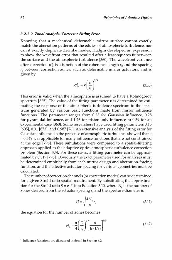
62 Principles of Adaptive Optics
3.2.2.2 Zonal Analysis: Corrector Fitting Error
Knowing that a mechanical deformable mirror surface cannot exactly match the aberration patterns of the eddies of atmospheric turbulence, nor can it exactly duplicate Zernike modes, Hudgin developed an expression to show the wavefront error that resulted after a least-squares fit between the surface and the atmospheric turbulence [360] The wavefront variance after correction σ fit
2 is a function of the coherence length r0 and the spacing rs between correction zones, such as deformable mirror actuators, and is given by
σ κfits2
0
5 3
=
rr
/
(310)
This error is valid when the atmosphere is assumed to have a Kolmogorov spectrum [325] The value of the fitting parameter κ is determined by esti-mating the response of the atmospheric turbulence spectrum to the spec-trum generated by various basic functions made from mirror influence functions* The parameter ranges from 023 for Gaussian influence, 028 for pyramidal influence, and 126 for piston-only influence to 039 for an experimental case [360] Some researchers have used fitting parameters 015 [605], 031 [873], and 0987 [76] An extensive analysis of the fitting error for Gaussian influence in the presence of atmospheric turbulence showed that κ = 0349 was applicable for many influence functions that are not constrained at the edge [796] These simulations were compared to a spatial-filtering approach applied to the adaptive optics atmospheric turbulence correction problem (Section 35) For these cases, a fitting parameter can be approxi-mated by 0319 [796] Obviously, the exact parameter used for analyses must be determined empirically from each mirror design and aberration-forcing function, and the effective actuator spacing for various geometries must be calculated
The number of correction channels (or correction modes) can be determined for a given Strehl ratio spatial requirement By substituting the approxima-tion for the Strehl ratio S = −e σ2 into Equation 310, where Na is the number of zones derived from the actuator spacing rs and the aperture diameter is
DN
r=4 a
sπ (311)
the equation for the number of zones becomes
NDr sa =
π κ4 10
2 6 5
ln( / )
/ (312)
* Influence functions are discussed in detail in Section 62
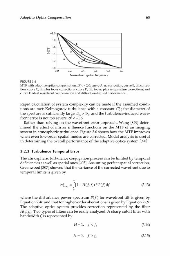
Adaptive Optics Compensation 63
Rapid calculation of system complexity can be made if the assumed condi-tions are met: Kolmogorov turbulence with a constant Cn
2 ; the diameter of the aperture is sufficiently large, DA > 4rs; and the turbulence-induced wave-front error is not too severe, σ2 < ∼16
Rather than relying on the wavefront error approach, Wang [849] deter-mined the effect of mirror influence functions on the MTF of an imaging system in atmospheric turbulence Figure 36 shows how the MTF improves when even low-order spatial modes are corrected Modal analysis is useful in determining the overall performance of the adaptive optics system [398]
3.2.3 Turbulence Temporal error
The atmospheric turbulence conjugation process can be limited by temporal deficiencies as well as spatial ones [405] Assuming perfect spatial correction, Greenwood [307] showed that the variance of the corrected wavefront due to temporal limits is given by
σ temp c d2 2
0
1= −∞
∫| ( , )| ( )H f f P f f (313)
where the disturbance power spectrum P( f ) for wavefront tilt is given by Equation 246 and that for higher-order aberrations is given by Equation 269 The adaptive optics system provides correction represented by the filter H( f, fc) Two types of filters can be easily analyzed A sharp cutoff filter with bandwidth fc is represented by
H f f= <1, c (314)
H f f= ≥0, c (315)
0.8
+1.0
0.6
0.0 0.2
A
B
E
D
C
0.6 0.8 1.00.4Normalized spatial frequency
MT
F
0.4
0.2
0.0
Figure 3.6MTF with adaptive optics compensation, D/r0 = 20: curve A, no correction; curve B, tilt correc-tion; curve C, tilt plus focus corrections; curve D, tilt, focus, plus astigmatism corrections; and curve E, ideal wavefront compensation and diffraction-limited performance

64 Principles of Adaptive Optics
An RC filter is represented by
Hiff
= +
−
11
c
(316)
For a tilt-control system with a bandwidth (3-dB cutoff frequency) of f3dB, the angular tilt variance after compensation is
α λcomp
TG
3dB
2
2 2
=
ff D
(317)
The tilt Greenwood frequency is Equation 254 The higher-order wavefront variance due to temporal constraints, σ temp
2 , is
σ tempG
dB
2
3
5 3
=
ff
/
(318)
where the Greenwood frequency is Equation 270Winocur combined the expression for modal spatial correction with
Greenwood’s temporal considerations [873] The result was not in analytic form, but an extensive numerical analysis showed how the relative intensity, or Strehl ratio, was improved by increasing spatial and temporal bandwidths Considering the control system requirements for transmission from ground to space (300 km altitude) with a 2-meter aperture at a 05 μm wavelength shows how 70 radial modes (2556 Zernike aberration terms) are required, at a servo bandwidth of greater than 300 Hz, to achieve a Strehl ratio of 09 (Figure 37)
1.0
0.8
0.6
0.4
0.2
0.010 100
Bandwidth (Hz)
2556
231
66
Rela
tive
inte
nsity
1000
Figure 3.7Spatial and temporal requirement for correcting ground-to-space transmission The number on each curve is the number of modes corrected

Adaptive Optics Compensation 65
One way to avoid the temporal limitations is to “get lucky” So-called lucky imaging systems take many short exposures with adaptive optics doing the best that it can, and then, choose the images that are sharpest because they were captured in the short period that the atmosphere was benign [852] To reduce the data storage and processing burden, wavefront sensor mea-surements can be used to select the images that were taken under the best atmospheric conditions [112] Clear imaging in visible wavelengths is now possible where only infrared adaptive optics were once considered [450]
3.2.4 Sensor Noise limitations
A restriction to the adaptive optics process, expressed in terms of wavefront variance, is due to the limitations of the wavefront sensor It is related to the signal strength and processing properties of the sensor Kern et al [410] use the expression
σ π λλWFS
2 A=
2 22
n (319)
where n is the number of photons detected per subaperture, usually less than 1000 [326] The mean wavelength of the wavefront sensor detection band is λA Hardy [321,326] shows an explicit expression for the variance for the spe-cial case of a shearing interferometer in visible light (Section 531),
σπγWFS(SI)
s22
2
2
2=n
ds
(320)
where γ is the fringe contrast, ds is the subaperture diameter, and s is the shear distance
For the case of the Hartmann sensor, the subaperture tilt measurement limitations apply The wavefront variance is
σ
π
WFS(H)2
2
2 2 1 2
23
16 8=
+
s/
SSNR (321)
The term s in Equation 321 is the size of the source For a natural star or an object at infinity, s = 0 Where a CCD array is used to determine the centroids in a Hartmann sensor, with npix pixels used in each subaperture, the SNR is
SNR
pix r bg
=+ +( )
N
N n σ σ2 21 2/
(322)

66 Principles of Adaptive Optics
where N is the number of signal electrons, σr are the noise electrons, and σbg are the background electrons
The wavefront sensor must have a sufficiently bright source to keep the SNR high For astronomical imaging, bright natural guide stars are required Roddier [661] suggests that there is about a 30% chance of finding a suitable guide star for an 8- to 10-m telescope Tip/tilt control of an 8-m telescope with low noise detectors is possible with about 10,000 stars per square degree Low-order compensation is possible with about 4,000 stars per square degree [20] If the angular density of stars with magnitude m or brighter is given by ρ(m), using for instance ρ(m) = 145 exp(096m) stars/rad2 [598], the prob-ability of detecting N stars in solid angle Ω in the magnitude range from m1 to m2 is [198]
P N m m
m m
Nm
m
mN
( , , )
( )
!exp ( )1 2
1
2
=
−∫ Ω
Ωρ
ρ
d
ddmm
m
1
2
∫
(323)
3.2.5 Thermal blooming Compensation
Thermal blooming can be partially corrected with adaptive optics [87] When thermal blooming is expressed in terms of the distortion number NB (Section 22), an adaptive optics system correcting Nm modes will reduce the wave-front variance to [575]
σπbloom
B
m
24
2
2 5
25
=
NN .
(324)
3.2.6 Anisoplanatism
The atmosphere can be considered a plane normal to the direction of the propagation of a beam This plane has various phase changes over the sur-face If a beam is sent through any portion of the plane and sees the same wavefront error, it would be considered isoplanatic From the discussion in Section 21, we know that this is not the case One part of the atmosphere distorts the beam in a different manner than another part Even though the statistics are the same, the atmospheric turbulence realizations are different Propagation through turbulence is anisoplanatic [123] There will be different wavefront errors for two small beams and different wavefront errors for dif-ferent parts of a large beam Anisoplanatism has serious consequences for adaptive optics for large apertures, compensating a large field of view, or for

Adaptive Optics Compensation 67
concepts such as spatial-sharing return-wave systems [308] Although aniso-planatism is a spatial phenomenon, it can arise under other stimuli Two beams displaced and parallel to each other produce displacement anisopla-natism Two beams propagating at slightly different angles with respect to each other produce angular anisoplanatism [745] Two beams whose sources are at a different distance from the receiver, where the region sampled by the receiver is in the shape of a cone, exhibit the cone effect or focal anisopla-natism A time delay between the propagation of two beams coupled with a wind that is moving the atmosphere results in temporal anisoplanatism Lastly, two beams of slightly different wavelengths that experience different amounts of turbulence-induced aberration represent an example of chromatic anisoplanatism (Section 56)
The amount of the angular anisoplanatic aberration can be calculated from the Kolmogorov spectrum [243] Experimental measurements have been made to verify these expressions [870] Referring to Figure 38, the wavefront variance (in square radians) for two beams separated by an angle θ pointing at a target or a turbulence layer a distance L away is
σ θisopath
d2 2 2 5 32 91= ∫. ( ) /k C z zn
L
(325)
When (D/r0)/(θ/ θ0) → ∞, the variance becomes
σ θθiso
2
0
5 3
=
/
(326)
Beacon
R
ΘL
ApertureD
Adaptiveopticssystem
Propagationreceiver
Starobject
Figure 3.8Geometry related to anisoplanatism

68 Principles of Adaptive Optics
where θ0 is defined as the isoplanatic angle as follows:
θ02 2
3 5
2 91 5 3=
∫
−
. ( ) /
/
k C z z zn
L
dpath
(327)
For constant Cn2, remembering that r k C Ln0
2 23 5
0 423= −
./
, the expression for the isoplanatic angle reduces to [659]
θ000 6
≈. rL (328)
If the angular separation θ is much smaller than the isoplanatic angle, the vari-ance between the different paths is small and adaptive optics correction can be very good When the opposite is true, the adaptive optics system will apply an incorrect conjugate and the correction will not be very good In some cases, no correction is better than the wrong correction Because the isoplanatic angle for tilt is approximately four times θ0, and the full aperture can be used to measure tilt from a natural guide star, the source can be faint and not as close to the science object as would be required for higher-order correction
Temporal anisoplanatism occurs in a beam-propagation scenario The light from the beacon is delayed by its time of flight Δt = L/c The corrected beam will reach the target another Δt later The atmosphere has had time to move and change [105] An analysis by Tyler [779] indicates that an old correction is worse than no correction at all in the case of small diameters For larger apertures, a correction, even if it is using time-delayed information, may be helpful
Some stellar imaging systems are so photon-starved that light from the object itself cannot be used for adaptive optics In other cases, the imaging system may be at a different wavelength than the adaptive optics sensing sys-tem A beacon or guide star in the approximate direction of the object star can be used Both chromatic and angular anisoplanatism are present In these instances, the angle between the beacon and the target (measured from the transmitter or observer’s position) becomes the important parameter [662] A temporal filter associated with the use of the beacon is [779]
H f i f t( ) exp( )= − 2π ∆ (329)
where f is temporal frequency; Δt is the time delay associated with the differ-ence of the two paths, ∆t = θ θ/ The effective movement of the atmosphere with respect to the optics is the time-derivative of the angle, denoted by θ The resul-tant wavefront error after anisoplanatic effects is the inverse Fourier transform of the filtered spectrum of the wavefront,
φ φ πcor unc d= −∫ F H f i ft f[ ( )]exp( )1 2 (330)

Adaptive Optics Compensation 69
The transform leads again to the expression
σ θθiso
2
0
5 3
=
/
(331)
which is similar to the expression for the wavefront variance due to finite servo bandwidth [307,779],
σ2
3
5 3
=
ff
G
dB
/
(332)
where f3dB is the adaptive optics system temporal bandwidthThe Greenwood frequency can be redefined here in terms of the angles,
fG =
12
8 32
3 5
Γ( / )/ θ
πθ (333)
Anisoplanatism can be thought of as a coupling of spatial and temporal effects Since the atmosphere is moving, a beam traversing a different por-tion of the air will be similar to a beam traversing the same portion of the air at a different time An old correction is almost the same as a correction over a slightly offset path Tyler [779] combined the two effects The wave-front variance due to a combination of finite bandwidth and the isoplanatic angle is
σ θθiso
2
0
5 3
= ′
/
(334)
The angle is limited by the atmosphere’s anisoplanatism as well as the band-width The angle is
′ = +
−−θ τ θθ τ θτd e G
dB
1 186 12
1 1860
3
5 30. .
/f
fff
fG
3dB
τ
∞
∫5 3
0
3 5/ /
(335)
where τ = 2πtf3dB
3.2.7 Postprocessing
In telescopes that have fields-of-view far exceeding the isoplanatic angle, the space-variant aberrations can be removed after the images are captured by any one of many postprocessing techniques [42,761]

70 Principles of Adaptive Optics
3.3 Artificial Guide Stars
The anisoplanatic effects translate into fundamental restrictions on field of view, which is roughly 2Lθ0 A beacon’s angular subtense should be as small as possible, ∼122λ/r0 Few natural visible guide stars fall within the isopla-natic angle of the object For infrared objects, the isoplanatic angle is larger and the system is less restricted Some researchers have investigated the effect of partially correcting for the atmosphere in astronomy [569,734] Since the early 1980s, researchers within the US Air Force [181,255,257,258] and the astronomy community [229,232,765] have been investigating the use of arti-ficial guide star techniques to sample the atmosphere [813] The technique employs lasers to stimulate a portion of the upper atmosphere to create an artificial guide star for sampling the atmospheric turbulence [210,541,751]
Rayleigh scattering [766] can create guide stars in the stratosphere at around 20 km altitude Since the atmosphere sampled and detected by the wave-front sensor is only the portion below the guide star in the cone between the guide star and the wavefront sensor aperture, there is the cone effect or focal anisoplanatism [751] The wavefront variance due to focal anisoplanatism was derived by Fried [244,248],
σcone2
0
5 3
=
Dd
/
(336)
where D is the full telescope aperture diameter Where β is the zenith angle, zLGS is the altitude of the laser guide star, and the Cn
2 profile is given, Tyler [783] gives the following expression for d0:
dz
zC z zn0
6 5 3 5
5 3
219 77=
∫λ β/ /
/
cos . ( )LGS
d
−3 5/
(337)
where zLGS is the altitude of the artificial star (in kilometers), the focal aniso-planatism parameter d0 (in meters) can be approximated from an empirical curve fit to the model results of Fried For the Hufnagel–Valley turbulence model,
d z0 5 7 0 018 0 39[ / ] . .HV LGS= + (338)
For the SLC – Day turbulence model,
d z0 0 041 0 29[ ] . .SLC Day LGS− = + (339)

Adaptive Optics Compensation 71
For the SLC – Night turbulence model [60],
d z0 0 046 0 42[ ] . .SLC Night LGS− = + (340)
For a wavefront error of λ/10 with an aperture of 4 m, the SLC – Night model results in a d0 of 7 m and a required laser guide star altitude of 143 km, a physically unrealizable result To overcome this difficulty and reduce the cone effect, multiple laser guide stars can be employed [245,247] The focal anisoplanatism parameter can then be approximated by
d N0 0 23 0 95[ ] . .Multiple Stars LGS= + (341)
where NLGS is the number of artificial guide stars There is a lot of work being done to merge the information from multiple guide stars to tomographically reconstruct a three-dimensional map of the atmosphere above the telescope [475,556,782]
Above 20 km, the atmosphere is too thin to provide enough backscatter to produce a sufficiently bright guide star Happer et al [319] suggested the use of resonant backscatter in the mesospheric sodium layer, which will pro-duce a guide star near 92-km altitude [597], well above most of the turbulent atmosphere [264, 854] Although chemical species other than sodium may be used for an artificial guide star [759], the bulk of guide star development is at the 589-nm sodium D2 line
Since the beacon cannot be placed directly in front of the object, angu-lar anisoplanatism effects still must be considered The guide star must be sufficiently bright to be detected and be within the anisoplanatic angle of the object These restrictions can be examined with an example calculation Equation 321 can be used to determine that a SNR of about 6 is required for a λ/10 residual wavefront error For a CCD array detector, the SNR is given by Equation 322 Assuming 10 noise electrons per pixel σr = 10, zero background photons σbg = 0, and 4 pixels in each wavefront sensor subap-erture npix = 4, we require 137 photons per subaperture To be slightly con-servative, we will look for conditions where we can detect 150 photons per subaperture
Assuming a site where the visible r0 is 15 cm (an average of the Keck and Lick observatories), a wavefront sensor subaperture is one r0, and a wave-front sensor sample rate of 100 Hz, from Equation 161, we find that we need a 12th magnitude star (mv = 12) or brighter to achieve the wavefront sensor requirement
There are, on average, 1 45 0 96. .e mv stars per square radian For magnitude 12 stars or brighter, there are roughly 150,000 stars per square radian Thus, for any specific region of the sky where a science object might be, there is probably not a natural mv = 12 star within a nominal 10 μradian isoplanatic patch Thus, artificial stars are needed

72 Principles of Adaptive Optics
3.3.1 rayleigh guide Star
For a given laser energy, the brightness of the guide star is proportional to the density of the air within the laser volume The detected Rayleigh photon flux is derived from the lidar equation,
F Tnz
z Ehc
R RRayleigh A
LGS= ησ
πλ
2
024
∆ (342)
where η is the telescope and detector efficiency, TA is the one-way transmis-sion of the atmosphere from the telescope to the guide star, σR is the Rayleigh backscatter cross section, nR is the atmospheric density, Δz is the thickness of the atmospheric layer that is observed, λLGS is the wavelength of the laser guide star, E is the laser energy per pulse, z0 is the height of the focused star above the telescope entrance, h is Planck’s constant (663 × 10−34 J • s), and c is the velocity of light (30 × 108 m/s)
The cross-sectional density product σRnR is a function of the altitude in the atmosphere where the guide star is formed and approximated by
σR Rt
kmn
z z≈ × − +
−2 0 10
64 0. exp
( ) (343)
where zt is the height of the laser transmitter above sea level For Equation 343, a laser wavelength of 351 nm was assumed The thickness of the layer Δz is derived from geometric considerations and the spreading of the laser energy up to the guide star altitude from a laser projector with aperture Dproj
∆zz
D r=
4 88 02
0
. λ
proj
(344)
For projector optics of 1 m, a site altitude of 3 km, and a guide star altitude of 20 km (above mean sea level), Δz = 33 m Using the basic geometry shown in Figure 39, the flux can be determined From Equation 342, with η = 0075 and TA = 085, the photon flux (in photons per square meter) is 62 × 105E; remem-ber that E is the laser energy in joules/pulse For a subaperture diameter r0, the number of photons per subaperture is
N r F Es =
= ×
π4
1 1 1002 4. (345)
For Ns = 150 photons, we require a 14 mJ/pulseThere are numerous engineering concerns dealing with Rayleigh laser
guide stars There is Rayleigh backscatter from the surface up to the focus

Adaptive Optics Compensation 73
of the laser guide star To eliminate the wavefront sensor from detecting the backscatter in the region below the guide star, range gating is employed [257] The pulse should be short in order to stay within the Δz layer About 66 μs after transmission, the pulse reaches the guide star altitude of 20 km The return energy (the guide star pulse) reaches the wavefront sensor at 132 μs after transmission Thus, to eliminate receiving energy continuously back-scattered all along the path, an electronic range gate equal to the length of Δz, centered at 132 μs after each pulse, triggers the opening of the wavefront sen-sor detector At 5 kHz, the next pulse is transmitted 200 μs after transmission and will not interfere or cause confusion from multiple pulses If the guide star is pulsed at a slower rate, 300 Hz for example, the pulse transmission and return in 132 μs is much quicker than the 3333 μs between pulses It has been shown that varying the range gate depth during closed-loop operation can help to optimize performance [542] Other engineering concerns include effects due to the direction of the laser guide star An operational laser guide star at Steward Observatory is shown in Figure 310
Atmospheric tilt cannot be sampled from a single laser guide star [647] Because the propagation path up from the laser to the artificial star posi-tion follows the same reciprocal path back down to the wavefront sensor, the absolute position of the guide star, and therefore its relative position with respect to an object or fixed reference frame, is unknown Use of multiple wavelengths [230,231,252] or extended artificial stars [65] has been proposed to overcome this difficulty [165] Other promising concepts are those that use multiple guide stars [856] and sensors and then computationally “stitch together” the information to achieve a measure of tilt and increase the size of the isoplanatic patch [560,598,686,692,712,752,780,784]
With multiple guide stars, the effect of focal anisoplanatism can be reduced However, because only one beacon can be on the optic axis, a conic tilt error
Sodium laserguide star
92 km
20 km
Rayleigh laserguide star
Figure 3.9Laser guide star geometry
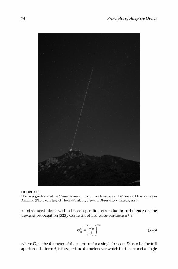
74 Principles of Adaptive Optics
is introduced along with a beacon position error due to turbulence on the upward propagation [323] Conic tilt phase-error variance σct
2 is
σctB
1d2
5 3
=
D/
(346)
where DB is the diameter of the aperture for a single beacon DB can be the full aperture The term d1 is the aperture diameter over which the tilt error of a single
Figure 3.10The laser guide star at the 65-meter monolithic mirror telescope at the Steward Observatory in Arizona (Photo courtesy of Thomas Stalcup, Steward Observatory, Tucson, AZ)

Adaptive Optics Compensation 75
beacon is 1 rad2 For example, at λ = 05 μm, at 0° zenith angle, d1 = 023 m for a 10-km beacon altitude (assuming a Hufnagel–Valley 20/20 model for turbu-lence) The calculation for beacon position error variance contains a term below the beacon separation height, σPL
2 , and a term above, σPH2
Two beams are focused by a telescope of diameter D to an altitude HB and are separated by distance b The beams begin to overlap at a height hc, which is below the altitude of the beacons themselves The oblique path length is L H= B secβ where β is the zenith angle The variance in radians squared of phase below the separation height is
σPL PLdc
2 2 2 1 3 2
0
= − ∫k b D zC z F b z D Ln
h
/ ( ) ( , , , ) (347)
where
F b z D LbzDL
zLPL( , , , ) .
/
=
−
−
0 6675 12 1 33 4 7 3
2 067 1
1 472
−
−
−
−
.
.
/bzDL
zL
bbzDL
zL
−
+
−14 3 3
1/
L
(348)
The variance in radians squared of phase above the separation height is
σPH PHdc
Bc
2 2 2 1 3 2= − ∫k b D zC z F b z D Lnh
H
/ ( ) ( , , , ) (349)
where
F b z D LzL
bzDPL( , , , ) . .
/
= −
−−
0 7600 1 0 66375 3
LLzL
bzDL
−
−
−1 3 2
1
0 0031
/
. −
−
−7 3 4
1/
zL
L (350)
The total beacon position error variance is
σ σ σP PL PH2 2 2= + (351)
The oblique path to the guide star and the size of the finite laser guide star must be considered [412] In many cases, the laser output aperture is not shared with the telescope-receiving aperture, avoiding unwanted backscat-ter from the optics, possible fluorescence in the optics, and the complexity of high power optical coatings on the receiving optics When multiple laser

76 Principles of Adaptive Optics
guide stars are used, all but one will have an oblique path and be elongated [763] When an off-axis guide star is used, both angular anisoplanatism and focal anisoplanatism must be considered Tyler [784] concludes that low- to mid-altitudes should be used when there is significant axial separation between the Rayleigh guide star path and the receiving telescope path For oblique paths (not to zenith), the amount of atmosphere traveled is longer until the laser pulse reaches 20 km and must be considered A larger and tem-porally longer guide star returns more photons, but since the approximation to a point source is corrupted [415], the pulse should be kept short [70] The flux is proportional to sec β where β is the zenith angle
3.3.2 Sodium guide Stars
The flux of a resonant sodium guide star can be calculated in a manner simi-lar to the Rayleigh guide star, recognizing that the density of sodium in the upper atmospheric layer and the resonant scattering limitations are consid-ered [881] The atomic sodium, a result of meteoric disintegration, remains at an altitude between 89 and 92 km because the conditions at this altitude pre-vent molecular reactions The detected sodium photon flux, at a wavelength of 5891583 nm, follows Equation 342
F Tz
EhcSodium A
Na col LGS= ησ ρ
πλ
2
024
(352)
where the altitude z0 is about 92 km, σNa is the resonant backscatter cross section, and ρcol is the column abundance, usually between 3 × 10⁹ atoms/cm2 and 1 × 10¹⁰ atoms/cm2 The product of the cross section and the col-umn abundance is roughly 002 [267] Because of the finite amount of sodium (less than 600 kg for the entire Earth), and the decay rate for the backscatter, a sodium guide star is limited to about 19 × 108 photons per second [251] Using Equation 346, for a subaperture diameter r0, the number of photons per subaperture Ns is
N r F Es =
=π4
55002 (353)
For Ns = 150 photons, we require 272 mJ/pulseIt is not enough just to shine a sodium wavelength beam into the meso-
sphere The sodium abundance (roughly 103–104 atoms/cm3) represented by the column density can vary as much as 25 magnitudes on a seasonal or diurnal scale or as short as 10 minutes [162,179] The effective height can vary between 89 and 92 km The wavefront sensor must be focused correctly or a false defocus term results [150,809] Techniques such as matched filtering [285] can improve performance over centroiding [284]

Adaptive Optics Compensation 77
The intention is to excite the D2 transition from the 32S1/2 state to the 32P3/2 state at 5892 nm in a very small volume (to create a point source) These two states are broadened by various mechanisms There is a magnetic interaction of the electron with nuclear spin The ground state splits to two levels (177 GHz) The excited state splits to four levels (100 MHz) They further split to magnetic sublevels There are 54 allowed transitions between the 8 sublevels
Actually, very few of the sodium atoms even in the beam will be excited The return flux should be proportional to beam intensity; however, at the saturation intensity, all the atoms are excited and an increase in beam power will not increase flux Continuous wave lasers often produce more return energy than pulsed lasers because they have a lower peak power
As a practical matter, suppression of Rayleigh backscatter in the sodium bea-con must be considered [164,879] For an atom, the radiative lifetime is 16 ns (10 MHz) The scattering rate is inversely proportional to the radiative lifetime In addition, the atoms are moving because of thermal motion This inhomoge-neous Doppler-broadening of 12 GHz makes the 5892 nm beam able to inter-act with only those in one “velocity group,” or only about 1% of the sodium atoms There have been suggestions to use multifrequency lasers to excite more velocity groups It is amazing that the sodium beacon will work at all
For large telescopes, off-axis sources can produce beacons that are not at all point sources They can have very large elongations that fluctuate with time The elongation angle can be approximated by αElong sep= 0 24. d , where dsep is the separation between the telescope and the laser projector in meters and αElong is in arc seconds The beam projector should be about 3r0 If the beacon is projected from behind the secondary mirror, some light pollution or field blockage can occur If the beacon is projected in the telescope optical train, scattered light and phosphorescence can occur Elongated beacons appear on Shack-Hartmann sensors as elongated spots and affect the accuracy of the wavefront measurement
The concept of multiconjugate adaptive optics [20,67,712,713] corrects for each “layer” of atmosphere independently By placing correction devices (deform-able mirrors) in series, and assigning each one a layer of atmosphere to cor-rect, the isoplanatic patch is effectively increased The terms multiconjugate adaptive optics, ground-layer adaptive optics [775], laser tomography adap-tive optics, multiobject adaptive optics, and extreme adaptive optics [534] are used to describe the various multiple guide star configurations Thus, we can replace what was once just an adaptive optics system with single conjugate adaptive optics [195,266,440,564,698,818,822,826]
In addition to conventional adaptive optics, many telescopes, such as those used to search for extrasolar planets, must use other novel optical tech-niques For example, the light coming from an extrasolar planet is typically 7 or 8 orders of magnitude fainter than the parent star The point spread function of the star often masks the planet Long-exposure phase diversity [546], the use of coherent waveguides to remap pupil geometry [431], or novel coronagraphs are often used to enhance the imaging In one case, an optical

78 Principles of Adaptive Optics
vortex is imparted onto the phase of the incoming beam, effectively creating a zero-intensity hole in the center that can block the starlight [225] Based upon the principles of Michelson stellar interferometry [753], large-aperture ground-based long-baseline interferometers, such as CHARA [760], are also candidates for adaptive optics [773]
3.4 Lasers for Guide Stars
Various lasers can be used for Rayleigh beacons Frequency-doubled lithium niobate solid state lasers, doubled Nd:YAG lasers (λ = 532 nm) [331], tripled Nd:YAG lasers (λ = 355 nm) [29], excimer lasers, and copper vapor lasers have all been successfully used
In addition, a number of laser sources can achieve the minimum power needed for sodium laser guide stars A few types are flashlamp pumped Nd:YAG lasers, excimer lasers with organic dyes in the laser cavity [13], both continuous and pulsed dye lasers, and fiber lasers [609] One fortuitous phe-nomena is the two laser wavelengths of Nd:YAG lasers, 106 and 132 μm When these lines are mixed in a nonlinear crystal, the resultant wavelength for the sum-frequency is (106 μm)−1 + (132 μm)−1 = (0589 μm)−1, precisely the wavelength needed to excite sodium [80,382,680,682]
In general, the laser-output beam quality should be a single transverse mode of TEM00, M2 < 12, and the bandwidth should be narrow compared with the Doppler-broadened sodium absorption spectrum (about 277 GHz) A continuous or quasi-continuous beam [169] of 4-W power should yield a stable photon return [682]
However, laser guide stars in adaptive optics systems have been demonstrated and used for astronomy and satellite imaging [44,249,250,366,376,383,473,510,581,767,764,769] Wavefront measurement from multiple guide stars has been demonstrated [445,549] A summary of the laser sources up to the mid-1990s is given in the literature on the subject [256] and elsewhere [181]
3.5 Combining the Limitations
The expressions used in this section can be combined to achieve an approxi-mation for the system performance The compensated wavefront vari-ance (expressed in square radians) is the sum of the contributors [268], as follows:
σ σ σ σ σ σ σ2 2 2 2 2 2= + + + + +fit temp WFS bloom iso cone2 (354)

Adaptive Optics Compensation 79
Equations 310, 318, 320 or 321, 324, 326, and 336 can be used for the con-tributors to approximate performance This combination assumes that the limitations are uncorrelated Though not strictly the case, the assumption is useful for system level analyses [855] The compensated wavefront Strehl ratio is just Equation 264 with the compensated wavefront error and the compensated jitter variance used in the expression
3.6 Linear Analysis
3.6.1 random Wavefronts
The preceding expressions assumed that wavefront aberrations were pri-marily caused by a Kolmogorov atmosphere As shown in Chapter 2, many forms of wavefront disturbance can be found The capability of an adap-tive optics system to compensate for other random aberrations often can be determined by the spatial filter method
When the aberrations can be expressed as random disturbances with a specified correlation distance, the adaptive optics system can be studied with the assumption that the system performs as a spatial filter [334] Since the spacing of correction zones rs limits the spatial resolution of the adap-tive optics system, it can be viewed as a high-pass filter, which removes all the low-frequency (low-order) modes but passes the high-frequency modes The exact form of the filter is determined by its correcting ability on a par-ticular wavefront [538,793] The corrected wavefront ϕc is the difference between the uncorrected wavefront and the surface of the phase-conjugat-ing mirror M(x, y), and is given by
φ φ γc u m( , ) ( , ) ( , )x y x y M x y= − (355)
where the constant γm is a function of the particular geometry of the adaptive optics beam train For a system where reflection from the correcting mirror is at an angle θ, the constant becomes γm = 2 cos θ For a nonlinear optics phase conjugating mirror (PCM), γm = 1 Taking the Fourier transform of Equation 349 and rearranging, we get
F FF M
F( ) ( )
( )( )
φ φγ
φc um
u
= −
1 (356)
The term in the brackets is the filter of the uncorrected wavefront spectrum and is a function of the spectrum This functionality makes the problem nonlin-ear in wavefront When only low-order modes are considered, this nonlinear-ity can be disregarded [429] Analytical aspects of the nonlinearity are often
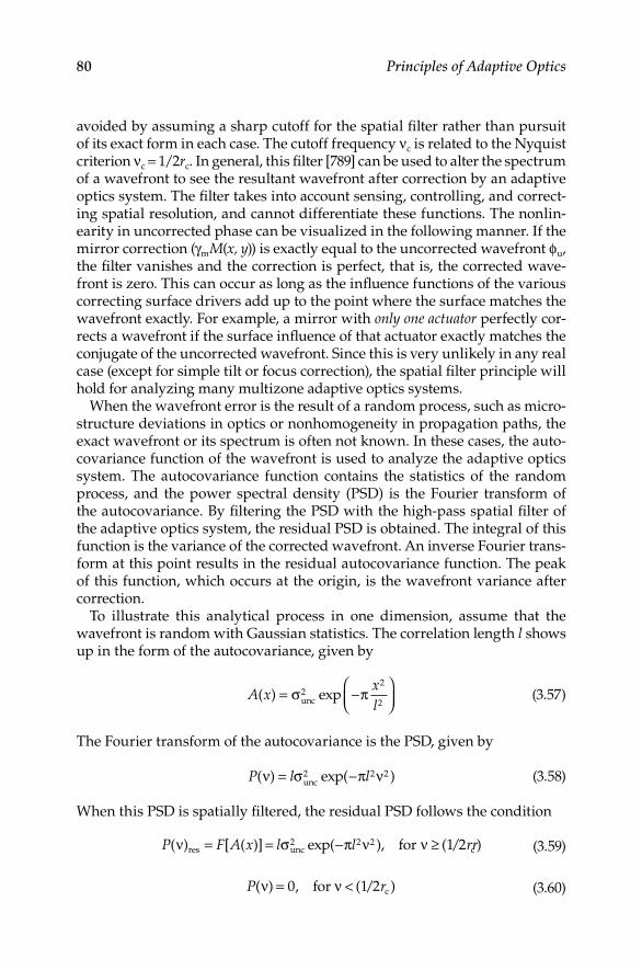
80 Principles of Adaptive Optics
avoided by assuming a sharp cutoff for the spatial filter rather than pursuit of its exact form in each case The cutoff frequency νc is related to the Nyquist criterion νc = 1/2rc In general, this filter [789] can be used to alter the spectrum of a wavefront to see the resultant wavefront after correction by an adaptive optics system The filter takes into account sensing, controlling, and correct-ing spatial resolution, and cannot differentiate these functions The nonlin-earity in uncorrected phase can be visualized in the following manner If the mirror correction (γmM(x, y)) is exactly equal to the uncorrected wavefront ϕu, the filter vanishes and the correction is perfect, that is, the corrected wave-front is zero This can occur as long as the influence functions of the various correcting surface drivers add up to the point where the surface matches the wavefront exactly For example, a mirror with only one actuator perfectly cor-rects a wavefront if the surface influence of that actuator exactly matches the conjugate of the uncorrected wavefront Since this is very unlikely in any real case (except for simple tilt or focus correction), the spatial filter principle will hold for analyzing many multizone adaptive optics systems
When the wavefront error is the result of a random process, such as micro-structure deviations in optics or nonhomogeneity in propagation paths, the exact wavefront or its spectrum is often not known In these cases, the auto-covariance function of the wavefront is used to analyze the adaptive optics system The autocovariance function contains the statistics of the random process, and the power spectral density (PSD) is the Fourier transform of the autocovariance By filtering the PSD with the high-pass spatial filter of the adaptive optics system, the residual PSD is obtained The integral of this function is the variance of the corrected wavefront An inverse Fourier trans-form at this point results in the residual autocovariance function The peak of this function, which occurs at the origin, is the wavefront variance after correction
To illustrate this analytical process in one dimension, assume that the wavefront is random with Gaussian statistics The correlation length l shows up in the form of the autocovariance, given by
A xxl
( ) exp= −
σ πunc2
2
2 (357)
The Fourier transform of the autocovariance is the PSD, given by
P l l( ) exp( )ν σ π ν= −unc2 2 2 (358)
When this PSD is spatially filtered, the residual PSD follows the condition
P F A x l l( ) [ ( )] exp( ), ( /ν σ π ν νres unc for= = − ≥2 2 2 1 2rrc ) (359)
P( ) , ( / )ν ν= <0 1 2for cr (360)

Adaptive Optics Compensation 81
The inverse transform of this PSD gives the residual wavefront autocovari-ance function as follows:
A xxl
ixl
lr
( ) expres unc erf= −
− − +σ π π π22
21
2 cc
(361)
where erf is the error function [1] The residual wavefront variance is the value of the autocovariance at the origin, given by
σ σ πcorr unc
c
erf20
2 12
= = −
→
lim ( )x
A xl
r
(362)
Defining correctability as C = −( )σ σ σunc corr unc2 2 2/ , the correctability of an adap-
tive optics system with correction zone spacing rc for a random disturbance with correlation length l becomes
Cl
r=
erf
c
π2
(363)
From this expression, one can see that almost half the variance can be removed when correction zones are twice the correlation distance, C = 047, for rc = 2l For rc = l, C = 078, and if the correction zone spacing is as low as rc = l/2, the adaptive optics system is almost a perfect phase conjugator, C = 099
3.6.2 Deterministic Wavefronts
When the uncorrected wavefront is deterministic, the spatial-filtering process can be followed to determine the corrected wavefront In this case, however, the wavefront itself is Fourier-transformed rather than the autocovariance The wavefront spectrum can be filtered in the same manner as before The sharp-cutoff high-pass filter is used to determine the residual spectrum and its transform gives the corrected wavefront directly Variances can be calcu-lated from the wavefronts or the wavefronts can be used to calculate prop-agation of the beam If we assume that the wavefront is a sum of Fourier components, then
φ π νunc m==
∞
∑ a m xm
cos( )20
∆ (364)

82 Principles of Adaptive Optics
The spatial filter removes the low-order components so that the corrected wavefront takes the form
φ π νν
corc
==
∞
∑ a m xmm r
cos( )/( )
21 2
∆∆
(365)
Since the variance is a weighted sum of the squares of the coefficients, the corrected wavefront must have a lower variance than the uncorrected wave-front In many cases, for example, atmospheric turbulence, the low-order coefficients are the largest contributors to Strehl ratio loss [570]
When the wavefront can be represented by Zernike polynomials, we can find the variance of the corrected wavefront From Equation 137, the vari-ance is determined from the Zernike coefficients Anm and Bnm by the sum
σ22 2
01 2 1=
++==
∞
∑∑ A Bn
nm nm
m
n
m ( ) (366)
The spatially filtered corrected wavefront variance is
σcor2
2 2
01 2 11= +
+− −
==
∞− ′∑∑ A B
nnm nm
m
n
n
n n
( )( )( )// ( ) , ,2
0
A A B B ZRr
n nnm n m nm n mm
n
′ ′′=
′
′
+ ′
∑
cnnm
n
n =
∞
==
∞
∑∑∑101
(367)
with Bn0 = 0 and R the radius of the aperture The correction function Z[(R/rc), n, n′] is found by spatially filtering the Fourier transforms of the Zernike polynomi-als [788]:
Z R r n nJ R J R
dn n[( / ), , ]( ) ( )/
c ′ = + ′+1 1
0
1 2 2 2πρ πρρ
ρrr
k Rr
n n kn n k
n
c
c
∫
=− + ′ + + ( )
+ +
+ ′+ +( ) ( )!
(
1 2 1
12
2 2π
kk n k n n k kk )!( )!( )! !′ + + + ′ + +=
∞
∑ 1 20
(368)
Therefore, by knowing the Zernike coefficients of the uncorrected wavefront Anm, Bnm and the correction zone, or actuator spacing, rc, the resultant wave-front variance can be found algebraically using the spatial frequency filter method

Adaptive Optics Compensation 83
3.7 Partial Phase Conjugation
No adaptive optics system can achieve perfect phase conjugation, although many systems can come close Winocur [873] and Noll [570] showed the effect of correction of individual modes and the residual effect of not cor-recting some of the atmospheric turbulence Systems with limited degrees of freedom can provide quite suitable image compensation for many practi-cal purposes [668,669] Bruns [101] shows how a simple five-mode correction system would provide compensation for meter-class telescopes In addition to image compensation, it has been shown that the log-intensity variance of scintillation with an adaptive optics system is inversely proportional to the number of Zernike modes that are being corrected [457] Although correct-ing many modes is desirable, the compensation of a few low-order modes presents the most significant improvement


85
4 Adaptive Optics Systems
In this chapter, we will review a number of adaptive optics concepts that have been used for applying correction to propagation and imaging systems Functional block diagrams are used to illustrate the concepts The blocks represent functions that can be optical, electronic, mechanical, or many com-binations of these The second half of this book deals with the details in the subsystems represented by the boxes in these diagrams At this conceptual level, we can regard these boxes as having the following functions:
Optics: A train of transmissive or reflective opticsCorrector: An optical element that can change the wavefront of a beamSampler: An optical element that can separate one beam from another
(presumably without distorting the phase)WFS: Wavefront sensorImager: A collection of optics that forms an image and delivers it to
detectorsTarget: The plane in space where a well-corrected beam is requiredReceiver: A device that converts optical information to electronic signalsControl: Electronic processingTagger: An optical device that can tag part of a beamLaser: The laser
The system concept should be chosen carefully A system used for correcting atmospheric turbulence in an astronomical telescope probably will not be useful correcting low-order modes in a high-power laser The brute-force techniques for moving large optics will be much too slow for correcting high-frequency vibrations We will examine these approaches and explore their pros and cons
4.1 Adaptive Optics Imaging Systems
4.1.1 Astronomical imaging Systems
By far, the most common application of adaptive optics is for imaging [688] Since 1982, adaptive optics have been used for imaging through the atmosphere [322] using the basic components that consist of a wavefront
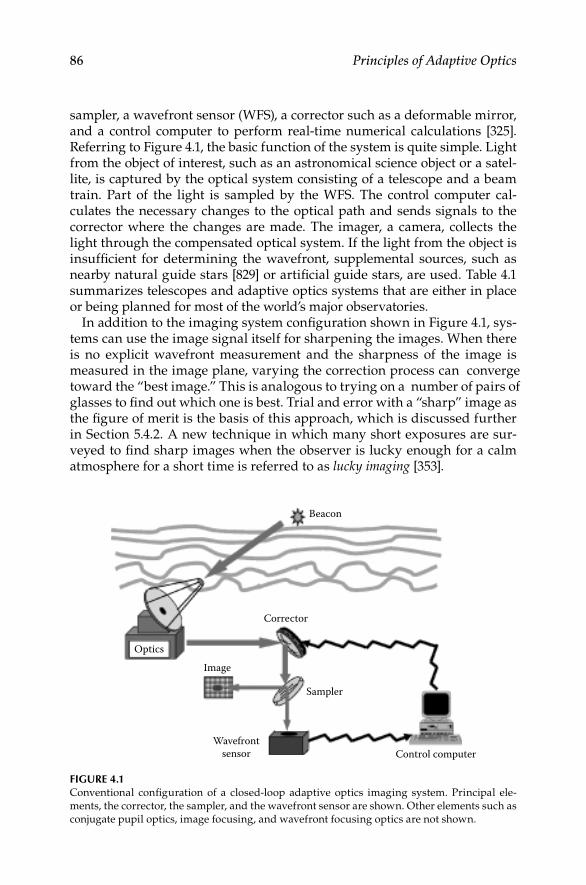
86 Principles of Adaptive Optics
sampler, a wavefront sensor (WFS), a corrector such as a deformable mirror, and a control computer to perform real-time numerical calculations [325] Referring to Figure 41, the basic function of the system is quite simple Light from the object of interest, such as an astronomical science object or a satel-lite, is captured by the optical system consisting of a telescope and a beam train Part of the light is sampled by the WFS The control computer cal-culates the necessary changes to the optical path and sends signals to the corrector where the changes are made The imager, a camera, collects the light through the compensated optical system If the light from the object is insufficient for determining the wavefront, supplemental sources, such as nearby natural guide stars [829] or artificial guide stars, are used Table 41 summarizes telescopes and adaptive optics systems that are either in place or being planned for most of the world’s major observatories
In addition to the imaging system configuration shown in Figure 41, sys-tems can use the image signal itself for sharpening the images When there is no explicit wavefront measurement and the sharpness of the image is measured in the image plane, varying the correction process can converge toward the “best image” This is analogous to trying on a number of pairs of glasses to find out which one is best Trial and error with a “sharp” image as the figure of merit is the basis of this approach, which is discussed further in Section 542 A new technique in which many short exposures are sur-veyed to find sharp images when the observer is lucky enough for a calm atmosphere for a short time is referred to as lucky imaging [353]
Beacon
Corrector
Sampler
Image
Wavefrontsensor Control computer
Optics
Figure 4.1Conventional configuration of a closed-loop adaptive optics imaging system Principal ele-ments, the corrector, the sampler, and the wavefront sensor are shown Other elements such as conjugate pupil optics, image focusing, and wavefront focusing optics are not shown
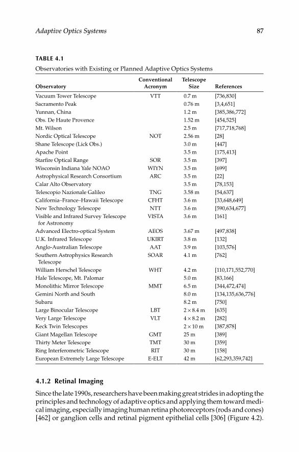
Adaptive Optics Systems 87
4.1.2 retinal imaging
Since the late 1990s, researchers have been making great strides in adopting the principles and technology of adaptive optics and applying them toward medi-cal imaging, especially imaging human retina photoreceptors (rods and cones) [462] or ganglion cells and retinal pigment epithelial cells [306] (Figure 42)
TAble 4.1
Observatories with Existing or Planned Adaptive Optics Systems
ObservatoryConventional
AcronymTelescope
Size References
Vacuum Tower Telescope VTT 07 m [736,830]Sacramento Peak 076 m [3,4,651]Yunnan, China 12 m [385,386,772]Obs De Haute Provence 152 m [454,525]Mt Wilson 25 m [717,718,768]Nordic Optical Telescope NOT 256 m [28]Shane Telescope (Lick Obs) 30 m [447]Apache Point 35 m [175,413]Starfire Optical Range SOR 35 m [397]Wisconsin Indiana Yale NOAO WIYN 35 m [699]Astrophysical Research Consortium ARC 35 m [22]Calar Alto Observatory 35 m [78,153]Telescopio Nazionale Galileo TNG 358 m [54,637]California–France–Hawaii Telescope CFHT 36 m [33,648,649]New Technology Telescope NTT 36 m [590,634,677]Visible and Infrared Survey Telescope for Astronomy
VISTA 36 m [161]
Advanced Electro-optical System AEOS 367 m [497,838]UK Infrared Telescope UKIRT 38 m [132]Anglo-Australian Telescope AAT 39 m [103,576]Southern Astrophysics Research Telescope
SOAR 41 m [762]
William Herschel Telescope WHT 42 m [110,171,552,770]Hale Telescope, Mt Palomar 50 m [83,166]Monolithic Mirror Telescope MMT 65 m [344,472,474]Gemini North and South 80 m [134,135,636,776]Subaru 82 m [750]Large Binocular Telescope LBT 2 × 84 m [635]Very Large Telescope VLT 4 × 82 m [282]Keck Twin Telescopes 2 × 10 m [387,878]Giant Magellan Telescope GMT 25 m [389]Thirty Meter Telescope TMT 30 m [359]Ring Interferometric Telescope RIT 30 m [158]European Extremely Large Telescope E-ELT 42 m [62,293,359,742]
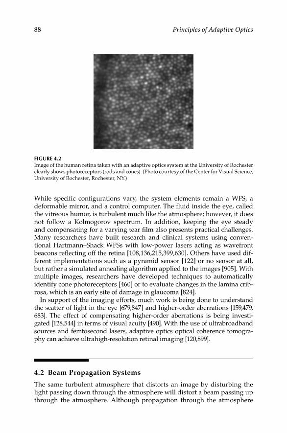
88 Principles of Adaptive Optics
While specific configurations vary, the system elements remain a WFS, a deformable mirror, and a control computer The fluid inside the eye, called the vitreous humor, is turbulent much like the atmosphere; however, it does not follow a Kolmogorov spectrum In addition, keeping the eye steady and compensating for a varying tear film also presents practical challenges Many researchers have built research and clinical systems using conven-tional Hartmann–Shack WFSs with low-power lasers acting as wavefront beacons reflecting off the retina [108,136,215,399,630] Others have used dif-ferent implementations such as a pyramid sensor [122] or no sensor at all, but rather a simulated annealing algorithm applied to the images [905] With multiple images, researchers have developed techniques to automatically identify cone photoreceptors [460] or to evaluate changes in the lamina crib-rosa, which is an early site of damage in glaucoma [824]
In support of the imaging efforts, much work is being done to understand the scatter of light in the eye [679,847] and higher-order aberrations [159,479, 683] The effect of compensating higher-order aberrations is being investi-gated [128,544] in terms of visual acuity [490] With the use of ultrabroadband sources and femtosecond lasers, adaptive optics optical coherence tomogra-phy can achieve ultrahigh-resolution retinal imaging [120,899]
4.2 Beam Propagation Systems
The same turbulent atmosphere that distorts an image by disturbing the light passing down through the atmosphere will distort a beam passing up through the atmosphere Although propagation through the atmosphere
Figure 4.2Image of the human retina taken with an adaptive optics system at the University of Rochester clearly shows photoreceptors (rods and cones) (Photo courtesy of the Center for Visual Science, University of Rochester, Rochester, NY)

Adaptive Optics Systems 89
[889] of weapons-class lasers for ballistic missile defense was the impe-tus for much of the early adaptive optics development, the technology and systems can also be used for various peacetime applications A system like that shown in Figure 43 can be used for laser power beaming to recharge batteries in orbiting satellites [254,531,555], laser power beaming to sup-ply energy for a lunar base [444], or ground-to-space laser communications [791,868]
Often, a dynamic disturbance or aberration occurs after propagation away from the optical system In this instance, it is difficult to predict the distur-bance and apply its phase conjugate without first sampling the aberration source The system shown in Figure 43 uses energy from the target, or near the target, to supply information about the aberrations If a signal from the target, possibly a cooperative beacon, a laser guide star, or a reflection of sunlight, propagates back through the atmosphere, the adaptive optics system can sense the wavefront distortion of the beam returning from the target By conjugating this field, remembering to scale for slightly different paths or wavelengths, the outgoing beam can be given a wavefront that allows radiation to reach the target near the diffraction limit If the return wave shares the same optical path or aperture as the outgoing wave, the approach is called the return-wave shared aperture approach Apertures can be shared spatially by physically dividing the return and outgoing beams into parts or can be shared temporally by dividing the two beams as a func-tion of time They can also be divided spectrally if the return wave and the outgoing wave are of a different wavelength or polarization Methods of sharing will be covered in Section 55 during the discussion of wavefront sampling
To target
From target
Sampler
Wavefrontsensor Control computer
Optics
Corrector
Laser
Opticalsystem
Figure 4.3Laser propagation system

90 Principles of Adaptive Optics
4.2.1 local-loop beam Cleanup Systems
If a beam is going toward a target, we can sometimes correct for aberrations in the beam in a local closed loop before it reaches the target An example of this is shown schematically in Figure 44 The beam is presumably aberrated in its formation or by an optical train A portion of this beam is sampled and sent to a WFS The sensor measures the wavefront, the controller generates signals to a corrector, and the corrector applies the phase conjugate In this concept, the sampler is after the corrector This allows the adaptive optics system to be dif-ferential, that is, the wavefront sensor sees the combined output of the beam, optics, and corrector The corrector will be driven flat if the wavefront is flat As the wavefront deviates from flat, the wavefront sensor will see the differ-ence between the beam and the corrector This difference will be applied to the corrector until the wavefront sensor no longer sees any difference, indi-cating that the phase conjugate has been applied to the beam Because of the need to avoid diffraction effects in the process, this must be done as close to the source of aberrations (the laser and optics) as possible It is used in high-power applications such as laser fusion Local loop beam cleanup is proposed as the principal adaptive optics configuration in each of the 192 optical trains in the 750-TW National Ignition Facility high-powered lasers [346]
If the sampler is before the corrector, the WFS sees only the beam and optics output The system applies an open-loop phase conjugate to the cor-rector If the beam changes, the WFS will detect a change, and, if the system is properly calibrated, the corrector will be moved to the conjugate position This variation should be able to provide the same amount of correction The conjugation process is the same; however, trusting the stability of the calibra-tion and assuming the output of the corrector is really a conjugate, without measuring it, are not good engineering practices
If the propagation of the beam, after it leaves the adaptive optics sys-tem, does not encounter any additional aberrations, the system is optimal However, if the transmitting optics downstream of the adaptive optics system
Controlcomputer
CorrectorSampler
Laser
Optics
To target
Wavefrontsensor
Opticalsystem
Figure 4.4Local-loop beam cleanup adaptive optics system
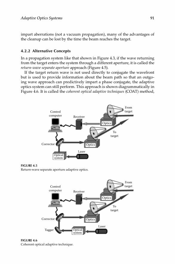
Adaptive Optics Systems 91
impart aberrations (not a vacuum propagation), many of the advantages of the cleanup can be lost by the time the beam reaches the target
4.2.2 Alternative Concepts
In a propagation system like that shown in Figure 43, if the wave returning from the target enters the system through a different aperture, it is called the return-wave separate aperture approach (Figure 45)
If the target return wave is not used directly to conjugate the wavefront but is used to provide information about the beam path so that an outgo-ing wave approach can predictively impart a phase conjugate, the adaptive optics system can still perform This approach is shown diagrammatically in Figure 46 It is called the coherent optical adaptive techniques (COAT) method,
Controlcomputer Receiver
Totarget
Laser
Corrector
Fromtarget
Optics
Optics
Opticalsystem
Figure 4.5Return-wave separate aperture adaptive optics
Controlcomputer Receiver
Totarget
LaserTagger
Corrector
Fromtarget
Optics
Optics
Opticalsystem
Figure 4.6Coherent optical adaptive technique
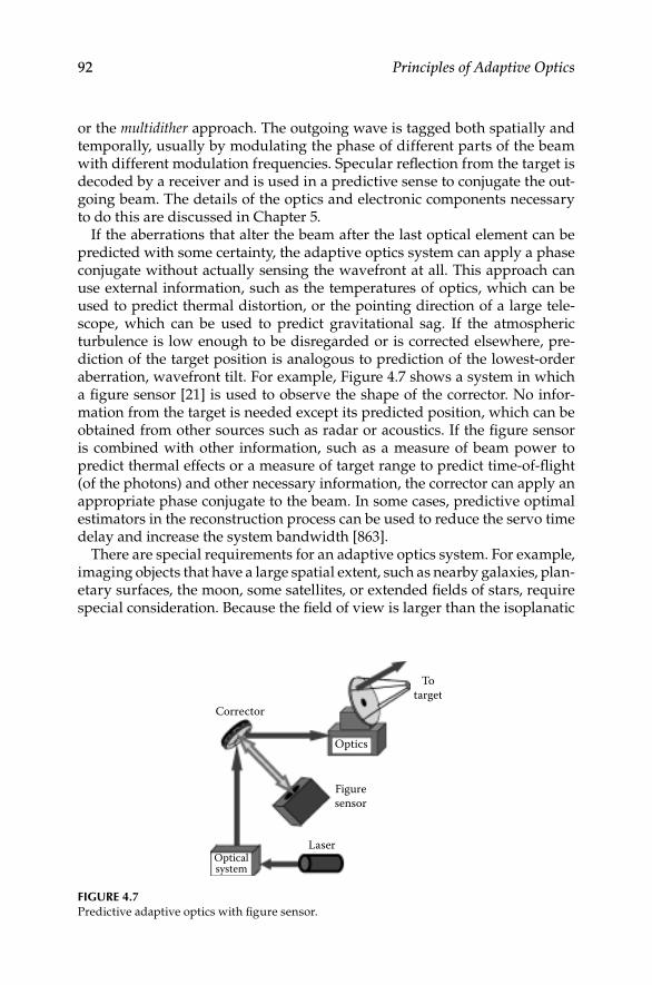
92 Principles of Adaptive Optics
or the multidither approach The outgoing wave is tagged both spatially and temporally, usually by modulating the phase of different parts of the beam with different modulation frequencies Specular reflection from the target is decoded by a receiver and is used in a predictive sense to conjugate the out-going beam The details of the optics and electronic components necessary to do this are discussed in Chapter 5
If the aberrations that alter the beam after the last optical element can be predicted with some certainty, the adaptive optics system can apply a phase conjugate without actually sensing the wavefront at all This approach can use external information, such as the temperatures of optics, which can be used to predict thermal distortion, or the pointing direction of a large tele-scope, which can be used to predict gravitational sag If the atmospheric turbulence is low enough to be disregarded or is corrected elsewhere, pre-diction of the target position is analogous to prediction of the lowest-order aberration, wavefront tilt For example, Figure 47 shows a system in which a figure sensor [21] is used to observe the shape of the corrector No infor-mation from the target is needed except its predicted position, which can be obtained from other sources such as radar or acoustics If the figure sensor is combined with other information, such as a measure of beam power to predict thermal effects or a measure of target range to predict time-of-flight (of the photons) and other necessary information, the corrector can apply an appropriate phase conjugate to the beam In some cases, predictive optimal estimators in the reconstruction process can be used to reduce the servo time delay and increase the system bandwidth [863]
There are special requirements for an adaptive optics system For example, imaging objects that have a large spatial extent, such as nearby galaxies, plan-etary surfaces, the moon, some satellites, or extended fields of stars, require special consideration Because the field of view is larger than the isoplanatic
Corrector
Totarget
Laser
Figuresensor
Optics
Opticalsystem
Figure 4.7Predictive adaptive optics with figure sensor

Adaptive Optics Systems 93
patch, methods such as deconvolution of the WFS signals themselves can be used to derive image information [670]
One variation on this method uses multiple views to gather sufficient data for tomographic reconstruction of the disturbances [378] and compensation of the images Multiconjugate adaptive optics systems use multiple WFSs and deformable mirrors to compensate for individual layers of the atmo-sphere instead of a single integrated path [393] Ellerbroek [195] presents an analysis of possible wide-field-of-view concepts
A passive phase-conjugation method uses an array of corner cubes to form a conventional phase-conjugate mirror (PCM) [61,591] Each small cor-ner cube will reverse the direction of a beam entering it The beam will be slightly offset (no more than the size of the cube aperture) If the cubes are small enough, each cube retroreflects a small portion of the beam (see Figure 48) The absolute phase is not maintained over the whole aperture, and the resolution is limited to the diffraction limit of one corner cube The recombined beam will have an approximate phase conjugate of the incoming beam
In addition to the variations of real-time systems, postprocessing of images taken with or without adaptive optics can be used to enhance the imaging capability of an optical system [294] The postprocessing methods can be as basic as frame selection (throwing away the bad images) [228] or as sophisti-cated as direct deconvolution [469] or blind deconvolution [133] Roggemann and Welsh [672] present an excellent description of the many postprocessing methods and a comprehensive discussion of hybrid systems (those that use postprocessing and real-time adaptive optics)
Wavefront Wavefront
Corner cube arrayphase conjugator
Conventionalmirror
(a) (b)
Figure 4.8An incident wavefront can be approximated by a corner cube array: (a) conventional mirror and (b) corner cube array

94 Principles of Adaptive Optics
4.2.3 Pros and Cons of Various Approaches
Each of the conventional approaches has both advantages and disadvantages Correcting for atmospheric turbulence in an astronomical imaging system is limited by the capabilities of the hardware to sense and correct the beam at a sufficient rate The very low signal-to-noise ratios generated by faint starlight require long integration times to achieve a sufficient signal The operating bandwidth of the system is seriously constrained
The return-wave phase conjugate approach is useful in vacuum propaga-tions or short-distance atmospheric propagations [436] For instance, optics errors in a beam train can be corrected using an unresolved object in dis-tance as a source of wavefront information The wavefront reaching the optics is essentially a plane wave Any wavefront error sampled by the adap-tive optics system came from the optics themselves and can be conjugated by the corrector The combination methods and the return-wave methods have limitations due to the time-of-flight characteristics The round-trip time for a photon to travel to and from a target at distance d away is t = 2d/c For disturbances that have significant spectra above 100 Hz (eg, atmospheric turbulence and mechanical vibrations), the range is limited to about 500 km This makes ground-to-space and satellite-to-satellite transmission with multidither impractical
4.2.4 Free-Space laser Communications Systems
There has been a recent growth in the need for and use of adaptive optics for free-space optical communications Combining the concepts of local-loop beam cleanup and return-wave adaptive optics, compensation of the atmo-sphere by conjugating the phase of the outgoing transmitted beam can sig-nificantly improve performance As the communication signal beam travels through the atmospheric turbulence, the phase changes result in scintilla-tion, which cause fades and surges at the receiver [19,21] The result of this is an increase in the bit-error rate that necessitates reduction of the bandwidth By compensating for the turbulence prior to transmission, much of the scin-tillation can be reduced [792] Various modulation schemes that have been studied include on-off keying [797], pulse position modulation [883], and optical vortex encoding [270] Ground-to-space links [868], space-to-ground links [791], air-to-space links [567], air-to-ground links [710], and ground-to-ground links [545] have been under investigation
There are a number of analyses to quantify the effect of turbulence, includ-ing understanding the fade statistics [64] and optimizing the aperture sizes in terms of level of disturbance and level of compensation [75] Earlier stud-ies have shown that using partially coherent beams can improve transmis-sion through the atmosphere [430,888] Determination of the correct level of coherence to optimize the transmission depends on the site, turbulence level, and range [125], but the level of coherence can be adjusted using devices such as adaptive arrays of fiber collimators [836,837]
Adaptive Optics Systems 95
Some systems use basic tip-tilt control [567,795], whereas some use higher-order controls [797] AOptix Technologies, Inc offers a commercially available two-way system that uses high-order adaptive optics [25] Each transceiver in the AOptix system precorrects the transmitted beams using part of the received signal as a wavefront beacon They report a communications capac-ity of 10 Gbps over distances up to 5 km
Because free-space laser communication links will have to be plentiful, they must be low cost One proposal is to use low-quality optics in the sys-tems, either the primary mirrors or the secondary mirrors, or both, and then use the correction capability of the turbulence-correcting adaptive optics to compensate for the static aberrations in the telescope [339]
4.3 Unconventional Adaptive Optics
Each of the concepts described as conventional assumes optics that could correct the wavefront of a beam through inertial methods, that is, moving something to alter the wavefront Some optical materials have the ability to alter the wavefront of a beam without inertial means on a macroscopic scale These materials make use of the fact that susceptibility χ of a mate-rial is electric-field-dependent, and it often depends on a power of the field higher than 1 These nonlinear effects lead to the definition that is most common when referring to adaptive optics: nonlinear optics (NLO) are unconventional adaptive optics and inertial adaptive optics are conventional Unfortunately, this is not always true There are methods of correction that use neither inertial motion nor the nonlinear optical properties of any material [61] These should probably be called unconventional because they are unique and interesting Other methods use nonlinear properties of materials such as the Pockels effect in an otherwise conventional method The confusion cannot easily be eliminated These special systems will be addressed separately
4.3.1 Nonlinear Optics
If the electric-field-dependent susceptibility is represented by an expansion given by
χ χ χ χ( ) ( ) ( ) ( )E E E= + + +…1 2 3 2 (41)
Then the polarization is represented by
P E E E E E E( ) ( ) ( ) ( ) ( )= = + + +…χ χ χ χ1 2 2 3 3 (42)

96 Principles of Adaptive Optics
The χ(1) terms represent linear effects such as refraction, absorption, gain, and birefringence; the χ(2) terms lead to second-harmonic generation, para-metric mixing, and the Pockels effect; and the χ(3) terms lead to effects such as third-harmonic generation, Raman scattering, the dc Kerr effect [831], nondegenerate four-wave mixing, and Brillouin scattering
Although many of these processes have some application to different aspects of adaptive optics, four effects are more commonly used in phase con-jugation Stimulated Raman scattering (SRS), stimulated Brillouin scattering (SBS), Brillouin-enhanced four-wave mixing [642], and degenerate four-wave mixing (DFWM) have been used extensively for adaptive optics [372,891]
As shown in Sections 41 and 42, conjugate beams are the basis for many applications of adaptive optics A beam propagating in the z direction is rep-resented by the electric field U(r, t), as follows:
U t U i t kz( , ) exp[ ( )]r = − − +12
ω c.c (43)
where cc indicates the complex conjugate With a phase aberration ϕ(r), this field obeys the scalar wave equation given by
∇ + ∂∂
=2 2 2 2 0U k U ik
Uz
[ ( ) ]ω µφ − +r (44)
A conjugate of this equation
∇ + − − ∂∂
=2 2 2 2 0U k U ik
Uz
* **
[ ( ) ]ω µφ r (45)
has a solution of the form
U t U i t kz( , ) exp[ ( )]r = − + +12
ω c.c (46)
which is a field propagating in the opposite direction Because the backward conjugate wave obeys the same wave equation as the forward wave, the effect of the aberration ϕ(r) is reversed This process holds for either inertial phase conjugators (Figure 32) or nonlinear (noninertial) conjugators [32]
4.3.2 elastic Photon Scattering: Degenerate Four-Wave Mixing
If three waves U1, U2, and Up are incident upon a nonlinear medium ( χ(3)), a fourth wave will be generated due to elastic photon scattering in the medium The two incoming waves are called pump beams
U t U i t k z1 1
12
1 1( , ) ( ) ( )r = +−r e c.cω (47)

Adaptive Optics Systems 97
U t U i t k z2 2
12
2 2( , ) ( ) ( )r = +−r e c.cω (48)
The third wave of smaller amplitude is called the probe beam, given by
U t U i t k zp p r e c.cp p( , ) ( ) ( )r = +−1
2ω (49)
A polarization will occur in the medium that is proportional to the product of these three waves and the third-order nonlinear optical susceptibility χ(3), and is given by
P U U U i kNL pr r r e p= + − −1
23
1 21 2 1χ ω ω ω( ) * [( ) (( ) ( ) ( ) ++ − ⋅ +k k2 p r c.c) ] (410)
Polarization radiates a fourth wave with a frequency ωc that is related to the frequencies of the other waves by
ω ω ω ωc p= + −1 2 (411)
The fourth wave is called the conjugate wave because it propagates in the direction opposite the probe wave when the pump frequencies are equal to the probe frequency (ω1 = ω2 = ωp = ω) In this degenerate case, the conjugate wave has the same frequency ω as the probe beam Because the pump beams are counterpropagating (k1 = −k2), the conjugate wave is counterpropagating to the probe beam (kc = −kp), which is equivalent to a phase conjugate of the probe wave:
U t U U ti t k zc c pr e c.cp( , ) ( ) ( , )( ) *r r= + =+1
2ω (412)
This method of phase conjugation is called DFWMAnother application of this process occurs when the beams are not degen-
erate, but nearly so [221] If the pump beams have equal frequencies ω and are opposite (k1 = −k2), but the probe is slightly frequency shifted, ωp = ω + δ, the conjugate will be shifted in the opposite direction, ωc = ω − δ
The coupled beams can be expressed as follows:
d
dep
p c
U
zi U kz
*
= −κ ∆ (413)
and
dd
ecc p
Uz
i U kz= +κ ∆* * (414)
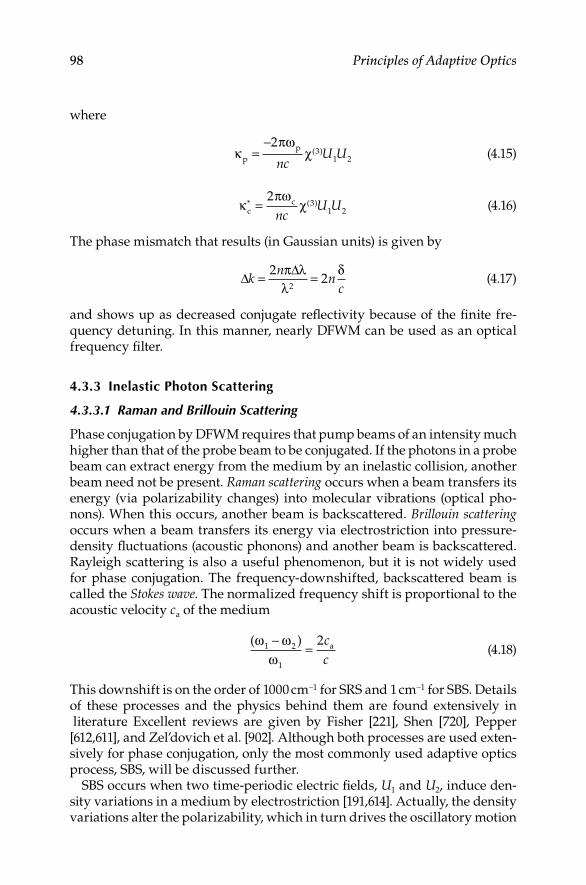
98 Principles of Adaptive Optics
where
κπω
χpp=
−23
1 2ncU U( ) (415)
κπω
χc* c=
23
1 2ncU U( ) (416)
The phase mismatch that results (in Gaussian units) is given by
∆ ∆k
nn
c= =2
22
π λλ
δ (417)
and shows up as decreased conjugate reflectivity because of the finite fre-quency detuning In this manner, nearly DFWM can be used as an optical frequency filter
4.3.3 inelastic Photon Scattering
4.3.3.1 Raman and Brillouin Scattering
Phase conjugation by DFWM requires that pump beams of an intensity much higher than that of the probe beam to be conjugated If the photons in a probe beam can extract energy from the medium by an inelastic collision, another beam need not be present Raman scattering occurs when a beam transfers its energy (via polarizability changes) into molecular vibrations (optical pho-nons) When this occurs, another beam is backscattered Brillouin scattering occurs when a beam transfers its energy via electrostriction into pressure-density fluctuations (acoustic phonons) and another beam is backscattered Rayleigh scattering is also a useful phenomenon, but it is not widely used for phase conjugation The frequency-downshifted, backscattered beam is called the Stokes wave The normalized frequency shift is proportional to the acoustic velocity ca of the medium
( )ω ω
ω1 2
1
2−=
cc
a (418)
This downshift is on the order of 1000 cm−1 for SRS and 1 cm−1 for SBS Details of these processes and the physics behind them are found extensively in literature Excellent reviews are given by Fisher [221], Shen [720], Pepper [612,611], and Zel’dovich et al [902] Although both processes are used exten-sively for phase conjugation, only the most commonly used adaptive optics process, SBS, will be discussed further
SBS occurs when two time-periodic electric fields, U1 and U2, induce den-sity variations in a medium by electrostriction [191,614] Actually, the density variations alter the polarizability, which in turn drives the oscillatory motion

Adaptive Optics Systems 99
of the electric fields The process is attractive for adaptive optics because there does not need to be a pump beam or beams as in DFWM, the gain can be very high (transferring much of the probe beam’s energy to the conjugate Stokes wave), and the SBS-reflected Stokes polarization state is like a conven-tional mirror [901] This last characteristic allows a practical way of substitut-ing a nonlinear optical PCM into a beam train using conventional optics
If the electric fields are represented by
U U i k z t1 1
1 1= −e ( )ω (419)
and
U U i k z t2 2
2 2= −e ( )ω (420)
and the acoustic wave field is
ρ ω= −A i k z te a a( ) (421)
then the coupled wave equations representing the SBS process (for the reso-nant case ωa = ω1 – ω2; ka = k1 – k2) become
∂ α ω ε
ρ∂+
= ∂∂z
Uik c
U A2 21
12
12 2 (422)
∂∂
+
= ∂∂z
Uik c
U Aα ω ε
ρ2 2222
12 1
* * (423)
∂∂
+
= ∂∂z c
Aik
cU U
Γ
a
a
a2
ρπ
ερ
01 24
* (424)
The frequency shift ωa is typically on the order of 30 GHz; the acoustic damp-ing coefficient Γ (the half-width of the line for spontaneous Brillouin scat-tering) is approximately 06 GHz The acoustic wave density variation ρ is assumed to be a variation about the mean density ρ0 of the medium, and ρ0 (∂ε/∂ρ) is the electrostrictive coefficient
These equations cannot be solved analytically for all configurations of acoustic and electric fields The gain can be determined for a particular case when the material properties are known The Brillouin gain is found to be
gnc cB
a
=′
∂∂
ω ρ ερ
12
03
2
Γ (425)
where ω1 is the pump frequency The acoustic velocity is ca, whereas the velocity of light is c The acoustic properties of the medium are absorbed into Γ′, whereas for liquid SBS media

100 Principles of Adaptive Optics
′ =Γ43
2
0
ηρka (426)
and η is the shear viscosity This gain factor has been measured for a num-ber of liquids [207] and ranges from 0005 cm/MW (water) to 013 cm/MW (carbon sulfide)
Studies involving xenon gas SBS cells show that there exists a threshold intensity for SBS to occur [859] For a cell of length L, the threshold It is found from the transcendental equation
g LIIIB t
t
n
=
ln (427)
where the initiation intensity In, arises from the random acoustic noise, is a function of the gas pressure and is on the order of 10 μW/cm2 For a 1-cm-long cell, the threshold intensity is on the order of 109 W/cm2 This was achievable for 1 μs pulses at 39 atm pressure with a 500-kW threshold power [860]
Adaptive optics systems that use NLO can appear in a number of configu-rations The required high intensities and breakdown mechanisms of many of the materials limit their applicability They usually cannot be used as the correcting optics in conventional outgoing or single-path concepts like those shown in Figures 41 and 46 Because the reflected wave is the (almost) exact conjugate of the incoming wave, the outgoing wave must repeat the path of the wave to be corrected in order for the “closed-loop” behavior to occur, and alternate system concepts are used
A high-power laser can be given a conjugate phase by using SRS In Figure 49, a beacon is sent backward through an aberrator like the atmo-sphere The laser pump stimulates the Raman effect, which produces a backscattered beacon beam (a phase conjugate of the incoming beacon) with most of the power transferred from the laser pump to the conjugate This is a very efficient way to impart a conjugate phase to a higher-power beam If a high-power beam is aberrated, we can use part of it as a seed for the
Beacon
Raman amplier
Optics
Ampliedlaser
Pump laser
Figure 4.9Wavefront conjugation with stimulated Raman scattering

Adaptive Optics Systems 101
Raman process [872] Figure 410 shows a system in which an aberrated high-power beam is wavefront corrected A fraction of the high-power beam is split away The small sample is spatial-filtered to remove high-order aberra-tions This acts as the Stokes wave and is injected into the Raman amplifier cell The gain of this beam depends on the intensity and aberrations present in the initial beam, because that beam acts as a pump wave In many cases, the amplified Stokes output beam is near diffraction limited
Another common usage of NLO is straightforward usage of an SBS cell as a PCM As described in Section 234, a gain medium in a laser amplifier can impart aberrations to a beam In general, the bigger the amplifier, the noisier the source, and the more aberrated the wavefront A number of small beams can be combined to simulate a large beam from a common ampli-fier In Figure 411, an SBS cell is used to combine and amplify a number of beams A seed laser beam of good quality and moderate power is split into a number of beams Each passes through a separate amplifier While passing through the amplifiers, the beams pick up aberrations from the gain medium When they are reflected off the PCM, the conjugate waves retrace their paths through the amplifiers The resultant output is a high-power beam with a wavefront nearly as good as the wavefront of the low-power seed
Laser Samplers
Ramanamplifier
Spatialfilter
Diffraction-limited
amplified StokesDiffraction-
limitedStokes seed
Figure 4.10Beam cleanup with stimulated Raman scattering
Seedlaser
PCM
AmplifiersSampler
Beamdivider/combiner
Near diffraction-limitedhigh-power output
Figure 4.11Beam combining with stimulated Brillouin scattering

102 Principles of Adaptive Optics
A similar situation arises for a single-beam case when the propagation path is highly aberrated The polarization conservation of SBS can be used to send a beam through an aberrating medium and back Figure 412 shows a sys-tem where the source beam is aberrated by the beam path Reflection from the PCM instills the phase conjugate so that the beam returning through the medium has a wavefront as good as the initial seed By placing a quarter-wave plate in the beam before the PCM, the polarization is changed with the double pass The outcoupler can be polarization-selective to deliver the beam
If the source of Figure 412 is replaced by a concave mirror and the aber-rating medium is a laser gain medium, the system has the form of a nonlin-ear optical resonator (see Figure 413) As the beam reflects back and forth between the concave mirror and the PCM, it alternately picks up the aber-rations present in the medium and, through conjugation, rejects them The output can have a wavefront limited only by the quality of the optics rather than by the disturbances of the gain medium [62,443,565,896]
When a wavefront is measured after the focus of a high-numerical-aper-ture optical system, a high-intensity laser beam will exhibit aberrations due to optical quality and alignment Adaptive correction can be achieved using a third-harmonic signal generated at an air-dielectric interface in conjunc-tion with a genetic algorithm [621]
Laser
Output
SBSPCM
Polarizationselectivesampler
Quarter-waveplate
Figure 4.12Aberration removal with stimulated Brillouin scattering (SBS)
Feedbackmirror
Output
SBSPCM
SamplerLaser gainmedium
Figure 4.13Nonlinear optical resonator with a stimulated Brillouin scattering phase-conjugate mirror (SBS PCM)

Adaptive Optics Systems 103
4.4 System Engineering
Adaptive optics systems can be designed and analyzed using a number of very effective system engineering tools The use of linear systems theory (Section 35) to describe the adaptive optics system as a spatial filter is one example, and the use of other tools, such as functional trees, performance trees, and interface matrices, also is effective Other system trees, such as hardware component trees, are used to identify and track the various pieces of hardware in a system [124,138,805,806]
The functional tree method describes the adaptive optics system, or any system, in terms of functions and subfunctions until the simplest functions are identified This can often be done to any degree of complexity and com-pleteness, because the definition of simple function is subjective An example of a functional tree for a conventional adaptive optics system is shown in Figure 414 A typical breakdown of the functions of the system has each function further reduced to subfunctions, and so on The highest level of this figure could also be considered a function of a much larger system, such as an imaging system The function blocks may or may not correspond directly to unique hardware components For example, the Wavefront sensor function has a subfunction Detection, which will probably be per-formed by hardware consisting of optics, electro-optic detectors, prepro-cessing and postprocessing, and the supporting power supplies and other
Conventionaladaptive optics
function
Wavefrontsampling
function (1)
Wavefrontdelivery
function (12)
Wavefrontdivision
function (21)
Matrixmultiplicationfunction (31)
Signalamplificationfunction (41)
Actuatorresponse
function (42)
Surfaceresponse
function (43)
Detection(23)
Temporallead-ahead
function (32)
Subaperturesample
function (22)
Decoding(24)
Surfaceconstraints
& damping (44)
Beam splitfunction
(11)
Wavefrontsensor
function (2)
Wavefrontreconstruction
function (3)
Wavefrontcorrection
function (4)
Figure 4.14Functional tree for a conventional adaptive optics system

104 Principles of Adaptive Optics
electronics Similarly, the subfunction Matrix Multiplication in the func-tion Reconstruction might consist of computer hardware, software, bulk storage, and supporting power and signal conditioning The functions can be subdivided to include these details or they can be left at this level Only whatever is necessary for understanding the hierarchy of system functions is needed [167]
Another type of system tree that is more quantitative in nature is the system performance tree [823] By defining the various quantities that affect the over-all adaptive optics performance, an error budget or performance hierarchy, is generated These quantities are often called system performance parameters, or SPPs Figure 415 shows an example of a simple adaptive optics system per-formance tree In this case, the tree represents an adaptive optics system used for controlling the wavefront of a beam delivery system Each of the blocks represents a quantity that could be either measurable or just expressed as a variable in an equation The nodes of the tree represent the equations or relationships between the quantities The highest measure of performance is the Peak Irradiance on Target It is the result of Brightness divided by Range to Target squared The units of these quantities are usually expressed in the most commonly used units, often with little regard for mixing units Therefore, a performance tree might have blocks on equal levels with differ-ent units and different sensitivity to the next higher quantity The example
Peak irradianceon target
180 W/cm2
Range on target10 km
Wavelength1 μ
Laserpowe r1 kW
Number ofmirrors
4
Mirrorabsorption
0.01
Focuscorrectability
0.8
Focusdisturbance
λ/13
High-frequencydisturbance
λ/16
High-frequencycorrectability
0.8
High-frequencyresidualλ/25
Low-frequencyresidualλ/40
Tilt ( > BW)disturbance
0.2 μrad
Tilt ( < BW)disturbance
2.2 mrad
Tiltcorrectability
0.8
Residualjitter
1 μrad
Brightness1.8×1014 W/sr
Geometryfactor
1
Wavefronterror
λ/20 rms
Aperture.diameter
1 m
Outputpowe r960 W
Figure 4.15Performance tree for a conventional adaptive optics system

Adaptive Optics Systems 105
shows how a brightness of 18 × 1014 W/sr and a range of 10 km combine for a peak intensity on target of 180 W/cm2 The brightness is computed from an equation that includes laser power, system optical transmission T, residual jitter, the aperture diameter D, the wavelength, and the resultant rms wave-front error Δϕ The equation for Node 1, relating these quantities (Equation 160), is repeated here; care should be taken, because the units are often mixed in a performance tree:
Brightness =−
π π φ
λ
λ
D PTK22
2
2
4 1
exp∆
++
2 22 2. αλ
jitD (428)
The output power is different from the laser power due to the absorption and scattering of the optics It is explicit in this example so that the effect of mirror absorption is emphasized For m identical partially absorbing optics (absorption α), the equation for Node 2 is simply
P P mout las= −( )1 α (429)
The adaptive optics system is shown as simple correctability in a perfor-mance tree The detailed calculations including integrals, bandwidth con-siderations, and correcting system limitations are absorbed into the nodes As the example tree indicates, the adaptive optics system is divided into low and high spatial frequency components to better identify the contributions to system performance They are root-sum-squared to compute the total residual rms wavefront error The system trees are often used as a quick look to identify sensitivities in overall performance They can also be used to track hardware performance and to provide a requirements flowdown to individual components The utility of the system trees is limited only by their complexity and the willingness to develop individual trees for the engineering discipline
One spin-off from the system functional tree is a system interface matrix This is a cross reference between functions to visualize the need for com-munications during the design process and hardware that might be needed This is particularly important when certain functions are performed only when other functions are performed The output of one function is often the input of another function An example of an interface matrix is shown in Figure 416 The various interface modalities are E, electronic; F, fluid; I, information; M, mechanical; and O, optical The user can add arrows to indicate the direction of the interface if it is important Any sort of modality can be chosen as well For instance, electronic can be subdivided into digital, analog, power, and so on The level of functions can be chosen to be any level of the functional tree

106 Principles of Adaptive Optics
These are by no means all the system analysis tools available for adaptive optics system design Many other forms are in use One method uses blocks to represent functions but does not display them in a hierarchy Rather, it rep-resents input and output data as lines entering and exiting horizontally; lines entering from the top represent controls or constraints, whereas lines entering each block from below represent supporting hardware segments [167] Many of these can be computerized to aid the analysis and design of more complex systems The main consideration is the information contained in the system analysis tool, not the strict adherence to any particular format [553,853]
An adaptive optics system normally is part of a larger optical system, and its purpose is to enhance the output of that optical system without degrading the performance The system designer must (1) determine the overall adap-tive optics system performance requirements, (2) consider the properties of the optical beam that the system is designed to enhance, and (3) integrate the system in such a way that it performs properly in the optical system environ-ment where it is placed
Adaptive optics systems are diverse, and their complexity varies greatly There is no simple “cookbook” formula for designing, assembling, or inte-grating an adaptive optics system Good engineering principles, balancing cost and performance, are needed at all levels of the design and installa-tion phases The development of adaptive optics systems over the past four decades has resulted in the identification of a number of issues that should be addressed during the system design effort
Functions
O
O
O
I
I
I I I
I
EI
E: ElectricalI: InformationO: OpticalF: FluidM: Mechanical
E
E E
OM OM
OM
EM FM
FM
OE Functions
11
11
12
12
21
21
22
22
23
23
24
24
31
31
32
32
41
41
42
42
43
43
44
Key
44
Figure 4.16Adaptive optics system interface matrix

Adaptive Optics Systems 107
4.4.1 System Performance requirements
The first consideration is the quantification of the adaptive optics system per-formance requirements Most systems will not perfectly conjugate a beam or compensate for all aberrations One must determine the level of the cor-rectability that can be tolerated Computer modeling and laboratory experi-mentation are imperative to reduce the overall design time and cost prior to building and integrating a system Theoretical modeling of atmospheric turbulence phase screens with realistic time delay characteristics [671] and laboratory wavefront generators with variable coherence lengths [345], tem-poral frequencies, and isoplanatic effects [503] are useful tools to avoid many engineering pitfalls
With knowledge of the aberration sources and the choice of a tolerable residual wavefront error, we can determine the spatial and temporal band-widths of the adaptive optics system The spatial bandwidth will be used to determine the number of correction zones or modes (number of actua-tors) The temporal bandwidth requirement determines the type of elec-tronic servo control The amplitude of the disturbances also is a factor For instance, if the amplitude of the tilt-mode disturbance is low, correction can be accomplished with only a deformable mirror However, if the tilt distur-bance is high, a separate tilt, or beam steering, mirror is used Fugate [255] suggests that, no matter what high-order adaptive optics system is used, the source or target must be tracked to within about 1/10 of a diffraction spot, or a fundamental tracking requirement of 03λ/D
4.4.2 Compensated beam Properties
The properties of the beam to be compensated often drive adaptive optics system component considerations The size and shape of the beam are impor-tant considerations If the beam is large, it may be advantageous to demag-nify it for adaptive optics compensation On the other hand, if it is small and has many higher-order aberration modes, it may be necessary to magnify it for correction If the beam has an unusual shape or obscurations, it may have to be reshaped for compensation, which can add optics to the system that are costly in performance and price
The beam power level is a major concern For very low light levels, such as those found in astronomy, the addition of beam splitters or special optics for sampling or correction can seriously degrade the overall performance For high-power beam propagation, the optics added for adaptive optics must be capable of withstanding the power levels while remaining operational Stray light must be controlled to prevent damage or degradation of the front mea-surement The adaptive optics system must operate when the beam power distribution is not spatially or temporally uniform Large intensity irregular-ities must be considered in overall adaptive optics system design For exam-ple, if most of the light is concentrated in one region of the beam, wavefront

108 Principles of Adaptive Optics
compensation is usually unnecessary elsewhere If this region moves around during operation, the system may need to monitor its location
4.4.3 Wavefront reference beam Properties
The physical location, power, temporal modulation, and spectral character-istics of the wavefront reference are very important Some WFSs work only with narrow-band, coherent sources Others need compensating optics to function in a broadband environment The selection of detectors is governed by their sensitivity and spectral band Optical throughput to the detectors must be managed so that the power reaching the detector is in its operating range Samples of a high-power laser must be attenuated greatly to avoid saturation or damage, but light from an astronomical object must be allowed to reach the detector with minimum attenuation The polarization state of the beam is important because sampling optics, such as beam splitters and gratings, and WFSs with diffraction gratings are sensitive to polarization
The temporal distribution of power is significant Many WFSs have differ-ent operating characteristics for pulsed or continuous beams The sensing technique must be considered if the beam is modulated, or chopped, or if it has an unusual pulse shape
4.4.4 Optical System integration
In most cases, the science objectives, the image collecting equipment, or the optical coatings drive the wavelength of operation for the adaptive optics system When one or more of these constraints is removed, we can optimize the wavelength in terms of limiting the distorting effects of the atmosphere [778] The choice of visible wavelength wavefront sensing and infrared imaging is driven by the low cost and low noise characteristics of visible wavelength CCD cameras and the better compensation at longer imaging wavelengths
The placement of the adaptive optics components in relationship to other optics is critical to system performance The wavefront that is measured should be the same as the one to be compensated The beam sampling com-ponents described in Chapter 5 and the optics that transfer the sample to the WFS must not distort the wavefront It is important that the components and the environment that contribute to the wavefront disturbance be in the path that is common to the correcting optics Optics that are not in the correction path (ie, that are in the uncommon path) should add minimal distortion to the wavefront
In an adaptive optics system that uses a WFS and deformable or segmented correcting mirror, the WFS detector array must be at a conjugate pupil of the correcting mirror It is often desirable to have them both at conjugate pupils of the telescope primary mirror Because the wavefront changes as it propagates from mirror to mirror, reimaging ensures that the correction

Adaptive Optics Systems 109
is applied to the same wavefront that it senses Correct pupil reimaging is required when line-of-sight variations are not removed by the beam-steering mirrors
To avoid cross talk between control channels and to enhance control sys-tem stability, the WFS subapertures should be aligned with the actuators on the corrector Most control systems and wavefront reconstructors use the absolute position of the actuators and subapertures and their relationship A one-for-one registration is neither possible nor necessary, because most systems have a different number of subapertures and actuators in differ-ent geometric patterns However, the positions should be well-characterized and maintained for optimum system operation


111
5Wavefront Sensing
An inertial adaptive optics system must have a way to sense the wavefront with enough spatial resolution and speed to apply a real-time correction [275] The direct approach employs a step where there is an explicit determi-nation of the phase or optical path difference (OPD) of the wave After the wavefront is reconstructed, the information is used as feedback to correct the unwanted components of the phase The indirect approach never reduces the information to an explicit indication of the wavefront; rather, it translates information related to the phase into signals that are used to compensate for the wavefront For example, the multidither system mentioned in Section 42 is an inertial indirect system
The requirements of wavefront sensing for adaptive optics differ from the requirements of phase or figure determination in optical testing in a num-ber of ways [320] In optical testing, the phase can be measured and recon-structed very slowly (minutes, hours, even days) Wavefront sensors in an adaptive optics system are used for real-time operation Because many dis-turbances can be on the order of hundreds of hertz, the sensors must operate much faster In some cases, the wavefront of individual pulses, which are as short as 2 μsec, must be measured in real time [641,867] The spatial resolu-tion requirement of adaptive optics wavefront sensors is usually very high It is not uncommon to require a resolution to 1/100 of an aperture diameter, which requires many channels of parallel sensing
In many cases, optical testing can be done in a narrow range of parameters, since the optics under test is well-characterized through previous examina-tions For instance, mass production optics have only a few aberrations to be checked each time, since some high-order components may not be important for the application On the other hand, adaptive optics are often required to deal with largely random wavefronts like atmospheric turbulence This ran-domness requires a greater number of degrees of freedom Adaptive optics wavefront sensing requires a large dynamic range (many wavelengths) to account for the vast OPD over the pupil of interest
The final, yet fundamental, requirement of adaptive optics wavefront sensing is its ability to determine OPD independent of intensity For many applications, imaging resolves objects through the atmosphere; for instance, the adaptive optics system will sense vast differences of intensity Since the adaptive optics system is only normally capable of varying OPD over the aperture, the OPD must be determined without the confusing variation in the amplitude, manifested by the intensity nonuniformity The use of

112 Principles of Adaptive Optics
broadband (white) light is required when the absolute OPD cannot be deter-mined at a single wavelength
5.1 Directly Measuring Phase
The effect of the phase on the propagation of light is calculated from the Huygens–Fresnel integrals discussed in Section 13:
U x yiAR s
SikRik s
( , )( )
= −+
∫∫−λ
Φe
e
Surf
d (51)
where U(x, y) is the complex amplitude of the input spherical wave repre-
sented by AR
ik Re ( )Φ− at distance s from a point on the aperture surface S
The projected intensity pattern is I(x, y) = |U(x, y)|2 Intensity is of great importance in most adaptive optics applications, and is determined by the amplitude and phase of the wave at the pupil, or input, plane The intensity pattern is the image of a resolved object, or it represents the point-spread function (PSF) of the optical system for an unresolved object
Unfortunately, there is no direct way to measure the phase of a single pho-ton There has been some progress in directly measuring the electric field, but not sufficient to be used in adaptive optics [851] A beam will interact with itself or another beam of light The principles of interference were dis-cussed briefly in Section 134 These principles, along with those of diffrac-tion, are the bridges between the optical phase and its intensity distribution Conventional adaptive optics is forced into using these interactions to infer the phase of a beam and apply a correction
A number of investigators have approached the problem Some meth-ods employ direct evaluation of the Fraunhofer diffraction pattern [297] Some authors evaluate the moments of the diffraction pattern [758] Others use multiple intensity measurements to extract the wavefront information [224,296,656,738] The multiple measurement approach is the basis for most adaptive optics wavefront sensors
5.1.1 Nonuniqueness of the Diffraction Pattern
If the diffraction pattern of a beam of light produced from a wave of the form
U x y U x y i x y( , ) ( , ) exp[ ( , )]= − Φ (52)
was unique, there would be solutions of the inverse equation that are func-tions of the field U(x, y) and its amplitude

Wavefront Sensing 113
Φ( )x y f U x y U x y, ( , ), ( , )= (53)
Similarly, since the function u(ξ, ν) is the Fourier transform of the input field U(x, y) (the Fraunhofer diffraction pattern of the pupil), there would be solu-tions of the form
Φ( , ) ( , )x y f u=
ξ ν 2
(54)
Solutions to this equation would make the wavefront sensing problem trivial One could just measure the diffraction-pattern intensity distribu-tion and operate on it to determine the phase Φ(x, y) either by a closed-form solution or by iteration For practical purposes, it would be only restricted by the speed of the optoelectronics and the number of degrees of freedom desired
It has been shown [224,296,656,657,758] that there is no unique solution in the general case for phase retrieval from a single measurement of the PSF Consider the following simple example based on the derivation of the Strehl ratio [86], where the intensity at the center of the PSF compared to the dif-fraction-limited intensity is given by a sum of aberration coefficients, namely the Zernike coefficients:
SR = −
++==
∞
∑∑12
2 1
2 2 2
01
πλ
A Bn
nm nm
m
n
n ( ) (55)
Clearly, there are an infinite number of coefficients Anm and Bnm that can sat-isfy this equation for SR < 1 This means that the intensity at the peak is not unique to any particular wavefront, and the rest of the intensity pattern is probably not unique This relationship (Equation 55) only holds for small aberrations, those that are on the order of 1/10 wave or less It is this level of aberration, however, that is most important in the realm of adaptive optics There are, however, approaches to the problem that have some degree of util-ity in a practical manner, such as only small phase disturbances [461]
5.1.2 Determining Phase information from intensity
Solutions to the phase retrieval problem can be found from multiple mea-surements of the pupil plane intensity and the image plane (Fraunhofer diffraction) intensity Fienup [216] reviews and compares a number of phase-retrieval techniques Gonsalves [296] shows how two measurements can lead to the solution of the phase if the field derived from the magnitude of the image plane intensity is “analytic,” that is, all derivatives must be finite [587] Foley and Abdul Jalil [224] show that a fourfold degeneracy (which they term “nonuniqueness”) can be reduced to a twofold degeneracy by judicious

114 Principles of Adaptive Optics
application of aperture stops Jeong et al [381] reconstructs the phase in the focal plane by comparing the inverse Fourier transform of the intensity dis-tribution with a reference electric field
Robinson [656] explains a twofold degeneracy that results from symmetric intensity distributions He derives, as many authors have done in various ways, the two solutions for the symmetric magnitude problem He shows that the two solutions for the phase differ by the sign The general result of his analysis is that there is always a solution to the problem under physical con-ditions However, it is not unique for large duration-spatial bandwidth prod-uct situations This result is not so surprising, since the large duration (big aperture), large spatial bandwidth (many aberration modes or cycles across the aperture) product would have so many cross terms in the diffraction integral that the uniqueness is almost certainly destroyed Robinson derives a method of determining the phase from a single image plane- intensity mea-surement under extremely restrictive conditions He shows that the phase Φ(x) is related to the magnitude of the image plane field U(x) through the Hilbert transform (HT) by
Φ( ) ln ( )x U x= − HT (56)
Unfortunately, this simple solution is only valid for the specific cases of mini-mum phase fields These fields, such as when the power is concentrated at the edge of an aperture, rarely occur in actual optical fields
A general technique called phase diversity can be used on image plane measurements requiring no pupil plane detectors [85,93,174,895] Another method, using multiple intensity measurements in the image plane, employs an iterative computation of the maximum likelihood of the wavefront [738] This computation is equivalent to minimizing the merit function
12
2
2
[ ]I Ii
i
meas −∑ σ (57)
where Ii are the intensities due to various wavefront error terms This minimization assumes a known amplitude and requires solution by non-linear methods The determination of the wavefront is found by using the two- dimensional basis functions based upon the intensity patterns from individual aberrations The iteration process begins by choosing a likely set of aberrations and then evaluating Equation 57 Convergence is achieved by forming derivatives of the merit function with respect to the phase param-eters A detailed analysis of this technique, using a maximum-likelihood algorithm, in the presence of noise, is given by Barrett et al [60]
Ivanov et al [375] describe the iterative algorithm that uses the Gerchberg–Saxton algorithm [279] They show how the use of pupil plane and image plane-intensity distributions can be used to recover the phase with improved

Wavefront Sensing 115
convergence over just image plane distributions Roddier and Roddier [656] employ dual out-of-focus images to recover the phase Their method is the basis for curvature sensing, described in Section 533
Harvey et al [336] proposed an interesting phase retrieval method using the spot of Arago that occurs on-axis behind a circular obscuration The edge-diffracted PSF characterizes the aberrations It is particularly useful for annular beams where no auxiliary beam sampling optics would be required It has not been applied to an adaptive optics wavefront sensing system
Teague [758] proposed a method of phase retrieval by measuring the irra-diance moments of the image plane-intensity distribution as follows:
M z I x y x y x ypqp q( ) ( , )= ∫∫ d d (58)
Making as many measurements (N) as unknown aberrations (N), allows a matrix multiplication scheme to be adopted The coefficients a, defined by
Φ( , ) ,x y a x yn m mn m m
m
n
n
= −−
==
∞
∑∑01
(59)
can be found from the multiplication of [Φ] = [U][M], where [Φ] and [M] are N-element row vectors, and [U] is an N × N matrix that is determined from basis functions dependent upon the pupil shape Although the calculation appears to be simple, it is only because of the simplified notation The cal-culation of moments in the image plane, the determination of the elements of [U], the effect of noise, and the limitations of a finite image plane com-plicate the problem and make its realization in a high-speed optical system difficult
The recovery of phase from intensity distributions was required to diag-nose the aberrations of the Hubble Space Telescope (HST) [432] Since the telescope was in orbit, only the intensity distributions from various images were known Because the HST is a multiple-element optical system, and the source of the aberrations is unknown, an iterative method using “Fresnel-like” transforms is employed Fienup [217] describes the method of phase retrieval that included consideration for absorption in the optics and bad detector pixels Similar to the work of Teague, these iterative methods are not yet applicable to real-time adaptive optics, but they can be used as a basis for limited iterative procedures as computational ability increases
Iterative techniques for real-time wavefront sensing have limitations because of the often large number of iterations required to generate a wave-front solution The solution must be found before the disturbance changes and these changes can be between tens of milliseconds (astronomy) and hundreds of microseconds (imaging low Earth orbiting satellites)
Algorithms [502] that have been demonstrated include genetic algorithms [292,621,757,894], simulated annealing [539,905], simplex [416], iterative Fourier

116 Principles of Adaptive Optics
transforms [295], and the iterative shadowgraphic method [623] One promis-ing method is Vorontsov’s modification to the gradient-descent algorithm that introduces a stochastic (random) component [832,833,839,893]
5.1.3 Modal and Zonal Sensing
The wavefront information that is derived from measured data will be used to close the loop to apply a phase correction The actual reconstruction of the phase from this data is discussed in Chapter 7 The format of the information often drives the ability to use it in an optimal manner Two basic types of wavefront information are used When the wavefront is expressed in terms of the OPD over a small spatial area, or zone, the wavefront is said to be zonal When the wavefront is expressed in terms of coefficients of the modes of a polynomial expansion over the entire pupil, it is said to be modal There are advantages and disadvantages of each method of presentation Some recon-struction schemes limit the flexibility in choosing the wavefront representa-tion Some wavefront sensing schemes lend themselves to one or the other presentation Both modal and zonal representations can be interchanged, since they represent the same wavefront; however, the complexity of the con-version will often limit their usefulness in a practical sense
The zonal method is easily understood by considering the wavefront over an aperture The wavefront is normally continuous unless it is in the plane of a physical stop If the wavefront is broken into N subapertures, and the phase at each subaperture is expressed as a number, then the entire wavefront is the characteristic set of N numbers If N approaches infinity, the wavefront is exactly represented If N is finite, each subaperture may be represented by more than one number; for instance, piston and local tilt In this case, each zone is represented by its fundamental modes
Sometimes a 2N representation is sufficient This is the case where only the tilt modes in each subaperture are represented It can be shown how these tilts, dΦ/dx and dΦ/dy, in each zone can be combined to determine the full aperture modes [499], which may be necessary if the wavefront sensor produces zonal information and the correcting optics require a full aperture phase or OPD For the specific case of correcting atmospheric turbulence, a combination of zonal and modal measurements is useful [172]
There are some wavefront sensing schemes in which measurements are made that generate modal information directly with the zonal informa-tion deduced [111] Measurements of the wavefront distortion due to atmo-spheric turbulence Φ(r, θ′), taken on the edge of an aperture of radius R, provide the basis to interpolate the wavefront Φ(r, θ) in the remainder of the aperture,
Φ( , )( , )
cos( )r
R r RR r Rr
θπ
φ θ θθ θ
= − ′ ′+ − − ′
2 2
2 202 2
d22π
∫ (510)

Wavefront Sensing 117
The decision to use modal, zonal, or a combination of sensing schemes to measure the wavefront is usually left to the application If low-order modes (tilt, defocus) are dominant, then modal analysis and corrections should be used If high-order aberrations are present, the zonal approach should be used For atmospheric turbulence compensation, both zonal and modal sens-ing have been used Using Equation 310 for fitting error, the Strehl ratio is
Srr
= −
exp/
κ s
0
5 3
(511)
An expression for the Strehl ratio in terms of the number of modes corrected, N, has a similar form [570], given by
S N= −exp( )σ2 (512)
For N ≤ 21,
σσσ
12
05 3
22
05 3
32
1 0299
0 582
0
===
. ( / )
. ( / )
.
/
/
D r
D r
1134
0 111
0 0880
05 3
42
05 3
52
( / )
. ( / )
. (
/
/
D r
D r
D
σσ
== // )
. ( / )
. ( / )
/
/
r
D r
D r
05 3
62
05 3
72
0
0 0648
0 0587
σσ
== 55 3
82
05 3
92
05 3
0 0525
0 0463
/
/
/
. ( / )
. ( / )
σσσ
==
D r
D r
1102
05 3
112
05 3
12
0 0401
0 0377
==
. ( / )
. ( / )
/
/
D r
D rσ
σ220
5 3
132
05 3
142
0 0352
0 0328
===
. ( / )
. ( / )
/
/
D r
D rσσ 000304
0 0279
0
05 3
152
05 3
162
. ( / )
. ( / )
.
/
/
D r
D rσσ
== 00267
0 0255
0 02
05 3
172
05 3
182
( / )
. ( / )
.
/
/
D r
D rσσ
== 443
0 0232
0 0220
05 3
192
05 3
202
( / )
. ( / )
.
/
/
D r
D rσσ
== (( / )
. ( / )
/
/
D r
D r0
5 3
212
05 30 0208σ =
For N > 21,
S NDrN>
−= −
213 2
0
5 3
0 2944exp . ( / )
/
(513)
These values are shown graphically in Figure 51For identical adaptive optics correction, using κ = 032 that is, equating
Equations 511 and 513, we find that N, the number of modes, is given by
NDr
=
0 921 93
..
s
(514)

118 Principles of Adaptive Optics
and is roughly equivalent to the number of zones, given by
ZDr
=
0 782 00
..
s
(515)
Both expressions represent the number of degrees of freedom for the system In conclusion, for the regions of practical interest in adaptive optics, the choice of zonal or modal correction transcends the theoretical analysis and reverts to the capabilities of the hardware and the level of correction desired
5.1.3.1 Dynamic Range of Tilt and Wavefront Measurement
The maximum amount of full aperture tilt through the atmosphere (from space) that will appear on a tilt sensor is
α λtilt tele=
2 20
5 6
./
Dr D
M (516)
where D is the full telescope aperture diameter and Mtele is the magnifica-tion of the telescope The tracking system should measure the tilt to half the tracking accuracy requirement; thus, the accuracy should be at least
Accuracy tele= 0 05.λD
M (517)
The wavefront should be measured to an accuracy of λ/10 to λ/20 with a maximum wavefront error dynamic range (DR) in a subaperture of
0.6
Tilt,
one
-axi
s
0.4Va
rianc
e (D
/r0)
5/3 (
rad)
2
0.2
0.00 5 10
Modes corrected15 20
Focu
sTi
lt, tw
o-ax
is
Ast
igm
atis
m
Figure 5.1Wavefront variance for varying levels of modal correction

Wavefront Sensing 119
DR s=
50
5 6rr
/
(518)
where the subaperture size is rs
5.2 Direct Wavefront Sensing—Modal
5.2.1 importance of Wavefront Tilt
Wavefront tilt, classically called distortion [89], is a mode that is fundamental in zonal sensing schemes As mentioned in Section 513, if the wavefront can be spatially divided and individual subaperture tilts (wavefront slopes) can be determined, then the entire wavefront across an aperture can be deter-mined Fitting a plane to the full aperture phase results in a value for the first Zernike term, the tilt term; thus, it is called Zernike tilt or Z-tilt Averaging the tilts across multiple subapertures results in an average gradient of the wavefront; tilt of this type is called gradient tilt or G-tilt Although some sen-sors more closely measure G-tilt and others measure Z-tilt, the difference in Strehl ratio calculation is less than 10%
The control of beam tilt is important in itself in any adaptive optics sys-tem In 1956, Babcock et al showed [48] that tilt compensation alone can significantly improve an image Modern adaptive optics systems have tilt control to stabilize the image or the propagated beam and improve the signal for low-order mode compensation Olivier and Gavel [580] calcu-late that tilt correction is possible with natural stars on the 10-m Keck telescope
Two methods are used to determine wavefront tilt The interference of two beams creates an intensity that is proportional to the difference in phase between the beams If those beams are small adjacent portions of the same beam, then the differential phase and the tilt in that region can be deter-mined Interference methods are discussed in Section 5311
Another method exploits the characteristic that wavefront tilt displaces a focused image in the direction of the tilt and at a distance proportional to amount of tilt [194] For example, recall the expression for the inten-sity of light near the axis at diffraction focus, given in Equation 11 and repeated here:
IAaR
i kkaR
r=
− −
λ
ρ θ ψπ
2
2
0
2
exp cos( )Φ∫∫∫ −
0
1 22
2
12
kzaR
ρ ρ ρ θd d (519)

120 Principles of Adaptive Optics
If the aberration consists of tilt in the x direction (K ρ sin θ) plus higher-order terms Φ′, the exponent in the integral [89] can be written*
i kkaR
r kzaR
′ − ′ − ′ −
Φ ρ θ ψ ρcos( )
12
22 (520)
which is the same form as Equation 519 The image intensity distribution will be the same as the unshifted image with the same contributions from higher-order aberrations The focus has not changed (z = z′), but the origin of the image plane has been shifted in a plane perpendicular to the direction of prop-agation by an amount (R/a)K The shift, proportional to the magnitude of the tilt term, K, is the basis for measurement of the wavefront tilt This principle is the basis for noninterferometric wavefront dividing methods and many full-aperture beam-tracking problems The practical techniques rely on measuring the image position shift and extrapolating that to the wavefront G-tilt
A simple geometric illustration shows this relationship As shown in Figure 52, a beam enters an aperture of radius a, with a tilt K, the small angle formed between the beam direction (normal to the wavefront) and the plane of the aperture is K/a The displacement after propagating a distance R to the image plane is simply (R/a)K
The determination of the image shift is done in many ways For an unaber-rated (except tilt) beam passing through a circular aperture, the center of the image is the position of the maximum intensity as follows:
IJ
∝ 12
2
( )υυ
(521)
where υ = kar/R
* The exponent kΦ′ + kK ρ sin θ – (ka/R)r ρ sin ψ sin θ – (ka/R)r ρ cos θ cos ψ – (1/2)kz(a/R)2ρ2 is transformed by making a linear displacement coordinate transformation in the image plane, x′ = x – (R/a)K, y′ = y, and z′ = z, which is equivalent to r′ sin ψ′ = r sin ψ – (R/a)K and r′ cos ψ′ = r cos ψ
K
K/aRK/aR
a
Figure 5.2Displacement of the center of a beam due to wavefront tilt of magnitude K

Wavefront Sensing 121
The position of the peak intensity is sensitive to tilt, and its absolute posi-tion is a function of all the aberrations The centroid of the intensity distri-bution, however, is equal to the shifted origin of the image plane, which is proportional to the tilt
The centroid is defined as the first moment of the pattern, and is given by
x I x y x x y I x y x y= ∫∫∫∫ ( , ) d d ( , )d d (522)
y I x y y x y I x y x y= ∫∫∫∫ ( , ) d d ( , )d d (523)
The limits of the integrals are −∞ to +∞ To illustrate the process, a Gaussian image distribution is assumed It is offset by the values x0, y0 The centroid is calculated from Equations 522 and 523 as follows:
x x x yx x y y= − − + −[ ]∫∫ e ( ) ( )02
02 d d (524)
y y x yx x y y= − − + −[ ]∫∫ e ( ) ( )02
02 d d (525)
x x y y= =0 0 , Q.E.D.
The centroid is equal to the offset, which is exactly what is required when determining wavefront tilt from the intensity distribution
Summarizing, tilt will shift the position of the intensity centroid in the focal plane Other aberrations change the shape of the pattern and position of the maximum, but do not shift the centroid Axially symmetric aberrations change the shape, but do not alter the position of the maximum or the centroid
As an example of the centroid’s insensitivity to aberrations, consider the centroid of an intensity pattern that is subject only to coma The intensity pattern is skewed in the direction of the comatic aberration The field in the image plane was shown to be [89]
U u C U i U i U i Um m m( , , ) ( ) ( )ln ln lnυ α α αψ = + + + +0 12
23
3 [ ] (526)
==
∞
∑C i Ums
ss
( )lnα0
(527)
The contributing fields Un are
UJ
012=( )υυ
(528)

122 Principles of Adaptive Optics
U iJ
142= cos( )
ψυ
υ (529)
U J J J J2 1 3 5 71
214
120
14
920
= − + − −υ
υ υ υ υ( ) ( ) ( ) ( ) coss ( ) ( )225
353 7ψ J Jυ υ+
where υ = kar/R and αln m are proportional to Zernike coefficientsThe resultant intensity pattern consists of products of Bessel functions
Ic
Jb
J( , ) (υυ
αψ α= −
+
−2
2
2
12
212
324
2 444
64 4
2 242
2
52
222
α ψ
α α
cos )J
Jb
+
+
JJ b J J J J72 2
1 1 32
1 5
2
158
38
158
+
−
+
α α
α bb JJb
J Jb
J2 1 7
21
3 5
22
5
−
−
α α8 8
JJb b
J J7
21 2
3 7+
α2
(530)
where the subscript of α is 031 (coma), the argument of all Bessel functions is υ, and
b11
2025
2= + cos ψ (531)
and
b2920
35 2= + cos ψ (532)
Without explicitly performing the centroid calculation, Equation 522, the integral takes the form
x xI= ∫ ( , ) d dυ ψ υ υ ψ (533)
x C J Js n ms
=
==∑υ
υυ υ υ υcos
cos( ) ( ) d dψ ψ ψ
∞ 2
20
000
2
0
π∞
∫∫ (534)
which, when evaluated term by term, will be zero from the azimuthal inte-gration, verifying the centroid’s insensitivity to aberrations
5.2.2 Measurement of Tilt
The actual physical measurement of the centroid can be done in many ways Placing a detector behind a narrow slit and scanning the slit across the inten-sity pattern will produce a signal that is proportional to the intensity in a small region in the direction of the scan while integrating the intensity in the

Wavefront Sensing 123
orthogonal direction (Figure 53) Another method commonly used in image trackers as well as wavefront sensors is the quadcell This device has four detectors that are closely spaced as illustrated in Figure 54 The intensity pat-tern is made to focus on these detectors Using the notation from Figure 54, the difference signals
xI S I S I S I S
I Sii
=+ − −∫ ∫ ∫ ∫
∫∑d d d d
d1 4 2 3
(535)
yI S I S I S I S
I Sii
=+ − −∫ ∫ ∫ ∫
∫∑d d d d
d1 2 3 3
(536)
are proportional to the position of the centroid This can be proven by solving the bicell integration problem using Gaussian quadrature
DetectorControlelectronics
Display
Intensitypattern
Figure 5.3Illustration of temporal scanning of an intensity pattern with the resultant signal trace
12
(a) (b)
3
Intensitypattern
12
44 3
Figure 5.4Quadcell geometries: (a) designation of the quadrants and (b) dumbbell-shaped image limitation

124 Principles of Adaptive Optics
Certain integrals can be approximated by their evaluation at the follow-ing two points [629]:
x f x aa
fa a
fa
a
a
( ) = − −
+
−∫ 3 3 3 3
(537)
f x a fa
fa
a
a
( ) = −
+
−∫ 3 3
(538)
By this method, the quadcell can perform the integrations to determine the beam centroid
xxI x x
I x x= −∞
−∞
∞
∫
∫
( )d
( )d
∞
(539)
=
− −
+ −a
Ia
Ia
Ia
Ia3
3 3
3 3
(540)
where I a 3( ) is the evaluation of the intensity at the point a 3( ) Although the quadcell actually integrates the energy on each quadrant, it is represented by a single point value
The quadcell angular tracking error σ TE is related to the voltage signal-to-noise ratio (SNR)v,
σ = 0 6./λ D
SNRv
(541)
where the SNR is a function of signal electrons NS, background electrons per pixel nB, dark current electrons per pixel nD, and read-noise electrons per pixel ne:
SNRvS
S B D e
=+ + +( )
N
N n n n4 2 (542)
State-of-the-art detectors have almost no background or dark current and can reach as low as 3 electrons per pixel read noise Using these parameters [255], a minimum SNR of 2 is achieved with 14 electrons per pixel To track 400 Hz, a 4-kHz signal is needed Assuming 80% quantum efficiency and 20% optical transmission, about 35 × 105 photons are needed at the telescope The astronomical brightness formula from Chapter 1 and the size of the tele-scope aperture can be used to calculate the minimum brightness object for sufficient tracking

Wavefront Sensing 125
The quadcell integration method is restricted to images that deposit at least some energy in all four quadrants and have nearly uniform intensity distri-butions in the image plane Quadrant detectors have limitations because of their geometry For instance, a “dumbbell”-shaped distribution on a quadcell (Figure 54b) will cause a false centroid indication
Resolved images on the quadcell can be used to determine wavefront tilt if errors due to the object shape and the SNR are not neglected The error in the angular measurement of tilt for a circular object on a quadcell is given as [786]
σ
π λ
qcvSNR
=
+
316 8 2
2 2 1 2
na
/
(543)
where n = (2ba)/(Rλ), with b the object diameter, R the range, a the radius of the aperture, and SNRv the voltage SNR When the object is unresolvable, that is, b is small, R is large, and n = 0, the centroid measurement error is
σ πqc
v8 (SNR )= b
R (544)
and when the object is large, the other limit (bλ/Ra) >> 3/16, then the error is proportional to object size b,
σπ
qcv32 (SNR )
=b aR
( / )λ 2
(545)
Another method of determining the centroid of an intensity pattern uses only three detectors [13] A mask that essentially performs the first-moment integration in real time covers each detector Masks can have continuously variable transmission, like commercially available filters, or they can be pho-toetched-transmissive patterns like those in Figure 55 These masks may take any shape as long as the transmission function is proportional to the measurement along one axis When two masks at orthogonal orientations are placed over separate detectors, and nothing (a “null mask”) is placed over a third detector, the centroids in two orthogonal directions can be deter-mined from the formulae
xI
Ix= det
tot
(546)
yI
Iy= det
tot
(547)

126 Principles of Adaptive Optics
With the advent of arrays of many small detectors, direct calculation of the centroid, Equation 522, is possible Some investigators use either three- or five-point curve fitting to determine intensity maxima The error associated with these measurements and algorithms was studied by Grossman and Emmons [311], who derived an expression for the error that is a function of detector geometry, the algorithm, the SNR, and array nonuniformity Down [176] showed that the error is dependent upon noise and the pixel-to-spot size ratio
Elbaum and Diament [193] derived similar expressions for the error of the centroid for rough and smooth extended targets They found these variances to be functions of coherence, object size, optical resolution, and sensor inte-gration time Their equation for the standard deviation takes the form
σ δerror SNR= + +
P B
AD2
2
22 2
( ) (548)
where P is the distance between detectors, B is algorithm error, A is sensor configuration error, D is algorithm nonuniformity error, and δ is the rms nonuniformity
The quadcell lends itself quite readily to analog processing where electronic nulls are used Some methods employing arrays use four or more adjacent cells to create a quadcell Allen et al [12] took advantage of the advances in digital infor-mation processing Specific applications of these techniques will be explored in detail in Section 532, which describes individual wavefront sensors
5.2.3 Focus Sensing
Sensing the focus of a beam directly is fundamental to any modal adaptive optics operation As will be shown rigorously in Chapter 7, the focus (or defo-cus) can be constructed from zonal measurements across the aperture The focus “aberration” is the most heavily weighted aberration when it comes to smearing an image Defocus can be measured directly A defocused image
“Null” mask Total-detector
Beam splitters
Incoming beamx-mask
x-detector
y-detector
y-mask
Figure 5.5Application of opaque masks to perform centroid calculation
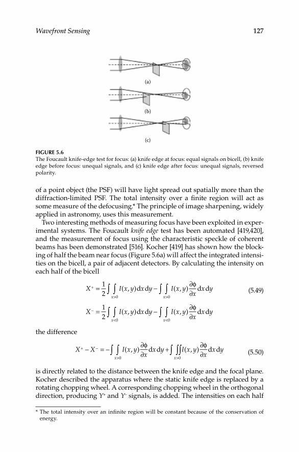
Wavefront Sensing 127
of a point object (the PSF) will have light spread out spatially more than the diffraction-limited PSF The total intensity over a finite region will act as some measure of the defocusing* The principle of image sharpening, widely applied in astronomy, uses this measurement
Two interesting methods of measuring focus have been exploited in exper-imental systems The Foucault knife edge test has been automated [419,420], and the measurement of focus using the characteristic speckle of coherent beams has been demonstrated [516] Kocher [419] has shown how the block-ing of half the beam near focus (Figure 56a) will affect the integrated intensi-ties on the bicell, a pair of adjacent detectors By calculating the intensity on each half of the bicell
X I x y x y I x yx
x yx x
+
> >
= −∫ ∫∫∫12 0 0
( , )d d ( , ) d d∂∂φ
(549)
X I x y x y I x yx
x yx x
−
< <
= −∂∫ ∫∫∫
12 0 0
( , )d d ( , ) d d∂φ
the difference
X X I x yx
x y I x yx
x yx x
+ −
> >
− = − ∂∂
+ ∂∂∫ ( , ) d d ( , ) d d
φ φ
0 0∫∫∫∫ (550)
is directly related to the distance between the knife edge and the focal plane Kocher described the apparatus where the static knife edge is replaced by a rotating chopping wheel A corresponding chopping wheel in the orthogonal direction, producing Y+ and Y− signals, is added The intensities on each half
* The total intensity over an infinite region will be constant because of the conservation of energy
(a)
(b)
(c)
Figure 5.6The Foucault knife-edge test for focus: (a) knife edge at focus: equal signals on bicell, (b) knife edge before focus: unequal signals, and (c) knife edge after focus: unequal signals, reversed polarity

128 Principles of Adaptive Optics
of the bicell are translated into sinusoidal ac signals The phase difference between the X+ and X− signals is proportional to the amount of focus (Figures 56b and 56c)
McLaughlin’s [516] method uses the principle that laser speckle (the local-ized interference between portions of a coherent wave) will move in rela-tion to the direction of the motion of the image plane or the source If an observer, detector, or recording medium, such as film, moves and is inside of the focus, the speckle will move in the opposite direction from the observer If the observer is outside of the focus, the speckle will move in the same direction as the observer (Figure 57) A linear expression relating the focal length change, Δr, the observation plane–speckle separation, s, the velocity of the speckle, υs, and the velocity of the observer near the focal plane, υf, is given as
∆rs K
=υυ
f
s (551)
where K is a proportionality constant evaluated at K = 128 The direction of motion is indicated by the difference in signs of υf and υs when the expres-sion is evaluated McLaughlin indicates that this method allows measure-ment of the position of the focal plane to within 002 of the Rayleigh limit
5.2.4 Modal Sensing of Higher-Order Aberrations
It is generally impractical to measure higher-order aberration modes in a modal sense The complexity of the higher-order diffraction phenomenon makes it difficult to separate the contributions from astigmatism or coma, for instance However, recent progress with interferometric methods has been shown to work up to Zernike mode 21 [448] The remainder of this chapter
Converging beamon two slits
Speckle
Motion ofspeckleMotion of
aperture
Figure 5.7Observation of speckle

Wavefront Sensing 129
will deal with the principles of wavefront sensing with spatially reduced fields, called subaperture division These methods can be applied to all orders of aberrations
5.3 Zonal Direct Wavefront Sensing
It is possible to reconstruct the wavefront of the entire field from the mea-surements of tilt in smaller regions Wavefront division has various names; subaperture division and the Hartmann test are most common By fitting a continuous curve to local tilted planes, a two-dimensional surface is gener-ated The tip and tilt of the local planes are measured using the methods of Section 522 The most common surface fitting methods are described in Section 74
5.3.1 interferometric Wavefront Sensing
Historically, the principle of optical interference has been used to prove that light has wavelike properties Adaptive optics systems use this principle for more practical applications [424] The methods of interferometry can be used to generate contours of the wavefront and also can be exploited to measure local wavefront tilts A mathematical description of the interference process will be followed by a description of basic interferometric methods, electronic signal processing methods such as heterodyning, and then detailed descrip-tions of the most widely used interferometers for wavefront sensing
Interference occurs when two or more coherent light beams are superim-posed The principle of interference was introduced in Section 134 If two linearly polarized transverse fields are superimposed, the magnitude of the sum of the two fields becomes
I I I I I= + +1 2 1 22 cosδ (552)
For the case, I1 = I2, the intensity of the superimposed beams is
I I=
4 1
2cosδ2
(553)
with the maximum intensity Imax = 4I1 and the minimum Imin = 0 While this method is straightforward for a single-phase measurement, the addition of integer multiples of 2π radians to δ results in a “2π ambiguity” of the mea-surement, essentially wrapping the phase back onto itself In strong atmo-spheric turbulence, this ambiguity presents itself and must be unwrapped to avoid phase discontinuity [819]

130 Principles of Adaptive Optics
5.3.1.1 Methods of Interference
There are two methods of interfering coherent beams The method of division of wavefront makes use of the spatial coherence of the beam and interferes two, or more, spatially separated parts of the same beam The method of division of amplitude interferes one part of the beam with itself after the beam is amplitude-divided
Division of wavefront is interference by division of wavefront This is the method that Young used to demonstrate the wave nature of light in 1803 Taking a plane wave that is generated by a point source at infinity, the wave passes through two slits separated by a distance d on an opaque screen (Figure 58) We wish to observe the intensity of light at points on a screen a distance a from the plane of the slits The distance from slit 1 to the observation point is a y x d2 2 22+ + −( / ) and the distance from slit 2 is
a y x d2 2 22+ + +( / ) The difference in the path is
∆ = − ≈+
s s sxd
s s2 12 1
2 (554)
For small wavelengths like those for visible light, d << a and
∆ =sxda (555)
The difference in OPD for this system in a medium of refractive index n is
OPD = ∆ =n snxd
a (556)
and the phase difference is
δ π= 2λ
nxda
(557)
SourceScreen
a
s1
s2d x
Figure 5.8Young’s double-slit experiment

Wavefront Sensing 131
Maxima occur when the phase difference is an integral multiple of wave-lengths, that is,
cos2
21
δ
= (558)
or
xmand
m= =λ0 1 2, , ,…
Therefore, the positions on the screen (the interference plane) where maxima occur are
and
and
and
λ λ λ, , ,2 3
… (559)
and those where minima occur are
and
and
and
λ λ λ2
32
52
, , ,… (560)
For the adaptive optics application, we need to measure the phase difference between one part of the beam (slit 1) and another part (slit 2) By observing the maxima, we can find that the phase difference is
δ πλ
= 2m
nxda
(561)
and by counting the orders m from the central fringe and measuring the distance x, we can determine the OPD difference
If the fringes are produced by light that is not purely monochromatic, the intensity of the pattern is the sum of the intensities of the composite mono-chromatic patterns The maxima are spread out by
∆ = ∆xmand
λ (562)
where the variation of the wavelength is ΔλOne spinoff from this method of interference is the determination of the
amount of coherence by observing the fringe visibility The visibility V, or fringe contrast, is given by
VI II I
=−+
max min
max min
(563)
For a purely monochromatic coherent beam, the result of Equation 553 is inserted into Equation 563 with the resulting visibility equal to unity When

132 Principles of Adaptive Optics
the fringes are spread out due to polychromaticity, the minima do not reach zero, and the visibility will always be less than one For completely incoher-ent light, the fringes do not exist at all, and the visibility is zero The fringe visibility can be used to determine the separation of sources at a long dis-tance A Michelson stellar interferometer is used to find the angular separa-tion of two sources, θ, by simultaneously varying the aperture separation d while measuring the fringe visibility The smallest value of the separation for which the fringe visibility is at a minimum is given by
dA= λθ
(564)
where A = 5 for point sources and A = 122 for a single uniformly illuminated disk
The division of wavefront method is used in a modified Young’s double-slit experiment for an adaptive optics system Van Workum et al [809] scan an opaque screen with two small apertures (the double slit) across a beam (Figure 59) The interference term is a convolution of the intensity from infinitesimal slits, Equation 553, and the diffraction pattern of the apertures For apertures of diameter D, Van Workum et al show this function to be
I x IJ x
f( )
( )cos=
0
12
22 α
απλd
(565)
where the Bessel function term is the aperture function (Airy pattern), α = πD/ λf, and the cosine-squared term (the interference contribution) con-tains the aperture separation and focal length As the apertures scan the wavefront, the slits will produce the fringe pattern on the detectors The lateral position of the central fringe is directly proportional to the tilt (Figure 510) To determine the position of that central maximum, a chopper is placed at a focal plane The relative position of the fringes on the square pattern of the chopper is decoded to determine the actual location of the fringe pattern, and thus the rela-tive tilt of the beam By rapidly scanning the apertures (10 μsec per element), and
Fringe patternformed
Image of fringepattern on detector
Rotatingchopper
Movingslits
Figure 5.9Wavefront sensor based on Young’s experiment

Wavefront Sensing 133
rapidly chopping the fringe pattern (1 MHz), a high-bandwidth, high- accuracy (focus changes measured to ±05%) wavefront sensor was demonstrated
In division of amplitude, a beam is split so that part of its amplitude tra-verses one path and part of its amplitude traverses another path; when the two beams are superimposed, the difference in the paths will produce inter-ference fringes A simple form of amplitude division, used in a Michelson interferometer, is performed with a transmissive beam splitter
In the Michelson interferometer, illustrated in Figure 511, a source from the left is partially reflected from the back surface of the beam splitter That portion (beam 1) travels and reflects off mirror 1, and part of it is transmitted through the beam splitter onto the interference plane The part of the beam that is transmitted through the beam splitter (beam 2) is reflected off mirror 2 and returns to the beam splitter to be reflected off the surface toward the interference plane The compensating plate is placed in beam 2 to equalize the number of times (3) each beam passes through a transmissive element The intensity at any point in the interference pattern is expressed by the interference equation, given in Equation 552,
I I I I I= + +1 2 1 22 cosδ (566)
Double-slitaperture
Interferencepattern infar field
x
OPD
Figure 5.10Position of the fringes is proportional to the wavefront tilt
Mirror 1
Mirror 2Source
Fringes appear onthe interference plane
Compensatingplate
Figure 5.11Michelson interferometer

134 Principles of Adaptive Optics
The reason for using the interferometer is manifested in the equation If the phase δ is retarded by any manner, tilts of the elements, for instance, or the insertion of an aberrating medium, the intensity of the fringes is a direct response to that change The use of a collimated source in a Michelson inter-ferometer is the basis of the Twyman–Green interferometer [774] Figure 512 shows the Twyman–Green interferometer in two configurations Figure 512a shows a method of measuring the aberrations due to a nonflat reflective sur-face Figure 512b shows the Twyman–Green interferometer used for measur-ing the aberrations of a transmissive medium
From Figure 512b, one can see a disadvantage of using a Twyman–Green interferometer for transmissive test objects The test beam must pass through the test object twice, thereby complicating alignment and data reduction One solution to this problem is the use of a Mach–Zehnder interferometer [492,896], which allows the paths to be separated by relatively large distances (see Figure 513) Figure 514 shows a Mach–Zehnder interferometer with a
Test object
Source
Test object
Mirror
Fringes appear onthe interference plane
(a) (b)
Figure 5.12Twyman–Green interferometers: (a) method for measuring aberrations due to nonflat reflec-tive surface and (b) Twyman–Green interferometer for measuring aberrations of a transmis-sive medium
Beam splitter
Beam splitter
Mirror
Source
Mirror
Fringeson the
interferenceplane
Figure 5.13Mach–Zehnder interferometer
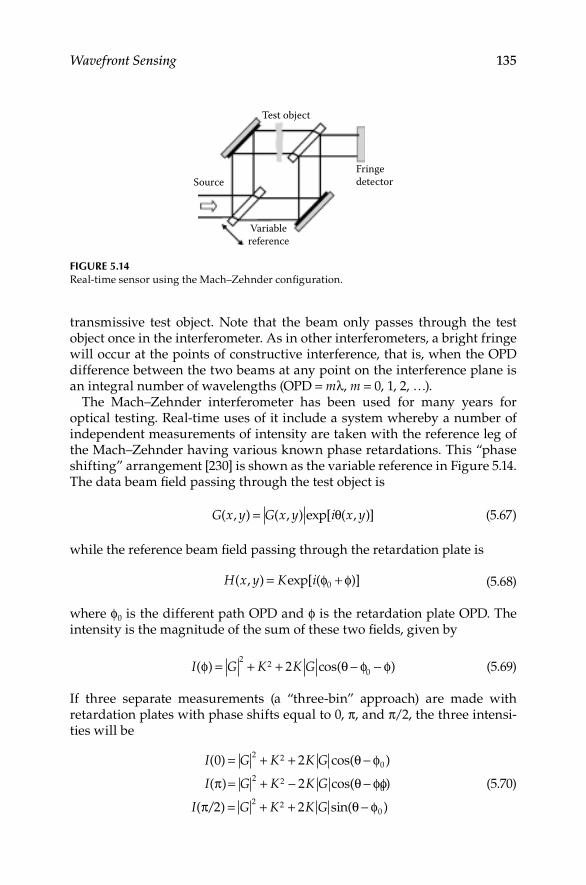
Wavefront Sensing 135
transmissive test object Note that the beam only passes through the test object once in the interferometer As in other interferometers, a bright fringe will occur at the points of constructive interference, that is, when the OPD difference between the two beams at any point on the interference plane is an integral number of wavelengths (OPD = mλ, m = 0, 1, 2, …)
The Mach–Zehnder interferometer has been used for many years for optical testing Real-time uses of it include a system whereby a number of independent measurements of intensity are taken with the reference leg of the Mach–Zehnder having various known phase retardations This “phase shifting” arrangement [230] is shown as the variable reference in Figure 514 The data beam field passing through the test object is
G x y G x y i x y( , ) ( , ) exp[ ( , )]= θ (567)
while the reference beam field passing through the retardation plate is
H x y K i( , ) exp[ ( )]= +φ φ0 (568)
where ϕ0 is the different path OPD and ϕ is the retardation plate OPD The intensity is the magnitude of the sum of these two fields, given by
I G K K G( ) cos( )φ θ φ φ= + + − −2
202 (569)
If three separate measurements (a “three-bin” approach) are made with retardation plates with phase shifts equal to 0, π, and π/2, the three intensi-ties will be
I G K K G
I G K K G
( ) cos( )
( ) cos(
0 2
2
2 20
2 2
= + + −
= + − −
θ φ
π θ φφ
π θ φ0
2 202 2
)
( / ) sin( )I G K K G= + + −
(570)
Test object
Source
Variablereference
Fringedetector
Figure 5.14Real-time sensor using the Mach–Zehnder configuration

136 Principles of Adaptive Optics
Combining the expressions in Equation 570, the phase of the data beam can be found from
θ φ
π π
π− =
− −
−0 2 212
012
0arctan
( ) ( )
( ) (
I I I
I I ))
(571)
and the magnitude is
K G I I I I I= − +
− −1
160
14
12
012
2[ ( ) ( )] ( ) (π π2
π))
/
2 1 2
(572)
The quadrant of the phase is determined by the signs of the real and imagi-nary parts of K|G| exp[−(θ – ϕ0)]
If this process is performed as stated, three distinct measurements, with interim replacement of the phase retardation plates, are required A varia-tion of this method that allows real-time operation employs a shutter in both beam trains and a single λ/2 retardation plate in the reference beam
As before, the intensities of the beams with the appropriate retardations are
I G K K G( ) cos( )0 22 20= + + −θ φ (573)
I G K K Gπ θ φ2
22 20
= + + −sin( ) (574)
By blocking the reference beam, that is, K = 0, the intensity on the detectors is
I GD =2
(575)
and similarly, by blocking the data beam, that is, G = 0, the reference inten-sity is
I KR = 2 (576)
By combining the detector signals from these four conditions, the phase can be found from
θ φπ/2
− =( ) − −
− −
0 0
arctan( )
I I I
I I ID R
D R
(577)
and the magnitude of the data beam is ID2 If the beam and the reference
intensity are not coaxial, polarization techniques can be used to remove non-common path errors [554]

Wavefront Sensing 137
The interferometer system described by Frantz et al [233] possesses the limitation that it cannot be used for an intermittent beam, since it is depen-dent upon temporally chopping the beam A system that can be used with a pulsed beam is a modified Mach–Zehnder interferometer that is split twice rather than just once [56] The interferometer, shown in Figure 515, will have intensity signals at each point in the beam according to
I I I
I I I
I I I
A
B
C
= −= += +
1 2
1 2
1 2
cos
sin
cos
δδδ
(578)
With the quarter-wave retardation plates, the phase can be reconstructed in real time from the intensity measurements as follows:
δ =−−
I II I
A B
C B
(579)
and the accuracy is only limited by the temporal and spatial response of the optical detectors Compensation for nonsinusoidal waveforms has been demonstrated with an iterative algorithm [596]
In Twyman–Green or Mach–Zehnder interferometers, it is assumed that a plane wave reference beam is available and the test objects can be placed in a beam In some cases of wavefront sensing, the beam itself, with no ref-erence, is to be tested Self-referencing interferometers, such as the Smartt point-diffraction interferometer [573,730], use a spatially filtered sample of the object beam itself for the reference The spatial filtering, either by a transmissive pinhole (Figure 516a) or by a reflective pinhole (Figure 516b), creates an essentially unaberrated reference This reference interferes with the object beam to create the interference pattern used in the analysis [49,803,55]
Source
Quarter-waveplates
IC
IBIA
Figure 5.15Double-split beam Mach–Zehnder interferometer

138 Principles of Adaptive Optics
5.3.1.2 Principle of a Shearing Interferometer
A fundamental modification to the Mach–Zehnder interferometer was intro-duced by Bates [66] By tilting the mirrors of a Mach–Zehnder a small amount about their optic axis, the two beams that form the interference fringes do not totally overlap as shown in Figure 517 Their centers are separated by a distance s, called the shear distance The pattern of fringes appears in the area of overlap; see Figure 518 The orders of the fringes are displaced by an amount proportional to the shear, Δm, which can be used to measure the dif-ferential OPD at any point in the beam and is given by
∆ ≈ms
xx
λdd
[ ( )]OPD (580)
A simple one-dimensional analysis can show how the shearing interferometer produces an interference pattern that is proportional to the slope of the wave-front Consider, first, the pattern produced by the interference of a wavefront Φ(x)
Wavefront
(a) (b)
WavefrontAluminized
pinhole
ReferenceReference
Figure 5.16Smartt point-diffraction interferometer: (a) spatial filtering by transmissive pinhole and (b) spatial filtering by reflective pinhole
Source
Mirror tiltedabout
optic axis
Overlappingfringes ondetector
s
Figure 5.17Example of a shearing interferometer

Wavefront Sensing 139
in Figure 519a and a plane wave (Φ′(x) = 0) The resultant interference pattern is proportional to the difference in phase and is given by
I x x x= − ′ =Φ Φ Φ( ) ( ) ( ) (581)
If the wavefront is shifted in the x direction (sheared), the two wavefronts, Φ(x) and Φ(x – s), are interfered (Figure 519b) with the resultant pattern being the difference, given by
I x s x= − −Φ Φ( ) ( ) (582)
If the interference pattern is normalized by the shear distance s, the pattern can be represented by
Ix s x
s= − −[ ( ) ( )]Φ Φ
(583)
If the shear distance is reduced, as shown in Figure 519c, the interference pattern then closely repre-sents the slope of the wavefront, dΦ(x)/dx By tak-ing the limit of Equation 583 as s → 0 (Figure 519d), we have precisely the definition of “the derivative of a function,” that is, dΦ/dx Thus, the interference
Shear distance
s
Figure 5.18Overlap fringes in a shearing interferometer
Wavefront
ss s→0
Φ(x)Φ(x)
Φ′(x)=0Plane wavereference
Φ′(x)−Φ′(x)Interference
Φ′(x)−Φ′(x)Interference
Φ′(x)−Φ′(x)Interference
Φ′(x)−Φ′(x)Interference
Φ′(x)= Φ (x− s)Sheared wavefront
large shear
Φ′(x)=Φ (x− s)Sheared wavefront
small shear
Φ′(x)=Φ (x− s)Sheared wavefrontinfinitesimal shear
(a) (b) (c) (d)
Figure 5.19One-dimensional illustration of the principle of wavefront shearing: (a) interference with plane reference, (b) interference of two wavefronts with a large shear, (c) interference of two wavefronts with a small shear, and (d) interference of two wavefronts with a shear approaching zero

140 Principles of Adaptive Optics
pattern of a shearing interferometer is precisely the wavefront slope in the limit of small shear distances
5.3.1.3 Practical Operation of a Shearing Interferometer
Shearing a wavefront makes use of the principle of self-referencing, that is, an interferogram can be produced without the need for a separate plane wave reference The resultant interferogram of two sheared wavefronts becomes a map of regions of constant slope of the wavefront [355,396,689] This is in contrast to the interferogram made between a wavefront and a plane wave, which results in a contour map of the wavefront, rather than the slope The advantages of this form of measurement will be addressed in detail in the discussion of wavefront reconstruction in Chapter 7 Besides self-referencing, the advantage of shearing is the ability to distinguish “bumps” from “holes” in the wavefront The sign of the slope is a direct realization of the “polarity” of the wavefront [439]
If a grating with spatial frequency ν is used to shear the wavefront, the wavefront slope can be extracted from the sinusoidal pattern of fringes in the interference plane When there are four detectors (bins) across each sinu-soidal fringe, and the intensities in the successive bins are I1, I2, I3, and I4, the phase angle ϕ is recovered by the four-bin algorithm,
tan φ =−−
I II I
1 3
2 4
(584)
The wavefront slope is dϕ/dx = ϕ/s where the shear distance is s = 2λzν The displacement of the grating from the image plane is z
5.3.1.4 Lateral Shearing Interferometers
The process of producing the shear is the topic of many engineering papers Lateral shearing interferometers are categorized by the method of producing the shear and the type of modulation* A dual-frequency grating shearing interferometer uses a Ronchi (square-wave) grating that diffracts the incom-ing light that is focused onto the grating The multiple orders are interfered By using a dual-frequency grating [885], the diffraction orders produced by the higher-order harmonics are outside the field of view and two low orders can be used Referring to Figure 520, the beam containing the unknown wavefront is focused onto a grating that has two different line spacings,
* In all cases of lateral shearing interferometers, there is a duplicate shear in the orthogonal direction to gain wavefront information in that orientation For clarity, the descriptions given here are limited to the x-shear direction and are simply duplicated for the y-shear direction by replacing x with y in the mathematics
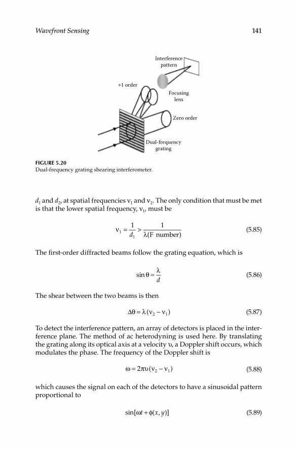
Wavefront Sensing 141
d1 and d2, at spatial frequencies ν1 and ν2 The only condition that must be met is that the lower spatial frequency, ν1, must be
ν11
1 1= >d λ( )F number
(585)
The first-order diffracted beams follow the grating equation, which is
sin θ λ=d
(586)
The shear between the two beams is then
∆θ λ ν ν= −( )2 1 (587)
To detect the interference pattern, an array of detectors is placed in the inter-ference plane The method of ac heterodyning is used here By translating the grating along its optical axis at a velocity υ, a Doppler shift occurs, which modulates the phase The frequency of the Doppler shift is
ω π= −2 2 1υ ν ν( ) (588)
which causes the signal on each of the detectors to have a sinusoidal pattern proportional to
sin[ ( , )]ω φt x y+ (589)
Interferencepattern
Focusinglens
+1 order
Zero order
Dual-frequencygrating
Figure 5.20Dual-frequency grating shearing interferometer

142 Principles of Adaptive Optics
The time t′ when the signal passes through zero can be electronically detected By substituting Equation 588 into Equation 589, we can find the phase of the fringe pattern as follows:
φ π ω( , )x y t= − ′ (590)
which, as noted earlier, is proportional to the slope of the wavefront at (x, y)Since interference only occurs between coherent beams, the shearing inter-
ferometer described earlier is limited to a single wavelength Since many wavefronts are multiwavelength, the fringe pattern generated by these would become washed out Errors associated with lateral shearing interfer-ometers are described by Dente et al [170] Incoherent beams, or an extended source, affect the contrast of the interference pattern (Equation 5102) Wyant [882] proposed a modification to the dual-frequency shearing interferometer that allowed its use in white light By Equation 587, the shear between the two beams is proportional to the wavelength, and the phase is proportional to 2π/λ; therefore, the fringe spacing is independent of wavelength To make the absolute fringe position also independent of wavelength, a grating is placed between the first dual-frequency grating and the interference plane If the angle of incidence to the first grating is θ, the angles of incidence leav-ing the dual-frequency grating are θ1 – θ = λν1 and θ2 – θ = λν2
If the additional grating has a spatial frequency (ν1 + ν2)/2, the angles asso-ciated with the second grating are
θ θ λ1 3
1 2
2− = +( )ν ν (591)
θ θ λ2 4
1 2
2− = +( )ν ν
(592)
and the angular deviation between the incident beam θ and the final beam is
∆ λ1
2 1
2= −( )ν ν
(593)
and
∆ λ ν ∆21 2
12= − = −( )ν
(594)
For a focal distance of f, the phase of the two beams on the interference plane will be ϕ1(x – f Δ, y) and ϕ2(x + f Δ, y) When these two beams interfere, a bright fringe will occur at ϕ1 – ϕ2 = mλ By expanding the phase terms, the resultant expression for the pattern of bright fringes is
m fx
fx
fx
λ φ φ ∂ φ∂
= ∆ ∂∂
+∆ ∂
∂+
∆
23 5
2 2 3 4 4 5
! ! (595)

Wavefront Sensing 143
which is the locus of points of equal wavefront slope even in the presence of white light
Not all lateral shearing interferometers interfere two beams of the first dif-fracted order like the one just described [40] One method [107] uses only one grating with a single frequency to diffract the beam The two opposing first orders, ±1, are interfered Although the result is the same, the description of the optical process can illustrate the general principle of shearing inter-ferometers Beams can be separated by polarization A birefringent prism will produce separate orthogonally polarized beams The interference is pro-duced by using an analyzer oriented at 45° [326]
Figure 521 shows a lateral ac shearing interferometer with a rotating grat-ing The chopping frequency, at 6–10 times the control bandwidth, is used in the heterodyne modulation process to eliminate the need for detector calibration With a focusing lens at the correct position, the wavefront Φ(x, y) that enters the system is Fourier transformed to W( , )ν η at the grating plane The transmission of the grating, G(x, y), is multiplied by the field at the grat-ing plane and inverse Fourier transformed by the second lens The result-ing field on the detector plane is the convolution of the wavefront with the Fourier transform of the grating function, given by
U x y G= ∗Φ( , ) ( , ) ν η (596)
The periodic grating of period d is rotating at a velocity υ In one dimension, the transform of this grating function is
G x x t ikf
x x x( ) ( )exp0 0= − −
−∞
∫ f f fdυ∞
(597)
where f is the focal length of the lenses, x0 is in the input plane, and xf is in the focal plane For the periodic grating, this reduces to
G x ikf
x t Gxf
ndn
n
( ) exp0 00= −
−
=−∞
∞
∑υ δλ
(598)
Detector array
W (x, y)+1
0−1
ω
f f
WG=WG~~
~WG
Dif fractedorder
Figure 5.21Rotating grating shearing interferometer

144 Principles of Adaptive Optics
where the Fourier coefficients are given by
Gd
G id
nnd
d
= −
−
∫1 2
2
2
( )exp/
/
ξ π ξ ξd (599)
with the result for the sinusoidal grating given by
G
n
i n=
=
± =
1 012
1
0
,
,
otherwise.
(5100)
The shear distance is s = λf/d, and the wavefront entering the interferometer is
Φ ϒ( ) ( ) e/ ( )x I i x= t1 2 φ (5101)
where ϒ is the degree of coherence (ϒ = 1 for a point source) From the van Cittert–Zernike theorem [86], for a target and aperture much smaller than the propagation distance z, the degree of coherence is
ϒ( , )( , )exp ( ) d d
s sI i
kz
s s
x y
x y
=− +
∫ t ξ η ξ η ξ η∫∫
∫∫ It ( , )d dξ η ξ η (5102)
where sx and sy are the x- and y-shears By adjusting the grating period, so that half a cycle equals the object size, the lateral shearing interferometer can use an extended object as its source
Equation 5102 can be solved for specific cases: for a square target of side 2a, angular size L = (2a)/z, we have
ϒsq =sin( / )
( / )2
2π λ
π λLs
Ls (5103)
or for a circular target of angular size L = diameter/z, the coherence is
ϒcirc =2 2
21J Ls
Ls( / )
( / )π λ
π λ (5104)
The signal on the sensors is the convolution, given by
U G= ∗Φ (5105)

Wavefront Sensing 145
( ) e ( )e ( ) ( )e/ϒI G x s G x G x si i tt
1 21 0 1
∗− +
−+ + + −δ δ δω ii tω[ ] (5106)
or
U I G G Gi x s t i x i= + +−+ +
+( ) e e e/ [ ( ) ] ( ) [ϒ t1 2
1 0 1φ ω φ φ(( ) ]x s t− − ω (5107)
The intensity on the detectors is the magnitude of the field squared and is given by
I x y U( , ) =2
(5108)
At this point, two options are available Applying Equation 5108 to the field of Equation 5106 results in terms containing dc (zero temporal dependence), 1ωt, or 2ωt If the signals are band-pass-filtered at frequency 1ω, the zero and first-order terms are processed and the result is
I x y G G Ix s x s
t( , ) cos( ) ( )= + − − +
420 1ϒ t
φ φ ω (5109)
If the band-pass filter is set at 2ωt, the two opposing first-order terms are interfered and the resultant intensity is
I x y G I x s x s t( , ) cos[ ( ) ( ) ]= + − − +2 212ϒ t φ φ ω (5110)
In either case, the intensity is a sinusoidal function of wavefront slope, given by
φ φ( ) ( )x s x s+ − − (5111)
and that slope can be determined Each channel can have four detectors or, with time or frequency multiplexing, the interferometer will operate with one sensor per channel A review of multiplexing and signal-processing techniques for shearing interferometers is given by Horwitz [355] Since the shear is proportional to the wavelength, this interferometer can be used with broadband sources Because of the temporal modulation, the ac shearing interferometer is best used with a continuous light source [326]
5.3.1.5 Rotation and Radial Shear Interferometers
Shearing interferometers are not limited to lateral shearing Rotational wavefront shearing was introduced in 1965 by Armitage and Lohmann [31] By rotating one beam 180°, the orthogonal component of radial shear (the tangential component) is measured Rotational shearing interferom-eters have been developed [95,658] for turbulence-degraded wavefront measurement

146 Principles of Adaptive Optics
The most common shear variation is the radial shear interferometer [439] In this type of wavefront sensor, the beams are separated and magnified by different values When the beams are superimposed, with their axes coinciding, interference occurs at the area of overlap, within the diameter of the smaller beam When the wavefront contains only radial aberrations, such as spherical aberration, radial shearing is very useful One variation, which uses only the small central portion of the wavefront and magnifies it to the full aperture, generates a constant phase reference The interfer-ence pattern then represents the phase rather than the slope Because of the large attenuation by using only a small portion of the wavefront (similar to the point–diffraction interferometer), it is not very useful for low-light-level applications
Figure 522 shows a system that uses radial shearing and another method of phase retrieval, multiple interferometer multiplexing, which Kwon [439] called “three-bucket phase-shifting interferometry” This method does not use modulation like that needed in heterodyning; rather, it compares mul-tiple interference patterns that represent the same wavefront slopes similar to techniques described for direct wavefront retrieval
In this interferometer, three orders, −1, 0, and +1, are separated The ±1 orders are phase-shifted ±90° The six beams are centered into three sheared pairs The radial shear distance s is the ratio of beam diameters (magnifications)
0 1< = <[ / ]s f fr R (5112)
To satisfy the grating equation sin θ = νλ, the focal lengths of the afocal tele-scopes are related to the grating frequencies by
ν νR R r rf f= (5113)
The phase slopes are retrieved from the three sets of signals through the use of Equation 570
Gratings Collimatingoptics Radial shear
fringes
+1
−10
+1
−10
Figure 5.22Radial shearing interferometer

Wavefront Sensing 147
5.3.2 Shack–Hartmann Wavefront Sensors
One method for testing a lens or mirror employs an opaque mask with holes placed behind the optical element under test Each of the holes acts as an aperture, and since the light passing through the lens is converging, the image produced is an array of spots With proper calibration, the position of the spots is a direct indication of the local wavefront tilt at each hole, and thus is a description of the lens quality This test is called the Hartmann test [332,333]
Variations of this technique, especially for real-time wavefront measure-ment, are used in adaptive optics wavefront sensors Shack placed lenses in the holes, which increased the light-gathering efficiency of the mask and, with the spots focused, reduced the disturbing diffraction effects of the holes A lens array for this purpose was first manufactured in 1971 [711] Members of the astronomy community began to use this sensor in the late 1970s for testing of large telescope optics Some astronomers use the term Hartmann–Shack (or Shack–Hartmann) wavefront sensor, but many shorten it to simply Hartmann sensor The measurement of the tilt and how it relates to the position of the focused spots was addressed in Section 522 A descrip-tion of some of the real-time techniques will show some of the diversity, advantages, and limitations of these noninterferometric methods
The Hartmann wavefront sensor is shown in Figure 523 The wavefront is divided by a mask, as in the classical test, an array of gratings, or an array of transmissive lenses Each of the beams in the subapertures is focused onto a detector To detect the position of the spot, various forms of modula-tion, detector geometry, and electro-optical processing are used For atmo-spheric turbulence compensation, the local wavefront tilt must be measured accurately in each subaperture of size r0 To do this, the subaperture must be large enough to resolve the isoplanatic patch During high turbulence, r0 is small and anisoplanatism degrades the process Hardy [318] discusses details of this large-versus-small subaperture trade for various optical and atmospheric parameters
A Hartmann sensor is composed of an array of lenses for wavefront divi-sion and typically a CCD array with multiple pixels used for spot position (wavefront tilt) determination The physical construction of lens arrays is a
Lenslet array
Wavefront
Source
Detectors
Figure 5.23Hartmann wavefront sensing technique

148 Principles of Adaptive Optics
major area for advanced engineering development One must achieve high alignment accuracy of the array along with the required high optical quality Many of these processes are proprietary to manufacturers, but some tech-niques have been described in the open literature on the subject [34,42,310,626] Techniques for designing and manufacturing lens arrays progress swiftly [160], and commercially available custom or catalog lens arrays are available from various sources [90,380,528,586,771]
A number of investigators have demonstrated Hartmann sensor modifica-tions that can be used to overcome the drawbacks [678] These can be done while maintaining the advantages of the Hartmann technique, that is, wide dynamic range [624], high optical efficiency, white light capability, no 2π ambiguity [906], the ability to use continuous or pulsed sources, and detec-tion of phase singularities [129]
If there is no expected channel-to-channel error, but only global misalign-ment, from bench vibration, for instance, one channel can be chosen as a reference and all measurements can be made in relation to the position of the spot in that channel
One method for removing alignment errors is the introduction of a refer-ence beam This beam should be a plane wave It does not have to be the same wavelength as the unknown wavefront beam, since no interference is needed or desired As shown in Figures 524 and 525, the reference must be distinctive so that the detector-processing electronics can discriminate between the signal beam and the reference beam
A number of other methods have been used to enhance specific aspects of Hartmann sensors [91,483,585] Optical binning [63] and optical amplifica-tion with an image intensifier [875] or rotating the square quadcells with
Beam splitterDetectors
Lensletarray
Referencesource
Referencewavefront
Source
Wavefront
Figure 5.24Hartmann sensor with reference
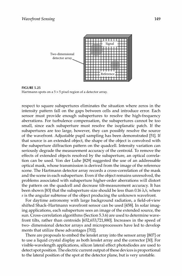
Wavefront Sensing 149
respect to square subapertures eliminates the situation where zeros in the intensity pattern fall on the gaps between cells and introduce error Each sensor must provide enough subapertures to resolve the high-frequency aberrations For turbulence compensation, the subapertures cannot be too small, since each subaperture must resolve the isoplanatic patch If the subapertures are too large, however, they can possibly resolve the source of the wavefront Adjustable pupil sampling has been demonstrated [51] If that source is an extended object, the shape of the object is convolved with the subaperture diffraction pattern on the quadcell Intensity variation can seriously degrade the measurement accuracy of the centroid To remove the effects of extended objects resolved by the subaperture, an optical correla-tion can be used Von der Luhe [829] suggested the use of an addressable optical mask, whose transmission is derived from the image of the reference scene The Hartmann detector array records a cross-correlation of the mask and the scene in each subaperture Even if the object remains unresolved, the problems associated with subaperture higher-order aberrations will distort the pattern on the quadcell and decrease tilt-measurement accuracy It has been shown [83] that the subaperture size should be less than 016 λ/s, where s is the angular subtense of the object producing the unknown wavefront
For daytime astronomy with large background radiation, a field-of-view shifted Shack–Hartmann wavefront sensor can be used [458] In solar imag-ing applications, each subaperture sees an image of the extended source, the sun Cross-correlation algorithms (Section 536) are used to determine wave-front tilts, rather than centroids [652,653,721,880] Increases in the speed of two- dimensional detector arrays and microprocessors have led to develop-ments that utilize these advantages [702]
There are proposals to embed the lenslet array into the sensor array [807] or to use a liquid crystal display as both lenslet array and the corrector [30] For visible-wavelength applications, silicon lateral effect photodiodes are used to detect spot position The electric current output of these devices is proportional to the lateral position of the spot at the detector plane, but is very unstable
Signal
Reference
Two-dimensionaldetector array
Figure 5.25Hartmann spots on a 5 × 5 pixel region of a detector array

150 Principles of Adaptive Optics
5.3.3 Curvature Sensing
Roddier et al [660,664] have shown how the methods of focus sensing described in Section 523 and the Hartmann subaperture division process can be combined The method, called curvature sensing, measures local wave-front curvature (second derivative) in each subaperture [201] By comparing two near-simultaneous irradiance distributions at equally spaced points on either side of the subaperture focal plane, the local curvature is found [213] Referring to Figure 526, two irradiance distributions I r1( )
and I r2 ( )
are
detected a distance s from focus on either side of the focal plane The rela-tionship between the irradiance and the phase is given by
I r I rI r I r
f f ss
fs
r1 2
1 2
2( ) ( )( ) ( )
( )
− −+ −
=−
∇ Φ
− ∂∂
=
n
fs
rf cs
Φ δcw2 2
(5116)
where cw is the local curvature at r expressed as c rw w= 1/ and rw is the local
radius of curvature The Dirac delta δc represents the outward pointing nor-mal derivatives on the edge of the signal To reconstruct the wavefront from the known local curvatures and the edge derivatives, an iterative procedure can be followed [666] to solve Poisson’s equation [663], or Zernike derivatives can be calculated [318] Hickson [341] describes conditions, namely when D r r z/ ( / ) /
0 02 6 5≤ λ , in which the wavefront can be reconstructed with a single
defocused image of a star To use the approximations necessary to get the right side of Equation 5116, the distance s should be
sf
f r≥
+λ
λ
2
02 (5117)
At optical wavelengths, this condition reduces to sf
r≥
λ 2
02
The standard
deviation of a single curvature measurement is σλ
c r=
02 1 2Np
/ where Np is the
photon count [660]
P1 P2
ss
f
I1(r) I2(r)
Figure 5.26Wavefront curvature sensor geometry

Wavefront Sensing 151
One appealing characteristic of this process is the possibility of applying a correction without the intermediate step of wavefront reconstruction Since some correction devices, specifically membrane mirrors [312] and bimorphs [226], can deform locally into near-spherical shapes and can be driven directly by the output of a single subaperture that measures local wavefront curvature [890] When the mirror gain is considered and the wavefront sen-sor subapertures and corrector actuators are aligned, a very efficient process for wavefront control results [305] Curvature sensing can be applied to sense atmospheric layers [289,395] for curvature-based tomographic reconstruction of atmospheric distortions [578]
5.3.4 Pyramid Wavefront Sensor
Another pupil-plane wavefront sensor uses a pyramidal prism in the image plane to create four subbeams that are then optically relayed to a detector (see Figure 527) [637] The intensity at position
r x y( , ) in each of the sub-
beams in the detector plane (I0,0 > I0,1 > I1,0 > I1,1) is used to find the x and y wavefront slopes at
r x y( , )
S rI r I r I r I r
Ix ( )( ) ( ) ( ) ( ), , , ,
=− + −0 0 1 0 0 1 1 1
tt
(5118)
S rI r I r I r I r
Iy ( )( ) ( ) ( ) ( ), , , ,
=+ − −0 0 1 0 0 1 1 1
tt
(5119)
It is the average intensity over the detector plane One advantage of the pyra-mid technique over the Shack–Hartmann sensor is that the spatial resolution of the sensor is the size of the detector pixel in contrast to the larger lenslet
Pupil plane
Image plane
Pyramid
Detector
Relaylens
Figure 5.27Pyramid wavefront sensor

152 Principles of Adaptive Optics
subaperture size of the Shack–Hartmann [820,821] Various improvements to the basic pyramid sensor and reconstructor have been recorded in literature [203,427,428,619,820,884]
5.3.5 Selecting a Method
The diverse direct wavefront measurement techniques described in this section are used to detect information about the phase It is important to consider specific requirements for the wavefront sensor in terms of the rest of the system [275] The relationship between the subaperture geometry [654] and the placement of correcting actuators can steer the system design toward one method or another [197] In some circumstances, wavefront sen-sors are used to directly detect coherent backscatter [369] or a satellite image [370] If the wavefront sensor is used to determine the Zernike coefficients [850] or other aberration measurements in optical testing [703], the speed and spatial resolution requirements might differ from real-time adaptive optics compensation In some circumstances, such as imaging of a solar disk, the source is extended Cross-correlation techniques, rather than subaperture tilt measurement, must be used to properly detect the atmospheric distor-tions [650]
A direct comparison between Hartmann sensors and shearing interferom-eters has been reported [610] as has a comparison of different models used in wavefront sensor and system design [876] Welsh et al [857] report that both types of sensors are comparable for good seeing conditions and small bea-cons, however, for poor seeing and extended beacons, the Hartmann sensor has lower error levels Similar theoretical comparisons between Hartmann sensors and curvature sensors [173,323] reveal the effects of seeing condi-tions and pixel readout noise Under most seeing conditions, the Hartmann sensor performs better because of lower noise
5.3.6 Correlation Tracker
When the wavefront source is an extended object, a centroid measure-ment, like that in a Shack–Hartmann sensor, is meaningless Each subap-erture contains a small image of the entire object with the image shifted according to subaperture tilt To overcome this problem, one image IR ( )x is chosen as a reference The cross-covariance between each image I is calculated by
CC I I I I( ) d ( ) ( ) [ ( )] [ (δ δ δ= − = ℑ ℑ × ℑ +∫∫ + − −∗x x x x xR R ))] (5120)
where x is the 2-D spatial coordinate, δ is the 2-D image displacement, ℑ ℑ+ −and is the forward and inverse Fourier transforms, and * indicates the complex conjugate This method has been applied in solar telescopes where photons are plentiful, but the object is large

Wavefront Sensing 153
5.4 Indirect Wavefront Sensing Methods
Many adaptive optics systems, including the human eye, do not carry out the process of making a measurement of the wavefront directly, calculating the amount of correction, and then applying that correction Methods that avoid a direct calculation of the wavefront are called indirect methods The indirect methods are mostly akin to trial and error If an optical system has a way of altering the phase of the desired signal, whether it is an image or a propagated beam, and a way of determining the final result of that phase change, the system is closed-loop and, therefore, adaptive optics
The coupling of the correction system and the indirect wavefront sens-ing system usually makes the two difficult to distinguish To illustrate this, consider a simple system of Figure 528, where the propagation system has two channels with an unknown phase lag on one of them By focusing the beams to a detector, the intensity pattern can be observed and processed For a two-beam system, the intensity distribution will be the interference pattern described by Young’s experiment, that is,
I I=
4
202 1cos
δ (5121)
where δ1 is the unknown phase delay in the one beamAs described in Section 531, the phase delay in the wavefront can be cal-
culated from an intensity measurement of the peak We could then apply an equivalent phase delay to the other beam to produce a maximum intensity in the detector plane This would require a method of calculating the following equation in real time:
δ11
0
24
= −cosII
(5122)
Indirect methods do not make a calculation and apply specific correction If the system of Figure 528 were modified so that the intensity detector was linked to the active phase delay device, a trial and error method of finding the phase that maximizes the intensity could be used (Figure 529)
δ1
Detector
Figure 5.28Two-beam simple adaptive optics system
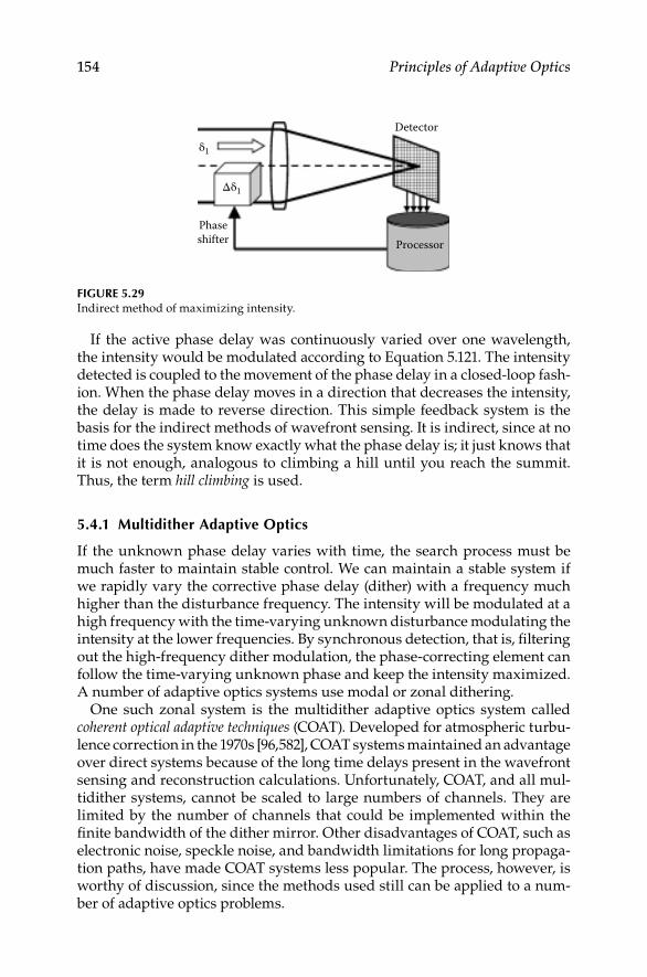
154 Principles of Adaptive Optics
If the active phase delay was continuously varied over one wavelength, the intensity would be modulated according to Equation 5121 The intensity detected is coupled to the movement of the phase delay in a closed-loop fash-ion When the phase delay moves in a direction that decreases the intensity, the delay is made to reverse direction This simple feedback system is the basis for the indirect methods of wavefront sensing It is indirect, since at no time does the system know exactly what the phase delay is; it just knows that it is not enough, analogous to climbing a hill until you reach the summit Thus, the term hill climbing is used
5.4.1 Multidither Adaptive Optics
If the unknown phase delay varies with time, the search process must be much faster to maintain stable control We can maintain a stable system if we rapidly vary the corrective phase delay (dither) with a frequency much higher than the disturbance frequency The intensity will be modulated at a high frequency with the time-varying unknown disturbance modulating the intensity at the lower frequencies By synchronous detection, that is, filtering out the high-frequency dither modulation, the phase-correcting element can follow the time-varying unknown phase and keep the intensity maximized A number of adaptive optics systems use modal or zonal dithering
One such zonal system is the multidither adaptive optics system called coherent optical adaptive techniques (COAT) Developed for atmospheric turbu-lence correction in the 1970s [96,582], COAT systems maintained an advantage over direct systems because of the long time delays present in the wavefront sensing and reconstruction calculations Unfortunately, COAT, and all mul-tidither systems, cannot be scaled to large numbers of channels They are limited by the number of channels that could be implemented within the finite bandwidth of the dither mirror Other disadvantages of COAT, such as electronic noise, speckle noise, and bandwidth limitations for long propaga-tion paths, have made COAT systems less popular The process, however, is worthy of discussion, since the methods used still can be applied to a num-ber of adaptive optics problems
δ1
Δδ1
Detector
Phaseshifter Processor
Figure 5.29Indirect method of maximizing intensity

Wavefront Sensing 155
The multidither process is basically a replication of the two-beam process described earlier in as many channels as necessary for spatial resolution For a system like the one shown in Figure 530, portions of the beam are tagged by phase-shifting elements that dither the phase The field at the target is the sum of all the individual fields and is given by
U U A p x yni
n
N
ntot e=
=∑0 0
1
Φ ( , ) (5123)
where Φn = ϕ + ψ0 sin(ωnt), ϕ is the average phase of the channel, and p0 is the aperture and intensity variance
The intensity at the target is the square of the combined fields and is given by
I U p A A Ann
N
k m k mk mk m
N
= + −
= =
≠
∑ ∑02
02 2
1 1
cos( ),
Φ Φ
(5124)
where the phases of the individual beams, given by
Φn nt= +φ ψ ω0 sin( ) (5125)
are dithered at amplitude ψ0 and at unique frequencies ωn Equation 5124 illustrates how the phase dithering translates into an intensity modulation on the target
Multiple inputbeams Combining
opticsPhase
distortions
Targetglint
Turbulentatmosphere
Noncoherentdetector
~
~
~
High-powerlaserarray
s
ω
ω
ωs
s
−ϕ1−Φ1
−Φ2
−Φ3
−ϕ2
−ϕ3
Figure 5.30Multidither COAT system

156 Principles of Adaptive Optics
A noncoherent detector can be placed in the focal plane at a cooperative target and the modulated intensity can be sensed For a noncooperative tar-get, the detector can be placed near the transmitter as shown in Figure 530 Energy from a bright spot on the target (called a glint) is reflected into the detector Light from the glint will have the same modulation in the intensity as on the target When the propagation time delay is removed, the closed-loop control can band-pass the signal at each dither frequency, then beat the remainder with the dither The resulting signal contains the information used for the servo to drive the average phase in the channel toward an inten-sity maximum [316]
Each element in the system attempts to drive itself and the weighted sum of all others to an intensity maximum When the amplitudes and average phase errors within each channel are equal, the peak intensity is [582]
I A N N N Jnpk ∝ + − 2 202
0( ) ( )ψ (5126)
where N is the number of channels and ψ0 is the dither amplitude For a sys-tem that employs this concept, a tradeoff analysis must be performed The SNR in the detector is proportional to the modulation strength, but a large modulation causes the peak intensity to be low because the modulation (the dither amplitude in Equation 5126) will force the system to be somewhat out of phase at all times The reduction in intensity caused by the Bessel func-tion term in Equation 5126 shows this O’Meara [582] calculated a theoretical value for the optimum dither amplitude based on detector parameters such as quantum efficiency and bandwidth, as well as optical design parameters that regulate the power reflected into the detector
Other COAT parameters are subject to restrictions placed by the methods used in decoding the dithered information The maximum dither frequency [602] should be
f N fmax [ . ( )]= + −10 1 6 1 OL (5127)
where N is the number of channels, and fOL is the open-loop unity-gain servo bandwidth The range of dither frequencies [601] is
f f N fmax min . ( )− = −3 2 1 CL (5128)
where fCL is the closed-loop control bandwidth that is desired These are theoretical limits When actual sensor noise and propagation time delays are considered, the minimum dither frequency should be at least 10 times the control bandwidth The number of dither frequencies can be cut in half if each dither pair is exactly 90° out of phase, that is, a sine function dither and a cosine function dither The signals at these frequencies can be band-pass-filtered, since the phase difference between the two is always an exact quadrant Even with this method, known as quadrature, to avoid aliasing, the separation of dither frequencies should be no less than four times the control

Wavefront Sensing 157
bandwidth The width of the band-pass filters must be slightly larger than the control bandwidth to retain the disturbance information [484]
A perfect COAT system will be stable for any number of channels [583]; however, most laboratory or field systems are far from perfect Some of these imperfections have engineering solutions, but the overall utility of COAT systems is decreased The first major problem with COAT occurs when there is no glint The returned energy, the feedback, is absolutely required for the multidither principle to work Variations of this problem occur if the glint is present and too dim, there are multiple glints, or the glint appears to move around because of changing target conditions (glint hopping) Any of these conditions reduce the system’s ability to distinguish the intensity variations caused by the dithering
It has been shown that cross-coupling between dithered phase elements, due possibly to continuous surface mirrors that have mechanical cross-cou-pling, will make possible an intensity maximization on a local rather than global maximum [584] The need for many channels with a high control bandwidth [418] and a large overall phase excursion for atmospheric tur-bulence correction has made scalability to large apertures difficult using COAT For atmospheric turbulence correction, with a propagation distance z, an aperture of diameter D, an atmospheric structure constant Cn
2 , and a wavelength λ, the number of channels required for correction to a Strehl ratio of S is [605]
N
C zDS
n= ( )
2 01
1
2 5 3
2
6 5.
ln /
//
λ (5129)
The bandwidth of the atmospheric turbulence correction system must be
f C znc ≅
0 652
2
2
3 5
.
/
vπ
λ (5130)
where v is the transverse wind velocity that moves the turbulence across the beam The total phase excursion for any channel is
∆φλ
= ( )3 58 2 5 3 1 2. / /C zDn (5131)
when the diameter is about half the turbulence outer scaleFor very long propagation distances, the delay in the signal reaching the
detector limits the control bandwidth Even with lead–lag control compensa-tion, the control signal phase delay must be kept below 30 or 40° With the phase delay proportional to the propagation distance R, we have
φ πdelay =
22
Rc
f (5132)

158 Principles of Adaptive Optics
one can see that the range–bandwidth ( fR) product must remain below 2 × 10⁷ This rules out atmospheric propagation from the ground to space (1000 km) using COAT, since the bandwidth achievable, 20 Hz, is well below the approximately 100 Hz correction bandwidth required
Since COAT by definition uses coherent light, the phenomenon of speckle must be considered [240] Any target that is rough, and they all are, will cause the signal at the receiver to appear speckled The mutual interference of various portions of the beam reflected from the rough surface will appear as speckled dots to the receiver A moving or spinning target will cause these dots to move across the receiver The intensity of the light onto the detector will then be modulated at a frequency of f = υs/λ, where υs is the speckle velocity across the receiver The problem occurs when this modulation frequency is at or near a dither frequency [422] The electrical interference of the signals causes a reduc-tion in performance of the entire system The intensity of the modulations at dither frequencies, ID, degrades the COAT convergence level by
I CPP
IDD
SM= (5133)
where C is the portion of ac modulation power that is near the dither fre-quency, PD is the power in the detected dither signal, PS is the power in the detected speckle signals, and IM is the nonspeckle convergence level The convergence level is roughly the Strehl ratio achieved by the system
IN
JNM = + −
−11
1 210
20 2
( ) ( cos )ψα
α (5134)
where α is the random distribution of phases of all the channelsKokorowski et al introduced a method to automatically cancel speckle
effects [420] A system, shown in Figure 531, was devised where part of the
Multichanneldithering
Pistondithering
Figure 5.31Automatic speckle cancellation technique
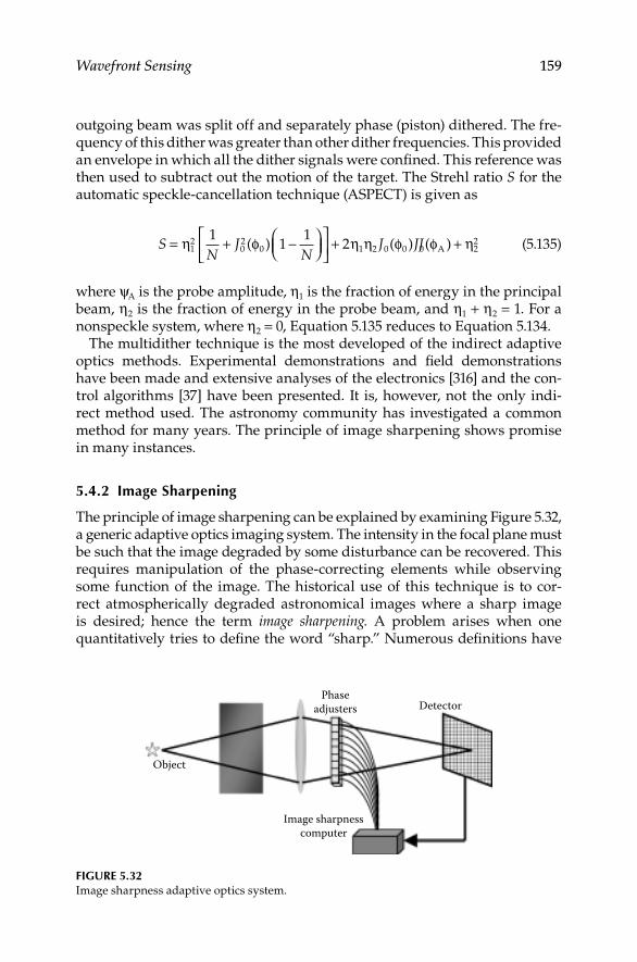
Wavefront Sensing 159
outgoing beam was split off and separately phase (piston) dithered The fre-quency of this dither was greater than other dither frequencies This provided an envelope in which all the dither signals were confined This reference was then used to subtract out the motion of the target The Strehl ratio S for the automatic speckle-cancellation technique (ASPECT) is given as
SN
JN
J= + −
+η φ η η φ12
02
0 1 2 0 01
11
2( ) ( )JJ0 22( )φ ηA + (5135)
where ψA is the probe amplitude, η1 is the fraction of energy in the principal beam, η2 is the fraction of energy in the probe beam, and η1 + η2 = 1 For a nonspeckle system, where η2 = 0, Equation 5135 reduces to Equation 5134
The multidither technique is the most developed of the indirect adaptive optics methods Experimental demonstrations and field demonstrations have been made and extensive analyses of the electronics [316] and the con-trol algorithms [37] have been presented It is, however, not the only indi-rect method used The astronomy community has investigated a common method for many years The principle of image sharpening shows promise in many instances
5.4.2 image Sharpening
The principle of image sharpening can be explained by examining Figure 532, a generic adaptive optics imaging system The intensity in the focal plane must be such that the image degraded by some disturbance can be recovered This requires manipulation of the phase-correcting elements while observing some function of the image The historical use of this technique is to cor-rect atmospherically degraded astronomical images where a sharp image is desired; hence the term image sharpening A problem arises when one quantitatively tries to define the word “sharp” Numerous definitions have
Object
Phaseadjusters Detector
Image sharpnesscomputer
Figure 5.32Image sharpness adaptive optics system

160 Principles of Adaptive Optics
been explored [547] Many more descriptions of a “good image” have been developed in the rapidly advancing science of image processing These latter developments are more structured to post–image processing than to real-time image formation, and they are not considered to be within the realm of adap-tive optics
The technique requires the maximization of a function defined as sharp-ness, S The simplest thing to maximize, by changing the phase of various parts of the imaging system, is the intensity at one point, most likely the cen-ter of the image This image-sharpening technique (S = I(x0, y0)) is simple—move each phase adjuster one at a time, watching the intensity at one point Then move the phase adjusters through at least one wavelength and leave them on the point where the intensity is maximized This, of course, has drawbacks; it does not use most of the information available and will only work well for bright point objects They must be bright to generate enough photons at the point of observation, and they must be point objects to ensure that the center of the image is near the optical axis
The most common image sharpness that is maximized is the integral of the square of the image intensity distribution [547], given by
S I x y x y= ∫ ( , ) d d2 (5136)
This sharpness definition will be maximized when there is zero wavefront error even in the presence of irregular object radiance distributions This amplitude insensitivity makes this method useful for large extended objects Other sharpness functions, such as higher-order moments of the distribution, expressions related to the Fourier transform of the image [841], or entropy minimization functions given by Equation 5137:
S I x y I x y x y= −∫ ( , ) ln[ ( , )]d d (5137)
have been tried and are proven to relate to low wavefront error The electrome-chanical techniques required to implement an image-sharpening system are similar to the techniques used in multidither In this case, however, the target is the image plane Each element is individually adjusted by trial and error The performance is limited by the number of degrees of freedom (channels) and the required bandwidth [547], because both cannot be increased simulta-neously For ground-based astronomy applications, as long as the aperture is within the same isoplanatic patch and enough light is present in each channel, the image-sharpening sensor methods can be, and have been, used success-fully For anisoplanatic situations, where the wavefront is derived from mul-tiple planes, image sharpness methods can still be successful with nonlinear optimization techniques [774] or optimizing a laser spot on the target [620]

Wavefront Sensing 161
5.5 Wavefront Sampling
The wavefront sampling subsystem redirects a portion of the incoming beam to the wavefront sensor It is often called by many less functional names, such as beam splitter or grating, usually because this subsystem often is a sin-gle component of a beam train In any case, it is important that the wavefront sensor gets a sample of the wavefront that is a high-fidelity replication of the wavefront that needs correction If a wavefront sensor is used in the purely diagnostic mode, there is no need for a sampler The beam just enters the sensor and data can be recorded Where conventional adaptive optics is used in a closed loop, the beam is propagated to a target or an image sensor with only a representative sample sent to the wavefront sensor It is important that the sample represents the wavefront that is propagated along the rest of the system
Many beam control systems, like the one shown in Figure 41, will show a beam splitter fulfilling the beam-sampling function The beam splitters can be actual coated glass components commonly called beam splitters, or they can represent any device that separates the ongoing beam and the sampled beam The details of the adaptive optics system and the operational require-ments often dictate the type of component that is required
5.5.1 beam Splitters
Transmissive beam splitters come in a variety of configurations They are generally specified as being flat-plate, cube, or pellicle beam splitters When beams of different wavelengths must be separated, as required by some return wave adaptive optics, a dichroic beam splitter is used Commercially available flat-plate beam splitters are usually thin glass plates with edges parallel on the order of a few milliradians The surface incident to the beam, usually called the front surface, is coated with a film having partial reflection properties for the wavelength of interest (Figure 533a) The transmitted portion of the beam exits the back surface, which has a broadband antireflection (AR) coat-ing The reflection–transmission ratios are specified along with the incidence angle and, sometimes, the polarization state (for example, T/R 50:50 ±5%; 45°) Off-the-shelf components have a surface flatness that is typically a few waves across the device For most applications in adaptive optics, this distortion can be corrected if it is passed to the wavefront sensor by the reflected beam and the distortion is imparted to the transmitted beam as well
Another source of beam distortion occurs when the beam splitter is mounted The stresses in the glass due to the clamping can distort the plane surface As long as the distortion shows up on both the transmitted and the reflected beams and is within the range of the adaptive optics system,

162 Principles of Adaptive Optics
the adaptive optics will be successful Only when the sampled beam sees a different distortion than the transmitted beam will problems occur The sample, then, is not a high-fidelity sample The adaptive optics system will try to correct for one distortion while the beam really has another distor-tion This is analogous to the atmospheric anisoplanatism problem, but, for-tunately, this fidelity problem is normally within the control of the optical engineer The differences between the sampled beam and the transmitted beam are important considerations for adaptive optics system layout and component selection
Cube beam splitters have some advantages over plate beam splitters A cube beam splitter is a matched pair of right-angle prisms (Figure 533b) This type of beam splitter deforms much less than a flat plate when it is stressed by mounting The partially reflecting coating is applied to the interface between the prisms before they are cemented together This reduces long-term degra-dation because the coating is sealed The specifications for cube splitters are similar to those for plate splitters
Beam splitters can be used in an uncollimated portion of the beam if a compensating beam splitter is inserted in the beam train This second split-ter, tilted in the opposite direction, compensates for aberrations introduced by the first splitter The finite thickness of the beam splitter imparts aberra-tions to the transmitted beam, thereby reducing the fidelity of the reflected sample The amount of spherical aberration, chromatic aberration, and astig-matism can be significant Since it is not imparted to the reflected beam, the adaptive optics system can have degraded performance
One possible way of avoiding the low-fidelity problem is through the use of pellicle beam splitters (Figure 533c) These devices consist of a mem-brane stretched over a frame Since the membrane is about 5 μm thick, the chromatic and spherical aberration of the transmitted beam are negligible Wavefront sampling is then possible in a diverging beam where a collimated portion is not easily found For example, in a photon-starved astronomical application, the addition of extra optics to provide a collimated beam may have too much absorption A pellicle beam splitter is a possible solution The nature of the pellicle beam splitter also can be a disadvantage Its small thickness allows it to be easily distorted by mounting stress and acoustic
R R R
T T T
(a) (b) (c)
Figure 5.33Beam splitters: (a) flat plate, (b) cube, and (c) pellicle R is the reflected beam; T is the transmit-ted beam
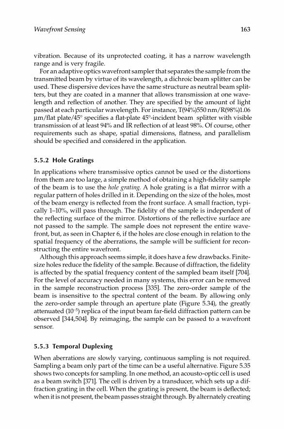
Wavefront Sensing 163
vibration Because of its unprotected coating, it has a narrow wavelength range and is very fragile
For an adaptive optics wavefront sampler that separates the sample from the transmitted beam by virtue of its wavelength, a dichroic beam splitter can be used These dispersive devices have the same structure as neutral beam split-ters, but they are coated in a manner that allows transmission at one wave-length and reflection of another They are specified by the amount of light passed at each particular wavelength For instance, T(94%)550 nm/R(98%)106 μm/flat plate/45° specifies a flat-plate 45°-incident beam splitter with visible transmission of at least 94% and IR reflection of at least 98% Of course, other requirements such as shape, spatial dimensions, flatness, and parallelism should be specified and considered in the application
5.5.2 Hole gratings
In applications where transmissive optics cannot be used or the distortions from them are too large, a simple method of obtaining a high-fidelity sample of the beam is to use the hole grating A hole grating is a flat mirror with a regular pattern of holes drilled in it Depending on the size of the holes, most of the beam energy is reflected from the front surface A small fraction, typi-cally 1–10%, will pass through The fidelity of the sample is independent of the reflecting surface of the mirror Distortions of the reflective surface are not passed to the sample The sample does not represent the entire wave-front, but, as seen in Chapter 6, if the holes are close enough in relation to the spatial frequency of the aberrations, the sample will be sufficient for recon-structing the entire wavefront
Although this approach seems simple, it does have a few drawbacks Finite-size holes reduce the fidelity of the sample Because of diffraction, the fidelity is affected by the spatial frequency content of the sampled beam itself [704] For the level of accuracy needed in many systems, this error can be removed in the sample reconstruction process [335] The zero-order sample of the beam is insensitive to the spectral content of the beam By allowing only the zero-order sample through an aperture plate (Figure 534), the greatly attenuated (10−5) replica of the input beam far-field diffraction pattern can be observed [344,504] By reimaging, the sample can be passed to a wavefront sensor
5.5.3 Temporal Duplexing
When aberrations are slowly varying, continuous sampling is not required Sampling a beam only part of the time can be a useful alternative Figure 535 shows two concepts for sampling In one method, an acousto-optic cell is used as a beam switch [371] The cell is driven by a transducer, which sets up a dif-fraction grating in the cell When the grating is present, the beam is deflected; when it is not present, the beam passes straight through By alternately creating

164 Principles of Adaptive Optics
the grating and removing it, the switch can direct a beam toward a different beam path (Figure 535a) This is workable for low-power applications where distortion in the cell is not a problem For a normally incident wave, the deflec-tion angle θD for the first order Raman–Nath diffraction wave is
sin θ λλD
a
= (5138)
where λ is the wavelength of the light and λa is the acoustic wavelength Since the transducer can be switched on and off at very high rates (easily fO MHz), the beam samples can represent very high-frequency components of the disturbed wavefront The major difficulties arise from the relatively small beams that can be used and the long paths required to separate the beams, since the ratio λ/λa is small
When beams are larger or even high-power, mechanical choppers can be used Figure 535b shows the conceptual makeup of such a device The beam is alternatively reflected and transmitted by the chopper, which can have various duty cycles For instance, a spinning flat plate with a hole equal to the beam diameter will transmit one sample per revolution If the plate is
Transducer
Acousto-optic cell
Choppingwheel
Rotation
(a) (b)
Figure 5.35Temporal duplexing concepts: (a) acousto-optic cell and (b) mechanical chopper
Reflected beam
Hole grating
Multiple orders
Sample beam towavefront sensor
Apertureplate
Figure 5.34Use of a hole grating The multiple orders from the grating are removed by the aperture plate

Wavefront Sensing 165
large enough to have four holes, the sample rate is RPM/15 Hz For slowly varying aberrations such as thermal distortion, a chopper with a diameter of five beam diameters (accounting for 45° incidence angle) could sample a beam at 200 Hz With consideration for control system delays, this could eas-ily allow for a 20-Hz correction bandwidth
An alternative design using precisely aligned blades would have the same performance parameters In either case, the fidelity concerns are similar to those with beam splitters or hole gratings The distortion imparted on the reflected beam must be as small as possible to have a sample that is repre-sentative of the zero-loss transmitted wavefront Engineering concerns such as wobble, bearing and surface cooling, beam path environment control, and long-duration stability must be studied for each case
5.5.4 reflective Wedges
A simple wedge can be used when one needs to spectrally separate two beams A wedge is a dispersive device that functions as a prism If the sample beam is a different wavelength than the main beam, the characteristic index of refraction differences of materials can be used Figure 536 shows two pos-sible configurations of a sampling wedge Figure 536a has an AR coating on the incident surface with a reflective coating on the back surface Two super-imposed beams of wavelengths λ1 and λ2 are incident at angle θi For a wedge angle θW, the angle of the reflected beam from the front surface is
sin sin cos cos sinθ θ θ ω θR W W= +n i i2 2 (5139)
The different directions of the two beams arise because the index of refrac-tion is slightly different for the two wavelengths For example, with a wedge angle of 5° and an incident angle of 10°, using SF11 glass, a visible beam (λ = 500 nm) is separated from an IR beam (λ = 1500 nm) by over 1/2° The indices of refraction [519] used are n500 nm = 180205 and n1500 nm = 174525
If a larger angular spread is desired, the front surface of the wedge can be coated to reflect one of the wavelengths From the preceding example, if the IR beam is reflected from the front surface, it leaves at an angle of 10° The visible beam is refracted in the material and leaves at an angle of 2863°
λ1 λ1
θw
λ2 λ2
(a) (b)
Figure 5.36Reflective wedges: (a) dispersive method and (b) reflective method

166 Principles of Adaptive Optics
This separation has the advantage of requiring much shorter propagation distances for the sampled beam It does suffer from fidelity problems, since the path for the refracted beam passes through the material and may pick up bulk material distortions, while the reflected beam picks up only surface distortions
Although reflective wedges seem simple, they suffer from many of the same deficiencies as beam splitters Deviation from flatness is a major con-cern Maintaining a constant wedge angle is as difficult as maintaining the parallelism of a flat plate Since their operation as adaptive optics wavefront samplers depends upon specialized reflective and antireflective coatings, the quality of the coating process must be at least as good as, if not better than, the coating process of other optics in the system
5.5.5 Diffraction gratings
Diffraction gratings are optical elements with a surface that is modulated with a regular groove or slit pattern They are used in adaptive optics primar-ily as a method of separating two beams One of the beams will be passed along (either by reflection or transmission) toward a wavefront sensor, which should retain the wavefront characteristics of the other beam The details of the diffraction taking place have been discussed by a number of authors [368,714,747]
Modern photoresist techniques and lasers make the production of highly efficient gratings possible The interference of two beams can produce a pattern of lines very close together When an interference pattern exposes photoresist, a very fine pattern can be etched into an optical substrate This holographic grating has an advantage over mechanically ruled gratings When the interference pattern is made without collimating optics, the holographic grating can be used to focus a beam Because the grooves are under optical rather than mechanical control, the unequal spacing can be used to manage the diffracted beams Focusing gratings of this type are used throughout the imaging and adaptive optics communities
Mathematical expressions from classical optics can be used for analyzing most types of gratings The behavior of ruled gratings and holographic grat-ings is explained by diffraction theory The different orders of diffraction for reflection or transmission gratings follow the basic grating equation
d mm i(sin sin )θ θ λ− = (5140)
where d is the separation of the grooves, θi is the incident angle measured from normal, and θm is the angle of the mth diffracted order The plane of incidence is perpendicular to the grooves When this strict condition is not met, the grating will operate with reduced fidelity (see Section 557) For focusing gratings, the d in Equation 5136 depends on the angle of incidence, and the expression loses its linearity

Wavefront Sensing 167
Most gratings in use in adaptive optics are either blazed or sinusoidal Blazed gratings have triangular-shaped grooves with their depth specified by a blaze angle, θB Low blaze angles (∼2°) are insensitive to polarization and have a clearly defined efficiency peak at λ/d = 2 sin θB Low blaze angle grat-ings exhibit almost 100% efficiency at this one order [478] Higher blaze angle gratings show high efficiencies for the higher orders, but become more sensi-tive to polarization The S-state polarization (light polarized perpendicular to the grooves) usually shows higher efficiency than the P-state (light polar-ized parallel to the grooves) Unusual behavior occurs for blaze angles larger than 20°, and each should be considered individually, depending upon the wavelength and the order of diffraction that is to be used [368]
Sinusoidal grooved gratings can be made easily with the photoresist process The modulation ratio h/d (where h is the peak-to-peak height of the grooves) determines the efficiency Low-modulation gratings (h/d < 005) exhibit a maximum efficiency at λ = 34h with very low efficiency for high orders When the modulation ratio is increased, the higher-order efficiency of the grating increases Although the grating efficiency is a function of groove profile, wavelength, angle of incidence, and surface material optical con-stants, approximations can be made For a perfectly conducting surface with sinusoidal grooves that have a depth that is short compared to the wave-length, scalar theory predicts that the efficiency E is
E Jh
n=
2 2πλ
(5141)
where Jn is the Bessel function for diffractive order n In general, diffraction gratings are a proven method for wavefront sampling for monochromatic operation and have widespread use Sensitivity to grating alignment and polarization effects are discussed in Section 557
5.5.6 Hybrids
Many adaptive optics systems cannot use a simple grating or beam splitter for beam sampling Transmissive beam splitters often cannot handle high-power flux without significant distortion or destruction A number of hybrid con-cepts have been introduced to overcome shortcomings of single-component samplers A variation on the wedge discussed in Section 554 is the buried mirror Whereas the wedge works by reflecting a beam from the front surface in a different direction from a beam reflected from the back surface, a bur-ied mirror is constructed so that the beam reflected from the back surface is focused differently than the beam reflected from the front surface Figure 537 illustrates two methods of employing this concept The system in Figure 537a has an annular outgoing beam coincident with an incoming beacon beam The outgoing beam is reflected from the front surface of the optics The bur-ied mirror transmits the beacon wavelength through its coating toward the
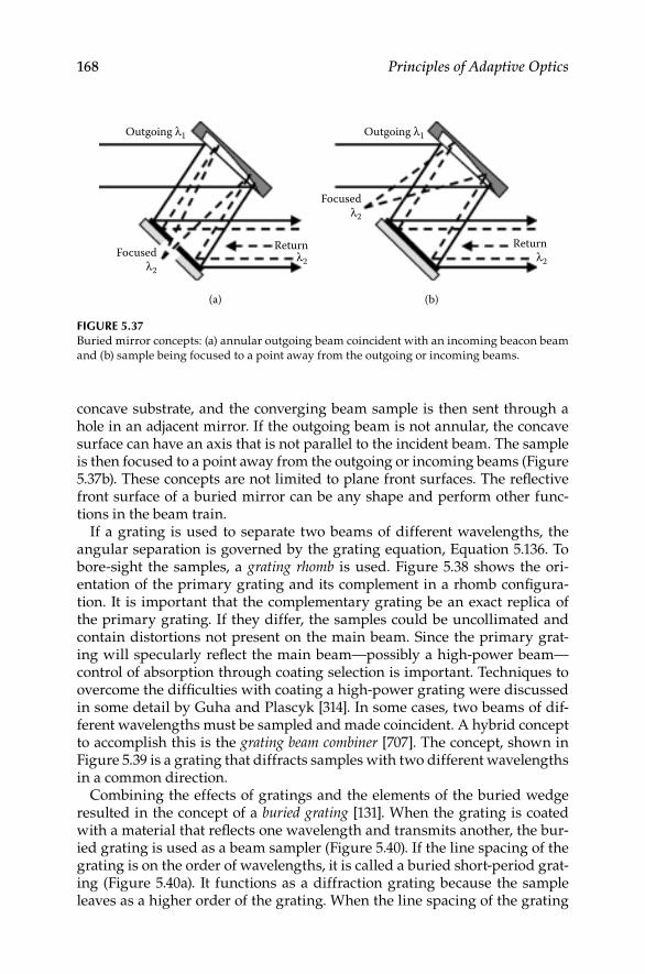
168 Principles of Adaptive Optics
concave substrate, and the converging beam sample is then sent through a hole in an adjacent mirror If the outgoing beam is not annular, the concave surface can have an axis that is not parallel to the incident beam The sample is then focused to a point away from the outgoing or incoming beams (Figure 537b) These concepts are not limited to plane front surfaces The reflective front surface of a buried mirror can be any shape and perform other func-tions in the beam train
If a grating is used to separate two beams of different wavelengths, the angular separation is governed by the grating equation, Equation 5136 To bore-sight the samples, a grating rhomb is used Figure 538 shows the ori-entation of the primary grating and its complement in a rhomb configura-tion It is important that the complementary grating be an exact replica of the primary grating If they differ, the samples could be uncollimated and contain distortions not present on the main beam Since the primary grat-ing will specularly reflect the main beam—possibly a high-power beam—control of absorption through coating selection is important Techniques to overcome the difficulties with coating a high-power grating were discussed in some detail by Guha and Plascyk [314] In some cases, two beams of dif-ferent wavelengths must be sampled and made coincident A hybrid concept to accomplish this is the grating beam combiner [707] The concept, shown in Figure 539 is a grating that diffracts samples with two different wavelengths in a common direction
Combining the effects of gratings and the elements of the buried wedge resulted in the concept of a buried grating [131] When the grating is coated with a material that reflects one wavelength and transmits another, the bur-ied grating is used as a beam sampler (Figure 540) If the line spacing of the grating is on the order of wavelengths, it is called a buried short-period grat-ing (Figure 540a) It functions as a diffraction grating because the sample leaves as a higher order of the grating When the line spacing of the grating
Outgoing λ1 Outgoing λ1
Focusedλ2
Focusedλ2
Return
(a) (b)
λ2
Returnλ2
Figure 5.37Buried mirror concepts: (a) annular outgoing beam coincident with an incoming beacon beam and (b) sample being focused to a point away from the outgoing or incoming beams
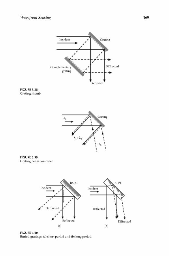
Wavefront Sensing 169
Incident
Complementarygrating
Grating
Dif fracted
Ref lected
Figure 5.38Grating rhomb
Gratingλ1
λ2
λ1+λ2
Figure 5.39Grating beam combiner
Incident
Dif fracted
Ref lected
(a) (b)
Incident
BLPGBSPG
Ref lected
Dif fracted
Figure 5.40Buried gratings: (a) short period and (b) long period

170 Principles of Adaptive Optics
is on the order of millimeters, it is called a buried long-period grating (BLPG) and it functions more like a buried mirror (Figure 540b) The transmitted beam reaches the grating surface and specularly reflects from each facet like a buried wedge with a faceted back surface Since the BLPG does not operate by diffraction, but rather by specular reflection, it is insensitive to polariza-tion It has low spectral dispersion (only what occurs from the transmissive layer) and it is aligned by normal mirror alignment techniques Although a number of samples have been made, a large-scale buried mirror device is expensive and difficult to manufacture Attempts to maintain surface con-tact between the faceted or grooved surface and the transmissive layer often result in disbonding
A number of other interesting concepts have been proposed for separat-ing a low-power beam sample from a high-power beam A compound inter-laced grating combines two gratings of different periods on one surface [131] Each wavelength responds to both gratings If the wavelengths are suffi-ciently separated (eg, one visible and one LWIR), the grating spacings can be very different For the case where the two spacings are an integer mul-tiple of each other, the grating can be manufactured by standard methods With those restrictions in mind, the buried and compound gratings could be used
5.5.7 Sensitivities of Sampler Concepts
Many of the wavefront sampler concepts presented make use of transmissive materials, which are wavelength-sensitive, or diffraction gratings, which are sensitive to polarization or misalignment Some of the concepts were devel-oped solely to eliminate some of these sensitivities (eg, the grating rhomb) Other concepts can be externally aligned to compensate for various anoma-lies in the sampler
The efficiency of diffraction gratings for different orders is closely tied to the polarization of the beam being diffracted When a beam is diffracted, the absolute value of the phase shift between its parallel and perpendicular components is given by [685]
cos[ ( )]
2 12
φ = −+ −⊥
⊥
I I I II I
(5142)
where I is the minimum or maximum intensity, I is the intensity of the component parallel to the grating grooves, and I⊥ is perpendicular to the grooves The angle ϕ is assumed to be in either the first or second quadrant This simple expression can be used to compute efficiencies for various orien-tations of a grating
If the plane of incidence is not exactly perpendicular to the grooves of the grating, aberrations can appear in the diffracted sample that are not present

Wavefront Sensing 171
in the incident beam The geometry is shown in Figure 541 If the wavefront of the incident beam is Φi(x′, y′) where the coordinate y′ is nearly parallel to the grooves, differing by a small angle δ, the wavefront of the mth-order diffracted beam is Φm(x, y) Simon and Gil [283,725] present the relationship for the sampled wavefront as a function of the incident wavefront and the geometrical considerations The incidence angle θi is related to the diffracted angle of order m, θm through the grating equation, Equation 5140 The dif-fracted wavefront takes the form
Φ Φ Φm i
i
m
ix y x y yx
( , )cos
,=
+ − ∂∂ ′
θθ
δ 12
+2 2 2
3
cos sin cos sincos
θ θ θ θθ
m i i m
m
x
−∂∂ ′
+ +∂∂ ′
δ δΦ Φi i
y y
22
212
siin sincosθ θ
θm i
m
x+
(5143)
Examination of this expression reveals that an angular deviation will intro-duce distortion into the diffracted wavefront If the incident wave is plane (∂Φ/∂x′ = ∂Φ/∂y′ = 0), the specularly reflected (θi = θm) wavefront is
Φ Φm i ix y y x= ′ ′ + −( , ) tanδ δ θ2 (5144)
which shows both x and y tilts in the diffracted beam Clearly, if δ → 0, the equation reduces to Φm = Φi, which is the desired high-fidelity sample needed for adaptive optics
Normal tograting plane
Plane ofincidence
Grating plane
Φ(x, y)
Φ(xi, yi)Θi Θd
δ
Figure 5.41
Geometry for a misaligned grating

172 Principles of Adaptive Optics
5.6 Detectors and Noise
Sensing light intensity is fundamental to any wavefront sensor tech-nique Sensing methods, whether they use interferometric techniques, the Hartmann test, or indirect methods, require an electrical signal output that is proportional to the intensity of light Electro-optical detectors provide this service
Many volumes have been written on the manufacture and use of detec-tors for visible, ultraviolet, and infrared energy [417,529,640] It is beyond the scope of this book to address all the issues relating to the physical processes involved or the electronic circuitry associated with each type of detector A summary of the basic types of detectors, their important characteristics for wavefront sensors, and their uses are given
For visible light, the silicon (Si) photodiode is the most common detector used It could be used in all types of wavefront sensors that are measuring the intensity of light in a small region Silicon detectors, by application of the photoelectric effect, convert incident light into electric current They are available for use from 350 nm (UV) to 1050 nm (IR) wavelengths
Detectors are usually characterized by a few basic parameters The responsivity (R) is a measure of the amount of electric current produced for each unit of incident light Responsivity is wavelength-dependent and usu-ally expressed in amps/watt For silicon detectors, the peak responsivity is about 05–07 A/W The rise time is the amount of time necessary for the detector to respond to the light In silicon detectors, the rise time is a func-tion of the charge collection process, the RC time constant of the equiva-lent electronic circuit, and the diffusion time for the electrons within the medium Silicon detectors have rise times ranging from one nanosecond to a few microseconds Both shot noise and thermal (Johnson) noise are pres-ent The dominant noise source depends upon light intensity The quantum efficiency of the detector is proportional to the responsivity and the inverse of the wavelength Silicon detectors have quantum efficiencies ranging from 50 to 90%
Wavefront sensing is very sensitive to noise [242], since many wavefront sensors have to perform in a photon-starved situation With small apertures and long ranges to dim sources, the noise parameters of a detector are very important The noise equivalent power (NEP) is a measure of detector “noisi-ness” It is expressed in units of power divided by the root of the bandwidth (watts/ Hz) Photodiodes made of silicon have NEPs from 10 15− W Hz/ to 10 12− W Hz/ Detectivity (D*, pronounced “D-star”) is related to this param-eter Detectivity normalizes the NEP by the size of the detector It is given by the equation D* = Area/NEP For silicon detectors, D* ranges from 1011 to 1013 cm Hz W/
Many wavefront sensor applications are in the infrared region of the spec-trum The atmosphere has transmission bands in the 3–5 μm and 8–12 μm

Wavefront Sensing 173
regions, but other bands are often used, especially for nonatmospheric correction An IR detector, by its nature, must detect small changes in the temperature, which are a result of the incident IR light To keep scattered radiation from fogging the detectors, the device is often kept in an insu-lated container, called a Dewar Although IR detectors that operate at room temperature exist, an understanding of the limitations in packaging and operation of cold detectors is needed before applying their capabilities to IR wavefront sensors IR detectors are usually grouped into thermal detec-tors, such as thermopiles and pyroelectrics, and solid-state detectors, such as indium antimonide (InSb, or “inz-bee”) and mercury cadmium telluride (HgCdTe, or “mercads”)
Thermal detectors produce a voltage proportional to a light intensity Pyroelectrics operate in the 8–14 μm range with responsivities from 10 to 50,000 V/W They can have rise times from as fast as 2 ns to upward of 150 ms Thermopiles can operate from 01 to 50 μm with responsivities up to 100 V/W They are generally slower than pyros with rise times from a few milliseconds to a few seconds
Solid-state detectors have responsivities in the 1–5 A/W range with D* from 109 to 1012 cm Hz W/ Indium antimonide detectors operate from 1 to 7 μm with about 500 ns rise times Mercury cadmium telluride detectors have been operated in the 1–20 μm range, but the most common are used in the 5–12 μm range, with 1–500-second rise times Germanium detectors operate in the low band (05–2 μm) with fast (01–50 ns) rise times Lead sulfide IR detec-tors operate from 1 to 55 μm with rise times on the order of 200 ns Gallium arsenide (GaAs, or “gas”) detectors operate in the near infrared (07–09 μm) with very fast (003 ns) rise times These and many other detector types are available The latest trade journals or manufacturers’ data sheets are the most helpful in evaluation for a specific use
IR and visible detectors are fabricated in linear or two-dimensional arrays Arrays are further classified as staring (observing the light continuously with the information output in parallel) or scanning (with the information or the deposition of the energy being dynamic) Both serial scanning and parallel scanning are used, sometimes in combination Quadcells, such as high quantum efficiency avalanche photodiodes [80], are used in tilt sens-ing, target tracking, or in subapertures for multichannel wavefront sensors Quadcells are often made by physically adjoining single detectors Since 2 × 2 arrays can be made easily, or 2 × 2 portions of larger arrays can be used as pseudo-quadcells, arrays play a very important part in wavefront sensor development
Silicon lateral effect photodiodes are single-element detectors that have out-put current proportional to the lateral position of the spot on the detector These very sensitive devices are used for full-aperture tilt sensing or for subaperture tilt sensing in each channel of a Hartmann sensor They have demonstrated position accuracies as low as 01% over the entire detector active area [804]

174 Principles of Adaptive Optics
The most commonly used array for wavefront sensing applications is the charge-coupled device (CCD) array [501] In silicon room-temperature arrays, a pocket of charge is created when light hits the material in an area called a picture element, or pixel IR arrays are usually cooled, but operate on the same principle The amount of charge is proportional to the integration time and the intensity The pockets of charge are created in a small region called a storage element Alternating pairs of electrodes surrounding these stor-age elements can be used to pass the charge out along a stream; that is, for each clock cycle, the charge pockets can be shifted over one pocket When all pockets have been clocked out, the array is capable of starting the cycle over again Like the operation of a computer’s shift register, the CCD clock-ing process is a very low loss This lack of noise and high efficiency is very useful for wavefront sensing [66,456] Noise is often expressed in electrons/pixel with values as low as 4e−/pixel typical for low-noise CCDs Circuits can process this information to determine the wavefront-sensitive issue, for example, the position or height of the peak, the centroid, or the difference between adjacent cells
CCDs can be operated in the GHz range and are suitable for high-speed adaptive optics wavefront sensors [272,273] The speed of the shifting of charge is generally limited by the speed of the electrons in the base mate-rial With thousands of elements, the processing must be capable of handling the high-speed clocked information The time it takes for all elements in the array frame to be clocked out is the frame time Some frame times are quoted including forms of signal conditioning, such as automatic gain control or thresholding The important question that must be asked for a wavefront sensing application is whether the total frame time, plus phase determina-tion algorithm processing, is sufficiently fast to capture the dynamics of the wavefront [400] One processing procedure that is well-suited to these types of signals is the N-bin phase detection algorithm [155] This algorithm is a form of discrete quadrature detection in which N is the number of discrete samples used in the digital equivalent of a radio frequency mixer [517]
In very low light level conditions, very sensitive detectors are needed A photomultiplier tube (PMT) is a sensitive detector where photons falling on a cathode generate surface photoelectrons An electron multiplier (dynode) chain amplifies this photon flux to produce current at the anode The output should be linearly proportional to the light intensity, but, because of satura-tion, the detector response can be nonlinear [214,491] and often lasts for a few milliseconds after a very bright pulse [146] Cathode sensitivity (mA/W or A/lumen), amplification (103–108), spectral response, and dark noise (001–10 nA) are parameters to be considered during selection Petroff et al [618] describe a solid-state photomultiplier with a quantum efficiency of nearly 50% The device has single-photon counting capability with operating wave-lengths from 05 to 28 μm A microchannel plate is a fast-response PMT with very closely spaced dynodes A microchannel plate-based image intensifier for a Hartmann sensor used in astronomy was described by Clampin [141]

Wavefront Sensing 175
Avalanche photodiodes and other image intensifier applications to adaptive optics have been reported [142,494,676]
The noise characteristics of detectors are very important [615], and how they relate to the error in wavefront sensing has been explored [887] For a single channel of a shearing interferometer, the signal current i(t) is
i t i t( ) [ sin( )]= + +s 1 γ ω φ (5145)
where ω is the modulation frequency, γ is the fringe visibility, and ϕ is the unknown phase The phase is measured by determining the time of zero crossing of this signal and the time of a reference signal crossing [508] It has been shown [729] that the error in this time determination is responsible for an error in the phase estimation The phase error is inversely proportional to the SNR
For a low light level photon-counting shearing interferometer, Wyant [887] showed that the variance in phase estimation is
σγ
2
20 9
=
. d
s ns (5146)
where ds is the distance between wavefront measurement points, s is the shear distance, and n is the number of photon counts in a period, given by
nN TA R= Ω
−
τe
(5147)
In this expression, N is the radiance of the source, Ω is the solid angle of the optics, T is the transmission of the optics, A is the aperture area, τ is the integration time, R is the responsivity of the detector, and e− is the electric charge See also Equation 320 and the discussion in Chapter 3
Other investigators [115,192] have analyzed the noise characteristics of wavefront sensors to explore the trades necessary between small aper-tures, which give high resolution, and large apertures, which maximize SNR One measure of a bound-on-wavefront sensor error is the Cramer–Rao parameter [811], which is derived for shearing interferometers by Cederquist et al [119]
In some cases of atmospheric propagation, it can be useful to sense the wavefront at one wavelength with a correction applied for propagation at another wavelength For instance, one may want to propagate a carbon diox-ide laser (106 μm) up through the atmosphere, but sense the aberrations from a visible beacon (05 μm) because of the availability of detectors Chromatic anisoplanatism, mentioned in Chapter 3, would result Phase conjugate the-ory for a uniform medium would predict that only a scale factor is needed to represent the difference in the index of refraction between the wavelengths In such a system, however, diffraction of the beam causes interference effects

176 Principles of Adaptive Optics
and amplitude modulation (scintillation) The difference in the measured wavefront and the wavefront needed to propagate a phase conjugate is a function of the zenith angle and the wavelength difference [348] Figure 542 shows the variance of the phase differences for a propagated beam that is sensed at 05 μm For transmission of short wavelengths, the adaptive optics sensing wavelengths must be close to the transmitted wavelength For lon-ger wavelength transmitters, the wavefront differences are less important
4
60°
30°
0°
Zenithangle
3
2
1
00.5 9.58.06.55.03.52.0
Varia
nce
of th
e ph
ase
dif fe
renc
eat
λ2=
0.5μ
m (r
adia
ns)2
Wavelength (μm)
Figure 5.42Phase difference for a laser transmitter at 05 μm with a sensor at another wavelength

177
6Wavefront Correction
Wavefronts can be corrected using many of the same mechanisms that cause wavefront distortion An image from a distorted mirror can be corrected by distorting another mirror into the proper shape to compensate for the wave-front variations Local variations in the refraction index that were the cause of an aberration can be reversed, or conjugated, to provide the correction Corrective lenses for eyes use this principle The aberrations due to a mal-formed or strained lens in the eye are removed by placing an external lens in the path of the light entering the eye The method of corrective eyeglasses is modal and static Usually, only focus (curvature of field) and astigmatism are corrected and they do not have any active capability This, then, is techni-cally not adaptive optics; however, correction to the wavefront on most adap-tive optics systems is based on the principle of adding a correcting device to the beam of light When the correction is made active, that is, by moving the corrective element, it is said to be “inertial,” with the correction linearly proportional to the stimulus
As with sensing, there are both modal and zonal means of correction, in addition to nonlinear optical methods of correction based on the systems described in Chapter 4 The need to engineer better systems with higher spatial resolution, more stroke capability, and higher operational bandwidth has been a catalyst in developing actuators, faceplate materials, and analyti-cal techniques that apply to many other areas of engineering
Although compensation can be performed with active lenses [327], the most common devices are active mirrors Devices used for real-time wave-front correction were reported in 1974 by several researchers [96,211,324,547] These were primarily used for demonstrating the closed-loop technology needed for scaling to larger systems to compensate for atmospheric turbu-lence Before the development of the deformable mirror (DM), however, scan-ning or tilt mirrors were widely used to correct for beam direction Whether these devices are classified as modal adaptive-optics correction devices, or as image- or beam-tracking mirrors, is academic The evolution of correction devices clearly emerged before the inception of adaptive optics as an engi-neering discipline
Typical frequency ranges for correction devices are shown in Figure 61 A tilt mirror that can move very fast is restricted to only one mode, and therefore has limited spatial frequency capability The opposite is the large active primary that can correct high spatial frequencies (many zones) but is limited in temporal frequency response An active secondary mirror (SM)

178 Principles of Adaptive Optics
on a telescope can be used to correct for focus, but because of strict require-ments to maintain alignment, it has limited temporal bandwidth A multi-actuator DM can correct many zones at a high speed and is a candidate for an all-purpose device
Figure 61 does not show the dynamic range or stroke of these devices, which is a major limiting factor in choosing a particular modality One might conclude that the DM would be best for most temporal and spatial spectra, but unfortunately, this is not always possible Low-order mode correction, such as tilt jitter, often requires large-amplitude motion A DM will reach the end of its actuator stroke correcting for the beam tilt without leaving any margin for the actuators to correct for the high spatial frequency aberrations For instance, a 20-cm DM, with a ±10 μm stroke limit, can only correct for a 10-mrad tilt Many sources of tilt impart tens of milliradians into a system A separate tip/tilt mirror in the system is normally required However, a DM mounted on a two-axis tip/tilt platform can be used [861] System design safety margins of at least 15 for temporal bandwidth and 20 for dynamic range are recommended
For atmospheric compensation, the stroke requirements for the tilt mirror and the DM can be calculated The standard deviation of the angular tilt imparted by the atmosphere is
α λSD
0
=
0 435 6
./
Dr D
(61)
where D is the telescope aperture The total stroke of the tilt mirror must be about 25 times the standard deviation The tilt mirror diameter, DTM, is smaller than the telescope aperture diameter, and its angular motion is
D/100 Large telescopeprimary mirror
Deformable mirrorTelescope
focusingsecondary
mirror
Tip/tiltmirror
D/10
1 10 100Temporal frequency (Hz)
Spat
ial f
requ
ency
(frac
tion
of d
iam
eter
)
1000
D/2
D
Figure 6.1Spatial frequency versus temporal frequency of correcting elements: tilt/steering mirror; tele-scope secondary mirror focus correction; multiactuator deformable mirror; active telescope primary mirror

Wavefront Correction 179
demagnified The angular motion of the tilt mirror must then be multiplied by the magnification of the optical system, namely D/DTM Combining the full-stroke requirement and the magnification requirement with Equation 61, the angular stroke of the tilt mirror will be
α λTMstroke
0 TM
= ±
1 15 6
./
Dr D
(62)
The requirements for a segmented mirror or a continuous faceplate DM can be determined similarly The standard deviation of phase in a subap-erture is
φSD0
waves=
0 065 6
./
Dr
(63)
The peak-to-peak motion is 5ϕSD The mechanical stroke of a mirror is half the phase change placed on the beam; thus, the total stroke required for each actuator is
sDr
=
0 155 6
./
0
λ (64)
There is no single best adaptive optics correcting device Design choice depends on structural materials, actuator characteristics, and the work-ing environment [187] For example, evaluation of the expected aberrations and their dynamics is required before making the basic decision between a bimorph and a stacked actuator DM [304] The correction requirements, bandwidth, stroke, and number of correction zones are driven by system considerations, such as sensing and control capability, and practical con-straints, such as cost and complexity
In some cases, an adaptive SM at the telescope is beneficial The SM is com-mon to all the telescope-imaging paths and it does not add another optical surface A few problems are introduced with this approach The most signifi-cant is that the DM is not near a conjugate image of atmospheric turbulence, which results in a smaller isoplanatic patch
6.1 Modal-Tilt Correction
The simplest form of wavefront correction is variation of the beam direction, or the tilt of the wavefront These methods preceded the concept of adaptive optics but serve as a basis for many more complicated forms of correction

180 Principles of Adaptive Optics
The amount of energy needed to control the tilt mode in an optical system is directly related to the stroke and bandwidth requirements for the steering mirror For a constant diameter–thickness ratio, the inertia of the scanning flat-plate mirror is proportional to the fifth power of the mirror diameter The subsequent force needed to move the mirror is proportional to the maxi-mum required torque τ, divided by the mirror diameter D The torque is given by the expression
τ ω θ ωω
ωω
= −
+
I dmn n
2
2 2 2
1 2
1 2/
(65)
where Im is the mass moment of inertia, ω is the frequency of oscillation, ωn is the mirror tilt-mode resonance, θ is the stroke of the mirror at frequency ω, and d is the system-damping factor The amplitude (stroke) and bandwidth considerations (θ, ω) of the disturbance will drive the requirements for the tilt mirror Equation 65 can be used for the initial approximations of the torque and the force required for tilt correction
Tilt mirrors that incorporate specific requirements for their applications have been built In addition to the stroke and bandwidth requirements for tilt and beam steering, some tilt mirrors have replaced the SMs of telescopes [147] Others have met the requirement that they be reactionless [592], that is, the motion of the tilt mirror does not translate back into the optical bench or supporting structure Tilt mirrors with both coarse and fine stroke separa-tion [280] and magnetostrictive actuators [9] have been developed Large-angle tilt mirrors are needed for wide-field-of-view systems Shen et al [719] describe a mirror with a 15-mrad stroke at 500 Hz and up to a 250-mrad stroke at 150 Hz Each of these advancements provides for precision tracking of the object and, by itself, adaptive-optics correction for the lowest distur-bance mode, the beam tilt
6.2 Modal Higher-Order Correction
The next most common form of correction is an active focus system When one peers through a telescope, an image is brought into focus by one’s knowl-edge that a “fuzzy” image is out of focus while a “sharp” image is not By cycling through the position of the sharpest focus, the system can be made to adapt to variations in the receiver’s lens system, the observer’s eye, or his or her camera Specialized devices for remote focus-only correction were dem-onstrated as early as 1973 [84,530]
Astigmatism can be corrected by moving a single lens or mirror If a cylin-drical mirror or lens is aligned with the beam and moved along the optical

Wavefront Correction 181
axis, astigmatism is changed By having two mirrors or lenses with their cylinder axes oriented 45° to each other, astigmatism for all orientations can be corrected When it is necessary to correct for modes higher than astigma-tism, the wavefront can be divided spatially Each part of the beam is cor-rected by applying the required strength of correction to that part Devices that work in this manner are called multichannel correctors, such as segmented mirrors or continuous faceplate DMs
6.3 Segmented Mirrors
The earliest implementation of a multichannel corrector was the segmented mirror This is a mirror made up of a number of closely spaced small mirrors with piston- or tilt-correction capabilities (Figure 62) Thus, higher-order modes of correction can be applied by determining the individual contribu-tion of each of the segments Some segmented mirrors of this type have been operated in a piston-only mode, whereby each segment is confined to simple up-and-down motions The piston/tip/tilt mode* has also been shown Each segment operates with three degrees of freedom: the up/down piston mode and two orthogonal axes of tilt A further consideration is the shape of the segments Square, hexagonal, and circular segments have been used A theo-retical comparison of these shapes was reported by Malakhov et al [498]
Segmented DMs can be used to correct static aberrations in an optical sys-tem [2] or to compensate for atmospheric turbulence [687] Segmented mir-rors are scalable to very large numbers of segments Mirrors with as many as 512 segments (076 cm in size) have been built [321,363] Modern technol-ogy, using modules as large as 14 × 14 segments, has made it possible to produce segmented mirrors with more than 10,000 segments The relative ease of assembly and maintenance are important factors to consider The cost and difficulty of replacing a single segment is much less than the equivalent maintenance of a continuous-surface mirror [178] On the other end of the size spectrum, microelectromechanical systems (MEMS)–based segmented mirrors have been developed (Figure 63) and can be produced in large quan-tities at a relatively low cost [338]
When used with a broadband source, a segmented mirror must be abso-lutely phased, because modulo-2π steps would seriously degrade perfor-mance Long stroke actuators are required to provide broadband correction Segments with a 6- to 10-micron stroke have been incorporated into a seg-mented mirror [364] However, the discontinuities (gaps) between segments have an impact on overall performance Energy is lost through the gaps, and
* Tip/tilt is the same as two-axis tilt

182 Principles of Adaptive Optics
because the gaps cause the mirror to act as a grating, energy is diffracted from the central lobe It is important that the area of the gaps be below 2% [364] Because each segment operates independently, there is no cross- coupling or need for actuator preloading The step response for a segment can be as low as 100 μs Segmented mirrors operating with closed-loop bandwidths as high as 5 kHz are currently in use [157,363] In some cases, electronic cross-coupling between segments or groups of segments is needed to increase the control bandwidth The 05-m phased-array mirror extensible large aperture [288] uses a control hierarchy that clusters segments and achieves a 2-kHz bandwidth [452]
Figure 6.3The Iris AO PTT111 segmented micromachined deformable mirror has 37 hexagonal seg-ments with 111 degrees of freedom over a 35-mm aperture (Photo courtesy of Iris AO, Inc Berkeley, CA)
Piston only Piston plustip and tilt
Actuators
Mirrorfaceplates
Figure 6.2
Segmented multichannel mirrors

Wavefront Correction 183
6.4 Deformable Mirrors
Other multichannel correctors fall under the class deformable mirrors or DMs These are generally continuous-surface mirrors with a mechanical means of deformation [606] to match the desired conjugate wavefront (Figure 64) The devices that perform the deformation—the actuators—can be continuous, such as in a membrane mirror [140,892] or a bimorph mirror [744] They can also have discrete actuators perpendicular to the surface [325], or can have discrete actuators on the edges that impart bending moments [259], as shown in Figure 64 Because the surface of the mirror appears to bend similar to a rubber membrane stretched across a frame, continuous-surface DMs are often called “rubber mirrors”*
Concurrent with the need for propagating high-energy lasers, the require-ment for correction devices that could provide high spatial frequency cor-rection, along with being able to survive the high flux loads on the surfaces, also arose Piezoelectric DMs with hundreds of actuators were developed by 1974
Discrete actuator DMs with stacked piezoelectric actuators were devel-oped in the late 1970s to address the large stroke requirements of infrared systems [184,186,235] To generate enough force to deform the mirror sur-face by 08 μm, stacks of piezoelectric disks were made The total voltage required for each stack was more than 1 kV, which usually is implemented by biasing to 500 V and then applying ±500 V Development of high-power discrete actuator DMs was a difficult extension of passive high-power mirrors A comparison of molybdenum faceplate mirrors with up to 61 actu-ator stacks has been reported [409] Various piezoelectric materials exhibit hysteresis, and actuator–faceplate configurations show different forms of influence functions [205]
Requirements for atmospheric turbulence compensation push the technol-ogy of DMs Hundreds of actuators must be close together Miniaturization of actuators, low operating voltages, position accuracy, and low hysteresis become important parameters [188,261,377] The dynamics of an actuator in a DM force train are complicated by the linkage between the actuator and the optical surface [505] Mechanical, chemical (glues), and electromagnetic connections are commonly used The stricture, spring rates, and damping within the mechanical structure can contribute to hysteresis Active control of hysteresis has been proposed [414], but low-hysteresis actuators reduce the complexity of the control system and increase the closed-loop bandwidth
Mirrors with low-voltage lead–manganese–niobate, or Pb(Mg1/3Nb2/3)O3 (PMN), actuators [11] or magnetostrictive actuators [514] have been devel-oped For high-power laser applications, DMs with multiple-layer dielectric
* A rubber membrane will stretch laterally, whereas a thin-plate mirror is very rigid in-plane Although not physically accurate, the jargon is still used

184 Principles of Adaptive Optics
coatings with very high reflectivity must be used [121] The coatings must withstand the thermal loads of the high-power beam and the stresses induced by the active deformation Methods of quantifying and characteriz-ing the performance of discrete actuator DMs have been evaluated [206,263] In addition to hysteresis and influence functions, the linearity of the actuator response, the faceplate–actuator resonance, and the limits of actuator stroke (throw) are important characteristics for evaluating the utility and perfor-mance of a DM
The need for adaptive optics in large telescope systems is clear Because of the requirement to minimize the number of optical surfaces in the beam train to reduce losses due to absorption and scattering, DMs have been incorporated into other optical elements [684,840] The SM of the converted Monolithic-Mirror Telescope (MMT) in Arizona, has 324 electromagnetic actu-ators [102,506] The SM of the Gemini 8-m telescope will be the adaptive optics system DM, as well as the chopping secondary for infrared operation [134]
Because total actuator stroke and (nearest neighbor) interactuator stroke can be limited, some systems require a large-stroke, low-actuator-density DM working in combination with a small-stroke, high-actuator-density DM, a so-called “woofer-tweeter” approach [109,149,356,411,504]
6.4.1 Actuation Techniques
Actuators used for discrete actuator and edge actuator DMs are generally placed into one of two classes: force actuators and displacement actuators The application and the mechanical structure define the conversion from force to displacement via Newton’s second law The most common materials used for DM actuators are piezoelectric ceramics [726], such as Pb(Zr,Ti)O3 or PZT [5,744], whereas Kokorowski [421] and Sato et al [696] report the use of polyvinylidene fluoride (PVDF) Developments in PMN ceramics have yielded large electrostrictions compared to PZTs [798]
(a) (b)
(c) (d)
Figure 6.4Continuous-surface deformable mirrors: (a) discrete position actuators, (b) discrete force actu-ators, (c) bending moment actuators, and (d) monolithic mirrors

Wavefront Correction 185
By layering PVDF [697] or stacking PZT [605], large strokes can be obtained with submicron accuracy for corrections equivalent to many waves The high voltages needed to drive the stacks of PZT (upward of 1000 V) often present serious design constraints that require large auxiliary support equipment The development of Terfenol magnetostrictive actuators for DMs reduces the requirement for high voltages, because magnetostrictives operate at only a few volts [26,298] However, the energy required to move the surface is the same [9]; thus, high currents (up to 1 A each) are required for these actuators Cooling of the actuators is often required to avoid thermal creep and misalignments
Other electromagnetic devices have been used for adaptive optics correct-ing devices Voice coil (solenoid) actuators are common in scanning mirrors because of their large forces and displacements produced A helical solenoid (helenoid) provides a very fast response time, which, when coupled with its low-voltage operation, results in a very attractive package for driving optics [16,709,724]
For low-frequency correction (up to 10 Hz), various types of mechanical drives have been used Worm gears and direct-acting direct current (DC) motors [401], hydraulic actuators [601], and differential ball screws [290] have been used to drive mirror surfaces
Ealey [185] presents the key design fundamentals and parametric trades necessary to choose a precise actuator for a specific application The anal-ysis includes a discussion of PZT, PMN, Terfenol, nickel–titanium-based NiTiNOL, bimetal alloys, and paraffin thermal actuators Light-driven PVDF actuators have been demonstrated and show that the force is proportional to the power of the laser beam illuminator [691]
6.4.2 Actuator influence Functions
Mirrors can be driven to many different shapes to compensate for a wide range of distorted wavefronts The choice of a particular design is based on the amount and nature of the correction required and the cost and complex-ity of its operation Some mirrors with as few as four actuators have been shown to correct for both focus and astigmatism [218] For instance, an astro-nomical imaging system with a 15-m aperture requires a DM with at least a ±06-μm stroke to correct for atmospheric turbulence Many wavefront reconstructors provide direct-drive signals to the segments or DM actuators (see Section 74) The greater the number of degrees of freedom of the correc-tor, the greater is the number of wavefront variations it can correct If many segments are placed close together, the constraint of flat surfaces fitting a curved wavefront can be overcome The advantages of continuous-surface mirrors—the absence of surface gaps that affect diffraction, for instance—often are reduced by the structural constraints that limit the surface shape that can be formed The stress and strain of the mirror materials result in structural coupling between elements of the mirror; this coupling conceiv-ably could enhance, but usually limits, the utility of a particular DM

186 Principles of Adaptive Optics
The actual shape of a DM surface, when it is pushed by an actuator, is called its influence function [342] It is a function of mirror faceplate parameters such as thickness, modulus of elasticity, and Poisson’s ratio (Figure 65) The location and distribution of the applied force and the structural inhomogeneities con-tribute to the uniqueness of a particular mirror or a particular actuator within a mirror Measurement of influence functions is a tedious, but necessary, pro-cess [263] Modeling the shape of the mirror surface, its influence function, has been a topic of discussion for a number of years To describe the shape of an actual DM would require detailed calculations, such as finite element analysis, that consider all the parameters mentioned in this section Approximations to finite element methods are needed to describe multiactuator mirrors
The spatial response of each channel (the influence function) is discussed by a number of authors For correction of turbulence, Hudgin [360] derives the fitting error for (1) piston, Gaussian, and pyramidal influence functions; and (2) a prototype mirror Taranenko et al [754] derive analytical expres-sions in exponential form for the influence of soft and stiff metal surfaces They also compute the resonant frequencies as functions of the material parameters as follows:
νρ σres =
−10 212 12 12 2
.( )
hR
Eπ
(66)
where h is plate thickness, ρ is material mass density, R is distance to the nearest clamped point, such as another actuator, E is Young’s modulus, and σ is Poisson’s ratio
Claflin and Bareket [140] calculate the influence function for continuous-surface mirrors from Poisson’s equation and then use least-squares prin-ciples to fit the surface of a multichannel mirror to Zernike polynomials for analysis Harvey and Callahan [334] proposed using methods of linear
0.2 0.4
Super-Gaussian
Cubic
Gaussian
Normalized distance from actuator
Nor
mal
ized
influ
ence
func
tion
0.6 0.8 1.00
Figure 6.5Analytical forms for DM influence functions: Gaussian exp(−βr2); super-Gaussian exp(−βr25); cubic polynomial
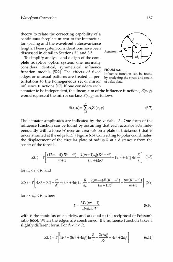
Wavefront Correction 187
theory to relate the correcting capability of a continuous-faceplate mirror to the interactua-tor spacing and the wavefront autocovariance length These system considerations have been discussed in detail in Sections 31 and 35
To simplify analysis and design of the com-plete adaptive optics system, one normally considers identical, symmetrical influence function models [522] The effects of fixed edges or unusual patterns are treated as per-turbations to the homogeneous set of mirror influence functions [10] If one considers each actuator to be independent, the linear sum of the influence functions, Z(x, y), would represent the mirror surface, S(x, y), as follows:
S x y A Z x yi ii
N
( , ) ( , )==∑
1
(67)
The actuator amplitudes are indicated by the variable Ai One form of the influence function can be found by assuming that each actuator acts inde-pendently with a force W over an area πd0
2 on a plate of thickness t that is unconstrained at the edge [655] (Figure 66) Converting to polar coordinates, the displacement of the circular plate of radius R at a distance r from the center of the force is
Z rm R r
mm d R r
m( )
( )( ) ( ) ( )(
= + −+
−− −
ϒ 12 41
2 12 202 2 2
++
− +
1
8 42
202
)( )ln
Rr d
Rr
(68)
for d0 < r < R, and
Z r R drd
r dRd
m( ) ( ) ln
(= − + − +
−ϒ 4 5 8 4
22 24
22 2
00
00
−− −+
+ −+
11
81
2 2 2
2
2 2) ( )( )
( )d R rm R
m R rm
0 (69)
for r < d0 < R, where
ϒ = −3 116
2W mEm t
( )π 2 3
(610)
with E the modulus of elasticity, and m equal to the reciprocal of Poisson’s ratio [655] When the edges are constrained, the influence function takes a slightly different form For d0 < r < R,
Z r R r dRr
r dR
r d( ) ( )ln= − + − − +ϒ 4 8 42
4 22 2 22 2
22 2
00
0
(611)
Actuator
R
2d0
r
Figure 6.6Influence function can be found by analyzing the stress and strain of a flat plate

188 Principles of Adaptive Optics
and for r < d0 < R,
Z r R r dRd
r dR
rd
( ) ( )ln= − + − + −ϒ 4 8 42
32 2 22 2
2
4
200
0
0
dd02
(612)
Although these expressions are quite accurate, a number of investigators have used different analytical forms to simplify their models An influence function that maintains Cartesian symmetry of a square pattern of actuators follows the following cubic form [390]:
Z x y x x y y( , ) ( )( )∝ 1 3 2 1 3 22 3 2 3− + − + (613)
Taranenko et al [754] measured the influence functions for aluminum, cop-per, and steel plates and found them closely following either a Gaussian or a super-Gaussian form within 5%:
Z r r( ) exp( )= −β12 for Al, Cu (614)
Z r r( ) exp( ).= −β22 5 for steel (615)
where β1 = 277 and β2 = 392 Similar Gaussian functional forms have been found experimentally [263,357] A comparison of these functional forms (Figure 65) shows that although there are slight differences, the simple form—the Gaussian—represents a DM influence function quite well
One difficulty occurs when the linear sum model is used If all the actua-tors are pushed identically, the model shows a surface composed of bumps of equal height This rippled surface does not correspond to the surface of an actual device with a stiff faceplate Because the load is equally distributed, the mirror surface will rise in a piston mode, leaving the surface flat, rather than rippled The model surface, appearing similar to a membrane backed by pins, exhibits an effect called pinning error
Another difficulty arises because coupling occurs If the stiffness of actua-tors is very high compared to the faceplate, there will be little coupling The surface will deform in the direction of the force near the actuator and deform in the opposite direction past the adjacent actuator This form is most often represented by the sin(r)/r function as follows:
Z r
rr
r( )
sin=
πs (616)
where rs is the interactuator spacing

Wavefront Correction 189
For simplicity, the Gaussian form (Equation 614) can be expressed in terms of its coupling, κ, as follows:
Z rr
r( ) expln( )=
κs2
2 (617)
Actuators can be arranged in various geometric patterns Many simple mirrors have square Cartesian layouts with 4, 9, or 16 actuators To avoid the expense of actuators being outside circular beams, the corner actuators are removed; thus, we see counts of 21 (5 × 5 minus 4 corner actuators), 69 (9 × 9 minus 12 corner actuators), 241 (17 × 17 minus 48 corner actuators), and 941 (35 × 35 minus 284 corner actuators) Maximizing the number of actuators in a circle results in hexagonal arrays of 1, 7, 19, 37, 61, 91, 127, and so forth The number simply follows the following form:
1 61
+=
∑nn
N
(618)
where N is the number of encircled hexagons
6.5 Bimorph Corrector Mirrors
A bimorph DM consists of a glass or metal mirror faceplate bonded to a sheet of piezoelectric ceramic [373] The ceramic is polarized normal to its surface The bonding is generally a glue that will not shrink after application The glued interface between the mirror and the ceramic contains a conducting electrode After the exposed piezoelectric ceramic is covered with a number of independent electrodes, the front is polished and coated to form the DM surface Wires are attached to the single front electrode and the various back electrodes (Figure 67) Various patterns of back electrodes have been used Steinhaus and Lipson [744] used conductive paint to form a pattern of 12 seg-ments Adelman [5] analyzed a pattern of concentric circles, and Halevi [317] used various patterns of large and small squares A 36-element bimorph
GlassReflecting surface
Innerelectrode
Backelectrodes
PPZT
Figure 6.7Cross section of a bimorph deformable mirror

190 Principles of Adaptive Optics
with three concentric rings of electrodes was optimized for the 82-m Subaru Telescope [593] A modular silicon bimorph with thick-film piezoelectric actuation, containing up to 133 electrodes, has been described [667]
When a voltage is applied between the front and back electrodes, the dimensions of the piezoelectric material [533] change by an amount depend-ing on the electric field and the coefficient of the piezoelectric tensor d13 Neglecting the stiffness of the layers, the local radius of curvature of the mirror, R, changes in proportion to the applied voltage V, and is given by
RVd
t= 13
2 (619)
where t is the thickness of the ceramic plus the facesheet [467] For a back electrode of diameter D, the voltage necessary for a center-to-edge deforma-tion of one wavelength is given by
Vt
D dλ ≈2 2
213
λ (620)
Because the local curvature of the corrector is proportional to the voltage, bimorphs are particularly well suited for integration with a wavefront cur-vature sensor [467,646] This greatly simplifies wavefront control and essen-tially eliminates an intermediate wavefront reconstructor
Regardless of the hysteresis or depolarization properties, typical values for Equation 620, d13 = 2 × 10⁻¹² m/V, t = 1 mm, D = 10 mm, λ = 05 μm, give a value of 50 V [744] This voltage range is easily obtained in practical applica-tions Halevi’s analysis [317] included a solution of the time-dependent equa-tion of state for a bimorph mirror with accompanying expressions for mirror deformation and resonant frequencies
Improvements on the basic design include the addition of a second piezo-electric sheet bonded to the first with reverse polarization When a voltage is applied to this configuration, the thickness does not increase, because one plate contracts while the other expands This opposing expansion– contraction results in the entire plate bending like a bimetal strip, with defor-mation occurring at the top and bottom surfaces Kokorowski [421] provided a detailed analysis of this effect for infinite slabs and finite square slabs
Vorontsov et al improved the configuration by using a conductive faceplate, such as copper, rather than separate electrodes and glass faceplates [835] Their flexible bimorph mirror was configured for both 9 and 13 back elec-trodes with auxiliary tilt mode control They demonstrated nearly 01 waves of correction for astigmatism, coma, and spherical aberration by applying about 30 V Vorontsov et al [835] also reported the development of a cooled bimorph with an 80-mm aperture Ning et al [568] analytically compared bimorphs with various configurations of layers in terms of their response function and sensitivity

Wavefront Correction 191
6.6 Membranes and Micromachined Mirrors
Another form of continuous-surface mirror is the membrane mirror [312] A reflective membrane is positioned between a transparent electrode and a series of individual electrodes at the back of the mirror, as shown in Figure 68 When no voltage differential is applied, the membrane remains flat When a voltage is applied, however, the electrostatic attraction between the electrodes deforms the membrane into a desired shape The local cur-vature of the surface can be represented as
∇ =∂
∂+
∂∂
= −22
2
2
2z x y
z x yx
z x yy
P x yT
( , )( , ) ( , ) ( , )
(621)
where T is the membrane tension (force/length) and P(x, y) is the pressure (force/area) at position x, y The membrane is suspended in a partially evacu-ated environment to reduce damping For large-stroke designs [438], damp-ing has been found necessary, because the surface tends to be unstable and pins the membrane against the electrodes In these circumstances, fluids are added to produce the required damping Because no piezoelectric ceramic is used, this type of mirror exhibits virtually no hysteresis The density of actuators is only limited by the need to place the back electrodes far enough apart so that they can withstand the voltages necessary for deflection of the membrane without snapping down the surface all the way to the substrate and destroying the mirror
Takami and Iye describe a membrane mirror used in the Subaru Telescope [749] The membrane is made of nitrocellulose of 50 mm diameter and 2 μm thickness, which allows a clear aperture of 25 mm The aluminum coating acts as both the electrode and the reflective surface A 33-kHz bandwidth was achieved Another membrane mirror constructed at the University of Heidelberg [523] consists of an aluminized polypropylene membrane placed between a transparent electrode on a glass window and 109 hexagonal back
Membraneelectrode
Control electrodes
Figure 6.8The principle of an electrostatic membrane mirror

192 Principles of Adaptive Optics
electrodes This mirror was studied by Claflin and Bareket [140] for use as a laboratory aberration generator
Stability between the electrostatic and mechanical energies of the mem-brane requires careful design and fabrication [437] One new class of mem-brane mirrors, called MEMS–DMs, are made from components that are micromachined on silicon or metal substrates [81,82,815] MEMS–DMs are the first low-cost mass-produced adaptive optics components [613] These devices, built as microchips, can be segmented [338] or have continuous faceplates [816,828] They use very little current to mechanically produce deformations [204] of the optical surface up to 20 μm [143] Because of their small size, thousands of actuators can be applied to mirrors [437] and inte-grated into wavefront sensors and reconstructors on a single microchip (Figure 69)
Figure 6.9Boston Micromachines microelectricalmechanical system deformable mirror with a contin-uous surface and a 93-mm aperture The electrostatically actuated mirror has 1020 actua-tors (32 × 32 array, with the corners cut off) and a stroke of 15 microns; it operates at speeds up to 60 kHz (Photo courtesy of Boston Micromachines Corporation, Cambridge, MA)

Wavefront Correction 193
With large telescopes, very large numbers of actuators are required (up to 15,000 for the Thirty Meter Telescope [843]) MEMS–DMs can be driven mod-ally or zonally [87,459]
6.7 Edge-Actuated Mirrors
DMs with actuators attached to the edge of the optical surface can be used to apply certain low-order optical modes By moving the actuators in the same plane as the surface, bending moments that correspond to focus or astigma-tism can be induced A prototype mirror was demonstrated by Fuschetto [260] Although the mirror was called a “three-actuator” mirror, it really con-sisted of six stacks of piezoceramic material placed 60° apart (Figure 610) The mirror substrate was molybdenum and it had a beryllium base for sup-port and a reference surface for the actuators
Analysis showed that about 10 μm of defocus error and 5 μm of astigma-tism could be corrected with a bandwidth of about 100 Hz Nichols et al [561,562] report that the performance of this mirror exceeded predictions and had less than 10% coupling between the modes whenever corrections were applied
An edge-actuated mirror made of Zerodur glass was demonstrated by Malin et al [500] The mirror surface was hexagonally shaped with a maxi-mum dimension of 24 inches It was deformed by two rings of 12 electrody-namic actuators One ring was tangential to the mirror edge, while the other 12 were positioned to apply forces radially This configuration supported both bending moments and shears Experimental testing showed peak- to-valley focus compensation greater than 2 μm and astigmatic correction of about 15 μm
Actuator assembly
Actuators
Centerpost
Baseplate
Mirrorfaceplate
Floating blockand flexure
Piezo-ceramic wafers
Figure 6.10Edge-actuated deformable mirror

194 Principles of Adaptive Optics
6.8 Large Correcting Optics
Gravitational loads and surfacing difficulties of large optics result in distor-tions that cannot be removed before use By placing actuators behind the faceplate of large primary mirrors, the latter become high spatial frequency DMs that can be self-correcting They can remove wavefront errors that appear in large optical elements used in beam propagation and astronomy [38,59] Performance trades arise because there is no “best” mirror facesheet thickness More actuators are required to maintain control of a thin faceplate, because it is less stiff However, if the faceplate is thickened, the actuators require more force Segmentation of the mirror is required when the mirror sizes become very large Although segmentation allows thinner individual facesheets, the segments require controlling mechanisms that maintain the alignment and phasing of the individual segments
Each of the 10-m Keck telescopes [379,471,520,521,532] has 36 active 09-m segments with an independent piston and two-axis tilt control [557,558] The Keck segmented primary mirror is not used for the compensation of the atmosphere The segment control is primarily designed to remove local vibra-tions and deformations as the telescope is moved An adaptive optics system for the two Keck telescopes operates in the near infrared region (10 to 22 μm) [511] The adaptive optics system provides tip/tilt correction for the SM
Large telescopes in space can avoid atmospheric effects and gravitational distortion Optics larger than those of the Hubble Space Telescope are being developed by the National Aeronautics and Space Administration (NASA), industrial partners, and universities The James Webb Space Telescope (JWST) will have a deployable 8-m primary mirror with a system designed for observ-ing wavelengths from 05 to 12 μm The JWST will include actuators on the primary mirror petals and a DM at a pupil of the optical system A number of lightweight technologies have been investigated for DM applications [407,408]
6.9 Special Correction Devices
In addition to the conventional inertial correcting devices described in Sections 61 through 68 and nonlinear phase conjugation devices, a number of other devices are useful in correcting distorted wavefronts They are used in specialized applications because of technical limitations These special devices have not exhibited the necessary robustness for use in large systems or for application under high-power or adverse thermal or vibrational envi-ronments They are employed mostly for low-power light valve applications in signal processing [675], compensated imaging [301], frequency filtering [253], and optical computing [512]
Wavefront Correction 195
6.9.1 liquid-Crystal Phase Modulators
Devices using liquid crystals [644] have been used in Fourier-plane filters for coherent optical processing and real-time correlators [223] These are pri-marily intensity switches, rather than phase switches, needed for conven-tional adaptive optics The response time of liquid crystals is about three magnitudes slower than that of the membranes [354]; however, the on–off modulation is usually greater than 90% [802] Modeling results indicate that atmospheric distortions can be compensated with liquid-crystal devices [202,313] There can be considerable fixed aberrations in some commercial systems [330] Recent research into parallel-aligned liquid-crystal spatial light modulators (LC-SLMs) shows that the optical quality of the LC-SLMs after the correction of a 22-λ aberration can be as low as 0124 λ with large numbers of pixels (1920 × 480) [117]
Nematic liquid crystals [486] can change their index of refraction by 02 under low applied voltages Optically addressed liquid crystals [589] have been evaluated An electrically addressable array can be used as a phase modulator with as much as 20 μm of phase change with 15 V applied [79] A number of adaptive optics demonstrations or operational systems with liquid-crystal correctors have been reported [116,117,137,468,485,643]
6.9.2 Spatial light Modulators
Spatial light modulators (SLMs) are transducers that modulate the incident light corresponding to the optical or electronic input The light can be modu-lated in phase, intensity, polarization, or direction Light modulation can be achieved by various electro-optical or magneto-optical effects [118] A high-density electronic circuit can be integrated with SLM technologies to pro-duce very high spatial resolution correcting devices A 1000 × 1000 pixel array in a 1-inch square area is achievable Full deflection of such devices can be achieved with 50 V or less at over 100-MHz rates A thin metalized polymer membrane stretched over a supporting grid acts as the deformable surface A 128 × 128 pixel device developed by Hornbeck [354], with 51-μm square pixels, had a peak deflection of 155 nm
One all-optical approach for an adaptive optics system uses a SLM as the correcting element [219,220] The monolithic SLM is placed behind a photo-cathode and a microchannel plate Microchannel plates can have rise times of less than 1 ns with gains over 106 and more than a million channels [877] When an interference pattern is imaged onto the photocathode, the electrons released are amplified by a microchannel plate and directed onto an electro-optical crystal that responds to the electric current The resulting deforma-tion is a map of the interference pattern and can be used as a phase conjugate An interference phase loop [487] shows how an uncompensated signal beam can be corrected using such a device (Figure 611) Spatial resolution of a million pixels over a 5-cm aperture at frame rates greater than 10 kHz is
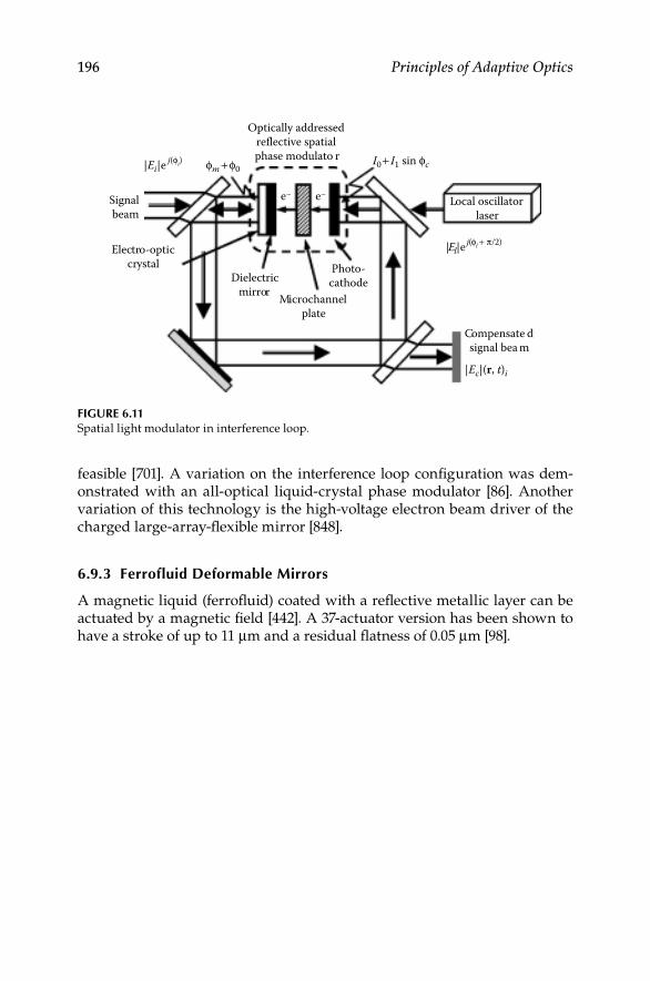
196 Principles of Adaptive Optics
feasible [701] A variation on the interference loop configuration was dem-onstrated with an all-optical liquid-crystal phase modulator [86] Another variation of this technology is the high-voltage electron beam driver of the charged large-array-flexible mirror [848]
6.9.3 Ferrofluid Deformable Mirrors
A magnetic liquid (ferrofluid) coated with a reflective metallic layer can be actuated by a magnetic field [442] A 37-actuator version has been shown to have a stroke of up to 11 μm and a residual flatness of 005 μm [98]
Signalbeam
Electro-opticcrystal
Dielectricmirror Microchannel
plate
Photo-cathode
e− e−
Optically addressedreflective spatialphase modulato r
Compensate dsignal bea m
Local oscillatorlaser
|Ec|(r, t)i
|Ei|ej(ϕi) ϕm+ϕ0
|El|ej(ϕl + π/2)
I0+ I1 sin ϕc
Figure 6.11Spatial light modulator in interference loop

197
7Reconstruction and Controls
7.1 Introduction
Wavefront sensors, described in Chapter 5, measure the condition of the wavefront and produce signals that represent the wavefront Both zonal and modal sensors may be used in a particular system It is up to the reconstructor to sort out the meaning of those signals, and then it is the control system that must determine how to treat the signals and relay them to the appropriate cor-rection device In Chapter 4, many system concepts showed the control system as a “black box,” that is, the controller received the signals from the wavefront sensor and magically translated them to signals for the correction devices This chapter aims to remove the mystery of the controller and to describe the fundamental principles behind the adaptive optics control system
Figure 71 is a rather complicated block diagram that shows the many paths that signals may take getting from the wavefront measurement to the cor-rection system In most cases, only a few of these paths are used However, in many cases parallel paths are used whereby the system controls lower-order aberration modes, such as focus and tilt, via one path and simultane-ously controls higher-order wavefront errors with a deformable mirror This method has been used in many adaptive optics systems The principles of those control methods are explained in detail in Section 73
I will use a terminology convention that refers to control systems that gen-erate a phase representation as direct and those that avoid an explicit deter-mination of the phase as indirect [801] Because the phase reconstruction is considered a fundamental intermediate step, any control system that avoids this step is hereafter called indirect This may appear backwards, because the most direct route (less processing time, fewer electrical connections, less software, and so on) from wavefront sensor data to correction commands might bypass an intermediate phase representation step The phase repre-sentation in the preceding context may take on many forms, such as a con-tinuous phase map where the wavefront is evaluated at all points, a zonal phase map where the wavefront is known at only specific locations, or a modal phase map where the phase can be found at any point by adding the contributions from each mode In addition, the phase representation may

198 Principles of Adaptive Optics
actually take the form of the derivatives of the wavefront at various points or even the derivatives of the aberration modes In any case, whenever this step is explicit within the control system, it is deemed direct
There are many books on linear control theory [43,113,126,513,579,810] This chapter will take the important parts of control system theory and show how they apply to the specific field of compensating for an aberrated wave-front Referring to Chapter 1, where adaptive optics was defined as being a closed-loop process, it is necessary to define the meaning of that term in a more formal manner
Control systems are often classified as either process control or servomech-anisms The former control, also called regulator control, is designed so that the controlled variable or output is held to a constant or desired value The human body-temperature regulation system is in the regulator control class The body attempts to maintain a constant 986°F despite external disturbances Servomechanisms do not maintain a constant output, but rather, they vary the output as the input varies The output mechanism serves as a slave to the input master; thus, the term “servomechanism” Both classes of control are closed-loop They respond to information from somewhere else in the system
However, an open-loop control does not use feedback A sequence control, where a series of switches turns on and off at predetermined times, is an example of open-loop control This has application in optics, for example, when a telescope must point to a particular star following the rotation of the Earth The preprogrammed movements are all that are necessary We assume that the absolute position of the star will not vary significantly through one evening! Although adaptive optics control systems often ana-lyze and direct many parallel channels of information, most of the systems in
Phase representations
Corrector commands
Indirect method
I
J
C
D
B
A E
F
G
H
(Direct method)
Zonal(continuous)phase map
Zonal corrector(deformable mirror)
commands
Modalcorrectors
Modal phaserepresentation
Beam tilt,focus, and
astigmatism
Measurements
Wavefrontslopes
Figure 7.1The various paths of wavefront control in a conventional adaptive optics system

Reconstruction and Controls 199
practice are based on single-channel linear processing algorithms Section 72 will address single-channel control from a temporal and frequency aspect Section 73 addresses the spatial aspects of parallel control The optical sys-tem under control may not be linear throughout its entire range; however, one can often assume that the optical and electronic signals are linear near the operating point of the control We can use classical linear optimal control theory for designing and analyzing the system [343,434]
Adaptive optics control systems can be optical, analog electronic, digital elec-tronic, and in some cases, fluidic The actual implementation of the controls is left to the designer, who is often constrained by factors such as cost and size Wavefront sensor signals can be gathered in the microvolt range, while correc-tor mirror drivers may need to operate in the kilovolt range Hydraulic actua-tors may need to be controlled by relays and valves or other means The details of electronic preprocessing, calibration, signal amplification, signal condition-ing, power supply conditioning, isolation, and filtering will not be covered in this chapter They will be addressed only when these specific processes become a part of the fundamental adaptive optics control problem Subjects such as electronic or digitization noise will be treated according to standard methods
7.2 Single-Channel Linear Control
The control of a single channel of an adaptive optics system is fundamental to the control of many channels of wavefront information It also applies directly to the control of single-channel adaptive optics systems like beam-steering systems that only have tilt signals as input and single-mode steering mirrors as output Although the two orthogonal axes of tilt may be operating simultaneously, it is usually possible to design a control to operate each axis as an individual linear control The example of a beam tilt control (Figure 72)
Inputbeam
++
DisturbanceActuator
driver
Controller Tiltsensor
OutputbeamTilt mirror
(corrector)
Figure 7.2Single-channel closed-loop beam tilt control

200 Principles of Adaptive Optics
will be used as a basis for the discussion of single-channel linear control An input beam enters the system from the left A disturbance is added to the beam The beam is deflected by a tilt mirror The disturbance plus correction output is sensed It is conditioned and amplified and fed to a controller that determines the degree of correction The control signal is then conditioned and amplified and drives an actuator in the tilt mirror to remove the dis-turbance The design of the controller will be an iterative process based on the results of analysis The analysis will indicate the response of the system to changes in the input or disturbances If that response is unsatisfactory, it often can be improved by changes in the controller algorithm, the amplifier, or the tilt mirror itself
If the disturbance changes suddenly from one value to another constant value, a step-function input is assumed There will be a certain period of time for the control system to respond so that the output levels off to its new value This transient period should be sufficiently short, but not so sudden that the response of the system is oscillatory or results in unacceptable overshoot After the transients have decayed, the system will demonstrate its steady-state response Any errors between the input beam and the output beam should be small The use of feedback, shown in Figure 72 as the tilt sensor–controller path, is the fundamental principle for the linear systems control operation Feedback and adjustments to the parameters in the feedback loop are present to reduce the effects of parameter variations, reduce the effects of disturbances, improve the transient response, and reduce steady-state errors The primary means of varying the control system, and its subsequent response, is by changing the gain of the control One may think of the controller as a signal amplifier of the error signal For large gains, the system response is more accurate (because small changes are noticed) and faster (because the tilt mirror responds more for a given input and, therefore, achieves its final position faster) The disad-vantage of simply increasing the gain to achieve optimum control is the fact that the rapid response of the tilt mirror will result in an overshoot, because it cannot necessarily stop quickly when it reaches its desired position Because the overshoot must then be compensated by continuing application of a coun-ter-drive signal, the system oscillations can increase, and in the worst case, it never reaches the correct value because it is unstable The relative stability of the system is maintained by keeping the overshoot of the response small This compromise between large gain for rapid response and small gain for stability is the crux of the control problem in all aspects of adaptive optics
7.2.1 Fundamental Control Tools
Linear control system theory is a well-developed field Most controls analy-ses use Laplace transforms They are used extensively as a manner of dealing with the complicated time-response of a system without having to constantly evaluate difficult integrals in the time domain By transforming the equa-tions of motion for the optical system into a Laplace space, the response can

Reconstruction and Controls 201
be determined and analyzed by fairly straightforward algebraic operations The variable in Laplace space is s It is a complex number represented by a real part σ and an imaginary part iω, where ω is the frequency in radians per second The Laplace transform of the function of time f(t) is defined by
F s L f t f t tst( ) [ ( )] ( )= = −∞
∫ e d0
(71)
As mentioned in the preceding example, an important way of evaluating a control system is by observing its response to a step input The step function of a constant amplitude A is given by f(t) = 0 for t < 0 and f(t) = A for t ≥ 0 The Laplace transform of the function is
L f t A tAs
st[ ( )] = =−∞
∫ e d0
(72)
Another common test input is the ramp function f(t) = At, and its Laplace transform is
L AtAs
[ ] =2
(73)
The transient response of many optical systems is a decaying exponential f(t) = Ae−αt, which has the transform
L AA
st[ ]e− = +
αα (74)
These and many other Laplace transforms can be found in handbooks and tables [1] They are used extensively to relate the physical phenomena f(t) to the controls phenomena F(s) How these transform methods are used and how they relate to the language of the controls analysis will be explained next
7.2.2 Transfer Functions
If the input of a system is given by the function r(t) and the output is given by c(t), assuming zero initial conditions (c(0) = 0, r(0) = 0), the dynamic behavior of a linear system is given by the differential equation
d
dd
dd
d
n
n n
n
n
c tt
ac t
ta
c tt
a c( ) ( ) ( )+ + + +−
−
−1
1
1 1 0 (( )t = (75)
br tt
br t
tb r tm
m
m
dd
dd
( ) ( )( )+ + + 1 0 (76)
If the Laplace transforms of the functions are defined to be
C s L c t( ) [ ( )]= (77)

202 Principles of Adaptive Optics
and
R s L r t( ) [ ( )]= (78)
then, the differential equation transforms to the following algebraic equation:
s a s a s a C s b s b s b Rnn
nm
m+ + + +( ) = + + +( )−−
11
1 0 1 0 ( ) (( )s (79)
The transfer function of the system G(s) is the ratio of the Laplace transforms of output and input and is given by
G sC sR s
( )( )( )
= (710)
The transform of the output C(s), then, is the transfer function of the system times the transform of the input, and is given by
C s G s R s( ) ( ) ( )= (711)
This is the temporal domain equivalent of the discussion of spatial optical transfer functions in Section 13
The assumption of zero initial conditions can be overcome by using the prin-ciple of superposition: the response of a linear system is the sum of the response to the input plus the response to the initial conditions If there are two elements of the control system (Figure 73) with individual transfer functions G1 and G2, linear theory shows that the open-loop transfer function of the system is the product of the transfer functions of the individual elements, as follows:
G s G G( ) = 1 2 (712)
If the feedback loop transfer function (eg, sensor element) is represented by H(s), then the closed-loop transfer function is the product of the open-loop transfer function divided by unity plus the loop gain function (the product of all transfer functions around the loop), as follows:
C sR s
G GG G H
( )( )
=+
1 2
1 21 (713)
InputR(s)
OutputC(s)
FeedbackH
G1++G2
Figure 7.3Transfer functions around a closed loop

Reconstruction and Controls 203
An example will be used to illustrate how one might use these methods to determine the performance of a control system Consider a system such as that shown in Figure 73 Assume that the first element G1 is composed of a simple amplifier of gain K The second element is a voltage-driven tilt mirror whose position in relation to the applied voltage is represented by a transfer function,
G ss s2
0 50 25 1
( ).
( . )=
+ (714)
Assuming unity feedback (H(s) = 1), we want to determine the output response of the system for a step-unit input In other words, we need to derive an expression for the mirror output position c(t) a time t after the mirror is com-manded to go to the value +1 The Laplace transform of unit step input is R(s) = 1/s The transform of the output C(s) is the product of the input trans-form and the system transfer function and is given by
C s R s G s( ) ( ) ( )= sys (715)
From the preceding, we find
G sKG s
KG ssys ( )( )
( )=
+2
21 (716)
and the output transform becomes
C sK
s s s K( )
( )=
+ +24 22
(717)
Our desired result is
c t L C s( ) ( )= −1 (718)
A number of methods can be used to invert Equation 717 The most straight-forward is a direct inverse Laplace transform, which can be found in tables [1] The inverse transform of Equation 717 is given by
Ls s s
t−
+ +
= +
−− +(1
2
2 2 22
21
11
1ωζ ω ζ
ω ζ θ( )
cos )) (719)
where
θζ
ζπ=
−
+−tan 121
2 (720)

204 Principles of Adaptive Optics
By properly substituting the constants in Equation 719, ω = 2K and ζ = 2K
, the output mirror position becomes
c t
K
K tt( ) cos= +−
− +( )−11
12
2 42e θ (721)
The phase angle θ is
θ π= −
+−tan 1
21
2K
(722)
Examination of Equation 721 reveals the properties of this solution First, the solution is only valid for large gains, K > 2; it has a singularity at K = 2 and is imaginary for lower values Second, the steady-state solution is eas-ily found, c(t) → 10 as t → ∞ Third, for this high-gain solution, the mirror should respond rapidly The disadvantage we see is overshoot during the transient The maximum overshoot is found from the fraction preceding the exponential term, 1 1 2/ /− K For a gain near the instability, the overshoot is large (K = 4, overshoot = 41%) For higher gains, the overshoot is reduced (K = 10, overshoot = 11%), but the ringing remains large, increasing the set-tling time toward its steady state
For the case in which the gain is less than 2, we must use another method of solution Partial fraction expansion is used to determine the characteristic behavior of the system as well as to examine some of the more common terms used in control theory Begin by expanding Equation 717 into partial fractions as follows:
C sK
s s s KAs
Bs a
Cs b
( )( )
=+ +
= ′ + ′+
+ ′+
24 22
(723)
The primed constants are called residues of the output response The term in the denominator, s2 + 4s + 2K, can be factored into (s + a)(s + b), where a K= + −2 2 1 2/ and b K= − −2 2 1 2/ We find the residues by multiplying C(s) by the appropriate term and evaluating at the poles
′ = =+ +
= ==
=
A sC sK
s a s bK
abss
[ ( )]( )( )0
0
2 21 (724)
′ = + =+
=
−=−=−
B s a C sK
s s bK
s as a
[( ) ( )]( )( )
2 2aa b a
Ka a b( ) ( )−
=−
2 (725)

Reconstruction and Controls 205
′ = + =+
=
−=−=−
C s b C sK
s s aK
s bs b
[( ) ( )]( )( )
2 2bb a b
Kb a b( ) ( )−
=− −
2 (726)
The result is a reduced fraction representation of the output transform, as follows:
C ss
K
KK
s a
K
KK
s b( ) = +
− + −
++
− − + −
+1
2
8 12
8 4
2
8 12
8 4 (727)
By the inverse Laplace transform of Equation 727, the time dependence for if K < 2 is found by
c tK
KK
K
Kat( ) = +
− + −
+− − +
−1
4 12
4 2 4 12
e
44 2−
−
K
bte (728)
This expression also converges to the steady-state solution properly, c(t) → 1 as t → ∞, and does not exhibit the drastic ringing that resulted from a high gain
We can see from Equation 727 that the transfer functions and input and output transforms are, in general, ratios of polynomials in s The zeros of the expression are the roots of the numerator polynomials The system zeros are the roots of the numerator of the system transfer function G(s) Similarly, the poles are the roots of the denominators, and the system poles are the roots of the denominator of G(s) The system poles have significance when we want to examine the stability of the control system Because the Laplace variable is complex, s = σ + iω, the poles can be plotted as points on a complex plane For a control system to be used in adaptive optics, the transient solution should decay to zero This will occur if all the real poles and the real parts of all complex poles are negative, that is, in the left half of the complex plane In Equation 727 the poles –a and –b can be evaluated for different gains K, showing their regions of stability If the transient is represented by an exponential, the system time constant is the time it takes for the decaying exponential to be reduced to a factor of e–1 = 0368 of its original value
The design of a stable control system that meets the system performance requirements reduces to establishing a transfer function with the proper characteristics For instance, a tilt mirror or multiactuator deformable mirror will have mechanical constraints because of the inertia of the masses being

206 Principles of Adaptive Optics
moved This is a direct consequence of dealing with inertial adaptive optics systems A motor position servo with gain K and a time constant τ = I/γ, where I is the inertia and γ is the damping constant, would have a transfer function given by
GK
s smotor =+( )τ 1
(729)
Moving a large-mass (large inertia) servomotor to respond to optical signals can be difficult A large gain is required to move it rapidly, but once it starts moving, it is equally difficult to stop This results in severe overshoot An increase in damping and various methods of feedback also can be used For instance, damping that is proportional to the velocity of the system is very useful If the damping is increased as the velocity is increased, the amount of overshoot can be curtailed Detailed discussions of velocity feedback and other methods of tailoring feedback to specific transfer function character-istics can be found in a number of sources devoted to these specific design problems [127,435]
7.2.3 Proportional Control
If an input signal r controls an output c, and the output is a linear function of the input c = Kr, the system is said to have a proportional controller If the proportionality constant, the gain K, is very large, the output will respond to very small changes in the input A system with this characteristic may have the output moving from its minimum to its maximum range with only slight changes in the input This “on–off” control is a basic form of control When the gain is lower and the output responds smoothly and linearly to the input, one has a true proportional controller If a resistance, or damping, is added near the output so that the system responds slowly, accumulating energy as time moves along (like winding up a watch), the controller is a proportional integral (PI) controller The final steady-state output will be a combination of the linear portion (the proportional) and the time-accumulated portion (the integral) The transfer function of this system is a sum of the proportional and integral parts, G(s) = Kp + Ki/s This type of system can show overshoot due to the accumulation of energy required for the control
When the resistance is added near the input, the control is a combination of the proportional control and its derivative The transfer function of a proportional derivative (PD) controller is G(s) = Kp + Kds Note that the Laplace transform of an integral is 1/s and the transform of a deriva-tive is s Controls of these types have been made by mechanical means ( spring–mass–damper), electronic means (resistor–capacitor–inductor), thermal means (insulation–thermal capacitance), and fluidic means (fluid resistance–inertia–compressibility) [810]
Reconstruction and Controls 207
7.2.4 First- and Second-Order lag
The important aspects of the system time constant can be seen by observ-ing the performance of a very common control, a lag It has the transfer function
G ss
( ) =+1
1τ (730)
For a step input, R(s) = 1/s, the output transform becomes
C ss s s s
( ) =+
= + −
+
1
111
τ
ττ
1 (731)
The inverse transform of Equation 731 is the transient response
c t t( ) /= − −1 e τ (732)
The first term is the forced solution, whereas the second one is the transient due to the system pole at −1/τ The output reduces to 0368 of its original value when e−t/τ = e−1 or when t = τ Thus, the time constant for a simple lag G(s) is simply τ The stability of the system is easily determined If the pole −1/τ is positive, then the exponential grows instead of decays This is an unstable situation For the stable case, τ > 0, the response speed can be made faster by reducing the time constant
From the example in Section 722, Equation 717 takes on a very common form The output transform has the form
C ss s s
( )( )
=+ +
ωζω ω
2
2 22 (733)
In this form, ω is the value of the undamped natural frequency and ζ is the damping ratio For ζ > 1, the system is overdamped (see Equation 719) The transient is the sum of two decaying exponentials with the form
1 2 21 1+ +− + − − − −a be e( )ω ζ ζ ω ζ ζ( ) (734)
This is the same as saying that the system is a series connection of simple lags, called a quadratic lag For ζ < 1 (the K > 2 case in Section 722), the sys-tem is underdamped and overshoot occurs The transient term is an oscil-lation with a damped natural frequency related to the resonant frequency, ω ζ1 2− , with a decaying amplitude e−ζωt The time constant for the system is τ = 1/(ζω)

208 Principles of Adaptive Optics
The important characteristics of simple or quadratic lag controllers are summarized by the parameters important to the performance of the system The time it takes for the system to come to 5% of its steady-state value is about 3τ To reach 2% of its value, it takes 4τ The percentage overshoot W% is
W% exp= −−
100
1 2
πζζ
(735)
and the time to reach its peak value is
τ πω ζpeak =
−1 2 (736)
7.2.5 Feedback
Feedback that is used to reduce the overshoot of a control system, as described in Section 722, is an example of the general application of feed-back to adaptive optics controls Feedback is used primarily to reduce the sensitivity of the control output to differences in the input or external distur-bances Equation 713 represents a standard control with a feedback loop as diagrammed in Figure 73 The closed-loop transfer function T(s) is given by
T sC sR s
G GG G H
( )( )( )
= =+
1 2
1 21 (737)
where H is the feedback If the loop gain, the product of the transfer func-tions around the loop, G G H1 2 1 , then T(s) = 1/H(s); that is, the closed-loop transfer function depends entirely on the feedback The sensitivity of this relationship is the ratio of the change of the closed-loop transfer function to the change of the forward path transfer function and is given by
Sensitivity =∂
∂=
+T s T s
G G G G G G( )/ ( )
( )/( )1 2 1 2 1
11 22H
(738)
The static sensitivity is evaluated as s → 0, and the dynamic sensitivity to frequency ω is evaluated for s = iω High loop gains help reduce the sensitiv-ity to parameter variations and disturbances For a unity feedback system (H = 1; G(s) = G1(s)G2(s)), the steady-state error is
εss = − =+→∞ →
lim[ ( ) ( )] lim( )( )t s
c t r tsR s
G s0 1 (739)

Reconstruction and Controls 209
Assuming a general form for G(s), we have
G sK s ss s s
kk
nl
l( ) =
+ + +( )+ + +( )
α αβ β
1
1
11
(740)
The gain K is the gain of the transfer function (when the constant terms are made unity) and is given by
K s G ss
n=→
lim ( )0
(741)
The exponent n of s in the denominator represents the type number Because, from Laplace transforming, each s represents an integration, the type num-ber represents the number of integrators in G(s) The position error constant is Kp for n = 0; the velocity error constant is K v for n = 1; and the acceleration error constant is Ka for n = 2 Higher-order constants are easily evaluated, but are not so easily named The steady-state error for any type of control is found simply by
εss =+
→lim
( )s
n
sR sKs
01
(742)
For example, for a step input (R(s) = 1/s) to a type-0 control, εss = 1/(1 + K) For a ramp input (R(s) = 1/s2) to a type-2 control, εss = 0 This shows that a type-0 control can respond to a step input with a constant steady-state error Similar analysis shows that the type-0 control cannot respond (ie, εss = ∞) to a higher-order input A type-2 control, with two integrators, can respond to both step and ramp inputs, leaving no steady-state error, and has a con-stant error for a second-order (acceleration) input The fundamental principle described in this section is that sensitivity, response to disturbances, and steady-state errors are all improved by increased gain Feedback can also be used to increase the dynamic response The velocity feedback mentioned in Section 722 has various applications in controlling adaptive optics wave-front compensating devices These will be described in the context in which they occur, but the reader is referred to a number of other texts for detailed explanations of the design principles and applications [113,579]
7.2.6 Frequency response of Control Systems
An adaptive optics control system is often required to respond to a dynamic periodic input The response to high-frequency noise or the response to a particular range of frequencies (bandwidth) is desired A linear quadratic Gaussian control law is often used [616,617] Based on the Laplace trans-form methods, frequency response analysis lets a control designer observe the system response in the frequency domain and stability of the system [480,481,482]

210 Principles of Adaptive Optics
A control system with a transfer function G(s) will respond to a sinusoidal input, r(t) = A sin(ωt), in an interesting manner Using Laplace transforms, the transform of the output will be
C sA G ss
As i
Bs i
( )( )=
+= ′
++ ′
−+ω
ω ω ω2 2 (743)
The coefficients of the expansion can be found by using the method of partial fractions as follows:
′ = −−
AAG i
i( )ω2
(744)
and
′ =BAG i
i( )ω
2 (745)
By inverse transforming, the forced response becomes
c tA G i G i
iAW
i t i t
( )[ ( ) ( ) ]
( ) sin[= − − + =−ω ω ω ω
ω ωe e2
tt+ φ( )ω ] (746)
where W is the ratio of output to input amplitude as follows:
W g g( ) ( ) ( )ω ω ω= +r i2 2 (747)
The parameters gr and gi are the real and imaginary parts of the transfer function G(s) evaluated at s = iω, that is, G(s)|s = iω = gr(ω) + igi(ω) The corre-sponding phase angle is the delay of the output relative to the input
φ(ω) = −tan 1 gg
i
r
(748)
From this result, we can see what happens to the general sinusoidal input The output retains the shape (sine function) with an amplitude reduced by the function W(ω) and delayed by a phase factor ϕ(ω) The simple lag control yields a common result The transfer function for the lag is
G sK
s( ) =
+τ 1 (749)
where the gain K and the time constant τ are given For a sinusoidal input, the frequency response function becomes
G iK
i( )ω
ωτ=
+ 1 (750)

Reconstruction and Controls 211
Its magnitude is
WK
( )( )
ω =+1 2ωτ
(751)
and the phase angle is
φ(ω) ωτ= − −tan 1 (752)
Although this example considers only a simple lag, the results are funda-mental to performance analysis Most control systems in practice are a com-bination of various controls
A control system is often composed of gain, integrators, differentiators, lead, or lag The gain is represented by K, where
K s G ss
n=→
lim ( )0
(753)
n integrators are represented by 1/(iω)n and n differentiators by (iω)n A simple lag is represented by 1/S = 1/(iωτ + 1), and a simple lead is S = (iωτ + 1) Quadratic lag is 1/Q = 1/[(iω / ωn)2 + 2ζ(iω / ωn) + 1], and qua-dratic lead is Q = (iω / ωn)2 + 2ζ(iω / ωn) + 1 A general form for a frequency response function is then
G iK
iS S
S SQ Q
Q Qnk k l l
( )( )
ωω
=+ + + +
1 2
1 2
1 2
1 2
(754)
Substituting values for time constants τ, damping ratios ζ, and natural frequencies ωn yields the necessary information to examine the system responses If M controls are cascaded in series, the response G(iω) is the product of the individual response The magnitudes W are multiplied, and the phase angles are added as follows:
G i G W W Wji i i
j
M
( )ω = = ==
∏ 1 21
1 2e e etottotφ φ φ (755)
where
W Wjj
M
tot ==
∏1
(756)
φ φtot ==∑ jj
M
1
(757)
A plot of W(ω) or ϕ(ω) versus ω is a simple graphical method for observing the performance of the control system A convenient method of plotting the

212 Principles of Adaptive Optics
performance, originated by Bode [810], uses a logarithmic frequency scale The magnitude W is expressed in units of decibels (dB) and the phase angle is expressed in degrees We can treat gain, integrators (or differentiators), and lag (or lead) as individual controllers that combine as shown in the preced-ing paragraph A Bode plot of the gain is simply a straight horizontal line at W(dB) = 20 log K and ϕ = 0°
Bode plots of other control parameters are relatively straightforward n integrators have the form W(dB) = 20 log |iω|−n = −20n log ω On a log scale, the magnitude plot of an integrator is a straight line crossing the 0 dB axis at ω = 1 with a slope of −20n dB/decade The phase angle is not a function of frequency, but is a constant ϕ = −n90° Differentiators are mirror images of integrators across the 0 dB and 0° axis
A simple lag with time constant τ has a magnitude dependency
W dB( ) = + −20 1 2 1 2log[ ( ) ] /ωτ (758)
and a phase dependency ϕ = −tan−1 (ωτ) For very low frequencies ( ),ωτ 1 the magnitude W and the phase asymptotically approach 0 dB and 0°, respectively For high frequencies ( )ωτ 1 , the magnitude W asymptoti-cally approaches −20 log ωτ and the phase approaches 90° The asymptotes meet at the break frequency ωτ = 1 A simple lead will have the same char-acteristics as the lag, except that it is a mirror image across the 0 dB and 0° axis
A more complicated, yet common, control is the quadratic lag or lead Instead of having a simple dependence on the time constant, a quadratic lag or lead closely follows the characteristics of resonances and damping The magnitude of a quadratic lag is given by
W( ) logdBn n
= −
+
20 1
22
2
2 2ωω
ζωω
−1 2/
(759)
The parameter ωn is the natural frequency of the system The phase angle follows the form
φ = −−
−tan//
12 2
21
ζω ωω ω
n
n (760)
For frequencies much lower than the natural frequency ( )ω ω n , W → 0 dB and ϕ → 0° For frequencies much higher than the natural frequency ( ), log( / )ω ω ω ω n nW → −40 and ϕ → −180° For frequencies close to the natural frequency, Equation 759 should be used The shape of the resonant peak is determined primarily by the damping ratio ζ For small values, the magnitude peak is very sharp and the phase change from 0° to 180° is very

Reconstruction and Controls 213
rapid The Bode plot for a quadratic lead follows the form of the lag, except it is also a mirror image about the 0 dB and 0° axis
Examples of Bode plots for various contributors are shown in Figures 74–79 The Bode plot of the gain of an integrator, Figure 74, shows the characteristic slope based on the number of integrators The phase angle in Figure 75 is constant The Bode plot of a simple lag controller, Figures 76 and 77, shows its break frequency at 1/τ The designer can “tune” the control to a particular frequency characteristic Similarly, the designer can tune the response by choosing the resonance of a quadratic lag or lead The position of the peak in Figure 78 corresponds to the resonant frequency and the width of the peak, and the sharpness of the phase change in Figure 79 corresponds to the choice of the damping factor
The combination of gain, lead, lag, integrators, and so on is a simple pro-cess for Bode plots Because the vertical axis for the magnitude W(ω) is loga-rithmic and the W’s are multiplicative, the Bode plots of each contributor
0.1 1.0ω
(iω)
(iω)21
1
−40 dB/dec
−20 dB/dec
Type 1
Type 2
W(d
B)
10−20
0
20
40
Figure 7.4Bode plot of the gain of an integrator
0°
−90°
−180°0.1 1.0 10
Type 2Phas
e an
gle
ω
Type 1
Figure 7.5Bode plot of the phase of an integrator

214 Principles of Adaptive Optics
can be added Similarly, the Bode plots of phase are on a linear scale and are additive; therefore, the phase contributions are added as well
Bode plots are useful for open-loop stable systems Two important defini-tions arise from examination of Bode plots The phase margin is defined as 180° plus the phase angle at the crossover frequency (where the magnitude curve crosses the 0 dB axis) The gain margin is defined as 1 divided by the magnitude at the frequency where the phase angle is −180° For closed-loop systems, the frequency response is determined by a number of features Many control systems have the form of the quadratic lag
C iR i i i
( )( )
ωω ω
ωζ ω
ω
=
+
+
1
2 12
n n
(761)
0°
−30°
−60°
ωτ
−90°0.1 1.0 10
Phas
e an
gle
Figure 7.7
Bode plot of the phase of a simple lag
−20
−10
0
1.0ωτ
0.1
W(d
B)
10
Figure 7.6
Bode plot of the gain of a simple lag

Reconstruction and Controls 215
The magnitude W is simply
W( )ωωω
ζωω
=
−
+
1
1 22
2
2 2
n n
(762)
The resonant peak is a measure of relative stability If the maximum of this function does not go too high, the system possesses relative stability The peak magnitude Wpeak is dependent upon the damping ratio
0
−20
+20
−40
ω/ωn
ζ=0.4
ζ=0.1
0.1 1.0 10
W (d
B)
Figure 7.8Bode plot of the gain of a quadratic lag
0°
−60°
−120°
−180°0.1 1.0 10
Phas
e an
gle
ω/ωn
ζ=0.4
ζ=0.1
Figure 7.9Bode plot of the phase of a quadratic lag

216 Principles of Adaptive Optics
Wpeak =−
12 1 2ζ ζ
(763)
The system bandwidth represents the response speed of the control system It is defined as the range of frequencies over which W is more than 2 2/ (or 0707) of its direct current (DC) value (the value at ω = 0) From Equation 762, the bandwidth B is
B = − + − −( )ω ζ ζ ζn 1 2 2 4 12 2 21 2
( )/
(764)
The resonant peak does not occur at the natural frequency ωn By taking the derivative of Equation 762, we see that the peak occurs at a frequencyω ω ζp n= −1 2 2 As seen in Equations 763 and 764, a low damping ratio ζ means severe resonant peaking and severe overshoot to a step input However, raising the bandwidth B by reducing the damping ratio results in a reduced settling time and a quicker rise time response to the step input This compromise is the ongoing concern of all control system designers, and it is a fundamental problem with adaptive optics as well as many other aspects of active control
7.2.7 Digital Controls
Each of the control structures mentioned in Sections 723 through 725 is applicable to many types of adaptive optics problems Analog computers and hard-wired circuits, such as resistor–capacitor–inductor networks [302], can implement various transfer functions The flexibility of digital computers allows the control to be implemented in software rather than in hardware, greatly reducing the difficulty in modifying the control or even altering the control in real time (adaptive control) [36] Adaptive optics systems are almost always dealing with multivariable controls Many inputs and many outputs must be simultaneously adjusted, and cross talk or coupling between nearby feedback loops must be reduced Digital construction of the control allows the flexibility to adjust parameters as the inputs change or the optical system hardware changes
For a computer to monitor and control numerous signals at rapid rates, it must time-share, which results in a loss of information As long as these lapses in information are understood and compensated for, the control can function as efficiently as a continuous analog system This latency can be a combination of many sources, digitization, computation, storing, and so on The time-sharing can be analyzed mathematically Consider a signal that is varying with time f(t) Sampling this function at equal intervals t′ is equiva-lent to multiplying the function by a sum of impulse functions (δ(t) = 1 for t = 0 and zero otherwise), as follows:

Reconstruction and Controls 217
f t f t t ntn
samp( ) ( ) ( )= − ′=
∞
∑δ0
(765)
Taking the function inside the summation and using the properties of the delta function, we have
f t f nt t ntn
samp ( )( ) ( )= ′ − ′=
∞
∑0
δ (766)
This shows that the sampled function is only known at the various times given by
t t t t= ′ ′ ′0 2 3, , , , (767)
The Laplace transform of the sampled signal is
F s L f t f ntt
F sinnt s
samp samp e( ) [ ( )] ( )= = ′ =′
+− ′ 1 2ππ′
=−∞
∞
=
∞
∑∑ tnn 0
(768)
where F(s) = Lf(t) The Laplace transform of the sampled signal is a sum of Laplace transforms of the original signal spaced exactly 2π/t′ apart The functions F(s + in2π/t′) for values of n ≠ 0 are called sidebands If the side-bands are close together, they overlap with the principal band and inde-terminacy can occur The value of the sampled transform is a summation If only one term contributes to the value at each point in s frequency space, the problem can be avoided If there is more than one nonzero component at each value of s, the signal is said to possess aliases If the sampling fre-quency 2π/t′ is at least twice the highest significant frequency in the sig-nal f(t), the aliases are suitably separated and no confusion occurs This condition is known as the Nyquist limit These conditions and problems must be overcome before implementing any sort of digital control Control designers use filters to remove high-frequency aliases and other treatments extensively [39,53,465]
In addition to the disadvantages of discrete sampling, a digital control also is limited by the resolution of the digitization itself The accuracy of the computations is limited by the accuracy of representing the continuous values by a digital bitstream An 8-bit number, for example, can represent only 256 possible values The subsequent accuracy of the numerical calcu-lations is limited to one part in 256 This 04% limit is often sufficient; how-ever, each control experiences the combined effect of many calculations Often, digitization limitations require control systems to have 16- or even 32-bit data words Although analog or digital electronic controls are most common, the use of optical processing for adaptive optics has not been overlooked [177]

218 Principles of Adaptive Optics
7.3 Multivariate Adaptive Optics Controls
This book will not delve deeper into specifics of general control theory or design, but will focus now on specific problems related to adaptive optics For any adaptive optics system, except for a single-mode control loop, for example, a one-axis tilt control, there is a need for controlling multiple cou-pled loops Each loop can be represented by the temporal transfer functions described in Section 72 Spatial coupling between multiple loops is described in this section
Referring to Figure 71, we can see how the adaptive optics control must often deal with sets of multiple coupled equations The choice of a modal or zonal reconstruction is dependent upon the type of corrector, the band-width requirement, and the sensing geometry involved [278] For low signal strength or a coarse spatial sample of phase measurements, a zonal system has been shown to be superior [735]
Calculations involving wavefront control can be digital, analog, or a hybrid of the two In most cases, they involve either the real-time inversion of a matrix or matrices or the real-time multiplication of a vector times a matrix Path A, for example, must calculate a continuous phase map from the measurement of wavefront slopes Decoding a number of measurements into a number of phase points will be treated as a linear problem Straightforward methods of linear algebra are usually sufficient, because most of the adaptive optics operation is in a linear regime In general, any of the paths in Figure 71 represents the solution to a set of linear equations Whether one is trying to determine the phase from measured modes or to determine the voltages for a deformable mirror from a Zernike representation of the phase, the methods of linear algebra can be used
7.3.1 Solution of linear equations
In the wavefront reconstruction and control problem, one usually encounters a set of M equations with N unknowns They can be written discretely as
y a B a B a B a B
y a B a B aN N1 1 11 2 12 3 13 1
2 1 21 2 22 3
= + += + +
BB aB
y a B a B a B a B
y a
N N
N N
M
23 2
3 1 31 2 32 3 33 3
1
= + +
= BB aB a B a BM M M N MN1 2 2 3 3+ +
or as a matrix equation as follows:
( ) [ ]( )y B a= (769)
Reconstruction and Controls 219
The vectors and coupling matrix are defined simply as
y
y
y
y
a
a
a
aM N
=
=
1
2
1
2
(770)
B
B B B
B B B
B B B
B B B
N
N
N
M M M
=
11 12 1
21 22 2
31 32 3
1 2
NN
(771)
The linearity requirement is satisfied when the parameters an are constants The basis functions Bmn can have any functional form They may be wave aber-ration polynomials needed for the calculation in path B in Figure 71, or they may be functions representing the coupling between actuator voltages for a deformable mirror and the wavefront at certain points, like that represented by path G in Figure 71
In any case, the required solution is an inversion of Equation 769 We must find the parameters an that fit the series of basis functions B to the known or measured values ym When the number of equations M is less than the number of unknowns, it is an underdetermined system and cannot be solved uniquely When M = N, the matrix [B] is square and, as long as it is not sin-gular, it can be directly inverted to solve Equation 769: a = [B]−1y In adap-tive optics control system problems, one often encounters the case where the number of equations M is greater than the number of unknowns N This overdetermined system is the basis for much research in numerical techniques, many of which apply to adaptive optics systems
The problem reduces to calculating the values of the unknowns such that the error is small between the measured, or known, parameters ym and the actual values of y An inverse for a nonsquare matrix cannot be calculated directly An approximation can be determined based on a specific merit function The merit function that represents a good determination is often a consideration, because there should be only one solution if not for real-world errors such as noise
One method, called a Gauss reconstructor, is the principal method used in calculating various multiparameter paths in a wavefront reconstruction or control By defining the merit function as the sum of the squares of the dif-ferences between the actual value of y and the estimated value of y from [B]a, the elements of the vector a can be determined The method of least squares finds the minimum of
220 Principles of Adaptive Optics
χ2
11
2
= −
==∑∑ y a Bi k ikk
N
i
M
(772)
By differentiating χ2 with respect to each element ak and setting dχ2/da = 0, a set of equations for the a’s can be found In matrix notation, this is equivalent to solving for the vector a by
a B B B yT T= −[ ] [ ]1 (773)
where [BT] is the transpose of the matrix [B] Note that the matrix [B], for an overdetermined system, has M rows and N columns The transpose has N rows and M columns, and the square invertible matrix [BTB] is M by M elements The matrix [BTB]−lBT is called the pseudoinverse of matrix [B]
Although this method appears straightforward, a number of difficul-ties can arise The inversion of matrix [BTB] is impossible if it is singular or if, numerically, it is close to singular Unfortunately, this occurs in many cases of real-world adaptive optics To get around this problem, singular value decomposition (SVD) is used The method is easily explained From the equation y = [B]a, we see that an inverse of [B] is required The following equation shows how the M × N matrix [B] can be broken into product of three matrices:
[ ] [ ][ ][ ]B U D VT= (774)
The matrix [U] is also an M × N matrix; the matrix [V T] is an N × N square matrix; and the matrix [ ]D is an N × N matrix that has only nonzero elements on the diagonal and is given by
[ ]D
d
d
dN
=
1
2
(775)
The elements of each of these matrices can be found by SVD computa-tional algorithms [629] The inverse of the decomposed matrices is relatively straightforward
[ ] [ ][ ] [ ]B V D UT− −=1 1 (776)
= [ ]
[ ]V
d
d
d
U
N
T
11
1
1
2
//
/
(777)
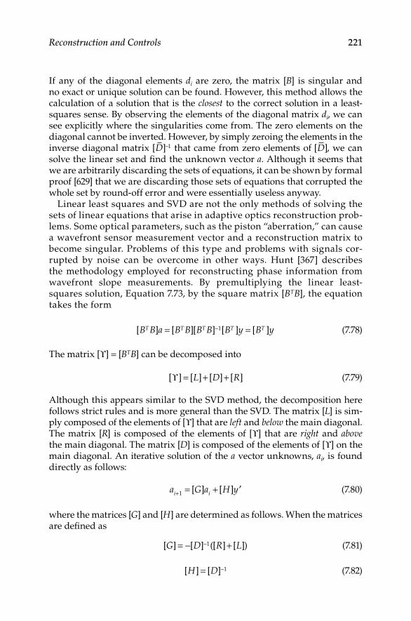
Reconstruction and Controls 221
If any of the diagonal elements di are zero, the matrix [B] is singular and no exact or unique solution can be found However, this method allows the calculation of a solution that is the closest to the correct solution in a least-squares sense By observing the elements of the diagonal matrix di, we can see explicitly where the singularities come from The zero elements on the diagonal cannot be inverted However, by simply zeroing the elements in the inverse diagonal matrix [ ]D −1 that came from zero elements of [ ]D , we can solve the linear set and find the unknown vector a Although it seems that we are arbitrarily discarding the sets of equations, it can be shown by formal proof [629] that we are discarding those sets of equations that corrupted the whole set by round-off error and were essentially useless anyway
Linear least squares and SVD are not the only methods of solving the sets of linear equations that arise in adaptive optics reconstruction prob-lems Some optical parameters, such as the piston “aberration,” can cause a wavefront sensor measurement vector and a reconstruction matrix to become singular Problems of this type and problems with signals cor-rupted by noise can be overcome in other ways Hunt [367] describes the methodology employed for reconstructing phase information from wavefront slope measurements By premultiplying the linear least-squares solution, Equation 773, by the square matrix [BTB], the equation takes the form
[ ] [ ][ ] [ ] [ ]B B a B B B B B y B yT T T T T= =−1 (778)
The matrix [ϒ] = [BTB] can be decomposed into
[ ] [ ] [ ] [ ]ϒ = + +L D R (779)
Although this appears similar to the SVD method, the decomposition here follows strict rules and is more general than the SVD The matrix [L] is sim-ply composed of the elements of [ϒ] that are left and below the main diagonal The matrix [R] is composed of the elements of [ϒ] that are right and above the main diagonal The matrix [D] is composed of the elements of [ϒ] on the main diagonal An iterative solution of the a vector unknowns, ai, is found directly as follows:
a G a H yi i+ = + ′1 [ ] [ ] (780)
where the matrices [G] and [H] are determined as follows When the matrices are defined as
[ ] [ ] ([ ] [ ])G D R L= − +−1 (781)
[ ] [ ]H D= −1 (782)

222 Principles of Adaptive Optics
the method is called a Jacobi iteration These methods have been used in adaptive optics reconstructions [241,360] When the matrices take on the slightly different form
[ ] ([ ] [ ]) [ ]G D L R= − + −1 (783)
[ ] ([ ] [ ])H D L= + −1 (784)
the method is a Gauss–Seidel iteration, which will converge faster than the Jacobi method Using a variable relaxation parameter w in the definitions leads to the successive-over-relation recommended by Hunt [367], given by
[ ] ([ ] [ ]) ( )[ ] [ ]G D w L w D w R= + − −−1 1 (785)
[ ] ([ ] [ ])H w D w L= + −1 (786)
The parameter w can be found by a number of methods specifically men-tioned in a text by Young [897] The advantage of the successive-over-relation method is that it can converge as much as two orders of magnitude faster than the Jacobi method
7.4 Direct Wavefront Reconstruction
7.4.1 Phase from Wavefront Slopes
The general methods described in Section 731 for solving sets of linear equa-tions are used extensively in determining the control parameters of adaptive optics systems One of the most common problems, illustrated by path A in Figure 71, is the determination of the phase at various points from knowl-edge of the wavefront slopes at other points on the wavefront plane [571] This is a fundamental problem of adaptive optics [361] The most common wavefront sensors (Shack–Hartmann sensors or pyramid sensors) produce output signals proportional to the wavefront slopes [8]
The number of unknown phase points is N and the number of wavefront slope measurements is M When M > N, the system is overdetermined, and solutions can be found by direct least-squares methods, SVD, or other meth-ods described in Section 731 The error between the calculated phase at the various points and the actual phase at those points (that produced the slope measurements) is important It is not only the merit function for the least-squares solution, but it is a physical limitation on the performance of the adaptive optics system

Reconstruction and Controls 223
The problem of phase determination from wavefront slopes depends upon the geometry of the problem and various numerical techniques [50,180] The phase estimation at N locations is ϕn The measured slopes at M locations are sm The matrix connecting the two is determined by the geometry of the prob-lem For instance, consider the geometry shown in Figure 710 The measured slopes from the wavefront sensor are represented by sm
x or smy The superscripts
represent the slope in the x or y direction The phase is to be determined at the points φ φ− − −1 1 1 0, , , , where the subscripts represent the coordinates of the unknown points A set of equations can be constructed as follows:
s
s
x
y
1 1 1 0 1
2 0 1 0 0
= −
= −−φ φ
φ φ, ,
, ,
and can be written in matrix form
s B= [ ]φ (787)
where the matrix [B] is the geometry matrix Often, as in this example, [B] is simply composed of sums and differences based on the geometrical con-figuration of wavefront sensor positions and phase determination positions Many of the elements are +1 or −1 However, in some cases [B] can be quite complicated If the geometry matrix includes the effects of a corrector, such as deformable mirror influence functions, it is called the influence matrix A derivation by Wallner [846] used weighting functions that were depen-dent upon the subaperture and the direction of the slope measurement in the subaperture In actual wavefront sensors, the slope measurement is seldom a simple difference between two wavefront points, but usually it is a spatial average over the subaperture Accounting for noise and spatial averaging, least-squares methods or SVD can be used to invert [B] and reconstruct the phase from the measured slopes
ϕ−1,1
ϕ−1,0
ϕ−1,−1 ϕ0,−1 ϕ1,−1
ϕ1,0ϕ0,0
ϕ0,1s1x
s3x
s1y s2
yContours3
y
s4y s5
y
s5x s6
x
s4x
s6y
s2x ϕ1,1
Figure 7.10Example of the Hudgin configuration Wavefront slope measurements superimposed on phase determination points

224 Principles of Adaptive Optics
A number of researchers have investigated numerical and physical problems that occur when this method is used [190,281] For example, if the summation of wavefront slope measurements along a contour (Figure 710) is not zero, the least-squares method breaks down [748] Although this is not a physical possibility, because the wavefront is continuous, the numeri-cal calculation or interferometric method of wavefront slope measurement can yield 2π discontinuities
The problem of singular matrices, which arise because of a nonunique solu-tion to the set of equations, can be overcome by numerical methods If the pis-ton component of the wavefront is disregarded, the solution matrix [B]−1 can be singular, because there are unlimited solutions that would give the same slope measurements Adding another row to the matrix [B] with each element equal to 10 forces the summation of all phase points to a particular value [694] The addition of another value in the slope vector s specifies the piston value, which is usually set to 0 The fixed piston value allows inversion as follows:
s
s
s
B
M
1
2
01 1 1 1
=
[ ]
φφ
φ
1
2
N
(788)
As an example of this process, consider the Hudgin geometry in Figure 710 Nine phase measurements should be computed from 12 slope measure-ments For direct phase reconstruction with no cross-correlation between phase points, the [B] matrix takes the form
[ ]B =
−−
−−
1 1 0 0 0 0 0 0 00 1 1 0 0 0 0 0 00 0 0 1 1 0 0 0 00 0 0 0 1 1 0 0 000 0 0 0 0 0 1 1 00 0 0 0 0 0 0 1 11 0 0 1 0 0 0 0 00 1 0 0 1 0 0 0 00
−−
−−
00 1 0 0 1 0 0 00 0 0 1 0 0 1 0 00 0 0 0 1 0 0 1 00 0 0 0 0 1 0 0 11 1 1
−−
−−
11 1 1 1 1 1
(789)

Reconstruction and Controls 225
The pseudoinverse [BTB]−1 [BT] can be calculated by Equation 773 With this result, a vector s of 12 wavefront slopes (and the dummy thirteenth element set to zero) can be converted to the 9 phase values
φ
φ
φ
φ
φ
φ
φ
φ
φ
−
−
− −
−
−
1 1
0 1
1 1
1 0
0 0
1 0
1 1
0 1
1 1
,
,
,
,
,
,
,
,
,
= −[ ]B
s
1
11
2
3
4
5
6
1
2
3
4
5
6
0
x
x
x
x
x
x
y
y
y
y
y
y
s
s
s
s
s
s
s
s
s
s
s
(790)
If there is cross-correlation between actuators, as in the case of finite influ-ence functions with coupling, the elements of matrix B are calculated by inte-grating the influence of each actuator to each slope measurement signals si
x and si
y using
s x I x, y x y s y I x, yix
i iy
i= =∫ ∫( ) d d and ( )subap subap
dd dx y (791)
for i = 1–9, the number of actuators, and inserting these results into the rows of [ ]B
The most common problem that can corrupt the numerical computation is the inclusion of noise in the slope measurements This is physically real-istic, because the wavefront slope measurement has uncertainty associ-ated with it The equation that describes this process is a modification to Equation 787:
s B n= +[ ]φ o (792)
where no represents noise When the wavefront slope errors are not corre-lated and each measurement has an error represented by a variance σn
2 , the mean square error of the Gauss reconstructor phase is [464]

226 Principles of Adaptive Optics
σ σphase2Tr2 1= [ ]−n
TB B[ ] (793)
where the trace Tr is the sum of diagonal elements of the matrixNot all noise is uncorrelated If the noise at one time or one place is depen-
dent upon the noise at another time or place, it is said to be correlated One such example is the misregistration of the wavefront sensor subapertures with the centers of the actuators on the deformable mirror [274] Errors of this sort may rotate with beam telescope pointing and may be spatially or tem-porally correlated The noise covariance matrix Cn represents the relationship between the noise from one point in time or space and that from another The covariance will be positive and high when the values are closely related It will be negative and high when one value forces an opposite response from the other The covariance will be zero when each value is independent (uncor-related) The covariance matrix for uncorrelated noise will be diagonal with equal elements If the noise is correlated with a covariance matrix [Cn], the phase equation is derived from the Gauss-Markov estimate [694] as follows:
φ = − − −B C B B C sTn
Tn
11
1[ ][ ] (794)
and the mean square error is
σphase Tr2 1 1= − −[ ]B C BTn (795)
The matrix B C B B CTn
Tn
− − − 11
1[ ][ ] is the reconstructor matrixIn some cases, the statistics of the phase noise are known When this occurs,
a Wiener estimate for the phase and the error can be used For instance, atmospheric turbulence is represented by a covariance matrix [CW] with ele-ments dependent upon the turbulence coherence length ro [570] The matrix representation of the phase is [694]
φ = +[ ]− − −C B C B B C sTn
TnW
1 1 1 (796)
and the mean square error of the wavefront phase estimation is
σphase WTr2 1 1 1= +[ ]− − −C B C BTn (797)
If the wavefront statistics are not known, CW → 0, these expressions reduce to Equations 794 and 795
The effect of different wavefront sensor choices and the method of adap-tive estimation were described using the known statistics and temporal bandwidth requirements of atmospheric turbulence [37] The shearing inter-ferometer can be arranged in a configuration whereby the noise covariance

Reconstruction and Controls 227
matrix is diagonal Similarly, a Hartmann sensor covariance matrix is a block diagonal 2 × 2 matrix This allows simple inversion of the covariance matri-ces and fast computation of the error matrices
A number of researchers have determined how the error of the phase is affected by the geometry of wavefront slope measurements [845,864] Figure 711 shows four possible configurations of wavefront slope measure-ments superimposed on a grid of points where the phase is to be determined: the Hudgin geometry [361]; the Southwell geometry [739]; the wavefront control experiment (WCE) geometry [864,866]; and the Fried geometry [241]
The number of slope measurements and the number of phase points N are constant The geometry matrices [B] would have different elements for each of the configurations The wavefront measurement noise is proportional to the slope measurement noise and a function of the following general form [236,241,571]:
( ) [ ln ] /σ σphase config g g g= +n a b K 1 2 (798)
The parameter a is estimated to be a ≤ 013; b and K depend on the configura-tion [236]
b K N
b K N
b K N
b
A A
B B
C C
D
= == =
= = −=
11
1 5 13 0
/ ;/ ;
. / ;.
ππ
π// ;π K ND = − 1
(799)
1 12 2
1 12 2
3 34 4
(b)(a)
(d)(c)
3 34 4
Figure 7.11Four configurations for measuring wavefront slope superimposed on phase determination points: (a) Hudgin geometry, (b) Southwell geometry, (c) wavefront control experiment geom-etry, and (d) Fried geometry

228 Principles of Adaptive Optics
7.4.2 Modes from Wavefront Slopes
Path B in Figure 71 shows a phase representation in terms of its modal coef-ficients, another common method of direct phase reconstruction The prob-lem with reconstructing the phase modes from wavefront slopes is similar to that of reconstruction of the phase values at various points as discussed in Section 741 The wavefront phase ϕ is described by a polynomial expansion
φ ==
∑ a Z x yk kk
K
( , )1
(7100)
where the coefficients are ak and the polynomial basis functions (modes) are Zk(x, y) A Hartmann or shearing interferometer wavefront sensor measures the slopes of the wavefront at various positions m There are M total mea-surements For example, assume that half of the measurements are slopes in the x direction and half are in the y direction The set of linear equations is
∂∂
=∂
∂=∑φ
xa
Z x yxm
kk
k
K
m
( , )
1
(7101)
∂∂
=∂
∂=∑φ
ya
Z x yy
mk
k
k
K
m
( , )
1
(7102)
The subscript m implies evaluation at the coordinates (xm, ym) This set can be represented by the familiar matrix equation, s = [B] • a, where the vector s is the slope vector and a is the mode coefficient vector, given by
s
x
x
x
y
y
y
M
M
=
∂
∂
∂
∂
∂
∂
φ
φ
φ
φ
φ
φ
d
d
d
d
d
d
1
2
2
1
2
2
/
/
a ==
a
a
a
aK
1
2
3
(7103)

Reconstruction and Controls 229
while matrix [B] is
[ ]
( , ) ( , ) ( , )
( ,
B
Z x yx
Z x yx
Z x yx
Z x
K
=
∂∂
∂∂
∂∂
∂
1
1
2
1 1
yyx
Z x yx
Z x yx
Z x yx
K
M
) ( , ) ( , )
( , )
1
2
2
2 2
1
∂∂
∂∂
∂
∂∂
22
2
2 2
1
1
∂∂
∂∂
∂∂
∂
Z x yx
Z x yx
Z x yy
Z x
M
K
M
( , ) ( , )
( , ) ( ,
yyy
Z x yy
Z x yy
Z x yy
K
M
) ( , )
( , ) ( , )
2
1 1
1
2
2
∂∂
∂
∂∂
∂∂
MM
K
M
Z x yy
2 2
∂
∂
( , )
(7104)
In this case, matrix [B] is not simply sums and differences based on the geometrical configuration of wavefront sensor positions and phase deter-mination positions The elements are the derivatives of the polynomial basis functions evaluated at the wavefront sensor subaperture positions A num-ber of basis sets can be used; they should be linearly independent [156], but it is not necessary that they be orthogonal [738] Naturally, there is also no requirement for a particular coordinate system Polar coordinates and slopes measured in the polar directions are equally valid and useful As before, the solution is found by finding the pseudoinverse of [B]
a B B B sT T= −[( ) ]1 (7105)
If the basis functions are Zernike polynomials (Section 133), the deriva-tives can be found explicitly [269] A straightforward approach can be used because Zernike polynomials are orthogonal over a circle of radius R′ The elements of the pseudoinverse can be found directly Recalling the notation of Section 133, the coefficients are found as a function of the derivatives of the phase with respect to Cartesian coordinates With the known values ∂ϕ/∂x and ∂ϕ/∂y, the modal coefficients are given as follows [499]:
AnmR
i Rr
Rr rnm n
m imR
= − +′
∂∂ ′
−′1
20π
φθ
θθe d d∫∫∫0
2π
(7106)

230 Principles of Adaptive Optics
Ann n r
Rr
Rr
R
n
n
0
0
11= + ∂
∂′
′
−π ( )+2
d
d
φ rrR
rR
rR
′
′
′
∫∫2
00
2
d dπ
θ (7107)
where the derivatives have the form
∂∂
= ∂∂
− ∂∂
∂∂
= ∂∂
−
φθ
φ θ φ θ
φ φ θ
rx y
r x
sin cos
cos∂∂∂φ θy
sin
If the noise covariance matrix of the measurements is Cn, the pseudoinverse least-squares solution [801] is
a B C B B CTn
Tn= ( )
− − −1 1 1 (7108)
The accuracy of the modal estimation is determined by the noise and the amount of overdetermination of the system Southwell [740] defines under-modeling as a system of reconstruction equations in which there are fewer modes required than can actually be projected out of the data A more serious problem occurs when undersampling occurs When the sampling density of the wavefront slopes is insufficient for the modes required, higher-order modes will appear as perturbations on the lower-order modes Elimination of this form of wavefront aliasing requires careful examination of the number and form of the polynomials for the modes in terms of the number and place-ment of available wavefront slope measurements In general, if more modes are desired, more samples should be acquired They should be in a geometry sufficient for coding the wavefront information For example, placing subap-ertures at the same radial distance from the optic axis, and only measuring tangential slopes, will be insufficient to determine the wavefront focus or spherical aberration
7.4.3 Phase from Wavefront Modes
Finding the continuous phase representation is straightforward when lower-order wavefront modes have been measured Path C in Figure 71 represents this operation The wavefront is represented by the Seidel aberrations:
Φ( , ) cos sin cosr T r T r Fr A r A rx yθ θ θ θ= + + + +20
245
2 22 cos sinθ θ (7109)
where the constants are the measured values of each mode, T is the tilt, F is the focus, and A is the astigmatism Each of these values must be
Reconstruction and Controls 231
normalized according to the measurement method For instance, Tx repre-sents a center-to-edge tilt in the x direction If the measurement is made by observing a centroid movement, the factor of 2 must be considered A mea-surement scheme that independently measures the primary modes T, F, and A can be used for this simple reconstructor
7.4.4 Modes from Wavefront Modes
For completeness, path D in Figure 71 is shown Although this method of recon-struction seems unnecessary at first, there may be situations where the desired phase representation is modal If some of the low-order modes are measured directly and the higher-order modes are determined by wavefront slopes, this direct mode-to-mode calculation needs to be performed The conversion of modal coefficients from their measurements to the specific representation needed is the only concern The measured modes Am can usually be converted to the modal representation AR through a matrix multiplication as follows:
A
A
A
C
A
A
A
R
R
RM
m
m
mM
1
2
1
2
=
(7110)
where the conversion matrix is [C] If the desired modal representation is Zernike polynomials and the measurements are taken in terms of a power series as in Section 743, the conversion matrix is known [151] Similarly, if the wavefront sensor has a modal output proportional to the Zernike terms, the power-series representation can be determined from a known conver-sion matrix [787]
7.4.5 Zonal Corrector from Continuous Phase
Once a phase map or a modal representation is constructed, it is necessary to determine the application of that information for driving a wavefront correc-tor The representation can be used in zonal correctors, such as deformable mirrors, or in modal correctors, such as tilt mirrors and focusing optics The process is represented by path E in Figure 71
A deformable mirror is assumed to be a linear system of electromechanical actuators that deform a mirror surface into a desired shape The details of the shapes are not important in the general case; however, the precise influ-ence of each actuator* is very important in the wavefront control scheme The desired surface S(x, y) is generated by applying the proper amplitude Ai to
* Discussed in Section 64

232 Principles of Adaptive Optics
N actuators The effect of each actuator on the surface Zi(x, y) is its influence function A set of linear equations can be constructed as follows:
S x y A Z x yi ii
N
( , ) ( , )==∑
1
(7111)
which can be written in matrix form as follows:
( ) [ ]( )S Z A= (7112)
For a surface represented by K points, the influence matrix [Z] has K rows and N columns A pseudoinversion of [Z] is required using least-squares, SVD, or another method The actuator commands are then derived from the actuator amplitude Ai by multiplying by the suitable gain factors and voltage conversions, and by accounting for the factor of 2 cos β multiplier between the wavefront and the mirror surface with an incidence angle of β
Constructing the influence matrix [Z] is not trivial The effect of each actu-ator on a point (x, y) in the wavefront plane must be determined Although the influences often couple, they are assumed to be linear The influences are often unsymmetric, and are especially so when the edge of the mirror is caged The geometric effect of clamping neighboring actuators has a compli-cated effect on the influence of each actuator These considerations, and their temporal characteristics, must be taken into account before constructing the influence matrix and inverting it
7.4.6 Modal Corrector from Continuous Phase
A system of modal correctors may be driven with knowledge of the correct-ing wavefront as a continuous phase map (see path F in Figure 71) The wave-front to be constructed by the modal devices, S′, is a sum of modes with basis functions Ψj (x, y) and coefficients cj, and is given by
′ ==∑S x y c x yj jj
J
( , ) ( , )Ψ1
(7113)
The modes of the wavefront for the corrector can be determined by inverting the linear set to solve for cj as follows:
( ) [ ] ( )c S= ′−Ψ 1 (7114)
If Ψj are orthogonal, the matrix is diagonal and the inversion is simple If the modal correctors do not form an orthogonal set, such as the optics that create the primary Seidel aberrations, the inversion is more complicated, but achievable

Reconstruction and Controls 233
7.4.7 Zonal Corrector from Modal Phase
If the phase is constructed and the corrector devices respond to commands in a zonal sense, another set of linear equations must be formed (see path G in Figure 71) Two similar reconstruction problems are combined The zonal corrector commands are derived by inverting the linear sum of influence functions as follows:
S x y A Z x yi ii
N
( , ) ( , )==∑
1
(7115)
If the wavefront Φ is represented by a sum of modes with basis functions Ψj(x, y) and coefficients cj and is given by
Φ Ψ( , ) ( , )x y c x yj jj
J
==∑
1 (7116)
and the two summations can be equated as follows:
S A Z x y c x yi i j jj
J
i
N
= = ===∑∑Φ Ψ( , ) ( , )
11 (7117)
then using matrix notation
[ ]( ) [ ]( )Z A c= Ψ (7118)
and inverting, the vector of zonal actuator commands is obtained as follows:
( ) [ ] [ ]( )A Z c= −1 Ψ (7119)
Note that the matrices such as [Z] and [Ψ] are probably not square and they might be near singular, so least-squares pseudoinverse or SVD methods may have to be used
7.4.8 Modal Corrector from Modal Phase
Another version of a direct reconstruction technique is modal correctors being driven by information from a modal phase representation A bimorph mir-ror driven by a curvature sensor is uniquely suited to this approach because the bimorph can be driven in curvature-reproducing modes [708] This is illustrated by path H in Figure 71 When the basis functions of the modal representation match the basis functions of the modal corrector, the com-mands are linearly proportional to the phase coefficients However, the most common application of this method uses primary aberration modal correc-tors with a Zernike representation of the phase Assume that the Zernike
234 Principles of Adaptive Optics
coefficients A11 and A20 for tilt and focus are known, and we want to drive a tilt mirror that responds with the form S11x = S11 r cos θ and a focus mir-ror that responds with the form S20r2 The matrix for converting the Zernike coefficients Anm to the drive commands Snm is given by [787]
S
S A
A20
11 1 0
0 211
20
=
(7120)
Other basis function sets can be used as long as they conform to the criteria of linearity They do not have to be orthogonal sets
7.4.9 indirect reconstructions
Paths I and J in Figure 71 show an adaptive optics phase reconstruction pro-cess that bypasses the direct method by avoiding an explicit representation of the wavefront The mathematics behind the indirect methods generally uses the intermediate step where the phase representation is shown, but then bury it in the matrix calculations that connect wavefront measurements to corrector commands
Some systems that do not use an explicit representation of the wave-front, such as the multidither system, use the connection between the intensity of a beam on the target and the actuator commands that maxi-mize that intensity Most analyses show that reconstruction matrices can be determined rather simply except for the limitations imposed by sys-tem noise [464] Asher and Ogrodnik [37] examined an optimal estima-tion technique that was used for a multidither system in the presence of photon noise, detector noise, and speckle It was determined elsewhere that the stability of a multichannel multidither system depended on the stability of a single loop Because each loop was actually acting indepen-dently against an average of the other loops, the cross-coupling between the loops was small [583]
7.4.10 Modal Corrector from Wavefront Modes
In some cases, an adaptive optics system may require correction of a few modes, such as tilt and focus, or just tilt, from measurements of the modes in a different coordinate system Path I in Figure 71 shows this case and is similar to the path H determination For example, consider the tilt correction device (the three-actuator steering mirror) shown in Figure 712 Three actua-tors must be driven to compensate for a center-to-edge tilt angle measured by the wavefront sensor or tilt sensor If the tilt angles are given as αx and αy and the actuators are placed on a radius R′, the following actuator commands are found from the set of linear equations:

Reconstruction and Controls 235
A R y x− = ′ − 1 1 3, α α (7121)
A R x0 2 2, = ′α (7122)
A R y x1 1 3, = − ′ − α α (7123)
These three equations convert a modal measurement to a modal correc-tion without directly computing the wavefront at any point or knowing the modal decomposition of the remainder of the wavefront
7.4.11 Zonal Corrector from Wavefront Slopes
The most common and perhaps the most interesting problem in adaptive optics controls is the indirect method applied when the input is a number of wavefront slopes measured with a wavefront sensor, and the output of the control is a number of signals to various actuators that apply a correction to the wavefront Unfortunately, there is hardly ever a one-to-one correspon-dence between the slope measurements and the actuator drive signals Even if there were, the signals are corrupted by noise Fortunately, the problem is linear and can be treated with the methods described in Section 73
Combining the methods for paths A and E, the matrices of the indirect path J in Figure 71 can be determined The measured slope vector s is given by
( ) [ ]( )s B= φ (7124)
where [B] is the geometry matrix The phase is corrected by a surface S, which is a sum of actuator influence functions, as follows:
( ) ( ) [ ]( )φ = =S Z A (7125)
Combining Equations 7124 and 7125 eliminates the central step of explicit phase representation,
( ) [ ][ ]( )s B Z A= (7126)
A0, 2
A1, 1A−1, 1
R′
R′2
Figure 7.12Actuator placement for a three-actuator tilt mirror
236 Principles of Adaptive Optics
The matrix [B] is M × P, where M is the number of slope measurements and P is the number of phase points determined, and [Z], the influence matrix, is P × J, where J is the number of actuators; thus, the matrix [B] • [Z] is an M × J matrix Pseudoinversion techniques can be used if it is overdetermined—that is, if the number of slopes, M, is greater than the number of actuator commands required, J
Inverting the matrix [B] [Z] can be done by multiplying these two matrices and performing a pseudoinverse, or by inverting each one by the methods described in Sections 741 and 745
([ ][ ]) [ ] [ ]B Z Z B− − −=1 1 1 (7127)
The result is a linear conversion of measured wavefront slopes to actuator commands
7.5 Beyond Linear Control
The first half of this chapter described general control theory as it applies to temporal lags between receiving a measurement signal and formulating a control signal to a corrector The conversion in terms of transfer functions is the fundamental single-channel problem The second half of this chapter dealt with the spatial reconstruction of phase information from measure-ments and derivation of the conversions to drive multichannel correction devices The speed of the multichannel calculations and delays associated with converting digital signals to analog drive voltages and so on show up as the transfer functions on the control system
In most cases, the difficult matrix inversions are system-configuration-dependent, and they need to be inserted into the system before operation, leaving only a single matrix multiplication, or possibly two, to be done in real time This still is a difficult task, because we know that atmospheric turbulence may require a system to have thousands of actuators [365] and thousands of wavefront slope measurements [329] Even with time-delayed measurements, the adaptive optics control system can be effective [600] At very high bandwidths, control stability is a concern [24,527] System band-width must be traded against spatial resolution and the statistics of the dis-turbances [823] Remember, for atmospheric turbulence compensation, the wavefront error is a function of the system closed-loop bandwidth f3dB
σ tempG
dB
2
3
5 3
=
ff
/
(7128)
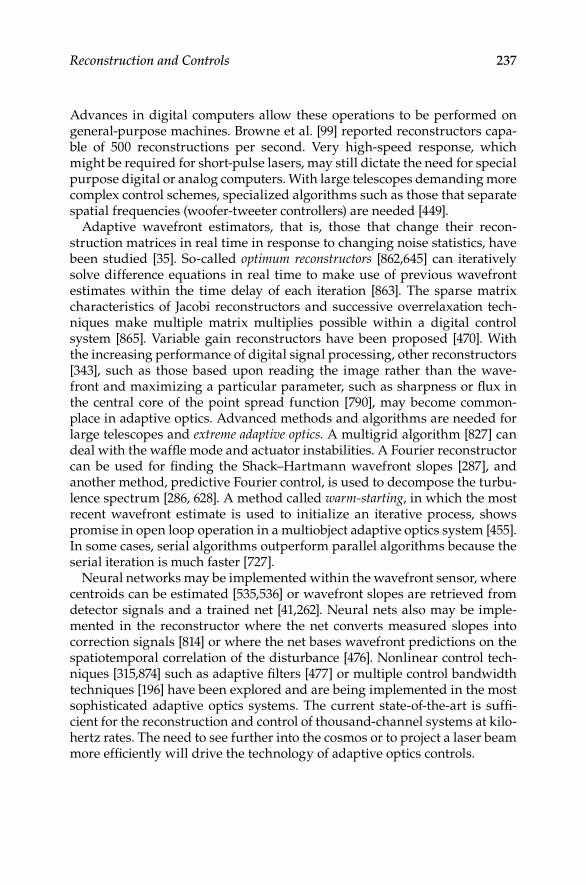
Reconstruction and Controls 237
Advances in digital computers allow these operations to be performed on general-purpose machines Browne et al [99] reported reconstructors capa-ble of 500 reconstructions per second Very high-speed response, which might be required for short-pulse lasers, may still dictate the need for special purpose digital or analog computers With large telescopes demanding more complex control schemes, specialized algorithms such as those that separate spatial frequencies (woofer-tweeter controllers) are needed [449]
Adaptive wavefront estimators, that is, those that change their recon-struction matrices in real time in response to changing noise statistics, have been studied [35] So-called optimum reconstructors [862,645] can iteratively solve difference equations in real time to make use of previous wavefront estimates within the time delay of each iteration [863] The sparse matrix characteristics of Jacobi reconstructors and successive overrelaxation tech-niques make multiple matrix multiplies possible within a digital control system [865] Variable gain reconstructors have been proposed [470] With the increasing performance of digital signal processing, other reconstructors [343], such as those based upon reading the image rather than the wave-front and maximizing a particular parameter, such as sharpness or flux in the central core of the point spread function [790], may become common-place in adaptive optics Advanced methods and algorithms are needed for large telescopes and extreme adaptive optics A multigrid algorithm [827] can deal with the waffle mode and actuator instabilities A Fourier reconstructor can be used for finding the Shack–Hartmann wavefront slopes [287], and another method, predictive Fourier control, is used to decompose the turbu-lence spectrum [286, 628] A method called warm-starting, in which the most recent wavefront estimate is used to initialize an iterative process, shows promise in open loop operation in a multiobject adaptive optics system [455] In some cases, serial algorithms outperform parallel algorithms because the serial iteration is much faster [727]
Neural networks may be implemented within the wavefront sensor, where centroids can be estimated [535,536] or wavefront slopes are retrieved from detector signals and a trained net [41,262] Neural nets also may be imple-mented in the reconstructor where the net converts measured slopes into correction signals [814] or where the net bases wavefront predictions on the spatiotemporal correlation of the disturbance [476] Nonlinear control tech-niques [315,874] such as adaptive filters [477] or multiple control bandwidth techniques [196] have been explored and are being implemented in the most sophisticated adaptive optics systems The current state-of-the-art is suffi-cient for the reconstruction and control of thousand-channel systems at kilo-hertz rates The need to see further into the cosmos or to project a laser beam more efficiently will drive the technology of adaptive optics controls


239
8 Summary of Important Equations
This chapter contains a summary of the most important equations and rela-tionships in adaptive optics The meaning and definition of each variable is described in the text near the original equation See Figures 81 and 82 for some relationships between the parameters
8.1 Atmospheric Turbulence Wavefront Expressions
Fried’s coherence length for plane waves (Equation 221) and for spherical waves (Equation 223):
r k C z zn
L
02 2
0
3 5
0 423=
∫
−
. sec( ) ( )d/
β (81)
r k C zzL
zn
L
02 2
5 3
0
0 423sph =
∫. sec( ) ( ) d
/
β
−3 5/
(82)
The isoplanatic angle (Equation 327):
θ02 2
3 5
2 91 5 3=
∫
−
. ( ) d/
/
k C z z zn
L
path
(83)
Wavefront tilt variance (Equation 243):
σ tilt2 2 2
0
2 2 11 60 2073= × +∫ −. d ( ) d [ ] /k zC z kn
L κ κ
−−∞
∞
−∞
∞
∫∫
16kD
JD
D
2 2 2
2
κ
κ
2
(84)
Tilt angle due to atmospheric turbulence for two uncorrelated axes or each axis (Equation 245):
α λ αtwo axis oneor− =
2
0
5 3 2
0 364./
Dr D −− =
axis
2
0
5 3 2
0 182./
Dr D
λ (85)

240 Principles of Adaptive Optics
Turbulencestrength r0
Fittingerror
Temporalerror
Tilttemporal
errorTilt
isoplanaticerror
Tiltmeasurement
error
Wavefronterror
Angularisoplanatic
error
Focalisoplanatic
error
Turbulencebandwidth fG
Backgroundradiation Background
radiation
Wavefront referencesource magnitude
Wavefront beacon direction
Isoplanaticangle 0
Tiltbandwidth
Tilt isoplanaticangle
LGSoffset angle
Resulting error
External factors
Tilt starmagnitude
LGSaltitude
Figure 8.1External factors and disturbances contribute to the resulting error that remains after compensation
ActuatorspacingActuator
influencefunctions
Servobandwidth
DM responsetime
Tilt detectorcharacteristics
Tilt servobandwidth
Tilttemporal
errorTilt
isoplanaticerror
Focalisoplanatic
error
Tiltmeasurement
error
Temporalerror
Fittingerror
Angularisoplanatic
error
Wavefronterror
Integrationtime
Detectorcharacteristics
Telescopeaperture
Number ofbeacons
System errors
Design factors
Figure 8.2The allowable system errors drive the technology, design, and cost of the adaptive optics system

Summary of Important Equations 241
Atmospheric turbulence tilt Greenwood frequency (Equation 254):
f D C z zn
L
T w=
− − ∫0 331 1 6 1 1 2 2 2
0
. sec ( ) d/ /λ β ν
1 2/
(86)
Full-aperture tilt through the atmosphere (from space) that will appear on a tilt sensor (Equation 516):
α λtilt
0tele=
2 25 6
./
Dr D
M (87)
The standard deviation of angular tilt of the atmosphere (Equation 61):
α λSD
0
=
0 435 6
./
Dr D
(88)
The standard deviation of phase error of the atmosphere (Equation 63):
φSD0
waves=
0 065 6
./
Dr
(89)
Higher-order atmospheric turbulence Greenwood frequency (Equation 270):
f C z z zn
L
G w5/3=
− ∫2 31 6 5 2
0
. sec ( ) ( )d/λ β υ33 5/
(810)
Focal anisoplanatism parameter d0 (Equation 337):
dz
zC z zn0 =
∫λ β6 5 3 5
5 3
219 77/ /
/
cos . ( )dLGS
−3 5/
(811)
Atmospheric turbulence modulation transfer function (Equations 274 and 275):
M z k C Lnturb = << ( )−1 0 4 2 2
05 3 1
, . / (812)
MF
rzturb = −
>>exp.
, ./
2 010 4
0
5 3ξ λ
kk CLn2 2
05 3 1/( )−
(813)

242 Principles of Adaptive Optics
Hufnagel–Valley boundary model (Equation 218):
C zW
nz2 23 10
2
16 25 94 1027
2 7 10= ×
+ ×− − − −. e . e zz hA/ e3 10+ − (814)
Bufton wind model (Equation 217):
υ( ) exp( . )
.z
z= + − −
5 30
309 44 8
2
(815)
8.2 Atmospheric Turbulence Amplitude Expressions
Log-amplitude variance for a plane wave (Equation 230) and a spherical wave (Equation 231):
σχ2 7 6 11 6 20 307= . / /k L Cn (816)
σχ2 7 6 11 6 20 124= . / /k L Cn (817)
Bradley–Herrmann thermal blooming distortion number (Equation 278):
NP n T k LC aB
p w
d d= −4 22
( / ) αρ υ
(818)
8.3 Adaptive Optics Compensation Expressions
The uncompensated turbulence wavefront variance (Equation 261):
σuncompuncomp0
2
5 3
1 02=
.
/D
r (819)
The wavefront variance after two-axis tilt is removed (Equation 262):
σ tiltcomp0
2
5 3
0 134=
./
Dr
(820)

Summary of Important Equations 243
The wavefront variance after tilt and focus are removed (derived from Equation 39):
σFoc2
0
= 0.111Dr
5 3/
(821)
The wavefront variance for higher-mode corrections (Equation 39):
σ2 3 2
0
5 3
0 2944=
−. ( )/
/
NDrm radians2 (822)
The resultant Strehl ratio for higher-mode corrections (Equation 513):
S NDrN>
−= −
21
3 2
0
5 3
0 2944exp . ( / )
/
(823)
Adaptive optics correction fitting error (Equation 310):
σ fits2
0
5 3
=
κrr
/
(824)
The angular tilt variance after compensation (Equation 317):
α λcomp
TG
3dB
2
2 2
=
ff D
(825)
The higher-order wavefront variance due to temporal constraints (Equation 318):
σ tempG
3dB
2
5 3
=
ff
/
(826)
The higher-order wavefront variance due to anisoplanatism (Equation 326):
σ θθiso
2
0
5 3
=
/
(827)
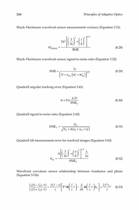
244 Principles of Adaptive Optics
Shack–Hartmann wavefront sensor measurement variance (Equation 321):
σ
π
WFS(H)2
2
2 2 1 2
23
16 8=
+
s/
SSNR (828)
Shack–Hartmann wavefront sensor signal-to-noise ratio (Equation 322):
SNRpix r bg
=+ +( )
N
N n σ σ2 21 2/ (829)
Quadcell angular tracking error (Equation 541):
σ λ= 0 6./D
SNRV
(830)
Quadcell signal-to-noise ratio (Equation 542):
SNR4
VS
S B D e
=+ + +
NN n n n( )2
(831)
Quadcell tilt measurement error for resolved images (Equation 543):
σπ
qcVSNR
=
+
316 8 2
2 2 1 2n
a
/λ
(832)
Wavefront curvature sensor relationship between irradiance and phase (Equation 5116):
I
sr1 2
1 2
2( ) ( )( ) ( )
( )
r I rI r I r
f f s fs
− −+ −
=−
∇ Φ
− ∂
∂
=
nfs
rfs
Φ δcw2 2c (833)

Summary of Important Equations 245
8.4 Laser Guide Star Expressions
The higher-order wavefront variance due to focal anisoplanatism (Equation 336):
σcone2
0
5 3
=
Dd
/
(834)
Detected Rayleigh photon flux (Equation 342):
F Tn E
cRayleigh A2 R R
0
= η σπ
λ4 2
LGS
zz
h∆
(835)
Detected sodium photon flux (Equation 352):
F Tz
EhcSodium A
Na col
02
LGS= ησ ρ
πλ
2
4 (836)
Laser brightness with wavefront error and jitter (Equation 428):
Brightness =
−
π π φλ
λ
D PTK2
22
4
exp∆
22
2
12 22
+
. αλ
jitD (837)


247
Bibliography
1 Abramowitz, M, and I A Stegun Handbook of Mathematical Functions New York: Dover, 1972
2 Acton, D S “Correction of static optical errors in a segmented adaptive optical system” Appl Opt 34 (1995): 7965
3 Acton, D S, and R B Dunn “Solar imaging at the National Solar Observatory using a segmented adaptive optics system” Proc SPIE 1920 (1993): 348
4 Acton, D S, and RC Smithson “Solar imaging with a segmented adaptive mirror” Appl Opt 31 (1992): 3161
5 Adelman, N T “Spherical mirror with piezoelectrically controlled curvature” Appl Opt 16 (1977): 3075
6 Agrawal, G P, and M Lax “Effects of interference on gain saturation in laser resonators” J Opt Soc Am 69 (1979): 1717
7 Akkapeddi, P R, E T Siebert, J Baker, G T Volpe, and H J Robertson “Target loop adaptive optics: thermal blooming correction” Appl Opt 20 (1981): 564
8 Aksenov, V P, and Y N Isaev “Analytical representation of the phase and its mode components reconstructed according to the wavefront slopes” Opt Lett 17 (1992): 1180
9 Aksinin, V I, S A Chetkin, V V Kijko, and S V Muraviev “Tilt corrector based on spring-type magnetostrictive actuators” Opt Eng 32 (1993): 447
10 Alda, J, and G D Boreman “Analysis of edge effects for deformable mirrors” Opt Eng 31 (1992): 2282
11 Aldrich, R E “Requirements for piezoelectric materials for deformable mir-rors” Ferroelectrics 27 (1980): 19
12 Allen, J B Baran, L Schmutz, and J Yorsz “Speckle and adaptive optics tech-niques” Photonic Spectra 22 (1988): 97
13 Alzetta, G, S Gozzini, A Lucchesini, S Cartaleva, T Karaulanov, C Marinelli, and L Moi “Complete electromagnetically induced transparency in sodium atoms excited by a multimode dye laser” Phys Rev A 69, (2004): 1
14 Anafi, D, J M Spinhirne, R H Freeman, and K E Oughstun “Intracavity adaptive optics 2: Tilt correction performance” Appl Opt 20 (1981): 1926
15 Anan’ev, Y A, and V E Sherstobitov “Influence of the edge effects on the prop-erties of unstable resonators” Sov J Quantum Electron 1 (1971): 263
16 Andersen, T, OGarpinger, MOwner-Petersen, F Bjoorn, R Svahn, and A Ardeberg “Novel concept for large deformable mirrors” Opt Eng 45 (2006): 073001
17 Andrews, L C “Aperture-averaging factor for optical scintillations of plane and spherical waves in the atmosphere” J Opt Soc Am A 9 (1992): 597
18 Andrews, L C, and R L Phillips Laser Beam Propagation through Random Media Bellingham, WA: SPIE Opt Eng Press, 1998
19 Andrews, L C, R L Phillips, and C Y Hopen Laser Beam Scintillation with Applications, Bellingham, WA: SPIE Press, 2001
20 Angel, J R P “Use of natural stars with laser beacons for large telescope adap-tive optics,” Proc. Laser Guide Star Adaptive Optics Workshop 2, 494 Albuquerque, NM: U S Air Force Phillips Laboratory, 1992

248 Bibliography
21 Angelbeck, A W, R C Pietro, E D Hasselmark, E Gagnon, A F Greiner, W C McClurg, G R Wisner, and R H Freeman “Development of a cooled metal mirror with active figure control” Internal United Technologies Report, United Technologies Corp, East Hartford, CT, 1975
22 Wilson, J K, et al “Annual reports of astronomical observations and depart-ments: University of Chicago” (abstract only), Bull Am Astron Soc 23, (1991): 173
23 Antsiferov, V N, A G Malinin, Y V Danchenko, and V V Timofeev “Mathematical modeling of deformation of a large mirror made from a high-porosity honeycombed metal” Sov J Opt Technol 55 (1988): 8
24 Anuskiewicz, J, M J Northcott, and J E Graves “Adaptive optics at the University of Hawaii II: control system with real-time diagnostics” Proc SPIE 2201 (1994): 879
25 AOptix Technologies, Inc, Campbell, CA Available at wwwaoptixcom 26 Apollonov, V V, V I Aksinin, S A Chetkin, V V Kijko, S V Muraviev, and
G V Vdovin “Magnetostrictive actuators in optical design” Proc SPIE 1543 (1991): 313
27 Ardeberg, A, and T Anderson “Low turbulence–high performance” Proc SPIE 1236 (1990): 543
28 Ardeberg, A, and T Anderson “Active optics at work” Proc ICO-16 Satellite Conf on Active and Adap Opt, ESO Conf and Workshop Proc 48 (1993) 433
29 Ardila, A, R Baptista, B Blum, J Rose, A Tokovinin, and S Zepf “SOAR for-ward look instrument plan,” 2008 Available at: wwwlnabr/soar
30 Arines, J, V Duran, Z Jaroszewicz, J Area, E Tajahuerce, P Prado, J Lancis, S Bara, and V Climent “Measurement and compensation of optical aberra-tions using a single spatial light modulator” Opt Expr 15 (2007): 15287
31 Armitage, J D, and A Lohmann “Rotary shearing interferometry” Optica Acta 12, (1965): 185
32 Arnoldus, H F, and T F George “Fresnel coefficients for a phase conjugator” J Opt Soc Am B 6 (1989) 30
33 Arsenault, R, D Salmon, F Roddier, G Monnet, J Kerr, and J Sovka “The Canada–France–Hawaii Telescope adaptive optics instrument adaptor” Proc SPIE 1920 (1993): 364
34 Artzner, G “Microlens arrays for Shack-Hartmann wavefront sensors” Opt Eng 31 (1992): 1311
35 Asher, R B “Wavefront estimation for adaptive optics, Interim Report I” U S Air Force Frank J Seiler Research Laboratory, SRL-TR-76-0010, July 1976
36 Asher, R B, and R D Neal “Adaptive estimation of aberration coefficients in adaptive optics” U S Air Force Frank J Seiler Research Laboratory, SRL-TR-77-0009, May 1977
37 Asher, R B, and R F Ogrodnik “Estimation and control in mutidither adaptive optics” J Opt Soc Am 67 (1977): 3
38 Aspinwall, D M, and R D Dotson “Actuator configurations for segmented mirror figure control” Proc SPIE 365 (1982): 123
39 Astrom, K J, and B Wittenmark Computer-Controlled Systems—Theory and Design 2nd ed Englewood Cliffs, NJ: Prentice-Hall, 1990
40 Atad, E, J W Harris, C M Humphries, and V C Salter “Lateral shearing inter-ferometry: evaluation and control of the optical performance of astronomical telescopes” Proc SPIE 1236 (1990): 575

Bibliography 249
41 Atad, E, G Catalan, J W Harris, C M Humphries, A M Smillie, A F Armitage, G S Hanspal, and R J McKeating “Hartmann wavefront sensing with an arti-ficial neural network processor” Proc SPIE 2201 (1994): 490
42 Aubailly, M, M C Roggemann, and T J Schulz “Approach for reconstructing anisoplanatic adaptive optics images” Appl Opt 46 (2007) 6055
43 Auslander, D M, Y Takahashi, and M J Rabins Introducing Systems and Control New York: McGraw-Hill, 1974
44 Avicola, K, J M Brase, J R Morris, H D Bissinger, J M Duff, H W Friedman, D T Gavel, C E Max, S S Olivier, R W Presta, D A Rapp, J T Salmon, and K E Waltjen “Sodium-layer laser-guide-star experimental results” J Opt Soc Am A 11 (1994): 825
45 Babcock, H W “The possibility of compensating astronomical seeing” Publ Astron Soc Pac 65 (1953): 229
46 Babcock, H W “Adaptive optics revisited” Science 249 (1990): 253 47 Babcock, H W “Astronomical background for adaptive optics,” Proc. Laser
Guide Star Adaptive Optics Workshop 1, 1 Albuquerque, NM: U S Air Force Phillips Laboratory, 1992
48 Babcock, H W, B H Rule, and J S Fassero “An improved automatic guider” Publ Astron Soc Pac 68 (1956): 256
49 Baker, K L “Interferometric wavefront sensors for high contrast imaging” Opt Expr 14 (2006): 10970
50 Band, O, and N Ben-Yosef “Number of correcting mirrors versus the number of measured points in adaptive optics” Opt Eng 33 (1994): 466
51 Baranec, C, and R Dekany “Study of a MEMS-based Shack-Hartmann wave-front sensor with adjustable pupil sampling for astronomical adaptive optics” Appl Opt 47 (2008): 5155
52 Barat, J “Some characteristics of clear-air turbulence in the middle strato-sphere” J Atmos Sci 39 (1982): 2553
53 Barbero, S, and L N Thibos “Error analysis and correction in wavefront recon-struction from the transport-of-intensity equation” Opt Eng 45 (2006): 94001
54 Barbieri, M, R Alonso, S Desidera, A Sozzetti, A F M Fiorenzano, J M Almenara, M Cecconi, R U Claudi, D Charbonneau, M Endl, V Granata, R Gratton, G Laughlin, and B Loeillet “Characterization of the HD 17156 planetary system” Astro Astrophys 503 (2009): 601
55 Barchers, J D, and T A Rhoadarmer “Evaluation of phase-shifting approaches for a point-diffraction interferometer with the mutual coherence function” Appl Opt 41 (2002): 7499
56 Bareket, N “Three-channel phase detector for pulsed wavefront sensing” Proc SPIE 551 (1985): 12
57 Barnard, J J “Fine scale thermal blooming instability: a linear stability analy-sis” Appl Opt 28 (1989): 438
58 Barnes, W P, Jr Optical materials—reflective In Applied Optics and Optical Engineering, Vol VII, eds R R Shannon and J C Wyant New York: Academic Press, 1979
59 Barr, L D “The 15-meter National New Technology Telescope - a progress report” Proc SPIE 365 (1982): 8
60 Barrett, H H, C Dainty, and D Lara “Maximum-likelihood methods in wave-front sensing: stochastic models and likelihood functions” J Opt Soc Am A 24 (2007): 391

250 Bibliography
61 Barrett, H H, and S F Jacobs “Retroreflective arrays as approximate phase conjugators” Opt Lett 4, (1979): 190
62 Basden, A, T Butterley, R Myers, and R Wilson “Durham extremely large tele-scope adaptive optics simulation platform” Appl Opt 46 (2007): 1089
63 Basden, A, D Geng, D Guzman, T Morris, R Myers, and C Saunter “ Shack-Hartmann sensor improvement using optical binning” Appl Opt 46 (2007): 6136
64 Basu, S, D Voelz, and D K Borah “Fade statistics of a ground-to-satellite opti-cal link in the presence of lead-ahead and aperture mismatch” Appl Opt 48 (2009) 1274
65 Batchelor, G K The Theory of Homogeneous Turbulence London: Cambridge Univ Press, 1953
66 Bates, W J “A wavefront shearing interferometer” Proc Phys Soc 59 (1947): 940 67 Beckers, J M “ESO symposium on large telescopes and their instrumentation,”
ESO-Proc 693 Garching, 1988 68 Beckers, J M “The VLT interferometer IV The utility of partial adaptive optics”
Proc SPIE 1236 (1990): 154 69 Beckers, J M “The VLT interferometer II Factors affecting on-axis operation”
Proc SPIE 1236 (1990): 364 70 Beckers, J M “Removing perspective elongation effects in laser guide stars and
their use in the ESO Very Large Telescope,” Proc. Laser Guide Star Adaptive Optics Workshop 2, 629 Albuquerque, NM: U S Air Force Phillips Laboratory, 1992
71 Beckers, J M “Introduction to the conference” Proc ICO-16 Satellite Conf on Active and Adap Opt, ESO Conf and Workshop Proc 48 (1993)
72 Beland, R, and Krause-Polstorff, J “Variation of Greenwood frequency mea-surements under different meteorological conditions,” Proc. Laser Guide Star Adaptive Optics Workshop 1, 289 Albuquerque, NM: U S Air Force Phillips Laboratory, 1992
73 Belen’kii, M S “Influence of stratospheric turbulence on infrared imaging” J Opt Soc Am A 12 (1995): 2517
74 Belen’kii, M S “Effect of the inner scale of turbulence on the atmospheric mod-ulation transfer function” J Opt Soc Am A 13 (1996): 1078
75 Belmonte, A, and J M Kahn “Capacity of coherent free-space optical links using atmospheric compensation techniques” Opt Expr 17 (2009): 2763
76 Belsher, J F, and D L Fried Adaptive Optics Mirror Fitting Error Placentia, CA: The Optical Sciences Co Report TR-521, 1983
77 Benedict, R, Jr, J B Breckinridge, and D L Fried “Atmospheric compensation technology: Introduction” J Opt Soc Am A 11 (1994) 257
78 Berkefeld, T, A Glindemann, and S Hippler “Multi-conjugate adaptive optics with two deformable mirrors - requirements and performance” Exp Astro 11 (2001): 1
79 Bickel, G, and G Hausler “Optical simulation of Huygens’s principle” J Opt Soc Am A 5 (1988): 843
80 Bienfang, J C, C A Denman, B W Grime, P D Hillman, G T Moore, and J M Telle “20 W of continuous-wave sodium D2 resonance radiation from sum-frequency generation with injection-locked lasers” Opt Lett 28 (2003): 2219
81 Bifano, T, P Bierden, and J Perreault “Micromachined deformable mirrors for dynamic wavefront control” Proc SPIE 5553 (2004): 1

Bibliography 251
82 Bifano, T G, R K Mali, J K Dorton, J Perreault, N Vandelli, M N Horenstein, and D A Castanon “Continuous-membrane surface-micromachined silicon deformable mirror” Opt Eng 36 (1997): 1354
83 Bikkannavar, S, C Ohara, and M Troy “Autonomous phase retrieval control for calibration of the Palomar adaptive optics system” Proc SPIE 7015 (2008) 70155K
84 Bin-Nun, E, and F Dothan-Deutsch “Mirror with adjustable radius of curva-ture” Rev Sci Instrum 44 (1973) 512
85 Blanc, A, L M Mugnier, and J Idier “Marginal estimation of aberrations and image restoration by use of phase diversity” J Opt Soc Am A 20 (2003): 1035
86 Bold, G T, T H Barnes, and T G Haskell “Aberration correction using optical feedback” Proc Top Mtg on Adap Opt, ESO Conf and Workshop Proc 54 (1996): 421
87 Bonora, S, and L Poletto “Push-pull membrane mirrors for adaptive optics” Opt Expr 14 (2006): 11935
88 Boreman, G D, and C Dainty “Zernike expansions for non-Kolmogorov tur-bulence” J Opt Soc Am A 13 (1996): 517
89 Born, M, and E Wolf Principles of Optics 5th ed Oxford: Pergamon, 1975 90 Boston Micromachines Corp Available at: wwwbostonmicromachinescom 91 Bowker, J K Pulsed Laser Wavefront Sensor Cambridge, MA: Adaptive Optics
Assoc Tech Report 78-1, 1978 92 Bradley, L C, and J Herrmann “Numerical calculation of light propagation in
a nonlinear medium” J Opt Soc Am 61 (1971): 668 (abstract) 93 Brady, G R, M Guizar-Sicairos, and J R Fienup “Optical wavefront measure-
ment using phase retrieval with transverse translation diversity” Opt Expr 17 (2009): 624
94 Breaux, H, W Evers, R Sepucha, and C Whitney “Algebraic model for cw thermal-blooming effects” Appl Opt 18 (1979): 15
95 Breckinridge, J B “Coherence interferometer and astronomical applications” Appl Opt 11 (1972): 2996
96 Bridges, W D, P T Brunner, S P Lazzara, T A Nussmeier, T R O’Meara, J A Sanguinet, and W P Brown “Coherent optical adaptive techniques” J Appl Opt 13 (1974): 2
97 Briggs, R J Models of High Spatial Frequency Thermal Blooming Instabilities Lawrence Livermore National Lab UCID-21118, 1987
98 Brousseay, D, E F Borra, and S Thibault “Wavefront correction with a 37-actuator ferrofluid deformable mirror” Opt Expr 15 (2007): 18190
99 Browne, S L, J L Vaughn, G A Tyler, and J D Gonglewski “A computation-ally efficient method for wavefront reconstruction” Proc Top Mtg on Adap Opt, ESO Conf. and Workshop Proc 54 (1996): 125
100 Bruno, T L, and A Wirth “Adaptive optics finds down-to-Earth applications” Photonics Spectra (June 1996): 139
101 Bruns, D G “Five-order adaptive optics for meter-class telescopes” Top Mtg on Adap Opt, Opt Soc Am Tech Dig Series 13 (1996): 63
102 Bruns, D G, T K Barrett, D G Sandler, H M Martin, G Brusa, J R P Angel, R Biasi, D Gallieni, and P Salinari “Force-actuated adaptive secondary mirror pro-totype” Proc Top Mtg on Adap Opt, ESO Conf and Workshop Proc 54 (1996): 251
103 Bryant, J J, J W O’Byrne, R A Minard, and P W Fekete “Low order adaptive optics at the Anglo-Australian Telescope” Proc Top Mtg on Adap Opt, ESO Conf and Workshop Proc 54 (1996): 23

252 Bibliography
104 Buchdahl, H A “Optical aberration coefficients” J Opt Soc Am 50 (1960): 539 105 Buchheim, R K, R Pringle, and H W Schaefgen “Lead-angle effects in
turbulence-compensating reciprocity tracking systems” Appl Opt 17 (1978): 165
106 Bufton, J L “Comparison of vertical profile turbulence structure with stellar observations” Appl Opt 12 (1973): 1785
107 Bures, K J TASC Tech Inform Memo 996-8, August 1977 108 Burns, S A, R Tumbar, A E Elsner, D Ferguson, and D X Hammer
“Large-field-of-view, modular, stabilized, adaptive-optics-based scanning laser ophthalmoscope” J Opt Soc Am 24 (2007): 1313
109 Burrows, A, M Marley, W B Hubbard, J I Lunine, T Guillot, D Saumon, R Freedman, D Sudarsky, and C Sharp “A nongray theory of extrasolar giant planets and brown dwarfs” Astrophys J 491 (1997): 856
110 Buscher, D, P Doel, R Humphreys, R Myers, M Wells, A Longmore, B Gentles, G Jones, and S Worswick “Natural guide star adaptive optics for the 42m William Herschel telescope” Top Mtg on Adap Opt, Opt Soc Am Tech Dig Series 13 (1996): 66
111 Butts, R R, and C B Hogge “Phase conjugate adaptive optics using perimeter phase measurement” J Opt Soc Am 67 (1977): 278
112 Calef, B, E Therkildsen, and M Roggemann “Wavefront-sensor-based frame selection” Opt Eng 44 (2005): 116003
113 Cannon, R H Dynamics of Physical Systems New York: McGraw-Hill, 1967 114 Carslaw, H S, and J C Jaeger Conduction of Heat in Solids 2nd ed London:
Oxford University Press, 1980 115 Cao, G, and X Yu “Accuracy analysis of a Hartmann-Shack wavefront sensor
operated with a faint object” Opt Eng 33 (1994): 2331 116 Cao, Z, Q Mu, L Hu, D Li, Z Peng, Y Liu, and L Xuan “Preliminary use of
nematic liquid crystal adaptive optics with a 216-meter reflecting telescope” Opt Expr 17 (2009): 2530
117 Cao, Z, Q Mu, L Hu, Y Liu, Z Peng, X Liu, and L Xuan “Achromatic sys-tem for a twisted alignment liquid crystal wavefront corrector” Appl Opt 47 (2008): 1020
118 Casasent, D “Spatial light modulators” Proc IEEE 65 (1977): 143 119 Cederquist, J, S R Robinson, D Kryskowski, J R Fienup, and C C Wackerman
“Cramer-Rao lower bound on wavefront sensor error” Opt Eng 25 (1986): 4 120 Cense, B, E Koperda, J M Brown, O P Kocaoglu, W Gao, R S Jonnal, and D T
Miller “Volumetric retinal imaging with ultrahigh-resolution spectral-domain optical coherence tomography and adaptive optics using two broadband light sources” Opt Expr 17 (2009): 4095
121 Chaffin, J H “Optical coatings for active components” Proc SPIE 1543 (1991): 165
122 Chamot, S R, C Dainty, and S Esposito “Adaptive optics for ophthalmic applications using a pyramid wavefront sensor” Opt Expr 14 (2006): 518
123 Chassat, F, G Rousset, and J Primot “Theoretical and experimental evaluation of isoplanatic patch size for adaptive optics” Proc SPIE 1114 (1989): 14
124 Checkland, P Systems Thinking, Systems Practice New York: Wiley, 1986 125 Chen, C, H Yang, X Feng, and H Wang “Optimization criterion for initial
coherence degree of lasers in free-space optical links through atmospheric tur-bulence” Opt Lett 34 (2009): 419

Bibliography 253
126 Chen, C F, and I J Haas Elements of Control Systems Analysis, Englewood Cliffs, NJ: Prentice-Hall, 1968
127 Chen, C T Linear System Theory and Design New York: Holt, Rinehart, and Winston, 1984
128 Chen, L, P B Kruger, H Hofer, B Singer, and D R Williams “Accommodation with higher-order monochromatic aberrations corrected with adaptive optics” J Opt Soc Am A 23 (2006): 1
129 Chen, M, F S Roux, and J C Olivier “Detection of phase singularities with a Shack-Hartmann wavefront sensor” J Opt Soc Am A 24 (2007): 1994
130 Chernov, L A Wave Propagation in a Random Medium New York: McGraw-Hill, 1960 131 Chi, C, N B James III, and P L Misuinas “Spectral shared aperture compo-
nent” Proc SPIE 171 (1979): 145 132 Christopher, N M, and I Smail “A catalogue of potential adaptive optics sur-
vey fields from the UKIRT archive” Mon Not Roy Astron Soc 365 (2006): 439 133 Christou, J C “Blind deconvolution post-processing of images corrected by
adaptive optics” Proc SPIE 2534 (1995): 226 134 Christou, J C “Reference-less detection, astrometry, and photometry of faint
companions with adaptive optics” Astrophys J 698 (2009): 28 135 Christou, J C “Gemini Observatory adaptive optics instrumentation and capa-
bilities” Am Astro Soc 215 (2009): 214 136 Chui, T Y P, H Song, and S A Burns “Adaptive-optics imaging of human
cone photoreceptor distribution” J Opt Soc Am A 25 (2008): 12 137 Chung, C-Y, K-C Cho, C-C Chang, C-H Lin, W-C Yen, and S-J Chen
“Adaptive-optics system with liquid-crystal phase-shift interferometer” Appl Opt 45 (2006): 3409
138 Churchman, C W The Systems Approach New York: Dell, 1983 139 Churnside, J H “Aperture averaging of optical scintillations in the turbulent
atmosphere” Appl Opt 30 (1991): 1982 140 Claflin, E S, and N Bareket “Configuring an electrostatic membrane mirror by
least-squares fitting with analytically derived influence functions” J Opt Soc Am A 3 (1986): 1833
141 Clampin, M “Optimization of MCP intensifier tubes in astronomical adaptive optics sensors” Proc SPIE 1114 (1989): 152
142 Clampin, M, J Crocker, F Paresce, and M Rafal “Optical Ranicon detectors for photon counting imaging: I” Rev Sci Instrum 59 (1988): 1
143 Clark, R, J Karpinsky, G Borek, E Johnson, and N Clark “High speed micro-machine device for adaptive correction of aero-optic effects” Proc Top Mtg on Adap Opt, ESO Conf and Workshop Proc 54 (1996): 433
144 Claus, A C “On Archimedes’ burning glass” Appl Opt 12 (1973): A14 145 Clifford, S F “The classical theory of wave propagation in a turbulent medium”
In Laser Beam Propagation in the Atmosphere, Chap 2, J W Strohbehn, ed, New York: Springer-Verlag, 1978
146 Coates, P B “A theory of afterpulse formation in photomultipliers and the pulse height distribution” J Phys D: Appl Phys 6 (1973): 1159
147 Close, L M, and D W McCarthy, Jr “Infrared imaging using a tip-tilt secondary mirror” Proc SPIE 1920 (1993): 353
148 Conan, R “Mean-square residual error of a wavefront after propagation through atmospheric turbulence and after correction with Zernike polynomials” J Opt Soc Am A 25 (2008): 526

254 Bibliography
149 Conan, R, C Bradley, P Hampton, O Keskin, A Hilton, and C Blain “Distributed modal command for a two-deformable-mirror adaptive optics system” Appl Opt 46 (2007): 4329
150 Conan, R, O Lardiere, G Herriot, C Bradley, and K Jackson “Experimental assessment of the matched filter for laser guide star wavefront sensing” Appl Opt 48 (2009): 1198
151 Conforti, G “Zernike aberration coefficients from Seidel and higher-order power-series coefficients” Opt Lett 8 (1983): 7
152 Corrsin, S “On the spectrum of isotropic temperature fluctuations in an isotro-pic turbulence” J Appl Phys 22 (1951): 469
153 Costa, J B, S Hippler, M Feldt, S Esposito, R Ragazzoni, P Bizenberger, E Puga, and T F E Henning “PYRAMIR: A near-infrared pyramid wavefront sensor for the Calar Alto adaptive optics system” Proc SPIE 4839 (2003): 280
154 Crawford, D P, R K Tyson, and R J Morgan “Interaction of thermal bloom-ing, turbulence, and slewing in ground-to-space propagation” Proc SPIE 1221 (1990): 146
155 Creath, K “Comparison of phase-measurement algorithms” Proc SPIE 680 (1986): 19
156 Cubalchini, R “Modal wavefront estimation from phase derivative measure-ments” J Opt Soc Am 69 (1979): 7
157 Cuellar, L, P Johnson, and D G Sandler “Performance tests of a 1500 degree-of-freedom adaptive optics system for atmospheric compensation” Proc SPIE 1542 (1991): 468
158 Dai, Y, Z Liu, Z Jin, J Xu, and J Lin “Active control of a 30 m ring interfero-metric telescope primary mirror” Appl Opt 48 (2009): 664
159 Dalimier, E, and C Dainty “Use of a customized vision model to analyze the effects of higher-order ocular aberrations and neural filtering on contrast thresh-old performance” J Opt Soc Am A 25 (2008): 2078
160 Daly, D Microlens Arrays Boca Raton, FL: CRC Press, 2000 161 Davies, R, S Rabien, C Lidman, M LeLouarn, M Kasper, N M Forster,
Schreibner, V Roccatagliata, N Ageorges, P Amico, C Dumas, and F Mannucci “Laser guidestar adaptive optics without tip-tilt” European Southern Observatory Messenger 131 (2008): 7
162 Davis, D S, P Hickson, G Herriot, and C-Y She “Temporal variability of the telluric sodium layer” Opt Lett 31 (2006): 3369
163 Dayton, D, B Pierson, B Spielbusch, and J Gonglewski “Atmospheric struc-ture function measurements with a Shack-Hartmann wavefront sensor” Opt Lett 17 (1992): 1737
164 de Chatellus, H G, I Moldovan, V Fesquet, and J-P Pique “Suppression of Rayleigh scattering noise in sodium laser guide stars by hyperfine depolariza-tion of fluorescence” Opt Expr 14 (2006): 11494
165 de Chatellus, H G, J-P Pique, and I C Moldovan “Return flux budget of poly-chromatic laser guide stars” J Opt Soc Am A 25 (2008): 400
166 Dekany, R G “The Palomar adaptive optics system” Top Mtg on Adap Opt, Opt Soc Am Tech Dig Series 13 (1996): 40
167 DeMarco, T Structured Analysis and Systems Specification Englewood Cliffs, NJ: Prentice-Hall, 1979
168 DeMaria, A “High-power carbon dioxide lasers” J Proc IEEE 61 (1973): 6

Bibliography 255
169 Denman, C A, P D Hillman, G T Moore, J M Telle, J E Preston, J D Drummond, and R Q Fugate “Realization of a 50 watt facility-class sodium guidestar pump laser” Proc SPIE 5707 (2005): 46
170 Dente, G C, D C Gardner, and P D Tannen “Error propagation in lateral shearing interferometry” WJSA-R-86-A-018, Albuquerque, NM: W J Schafer Associates, Inc, 1986
171 Devaney, N “Adaptive optics specification for a 10m telescope on the ORM” Top Mtg on Adap Opt, Opt Soc Am Tech Dig Series 13 (1996): 24
172 Dimov, N A, A A Kornienko, G N Mal’tsev, and A S Pechenov “Investigation of the quality of a spatial approximation of a wavefront for a zonal-modal cor-rection” Sov J Opt Technol 52 (1985): 317
173 Doel, P “A comparison of Shack-Hartmann and curvature sensing for large tele-scopes” Proc SPIE 2534 (1995): 265
174 Dolne, J J, R J Tansey, K A Black, J H Deville, P R Cunningham, K C Widen, and P S Idell “Practical issues in wavefront sensing by use of phase diversity” Appl Opt 42 (2003): 5284
175 Dooling, D “Peeking behind the veil of Venus” Nat Sol Obs Press release February 10, 2006
176 Down, D “Image-position error associated with a focal plane array” J Opt Soc Am A 9 (1992): 700
177 Downie, J D, and J W Goodman “Accuracy requirements of optical linear algebra processors in adaptive optics imaging systems” Appl Opt 28 (1989): 4298
178 Downie, J D, and J W Goodman “Optimal wavefront control for adaptive segmented mirrors” Appl Opt 28 (1989): 5326
179 Drummond, J, J Telle, C Denman, P Hillman, and A Tuffli “Photometry of a sodium laser guide star at the Starfire Optical Range” Publ Astron Soc Pac 116 (2004): 278
180 Dubra, A “Wavefront sensor and wavefront corrector matching in adaptive optics” Opt Expr 15 (2007): 2762
181 Duffner, R W The Adaptive Optics Revolution: A History Albuquerque, NM: University of New Mexico Press, 2009
182 Dunkle, T “The Big Glass,” Discover, July 1989 183 Dunphy, J R, and D C Smith “Multiple-pulse thermal blooming and phase
compensation” J Opt Soc Am A 67 (1977): 295 184 Ealey, M A “Deformable mirrors at Litton/Itek: A historical perspective” Proc
SPIE 1167 (1989): Paper No 4 185 Ealey, M A “Actuators: Design fundamentals, key performance specifications,
and parametric trades” Proc SPIE 1543 (1991): 346 186 Ealey, M A, and J F Washeba “Continuous facesheet low voltage deformable
mirrors” Opt Eng 29 (1990): 1191 187 Ealey, M A, and J A Wellman “Deformable mirrors: Design fundamen-
tals, key performance specifications, and parametric trades” Proc SPIE 1543 (1991): 36
188 Ealey, M A, and J A Wellman “Xinetics low cost deformable mirrors with actuator replacement cartridges” Proc SPIE 2201 (1994): 680
189 Edlen, B “The refractive index of air” Metrologia 2 (1966): 71 190 Eichel, P H, and C V Jakowatz, Jr “Phase-gradient algorithm as an optimal
estimator of the phase derivative” Opt Lett 14 (1989): 1101

256 Bibliography
191 Eichler, H J, A Haase, and R Menzel “Solid-state laser amplifier with SBS-phase conjugation” Proc ICO-16 Satellite Conf on Active and Adap Opt, ESO Conf and Workshop Proc 48, (1993): 401
192 Elbaum, M, and P Diament “SNR in photocounting images of rough objects in partially coherent light” Appl Opt 15 (1976): 2268
193 Elbaum, M, and P Diament “Estimation of image centroid, size, and orienta-tion with laser radar” Appl Opt 16 (1977): 2433
194 Elbaum, M, and M Greenebaum “Annular apertures for angular tracking” Appl Opt 16 (1977): 2438
195 Ellerbroek, B L “First-order performance evaluation of adaptive-optics systems for atmospheric-turbulence compensation in extended-field-of-view astronomi-cal telescopes” J Opt Soc Am A 11 (1994): 783
196 Ellerbroek, B L, C Van Loan, N P Pitsianis, and R J Plemmons “Optimizing closed loop adaptive optics performance using multiple control bandwidths” Proc SPIE 2201 (1994): 935
197 Ellerbroek, B L, and T A Rhoadarmer “Optimization of closed-loop adap-tive-optics control algorithms using measured performance data: Experimental results” Top Mtg on Adap Opt, Opt Soc Am Tech Dig Series 13 (1996): 233
198 Ellerbroek, B L, D W Tyler, and R Racine “Sky coverage calculations for Shack-Hartmann NGS AO systems” Proc Top Mtg on Adap Opt, ESO Conf and Workshop Proc 54 (1996): 357
199 Elson, J M, H E Bennett, and J M Bennett Scattering from optical surfaces In Applied Optics and Optical Engineering, eds R R Shannon, J C Wyant, Vol VII, New York: Academic Press, 1979
200 Enguehard, S, and B Hatfield “Perturbative approach to the small-scale physics of the interaction of thermal blooming and turbulence” J Opt Soc Am A 8 (1991): 637
201 Erry, G, P Harrison, J Burnett, D Benton, A Scott, and S Woods “Results of atmospheric compensation using a wavefront curvature based adaptive optics system” Proc SPIE 4884 (2003): 245
202 Esposito, S, G Brusa, and D Bonaccini “Liquid crystal wavefront correctors: Computer simulation results” Proc ICO-16 Satellite Conf on Active and Adap Opt, ESO Conf and Workshop Proc 48 (1993): 289
203 Esposito, S, and A Riccardi “Pyramid wavefront sensor behavior in partial correction adaptive optic systems” Astron Astrophys 369 (2001): L9
204 Evans, J W, B Macintosh, L Poyneer, K Morzinski, S Severson, D Dillon, D Gavel, and L Reza “Demonstrating sub-nm closed loop MEMS flattening” Opt Expr 14 (2006): 5558
205 Everson, J H, R E Aldrich, and N P Albertinetti “Discrete actuator deform-able mirror” Opt Eng 20 (1981): 316
206 Everson, J H, and J A Greenough “Evaluation of a deformable monolithic mirror/heat exchanger unit” Proc SPIE 179 (1979): 91
207 Fabellinskii, I L Molecular Scattering of Light, New York: Plenum, 1968 208 Fante, R L “The effect of source temporal coherence on light scintillations in
weak turbulence” J Opt Soc Am 69 (1979): 71 209 Fante, R L “Electromagnetic beam propagation in turbulent media: An update”
Proc IEEE 68 (1980): 1434 210 Feinleib, J Proposal 82-P4 Cambridge, MA: Adaptive Optics Associates, 1982 211 Feinleib, J, S G Lipson, and P F Cone “Monolithic piezoelectric mirror for
wavefront correction” Appl Phys Lett 25 (1974): 311
Bibliography 257
212 Fender, J S ed “Synthetic aperture systems” Proc SPIE 440 (1984) 213 Fengjie, X, J Zongfu, X Xiaojun, and G Yifeng “High-diffractive-efficiency defo-
cus grating for wavefont curvature sensing” J Opt Soc Am A 24 (2007): 3444 214 Fenster, A, J C Leblanc, W B Taylor, and H E Johns “Linearity and fatigue in
photo-multipliers” Rev Sci Instrum 44 (1973): 689 215 Fernandez, E J, and P Artal “Ocular aberrations up to the infrared range: From
6328 to 1070 nm” Opt Expr 16 (2008): 21199 216 Fienup, J R “Phase retrieval algorithms: A comparison” Appl Opt 21 (1982): 2758 217 Fienup, J R “Phase-retrieval algorithms for a complicated optical system” Appl
Opt 32 (1993): 1737 218 Figueira, G, J Wemans, H, Pires, N Lopes, and L Cardoso “Single adjuster
deformable mirror with four contact points for simultaneous correction of astig-matism and defocus” Opt Expr 15 (2007): 5664
219 Fisher, A D “Self-referenced high resolution adaptive wavefront estimation and compensation” Proc SPIE 551 (1985): 102
220 Fisher, A D, and C Warde “Technique for real-time high-resolution adaptive phase compensation” Opt Lett 8 (1983): 353
221 Fisher, R A Optical Phase Conjugation New York: Academic Press, 1983 222 Flath, L, J An, J Brase, C Carrano, C B Dane, S Fochs, R Hurd, M Kartz, and
R Sawvel “Development of adaptive techniques for high-power lasers” Proc 2nd Int Workshop on Ad Opt for Industry and Medicine, G Love, ed Singapore: World Scientific, 1999
223 Florence, J M “Joint-transform correlator systems using deformable-mirror spatial light modulators” Opt Lett 14 (1989): 341
224 Foley, J T, and M A Abdul Jalil “Role of diffraction in phase retrieval from intensity measurements” Proc SPIE 351 (1982): 80
225 Foo, G, D M Palacios, and G A Swartzlander, Jr “Optical vortex corona-graph” Opt Lett 30 (2005): 3308
226 Forbes, F F “Bimorph PZT active mirror” Proc SPIE 1114 (1989): 146 227 Forbes, F F, D A Morse, and G A Poczulp “Site survey instrumentation for
the National New Technology Telescope (NNTT)” Opt Eng 27 (1988): 845 228 Ford, S D, M C Roggemann, and B M Welsh “Frame selection performance
limits for statistical image reconstruction of adaptive optics compensated images” Opt Eng 35 (1996): 1025
229 Foy, R, and A Labeyrie “Feasibility of adaptive optics telescope with laser probe” Astron Astrophys 152 (1985): L29
230 Foy, R, A Migus, F Biraben, G Grynberg, P R McCullough, and M Tallon “The polychromatic artificial sodium star: A new concept for correcting atmo-spheric tilt” Astron Astrophys Supp Ser 111 (1995): 569
231 Foy, R, J P Pique, V Bellanger, P Chevrou, A Petit, C Hogemann, L Noethe, M Schock, J Girard, M Tallon, E Thiebaut, J Vaillant, F C Foy, and M Van Dam “Feasibility study of the polychromatic laser guide star” Proc SPIE 4839 (2003): 484
232 Foy, R, M Tallon, M Sechaud, and N Hubin “ATLAS experiment to test the laser probe technique for wavefront measurements” Proc SPIE 1114 (1989): 174
233 Frantz, L M, A A Sawchuk, and W von der Ohe “Optical phase measurement in real time” Appl Opt 18 (1979): 19

258 Bibliography
234 Freeman, R H, R J Freiberg, and H R Garcia “Adaptive laser resonator” Opt Lett 2 (1978): 3
235 Freeman, R H, H R Garcia, J DiTucci, and G R Wisner “High-Speed Deformable Mirror System,” US Air Force Weapons Laboratory Report AFWL-TR-76-146, Kirtland Air Force Base, New Mexico (unpublished), 1977
236 Freischlad, K R, and C L Koliopoulos “Modal estimation of a wavefront from difference measurements using the discrete Fourier transform” J Opt Soc Am A 3 (1986): 11
237 Fried, D L “The effect of wavefront distortion on the performance of an ideal optical heterodyne receiver and an ideal camera” Conf on Atmospheric Limitations to Optical Propagation Gaithersburg, MD: U S Nat Bur Stds CRPL, 1965
238 Fried, D L “Statistics of a geometric representation of wavefront distortion” J Opt Soc Am 55 (1965): 1427
239 Fried, D L “Limiting resolution looking down through the atmosphere” J Opt Soc Am 56 (1966): 1380
240 Fried, D L Effect of Speckle on Wavefront Distortion Sensing Placentia, CA: The Optical Sciences Company Report TR-251, 1977
241 Fried, D L “Least-square fitting a wavefront distortion estimate to an array of phase-difference measurements” J Opt Soc Am 67 (1977): 370
242 Fried, D L “Resolution, signal-to-noise ratio, and measurement precision” J Opt Soc Am 69 (1979): 399
243 Fried, D L “Anisoplanatism in adaptive optics” J Opt Soc Am 72 (1982): 52 244 Fried, D L “Analysis of focus anisoplanatism: The fundamental limit in perfor-
mance of artificial guide star adaptive optics systems (AGS/AOS)” Proc Laser Guide Star Adaptive Optics Workshop 1, 37 Albuquerque, NM: U S Air Force Phillips Laboratory, 1992
245 Fried, D L “Focus anisoplanatism in the limit of infinitely many artificial-guide-star reference spots” J Opt Soc Am A 12 (1995): 939
246 Fried, D L, and G E Mevers “Evaluation of ro for propagation down through the atmosphere” Appl Opt 13 (1974): 11
247 Fried, D L, and J L Vaughn Focus Anisoplanatism for a Multiple Spot Artificial Guide-Star Pattern Placentia, CA: The Optical Sciences Company Report BC-641, 1991
248 Fried, D L, and J F Belsher “Analysis of fundamental limits to artificial-guide-star adaptive-optics-system performance for astronomical imaging” J Opt Soc Am A 11 (1994): 277
249 Friedman, H, K Avicola, H Bissinger, J Brase, J Duff, D Gavel, J Horton, C Max, S Olivier, D Rapp, T Salmon, D Smauley, and K Waltjen “Laser guide star mea-surements at Lawrence Livermore National Laboratory” Proc SPIE 1920 (1993): 52
250 Friedman, H, G Erbert, T Kuklo, T Salmon, D Smauley, G Thompson, J Malik, N Wong, K Kanz, and K Neeb “Sodium beacon laser system for the Lick Observatory” Proc SPIE 2534 (1995): 150
251 Friedman, H, J Morris, and J Horton “System design for a high power sodium laser beacon” Proc Laser Guide Star Adaptive Optics Workshop 2, 639 Albuquerque, NM: U S Air Force Phillips Laboratory, 1992
252 Friedman, H, R Foy, M Tallon, and A Migus “First results of a polychromatic artificial sodium star for correction of tilt” Top Mtg on Adap Opt, Opt Soc Am Tech Dig Series 13 (1996): 78

Bibliography 259
253 Fu, T Y, and M Sargent III “Effects of signal detuning on phase conjugation” Opt Lett 4 (1979): 366
254 Fugate, R Q “Laser beacon adaptive optics for power beaming applications,” Proc SPIE 2121 (1994): 68
255 Fugate, R Q “Observations of faint objects with laser beacon adaptive optics,” Proc SPIE 2201 (1994): 10
256 Fugate, R Q, D L Fried, G A Ameer, B R Boeke, S L Browne, P H Roberts, R E Ruane, and L M Wopat “Measurement of atmospheric wavefront distor-tion using scattered light from a laser guide star,” Nature 353 (1991): 144
257 Fugate, R Q, C H Higgins, B L Ellerbroek, J M Spinhirne, B R Boeke, R A Cleis, D W Swindle, and M D Oliker “Laser beacon adaptive optics with an unintensified CCD wavefront sensor and fiber optic synthesized array of silicon avalanche photodiodes for fast guiding,” Proc ICO-16 Satellite Conf on Active and Adap Opt, ESO Conf and Workshop Proc 48 (1993): 487
258 Fugate, R Q, J F Riker, J T Roark, S Stogsdill, and B D O’Neil “Laser beacon compensated images of Saturn using a high-speed, near-infrared correlation tracker,” Proc Top Mtg on Adap Opt, ESO Conf and Workshop Proc 54 (1996): 287
259 Fuschetto, A “Three-actuator deformable water-cooled mirror,” Opt Eng 20 (1981): 310
260 Fuschetto, A “Three-actuator deformable water-cooled mirror,” Proc SPIE 179 (1979)
261 Gaffard, J-P, P Jagourel, and P Gigan “Adaptive optics: Description of avail-able components at LASERDOT,” Proc SPIE 2201 (1994): 688
262 Gallant, P J, and G J M Aitken “Simple neural networks as wavefront slope predictors: Training and performance issues,” Top Mtg on Adap Opt, Opt Soc Am Tech Dig Series 13 (1996): 253
263 Garcia, H R, and L D Brooks “Characterization techniques for deformable metal mirrors,” Proc SPIE 141 (1978): 74
264 Gardner, C S, B M Welsh, and L A Thompson “Design and performance analysis of adaptive optical telescopes using laser guide stars,” Proc IEEE 78 (1990): 1721
265 Gaskill, J D Linear Systems, Fourier Transforms, and Optics New York: Wiley, 1978
266 Gavel, D T “Tomography for multiconjugate adaptive optics systems using laser guide stars,” Proc SPIE 5490 (2004): 1356
267 Gavel, D T, C E Max, K Avicola, H D Bissinger, J M Brase, J Duff, H W Friedman, J R Morris, S S Olivier, D A Rapp, J T Salmon, and K E Waltjen “Design and early results of the sodium-layer laser guide star adap-tive optics experiment at the Lawrence Livermore National Laboratory,” Proc ICO-16 Satellite Conf on Active and Adap Opt, ESO Conf and Workshop Proc 48 (1993): 493
268 Gavel, D T, and S S Olivier “Simulation and analysis of laser guide star adap-tive optics systems for the eight to ten meter class telescopes,” Proc SPIE 2201 (1994): 295
269 Gavrielides, A “Vector polynomials orthogonal to the gradient of Zernike poly-nomials,” Opt Lett 7 (1982): 526
270 Gbur, G, and R K Tyson “Vortex beam propagation through atmospheric tur-bulence and topological charge conservation,” J Opt Soc Am A 25 (2008): 225

260 Bibliography
271 Ge, J, B Jacobsen, J R P Angle, N Woolf, J H Black, M Lloyd-Hart, P Gray, and R Q Fugate “An optical ultrahigh resolution spectrograph with the adap-tive optics,” Top Mtg on Adap Opt, Opt Soc Am Tech Dig Series 13 (1996): 122
272 Geary, J C “Rapid-framing CCDs with 16 output ports for laser guide star sen-sors,” Proc SPIE 2201 (1994): 607
273 Geary, J C, and G A Luppino “New circular radial-scan frame-storage CCDs for low-order adaptive optics wavefront curvature sensing,” Proc SPIE 2201 (1994): 588
274 Geary, J M “Ray misidentification errors in Hartmann-like wavefront sensors,” Opt Eng 30 (1991): 1388
275 Geary, J M Introduction to Wavefront Sensors Bellingham, WA: SPIE Optical Engineering Press, 1995
276 Gebhardt, F G “High power laser propagation,” Appl Opt 15 (1976): 1479 277 Gebhardt, F G “Twenty-five years of thermal blooming: An overview,” Proc
SPIE 1221 (1990): 2 278 Gendron, E “Modal control optimization in an adaptive optics system,” Proc
ICO-16 Satellite Conf on Active and Adap Opt, ESO Conf and Workshop Proc 48 (1993): 187
279 Gerchberg, R W, and W O Saxton “A practical algorithm for the determina-tion of phase from image and diffraction plane pictures,” Optic (Stuttgart) 35 (1972): 237
280 Germann, L M “Specification of fine-steering mirrors for line-of-sight stabiliza-tion systems,” Proc SPIE 1543 (1991): 202
281 Ghiglia, D C, and L A Romero “Direct phase estimation from phase dif-ferences using fast elliptic partial differential equation solvers,” Opt Lett 14 (1989): 1107
282 Giacconi, R VLT Whitebook European Southern Observatory: Garching bei Munchen, 1998
283 Gil, M A, and J M Simon “Diffraction grating and optical aberrations: A new and exact formulation,” Appl Opt 24: (1985): 2956
284 Gilles, L, and B Ellerbroek “Shack-Hartmann wavefront sensing with elon-gated sodium laser beacons: Centroiding versus matched filtering,” Appl Opt 45 (2006): 6568
285 Gilles, L, and B L Ellerbroek “Constrained matched filtering for extended dynamic range and improved noise rejection for Shack-Hartmann wavefront sensing,” Opt Lett 33 (2008): 1159–61
286 Give’on, A, N J Kasdin, R J Vanderbei, and Y Avitzour “On representing and correcting wavefront errors in high-contrast imaging systems,” J Opt Soc Am A 23 (2006): 1063
287 Glazer, O, E N Ribak, and L Mirkin “Adaptive optics implementation with a Fourier reconstructor,” Appl Opt 46 (2007): 574
288 Gleckler, A D, D J Markason, and G H Ames “PAMELA: Control of a seg-mented mirror via wavefront tilt and segment piston sensing,” Proc SPIE 1543 (1991): 176
289 Glindemann, A, and T Berkefeld “A new method for separating atmospheric layers using a Shack-Hartmann curvature sensor,” Top Mtg on Adap Opt, Opt Soc Am Tech Dig Series 13 (1996): 153
290 Goede, P, T Heinz, F Johnson, and A MacCollum “Diamond turned deform-able mirror,” Proc SPIE 365 (1982): 138

Bibliography 261
291 Golbraikh, E, and N Kopeika “Turbulence strength parameter in laboratory and natural optical experiments in non-Kolmogorov cases,” Opt Commun 242 (2008): 333
292 Goldberg, D Genetic Algorithms in Search, Optimization and Machine Learning Reading, MA: Addison Wesley Longman, 1989
293 Goncharov, A V, N Devaney, and C Dainty “Atmospheric dispersion compen-sation for extremely large telescopes,” Opt Expr 15 (2007): 1534
294 Gonglewski, J D, D G Voelz, J S Fender, D C Dayton, B K Spielbusch, and R E Pierson “First astronomical application of postdetection turbulence com-pensation: Images of α Aurigae, ν Ursae Majoris, and α Germinorum using self-referenced speckle holography,” Appl Opt 29 (1990): 4527
295 Gonsalves, R “Phase retrieval from modulus data,” J Opt Soc Am 66 (1976): 961 296 Gonsalves, R A “Fundamentals of wavefront sensing by phase retrieval,” Proc
SPIE 351 (1982): 56 297 Gonsalves, R A “Phase retrieval by differential intensity measurements,” J Opt
Soc Am A 4 (1987): 166 298 Goodfriend, M J, K M Shoop, and C G Miller “High force, high strain, wide
band width linear actuator using the magnetostrictive material, Terfenol-D,” Proc SPIE 1543 (1991): 301
299 Goodman, J W Introduction to Fourier Optics New York: McGraw-Hill, 1968 300 Goodman, J W Statistical Optics, 413 New York: Wiley, 1985 301 Goodman, J W, W H Huntley, Jr, D W Jackson, and M Lehman “Wavefront-
reconstruction imaging through random media,” Appl Phys Lett 8 (1966): 311 302 Goodman, J W, and M S Song “Performance limitations of an analog method
for solving simultaneous linear equations,” Appl Opt 21 (1982): 502 303 Gordeyev, S, T E Hayden, and E J Jumper “Aero-optical and flow measure-
ments over a flat-windowed turret,” AIAA J 45 (2007): 347 304 Gosselin, P, P Jagourel, and J Peysson “Objective comparisons between stacked
array mirrors and bimorph mirrors,” Proc SPIE 1920 (1993): 81 305 Graves, J E “Future directions for the University of Hawaii adaptive optics
program,” Top Mtg on Adap Opt, Opt Soc Am Tech Dig Series 13 (1996): 49 306 Gray, D C, W Merigan, J I Wolfing, B P Gee, J Porter, A Dubra, T H
Twietmeyer, and K Ahmad “In vivo fluorescence imaging of primate retinal ganglion cells and retinal pigment epithelial cells,” Opt Expr 14 (2006): 7144
307 Greenwood, D P “Bandwidth specification for adaptive optics systems,” J Opt Soc Am 67 (1977): 390
308 Greenwood, D P “Tracking turbulence-induced tilt errors with shared and adjacent apertures,” J Opt Soc Am 67 (1977): 282
309 Greenwood D P, and C A Primmerman “Adaptive optics research at Lincoln Laboratory,” Lincoln Lab J 5 (1992): 3; Greenwood, D P, and C A Primmerman “The history of adaptive-optics development at the MIT Lincoln Laboratory,” Proc SPIE 1920 (1993): 220
310 Greivenkamp, J E, and D G Smith “Graphical approach to Shack-Hartmann lenslet array design,” Opt Eng 47 (2008): 063601
311 Grossman, S B, and R B Emmons “Performance analysis and size optimiza-tion of focal planes for point-source tracking algorithm applications,” Opt Eng 23 (1984): 167
312 Grosso, R P, and M Yellin “The membrane mirror as an adaptive optical ele-ment,” J Opt Soc Am 67 (1977): 399

262 Bibliography
313 Gruneisen, M T, R C Dymale, J R Rotge, L F DeSandre, and D L Lubin Wavelength-dependent characteristics of a telescope system with diffractive wavefront compensation,” Opt Eng 44 (2005): 068002
314 Guha, J K, and J A Plascyk “Low-absorption grating beam samplers,” Proc SPIE 171 (1979): 117
315 Gully, S W, J Huang, N Denis, D P Looze, A Wirth, A J Jankevics, and D A Castaflon “Experiments with adaptive nonlinear control systems for atmospheric correction,” Proc SPIE 2201 (1994): 920
316 Gurski, G F, N T Nomiyama, R J Radley, and J Wilson “An initial evaluation of performance of adaptive optical systems with extended dynamic targets,” J Opt Soc Am 67 (1977): 345
317 Halevi, P “Bimorph piezoelectric flexible mirror: Graphical solution and com-parison with experiment,” J Opt Soc Am 73 (1983): 110
318 Han, I “New method for estimating wavefront from curvature signal by curve fitting,” Opt Eng 34 (1995): 1232
319 Happer, W, G J MacDonald, C E Max, and F J Dyson “Atmospheric-turbulence compensation by resonant optical backscattering from the sodium layer in the upper atmosphere,” J Opt Soc Am A 11 (1994): 263
320 Hardy, J W “Active optics: A new technology for the control of light,” Proc IEEE 66 (1978): 651
321 Hardy, J W “Instrumental limitations in adaptive optics for astronomy,” Proc SPIE 1114 (1989): 2
322 Hardy, J W “Adaptive optics—a progress review,” Proc SPIE 1542 (1991): 2 323 Hardy, J W Adaptive Optics for Astronomical Telescopes New York: Oxford Univ
Press, 1998 324 Hardy, J W, J Feinleib, and J C Wyant “Real-time correction of optical imag-
ing systems,” OSA Meeting on Optical Propagation through Turbulence, Boulder, CO, 1974
325 Hardy, J W, J E Lefebvre, and C L Koliopoulos “Real-time atmospheric com-pensation,” J Opt Soc Am 67 (1977): 360
326 Hardy, J W, and A J MacGovern “Shearing interferometry: A flexible tech-nique for wavefront measurement,” Proc SPIE 816 (1987)
327 Hardy, J W and E P Wallner “Wavefront compensation using active lenses,” Proc SPIE 2201 (1994): 77
328 Harney, R C “Active laser resonator control techniques,” Appl Opt 17 (1978): 11 329 Harrington, P M, and B M Welsh “Frequency-domain analysis of an adaptive
optical systems’ temporal response,” Opt Eng 33 (1994): 2336 330 Hart, N W, M C Roggemann, A Sergeyev, and T J Schulz “Characterizing
static aberrations in liquid crystal spatial light modulators using phase retrieval,” Opt Eng 46 (2007): 086601
331 Hart, M, N M Milton, C Baranec, T Stalcup, K Powell, E Bendek, D McCarthy, and C Kulesa “Wide field astronomical image compensation with multiple laser-guided adaptive optics,” Proc SPIE 7486 (2009): L1
332 Hartmann, J “Bemerkungen uber den Bau und die Justirung von Spektrographen,” Z. Instrumentenkd 20 (1900): 47
333 Hartmann, J “Objektuvuntersuchungen,” Z. Instrumentenkd 24 (1904): 1 334 Harvey, J E, and G M Callahan “Transfer function characterization of deform-
able mirrors,” J Opt Soc Am 67 (1978)
Bibliography 263
335 Harvey, J E and M L Scott “The hole grating beam sampler,” Opt Eng 20 (1981): 881
336 Harvey, J E, J L Forgham, and K von Bieren “The spot of Arago and its role in wavefront analysis,” Proc SPIE 351 (1982): 2
337 Hatfield, B Thermal Blooming in the Presence of Turbulence and Diffusion Woburn, MA: North East Research Assoc, Inc, presented to PCAP Committee, Lexington, MA, 1988
338 Helmbrecht, M A, and T Juneau “Piston-tip-tilt positioning of a segmented MEMS deformable mirror,” Proc SPIE 6467 (2007)
339 Hemmati, H, and Y Chen “Active optical compensation of low-quality optical system aberrations,” Opt Lett 31 (2006):1630
340 Herrmann, J “Properties of phase conjugate adaptive optical systems,” J Opt Soc Am 67 (1997): 290
341 Hickson, P “Wavefront curvature sensing from a single defocused image,” J Opt Soc Am A 11 (1994): 1667
342 Hiddleston, H R, D D Lyman, and E L Schafer “Comparisons of deformable mirror models and influence functions,” Proc SPIE 1542 (1991): 20
343 Hinnen, K, M Verhaegen, and N Doelman “Exploiting the spatiotemporal correlation in adaptive optics using data-driven H2-optimal control,” J Opt Soc Am A 24 (2007): 1714
344 Hinz, PM, A N Heinze, S Sivanandam, D L Miller, M A Kenworthy, G Brusa, M Freed, and J R P Angel “Thermal infrared constraint to a planetary compan-ion of Vega with the MMT adaptive optics system,” Astrophys J 653 (2006): 1486
345 Hippler, S, F Hormuth, D J Butler, W Brandner, and T Henning “ Atmosphere-like turbulence generation with surface-etched phase-screens,” Opt Expr 14 (2006): 10139
346 Hogan, W J, L J Atherton, and J A Paisner “National ignition facility design focuses on optics,” Laser Focus World 32 (1996): 107
347 Hogge, C B, and R R Butts U S Air Force Weapons Laboratory Report, AFWL-TR-78-15, Kirtland Air Force Base, New Mexico (unpublished), 1978
348 Hogge, C B, and R R Butts “Effects of using different wavelengths in wave-front sensing and correction,” J Opt Soc Am 72 (1982): 606
349 Holmes, D A, and P V Avizonis “Approximate optical system model,” Appl Opt 15 (1976): 1075
350 Holmes, R “Scintillation-induced jitter of projected light with centroid track-ers,” J Opt Soc Am A 26 (2009): 313
351 Hopkins, M M “The frequency response of a defocused optical system,” Optica Acta 2 (1955): 91
352 Hopkins, M M “The frequency response of optical systems,” Proc Phys Soc London, Sect B 69 (1956): 562
353 Hormuth, F, W Brandner, S Hippler, and T Henning “Astralux - the Calar Alto 22-m telescope lucky imaging camera,” J Phys Conf Series 131 (2008): 012051
354 Hornbeck, L J “128 x 128 deformable mirror device,” IEEE Trans Electron Dev ED-30 (1983): 539
355 Horwitz, B A “Multiplex techniques for real-time shearing interferometry,” Opt Eng 29 (1990): 1223
356 Hu, S, B Xu, X Zhang, J Hou, J Wu, and W Jiang “Double-deformable-mirror adaptive optics system for phase compensation,” Appl Opt 45 (2006): 2638

264 Bibliography
357 Huang, L, C Rao, and W Jiang “Modified Gaussian influence function of deformable mirror actuators,” Opt Expr 16 (2008): 108
358 Hubin, N “The ESO VLT adaptive optics programme,” Astro Astrophys Trans 13 (1997)
359 Hubin, N, B L Ellerbroek, R Arsenault, R M Clare, R Dekany, L Gilles, M Kasper, G Herriot, M Le Louarn, E Marchetti, S Oberti, J Stoesz, J P Veran, and C Verinaud “Adaptive optics for extremely large telescopes,” Proc IAU Symp 232 (2005): 60
360 Hudgin, R H “Wavefront compensation error due to finite corrector-element size,” J Opt Soc Am 67 (1977): 393
361 Hudgin, R H “Wavefront reconstruction for compensated imaging,” J Opt Soc Am 67 (1977): 375
362 Hufnagel, R E Proc. Topical Meeting on Optical Propagation through Turbulence, Boulder, CO, 1974; Hufnagel, R E “Propagation through atmospheric turbu-lence,” The Infrared Handbook, eds W L Wolfe and G J Zissis, Chap 6Ann Arbor, MI: Env Res Inst Mich, 1989
363 Hulburd, B, and Sandler, D “Segmented mirrors for atmospheric compensa-tion,” Opt Eng 29 (1990): 1186
364 Hulburd, B, T Barrett, L Cuellar, and D Sandler “High bandwidth, long stroke segmented mirror for atmospheric compensation,” Proc SPIE 1543 (1991): 64
365 Hull, W C, R B Dunn, and M J Small “A 256-channel digital wavefront recon-structor,” Proc SPIE 1920 (1993): 200
366 Humphreys, R A, C A Primmerman, L C Bradley, and J Herrmann “Atmospheric-turbulence measurements using a synthetic beacon in the meso-spheric sodium layer,” Opt Lett 16 (1991): 1367
367 Hunt, B R “Matrix formulation of the reconstruction of phase values from phase differences,” J Opt Soc Am 69 (1979): 393
368 Hutley, M C Diffraction Gratings New York: Academic Press, 1982 369 Idell, P S, and J D Gonglewski “Image synthesis from wavefront sensor mea-
surements of a coherent diffraction field,” Opt Lett 15 (1990): 1309 370 Idell, P S, and D G Voelz “Non conventional laser imaging using sampled-
aperture receivers,” Opt Phot News 8 (April 1992) 371 Iizuka, K Engineering Optics 2nd ed Berlin: Springer-Verlag, 1986 372 Ikeda, O, M Takehara, and T Sato “High-performance image-transmission
system through a turbulent medium using multiple reflectors and adaptive focusing combined with four-wave mixing,” J Opt Soc Am A 1 (1984): 176
373 Ikramov, A V, I M Rotshupkin, and A G Safronov “Investigations of the bimorph piezoelectric mirrors for use in astronomic telescope,” Proc ICO-16 Satellite Conf on Active and Adap Opt, ESO Conf and Workshop Proc 48 (1993): 235
374 Ishimaru, A Wave Propagation and Scattering in Random Media New York: Academic Press, 1977
375 Ivanov, V Yu, V P Sivokon, and M A Vorontsov “Phase retrieval from a set of intensity measurements: Theory and experiment,” J Opt Soc Am A 9 (1992): 1515
376 Jacobsen, B, T Martinez, R Angel, M Lloyd-Hart, S Benda, D Middleton, H Friedman, and G Erbert “Field evaluation of two new continuous-wave dye laser systems optimized for sodium beacon excitation,” Proc SPIE 2201 (1994): 342

Bibliography 265
377 Jagourel, P, and J-P Gaffard “Adaptive optics components in laser-dot,” Proc SPIE 1543 (1991): 76
378 Jankevics, A J, and A Wirth “Wide field of view adaptive optics,” Proc SPIE 1543 (1991): 438
379 Jared, R C, A A Arthur, S Andreae, A K Biocca, R W Cohen, J M Fuertes, J Franck, G Gabor, J Llacer, T S Mast, J D Meng, T L Merrick, R H Minor, J Nelson, M Orayani, P Salz, B A Schaefer, and C Witebsky “The W M Keck telescope segmented primary mirror active control system,” Proc SPIE 1236 (1990): 996
380 MEMS Optical, Technical Information Datasheets wwwmemsopticalcom/techinfo/datasheetshtm
381 Jeong, T M, D Ko, and J Lee “Method of reconstructing wavefront aberrations from the intensity measurement,” Opt Lett 32 (2007): 3507
382 Jeys, T H, A A Brailove, and A Mooradian “Sum frequency generation of sodium resonance radiation,” Appl Opt 28 (1989): 2588
383 Jeys, T H, R M Heinrichs, K F Wall, J Korn, T C Hotaling, and E Kibblewhite “Optical pumping of mesospheric sodium,” Proc Laser Guide Star Adaptive Optics Workshop 1, 238 Albuquerque, NM: U S Air Force Phillips Laboratory, 1992
384 Ji, X, and X Li “Directionality of Gaussian array beams propagating in atmo-spheric turbulence,” J Opt Soc Am A 26 (2009): 236
385 Jiang, W, H Li, C Liu, X Wu, S Huang, H Xian, Z Rong, C Wang, M Li, N Ling, and C Guan “A 37 element adaptive optics system with H-S wave-front sensor,” Proc ICO-16 Satellite Conf on Active and Adap Opt, ESO Conf and Workshop Proc 48 (1993): 127
386 Jiang, W, M Li, G Tang, M Li, and D Zheng “Adaptive optical image com-pensation experiments on stellar objects,” Opt Eng 34 (1995): 15
387 Johansson, E M, M A van Dam, P J Stanski, J M Bell, J C Chin, R C Sumner, P L Wizinowich, R Biasi, M Andrgihettoni, and D Pescoller “Upgrading the Keck wavefront controllers,” Proc SPIE 7015 (2008): 70153E
388 Johns, M “The Giant Magellan telescope,” Proc SPIE 6267 (2006) 389 Johns, M “Progress on the GMT,” Proc SPIE 7012 (2008): 701246 390 Johnson, B, and D V Murphy “Thermal blooming laboratory experiment, Part
I” In Lincoln Laboratory MIT Project Report, Cambridge, MA: MIT Press, 1988 391 Johnson, B, and C A Primmerman “Experimental observation of thermal-blooming
phase-compensation instability,” Opt Lett 14 (1989): 12 392 Johnson, B, and J F Schonfeld “Demonstration of spontaneous thermal-blooming
phase-compensation instability,” Opt Lett 16 (1991): 1258 393 Johnston, D C, and B M Welsh “Atmospheric turbulence sensing for a multi-
conjugate adaptive optics system,” Proc SPIE 1542 (1991): 76 394 Johnston, D C, and B M Welsh “Analysis of multiconjugate adaptive optics,”
J Opt Soc Am A 11 (1994): 394 395 Johnston, D C, B L Ellerbroek, and S M Pompea “Curvature sensing analy-
sis,” Proc SPIE 2201 (1994): 528 396 Johnson P, R Trissel, L Cuellar, B Arnold, and D Sandler “Real time wave-
front reconstruction for a 512 subaperture adaptive optical system,” Proc SPIE 1543 (1991): 460
397 Johnsopn, R, D Montera, T Schneeberger, and J Spinhirne “A new sodium guidestar adaptive optics system for the Starfire Optical Range 35 m telescope,” AFRL-RD-PS, TP-2009-1018, 2009

266 Bibliography
398 Jolissaint, L, J-P Veran, and R Conan “Analytical modeling of adaptive optics: Foundations of the phase spatial power spectrum approach,” J Opt Soc Am A 23 (1006): 382
399 Jonnal, R S, J Rha, Y Zhang, B Cense, W Gao, and D T Miller “In vivo func-tional imaging of human cone photoreceptors,” Opt Expr 15 (2007): 16141
400 Kane, T J, C S Gardner, and L A Thompson “Effects of wavefront sampling speed on the performance of adaptive astronomical telescopes,” Appl Opt 30 (1991): 214
401 Karcher, H J, and H Nicklas “Active structural control of very large tele-scopes,” Proc SPIE 1114 (1989): 320
402 Karr, T J Ground Based Laser Propagation: Status and Prospects Presented to DEW Technology Base Review Panel, San Diego, CA, 1987
403 Karr, T J Ground Based Laser Propagation Review Presented to JASON meeting, San Diego, CA, 1987
404 Karr, T J “Thermal blooming compensation instabilities” J Opt Soc Am A 6 (1989):1038
405 Karr, T J “Temporal response of atmospheric turbulence compensation” Appl Opt 30 (1991): 363
406 Kelsall, D, and R D’Amato “AFWL/OPTICS optical degradation by aero-dynamic boundary layers” MIT Lincoln Laboratory Report, ESD-TR-78-243, 1977
407 Kenrew, S, P Doel, D Brooks, C Dorn, C Yates, R M Dwan, I Richardson, and G Evans “Developments of a carbon fiber composite active mirror: design and testing” Opt Eng 45 (2006): 033401
408 Kenrew, S, P Doel, D Brooks, A M King, C Dorn, C Yates, R M Dwan, I Richardson, and G Evans “Prototype carbon fiber composite deformable mirror” Opt Eng 46 (2007): 094003
409 Kenemuth, J R “Multiactuator deformable mirror evaluations” Proc SPIE 171 (1979): 32
410 Kern, P, P Lena, P Gigan, J Fontanella, G Rousset, F Merkle, and J Gaffard “COME-ON: An adaptive optics prototype dedicated to infrared astronomy” Proc SPIE 1114 (1989): 54
411 Keskin, O, R Conan, P Hampton, and C Bradley “Derivation and experimen-tal evaluation of a point-spread-function reconstruction from a dual-deform-able-mirror adaptive optics system” Opt Eng 47 (2008): 046601
412 Kibblewhite, E “Laser beacons for astronomy,” Proc. Laser Guide Star Adaptive Optics Workshop 1, 24 Albuquerque, NM: U S Air Force Phillips Laboratory, 1992
413 Kibblewhite, E, W Wild, B Carter, M Chun, F Shi, and M Smutko “A descrip-tion of the Chicago Adaptive Optics System (ChAOS),” Proc. Laser Guide Star Adaptive Optics Workshop 2, 522 Albuquerque, NM: U S Air Force Phillips Laboratory, 1992
414 Kibblewhite, E, M F Smutko, and F Shi “The effect of hysteresis on the perfor-mance of deformable mirrors and methods of its compensation” Proc SPIE 2201 (1994): 754
415 Kibblewhite, E J, R Vuilleumier, B Carter, W J Wild, and T H Jeys “Implementation of CW and pulsed laser beacons for astronomical adaptive optics systems” Proc SPIE 2201 (1994): 272
Bibliography 267
416 Kim, Y “Refined simplex method for data fitting” Astron. Data Anal. Software and Sys 125 (1997): 206
417 Kingslake, R, ed Applied Optics and Optical Engineering, Volume II: The Detection of Light and Infrared Radiation New York: Academic Press, 1965; Kingslake, R, and B J Thompson, eds Applied Optics and Optical Engineering, Volume VI: Coherent Optical Devices and Systems New York: Academic Press, 1980
418 Kline-Schoder, R J, and M J Wright “Design of a dither mirror control sys-tem” Mechatronics 2 (1992): 115
419 Kocher, D G “Point image focus sensing using an automated Foucault test” Proc SPIE 351 (1982): 148
420 Kocher, D G “Automated Foucault test for focus sensing” Appl Opt 22 (1983): 1887 421 Kokorowski, S A “Analysis of adaptive optical elements made from piezolec-
tric bimorphs” J Opt Soc Am 69 (1979): 181 422 Kokorowski, S A, M E Pedinoff, and J E Pearson “Analytical, experimental,
and computer-simulation results on the interactive effects of speckle with mul-tidither adaptive optics systems” J Opt Soc Am 67 (1977): 333
423 Kokorowski, S A, T R O’Meara, R C Lind, and T Calderone “Automatic speckle cancellation techniques for multidither adaptive optics” Appl Opt 19 (1980): 371
424 Koliopoulos, C L “Avoiding phase-measuring interferometry’s pitfalls” Photon Spectra (1988): 169
425 Kolmogorov, A “Dissipation of energy in locally isotropic turbulence” In Turbulence, Classic Papers on Statistical Theory, eds S K Friedlander, and L Topper New York: Wiley (Interscience), 1961
426 Konyaev, P A, and V P Lukin “Thermal distortions of focused laser beams in the atmosphere” Appl Opt 24 (1985): 415
427 Korkiakoski, V, C Verinaud, M Le Louarn, and R Conan “Comparison between a model-based and a conventional pyramid sensor reconstructor” Appl Opt 46 (2007): 6176
428 Korkiakoski, V, C Verinaud, and M Le Louarn “Improving the performance of a pyramid wavefront sensor with modal sensitivity compensation” Appl Opt 47 (2008): 79
429 Kornienko, A A, and G N Mal’tsev “Use of spectral expansions of Zernike polynomials for investigating the aberrations of adaptive optical systems” Sov J Opt Technol 55 (1988): 341
430 Korotkova, O, L C Andrews, and R L Phillips “The effect of partially coher-ent quasi-monochromatic Gaussian-beam on the probability of fade” Proc SPIE 5160 (2004): 68
431 Kotani, T, S Lacour, G Perrin, G Robertson, and P Tuthill “Pupil remapping for high contrast astronomy: results from an optical test bed” Opt Expr 17 (2009): 1925
432 Krist, J E, and C J Burrows “Phase-retrieval analysis of pre- and post-repair Hubble Space Telescope images Appl Opt 34 (1995): 4951
433 Krupke, W F, and W R Sooy “Properties of an unstable confocal resonator CO2 laser system” IEEE J Quantum Electron QE-5 (1969)
434 Kulesar, C, H -F Raynaud, C Petit, J -M Conan, and P V de Lesegno “Optimal control, observers and integrators in adaptive optics” Opt Expr 14 (2006): 7464
435 Kuo, B C Automatic Control Systems 5th ed Englewood Cliffs, NJ: Prentice-Hall, 1987

268 Bibliography
436 Kuo, C “Optical tests of an intelligently deformable mirror for space telescope technology” Opt Eng 33 (1994): 791
437 Kurczynski, P, H M Dyson, and B Sadoulet “Stability of electrostatic actuated membrane mirror devices” Appl Opt 45 (2006): 8288
438 Kurczynski, P, H M Dyson, and B Sadoulet “Large amplitude wavefront gen-eration and correction with membrane mirrors” Opt Expr 14 (2006): 509
439 Kwon, O Y, Real-time radial-shear interferometer” Proc SPIE 551 (1985): 32 440 Laag, E A, S M Ammons, D T Gavel, and R Kupke “Multiconjugate adap-
tive optics results from the laboratory for adaptive optics MCAO/MOAO test-bed” J Opt Soc Am A 25 (2008): 2114
441 Labeyrie, A “Attainment of diffraction-limited resolution on large telescope by Fourier analyses speckle pattern in stars images” Astron Astrophys 6 (1970): 85
442 Laird, P, E F Borra, R Bergamesco, J Gingras, L Truong, and A Ritcey “Deformable mirrors based on magnetic liquids” Proc SPIE 5490 (2004): 1493
443 Lam, J F, and W P Brown “Optical resonators with phase-conjugate mirrors” Opt Lett 5 (1980): 61
444 Landis, G A “Letter” Physics Today 13, July 1992 445 Lardiere, O, R Conan, C Bradley, K Jackson, and G Herriot “A laser guide
star wavefront sensor bench demonstrator to TMT” Opt Expr 16 (2008): 5527 446 Large Aperture Mirror Program Large Optics Demonstration Experiment
Washington, DC: Strategic Defense Initiative Organization, unpublished, 1985 447 “Laser guide star teams with adaptive optics to shed light on massive star,”
University of California Newsroon, 26 February 2004 448 Lauterbach, M A, M Ruckel, and W Denk “Light-efficient, quantum-limited
interferometric wavefront estimation by virtual mode sensing” Opt Expr 14 (2006): 3700
449 Lavigne, J -F, and J -P Veran “Woofer-tweeter control in an adaptive optics system using a Fourier reconstructor” J Opt Soc Am A 25 (2008): 2271
450 Law, N M, R G Dekany, C D Mackay, A M Moore, M C Britton, and V Velur “Getting lucky with adaptive optics: Diffraction-limited resolution in the visible with current AO systems on large and small telescopes” Proc SPIE 7014 (2008): 1152
451 Lawrence, R S, G R Ochs, and S F Clifford “Measurements of atmospheric turbulence relevant to optical propagation” J Opt Soc Am A 60 (1970): 826
452 Lazzarini, A, G H Ames, and E Conklin “Methods of hierarchical control for a segmented active mirror Proc SPIE 2121 (1994): 147
453 Lei, F, and H J Tiziani “Atmospheric influence on image quality of airborne photographs” Opt Eng 32 (1993): 2271
454 Lena, P “Adaptive optics: a breakthrough in astronomy” Exp Astron 26 (2009): 35 455 Lessard, L, M West, D MacMynowski, and S Lall “Warm-started wavefront
reconstruction for adaptive optics” J Opt Soc Am A 25 (2008): 1147 456 Levine, B M, J J Janesick, and J C Shelton “Development of a low noise high
frame rate CCD for adaptive optics” Proc SPIE 2201 (1994): 596 457 Levine, B M, and K Kiasaleh “Intensity fluctuations in the Compensated Earth
Moon Earth Laser Link (CEMERLL) experiment” Proc SPIE 2123 (1994): 409 458 Li, C, H Xian, C Rao, and W Jiang “Field-of-view shifted Shack-Hartmann
wavefront sensor for daytime adaptive optics system” Opt Lett 31 (2006): 2821

Bibliography 269
459 Li, E, Y Dai, H Wang, and Y Zhang “Application of eigenmode in the adaptive optics system based on a micromachined membrane deformable mirror” Appl Opt 45 (2006): 5651
460 Li, K Y, and A Roorda “Automated identification of cone photoreceptors in adaptive optics retinal images” J Opt Soc Am A 24 (2007): 1358
461 Li, M, X Li, and W Jiang “Small-phase retrieval with a single far-field image” Opt Expr 16 (2008): 8190
462 Liang, J, and D R Williams “Aberrations and retinal image quality of the nor-mal human eye” J Opt Soc Am A 14 (1997): 2873
463 Liang, J, D R Williams, and D T Miller “Supernormal vision and high-res-olution retinal imaging through adaptive optics” J Opt Soc Am A 14 (1997): 2884
464 Liebelt, P B An Introduction to Optimal Estimation Reading, MA: Addison-Wesley, 1967
465 Lindorff, D P Theory of Sampled-Data Control Systems New York: Wiley, 1965 466 Linnik, V P “On the possibility of reducing the influence of atmospheric seeing
on the image quality of stars” Opt Spectrosc 3 (1957): 401 467 Lipson, S G, E N Ribak, and C Schwartz “Bimorph deformable mirror
design” Proc SPIE 2201 (1994): 703 468 Liu, Y, Z Cao, D Li, Q Mu, L Hu, X Lu, and L Xuan “Correction for large
aberration with phase-only liquid-crystal wavefront corrector” Opt Eng 45 (2006): 128001
469 Liu, Y, and J G Walker “Post-compensation for extended object imaging” Proc ICO-16 Satellite Conf on Active and Adap Opt, ESO Conf and Workshop Proc 48 (1993): 137
470 Liu, Y -T, and J Steve Gibson “Adaptive control in adaptive optics for directed-energy systems” Opt Eng 46 (2007): 046601
471 Llacer, J, R C Jared, and J M Fuertes “Analysis of the W M Keck telescope primary mirror control loop” Proc SPIE 1236 (1990): 1024
472 Lloyd-Hart, M, R Dekany, D Sandler, D Wittman, R Angel, and D McCarthy “Progress in diffraction-limited imaging at the Multiple Mirror Telescope with adaptive optics” J Opt Soc Am A 11 (1994): 846
473 Lloyd-Hart, M, R Angel, B Jacobsen, D Wittman, D McCarthy, E Kibblewhite, B Carter, and W Wild “Preliminary closed-loop results from an adaptive optics system using a sodium resonance guide star” Proc SPIE 2201 (1994): 364
474 Lloyd-Hart, M, J R P Angel, D G Sandler, P Salinari, D Bruns, and T K Barrett “Progress toward the 65-m MMT infrared adaptive optics system” Top Mtg on Adap Opt, Opt Soc Am Tech Dig Series 13 (1996): 28
475 Lloyd-Hart, M, C Baranec, N M Milton, M Snyder, T Stalcup, and J R P Angel “Experimental results of ground-layer and tomographic wavefront reconstruction from multiple laser guide stars” Opt Expr 14 (2006): 7541
476 Lloyd-Hart, M, and P McGuire “Spatio-temporal prediction for adaptive optics wavefront reconstructors” Proc Top Mtg on Adap Opt, ESO Conf and Workshop Proc 54 (1996): 95
477 Lloyd-Hart, M, and T Rhoadarmer “Wavefront control optimization using adaptive filters” Top Mtg on Adap Opt, Opt Soc Am Tech Dig Series 13 (1996): 268
478 Loewen, E G, and M Neviere “Simple selection rules for VUV and XUV dif-fraction gratings” Appl Opt 17 (1978): 1087

270 Bibliography
479 Logean, E, E Dalimier, and C Dainty “Measured double-pass intensity point-spread function after adaptive optics correction of ocular aberrations” Opt Expr 16 (2008): 17384
480 Looze, D P “Minimum variance control structure for adaptive optics systems” J Opt Soc Am A 23 (2006): 603
481 Looze, D P “Discrete-time model of an adaptive optics system” J Opt Soc Am A 24 (2007): 2850
482 Looze, D P “Linear-quadratic-Gaussian control for adaptive optics systems using a hybrid model” J Opt Soc Am A 26 (2009): 1
483 Lors, C A “I-cubed sensor wavefront correction system” Pratt and Whitney Aircraft, FL Internal memorandum August 28, 1978
484 Lors, C A “CLAWS multidither COAT system” Pratt and Whitney Aircraft, FL Internal memorandum May 26, 1978
485 Love, G D “Wavefront correction and production of Zernike modes with a liquid-crystal spatial light modulator” Appl Opt 36 (1997): 1517
486 Love, G, R Myers, A Purvis, R Sharples, and A Glindemann “A new approach to adaptive wavefront correction using a liquid crystal half-wave phase shifter” Proc ICO-16 Satellite Conf on Active and Adap Opt, ESO Conf and Workshop Proc 48 (1993): 295
487 Ludman, J E, H J Caulfield, V Morozov, and J L Sampson “Wavefront recon-struction using self-referenced direct-drive adaptive optics” Opt Eng 33 (1994): 4020
488 Lukin, V P Atmospheric Adaptive Optics Bellingham, WA: SPIE Optical Engineering Press, 1995
489 Lukin, V P, B V Fortes, F Y Kanev, and P A Konyaev “Potential capabili-ties of adaptive-optical systems in the atmosphere” J Opt Soc Am A 11 (1994): 903
490 Lundstrom, L, S Manzanera, P M Prieto, D B Ayala, N Gorceix, J Gustafsson, P Unsbo, and P Artal “Effect of optical correction and remaining aberrations on peripheral resolution acuity in the human eye” Opt Expr 15 (2007): 12654
491 Lush, H J “Photomultiplier linearity” J Sci Instrum 42 (1965): 597 492 Lutomirski, R F “Atmospheric degradation of electrooptical system perfor-
mance” Appl Opt 17 (1978): 3915 493 Lutomirski, R F, and H T Yura “Propagation of a finite optical beam in an
inhomogeneous medium” Appl Opt 10 (1971): 1652 494 Lyons, A “Design of proximity-focused electron lenses” J Phys E 8 (1985): 127 495 Mach, L “Communication of the notices of the Viennese Academy”
Z Instrumentenkd 12 (1892): 89 496 Mahajan, V N “Zernike annular polynomials for imaging systems with annular
pupils” J Opt Soc Am 71 (1981): erratum 1408 497 Makidon, R B, A Sivaramakrishnan, R Soummer, B R Oppenheimer,
L C Roberts Jr, J R Graham, and M D Perrin “The Lyot project: Understanding the AEOS adaptive optics PSF” Proc IAU Coll 200 (2005): 603
498 Malakhov, M N, V F Matyukhin, and B V Pilepskii “Estimating the param-eters of a multielement mirror of an adaptive optical system” Sov J Opt Technol 51 (1984): 141
499 Malakhov, M N, and B V Prilepskii “Method of determining the wavefront profile from information using a detector of the Hartmann type” Opt Spectrosc (USSR) 58 (1985): 271

Bibliography 271
500 Malin, M, W Macy, and G Ferguson “Edge actuation for figure control” Proc SPIE 365 (1982): 114
501 Mannion, P “CCDs ride the tailcoat of digital convergence” Electron Prod 27, April 1996
502 Marchesini, S “A unified evaluation of iterative projection algorithms for phase retrieval” Rev Sci Instrum 78 (2007): 011301
503 Marchetti, E, and R Ragazzoni “Wavefront generator for adaptive optics test-ing” Proc Top Mtg on Adap Opt, ESO Conf and Workshop Proc 54 (1996): 229
504 Marcy, G W “California and Carnegie planet search,” 2005 Available at: http://exoplanetsorg
505 Marlow, W C “Dynamics of a deformable mirror actuator” Opt Eng 33 (1994): 1016
506 Martin, H M, and D S Anderson “Techniques for optical fabrication of a 2-mm-thick adaptive secondary mirror” Proc SPIE 2534 (1995):134
507 Marquet L C “Transmission diffraction grating attenuator for analysis of high power laser beam quality” Appl Opt 10 (1971): 960
508 Massie, N A, R D Nelson, and S Holly “High-performance real-time hetero-dyne interferometry” Appl Opt 18 (1979): 1797
509 Massie, N A, Y Oster, G Poe, L Seppala, and M Shao “Low-cost, high-resolu-tion, single-structure array telescopes for imaging of low-Earth-orbit satellites” Appl Opt 31 (1992): 447
510 Max, C E, K Avicola, J M Brase, H W Friedman, H D Bissinger, J Duff, D T Gavel, J A Horton, R Kiefer, J R Morris, S S Olivier, R W Presta, D A Rapp, J T Salmon, and K E Waltjen “Design, layout, and early results of a feasibility experiment for sodium-layer laser-guide-star adaptive optics” J Opt Soc Am A 11 (1994): 813
511 Max, C E, D T Gavel, S S Olivier, J M Brase, H W Friedman, K Avicola, J T Salmon, A D Gleckler, T S Mast, J E Nelson, P L Wizinowich, and G A Chanan “Issues in the design and optimization of adaptive optics and laser guide stars for the Keck telescopes” Proc SPIE 2201 (1994): 189
512 McAulay, A D “Deformable mirror nearest neighbor optical digital computer” Opt Eng 25 (1986): 76; Caulfield, H J, W T Rhodes, M J Foster, and S Horvitz “Optical implementation of systolic array processing” Opt Commun 40 (1981): 86; Pape, D R, and L J Hornbeck “Characteristics of the deformable mirror device for optical information processing” Opt Eng 22 (1983): 675
513 McCausland I Introduction to Optimal Control New York: Wiley, 1979 514 McDonald, T B, and M A Ealey, personal communication, 1985 515 McKinley, W G, H T Yura, and S G Hanson “Optical system defect propaga-
tion in ABCD systems” Opt Lett 13 (1988): 333 516 McLaughlin, J L “Focus-position sensing using laser speckle” Appl Opt 18
(1979): 1042 517 McLaughlin, J L and B A Horwitz “Real-time snapshot interferometer” Proc
SPIE 680 (1986): 35 518 McLeod, J H “The axicon: A new type of optical element” J Opt Soc Am 44
(1954): 592 519 Melles Griot Optics Guide, CVI Melles Griot, Irvine, CA, 2009 520 Meng, J D, R Minor, T Merrick, and G Gabor “Position control of the mirror
figure control actuator for the Keck Observatory ten meter primary mirror” Proc SPIE 1114 (1989): 266

272 Bibliography
521 Meng, J D, J Franck, G Gabor, R C Jared, RH Minor, and BA Schaefer “Position actuators for the primary mirror of the W M Keck telescope” Proc SPIE 1236 (1990): 1018
522 Menikoff, A “Actuator influence functions of active mirrors” Appl Opt 30 (1991): 833
523 Merkle, F, K Freischlad, and J Bille “Development of an active optical mirror for astronomical applications,” ESO Conference, Garching: FRG, 1981
524 Merkle, F, and J M Beckers “Application of adaptive optics to astronomy” Proc SPIE 1114 (1989): 36
525 Merkle, F, G Rousset, P Kern, and J P Gaffard “First diffraction-limited astro-nomical images with adaptive optics” Proc SPIE 1236 (1990): 193
526 Merkle, F, and N Hubin “Adaptive optics for the European very large tele-scope” Proc SPIE 1542 (1991): 283
527 Merritt, P H, L Sher, and R E Walter “Stability measures of adaptive optics control systems,” Proc. Laser Guide Star Adaptive Optics Workshop 1, 352 Albuquerque, NM: U S Air Force Phillips Laboratory, 1992
528 Microfab Technologies, Inc, Available at: wwwmicrofabcom 529 Middelhoek, S, and S Audet Silicon Sensors London: Academic Press, 1989 530 Mikoshiba, S, and B Ahlborn “Laser mirror with variable focal length” Rev Sci
Instrum 44 (1973): 508 531 Milman, M, A Fijany, and D Redding “Wavefront control algorithms and
analysis for a dense adaptive optics system” Proc SPIE 2121 (1994): 114 532 Minor, R H, A A Arthur, G Gabor, H G Jackson, R C Jared, T S Mast, and
B A Schaefer “Displacement sensors for the primary mirror of the W M Keck telescope” Proc SPIE 1236 (1990): 1009
533 Moini, H “Systematic design of a deformable mirror with low-order wavefront compensation capability” Opt Eng 35 (1996): 2012
534 Montagnier, G, T Fusco, J-L Beuzit, D Mouillet, J Charton, and L Jacou “Pupil stabilization for SPHERE’s extreme AO and high performance corona-graph system” Opt Expr 15 (2007): 15293
535 Montera, D A, B M Welsh, M C Roggemann, and D W Ruck “Processing wavefront-sensor slope measurements using artificial neural networks” Appl Opt 35 (1996): 4238
536 Montera, D A, B M Welsh, M C Roggemann, and D W Ruck “Use of artifi-cial neural networks for Hartman sensor lenslet centroid estimation” Top Mtg on Adap Opt, Opt Soc Am Tech Dig Series 13 (1996): 250
537 Montera, D A, B M Welsh, M C Roggemann, and D W Ruck “Prediciton of wavefront sensor slope measurements using artificial neural networks” Top Mtg on Adap Opt, Opt Soc Am Tech Dig Series 13 (1996): 226
538 Moore, K E, and G N Lawrence “Zonal model of an adaptive mirror” Appl Opt 29 (1990): 4622
539 Morris, D “Simulated annealing applied to the Misell algorithm for phase retrieval” IEE Proc Micro Ant Prop 143 (1996): 208
540 Morris, J R “Atmospheric propagation modeling: Closed-loop instability growth” Lawrence Livermore National Lab, presented to JASON group, La Jolla, CA, 1988
541 Morris, J R “Efficient excitation of a mesospheric sodium laser guide star by intermediate-duration pulses” J Opt Soc Am A 11 (1994): 832
542 Morris, T J, and R W Wilson “Optimizing Rayleigh laser guide star range-gate depth during initial loop closing” Opt Lett 32 (2007): 2004

Bibliography 273
543 Moses, E Science and Technology Review, Lawrence Livermore National Laboratory, April/May 2009 Available at: strllnlgov
544 Mu, Q, Z Cao, D Li, L Hu, and L Xuan “Liquid crystal based adaptive optics system to compensate both low and high order aberrations in a model eye” Opt Expr 15 (2007): 1946
545 Mu, Q, Z Cao, D Li, L Hu, and L Xuan “Open-loop correction of horizontal turbulence: system design and result” Appl Opt 47 (2008): 4297
546 Mugnier, L M, J-F Sauvage, T Fusco, A Cornia, and S Dandy “On-line long-exposure phase diversity: a powerful tool for sensing quasi-static aberra-tions of extreme adaptive optics imaging systems” Opt Expr 16 (2008): 18406
547 Muller, R A, and A Buffington “Real-time correction of atmospherically degraded telescope images through image sharpening,” J Opt Soc Am 64 (1974): 1200
548 Mumola, P B, H J Robertson, G N Steinberg, J L Kreuzer, and A W McCullough “Unstable resonators for annular gain volume lasers” Appl Opt 17 (1978): 936
549 Murphy, D V, C A Primmerman, B G Zollars, and H T Barclay “Experimental demonstration of atmospheric compensation using multiple synthetic beacons” Opt Lett 16 (1991): 1797
550 Myers, C J, and R C Allen “Development of an analytical mirror model addressing the problem of thermoelastic deformation” Appl Opt 24 (1985): 1933
551 Myers, R B Unified Theory of Thermal Blooming and Turbulence in the Atmosphere Woburn, MA: North East Research Assoc, Inc, 1988
552 Myers, R, A Longmore, R Humphreys, G Gilmore, B Gentiles, M Wells, and R Wilson “The UK adaptive optics programme” Proc SPIE 2534 (1995): 48
553 Nadler, G “Systems methodology and design” Mech Eng 108 (1986): 86 554 Nakata, T, and M Watanabe “Ultracompact and highly sensitive common-
path phase-shifting interferometer using photonic crystal polarizers as a refer-ence mirror and a phase shifter” Appl Opt 48 (2009): 1322
555 Neal, R D, T S McKechnie, and D R Neal “System requirements for laser power beaming to geosynchronous satellites” Proc SPIE 2121 (1994): 211
556 Neichel, B, T Fusco, and J-M Conan “Tomographic reconstruction for wide-field adaptive optics systems: Fourier domain analysis and fundamental limita-tions,” J Opt Soc Am A, 26 (2009): 219
557 Nelson, J, T Mast, and G Chanan “Aberration correction in a telescope with a segmented primary” Proc SPIE 1114 (1989): 241
558 Nelson, J, and T S Mast “The construction of the Keck observatory” Proc SPIE 1236 (1990): 47
559 Newton, I Opticks 4th ed New York: Dover, 1979 560 Neyman, C R, and L A Thompson “Experiments to assess the effectiveness of
multiple laser guide stars for adaptively corrected telescopes” Proc SPIE 2534 (1995): 161
561 Nichols, J S, and DC Duneman “Frequency response of a thermally driven atmosphere” Appl Opt 21 (1982): 421
562 Nichols, J S, D Duneman, and J Jasso “Performance evaluation of an edge-actuated, modal, deformable mirror” Opt Eng 22 (1983): 366
563 Nicholls, T, N J Wooder, and C Dainty “Measurement of a non-Kolmogorov structure function” Top Mtg on Adap Opt, Opt Soc Am Tech Dig Series 13 (1996): 203

274 Bibliography
564 Nicolle, M, T Fusco, V Michau, G Rousset, and J-L Beuzit “Optimization of star-oriented and layer-oriented wavefront sensing concepts for ground layer adaptive optics” J Opt Soc Am A, 23 (2006): 2233
565 Nieto-Vesperinas, M “Fields generated by a Fabry-Perot interferometer with a phase-conjugate mirror” J Opt Soc Am A 2 (1985): 427
566 Nijboer, B R A “The diffraction theory of optical aberrations; Part II: Diffraction pattern in the presence of small aberrations” Physica 23 (1947): 606
567 Nikulin, V V “Fusion of adaptive beam steering and optimization-based wavefront control for laser communications in atmosphere” Opt Eng 44 (2005): 106001-1
568 Ning, Y, W Jiang, N Ling, and C Rao “Response function calculation and sen-sitivity comparison analysis of various bimorph deformable mirrors” Opt Expr 15 (2007): 12030
569 Nisenson, P, and R Barakat “Partial atmospheric correction with adaptive optics” J Opt Soc Am A 4 (1987): 2249
570 Noll, R J “Zernike polynomials and atmospheric turbulence” J Opt Soc Am 66 (1976): 207
571 Noll, R J “Phase estimates from slope-type wavefront sensors” J Opt Soc Am 68 (1978): 139
572 Norton, M A, N P Smith, and C Higgs “Laboratory multidither outgoing wave adaptive optics compensation for thermal blooming and turbulence,” MIT Lincoln Laboratory Project Report, NLP-21, Lexington, MA, 1985
573 Notaras, J, and C Paterson “Demonstration of closed-loop adaptive optics with a point-diffraction interferometer in strong scintillation with optical vorti-ces” Opt Expr 15 (2007): 13745
574 Novoseller, D E “Correction of aberrations displaced from the corrector mir-ror” Appl Opt 26 (1987): 4151
575 Novoseller, D E “Zernike-ordered adaptive-optics correction of thermal blooming” J Opt Soc Am A 5 (1988): 1937
576 O’Byrne, J W, J J Bryant, R A Minard, P W Fekete, and L E Cram “Adaptive optics at the Anglo-Australian telescope” Pub Astron Soc Aust 12 (1995): 106
577 Ochs, G R, and R J Hill “Optical-scintillation method of measuring turbu-lence inner scale” Appl Opt 24 (1985): 2430
578 O’Connor, D J, J E Graves, M J Northcott, D W Toomey, R D Joseph, and J C Shelton “Curvature-based adaptive optics for the NASA IRTF” Proc SPIE 4007 (2000): 180
579 Ogata, K Modern Control Engineering NJ: Englewood Cliffs, 1970 580 Olivier, S S, and D T Gavel “Tip-tilt compensation for astronomical imaging”
J Opt Soc Am A 11 (1994): 368 581 Olivier, S S, J An, K Avicola, H D Bissinger, J M Brase, H W Friedman,
D T Gavel, C E Max, J T Salmon, and K E Waltjen, “Performance of laser guide star adaptive optics at Lick observatory” Proc SPIE 2534 (1995): 26
582 O’Meara, T R “The multidither principle in adaptive optics” J Opt Soc Am 67 (1977): 306
583 O’Meara, T R “Stability of an N-loop ensemble-reference phase control sys-tem” J Opt Soc Am 67 (1977): 315
584 O’Meara, T R “Theory of multidither adaptive optical systems operating with zonal control of deformable mirrors” J Opt Soc Am 67 (1977): 318
585 O’Meara, T R “A comparison of conical scan Hartmann systems” Conf. on Lasers and Electro-optics Applications, Washington, DC, 1979

Bibliography 275
586 Omron Available at: wwwomroncom 587 O’Neill, E L, and A Walther “The question of phase in image formation”
Optica Acta 10 (1963): 33 588 O’Neill, R W, H Kleiman, and H R Zwicker “Experimental determination
of single and multiple pulse propagation” NATO Advisory Group for Aerospace Research and Development Conf. on Optical Propagation in the Atmosphere, Lyngby, Denmark, 1975
589 Onokhov, A P, V V Reznichenko, D N Yeskov, and V I Sidorov “Optical wavefront corrector based on liquid crystal concept” Proc SPIE 2201 (1994): 1020
590 Origlia, L, S Lena, E Diolaiti, F R Ferraro, E Valenti, S Fabbri, and G Beccari “Probing the galactic bulge with deep adaptive optics imaging: The age of NGC 6440” Astrophys J 687 (2008): L79
591 Orlov, V K, Ya Z Virnik, S P Vorotilin, V B Gerasimov, Yu A Kalinin, and A Ya Sagalovich “Retroreflecting mirror for dynamic compensation of optical inhomogeneities” Sov J Quantum Electron 8 (1978): 799
592 Ostaszewski, M A, and R T Summers “High performance reactionless scan mechanism” Proc SPIE 1920 (1993): 174
593 Otsubo, M, H Takami, and M Iye, “Optimization of bimorph mirror electrode pattern for SUBARU AO system” Top Mtg on Adap Opt, Opt Soc Am Tech Dig Series 13 (1996): 265
594 Oughstun, K E “Intracavity compensation of quadratic phase aberrations” J Opt Soc Am 72 (1982): 1529
595 Oughstun, K E “Unstable-cavity sensitivity to spatially localized intracavity phase aberrations” J Opt Soc Am A 3 (1986): 1585
596 Pan, B, Q Kemao, L Huang, and A Asundi “Phase error analysis and compen-sation for nonsinusoidal waveforms in phase-shifting digital fringe projection profilometry” Opt Lett 34 (2009): 416
597 Papen, G C, C S Gardner, and J Yu “Characterization of the mesospheric sodium layer” Top Mtg on Adap Opt, Opt Soc Am Tech Dig Series 13 (1996): 96
598 Parenti, R R “Adaptive optics for astronomy” The Lincoln Laboratory Journal 5 (1992): 93
599 Parmentier, E M, and R A Greenberg, “Supersonic flow aerodynamic windows for high-power lasers” AIAA J 11(1973): 943
600 Paschall, R N, and D J Anderson “Linear quadratic Gaussian control of a deformable mirror adaptive optics system with time-delayed measurements” Appl Opt 32 (1993): 6347
601 Pearson, J E “Atmospheric turbulence compensation using coherent optical adaptive techniques” Appl Opt 15 (1976): 622
602 Pearson, J E “Thermal blooming compensation with adaptive optics” Opt Lett 2 (1978): 7
603 Pearson, J E ”Recent advances in adaptive optics” Conf. on Lasers and Electro-optical Systems, San Diego, CA, 1980
604 Pearson, J E S A Kokorowski, and M E Pedinoff “Effects of speckle in adap-tive optical systems” J Opt Soc Am 66 (1976): 1261
605 Pearson, J E, and S Hansen “Experimental studies of a deformable-mirror adaptive optical system” J Opt Soc Am 67 (1977): 325
606 Pearson, J E, and R H Freeman “Deformable mirrors for all seasons and rea-sons” Appl Opt 21 (1982): 580

276 Bibliography
607 Peleg, A, and J V Moloney, “Scintillation index for two Gaussian laser beams with different wavelengths in weak atmospheric turbulence,” J Opt Soc Am A 23 (2006): 3114
608 Penndorf, R “Tables of the refractive index for standard air and the Rayleigh scattering coefficient for the spectral region between 02 and 200 μ and their application to atmospheric optics” J Opt Soc Am 47 (1957): 176
609 Pennington, D M, R Beach, J Dawson, A Drobshoff, Z Liao, S Payne, D Bonaccini, W Hackenberg, and L Taylor “Compact fiber laser approach to generating 589 nm laser guidestars ” Proc Conf. Lasers and Electro-optics Europe, (2003): 730
610 Pennington, T L, B M Welsh, and M C Roggemann “Performance compari-son of the shearing interferometer and Hartmann wavefront sensors” Proc SPIE 2201 (1994): 508
611 Pepper, D M “Special issue on non-linear optical phase conjugation” Opt Eng 21 (1982): 155
612 Pepper, D M Nonlinear optical phase conjugation Laser Handbook, Vol 4, eds M L Stitch and M Bass Amsterdam: North Holland, 1985
613 Perreault, J A, T G Bifano, B M Levine, and M N Horenstein “Adaptive optic correction using micro-electrical-mechanical deformable mirrors” Opt Eng 41 (2002): 561
614 Perrone, M R, and Y B Yao “Improved performance of SBS mirrors excited by broad-band radiation” Proc. ICO-16 Satellite Conf. on Active and Adap Opt, ESO Conf. and Workshop Proc 48 (1993): 389
615 Peters, W N, R A Arnold, and S Gowrinathan “Stellar interferometer for figure sensing of orbiting astronomical telescopes” Appl Opt 13 (1974): 1785
616 Petit, C, J-M Conan, C Kulesar, H-F Raynaud, and T Fusco “First laboratory validation of vibration filtering with LQG control law for adaptive optics” Opt Expr 16 (2008): 87
617 Petit, C, F Quiros-Pacheco, J-M Conan, C Kulesar, H-F Raynaud, T Fusco, and G Rousset “Kalman filter based control loop for adaptive optics” Proc SPIE 5490 (2004): 1414
618 Petroff, M D, M G Stapelbroek, and W A Kleinhous “Direction of individual 04-28 micron wavelength photons via impurity-impact ionization in a solid-state photomultiplier” Appl Phys Lett 51 (1987): 6
619 Phillion, D W, and K Baker “Two-sided pyramid wavefront sensor in the direct phase mode” Proc SPIE 6272 (2006): 627228
620 Piatrou, P, and M Roggemann “Beaconless stochastic parallel gradient descent laser beam control: Numerical experiments” Appl Opt 46 (2007): 6831
621 Planchon, T A, W Amir, J J Field, C G Durfee, and J A Squier “Adaptive cor-rection of a tightly focused, high-intensity laser beam by use of a third-harmonic signal generated at an interface” Opt Lett 31 (2006): 2214
622 Plass, G N, and G W Kattawar “Radiative transfer of the Earth’s atmosphere-ocean-system II Radiance in the atmosphere and ocean” J Phys Oceanogr 2 (1972): 139
623 Pliakis, D, and S Minardi “Phase front retrieval by means of an iterative shad-owgraph method” J Opt Soc Am A 26 (2009): 99
624 Podanchuk, D V, V P Dan’ko, M M Kotov, J-Y Son, and Y-J Choi “Extended-range Shack-Hartmann wavefront sensor with nonlinear holographic lenslet array” Opt Eng 45 (2006): 053605

Bibliography 277
625 Polejaev, V I, A V Koryabin, and V I Shmalhausen “Combined intra-cavity and outer cavity adaptive correction of aberrations in a solid state laser” Top Mtg on Adap Opt, Opt Soc Am Tech Dig Series 13 (1996): 187
626 Popovic, Z D, R A Sprague, and G A Neville Connell “Technique for mono-lithic fabrication of microlens arrays” Appl Opt 27 (1988): 7
627 Poyneer, L A, D Dillon, S Thomas, and B A Macintosh “Laboratory demon-stration of accurate and efficient nanometer-level wavefront control for extreme adaptive optics” Appl Opt 47 (2008): 1317
628 Poyneer, L A, B A Macintosh, and J-P Veran “Fourier transform wavefront control with adaptive prediction of the atmosphere” J Opt Soc Am A 24 (2007): 2645
629 Press, W H, B P Flannery, S A Teukolsky, and W T Vetterling Numerical Recipes Cambridge: Cambridge University Press, 1989
630 Prieto, P M, F Vargas-Martin, S Goelz, and P Artal “Analysis of the perfor-mance of the Hartmann-Shack sensor in the human eye” J Opt Soc Am A 17 (2000): 1388
631 Primmerman, C A, and D G Fouche “Thermal-blooming compensation: Experimental observations using a deformable-mirror system” Appl Opt 15 (1976): 990
632 Primmerman, C A, D V Murphy, D A Page, B G Zollars, and H T Barclay “Compensation of atmospheric turbulence optical distortion using a synthetic beacon” Nature 353 (1991): 141
633 Primmerman, C A, T R Price, R A Humphreys, B G Zollars, H T Barclay, and J Hermann, “Atmospheric-compensation experiments in strong- scintillation conditions” Appl Opt 34 (1995): 2081
634 Quirrenbach, A “Adaptive optics at MPE: Astronomical results and future plans” Top Mtg on Adap Opt, Opt Soc Am Tech Dig Series 13 (1996): 166
635 Rabien, S, N Ageorges, R Angel, G Brusa, JBrynnel, LBusoni, RDavies, M Deysenroth, S Esposito, WGaessler, R Genzel, R Green, M Haug, MLloyd-Hart, E Holzl, E Masciadri, R Pogge, A Quirrenbach, M Rademaker, H W Rix, P Salinari, T Schwab, T Stalcup, J Storm, M Thiel, G Weigelt, and J Ziegleder “The laser guide star program for the LBT” Proc SPIE 7015 (2008): 701515
636 Racine, R, G Herriot, and R D McClure “The Gemini adaptive optics system” Proc. Top. Mtg. on Adap Opt, ESO Conf. and Workshop Proc 54 (1996): 35
637 Ragazzoni, R, and D Bonaccini “The adaptive optics system for the Telescopio Nazionale Galileo” Proc. Top. Mtg. on Adap Opt, ESO Conf. and Workshop Proc 54 (1996): 17
638 Rasigni, G, F Varnier, M Rasagni, J P Palmeri, and A Llebaria “Autocovariance functions for polished optical surfaces” J Opt Soc Am 73 (1983): 222
639 Rayleigh, L “Investigation in optics, with a special reference to the spectro-scope: On the accuracy required in optical surfaces” Philos Mag 5 (1879): 8
640 RCA Electro-optics Handbook, Technical Series EOH-11, Haddonfield, NJ: RCA Corp, 1974
641 Rediker, R H, B G Zollars, T A Lind, R E Hatch, and B E Burke “Measurement of the wavefront of a pulsed dye laser using an integrated-optics sensor with 200-nsec temporal resolution” Opt Lett 14 (1989): 381
642 Reintjes, J F ”Nonlinear and adaptive techniques control laser wavefronts” Laser Focus 12 (1988): 63

278 Bibliography
643 Restaino, S R, D Dayton, S Browne, J Gonglewski, J Baker, S Rogers, S McDermott, J Gallegos, and M Shilko “On the use of dual frequency nem-atic material for adaptive optics systems: First results of a closed-loop experi-ment” Opt Expr 6 (2000): 2
644 Reznichenko, V V, V V Nicitin, A P Onokhov, M V Isaev, N L Ivanova, and L A Beresnev “Liquid crystal spatial modulators with segmented mirror for adaptive optics” Top Mtg on Adap Opt, Opt Soc Am Tech Dig Series 13 (1996): 282
645 Rhoadarmer, T A, and B L Ellerbroek “A method for optimizing closed-loop adaptive optics wavefront reconstruction algorithms on the basis of experimen-tally measured performance data” Proc SPIE 2534 (1995); 213
646 Ribak, E, C Schwartz, and S G Lipson “Bimorph adaptive mirrors: construc-tion and theory” Proc. ICO-16 Satellite Conf. on Active and Adap Opt, ESO Conf. and Workshop Proc 48 (1993): 313
647 Rigaut, F, and E Gendron “Laser guide star in adaptive optics: The tilt deter-mination problem” Astron Astrophys 261 (1992): 677
648 Rigaut, F, D Salmon, R Arsenault, S McArthur, J Thomas, O Lai, D Rouan, P Gigan, J-P Veran, D Crampton, M Fletcher, J Stilburn, B Leckie, S Roberts, R Woof, C Boyer, P Jagourel, and J-P Gaffard “First results of the CFHT adap-tive optics bonnette on the telescope” Top Mtg on Adap Opt, Opt Soc Am Tech Dig Series 13 (1996): 46
649 Rigaut, F, D Salmon, R Arsenault, J Thomas, O Lai, D Rouan, J-P Veran, D Crampton, J M Fletcher, and J Stilburn “Performance of the Canada-France-Hawaii Telescope adaptive optics bonnette” Pub Astro Soc Pac 110 (1998): 152
650 Rimmele, T R, and R R Radick “Experimental comparison of two approaches for solar wavefront sensing” Top Mtg on Adap Opt, Opt Soc Am Tech Dig Series 13 (1996): 247
651 Rimmele, T, K Richards, J Roche, S Hegwer, and A Tritschler “Progress with solar multi-conjugate adaptive optics at NSO” Proc SPIE 6272 (2006): 627206
652 Rimmele, T, K Richards, J M Roche, S L Hegwer, R P Hubbard, E R Hanson, B Goodrich, and R S Upton “The wavefront correction system for the advanced technology solar telescope” Proc SPIE 6272 (2006): 627212
653 Rimmele, T, O von der Luhe, P H Wiborg, A L Widener, R B Dunn, and G Spence “Solar feature correlation tracker” Proc SPIE 1542 (1991): 186
654 Rimmer, M P “Methods for evaluating lateral shear interferograms” Appl Opt 13 (1974): 623
655 Roark, R J Formulas for Stress and Strain 4th ed New York: McGraw-Hill, 1965
656 Robinson, S R “On the problem of phase from intensity measurements” J Opt Soc Am 68 (1978): 87
657 Robinson, S R “Fundamental performance limitations for the phase retrieval problem” Proc SPIE 351 (1982): 66
658 Roddier, C, F Roddier, and J Demarcq “Compact rotational shearing interfer-ometer for astronomical applications” Opt Eng 28 (1989): 66
659 Roddier, C, and F Roddier “Wavefront reconstruction from defocused images and the testing of ground-based optical telescopes” J Opt Soc Am A 10 (1993): 2277
660 Roddier, F “Curvature sensing and compensation: A new concept in adaptive optics” Appl Opt 27 (1988): 1223

Bibliography 279
661 Roddier, F “Astronomical adaptive optics with natural reference stars,” Proc. Laser Guide Star Adaptive Optics Workshop 1, 19 Albuquerque, NM: U S Air Force Phillips Laboratory, 1992
662 Roddier, F, and C Roddier “NOAO infrared adaptive optics program II: Modeling atmospheric effects in adaptive optics systems for astronomical tele-scopes” Proc SPIE 628 (1986): 299
663 Roddier, F, C Roddier, and N Roddier “Curvature sensing: A new wavefront sensing method” Proc SPIE 976 (1988): 203
664 Roddier, F, J E Graves, and E Limburg “Seeing monitor based on wavefront curvature sensing” Proc SPIE 1236 (1990): 475
665 Roddier, N “Atmospheric wavefront simulation using Zernike polynomials” Opt Eng 29 (1990): 1174
666 Roddier, N “Algorithms for wavefront reconstruction out of curvature sensing data” Proc SPIE 1542 (1991): 120
667 Rodrigues, G, R Bastaits, S Roose, Y Stockman, S Gebhardt, A Schoenecker, P Villon, and A Preumont “Modular bimorph mirrors for adaptive optics” Opt Eng 48 (2009): 034001
668 Roggemann, M C “Limited degree-of-freedom adaptive optics and image reconstruction” Appl Opt 30 (1991): 4227
669 Roggemann, M C “Optical performance of fully and partially compensated adaptive optics systems using least-squares and minimum variance phase reconstruction” Comput Electron Eng 18 (1992): 451
670 Roggemann, M C, B L Ellerbroek, and T A Rhoadarmer “Widening the effective field-of-view of adaptive optics telescopes using deconvolution from wavefront sensing: Average and signal-to-noise ratio performance” Appl Opt 34 (1995): 1432
671 Roggemann, M C, B M Welsh, D Montera, and T A Rhoadarmer “Method for simulating atmospheric turbulence phase effects for multiple time slices and anisoplanatic conditions” Appl Opt 34 (1995): 4037
672 Roggemann, M C, and B Welsh Imaging through Turbulence FL: CRC Press, 1996
673 Rosenberg, B, and P R Barbier “Simulation of adaptive optics improvement on laser communication link performance” Top Mtg on Adap Opt, Opt Soc Am Tech Dig Series 13 (1996): 184
674 Rosenstock, H B, and J H Hancock “Light propagation through a moving gas” Appl Opt 10 (1971): 1299
675 Ross, W E Electronic Imaging, February 1984: 48 676 Rougeot, H, and C Baud “Negative electron affinity photoemitters” Adv Elect
Electron Phys 48 (1986): 1 677 Rousset, G, J-C Fontanella, P Kern, P Lena, P Gigan, F Rigaut, J-P Gaffard,
C Boyer, P Jagourel, and F Merkle “Adaptive optics prototype system for infrared astronomy, I: System description” Proc SPIE 1237 (1990): 336
678 Rousset, G, J L Bauzit, N Hubin, E Gendron, C Boyer, P Y Madec, P Gigan, J C Richard, M Vittot, J P Gaffard, F Rigaut, and P Lena “The COME-ON- PLUS adaptive optics system: Results and performance” Proc. ICO-16 Satellite Conf. on Active and Adap Opt, ESO Conf. and Workshop Proc 48 (1993): 65
679 Rueckel, M, and W Denk “Properties of coherence-gated wavefront sensing” J Opt Soc Am A 24 (2007): 3517

280 Bibliography
680 Rutten, T P, P J Veitch, C d’Orgeville, and J Much “Injection mode-locked guide star laser concept and design verification experiments” Opt Expr 15 (2007): 2369
681 Rytov, S M “Diffraction of light by ultrasonic waves” Izv Akad Nauk SSSR Ser Fiz 2 (1937): 223
682 Saito, N, K Akagawa, M Ito, A Takazawa, Y Hayano, Y Saito, M Ito, H Takami, M Iye, and S Wada “Sodium D2 resonance radiation in single-pass sum-frequency generation with actively mode-locked Nd:YAG lasers” Opt Lett 32 (2007): 1965
683 Sakamoto, J A, H H Barrett, and A V Goncharov “Inverse optical design of the human eye using likelihood methods and wavefront sensing” Opt Expr 16 (2008): 304
684 Salinari, P, C Del Vecchio, and V Biliotti “A study of an adaptive second-ary mirror” Proc. ICO-16 Satellite Conf. on Active and Adap Opt, ESO Conf and Workshop Proc 48 (1993): 247
685 Sanchez, H R, M C Simon, and J M Simon “Polarization properties of dif-fraction gratings” J Opt Soc Am 66 (1976): 1055
686 Sandler, D “A multiple spot laser beacon for high-order wavefront control: Theory and experiment,” Proc. Laser Guide Star Adaptive Optics Workshop 1, 164 Albuquerque, NM: U S Air Force Phillips Laboratory, 1992
687 Sandler, D G, M LeFebvre, L Cuellar, S Stahl, T Barrett, R Arnold, and F Tart, “Atmospheric tests of shearing interferometry for laser guide star adaptive optics” Proc ICO-16 Satellite Conf on Active and Adap Opt, ESO Conf and Workshop Proc 48 (1993): 503
688 Sandler, D G, S Stahl, J R P Angel, M Lloyd-Hart, and D McCarthy “Adaptive optics for diffraction-limited infrared imaging with 8-m telescopes” J Opt Soc Am A 11 (1994): 925
689 Sandler, D G, L Cuellar, M Lefebvre, T Barrett, R Arnold, P Johnson, A Rego, G Smith, G Taylor, and B Spivey “Shearing interferometry for laser-guide-star atmospheric correction at large D/ro” J Opt Soc Am A 11 (1994): 858
690 Sarazin, M, and F Roddier “The ESO differential image motion monitor” Astron Astrophys 227 (1990): 294
691 Sarkisov, S S, M J Curley, L Huey, A Fields, S S Sarkisov II, and G Adamovsky “Light-driven actuators based on polymer films” Opt Eng 45 (2006): 034302
692 Sasiela, R J “Wavefront correction by one or more synthetic beacons” J Opt Soc Am A 11 (1994): 379
693 Sasiela, R J Electromagnetic wave propagation—Evaluation and application of Mellin transforms, Springer Series on Wave Phenomena Berlin: Springer-Verlag, 1994
694 Sasiela, R J, and J G Mooney “An optical phase reconstructor based on using a multiplier-accumulator approach” Proc SPIE 551 (1985): 170
695 Sasiela, R J, and J D Shelton “Mellin transform techniques applied to inte-gral evaluation: Taylor series and asymptotic approximations” J Math Phys 34 (1993): 2572
696 Sato, T, H Ishida, and O Ikeda “Adaptive PVDF piezoelectric deformable mir-ror system” Appl Opt 19 (1980): 1430
697 Sato, T, H Ishikawa, O Ikeda, S Nomura, and K Uchino “Deformable 2-D mirror using multilayered electrostrictors” Appl Opt 21 (1982): 3669; Sato, T, H Ishikawa, and O Ikeda “Multilayered deformable mirror using PVDF films” Appl Opt 21 (1982): 3664

Bibliography 281
698 Sauvage, J-F, T Fusco, G Rousset, and C Petit, “Calibration and precompensa-tion of noncommon path aberrations for extreme adaptive optics” J Opt Soc Am A 24 (2007): 2334
699 Sawyer, D G, C Corson, and A Saha “Optimizing the delivered image quality at the WIYN 3,5-m telescope” Proc SPIE 4004 (2000): 422
700 Scheglov, P V “Site testing on Soviet Middle Asia in 1970–1980” Proc. Conf. Astron. Climate and Telescope Efficiency (1981): 126
701 Schiller, C M, T N Horsky, D M O’Mara, W S Hamnett, G J Genetti, and C Warde “Charge-transfer-plate deformable membrane mirrors for adaptive optics applications” Proc SPIE 1543 (1991): 120
702 Schmutz, L E “Hartmann sensing at adaptive optics associates” Proc SPIE 779 (1987): 13
703 Schmutz, L E, and B M Levine “Hartmann sensors detect optical fabrication errors” Laser Focus World 32 (1996): 111
704 Scholl, M S “Wavefront distortion introduced by sampling with a hole grat-ing” Proc SPIE 293 (1981): 74
705 Schonfeld, J F “Analysis and modeling of thermal blooming compensation” Proc SPIE 1221 (1990): 118
706 Schonfeld, J F “Linearized analysis of phase-conjugate instability with realistic adaptive optics,” Lincoln Laboratory, Project Report BCP-14, 1989; Schonfeld, J F “Linearized theory of thermal-blooming phase-compensation instability with realistic adaptive-optics geometry” J Opt Soc Am B 9 (1992): 1803
707 Schroeder, M E, K D Stumpf, and M A Mullahy, “Grating beam combiner,” Rome Air Development Center Report, RADC-TR-82-311, Griffiss AFB, New York, 1982
708 Schwartz, C, E Ribak, and S G Lipson “Bimorph adaptive mirrors and curva-ture sensing” J Opt Soc Am A 11 (1994): 895
709 Seilly, A H “Helenoid actuators—A new concept in extremely fast acting sole-noids,” presented at SAE Congress and Exposition, Detroit, 1979
710 Sergeyev, A V, P Piatrou, and M C Roggemann “Bootstrap beacon creation for overcoming the effects of beacon anisoplanatism in a laser beam projection system” Appl Opt 47 (2008): 2399
711 Shack, R B, and B C Platt “Production and use of a lenticular Hartmann screen” J Opt Soc Am 61 (1971): 656
712 Shamir, J, and D G Crowe “Increasing the compensated field of view using multiple adaptive mirror telescope systems,” Proc. Laser Guide Star Adaptive Optics Workshop 2, 591 Albuquerque, NM: U S Air Force Phillips Laboratory, 1992
713 Shamir, J, D G Crowe, and J W Beletic “Improved compensation of atmo-spheric turbulence effects by multiple adaptive mirror systems” Appl Opt 32 (1993): 4618
714 Shannon, R, and J Wyant, eds Applied Optics and Optical Engineering Vol IX, Chap 2, New York: Academic Press, 1983
715 Shellan, J B “Phased-array performance degradation due to mirror misfigures, piston errors, jitter, and polarization errors” J Opt Soc Am A 2 (1985): 555
716 Shellan, J B, D A Holmes, M L Bernabe, and A M Simonoff “Adaptive mir-ror effects on the performance of annular resonators” Appl Opt 19 (1980): 610
717 Shelton, C, and S Baliunas “Results of adaptive optics at Mount Wilson Observatory” Proc SPIE 1920 (1993): 371

282 Bibliography
718 Shelton, J C, T G Schneider, D McKenna, and S L Baliunas “Results from the Cassegrain adaptive optics system of the Mount Wilson 100-inch telescope” Top Mtg on Adap Opt, Opt Soc Am Tech Dig Series 13 (1996): 43
719 Shen, G, A Gayhart, D Eaton, E Kaelber, and W Zukowski “Large angle fast steering mirrors” Proc SPIE 1543 (1991): 286
720 Shen, Y R The Principles of Nonlinear Optics New York: Wiley, 1984 721 Sidisk, E, J J Green, R M Morgan, C M Ohara, and D C Redding “Adaptive
cross-correlation algorithm for extended scene Shack-Hartmann wavefront sensing” Opt Lett 33 (2008): 213
722 Siegman, A E “Absolute frequency stabilization of a laser oscillator against a laser amplifier” IEEE J Quantum Electron QE-3 (1967): 377
723 Siegman, A E “A canonical formulation for multi-element unstable resonator calculations” IEEE J Quantum Electron QE-12 (1976): 35
724 Simmons, A C, P T Stroud, and S G Simmons “Application of helenoid actu-ators to deformable mirrors” Appl Opt 19 (1980): 1388
725 Simon, J M, and M A Gil “Diffraction gratings and optical aberrations” Appl Opt 23 (1984): 1075
726 Simonov, A N, S Hong, and G Vdovin “Piezoelectric deformable mirror with adaptive multiplexing control” Opt Eng 45 (2006): 070501
727 Simpkins, T, J Hui, and C Warde “Optimizing stochastic gradient descent algorithms for serially addressed adaptive-optics wavefront modulators” Appl Opt 46 (2007): 7566
728 Sintsov, V N, and A F Zapryagaev “Aperture synthesis in optics” Sov Phys Usp 17 (1975): 931
729 Skolnik, M I Introduction to Radar Systems New York: McGraw-Hill, 1962 730 Smartt, R N, and W H Steel “Theory and application of point-diffraction
interferometers” Jpn J Appl Phys 14 (1975): 351 731 Smith, D C “High-power laser propagation: thermal blooming” IEEE J
Quantum Electron QE-5 (1969): 1679 732 Smith, D C “High-power laser propagation: thermal blooming” Proc IEEE 65
(1977): 1679 733 Smith, D C, and R G Meyerand Laser Radiation Induced Gas Breakdown In
Principles of Laser Plasmas, New York: Wiley, 1976 734 Smithson, R C, and M L Peri “Partial correction of astronomical images with
active mirrors” J Opt Soc Am A 6 (1989): 92 735 Solomon, C J, and D L Ash, “A study of wavefront reconstruction methods,”
Proc. Top. Mtg. on Adaptive Optics, ESO Conf. and Workshop Proc 54 (1996): 113 736 Soltau, D, D S Acton, T Kentischer, M Roser, W Schmidt, and M Stix
“Adaptive optics for a 70 cm solar telescope,” Top Mtg on Adap Opt, Opt Soc Am Tech Dig Series 13 (1996): 53
737 Song, H, G Vdovin, R Fraanje, G Schitter, and M Verhaegen “Extracting hys-teresis from nonlinear measurement of wavefront-sensorless adaptive optics system” Opt Lett 34 (2009): 61
738 Southwell, W H “Wavefront analyzer using a maximum likelihood algorithm” J Opt Soc Am 67 (1977): 396
739 Southwell, W H “Wavefront estimation from wavefront slope measurements” J Opt Soc Am 70 (1980): 998
740 Southwell, W H “What’s wrong with cross coupling in modal wavefront esti-mation?” Proc SPIE 365 (1982): 97

Bibliography 283
741 Spinhirne, J M, D Anafi, R H Freeman, and H R Garcia “Intracavity adap-tive optics 1: Astigmatism correction performance” Appl Opt 20 (1981): 976
742 Spyromilio, J, F Comeron, S D’Odorico, M Kissler-Patig, and R Gilmozzi “Progress on the European Extremely Large Telescope,” European Southern Observatory, Garching bei Munchen, The Messenger 133 (2008): 2
743 Stavroudis, O N “Comments on: On Archimedes’ burning glass” Appl Opt 12 (1973): A16
744 Steinhaus, E, and S G Lipson “Bimorph piezoelectric flexible mirror” J Opt Soc Am 69 (1979): 478
745 Stone, J, P H Hu, S P Mills, and S Ma “Anisoplanatic effects in finite-aperture optical systems” J Opt Soc Am A 11 (1994): 347
746 Strohbehn, J W ed Laser Beam Propagation in the Atmosphere New York: Springer-Verlag, 1978
747 Stroke, G W Diffraction Gratings In Handbuch der Physik, Vol 29, S Flugge, ed, Berlin: Springer-Verlag, 1967
748 Takajo, H, and T Takahashi “Noniterative method for obtaining the exact solu-tion for the normal equation in least-square phase estimation from the phase difference” J Opt Soc Am A 5 (1988): 1818
749 Takami, H, and M Iye “Membrane deformable mirror for SUBARU adaptive optics” Proc SPIE 2201 (1994): 762
750 Takami, H, M Iye, N Takato, M Otsubo, and K Nakashima “SUBARU adap-tive optics program,” Proc. Top. Mtg. on Adaptive Optics, ESO Conf. and Workshop Proc 54 (1996): 43
751 Talon, M, and R Foy “Adaptive telescope with laser probe: Isoplanatism and cone effect” Astro Astrophys 235 (1990): 549
752 Talon, M, R Foy, and J Vernin “Wide field adaptive optics using an array of laser guide stars,” Proc. Laser Guide Star Adaptive Optics Workshop 2, 555 Albuquerque, NM: U S Air Force Phillips Laboratory, 1992
753 Tango, W J, and R Q Twiss Michelson stellar interferometry In Progress in Optics, Vol XVII, 239 Amsterdam: Elsevier, 1980
754 Taranenko, V G, G P Koshelev, and N S Romanyuk “Local deformations of solid mirrors and their frequency dependence” Sov J Opt Technol 48 (1981): 650
755 Tatarskii, V I Wave Propagation in a Turbulent Medium New York: McGraw-Hill, 1961
756 Tatarskii, V I The Effects of the Turbulent Atmosphere on Wave Propagation Springfield, Virginia: U S Dept of Commerce, National Technical Information Service, 1971
757 Taylor, J R “Phase retrieval using a genetic algorithm on the systematic image-based optical alignment testbed,” NASA/ASEE Faculty Fellowship Program, Marshall Space Flight Center, The University of Alabama, Part XLIX, 2002
758 Teague, M R “Irradiance moments: their propagation and use for unique retrieval of phase” J Opt Soc Am 72 (1982): 1199
759 Telle, J M “Exploring high altitude beacon concepts other than sodium,” Top Mtg on Adap Opt, Opt Soc Am Tech Dig Series 13 (1996): 100
760 ten Brummelaar, T A, W G Bagnuolo, and S T Ridgway “Strehl ratio and vis-ibility in long-baseline stelolar interferometry” Opt Lett 20 (1995): 521
761 Thelen, B J, R G Paxman, D A Carrara, and J H Seldin “Overcoming turbulence-induced space-variant blur by using phase-diverse speckle” J Opt Soc Am A 26 (2009): 206

284 Bibliography
762 Thomas, S “SAM—The SOAR Adaptive Module” EAS Pub Series 12 (2004): 177
763 Thomas, S J, S Adkins, D Gavel, T Fisco, and V Michau “Study of optimal wavefront sensing with elongated laser guide stars” Mon Not R Astron Soc 387 (2008): 173
764 Thompson, L A “Experimental demonstration of a Rayleigh guide star at 351 nm,” Proc. Laser Guide Star Adaptive Optics Workshop 2, 491 Albuquerque, NM: U S Air Force Phillips Laboratory, 1992
765 Thompson, L A “UnISIS: University of Illinois Seeing Improvement System; An adaptive optics instrument for the Mt Wilson 25-m telescope” Proc SPIE 2201 (1994): 1074
766 Thompson, L A, and C S Gardner “Excimer laser guide star techniques for adaptive imaging in astronomy” Proc SPIE 1114 (1989): 184
767 Thompson, L A, and R M Castle “Experimental demonstration of a Rayleigh-scattered laser guide star at 351 nm” Opt Lett 17 (1992): 1485
768 Thompson, L A, S W Teare, C R Neyman, and D G Sandler “UnISIS adap-tive optics system at the 25-m telescope” Proc SPIE 4839 (2003): 44
769 Thompson, L A, and X Yao-Heng “Laser beacon system for the UnISIS adaptive optics system at the Mt Wilson 25 meter telescope” Proc SPIE 2534 (1995): 38
770 Thompson, S J, A P Doel, R G Bingham, A Charalambous, R M Myers, N Bissonauth, P Clark, and G Talbot “Results from the adaptive optics coro-nagraph at the WHT” Mon Not Roy Astron Soc 364 (2005), 1203
771 Thorlabs Available at: wwwthorlabscom 772 Tian, Y, C Rao, and K Wei “Adaptive optics image restoration based on frame
selection and multi-frame blind deconvolution” Chinese Astron Astrophys 33 (2009): 223
773 Ting, C, M K Giles, and D G Voelz “Effectiveness of high-order adaptive optics in ground-based stellar interferometry” Opt Eng 45 (2006): 026001
774 Tippie, A E, and J R Fienup “Phase-error correction for multiple planes using a sharpness metric” Opt Lett 34 (2009): 701
775 Travouillon, T, J S Lawrence, and L Jolissaint “Ground layer adaptive optics performance in Antarctica” Proc SPIE 5490 (2005): 934
776 Trujillo, C A, F Rigaut, D Graadour, and M Hartung “Science using the Gemini North laser adaptive optics system” Bull Am Astro Soc 39 (2007): 748
777 Twyman, F, and A Green British Patent 103832, 1916 778 Tyler, D W “Optimal wavelength selection for adaptive optics telescopes” Proc
SPIE 2201 (1994): 227 779 Tyler, G A “Turbulence-induced adaptive-optics performance degradation:
evaluation in the time domain” J Opt Soc Am A 1 (1984): 251 780 Tyler, G A “Summary of theoretical performance and limitations of laser guide
star adaptive optics for astronomical applications,” Proc Laser Guide Star Adaptive Optics Workshop 1, 405 Albuquerque, NM: U S Air Force Phillips Laboratory, 1992
781 Tyler, G A “Bandwidth considerations for tracking through turbulence” J Opt Soc Am A 11 (1994): 358
782 Tyler, G A “Merging: a new method for tomography through random media” J Opt Soc Am A 11 (1994): 409

Bibliography 285
783 Tyler, G A “Rapid evaluation of do: the effective diameter of a laser guide-star adaptive-optics system” J Opt Soc Am A 11 (1994): 325
784 Tyler, G A “Wavefront compensation for imaging with off-axis guide stars” J Opt Soc Am A 11 (1994): 339
785 Tyler, G A “Assessment of the statistics of the Strehl ratio: predictions of central limit theorem analysis” J Opt Soc Am A 23 (2006): 2834
786 Tyler, G A, and D L Fried “Image-position error associated with a quadrant detector” J Opt Soc Am 72 (1982): 804
787 Tyson, R K “Conversion of Zernike aberration coefficients to Seidel and higher-order power-series aberration coefficients” Opt Lett 7 (1982): 262
788 Tyson, R K “Using the deformable mirror as a spatial filter: application to cir-cular beams” Appl Opt 21 (1982): 787
789 Tyson, R K “Adaptive optics system performance approximations for atmo-spheric turbulence correction” Opt Eng 29 (1990): 1165
790 Tyson, R K “Aperture sizing strategies for astronomical adaptive optics sys-tem optimization,” Proc. ICO-16 Satellite Conf. on Active and Adaptive Optics, ESO Conf. and Workshop Proc 48 (1993)
791 Tyson, R K “Adaptive optics and ground-to-space laser communications” Appl Opt 35 (1996): 3640
792 Tyson, R K “Bit error rate for free space adaptive optics laser communications” J Opt Soc Am A 19 (2002): 753
793 Tyson, R K, and D M Byrne “The effect of wavefront sensor characteristics and spatiotemporal coupling on the correcting capability of a deformable mir-ror” Proc SPIE 228 (1980): 21
794 Tyson, R K, and J Schulte in den Bäumen, eds, Adaptive Optics and Optical Structures, Proc SPIE 1271 (1990)
795 Tyson, R K, and D E Canning “Indirect measurement of a laser communi-cations bit error rate reduction with low order adaptive optics” Appl Opt 42 (2003): 4239
796 Tyson, R K, D P Crawford, and R J Morgan “Adaptive optics system consid-erations for ground-to-space propagation” Proc SPIE 1221 (1990): 146
797 Tyson, R K, J S Tharpe, and D E Canning “Measurement of the bit error rate of an adaptive optics free space laser communications system Part 2: mul-tichannel configuration, aberration characterization, and closed loop results” Opt Eng 44 (2005): 096003
798 Uchino, K, Y Tsuchiya, S Nomura, T Sato, H Ishikawa, and O Ikeda “Deformable mirror using the PMN electrostrictor” Appl Opt 20 (1981): 3077
799 Ulrich, P B “Requirements for experimental verification of thermal-blooming computer results” J Opt Soc Am 63 (1973): 897
800 Ulrich, P B Hufnagel–Valley Profiles for Specified Values of the Coherence Length and Isoplanatic Patch Angle Arlington, Virginia: W J Schafer Associates, WJSA/MA/TN-88-013, 1988
801 Um, G S, B F Smithgall, and C L O’Bryan “Minimum variance estimation of wavefront aberration” Proc SPIE 351 (1982): 96
802 Underwood, I, D G Vass, and R M Sillitto “Evaluation of an nMOS VLSI array for an adaptive liquid-crystal spatial light modulator” IEE Proc 133, Pt J (1986): 77
803 Underwood, K, J C Wyant, and C L Koliopoulos “Self-referencing wavefront sensor” Proc SPIE 351 (1982): 108

286 Bibliography
804 United Detector Technology 1990 Catalog, Hawthorne, CA Updates available from wwwudtinstrumentscom
805 U S Air Force Systems, Command Manual, AFSCM 375-5, Andrews Air Force Base, Maryland, 1964
806 U S Military, Standards 490 and 490a, superseded by Mil Std 961 Air Force Material Command Standardization Office, 1995
807 Vaillant, J “Wavefront sensor architectures fully embedded in an image sensor” Appl Opt 46 (2007): 7110
808 Valley, G C “Isoplanatic degradation of tilt correction and short-term imaging systems” Appl Opt 19 (1980): 574
809 van Dam, M A, A H Bouchez, D Le Mignant, E M Johansson, P L Wizinowich, R D Campbell, J C Y Chin, S K Hartman, R E Lafon, P J Stomski, Jr, and D M Summers “The W M Keck Observatory laser guide star adaptive optics system: performance characterization” Publ Astron Soc Pac 118 (2006): 310
810 Van de Vegte, J Feedback Control Systems 2nd ed Englewood Cliffs, New Jersey: Prentice-Hall, 1990
811 Van Trees, H L Detection, Estimation, and Modulation Theory, Part I New York: Wiley, 1968
812 Van Workum, J, J A Plascyk, and M L Skolnick “Laser wavefront analyzer for diagnosing high-energy lasers” Proc SPIE 141 (1978): 58
813 Vaughn, J L, and D L Fried “M-method performance for M=3,” the Optical Sciences Co Report, TR-995, Placentia, California, 1991
814 Vdovin, G “Model of an adaptive optical system controlled by a neural net-work” Opt Eng 34 (1995): 3249
815 Vdovin, G, S Middelhoek, M Bartek, P M Sarro, and D Solomatine “Technology, characterization and applications of adaptive mirrors fabricated with IC-compatible micromachining” Proc SPIE 2534 (1995): 116
816 Vdovin, G, O Soloviev, A Samokhin, and M Loktev “Correction of low order aberrations using continuous deformable mirrors” Opt Express 16 (2008): 2859
817 Vedrenne, N, V Michau, C Robert, and J-M Conan “Cn2 profile measurement from Shack-Hartmann data” Opt Lett 32 (2007): 2659
818 Velur, V, R C Flicker, B C Piatt, M C Britton, R G Dekany, M Troy, J E Roberts, J C Shelton, and J Hickey “Multiple guide star tomography demon-stration at Palomar observatory” Proc SPIE 6272 (2006): 62725C
819 Venema, T M, and J D Schmidt “Optical phase unwrapping in the presence of branch points” Opt Express 16 (2008): 6985
820 Verinaud, C “On the nature of the measurements provided by a pyramid wave-front sensor” Opt Commun 233 (2004): 27
821 Verinaud, C, M Le Louarn, V Korkiakoski, and M Carbillet “Adaptive optics for high-contrast imaging: pyramid sensor versus spatially filtered Shack-Hartmann sensor” Mon Not R Astron Soc 357 (2005): L26
822 Vernet, E, C Arcidiancono, A Baruffolo, E Diolaiti, J Farinato, M Lombini, and R Ragazzoni “Layer-oriented wavefront sensor for a multiconjugate adap-tive optics demonstrator” Opt Eng 44 (2005): 096601
823 Vernon, R G, and D J Link “Specifying servo bandwidth requirements for astronomical higher order and tilt control subsystems,” Proc. Laser Guide Star Adaptive Optics Workshop 1, 311 Albuquerque, NM: U S Air Force Phillips Laboratory, 1992
Bibliography 287
824 Vilupuru, A S, N V Rangaswamy, L J Frishman, E L Smith III, R S Harwerth, and A Roorda “Adaptive optics scanning laser ophthalmoscopy for in vivo imaging of lamina cribrosa” J Opt Soc Am A 24 (2007): 1417
825 Viswanathan, V K, J V Parker, T A Nussmeier, C J Swigert, W King, A S Lau, and K Price “An adaptive wavefront error correction system for the LASL Gemini laser fusion system” J Quantum Electron 15 (1979): 983
826 Vogel, C R, and Q Yang “Fast optimal wavefront reconstruction for multi-conjugate adaptive optics using the Fourier domain preconditioned conjugate gradient algorithm” Opt Express 14 (2006): 7487
827 Vogel, C R, and Q Yang “Multigrid algorithm for least-squares wavefront reconstruction” Appl Opt 45 (2006): 705
828 Vogel, C R, and Q Yang “Modeling, simulation, and open-loop control of a con-tinuous facesheet MEMS deformable mirror” J Opt Soc Am A 23 (2006): 1074
829 Von der Luhe, O “Wavefront measurement error technique using extended, incoherent light sources” Opt Eng 27 (1988): 1078
830 von der Luhe, O, T Berkefeld, and D Soltau “Multi-conjugate solar adaptive optics at the Vacuum Tower Telescope on Tenerife” C R Physique 6 (2005): 1139
831 Vorontsov, M A “All-optical adaptive systems: nonlinear optics approach for phase distortion suppression” Top Mtg on Adap Opt, Opt Soc Am Tech Dig Series 13 (1996): 312
832 Vorontsov, M A, and G W Carhart “Adaptive optics based on analog parallel stochastic optimization: analysis and experimental demonstration” J Opt Soc Am A 17 (2000): 1440
833 Vorontzov, M A, G W Carhart, D V Pruidze, J C Ricklin, and D G Voelz “Adaptive imaging system for phase-distorted extended source and multiple-distance objects” Appl Opt 36 (1997): 3319
834 Vorontsov, M A, V V Kolosov, and E Polnau “Target-in-the-loop wavefront sensing and control with a Collett-Wolf beacon: speckle-average phase conjuga-tion” Appl Opt 48 (2009): A13
835 Vorontsov, M A, A V Kudryashov, S I Nazarkin, and V I Shmal’gauzen “Flexible mirror for adaptive light-beam formation systems” Sov J Quantum Electron 14 (1984): 839
836 Vorontsov, M A, and S L Lachinova “Laser beam projection with adaptive array of fiber collimators I Basic considerations for analysis” J Opt Soc Am A 25 (2008): 1949
837 Vorontsov, M A, and S L Lachinova “Laser beam projection with adaptive array of fiber collimators II Analysis of atmospheric compensation efficiency” J Opt Soc Am A 25 (2008): 1960
838 Vorontsov, M A, J Riker, G Carhart, V S Rao Gudimetla, L Beresnev, T Weyrauch, and L C Roberts, Jr “Deep turbulence effects compensation experiments with a cascaded adaptive optics system using a 363 m telescope” Appl Opt 48 (2009): A47
839 Vorontsov, M A, and V P Sivokin “Stochastic parallel-gradient-descent tech-nique for high-resolution wavefront phase-distortion correction” J Opt Soc Am A 15 (1998): 2745
840 Walker, D D, R G Bingham, and B C Bigelow “Adaptive correction at tele-scope secondary mirrors,” Proc. ICO-16 Satellite Conf. on Active and Adaptive Optics, ESO Conf. and Workshop Proc 48 (1993)

288 Bibliography
841 Walker, K N, and R K Tyson “Wavefront correction using a Fourier-based image sharpness metric” Proc. SPIE 7468 (2009): 746821
842 Wallace, J “Presentation on atmospheric propagation to JASON committee,” Far Field, Inc, presented to JASON group, San Diego, CA, 1988
843 Wallace, B P, P J Hampton, C H Bradley, and R Conan “Evaluation of a MEMS deformable mirror for an adaptive optics test bed” Opt Express 14 (2006): 10132
844 Wallace, J, I Itzkam, and J Camm “Irradiance tailoring as a method of reduc-ing thermal blooming in an absorbing medium” J Opt Soc Am 64 (1974): 1123
845 Wallner, E P “Comparison of wavefront sensor configurations using optimal reconstruction and correction” Proc SPIE 351 (1982): 42
846 Wallner, E P “Optimal wavefront correction using slope measurements” J Opt Soc Am 73 (1983): 1771
847 Wanek, J M, M Mori, and M Shahidi “Effect of aberrations and scatter on image resolution assessed by adaptive optics retinal section imaging” J Opt Soc Am A 24 (2007): 1296
848 Wang, C P, and P L Smith “Charged-large-array-flexible mirror” Appl Opt 24 (1985): 1838
849 Wang, J Y “Optical resolution through a turbulent medium with adaptive phase compensations” J Opt Soc Am 67 (1977): 383
850 Wang, J Y, and D E Silva “Wavefront interpretation with Zernike polynomi-als” Appl Opt 19 (1980): 1510
851 Wang, W C, H Lotem, and R Forber “Optical electric-field sensors” Opt Eng 45 (2006), 124402
852 Ward, J E, W T Rhodes, and J T Sheridan “Lucky imaging and aperture syn-thesis with low-redundancy apertures” Appl Opt 48 (2009): A63
853 Weinberg, G M An Introduction to General Systems Thinking New York: Wiley, 1975
854 Welsh, B M, C S Gardner, and L A Thompson “Effects of nonlinear resonant absorption on sodium laser guide stars” Proc SPIE 1114 (1989): 203
855 Welsh, B M, and C S Gardner “Performance analysis of adaptive-optics sys-tems using laser guide stars and slope sensors” J Opt Soc Am A 6 (1989): 1913
856 Welsh, B M, and C S Gardner “Effects of turbulence-induced anisoplanatism on the imaging performance of adaptive-astronomical telescopes using laser guide stars” J Opt Soc Am A 8 (1991): 69
857 Welsh, B M, B L Ellerbroek, M C Roggemann, and T L Pennington “Shot noise performance of Hartmann and shearing interferometer wavefront sen-sors” Proc SPIE 2534 (1995): 277
858 Whitman, A M, and M J Beran “Two-scale solution for atmospheric scintilla-tion from a point source” J Opt Soc Am A 5 (1988): 735
859 Duignan, M T, B J Feldman, and W T Whitney, “Stimulated Brillouin scat-tering and phase conjugation of hydrogen fluoride laser radiation” Opt Lett 12 (1987): 111
860 Whitney, W T, M T Duignan, and B J Feldman “Stimulated Brillouin scatter-ing phase conjugation of an amplified hydrogen fluoride laser beam” Appl Opt 31 (1992): 699
861 Wilcox, C C, J R Andrews, S R Restaino, S W Teare, D M Payne, and S Krishna “Analysis of a combined tip-tilt and deformable mirror” Opt Lett 31 (2006): 679

Bibliography 289
862 Wild, W J “Optimal estimators for astronomical adaptive optics” Top Mtg on Adap Opt, Opt Soc Am Tech Dig Series 13 (1996): 230
863 Wild, W J “Predictive optimal estimators for adaptive-optics systems” Opt Lett 21 (1996): 1433
864 Wild, W, E Kibblewhite, and V Scor “Quasi-hexagonal deformable mirror geometries” Proc SPIE 2201 (1994): 726
865 Wild, W J, E J Kibblewhite, and R Vuilleumier “Sparse matrix wavefront esti-mators for adaptive-optics systems for large ground-based telescopes” Opt Lett 20 (1995): 955
866 Wild, W J, E J Kibblewhite, R Vuillemier, V Scor, F Shi, and N Farmiga “Investigation of wavefront estimators using the Wavefront Control Experiment at Yerkes Observatory” Proc SPIE 2534 (1995): 194
867 Williams, K, P Glezeu, and R Gupta “Real-time measurement of the spatial profile of a pulsed laser by photothermal spectroscopy” Opt Lett 13 (1988): 740
868 Wilson, K, M Troy, M Srinivasan, B Platt, V Vilnrotter, M W Wright, V Garkanian, and H Hemmati “Daytime adaptive optics for deep space opti-cal communications,” Proc. 10th ISCOPS Conf, 2003
869 Wilson, R N, F Franza, and L Noethe “Active optics I: A system for optimiz-ing the optical quality and reducing the costs of large telescopes” J Mod Opt 34 (1987): 485
870 Winick, K A, and D vL Marquis “Stellar scintillation technique for the mea-surement of tilt anisoplanatism” J Opt Soc Am A 5 (1988): 1929
871 Winker, D M “Effect of finite outer scale on the Zernike decomposition of atmo-spheric optical turbulence” J Opt Soc Am A 8 (1991): 1568
872 Winkler, I C, M A Norton, and C Higgs “Adaptive phase compensation in a Raman look-through configuration” Opt Lett 14 (1989): 69
873 Winocur, J “Modal compensation of atmospheric turbulence induced wave-front aberrations” Appl Opt 21 (1982): 433
874 Wirth, A, and A J Jankevics “Adaptive nonlinear control systems for atmo-spheric correction” Proc SPIE 1920 (1993): 245
875 Witthoft, C “Wavefront sensor noise reduction and dynamic range expansion by means of optical image intensification” Opt Eng 29 (1990): 1233
876 Wiu, Z, A Enmark, M Owner-Petersen, and T Anderson “Comparison of wavefront sensor models for simulation of adaptive optics” Opt Express 17 (2009): 20575
877 Wiza, J L “Microchannel plate detectors” Nucl Instrum Methods 162 (1979): 587 878 Wizinowich, P, D S Acton, A Gleckler, T Gregory, P Stomski, K Avicola, J
Brase, H Friedman, D Gavel, and C Max “W M Keck Observatory adaptive optics facility” Top Mtg on Adap Opt, Opt Soc Am Tech Dig Series 13 (1996): 8
879 Wizinowich, P, D Le Mignant, A H Bouchez, R D Campbell, J C Y Chin, A R Contos, M A van Dam, S K Hartman, E M Johansson, R E Lafon, H Lewis, P J Stomski, and D M Summers “The W M Keck Observatory laser guide star adaptive optics system: overview” Publ Astron Soc Pac 118 (2006): 297
880 Woger, F, and T Rimmele “Effect of anisoplanatism on the measurement accu-racy of an extended-source Hartmann-Shack wavefront sensor” Appl Opt 48 (2009): A35
881 Wood, R W, and F L Mohler “Resonance radiation of sodium vapor excited by one of the D lines” Phys Rev 11 (1918): 70

290 Bibliography
882 Woodruff, C J “A comparison, using orthogonal coefficients, of two forms of aberration balancing” Optica Acta 22 (1975): 933
883 Wright, M W, J Roberts, W Farr, and K Wilson “Improved optical commu-nications performance combining adaptive optics and pulse position modula-tion” Opt Eng 47 (2008): 016003
884 Wulff, O, and D Looze “Nonlinear control for pyramid sensors in adaptive optics” Proc SPIE 6272 (2006): 62721S
885 Wyant, J C “Double frequency grating lateral shear interferometer” Appl Opt 12 (1973): 2057
886 Wyant, J C “White light extended source shearing interferometer” Appl Opt 13 (1974): 200
887 Wyant, J C “Use of an ac heterodyne lateral shear interferometer with real-time wavefront correction systems” Appl Opt 14 (1975): 2622
888 Xiao, X, and D Voelz “On-axis probability density function and fade behav-ior of partially coherent beams propagating through turbulence” Appl Opt 48 (2009): 167
889 Yahel, R Z “Turbulence effects on high energy laser beam propagation in the atmosphere” Appl Opt 29 (1990): 3088
890 Yang, Q, C Ftaclas, and M Chun “Wavefront correction with high-order cur-vature adaptive optics systems” J Opt Soc Am A 23 (2006): 1375
891 Yariv, A, and T L Koch “One-way coherent imaging through a distorting medium using four-wave mixing” Opt Lett 7 (1982): 113
892 Yellin, M “Using membrane mirrors in adaptive optics” Proc SPIE 75 (1976): 97
893 Yang, H, X Li, C Gong, and W Jiang “Restoration of turbulence-degraded extended object using the stochastic parallel gradient descent algorithm: numer-ical simulation” Opt Express 17 (2009): 3052
894 Yang, P, M Ao, Y Liu, B Xu, and W Jiang “Intracavity transverse modes con-trolled by a genetic algorithm based on Zernike mode coefficients” Opt Express 15 (2007): 17051
895 Yang, P, M Ao, B Xu, and X Yuan “Way of detecting entire beam path aberra-tions of laser systems based on a phase-retrieval method” Appl Opt 48 (2009): 1402
896 Au Yaung, J, D Fekete, D M Pepper, and A Yariv “A theoretical and experi-mental investigation of the modes of optical resonators with phase-conjugate mirrors” IEEE J Quantum Electron 15 (1979): 1180
897 Young, D Iterative Solution of Large Linear Systems New York: Academic Press, 1971
898 Yura, H T, and S G Hanson “Optical beam wave propagation through com-plex optical systems” J Opt Soc Am A 4 (1987): 1931
899 Zawadzki, R J, B Cense, S M Jones, S S Olivier, D T Miller, and J S Werner “Ultra-high-resolution optical coherence tomography gets adaptive-optic ‘glasses’” Laser Focus World 44 (2008): 55
900 Zehnder, L “A new interferometer” Z Instrumentenkd 11 (1891): 275 901 Zel’dovich, B Ya, and V V Shkunov “Optical phase conjugation by a depolar-
ized pump” Sov Phys JETP Lett 27 (1978): 214 902 Zel’dovich, B Ya, N F Pilipetsky, and V V Shkunov Principles of Phase
Conjugation, Springer Ser Opt Sci 42, T Tamir, ed, Berlin: Springer-Verlag, 1985

Bibliography 291
903 Zernike, F ”Diffraction theory of the knife-edge test and its improved form, the phase contrast method” Physica 1 (1934): 689
904 Zilberman, A, E Golbraikh, and N S Kopeika “Propagation of electromag-netic waves in Kolmogorov and non-Kolmogorov atmospheric turbulence: three-layer altitude model” Appl Opt 47 (2008): 6385
905 Zommer, S, E N Ribak, S G Lipson, and J Adler “Simulated annealing in ocular adaptive optics” Opt Lett 31 (2006): 939
906 Zon, N, O Srour, and E N Ribak “Hartmann-Shack analysis errors” Opt Express 14 (2006): 635
907 Zuev, V E, and V P Lukin “Dynamic characteristics of optical adaptive systems” Appl Opt 26 (1987): 139

293
A
Aberrationaircraft boundary layer, 53imaging with, 8–12in large mirrors, 47–48in laser resonators, 54measuring, method for, 134modes, 15–16phase conjugation for, 55propagation with, 5–8sources, 23, 53
manufacturing, 51–53microerrors, 51–53nonatmospheric, 46
spatial frequency of, 48Ac heterodyning, 141Active optics, 2Active secondary mirror, 177Actuator influence functions, 185–189Adaptive optics
applications, 53compensation expressions, 242–244control systems, 199definition, 1–2history, 3–4system errors, 240systems, 103–106
Adaptive wavefront estimators, 237Amplitude division, 130, 133Angular anisoplanatism, 67–68Anisoplanatism, 66–69Aperture-averaging factor, 32Aperture function, 9Apertures, 9–10, 11, 68, 89, 114, 119Archimedes, 3Artificial guide stars, 70ASPECT, see Automatic speckle
cancellation techniqueAstigmatism, 128, 162, 180–181, 193Astronomical brightness, 22Astronomical imaging systems,
85–87Atmospheric distortion, 151–152
Atmospheric turbulence, 23–24, 111amplitude expressions, 242compensation, 147, 149correction, 154, 157descriptions of, 24–27effects of, 24, 29jitter, thermal blooming and, 45–46multiple layers of, 40wavefront expressions, 239–242zonal and modal measurement,
116–117Autocovariance length, 52Automatic speckle cancellation
technique (ASPECT), 158–159Avalanche photodiodes, 173, 175
B
Babinet’s principle, 21Bandwidth, 94, 107, 160, 216, 236Beam
distortion, 161divergence, 20drift, 20, 33properties
compensated, 107wavefront reference, 108
quality, 20splitters, 161–163spread, 29, 36tilt control, 199wander, 29, 33–35
Beam propagation systems, 88alternative concepts, 92–93local-loop beam cleanup systems,
90–91pros and cons of various
approaches, 94Bicell, signals on, 127Bimorph corrector mirrors, 151,
189–190, 233Blazed gratings, 167Blooming, thermal, see Thermal
blooming
Index

294 Index
Bode plots, 212gain and phase of simple lag,
214–215gain of integrator, 213
Bowing distortion, 50Bradley–Herrmann blooming distortion
number, 42, 242Brightness, 22Brillouin scattering, 98–102Buried long-period grating (BLPG),
169–170Buried mirror, 167–168Buried short-period grating, 168–169Burning glass approach, 3
C
CCD array, see Charge-coupled device array
Centroid, 121–122Charge-coupled device (CCD) array,
71, 147, 174Chromatic aberration, 162Chromatic anisoplanatism, 67–68Closed loop, 2, 18, 154, 156Closed-loop transfer function, 202, 208COAT, see Coherent optical adaptive
techniquesCoherence distance, 35Coherence length, 28–31, 38, 53, 239Coherent optical adaptive techniques
(COAT), 91, 154–155, 157Compound interlaced grating, 170Continuous-surface deformable mirrors,
184, 186Continuous-surface mirrors, 157, 181,
185, 191Conventional approaches, 55, 94Correlation tracker, 152Cramer–Rao parameter, 175Cube beam splitter, 162Curvature sensing, 150–151
D
Defocus, 126–127Deformable mirrors (DMs), 178, 183–184,
186, 192, 231Deformable optical element, 3
Degenerate four-wave mixing (DFWM), 96–98
Detectors, 172–176Deterministic wavefronts, 81–82Dewar, 173DFWM, see Degenerate four-wave
mixingDiffraction gratings, 166–167, 170Diffraction pattern, nonuniqueness,
112–113Digital controls, 216–217Direct inverse Laplace transform,
203Discrete actuator DMs, 183–184Displacement anisoplanatism, 67Distortion, 119, 161, 163Division of amplitude, 133Division of wavefront, 130–131DMs, see Deformable mirrorsDoppler shift, 141Dual-frequency grating shearing
interferometer, 140–142
E
Edge-actuated mirrors, 193Elastic photon scattering, 96–98Electrical interference, 158Electrostatically actuated mirror, 192Electrostatic membrane, 191–192Eye–brain system, 2
F
Feedback, 208–209Feedback loop transfer function, 202Ferrofluid deformable mirrors, 196Finite element analysis, 186Flat-plate beam splitters, 161Flux-induced distortion, see Thermal-
mapping distortionFocus aberration, 126Focus sensing, 126–128Foucault knife edge test, 127Four-bin algorithm, 140Fourier reconstructor, 237Fraunhofer diffraction, 9–10, 112–113Free-space laser communications
systems, 94–95

Index 295
Frequency response, 211, 214Bode plots, 212–215closed-loop systems, 214control systems, 209–211for sinusoidal input, 210
Fresnel number, 7Fried geometry, 227Fried’s coherence length, 29–31, 239Fringe visibility, 131–132Full-field compensation, 46Full-width-half-maximum (FWHM), 37Functional tree method, 103
G
Gain margin, 214Gallium arsenide detectors, 173Gas breakdown, 44Gaussian beam, 20, 36, 43Gauss-Markov estimate, 226Gauss reconstructor, 219, 225Gauss–Seidel iteration, 222Geometry matrix, 223Gerchberg–Saxton algorithm, 114Germanium detectors, 173Glint, 156–157Gradient tilt (G-tilt), 34–35, 119Grating, 161
aberration, 170beam combiner, 168–169geometry for misaligned, 171rhomb, 168–169
Greenwood frequency, 38–39, 64, 69, 241
H
Hartmann sensor, 65, 77, 147–148, 152covariance matrix, 227
Hartmann–Shack wavefront sensor, see Hartmann sensor
Hartmann test, 147Helical solenoid actuators, 185Heterodyning, 129, 141, 143Higher-order diffraction
phenomenon, 128Higher-order phase variation, 35–39Hill climbing, 154Hole grating, 163Holographic grating, 166
Hubble Space Telescope (HST), 115, 194Hudgin configuration, 223Hudgin geometry, 227Hufnagel–Valley boundary (HVB)
model, 28, 242Hufnagel–Valley 5/7 model, 28Huygens–Fresnel integrals, 112Huygens–Fresnel principle, 36Hydraulic actuators, 199
I
Image sharpening, 159–160Imaging systems
with aberrating lens, 58astronomical, 85–87for retinal imaging, 87–88
Index of refraction, see Refractive indexIndirect phase reconstructions, 234Indium antimonide detectors, 173Inelastic photon scattering, 98–102Inertial adaptive optics, 111Influence matrix, 223, 232Intensity-mapping distortion, see
Thermal-mapping distortionInterface matrix, 105–106Interference, 16–18
of beam, 119, 142, 166methods of, 130–133phase loop, 195–196
Interferometric wavefront sensing, 129IR detector, 173Iris AO PTT111 deformable mirror, 182Isoplanatic angle, 28, 239
J
Jacobi iteration, 222Jitter, 20–21, 36–37, 47–48
beam, 33, 36, 45error, 60optical misalignments and, 46–47
K
Keck telescope, 194Kirchoff’s formula, 8Kolmogorov spectrum, 26, 29, 31Kolmogorov turbulence, 29, 30, 61
296 Index
L
Laplace transforms, 200–202, 209, 217Large-mass (large inertia) servomotor,
206Large optics, segmenting and phasing,
47–48Laser resonators, 54Laser speckle, 128Lateral shearing interferometers, 140,
143–145Lens transmission function, 10Light modulation, 195Linear control system theory, 200Linear equations, solution of, 218–222Linear sum model, 188Liquid-crystal phase modulators, 195Local loop, 18Local loop beam cleanup systems, 90–91Log-amplitude fluctuations, 31Long stroke actuators, 181Low-frequency correction, 185Low-order mode correction, 178Lucky imaging system, 65, 86
M
Mach–Zehnder interferometer, 134modified, 137–138real-time, 135
Maximum-likelihood algorithm, 114Mean square error, 225–226Membrane mirrors, 151, 191–192Mercury cadmium telluride detectors, 173Merit function, 219Method of least squares, 219, 221, 224Michelson stellar interferometer,
132–133Microchannel plate, 174Minimum phase fields, 114Modal analysis, 61, 63Modal correction, 19Modal corrector
from continuous phase, 232from modal phase, 233–234from wavefront modes, 234–235
Modal higher-order correction, 180–181Modal sensing, 116–118, 128–129Modular silicon bimorph, 190
Modal-tilt correction, 179–180Modulation transfer function (MTF), 12,
39, 55, 241Multichannel correctors, 181Multiconjugate adaptive optics, 77Multidither adaptive optics
system, 154–159, 234Multigrid algorithm, 237Multiple interferometer multiplexing,
146Multivariate adaptive optics controls,
solution of linear equations, 218–222
Mutual interference, 158
N
Nematic liquid crystals, 195Neural networks, 237NLO, see Nonlinear opticsNoise
covariance matrix, 226, 230detectors and, 172–176
Noise equivalent power (NEP), 172Noncoherent detectors, 156Non-Kolmogorov turbulence, 14Nonlinear control technique, 237Nonlinear optics (NLO), 60, 95–96Nonlinear phase conjugation
devices, 194Nyquist limit, 217
O
Observatories with adaptive optics systems, 87
Open-loop control, 198Open-loop transfer function, 202Optical interference, 129Optical system integration, 108–109Optical testing, 111Optical transfer function (OTF), 11–12Optimum reconstructors, 237Outgoing wave, 18
P
Partial fraction expansion, 204PD controller, see Proportional
derivative controller
Index 297
Pellicle beam splitters, 162Phase-conjugate mirror (PCM),
93, 101–102 Phase conjugation
limitations of, 60partial, 83principle of, 55, 59
Phase diversity, 114Phase information, 12, 113–116, 221Phase margin, 214Phase measuring, 112Phase-only correction, 2Phase reconstruction, 197Phase retrieval, 113, 115, 135, 146Phase-shift interferometry, 135, 146Phase structure function, 29–30, 35Photomultiplier tube (PMT), 174Physical optics, 4Piezoelectric actuators, 183Piezoelectric ceramics, 184–185Pinning error, 188Piston/tip/tilt mode, 181Point spread function (PSF), 10–11,
37, 112Polarization, 97, 102, 136, 142, 170Postprocessing techniques, 69Power-induced distortion, 50Power-in-the-bucket, 21Power spectral density (PSD), 26, 80Proportional control, 206Proportional derivative (PD) controller
transfer function, 206Prototype mirror, 193Pseudoinverse of matrix, 220,
225, 232Pseudoinversion technique, 236PSF, see Point spread functionPulse lasers, 44Pupil function, 9–11Pyramid wavefront sensor,
151–152Pyroelectric detector, 173
Q
Quadcell, 123angular tracking error, 244detectors, 173integration method, 125
resolved images, 125signal-to-noise ratio, 244tilt measurement error, 244tracking error, 124
Quadrant detectors, 125Quadratic lag, 207, 212Quadrature, 156
R
Radial shear interferometers, 146Raman–Nath diffraction wave, 164Raman scattering, 98–102Random wavefronts, 79–81Rayleigh criterion, 11Rayleigh guide stars, 72–76Rayleigh scattering, 70Real-time wavefront sensing, 115, 147Reconstructor matrix, 226Reflective wedges, 165–166Refractive index, 23, 35, 42, 53Refractive index structure constant,
25, 27–29Regulator control, 198Resonant frequency, 207Response time of liquid crystals, 195Retinal imaging, 87–88Return wave methods, 18, 89, 91, 94Root-mean-square phase error, 7Rotational wavefront shearing, 145–146Rubber mirrors, 183Ruled grating, 166Rytov approximation, 31
S
Scintillation, 31–32Segmented mirrors, 181–182Seidel aberrations, 230Self-referencing interferometers,
137, 140Sensor noise limitations, 65–66Servomechanisms, 198Shack–Hartmann wavefront sensor, see
Hartmann sensormeasurement variance, 244signal-to-noise ratio, 244
Sharpness, 86, 160, 237Shear distance, 138–139, 144, 146

298 Index
Shearing interferometer, 138–140Sidebands, 217Signal processing, 129, 145Signal-to-noise ratio (SNR), 55, 124,
156, 175Silicon lateral effect photodiodes, 173Silicon (Si) photodiode, 172Simple lag controllers, 207–208Single-channel linear control, 199–200
digital controls, 216–217first- and second-order lag, 207–208fundamental control tools, 200–201proportional control, 206transfer functions
closed and open loop, 202Laplace transforms, 201–203, 205partial fraction expansion, 204system poles and zeros, 205
Singular value decomposition (SVD), 220–221
Sinusoidal grooved gratings, 167Smartt point-diffraction interferometer,
138SNR, see Signal-to-noise ratioSodium guide star, 76–78Solid-state detectors, 173Southwell geometry, 227Spatial bandwidth, 107Spatial frequency, 10, 48, 178Spatial light modulators (SLMs),
195–196Speckle, 128, 158Speckle-average phase conjugation, 19Spherical aberration, 162Spot size, 19–20Stars, turbulence effect on, 24Steady-state error, 200, 208–209Steady-state response, 200Stimulated Brillouin scattering (SBS),
aberration removal with, 102Strehl ratio, 6–7, 20, 36–38, 157–159
fitting error, 117for higher-mode corrections, 243for thermal blooming distortion, 43
Subaperture division, 129Submarine laser communications
(SLC)–Night model, 29Successive-over-relation, 222Synchronous detection, 154
System interface matrix, 105System performance tree, 104–105System poles, 205System time constant, 205System zeros, 205
T
Target loop, 18–19Telescopes, 3–4Temporal anisoplanatism, 67–68Temporal bandwidth, 107Temporal duplexing, 163–165Temporal frequency, 48, 178Terfenol magnetostrictive actuators, 185Thermal blooming, 40–41
compensation, 66critical power, 43distortion, 42–43multiple-pulse, 45strength, 41–45t-cubed, 44turbulence, jitter, and, 45–46
Thermal defocusing, 41Thermal detectors, 173Thermal distortion, 49–51, 165Thermal-mapping distortion, 50Thermopile detectors, 173Three-bucket phase-shifting
interferometry, see Multiple interferometer multiplexing
Tilt, 46–47of atmospheric turbulence, 33–35dynamic range of, 118–119measurement of, 122–126mirror, 177, 180
stroke of, 178–179three-actuator, 234–235
sensor–controller path, 200Tilt Greenwood frequency, 35, 241Total integrated power, 21Total integrated scatter (TIS), 52Transducer, 163–164Transfer functions, 210
closed and open loop, 202Laplace transforms, 201–203, 205partial fraction expansion, 204of PD controller, 206system poles and zeros, 205

Index 299
Turbulenceatmospheric, see Atmospheric
turbulencehigher-order spatial error, 61–63modulation transfer function, 39, 241temporal error, 63–65tilt, 60
Twyman–Green interferometer, 134, 137
Type number, 209
U
Unconventional adaptive optics, 95Undermodeling, 230
V
Van Cittert–Zernike theorem, 18, 144Variable gain reconstructors, 237Velocity feedback, 206Voice coil (solenoid) actuators, 185Von Karman spectrum, 26, 31
W
Warm-starting method, 237Wavefront, 6–7
control, 198control experiment geometry, 227corrections, 177distortion, 56, 116, 177division, 130, 132error, 236measurement of, 58, 118–119modes
modes from, 231phase from, 230–231
power-series representation of, 13random, 79–81
reconstructors, 185reference beam properties, 108representing, 12–13sampling, 161sensing
direct, 129indirect, 153–154
tilt, 119–122Wavefront sensor (WFS), 86, 90, 108,
222–223Wavefront slopes
modes from, 228–230phase determination, 223, 227
Hudgin configuration, 223noise in, 225–226
Wind model, 28, 242Worm factor, 50
Y
Young’s double-slit experiment, 130, 132, 153
Z
Zernikeannular polynomials, 15coefficients, 113, 152modes, 14, 33, 61–62polynomials, 229, 231series, 13–15tilt (Z-tilt), 34–35, 119
Zonal analysis, 62Zonal correction, 19Zonal corrector
from continuous phase, 231–232from modal phase, 233from wavefront slopes, 235–236
Zonal sensing, 116–118, 129