Principe, J.C. “Artificial Neural Networks”The Electrical Engineering HandbookEd. Richard C. DorfBoca Raton: CRC Press LLC, 2000

20Artificial Neural

Networks

20.1 Definitions and ScopeIntroduction • Definitions and Style of Computation • ANN Types and Applications

20.2 Multilayer PerceptronsFunction of Each PE • How to Train MLPs • Applying Back-Propagation in Practice • A Posteriori Probabilities

20.3 Radial Basis Function Networks20.4 Time Lagged Networks

Memory Structures • Training-Focused TLN Architectures

20.5 Hebbian Learning and Principal Component Analysis NetworksHebbian Learning • Principal Component Analysis • Associative Memories

20.6 Competitive Learning and Kohonen Networks

20.1 Definitions and Scope

IntroductionArtificial neural networks (ANN) are among the newest signal-processing technologies in the engineer’s toolbox.The field is highly interdisciplinary, but our approach will restrict the view to the engineering perspective. Inengineering, neural networks serve two important functions: as pattern classifiers and as nonlinear adaptivefilters. We will provide a brief overview of the theory, learning rules, and applications of the most importantneural network models.

Definitions and Style of ComputationAn ANN is an adaptive, most often nonlinear system that learns to perform a function (an input/output map)from data. Adaptive means that the system parameters are changed during operation, normally called thetraining phase. After the training phase the ANN parameters are fixed and the system is deployed to solve theproblem at hand (the testing phase). The ANN is built with a systematic step-by-step procedure to optimize aperformance criterion or to follow some implicit internal constraint, which is commonly referred to as thelearning rule. The input/output training data are fundamental in neural network technology, because theyconvey the necessary information to “discover” the optimal operating point. The nonlinear nature of the neuralnetwork processing elements (PEs) provides the system with lots of flexibility to achieve practically any desiredinput/output map, i.e., some ANNs are universal mappers.

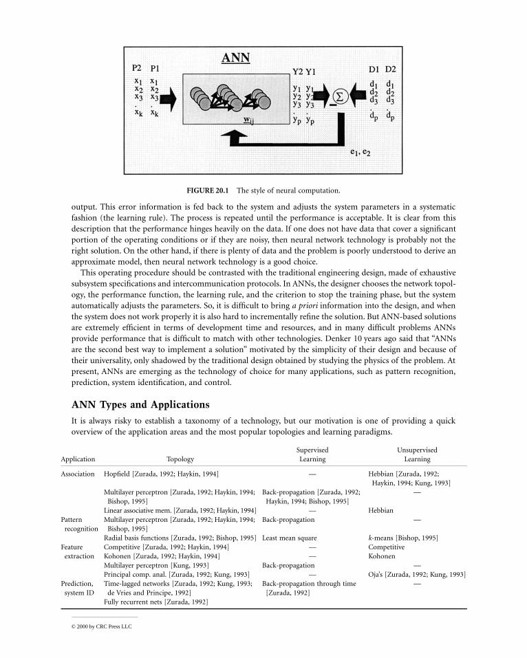
There is a style in neural computation that is worth describing (Fig. 20.1). An input is presented to thenetwork and a corresponding desired or target response set at the output (when this is the case the training iscalled supervised). An error is composed from the difference between the desired response and the system

Jose C. PrincipeUniversity of Florida

© 2000 by CRC Press LLC

A

A

P

F

P

output. This error information is fed back to the system and adjusts the system parameters in a systematicfashion (the learning rule). The process is repeated until the performance is acceptable. It is clear from thisdescription that the performance hinges heavily on the data. If one does not have data that cover a significantportion of the operating conditions or if they are noisy, then neural network technology is probably not theright solution. On the other hand, if there is plenty of data and the problem is poorly understood to derive anapproximate model, then neural network technology is a good choice.

This operating procedure should be contrasted with the traditional engineering design, made of exhaustivesubsystem specifications and intercommunication protocols. In ANNs, the designer chooses the network topol-ogy, the performance function, the learning rule, and the criterion to stop the training phase, but the systemautomatically adjusts the parameters. So, it is difficult to bring a priori information into the design, and whenthe system does not work properly it is also hard to incrementally refine the solution. But ANN-based solutionsare extremely efficient in terms of development time and resources, and in many difficult problems ANNsprovide performance that is difficult to match with other technologies. Denker 10 years ago said that “ANNsare the second best way to implement a solution” motivated by the simplicity of their design and because oftheir universality, only shadowed by the traditional design obtained by studying the physics of the problem. Atpresent, ANNs are emerging as the technology of choice for many applications, such as pattern recognition,prediction, system identification, and control.

ANN Types and Applications

It is always risky to establish a taxonomy of a technology, but our motivation is one of providing a quickoverview of the application areas and the most popular topologies and learning paradigms.

FIGURE 20.1 The style of neural computation.

Supervised Unsupervisedpplication Topology Learning Learning

ssociation Hopfield [Zurada, 1992; Haykin, 1994] — Hebbian [Zurada, 1992; Haykin, 1994; Kung, 1993]

Multilayer perceptron [Zurada, 1992; Haykin, 1994; Bishop, 1995]

Back-propagation [Zurada, 1992; Haykin, 1994; Bishop, 1995]

—

Linear associative mem. [Zurada, 1992; Haykin, 1994] — Hebbianattern recognition

Multilayer perceptron [Zurada, 1992; Haykin, 1994; Bishop, 1995]

Back-propagation —

Radial basis functions [Zurada, 1992; Bishop, 1995] Least mean square k-means [Bishop, 1995]eature extraction

Competitive [Zurada, 1992; Haykin, 1994] — CompetitiveKohonen [Zurada, 1992; Haykin, 1994] — KohonenMultilayer perceptron [Kung, 1993] Back-propagation —Principal comp. anal. [Zurada, 1992; Kung, 1993] — Oja’s [Zurada, 1992; Kung, 1993]

rediction, system ID

Time-lagged networks [Zurada, 1992; Kung, 1993; de Vries and Principe, 1992]

Back-propagation through time [Zurada, 1992]

—

Fully recurrent nets [Zurada, 1992]

© 2000 by CRC Press LLC

It is clear that multilayer perceptrons (MLPs), the back-propagation algorithm and its extensions — time-laggednetworks (TLN) and back-propagation through time (BPTT), respectively — hold a prominent position inANN technology. It is therefore only natural to spend most of our overview presenting the theory and tools ofback-propagation learning. It is also important to notice that Hebbian learning (and its extension, the Oja rule)is also a very useful (and biologically plausible) learning mechanism. It is an unsupervised learning methodsince there is no need to specify the desired or target response to the ANN.

20.2 Multilayer Perceptrons

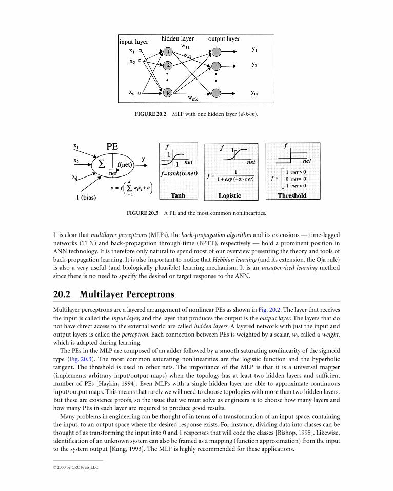
Multilayer perceptrons are a layered arrangement of nonlinear PEs as shown in Fig. 20.2. The layer that receivesthe input is called the input layer, and the layer that produces the output is the output layer. The layers that donot have direct access to the external world are called hidden layers. A layered network with just the input andoutput layers is called the perceptron. Each connection between PEs is weighted by a scalar, wi, called a weight,which is adapted during learning.

The PEs in the MLP are composed of an adder followed by a smooth saturating nonlinearity of the sigmoidtype (Fig. 20.3). The most common saturating nonlinearities are the logistic function and the hyperbolictangent. The threshold is used in other nets. The importance of the MLP is that it is a universal mapper(implements arbitrary input/output maps) when the topology has at least two hidden layers and sufficientnumber of PEs [Haykin, 1994]. Even MLPs with a single hidden layer are able to approximate continuousinput/output maps. This means that rarely we will need to choose topologies with more than two hidden layers.But these are existence proofs, so the issue that we must solve as engineers is to choose how many layers andhow many PEs in each layer are required to produce good results.

Many problems in engineering can be thought of in terms of a transformation of an input space, containingthe input, to an output space where the desired response exists. For instance, dividing data into classes can bethought of as transforming the input into 0 and 1 responses that will code the classes [Bishop, 1995]. Likewise,identification of an unknown system can also be framed as a mapping (function approximation) from the inputto the system output [Kung, 1993]. The MLP is highly recommended for these applications.

FIGURE 20.2 MLP with one hidden layer (d-k-m).

FIGURE 20.3 A PE and the most common nonlinearities.

© 2000 by CRC Press LLC

Function of Each PE

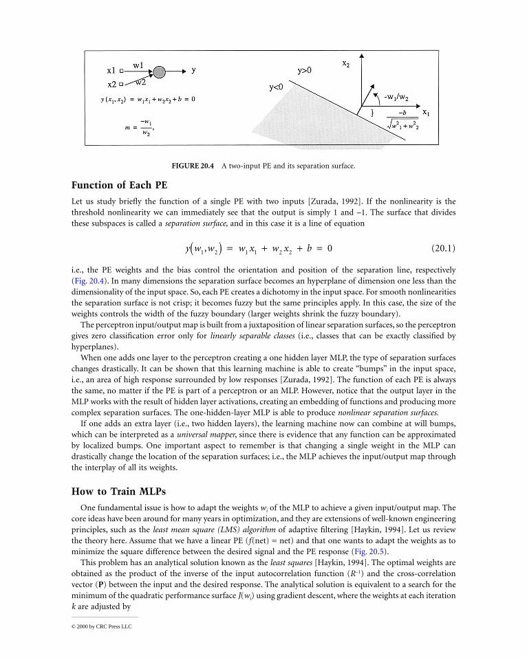
Let us study briefly the function of a single PE with two inputs [Zurada, 1992]. If the nonlinearity is thethreshold nonlinearity we can immediately see that the output is simply 1 and –1. The surface that dividesthese subspaces is called a separation surface, and in this case it is a line of equation

(20.1)

i.e., the PE weights and the bias control the orientation and position of the separation line, respectively(Fig. 20.4). In many dimensions the separation surface becomes an hyperplane of dimension one less than thedimensionality of the input space. So, each PE creates a dichotomy in the input space. For smooth nonlinearitiesthe separation surface is not crisp; it becomes fuzzy but the same principles apply. In this case, the size of theweights controls the width of the fuzzy boundary (larger weights shrink the fuzzy boundary).

The perceptron input/output map is built from a juxtaposition of linear separation surfaces, so the perceptrongives zero classification error only for linearly separable classes (i.e., classes that can be exactly classified byhyperplanes).

When one adds one layer to the perceptron creating a one hidden layer MLP, the type of separation surfaceschanges drastically. It can be shown that this learning machine is able to create “bumps” in the input space,i.e., an area of high response surrounded by low responses [Zurada, 1992]. The function of each PE is alwaysthe same, no matter if the PE is part of a perceptron or an MLP. However, notice that the output layer in theMLP works with the result of hidden layer activations, creating an embedding of functions and producing morecomplex separation surfaces. The one-hidden-layer MLP is able to produce nonlinear separation surfaces.

If one adds an extra layer (i.e., two hidden layers), the learning machine now can combine at will bumps,which can be interpreted as a universal mapper, since there is evidence that any function can be approximatedby localized bumps. One important aspect to remember is that changing a single weight in the MLP candrastically change the location of the separation surfaces; i.e., the MLP achieves the input/output map throughthe interplay of all its weights.

How to Train MLPs

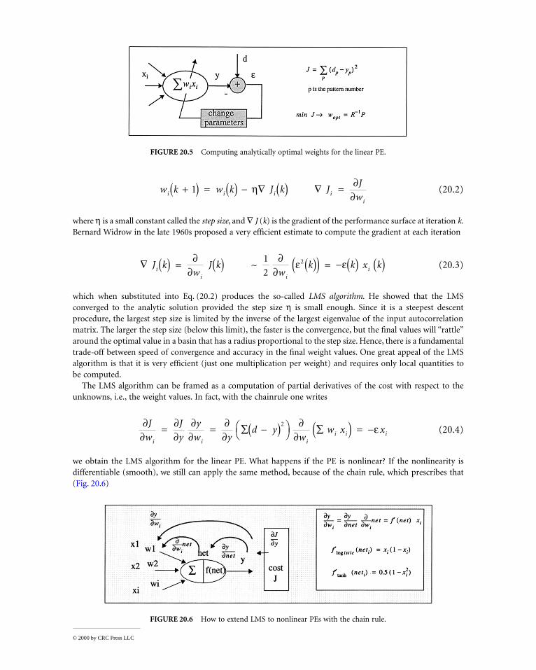
One fundamental issue is how to adapt the weights wi of the MLP to achieve a given input/output map. Thecore ideas have been around for many years in optimization, and they are extensions of well-known engineeringprinciples, such as the least mean square (LMS) algorithm of adaptive filtering [Haykin, 1994]. Let us reviewthe theory here. Assume that we have a linear PE (f(net) = net) and that one wants to adapt the weights as tominimize the square difference between the desired signal and the PE response (Fig. 20.5).

This problem has an analytical solution known as the least squares [Haykin, 1994]. The optimal weights areobtained as the product of the inverse of the input autocorrelation function (R–1) and the cross-correlationvector (P) between the input and the desired response. The analytical solution is equivalent to a search for theminimum of the quadratic performance surface J(wi) using gradient descent, where the weights at each iterationk are adjusted by

FIGURE 20.4 A two-input PE and its separation surface.

y w w w x w x b1 2 1 1 2 2 0,( ) = + + =

© 2000 by CRC Press LLC

(20.2)

where h is a small constant called the step size, and Ñ J (k) is the gradient of the performance surface at iteration k.Bernard Widrow in the late 1960s proposed a very efficient estimate to compute the gradient at each iteration

(20.3)

which when substituted into Eq. (20.2) produces the so-called LMS algorithm. He showed that the LMSconverged to the analytic solution provided the step size h is small enough. Since it is a steepest descentprocedure, the largest step size is limited by the inverse of the largest eigenvalue of the input autocorrelationmatrix. The larger the step size (below this limit), the faster is the convergence, but the final values will “rattle”around the optimal value in a basin that has a radius proportional to the step size. Hence, there is a fundamentaltrade-off between speed of convergence and accuracy in the final weight values. One great appeal of the LMSalgorithm is that it is very efficient (just one multiplication per weight) and requires only local quantities tobe computed.

The LMS algorithm can be framed as a computation of partial derivatives of the cost with respect to theunknowns, i.e., the weight values. In fact, with the chainrule one writes

(20.4)

we obtain the LMS algorithm for the linear PE. What happens if the PE is nonlinear? If the nonlinearity isdifferentiable (smooth), we still can apply the same method, because of the chain rule, which prescribes that(Fig. 20.6)

FIGURE 20.5 Computing analytically optimal weights for the linear PE.

FIGURE 20.6 How to extend LMS to nonlinear PEs with the chain rule.

w k w k J k JJ

wi i i ii

+( ) = ( ) - Ñ ( ) Ñ =1 h ¶¶

Ñ ( ) = ( ) ( )( ) = - ( ) ( )J kw

J kw

k k x kii i

i

¶¶

¶¶

e e~1

22

¶¶

¶¶

¶¶

¶¶

¶¶

eJ

w

J

y

y

w yd y

ww x x

i i ii i i= = å -( )æ

èöø å( ) = -

2

© 2000 by CRC Press LLC

(20.5)

where f ¢(net) is the derivative of the nonlinearity computed at the operating point. Equation (20.5) is knownas the delta rule, and it will train the perceptron [Haykin, 1994]. Note that throughout the derivation we skippedthe pattern index p for simplicity, but this rule is applied for each input pattern. However, the delta rule cannottrain MLPs since it requires the knowledge of the error signal at each PE.

The principle of the ordered derivatives can be extended to multilayer networks, provided we organize thecomputations in flows of activation and error propagation. The principle is very easy to understand, but a littlecomplex to formulate in equation form [Haykin, 1994].

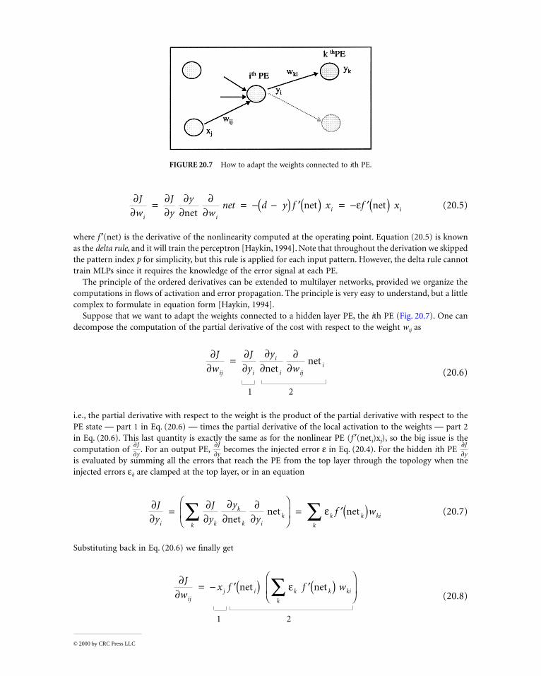
Suppose that we want to adapt the weights connected to a hidden layer PE, the ith PE (Fig. 20.7). One candecompose the computation of the partial derivative of the cost with respect to the weight wij as

(20.6)

i.e., the partial derivative with respect to the weight is the product of the partial derivative with respect to thePE state — part 1 in Eq. (20.6) — times the partial derivative of the local activation to the weights — part 2in Eq. (20.6). This last quantity is exactly the same as for the nonlinear PE (f ¢(neti)xj), so the big issue is thecomputation of . For an output PE, becomes the injected error e in Eq. (20.4). For the hidden ith PE is evaluated by summing all the errors that reach the PE from the top layer through the topology when theinjected errors ek are clamped at the top layer, or in an equation

(20.7)

Substituting back in Eq. (20.6) we finally get

(20.8)

FIGURE 20.7 How to adapt the weights connected to ith PE.

¶¶

¶¶

¶¶

¶¶

eJ

w

J

y

y

wnet d y f x f x

i ii i= = - -( ) ¢( ) = - ¢( )

netnet net

¶¶

¶¶

¶¶

¶¶

J

w

J

y

y

wij i

i

i iji=

netnet

1 2

¶¶

J

y

¶¶

J

y

¶¶

J

y

¶¶

¶¶

¶¶

¶¶

eJ

y

J

y

y

yf w

i k

k

kk ik k k ki

k

=æ

èç

ö

ø÷ = ¢( )å ånet

net net

¶¶

eJ

wx f f w

ijj i k k ki

k

= - ¢( ) ¢( )æ

èç

ö

ø÷ånet net

1 2

© 2000 by CRC Press LLC

This equation embodies the back-propagation training algorithm [Haykin, 1994; Bishop, 1995]. It can berewritten as the product of a local activation (part 1) and a local error (part 2), exactly as the LMS and thedelta rules. But now the local error is a composition of errors that flow through the topology, which becomesequivalent to the existence of a desired response at the PE.

There is an intrinsic flow in the implementation of the back-propagation algorithm: first, inputs are appliedto the net and activations computed everywhere to yield the output activation. Second, the external errors arecomputed by subtracting the net output from the desired response. Third, these external errors are utilized inEq. (20.8) to compute the local errors for the layer immediately preceding the output layer, and the computationschained up to the input layer. Once all the local errors are available, Eq. (20.2) can be used to update everyweight. These three steps are then repeated for other training patterns until the error is acceptable.

Step three is equivalent to injecting the external errors in the dual topology and back-propagating them upto the input layer [Haykin, 1994]. The dual topology is obtained from the original one by reversing data flowand substituting summing junctions by splitting nodes and vice versa. The error at each PE of the dual topologyis then multiplied by the activation of the original network to compute the weight updates. So, effectively thedual topology is being used to compute the local errors which makes the procedure highly efficient. This is thereason back-propagation trains a network of N weights with a number of multiplications proportional to N,(O(N)), instead of (O(N2)) for previous methods of computing partial derivatives known in control theory.Using the dual topology to implement back-propagation is the best and most general method to program thealgorithm in a digital computer.

Applying Back-Propagation in Practice

Now that we know an algorithm to train MLPs, let us see what are the practical issues to apply it. We willaddress the following aspects: size of training set vs. weights, search procedures, how to stop training, and howto set the topology for maximum generalization.

Size of Training Set

The size of the training set is very important for good performance. Remember that the ANN gets its informationfrom the training set. If the training data do not cover the full range of operating conditions, the system mayperform badly when deployed. Under no circumstances should the training set be less than the number ofweights in the ANN. A good size of the training data is ten times the number of weights in the network, withthe lower limit being set around three times the number of weights (these values should be taken as an indication,subject to experimentation for each case) [Haykin, 1994].

Search Procedures

Searching along the direction of the gradient is fine if the performance surface is quadratic. However, in ANNsrarely is this the case, because of the use of nonlinear PEs and topologies with several layers. So, gradient descentcan be caught in local minima, which makes the search very slow in regions of small curvature. One efficientway to speed up the search in regions of small curvature and, at the same time, to stabilize it in narrow valleysis to include a momentum term in the weight adaptation

(20.9)

The value of momentum a should be set experimentally between 0.5 and 0.9. There are many more modifi-cations to the conventional gradient search, such as adaptive step sizes, annealed noise, conjugate gradients,and second-order methods (using information contained in the Hessian matrix), but the simplicity and powerof momentum learning is hard to beat [Haykin, 1994; Bishop, 1995].

How to Stop Training

The stop criterion is a fundamental aspect of training. The simple ideas of capping the number of iterationsor of letting the system train until a predetermined error value are not recommended. The reason is that wewant the ANN to perform well in the test set data; i.e., we would like the system to perform well in data it

w n w n n x n w n w nij ij j ij ij+( ) = ( ) + ( ) ( ) + ( ) - -( )( )1 1hd a

© 2000 by CRC Press LLC

never saw before (good generalization) [Bishop, 1995]. The error in the training set tends to decrease withiteration when the ANN has enough degrees of freedom to represent the input/output map. However, thesystem may be remembering the training patterns (overfitting) instead of finding the underlying mapping rule.This is called overtraining. To avoid overtraining the performance in a validation set, i.e., a set of input datathat the system never saw before, must be checked regularly during training (i.e., once every 50 passes over thetraining set). The training should be stopped when the performance in the validation set starts to increase,despite the fact that the performance in the training set continues to decrease. This method is called crossvalidation. The validation set should be 10% of the training set, and distinct from it.

Size of the Topology

The size of the topology should also be carefully selected. If the number of layers or the size of each layer istoo small, the network does not have enough degrees of freedom to classify the data or to approximate thefunction, and the performance suffers.

On the other hand, if the size of the network is too large, performance may also suffer. This is the phenomenonof overfitting that we mentioned above. But one alternative way to control it is to reduce the size of the network.There are basically two procedures to set the size of the network: either one starts small and adds new PEs orone starts with a large network and prunes PEs [Haykin, 1994]. One quick way to prune the network is toimpose a penalty term in the performance function — a regularizing term — such as limiting the slope of theinput/output map [Bishop, 1995]. A regularization term that can be implemented locally is

(20.10)

where l is the weight decay parameter and d the local error. Weight decay tends to drive unimportant weightsto zero.

A Posteriori Probabilities

We will finish the discussion of the MLP by noting that this topology when trained with the mean squareerror is able to estimate directly at its outputs a posteriori probabilities, i.e., the probability that a given inputpattern belongs to a given class [Bishop, 1995]. This property is very useful because the MLP outputs can beinterpreted as probabilities and operated as numbers. In order to guarantee this property, one has to make surethat each class is attributed to one output PE, that the topology is sufficiently large to represent the mapping,that the training has converged to the absolute minimum, and that the outputs are normalized between 0 and1. The first requirements are met by good design, while the last can be easily enforced if the softmax activationis used as the output PE [Bishop, 1995],

(20.11)

20.3 Radial Basis Function Networks

The radial basis function (RBF) network constitutes another way of implementing arbitrary input/outputmappings. The most significant difference between the MLP and RBF lies in the PE nonlinearity. While the PEin the MLP responds to the full input space, the PE in the RBF is local, normally a Gaussian kernel in the inputspace. Hence, it only responds to inputs that are close to its center; i.e., it has basically a local response.

w n w nw n

n x nij ij

ij

i j+( ) = ( ) -+ ( )( )

æ

è

çç

ö

ø

÷÷

+ ( ) ( )1 11

2

l hd

yj

j

=( )

( )åexp

exp

net

net

© 2000 by CRC Press LLC

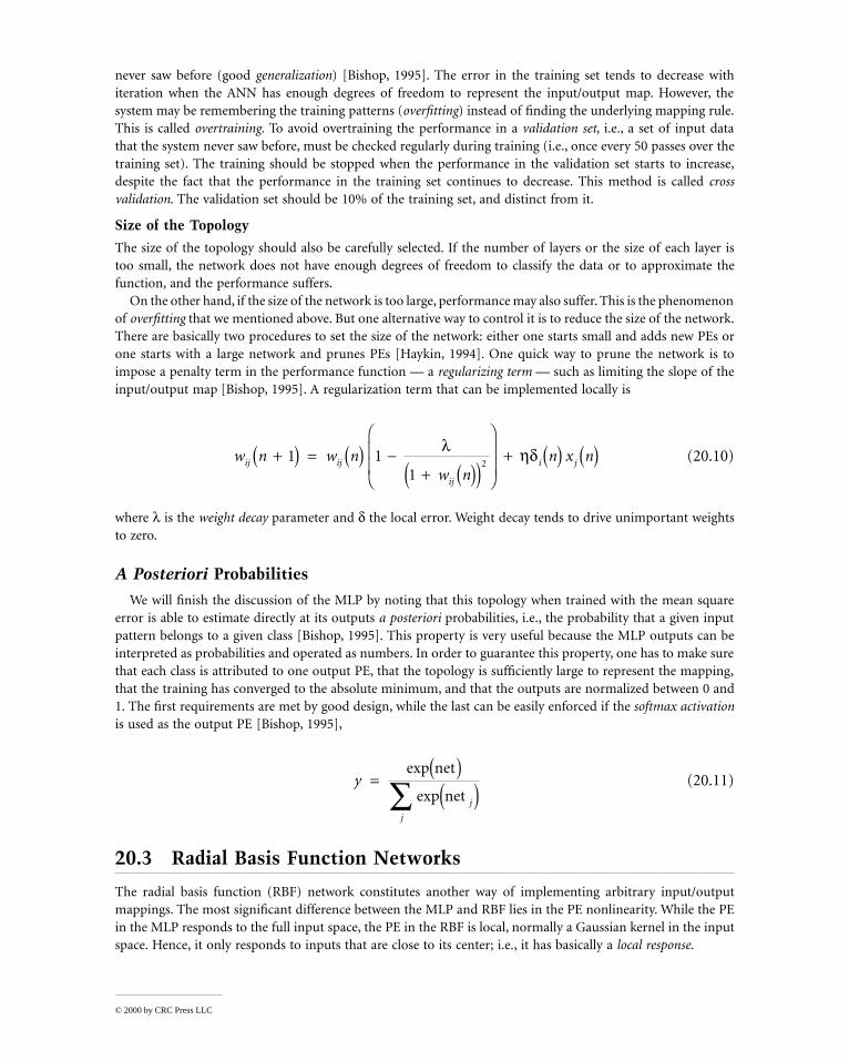
The RBF network is also a layered net with the hidden layer built from Gaussian kernels and a linear (ornonlinear) output layer (Fig. 20.8). Training of the RBF network is done normally in two stages [Haykin, 1994]:first, the centers xi are adaptively placed in the input space using competitive learning or k means clustering[Bishop, 1995], which are unsupervised procedures. Competitive learning is explained later in the chapter. Thevariances of each Gaussian are chosen as a percentage (30 to 50%) to the distance to the nearest center. Thegoal is to cover adequately the input data distribution. Once the RBF is located, the second layer weights wi

are trained using the LMS procedure.RBF networks are easy to work with, they train very fast, and they have shown good properties both for

function approximation as classification. The problem is that they require lots of Gaussian kernels in high-dimensional spaces.

20.4 Time-Lagged Networks

The MLP is the most common neural network topology, but it can only handle instantaneous information,since the system has no memory and it is feedforward. In engineering, the processing of signals that exist intime requires systems with memory, i.e., linear filters. Another alternative to implement memory is to usefeedback, which gives rise to recurrent networks. Fully recurrent networks are difficult to train and to stabilize,so it is preferable to develop topologies based on MLPs but where explicit subsystems to store the past informationare included. These subsystems are called short-term memory structures [de Vries and Principe, 1992]. Thecombination of an MLP with short-term memory structures is called a time-lagged network (TLN). The memorystructures can be eventually recurrent, but the feedback is local, so stability is still easy to guarantee. Here, wewill cover just one TLN topology, called focused, where the memory is at the input layer. The most general TLNhave memory added anywhere in the network, but they require other more-involved training strategies (BPTT[Haykin, 1994]). The interested reader is referred to de Vries and Principe [1992] for further details.

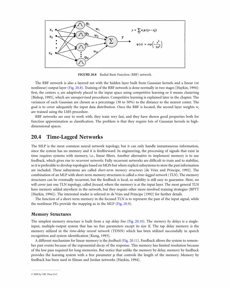
The function of a short-term memory in the focused TLN is to represent the past of the input signal, whilethe nonlinear PEs provide the mapping as in the MLP (Fig. 20.9).

Memory Structures

The simplest memory structure is built from a tap delay line (Fig. 20.10). The memory by delays is a single-input, multiple-output system that has no free parameters except its size K. The tap delay memory is thememory utilized in the time-delay neural network (TDNN) which has been utilized successfully in speechrecognition and system identification [Kung, 1993].

A different mechanism for linear memory is the feedback (Fig. 20.11). Feedback allows the system to remem-ber past events because of the exponential decay of the response. This memory has limited resolution becauseof the low pass required for long memories. But notice that unlike the memory by delay, memory by feedbackprovides the learning system with a free parameter m that controls the length of the memory. Memory byfeedback has been used in Elman and Jordan networks [Haykin, 1994].

FIGURE 20.8 Radial Basis Function (RBF) network.

© 2000 by CRC Press LLC

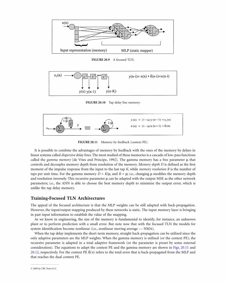
It is possible to combine the advantages of memory by feedback with the ones of the memory by delays inlinear systems called dispersive delay lines. The most studied of these memories is a cascade of low-pass functionscalled the gamma memory [de Vries and Principe, 1992]. The gamma memory has a free parameter m thatcontrols and decouples memory depth from resolution of the memory. Memory depth D is defined as the firstmoment of the impulse response from the input to the last tap K, while memory resolution R is the number oftaps per unit time. For the gamma memory D = K/m, and R = m; i.e., changing m modifies the memory depthand resolution inversely. This recursive parameter m can be adapted with the output MSE as the other networkparameters; i.e., the ANN is able to choose the best memory depth to minimize the output error, which isunlike the tap delay memory.

Training-Focused TLN Architectures

The appeal of the focused architecture is that the MLP weights can be still adapted with back-propagation.However, the input/output mapping produced by these networks is static. The input memory layer is bringingin past input information to establish the value of the mapping.

As we know in engineering, the size of the memory is fundamental to identify, for instance, an unknownplant or to perform prediction with a small error. But note now that with the focused TLN the models forsystem identification become nonlinear (i.e., nonlinear moving average — NMA).

When the tap delay implements the short-term memory, straight back-propagation can be utilized since theonly adaptive parameters are the MLP weights. When the gamma memory is utilized (or the context PE), therecursive parameter is adapted in a total adaptive framework (or the parameter is preset by some externalconsideration). The equations to adapt the context PE and the gamma memory are shown in Figs. 20.11 and20.12, respectively. For the context PE d(n) refers to the total error that is back-propagated from the MLP andthat reaches the dual context PE.

FIGURE 20.9 A focused TLN.

FIGURE 20.10 Tap delay line memory.

FIGURE 20.11 Memory by feedback (context PE).

© 2000 by CRC Press LLC

20.5 Hebbian Learning and Principal Component Analysis Networks

Hebbian Learning

Hebbian learning is an unsupervised learning rule that captures similarity between an input and an outputthrough correlation. To adapt a weight wi using Hebbian learning we adjust the weights according to Dwi =hxi y or in an equation [Haykin, 1994]

(20.12)

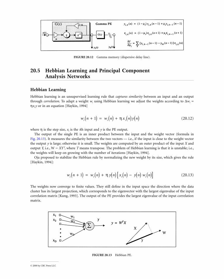
where h is the step size, xi is the ith input and y is the PE output.The output of the single PE is an inner product between the input and the weight vector (formula in

Fig. 20.13). It measures the similarity between the two vectors — i.e., if the input is close to the weight vectorthe output y is large; otherwise it is small. The weights are computed by an outer product of the input X andoutput Y, i.e., W = XY T, where T means transpose. The problem of Hebbian learning is that it is unstable; i.e.,the weights will keep on growing with the number of iterations [Haykin, 1994].

Oja proposed to stabilize the Hebbian rule by normalizing the new weight by its size, which gives the rule[Haykin, 1994]:

(20.13)

The weights now converge to finite values. They still define in the input space the direction where the datacluster has its largest projection, which corresponds to the eigenvector with the largest eigenvalue of the inputcorrelation matrix [Kung, 1993]. The output of the PE provides the largest eigenvalue of the input correlationmatrix.

FIGURE 20.12 Gamma memory (dispersive delay line).

FIGURE 20.13 Hebbian PE.

w n w n x n y ni i i+( ) = ( ) + ( ) ( )1 h

w n w n y n x n y n w ni i i i+( ) = ( ) + ( ) ( ) - ( ) ( )[ ]1 h

© 2000 by CRC Press LLC

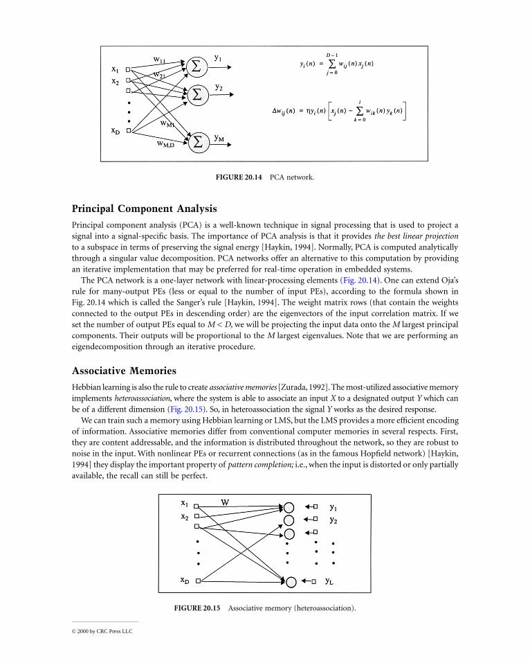
Principal Component Analysis

Principal component analysis (PCA) is a well-known technique in signal processing that is used to project asignal into a signal-specific basis. The importance of PCA analysis is that it provides the best linear projectionto a subspace in terms of preserving the signal energy [Haykin, 1994]. Normally, PCA is computed analyticallythrough a singular value decomposition. PCA networks offer an alternative to this computation by providingan iterative implementation that may be preferred for real-time operation in embedded systems.

The PCA network is a one-layer network with linear-processing elements (Fig. 20.14). One can extend Oja’srule for many-output PEs (less or equal to the number of input PEs), according to the formula shown inFig. 20.14 which is called the Sanger’s rule [Haykin, 1994]. The weight matrix rows (that contain the weightsconnected to the output PEs in descending order) are the eigenvectors of the input correlation matrix. If weset the number of output PEs equal to M < D, we will be projecting the input data onto the M largest principalcomponents. Their outputs will be proportional to the M largest eigenvalues. Note that we are performing aneigendecomposition through an iterative procedure.

Associative Memories

Hebbian learning is also the rule to create associative memories [Zurada, 1992]. The most-utilized associative memoryimplements heteroassociation, where the system is able to associate an input X to a designated output Y which canbe of a different dimension (Fig. 20.15). So, in heteroassociation the signal Y works as the desired response.

We can train such a memory using Hebbian learning or LMS, but the LMS provides a more efficient encodingof information. Associative memories differ from conventional computer memories in several respects. First,they are content addressable, and the information is distributed throughout the network, so they are robust tonoise in the input. With nonlinear PEs or recurrent connections (as in the famous Hopfield network) [Haykin,1994] they display the important property of pattern completion; i.e., when the input is distorted or only partiallyavailable, the recall can still be perfect.

FIGURE 20.14 PCA network.

FIGURE 20.15 Associative memory (heteroassociation).

© 2000 by CRC Press LLC

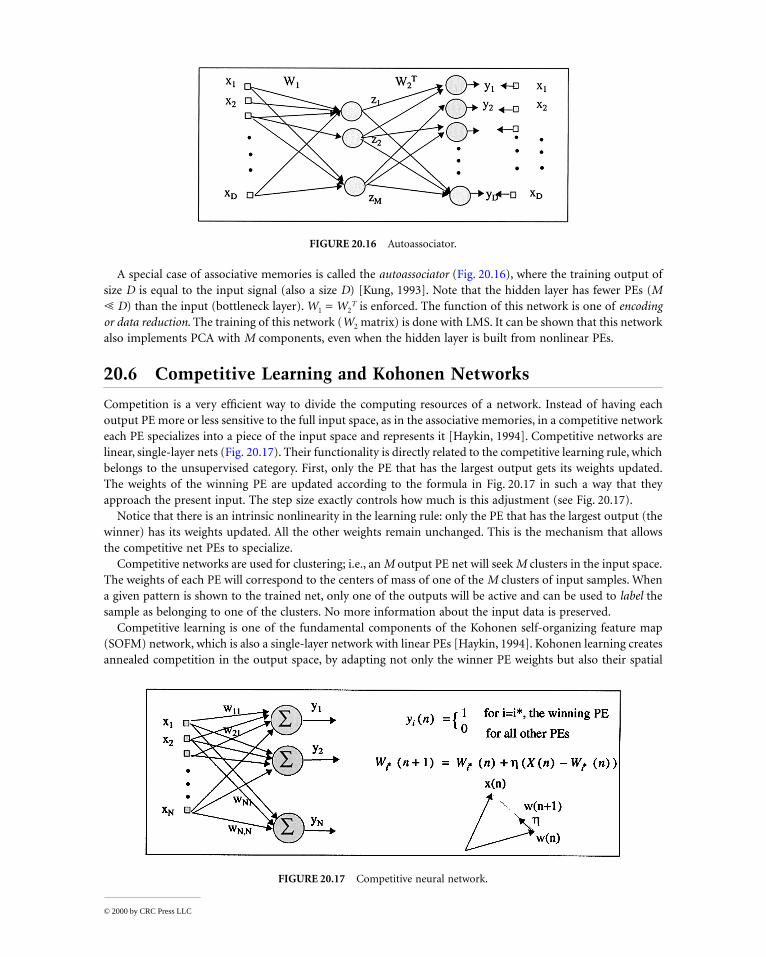
A special case of associative memories is called the autoassociator (Fig. 20.16), where the training output ofsize D is equal to the input signal (also a size D) [Kung, 1993]. Note that the hidden layer has fewer PEs (M! D) than the input (bottleneck layer). W1 = W2

T is enforced. The function of this network is one of encodingor data reduction. The training of this network (W2 matrix) is done with LMS. It can be shown that this networkalso implements PCA with M components, even when the hidden layer is built from nonlinear PEs.

20.6 Competitive Learning and Kohonen Networks

Competition is a very efficient way to divide the computing resources of a network. Instead of having eachoutput PE more or less sensitive to the full input space, as in the associative memories, in a competitive networkeach PE specializes into a piece of the input space and represents it [Haykin, 1994]. Competitive networks arelinear, single-layer nets (Fig. 20.17). Their functionality is directly related to the competitive learning rule, whichbelongs to the unsupervised category. First, only the PE that has the largest output gets its weights updated.The weights of the winning PE are updated according to the formula in Fig. 20.17 in such a way that theyapproach the present input. The step size exactly controls how much is this adjustment (see Fig. 20.17).

Notice that there is an intrinsic nonlinearity in the learning rule: only the PE that has the largest output (thewinner) has its weights updated. All the other weights remain unchanged. This is the mechanism that allowsthe competitive net PEs to specialize.

Competitive networks are used for clustering; i.e., an M output PE net will seek M clusters in the input space.The weights of each PE will correspond to the centers of mass of one of the M clusters of input samples. Whena given pattern is shown to the trained net, only one of the outputs will be active and can be used to label thesample as belonging to one of the clusters. No more information about the input data is preserved.

Competitive learning is one of the fundamental components of the Kohonen self-organizing feature map(SOFM) network, which is also a single-layer network with linear PEs [Haykin, 1994]. Kohonen learning createsannealed competition in the output space, by adapting not only the winner PE weights but also their spatial

FIGURE 20.16 Autoassociator.

FIGURE 20.17 Competitive neural network.

© 2000 by CRC Press LLC

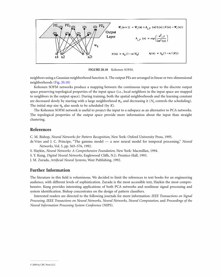
neighbors using a Gaussian neighborhood function L. The output PEs are arranged in linear or two-dimensionalneighborhoods (Fig. 20.18)

Kohonen SOFM networks produce a mapping between the continuous input space to the discrete outputspace preserving topological properties of the input space (i.e., local neighbors in the input space are mappedto neighbors in the output space). During training, both the spatial neighborhoods and the learning constantare decreased slowly by starting with a large neighborhood s0, and decreasing it (N0 controls the scheduling).The initial step size h0 also needs to be scheduled (by K).

The Kohonen SOFM network is useful to project the input to a subspace as an alternative to PCA networks.The topological properties of the output space provide more information about the input than straightclustering.

References

C. M. Bishop, Neural Networks for Pattern Recognition, New York: Oxford University Press, 1995.de Vries and J. C. Principe, “The gamma model — a new neural model for temporal processing,” Neural

Networks, Vol. 5, pp. 565–576, 1992.S. Haykin, Neural Networks: A Comprehensive Foundation, New York: Macmillan, 1994.S. Y. Kung, Digital Neural Networks, Englewood Cliffs, N.J.: Prentice-Hall, 1993.J. M. Zurada, Artificial Neural Systems, West Publishing, 1992.

Further Information

The literature in this field is voluminous. We decided to limit the references to text books for an engineeringaudience, with different levels of sophistication. Zurada is the most accessible text, Haykin the most compre-hensive. Kung provides interesting applications of both PCA networks and nonlinear signal processing andsystem identification. Bishop concentrates on the design of pattern classifiers.

Interested readers are directed to the following journals for more information: IEEE Transactions on SignalProcessing, IEEE Tranactions on Neural Networks, Neural Networks, Neural Computation, and Proceedings of theNeural Information Processing System Conference (NIPS).

FIGURE 20.18 Kohonen SOFM.

© 2000 by CRC Press LLC