Principal)Component)Analysis) and …mgormley/courses/10701-f16/...SVD and PCA " The first root is called the prinicipal eigenvalue which has an associated orthonormal (uTu = 1) eigenvector

Principal Component Analysis and

Dimensionality Reduction

1

Matt Gormley Lecture 14

October 24, 2016

School of Computer Science

Readings: Bishop Ch. 12 Murphy Ch. 12

10-‐701 Introduction to Machine Learning

Reminders

•  Homework 3: – due 10/24/16 (tonight)

2

DIMENSIONALITY REDUCTION

3

•  High-‐Dimensions = Lot of Features Document classification Features per document = thousands of words/unigrams millions of bigrams, contextual information

Surveys -‐ Netflix 480189 users x 17770 movies

Big & High-‐Dimensional Data

Slide from Nina Balcan

•  High-‐Dimensions = Lot of Features

MEG Brain Imaging 120 locations x 500 time points x 20 objects

Big & High-‐Dimensional Data

Or any high-‐dimensional image data


•  Useful to learn lower dimensional representations of the data.

•  Big & High-‐Dimensional Data.


PCA, Kernel PCA, ICA: Powerful unsupervised learning techniques for extracting hidden (potentially lower dimensional) structure from high dimensional datasets.

Learning Representations

Useful for:

•  Visualization

•  Further processing by machine learning algorithms

•  More efficient use of resources (e.g., time, memory, communication)

•  Statistical: fewer dimensions à better generalization

•  Noise removal (improving data quality)


Principal Component Analysis (PCA)

What is PCA: Unsupervised technique for extracting variance structure from high dimensional datasets.

•  PCA is an orthogonal projection or transformation of the data into a (possibly lower dimensional) subspace so that the variance of the projected data is maximized.



Both features are relevant Only one relevant feature

Question: Can we transform the features so that we only need to preserve one latent feature?

Intrinsically lower dimensional than the dimension of the ambient space.

If we rotate data, again only one coordinate is more important.



In case where data lies on or near a low d-‐dimensional linear subspace, axes of this subspace are an effective representation of the data.

Identifying the axes is known as Principal Components Analysis, and can be obtained by using classic matrix computation tools (Eigen or Singular Value Decomposition).


2D Gaussian dataset

Slide from Barnabas Poczos

1st PCA axis


2nd PCA axis


PCA ALGORITHMS

14

PCA algorithm I (sequential)

∑ ∑=

−

==

−=m

i

k

ji

Tjji

Tk m 1

21

11})]({[1maxarg xwwxww

w

}){(1maxarg1

2i11 ∑

==

=m

i

T

mxww

w

We maximize the variance of the projection in the residual subspace

We maximize the variance of projection of x

x’ PCA reconstruction

Given the centered data {x1, …, xm}, compute the principal vectors:

1st PCA vector

kth PCA vector

w1(w1Tx)

w2(w2Tx)

x

w1

w2 x’=w1(w1

Tx)+w2(w2Tx)

w


Maximizing the Variance

•  Consider the two projections below •  Which maximizes the variance?

16

4

We see that the projected data still has a fairly large variance, and thepoints tend to be far from zero. In contrast, suppose had instead picked thefollowing direction:

Here, the projections have a significantly smaller variance, and are muchcloser to the origin.

We would like to automatically select the direction u corresponding tothe first of the two figures shown above. To formalize this, note that given a

Figures from Andrew Ng (CS229 Lecture Notes)

4

We see that the projected data still has a fairly large variance, and thepoints tend to be far from zero. In contrast, suppose had instead picked thefollowing direction:

Here, the projections have a significantly smaller variance, and are muchcloser to the origin.

We would like to automatically select the direction u corresponding tothe first of the two figures shown above. To formalize this, note that given a

Option A Option B

PCA algorithm I (sequential)

∑ ∑=

−

==

−=m

i

k

ji

Tjji

Tk m 1

21

11})]({[1maxarg xwwxww

w

}){(1maxarg1

2i11 ∑

==

=m

i

T

mxww

w

We maximize the variance of the projection in the residual subspace

We maximize the variance of projection of x

x’ PCA reconstruction

Given the centered data {x1, …, xm}, compute the principal vectors:

1st PCA vector

kth PCA vector

w1(w1Tx)

w2(w2Tx)

x

w1

w2 x’=w1(w1

Tx)+w2(w2Tx)

w


PCA algorithm II (sample covariance matrix)

•  Given data {x1, …, xm}, compute covariance matrix Σ

•  PCA basis vectors = the eigenvectors of Σ

•  Larger eigenvalue ⇒ more important eigenvectors

∑=

−−=Σm

i

Tim 1

))((1 xxxx ∑=

=m

iim 1

1 xxwhere


We get the eigvectors using an eigendecomposition. Power iteration (Von Mises iteration is a standard algorithm for this)

Why the Eigenvectors? Maximise uTXXTu

s.t uTu = 1 Construct Langrangian uTXXTu – λuTu Vector of partial derivatives set to zero

xxTu – λu = (xxT – λI) u = 0 As u ≠ 0 then u must be an eigenvector of XXT with eigenvalue λ

© Eric Xing @ CMU, 2006-2011 19

Eigenvalues & Eigenvectors l  For symmetric matrices, eigenvectors for distinct eigenvalues

are orthogonal

l  All eigenvalues of a real symmetric matrix are real.

l  All eigenvalues of a positive semidefinite matrix are non-negative

© Eric Xing @ CMU, 2006-2011 20

ℜ∈⇒==− λλ TSS and 0 if IS

0vSv if then ,0, ≥⇒=≥ℜ∈∀ λλSwww Tn

02121212121 =•⇒≠= vvvSv λλλ and ,},{},{},{

Eigen/diagonal Decomposition l  Let be a square matrix with m linearly

independent eigenvectors (a “non-defective” matrix)

l  Theorem: Exists an eigen decomposition

(cf. matrix diagonalization theorem)

l  Columns of U are eigenvectors of S

l  Diagonal elements of are eigenvalues of

© Eric Xing @ CMU, 2006-2011 21

diagonal

Unique for

distinct eigen-values

0

5

10

15

20

25

PC1 PC2 PC3 PC4 PC5 PC6 PC7 PC8 PC9 PC10

Varia

nce

(%)

How Many PCs? l  For n original dimensions, sample covariance matrix is nxn, and has

up to n eigenvectors. So n PCs. l  Where does dimensionality reduction come from?

Can ignore the components of lesser significance.

You do lose some information, but if the eigenvalues are small, you don’t lose much l  n dimensions in original data l  calculate n eigenvectors and eigenvalues l  choose only the first p eigenvectors, based on their eigenvalues l  final data set has only p dimensions

© Eric Xing @ CMU, 2006-2011 22

Eigen/diagonal Decomposition l  Let be a square matrix with m linearly

independent eigenvectors (a “non-defective” matrix)

l  Theorem: Exists an eigen decomposition

(cf. matrix diagonalization theorem)

l  Columns of U are eigenvectors of S

l  Diagonal elements of are eigenvalues of

© Eric Xing @ CMU, 2006-2011 23

diagonal

Unique for

distinct eigen-values

Singular Value Decomposition

TVUA Σ=

m×m m×m V is m×n

For an m× n matrix A of rank r there exists a factorization (Singular Value Decomposition = SVD) as follows:

The columns of U are orthogonal eigenvectors of AAT.

The columns of V are orthogonal eigenvectors of ATA.

ii λσ =

( )rdiag σσ ...1=Σ Singular values.

Eigenvalues λ1 … λr of AAT are the eigenvalues of ATA.

24 © Eric Xing @ CMU, 2006-2011

PCA: Two Interpretations

Maximum Variance Direction: 1st PC a vector v such that projection on to this vector capture maximum variance in the data (out of all possible one dimensional projections)

Minimum Reconstruction Error: 1st PC a vector v such that projection on to this vector yields minimum MSE reconstruction

E.g., for the first component.


v

PCA: Two Interpretations

blue2 + green2 = black2

black2 is fixed (it’s just the data)

So, maximizing blue2 is equivalent to minimizing green2

Maximum Variance Direction: 1st PC a vector v such that projection on to this vector capture maximum variance in the data (out of all possible one dimensional projections)

Minimum Reconstruction Error: 1st PC a vector v such that projection on to this vector yields minimum MSE reconstruction

E.g., for the first component.


PCA algorithm III (SVD of the data matrix)

Singular Value Decomposition of the centered data matrix X.

Xfeatures × samples = USVT

X VT S U =

samples

significant

noise

nois

e noise

sign

ifica

nt

sig.


PCA algorithm III •  Columns of U

–  the principal vectors, { u(1), …, u(k) } –  orthogonal and has unit norm – so UTU = I –  Can reconstruct the data using linear combinations

of { u(1), …, u(k) }

•  Matrix S –  Diagonal –  Shows importance of each eigenvector

•  Columns of VT –  The coefficients for reconstructing the samples


SVD and PCA l  The first root is called the prinicipal eigenvalue which has an

associated orthonormal (uTu = 1) eigenvector u

l  Subsequent roots are ordered such that λ1> λ2 >… > λM with rank(D) non-zero values.

l  Eigenvectors form an orthonormal basis i.e. uiTuj = δij

l  The eigenvalue decomposition of XXT = UΣUT

l  where U = [u1, u2, …, uM] and Σ = diag[λ 1, λ 2, …, λ M]

l  Similarly the eigenvalue decomposition of XTX = VΣVT

l  The SVD is closely related to the above X=U Σ1/2 VT

l  The left eigenvectors U, right eigenvectors V,

l  singular values = square root of eigenvalues.

29 © Eric Xing @ CMU, 2006-2011

l  Solution via SVD

Low-rank Approximation

set smallest r-k singular values to zero

Tkk VUA )0,...,0,,...,(diag 1 σσ=

column notation: sum of rank 1 matrices

Tii

k

i ik vuA ∑ ==

1σ

k

30 © Eric Xing @ CMU, 2006-2011

Approximation error l  How good (bad) is this approximation? l  It’s the best possible, measured by the Frobenius norm of the

error:

where the σi are ordered such that σi ≥ σi+1. Suggests why Frobenius error drops as k increased.

1)(:

min +=

=−=− kFkFkXrankX

AAXA σ

31 © Eric Xing @ CMU, 2006-2011

PCA EXAMPLES

Slides from Barnabas Poczos Original sources include:

•  Karl Booksh Research group •  Tom Mitchell •  Ron Parr

32

Face recognition

Challenge: Facial Recognition •  Want to identify specific person, based on facial image •  Robust to glasses, lighting,…

⇒ Can’t just use the given 256 x 256 pixels

Applying PCA: Eigenfaces

•  Example data set: Images of faces –  Famous Eigenface approach

[Turk & Pentland], [Sirovich & Kirby] •  Each face x is …

•  256 × 256 values (luminance at location) –  x in ℜ256×256 (view as 64K dim vector)

•  Form X = [ x1 , …, xm ] centered data mtx

•  Compute Σ = XXT

•  Problem: Σ is 64K × 64K … HUGE!!! 256 x 256 real values

m faces

X =

x1, …, xm

Method A: Build a PCA subspace for each person and check which subspace can reconstruct the test image the best

Method B: Build one PCA database for the whole dataset and then classify based on the weights.

Computational Complexity

•  Suppose m instances, each of size N – Eigenfaces: m=500 faces, each of size N=64K

•  Given N×N covariance matrix Σ, can compute – all N eigenvectors/eigenvalues in O(N3) –  first k eigenvectors/eigenvalues in O(k N2)

•  But if N=64K, EXPENSIVE!

A Clever Workaround

•  Note that m<<64K •  Use L=XTX instead of Σ=XXT

•  If v is eigenvector of L then Xv is eigenvector of Σ

Proof: L v = γ v XTX v = γ v X (XTX v) = X(γ v) = γ

Xv (XXT)X v = γ (Xv) Σ (Xv) = γ (Xv)

256 x 256 real values

m faces

X =

x1, …, xm

Principle Components (Method B)

Reconstructing… (Method B)

•  … faster if train with… –  only people w/out glasses –  same lighting conditions

Shortcomings •  Requires carefully controlled data:

–  All faces centered in frame –  Same size –  Some sensitivity to angle

•  Alternative: –  “Learn” one set of PCA vectors for each angle –  Use the one with lowest error

•  Method is completely knowledge free –  (sometimes this is good!) –  Doesn’t know that faces are wrapped around 3D objects

(heads) –  Makes no effort to preserve class distinctions

Facial expression recognition

Happiness subspace (method A)

Disgust subspace (method A)

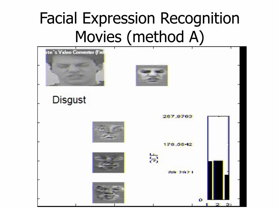
Facial Expression Recognition Movies (method A)



Image Compression

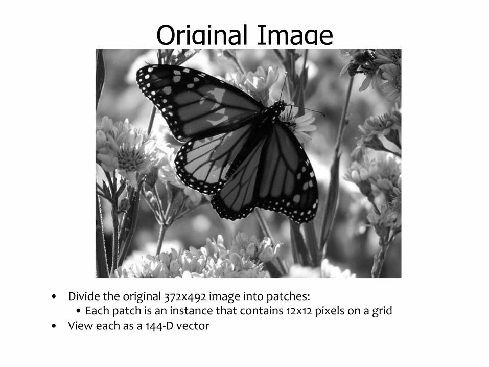
Original Image

•  Divide the original 372x492 image into patches: •  Each patch is an instance that contains 12x12 pixels on a grid

•  View each as a 144-‐D vector

L2 error and PCA dim

PCA compression: 144D ) 60D


16 most important eigenvectors

2 4 6 8 10 12

24681012

2 4 6 8 10 12

24681012

2 4 6 8 10 12

24681012

2 4 6 8 10 12

24681012

2 4 6 8 10 12

24681012

2 4 6 8 10 12

24681012

2 4 6 8 10 12

24681012

2 4 6 8 10 12

24681012

2 4 6 8 10 12

24681012

2 4 6 8 10 12

24681012

2 4 6 8 10 12

24681012

2 4 6 8 10 12

24681012

2 4 6 8 10 12

24681012

2 4 6 8 10 12

24681012

2 4 6 8 10 12

24681012

2 4 6 8 10 12

24681012


2 4 6 8 10 12

24681012

2 4 6 8 10 12

24681012

2 4 6 8 10 12

24681012

2 4 6 8 10 12

24681012

2 4 6 8 10 12

24681012

2 4 6 8 10 12

24681012



2 4 6 8 10 12

2

4

6

8

10

122 4 6 8 10 12

2

4

6

8

10

12

2 4 6 8 10 12

2

4

6

8

10

12




Looks like the discrete cosine bases of JPG!...

2D Discrete Cosine Basis

http://en.wikipedia.org/wiki/Discrete_cosine_transform

Noise Filtering

Noise Filtering, Auto-Encoder…

x x’

U x

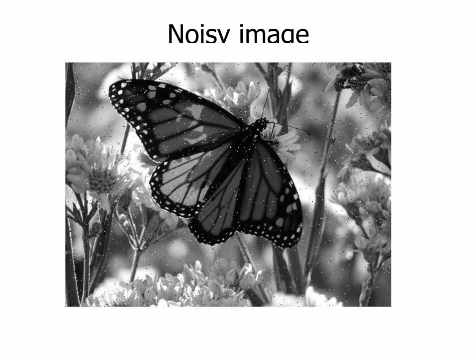
Noisy image

Denoised image using 15 PCA components

Documents

Principal)Component)Analysis) and …mgormley/courses/10701-f16/...SVD and PCA " The first root is called the prinicipal eigenvalue which has an associated orthonormal (uTu = 1) eigenvector