Princess Nora University Faculty of Computer & Information ...pnu-cs-ai.yolasite.com/resources/ch9- CS370 -Learning from examples... · Dr. Abeer Mahmoud (course coordinator) assume

ARTIFICIAL INTELLIGENCE (CS 370D)

Princess Nora University Faculty of Computer & Information Systems

(CHAPTER-18)

LEARNING FROM EXAMPLES

DECISION TREES

Dr. Abeer Mahmoud

(course coordinator) 3

Outline

1- Introduction

2- know your data

3- Classification tree construction

schema

3

Dr. Abeer Mahmoud

(course coordinator)

Know your data?

4

Dr. Abeer Mahmoud


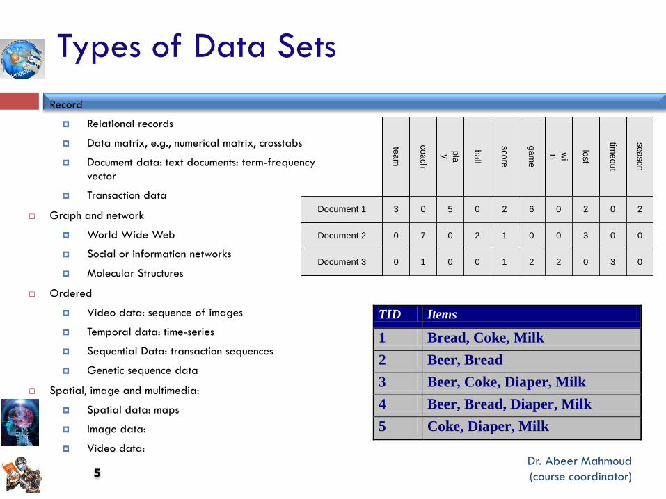
Types of Data Sets

Record

Relational records

Data matrix, e.g., numerical matrix, crosstabs

Document data: text documents: term-frequency

vector

Transaction data

Graph and network

World Wide Web

Social or information networks

Molecular Structures

Ordered

Video data: sequence of images

Temporal data: time-series

Sequential Data: transaction sequences

Genetic sequence data

Spatial, image and multimedia:

Spatial data: maps

Image data:

Video data:

Document 1

se

aso

n

time

ou

t

lost

wi

n

ga

me

sco

re

ba

ll

play

co

ach

tea

m

Document 2

Document 3

3 0 5 0 2 6 0 2 0 2

0

0

7 0 2 1 0 0 3 0 0

1 0 0 1 2 2 0 3 0

TID Items

1 Bread, Coke, Milk

2 Beer, Bread

3 Beer, Coke, Diaper, Milk

4 Beer, Bread, Diaper, Milk

5 Coke, Diaper, Milk

Dr. Abeer Mahmoud


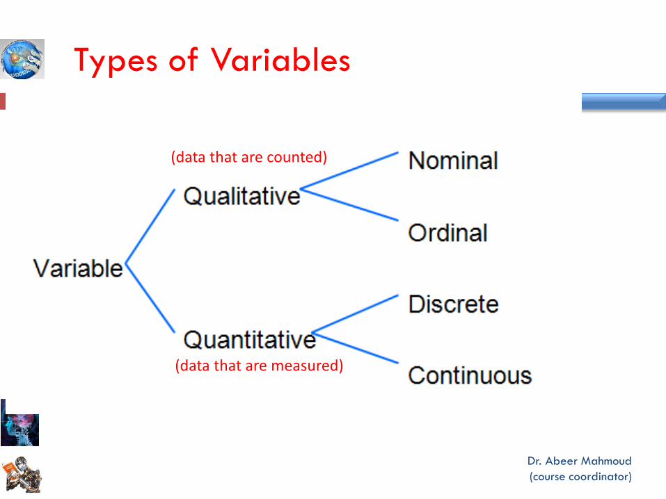
Types of Variables

(data that are counted)

(data that are measured)

Dr. Abeer Mahmoud


Types of Variables



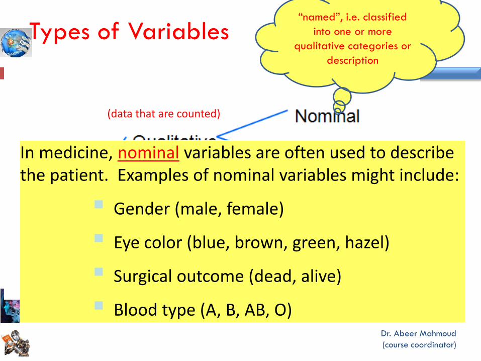
“named”, i.e. classified

into one or more

qualitative categories or

description

In medicine, nominal variables are often used to describe the patient. Examples of nominal variables might include:

Gender (male, female)

Eye color (blue, brown, green, hazel)

Surgical outcome (dead, alive)

Blood type (A, B, AB, O)

Dr. Abeer Mahmoud


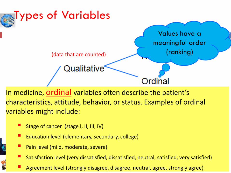
Values have a

meaningful order

(ranking)

Types of Variables



In medicine, ordinal variables often describe the patient’s characteristics, attitude, behavior, or status. Examples of ordinal variables might include:

Stage of cancer (stage I, II, III, IV)

Education level (elementary, secondary, college)

Pain level (mild, moderate, severe)

Satisfaction level (very dissatisfied, dissatisfied, neutral, satisfied, very satisfied)

Agreement level (strongly disagree, disagree, neutral, agree, strongly agree)

Dr. Abeer Mahmoud


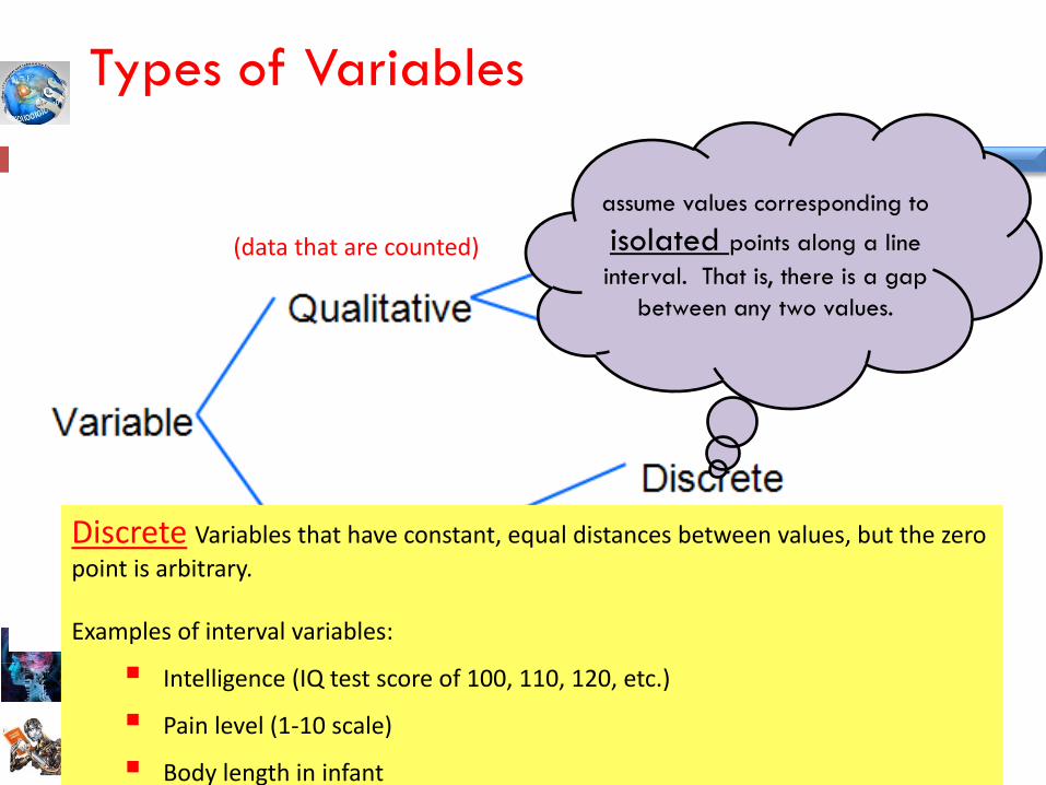
assume values corresponding to

isolated points along a line

interval. That is, there is a gap

between any two values.

Types of Variables



Discrete Variables that have constant, equal distances between values, but the zero

point is arbitrary. Examples of interval variables:

Intelligence (IQ test score of 100, 110, 120, etc.)

Pain level (1-10 scale)

Body length in infant

Dr. Abeer Mahmoud


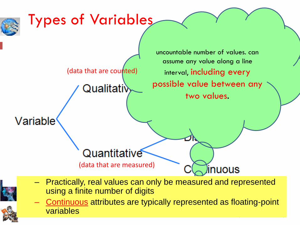
uncountable number of values. can

assume any value along a line

interval, including every

possible value between any

two values.

Types of Variables



– Practically, real values can only be measured and represented using a finite number of digits

– Continuous attributes are typically represented as floating-point variables

Dr. Abeer Mahmoud


Classification

11

Dr. Abeer Mahmoud


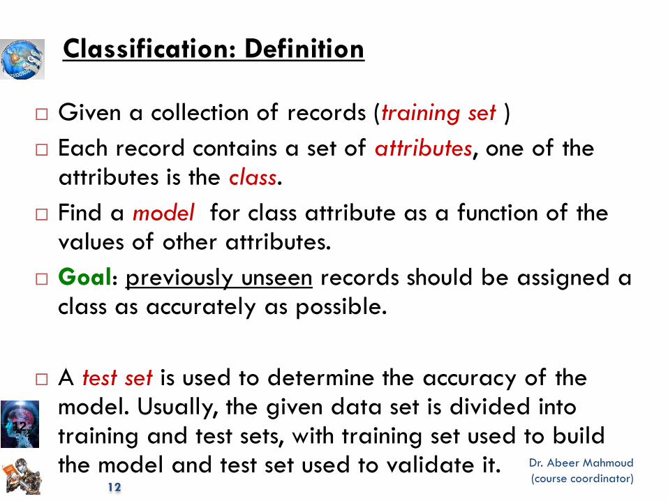
Classification: Definition

Given a collection of records (training set )

Each record contains a set of attributes, one of the attributes is the class.

Find a model for class attribute as a function of the values of other attributes.

Goal: previously unseen records should be assigned a class as accurately as possible.

A test set is used to determine the accuracy of the model. Usually, the given data set is divided into training and test sets, with training set used to build the model and test set used to validate it.

12

Dr. Abeer Mahmoud


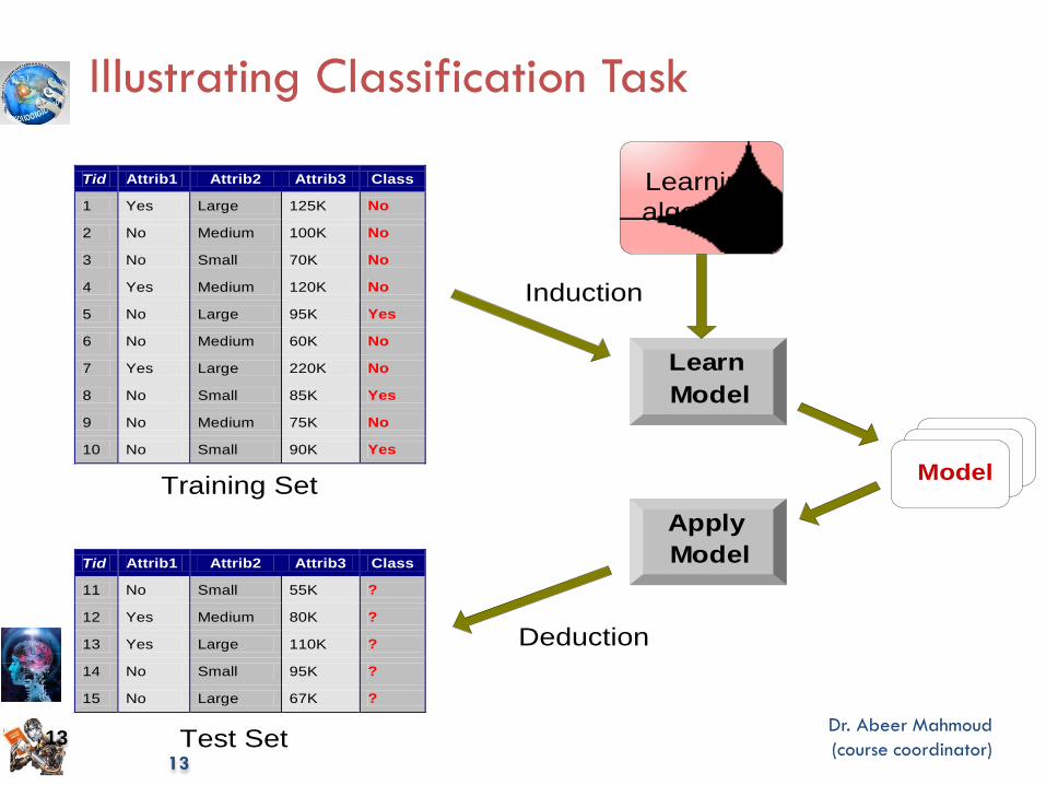
Illustrating Classification Task

Apply

Model

Induction

Deduction

Learn

Model

Model

Tid Attrib1 Attrib2 Attrib3 Class

1 Yes Large 125K No

2 No Medium 100K No

3 No Small 70K No

4 Yes Medium 120K No

5 No Large 95K Yes

6 No Medium 60K No

7 Yes Large 220K No

8 No Small 85K Yes

9 No Medium 75K No

10 No Small 90K Yes 10

Tid Attrib1 Attrib2 Attrib3 Class

11 No Small 55K ?

12 Yes Medium 80K ?

13 Yes Large 110K ?

14 No Small 95K ?

15 No Large 67K ? 10

Test Set

Learning

algorithm

Training Set

13

Dr. Abeer Mahmoud


Decision Tree Learning

14

Dr. Abeer Mahmoud


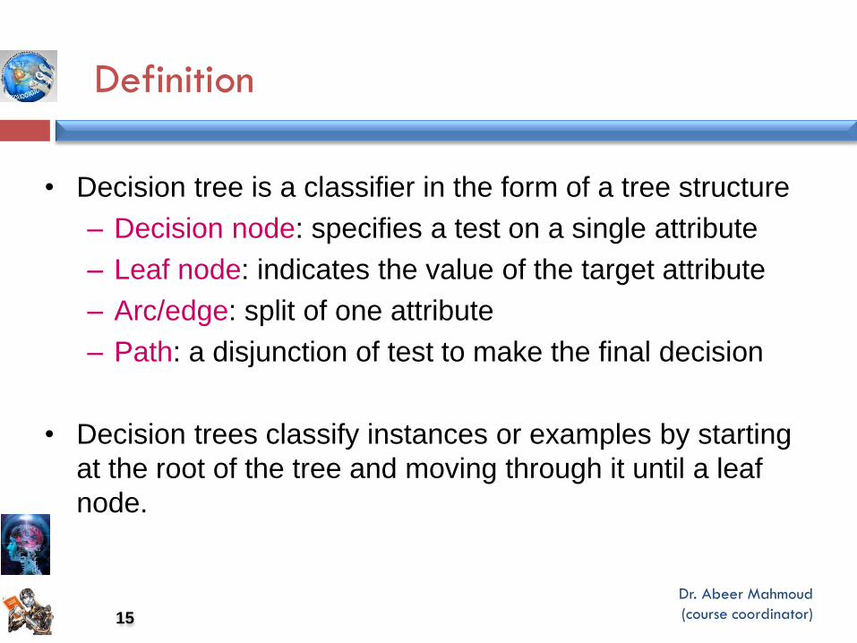
• Decision tree is a classifier in the form of a tree structure

– Decision node: specifies a test on a single attribute

– Leaf node: indicates the value of the target attribute

– Arc/edge: split of one attribute

– Path: a disjunction of test to make the final decision

• Decision trees classify instances or examples by starting

at the root of the tree and moving through it until a leaf

node.

Definition

15

Dr. Abeer Mahmoud


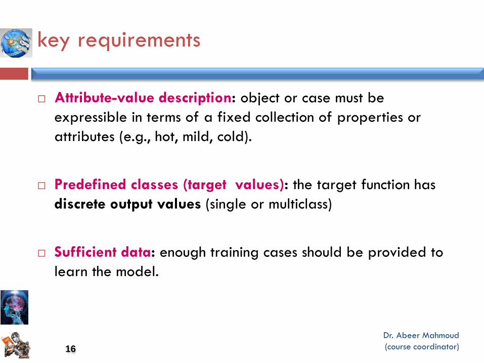
key requirements

Attribute-value description: object or case must be

expressible in terms of a fixed collection of properties or

attributes (e.g., hot, mild, cold).

Predefined classes (target values): the target function has

discrete output values (single or multiclass)

Sufficient data: enough training cases should be provided to

learn the model.

16

Dr. Abeer Mahmoud


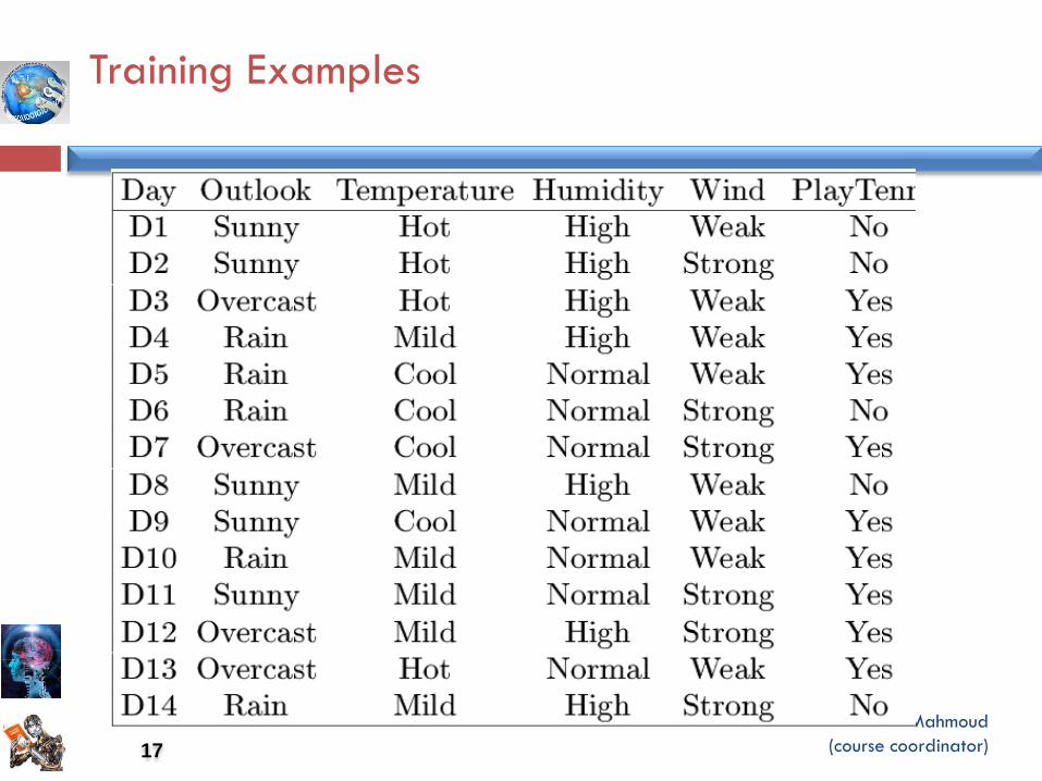
Training Examples

17

Dr. Abeer Mahmoud


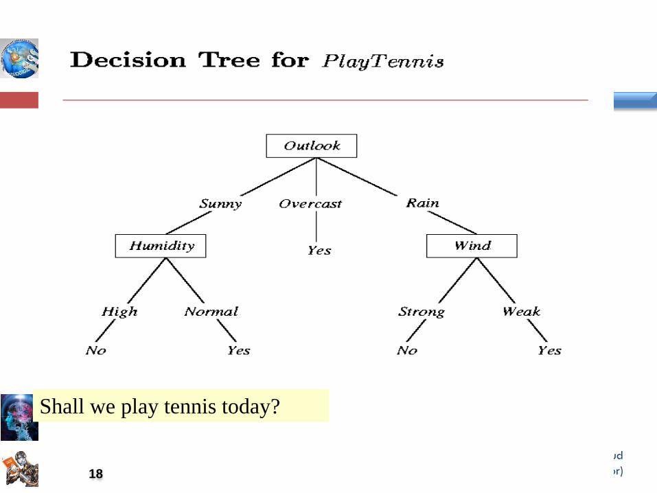
Shall we play tennis today?

18

Dr. Abeer Mahmoud


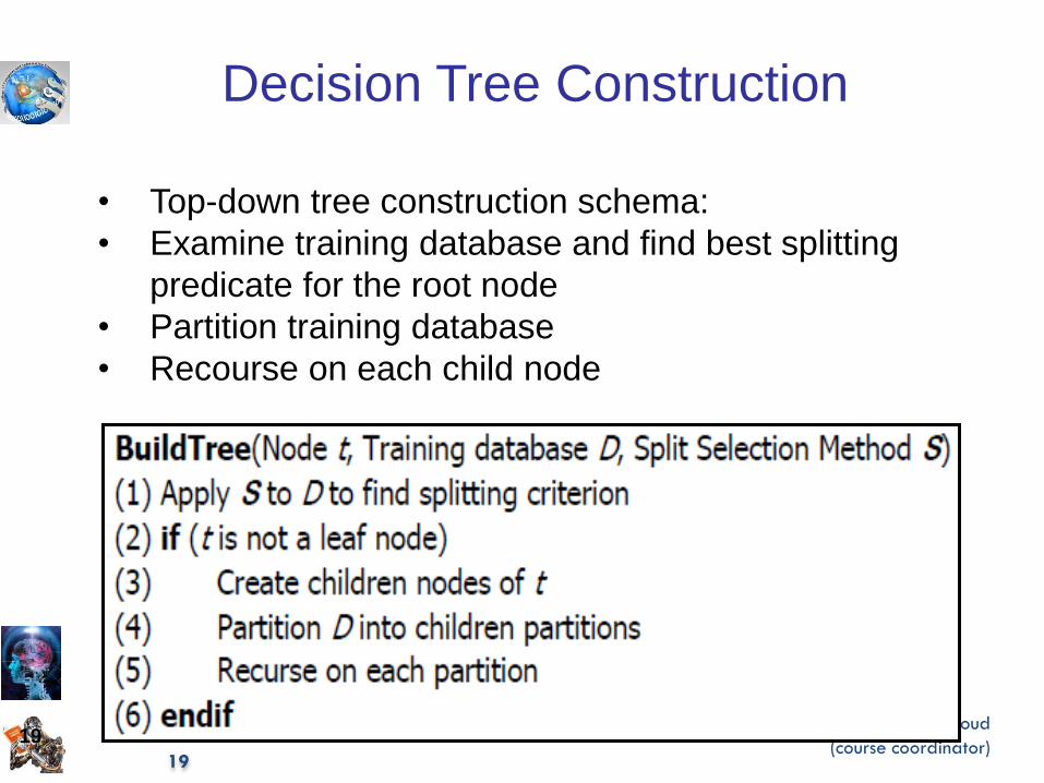
• Top-down tree construction schema:

• Examine training database and find best splitting

predicate for the root node

• Partition training database

• Recourse on each child node

Decision Tree Construction

19

Dr. Abeer Mahmoud


Advantages of using DT

Fast to implement

Simple to implement because it perform classification without

much computation

Can convert result to a set of easily interpretable rules that can

be used in knowledge system such as database, where rules

are built from the label of the nodes and the labels of the arcs.

Can handle continuous and categorical variables

Can handle noisy data

provide a clear indication of which fields are most important

for prediction or classification

20

Dr. Abeer Mahmoud


"Univariate" splits/partitioning using only one attribute at a time

so limits types of possible trees

large decision trees may be hard to understand

Perform poorly with many class and small data.

Disadvantages of using DT

21

Dr. Abeer Mahmoud


Two important algorithmic components:

Decision Tree Construction (cont..)

1. Splitting (ID3, CART, C4.5, QUEST, CHAID, ……)

2. Missing Values

22

Dr. Abeer Mahmoud


1-Splitting

23

Dr. Abeer Mahmoud


2.1- Splitting

Depends on

Data base

Attributes types

Statistical calculation

technique or method

(ID3, CART, C4.5, QUEST, CHAID, ……)

24

Dr. Abeer Mahmoud


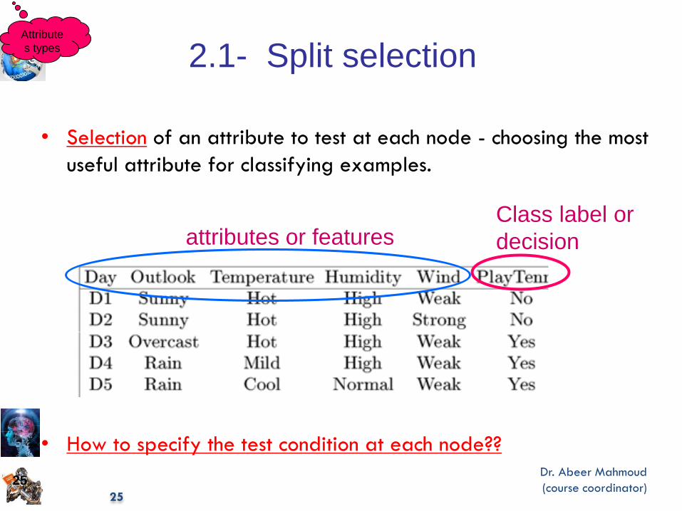
2.1- Split selection

• Selection of an attribute to test at each node - choosing the most

useful attribute for classifying examples.

• How to specify the test condition at each node??

attributes or features Class label or

decision

Attribute

s types

25

Dr. Abeer Mahmoud


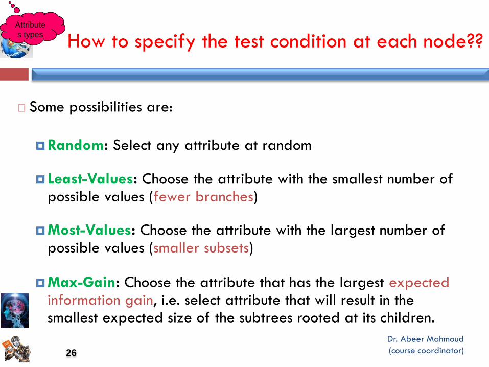
Some possibilities are:

Random: Select any attribute at random

Least-Values: Choose the attribute with the smallest number of possible values (fewer branches)

Most-Values: Choose the attribute with the largest number of possible values (smaller subsets)

Max-Gain: Choose the attribute that has the largest expected information gain, i.e. select attribute that will result in the smallest expected size of the subtrees rooted at its children.

How to specify the test condition at each node??

Attribute

s types

26

Dr. Abeer Mahmoud


Depends on attribute types

2.1.1 Nominal

2.1.2 Continuous

How to specify the test condition at each node??

Attribute

s types

27

Dr. Abeer Mahmoud


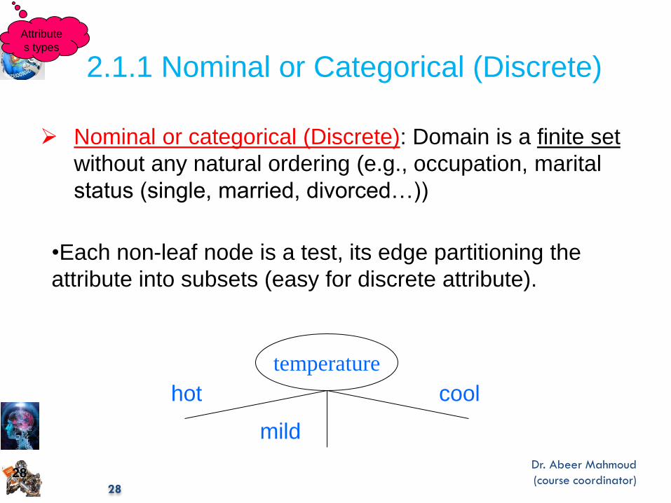
Nominal or categorical (Discrete): Domain is a finite set

without any natural ordering (e.g., occupation, marital

status (single, married, divorced…))

2.1.1 Nominal or Categorical (Discrete)

•Each non-leaf node is a test, its edge partitioning the

attribute into subsets (easy for discrete attribute).

temperature

hot

mild

cool

Attribute

s types

28

Dr. Abeer Mahmoud


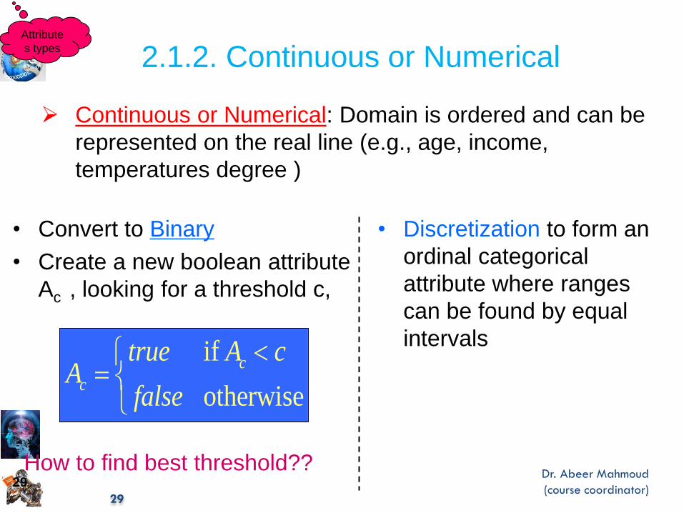
Continuous or Numerical: Domain is ordered and can be

represented on the real line (e.g., age, income,

temperatures degree )

2.1.2. Continuous or Numerical

• Convert to Binary

• Create a new boolean attribute

Ac , looking for a threshold c,

if

otherwise

c

c

true A cA

false

• Discretization to form an

ordinal categorical

attribute where ranges

can be found by equal

intervals

How to find best threshold??

Attribute

s types

29

Dr. Abeer Mahmoud


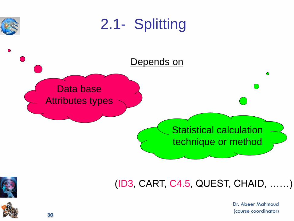
2.1- Splitting

Depends on

Data base

Attributes types

Statistical calculation

technique or method

(ID3, CART, C4.5, QUEST, CHAID, ……)

30

Dr. Abeer Mahmoud


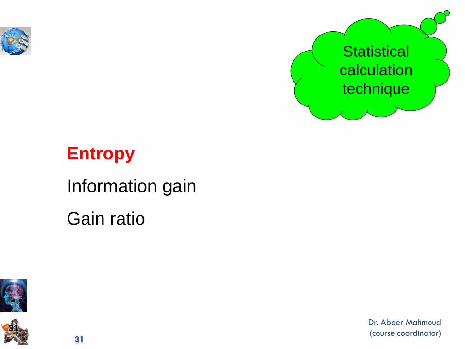
Statistical

calculation

technique

Entropy

Information gain

Gain ratio

31

Dr. Abeer Mahmoud


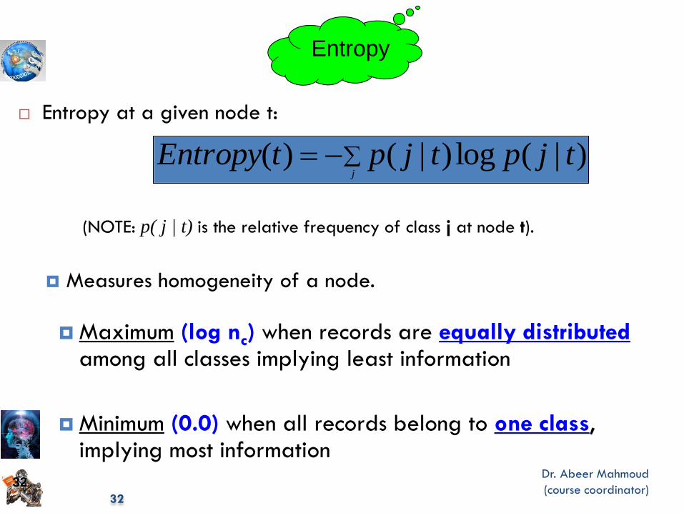
Entropy at a given node t:

(NOTE: p( j | t) is the relative frequency of class j at node t).

Measures homogeneity of a node.

Maximum (log nc) when records are equally distributed among all classes implying least information

Minimum (0.0) when all records belong to one class, implying most information

j

tjptjptEntropy )|(log)|()(

Entropy

32

Dr. Abeer Mahmoud


33

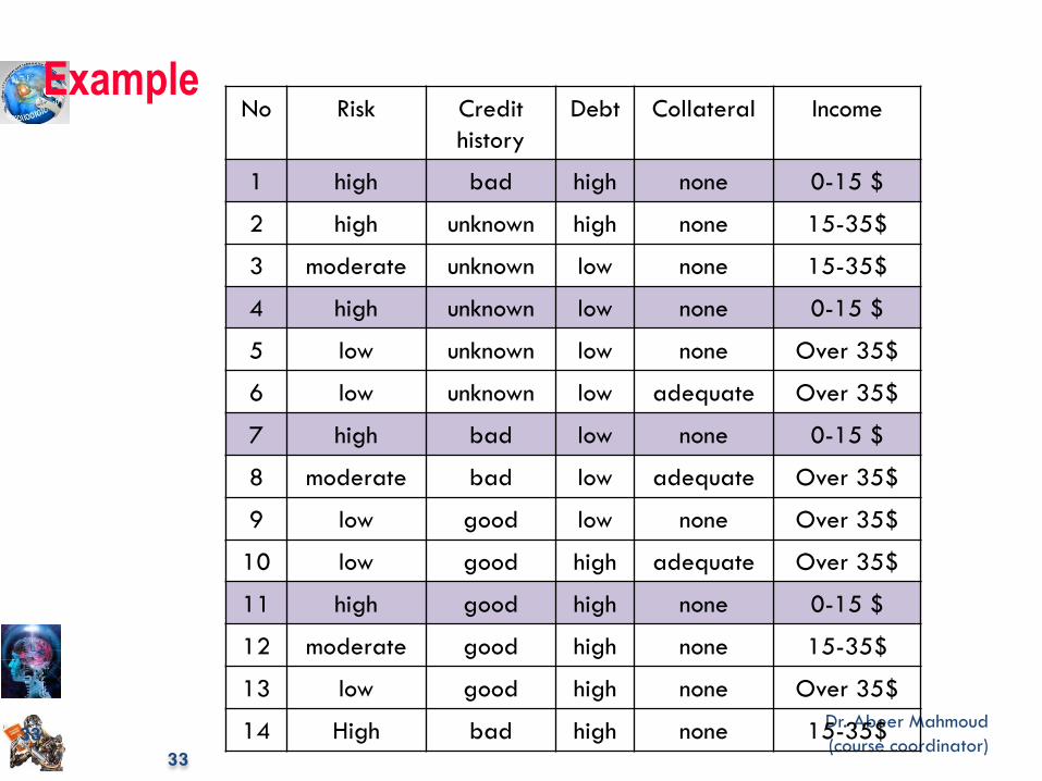
No Risk Credit

history

Debt Collateral Income

1 high bad high none 0-15 $

2 high unknown high none 15-35$

3 moderate unknown low none 15-35$

4 high unknown low none 0-15 $

5 low unknown low none Over 35$

6 low unknown low adequate Over 35$

7 high bad low none 0-15 $

8 moderate bad low adequate Over 35$

9 low good low none Over 35$

10 low good high adequate Over 35$

11 high good high none 0-15 $

12 moderate good high none 15-35$

13 low good high none Over 35$

14 High bad high none 15-35$

Example

Dr. Abeer Mahmoud


34

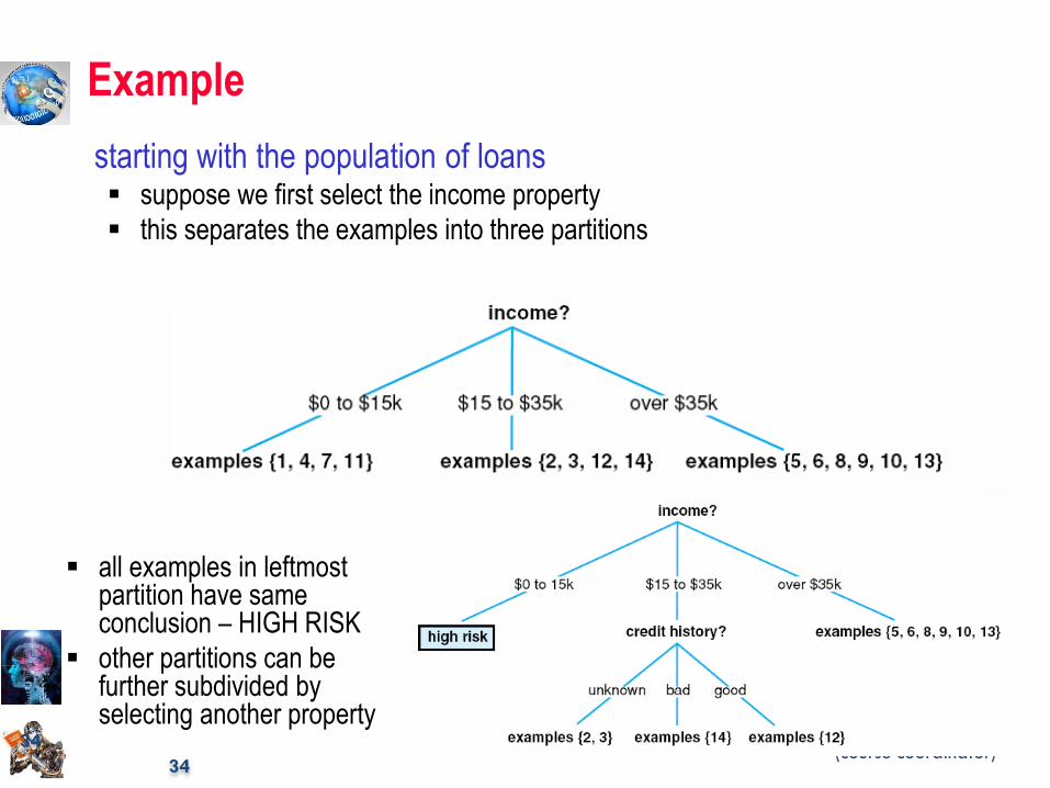
Example

starting with the population of loans suppose we first select the income property

this separates the examples into three partitions

all examples in leftmost partition have same conclusion – HIGH RISK

other partitions can be further subdivided by selecting another property

Dr. Abeer Mahmoud


ID3 & information theory

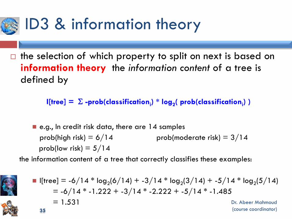
the selection of which property to split on next is based on information theory the information content of a tree is defined by

I[tree] = -prob(classificationi) * log2( prob(classificationi) )

e.g., In credit risk data, there are 14 samples

prob(high risk) = 6/14 prob(moderate risk) = 3/14

prob(low risk) = 5/14

the information content of a tree that correctly classifies these examples:

I[tree] = -6/14 * log2(6/14) + -3/14 * log2(3/14) + -5/14 * log2(5/14)

= -6/14 * -1.222 + -3/14 * -2.222 + -5/14 * -1.485

= 1.531

Dr. Abeer Mahmoud


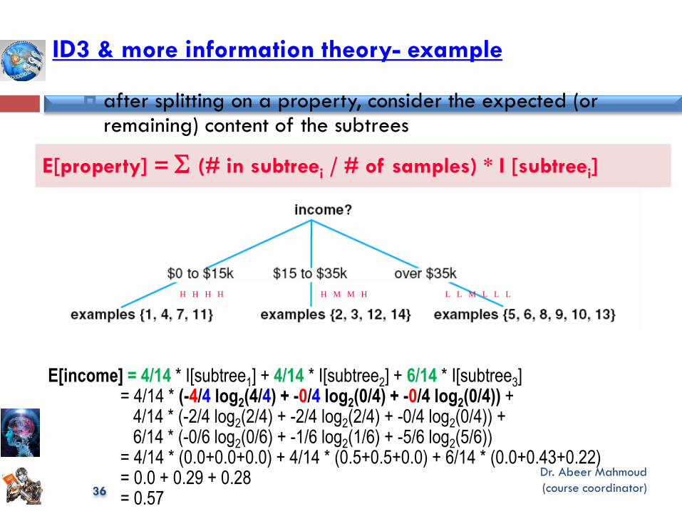
ID3 & more information theory- example

after splitting on a property, consider the expected (or remaining) content of the subtrees

E[income] = 4/14 * I[subtree1] + 4/14 * I[subtree2] + 6/14 * I[subtree3] = 4/14 * (-4/4 log2(4/4) + -0/4 log2(0/4) + -0/4 log2(0/4)) + 4/14 * (-2/4 log2(2/4) + -2/4 log2(2/4) + -0/4 log2(0/4)) + 6/14 * (-0/6 log2(0/6) + -1/6 log2(1/6) + -5/6 log2(5/6)) = 4/14 * (0.0+0.0+0.0) + 4/14 * (0.5+0.5+0.0) + 6/14 * (0.0+0.43+0.22) = 0.0 + 0.29 + 0.28 = 0.57

H H H H H M M H L L M L L L

E[property] = (# in subtreei / # of samples) * I [subtreei]

Dr. Abeer Mahmoud


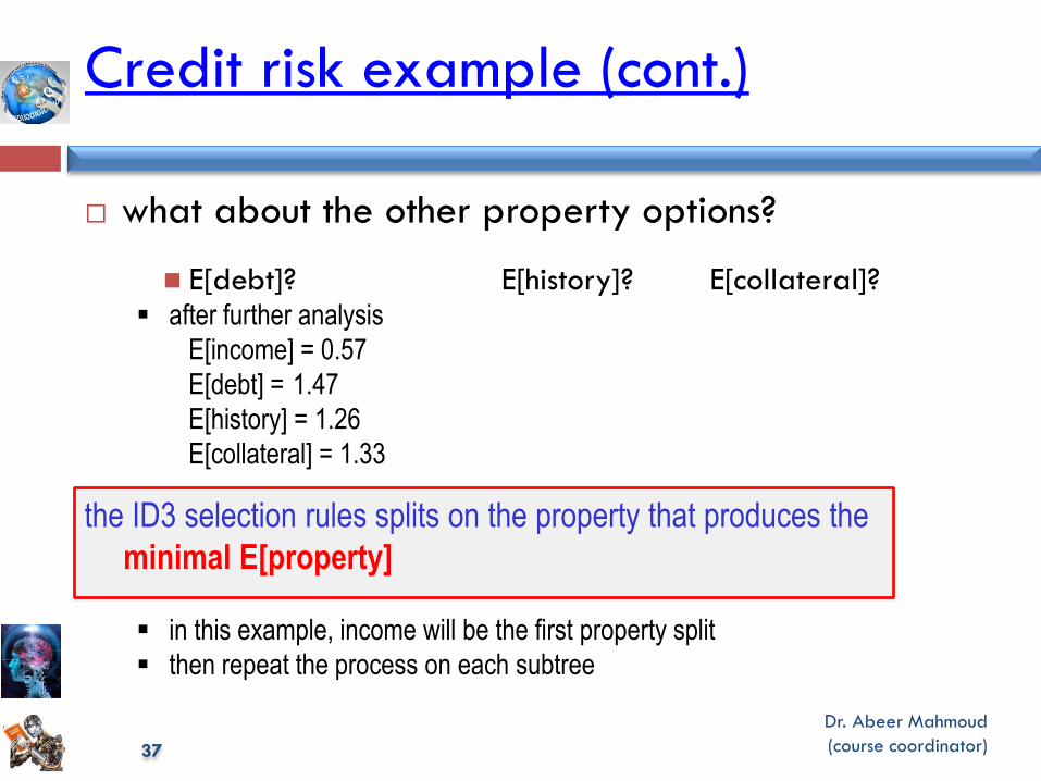
Credit risk example (cont.)

what about the other property options?

E[debt]? E[history]? E[collateral]? after further analysis

E[income] = 0.57

E[debt] = 1.47

E[history] = 1.26

E[collateral] = 1.33

the ID3 selection rules splits on the property that produces the

minimal E[property]

in this example, income will be the first property split

then repeat the process on each subtree

Dr. Abeer Mahmoud


2.3- Missing Values

What is the problem?

During computation of the splitting predicate, we can

selectively ignore records with missing values (note that

this has some problems)

But if a record r misses the value of the variable in the

splitting attribute, r can not participate further in tree

construction Algorithms for missing values address this

problem.

Simplest algorithm to solve this problem :

-If X is numerical (categorical), impute the overall mean

- if X is discrete attribute set the most common value

38

Dr. Abeer Mahmoud


Thank you

End of

Chapter 18-part 2

39

Documents

Princess Nora University Faculty of Computer & Information ...pnu-cs-ai.yolasite.com/resources/ch9- CS370 -Learning from examples... · Dr. Abeer Mahmoud (course coordinator) assume