PRIMORDIAL GRAVITATIONAL WAVES AND

CMB POLARIZATIONAlexander Polnarev

Queen Mary, University of London

Zeldovich100, 21 March 2014

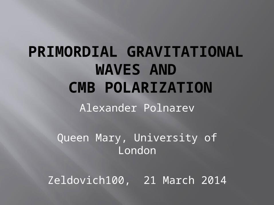
Talk Overview:

The role of CMB polarization in Cosmology predicted by YaB in 1979

Introduction to CMB polarization Imprints of Primordial Gravitational

Waves on the CMB Detection of these imprints by the BICEP-2 in 2014 Summary and Conclusions

03.08.1914 -12.02.1987

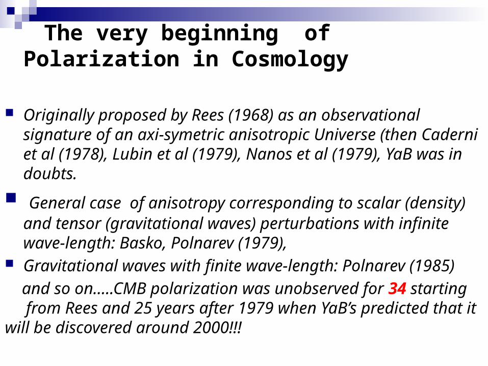
The very beginning of Polarization in Cosmology

Originally proposed by Rees (1968) as an observational signature of an axi-symetric anisotropic Universe (then Caderni et al (1978), Lubin et al (1979), Nanos et al (1979), YaB was in doubts.

General case of anisotropy corresponding to scalar (density) and tensor (gravitational waves) perturbations with infinite wave-length: Basko, Polnarev (1979),

Gravitational waves with finite wave-length: Polnarev (1985)

and so on…..CMB polarization was unobserved for 34 starting from Rees and 25 years after 1979 when YaB’s predicted that it will be discovered around 2000!!!

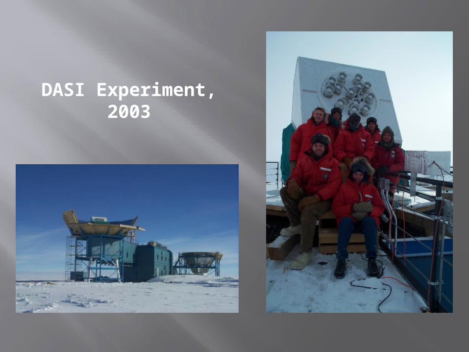
DASI Experiment, 2003

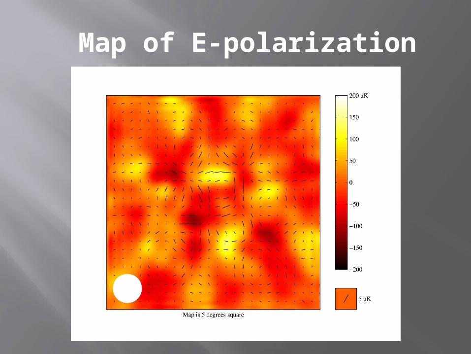
Map of E-polarization

April 19, 2023 8

Introduction to CMB Polarization

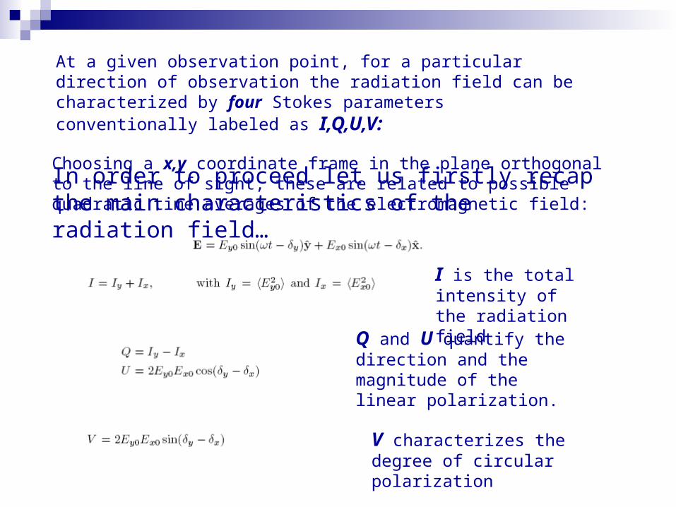
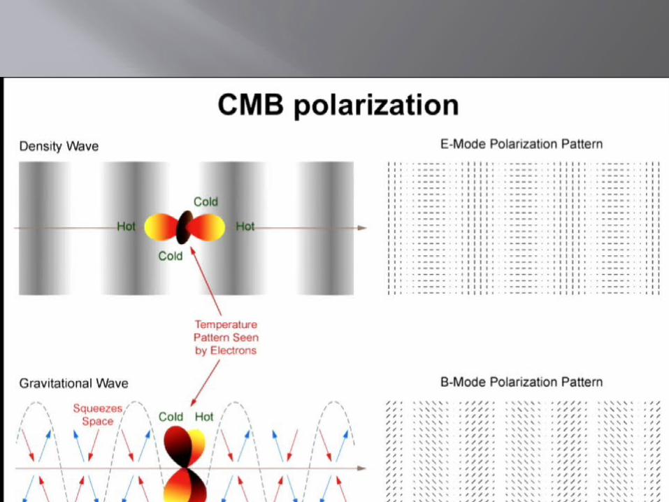
At a given observation point, for a particular direction of observation the radiation field can be characterized by four Stokes parameters conventionally labeled as I,Q,U,V:

Choosing a x,y coordinate frame in the plane orthogonal to the line of sight, these are related to possible quadratic time averages of the electromagnetic field:

I is the total intensity of the radiation field

Q and U quantify the direction and the magnitude of the linear polarization.

V characterizes the degree of circular polarization

In order to proceed let us firstly recap the main characteristics of the radiation field…

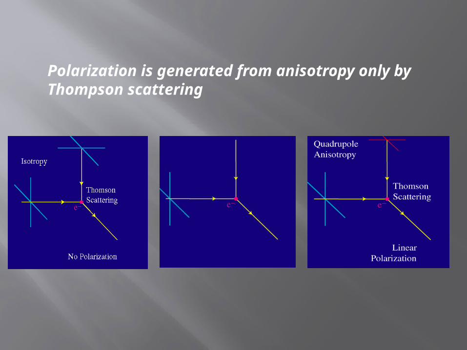
Polarization is generated from anisotropy only by Thompson scattering

11

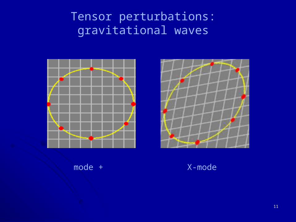
+mode X-mode

Tensor perturbations: gravitational waves

12

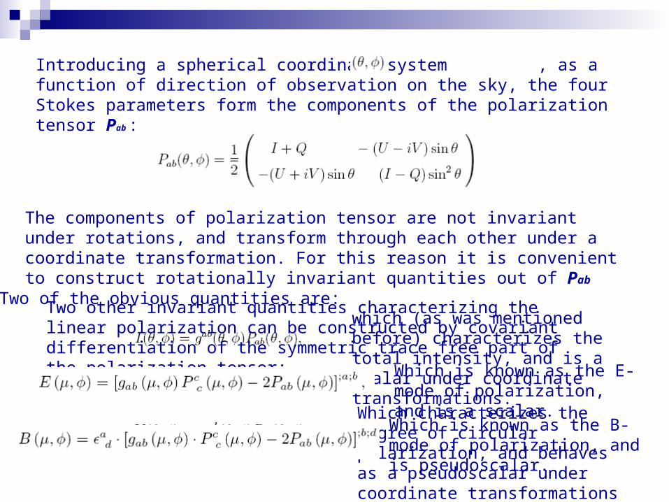
The components of polarization tensor are not invariant under rotations, and transform through each other under a coordinate transformation. For this reason it is convenient to construct rotationally invariant quantities out of Pab

Introducing a spherical coordinate system , as a function of direction of observation on the sky, the four Stokes parameters form the components of the polarization tensor Pab :

Two of the obvious quantities are:which (as was mentioned before) characterizes the total intensity, and is a scalar under coordinate transformations.

Which characterizes the degree of circular polarization, and behaves as a pseudoscalar under coordinate transformations

Two other invariant quantities characterizing the linear polarization can be constructed by covariant differentiation of the symmetric trace free part of the polarization tensor:

Which is known as the E-mode of polarization, and is a scalar.

Which is known as the B-mode of polarization, and is pseudoscalar.

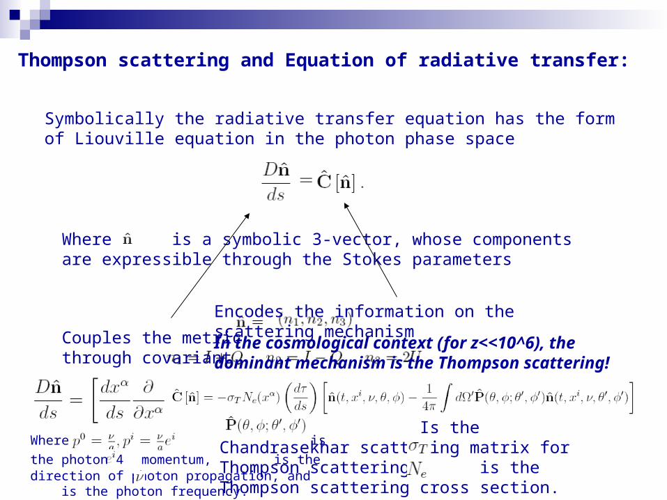
Thompson scattering and Equation of radiative transfer:

Symbolically the radiative transfer equation has the form of Liouville equation in the photon phase space

Where is a symbolic 3-vector, whose components are expressible through the Stokes parameters

Couples the metric through covariant differentiation

Where is the photon 4 momentum, is the direction of photon propagation, and is the photon frequency.

Encodes the information on the scattering mechanism

In the cosmological context (for z<<10^6), the dominant mechanism is the Thompson scattering!

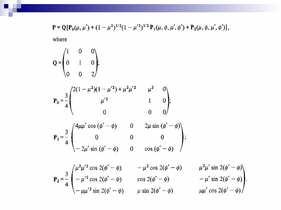
Is the Chandrasekhar scattering matrix for Thompson scattering. is the Thompson scattering cross section. is the density of free electrons

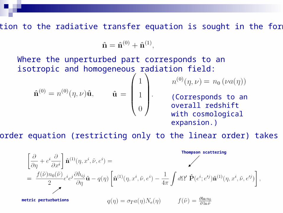
The solution to the radiative transfer equation is sought in the form:

Where the unperturbed part corresponds to an isotropic and homogeneous radiation field:

(Corresponds to an overall redshift with cosmological expansion.)

The first order equation (restricting only to the linear order) takes the form:

metric perturbations

Thompson scattering

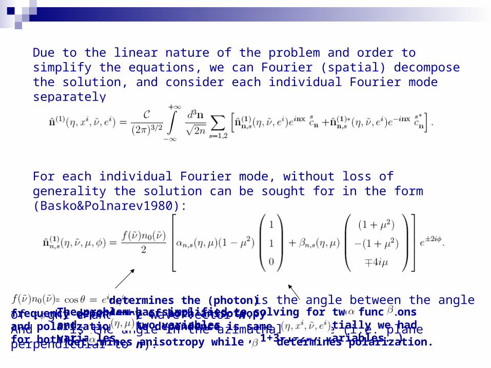
Due to the linear nature of the problem and order to simplify the equations, we can Fourier (spatial) decompose the solution, and consider each individual Fourier mode separately

For each individual Fourier mode, without loss of generality the solution can be sought for in the form (Basko&Polnarev1980):

Here is the angle between the angle of sight e and the wave vector n.And is the angle in the azimuthal plane (i.e. plane perpendicular to n). determines the (photon) frequency dependency of both anisotropy and polarization (the dependence is same for both)!

The problem has simplified to solving for two functions and of two variables . (initially we had variables , 1+3+1+2=7 variables. )

determines anisotropy while determines polarization.

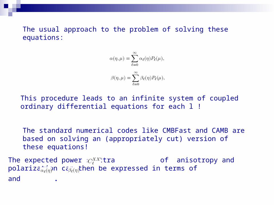
The usual approach to the problem of solving these equations:

This procedure leads to an infinite system of coupled ordinary differential equations for each l !

The standard numerical codes like CMBFast and CAMB are based on solving an (appropriately cut) version of these equations!

The expected power spectra of anisotropy and polarization can then be expressed in

terms of and .

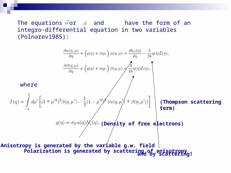
The equations for and have the form of an integro-differential equation in two variables (Polnarev1985):

where

(Thompson scattering term)

(Density of free electrons)

Anisotropy is generated by the variable g.w. field

and by scattering!Polarization is generated by scattering of anisotropy

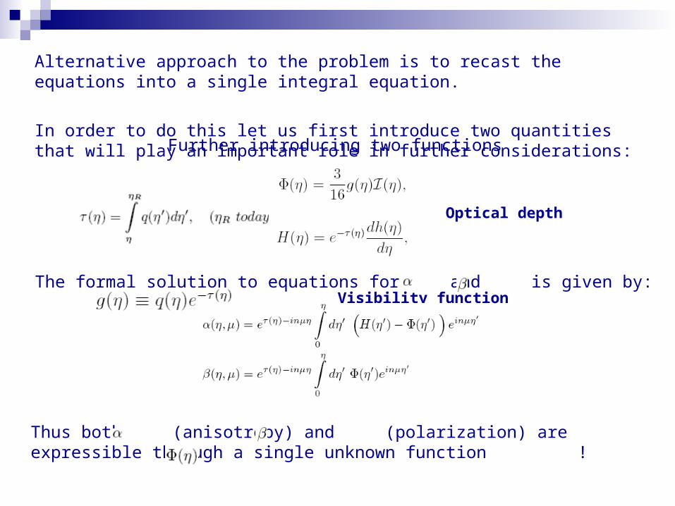
Alternative approach to the problem is to recast the equations into a single integral equation.

In order to do this let us first introduce two quantities that will play an important role in further considerations:

Optical depth

Visibility function

Further introducing two functions

The formal solution to equations for and is given by:

Thus both (anisotropy) and (polarization) are expressible through a single unknown function !

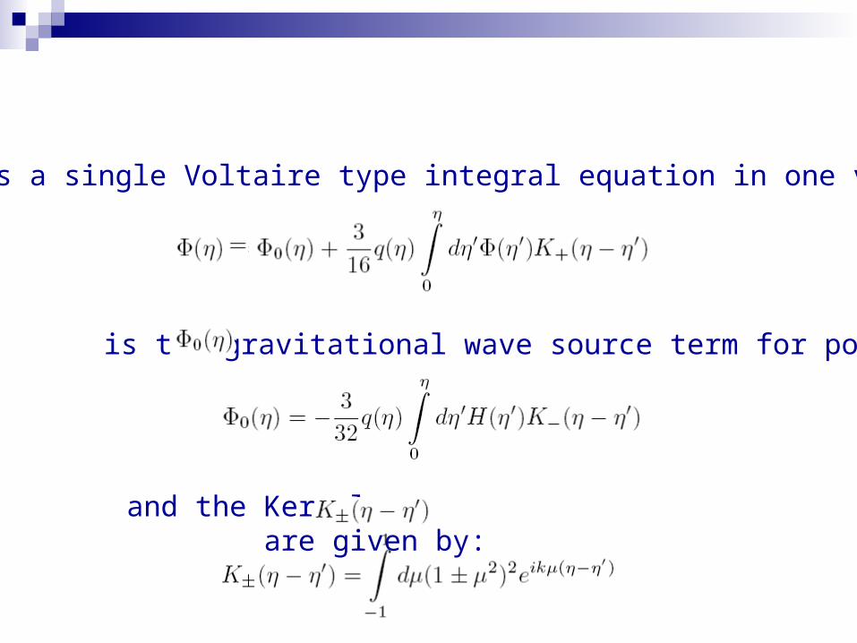
The result is a single Voltaire type integral equation in one variable:

Where is the gravitational wave source term for polarization

and the Kernels are given by:

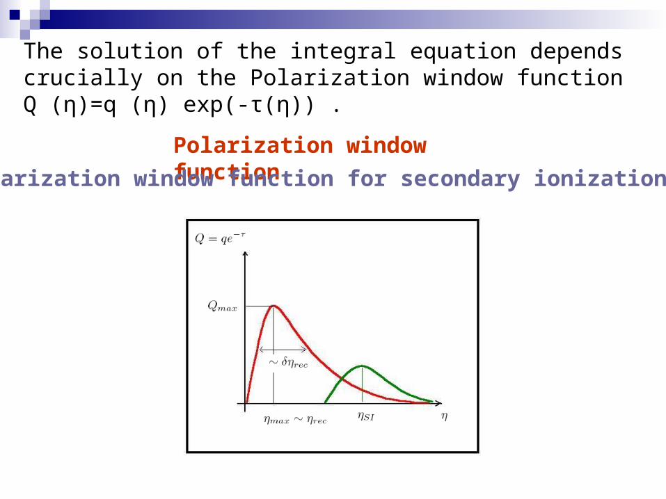
Polarization window function

Polarization window function for secondary ionization

The solution of the integral equation depends crucially on the Polarization window function Q (η)=q (η) exp(-τ(η)) .

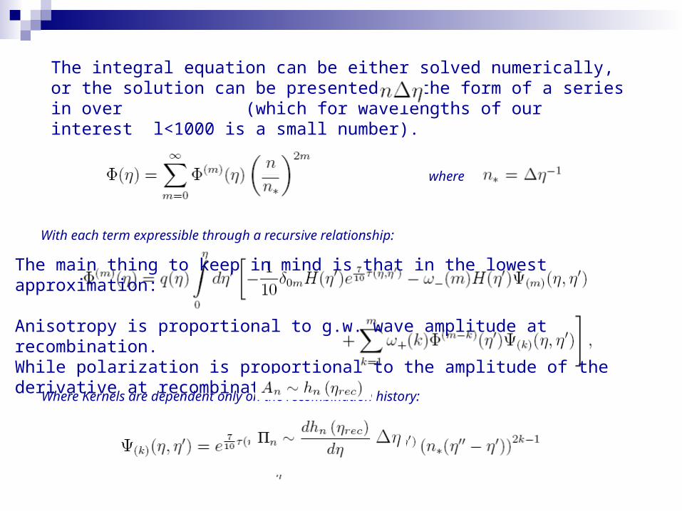
The integral equation can be either solved numerically, or the solution can be presented in the form of a series in over (which for wavelengths of our interest l<1000 is a small number).

where

With each term expressible through a recursive relationship:

Where Kernels are dependent only on the recombination history:

The main thing to keep in mind is that in the lowest approximation:

Anisotropy is proportional to g.w. wave amplitude at recombination.While polarization is proportional to the amplitude of the derivative at recombination.

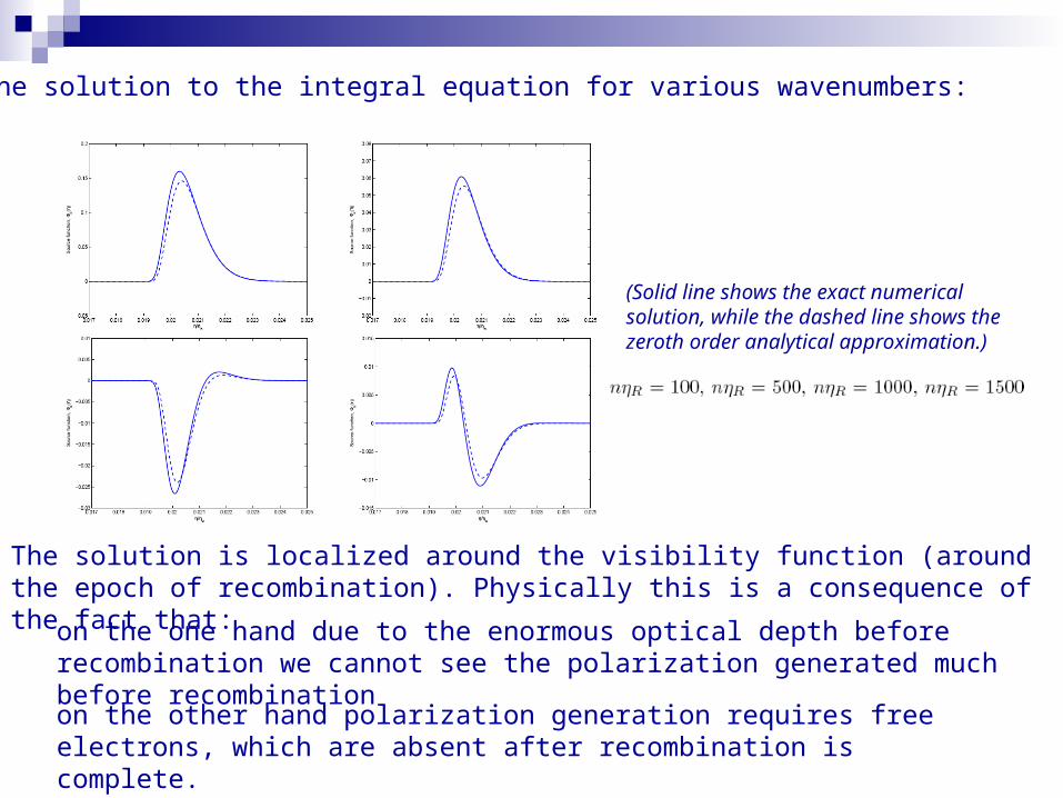
The solution to the integral equation for various wavenumbers:

(Solid line shows the exact numerical solution, while the dashed line shows the zeroth order analytical approximation.)

The solution is localized around the visibility function (around the epoch of recombination). Physically this is a consequence of the fact that:

on the one hand due to the enormous optical depth before recombination we cannot see the polarization generated much before recombination

on the other hand polarization generation requires free electrons, which are absent after recombination is complete.

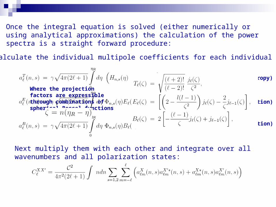
Once the integral equation is solved (either numerically or using analytical approximations) the calculation of the power spectra is a straight forward procedure:

First calculate the individual multipole coefficients for each individual wave:

(Temperature anisotropy)

(E mode of polarization)

(B mode of polarization)

Where the projection factors are expressible through combinations of spherical Bessel functions

Next multiply them with each other and integrate over all wavenumbers and all polarization states:

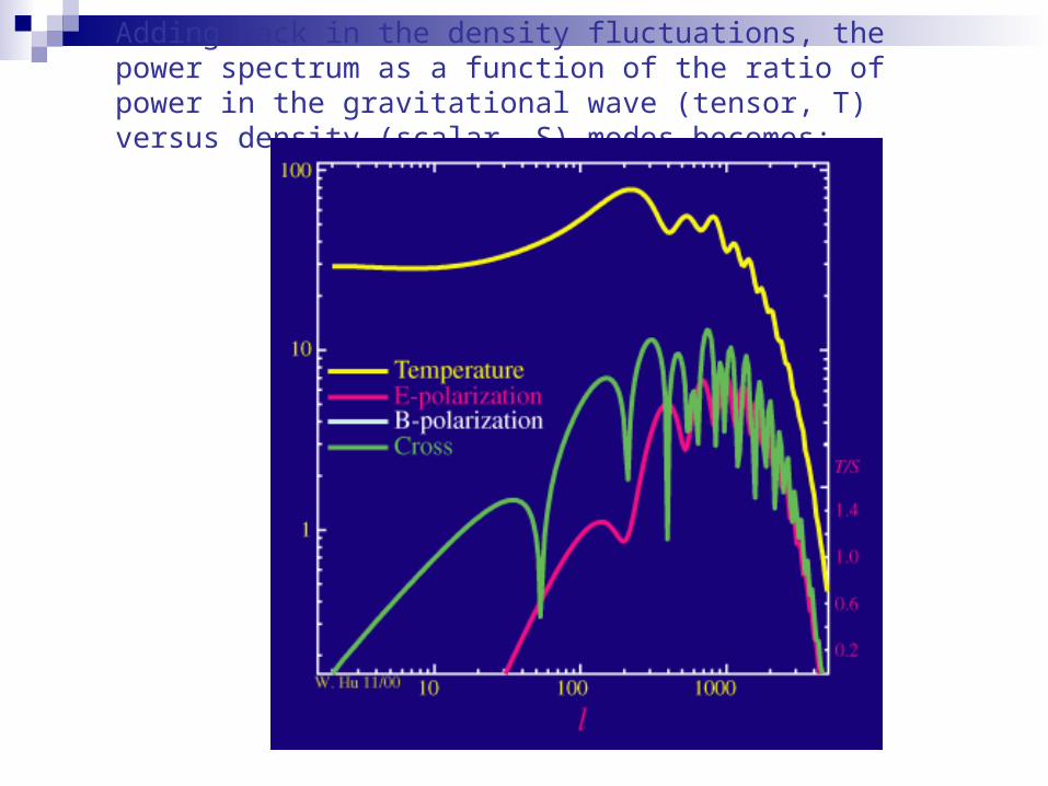
Adding back in the density fluctuations, the power spectrum as a function of the ratio of power in the gravitational wave (tensor, T) versus density (scalar, S) modes becomes:

Imprints of Primordial Gravitational Waves on the CMB

27

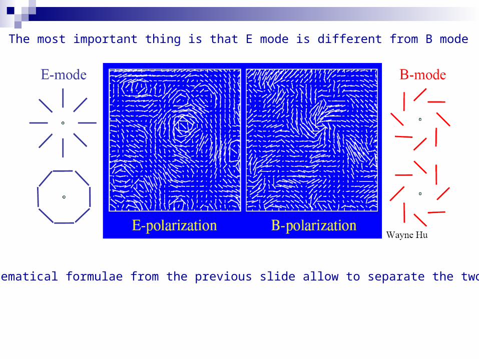
The most important thing is that E mode is different from B mode

The mathematical formulae from the previous slide allow to separate the two types

April 19, 2023 30

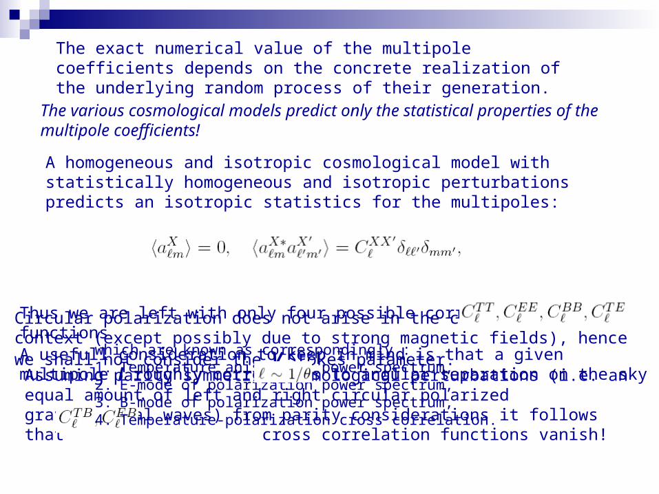
The exact numerical value of the multipole coefficients depends on the concrete realization of the underlying random process of their generation.

The various cosmological models predict only the statistical properties of the multipole coefficients!

A homogeneous and isotropic cosmological model with statistically homogeneous and isotropic perturbations predicts an isotropic statistics for the multipoles:

Circular polarization does not arise in the cosmological context (except possibly due to strong magnetic fields), hence we shall not consider the V Stokes parameter.

Assuming parity symmetric cosmological perturbations (i.e. an equal amount of left and right circular polarized gravitational waves) from parity considerations it follows that cross correlation functions vanish!

Thus we are left with only four possible correlation functions

which are known as correspondingly :1. Temperature anisotropy power spectrum,2. E-mode of polarization power spectrum,3. B-mode of polarization power spectrum,4. Temperature-polarization cross correlation.

A usefull consideration to keep in mind is that a given multipole l roughly corresponds to angular separation on the sky .

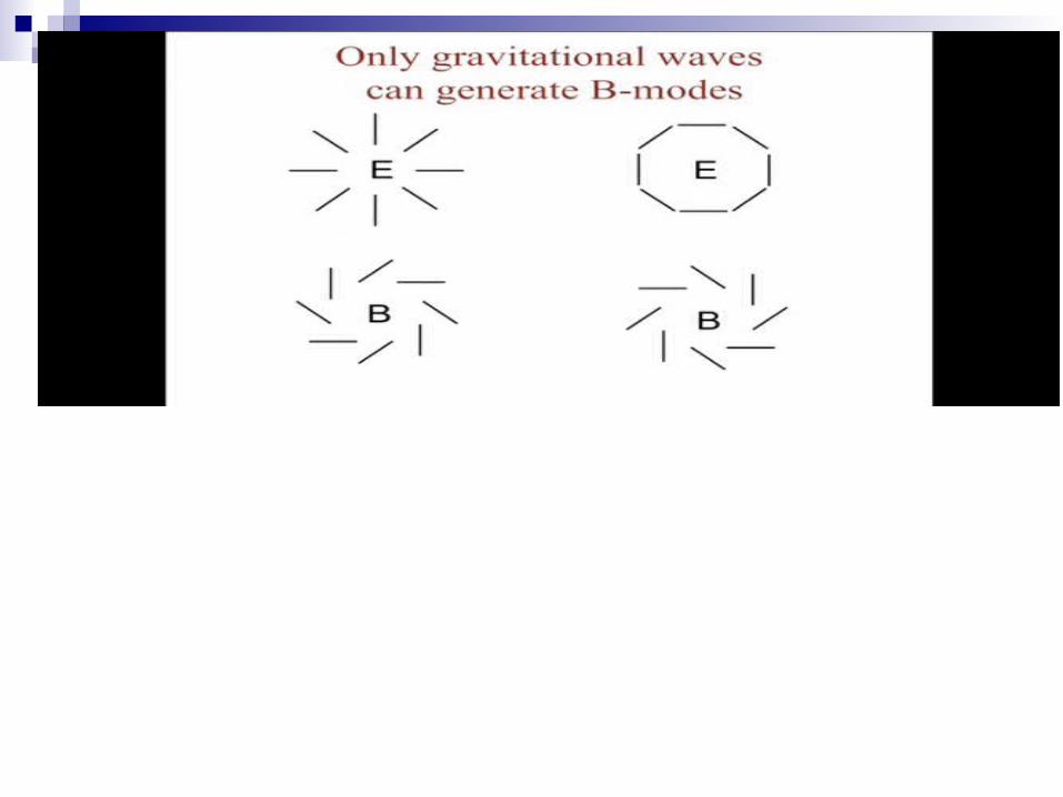
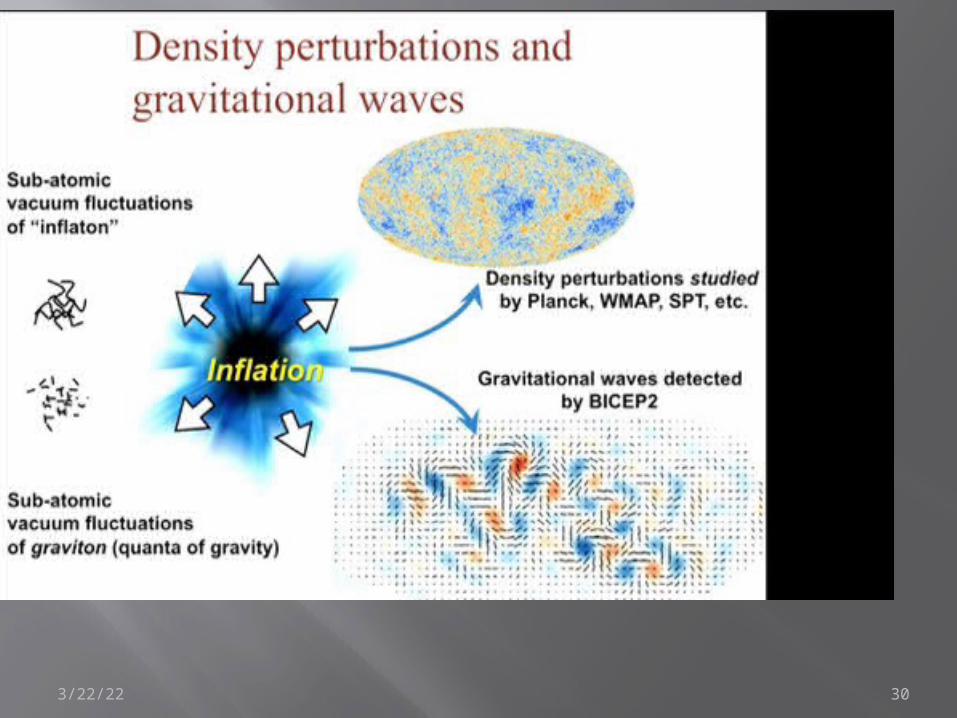
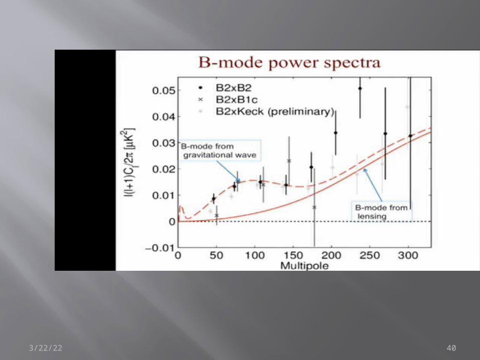
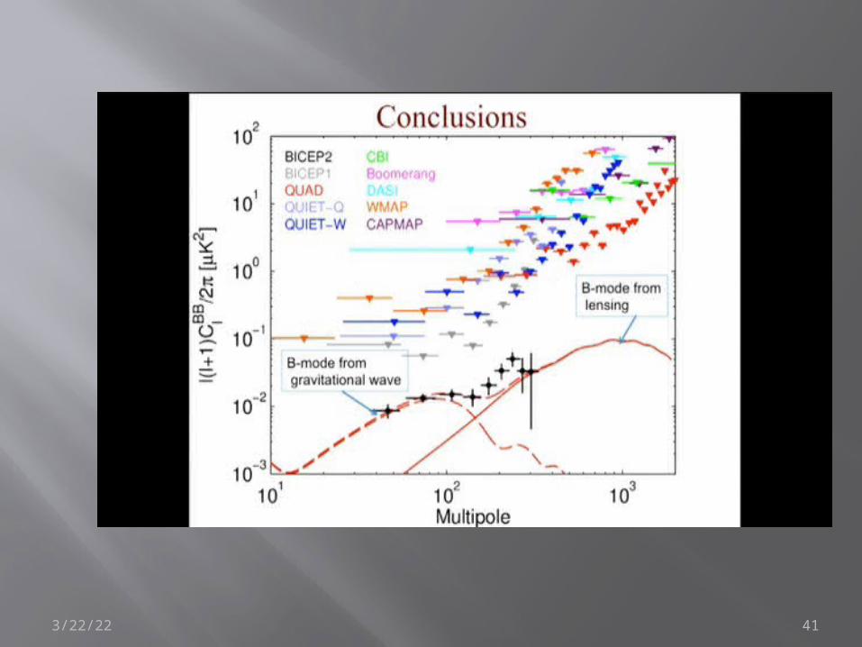
• Gravitational waves show  a power spectrum with both E and B mode contributions

• Gravitational waves contribution to B-modes is a few tenths of a μK at l~100.

• Gravitational waves probe the physics of inflation but will require a thorough understanding of foregrounds and secondary effects for their detection.

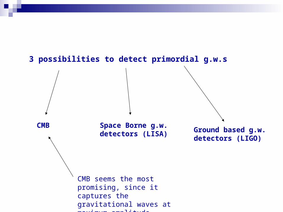
3 possibilities to detect primordial g.w.s

CMB Space Borne g.w. detectors (LISA)

Ground based g.w.detectors (LIGO)

CMB seems the most promising, since it captures the gravitational waves at maximum amplitude.

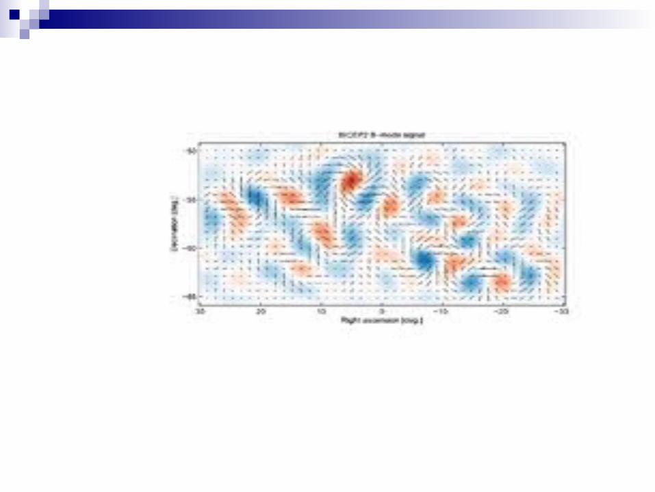
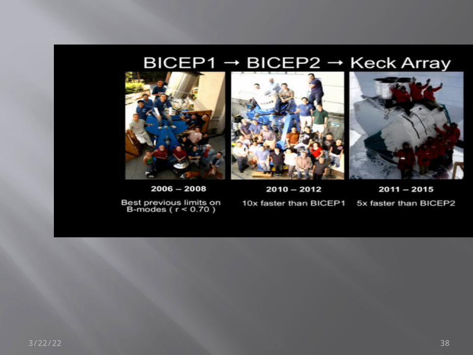
Detection of these imprints by the BICEP-2 in 2014

36

April 19, 2023 37

April 19, 2023 38

April 19, 2023 39

April 19, 2023 40

April 19, 2023 41

Summary and Conclusions:

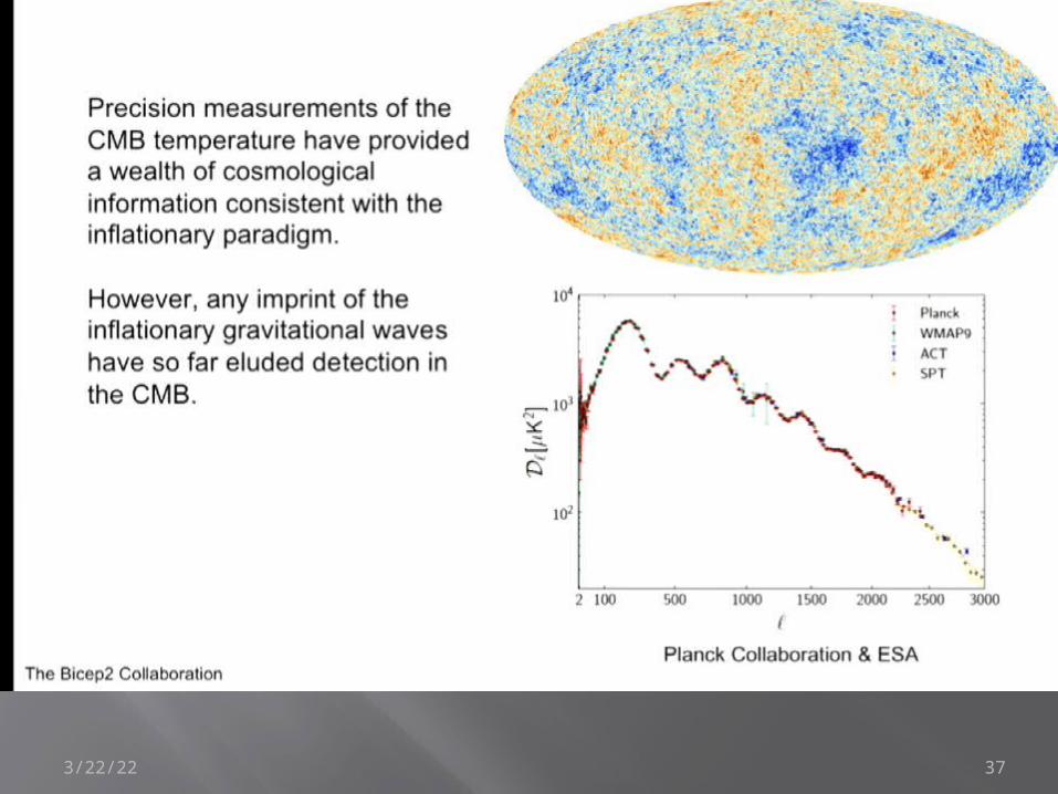
The main features in the anisotropy and polarization spectra due to primordial gravitational waves have been understood and explained.

There seems that BICEP 2 already observes primordial gravitational waves. CMB promises to be our clearest window (i.e. CMB works like good antenna) for gravitational-wave astronomy to observe primordial gravitational waves and see the Very Very Early Universe .

YaB’s prediction is coming true.