Embed Size (px)
Citation preview
SIAM J. Optimization c©1992 Society for Industrial and Applied Mathematics
Vol. ???, No. ???, pp. ???–???, ??? 1992 ???
PRIMAL-DUAL PROJECTED GRADIENT ALGORITHMSFOR EXTENDED LINEAR-QUADRATIC PROGRAMMING*
CIYOU ZHU† and R. T. ROCKAFELLAR‡
Abstract. Many large-scale problems in dynamic and stochastic optimization can be modeledwith extended linear-quadratic programming, which admits penalty terms and treats them through
duality. In general the objective functions in such problems are only piecewise smooth and must beminimized or maximized relative to polyhedral sets of high dimensionality. This paper proposes a
new class of numerical methods for “fully quadratic” problems within this framework, which exhibitsecond-order nonsmoothness. These methods, combining the idea of finite-envelope representationwith that of modified gradient projection, work with local structure in the primal and dual problems
simultaneously, feeding information back and forth to trigger advantageous restarts.
Versions resembling steepest descent methods and conjugate gradient methods are presented.When a positive threshold of ε-optimality is specified, both methods converge in a finite number of
iterations. With threshold 0, it is shown under mild assumptions that the steepest descent versionconverges linearly, while the conjugate gradient version still has a finite termination property. The
algorithms are designed to exploit features of primal and dual decomposability of the Lagrangian,which are typically available in a large-scale setting, and they are open to considerable parallelization.
Key words. Extended linear-quadratic programming, large-scale numerical optimization,
finite-envelope representation, gradient projection, primal-dual methods, steepest descent methods,
conjugate gradient methods.
AMS(MOS) subject classifications. 65K05, 65K10, 90C20
1. Introduction. A number of recent papers have described “extended linear-quadratic programming” as a modeling scheme that is much more flexible for problemsof optimization than conventional quadratic programming and seems especially suitedto large-scale applications, in particular because of way penalty terms can be incorpo-rated. Rockafellar and Wets in [1], [2], first used the concept in two-stage stochasticprogramming, where the primal dimension is low but the dual dimension is high. It wasdeveloped further in its own right in Rockafellar [3], [4], and carried in the latter paperto the context of continuous-time optimal control. Discrete-time problems of optimalcontrol, both deterministic and stochastic (i.e., multistage stochastic programming)were analyzed as extended linear-quadratic programming problems in Rockafellar andWets [5] and shown to have a remarkable property of Lagrangian decomposability inthe primal and dual arguments, both of which can be high dimensional. These modelsraise new computational challenges and possibilities.
A foundation for numerical schemes in large-scale extended linear-quadratic pro-gramming has been laid in Rockafellar [6] and elaborated for problems in multistageformat in Rockafellar [7]. The emphasis in [6] is on basic finite-envelope methods, whichuse duality in generating envelope approximations to the primal and dual objectivefunctions through a finite sequence of separate minimizations or maximizations of theLagrangian. These methods generalize the one originally proposed in [1] for two-stagestochastic programming and implemented by King [8] and Wagner [9]. They center
*Received by the editors December ???, 1990; accepted for publication (in revised form) ???
???, 1992. This work was supported in part by AFOSR grants 87-0281 and 89-0081 and NSF grantsDMS-8701768 and DMS-8819586.
†Department of Mathematical Sciences, The Johns Hopkins University, Baltimore, MD 21218.
‡Department of Applied Mathematics, FS-20, University of Washington, Seattle, WA 98195.
1
2 c. zhu and r. t. rockafellar
on the “fully quadratic” case, where strong convexity is present in both the primaland dual objectives, relying on exterior schemes such as the proximal point algorithmto create such strong convexity iteratively when it might otherwise be lacking.
Here we propose new algorithms which for fully quadratic problems combine theidea of finite-envelope representation with that of nonlinear gradient projection. Inthese methods the envelope approximations are utilized in a sort of steepest descentformat or conjugate gradient format in the primal and dual problems simultaneously.A type of feedback is introduced between primal and dual that takes advantage ofinformation jointly uncovered in computations, which in practice greatly speeds con-vergence. Both algorithms fit into a fundamental scheme for which global convergenceis established. Under a weak geometric assumption akin to strict complementaryslackness at optimality, the steepest descent version is shown to converge at a linearrate, while the conjugate gradient version has a finite termination property.
Both versions differ significantly from their traditional namesakes not only throughthe incorporation of a primal-dual scheme of gradient projection, but also in handlingobjective functions that generally could involve a complicated polyhedral “cell” struc-ture not conducive to explicit description by linear equations and inequalities. Theytreat the underlying constraints without resorting to an active set strategy, whichwould not be suitable for problems having high dimensionality in both primal anddual.
An important feature is that the computations are not carried out in terms ofa large, sparse matrix, such as might in principle serve in part to specify the twoproblems, but through subroutines for separate minimization and maximization of theLagrangian in its primal and dual arguments. This framework appears much betteradapted to the special structure available in dynamic and stochastic applications, andit supports extensive parallelization. To make this point clearer, and to introduce factsand notation that will later be needed, we discuss briefly the nature of extended linear-quadratic programming and the way it differs from ordinary quadratic programming.
From the Lagrangian point of view, extended linear-quadratic programming isdirected toward finding a saddle point (u, v) of a function
(1.1) L(u, v) = p·u + 12u·Pu + q·v − 1
2v·Qv − v·Ru over U × V,
where U and V are nonempty polyhedral (convex) sets in lRn and lRm respectively,and the matrices P ∈ lRn×n and Q ∈ lRm×m are symmetric and positive semidefinite.(One has p ∈ lRn, q ∈ lRm, and R ∈ lRm×n.) Associated with L, U and V are theprimal and dual problems
minimize f(u) over all u ∈ U, where f(u) := supv∈V
L(u, v),(P)
maximize g(v) over all v ∈ V, where g(v) := infu∈U
L(u, v).(Q)
We speak of the fully quadratic case of (P) and (Q) when both of the matrices P andQ are actually positive definite.
Standard quadratic programming would correspond to Q = 0 and V = lRm1+ ×
lRm2 . Then f would consist of a quadratic function plus the indicator of a systemof m1 linear inequality constraints and m2 linear equations, the indicator being thefunction which assigns an infinite penalty whenever these constraints are violated.Other choices of Q and V yield finite penalty expressions of various kinds. This isexplained in [4, Secs. 2 and 3] with many examples. For sound modeling in large-scale
primal-dual projected gradient algorithms for elqp 3
applications with dynamics and stochastics such as in [1], [2] and [5], it appears wiseto use finite rather than infinite penalties whenever constraints are “soft.” Extendedlinear-quadratic programming makes this option conveniently available. To the extentthat constraints in the primal problem are “hard,” they can be handled either by plac-ing them in the definition of the polyhedron U or through an augmented Lagrangiantechnique which corresponds to an exterior scheme of iterations of the proximal pointalgorithm, as already mentioned.
Theorem 1.1. [4] (Properties of the objective functions.) The objective functionsf in (P) and g in (Q) are piecewise linear-quadratic: in each case the space can bepartitioned in principle into a finite collection of polyhedral cells, relative to which thefunction has a linear or quadratic formula. Moreover, f is convex while g is concave.In the fully quadratic case of (P) and (Q), f is strongly convex and g is stronglyconcave, both functions having continuous first derivatives.
Theorem 1.2. [4], [1] (Duality and optimality.)(a) If either of the optimal values inf(P) or sup(Q) is finite, then both are finite
and equal, in which event optimal solutions u and v exist for the two problems. In thefully quadratic case in particular, the optimal values inf(P) and sup(Q) are finite andequal; then, moreover, the optimal solutions u and v are unique.
(b) A pair (u, v) is a saddle point of L(u, v) over U ×V if and only if u solves (P)and v solves (Q), or equivalently, f(u) = g(v).
Current numerical methods in standard quadratic programming, and the some-what more general area of linear complementarity problems [10], where U = lRn
+,V = lRm
+ , and Q is not necessarily the zero matrix, are surveyed by Lin and Pang [11].Other efforts in recent times have been made by Ye and Tse [12], Monteiro and Adler[13], Goldfarb and Liu [14].
None of these approaches is consonant with the large-scale applications that at-tract our interest, because the structure in such applications is not well served by thewholesale reformulations that would be required when penalty expressions are muchinvolved. Although any problem of extended linear-quadratic programming can inprinciple be recast as a standard problem in quadratic programming, as establishedin [1, Theorem 1], there is a substantial price to be paid in dimensionality and lossof symmetry, as well as in potential ill-conditioning. If the original problem had nprimal and m dual variables, and the expression of U and V involved m′ and n′ con-straints beyond nonnegavity of variables, then the reformulated problem in standardformat would generally have n+n′+m primal and m+m′ dual variables, and its fullconstraint system would tend to degeneracy (see [1, proof of Theorem 1]). The dualproblem would be quite different in its theoretical properties from the primal problem,so that computational ideas developed for the one could not be applied to the other.
Any problem of extended linear-quadratic programming can alternatively beposed in terms of solving a certain linear variational inequality (generalized equa-tion) as explained in [6, Theorem 2.3], and from that one could pass to a linearcomplementarity model. Symmetry and the meaningful representation of dynamicand stochastic structure could be maintained to a larger extent in this manner. Butlinear complementarity algorithms tend to be less robust than methods utilizing ob-jective function values, and an increase in dimensionality would still be required inhandling constraints, even if these are simply upper and lower bounds on the variables.Furthermore, such algorithms typically have to be carried to completion. They do notgenerate sequences of primal-feasible and dual-feasible solutions along with estimatesof how far these are from being optimal, as is highly desirable when problem sizeborders on the difficult.
4 c. zhu and r. t. rockafellar
While much could be said about the special problem structure in dynamic andstochastic applications [5], [7], it can be summarized for present purposes in the asser-tion that such problems, when formulated with care, satisfy the double decomposabilityassumption [6]. This means that for any fixed u ∈ U it is relatively easy to maximizeL(u, v) over v ∈ V , and likewise, for any fixed v ∈ V it is relatively easy to minimizeL(u, v) over u ∈ U , usually because of separability when either of the Lagrangian ar-guments is considered by itself. These subproblems of maximization and minimizationcalculate not only the objective values f(u) and g(v) but also, in the fully quadraticcase where L is strongly convex-concave, the uniquely determined vectors
(1.2) F (u) = argmaxv∈V
L(u, v) and G(v) = argminu∈U
L(u, v).
The issue is how to make use of such information in the design of numerical methods.Some proposals have already been made in Rockafellar [6]. Other ideas, which involvesplitting algorithms, have been explored by Tseng [15], [16]. Here we aim at adaptingclassical descent algorithms with help from convex analysis [17].
In this paper we make the blanket assumption of double decomposability, takingit as license also for exact line searchability [6]: the supposition that it is possible tominimize f(u) over any line segment joining two points in U , and likewise, to maximizeg(v) over any line segment joining two points in V . We focus on the fully quadraticcase, even though standard quadratic programming is thereby excluded and a di-rect comparison with other computational approaches, apart from the finite-envelopemethods in [6], becomes difficult. Our attention to that case is justified by its own po-tential in mathematical modeling (cf. [2], [4]) and because strong convexity-concavityof the Lagrangian can be created, if need be, through some outer implementation ofthe proximal point algorithm [18], [19], as carried out in [1] and [8]. The questionsconcerning such an outer algorithm are best handled elsewhere, since they have adifferent character and relate to a host of primal-dual procedures in extended linear-quadratic programming besides the ones developed here, cf. [1], [2], [6]. In particular,such questions are taken up in Zhu [20].
The supposition that line searches can be carried out exactly is an expedient toallow us to concentrate on more important matters for now. It is also in keeping withthe exploration of finite termination properties of the kind usually associated withconjugate gradient-like algorithms, which is part of our agenda. One may observealso that because of the piecewise linear-quadratic nature of the objective functionsin Theorem 1.1, line searches in our context are of a special kind where “exactness”is not far-fetched.
A common sort of problem structure which fits with double decomposability isthe box-diagonal case, where P and Q are diagonal matrices,
(1.3) P = diag[α1, . . . , αn] and Q = diag[β1, . . . , βm],
the entries αj and βi being positive (for fully quadratic problems), while U and V areboxes representing upper and lower bounds (not necessarily finite) on the componentsof u = (u1, . . . , un) and v = (v1, . . . , vm):
(1.4) U = [u−1 , u+1 ]× · · · × [u−n , u+
n ] and V = [v−1 , v+1 ]× · · · × [v−m, v+
m].
In this case, we have for each u ∈ U that the problem of maximizing L(u, v) over v ∈ Vto obtain f(u) and F (u) decomposes into separate one-dimensional subproblems in
primal-dual projected gradient algorithms for elqp 5
the individual coordinates: for i = 1, . . . ,m
(1.5) maximize[qi −
n∑j=1
rijuj
]·vi − 1
2βiv2i subject to v−i ≤ vi ≤ v+
i .
Likewise, the problem of minimizing L(u, v) over u ∈ U for given v ∈ V , so as tocalculate g(v) and G(v), reduces to the separate problems
(1.6) minimize[pj −
m∑i=1
virij
]·ui + 1
2αju2j subject to u−j ≤ uj ≤ u+
j .
Clearly, there exist very simple closed-form solutions to these one-dimensional sub-problems. No actual minimization or maximization routine needs to be invoked. Oftenthere are ways also of obtaining the answers without explicitly introducing the rij ’s.
In notation, we shall refer consistently to
(1.7)u = the unique optimal solution to (P),v = the unique optimal solution to (Q),
these properties meaning by Theorem 1.2 that
(1.8) (u, v) = the unique saddle point of L on U × V,
or equivalently in terms of the mappings F and G that
(1.9) v = F (u) and u = G(v).
Furthermore, we shall write
(1.10) ‖u‖P = [u·Pu]12 and ‖v‖Q = [v·Qv]
12 ,
〈w, u〉P = w·Pu and 〈z, v〉Q = z·Qv
for the norms and inner products corresponding to the positive definite matrices Pand Q. It is these norms and inner products, rather than the canonical ones, thatintrinsically underlie the analysis of our problems, and it is well to bear this in mind.Just as the function f , if it is C2 around a point u, can be expanded as
f(u′) = f(u) +⟨∇f(u), u′ − u
⟩+ 1
2
⟨u′ − u,∇2f(u)(u′ − u)
⟩+ o(‖u′ − u‖2
),
it can also be expanded as
f(u′) = f(u) +⟨∇P f(u), u′ − u
⟩P
+ 12
⟨u′ − u,∇2
P f(u)(u′ − u)⟩P
+ o(‖u′ − u‖2P
)for a certain vector ∇P f(u) and a certain matrix ∇2
P f(u); similarly for g in terms of∇Qg(v) and ∇2
Qg(v). Clearly,
(1.11)∇P f(u) = P−1∇f(u), ∇2
P f(u) = P−1∇2f(u),∇Qg(v) = Q−1∇g(v), ∇2
Qg(v) = Q−1∇2g(v).
6 c. zhu and r. t. rockafellar
In appealing to this symbolism we shall better be able to bring out the basic structureand convergence properties of the proposed algorithms.
We cite now from [6] several fundamental properties on which the algorithmicdevelopments in this paper will depend.
Proposition 1.3. [6, p. 459] (Optimality estimates.) Suppose u and v are ele-ments of U and V satisfying f(u)−g(v) ≤ ε, where ε ≥ 0. Then u and v are ε-optimalin the sense that |f(u)− f(u)| ≤ ε and |g(v)− g(v)| ≤ ε. Moreover, ‖u− u‖P ≤
√2ε
and ‖v − v‖Q ≤√
2ε.Proposition 1.4. [6, pp. 438, 469] (Regularity properties.) The functions f and
g are continuously differentiable everywhere, and the mappings F and G are Lipschitzcontinuous:
(1.12)∇f(u) = ∇uL(u, F (u)) = p + Pu−RT F (u),∇g(v) = ∇vL(G(v), v) = q −Qv −RG(v),
where in terms of the constant
(1.13) γ(P,Q,R) := ‖Q−12 RP−
12 ‖
one has
(1.14)‖F (u′)− F (u)‖Q ≤ γ(P,Q,R)‖u′ − u‖P for all u and u′,
‖G(v′)−G(v)‖P ≤ γ(P,Q,R)‖v′ − v‖Q for all v and v′.
The finite-envelope idea enters through repeated application of the mappings Fand G. The rationale is discussed at length in [6], but the main facts needed here arein the next two propositions.
Proposition 1.5. [6, p. 460] (Envelope properties.) For arbitrary u0 ∈ U andv0 ∈ V , let v1 = F (u0) and u1 = G(v0), followed by v2 = F (u1) and u2 = G(v1).Then in the primal problem(1.15)
f(u) ≥ L(u, v1) for all u, with L(u0, v1) = f(u0) and ∇uL(u0, v1) = ∇f(u0),f(u) ≥ L(u, v2) for all u, with L(u1, v2) = f(u1) and ∇uL(u1, v2) = ∇f(u1),
while in the dual problem(1.16)
g(v) ≤ L(u1, v) for all v, with L(u1, v0) = g(v0) and ∇vL(u1, v0) = ∇g(v0),g(v) ≤ L(u2, v) for all v, with L(u2, v1) = g(v1) and ∇vL(u2, v1) = ∇g(v1).
Proposition 1.6. [6, p. 470] (Modified gradient projection.) For arbitrary u0 ∈U and v0 ∈ V , let v1 = F (u0) and u1 = G(v0), followed by v2 = F (u1) and u2 = G(v1).Then
L(u, v1) = f(u0) +∇f(u0)·(u− u0) + 12 (u− u0)·P (u− u0)
= f(u0) + 〈∇P f(u0), u− u0〉P + 12‖u− u0‖2P ,
= 12
∥∥(u− u0) +∇P f(u0)∥∥2
P+ const.(1.17)
L(u1, v) = g(v0) +∇g(v0)·(v − v0)− 12 (v − v0)·Q(v − v0)
= g(v0) + 〈∇Qg(v0), v − v0〉Q −12‖v − v0‖2Q,
= − 12
∥∥(v − v0)−∇Qg(v0)∥∥2
Q+ const.(1.18)
primal-dual projected gradient algorithms for elqp 7
so from the definition of u2 and v2 one has that
(1.19)u2 − u0 = P -projection of −∇P f(u0) on U − u0,
v2 − v0 = Q-projection of ∇Qg(v0) on V − v0.
Proof. The first equation in (1.17) expands L( · , v1) at u0 in accordance with(1.15), and the rest of (1.17) re-expresses this via (1.10) and (1.11). Since u2 :=argminu∈U L(u, v1), u2 is thus the ‖ · ‖P -nearest point of U to u0−∇P f(u0), so u2−u0
is the ‖ · ‖P -projection of −∇P f(u0) on U −u0. The assertions in the v-argument areverified similarly.
The formulas in (1.19) give the precise form of (nonlinear) gradient projectionthat is available through our assumed ability to calculate F (u) and G(v) wheneverwe please. It is this form, therefore, that we shall incorporate in our algorithms.The reader should note this carefully, or a crucial feature of our approach, in itsapplicability to large-scale problems, will be missed. Although the gradients of fand g exist and are expressed by the formulas in Proposition 1.4, we do not haveto calculate them through these formulas, much less apply a subroutine for gradientprojection. In particular, it is not necessary to generate or store the potentially hugeor dense matrix R. To execute our algorithms, one only needs to be able to generatethe points u1, u2, v1 and v2 from a given pair u0 and v0. As explained, this can be donethrough subroutines which minimize or maximize the Lagrangian individually in theprimal or dual argument, cf. (1.2). For multistage, possibly stochastic, optimizationproblems expressed in the format of [1], [2], and [6], such subroutines can easily bewritten in terms of the underlying data structure (without ever introducing R!).
In obtaining our results about local rates of convergence, a mild condition on theoptimal solutions u and v will eventually be required. To formulate it, we introducethe sets
U0 := argminu∈U
∇uL(u, v)·u = argminu∈U
∇f(u)·u = argminu∈U
⟨∇P f(u), u
⟩P
,(1.20)
V0 := argmaxv∈V
∇vL(u, v)·v = argmaxv∈V
∇g(v)·v = argmaxv∈V
⟨∇Qg(v), v
⟩Q
,(1.21)
which are called the critical faces of U and V in (P) and (Q) [6]. They are closedfaces of the polyhedral sets U and V , and they contain the optimal solutions u andv, respectively, by virtue of the elementary conditions for the minimum of a smoothconvex function (or the maximum of a smooth concave function).
Definition 1.7. (Critical face condition.) The critical face condition will be saidto be satisfied at the optimal solutions u and v if u ∈ riU0 and v ∈ riV0 (where “ri”denotes relative interior in the sense of convex analysis).
We do not add this condition as a standing assumption, but it will be invokedseveral times in connection with the following property of the envelope mappings Fand G, which is implicit in [6, Theorem 5.4] in its proof, but is stated here explicitly.
Proposition 1.8. (Envelope behavior near the critical faces.) There exist neigh-borhoods of u and v with the property that if the points u0 ∈ U and v0 ∈ V belong tothese neighborhoods, then the points
v1 = F (u0), u1 = G(v0), v2 = F (u1), u2 = G(v1),
will be such that u1 and u2 belong to the primal critical face U0, while v1 and v2 belongto the dual critical face V0. Under the critical face condition, the neighborhoods canbe chosen so that u1 and u2 actually belong to riU0, while v1 and v2 belong to riV0.
8 c. zhu and r. t. rockafellar
Proof. We adapt the argument given for [6, Theorem 5.4]. From (1.9) and thecontinuity of F and G in Proposition 1.4, we know that by making u0 and v0 close tou and v we will make u1 and u2 close to u and v1 and v2 close to v. For each vectorw ∈ lRn, let M(w) be the closed face of the polyhedron U on which the functionu 7→ w·u achieves its minimum. This could be empty for some choices of w, but inthe case of w = ∇uL(u, v) it is U0, which contains u. The graph of M as a set-valued mapping is closed (as can be verified directly or through the observation thatM is the subdifferential of the support function of U , cf. [17, Secs. 13, 23]), and Mhas only finitely many values (since U has only finitely many faces). It follows thatM(w) ⊂ M(w) = U0 when w is in some neighborhood of w. We can apply this inparticular to w = ∇uL(u1, v0), noting that this vector will be close to w when u0 andv0 are sufficiently close to u and v. The point u1 minimizes L(u, v0) over u ∈ U andtherefore has the property that ∇uL(u1, v0)·(u − u1) ≤ 0 for all u ∈ U , which meansu1 ∈ M(w). Therefore u1 ∈ U0 when u0 and v0 are sufficiently close to u and v.
Parallel reasoning demonstrates that v1 ∈ V0 under such circumstances. If thecritical face condition holds, then as u1 and v1 approach u and v they must actuallyenter the relative interiors riU0 and riV0. The same argument can be applied now toreach these conclusions for u2 and v2.
2. Formulation of the Algorithms. The new methods for the fully quadraticcase of problems (P) and (Q) will be formulated as conceptual algorithms involvingline search. The convergence analysis will be undertaken in Sections 3, 4, and 5, andthe numerical test results will be given in Section 6.
In what follows, we use [w1, w2] to denote the line segment between two pointsw1 and w2, and we use ν as the running index for iterations.
The main characteristic of the new methods is the coupling of line search proce-dures in the primal and dual problems with interactive restarts. To assist the readerin understanding this, we first formulate the method analogous to steepest descent,where there are fewer parameters and the algorithmic logic is simpler.
Algorithm 1. (Primal-Dual Steepest Descent Algorithm, PDSD.) Construct pri-mal and dual sequences {uν
0} ⊂ U and {vν0} ⊂ V as follows.
Step 0 (initialization). Choose a real value for the parameter ε ≥ 0 (optimalitythreshold). Set ν := 0 (iteration counter). Specify starting points u0
0 ∈ U and v00 ∈ V
for the sequences {uν0} ⊂ U and {vν
0} ⊂ V that will be generated along with {uν0} and
{vν0}.
Step 1 (evaluation). Calculate{f(uν
0), g(vν0 ), obtaining as by-products vν
1 = F (uν0), uν
1 = G(vν0 ),
g(vν1 ), f(uν
1), obtaining as by-products uν2 = G(vν
1 ), vν2 = F (uν
1).
Step 2 (interactive restarts). Take{uν
0 := uν0 , vν
1 := vν1 , uν
2 := uν2 if f(uν
0) ≤ f(uν1),
uν0 := uν
1 , vν1 := vν
2 , uν2 := G(vν
1 ) otherwise (this is an interactive primal restart).{vν0 := vν
0 , uν1 := uν
1 , vν2 := vν
2 if g(vν0 ) ≥ g(vν
1 ),vν0 := vν
1 , uν1 := uν
2 , vν2 := F (uν
1) otherwise (this is an interactive dual restart).
(In an interactive primal restart, the calculation of G(vν1 ) yields the new g(vν
1 ). Like-wise, in an interactive dual restart, the calculation of F (uν
1) yields the new f(uν1).)
primal-dual projected gradient algorithms for elqp 9
Step 3 (optimality test). Let
u :={
uν0 if f(uν
0) ≤ f(uν1),
uν1 if f(uν
0) > f(uν1), and v :=
{vν0 if g(vν
0 ) ≥ g(vν1 ),
vν1 if g(vν
0 ) < g(vν1 ).
If f(u)− g(v) ≤ ε, terminate with u and v being ε-optimal solutions to (P) and (Q).Step 4 (line segment search). Search for
uν+10 := argmin
u∈[uν0 ,uν
2 ]
f(u) and vν+10 := argmax
v∈[vν0 ,vν
2 ]
g(v).
Return then to Step 1 with the counter ν increased by 1.Basically, the idea in this method is that if the point uν
1 calculated as a by-productof finding the projected gradient (1.19) in the dual problem gives a better value tothe objective in the primal problem than does the current primal point uν
0 , we take itinstead as the current primal point (and accordingly recalculate the projected gradientin the primal problem). Likewise, if the point vν
1 calculated as a by-product of findingthe projected gradient (1.19) in the primal problem happens to give a better value tothe objective in the primal problem than the current dual point vν
0 , we take it insteadas the current dual point (and accordingly recalculate the projected gradient in thedual problem). Here it may be recalled that uν
1 minimizes over U the convex quadraticfunction L( · , vν
0 ), which is a lower approximant to the objective function f in (P) thatwould have the same minimum value as f over U if vν
0 were dual optimal. By thesame token, vν
1 maximizes over V the concave quadratic function L(uν0 , ·), which is
an upper approximant to the objective function g in (Q) that would have the samemaximum value as g over V is uν
0 were primal optimal.Once the issue of triggering a primal or dual interactive restart (or both) settles
down in a given iteration, we perform line searches in the directions indicated by theprojected gradients in the two problems. If U were the whole space lRn, the primalsearch direction would be the true direction of steepest descent for f (relative to thegeometry induced by the Euclidean norm ‖ · ‖P on lRn). Similarly, if V were the wholespace lRm, the dual search direction would be the true direction of steepest ascent forg (relative to the geometry of the Euclidean norm ‖ · ‖Q on lRm). However, even inthis unconstrained case there would be a difference in the way the searches are carriedout, in comparison with classical steepest descent, because instead of looking alongan entire half-line we only optimize along a line segment whose length is that of thegradient, i.e., we restrict the step size to be at most 1. (Also, we call for an “exact”optimum because the objective is piecewise strictly quadratic with only finitely manypieces. Clearly, this requirement could be loosened, but the issue is minor and we donot wish to be distracted by it here.)
The restriction to a line segment instead of a half-line is motivated in part by thefact that the line segment is known to lie entirely in the feasible set. A search overa half-line would have to cope with detecting the feasibility boundary in the searchparameter, which could be a disadvantage in a high-dimensional setting, althoughthis topic could be explored further. Heuristic motivation for the restriction comesalso from evidence of second-order effects induced by the primal-dual feedback, asdiscussed below. It turns out that under mild assumptions the optimal step sizesalong a half-line would eventually be no greater than 1 anyway.
The interactive restarts may seem like a merely opportunistic feature of Algo-rithm 1, but they have a marked effect, as the numerical tests in Section 6 will re-veal. When interactive restarts are blocked, so that the algorithm reverts to two
10 c. zhu and r. t. rockafellar
independent procedures in the primal and dual settings (through a sort of computa-tional “lobotomy”), the performance is slowed down to what one might expect froma steepest-descent-like algorithm. On the other hand, when the interactions are per-mitted the performance in practice is quite comparable to that of more complicatedprocedures which attempt to exploit second-order properties. The feedback betweenprimal and dual appears able to supply some such information to the calculations.
In order to develop a broader range of interactive-restart methods, analogous notonly to steepest descent but to conjugate gradients, we next formulate as Algorithm 0a bare-bones procedure which will serve in establishing convergence properties of suchmethods, including Algorithm 1. The chief complication in Algorithm 0 beyond whathas already been seen in Algorithm 1 comes through the introduction of cycles forprimal and dual restarts. With respect to these cycles an additional threshold param-eter is introduced as a technical safeguard against interactive restarts being triggeredtoo freely, without assurance of adequate progress.
Algorithm 0. (General Primal-Dual Projected Gradient Algorithm, PDPG.)Construct primal and dual sequences {uν
0} ⊂ U and {vν0} ⊂ V as follows.
Step 0 (initialization). Choose an integer value for the parameter k > 0 (cyclesize) and real values for the parameters ε ≥ 0 (optimality threshold) and δ > 0(progress threshold). Set ν := 0 (iteration counter), kp := 0 (primal restart counter),and kd := 0 (dual restart counter). Specify starting points u0
0 ∈ U and v00 ∈ V for the
sequences {uν0} ⊂ U and {vν
0} ⊂ V that will be generated along with {uν0} and {vν
0}.Step 1 (evaluation). Calculate{
f(uν0), g(vν
0 ), obtaining as by-products vν1 = F (uν
0), uν1 = G(vν
0 ),g(vν
1 ), f(uν1), obtaining as by-products uν
2 = G(vν1 ), vν
2 = F (uν1).
Step 2 (interactive restarts). Take{uν
0 := uν0 , vν
1 := vν1 , uν
2 := uν2 if f(uν
0) ≤ f(uν1), or f(uν
0) < f(uν1)+δ and kp < k,
uν0 := uν
1 , vν1 := vν
2 , uν2 := G(vν
1 ) otherwise (this is an interactive primal restart).{vν0 := vν
0 , uν1 := uν
1 , vν2 := vν
2 if g(vν0 ) ≥ g(vν
1 ), or g(vν0 ) > g(vν
1 )− δ and kd < k,vν0 := vν
1 , uν1 := uν
2 , vν2 := F (uν
1) otherwise (this is an interactive dual restart).
(In an interactive primal restart the calculation of G(vν1 ) yields the new g(vν
1 ). Like-wise, in an interactive dual restart the calculation of F (uν
1) yields the new f(uν1).)
Set {kp := 0 if an interactive primal restart occurred in this step,kd := 0 if an interactive dual restart occurred in this step.
Step 3 (optimality test). Let
u :={
uν0 if f(uν
0) ≤ f(uν1),
uν1 if f(uν
0) > f(uν1), and v :=
{vν0 if g(vν
0 ) ≥ g(vν1 ),
vν1 if g(vν
0 ) < g(vν1 ).
If f(u)− g(v) ≤ ε, terminate with u and v being ε-optimal solutions to (P) and (Q).Step 4 (search endpoint generation). Take{
uνe := uν
2 if kp ≡ 0(mod k),uν
e ∈ U according to an auxiliary rule otherwise.{vν
e := vν2 if kd ≡ 0(mod k),
vνe ∈ V according an auxiliary rule otherwise.
primal-dual projected gradient algorithms for elqp 11
Step 5 (line segment search). Search for
uν+10 := argmin
u∈[uν0 ,uν
e ]
f(u) and vν+10 := argmax
v∈[vν0 ,vν
e ]
g(v).
Return then to Step 1 with the counters ν, kp and kd increased by 1.By specifying the auxiliary rules in Step 4 for generating the search interval end-
points uνe and vν
e in iterations where kp or kd is not a multiple of k, we obtain particularrealizations of Algorithm 0. An attractive case in which these rules correspond to a“conjugate gradient” approach with cycle size k will be developed presently as Algo-rithm 2. Before proceeding, however, we want to emphasize for theoretical purposesthat Algorithm 1 is itself a particular realization of Algorithm 0.
Proposition 2.1. Algorithm 0 reduces to Algorithm 1 when the cycle size isk = 1 (except for a slight difference in iteration ν = 0).
Proof. In returning from Step 4 of Algorithm 0 to Step 1, the counters kp and kd
are always at least 1. It follows that if k = 1 the condition in Step 2 with progressthreshold δ will never come into play after such a return. Thus, the only possible effectof this threshold will be in iteration ν = 0, where a restart will be avoided unless itimproves the objective by at least δ. In Step 4, kp and kd will always be multiples ofk, so we will always have uν
e = uν2 and vν
e = vν2 . Thus the counters kp and kd become
redundant and the auxiliary rules moot.In Algorithm 0 in general, kp counts iterations in the primal problem from the
start or the most recent interactive primal restart. An iteration that begins with kp
being a positive multiple of k is said to be one in which an ordinary primal restart takesplace (whether or not an interactive primal restart also takes place), because it marksthe completion of a cycle of k iterations not cut short by an interactive primal restart.Every iteration involving an ordinary or interactive primal restart ends by searchingthe line segment [uν
0 , uν2 ], where uν
2−uν0 is the negative of the current projected gradient
of f in (1.19). The dual situation is parallel in terms of the counter kd and the notionof an ordinary dual restart.
The role of the parameter δ > 0 is to control the extent to which the algorithmforgoes interactive restarts and insists on waiting for ordinary restarts. Interactiverestarts are always accepted if they improve the corresponding objective value bythe amount δ or more, but there can only be finitely many iterations with this size ofimprovement, due to the finiteness of the joint optimal value in (P) and (Q) (Theorem1.1). When such improvement is no longer possible, interactive restarts are blockedin the primal until an ordinary restart has again intervened, unless one is alreadyoccurring in the same iteration; the same holds in the dual. This feature ensures thatfull cycles of k iterations will continue to be performed in the primal and dual as longas the algorithm keeps running, which is important in establishing certain propertiesof convergence.
Recall that the point uν2 minimizes over U the lower envelope function L(u, v1)
as a representation of f(u) at uν0 (Proposition 1.5), which has ∇uL(uν
0 , vν1 ) = ∇f(uν
0).Even apart from the projected gradient interpretation, therefore, there is motivationin searching the line segment [uν
0 , uν2 ] in order to reduce the objective value f(u) in
primal. The same motivation exists for searching [vν0 , vν
2 ] in the dual.As a matter of fact, we shall prove in Proposition 5.1 that on exiting from Step 5
(line segment search) of Algorithm 0, the point uν+11 = G(vν+1
0 ) will be the minimumpoint relative to U for the envelope function
fν(u) := maxv∈[vν
0 ,vν2 ]
L(u, v) ≤ maxv∈V
L(u, v) = f(u).
12 c. zhu and r. t. rockafellar
When the algorithm reaches Step 2 in the iteration, it will compare the point uν+10
resulting from the just-completed line search in the primal with the point uν+11 result-
ing from minimizing the lower envelope function fν(u), and it will take the “better”of the two as the next primal iterate. In the dual procedure there are correspondingcomparisons between vν+1
0 and vν+11 .
We focus now on a specialization of Algorithm 0 in which, in contrast to Algo-rithm 1, the cycle provisions are crucial and the auxiliary rules nontrivial. The rulesemulate those of the classical conjugate gradient method (Hestenes-Stiefel).
Algorithm 2. (Primal-Dual Conjugate Gradient Method, PDCG.) In the imple-mentation of Algorithm 0, choose a cycle size k > 1 and use the following auxiliaryrules to get the search intervals in Step 4. Unless kp ≡ 0(mod k), set
wνp := ∇P f(uν
0)−∇P f(uν−10 ),(2.1)
βνp :=
{max{0, 〈wν
p , uν0− uν
2〉P }/〈wνp , uν−1
e − uν0〉P if 〈wν
p , uν−1e − uν
0〉P > 0,0 otherwise,
(2.2)
uνcg := (uν
2 + βνpuν−1
e )/(1 + βνp ),(2.3)
[uν0 , uν
e ] :={
[uν0 , uν
cg] if ‖uνcg − uν
0‖P ≥ 1,Lν
p ∩ U otherwise,(2.4)
where Lνp =
{u ∈ lRn | u = uν
0 +λ(uνcg−uν
0), 0 ≤ λ ≤ ‖uνcg−uν
0‖−1P
}. Similarly, unless
kd ≡ 0(mod k), set
wνd := −∇Qg(vν
0 ) +∇Qg(vν−10 ),(2.5)
βνd :=
{max{0, 〈wν
d , vν0− vν
2 〉Q}/〈wνd , vν−1
e − vν0 〉Q if 〈wν
d , vν−1e − vν
0 〉Q > 0,0 otherwise,
(2.6)
vνcg := (vν
2 + βνdvν−1
e )/(1 + βνd ),(2.7)
[vν0 , vν
e ] :={
[vν0 , vν
cg] if ‖vνcg − vν
0‖Q ≥ 1,Lν
d ∩ V otherwise,(2.8)
where Lνd =
{v ∈ lRm | v = vν
0 + λ(vνcg − vν
0 ), 0 ≤ λ ≤ ‖vνcg − vν
0‖−1Q
}.
Note that because the auxiliary rules are never invoked in iteration ν = 0 (wherekp = 0 and kd = 0), the points indexed with ν − 1 in the statement of Algorithm 2are all well defined. Another thing to observe is the fact that in (2.2) and (2.6) weactually have
(2.9) 〈wνp , uν−1
e − uν0〉P ≥ 0 and 〈wν
d , vν−1e − vν
0 〉Q ≥ 0.
These inequalities follow from (2.1) and (2.5) and the monotonicity of gradient map-pings of convex functions. In Proposition 4.4 we shall prove that under the criticalface condition the inequalities in (2.9) hold strictly in a vicinity of the optimal solutionif the critical faces are reached by the corresponding iterates.
On the other hand, it is apparent from (2.3) and (2.7) that(2.10)
uνcg − uν
0 =uν
2 − uν0 + βν
p (uν−1e − uν
0)(1 + βν
p )and vν
cg − vν0 =
vν2 − vν
0 + βνd (uν−1
e − vν0 )
(1 + βνd )
.
Hence, the search direction vector in the primal is, in fact, a convex combination ofthe P -projection of −∇P f(u0) and the search direction vector in the previous primal
primal-dual projected gradient algorithms for elqp 13
iteration. Similarly, the search direction vector in the dual is a convex combinationof the Q-projection of ∇Qg(v0) and the search direction vector in the previous dualiteration.
We shall prove in Theorem 4.5 that under the critical face condition, the primaliterations in Algorithm 2 reduce in a vicinity of the optimal solution to (P) to theexecution of the Hestenes-Stiefel conjugate gradient method if the critical face U0 iseventually reached by the primal iterates, and similarly for the dual iterations. Fromthis we will obtain a termination property for Algorithm 2, which will be invoked byan interactive restart of the algorithm.
Algorithm 2 departs a bit from the philosophy of Algorithm 1 in utilizing un-projected gradients in (2.1) and (2.5) instead of just projected gradients. These un-projected gradients are available through (1.11) and (1.12) (also (1.15) or (1.16)),and for multistage optimization problems in the pattern laid out in [7] they can stillbe calculated without having to invoke the gigantic R matrix. An earlier version ofAlgorithm 2 that we worked with did use the projected gradients exclusively, and itperformed similarly, but there were technical difficulties in establishing a finite termi-nation property. Future research may shed more light on this issue. The same can besaid of another small departure in Algorithm 2 from the philosophy one might hopemaintain in a “conjugate gradient” method: the introduction on occasion of step sizespossibly greater than 1 relative to [uν
0 , uνcg] or [vν
0 , vνcg] (although not, of course, relative
to the designated intervals [uν0 , uν
e ] or [vν0 , vν
e ]) through the second alternatives in (2.4)or (2.8).
3. Global Convergence and Local Quadratic Structure. This section es-tablishes some basic convergence properties of Algorithms 0, 1 and 2. It also revealsthe special quadratic structure in (P) and (Q) around the optimal solutions u and v inthe case where the critical face condition is satisfied, which will be utilized in furtherconvergence analysis in Section 5.
Proposition 3.1. (Feasible descent and ascent.)(a) In Algorithm 0 (hence also in Algorithms 1 and 2) the vector uν
2 − uν0 gives a
feasible descent direction for the primal objective function f at uν0 (unless uν
2−uν0 = 0,
in which case uν0 = u). Similarly, the vector vν
2 − vν0 gives a feasible ascent direction
for the dual objective function g at vν0 (unless vν
2 − vν0 = 0, in which case vν
0 = v).(b) In Algorithm 2, the vector uν
cg − uν0 gives a feasible descent direction for the
primal objective f at uν0 unless uν
0 = u. Similarly, the vector vνcg − vν
0 gives a feasibleascent direction for the dual objective g at vν
0 unless vν0 = v. Thus, Algorithm 2 is
well defined in the sense that, regardless of the type of iteration, as long as it does notterminate in optimality, the vector uν
e − uν0 gives a feasible descent direction at uν
0 inthe primal while the vector vν
e − vν0 gives a feasible ascent direction at vν
0 in the dual.Proof. (a) We know that uν
2 minimizes L(u, vν1 ) over u ∈ U , where L(u, vν
1 ) isgiven by formula (1.17). We obtain from this formula that unless uν
2 = uν0 , implying
uν0 is optimal for the primal, we must have ∇f(uν
0)·(uν2 − uν
0) < 0. Descent in thisdirection is feasible because the line segment [uν
0 , uν2 ] is included in U by convexity.
The proof of the dual part is parallel.(b) The argument is by induction. From the optimality test in Step 3 we see that
the algorithm will terminate at (u, v) if either uν0 = u in the primal or vν
0 = v in thedual. (For instance, if uν
0 = u, then vν1 = v, so that f(u)− g(v) = 0.) Suppose neither
uν0 nor vν
0 is optimal. Proposition 3.1(a) covers our claims for the initial iteration ofeach primal or dual cycle. Suppose that the claims are true for iteration l − 1 of aprimal cycle, 0 < l < k, this corresponding to iteration ν − 1 of the algorithm as a
14 c. zhu and r. t. rockafellar
whole. We have (uν2−uν
0)·∇f(uν0) < 0 by part (a) and (uν−1
e −uν0)·∇f(uν
0) ≤ 0 throughthe line search. (Note that we get this inequality instead of an equation because thesearch is over a segment rather than a half-line; the minimizing point could be at theend of the segment.) Hence
(uνcg − uν
0)·∇f(uν0) =
(uν2 − uν
0)·∇f(uν0) + βν
p (uν−1e − uν
0)·∇f(uν0)
1 + βνp
< 0.
Therefore, the vector uνcg − uν
0 6= 0 gives a descent direction, so the segment Lνp in
(2.4) is nontrivial. From (2.3), we see further that uνcg is a convex combination of two
feasible points uν2 ∈ U and uν−1
e ∈ U . Hence the point uνcg is feasible, i.e., uν
cg ∈ U ,and the direction of uν
cg − uν0 is a feasible direction in the primal at uν
0 . The vectoruν
e − uν0 therefore gives a feasible descent direction for f at uν
0 , since it results from ascaling of the vector uν
cg − uν0 . Iteration l of the primal cycle thus again satisfies the
claim. The case of dual cycles is handled similarly.Theorem 3.2. (Global convergence.) In Algorithm 0 (hence also in Algorithms 1
and 2) with optimality threshold ε > 0, termination must come with ε-optimal solutionsu and v in just a finite number of iterations. With ε = 0, unless the procedure happensto terminate with the exact optimal solutions u and v in a finite number of iterations,the sequences generated will be such that uν
0 → u and vν0 → v as ν →∞. Furthermore,
then uν1 → u and uν
2 → u, as well as vν1 → v and vν
2 → v.Proof. Consider first the case where ε = 0. From Proposition 1.4, the point
u2 = G(F (u0)
)depends continuously on u0. Denote by D the continuous mapping
u0 7→ (u0, u2 − u0) from U to U × lRn. Let M : U × lRn → U be the line searchmapping defined by
M(u0, d) = argminu∈[u0,u0+d]
f(u).
The mapping M is closed at the point (u0, d) with d 6= 0, cf. [21, Theorem 8.3.1]. Nowby Proposition 3.1(a), u2 − u0 6= 0 for u0 6= u. Hence the composite mapping M◦D isclosed on U \ {u}, cf. [21, Theorem 7.3.2]. Define
A = B◦M◦D,
where B : U →→ U is the point-to-set mapping B(u) = {u′ ∈ U | f(u′) ≤ f(u)}. Notethat the sequence {f(uν
0)} is nonincreasing. Now let Kp be the sequence consists of theindices of those iterations in which a line search on [uν
0 , uν2 ] is performed for the primal
objective function. Then Kp is an infinite subsequence of {ν} unless the procedurehappens to terminate with the exact optimal solutions u and v in a finite number ofiterations. Let ν′′ and ν′ be two consecutive elements in Kp with ν′′ > ν′. Then wecan write
uν′′
0 ∈ A(uν′
0 ).
By Proposition 3.1, moreover, the vector u2 − u0 is a descent direction for the primalobjective f(u) at u0 unless u0 is already optimal. Since we are in the fully quadraticcase, the set {u ∈ lRn | f(u) ≤ f(u0
0)} is compact, and the optimal solution u forproblem (P) is unique. It follows then that uν
0 → u as ν → ∞, ν ∈ Kp, cf. [21,Theorem 7.3.4]. Therefore f(uν
0) → f(u) as ν →∞, which in turn implies uν0 → u as
ν →∞ since f is strongly convex (Theorem 1.1).For analogous reasons, vν
0 → v. Then since uν1 = G(vν
0 ) and u = G(v) with themapping G continuous (Proposition 1.4), we have uν
1 → u. Likewise, vν1 → v. The
primal-dual projected gradient algorithms for elqp 15
argument can be applied then again: we have uν2 = G(vν
1 ), so uν2 → u and in parallel
fashion vν2 → v.
In particular, we have f(uν0) − g(vν
0 ) → f(u) − g(v) = 0 because f and g arecontinuous (Theorems 1.1 and 1.2(a)). In the case where ε > 0, this guaranteestermination in finitely many iterations.
Corollary 3.3. (Points in the critical faces.) The sequences generated by Algo-rithm 0 have the property that eventually uν
1 and uν2 belong to the primal critical face
U0, while vν1 and vν
2 belong to the dual critical face V0.Proof. This follows via Proposition 1.8.Corollary 3.4. (A special case of finite termination.) If ε = 0 and either of the
critical faces U0 or V0 consists of just a single point, Algorithm 0 (and therefore alsoAlgorithms 1 and 2) will terminate at the optimal solution pair (u, v) after a finitenumber of iterations.
Proof. When U0 consists of the single point u, we have by Corollary 3.3 thatuν
2 = u for all sufficiently large ν. Once this is the situation, the line search in thefirst iteration of the next primal cycle will yield u. On returning to Step 1 for thesucceeding iteration, v will be generated as F (u), and termination must then come inStep 3. The situation is analogous when V0 consists of just v.
A companion result to Corollary 3.3 is the following.Proposition 3.5. (Convergence onto critical faces.) Let {uν
0} and {vν0} be se-
quences generated by Algorithm 1 or Algorithm 2. Then for the primal critical faceU0, we have either uν
0 ∈ U0 for all sufficiently large ν or uν0 6∈ U0 for all sufficiently
large ν. Similarly, for the dual critical face V0 we have either vν0 ∈ V0 for all suffi-
ciently large ν or vν0 6∈ V0 for all sufficiently large ν.
Proof. We prove the primal part. The proof of the dual part is similar. Observethat vν
0 → v as vν0 → v in the algorithm. Hence by Proposition 1.8, we have uν
1 ∈ U0
as well as uν2 ∈ U0 for sufficiently large ν. Then in Algorithm 1 we have
uν0 ∈ U0 ⇒ [uν
0 , uν2 ] ⊂ U0 ⇒ uν+1
0 ∈ U0 ⇒ uν+10 ∈ U0
since uν+10 is defined either as uν+1
0 or as uν+11 . From this it is apparent that our
assertion is valid in the case of sequences generated by Algorithm 1.For Algorithm 2, we claim that for sufficiently large ν we have uν
e ∈ U0 whenuν
0 ∈ U0. For if uνe = uν
2 , we certainly have uνe = uν
2 ∈ U0. If uνe 6= uν
2 , then uνcg
is a convex combination of uν−1e and uν
2 ∈ U0, and there is no interactive restart initeration ν, i.e., uν
0 = uν0 ∈ U0. Now uν
0 6= uν−10 by Proposition 3.1(b). Hence we have
either uν0 = uν−1
e which implies uν−1e ∈ U0, or uν
0 ∈ ri[uν−10 , uν−1
e ], which also impliesuν−1
e ∈ U0 since U0 is a face of U . Then uνcg ∈ U0, and by the definition of uν
e in thealgorithm we have uν
e ∈ U0. Therefore
uν0 ∈ U0 ⇒ [uν
0 , uνe ] ⊂ U0 ⇒ uν+1
0 ∈ U0 ⇒ uν+10 ∈ U0
for sufficiently large ν. Thus, our assertion is valid also in the case of sequencesgenerated by Algorithm 2.
Remark. With the aid of the concept of an ultimate quadratic region introducedlater in Definition 3.7, it will be seen that when the critical face condition is satisfied,the assertion of the proposition can be written as follows: after the sequences {uν
0}and {vν
0} have entered an ultimate quadratic region, once uν′
0 ∈ U0 for some ν′, thenuν
0 ∈ U0 for all ν ≥ ν′; and similarly once vν′′
0 ∈ V0 for some ν′′, then vν0 ∈ V0 for all
ν ≥ ν′′.
16 c. zhu and r. t. rockafellar
For Algorithm 2, broader results on finite termination than the one in Corollary3.4 will be obtained when the critical face condition is satisfied through reduction toa simpler quadratic structure which is identified as governing in a neighborhood ofthe solution. This local structure will also be the basis for developing convergencerates for Algorithms 1 and 2 in cases without finite termination. In developing it inthe next theorem, we recall the notion of the affine hull aff C of a convex set C: thisis the smallest affine set that includes C, or equivalently, the intersection of all thehyperplanes that include C [17].
Theorem 3.6. (Quadratic structure near optimality.) Suppose the critical facecondition is satisfied. Then f is quadratic in some neighborhood of u, while g isquadratic in some neighborhood of v. Furthermore, for points u0 ∈ U and v0 ∈ Vsufficiently close to u and v, the P -projection of −∇P f(u0) on U − u0 is the same asthat on aff U0 − u0, while the Q-projection of ∇Qg(v0) on V − v0 is the same as thaton aff V0 − v0.
Proof. Since by Proposition 1.8 the point v1 = F (u0) lies in the critical face V0
when u0 is sufficiently close to u, we have
(3.1) maxv∈V
{v·(q −Ru)− 12v·Qv} = max
v∈V0{v·(q −Ru)− 1
2v·Qv}.
The mapping F is continuous (Proposition 1.4) and v ∈ riV0 by assumption, so wehave v1 ∈ riV0 when u0 is sufficiently close to u. Then (3.1) can further be writteninstead as
maxv∈V
{v·(q −Ru)− 12v·Qv} = max
v∈affV0
{v·(q −Ru)− 12v·Qv}.
Locally, therefore,
(3.2) f(u) = p·u + 12u·Pu + max
v∈affV0
{v·(q −Ru)− 12v·Qv}.
Similarly, for v in some neighborhood of v we have
(3.3) g(v) = q·v − 12v·Qv + min
u∈affU0
{u·(p−RT v) + 12u·Pu}.
The set aff V0, because it is affine and contains v, has the form v + S for a certainsubspace S of lRm, which in turn can be written as the set of all vectors of the formv′ = Dw for a certain m× d matrix D of rank d (the dimension of S). In substitutingv = v +Dw in (3.2) and taking the maximum instead over all w ∈ lRd, we see throughelementary calculus and linear algebra that the maximum value is a quadratic functionof u. This establishes that f(u) is quadratic in u on a neighborhood of u. The sameargument can be pursued in (3.3) to verify that g(v) is quadratic around v.
Next we consider the projected gradients. According to Proposition 1.6, the P -projection of −∇P f(u0) on U −u0 is the vector u2−u0, where u2 = G
(F (u0)
). When
u0 is close enough to u in U , u2 belongs by Proposition 1.8 to ri U0, which is theinterior of U0 relative to aff U0. Thus, for u0 in some neighborhood of u in U0 theP -projection of −∇P f(u0) on U − u0 belongs to the relatively open convex subsetriU0 − u0 of U − u0 and must be the same as the projection on this subset or onU0−u0 itself. When the nearest point of a convex set C belongs to riC, it is the samethe nearest point of aff C. The P -projection of −∇P f(u0) on U − u0 is therefore the
primal-dual projected gradient algorithms for elqp 17
same as the P -projection of −∇P f(u0) on aff U0 − u0. The Q-projection of ∇Qg(v0)on V − v0 is analyzed in parallel fashion.
Theorem 3.6 together with Proposition 1.8 makes it possible for us to concentrateour analysis of the terminal behavior of our algorithms, in the case of optimalitythreshold ε = 0, on regions around (u, v) of the following special kind.
Definition 3.7. (Ultimate quadratic regions.) By an ultimate quadratic regionfor problems (P) and (Q) when the critical face condition is satisfied, we shall meanan open convex neighborhood U∗ × V ∗ of (u, v) with the properties that
(a) U∗ ∩ U0 = U∗ ∩ riU0 and V ∗ ∩ V0 = V ∗ ∩ riV0,(b) f is quadratic on U∗ and g is quadratic on V ∗,(c) for all u0 ∈ U∗∩U the P -projection of −∇P f(u0) on U−u0 is that on (aff U0)−
u0, while for all v0 ∈ V ∗ ∩ V the Q-projection of ∇Qg(v0) on V − v0 is that on(aff V0)− v0,
(d) for all u0 ∈ U∗ ∩ U and v0 ∈ V ∗ ∩ V the points u1 = G(v0), v1 = F (u0),u2 = G(v1) and v2 = F (u1) are such that u1 and u2 belong to ri U0, while v1 and v2
belong to ri V0.Here we recognize that the affine sets aff U0 and aff V0 are translates of certain
subspaces, which in fact are the sets (aff U0)− u and (aff V0)− v. The projections in(c) of this definition can be described also in terms of these subspaces. Let
(3.4)Sp = P -projection mapping onto the subspace (aff U0)− u,
Sd = Q-projection mapping onto the subspace (aff V0)− v,
S⊥p = I − Sp, S⊥d = I − Sd.
The mapping S⊥p projects onto the subspace of lRn that is orthogonally complementaryto (aff U0) − u with respect to the P -inner product in (1.10), while the mapping S⊥dprojects onto the subspace of lRm that is orthogonally complementary to (aff V0)− vwith respect to the Q-inner product. All these projections are linear transformations,of course.
Proposition 3.8. (Projection decomposition.) For (u0, v0) in an ultimatequadratic region U∗ × V ∗, one has for u2 := G(F (u0)) and v2 := F (G(v0)) that
u2 − u0 = Sp
(−∇P f(u0)
)− S⊥p (u0 − u) = −Sp
(∇2
P f(u)(u0 − u))− S⊥p (u0 − u),
v2 − v0 = Sd
(∇Qg(v0)
)− S⊥d (v0 − v) = Sd
(∇2
Qg(v)(v0 − v))− S⊥d (v0 − v).
Proof. The P -projection of −∇P f(u0) on (aff U0)− u0 can be realized by takingthe P -projection of −∇P f(u0) + (u0 − u) on the set (aff U0)− u0 + (u0 − u) and thensubtracting (u0 − u). Therefore, in a region with property (c) of Definition 3.7 wehave by (1.17) in Proposition 1.6 that
u2 − u0 = Sp
(−∇P f(u0) + (u0 − u)
)− (u0 − u) = Sp
(−∇P f(u0)
)− (I − Sp)(u0 − u),
which is the first equality asserted. The second equality comes from having∇P f(u0) = ∇P f(u) + ∇2
P f(u)(u0 − u) (since f is quadratic in the region in ques-tion), and Sp
(∇P f(u)
)= 0 by the optimality of u. The proof of the dual equalities is
along the same lines.
4. Rate of Convergence. In taking advantage of the existence of an ultimatequadratic region, we shall utilize in our technical arguments a change of variables thatwill make a number of basic properties clearer. This change of variables amounts
18 c. zhu and r. t. rockafellar
to the introduction of orthonormal coordinate systems relative to the inner productsnaturally associated with our problems, namely 〈· , ·〉P on lRn and 〈· , ·〉Q on lRm,as given in (1.10). The coordinate systems are introduced in such a way that thesubspaces (aff U0)− u and (aff V0)− v for the projections in (3.4) and Proposition 3.8take a very simple form.
Let W be an n× n orthogonal matrix and Z an m×m orthogonal matrix. Our
shift will be from u and v to u = WP12 u and v = ZQ
12 v. In these variables and with
U = WP12 U, V = ZQ
12 V,
our primal and dual problems take the form
minimize f(u) over all u ∈ U ,(P)maximize g(v) over all v ∈ V ,(Q)
where we have
(4.1) f(u) = supv∈V
L(u, v) and g(v) = infu∈U
L(u, v),
(4.2) F (u) = argmaxv∈V
L(u, v) and G(v) = argminu∈U
L(u, v),
in the notation that
(4.3) L(u, v) = p·u + 12‖u‖2 + q·v − 1
2‖v‖2 − v·Ru on U × V ,
(4.4) p = WP−12 p, q = ZQ−
12 q, R = ZQ−
12 RP−
12 WT .
The optimal solutions u and u to (P) and (Q) translate into optimal solutions ¯u and¯v to (P) and (Q), namely
(4.5) ¯u = WP12 u and ¯v = ZQ
12 v.
Let d1 be the dimension of the subspace (aff U0)− u and d2 the dimension of thesubspace (aff V0)− v. We choose W such that, in the new coordinates corresponding
to the components of u, the set WP12 (aff U0− u) = aff U0− ¯u is the subspace spanned
by the first d1 columns of In. Likewise, we choose Z such that in the v coordinates
the set ZQ12 (aff V0 − v) = aff V0 − ¯v is the subspace spanned by the first d2 columns
of Im. We partition the vectors u ∈ lRn and v ∈ lRm into
(4.6) u =(
uf
ur
)and v =
(vf
vr
),
where uf consists first d1 components of u and vf consists first d2 components ofv. (Here uf is the “free” part of u, relative to (aff U0) − u being the subspace thatindicates the remaining degrees of freedom in the tail of our convergence analysis when
primal-dual projected gradient algorithms for elqp 19
the critical face condition is satisfied, whereas ur is the “restricted” part of u.) Theprojection mappings Sp, S⊥p , Sd, and S⊥d reduce in this way to the simple projections
(4.7)Sp :
(uf
ur
)7→(
uf
0
), S⊥p :
(uf
ur
)7→(
0ur
),
Sd :(
vf
vr
)7→(
vf
0
), S⊥d :
(vf
vr
)7→(
0vr
).
We partition the columns of the matrix R in accordance with u and the rows inaccordance with v. Thus,
(4.8) R =(
Rff Rfr
Rrf Rrr
).
In this notation the primal objective function in the transformed problem (P)takes, in an ultimate quadratic region, the simple form
(4.9)f(u) = 1
2 (u− u∗)·A(u− u∗) + const. for some u∗, where
A : = I +(Rff Rfr
)T(Rff Rfr
),
while in the dual problem one similarly has
(4.10)g(v) = − 1
2 (v − v∗)·B(v − v∗) + const. for some v∗, where
B : = I +(
Rff
Rrf
)(Rff
Rrf
)T
.
In fact, in the notation (4.5) and with U0 and V0 denoting the critical faces WP12 U0
and ZQ12 V0 in the transformed problems, one has the expansions
f(u) = f(¯u) + 12 (uf − ¯uf )·
(I + RT
ff Rff
)(uf − ¯uf ) for u ∈ aff U0,(4.11)
g(v) = g(¯v)− 12 (vf − ¯vf )·
(I + Rff RT
ff
)(vf − ¯vf ) for v ∈ aff V0.(4.12)
It will be helpful to write the Hessian matrices A and B in (4.9) and (4.10) as
(4.13) A =[
Aff Afr
Arf Arr
]=[
I + RTff Rff RT
ff Rfr,
RTfrRff I + RT
frRfr
],
(4.14) B =[
Bff Bfr
Brf Brr
]=[
I + Rff RTff Rff RT
rf
Rrf RTff I + Rrf RT
rf
].
A crucial property of our change of variables u = WP12 u and v = ZQ
12 v is that
‖u‖ = ‖u‖P and ‖v‖ = ‖v‖Q,
20 c. zhu and r. t. rockafellar
and accordingly
‖∇f(u)‖ = ‖∇P f(u)‖P and ‖∇g(v)‖ = ‖∇Qg(v)‖Q,
‖∇2f(u)‖ = ‖∇2P f(u)‖P and ‖∇2g(v)‖ = ‖∇2
Qg(v)‖Q.
The following result is a strengthening of Proposition 3.1 in the sense that itgives a quantitative estimate for the relationship between ‖u0 − u2‖P and ‖u0 − u‖P
in primal, and between ‖v0 − v2‖Q and ‖v0 − v‖Q in the dual.Proposition 4.1. (Norm estimates.) Suppose the critical face condition is sat-
isfied. Then for u0 and v0 in an ultimate quadratic region for problems (P) and (Q),and with u2 := G(F (u0)) and v2 := F (G(v0)), one has
(4.15) (5+4‖∇2P f(u)‖2P )−
12 ‖u0− u‖P ≤ ‖u0−u2‖P ≤ (1+ ‖∇2
P f(u)‖2P )12 ‖u0− u‖P ,
(4.16) (5 + 4‖∇2Qg(v)‖2Q)−
12 ‖v0 − v‖Q ≤ ‖v0 − v2‖Q ≤ (1 + ‖∇2
Qg(v)‖2Q)12 ‖v0 − v‖Q.
Proof. In the transformed coordinates the first equation in Proposition 3.8 givesus u2 − u0 = −Sp
(∇2f(˜u)(u0 − ˜u)
)− S⊥p (u0 − ˜u). In the notation (4.13) for ∇2f(¯u)
this gives
‖u0 − u2‖2 = ‖Sp
(A(u0 − ¯u)
)‖2 + ‖S⊥p (u0 − ¯u)‖2
≤ ‖A(u0 − ¯u)‖2 + ‖u0 − ¯u‖2 ≤ (‖A‖2 + 1) ‖u0 − ¯u‖2.
This gives the right half of (4.15). To get the left half, decompose u0− ¯u into µ1ξ+µ2η,where ξ is a unit vector in the null space of (Aff Afr) while η is a unit vector in theorthogonal complement of that null space, and the direction of η is so chosen thatµ2 > 0. Partition ξ and η as well:
ξ =(
ξf
ξr
), η =
(ηf
ηr
).
It follows from (Aff Afr)ξ = Affξf + Afrξr = 0 that ξf = −A−1ff Afrξr and
‖ξf‖2 ≤ ‖A−1ff ‖2‖Afr‖2‖ξr‖2 ≤ ‖Afr‖2‖ξr‖2,
because the smallest eigenvalue of Aff is no less than 1. Therefore
‖ξ‖2 = ‖ξf‖2 + ‖ξr‖2 ≤ (1 + ‖Afr‖2)‖ξr‖2 ⇒ ‖ξr‖2 ≥1
1 + ‖Afr‖2≥ 1
1 + ‖A‖2.
Denote ‖u0 − ¯u‖ by κ. We get
‖µ1ξr + µ2ηr‖ ≥ µ1‖ξr‖ − µ2‖ηr‖ ≥ (κ2 − (µ2)2)1/2(1 + ‖A‖2)−1/2 − µ2.
Recalling that all the eigenvalues of Aff are no less than 1, we obtain
‖u0 − u2‖2 = ‖(Aff Afr)µ2η‖2 + ‖µ1ξr + µ2ηr‖2
≥ µ22 +
(max{0, (κ2 − µ2
2)1/2(1 + ‖A‖2)−1/2 − µ2 })2
.
primal-dual projected gradient algorithms for elqp 21
But the term (κ2−µ22)1/2(1+ ‖A‖2)−1/2−µ2 decreases monotonically as µ2 increases
from 0. This term equals µ2 := (5+4‖A‖2)−1/2κ when µ2 = µ2. Therefore ‖u0−u2‖2 ≥(µ2)2, from which the left half of (4.15) follows. The proof of (4.16) is similar.
Theorem 4.2. (Rate of convergence of PDSD.) Consider Algorithm 1 in the caseof threshold ε = 0, and suppose the critical face condition is satisfied. In terms of
γ := γ(P,Q,R) := ‖Q−12 RP−
12 ‖, let
c1 := 1− 1(1 + γ2)
[2 + 5(1 + γ2) + 4(1 + γ2)3
] < 1,(4.17)
c2 :=(
1− 11 + γ2/2
)2
< 1.(4.18)
Unless the algorithm actually terminates in a finite number of iterations with (u, v) =(u, v), the sequences {f(uν
0)} and {g(vν0 )} generated by it converge linearly to the com-
mon optimal value f(u) = g(v) in the sense that
(4.19) limsupν→∞
f(uν+10 )− f(u)
f(uν0)− f(u)
≤ c1 and limsupν→∞
g(vν+10 )− g(v)
g(vν0 )− g(v)
≤ c1.
Moreover let ν be an iteration number such that for ν ≥ ν all the points uν0 , uν
2 andvν0 , vν
2 are in an ultimate quadratic region in Definition 3.7. Then once uν′
0 ∈ U0 forsome ν′ ≥ ν (as is sure to happen in an interactive primal restart at that stage) onehas
(4.20)f(uν+1
0 )− f(u)f(uν
0)− f(u)≤ c2 ∀ν ≥ ν′,
and similarly, once vν′′
0 ∈ V0 for some ν′′ ≥ ν (as is sure to happen in an interactivedual restart at that stage) one has
(4.21)g(vν+1
0 )− g(v)g(vν
0 )− g(v)≤ c2 ∀ν ≥ ν′′.
Proof. Under the assumption that the algorithm does not terminate after a finitenumber of iterations at (u, v), neither uν
0 nor vν0 is optimal, as we have shown in the
proof of Proposition 3.1(b).Again we work in the transformed coordinates. Consider ν ≥ ν, i.e., the sequences
{uν0}, {uν
2} and {vν0}, {vν
2} have entered the ultimate quadratic region. With respectto the direction vector dν := uν
2 − uν0 , the optimal step length λν for u = uν
0 + λdν tominimize the quadratic form (4.9) over all λ ∈ [0,∞) can be written as
(4.22)λν =
−dν·A(uν0 − u∗)
dν·Adν
=
[SpA(uν
0 − u∗) + S⊥p (uν0 − ¯u)
]·A(uν
0 − u∗)[SpA(uν
0 − u∗) + S⊥p (uν0 − ¯u)
]·A[SpA(uν
0 − u∗) + S⊥p (uν0 − ¯u)
].
In the following, we first show that λν ≤ 1. Then the search on [uν0 , uν
2 ] in Step 5 ofthe algorithm is equivalent to a search on the corresponding half-line (or is “perfect,”for short), and there exist easy ways to estimate progress in the line search step. ByProposition 3.5 (cf. also the remark afterward), we have
22 c. zhu and r. t. rockafellar
Case 1: there exists some ν′ ≥ ν such that uν0 ∈ U0 for all ν ≥ ν′, or
Case 2: uν0 6∈ U0 for all ν ≥ ν.
In Case 1 the equation S⊥p (uν0 − ¯u) = 0 holds for all ν ≥ ν′. Then it follows from
(4.22) that
λν =Sp
(A(uν
0 − u∗))·A(uν
0 − u∗)
Sp
(A(uν
0 − u∗))·ASp
(A(uν
0 − u∗)) =
Sp
(A(uν
0 − u∗))·Sp
(A(uν
0 − u∗))
Sp
(A(uν
0 − u∗))·ASp
(A(uν
0 − u∗)) ≤ 1,
because all the eigenvalues of A are at least 1. Now Step 5 of the algorithm mustcoincide with the steepest descent method for f on aff U0 with “perfect” line search,since [uν
0 , uν2 ] is in an ultimate quadratic region of the problem. Note that all the
eigenvalues of the Hessian matrix Aff are in the interval [1, 1 + ‖Rff‖2], where‖Rff‖2 ≤ ‖R‖2 = γ2. Hence by using the expression of f in (4.11), we have [22]
(4.23)f(ˆu
ν+10 )− f(¯u)
f(uν0)− f(¯u)
≤
(‖Rff‖2
‖Rff‖2 + 2
)2
≤
(1− 1
1 + 12‖R‖2
)2
,
which yields (4.20) since f(uν+10 ) ≤ f(ˆu
ν+10 ) in the algorithm.
In Case 2 we have λν < 1 for all ν ≥ ν, since otherwise uν2 would be taken as the
next point uν+10 and the iteration would be on the critical face U0 thereafter. Hence
the line search restricted to [uν0 , uν
2 ] is again “perfect.” On exiting from the line searchin Step 5, we have
f(uν0)− f(ˆuν+1
0 )f(uν
0)− f(¯u)=
(λν)2dν·Adν
2[f(uν
0)− f(¯u)]
=
[A(uν
0 − u∗)·Sp
(A(uν
0 − u∗))
+ A(uν0 − u∗)·S⊥p (uν
0 − u)]2
(dν·Adν)[(uν
0 − u∗)·A(uν0 − u∗)− (¯u− u∗)·A(¯u− u∗)
]=
[dν·dν −
(uν
0 − ¯u−A(uν0 − u∗)
)·S⊥p (uν
0 − ¯u)]2
(dν·Adν)[(uν
0 − ¯u)·A(uν0 − ¯u) + 2(uν
0 − ¯u)·A(¯u− u∗)] .
Defining b(u) := u− ¯u−A(u− u∗) and observing f(uν+10 ) ≤ f(ˆuν+1
0 ), we obtain fromthe equation Sp
(A(¯u− u∗)
)= 0 (which is based on the optimality of ˆu) that
f(uν0)− f(uν+1
0 )f(uν
0)− f(¯u)≥
[dν·dν + b(uν
0)·S⊥p (uν0 − ¯u)
]2(dν·Adν)
[(uν
0 − ¯u)·A(uν0 − ¯u)− 2b(¯u)·S⊥p (uν
0 − ¯u)]
≥(dν·dν)2 +
[b(uν
0)·S⊥p (uν0 − ¯u)
]2(dν·Adν)
[(uν
0 − ¯u)·A(uν0 − ¯u)− 2b(¯u)·S⊥p (uν
0 − ¯u)] .
By Theorem 3.2 the algorithm converges, hence for arbitrarily chosen ε > 0, we have‖b(uν
0)− b(¯u)‖ ≤ ε for sufficiently large ν. Then
|b(uν0)·S⊥p (uν
0 − ¯u)| = |b(¯u)·S⊥p (uν0 − ¯u) +
(b(uν
0)− b(¯u))·S⊥p (uν
0 − ¯u)|≥ |b(¯u)·S⊥p (uν
0 − ¯u)| − |(b(uν
0)− b(¯u))·S⊥p (uν
0 − ¯u)|≥ |b(¯u)·S⊥p (uν
0 − ¯u)| − ε‖S⊥p (uν0 − ¯u)‖.
primal-dual projected gradient algorithms for elqp 23
But |b(¯u)·S⊥p (uν0 − ¯u)| = ‖∇f(¯u)‖·‖S⊥p (uν
0 − ¯u)‖. Therefore
(4.24)|b(uν
0)·S⊥p (uν0 − ¯u)|
|b(¯u)·S⊥p (uν0 − ¯u)|
≥ 1− ε
‖∇f(¯u)‖
where ∇f(¯u) 6= 0, for otherwise U0 = U and then uν0 ∈ U0 in contradiction to our
assumption in Case 2.Now, if dν·dν ≥ −b(uν
0)·S⊥p (uν0 − ¯u), we obtain from (4.15) that
f(uν0)− f(uν+1
0 )f(uν
0)− f(¯u)≥ (dν·dν)2
(dν·Adν)[(uν
0 − ¯u)·A(uν0 − ¯u) + 2dν·dν
]≥ 1‖A‖
[2 + ‖A‖(5 + 4‖A‖2)
] .Otherwise dν·dν < −b(uν
0)·S⊥p (uν0 − ¯u), and then
f(uν0)− f(uν+1
0 )f(uν
0)− f(¯u)
≥[b(uν
0)·S⊥p (uν0 − ¯u)
]2‖A‖
[b(¯u)·S⊥p (uν
0 − ¯u)][‖A‖(5 + 4‖A‖2)b(¯u)·S⊥p (uν
0 − ¯u) + 2b(¯u)·S⊥p (uν0 − ¯u)
]=
1‖A‖
(2 + ‖A‖(5 + 4‖A‖2)
)(1− ε
‖∇f(¯u)‖
)by (4.24). Thus, we have
liminfν→∞
f(uν0)− f(uν+1
0 )f(uν
0)− f(¯u)≥ 1‖A‖
(2 + ‖A‖(5 + 4‖A‖2)
) ,which can be written as
(4.25) limsupν→∞
f(uν+10 )− f(¯u)
f(uν0)− f(¯u)
≤ 1− 1‖A‖
(2 + ‖A‖(5 + 4‖A‖2)
) .Noting that ‖A‖ = 1 + ‖(Rff Rfr)‖2 ≤ 1 + ‖R‖2 = 1 + γ2, we get the first inequalityin (4.19), which is also true for Case 1 in view of (4.20) since c2 < c1. The dual parthas a parallel argument.
Observe that the rates in (4.20) and (4.21) are much better than the ones in(4.19). The former will be effective if any interactive restarts occur for ν ≥ ν, asindicated in the theorem. This partially explains the effects of interactive restarts onthe algorithm as observed in our numerical tests.
The role of the constant γ = γ(P,Q,R) in the convergence rate in Theorem 4.2 hasbeen borne out in our numerical tests, although because of the interactive restarts themethod appears to work much better than one might expect from “steepest descent.”We have definitely observed in small-scale problems where some idea of the size of γis available that the convergence is faster with low γ than with high γ.
Although Theorem 4.2 centers on the specialization of Algorithm 0 to Algorithm 1,the argument has content also for Algorithm 2. Recall from the discussion after the
24 c. zhu and r. t. rockafellar
statement of Algorithm 0 in Section 2 that in every k iterations of Algorithm 0 (whenimplemented with cycle size k > 1) there is at least one primal line search on [uν
0 , uν2 ]
and at least one dual line search on [vν0 , vν
2 ]. This gives us the following result aboutAlgorithm 2, which will be complemented by a finite termination result in Theorem4.5.
Corollary 4.3. (Rate of convergence of PDCG.) Suppose the critical face con-dition is satisfied. Then Algorithm 2 with ε = 0 converges at least k-step linearly inthe sense that
(4.26) limsupν→∞
f(uν+k0 )− f(u)
f(uν0)− f(u)
≤ c1 and limsupν→∞
g(vν+k0 )− g(v)
g(vν0 )− g(v)
≤ c1,
where c1 is the value defined in (4.17), unless the algorithm terminates after a finitenumber of iterations with (u, v) = (u, v).
To derive a special finite termination property of Algorithm 2, we need the fol-lowing.
Proposition 4.4. (inequalities in PDCG.) Suppose the critical face condition issatisfied. Let ν be an iteration number such that for ν ≥ ν, all the points uν
0 , uν2 and
vν0 , vν
2 are in an ultimate quadratic region U∗ × V ∗ in Definition 3.7, where U∗ iscontained in the ‖ · ‖P -ball around u of radius 1
2 , and likewise V ∗ is contained in the‖ · ‖Q-ball around v of radius 1
2 . If uν′
0 ∈ U0 for some ν′ ≥ ν, then in Algorithm 2 onehas
(4.27) 〈wνp , uν−1
e − uν0〉P > 0
whenever (2.1)–(2.4) are used to generate uνe for ν > ν′, and similarly if vν′′
0 ∈ V0 forsome ν′′ ≥ ν, then in Algorithm 2 one has
(4.28) 〈wνd , vν−1
e − vν0 〉Q > 0
whenever (2.5)–(2.8) are used to generate vνe for ν > ν′′.
Proof. It suffices once more to give the argument in the context of the transformedvariables. Observe that the gradient mapping ∇f is strongly monotone, and thatwν
p = ∇f(uν0)−∇f(uν−1
0 ) with uν0 ∈ [uν−1
0 , uν−1e ] when (2.1)–(2.4) are used to generate
uνe in the primal. Hence the primal part of the assertion is true if uν
0 6= uν−1e for ν > ν′.
According to Proposition 3.5 (cf. also the remark after it), one has uν0 ∈ U0 for all
ν ≥ ν′. We partition all vectors in conformity with the scheme in (4.6). Then uν0,r = ¯ur
and uν2,r = ¯ur.
If the (ν−1)th iteration with ν > ν′ is the first iteration of a primal cycle, then theline search is performed on [uν−1
0 , uν−12 ]. For the direction vector dν−1 := uν−1
2 − uν−10 ,
the optimal step length λν for u = uν0 +λdν to minimize the quadratic form (4.9) over
all λ ∈ [0,∞) can be derived from the expression in (4.11) as
λν−1 =−dν−1·∇f(uν−1
0 )dν−1·Adν−1
=dν−1
f ·dν−1f
dν−1f ·Affdν−1
f
,
where the first equation in Proposition 3.8 has been used with ∇f(uν−10 ), and Aff is
the Hessian component in (4.13). Note that none of the eigenvalues of Aff is less than1. Hence λν−1 ≤ 1, and the equality holds only if dν−1
f is an eigenvector correspondingto 1 as an eigenvalue of Aff , i.e., Affdν−1
f = dν−1f . But it follows from (4.11) and the
primal-dual projected gradient algorithms for elqp 25
first equation in Proposition 3.8 that we also have Aff (¯uf − uν−10,f ) = dν−1
f . Thereforeλν−1 = 1 implies uν−1
2,f = ¯uf and uν−12 = ¯u. And then uν
0 = ¯u, i.e., the iterationterminates at the primal optimal solution.
If the (ν − 1)th iteration with ν > ν′ is not the first iteration of a primal cycle,then formulas (2.1)–(2.4) are used to define uν−1
e . In the proof of Proposition 3.5,we have actually shown that uν−1
e ∈ U0 for all ν > ν′. Hence [uν−10 , uν−1
e ] ⊂ U0 forall ν > ν′. Then it follows from (2.4) that ‖uν−1
e − uν−10 ‖ ≥ 1 unless uν−1
e is on therelative boundary of U0. In either case we have uν
0 6= uν−1e again, since uν−1
0 ∈ U∗ forν > ν′ and U∗ is contained in the ‖ · ‖P -ball around u of radius 1
2 . The dual claimscan be verified similarly.
Theorem 4.5. (A finite termination property of PDCG.) Assume that the crit-ical face condition is satisfied. Suppose that the cycle size k chosen in Algorithm2 is such that k > k, where k denotes the rank of the linear transformation u 7→Sd
(RSp(u)
). (It suffices in this to have k > min{m,n}.) Let ν be an iteration num-
ber as defined in Proposition 4.4 and satisfying the conditions there. If uν′
0 ∈ U0 forsome ν′ ≥ ν (as is sure to happen in an interactive primal restart at that stage), thenthe algorithm will terminate in the next full primal cycle, if not earlier. Similarly, ifvν′′
0 ∈ V0 for some ν′′ ≥ ν (as is sure to happen in an interactive dual restart at thatstage), then the algorithm will terminate in the next full dual cycle, if not earlier.
Proof. We concentrate on the primal part; the proof of the dual part is parallel.In the transformed variables, where we place the argument once more, k is the rankof the submatrix Rff of R in (4.8). Note that for ν ≥ ν the process is in an quadraticregion of the problem as specified in Proposition 4.4. In the proof of Proposition 4.4,we have shown that for all ν ≥ ν′, [uν
0 , uνe ] ⊂ U0, and that the line searches on [uν
0 , uνe ]
are “perfect” in the sense that, on exiting Step 5 of iteration ν, uν+10 minimizes f
on the half-line from uν0 in the direction of uν
e − uν0 . Observe there is no interactive
primal restart in the first k− 1 iterations of a full primal cycle, i.e., ˆuν0 = uν
0 for theseiterations. We claim now that the search direction vectors uν
e − uν0 and vν
e − vν0 are
the same as the ones that would be generated by a conjugate gradient algorithm on frelative to aff U0. The finite termination property will be a consequence of observingthat the Hessians of f in an quadratic region of the problem (cf. (4.11)) have at mostk + 1 different eigenvalues.
The proof of the claim will go by induction. We know from Proposition 3.8 thatthe claim is true for the first iteration of the full primal cycle in question. Supposeit is true for the (ν − 1)th iteration generating uν
0 in that cycle, but uν0 6= ¯u. Then
by (4.27) in Proposition 4.4, the first alternative of (2.2) will be used to generate βνp .
Hence it follows from (2.1)–(2.3) and Proposition 3.8 that(4.29)
(uνcg − uν
0)f =(uν
2 − uν0)f + βν
p (uν−1e − uν
0)f
1 + βνp
=−∇f(uν
0)f + βνp (uν−1
e − uν0)f
1 + βνp
,
βνp (uν−1
e − uν0)f =
max{0, (∇f(uν0)f −∇f(uν−1
0 )f )·∇f(uν0)f}
(∇f(uν0)f −∇f(uν−1
0 )f )·(uν−1e − uν
0)f
(uν−1e − uν
0)f ,
where all the points uν−1e , uν
0 and uν2 are on the critical face U0. By the induction
hypothesis, the directions of line search are the same as the ones generated by theconjugate gradient algorithm in all the previous iterations of the cycle. Hence
∇f(uν0)f ·∇f(uν−1
0 )f = 0
26 c. zhu and r. t. rockafellar
which implies (∇f(uν0)f−∇f(uν−1
0 )f )·∇f(uν0)f ≥ 0. Therefore, by noting that uν−1
e −uν
0 is a positive multiple of uν0 − uν−1
0 , we obtain
(4.30) βνp (uν−1
e − uν0)f =
(∇f(uν0)f −∇f(uν−1
0 )f )·∇f(uν0)f
(∇f(uν0)f −∇f(uν−1
0 )f )·(uν−10 − uν
0)f
(uν−10 − uν
0)f .
Comparing (4.29) and (4.30) with the conjugate gradient formulas of Hestenes andStiefel [22], we see that the vector uν
cg − uν0 is equivalent to the search direction vector
in a standard conjugate gradient algorithm for f relative to the free variables, i.e.,over aff U0.
Observe that the rank of linear transformation in Theorem 4.5 is bounded aboveby the ranks of the projection mappings Sp and Sd, which are dim U0 and dim V0.Hence
k ≤ min{dim U0, dim V0}.
Therefore, even in the case that the original problems (P) and (Q) are of high dimen-sion, the optimal solution can still be reached in a relatively short cycle after enteringan ultimate quadratic regions for the problem if merely one of the critical faces U0
and V0 happens to be of low dimension, provided that at least one of the critical facesis eventually reached by the corresponding iterates. This condition will certainly besatisfied if any interactive restarts occur for ν ≥ ν, since all points uν
1 and vν1 will be
on the critical faces U0 and V0 by Proposition 1.8, and once uν0 or vν
0 are on the criticalfaces, they will stay there (Proposition 3.5).
There are ways to force this condition to be satisfied, such as to insert at the be-ginning of each primal cycle a line search in the direction of the projection of −∇f(uν
0)on the tangent cone to U at uν
0 , and similarly in the dual. (See Burke and More [23].)But even without such remedies, we often find in our test problems that the criticalfaces are identified in the tail of iteration, and that restarts do occur in most cases,after which the iteration terminates at the optimal solution in a few steps.
5. Envelope Properties. To finish off, we establish two results on the finite-envelope property of the points uν
1 and vν1 in our algorithms.
Proposition 5.1. (General saddle point property of iterates.) On exiting fromStep 5 of Algorithm 0 with uν+1
0 and vν+10 , the elements uν+1
1 ∈ G(vν+10 ) and vν+1
1 ∈F (uν+1
0 ) that will be calculated on return to Step 1 will be such that the pair (uν+10 , vν+1
1 )is the unique saddle point of L(u, v) on [uν
0 , uν2 ]×V , while the pair (uν+1
1 , vν+10 ) is the
unique saddle point of L(u, v) on U × [vν0 , vν
2 ]. In particular, uν+11 will be the unique
minimizing point relative to U for the envelope function
fν(u) := maxv∈[vν
0 ,vν2 ]
L(u, v) ≤ maxv∈V
L(u, v) = f(u),
whereas vν+11 will be the unique maximizing point relative to V for the envelope function
gν(u) := minu∈[uν
0 ,uν2 ]
L(u, v) ≥ minu∈U
L(u, v) = g(u).
Proof. Recall that because we are in the fully quadratic case, L(u, v) and f(u)are strictly convex in u, while L(u, v) and g(v) are strictly concave in v. In particular,uν+1
0 must be the unique solution to the problem in Step 5 of minimizing f(u) overu ∈ [uν
0 , uν2 ]. This is the primal problem of extended linear-quadratic programming
that corresponds to L on [uν0 , uν
2 ] × V instead of U × V . Applying Theorem 1.1 to
primal-dual projected gradient algorithms for elqp 27
it instead of to the original problem we deduce the existence of a vector v′ such that(uν+1
0 , v′) is a saddle point of L relative to [uν0 , uν
2 ] × V . Then v′ is the unique pointmaximizing L(uν+1
0 , v) with respect to v ∈ V (by the strict concavity of L(u, v) in v).Thus, v′ is the unique element of F (uν+1
0 ), so v′ = vν+11 . It follows from Theorem 1.1
again that (uν+10 , vν+1
1 ) is the unique saddle point of L(u, v) on [uν0 , uν
2 ]×V , and vν+11
is the unique solution to the corresponding dual problem, which by definition consistsof maximizing the function gν over V .
The rest of the assertions are true by a parallel argument in which Theorem 1.1is applied to the primal and dual problems that correspond to L on U × [vν
0 , vν2 ].
Proposition 5.2. (Ultimate saddle point property of iterates.) Suppose the crit-ical face condition is satisfied. Let ν be an iteration number as specified in Proposition4.4 and satisfying the conditions there. If ν = r ≥ ν is the first iteration of someprimal cycle with vr
0 ∈ U0, then for all ν ≥ r in that cycle, on exiting from Step 5 ofAlgorithm 2 with uν+1
0 the element vν+11 ∈ F (uν+1
0 ) that will be calculated on return toStep 1 will be such that (uν+1
0 , vν+11 ) is the unique saddle point of L(u, v) on Uν × V ,
where
(5.1) Uν := aff{[ur
0, ure]× · · · × [uν
0 , uνe ]}∩ U0
and dim(aff{[ur
0, ure] × · · · × [uν
0 , uνe ]}) = ν − r + 1. In particular, vν+1
1 will be theunique maximizing point relative to V for the envelope function
gν(v) := minu∈Uν
L(u, v) ≥ minu∈U
L(u, v) = g(u),
and one will have gν+1 ≤ gν in that primal cycle. Moreover, for ν = r + d1 − 1with d1 := dim U0, it will be true that gν = g in an ultimate quadratic region for theproblem, and also that vν+1
1 = v, as long as the algorithm does not terminate earlier.Similarly, if ν = s ≥ ν is the first iteration of some dual cycle with vs
0 ∈ V0,then for all ν ≥ s in that cycle, on exiting from Step 5 of Algorithm 2 with vν+1
0 theelement uν+1
1 ∈ G(vν+10 ) that will be calculated on return to Step 1 will be such that
(uν+11 , vν+1
0 ) is the unique saddle point of L(u, v) on U × V ν , where
(5.2) V ν := aff{[vs
0, vse ]× · · · × [vν
0 , vνe ]}∩ V0,
with dim(aff{[vs
0, vse ] × · · · × [vν
0 , vνe ]}) = ν − s + 1. In particular, uν+1
1 will be theunique minimizing point relative to U for the envelope function
fν(u) := maxv∈V ν
L(u, v) ≤ maxv∈V
L(u, v) = f(u),
and one will have fν+1 ≥ fν in that dual cycle. Moreover, for ν = s + d2 − 1 withd2 := dim V0, it will be true that fν = f in an ultimate quadratic region for theproblem, and also that uν+1
1 = u, as long as the algorithm does not terminate earlier.Proof. We concentrate on the primal part; the proof of the dual part is parallel.
The argument is similar to the one given for Proposition 5.1, but with the segment[uν
0 , uν2 ] replaced by Uν . Recall from the proof of Theorem 4.5 that for ν ≥ r, the primal
procedure is equivalent to the conjugate gradient algorithm on the restriction of f tothe affine hull aff U0 of the critical face U0. Therefore the vectors ur
e−ur0, · · · , uν
e −uν0
are linearly independent, and uν+10 minimizes f(u) over u ∈ Uν . The inequality
gν+1 ≤ gν follows from the inclusion Uν+1 ⊃ Uν . When ν = r + d1 − 1 we havedim
([ur
0, ure]× · · · × [uν
0 , uνe ])
= d1, and then Uν = U0. From the fact that (3.3) holds
28 c. zhu and r. t. rockafellar
in V ∗ (cf. the derivation of this relation in the proof of Theorem 3.6) we get gν = gin an ultimate quadratic region.
This result tells us that on entering an ultimate quadratic region, the primal iter-ations in Algorithm 2 produce an improving envelope for the dual objective functionwhich approaches that function, whereas the dual iterations produce an improvingenvelope for the primal objectives which approaches that function. To some extentthis explains the phenomenon we have observed in our numerical experiments thatrestarts often incur fast termination, or at least bring significant progress in the nextfew iterations.
6. Numerical Tests. Numerical tests of Algorithm 1, the Primal-Dual SteepestDescent Algorithm (PDSD), and Algorithm 2, the Primal-Dual Conjugate GradientAlgorithm (PDCG), have been conducted on a DECstation 3100 with double precisionon some medium to large-sized problems. For comparisons we have used the BasicFinite Envelope Method (BFEM) of [6] and the Stanford LSSOL code of Gill, Ham-marling, Murray, Saunders and Wright [24] for quadratic programming. To enhancethe performance of LSSOL in this situation, we tailored its Cholesky factorizationsubroutine to take advantage of the special structure of the P and Q matrices in ourexamples.
Comparisons with LSSOL are based on the fact that any extended-linear-quadraticprogramming problem can be converted into a standard quadratic programming prob-lem by introducing auxiliary variables and additional constraints [1, Theorem 1]. Itmust be kept in mind, however, that such a transformation not only increases thedimension substantially but disrupts much of the large-scale structure that might beput to use. A fundamental difficulty with any comparisons with available QP meth-ods, therefore, is that such methods are not really designed to handle the kinds ofproblems we wish to tackle, which stem from [1], [2] and [6]. They typically requiresetting up and working with the huge R matrix, and trying to exploit any sparsitypatterns that might be present in it, whereas we never need this matrix but workwith decomposition in the calculation of the F and G, as explained in Section 1, afterProposition 1.6.
The integer recorded as the “size” of each problem is the number of primal vari-ables and also the number of dual variables. (The two would not have to be the same.)Thus, size = 100 means that problem (P) is an extended linear-quadratic program-ming problem on lR100 for which the dual (D) is likewise such a problem on lR100, whilethe associated Lagrangian saddle point problem concerns a quadratic convex-concavefunction on a product of polyhedral sets in lR100 × lR100. In order to solve such aproblem using LSSOL, it must be reformulated as a primal problem in 400 variableswith 100 general equality constraints and 200 lower bounds on the auxiliary variables,in addition to having the original polyhedral constraints on the 100 primal variables.
In all the tests of PDCG and PDSD we have taken δ = 10−2 as the progressthreshold and ε = 10−8 as the optimality threshold. For PDCG we have taken k = 5as the cycle size parameter (whereas PDSD always has k = 1 by definition). We haverun BFEM with “mode=1,” which means that in each iteration a quadratic saddlepoint subproblem is solved over a product of two triangles. For the sake of expediencyin solving this small subproblem we have set it up as a standard QP problem in themanner of [1, Theorem 1] and have applied LSSOL. No doubt the CPU time could beimproved by using a customized procedure within BFEM instead of this heavy-handedapproach.
The generation of test problems of large size raises serious questions about the
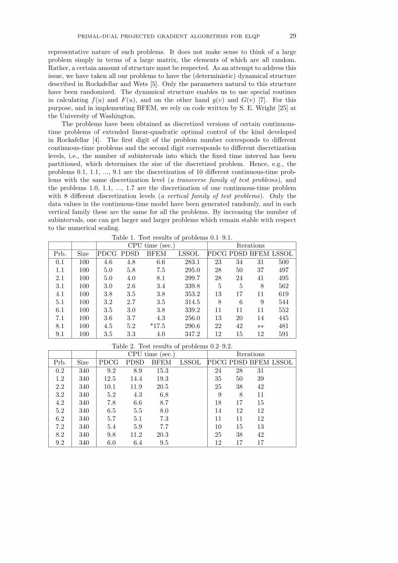
primal-dual projected gradient algorithms for elqp 29
representative nature of such problems. It does not make sense to think of a largeproblem simply in terms of a large matrix, the elements of which are all random.Rather, a certain amount of structure must be respected. As an attempt to address thisissue, we have taken all our problems to have the (deterministic) dynamical structuredescribed in Rockafellar and Wets [5]. Only the parameters natural to this structurehave been randomized. The dynamical structure enables us to use special routinesin calculating f(u) and F (u), and on the other hand g(v) and G(v) [7]. For thispurpose, and in implementing BFEM, we rely on code written by S. E. Wright [25] atthe University of Washington.
The problems have been obtained as discretized versions of certain continuous-time problems of extended linear-quadratic optimal control of the kind developedin Rockafellar [4]. The first digit of the problem number corresponds to differentcontinuous-time problems and the second digit corresponds to different discretizationlevels, i.e., the number of subintervals into which the fixed time interval has beenpartitioned, which determines the size of the discretized problem. Hence, e.g., theproblems 0.1, 1.1, ..., 9.1 are the discretization of 10 different continuous-time prob-lems with the same discretization level (a transverse family of test problems), andthe problems 1.0, 1.1, ..., 1.7 are the discretization of one continuous-time problemwith 8 different discretization levels (a vertical family of test problems). Only thedata values in the continuous-time model have been generated randomly, and in eachvertical family these are the same for all the problems. By increasing the number ofsubintervals, one can get larger and larger problems which remain stable with respectto the numerical scaling.
Table 1. Test results of problems 0.1–9.1.CPU time (sec.) Iterations
Prb. Size PDCG PDSD BFEM LSSOL PDCG PDSD BFEM LSSOL0.1 100 4.6 4.8 6.6 283.1 23 34 31 5001.1 100 5.0 5.8 7.5 295.0 28 50 37 4972.1 100 5.0 4.0 8.1 299.7 28 24 41 4953.1 100 3.0 2.6 3.4 339.8 5 5 8 5624.1 100 3.8 3.5 3.8 353.2 13 17 11 6195.1 100 3.2 2.7 3.5 314.5 8 6 9 5446.1 100 3.5 3.0 3.8 339.2 11 11 11 5527.1 100 3.6 3.7 4.3 256.0 13 20 14 4458.1 100 4.5 5.2 *17.5 290.6 22 42 ∗∗ 4819.1 100 3.5 3.3 4.0 347.2 12 15 12 591
Table 2. Test results of problems 0.2–9.2.CPU time (sec.) Iterations
Prb. Size PDCG PDSD BFEM LSSOL PDCG PDSD BFEM LSSOL0.2 340 9.2 8.9 15.3 24 28 311.2 340 12.5 14.4 19.3 35 50 392.2 340 10.1 11.9 20.5 25 38 423.2 340 5.2 4.3 6.8 9 8 114.2 340 7.8 6.6 8.7 18 17 155.2 340 6.5 5.5 8.0 14 12 126.2 340 5.7 5.1 7.3 11 11 127.2 340 5.4 5.9 7.7 10 15 138.2 340 9.8 11.2 20.3 25 38 429.2 340 6.0 6.4 9.5 12 17 17
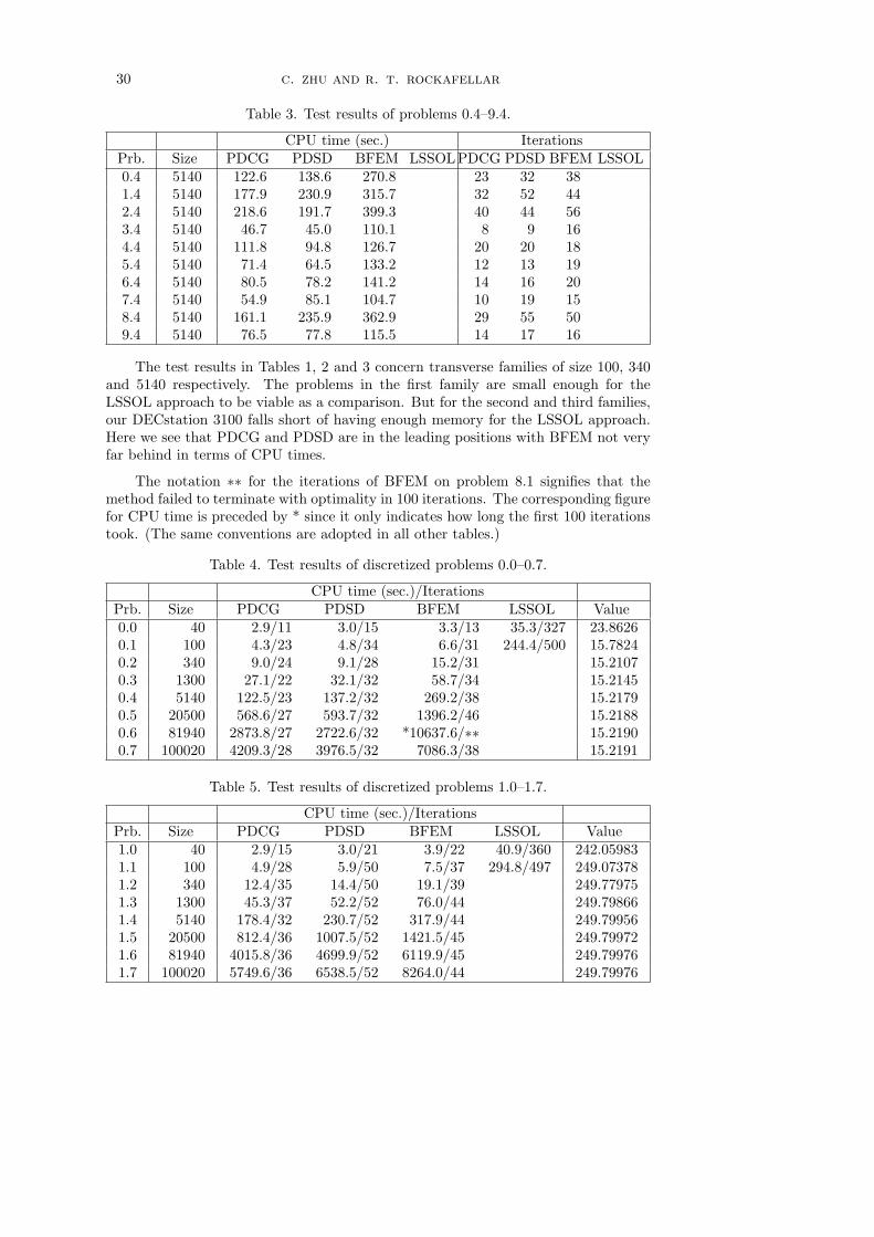
30 c. zhu and r. t. rockafellar
Table 3. Test results of problems 0.4–9.4.
CPU time (sec.) IterationsPrb. Size PDCG PDSD BFEM LSSOLPDCG PDSD BFEM LSSOL0.4 5140 122.6 138.6 270.8 23 32 381.4 5140 177.9 230.9 315.7 32 52 442.4 5140 218.6 191.7 399.3 40 44 563.4 5140 46.7 45.0 110.1 8 9 164.4 5140 111.8 94.8 126.7 20 20 185.4 5140 71.4 64.5 133.2 12 13 196.4 5140 80.5 78.2 141.2 14 16 207.4 5140 54.9 85.1 104.7 10 19 158.4 5140 161.1 235.9 362.9 29 55 509.4 5140 76.5 77.8 115.5 14 17 16
The test results in Tables 1, 2 and 3 concern transverse families of size 100, 340and 5140 respectively. The problems in the first family are small enough for theLSSOL approach to be viable as a comparison. But for the second and third families,our DECstation 3100 falls short of having enough memory for the LSSOL approach.Here we see that PDCG and PDSD are in the leading positions with BFEM not veryfar behind in terms of CPU times.
The notation ∗∗ for the iterations of BFEM on problem 8.1 signifies that themethod failed to terminate with optimality in 100 iterations. The corresponding figurefor CPU time is preceded by * since it only indicates how long the first 100 iterationstook. (The same conventions are adopted in all other tables.)
Table 4. Test results of discretized problems 0.0–0.7.
CPU time (sec.)/IterationsPrb. Size PDCG PDSD BFEM LSSOL Value0.0 40 2.9/11 3.0/15 3.3/13 35.3/327 23.86260.1 100 4.3/23 4.8/34 6.6/31 244.4/500 15.78240.2 340 9.0/24 9.1/28 15.2/31 15.21070.3 1300 27.1/22 32.1/32 58.7/34 15.21450.4 5140 122.5/23 137.2/32 269.2/38 15.21790.5 20500 568.6/27 593.7/32 1396.2/46 15.21880.6 81940 2873.8/27 2722.6/32 *10637.6/∗∗ 15.21900.7 100020 4209.3/28 3976.5/32 7086.3/38 15.2191
Table 5. Test results of discretized problems 1.0–1.7.
CPU time (sec.)/IterationsPrb. Size PDCG PDSD BFEM LSSOL Value1.0 40 2.9/15 3.0/21 3.9/22 40.9/360 242.059831.1 100 4.9/28 5.9/50 7.5/37 294.8/497 249.073781.2 340 12.4/35 14.4/50 19.1/39 249.779751.3 1300 45.3/37 52.2/52 76.0/44 249.798661.4 5140 178.4/32 230.7/52 317.9/44 249.799561.5 20500 812.4/36 1007.5/52 1421.5/45 249.799721.6 81940 4015.8/36 4699.9/52 6119.9/45 249.799761.7 100020 5749.6/36 6538.5/52 8264.0/44 249.79976
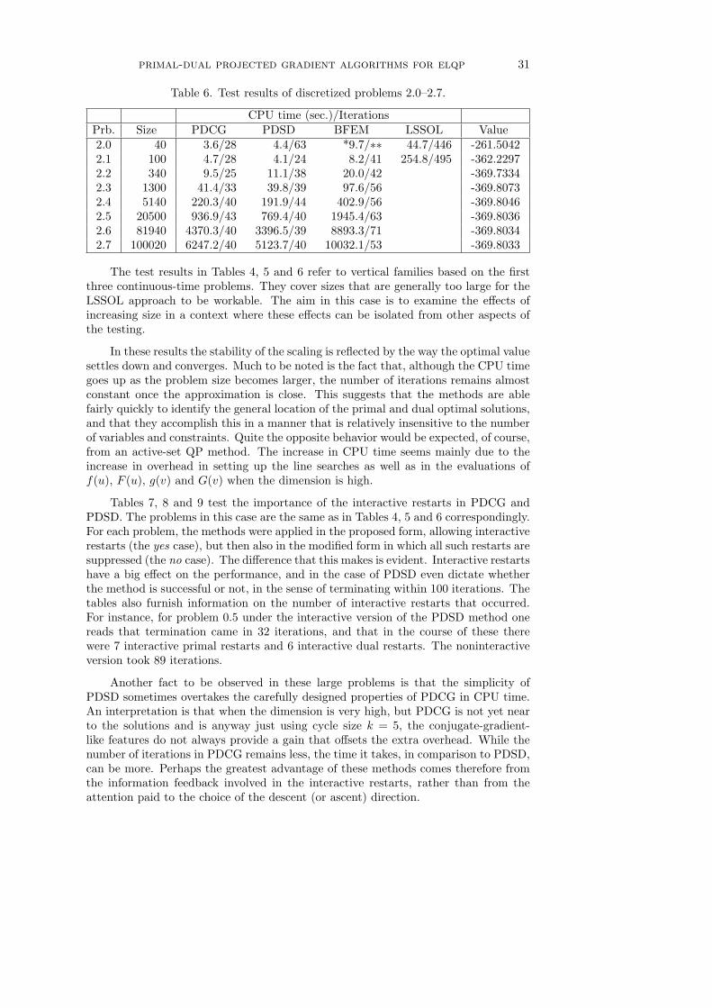
primal-dual projected gradient algorithms for elqp 31
Table 6. Test results of discretized problems 2.0–2.7.
CPU time (sec.)/IterationsPrb. Size PDCG PDSD BFEM LSSOL Value2.0 40 3.6/28 4.4/63 *9.7/∗∗ 44.7/446 -261.50422.1 100 4.7/28 4.1/24 8.2/41 254.8/495 -362.22972.2 340 9.5/25 11.1/38 20.0/42 -369.73342.3 1300 41.4/33 39.8/39 97.6/56 -369.80732.4 5140 220.3/40 191.9/44 402.9/56 -369.80462.5 20500 936.9/43 769.4/40 1945.4/63 -369.80362.6 81940 4370.3/40 3396.5/39 8893.3/71 -369.80342.7 100020 6247.2/40 5123.7/40 10032.1/53 -369.8033
The test results in Tables 4, 5 and 6 refer to vertical families based on the firstthree continuous-time problems. They cover sizes that are generally too large for theLSSOL approach to be workable. The aim in this case is to examine the effects ofincreasing size in a context where these effects can be isolated from other aspects ofthe testing.
In these results the stability of the scaling is reflected by the way the optimal valuesettles down and converges. Much to be noted is the fact that, although the CPU timegoes up as the problem size becomes larger, the number of iterations remains almostconstant once the approximation is close. This suggests that the methods are ablefairly quickly to identify the general location of the primal and dual optimal solutions,and that they accomplish this in a manner that is relatively insensitive to the numberof variables and constraints. Quite the opposite behavior would be expected, of course,from an active-set QP method. The increase in CPU time seems mainly due to theincrease in overhead in setting up the line searches as well as in the evaluations off(u), F (u), g(v) and G(v) when the dimension is high.
Tables 7, 8 and 9 test the importance of the interactive restarts in PDCG andPDSD. The problems in this case are the same as in Tables 4, 5 and 6 correspondingly.For each problem, the methods were applied in the proposed form, allowing interactiverestarts (the yes case), but then also in the modified form in which all such restarts aresuppressed (the no case). The difference that this makes is evident. Interactive restartshave a big effect on the performance, and in the case of PDSD even dictate whetherthe method is successful or not, in the sense of terminating within 100 iterations. Thetables also furnish information on the number of interactive restarts that occurred.For instance, for problem 0.5 under the interactive version of the PDSD method onereads that termination came in 32 iterations, and that in the course of these therewere 7 interactive primal restarts and 6 interactive dual restarts. The noninteractiveversion took 89 iterations.
Another fact to be observed in these large problems is that the simplicity ofPDSD sometimes overtakes the carefully designed properties of PDCG in CPU time.An interpretation is that when the dimension is very high, but PDCG is not yet nearto the solutions and is anyway just using cycle size k = 5, the conjugate-gradient-like features do not always provide a gain that offsets the extra overhead. While thenumber of iterations in PDCG remains less, the time it takes, in comparison to PDSD,can be more. Perhaps the greatest advantage of these methods comes therefore fromthe information feedback involved in the interactive restarts, rather than from theattention paid to the choice of the descent (or ascent) direction.
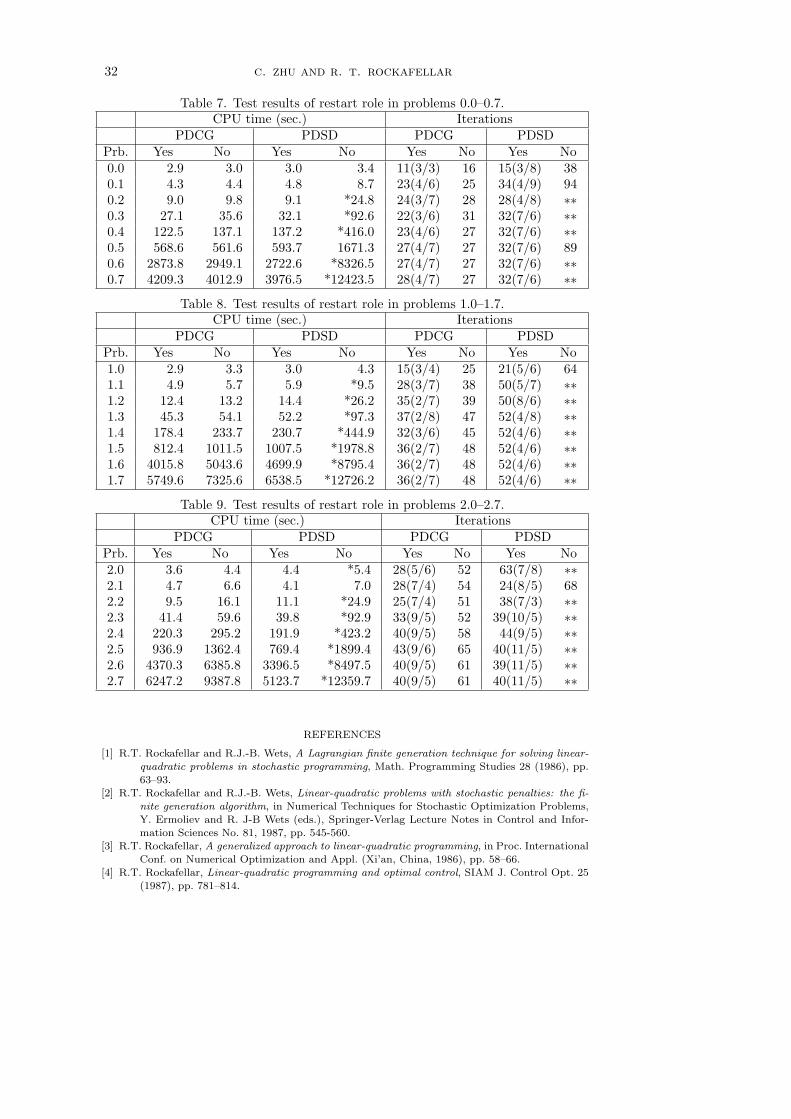
32 c. zhu and r. t. rockafellar
Table 7. Test results of restart role in problems 0.0–0.7.CPU time (sec.) Iterations
PDCG PDSD PDCG PDSDPrb. Yes No Yes No Yes No Yes No0.0 2.9 3.0 3.0 3.4 11(3/3) 16 15(3/8) 380.1 4.3 4.4 4.8 8.7 23(4/6) 25 34(4/9) 940.2 9.0 9.8 9.1 *24.8 24(3/7) 28 28(4/8) ∗∗0.3 27.1 35.6 32.1 *92.6 22(3/6) 31 32(7/6) ∗∗0.4 122.5 137.1 137.2 *416.0 23(4/6) 27 32(7/6) ∗∗0.5 568.6 561.6 593.7 1671.3 27(4/7) 27 32(7/6) 890.6 2873.8 2949.1 2722.6 *8326.5 27(4/7) 27 32(7/6) ∗∗0.7 4209.3 4012.9 3976.5 *12423.5 28(4/7) 27 32(7/6) ∗∗
Table 8. Test results of restart role in problems 1.0–1.7.CPU time (sec.) Iterations
PDCG PDSD PDCG PDSDPrb. Yes No Yes No Yes No Yes No1.0 2.9 3.3 3.0 4.3 15(3/4) 25 21(5/6) 641.1 4.9 5.7 5.9 *9.5 28(3/7) 38 50(5/7) ∗∗1.2 12.4 13.2 14.4 *26.2 35(2/7) 39 50(8/6) ∗∗1.3 45.3 54.1 52.2 *97.3 37(2/8) 47 52(4/8) ∗∗1.4 178.4 233.7 230.7 *444.9 32(3/6) 45 52(4/6) ∗∗1.5 812.4 1011.5 1007.5 *1978.8 36(2/7) 48 52(4/6) ∗∗1.6 4015.8 5043.6 4699.9 *8795.4 36(2/7) 48 52(4/6) ∗∗1.7 5749.6 7325.6 6538.5 *12726.2 36(2/7) 48 52(4/6) ∗∗
Table 9. Test results of restart role in problems 2.0–2.7.CPU time (sec.) Iterations
PDCG PDSD PDCG PDSDPrb. Yes No Yes No Yes No Yes No2.0 3.6 4.4 4.4 *5.4 28(5/6) 52 63(7/8) ∗∗2.1 4.7 6.6 4.1 7.0 28(7/4) 54 24(8/5) 682.2 9.5 16.1 11.1 *24.9 25(7/4) 51 38(7/3) ∗∗2.3 41.4 59.6 39.8 *92.9 33(9/5) 52 39(10/5) ∗∗2.4 220.3 295.2 191.9 *423.2 40(9/5) 58 44(9/5) ∗∗2.5 936.9 1362.4 769.4 *1899.4 43(9/6) 65 40(11/5) ∗∗2.6 4370.3 6385.8 3396.5 *8497.5 40(9/5) 61 39(11/5) ∗∗2.7 6247.2 9387.8 5123.7 *12359.7 40(9/5) 61 40(11/5) ∗∗
REFERENCES
[1] R.T. Rockafellar and R.J.-B. Wets, A Lagrangian finite generation technique for solving linear-quadratic problems in stochastic programming, Math. Programming Studies 28 (1986), pp.63–93.
[2] R.T. Rockafellar and R.J.-B. Wets, Linear-quadratic problems with stochastic penalties: the fi-nite generation algorithm, in Numerical Techniques for Stochastic Optimization Problems,
Y. Ermoliev and R. J-B Wets (eds.), Springer-Verlag Lecture Notes in Control and Infor-
mation Sciences No. 81, 1987, pp. 545-560.[3] R.T. Rockafellar, A generalized approach to linear-quadratic programming, in Proc. International
Conf. on Numerical Optimization and Appl. (Xi’an, China, 1986), pp. 58–66.[4] R.T. Rockafellar, Linear-quadratic programming and optimal control, SIAM J. Control Opt. 25
(1987), pp. 781–814.
primal-dual projected gradient algorithms for elqp 33
[5] R.T. Rockafellar and R.J.-B.Wets, Generalized linear-quadratic problems of deterministic andstochastic optimal control in discrete time, SIAM J. Control Opt. 28 (1990), pp. 810-822.
[6] R.T. Rockafellar, Computational schemes for solving large-scale problems in extended linear-
quadratic programming, Math. Programming 48 (1990), pp. 447-474.[7] R.T. Rockafellar, Large-scale extended linear-quadratic programming and multistage optimiza-
tion, in Proc. Fifth Mexico-U.S. Workshop on Numerical Analysis (S. Gomez, J.-P. Hennart,
R. Tapia, eds.), SIAM Publications, 1990.[8] A. King, An implementation of the Lagrangian finite generation method, in Numerical Tech-
niques for Stochastic Programming Problems, Y. Ermoliev and R. J-B Wets (eds.), Springer-
Verlag, 1988.[9] J.M. Wagner, Stochastic Programming with Recourse Applied to Groundwater Quality Manage-
ment, doctoral dissertation, M.I.T., 1988.
[10] J.-S. Pang, Methods for quadratic programming: a survey, Computers and Chem. Engineering7 (1983), pp. 583–594.
[11] Y.-Y. Lin and J.-S. Pang, Iterative methods for large convex quadratic programs: a survey, SIAMJ. Control Opt. 25 (1987), pp. 383–411.
[12] Y. Ye and E. Tse, An extension of Karmarkar’s projective algorithm for convex quadratic pro-
gramming, Math. Programming 44 (1989), pp. 157-179.[13] R.D.C. Monteiro and I. Adler, Interior path following primal-dual algorithms. Part II: Convex
quadratic programming, Math. Programming 44 (1989), pp. 43-66.
[14] D. Goldfarb and S. Liu, it An 0(n3L) primal interior point algorithm for convex quadraticprogramming, preprint.
[15] P. Tseng, Applications of a splitting algorithm to decomposition in convex programming and
variational inequalities, SIAM J. Control Opt. 29 (1991), pp. 119–138.[16] P. Tseng, �Further applications of a splitting algorithm to decomposition in variational inequali-
ties and convex programming, Math. Programming Studies 48 (1990), pp. 249–263.
[17] R.T. Rockafellar, Convex Analysis, Princeton Univ. Press, Princeton, NJ, 1970.[18] R.T. Rockafellar, Monotone operators and the proximal point algorithm, SIAM J. Control Opt.
14 (1976), pp. 877–898.[19] R.T. Rockafellar, Augmented Lagrangians and applications of the proximal point algorithm in
convex programming, Math. of Op. Research 1 (1976), pp. 97–116.
[20] C. Zhu, Modified proximal point algorithm for extended linear-quadratic programming, acceptedby Comput. Optim. and Appl., 1992.
[21] M.S. Bazaraa and C.M. Shetty, Nonlinear Programming: Theory and Algorithms, Wiley, 1979.
[22] M. Avriel, Nonlinear Programming: Analysis and Methods, Prentice Hall, 1976[23] J.V. Burke and J.J. More, On the identification of active constraints, SIAM J. Numer. Anal. 25
(1988), pp. 1197–1211.
[24] P.E. Gill, S.J. Hammarling, W. Murray, M.A. Saunders, and M.H. Wright, User’s guide forLSSOL (Version 1.0): a FORTRAN package for constrained linear least-squares and convex
quadratic programming, Tech. Rept. SOL 86–1, Dept. of Operations Research, Stanford
University, 1986.[25] S.E. Wright (with introduction by R.T. Rockafellar), DYNFGM: Dynamic Finite Generation
Method, report, Department of Mathematics, University of Washington, 1989.