Embed Size (px)
Citation preview
Pricing Futures by Deterministic Methods
Olivier Pironneau 1
March 13, 2012
1Laboratoire Jacques Louis Lions, Universite Pierre & Marie Curie, Boite 187,F-75252 Paris. ([email protected])

2
Contents
1 Modeling Financial Assets and Derivatives 91.1 Financial Assets . . . . . . . . . . . . . . . . . . . . . . . . . . . 91.2 Models with Local Volatilities . . . . . . . . . . . . . . . . . . . . 111.3 Stochastic Volatility Models . . . . . . . . . . . . . . . . . . . . . 111.4 Models with Jump-Diffusion Processes . . . . . . . . . . . . . . . 13
1.4.1 Poisson Process . . . . . . . . . . . . . . . . . . . . . . . . 131.4.2 Jump-Diffusion Process . . . . . . . . . . . . . . . . . . . 14
1.5 Financial Derivatives . . . . . . . . . . . . . . . . . . . . . . . . . 141.5.1 European Options . . . . . . . . . . . . . . . . . . . . . . 141.5.2 Barrier Option . . . . . . . . . . . . . . . . . . . . . . . . 171.5.3 American and Bermuda Options . . . . . . . . . . . . . . 181.5.4 Path Dependent Options . . . . . . . . . . . . . . . . . . 181.5.5 Basket Options . . . . . . . . . . . . . . . . . . . . . . . . 181.5.6 Convertible Bonds . . . . . . . . . . . . . . . . . . . . . . 201.5.7 Interest Rates, Swaps and Swaptions . . . . . . . . . . . . 201.5.8 CDS: Credit Default Swap . . . . . . . . . . . . . . . . . . 221.5.9 CDO: Collateralized Debt Obligation . . . . . . . . . . . . 23
1.6 Conclusion . . . . . . . . . . . . . . . . . . . . . . . . . . . . . . 23
2 sde based Numerical Methods 252.0.1 Principles of Numerical Simulation by Monte-Carlo . . . . 252.0.2 The Longstaff-Schwartz Algorithm for Bermudas . . . . . 272.0.3 Methods using the Process PDF for Basket Options . . . 282.0.4 A Binomial Tree for American Options . . . . . . . . . . 29
3 Some Partial Differential Equations of Finance 313.1 From sde to pde and pide . . . . . . . . . . . . . . . . . . . . . 313.2 Fokker-Planck and Kolmogorov Equations . . . . . . . . . . . . . 31
3.2.1 Ito’s Lemma and Hedging . . . . . . . . . . . . . . . . . . 323.2.2 Application to European Options . . . . . . . . . . . . . . 333.2.3 Application to Hedging . . . . . . . . . . . . . . . . . . . 333.2.4 Application to Basket Option . . . . . . . . . . . . . . . . 343.2.5 From Jump Processes to Partial Integro-Differential Equa-
tions . . . . . . . . . . . . . . . . . . . . . . . . . . . . . . 35
3
4 CONTENTS
3.2.6 Levy Copula . . . . . . . . . . . . . . . . . . . . . . . . . 373.2.7 From Constrained SDE to PDI . . . . . . . . . . . . . . . 383.2.8 PDE for Interest rates and Swaps . . . . . . . . . . . . . . 38
3.3 Some Existence and Regularity Results . . . . . . . . . . . . . . 393.3.1 Existence Results for the Black-Scholes PDE . . . . . . . 393.3.2 Existence Results for Basket Options . . . . . . . . . . . . 423.3.3 Existence Result for an Asian Option . . . . . . . . . . . 433.3.4 Analysis of the PDE for Stochastic Volatilities . . . . . . 433.3.5 Partial Integro Differential Variational Equations . . . . . 44
4 Numerical Methods 474.1 A Finite Difference Method for the Black-Scholes pde . . . . . . 47
4.1.1 Alternate Directions for Basket Options . . . . . . . . . . 484.1.2 Numerical Method for PIDEs . . . . . . . . . . . . . . . . 50
4.2 Spectral Methods . . . . . . . . . . . . . . . . . . . . . . . . . . . 504.3 Finite Element Methods . . . . . . . . . . . . . . . . . . . . . . . 51
4.3.1 Galerkin Method . . . . . . . . . . . . . . . . . . . . . . . 524.3.2 Finite Elements in 1D . . . . . . . . . . . . . . . . . . . . 53
4.4 Variational Method for American Option . . . . . . . . . . . . . 554.4.1 Discretization by FEM . . . . . . . . . . . . . . . . . . . . 564.4.2 Semi-Smooth Newton Algorithm . . . . . . . . . . . . . . 58
4.5 A Stochastic Volatility Model Solved by FEM . . . . . . . . . . . 594.5.1 Finite Elements for a 2D Stochastic Volatility Model . . . 594.5.2 Numerical Implementation . . . . . . . . . . . . . . . . . 60
4.6 Asian Put . . . . . . . . . . . . . . . . . . . . . . . . . . . . . . . 624.7 Automatically adapted Mesh . . . . . . . . . . . . . . . . . . . . 63
4.7.1 Delaunay mesh generator . . . . . . . . . . . . . . . . . . 634.7.2 Anisotropic Delaunay Mesh Generator . . . . . . . . . . . 644.7.3 Metric adapted to the Solution of the pde . . . . . . . . . 65
4.8 Greeks . . . . . . . . . . . . . . . . . . . . . . . . . . . . . . . . . 654.8.1 Greeks for American Options . . . . . . . . . . . . . . . . 66
4.9 Reduced Order Modeling . . . . . . . . . . . . . . . . . . . . . . 674.9.1 Galerkin Approximation on the Basis . . . . . . . . . . . 684.9.2 Numerical Tests . . . . . . . . . . . . . . . . . . . . . . . 704.9.3 Sparse Grids . . . . . . . . . . . . . . . . . . . . . . . . . 71
5 Calibration 775.1 Introduction . . . . . . . . . . . . . . . . . . . . . . . . . . . . . . 775.2 Dupire’s Equation . . . . . . . . . . . . . . . . . . . . . . . . . . 78
5.2.1 Example of Generalization: Dupire’s for Binary Calls . . 795.2.2 Dupire’s Equation for Barrier Options . . . . . . . . . . . 795.2.3 Dupire’s Equation for Options on Levy Driven Assets . . 805.2.4 Dupire’s identity in the discrete case . . . . . . . . . . . . 81
5.3 Calibration of the Local Volatility with Dupire’s Equation . . . . 825.4 Calibration of Implied Volatility . . . . . . . . . . . . . . . . . . 835.5 Calibration on a Reduced Basis . . . . . . . . . . . . . . . . . . . 83
6 Open-source Tools 896.1 Premia . . . . . . . . . . . . . . . . . . . . . . . . . . . . . . . . . 896.2 QuantLib . . . . . . . . . . . . . . . . . . . . . . . . . . . . . . . 906.3 FreeFem++ . . . . . . . . . . . . . . . . . . . . . . . . . . . . . . 91
6.3.1 Two-dimensional Black-Scholes equation . . . . . . . . . . 926.3.2 Three-dimensional Basket . . . . . . . . . . . . . . . . . . 94
6.4 CUDA and Other Tools . . . . . . . . . . . . . . . . . . . . . . . 946.4.1 Matlab, Scilab, Octave,Mathematica, SAGE... . . . . . . . 946.4.2 Stream Programming (CUDA, openCL) . . . . . . . . . . 97
5
6 Olivier Pironneau
Forewords
In these chapters we focus on a small part of financial mathematics, namelyonly on the use of partial differential equations for pricing futures. Even withinthis narrow range it is hard to be systematic and complete or even do betterthan already existing books like [68], [1], or software manuals like [56]. Sothese chapters may be valuable only to the extent that they reflect ten years ofteaching, conferences and interaction with the actors of financial mathematics.
Also, because the theory of partial differential equations is not always wellknown, I have chosen a pragmatic approach and left out the details of the theoryor the proofs of some results and refer the reader to other books. The numericalalgorithms, on the other hand are given in detail.
These chapters contain also some of my own research, perhaps not so im-portant as the rest, the reader will decide for himself.
I would like to thank my research collaborators, Yves Achdou, Rama Cont,Nicolas Dicesare, Frederic Hecht, Gregoire Loeper and Nicolas Lantos .
Introduction
Except for the pioneering work of Louis Bachelier [10], financial mathematics isrelatively new. Perhaps the right landmark is the paper in the seventies by Blackand Scholes and the work of Merton which led to their Nobel prize. Forty yearslater, because of the explosion of applications, more and more mathematicians,physicists, economists and computer scientists joined the fun; despite severalworld threatening crises the subject is exploding and the literature around it.
Banks, insurance companies , hedge funds etc, have also been very innovativein inventing new contingent claims and since no one sees the global picture, everyday there seems to be a new challenge to solve. The field is huge : 3000 times thevalue of financial assets is in derivatives; the domain is very lively with careeropportunities unheard of in other fields of applied mathematics and it attractsstudents also because there is a lot to do and still lots of jobs despite systemicinstabilities.
It is true that the field of financial mathematics is in its infancy, the modelsare crude and focused on a small set of futures; global models are just beinginitiated with game theory and utility functions [47]. The lack of global vision ofscientists and their incapacity to predict systemic risks have given a bad name tothe “quants”. A French politician has even accused financial mathematicians of”crime against mankind”. Let’s be reasonable: if there is a culprit it is internet.With it, “banksters” have been given a Kalachnikov - electronic trading- andmathematicians are only providing tiny bullet proof shields to the system.
Futures are modeled by using advanced stochastic tools and then pricedusing simple Monte-Carlo algorithms or limited analytical formulae. But thedays of closed form solutions are numbered because models are increasinglycomplex; the numerical algorithms will have to be more efficient because speedis becoming a dominant factor with high frequency trading: 40% of transactionsare done automatically by ”robots”, computer programs taking instant decisionsbased on overnight calculations and in house know-how. Some banks currentlydouble their computing facilities every six months and try to shorten the wiresbetween their IT centers and stock markets to improve transaction speed (nojoke implied); at the current rate they will soon be the biggest users of HighPerformance Computing (HPC).
Monte-Carlo is often slow but it is akin to the stochastic models and it ishighly parallel and easy to implement in hybrid computers (GPU). Alternativesare binomial or trinomial trees, Fast Fourier Transform, when the characteristic
7
8 Olivier Pironneau
functions of the stochastic processes are known, and the partial differentialequations derived by Ito’s Lemma.
Most option pricing problems can be formulated as partial differential equa-tions (pde) or integro-differential equations (pide) or inequations (PDI). Theyresult in clean and fast algorithms but they are cursed by the dimensionality ofthe problem and hard paralelization procedures.
As a coauthor of [1] and [2] I do not intend to present here the same materialor to present it in the same way. Here the mathematical details are not given,only the essence of the methods, the more recent developments and, in moredetails, the numerical algorithms.
The material is structured in 6 chapters:
• Chapter 1 starts with an introduction to financial assets, then a presenta-tion of some of the models, followed by a list of the most popular deriva-tives.
• Chapter 2 begins with a short section on Monte-Carlo methods and thendeals with deterministic methods based on the knowledge of the probabil-ity density of the processes or their characteristic functions.
• In chapter 3 we shall derive the partial differential equations of financeand present some mathematical results on their existence and regularity.
• Then in chapter 4, the main algorithms based on pde formulations aregiven; as in [1] more emphasis is put on variational method with meshadaptivity in mind. Some acceleration techniques like Proper OrthogonalDecomposition and sparse grids are presented.
• Calibration is dealt with shortly in chapter 5 with a more consistent sectionon Dupire’s equations.
• The last chapter is a review of some numerical tools and toolboxes forfinancial derivatives.
Chapter 1
Modeling Financial Assetsand Derivatives
Pricing with mathematical and computational tools is practiced by institutionsor individuals who observe a financial asset, i.e. a share, a bond, a commodityetc, and wish to draw some conclusion on their future value and the risk involvedin dealing with them.
1.1 Financial Assets
No arbitrage assumes that the asset’s market price is public, fluid, and that itis not possible to make a profit in a loop of buys and sells without taking arisk of losing something. The current pricing theory assumes also that thereis a riskless asset, a numeraire (money in one currency for example), whichcan be borrowed or lent at a fixed interest rate r, possibly function of time t.Consequently any riskless asset of price St at time t obeys the following:
dSt = Str(t)dt, S0 known, i.e. St = S0e
∫ t0r(s)ds
(1.1)
By convention t = 0 is today and the price of the asset today, being public, isknown.
Obviously most financial assets are not riskless and for lack of information (orunderstanding) their variations are assumed random. The simplest model withrandomness is
dSt = St(µtdt+ σtdWt), S0 known (1.2)
where µt = E[dSt/St|S0] is the tendency (or drift) of St and σt, the volatility attime t, measures the amplitude of the random variations and Wt is assumed tobe a Brownian motion for simplicity. This last assumption will be relaxed later;
9
10 Olivier Pironneau
E[·|·] is the conditional expected value in the same probability space where Wt
is defined.
Remark 1 Recall that a Brownian motion (also called a Wiener process) Wt
has zero mean and variance such that E[(Wt−Ws)2] = t−s, t > s, and Wt−Ws
is the Gaussian random variable Wt − Ws = N(0, 1)√t− s: its probability
density function (pdf) is θ → exp(− θ2
2(t−s) )/√
2π(t− s) and so its cumulative
distribution function (CDF) is
P(Wt −Ws < x) =1√
2π(t− s)
∫ x
−∞exp(− θ2
2(t− s))dθ
=1
2(1 + erf(
x√2(t− s)
)) (1.3)
Notice that the model is set in a probability space of which not much is said. No-arbitrage implies in this case the existence of a risk-neutral probability measureunder which Wt is still a Brownian motion but1 E[dSt/St|S0] = r(t). Numeri-cally, E is often replaced by a statistical average (central limit theorem 3) so theprobability measure does not appear explicitly in the numerical computations.Hence, for practical purpose, the model for St is
dSt = St(r(t)dt+ σtdWt), S0 known (1.4)
The precise meaning of an sde (Stochastic Differential Equation) like (1.4) re-quires the theory of stochastic integrals; the reader is sent to [44] for moredetails. From a practical numerical point of view it suffices to view (1.4) as thelimit of (2.3) below, when δt→ 0.
With Ito’s lemma (3.7), it is not hard to show that (1.4) has an explicitsolution when r and σ are constant2:
Proposition 1 The random process Xt = logSt satisfies
dXt = (r − 1
2σ2t )dt+ σtdWt (1.5)
and when σt and r are constant then
St = S0e(r−σ2
2 )t+σ(Wt−W0) (1.6)
ProofBy Ito’s lemma (3.7)
d lnSt = (lnSt)′dSt+
1
2(lnSt)
′′(σSt)2dt =
dStSt− σ
2S2t dt
2S2t
= rdt+σdWt−1
2σ2dt
1If µ is a random variable in a probability space of measure P and P∗ is another probability
measure in the same space then E∗[µ] = E[ dP∗dP
µ], where dP∗dP
is the Radon-Nicodyn derivative
of P∗ with respect to P. Obviously if ρ and ρ∗ are the pdf of P and P∗, dP∗dP
= ρ∗
ρ.
2 If r is not constant, the same formula holds with∫ t
0r(τ)dτ instead of rt
Pricing Futures by Deterministic Methods 11
Hence Xt = lnSt satisfies (1.5) and so
Xt −X0 = (r − 1
2σ2)t+ σ(Wt −W0)
Remark 2 This shows that Yt = Ste−rt is a martingale, i.e.
E(Yt|Yτ ) = Yτ , ∀τ < t
The concept of martingales (see [44] for details) is important for arbitrage-freemarkets.
1.2 Models with Local Volatilities
In practice the Black-Scholes model with constant volatility is too simple. So itis common practice to calibrate the model by finding a so called local volatilitysurface σ(S, t) for (1.4) in order to reproduce the observations3.
One such local volatility model, known as cev (constant elasticity of vari-ance) has been proposed by Cox[22].
dSt = St(rdt+ δSβ2−1t dW1t, ) S0 known, 0 < β < 2. (1.7)
It is of numerical interest because it will lead to semi-analytical solution, as theprobability density function of ST knowing that St = S is (see [63])
ρ(ST |St) = (2− β)k1
1−2β x1
4−2βw1−2β4−2β e−x−wI 1
2−β(2√xw) (1.8)
with τ = T − t, Ia the modified Bessel function of the first kind of order a and
k =2r
δ2(2− β)(er(2−β)τ − 1), x = kS2−βer(2−β)τ , w = kS2−β
T (1.9)
1.3 Stochastic Volatility Models
By assuming a stochastic volatility defined by a scalar or vector sde one obtainsa large class of models with fewer parameters than with a general local volatilitysurface.
As before
dSt = St(µtdt+ σtdW1t), (1.10)
where µt is the tendency of St, taken to be rt the interest rate if a risk neutralprobability exists, and W1t is a Brownian motion. Now we assume that σt is
3Hence it is important to remember that a mathematical result or a numerical method for(1.4) confined to constant volatilities is of limited interest.
12 Olivier Pironneau
a stochastic process satisfying a sde driven by a second Brownian motion W2t,correlated to W1t: E[dW1tdW2t] = ρdt,
dvt = κ(m− vt)dt+ βdW2t, σt = f(vt) (1.11)
where κ, β,m are given, possibly functions of vt and t, f is a given positivefunction and (vt) is the driving process. Popular choices include,
• lognormal process: κ < 0, β constant, m = 0.
• Mean reverting ou (Orstein-Uhlenbeck) process: κ > 0, β,m > 0 constant.
• Cox-Ingersoll-Ross process (cir ): β = λ√vt, κ > 0,m > 0, λ constant.
The volatility of vt, β is commonly referred as volvol (volatility of the volatility).In the case of ou and cir , m is the limit of vt when t→∞ (the process is saidto be mean reverting), κ controls the rate at which the limit is reached and βthe randomness about this limit.
When the Brownian motion W2t is correlated to W1t: it can be written as alinear combination of W1t and an independent Brownian motion Zt:
Zt = ρW1t +√
1− ρ2Zt, (1.12)
where the correlation factor ρ lies in [−1, 1].Table 1.3 summarizes some popular choices for f(v) and ρ
Authors ρ f(y) vt processHull-White [36] ρ = 0 f(y) =
√y Lognormal
Stein-Stein [65] ρ = 0 f(y) = |y| Mean reverting ouHeston [34] ρ 6= 0 f(y) =
√y cir
Table 1.1: Frequently used models of stochastic volatilities
Following [12], with τ = t − t0, the characteristic function of Xt = lnSt,knowing St0 and vt0 when St obeys Heston’s model is
Φ(z) = exp(izrτ +
ρ
λ(vt − vt0 − κmτ)
)φ(z(
κρ
λ− 1
2) +
1
2iz2(1− ρ2))
with φ(z) = γ(z)e−
12 (γ(z)−κ)τ (1− e−κτ )
κ(1− e−γ(z)τ )
× e
vt0+vt
κ2
[κ(1+e−κτ )
1−e−κτ
]I d
2−1
(√vt0vT
4γ(z)e−12γ(z)τ
λ2(1−e−κτ )
)I d
2−1
(√vt0vT
4κe−12κτ
λ2(1−e−κτ )
) (1.13)
with γ(z) =√κ2 − 2λ2iz, d = 4m/λ2 and Ia(x) the modified Bessel function of
the first kind.
Pricing Futures by Deterministic Methods 13
1.4 Models with Jump-Diffusion Processes
To account for sudden discontinuous variations of St one adds random jumps toWt. Jump processes have been introduced by P. Levy[46]. For details the readeris sent to [20]. We present below, without mathematical rigor, the minimumneeded to generate numerically a Levy process.
1.4.1 Poisson Process
A positive random variable τ with exponential law (ELVR) is defined by theprobability law
P(τ > y) = e−λy (1.14)
Let τi be a set of independent ELVR with the same λ. Let
Tn =
n∑1
τi, Nt =∑n≥1
1t≥Tn (1.15)
By definition Nt is a Poisson process.
It is very useful in queuing theory; for instance it can be used to model thenumber of buses which arrive at one bus station.
Proposition 2 Nt −Ns and Nt−s have the same law.
P (Nt = n) = e−λt(λt)n
n!
Furthermore if it is known that NT = n then T1, ..., Tn are uniformly distributedon (0, T ).
Definition 1 A compound Poisson process on f is Zt =∑Nt
1 vi where vi areindependent r.v. with law f .
Consequently a numerical method to generate Zt is as follows:
Algorithm to generates a compound Poisson process Zt
1. Generate NT by (1.14),(1.15)
2. Generate UiNT1 uniform and random on (0, T ).
3. Generate NT random variables viNT1 of law f
4. Set Zt =∑NT
1 vi1Ui≤t
14 Olivier Pironneau
1.4.2 Jump-Diffusion Process
Let Wt be a Brownian process and Zt be a compound Poisson process. Letσ, γ ∈ R, then
Xt = γt+ σWt + Zt (1.16)
is, by definition, a jump-diffusion process.
Theorem 1 Let ν(x) = λf(x); the characteristic function of Xt is
E(eiuXt) = exp
(t[iγu− σ2u2
2+
∫R
(eiux − 1− iu1|x|<1)ν(dx)]
)(1.17)
Conversely if ν ∈ L1(R) and∫ 1
−1x2ν(dx) <∞, (1.17) defines the characteristic
function of a generalized jump-diffusion process. Formula (1.17) is referred asthe Levy-Khinchin formula.
Theorem 2 The infinitesimal generator of the semi-group associated to Xt is
LXφ := limt→0
1
t(E(φ(x+Xt)− φ(x))
=σ2
2∂xxφ+ γ∂xφ+
∫R
(φ(x+ y)− φ(x)− y1|y|<1∂xφ(x)
)ν(dy)(1.18)
The following property will be useful later
Proposition 3 The process eXt is a martingale if and only if
γ +σ2
2+
∫R
(ex − 1− x1|x|<1)ν(dx) = 0 (1.19)
and with this value for γ the infinitesimal generator of Xt is
LXφ =σ2
2(∂xxφ− ∂xφ)
+
∫R
(φ(x+ y)− φ(x)− (ey − 1)∂xφ(x)) ν(dy) (1.20)
1.5 Financial Derivatives
1.5.1 European Options
Given a financial asset St, an option on S is a contract for buying or selling S ata future time T. Such a product is also called a financial derivative or a futureon S.
The European contract is the simplest: it gives to its owner the right to buy(call) or sell (put) S at time T (maturity) at price K (the strike).
Such contracts have a market value; they too can be bought or sold. Noarbitrage implies that the fair value Ct (resp. Pt) of a European call (resp. put)
Pricing Futures by Deterministic Methods 15
at time t < T is the expected value of the owner’s profit at time T discountedby the interest rate r down to time t:
Ct = e−r(T−t)E[(ST −K)+|St], Pt = e−r(T−t)E[(K − ST )+|St] (1.21)
Recall the notation a+ = max(a, 0).Note that Ct − Pt pays (ST −K)+ − (K − ST )+ at maturity which is equal
to (ST −K). Because it is riskless, no arbitrage implies that they must be equalat time t discounted by r, namely
Ct − Pt = e−r(T−t)(ST −K) (1.22)
This relation is known as the put-call parity.Calling P (S, t) the price of an option with maturity T and pay-off function
P0 and assuming that r and σ > 0 are constant, the Black-Scholes formula is(see (1.6))
P (S, t) = e−r(T−t)E∗(P0(Ser(T−t)eσ(WT−Wt)−σ2
2 (T−t))), (1.23)
and since under P ∗, WT −Wt is a centered Gaussian distribution with varianceT − t,
P (S, t) =1√2πe−r(T−t)
∫RP0(Se(r−σ2
2 )(T−t)+σx√T−t)e−
x2
2 dx. (1.24)
When the option is a vanilla European option a more explicit formula can bededuced from (1.24). Take for example a call:
C(S, t) =1√2π
∫ +∞
−d2
(Se−
σ2
2 (T−t)+σx√T−t −Ke−r(T−t)
)e−
x2
2 dx
=1√2π
∫ d2
−∞
(Se−
σ2
2 (T−t)−σx√T−t −Ke−r(T−t)
)e−
x2
2 dx,
(1.25)
where
d1 =log( SK ) + (r + σ2
2 )(T − t)σ√T − t
and d2 = d1 − σ√T − t. (1.26)
Finally, introducing the upper tail of the Gaussian function
N(d) =1√2π
∫ d
−∞e−
x2
2 dx, (1.27)
and using (1.25), (1.26), we obtain the Black-Scholes formula:
Proposition 4 When σ and r are constant, the price of the call is given by
C(S, t) = SN(d1)−Ke−r(T−t)N(d2), (1.28)
and the price of the put is given by
P (S, t) = −SN(−d1) +Ke−r(T−t)N(−d2), (1.29)
where d1 and d2 are given by (1.26) and N is given by (1.27).
16 Olivier Pironneau
Proposition 5 With cev volatilities σt = δSβ2−1t
Ct = StQ(2kK2−β ; 2 +2
2− β, 2x)−Ke−r(T−t)(1−Q(2x;
2
2− β, 2kK2−β))(1.30)
where Q is non central Chi-square distribution (see [63] ) with x, k defined by(1.9). When β = 4/3 the needed Q are
Q(z; 1, κ) = N(√κ−√z) +N(−
√κ−√z)
Q(z; 3, κ) = Q(z; 1, κ) +1√κ
[N ′(√κ−√z)−N ′(
√κ+√z)]
Q(z; 5, κ) = Q(z; 1, κ) +1√κ
3 [(κ− 1 +√κz)N ′(
√κ−√z)
−(κ− 1−√κz)N ′(
√κ+√z)] (1.31)
where N ′(x) = ex2
2 /√
2π is the standard normal density function and N(x) =(1 + erf( x√
2))/2 is the the normal probability distribution.
Proof see [63]
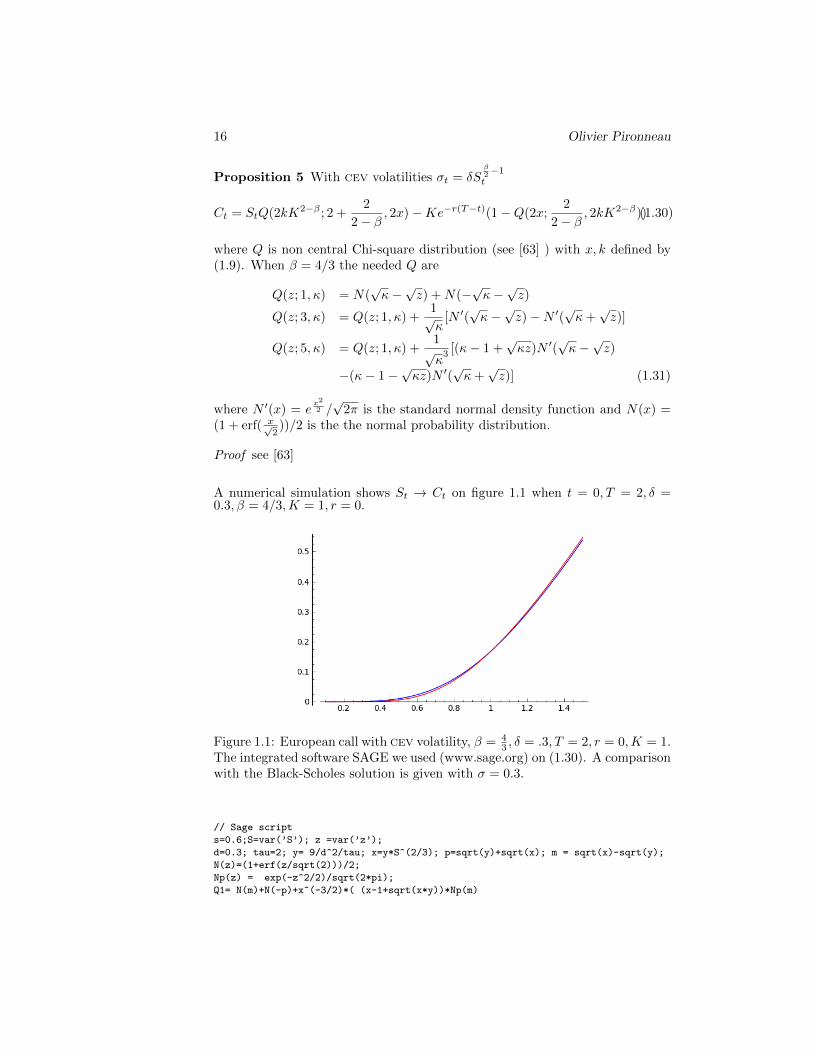
A numerical simulation shows St → Ct on figure 1.1 when t = 0, T = 2, δ =0.3, β = 4/3,K = 1, r = 0.
Figure 1.1: European call with cev volatility, β = 43 , δ = .3, T = 2, r = 0,K = 1.
The integrated software SAGE we used (www.sage.org) on (1.30). A comparisonwith the Black-Scholes solution is given with σ = 0.3.
// Sage script
s=0.6;S=var(’S’); z =var(’z’);
d=0.3; tau=2; y= 9/d^2/tau; x=y*S^(2/3); p=sqrt(y)+sqrt(x); m = sqrt(x)-sqrt(y);
N(z)=(1+erf(z/sqrt(2)))/2;
Np(z) = exp(-z^2/2)/sqrt(2*pi);
Q1= N(m)+N(-p)+x^(-3/2)*( (x-1+sqrt(x*y))*Np(m)
Pricing Futures by Deterministic Methods 17
-(x-1-sqrt(x*y))*Np(p));
Q2= N(-m)+N(-p)+y^(-1/2)*(Np(-m)-Np(p));
C=S*Q1-1+Q2;
v=(S*(1-erf(-ln(S)/s - s/4))-1-erf(ln(S)/s - s/4))/2;
for i in range (1,15) : print numerical_approx(C(0.1*i));
A=plot(C,(0.1,1.5),color=’blue’); B=plot(v,(0.1,1.5),color=’red’); A+B;
Proposition 6 With Heston’s model (1.10),(1.11),(1.12), knowing that S =S0, v = v0 at t = 0 , the European call is
C =1
2(S0 −Ke−rT ) +
1
π
∫ ∞0
(erT f1 −Kf2)du
fj = Reφ(u+ (j − 2)i)
iuKiu
φ(u) = erTSiu0
(1− ge−dT
1− g
)−2mκλ2
exp(mκT
λ2(κ− ρλiu− d))
exp(v0
λ2(κ− ρλiu+ d)
1− edT
1− gedT)
d =√
(ρλui− κ)2 + λ2(iu+ u2), g =κ− ρλiu− dκ− ρλiu+ d
(1.32)
The proof is due to Cox, Ingersoll and Ross [23] revised by Albrecher et al [5].A summary can be found in [50] with hints on how to compute the complexintegral in [5].
# Sage script for Heston model by a complex integral when K=1
umax=1000; N=10000; du=umax/N;
S0=1; T=2;Y0=0.0175; r=0.025;
kappa=1.5768;m=0.0398; lambd=0.5751;rho=-0.5711;
aa= m*kappa*T/lambd^2; bb= -2*m*kappa/lambd^2;
P=0;
for i in range (1,N) :
u2=i*du
u1=u2-I
a1=rho*lambd*u1*I
a2=rho*lambd*u2*I
d1=sqrt((a1-kappa)^2+lambd^2*(u1*I+u1^2))
d2=sqrt((a2-kappa)^2+lambd^2*(u2*I+u2^2))
g1=(kappa-a1-d1)/(kappa-a1+d1)
g2=(kappa-a2-d2)/(kappa-a2+d2)
b1=exp(u1*I*(log(S0)+r*T)) *( (1-g1*exp(-d1*T))/(1-g1) )^bb
b2=exp(u2*I*(log(S0)+r*T)) *( (1-g2*exp(-d2*T))/(1-g2) )^bb
phi1=b1*exp(aa*(kappa-a1-d1)+Y0*(kappa-a1-d1)*(1-exp(-d1*T))/(1-g1*exp(-d1*T))/lambd^2)
phi2=b2*exp(aa*(kappa-a2-d2)+Y0*(kappa-a2-d2)*(1-exp(-d2*T))/(1-g2*exp(-d2*T))/lambd^2)
P+= real((phi1-phi2)/(u2*I))*du
print numerical_approx((S0-exp(-r*T))/2+P/pi)
1.5.2 Barrier Option
Barriers are introduced in case the market goes wild; the contracts include aclause that cancels the deal if St crosses over a specified price SM or under Sm.
18 Olivier Pironneau
1.5.3 American and Bermuda Options
With American option the owner of the contract can exercise his right and forcethe deal anytime before maturity T. To decide to exercise the option at timeτ one must compare the profit gain now, namely Sτ − K for a call, with theexpected profit if one waits, namely e−r(T−τ)E(ST − K)+. Thus the value ofthe American put option is
Pt = supτ∈T (t,T )
E[e−r(τ−t)(K − Sτ )+|St] (1.33)
where T is the set of stopping times in (t, T ) adapted to the probability space.
Bermuda Option
The mechanism of Bermudas is similar to Americans except that the decisions toexercise are made only at fixed, given time intervals, every month for instance,the Bermuda islands being in between America and Europe.
1.5.4 Path Dependent Options
A path dependent or Asian (or Asiatic) option tries to smooth the oscillations ofthe underlying asset at maturity. Some average of St over a time period is usedin place of ST in the pay-off (AT −K)+ for a call, with arithmetic averaging,for instance
At =1
t
∫ t
0
Sτdτ,
or geometric averaging
At = exp(1
t
∫ t
0
log(Sτ )dτ).
Another example is the call with floating strike with pay-off (ST − AT )+. Noarbitrage gives
Ct = e−r(T−t)E[(ST −AT )+|St, At]. (1.34)
Another class of Asian options, the so-called lookback options, involve theextremal values of the asset price for t ≤ T . The floating strike lookback callhas a pay-off of (ST −min0≤τ≤T Sτ )+, whereas the lookback put has a pay-offof (max0≤τ≤T Sτ − ST )+. Similarly, the fixed strike lookback call (resp. put)has a pay-off (max0≤τ≤T Sτ −K)+ (resp. (K −min0≤τ≤T Sτ )+). One can alsodefine lookback options on averages.
1.5.5 Basket Options
Consider d risky assets Sit, i = 1, . . . , d each modeled by a separate sde
dSit = Sit (rdt+ σidWit) (1.35)
Pricing Futures by Deterministic Methods 19
However the standard Brownian motions (Wit), 1 ≤ i ≤ d, are possibly corre-lated: ρij := 1
tE[WitWjt]. As usual r is the interest rate. In what follows, thenotation S is used for the vector (S1, . . . , Sd)
T .
Remark 3 As in the one dimensional case, if σi is constant for all i,
Sit = Si0 exp
((r − 1
2σ2i )t+ σi(Wit −W0t)
)(1.36)
A European option with pay-off π(ST ) at maturity T will be priced by
Pt = e−r(T−t)E[π(ST )|St] (1.37)
The pay-off function could be a function of a weighted sum of the assets, i.e. inthe case of a put:
π(S) =
(K −
d∑i=1
αiSi
)+
As in the scalar case, the put-call parity holds:
Ct − Pt =
d∑i=1
αiSit −Ke−r(T−t)
The pay-off could also be a function of maxi=1,...,d Si: these options are calledbest-of options: the best-of put option yields
π(S) =
(K − max
i=1,...,dSi
)+
In contrast with the previous case, there is no put-call parity for best-of options.For a detailed mathematical treatment of the problem in the presence of
jumps (see [28]).
Remark 4 Another presentation of the same can be made with independentBrownian motions Wi and
dSit = Sit(rdt+
i∑j=1
σijdWjt) (1.38)
with∑k≤i,j σikσjk = σiσjρij .
Then when r, σij are constant
SiT (X) = Si0 exp
(r − 1
2
∑j
σ2ij)T +
∑j
σijXj
√T
(1.39)
20 Olivier Pironneau
where X = Xjd1 are d normal random variables. The computation of π(S0) :=e−rTE[(K −H(ST))+|S0] reduces to the multiple integral
π(S0) = e−rT∫Rd
(K −H(ST(X)))+∏j
e−X2
j2
√2π
dX1..dXd
=e−rT
(2π)d2
∫Rd
(K −H(Si0e(r− 1
2
∑jσ2ij)T+
∑jσijXj
√T
))+e−|X|2
2 dX(1.40)
1.5.6 Convertible Bonds
Historically bonds issued by a company, whose share is denoted here by St, wererefunded in cash; convertible bonds can be refunded in shares of the company;when this happens the debts of the company is reduced; conversely the bond’sowner can participate to the growth of the company.
The market for convertible bonds is also very large (>$500 billion in 2002).The challenge here is to price such a convertible debenture and possibly tellwhen it is best to convert bonds into shares. The difficulty comes from thespread between the put price Bp and the call price Bc.
Following [9] we assume that St is driven by a standard sde like (1.1); thebond is exchangeable for κSt.
As any contingent claim on St, no arbitrage implies that the value of theconvertible bond be
V0 = e−r(T−t)E[maxBT , κST |S0],
where BT is the agreed refund value of the bond at maturity. However thereare constraints, due to the convertibility of Vt into κSt or Bc and of Bp into Vt:if Bc < κSt then Vt = κSt, otherwise
maxBp, κSt ≤ Vt ≤ Bc (1.41)
So the situation is similar, though more complex, to American option and evenmore so if the bond is itself a risky asset.
1.5.7 Interest Rates, Swaps and Swaptions
The fluctuation of interest rate r cannot be ignored for assets with long maturity,such as zero coupon bonds sometimes used in retirement plans for instance: thereceiver of a given sum today B0, signs an obligation to pay a certain amountBT at time T and no yearly interest (zero coupon) is paid in between. A fair
price for the bond would be B0 = E[exp(∫ T
0rsds)BT |r0].
The simplest model to describe the fluctuations of the interest rate is theone factor model of Vasicek
drt = λ(m− rt)dt+ ηdW1t, r0 given , (1.42)
Pricing Futures by Deterministic Methods 21
Similar problems arise in conjunction with derivatives on St when T is large.SABR (Stochastic alpha-beta-rho) [14] can be used for St
dStSt
= rtdt+ σtSβ−1t dW2t, S0 given (1.43)
combined with Vasicek and Hull-White as in [16]
σt = g(t)κt,dκtκt
= h(t)dW3t, κ0 given , (1.44)
with given functions g(t), h(t), constant parameters 0 < β < 1, and λ, η,m > 0and given correlations ρijdt = E[dWitdWjt], i, j = 1, 2, 3.
Another way is to use a Heston-Hull-White model in conjunction with (1.42)
dStSt
= rtdt+õtdW2t, S0 given
dµt = κ(µ− µt)dt+ γ√µtdW1t µ0 given (1.45)
Interest Rate Swap
An interest rate swap is an agreement between the payer A and the receiver Bto exchange interest rate payments on a notational (imaginary) amount, undersome conditions on time and amount.
Typically A must pay the LIBOR floating interest rate (London Inter BankOffered Rates) while B must pay a fixed interest rate on the same notationalamount.
If A wants the security of B’s rate, he has to pay B a fixed coupon (calledthe fixed leg) which is the interest rate that B has to pay plus a premium, saysemi-annually.
In exchange B will give to A the cash to pay the LIBOR rate plus possiblya fixed coupon the two making the floating leg, paid at some time interval δ(quarterly, for instance). Naturally the value of a swap is the difference betweenthe two legs; at time 0 it is usually 0.
The modeling begins with an assumption on the short interest rate rt, forinstance the sde (1.42). Next the dematerialized sum on which the swap isbased could be modeled as a zero coupon bond Bt driven by
dBtBt
= rtdt+ σBt dWBt , B0 given (1.46)
If Lt is the value of the LIBOR, then Bt+δ = Bt/(1 + δLt). The LIBOR isalso modeled by an sde
dLtLt
= µtdt+ σLt dWLt , L0 given (1.47)
Model coherence requires to relate σBt to Lt and σLt , thus making σB stochasticeven if σL is a fixed number.
22 Olivier Pironneau
If the times of swaps are TiI1 and Bt(T ) denotes the value at t of the zerocoupon fixed at T , then the value of the swap is
Vt(T, TI) =Bt(T )−Bt(TI)∑I
1 δBt(Ti)
Interest Rate derivative, Swaption
An interest rate derivative is a future where the underlying asset is the rightto pay or receive a notional amount at a given interest rate. The interestrate derivative market is huge, more than $500 trillion in 2010. Interest ratederivatives are used to hedge over interest rate risk. Swaption is one such tool.A swaption is a future on the swap; it is priced as
SW = Bt(T )E[
I∑1
e−∫ TiT
rsdsδ(VT (T, TI)−K)+]
where T is the maturity of the contract and K the strike. More details can befound in [27],[70],[4]
1.5.8 CDS: Credit Default Swap
A CDS is a sort of insurance contract against the event that a firm or a sovereigndefaults on its debt. The seller of the swap will refund some of the loss to thebuyer in case of default, in exchange for annuities (spread) up to the maturityof the contract.
In 2008, CDS (there were $58 trillions of those, twice the US stock market)and CDO triggered the domino effect in the subprime crisis that lead to thebankruptcy of AIG and Lehman Brothers.
In an interesting article, Ang and Longstaff [8] model the contract assumingtwo causes triggering default: one due to a jump in the model for the underlyingasset, a bond, and characterized by the intensity of the jump, ξt and the otherdue to a systemic jump, also characterized by the intensity of the jump λt; bothare modeled by a mean reverting process
dξt = a(ξm − ξt)dt+ c√ξtdW1t
dλt = α(λm − λ)dt+ σ√λdW2t (1.48)
In the second cause the probability of default conditional to systemic jump, γ,is specific to bond.
It is shown in [8] that the instantaneous probability of default is γλ + ξ.Assuming that, in case of default, the bond holder recovers 1 − w of the parvalue of the bond, the protection leg of the CDS and the spread leg are
wE[
∫ T
0
e−rt(γλ+ ξ)e−∫ t
0pτdτdt] and sE[
∫ T
0
e−rte−∫ t
0pτdτdt] (1.49)
A formula for s, the spread paid by the buyer of the default protection, is foundby writing that both legs are equal (no arbitrage).
Pricing Futures by Deterministic Methods 23
1.5.9 CDO: Collateralized Debt Obligation
Companies who own hundred or more underlying assets structure them into asingle financial product of the same value. Yet the product is usually dividedin several tranches each with its own default risk.
Following [43] let us consider a very simple model for CDO with a singletranche. Each asset has its own sde
dSit = Sit(rdt+ σidWit), with Wit = ρZt +√
1− ρ2Zit
where Zt and Zit are independent Wiener processes. We assume also that eachasset defaults according to a Poisson process with deterministic intensity λi (cf(1.14)). Then the cumulative default probability Pi and hence the correlateddefaults τi are
Pi(τ) = 1− e−∫ τ
0λi(s)ds, τi = P−1
i (P(Wi))
where P(x) = (1 + erf( x√2))/2 is the normal CDF. If λj is independent of time,
τi =1
λiln(
1
2(1− erf(Wi)))
Once the default times are known the pay-off can be calculated. For example,the contract can say that if 10 assets default before maturity full refund of thesewill be given.
The difficulty however is that very few path of a Monte-Carlo method willlead to a non-zero pay-off; importance sampling must be used.
1.6 Conclusion
In the beginning the models were simple but now some contain several correlatedprocesses, no longer Gaussian, leading to integral differential systems in highdimensions with inequalities and unusual boundary conditions.
Analytical solutions to the models are no longer available; numerical simu-lations are necessary.
So far each future is simulated separately but the threat of a systemic riskbeing real it is expected that the next generation of models will involve mul-tiple financial assets and derivatives. If so, massive computing power will benecessary.

24 Olivier Pironneau
Chapter 2
sde based NumericalMethods
In this section we intend to give a pragmatic account of a few algorithms basedon the stochastic formulation of the problems.
2.0.1 Principles of Numerical Simulation by Monte-Carlo
Notice that it is easy to simulate (1.4) or (1.6) numerically. One way is to use theC-function rand() which returns each time it is called, a different equiprobableinteger between 0 and RAND MAX (a machine dependent large integer) and theCox-Mueller formula to generate a normal Gaussian random variable
N0,1 =
√2 ln
1
xcos 2πy (2.1)
where x and y are generated by rand()/RAND MAX, then set
Wt −W0 = N0,1
√t, δWt = N0,1
√δt (2.2)
and then use (1.6) directly or, if σ is not constant, use a finite difference ap-proximation of (1.4):
St+δt = St(1 + rδt+ σtδWt) (2.3)
Any mean quantity function of ST such as C = e−rTE[(ST − K)+] can becomputed by using the law of large numbers
C ≈ e−rT
N
N∑n=1
maxSnJδt −K, 0 (2.4)
where Snt are N independent computations with (2.3) There are two sources ofnumerical error on C; one due to the Euler scheme which is first order accurate
25
26 Olivier Pironneau
only and another due to the replacement of the mean with respect to the riskneutral probability by a sample average. The following addresses the secondsource of errors.
Theorem 3 (Central limit)Let x be a random variable with probability density p, expectation E[x] andvariance
var(x) = E[(x−E([x])2]
Let xiN1 be N samples of x. The following approximation
E[x] :=
∫ +∞
−∞p(x)xdx ≈ EN [x] :=
1
N
N∑1
xi (2.5)
verifies for all c1 < 0 < c2:
limN→∞
P
(E[x]−EN [x] ∈
(c1
√var(x)
N, c2
√var(x)
N
))=
1√2π
∫ c2
c1
e−x2
2 dx (2.6)
where P(y ∈ Y ) stands for the probability that y belongs to Y .
The error due to the Euler scheme is as follows:
Theorem 4 Assume that r, σ are bounded and uniformly Lipschitz continuousin time and space (implying at most linear growth at infinity). Then the L∞(Lp)error, p < 1 is bounded by c
√δt(1− ln δt), for some constant c.
A proof is available in [54] for instance.
Theorem 5 ((Talay-Tubaro [67]) Let f ∈ C∞(R) If r and σ are uniformlyLipschitz in time and Lipschitz in space, the error on E(f(ST )) when ST iscomputed by (2.3) is of order O(δt).
Remark 5 Note that f : ST → (K − ST )+ is not in C∞(R). Consequentlythe precision of (2.4) is O(
√δt) +O( 1√
N). However if f was regular it would be
O(δt) +O( 1√N
).
Remark 6 Schemes more precise than (2.3) exist (see Remark 7) but to theauthor’s experience the improvement seems more theoretical than actual. Onthe other hand there are many extremely effective variance reduction techniqueswhich reduce the constants multiplying the term O( 1√
N).
Most options can be simulated by the Monte-Carlo method; for instance aMonte-Carlo simulation to price an Asian Option (1.34) with arithmetic aver-aging is
• Choose N, δt, set C0 = 0
Pricing Futures by Deterministic Methods 27
• For(n = 0 ;n ≤ N ; n = n+ 1)
– S0 given, set A = 0.
– For(t = 0 ; t ≤ T ; t = t+ δt)
∗ Call the random generator to simulate Wt+δt −Wt.
∗ Compute St+δt = St(1 + rδt+ σ(Wt+δt −Wt)).
∗ Do A = A+ δt2t (St + St+δt).
– Compute e−rT
N (ST −AT )+ and add it to C0
Multi-level Monte-Carlo
The most common method to speed-up MC is variance reduction, whereby onesearches for an equivalent random process x with larger var(x), thus giving abetter estimate in (2.6). Quasi Monte-Carlo is also popular but Multi-level MCachieves the same efficiency at less programming cost.
Following Giles[31] a multi-level technique similar to multi-grid is used.While standard MC cost O(ε−3) operations (using the optimistic Theorem 4with δt = O(ε) and N = O(ε−2) ) to reach a mean-square precision O(ε2),ML-MC does the same in O(ε−2 ln2 ε).
So consider a multiple set of simulation with δt = T2m , m = 0..M to compute
the pay-off Pm and write
E[PM ] = E[P 0] +
M∑1
E[Pm − Pm−1]
The key point is to approximate E[Pm − Pm−1] by the law of large numberswith Nm simulations using the same Brownian path
E[Pm − Pm−1] ≈ 1
Nm
Nm∑i=1
(Pm,i − Pm−1,i)
Remark 7 The theory suggests to use the Milstein scheme which is O(δt) inL∞ norm and gives a more robust error estimator and O(ε2) operations:
St+δt = St(1 + rδt+ σ(Wt+δt −Wt)) +S2t σ∂tσ
2
((Wt+δt −Wt)
2 − δt)
2.0.2 The Longstaff-Schwartz Algorithm for Bermudas
We follow the presentation of Clement et al [17]. For clarity assume r = 0.After discretization on the early exercise set times, tjJ1 , (1.33) becomes
Pj = maxk≥j
E[(K − Sk)+|Sj ], j = 1..J
28 Olivier Pironneau
Following the usual dynamic programing paradigm, the same can be written as
PJ = (K − SJ)+, Pj = max(K − Sj)+,E[Pj+1|Sj ]
It can also be rewritten so as to compute the exercise times τj :
τJ = T, PJ = (K − SJ)+;for ( j = J down to j = 1)if (K − Sj)+ ≥ E[Pj+1|Sj ] do τj = tj , Pj = (K − Sj)+
else do τj = τj+1, Pj = E[Pj+1|Sj ] (2.7)
Longstaff and Schwarz[49] suggest to use a least-square projection on a polyno-mial basis to compute E[Pj+1|Sj ].
For this St is computed on a set of Monte-Carlo paths indexed by i, givingSij . E[Pj+1|S] being known from the previous iteration at the sample points
S = Sij+1i, then E[Pj+1|S = Sj ] is computed by interpolation.
To project a function y → f(y) on 1, y, y2..yn from a known set of valuesf(yi), i = 1..I, one solves
mina1,..an
I∑i=1
‖n∑
m=1
amymi − f(yi)‖2
An implementation in C++ written by Tobia Lipp is available upon request byemail to [email protected] or [email protected].
2.0.3 Methods using the Process PDF for Basket Options
Basket Options with Constant Volatilities
When the volatilities of the elements of a basket are constant, the computationof an option on the basket reduces to a multiple integral (1.40). For a basketwith many elements (d >> 1) we will show below how to use sparse grids tocompute this integral efficiently.
Numerical Simulation by Fourier Transform
Take the case of a vanilla European call. XT = ln(ST ) is a martingale so thepdf is ρ(XT −X0). As above the option is
C0(X0) =
∫R
(eXT −K)+ρ(XT −X0)dXT
As the right hand side is a convolution, a Fourier transform changes the integralinto a product. However the pay-off (ex −K)+ is not an integrable function onR so its Fourier transform is undefined. With an appropriate damping factoreax. Carr and Madan [15] arrived at:
F [eaxC0] =e−rTΦ(z − (a+ 1)i)
(ai− z)(z − i(1 + a))(2.8)
Pricing Futures by Deterministic Methods 29
When Xt is driven by (1.5), with constant volatility, the characteristic functionis
Φ(z) = eiz(r−σ2
2 )T−σ2
2 Tz2
However this so called CONV method applies to more complex situations, when-ever Φ is known for a monotone function of St, as is the case with Levy processes(see [48]). The computational cost is a single Fourier transform.
Basket Options The method applies also to basket options. With (4.18) thejoint characteristic function is
Φ(~z) := E[ei~z·~S |~S0] = S0e
iT∑
i(r−
σ2i2 zi)−
T2
∑i,jzizjσiσjρij (2.9)
Damping factors don’t seem to work, so the domain is truncated, Rd ≈ D :=(−L,L)d, and the following is computed approximately by using two FFT:
C0 = e−rTF−1
[F [(∑i
αieyi −K)+1D(~y)]Φ(−~z)
](2.10)
Bermuda Options The same method is applied backward in time on eachintervals [ti, ti+1] where the contract cannot be exercised early. Then the pay-off is compared with the constraint ((S − K)+ for a call) and the process iscontinued unless early exercise is better.
2.0.4 A Binomial Tree for American Options
Trees are perhaps among the most popular tools for numerical finance. Theyare easy to understand and close to the modelisation but their convergence isnot so easy to establish. There are parallels between binomial trees and explicitfinite difference methods. Because it is so well documented only one example isgiven here, for the computation of an American option.
The time interval to maturity (0, T ) is divided into smaller intervals of sizeδt, days, for example. It is also assumed that the underlying asset is S0 initiallyand can only take a finite set of values ujS0, indexed by j = 1, 2..J . After ndays, the underlying asset takes one of its possible value Snj ; then it could either
go up with probability p the next day to Sn+1j+1 = uSnj or down to Sn+1
j−1 = 1uS
nj
with probability 1− p. At time T = Nδt, the probability pNj that ST = ujS0 isknown.
The American call is computed backward in time from its value at T , know-ing that ST is ujS0: CNj = (ujS0 −K)+.
Cnj = maxe−rδt(pCn+1j+1 + (1− p)Cn+1
j−1 ), (S0uj −K)+ (2.11)
30 Olivier Pironneau
Equivalence with a Finite Difference Method It will be shown later thatC is also such that C(T, x) = (ex −K)+ and
min−∂tC −σ2
2∂xxC − (r − σ2
2)∂xC + rC,C − (ex −K)+ = 0
where x = lnS. Applying an explicit Euler scheme in time and central differ-ences in x, the problem becomes
min − 1
δt(Cn+1
j − Cnj )− σ2
2δx2(Cn+1
j+1 − 2Cn+1j + Cn+1
j−1 )
−(r − σ2
2)Cn+1j+1 − C
n+1j−1
2δx+ rCn+1
j , Cn+1j − (ejδx −K)+ = 0(2.12)
When δx = σ√δt and p = 1
2 +√δt
2σ (r − σ2
2 ), and u such that S0uj = jδx, then
both schemes are identical up to higher order terms in δt. See [42] for moredetails.
The web site http://finance.bi.no/∼bernt/gcc prog/recipes/recipes/
of Bernt Arne Ødegaard has more applications of binomial trees with the cor-responding C++ codes.
Chapter 3
Some Partial DifferentialEquations of Finance
3.1 From sde to pde and pide
Numerical methods based on the stochastic differential equations are usuallyeasy to understand and very close to the modeling; on the other hand they canbe slow. The duality between the stochastic formulation and the deterministicone is known at least since the discovery of molecular agitation as the underly-ing principle of temperature. Indeed the heat equation is the macroscopic resultof the Brownian molecular agitation. The general rule is that if a deterministicquantity is a function of a Markov process, then there is a deterministic equationfor it. Kolmogorov and Ito have laid the foundations and given the mathemat-ical tools to understand and derive the - possibly integro - partial differentialequations and inequations of finance. Dupire has also contributed to the fieldas we shall see.
3.2 Fokker-Planck and Kolmogorov Equations
Recall that, almost by definition, the conditional probability density functionx → ρ(x) of a random variable X knowing that an event A has occurred isrelated to the conditional expectation of f(Xt) knowing A by
E(f(X)|A) =
∫Rf(x)ρ(x|A)dx (3.1)
Consider the sde
dXt = µtdt+ σtdWt, X0 given (3.2)
31
32 Olivier Pironneau
In 1931 Kolmogorov showed that, when µt, σt are explicit functions of t,Xt thepdf X,T → ρ(XT |x, t) of Xτ knowing that Xt = x satisfies
∂T ρ− ∂XX(σ(X,T )2
2ρ) + ∂X(µρ(X,T )) = 0, ρ|t given, T > t. (3.3)
This equation is known as the Kolmogorov forward or Fokker-Planck equationof XT . It can be used to compute an European call for instance:
C0 = e−(r−σ2
2 )T
∫R+
ρ(X,T )(eX −K)+dX
where ρ is the solution of (3.3) with initial condition ρ(x, 0) = δ(ex − S0), theDirac mass at S0 (see (1.5)).
Conversely if the statistics of XT are known instead of those of Xt, theKolmogorov backward equation may be used to compute x, t→ ρ :
∂tρ+σ(x, t)2
2∂xxρ+ µ(x, t)∂xρ = 0, ρ|T known, t < T. (3.4)
From this the Feynman-Kac formula can be derived: let u be the solution of
∂tu+σ(x, t)2
2∂xxu+ µ(x, t)∂xu− ru = 0, u|T known, t < T. (3.5)
Let Xt be a solution of the sde (3.2) then
u(x, t) = E[e−r(T−t)u(XT , T )|Xt = x]. (3.6)
Corollary 1 The European call (1.21) can computed by
Ct = u(log(St), t)
where u is the solution of (3.5) with u(x, T ) = (ex −K)+ and µ = r − 12σ
2.
Proof The Feynman-Kac formula can be applied to (1.5) with u(x, t) = Ct|Xt =x. It shows that if u satisfies (3.5) with u(x, T ) = (ex −K)+ then (3.6) holdsand it is the definition of Ct.
3.2.1 Ito’s Lemma and Hedging
Let Xt be a solution of the sde (3.2) with ; let f(x, t) be twice differentiable inx and once in t. Then Ito’s lemma says
df(Xt, t) =∂f
∂x(Xt, t)dXt +
∂f
∂t(Xt, t)dt+
σ2t
2
∂2f
∂x2(Xt, t)dt (3.7)
Notice that when f is non random, i.e. f = f := E[f(Xτ , τ |Xt = x] then bytaking the expected value of (3.7) and of (3.2):
df(Xt, t) =∂f
∂x(Xt, t)µdt+
∂f
∂t(Xt, t)dt+
E[σ2t ]
2
∂2f
∂x2(Xt, t)dt (3.8)
For more details see for example [53].
Pricing Futures by Deterministic Methods 33
3.2.2 Application to European Options
Let us apply (3.7) to
C(S, t) := E[e−r(T−t)(ST −K)+|St = S] with dSt = St(rdt+ σtdWt). Then
dC =∂C
∂S(St, t)dSt +
∂C
∂t(St, t)dt+
S2t σ
2t
2
∂2C
∂S2(St, t)dt
=
(rSt
∂C
∂S+∂C
∂t+S2t σ
2t
2
∂2C
∂S2
)dt+
∂C
∂SStσtdWt + o(dt) (3.9)
Notice that while Ct is not random, dC is.
3.2.3 Application to Hedging
Is it possible to build a riskless portfolio πt made of κ parts of St plus one Ct? Ifso, no arbitrage requires that it evolves like a riskless asset, hence dπt = rπtdt.On the other hand
dπt = κdSt + dCt = κSt(rdt+ σtdWt) +∂C
∂SStσtdWt
+
(rSt
∂C
∂S+∂C
∂t+S2t σ
2t
2
∂2C
∂S2
)dt (3.10)
Accordingly πt is non random only if the factor of dWt vanishes, namely κ =−S∂SC. Furthermore the above simplifies to
rπtdt = r(κSt + Ct)dt = κStrdt+
(rSt
∂C
∂S+∂C
∂t+S2t σ
2t
2
∂2C
∂S2
)dt
Consequently
Theorem 6 An European call Ct on S, knowing St can be priced by solvingfor C(S, t) the time backward parabolic pde
∂tC +S2σ2
2∂SSC + rS∂SC − rC = 0, ∀S, t ∈ R+ × (0, T )
C(S, T ) = (S −K)+, ∀S ∈ R+ (3.11)
and then set Ct = C(St, t). Furthermore the portfolio κSt +Ct is riskless whenκ = −S∂SC(St, t).
Remarks
• Equation (3.11) is known as the Black-Scholes pde.
• By a change of coordinate x = log(S) it is seen that (3.11) and (3.5) arethe same.
34 Olivier Pironneau
• Hedging is not necessary to derive (3.11); it is not an additional hypothesisto the Black-Scholes model. Since it leads to an extra result on risklessportfolios, it is generally preferred over Feynman-Kac’s to derive the pdesof finance.
• A Similar equation can be derived for the European put, either with ariskless portfolio made of a put and the asset, or by using the put-callparity on (3.11).
• More generally if the premium is φ(ST ) instead of (ST − K)+ and/or ifr, σ depend on time and/or St, the same equation (3.11) holds but withC(S, T ) = φ(S) .
3.2.4 Application to Basket Option
Recall (1.35) written under the risk neutral probability law, namely that thepay-off φ of the option is a function of
dSit = Sit (rdt+ σidWit) , with ρi,jdt := E[WitWjt] (3.12)
No arbitrage and Ito calculus says that
ertφdt = dφ = E[∂tφdt+∑i
∂SiφdSit +1
2
∑ij
∂SiSjφSiSjdWitdWjtφ|Si0]
= [∂tφ+∑i
rSi∂Siφ+1
2
∑ij
SiSjσitσjtρij∂SiSjφ]dt (3.13)
With τ = T − t this equation can be written in compact form as
∂τφ− r~S · ∇φ− Ξ : ∇∇φ+ rφ = 0, φ(~S, 0) given (3.14)
with Ξij = SiSjσitσjtρij/2 and the notation A : B =∑ij AijBij as the trace
of the matrix ABT .
Application to Asian Option
With At = 1t
∫ t0Sτdτ and dSt = St(rdt + σtdWt), S(0) = S0, an Asian call
Ct = e−r(T−t)E[(AT −K)+|St] satisfies
dCt = ∂tCdt+ ∂ACdAt +1
2∂AAC(dA)2 + ∂SCdSt +
1
2∂SSC(dS)2 + ∂ASCdSdA
= ∂tCdt+ ∂AC(S −A)dt
t+ ∂SC(Srdt+ SσdWt) +
1
2∂SSC(σS)2dt
+o(dt) (3.15)
because d(tAt) = tdAt +Atdt = Stdt.
Pricing Futures by Deterministic Methods 35
As for vanilla European calls, a portfolio πt = κSt + Ct with variationκdSt + dCt will be riskless only if κ = −S∂SC(St, t) and so by saying thatdπ = rπdt, the following is found ∀ S ∈ R+, A ∈ R+, t ∈ (0, T ):
∂tC + S−At ∂AC + rS∂SC +
σ2S2
2∂SSC − rC = 0,
C(S,A, T ) = (A−K)+ (3.16)
Let us set C(S,A, t) = u(er(T−t)S, tA, T−t). Then in terms of x = er(T−t)S, y =tA, τ = T − t, the pde for u is
∂τu− xe−rτ∂yu−σ2x2
2∂xxu+ ru = 0,
u(x, y, 0) = (y
T−K)+, ∀x, y, τ ∈ R+ ×R+ × (0, T ) (3.17)
Additional boundary conditions are needed such as :
u(x, 0, τ) = 0, u(0, y, τ) = e−rτ (y
T−K)+, ∀x, y, τ ∈ R+ ×R+ × (0, T )(3.18)
An asymptotic condition can be found if yT > K and x→∞. Then
u ∼ e−rτ [y +1− e−rτ
rx−KT ]/T
3.2.5 From Jump Processes to Partial Integro-DifferentialEquations
The Generalized Black-Scholes Model uses a jump-diffusion process Xt,given by (1.16) instead of the Wiener process Wt. Hence consider the followingmodel for the underlying asset St:
dSt = S−t (rdt+ dXt), S0 given, i.e. St = S0ert+Xt (3.19)
A corollary to (1.19) is that ertSt is a martingale if and only if
γ +σ2
2+
∫R
(ex − 1− x1|x|<1)ν(dx) = 0 (3.20)
Now, because (1.18) holds, it can be proved [66] that a call option on St withpay-off (St −K)+, namely Ct = e−r(T−t)E[(ST −K)+|St = S) is also given byC(S, t) where C is the solution of
∂tC +σ2S2
2∂SSC + r∂SC − rC
+
∫R
[C(Sey, t)− C(S, t)− S(ey − 1)∂SC(S, t)]ν(dy) = 0
C(S, T ) = (S −K)+ (3.21)
36 Olivier Pironneau
Remark 8 With x = lnS, τ = T − t and u(x, τ) = C(ex, T − τ) then (3.22)becomes
∂τu − σ2
2∂xxu− (r − σ2
2)∂xu+ ru
−∫R
[u(x+ y, τ)− u(x, τ)− (ey − 1)∂xu(x, τ)]ν(dy) = 0
u(x, 0) = (ex −K)+ (3.22)
Theorem 7 Assume σ > 0 and, for some β ∈ (0, 2)∫|y|>1
e2yν(dy) <∞, lim infε→0
ε−β∫ ε
−ε|y|2ν(dy) > 0 (3.23)
Then C(S, t) = e−r(T−t)E[(ST −K)+|St = S] is continuous on R+ × [0, T ], C1
in t and C2 in S on R+ × (0, T ) and satisfies (3.22).
ProofThe leading idea is to apply Ito’s formula to the martingale Ct = erτC(St, t)
with τ = T − t.The second condition in (3.23) implies that Xt has a smooth C2 density and
so C(S, t) has the regularity mentioned in the theorem.The fact that
∫|y|>1
e2yν(dy) <∞ implies that there exists JX such that
dSt = St
(σdWt +
∫R
(ex − 1)JX(dxdt)
)Skipping the details,(see [19, 20])
dCt = adt+ dMt (3.24)
with
e−rτa = −rC + ∂tC +σ2S2
2∂SSC + rS∂SC
+
∫R
(C(Sex, t)− C(S, t)− S(ex − 1)∂SC(S, t))ν(dx)
e−rτdMt = ∂SCσSdWt +
∫R
(C(Sex, t)− C(S, t)JX(dtdx) (3.25)
Then one shows that Mt is a square integrable martingale and so is Ct −Mt;therefore by taking the expected value of (3.24) we obtain that a = 0.
Popular choices for ν are ν(dy) = k(y)dy with
Variance Gamma Model
k(y) =ω
|y|e−y
+η+−y−η− (3.26)
with η± > 2
Pricing Futures by Deterministic Methods 37
CGMY Model
k(y) =ω
|y|1+Ye−y
+η+−y−η− (3.27)
with 0 < Y < 2, 0 < η−, 2 < η+
Merton’s model
In Merton’s model k(x) = λ√2πδ
exp(− (y−µ)2
2δ2 )
Theorem 8 In the case of Merton’s model C the call on S at t=0, can becomputed by
C = e−rT∞∑0
e−λT (λT )n
n!ernTCBS(S0e
nδ2/T ,K, T, σn, rn)
where CBS refers to the Black-Scholes formula and
rn = r − λ(eµ+δ2/2 − 1) + µnT σn =
√σ2 + n
δ2
2
Remark 9 Notice that the Variance Gamma model and the CGMY model donot verify the second hypothesis in (3.23); another proof must be made, usingviscosity solutions for instance.
3.2.6 Levy Copula
An extension to basket option can be found in [28]. The following pide is found,in variational form (see below)∫Rd
∂τu(x, τ)v(x)dx+
∫Rd∇vTΞ∇u−
∫Rd
vb · ∇u = J(u, v), ∀v ∈ V (3.28)
where
J(u, v) =1
2
∫x∈Rd
∫y∈Rd
(u(x+ y)− u(x))(v(x+ y)− v(x))ν(dy)dx
V is a Sobolev space with anisotropic weight, Ξ is the variance-correlationmatrix (see (3.14)) and b is the drift in log price variables, made of the usualdrift proportional to r plus the term proportional to ∇Ξ plus the part of theintegro-differential term corresponding to (ey − 1)∂xu in the scalar case. Thesymmetry of J corresponds to a special case in the general theory.
38 Olivier Pironneau
3.2.7 From Constrained SDE to PDI
American Option
Let Pt be an American put on St with strike K and maturity T . We haveseen above that unless Pt ≥ (K − St)+ the contract ceases to exist. As for aEuropean call, the put u(St, t) = e−(T−t)E[(K − ST )+|St] can be estimated bycomputing E[du] with Ito’s lemma. Intuitively, no arbitrage implies that thatE[du] ≤ rudt, so in addition to P (S, T ) = (K − ST )+, we have either
∂tP +σ2S2
2∂SSP + rS∂SP − rP ≤ 0, or P (S, t) ≥ (K − S)+ (3.29)
and at every S, t, one of the two, at least, is an equality. This can be summarizedinto: ∀S > 0, t ∈ (0, T ),
min−∂tP −σ2S2
2∂SSP − rS∂SP + rP, P − (K − S)+ = 0. (3.30)
Convertible Bond
Suppose the bond has a probability of default p with a fraction of return R.Let V denote the convertible, B the bond component, q the dividend and S theshare. Then Hull [35] suggests the following,
∂tV +σ2S2
2∂SSV + (r − q)S∂SV − rV = sB, VT = maxBT , κST
∂tB +σ2S2
2∂SSB + rS∂SB − (r + s)B = 0, BT given
if Bc < κS then V = κS else maxBp, κSt ≤ Vt ≤ Bc, (3.31)
where the spread s is related to p and R by s = p(1−R). Assuming Bc constantin time, for simplicity, the ambiguity between the constraints and the pde isresolved by
if Bc < κS then V = κS else
maxmaxBp, κS − V, ∂tV +σ2S2
2∂SSV + (r − q)S∂SV − rV + sB = 0
(3.32)
3.2.8 PDE for Interest rates and Swaps
Options on interest rates
Denoting by r(t) the mean interest rate at T and coming back to (1.43) and(1.42), an option on St with pay-off
C(S, r, σ, t) = E[e− 1T
∫ Ttr(s)ds
φ(ST )|St = S, rt = r, σt = σ]
will satisfy, by Ito’s lemma and the no arbitrage rule,
C(S, r, σ, t)rdt = dC = ∂tCdt+ ∂SCE[dS] + ∂rCE[dr] + ∂σCE[dσ]
Pricing Futures by Deterministic Methods 39
+1
2∂SSCE[dS2] +
1
2∂rrCE[dr2] +
1
2∂σσCE[dσ2]
+∂SrCE[dSdr] + ∂SσCE[dSdσ] + ∂rσCE[dSdσ]= ∂tCdt+ Srdt∂SC + λ(m− r)dt∂rC+
1
2σ2S2βρ22dt∂SSC +
1
2η2ρ11dt∂rrC +
1
2γ2ρ33dt∂σσC
+σSβηρ21dt∂SrC + γσSβρ23dt∂SσC + γηρ31dt∂rσC (3.33)
So the pde of the problem is in R+3: find C with C(S, r, σ, T ) = φ(S) and
∂tC − rC + Sr∂SC + λ(m− r)∂rC+
1
2σ2S2βρ22∂SSC +
1
2η2ρ11∂rrC +
1
2γ2ρ33∂σσC
+σSβηρ21∂SrC + γσSβρ23∂SσC + γηρ31∂rσC = 0 (3.34)
Credit Default Swap
We have seen above that the spread paid s by the buyer is a deterministicfunction of the probability of default which is itself a linear function of the twosde (1.48). Ito calculus gives
ds = ∂tsdt+ ∂ξsE[dξ] + ∂λsE[dλ] +1
2∂ξξsE[dξ2] + ∂ξλsE[dξdλ]
+1
2∂λλsE[dλ2] = dt(∂ts+ a(ξm − ξ)∂ξs+ α(λm − λ)∂λs
+c2ξ
2∂ξξs+ cσ
√ξλ∂ξλs+
σ2λ
2∂λλs) (3.35)
If the buyer’s spread evolves with the current interest rate then the followingpde holds for s:
∂ts+ a(ξm − ξ)∂ξs+ α(λm − λ)∂λs+c2ξ
2∂ξξs+ cσ
√ξλ∂ξλs+
σ2λ
2∂λλs = rs
s(ξ, λ, T ) = φ(ξ, λ) given by (1.49) (3.36)
3.3 Some Existence and Regularity Results
3.3.1 Existence Results for the Black-Scholes PDE
By Theorem 6 a plain vanilla put P can be computed by solving ∀S, t ∈ R+ ×(0, T )
∂tP +σ2S2
2∂SSP + rS∂SP − rP = 0, or P (S, t) ≥ (K − S)+ (3.37)
For clarity we assume r constant (but not σ).
40 Olivier Pironneau
Change of variable
Let
• τ := T − t, the time to maturity,
• y := er(T−t) SK , known as the forward moneyness,
• x := ln y (i.e. S = Kex−(r−d)τ ), the log forward moneyness variable.
Proposition 7 Let P (S, t) be a solution of (3.37) and let
v(y, τ) :=erτ
KP (yKe−rτ , T − τ), u(x, τ) :=
erτ
KP (Kex−rτ , T − τ) (3.38)
Then
∂τv −σ2y2
2∂yyv = 0 in R+ × (0, T ), v(y, 0) = (1− y)+ (3.39)
∂τu+σ2
2∂xu−
σ2
2∂xxu = 0 in R× (0, T ), u(x, 0) = (1− ex)+(3.40)
Proof Notice that (S − K)+ = K( SK − 1)+ and S2∂SS = ( SK )2∂ SKSK
. Finally
note that
K∂τv(y, τ) = ∂τ(erτP (yKe−rτ , T − τ)
)= rerτP (S, t)− erτ∂tP (S, t)− erτrKye−rτ∂SP (S, t)= erτ (rP − ∂tP − S∂SP ) (3.41)
To obtain the equation for u, one makes the change of variable x = ln y in (3.39):
∂x = ∂x(y)∂y = ∂x(ex)∂y = y∂y, ∂y(∂y) = e−x∂x(e−x∂x) = (e−x)2(∂xx − ∂x)
A direct proof of existence of solution for (3.39) or (3.40) is possible but hardto generalize to the multidimensional case, so we prefer to use the variationalframework, at the cost of imposing some regularity on σ.
Variational Formulation
Consider
H = w ∈ L2(R+) : y∂yw ∈ L2(R+) (3.42)
It can be shown [1] that H is a Hilbert space with the scalar product and norm
< a, b >=
∫R+
[ab+ y2∂ya∂yb]dy, ‖a‖ =
(∫R+
[a2 + y2(∂ya)2]dy
) 12
, a, b ∈ H
The variational formulation of (3.39) is obtained by multiplying it by w ∈ H,integrate it on R+ and integrate by part the second derivative in y:
Find v ∈ L2(0, T ;H) with v(y, 0) = (1− y)+, such that for all w ∈ H,
Pricing Futures by Deterministic Methods 41
∫R+
[w(y)∂τv(y, τ) + ∂y
(w(y)
σ2y2
2
)∂yv(y, τ)]dy = 0, a.e. in (0, T )(3.43)
We recall the result established in [1]
Theorem 9 If there exists 3 positive constants σm, σM , Cσ such that
σm ≤ σ(S, t) ≤ σM , |S∂Sσ(S, t)| ≤ Cσ (3.44)
then (3.43) has a solution in L2(0, T ;H) and the solution is unique. FurthermoreS → P (S, t) is positive bounded by Ke−r(T−t) and convex almost everywhere.
Proof : The proof relies on an extension of the usual theory of parabolic equationwhere the coercivity of the bilinear form is established with Garding’s inequality(see [1]) for the bilinear form of the pde:
a(u, u) ≥ α‖u‖2 − β‖u‖2L2(R+)
Indeed by replacing the time derivative by a time difference of size δτ andrenaming vm(y) := v(y,mδτ), (3.43) becomes∫
R+
[wvm − vm−1
δt+ ∂y
(wσ2y2
2
)∂yv
m]dy = 0
It is a problem of the type
find vm ∈ H such that a(vm, w) = (f, w) ∀w ∈ H
where
a(v, w) =
∫R+
[wv
δt+ ∂y
(wσ2y2
2
)∂yv]dy and f =
vm−1
δτ
The fundamental result of the variational framework is that if a is bilinearcontinuous and satisfies Garding’s inequality for some strictly positive α, β andif f ∈ H, then the solution v exists and is unique. Here
a(v, v) ≥∫R+
[v2
δτ+σ2m
2y2(∂yv)2] +
∫R+
(∂yyσ2
2)v(y∂yv)
≥ min 1
δτ,σ2m
2‖v‖2 − (max
y∂yyσ2
2)‖v‖‖v‖0
≥ min 1
δτ,σ2m
2‖v‖2 − (
σ2m
4‖v‖2 + λ‖v‖20) (3.45)
for some λ bounded so long as ∂y(yσ2) is bounded too, pointwise.
The following measures the effect of localization, i.e. the error due to the re-placement of R+ in (3.37) by (0, SM . Naturally a boundary condition is needed:P (SM , t) = 0 for all t ∈ (0, T ).
42 Olivier Pironneau
Proposition 8 With the hypotheses of Theorem 9, the L∞(R+× (0, T )) errorbetween the solution of (3.43) and the solution of (3.43) in which R+ and Hare replaced by (0, SM ) and w ∈ H : w(SM ) = 0, decays faster than anyexponential e−ηSM as SM →∞.
Proof see [1]
Further Change of Variable
Assume σ constant. Notice that
d
dτu(τ, x+
σ2
2τ) = ∂τu+
σ2
2∂xu
Let w(x, τ) = u(τ, x+ σ2
2 τ) where u is the solution of (3.40). Then
∂τw −σ2
2∂xxw = ∂τu+
σ2
2∂xu−
σ2
2∂xxu = 0
and w(x, 0) = (1 − ex)+. Finally notice that changing τ → τ√
2√σ
brings the
equation to the one below. The Green function of the one dimensional heatequation is known
∂τG− ∂xxG = 0, G(x, 0) = δ(x− x0) ⇒ G(x, t) =1√4πt
e−|x−x0|
2
4t
so w =∫R+ G(x − x′)(1 − ex′)+dx′. Hence we have a closed form solution for
(3.40). This leads to the Black-Scholes formula for v; it can be written in amore C-friendly form with erf functions:
Black-Scholes Formula for a Vanilla Put
vσ(y, τ) =y
2
(1 + erf(
ln y
σ√
2τ+ σ
√τ
8)
)− 1
2
(1 + erf(
ln y
σ√
2τ− σ
√τ
8)
)+ 1− y
and erf(y) =2√π
∫ y
0
e−x2
dx (3.46)
3.3.2 Existence Results for Basket Options
The above results extend without difficulties to basket options. Using the mon-eyness prices yi = erτSi/K, (3.14) becomes
∂τu− Ξ′ : ∇∇u = 0, u(y, 0) = φ′(y) with Ξ′ij =yiyj
2σiσjρij , i, j = 1..d(3.47)
The variational formulation is: find
u ∈ V := v ∈ L2(R+d) : yi∂iu ∈ L2(R+d) such that∫R+d
[w∂τu+∑ij
∂i(wΞ′ij)∂ju] = 0 ∀w ∈ V, u|T given (3.48)
Pricing Futures by Deterministic Methods 43
Theorem 10 If σiσjρij is a positive definite matrix and if there existsσm, σM , Cσ with 0 < σm ≤ σi ≤ σM , |yiσi| < Cσ, ∀i, yi > 0 then (3.48)has one and only one solution.
The proof is established exactly as in the one dimensional case.
3.3.3 Existence Result for an Asian Option
Consider (3.16) and the following change of unknown C(S,A, t) = Su(z, t)|z=KS −
tTAS
.
We have
∂AC = − t
T∂zu, ∂SC = u− 1
S(K − At
T)∂zu, ∂tC = S∂tu−
A
T∂zu
∂SSC =1
S3(K −A t
T)2∂zzu
This leads to
∂tu+z2σ2
2∂zzu− (
1
T+ rz)∂zu = 0, u(z, T ) = z+, ∀z, t ∈ R× (0, T ) (3.49)
Appropriate behavior for z >> 1 is required: u(z) ∼ ertz.Note that the drift term gives a contribution b(u, u) to the bilinear form of
the variational formulation which is compatible with Garding’s inequality:
b(u, u) =
∫R
(1
T+ rz)∂zu
2 = −∫Rru2 ≥ −r‖u‖20
Existence and uniqueness hold for this problem too; however there is a technicaldifficulty due to the fact that the second order term vanishes at z = 0, whichis in the middle of the domain of z. Existence can be established by using theconcept of viscosity solutions of the pde (see [11]).
3.3.4 Analysis of the PDE for Stochastic Volatilities
It is shown in [1][2] that the pde for a European put Pt on S driven by thestochastic volatility model (1.10,1.11) is
∂τu−f(y)2S2
2∂SSu− ρβSf(y)∂Syu−
β2
2∂yyu− rS∂Su
+
(β[ρ
µ− rf(y)
+ γ√
1− ρ2]− α(m− y)
)∂yu+ ru = 0
u(S, y, 0) = (K − S)+; (3.50)
as usual τ = T − t and u(S, y, τ) = P |T−τ,S0=S,Y0=y. The return on volatility atrisk γ is a function of S, y, τ which is part of the model and which comes fromthe fact that the pde derived by Ito calculus and hedging from (1.10,1.11) isnot unique.
44 Olivier Pironneau
With x = ln y, v(x, y, τ) = u(ex, y, τ), the pde becomes
∂τv−f(y)2
2∂xxv − ρβf(y)∂xyv −
β2
2∂yyv − (r − f(y)2
2)∂xv
+
(β[ρ
µ− rf(y)
+ γ√
1− ρ2]− α(m− y)
)∂yv + rv = 0
v(x, y, 0) = (K − ex)+ (3.51)
The characteristic polynomial π(X,Y ) of the second order terms satisfies
2π(X,Y ) = f(y)2X2 + 2ρβXY + β2Y 2
The discriminant D = β2(ρ2 − f2) must be negative to secure a stronglyparabolic pde (3.51):
|ρ| < |f | (3.52)
This condition is violated by the CIR model because f(y) =√y; numerical
difficulties are expected (change of type from elliptic to hyperbolic could causediscontinuous solutions and non uniqueness). On the other hand, when thecondition is satisfied, the problem can be studied in variational form in
V =w : w
√1 + y2, ∂yw, S|y|∂Sw ∈ L2(R+ ×R)
Let Ω = R+ ×R. Find u ∈ L2(0, T ;V ) such that for all w ∈ V :∫
Ω
(w∂τu+ ruw) +
∫Ω
[f(y)2
2∂S(wS2)∂Su+ ∂y(w
β2
2)∂yu
]+
1
2
∫Ω
[βf(y)∂S(wρS)∂yu+ S∂y(wρβf(y))∂Su]
+
∫Ω
[−rS∂Su+
(β[ρ
µ− rf(y)
+ γ√
1− ρ2]− α(m− y)
)∂yu
]w = 0(3.53)
3.3.5 Partial Integro Differential Variational Equations
Consider a basket S1t, S2t..Sdt described by d sde with Levy processes. LetXit = lnSit and let g(Xt) be the pay-off of the option. By an argument closeto the one made for Theorem 7, one shows that
∂τC+ Ξij∂xixjC + ri∂xiC − rC
+
∫R
[C(x+ y, t)− C(x, t)− (eyi − 1)∂xiC(x, t)]ν(dy) = 0
C(x, T ) = g(x) (3.54)
where ri are the tendencies of the Si (there may not be a risk neutral d-dimensional measure that brings all ri to the value r) and Ξ is computed fromthe volatilities σi and the correlation ρij of the Brownian parts; for instance, if
Pricing Futures by Deterministic Methods 45
σ1, σ2 are the volatilities of S1 and S2 and ρ is the correlation of the Brownianmotions,
Ξ =
(σ2
12ρσ1σ2
1+ρ2
2ρσ1σ2
1+ρ2 σ22
)(3.55)
In variational form, for u(x, τ) = C(T − τ, ex), the pde reads: for all v ∈ V , theset of square integrable functions with square integrable derivatives in Rd,∫
Rd
(v∂τu+ ∂xi(Ξijv)∂xju− riv∂xiu+ rvu
)=∫
x,y∈Rd[(u(x+ y)− u(x))v(x)− (eyi − 1)∂xiu v(x)]ν(dy)dx (3.56)
As mentioned before this vector pide can be written as in (3.28) and when theintegral is symmetric with respect to u and v, existence and uniqueness havebeen obtained by Farkas et al[28] (see also [66]).

46 Olivier Pironneau
Chapter 4
Numerical Methods
4.1 A Finite Difference Method for the Black-Scholes pde
One of the oldest numerical method to integrate a pde is to replace the partialderivatives by finite differences on a grid; namely, given x, t→ f(x, t) and a stepsize δx and a time step δt, fmi is the computed approximation of f(jδx,mδt).For instance (3.39) for a vanilla put written with the moneyness variable y andtime to maturity τ is approximated on the lattice yj = jδy by
Pm+1j − Pmj
δτ−y2jσ
m+ 12
j
2
2δy2(P
m+ 12
j+1 − 2Pm+ 1
2j + P
m+ 12
j−1 ) = 0, j = 1..J − 1
P 0j = (1− yj)+, j = 0..J ; Pm0 = 1, PmJ = 0, m > 0 (4.1)
with the convention that fm+ 12 := 1
2 (fm+1 + fm). This is certainly the bestamong the easily implemented schemes because at each stage m it involves atridiagonal system which is very fast to solve by Gauss factorization.
When σ is not time dependent, stability of this Crank-Nicolson scheme is easyto establish.
Proposition 9 When σ does not depend on t, scheme (4.1) is unconditionallystable and second order accurate in space and time
ProofThe proof requires a translation so as to replace the non homogeneous boundaryconditions by zero at the cost of adding a non-zero right hand side. So letw(y) = a(y − b)(Jδy − y)2 when y > 1
2 and w(y) = 1 − y otherwise, with a, bsuch that w( 1
2 ) = 12 and w′( 1
2 ) = −1. The scheme for u = P − w is
um+1j − umj
δτ−y2jσj
2
2δy2(um+ 1
2j+1 − 2u
m+ 12
j + um+ 1
2j−1 ) = y2
jσjfj , j = 1..J − 1
47
48 Olivier Pironneau
u0j = (1− yj)+ − w(yj), j = 0..J ; um0 = 0, umJ = 0, m > 0 (4.2)
where fj = 12 (wj+1 − 2wj + wj−1)/δy2 is the centered finite difference approx-
imation of 12w”. For what follows it is important to notice that u0
j = 0 when
jδy < 12 .
Let (4.2) be multiplied by um+ 1
2j δτ/(y2
jσ2j ) and summed in j:
J−1∑j=1
um+1j
2 − umj 2
y2jσ
2j
=δτ
2δy2
J−1∑j=1
um+ 1
2j (u
m+ 12
j+1 − 2um+ 1
2j + u
m+ 12
j−1 ) +
J−1∑j=1
δτfjumj+ 1
2
= − δτ
2δy2
J−2∑j=0
(um+ 1
2j+1 − u
m+ 12
j )2 + um+ 1
2
J−1
2
+ (um+ 1
21 − um+ 1
20 )u
m+ 12
0
+δτ
J−1∑j=1
fjum+ 1
2j ≤ δτ
J−1∑j=1
fjum+ 1
2j ≤ δτ
J−1∑j=1
y2jσ
2j fj
2
12J−1∑j=1
um+ 1
2j
2
y2jσ
2j
12
(4.3)
This is an inequality of the type Am+1−Am ≤ δτF√Am+ 1
2 which leads to theboundedness of AM because Am+1 −Am = (
√Am+1 +
√Am)(
√Am+1 −
√Am)
and√Am+1 +
√Am ≥
√2√Am+ 1
2 So finally, after a summation in m
J−1∑j=1
uMj2
y2jσ
2j
≤J−1∑j> 1
2δy
u0j2
y2jσ
2j
+ 2
M−1∑m=1
δτ
J−1∑j=1
y2jσ
2j f
2j
12
2
The scheme is shown to be second order consistent by a Taylor expansion intime and space of u(jδy,mδτ) as usual [62].
Remark 10 In a different context Rannacher [61] showed that for problemswith non smooth initial conditions (which is the case here since the secondderivative of u0 is a Dirac mass), the Crank-Nicolson scheme is not secondorder and may have oscillations near τ = 0; it can be cured by starting with 4smaller time steps of implicit Euler. More precisely, to integrate u + Au = 0one should do
(I +δτ
2A)um+ 1
2 = um, m = 0,1
2, 1,
3
2(Euler)
(I +δτ
2A)um+1 = (I − δτ
2A)um, m = 2, 3... (Crank-Nicolson) (4.4)
4.1.1 Alternate Directions for Basket Options
Consider a basket option, with pay-off φ = (K − S1T − S2T )+, on S1, S2. By achange to the moneyness variables y = y1, y2 and time to maturity τ the pde(3.14) is written in R+ ×R+ × (0, T ) as
∂τu− Ξ : ∇∇u = 0, u(y, 0) = φ(y) (4.5)
Pricing Futures by Deterministic Methods 49
Assuming Ξ12 = Ξ21, Crank-Nicolson centered differences would lead to
um+1ij − umij
δτ−
Ξm+ 1
211ij
δy21
(um+ 1
2i+1 j − 2u
m+ 12
ij + um+ 1
2i−1 j)
−Ξm+ 1
212ij
2δy1δy2(um+ 1
2i+1 j+1 − u
m+ 12
i+1 j−1 − um+ 1
2i−1 j+1 + u
m+ 12
i−1 j−1)
−Ξm+ 1
222ij
δy22
(um+ 1
2i j+1 − 2u
m+ 12
ij + um+ 1
2i j+1) = 0 (4.6)
The linear system generated by this scheme is pentadiagonal and so an efficientnumerical solution requires the use of a linear algebra library and/or writing acomplex computer program. An alternative is to use a fractional step method.
Following [38] if the cross derivative is approximated by
(∂y1y2u)ij ≈1
2δy1δy2[2uij − ui−1 j+1 − ui+1 j−1 −
∑k=1,2
δy2k(∂ykyku)ij ] (4.7)
and centered finite differences for ∂ykyku then, when Ξ12 ≤ 0, the matrices ofthe linear systems are M-matrices and the scheme is second order and uncondi-tionally stable. The scheme is not superior to (4.6) but it is appropriate to AD(alternate directions).
With an implicit Euler time scheme scheme (4.7) leads to
um+1 − um
δτ+A1u
m+1 +Acum+1 +A2u
m+1 = 0 (4.8)
where Ai contains the approximation of ∂yiyiu and Ac the rest of the crossderivative ∂y1y2u.
AD is a fractional time step method (where m+ 13 is no longer the value at
(m+ 13 )δt):
um+ 13 − um
δτ+A1u
m+ 13 +Acu
m +A2um = 0
um+ 23 − um
δτ+A1u
m+ 13 +Acu
m+ 23 +A2u
m+ 13 = 0
um+1 − um
δτ+A1u
m+ 23 +Acu
m+ 23 +A2u
m+1 = 0 (4.9)
Each equation is one dimension like, so it yields a tridiagonal linear system.The first one involves an horizontal stencil, the second one a diagonal stenciland the third a vertical stencil.
The same idea can used with a Crank-Nicolson time discretization; Strangsymmetrization can be added to obtain a fully second order scheme.
50 Olivier Pironneau
4.1.2 Numerical Method for PIDEs
The finite difference method applies equally well to pide like (3.21), however toavoid solving a full linear system it is wise to use a semi-implicit time schemewhereby the integro-differential term is discretized explicitly.
For instance in the case of a finite difference scheme for (3.21), at each timestep the right hand side of the linear system is Pm+1δt+ vm+1δt and
v =
∫R
(P (Sey)− P (S)− S(ey − 1)∂SP (S))ν(dy)
≈N∑j=0
ν(logSjSi
)[Pj − Pi − (Pi+1 − Pi)]Sj − Si
(j + 12 )δx
(4.10)
Furthermore the sums can be restricted to |i− j| < M , large, when ν(y) decaysexponentially with y.
Theorem 11 The scheme is stable if δt ≤ C δxλ+δx
For a proof the reader is sent to [21].
4.2 Spectral Methods
As shown by Jackson et al [41], Fourier transform of the pide is very powerfulfor pricing options on assets modeled with a jump process when σ is constant.Consider (3.22) written with x = lnS, τ = T − t and v(x, τ) = erτC(ex, T − τ)
∂τv − r∂xv −σ2
2∂xxv −
∫R
[v(x+ y, τ)− v(x, τ)− y1|y|<1∂xv(x, τ)
]ν(dy) = 0
v(x, 0) = v0 := (ex −K)+ (4.11)
Let
F(u) =
∫Re−iωxu(x)dx and F−1(u) =
1
2π
∫Reiωxu(ω)dω
Applying the operator F to (4.11) gives
∂τ v −Ψv = 0 in R, v(ω, 0) = F(ex −K)+
where Ψ is
Ψ(ω) = irω − σ2
2ω2 +
∫R
(eiωy − 1− iyω1|y|<1)ν(dy)
So the solution isvT (x) = F−1[Fv0(ω)eΨ(ω)T ]
It is numerically approximated by using discrete Fast Fourier Transforms, sothe solution is computed with only two of those.
Pricing Futures by Deterministic Methods 51
The problem must be localized into (xm, xM ) and a grid is chosen withδx = 1
N (xM − xm), xk = xm + kδx. Similarly a mesh in the frequency domainis chosen, but to avoid aliasing errors the best is to use the Nyquist criticalfrequency so that ωM (xM − xm) = N
2 , δω = 2N ωM , ωj = jδω. Then Fv is
approximated by
vj = Fv(ωj) ≈N−1∑k=0
e−iωjxkvkδx, vk = v(xk)
= eiωjxmFFT(v) (4.12)
where FFT(v) is a numerical fast Fourier transform algorithm. Finally
vT = FFT−1(eΨT FFT(v0)
)4.3 Finite Element Methods
Finite difference methods have one limitation: they are not easy to adapt toarbitrary meshes. Yet for a given precision, the gain in computing time ob-tained by using a mesh adapted to the problem is tremendous. While it is notimpossible to use arbitrary meshes with finite difference methods, the formulasare rapidly inextricable so it is better to use a finite element method.
Let us consider a system of equations such as (3.50) for stochastic volatilitymodels, which we write symbolically as
∂τu− Ξ : ∇∇u+ b · ∇u+ ru = 0,u(x, τ) = uΓ ∀x ∈ Γ1, n
TΞ∇u(x, t) = 0 ∀x ∈ ∂Ω\Γ1
u(x, 0) = φ(x) ∀x ∈ Ω; ∀τ ∈ (0, T ) (4.13)
For (3.50), Ξ11 = f(x2)x21, Ξ12 = Ξ21 = 1
2ρβx1f(x2), Ξ22 = β2/2, b1 = rx1,
b2 = β[ρ µ−rf(x2) + γ
√1− ρ2]− α(m− x2)
The domain Ω is a d-dimensional cartesian product of R or R+; in the caseof (3.50), d = 2 and Ω = R+ ×R.
Note that this formalism contains a wide variety of pde of finance. Forexample a plain vanilla european put with local volatility corresponds to d = 1,Ω = R+, Ξ = σ2(x, τ)x2/2, b = −rx, φ(x) = (K − x)+.
The variational formulation of (4.13) consists in seeking for u− uΓ ∈ V0 suchthat ∫
Ω
[w∂τu+∇ · (wΞ∇u) + wb · ∇u+ rwu] dx = 0 ∀w ∈ V0
u|τ=0 = φ (4.14)
As before V is a the space of square integrable functions with weighted squareintegrable derivatives. In the case of (3.50)
V =
v : v
√1 + f(y)2,
∂v
∂y, x|f(y)|∂v
∂x∈ L2(Ω× (0, T )))
, (4.15)

52 Olivier Pironneau
V0 is the subspace of functions of V which are zero on Γ1. Finally uΓ is anextension in V of uΓ. We write (4.14) formally as
Find u− uΓ ∈ V0 such that u|τ=0 = φ andd
dτ(w, u) + aτ (w, u) = 0 ∀w ∈ V0 (4.16)
It goes without saying that
(w, u) =
∫Ω
wudx, aτ (w, u) =
∫Ω
[∇ · (wΞ∇u) + wb · ∇u+ rwu] dx
4.3.1 Galerkin Method
The Galerkin method obtains a discrete version of (4.16) by replacing V with afinite dimensional space Vh ⊂ V . The following is needed for Vh:
• Given ε > 0 and v ∈ V , there exists vh ∈ Vh such that ‖vh − v‖ ≤ ε
• Accumulation points of sequences vh ∈ Vh, h→ 0 belong to V .
So consider the problem of finding uh ∈ Vh with uh − uΓh ∈ V0h and
d
dτ(wh, uh) + aτ (wh, uh) = 0 (4.17)
If wiN1 is a basis of Vh then (4.17) is equivalent to
uh(x, τ) = uΓh(x) +
N∑1
uj(τ)wj(x)
d
dτ(wi,
N∑1
ujwj) + aτ (wi,
N∑1
ujwj) = 0 i = 1, . . . , N, (4.18)
which is a system of differential equations
MU +A(τ)U = 0 (4.19)
with Mij = (wj , wi), Aij(τ) = aτ (wj , wi). A discrete time stepping scheme hasstill to be applied to (4.19), for instance the Crank-Nicolson scheme
MUm+1 − Um
δtm+Am+ 1
2Um+ 12 = 0, (4.20)
where Am = A(tm) and Am+ 12 = A( 1
2 (τm + τm+1)).
Pricing Futures by Deterministic Methods 53
4.3.2 Finite Elements in 1D
Consider a plain vanilla put with local volatility and “localize” the problem byapproximating R+ by Ω := (0, L), L large. Then take
V0 = v ∈ L2(0, 1) : x∂xv ∈ L2(0, 1), V0 = v ∈ V : v(L) = 0
The easiest is to choose a mesh ∪I1[xi−1, xi] = [0, L] and take Vh to be the spaceof piecewise linear functions,
V0h = vh continuous, linear on each subinterval [xi−1, xi], vh(L) = 0
The canonical basis for V0h is the set of wiI−10 , uniquely defined by
wi(xj) = δij , wi ∈ V0h i, j = 0..I − 1
With this basis, called the nodal basis (or the hat functions), the integralsMij and Aij can be computed exactly, or up to quadrature errors due to σ if itis not piecewise polynomial on the intervals [xi−1, xi] (see [1]).It is easy to show that the matrices A and M are tridiagonal so that a resolutionof the linear system (4.20) at each time step is best done with a LU factorization.In the end the computational complexity is the same as for a finite differencemethod. In fact both methods are identical when the mesh is uniform.
Convergence in the V -norm can be proved to be of the order h2 + δt2 in theL2-norm and of order h+ δt2 in the V−norm
Most interesting is the following a posteriori estimate:
Proposition 10 (Achdou[1]) The following a posteriori estimate holds
[[u− uh,δt]](tn) ≤ c(u0)δt
+cµ
σ2m
(n∑
m=1
ηm2 + (1 + ρ)2 max(2, 1 + ρ)
n∑m=1
δtmσ2m
m−1∏i=1
(1− 2λδti)∑
ω∈Tmh
ηm,ω2
) 12
where µ is the continuity constant of at, ρ = max2≤n≤Nδtnδtn−1
, Tmh is the
partition of (0, L) in small intervals ω at time tm and
η2m = δtme
−2λtm−1σ2m
2|umh − um−1
h |2V ,
ηm,ω =hω
xmax(ω)
∥∥∥∥umh − um−1h
δtm− rx∂u
mh
∂x+ rumh
∥∥∥∥L2(ω)
,
and hω is the size of ω.
Note that everything is known after the computation of uh; the mesh can thenbe adapted by using the error indicator ηm to adjust δt and ηm,ω to adjusth. Figure 4.1 shows the computed a posteriori error and the actual error fora vanilla put with constant volatility and comparison with the Black-Scholesanalytic formula.
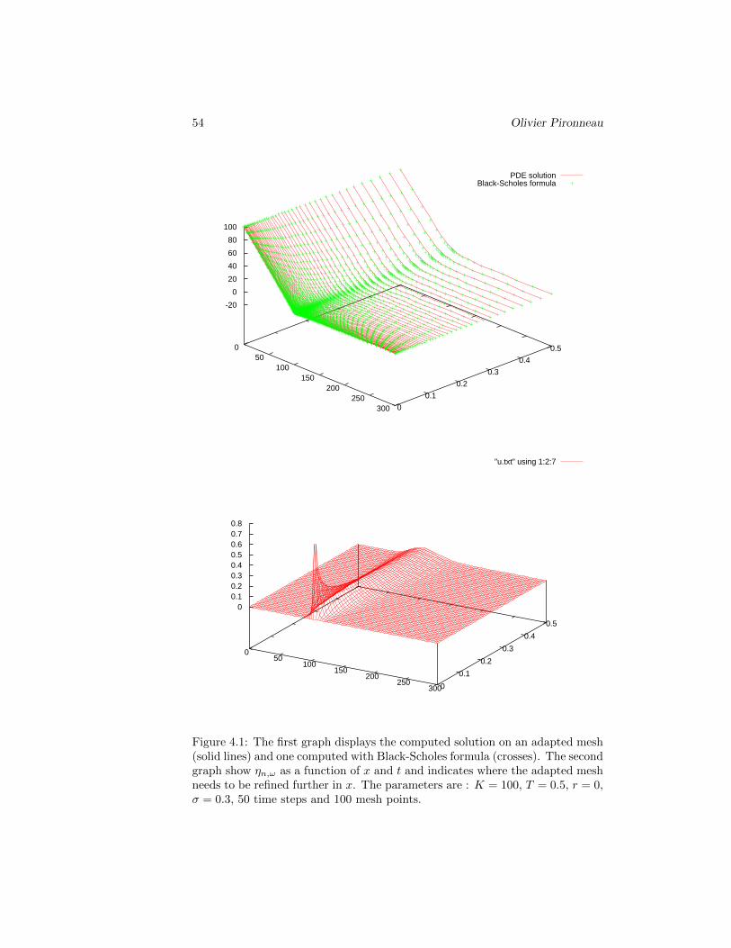
54 Olivier Pironneau
0 50
100 150
200 250
300 0
0.1
0.2
0.3
0.4
0.5
-20
0
20
40
60
80
100
PDE solutionBlack-Scholes formula
0 50
100 150
200 250
300 0
0.1
0.2
0.3
0.4
0.5
0 0.1 0.2 0.3 0.4 0.5 0.6 0.7 0.8
"u.txt" using 1:2:7
Figure 4.1: The first graph displays the computed solution on an adapted mesh(solid lines) and one computed with Black-Scholes formula (crosses). The secondgraph show ηn,ω as a function of x and t and indicates where the adapted meshneeds to be refined further in x. The parameters are : K = 100, T = 0.5, r = 0,σ = 0.3, 50 time steps and 100 mesh points.
Pricing Futures by Deterministic Methods 55
4.4 Variational Method for American Option
Referring to (3.30) an American put on S can be valued by solving
∂tP +σ2S2
2∂SSP + rS∂SP − rP,≤ 0,
P − (K − S)+ ≥ 0 ∀S ∈ R+, t ∈ (0, T ), (4.21)
with, at all (S, t), one of the two inequalities at least being an equality. Let(u, v) :=
∫∞0uvdS and a, b : V × V → R be the 2 bilinear forms
a(u, v) :=
∫R+
(σ2S2
2∂Su∂Sv + rvu)
b(u, v) :=
∫R+
(∂S(σ2S2
2)− rS)v∂Su (4.22)
where V is the Sobolev space, already used for European options
V = v ∈ L2(R+) : S∂Sv ∈ L2(R+)
The problem becomes: find u ∈ L2(0, T ;V ) with u(S, T ) = φ(S) := (K − S)+
and a.e. in (0, T ), u ≥ φ and
(∂tu, v − φ)− a(u, v − φ) −b(u, v − φ) ≤ 0∀v ∈ V φ = v ∈ V : v ≥ φ (4.23)
Let us callV + := v ∈ V : v(S) ≥ 0, a.e. in R+
Let w = v − φ, τ = T − t so as to prove the following
Proposition 11 The variational inequality:find u ∈ L2(0, T ;V ) with u(S, T ) = φ(S) := (K − S)+ and a.e. in (0, T )
u− φ ∈ V +, ∂τ (u,w) + a(u,w) + b(u,w) ≥ 0 ∀w ∈ V + (4.24)
has one and only one solution. Furthermore, for regular σ, u is a solution of(4.21).
ProofThe complete proof can be found in [1]. Let us give here only a simple argument.If (4.23) is discretized in time by(
um+1 − um
δt, v − φ
)− a(um, v − φ)− b(um+1, v − φ) ≤ 0 ∀v ∈ V φ (4.25)
with Mδt = T . As uM is known, (4.25) is solved backward in time. With
A(u, v) = (u
δt, v) + a(u, v) and L(v) := (
um+1
δt, v)− b(um+1, v)
56 Olivier Pironneau
it is : find um ∈ V φ such that
A(um, v − φ) ≥ L(v − φ) ∀v ∈ V φ (4.26)
Let us show that it is equivalent to um being the solution of
minu∈V φ
1
2A(u, u)− L(u) (4.27)
The minimum exists and is unique because the functional is strictly convex andV φ is a closed cone in V . By definition, if um is the solution
1
2A(um +w, um +w)− L(um +w) ≥ 1
2A(um, um)− L(um) ∀w : um +w ∈ V φ
Take w = λv, λ > 0 and let λ→ 0. At the limit
A(um, v) ≥ L(v) ∀v ∈ V such that limλ→0
um + λv ≥ φ
If um is smooth, by integration by parts, this is also∫Ω
(um − um+1
δt+ rum − ∂S(
σ2S2
2∂Su
m)− (rS − ∂Sσ2S2
2)∂Su
m+1
)v ≥ 0
which implies that the integrand is positive everywhere. Consider an S whereum(S) > φ(S); then for any v ∈ V there exists an interval (S1, S2) containing Swhere limλ→0 u
m + λv ≥ φ holds if the support of v is in (S1, S2). This in turnimplies that at that S, t either um(S) = φ(S) or
um − um+1
δt+ rum − ∂S(
σ2S2
2∂Su
m)− (rS − ∂Sσ2S2
2)∂Su
m+1 = 0
To complete the proof one must show that the finite difference scheme convergeswhen δt → 0. Note that there will be a stability condition because the firstorder terms have been discretized explicitly in time (i.e. at tm+1 instead of tm
or tm+ 12 ).
4.4.1 Discretization by FEM
Variational methods lead naturally to Galerkin and finite element methods.First the problem is localized : R+ ≈ (0, L) with L large, typically 3 times K.Then V is approximated by the piecewise linear continuous finite element space
V0h = vh ∈ C0(0, L) : vh|Tk ∈ P 1, vh(L) = 0 (4.28)
and V φ by
V φ0h = vh ∈ V0h : vh ≥ φh (4.29)
Pricing Futures by Deterministic Methods 57
where φh is the continuous piecewise linear interpolate of φ on the triangulation,uniquely defined by
φh ∈ V0h, φh(qj) = φ(qj) for all vertices qj of the triangulation
The discretized problem is: find umi Ii=1 such that
(um+1h − umh
δt, vh − φh)− a(umh , vh − φh)− b(umh , vh − φh) ≤ 0 ∀vh ∈ V φ0h
with umh (x) =
I∑i=1
umi wi(x) (4.30)
Notice that wi(x) ≥ 0 ∀x, so
vh ≥ φh ⇔ vj ≥ φj for all vertices qj
Thus and because wj(x) ≥ 0 for all j, (4.30) is also
(um+1h − umh
δtwj)− a(umh , w
j)− b(umh , wj) ≤ 0 j = 1..I
which we write as
a(uh, wj) ≥ (f, wj), j = 1..I (4.31)
uh(x) =
I∑1
uiwi(x) ≥ φh(x)
where a(u, v) =1
δt(u, v) + a(, v) + b(u, v), f =
um+1h
δt(4.32)
Ito et al[39] suggested to reformulated (4.31) as
Proposition 12 For any given constant c > 0, Problem (4.31) is equivalent to
a(uh, wh) + (λ,wh) = (f, wh) ∀wh ∈ V0h,λ(x)−min0, λ(x) + c(uh(x)− φh(x)) = 0, ∀x (4.33)
ProofThe last equality is equivalent to
λ ≤ 0, λ ≤ λ+ c(uh − φh) i.e. uh ≥ φh, λ ≤ 0, λ(x)(uh(x)− φ(x)) = 0 ∀x
The last statement means that for each x one of the two inequalities at leastone is an equality. The rest of the proof is a classical argument on Lagrangemultipliers:
a(uh, wh) + (λ,wh) = (f, wh), λ(x) ≤ 0, wh(x) ≥ 0⇒ a(uh, wh) ≥ (f, wh) ∀wh ≥ 0 (4.34)
58 Olivier Pironneau
Recall that an equation like F (x) = 0 (with F : Rn → Rn) can be solved byNewton’s method:
xk+1 = xk −G(xk)−1F (xk)
with G = F ′ the jacobian of F . Hintermuller et al[40] observed that Newton’salgorithm converges even if F is not differentiable provided that there exists Gsuch that
for all x lim‖h‖→0
‖F (x+ h)− F (x)−G(x+ h)h‖ = 0
a property which is satisfied by F (x) = max0, x for instance with G(x) =max0, x/x.
4.4.2 Semi-Smooth Newton Algorithm
Denote by Aij := a(wi, wj). Newton’s algorithm applied to (4.33) gives
1. Choose c > 0, , u0, λ0 ≤ 0, set k = 0.
2. FindAk := x : λk(x) + c(uk(x)− φ(x)) < 0
3. Set
uk+1 = arg minu∈H1(R+)
1
2a(u, u)− (f, u) : u = φ on Ak
4. Setλk+1 = f −Auk+1
Set k = k + 1 and go to 2.
The beauty of the method is that its implementation is almost painless froman implicit finite element or finite difference solver with the following “tgv”trick:
To compute the solution vh of
a(vh, wj) = (f , wj) ∀j /∈ K, vh(qj) = φ(qj), j ∈ K, j = 1..I
• Compute Aij = a(wii, wj) and fj = (f, wj). for all i, j.
• Reset Aii = 1030, fi = 1030φ(qj) for all i ∈ K
• Solve Av = f
Although it look as if the modification of A would ruin its condition numberin reality it doesn’t because it is essentially equivalent to the elimination of therows and columns of indices in K. It would be equivalent to rows and columnselimination if instead of 1030 the largest integer number that the computer canstore is used so that the addition of
∑j 6=iAijvj to Aiivi does not affect the
significant digits.
Pricing Futures by Deterministic Methods 59
Theorem 12 Algorithm 4.4.2 converges locally super linearly provided A is anM-matrix
The proof can be found in [39]; A is an M-matrix if mass-lumping (a reducedintegration formula with Gauss points at the vertices) is applied to the part ofA which comes from (wi, wj)/δt and provided the triangulation has no anglegreater than π/2. If it is not the case the method still converges providedu0, λ0 is not too far from the solution. It is also shown in [39] that the semi-smooth Newton method converges if applied to the continuous problem, beforediscretization, but the precision is proportional to c−1, so c must be large.
4.5 A Stochastic Volatility Model Solved by FEM
We now return to (4.13) for the stochastic volatility model (3.50). When f(0) =0 the problem is complicated by the fact the pde degenerates at y = 0. In theStein-Stein case f(y) = |y|, at least, it shown in [3, 2] that the solution existsand is unique if the data are smooth and if
r(t) ≥ r0 > 0, α2 > 2β2, 2α2η(1− η) > β2,
4.5.1 Finite Elements for a 2D Stochastic Volatility Model
As above we localize the problem in Ω := (0, Lx) × (−Ly, Ly). No boundarycondition is needed on the axis x = 0 since the pde is degenerate there. Noticealso that u is expected to tend to zero as x tends to infinity. For large y noarguments seems to give a boundary condition. However, if Ly is chosen suchthat
α(Ly ±m) β[ρµ− rf(Ly)
+ γ√
1− ρ2]
then for y ∼ ±Ly, the coefficient of the advection term in the y direction, and asthe advective effects will dominate the diffusive ones, even if a wrong boundarycondition is imposed, it will not propagate inside the domain. Hence we mayapply a Neumann condition.
Now Ω is triangulated into a set of non-intersecting triangles TkK1 withvertices qj satisfying
Ωh := ∪Kk=1Tk ≈ Ω, Tk ∩ Tl = ∅ or a vertex, or an entire edgeVertices on Γh = ∂Ωh are on Γ; corners of Γ are vertices of Γh (4.35)
V0 is approximated by V0h the space of continuous piecewise linear functions onthe triangulation which vanish at x = Lx.
V0h := vh ∈ C0(Ωh) : vh|Tk ∈ P 1(Tk) k = 1..K, vh(Lx, y) = 0
The basis wiI1 is uniquely defined by
wi ∈ V0h, wi(qj) = δij ∀j
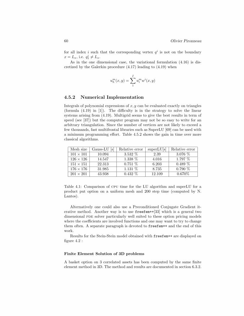
60 Olivier Pironneau
for all index i such that the corresponding vertex qi is not on the boundaryx = Lx, i.e. qi1 6= Lx.
As in the one dimensional case, the variational formulation (4.16) is dis-cretized by the Galerkin procedure (4.17) leading to (4.19) when
umh (x, y) =
I∑1
umi wi(x, y)
4.5.2 Numerical Implementation
Integrals of polynomial expressions of x, y can be evaluated exactly on triangles(formula (4.19) in [1]). The difficulty is in the strategy to solve the linearsystems arising from (4.19). Multigrid seems to give the best results in term ofspeed (see [37]) but the computer program may not be so easy to write for anarbitrary triangulation. Since the number of vertices are not likely to exceed afew thousands, fast multifrontal libraries such as SuperLU [69] can be used witha minimum programming effort. Table 4.5.2 shows the gain in time over moreclassical algorithms.
Mesh size Gauss-LU [s] Relative error superLU[s] Relative error101× 101 10.094 3.532 % 2.39 3.076 %126× 126 14.547 1.338 % 4.016 1.797 %151× 151 22.313 0.751 % 6.203 0.489 %176× 176 31.985 1.131 % 8.735 0.790 %201× 201 43.938 0.432 % 12.109 0.670%
Table 4.1: Comparison of cpu time for the LU algorithm and superLU for aproduct put option on a uniform mesh and 200 step time (computed by N.Lantos).
Alternatively one could also use a Preconditioned Conjugate Gradient it-erative method. Another way is to use freefem++[33] which is a general twodimensional pde solver particularly well suited to these option pricing modelswhere the coefficients are involved functions and one may want to try to changethem often. A separate paragraph is devoted to freefem++ and the end of thiswork.
Results for the Stein-Stein model obtained with freefem++ are displayed onfigure 4.2 :
Finite Element Solution of 3D problems
A basket option on 3 correlated assets has been computed by the same finiteelement method in 3D. The method and results are documented in section 6.3.2.
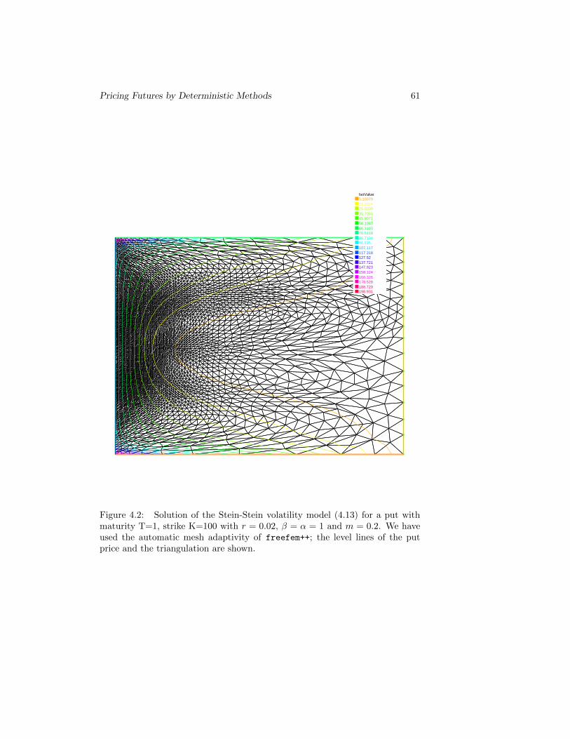
Pricing Futures by Deterministic Methods 61
IsoValue5.1007915.302425.503935.705545.907156.108766.310376.511886.713496.915107.117117.318127.52137.721147.923158.124168.326178.528188.729198.931
Figure 4.2: Solution of the Stein-Stein volatility model (4.13) for a put withmaturity T=1, strike K=100 with r = 0.02, β = α = 1 and m = 0.2. We haveused the automatic mesh adaptivity of freefem++; the level lines of the putprice and the triangulation are shown.
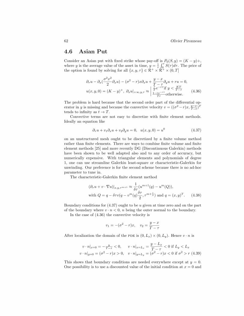
62 Olivier Pironneau
4.6 Asian Put
Consider an Asian put with fixed strike whose pay-off is P0(S, y) = (K − y)+,where y is the average value of the asset in time, y = 1
τ
∫ τ0S(τ)dτ . The price of
the option is found by solving for all x, y, τ ∈ R+ ×R+ × (0, T ]
∂τu− ∂x(σ2x2
2∂xu)− (σ2 − r)x∂xu+
y − xT − τ
∂yu+ ru = 0,
u(x, y, 0) = (K − y)+, ∂xu|+∞,y,τ ≈∣∣∣∣ τT e−rτ if y < KT
T−τ1−re−rτ
Tr otherwise.(4.36)
The problem is hard because that the second order part of the differential op-erator in y is missing and because the convective velocity v = ((σ2− r)x, y−xT−t )
T
tends to infinity as t→ T .Convective terms are not easy to discretize with finite element methods.
Ideally an equation like
∂τu+ v1∂xu+ v2∂yu = 0, u(x, y, 0) = u0 (4.37)
on an unstructured mesh ought to be discretized by a finite volume methodrather than finite elements. There are ways to combine finite volume and finiteelement methods [25] and more recently DG (Discontinuous Galerkin) methodshave been shown to be well adapted also and to any order of accuracy, butnumerically expensive. With triangular elements and polynomials of degree1, one can use streamline Galerkin least-square or characteristic-Galerkin forunwinding. Our preference is for the second scheme because there is no ad-hocparameter to tune in.
The characteristic-Galerkin finite element method
(∂τu+ v · ∇u)|x,y,τm+1 ≈ 1
δτ(um+1(q)− um(Q)),
with Q = q − δτv(q − vm(q)δτ
2, τm+ 1
2 ) and q = (x, y)T . (4.38)
Boundary conditions for (4.37) ought to be u given at time zero and on the partof the boundary where v · n < 0, n being the outer normal to the boundary.
In the case of (4.36) the convective velocity is
v1 = −(σ2 − r)x, v2 =y − xT − τ
After localization the domain of the pde is (0, Lx)× (0, Ly). Hence v · n is
v · n|x=0 = − yT−τ < 0, v · n|x=Lx =
y − LxT − τ
< 0 if Ly < Lx
v · n|y=0 = (σ2 − r)x > 0, v · n|y=Ly = (σ2 − r)x < 0 if σ2 > r (4.39)
This shows that boundary conditions are needed everywhere except at y = 0.One possibility is to use a discounted value of the initial condition at x = 0 and
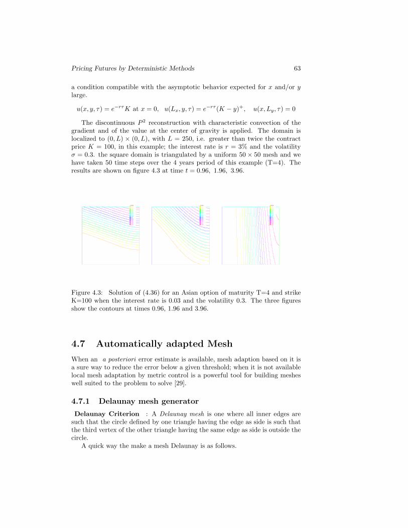
Pricing Futures by Deterministic Methods 63
a condition compatible with the asymptotic behavior expected for x and/or ylarge.
u(x, y, τ) = e−rτK at x = 0, u(Lx, y, τ) = e−rτ (K − y)+, u(x, Ly, τ) = 0
The discontinuous P 2 reconstruction with characteristic convection of thegradient and of the value at the center of gravity is applied. The domain islocalized to (0, L) × (0, L), with L = 250, i.e. greater than twice the contractprice K = 100, in this example; the interest rate is r = 3% and the volatilityσ = 0.3. the square domain is triangulated by a uniform 50× 50 mesh and wehave taken 50 time steps over the 4 years period of this example (T=4). Theresults are shown on figure 4.3 at time t = 0.96, 1.96, 3.96.
IsoValue3.3866110.196917.007223.817530.627837.43844.248351.058657.868964.679271.489578.299785.1191.920398.7306105.541112.351119.161125.972132.782
IsoValue2.961878.8882614.814620.74126.667432.593838.520244.446650.37356.299462.225868.152274.078580.004985.931391.857797.7841103.71109.637115.563
IsoValue1.954695.86499.7751113.685317.595521.505725.41629.326233.236437.146641.056844.96748.877252.787456.697660.607964.518168.428372.338576.2487
Figure 4.3: Solution of (4.36) for an Asian option of maturity T=4 and strikeK=100 when the interest rate is 0.03 and the volatility 0.3. The three figuresshow the contours at times 0.96, 1.96 and 3.96.
4.7 Automatically adapted Mesh
When an a posteriori error estimate is available, mesh adaption based on it isa sure way to reduce the error below a given threshold; when it is not availablelocal mesh adaptation by metric control is a powerful tool for building mesheswell suited to the problem to solve [29].
4.7.1 Delaunay mesh generator
Delaunay Criterion : A Delaunay mesh is one where all inner edges aresuch that the circle defined by one triangle having the edge as side is such thatthe third vertex of the other triangle having the same edge as side is outside thecircle.
A quick way the make a mesh Delaunay is as follows.
64 Olivier Pironneau
1. Unmark all edges
2. Loop on the unmarked inner edges until all are marked
• For each edge identify the two triangles which have this edge as side.If the edge fails the Delaunay test above, then swap the edge withthe other diagonal of the quadrilateral made by the two trianglesand update the triangulation by replacing the two old triangles bythe two new ones.
• Mark the new edge and unmark the four edges of the quadrilateral.
It can be shown that the loop stops in finite time because the minimum angle inthe triangulation is strictly increased at each loop and that the resulting meshis Delaunay if the domain is convex.
If the domain is not convex, a complicate recovery of the boundary edgesmust be performed, but still the mesh has similar good qualities in most cases(see [29]). In fact it can be shown that the Delaunay mesh is the nearest to aquasi-equilateral mesh, in the sense that the smallest angle in the triangulationis maximized by the edge swaps implied by the Delaunay criteria.
4.7.2 Anisotropic Delaunay Mesh Generator
Note that if the local metric is Euclidean, the mesh elements are isotropic inthe sense that there are no preferred direction in the algorithm.
To obtain an anisotropic mesh one must replace circles by ellipses in theDelaunay criteria.
Given a positive definite matrixM(x) we define a variable metric by ‖x− y‖2 =(x−y)TM(x)(x−y) . M -circles, i.e. circles with respect to the variable metric,are ellipses in the Euclidean space.
A given triangulation is said to satisfy the M -Delaunay criteria if for allinner edges the quadrangle made by the its two adjacent triangles are such thatthe fourth vertex is outside the M-circle passing by the three other vertices.
The adaptive Delaunay mesh generator of [29] is based on five steps:
1. Discretize the Boundary of Ω, the domain for which we seek a triangula-tion.
2. Build a M-Delaunay triangulation of the convex hull of all the boundarynodes ( no internal point).
3. Add an internal points to all edges which are longer (in the variable metric)than the prescribed length.
4. Rebuild the triangulation with internal nodes now, using the Delaunaycriteria and the variable metric.
5. Remove the triangles which are outside Ω.
Pricing Futures by Deterministic Methods 65
6. Goto 3 until the elements have the required quality.
So anisotropy is controlled by M , the local metric.
4.7.3 Metric adapted to the Solution of the pde
As stated earlier, if we want the mesh to be adapted to the solution, we needto define the metric at each point of the domain and use it in the Delaunayalgorithm above.
The definition of the metric is based on the Hessian of the state variablesof the problem. Indeed, for a P 1 Lagrange discretization of a variable u, theinterpolation error is bounded by:
E := |u−Πhu|0 ≤ ch2|D2u|0, (4.40)
where h is the element size, Πhu the P 1 interpolation of u and D2u its Hessianmatrix. This matrix is symmetric and diagonizable
D2u =
(∂2u/∂x2 ∂2u/∂x∂y∂2u/∂x∂y ∂2u/∂y2
)= R
(λ1 00 λ2
)R−1, (4.41)
Using this information, we introduce the following metric tensor M:
M = R(λ1 0
0 λ2
)R−1, (4.42)
where
λi = min
(max(|λi|,
1
h2max
),1
h2min
), (4.43)
with hmin and hmax being the minimal and maximal edge lengths allowed in themesh.
Now, if we generate, by a Delaunay procedure, an equilateral mesh withedges of length of 1 in the metric M/(cE), the interpolation error E is equi-distributed over the edges of length ai if
1
cEaTi Mai = 1. (4.44)
4.8 Greeks
Probably due to the fact that mathematicians have used greek letters to namethe partial derivatives of option prices with respect to the relevant parametersthese are called the Greeks: let P be the price of a vanilla European put:
• The δ (delta) is its derivative with respect to the stock price S : ∂SP ..
• The Θ or time-decay is its derivative with respect to time: ∂tP .
• The vega κ is its derivative with respect to the volatility σ, ∂σP .
66 Olivier Pironneau
• The rho ρ is its derivative with respect to the interest rate, ∂rP .
• η is its derivative with respect to the strike K
• Finally, the gamma is the rate of change of its delta : γ = ∂SSP = ∂Sδ.
Computing greeks from the sde of the asset can be challenging but the sameis very easily done with the pde of the option. For illustration take the vanillaput on St written in moneyness y and time to maturity τ
∂τu−y2σ2
2∂yyu = 0, u(y, 0) = (1− y)+
A FEM of FDM numerical solution will give the δ with order 1 precision. Ifmore precision is needed, by differentiation of the pde with respect to y, v = ∂yusatisfies
∂τv −y2σ2
2∂yyv = (yσ2 + y2σ∂yσ)∂yyu, v(y, 0) = H(y − 1)− 1
with H(x) the Heaviside function which is zero for x < 0 and one otherwise. Infine the delta is δ = Kv(e−r(T−t)S/K , T − t). It is also
∂τv −y2σ2
2∂yyv − (yσ2 + y2σ∂yσ)∂yv = 0, v(y, 0) = H(y − 1)− 1
The Θ can be computed by Θ = y2σ2∂yv/2 or by differentiating the equationfor v.
The vega satisfies
∂τκ−y2σ2
2∂yyκ = y2σ∂yyu, κ(y, 0) = 0
Alternatively, as explained in [1] and [2], if the numerical solver for u is writ-ten in C++, all greeks can be computed at no programing cost by automaticdifferentiation using operator overloading and template classes.
4.8.1 Greeks for American Options
American options have been framed into variational inequalities like (4.24):
u− φ ∈ V + : ∂τ (u,w) + aτ (u,w) ≥ (f, w) ∀w ∈ V + = w ∈ V : w ≥ 0
where (·, ·) is the scalar product of L2, aτ (·, ·) is a τ -dependent continuouscoercive bilinear form on the Hilbert space V and f ∈ V . Another form of thesame is, for some operator A
u− φ ∈ V + : ∂τu+Au ≥ f ∀w ∈ V + = w ∈ V : w ≥ 0
Pricing Futures by Deterministic Methods 67
To compute the sensitivity of u with respect to a parameter α the best is toreturn to the definition of derivatives and work out the equation/inequation forthe increments. For instance
u(α) ≥ φ(α), u(α+ δα) ≥ φ(α+ δα) ⇒ u′α ≥ φ′α at S, τ where u(α) = φ(α)
Similarly
∂τu′α +Au′α + λ′ = f ′α −A′αu
with λ′ ≤ 0 at all S, τ where ∂τu+ Au = f and λ′ = 0 at all other points; butby (4.24) we know that at point where ∂τu+Au 6= f then u = φ, consequentlyu′α is solution of
u′α ≥ φ′α, ∂τu′α +Au′α ≥ f ′α −A′αu
or equivalently
u′α − φ′α ∈ V + : ∂τ (u′α, w) + a(u′α, w) ≥ (f ′α, w)− a′α(u,w) ∀w ∈ V +
The semi-smooth Newton algorithm can be used for u′α exactly as for u.
4.9 Reduced Order Modeling
Derivatives like European calls and puts on a single or compound assets arecomputed a very large number of times every day. When a closed form solutionis not available, an alternative to Monte-Carlo simulation is to solve the Black-Scholes partial differential equation.
A complement to the Finite Element or Finite Difference Method for a nu-merical solution of the problem is to construct an appropriate basis, smaller insize but with larger support. Proper Orthogonal Decomposition is the usualtool for it.
In [18] it was shown that a set of rescaled calls with constant volatilitiesforms a reduced basis with similar performance as POD.
If τ is the time to maturity, K is the strike, r the interest rate, y = erτ SKthe moneyness, then the pricing of a put P can be made by solving
∂τvσ −σ2y2
2∂yyvσ = 0, vσ(0) = (1− y)+ (4.45)
where vσ = Perτ .
When σ is constant, the Black-Scholes formula provides an analytical solu-tion
vσ =y
2(1 + erf(
ln y
σ√
2τ+ σ
√τ
8))− 1
2(1 + erf(
ln y
σ√
2τ− σ
√τ
8)) + 1− y
and erf(y) =2√π
∫ y
0
e−x2
dx (4.46)
68 Olivier Pironneau
Notice that only σ√τ appears so to change the volatility or to change τ is the
same thing. Hence a basis of snapshots in time for (4.45) can also be
vσ(y, τ) = vΣ(y, τ) +
I∑i=1
ai(τ)wi(y) with wi := vσi(y, T )− vΣ(y, T ) (4.47)
where σii∈I is an appropriate set of constant volatilities and Σ is a chosenreference volatility. The pde verified by u := vσ − vΣ is
∂τu−σ2y2
2∂yyu = −(∂τvΣ −
σ2y2
2∂yyvΣ), u(0) = 0. (4.48)
Applying Galerkin’s method to (4.48) with (4.47) will give the ai(τ). How-ever it is numerically much easier to work with wi := ∂yyvσi(y, T ) instead ofwi = vσi(y, T )−vΣ(y, T ) and since ∂yy is a bijection with appropriate boundaryconditions it shouldn’t make much of a difference!
As we shall see a good choice is σi = (2c T i)−12 , i = 1, 2... where c is a
chosen constant. A rapid computation shows that wi is proportional to
wi :=√ye−αi ln2 y with αi = c i.
This will be the basis chosen here, and c = 1 in the numerical tests.
The POD algorithm In this framework POD means
1. Choose I << 100
2. Apply the Gram-Schmidt algorithm to orthogonalize the wii∈I withrespect to the L2(R+) or H1(R+) scalar product (·, ·). Let pii∈I be theresult.
3. Solve (4.48) on this basis by the Galerkin method
4. If the result is not precise enough, add a new element in I and go back toStep 2.
The ”not precise enough” of Step 4 needs in principle an a posteriori estimateto become mathematically sound. The selection of a “good new basis vector”is also difficult in Step 4 and one way is to order the vectors pi so as to havea decreasing sequence of eigenvalues of the correlation matrix (wi, wj) (see [58]for details).
4.9.1 Galerkin Approximation on the Basis
Mathematical Result
Decomposition (4.47) gives a vσ which satisfies the initial and boundary con-ditions of the Black-Scholes equations (4.45); it has also the right exponentialbehavior when y →∞. Consider y → u(y)/
√y and as before u = vσ − vΣ.
Pricing Futures by Deterministic Methods 69
Note that e−ic ln2 y = f(y)i with f(y) = e−c ln2 y. By the Stone-Weirstrasstheorem f(y)nn=0,1.. is a basis if y → f(y) is a separating function; however
e−c ln2 y is a separating function only on the interval (0, 1) or on (1,∞) but noton (0,∞). So we need a symmetry assumption about 1: u( 1
y ) = 1yu(y) for (4.47)
to work. Fortunately if σ( 1y , τ) = σ(y, τ) then it is easy to show that u has the
required symmetry. If symmetry does not hold then another set of vectors mustbe added in the basis, such as √ywi(y)i=1,2... More details can be found in[18].
Implementation
Note that
∂yywi =
e−αi ln2 y
y√y
(4α2i ln2 y − 1
4− 2αi)
∂τvΣ −σ2y2
2∂yyvΣ =
(Σ2 − σ2)y2
2∂yyvΣ =
e−Σ2τ
8
2Σ√
2πτ(Σ2 − σ2)
√ye− ln2 y
2Σ2τ (4.49)
So (4.47) is
I∑1
ai√ye−αi ln2 y−
I∑1
aie−αi ln2 yσ2√y(2α2
i ln2 y − 1
8− αi)
= − e−Σ2τ
8
2Σ√
2πτ(Σ2 − σ2)
√ye−
ln2 y
2Σ2τ (4.50)
The Galerkin method requires to multiply this equation by γ(y)√ye−αj ln2 y (the
extra factor γ(y) is a weight) and integrate over R+. We obtain an ODE systemfor for a = (a1(τ), .., aI(τ))T :
Ma+Ba = F (4.51)
with
Mij :=
∫ ∞0
e−(αi+αj) ln2 yγ(y)ydy
Bij := −∫ ∞
0
e−(αi+αj) ln2 yσ2(2α2i ln2 y − 1
8− αi)γ(y)ydy
Fj := − e−Σ2τ
8
2Σ√
2πτ
∫ ∞0
e−(αj+1
2Σ2τ) ln2 y(Σ2 − σ2)γ(y)ydy (4.52)
The Case σ Constant
When σ is constant and γ(y) = y−2:
Mij =
√π
αi + αj
70 Olivier Pironneau
Bij =
√πσ2
(αi + αj)12
(αiαjαi + αj
+1
8)
Fj = −e−Σ2τ
8 (Σ2 − σ2)
2√
2αjΣ2τ + 1(4.53)
The Non Constant Case
If σ is a function of y and τ , with σ( 1y , τ) = σ(y, τ) it is best to express it on an
exponential basis as:
σ(x, t) = σ0 +
J∑1
σj(t)e−αj ln2 y (4.54)
because then all integrals can be computed analytically.
Another choice for γ
Later on we will change variable to z = e− ln2 y; then in view of the fact thatdz = 2
y e− ln2 y ln 1
ydy we will need to choose
γ(y) =2
y2| ln y| so as to have e− ln2 yyγ(y)dy = e− ln2 y 2
y| ln y|dy = dz.
Then with σ constant:
Mij =1
αi + αj
Bij =σ2
αi + αj[1
8+ αi −
2α2i
αi + αj]
Fj = −(Σ2 − σ2)e−
Σ2τ8
√2Σ2τ
2√π(1 + 2Σ2ταj)
(4.55)
The computation of the integrals rely on the following:∫ ∞0
e−k ln2 yγ(y)ydy = 2
∫ 1
0
zkdz =2
k + 1∫ ∞0
e−k ln2 y ln2 1
yγ(y)ydy = 2
∫ 1
0
zk ln1
zdz =
2
(k + 1)2(4.56)
4.9.2 Numerical Tests
The method was thoroughly tested in [18] but since we are concerned with aminor variation of the original we retested the method for the computation ofa vanilla call of volatility σ =
√0.9 using Σ =
√0.5 and I ranging from 5 to 30
(using multi precision arithmetics when I > 20). The maturity is T = 2 and 10time steps are used to integrate (4.51); with 20 time steps the precision is notsignificantly improved.
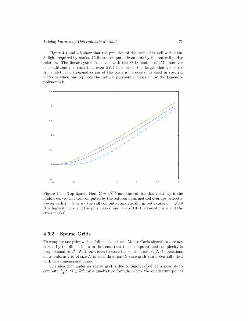
Pricing Futures by Deterministic Methods 71
Figure 4.4 and 4.5 show that the precision of the method is well within the3 digits required by banks. Calls are computed from puts by the put-call parityrelation. The linear system is solved with the SVD module of [57]; howeverill conditioning is such that even SVD fails when I is larger that 20 or so.An analytical orthogonalization of the basis is necessary, as used in spectralmethods when one replaces the natural polynomial basis zn by the Legendrepolynomials.
Figure 4.4: Top figure: Here Σ =√
0.5 and the call for this volatility is themiddle curve. The call computed by the reduced basis method overlaps perfectly- even with I = 5 here - the call computed analytically in both cases σ =
√0.9
(the highest curve and the plus marks) and σ =√
0.3 (the lowest curve and thecross marks).
4.9.3 Sparse Grids
To compute one price with a d-dimensional sde, Monte-Carlo algorithms are notcursed by the dimension d in the sense that their computational complexity isproportional to d2. With pde even to store the solution cost O(Nd) operationson a uniform grid of size N in each direction. Sparse grids can potentially dealwith this dimensional curse.
The idea that underlies sparse grid is due to Smolyak[64]: It is possible tocompute
∫Ωf, Ω ⊂ Rd, by a quadrature formula, where the quadrature points
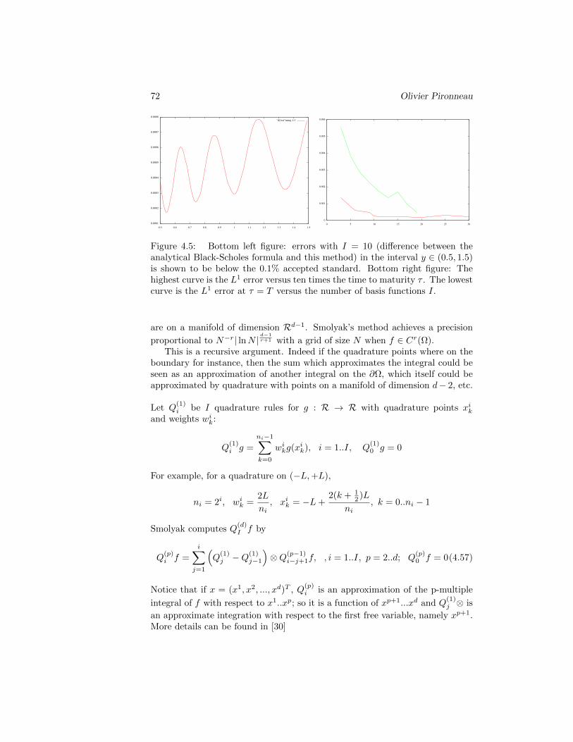
72 Olivier Pironneau
Figure 4.5: Bottom left figure: errors with I = 10 (difference between theanalytical Black-Scholes formula and this method) in the interval y ∈ (0.5, 1.5)is shown to be below the 0.1% accepted standard. Bottom right figure: Thehighest curve is the L1 error versus ten times the time to maturity τ . The lowestcurve is the L1 error at τ = T versus the number of basis functions I.
are on a manifold of dimension Rd−1. Smolyak’s method achieves a precision
proportional to N−r| lnN |d−1r+1 with a grid of size N when f ∈ Cr(Ω).
This is a recursive argument. Indeed if the quadrature points where on theboundary for instance, then the sum which approximates the integral could beseen as an approximation of another integral on the ∂Ω, which itself could beapproximated by quadrature with points on a manifold of dimension d− 2, etc.
Let Q(1)i be I quadrature rules for g : R → R with quadrature points xik
and weights wik:
Q(1)i g =
ni−1∑k=0
wikg(xik), i = 1..I, Q(1)0 g = 0
For example, for a quadrature on (−L,+L),
ni = 2i, wik =2L
ni, xik = −L+
2(k + 12 )L
ni, k = 0..ni − 1
Smolyak computes Q(d)I f by
Q(p)i f =
i∑j=1
(Q
(1)j −Q
(1)j−1
)⊗Q(p−1)
i−j+1f, , i = 1..I, p = 2..d; Q(p)0 f = 0(4.57)
Notice that if x = (x1, x2, ..., xd)T , Q(p)i is an approximation of the p-multiple
integral of f with respect to x1..xp; so it is a function of xp+1...xd and Q(1)j ⊗ is
an approximate integration with respect to the first free variable, namely xp+1.More details can be found in [30]
Pricing Futures by Deterministic Methods 73
Remark 11 Equivalently
Q(p)i f =
∑|j|≤i+p−1
Dj1 ⊗ ...⊗Djpf with Dk = Q(1)k −Q
(1)k−1 (4.58)
The method is easy to apply to the computation of a basket option by (1.40).Even though the regularity is r = 0, the method gives reasonably good results.The following program implements (4.58). Results are shown on figure 4.6. Im-provement can be obtained by using recursively embedded grids are computingdirectly Qk −Qk−1 instead of Qk and Qk−1 separately.
#include <iostream>
#include <cmath>
#include <ctime>
using namespace std;
#define d 5 // dimension of the integration space
const double L=2*atan(1.); // size of the cube (-L,L)^d;
const int m=4; // max number of points of quadrature in each dim
int *y, ik[d]; // container of a distribution of integers with sum<m+d
double *z; // will be all the quadrature points in R^d, each in turn
void explore(int p, int s); // finds a set of y[] s.t. sum of y<=s, recursively in p;
double f(double *y); // the function to integrate
void QId(int* y); // the 1d integration procedure
int *ni,*kd; // working array
double somme=0, L2=2*L, pi=4*atan(1.0), xpi=sqrt(pow(2*pi,d)); // auxiliary variables
double f(double *x) double aux=1; for (int i=0;i<d;i++) aux*=cos(x[i]/2); return aux;
/* double f(double *z) double aux=0, aux1=0, pid2=1;
for (int i=0;i<d;i++) aux+= z[i]; aux1+=z[i]*z[i];pid2*=2*pi;
return max(1-exp(aux),0.)*exp(-aux1/2)/sqrt(pid2);
*/ // change to this f for finance
void explore(int p, int s) // p ends recursion
if(p>0)
for(y[p]=0;y[p]<=s;y[p]++)
explore(p-1,s-y[p]);
else
y[p]=s;// here p==0
QId(y);
void QId(int* y)
double dd;
for( ik[0]=0;ik[0]<=1;ik[0]++) // to add dimensions add loops below
for( kd[0]=0;kd[0]<ni[y[0]-ik[0]];kd[0]++)
#if(d>1)
for( ik[1]=0;ik[1]<=1;ik[1]++) for( kd[1]=0;kd[1]<ni[y[1]-ik[1]];kd[1]++)
#endif
#if(d>2)
for( ik[2]=0;ik[2]<=1;ik[2]++) for( kd[2]=0;kd[2]<ni[y[2]-ik[2]];kd[2]++)
#endif
#if(d>3)
for( ik[3]=0;ik[3]<=1;ik[3]++) for( kd[3]=0;kd[3]<ni[y[3]-ik[3]];kd[3]++)
#endif
#if(d>4)

74 Olivier Pironneau
for( ik[4]=0;ik[4]<=1;ik[4]++) for( kd[4]=0;kd[4]<ni[y[4]-ik[4]];kd[4]++)
#endif
#if(d>5)
for( ik[5]=0;ik[5]<=1;ik[5]++) for( kd[5]=0;kd[5]<ni[y[5]-ik[5]];kd[5]++)
#endif
#if(d>6)
for( ik[6]=0;ik[6]<=1;ik[6]++) for( kd[6]=0;kd[6]<ni[y[6]-ik[6]];kd[6]++)
#endif
dd=1;
for(int k=0;k<d;k++)
int iy=y[k]-ik[k], nk = ni[iy];
if(iy>=1)
z[k] = -L + (L2*kd[k]+L)/nk;
dd *= ik[k]? -L2/nk : L2/nk;
else dd=0;
if(dd==0)break;
if(dd!=0) somme += f(z)*dd;
int main()
y = new int[d];
ni = new int[m+1];
kd = new int[d];
z = new double[d];
ni[0]=1; for(int k=1;k<=m;k++) ni[k] =2*ni[k-1]; // ni[k]=2^k;
time_t time0=clock();
for(int n=1;n<m+d;n++) explore(d-1,n); // gets all y[] with sum_0^d-1 y[j]=n
cout <<"\sc cpu=\t"<<double(clock()-time0)/CLOCKS_PER_SEC
<<"\t relative error = \t"<<fabs(1-pow(4*sin(L/2),d)/somme)<<" "<<somme<<endl;
return 0;
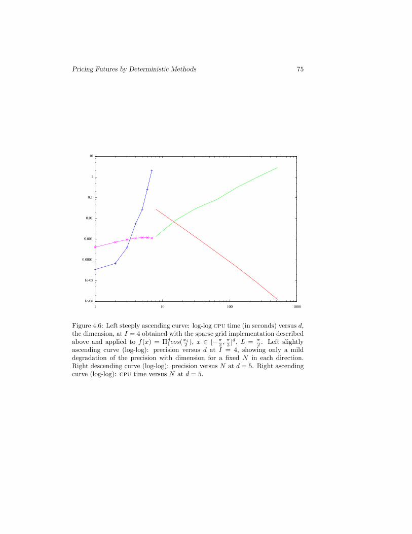
Pricing Futures by Deterministic Methods 75
Figure 4.6: Left steeply ascending curve: log-log cpu time (in seconds) versus d,the dimension, at I = 4 obtained with the sparse grid implementation describedabove and applied to f(x) = Πd
1cos(xi2 ), x ∈ [−π2 ,
π2 ]d, L = π
2 . Left slightlyascending curve (log-log): precision versus d at I = 4, showing only a milddegradation of the precision with dimension for a fixed N in each direction.Right descending curve (log-log): precision versus N at d = 5. Right ascendingcurve (log-log): cpu time versus N at d = 5.

76 Olivier Pironneau
Chapter 5
Calibration
5.1 Introduction
Whatever the quality of the modeling, the simulations usually do not reproducethe market data. Besides, some parameters like the volatilities are not easyto estimate. On the other hand many assets and options are observable, andavailable, perhaps at a cost (Reuters).
Consider the problem of building an accurate model for a vanilla european callon St. Today, at time t = 0, we can observe
• The underlying asset S0
• The values (ci)i∈I of calls (CKi,Ti(S0, 0))i∈I of maturity Ti and strike Ki.
We wish to use the Black-Scholes pde with a local (i.e. non constant) volatility,so we must:
Find x, t→ σ(x, t) such that the Cii∈I computed by
∂tCi +σ2S2
2∂2SSCi + rS∂SCi − rCi = 0,
Ci(S, Ti) = (S −Ki)+, for all t ∈ [0,Ti[, x ∈ R+, (5.1)
satisfy Ci(S0, 0) = ciThe most natural way to proceed is to solve this inverse problem by least
squares
minσ∈S
∑|Ci(S0, 0)− ci|2 : subject to (5.1)
This problem has 3 difficulties
1. It is ill posed unless S is severely constrained or a Tikhonov regularizationis added to the cost function (see [24]).
2. It has infinitely many solutions as we shall see
77
78 Olivier Pironneau
3. It is numerically expensive to solve.
Curse number 3 is problematic. One reason is that it is an optimal controlproblem with card(I) pdes. Working with the moneyness variables τ = T −t, y = erτ SK ,Ku(y, τ) = erτC(Ke−rτy, T − τ) reduces the number of pdes toone and the problem becomes
minσ∈S
∑|erTiKiu(erTi
S0
Ki, Ti)− ci|2
subject to ∂τu−σ2y2
2∂yyu = 0, u(y, 0) = (y − 1)+ (5.2)
With S = σ(y, τ) : σm ≤ σ(y, τ) ≤ σM and if a Tikhonov regularization ofthe type
‖σ‖20 + ‖∂yσ‖20 + ‖∂τσ‖20 + ‖∂yτσ‖20is added to the cost function, then the problem is well posed and doable numer-ically by a conjugate gradient method for example (see [1]).
However explicit dependency of C with respect to K is specific to this prob-lem and the method is not general. Dupire had a better idea!
5.2 Dupire’s Equation
Consider a call priced by (3.11). To stress explicitly the dependence on theparameters K,T we write the solution as CK,T (S, t).Dupire[26] observed that an equation for CS,t(K,T ) can be derived where S, tare now parameters:
∂τC −1
2σ2K2∂KKC + rK∂KC = 0, C(K, t0) = (S −K)+ ∀K > 0, τ ≥ t0(5.3)
Dupire’s proof[26] uses the Green function of the differential operator in (3.11).We shall give a proof which can be extended to any financial object governed bya linear system. The proof relies on a duality argument, like the forward andbackward Kolmogorov equation. The proof also shows that a double primitiveof the dual of Black-Scholes’ pde is involved. Thus it is misleading to use K,Tas variables in (5.3).
Proposition 13 (Dupire) Let v be solution in R+ × (t0, T ) of
∂tv −1
2σ2S2∂SSv + rS∂Sv = 0, v(S, t0) = (S0 − S)+ (5.4)
then CK,T (S0, t0) = v(K,T ) and p = ∂SSv is solution of the adjoint of (3.11):
∂tp− ∂SS(σ2S2
2p) + ∂S(rSp) + rp = 0, p(t0) = δ(S − S0) (5.5)
Pricing Futures by Deterministic Methods 79
ProofAn integration by parts in time and Green’s formula in space applied to (3.11)multiplied by p and integrated over R+ × (t0, T ) yields
C(S0, t0) =
∫ ∞0
dS
[CT p(T ) +
∫ T
t0
(pσ2S2
2∂SC − C∂S(
σ2S2
2p)
)dt
](5.6)
where CT (S) is the option’s premium. By the properties of C and p at zeroand infinity the boundary term vanishes. Let v be the double primitive of p, i.e.∂SSv = p then, (5.5) integrated twice becomes (5.4) for an appropriated choiceof the integration constants.
5.2.1 Example of Generalization: Dupire’s for Binary Calls
The premium is one monetary unit if ST > K and zero otherwise. It can betreated by the same method. The adjoint equation is integrated once only andthe result is:
u(S0, t0) =
∫ ∞0
uT∂SwdS = −∫ ∞
0
w∂SuTdS + [uTw]∞0 = −w(K,T ) with
∂tw − ∂S(σ2S2
2∂Sw) + rS∂Sw + rw = 0, w(t0) = 1S>S0
− 1. (5.7)
5.2.2 Dupire’s Equation for Barrier Options
Consider a European barrier option which stops to exist if St /∈ (Smert, SMe
rt).The change of variable c(s, t) = e−rtC(sert, t) reduces (3.11) with barriers to
∂tc+1
2σ2s2∂ssc = 0, c(s, T ) = (s−Ke−rT )+,
c(Sm, t) = c(SM , t) = 0, ∀s, t ∈ (Sm, SM )× (0, T ) (5.8)
Proposition 14 Assume that Sm < Ke−rT < SM . If c verifies (5.8) then
c(s0, t0) = v(Ke−rT , T ) + (SM −Ke−rT )+∂Sv|SM ,T (5.9)
where v is the solution of
∂tv −1
2σ2s2∂ssv = 0, v(s, t0) = (s0 − S)+
v(Sm, t) = (s0 − Sm)+, v(SM , t) = 0 ∀t ∈ (t0, T ) (5.10)
ProofNow the boundary conditions in (5.5) with r = 0 are p(Sm, t) = p(SM , t) = 0for all t. For v, the double primitive of p, it translates into ∂ssv = 0 which inturn implies ∂tv = 0 which means that v is constant at the barriers. NaturallyC(S0, t0) can be recovered from c by choosing s0 = S0e
rt0 .
80 Olivier Pironneau
5.2.3 Dupire’s Equation for Options on Levy Driven As-sets
If a Poisson-Levy process is used in the Back-Scholes model, as in [20], a termappears in the right hand side of (3.11):∫
R
(C(Sey, t)− C(S, t)− S(ey − 1)
∂C
∂S
)k(y)dy (5.11)
where k, the kernel of the process is usually singular at the origin and decayingfast at infinity.When multiplied by p and integrated in S, with z = Se−y this term can betransformed into an integral of C(S, t)χ(S, t) for an appropriate χ leading tothe integro-differential equation for p. The resulting equation is again integratedtwice and leads to the following result:
Proposition 15 A Poisson-Levy driven option CK,T (S, t), solution of (3.11)with (5.11) on the right hand side, verifies Dupire’s identity
CK,T (S0, t0) = v(K,T ) where v is the solution of
∂tv −σ2S2
2∂SSv + rS∂Sv
−∫R
(ey(v(Se−y, t)− v(S, t)) + (ey − 1)S∂Sv(S, t)
)k(y)dy = 0
v(S, t0) = (S0 − S)+ v(0, t) = S0, limS→∞
v(S, t) = 0 ∀t ∈ (t0, T )(5.12)
Theorem 13 Consider a call on S modeled by
∂tC + σ2S2
2 ∂SSv +rS∂SC − rC
+
∫R
(C(Sey, t)− C(S, t)− S(ey − 1)∂SC(S, t)) ν(dy)
C(S, T ) = (S −K)+ (5.13)
Dupire’s identity hold CK,T (S0, 0) = v(K,T ) when v is the solution of
∂tv −σ2S2
2∂SSv + rS∂Sv
−∫R
(ey(v(Se−y, t)− v(S, t)) + (ey − 1)S∂Sv(S, t)
)ν(dy) = 0
v(S, 0) = (S0 − S)+ v(0, t) = S0, limS→∞
v(S, t) = 0 ∀t ∈ (0, T ) (5.14)
The proof has (5.13) multiplied by p and integrated in S by parts. At on stage achange of integration variable is necessary, z = Se−y. Then as for Black-Scholesequation one introduces v such that ∂SSu = p.
Pricing Futures by Deterministic Methods 81
Calibration: Now assuming that Ci = CKi,Ti(S0, 0) are market observationsthen to calibrate the model one may solve
min∑i∈I|v(Ki, Ti)− Ci|2
where the optimization variables are the parameters of the model, i.e. λ, γ, σ, µ, δin the case of Merton’s model for example.
5.2.4 Dupire’s identity in the discrete case
Extension to more complex option is possible as long as the pde is linear. Forinstance, Dupire’s argument does not work with American options. FurthermoreIt is not always possible to find a double primitive of the adjoint equation like(5.5) which as it stands is numerically very hard because of the singularity ofthe initial condition. On the other hand, at the discrete level the same difficultyis not there with the variational approach.For simplicity assume that the coefficients in (5.5) do not depend of time andconsider a time discretization with an Euler implicit scheme with time step δtand a space discretization with piecewise linear finite elements in the variableS. The vertices of the grid are called qi, 0 ≤ i ≤ I, and we set L = qI . Thescheme can be written in matrix form
(M + A)un −Mun+1 = 0, (5.15)
where un is the vector of the nodal values of the piecewise linear function unhwhich approximates u(·, nδt). We have
Mij =1
δt
∫ L
0
wiwj , Aij =
∫ L
0
(∂S(
y2σ2
2wj)∂Sw
i +y2σ2
2wj∂Sw
i + rwiwj)
(5.16)where the hat functions wi are by definition piecewise linear continuous andtake values 0 at qj , j 6= i and 1 at qi. Given a vector p0, introduce the sequenceof vectors pn obtained by iterating
(A + M)Tpn+1 −MTpn = 0, p0 given (5.17)
Now notice that (5.15) multiplied by (pn+1)T gives
0 = (pn+1)T (A + M)un − (pn+1)TMun+1 = (pn)TMun − (pn+1)TMun+1,(5.18)
where the last equality has used (5.10). Summing up over all n gives
(p0)TMu0 = (pN )TMuN (5.19)
Let
p0i the solution of MTp0
i = δij j = 0, . . . , I (5.20)
82 Olivier Pironneau
and let pNi be given by (5.17). Then (5.19) gives the discrete Dupire equation
u0i = (pNi )TMuN (5.21)
Remark 12 It is not necessary to solve for p0; the knowledge of MTp0 issufficient to start (5.17).
5.3 Calibration of the Local Volatility with Dupire’sEquation
We return to the calibration of the local volatility but with Dupire’s equationnow.
Knowing the spot price S0 and some values cid1 of calls on St, find σ(S, t)solution of
minσ∈S
∑|u(Ki, Ti)− ci|2
with ∂tu−σ2x2
2∂2xxu+ rx∂xu = 0, u(x, 0) = (S0 − x)+ (5.22)
The problem has an obvious candidate solution:Let u be a C2 interpolation of Ki, Ti, ciI , then
σ2 = (∂tu+ rx∂xu)/1
2∂2xxu (5.23)
is a solution.Evidently these (infinitely many) solutions are not robust with respect to
the data in the sense that a small change in one ci can cause a large change ofσ. This can be fixed, however; for instance Bezier splines are less sensitive toparameter change. Yet the main reason for not using this simple constructionis that it is quite specific to the one dimensional case. It would not work with abasket option for instance and it is usually not a good idea to invest numericallyon a solution limited in scope.
Stabilization of (5.22) is achieved either by adding a Tikhonov regulariza-tion or by restricting the space S. When the second solution is used and theoptimization problem is solved by a conjugate gradient and automatic differen-tiation for the sensitivities (see [1]) it is not that expensive if the dimension ofS is small. For example if σ(x, t) is C1, bilinear in an (x,t) parallelogram, growslarge outside and is parametrized by 8 values zk7k=0 giving Sij , σij as in
S11 = z20 , S21 = z2
1 , S12 = S11 + z22 , S22 = S21 + z2
3 ,
σ1j =z2
3+j
1 + z23+j
σ2j =z2
5+j
1 + z25+j
, j = 1, 2 (5.24)
Pricing Futures by Deterministic Methods 83
Let Si, σi, i = 1, 2 be linear in t:
Si = Si1(1− t
T) + Si2
t
T, σi = σi1(1− t
T) + σi2
t
T(5.25)
The vol surface is (a = σ(0, t)):
σ(S, t) =
a+ (2σ1−a
S1− σ2−σ1
S2−S1)S + ( σ2−σ1
S2−S1− σ1−a
S1)S
2
S1if (S < S1)
σ2S−S1
S2−S1+ σ1
S2−SS2−S1
if S1 ≤ S ≤ S2
σ2 + (S − S2) σ2−σ1
S2−S1+(
(S − S2) σ2−σ1
S2−S1
)2
if S > S2
(5.26)The parametrization is such that for all values of zi70, σij is positive andbounded from below and above and smooth so no Tikhonov regularization isneed: the optimization is done now with respect to zi70, unconstrained.
Results on the SPX index of 21.12.2006 at S0 = 1418.3, r = 3% for some fiftyobservations are shown on figure 5.1. The table of calls used is shown on Table5.1.
The method is tested on the data shown in Table 5.1 . r = 0.03 and thespot price is S0 = 1418.3.
5.4 Calibration of Implied Volatility
Given a spot price S0, and an option price u at t0 = 0, the Black-Scholes formula canbe solved for σl:
CBS(S0, r,K, T, σI) = u(K,T ) (5.27)
where K,T are the strike and maturity of u and r is the interest rate.The solution is called the implied volatility. In practice a Newton algorithm inverts
the formula in less than 5 iterations.Now to fit a set of discrete observations we solve
minσI∈B
∑|CBS(S0, r,Ki, Ti, σI)− ui|2 (5.28)
The local vol σL is recovered from (5.23 ) in terms of u(K,T ) := CBS(S0, r,K, T, σI)just so computed.
The method is limited to cases where an analytical solution is known in the con-stant case, but the method is very fast because no pde is solved but it seems hard toextend to multidimensional cases. Results with this method are shown on figure 5.2.
5.5 Calibration on a Reduced Basis
As before one observes at t = 0 some calls ujJj=1 all based on the same asset S;these have strikes Kj and maturity Tj .
Consider Dupire’s equation
∂Tuσ −σ2
2∂KKuσ + r∂Kuσ = 0, uσ(K, 0) = (S −K)+ (5.29)
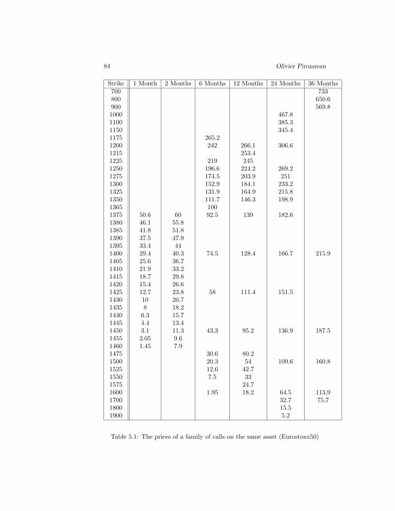
84 Olivier Pironneau
Strike 1 Month 2 Months 6 Months 12 Months 24 Months 36 Months700 733800 650.6900 569.81000 467.81100 385.31150 345.41175 265.21200 242 266.1 306.61215 253.41225 219 2451250 196.6 224.2 269.21275 174.5 203.9 2511300 152.9 184.1 233.21325 131.9 164.9 215.81350 111.7 146.3 198.91365 1001375 50.6 60 92.5 139 182.61380 46.1 55.81385 41.8 51.81390 37.5 47.91395 33.4 441400 29.4 40.3 74.5 128.4 166.7 215.91405 25.6 36.71410 21.9 33.21415 18.7 29.81420 15.4 26.61425 12.7 23.8 58 111.4 151.51430 10 20.71435 8 18.21440 6.3 15.71445 4.4 13.41450 3.1 11.3 43.3 95.2 136.9 187.51455 2.05 9.61460 1.45 7.91475 30.6 80.21500 20.3 54 109.6 160.81525 12.6 42.71550 7.5 331575 24.71600 1.95 18.2 64.5 113,91700 32.7 75,71800 15.51900 5.2
Table 5.1: The prices of a family of calls on the same asset (Eurostoxx50)
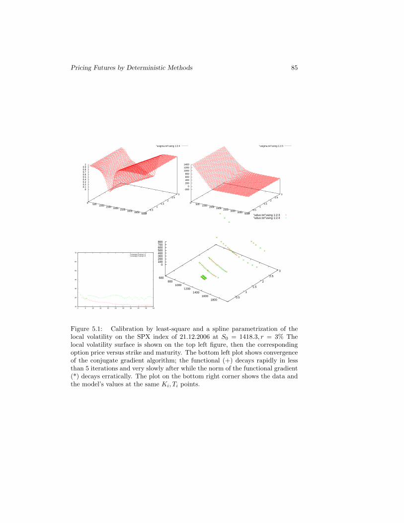
Pricing Futures by Deterministic Methods 85
0 500 1000 1500 2000 2500 3000 3500 4000 0 0.5
1 1.5
2 2.5
3
0 0.1 0.2 0.3 0.4 0.5 0.6 0.7 0.8 0.9
1
"usigma.txt"using 1:2:4
0 500 1000 1500 2000 2500 3000 3500 4000 0 0.5
1 1.5
2 2.5
3
-200 0
200 400 600 800
1000 1200 1400
"usigma.txt"using 1:2:3
10
20
30
40
50
60
70
0 5 10 15 20 25 30 35 40 45 50
"converge.h"using 1:2"converge.h"using 1:3
600 800
1000 1200
1400 1600
1800 0.5
1
1.5
2
2.5
3
0 100 200 300 400 500 600 700 800
"uduo.txt"using 1:2:3"uduo.txt"using 1:2:4
Figure 5.1: Calibration by least-square and a spline parametrization of thelocal volatility on the SPX index of 21.12.2006 at S0 = 1418.3, r = 3% Thelocal volatility surface is shown on the top left figure, then the correspondingoption price versus strike and maturity. The bottom left plot shows convergenceof the conjugate gradient algorithm; the functional (+) decays rapidly in lessthan 5 iterations and very slowly after while the norm of the functional gradient(*) decays erratically. The plot on the bottom right corner shows the data andthe model’s values at the same Ki, Ti points.
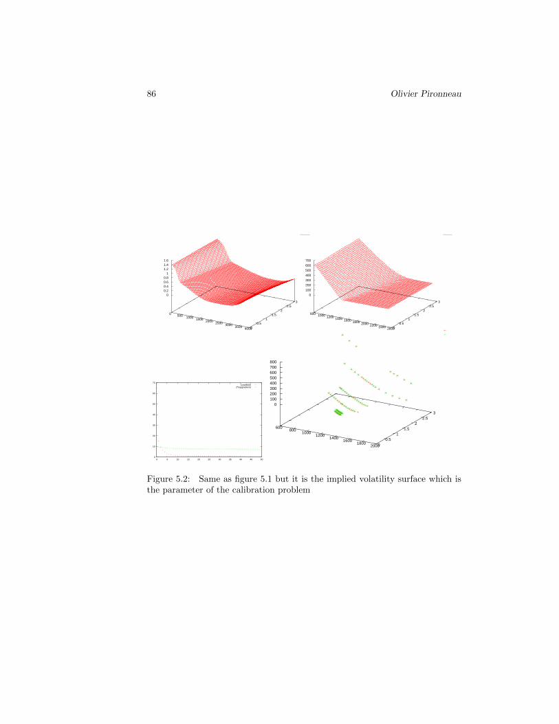
86 Olivier Pironneau
0 500 1000 1500 2000 2500 3000 3500 4000 0 0.5
1 1.5
2 2.5
3
0 0.2 0.4 0.6 0.8
1 1.2 1.4 1.6
800 1000 1200 1400 1600 1800 2000 2200 2400 2600 0 0.5
1 1.5
2 2.5
3
0
100
200
300
400
500
600
700
0
10
20
30
40
50
60
70
0 5 10 15 20 25 30 35 40 45 50
Cost/80002*log(gradient)
600 800
1000 1200
1400 1600
1800 2000 0
0.5 1
1.5 2
2.5 3
0 100 200 300 400 500 600 700 800
Figure 5.2: Same as figure 5.1 but it is the implied volatility surface which isthe parameter of the calibration problem
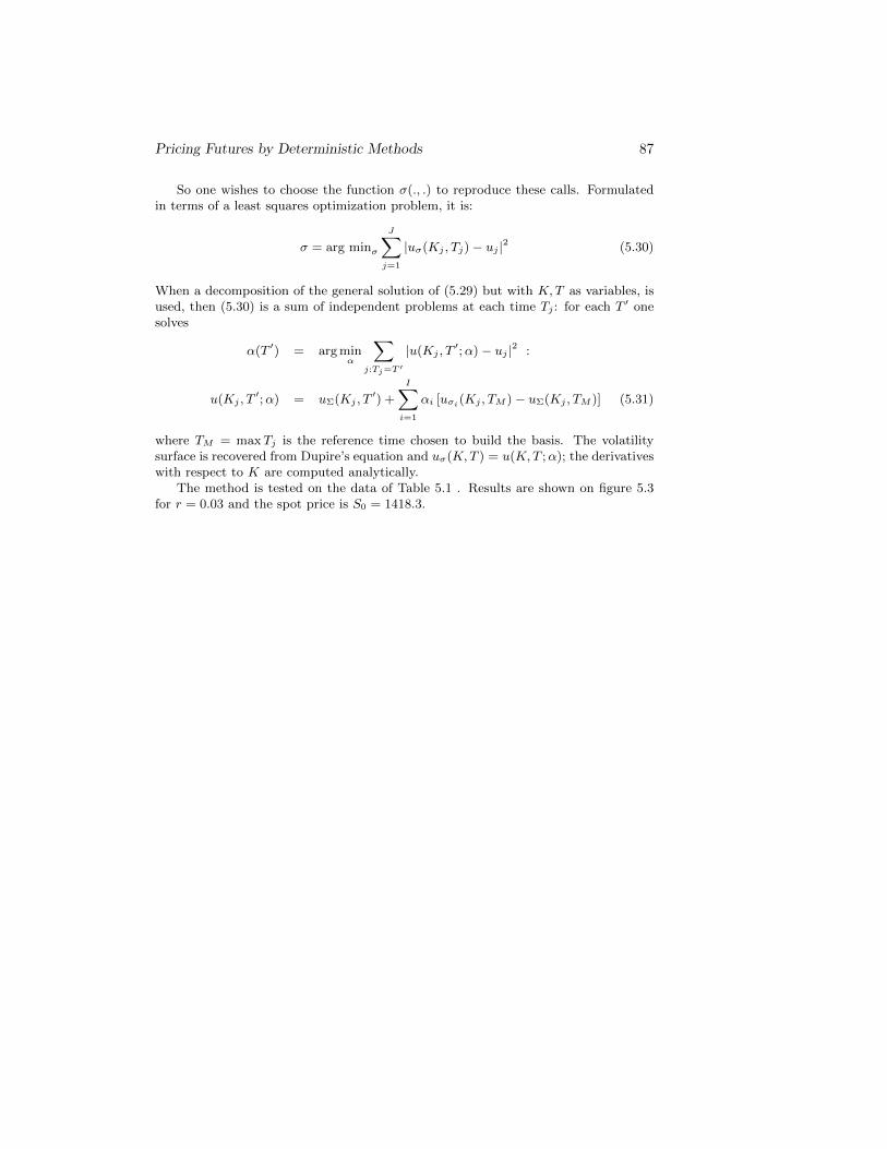
Pricing Futures by Deterministic Methods 87
So one wishes to choose the function σ(., .) to reproduce these calls. Formulatedin terms of a least squares optimization problem, it is:
σ = arg minσ
J∑j=1
|uσ(Kj , Tj)− uj |2 (5.30)
When a decomposition of the general solution of (5.29) but with K,T as variables, isused, then (5.30) is a sum of independent problems at each time Tj : for each T ′ onesolves
α(T ′) = arg minα
∑j:Tj=T ′
|u(Kj , T′;α)− uj |2 :
u(Kj , T′;α) = uΣ(Kj , T
′) +
I∑i=1
αi [uσi(Kj , TM )− uΣ(Kj , TM )] (5.31)
where TM = maxTj is the reference time chosen to build the basis. The volatilitysurface is recovered from Dupire’s equation and uσ(K,T ) = u(K,T ;α); the derivativeswith respect to K are computed analytically.
The method is tested on the data of Table 5.1 . Results are shown on figure 5.3for r = 0.03 and the spot price is S0 = 1418.3.
88 Olivier Pironneau
Figure 5.3: Same as in Figure 5.1 but calibrated on a reduced basis. Top:Observed prices and model predictions for the calls at the observation points;errors are hardly visible (between 1 and 9$) is 4$ at each point on the average.Bottom: the local volatility recovered from the Dupire equation at the observedpoints. For both graphs the horizontal axis is time, the vertical axis is the priceof calls and the other axis is the strike.

Chapter 6
Open-source Tools
6.1 Premia
Premia (see http://www-rocq.inria.fr/mathfi/Premia/) is a platform and a con-sortium for pricing financial derivatives. Recently it has been integrated with NSP, aMatlab-like software by a member of INRIA. The C++ functions are written and main-tained by the members of the consortium (including several banks and edge funds)under the leadership of INRIA and ENPC lab in France.
Figure 6.1: Under NSP, Premia is mouse/menu driven, making the learningcurve very short (see fig. 6.1). This implementation runs under Windows,Linux and Mac OS X.
Premia solves the following
89
90 Olivier Pironneau
Equity derivatives
• Black-Scholes model (up to dimension 10), stochastic volatility models(Hull-White, Heston, Fouque-Papanicolaou-Sircar), models with jumps(Merton, Kou, Tempered stable processes, Variance gamma, Normal in-verse Gaussian), Bates model.
• For high dimensional American options, Premia provides the most recentMonte-Carlo algorithms: Andersen-Broadie, Longstaff-Schwartz, Barraquand-Martineau, Tsitsklis-Van Roy, Broadie-Glassermann, quantization meth-ods Malliavin calculus based methods.
• Dynamic Hedging for Black-Scholes and jump models is available.
• Calibration algorithms for some models with jumps, local volatility andstochastic volatility are implemented.
Interest rate derivatives
• HJM and LIBOR Market Models (LMM): affine models, Hull-White, CIR++,Black-Karasinsky, Squared-Gaussian, Li-Ritchken-Sankara-subramanian,Bhar-Chiarella, Jump diffusion LMM, Markov functional LMM, LMM withstochastic volatility.
• Premia provides a calibration toolbox for LIBOR Market models using adatabase of swaptions and caps implied volatilities.
Credit derivatives: CDS, CDO
• Reduced form models and copula models are considered.
• Premia provides a toolbox for pricing CDOs using the most recent algo-rithms (Hull-White, Laurent-Gregory, El Karoui-Jiao, Yang-Zhang)
Hybrid products
• pde solver for pricing derivatives on hybrid products like options on infla-tion and interest or change rates is implemented.
Energy derivatives: swing options
• Mean reverting and jump models are considered.
• Premia provides a toolbox for pricing swing options using finite differences,Monte-Carlo Malliavin-based approach and quantization algorithms.
The main methods of solution are written on figure 6.2.
6.2 QuantLib
QuanLib (see quantlib.org) is an open-source C++ library of functions and a classhierarchy to build complex finance solvers. It contains many functions to generaterandom numbers and variables of all types. There are also several functions for interestrate models, Black-Scholes pricers, Orstein-Uhlenbeck, Heston etc. It can be used asa base to build more complex solvers.
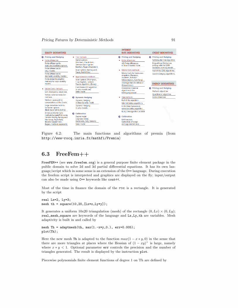
Pricing Futures by Deterministic Methods 91
Figure 6.2: The main functions and algorithms of premia (fromhttp://www-rocq.inria.fr/mathfi/Premia)
6.3 FreeFem++
FreeFEM++ (see www.freefem.org) is a general purpose finite element package in thepublic domain to solve 2d and 3d partial differential equations. It has its own lan-guage/script which in some sense is an extension of the C++ language. During executionthe freefem script is interpreted and graphics are displayed on the fly; input/outputcan also be made using C++ keywords like cout<<.
Most of the time in finance the domain of the pde is a rectangle. It is generatedby the script
real Lx=2, Ly=3;
mesh th = square(10,20,[Lx*x,Ly*y]);
It generates a uniform 10x20 triangulation (mesh) of the rectangle (0, Lx) × (0, Ly);real,mesh,square are keywords of the language and Lx,Ly,th are variables. Meshadaptivity is built in and called by
mesh Th = adaptmesh(th, max(1.-x*y,0.), err=0.005);
plot(Th);
Here the new mesh Th is adapted to the function max(1 − x ∗ y, 0) in the sense thatthere are more triangles at places where the Hessian of (1 − xy)+ is large, namelywhere x ∗ y < 1. Optional parameter err controls the precision and the number oftriangles generated. The result is displayed by the instruction plot.
Piecewise polynomials finite element functions of degree 1 on Th are defined by
92 Olivier Pironneau
fespace Vh(Th,P1);
Vh u,v,uold=max(1.-x*y,0.);
Here u, v are declared only while uold is declared and assigned to the piecewise linearcontinuous interpolation of (1 − xy)+ on the vertices of Th; u will be used for um+1
and uold for um, the values of the basket option at times to maturity (m+1)δt andmδt.
The Black-Scholes pde (4.13) for a basket with two assets x, y discretized in timeby a semi-implicit Euler scheme and P 1 continuous elements in space is entered invariational form as
problem basket(u,v) = int2d(Th) ( u*v/dt
+ sigmax^2*x^2*dx(u)*dx(v)/2 + sigmay^2*y^2*dy(u)*dy(v)/2
+ sigmax*sigmay*x*y*rho*dx(u)*dy(v) )
- int2d(Th)(uold*v/dt + sigmax*x*dx(uold)*v+sigmay*y*dy(uold)*v);
Here problem,int2d,x,y,dx,dy are keywords and sigmax,sigmay,rho,dt are param-eters or functions which must be defined earlier.
Finally the time loop to compute u at maturity T is
for(real t=0;t<T;t+=dt)
basket; uold = u;
6.3.1 Two-dimensional Black-Scholes equation
The complete script and results are given below for a basket put option with multi-plicative pay-off
real Lx=2, Ly=3;
mesh th = square(10,20,[Lx*x,Ly*y]);
mesh Th = adaptmesh(th, max(1.-x*y,0.),err=0.005);
fespace Vh(Th,P1);
Vh v,u, uold=max(1.-x*y,0.);
plot(Th,wait=1,ps="Th.ps");
real dt=0.01, sigmax=0.5, sigmay=0.3, rho=-0.5, T=1;
problem basket(u,v) = int2d(Th) ( u*v/dt
+ sigmax^2*x^2*dx(u)*dx(v)/2 + sigmay^2*y^2*dy(u)*dy(v)/2
+ sigmax*sigmay*x*y*rho*dx(u)*dy(v) )
- int2d(Th)(uold*v/dt - sigmax*x*dx(uold)*v - sigmay*y*dy(uold)*v);
for(real t=0;t<T;t+=dt)
basket; uold = u;
plot(u);
Remark 13 A large number of finite elements are built in freefem++ including dis-continuous Galerkin methods.
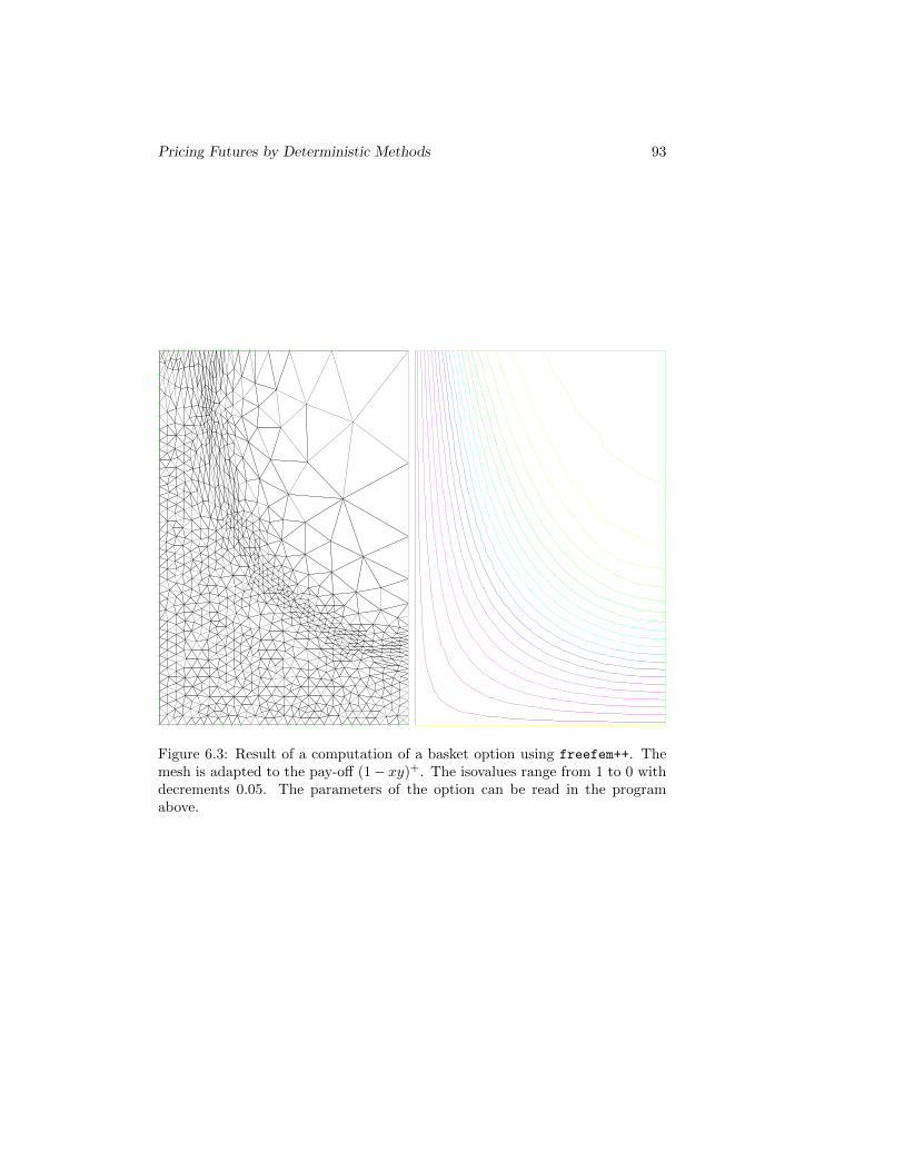
Pricing Futures by Deterministic Methods 93
Figure 6.3: Result of a computation of a basket option using freefem++. Themesh is adapted to the pay-off (1− xy)+. The isovalues range from 1 to 0 withdecrements 0.05. The parameters of the option can be read in the programabove.
94 Olivier Pironneau
freefem++ was not designed to solve one dimensional problems, yet it can be doneby making them 2d and invariant with respect to the added coordinate. The followingis a script to compute a plain vanilla put and compare it with the Black-Scholesformula.
real Lx=4, Ly=0.1;
mesh Th = square(150,2,[Lx*x,Ly*y]);
fespace Vh(Th,P1);
Vh v,u, uold=max(1.-x,0.);
plot(Th,wait=1);
real dt=0.01, sigmax=0.5, T=1;
problem basket(u,v) = int2d(Th) ( u*v/dt
+ sigmax^2*x^2*dx(u)*dx(v)/2 )
- int2d(Th)(uold*v/dt - sigmax^2*x*dx(uold)*v) + on(2,u=0);
for(real t=0;t<T;t+=dt)
basket; uold = u;
plot(u);
ofstream fich("u.txt");
real x0=0,x1=Lx, y0=0;
for(real t=0;t<=1;t+=0.05)
real c=x0+t*x1;
real BS=0.5*c*(1+ erf(log(c)/(sigmax*sqrt(2*T)) + sigmax * sqrt(T/8.)))
-0.5*(1+erf(log(c)/(sigmax*sqrt(2*T)) -sigmax * sqrt(T/8.)))+1-c;
real error = u(c,y0)-BS;
fich<<c<<" "<< u(c,y0)<<" "<<BS<<" "<<error<<endl;
// display "u.txt" by gnuplot: plot "u.txt"using 1:2 w l
// display the error by plot "u.txt"using 1:4 w l
Using freefem++ to compute a one dimensional option requires about 4 times thecpu of an hand written C++ program.
6.3.2 Three-dimensional Basket
The same problem with 3 assets in the basket can be solved with freefem++. Thescript and the results are given below for a put on a basket with linear pay-off (1 −x/2−y/3−z/4)+. A fully implicit Euler scheme is used combined with a characteristic-Galerkin method (keyword convect). The mesh is built by extrusion of the mesh of asquare. Results are shown on figure 6.6
6.4 CUDA and Other Tools
6.4.1 Matlab, Scilab, Octave,Mathematica, SAGE...
Several programming environments provide tools for option pricing, like matlab andmathematica. The open-source project Sage has tools to compute options (see
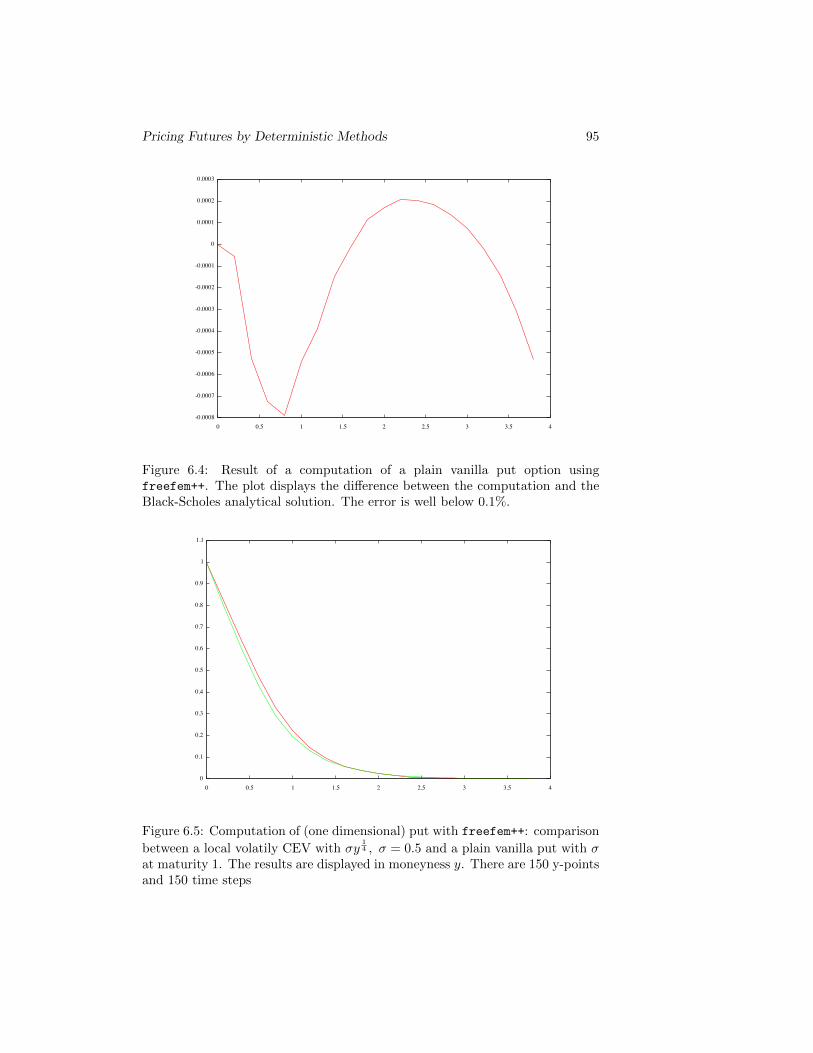
Pricing Futures by Deterministic Methods 95
Figure 6.4: Result of a computation of a plain vanilla put option usingfreefem++. The plot displays the difference between the computation and theBlack-Scholes analytical solution. The error is well below 0.1%.
Figure 6.5: Computation of (one dimensional) put with freefem++: comparison
between a local volatily CEV with σy14 , σ = 0.5 and a plain vanilla put with σ
at maturity 1. The results are displayed in moneyness y. There are 150 y-pointsand 150 time steps
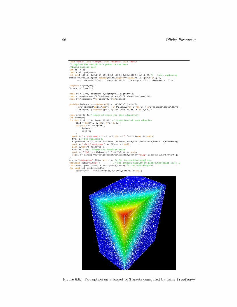
96 Olivier Pironneau
load "msh3" load "tetgen" load "mshmet" load "medit"// improve the search of a point in the mesh//build initial meshint nn = 6;real Lx=2,Ly=3,Lz=4;int[int] l1111=[1,2,2,1],l01=[0,1],l02=[0,2],l1122=[1,1,2,2];// label numbering mesh3 Th3=buildlayers(square(nn,nn,region=0,label=l1111,[x*Lx,y*Ly]), nn, zbound=[0,Lz], labelmid=l1122, labelup = l02, labeldown = l01);
fespace Vh(Th3,P1);Vh u,v,uold,usol,h;
real dt = 0.02, sigmax=0.3,sigmay=0.2,sigmaz=0.1;real sigmax2=sigmax^2/2,sigmay2=sigmay^2/2,sigmaz2=sigmaz^2/2;real U=x*sigmax2, V=y*sigmay2, W=z*sigmaz2;
problem Poisson(u,v,solver=CG) = int3d(Th3)( u*v/dt + x^2*sigmax2*dx(u)*dx(v) + y^2*sigmay2*dy(u)*dy(v) + z^2*sigmaz2*dz(u)*dz(v) )
- int3d(Th3)( convect([U,V,W],-dt,uold)*v/dt) + on(2,u=0);
real errm=1e-3;// level of error for mesh adaptivityint iimax=2;for(int ii=0; ii<=iimax; ii++) // iterations of mesh adaption uold = max(0., 1.-x/2.-y/3.-z/4.);
for(int k=0;k<50;k++)Poisson;uold=u;
cout <<" u min, max = " << u[].min << " "<< u[].max << endl; h=0. ;// for resizing h h[]=mshmet(Th3,u,normalization=1,aniso=0,nbregul=1,hmin=1e-3,hmax=0.3,err=errm); cout <<" nb of vertices " << Th3.nv << endl; plot(u,wait=0,nbiso=15); errm *= 0.5;// change the level of error cout << " Th3" << Th3.nv < " " << Th3.nt << endl; if(ii != iimax) Th3=tetgreconstruction(Th3,switch="raAQ",sizeofvolume=h*h*h/6.);medit("U-adap-iso",Th3,u,wait=1); // for interactive graphicsofstream fich("u.txt"); // for gnuplot display by plot"u.txt"using 1:2 w lreal x0=0, y0=0, z0=0, x1=Lx, y1=Ly,z1=Lz; // the cube diagonalfor(real t=0;t<=1;t+=0.05)
fich<<t<<" "<< u(x0+t*x1,y0+t*y1,z0+t*z1)<<endl;
Figure 6.6: Put option on a basket of 3 assets computed by using freefem++
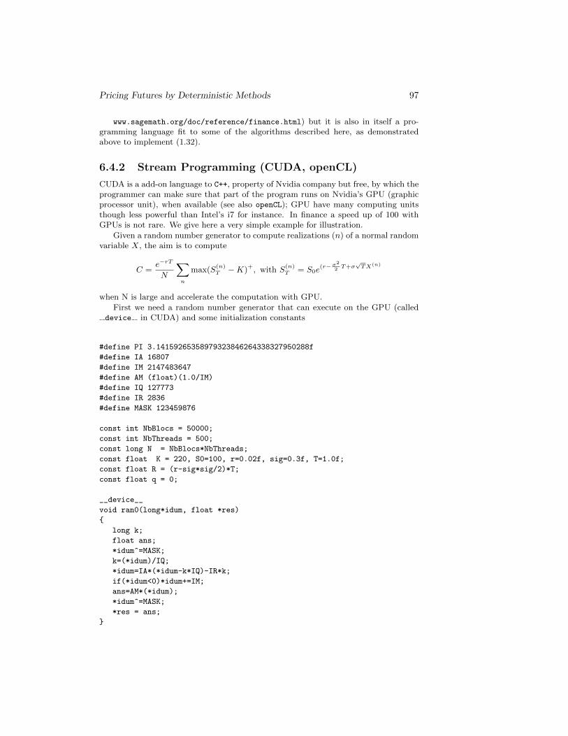
Pricing Futures by Deterministic Methods 97
www.sagemath.org/doc/reference/finance.html) but it is also in itself a pro-gramming language fit to some of the algorithms described here, as demonstratedabove to implement (1.32).
6.4.2 Stream Programming (CUDA, openCL)
CUDA is a add-on language to C++, property of Nvidia company but free, by which theprogrammer can make sure that part of the program runs on Nvidia’s GPU (graphicprocessor unit), when available (see also openCL); GPU have many computing unitsthough less powerful than Intel’s i7 for instance. In finance a speed up of 100 withGPUs is not rare. We give here a very simple example for illustration.
Given a random number generator to compute realizations (n) of a normal randomvariable X, the aim is to compute
C =e−rT
N
∑n
max(S(n)T −K)+, with S
(n)T = S0e
(r−σ2
2T+σ
√TX(n)
when N is large and accelerate the computation with GPU.
First we need a random number generator that can execute on the GPU (calleddevice in CUDA) and some initialization constants
#define PI 3.14159265358979323846264338327950288f
#define IA 16807
#define IM 2147483647
#define AM (float)(1.0/IM)
#define IQ 127773
#define IR 2836
#define MASK 123459876
const int NbBlocs = 50000;
const int NbThreads = 500;
const long N = NbBlocs*NbThreads;
const float K = 220, S0=100, r=0.02f, sig=0.3f, T=1.0f;
const float R = (r-sig*sig/2)*T;
const float q = 0;
__device__
void ran0(long*idum, float *res)
long k;
float ans;
*idum^=MASK;
k=(*idum)/IQ;
*idum=IA*(*idum-k*IQ)-IR*k;
if(*idum<0)*idum+=IM;
ans=AM*(*idum);
*idum^=MASK;
*res = ans;
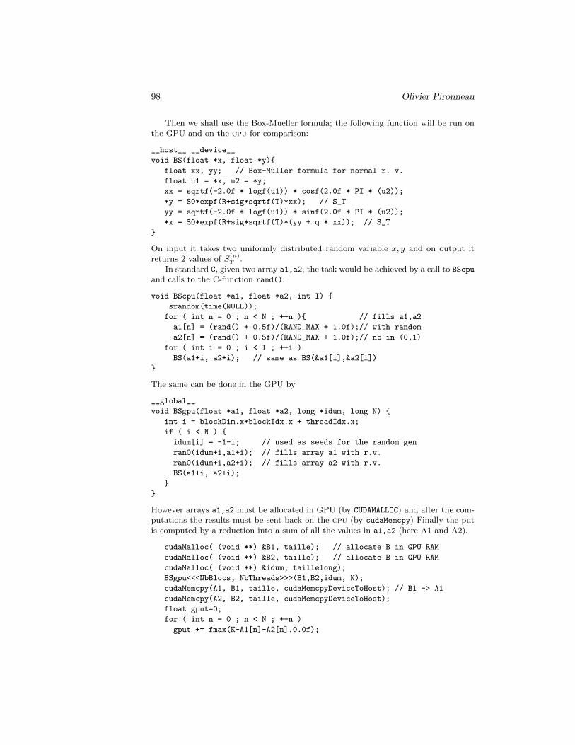
98 Olivier Pironneau
Then we shall use the Box-Mueller formula; the following function will be run onthe GPU and on the cpu for comparison:
__host__ __device__
void BS(float *x, float *y)
float xx, yy; // Box-Muller formula for normal r. v.
float u1 = *x, u2 = *y;
xx = sqrtf(-2.0f * logf(u1)) * cosf(2.0f * PI * (u2));
*y = S0*expf(R+sig*sqrtf(T)*xx); // S_T
yy = sqrtf(-2.0f * logf(u1)) * sinf(2.0f * PI * (u2));
*x = S0*expf(R+sig*sqrtf(T)*(yy + q * xx)); // S_T
On input it takes two uniformly distributed random variable x, y and on output itreturns 2 values of S
(n)T .
In standard C, given two array a1,a2, the task would be achieved by a call to BScpu
and calls to the C-function rand():
void BScpu(float *a1, float *a2, int I)
srandom(time(NULL));
for ( int n = 0 ; n < N ; ++n ) // fills a1,a2
a1[n] = (rand() + 0.5f)/(RAND_MAX + 1.0f);// with random
a2[n] = (rand() + 0.5f)/(RAND_MAX + 1.0f);// nb in (0,1)
for ( int i = 0 ; i < I ; ++i )
BS(a1+i, a2+i); // same as BS(&a1[i],&a2[i])
The same can be done in the GPU by
__global__
void BSgpu(float *a1, float *a2, long *idum, long N)
int i = blockDim.x*blockIdx.x + threadIdx.x;
if ( i < N )
idum[i] = -1-i; // used as seeds for the random gen
ran0(idum+i,a1+i); // fills array a1 with r.v.
ran0(idum+i,a2+i); // fills array a2 with r.v.
BS(a1+i, a2+i);
However arrays a1,a2 must be allocated in GPU (by CUDAMALLOC) and after the com-putations the results must be sent back on the cpu (by cudaMemcpy) Finally the putis computed by a reduction into a sum of all the values in a1,a2 (here A1 and A2).
cudaMalloc( (void **) &B1, taille); // allocate B in GPU RAM
cudaMalloc( (void **) &B2, taille); // allocate B in GPU RAM
cudaMalloc( (void **) &idum, taillelong);
BSgpu<<<NbBlocs, NbThreads>>>(B1,B2,idum, N);
cudaMemcpy(A1, B1, taille, cudaMemcpyDeviceToHost); // B1 -> A1
cudaMemcpy(A2, B2, taille, cudaMemcpyDeviceToHost);
float gput=0;
for ( int n = 0 ; n < N ; ++n )
gput += fmax(K-A1[n]-A2[n],0.0f);

Pricing Futures by Deterministic Methods 99
Notice the peculiar syntax to call BSgpu(). The modifiers NbBlocs, NbThreads influ-ence the computing time in the GPU because they specify how the data are arrangedin blocs and the number of threads.

100 Olivier Pironneau
Conclusion
We hope to have convinced the reader that computing financial assets by deterministicmethods, in particular by solving pde, pdi, pide can be a good choice: precision forsure, speed maybe, and a sound treatment of singularities if any. And also more flexiblefor calibration and greeks. Yet many pricing problems such as complex contracts withdiscrete dates, are hard to formulate in terms of partial differential equations.
In Computational Fluid Dynamics, it took many years to convince airplane manu-factures to use variational methods instead of finite difference methods. The difficultywas in training engineers but the advantage was that an entire airplane could be dis-cretized by an arbitrary mesh instead of the painful task of matching uniform blocksas needed by finite difference methods.
Here in finance the domain of integration is simple, usually (0, L1) × .. × (0, Ld)and so the plus of variational methods is not so much in the mesh rather than in theoptimal mesh: a mesh where the points are where they are needed for the precisionand for resolving singularities if any.
Parallelism continues to grow on the hardware side and certainly it is in favorof Monte-Carlo methods; variational methods can be parallelized as well, but it iscomplex and much harder to implement.
In the end, the method which performs the best ratio of speed over precision willwin and it is only after several years of numerical experimentation that it will beknown; meanwhile innovation and optimization of existing methods will go on: it isjust the beginning!
101

102 Olivier Pironneau
Bibliography
[1] Yves Achdou and Olivier Pironneau, Computational methods for option pric-ing. Vol. 30, Frontiers in Applied Mathematics, SIAM, 2005.
[2] Yves Achdou and Olivier Pironneau, Handbook of Numerical Analysis, volXV, Mathematical Modeling and Numerical Methods in Finance. P.G. Ciarlet A.Bensoussan, Q. Zhang ed. North Holland (2009)
[3] Yves Achdou and Nicoletta Tchou, Variational analysis for the Black andScholes equation with stochastic volatility, M2AN Math. Model. Numer. Anal.,vol 36, no 3, pp 373–395, (2002).
[4] C. Albanese and M. Trovato. A Stochastic Volatility Model for BermudaSwapsions and Callable SMC Swaps. (2005)
[5] H. Albrecher, P. Mayer, W. Schoutens, and J. Tistaert. The little HestonTrap. Wilmott journal, 2007
[6] Amel Bentata and Rama Cont, Forward equations for option prices in semi-martingale models, forthcoming in Finance & Stochastics, 2009.
[7] Leif Andersen and Jesper Andreasen, Jump diffusion models: Volatilitysmile fitting and numerical methods for pricing, Review of Derivatives Research,4 (2000), pp. 231–262.
[8] Andrew Ang and Francis Longstaff, Systemic SovereignCredit Risk: Lessons from the U.S. and Europe NBERWorking Paper No. 16982 April 2011. Also available athttp://www.scribd.com/doc/55649615/7/MODELING-CDS-SPREADS-WITH-SYSTEMIC-RISK
[9] E. Ayache and P. A. Forsyth and K. R. Vetzal. The Valuation of Convertible BondsWith Credit Risk. April 22, 2003
[10] Louis Bachelier Theorie de la speculation , Annales scientifiques de l’Ecole normalesuperieure, vol. 3, no 17, 1900.
[11] G. Barles, Convergence of numerical schemes for degenerate parabolic equations arisingin finance. In L. C. G. Rogers and D. Talay, editors, Numerical Methods in Finance, pages1-21. Cambridge University Press, Cambridge, 1997.
[12] F. Bervoets. Model Risk for Exotic Equity Options, Master Thesis, 2006, Delft Univer-sity of Technology, Netherlands.
[13] Damiano Brigo & Fabio Mercurio, Lognormal mixture dynamics and calibration tomarket volatility smiles, International Journal of Theoretical and Applied Finance, Vol.5, No. 4, 427–446, 2002.
[14] D. Brigo and F. Mercurio. Interest Rate Models - Theory and Practice: With Smile,Inflation and Credit. Springer Finance, second edition, 2007.
103
104 Olivier Pironneau
[15] Peter Carr and Dilip B. Madan Option valuation using the fast Fourier transform,J. Comput. Finance, 61–73, 2,1998.
[16] Bin Chen Lech A. Grzelak Cornelis W. Oosterlee. Calibration of A Stochastic In-terest Rate SAB. Quantitative Methods in Financial and Insurance Mathematics LorentzCenter, Leiden, the Netherlands Apirl 19, 2011
[17] sc Clement, Lamberton, Pottier. Longstaff
[18] Rama Cont, Nicolas Lantos and Olivier Pironneau A reduced basis for optionpricing. SIAM on mathematical Finance, vol. 2, pp 287-316, 2011.
[19] Rama Cont and Ekaterina Voltchkova, Integro-differential equations for optionprices in exponential Levy models, CMAPX report R.I.547, Ecole Polytechnique (2004)
[20] Rama Cont and Peter Tankov Financial modelling with jump processes, Chapmanand Hall, 2003.
[21] Rama Cont and Ekaterina Voltchkova, A finite difference scheme for option pricingin jump diffusion and exponential Levy models, SIAM J. Numer. Anal., Vol 43, 4, 1596–1626, 2005.
[22] John Cox Notes on option pricing I: Constant Elasticity of Variance diffusions, Work-ing Paper Stanford University, 1975.
[23] Cox, J., J. Ingersoll and S. Ross A theory of the term structure of interest rates.Econometrica, 53: 389-408. (1985)
[24] S. Crepey: Calibration of the local volatility in a generalized Black-Scholes model usingTikhonov regularization. SIAM J. Math. Anal. 34(5), p1183-1206, 2003.
[25] Alain Dervieux About the basic Methods. in Handbook of computational Fluid Dy-namics. R. Peyret ed. Academci Press, p1-23, 1996.
[26] Bruno Dupire, Pricing and hedging with smiles, in Mathematics of Derivative Securities,M. Dempster and S. Pliska, eds., Cambridge University Press, 1997, pp. 103–111.
[27] Nicole El Karoui. Couverture des risques dans les marches financiers. Cours de l’EcolePolytechnique. (2003)
[28] W. Farkas and N. Reich and C. Schwab Anisotropic Stable Levy Copula Processes ?Analytical and Numerical Aspects. ETH Research Report No. 2006-08 Zurich May 2006.
[29] Paul-Louis George and Houman Borouchaki. Delaunay triangulation and me- shing.Editions Hermes, Paris, 1998. Application to finite elements, Translated from the 1997French original P. J. Frey and Scott A. Canann.
[30] Gerstner, T and Griebel, M. Numerical Integration using Sparse Grids. Numer. Al-gorithms, 18:209-232, 1998.
[31] Mike Giles Multilevel Monte Carlo path simulation. Operations Research 56 (3):981?986. 2008.
[32] Paul Glasserman, Monte Carlo Methods in Financial Engineering, Series: StochasticModelling and Applied Probability , Vol. 53, 2003.
[33] F. Hecht, O. Pironneau, A. Le Hyaric and K. Otsuka The freefem++ documentation(2008). UPMC publications. See also www.freefem.org.
[34] S.Heston. A closed form solution for options with stochastic volatility with applicationto bond and currency options. Review with Financial Studies, pages 327–343, 1993.
[35] J. Hull Options, Futures and Other Derivatives (5th ed.). Prentice Hall, Upper SaddleRiver, NJ. (2003).
[36] J.C. Hull and A. White. The pricing of options on assets with stochastic volatilities.J. Finance, 42:281–300, 1987.
[37] S. Ikonen and J. Toivanen Efficient Numerical Methods for Pricing American Op-tions under Stochastic Volatility, Numerical Methods for Partial Differential Equations,Volume 24, Issue 1, pp. 104-126, 2008.
Pricing Futures by Deterministic Methods 105
[38] S. Ikonen and J. Toivanen Operator Splitting Methods for Pricing American Optionsunder Stochastic Volatility, Numerische Mathematik, Volume 113, Number 2, pp. 299-324, 2009.
[39] M. Hintermueller, V. A. Kovtunenko and K. Kunisch Semi-smooth Newton meth-ods for a class of unilaterally constrained variational problems Adv. in Math. Sci. andAppl., 14(2004), 513-535
[40] Kazufumi Ito, and Karl Kunisch Parabolic variational inequalities: The Lagrangemultiplier approach. Journal de Mathematiques Pures et Appliquees. Vol 85, Issue 3,March 2006, pp 415-449.
[41] Kenneth R. Jacksona, Sebastian Jaimungalb, and Vladimir Surkovc Fourier SpaceTime-stepping for Option Pricing with Levy Models.Journal of Computational Finance,Vol. 12, No. 2, pp. 1-29, 2008
[42] Lishang Jiand, Min Dai Convergence of binomial Tree Method for American Option.Partial Differential Equations and their Applications, p106-108, 1999.
[43] Mark S. Joshi More Mathematical Finance Pilot Whale Press Melbourne 2011.
[44] D. Lamberton and B. Lapeyre. Introduction au calcul stochastique applique a la fi-nance. Ellipses, 1997
[45] Alan Lewis A simple option formula for general jump-diffusion and other exponentialLevy processes. available from http://www.optioncity.net, 2001
[46] Jean Bertoin Levy Processes, Cambridge University Press, Cambridge, 1996.
[47] P-L. Lions and J-M. Lassery Mean field games
[48] R. Lord, F. Fang, F. Bervoets, and C.W. Oosterlee. A fast and accurate FFT-basedmethod for pricing early-exercise options under Levy processes.
[49] Longstaff, Schwarz
[50] Sergei Mikhailov, Ulrich Noegel. Heston’s Stochastic Volatility Model Implementa-tion, Calibration and Some Extensions. Willmott Magazine, article 3, 2003.
[51] Ana-Maria Matache, Tobias von Petersdoff and Christoph Schwab, Fast deter-ministic pricing of Levy driven assets, J.Mathematical Modelling and Numerical Anal-ysis, Vol.38, 1, 37–72, 2004.
[52] Robert C. Merton Option pricing when underlying stock returns are discontinuous,J. Financ. Econ., Vol.3, 125–144, 1976.
[53] B. Oksendal Stochastic Differential Equations. Springer (1998).
[54] G. Pages. Methodes de Mont-Carlo. Notes de cours Master 2. Universite Pierre et MarieCurie, 2008.
[55] Olivier Pironneau Calibration of options on a reduced basis, Journal of Computationaland Applied Mathematics, Vol. 232, 1, 139–147, 2009.
[56] Bernard Lapeyre, Claude Martini and Agnes Sulem The premia consortium and software.http://www.premia.fr (2010).
[57] W.H. Press, S.A. Teukolsky, W.T. Vettering and B.P. Flannery NumericalRecipes in C, 2nd edition, Cambridge University Press, 1992.
[58] C. Prud’homme, D. Rovas, K. Veroy, Y. Maday, A.T. Patera, G. Turinici. Reliablereal-time solution of parametrized partial differential equations: Reduced-basis outputbound methods. Journal of Fluid Engineering, 124(1):70-80, 2002.
[59] W.H. Press, S.A. Teukolsky, W.T. Vettering and B.P. Flannery NumericalRecipes in C, 2nd edition, Cambridge University Press, 1992.
[60] Ekkehard W. Sachs and Matthias Schu Reduced Order Models (POD) for calibrationProblems in Finance, Proceedings of ENUMATH 2007, 361–368, 2008.
[61] R. Rannacher
106 Olivier Pironneau
[62] Richmeyer and Morton
[63] M. Schroder Computing the Constant Elasticity of Variance option pricing formula,J. of Finance, Vol. 44, 1, 211-219, 1989.
[64] S.A. Smolyak. Quadrature and interpolation formulas for tensor products of certainclasses of functions. Dokl. Akad. Nauk. USSR 4: 240-243, 1963.
[65] E. Stein and J. Stein. Stock price distributions with stochastic volatility : an analyticapproach. The review of financial studies, 4(4):727–752, 1991.
[66] P. Tankov and E. Voltchkova. Jump-diffusion models: a practitioner’s guide. (toappear (2009).
[67] D. Talay and L. Tubaro Probabilistic Models for Non-linear pde. Lecture notes inmathematics. Springer (1996).
[68] Paul Wilmott, Sam Howison, and Jeff Dewynne. The mathematics of financialderivatives. Cambridge University Press, Cambridge, 1995. A student introduction.
[69] Xiaoye S. Li, J. W. Demmel and J. R. Gilbert: The superLU library, see http://crd.
lbl.gov/~xiaoye/SuperLU).
[70] Xuan Luo. Bermudan Swaption Hedging in Black-Karasinski Model. PhD. (2007)