Embed Size (px)
Citation preview

.TECHNICAL REPORT STANDARD TITLE PAGE
1. Report No. 2. Government Accession No. 3. Recipient's Catalog No.
4. Title and S otitle . eport Dote
An Evaluation of the Suitability of ERTS June 1974Data for the Purpose of Petroleum Exploration 6. Performing Organization Code
7. Author(sl 8. Performing Organization Report No.
See Front Cover9. Performing Organization Name and Address 10. Work Unit No.
Eason Oil Company5225 Shartel Avenue 11. Contract or Grant No.
Oklahoma City, Oklahoma 73118 NAS5-2173513. Type of Report and Period Covered
12. Sponsoring Agency Name and Address Type III Final
Goddard Space Flight Center ReportGreenbelt, Maryland 20771 Jan,1973 - Jan.1974
14. Sponsoring Agency Code
15. Supplementary Notes
ERTS Experiment No. NASA #173
16. AbstractERTS-1 data give exploration geologists a new pers-
pective for looking at the earth. The data are excellent
for interpreting regional lithologic and structural relat-ionships and quickly directing attention to areas of
greatest exploration interest. Information derived from
ERTS data useful for petroleum exploration include: linear
features, general lithologic distribution, identification of
various anomalous features, some details of structures con-
trolling hydrocarbon accumulation, overall structuralrelationships, and the regional context of the explorationprovince. Many anomalies (particularly geomor-phic anomalies) correlate with known features of petroleum
exploration interest. Linears interpreted from the imagery
that were checked in the field correlate with fractures.Bands 5 and 7 and color composite imagery acquired duringperiods of maximum and minimum vegetation vigor are best
for geologic interpretation. Preliminary analysis indicatesthat use of ERTS imagery can substantially reduce the costof petroleum exploration in relatively unexplored areas.
17. Key Words (S, leeted by Author(s)) 18. Distribution Statement
Reproduced by
Geology, Petroleum Exploration, NATIONAL TECHNICALAnadarko Basin INFORMATION SERVICE
US Department of CommerceSpringfield, VA. 22151
19. Security Classil. (of this report) 20. Security Classif. (of this page) 21. No. of Pages •
Unclassified Unclassified
*For sale by the Clcaringnouse for Federal Scientific and Technical Information. Sprinlgfield. Virginia 22151.
PRICES SUBJECT TO VGE/
https://ntrs.nasa.gov/search.jsp?R=19740022580 2019-08-05T13:05:28+00:00Z

AN EVALUATION OF THE SUITABILITY OF ERTS DATA FOR THEPURPOSES OF PETROLEUM EXPLORATION
Robert J. Collins, Frederic P. McCown, Leo P. Stonis,Gerald J. Petzel, and John R. EverettEason Oil Company5225 North Shartel AvenueOklahoma City, Oklahoma 73118
June 1974
Final Report
Prepared for
GODDARD SPACE FLIGHT CENTERGreenbelt, Maryland 20771
I1!

CONTENTS
Page
I. PREFACE . . . . . . . . . . . . . . . 1
II. SUMMARY OF RESULTS . . . . . . . . . 3
III. INTRODUCTION . . . . . . . . . . . . 5Background 5Objective 6General Considerations 7Acknowledgements 9
IV. APPROACH . . . . . . . . . . . . . . 11
V. ANADARKO BASIN TEST SITE . . . . . . 18
General Description 18
Geology 20
Possible Role of ERTS 28
VI. EVALUATION OF ERTS IMAGERY . . . . . 32
Comparison of Scale and Format 33
Resolution of Imagery 36
Comparison of Bands 38
Standing Water 40
Stream Valleys 41Linear Features 43
Lithologic Boundaries 47
Tonal Anomalies 53
Other Factors 53
False Color Composite Imagery 54
Summary 55
Comparison of Seasonal Coverage 56
ii
PageVII. RESULTS . . . . . . . . . . . . . . . 65
Linear Features 65Lithologic Mapping 75Structural Interpretation of the
Geologic Map 83Recognition of Anomalies 90Interpretation of Areas of Special
Interest 97Elk City Area 97Woodward Area 99Buffalo Wallow Field 101Mobeetie Field 101
Cement-Chickasha Area 103Enhancement Procedures 106
VIII. ROLE OF ERTS DATA IN EXPLORATIONSTRATEGY . . . . . . . . . . . . 116
IX. PROGRAM COSTS AND BENEFITS . . . . . 120
X. APPENDICES . . . . . . . . . . . . . 125A. Imagery Supplied by NASA 126B. ERTS Data Problems 129C. ERTS Descriptor Forms 131D. Acronyms 141
XI. BIBLIOGRAPHY . . . . . . . . . . . . 142
iii
Illustrations
No. Page
1 NASA aircraft flight lines 14
2 Location map 19
3 Generalized stratigraphic column 22
4 Geologic map of Anadarko Basin 24
5 Cross section of Anadarko Basin 29
6 Location map of significant fields 30
7 Seasonal differences in lithogic interpretation 46
8 ERTS linears, bands 7, 5, 4 58
9 Rose diagram of ERTS linears 66
10 Pennsylvanian isochore maps 69
11 a)Known faults and linears 72b)Comparison of ERTS linears with known linears 73
12 Lithology: Wellington-Garber-Hennessey Contact 76
13 Lithology: Permian between Cimarron and North 77Canadian River
14 Lithology: Comparison of ERTS to large scale 79mapping
15 Lithology: Western end of basin 81
16 ERTS geologic map 85
17 Miscellaneous anomalies 91
18 "Hazy" anomalies 93
19 Closed anomalies 95
20 Interpretation: Elk City Area 98
21 Interpretation: Woodward Area 100
22 Interpretation: Buffalo Wallow and Mobeetie 102
23 Interpretation: Cement-Chickasha area fields 104
(Cont.)IV

Illustrations (Cont.)
No. Page
24 Enhancement: optical - bands 6, 7 110
25 Enhancement: optical - bands 5, 6, 7 111
26 Enhancement: optical - bands 4, 6, 7 112
27 Enhancement: digital - band 5 114
28 Enhancement: digital - band 7 114
Tables
No. Page
1 ERTS mosaics 12
2 Cost comparison of ERTS exploration 123
program with conventional program
1'
I PREFACE
The objective of this experiment is an evaluation of
the applicability of Earth Resources Technology Satellite-1
(ERTS-1) data for the purposes of petroleum exploration and
a preliminary assessment of the costs of using the data
relative to the costs of customary exploration approaches.
In particular, we wanted to determine the ability of ERTS
data to delineate major structural and lithologic features
and to test ERTS as a reconnaissance exploration tool in a
geologically well known area (the Anadarko Basin) in order
to assess its usefulness in an unknown area.
The experiment involves: interpreting black and white
and color composite ERTS imagery in the form of positive and
negative transparencies, and positive paper prints at scales
ranging from 1:1,000,000 to 1:250,000; testing and evaluat-
ing a variety of enhancement procedures - optical, electronic,
and digital; comparing the results obtained against published
maps and reports, geophysical data, and field work; and
evaluating the results in order to determine what useful
information can be obtained from the data and what bands,
formats, scales and techniques and procedures are best for
extracting the information. The work also includes a
careful comparison of spring and fall acquired imagery in
order to determine the best time of year to acquire imagery
for geological interpretation and make a preliminary
estimate of the number of times an area should be covered
1

for optimum interpretation,
Data from Earth Resources Technology Satellite-1
(ERTS-1) are exceedingly useful for petroleum exploration
purposes. ERTS data give exploration geologists a new
perspective for looking at the earth and reveal new avenues
of inquiry. The data are excellent for interpreting
regional lithologic and structural relationships and for
quickly directing attention to areas of greatest exploration
interest.
2

II. SUMMARY OF RESULTS
ERTS data are extremely useful for petroleum exploration
purposes. The data are excellent for interpreting regional
lithologic and structural relationships and quickly directing
attention to areas of greatest exploration interest. Per-
haps the most important contribution of ERTS is that it
provides the exploration geologist a new perspective for
looking at the earth and reveals new avenues of inquiry.
We found that most anomalies of various types (parti-
cularly the closed geomorphic anomalies) correlate with
known features of interest in petroleum exploration.
Many of the linear features interpreted from the imagery
correlate with previously mapped fractures and all inter-
preted linears checked in the field correlate with fractures
at the surface. In general, lithologic boundaries inferred
from the imagery parallel but do not coincide with mapped
boundaries of established stratigraphic units. In some
instances interpretation from ERTS imagery actually revises
mapping done at much larger scales. Analysis of the lith-
ologic and fracture maps produced from ERTS interpretation
focuses attention on some major questions about regional
features.
The results of the experiment indicate that bands
5 and 7 and color composites are generally the most
useful for geologic interpretation, and that 1:1,000,000
positive transparencies and 1:250,000 paper prints provide
the best format for geologic work. However, all bands must
3
be interpreted in order to extract the maximum amount
of information because each band contains some unique
information.
Additive color viewing is an easy, flexible, and
useful enhancement procedure, but digital processing of
the computer compatible tapes (CCT) holds the best potential
for enhancement in the future.
Detailed comparisons of all spring and fall acquired
imagery (essentially 6 cycles of imagery) indicates that
imagery acquired early in a dry fall and late in a wet
spring are generally the best for geological interpret-
ation, if one were restricted to using a limited amount
of imagery. However, this comparison reveals that each
set of imagery over an area contains a significant amount
of unique information and optimum interpretation would
require examination of imagery acquired over several years.
4

III. INTRODUCTION
Background
In our original proposal submitted to NASA in
April of 1971 we noted that:
"The United States petroleum industry must
find some means of arresting the currently
deteriorating cost/success ratio of domestic
petroleum exploration. The present state-of-
the-art of petroleum exploration could be
improved by the infusion of new financially
efficient exploration procedures, and we
believe that orbital imagery may constitute
one of these.
The results of this experiment indicate that this
intuitive postulate is true, particularly for the less
explored areas of this country and relatively unexplored
areas abroad.
This need for new, more cost-effective techniques
is particularly important. Our original proposal noted:
"Numerous governmental commissions and agencies as well
as oil and gas industry associations have recently
spotlighted the fact that the nation is now in
(and faces in the forseeable future) an energy
shortage of serious dimensions. Salient facts
and considerations are:
* Gas distribution companies have long lists of
customers waiting for new connections;
* Many industrial or utility plants face problems
of converting from gas to coal or oil with all
the attendant pollution and ecological problems;
* Importation of crude oil and liquid natural gas
is on and will be on the upswing -- the nation
is dependent on foreign supply.
5

* Prices for oil and gas at all levels of distribution
are rising (both foreign and domestic) thus bringingmore fuel to the furnace of inflation:
* Domestic inland exploratory spending and drilling
activity are at a record low level since WorldWar II:
* Domestic oil and gas reserves are decliningdespite substantial increases in demand; and
* The nuclear power industry has not expanded atthe rates predicted for earlier forecasts becauseof public opposition."
The need for increased effectiveness in domestic
petroleum exploration was urgent at the time we submitted
the proposal and has become even more so consequent to the
events of the past year.
A thoughtful appraisal of this situation can only
lead to the conclusion that every aspect of new technology
applicable to petroleum exploration must be exhaustively
tested in order to:
* Best utilize technical efforts using customary
tools by rapidly focusing exploration attentionon the most promising areas;
* Reduce the time required to go through theexploration cycle;
* Maximize the cost savings in both of these.
Objective
As stated in our original proposal the objectives of
this experiment are to:
1. Evaluate the ability of ERTS-1 imagery to contribute
to an understanding of the geology of the Anadarko Basin--
particularly to contrihute to our understanding of the
6
tectonic history of that basin as it relates to hypotheses
for oil and gas exploration; and,
2. Assess the realistic costs for utilization of
such data and specifically to assess the incremental value
of specialized advanced analytical techniques available to
small and middle-sized oil exploration companies.
As work progressed the objectives were broadened and
became an effort to determine:
The types and amounts of information of value topetroleum exploration that can be extracted fromERTS data.
The best data products, methods, and techniques touse to extract this information.
The costs of acquiring and using these data forSpetroleum exploration relative to the costs ofobtaining similar information using conventional means.
In particular we wanted to determine the ability of
ERTS data to delineate major structural features and to
test ERTS as a reconnaissance exploration tool in a geolog-
ically well known area in order to assess its usefulness
in an unknown area. We did not set out to find oil in the
Anadarko Basin, but rather have used it as a geologically
well known area with which to test a new exploration tool.
General Considerations
The Anadarko Basin lies in western Oklahoma and the
Panhandle of Texas. It is an area that has been extensively
explored for petroleum for more than 50 years.
In pursuing the experiment we relied primarily on
7

standard image interpretation techniques, and applied
these techniques to black and white and color composite
products in transparency and positive print forms. In
addition to this work we evaluated several photographic,
optical, electronic and computer enhancement techniques.
Throughout the experiment supplementary imagery acted
as a cognitive bridge between field work and published data
and ERTS-1 imagery and data. This imagery included high
altitude black and white multiband, color and color infra-
red photography, and infrared scanner data supplied by
NASA, and side-looking airborne radar (SLAR) provided by
the Strategic Air Command.
As noted by many other remote sensing workers, one
of the most important lessons learned during this experiment
is that optimum exploitation of the space acquired imagery
depends upon effectively integrating the space acquired
data, aircraft acquired imagery, and ground data (field
work, published information and geophysical data). The
value of integrating all of these information sources
cannot be emphasized too strongly.
From our experiment we have found ERTS-1 data to be
an exceedingly valuable tool for obtaining a rapid geologic
assessment of large areas. In particular, ERTS data
provide a host of information on lithologic distribution
and structural features, and quickly draw attention to
anomalous features and areas that are of interest from the
8
standpoint of petroleum exploration. Such features include
major fracture trends and several types of anomalies which
are discussed below. ERTS data enable one to confirm,
refine or modify existing interpretations, and supply
a certain amount of new information, particularly about
regional relationships. Perhaps most important of all,
ERTS gives one a new perspective for looking at the earth
and raises many new questions that serve as a basis for
additional inquiry. ERTS is not a cure-all find-all, but
rather a starting point for regional explorations. In
order for information derived from ERTS-1 data to be useful
in petroleum exploration, it must be combined with a wide
variety of other types of data and included within the
structure of a rational exploration strategy.
Acknowledgements
We extend our gratitude to NASA for including us in
the ERTS-1 Principal Investigator Program and to those
individuals who made the program work, particularly Mr.
Richard Stonesifer, Mr. Herbert Blodget, Dr. Nicholas Short,
and the people of the NASA aircraft program. We thank the
many people who have shared their knowledge and experience
in the Anadarko Basin with us, including Drs. Mankin, Johnson
and Fay, and John Roberts of the Oklahoma Geological Survey,
Drs. Myers, Wickham, and Kitts of the School of Geology at the
University of Oklahoma, and Bill Jackson and Les Hellen of
Eason Oil Company. We are grateful to the many people who
9

have offered helpful criticism and suggestions during the
progress of the experiment. Special thanks go to Louise
Skinner and all the people who have typed, retyped and
reproduced this and our other reports, and to Don Bernard
of Eason Oil Company for his drafting.
10
IV. APPROACH
Members of the study team were generally familiar
with published materials on the Anadarko Basin and its
hydrocarbon potential. Additional library research was
done before arrival of the first ERTS-1 data and later on
in the course of the study. The interpretations and
analyses of the interpretations were done without direct
reference to any surface or subsurface maps or published
reports. Such comparisons and checks were made only
later in the study.
Our original request included RBV and MSS imagery.
Due to early switching and electrical problems on ERTS-1,
we have received the MSS coverage only. We used 70 mm.
positive and negative transparencies for production of
other photographic and enhanced products. 9.5 in. x
9.5 in. transparencies and prints at a 1:1,000,000 scale
were interpreted individually and as mosaics. Prints of
fall imagery, bands 5 and 7 at 1:250,000 were produced
and studied. We created six mosaics; four of fall and
two of spring coverage as shown in table 1 . Prints at
1:1,000,000 of fall imagery as received from NASA were
very dark. We did not print our own. Consequently, the
mosaic made from these prints was useful only marginally.
Also, we employed tapes of selected scenes, both fall and
spring. Complementary imagery employed included high
11

1:1,000,000 1:250,000
Fall Color, band 6 Bands 5, 71972
Spring Color band 61973
Table 1. Mosaics of ERTS-1imagery over the Anadarko Basin.
12

altitude multiband aerial photographs. This photography
was collected and supplied by NASA as an integral part of
our ERTS evaluation. It includes five rolls of 70 mm.
black and white, color and color-infrared photos, and
three rolls of 242 mm. (9.5" X 9.5") color and color-
infrared photos. In addition, the RS-7 Thermal Infrared
Scanner collected data on the same flight. The Strategic
Air Command supplied three short strips of Side-Looking
Airborne Radar (SLAR). Location of flight lines and
approximate ground coverage of the airborne imagery is
shown in figure 1. A complete inventory of imagery
received from NASA is included at the end of this report
as Appendix A. A description of the enhanced imagery is
included in another section of this report ( p.10 6).
Several types of interpretive maps were made on clear
acetate overlays from the imagery, photographs and enhanced
images. Initially, these were all done on one overlay
with colors used to distinguish one type of interpretation
from the other. We soon found that there was such a mass
of information derivable from ERTS, that each type of
information was best recorded on a separate overlay. There-
fore, we produced a set of overlays consisting of inferred
lithology, of linear features and of anomalies for bands
5 and 7 and the color composite of each frame.
We say "inferred" lithology because, in general, we
cannot recognize tonal or textural differences due directly
13

0"00.... . . ..... .- ........ Pm
exas! i !
-- - -- ----- -_.
-- - - -I- ---- .
._ '. . .. . ........
r r
Figure 1. '
Location and coverage of ERTSunderflight photography. 40 80 KIlometers
0 k 25 5Ml0 25 50 Miles

to exposed bedrock. What is seen on the imagery are tones,
textures, lines or patterns created by differences in dis-
tribution and reflectivity of various plant types, both
natural and agricultural and of soils and alluvium. Tonal
and textural differences may result from topographic effects
or contrasts in drainage patterns and densities.
Lithology was interpreted from bands 5 and 7 and from
the color composites of every usable scene. Only certain
scenes were interpreted for lithology from bands 4 and 6.
This same statement holds true for all interpretations.
A complete set exists for 5, 7 and color frames. Bands 4
and 6 were interpreted where a refined understanding was
desired or when we wished to compare and contrast information
and usefulness of all bands.
Linears or linear features include straight segments
of streams, alinements of streams, tonal linear anomalies
(dark or light zones), topographic alinements, tonal
contrasts across a line, linear lithologic contacts, or
any combination of these, one in line with the other.
Anomalies are of several kinds and these were inter-
preted onto acetate overlays as they were noted on the
imagery. They were keyed as to their basis on the imagery
or their geologic origin where this could reasonably be
inferred. Thus, there are tonal and textural anomalies
in the imagery. Geomorphic anomalies due to topography
or drainage patterns were recorded. There are "hazy"
15

anomalies which appear as slightly blurred areas. Many
of the anomalies are "closed" or roughly circular. Some
are due to radial or annular drainage patterns or to tone
contrasts. The basis for others is still obscure.
The individual overlays were compiled into regional
maps. This resulted in ERTS maps of:
- lithology (Spring and Fall)
- linears 10 km. or longer (Spring and Fall)
- linears 25 km. or longer (Spring and Fall)
- hazy anomalies (all imagery)
- closed anomalies (all imagery)
- miscellaneous anomalies (all imagery)
These regional compilations were used to locate and compare
ERTS features with geophysical data, surface and subsurface
geological maps and studies of known structures and features
of interest in petroleum exploration and with high-altitude
multiband photographs. The regional maps were analyzed
and interpreted both to evaluate ERTS imagery and for
further understanding of information derived from the
imagery.
Individual interpretations and regional compilations
of this material total 120 overlays. In addition, a number
of interpretations were done from the auxiliary photographs,
TIR and SLAR imagery. The high altitude photography was
particularly valuable as a bridge between the space acquired
ERTS imagery and ground features. It provided a means of
16

understanding the nature and origins of features detected
on ERTS images, reducing field checks. The photography
is particularly valuable for furthering study of anomalies
first noted on ERTS. The photography is also valuable for
working in the opposite direction. That is, interesting
features or anomalies are frequently noted on the photos
and it is desirable either to focus on these at the smaller
ERTS scale in order to understand what a particular feature
looks like on ERTS or to place them into the regional
perspective provided by ERTS. Initially, the photography
is also extremely valuable for learning and understanding
the kinds and nature of responses seen on ERTS images and
in general, becoming familiar with ERTS data.
In summary, small-scale photos and ERTS imagery contin-
ually feed back on each other, one serving to focus attention
on some part or aspect of the other, continually enriching
understanding of both sets of data.
17

V. ANADARKO BASIN TEST SITE
General Description
The Anadarko Basin occupies about 76,800 square
kilometers in western Oklahoma and the Panhandle of Texas
and is bounded approximately by 34045' and 37 0north
latitude and 97 30' and 101o30 ' west longitude. (figure 2 )
The basin was chosen as a test site because there is a
great deal of published information available on the surface
and sub-surface geology of the area, there are many struc-
tures that.act as traps for hydrocarbons, the Anadarko
Basin is similar to several other large epicontinental
sedimentary basins, Eason's geologists know the area well,
and it is convenient to our offices in Oklahoma City.
Climate of the area ranges from moist sub-humid in
the northand eastern parts of the area to semi-arid in
the westernpart of the area. Rainfall ranges from one
meter per year in the east to less than 40 centimeters
per year in the far west. Consequently, native vegetation
ranges from scrub oak in the east to short prairie grass
and sage in the west.
The entire area is extensively farmed and ranched
and most land holdings are divided along township and
range survey lines. This imposes a Pervasive north-south
and east-west oriented cultural lineation over much of the
area. Whereas this cultural lineation breaks up and other-
wise obscures many natural boundaries and lineations that
18

L i F
....... .. . . ...... . ._ _ _ _L....... . . . . -- Y... . . ... r~L
- ---- -
.. . . .i . . ... ! r 1 .. .
. . . . r.. . .r
- -- -- --- -- ----- ,--. .. ..--.
0 40 80 Kilometers
0 25 50 Miles
Figure 2. Map showing location of the Anadarko Basin andassociated features. Crosshatched area denoteslower Paleozoic sedimentary and crystallinerocks exposed in the Wichita Mountain Uplift.
19

might ordinarily be visible in the area, constancy of the
pattern makes it rather easy to separate man-made linears
from natural linears.
A second aspect of the extensive agricultural usage
of the area is that the tonal patterns produced by the
vegetation are bounded by the cultural linears. Much of
what we interpret is, in the final analysis, sensor
response to vegetation. Thus at some seasons of the year
the cultivated vegetation tends to mask natural boundaries
and at other times of the year vegetation serves to
accurately mark these boundaries.
In general, changes in topography parallel the changes
in climate and vegetation. Altitude of the surface steadily
rises from 300 meters in the east to 1,500 meters in the
west. Topography of the eastern part of the area is char-
acterized by gently rolling hills with local relief of
approximately 60 meters. In the west the topography is
characterized by flat undissected uplands and mesas and deep
canyons with local relief on the order of 350 meters.
Geology
The Anadarko Basin is a large west-northwest trending
asymmetric syncline. The south flank of the basin is much
steeper than the north flank. For the purposes of this
paper it can be defined by the -1000 meter structural
contour on the top of the Mississippian rocks. The axis of the
basin lies about 40 kilometers north of the Wichita Mountains
20
which expose early Cambrian crystalline rocks. The basin
is filled with approximately 18,000 meters of late Pre-
Cambrian and Paleozoic sedimentary and layered volcanic
rocks. The western end of the basin is covered by flat-
lying late Tertiary continental sedimentary rocks.
Rocks in the basin have undergone several periods of
deformation the most severe of which began in early
Pennsylvanian time and continued intermittently until
early Permian time, producing many structures of importance
to geologic exploration. The basin is bounded by the
Nemaha Ridge on the east, the Amarillo-Wichita mountain
front on the south, the Cimarron uplift on the west end
and the Central Kansas uplift on the north.
Stratigraphy and Geologic History
In general terms the layered rocks in the Anadarko
Basin can be divided into six major groups. (figure 3 )
The oldest.rocks in the basin consist of more than
7,000 meters of late Precambrian and early Cambrian sedi-
mentary and layered igneous rocks. Above the Cambrian
series are about 5,000 meters of pre-early Pennsylvanian
rocks - - sandstone, shale, and limestone, and approximately
5,000 meters of Pennsylvanian and early Permian clastic
rocks that mark a period of rapid subsidence and orogenic
deformation. Next higher in the sequence are about 1,000
meters of gently dipping Permian rocks - - mostly red beds
and evaporites that accumulated during late gentle basin
21

5ooo m, l------------------
-\\\\\\\\\\"
TTQT-7T iI5000 M I I I pre
I I I I I II I !1
7000 MU4U.
pre C
Figure 3. Simplified stratigraphic column for theAnadarko Basin, showing the late Precam-brian and Cambrian (pre-C, C) sedimentaryand igneous rocks, pre-Pennsylvanian.(pre-P) miogeosynclinal rocks, Pennsylvan-ian (P) clastic sedimentary rocks depositedduring orogenic downwarp of the basin anduplift of the Wichita-Amarillo Mountainsystem, and Permian (P) late stage basinfill composed of red beds and evaporites.A thin cover of Tertiary rocks (T)occurs in the western part of the basin.
22
subsidence with periods of restricted circulation (marking
the end of the evolution of the Anadarko Basin per se.)
Tertiary (primarily Pliocene Ogallala) fluvial and deltaic
clastic rocks overlie the west end of the basin, and
Quaternary deposits occur along the major rivers and as
large areas of wind-blown sand on the uplands (figure 4).
Evolution of the Anadarko Basin began in late Cambrian
time when seas spread into the mid-continent from the
Ouachita trough to the south. In the southern Oklahoma
embayment Precambrian clastic rocks were reworked and
deposited as the Reagan sandstone.
The embayment axis trended west-northwest from
central Oklahoma to the Sierra Grande highland to the west.
Several areas of high relief affected sedimentation. Among
these were Sierra Grande in the west, Llanoria to the
south, and the central Kansas arch on the northeast. By
the time of deposition of the Cambrian-Ordovician Arbuckle
group the crust in the vicinity of the present Anadarko
Basin had developed into a broad sag. Minor structural
adjustments caused thinning and local unconformities in
units near the margin of the basin. This pattern of
deposition continued essentially uninterrupted into mid-
Devonian time. As the basin gradually subsided, the
sea encroached on wider and wider areas during the deposi-
tion of the Simpson, Viola, Sylvan and Hunton formations.
Deposition was continuous near the center of the basin but
23

A'
Oto
S o -P.. .
Qtaa--.Anadarko~~ -i! ...- -_ ! -- - -...... --
--t - ----------- oo
Figure 4. Generalized -Geologic Map Of TheAnadarko Basin, --
ato - - -
---- - - - - - ----
9-)
- -- - - -
-Quaternary: terrace and - -alluvial deposits. -------- - - -
SQuaternary: cover sand - - - - -
on uplands Triassic A
I Tertiary: pilocene, Ogallala Permian: redbeds, undifferentiated. 0 0 2 soulo10 20 o0 40 50K .Scale: ,:2,000,000
Cretaceous Cambrian and Ordovcianoutcrops of Wichita Mtns. (After Branson B Johnson, 1972)

was repeatedly interrupted on shelf areas.
The entire region was uplifted in middle Devonian time.
The Hunton formation, a primary target in current deep
drilling programs, and all older rocks were bevelled, part-
icularly to the north and northeast exposing Precambrian
rocks in places. Wheeler (1955) suggests that.by this time
the Amarillo-Wichita trend was already a positive feature.
The siliceous shales of the Devonian-Mississippian
Woodford Formation accumulated on this irregular surface.
Woodford deposition continued into Mississippian times.
A thick carbonate section was deposited during the relatively
stable Mississippian period. At the end of Mississippian
time epierogenic uplift again occurred, seas retreated to
the basin deeps, and the top of the Mississippian was
eroded. Many features which later became prominent struct-
ural features began to develop as gentle folds and local
warps.
Springeran deposition was restricted to the deep part
of the basin. In the center of the basin deposition was
continuous into Morrowan time. Morrowan deposits over-
lapped Springer deposits toward the edges of the basin.
The Anadarko Basin and the Amarillo-Wichita-Criner Hills
uplift as they exist today developed within the large basin
in late Morrowan and Atokan time. This tectonic activity
known as the Wichita Orogeny raised the Amarillo and Wichita
Mountains by high angle faulting and developed a foredeep
to the north, creating the strong asymmetry of the Anadarko
25

Basin. This fault system parallels older structural trends
and consists mostly of normal faults (Wroblewski, 1967).
Marine deposition continued in the basin through Atoka
and Des Moines time. However, there is a wide spread un-
conformity at the top of the Atoka and there are local
onlap-offlap relationships throughout the Atoka and Des
Moines sections on the shelf. Coarse clastic rocks thin
northward from the mountains, interfingering and grading
into finer grained basin and shelf deposits.
The basin deepened rapidly during the Pennsylvanian
period. A new north 3 0 °west trending system of faults
formed,cutting older folds and faults (Wroblewski, 1967).
These structures formed during a period of down-to-the-
basin normal faulting. A third episode of Pennsylvanian
tectonic activity produced faults that trend north 450east.
These faults cut other Pennsylvanian faults but may have
been active in pre-Pennsylvanian time (Wroblewski, 1967).
Both the north 300 west and north 450 east sets of faults
are transverse to and apparently unrelated to previously
established structural trends.
The importance and persistence of old structures is
demonstrated by the Ft. Cobb, Cordell, Sayre and Mobeetie
features. These are pre-Mississippian faulted anticlines
trending northwest that were again deformed during Penn-
sylvanian time (Wroblewski, 1967).
26

Renewed orogeny in late Pennsylvanian time rejuvenated
older structures but deformation did not extend as far north
into the Anadarko Basin as did earlier activity. Missourian
and Virgilian deposition was widespread and continuous with the
lower Permian. Clastic rocks consistently grade into
finer grained basin deposits to the north. By late
Pennsylvanian times all but a few topographically high
remnants of earlier tectonic activity had been covered by
these deposits.
During Permian time the basin gently subsided. The
basin became filled and land locked and great evaporite
sequences accumulated.
Triassic and Jurassic deposits consist of isolated
evaporites and terrestrial materials that accumulated in
an arid upland. Little remains of Cretaceous rocks which
may or may not have once covered much of the region.
Apparently, the entire area was elevated and tilted to
the east during Laramide deformation.
Tertiary activity consisted of minor warping and the
accumulation of terrestrial deposits.
Rocks that crop out in the area include Permian red
beds and evaporites, Tertiary fluvial and deltaic clastic
sedimentary rocks, and Quaternary alluvium along major
rivers and the terraces adjacent to the rivers, and large
areas of wind borne sand on the uplands.
27
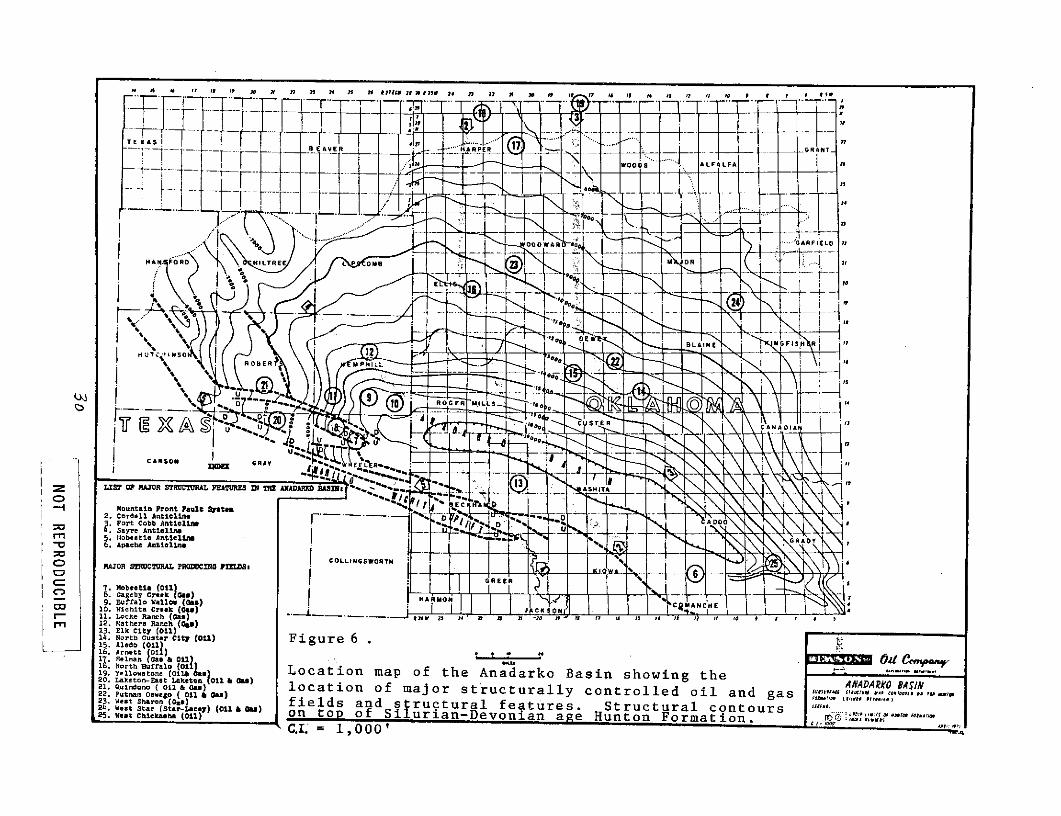
Most of the structures that trap hydrocarbons were
created during the intermittent tectonism that began in
earliest Pennsylvanian time and continued into earliest
Permian time. Most of the structural traps in the basin
are located in the highly deformed frontal zone north of
the Wichita-Amarillo Mountain trend (figures 5 and 6).
Possible Role of ERTS
Exploration for structurally trapped hydrocarbons in
the basin is exceedingly difficult because the important
structures are buried by Permian and younger rocks up to
2,000 meters thick that have undergone at most only gentle
deformation and for the most part mask the more highly
deformed lower Paleozoic rocks. The surface features that
reflect the deeply buried structures are extremely subtle
and may be masked by much younger structures produced by
the solution of Permian evaporite deposits.
Features of interest in petroleum exploration result-
ing from this complex history that might be detected in
ERTS imagery include:
Linear features marking old fracture trends thatmay have controlled deposition, formation ofstructural traps or routes of migration forhydrocarbons.
Patterns of lithologic units of the surface thatcould give clues as to the overall structure ofthe basin and the existence of hydrocarbon trap-ping structures.
Closed geomorphic, tonal or textural anomaliesthat might indicate buried structural featuressuch as fault blocks, domes or anticlines.
28

HOLLIS WICHITA ANADARKOSouth BASIN MTS. BASIN North
ASe a Le . -
-40,000
FEET ' 40 l- - ,
_zroc, , ?' -;-, . ... *u..* v ,. ... . -' + * . ' i ,!r< Av '
4 . . . . . j vr , 4, *
.... ,.,,f..,r ..... tnen 972
0 50 MILES O0 150 oter Johnson 972
Permian Ordovican and Cambrian(sedimentary rocks)
Pennsylvanian , Combrian (igneous ande imetomorphic rocks)
Mitelsippian, Devonian,and Silurian. ePrecambrian
S Fault, with relativemovement indicated.
Figure 5. Cross section through the Wichita Mountains andAnadarko Basin showing asymmetry of the basin andthe complex frontal structure composed of foldsand high angle faults. Line of section shown infigure 4.
29
0 7 C '7 9 9 39 n 4 14 t4 33 7 39 3 39 12 to I 4 1 S rd I 7r 7 9 ' 7 v I 13
r---T EXAS f F- .- ....... ........
7
- - _onG R- b--- -ORAVF OO-- A 7F ALFA
HAll FORD HLR P O6M O
6000
12
-- D T-- NS __ 8E MVR h i O R LS
I U, . U
...... ... ........
CARSON GAY EL)
LST R 1MAJOR STC L FEATURES IN TE ANADAPD RBASI t
2. Cordell AntlclinehsP ort Cobb AnticlineDC00
6. Apache Antiolins
0 MAJOR STRUCTURAL PRODUCING FIEEmic8tuwer
GRE
7. Hobeetia (011lI
oCA n )HAM
10. Wichita Creek J(CSOas)A H
. I oters anch (Gas) * ta s 2 s -o a s r t s r s s t t
ni 13. Elk City (Oil)1. North Custer Cit/ (--) Figre 615. Aledo (O l
16. Arnett i1)
19. Yelowstone(onlz *Location map of the Anadarko Basin showing the20. Laketon-East laketon (Oi & Gas)AADRQ:0"indunsOOil Gas) locatiOn Of major Structurally controlled oil and gas "i" 77(-**77977799 0...
23Wet Sharo (Gas)ono. fields and s ructural features. Structural contours ""i --.WestSarSRD..Rao) on top of Si ur0an-Devonian Hunton25. We Cticie )aeForatio n.
C~E =1,000
20 ' I-I. C
Sof GRRAY
r- 12. Cordell RAntcli(n
le o b 0 1 1) e ; _,'JA
i I . ~o, L o c t i o m ape l o f1 t h e A n d a k B a i h w n h e... .. . .:....o o o, locatio of ma o s r ct ra l c n ro le il a d a
M AJOR o, , STRU TURA a nd.V s t r u t u r a f e t u e . t r c u r l c o t orG. ...W O... .. ...
10. Gas .,00 SO$

Our hypothesis was that the synoptic view provided
by ERTS imagery might allow integration of a sufficient
number of these subtle features so, as in effect, to see
the deeply buried structures through the overlying rocks
(Melton, 1959), (Doeringsfeld, 19 6 4),(Trollinger, 1968).
Intensive petroleum exploration began in the basin
in 1917. Traditionally, exploration has concentrated on
structures along the south flank of the basin and on
shallow stratigraphic traps on the northern shelf of the
basin. It is only during the past five years that the
deeper parts of the basin have received extensive explor-
ation attention. At present there are more than 75 rigs
drilling in the basin for targets that range in depth from
several hundred meters to 7,800 meters. Since distribution
of the draft of this report, a new drilling record has been
set in western Oklahoma. The Lone Star #1 Bertha Rogers,
at 9,570 meters (31,441 ft.) is the deepest hole in the world.
However, it will have to be plugged back to 4,260 meters.
The Rogers exceeds the Lone Star #1 Baden (record holder
since 1972) by 410 meters.
31
VI. EVALUATION OF THE ERTS IMAGERY
An important step in evaluating the applicability of
ERTS imagery to petroleum exploration was to determine
which bands, scales and formats of imagery were best for
geologic interpretation in the Anadarko Basin, what times
of the year were best for acquiring imagery with the maximum
amount of interpretable geologic information and what kind
of resolution could be expected in the imagery. To do this
we carefully compared several different types of inter-
pretations made from prints and transparencies at several
scales of all bands and color composites of imagery acquired
at several times of the year.
From these comparisons we concluded that if one were
constrained to use a limited amount of imagery, by time or
funds available, one should use band 5 and 7 and color
composites of imagery acquired during periods of maximum
or minimum vegetation vigor either in the form of 1:1,000,000
scale transparencies or 1:250,000 paper prints. However,
if at all possible, one should interpret all bands of
imagery acquired at several different times of year. In
fact, in an area like Oklahoma, where the annual climatic
cycle is highly variable, one would at least want to
examine, if not interpret in detail, imagery acquired over
several years time.
32

Comparison of Scale and Format
We used prints at a scale of 1:250,000 (1" = 4 mi.)
for interpretation and compilation. At this scale, prints
of entire ERTS frames are inconvenient to handle, but
manageable. Imagery at this scale has several advantages
over small scale images. No magnification is needed for
most of our purposes and little or no detail is lost in the
enlarging process. The 1:250,000 scale permits careful
interpretation and precise location of data points and
geologic features and resolves features that are ambiguous
or difficult to define at smaller scales. It matches the
scale of standard 10 x 2 o USGS topographic maps. Also,
it is convenient for discussion and compilation purposes.
Transparencies of ERTS frames at 1:1,000,000 (l" = 16 mi.)
are convenient for handling, storage and study (provided a
light table is available). A near-maximum amount of
information can be derived from them although moderate
magnification (3x to 10x) is frequently required. The
same can be said for prints at the same scale except for
lighting difficulties. Transparencies eliminate glare and
a need for properly positioned overhead lighting and preserve
a bit more visual detail. However, prints can be made into
mosaics. Mosaics are convenient up to 30 or 35 frames, but
at 1:250,000, mosaics of 4 or 6 frames become difficult to
display and handle.
We used 70 mm. (1:3,369,000) positive and negative
33
transparencies mainly for enhancement and/or photographic
reproduction. The positives are also occasionally useful
for reference and projection in lantern slides.
Interpretation at scales of 1:1,000,000 and at 1:250,000
showed little difference in the amount and kind of information
derived from imagery. Tonal and geomorphic anomalies were
the same but there were some "new" textural anomalies
found at 1:250,000 that had not been noted at 1:1,000,000.
The larger scale permits more detailed and precise location
of lithologic boundaries than the smaller. We did, how-
ever, recognize the same units at both scales.
In mapping linears we noted differences in the number
and lengths of linears appearing on imagery of the same
frame at these two scales. In one test case (frame 1131-
16465) on band 7 we counted 1,557 linears. 186 of these
were unique to the larger scale image while 457 were unique
to the smaller. On band 5 there were 1,950 linears, 520
unique to the smaller scale, 565 unique to the larger.
Although there may be several reasons for varying counts
of linears from interpretation to interpretation, these
figures demonstrate that a maximum amount of information
on linears can be derived by employing at least two different
scales.
Interpretation at 1:250,000 consistently produced
linears of greater length than did those at 1:1,000,000.
The larger scale significantly extended the lengths of
34

linears previously noted on imagery at 1:1,000,000. Only
in a few instances did the smaller scale extend linears
from the larger.
In summary, we feel that one scale has no real inter-
pretive advantages over the other. The main advantages are
in terms of convenient format for study or display. Certainly
both scales add something and both should be used when
possible.
Parts of one scene were enlarged to 1:100,000 with
little apparent loss of definition. This is probably the
working limit for geologic purposes. An entire image
enlarged to this scale would be an unwieldy object. Enlarge-
ment to this scale should be produced only for areas of
special interest.
35

Resolution of Imagery
It is difficult to assess apparent resolution of
the imagery in the Anadarko Basin because of the variables
involved in recognition of different kinds of cultural
and geological features and the difficulty in distinguishing
recognition from resolution. We might generalize about
recognition of non-linear and linear features. Non-linear
features include warehouses, ponds, quarries, buttes,
fields, woodlots, etc. Ponds as small as one acre (68
meters in diameter) can be recognized on band 7 in high-
contrast situations. However, 100 meters seems to be the
practical minimum dimension needed for recognition of
individual fields, buildings and other features as well
as ponds.
Linear features (bedrock joints, roads, creeks, etc.)
whose width is much less than 64 meters are easily recognized
because of their length, either from their own reflectivities
if they stand in strong contrast to their surroundings, or
from the difference in reflectivities of areally extensive
features on either side. For example, creek beds as
narrow as 15 meters can be recognized by topography,
shadow, or vegetation contrasts or a combination of these.
The length of creeks and their meandering habit distinguish
them from hedgerows, or fence rows, for instance. The
smallest feature we have noted is in a high contrast
36

situation on band 7 where two highly reflective bridges
cross a lake. One visible bridge has a roadway 8.5 meters
wide plus two sidewalks 1 meter each or a total of 10.5
meters (34 ft.). The other bridge has only 7.3 meters
(24 ft.) of roadway and no sidewalks, yet is visible on
ERTS images. A working limit for recognition of linears
by their own reflectivity seems to be 20 meters. Linears
of essentially zero width such as fence lines, lithologic
contacts or faults are recognized by contrasts in reflect-
ivity on either side of the line.
37

Comparison of Bands
One of the first steps in handling and interpreting
ERTS-1 imagery was to determine the applicability and
utility of each of the four MSS bands to analysis of struct-
ural and lithologic features. We concluded that bands 5
and 7 are most useful for initial geologic interpretation.
Their utility is optimized when they are used together.
Band 4 is the least useful. Bands 6 and 7 contain largely
redundant information, yet the minor differences between
the two are exceedingly important for geologic interpretation.
The subtleties of tonal difference in many instances corres-
pond to differences in lithology or surficial composition.
We emphasize that these conclusions are of a general nature
only. No study is complete until all four bands have been
studied and compared. There are items of information
unique to each band.
Another conclusion is that color composites contain
the most information of any single product. In addition to
tonal variations, there are color differences in the com-
posites which either add information or make interpretation
quicker and easier. One drawback is the imperfect regis-
tration of bands in making the composites. This causes
loss of resolution and detail and renders them less "sharp"
than individual black-and-white bands.
We compared the following aspects of the imagery
examined: overall contrast; tonal signatures and relative
38

visibility on each band of common features such as roads,
quarries, towns, clouds, snow, native and cultivated
vegetation, gross lithologic types, bare soil, shadows,
river bottoms, clear and silty water bodies, etc.; scan-
line visibility; variations in tone between lines; atmos-
pheric haze; effects of contrast reversals between bands,
and effective resolution. Examples of some of the above
are:
Healthy plants appear white on band 7, black onband 5.
Water is black and in high contrast to allother features on band 7, while it may belight gray to black on band 5 depending onsilt content.
Most standing bodies of water are difficultor impossible to locate on band 4 because thereflectivity of turbid water in this band isvery close to that of several types of soils,rocks and plants. This results in overalllow contrast.
'Cities, large towns and major roads stand outas light areas in a background of medium grayson band 4.
In comparing bands, we found that for the same types
of information, contrasts and tonal quality vary from
region to region and even within regions. Thus, a state-
ment here that a given band is best for fracture analysis
means it is best for this purpose in western Oklahoma and
the Texas Panhandle and not necessarily everywhere. The
reason for this variation is that overall contrast and tonal
signature are determined by the distribution of relative
sizes of areas covered by, and degree of intermixing of
39

areally extensive features (particularly soil and rock types
and vegetation types). The distribution and reflectance of
these features will vary with climate, season and topography.
Thus, the sparse vegetation of western Oklahoma may provide
a high contrast situation in band 5 but images in band 5
taken over southeast Oklahoma or southern Missouri may be of
very low contast due to profuse vegetation in those areas.
Standing Water:
Lakes and ponds appear black on band 7. Since plants
are ubiquitous and on band 7 are white to light gray when
healthy, ponded water stands in stark contrast to light
background. This makes locating and inventorying water easy
and rapid. Moreover, ponds are visible at the limits of
resolution of the imagery, namely as small as 34 meters in
radius. Band 6 generally reveals standing water quite well
but is somewhat more subject to scatter by atmospheric
moisture and haze. In some instances, there is less contrast
between land and water than in 7, and some small ponds that
are quite visible on band 7 are not seen on 6. Band 6 is
more sensitive to turbidity in water than is 7 and may show
strong plumes of silt when no hint is these is seen on 7.
The tonal qualities of water are quite variable on
band 5. Clear water is near black. Silty water may appear
medium to dark gray on 5, depending mainly on the silt
content and its dispersion in the upper portions of water
bodies. Because its tone varies on 5, water may produce a
40

low or high contrast with adjacent surface materials. In
addition, since 5 is generally a high contrast band, many
kinds of features show up well and, as a result, water bodies
may be lost among many other high contrast features.
Terrestrial water bodies are difficult to locate on
band 4 images. Regardless of turbidity, water is seen as
middle gray tones similar to the tones of many rock, soil
and vegetation types, and shorelines may be impossible to
detect. Often a water body can be distinguished from surr-
ounding features only by its "smooth" uniform tone. Subtle
tone differences and light shadows may lend a slight texture
to the surrounding surfaces.
Stream Valleys:
The varying appearances of stream valleys between
bands 5 and 7 and in different parts of the study region
reinforce the observation that the generalizations made
are valid only for the region considered. In some frames,
small and intermediate size streams (3 to 70 kilometers long)
are seen easily on band 5 in situations where live plants
(low reflectivity in this' band) are concentrated in the valleys,
and slopes and uplands are of high or moderate reflectivity.
The valleys then are dark or almost black and stand in
marked contrast to some of the slopes and uplands which
appear light gray.
On some of these frames in band 7, the plants near the
streams are white or at least irregularly bright and higher
41
surfaces are also moderately bright to medium gray in tone.
The resulting contrast is lower than in 5 and opposite in
tone. Thus, in some frames both 5 and 7 may be useful for
drainage analysis but, when contrast is good in both 5 and
7, band 7 often proves more useful for locating and tracing
small streams and valleys. Band 6 is similar to 7.
Short streams are often difficult to see on band 4
because contrast is low. Rugged or badlands topography
enhances valleys in this band as it does in all others.
Major streams such as the Red, Washita, Canadian and
Cimarron Rivers are markedly different from the small
streams because they have large meanders, wide valleys,
braided channels and broad expanses of their beds exposed.
The beds of the Red, Canadian and Cimarron usually show as
continuous bright strings on bands 4 and 5. These river
beds contain large expanses of quartz sand which in the
field is white to pale yellow to reddish brown to pale red.
In band 7, the bed material has a lower reflectivity over-
all. Band 7 is sensitive to a variety of factors which
affect reflectivity and make the beds of these rivers much
less distinct than they are on 4 and 5. The freshly
washed channel is bright, but moisture and standing water
along with some vegetation and surface particle types
reduce reflection at points along the stream. The result
is a discontinuous or mottled, moderately bright thread on
the imagery which is easily lost among surrounding features.
42

The beds and valleys of the Washita and North Canadian
are generally narrower than those of the aforementioned
streams. Water is restricted to narrow channels, and trees
and shrubs close in the banks. Farming and ranching extend
close to the channels. Farming does not reach into the
wide, braided beds of the other major streams but is
restricted to the adjacent floodplain and, in some instances,
to older terraces. White or highly reflective sand is
exposed only occasionally because trees and shadows cover
portions of the channels and because much of the riverbeds
are wet or water-covered. Moreover, the narrow riverbed
easily is lost among varied tones produced by the agricultural
lands lining the banks. In addition, the vegetation is
spotty, being variously dense, scattered or absent. Different
reflectivities are also produced by variations in soils and
lithology exposed in riverbanks which produces a string of
irregular bright and dark features against a "mottled"
background. These factors all make it difficult to determine
the exact courses of the Washita and North Canadian.
Linear Features:
Most of the above discussion on minor streams is
applicable to linear features. In fact, fault and joint
traces are most frequently revealed by drainage alinements.
Linear features in the imagery may include a variety of
things: roads, imagery processing effects, scanlines,
strike of rock units, drainage alinements,anomalously straight
43

stretches in streams; lines of vegetation, springs and water
bodies; plateau and fault scarps; anomalous alinement of
tonal features; even political boundaries where surveying or
land use practices change abruptly. As used here the mean-
ing of "linear features" or "iinears" is restricted to
naturally occurring features that are inferred to be related
to fractures in the crust. This excludes all cultural and
political effects and artifacts of imagery production and
handling. Lineation may refer to joints, faults or an
expression of layering, thus is a non-specific term.
An early surprise in viewing ERTS-1 imagery was the
discovery of linears of great length that seemed not to
have been recorded in the literature. Most of these are
subtle alinements not defined by any single major feature.
These linears may be 20 to 150 kilometers or more long
and be indicated by a subtle alinement of many kinds of
features such as vegetation lines; straight streams;
abrupt changes of streams from meandering to linear
channels; tonal differences in soils, cultivation in
elongate fields perhaps influenced by the topography
near the linear; and unresolved tonal alinements.
No generalizations can be made about the appearance
of such extended linears on various bands. Only a small
number appear on all bands. Many are so subtle that a
particular linear may be seen on one band, or two, but
not on the other bands. Or, they may be so subtle that
44

they can be seen on a.second band only after being "dis-
covered" on a first. Some of these linears are related
to the very old, regional tectonic features. Those we have
checked in the field are expressed at the surface as joints
and faults. That is, they are real and have structural
significance.
Most linears, ranging from 3 to 20 or 25 kilometers
long, were recognized most easily on band 5 and 7, although
large numbers can be recognized on 4 and 6 with more care-
ful study (figure 7). These linears are defined by straight
streams, alinement of 2 or more stream valleys, vegetation
alinements, by tone difference in surface materials (mainly
soil and weathered rock), by anomalous cultivation patterns,
and by combinations of these factors. Comparisons of
several overlays of linears show that some linears match
between the two bands but that the majority are different.
That is, although bands 5 and 7 are both excellent for
tracing linears, they exhibit different fractures and must
be used to complement each other (figure 7). Band 6 is
generally as useful as 7 and because of slight differences
from 7, it may reveal some linears better than 7. Band 4
also can be used for tracing linears, and these will usually
be helpful additions to the other bands. Contrast is lower
in 4, but the marked differences in reflectivities of various
features from other bands is important. There are linears
seen on 4 that cannot be seen on other bands.
45

B
A
CC
< D
Figure 7. Comparison of lithologic interpretations derived fromimagery collected in October, 1972 (left) and in April, 1973(right). A shows detail obtained in spring which is absent inthe fall. B, C and E show boundaries derived from fall imagerywhich are either indecipherable or only poorly defined in thespring. D shows a contact drawn with more detail and precisionin the spring than in the fall. u
Lithologic Boundaries:
Agricultural activities affect most of the surface
area of the test site. The disturbances caused by man's
activities generally obscure geologic features, lithologic
boundaries in particular. As a result, no single band can
easily be accepted as most useful for purposes of delin-
eating rock units. All bands must be studied, compared,
contrasted and the results combined into a reasonable
interpretation.
In general, we found it difficult to recognize many
mapped lithologic boundaries. The difficulty arises partly
because of the effects of agriculture and the fact that
on ERTS images most rock units in the area have no readily
distinguishable tonal differences from adjacent mapped
units. This may in part be because several of the estab-
lished units are defined on features that do not affect
reflectivity, such as fossil evidence. There are many
exceptions to this generalization. Many factors aid in
distinguishing known units. These same factors can be used
to define new "imaged units" or"photolithologic units".
Units are easily established when there are contrasts in
any or all of the following features: grain size, degree
of consolidation, plant growth, agricultural practices,
surface effects of ground water, topographic expression
(e.g., plateaus, badlands, rolling hills, cliffs, stream
density and/or pattern), tone or reflectivity. Such features
47

may or may not coincide with established rock units. More-
over, their occurrence may be irregular and interrupted.
In such cases, either a new set of units, termed here
"image units" is established, or disconnected, irregular
units are mapped which are difficult to interrelate and
analyze.
One example of successful lithologic mapping is the
Wellington-Garber contact where a moderate topographic and
vegetation contrast occurs. In fact, we were able to re-
define the contact and revise existing maps changing the
position of the contact 10 to 12 kilometers in some places.
Second, the region around and to the west of Elk City,
Oklahoma, is a generally flat to rolling surface. It is
underlain by Quaternary and Tertiary deposits above gently
dipping more dissected Permian strata. Agriculture domin-
ates the flat upland and groundwater and planting practices
differ slightly between Quaternary and Tertiary areas. In
addition, there is less agriculture and a different topography
in the Permian. Generally, it is not possible to distinguish
one Permian unit from another.
Several features are used to interpret lithologic
boundaries in the imagery; all of them can give ambiguous
results. These are tonal and textural clues, created by
any or all features such as: stream patterns and density,
topographic breaks and shadows, vegetation types and dis-
tribution, tones of soil and bedrock, and even the distribution
48
of farming patterns.
One example is found in southwestern Oklahoma in an
area where agriculture is limited to high, flat areas above
lower, dissected or badland topography. Most of the high,
farmed areas have a high reflectivity on bands 5 and 7 and
include Tertiary and Permian units. These bright areas
might well be interpreted from band 7 as one unit as is
done in the band 7 geologic map west of Elk City (figure 16,
p.8 5 ). This interpretation is satisfactory if it is under-
stood that the unit is an "image unit" and may bear no
relation to established stratigraphic units. If one wishes
to map units that can be properly interpreted as rock units
or mapped formations, other bands must be studied. Band 5
yields much the same results although subtle differences
are apparent within the area. Figure 15, p.81 combines
information from all bands. Compare the Elk City area in
this illustration with the same area in figure 16. Band 4
interpretation compares well to a geologic map and clearly
distinguishes the Tertiary (light) unit from Permian units
which are dark in this band. Band 5 and 7 are generally
most useful for study of rock units, but all bands must be
examined for a complete analysis. Band 7 on some frames shows
more detail than 5 and more units (not necessarily equivalent
to mapped rock units) are mapped with more clearly defined
boundaries. Conversely, interpretations made from band 5
show fewer units and different units with more generalized
49

boundaries. At some times of the year, where surface and
vegetation contrasts are just right, 5 and 7 are remarkably
similar in overall appearance and in much detail. Commonly
as noted earlier, a contrast reversal exists between 5 and 7,
resulting in a difference in the kind and/or amount of
information extractable from the bands.
Native vegetation is sensitive to underlying rock
composition, topography and drainage and is often a good
indicator of the extent of rock units. This then makes
band 5 and 7 particularly useful for mapping rock units,
because vegetation is usually dark in 5 and, when healthy,
bright in 7. These bands are most useful where plants
growing on one unit stand in strong contrast to the soils
and rocks of an adjacent unit and where adjacent units
support different biotas. For instance, Hennessey and
Wellington shales support grasses, shrubs and associated
low growing plants with trees near streams and in draws.
Thus, these units appear lighter than the associated
Garber which supports a tangled growth of scrub oaks and
hickories on a well-dissected surface. The contrast
between grassland and timber is easily traced. In fact,
our interpretation suggests that some parts of the contact
between Garber and Wellington should be revised. Native
vegetation, like agricultural practices and plant species,
is sensitive to factors related to the underlying geology
and hydrology. Crops that dominate the agriculture of one
50

area are only minor crops elsewhere. Farming is limited
to relatively flat or rolling areas and is only spotty in
more rugged lands. The presence of cultivated areas on a
flatland will emphasize the contrast between flat and
dissected lands.
Where vegetation is sparse, units (again, not nec-
essarily matching published lithologic units) may often
be distinguished by the tone differences seen on different
bands. An area of exposed rock might appear all of the
same tone on 6 while two shades of gray are distinguishable
in the same area on 4.
Textures created by degree of dissection of the surface
or by varying resistances of rock layers to erosion are also
helpful for interpretation of units. Visibility of textures
varies in different bands, and band 4 may be more useful than
5, 6 or 7.
Care must be taken in defining units, especially on
the basis of tone. Rocks may appear in various shades of.
gray for any number of reasons including moisture content,
grain size of surface materials, degree of compaction of
grains, density and type of vegetation, health of vegetation,
lateral variation in atmospheric haze, color and composition
of rocks, degree of weathering, slope, and agricultural
practices. Likewise, textural differences may provide a
convenient basis for defining units, but these units may
subdivide or combine mapped formations.
51

Fresh bedrock and soil exposures generally appear
brighter on all bands than do corresponding weathered and
plant covered exposures. For example, most new roads are
quite conspicuous (on band 4 in particular) as bright
lines. Older roads are usually difficult to see. Appar-
ently, weathering and plant growth on the shoulders and
adjacent stripped land lowers the reflectivity of these
surfaces. Paved surfaces likewise become darker in time.
Dunes, quarries and salt seeps all are highly reflective.
Active sand dunes are bright on all bands. Their tone on
7 is just discernably brighter than on 5 and 6. They are
somewhat less bright on 4. Gypsum quarries show a moderately
high reflectivity on bands 5 and 4 and a slightly lower
reflectivity on 6 and 7. Areas encrusted by salt such as
Salt Creek, Great Salt Plains and several other areas along
the Cimarron River, generally are highly reflective in
bands 4 and 5 and moderately so in 6 and 7. The presence of
detrital material such as clay, mixed with the salt may tend
to lower reflectivity in one or more bands. This is apparent
in Salt Creek Canyon which is visible but not readily
detectable on all bands. Large limestone and sandstone
quarries and sand and gravel pits are bright on all bands.
Both contrast and reflectivity are lower on 7 than on the
other bands. Highest contrast between quarries and back-
ground is found in band 4 and is also good in 5. Quarries
in granite are generally smaller than those in other types
52

of rocks. Because they are small their apparent bright-
ness is lower than other fresh rock types. Granite is
brightest on bands 4 and 5, less so on 6, and is only
moderately bright on 7.
The preceding visual comparisons of the reflectivities
of several rock types on the 4 MSS bands do not necessarily
indicate that automatic discrimination of gross rock types
may be feasible. The apparent reflectivites on the imagery
at our disposal are subject to many variations in collection,
handling, and processing.
Tonal Anomalies:
These are places within areas of more or less uniform
tone which exhibit a tone either brighter or darker than
that of the surrounding area. The basis for the tonal
anomaly may or may not be related to geologic features.
For instance, a narrow elongate zone somewhat lighter
than nearby surfaces may indicate a linear fracture zone.
Other features such as carbon black plants, irrigation
districts and unrecognized thin clouds may create similar
tonal anomalies. We did not specifically study different
types of tonal anomalies and their comparative detectability
on various bands.
Other Factors Influencing Geologic Interpretation of ERTS-1Imagery:
Haze and clouds may affect geological interpretation.
Clouds and haze are most transparent to the wave lengths of
53
light recorded by band 7 and least transparent to those
recorded by band 4. Cloud shadows are most clearly seen
on band 7 and least noticeable on band 4. In general, the
presence of clouds and even thin haze or fog can be detected
by comparing the apparent area of cloud coverage as seen in
band 4 and 5 with cloud shadows seen on bands 6 or 7. One
must exercise caution when interpreting features seen through
clouds on bands 6 and 7 because thin clouds or haze can
alter tone or reduce contrast in such a way as to lead to
erroneous conclusions.
Cities, new roads and major roads have moderate to
high reflectivity in all bands. They are best detected
on band 4 which exhibits a more even, lower overall contrast
than the others. Band 5 usually offers the most detail
within large cities. Urban areas have lowest contrast
with other features on band 7.
Light snow cover often enhances linear features and is
an aid for interpretation. Reflectivity is highest on
bands 4 and 5, lower on 6 and 7. Thin snow cover or a
light "dusting" of snow is seen most easily on band 5.
False-Color Composite Imagery:
Color imagery adds the advantage of hue. Because the
eye can detect so many subtleties of hue and shade, a great
deal more information is available and is more easily
extracted than from black and white imagery.. In fact, some
subtleties supply information which cannot be garnered from
54
one band alone or even two. As one example, some bright
areas on band 7 might easily be interpreted as having a
healthy vegetation cover, while a color composite might
show these areas are better interpreted as fallow fields with
highly reflective sandy soils.
There are a few drawbacks to the use of color images.
Bands must be combined in perfect registration which is
often impossible. Imperfect registration causes color
haloes and loss of sharpness or definition. Also, there are
a few subtle features visible only on a single band which
may be masked by combination with other bands.
Summary:
Color imagery is the most readily useable and contains
the greatest amount of information, combining as it does
two or more bands. Some details and subtleties are best
studied on individual bands. Band 4 has the lowest over-
all contrast and is most affected by haze. In fact, this
band gives an impression of having been fogged. Band 5
and 7 are most useful for geologic uses. They offer high-
est contrast in areas where there is a variety of vegetation,
soil, rock, stream and cultural features. Contrast is
lowest where entire regions have a more or less homogeneous
plant cover. Band 6 is largely redundant with 7.
55

Comparison of Season Coverage
In the Anadarko Basin the primary sensor response is
to vegetation while the surfaces of bare rock and soil
play the next most important role in creating image responses.
Atmospheric conditions particularly affect responses seen
on band 4. There is no subsurface information received
directly by ERTS. Vegetation, both native and agricultural,
vary with climatic and topographic conditions. The Anadarko
Basin is located in a climate zone where seasonal changes
are strong and both plants and soils contribute significantly
to image responses. Thus,differences in imagery collected
at different times is substantial. Furthermore, the
climatic cycle in this area is highly variable and imagery
would have to be collected over a period of several years
(5 - 10) to even begin to sample the possible variations.
Response in areas drier than the Anadarko Basin depends
mainly on soil and rock while moister and warmer areas
present mainly vegetation responses to ERTS. Applicability
of ERTS data to other basins was not tested by us.
The comparison presented here is based on images
acquired from October 25, 1972, through December 2, 1972,
and from March 20, 1973, through April 23, 1973. It is
drawn from extensive notes made about the imagery during
the course of interpretation. We have no summer or winter
coverage.
56

Because vegetation responses play a vital role in the
information content of the ERTS imagery of the area, one
would need to study imagery from all four seasons in order
to evaluate fully ERTS-1 imagery (see figure 8). Indeed,
several years' coverage is needed for exhaustive study since
seasons are variable, arriving earlier or later one year
than the next, varying in calendar length, and being affected
by different combinations of climatological factors and
extremes.
We concluded that, if we were forced to choose a
limited amount of imagery for geological studies, we would
choose imagery from an early dry fall and a late wet spring.
In particular, we concluded that a combination of
band 5 dry-fall imagery and band 7 wet-spring imagery are
the most readily interpretible for our purposes. That is,
given a budget short on time and money, the above combination
would allow the greatest amount of information to be
derived in a minimum of time at lowest cost. Ideally, of
course, all bands of every coverage should be studied for
optimum information. In practice, however, as the number
of bands and coverages increase so do requirements of time
and manpower, even considering the synoptic nature of
ERTS data.
The choice of combinations was made because not only
are spring and fall in contrast to each other, but also the
greatest differences between band 5 and band 7 are found
57

, ," ..-. '.- ." - .' ". .- > i '-1 ', 1 I ., \ F' " , '>- 1Y '. '
\\\
7" . k % 1, .'7\ , -- \ , _' .r\t -, '-' ' . , ' . , , " >, ,
0 5 10 20.
N m<
ivm
0 10 20 30m
Figure 8 . Each ERTS band contains some unique informationas shown here. Band 7 linears were compiled for part of oneframe. Next, linears were added from band 5 that did notmatch any from band 7. Examples are A and B. Last, band 4linears (such as C and D) that matched neither band 7 nor 5were added.
58
• " I " ""\ " ' "" "] ...z ... '" / ,, ,,', J . 9 ;l l __ 7 ". , I{ .,, "7- ,'
' .. I , 1 " . " , ' t " ' ' ' ../ " ' ; I J S ~ - " , ; '
I .' f '
..... "...., "', 1 , " ! .,. I i _( 1 ,... ./ ,. , " " F .II- -S
\~~~ A, ., , , / .. .. -. .>' \ _-! \ ' .,, ,<"/ , ' ,, " ,..,., .: P -- " ".,A"$L / , .
1~~~~ ~ ~~ ~~~ 5' 10 2,0 , , . " Y-. -. . -, r .
0 510 230
Figure 8. Each ERTS bnd contains some unique informationas shown here. Band 7 linears were compiled for part of oneframe. Next, linears were added from band 5 that did notmatch any from band 7. Examples are A and B. Last, band 4linears (such as C and D) that matched neither band 7 nor 5
were added.
58

from one season to the next. A more practical approach is
to use both bands 5 and 7 for both seasonal extremes.
Addition of bands 4 and 6 will provide the broadest inform-
ation base possible, but 5 and 7 contain the greatest amount
of easily extractable geologic information.
Analysis shows that band 7 spring imagery has some
advantages over fall imagery in the same band. Cultivated
areas have a more uniform tone on spring imagery, decreas-
ing cultural effects and increasing perceptibility of
lithologic trends which are longer and more continuous
than on fall images. These trends are interrupted and/or
are interpretable with difficulty in the fall. However,
fall imagery is useful for adding detail to gross litho-
logic units as interpreted from spring coverage. Whereas,
spring imagery may mask certain important lithologic
boundaries, and fall image interpretation may create a
confusing arrangement and large number of units, combining
interpretations from the two seasons refines the results
with fall detail added to gross spring units.
Stream valleys and badlands stand in strong to moderate
contrast with agricultural patterns on spring images.
Valleys of most large rivers are especially apparent in
the spring probably because of recent high water and the
presence of flowing water in the channels. The North
Canadian River channel is the main exception to this
statement. It is practically indistinguishable on all
frames and bands except for spring band 5.
59

On band 7 spring images where uplands are cultivated
and slopes contain little vegetation, uplands are light
and bluffs, badlands and valleys are darker. In other areas,
well-vegetated (mainly agricultural) stream valleys stand
out light against darker hills on the same image.
Comparison of two frames of band 7 taken over the
same area in spring (5 April and 23 April) demonstrates
the value of using as much seasonal coverage as is pract-
icable. The overall contrast of 23 April is greater than
on 5 April. Tonal anomalies such as those near Watonga
and Drummond Oklahoma, are more marked. In fact, the later
images are superior in all respects to the earlier. Streams,
topography and detail within cities are more distinct in
the 23 April images.
We conclude that a combination of band 5 fall imagery
with band 7 spring imagery is the prime minimum choice of
imagery because of the extreme differences between the bands
in these seasons. However, we cannot make a clear choice
of seasons for band 5 alone. Band 5 images acquired in the
two seasons should be studied together since they complement
each other, one revealing what the other does not. In
other words, trade-offs of types and amounts of information
and/or relative ease of interpretation involved in such a
choosing do not favor one coverage or the other. They
both contain unique and valuable information.
60

In general, roads, towns, airfields and quarries are
more visible on the fall band 5 images (30 November) than
on the spring (5 April). There are some exceptions, e.g.,
detail within many cities is enhanced by spring vegetation,
and a few roads and towns stand in higher contrast to
surrounding vegetated areas than in the fall.
Topographically and texturally expressed features are
better expressed on fall imagery because there is less
visual confusion being provided by agricultural patterns,
vegetation dominating valleys and a lower sun elevation
angle. Bluffs, badlands, stream valleys and certain
textural anomalies also appear more clearly on fall imagery.
Rock and soil types all tend to have similar bright-
ness and are relatively difficult to distinguish one from
another. Where contrasts do exist, however, they are more
easily recognized on fall images, where they are not
obscured by vegetation and cultivated patterns. One example
is the contrast between Quaternary alluvium and Permian
rocks or soils on the north side of the Cimarron River.
Variations in soils, rocks, topography, drainage,
availability of groundwater, and farming practices create
many contrasts in vegetation on spring images that are not
visible in the fall. The vegetation in many places creates
continuities within inferred units, while the appearance
of the same unit on fall coverage may be interrupted. The
reverse is true in some instances. For example, alluvium
61

along the north side of the Cimarron is easily distinguished
by its high reflectivity from Permian units in fall band 5
images. The alluvium cannot be mapped as one widespread
unit from spring images.
Major river beds are more easily distinguished in the
fall, but visibility varies along the course of the streams.
Some stretches of the beds are more easily discerned in
one season than in the other.
Lakes are more turbid in the spring than in the fall.
Turbidity frequently lowers contrasts between water and
surrounding areas, making interpretation more difficult.
In brief, band 5 is best- interpreted for two or more
seasons because one complements the other.
Band 5 coverage of late spring is more useful than
the same coverage earlier in the spring. In comparing
coverage from 5 April 1973, with 23 April 1973, we noted
lakes were less turbid and stood in higher contrast on
23 April images than on 5 April. Likewise, river beds were
brighter and vegetation was more widespread and darker,
resulting in higher contrast and greater continuity of
units. Images from 23 April contain light-toned anomalies
which are more apparent than on earlier images. Details
of drainage may be somewhat enhanced by the higher 23 April
contrast (between Canton and Waynoka, Oklahoma,) or may
be obscured as compared to 5 April by a wider and denser
distribution of agricultural areas which may "camouflage"
details.
62

We found imagery in both band 5 and 7 acquired early
in a dry fall to be preferable to late wet-fall imagery.
For band 5, though overall contrast is higher and atmosphere
clearer on 30 November, more detail and continuity can be
seen on 25 October imagery. For example, several litho-
logic contacts are easily distinguished in October which
are not visible, or at least are less discernable in
November. Some small streams are obscured in November,
but major river valleys are more easily detected than in
October.
Strong differences appear on band 7 between 25 October
and 30 November of the Oklahoma City area. Comparison
emphasizes the advantages of using both coverages when
practicable. While many details are enhanced on November
imagery, several large rock or alluvial units are more
distinguishable on October scenes. November scenes are
camouflaged by growing agricultural crops (mainly winter
wheat) while October scenes have large areas dominated by
dead or dormant plants, live plants, fallow fields and
exposed soils. Many streams or valleys are obscured in
November where both uplands and lowlands are cultivated
or where vegetation response is similar in both places.
In other places, especially the east side of the frames
where uplands are not farmed and are dominated by trees and
brush, creeks and lowlands are quite noticeable on November
63
but obscure or indistinguishable on October. Vegetation
contrasts are greater in October and bare rock-(or soil)
vegetation contrasts are lowest. November images show bare
rock (or soil) is clearly differentiated from vegetated areas.
In addition to the difference noted among the various
cycles of imagery, we noted some variations across the
area on the same cycle of imagery. We believe these are
largely the result of the climatic gradient across the
test site.
We made no detailed comparison of seasonal coverage
in bands 4 and 6. What study we did on these two bands
and on their seasonal differences, quickly lead to the
conclusion that coverage acquired in at least two contrast-
ing seasons must be interpreted for optimum results.
64

VII. RESULTS
Linear Features
Evaluating information on linear features interpreted
from ERTS data is difficult. We noted literally thousands
of linears ranging in length from 2 kilometers to more than
150 kilometers.
Most of the test site is farmed and ranched and surveyed
on a one-mile township-range grid. The greatest part of
the grid is defined by roads. While the road and field
pattern imposes a strong north-south and east-west linear
system, the system is generally quite distinct, not easily
confused with natural linears. Our rose diagram(figure 9 ) of
directional frequency of linears shows a strong maximum
centered approximately on north 4 east. This peak is
a legitimate result of our interpretation of linear
features. We took care during interpretation on 1:1,000,000
scale imagery to avoid including cultural linears. Frequent
checks were performed against topographic and base maps and
against ERTS imagery at a 1:250,000 scale. Since compiling
these statistics we have re-checked many linears to be
sure they are not cultural. Moreover, the peak is just
east of north, not directly north. And there is no strong
east-west peak which might be expected to accompany a
strong north-south trend if the trends resulted from the
surveyed grid.
It is difficult or impossible in most instances, to
65

330 340 350 360"30 20 10 0 10 20 30
32040 40
310 so5050
300 60
60 60
290 7070
280 80
80 80
270 90 I i 909 0
. .
Figure 9
Azimuths of linears > 10 km. in length.0
Groups = 10 . (Derived from ERTS imageryacquired Fall 1972 and Spring 1973).Total number of Linears: 2,817
distinguish fault related from joint related linears or
either of these from stratigraphic linears. It is easier
to make distinctions when abundant surface and subsurface
data are available, where field checks can be made or where
aerial photographs are available.
Because of the widespread occurrence of Quaternary
surficial materials and lack of aereally extensive outcrops
of bedrock over the region, it is generally impossible to
tell type, direction and amount of movement involved along
interpreted faults. It is possible to formulate generalized
hypotheses about the tectonics of the basin and associated
Amarillo-Wichita uplift, but not to give even approximate
figures on fault movement.
One result of our interpretation of linears is
summarized in the rose diagram. The length of the graphs
of each subgroup is directly proportional to the number
of linears equal to or greater than 10 kilometers in each
azimuth group. Inspection shows three maxima. These
peaks center near north 45 0 west, north 4 0east and north
45 0 east. The peaks coincide with the azimuths of linear
sets which are quite noticeable upon visual inspection
of compilations of linears. In addition, the set centering
on north 83 0west is visually prominent because of the
great lengths of some of the linears in this set.
Although the regional sets of linears are easily
defined, their significance is not easily determined.
67
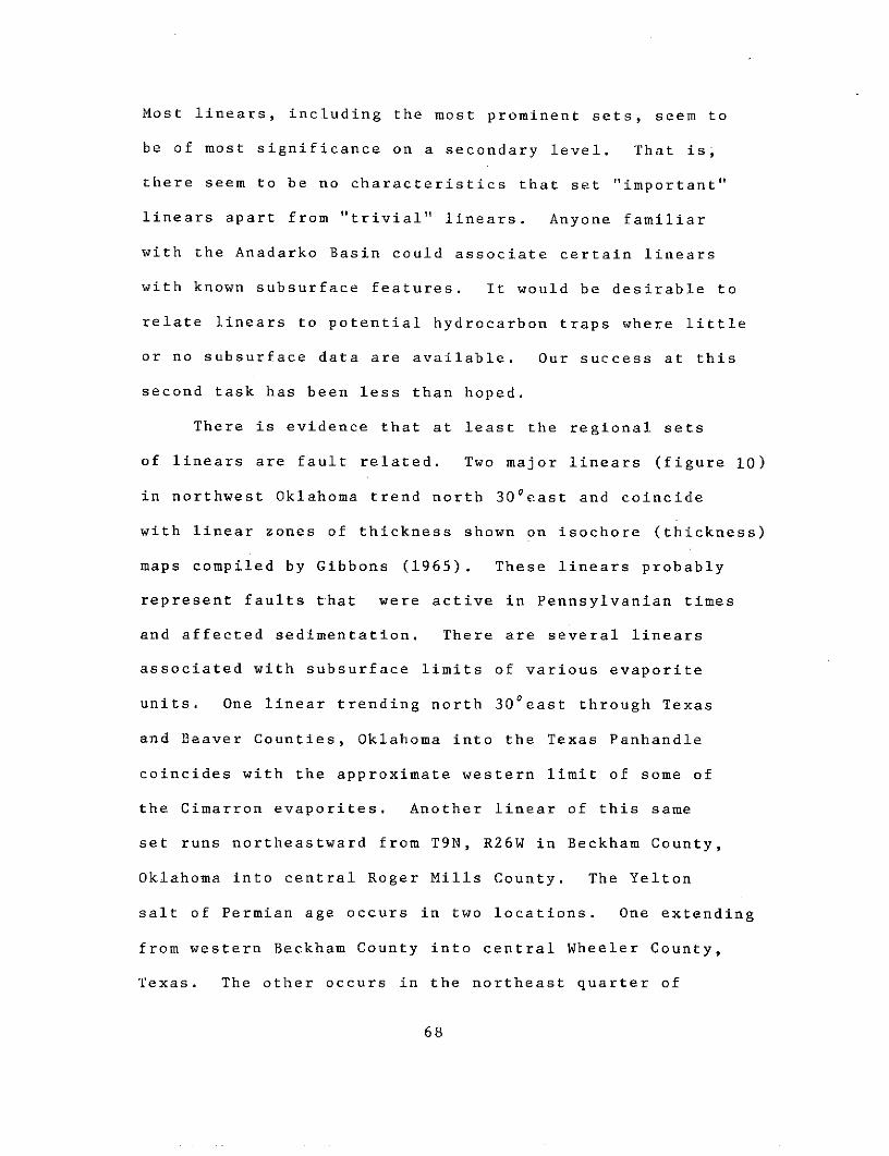
Most linears, including the most prominent sets, seem to
be of most significance on a secondary level. That is,
there seem to be no characteristics that set "important"
linears apart from "trivial" linears. Anyone familiar
with the Anadarko Basin could associate certain linears
with known subsurface features. It would be desirable to
relate linears to potential hydrocarbon traps where little
or no subsurface data are available. Our success at this
second task has been less than hoped.
There is evidence that at least the regional sets
of linears are fault related. Two major linears (figure 10)
in northwest Oklahoma trend north 3 0 oeast and coincide
with linear zones of thickness shown on isochore (thickness)
maps compiled by Gibbons (1965). These linears probably
represent faults that were active in Pennsylvanian times
and affected sedimentation. There are several linears
associated with subsurface limits of various evaporite
units. One linear trending north 3 0 °east through Texas
and Beaver Counties, Oklahoma into the Texas Panhandle
coincides with the approximate western limit of some of
the Cimarron evaporites. Another linear of this same
set runs northeastward from T9N, R26W in Beckham County,
Oklahoma into central Roger Mills County. The Yelton
salt of Permian age occurs in two locations. One extending
from western Beckham County into central Wheeler County,
Texas. The other occurs in the northeast quarter of
68

TEXAS OKLAHOMA
Atoka -Des Moines
0 6 12 Knm.
KANSAS* - - - -- - - e
C7
TE AS 0KLAHOMA
Lower Missouri
0 6 12 Knm.
After Gibbons (1962)
Figure 10. Isochore map of Pennsylvanian sediments in northern AnadarkoB W showing correlations of regional lnears (heavy lines), trending30 with thick strata (patterned areas).
69

Beckham County and extends into northwest Washita County,
Oklahoma. The linear lies between these two salt bodies
and within 4 kilometers of the western occurrence. We
have field checked this linear and found that one portion
of it is occupied by an anomalous straight segment of the
Washita River where the river makes an abrupt northeastward
turn. The portion of the linear west of Elk City is a
zone of anomalous dips (up to 150 as compared to regional
dips of 10 to 2 o ),.subdued topographic lows, and contains
native brush and grass instead of agricultural or grazing
crops.
One linear trending north 50 west appears to be a
fault truncating the west end of the main Wichita Mountains
near the western border of Commanche County. Other linears
coincide with the frontal deformed zone of the Wichitas
which form the south flank of the basin. These linears
also coincide with producing structures which are part
of the frontal zone and they trend about north 400 west
from near Duncan, Oklahoma to the Alden and Apache fields
in T6N, R12W. They can be traced north 700 to 80 o west to
the Erick field in Beckham County, Oklahoma.
Another linear that coincides closely with oil and
gas fields is parallel to the previously described north
400 west linears, and extends from T9N, R15W in southeastern
Washita County, Oklahoma into T22N, R26W in northwest Ellis
County, Oklahoma. Figure 2 shows that the axis of the
70
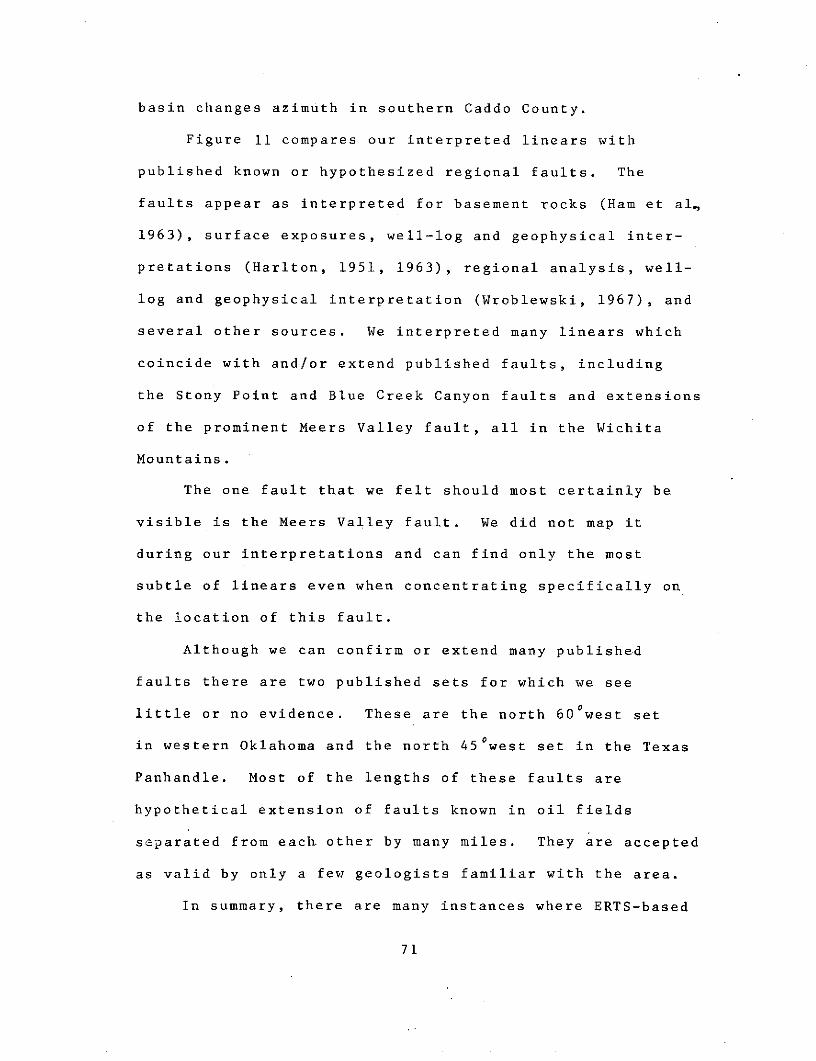
basin changes azimuth in southern Caddo County.
Figure 11 compares our interpreted linears with
published known or hypothesized regional faults. The
faults appear as interpreted for basement rocks (Ham et al,
1963), surface exposures, well-log and geophysical inter-
pretations (Harlton, 1951, 1963), regional analysis, well-
log and geophysical interpretation (Wroblewski, 1967), and
several other sources. We interpreted many linears which
coincide with and/or extend published faults, including
the Stony Point and Blue Creek Canyon faults and extensions
of the prominent Meers Valley fault, all in the Wichita
Mountains.
The one fault that we felt should most certainly be
visible is the Meers Valley fault. We did not map it
during our interpretations and can find only the most
subtle of linears even when concentrating specifically on
the location of this fault.
Although we can confirm or extend many published
faults there are two published sets for which we see
little or no evidence. These are the north 60 west set
in western Oklahoma and the north 45 west set in the Texas
Panhandle. Most of the lengths of these faults are
hypothetical extension of faults known in oil fields
separated from each other by many miles. They are accepted
as valid by only a few geologists familiar with the area.
In summary, there are many instances where ERTS-based
71

I LOK L A.
TEXAS
Figure Ila. Base map showing knownand hypothesized faults and linears.

Figure 1Ib. Heavy linesemphasize ERTS linears thatcoincide with and/or extendpreviously known orhypothesized linears as shown in I
11 a.

linears coincide with known or hypothesized faults and
linears compiled from studies of basement rocks, inter-
pretations of specific oil and gas fields and seismic
studies, older air photo interpretation and from maps of
surface geology. They coincide with the main features of
the Anadarko Basin and Wichita Mountains. Many linears or
systems of linears were previously unknown or unmapped.
They are prominent and of great length. There are a few
concentration of linears, for instance, in the region just
south of Weatherford, Oklahoma. However, there is little
evidence the imagery would set any given linear or set
of linears apart from others or which indicate that they
hold any particular significance to petroleum geology.
74

Lithologic Mapping
ERTS is useful for inferring lithologic distribution.
This statement is true even in the Anadarko Basin, which
is an area of low relief and gentle dips. Local relief
varies from 30 m. to 150 m. with extremes of 350 m. in
Palo Duro Canyon and the Wichita Mountains. Dip of surface
rock varies from less than 1 degree over much of the area
to 3 to 6 degrees in some areas. Rocks in local highly
deformed areas such as the frontal Wichita Mountains may
dip 10 or 20 degrees to as much as 60 degrees.
Although relief is low and dips are gentle, we are
able to map some lithologic units that correspond to
published map units. The correspondence of ERTS-derived
units to published units is generally inexact. That is,
many ERTS-units combine two or more mapped units or ERTS
"lithologic boundaries" may be located slightly to one side
or the other of published contacts. ERTS contacts may also
extend beyond published contacts or terminate more abruptly.
In some instances, contacts seen on ERTS imagery are so
distinct and clear we believe that they can be used to
revise published information. One example (figure 12 )
occurs near Guthrie, Oklahoma where it appears that the
Wellington-Garber contact lies some 13 km. to the east of
where it is shown on published maps. This shift has been
confirmed by field work and aerial photo interpretation
done by Dr. R. O. Fay (verbal communication 1973) of the
Oklahoma Geological Survey.
75

Ph9
~~NORMAN
O 10 20 30 km '
Figure 12.ERTS interpretation (right) of the contact between Henneseyshale (Phy) and Garber sandstone (Pg) from Norman tonorthern Oklahoma County matches the contact published on
the State Geologic Map (left). From the county line, thecontact trends northeasterly until it approximates theGarber-Wellington (Pw) contact as interpreted by R. O. Fay
of the Oklahoma Geological Survey (dashed line). The ERTSinterpretation may indicate a facies change within the Garberand Wellington which in turn affects groundwater distributionand plant types (Fay, oral communication). Differencesbetween published maps and ERTS-1 maps are important forremapping of formations and for posing questions for furtherstudy.
76

Fort Supplyo "t Con d'an 0RiveO
.... Canton Reservoir mOklahoma
0City
0 5 10 20
0 10 20 30 km
Figure 13. Permian units in the vicinity of Canton Reservoir (center), western Oklahoma.The state geologic map (top) contains more units and contacts are more precisely definedthan on the ERTS-derived map (bottom). The same general structure and stratigraphicrelationships are apparent on both maps, however. Lakes are shown by a cross hatched pattern.
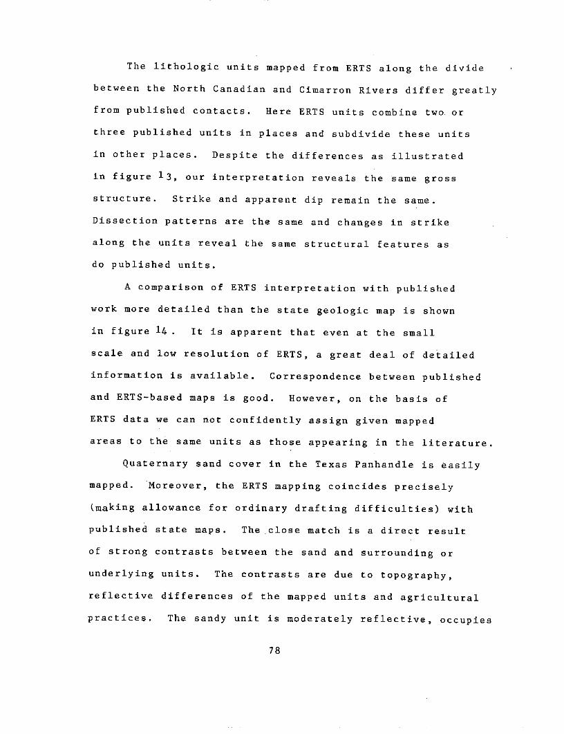
The lithologic units mapped from ERTS along the divide
between the North Canadian and Cimarron Rivers differ greatly
from published contacts. Here ERTS units combine two or
three published units in places and subdivide these units
in other places. Despite the differences as illustrated
in figure 13, our interpretation reveals the same gross
structure. Strike and apparent dip remain the same.
Dissection patterns are the same and changes in strike
along the units reveal the same structural features as
do published units.
A comparison of ERTS interpretation with published
work more detailed than the state geologic map is shown
in figure 14. It is apparent that even at the small
scale and low resolution of ERTS, a great deal of detailed
information is available. Correspondence between published
and ERTS-based maps is good. However, on the basis of
ERTS data we can not confidently assign given mapped
areas to the same units as those appearing in the literature.
Quaternary sand cover in the Texas Panhandle is easily
mapped. Moreover, the ERTS mapping coincides precisely
(making allowance for ordinary drafting difficulties) with
published state maps. The close match is a direct result
of strong contrasts between the sand and surrounding or
underlying units. The contrasts are due to topography,
reflective differences of the mapped units and agricultural
practices. The sandy unit is moderately reflective, occupies
78

P
q
PQ VO
Tf P
0 . 5 10 20 i
Skm
10 10 20 30.~ 30
Figure 14
The map at top is derived from two large scale maps,1:126,000 (Kitts, 1965) and 1:84,000 (Kitts 1959),of Ellis and Roger Mills Counties, Western Oklahoma.The lower-map was made from ERTS images at 1:1,000,000(as shown). While the amount of detail is far greaterin the published maps, the ERTS map preserves themain features of the.area, even to defining riverterraces at some places.
Key: P = Permian, Tpo = Pliocene Ogallala, Q = Quaternary
79

high, flat areas, is extensively farmed and contains
hundreds of small, shallow playa lakes. In contrast is
the underlying Pliocene Ogallala formation which has low
reflectivity, is dry and dissected, and is used mainly for
ranching (figure 15).
Reflective differences of surface materials and
vegetation differences enable us to distinguish among
several types of surficial Recent or Quaternary deposits.
One example is in the Elk City, Oklahoma area(figure 15).
On band 5, but not band 7, of fall coverage of the area,
one can distinguish a 40 square kilometer patch of
Quaternary sand from the underlying (and surrounding)
soils derived from the Elk City formation. Moreover,
both these units are distinguishable from sandy deposits
associated with the North Fork Red River just to the
south and from Ogallala sediments to the west. Indeed,
our ERTS mapping in this area subdivides part of the
Ogallala. Based on these observations these units should
be restudied to see if reassignment or subdivision of units
need be made. It may be that the differences we detect
are so subtle that no practical distinction is possible or
desirable. On the other hand, the fact that such distinc-
tions can be made from ERTS is important and suggests that
ERTS imagery can help provide answers to long standing
stratigraphic problems.
Our conclusions on using ERTS imagery for lighologic
mapping are summarized on the following page:
80

FORT SUPPLY
GS W
64;
as
QQs
f Q Pec *ELK CITY e
a P No RTHFORK
0 5 10 20MLI *I
0 10 20 30Km.
Figure 15. The area shown extends from Sanford Reservoir in Hutchinson County,Texas to Elk City in Beckham County, Oklahoma. Qs, Quaternary cover sandoccupies flat topped uplands in Texas. To, Tertiary Ogallala (Pliocene)is actually mapped as four units on ERTS. My subdivisions are shown bysubscripts. P = undifferentiated Permian units. Pec = Elk City unit(Permian). A patch of surface material just west of Elk City was mappedas Ogallala from ERTS images, but was originally field mapped as Quaternarysand (Qts). Qal = Quaternary alluvium.

Difficulties and limitations of ERTS for lithologic
mapping:
- Many mapped rock units have similar reflectivitiesand cannot be distinguished from each other on ERTS.
- Large areas are covered by Recent to Quaternarydeposits. The total area is somewhat greater thanpreviously mapped. These deposits mask older units.
- Small scale and low resolution limit precision oflocating boundaries and identifying small orisolated lithologic features.
- ERTS rock units usually do not coincide exactlywith published units. Even the multispectralnature of ERTS data does not permit identifica-tion of lithology or rock composition. Theseparameters can only be inferred crudely fromgeomorphology, drainage texture, relief, etc.
Value and advantages of ERTS for lithologic mapping.
- Large areas can be mapped quickly.
- Major structural and lithologic features arediscernable.
- Existing interpretations of some local areas canbe improved.
- Regional relationships among lithologic, structuraland geomorphic features can be studied.
- Areas for further study or geophysical work canbe located.
- Some units can be subdivided on the basis of theirreflectivities.
- Interpretation permits evaluation and revision ofpublished information.
- Low resolution and regional coverage suppress oreliminate a large amount of distracting detailpermitting subtle large scale differences to bedefined and studied.
82
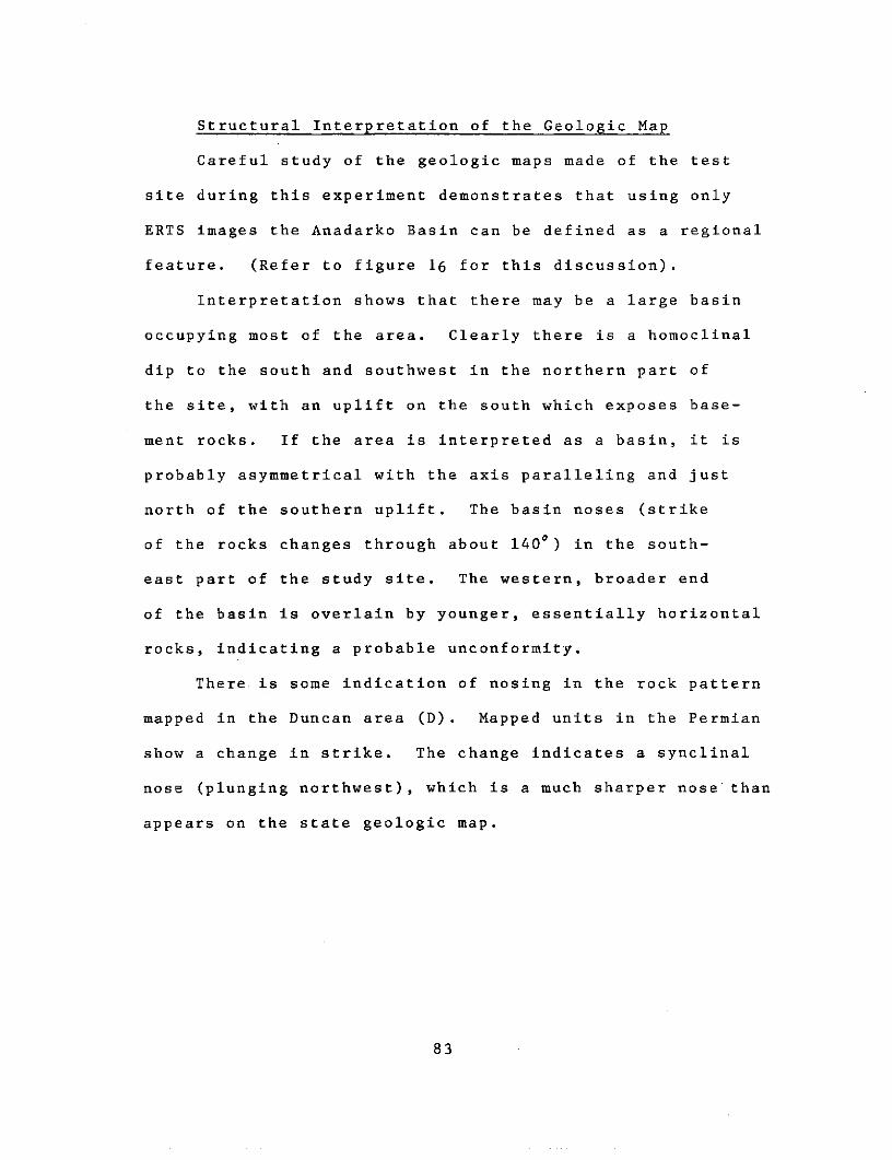
Structural Interpretation of the Geologic Map
Careful study of the geologic maps made of the test
site during this experiment demonstrates that using only
ERTS images the Anadarko Basin can be defined as a regional
feature. (Refer to figure 16 for this discussion).
Interpretation shows that there may be a large basin
occupying most of the area. Clearly there is a homoclinal
dip to the south and southwest in the northern part of
the site, with an uplift on the south which exposes base-
ment rocks. If the area is interpreted as a basin, it is
probably asymmetrical with the axis paralleling and just
north of the southern uplift. The basin noses (strike
of the rocks changes through about 1400) in the south-
east part of the study site. The western, broader end
of the basin is overlain by younger, essentially horizontal
rocks, indicating a probable unconformity.
There is some indication of nosing in the rock pattern
mapped in the Duncan area (D). Mapped units in the Permian
show a change in strike. The change indicates a synclinal
nose (plunging northwest), which is a much sharper nose than
appears on the state geologic map.
83

The inability to distinguish some major mapped rock
units points up one of the difficulties encountered in
mapping from ERTS imagery. Units are distinguished on the
basis of tone, texture, pattern of tones and standard
photogeologic inferences. In addition, hue or color is
used when mapping from color composite imagery. Factors
that can affect the tone, texture, and other visual
clues recorded on the imagery include moisture, facies
and vegetation changes, differences in climate, topography,
slope, and weathering products. Where these factors
produce similar photo-responses on adjacent rock units,
the units can easily be combined as one image unit. This
is the reason El Reno, Hennessey and Wellington rocks may
be combined at one place, but distinguishable at another.
Several features in the north indicate the broad
outlines of a basin or at least a homoclinal structure.
Valleys of the Washita (W), Cimarron (C) and in particular
the Canadian (Cn) and North Canadian (N) rivers trace
broad arcs from west to east. The assumption might be made
that these major streams reflect an adjustment to regional
structure, in particular to changes in strike of the
underlying rocks and thus partly define the northern
reaches of a basin. Supporting this hypothesis are
several features. In Oklahoma, north and northeast-
facing bluffs and slopes parallel these rivers. Likewise,
small streams interpreted as obsequent and resequent flow
84

Reproduced frombest available copy.
Qts :
Figure 16. Geologic map derived from ERTS imagery of
the Anadarko Basin test site. Key: C = Cimarron River;Qts = alluvial plain; Tpo = horizontal Tertiary sediments;N = North Canadian River; Cn = Canadian River; W = Washita
River; Pdy = Doxey Shale; Pec = Elk City member; WM =Wichita Mountains (crystalline); S = sedimentary Wichita
Mountains; D = Duncan area.
85

northeast and southwest, respectively, into the major streams.
The bluffs and small streams indicate the underlying rocks
dip southwestward on the east, but dip more southerly as one
moves west or northwestward along the main rivers. Moreover,
the Cimarron and North Canadian have large alluvial plains
(Qts) on the northeast indicating the combined effects of
several factors. Migration of streams downdip has cut
steep slopes on the southwest and left broad plains northeast.
Westerly winds have carried material out of the river beds
onto their northeast flanks. The major rivers turn eastward
at about 98 o west longitude, (the Washita turns at about
98030 ' west), indicating a change in structure or a cross-
strike course.
Another clue to the synclinal nature of the area can
be seen in the rock pattern in the Elk City - Burns Flat
area. The Doxey (Pdy) member of the Quartermaster formation
crops out continuously on the north, east and south of the
Elk City (Pec) member (or Quaternary terrace material cover-
ing the Elk City member), forming a southwesterly-directed
nose. However, the Quartermaster units at this scale appear
to be nearly horizontal or at least of low dip indicating
they are little-deformed. They may have been deposited
after the greatest subsidence had occurred or they may
indicate this is merely a gentle regional downwarp, not a
basin which has undergone strong subsidence and deformation.
86

Some inferred lithologic units indicate the basin is
asymmetric. They have a narrower outcrop pattern just north
of the Wichitas than they do farther north and east.
To the west of Elk City is a region of horizontal strata
(Tpo) which contrasts with the dipping rocks of the basin
and overlie the latter with unconformity. It is difficult
to determine the dip of bhe strata exposed in the deeper
parts of river valleys in the Oklahoma-Texas Panhandles,
but those exposed in the bluffs and slopes appear horizontal.
Likewise, the uplands appear topped by flat-lying Quaternary
deposits.
Within this region of horizontal strata there is one
slight indication of a broad structure. The Canadian River
flows within a wide, broadly curved valley flowing northeast
in eastern Hutchinson County, Texas, then curving eastward
in northern Roberts County and flowing east-southeast in
northwestern Hemphill County. The rocks in the area belong
to the Tertiary (Pliocene) Ogallala formation. Within the
upper part of this formation there are several layers of
caliche. An attempt was made to map the caliche since
its reflectivity is considerably higher than that of the
rest of Ogallala sediments. Mapping the caliche indicates
that there is a slight nosing of strata in the Roberts-
Hemphill area. The Canadian may breach a slight fold that
is asymmetric, the north side having steeper dips.
However, the caliche is irregular in occurrence, appears
87

to wash out and cover lower slopes in some places, and is
difficult to define and trace on the imagery. As a result,
the inferred structure may be based upon a fortuitous
pattern produced by other conditions. That is, the
caliche may occur in a series of localities such that these
places form an arcuate pattern. Nonetheless, there is the
possibility this broad bend in the Canadian results from
a breaching of an anticlinal feature.
In the southern part of the study site there is an
uplift of faulted and abundantly jointed rocks. The out-
crop of these rocks can be traced from Lawton westward to
the area of Mangum, Oklahoma. These outcrops comprise
the Wichita Mountains (WM). The strongly jointed rocks
can be interpreted from ERTS imagery as exposed basement.
There is another large outcrop of rocks (S) north of this
main mass of basement rock, which is neither obviously
jointed nor layered. The exposure may be interpreted
as sedimentary rocks involved and associated with the
deformation and uplift of the basement rocks to the south.
There is some evidence on the imagery that the Wichita
uplift limits or is involved in the structure of the basin
previously described. There is a trend of tonal and linear
anomalies extending eastward from the Texas-Oklahoma
border near Erick, Oklahoma. It passes just north of the
Wichitas and bends around to the southeast at what appears
to be the eastern end of-the Wichitas near Lawton. Such
a trend might be construed as a fault zone forming a
88

boundary between the basin and the uplift. Another poss-
ibility is that this is a zone of steeply dipping beds
which are the southern flank of the basin. Thus, analysis
of the information interpreted from the ERTS imagery would
lead to the correct conclusion that the area is underlain
by a large west-northwest trending asymmetrical syncline.
89

Recognition of Anomalies
During interpretation of ERTS imagery we identified
a variety of different types of anomalies.
We found fewer than 30 anomalies that could be described
as tonal and fewer than a dozen textural anomalies. The
tonal anomalies are the result of unusual reflectivities
possibly produced by peculiar conditions in the rock, soil,
plant cover or cultural activity in any given locality
(see figure 17).
Where it was possible to identify cultural causes for
a tonal anomaly we eliminated it from further study. Pre-
liminary analysis shows a strong correlation between oil
fields and tonal anomalies. No attempt was made to relate
correlating fields to depth of production or type of trap.
This correlation may not necessarily reflect underlying
geologic conditions but may be fortuitous or result from the
activities of man.
Textural anomalies may be the result of drainage patterns
that are more dense than patterns in adjacent areas. They
may reflect differences in size and shape of agricultural
fields in a cluster, which in turn may reflect anomalous
topographic or soil conditions. Other textural anomalies
appear as a mottled surface surrounded by a surface of more
even overall tone or from indistinct effects which might be
described as "grainy" or "jumbled" or "rough" as opposed to
adjacent "smooth" or regular surfaces. A preliminary
90

-- --- 4-... . L , 0,
ml
: _
... A 0.
F 0'
KC
- -.-.---I----- - - o
rei 0
Figure 17. Compilation of several anomaly types. Included are several circular and arcuateanomalies, two hazy anomalies (H), drainage and topographic anomalies, repeated patterns, tonal(To), textural (Tx) and geomorphic anomalies (Ge).

comparison of maps of textural anomalies to an oil and gas
field map shows some correlation between fields and anomalies.
Textural anomalies need further testing.
We have mapped about 60 "hazy" anomalies (figure 18).
"Hazy" areas appear on the imagery as if image detail is
lost or the scene has been smudged or partially erased.
They are not atmospheric or photographic processing'effects.
The number of these anomalies varies with changes in season,
but many of them persist from season to season. They are
more numerous in western portions of the test site than
in the east. "Hazy" anomalies are located mostly in areas
of Quaternary deposits near major streams and along the
eastern thin edge of Tertiary Ogallala sediments. That is,
they occur mostly in areas with sandy material at the
surface. Some of these anomalies are located on stabilized
dunes as indicated by a check of three areas containing
"hazy" anomalies. Examples are the large anomaly in the
large meander of the Canadian River in Ellis County, Oklahoma,
and several others along the north side of the Canadian in
Texas. However, the correlation with sandy areas is not
entirely consistent. One of the sites checked has no dunes
or thick sand deposits. Published maps also show that some
"hazy" areas are not on sandy surfaces. "Hazy" anomalies
have a high correlation with known producing oil and gas
fields. Most of these fields are stratigraphic traps rather
than structural traps. We did not check against depth of
production. These anomalies may be the result of man's
92

OKLAHOMA
TEXAS
1107
,o
SI I _ I
0%0
I s I g o1
Dashed where limits are uncertain.
activities during oil exploitation, they may reflect the
nature of the substrata or may have their origin in some
type of geochemical effect caused by hydrocarbons leaking
from the reservoir or production equipment. "Hazy" anomalies
seem to be unique to ERTS imagery, and are most easily
identified on band 4. Moreover, a brief inspection of
available SKYLAB S190A photographs did not reveal any "hazy"
areas.
The most numerous anomalies (figure 19), are arcuate
or near-circular features which we term closed anomalies.
Most closed anomalies are geomorphic features such as
annular or radial drainage patterns, bends and arcs in
stream valleys, circular or arcuate tonal and topographic
features, field patterns, etc. We believe closed anomalies
hold the most promise for locating potential hydrocarbon
reservoirs. Although other anomaly types may have a higher
correlation with producing fields of all kinds; closed
anomalies show a higher correlation with known subsurface
structures and/or structurally controlled hydrocarbon fields.
Other types of anomalies are numerous. We have marked
many other localities of interest on the basis of drainage
peculiarities, indistinct series of arcuate stream valleys
or arcuate linears, topographic peculiarities, and other
indistinct but interesting patterns, shapes or concentrations
of features. Figure 17 locates some of these anomalies.
The kinds of anomalies discussed above are generally
94

I
o
o -
a It I, P.... .TE oAS _ _ o ol ' \o
o , •. .. . .
I I °. . . -
I*,o
ooo
,O oo a-'- " ---o- . o a ,
-- ---. .....i - --..0
Fgure 19. omplation of cicular ad acuate aomalies. Dashed or dotted where boundaries
ae unce0a .
C11V\
0'
Igo
Figurne 19.'Compilation of circular and arcuate anomalies. Dashed or dotted where boundaries
exclusive. That is, relatively few anomalies of one kind
coincide with anomalies of another kind. For instance, only
5 tonal and textural anomalies coincide, and only 22 closed
and hazy anomalies coincide. There are more than 250 closed
anomalies and about 57 "hazy" anomalies. One method which
might be used for locating promising exploration sites is
to define sites where two or more anomaly types coincide.
On one composite overlay of fall imagery we counted 76 anom-
alous features. We classified these as geomorphic, tonal
and "hazy" areas. Of 76 anomalies, 59 correlate with produc-
ing oil and gas fields, 9 are on known but non-producing
structures, and the remaining 8 could not be correlated
with known features. Twenty-nine geomorphic features are
included. Twenty-three correspond with producing areas,
3 with non-productive structures. Three show no correlations.
Eight of 12 tonal anomalies correlate with production. One
correlates with a known structure and 3 correlate with no
known features. Of 35 "hazy" anomalies,'33 correlate with
producing fields or drilled structures.
On a more recent compilation, after additional inter-
pretation, 42 of a total of 57 "hazy" areas coincide with
producing fields. Six additional areas correlate with known
but non-productive structures. Nine have no correlation
with known structures.
96

Interpretation of Areas of Special Interest
One fruitful method of using ERTS data is to select
small areas and concentrate on refining the original
interpretation by extracting as much information as
possible. We will discuss briefly several sites selected
from previous ERTS interpretations, from high altitude
photographs and from suggestions by our petroleum geologists.
Elk City Area:
The entire Elk City area was identified early in our
studies as a site of particular interest. We first identi-
fied the Elk City Field, South as a closed anomaly. Later
study showed that the anomaly resulted from apparent
concentric or annular drainage. Several prominent, through-
going linears were recorded. Our interpretation is shown
in figure 20. Most earlier interpretations (Natural Petrol-
eum Bibliography, 1961), (Lang, 1955) show the
Elk City structure as an anticline lying in the axis of
the basin. The structure was assumed by some to die out
at depth. Wroblewski (1967) suggested that the anticline
was bounded along its northeast side by a normal fault
trending north 45 0west. It was suggested by Harlton (1972)
that this fault is part of a regional lineament called the
Cordell fault. Scott (1966) published the results of a
gravity traverse in which he interpreted the Elk City
field as a superficial fold associated with a much larger,
97

. -ION "-. ,<..
P. IW120 W
A B C
/ H VA / ... . .
H //
Figure 20. The Elk City structure is shown by subsurfacestructural contours in (A). Producing areas are shaded.ERTS interpretation of the Elk City anomaly is sho-wn in (C).Both figures are at their original scale of 1:1,000,000.(B) is a reduction of an interpretation done from a colorinfrared photo at 1:55,000, scale shown is 1:240,000.This interpretation includes lithology. That the ERTSanomaly is a geomorphic feature is apparent from thephoto-interpretation.
98
deeper-seated fault-bounded structure. He places the axis
of the deep structure about 3t kilometers north of the axis
of the Elk City field.
Our ERTS interpretation located a closed anomaly
directly over the center of production of the field. The
most prominent linears trend north 450 west and north 400
west, bounding the center of the structure. The linear
trending north 45 o west through the southeast part of the
area may represent a fault bounding the deep structure
along its northeast side. One linear running about north
100 west intersects the east end of the Elk City structure
where its axis shifts to an easterly direction at the
township line between 20W and 21W.
Woodward Area:
The subsurface geology of the Woodward area is less
complicated than that of the Elk City area and the fields
of the Wichita frontal zone (Weinkauf, 1968), (Forgotson,
1969).
This area was selected for further study for three
reasons. We had noted several strong linears on high-
altitude infrared photographs of the area, there are several
closed and "hazy" anomalies here and the Morrowan rocks
(lower Pennsylvanian) include a prominent channel sand
body (shaded area in figure 21) at about 2,480 meters below
the surface.
99

--]- " "> -'i / jrA .
1//
22' 20W 8L S ' .
. -1W 20W
-P _E R .. i , /26N J."
24N
Figure 2. . Woodward area.
(A) locates a subsurface channel sand body (Morrowan,
# i, ,,=, -+', 23 N
Pennsylvanian).
(B) shows a variety of anomalies interpreted from ERTS,including: Hhazy, To~tonal, and several closed andarcuate anomalies.
(C) combines ERTS linears with the anomalies. There
20N~ ~ ., .)... .,, ... ..~= ,...
2 2 W 2 0 W IB W I ? O
Figure 21. Woodward area.
(A)is no evidence at the subsurface of the channel sand body (Morrowan,
Pennsylvanian) .
(B) shows a variety of anomalies interpreted from ERTS,including: H=hazy, To=tonal, and several closed and
arcuate anomalies.
(C) combines ERTS linears with the anomalies. There
is no evidence at the surface of the channel or of
structures controlling the location of the channel,with the possible exception of the north-south trending
linears. Scale = 1:1,000,000.
/00oo

We found no evidence of the channel expressed at the
surface. There is a set of linears trending about north-
south which might be interpreted as flanking structures of
the channel. A large closed anomaly and a "hazy" anomaly
coincide with the north Woodward field. A linear trending
about north 40°east flanks the northwest side of the West
Sharon field. It coincides with and extends a linear seen
on the high altitude photos and with a fault appearing in
various interpretations of the West Sharon field.
Buffalo Wallow Field:
This area was chosen for further study because it was
first noted as a closed anomaly on ERTS imagery (figure 22).
The center of the anomaly is a nearly perfect circular
pattern of fields which also appears as a light-toned anomaly
on spring images and coincides exactly with the center of
production in the field, Tutten (1972) and others interpret
the deep structure (below the Morrow or deeper than 2800 m.)
as an anticline closed by normal faults on the north and
east. Although our anomaly exactly coincides with the
field and although the anomaly is bounded by prominent
linears, none of the linears exactly coincides with inter-
preted faults.
Mobeetie Field:
This field, like the Elk City and the Buffalo Wallow
fields, was chosen on the basis of an ERTS anomaly. The
anomaly is not as prominent as those associated with the
101

"QUINDUNO 1''
ASHITA CREEK .
LAKETON 5 N
bOer Elk City
WA"ELK CITY
.O v ERICKBff1
FAU1A WALLO .f WallowDD "IN....
C 0 , a Z R T H ERICKf
o A'BMobeetie o ,OKm.C D 5 .,.
"-os ./ / o .
AEYWASHITA CREEKCREEK
BUFFALO WALLOW =3
o .f \STRUCTIME*' o aB.PEZlN. 111C.
** esyMOBEETIE FIELD
0 WHEM2i11 CONTTEA
+1 '+ ACEBY CREEK a11R11 Co. NW REVDON *s
S* --- LINE OF CROSS SECTION
+ HUNTON GAS 0 8 K.
* MORROW GAS I+ + MORROW GAS-DRY HUNTON 0 5Mi.
. HUNTON NOT PENETRATED
Figure 22. Buffalo Wallow and Mobeetie fields. (A) Tectonic setting of the fields (Sahl, 1970).(B) ERTS interpretations at 1:1,000,000 of Buffalo Wallow and Mobeetie anomalies. (C) Inter-pretation of Buffalo Wallow structure by Tutten (1973). (D) Mobeetie structure according to
Sahl (1970). The ERTS closed anomalies coincide exactly with their respective fields. ERTSlinears may reveal undiscovered aspects of the fault control of the fields.

other two fields. Our interpretation (figure 22) closely
matches published interpretations (Sahl, 1970), (Wroblewski,
1967). We find a partially closed anomaly, flanked by
linears trending north 450 west, overlying the buried
structure.
Published analyses describe Mobeetie as an anticline
flanked by high angle faults; i.e., a horst. Interpretations
of strike of the faults vary from north 450 west to north
700 west.
Cement-Chickasha Area:
One of the most perplexing areas has been the strongly
folded and faulted Cement and Chickasha fields. These
fields were mapped at the surface in 1916 (Withrow, 1967),
from aerial photographs (Trollinger, 1968) and from drilling
data (Herrman, 1961). Although the structures controlling
these two fields are fairly prominent at the surface, we
found nothing to attract our attention to the area, nor were
we able to map the structures when studying the ERTS imagery
specifically for this purpose. Refer to figure 23.
The surficial rock units we mapped correspond closely
with the units of the Cement-Chickasha area as compiled
on the state geologic map at 1:500,000 scale. They include
the Cloud Chief and Rush Springs formations of Permian age
and Quaternary sand associated with the Washita River.
We mapped three closed anomalies, none of which coin-
cides with major structural features in the subsurface.
103

I I<
RIOW R9W iR.IOW. R.9W.R W
7.K1.7f7V - ~~- WHCEMENJ~--
NORTHWESTWE ST CEMENT, EAST CEMENT AND CHICKASA FIELS
MORROW STRUCTURE
T D
~12W lOW 8W 6W
NCN. QN
I, L C- - - , -
Figure 23 • Cement-Chickasha area.
(A) is a published airphoto interpretation of the structure of theCement area (Trollinger, 1968).
(B) is an interpretation of subsurface structure, after Herrman (1961) .
(C) shows an ERTS interpretation of the area. Lithology closely
matches the state geologic map. The linears for the most part
match joint patterns but not faults. Note two closed anomalies.
The Cement and Chickasha fields are shown by the shaded areas.
Scale = 1:1,000,000
(D) shows only ERTS linears. Scale = 1:1,000,000
104
IWEST CE.ENT FIELD -
~~EAST CEMENTFIL
-* N. t - \ ICXASHA
RIOW I 1 9Ai2WWEST CEMENT, EAST CEMENT AND CHICKASHA FIELDS
MOR ROW STRUCTURE
A BC..r'
C D
6 NW
Figure 23 . Cement-Chickasha area.
(A) is a published airphoto interpretation of the structure of the
Cement area (Trollinger, 1968).
(B) is an interpretation of subsurface structure, after Herrman (1961).
(C) shows an ERTS interpretation of the area. Lithology closely
matches the state geologic map. The linears for the most part
match joint patterns but not faults. Note two closed anomalies.
The Cement and Chickasha fields are shown by the shaded areas.
Scale = 1:1,000,000
(D) shows only ERTS linears. Scale = 1:1,000,000
104
None is prominent enough to draw specific attention to the
area.
Two linears parallel but do not coincide precisely
with deep faults associated with the structures. One linear
runs north-northwest along the east side of the Chickasha
field. The other runs northwest through the north side of
the Cement field. There are two other sets of linears
which may reflect subsurface conditions. The north trend-
ing set probably is a result of a joint pattern, based on
our field checks. The northeastward set may represent
crossfaulting at depth (Trollinger, 1968).
105

Enhancement Procedures
We tested several enhancement procedures in order to
evaluate the contribution of enhancement to image inter-
pretation for geologic exploration purposes. Enhancement
included photographic techniques, color additive viewing,
electronic density slicing and edge enhancement, and
various digital operations. From our work, which was not
exhaustive, we drew the following conclusions (these
apply only in the Anadarko Basin, we have not tested
them elsewhere):
* Electronic edge enhancement and density slicing
helped little.
* Photographic techniques are cheap, simple,and
can be quite useful. Techniques used includedhigh contrast printing, gray scale adjustment,and film sandwiches.
* Color additive viewing is flexible and is
useful for enhancing specific features such aslinears, closed anomalies, and lithologicboundaries.
* Digital processes offer the greatest range of
possibilities but must be "fine tuned" foreach area. Unless a completely interactivesystem is available this can be a long process.Techniques that seem to be the most useful aredensity slicing, gray scale adjustment and ratiooperations.
* Several types of enhancement (photographic,
additive color viewing, etc.,) should be triedin any operational program once areas of interestare defined.
We found no enhancement procedure we felt was worth
applying to the area as a whole. However, we are convinced
that as digital iwage processing procedures continue to
develop and be adjusted to specific environments several
106

types of digital preprocessing will become standard before
any interpretation begins.
Using August 1972 imagery we made a preliminary test
of electronic density-slicing and edge enhancement using
an 12 S Digicol. In the Anadarko Basin these procedures
did little to aid interpretation. The area tested lies
in the south central part of the Basin - an area that is
extensively farmed. The problem was that these procedures
either emphasized the boundaries between fields or differences
in the contents of fields, masking inferred lithologic and
structural features. Both of these effects would be desir-
able for conducting a crop inventory, but do not help geologic
interpretation.
It is possible that these techniques would be useful
for detecting differences in surface material, lithologic
boundaries and linear features in other parts of the area
that are less extensively farmed.
Photographic techniques included high contrast printing,
gray scale adjustment and film sandwich techniques. By
making new negatives from the extremely dark positive trans-
parencies and printing these on high contrast paper we were
able to make interpretable 1:250,000 enlargements of the
otherwise unusable fall imagery. We found that high contrast
paper improved the usefulness of greatly enlarged images.
We attempted to produce a useful edge enhancement using
film sandwich (positive and negative of band 7 images).
107

However, no matter which way the transparencies were offset
the technique tended to enhance section line roads rather
than natural linears. We did not test this procedure
throughout the Basin and, as with the electronic enhancement
techniques, the procedure may be useful in areas with less
cultural noise.
One technique we did not try, that could be helpful,
based on work with the Addcol is differencing bands. A
particularly useful combination uses the positive of band
6 or 7 and the negative of the other to produce a new image.
The lighter the area the greater the differences. When
attempted on the additive color viewer this technique enhanced
some inferred lithologic contacts.
An 12S Mini-Addcol was used to make a large number of
color composite images. Several dozen of these were recorded
using a Pentax 35 mm. single lense reflex camera loaded
with Ektacolor Professional color film (ASA 100). A limited
number of 9" x 9" color composite images were made using a
film back built for the Addcol by 12S.
This technique has the great advantage that the inter-
preter can adjust the machine to enhance various features
and can immediately see the results without having to wait
for photo or computer processing. If a desirable combination
is found, it can be recorded on film with reasonable fidelity
using relatively simple equipment. We found that the 9" x 9"
images produced have nearly the resolution of standard color
composites.
108

In addition to producing color composites the viewer
can be used to produce a type of differenced image by using
the positive of one band and the negative of another. Edge
enhancements can be made by using the positive and negative
of the same band and putting the two images slightly out of
registration. Figure 24 is a copy of a 9" x 9" image made
by illuminating a band 6 negative transparency with green
light and a band 7 positive transparency with red light and
offsetting the two images approximately 0.5 mm. to the
northeast. The result brings out subtle differences in
inferred lithology and enhances northwest trending features.
At the same time it suppresses northeast trending linears.
Other additive color products selectively enhanced
one or several features. Figure 25 is a copy of a band
5, 6, and 7 composite, which emphasizes hazy anomalies.
This composite is good for detecting other types of closed
anomalies and linear features. Figure 26 is a copy of a
composite that brings out a strong linear feature that went
undetected until the scene was viewed on the Addcol.
We found additive color viewing to be a very useful
technique. However, a particular combination of bands, filters,
and light intensities which is successful for one scene
must be adjusted for all other scenes and for the same
scene acquired at a different time of year.
Various types of digital processing were attempted
on a test area just south of the Canadian River in the
109

RW0uced from,,,jO able COPY-
Figure 24. Color composite produced on
12S additive color viewer using a nega-
tive of band 6 (green) and a positive
of band 7 (red) and offset to enhance
linear features.
110

CJ
Figure 25. Copy of a false-color compositeof bands 5, 6 and 7. This composite empha-sizes "hazy" anomalies and linears.
111
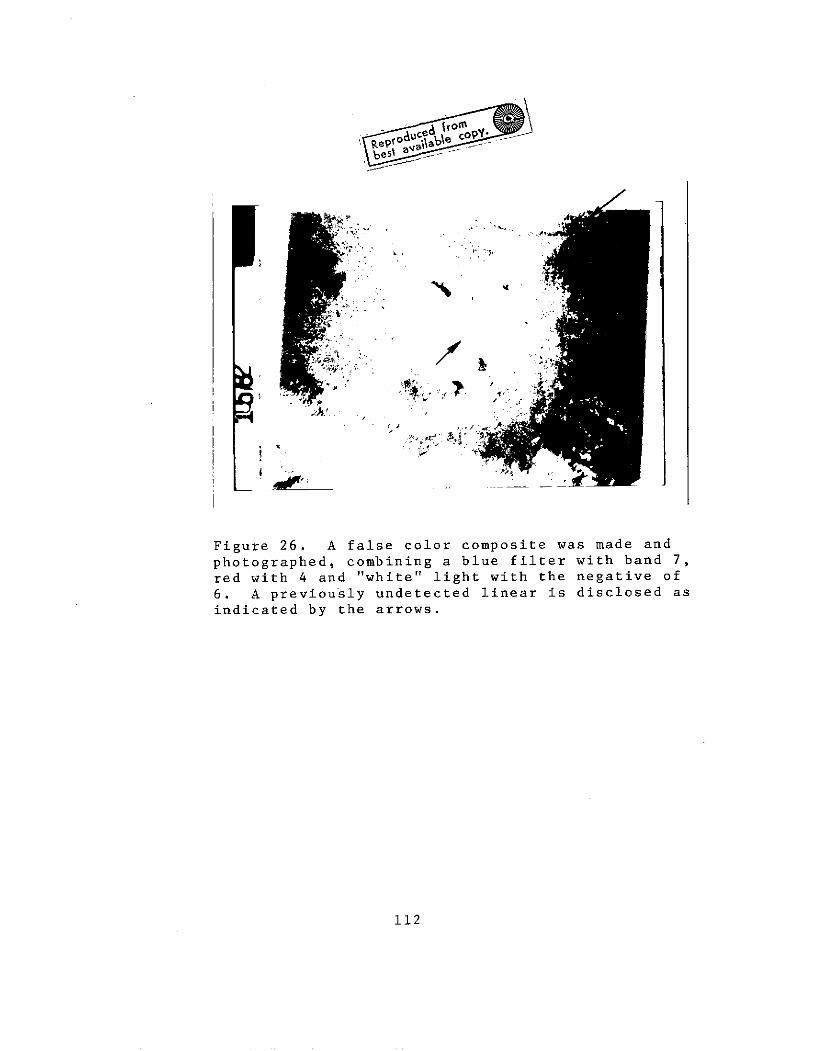
~ceA 1MCOPY-
Figure 26. A false color composite was made and
photographed, combining a blue filter with band 7,
red with 4 and "white" light with the negative of
6. A previously undetected linear is disclosed as
indicated by the arrows.
112

vicinity of the Aledo field. We did not exhaustively test
digital processing. We wanted to assess the value of various
types of processing in terms of their inclusion in an oper-
ational program without attempting to develop the optimum
set of processes for the Anadarko Basin. The processes
used included gray scale adjustment (histogram equalization),
density slicing and stretching and ratioing. Most of the
results were out put as histograms and shade prints.
From this work we conclude that any major operational
use of ERTS data for petroleum exploration should consider
inclusion of digital processing in the form of gray scale
adjustment for at least one band and ratioing of bands 6
and 7 would probably provide the most generally useful
products. Such a program might involve a considerable
amount of "fine tuning" of the programs to the particular
areas. The above conclusion is based not only on our work,
but work by Bernstein (1973), Goetz et al.(1973), and
Vincent (1973).
We found that gray scale adjustment programs (histogram
equalizations) made many linear features stand out and seemed
to make lithologic differences more obvious. However, it
also made field boundaries and roads more obvious (figures
27 and 28).
A ratio of band 6 to band 7 produced a map in which
differences between agricultural fields almost disappeared,
greatly reducing the cultural noise in the scene. However,
113
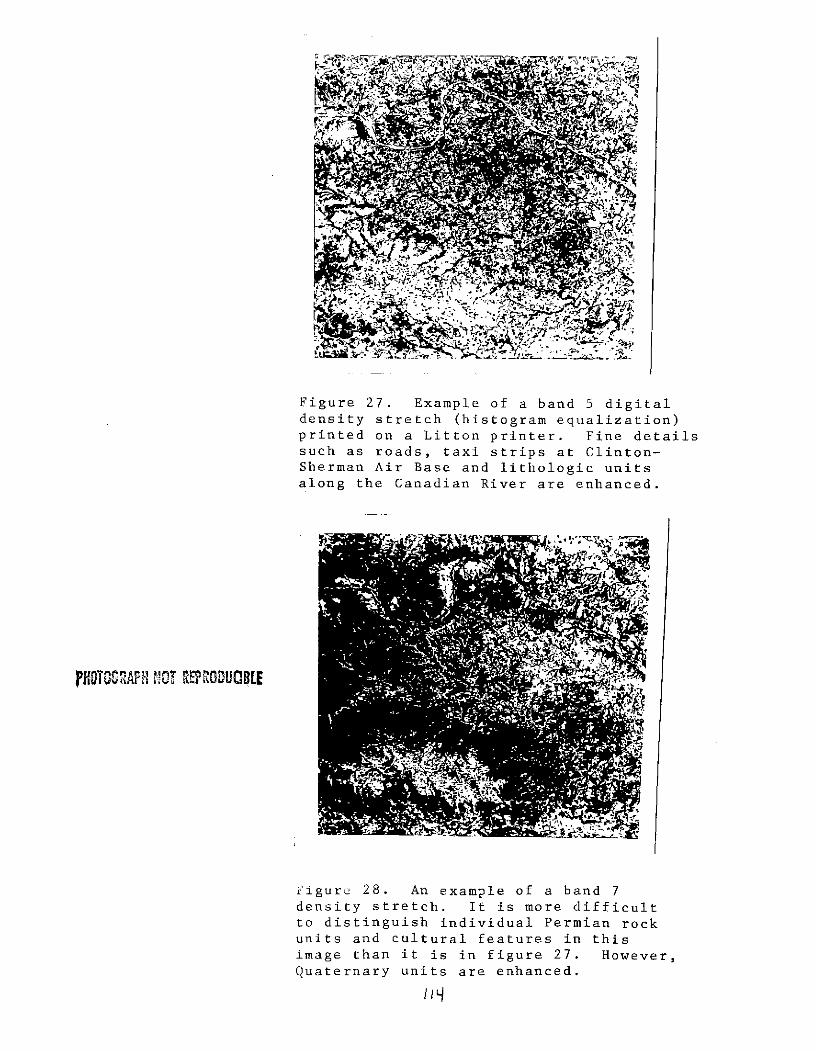
-44~
Figure 27. Example of a band 5 digitaldensity stretch (histogram equalization)printed on a Litton printer. Fine details
such as roads, taxi strips at Clinton-Sherman Air Base and lithologic unitsalong the Canadian River are enhanced.
FROTOCRAF MIT rREF-RODUCKBE
Figur2 28. An example of a band 7
density stretch. It is more difficultto distinguish individual Permian rockunits and cultural features in thisimage than it is in figure 27. However,Quaternary units are enhanced.
/19I

differences among some surficial materials also seemed to
be reduced. Nevertheless, based on our limited work and
the reports by Vincent (1973) and Goetz (1973) we are
convinced these problems could be overcome with further
adjustment and testing.
In summary, an operational program should employ
digital processing to enhance selected areas of particular
interest, at least. It seems that as more programs are
developed and costs drop one should consider applying at
least a gray scale adjustment operation to the entire area
of interest.
115

VIII. ROLE OF ERTS-1 DATA IN EXPLORATION STRATEGY
ERTS-1 data are extremely useful during the initial
phases of petroleum exploration, and can make significant
contributions later in the exploration process. Our work
convinces us that by studying ERTS data one can gain an
understanding of regional lithologic and structural relat-
ionships and rapidly focus attention on areas of exploration
interest, even in an area that is as complex and difficult
from the standpoint of surface exploration as the Anadarko
Basin. Once specific areas of interest are identified
one can derive significant detailed information by
detailed interpretation of these areas on ERTS imagery.
We believe that ERTS imagery will be most important in
the exploration of poorly known areas rather than in
highly developed exploration provinces such as the Anadarko
Basin.
Aspects of ERTS interpretation that are important in
the regional analysis phase of exploration are : mapping
inferred lithology and major structural features, such as
the axes of large synclines and anticlines, mapping of
major fracture systems (if they can be separated from
other linears) and mapping of closed anomalies recognized
on the basis of tone, texture, geomorphology or inferred
structure. Interpretation of this type can be used to
postulate the geologic framework of the region and to
focus attention on specific areas. An interpretation of
116

linear features may contribute to overall understanding at
this point, but we found it helped little. This preliminary
interpretation should be done "blind", that is,without
extensive reference to known or published data. Available
data should be used to refine and modify the preliminary
ERTS interpretation and analysis and to arrive at a regional
synthesis of the geology.
Once this preliminary synthesis is complete, areas
chosen as interesting or anomalous can be examined in
greater detail in order to extract as much information as
possible. It is at this level of study that interpretations
of linears become important because the linears may coincide with
or define alinements of anomalies or may contributeto a
greater understanding of specific anomalies. In explored
petroleum provinces features identified as being of
interest in petroleum exploration should be carefully
examined on the ERTS imagery to see if it is possible to
extract additional information or discern regional relation-
ships. These interpretations and analyses can be used to
plan regional reconnaissance, geological and geophysical
programs, and to begin planning more detailed programs for
specific anomalies. Any anomalies identified in the ERTS
imagery almost certainly would be checked on normal air
photographs before undertaking a seismic survey over them.
In addition to providing the interpretive base for
planning regional surveys, ERTS imagery is an excellent map
117

for planning logistics, overflights, the location of
operations bases, etc.
Because of small scale and low resolution ERTS
interpretation can contribute relatively little during the
detailed phases of exploration. In some instances it
could help in choosing a well site (e.g., locating a well
on the side of a river near access roads instead of the
other side). There may be a few instances where ERTS
might be useful in actual selection of a location (e.g.,
extension of known fracture porosity, extension of known
fields, etc.), but these situations are expected to be rare.
In all instances one would want to obtain confirmation with
the more customary exploration tools.
It is necessary, at all levels of ERTS interpretation,
to continuously integrate ERTS imagery, aircraft acquired
imagery, and ground data. This integration enables the
interpreter to fully understand the information content
of ERTS imagery, to form a geological synthesis and pro-
pose the most reasonable hypotheses.
ERTS provides a means of quickly understanding the
geology of an exploration province and it rapidly focuses
attention on features that may be of exploration interest.
We believe these two advantages will be the main contri-
butions ERTS can make to a petroleum exploration program.
These types of information can greatly reduce the amount
of reconnaissance geological and geophysical work necessary
118

and result in a great saving of time and of man power.
119
IX. PROGRAM COSTS AND BENEFITS
The cost of this experiment is easy to calculate. The
cost of obtaining similar or equivalent information by more
customary means is difficult to estimate principally
because there are a variety of options and hence prices
available for obtaining reconnaissance data. Moreover, the
types of data obtained by the two approaches are not
precisely comparable.
An oil company can obtain regional geophysical and
geological data in any one of several ways. It can:
1. Pay for the survey itself and have the data
on a proprietary basis - very expensive.
2. Join a "group shoot" and pay for and obtain
the data jointly with several other companies -
less expensive.
3. Wait until after reconnaissance surveys are
run and then obtain the data essentially
second hand when it has been released by
the group who paid for the survey - least
expensive and least timely.
The second problem of estimating costs is that the
types of information obtained by ERTS and customary
reconnaissance techniques essentially are not comparable.
ERTS interpretation for instance, provides much more
information on closed anomalies and linears (inferred to
reflect fracture patterns) than customary methods.
120

On the other hand, reconnaissance geologic field work and
seismic and aeromagnetic surveys provide a great deal more
detailed and quantitative data than is obtainable from ERTS.
One method of dealing with this problem is to attempt to
estimate the costs of arriving at a particular common
point in an exploration program with ERTS and without ERTS.
The common point we have tentatively chosen for this com-
parison is the point at which one would begin detailed
surface mapping and begin to plan detailed seismic surveys
and geochemical surveys (if indicated).
The ERTS program in order to be comparable to the
conventional program would have to include the cost of
air photo interpretation, reconnaissance geology, and
seismic work over anomalies identified in the ERTS imagery.
For instance, we found approximately 70 anomalies with an
average radius of 8 kilometers and a total area of about
14,000 square kilometers. On the basis of air photo
interpretation and field work one might choose 30 of these
on which to acquire seismic information. Acquisition
of a cross pattern of seismic information (lines) over
these anomalies would require about 900 line kilometers of
seismic work. The cost of the ERTS data are assumed to be
small and are included in the cost of the interpretation.
Using a customary approach to regional exploration
probably would entail acquiring an.air photo interpretation
and reconnaissance seismic coverage over the entire area.
A reconnaissance seismic survey would require about 4,600
121

line kilometers of shooting (covering the 80,000 square
kilometers area on a 30 x 40 kilometer grid). One probably
would want to obtain a standard airphoto interpretation of
the entire area. Anomalies located with regional seismic
work and airphoto interpretations would be covered with a
cross pattern of seismic lines. For purposes of comparison
we assume that about the same number of anomalies would be
examined in both programs. This would require an additional
900 line kilometers of seismic survey.
Both the conventional and ERTS exploration programs
probably would include reconnaissance aeromagnetic surveys
and regional gravity surveys of the entire area. However,
it is probable that the ERTS interpretation could reduce
the amount of gravity data-required. Both programs would
include a review of available geologic information.
In the conventional survey the reconnaissance seismic
and airphoto interpretation would probably be acquired on
a non-exclusive basis. In the ERTS program the air photo
interpretation would probably be acquired on an exclusive
basis so as not to reveal one's intentions. In both surveys
the seismic work over anomalies would almost certainly be
acquired on an exclusive basis. Under this set of assumptions
(probable mode) the conventional program would cost about
1.6 million dollars and the ERTS program would cost approx-
imately 1.1 million dollars. The ERTS program would represent
approximately a 30% savings over the conventional program.
122

Expenses involved in this comparison between a conven-
tional exploration program and an ERTS-based program are
summarized in the following table.
A. Conventional Program
Non-Exclusive Exclusive Probable Mode
of Acquisition
Reconnaissance SeismicSurvey (4600 Kilometers) $400,000* $5,060,000 $ 400,000
Air Photo Interpretation
(80,000 Square Kilometers) 64,000* 160,000 64,000
Reconnaissance SurfaceGeology 200,000 200,000* 200,000
Seismic Survey Across
Anomalies(900 Kilometers) 76,000 990,000* 990,000
TOTAL $740,000 $6,410,000 $1,664 ,000
B. ERTS Program
Non-Exclusive Exclusive Probable Modeof Acquisition
ERTS InterpretationIncluding Comparisonto Air Photos $ 25,000 $ 25,000* $ 25,000
Seismic Survey AcrossAnomalies (900 Kilometers) 76,000 990,000* 990,000
Air Photo Interpretation
of Anomalies(14,000 Square Kilometers)11,200 28,000* 28,000
Reconnaissance SurfaceGeology Over Anomalies(14,000 Square Kilometers) 35,000 35,000* 35,000
TOTAL $147,000 $1,078,000 $1,078,000
*Indicates probable mode of acquiring the data.
Table 2.Comparison of cost of a regional exploration program:A. Using conventional methods, B. Using ERTS data.
The above represents only one of many possible permuta-
tions and combinations of ways in which the data in each
program could be acquired or exactly what data will be
123

acquired. This last factor depends on the area to be
studied and the experience of the exploration group con-
ducting the study. For instance, it is unlikely that al
of the anomalies found in either program would be covered
by seismic lines. A company could very well choose to
examine only part of a basin in detail based on preliminary
seismic work conducted in either program. Thus the prices
of the two approaches may be nearly the same at one extreme.
At the other extreme, the conventional approach would cost
almost twice as much as the ERTS approach. The costs of
both programs are most sensitive to the amount of seismic
data acquired and to the basis on which it is acquired.
The costs of individual elements of the program can
also vary considerably. For example, field geology in all
but the most straight forward well-developed area (good
roads) would certainly cost considerably more. The same
is true of seismic surveys. Because the conventional
program includes a larger proportion of both these
elements, it is probable that,under most circumstances, the
cost ratios will be even more in favor of the ERTS approach
than is indicated here.
Under almost any set of assumptions the ERTS program
could be executed much morequickly than the conventional
program resulting in a considerable saving of time and
technical manpower. The magnitude or dollar value of this
type of savings is almost impossible to estimate.
124

SAPPENDICES
125

APPENDIX A (Cont.)
ERTS-1 Center Point 9.5"X9.5" 70 mm. Color Tape Date CommentsMSS North West Prt. +Trn Neg. Pos. PI Acquired
Frame I.D. Lat. Long. 4567 4567 4567 4567
1240-16523 39 29'100 28'xxxx xxxx xxxx xxxx x 20Mar73 Excellent - air clear, some sn w1240-16525 36 03'100 55'xxxx xxxx xxxx xxxx x " it ,1240-16532 34 39'101 21'xxxx xxxx xxxx xxxx x x x " i ,1241-16581 37 30'101 54'xxxx xxxx xxxx xxxx 21Mar73 West of study site.1241-16584 36 04'102 21'xxxx xxxx xxxx xxxx " t o , it1241-16590 34 39'102 48'xxxx xxxx xxxx xxxx " i i ,1255-16354 36 04' 96 41'xxxx xxxx xxxx xxxx 4Apr73 East of study site.1255-16361 34 38? 97 07'xxxx xxxx xxxx xxxx " it of t ,,1256-16410 37 30' 97 38'xxxx xxxx xxxx xxxx x x x 5Apr73 Excellent, no clouds, air clea1256-16412 36 05' 98 06'xxxx xxxx xxxx xxxx x x x " , e, ,, ,, ,,1256-16415 34 39' 98 33'xxxx xxxx xxxx xxxx x x x "1257-16464 37 32' 99 05'xxxx xxxx xxxx xxxx x x x 6Apr73 i i1257-16471 36 07' 99 32'xxxx xxxx xxxx xxxx x x x " I n1257-16473 34 41' 99 59'xxxx xxxx xxxx xxxx x x x " .60% Clouds south .1273-16354 36 10' 96 39'xxxx xxxx xxxx xxxx 22Apr73 East of area - scattered cloud1273-16360 34 44' 97 07'xxxx xxxx xxxx xxxx " E o r - cloudy.1274-16405 37 37' 97 35'xxxx xxxx xxxx xxxx x x x 23Apr73 Excellent1274-16412 36 10' 98 03'xxxx xxxx xxxx xxxx x " ,
1274-16414 34 44' 99 30'xxxx xxxx xxxx xxxx x "1275-16473 34 43'100 00'xxxx xxxx xxxx xxxx 24Apr73 Cloudy
Continued

APPENDIX AImagery Supplied by NASA
ERTS-1 Center Point 9.5"X9.5" 70 mm. Color Tape Date CommentsMSS North West Prt. +Trn Neg. Pos. P T Acquired
Frame I.D. Lat. Long. 4567 4567 4567 4567
1004-16403 34 49' 98 16 xx x x 27July72 Cloud1007-16572 35 42'102 14'xxxx xxxx xx x 30July72 West Xf site1077-16461 36 03' 99 13'xxxx xxxx xxxx xxxx 8 0ct72 Good - 5% clouds in N.1077-16463 34 38' 99 41'xxxx xxxx xxxx xxxx " Good - clear1094-16404 35 56' 97 53'xxxx xxxx xxxx xxxx 2 5 0ct72 Good - 15% clouds in N.1094-16411 34 31' 98 16'xxxx xxxx xxxx xxxx x " Fair - scattered clouds1095-16460 37 37' 98 86 xxxx xxxx xxxx 2 60ct72 Cloudy1097-16582 34 28'102 42 xxxx xxxx xxxx xxxx 2 80ct72 Good - west of site1111-16351 35 51' 96 33 xxxx xxxx xxxx 11Nov72 East of site - cloudy1111-16354 34 25' 97 00' xxxx xxxx xxxx " " 11114-16523 36 00'100 4 8'xxxx xxxx xxxx xxxx 14Nov72 Good - clouds east1114-16525 34 34'101 15'xxxx xxxx xxxx xxxx " " " "1130-16404 37 23' 97 2 8'xxxx xxxx xxxx xxxx x x 30Nov72 Good - clear1130-16410 35 57' 97 55'xxxx xxxx xxxx xxxx " " i1130-16413 34 31' 98 2 2 'xxxx xxxx xxxx xxxx x x " " - 15% clouds in SE only1131-16462 37 24' 98 54'xxxx xxxx xxxx xxxx x x x iDec72 " - clear1131-16465 35 58' 99 2 2 'xxxx xxxx xxxx xxxx x x x " " "1131-16471 34 33' 99 4 9'xxxx xxxx xxxx xxxx x x x " " - clear, 5% snow in NW1132-16521 37 22'100 2 1'xxxx xxxx xxxx xxxx x x 2Dec72 " - " 30% " " SW1132-16523 35 56'100 4 8 'xxxx xxxx xxxx xxxx x x " - " 50% NW1132-16530 34 30'101 15'xxxx xxxx xxxx xxxx " " i1220-16405 37 26' 97 3 3 'xxxx xxxx xxxx 28Feb73 Cloudy1221-16473 34 36' 99 55'xxxx xxxx xxx IMar73 Cloudy1222-16531 34 36'101 2 0'xxxx xxxx xxxx 2Mar73 SW of area1223-16590 34 37'102 4 6 'xxxx xxxx xxxx 3Mar73 West of area1237-16354 36 01' 96 39'xxxx xxxx xxxx xxxx x 17Mar73 Excellent - east of area1237-16360 34 34' 97 06'xxxx xxxx xxxx xxxx x " " , i1238-16410 37 26' 97 3 7'xxxx xxxx xxxx 18Mar73 Fair - scattered clouds1238-16412 36 00' 98 04'xxxx xxxx xxxx " ,,1238-16415 34 35' 98 3 1'xxxx xxxx xxxx
Continued
APPENDIX A (Cont.)
NASA Aerial Photography
70 mm. B/W TIR Scanner
240 mm. Color I-R 1:110,000
240 mm. Color I-R 1:55,000
240 mm. Color 1:110,000
70 mm. Color
70 mm. Color I-R
70 mm. B/W Pan
70 mm. B/W I-R
70 mm. B/W Green
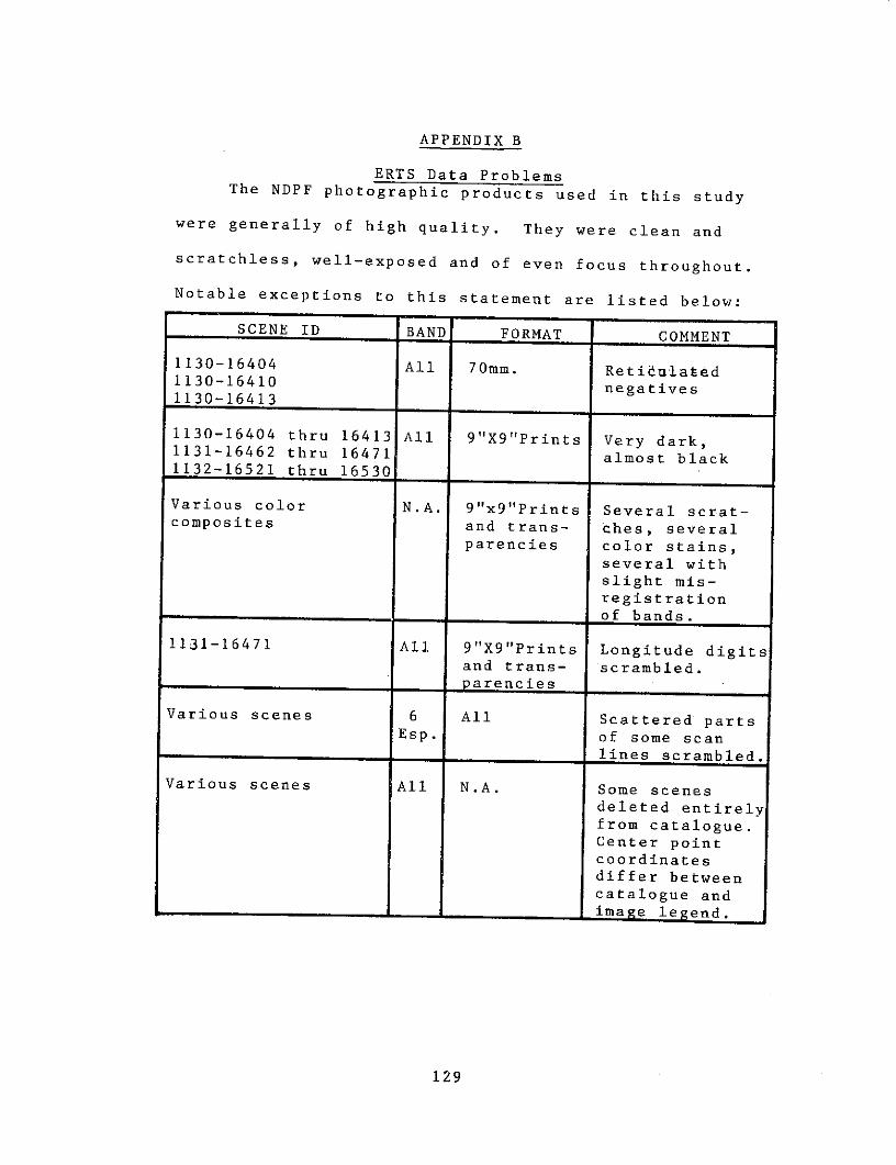
APPENDIX B
ERTS Data ProblemsThe NDPF photographic products used in this study
were generally of high quality. They were clean and
scratchless, well-exposed and of even focus throughout.
Notable exceptions to this statement are listed below:
SCENE ID BAND FORMAT COMMENT
1130-16404 All 70mm. RetiduIated1130-16410
negatives1130-16413
1130-16404 thru 16413 All 9"X9"Prints Very dark,1131-16462 thru 16471 almost black1132-16521 thru 16530
Various color N.A. 9 "x9"Prints Several scrat-composites and trans- ches, several
parencies color stains,several withslight mis-registrationof bands.
1131-16471 All 9"X9"Prints Longitude digitsand trans- scrambled.parencies
Various scenes 6 All Scattered partsEsp. of some scan
lines scrambled.
Various scenes All N.A. Some scenesdeleted entirelyfrom catalogue.Center pointcoordinatesdiffer between
catalogue andimage legend.
129

In addition, there are two problems which persist
throughout the imagery. These are mislocation of
latitude and longitude tick marks and scale problems.
Tickmarks for latitude and longitude are consistently
in error when judged by existing topographic and base
maps. The errors range up to 4 kilometers in any
direction and are not appreciably better on Fall 1972
or Spring 1973 images. Tickmarks locating lines of
latitude and longitude within one kilometer at
1:1,000,000 would be satisfactory for our purposes.
One scene was even found to have the tick marks
rotated slightly so that lines of equal latitudes
run slightly north of east. Consequently, whenever
necessary, we had to determine exact lines of
latitude and longitude for ourselves. We simply
cannot assume the correctness of the lines as located
by tick marks. Scale problems were serious only when
making and using regional maps. Existing U.S.G.S.
base maps are of a scale slightly smaller than
1:1,000,000 while the scale of the images is slightly
greater than this. Mismatch in scale between images
and maps is about 5 kilometers across the study
site (350 km.)
1.30

APPENDIX C
ERTS Descriptor Forms
131

ERTS IMAGE DESCRIPTOR FORM(See Instructions on Back)
NDPF USE ONLY
DATE February 2, 1974 D
PRINCIPAL INVESTIGATOR Dr. Robert J. CollinsID ID______
GSFC PR -043
ORGANIZATION Eason Oil Company
PRODUCT ID FREQUENTLY USED DESCRIPTORS*(INCLUDE BAND AND PRODUCT) DESCRIPTORS
la. 1077-16463-M oil field, basementrock, alluvial terrac,lineament, aquifer,lake, alluvium,(RedRiver, Okla.-Texas),
agridultre, braidedstream, erosion
lb. 1077-16461-M lineament, lake, dune
clouds, airfield,(Elk
City, Okla.), (Canadian
River, Okla), basin,
barbed tributary,
alluvial terrace,erosion, oil field,meander, highway,
agriculture, pipelineirrigation, Woodward,
Oklahoma)
2 1094-16404-M lake, braided stream,
Oklahoma City, dam,
salt flat, erosion,
alluvial terrace, barbed tributary, bimarr n
River, Okla., (CanadiaiRiver, Okla., lineame t,
oil field, meander,quarry, airfield,channelized stream,
urban area, highway.
FOR DESCRIPTORS WHICH WILL OCCUR FREQUENTLY, WRITE THE DESCRIPTOR TERMS IN THESECOLUMN HEADING SPACES NOW AND USE A CHECK (/) MARK IN THE APPROPRIATE PRODUCTID LINES. (FOR OTHER DESCRIPTORS, WRITE THE TERM UNDER THE DESCRIPTORS COLUMN).
MAIL TO ERTS USER SERVICESCODE 563BLDG 23 ROOM E413NASA GSFCGREENBELT, MD. 20771301-982-5406
GSFC 37-2 (7/72)
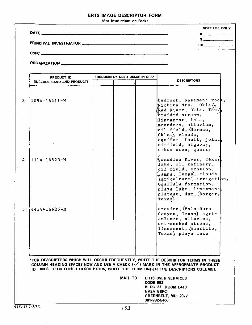
ERTS IMAGE DESCRIPTOR FORM(See Instructions on Back)
NDPF USE ONLYDATE D
NPRINCIPAL INVESTIGATOR ID
GSFC
ORGANIZATION
PRODUCT ID FREQUENTLY USED DESCRIPTORS*(INCLUDE BAND AND PRODUCT) - DESCRIPTORS
3 1094-16411-M bedrock, basement roc,
ichita Mts., Okla ),Red River, Okla.-Tex.,braided stream,lineament, lake,
meanders, alluvium,oil field, (Norman,
Okla.), clouds,
aquifer, fault, joint,airfield, highway,urban area, quarry
4 1114-16523-M Canadian River, Texas,lake, oil refinery,
oil field, erosion,Pampa, Texas), clouds,
agriculture, irrigation,
Ogallala formation,playa lake, lineament,
plateau, dam, (Borger,Texas
51 '1-1416525-M erosion, (Palo-Duro
Canyon, Texas agri-culture, alluvium,entrenched stream,
lineament, (Amarillo,
Texas) playa lake
*FOR DESCRIPTORS WHICH WILL OCCUR FREQUENTLY, WRITE THE DESCRIPTOR TERMS IN THESECOLUMN HEADING SPACES NOW AND USE A CHECK (/) MARK IN THE APPROPRIATE PRODUCTID LINES. (FOR OTHER DESCRIPTORS, WRITE THE TERM UNDER THE DESCRIPTORS COLUMN).
MAIL TO ERTS USER SERVICESCODE 563BLDG 23 ROOM E413NASA GSFCGREENBELT, MD. 20771301-982-5406
GSFC 37-2 (7/72)

ERTS IMAGE DESCRIPTOR FORM(See Instructions on Back)
NDPF USE ONLYDATE D
NPRINCIPAL INVESTIGATOR ID
GSFC
ORGANIZATION
PRODUCT ID FREQUENTLY USED DESCRIPTORS*(INCLUDE BAND AND PRODUCT) DESCRIPTORS
6 1130-16404-M lake, (Arkansas River,
Kansas, salt flat,
lineament, (Wichita,Kansas)
7 1130-16410-M lake, braided stream,
Oklahoma City, dam,
salt flat, erosion,alluvial terrace,barbed tributary,Cimarron River, Okla.,Canadian River, Okla.,lineament, oil field,meander, quarry,airfield, channelizedstream, urban area,highway
8 1130-16413-M bedrock, basement
rock, (Wichita Mts.,
Okla.), (Red River
Okla.-Tex.), braidedstream, lineament,
lake, meanders,
alluvium, oil field,
Lawton, Okla),aquifer,
fault, joint, wild-
life refuge, airfieldFort Sill, Okla.),highway, urban area,
quarry
*FOR DESCRIPTORS WHICH WILL OCCUR FREQUENTLY, WRITE THE DESCRIPTOR TERMS IN THESECOLUMN HEADING SPACES NOW AND USE A CHECK (,/) MARK IN THE APPROPRIATE PRODUCTID LINES. (FOR OTHER DESCRIPTORS, WRITE THE TERM UNDER THE DESCRIPTORS COLUMN).
MAIL TO ERTS USER SERVICESCODE 563BLDG 23 ROOM E413NASA GSFCGREENBELT, MD. 20771301-982-5406
GSFC 37-2 (7/72) 34

ERTS IMAGE DESCRIPTOR FORM(See Instructions on Back)
NDPF USE ONLY
DATE D
NPRINCIPAL INVESTIGATOR ID
GSFC
ORGANIZATION
PRODUCT ID FREQUENTLY USED DESCRIPTORS*
(INCLUDE BAND AND PRODUCT) - DESCRIPTORS
9 1131-16462-M lake, salt flat,dune,Cimarron River, Okla-Kansas) lineament,
agriculture
10 1131-16465-M lineament, lake,dune,
snow, airfield,(Elk
City, Okla),(Canadian
River, Okla.), basin,
barbed tributary,
alluvial terrace,erosion, oil field,
meander, highway,
agriculture, pipeline,irrigation, Woodward,
Oklahoma)
11 1131-16471-M oil field, basement
rock, alluvial terrace,
lineament, aquifer,
lake, alluvium,( Red
River, Okla.,-Texas),
agriculture, braided
stream, erosion
*FOR DESCRIPTORS WHICH WILL OCCUR FREQUENTLY, WRITE THE DESCRIPTOR TERMS IN THESE
COLUMN HEADING SPACES NOW AND USE A CHECK (/) MARK IN THE APPROPRIATE PRODUCTID LINES. (FOR OTHER DESCRIPTORS, WRITE THE TERM UNDER THE DESCRIPTORS COLUMN).
MAIL TO ERTS USER SERVICESCODE 563BLDG 23 ROOM E413NASA GSFCGREENBELT, MD. 20771301-982-5406
GSFC 37-2 (7/72) / 3

ERTS IMAGE DESCRIPTOR FORM(See Instructions on Back)
NDPF USE ONLYDATE D
NPRINCIPAL INVESTIGATOR ID
GSFC
ORGANIZATION
PRODUCT ID FREQUENTLY USED DESCRIPTORS*(INCLUDE BAND AND PRODUCT) DESCRIPTORS
12 1132-16523-M plateau, lake, sanddune, snow,refinery,highway, lineament,dam, agriculture,playa lake, (CanadianRiver, Tex.-Okla.),oil field, irrigation,P ampa, Tex.), (Borger,
Tex.), (Sh amrock, Tex.,
Ogallala formation
13 1132-16530-M erosion, Palo-Duro
Canyon, Tex.), agri-
culture, alluvium,entrenched stream,lineament, (Amarillo,Tex.), playa lake
14 1221-16473-M Red River, Okla..-Tex ),lake, agriculture,wildlife refuge,cloud
15 1237-16354-M OKC,Okla), Tulsa,Okla)No. Canadian R.,Okla),
Cimmaron R., Okla.,)
Arkansas R., Okla.)
lake, Deep Fork R.
16 1237-16360-M Lake Texhoma, Okla.,-Tex)., Arbuckle Mts.,
Okla, lake, Norman,Okla) ,(Red River, Okla,-Tex), bedrock, (Cont.)
r*FOR DESCRIPTORS WHICH WILL OCCUR FREQUENTLY, WRITE THE DESCRIPTOR TERMS IN THESECOLUMN HEADING SPACES NOW AND USE A CHECK (,/) MARK IN THE APPROPRIATE PRODUCTID LINES. (FOR OTHER DESCRIPTORS, WRITE THE TERM UNDER THE DESCRIPTORS COLUMN).
MAIL TO ERTS USER SERVICESCODE 563BLDG 23 ROOM E413NASA GSFCGREENBELT, MD. 20771301-982-5406
GSFC 37-2 (7/72) ) 3€

ERTS IMAGE DESCRIPTOR FORM(See Instructions on Back)
NDPF USE ONLY
DATE D
NPRINCIPAL INVESTIGATOR ID
GSFC
ORGANIZATION
PRODUCT ID FREQUENTLY USED DESCRIPTORS*
(INCLUDE BAND AND PRODUCT) DESCRIPTORS
16 1237-16360-M cotd, anticline, fault,lineament, silt
17 1240-16525-M plateau, lake, sanddune, refinery, high-way, lineament, dam,agriculture, playa la ke,Canadian River,Tex.-Okla.), oil field,irrigation,( Pampa,Tex.) Borger, Tex.),Shamrock, Tex.), Ogal-lala formation
18 1240-16532-M erosion, (Palo-DuroCanyon, Texas), agri-culture, alluvium,entrenched stream,lineament, (Amarillo,Texas.), playa lake
19 1255-16361-M ake Texhoma, Okla.-Tex),(Arbuckle Mts.,Okla.), lake,(Norman,Okla),(Red River, Okli.Tex.), bedrock, anti-cline, fault, linea-ment, silt
*FOR DESCRIPTORS WHICH WILL OCCUR FREQUENTLY, WRITE THE DESCRIPTOR TERMS IN THESECOLUMN HEADING SPACES NOW AND USE A CHECK (./) MARK IN THE APPROPRIATE PRODUCTID LINES. (FOR OTHER DESCRIPTORS, WRITE THE TERM UNDER THE DESCRIPTORS COLUMN).
MAIL TO ERTS USER SERVICESCODE 563BLDG 23 ROOM E413NASA GSFCGREENBELT, MD. 20771301-982-5406
GSFC 37-2 (7/72) 131

ERTS IMAGE DESCRIPTOR FORM(See Instructions on Back)
NDPF USE ONLYDATE D
NPRINCIPAL INVESTIGATOR IDID______
GSFC
ORGANIZATION
PRODUCT ID FREQUENTLY USED DESCRIPTORS*
(INCLUDE BAND AND PRODUCT) - DESCRIPTORS
20 1256-16412-M lake, braided stream,
Oklahoma City, dam,
salt flat, dune,
erosion, alluvial
terrace, barbed tri-
butary, (Cimarron R.,
Okla.), (Canadian R.,
Okla.), lineament,oil field, meander,
quarry, airfield,channelized stream,
urban area, highway
21 1256-16415-M bedrock, basement
rock, (Wichita Mts.,Okla.), (Red River,
Okla.-Tex.), braided
stream, lineament,lake, meanders,
alluvium, oil field,awton, Okla.), aquifer,
fault, joint, wild-
life refuge, airfielc
ort Sill, Okla)highway, urban area,
quarry
22a 1257-164c71-M lineament, lake, duneairfield, (Elk City,
Okla.), (Canadian R.,
Okla.), basin, barbed
tributary,alluvial
terrace, erosion, (Co t)
*FOR DESCRIPTORS WHICH WILL OCCUR FREQUENTLY, WRITE THE DESCRIPTOR TERMS IN THESECOLUMN HEADING SPACES NOW AND USE A CHECK (/) MARK IN THE APPROPRIATE PRODUCTID LINES. (FOR OTHER DESCRIPTORS, WRITE THE TERM UNDER THE DESCRIPTORS COLUMN).
MAIL TO ERTS USER SERVICESCODE 563BLDG 23 ROOM E413NASA GSFCGREENBELT, MD. 20771301-982-5406
GSFC 37-2 (7/72)

ERTS IMAGE DESCRIPTOR FORM(See Instructions on Back)
NDPF USE ONLYDATE D
NPRINCIPAL INVESTIGATOR ID
GSFC
ORGANIZATION
PRODUCT ID FREQUENTLY USED DESCRIPTORS*(INCLUDE BAND AND PRODUCT) - DESCRIPTORS
22a 1257-16471-M oil field, meander,highway, agriculture,ipeline, irrigation,oodward, Okla
22b 1257-16473-M oil field, basementrock, alluvial terrace,lineament, aquifer,lake, clouds, alluvium,
ed River, Okla.-Tex.agriculture, braidedstream, erosion
22c 1274-16412-M lake, braided stream,Oklahoma City, dam,salt flat, dune, ero-sion, alluvial terracarbed tributary,Cimarron R., Okla.,Canadian R., Okla),lineament, oil field,meander, quarry,airfield, channelizedstream, urban area,highway
23 1274-16414-M bedrock, basementrock, (Wichita Mts.,Okla,), braided streamlineament, lake,meanders, alluvium,oil field, aquifer,fault, ioint.(cont.)
*FOR DESCRIPTORS WHICH WILL OCCUR FREQUENTLY, WRITE THE DESCRIPTOR TERMS IN THESECOLUMN HEADING SPACES NOW AND USE A CHECK (7) MARK IN THE APPROPRIATE PRODUCTID LINES. (FOR OTHER DESCRIPTORS, WRITE THE TERM UNDER THE DESCRIPTORS COLUMN).
MAIL TO ERTS USER SERVICESCODE 563BLDG 23 ROOM E413NASA GSFCGREENBELT, MD. 20771301-982-5406
GSFC 37-2 (7/72)

ERTS IMAGE DESCRIPTOR FORM(See Instructions on Back)
NDPF USE ONLY
DATE D_,
NPRINCIPAL INVESTIGATOR ID
GSFC
ORGANIZATION
PRODUCT ID FREQUENTLY USED DESCRIPTORS*(INCLUDE BAND AND PRODUCT) - DESCRIPTORS
23 1274-16414-M wildlife refuge,
airfield, highway,urban area.
FOR DESCRIPTORS WHICH WILL OCCUR FREQUENTLY, WRITE THE DESCRIPTOR TERMS IN THESECOLUMN HEADING SPACES NOW AND USE A CHECK (/) MARK IN THE APPROPRIATE PRODUCTID LINES. (FOR OTHER DESCRIPTORS, WRITE THE TERM UNDER THE DESCRIPTORS COLUMN).
MAIL TO ERTS USER SERVICESCODE 563BLDG 23 ROOM E413NASA GSFCGREENBELT, MD. 20771301-982-5406
GSFC 37-2 (7/72) 0

APPENDIX DAcronyms
CCT Computer Compatible Tapes
EOC Eason Oil Company
IR Infrared
MSS MultiSpectral Scanner
NASA National Aeronautics and Space Administration
NDPF NASA Data Processing Facility
OGS Oklahoma Geological Survey
RBV Return Beam Vidicon
SAC Strategic Air Command
SLAR Side Looking Airborne Radar
TIR Thermal Infrared
141

XI. BIBLIOGRAPHY
Abels, T. A. (1959), A subsurface lithofacies study ofthe Morrowan series in the northern Anadarko Basin:Shale Shaker, v.9, n.7, p.5.
Allen, A. E. (1955), The subsurface geology of Woodsand Alfalfa Counties, northwestern Oklahoma: ShaleShaker, v. 4, n.8, p.5.
Anderson, E. M. (1951), The dynamics of faulting and dykeformation with applications to Britain 1972, reprintof 1951 edition: Hafner Pub. Co., N. Y., 206 pp.
Ardmore Geology Society, Petroleum geology of southernOklahoma, a symposium: Tulsa, Okla., Am. Assoc.Petrol. Geologists, vol. 1 (1956), 402 pp., vol. 2(1959), 341 pp.
Beams, R. J. (1951), Geology of the Elk City field (Oklahoma)(abstract), Shale Shaker, v.1, n. 10, p. 8 .
Bernstein, R. (1973), Scene correction (precision proces-sing) of ERTS sensor data using digital image pro-cessing techniques: National Aeronautics and SpaceAdministration, Third ERTS symposium, Washington, D.C.,December 10-14, p. 112 (abstract).
Blazenko, E. J. (1964), Geology of the south Erick gasarea Beckham and Greer Counties, Oklahoma: ShaleShaker, V. 15, n.4, p. 53.
Boler, M. E. (1959), Pre-Desmoinesian isopach and paleo-geologic study of northwestern Oklahoma: Shale Shaker,v. 9, n.10, p.6.
Bowles, P. F. (1959), Subsurface geology of Woods County,Oklahoma: Shale Shaker, v.10, n.4, p.2.
Braun, J. C. (1959), A stratigraphic study of the Sycamoreand related formations in the southeastern AnadarkoBasin, Shale Shaker, v.10, n.l, p.6.
Brown, H. A. (1967), Structural control of the CanadianRiver in western Oklahoma: Shale Shaker, v.18, n.3.,p. 42.
Culp, C. K. (1961), Stratigraphic relations of the SycamoreLimestone (Mississippian) in southern Oklahoma: ShaleShaker, v.11, n.10, p.7.
142

Cunningham, B. J. (1961), Stratigraphy: Oklahoma-TexasPanhandles, in Oil and gas fields of the Texas andOklahoma Panhandles: Panhandle Geol. Soc., p. 45.
Davis, H. G. (1971), The Morrow-Springer trend, AnadarkoBasin, target for the 70's: Shale Shaker, v.22,n.3, p.64.
Dietrich, R. F. (1955), Simpson group along the northflank of the Anadarko Basin: Shale Shaker, v.5,n.5, p.5.
Dietz, G. P. (1967), The geology of the Gageby Creek FieldWheeler County, Texas: Shale Shaker, v. 17, n.7, p.137.
Doeringsfeld, W. W. and Ivey, J. B. (1964), Use of photo-geology and geomorphic criteria to locate subsurfacestructure: The Mountain Geologist, v.1, n.4, p.183.
Eddleman, M. W. (1961), Tectonics and geologic history ofthe Texas and Oklahoma Panhandles, in Oil and gasfields of the Texas and Oklahoma Panhandles: Pan-handle Geological Soc., 264 pp.
Fay, R. O. (1959), Guide to Roman Nose state park, BlaineCounty, Oklahoma: Okla. Geol. Surv. Guidebook 9, 31 pp.
Fay, R. O. and Ham, Bado, Jordan, (1962), Geology andmineral resources of Blaine County, Oklahoma: Okla.Geol. Surv., Bull. 89, 258 pp.
Flawn, P. T. (1956), Basement rocks of Texas and southeastNew Mexico: Univ. of Texas Pub. No. 5606, 261 pp.
Forgotson, J. A. (1969), Factors controlling occurrence ofMorrow sandstones and their relation to production inthe Anadarko Basin: Shale Shaker, v. 20, n.2, p.24.
Freie, A. J. (1930), Sedimentation in the Anadarko Basin:Okla. Geol. Surv. Bull. 48, 80 pp.
Gelphman, N. R. (1960), West Sentinel oil field, WashitaCounty, Oklahoma: Sedimentology of the granite washand structural geology: Shale Shaker, v.10, n.6,p.2.
Gibbons, K. E. (1962), Pennsylvanian of the north flank ofthe Anadarko Basin: Shale Shaker, v.12, n.5, p.2.
Goetz, A. F. H. and Billingsley, F. C. (1973), Digitalimage enhancement techniques used in some ERTSapplication problems: NASA, Third ERTS Symposium,Washington, D.C., December 10-14, p. 1 1 4 (abstract).
143

Gouin, Frank (1956), Surface criteria of southern Oklahomaoil fields: Petrol. Geol. of Southern OklahomaSymposium, Ardmore Geol. Soc. V.1, p. 1 4 .
Gould, D. B. and Anderson, R. L. (1957), Applications ofphotogeology to the Panhandle area: PanhandleGeonews, v.4, n.3, p.7.
Ham, W. E., Denison, R. E. and Merritt, C. A. (1964),Basement rocks and structural evolution of southernOklahoma: Okla. Geol. Surv., Bull.95, 302 pp., 16plates.
Harlton, B. H. (1951), Faults in sedimentary part ofWichita Mountains of Oklahoma: in Bull. AAPG v.35,n.5, p 988.
Harlton, B. H. (1963), Frontal Wichita fault system ofsouthwestern Oklahoma: Am. Assoc. Petrol. Geol.Bull., v.47, p.1552.
Harlton, B. H. (1972), Faulted fold belts of southernAnadarko Basin adjacent to frontal Wichitas: Am.Assoc. Petrol Geol. Bull., v.56, p.1544.
Harp, L. J. (1966), Do not overlook fractured zones:World Oil, v.162, n.5, p.119.
Harris, S. A. (1970), Bends of the South Canadian: ShaleShaker, v.20., n.5, p.80.
Hayes, L. N. (1955), A study of the subsurface geologyof the northeastern part of Comanche County, Oklahoma:Shale Shaker, v.3, n.2, p.5.
Herrman, L. A. (1961), Structural geology of the Cement-Chickasha area, Caddo and Grady Counties, Oklahoma:Am. Assoc. Petrol. Geologists Bull., v.45, p.1791.
Huffman, G. G. (1959), Pre-DesMoinesian isopachous andpaleogeologic studies in central mid-continent region:Am. Assoc. Petrol.Geologists Bull., v.43, p.2541.
Irwin, J. H. and Morton, R. B. (1969), Hydrogeologicinformation on the Glorieta Sandstone and the Ogallalaformation in the Oklahoma Panhandle and adjoiningareas as related to underground waste disposal:U. S. Geol. Surv. Circular 630, 26 pp., 4 plates.
Johnson, K. S. (1962), Areal geology of the Sentinel-Gotebo area, Kiowa and Washita Counties, Oklahoma:Univ. of Okla., M. S. Thesis, 99 pp.
144

Johnson, K. S. et al (1972), Geology and earth resourcesof Oklahoma: Okla. Geol. Surv. Educational Publ. 1,8 pp.
Jordan, L. and Vosburg, D. L. (1963), Permian salt andassociated evaporites in the Anadarko Basin of thewestern Oklahoma-Texas Panhandle region: Okla.Geol. Surv. Bull. 102, 76 pp.
Kitts, D. B. (1959), Cenozoic geology of northern RogerMills County, Oklahoma: Okla. Geol. Surv. Circular48, 48 pp.
Kitts, D. B. (1965), Cenozoic geology of Ellis County:Okla. Geol. Surv. Circular 69, 32 pp.
Lang, R. C. (1951), A geological cross section from theWichita Mountains to the Elk City pool: ShaleShaker, v.1, n.7, p.7.
Lintz, Joseph, Jr., (1972), Remote sensing for petroleum:Am. Assoc. Petrol.Geol. Bull., v. 56, n.3, p542.
MacLachlan, M. E. (1964), The Anadarko Basin' U.S.G.S.report prepared on behalf of U.S. Atomic EnergyCommission, Report TEI-831, March 1964, 76 pp.
MacLachlan, M. E. (1967), Paleotectonic investigationsof the Permian system in the U.S.: Oklahoma. InMcKee, E. D., et al., paleotectonic investigationsof the Permian system in the U.S.: U.S. Geol.Surv. Prof. Paper 515, 271 pp.
McDaniel, G. A., (1959), Isopachous and paleogeologicstudies of southwest Oklahoma: Shale Shaker, v.10,n.3, p.4.
McNeal, R. P. (1953), Subsurface geology of south-centralAnadarko Basin, Oklahoma: Am. Assoc. Petrol. Geol.Bull., v.37, n.12, p.2677.
McNeal, R. P. (1952), The stratigraphy and tectonics ofWashita, Beckham and Roger Mills Counties, Oklahoma:Shale Shaker, v.2, n.10, p.5.
Melton, F. A. (1934), Fracture systems in central Texas:in v. 2 of the geology of Texas: structural andeconomic geology: p.118, Univ. of Texas Bull. n. 3401,884 pp.
Melton, F. E. (1955), Photo-geology in "flatland" regionof low dip: Shale Shaker, v.6, n.3, p.5.
145

Melton, F. E. (1959), Aerial photographs and structuralgeomorphology: Jour.Geol., v.67, n.4, p.351.
Melton, F. A. (1956), Problems of the photogeologist in"flatland" regions of low dip: Photogrammetric Engin-eering, v.22, n.1, pp. 52-63.
Moody, J. D. and M. J. Hill (1956), Wrench fault tectonics:in Bull. G. S. A., v.67, n.9, p.1207.
Murray, A. N. (1953), Identification of geological form-ations by growing vegetation: Shale Shaker v.4, n.4,p. 5 .
Nicholson, J. H. (1960), Geology of the Texas Panhandle,p. 51, in aspects of the geology of Texas: Asymposium: Univ. of Texas, Pub. No. 6017, 117 pp.
Oil and Gas in Oklahoma (1928), V. 1, 288 pp., Okla. Geol.Surv. Bull. 40.
Oil and Gas in Oklahoma (1930), V. 2, 501 pp., Okla. Geol.Surv. Bull.40.
Oklahoma City Geological Society (1963), Oil and GasFields of Oklahoma, v. 1: Cramer, R. D. et al, editorsOklahoma City, Oklahoma.
Panhandle Geological Society (1961), Oil and gas fields ofthe Texas and Oklahoma Panhandles, a symposium, 264 pp.
Panhandle Geological Society (1969), Stratigraphic Com.,W. M. Quackenbush, Chairman; Pre-Pennsylvanian Geologyof the western Anadarko Basin, 34 pp., 12 plates.
Powell, B. P. H. (1953), The subsurface geology of WoodwardCounty, Oklahoma, v.4, n.l.
Rascoe, B. (1962), Regional stratigraphic analysis ofPennsylvanian and Permian rocks in western mid-con-tinent, Colorado, Kansas, Oklahoma, Texas: Bull.Am. Assoc. Petrol. Geologists, v.46, n.8, p.1345.
Reed, L. C. and 0. M. Longnecker(1932), The geology ofHemphill County, Texas: Univ. of Texas, Bur. ofEcon. Geol., Bull. n. 3231, 98 pp.
Richardson, J. L. (1970), Areal Geology of westernWashita County, Oklahoma: Univ. of Oklahoma,M. S. Thesis, 67 pp.
146

Riggs, Richard M. (1957), Thrust faulting along the WichitaMountain front: Shale Shaker, v.8, n.4, p.7.
Sahl, H. L. (1970), Mobeetie field Wheeler County, Texas:Shale Shaker, v.20, n.6, p. 108.
Schramm, M. W. (1967), Application of trend analysis topre-Morrow surface, southeastern Hugoton Embaymentarea: Shale Shaker, v.18, n.2, p.27.
Scott, G. L. (1955), Areal geology of portions of Beckham,Greer, Kiowa, and Washita Counties, Oklahoma: Univ.of Oklahoma, M. S. Thesis, 108 pp.
Scott, G. L. and William E. Ham (1957), Geology and gypsumresources of the Carter area, Oklahoma: OGS Cir. 42,64 pp.
Scott, R. L. (1968), The exploratory significance ofgravity in the Anadarko Basin: Shale Shaker v.18,n.7, p. 132.
Sellards, E. H. and W. S. Adkins and F. B. Plummer (1932),The geology of Texas, v.1, Stratigraphy: Univ. ofTexas Bull. 3232, 1007 pp.
Sellards,E. H. and C. L. Baker (1934), The geology ofTexas, v.2, structural and economic geology: Univ.of Texas Bull. 3401, 884 pp.
Slate, H. L. (1962), Petroleum geology of the Taloga-CusterCity area, Dewey and Custer Counties, Oklahoma:Shale Shaker, v.13, n.3, p.2.
Swanson, D. C. (1967), Some major factors controlling theAccumulatioof hydrocarbons in the Anadarko Basin:Shale Shaker, v.17, n.6, p.106.
Takken, S. (1967), Subsurface geology of the north GateboArea, Oklahoma: Shale Shaker, v.17, n.6, p.115.
Tanaka, H. H. and L. V. Davis (1963), Groundwater resourcesof the Rush Springs Sandstone in the Caddo Countyarea, Oklahoma: Okla. Geol. Surv. Circ. 61, 63 pp.
Totten, R. B. (1956), General Geology and historical Devel-opment, Texas and Oklahoma Panhandles: in Bull. AAPGv. 40, n.8, p.1945.
Trollinger, William V. (1968), Surface evidence of deepstructure in the Anadarko Basin: Shale Shaker, v.18,n.8, p. 162.
147

Tutten, William D., (1973), Geology and development ofWashita Creek field: Shale Shaker, v.23, n.8, p. 180.
Vincent, R. K. (1973), Ratio maps of iron ore depositsAtlantic City district, Wyoming: Nat. Aeronauticsand Space Admin. Symposium on significant 'resultsobtained from the Earth Resources Technology Satellite-l.Washington, D. C., March 5-9, NASA SP-327, v.1, sec.A, p. 379.
Walper, J. L. (1970), Wrench faulting in the mid-continent:Shale Shaker, v.21, n.2, p.32.
Weinkauf, D. G. (1968), Field study of the southeast Wood-ward gas field, Woodward County, Oklahoma: ShaleShaker, v.18, n.10, p.207.
Wheeler, R. R. (1951), Origin and oil possibilities of theAnadarko Basin: Shale Shaker, v.2, n.2, p.4.
Withrow, P. C. (1966), Early exploration in the AnadarkoBasin: Shale Shaker, v.16, n.8, p.183.
Withrow, P. C. (1967), The discovery of oil in the AnadarkoBasin: Shale Shaker, v.17, n.6, cover.
Withrow, Phil C. (1968), Oklahoma's early oil industry:Shale Shaker, v.5, p.449.
Wrobleski, E. F. (1967), Exploration problems in the deepAnadarko Basin: Shale Shaker, v.17, n.7, p.131.
148

Maps
Amsden, T. W. and Rowland, T. L. (1967), Geologic maps
and stratigraphic cross sections of Silurian strata
and lower Devonian formations in Oklahoma: Okla.
Geol. Survey, Map GM-14.
Arbenz, J. K. (1956), Tectonic map of Oklahoma: Okla.
Geol. Survey, Map GM-3.
Barnes, V. E., director, Geologic Atlas of Texas: Univ.
of Texas at Austin, Bureau of Economic Geology.
Scale: 1:250,000
Amarillo Sheet, (1969)Perryton Sheet, (1970)
Plainview Sheet, (1968)
Jones, V. L. and Lyons, P. L. (1964), Vertical intensity
magnetic map of Oklahoma: Okla. Geol. Survey,
Map GM-6.
Jordan L. (1962), Geologic map and section of pre-Penn-
syvanian rocks in Oklahoma: Okla. Geol. Survey,
Map GM-5.
Jordan, L. (1966), Oil and gas fields of Oklahoma: Okla.
Geological Survey, Map GM-10.
Lyons, P. L. (1964), Bouguer gravity - anomaly map of
Oklahoma: Okla. Geol. Survey, Map GM-7.
Miser, H. D. (1954), Geologic map of Oklahoma: U.S. Geol.
Survey and Okla. Geol. Survey, Scale 1:500,000.
Oetking, P. F. and Feray, D. E. (1963), Geological highway
map of Texas: Dallas Geological Society.
Oetking, P. F., Feray, D. E. and Renfro, H. B. (1966),
Geological highway map of the mid-continent region,
Kansas, Missouri, Oklahoma, Arkansas: Am. Assoc.
Petrol.Geologists, U.S. Geological Highway Map
Series, Map No. 1.
Petroleum Information Corp. (1971), Oil and gas road map
of Oklahoma.
Tarr, R. S., Jordan, L. and Rowland, T. L. (1965), Geologic
map and section of pre-Woodford rocks in Oklahoma:
Okla. Geol. Gurvey, Map GM-9.
149