Price Regulation in Australia: How consistent has it been?*

Robert Breunig

School of Economics Australian National University

Scott Stacey CRA International

Jeremy Hornby CRA International

Flavio Menezes CRA International and

Australian Centre of Regulatory Economics The Australian National University

3 October 2005

Abstract

We assemble a database consisting of fifty-two regulatory decisions made by seven different regulators across five different industries. We examine how the proportion of firms’ revenue requirements that were disallowed by the regulator vary by regulator, industry and time. Despite the differences in the implementation of price regulation across industries and across jurisdictions in Australia, outcomes are surprisingly consistent. For example, we show that it is not possible to reject the hypothesis that the regulatory outcomes in South Australia, New South Wales, the Australian Capital Territory and Victoria are similar despite the different regulatory approaches undertaken in these jurisdictions. Keywords: price regulation, energy, water, consistency JEL: L51, L94, L95

Suggested Running Head: consistent price regulation

*We thank the editor and two anonymous referees for useful comments. The viewpoints and opinions expressed in this paper are the views of the authors and are not necessarily those of any of the affiliated organisations. CRA International respects the rights of individuals to express opinions but assumes no responsibility for any errors or omissions contained therein. Contact author: Flavio M. Menezes, Australian Centre of Regulatory Economics, Faculty of Economics and Commerce, The Australian National University, Canberra, ACT, 0200, Australia. Email: Flavio.menezes@anu.edu.au.

I. Introduction In Australia, a national-level regulator and a variety of state-level regulators

undertake price regulation. None of these regulators use exactly the same process for

generating the maximum allowable revenue that a business can charge. Using a database

we assemble of 254 observations on 52 regulatory decisions spanning five industries—

electricity and gas distribution and transmission and water—we address the following

question: Does the absence of a common set of regulatory rules lead to different

regulatory outcomes across industries and across jurisdictions?

Indeed, one of the justifications for the recent establishment of the Australian

Energy Regulator has been the worry that the diversity of regulatory approaches has led

to inconsistent outcomes. However, while the concern with the diversity of approaches is

widespread1, this is the first paper, to our knowledge, which addresses whether any

inconsistency arises from this diversity of approaches.

In this paper we pursue an exploratory analysis of the patterns of regulatory

decisions across jurisdictions and industries in Australia. Given the exploratory nature of

our investigation, our approach is non-structural. We compare regulatory decisions,

expressed by the proportion of firms’ revenue requirement claims disallowed by the

regulator when determining the maximum revenue, across regulator, industry and time

period. We do not specify a model of the regulatory decision-making process, but take an

econometric approach which will allow us to address the research question of regulatory

consistency.

Our approach will serve, we hope, as a useful step towards development of more

complete structural models of regulatory decisions. Any such model must be able to

1

account for the stylized facts. For example, we find evidence that, despite differences in

the implementation of price regulation across jurisdictions and across industries, it is not

possible to reject the hypothesis that the regulatory outcomes in South Australia, New

South Wales, the Australian Capital Territory (ACT) and Victoria are similar.2 We also

provide evidence that the Queensland and Western Australia regulators are consistent

with one another, but are associated with regulatory outcomes that seem tougher than

those of the regulators in the other jurisdictions, after controlling for industry and time

period. These results have important implications for the development of theory aimed at

explaining how different regulators make decisions.

We would like to be able to assess how the regulatory decisions taken by the

federal regulator, the Australian Competition and Consumer Commission (ACCC), relate

to those taken by the state regulators. The difficulty in conducting this assessment is the

lack of overlap in the industries being regulated. We provide lower and upper bounds

that are consistent with both the notion that the ACCC is tougher and that it is less tough

than state regulators.

While we provide evidence that price regulation has been reasonably consistent

across industries and jurisdictions (with some exceptions), our analysis is silent on how

effective this regulation has been. This is an important theme for future research.3

Our paper is similar in nature to Hagerman and Ratchford (1978) in that we also

advance a fact-finding approach with the aim of informing the development of theory. It

also fits with a recent, albeit small, literature that aims to explain the variability of

regulatory outcomes. Examples include Lehman and Weisman (2000), de Figueiredo and

Edwards (2004), and Edwards and Waverman (2004).

2

This paper is organised as follows. In the next section we provide background on

the regulatory environment in Australia and a brief description of the institutional

framework of the industries we analyse. Section 3 contains the conceptual framework and

a description of our empirical strategy. Section 4 describes the database that we

assembled while Section 5 contains our empirical results. In that section we address our

main hypotheses, undertake some robustness checking of our results and investigate

whether the nature of ownership of regulated firms can explain the variability of our

endogenous variable. Section 6 concludes.

II. Background (i) Regulation

The Productivity Commission (2004a) estimates the total value of government-

owned assets in water (including sewerage and irrigation), electricity, rail, ports and

urban transport at approximately $125 billion. If one adds the value of total assets of the

telecommunications and gas industries and the value of total assets in these industries

under private ownership, it is possible to conclude that the total value of assets in the

energy, water, telecommunications and transport industries add up to over $150 billion.

These industries underwent significant changes in the 1990s along the lines

prescribed by the Hilmer report. These changes included privatisation, corporatisation,

and vertical separation of government owned enterprises. The separation of natural

monopoly components from segments where competition could be introduced was

accomplished either by actual separation or by the requirements of firms to unbundle the

goods and services they provide. The natural monopoly segments were re-regulated with

the introduction of industry-specific access regimes and the establishment of independent

3

regulators. Competitive segments were subjected to industry-specific regulatory

frameworks and competition law.4

Price regulation of the natural monopoly elements of these industries usually takes

the form of maximum prices that these businesses are allowed to charge for the services

they provide.5 Who sets these maximum prices and how they are set depends very much

on the industry. For example, the ACCC sets the maximum prices that can be charged by

electricity and gas transmission businesses.6 Economic regulators in the states and

territories set the maximum prices to be charged by gas and electricity distribution and

water businesses.

In Australia, the dominant regulatory practice is such that maximum prices are not

set directly. Instead, regulators determine the efficient costs to provide a particular

service (usually in a forward looking manner—for example, for the next five years) and

this generates the maximum allowable revenue that a business can generate. This model

is known as the building blocks approach to price regulation. Very significantly, these

efficient costs include the costs on and of capital, in addition to operational expenditures.

Based on the maximum allowable revenue, prices of individual services are then

calculated by using, for example, forecasted demand or the quantities observed in

previous periods. That is, prices are linked to costs through the maximum allowable

revenue and the demand function. Although general principles for setting prices are

similar across different jurisdictions and industries, there remains scope for significant

differences on how these principles are implemented.

For example, the allowed rate of return, which is embedded in the determination

of efficient capital costs, varies quite considerably across jurisdictions and industries.7

Other examples that illustrate the scope for variation in the implementation of price

4

regulation include the existence of efficiency carryover mechanisms in some jurisdictions

and for some industries8, different rights of appeal across industries, and whether

maximum prices are determined by a revenue cap or a weighted average price cap.

One could take this diversity of approaches to price regulation across jurisdictions

and across industries as a prima facie case of regulatory mayhem. As we discuss below,

the evidence indicates that this conclusion would be premature.

(ii) Institutional Framework

The institutional arrangements that have prevailed since the deregulation of the

network utility sectors have seen regulatory responsibilities spread between State,

Territory and national regulators. Even within industries, different segments of the

supply chain have been regulated by different regulators and at different jurisdictional

levels. The remainder of this section will describe the different regulatory frameworks

that apply for the industry sectors covered in this study.

Electricity

The responsibility for electricity regulation in Australia has been divided amongst

State, Territory and national regulators since the introduction of deregulation. As part of

the deregulation process a National Electricity Market (NEM) was developed. This

market comprises Queensland, New South Wales, Australian Capital Territory, Victoria

and South Australia. Jurisdictions in the NEM are required to regulate the electricity

industry according to an industry access code developed under Part IIIA of the Trade

Practices Act 1974; the National Electricity Code (NEC).

Price regulation for transmission networks is conducted according to Part C of the

NEC, while Part E prescribes the rules for distribution pricing. Price regulation under the

NEC is focused on an incentive based mechanism that applies a CPI-X approach. The

5

regulation of electricity transmission companies in NEM jurisdictions is currently

conducted by the ACCC. Distribution companies are regulated via the relevant State or

Territory based economic regulator.

While the ACCC regulates electricity transmission under the NEC, there is

sufficient scope within the NEC to allow the ACCC to interpret regulatory pricing

components as it wishes. Therefore, consistent with the introductory explanation to

Chapter 6 of the NEC, the ACCC has developed a Statement of Regulatory Intent.

Section 6.11(e) of the NEC allows State-based regulators to develop alternative

pricing principles to those set out in Part E of the NEC. As a result, the form of

regulation has developed differently amongst State-based regulators. For example, while

the NSW regulator has applied a revenue cap regime, the Victorian regulator has applied

a price cap regime. In addition, other incentive based mechanisms of the regulatory

regime can also vary. For instance, Victoria is currently the only jurisdiction to apply a

service incentive scheme and an efficiency carryover mechanism. These instruments are

designed to promote efficiency by allowing the businesses to hold onto efficiency

benefits achieved while also setting service quality targets to ensure that an appropriate

level of service is maintained.

For those jurisdictions that are outside the NEM, State-based regulation applies

for both transmission and distribution regulation. Increasingly, non-NEM states are

moving towards regulatory regimes similar to the NEM style of price control.

Gas

Gas industry regulation in Australia is conducted under the National Third Party

Access Regime for Natural Gas Pipelines (the Gas Access Regime). This regime applies

to third party access to natural gas transmission and distribution pipelines. Underpinning

6

the Gas Access Regime is the National Third Party Access Code for Natural Gas Pipeline

Systems (the Gas Code). Unlike for electricity, the Gas Access Regime operates in each

State and Territory through the corresponding gas law. Except in Western Australia,

transmission pipeline access arrangements are the responsibility of the ACCC, while

distribution pipelines are the responsibility of State or Territory based economic

regulators. As a result, differences in interpretation of the Gas Code can arise over time.

Water

Water regulation in Australia is conducted on a State and Territory basis with

different jurisdictional arrangements applying between States and Territories. There has

been a trend recently for water-pricing regulatory frameworks to move towards a user-

pays system to reflect scarcity. Water pricing decisions usually consider bulk water,

storm water, wastewater as well as general water supply services. Water price regulation

is conducted under specific State and Territory based water legislation with regulatory

powers provided through the legislation specific to the regulator.

III. The Analytical framework and the empirical strategy

Our aim is to examine the consistency of regulatory decisions across jurisdictions

and across industries. In particular, we want to explore the relationship between firms’

revenue requirements and the regulator’s allowable revenue determination as a function

of variables such as the nature of the industry, the regulator, and the time period.

That is, we are mainly interested in the difference between Y—defined as a firm’s

revenue requirements measured in dollars—and MAR—the maximum allowable revenue.

We define the following unit-free variable:

7

t tt

t

Y MARyY

−= (1)

where t indexes time. Note that in principle we have 0 1ty< < as in one extreme the

regulator can set the maximum allowable revenue to exactly cover the firm’s revenue

requirement claims making .0ty = 9 At the other extreme, the regulator sets the

maximum allowable revenue to zero making 1.ty = 10

y, the fraction of firms’ revenue requirement claims that are disallowed by the

regulator, is what we aim to explain. The interpretation of y is not trivial. For example, if

regulators had access to an efficiometer, a clever machine that measures precisely the

extent to which firms’ claims are efficient, then y could be interpreted as a measure of

firm’s deviation from the efficiency frontier; a higher y indicating a more inefficient firm.

By the same token, in the absence of an efficiometer and if firms’ behaviour across

industries were the same, then y can be interpreted as a measure of the toughness of the

regulator, a higher y indicating a tougher regulator. In our approach, we control for the

possibility that the behaviour of firms in gas distribution is different from the behaviour

of firms in gas transmission or electricity or water. We also control for the possibility that

different regulators behave differently and we allow their behaviour to change over time.

That is, we estimate the following equation:

' ' ' ,r iirt t irty RD ID TDα β γ δ ε= + + + + (2)

where subscripts irt indicate, respectively, the industry, regulator and time of the

decision, RD are dummy variables indicating which regulator took the decision, ID are

dummy variables representing the industry to which the decision applies, and TD are

dummy variables representing the time period. α, β, δ, and γ are parameters to be

8

estimated while irtε is a random term. We allow for correlation in irtε in our estimation

strategy. The model may be viewed as a three-way error component model. Our

approach can also be viewed as a flexible, non-parametric model where we group the data

into cells by time period, regulator and industry. We then calculate means for each cell,

which we can use to make cross-cell comparisons. The regression framework allows us

to easily conduct hypothesis tests for pairs and groups of cells.

IV. Data

The data we use is presented as the revenue requirement of the business compared

to the revenue determination of the regulator. The data is presented on a financial year

basis over the corresponding regulatory period.11 The method used to obtain the data was

to search the websites of all Australian utility regulators for their pricing determinations.

Therefore, the data is limited to those decisions where the regulator has provided the

information on both the proposal and the determination on the Internet. 12

The data contain information on firm revenue requirement and allowable revenue

set by the regulator for 254 annual observations on 52 separate projects (decisions). The

average decision/project covers 5 years.13 Tables 1 and 2 summarise the data. The raw

data suggests that the Western Australia regulator behaves quite differently, based upon

y, than the other regulators. There also appears to be a similarity between gas and

electricity within distribution and transmission but a clear distinction between

transmission and distribution. When we graph y against time, no particular pattern.14

Figure 1 is a non-parametric kernel estimate of the density of y. We note the

bimodality in the distribution of y, which we explore below. Before we present our

empirical results, it is worth commenting on some peculiarities of the data. Firstly, in four

ACCC decisions (two in electricity transmission and two in gas transmission), the firm’s

9

claim covered an entire year but the allowable revenue only covered half of the year

(ElectraNet, 2002; SPI Powernet, 2002; Epic Moomba to Adelaide, 2000; EAPL

Moomba to Sydney, 2003). To include these years, we multiplied the allowable revenue

by two and used the firm’s annual cost claim. Omitting these half-year observations has

only the most trivial effect on the results presented below.

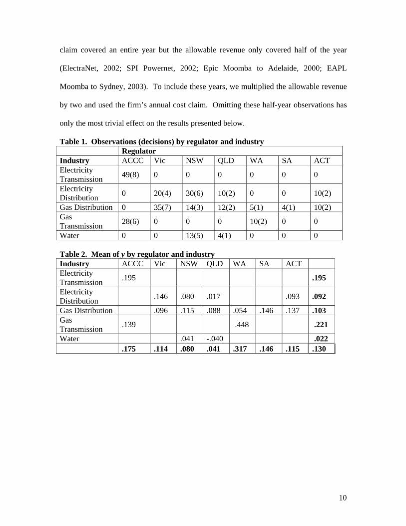
Table 1. Observations (decisions) by regulator and industry Regulator Industry ACCC Vic NSW QLD WA SA ACT Electricity Transmission 49(8) 0 0 0 0 0 0

Electricity Distribution 0 20(4) 30(6) 10(2) 0 0 10(2)

Gas Distribution 0 35(7) 14(3) 12(2) 5(1) 4(1) 10(2) Gas Transmission 28(6) 0 0 0 10(2) 0 0

Water 0 0 13(5) 4(1) 0 0 0 Table 2. Mean of y by regulator and industry Industry ACCC Vic NSW QLD WA SA ACT Electricity Transmission .195 .195

Electricity Distribution .146 .080 .017 .093 .092

Gas Distribution .096 .115 .088 .054 .146 .137 .103 Gas Transmission .139 .448 .221

Water .041 -.040 .022 .175 .114 .080 .041 .317 .146 .115 .130

10

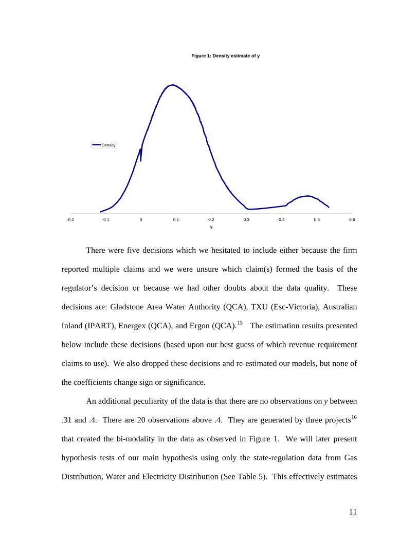
Figure 1: Density estimate of y

-0.2 -0.1 0 0.1 0.2 0.3 0.4 0.5 0.6

y

Density

There were five decisions which we hesitated to include either because the firm

reported multiple claims and we were unsure which claim(s) formed the basis of the

regulator’s decision or because we had other doubts about the data quality. These

decisions are: Gladstone Area Water Authority (QCA), TXU (Esc-Victoria), Australian

Inland (IPART), Energex (QCA), and Ergon (QCA).15 The estimation results presented

below include these decisions (based upon our best guess of which revenue requirement

claims to use). We also dropped these decisions and re-estimated our models, but none of

the coefficients change sign or significance.

An additional peculiarity of the data is that there are no observations on y between

.31 and .4. There are 20 observations above .4. They are generated by three projects16

that created the bi-modality in the data as observed in Figure 1. We will later present

hypothesis tests of our main hypothesis using only the state-regulation data from Gas

Distribution, Water and Electricity Distribution (See Table 5). This effectively estimates

11

the model only on a subset of the data in the first mode, which appears to be roughly

normally distributed. It is worth noting that this does not affect our results.

To summarise, the results presented below include all the decisions from our

database. If we omit any or all of the peculiar data, as described above, our estimates do

not change in any significant way.

V. Results

We now present and discuss our initial results. The second column in Table 3

reports the results of estimating equation 2 by Ordinary Least Squares (OLS) regression.

Note that water is the omitted industry dummy and the ACCC the omitted regulatory

agency. Therefore, the coefficients on the variables have to be interpreted as relative to

the omitted dummies. A positive coefficient implies a less favourable treatment of firms’

claims vis-à-vis the omitted categories17.

The third column of Table 3 corrects for the fact that our data consists of 254

observations from 52 different regulatory decisions and as such the individual

observations are not independent. While the standard errors change by a factor of two or

three in some cases, these do not generate any substantive differences in the significance

of coefficients between the two columns.

Both regressions include time dummies. We group years 2009—2012 (5

observations on two projects) and use this as the omitted category. All of the time

dummies for 1997 through 2008 are negative and significant. If we include separate time

dummies for 2009, 2010, and 2011, they are—unsurprisingly—not significantly different

from zero, further confirming our decision to group these dummies.

12

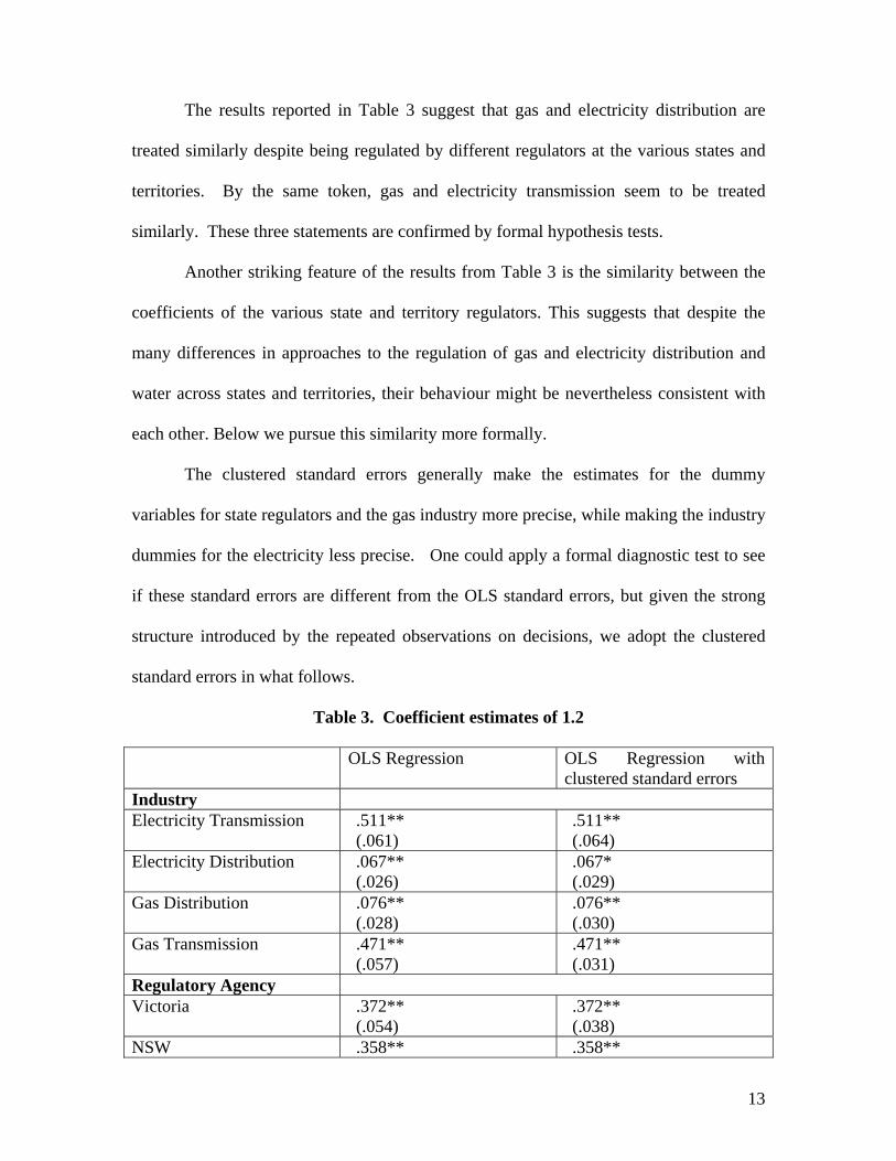
The results reported in Table 3 suggest that gas and electricity distribution are

treated similarly despite being regulated by different regulators at the various states and

territories. By the same token, gas and electricity transmission seem to be treated

similarly. These three statements are confirmed by formal hypothesis tests.

Another striking feature of the results from Table 3 is the similarity between the

coefficients of the various state and territory regulators. This suggests that despite the

many differences in approaches to the regulation of gas and electricity distribution and

water across states and territories, their behaviour might be nevertheless consistent with

each other. Below we pursue this similarity more formally.

The clustered standard errors generally make the estimates for the dummy

variables for state regulators and the gas industry more precise, while making the industry

dummies for the electricity less precise. One could apply a formal diagnostic test to see

if these standard errors are different from the OLS standard errors, but given the strong

structure introduced by the repeated observations on decisions, we adopt the clustered

standard errors in what follows.

Table 3. Coefficient estimates of 1.2

OLS Regression OLS Regression with clustered standard errors

Industry Electricity Transmission .511**

(.061) .511** (.064)

Electricity Distribution .067** (.026)

.067* (.029)

Gas Distribution .076** (.028)

.076** (.030)

Gas Transmission .471** (.057)

.471** (.031)

Regulatory Agency Victoria .372**

(.054) .372** (.038)

NSW .358** .358**

13

(.056) (.036) Queensland .306**

(.056) .306** (.047)

Western Australia .306** (.034)

.306** (.025)

South Australia .395** (.070)

.395** (.024)

ACT .366** (.057)

.366** (.034)

R-squared 50.5% 50.5% Sample size 254 254 ** Significant at 5% level * Significant at 10% level

Finally, note that the positive coefficients on all dummy variables for state

regulators would suggest that their decisions are less generous than that of the ACCC, the

omitted variable. However, to understand this relationship one needs to take into account

that the ACCC regulates gas and electricity transmission and the coefficients on these

variables were substantially higher than the coefficients on the gas and electricity

distribution variables. It is also important to note (see Table 1) that all electricity

transmission decisions included in our database were taken by the ACCC whereas gas

transmission decisions were taken both by the ACCC (six decisions) and the Western

Australian regulator (two decisions).

(i) Testing regulatory consistency

Using the above regression results, it is straightforward to test whether the

different state-based regulatory outcomes are consistent with one another. There are two

ways in which we approach this question. The first is to consider pair-wise tests between

the coefficients for the different state regulators. The second is to consider testing the

equality of similar-appearing groups of states/territories.

14

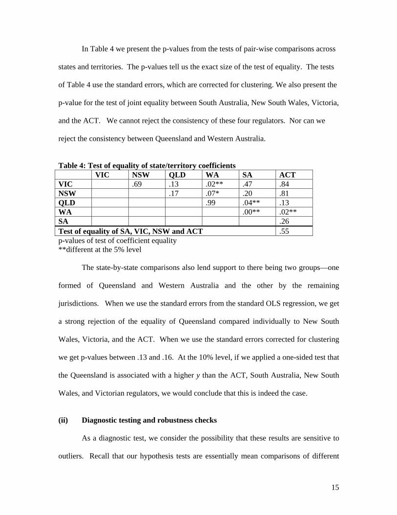
In Table 4 we present the p-values from the tests of pair-wise comparisons across

states and territories. The p-values tell us the exact size of the test of equality. The tests

of Table 4 use the standard errors, which are corrected for clustering. We also present the

p-value for the test of joint equality between South Australia, New South Wales, Victoria,

and the ACT. We cannot reject the consistency of these four regulators. Nor can we

reject the consistency between Queensland and Western Australia.

Table 4: Test of equality of state/territory coefficients VIC NSW QLD WA SA ACT VIC .69 .13 .02** .47 .84 NSW .17 .07* .20 .81 QLD .99 .04** .13 WA .00** .02** SA .26 Test of equality of SA, VIC, NSW and ACT .55 p-values of test of coefficient equality **different at the 5% level

The state-by-state comparisons also lend support to there being two groups—one

formed of Queensland and Western Australia and the other by the remaining

jurisdictions. When we use the standard errors from the standard OLS regression, we get

a strong rejection of the equality of Queensland compared individually to New South

Wales, Victoria, and the ACT. When we use the standard errors corrected for clustering

we get p-values between .13 and .16. At the 10% level, if we applied a one-sided test that

the Queensland is associated with a higher y than the ACT, South Australia, New South

Wales, and Victorian regulators, we would conclude that this is indeed the case.

(ii) Diagnostic testing and robustness checks

As a diagnostic test, we consider the possibility that these results are sensitive to

outliers. Recall that our hypothesis tests are essentially mean comparisons of different

15

cells. In order to test the sensitivity to outliers, we re-estimate the model using quantile

regression, which provides median comparisons of different cells. The coefficient values

are slightly lower than in Table 3 (not surprising given the positive skewness in Figure 1)

but the substantive results of the hypothesis tests of Table 4 are unchanged.

Western Australia is the only state that regulates gas transmission and it may be

that the coefficient for Western Australia is heavily influenced by these observations.

Therefore, to verify the validity of the above conclusions, we re-estimate the model using

only the observations involving electricity and gas distribution and water. These are the

main industries regulated by states (see Table 1) and the industries where for each

industry there are at least two states involved in regulation.

In Table 5, we present the p-values from the tests of state-by-state equality and the

grouped equality of South Australia, New South Wales, Victoria, and the ACT.

(Regression results available from the authors.) Our tentative conclusions that

Queensland and Western Australia are consistent with one another, but associated with

lower ys than the other jurisdictions (who are consistent with one another) is sharpened.

The difficulty in assessing whether the ACCC is associated with higher or lower

ys than the state regulator is the lack of overlap in the industries being regulated.18

Holding year constant, electricity transmission regulated by ACCC has an average value

of y predicted from the model of .405. (Without the constant and year effects, both of

which are negative). Electricity distribution regulated by NSW has a predicted value of y

of .332. The difference is significant, but we are econometrically unable to split the

difference into that due to the regulator and that due to the fact that the industry being

regulated is different.19 The coefficients in Table 3, by omitting ACCC, attribute all of

the difference to the industry and none to the regulator.

16

Table 5: Test of equality of state/territory coefficients (Excluding gas transmission from industries considered)

VIC NSW QLD WA SA ACT VIC .90 .13 .01** .56 .56 NSW .099* .02** .42 .42 QLD .90 .046** .03** WA .00** .00** SA .96 Test of equality of SA, VIC, NSW and ACT .82 p-values of test of coefficient equality **different at the 5% level

In Table 6, we present the polar opposite case, where all the difference is

attributed to the regulator and none to the industry. We impose common coefficients on

NSW, ACT, and Victoria (confirmed by a test of equality). That is, we estimate:

' ' ,rirt t irty RD TDα β δ ε= + + + (3)

If we test the hypothesis of equality of the coefficient on the NSW/ACT/Victoria

group against the ACCC, we reject the null in favour of the alternative that the ACCC is

tougher at the 10% level (p-value is .07). Likewise the ACCC is tougher than

Queensland. There appears to be no difference between the ACCC and South Australia,

although it’s notable that there are few observations for South Australia.

Table 6. Coefficient estimates of (1.3)

OLS Regression with

clustered standard errors Regulatory Agency Victoria/ACT/ New South Wales (grouped)

-.065* (.036)

South Australia -.019 (.030)

Western Australia .152 (.116)

Queensland -.125** (.047)

17

Both the ACCC and Western Australia appear tougher than the other states,

although this may be driven by differences between the regulation of gas transmission

(only done by Western Australia and the ACCC) and other industries. These differences

are evident in the means presented in Table 2. Again, we have no statistical way of

separating out these differences.

(iii) Private vs. Public Ownership

A common view is that privately owned firms might play the regulatory game

more aggressively, by overstating their costs, than publicly owned companies. The

underlying reason is that as shareholders individuals might be more profit-driven than the

government. A contrary view suggests that private companies might actually be less

capable of overstating their costs given that they are subjected to more public scrutiny

(e.g., by their many shareholders) than their public counterparts.

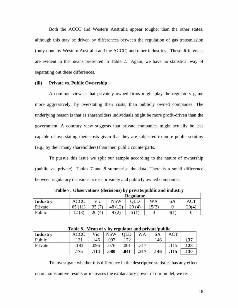
To pursue this issue we split our sample according to the nature of ownership

(public vs. private). Tables 7 and 8 summarise the data. There is a small difference

between regulatory decisions across privately and publicly owned companies.

Table 7. Observations (decisions) by private/public and industry Regulator Industry ACCC Vic NSW QLD WA SA ACT Private 65 (11) 35 (7) 48 (12) 20 (4) 15(3) 0 20(4) Public 12 (3) 20 (4) 9 (2) 6 (1) 0 4(1) 0

Table 8. Mean of y by regulator and private/public Industry ACCC Vic NSW QLD WA SA ACT Public .131 .146 .097 .172 .146 .137 Private .183 .096 .076 .001 .317 .115 .128 .175 .114 .080 .041 .317 .146 .115 .130

To investigate whether this difference in the descriptive statistics has any effect

on our substantive results or increases the explanatory power of our model, we re-

18

estimate equations (2) and (3) incorporating this new categorical variable. The private

variable is negative and significant in equation (2)—consistent with the lower y for

privately owned firms in the descriptive statistics. Inclusion of the private variable only

seems to affect the results for South Australia—principally by increasing the standard

error on the coefficient. The significant differences between South Australia and

Queensland and South Australia and Western Australia become marginally insignificant.

However, we continue to find that South Australia can be grouped with Victoria, New

South Wales and the ACT. In every other respect our substantive conclusions remain the

same. In equation (3), the private variable is insignificant.

VI. Discussions and Conclusion

The issue of regulatory consistency — the notion that regulatory decisions should

not favour particular industries or firms in particular jurisdictions—has been raised as one

of the rationales for the establishment of the new Australian Energy Regulator. This is

not surprising given the different approaches to the implementation of price regulation in

electricity and gas distribution and transmission across jurisdictions. Similarly, a national

water policy, involving possibly a more consistent regulatory framework across

jurisdictions, is again a high priority in the political agenda.

In this paper we provide evidence that despite the differences in the

implementation of price regulation across industries and across jurisdictions in Australia,

there is a considerable degree of consistency in regulatory decisions as measured by the

proportion of the firms’ revenue requirement claims that were disallowed by the regulator

when determining the maximum revenue. We discuss several points arising from our

exploration.

19

Firstly, our results suggest that when we control for different regulators and

different time periods, regulatory decisions are reasonably consistent across the electricity

and gas distribution industries. The apparent lack of consistency between transmission

and distribution has to be taken more cautiously given that the ACCC is the only

regulator for electricity transmission in our sample and so it is impossible to statistically

separate the regulator and industry effects.

Secondly, it is not possible to reject the hypothesis that the regulatory outcomes in

South Australia, New South Wales, the ACT and Victoria are similar. We also provide

evidence that the Queensland and Western Australia regulators are consistent with one

another, but are associated with regulatory outcomes that seem tougher than those of the

other state regulators. This empirical evidence highlights an important topic for further

theoretical investigation: the mechanism by which this consistency in price regulation has

been achieved. Furthermore, we find the nature of ownership of regulated companies

does not affect the conclusions stated above. Private ownership has only a small negative

effect on the percentage of cost claims that firms are allowed to recover and this effect is

insignificant when we consider only the state-level regulators. This again has important

theoretical implications as it suggests that models that rely on the nature of ownership to

explain the behaviour of regulators and regulated firms might not be appropriate.

Finally, we would like to be able to assess how the regulatory decisions taken by

the federal regulator, the ACCC, relate to those taken by the state regulators. The

difficulty in conducting this assessment is the lack of overlap in the industries being

regulated. We provide some lower and upper bounds that are consistent with both the

notion that the ACCC is tougher and that it is less tough than state regulators.

20

The implicit assumption we make when interpreting our results is that any gaming

behaviour by firms (in overstating their costs), which is attributable only to a particular

industry, is captured by the industry-specific dummies. Regulator dummies likewise also

capture any gaming behaviour specific to certain regulators. Thus, our interpretation

remains valid in the presence of gaming behaviour, provided that this behaviour is

roughly constant across one of our included categories.

It is our hope that the stylized facts we have presented here, which contribute to

the on-going debate in Australia about regulation, will also stimulate further research on

the determinants of regulatory decision-making and its application across different

industries by different regulators.

21

References

de Figueiredo, Rui José P. and Geoff Edwards, Why do Regulatory Outcomes Vary so Much?

Economic, Political and Institutional Determinants of Regulated Prices in the US

Telecommunications Industry, Working Paper, 2004. Available at http://ssrn.com/

abstract=547263.

Edwards, G. and L. Waverman (2004), ‘The Effects of Public Ownership and Regulatory

Independence on Regulatory Outcomes: A Study of Interconnect Rates in EU

Telecommunications’, Working Paper, Available at http://ssrn.com/abstract=588722.

Exports and Infrastructure Taskforce (2005), ‘Australia’s Export Infrastructure’, Report to

the Prime Minister, Canberra, May.

Hagerman, R. L. and B. T. Ratchford (1978), ‘Some Determinants of Allowed Rates of

Return on Equity to Electric Utilities’, The Bell Journal of Economics, 9, 46–55.

Lehman, D. and D. Weisman (2000), The Telecommunications Act of 1996: the Costs of

Managed Competition, Kluwer, Boston.

NECG (2003), ‘International Comparison of WACC decisions’, Submission to the

Productivity Commission Review of the Gas Access Regime, Submission 56,

September.

Productivity Commission (2004a), ‘Financial Performance of Government Trading

Enterprises, 1998–99 to 2002–2003’, Commission Research Paper, Canberra.

Productivity Commission (2004b), ‘Review of the Gas Access Regime’, Report number 31,

Canberra.

Productivity Commission (2005), ‘Review of National Competition Policy Reforms’, Report

number 33, Canberra.

22

Endnotes

1 See, for example, the recent review of Australian National Competition Policy (Productivity Commission,

2005) and the review of Australia’s export infrastructure (Exports and Infrastructure Taskforce, 2005).

2 The legislative instruments establishing independent regulatory agencies in the various jurisdictions often

cite national and cross-jurisdiction regulatory consistency as explicit objectives.

3 The recent review of the Australian Gas Access Regime (Productivity Commission, 2004b) provided an

opportunity for an evaluation of regulatory outcomes.

4 For example, the electricity industry, previously characterised by vertically integrated firms, was

restructured and divided into generation, transmission, distribution and retail businesses. The natural

monopoly elements of the industry, distribution and transmission, were subjected to price regulation and, in

principle, the other two elements of the industry, generation and retail, were de-regulated with the

requirement that generators sell and retailers buy their electricity through the electricity spot market (the

pool). The practice, however, is more complex. Retail prices remain regulated despite introduction of full

retail contestability in many jurisdictions. Similarly, there are services associated with the distribution of

electricity (e.g., remote meter reading) that might not be natural monopolies. In the same vein, new (and

existing) transmission links might not be natural monopolies in as much as they can compete with existing

links.

5 In this discussion we ignore service regulation—the requirement to provide minimum service standards.

6 With the exception of some significant gas transmission pipelines inside the Western Australian state

boundary and electricity transmission in Western Australia and the Northern Territory.

7 NECG (2003) compares rates of return in regulatory decisions in Australia and overseas.

8 To illustrate how these mechanisms work, consider a five-year regulatory period. In many jurisdictions, if

a firm spends less than its allowable efficient costs say in the fourth year of the regulatory period, then the

firm can retain the additional profits for only one more year, with the new prices being set at the lower

efficient cost. This of course might lead a firm to postpone process innovations that reduce costs until the

beginning of the new regulatory period. An efficiency carryover mechanism instead allows the firm to carry

over the cost savings for the next five years.

23

0.ty9 In practice it is possible to observe < This can be the result, for example, of the regulator allowing

the firm to anticipate to period t certain expenses that would be incurred at a later date.

10 indicates that for this particular year and this particular decision, the firm was allowed to

recover fifty per cent of the costs it claimed. Similarly,

0.5ty =

0.3ty = indicates that for this particular year and

this particular decision, the firm was allowed to recover seventy per cent of the costs it claimed.

11 Those decisions that are made on a calendar year basis are presented as the earliest financial year that

corresponds to the calendar year to provide simplicity.

12 In most cases the business proposed revenue requirement and the regulators maximum allowable revenue

determination were found in the regulator’s Final Decision report for that business or industry. In some

instances the businesses proposed revenue requirements were not available in the Final Decision. When this

was the case, the business’s initial submission was used to obtain the data.

13 The database and the STATA code for reproducing the results are available at www.acore.org.au. Full

regression results from section 5.3 can be reproduced using this code and are available from the authors.

14 This graph is available from the authors. In the regressions where we include time dummies, discussed

below, we find a small negative effect for observations early in the sample period.

15 In the Energex and Ergon decisions, there were several different proposals by the firm. In the case of the

other three decisions, we have an anomalous situation where the sum of the maximum allowable revenue

over the entire regulatory period exceeds the firm’s claims. There are possible explanations for this. For

example, it is possible that demand might have been underestimated in the original firm’s submission and

that the regulator’s decision process revealed this.

16 MTC (Electricity Transmission, ACCC, October 2003); Goldfield Gas Pipeline (Gas Transmission,

Offgar, April 2001); and Dampier to Bunbury (Gas Transmission, Offgar, May 2003).

17 While changing the omitted categories will change the estimated coefficient values and may change the

individual significance of the coefficients, the hypothesis tests of Tables 4 and 5 and the discussion of

predicted values below are invariant to changing the omitted categories.

18 The significant, positive coefficients on the state regulators in table 3 indicate that the ACCC is less

tough than the state regulators. But the large significant coefficients on gas and electricity transmission

24

(mostly regulated by ACCC in the case of the former and only by ACCC in the case of the latter) may be

interpreted to mean that the ACCC is tougher. 19 There are no examples of state-regulated electricity transmission (or ACCC regulated electricity or gas

distribution or water) that would allow us to split this difference into these two pieces.

25