Price Of Anarchy: Routing

Lecturer: Yishay Mansour

Ido Trivizki and Mille Gandelsman

Routing – Lecture Overview

Optimize the performance of a congested and unregulated network: Network. Rate of traffic between each pair of nodes. Latency function.

Selfish behavior does not perform as well as an optimized regulated network.

Investigating the price of anarchy (PoA) by exploring the characteristics of Nash Equilibrium and mininal latency optimal flow.

Lecture overview – cont. We will prove that:

If the latency of each edge is a linear function, PoA is at most 4/3.

In atomic routing the PoA is bounded by 2.6.

I the latency function is known to be continuous, non-decreasing and differentiable, there is no bounded coordination ratio.

Introduction Job scheduling, discussed last time, can

be viewed as a private case of routing. Each player has to choose exactly one

line to pass his traffic through. Parallel lines routing:

Introduction – cont. Today – the problem of routing traffic in

a network: Given a rate of traffic between pairs of

nodes in the network, find an assignment of the traffic to paths so that the total latency is minimized.

It is often impossible to impose regulation, so we are interested in those settings where each user selects his minimum latency path: Non-cooperative game in which each player

plays best response – expect the routes to form a Nash Equilibrium.

Two player models Non-atomic: we can split up traffic to

several paths. Atomic: each user chooses a single path

on which he transports all of his traffic.

The global target function in both cases is to

minimize the total latency suffered by all users.

Reminder: The Price of Anarchy

The ration between the worst value of an equilibrium and that of the optimal:

Where OPT denotes the minimum latency among all feasible flows and C(x) is total cost of flow x.

Our goal is to bound the PoA.

OPT

xCPoA PNEx

)(max

Example 1: routing on parallel lines

n players with weights m lines with speeds The players are allowed to split

their flow between different lines. Nash Equilibrium is achieved

when the load on each line is:

)0(,...,1, ii wniw

misi ,...,1,

S

W

s

waL m

j j

n

i ii

1

1)(

Example 1 – cont.Routing on parallel lines

The optimum is achieved by dividing the flow equally between the lines.

Therefore – we achieve a PoA=1

Example 2:Pigou’s Network

Nash flow will only traverse in the lower path.

OPT will divide the flow equally among the two paths.

S T

C(x)=1

C(x)=x

Example 2 – cont.

The target function is and it reaches minimum with value ¾, when x=1/2, giving a PoA of 4/3.

Combing the example with the tighter upper bound to be shown, it is a demonstration of a tight bound of 4/3 for linear latency functions.

xxx )1(1

Example 3:Pigou’s Non-Linear Network

The flow at Nash will continue to use only the lower path.

pxxc )(

S T

C(x)=1

Example 3 – cont.

Let (1-x) be the flow on the upper path in the optimum solution, and x - the flow on the lower path, respectively.

The overall cost is .

Proof that : if we choose :

111)1( pp xxxxx

0lim OPT

p

1

log)1(

p

px

01

1

loglim)1(limlim 1

pp

pxxOPT

p

p

pp

Example 3 – summary

In this case It means that the PoA cannot be

bounded from above in some cases when nonlinear latency functions are allowed.

PoA

plim

Example 4 – Braess’s paradox

There are exactly two disjoint paths from s to t, each of them follows exactly two edges.

Example 4 – cont.

The optimal flow coincides with the Nash equilibrium: half of the traffic takes the upper path, and

the half the lower. The latency perceived by each user is

3/2. In any other non-equal distribution,

there will be a difference in the total latency.

Users will be motivated to reroute to the less congested path.

Example 4 – cont.

Consider adding a fifth edge with latency 0.

The optimal flow stays 3/2. Nash will only

occur by routing theentire traffic on the single svwt path.

Example 4 – cont.

The latency each user experiences increases to 2.

Amazingly, adding a new zero latency link had a negative effect for all agents.

Formal Definition of the Problem

Consider a directed graph Input:

k pairs of source and destination vertices Demand ( the amount of required flow

between and ). Assume: . Each edge is given a load dependant

non decreasing and differentiable latency function

Output: Flow - a function that defines for each

path a flow . induces flow on edge :

),( EVG

),( ii ts

ir is

it 0ir

RRle :

Ee

f

pf

p

f e

pep pe ff:

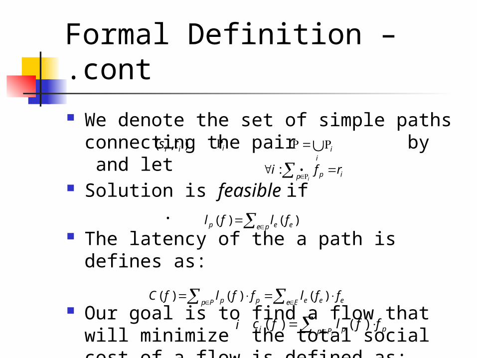
Formal Definition – cont.

We denote the set of simple paths connecting the pair by and let .

Solution is feasible if . The latency of the a path is defines as:

Our goal is to find a flow that will minimize the total social cost of a flow is defined as:

The cost of player :

),( ii ts i i

i

ip ip rfi :

pe eep flfl )()(

eEe eepPp p fflfflfC )()()(

i pPp pi fflfci

)()(

Flows at Nash equilibrium

Lemma: A feasible flow for instance

is Nash Equilibrium if for every and

Corollary: is a flow at Nash Equilibrium for

instance if and only if

, where

},...,1{ ki

),,( lrGf

:', ipp

)()(0 ' flflthenfif ppp

f

),,( lrGii i rfLfC )()(

)(min)( flfL ppi i

Optimal Solution – flow

Our goal is find a feasible flow that will minimize the total cost. Let . Clearly, it follows that To find the optimal flow , we

will look at . We assume that for each edge :

is convex and therefore is also convex.

is differentiable.

xxlxc ee )()(

f

)()( eEe e fcfC

)(* xc e

)(')()(' xlxxlxc eee

Ee )(xce)( fC

)(xce

The Optimality Condition

Define: and Let be a dividable game. For

each edge the function is

convex, continuous and differentiable function. A flow is optimal for if and only if:

xxlxc ee )()(

pe ep xcxc )(')('

),,( lrG

Ee

)(')('0:', ' fcfcfpp pppi

),,( lrGf

)()(' xcdx

dxc ee

The Optimality Condition – cont .

Notice the resemblance between the characterization of optimality conditions and Nash Equilibrium.

An optimal flow can be interpreted as a Nash Equilibrium with respect to a different edge latency functions.

We will use this resemblance to reach the bound on PoA.

Where OPT denotes the minimum latency among all feasible flows and C(x) is total cost of flow x.

Our goal is to bound the PoA.

The Optimality Condition – cont .

Let: Corollary:

is an optimal flow for if and only if it is Nash Equilibrium for the instance

Proof: By the optimality condition: is

optimal for if and only if

, if and only if (by def.) , if and only if is Nash Equilibrium for .

pe ep

eeeee

xlxl

xlxxlxxlxccl

)(*)(*

)(')()')(()(')(*

f ),,( lrG

*),,( lrG

f

l )(')('0:',, ' fcfcfppi pppi

)(*)(*0:',, ' flflfppi pppi

f *l

The optimality condition - proof

Definition: a set is called a convex set if

Intuitively it means that a set is convex if the linear segment connecting twopoints in the set, is entirelyin the set.

S

SBASBA )1(,10,,

S

The optimality condition - proof

Definition: a function is called convex function if

f

)()1()())1((:10,, yfxfyxfyx

The optimality condition - proof Let be a convex function, and a

convex set. A convex programming is of the form:

Lemma: If is strictly convex, then the solution is

unique.

Proof: Assume that are both minimum solutions. Let , because is convex: . Since is strictly convex:

, contradicting and being minimal .

)(xF S

SxtsxF ..),(min

)(xF

S

yx yxz

2

1

2

1 Sz)(xF )(

2

1)(

2

1)( yFxFzF

)(xF )(yF

The optimality condition - proof Lemma:

If is convex, then the solution set is convex.

Lemma: If is convex and is not optimal then

is not a local minimum. Consequently, any local minimum is also a global minimum.

Proof: Assume that is not optimal, i.e.

let , Since is convex:

for every .

)(xF U

y)(xF y

y )()(: yFxFx

yxz )1( F

)()()1()()( yFyFxFzF

0 1

Existence of flows at Nash Equilibrium

Theorem: For every splittable game

There exists at least one Nash

Equilibrium If and are Nash equilibria then

for every ,

( , , )G r l

f 'f

e ( ) ( )e ef cc f

Existence of flows at Nash Equilibrium - Proof

Define: , so that

Further define a potential function:

is non-negative, monotonous,

increasing and differential. Is a convex function.

Nash equillibrium flows are global minimizers of

0 ( ) ( )

x

e eh x l y dy ( ) )' (e eh x l x

(( )) e ee

h ff

eh

Existence of flows at Nash Equilibrium – Proof Cont.

By Weierstrass’s Theorem, has a minimum, and therefore Nash equilibrium exists.

Let and be Nash equillibria: Define and minimize , and we get

is sum of convex functions, and therefore it’s

possible only if all members of the sum are equal, and therefore:

f 'f(1 ) for [0,1]fg f

is convex ( ) ( ) (1 ) ( )g f f f 'f ( ) ( ) ( )f f g

( ) ( ) ( )e e eg c f c fc

Bounding the Price of Anarchy

Theorem: If there exists a constant

such that then

Corollary: If the latency function is polynomial function of degree , then

NashPoA

OPT

1 : ( ) ( )e ex h x c x PoA

( ) ( by assumption)

( ) ( f is OPT for )

( *) ( is non decreasing ( ) ( ))

( *) ( *)

( ) e ee

e e ee

e e e e ee

e ee

cNas f

h f h

h f l h x c x

c f C f

h f

OPT

C

1PoA d d

A tight bound for linear latency functions

A natural example for such a model: Network with congestion control (e.g.: TCP)

Using the corollary, we get a bound of 2

We’ll show a bound of 4/3 (which is tight, as we’ve seen in Example 2)

When , both Nash and OPT (equal) will

route all the flow in the shortest paths.

e e ebal x

e el b

A tight bound for linear latency functions - Proof

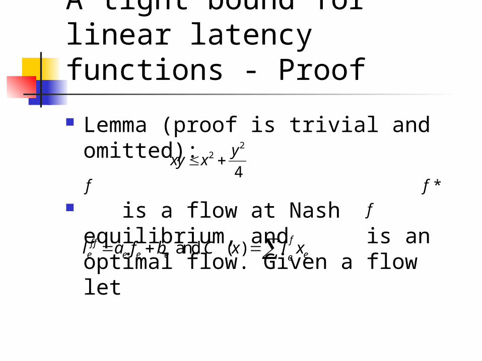
Lemma (proof is trivial and omitted):

is a flow at Nash equilibrium,

and is an optimal flow. Given a flow let

22

4y xx

y

f *f

f

and ( )ff f

e e e e eea f b C x l xl

A tight bound for linear latency functions – Proof Cont

2 2

( ) ( ) ( ) (by the lemma)

1 1( ) ( ) ( )

4 4

As : ( ) ( ) :

1( ) ( ) ( *) ( )

43

( ) ( *)4

4( ) ( *)

34

3

fe e e e e e e e e

e e e e e e

f f

f

x a f b x a f x b x

a x b x a f C x C f

x C f C x

C f C f C f C f

C f C f

C f C f

P A

C

o

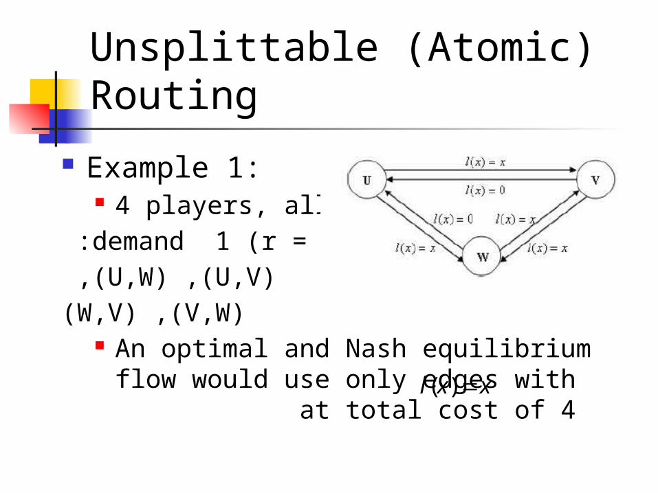
Unsplittable (Atomic) Routing

Example 1: 4 players, all withdemand 1 (r = 1): (U,V), (U,W), (V,W), (W,V) An optimal and Nash equilibrium

flow would use only edges with at total cost of 4

( )l x x

Unsplittable (Atomic) Routing – Exmaple 1 Cont.

Example 1 (cont.): But the optimalsolution is not theonly NE. Another Nash equilibrium:Player 1: U->W->V; Player 2: U->V-

>W;Player 3: V->U->W; Player 4: W->U->VWith total cost of 10, which gives PoA

= 2.5.

Unsplittable (Atomic) Routing – Exmaple 2

Both players haves=S and t=T, but,player 1 has r=1,While player 2, r=2. Possible paths S->T:p1: S->T; p2: S->V->T; p3: S->W-

>T;p4: S->V->W->T

Unsplittable (Atomic) Routing – Exmaple 2 Cont.

In this example there is no pureequilibrium. Easy to show thefollowing facts:

If player 2 chooses p1 or p2, player 1 will choose p4. If player 1 chooses p4, player 2 will choose p3. If player 2 chooses p3 or p4, player 1 will choose p1. If player 1 chooses p1, player 2 will choose p2.

Unsplittable (Atomic) Routing – Existence of Nash Equilibrium

We’ve shown that NE does not always exist.

Theorem: If is an unsplittable game with then there exists a Nash equilibrium. Proof:Define a potential function

When player I moves from p to p’:

( , , )G r l

: 1ii N r

( )

1

( ) ( )f e

a ee i

f l i

( ) ( ) ( 1) ( )p p e ee p p e p p

f l f l f l fl

Unsplittable (Atomic) Routing – Existence of Nash EquilibriumCont.

And:

So: So when the players plays “best

response” the potential decreases, and as it’s non-negative,

s series of “best responses” will converge to a Nash equilibrium.

( ') ( )a af f

( 1) if e ef e pl p

( ) if 'e ef el p p

0 otherwise

( ) ( ) ( ) ( )p p a af l fl f f

Bounding the price of anarchy for unsplittable linear games

Theorem: let be an unsplittable routing game with linear cost functions, then

Proof: Let be a nash equillibirim (we assume

it exists) flow, and be an optimal flow.

( , , )G r l

3 52.618

3PoA

f

*f

*

( ) (( ) ( ) )i

i i

p e e e e e i ee p e p

c rf a f b a f b

Bounding the price of anarchy for unsplittable linear games – Cont.

Lemma: Proof (of lemma):

Using Cauchy-Schwartz:

*

*

* * *

* 2 * *

* *

( ( ) )

( ( ) ) ( ( ) )

( ( )

)

( )

(

i

i

i e e i ei e p

i e e e e e e e e ei e Ee p

e e e e e e ee E e E

e e ee E

r a f r b

r a f f b a f f b f

a f b f a f f

a f f

C f

C f

* *( )( ) e e ee

C f a fC ff

* 2 * 2 *) (( ( ))e e e e e e ee e e

a f f a a f fC Cff

Bounding the price of anarchy for unsplittable linear games – Cont.

We get:

Solving the equation forWe get :

* *

* *

( ) (( ) )

1)

) (

( ) ( )

( ( )

C f C f C f

C f C f

C f C

C

f

f

*

(

)

)

(

C f

C f

*

( ) 3 5. 8

2)2 61

(

C f

C f