Embed Size (px)
Citation preview
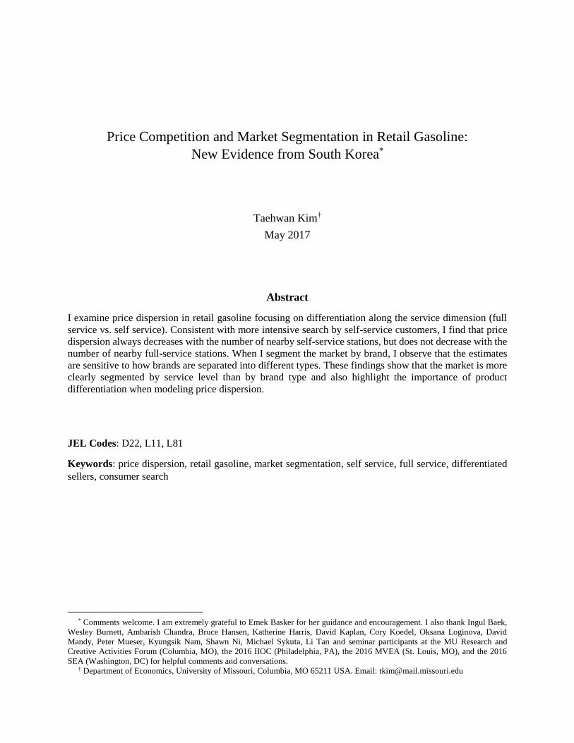
Price Competition and Market Segmentation in Retail Gasoline:
New Evidence from South Korea*
Taehwan Kim†
May 2017
Abstract
I examine price dispersion in retail gasoline focusing on differentiation along the service dimension (full
service vs. self service). Consistent with more intensive search by self-service customers, I find that price
dispersion always decreases with the number of nearby self-service stations, but does not decrease with the
number of nearby full-service stations. When I segment the market by brand, I observe that the estimates
are sensitive to how brands are separated into different types. These findings show that the market is more
clearly segmented by service level than by brand type and also highlight the importance of product
differentiation when modeling price dispersion.
JEL Codes: D22, L11, L81
Keywords: price dispersion, retail gasoline, market segmentation, self service, full service, differentiated
sellers, consumer search
* Comments welcome. I am extremely grateful to Emek Basker for her guidance and encouragement. I also thank Ingul Baek,
Wesley Burnett, Ambarish Chandra, Bruce Hansen, Katherine Harris, David Kaplan, Cory Koedel, Oksana Loginova, David
Mandy, Peter Mueser, Kyungsik Nam, Shawn Ni, Michael Sykuta, Li Tan and seminar participants at the MU Research and
Creative Activities Forum (Columbia, MO), the 2016 IIOC (Philadelphia, PA), the 2016 MVEA (St. Louis, MO), and the 2016
SEA (Washington, DC) for helpful comments and conversations.
† Department of Economics, University of Missouri, Columbia, MO 65211 USA. Email: [email protected]
1
1. Introduction
Price dispersion is universal even in markets for seemingly homogeneous goods. One possible explanation
for price dispersion is that markets may be segmented in ways unobservable to the econometrician, so that
seemingly homogeneous goods are in fact perceived by consumers as heterogeneous. In this paper, I exploit
the recent transition of gasoline stations in Seoul, South Korea, from full service to self service to jointly
examine price dispersion and competition in the context of service differentiation. I find that price
dispersion always decreases with the number of nearby self-service stations, whereas greater competition
is not always related to low dispersion for full service. This finding suggests that the recognition of market
segmentation is important when applying insights from models of price dispersion to real markets.
My analysis makes two contributions. First, I use service level to identify sellers of different types.
Existing papers on gasoline pricing have often used brand type. For example, Hastings (2004) studies the
price effects of brand-contract changes from an independent retailer to ARCO in Southern California, and
Lewis (2008) shows that price dispersion varies depending on the brand composition of local competitors
in San Diego. Both papers assume that the cross-price elasticity of demand across brands is low, but this
may not be justified in retail gasoline. My analysis utilizes a difference between customers at full-service
vs. self-service stations to identify search intensity, arguing that self-service customers’ revealed preference
for trading effort for lower prices implies that they are more likely to engage in costly search.1
The paper’s second contribution derives from the empirical finding. I find that the relationship between
price dispersion and local competition varies across sellers of different service levels, but this evidence is
a finding that does not have a clear corollary in search models. For example, the classic models of search,
such as Varian (1980) and Stahl (1986), attempt to explain the presence of price dispersion and show that
price dispersion is nonmonotonic in consumers’ search intensity, but are not designed for a market with
differentiated sellers that attract buyers of different types. My setting provides a natural experiment for
examining how price dispersion varies with number of sellers by service level and indirectly with
consumers’ search intensity.2
Specifically, I show that price dispersion varies systematically with the number of sellers, as well as
with seller characteristics such as presence of a store and/or a carwash facility and service level. Considering
market segmentation by service level, I find that price dispersion among self-service stations is lowest when
their density is high, but there is no evidence of such a relationship for full-service stations. Regarding
competition across service levels, I find that the elasticity of self-service price dispersion with respect to
the number of nearby full-service stations is approximately double the elasticity of full-service price
dispersion with respect to the number of nearby self-service stations. These results indicate that self-service
stations are responsible for lower dispersion, consistent with the claim that self-service buyers are more
likely to engage in costly search for arbitrage.
This paper is in line with a small but growing literature studying self-service gasoline stations (for a
recent review, see Noel, 2016). Shephard (1991) estimates the self-service discount in four Massachusetts
counties in 1987 and argues that service-level differentiation allows stations to price discriminate over and
above cost-based price differences. Kim and Kim (2011) study the entry effects of self-service stations in
the Korean market and find a four-cent-per-gallon reduction in price. Finally, using US data from the period
1 Korean full-service lovers are reluctant to engage in costly behavior. Kim et al. (2010) conduct a survey of 1000 consumers
who buy gasoline in three months, and document that 22.5% of the consumers report “I am not willing to use self-service stations.”
About 40% of those unwilling to buy self-serve gasoline report “inconvenience of getting in and out of the car” as the reason.
2 Identifying search intensity empirically is not trivial. Marvel (1976) and Houde (2012) argue that commuters have lower search
costs, and Lewis and Marvel (2011) use the number of visits to a website that provides gas price information as a proxy for consumer
search.
2
1977 to 1992, Basker et al. (2017) examine the effects of self-service adoption on station-level employment
and find about a third fewer workers per pump at self-service stations.
The rest of this paper is organized as follows. I describe the data and provide an overview of the market
in Section 2, and discuss my empirical methodology in Section 3. I present my main results, as well as
several robustness tests, in Sections 4 and 5. Section 6 concludes.
2. Data and Market Overview
2.1 Data
My data cover the period from May 2010 to September 2014. Over this period, I have daily price
information on all gasoline stations in Seoul, and each station’s address, service level, brand, and shop
name, also at a daily frequency. The data come from the Oil Price Information Network (OPINET) in Korea.
OPINET is a website operated by Korea National Oil Corporation to provide retail gasoline prices to the
public for market transparency. Most stations upload price information to the website automatically based
on transactions data.3
I use data from the Wednesday of each week because using the full dataset is computationally
burdensome.4 Information on stations’ entry and exit is not explicitly available from the dataset, but the
enforcement in Korea enables me to infer the information – stations must report at least once a week even
if there is no price change. To be conservative, I assume that a station that does not report prices for up to
30 days remains open, as long as its observed characteristics (such as name or service level) do not change.5
Using the address information, I geocode all stations in my dataset and count the number of full- and
self-service stations within a mile, a mile and a half, and two miles.6 OPINET also provides station
characteristics including level of service. A unique market feature in Korea is that stations are perfectly
partitioned by service level at each point in time, with no station offering a combination of full-service and
self-service pumps.
I restrict the sample by removing 43 stations that have no self-service stations within 1.5 miles over the
sample period (because the log number of these stations is undefined in my specification in the next section).
To ensure that my analysis is robust to the missing stations, I also define the number of full- and self-service
stations within a five-mile radius.7 Since my analysis is robust to this change, I use a 1.5-mile metric to be
consistent with earlier literature in this field of studies.
To control for demand characteristics, I include population density and a housing rent index (as a proxy
for household income), both of which are provided at the district level at a quarterly frequency and come
from Seoul Statistics, a website operated by the Seoul government. There are 25 districts in Seoul, each
3 If stations choose a manual update, they must report their price within 24 hours of a change in price.
4 The loss of the data is minimal due to the fact that station-level prices change once every 12 days on average. I chose
Wednesday because Tuesday is the modal day for price changes. See Figure C1 in Appendix C for details.
5 There are 79 instances of stations not reporting prices for over a week without a chance in station characteristics. In my dataset,
when stations drop out of the sample for longer than seven days, observed station characteristics typically change, in which case I
assume that the stations temporally closed to make that change. See Figure C2 in Appendix C.
6 My estimation results are qualitatively similar using one, one and half, and two-mile radii. I report results using a 1.5-mile
radius to be consistent with previous studies.
7 When using a five-mile radius, no stations are dropped. I reestimate the main regressions of this paper, and the results are
shown in Table A7 in Appendix A. In addition, using a logistic regression with odds ratios, I find that the dropped stations are
about twice as likely to be full service and to have a convenience store, but are about a third less likely to have other station
amenities such as a carwash or repair facility. They are also less likely to be located at an intersection. These results are shown in
Table A8 in Appendix A.
3
with 30 stations on average. Population density is the actual level data.8 The rent index is constructed from
a repeat-sales model and is normalized to 100 for all districts in January 2006. Table 1 summarizes the data
described in this section.
<Table 1. Summary Statistics>
2.2 Market Overview
The first gas station with self-service pumps opened in Seoul in 1993, but at the end of 2007 more than 99%
of stations in Seoul still offered only full-serve gasoline. Since 2008, the conversion of the market to self
service has dramatically accelerated, possibly due to a large spike in crude oil prices. As of September 2014,
self-service stations accounted for about 20% of Seoul’s 583 stations. One or two new self-service stations
have opened every month on average since 2008. In many cases these are a result of switching rather than
de novo entry. Self-service customers generally pay 2-4% less per gallon.
There are seven brands operating in the market. In descending order by market share, these are: SK
Energy, GS Caltex, S-Oil, Hyundai Oilbank, Alddle, Nonghyup Oil, and Namhae Oil. In my analysis, I
drop Nonghyup Oil and Namhae Oil. Each brand has only one station in the market; Nonghyup is a non-
private company and Namhae exited the market in June 2012.
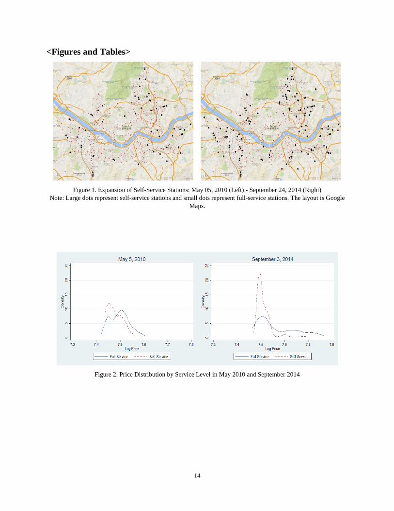
<Figure 1. Location of Gasoline Stations>
Figure 1 shows the locations of gasoline stations in the first day of my sample (May 5, 2010) and the
last day (September 24, 2015). Large dots indicate self-service stations, and small dots are full-service
stations. Seoul is the largest city (234 square miles) in Korea and highly dense (43,600 residents per square
mile), and located in a small basin that minimizes concerns about stations near the city boundary.
<Figure 2. Price Distributions by Service Level>
Figure 2 shows price distributions by service level on the first Wednesday of May 2010 and September
2014, respectively. Gasoline prices are widely dispersed in this market. For example, the highest price was
20% above the lowest price in May 2010 and this gap was 37% in September 2014. More interestingly, the
shape of price distributions changes in opposite directions for the two service levels: the distribution of self-
service prices narrowed while the distribution of full-service stations widened over time. These changes in
distributions suggest that as time goes by, full-service stations may be differentiated from self-service
stations and possibly differentiate on other dimensions such as extra services (e.g., free carwash, coffee, or
raffle tickets).
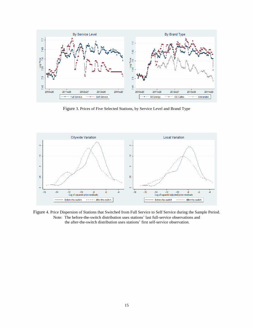
Following Lewis (2008), I arbitrarily select five stations – a focal station and the four stations within 0.5
miles of it – to trace the evolution of their relative prices.9 Figure 3 shows the average prices of the five
stations over time, by service level and by brand type. This exercise is useful for checking a general notion
of gasoline pricing in this market, although these stations are not representative of the entire sample.
<Figure 3. Prices of the Five Selected Stations>
8 Korean residents are required to report relocations as well as births and deaths to a local administrative office.
9 The focal station is full service and SK Energy. The nearby stations consist of three full-service and one self-service stations;
these include two SK Energy, one GS Caltex, and one unbranded station.
4
I take two lessons from this exercise. First, price ranking is volatile in the entire period, which makes it
costly for consumers to stay well informed about the price distribution.10 Second, when prices increase
sharply (i.e., up to around mid-2011), the price differences between services as well as among brands are
relatively low compared to the differences during the rest of the period. This phenomenon alludes to
“rockets and feathers” in retail gasoline, whereby gasoline stations generally earn lower margins (and
exhibit lower price dispersion) when prices increase than they do when prices fall.11
3. Empirical Methodology
3.1 Measure of price dispersion
I calculate price dispersion as the variance of residuals from the price equation, or “cleaned” prices, rather
than actual prices. My analysis focuses on the price dispersion that cannot be explained by station
characteristics, and a fixed-effects specification is a basic framework for this.12 To decompose actual prices
more precisely into explained and unexplained components, I also control for the number of nearby sellers
by service level, which is very likely related to gasoline pricing but is time-variant in my setting, as well as
a few more time-variant demand characteristics. The price specification is as follows:
(1) ln(Priceit) = βiFSFullit + βi
SSSelfit + θln(NumFSit) + λln(NumSSit) + δ𝐗it + ϕt + uit
The station fixed effects βi capture price differences due to observed and unobserved time-invariant
station characteristics; Fullit and Selfit are indicators for full service and self service, respectively. I allow
station fixed effects to change if the station switches from full service to self service; each station i can
therefore have up to two fixed effects: βiFS if it offers full service at time t and βi
SS if it offers self service.
NumFSit and NumSSit indicate the number of full-service and self-service stations within 1.5 miles,
respectively. The vector 𝑿 includes time-varying controls that are potentially correlated with gasoline
pricing, such as the station’s brand and district-level population density and rent, and the time fixed effects
𝜙𝑡 reflect changes in average prices, mostly driven by wholesale gasoline prices. With the exception of
service level, station characteristics are generally time invariant in my dataset.
From Equation (1), my primary focus is on the variance of the residuals. The residual ��𝑖𝑡 represents the
price deviation of station i on day t from its average position relative to the city average, so that the variance
of these residuals can be interpreted as a citywide measure of price dispersion. The validity of my approach
to computing a “clean” measure of price dispersion depends on how well Equation (1) describes the
expected price. The adjusted R2 represents a relative measure of the variation in prices explained by the
model, although it is generally not informative on an absolute magnitude of the variation left unexplained
by the model. The adjusted R2 of the regression is 0.90 and much of the variation is accounted by fixed
effects. In addition to estimating the price equation, I also examine how station fixed effects are correlated
with station characteristics. Both results are shown in Table A1 and in Table A2 in Appendix A, respectively.
I have an alternative approach to measuring dispersion, which captures the fact that price competition
tends to be localized in the retail gasoline market. Lewis (2008) finds local price dispersion useful in
10 This practice is called obfuscation in the search literature. See Ellison (2016) for an overview of search and obfuscation.
11 Hosken et al. (2008) and Brewer et al. (2014) conduct an empirical study of this phenomenon; and Tappata (2009) and Lewis
(2011) approach this phenomenon theoretically.
12 A fixed-effects approach has been used to measure price dispersion for this purpose in many other settings – e.g., Sorensen
(2000) for prescription drugs, Lach (2002) for supermarkets, and Lewis (2008) for retail gasoline.
5
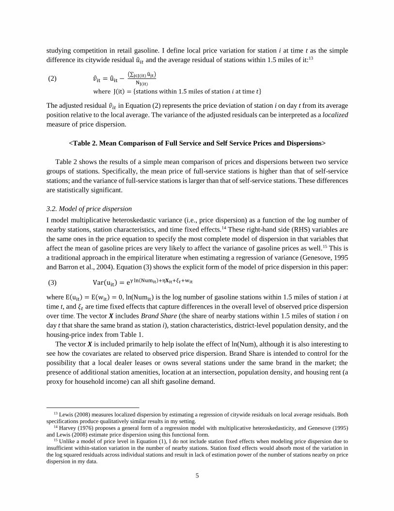
studying competition in retail gasoline. I define local price variation for station i at time t as the simple
difference its citywide residual ��𝑖𝑡 and the average residual of stations within 1.5 miles of it:13
(2) 𝑣it = uit − (∑ ujtj∈J(it) )
NJ(it)
where J(it) = {stations within 1.5 miles of station 𝑖 at time 𝑡}
The adjusted residual ��𝑖𝑡 in Equation (2) represents the price deviation of station i on day t from its average
position relative to the local average. The variance of the adjusted residuals can be interpreted as a localized
measure of price dispersion.
<Table 2. Mean Comparison of Full Service and Self Service Prices and Dispersions>
Table 2 shows the results of a simple mean comparison of prices and dispersions between two service
groups of stations. Specifically, the mean price of full-service stations is higher than that of self-service
stations; and the variance of full-service stations is larger than that of self-service stations. These differences
are statistically significant.
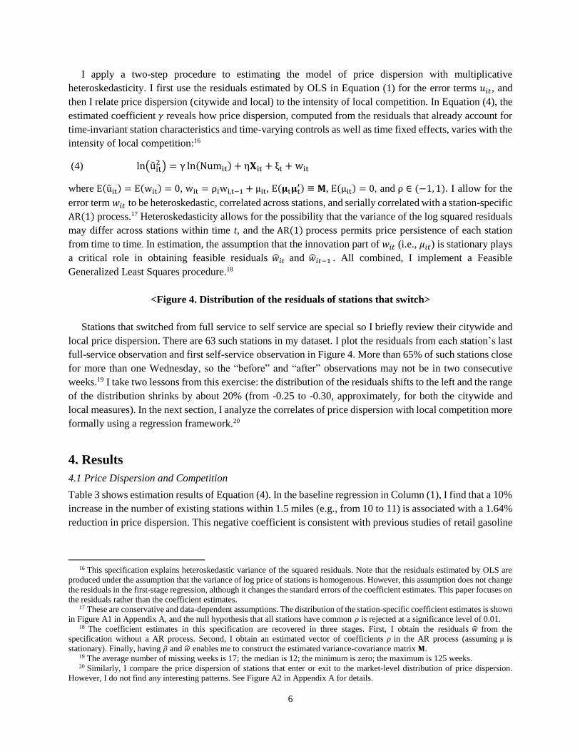
3.2. Model of price dispersion
I model multiplicative heteroskedastic variance (i.e., price dispersion) as a function of the log number of
nearby stations, station characteristics, and time fixed effects.14 These right-hand side (RHS) variables are
the same ones in the price equation to specify the most complete model of dispersion in that variables that
affect the mean of gasoline prices are very likely to affect the variance of gasoline prices as well.15 This is
a traditional approach in the empirical literature when estimating a regression of variance (Genesove, 1995
and Barron et al., 2004). Equation (3) shows the explicit form of the model of price dispersion in this paper:
(3) Var(uit) = eγ ln(Numit)+η𝐗it+𝜉𝑡+wit
where E(uit) = E(wit) = 0, ln(Numit) is the log number of gasoline stations within 1.5 miles of station i at
time t, and 𝜉𝑡 are time fixed effects that capture differences in the overall level of observed price dispersion
over time. The vector 𝑿 includes Brand Share (the share of nearby stations within 1.5 miles of station i on
day t that share the same brand as station i), station characteristics, district-level population density, and the
housing-price index from Table 1.
The vector 𝑿 is included primarily to help isolate the effect of ln(Num), although it is also interesting to
see how the covariates are related to observed price dispersion. Brand Share is intended to control for the
possibility that a local dealer leases or owns several stations under the same brand in the market; the
presence of additional station amenities, location at an intersection, population density, and housing rent (a
proxy for household income) can all shift gasoline demand.
13 Lewis (2008) measures localized dispersion by estimating a regression of citywide residuals on local average residuals. Both
specifications produce qualitatively similar results in my setting.
14 Harvey (1976) proposes a general form of a regression model with multiplicative heteroskedasticity, and Genesove (1995)
and Lewis (2008) estimate price dispersion using this functional form.
15 Unlike a model of price level in Equation (1), I do not include station fixed effects when modeling price dispersion due to
insufficient within-station variation in the number of nearby stations. Station fixed effects would absorb most of the variation in
the log squared residuals across individual stations and result in lack of estimation power of the number of stations nearby on price
dispersion in my data.
6
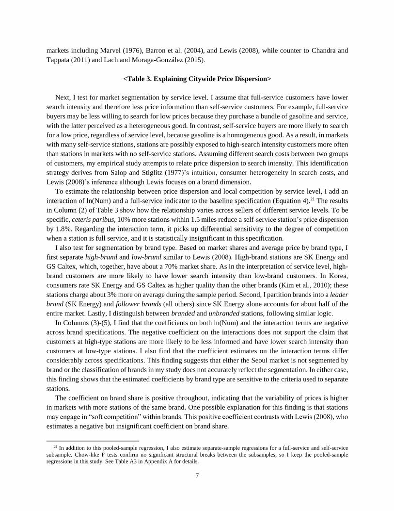
I apply a two-step procedure to estimating the model of price dispersion with multiplicative
heteroskedasticity. I first use the residuals estimated by OLS in Equation (1) for the error terms 𝑢𝑖𝑡, and
then I relate price dispersion (citywide and local) to the intensity of local competition. In Equation (4), the
estimated coefficient 𝛾 reveals how price dispersion, computed from the residuals that already account for
time-invariant station characteristics and time-varying controls as well as time fixed effects, varies with the
intensity of local competition:16
(4) ln(uit2 ) = γ ln(Numit) + η𝐗it + ξt + wit
where E(uit) = E(wit) = 0, wit = ρiwi,t−1 + μit, E(𝛍t𝛍t′) ≡ 𝚳, E(μit) = 0, and ρ ∈ (−1, 1). I allow for the
error term 𝑤𝑖𝑡 to be heteroskedastic, correlated across stations, and serially correlated with a station-specific
AR(1) process.17 Heteroskedasticity allows for the possibility that the variance of the log squared residuals
may differ across stations within time t, and the AR(1) process permits price persistence of each station
from time to time. In estimation, the assumption that the innovation part of 𝑤𝑖𝑡 (i.e., 𝜇𝑖𝑡) is stationary plays
a critical role in obtaining feasible residuals ��𝑖𝑡 and ��𝑖𝑡−1 . All combined, I implement a Feasible
Generalized Least Squares procedure.18
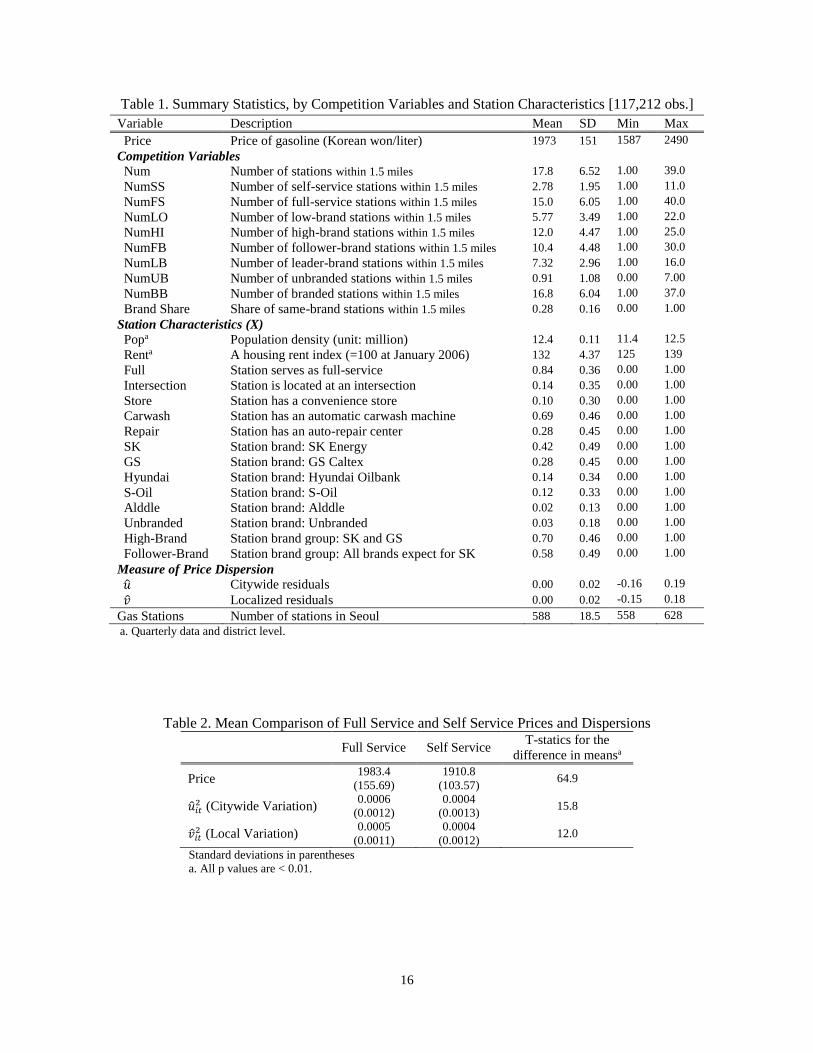
<Figure 4. Distribution of the residuals of stations that switch>
Stations that switched from full service to self service are special so I briefly review their citywide and
local price dispersion. There are 63 such stations in my dataset. I plot the residuals from each station’s last
full-service observation and first self-service observation in Figure 4. More than 65% of such stations close
for more than one Wednesday, so the “before” and “after” observations may not be in two consecutive
weeks.19 I take two lessons from this exercise: the distribution of the residuals shifts to the left and the range
of the distribution shrinks by about 20% (from -0.25 to -0.30, approximately, for both the citywide and
local measures). In the next section, I analyze the correlates of price dispersion with local competition more
formally using a regression framework.20
4. Results
4.1 Price Dispersion and Competition
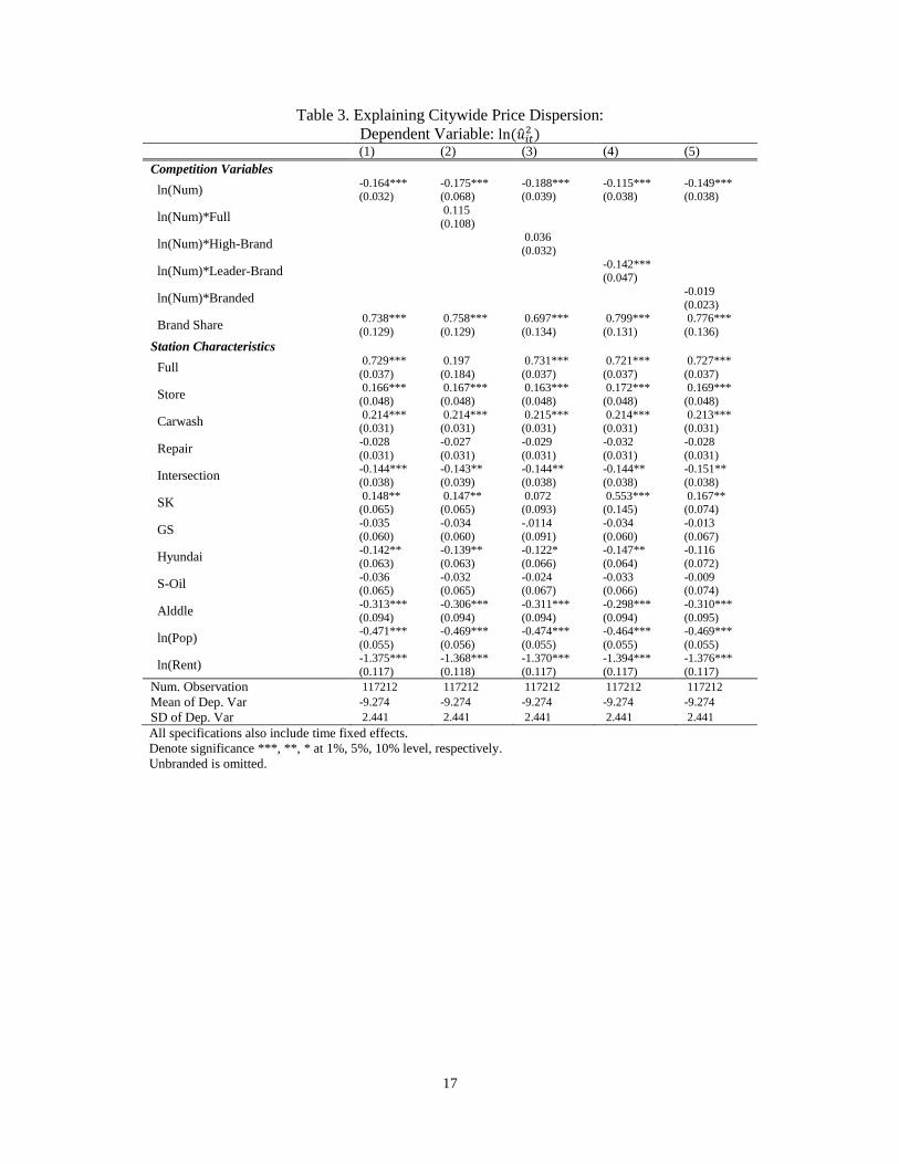
Table 3 shows estimation results of Equation (4). In the baseline regression in Column (1), I find that a 10%
increase in the number of existing stations within 1.5 miles (e.g., from 10 to 11) is associated with a 1.64%
reduction in price dispersion. This negative coefficient is consistent with previous studies of retail gasoline
16 This specification explains heteroskedastic variance of the squared residuals. Note that the residuals estimated by OLS are
produced under the assumption that the variance of log price of stations is homogenous. However, this assumption does not change
the residuals in the first-stage regression, although it changes the standard errors of the coefficient estimates. This paper focuses on
the residuals rather than the coefficient estimates.
17 These are conservative and data-dependent assumptions. The distribution of the station-specific coefficient estimates is shown
in Figure A1 in Appendix A, and the null hypothesis that all stations have common 𝜌 is rejected at a significance level of 0.01.
18 The coefficient estimates in this specification are recovered in three stages. First, I obtain the residuals �� from the
specification without a AR process. Second, I obtain an estimated vector of coefficients 𝜌 in the AR process (assuming μ is
stationary). Finally, having �� and �� enables me to construct the estimated variance-covariance matrix 𝐌.
19 The average number of missing weeks is 17; the median is 12; the minimum is zero; the maximum is 125 weeks.
20 Similarly, I compare the price dispersion of stations that enter or exit to the market-level distribution of price dispersion.
However, I do not find any interesting patterns. See Figure A2 in Appendix A for details.
7
markets including Marvel (1976), Barron et al. (2004), and Lewis (2008), while counter to Chandra and
Tappata (2011) and Lach and Moraga-González (2015).
<Table 3. Explaining Citywide Price Dispersion>
Next, I test for market segmentation by service level. I assume that full-service customers have lower
search intensity and therefore less price information than self-service customers. For example, full-service
buyers may be less willing to search for low prices because they purchase a bundle of gasoline and service,
with the latter perceived as a heterogeneous good. In contrast, self-service buyers are more likely to search
for a low price, regardless of service level, because gasoline is a homogeneous good. As a result, in markets
with many self-service stations, stations are possibly exposed to high-search intensity customers more often
than stations in markets with no self-service stations. Assuming different search costs between two groups
of customers, my empirical study attempts to relate price dispersion to search intensity. This identification
strategy derives from Salop and Stiglitz (1977)’s intuition, consumer heterogeneity in search costs, and
Lewis (2008)’s inference although Lewis focuses on a brand dimension.
To estimate the relationship between price dispersion and local competition by service level, I add an
interaction of ln(Num) and a full-service indicator to the baseline specification (Equation 4).21 The results
in Column (2) of Table 3 show how the relationship varies across sellers of different service levels. To be
specific, ceteris paribus, 10% more stations within 1.5 miles reduce a self-service station’s price dispersion
by 1.8%. Regarding the interaction term, it picks up differential sensitivity to the degree of competition
when a station is full service, and it is statistically insignificant in this specification.
I also test for segmentation by brand type. Based on market shares and average price by brand type, I
first separate high-brand and low-brand similar to Lewis (2008). High-brand stations are SK Energy and
GS Caltex, which, together, have about a 70% market share. As in the interpretation of service level, high-
brand customers are more likely to have lower search intensity than low-brand customers. In Korea,
consumers rate SK Energy and GS Caltex as higher quality than the other brands (Kim et al., 2010); these
stations charge about 3% more on average during the sample period. Second, I partition brands into a leader
brand (SK Energy) and follower brands (all others) since SK Energy alone accounts for about half of the
entire market. Lastly, I distinguish between branded and unbranded stations, following similar logic.
In Columns (3)-(5), I find that the coefficients on both ln(Num) and the interaction terms are negative
across brand specifications. The negative coefficient on the interactions does not support the claim that
customers at high-type stations are more likely to be less informed and have lower search intensity than
customers at low-type stations. I also find that the coefficient estimates on the interaction terms differ
considerably across specifications. This finding suggests that either the Seoul market is not segmented by
brand or the classification of brands in my study does not accurately reflect the segmentation. In either case,
this finding shows that the estimated coefficients by brand type are sensitive to the criteria used to separate
stations.
The coefficient on brand share is positive throughout, indicating that the variability of prices is higher
in markets with more stations of the same brand. One possible explanation for this finding is that stations
may engage in “soft competition” within brands. This positive coefficient contrasts with Lewis (2008), who
estimates a negative but insignificant coefficient on brand share.
21 In addition to this pooled-sample regression, I also estimate separate-sample regressions for a full-service and self-service
subsample. Chow-like F tests confirm no significant structural breaks between the subsamples, so I keep the pooled-sample
regressions in this study. See Table A3 in Appendix A for details.
8
In the lower part of Table 3, I present the coefficient estimates on station characteristics. Specifically,
when ln(Num) is zero and holding all else equal, stations located at an intersection have 15% lower price
dispersion than those not located at an intersection. Stations selling full-serve gasoline have up to 70%
higher price dispersion than stations selling self-service gasoline, and stations with a store or a carwash
facility have up to 17% and 21% higher price dispersion than stations without those amenities. These
findings suggest that consumers buying gasoline at a full-service station or at a station with a store or a
carwash facility may be less informed about prices or more interested in these extra amenities.
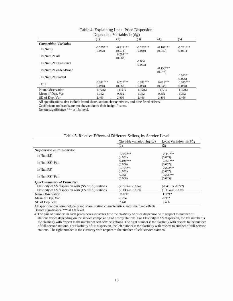
<Table 4. Explaining Local Price Dispersion>
I estimate the same specifications replacing citywide price variation with local price variation as the
dependent variable. These results are shown in Table 4. I find similar patterns as observed in the citywide
price dispersion and an even clearer pattern in the service-level specification. For example, in Column (2)
of Table 4, the coefficient on ln(Num) becomes larger in absolute value (more negative) and the interaction
term becomes larger (more positive) and is significant at the 1% level. The positive coefficient on the
interaction term implies that self-service price dispersion is much more elastic than full-service price
dispersion with respect to the number of nearby stations. As for market segmentation by brand type, the
coefficients on the interaction terms remain unchanged except for the branded-unbranded setting, which
changes sign and statistical significance relative to Table 3.
Overall my results are consistent with previous studies showing that price dispersion varies with
heterogeneity of sellers and buyers, although my setting is significantly different and my specifications
extend the notion of differentiated sellers in retail gasoline (commonly proxied by brand) into service level.
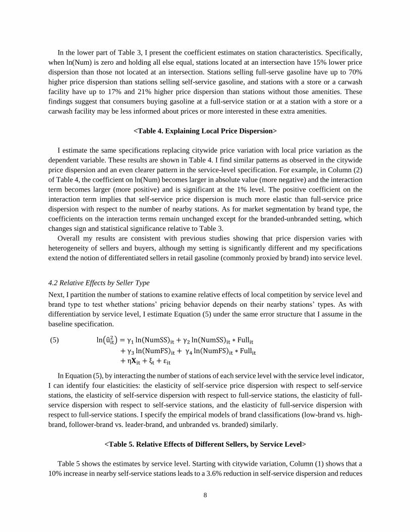
4.2 Relative Effects by Seller Type
Next, I partition the number of stations to examine relative effects of local competition by service level and
brand type to test whether stations’ pricing behavior depends on their nearby stations’ types. As with
differentiation by service level, I estimate Equation (5) under the same error structure that I assume in the
baseline specification.
(5) ln(uit2 ) = γ1 ln(NumSS)it + γ2 ln(NumSS)it ∗ Fullit
+ γ3 ln(NumFS)it + γ4 ln(NumFS)it ∗ Fullit
+ η𝐗it + ξt + εit
In Equation (5), by interacting the number of stations of each service level with the service level indicator,
I can identify four elasticities: the elasticity of self-service price dispersion with respect to self-service
stations, the elasticity of self-service dispersion with respect to full-service stations, the elasticity of full-
service dispersion with respect to self-service stations, and the elasticity of full-service dispersion with
respect to full-service stations. I specify the empirical models of brand classifications (low-brand vs. high-
brand, follower-brand vs. leader-brand, and unbranded vs. branded) similarly.
<Table 5. Relative Effects of Different Sellers, by Service Level>
Table 5 shows the estimates by service level. Starting with citywide variation, Column (1) shows that a
10% increase in nearby self-service stations leads to a 3.6% reduction in self-service dispersion and reduces
9
full-service dispersion by about 1.7%.22 This result is consistent with the finding in the previous section
that having more self-service stations nearby, or high search intensity, is associated with lower price
dispersion. The number of full-service stations barely affects the level of full-service dispersion, however.
My main specification assumes a monotonic relationship between search intensity and dispersion, even
though models of search generally present a non-monotonic relationship. To test whether the relationship
is non-monotonic, I estimate a modified specification in Equation (6) where I add squared terms of
ln(NumSS) and ln(NumFS) and an interaction of ln(NumSS) and ln(NumFS):
(6) ln(uit2 ) = γ1 ln(NumSSit) + γ2(ln(NumSSit))2 + γ3 ln(NumFSit) + γ4(ln(NumFSit))2
+ γ5(ln(NumSSit) ∗ ln(NumFSit)) + η𝐗it + ξt + wit
Holding all other variables constant, I plot the expected price dispersion as a function of the number of
self-service stations for the range of the number of staions that I observe in my data, using the estimated
coefficients in Table A4 in Appendix A. The graph is shown in Figure A3 in Appendix A. I find that the
number of self-service stations nearby still decreases dispersion even when I allow for the possibility of
non-monotonicity. In addition, once I interact the squared terms with a full-service indicator as in Equation
(5), I can identify the complete relative effects within service and across services, but my estimates are also
robust to this generalization. These findings confirm that in my setting, high search intensity limits
dispersion.
The patterns I observe in local price variation mirror those for citywide price variation. In Column (2)
of Table 5, self-service dispersion always decreases with local competition: It decreases by 4.8% with a 10%
increase in self-service stations nearby and by 2.7% with a 10% increase in full-service stations nearby.
The effect of full-service stations on full-service dispersion is statistically not different from zero, although
full-service dispersion does decrease with the number of self-service stations nearby. These results show
that greater competition is not always related to less dispersion, as is often suggested in empirical studies
in the gasoline literature.
I also find that the relationship between local price dispersion and number of sellers by service level is
asymmetric across service levels. For example, focusing on local variation in Column (2) of Table 5, I find
that the elasticity of self-service price dispersion with respect to the number of nearby full-service stations
is one and a half times larger than the elasticity of full-service price dispersion with respect to the number
of nearby self-service stations. Overall, across specification, self-service price dispersion exhibits greater
sensitivity to the number of sellers than does full-service dispersion.
The primary difference between Lewis’s (2008) results and mine is in the coefficient that captures the
elasticity of low-type station dispersion with respect to low-type stations, where the low type refers to self-
service stations in my paper and low-brand stations in Lewis’s paper. I find a large and statistically
significant elasticity, whereas Lewis found a small and insignificant coefficient. There are two possible
reasons for this difference. First, the conversion of many full-service stations to self-service stations may
have increased price competition among self-service stations, so the large coefficient in my setting may be
attributed to the market transformation. Second, the difference between full-service and self-service prices
may be large enough to divide consumers by their search intensity, whereas in Lewis’s setting price
differences between brands are smaller and may not fully partition consumers by their search intensity.
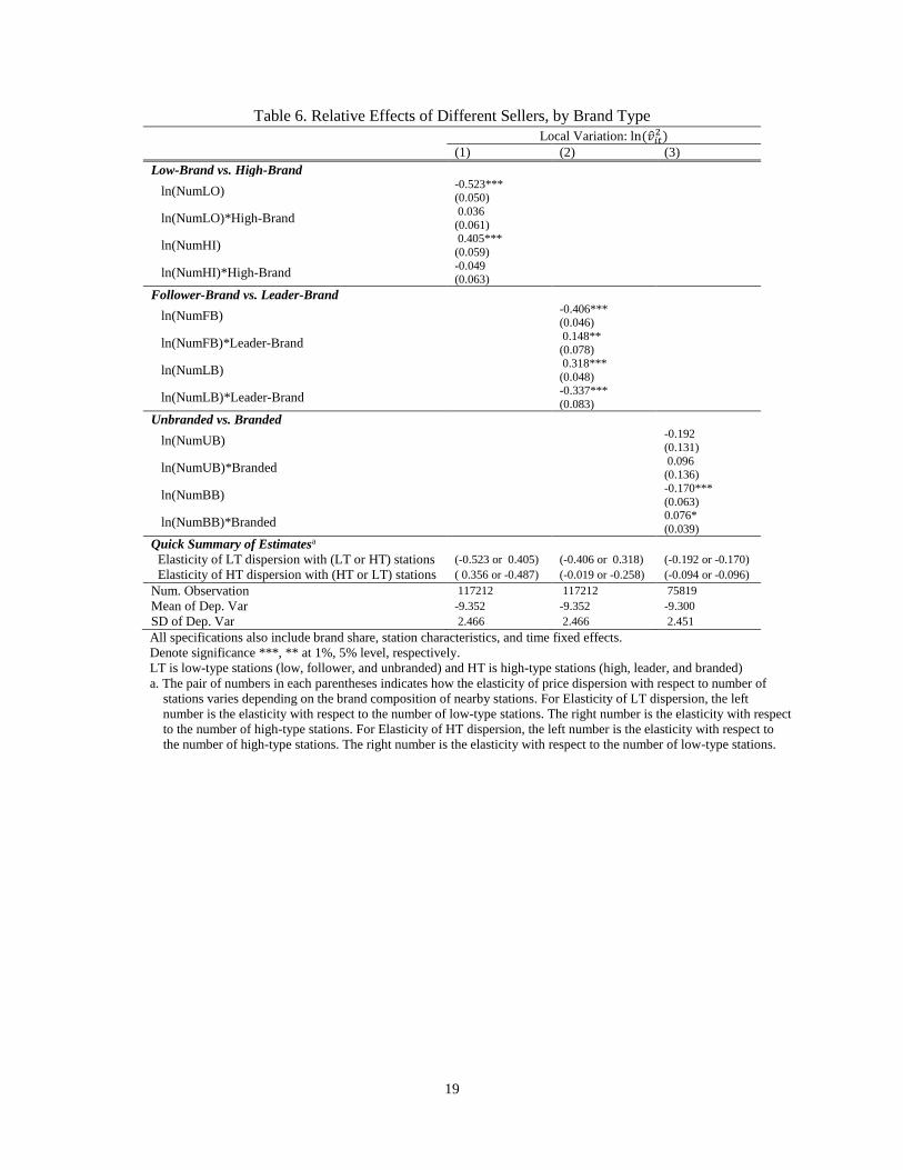
<Table 6. Relative Effects of Different Sellers, by Brand Type>
22 These coefficient estimates are summarized in the row labeled “Quick Summary of Estimates” in Table 4.
10
Finally, I estimate a variant of Equation (5), replacing the full- and self-service interactions with
interactions by brand types, and I show results for local variation in Table 6; results for citywide variation
are shown in Table A5 in Appendix A. In Column (1)-(2) of Table 6, I generally find qualitatively similar
results to those I report in the service-level segmentation. One difference is that the relationship between
price dispersion and local competition can even be positive depending on the composition of the existing
stations. For example, in Column (1), price dispersion for low-brand stations decreases with the number of
nearby low-brand stations but increases with the number of nearby high-brand stations.23 To summarize the
results from the brand-segmentation exercises, the coefficients on both local competition and the interaction
of local competition and the brand-type indicator are sensitive to how brands are classified into different
types, which suggests that service level is a cleaner dimension on which to segment the market.
4.3 Potential bias with coefficient estimates
Neither the location of a gas-station nor the decision to convert a full-service station to a self-service station
is exogenous. For example, full-service stations may prefer to locate in a district populated by customers
with high search costs. In this case, the relationship between dispersion and station configuration is, at least
in part, due to reverse causality; the coefficient on ln(NumFS) would therefore be biased upward in absolute
value. By the same logic, the coefficient on ln(NumSS) could be biased downward in absolute value. To
mitigate endogeneity bias, I add district fixed effects to the main specification. In Table A6 in Appendix A,
I confirm that the results in Table 5 are robust to controlling for time-invariant districts effects.
4.4 Applying search model
Search-theoretic models have been developed to generate equilibrium price dispersion as a function of
information costs generally with an assumption of one homogeneous product. For example, some
homogenous-product models (such as Varian, 1980) predict, ceteris paribus, a positive relationship
between price dispersion and the number of sellers; or a non-monotonic relationship between price
dispersion and search intensity.24
In this empirical study, I consider the co-movement of three variables: price dispersion, number of
differentiated sellers, and search intensity. My findings are consistent with the notion that the self-service
market has a higher fraction of searchers than the full-service market, and that the higher fraction of
searchers in the self-service market limits the extent of self-service dispersion. Nevertheless, my setting is
not well-suited to a direct test of search models because the co-movement of three variables does not satisfy
the ceteris paribus assumption. In this sense, the extant theories of dispersion may not be sufficient to
explain my empirical results.25
23 In the unbranded/branded setting in Column (3), the results are generally insignificant; the sample size is much smaller
because many stations have no unbranded stations within 1.5 miles. I reestimate the same specification using a five-mile radius in
which most stations have both branded and unbranded stations nearby, and continue to find insignificant coefficients. The results
are omitted in this paper.
24 Search-based models differ with respect to assumptions such as information acquisition channel and firm and consumer
heterogeneity. As a result, model predictions about the sign of the relationship between price dispersion and information costs vary
– predicting, variously, a positive relationship (Reinganum, 1979), a negative relationship (MacMinn, 1980), or a non-monotonic
relationship (Varian, 1980). Empirical counterparts of the relationship are also not uniform – studies have found a positive
relationship (Borenstein and Rose, 1994), a negatizve relationship (Gerardi and Shapiro, 2009), or a non-monotonic relationship
(Chandra and Lederman, 2015). See Baye et al. (2006) for a review on a wide range of search models from both theoretic and
empirical perspectives.
25 Wildenbeest (2011) provides a model-based framework for studying price dispersion in markets with product differentiation
and search frictions with simplification assumptions on consumer preference and firm’s quality input factors.
11
5. Robustness Checks
I perform several robustness checks on all regressions above: using both citywide and local variation as
LHS variables, and estimating the relative effects of both variation by service level and brand type. The
results of the robustness checks on relative effects by service level are in Appendix B.
5.1 Shorter sample period
An important assumption in the fixed-effects specification is that station fixed effects control for price
differences driven by station characteristics across stations, so price dispersion in this paper is not a result
of station characteristics. My sample is long (about 230 weeks), and it may be long enough to allow for
significant changes in station characteristics. In Table B1, I use a subsample of 108 weeks (from September
5, 2012 to September 24, 2014) to test robustness of the results. The observed patterns of estimates are
generally robust to the subsample regression, even though I lose some observations on the stations that
switch from full service to self service before September 2012, weakening statistical significance.
5.2 Alternative measure of price dispersion
Measuring price dispersion as multiplicative heterogeneous variance imposes a symmetric relationship
between price dispersion and local competition (i.e., residuals are squared). To investigate whether positive
and negative residuals are differentially correlated with competitive conditions, I separate my sample into
two subsamples, one containing only observations for which residuals are non-negative, and the other
containing the negative residuals. In a related exercise, I replace the variance with the absolute value of the
residuals. Both sets of results are shown in Table B2. The main estimates are generally robust to these
changes.26
6. Concluding Remarks
This paper argues on ex ante grounds that demand for gasoline is segmented by service level, and
demonstrates that price dispersion patterns are consistent with this segmentation. Gasoline stations sell a
nearly identical quality of gasoline. Because driving is costly to consumers, spatial differentiation is a first-
order dimension along which the market is segmented. Lewis (2008) shows the importance of brand as
another dimension on which the gasoline market is segmented. In addition to those dimensions of
differentiation, I show that the service dimension – full service vs. self service – is important, and I argue
that it is more intuitive and robust than brand segmentation.
Using the transition of service level in the Korean gasoline market, I find that price dispersion always
decreases with the number of nearby self-service stations, whereas the number of full-service stations does
not predict the level of price dispersion; a higher number of full-service stations can even exist with high
dispersion. This result suggests that dimensions other than price, unobserved in many cases, are too
important to ignore when studying price dispersion.
26 I only present results from local variation in Table B2 since results from citywide variation and those from local variation are
qualitatively similar.
12
References
Barron, J. M., Taylor, B. A., & Umbeck, J. R. (2004). Number of Sellers, Average Prices, and Price
Dispersion. International Journal of Industrial Organization, 22(8), 1041-1066.
Basker, E., Foster, L., & Klimek, S. D. (2017). Customer-Labor Substitution: Evidence from Gasoline
Stations. Working paper.
Baye, M. R., Morgan, J., & Scholten, P. (2006). In T. Hendershott (Ed.), Information, Search, and Price
Dispersion. Handbook on Economics and Information Systems, Elsevier Press, 323-371.
Borenstein, S., & Rose, N. L. (1994). Competition and Price Dispersion in the US Airline Industry. Journal
of Political Economy, 102(4), 653-683.
Brewer, J., Nelson, D. M., & Overstreet, G. (2014). The Economic Significance of Gasoline Wholesale
Price Volatility to Retailers. Energy Economics, 43(3), 274-283.
Carlson, J. A., & McAfee, R. P. (1983). Discrete Equilibrium Price Dispersion. Journal of Political
Economy, 91(3), 480-493.
Chandra, A., & Lederman, M. (2015). Revisiting the Relationship between Competition and Price
Discrimination: New Evidence from the Canadian Airline Industry. Working paper.
Chandra, A., & Tappata, M. (2011). Consumer Search and Dynamic Price Dispersion: An Application to
Gasoline Markets. RAND Journal of Economics, 42(4), 681-704.
Ellison, S. F. (2016). Price Search and Obfuscation: An Overview of the Theory and Empirics. In E. Basker
(Ed.), Handbook on the Economics of Retailing and Distribution, Edward Edgar, 287-305.
Genesove, D. (1995). Search at Wholesale Auto Auctions. Quarterly Journal of Economics, 110(1), 23-49.
Gerardi, K. S., & Shapiro, A. H. (2009). Does Competition Reduce Price Dispersion? New Evidence from
the Airline Industry. Journal of Political Economy, 117(1), 1-37.
Harvey, A. C. (1976). Estimating Regression Models with Multiplicative Heteroscedasticity. Econometrica,
44(3), 461-465.
Hastings, J. S. (2004). Vertical Relationships and Competition in Retail Gasoline Markets: Empirical
Evidence from Contract Changes in Southern California. American Economic Review, 94(1), 317-328.
Hosken, D. S., McMillan, R. S., & Taylor, C. T. (2008). Retail Gasoline Pricing: What Do We Know?.
International Journal of Industrial Organization, 26(6), 1425-1436.
Houde, J. F. (2012). Spatial Differentiation and Vertical Mergers in Retail Markets for Gasoline. American
Economic Review, 102(5), 2147-2182.
Kim, D.-W., & Kim, J.-H. (2011). The Impact of the Entry of Self-Service Stations in the Korean Retail
Gasoline Market: Evidence from the Difference-in-Differences Methods. Korean Journal of Economic
Studies, 59(2), 77-99.
Kim, H. G., Won, D. H., Hankook Research, & Koo, H. M (2010). 소비자의 주유소 구매행태 설문조사
(Survey on Consumers’ Shopping Pattern for Gasoline), Korea Energy Economics Institute, available at
http://www.keei.re.kr/web_keei (accessed 19 February 2017).
Lach, S. (2002). Existence and Persistence of Price Dispersion: An Empirical Analysis. Review of
Economics and Statistics, 84(3), 433-444.
13
Lach, S., & Moraga-González, J. L. (2015). Asymmetric Price Effects of Competition. Centre for Economic
Policy Research (CEPR) Discussion Papers 10456.
Lewis, M. (2008). Price Dispersion and Competition with Differentiated Sellers. Journal of Industrial
Economics, 56(3), 654-678.
Lewis, M. S. (2011). Asymmetric Price Adjustment and Consumer Search: An Examination of the Retail
Gasoline Market. Journal of Economics & Management Strategy, 20(2), 409-449.
Lewis, M. S., & Marvel, H. P. (2011). When Do Consumers Search? Journal of Industrial Economics,
59(3), 457-483.
MacMinn, R. D. (1980). Search and Market Equilibrium. Journal of Political Economy, 88(2), 308-327.
Marvel, H. P. (1976). The Economics of Information and Retail Gasoline Price Behavior: An Empirical
Analysis. Journal of Political Economy, 84(5), 1033-1060.
Noel, M. D. (2016). Retail Gasoline Markets. In E. Basker (Ed.), Handbook on the Economics of Retailing
and Distribution, Edward Edgar, 392-412.
Reinganum, J. F. (1979). A Simple Model of Equilibrium Price Dispersion. Journal of Political Economy,
87(4), 851-858.
Salop, S., & Stiglitz, J. (1977). Bargains and Ripoffs: A Model of Monopolistically Competitive Price
Dispersion. Review of Economic Studies, 44(3), 493-510.
Stahl, D. O. (1989). Oligopolistic Pricing with Sequential Consumer Search. American Economic
Review, 79(4), 700-712.
Shepard, A. (1991). Price Discrimination and Retail Configuration. Journal of Political Economy, 99(1)
30-53.
Sorensen, A. T. (2000). Equilibrium Price Dispersion in Retail Markets for Prescription Drugs. Journal of
Political Economy, 108(4), 833-850.
Saxonhouse, G. R. (1976). Estimated Parameters as Dependent Variables. American Economic Review,
66(1), 178-183.
Tappata, M. (2009). Rockets and Feathers: Understanding Asymmetric Pricing. RAND Journal of
Economics, 40(4), 673-687.
Varian, H. R. (1980). A Model of Sales. American Economic Review, 70(4), 651-659.
Wildenbeest, M. R. (2011). An Empirical Model of Search with Vertically Differentiated Products. RAND
Journal of Economics, 42(4), 729-757.
14
<Figures and Tables>
Figure 1. Expansion of Self-Service Stations: May 05, 2010 (Left) - September 24, 2014 (Right)
Note: Large dots represent self-service stations and small dots represent full-service stations. The layout is Google
Maps.
Figure 2. Price Distribution by Service Level in May 2010 and September 2014
15
Figure 3. Prices of Five Selected Stations, by Service Level and Brand Type
Figure 4. Price Dispersion of Stations that Switched from Full Service to Self Service during the Sample Period.
Note: The before-the-switch distribution uses stations’ last full-service observations and
the after-the-switch distribution uses stations’ first self-service observation.
16
Table 1. Summary Statistics, by Competition Variables and Station Characteristics [117,212 obs.]
Variable Description Mean SD Min Max
Price Price of gasoline (Korean won/liter) 1973 151 1587 2490
Competition Variables
Num Number of stations within 1.5 miles 17.8 6.52 1.00 39.0
NumSS Number of self-service stations within 1.5 miles 2.78 1.95 1.00 11.0
NumFS Number of full-service stations within 1.5 miles 15.0 6.05 1.00 40.0
NumLO Number of low-brand stations within 1.5 miles 5.77 3.49 1.00 22.0
NumHI Number of high-brand stations within 1.5 miles 12.0 4.47 1.00 25.0
NumFB Number of follower-brand stations within 1.5 miles 10.4 4.48 1.00 30.0
NumLB Number of leader-brand stations within 1.5 miles 7.32 2.96 1.00 16.0
NumUB Number of unbranded stations within 1.5 miles 0.91 1.08 0.00 7.00
NumBB Number of branded stations within 1.5 miles 16.8 6.04 1.00 37.0
Brand Share Share of same-brand stations within 1.5 miles 0.28 0.16 0.00 1.00
Station Characteristics (X)
Popa Population density (unit: million) 12.4 0.11 11.4 12.5
Renta A housing rent index (=100 at January 2006) 132 4.37 125 139
Full Station serves as full-service 0.84 0.36 0.00 1.00
Intersection Station is located at an intersection 0.14 0.35 0.00 1.00
Store Station has a convenience store 0.10 0.30 0.00 1.00
Carwash Station has an automatic carwash machine 0.69 0.46 0.00 1.00
Repair Station has an auto-repair center 0.28 0.45 0.00 1.00
SK Station brand: SK Energy 0.42 0.49 0.00 1.00
GS Station brand: GS Caltex 0.28 0.45 0.00 1.00
Hyundai Station brand: Hyundai Oilbank 0.14 0.34 0.00 1.00
S-Oil Station brand: S-Oil 0.12 0.33 0.00 1.00
Alddle Station brand: Alddle 0.02 0.13 0.00 1.00
Unbranded Station brand: Unbranded 0.03 0.18 0.00 1.00
High-Brand Station brand group: SK and GS 0.70 0.46 0.00 1.00
Follower-Brand Station brand group: All brands expect for SK 0.58 0.49 0.00 1.00
Measure of Price Dispersion
�� Citywide residuals 0.00 0.02 -0.16 0.19
�� Localized residuals 0.00 0.02 -0.15 0.18
Gas Stations Number of stations in Seoul 588 18.5 558 628
a. Quarterly data and district level.
Table 2. Mean Comparison of Full Service and Self Service Prices and Dispersions
Full Service Self Service T-statics for the
difference in meansa
Price 1983.4
(155.69)
1910.8
(103.57) 64.9
��𝑖𝑡2 (Citywide Variation)
0.0006
(0.0012)
0.0004
(0.0013) 15.8
𝑣𝑖𝑡2 (Local Variation)
0.0005
(0.0011)
0.0004
(0.0012) 12.0
Standard deviations in parentheses
a. All p values are < 0.01.
17
Table 3. Explaining Citywide Price Dispersion:
Dependent Variable: ln(��𝑖𝑡2 )
(1) (2) (3) (4) (5)
Competition Variables
ln(Num) -0.164*** (0.032)
-0.175*** (0.068)
-0.188*** (0.039)
-0.115*** (0.038)
-0.149*** (0.038)
ln(Num)*Full 0.115
(0.108)
ln(Num)*High-Brand 0.036
(0.032)
ln(Num)*Leader-Brand -0.142*** (0.047)
ln(Num)*Branded -0.019
(0.023)
Brand Share 0.738***
(0.129)
0.758***
(0.129)
0.697***
(0.134)
0.799***
(0.131)
0.776***
(0.136)
Station Characteristics
Full 0.729***
(0.037)
0.197
(0.184)
0.731***
(0.037)
0.721***
(0.037)
0.727***
(0.037)
Store 0.166***
(0.048)
0.167***
(0.048)
0.163***
(0.048)
0.172***
(0.048)
0.169***
(0.048)
Carwash 0.214*** (0.031)
0.214*** (0.031)
0.215*** (0.031)
0.214*** (0.031)
0.213*** (0.031)
Repair -0.028
(0.031)
-0.027
(0.031)
-0.029
(0.031)
-0.032
(0.031)
-0.028
(0.031)
Intersection -0.144***
(0.038)
-0.143**
(0.039)
-0.144**
(0.038)
-0.144**
(0.038)
-0.151**
(0.038)
SK 0.148** (0.065)
0.147** (0.065)
0.072 (0.093)
0.553*** (0.145)
0.167** (0.074)
GS -0.035
(0.060)
-0.034
(0.060)
-.0114
(0.091)
-0.034
(0.060)
-0.013
(0.067)
Hyundai -0.142**
(0.063)
-0.139**
(0.063)
-0.122*
(0.066)
-0.147**
(0.064)
-0.116
(0.072)
S-Oil -0.036 (0.065)
-0.032 (0.065)
-0.024 (0.067)
-0.033 (0.066)
-0.009 (0.074)
Alddle -0.313***
(0.094)
-0.306***
(0.094)
-0.311***
(0.094)
-0.298***
(0.094)
-0.310***
(0.095)
ln(Pop) -0.471***
(0.055)
-0.469***
(0.056)
-0.474***
(0.055)
-0.464***
(0.055)
-0.469***
(0.055)
ln(Rent) -1.375***
(0.117)
-1.368***
(0.118)
-1.370***
(0.117)
-1.394***
(0.117)
-1.376***
(0.117)
Num. Observation 117212 117212 117212 117212 117212
Mean of Dep. Var -9.274 -9.274 -9.274 -9.274 -9.274
SD of Dep. Var 2.441 2.441 2.441 2.441 2.441
All specifications also include time fixed effects.
Denote significance ***, **, * at 1%, 5%, 10% level, respectively.
Unbranded is omitted.
18
Table 4. Explaining Local Price Dispersion:
Dependent Variable: ln(��𝑖𝑡2 )
(1) (2) (3) (4) (5)
Competition Variables
ln(Num) -0.235*** (0.033)
-0.414*** (0.074)
-0.232*** (0.040)
-0.162*** (0.040)
-0.291*** (0.041)
ln(Num)*Full 0.214***
(0.083)
ln(Num)*High-Brand -0.004
(0.033)
ln(Num)*Leader-Brand -0.156*** (0.046)
ln(Num)*Branded 0.063**
(0.026)
Full 0.681***
(0.038)
0.237***
(0.067)
0.681***
(0.038)
0.681***
(0.038)
0.685***
(0.038)
Num. Observation 117212 117212 117212 117212 117212
Mean of Dep. Var -9.352 -9.352 -9.352 -9.352 -9.352
SD of Dep. Var 2.466 2.466 2.466 2.466 2.466
All specifications also include brand share, station characteristics, and time fixed effects.
Coefficients on brands are not shown due to their insignificance.
Denote significance *** at 1% level.
Table 5. Relative Effects of Different Sellers, by Service Level
Citywide variation: ln(��𝑖𝑡
2 ) Local Variation: ln(��𝑖𝑡2 )
(1) (2)
Self-Service vs. Full-Service
ln(NumSS) -0.363***
(0.052)
-0.481***
(0.053)
ln(NumSS)*Full 0.194*** (0.056)
0.301*** (0.057)
ln(NumFS) -0.104**
(0.051)
-0.272***
(0.057)
ln(NumFS)*Full 0.061
(0.060)
0.208***
(0.065)
Quick Summary of Estimatesa
Elasticity of SS dispersion with (SS or FS) stations (-0.363 or -0.104) (-0.481 or -0.272)
Elasticity of FS dispersion with (FS or SS) stations (-0.043 or -0.169) ( 0.064 or -0.180)
Num. Observation 117212 117212
Mean of Dep. Var -9.274 -9.352
SD of Dep. Var 2.441 2.466
All specifications also include brand share, station characteristics, and time fixed effects.
Denote significance *** at 1% level.
a. The pair of numbers in each parentheses indicates how the elasticity of price dispersion with respect to number of
stations varies depending on the service composition of nearby stations. For Elasticity of SS dispersion, the left number is
the elasticity with respect to the number of self-service stations. The right number is the elasticity with respect to the number
of full-service stations. For Elasticity of FS dispersion, the left number is the elasticity with respect to number of full-service
stations. The right number is the elasticity with respect to the number of self-service stations.
19
Table 6. Relative Effects of Different Sellers, by Brand Type
Local Variation: ln(��𝑖𝑡
2 )
(1) (2) (3)
Low-Brand vs. High-Brand
ln(NumLO) -0.523*** (0.050)
ln(NumLO)*High-Brand 0.036
(0.061)
ln(NumHI) 0.405***
(0.059)
ln(NumHI)*High-Brand -0.049 (0.063)
Follower-Brand vs. Leader-Brand
ln(NumFB) -0.406*** (0.046)
ln(NumFB)*Leader-Brand 0.148**
(0.078)
ln(NumLB) 0.318***
(0.048)
ln(NumLB)*Leader-Brand -0.337***
(0.083)
Unbranded vs. Branded
ln(NumUB) -0.192
(0.131)
ln(NumUB)*Branded 0.096 (0.136)
ln(NumBB) -0.170***
(0.063)
ln(NumBB)*Branded 0.076*
(0.039)
Quick Summary of Estimatesa
Elasticity of LT dispersion with (LT or HT) stations (-0.523 or 0.405) (-0.406 or 0.318) (-0.192 or -0.170)
Elasticity of HT dispersion with (HT or LT) stations ( 0.356 or -0.487) (-0.019 or -0.258) (-0.094 or -0.096)
Num. Observation 117212 117212 75819
Mean of Dep. Var -9.352 -9.352 -9.300
SD of Dep. Var 2.466 2.466 2.451
All specifications also include brand share, station characteristics, and time fixed effects.
Denote significance ***, ** at 1%, 5% level, respectively.
LT is low-type stations (low, follower, and unbranded) and HT is high-type stations (high, leader, and branded)
a. The pair of numbers in each parentheses indicates how the elasticity of price dispersion with respect to number of
stations varies depending on the brand composition of nearby stations. For Elasticity of LT dispersion, the left
number is the elasticity with respect to the number of low-type stations. The right number is the elasticity with respect
to the number of high-type stations. For Elasticity of HT dispersion, the left number is the elasticity with respect to
the number of high-type stations. The right number is the elasticity with respect to the number of low-type stations.
20
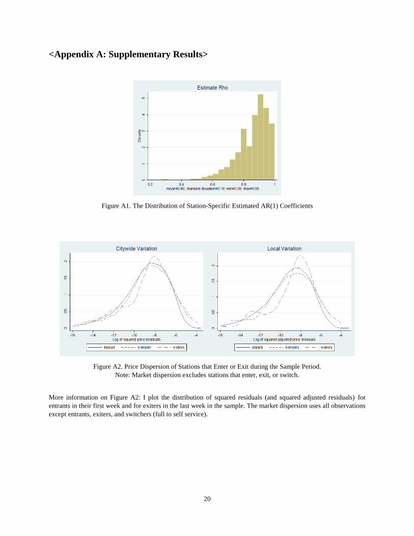
<Appendix A: Supplementary Results>
Figure A1. The Distribution of Station-Specific Estimated AR(1) Coefficients
Figure A2. Price Dispersion of Stations that Enter or Exit during the Sample Period.
Note: Market dispersion excludes stations that enter, exit, or switch.
More information on Figure A2: I plot the distribution of squared residuals (and squared adjusted residuals) for
entrants in their first week and for exiters in the last week in the sample. The market dispersion uses all observations
except entrants, exiters, and switchers (full to self service).
21
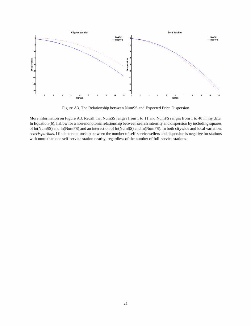
Figure A3. The Relationship between NumSS and Expected Price Dispersion
More information on Figure A3: Recall that NumSS ranges from 1 to 11 and NumFS ranges from 1 to 40 in my data.
In Equation (6), I allow for a non-monotonic relationship between search intensity and dispersion by including squares
of ln(NumSS) and ln(NumFS) and an interaction of ln(NumSS) and ln(NumFS). In both citywide and local variation,
ceteris paribus, I find the relationship between the number of self-service sellers and dispersion is negative for stations
with more than one self-service station nearby, regardless of the number of full-service stations.
22
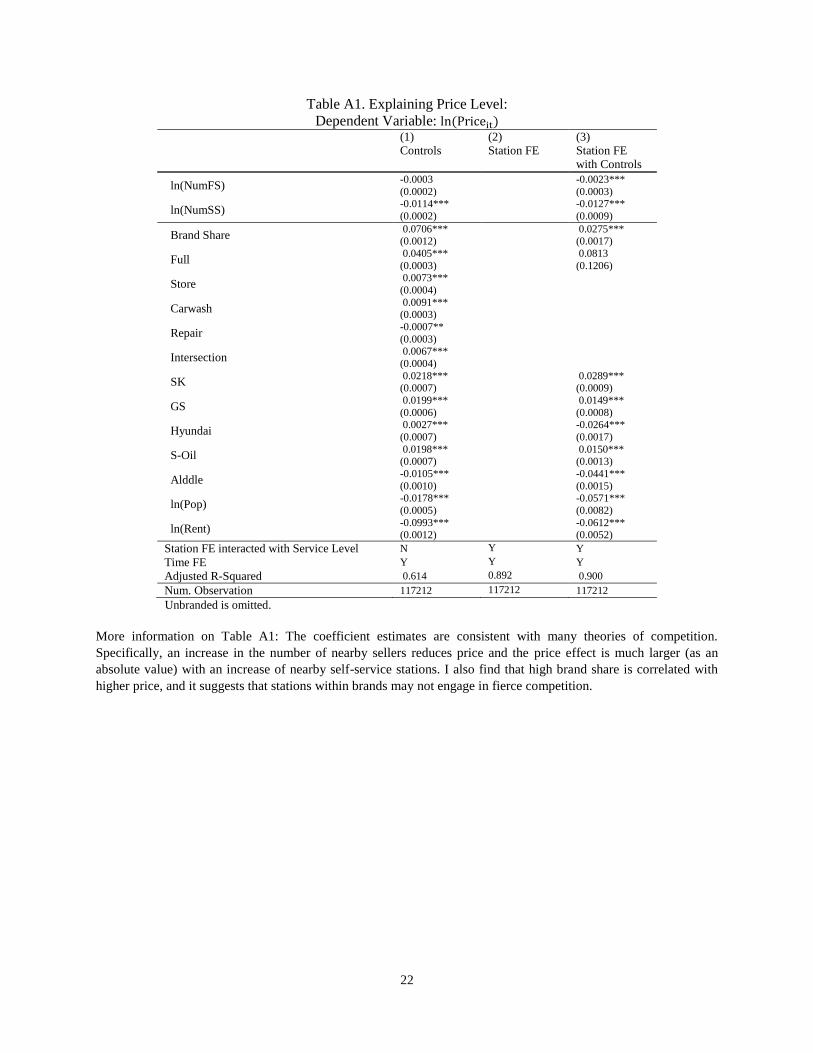
Table A1. Explaining Price Level:
Dependent Variable: ln(Priceit)
(1)
Controls
(2)
Station FE
(3)
Station FE
with Controls
ln(NumFS) -0.0003
(0.0002)
-0.0023***
(0.0003)
ln(NumSS) -0.0114***
(0.0002)
-0.0127***
(0.0009)
Brand Share 0.0706*** (0.0012)
0.0275*** (0.0017)
Full 0.0405***
(0.0003)
0.0813
(0.1206)
Store 0.0073***
(0.0004)
Carwash 0.0091*** (0.0003)
Repair -0.0007**
(0.0003)
Intersection 0.0067***
(0.0004)
SK 0.0218*** (0.0007)
0.0289*** (0.0009)
GS 0.0199***
(0.0006)
0.0149***
(0.0008)
Hyundai 0.0027***
(0.0007)
-0.0264***
(0.0017)
S-Oil 0.0198*** (0.0007)
0.0150*** (0.0013)
Alddle -0.0105***
(0.0010)
-0.0441***
(0.0015)
ln(Pop) -0.0178***
(0.0005)
-0.0571***
(0.0082)
ln(Rent) -0.0993*** (0.0012)
-0.0612*** (0.0052)
Station FE interacted with Service Level N Y Y
Time FE Y Y Y
Adjusted R-Squared 0.614 0.892 0.900
Num. Observation 117212 117212 117212
Unbranded is omitted.
More information on Table A1: The coefficient estimates are consistent with many theories of competition.
Specifically, an increase in the number of nearby sellers reduces price and the price effect is much larger (as an
absolute value) with an increase of nearby self-service stations. I also find that high brand share is correlated with
higher price, and it suggests that stations within brands may not engage in fierce competition.
23
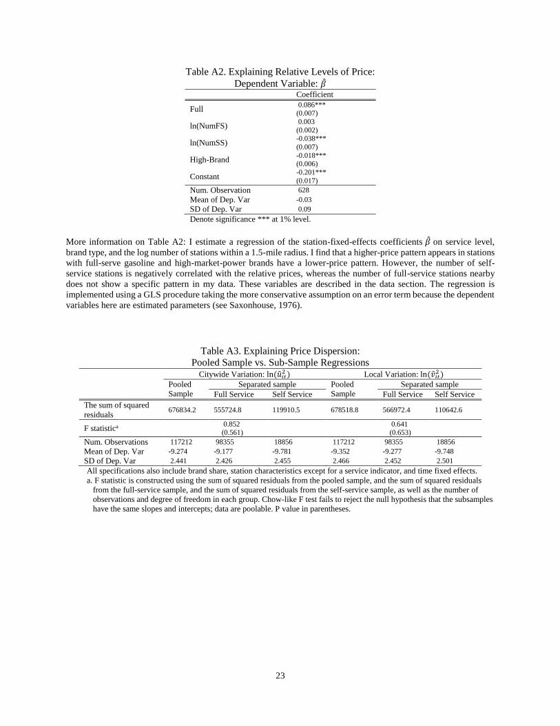
Table A2. Explaining Relative Levels of Price:
Dependent Variable: �� Coefficient
Full 0.086*** (0.007)
ln(NumFS) 0.003
(0.002)
ln(NumSS) -0.038***
(0.007)
High-Brand -0.018*** (0.006)
Constant -0.201***
(0.017)
Num. Observation 628
Mean of Dep. Var -0.03
SD of Dep. Var 0.09
Denote significance *** at 1% level.
More information on Table A2: I estimate a regression of the station-fixed-effects coefficients �� on service level,
brand type, and the log number of stations within a 1.5-mile radius. I find that a higher-price pattern appears in stations
with full-serve gasoline and high-market-power brands have a lower-price pattern. However, the number of self-
service stations is negatively correlated with the relative prices, whereas the number of full-service stations nearby
does not show a specific pattern in my data. These variables are described in the data section. The regression is
implemented using a GLS procedure taking the more conservative assumption on an error term because the dependent
variables here are estimated parameters (see Saxonhouse, 1976).
Table A3. Explaining Price Dispersion:
Pooled Sample vs. Sub-Sample Regressions
Citywide Variation: ln(��𝑖𝑡2 ) Local Variation: ln(��𝑖𝑡
2 )
Pooled
Sample
Separated sample Pooled
Sample
Separated sample
Full Service Self Service Full Service Self Service
The sum of squared
residuals 676834.2 555724.8 119910.5 678518.8 566972.4 110642.6
F statistica 0.852 (0.561)
0.641 (0.653)
Num. Observations 117212 98355 18856 117212 98355 18856
Mean of Dep. Var -9.274 -9.177 -9.781 -9.352 -9.277 -9.748
SD of Dep. Var 2.441 2.426 2.455 2.466 2.452 2.501
All specifications also include brand share, station characteristics except for a service indicator, and time fixed effects.
a. F statistic is constructed using the sum of squared residuals from the pooled sample, and the sum of squared residuals
from the full-service sample, and the sum of squared residuals from the self-service sample, as well as the number of
observations and degree of freedom in each group. Chow-like F test fails to reject the null hypothesis that the subsamples
have the same slopes and intercepts; data are poolable. P value in parentheses.
24
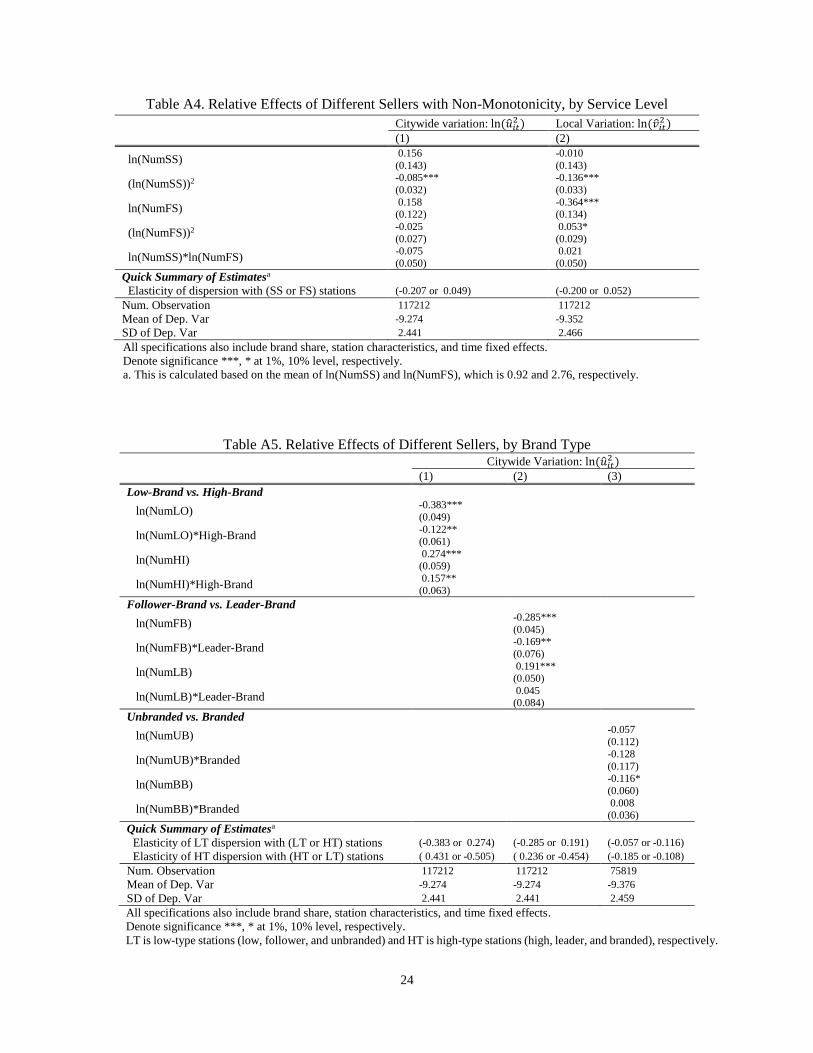
Table A4. Relative Effects of Different Sellers with Non-Monotonicity, by Service Level
Citywide variation: ln(��𝑖𝑡
2 ) Local Variation: ln(��𝑖𝑡2 )
(1) (2)
ln(NumSS) 0.156
(0.143)
-0.010
(0.143)
(ln(NumSS))2 -0.085***
(0.032)
-0.136***
(0.033)
ln(NumFS) 0.158 (0.122)
-0.364*** (0.134)
(ln(NumFS))2 -0.025
(0.027)
0.053*
(0.029)
ln(NumSS)*ln(NumFS) -0.075
(0.050)
0.021
(0.050)
Quick Summary of Estimatesa
Elasticity of dispersion with (SS or FS) stations (-0.207 or 0.049) (-0.200 or 0.052)
Num. Observation 117212 117212
Mean of Dep. Var -9.274 -9.352
SD of Dep. Var 2.441 2.466
All specifications also include brand share, station characteristics, and time fixed effects.
Denote significance ***, * at 1%, 10% level, respectively.
a. This is calculated based on the mean of ln(NumSS) and ln(NumFS), which is 0.92 and 2.76, respectively.
Table A5. Relative Effects of Different Sellers, by Brand Type
Citywide Variation: ln(��𝑖𝑡
2 )
(1) (2) (3)
Low-Brand vs. High-Brand
ln(NumLO) -0.383***
(0.049)
ln(NumLO)*High-Brand -0.122** (0.061)
ln(NumHI) 0.274*** (0.059)
ln(NumHI)*High-Brand 0.157**
(0.063)
Follower-Brand vs. Leader-Brand
ln(NumFB) -0.285***
(0.045)
ln(NumFB)*Leader-Brand -0.169**
(0.076)
ln(NumLB) 0.191*** (0.050)
ln(NumLB)*Leader-Brand 0.045 (0.084)
Unbranded vs. Branded
ln(NumUB) -0.057 (0.112)
ln(NumUB)*Branded -0.128
(0.117)
ln(NumBB) -0.116*
(0.060)
ln(NumBB)*Branded 0.008 (0.036)
Quick Summary of Estimatesa
Elasticity of LT dispersion with (LT or HT) stations (-0.383 or 0.274) (-0.285 or 0.191) (-0.057 or -0.116)
Elasticity of HT dispersion with (HT or LT) stations ( 0.431 or -0.505) ( 0.236 or -0.454) (-0.185 or -0.108)
Num. Observation 117212 117212 75819
Mean of Dep. Var -9.274 -9.274 -9.376
SD of Dep. Var 2.441 2.441 2.459
All specifications also include brand share, station characteristics, and time fixed effects.
Denote significance ***, * at 1%, 10% level, respectively.
LT is low-type stations (low, follower, and unbranded) and HT is high-type stations (high, leader, and branded), respectively.
25
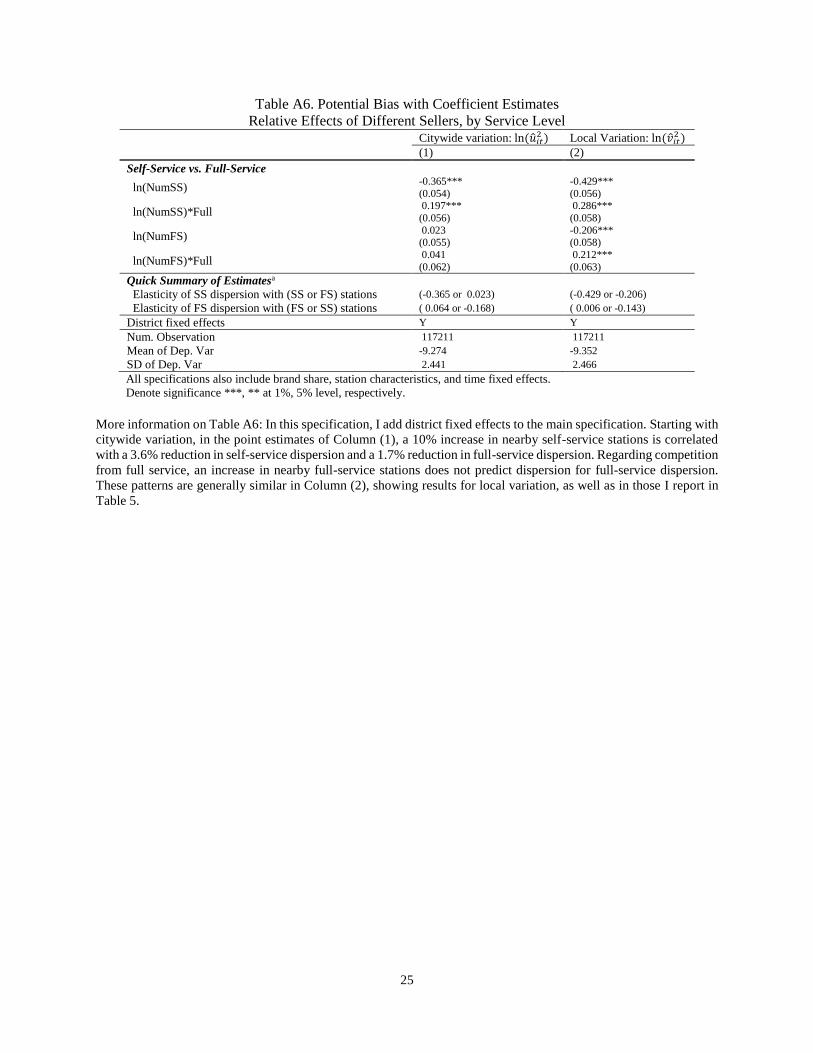
Table A6. Potential Bias with Coefficient Estimates
Relative Effects of Different Sellers, by Service Level
Citywide variation: ln(��𝑖𝑡
2 ) Local Variation: ln(��𝑖𝑡2 )
(1) (2)
Self-Service vs. Full-Service
ln(NumSS) -0.365***
(0.054)
-0.429***
(0.056)
ln(NumSS)*Full 0.197***
(0.056)
0.286***
(0.058)
ln(NumFS) 0.023 (0.055)
-0.206*** (0.058)
ln(NumFS)*Full 0.041
(0.062)
0.212***
(0.063)
Quick Summary of Estimatesa
Elasticity of SS dispersion with (SS or FS) stations (-0.365 or 0.023) (-0.429 or -0.206)
Elasticity of FS dispersion with (FS or SS) stations ( 0.064 or -0.168) ( 0.006 or -0.143)
District fixed effects Y Y
Num. Observation 117211 117211
Mean of Dep. Var -9.274 -9.352
SD of Dep. Var 2.441 2.466
All specifications also include brand share, station characteristics, and time fixed effects.
Denote significance ***, ** at 1%, 5% level, respectively.
More information on Table A6: In this specification, I add district fixed effects to the main specification. Starting with
citywide variation, in the point estimates of Column (1), a 10% increase in nearby self-service stations is correlated
with a 3.6% reduction in self-service dispersion and a 1.7% reduction in full-service dispersion. Regarding competition
from full service, an increase in nearby full-service stations does not predict dispersion for full-service dispersion.
These patterns are generally similar in Column (2), showing results for local variation, as well as in those I report in
Table 5.
26
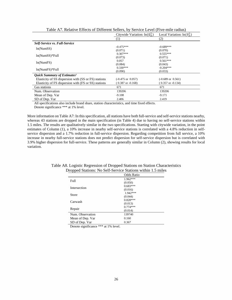
Table A7. Relative Effects of Different Sellers, by Service Level (Five-mile radius)
Citywide Variation: ln(��𝑖𝑡
2 ) Local Variation: ln(��𝑖𝑡2 )
(1) (2)
Self-Service vs. Full-Service
ln(NumSS) -0.475***
(0.071)
-0.689***
(0.070)
ln(NumSS)*Full 0.307*** (0.073)
0.555*** (0.071)
ln(NumFS) 0.057
(0.084)
0.561***
(0.043)
ln(NumFS)*Full 0.330***
(0.090)
-0.204***
(0.033)
Quick Summary of Estimatesa
Elasticity of SS dispersion with (SS or FS) stations (-0.475 or 0.057) (-0.689 or 0.561)
Elasticity of FS dispersion with (FS or SS) stations ( 0.387 or -0.168) ( 0.357 or -0.134)
Gas stations 671 671
Num. Observation 139206 139206
Mean of Dep. Var -9.108 -9.171
SD of Dep. Var 2.406 2.419
All specifications also include brand share, station characteristics, and time fixed effects.
Denote significance *** at 1% level. More information on Table A7: In this specification, all stations have both full-service and self-service stations nearby,
whereas 43 stations are dropped in the main specification (in Table 4) due to having no self-service stations within
1.5 miles. The results are qualitatively similar in the two specifications. Starting with citywide variation, in the point
estimates of Column (1), a 10% increase in nearby self-service stations is correlated with a 4.8% reduction in self-
service dispersion and a 1.7% reduction in full-service dispersion. Regarding competition from full service, a 10%
increase in nearby full-service stations does not predict dispersion for self-service dispersion but is correlated with
3.9% higher dispersion for full-service. These patterns are generally similar in Column (2), showing results for local
variation.
Table A8. Logistic Regression of Dropped Stations on Station Characteristics
Dropped Stations: No Self-Service Stations within 1.5 miles Odds Ratio
Full 1.962*** (0.050)
Intersection 0.683***
(0.016)
Store 1.942***
(0.044)
Carwash 0.828*** (0.013)
Repair 0.774***
(0.014)
Num. Observation 139740
Mean of Dep. Var 0.160
SD of Dep. Var 0.367
Denote significance *** at 1% level.
27
<Appendix B: Robustness Checks>
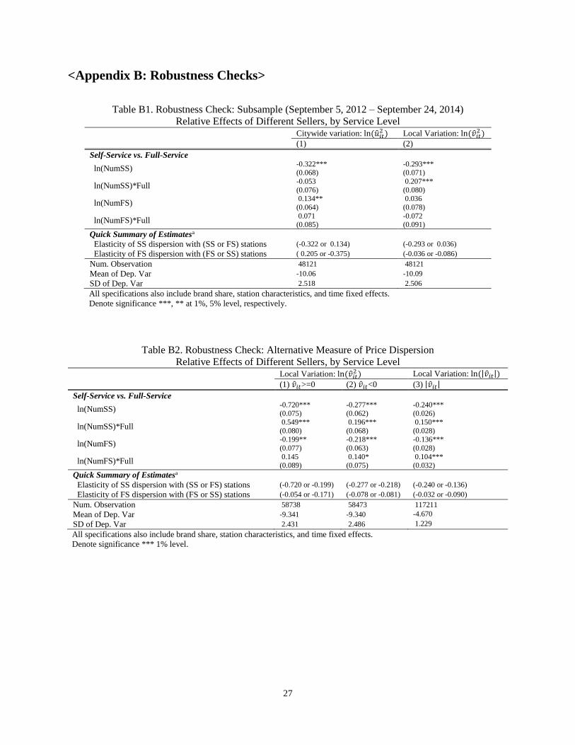
Table B1. Robustness Check: Subsample (September 5, 2012 – September 24, 2014)
Relative Effects of Different Sellers, by Service Level
Citywide variation: ln(��𝑖𝑡
2 ) Local Variation: ln(��𝑖𝑡2 )
(1) (2)
Self-Service vs. Full-Service
ln(NumSS) -0.322*** (0.068)
-0.293*** (0.071)
ln(NumSS)*Full -0.053
(0.076)
0.207***
(0.080)
ln(NumFS) 0.134**
(0.064)
0.036
(0.078)
ln(NumFS)*Full 0.071 (0.085)
-0.072 (0.091)
Quick Summary of Estimatesa
Elasticity of SS dispersion with (SS or FS) stations (-0.322 or 0.134) (-0.293 or 0.036)
Elasticity of FS dispersion with (FS or SS) stations ( 0.205 or -0.375) (-0.036 or -0.086)
Num. Observation 48121 48121
Mean of Dep. Var -10.06 -10.09
SD of Dep. Var 2.518 2.506
All specifications also include brand share, station characteristics, and time fixed effects.
Denote significance ***, ** at 1%, 5% level, respectively.
Table B2. Robustness Check: Alternative Measure of Price Dispersion
Relative Effects of Different Sellers, by Service Level
Local Variation: ln(��𝑖𝑡
2 ) Local Variation: ln(|��𝑖𝑡|)
(1) ��𝑖𝑡>=0 (2) ��𝑖𝑡<0 (3) |��𝑖𝑡|
Self-Service vs. Full-Service
ln(NumSS) -0.720*** (0.075)
-0.277*** (0.062)
-0.240*** (0.026)
ln(NumSS)*Full 0.549***
(0.080)
0.196***
(0.068)
0.150***
(0.028)
ln(NumFS) -0.199**
(0.077)
-0.218***
(0.063)
-0.136***
(0.028)
ln(NumFS)*Full 0.145 (0.089)
0.140* (0.075)
0.104*** (0.032)
Quick Summary of Estimatesa
Elasticity of SS dispersion with (SS or FS) stations (-0.720 or -0.199) (-0.277 or -0.218) (-0.240 or -0.136)
Elasticity of FS dispersion with (FS or SS) stations (-0.054 or -0.171) (-0.078 or -0.081) (-0.032 or -0.090)
Num. Observation 58738 58473 117211
Mean of Dep. Var -9.341 -9.340 -4.670
SD of Dep. Var 2.431 2.486 1.229
All specifications also include brand share, station characteristics, and time fixed effects.
Denote significance *** 1% level.
28
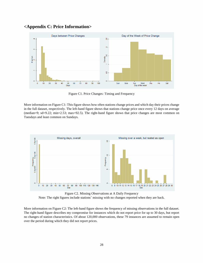
<Appendix C: Price Information>
Figure C1. Price Changes: Timing and Frequency
More information on Figure C1: This figure shows how often stations change prices and which day their prices change
in the full dataset, respectively. The left-hand figure shows that stations change price once every 12 days on average
(median=9; sd=9.22; min=2.53; max=92.5). The right-hand figure shows that price changes are most common on
Tuesdays and least common on Sundays.
Figure C2. Missing Observations at A Daily Frequency
Note: The right figures include stations’ missing with no changes reported when they are back.
More information on Figure C2: The left-hand figure shows the frequency of missing observations in the full dataset.
The right-hand figure describes my compromise for instances which do not report price for up to 30 days, but report
no changes of station characteristics. Of about 120,000 observations, these 79 instances are assumed to remain open
over the period during which they did not report prices.