Price Change, Volatility, and Accurate VaR: Evidence from ...jai.iijournals.com/content/iijaltinv/20/4/82.full.pdf · S. Pingr. 2018. R. angga. H. andika. ... parable power markets

the NSW and QLD Power MarketsEvidence fromPrice Change, Volatility, and Accurate VaR:

Rangga Handika and Yusuf Khudri

http://jai.iijournals.com/content/20/4/82https://doi.org/10.3905/jai.2018.20.4.082doi: 2018, 20 (4) 82-95JAI

This information is current as of June 26, 2018.

Email Alertshttp://jai.iijournals.com/alertsReceive free email-alerts when new articles cite this article. Sign up at:

© 2017 Institutional Investor LLC. All Rights Reserved New York, NY 10036, Phone: +1 212-224-35891120 Avenue of the Americas, 6th floor,Institutional Investor Journals

by guest on June 26, 2018http://jai.iijournals.com/Downloaded from by guest on June 26, 2018http://jai.iijournals.com/Downloaded from

https://doi.org/10.3905/jai.2018.20.4.082

http://jai.iijournals.com/content/20/4/82

http://jai.iijournals.com/alerts

http://jai.iijournals.com/


82 Price change, Volatility, and accurate Var: EvidEncE from thE nSW and QLd PoWEr markEtS SPring 2018

Rangga Handika

is a lecturer at the Institute of International Strategy, Tokyo International University in [email protected]

Yusuf kHudRi

is a lecturer in the Department of Accounting, Faculty of Economics and Business at the Universitas Indonesia in [email protected]@ui.ac.id

Price Change, Volatility, and Accurate VaR: Evidence from the NSW and QLD Power MarketsRangga Handika and Yusuf kHudRi

There are few research works dis-cussing risk measurement using Value-at-Risk (VaR) in power markets. A possible reason is that

VaR is normally used in discussing stan-dard f inancial assets, like stocks and bond markets. However, after financialization of commodity markets (as documented in Stoll and Whaley [2010], Tang and Xiong [2012], Basak and Pavlova [2016]), it seems that the power market can be treated like other finan-cial instruments. Furthermore, Adams and Glück [2015] document that commodities have become increasingly important for insti-tutional investors. Joskow and Kahn [2001] argue that spot power market is a commodity. Therefore, it is likely that market participants in the power market will use VaR analysis and trigger a new research area.

Recent investigations of VaR in power markets have been conducted by Chan and Gray [2006], Walls and Zhang [2006], Frauendorfer and Vinarski [2007], Herrera and González [2012], and Andriosopoulos and Nomikos [2012]. However, none of that work addresses the relationship among price changes, volatility forecasts, and accu-rate VaR in the power market. Recent works in power market volatility (Pen and Sévi [2010], Haugom et al. [2011], Ullrich [2012], Kalantzis and Milonas [2015], and Qu et al. [2016]) still do not address the ques-tion. Indeed, the question concerning that

relationship is essential; otherwise, market participants could argue that there is no need to do a good job in forecasting volatility and VaR in the power market. If we could report a significant relationship between volatility forecasts, accurate VaR estimates, and price changes, then markets participant will pay more attention to the VaR estimate.

We use the GARCH (Bollerslev [1986]) VaR estimate and investigate the relation-ship among price changes, volatility forecasts, and accurate VaR estimates in the Australian interconnected power markets, specifically New South Wales (NSW) and Queensland (QLD). The Australian interconnected power markets are significantly more volatile than other comparable power markets, and similarly to Higgs and Worthington [2008], we use daily spot series. The characteristics of high volatility and daily series in Australian interconnected power markets are the rea-sons for using GARCH in volatility model-ling, similar to Koopman et al. [2007] and Efimova and Serletis [2014].

The remainder of the article is orga-nized as follows. The next section provides an overview about Australian interconnected power markets. The third section reviews rel-evant studies about volatility modelling and VaR in power markets. The fourth section describes the methodology. The fifth section explains the data and discusses the empirical results. The final section concludes.

by guest on June 26, 2018http://jai.iijournals.com/Downloaded from

mailto:[email protected]

mailto:[email protected]


the Journal of alternatiVe inVeStmentS 83Spring 2018

AUSTRALIAN INTERCONNECTED POWER MARKETS

Over the last twenty-five years, the Australian power market has been transformed from monopolies that existed prior to 1997 to open competition. In the late 1990s, the Australian government announced a sig-nificant structural reform by separating power genera-tion and power transmission from power distribution and the retail supply. Therefore, as customers were free to choose their supplier, competition was introduced into the retail power market. Currently, the Australian power market, the National Electricity Market, (NEM), one of the world’s longest interconnected power systems, is interconnected through several regional networks. The price mechanism in the NEM can be explained as follows. The generators submit offers every five minutes, and the number of generators required to produce electricity is determined by the submitted offers. After that, the final price is constructed every half-hour for each of the regions by averaging the five-minute spot price. Therefore, there are 48 different half-hourly spot prices in a day for each region in the NEM.

We should note that Higgs and Worthington [2008], who f ind that price spikes occur more fre-quently in Australian power markets than in the U.S. pool (Pennsylvania—New Jersey—Maryland). Thus, the Australian interconnected power markets are con-sidered more spike-prone and volatile than many com-parable power markets and risk analysis in Australian power markets is essential. Clearly, this will contribute to the energy finance literature over time.

This article focuses on only two Australian power markets, NSW and QLD, because these regions are juris-dictions representative in Australian electricity markets for investigating macroeconomic costs associated with “Time of Use” pricing (see Nelson and Orton [2013]). Furthermore, according to Anderson et al. [2007], NSW and QLD have the two highest installed capacities; they are the only regions with more than 10,000 megawatts (MW) in the Australian power markets. We also chose to exclude South Australia (SA) and Victoria (VIC) regions because we found (in unreported results) that SA and VIC GARCH(1,2) and GARCH(2,2) estimates are explosive. Explosive GARCH estimates sometimes occur in certain markets such as the Sudanese (Ahmed and Suliman [2011]) or Ugandan (Namugaya et al. [2014]) stock exchanges. We could have used another

type of GARCH model for the SA and VIC power markets, but this would have generated inconsistent comparisons since this article focuses on GARCH(p,q) models. Therefore, we will only cover the NSW and QLD power markets.

LITERATURE REVIEW

There are a number of studies examining VaR in the power market. Most of the works tend to extend the standard VaR model. For instance, Chan and Gray [2006] incorporate weekly seasonality and autoregres-sion in their EGARCH specification. They model the tails of the return distribution by applying the extreme value theory (EVT). Another article by Walls and Zhang [2006] uses EVT in their extended VaR model. They report that their extended VaR is more accurate in the Alberta power market. Herrera and González [2012] also extend VaR in power market by adopting EVT. Another version of extending VaR is performed by Frauendorfer and Vinarski [2007], who report the limits of the tra-ditional VaR in the power markets. They propose a quasi-sensitivity analysis of the VaR with respect to the risk factors, price, and volatility. Andriosopoulos and Nomikos [2012] capture the dynamics of energy prices by extending a set of VaR models. However, none of these studies determines whether the forecast volatility and an accurate VaR estimate can explain price changes in power markets.

Recent works on volatility modelling in power markets do not address the relationship among price changes, volatility forecasts, and accurate VaR measures in power markets either. For instance, Haugom et al. [2011] apply market measures for the prediction of volatility in the Nord Pool electricity forward market. Kalantzis and Milonas [2015] investigate the impact of the introduction of electricity futures on the spot-price volatility of the French (Powernext) and German (EEX) electricity markets. Pen and Sévi [2010] estimate a VAR-BEKK model and find evidence of return and volatility in three different forward electricity markets. Another article by Qu et al. [2016] measures volatility and jumps in power prices by using the non-parametric realized volatility technique and the associated jump detection. Ullrich [2012] estimates realized volatility and the frequency of price spikes in eight wholesale electricity markets.




Overall, to the best of our knowledge, no study addresses the question as to whether forecast volatility and accurate VaR estimates can explain price changes. We also realize that works on electricity volatility of the present analyses from the generators’, that is, the sellers’ side. No one has discussed electricity volatility in power markets from the retailer and buyer perspectives. Indeed, analyses coming from both sides are essential because the price spike generates market risks that should be moni-tored and managed thoroughly. A dramatic increase (i.e., huge positive “return”) is favorable for generators in the power market, while a dramatic decrease (i.e., huge negative “return”) is favorable for retailers in the power market. We can see that a price change might be favor-able for generators but unfavorable for retailers and vice versa. Therefore, we argue that a comprehensive analysis should encompass the perspectives of both generators and retailers.

METHOD

We use the GARCH model for estimating VaR in the interconnected power markets, similar to Koopman et al. [2007] and Efimova and Serletis [2014]. According to Bollerslev [1986], the GARCH(p,q) model can be written as follow:

2 2 2

11

yt i t i j t jj

p

i

q

∑∑σ = ω + α + β σ− −==

(1)

where σt denotes the volatility forecast for time t and yt is the realized return at time t.

We compare and determine the most fitted various p and q values up to GARCH (2,2). This method fol-lows Chinn and Coibion [2014] for dynamic GARCH in commodity markets.

A standard risk measurement VaR can be formally expressed (Hull [2007], Jorion [2007]) as follows:

VaR ( )1= σ Φ αα− (2)

where σ denotes volatility of the return of an asset and Φ–1(α) is the inverse cumulative normal distribu-tion at α confidence level. However, He et al. [2016] f ind that switching from the normal distribution to Student’s t distribution improves the model performance in the Australian power markets data. Thus, we modify

Equation (2) by using Student’s t distribution instead of normal distribution as follows:

VaR tdf= σα α (3)

where σ denotes volatility of the return of an asset and tdfα

is the critical value of t-distribution at α confidence level and df degrees of freedom. We can see from Equation (2) and Equation (3) that a VaR estimate value largely depends on the volatility estimate. Therefore, an accu-rate volatility estimate implies an accurate VaR. In this article, we analyze left-tailed VaR for the generators’ side (because a negative price change means a loss for genera-tors) and right-tailed VaR for the retailers’ side (because a positive price change means a loss for retailers).

We explore the relationship among price changes, volatility forecasts, and accurate VaR using regres-sion Equation (4). According to Pindyck [2004], vola-tility is one of the explanatory variables of commodity return. Then, we modify the Pindyck [2004] model by including both forecasted volatility and a dummy vari-able about the accurate VaR estimate. Our model is sim-ilar to Handika and Sondi [2017] and can be expressed as follows:

DUMVAR1 2RET et t t t= α + β σ + β + (4)

where RETt denotes the return (i.e., price change) of a commodity at day t, σt denotes the volatility forecast for day t, and DUMVAR is the dummy variable explaining the VaR performance at day t: it is 1 when the forecasted volatility is accurate (i.e., the realized price change does not violate the forecasted VaR limit), and 0 otherwise.

EMPIRICAL ANALYSIS

We obtained the half-hourly prices series of Australian power market prices in NSW and QLD regions from the AEMO website.1 Then, we calculated the daily price for each region by averaging the dif-ferent 48 half-hour power prices. Our in-sample period runs from January 1, 2000 to December 31, 2009, and the out-of-sample period runs from January 1, 2010 to December 31, 2015 (a 10-year in-sample period and a six-year out-of-sample period). Our choice with regard to these in-sample and out-of-sample periods ref lects the fact that f inancialization of commodity markets only started in the 2000s (Rossi [2012], Tang and




Xiong [2012], Handika and Sondi [2017]). We find that 10 years is a standard time frame for empirical f inance studies (Ledoit and Wolf [2008]). We also perform robustness checks in the yearly sub-sample analysis during the out-of-sample period. These yearly robustness checks follow the method from Gorton and Rouwenhorst [2006], Wong [2010], and Perignon et al. [2008], and they are similar to those used by Handika and Sondi [2017].

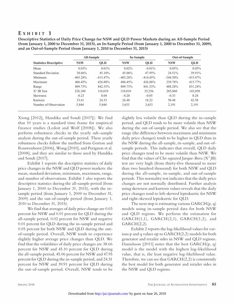
Exhibit 1 reports the descriptive statistics of daily price changes in the NSW and QLD power markets: the mean, standard deviation, minimum, maximum, range, and number of observations. Exhibit 1 also reports the descriptive statistics during the all-sample period (from January 1, 2000 to December 31, 2015), with the in-sample period (from January 1, 2000 to December 31, 2009) and the out-of-sample period (from January 1, 2010 to December 31, 2015).

We find that averages of daily price change are 0.03 percent for NSW and 0.01 percent for QLD during the all-sample period, 0.02 percent for NSW and negative 0.01 percent for QLD during the in-sample period and 0.05 percent for both NSW and QLD during the out-of-sample period. Overall, NSW tends to experience slightly higher average price changes than QLD. We find that the volatilities of daily price changes are 38.66 percent for NSW and 45.10 percent for QLD during the all-sample period, 45.06 percent for NSW and 47.95 percent for QLD during the in-sample period, and 24.51 percent for NSW and 39.91 percent for QLD during the out-of-sample period. Overall, NSW tends to be

slightly less volatile than QLD during the in-sample period, and QLD tends to be more volatile than NSW during the out-of-sample period. We also see that the range (the difference between maximum and minimum daily price changes) tends to be higher in QLD than in the NSW during the all-sample, in-sample, and out-of-sample periods. This indicates that overall, QLD daily price changes tend to be more volatile than NSW. We find that the values of Chi-squared Jarque-Bera (X2 JB) test are very high (from thirty-five thousand to more than two hundred thousand) for both NSW and QLD during the all-sample, in-sample, and out-of-sample periods. This normality test indicates that the daily price changes are not normally distributed. Further analysis using skewness and kurtosis values reveals that the daily price changes tend to left-skewed leptokurtic for NSW and right-skewed leptokurtic for QLD.

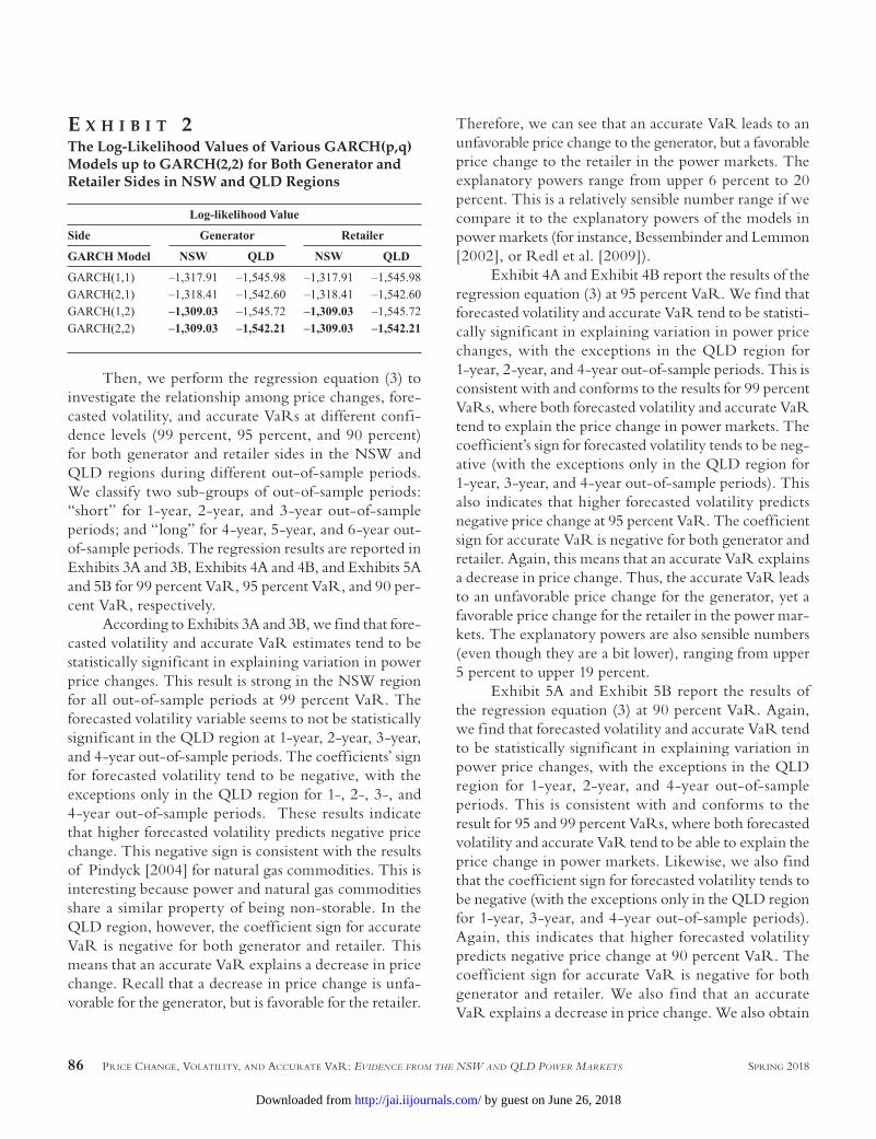
The next step is estimating various GARCH(p, q) models using in-sample period data for both NSW and QLD regions. We perform the estimation for GARCH(1,1), GARCH(2,1), GARCH(1,2), and GARCH(2,2).

Exhibit 2 reports the log-likelihood values for var-ious p and q values up to GARCH(2,2) models for both generator and retailer sides in NSW and QLD regions. Danielsson [2011] notes that the best GARCH(p, q) model is the model with the highest log-likelihood value, that is, the least negative log-likelihood value. Therefore, we can see that GARCH(2,2) is consistently the best model for both generator and retailer sides in the NSW and QLD regions.

E x H i b i t 1Descriptive Statistics of Daily Price Change for NSW and QLD Power Markets during an All-Sample Period (from January 1, 2000 to December 31, 2015), an In-Sample Period (from January 1, 2000 to December 31, 2009), and an Out-of-Sample Period (from January 1, 2010 to December 31, 2015)




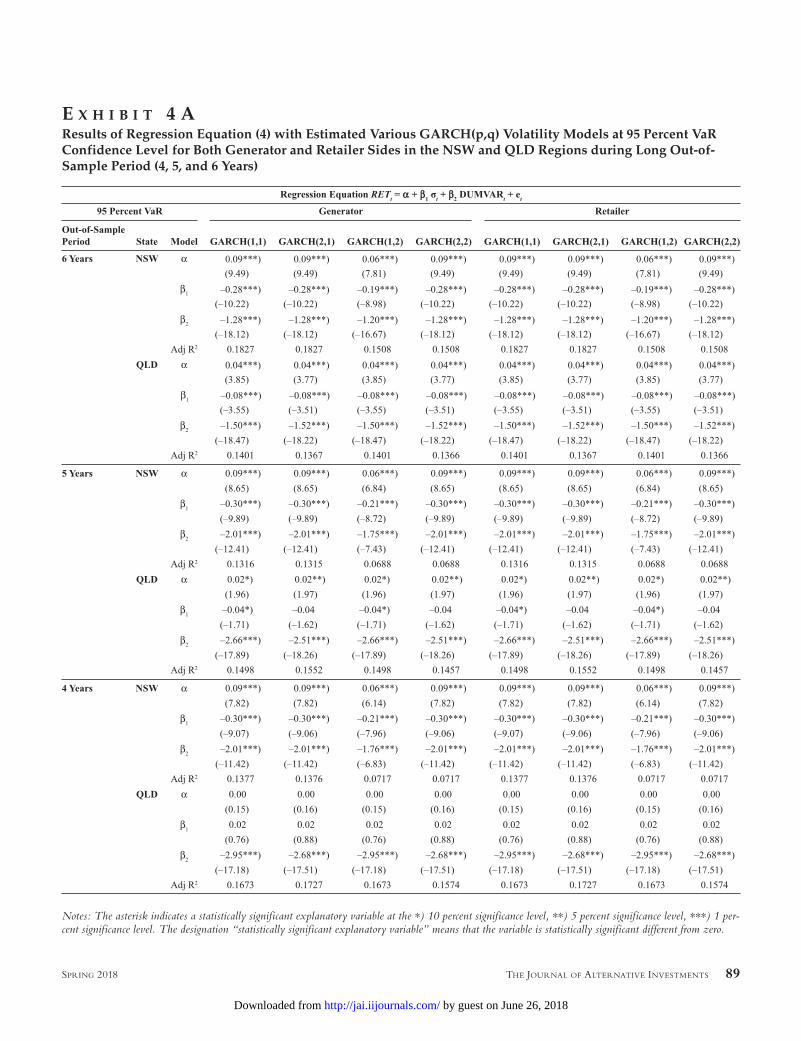
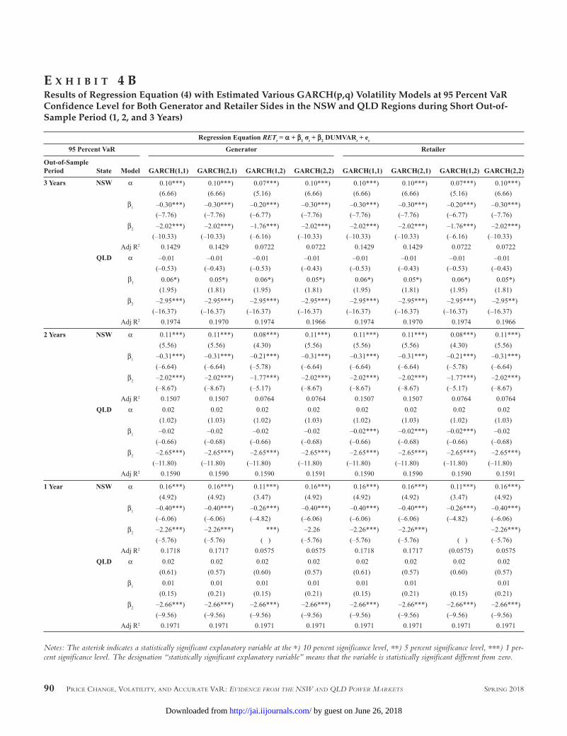
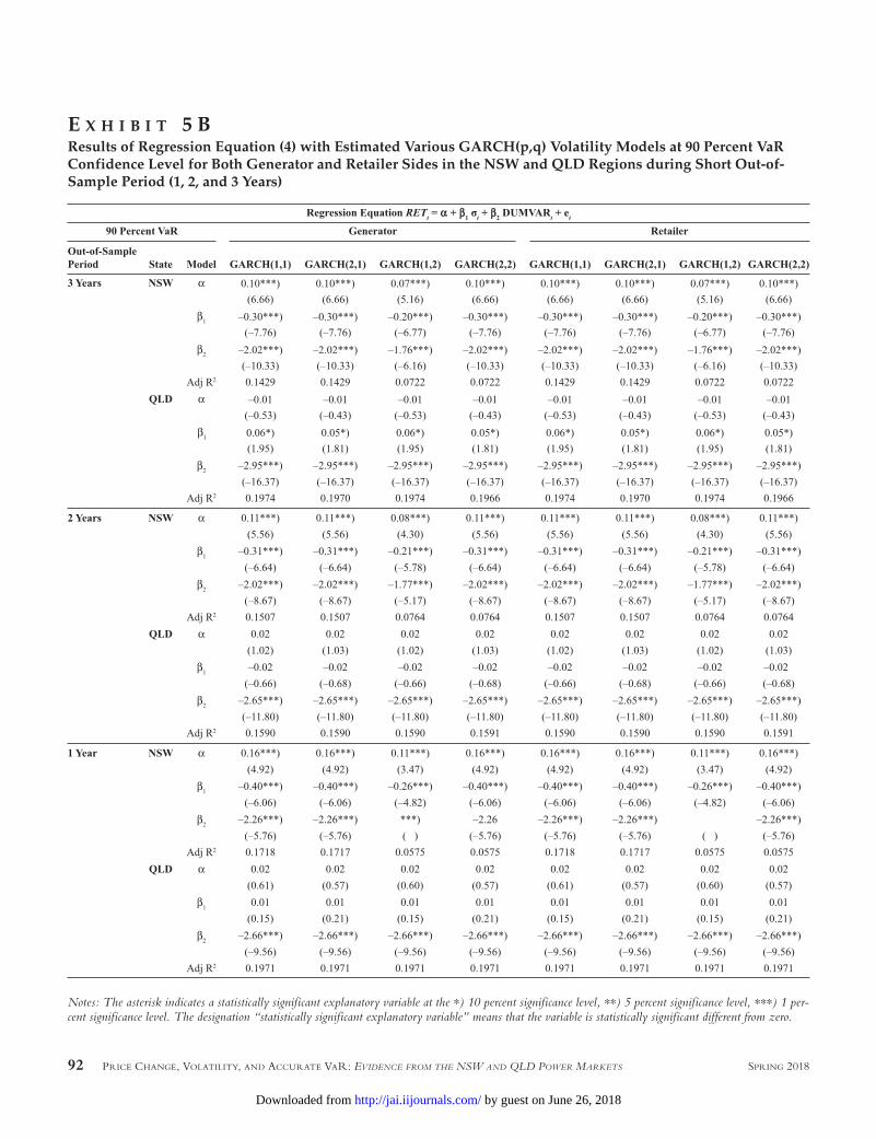
Then, we perform the regression equation (3) to investigate the relationship among price changes, fore-casted volatility, and accurate VaRs at different confi-dence levels (99 percent, 95 percent, and 90 percent) for both generator and retailer sides in the NSW and QLD regions during different out-of-sample periods. We classify two sub-groups of out-of-sample periods: “short” for 1-year, 2-year, and 3-year out-of-sample periods; and “long” for 4-year, 5-year, and 6-year out-of-sample periods. The regression results are reported in Exhibits 3A and 3B, Exhibits 4A and 4B, and Exhibits 5A and 5B for 99 percent VaR, 95 percent VaR, and 90 per-cent VaR, respectively.

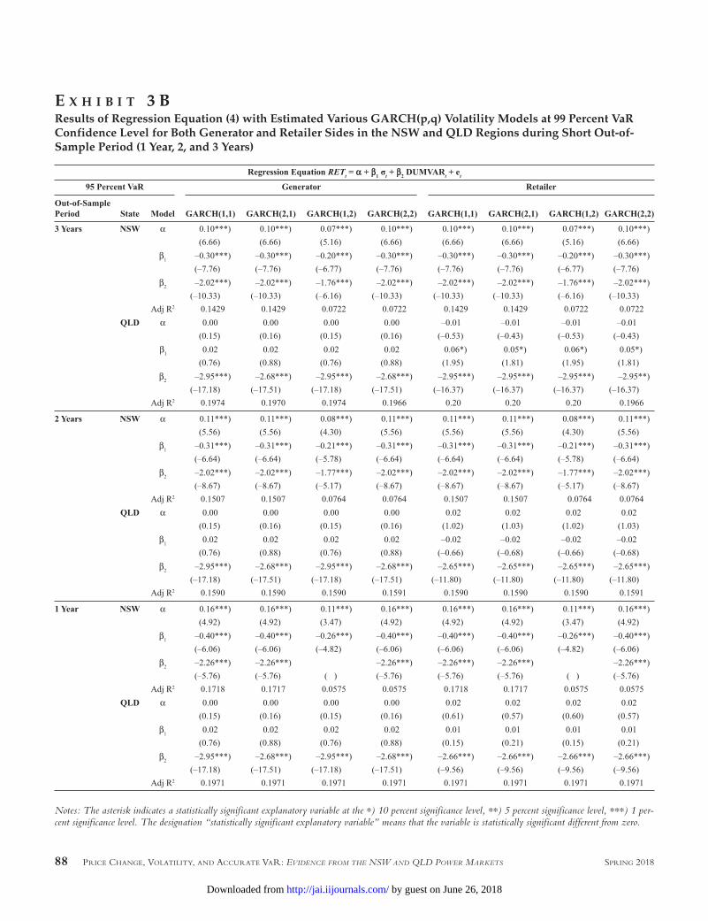
According to Exhibits 3A and 3B, we find that fore-casted volatility and accurate VaR estimates tend to be statistically significant in explaining variation in power price changes. This result is strong in the NSW region for all out-of-sample periods at 99 percent VaR. The forecasted volatility variable seems to not be statistically significant in the QLD region at 1-year, 2-year, 3-year, and 4-year out-of-sample periods. The coefficients’ sign for forecasted volatility tend to be negative, with the exceptions only in the QLD region for 1-, 2-, 3-, and 4-year out-of-sample periods. These results indicate that higher forecasted volatility predicts negative price change. This negative sign is consistent with the results of Pindyck [2004] for natural gas commodities. This is interesting because power and natural gas commodities share a similar property of being non-storable. In the QLD region, however, the coefficient sign for accurate VaR is negative for both generator and retailer. This means that an accurate VaR explains a decrease in price change. Recall that a decrease in price change is unfa-vorable for the generator, but is favorable for the retailer.

Therefore, we can see that an accurate VaR leads to an unfavorable price change to the generator, but a favorable price change to the retailer in the power markets. The explanatory powers range from upper 6 percent to 20 percent. This is a relatively sensible number range if we compare it to the explanatory powers of the models in power markets (for instance, Bessembinder and Lemmon [2002], or Redl et al. [2009]).

Exhibit 4A and Exhibit 4B report the results of the regression equation (3) at 95 percent VaR. We find that forecasted volatility and accurate VaR tend to be statisti-cally significant in explaining variation in power price changes, with the exceptions in the QLD region for 1-year, 2-year, and 4-year out-of-sample periods. This is consistent with and conforms to the results for 99 percent VaRs, where both forecasted volatility and accurate VaR tend to explain the price change in power markets. The coefficient’s sign for forecasted volatility tends to be neg-ative (with the exceptions only in the QLD region for 1-year, 3-year, and 4-year out-of-sample periods). This also indicates that higher forecasted volatility predicts negative price change at 95 percent VaR. The coefficient sign for accurate VaR is negative for both generator and retailer. Again, this means that an accurate VaR explains a decrease in price change. Thus, the accurate VaR leads to an unfavorable price change for the generator, yet a favorable price change for the retailer in the power mar-kets. The explanatory powers are also sensible numbers (even though they are a bit lower), ranging from upper 5 percent to upper 19 percent.

Exhibit 5A and Exhibit 5B report the results of the regression equation (3) at 90 percent VaR. Again, we find that forecasted volatility and accurate VaR tend to be statistically significant in explaining variation in power price changes, with the exceptions in the QLD region for 1-year, 2-year, and 4-year out-of-sample periods. This is consistent with and conforms to the result for 95 and 99 percent VaRs, where both forecasted volatility and accurate VaR tend to be able to explain the price change in power markets. Likewise, we also find that the coefficient sign for forecasted volatility tends to be negative (with the exceptions only in the QLD region for 1-year, 3-year, and 4-year out-of-sample periods). Again, this indicates that higher forecasted volatility predicts negative price change at 90 percent VaR. The coefficient sign for accurate VaR is negative for both generator and retailer. We also f ind that an accurate VaR explains a decrease in price change. We also obtain

E x H i b i t 2The Log-Likelihood Values of Various GARCH(p,q) Models up to GARCH(2,2) for Both Generator and Retailer Sides in NSW and QLD Regions




E x H i b i t 3 aResults of Regression Equation (4) with Estimated Various GARCH(p,q) Volatility Models at 99 Percent VaR Confidence Level for Both Generator and Retailer Sides in the NSW and QLD Regions during Long Out-of-Sample Period (4, 5, and 6 Years)

Notes: The asterisk indicates a statistically significant explanatory variable at the *) 10 percent significance level, **) 5 percent significance level, ***) 1 per-cent significance level. The designation “statistically significant explanatory variable” means that the variable is statistically significant different from zero.




E x H i b i t 3 bResults of Regression Equation (4) with Estimated Various GARCH(p,q) Volatility Models at 99 Percent VaR Confidence Level for Both Generator and Retailer Sides in the NSW and QLD Regions during Short Out-of-Sample Period (1 Year, 2, and 3 Years)





E x H i b i t 4 aResults of Regression Equation (4) with Estimated Various GARCH(p,q) Volatility Models at 95 Percent VaR Confidence Level for Both Generator and Retailer Sides in the NSW and QLD Regions during Long Out-of-Sample Period (4, 5, and 6 Years)





E x H i b i t 4 bResults of Regression Equation (4) with Estimated Various GARCH(p,q) Volatility Models at 95 Percent VaR Confidence Level for Both Generator and Retailer Sides in the NSW and QLD Regions during Short Out-of-Sample Period (1, 2, and 3 Years)





E x H i b i t 5 aResults of Regression Equation (4) with Estimated Various GARCH(p,q) Volatility Models at 90 Percent VaR Confidence Level for Both Generator and Retailer Sides in the NSW and QLD Regions during Long Out-of- Sample Period (4, 5, and 6 Years)





E x H i b i t 5 bResults of Regression Equation (4) with Estimated Various GARCH(p,q) Volatility Models at 90 Percent VaR Confidence Level for Both Generator and Retailer Sides in the NSW and QLD Regions during Short Out-of-Sample Period (1, 2, and 3 Years)





sensible numbers for the explanatory powers. They range from upper 5 percent to lower 31 percent.

Overall, we find that: (i) forecasted volatility and accurate VaR variables tend to be statistically significant in explaining variation in power price changes, (ii) the coefficients of forecasted volatility tend to be negative, indicating that higher forecasted volatility predicts nega-tive price change, (iii) accurate VaR tends to lead to a decrease in price change, implying that well-functioning market risk management explains an unfavorable price change for the generator, but a favorable price change for the retailer. The results are strong for both gen-erator and retailer, at different VaR confidence levels and different out-of-sample periods in both NSW and QLD power markets. We also see that the explanatory powers of model (4) are sensible enough, yet the better GARCH(p,q) models with higher log likelihood values tend to have lower explanatory powers in model (4).

CONCLUSION

This article addresses the relationship among price changes, volatility forecasts, and accurate VaRs in the power market. We use various GARCH(p,q) methods to model daily volatility and VaR in the NSW and QLD regions. Then, we explore the relationship among price changes, volatility forecasts, and accurate VaRs. We perform the tests for both generator and retailer sides, at 99 percent, 95 percent, and 90 percent VaR, at six different out-of-sample periods in the NSW and QLD power markets.

We f ind that forecasted volatility and accurate VaR variables tend to be statistically signif icant in explaining variation in price changes in the power mar-kets. The sensible explanatory power indicates strong relationships among price changes, forecasted volatility, and accurate VaRs in power markets. We also find that the coefficients of forecasted volatility tend to be nega-tive. This indicates that higher forecasted volatility predicts negative price changes. Therefore, market participants in the power markets, either generator or retailer, should expect negative price change when their volatility forecast is high. Our result is consistent with Pindyck [2004] in analyzing the natural gas market. Therefore, we discover a similar property in non-storable commodities (both natural gas and power). Furthermore, we find that is the case, because accurate VaRs tends to lead to a decrease in price changes. This implies that

well-functioning market risk management explains an unfavorable price change for the generator, but a favor-able price change for the retailer in the Australian power markets. Our results are robust for different VaR confi-dence levels and different out-of-sample periods. How-ever, our research is limited in standard GARCH(p,q) models. Future research using more advanced GARCH models is highly encouraged to explore the relationship between price changes, volatility forecasts, and accurate VaRs in the power markets in greater depth.

ENDNOTES

We thank to the anonymous referee who provide valu-able comments and suggestions to improve the quality of our manuscript.

1http://www.aemo.com.au/Electricity/National-Electricity-Market-NEM/Data-dashboard#aggregated-data, as viewed January 17, 2018.

REFERENCES

Adams, Z., and T. Glück. “Financialization in Commodity Markets: A Passing Trend or the New Normal?” Journal of Banking and Finance, No. 60 (2015), pp. 93111.

Ahmed, A.E.M., and S.Z. Suliman. “Modelling Stock Market Volatility Using GARCH Models Evidence from Sudan.” International Journal of Business and Social Science, Vol. 2, No. 23 (2011), pp. 114-128.

Anderson, E.J., X. Hu, and D. Winchester. “Forward Contracts in Electricity Markets: The Australian Experience.” Energy Policy, No. 35 (2007), pp. 3089-3103.

Andriosopoulos, K., and N. Nomikos. “Risk Management in the Energy Markets and Value-at-Risk Modelling: A Hybrid Approach.” Working paper, EU, 2012.

Basak, S., and A. Pavlova. “A Model of Financialization of Commodities.” The Journal of Finance, Vol. 71, No. 4 (2016), pp. 1511-1556.

Bessembinder, H., and M.L. Lemmon. “Equilibrium Pricing and Optimal Hedging in Electricity Forward Markets.” The Journal of Finance, Vol. 57, No. 3 (2002), pp. 1347-1381.

Bollerslev, T. “Generalized Autoregressive Conditional Heteroskedasticity.” Journal of Econometrics, Vol. 31, No. 3 (1986), pp. 307-327.




Chan, K.F., and P. Gray. “Using Extreme Value Theory to Measure Value-at-Risk for Daily Electricity Spot Prices.” International Journal of Forecasting, No. 22 (2006), pp. 283-300.

Chinn, M.D., and O. Coibion. “The Predictive Content of Commodity Futures.” The Journal of Futures Markets, Vol. 34, No. 7 (2014), pp. 607-636.

Danielsson, J. Financial Risk Forecasting. John Wiley & Sons Ltd., 2011.

Efimova, O., and A. Serletis. “Energy Markets Volatility Modelling Using GARCH.” Energy Economics, No. 43 (2014), pp. 264-273.

Frauendorfer, K., and A. Vinarski. “Risk Measurement in Electricity Markets.” Working paper, Universität St. Gallen, 2007.

Gorton, G., and K.G. Rouwenhorst. “Facts and Fanta-sies about Commodity Futures.” Financial Analysts Journal, Vol. 62, No. 2 (2006), pp. 47-68.

Handika, R., and I. Sondi. “Commodities Returns’ Volatility in Financialization Era.” Studies in Economics and Finance, Vol. 34, No. 3 (2017), pp 344-362.

Haugom, E., S. Westgaard, P.B. Solibakke, and G. Lien. “Realized Volatility and the Inf luence of Market Measures on Predictability: Analysis of Nord Pool Forward Electricity Data.” Energy Economics, No. 33 (2011), pp. 1206-1215.

He, K., H. Wang, J. Du, and Y. Zou. “Forecasting Elec-tricity Market Risk Using Empirical Mode Decomposition (EMD)—Based Multiscale Methodology.” Energies, Vol. 9, No. 931 (2016), pp. 1-11.

Herrera, R., and N. González. “Computing Value-at-Risk on Electricity Markets through Modelling Inter-exceedances Times.” Working paper, CLAIO SBPO, 2012.

Higgs, H., and A. Worthington. “Stochastic Prices Mod-eling of High Volatility, Mean Reverting, Spike-prone Com-modities: The Australia Wholesale Spot Electricity Market.” Energy Economics, No. 30 (2008), pp. 3172-3185.

Hull, J. Risk Management and Financial Institutions. Pearson Prentice Hall, 2007, 1st edition.

Jorion, P. Value-at-Risk the New Benchmark for Managing Financial Risk, The McGraw-Hill Companies, 2007, 3rd edition.

Joskow, P.L., and E. Kahn. “Commodity Index Investing and Commodity Futures Prices.” Working Paper, MIT Center for Energy and Environmental Policy Research, 2001.

Kalantzis, F.G., and N.T. Milonas. “Analyzing the Impact of Futures Trading on Spot Price Volatility: Evidence from the Spot Electricity Market in France and Germany.” Energy Economics, No. 36 (2015), pp. 454-463.

Koopman, S.J., M. Ooms, and M.A. Carnero. “Periodic Seasonal Reg-ARFIMA-GARCH Models for Daily Elec-tricity Spot Prices.” Journal of the American Statistical Association, Vol. 102, No. 477 (2007), pp. 16-27.

Ledoit, O., and M. Wolf. “Robust Performance Hypothesis Testing with the Sharpe Ratio.” Journal of Empirical Finance, No. 15 (2008), pp. 850-859.

Namugaya, J., P.G.O. Weke, and W.M. Charles. “Modelling Volatility of Stock Returns: Is GARCH(1,1) Enough?” Inter-national Journal of Sciences: Basic and Applied Research, Vol. 16, No. 2 (2014), pp. 216-223.

Nelson, T., and F. Orton. “A New Approach to Congestion Pricing in Electricity Markets: Improving User Pays Pricing Incentives.” Energy Economics, No. 40 (2013), pp. 1-7.

Pen, Y.L., and B. Sévi. “Volatility Transmission and Volatility Impulse Response Functions in European Electricity Forward Markets.” Energy Economics, No. 32 (2010), pp. 758-770.

Perignon, C., Z.Y. Deng, and Z.J. Wang. “Do Banks Over-state Their Value-at-Risk?” Journal of Banking and Finance, Vol. 32, No. 5 (2008), pp. 783-794.

Pindyck, R.S. “Volatility in Natural Gas and Oil Markets.” The Journal of Energy and Development, Vol. 30, No. 1 (2004), pp. 1-19.

Qu, H., W. Chen, M. Niu, and X. Li. “Forecasting Real-ized Volatility in Electricity Markets Using Logistic Smooth Transition Heterogeneous Autoregressive Models.” Energy Economics, No. 54 (2016), pp. 68-76.

Redl, C., R. Haas, C. Huber, and B. Böhm. “Price Forma-tion in Electricity Forward Markets and the Relevance of Systematic Forecast Errors.” Energy Economics, No. 31 (2009), pp. 356-364.

Rossi, B. “The Changing Relationship between Commodity Prices and Equity Prices in Commodity Exporting Coun-tries.” Working paper, IMF, 2012.




Stoll, H.A., and R.E. Whaley. “Commodity Index Investing and Commodity Futures Prices.” Journal of Applied Finance, Vol. 20, No. 1 (2010), pp. 7-46.

Tang, K., and W. Xiong. “Index Investment and the Financialization of Commodities.” Financial Analysts Journal, Vol. 68, No. 6 (2012), pp. 54-74.

Ullrich, C.J. “Realized Volatility and Price Spikes in Electricity Markets: The Importance of Observation Frequency.” Energy Economics, No. 34 (2012), pp. 1809-1818.

Walls, W.D., and W. Zhang. “Using Extreme Value Theory to Model Electricity Price Risk with an Application to the Alberta Power Market.” Energy, Exploration & Exploitation, Vol. 23, No. 5 (2006), pp. 375-404.

Wong, W.K. “Backtesting Value-at-Risk Based on Tail Losses.” Journal of Empirical Finance, Vol. 17, No. 3 (2010), pp. 526-538.

To order reprints of this article, please contact David Rowe at [email protected] or 212-224-3045.


http://[email protected]


Documents

Price Change, Volatility, and Accurate VaR: Evidence from ...jai.iijournals.com/content/iijaltinv/20/4/82.full.pdf · S. Pingr. 2018. R. angga. H. andika. ... parable power markets