Price and Wage Rigidity in Nepal · winter seasons, price of various commodities changing at beginning of fiscal year after budget, school and college’s admission and fees changing

NRB Working Paper No. 47

December 2019

Price and Wage Rigidity in Nepal

Sushil Poudel*

ABSTRACT

This paper estimates price and wage rigidity by using 5.5 million micro datasets

compiled by Nepal Rastra Bank for producing Consumer Price Index, Wholesale Price

Index and Salary and Wage Rate Index. The study is first of its kind in Nepal. This paper

uses un-weighted arithmetic mean for estimation of aggregates at elementary level and

weighted arithmetic mean for aggregates at subgroup, overall and analytical group level.

Average duration of price spell, average duration of increasing price spell, average

duration of decreasing price spell, share of direction of price spell and size of price

adjustment in increasing and decreasing direction are estimated for analyzing the price

and wage rigidity in Nepal. The study estimates degree of price rigidity as 68.73% for

overall retail prices and degree of wage rigidity as 79.82% for overall salary and wage

rates. High degree of heterogeneity in period of price and wage adjustment is observed

among sub-group of retail prices and salary and wage rates. The study also finds that

prices and wages are downward rigid. The estimated rigidities can be used as an

unbiased benchmark for price and wage rigidity in DSGE model with time path of price

following Calvo staggered price model.

JEL Classification: E31, E52, E58

Key Words: Price rigidity, wage rigidity, consumer price rigidity, wholesale price rigidity,

salary and wage rigidity, average duration of price spell, direction of price change, size of

price change

* Deputy Director, Nepal Rastra Bank (email: [email protected]). The author would like to thank

Mr. Madhav Dangal, Act Director, NRB for special support in this study. The author would also like to

thank Dr. Gunakar Bhatta, Executive Director, Research Department, NRB for departmental support.

© 2019 Nepal Rastra Bank

Price and Wage Rigidity in Nepal NRBWP47

2

I. BACKGROUND

In this paper, I investigate the pattern of price and wage adjustment in Nepal by using micro

datasets compiled by Nepal Rastra Bank (NRB) for producing Consumer Price Index (CPI),

Wholesale Price Index (WPI) and Salary and Wage Rate Index (SWRI). The sample is quite

extensive. Analysis of retail price is based on 496 varieties of goods and services collected

from retail outlets across 60 different market places for 5 year period. Wholesale price

analysis is based on 262 goods prices collected from major markets and producers for 2

years. Salary and wage rate analysis is based on 170 different types of jobs and profession

from different industry for 15 years.

A large number of theoretical models along with empirical evidence in macroeconomics

supporting monetary non-neutrality are based on the assumptions that prices and wages adjust

sluggishly to changes in aggregate conditions. When prices are very flexible, demand as well

as supply shock translates to change in prices immediately and proportionately without

altering real quantities. Thus as found in classical economic models, real interest rates and

real output are completely divorced from movements in the money supply and nominal

interest rates. However, if price adjustment is sluggish, reductions of nominal interest rates by

the central bank translates into a reduction in real interest rates. As a result, negative output

gap closes to zero and growth in output is realized. Degrees of price and wage rigidity are

considered as two important parameter of the economy that influence the length of time

required for output gap to close. This study attempts to measure the degree of price and wage

rigidity in Nepal.

I have organized this paper in six sections. Section 1 presents background for measuring price

rigidity. Section 2 reviews the theories supporting price rigidity along with empirical findings

in different countries and region. Section 3 presents the data and methodology used in this

paper. Section 4 presents results of analysis. Section 5 presents the implication for monetary

policy and section 6 concludes.

II. LITERATURE REVIEW

Large numbers of literatures have proposed various reasons for price rigidity. Some studies

are based on fact that the price does not change frequently for the reason that costs of price

adjustment are large while other studies are based on the fact that price does not change for

the reason that that economic environment is stable and hence no need for change is felt.

Literatures supporting rigidities in price are discussed in this section.

Blinder (1991) used interview questionnaires survey to study the relevance of 12 theories

explaining price rigidities in real world. Blinder, from the survey results estimates mean score

for each theory and rank 12 theories in descending order of mean score. The order for 12

theories are delivery lags/services, coordination failure, cost based pricing, implicit contracts,

explicit nominal contracts, cost of price adjustment, pro cyclical behaviour of elasticity,

pricing points, inventories, constant marginal cost, hierarchies and judging quality by price.


3

The next paragraph briefly explains theories that Blinder have surveyed for relevance in real

world.

Deliveries lags/services explain that price do not change for the reason that price is only one

element among large varieties of features that matters to customer. Firms might like to raise

or lower price but hesitate to do so unless and until other firms moves first, hence making

price change more rigid due coordination failure. The cost based pricing states that the firms

do not change price until the cost of labour, energy and raw materials do not change. Firms

have implicit understanding with customers that firms charge a fair price and prescribe price

changes only when markets are tight to avoid anger by consumers. The written explicit price

contracts may disable firms to change price until the expiry of contract period. Cost of price

adjustment, also known as menu cost, explains that firms do not change price for the reason

that cost associated with price changes are higher compared to not changing price. Pro

cyclical behaviour of elasticity explains that when demand curve shift inward; price becomes

less elastic and do not change. A pricing point also known as attractive prices explanation of

nominal rigidities is based on the observation that firms prefer to charge prices ending in a

nine or round prices. For this reason firms wait for conditions sufficient to set next attractive

prices. Inventories are building up when demand decreases and inventories are depleted when

demand increase instead of price being changed. Constant marginal cost argues that cost of

production does not change significantly with business cycles and hence price stays constant.

When pricing decisions have to flow through long chain of hierarchies, price usually does

not change. Such behaviour can be seen in regime with price regulation, where changes of

price have to be sanctioned by relevant authorities and hence leading to less frequent and

larger price changes. Judging quality by price explains that most of customer interpret price

cut as reduction of quality and hence firm are reluctant to reduce price.

Álvarez et al (2008) uses micro data from Spain to explain the seasonal behaviour of price

changes that can be attributed to exogenous, calendar related causes. The example of such

behaviour can be seen in price of clothes changing at the beginning of the festival, summer or

winter seasons, price of various commodities changing at beginning of fiscal year after

budget, school and college’s admission and fees changing at the beginning of session etc.

This is evidenced by the observed unconditional hazard functions that are, in general,

decreasing but show large peaks at 12, 24 and 36 months.

Apart from theoretical explanations, mathematical models that are used in micro founded

Dynamic Stochastic General Equilibrium (DSGE) model are grouped into two broader

categories of time dependent and state dependent model. In time dependent models, timing of

price changes by an individual firm is exogenous. In a Time dependent set up, a firm can

adjust price at a fixed interval of time (Taylor, 1980) or randomly (Calvo, 1983). In both

cases, it is assumed that the fraction of firms adjusting their prices each period is constant.

Most of the empirical analysis of price behaviour suggests Calvo price model as more

descriptive of real economy. In Calvo staggered price model, natural index of price stickiness

is measured by using formula, where the natural index of price stickiness and

AD is average duration of price spell i.e. period for which firms do not change price.


4

Blanchard, Gali (2007) by extending the baseline new Keynesian model to allow for real

wage rigidities, explains that the divine coincidence (no trade-off between stabilizing output

gap and stabilizing inflation) disappears, and central banks indeed face a trade-off between

stabilizing inflation and stabilizing the welfare-relevant output gap. Gali (2008) in his book

develops a DSGE model for closed economy with sticky wages and prices using Calvo model

of price and wage adjustment that is is log linearized around the steady state. The model

explains the price inflation as function of optimal price setting decisions made by firms

resetting their price in current period. The optimal price setting by profit optimizing firms is

expressed as function of current price mark-up and present value of desired future price

mark-up weighted by price rigidity index and consumer preference parameter. Price mark-up

for firm is expressed as excess of price over marginal cost for firms resetting price in a given

period. Inflation and optimal price set by firms resetting price is expressed in equation as

πtp

= (1 − θp) pt∗ − pt−1

pt∗ = μp + 1 − βθp βθp

kEt{mct+k|t

∞

k=0

+ pt+k|t}

where stands for price inflation, stands for degree of price rigidity, stands for log

of previous price level, stands for newly reset price, stands for current price mark-up,

stands for consumer preference parameter, k stands for time period, stands for

expected marginal cost at period t+k for firms resetting price at period t, and stands for

price at period t+k for firms resetting price at period t.

The model also explains the wage inflation as function of optimal wage setting decisions

made by group of households resetting their wages in current period. The optimal wage

setting by utility optimizing households is expressed as function current wage mark-up and

present value of desired future wage mark-up weighted by wage rigidity index and consumer

preference parameter. Wage mark-up for household is expressed as sum of marginal rate of

substitution of labour for consumption and price level during given period. Wage inflation

and optimal price set by firms resetting price is expressed in equation as

πtw = (1 − 𝜃𝑤) wt

∗ − wt−1

wt∗ = μw + 1 − βθw βθw kEt{mrst+k|t

∞

k=0

+ pt+k|t}

where stands for wage inflation, stands for degree of wage rigidity, stands for

log of previous wage level, stands for newly reset wage, stands for current wage mark-

up, stands for consumer preference parameter, k stands for time period, stands for


5

marginal rate of substitution of labour for consumption at period t+k for households resetting

wage at period t, and price, stands for price at period t+k.

In other type of state-dependent price adjustment model, a small deviation from the optimal

price is found to be less costly than the cost of not changing price, and hence price change

occurs only at a point when the cost of not changing the price is higher. Fixed menu costs

(Mankiw, 1985), Stochastic Menu cost (Dotsey, King, and Wolman, 1999), Generalized (S,

s) model (Caballero and Engel 1999), Information processing (Woodford 2008) and

Quadratic adjustment costs (Rotemberg 1982) are mostly used state contingent models in

DSGE framework. State-dependent price adjustment models are more realistic for economy,

but with increasing heterogeneity in price adjustment among various commodities in real

world, exact mathematical formulation become challenging. For this reason, time dependent

price adjustment model are mostly advised as approximation of state-dependent model

comprising heterogeneous set of price adjustment for different commodities within nation.

Empirical studies for price rigidities are found for various countries and regions. In south

Asia, such study is found for India alone. The study will add Nepal in the directory of

countries doing such kind of studies. Banerjee, and Bhattacharya (2017), estimates price

spells for India across the industries is 5.4 months which can be expressed other way as 18.3

% (1/5.4x100) of prices change every month. If quarter is taken as period the degree of price

rigidity in India is 45.1 %. Dhyne, Konieczny, Rumler and Sevestre (2009) estimates the

average frequency of price change for all goods in Euro Area varies between 15% per month

in Italy to 25% in France. Solange Gouvea, (2007) estimates for Brazil is around 26.3% of

price changes every month.

III. DATA AND METHODOLOGY

The price rigidity in Nepal is estimated by using 5.4 million high frequency micro data sets

collected during the 5 year period starting from July, 2014 to July 2019 by Price Division,

NRB for producing CPI. However, due to inclusion of abnormal period, when Nepal was hit

by earthquake and faced long lasting obstruction in Terai, aggregates are calculated on

truncated data constituting 3 years starting from 2016 July to 2019 July. The data covers

prices for 496 varieties of goods and services from 60 different market places. Three outlets

are assigned to each market. Data are collected on weekly, monthly and quarterly frequency.

Prices for all commodities from each market and each outlet are arranged in ascending order

of date of price collection to form a time series with interval of related frequency.

Since the aim of study is to estimate the duration for price adjustment, all collected prices

along price time series for which price in immediate previous collection is same are deleted.

Therefore the final price time series will consist of price and date of price collection starting

from first collection and sets of prices that are different from remaining immediate previous

collection. The notations used in study are described as,


6

i = commodity, i=1,2....496,

wi=weight of the ith commodity

j = market centre, j=1,2 ... 60

k = outlet, k=1,2,3

t =order rank of price in price time series which take the value as s= starting collection i.e

(t=0), 1= price observation with different price from that of starting collection, t= price

observation such that price observation is different from that of price of t-1 period, and

T=period from which price observation are not different till the period being analyzed and

e=last collected price in study period.

Pijk,t = Price of the ith commodity collected from jth market and from kth outlet of th oder,

cd(Pijk,t )=calendar date of price observed.

The set of price along with calendar date of price observation in price time series starting

from first prices that is different from starting collection and all other prices such that

is defined as price trajectory. The duration of price adjustment, called as

duration of price spell, along price trajectory is calculated as difference of calendar date

between two different prices along the price trajectory, which is expressed as,

- cd( ).

Price trajectory will consist T-1 number observation for durations of price adjustment. There

should be at least three different prices for each combination of commodity, market and

outlet to form a price trajectory. Price time series without three different price observations

are not usable to estimate duration of price adjustment and hence omitted in this study. Due

to such omission the total weight in the analysis for overall commodities may not total to

100.00. In addition, such omission will exclude the commodity with larger duration for price

adjustment and hence likely to underestimate average duration of price adjustment. However,

price of commodity such as vegetable and fruits are recorded only once in a week despite

chances of price change before week, is likely to overestimate average duration of price

adjustment. I assume underestimations caused by the missing commodities are compensated

with overestimation of average duration of vegetable and fruit prices and hence producing

unbiased estimate of duration of price adjustment. Graphical representation of above

mentioned process is shown in Figure 1.


7

Figure 1

The data points from starting price collection date to next price change ( )

are left censored and the price from which date no changes in price are observed till last

observation ( ) are right censored. The analysis is based on data censored

on both sides.

Un-weighted arithmetic mean is used to derive aggregates at elementary level i.e.

commodities level and weighted by its respective commodity weights to derive mean at

group, overall and analytical level. The study uses common methodology of aggregation used

in all study of this kind.

Average duration of price spell is derived using direct approach i.e. from average of price

spell. The indirect approach also known as frequency approach uses harmonic mean of

duration to estimate aggregate. Harmonic mean results in underestimation of average duration

which is more likely to lower for overall commodity with high degree of heterogeneity. The

study is based on direct method for estimation of aggregates. Aggregate statistics estimated in

this study includes

i) average duration of price spell along with average duration while increasing and

decreasing

ii) share of price adjustment along increasing and decreasing direction

iii) average size of price changes along increasing and decreasing direction

The observations in the price trajectory will consist of set of prices that are either increasing

or decreasing from that of previous price observation. The study will use subset of

observations in price trajectory for estimation of aggregates in increasing and decreasing

direction as described by;

Price spell is increasing if ,

Price spell is decreasing if and

Size of price change (Price ratio) =


8

All durations calculated as - cd( ) are averaged using

arithmetic mean for individual commodity i to derive average duration of price adjustment

(average duration of price spell) for individual commodity (elementary level). Average

duration of price spell for individual commodity is weighted by respective weight (derived

from Household survey and used in current Consumer Price Index for weighing price index)

to derive the overall duration of price spell. In notational form, average duration of price

change for individual commodity across whole nation , average duration for commodity

subgroup and overall commodity are calculated as,

𝐴𝐷𝑖 = 𝐷𝑖𝑗𝑘 ,𝑡 ,𝑡−1

𝑇1

3𝑘=1

60𝑗=1

1𝑇1

3𝑘=1

60𝑗=1

, 𝐴𝐷𝑠 = 𝐴𝐷𝑖𝑥𝑤𝑖 ,

𝑖∈𝑠

𝐴𝐷 = 𝐴𝐷𝑖𝑥𝑤𝑖

496

𝑖=1

,

where, represents the weight of respective individual commodity.

The degree of price rigidity is calculated as defined as , where AD in day is

expressed in total days within period. For example, for quarter as period, AD is found by

dividing AD in days by 90, for monthly AD in days by 30 and for annual AD in days by 365.

Average duration for increasing price spell is calculated with same formula on subset of data

with increasing price spell. Average duration for decreasing price spell is calculated with

same formula on subset of data with decreasing price spell. Direction of price change is

calculated for increasing spell as well as decreasing as a fraction of total price change for

individual commodity, subgroup and overall as,

𝐷𝐼𝑁𝐶𝑖 = 𝑁𝑖𝑗𝑘 ,𝑡 ,𝑡−1

+𝑇1 /𝑁𝑖𝑗𝑘 ,𝑡 ,𝑡−1

𝑐3𝑘=1

60𝑗=1 𝑥100

1𝑇1

3𝑘=1

60𝑗=1

, 𝐷𝐼𝑁𝐶𝑠 = 𝐷𝐼𝑁𝐶𝑖𝑥 𝑤𝑖 ,𝑖∈𝑠 𝐷𝐼𝑁𝐶 = 𝐷𝐼𝑁𝐶𝑖𝑥 𝑤𝑖496𝑖=1 , and

𝐷𝐷𝐸𝐶𝑖 = 𝑁𝑖𝑗𝑘 ,𝑡 ,𝑡−1

−𝑇1 /𝑁𝑖𝑗𝑘 ,𝑡 ,𝑡−1

𝑐 𝑥1003𝑘=1

60𝑗=1

1𝑇1

3𝑘=1

60𝑗=1

, 𝐷𝐷𝐸𝐶𝑠 = 𝐷𝐷𝐸𝐶𝑖𝑥 𝑤𝑖 ,

𝑖∈𝑠

𝐷𝐷𝐸𝐶 = 𝐷𝐷𝐸𝐶𝑖𝑥 𝑤𝑖

496

𝑖=1

,

Where represents the number of increasing price spells, represent number of

decreasing price spells and total number of price spells in the trajectory.

Size of price change is calculated as average of price ratio for increasing and decreasing price

spells for individual commodity, subgroup and overall as,

𝑃𝐼𝑁𝐶𝑖 =

𝑃𝑖𝑗𝑘,𝑡=𝑡𝑃𝑖𝑗𝑘,𝑡=𝑡−1

3𝑘=1

60𝑗=1

1𝑇1

3𝑘=1

60𝑗=1

, 𝑓𝑜𝑟 𝑎𝑙𝑙 𝑃𝑖𝑗𝑘,𝑡=𝑡

𝑃𝑖𝑗𝑘,𝑡=𝑡−1> 1, 𝑃𝐼𝑁𝐶𝑠 = 𝑃𝐼𝑁𝐶𝑖𝑥𝑤𝑖 ,𝑖∈𝑠 𝑃𝐼𝑁𝐶 = 𝑃𝐼𝑁𝐶𝑖𝑥𝑤𝑖

496𝑖=1 , and

𝑃𝐷𝐸𝐶𝑖 =

𝑃𝑖𝑗𝑘,𝑡=𝑡

𝑃𝑖𝑗𝑘,𝑡=𝑡−1 3

𝑘=160𝑗=1

1𝑇1

3𝑘=1

60𝑗=1

, 𝑓𝑜𝑟 𝑎𝑙𝑙 𝑃𝑖𝑗𝑘,𝑡=𝑡

𝑃𝑖𝑗𝑘,𝑡=𝑡−1< 1, 𝑃𝐷𝐸𝐶𝑠 = 𝑃𝐷𝐸𝐶𝑖𝑥𝑤𝑖 ,

𝑖∈𝑠

𝐼𝑁𝐶 = 𝑃𝐷𝐸𝐶𝑖𝑥𝑤𝑖

496

𝑖=1

,


9

The size of decrease in percent is calculated as 100- Average ratio of price increase*100 and

the size of decrease is percentage is calculated as Average ratio of price increase*100 -100.

Wholesale price Index (WPI) are calculated on the basis of data collected by NRB on

fortnightly, monthly and quarterly basis from outlets across the nation chosen on the basis of

probability proportional to size. Wholesale price rigidity is estimated using 70,000 micro

datasets starting from period 2017 August to 2019 September. The same aggregation

procedure used for retail price aggregates is applied in the derivation of aggregates for

wholesale price.

Salary and Wage Rate Index are calculated on the basis of data collected by NRB on monthly

basis from 11 different major markets and different organization for different type of jobs.

Salary and wage rates rigidity are calculated by using 30,600 micro data sets starting from

2004 August to 2019 August. Weights are available for 170 different types of jobs from

different market place and organization. The 170 groups are defined as similar to product

level data as used in retail and wholesale price data. The same aggregation procedure used for

retail price and wholesale price aggregates are applied in the derivation of aggregates for

salary and wage rates.

IV. DISCUSSION OF THE RESULTS

Results from CPI Data

The Figure 2 shows that the total number of increases exceeds the total number of decreases

for all year and month during the study period. Highest number of price increases is recorded

in month of August (Shrawan i.e. the start of fiscal year). The changes can be attributed to

revision in tax rates and rise in salary of government officials. Although the numbers of price

changes are highest during August, comparatively similar numbers of prices changes are

observed during other months. Price changes in Nepal can be considered as randomly

distributed over different period.

Figure 2

The Figure 2 along the time dimension shows that the highest numbers of price increases

were recorded in period starting from November 2015 to August 2016, during the period


10

when disturbance in Terai led to severe crisis of fuel, leading to higher cost of transportation

and shortage of goods. During the period of June 2014, when the high magnitude earthquake

strike Nepal, the total numbers of price increases were normal compared to other period of

the study period. However, it later increased demand for construction materials and pushed

up construction material price for four years. The effect of supply shocks emanating from

import disturbances are higher compared to domestic disturbances. The trade openness has

increased inflation resistance to internal shocks.

The Figure 3 for vegetable and fruits subgroup, whose price are highly influenced by

seasonality, shows that the number of price increases and decreases intersect each other in

many periods. This suggests that price in this subgroup are flexible in both direction. The

Figure 4 excluding fruits and vegetable subgroup shows that the majority number of price

change consists of price increases compared to price decreases, revealing the upward trending

and downward rigid price behaviour in Nepal.

Figure 3

Figure 4


11

Figure 5

Average duration of price spell for all commodities is grouped by duration (in months) of

price adjustment along weights used in CPI. The figure 5 shows varying degree of price

rigidity among commodities. Time required for price adjustment ranges from one month to

twenty three month. Higher variation in period makes the price adjustment as more random

process.

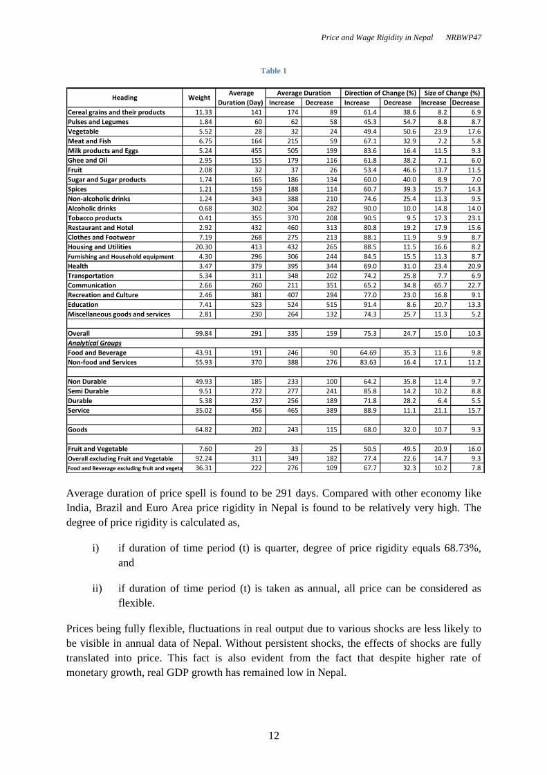
The summary Table 1 presents the average duration of price spell, average duration of price

spell in increasing and decreasing direction, distribution of total changes in increasing and

decreasing direction, and average size of change per each spell in increasing and decreasing

direction.


12

Table 1

Increase Decrease Increase Decrease Increase Decrease

Cereal grains and their products 11.33 141 174 89 61.4 38.6 8.2 6.9

Pulses and Legumes 1.84 60 62 58 45.3 54.7 8.8 8.7

Vegetable 5.52 28 32 24 49.4 50.6 23.9 17.6

Meat and Fish 6.75 164 215 59 67.1 32.9 7.2 5.8

Milk products and Eggs 5.24 455 505 199 83.6 16.4 11.5 9.3

Ghee and Oil 2.95 155 179 116 61.8 38.2 7.1 6.0

Fruit 2.08 32 37 26 53.4 46.6 13.7 11.5

Sugar and Sugar products 1.74 165 186 134 60.0 40.0 8.9 7.0

Spices 1.21 159 188 114 60.7 39.3 15.7 14.3

Non-alcoholic drinks 1.24 343 388 210 74.6 25.4 11.3 9.5

Alcoholic drinks 0.68 302 304 282 90.0 10.0 14.8 14.0

Tobacco products 0.41 355 370 208 90.5 9.5 17.3 23.1

Restaurant and Hotel 2.92 432 460 313 80.8 19.2 17.9 15.6

Clothes and Footwear 7.19 268 275 213 88.1 11.9 9.9 8.7

Housing and Utilities 20.30 413 432 265 88.5 11.5 16.6 8.2

Furnishing and Household equipment 4.30 296 306 244 84.5 15.5 11.3 8.7

Health 3.47 379 395 344 69.0 31.0 23.4 20.9

Transportation 5.34 311 348 202 74.2 25.8 7.7 6.9

Communication 2.66 260 211 351 65.2 34.8 65.7 22.7

Recreation and Culture 2.46 381 407 294 77.0 23.0 16.8 9.1

Education 7.41 523 524 515 91.4 8.6 20.7 13.3

Miscellaneous goods and services 2.81 230 264 132 74.3 25.7 11.3 5.2

Overall 99.84 291 335 159 75.3 24.7 15.0 10.3

Analytical Groups

Food and Beverage 43.91 191 246 90 64.69 35.3 11.6 9.8

Non-food and Services 55.93 370 388 276 83.63 16.4 17.1 11.2

Non Durable 49.93 185 233 100 64.2 35.8 11.4 9.7

Semi Durable 9.51 272 277 241 85.8 14.2 10.2 8.8

Durable 5.38 237 256 189 71.8 28.2 6.4 5.5

Service 35.02 456 465 389 88.9 11.1 21.1 15.7

Goods 64.82 202 243 115 68.0 32.0 10.7 9.3

Fruit and Vegetable 7.60 29 33 25 50.5 49.5 20.9 16.0

Overall excluding Fruit and Vegetable 92.24 311 349 182 77.4 22.6 14.7 9.3

Food and Beverage excluding fruit and vegetable 36.31 222 276 109 67.7 32.3 10.2 7.8

Size of Change (%)Heading Weight

Average

Duration (Day)

Average Duration Direction of Change (%)

Average duration of price spell is found to be 291 days. Compared with other economy like

India, Brazil and Euro Area price rigidity in Nepal is found to be relatively very high. The

degree of price rigidity is calculated as,

i) if duration of time period (t) is quarter, degree of price rigidity equals 68.73%,

and

ii) if duration of time period (t) is taken as annual, all price can be considered as

flexible.

Prices being fully flexible, fluctuations in real output due to various shocks are less likely to

be visible in annual data of Nepal. Without persistent shocks, the effects of shocks are fully

translated into price. This fact is also evident from the fact that despite higher rate of

monetary growth, real GDP growth has remained low in Nepal.


13

Fruit and vegetable prices change at average duration of 26 days. Goods record short price

spells compared to service. Service prices changes infrequently compared to nondurable,

semi durable and durable goods. Food and beverage records relatively short price spells

compared to non food and services group. The average duration of price spells are found to

be varying across different sub groups. Hence it can be inferred that price change behaviour

of different goods and services are heterogeneous. The Figure 6 shows that the price spells of

subgroups from highest average duration of price change to lowest duration. This figure also

suggests that the price changes are randomly distributed in different time.

Figure 6

The average duration of price decrease is found to be 159 days and the average duration of

price increase in found to be 335 days. The total changes consist of 24.7 percent of price

decrease and 75.3 percent of price increases. On an average, size of price decrease is 10.3

percent and the size of price increase is 15.0 percent. The price decreases are quicker but size

and frequency of price increase is higher and hence leading to consistent price increase in

Nepal.

Percentage of price increases and decreases for fruit and vegetable group are found to be

symmetric in both direction but size of increases is higher than decreases. Food and beverage

prices are found to be flexible in both direction showing similar size of change but fraction of

increases are relatively higher than the fraction of decreases. Service prices are highly skewed

towards increases and also higher compared to size of decrease. Hence, it can be concluded

that the goods prices are flexible but slowly increasing and services prices are downward

rigid and always increasing.

State contingent model are explained as more realistic but heterogeneity observed in price

adjustment makes the construction of lower and upper bound as more data intensive and

unrealistic. Thus for DSGE modelling, Calvo Pricing Model with 68.73% as degree of price

rigidity represents the price adjustment pattern in Nepal.


14

In Calvo model of price adjustment with high degree of price rigidity, few firms will adjust

price and hence high level of inertia exists in current price level. However, if firms expect

future cost to rise or expect high inflation, the firms resetting price will increase price at

higher rate and hence higher will be the inflation in current period. Thus for country with

high degree of price rigidity, such as estimated for Nepal, low inflation can be achieved by

lowering inflation expectation. Nepal Rastra Bank should stick to low inflation target with

strong commitment towards the stated target. Central banks committed towards inflation

target have high degree of control in inflation expectations. Nepal Rastra Bank should

conduct inflation expectation survey to determine inflation expectation and revise its policy

rates accordingly.

In addition to this, there exists high degree of heterogeneity in the average duration for price

adjustment among subgroup of commodities. Impacts of shocks are different among various

commodity sub-groups. This creates difference in relative prices and hence distorts the

quantities of different goods and services being produced and consumed. These types of

distortion brought by change in relative price are one of the major sources of welfare loss for

economy. Since policies and tools suggested for minimizing this type of distortion are harder

and costlier to implement, the wisest solution referred by economist is sticking to low

inflation. Nepal Rastra Bank thus should lower inflation target for minimizing welfare loss

created from such distortion.

Food and beverage price are found to be stable compared to non-food and service prices.

Variations in fruits and vegetable prices are found to be higher but symmetric in increases

and decreases. In addition to this, service prices are found to be downward rigid and upward

trending. This fact shows that core inflation will include baskets that are increasing,

downward rigid and most of which belongs to imported basket. Core inflation will be higher

than headline inflation. In addition to this headline inflation are easily understood and

acceptable to all stakeholders. Therefore, targeting headline inflation has higher advantage

compared to core inflation for Nepal.

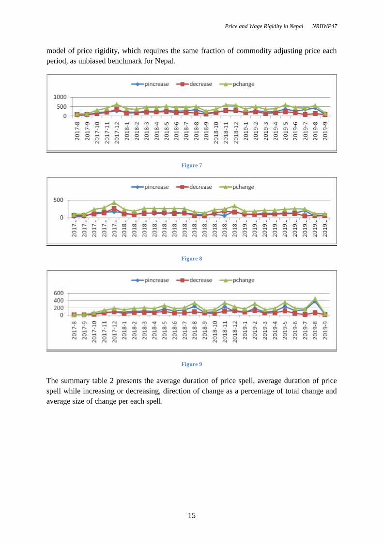
Results from WPI Data

The wholesale price index in Nepal covers only good market. The price adjustment pattern in

wholesale market can be compared with goods market in retail sector for assessment of

degree of pass through. The figure 8 with number of price change during a given year and

month shows that the total number of increases exceeds the total number of decreases. The

figure 9 for vegetable and fruits subgroup shows that the numbers of price changes are found

to be similar in both directions. Intersecting graph with lines above and below shows the

symmetric nature of price adjustment in this sub-group. This fact is in line with price

behaviour in retail sector for fruits and vegetables sub-group. The figure 10, for commodities

except fruit and vegetable, shows that the number of increases is greater than the number of

decreases. The number of price changes at quarter ends i.e. (month ending on 2, 5, 8, 11 of

English date) are recorded as higher compared to other months. Therefore on each quarter

equal proportion of price are likely to change. The fact also supports the assumption of Calvo


15

model of price rigidity, which requires the same fraction of commodity adjusting price each

period, as unbiased benchmark for Nepal.

Figure 7

Figure 8

Figure 9

The summary table 2 presents the average duration of price spell, average duration of price

spell while increasing or decreasing, direction of change as a percentage of total change and

average size of change per each spell.


16

Table 2

Increase Decrease Increase Decrease Increase Decrease

Food 31.18 61 70 46 62.98 37.02 12.6 14.2

Nonfood 2.08 155 150 164 62.67 37.33 11.8 13.1

Fuel and Power 5.66 67 59 102 81.65 18.35 3.8 1.2

Manufacture Of Food, Beverage & Tobacco 14.53 119 132 84 72.06 27.94 5.9 6.9

Manufacture Of Textiles 0.98 189 187 216 93.79 6.21 12.5 9.9

Manufacture Of Leather And Leather Products 0.29 261 280 154 85.45 14.55 4.8 4.8

Manufacture Of Wood And Wood Products 2.07 204 231 148 67.87 32.13 11.3 16.1

Manufacture Of Paper And Paper Products 1.07 235 209 274 60.81 39.19 5.6 16.8

Manufacture Of Chemicals And Chemical Products 6.55 201 211 138 86.04 13.96 10.0 10.5

Manufacture Of Rubber And Plastics Products 1.92 228 228 227 83.07 16.93 6.1 2.3

Manufacture of non-metallic mineral products 3.44 148 162 130 55.17 44.83 10.4 14.0

Manufacture of basic metals 12.07 84 89 69 71.03 28.97 6.0 4.3

Manufacture Of Elctric And Electronic Products 3.10 166 206 151 27.08 72.92 6.2 4.9

Manufacture Of Machinery And Equipment 2.64 222 232 179 82.13 17.87 5.4 4.6

Manufacture Of Transport, Equipments And Parts 3.80 213 219 91 95.74 4.26 5.4 1.8

Other 0.95 324 324 100.00 - 13.0

Overall 92.33 116 129 87 69.91 30.09 8.7 10.2

Intermediate Goods 50.96 107 113 91 72.35 27.65 7.6 8.7

Consumption Goods 31.63 115 137 67 68.10 31.90 11.5 14.0

Capital Goods 9.73 170 194 129 63.02 36.98 5.6 5.1

Overall except fruit and vegetable 85.19 124 135 97 71.53 28.47 7.1 8.4

Fruits and Vegetable 7.14 24 26 22 50.65 49.35 34.6 22.4

Size of Change (%)Heading Weight

Average

Duration (Day)

Average Duration (Day) Direction of Change (%)

Average duration of price spell in wholesale market is found to be 116 days. The duration is

relatively low compared to 202 days in retail market. Also, 7.67 % of commodities price such

as electricity do not have at least three price changes to form a price trajectory and hence

missing in the estimation. The exclusion of commodity with long price spell is likely to

underestimate average duration. Also vegetable price are measured every fortnightly instead

of daily, the average duration for vegetable and fruits are overestimated. This error

compensates some part of missing commodities with larger price spell but the weight of

missing commodity are higher and hence the average duration of price adjustment for

wholesale market is more likely to be underestimated.

Compared to retail sector, average duration of price change in wholesale sector is less.

Therefore, retail sector can be seen as absorbing pass through from producer to consumer.

The absorption of such pass through is one of the sources of welfare loss for the economy.

The share of price changes along increasing and decreasing direction is found similar

compared to goods price movement in retail sector.

Results from Salary and Wage Rate Data

The figure 11 shows that all changes in salary are increment which occurs mostly in the

month of August i.e. month of Shrawan or beginning of fiscal year. The increment can be

attributed to salary increment for civil servant in Nepal’s Central Budget. The data do not

include annual grade in salary which I assume to be associated with increase in productivity

due experience earned during the year and hence do not impact real wage. For this reason, the

result obtained is considered to be unbiased estimate of salary and wage rigidity. The figure

12 shows that wage rates changes more frequently compared to salaries. In addition to this,


17

wage rate changes are found in all month as opposed to salary changes occurring at some

specific month. Of the total employment in Nepal, wage earners comprise relatively large

share in total employment and hence changes in wages are dominant factor in determination

of overall salary and wage rate adjustments. Hence the salary and wage adjustment can be

also generalized as randomly distributed over different period.

Figure 10

Figure 11

The summary of average duration, direction and magnitude of changes are presented in the

table 3. The average duration of overall salary and wage rate are found to be 451 days.

Salaries are more rigid compared to wage rates. Average duration among various sub-groups

is found to be heterogeneous. The size of increase is found to be 16.3 percent and decreases

are rare. The salary and wage rates changes are unidirectional and downward rigid.


18

Table 3

Decrease Increase

Salary Army & Police Forces 4.02 578 18.7 - 100.0

Salary Bank & Financial Institutions 0.55 643 28.2 - 100.0

Salary Civil service 2.82 517 16.8 - 100.0

Salary Education 10.55 515 16.1 - 100.0

Salary Public Corporations 1.13 624 18.3 2.4 97.6

Wage Agricultural Labourer 39.49 391 16.0 4.2 95.8

Wage Construction Labourer 8.29 458 16.1 4.8 95.2

Wage Industrial Labourer 25.25 477 16.2 1.0 99.0

92.10 451 16.3 2.5 97.5

19.07 539 17.2 0.1 99.9

73.03 428 16.1 3.2 96.8

Overall

Monthly Salary

Daily Wages

Direction of Change %Size of

Change

Average

Duration(Day) Weight

Payment

TypeProfession

Larger share of wage rates accompanied by heterogeneity within sub-groups makes salary

and wage rate adjustment process as more random as opposed to calendar specific changes

occurring in salary. Hence, Calvo model for wage determination with wage rigidity can be

used as benchmark for DSGE model in Nepal.

For Calvo model of wage rigidity,

i) degree of wage rigidity for quarter as period (t) is found to be 79.82%,

ii) degree of price rigidity for annual period (t) is found to be 19.07%.

Salary and wage rates are highly rigid and hence creating strong inertia for existing salary

and wage rates. However, the remaining fraction of unions and workers interest group will

revise their salaries and wages in a way that maintain their current and anticipated real wages

mark-ups. This revision pushes wage inflation. Expected real wage mark-ups depend upon

expected nominal wages and expected price inflation. Therefore when inflation expectations

are low, lower will be the wage inflation.

Salary and wage rates are adjusted slowly compared to price. Therefore, positive demand

shocks lead to negative real wage gap. Although negative real wage gaps provides incentive

to producer, size of salary and wage rate increases are higher compared to size of price

change, leading to shorter life of incentives. In addition to this, when negative demand shocks

hit economy, positive real wage gap creates disincentive to producer. Negative as well as

positive real wage gap are considered as one of the major source of welfare loss for economy.

Therefore, sticking to lower price inflation accompanied by lower rate of increase in nominal

salary and wages that compensates for constant real wage and increase in productivity will

minimize welfare loss.


19

V. IMPLICATION FOR MONETARY POLICY

Nepal Rastra Bank should be committed towards achievement of its inflation target to

get high degree of control in inflation expectations. Inflation expectations are found to

be crucial element in determination of current price and wage inflation.

Low inflation target will minimize welfare loss related with heterogeneous impact of

shocks among various commodity groups and salary and wage rate groups.

Fluctuation in output due to onetime shocks is less likely to be visible in annual data

and hence policy prescription for business cycles due to shocks should be based on

quarterly output data.

Targeting headline inflation has higher advantage to Nepal Rastra Bank compared to

core inflation.

Retail sector reforms can increase price pass through from producer to consumer and

hence reduce welfare loss.

VI. CONCLUSION

The study provides the unbiased estimate of degree of price rigidity as 68.73% and degree of

wage rigidity as 79.82%. The price and wage rate adjustments are found to be random and

time dependent. Thus, Calvo model of price and wage adjustment is found to be best

benchamark for price adjustment model in DSGE modelling for Nepal.

There is wider heterogeneity in average duration of price change among subgroup of

commodities. Most of the price changes are increase. Size of increases are larger compared to

decreases. Retail prices are found to be more rigid compared to wholesale price. Salary and

wage rates are to found be downward rigid and less heterogeneous compared to heterogeneity

in retail price.

The inflation in Nepal are found to be higher compared to targeted inflation in past periods

which have led consumers, firms and wage setters to expect inflation on higher side. The

higher inflation expectation have fed on own self leading to higher price and wage inflation

in the current period. Strong commitment towards targeted inflation is required for achieving

higher control in inflation expectation. Strong commitment are possible only if central bank is

committed towards the benefit of low inflation, are politically independent and bad thing

happens to chief central bankers when inflation target is not met.


20

REFERENCES

Alvarez, Luis J. and Ignacio, Hernando. 2005. "Price Setting Behaviour in Spain. Evidence

from Consumer Price Micro-data, Economic Modelling."

Alvarez, Luis J., Pablo, Burriel. and Ignacio, Hernando. 2008. "Price setting behaviour in

Spain: evidence from micro PPI data, Managerial and Decision Economics."

Blanchard, Oliver. and Gali, Jordi. 2007. “Real wage rigidity and the New Keynesian

Model.” Journal of Money, Credit and Banking, Supplement to Vol. 39 No. 1

Blinder, Alan S. 1991. "Why Are Prices Sticky? Preliminary Results from an Interview

Study." American Economic Review

Caballero, Ricardo J. and Eduardo, M.R.A. 2006. "Engel, Price Stickiness in Ss Models:

Basic Properties." MIT Working Paper

Calvo, Guillermo. 1983. “Staggered Prices in a Utility-Maximizing Framework.” Journal of

Monetary Economics

Dotsey, M., R. King. and Alexander, Wolman. 1999. "State-Dependent Pricing and the

General Equilibrium Dynamics of Money and Output." Quarterly Journal of Economics

Emmanuel, Dhyne., Jerzy, Konieczny., Fabio, Rumler. and Patrick Sevestre. 2009. "Price

rigidity in the euro area-An assessment." Economic Papers pp 380

Gali, Jordi. 2008. "Monetary Policy, Inflation, and the Business Cycle, An Introduction to the

New Keynesian Framework." Chapter 6, A model with sticky wages and prices,

Princeton University Press

Mankiw, N. Gregory. 1985. "Small Menu Costs And Large Business Cycles: A

Macroeconomic Model Of Monopoly." Published by John Wiley & Sons, Inc. The

Quarterly Journal of Economics

Shesadri, Banerjee. and Rudrani, Bhattacharya. 2017. "Micro-level Price Setting Behaviour

in India: Evidence from Group and Sub-Group Level CPI-IW Data." No. 217, National

Institute of Public Finance and Policy

Rotemberg, Julio J. 1982. "Monopolistic Price Adjustment and Aggregate Output." Review of

Economic Studies, 517-31

Solange, Gouvea. 2007. "Price Rigidity in Brazil: Evidence from CPI micro data." Working

Paper series, September

Taylor, John. 1980. “Aggregate Dynamics and Staggered Contracts.” Journal of Political

Economy, Vol 88, pp. 1-23

Woodford, Michael. 2008. "Information-Constrained State-Dependent Pricing." NBER

Working Paper No. 14620, (Revised in 2011)

https://www.nber.org/people/michael_woodford

Documents

Price and Wage Rigidity in Nepal · winter seasons, price of various commodities changing at beginning of fiscal year after budget, school and college’s admission and fees changing