1

Price and Volume Effects of Changes in MSCI Indices – Nature and Causes

Rajesh Chakrabarti a, Wei Huang b , Narayanan Jayaraman a,*, Jinsoo Lee a

a College of Management, Georgia Institute of Technology, 800 West Peachtree Street, Atlanta, GA 30332, USA

b College of Business Administration, University of Hawaii at Manoa, Honolulu, HI 96822, USA

ABSTRACT

Using changes in the MSCI Standard Country Indices for 29 countries between 1998 and 2001,

we document that stock returns and volumes exhibit “index effects” in international markets

similar to those detected by the studies of US stocks. The stocks added to the indices experience a

sharp rise in prices after the announcement and a further rise during the period preceding the

actual change, though part of the gain is lost after the actual change date. The stocks that are

deleted from the indices, on the other hand, witness a steady and marked decline in their prices.

Trading volumes increase significantly and remain at high levels after the change date for the

added stocks. There are also considerable cross-country variations in these effects. Tests using

data on various measures reflecting the different hypotheses fail to turn up any evidence in

support of information effects. Our evidence appears to be more supportive of the downward

sloping demand curve hypothesis. There is some evidence of price-pressure and mild evidence of

liquidity effect, particularly in Japan and UK.

JEL classification: G14, G15

Keywords: Index effects; Downward sloping demand curve; MSCI; Liquidity

* Corresponding author. Tel: +1-404-894-4389; fax: +1-404-894-6030. E-mail: narayanan.jayaraman@dupree.gatech.edu (N. Jayaraman)

2

“… much of the loss in Hong Kong was due to an 8.7% plunge by property giant Cheng Kong

Holdings, which will be deleted from the MSCI Hong Kong Index. ….. On the winning side was

Pacific Century Works Ltd. The Internet company rose more than 5% after MSCI said it will be

included in the MSCI Hong Kong index.”

The Wall Street Journal, May 19, 2000

I. Introduction

Additions of stocks to major stock indices usually increase their trading volume as

well as their returns. Deletions are known to depress returns. This phenomenon has been

widely studied in finance (e.g. Shleifer (1986), Harris and Gurel (1986) and Lynch and

Mendenhall (1997)). Most studies to date have focused on US stocks, with the S&P 500

being the index of choice. Some recent studies (see Liu (2000) and Hanaeda and Sarita

(2001)) have documented similar effects in the Nikkei indices of Japan. Rebalancing

activities of fund managers are often thought to be responsible for such effects.

Given the dramatic growth in international portfolio investment in the ‘90s1 and in

the number of funds benchmarked to different national and regional stock indices

* We are grateful to Sandy Lai and Michael Doherty for excellent research assistance and Ajay Khorana,

Chris Anderson, Kalpana Narayanan, Sanjiv Sabherwal, Dilip Patro, Suluck Pattarathammas, Gregory

Koutmos, Ernest Biktimirov, Ghon Rhee, the editor, participants at the University of Hawaii seminar,

University of Kansas seminar, Georgia Tech-Fortis International Finance Conference, Atlanta, 2002, the

EFMA conference, London, 2002, the PACAP conference, Tokyo, 2002, the FMA Annual Meetings,

Denver, 2003 and especially two anonymous referees for helpful comments. The first author thanks the

Federal Reserve Bank of Atlanta for support. We alone are responsible for all remaining errors.

1 There are currently 832 mutual funds classified as “International” compared to 361 such funds in 1996.

(The Wall Street Journal, February 4, 2002)

3

maintained by global organizations, it is natural to ask whether such effects exist in the

international scenario. International portfolio investing has several distinguishing

features. Individual stock information is often less easily available to international fund

managers. Liquidity concerns are considerably higher, particularly in emerging market

countries. Finally, changes in international stock indices presumably affect the

international investors and fund managers more directly than their domestic counterparts.

Consequently, the effect of changes in international indices on constituent stock returns

remains an open question and is a matter of interest to academicians and international

investors alike.

The present study addressing this issue is also important to the growing literature

on index changes. Stepping beyond the confines of a single market, it allows

simultaneous and comparative analysis of the several competing hypotheses in the

literature about the causes of “index effects”. The greater cross-sectional power of the

international data allows us to investigate the relative importance of these hypotheses. For

instance there is considerable variation in the “float” of the stocks in question for MSCI

changes as opposed to S&P 500 changes – a fact that becomes useful in testing the

downward sloping demand curve hypothesis. Thus the present analysis should help us

develop a better understanding of the drivers of index effects even in a national context.

We document and analyze return and volume reactions to additions and deletions

of stocks in Morgan Stanley Capital International (MSCI) country indices for 29

countries using the quarterly rebalancing of these indices. These rebalancing events have

several features that make them a natural choice for such an analysis. First, the MSCI

indices are perhaps the single most important group of international equity indices

4

tracked by international fund managers. Over $3 trillion worldwide is benchmarked to

these indices, with more than $600 billion of that amount passively managed2. Exchange

Traded Funds or iShares, tracking these indices have also become very popular in recent

years. Changes in these indices, therefore, attract considerable attention among investors

worldwide. Second, these changes – the quarterly rebalancing – take place at regular and

known intervals (in February, May, August and November of each year). The

simultaneity of changes in several national indices thus assures the cross-border

comparability of our results. Finally, like the S&P 500 after 1989, changes in the MSCI

national indices are announced two weeks before the effective date. This announcement

window allows us (as in Lynch and Mendenhall (1997)) to interpret our results in terms

of the relative efficiency of the different national stock markets considered. We therefore

document and analyze the reactions in individual stock returns and trading volumes to 12

such quarterly rebalancing adjustments of MSCI indices for the 29 countries.

We find that the stocks added to the MSCI national indices experience a

significantly positive abnormal return of about 3.4% on the day following the

announcement. From the next day to the effective date of the change, they experience a

further rise of 4.5%, which declines somewhat over the 10 days following the actual

change yet remains significantly positive. The total cumulative change from the

announcement to 10 days after the change is not only statistically significant, but also

economically impressive at almost 5.3%. For deleted companies, the cumulative

abnormal return over the entire period is significantly negative and even higher in

magnitude at about –7.5%.

2 The Wall Street Journal, February 27, 2002.

5

We also examine trading volume during this period. Additions experience a surge

in abnormal trading volume of about 3.3% on the day following the addition and continue

to rise throughout the post-announcement window. The cumulative abnormal volume

from the announcement day to 10 days after the change day stands at over 38%. For

deletions, the corresponding figures are 1.4%, and 16.5%, respectively, all statistically

significant. Even this, however, is an understatement since just prior to the

announcement, these stocks trade at vastly reduced volumes compared to their previous

levels. Thus, it appears that the announcement of deletion lifts the volume traded from

already depressed levels to above normal levels.

There is also considerable variation in these reactions across the different national

stock markets. All developed countries in our data set exhibit a significant rise in returns

on the day following the announcement, but the emerging markets as a group do not.

Returns in UK, Japan, and emerging markets rise in the run-up period (from two days

after the announcement till the change day) and experience a permanent rise in stock

prices, while US and other developed countries in our sample show no such increase.

Volumes rise on addition everywhere except in the US and on deletion in developed

countries except the US and UK. Overall, our evidence indicates the presence of

downward sloping demand curve effect with some liquidity and price-pressure effects.

We carry out additional tests to disentangle the liquidity and information

hypotheses from the downward sloping demand curve. Using the “liquidity ratio test” of

Amihud et al (1997), we find that there is no increase in liquidity of the stocks added to

the indices, though declines appear to reduce liquidity. Using an approach similar to the

one suggested by Denis et al (2003), we find that in none of the countries does addition

6

lead to a significant change in earnings per share. This enables us to conclude that the

information effects are minimal in the changes.

The rest of the paper is organized as follows. The following section provides a

brief discussion of the relevant literature. Section III provides an introduction to the

MSCI indices describing their composition as well as the quarterly rebalancing process.

Section IV describes the data used in this paper, while Section V discusses the

methodology adopted. Section VI and VII discuss the results and Section VIII concludes

the paper with suggestions for future research.

II. Relevant Literature

The literature on effects of index changes on returns and trading volumes of

affected stocks is sizeable. Methodologically, with the exception of Goetzmann and

Massa (2003), the event-study approach is used in almost all cases. It is well established

that the addition of a stock to the S&P 500 index leads to positive abnormal returns of

about 5% (see Harris and Gurel (1986), Shleifer (1986) and Dhillon and Johnson (1991)).

Deleted stocks, on the other hand, witness a significant, though generally smaller, drop in

returns (see Goetzmann and Gary (1986) and Harris and Gurel (1986)).

Several competing hypotheses are proffered as explanations. Harris and Gurel

(1986) find that, unlike the permanent volume effect, the price effect is reversed over

time. They therefore surmise that these effects are due to price-pressure – owing to index

fund purchases (or sales). Shleifer (1986), Beneish and Whaley (1996), and Dhillon and

Johnson (1991), on the other hand, find more permanent price changes and attribute them

to the downward sloping demand curve for stocks – the fact that stocks are imperfect

7

substitutes for one another. Amihud and Mendelson (1986) advocate (and Hegde and

McDermott (2003) study) the liquidity hypothesis – permanent reduction in trading costs

owing to excess demand for the added stocks by fund managers. Finally, Jain (1987) and

Dhillon and Johnson (1991) argue that there may be an information effect in the inclusion

or exclusion of stocks to a major index.

Lynch and Mendenhall (1997) look at S&P 500 changes data in the post-1989

period, with pre-announced changes. They find a large positive impact on returns for

added stocks after the announcement day, part of which is reversed in the post-change

period – results consistent with both the price-pressure effect as well as the downward

sloping demand curves.

Morck and Yang (2001) report higher Tobin’s q for S&P 500 index members as

further evidence of the downward sloping demand curves for stocks. As a next step,

Wurgler and Zhuravskaya (2002) demonstrate that stocks with no close substitutes

experience a higher rise in returns on inclusion in the S&P 500 index—strong

corroborating evidence for the downward sloping demand curve view.

The four hypotheses provide different explanations for the observed changes in

return and volume in the stocks added to or deleted from the index. Imperfect substitute

or downward sloping demand curve (DSDC) implies a permanent price change, whereas

the price pressure hypothesis posits a short term downward sloping demand curve

therefore suggesting a temporary price effect. As the index funds complete their

rebalancing, the stock prices will return to their equilibrium level and hence the gains will

be reversed. The information signaling hypothesis interprets the price effect differently

from those of DSDC and price pressure, in that it postulates positive effect of price

8

change for added stocks and negative price effect for deleted stocks are due to the fact the

index provider have superior information about the companies involved in the index

change. However, DSDC and information hypothesis, both of which produce a

permanent price effect, are not mutually exclusive. Finding of information related effect

does not necessarily mean that the demand curve for stocks is not downward sloping. It is

possible, in fact likely, that more than one of the hypotheses coexist to account for the

index effect.

Establishing the dominant source of the “index effect” empirically remains a

challenging issue. However recent research has developed several measures of the

variables involved in the different hypotheses. Price pressure is more easily differentiable

from the others – unlike the other effects it is temporary. Different tests of liquidity

including the Liquidity Ratio test of Amihud et al (1997) and Chen et al (2002) and the

Change in Proportion of Zero Daily Return developed by Lesmond et al (1999) – the two

measures we use – as well as that of Roll (1984) can show if indeed inclusion (deletion)

of a stock increases (decreases) its liquidity. Information hypothesis is harder to capture

but the methodology developed using analysts’ forecasts in Denis et al (2003) can help us

find out if the inclusion results in greater expected earnings. Finally, the downward-

sloping demand curve, arguably the most elusive of the four effects, can also be captured

to some extent using regressions of abnormal return on abnormal volume as in Shleifer

(1986) as well as the Arbitrage Risk Measure (ARM) developed by Wurgler and

Zhuravskaya (2002). These tests allow us to ascertain if indeed liquidity and/or

information improved after an inclusion. An association of the price effect with the ARM

would indicate that the downward-sloping demand curve is important. The detection of

9

individual effects is now possible. However, ascribing the guilt appropriately amongst

multiple offenders remains a methodological challenge.3

While the S&P 500 has commanded most attention, in recent years, other US

indices as well as prominent non-US indices have also been examined --- Russell 2000

index (Petajisto (2003)); Nikkei 500 index (Liu (2000)); Nikkei 225 index ( Hanaeda and

Sarita (2001)). Kaul et al (2000) study the effects of redefinition of the public float in the

Toronto Stock Exchange 300 index and find strong support for the downward sloping

demand curve hypothesis.

While these studies have examined various important country level stock indices,

none (to our knowledge) has so far examined whether such effects persist in international

investing. Would international fund managers, managing an ever-increasing fund of

international portfolio investments, react in the same way as domestic investors do to

changes in their national indices? Given that international investors are sometimes

believed to be at an informational disadvantage compared to local investors (see, for

instance Kang and Stulz (1997) and Brennan and Cao (1997)), would the inclusions or

deletions have greater “information effect” in the international investment environment?

Index-change arbitrage is an increasingly important feature for domestic indices. As

Wurgler and Zhuravskaya (2002) show, arbitrageurs have a crucial impact on stock prices

3 Another branch of the literature, though not directly studying the effect of index changes, also

has significant implications for the downward sloping demand curve hypothesis. (See Chan and

Lakonishok (1993, 1995), Warther (1995), Zheng (1999), Fridson and Jonsson (1995), Bakshi and Chen

(1994), Constantinides et al (1998), and Goetzmann and Massa (2003))

10

around index changes and their impact depends upon the nature and substitutability of the

stocks. It is germane to ask if their role is equally pronounced in the international market.

III. An Introduction to MSCI indices

A. Overview of MSCI index family

MSCI is a leading provider of global indices and related services to investors

worldwide with the most widely used benchmarks for non-US stock markets since 1969.

Over 90% of international institutional equity assets in the USA and Asia and two-thirds

of Continental European funds are benchmarked to MSCI Indices.4

Of all the MSCI indices, Standard Country/Regional Indices are the most popular.

Among others, MSCI standard indices are the basis for international iShares offerings,

formerly known as World Equity Benchmark Shares (WEBS). iShares, featuring both

stocks and index funds, are managed by Barclays Global Investors and have been traded

on the American Stock Exchange since 1996. The number of iShares is increasing. As of

January 20, 2004, there were 25 iShares, 21 of which target MSCI Standard Country

Indices with the remaining four targeting the MSCI Standard Regional indices.

B. The Construction of MSCI Standard Country Indices

The MSCI index construction method has evolved over time. The Standard

Country Index studied in this paper is constructed in accordance with MSCI Methodology

& Index Policy as of March 1998. Like the S&P 500 index, MSCI index construction

does not carry special informational content on the firm’s operating efficiency or on

future stock market performance. To offer a proxy for a market, MSCI tracks virtually

4 Much of the information in this section has been drawn from www.msci.com and www.ishares.com.

11

every single company in the 51 national markets covered in the MSCI index family.

Companies in each country are then sorted by industry group and 60% are selected for

inclusion in the Standard Country Index5. Size, industry representation, cross-ownership,

float (percentage of shares freely tradable), and liquidity as measured by long- and short-

term volume are among the major criteria used in the selection process.

Although MSCI generally selects stocks with good liquidity, this has been a

relative criterion in the context of country, firm size and industry. Firms in many

countries are not fully accessible by the international investors. MSCI uses Market

Capitalization Factor (MCF) to address this issue. Companies with low “free float” (the

difference between the total number of shares outstanding and shareholdings classified as

strategic and shares restricted from trading by international investors6) are included in the

indices at MCF (40%, 60% or 80%) times their full market capitalization. Since July

2000, all companies with free float of less than 40% are added with a Market

Capitalization Factor. MSCI now uses what it terms, “Foreign Inclusion Factors (FIFs)”

to reflect the actual percentage of shares available to international investors. For

constituents with free float greater than or equal to 15%, the security’s Inclusion Factor is

equal to its estimated free float, being rounded up to the closest 5%. Securities with free

float less than 15% are usually not eligible for inclusion in the indices. For companies

that impose foreign ownership limit, if the limit is less than the free float, Foreign

5 MSCI has instituted certain important changes in the construction of their indices since June 2002,

including an increase in coverage to 80% and a full adjustment of free float. These changes, however, do

not affect our data.

6 The free float for the countries involved in our study can be found in the appendix of a previous version of

this paper available at SSRN.

12

Inclusion Factors are equal to foreign ownership limit, rounded to nearest 1%. This

system matches the supply of shares on the market to the demand for shares in the

portfolios tracking the index.

C. Changes in the constituents of the MSCI indices

The MSCI Equity Indices are regularly maintained to reflect the evolving market

change. MSCI classifies index maintenance in two broad categories: index rebalancing

and market or corporate event-driven changes.

Regular index rebalancing ensures that the indices continue to accurately reflect

an evolving marketplace. The market evolution may be due, for example, to a change in

the composition or structure of an industry or to other developments, including regular

updates in shareholder information used in the estimation of the free float.

During an index rebalancing, securities may be added to a country index for a

variety of reasons, including changes in investors’ interests, changes in regulations,

changes in industry classification, increase in free float, and availability of new

opportunities for inclusion created by privatizations, new issues, or restructurings.

On the other hand, deletion of securities may take place whenever better industry

representatives emerge (either a new issue or an existing company). Besides, significant

decreases in free float-adjusted market capitalization, significant deterioration in

liquidity, and more restrictive foreign ownership limits may also cause certain securities

to be deleted from the index.

Finally, in order to keep the coverage within the target coverage of industries and

countries, adding new index companies may entail corresponding deletions. Unlike the

13

S&P 500, however, MSCI indices do not comprise a specified number of securities, so

every addition does not automatically imply a deletion. It is worth noting that, as in the

case of inclusions, most MSCI rebalancing deletions result from industry evolution and,

therefore, do not reflect information about the firm’s performance.

Quarterly rebalancing for the MSCI Country Indices generally occurs on four

dates throughout the year: close of the last trading day of February, May, August and

November with the changes announced two weeks prior to the effective change day.

However, MSCI may occasionally decide not to make a quarterly rebalancing during

those dates.

In contrast to index rebalancing or so-called structural changes, event-driven

changes result from new issues, mergers, acquisitions, bankruptcies, and other similar

corporate events. These changes are announced and implemented as they occur; they are

not confined to those four dates for the quarterly structural changes. Such event-driven

changes are not within the scope of our study.

IV. The Data

Our data includes 12 out of 14 quarterly structural changes occurring between

February 1998 and August 2001.7 Information about these changes, as well as the list of

7 The twelve changes in our sample occurred in February, May, August, November 1998, February, May,

August, November 1999, May, August, November 2000 and May 2001. In February 2001, no changes were

made to the standard index while in August 2001 there was only one change for our sample (in the India

standard index). Since in the latter case the implementation took place on the eleventh day instead of the

usual tenth day after announcement, we excluded that single change in August 2001 from our sample to

maintain uniformity in the daily effects.

14

companies added or deleted in each case, was obtained from Bloomberg. The

announcement of the changes is released on the middle of each month,8 while the

implementation of the index change takes place on the tenth trading day after the

announcement date, which usually falls on the last trading day of the month.9 The

structural changes include MSCI Standard Country Index, MSCI Small Cap Index, and

MSCI Extended Index. However, we focus only on the changes in the Standard Indices as

these are the most popular among MSCI indices and also form the basis for international

iShares.

The 12 announcements include as many as 46 countries. If a company was deleted

from one index and was added to another,10 we discard the change from our sample.

Finally, after accounting for missing data on some countries and companies, we have 455

additions or deletions from 29 countries. The number of changes considered for volume

analysis is slightly less than that for return analysis since the volume analysis also

requires past data for the relevant companies.

8 The announcement dates were February 12, May 15, August 17, November 16, 1998, February 12, May

17, August 17, November 16, 1999, May 17, August 17, November 16, 2000, and May 17, 2001

respectively.

9 The corresponding effective dates were February 27, May 29, August 31, November 30, 1998, February

26, May 31, August 31, November 30, 1999, May 31, August 31, November 30, 2000, and May 31, 2001

respectively.

10 For example, AGIV in Germany was deleted from MSCI standard index and was added to MSCI small

index on November 30, 2000.

15

Table 1 shows the country-wise breakdown of our sample. The US, with 23

additions and 45 deletions, and Japan, with 30 additions and 38 deletions, top the list

while the UK, with 18 additions and 19 deletions, follows.

We compute the daily return for the stocks involved using the return index (with

dividend reinvested) obtained from Datastream. The Datastream country return index is

used to calculate the proxy for daily market returns. Daily volume data is also obtained

from Datastream. All returns are in local currency.

V. Methodology

The methodology broadly follows that in Lynch and Mendenhall (1997). As in

their data for post-1989 changes in the S&P 500, our data also provides us with two

distinct event dates – the announcement date and the change date. Because our data is

international, we have to consider the time-zone effects in deciding on our dates. Since

the announcements are made in terms of Central European Time when markets in Asia,

particularly Japan, have already closed for the day, we, like Lynch and Mendenhall

(1997), expect to see the effects, if any, on the day following the announcement day

(AD+1) or the change day (CD+1). For a particular stock i from a country c, the

abnormal return on a day τ, ARi,c(τ), is defined as the excess of the stock’s raw return

over that of the market. The relevant “market” for a stock is represented by a stock index

of its country – the national stock index computed by Datastream. This assures cross-

country uniformity market portfolio computations, as well as independence between the

respective market portfolios and the indices under examination, namely, the MSCI

indices. Sample mean abnormal return MARc(τ) for the country c on day τ is obtained by

16

averaging across ARi,c(τ) for stocks in a particular country for a given day τ. The overall

sample mean abnormal return, MAR(τ), is the weighted average of the different country

mean abnormal returns, the weights being proportional to the number of observations in

each country. The cumulative abnormal return between two days, τ1 and τ2, CARi,c(τ1,τ2),

is the sum of abnormal returns during that period. The country and the overall averages of

CARi,c(τ1,τ2) – mean cumulative abnormal return MCARc(τ1,τ2) (country averages) and

MCAR(τ1,τ2) (overall average) – are obtained in a manner analogous to that of MARc(τ)

and MAR(τ), respectively.

For abnormal volume, we follow Lynch and Mendenhall (1997) to first define the

measure of volume υi(τ) as follows:

υi(τ) = log[1+Vi(τ)]/log[1+Ei(τ)], (1)

where Vi(τ) is the local currency traded volume on day τ for stock I and Ei(τ) is the local

currency value of the outstanding shares of the stock on that day.

Next we regress the υi(τ) for a stock on the analogous measure of “country”

volume, υc(τ):

υi(τ) = φ0,i + φ1,i υc(τ) + ei(τ) for τ = AD – 258,…, AD – 109. (2)

To account for possible AR(1) effect in the residuals and to achieve an efficient

estimation, we use an estimated generalized least squares (EGLS) procedure as detailed

in Lynch and Mendenhall (1997) to estimate the regression coefficients, φ0,I and φ1,i. As

before, the υc(τ) figures are obtained from the Datastream computed local currency

17

national stock market volumes. This regression provides us with the estimates for the

coefficients φ0,i and φ1,i for the stock i in question. Using these estimates and plugging in

the values of υc(τ) for the relevant date τ, we can obtain the “normal” or “expected”

volume for stock i on day τ. The abnormal volume for stock i on day τ, AVi,c(τ), is then

defined as the difference between the actual volume and this “normal” volume:

AVi,c(τ) = υi(τ) – [φ0,i + φ1,i υc(τ)] (3)

The different averages for this abnormal volume, MAV and MCAV are obtained in a

manner analogous to the abnormal returns calculation.

Given the similarities in time interval for announcement and actual change

between S&P 500 index examined in Lynch and Mendenhall (1997) and MSCI standard

indices in our study, our time window selection resembles theirs, aiding the comparability

of the results of the two studies. The pre-announcement window runs from 10 days before

the announcement (AD-10) through the day before the announcement (AD-1), the run-up

window runs from two days after the announcement day (AD+2) through the change day

(CD), the post-AD permanent effect window begins with the run-up window and ends 10

trading days after the change day (CD+10), and the total permanent effect window runs

from the announcement day (AD) until (CD+10). We report abnormal returns and

volumes for AD and AD+1 separately. Values of and movements in the abnormal returns

and abnormal volumes on AD and AD+1 will give us an idea of the “announcement

effect” that may be present, while those during the run-up window may reflect the effect

of portfolio rebalancing by funds. The post-AD permanent effect windows will help us

Comment [hw1]: Delete -1

18

find out whether these effects are permanent or temporary. The total permanent effect

window measures the total magnitude of CAR associated with being added to or deleted

from the index.

We differ from Lynch and Mendenhall (1997) in reporting AD and AD+1

separately. As MSCI change announcements are from Geneva and are often spread over

the entire day, markets in a country may or may not be open at the time of the

announcement depending upon its location and the announcement time. In particular,

countries in the Far East, including Japan, certainly finish trading for the day when the

announcement is made, while the US, on the other hand, always has a few hours of

trading remaining regardless of when in the day the announcement is made. It is therefore

difficult to know a priori the date at which the announcement effect will be perceptible in

a country, AD or AD+1. We therefore report the results for these two days separately to

find out when exactly the announcement effect takes place.

VI. Results

A. Returns

i) Effect of Additions to Stock Index

Table 2 presents the daily average market-adjusted abnormal returns, MAR (τ), for

stocks added to or deleted from the respective MSCI Standard Country Indices around the

announcement date, effective dates, and four different windows defined in the previous

section. Figure 1 Panel A shows daily abnormal returns on stocks added to the MSCI

Standard Country Index for the total sample. As Figure 1 and Table 2 indicate, the

19

announcement-day abnormal return (AD+1) for additions is positive and significant. The

abnormal return for the full sample is 3.35 %, with a t-statistic of 9.54.

The US, Japan and the UK are among the world leaders in international

transactions and portfolio flows11.Our sample of changes also has a relatively large

number of firms from these three countries. Therefore, for expositional convenience, in

the rest of the paper, we break our sample into five sub-samples – US, UK, Japan,

Developed Countries, and Developing Countries.12 While any such country grouping is

somewhat arbitrary, we believe we should separate the developed countries from the

developing ones in view of their greater openness to international investment and the

stability of their financial markets. With the exception of developing countries, abnormal

returns for AD+1 are positive and significant everywhere, ranging from 1.81% in the US

to 8.40% in Japan. In the case of developing countries, abnormal return on AD+1 is

positive but only marginally significant at the 10% level. This finding is consistent with

the argument that the developing countries face lower “indexing demand” than other

countries.

There are a few curious features of the return and volume effects. For

instance, the US stock markets are open around the time of index change announcements

11

For the period in our study (1998-2001), international equity portfolio inflows were largest for the US ($

469.18 billion), followed by UK ($ 384.29 billion) and Japan (157.81 billion $). [International Financial

Statistics, IMF, October 2002].

12 Developed Countries sub sample include Australia, Canada, Denmark, Finland, France, Germany, Hong

Kong, Italy, Netherlands, New Zealand, Norway, Singapore, Sweden, and Switzerland. The Developing

Countries sub sample includes Brazil, China, India, Indonesia, Malaysia, Philippines, South Africa, South

Korea, Taiwan, Thailand, Turkey, and Venezuela.

20

and yet its MAR for AD is insignificant but for AD+1 highly significant. Our

explanation for this apparently incongruous result is that it is the international investors

who are affected by these changes, likely to be in Europe and Asia, who act after the US

markets close. Also MCARs in Japan and UK are considerably higher than in the USA.

As we shall see in the next sections these countries appear to have steeper downward

sloping demand curves for stocks as well as some liquidity effect. The existence of

Exchange Traded Funds or iShares in these countries based on the MSCI indices

probably contributes to this effect. Japan, UK and Germany are the countries with the

three largest iShare Net Asset Values with Japan being the leader by far.13 However, the

negative MCAR for developing countries on AD remains a puzzling feature. Resolving

these questions and verifying our hypotheses requires more work in the area.

MCAR for the run-up window (AD+2 to CD) in Table 2 is 4.51% for the total

sample and is statistically significant at the 1% level (t-statistic of 5.75). Furthermore,

the run-up effects are significant in all subsamples except for the US (marginally

significant at about 10% level) and Developed Countries. There is also a partial to

complete reversal in the abnormal returns following the change day. For Japan, the

overall effect in the post-AD permanent window is insignificant. For the Developed

Countries subsample, MCAR in the post-AD permanent window is actually significantly

negative. When we look at the total permanent effect (AD to CD+10), however, it is

significantly positive everywhere except in the case of the US and Developed countries

subsamples. For the total sample, the MCAR over the total permanent window stands at

5.28% with a t-statistic of 4.92. Furthermore, the fraction of companies having a positive

13 see www.ishares.com.

21

cumulative abnormal return over the total permanent window is 63% — significantly (at

the 1% level) greater than 50%. The evidence so far points to the permanent effect of

index addition, despite the substantial price reversals.

If price pressure drives positive market-adjusted abnormal return on the

announcement day, we should expect the cumulative abnormal return to be insignificant

over the total permanent window. On the other hand, if the cumulative abnormal return

in the permanent window is positive and significant, i.e., the index effect is permanent- ,

it may provide evidence in support of the downward sloping demand curve hypothesis.

The results thus far are consistent with both the price-pressure and downward sloping

demand hypotheses. However, the significant MCAR in the total permanent window

could also be interpreted as supporting the information or liquidity hypotheses. The

MCAR during the post-AD permanent window (AD+2 to CD+10) is a measure of lower

bound on the permanent price effect predicted by downward sloping demand curve

hypothesis. The fact that there is a reversal of at least part of the run-up gains in the post-

CD period points out that some price-pressure effect is present in all non-US countries

(or country groups) in our study. To the extent that the total permanent effect remains

significantly positive for the total sample, the UK, Japan, and developing countries, the

results are also consistent with a downward sloping demand curve (though not only with

that hypothesis).

It is interesting to note from Table 2 that UK has the highest MCAR of nearly

19% over the total permanent window. Japan, with a MCAR of 11.15%, follows. It is

reasonable to expect cross-country variation in the effects of changes of the MSCI

country indices. To the extent that index-tracking institutional investors (mostly

22

international fund managers) cause these effects, we should expect a greater impact in

countries with a greater proportion of international investors, like the UK and Japan.

Thus, there may be what we can term a “country effect.” By contrast, the statistically

insignificant MCAR for the US may be explained by the lack of index tracking on the

MSCI US country index.14

ii) Effect of Deletions from Stock Index

The cumulative abnormal returns, MCAR (τ1,τ2), for the different windows for

stocks deleted from the MSCI indices are reported in Table 2 (right panel). For the total

sample, the stocks deleted sustain a price loss in the announcement window and the loss

continues over the run-up window and most of the post-CD period. Figure 1 Panel B

shows daily abnormal returns on stocks deleted from the MSCI Standard Country Index

for the total sample. For the total sample, the deleted stocks experience clear and

statistically significant negative abnormal returns on AD+1 (-2.59%) and during the run-

up window (-5.14%) as well as beyond it. There is no reversal of the announcement

effect in the post-CD period. In fact, the negative impact on the abnormal returns

exceeds the positive impact of additions. US stocks experience a negative MCAR of

4.22% during the run-up window and exhibit a permanent negative impact of 5.77%. All

other subsamples experience a steep decline on AD+1, with the most dramatic being

Japan (-7.24%). The run-up effect is significantly negative for all subsamples except in

the case of the developing countries subsample, (marginally significant (negative) at the

14 For example, MSCI US standard country index is not one of the 25 existing iShares that invest in the

MSCI country/regional indices.

23

10% level). There is partial reversal in the post-CD period for all subsamples except for

the US and Japan. However, the total permanent window MCAR for deletions is

significantly negative in every subsample.

Similar to additions, the partial reversal of the trend in the post-CD period

indicates some price-pressure effects, while the significance of the total permanent effect

in every sub-sample is again consistent with the downward sloping demand curve

hypothesis. As in Lynch and Mendenhall (1997), deletions present stronger support for

the latter hypothesis than additions. However liquidity and information effects cannot be

ruled out. We will address this issue in section VII.

B. Volume

i) Effects of Additions to Stock Index

Table 3 presents the cumulative average abnormal volumes, MAV (τ), for stocks

added to or deleted from the respective MSCI Country Indices around the

announcement, effective dates, and around different event windows. For the total

sample, the daily trading volume increases significantly on AD+1. Figure 1 Panel C

shows the daily abnormal volume MAV for the same windows for stocks added.

As is evident from Figure 1 Panel C and Table 3, for the total sample, additions

exhibit statistically significant positive abnormal volume of 3.33% on the day following

the announcement and a further cumulative abnormal volume of over 20% during the

run-up window. The rise in volume is clearly permanent and over the entire window

(AD through CD+10), the cumulative abnormal volume exceeds 38%.

24

Once again there is considerable cross-country variation. There is no noticeable

volume effect on US stocks – consistent with the lack of international institutional

investors tracking the MSCI US country index. However all non-US stocks exhibit the

same overall pattern though the strength of the effect on AD+1 ranges from 2.58% in

developing countries to 4.70% in Japan and 4.90% in developed countries. During the

run-up window, too, the effect is always significant and permanent for all non-US

countries, with an average cumulative abnormal volume of around 20% in all countries

over the period. The permanence of the volume effect of additions for all non-US

countries appears to further support the downward sloping demand curve view.

ii) Effects of Deletions from Stock Index

Figure 1 Panel D shows the daily abnormal volume MAV for the stocks deleted,

while the right panel of Table 3 presents the cumulative abnormal volumes, MCAV

(τ1,τ2), for different windows as previously defined. As in the case of additions Table 3

shows that the largest abnormal volume occurs on CD, consistent with index funds

rebalancing most of their portfolios on the change day to minimize tracking errors.

Table 3 and Figure 1 Panel D suggest that the deleted stocks experience slightly

different effects on volume as compared to the cases of addition. The first notable

feature here is that in the overall sample, the stocks experience significantly negative

abnormal volume in the pre-AD window and on AD. In all subsequent windows, the

abnormal volume is significantly positive. Thus, deletions lift traded volumes

considerably higher from their “normal” volume levels, which, as may be recalled,

reflect the situation six months prior to the deletions.

25

Once again, US stocks show no volume effect of deletions – in fact, abnormal

volume is significantly negative on the day following the announcements. For all non-

US countries (and country groups except developing countries), however, there is an

overall pattern of positive abnormal volume following the announcement. Japan shows,

the strongest effects with a significantly positive abnormal volume of 5.71% on the day

following the announcement and a cumulative rise of over 51% during the total

permanent window (AD through CD+10). What makes these results even more

pronounced is the fact that in the pre-AD window, these Japanese stocks experience a

significantly negative abnormal volume in the case of index deletion of about -14.85%.

The rise in volume is permanent for the total sample, Japan and developed countries.

As in the case of additions, volume changes resulting from deletions are also

consistent with the downward sloping demand curve in the overall sample and in all non-

US sub-samples with the exception of US, UK and developing countries, where there

appears to be a less permanent price-pressure effect.

C. The relationship between abnormal volume and abnormal return

The relationship between abnormal returns and abnormal volumes can shed some

additional light on the plausibility of the downward sloping demand curve hypothesis. In

cases where high abnormal returns are associated with high abnormal volumes, we can

surmise that new demand (or supply in case of deletions) is behind the observed

abnormal returns— important support for the downward sloping demand curve

hypothesis. Abnormal volume (AV) also proxies for liquidity. A negative relation

between AV and AR is consistent with the liquidity interpretation, while a positive

26

relation is supportive of DSDC. On the other hand, lack of such a result would leave us in

the dark about what actually drives these abnormal returns—information, liquidity, or

downward sloping demand curves.

We follow Shleifer (1986) and regress abnormal returns on abnormal volumes for

AD+1 and for the run-up window separately for additions. For additions, the coefficient

of abnormal volume is significantly positive in both cases, supporting the downward

sloping demand curve hypothesis. For deletions, the slope coefficient is negative and

significant only for AD+115.

VII. Tests of the alternative hypotheses

While the evidence so far has suggested that there are reasons to trust the

downward sloping demand curve view, it is difficult to rule out the possibility that

information or liquidity is driving our results. In this subsection, we carry out further tests

that will evince more information about these three competing hypotheses.

A. The Liquidity Hypothesis

Inclusion of a stock in an index can affect its liquidity through several channels.

Often an added stock gains in popularity and analyst following leading to greater

information release about the stock. Greater trading by liquidity traders can also lead to a

rise in liquidity. On the other hand, given that index fund managers scoop up a part of the

total supply of the stock following its addition to the index, it may be argued that liquidity

15 Results are not reported for space considerations. They are available upon request.

27

may actually diminish on addition owing to the reduction in free float. The effect of

deletions is perhaps less ambiguously negative.

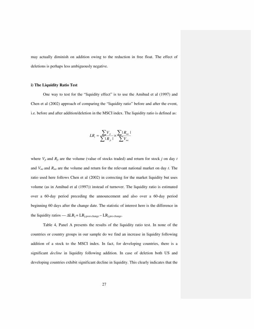
i) The Liquidity Ratio Test

One way to test for the “liquidity effect” is to use the Amihud et al (1997) and

Chen et al (2002) approach of comparing the “liquidity ratio” before and after the event,

i.e. before and after addition/deletion in the MSCI index. The liquidity ratio is defined as:

∑∑

∑∑

×=mt

mt

jt

jt

iV

R

R

VLR

||

||

where Vjt and Rjt are the volume (value of stocks traded) and return for stock j on day t

and Vmt and Rmt are the volume and return for the relevant national market on day t. The

ratio used here follows Chen et al (2002) in correcting for the market liquidity but uses

volume (as in Amihud et al (1997)) instead of turnover. The liquidity ratio is estimated

over a 60-day period preceding the announcement and also over a 60-day period

beginning 60 days after the change date. The statistic of interest here is the difference in

the liquidity ratios — ∆LRj = LRj,post-change – LRj,pre-change.

Table 4, Panel A presents the results of the liquidity ratio test. In none of the

countries or country groups in our sample do we find an increase in liquidity following

addition of a stock to the MSCI index. In fact, for developing countries, there is a

significant decline in liquidity following addition. In case of deletion both US and

developing countries exhibit significant decline in liquidity. This clearly indicates that the

28

positive abnormal returns associated with additions are not driven by a rise in liquidity

though expected drop in liquidity may have a role to play in the case of deletions.16

ii) Relative Frequency of Zero Daily Returns

As an alternative way of looking at the liquidity, we now measure the liquidity of

a stock by the relative frequency of zero daily returns as used in Lesmond et al (1999).17

Assuming that a zero return is observed if the transaction cost of a stock exceeds the

expected return of the transaction, we expect that more zero daily returns are observed in

a less liquid stock than in a more liquid stock. Indeed, Lesmond et al (1999) report that

the proportion of zero daily returns is closely related with the specialist bid-ask spread in

the US stock market. Bekaert et al (2003) use this measure to examine the impact of

liquidity on expected returns in 19 emerging equity markets. Lesmond (2002) also uses

this measure to study the liquidity of 31 emerging markets. Both of these studies on

emerging markets document that the proportion of zero daily returns is highly correlated

with the bid-ask spread in the emerging markets where the data on the bid-ask spread are

available.

16 There are, of course, other ways of testing for liquidity effects. Hegde and McDermott (2003) use

transaction data to show that the inclusion of a stock in the S&P 500 index leads to a permanent

improvement in its liquidity. Specifically, they document that the median quotes and effective spreads

decrease and the median quoted depth, trading volume, and trade frequencies increase over the three

months following the inclusion of stock in the S&P 500 index. Similar data is not available to us.

17 We also used Roll’s (1984) spread measure to examine the changes in liquidity around the event. There is

no evidence that Roll’s spread measure changes significantly after the event.

29

To measure the changes in liquidity around the event, we compute the difference

in the proportions of zero daily returns between the one-year period before and after the

event. For the proportion of zero daily returns before the event, we calculate the

proportions of zero daily returns for the one-year period ending in 10 trading days before

the announcement date. For the proportion of zero daily returns after the event, we

compute the proportions of zero daily returns for the one-year period starting 20 trading

days after the change date. An increase (decrease) in the proportion of zero daily returns,

or a positive (negative) sign of our CZDR variable therefore, signifies a decrease

(increase) in liquidity.

The result of the test is reported in Table 4 panel B. In the sample as a whole we

find that additions result in insignificant liquidity change. However, liquidity improves

significantly for the UK (close to 6%) and Japan (about 5%) and declines for the

developing nations.18 Deletions, however, result in substantial declines in the whole

sample. The decline in liquidity is more evident for the US and developing countries than

for other countries. These results corroborate the results of the Liquidity Ratio test in the

previous subsection and suggest that perhaps there is an element of liquidity

improvement in UK and Japan that escaped detection in the Liquidity Ratio test.

B. The Information Hypothesis

18 The decline in liquidity in developing countries may seem surprising at a first glance but note that

liquidity can, in principle, move in either direction following addition to the index. It may increase because

of greater trading interest or decline if the index trackers suck up most of the available supply.

30

For a direct test of the information hypothesis, we take an approach similar to that

of Denis et al (2003). For each added company, we take analysts’ current-year earnings

forecasts from Institutional Brokers’ Estimate System International, Inc. (I/B/E/S) before

and after the addition and compute the changes in the earnings forecasts.

To control for the possibility that the number of analysts who followed the

company changed after the addition, we only include the EPS forecasts by the analysts

who issued EPS forecasts both before and after the addition. For each analyst, we take the

last EPS forecast before the addition and the most recent EPS forecast after the addition.

To ensure that the EPS forecasts reflect the current condition of the company, the forecast

before (after) the addition should have been issued within a four-month period before

(after) the addition. Since firms in our sample differ in size and are from different

counties, we standardize the changes in EPS forecast by the last EPS forecast before the

addition. We compute the median EPS forecasts for the firm as the consensus EPS

forecasts before and after the addition, respectively. Then we compute the difference in

the median EPS forecasts between before and after the addition.

As a benchmark, we also compute changes in the median EPS forecasts for all

other companies in the same country for which analysts issued EPS forecasts for the

same period. To capture the information effect of the addition, we compute the difference

in the mean between the changes in the median EPS forecasts for the added companies

and those for the benchmark companies.

The tests of the information hypothesis are summarized in the Table 5. In none of

the countries does addition lead to a significant change in current-year EPS forecasts. For

the firms in the entire sample, the average median EPS forecast practically stays

31

unchanged. Therefore it appears that in our sample there is no significant information

effect of addition to the MSCI index.

Another possible indicator of the importance of the information hypothesis

involves the changes in MSCI Small Cap indices. If the information hypothesis were

valid, we would expect to find significant positive announcement effects for the stocks

added to the small cap index. Using data for 354 additions from 14 developed countries

(including 126, 81 and 37 additions from the USA, Japan and the UK respectively), we

find that abnormal returns for the total sample are statistically insignificant for all four

windows as well as for AD+1. 19,20 Furthermore, we do not observe any significantly

positive announcement effect (AD+1) in any of the sub-samples. Thus, once again, there

appears to be no evidence of an information effect.

C. A Comparative Analysis of the three Hypotheses

For a final “horse-race” for the three competing hypotheses, we now carry out a

regression analysis using variables capturing the three competing hypotheses. The

dependent variable is the cumulative abnormal returns from AD through CD while the

independent variables, described below, capture the different effects. It is important to

note that though we use the tool of regression, we are not assuming that there is a linear

relationship between the dependent and the independent variables. In other words, we do

not claim that the regression is well specified. We use it simply as an agnostic tool to

19 The 14 countries are Australia, Canada, Denmark, Finland, France, Germany, Italy, Japan, Norway,

Singapore, Sweden, Switzerland, UK and US.

20 We do not report the figures. They are available on request.

32

capture the relative importance of the different variables in affecting the abnormal

returns.

It is difficult to obtain direct measures of the downward sloping demand curve

hypothesis. While data on investment flows for funds tracking the MSCI indices would

perhaps be ideal, as a second best we examine the free float on the relevant stocks. In

May 2001, MSCI released provisional index constituents with weights adjusted by

“Foreign Inclusion Factors” (FIFs) in an effort to assist investors in understanding the

changes that would occur if the free float adjustment were immediately implemented in

the MSCI Standard Index. We collect data on these FIFs from the provisional index

constituents for the sample countries and call it “Free Float”.21 We argue that controlling

for market capitalization, which may partially proxy for the strength of demand, the

stocks added to the index with lower free float would face higher demand pressure given

its limited supply. In other words, for stocks with lower free float, the supply of shares on

the market does not match the demand for shares in the (especially passively managed)

index fund portfolios22. If we observe that the price effect is greater for stocks added with

low free float, it would be consistent with the downward sloping demand hypothesis.

Note that the argument that low free float poxies for low liquidity would imply in contrast

a negative relation between ARs and free float.

21 While it is conceivable that these FIFs may have changed between the actual inclusion date of a stock

and May 2001, when it was recorded, such changes are rather infrequent and are not likely to affect our

analysis.

22 The analysis would undoubtedly be more complete and convincing if we could use the index weights of

the individual stocks in the regression as well. Unfortunately, that information was not available to us.

33

Next, following Wurgler and Zhuravskaya (2002), we include “arbitrage risk

measures (ARM)” in our regression analysis. Higher arbitrage risk indicates greater

difficulty in replicating the returns of a stock using other securities – in other words, it is

more difficult to “substitute” the stock. Wurgler and Zhuravskaya examine the S&P index

additions for the period 1976 to 1989 and report that stocks with higher arbitrage risks

showed higher excess returns than stocks with lower arbitrage risks. Their results suggest

that arbitrage risk prevents arbitrageurs from flattening demand curves for stocks.

Arbitrage risk measures (ARM) may, therefore, be used as a measure of the slope of the

demand curve (or non-substitutability) for a stock. We compute the arbitrage risk

measure for a stock by regressing the daily returns of the stock on the daily market

returns for the one-year period ending in 10 trading days before the announcement date.23

Then we compute the residuals of the regression and define the standard deviation of the

residuals over the period as the arbitrage risk of the stock.24 Finally we also include

Abnormal Volume since its association with abnormal returns can also suggest downward

sloping demand curve effect.

We include the difference in the proportions of zero daily returns between the

one-year period before and after the event (CZDR) as discussed before to capture the

changes in liquidity around the event. We expect the coefficient of this variable is

23 Wurgler and Zhuravskaya (2002) use a slightly different technique but mention that the results of the two

techniques are very similar.

24 We also gathered data on the constraints on short selling in different countries from Bris, Goetzmann,

and Zhu (2003). A “short sale” dummy is motivated by the fact that the short sale constraint might weaken

the ability of arbitrageurs to flatten the demand for stocks. However the dummy turned out to be highly

correlated with a few other variables and hence we did not include it in our regression analysis.

34

negative if the liquidity hypothesis holds in our sample. We also include the proportion of

zero daily returns before the event in order to capture the liquidity condition of countries

at the time of the inclusion to the index.

The variable iShare takes the value of unity if there was an iShare for the country

at the time of the index change and zero otherwise. This variable reflects the importance

of index funds. If the role of arbitrageurs and the importance of index funds are positively

related, then we can expect that the abnormal returns would be higher on inclusion to the

index in countries with iShares.

Since international investors probably know more about larger stocks in a country

than the smaller ones, we also include the firm size variable in our regressions. Therefore,

if the information hypothesis holds (notwithstanding our previous negative results), the

coefficient of the size variable should be negative.25

We report the results of this regression in the column “Model 1” in Table 6. The

significance of the variable CZDR and iShare indicates some liquidity effect as well as

some “downward sloping demand curve” effect.26

Since these variables are likely to have different effects based on the countries in

question, we next introduce four dummy variables – US, UK, Japan and Developing –

25 For non-US stocks we also tried an alternative proxy for information – the existence of an ADR on the

stock at the time of its inclusion/deletion. The reasoning was that stocks with ADR are likely to be better

known to international (US) investors and hence the information effect of the index change is likely to be

less. However, it turned out to be insignificant in all our tests and we have not reported it.

26 When we replace CZDR with ∆LR, the other measure of liquidity, we do not find any liquidity effect.

This is not surprising though, since in our previous tests too, CZDR appeared to detect liquidity more

frequently than ∆LR.

35

each taking a value of unity for the stock that trades in the respective country (or country

group) and zero otherwise. We include the interaction of these four dummy variables

with ARM to capture the possibly different country-specific effects of these two

variables.

We report these results in the column “Model 2” in Table 6. We observe that the

interaction term of ARM with UK and Japan are significantly positive signaling that the

downward sloping demand curve effects are perhaps more pronounced in these countries.

However, the Free Float variable is highly significant in this regression as opposed to the

iShare variable in Model 1. Both of these relate to the downward sloping demand curve.

The coefficient of abnormal volume is significant at the ten percent level. Abnormal

Volume is marginally significant in “Model 2”, its strength reduced from the univariate

regressions, presumably by the presence of other indicators of downward sloping demand

curve. While the effects of these alternative measures appear to be sensitive to the model

specification, together they reflect the presence of some downward sloping demand

effect.

On the whole then, these regressions seem to suggest the presence of a downward

sloping demand curve effect and some indication of liquidity effect. The former seems to

be particularly marked in Japan and UK. It is important to note here that in addition to

pointing to the downward sloping demand curve effect, our use of the arbitrage risk

measure of Wurgler and Zhuravskaya (2002) underlines the important role that index-

change arbitrageurs play in the international investment scenario. Clearly in the UK and

Japan, index-change arbitrageurs have an impact on prices. Their role in other markets is

perhaps relatively less pronounced.

36

A few caveats may be in order at this point. We are aware that a failure to reject a

zero coefficient is not tantamount to accepting the same. Besides, the variables in the

regression are, at best, instrumental variables, with all their associated problems. The

results of these regressions should, therefore, be interpreted with caution. Similar to

previous studies, e.g., Shleifer (1986) and Harris and Gurel (1987), which refute the

information hypothesis using indirect arguments, our results do not rule out the presence

of information effects, but rather shows that, under certain reasonable assumptions, these

effects do not appear to be very strong, while the downward sloping demand curve effect

seem to be stronger.

VII. Conclusions

We document the effect of changes in a widely used set of country equity indices

– the MSCI country indices – on the returns and trading volumes of stocks added to or

removed from these indices around the event dates. There is clear evidence of an impact

on returns, as well as on trading volumes, on these stocks for the non-US countries under

study. The stocks added to the indices experience a sharp rise in prices after the

announcement and a further rise during the period preceding the actual change, though

part of the gain is lost after the actual change date. The deleted stocks, on the other hand,

witness a steady and marked decline in their prices. Volumes traded go up significantly

for both sets of stocks relative to their normal relationship with the respective markets.

Among the four competing views held in the literature—information effect,

liquidity effect, price-pressure and downward sloping demand curve view—our evidence

appears to favor the downward sloping demand curve view although there is some

37

evidence of price-pressure and mild evidence of liquidity effect as well. Both liquidity

and downward sloping demand curve effects appear to be most pronounced in Japan and

UK. Using data on a series of variables reflecting the different “effects”, we do not find

any evidence in support of the information hypothesis. Thus, our results are broadly

similar to those that Lynch and Mendenhall (1997) found in the US context.

While extending the previous empirical literature on “index effect” to the

international context, these results also contribute to the literature in international finance

in another distinct way. Given the popularity of the MSCI family of indices among

international fund managers, they demonstrate the importance of international portfolio

investments in different countries. The fact that inclusion in or deletion from an

international index can cause significant permanent changes in returns and volumes of

stocks in different countries around the world demonstrate the impact international

institutional investors can have in non-US markets.

The country-specific results in this paper prohibit sweeping generalizations. They

may well reflect the role and importance of international investors in the various national

markets. In future, these cross-country variations need to be analyzed with different

features of these markets including breadth, depth, and rules concerning foreign investors

in order to better understand the reasons for these effects and confirm the conclusion that

it is indeed international institutional investors that cause the movements detected in this

paper. International fund flow data can also be used to further analyze these results.

Comparison of the effects found here with the effects of changes in the IFC country

indices, another popular index family, could provide further information about the

relative importance of these indices in international institutional investments as well.

38

References

Amihud, Y., Mendelson, H., 1986. Asset pricing and the bid-ask spread. Journal of Financial

Economics 17, 223--249.

Amihud, Y., Mendelson, H., Lauterbach, B., 1997. Market Microstructure and Securities Values:

Evidence from the Tel Aviv Stock Exchange. Journal of Financial Economics 45, 365--

390.

Bakshi, G. S., Chen, Z., 1994. Baby boom, population aging and capital markets, Journal of

Business 67, 165--201.

Bekaert, G., Harvey, C., Lundblad, C., 2003. Liquidity and Expected Returns: Lessons from

Emerging Markets. Duke University Working Paper.

Beneish, M., Whaley, R., 1996. An anatomy of the 'S&P game': the effects of changing the

game. Journal of Finance 51, 1909--1930.

Bris, A., Goetzmann, W., Zhu, N., 2003. Efficiency and the Bear: Short Sales and Markets around

the World. Yale University Working Paper.

Brennan, M. J., Cao, H., 1997. International Portfolio Investment Flows. Journal of Finance 52,

1851--1880.

Chan, L., Lakonishok, J., 1993. Institutional trades and intraday stock price behavior.

Journal of Financial Economics 33, 173--199.

Chan, L., Lakonishok, J., 1995. The behavior of stock prices around institutional trades.

Journal of Finance 50, 1147--74.

Chen, H., Noronha, G., Singhal, V., 2002. Investor Recognition and Market Segmentation:

Evidence from S&P 500 Index Changes. Virginia Polytechnic Institute Working Paper.

Constantinides, G., Donaldson J., Mehra, R, 1998. Junior can't borrow: A new

perspective on the equity premium puzzle. NBER Working Paper no. 6617.

Denis, D., McConnell, J., Ovtchinnikov, A., Yu, Y., 2003. S&P 500 Index Additions and

Earnings Expectations, Journal of Finance 63, 1821--1840

39

Dhillon, U., Johnson, H., 1991. Changes in the Standard and Poor's list. Journal of Business 64,

75--85.

Fridson, M. S., Jonsson, J.G., 1995. Spread versus Treasuries and the Riskiness of High-

yield Bonds. Journal of Fixed Income 5, 79--88.

Goetzmann, W. N., Garry, M. 1986. Does Delisting from the S&P 500 Affect Stock Price?

Financial Analyst Journal 42, 64--69.

Goetzmann, W. N., Massa, M., 2003. Index Funds and Stock Market Growth. Journal of Business

76, 1--28.

Ghosh, C., Woolridge, J., 1986. Institutional trading and security prices: the case of changes in

the composition of the S&P 500 index. Journal of Financial Research 9, 13--24.

Hanaeda, H., Sarita T., 2001. Price and Volume Effects Associated with a Change in the Nikkei

225 Index List: Evidence from the Tokyo Stock Exchange. Working Paper No. 68.

Graduate School of Commerce and Management, Hitotsubashi University.

Harris, L., Gurel, E., 1986. Price and volume effects associated with changes in the S&P 500 list:

new evidence for the existence of price pressures. Journal of Finance 41, 815--829.

Hegde, S. P., McDermott, J. B., 2003. The liquidity effects of additions to the S&P 500 index: an

empirical analysis. Journal of Financial Markets 6, 413--459.

Jain, P., 1987. The effect on stock price of inclusion or exclusion from the S&P 500. Financial

Analysts Journal 43, 58--65.

Kang, J., Stulz, R., 1997. Why is there a home bias? An analysis of foreign portfolio equity

ownership in Japan. Journal of Financial Economics 46, 3--28.

Kaul, A., Mehrotra, V., Morck, R., 2000. Demand Curves for Stocks Do Slope Down: New

Evidence from an Index Weights Adjustment. Journal of Finance 55, 893--912.

Lesmond, D., 2002. Liquidity of Emerging Markets. Tulane University Working Paper.

40

Lesmond, D., Ogden, J., Trzcinka, C., 1999. A New Estimate of Transaction Costs. Review of

Financial Studies 12, 1113--1141.

Liu, S., 2000. Changes in the Nikkei 500: New Evidence for Downward Sloping Demand Curves

for Stocks. International Review of Finance 1,. 245--267.

Lynch, A., Mendenhall, R., 1997. New evidence on stock price effects associated with changes in

the S&P 500 index. Journal of Business 70, 351--383.

Morck, R., Yang, F., 2001. The Mysterious Growing Value of S&P 500 Membership. NBER

Working Paper No. 8654.

Petajisto, A., 2003. What Makes Demand Curves for Stocks Slope Down? MIT working paper.

Roll, R., 1984. A Simple Implicit Measure of the Effective Bid-Ask Spread in an Efficient

Market. Journal of Finance 39, 1127--1140.

Shleifer, A., 1986. Do demand curves for stocks slope down? Journal of Finance 41, 579--590.

Warther, V. A, 1995. Aggregate mutual fund flows and security returns, Journal of

Financial Economics 39, 209--35.

Wurgler, J., Zhuravskaya, E., 2002. Does Arbitrage Flatten Demand Curves for Stocks? Journal

of Business 75,. 583--608.

Zheng, L, 1999. Is money smart? A study of mutual fund investors' fund selection ability,

Journal of Finance 54, 901--33.

41

Table 1: Country-wise breakdown of MSCI changes included in our data

Country Return Data Volume Data

Number of Additions

Number of Deletions

Number of Additions

Number of Deletions

Australia 8 1 8 1 Brazil NA 6 NA 5 Canada 13 13 13 13 China 1 NA 1 NA Denmark 2 5 2 5 Finland 7 NA 5 NA France 1 4 1 4 Germany 5 2 5 2 Hong Kong 4 6 4 6 India 19 15 19 13 Indonesia 6 13 6 13 Italy 8 4 7 3 Japan 30 38 28 38 Malaysia 10 7 10 5 Netherlands 2 NA 2 NA New Zealand 1 1 1 NA Norway 8 4 8 4 Philippines 2 12 2 12 Singapore 4 7 4 7 South Africa 7 4 3 3 South Korea 10 25 10 25 Sweden 7 2 7 2 Switzerland 1 NA 1 NA Taiwan 3 10 3 10 Thailand 3 NA 3 NA Turkey 1 4 1 4 U.K 18 19 16 19 USA. 23 45 23 45 Venezuela 1 3 1 3

Total 205 250 194 242

42

Table 2: Statistics for Market-Adjusted Mean Cumulative Abnormal Returns (MCAR) for different event windows. (AD = Announcement Day, CD = Change Day, Pre_AD = from AD –10 to AD–1, Run_up = from AD+2 to CD, Post-AD Permanent = from AD+2 to CD+10, Total Permanent = from AD to CD+10)

Additions Deletions

Windows N MCAR tMCAR %CAR > 0# N MCAR tMCAR %CAR > 0 #

All

Pre_AD 205 -0.46% -0.59 49% 250 -0.58% -0.93 48%

AD 205 -0.40% -1.64 44% 250 -1.19% -4.34 ** 36% **

AD +1 205 3.35% 9.54** 79% ** 250 -2.59% -7.55 ** 28% **

CD 205 1.80% 6.26** 71% ** 250 -1.83% -4.89 ** 33% **

Run_up 205 4.51% 5.75** 73% ** 250 -5.14% -4.90 ** 28% **

Post-AD Permanent 205 2.33% 2.28* 54% 250 -3.73% -3.07 ** 36% **

Total Permanent 205 5.28% 4.92** 63% ** 250 -7.50% -6.62 ** 31% **

US

Pre_AD 23 -0.49% -0.28 48% 45 -2.41% -2.46 * 42%

AD 23 0.19% 0.30 43% 45 -0.12% -0.31 40%

AD +1 23 1.81% 2.90** 70% 45 -0.51% -1.77 36%

Run_up 23 2.51% 1.67 61% 45 -4.22% -2.88 ** 20% **

Post-AD Permanent 23 2.91% 1.29 70% 45 -5.14% -1.88 33% *

Total Permanent 23 4.91% 1.63 65% 45 -5.77% -2.14 * 31% *

UK

Pre_AD 18 7.90% 3.35** 72% 19 -2.30% -1.03 42%

AD 18 -0.11% -0.18 56% 19 -0.52% -1.05 16% **

AD +1 18 5.13% 3.54** 89% ** 19 -1.97% -3.86 ** 21% *

Run_up 18 10.50% 6.44** 94% ** 19 -9.30% -5.95 ** 0% **

Post-AD Permanent 18 13.81% 4.59** 83% ** 19 -6.67% -2.56 * 16% **

Total Permanent 18 18.83% 5.33** 89% ** 19 -9.16% -3.05 ** 11% **

Japan

Pre_AD 30 -0.79% -0.53 37% 38 -0.12% -0.16 50%

AD 30 -0.33% -0.57 37% 38 -1.70% -5.08 ** 21% **

AD +1 30 8.40% 11.86** 100% ** 38 -7.24% -15.26 ** 3% **

Run_up 30 8.51% 6.32** 97% ** 38 -3.87% -3.79 ** 24% **

Post-AD Permanent 30 3.09% 1.02 47% 38 -7.52% -4.92 ** 8% **

Total Permanent 30 11.15% 3.70** 67% 38 -16.46% -9.12 ** 5% **

*: Significant at the 5% level; **: Significant at the 1% level

43

Table 2(contd.): Statistics for Market-Adjusted Mean Cumulative Abnormal Returns for different event windows. (AD = Announcement Day, CD = Change Day, Pre_AD = from AD –10 to AD–1, Run_up = from AD+2 to CD, Post-AD Permanent = from AD+2 to CD+10, Total Permanent = from AD to CD+10)

Additions Deletions

Windows N MCAR tMCAR %CAR > 0# N MCAR tMCAR %CAR > 0#

Developed

Countries1

Pre_AD 71 -3.26% -2.53* 38% * 49 0.38% 0.26 51%

AD 71 0.43% 1.24 52% 49 -0.20% -0.42 53%

AD +1 71 3.29% 6.54** 80% ** 49 -4.51% -3.57 ** 20% **

Run_up 71 1.67% 1.08 61% 49 -8.33% -2.63 * 35% *

Post-AD Permanent 71 -3.09% -2.11* 42% 49 -1.84% -0.61 55%

Total Permanent 71 0.64% 0.41 58% 49 -6.55% -2.99 ** 39%

Developing

Countries2

Pre_AD 63 0.48% 0.30 60% 99 -0.07% -0.05 49%

AD 63 -1.67% -3.14** 37% * 99 -2.11% -3.55 ** 34% **

AD +1 63 1.06% 1.76 67% ** 99 -0.91% -2.33 * 40%

Run_up 63 4.84% 3.27** 73% ** 99 -3.66% -1.88 36% **

Post-AD Permanent 63 4.57% 2.34* 56% 99 -2.00% -0.89 43%

Total Permanent 63 3.96% 2.11* 60% 99 -5.01% -2.38 * 41%

*: Significant at the 5% level; **: Significant at the 1% level

1. Developed countries: Australia, Canada, Denmark, Finland, France, Germany, Hong Kong, Italy, Netherlands, New Zealand, Norway, Singapore, Sweden, Switzerland

2. Developing countries: Brazil, China, India, Indonesia, Malaysia, Philippines, South Africa, South Korea, Taiwan, Thailand, Turkey, Venezuela

# The fraction of companies having a positive abnormal return. * (**) indicates that % > 0 is significantly different from 50 percent based on a binomial test with a 5% (1%) cutoff.

44

Table 3: Statistics for Market-Adjusted Mean Cumulative Abnormal Volumes (MCAV) for different event windows(AD = Announcement Day, CD = Change Day, Pre_AD = from AD – 10 to AD – 1, Run_up = from AD+2 to CD, Post-AD Permanent = from AD+2 to CD+10, Total Permanent = from AD to CD+10)

Additions Deletions

Windows N MCAV tMCAV %CAV >0# N MCAV tMCAV %CAV > 0 #

All

Pre_AD 194 1.21% 0.40 48% 239 -12.74% -4.47 ** 33% **

AD 192 0.14% 0.33 47% 226 -2.02% -4.29 ** 33% **

AD +1 182 3.33% 8.43 ** 77% ** 219 1.41% 2.75 ** 53%

CD 189 5.17% 10.32 ** 84% ** 233 4.33% 7.68 ** 73% **

Run_up 194 20.30% 6.32 ** 76% ** 242 14.24% 4.19 ** 60% **

Post-AD Permanent 194 35.29% 5.22 ** 70% ** 242 17.10% 2.69 ** 55%

Total Permanent 194 38.55% 5.29 ** 70% ** 242 16.49% 2.44 * 53%

US

Pre_AD 23 -6.49% -1.33 26% * 43 -7.05% -1.91 33% *

AD 22 -0.80% -1.73 27% * 43 -0.56% -1.22 42%

AD +1 22 -0.80% -1.33 36% 43 -0.92% -2.07 * 33% *

Run_up 23 -0.67% -0.20 52% 45 0.54% 0.17 49%

Post-AD Permanent 23 -2.92% -0.47 52% 45 -4.92% -0.77 38%

Total Permanent 23 -4.45% -0.67 48% 45 -6.35% -0.92 38%

UK

Pre_AD 16 8.31% 1.04 50% 19 -4.25% -0.48 37%

AD 16 -0.79% -0.76 50% 19 -2.16% -2.03 42%

AD +1 15 2.62% 3.48 ** 73% 19 0.52% 0.42 68%

Run_up 16 25.66% 4.26 ** 94% ** 19 27.28% 2.32 * 95% **

Post-AD Permanent 16 52.99% 4.29 ** 88% ** 19 23.47% 0.91 89% **

Total Permanent 16 54.66% 4.15 ** 88% ** 19 21.82% 0.81 89% **

Japan

Pre_AD 28 1.91% 0.45 64% 38 -14.85% -5.55 ** 21% **

AD 28 -0.15% -0.26 50% 38 -2.09% -3.58 ** 29% **

AD +1 28 4.70% 8.60 ** 93% ** 38 5.71% 11.52 ** 92% **

Run_up 28 25.17% 5.45 ** 93% ** 38 39.58% 9.12 ** 89% **

Post-AD Permanent 28 35.61% 4.29 ** 79% ** 38 47.66% 6.20 ** 82% **

Total Permanent 28 40.16% 4.53 ** 82% ** 38 51.28% 6.12 ** 79% **

*: Significant at the 5% level; **: Significant at the 1% level

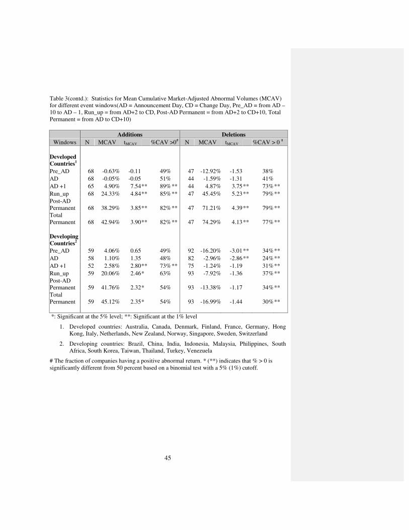
45

Table 3(contd.): Statistics for Mean Cumulative Market-Adjusted Abnormal Volumes (MCAV) for different event windows(AD = Announcement Day, CD = Change Day, Pre_AD = from AD – 10 to AD – 1, Run_up = from AD+2 to CD, Post-AD Permanent = from AD+2 to CD+10, Total Permanent = from AD to CD+10)

Additions Deletions

Windows N MCAV tMCAV %CAV >0# N MCAV tMCAV %CAV > 0 #

Developed

Countries1

Pre_AD 68 -0.63% -0.11 49% 47 -12.92% -1.53 38%

AD 68 -0.05% -0.05 51% 44 -1.59% -1.31 41%

AD +1 65 4.90% 7.54** 89% ** 44 4.87% 3.75 ** 73% **

Run_up 68 24.33% 4.84** 85% ** 47 45.45% 5.23 ** 79% **

Post-AD Permanent 68 38.29% 3.85** 82% ** 47 71.21% 4.39 ** 79% **

Total Permanent 68 42.94% 3.90** 82% ** 47 74.29% 4.13 ** 77% **

Developing

Countries2

Pre_AD 59 4.06% 0.65 49% 92 -16.20% -3.01 ** 34% **

AD 58 1.10% 1.35 48% 82 -2.96% -2.86 ** 24% **

AD +1 52 2.58% 2.80** 73% ** 75 -1.24% -1.19 31% **

Run_up 59 20.06% 2.46* 63% 93 -7.92% -1.36 37% **

Post-AD Permanent 59 41.76% 2.32* 54% 93 -13.38% -1.17 34% **

Total Permanent 59 45.12% 2.35* 54% 93 -16.99% -1.44 30% **

*: Significant at the 5% level; **: Significant at the 1% level

1. Developed countries: Australia, Canada, Denmark, Finland, France, Germany, Hong Kong, Italy, Netherlands, New Zealand, Norway, Singapore, Sweden, Switzerland

2. Developing countries: Brazil, China, India, Indonesia, Malaysia, Philippines, South Africa, South Korea, Taiwan, Thailand, Turkey, Venezuela

# The fraction of companies having a positive abnormal return. * (**) indicates that % > 0 is significantly different from 50 percent based on a binomial test with a 5% (1%) cutoff.

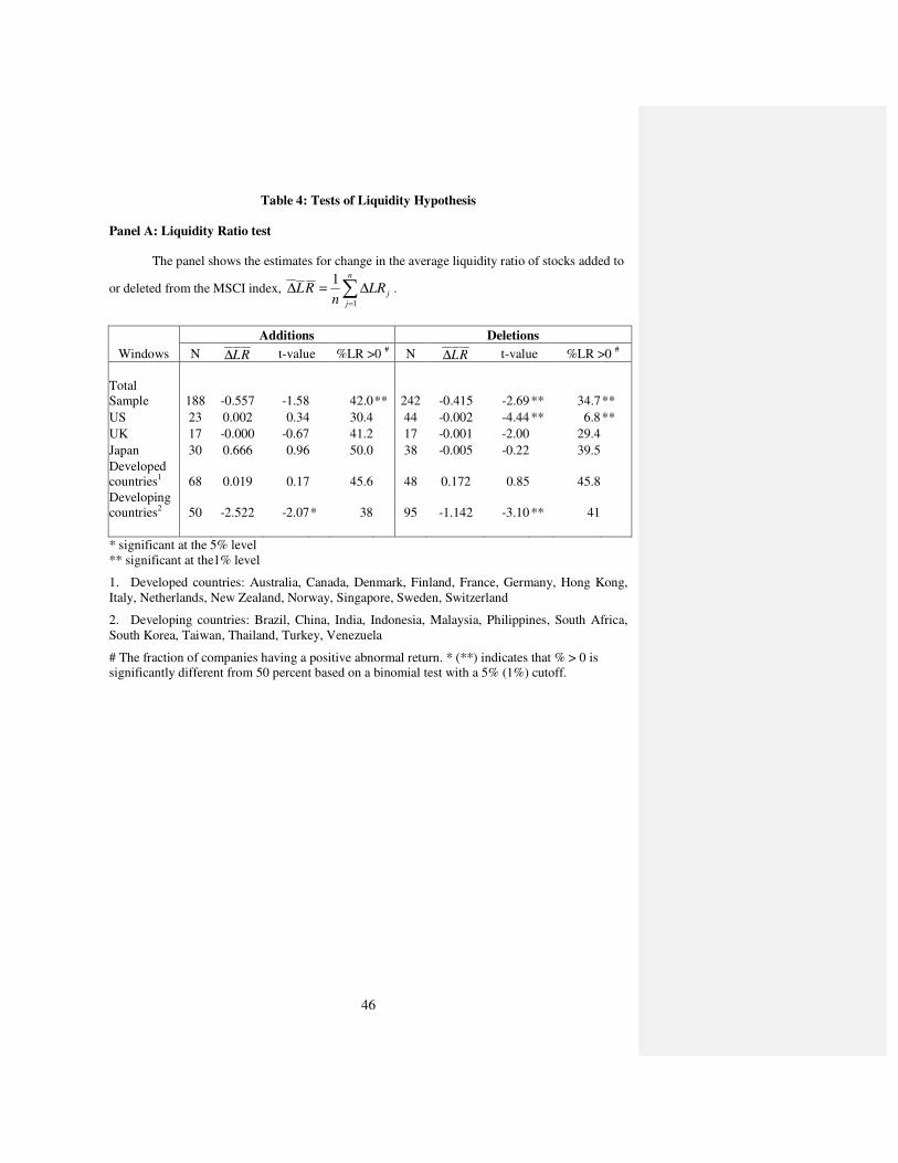
46

Table 4: Tests of Liquidity Hypothesis

Panel A: Liquidity Ratio test

The panel shows the estimates for change in the average liquidity ratio of stocks added to

or deleted from the MSCI index, ∑=

∆=∆n

j

jLRn

RL1

1.

Additions Deletions

Windows N RL∆ t-value %LR >0 # N RL∆ t-value %LR >0 #

Total Sample 188 -0.557 -1.58 42.0 ** 242

-0.415 -2.69 ** 34.7 **

US 23 0.002 0.34 30.4 44 -0.002 -4.44 ** 6.8 **

UK 17 -0.000 -0.67 41.2 17 -0.001 -2.00 29.4

Japan 30 0.666 0.96 50.0 38 -0.005 -0.22 39.5

Developed countries1 68 0.019 0.17 45.6 48 0.172 0.85 45.8

Developing countries2 50 -2.522 -2.07* 38 95 -1.142 -3.10 ** 41

* significant at the 5% level ** significant at the1% level

1. Developed countries: Australia, Canada, Denmark, Finland, France, Germany, Hong Kong, Italy, Netherlands, New Zealand, Norway, Singapore, Sweden, Switzerland

2. Developing countries: Brazil, China, India, Indonesia, Malaysia, Philippines, South Africa, South Korea, Taiwan, Thailand, Turkey, Venezuela

# The fraction of companies having a positive abnormal return. * (**) indicates that % > 0 is significantly different from 50 percent based on a binomial test with a 5% (1%) cutoff.

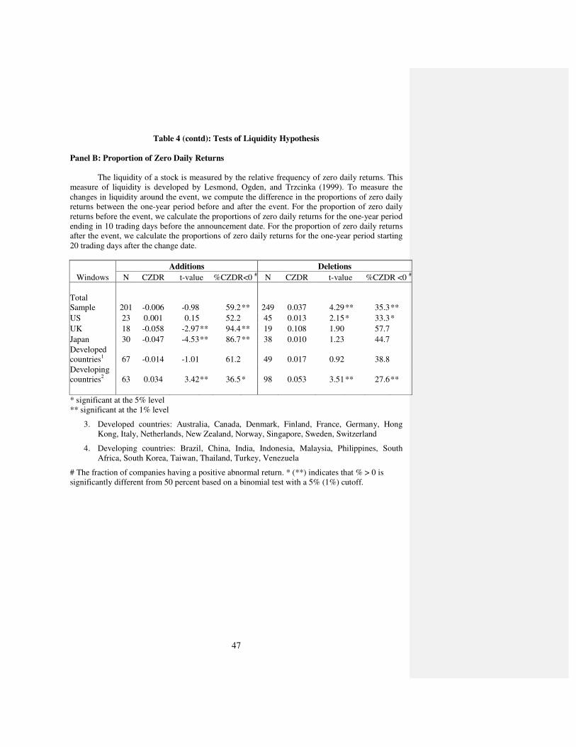
47

Table 4 (contd): Tests of Liquidity Hypothesis

Panel B: Proportion of Zero Daily Returns The liquidity of a stock is measured by the relative frequency of zero daily returns. This

measure of liquidity is developed by Lesmond, Ogden, and Trzcinka (1999). To measure the changes in liquidity around the event, we compute the difference in the proportions of zero daily returns between the one-year period before and after the event. For the proportion of zero daily returns before the event, we calculate the proportions of zero daily returns for the one-year period ending in 10 trading days before the announcement date. For the proportion of zero daily returns after the event, we calculate the proportions of zero daily returns for the one-year period starting 20 trading days after the change date.

Additions Deletions

Windows N CZDR t-value %CZDR<0 # N CZDR t-value %CZDR <0 #

Total Sample 201 -0.006 -0.98 59.2 ** 249

0.037 4.29 ** 35.3 **

US 23 0.001 0.15 52.2 45 0.013 2.15 * 33.3 *

UK 18 -0.058 -2.97** 94.4 ** 19 0.108 1.90 57.7

Japan 30 -0.047 -4.53** 86.7 ** 38 0.010 1.23 44.7

Developed countries1 67 -0.014 -1.01 61.2 49 0.017 0.92 38.8

Developing countries2 63 0.034 3.42** 36.5 * 98 0.053 3.51 ** 27.6 **

* significant at the 5% level ** significant at the 1% level

3. Developed countries: Australia, Canada, Denmark, Finland, France, Germany, Hong Kong, Italy, Netherlands, New Zealand, Norway, Singapore, Sweden, Switzerland

4. Developing countries: Brazil, China, India, Indonesia, Malaysia, Philippines, South Africa, South Korea, Taiwan, Thailand, Turkey, Venezuela

# The fraction of companies having a positive abnormal return. * (**) indicates that % > 0 is significantly different from 50 percent based on a binomial test with a 5% (1%) cutoff.

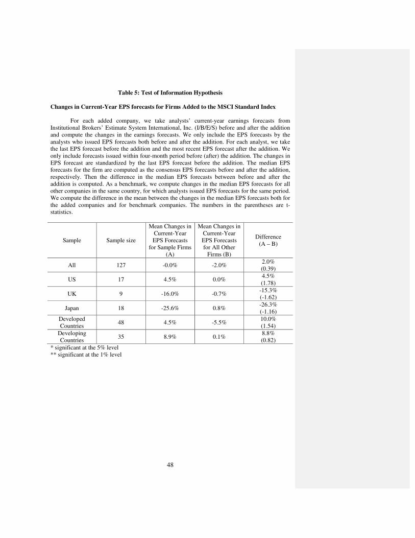
48

Table 5: Test of Information Hypothesis

Changes in Current-Year EPS forecasts for Firms Added to the MSCI Standard Index

For each added company, we take analysts’ current-year earnings forecasts from

Institutional Brokers’ Estimate System International, Inc. (I/B/E/S) before and after the addition and compute the changes in the earnings forecasts. We only include the EPS forecasts by the analysts who issued EPS forecasts both before and after the addition. For each analyst, we take the last EPS forecast before the addition and the most recent EPS forecast after the addition. We only include forecasts issued within four-month period before (after) the addition. The changes in EPS forecast are standardized by the last EPS forecast before the addition. The median EPS forecasts for the firm are computed as the consensus EPS forecasts before and after the addition, respectively. Then the difference in the median EPS forecasts between before and after the addition is computed. As a benchmark, we compute changes in the median EPS forecasts for all other companies in the same country, for which analysts issued EPS forecasts for the same period. We compute the difference in the mean between the changes in the median EPS forecasts both for the added companies and for benchmark companies. The numbers in the parentheses are t-statistics.

Sample Sample size

Mean Changes in Current-Year EPS Forecasts

for Sample Firms (A)

Mean Changes in Current-Year EPS Forecasts for All Other

Firms (B)

Difference (A – B)

All 127 -0.0% -2.0% 2.0% (0.39)

US 17 4.5% 0.0% 4.5% (1.78)

UK 9 -16.0% -0.7% -15.3% (-1.62)

Japan 18 -25.6% 0.8% -26.3% (-1.16)

Developed Countries

48 4.5% -5.5% 10.0% (1.54)

Developing Countries

35 8.9% 0.1% 8.8% (0.82)

* significant at the 5% level ** significant at the 1% level

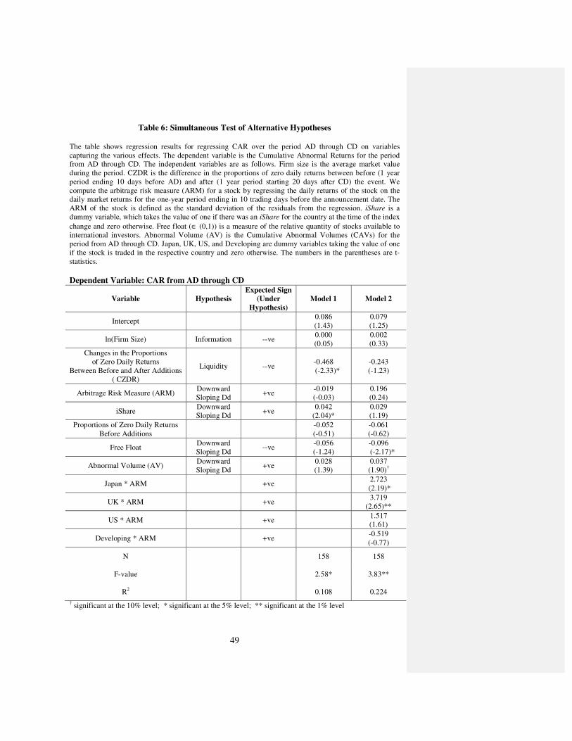
49

Table 6: Simultaneous Test of Alternative Hypotheses

The table shows regression results for regressing CAR over the period AD through CD on variables capturing the various effects. The dependent variable is the Cumulative Abnormal Returns for the period from AD through CD. The independent variables are as follows. Firm size is the average market value during the period. CZDR is the difference in the proportions of zero daily returns between before (1 year period ending 10 days before AD) and after (1 year period starting 20 days after CD) the event. We compute the arbitrage risk measure (ARM) for a stock by regressing the daily returns of the stock on the daily market returns for the one-year period ending in 10 trading days before the announcement date. The ARM of the stock is defined as the standard deviation of the residuals from the regression. iShare is a dummy variable, which takes the value of one if there was an iShare for the country at the time of the index

change and zero otherwise. Free float (∈ (0,1)) is a measure of the relative quantity of stocks available to international investors. Abnormal Volume (AV) is the Cumulative Abnormal Volumes (CAVs) for the period from AD through CD. Japan, UK, US, and Developing are dummy variables taking the value of one if the stock is traded in the respective country and zero otherwise. The numbers in the parentheses are t-statistics.

Dependent Variable: CAR from AD through CD

Variable Hypothesis

Expected Sign

(Under

Hypothesis)

Model 1 Model 2

Intercept 0.086 (1.43)

0.079 (1.25)

ln(Firm Size) Information --ve 0.000 (0.05)

0.002 (0.33)

Changes in the Proportions of Zero Daily Returns

Between Before and After Additions ( CZDR)

Liquidity --ve -0.468

(-2.33)* -0.243 (-1.23)

Arbitrage Risk Measure (ARM) Downward Sloping Dd

+ve -0.019 (-0.03)

0.196 (0.24)

iShare Downward Sloping Dd

+ve 0.042

(2.04)* 0.029 (1.19)

Proportions of Zero Daily Returns Before Additions

-0.052 (-0.51)

-0.061 (-0.62)

Free Float Downward Sloping Dd

--ve -0.056 (-1.24)

-0.096 (-2.17)*

Abnormal Volume (AV) Downward Sloping Dd

+ve 0.028 (1.39)

0.037 (1.90)†

Japan * ARM +ve 2.723

(2.19)*

UK * ARM +ve 3.719

(2.65)**

US * ARM +ve 1.517 (1.61)

Developing * ARM +ve -0.519 (-0.77)

N 158 158

F-value 2.58* 3.83**

R2 0.108 0.224

† significant at the 10% level; * significant at the 5% level; ** significant at the 1% level

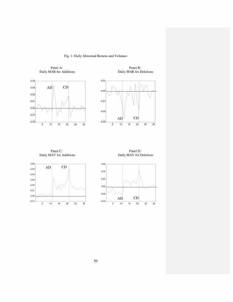
50

Fig. 1: Daily Abnormal Returns and Volumes

Panel A: Panel B: Daily MAR for Additions Daily MAR for Deletions

-0.02

-0.01

0.00

0.01

0.02

0.03

0.04

5 10 15 20 25 30

ALL

-0.03

-0.02

-0.01

0.00

0.01

5 10 15 20 25 30

ALL

Panel C: Panel D: Daily MAV for Additions Daily MAV for Deletions

-0.01

0.00

0.01

0.02

0.03

0.04

0.05

0.06

5 10 15 20 25 30

ALL

-0.04

-0.02

0.00

0.02

0.04

0.06

5 10 15 20 25 30

ALL

AD CD

AD CD

AD CD

AD CD