Example: p'o = 150; s..., = 75 kPa; Ir = 35;and need LBy BjerrunVs chart (a) obtain ). = 0.85 at / r = 35.

V d * = ^ * . = 0.85 x 75 = 65kPaBy Aas et al. charts (b\ enter top chart at IP = 35 and projecthorizontally to su%jp'm = 75/150 = 0.5 (appears in overconsolidatedzone) and vertically to the OC curve to obtain A = 0.5

V d e , * n = 0 . 5 x 7 5 = 37kPaIn this case, probably use sB.desifB = 40 to 50 kPa.

Figure 3-26 Vane shear correction factor A.

there be a need to attempt to obtain separate values for the vertical and horizontal shearstrengths, somewhat similar to that attempted by Garga and Khan (1992).

Since the FVST, like the CPT, does not recover samples for visual classification or forconfirmation tests, it is usually necessary to obtain samples by some alternative test method.This step might be omitted if the geotechnical engineer has done other work in the vicinityof the current exploration.

3-13 THEBOREHOLESHEARTEST(BST)

This test consists in carefully drilling a 76-mm diameter hole (usually vertical but may beinclined or horizontal) to a depth somewhat greater than the location of interest. Next theshear head is carefully inserted into the hole to the point where the shear strength is to bemeasured.

(a) Bjerrum's correction factor for vane shear test.[After Bjerrum (1972) and Ladd et al. (1977).]

Vane strength ratio, Sn^Jp'9

(b) Reinterpretation of the Bjerrum chart of part a by Aas et al.(1986) to include effects of aging and OCR. For interpretationof numbers and symbols on data points see cited reference.

A

/P.%

A

shells

EmbankmentsExcavations

Previous Page

The test proceeds by expanding the serrated cylinder halves into the soil by applying pres-sure from the surface through a piping system. Next the cylinder is pulled with the pullingload and displacements recorded. The expansion pressure is an and the pulling load can beconverted to the shear strength s to make a plot as in Fig. 2-21 b to obtain the in situ strengthparameters </> and c.

Figure 3-27 illustrates the essential details of the test, which was developed by Dr. R.Handy at Iowa State University around 1967 and is sometimes called the Iowa BoreholeShear Test. The test undoubtedly is a drained shear test where the soil is relatively free-draining, since the drainage path from the shear head serrations is short and if the test isperformed in the displacement range of about 0.5 mm/min or less. This rate might be too fast,however, for saturated clays, and Demartinecourt and Bauer (1983) have proposed adding apore-pressure transducer to the shear heads and motorizing the pull (which was initially doneby hand cranking with reduction gearing). With pore pressure measurements it is possible toobtain both total and effective stress parameters from any borehole shear test. Handy (1986)describes the BST in some detail, including its usefulness in collecting data for slope stabilityanalyses.

The BST is applicable for all fine-grained soils and may be done even where a trace ofgravel is present. It has particular appeal if a good-quality borehole can be produced and formodest depths in lieu of "undisturbed" sample recovery and laboratory testing.

3-14 THE FLAT DILATOMETER TEST (DMT)

This test consists of inserting the dilatometer probe of Fig. 3-28 to the depth of interest z bypushing or driving. The CPT pushing equipment can be used for insertion of the device, andin soils where the SPT TV is greater than 35 to 40 the device can be driven or pushed from thebottom of a predrilled borehole using SPT drilling and testing equipment.

Figure 3-27 Borehole shear device.[After Wineland (1975).]

Hydraulicgauge

Hydraulicjack

Shear head

Bottledgas

Console

Pressureregulator

Pressuregauge

Worm gear

Gas lines

(b) The dilatometer pushed to depth z for test

Figure 3-28 The flat dilatometer test (DMT).

(a) Marchetti dilatometer [After M arc he in (1980)]

Flexiblemembraneof diameter D

Wire to data acquisition equipment

Pneumatictubing

Flexiblemembrane

Push

rod

Making a DMT after insertion to the depth of interest uses the following steps:

1. Take a pressure reading at the membrane in the dilatometer just flush with the plate (termedat liftoff), make appropriate zero corrections, and call this pressure p\. The operator getsa signal at liftoff.

2. Increase the probe pressure until the membrane expands Ad = 1.1 mm into the adjacentsoil and correct this pressure as /?2. Again the operator receives a signal so the pressurereading can be taken.

3. Decrease the pressure and take a reading when the membrane has returned to the liftoffposition and correct for pi,. According to Schmertmann (1986) this latter reading can berelated to excess pore pressure.

The probe is then pushed to the next depth position, which is from 150 to 200 mm (ormore) further down, and another set of readings taken. A cycle takes about 2 minutes, so a10-m depth can be probed in about 30 minutes including setup time.

Data are reduced to obtain the following:

1. Dilatometer modulus Ep. According to Marchetti (1980) we have

= 2D(P2 - P l ) A - ^ N\ Es )

and for Ad = 1.1 mm, D = 60 mm (see Fig. 3-28) we have on rearranging

ED = y^-2 = 34.7(p2 - Pi) (3-28)

2. The lateral stress index KD is defined as

KD = ELZJL = EL (3-29)Po Po

3. The material or deposit index ID is defined as

j = P1Z11 ( 3 _ 3 0 )

p2~u

The effective overburden pressure p'o = y'z must be computed in some manner by estimatingthe unit weight of the soil or taking tube samples for a more direct determination. The porepressure u may be computed as the static pressure from the GWT, which must also be knownor estimated.

The DMT modulus ED is related to Es as shown in Eq. (3-28) and includes the effect ofPoisson's ratio /x, which must be estimated if Es is computed. The ED modulus is also relatedto mv of Eq. (2-34) from a consolidation test and thus has some value in making an estimateof consolidation settlements in lieu of performing a laboratory consolidation test.

The lateral stress index KD is related to K0 and therefore indirectly to the OCR. Determi-nation of K0 is approximate since the probe blade of finite thickness has been inserted intothe soil. Figure 3-29 may be used to estimate K0 from KD- Baldi et al. (1986) give someequations that they claim offer some improvement over those shown in Fig. 3-29; however,

The Marchetti (1980) equation:

( K \a

where pD a CD

Marchetti 1.5 0.47 0.6 (KD < 8)Others 1.25-?? 0.44-0.64 0-0.6

7.4 0.54 0Sensitive

clay 2.0 0.47 0.6

General Equation format: OCR = (nKD )m

where n m

Marchetti 0.5 1.56 (KD < 8; ID< 1.2)Others 0.225-?? 1.30-1.75ID 0.225 1.67 (a!so/D < 1.2)

Figure 3-29 Correlation between KD and K0. Note for the Schmertmann curves one must have some estimateof </>. [After Baldi et al (1986).]

they are based heavily on laboratory tests that include Dr. In the field Dr might be somewhatdifficult to determine at any reasonable test depth.

The material or deposit index ID is related (with ED) as illustrated in Fig. 3-30 to the soiltype and state or consistency.

Proper interpretation of the DMT requires that the user have some field experience inthe area being tested or that the DMT data be supplemented with information obtained from

In s

itu

K0

Lateral stress index KD

Marchetti (1980)Schmertmann as citedby Baldi etal. (1986)

Figure 3-30 Correlation between soil type and ID

and ED. [After Lacasse and Lunne (1986).]

Dila

tom

eter

mod

ulus

ED,

MP

a

Material index ID

CLAY

SILTSandy

SAND

Silty

Clayey

Silty

MUD or PEAT

borings and sample recovery for visual verification of soil classification and from laboratory(or other) tests to corroborate the findings.

A typical data set might be as follows:

z,m T,kg(depth) (rod push) /^9 bar P2, bar «, bar

2.10 1,400 2.97 14.53 0.212.40 1,250 1.69 8.75 0.242.70 980 1.25 7.65 0.26

lbar« 100 kPa

Here the depths shown are from 2.1 to 2.7 m. The probe push ranged from 1,400 kg to 980kg (the soil became softer) and, as should be obvious, values of p2 are greater than p\. Withthe GWT at the ground surface the static pore pressure u is directly computed as 9.807z/100to obtain u in bars.

According to both Marchetti (1980) and Schmertmann (1986) the DMT can be used toobtain the fiill range of soil parameters (ED, K0, OCR, su, 0, and mv) for both strength andcompressibility analyses.

3-15 THE PRESSUREMETER TEST (PMT)

The borehole pressuremeter test is an in situ test developed ca. 1956 [Menard (1956)] wherea carefully prepared borehole that is sufficiently—but not over about 10 percent—oversizedis used. The pressuremeter probe consisting of three parts (top, cell, and bottom) as shown inFig. 3-3Ia is then inserted and expanded to and then into the soil. The top and bottom guardcells are expanded to reduce end-condition effects on the middle (the cell) part, which is usedto obtain the volume versus cell pressure relationship used in data reduction.

A pressuremeter test is not a trivial task, as fairly high pressures are involved and cali-brations for pressure and volume losses must be made giving data to plot curves as in Fig.3-32a. These data are used to correct the pressure-volume data taken during a test so thata curve such as Fig. 3-32b can be made. It is evident that a microcomputer can be used toconsiderable advantage here by installing the calibration data in memory. With the probe datadirectly input, the data can be automatically reduced and, with a plot routine, the curve canbe developed as the test proceeds.

The interested reader should refer to Winter (1982) for test and calibration details and toBriaud and Gambin (1984) for borehole preparation (which is extremely critical). It shouldbe evident that the PMT can only be performed in soils where the borehole can be shaped andwill stand open until the probe is inserted. Although the use of drilling mud/fluid is possible,hole quality cannot be inspected and there is the possibility of a mud layer being trappedbetween the cell membrane and the soil. Another factor of some to considerable concern isthat the soil tends to expand into the cavity when the hole is opened so that the test often hasconsiderable disturbance effects included.

To overcome the problems of hole preparation and soil expansion, self-boring pressureme-ters were almost simultaneously developed in France [Baguelin et al. (1974)] and England[Wroth (1975)]. The self-boring pressuremeter test (SBPMT) is qualitatively illustrated inFig. 3-316 and c.

Figure 3-31 Pressuremeter testing; (b) and (c) above are self-boring, or capable of advancing the distance AB of (a) so that in situ lateralstress is not lost.

Hollowdrill rod

Rotatablechopping tool

Cutting edge

( < ) French device.

(a) Pressuremeter schematicin borehole.

Guard cell

Guard cell

Measuring cellDxL

Loadcell

Cuttinghead

Prebored

liole

[b) Camkometer.

Flow of slurriedsoil and waterCutter

Taper <10 '

Soft water-proof filler

Web L3

Face plate

Load cellface plate

Section A-A

Load cell

1|3D p*oqXpoq

housing

Diameter = 80 mm

Hollowrotatingshaft

Distancefunction.ground

strength

Web L1

The pressuremeter operates on the principle of expanding a rigid cylinder into the soiland being resisted by an infinitely thick cylinder (the soil). The basic equation in terms ofvolumetric strain ev is

where terms not previously defined are

ri, Ar = initial radius at contact with hole and change in hole radius, respectivelyp = cell expansion pressure in units of Es

In practice we obtain the slope (AV/Ap) from the linear part of the cell pressure versus volumeplot and rearrange Eq. (3-31) to obtain the lateral static shear modulus as

U 2 (1+ /x) V°AV ( 3 J 2 )

where V0 = volume of the measuring cell at average pressure Ap = V0 + Vc

Ap9 AV = as defined on Fig. 3-32b along with a sample computation for G'

The pressuremeter modulus Esp is then computed using an estimated value of /x as Esp =E5 = G'[2(l + /A)]. Unless the soil is isotropic this lateral E5 is different from the verticalvalue usually needed for settlement analyses. For this reason the pressuremeter modulus Esp

usually has more application for laterally loaded piles and drilled caissons.The value ph shown on Fig. 3-32b is usually taken as the expansion pressure of the cell

membrane in solid contact with the soil and is approximately the in situ lateral pressure (de-pending on procedure and insertion disturbance). If we take this as the in situ lateral pressure,then it is a fairly simple computation to obtain K0 as

K0 = ^- (3-33)Po

which would be valid using either total or effective stresses (total is shown in the equation). Itis necessary to estimate or somehow determine the unit weight of the several strata overlyingthe test point so that po can be computed.

With suitable interpretation of data as shown on Fig. 3-32b and replotting, one can estimatethe undrained shear strength S1^1, for clay [see Ladanyi (1972) for theory, example data, andcomputations] and the angle of internal friction <f> [Ladanyi (1963), Winter and Rodriguez(1975)] for cohesionless soils.

It appears that the pressuremeter gives s^p which are consistently higher than determinedby other methods. They may be on the order of 1.5 to 1.7s^ (and we already reduce thevane shear strength by As11^). The PMT also appears to give values on the order of 1.3 to1-5^tJi3xJaI.

The pressuremeter seems to have best applications in the same soils that are suitable forthe CPT and DMT, that is, relatively fine-grained sedimentary deposits. In spite of the ap-parently considerable potential of this device, inconsistencies in results are common. Clough[see Benoit and Clough (1986) with references] has made an extensive study of some ofthe variables, of which both equipment configuration and user technique seem to be criticalparameters.

Total pressure pt> kg/cm2

(h) Data from a pressuremeter test in soft clay.

Figure 3-32 Pressuremeter calibration and data.

Tot

al i

njec

ted

volu

me,

cm

3 ( x

100

)

Example:po = 4 x 19.81 = 79.24 kPa (in situ)

ph 0.38 x 98.07Ko = ir 79.24 ~° ' 4 7

average over Ap044

V0 = - ^ - x 100 + 88 = 110cm3

For S= 100% take // = 0.5

Note: For soft clay the calibration volume V'c s 0

Calibration pressure />', kg/cm2, kPa, etc.

(a) Calibration curves for pressuremeter. This data may beput in a microcomputer so (b) can be quickly obtained.

Cal

ibra

tion

vol

ume

V' c,

cm

3/4 = pressure calibration curve obtained by

expanding probe in air in 0.1 kg/cm2 (or equivalentpressure increments)

B - volume calibration obtained by expanding probe inheavy steel container

Extend curve B to obtain V0 as shown

Cor

rect

ed v

olum

e K

0 cm

3 (x

100)

Lim

it p

ress

ure

3-16 OTHER METHODS FOR IN SITU K0

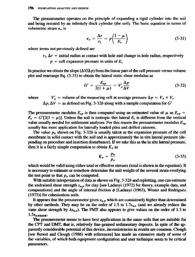
The Glotzl cell of Fig. 3-33 is a device to measure K0 in soft clays. It is pushed to about 300mm above the test depth in the protective metal sheath, then the blade is extended to the testdepth. The device is 100 X 200 mm long X 4 mm thick [Massarsch (1975)]. The cell containsoil, which is pressurized from the surface to obtain the expansion pressure = lateral pressure.According to Massarsch (1975) and Massarsch et al. (1975), one should wait about a weekfor the excess pore pressure from the volume displacement to dissipate. It may be noted thatthe DMT, which has a displacement volume of about four times this device, uses no timedelay for pore-pressure dissipation.

The Iowa stepped blade [Handy et al. (1982)] of Fig. 3-34 can be used to estimate K0

somewhat indirectly. In use the first step (3-mm part) is inserted at the depth of interest anda pressure reading taken. The blade is then pushed so the next step is at the point of interestand a reading taken, etc., for the four steps. Data of pressure versus blade thickness t can beplotted using a semilog scale as in Fig. 3-34. The best-fit curve can be extended to t = 0 toobtain the in situ lateral pressure ph so that K0 can be computed using Eq. (3-33).

Lutenegger and Timian (1986) found that for some soils the thicker steps gave smallerpressure readings than for the previous step (with thinner blade). This result was attributedto the soil reaching its "limiting pressure" and resulted in increasing the original three-stepblade to one now using four steps. This limit pressure is illustrated on the pressuremetercurve of Fig. 3-32fe. Noting the stepped blade goes from 3 to 7.5 mm and the flat dilatometer

Figure 3-33 Glotzl earth-pressure cell with protection frame to measure lateral earth pressure after the protectionframe is withdrawn.

LxWxT20Ox 100 x 4 mm

t, mm(a) Typical log - log data plot. (b) Dimensions, mm.

Figure 3-34 Iowa stepped blade for K0 estimation.

has a thickness of 14 mm we can well ask why this apparent limit pressure does not developwith the thicker—but tapered—dilatometer blade. It may be that the blade steps produce adifferent stress pattern in the ground than the tapered DMT blade.

Hydraulic fracture is a method that may be used in both rock and clay soils. It cannotbe used in cohesionless soils with large coefficients of permeability. Water under pressure ispumped through a piezometer that has been carefully installed in a borehole to sustain con-siderable hydraulic pressure before a breakout occurs in the soil around the piezometer point.At a sufficiently high hydraulic pressure a crack will develop in the soil at the level of waterinjection. At this time the water pressure will rapidly drop and level off at an approximateconstant pressure and flow rate. Closing the system will cause a rapid drop in pressure as thewater flows out through the crack in the wall of the boring. The crack will then close as thepressure drops to some value with a resulting decrease in flow from the piezometer system.By close monitoring of the system and making a plot as in Fig. 3-35/?, one can approximatethe pressure at which the crack opens.

Steps in performing a fracture test are as follows (refer to Fig. 3-35«):

1. Prepare a saturated piezometer with a 6-mm standpipe tube filled with deaerated waterwith the top plugged and pushed to the desired depth L using a series of drill rods. Theplug will keep water from flowing into the system under excess pore pressure developedby pushing the piezometer into the ground.

2. Measure Lw and Lf, and compute depth of embedment of piezometer and transducer volt-age V.

3. After about \ hr unplug the 6-mm standpipe tube and connect the fracture apparatus tothe standpipe using an appropriate tube connector at G.

4. Fill the fracture system with deaerated water from the 1- or 2-liter reservoir bottle byopening and closing the appropriate valves. Use the hand-operated pump/metering deviceto accomplish this.

5. Take a zero reading on the pressure transducer—usually in millivolts, mV.

P, k

Pa

Pressuresensor for ph

6. Apply system pressure at a slow rate using the hand pump until fracture occurs as observedby a sudden drop-off in pressure.

7. Quickly close valve E.8. From the plot of pressure transducer readings versus time, the break in the curve is inter-

preted as relating to cr3.

Lefebvre et al. (1991) used a series of field tests in soils with apparently known OCRs inthe range of 1.6 to 4.8 to see the effect of piezometer tip size and what range of K0 might beobtained. The tests appear to establish that K0 -> 1.0 when the OCR is on the order of 2.1.The K0 values ranged from about 0.59 to 3.70 and were generally higher as OCR increased,but not always for the smaller OCR. In the low-OCR region a K0 = 0.59 was found for OCR= 1.7, whereas a value of 0.88 was found for OCR = 1.6. These variations were likely dueto soil anomalies or correctness of the "known" OCR.

This test may also be performed in rock, but for procedures the reader should consultJaworski et al. (1981).

The following example is edited from Bozozuk (1974) to illustrate the method of obtainingK0 from a fracture test in soil.

Example 3-7. Data from a hydraulic fracture test are as follows (refer to Fig. 3-35):

Length of casing used = L^ + z = 6.25 m

Distance from top of casing to ground Lf = 1.55 m

Distance Ln, measured inside drill rods (or standpipe) with a probe = 2.02 m

Saturated unit weight of soil, assuming groundwater nearly to surface and

S = 100 percent for full depth, y ^ = 17.12kN/m3

Figure 3-35

(a) Schematic of hydraulic fracture test setup (b) Qualitative data plot from fracture test.Value of 1.84 is used in Example 3-7.[After Bozozuk (1974).]

Time, min

Tra

nsdu

cer

read

ing,

mV

Airbleed

Plastic tubingTop ofcasing Connector

Standpipe

CasingWaterreservoir

Pressuretransducer

To chartrecorder

Pump

Assumed fracture zone

GWT

Geonor piezometer

y measured when fracture apparatus connected = 0.265 m

The pressure transducer output is calibrated to 12.162 kPa/mV.

Required. Find the at-rest earth-pressure coefficient K0.

Solution.

z = 6.25 - 2.02 = 4.23 m (see Fig. 3-35a)

Lwi = Lw-y = 2.02 - 0.265 = 1.755 m

Total soil depth to piezometer tip, hs = Lw + z — Lf

= 6.25 - 1.55 = 4.70 m

Total overburden pressure, po = ySat^

= 17.12(4.70) = 80.46 kPa

This po assumes soil is saturated from the ground surface. Now we compute the static pore pressureuo before test starts:

Uo = ZJw = 4.23(9.807) = 41.98 kPa

The effective pressure is expressed as

Po = Po- U0

= 80.46 - 41.48 = 38.98 kPa

Since hs = 4.70 and z = 4.23 m, the GWT is 0.47 m below ground surface. With some capillaryrise, the use of ysat = 17.12 kN/m3 for full depth of hs produces negligible error.The fracture pressure is a constant X the reading (of 1.84), giving

FP = (12.162 kPa/mV)(l.84 mV) = 22.38 kPa

The additional pore pressure from water in the piezometer above the existing GWT is

Uwi = Lwi7w = 1.755(9.807) = 17.21 kPa

Total pore pressure ut is the sum of the measured value FP and the static value of uwi just computed,giving

ut = FP + uwi = 22.38 + 17.21 = 39.59 kPa

K0 = q\Jqv

And using ut = qn and qv = p'o, we can compute K0 as

K0 = total pore pressure//?^ = ut/p'o

= 39.59/38.98 = 1.03

This value of K0 is larger than 1.00, so this example may not be valid. To verify these com-putations, use a copy machine to enlarge Fig. 3-35<a, then put the known and computed valueson it.

////

Considerable research has been done on hydraulic fracture theory to produce a methodthat can be used to predict hydraulic fracture in soil more reliably. In addition to estimatingthe OCR and ko there is particular application in offshore oil production, where a large headof drilling fluid may produce hydraulic fracture (and loss of fluid) into the soil being drilled.A recent summary of this work is given by Anderson et al. (1994).

3-17 ROCKSAMPLING

In rock, except for very soft or partially decomposed sandstone or limestone, blow counts areat the refusal level (N > 100). If samples for rock quality or for strength testing are required itwill be necessary to replace the soil drill with rock drilling equipment. Of course, if the rock isclose to the ground surface, it will be necessary to ascertain whether it represents a competentrock stratum or is only a suspended boulder(s). Where rock is involved, it is useful to havesome background in geology. A knowledge of the area geology will be useful to detect rockstrata versus suspended boulders, whose size can be approximately determined by probing(or drilling) for the outline. A knowledge of area geology is also useful to delineate both thetype of rock and probable quality (as sound, substantially fractured from earth movements,etc.). This may save considerable expense in taking core samples, since their quantity anddepth are dependent on both anticipated type and quality of the rock.

Rock cores are necessary if the soundness of the rock is to be established; however, coressmaller than those from the AWT core bit (Table 3-6) tend to break up inside the drill barrel.Larger cores also have a tendency to break up (rotate inside the barrel and degrade), especiallyif the rock is soft or fissured. Drilling small holes and injecting colored grout (a water-cementmixture) into the seams can sometimes be used to recover relatively intact samples. Coloredgrout outlines the fissure, and with some care the corings from several adjacent corings canbe used to orient the fissure(s).

Unconfined and high-pressure triaxial tests can be performed on recovered cores to de-termine the elastic properties of the rock. These tests are performed on pieces of sound rockfrom the core sample and may give much higher compressive strengths in laboratory testingthan the "effective" strength available from the rock mass, similar to results in fissured clay.

Figure 3-36 illustrates several commonly used drill bits, which are attached to a piece ofhardened steel tube (casing) 0.6 to 3 m long. In the drilling operation the bit and casing rotatewhile pressure is applied, thus grinding a groove around the core. Water under pressure isforced down the barrel and into the bit to carry the rock dust out of the hole as the water iscirculated.

The recovery ratio term used earlier also has significance for core samples. A recoveryratio near 1.0 usually indicates good-quality rock. In badly fissured or soft rocks the recoveryratio may be 0.5 or less.

TABLE 3-6

Typical standard designation and sizes for rock drillcasing (barrel) and bits*

Casing OD, mm Core bit OD, mm Bit ID, mm

RW 29 EWT 37 23EW 46 AWT 48 32AW 57 BWT 60 44BW 73 NWT 75 59NW 89 HWT 100 81PW 140 194 152

* See ASTM D 2113 for the complete range in core bit, casing, and drill rod sizes incurrent use. Sizes are nominal—use actual diameter of recovered core.

(a) Core barrels to collect rock cores (b) Coring bits to attach to core barrel. (The Acker Drill Company)

Figure 3-36 Rock coring equipment. See such sources as DCDMA (1991) for standard dimensions, details, and a morecomplete list of available equipment for both rock and soil exploration.

Rock quality designation (RQD) is an index or measure of the quality of a rock mass[Stagg and Zienkiewicz (1968)] used by many engineers. RQD is computed from recoveredcore samples as

_ X Lengths of intact pieces of core > 100 mmLength of core advance

For example, a core advance of 1500 mm produced a sample length of 1310 mm consisting ofdust, gravel, and intact pieces of rock. The sum of lengths of pieces 100 mm or larger9 (piecesvary from gravel to 280 mm) in length is 890 mm. The recovery ratio Lr = 1310/1500 =0.87 and RQD = 890/1500 = 0.59.

The rating of rock quality may be used to approximately establish the field reduction ofmodulus of elasticity and/or compressive strength and the following may be used as a guide:

9 Some persons use a modified RQD in which the pieces 100 mm and longer are sufficiently intact if they cannotbe broken into shorter fragments by hand.

Series "NTdouble-tubecore barrel

Standarddouble-tubecore barrel

RQD Rock description EfIElah*

<0.25 Very poor 0.150.25-0.50 Poor 0.200.50-0.75 Fair 0.250.75-0.90 Good 0.3-0.7>0.90 Excellent 0.7-1.0

* Approximately for field/laboratory compression strengthsalso.

Depth of Rock Cores

There are no fast rules for rock core depths. Generally one should core approximately asfollows:

1. A depth sufficient to locate sound rock or to ascertain that it is fractured and jointed to avery great depth.

2. For heavily loaded members such as piles or drilled piers, a depth of approximately 3 to4 m below the location of the base. The purpose is to check that the "sound" rock doesnot have discontinuities at a lower depth in the stress influence zone and is not a largesuspended boulder.

Local building codes may give requirements for coring; however, more often they giveallowable bearing pressures that can be used if one can somehow ascertain the rock qualitywithout coring.

Adjacent core holes can be used to obtain relative rock quality by comparing cross-holeseismic wave velocities in situ to laboratory values on intact samples. If the field value isless, it indicates fractures and jointing in the rock mass between holes. Down-hole and surfacemethods are of little value in this procedure, since a part of the wave travel is in the overlayingsoil and separating the two with any confidence is nearly impossible.

3-18 GROUNDWATER TABLE (GWT) LOCATION

Groundwater affects many elements of foundation design and construction, so the GWTshould be established as accurately as possible if it is within the probable construction zone;otherwise, it is only necessary to determine where it is not. For the latter case the locationwithin ±0.3 to 0.5 m is usually adequate.

Soil strength (or bearing pressure) is usually reduced for foundations located below thewater table. Foundations below the water table will be uplifted by the water pressure, andof course some kind of dewatering scheme must be employed if the foundations are to beconstructed "in the dry."

The GWT is generally determined by directly measuring to the stabilized water level inthe borehole after a suitable time lapse, often 24 to 48 hr later. This measurement is doneby lowering a weighted tape down the hole until water contact is made. In soils with a highpermeability, such as sands and gravels, 24 hr is usually a sufficient time for the water levelto stabilize unless the hole wall has been somewhat sealed with drilling mud.

In soils with low permeability such as silts, fine silty sands, and clays, it may take sev-eral days to several weeks (or longer) for the GWT to stabilize. In this case an alternative is to

install a piezometer (small vertical pipe) with a porous base and a removable top cap in theborehole. Backfill is then carefully placed around the piezometer so that surface water cannotenter the boring. This procedure allows periodic checking until the water level stabilizes, thatis, the depth to the water has not changed since the previous water level measurement wastaken. Clearly this method will be expensive because of the additional labor involved in theinstallation and subsequent depth checks.

In theory we might do the following:

1. Plot the degree of saturation S with depth if it is possible to compute it reliably. A directplot of the in situ water content may be useful, but for S = 100 percent wN can decreaseas the void ratio decreases from overburden pressure.

2. Fill the hole and bail it out. After bailing a quantity, observe whether the water level in thehole is rising or falling. The true level is between the bailed depth where the water wasfalling and the bailed depth where it is rising. This method implies a large permeability,so it would be more practical simply to bail the hole, then move to the next boring locationwhile the GWT stabilizes.

One may apply a computational method; however, this requires capping the hole and tak-ing periodic depth measurements to the water table (as done for direct measurements), andsince no one (to the author's knowledge) computes the depth, the computational method isno longer given. This method was given in the first through third editions of this book.

3-19 NUMBER AND DEPTH OF BORINGS

There are no clear-cut criteria for determining directly the number and depth of borings (orprobings) required on a project in advance of some subsurface exploration. For buildings aminimum of three borings, where the surface is level and the first two borings indicate regularstratification, may be adequate. Five borings are generally preferable (at building corners andcenter), especially if the site is not level. On the other hand, a single boring may be sufficientfor an antenna or industrial process tower base in a fixed location with the hole made at thepoint.

Four or five borings are sufficient if the site soil is nonuniform (both to determine this andfor the exploration program). This number will usually be enough to delineate a layer of softclay (or a silt or peat seam) and to determine the properties of the poorest material so that adesign can be made that adequately limits settlements for most other situations.

Additional borings may be required in very uneven sites or where fill areas have beenmade and the soil varies horizontally rather than vertically. Even though the geotechnicalengineer may be furnished with a tentative site plan locating the building(s), often these arestill in the stage where horizontal relocations can occur, so the borings should be sufficientlyspread to allow this without having to make any (or at least no more than a few) additionalborings.

In practice, the exploration contract is somewhat open as to the number of borings. Thedrilling operation starts. Based on discovery from the first holes (or CPT, DMT, etc.) thedrilling program advances so that sufficient exploration is made for the geotechnical engineerto make a design recommendation that has an adequate margin of safety and is economicallyfeasible for the client. Sometimes the exploration, particularly if preliminary, discloses thatthe site is totally unsuitable for the intended construction.

Borings should extend below the depth where the stress increase from the foundation loadis significant. This value is often taken as 10 percent (or less) of the contact stress qo. For thesquare footing of Fig. \-\a the vertical pressure profile shows this depth to be about 2B. Sincefooting sizes are seldom known in advance of the borings, a general rule of thumb is 2 x theleast lateral plan dimensions of the building or 10 m below the lowest building elevation.

Where the 2 X width is not practical as, say, for a one-story warehouse or department store,boring depths of 6 to 15 m may be adequate. On the other hand, for important (or high-rise)structures that have small plan dimensions, it is common to extend one or more of the boringsto bedrock or to competent (hard) soil regardless of depth. It is axiomatic that at least one ofthe borings for an important structure terminate into bedrock if there are intermediate strataof soft or compressible materials.

Summarizing, there are no binding rules on either the number or the depth of exploratorysoil borings. Each site must be carefully considered with engineering judgment in combina-tion with site discovery to finalize the program and to provide an adequate margin of safety.

3-20 DRILLING AND/OR EXPLORATION OF CLOSEDLANDFILLS OR HAZARDOUS WASTE SITES

Seldom is a soil exploration done to place a structure over a closed landfill or hazardous wastesite. Where exploration is necessary, extreme caution is required so that the drilling crew isnot exposed to hazardous materials brought to the surface by the drill. Various gases that maybe dangerous if inhaled or subject to explosion from a chance spark may also exit the drillhole. In addition to providing the drilling crew with protective clothing it may be necessaryalso to provide gas masks.

When drilling these sites, it is necessary to attempt to ascertain what types of materialsmight be buried in the fill. It is also of extreme importance that the drilling procedure notpenetrate any protective lining, which would allow leachate contained in the fill to escapeinto the underlying soil or groundwater. If the boring is to penetrate the protective liner, itis absolutely essential to obtain approval from the appropriate governmental agencies of theprocedure to use to avoid escape of the fill leachate. This approval is also necessary to givesome protection against any litigation (which is very likely to occur). At the current (1995)level of drilling technology there is no known drilling procedure that will give an absoluteguarantee that leachate will not escape if a drill hole is advanced through a protective liner,even if casing is used.

3-21 THE SOIL REPORT

When the borings or other field work has been done and any laboratory testing completed, thegeotechnical engineer then assembles the data for a recommendation to the client. Computeranalyses may be made where a parametric study of the engineering properties of the soil isnecessary to make a "best" value(s) recommendation of the following:

1. Soil strength parameters of angle of internal friction <f> and cohesion c2. Allowable bearing capacity (considering both strength and probable or tolerable settle-

ments)3. Engineering parameters such as Es, JJL, G', or ks.

A plan and profile of the borings may be made as on Fig. 3-37, or the boring informationmay be compiled from the field and laboratory data sheets as shown on Fig. 3-38. Field anddata summary sheets are far from standardized between different organizations [see Bowles(1984), Fig. 6-6 for similar presentation], and further, the ASTM D 653 (Standard Terms andSymbols Relating to Soil and Rock) is seldom well followed.

In Fig. 3-38 the units are shown in Fps because the United States has not converted asof this date (1995) to SI. On the left is the visual soil description as given by the drillingsupervisor. The depth scale is shown to identify stratum thickness; the glacial silty clay till isfound from 6 in. to nearly 12 ft (about 11 ft thick). The SS indicates that split spoon sampleswere recovered. The N column shows for each location the blows to seat the sampler 6 in. (150mm) and to drive it for the next two 6-in. (150-mm) increments. At the 3-ft depth it took fiveblows to drive the split spoon 6 in., then 10 and 15 each for the next two 6-in. increments—the total Af count = 1 0 + 1 5 = 25 as shown. A pocket penetrometer was used to obtain theunconfined compression strength of samples from the split spoon (usually 2 + tests) with theaverage shown as Qp. At the 3-ft depth Qp = qu = 4.5+ ton/ft2 (43O+ kPa). The pocketpenetrometers currently in use read directly in both ton/ft2 and kg/cm2, the slight differencebetween the two units being negligible (i.e., 1 ton/ft2 ~ 1 kg/cm2) and ignored. The nextcolumn is the laboratory-determined Qu = qu values, and for the 3-ft depth qu = 7.0 tsf(670 kPa). Based on the natural water content Mc = w^ = 15 percent, the dry unit weightDd = 7d = 121 lb/ft3 (or 19.02 kN/m3). The GWT appears to be at about elevation 793.6 ft.Note that a hollow-stem continuous-flight auger was used, so that the SPT was done withoutusing casing.

The client report is usually bound with a durable cover. The means of presentation canrange from simple stapling to binding using plastic rings. At a minimum the report generallycontains the following:

1. Letter of transmittal.

2. Title.

3. Table of contents.

4. Narrative of work done and recommendations. This may include a foldout such as Fig.3-37. The narrative points out possible problems and is usually written in fairly generalterms because of possible legal liabilities. The quality varies widely. The author used onein which the four-page narrative consisted of three pages of "hard sell" to use the firm forsome follow-up work.

5. Summary of findings (and recommendations). This is usually necessary so that after thegeneralities of the narrative the client can quickly find values to use. Some clients maynot read the narrative very carefully.

6. Appendices that contain log sheets of each boring, such as Fig. 3-35; laboratory datasheets as appropriate (as for consolidation, but not usually stress-strain curves from tri-axial tests—unless specifically requested); and any other substantiating material.

The sample jars may be given to the client or retained by the geotechnical firm for a rea-sonable period of time, after which the soil is discarded. How the soil samples are disposedof may be stated in the contract between client and consultant.

Figure 3-37 A method of presenting the boring information on a project. All dimensions are in meters unless shown otherwise.

Notes:1. All elevations are in accordance with plot plan furnished by architect.2. Borings were made using standard procedures with 50.8 mm OD split spoon.3. Figures to the right of each boring log indicate the number of blows required

to drive the split spoon 300 mm using a 63.5 kg mass falling 760 mm.4. No water encountered in any of the borings.

LegendFine to medium brown silty sand—some small to medium gravel

Fine brown silty sand—small to medium gravel

Fine brown silty sand—trace of coarse sand

Topsoil

Brown silty clay

Boring No. 1Boring No. 5

Boring No. 2 Boring No. 3 Boring No. 4 Elevation

Got firmer

Got firmer

Hard

ElevationElevation

Elevation

Elevation

Got firmer

Got firmer

Hard!

6 in boulder

UOtfirmer

Got firmer,

Got firmer

GoIfirmer

Hardproperty lineApproximate

BoringsperformedAugust, 19

Boring No. 2Elevation 90.2

Boring No. 1Elevation 89.1

Boring No. 5Elevation 92.5

Boring No. 4Elevation

BoringNo. 3Elevation

BORING NO.BrO4_DATE 1 2 - 0 3 - 9 2

W. & A. FILE NO. **5

SHEET * HP 7PROJECT OJtIO-MEtIOm EyBfATED HATOI STOHAHB TAMK LOCATION 0*4©BORING LOCATION 9— Plot (PJIt Stl—t DRILLED BY J t i S l ^ lBORINGTYPE Hollow-SUm kuqmr WFATHFR nnisinmnMs P a r t l y C l o u d y & C o o lSOIL CLASSIFICATION SYSTEM t l# S« B« S « C« SEEPAGE WATER ENCOUNTERED AT ELEVATION IJOIW

GROUND SURFACE ILEVATION HO4« 2 GROUND WATER ELEVATION AT 2 4 » HRS. 7 9 3 . 6

BORING DISCONTINUED AT ELEVATION 767« 2 GROUND WATER ELEVATION AT COMPLETION 793* 4

BORING LOGWHITNEY & ASSOCIATES

mCCNMHMMTBO

2406 WMt Ntbratkft AVMMJ*

KORIA, IULINOIS 61604

DESCRIPTION

Brown SItTY CUY LMII OrganicTopgollKurd, Brown, tte*th*r«<l GUCIALSILTY CLAY TILL

SILTY CUY TILL

GUCIAL SILTY CUY TILL

Hmr6, Barmy LIHESTOiIEEXPLORATORY BQRIHG DISCONTINUED

DEPTHIN FEET

_03

_06

_09

- 12

- 15

- 18

SAMPLETYPE

SS

SS

SS

SS

SS

SS

N

51015(25)

81218(30)

91419(33)

81318(31)

57

11(18)

558(133

QP

4.5*

4*5*

4.5*

4.5«

4.5«

2.3

Qu

7.0

6.0

5.1

S. 2

5.1

2.2

Dd

121

118

119

124

113

109

Mc

15

14

15

13

18

20

N - SLOWS OELIVERED PER FOOT 8Y A 140 LB. HAMMERFALLING 30 INCHES

§S - SPLIT SPOON SAMPLET - SHELBY TUBE SAMPLE

Qp - CALIBRATED PENETROMETER READING - TSF.Qu - UNCONFINED COMPRESSIVE STRENGTH - TSF,Del - NATURAL DRY DENSITY - PCF.Mc - NATURAL MOISTURE CONTENT - %

WHITNEY & ASSOCIATESPCOftlA, ILLiMOiS

Figure 3-38 Boring log as furnished to client. TV = SPT value; Qp = pocket penetrometer; Qu = unconfined compressiontest; Dd - estimated unit weight ys;Mc = natural water content wN in percent.

PROBLEMS

Problems are in order of text coverage.

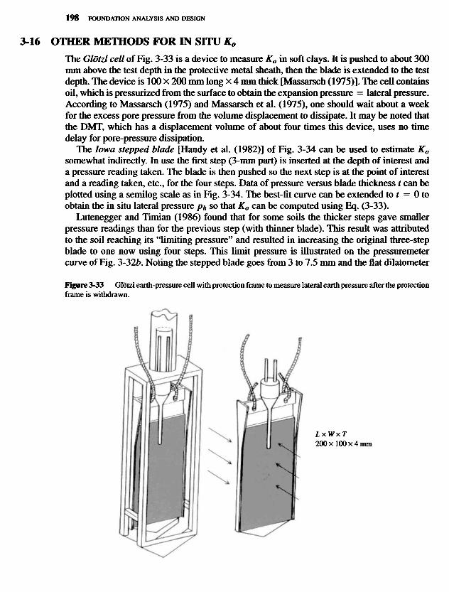
3-1. Sound cohesive samples from the SPT (returned to the laboratory in glass jars) were obtainedfor a y determination using a 500 mL (mL = cm3) volume jar as follows:

Trimmed Water added,Boring Depth, m weight, g cm3

B-I 6.00 142.3 426B-3 8.00 145.2 427

i.e., weighed samples put in volume jar and water shownadded. Volume of first sample = 500 — 426 = 74 cm3

Required: Estimate the average unit weight of the clay stratum from depth = 5 to 9 m. If theGWT is at 2 m depth, what is ydry? Hint: Assume G5.

Answer: y ^ « 19.18 kN/m3; ydry = 14.99 kN/m3.

3-2. What are po and p'o at the 9-m depth of Prob. 3-1 if y = 17.7 kN/m3 for the first 2 m of depthabove the GWT?

Answer: p'o = 101.0 kPa.

3-3. Compute the area ratio of the standard split spoon dimensions shown on Fig. 3-5a. W hat IDwould be required to give Ar = 10 percent?

3-4. The dimensions of two thin-walled sample tubes (from supplier's catalog) are as follows:

OD, mm ID, mm Length, mm

76.2 73 61089 86 610

Required: What is the area ratio of each of these two sample tubes? What kind of sample distur-bance might you expect using either tube size?

Answer: Ar = 8.96,7.1 percent

3-5. A thin-walled tube sampler was pushed into a soft clay at the bottom of a borehole a distanceof 600 mm. When the tube was recovered, a measurement down inside the tube indicated arecovered sample length of 585 mm. What is the recovery ratio, and what (if anything) happenedto the sample? If the 76.2 mm OD tube of Prob. 3-4 was used, what is the probable samplequality?

3-6. Make a plot of CN (of Sec. 3-7) for p'o from 50 to 1000 kPa.

3-7. From a copy of Table 3-4 remove the N10 values and replace them with N^0 values. Commenton whether this improves or degrades the value of the table.

3-8. Discuss why Table 3-5 shows that the clays from consistency "medium" to "hard" show probableOCR > 1 where the soft clays are labeled "young."

3-9. If N10 = 25 and p'o = 100 kPa, for Eq. (3-5«), what is Drl What is your best estimate for Dr ifthe OCR = 3? Estimate </> from Table 3-4 for a medium (coarse) sand.

3-10. Referring to Fig. P3-10 and Table 3-4, make reasonable estimates of the relative density Dr and<f> for the sand both above (separately) and below the GWT shown. Assume Er — 60 for the Afvalues shown. Assume the unit weight of the sand increases linearly from 15 to 18.1 kN/m3 from

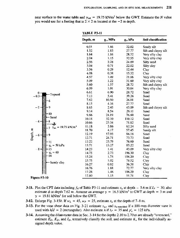
near surface to the water table and ysat = 19.75 kN/m3 below the GWT. Estimate the N valueyou would use for a footing that is 2 X 2 m located at the - 2 m depth.

TABLE P3-11

Depth, m #oMPa qs, kPa Soil classification

0.51 1.86 22.02 Sandy silt1.52 1.83 27.77 Silt and clayey silt1.64 1.16 28.72 Very silty clay2.04 1.15 32.55 Very silty clay2.56 2.28 24.89 Silty sand3.04 0.71 22.02 Silty clay3.56 0.29 12.44 Clay4.08 0.38 15.32 Clay4.57 1.09 21.06 Very silty clay5.09 1.22 31.60 Very silty clay5.60 1.57 28.72 Silt and clayey silt6.09 1.01 30.64 Very silty clay6.61 6.90 28.72 Sand7.13 5.41 39.26 Sand7.62 10.50 26.81 Sand8.13 4.16 27.77 Sand8.65 2.45 43.09 Silt and clayey silt9.14 8.54 26.11 Sand9.66 24.19 76.60 Sand

10.18 32.10 110.12 Sand10.66 23.34 71.82 Sand11.18 5.86 62.24 Silty sand11.70 4.17 57.45 Sandy silt12.19 17.93 86.18 Sand12.71 24.71 73.73 Sand13.22 25.79 76.60 Sand13.71 13.27 85.22 Sand14.23 1.41 43.09 Very silty clay14.75 2.73 196.30 Clay15.24 1.75 108.20 Clay15.75 1.02 78.52 Clay16.27 0.82 36.38 Clay16.76 1.88 72.77 Very silty clay17.28 1.46 106.29 Clay17.80 1.15 51.71 Clay

3-11. Plot the CPT data including /* of Table P3-11 and estimate^ at depth = 5.6 m if/P = 30; alsoestimate cf) at depth 7.62 m. Assume an average y = 16.5 kN/m3 to GWT at depth = 3 m andy = 19.81 kN/m3 for soil below the GWT.

3-12. Enlarge Fig. 3-l5b. lfwL = 45, wP = 25, estimate su at the depth of 7-8 m.

3-13. For the vane shear data on Fig. 3-21 estimate sUtV and sW)remoided if a 100-mm diameter vane isused with h/d = 2 (rectangular). Also estimate A if IP = 35 and p'o = 125 kPa.

3-14. Assuming the dilatometer data in Sec. 3-14 for the depths 2.10 to 2.70 m are already "corrected,"estimate ED, KD, and ID, tentatively classify the soil, and estimate K0 for the individually as-signed depth value.

Figure P3-10

Dep

th,

m

Topsoil

Sand

Sandy clay

3-15. Plot the following corrected pressuremeter data and estimate /?/,, Esp, and K0. For Esp take /JL =0.2 and 0.4. Also assume average y = 17.65 kN/m3 and test depth = 2.60 m. What is the"limiting pressure"?

V, cm3 55 88 110 130 175 195 230 300 400 500

p,kPa 10 30 110 192 290 325 390 430 460 475

Answer: Based on V'o = 123, /x, = 0.2, obtain E5 = 860 kPa, K0 = 1.09.3-16. What would the hydraulic fracture K0 have been if the transducer reading was ±5 percent of the

1.84 value shown on Fig. 3-35?3-17. Referring to the boring log of Fig. 3-38, state what value you would use for qu at the 6-ft depth.3-18. Research the in situ test procedure you have been assigned from Table 3-2. You should find

at least five references—preferably in addition to any cited/used by the author. Write a shortsummary of this literature survey, and if your conclusions (or later data) conflict with that in thistext, include this in your discussion. If you find additional data that have not been used in anycorrelations presented, you should plot these data over an enlargement of the correlation chartfor your own later use.