Embed Size (px)
Citation preview

Institute for International Political Economy Berlin
Previous financial crises leading to stagnation – selected case studiesAuthors: Nina Dodig and Hansjörg Herr
Working Paper, No. 33/2014
Editors:
Sigrid Betzelt ■ Trevor Evans ■ Eckhard Hein ■ Hansjörg Herr ■ Martin Kronauer ■ Birgit Mahnkopf ■ Achim Truger

Previous financial crises leading to stagnation – selected case
studies
Nina Dodig, Hansjörg Herr
Institute for International Political Economy, Berlin School of Economics and Law (www.ipe-berlin.org)
Abstract: This paper analyses several severe financial crises observed in the history of capitalism which led
to a longer period of stagnation or low growth. Comparative case studies of the Great Depression, the Latin
American debt crisis of the 1980s and the Japanese crisis of the 1990s and 2000s are presented. The
following questions are asked: What triggered big financial crises? Which factors intensified financial crises?
And most importantly, which factors prevented the return of prosperity for a long time? The main conclusion
is that stagnation after big financial crises becomes likely when the balance sheets of economic units are not
quickly cleaned, when the nominal wage anchor breaks, and when there is no big and longer growth
stimulus by the state. Some tentative conclusions for the subprime financial crisis and the Great Recession
are drawn.
Keywords: financial crises, stagnation, deflation, lost decade, Great Depression, Latin American debt crisis,
Japanese crisis, Great Recession
JEL classification: E65, G01, N12, N15, N16
Contact details: Nina Dodig, [email protected]; Hansjörg Herr, [email protected]
Berlin School of Economics and Law, Badensche Str. 50 – 51, 10825 Berlin
Acknowledgments:
This paper is part of the results of the project Financialisation, Economy, Society and Sustainable
Development (FESSUD). It has received funding from the European Union Seventh Framework Programme
(FP7/2007-2013) under grant agreement n° 266800. For helpful comments we would like to thank Daniel
Detzer, Trevor Evans, Eckhard Hein, Barbara Schmitz, and the participants in the FESSUD Annual
Conference 2013 in Amsterdam as well as in the FMM Annual Conference 2013 in Berlin. Remaining errors
are, of course, ours.
Website: www.fessud.eu
This project is funded by the European Union under
the 7th Research Framework programme (theme SSH)
Grant Agreement nr 266800

1
1. Introduction
Capitalist development is not characterised by smooth economic development measured as a stable GDP
growth rate or other economic indicators like employment, inflation rate or credit expansion. Historically,
capitalism is rather characterised by a cyclical development pattern that produces a positive GDP growth
rate in most countries in the long-run. The ups and downs don’t follow the regular swings of the sinus curve.
Periods of high growth can be more or less pronounced. This paper focuses more on economic downturns of
different characters. Usually, cyclical downturns fade out within a short period of time and make room for a
new expansion period. But history demonstrated that periods of economic crises can get out of control and
showed that the market mechanism cannot stop the economy from a cumulative shrinking. And history also
demonstrated that an economic crisis can lead to a stagnation that lasts for a long period. Typically, these
two negative scenarios, cumulative shrinking and long-term stagnation, follow after a financial crisis.
The Great Recession in 2009 that occurred after the outbreak of the subprime financial crisis and affected
the whole developed world is a good example for a sharp financial crisis. In comparison to the Great
Depression in the early 1930s, the cumulative collapse of many economies could be avoided. But the
unresolved question is whether GDP growth will be low for a long period in the crises countries and what
negative repercussions for employment, poverty, living conditions, and political developments in societies
can be expected. This paper tries to answer these questions by analysing severe financial crises observed in
the history of capitalism. There are several key questions which could be answered by understanding
historical financial crises.
a) What triggered big financial crises? This question focuses on explaining what caused the economic
boom or the asset price bubble before the financial crisis.
b) Which factors intensify the financial crises further?
c) And most importantly, which factors prevented the return of prosperity for a long time? Which factors
caused low growth or even stagnation for a long period?
As a methodology comparative case studies are used.
This leads us to the question of which financial crises should be selected. This question is not easy to
answer because the capitalist history is full of financial crises. Capitalism defined as a comprehensive
system dominating production and employment was established around 1800. Before 1800, financial crises
existed, for example, the Dutch tulip crisis in 1637, but they were of different characters because the
capitalist system was not yet well developed. During the first half of the 19th century, though, when capitalist
mode of production became the dominant one, the industrialised world began to experience a sequence of
financial crises. Monetary policy at that time did not understand to stabilise economies and financial market
regulations did not exist – for example, private banks could issue their own banknotes. Due to some
regulatory attempts later on, such as the Bank Act in England of 1844, economic stability could be improved.
However, in the second half of the 19th century a severe and prolonged crises hit the, at that time developed,
world. The ‘Long Depression’ of 1873-1896 inaugurated a period of recurring financial crises and low GDP
growth. The first two decades of the 20th century up until the end of World War I were marked by a relative
2
stability and high growth rates under the regime of the classical Gold Standard – with the exception of the
short 1907 banking panic in the US. This system came to an end with World War I (1914–1918). After World
War I the reestablishment of the classical Gold Standard failed. Long-term prosperity could not be achieved.
This paper concentrated the analysis on crises during the 20th and 21
st century. Three crises, in our view,
stand of particular importance because all three of them led to a long-term period of low GDP growth.
- Firstly, the Great Depression in the early 1930s which only could be overcome with the beginning of
World War II or during the preparation for it.
- Secondly, the crisis in Latin America in the 1980s. The lost decade of the 1980s reached well into
the end of the 1990s. Whereas the Great Depression and the Japanese crisis were mainly triggered
by financial problems inside the countries,1 the crisis in Latin America was triggered by foreign
indebtedness denominated in foreign currency.
- Thirdly, the Japanese stagnation after the bubble in the 1980s. This crisis is of special interest to us
because Japan could not overcome stagnation and low GDP growth until today. It has been debated
that the US or Europe may follow Japan.
In what follows we analyse the logic of the crises, approaching them in chronological order. Subsequently we
compare the crises and draw conclusions in Chapter 5.
2. The Great Depression
2.1. The background
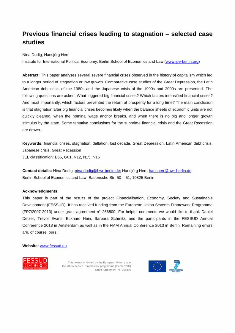
The ‘roaring twenties’ were usually considered a period of high economic prosperity in the US. Rapid growth
began after a deflationary recession in 1920-1921. The first half of the 1920s saw an unprecedented
expansion of industrial production (Figure 1a). This reflected the tendency towards the Fordist mass
production, made available by new technologies and production methods. Automobiles, telephones,
electrical kitchen appliances, radio and film were brought to the middle class on a large scale. In the
aftermath of World War I (WWI) the US became the richest country in the world measured in GDP per
capita, with a booming industry and a society adapting to consumerism.
Employment2 increased by 40 per cent between 1921 and 1929 (Figure 1b). However, despite the initial
boom the volume of production did not increase much from 1923 to 1929. This had likely to do with the fact
that the prosperity of the 1920s was not equally distributed. Income inequality was increasing throughout the
1920s and from these developments one would expect that the overall consumption would decrease.
1 For the Great Depression this is only true for the USA.
2 Data on unemployment rates prior to 1929 are not available, nor those on total workforce during the 1920s.
3
Figure 1(a,b): Production (index, Jan 1921=100) and employment in persons in the US, 1921-1933.
a. b.
Source: Federal Reserve Bank of St. Louis (2013) FRED database, own calculations.
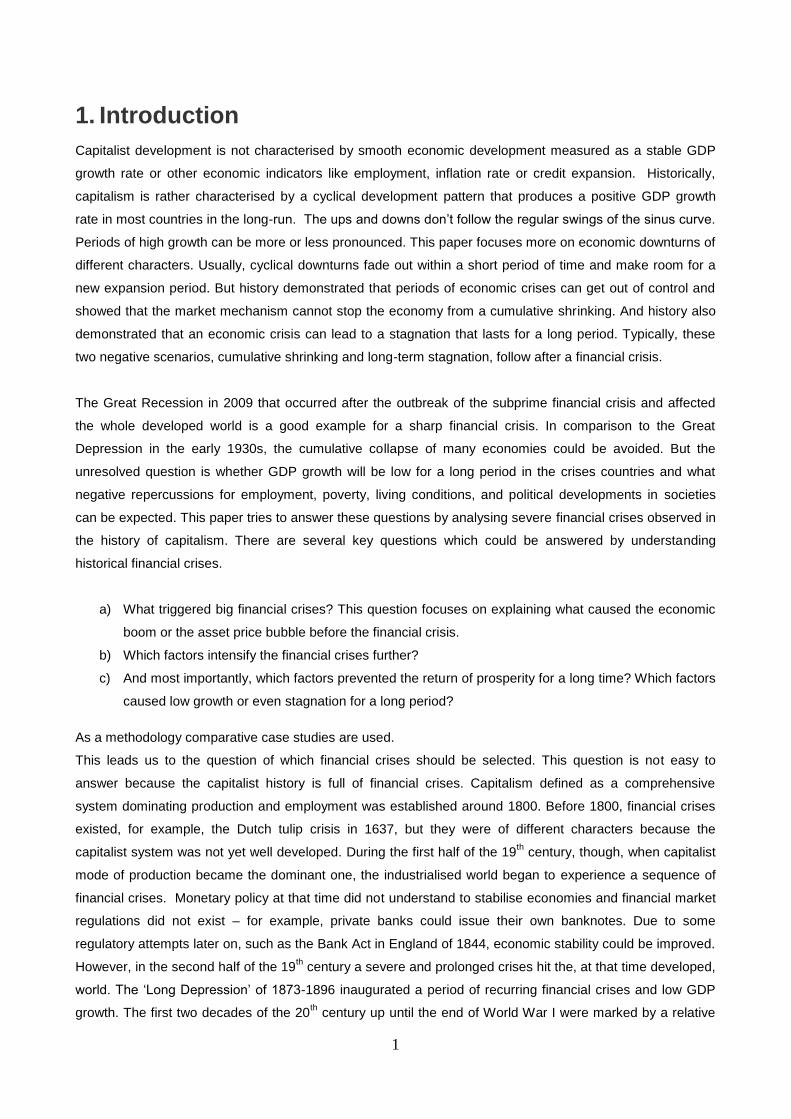
What we observe for the 1920s, however, is an increase of household consumption, in particular of durable
goods and real estate. Mass consumption, in the face of increasing income inequality, was supported by
high consumer credits. Instalment buying accounted for much of households’ credit in the 1920s (Olney
1999). Figure 2 shows how the non-mortgage debt as a percentage of income doubled from 4.7 per cent in
1920 to 9.3 per cent in 1929 which for that time was an unprecedented rise.
Figure 2: Real outstanding consumer debt and consumer non-mortgage debt as a percentage of
income in the US, 1900 – 1938.
Source: data from Olney (1999), own calculations.
40
60
80
100
120
140
160
19
21
19
22
19
23
19
24
19
25
19
26
19
27
19
28
19
29
19
30
19
31
19
32
19
33
Index of Industrial Production and Trade forUnited States, Index, (Jan 1921=100)
24000
26000
28000
30000
32000
34000
36000
38000
1921 1923 1925 1927 1929 1931 1933
Nonagricultural Employment for UnitedStates, Thousands Of Persons
00
02
04
06
08
10
12
0
5000
10000
15000
20000
25000
30000
35000
19
00
19
02
19
04
19
06
19
08
19
10
19
12
19
14
19
16
19
18
19
20
19
22
19
24
19
26
19
28
19
30
19
32
19
34
19
36
19
38
Total Real Outstanding Consumer Debt (Millions of 1982 $, LHS)
Consumer non-mortgage debt as per cent of income (RHS)
4
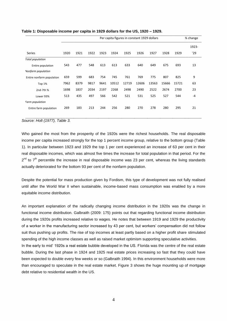
Table 1: Disposable income per capita in 1929 dollars for the US, 1920 – 1929.
Per capita figures in constant 1929 dollars % change
Series 1920 1921 1922 1923 1924 1925 1926 1927 1928 1929
1923-
'29
Total population
Entire population 543 477 548 613 613 633 640 649 675 693
13
Nonfarm population
Entire nonfarm population 659 599 683 754 745 761 769 775 807 825
9
Top 1% 7962 8379 9817 9641 10512 12719 12606 13563 15666 15721
63
2nd-7th % 1698 1837 2034 2197 2268 2498 2490 2522 2674 2700
23
Lower 93% 513 435 497 566 542 521 531 525 527 544
-4
Farm population
Entire farm population 269 183 213 244 256 280 270 278 280 295
21
Source: Holt (1977), Table 3.
Who gained the most from the prosperity of the 1920s were the richest households. The real disposable
income per capita increased strongly for the top 1 percent income group, relative to the bottom group (Table
1). In particular between 1923 and 1929 the top 1 per cent experienced an increase of 63 per cent in their
real disposable incomes, which was almost five times the increase for total population in that period. For the
2nd
to 7th percentile the increase in real disposable income was 23 per cent, whereas the living standards
actually deteriorated for the bottom 93 per cent of the nonfarm population.
Despite the potential for mass production given by Fordism, this type of development was not fully realised
until after the World War II when sustainable, income-based mass consumption was enabled by a more
equitable income distribution.
An important explanation of the radically changing income distribution in the 1920s was the change in
functional income distribution. Galbraith (2009: 175) points out that regarding functional income distribution
during the 1920s profits increased relative to wages. He notes that between 1919 and 1929 the productivity
of a worker in the manufacturing sector increased by 43 per cent, but workers’ compensation did not follow
suit thus pushing up profits. The rise of top incomes at least partly based on a higher profit share stimulated
spending of the high income classes as well as raised market optimism supporting speculative activities.
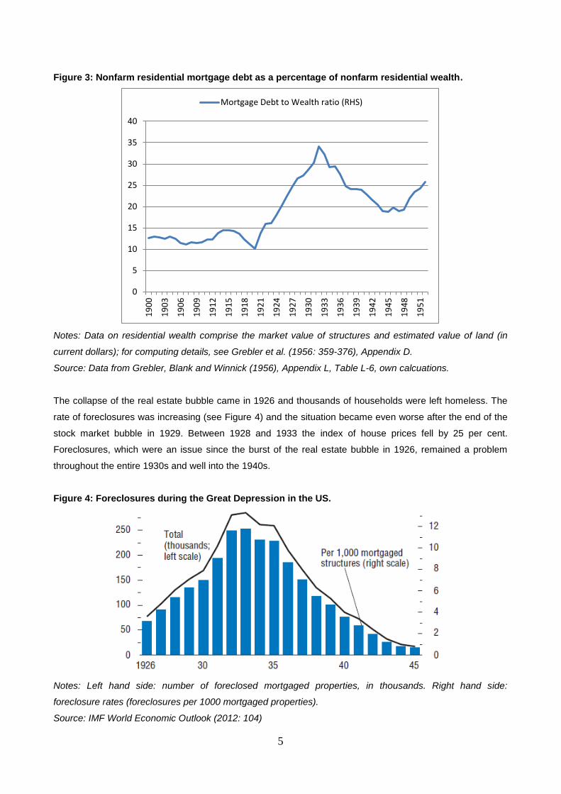
In the early to mid’ 1920s a real estate bubble developed in the US. Florida was the centre of the real estate
bubble. During the last phase in 1924 and 1925 real estate prices increasing so fast that they could have
been expected to double every few weeks or so (Galbraith 1994). In this environment households were more
than encouraged to speculate in the real estate market. Figure 3 shows the huge mounting up of mortgage
debt relative to residential wealth in the US.
5
Figure 3: Nonfarm residential mortgage debt as a percentage of nonfarm residential wealth.
Notes: Data on residential wealth comprise the market value of structures and estimated value of land (in
current dollars); for computing details, see Grebler et al. (1956: 359-376), Appendix D.
Source: Data from Grebler, Blank and Winnick (1956), Appendix L, Table L-6, own calcuations.
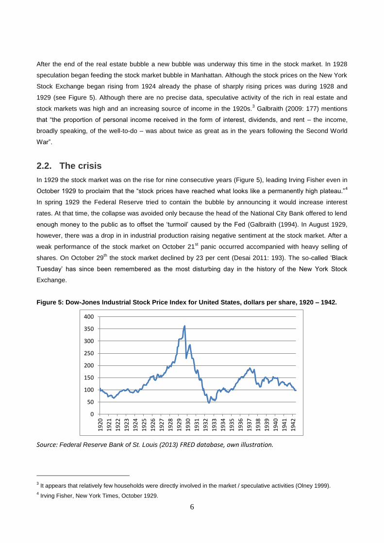
The collapse of the real estate bubble came in 1926 and thousands of households were left homeless. The
rate of foreclosures was increasing (see Figure 4) and the situation became even worse after the end of the
stock market bubble in 1929. Between 1928 and 1933 the index of house prices fell by 25 per cent.
Foreclosures, which were an issue since the burst of the real estate bubble in 1926, remained a problem
throughout the entire 1930s and well into the 1940s.
Figure 4: Foreclosures during the Great Depression in the US.
Notes: Left hand side: number of foreclosed mortgaged properties, in thousands. Right hand side:
foreclosure rates (foreclosures per 1000 mortgaged properties).
Source: IMF World Economic Outlook (2012: 104)
0
5
10
15
20
25
30
35
40
19
00
19
03
19
06
19
09
19
12
19
15
19
18
19
21
19
24
19
27
19
30
19
33
19
36
19
39
19
42
19
45
19
48
19
51
Mortgage Debt to Wealth ratio (RHS)
6
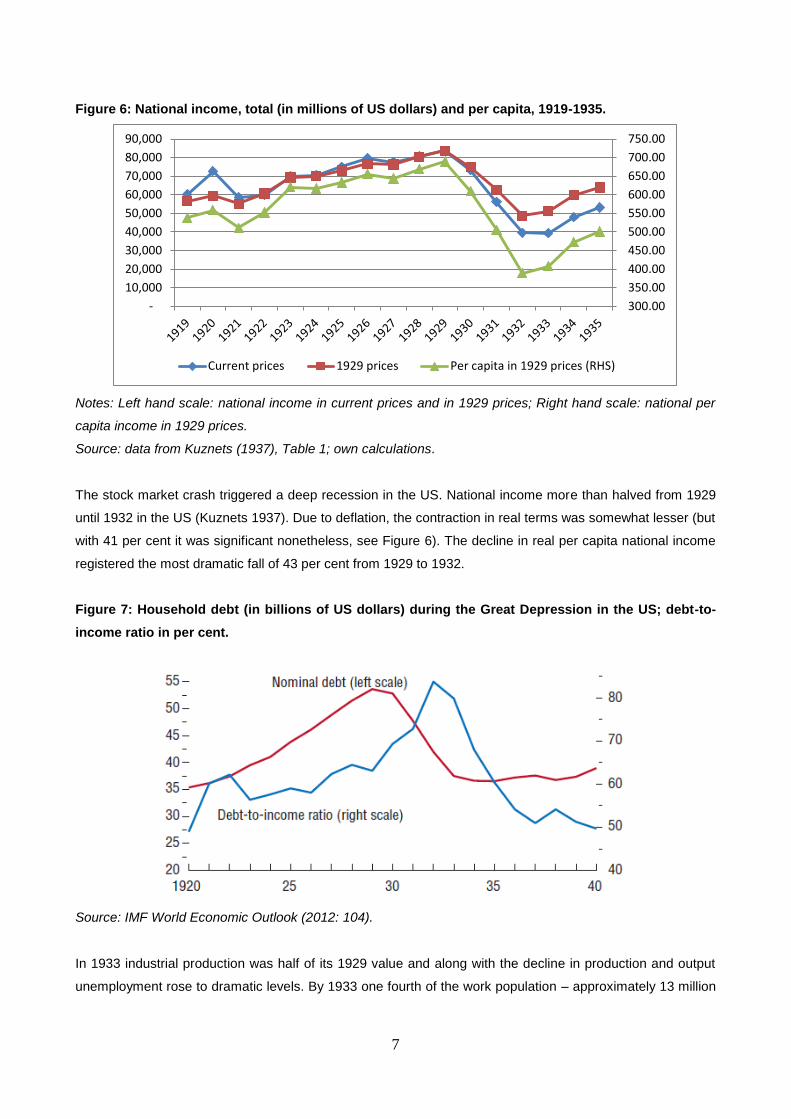
After the end of the real estate bubble a new bubble was underway this time in the stock market. In 1928
speculation began feeding the stock market bubble in Manhattan. Although the stock prices on the New York
Stock Exchange began rising from 1924 already the phase of sharply rising prices was during 1928 and
1929 (see Figure 5). Although there are no precise data, speculative activity of the rich in real estate and
stock markets was high and an increasing source of income in the 1920s.3 Galbraith (2009: 177) mentions
that “the proportion of personal income received in the form of interest, dividends, and rent – the income,
broadly speaking, of the well-to-do – was about twice as great as in the years following the Second World
War”.
2.2. The crisis
In 1929 the stock market was on the rise for nine consecutive years (Figure 5), leading Irving Fisher even in
October 1929 to proclaim that the “stock prices have reached what looks like a permanently high plateau.”4
In spring 1929 the Federal Reserve tried to contain the bubble by announcing it would increase interest
rates. At that time, the collapse was avoided only because the head of the National City Bank offered to lend
enough money to the public as to offset the ‘turmoil’ caused by the Fed (Galbraith (1994). In August 1929,
however, there was a drop in in industrial production raising negative sentiment at the stock market. After a
weak performance of the stock market on October 21st panic occurred accompanied with heavy selling of
shares. On October 29th the stock market declined by 23 per cent (Desai 2011: 193). The so-called ‘Black
Tuesday’ has since been remembered as the most disturbing day in the history of the New York Stock
Exchange.
Figure 5: Dow-Jones Industrial Stock Price Index for United States, dollars per share, 1920 – 1942.
Source: Federal Reserve Bank of St. Louis (2013) FRED database, own illustration.
3 It appears that relatively few households were directly involved in the market / speculative activities (Olney 1999).
4 Irving Fisher, New York Times, October 1929.
0
50
100
150
200
250
300
350
400
19
20
19
21
19
22
19
23
19
24
19
25
19
26
19
27
19
28
19
29
19
30
19
31
19
32
19
33
19
34
19
35
19
36
19
37
19
38
19
39
19
40
19
41
19
42
7
Figure 6: National income, total (in millions of US dollars) and per capita, 1919-1935.
Notes: Left hand scale: national income in current prices and in 1929 prices; Right hand scale: national per
capita income in 1929 prices.
Source: data from Kuznets (1937), Table 1; own calculations.
The stock market crash triggered a deep recession in the US. National income more than halved from 1929
until 1932 in the US (Kuznets 1937). Due to deflation, the contraction in real terms was somewhat lesser (but
with 41 per cent it was significant nonetheless, see Figure 6). The decline in real per capita national income
registered the most dramatic fall of 43 per cent from 1929 to 1932.
Figure 7: Household debt (in billions of US dollars) during the Great Depression in the US; debt-to-
income ratio in per cent.
Source: IMF World Economic Outlook (2012: 104).
In 1933 industrial production was half of its 1929 value and along with the decline in production and output
unemployment rose to dramatic levels. By 1933 one fourth of the work population – approximately 13 million
300.00
350.00
400.00
450.00
500.00
550.00
600.00
650.00
700.00
750.00
-
10,000
20,000
30,000
40,000
50,000
60,000
70,000
80,000
90,000
Current prices 1929 prices Per capita in 1929 prices (RHS)
8
people – were unemployed (Galbraith 2009). Debt-to-income ratios of the households exploded, as shown in
Figure 7, rising from over 60 per cent at the peak of the bubble to well over 80 per cent in 1932.
Debt deflation
An asset price deflation is the result of the end of all bubbles – this was also the case after end of stock
market bubble in the US. Asset price deflations lead to a destruction of wealth as well as to increasing
difficulties of debtors and especially speculators speculation with credit to pay back their debts. Non-
performing loans begin to appear and eventually can flood the market. Distress selling of assets takes place,
yet this exacerbates the asset price deflation. In such a constellation an economic downturn is almost
inevitable.
In some financial crises – as was the case of the Great Depression – a goods market deflation can appear
as well. The price level in the US fell 25 per cent from 1929 to 1933 (Wheelock 1995). Goods market
deflations occur when, on the one hand, the demand for goods and services declines, due to the breakdown
of investment resulting in unemployment and depressed consumption demand. But, on the other hand,
supply can increases despite of the declining demand when firms with liquidity and solvency problems still
desperately try to sell everything in their fight for survival.
The huge drop in the price level during the Great Depression cannot be explained alone by disequilibrium
between goods market demand and supply. The most important factor to explain the deflation was the fall in
nominal wages unit-labour costs. Nominal (hourly) wages declined by more than 20 per cent in the US from
1929 to 1933, as can be seen in Figure 8. The high level of unemployment and the lack government support
to stop falling nominal wages led to the breakdown of the nominal wage anchor and falling wage costs with
the consequence of cost-driven deflationary process. Such a process was already analysed by Keynes
(1930) in his Treatise on Money. With goods market deflation a downward spiral was created which led to
the Great Depression.
Contrary to the neoclassical view, nominal wage cuts pushed the deflation even further and led to the
explosion of the debt burden and the collapse of the economy. A key point is that workers are not even able
to reduce real wages by cutting nominal wages. In Keynes' words: "There may exist no expedient by which
labour as a whole can reduce its real wage to a given figure by making revised money bargains with the
entrepreneurs" (1936: 13). As to wages and the Great Depression, Keynes argues: "It is not very plausible
to assert that unemployment in the United States in 1932 was due either to labour obstinately refusing to
accept a reduction of money-wages or to its obstinately demanding a real wage beyond what the productivity
of the economic machine was capable of furnishing" (1936: 9).
Deflation is one of the biggest feedback mechanism which leads to a cumulative contraction. Irving Fisher
(1933) correctly argued that high levels of nominal debt and goods market deflation were the key factors in
explaining the destructive power of the financial crisis in the Great Depression.The combination of goods
market deflation and over-indebtedness leads to an increase of the real debt burden of all the debtors in
domestic currency. The more firms are forced or try to pay back loans the more they owe in real terms. The
9
non-performing loan problem explodes, the coherence of financial markets erodes and the economic boat
not only shakes, it capsizes. Bank failures increase as well, as debtors default and panicked depositors
attempt to quickly withdraw their loans.
The Bank of America failed in December 1930, and between August 1931 and January 1932 1.860 banks
failed (Bernanke and James 1991). Even bigger was the overall number of banks in the US which
suspended their operations between 1929 and 1933, which amounted to 9.000 banks (Wheelock 1995). In
such an environment, surviving banks became much more cautious in their lending policies, but also the
incentives for productive investment ceased in the face of low demand and worsening profit expectations.
Aggregate net profits of the US corporations had fallen dramatically, from 1.7 billion dollars in July 1929 to
minus 677 million dollars in July 1932, and did not reach the pre-crisis level for the rest of the decade
(Federal Reserve Bank of St. Louis 2013).
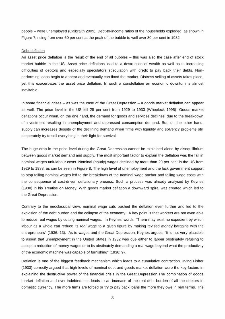
Figure 8: Index of composite nominal wages for the US (index 1926=100), 1919 to 1940.
Source: Federal Reserve Bank of St. Louis (2013) FRED database, own calculations.
In Fisher’s debt-deflation theory of depressions there is no talk of the role of the nominal wage level as a
nominal anchor against deflation. Yet the wage deflation argument is important in understanding the Great
Depression. Bernanke (2000) and others argued that the huge employment losses during the Great
Depression were caused by insufficient nominal wage cuts, which led real wages to explode. High real
wages, so the argument runs, lead to falling labour demand and high unemployment. The focus on the
supposed wage stickiness as the major factor behind the Great Depression and the inhibitor of the economic
recovery during the 1930s is, in our view, completely unfounded. Interestingly, it was Robert Lucas, a
proponent of the New Classical approach, who said: “Nominal wages and prices came down by half between
60.0
70.0
80.0
90.0
100.0
110.0
120.0
130.0
19
19
19
20
19
21
19
22
19
23
19
24
19
25
19
26
19
27
19
28
19
29
19
30
19
31
19
32
19
33
19
34
19
35
19
36
19
37
19
38
19
39
19
40
10
1929 and 1933. Why would anyone look at a period like that and say that the difficult problem would be to
explain rigid wages? I don’t understand it”5. We follow here Lucas.
Policies during 1929-1933
The policies during the Hoover administration (1929-1933) were non-interventionist. Temin (1993 and 1994),
for example, argued strongly against Hoover’s “deflationary policy” caused by his orthodox adherence to the
Gold Standard and believe in neoclassical remedies to solve the crisis. The view which then prevailed was
that countercyclical fiscal policy would undermine the credibility of the government, whereas monetary
easing would damage the value of the dollar (Desai 2011). The Federal Reserve maintained a passive
stance initially, but then actually raised the interest rates in the fourth quarter of 1931 (Federal Reserve Bank
of St. Louis 2013), with the intent of stabilising the dollar without going off the Gold Standard.6 There was
also no attempt to engage in open-market operations to inject new reserves and/or lend to distressed banks.
The function as a lender of last resort was violated by the Fed. Nothing, in sum, was done by the monetary
authorities to prevent the wave of bank failures in those years. Fiscal policy as well provided no remedies,
quite the contrary. As a response to a drop in government revenues given the shrinking tax base in the crisis
the government doubled the income tax in 1932.
The Smoot-Hawley Tariff Act of 1930 imposed the highest tariffs on imports by then in the US to is to
encourage the purchases of domestically produced goods. This decision may be understandable from a
point of view of a country in a deep recession, , but it provoked counter-reactions from other governments
which began increasing their import tariffs as well. This then led to a collapse of the world trade and a deeper
international recession. Over the next several years, countries worldwide abandoned the Gold Standard and
began to devalue their currencies. Overall, the early reactions to the crisis consisted in attempts to balance
the budget, not to bailout banks in trouble and introducing protectionism so as to reduce the current account
deficits under the Gold Standard.
2.3. The Great Depression in the US and the New Deal
Gold inflows to the US increased strongly after 1933, due both to Roosevelt’s devaluation of the dollar in
1933-34 and to the capital flight from European countries where an increasing threat of another war was
building up. This was described by Friedman and Schwartz (1963:544): “The money stock grew at a rapid
rate in the three successive years from June 1933 to June 1936 (…) The rapid rise was a consequence of
the gold inflow produced by the revaluation of gold plus the flight of capital to the United States. It was in no
way a consequence of the contemporaneous business expansion”. Production remained meagre and
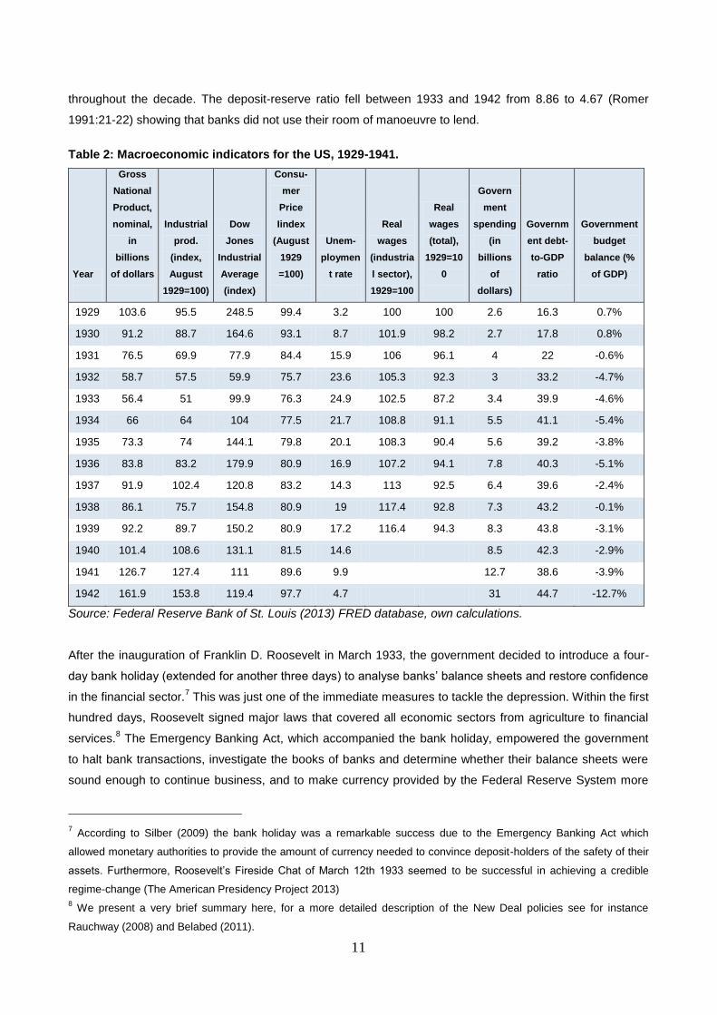
unemployment remained high throughout the first half of the 1930s (Table 2). Bank lending remained weak
5 Quote from Dighe and Dunne-Schmitt (2010: 165).
6 Temin (1994) argues that when in the summer of 1931 a series of currency crises hit Europe and both Germany and
Britain went off the Gold Standard, Reichsmark as well as the British pound devalued. There was a sentiment in the
market that the US dollar will be next, and the investors rushed to sell their holdings of dollars. The action of Fed was
thus to preserve the value of the dollar.
11
throughout the decade. The deposit-reserve ratio fell between 1933 and 1942 from 8.86 to 4.67 (Romer
1991:21-22) showing that banks did not use their room of manoeuvre to lend.
Table 2: Macroeconomic indicators for the US, 1929-1941.
Year
Gross
National
Product,
nominal,
in
billions
of dollars
Industrial
prod.
(index,
August
1929=100)
Dow
Jones
Industrial
Average
(index)
Consu-
mer
Price
Iindex
(August
1929
=100)
Unem-
ploymen
t rate
Real
wages
(industria
l sector),
1929=100
Real
wages
(total),
1929=10
0
Govern
ment
spending
(in
billions
of
dollars)
Governm
ent debt-
to-GDP
ratio
Government
budget
balance (%
of GDP)
1929 103.6 95.5 248.5 99.4 3.2 100 100 2.6 16.3 0.7%
1930 91.2 88.7 164.6 93.1 8.7 101.9 98.2 2.7 17.8 0.8%
1931 76.5 69.9 77.9 84.4 15.9 106 96.1 4 22 -0.6%
1932 58.7 57.5 59.9 75.7 23.6 105.3 92.3 3 33.2 -4.7%
1933 56.4 51 99.9 76.3 24.9 102.5 87.2 3.4 39.9 -4.6%
1934 66 64 104 77.5 21.7 108.8 91.1 5.5 41.1 -5.4%
1935 73.3 74 144.1 79.8 20.1 108.3 90.4 5.6 39.2 -3.8%
1936 83.8 83.2 179.9 80.9 16.9 107.2 94.1 7.8 40.3 -5.1%
1937 91.9 102.4 120.8 83.2 14.3 113 92.5 6.4 39.6 -2.4%
1938 86.1 75.7 154.8 80.9 19 117.4 92.8 7.3 43.2 -0.1%
1939 92.2 89.7 150.2 80.9 17.2 116.4 94.3 8.3 43.8 -3.1%
1940 101.4 108.6 131.1 81.5 14.6 8.5 42.3 -2.9%
1941 126.7 127.4 111 89.6 9.9
12.7 38.6 -3.9%
1942 161.9 153.8 119.4 97.7 4.7 31 44.7 -12.7%
Source: Federal Reserve Bank of St. Louis (2013) FRED database, own calculations.
After the inauguration of Franklin D. Roosevelt in March 1933, the government decided to introduce a four-
day bank holiday (extended for another three days) to analyse banks’ balance sheets and restore confidence
in the financial sector.7 This was just one of the immediate measures to tackle the depression. Within the first
hundred days, Roosevelt signed major laws that covered all economic sectors from agriculture to financial
services.8 The Emergency Banking Act, which accompanied the bank holiday, empowered the government
to halt bank transactions, investigate the books of banks and determine whether their balance sheets were
sound enough to continue business, and to make currency provided by the Federal Reserve System more
7 According to Silber (2009) the bank holiday was a remarkable success due to the Emergency Banking Act which
allowed monetary authorities to provide the amount of currency needed to convince deposit-holders of the safety of their
assets. Furthermore, Roosevelt’s Fireside Chat of March 12th 1933 seemed to be successful in achieving a credible
regime-change (The American Presidency Project 2013)
8 We present a very brief summary here, for a more detailed description of the New Deal policies see for instance
Rauchway (2008) and Belabed (2011).
12
easily available. The Thomas Amendment of the Agricultural Adjustment Act was the first step towards going
off the Gold Standard, which was the single most important step towards reflation. The Federal Emergency
Relief Act allotted $500m from the Reconstruction Finance Corporation (RFC) to the states. The Securities
Exchange Act created the Securities Exchange Commission, which is still supervising trade of stocks in the
U.S. today. The Banking Act of 1933 - the famous Glass-Steagall Act - separated investment from
commercial banks, increased the power of the Federal Reserve Board to oversee transactions in the Federal
Reserve System and created the Federal Deposit Insurance Corporation (FDIC).
Roosevelt believed that falling wages and prices were the main factors exacerbating the depression
therefore he attempted – successfully – to prevent a further fall in nominal wages and prices. The National
Industrial Recovery Act of 1933 forced employers to agree to “codes of fair competition” and granted them
the suspension of anti-trust legislation. In 1935, the Social Security Act created the first basic social safety
net in the U.S. The Banking Act of 1935 made the FDIC a permanent authority in financial markets and
shifted power from the regional banks of the Federal Reserve System to the Governors of the Federal
Reserve System. The National Labour Relations Act granted workers the right to organize and bargain
collectively as well as prevent them from unfair labour practices. The administration created many
organizations to employ the unemployed (e.g. Works Progress Administration). The Fair Labour Standards
Act introduced a minimum wage, maximum work hours and finally banned child labour.
The purpose of Roosevelt’s policies was to turn a deflationary and contractionary economic situation into a
situation without deflation and economic expansion. This was also the reason why he decided to devalue in
1933-34 and why the Fed made no attempt to sterilise the vast gold inflows throughout the 1930s. By early
1937, the recovery appeared to be underway - with the exception of unemployment which was still high –
and industrial production surpassed its 1929 level (Table 2). Eggertson (2008) argues that the recovery was
driven by a shift in expectations, which was caused by Roosevelt’s policy decisions. But in June 1937,
Roosevelt opted for balancing the budget by cutting spending and increasing the taxes. Another recession
followed in 1938 when industrial production fell by 30 per cent over the course of few months. In 1938, every
fifth person in the US was still out of work (Galbraith 2009). In fact, unemployment and real Gross National
Product (GNP) did not return to its pre-crisis levels until the US was well into the World War II.
The New Deal no doubt created the institutional foundation for a subsequent three decade long expansion of
economic activity which lasted until the 1970s. However, during the 1930s despite the benefits of ending the
wage and price deflation and thus preventing a further downward-spiral, nothing was really done to boost
aggregate demand. Cary Brown famously put it: “Fiscal policy, then, seems to have been an unsuccessful
recovery device in the 'thirties’ – not because it did not work, but because it was not tried”, (Brown 1956:
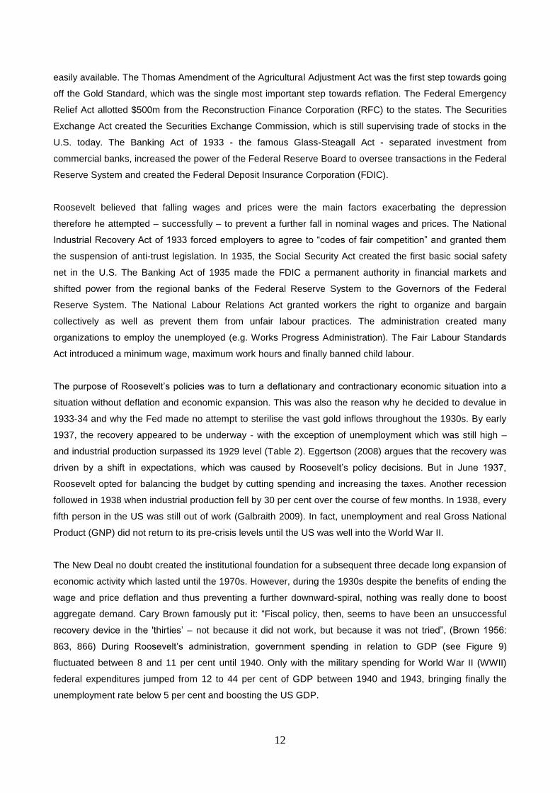
863, 866) During Roosevelt’s administration, government spending in relation to GDP (see Figure 9)
fluctuated between 8 and 11 per cent until 1940. Only with the military spending for World War II (WWII)
federal expenditures jumped from 12 to 44 per cent of GDP between 1940 and 1943, bringing finally the
unemployment rate below 5 per cent and boosting the US GDP.
13
Figure 9: Government expenditure in per cent of GDP for the US, 1930-1944.
Source: Federal Reserve Bank of St. Louis (2013) FRED database, own calculations.
2.4. Concluding remarks
Although the Great Depression in the US is usually associated with the stock market crash of 1929, it is
important to take a look at prior developments taking place during the ‘Roaring Twenties’. In the mid’ 1920s,
a real estate boom took place in the US, with increasing speculation in the years 1924 and 1925 resulting in
strong increases of real estate prices. Leverage was high and there was an unprecedented mounting up of
mortgage debt. In 1926 the real estate bubble came to an end and brought about a long process of
foreclosures, with non-performing loans increasing over time and remaining a serious issue throughout the
1930s. In general, real estate bubbles have longer-lasting negative consequences then stock market
bubbles, as the former usually involve much more credit, so the process of deleveraging is typically much
longer and can last well over a decade. The stock market bubble and the subsequent October 1929 crash
added to the already existing problem of foreclosures and non-performing loans. This led to a first wave of
massive failures of households, business as well as banks during the 1929-1933 recession.
Under the Hoover administration (1929-1933) there was no active policy to solve the crisis after it broke out.
There was no bailout of banks from the government and not even the central bank. Fiscal policy dominated
to balance the public budget which Hoover administration (1929-1933) increased as a result of the
recession. And there was no policy to stop disastrous nominal wage cuts.
As Irving Fisher (1933) argued, asset price deflation and then the goods market deflation in a situation of
high domestic debt is the worst thing that can happen as it increases the real debt burden. During deflation
non-performing loans increase and eventually flood the market. Deflation also discourages new investment
because it erodes the expected profitability and entrepreneurs abstain from investing. Also consumption
demand is depressed as households wait to by durables until their price is lower. Fisher did not talk about
0%
5%
10%
15%
20%
25%
30%
35%
40%
45%
50%
1930 1931 1932 1933 1934 1935 1936 1937 1938 1939 1940 1941 1942 1943 1944
Government outlays (per cent of GDP)
14
the role of the nominal wage level as a nominal anchor against deflation, yet the wage deflation argument is
important in understanding the Great Depression. Many mainstream economists (for instance, Bernanke and
James (1991)) argued that the huge employment losses during the Great Depression were caused by
insufficient nominal wage cuts, causing real wages to explode and thus leading to high unemployment. From
1929 to 1933 in the US, nominal wages fell by more than 20 per cent. In our view, it was in fact the nominal
wage cuts that deepened the deflation and led to the explosion of the debt burden and the collapse of the
economy.
During Roosevelt’s administration (1933-1945) the New Deal policies aimed, among other, at the
strengthening of workers’ bargaining position and consequently further reductions in nominal wages were
prevented. Other Roosevelt’s programmes such as the Banking Act of 1933 (the Glass-Steagall Act) have
helped in creating an institutional foundation for the ‘golden age’ of capitalism following World War II.
However, during the 1930s fiscal stimulus was not used to boost demand and accelerate the recovery.
Unemployment remained very high throughout the 1930s and US output did not return to its pre-crisis levels
until the outbreak of World War II. Expansionary fiscal policy in the US was prompted only by the entrance of
the US in World War II in 1941, soon after which the unemployment fell below 10 per cent for the first time in
over a decade.
3. The Latin American debt crisis
3.1. The background
In the period from 1950 to 1980, the countries of Latin America grew by around 5.5 per cent annually
(weighted average, see Ocampo 2004), mostly under a regime of regulated international capital flows. In the
late 1960s and early 1970s, however, many developed countries and then also Latin American countries
deregulated international capital flows. When developed countries entered into a recession in 1973-75 Latin
American countries were negatively impacted by the trade channel. However, GDP growth rates did not
suffer as much as in the developed world. Given the open capital account this made them an attractive
destination for international capital flows. The sweet poison of foreign debt made financing of public
households and other economic units in Latin America easier and stimulated Latin American growth. During
the 1970s, capital inflows to Latin America came in particular in the form of foreign loans. Throughout the
1970s in Latin America long-term foreign debt increased from $68 billion or 20 per cent of the region’s GDP
in 1975, to $238 billion or 35 per cent of the region’s GDP in 1982 (Ramos-Francia et al. 2013). After
Mexico’s default in 19829, capital inflows stopped abruptly and the decade thereafter was characterised by
large capital outflows not only due to debt servicing obligations, but also because of capital flight.
Subsequently, Latin America fell into stagnation for a long period. “The 1980s were a lost decade for Latin
America” (Dornbusch 1990a: 1). Additionally, it suffered form an external boom-bust cycle which led to a
long-term stagnation.
9 By the end of 1982 the total external debt of Latin America, including short- and long-term debt and the IMF credit, was
$332 billion, or 49 per cent of the region’s GDP (Ramos-Francia et al. 2013).
15
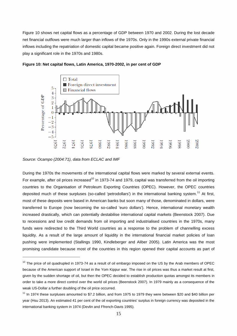
Figure 10 shows net capital flows as a percentage of GDP between 1970 and 2002. During the lost decade
net financial outflows were much larger than inflows of the 1970s. Only in the 1990s external private financial
inflows including the repatriation of domestic capital became positive again. Foreign direct investment did not
play a significant role in the 1970s and 1980s.
Figure 10: Net capital flows, Latin America, 1970-2002, in per cent of GDP
Source: Ocampo (2004:71), data from ECLAC and IMF
During the 1970s the movements of the international capital flows were marked by several external events.
For example, after oil prices increased10
in 1973-74 and 1979, capital was transferred from the oil importing
countries to the Organisation of Petroleum Exporting Countries (OPEC). However, the OPEC countries
deposited much of these surpluses (so-called 'petrodollars') in the international banking system.11
At first,
most of these deposits were based in American banks but soon many of those, denominated in dollars, were
transferred to Europe (now becoming the so-called 'euro dollars'). Hence, international monetary wealth
increased drastically, which can potentially destabilise international capital markets (Beenstock 2007). Due
to recessions and low credit demands from oil importing and industrialised countries in the 1970s, many
funds were redirected to the Third World countries as a response to the problem of channelling excess
liquidity. As a result of the large amount of liquidity in the international financial market policies of loan
pushing were implemented (Stallings 1990, Kindleberger and Aliber 2005). Latin America was the most
promising candidate because most of the countries in this region opened their capital accounts as part of
10 The price of oil quadrupled in 1973-74 as a result of oil embargo imposed on the US by the Arab members of OPEC
because of the American support of Israel in the Yom Kippur war. The rise in oil prices was thus a market result at first,
given by the sudden shortage of oil, but then the OPEC decided to establish production quotas amongst its members in
order to take a more direct control over the world oil prices (Beenstock 2007). In 1979 mainly as a consequence of the
weak US-Dollar a further doubling of the oil price occurred.
11 In 1974 these surpluses amounted to $7.2 billion, and from 1975 to 1979 they were between $20 and $40 billion per
year (Hsu 2013). An estimated 41 per cent of the oil exporting countries' surplus in foreign currency was deposited in the
international banking system in 1974 (Devlin and Ffrench-Davis 1995).
16
their financial deregulation and liberalisation (Damill et al. 2013) in the late 1960s (Brazil) or during the 1970s
(Argentina, Chile, Colombia, Mexico, Peru and Venezuela). This region also performed much better in
comparison to other Third World countries and its ties with the United States were traditionally close. Latin
American countries were considered the ‘new stars’ of developing economies. Therefore, capital flew to
those countries because of positive expectations about their potential economic development in the future.
Latin American governments did not reject these capital inflows rather the opposite was the case.
Governments welcomed the ease of foreign credit and used it to safeguard their own legitimacy by
increasing the external value of Latin American currencies. In addition to this governments used those
credits to extended their expenditures and to promote industrialisation. Correspondingly, most of the foreign
debt in Latin America was government debt. Overall, Third World countries increased their debt to private
banks from $11 billion in 1970 to $261 billion in 1982, of which Brazil and Mexico accounted for 43 per cent,
and Argentina, Venezuela and Chile for additional 14 per cent in 1982 (Stallings 1990).
Developing countries are generally only able to get credit denominated in foreign currencies, which reflects
the unpredictability of their own currencies and has often been referred to as an original sin with which they
have to live (Eichengreen et al. 2003). As a result, a currency mismatch is created in which debtors often
receive revenues in the domestic currency but simultaneously have to repay principle and interest in the
foreign currency. Consequently, a sharp domestic depreciation in countries where foreign debt is high leads
to liquidity and solvency problems. Thus, in developing countries, big depreciations and domestic financial
crises actually reinforce each other and are likely to result in twin crises (Kaminsky and Reinhart 1999).
Large capital inflows lead to greater economic fragility, because; (a) high net capital inflows makes it easy to
finance current account deficit or even create them; (b) high gross capital inflows increase foreign debt in
proportion to GDP. Here one has to take into account that some of the gross capital inflows finance capital
outflows or dollarisation in the worst case in the form of capital flight. Countries caught in this situation are
very vulnerable to small changes in future expectations or any kind of economic shocks that lead to large
shifts in wealth or capital flows.
Dollarisation can be considered as capital flight within the country. It refers to the phenomenon in which part
of the domestic monetary wealth is kept in a “stronger” foreign currency, in particular the US dollar or later
also the Euro.12
As a consequence banks also provide loans to the domestic economy denominated in
foreign currency and thus create a currency mismatch comparable with foreign credits in foreign currency.
Dollarisation and capital flight also prevent countries to access a stable domestically financed credit-
investment-income process (Herr 2008). Credit generated by the domestic banking system causes an
equivalent increase in monetary wealth. If a substantial proportion of monetary wealth ”leaks” out of the
system it is immediately exchanged into higher-quality currency culminating in a virtuous cycle where the
12 This stems from the fact that different currencies have different currency premiums, namely they are perceived to be of
different quality and the reasons for this range from economic to political considerations. Thus lower-quality currencies
will have a higher currency premium and – given the same pecuniary returns – leads to higher wealth holding in foreign
currency than in domestic currency. In developing countries, the degree of dollarisation can be extremely high, to the
point that domestic currency plays a subordinate role and is used for not much more than domestic transaction purposes
(see Herr 2008 and Herr 2011).
17
credit-investment-income, ceteris paribus, leads to a depreciation of the domestic currency. On the one
hand, a depreciated currency may lead to inflation, in particular when domestic prices and wages are
pegged to the exchange rate (which is often the case in developing countries). On the other hand, if the
country’s debt is denominated in foreign currency, a depreciation of the domestic currency will increase the
real debt burden. For these reasons, central banks often do not have much room to manoeuvre and are
constraint to limit credit expansion to lower the risk of triggering a harmful depreciation. Nevertheless, other
possibilities to continue credit expansion exist for economies with deregulated capital markets and a low
reputation of the domestic currency, because as long as credit is taken from abroad investment can continue
without causing a depreciation. Also, when domestic credits denominated in domestic currency expand
large, capital outflows can be compensated by capital inflows of any kind ,for example, through foreign
credits by the government. However, this would make the country more and more fragile.
Surges of capital inflows also lead to higher stock market growth in those countries. For example, particularly
in Chile the dollar-denominated value of stocks grew on average 87 per cent annually during the period
between 1975 and 1981 (Palma 2013). This was 12 times faster than Chile’s GDP growth during the same
time. Thus, the external boom-bust cycle reinforced domestic asset price bubbles in Latin American
countries.
When the countries of Latin America relaxed or eliminated controls on capital inflows and outflows more
fragility was brought into their underdeveloped financial systems. Furthermore, dollarisation increased
drastically in Latin America, especially because most elites kept their monetary wealth abroad. Due to this,
part of the capital inflows were needed to finance the capital outflows of the rich to offset dollarisation.
3.2. The crisis
During the 1970s, Latin America welcomed high foreign inflows of credit, as highlighted above. The mounting
debt did not cause any concern for the Latin American governments, nor for the international community.13
Although, capital flight and dollarisation can have potentially disastrous consequences, for instance, a real
currency depreciation could greatly undermine the stability of those countries which are highly indebted in
foreign currency. Additionally, at the end of the 1970s, another threat manifested itself stemming from the
fact that loans were contracted at floating interest rates, which were entirely beyond the control of Latin
American governments.
Both the sharp depreciation of the US dollar in 1979 and the increasing US inflation rate were of great
concern for the US. In 1979 Paul Volcker the newly appointed president of the Federal Reserve implemented
an extremely restrictive monetary policy The federal funds rate, already at around 10 per cent by early 1979,
peaked at almost 20 per cent in June/July 1981 (Federal Reserve Bank of St. Louis 2013). Higher interest
rates combined with the election of President Ronald Reagan in the 1980s – who advocated a revitalisation
of the hegemonic position of the US that weakened under President Jimmy Carter – strengthened the US
dollar, but also triggered a sharp recession in the US and most of the other industrialised countries in 1980
13 Neither the IMF nor the World Bank did express worries, quite the contrary, debtor countries were being encouraged to
remove capital controls (Devlin and Ffrench-Davis 1995).
18
and 1981 (Hsu 2013). Commodity and raw material prices fell substantially, and the recession caused
demand for imports to decline in many industrialised countries (Ruggiero 1999). Subsequently, higher
interest rates increased the debt burden for indebted developing countries (the interest on debt rose from
around 4-5 per cent to almost 19 per cent in 1980). Furthermore, a reduction in exports made it even harder
for developing countries to earn foreign currency to meet their debt obligations. Only when in 1982 the Latin
American debt crises broke out and US banks were massively affected by this restrictive monetary policy
was given up. Confidence in the US dollar at that time was established and the inflation rate in the US was
brought down at high economic costs. Thus the cut in US interest rates in 1982 did lead to a new weakness
of the US dollar. The opposite was the case, the US dollar appreciated substantially until 1985 when a
depreciation of the US dollar was triggered.
On the 12 August 1982, the Mexican Finance Minister announced that Mexico was unable to meet its debt
servicing obligations, after which private banks stopped lending abruptly. In the face of the Mexican default,
the US Federal Reserve together with the International Monetary Fund (IMF) arranged a short-term rescue
package. Following this, Mexico’s government negotiated with the IMF to commit to a long-term loan.
However, quickly after Mexico's default other Latin American countries began to report solvency problems as
well. The cessation of new foreign loans led to a general crisis in Latin America and within one year the
majority of the countries in this region were negotiating to reschedule their debts. In the first round of
negotiations the interest charged was substantially higher compared to those for the original loans.
Furthermore, the loans provided by the Bretton Woods institutions – at that time especially by the World
Bank which joint the rescue packages – came with attached conditionalities of economic reforms. Initially it
was mostly about cuts in public expenditures and fiscal discipline. Later so-called Structural Adjustment
Programmes forced countries to privatise state-owned industries, liberalise their domestic financial systems,
deregulate protected sectors, etc. under the agenda famously known as the Washington Consensus.14
The creditors15
combined were much more organised than the debtor countries (Stallings 1990, Devlin and
Ffrench-Davis 1995). The potential insolvency of Latin American countries caused a panic in international
14 Williamson (2000 and 2004) summarised in ten points set by the Washington Consensus “which most of official
Washington thought would be good for Latin American countries” (Williamson 2000: 252). The ten points were: (1) fiscal
discipline; (2) a redirection of public expenditure priorities toward fields offering both high economic returns and the
potential to improve income distribution, such as primary health care, primary education, and infrastructure; (3) tax
reform (to lower marginal rates and broaden the tax base); (4) interest rate liberalization; (5) a competitive exchange
rate; (6) trade liberalization; (7) liberalization of FDI inflows; (8) privatization; (9) deregulation (in the sense of abolishing
barriers to entry and exit for example in the field of public utilities); and (10) to secure property rights. For a critique on
the Washington Consensus see Herr and Priewe 2006). 15
With regard to the origin of creditors, Stallings (1990) reports that US based banks managed about 42% of the Latin
American debt. Japan, surprisingly, has also played a substantial role in lending to the region, holding almost 16% of the
Latin American debt to private banks by 1982. Japanese lending was mostly a result of coordinated national projects,
with private banks working jointly with the Japanese government and trading companies. Other big creditors were
European countries, in particular Great Britain, France, and West Germany, and Canada.
19
financial markets: the Latin American debt crisis was not just a crisis of the Third World, but also threatened
the stability and solvency of the international banking system as a whole.16
Between 1982 and 1988 repeated rounds of rescheduling and debt restructuring took place, including an
attempt by the IMF and the World Bank to tackle the international debt crisis via the so-called Baker Plan17
.
The Baker PlanThis was discussed at the annual meeting in Seoul in October 1985, and it comprised the
provision of funds by international financial institutions to the region without involving foreign governments
(Ruggiero 1999). However, the Baker Plan was never successfully implemented. When Brazil declared a
moratorium on its debt services in February 1987 despite multiple attempts to reschedule and renegotiate its
debt, it was widely accepted that the majority of debtor countries was no closer to financial health than in
1982, and that a substantial part of loans would never be entirely repaid. This led to the Brady Plan in March
1989, which involved both a partial debt relief (debtor countries were forgiven 3 per cent of the principal per
year) as well as a decrease in interest payments on serviced debt. The adherence to the Brady Plan, of
course, was linked to assurances of economic reform in the spirit of the Washington Consensus. Mexico was
the first candidate to implement the Brady Plan and its debt servicing obligations were ultimately reduced by
35 per cent (Devlin and Ffrench-Davis 1995, Ruggiero 1999).18
Considering the high indebtedness of Latin
American countries a 3 per cent debt relief per year was not enough to solve the problem of over-
indebtedness sufficiently. Even more importantly, the fact that the foreign debt problem was not dealt with
hands-on and timely, but was rather postponed until 1989, has prolonged and exacerbated the exasperate
situation of Latin America, turning it in fact into a lost decade.
3.3. The lost decade
Debt service and net capital flight
After 1982, Latin American countries experienced huge net financial outflows due to, principal payments and
because domestic residents increasingly moved their private capital abroad as they saw the crisis
progressing. Further, interest payments on foreign debt were high. The magnitude of annual net transfers as
a consequence of debt servicing obligations was impressive; it was equivalent to about 4 per cent of the
region's GDP which was even more than the reparation payments faced by Germany after World War I
(Devlin and Ffrench-Davis 1995:135, see also Figure 10). The external debt problem was allowed to persist
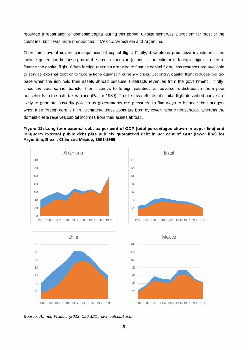
too long in Latin America. This was predominantly public and publicly guaranteed debt, as can be seen in
Figure 11. As the Brady Plan was not put in place until 1989, the indebtedness of Latin American countries
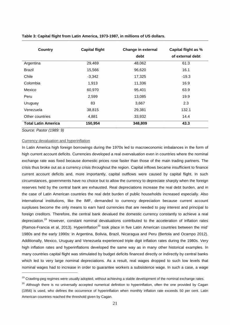
did not decrease substantially throughout the entire decade. Furthermore, in Latin America capital flight
amounted to $151 billion from 1973 to 1987, which was equivalent to 43 per cent of the region’s external
debt acquired within the same period (Table 3). In Venezuela’s extreme case capital flight was even higher
than the external debt attained. Chile, on the other hand, was the only Latin American country which
16 Hsu (2013:51) reports that American banks had an exposure of as much as 177 per cent of capital to the four largest
Latin American debtor countries (Argentina, Brazil, Mexico, and Venezuela). 17
James Baker was the US Treasury Secretary at that time. Bill Brady (Brady plan) was a Senator from the US. 18
Other Latin American countries to restructure under the Brady Plan were Argentina, Brazil, Costa Rica, Ecuador,
Panama, Uruguay, and Venezuela.
20
recorded a repatriation of domestic capital during this period. Capital flight was a problem for most of the
countries, but it was more pronounced in Mexico, Venezuela and Argentina.
There are several severe consequences of capital flight. Firstly, it weakens productive investments and
income generation because part of the credit expansion (either of domestic or of foreign origin) is used to
finance the capital flight. When foreign reserves are used to finance capital flight, less reserves are available
to service external debt or to take actions against a currency crisis. Secondly, capital flight reduces the tax
base when the rich hold their assets abroad because it detracts revenues from the government. Thirdly,
since the poor cannot transfer their incomes to foreign countries an adverse re-distribution -from poor
households to the rich- takes place (Pastor 1989). The first two effects of capital flight described above are
likely to generate austerity policies as governments are pressured to find ways to balance their budgets
when their foreign debt is high. Ultimately, these costs are born by lower-income households, whereas the
domestic elite receives capital incomes from their assets abroad.
Figure 11: Long-term external debt as per cent of GDP (total percentages shown in upper line) and
long-term external public debt plus publicly guaranteed debt in per cent of GDP (lower line) for
Argentina, Brazil, Chile and Mexico, 1981-1989.
Source: Ramos-Francia (2013: 120-121), own calculations.
0
20
40
60
80
100
120
140
1981 1982 1983 1984 1985 1986 1987 1988 1989
Argentina
0
20
40
60
80
100
120
140
1981 1982 1983 1984 1985 1986 1987 1988 1989
Brazil
0
20
40
60
80
100
120
140
1981 1982 1983 1984 1985 1986 1987 1988 1989
Chile
0
20
40
60
80
100
120
140
1981 1982 1983 1984 1985 1986 1987 1988 1989
Mexico
21
Table 3: Capital flight from Latin America, 1973-1987, in millions of US dollars.
Country
Capital flight
Change in external
debt
Capital flight as %
of external debt
Argentina 29,469 48,062 61.3
Brazil 15,566 96,620 16.1
Chile -3,342 17,325 -19.3
Colombia 1,913 11,336 16.9
Mexico 60,970 95,401 63.9
Peru 2,599 13,085 19.9
Uruguay 83 3,667 2.3
Venezuela 38,815 29,381 132.1
Other countries 4,881 33,932 14.4
Total Latin America 150,954 348,809 43.3
Source: Pastor (1989: 9)
Currency devaluation and hyperinflation
In Latin America high foreign borrowings during the 1970s led to macroeconomic imbalances in the form of
high current account deficits. Currencies developed a real overvaluation even in countries where the nominal
exchange rate was fixed because domestic prices rose faster than those of the main trading partners. The
crisis thus broke out as a currency crisis throughout the region. Capital inflows became insufficient to finance
current account deficits and, more importantly, capital outflows were caused by capital flight. In such
circumstances, governments have no choice but to allow the currency to depreciate sharply when the foreign
reserves held by the central bank are exhausted. Real depreciations increase the real debt burden, and in
the case of Latin American countries the real debt burden of public households increased especially. Also
international institutions, like the IMF, demanded to currency depreciation because current account
surpluses become the only means to earn hard currencies that are needed to pay interest and principal to
foreign creditors. Therefore, the central bank devalued the domestic currency constantly to achieve a real
depreciation.19
However, constant nominal devaluations contributed to the acceleration of inflation rates
(Ramos-Francia et al, 2013). Hyperinflation20
took place in five Latin American countries between the mid’
1980s and the early 1990s: in Argentina, Bolivia, Brazil, Nicaragua and Peru (Bertola and Ocampo 2012).
Additionally, Mexico, Uruguay and Venezuela experienced triple digit inflation rates during the 1980s. Very
high inflation rates and hyperinflations developed the same way as in many other historical examples. In
many countries capital flight was stimulated by budget deficits financed directly or indirectly by central banks
which led to very large nominal depreciations. As a result, real wages dropped to such low levels that
nominal wages had to increase in order to guarantee workers a subsistence wage. In such a case, a wage
19 Crawling-peg regimes were usually adopted, without achieving a stable development of the nominal exchange rates.
20 Although there is no universally accepted numerical definition to hyperinflation, often the one provided by Cagan
(1956) is used, who defines the occurrence of hyperinflation when monthly inflation rate exceeds 50 per cent. Latin
American countries reached the threshold given by Cagan.
22
inflation will add to the price inflation initially caused by the depreciation and the economy falls into a
depreciation-wage-price spiral (Robinson 1938; Fischer, Sahay and Végh 2002). Thus, high inflation rates
make it even more difficult for the government to balance the budget.
When countries are not able to create net capital inflows their current accounts become automatically
balanced, whereas large capital flight and net capital outflows make the current accounts positive. This also
happened in Latin American countries. After the crisis, those countries quickly reduced their current account
deficits and realised substantial trade surpluses. However, given the relatively weak overall demand21
during
the economic slowdown worldwide in the early 1980s, the surplus was mainly caused by a reduction in
imports. Living standards dropped substantially due to deteriorating terms of trades and profound domestic
recessions in Latin America. When export surpluses are accumulated on the backbone of real depreciation,
and are not accompanied by any signs of recovery and growth, we have a situation Dornbusch (1990b)
referred to as ‘emperor without clothes’: “If the private sector does not respond with investment and capacity
expansion, and if confidence and inflation issues bar a public sector expansion, then of course the policy
maker becomes the proverbial emperor without clothes: he has sharply increased profitability in the traded
goods sector and the profits are taken out as capital flight; there is no growth, there is social injustice and
social conflict” (Dornbusch 1990b: 13).
Per capita income, aggregate demand and growth
Looking at GDP growth rates in Table 4 it becomes clear that the 1980s were a lost decade. During the
recovery of the first half of the 1990s growth was also substantially lower than the region’s GDP growth rates
before the onset of the debt crisis. In addition to this, Latin America could not return to financial stability. For
example, in 1994 the Mexican ”tequila” crisis affected the continent. Also after the Asian crisis in 1997 most
Latin American countries fought to prevent currency crises of which Argentina’s crisis in 2001-02 was the
most prominent example. Compared to 2.7 per cent of annual per capita GDP growth between 1950 and
1980, in the lost decade of the 1980s per capita GDP grew by only 0.9 per cent annually (Ocampo 2004).
Per capita GDP growth rates declined mainly in the first half of the 1980s (see Table 5), and were particular
severe in Bolivia, El Salvador, Venezuela, Argentina, Uruguay and Guatemala. Poverty rates increased
reaching 48.3 per cent by the end of the decade, which was 8 per cent higher than in 1980 (Ocampo 2004).
Table 4: Latin America’s growth rates, 1950-2002.
1950-1980 1980-1990 1990-1997 1997-2002
GDP growth
Weighted average 5.5 1.1 3.6 1.3
simple average 4.8 1.0 3.9 1.7
GDP per capita
weighted average 2.7 -0.9 2.0 -0.3
simple average 2.1 -1.2 1.9 -0.3
Source: Ocampo (2004:70)
21 In 1981-82 trade price indexes reported a decline in trade prices relative to 1980 (Devlin and Ffrench-Davis 1995).
23
Table 5: Changes in per capita GDP in Latin America, 1981-1985.
Country
Cumulative
change in per
capita GDP,
1981-1985 Country
Cumulative
change in
per capita
GDP, 1981-
1985 Country
Cumulative
change in per
capita GDP,
1981-1985
Argentina -18,5 Ecuador -3,9 Panama 0,7
Bolivia -28,4 El Salvador -24 Peru -14,8
Colombia -0,1 Guatemala -18,3 Uruguay -18,6
Costa Rica -11,2 Mexico -4,3 Venezuela -21,6
Chile -8,7
Source: Sachs (1986:43), data from the Economic Commission for Latin America and the Caribbean
(ECLAC)
In the early 1980s, first the collapse and later the stagnation of aggregate demand caused the severe
economic crisis and the stagnation thereafter. From the 1950s until mid’ 1970s, the rate of investment,
measured as a weighted average for the combined region, fluctuated between 19 and 22 per cent of GDP
and climbed up to 25 per cent just before the crisis (Bertola and Ocampo 2012). This trend reversed after the
crisis hit in the 1980s. In Latin America investments decreased until 1990 whereby capital formation per
capita decreased between 1883 and 1990 to one third of the value it had in 1980 (Devlin and Ffrench-Davis
1995:138). 22
According to Ruediger Dornbusch, investors “have an option to postpone the return of flight
capital and they will wait until the front loading of investment returns is sufficient to compensate for the risk of
relinquishing the liquidity option of a wait-and-see position. […] There is definitely little commitment to a rapid
resumption of real investment. The reason for this is residual uncertainty whether stabilisation can in fact be
sustained.” (Dornbusch 1990b: 17-18)
High interest rates on credits, cautious behaviour by banks and negative expectations by firms kept
investments low. Actually, there was no incentive for investment as other demand elements were insufficient.
Consumption demand was depressed because of high unemployment. Furthermore, fiscal stimulus was not
allowed because the IMF and other foreign creditors demanded fiscal consolidation as part of the
Washington Consensus. Even though positive trade and service balances increased aggregate demand, this
component of demand was still too small to trigger economic growth.
3.4. Concluding remarks
In the 1970s and 1980s Latin American countries suffered from a boom-bust cycle which was analysed by
many scholars (see for example Kaminsky and Reinhart 1999, Williamson 2005, Damill et al. 2013). A
special characteristic of the Latin American boom-bust cycle was that it led to a long-term stagnation.
22 For instance, in Argentina total investment as percentage of GDP declined from 25 per cent in 1980 to 14 percent in
1990, and in the case of Mexico there was a 7 per cent decline in this period (for more detailed data, see Ramos-Francia
et al. 2013).
24
Initially, large capital inflows mainly advocated by governments led to overvalued real exchange rates,
current account deficits and increased foreign debt denominated in foreign currency. Foreign indebtedness
and dollarisation created a currency mismatch in these countries. An overvaluation is independent of the
exchange rate regime. In Latin America most countries pegged their exchange rate to the US dollar. Current
account deficits rose because of relatively high domestic interest rates and relatively high GDP growth rates
during the boom phase. Flexible exchange rates would have increased current account deficits even faster
due to nominal currency appreciations. Additionally, rising asset prices combined with economic expansion
destabilised these economies further.
A progressive worsening of the current account balance and increasing foreign debt undermines the
credibility of exchange rate stability. When the possibility of a devaluation of the domestic currency appears
more likely, the level of uncertainty increases and risk-averse investors start to reduce their financial
commitments to the indebted country. Then, any type of shock can lead to a halt of capital inflows and
stimulate cumulative capital outflows. Considering Latin America the boom phase of the 1970s came to an
end due to the impact restrictive monetary policies in the US had on the indebted countries. Capital outflows
depleted central bank reserves -as long as the central bank intervened in foreign exchange markets- and led
to very large depreciations, which triggered an extreme over-indebtedness in the domestic economy
because their debts were denominated in foreign currency. Eventually, governments have to start
negotiating with other creditors or international institutions. According to the policies enforced by external
creditors, governments had to renounce the possibility of stimulating the economy via fiscal expansion or
other measures which reduce government revenues. Latin America suffered from the severe crisis and its
long stagnation for two main reasons. Firstly, the external debt problem could not be solved in a quick and
efficient way. For instance, the debt crisis broke out in 1982, but the first plan to reduce the foreign debt
burden was implemented in 1986. Nevertheless, this plan reduced the debt burden only moderately. The
reduction of the debt burden came too late and was not sufficient to allow a quick recovery of the economy.
From a historical perspective, the Latin American debt crisis was remarkable in regards to the strong
coordination between creditors observed and their commitment to reduce the risk of potential illiquidity and
insolvency of the international banking system. In response to the financial turmoil they quickly organised a
form of international lender of last resort to contain the danger created by the Latin America crisis. Yet, as
Devlin and Ffrench-Davis (1995) pointed out, a national lender of last resort would usually take action to
minimise the overall social costs generated by the financial crisis. But in this case, the creditor community
focussed primarily on minimising the losses of the financial system.
Secondly, the creditor community enforced Washington Consensus policies on the debtor countries. These
policies implied not only balancing the budget especially through a cut in social expenditure but also low
inflation and a depreciation of the currency. Correspondingly, a neoclassical change in institutions – a
neoclassical “ordnungspolitik” – was needed including privatisation, deregulation, liberalisation and the
establishment of clear property rights to name only a few. All of these policies combined do not support
economic growth in any active way. Instead, some, like the policy to reduce budget deficits, even hamper
economic growth during an economic crisis. Also, privatisation can quickly create an increase in
unemployment (Herr and Priewe 2006). But because of high external debt and pressure from foreign
25
creditors the countries were not able to strike off the straitjacket of Washington Consensus policies.
Moreover, during crisis and stagnation and all economic and political uncertainties that come with it positive
expectation could not develop. Wait-and-see attitudes led to low investment. And last but not least,
consumption demand was low because of policies implemented that made the poorer more poor and the rich
more rich. There is no doubt that the over-adjustment imposed upon the debtor countries and the wrong
policies enforced have arguably prolonged and deepened the Latin American debt crisis, and thus had
created a lost decade for the region.
4. The Japanese crisis
4.1. The background
Until the 1980s Japan was considered as one of the Asian miracle countries with high GDP growth, fast
productivity development, successful export orientation and an efficient government which supported
economic development (Stiglitz 1996). Japan had been a highly regulated economy with much more
government intervention than in developed Western countries. Cooperation between the government and
big companies combined with successful industrial policy created big Japanese multinational enterprises.
The financial system was especially highly regulated (Stiglitz and Uy 1996). For example, international
capital flows were regulated; the banking system channelled credits to the industrial sector as part of
industrial policy; stock markets played an overall unimportant role; credits to the real estate or household
sectors were highly restricted, to name only a few. The Bank of Japan fixed interest rates at low levels and
determined the maximum volume of credits commercial banks could grant. This credit rationing system,
referred to as ‘window guidance’, was supported by the rule that enterprises were not allowed to take credit
from abroad or to issue debt securities in the domestic market. Within this framework, the Bank of Japan
had a substantial control over the developments in the real sector of the economy including the allocation
of credits. Before the 1980s, there was no room for asset market bubbles. Japanese corporate governance
had traditionally been characterised by an intense cross-holding system, where the creditor-bank was
typically among the top five shareholders of a firm (McCauley 2013). Conversely, banks’ shares were
owned by the bank’s borrowers. Such a cross-shareholding system, similar to the one in Germany but
more developed, was very ‘local’ by nature and foreign investors or firms were not playing a significant role
in Japan’s corporate governance.
Japan has had an export-oriented economy since World War II, but only started to build-up permanent and
high current account surpluses in the 1970s (Herr 1990). Japan became one of the world’s major surplus
countries whereby the bilateral trade imbalance between the United States (US) and Japan exploded in the
1980s, which especially contributed to it. The cause of the US current account deficit goes back to the late
1970s. In 1979, in the middle of a severe currency crisis of the US dollar, Paul Volcker was appointed as
Chairman of the Federal Reserve (Fed) and implemented a strict anti-inflationary policy which successfully
brought down inflation rates, but also created a pronounced recession. One year later, Ronald Reagan was
elected as the new US president. Positive expectations about Reagan’s policy regime, which was assumed
to implement business friendly economic policies and to revitalise the military, political and economic power
of the US, increased the international reputation of the US dollar. These changes triggered high capital
26
inflows and led to a substantial appreciation of its currency. Consequently, this pushed the US current
account deficit from a balanced position at the end of the 1970s into a deep deficit. In the 1980s, the high
current account deficit hampered US industrial development and reduced employment which became a hot
topic in the US and in international policy debate. The US government pushed for joint international actions
to stop a further appreciation of the US dollar and to reduce the current account deficit. In the US, Japan
bashing at that time was very common.
This occurrence led to two agreements which are important to understand the development in Japan. The
Plaza Agreement in 1985 by the, at that time, G-5 countries23
attempted to prevent the collapse of the US
dollar by pressuring central banks outside the US to sell dollars from their foreign currency reserves. Also,
the agreement demanded to deregulate the Japanese financial system to stimulate more capital inflows to
Japan. Over the following two years, the external value of the US dollar lost more than 50 per cent of its
value against major currencies. This led to the Louvre Accord in 1987 which aimed to stop the depreciation
of the US dollar. Moreover, there was also the problem that, in spite of a sharp appreciation of the
Japanese Yen, the high Japanese current account surplus with the US did not disappear. Among other
things, G-6 governments24
agreed that Japan should stimulate its economy and cut its interest rates to
increase imports. The Japanese government, which was pleased by its new international role, was eager to
fulfil its international obligations. This was the historical background of Japan’s policy changes after which it
implemented a very expansionary monetary policy including deregulation of its financial system during the
second half of the 1980s. These policies stimulated the real economy, but also began to fuel a huge asset
price bubbles. For the development of main economic indicators see Table 6 on the next page.
4.2. The boom phase
The reduction of protectionist measures and the deregulation of the financial system combined with a very
expansionary monetary policy led to huge bubbles in the stock and real estate markets during the second
half of the 1980s. Between 1985 and 1989, share prices increased by 240 per cent, and property prices by
245 per cent (Werner 2003: 89). Restrictive monetary policy ended those bubbles successfully. In order to
prevent inflation in the goods market during the strong boom in the second half of the 1980s, the Bank of
Japan increased the money market interest rate five times between May 1989 and August 1990. More
importantly, the window guidance system was used to drastically reduce credit expansion. At the end of
1989, there were signs that asset prices would not increase further. The stock market bubble came to an
end, so did the real estate bubble about one year later. Up until about 1992, stock prices halved, and they
have remained at a low level ever since. Real estate prices started to fall over a long course of around 15
years and remained low (Figure 12).
23 Participants of the Plaza Agreement were France, West Germany, Japan, the United States and the United Kingdom.
24 Participants of the Louvre Accord were France, West Germany, Japan, Canada, the United States and the United
Kingdom.
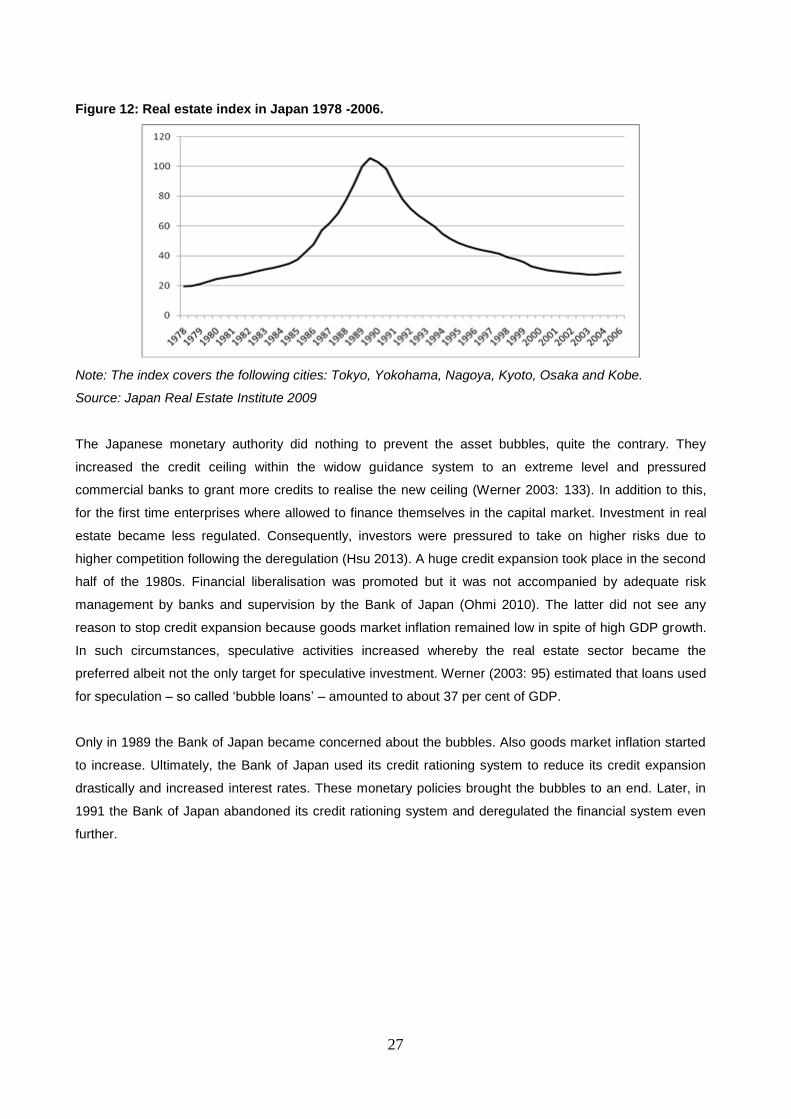
27
Figure 12: Real estate index in Japan 1978 -2006.
Note: The index covers the following cities: Tokyo, Yokohama, Nagoya, Kyoto, Osaka and Kobe.
Source: Japan Real Estate Institute 2009
The Japanese monetary authority did nothing to prevent the asset bubbles, quite the contrary. They
increased the credit ceiling within the widow guidance system to an extreme level and pressured
commercial banks to grant more credits to realise the new ceiling (Werner 2003: 133). In addition to this,
for the first time enterprises where allowed to finance themselves in the capital market. Investment in real
estate became less regulated. Consequently, investors were pressured to take on higher risks due to
higher competition following the deregulation (Hsu 2013). A huge credit expansion took place in the second
half of the 1980s. Financial liberalisation was promoted but it was not accompanied by adequate risk
management by banks and supervision by the Bank of Japan (Ohmi 2010). The latter did not see any
reason to stop credit expansion because goods market inflation remained low in spite of high GDP growth.
In such circumstances, speculative activities increased whereby the real estate sector became the
preferred albeit not the only target for speculative investment. Werner (2003: 95) estimated that loans used
for speculation – so called ‘bubble loans’ – amounted to about 37 per cent of GDP.
Only in 1989 the Bank of Japan became concerned about the bubbles. Also goods market inflation started
to increase. Ultimately, the Bank of Japan used its credit rationing system to reduce its credit expansion
drastically and increased interest rates. These monetary policies brought the bubbles to an end. Later, in
1991 the Bank of Japan abandoned its credit rationing system and deregulated the financial system even
further.
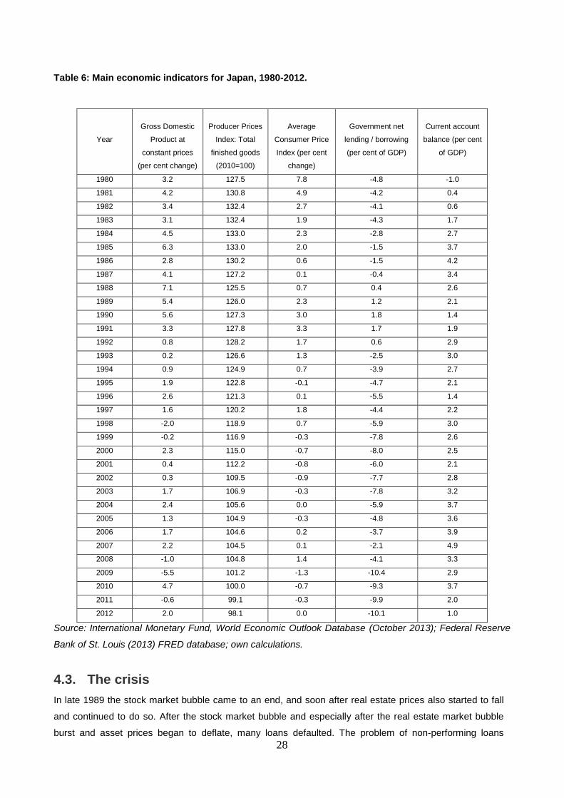
28
Table 6: Main economic indicators for Japan, 1980-2012.
Source: International Monetary Fund, World Economic Outlook Database (October 2013); Federal Reserve
Bank of St. Louis (2013) FRED database; own calculations.
4.3. The crisis
In late 1989 the stock market bubble came to an end, and soon after real estate prices also started to fall
and continued to do so. After the stock market bubble and especially after the real estate market bubble
burst and asset prices began to deflate, many loans defaulted. The problem of non-performing loans
Year
Gross Domestic
Product at
constant prices
(per cent change)
Producer Prices
Index: Total
finished goods
(2010=100)
Average
Consumer Price
Index (per cent
change)
Government net
lending / borrowing
(per cent of GDP)
Current account
balance (per cent
of GDP)
1980 3.2 127.5 7.8 -4.8 -1.0
1981 4.2 130.8 4.9 -4.2 0.4
1982 3.4 132.4 2.7 -4.1 0.6
1983 3.1 132.4 1.9 -4.3 1.7
1984 4.5 133.0 2.3 -2.8 2.7
1985 6.3 133.0 2.0 -1.5 3.7
1986 2.8 130.2 0.6 -1.5 4.2
1987 4.1 127.2 0.1 -0.4 3.4
1988 7.1 125.5 0.7 0.4 2.6
1989 5.4 126.0 2.3 1.2 2.1
1990 5.6 127.3 3.0 1.8 1.4
1991 3.3 127.8 3.3 1.7 1.9
1992 0.8 128.2 1.7 0.6 2.9
1993 0.2 126.6 1.3 -2.5 3.0
1994 0.9 124.9 0.7 -3.9 2.7
1995 1.9 122.8 -0.1 -4.7 2.1
1996 2.6 121.3 0.1 -5.5 1.4
1997 1.6 120.2 1.8 -4.4 2.2
1998 -2.0 118.9 0.7 -5.9 3.0
1999 -0.2 116.9 -0.3 -7.8 2.6
2000 2.3 115.0 -0.7 -8.0 2.5
2001 0.4 112.2 -0.8 -6.0 2.1
2002 0.3 109.5 -0.9 -7.7 2.8
2003 1.7 106.9 -0.3 -7.8 3.2
2004 2.4 105.6 0.0 -5.9 3.7
2005 1.3 104.9 -0.3 -4.8 3.6
2006 1.7 104.6 0.2 -3.7 3.9
2007 2.2 104.5 0.1 -2.1 4.9
2008 -1.0 104.8 1.4 -4.1 3.3
2009 -5.5 101.2 -1.3 -10.4 2.9
2010 4.7 100.0 -0.7 -9.3 3.7
2011 -0.6 99.1 -0.3 -9.9 2.0
2012 2.0 98.1 0.0 -10.1 1.0
29
remained a grave issue throughout the 1990s, and they represented 17 per cent of GDP cumulatively from
1992 to 2000 (Hsu 2013).
At the latest in 1992, the government realised that a threat of a severe recession existed. However, after
the crisis began, the Bank of Japan was not quick enough to respond with a suitable monetary policy and
took several years – until 1995 – to cut the interest rate to 1 per cent (Herr and Kazandziska 2011: 210).
By that time, the lower interest rates were already ineffective. Firms did not borrow regardless of low
interest rates because high accumulated debt and firm strategies to deleverage seriously undermined the
ability of productive investments to pick up.25
The decline in productive investment can be seen in the
shrinking quota of non-financial business debt in relation to GDP during the 1990s and 2000s.
The government did not attempt to find a quick and comprehensive solution for the non-performing loan
problem. Insolvent institutions were either merged with healthy ones under the guidance of the Bank of
Japan, or their bad loans were taken over by a new institution especially designed for this. However, in the
mid’ 1990s the jusen, bank subsidiaries specialised in real estate lending registered such immense losses
that they could not be neutralised via existing structures. In 1996 the government was eventually compelled
to take actions and injected capital into the market and set up two new institutions designed to take over
most of non-performing loans, which were still floating in the market. Almost seven years after the
beginning of the crisis, the government started to solve the problems (Ohmi 2010). This demonstrated the
reluctance of the Japanese government to undertake decisive political action, primarily because of re-
distributional concerns.
4.4. The lost decades
The culmination of problems and long-term stagnation
The problems of the Japanese economy culminated in the second half of the 1990s. There were four main
issues of concern: (i) the stagnation of the domestic credit expansion and GDP growth during the period
after the bubble burst; (ii) the spill-overs from the 1997 Asian crisis and the 1998 Russian crisis; (iii) the
goods market deflation; and (iv) the continuation of the non-performing loan problem. These problems
reinforced each other.
(i) Companies implemented a strategy to deleverage drastically. Even with zero interest rates the corporate
sector did not increase borrowing from banks. Additionally, foreign banks retreated due to the lack of
clients. Also corporations did not turn to capital market for financing. Firms with relatively robust cash flows,
especially those in the export sector, used their surpluses to repair their balance sheets. Richard Koo
(2009) referred to this phenomenon as the ‘balance sheet recession’ and illustrated how Japanese
companies focused primarily on repairing their balance sheets by paying down debt for several years after
the collapse of asset prices occurred. He also pointed out that Japan did not suffer from a classical credit
25 Dornbusch (1990) described such a behavior in the Latin American crisis in the 1980s as wait-and-see attitude by
investors.
30
crunch because the banking sector did not act as a bottleneck for the economy. There were also no
institutional impediments for firms to get finance via foreign banks, or by issuing corporate bonds. It was
the unwillingness of companies to take credit to invest.
Consumption demand remained weak as well. Firstly, low investment demand leads to low income creation
which in turn leads to low consumption demand. This is the essence of a negative goods market multiplier.
Secondly, asset prices remained depressed dampening consumption demand. Thirdly, private households
deleveraged and tried to reduce their debt. Fourthly, higher unemployment, labour market deregulation and
higher uncertainty also depressed consumption demand. Fifthly, the share of wages in national income had
shrunk in Japan throughout the previous three decades, from over 70 per cent in the 1970s to 57 per cent
in 2008 (Ameco, 2010). Higher profit shares in national income reflect the increased power of the financial
system and firms in Japan. The Gini coefficient for disposable income increased from 0.30 in 1985 to 0.35
in 2005. In comparison, Japan still has a relatively equal income distribution, but the change is substantial.
All of this contributed to the poor consumption demand. Private domestic demand and GDP growth
remained very weak. Insufficient domestic demand could not be offset by constant high current account
surpluses. As a result, Japan experienced a long-term stagnation and several ‘lost decades’.
(ii) The instability of the financial system became apparent again after the Asian crisis in 1997 or the
Russian crisis one year later. As a consequences of these crises several big banks and other financial
institutions, which were giving credits to crises countries, failed. The crisis triggered further financial
deregulation. In 1997 and 1998 large reforms within the financial sector took place often referred to as the
so-called ‘Big Bang’ policies (Hsu 2013). These abolished all restrictions on international capital flows and
on foreign ownership in the domestic financial system.
(iii) Japan began to suffer from goods market deflation. In the period between 1994 and 2008 the
Consumer Price Index (CPI) decreased slightly, but the Producer Price Index (PPI) – which is a better
indicator to describe the development of the overall inflation rate – decreased more pronouncedly, as
shown in Figure 13. After the Asian crisis, deflationary trends got worse and over the turn of the century,
the Bank of Japan adopted a policy of ‘quantitative easing’ in addition to the zero-interest rate policy it
implemented earlier. Investment and GDP slowly picked up in the first half of the 2000s and the Japanese
economy was recovering gradually during this period (Ohmi 2010). The subprime crisis and the ensuing
Great Recession, however, pushed Japan back into stagnation and deflation (Figure 13).
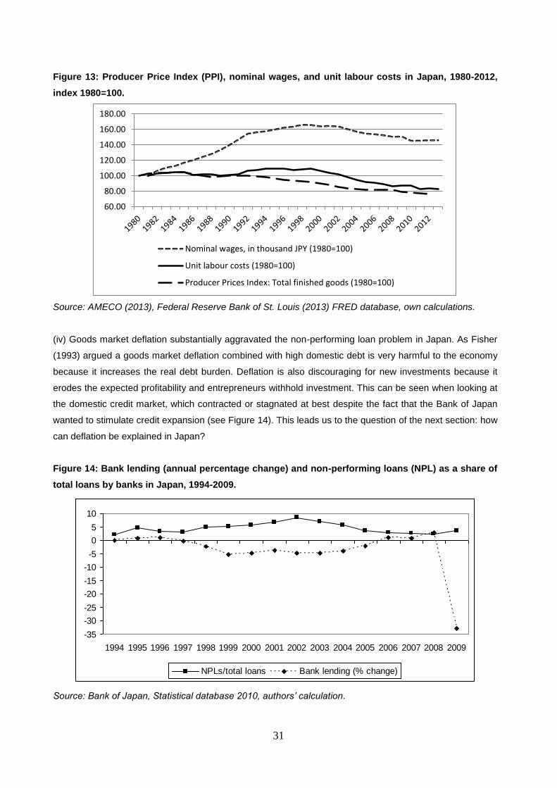
31
Figure 13: Producer Price Index (PPI), nominal wages, and unit labour costs in Japan, 1980-2012,
index 1980=100.
Source: AMECO (2013), Federal Reserve Bank of St. Louis (2013) FRED database, own calculations.
(iv) Goods market deflation substantially aggravated the non-performing loan problem in Japan. As Fisher
(1993) argued a goods market deflation combined with high domestic debt is very harmful to the economy
because it increases the real debt burden. Deflation is also discouraging for new investments because it
erodes the expected profitability and entrepreneurs withhold investment. This can be seen when looking at
the domestic credit market, which contracted or stagnated at best despite the fact that the Bank of Japan
wanted to stimulate credit expansion (see Figure 14). This leads us to the question of the next section: how
can deflation be explained in Japan?
Figure 14: Bank lending (annual percentage change) and non-performing loans (NPL) as a share of
total loans by banks in Japan, 1994-2009.
Source: Bank of Japan, Statistical database 2010, authors’ calculation.
60.00
80.00
100.00
120.00
140.00
160.00
180.00
Nominal wages, in thousand JPY (1980=100)
Unit labour costs (1980=100)
Producer Prices Index: Total finished goods (1980=100)
-35
-30
-25
-20
-15
-10
-5
0
5
10
1994 1995 1996 1997 1998 1999 2000 2001 2002 2003 2004 2005 2006 2007 2008 2009
NPLs/total loans Bank lending (% change)
32
The special role of the labour market and wage policy
Keynes (1930) rightly argued that changes in nominal unit-labour costs are the foundation of inflationary
and deflationary processes. In an environment of excess supply in the goods market, falling production and
increasing unemployment wage deflation occurs when nominal wages do not even increase in line with
productivity. In such a situation the nominal wage anchor can break and trigger a deflationary wage-price
spiral (Herr 2009). This is exactly what happened in Japan – bringing back memories of the deflation in the
1930s during the Great Depression in all developed Western countries. Japanese nominal wage increases
were already very low in the early 1990s when the end of the bubble was near. After that, nominal wages
began to decrease (Figure 13). As trend-productivity increased further unit-labour costs and the inflation
rate started to fall over a longer period of time. Therefore, this paper argues that the main explanation of
the Japanese deflation lies with wage developments. Real wages did not decline, which would be the
conclusion drawn from the neoclassical arguments; but quite the contrary took place. Real hourly
compensations of employees increased, after productivity increased.26
How to explain this development? The decline in aggregate demand and production had serious
repercussions on the labour market in Japan. At the peak of the bubble the unemployment rate stood at
around 2 per cent. After the crisis emerged, unemployment continued to rise throughout the 1990s up until
2003, when it reached a high of 6 per cent, a rate which was current again in 2009 after unemployment
improved slightly for a couple of years (AMECO). However, real unemployment figures are arguably higher,
since many unemployed people are not registered. Decades earlier Japan was used to very low
unemployment rates and thus experienced these high rates as a severe shock.
Labour market reforms and wage policies supported wage deflation. After the bubble burst labour market
deregulation took place. For example, the 1985 Worker Dispatch Law was revised on several occasions to
relax the limits – in terms of numbers and sectors – on temporary placement of workers (Ohmi 2010).
Traditionally, Japan’s labour market consisted of regular workers, who have indeterminate contracts and
long-term career perspectives, relatively high wages and securities, and in contrast to this, of non-regular
workers, who get short-term or part-time contracts and can be fired relatively easily. Institutional changes
decreased the number of regular workers from 83 per cent of all workers in 1982 to 68 per cent in 2002,
and to 66 per cent in 2008 (Nakata and Miyazaki 2010). It is worth noting that before the 1980s (i.e. during
the Japanese miracle) the income distribution in Japan was remarkably equal. The deregulation in the
labour market caused a bipolarisation of the workforce which had negative repercussions on the Japanese
middle class and therefore an overall income distribution. Increasing uncertainty of many Japanese
employees further depressed consumption demand (Hsu 2013).
In order to understand the loss of the nominal wage anchor in Japan, one must also look at the wage-
bargaining system and the state of labour unions in Japan (Soskice 1990; Herr and Kazandziska 2010).
There are thousands of firm unions in Japan which belong to one of the national union federations. Many of
26 This simply confirms what Keynes (1930) and (1936) pointed out, namely that nominal wages do not determine real
wages.
33
these unions exclusively organise regular employees only. Thus, on the one hand, non-regular workers –
which were persistently increasing in Japan – were almost entirely excluded in wage bargaining processes.
On the other hand, regular workers negotiate wages at company level. Japanese unions usually linked
their wage policy to the interests of companies. During economic hardship, the microeconomic logic of firm-
based wage development led not only to falling nominal wages, but also to a disastrous macroeconomic
deflation. In Japan wage bargaining starts in a small number of big companies and the outcome of these
negotiations signals the level of wage increases for the rest of the economy, determining thus the country’s
wage developments. And finally, due to Japan’s export-orientated and mercantile strategies it increased
nominal wages traditionally more slowly. These institutions naturally led to a perverse coordination
generating lower nominal wages during crises.
Government also contributed to this development. Besides deregulating the labour market the government
did not use minimum wages to reduce deflationary pressures. During the deflationary period, the National
Council, which recommends annual changes of the statutory minimum wage, almost froze minimum wage
developments completely. Between 1999 and 2006, only very small changes in minimum wages were
observed.
The role of fiscal policy
The Japanese government experienced high budget deficits - often exceeding 5 per cent of GDP - since
1993 (Table 6), and government indebtedness increased remarkably from around 67 per cent of GDP at
the beginning of the crisis in 1990 to around 243 per cent of GDP in 2012, as illustrated in Figure 15.
Without the stabilisation of aggregate demand by the Japanese government a scenario comparable to the
Great Depression would have been likely.
Figure 15: Japan’s General Government gross debt in percent of GDP, 1980-2012.
Note: Estimates start after 2011.
Source: International Monetary Fund, World Economic Outlook Database, October 2013
0
50
100
150
200
250
19801982198419861988199019921994199619982000200220042006200820102012
per
cen
t o
f G
DP
Tau
sen
de
34
The high budget deficit and in turn the high public debt were not the result of an expansionary fiscal policy
implemented to stimulate aggregate demand. The preoccupation with budget consolidation was evident as
fiscal policy was tightened as soon as a slight recovery was in sight. When, for example, a recovery of the
real GDP was observed in 1995 and 1996, the Hashimoto administration initiated fiscal and social welfare
reforms with a restrictive fiscal policy. The consumption tax was increased from 3 to 5 per cent in 1996 and
a programme for public spending cuts was enacted in 1997 (Ohmi 2010). This had adverse effects on GDP
growth and led to a new recession when combined with the spill-over of the Asian crisis. After 2003 there
was an another attempt by the Japanese government to gradually consolidate the budget, effective until
2007 (Figure 15), but following the Great Recession triggered by the subprime crisis in the US, Japanese
public debt exploded again. Overall, a more long-term oriented fiscal policy with less concern about budget
consolidation – which in the end failed – would have been more helpful.
4.5. Concluding remarks
In Japan the bubble was caused by the deregulation of the financial system and an expansionary monetary
policy that emphasised the expansion of credits. These policies were mainly implemented due to
international pressures not only from the United States, which was afflicted by a large current account
deficit with Japan during that time. Monetary policy and supervisory institutions completely neglected asset
market development. The huge stock market and real estate bubble came to a halt when the central bank
finally imposed a restrictive monetary policy.
Bubbles of any type are dangerous but real estate bubbles are particularly problematic as these usually
involve much higher amounts of credit, and are also more closely linked to the consumption behaviour of
households. Japan is an example for this. The asset price deflation, especially in the real estate sector,
created a large volume of non-performing loans. Monetary policy did not respond to this in time. Before,
monetary policy was too loose when the bubble culminated, and after, it was too restrictive during the first
couple of years after the bubble burst. Later, the Bank of Japan implemented a zero-interest-rate policy for
many years. However, monetary policy was not able to prevent a long-term stagnation due to deflation and
the inability to cut nominal interest rates further.
The non-performing loan problem was not handled in an efficient and timely manner in Japan. The problem
was allowed to develop for too long and government intervention was too weak. The government should
have acted timely and more decisively to allow the economy to clear its balance sheets quickly and to
reinstate the credit-investment mechanism. A possible strategy would have been to immediately nationalise
the unhealthy banks and eventually re-privatise them after stabilising them. The reluctance of the
government to act was likely due to re-distributional concerns, namely, the concern who would bear the
costs of restructuring or bailouts. Lobbying is also quite present in Japan and might have been detrimental
to the government decision making process.
35
The continuity of the non-performing-loan problem was a decisive factor for the long-term stagnation and
depended substantially on the good market deflation, which increased the real debt burden of all domestic
loans in Japan. In the developed world a dangerous deflation was unknown after the Great Depression up
until it happened again in Japan in the 1990s. The deflation was caused by low GDP growth combined with
increased unemployment, which led to the break of the nominal wage anchor, which in turn triggered a
wage deflation. The lesson learned from Japan is that weak labour market institutions, that do not defend a
nominal wage anchor, are extremely dangerous for economic growth. The wage bargaining system based
on the firm level followed a microeconomic logic of wage development and was not suited to preventing
wage deflation. Deregulation of labour markets and an insufficient statutory minimum wage policy added to
the weak wage bargaining institutions in Japan. The zero-interest-rate policy implemented by the Bank of
Japan combined with fiscal policy prevented a cumulative downward spiral as experienced during the
Great Depression in1929.
In retrospect, after the bubble burst a more expansionary fiscal policy would have been better. The
Japanese government did provide fiscal stimuli but as soon as the economy showed some signs of
improvement it began to consolidate the budget too soon – without much success. Here, a more decisive
action would have been more beneficial, even if it would have meant accepting double-digit fiscal deficits
for several years.
The Japanese financial crisis and long-term stagnation had no big repercussion on the world economy.
The style of corporate governance and the local character of the Japanese financial system, which inherits
financial institutions unwilling to take credit from abroad or in foreign currency, are the explanations for this.
Due to high current account surpluses financial institutions invested considerably abroad. But credit-
relations were asymmetric in the sense that neither Japanese firms, financial institutions nor the
government accumulated foreign debt. This is a major difference to the Latin American crisis in the 1980s.
5. Conclusions
In the first part of this section lessons from the historical analyses are discussed. Then, some tentative
conclusions for the subprime financial and the Great Recession and their long-term repercussions are
drawn.
All three financial crises analysed in detail above, the Great Depression in the 1930s, the Latina American
Crisis in the 1980s and the Japanese crises in the 1990s and 2000s, led to “lost decades”, that means to
long periods of low growth and its entire negative effects. Not all financial crises follow such a pattern. Some
severe financial crises were overcome relatively quickly, and the costs in respect to losses of GDP growth,
employment or income distribution were high, but compared to the three crises we analysed relatively low
(see for a comprehensive overview of historical crises Kindelberger and Aliber 2005). For example, relatively
short were the Asian financial crises, which broke out in 1997 in most of the affected countries. Another
example is the financial crisis in Sweden in 1991 and 1992 which could be overcome relatively quickly. We
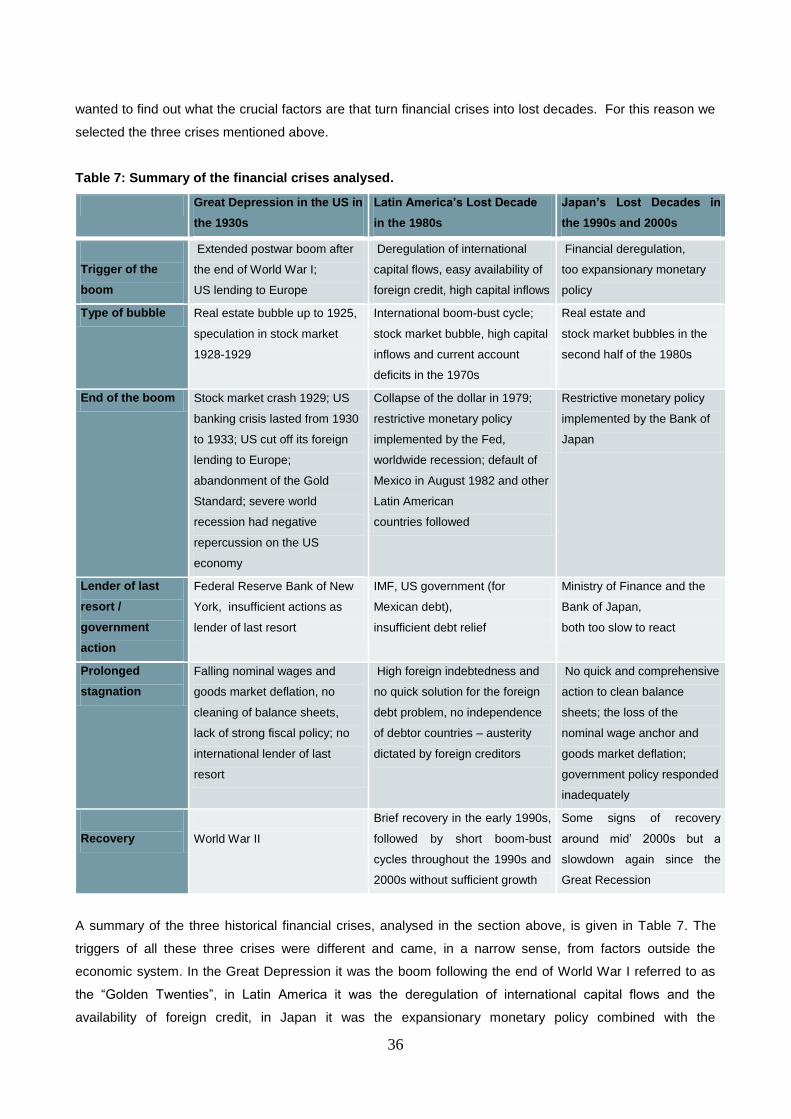
36
wanted to find out what the crucial factors are that turn financial crises into lost decades. For this reason we
selected the three crises mentioned above.
Table 7: Summary of the financial crises analysed.
Great Depression in the US in
the 1930s
Latin America’s Lost Decade
in the 1980s
Japan’s Lost Decades in
the 1990s and 2000s
Trigger of the
boom
Extended postwar boom after
the end of World War I;
US lending to Europe
Deregulation of international
capital flows, easy availability of
foreign credit, high capital inflows
Financial deregulation,
too expansionary monetary
policy
Type of bubble Real estate bubble up to 1925,
speculation in stock market
1928-1929
International boom-bust cycle;
stock market bubble, high capital
inflows and current account
deficits in the 1970s
Real estate and
stock market bubbles in the
second half of the 1980s
End of the boom Stock market crash 1929; US
banking crisis lasted from 1930
to 1933; US cut off its foreign
lending to Europe;
abandonment of the Gold
Standard; severe world
recession had negative
repercussion on the US
economy
Collapse of the dollar in 1979;
restrictive monetary policy
implemented by the Fed,
worldwide recession; default of
Mexico in August 1982 and other
Latin American
countries followed
Restrictive monetary policy
implemented by the Bank of
Japan
Lender of last
resort /
government
action
Federal Reserve Bank of New
York, insufficient actions as
lender of last resort
IMF, US government (for
Mexican debt),
insufficient debt relief
Ministry of Finance and the
Bank of Japan,
both too slow to react
Prolonged
stagnation
Falling nominal wages and
goods market deflation, no
cleaning of balance sheets,
lack of strong fiscal policy; no
international lender of last
resort
High foreign indebtedness and
no quick solution for the foreign
debt problem, no independence
of debtor countries – austerity
dictated by foreign creditors
No quick and comprehensive
action to clean balance
sheets; the loss of the
nominal wage anchor and
goods market deflation;
government policy responded
inadequately
Recovery
World War II
Brief recovery in the early 1990s,
followed by short boom-bust
cycles throughout the 1990s and
2000s without sufficient growth
Some signs of recovery
around mid’ 2000s but a
slowdown again since the
Great Recession
A summary of the three historical financial crises, analysed in the section above, is given in Table 7. The
triggers of all these three crises were different and came, in a narrow sense, from factors outside the
economic system. In the Great Depression it was the boom following the end of World War I referred to as
the “Golden Twenties”, in Latin America it was the deregulation of international capital flows and the
availability of foreign credit, in Japan it was the expansionary monetary policy combined with the
37
deregulation of the domestic financial system. In all of these examples unsustainable credit expansions
played a central role and increased fragility, which later led to the systemic financial crises. Before the Great
Depression and the Japanese crises in the 1990s and 2000s, a real estate bubble developed. Also, in both
crises stock market speculation played an important role whereas credit driven speculation in the stock
market was especially important before the Great Depression. Before the Latin American crises, the late
affected countries accumulated high stock of foreign debt. In all three cases credit expansion and asset
prices bubbles were accompanied by a strong real economic expansion which strengthened the confidence
in the economic development. In two of the cases restrictive monetary policy stopped the boom. In Japan the
Bank of Japan started to fight against the slowly developing goods market inflation caused by high GDP
growth. In Latin America the crisis was triggered by the very restrictive US monetary policy, which was
fighting against the collapse of the US dollar and an increasing US inflation rate at the end of the 1970s. The
Great Depression began with the collapse of the stock market bubble in 1929, which was largely
independent of monetary policy.
In all three cases the financial crises that followed the expansions led to prolonged stagnation. The question
in our focus is: How to explain such lost decades? What went wrong after each of these crises broke out?
From the historical analysis four lessons can be drawn
The first lesson is that balance sheets have to be cleaned-up very quickly. To clean balance sheets from
non-performing loans is extremely important, because the perpetuation of bad loans hinders productive
investment and delays a virtuous credit-investment-production-income cycle. Financial institutions will
simply not be able or not willing to give credit when they suffer from high levels of non-performing loans.
Firms with high debt will also be reluctant to take on new credits for investments. In these three countries
balance sheets were not cleaned-up quickly. During the Great Depression banks were allowed to break
down as the central bank and the government did save them. Breakdowns of banks can be interpreted as a
violent method to clean balance sheets. However, when deposits of the general public are affected and
there is no policy in place to stimulate new credit expansion, after the breakdown of banks, a recovery is
almost impossible. Additionally, in the US non-performing loans in the real estate sector and the enterprise
sector remained on a high level for many years after the Great Depression. In Japan central banks and
governments did not do much to clean balance sheets of financial institutions for a long time. The hope
was that the problem would slowly disappear when growth rates recover. In Latin America foreign creditors
did not allow to clean balance sheets.
When we draw the lesson that non-performing loans should be eliminated in the private sector after a
financial crises broke out, we know that this is very difficult. The difficulty is that each way to clean balance
sheets involves deep distributional consequences. When the government takes over non-performing loans
from financial institutions, firms or even private households, the tax payer has to pay in the end. A currency
reform privileges holders of real estates and debtors and punishes creditors including deposit holders in
banks. International debt relief implies losses of international creditors. Domestic debt can be taken over to
a certain extent by the domestic central bank. However, this may be considered as unfair privileging only
some groups in the society.
38
The second lesson is that a severe economic recession and/or a long stagnation increase the danger of
deflation, which could lead to the erosion of the nominal wage anchor and to decreasing unit-labour costs
that stimulate a wage-price downward spiral. The instabilities resulting from wage deflation have been
illustrated in the cases of the Great Depression and of the Japanese crisis. In mainstream economics this
argument has not been recognised. For instance, Bernanke (2000) and others argued that the huge
employment losses during the Great Depression were caused by insufficient nominal wage cuts, which led to
dramatic increases in real wages. High real wages, so the argument runs, lead to falling labour demand and
high unemployment. We disagree with these neoclassical arguments. Nominal wage cuts drove deflation
further and led to the explosion of the real debt burden and to the collapse of the economy. The key point
here is that workers are not even able to reduce real wages by cutting nominal wages. In Keynes' words:
"There may exist no expedient by which labour as a whole can reduce its real wage to a given figure by
making revised money bargains with the entrepreneurs" (1936: 13). In regards to wages during the Great
Depression, Keynes argued: "It is not very plausible to assert that unemployment in the United States in
1932 was due either to labour obstinately refusing to accept a reduction of money-wages or to its obstinately
demanding a real wage beyond what the productivity of the economic machine was capable of furnishing"
(Keynes 1936: 9).
The same argument was used for Japan. In the traditional neoclassical and New Keynesian view, real wages
in Japan were excessively high and labour markets were not flexible enough after the 1980s. Unions were
accused of reacting inadequately and of opposing sufficient nominal and real wage cuts. But in fact, a period
of low GDP growth caused deflation and increased unemployment, which combined led to the breakdown of
the nominal wage anchor and to a wage deflation in Japan. The lesson learned from Japan is that weak
labour market institutions, which do not defend a nominal wage anchor, are extremely dangerous for
economic growth. A key problem of the Japanese wage bargaining system is that wage negotiations in the
private sector take place within the firm level. Consequently, wage developments are linked to the economic
situation of an individual firm. When, for example, firms’ do not perform very good during a crisis, they have
strong incentives to follow the microeconomic logic and cut wages – if all firms reduce wages either through
competitive pressures or through bad performance, a deflation is set in motion. Deregulation of labour
markets and insufficient wage bargaining institutions including an insufficient statutory minimum wage policy
led to the Japanese deflation and the permanent reproduction of non-performing loans (see the case study in
Herr and Kazandziska 2011).
A real depreciation of the domestic currency in countries that accumulated high debt denominated in foreign
currency has a comparable effect as to a deflation, because in this case the real debt burden also increases
throughout the whole economy and leads to a systemic financial crisis. Here, the conclusion is that foreign
debt in foreign currency is extremely dangerous. Depreciation can never be excluded. The conclusion is that
countries should be very cautious to accumulate foreign debt. Capital imports need financial market
supervision, which does not allow currency mismatch, to avoid crises as in Latin America during the 1980s.
The third lesson is that after a systemic financial crisis, active government policies are needed. Otherwise,
the economy might get caught into a prolonged stagnation, and there are no self-adjusting mechanisms
39
through which a recovery will initiate spontaneously. In the United States during the Great Depression
monetary policy was not sufficiently expansionary to help to stabilise the crisis. In Japan, monetary policy
was too loose while the bubble was developing, and too restrictive during the first years after the bubble
burst. A much faster cut of interest rates would have been better directly after the end of the stock market
and real estate bubbles. Later, the refinancing rate in Japan has been remaining at zero for a long time. But
monetary policy during deflation is toothless. The Latin American countries had no sufficient control over
their own interest rates, because capital flights restricted low domestic interest rates. Real interest rates for
foreign credit exploded after the real depreciation and could not be cut by the indebted countries.
The more toothless monetary policy becomes the more important gets fiscal policy. In the 1930s, the lack of
fiscal policy led the crises develop out of hands with catastrophic results. From Japan we can learn that
expansionary fiscal policy can prevent a deflationary development that leads to a Great Depression.
However, during the lost decades after the end of the bubbles, the Japanese government would re-focus on
balancing the budget at the faintest sign of recovery. It did not seem to realise that it was sovereign in its
decisions and that there is no limit imposed to its public deficit. A more decisive fiscal policy in Japan
probably would have helped to overcome the long stagnation. The Latin American countries had no
autonomy to follow expansionary fiscal policy. Foreign creditors and their adjustment programs simply did
not allow expansionary fiscal policy.
A fourth lesson is that an international financial crisis needs international stabilisation. As Kindleberger and
Aliber (2005) pointed out, during a severe crisis that affect various countries or regions in the world, which
were characterised by a distressed banking sector and a high level of debt that entailed a high risk of
contagion, an entity (a hegemonic country or international institution) is needed to act as a stabiliser for the
economy as a whole. Thus, an international lender of last resort is needed that provides liquidity during a
financial crisis and guarantees counter-cyclical long-term lending. Also, a mechanism is needed that
manages international current account imbalances and unstable capital flows. An entity or institution of this
kind does not exist in the present state. The Great Depression clearly showed that a lack of an international
lender of last resort can fundamentally worsen an international financial crisis.
What can we learn from these four lessons for the subprime financial crisis, the Great Recession and the
development thereafter? Looking at the subprime crises and its management we find mixed results. Banks
were comprehensively bailed out in all of the crises countries involved, and further, many banks were in
some cases even nationalised. This was partly achieved through heavy fiscal interventions and partly by
central banks interventions. A systemic breakdown of commercial banks as experienced, for example, in the
1930s during the Great Depression did not occur. Given that consumption demand remains structurally
weak, due to very unequal income distributions and continuing debt problems for private households, a not
very dynamic consumption demand can be expected in most Western countries. A big shortcoming of these
bail-out packages was that they did not combine them with debt relieve for households, but instead saved
the owners of bad loans and focused mainly on supporting big creditors of financial institutions (Stiglitz
2012). There are shortcomings especially in the European Monetary Union (EMU). Balance sheets of banks
are still afflicted with high non-performing loans from the real estate sector in Southern European countries.
40
In spite of the bail-outs paid since the beginning of the crises, non-performing loans, nevertheless, doubled
in Europe.27
In autumn 2013, especially banks from Spain and Italy were more afflicted with non-performing
loans measured as per cent of total loans than several years ago before the crisis broke out.28
Consumer price inflation and especially core inflation rates were very low in many countries after GDP
growth slowed down or after the second recession of the Great Recession in 2012.29
Any economic shock
can push economies into deflation, which in turn can lead to nominal wage cuts. In Japan, deflation took also
place when it was hit by a second shock induced by the Asian crisis in 1997. By that time, Japan already
experienced very low GDP growth rates for more than seven years. Since fundamental reforms are missing
in the global and national financial system, the shadow banking system has mainly remained unchanged.
Also, the connections between commercial banks and shadow financial institutions are still tight, which does
not allow us to assume that future global financial crises can be ruled out. Current labour market policies do
not in any substantial way reregulate labour markets or wage bargaining institutions, so that another
economic shock could cause the nominal wage anchor to erode. Japan showed that deflation is not a
problem of past centuries.
For a long time already, international institutions pressure for wage negotiations at the firm level and
recommend wage flexibility according to microeconomic needs (see for example OECD 1994, 2011). In
Europe, the Troika (EU Commission, ECB and International Monetary Fund) pressures crises countries like
Spain, Portugal, Greece, and Italy (to name only a few) to accept more firm based wage negotiations and to
implement a radical reduction of extension mechanisms (see Blanchard et al. 2013). This means labour
market institutions are pushed so that it weakens the nominal wage anchor that prevents deflation. The
Troika is urging to reduce nominal wages in these countries to simulate a non-existing exchange rate
depreciation to enhance their lost price competitiveness. In these countries competiveness was lost because
their nominal unit-labour cost developments were not in line with the countries’ productivity trend increases
plus their inflation target as would a functional wage development suggest, but rather they were too high to
the same degree as they were too low in Germany (Herr and Horn 2012).30
In crises countries cutting wages
and simultaneously reducing the price level are in the final analysis a suicide strategy. It may increase price
competitiveness but at the same time it increases the real debt burden on a broad scale. This effect can
even be observed when inflation rates drop to very low levels. In Greece deflation emerged for the first time
since 1968 in March 2013, and other Southern European countries seem to follow (Financial Times 2013b).
In October 2013, the Financial Times (2013c) correctly stated that Mario Draghi, president of the ECB, was
27 European banks’ non-performing loans have doubled in just four years to reach close to €1.2tn and are expected to
keep rising. (…) Rises in the most recent year driven by deteriorating conditions in Spain, Ireland, Italy and Greece”
(Financial Times 2013d). 28
See Financial Times (2013a).
29 When we speak about low inflation rates this implies, in 2013, an inflation rate of around zero per cent in Japan and of
around one per cent in the US and the EMU (Eurostat (2013)).
30 The improvement of current account balances in the EMU crises countries after begin of the crisis is mainly caused by
their low GDP growth rate and not by increasing price competiveness.
41
on the edge of deflation. Indeed, a deflationary development in the EMU, in the near future or in the years to
come, cannot be excluded. Deflationary developments in Western countries cannot be excluded in the
future. Japan has not overcome its deflation, yet, and Europe and especially the EMU is in danger to slide
into deflation, too. Also, in the USA an additional economic shock could lead to a deflationary development
and therefore, can also not be excluded.
After the end of the internet bubble in the 1990s and even more after the real estate bubble in the 2000s, the
Fed learned its lesson from the mistakes the Bank of Japan made and decided to cut interest rates much
earlier and much more radical and reduced it down to zero. Also, the Bank of England followed into the
footsteps of the Fed. In contrast, the ECB acted more slowly. A faster cut of the interest rate after the
outbreak of the crisis would have been better. Until today (December 2013), refinancing rates of the ECB are
not zero, but are with 0.25% almost zero. Even though monetary policy was extremely expansionary at zero
interest rates and the central bank intervened by drastically buying bonds and toxic assets in the framework
of quantitative easing, it was not able to bring economies back to a sustainable growth path. Monetary policy
helped to stabilise the situation, but, as is well known, its power is asymmetric. It can stop a boom but it
cannot create one. In the EMU, monetary policy failed, as mentioned above, to take on the role as a lender
of last resort for EMU countries that suffered from a sovereign debt crises. In July 2012, when Mario Draghi
promised to bail out those crises countries of the EMU that were hit most severally provided that they follow
the dictate of the Troika, it was very late and it remains unclear to which extent it will really happen.
In the US as well as in Europe, the government implemented expansionary fiscal policy immediately after the
outbreak of the subprime crisis and the Great Recession, which therefore could be softened substantially.
However, further fiscal stimuli would have been needed since the economies only recovered very slowly
from the Great Recession and growth rates remained low. But, in the US and in the EMU political authorities
pressured to balance the budgets much stronger. The slowdown of worldwide growth, in 2012 and 2013, has
been caused to a large extend through the reduction of fiscal stimuli. Fiscal policy seems to be the most
problematic in the EMU today. Especially in the Euro-area too much attention focuses on budget
consolidation and various austerity measures. The crisis experienced in Southern European countries is
similar to the situation experienced in Latin America during the 1980s. The austerity measures imposed by
the IMF on the Latin American countries closely resemble the measures stressed by the Troika in Southern
European countries. What we can learn from the Latin American experience is that economic, and especially
social costs associated with austerity are massive. There is a risk that the “lost decade” of many Southern
European countries turns into a “lost generation” carrying extreme negative repercussions. In sum: Overall
monetary and fiscal policy stabilised the first period after the outbreak of the subprime crises and prevented
the Great Recession to develop into a Great Depression. However, fiscal austerity was introduced after the
Great Recession was overcome. As a result, economies fell into a new stagnation or even recession.
Without continuing expansionary monetary policy and a new wave a fiscal stimulation it is unlikely that a
sufficient growth rate can be achieved.
Looking at the international level there is no mechanism established which could handle an international
crisis in an efficient way. There is also no mechanism in place which would restrict high current account
42
imbalances or destabilising international capital flows. Overall, drawing on the lessons from our historical
analysis we come to conclusion that the policies in almost all macroeconomic areas are currently not suitable
to overcome the danger of a long period of low growth after the Great Recession.
References
Bank of Japan (2010): Statistical database, http://www.stat-search.boj.or.jp/index_en.html.
Beenstock, M. (2007): The rise, fall and rise again of OPEC, in: M. J. Oliver and D. H. Aldcroft (eds.),
Economic Disasters of the Twentieth Century, Cheltenham, Edward Elgar.
Belabed, C. A. (2011): Die Große Depression und der New Deal aus Makroökonomischer Sicht, Linz,
Trauner Verlag.
Bernanke, B. S. (2000): Essays on the Great Depression, Princeton University Press.
Bernanke, B.S., James, H. (1990): The Gold Standard, deflation, and financial crisis in the Great Depression:
an international comparison’, in: R. Glenn Hubbard (ed.), Financial Markets and Financial Crises,
Chicago, University of Chicago Press.
Bertola, L., Ocampo, J. A. (2012): Latin America's debt crisis and 'lost decade', Institute for the Study of the
Americas: Learning from Latin America: Debt crises, debt rescues and when they work, February 20th
2012.
Blanchard, O., Jaumotte, F., Loungani, P. (2013): Labour market policies and IMF advice in advanced
economies during the Great Recession, IMF Staff Discussion Note 13/02, March 2013.
Brown, C. (1956): Fiscal policy in the ‘Thirties’: a reappraisal, The American Economic Review, 46 (5): 857-
879.
Cagan, P. (1956): The monetary dynamics of hyperinflation, in: Milton Friedman (ed.), Studies in the
Quantity Theory of Money, Chicago, University of Chicago Press.
Damill, M., Frenkel, R., Rapetti, M. (2013): Financial and currency crises in Latin America, in: M. H. Wolfson
and G. A. Epstein (eds.) The Handbook of the Political Economy of Financial Crises, Oxford, Oxford
University Press.
Desai, P. (2011): From Financial Crisis to Global Recovery, New York, Columbia University Press.
Devlin, R., Ffrench-Davis, R. (1995): The great Latin American debt crisis: a decade of asymmetric
adjustment, Revista de Economia Politica, Jul-Sep, 15 (3): 117-142.
Dighe, R.S., Dunne Schmitt, E. (2010): Did US wages become stickier between the world wars?, The North
American Journal of Economics and Finance, 21 (2): 165 – 181.
Dornbusch, R. (1990a): From Stabilisation to Growth, NBER Working Paper No. 3302, March 1990,
Cambridge, MA, National Bureau of Economic Research.
Dornbusch, R. (1990b): Policies to move from stabilization to growth, CEPR Discussion Paper No. 456,
September 1990, Centre for Economic Policy Research.
ECLAC (2013) Economic Commission for Latin America and the Caribbean database,
http://estadisticas.cepal.org/cepalstat/WEB_CEPALSTAT/Portada.asp?idioma=i.
Economic and Financial Affairs database of the European Commission (several years), AMECO database,
http://ec.europa.eu/economy_finance/ameco/user/
43
Eggertson, G. B. (2008): Great expectations and the end of the depression, American Economic Review,
September, 98 (4): 1476 – 1516.
Eichengreen, B., Hausmann, R., Panizza, U. (2003): Currency mismatches, debt intolerance and original sin.
Why they are not the same and why it matters, NBER Working Paper No. 10036, Cambridge, MA,
National Bureau of Economic Research.
Eurostat (2013): European Commission Earnings Database, gender pay gap statistics.
Federal Reserve Bank of St. Louis (2013): FRED Database, http://research.stlouisfed.org/fred2/.
Financial Times (2013a): The NPL standardization factor, Financial Times, November 5th 2013.
Financial Times (2013b): Greek deflation accelerates after wages drop, Financial Times, November 8th
2013.
Financial Times (2013d): Troubled loans at Europe’s banks double in value, Financial Times, October 29th
2013.
Financial Times (2014c): Draghi on the edge of deflation, Financial Times, October 25th 2013.
Fischer, S., Sahay, R., Végh, C.A. (2002): Modern hyper inflations, Journal of Economic Literature, 40 (3):
837–80.
Fisher, I. (1933): The debt-deflation theory of great depressions, Econometrica 1: 337 - 357.
Friedman, M., Schwartz, A. (1963): A Monetary History of the United States, 1867-1960, Princeton University
Press.
Galbraith, J. K. ([1954]2009): The Great Crash 1929, New York, Mariner Books.
Galbraith, J. K. ([1990]1994): A Short History of Financial Euphoria, London, Penguin Books.
Grebler, L., Blank, D. M., Winnick, L. (eds.) (1956): Capital Formation in Residential Real Estate: Trends and
Prospects, Princeton University Press.
Herr, H. (1990): Der bundesdeutsche und japanische Merkantilismus, in: H.-P. Spahn, H.-P. (ed.),
Wirtschaftspolitische Strategien - Probleme ökonomischer Stabilität und Entwicklung in
Industrieländern und der Europäischen Gemeinschaft, Regensburg.
Herr, H. (2008): Financial systems in developing countries and economic development, in: E. Hein, T.
Niechoj, P. Spahn and A. Truger (eds.), Finance-led Capitalism? Macroeconomic Effects of Changes
in the Financial Sector, Marburg, Metropolis.
Herr, H. (2009): The labour market in a Keynesian economic regime: theoretical debate and empirical
findings, Cambridge Journal of Economics, 33: 949-965.
Herr, H. (2011): International monetary and financial architecture, in: E. Hein and E. Stockhammer (eds.), A
Modern Guide to Keynesian Macroeconomics and Economic Policies, Cheltenham, Edward Elgar.
Herr, H. and Kazandziska, M. (2010): The labour market and deflation in Japan, International Journal of
Labour Research, Financial Crises, Deflation and Trade Union Responses: What are the Lessons?, 2
(1): 79-98, Geneva, International Labour Office.
Herr, H., Kazandziska, M. (2011): Macroeconomic Policy Regimes in Western Industrial Countries, London,
Routledge.
Herr, H., Priewe, J. (2006): The Washington Consensus and (non-)development, in: L. R. Wray and M.
Forstater (eds.), Money, Financial Instability and Stabilization Policy, Cheltenham, UK, Northampton,
MA, USA.
Herr, H., Horn, G. (2012): Wage Policy Today, Global Labour University Working paper No. 16 August 2012.
44
Holt, C. F. (1977): Who Benefited from the Prosperity of the Twenties?, Explorations in Economic History, 14
(3): 277 - 289.
Hsu, S. (2013): Financial Crises, 1929 to the Present, Cheltenham, Edward Elgar.
IMF (2012): World Economic Outlook: Growth resuming, dangers remain, April, Washington, International
Monetary Fund.
IMF (2013): Data and Statistics, http://www.imf.org/external/data.htm.
Japan Real Estate Institute (2009): http://www.reinet.or.jp/en/.
Kaminsky, G. L., Reinhart, C. M. (1999): The twin crises: the causes of banking and balance-of-payment
problems, The American Economic Review, June 1999.
Keynes, J. M. (1930): A Treatise on Money, Collected Writings, Vol. V., London Macmillan.
Keynes, J. M. (1936): The General Theory of Employment, Interest and Money, Cambridge, Cambridge
University Press.
Kindleberger, C. P. and Aliber, R. Z. (2005): Manias, Panics, and Crashes, Hoboken, New Jersey, John
Wiley and Sons, 5th ed.
Koo, R. (2011): The Holy Grail of Macroeconomics: Lessons from Japans Great Recession, Singapore, John
Wiley & Sons.
Kuznets, S. (1937): National income and capital formation, 1919-1935, NBER Books, Cambridge, MA,
National Bureau of Economic Research.
McCauley, R. N. (2013): The Japanese boom and bust: ‘lean’ and ‘clean’ lessons, in: M. J. Oliver and D. H.
Aldcroft (eds.), Economic Disasters of the Twentieth Century, Cheltenham, Edward Elgar.
Nakata, Y. F., Miyazaki, S. (2010): Increasing labour flexibility during the recession in Japan: the role of
female workers in manufacturing, in: C. Brown, B. Eichengreen and M. Reich (eds.) Labour in the Era
of Globalisation, Cambridge, Cambridge University Press.
Ocampo, J. A. (2004): Latin America's growth and equity frustrations during structural reforms, Journal of
Economic Perspectives, 18 (2): 67-88.
OECD (1994): The OECD Jobs Study: Facts, Analysis, Strategies, OECD Publishing.
OECD (2011): Divided We Stand: Why Inequality Keeps Rising, OECD Publishing.
Ohmi, N. (2010): The Japanese economic crisis of the 1990s, International Journal of Labour Research,
Financial Crises, Deflation and Trade Union Responses: What are the Lessons?, 2 (1): 61-77,
Geneva, International Labour Office.
Olney, M. L. (1999): Avoiding default: The role of credit in the consumption collapse of 1930, The Quarterly
Journal of Economics, February, 319 – 335.
Palma, J. G. (2013): How the full opening of the capital account to highly liquid and unstable financial
markets led Latin America to two and a half cycles of 'mania, panic and crash'”, in: M. H. Wolfson and
G. A. Epstein (eds.) The Handbook of the Political Economy of Financial Crises, Oxford, Oxford
University Press.
Pastor Jr., M. (1989): Capital flight and the Latin American debt crisis, Washington DC, Economic Policy
Institute.
Ramos-Francia, M., Aguilar-Argaez, A. M., Garcia-Verdu, S., and Cuadra-Garcia, G. (2013): Heading into
trouble: a comparison of the Latin American crises and the euro area's current crisis, Monetaria,
January-June 2013, 87-165.
45
Rauchway, E. (2008): The Great Depression and the New Deal: A Very Short Introduction, Oxford University
Press.
Robinson, J. (1938): The economics of inflation, The Economic Journal, 48 (3): 507–13.
Romer, C.D. (1991): What Ended the Great Depression?’, NBER Working Paper No. 3829, Cambridge, MA,
National Bureau of Economic Research.
Ruggiero, G. (1999): Latin American debt crisis: what were its causes and is it over?, independent study,
http://www.angelfire.com/nj/GregoryRuggiero/latinamericancrisis.html.
Sachs, J.D. (1986): A new approach to managing the debt crisis, Columbia Journal of World Business, Fall
1986, 41-49.
Silber, W.L. (2009): Why did FDR’s bank holiday succeed?’, Federal Reserve Bank of New York Economic
Policy Review, July, 19 – 30.
Soskice, D. (1990): Wage Determination: The Changing Role of Institutions in Advanced Industrialized
Countries, Oxford Review of Economic Policy, Winter 1990, 6 (4): 36-61.
Stallings, Barbara (1990): The reluctant giant: Japan and the Latin American debt crisis, Journal of Latin
American Studies, 22: 1-30.
Stiglitz, J. (2012): The Price of Inequality, London:Norton.
Stiglitz, J.E., Uy, M. (1996): Financial Markets, Public Policy, and the East Asian Miracle, in: The World Bank
Observer, 11, 249-276.
Stiglitz, J. (1996): Some Lessons from the East Asian Miracle, The World Bank Research Observer, 11 (2):
151-77.
Temin, P. (1993): Transmission of the Great Depression, Journal of Economic Perspectives 7 (2): 87 - 102.
Temin, P. (1994): The Great Depression, NBER Working Paper, No. 62, Cambridge, MA, National Bureau of
Economic Research.
The American Presidency Project, Franklin D. Roosevelt, available at:
http://www.presidency.ucsb.edu/ws/index.php?pid=14540
Werner, R. (2003): Princes of the Yen: Japan's Central Bankers and the Transformation of the Economy, ME
Sharpe.
Wheelock, D. C. (1995): Regulation, market structure, and the bank failures of the Great Depression,
Federal Reserve Bank of St. Louis Review, March/April 1995, 27-38.
Wheelock, D. C. (2008): The federal response to home mortgage distress: lessons from the Great
Depression, Federal Reserve Bank of St. Louis Review, May/June 2008, 90(3): 133-48.
Williamson, J. (2000): What should the Bank think about the Washington Consensus?, The World Bank
Research Observer, August 2000, 15 (2).
Williamson, J. (2004): A short history of the Washington Consensus, Paper commissioned by Fundacion
CUDOB for a conference ‘From the Washington Consensus towards a new Global Governance’,
Barcelona, September 24-25.
Williamson, J. (2005): Curbing the Boom-Bust Cycle: Stabilising Capital Flows to Emerging Markets. Institute
for International Economics, Washington, DC.

Paper No. 00, 09/2009Section Blindtexte & Wörter
EditorsVorname NameVorname Name
Imprint
Editors Sigrid Betzelt ■ Trevor Evans ■ Eckhard Hein ■ Hansjörg Herr ■ Martin Kronauer ■ Birgit Mahnkopf ■ Achim Truger
ISSN 1869-6406
Printed by HWR Berlin
Berlin February 2014
www.ipe-berlin.org