Embed Size (px)
Citation preview
PRESTRESSED CONCRETE STRUCTURES
Amlan K. Sengupta, PhD PE
Department of Civil Engineering,
Indian Institute of Technology Madras
Module – 9: Special Topics
Lecture – 39: Compression Members
Welcome back to prestressed concrete structures. This is the fifth lecture of module nine
on special topics. In today’s lecture, we shall cover compression members.
(Refer Slide Time: 01:29)
After the Introduction, we shall study about the analysis, development of interaction
diagram and effect of prestressing force.
(Refer Slide Time: 01:34)
Prestressing is meaningful when the concrete in a member is in tension due to the
external loads. Hence, for a member subjected to compression with minor bending,
prestressing is not necessary. But when a member is subjected to compression with
substantial moment under higher loads, prestressing is applied to counteract the tensile
stresses. Examples of such members are piles, towers and exterior columns of framed
structures.
Earlier, when we studied the behaviour of axial members, we had known that the
prestressing is effective only when the concrete is under tension. In fact, prestressing may
be harmful if the concrete is under compression, because the compressive capacity of the
member gets reduced. Thus, prestressing is applied to mostly tensile members. But, if a
compression member is subjected to substantial moment along with compression then
prestressing may be meaningful. Thus, for compression members prestressing is applied
to piles, towers or columns in a building only if they are subjected to high moments due
to lateral forces.
As the seismic forces are reversible in nature, the prestressing of piles or columns is
concentric with the cross-section. Some typical cross-sections are shown below.
(Refer Slide Time: 03:24)
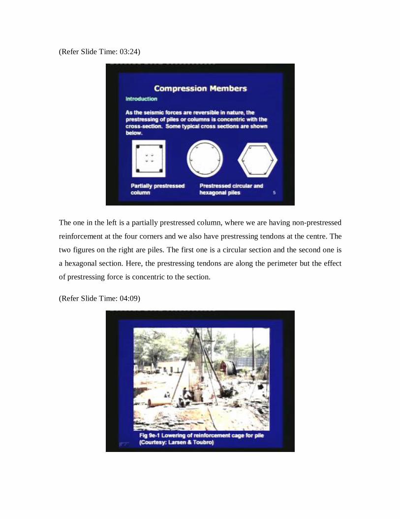
The one in the left is a partially prestressed column, where we are having non-prestressed
reinforcement at the four corners and we also have prestressing tendons at the centre. The
two figures on the right are piles. The first one is a circular section and the second one is
a hexagonal section. Here, the prestressing tendons are along the perimeter but the effect
of prestressing force is concentric to the section.
(Refer Slide Time: 04:09)
This is a figure which shows the lowering of the reinforcement cage for a pile.
(Refer Slide Time: 04:16)
Since a prestressed member is under self-equilibrium, there is no buckling of a column
due to internal prestressing with bonded tendons. In a deflected shape, there is no internal
moment due to prestressing. The justification is explained in the next figure.
(Refer Slide Time: 04:44)

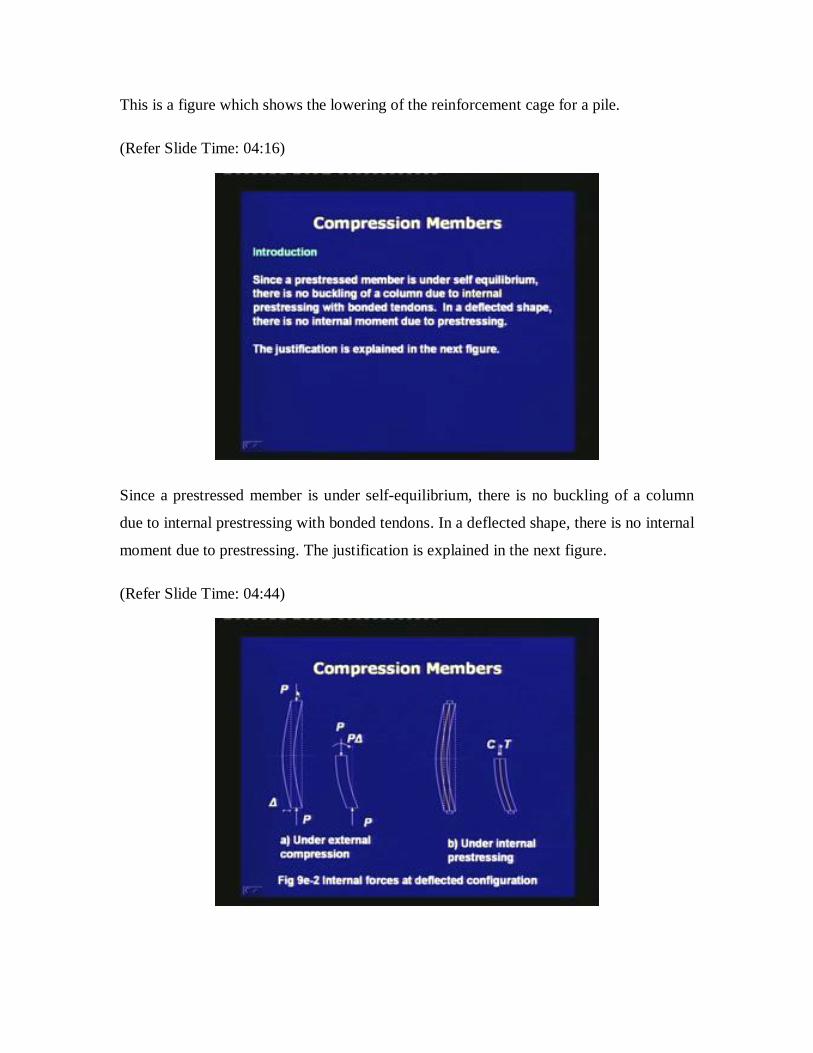
If a column or a pile is subjected to an axial force then, when it gets deflected there will
be a moment due to the deflected shape. For a deflection of at the middle, the moment
at mid-height is represented as P. This happens under an external axial compression.
Whereas for an internal prestressing we observe that, even under the deflected shape, the
internal prestressing is under equilibrium with the tension in the prestressing tendon, and
there is no internal moment generated under the deflected shape.
(Refer Slide Time: 05:33)
Thus, in the free body sketch of Figure 9e-a, the external compression P causes an
additional moment due to the deflection of the member. The value of the moment at mid-
height is P. This is known as the member stability effect, which is one type of P-
effect. If this deflection is not stable, then buckling of the member occurs.
Thus, the external compression can cause buckling of a member depending upon the
slenderness ratio.
(Refer Slide Time: 06:26)
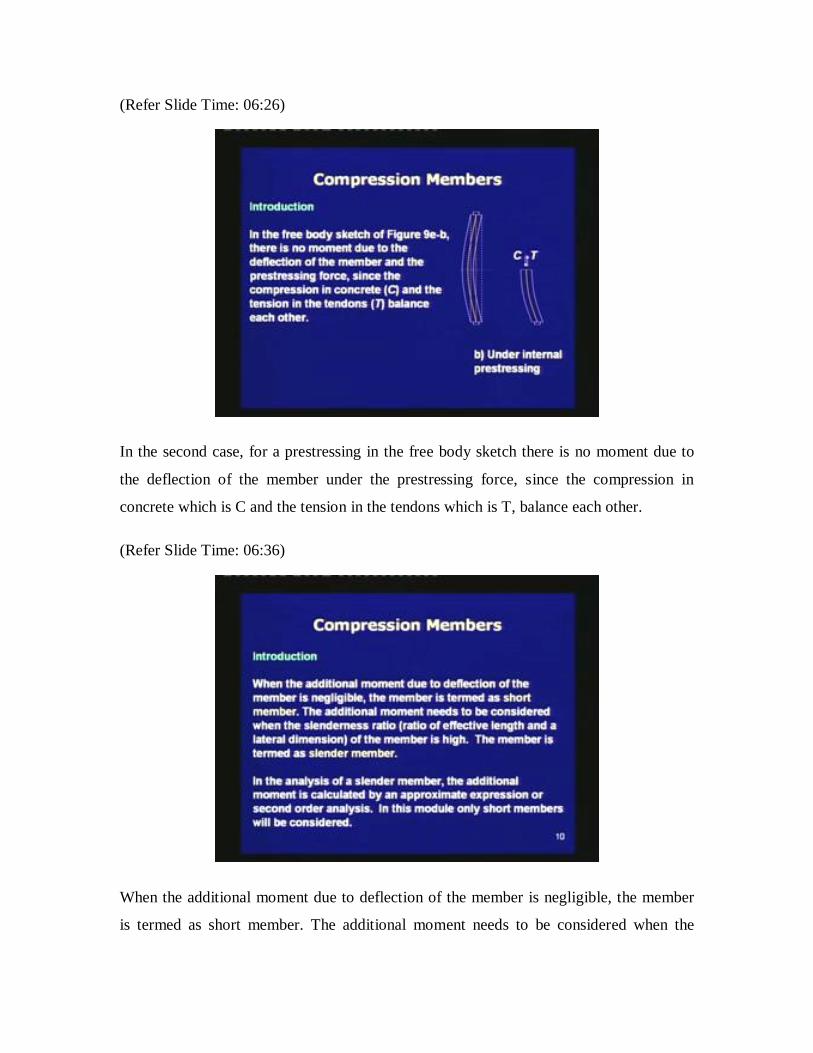
In the second case, for a prestressing in the free body sketch there is no moment due to
the deflection of the member under the prestressing force, since the compression in
concrete which is C and the tension in the tendons which is T, balance each other.
(Refer Slide Time: 06:36)
When the additional moment due to deflection of the member is negligible, the member
is termed as short member. The additional moment needs to be considered when the

slenderness ratio of the member is high (The slenderness ratio is the ratio of the effective
length and lateral dimension). This type of member is termed as slender member, where
the additional moment needs to be considered.
In the analysis of a slender member, the additional moment is calculated by an
approximate expression or second order analysis. Thus, if we have a slender member
with the slenderness ratio greater than a certain value then we need to account for the
additional moment generated due to the external compression. In this lecture, we are
considering only short members where the additional moment due to the deflection of the
member is negligible.
(Refer Slide Time: 08:06)
Next, we move on to the analysis of compression members. The stress in the section can
be calculated as follows.
fc = P0/A
Here, A is the area of concrete and P0 is prestress at transfer after short-term losses. Thus,
after the concrete is cast and then the prestress is transferred to the member, the stress in
the member is compressive and it is uniform since the prestressing is concentric. This
stress is given as the prestress at transfer, which is P0 divided by the area of the concrete,
which is A. For members under compression, a compressive stress is considered to be
positive. In this lecture, we shall consider that the compressive stress is positive and the
tensile stress is negative. This is the convention which is used for compression members.
(Refer Slide Time: 09:34)
The permissible prestress and the cross-sectional area are determined based on the stress
to be within the allowable stress at transfer (fcc,all). Thus, given the compressive stress to
be within the allowable value, we can determine P0 and A; a suitable combination of the
two variables.
(Refer Slide Time: 10:12)
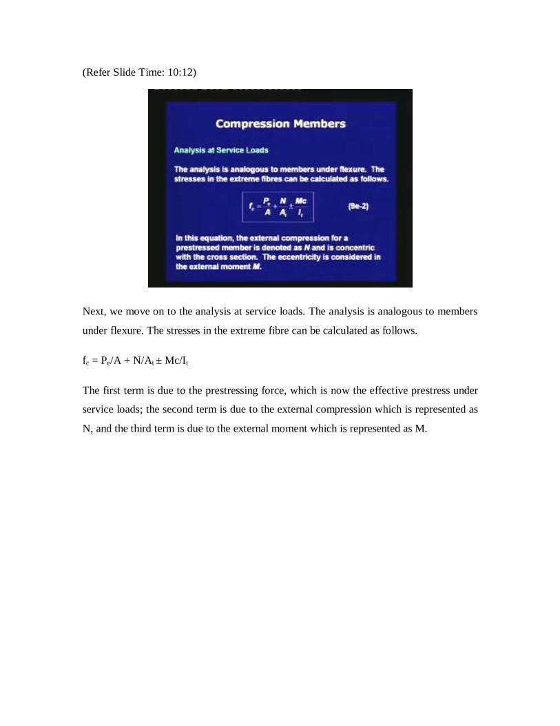
Next, we move on to the analysis at service loads. The analysis is analogous to members
under flexure. The stresses in the extreme fibre can be calculated as follows.
fc = Pe/A + N/At ± Mc/It
The first term is due to the prestressing force, which is now the effective prestress under
service loads; the second term is due to the external compression which is represented as
N, and the third term is due to the external moment which is represented as M.

(Refer Slide Time: 11:18)
In this equation, the external compression for a prestressed member is denoted as N and
is concentric with the cross-section. Any eccentricity is considered in the external
moment M. A is the area of concrete; At is the area of transformed section; c is the
distance of the extreme fibre from the centroid of the section which is CGC; It is the
moment of inertia of the transformed section; Pe is the effective prestress. The value of
the fc should be within the allowable stress under service conditions.
Next we move on to the analysis at ultimate.
(Refer Slide Time 11:42)
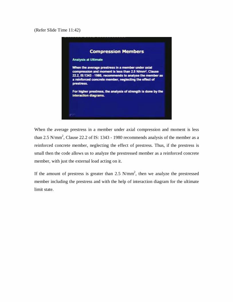
When the average prestress in a member under axial compression and moment is less
than 2.5 N/mm2, Clause 22.2 of IS: 1343 - 1980 recommends analysis of the member as a
reinforced concrete member, neglecting the effect of prestress. Thus, if the prestress is
small then the code allows us to analyze the prestressed member as a reinforced concrete
member, with just the external load acting on it.
If the amount of prestress is greater than 2.5 N/mm2, then we analyze the prestressed
member including the prestress and with the help of interaction diagram for the ultimate
limit state.

(Refer Slide Time: 13:02)
At the ultimate state, an interaction diagram relates the axial load capacity, which is
represented as NuR and the moment capacity which is represented as MuR. The subscripts
u and R stand for ultimate and resistance, respectively. The interaction diagram
represents a failure envelop. Any combination of factored external loads Nu and Mu that
fall within the interaction diagram is safe. Let us understand this by the help of a sketch.
A typical interaction diagram is shown below.
(Refer Slide Time: 13:35)

The shaded area inside gives combinations of external loads Mu and Nu those are safe.
Thus, this boundary is a failure envelope and any combination of the external loads which
falls within this boundary is safe. The combination which falls outside the boundary is
unsafe. In this boundary, we have two types of failure conditions. One is the compression
failure and the other is the tension failure. The transition between them is called the
balanced failure.
(Refer Slide Time: 14:47)
The radial line in the previous sketch represents the load path. Usually, the external loads
increase proportionally. At any load stage, M and N are related as follows.
M = NeN
Here, eN represents the eccentricity of N which generates the same moment M. The slope
of the radial line represents the inverse of the eccentricity, which is 1/eN. In most of the
cases, the axial load and the moment increase proportionally. Hence, the load path is a
straight line which passes through the origin and move towards to the failure envelope.
Note that eN is the ratio of the moment M and the axial force N. At ultimate, the values of
M and N, which are represented as Mu and Nu respectively, correspond to the values on
the interaction diagram. As the load increases along the load path, at ultimate the load
state falls on the interaction diagram, then a failure occurs.
(Refer Slide Time: 16:15)
For high values of N as compared to M, that is eN is small, the concrete in the
compression fibre will crush before the steel on the other side yields in tension. This is
called the compression failure. For high values of M as compared to N, that is eN is large,
the concrete will crush after the steel yields in tension. This is called the tension failure.
The transition of these two cases is referred to as the balanced failure, when the crushing
of concrete and yielding of steel occur simultaneously.
Thus, the significance of compression failure is that the concrete is crushing before the
steel has the chance to yield. The tension failure means the concrete is crushing after the
steel has yielded. The transition between them is called the balanced failure where the
crushing of concrete and yielding of steel occur simultaneously.
(Refer Slide Time: 17:20)
For a prestressed compression member, since the prestressing steel does not have a
definite yield point, there is no explicit balanced failure. The steel for a reinforced
concrete member, such as mild steel, tend to have a sharp yield point. Hence, the
definition of a balanced failure is not explicit for a prestressed compression member, as
compared to a reinforced concrete member under compression.
Next, we shall learn about the development of interaction diagram.

(Refer Slide Time: 18:18)
An interaction diagram can be developed from the first principles using the non-linear
stress-strain curves of concrete under compression and steel under tension. Several sets of
NuR and MuR for given values of eN or xu are calculated. The distance of neutral axis from
the extreme compressive face is denoted as xu. Partial safety factors for concrete and
prestressing steel can be introduced, when the interaction diagram is used for design.
Thus, the interaction diagram is developed by calculating values of the capacities NuR and
MuR for a given eccentricity eN. Also, one can do similar calculation, for a given value of
xu, where xu is the depth of the neutral axis from the extreme face under compression.
Once we calculate a set of NuR and MuR values, we can join those points to get an
approximate interaction diagram for that particular member. If we use partial safety
factors, then this curve can be used for design.
(Refer Slide Time: 19:57)
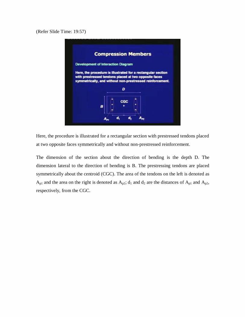
Here, the procedure is illustrated for a rectangular section with prestressed tendons placed
at two opposite faces symmetrically and without non-prestressed reinforcement.
The dimension of the section about the direction of bending is the depth D. The
dimension lateral to the direction of bending is B. The prestressing tendons are placed
symmetrically about the centroid (CGC). The area of the tendons on the left is denoted as
Ap1 and the area on the right is denoted as Ap2; d1 and d2 are the distances of Ap1 and Ap2,
respectively, from the CGC.

(Refer Slide Time: 20:52)
The notations thus used are as follows:
B is the dimension of the section transverse to bending; D is the dimension of section in
the direction of bending; Ap1 is the area of prestressing tendons at the tension face; Ap2 is
the area of prestressing tendons at the compression face; d1 and d2 are the distances of
centers of Ap1 and Ap2, respectively, from the centroid of the section which is CGC.
(Refer Slide Time: 21:22)
For a prestressed member, the strain compatibility equation is necessary. It relates the
strain in a prestressing tendon with that of the adjacent concrete. Due to a concentric
prestress, the concrete at a section undergoes a uniform compressive strain. With time,
the strain increases due to the effects of creep and shrinkage. At service, after the long-
term losses, let the strain in concrete be ce. Let the strain in the prestressing steel due to
effective prestress be pe.
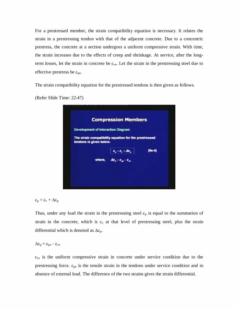
The strain compatibility equation for the prestressed tendons is then given as follows.
(Refer Slide Time: 22:47)
p = c + p
Thus, under any load the strain in the prestressing steel p is equal to the summation of
strain in the concrete, which is c at that level of prestressing steel, plus the strain
differential which is denoted as p.
p = pe ‒ ce
ce is the uniform compressive strain in concrete under service condition due to the
prestressing force. pe is the tensile strain in the tendons under service condition and in
absence of external load. The difference of the two strains gives the strain differential.
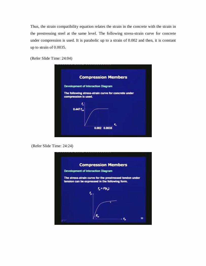
Thus, the strain compatibility equation relates the strain in the concrete with the strain in
the prestressing steel at the same level. The following stress-strain curve for concrete
under compression is used. It is parabolic up to a strain of 0.002 and then, it is constant
up to strain of 0.0035.
(Refer Slide Time: 24:04)
(Refer Slide Time: 24:24)

The stress-strain curve for the prestressed tendon under tension can be expressed in the
following form.
fp = F(p)
This curve is not elasto-plastic behaviour. It has a gradual transition from the elastic
behaviour with increasing plastic strain.
(Refer Slide Time: 24:52)
The calculation of NuR and MuR for typical cases of eN or xu are illustrated. The typical
cases are as follows.
1. The case of pure compression, where eN = 0 and xu =
2. Full section under compression, where eN can vary between 0.05D and less than
eN corresponding to xu = D; xu is greater or equal to D
3. Part of section under tension, where eN is greater than the value corresponding to
xu = D, but it is less than infinite (); xu is less than D
4. Pure bending, where eN = and xu = xu,min, which is the minimum value of xu.

(Refer Slide Time: 25:57)
In addition to the above cases, the case of pure axial tension is also calculated. The
straight line between the points of pure bending and pure axial tension provides the
interaction between the tensile force capacity and the moment capacity.
Thus, this part of the interaction diagram is in the lower quadrant, where the tensile axial
force is given by a negative value. We calculate the moment capacity of the section under
pure bending. We calculate the tensile force capacity of the member. The two points are
plotted and joined by a straight line. Any combination of the external loads that lie within
the green region is safe.
Next, we move on to the calculations for each of the typical cases separately.
(Refer Slide Time: 27:25)
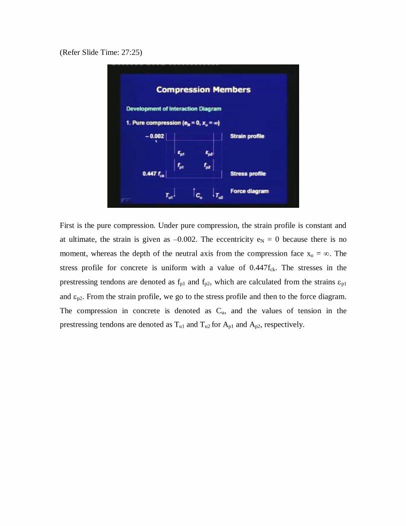
First is the pure compression. Under pure compression, the strain profile is constant and
at ultimate, the strain is given as ‒0.002. The eccentricity eN = 0 because there is no
moment, whereas the depth of the neutral axis from the compression face xu = . The
stress profile for concrete is uniform with a value of 0.447fck. The stresses in the
prestressing tendons are denoted as fp1 and fp2, which are calculated from the strains p1
and p2. From the strain profile, we go to the stress profile and then to the force diagram.
The compression in concrete is denoted as Cu, and the values of tension in the
prestressing tendons are denoted as Tu1 and Tu2 for Ap1 and Ap2, respectively.
(Refer Slide Time: 29:18)
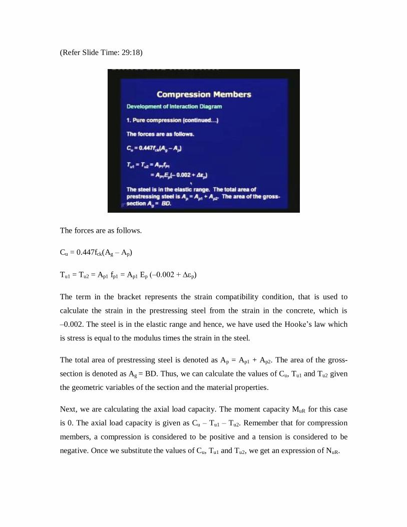
The forces are as follows.
Cu = 0.447fck(Ag ‒ Ap)
Tu1 = Tu2 = Ap1 fp1 = Ap1 Ep (‒0.002 + p)
The term in the bracket represents the strain compatibility condition, that is used to
calculate the strain in the prestressing steel from the strain in the concrete, which is
‒0.002. The steel is in the elastic range and hence, we have used the Hooke’s law which
is stress is equal to the modulus times the strain in the steel.
The total area of prestressing steel is denoted as Ap = Ap1 + Ap2. The area of the gross-
section is denoted as Ag = BD. Thus, we can calculate the values of Cu, Tu1 and Tu2 given
the geometric variables of the section and the material properties.
Next, we are calculating the axial load capacity. The moment capacity MuR for this case
is 0. The axial load capacity is given as Cu ‒ Tu1 ‒ Tu2. Remember that for compression
members, a compression is considered to be positive and a tension is considered to be
negative. Once we substitute the values of Cu, Tu1 and Tu2, we get an expression of NuR.

(Refer Slide Time: 30:27)
In design, to approximate the effect of moment for eccentricities eN ≤ 0.05D, the axial
force capacity is reduced by 10%. If a member is subjected to small moment (eccentricity
is less than 5% of the dimension D), then the use of the interaction diagram is bye-passed
by considering a reduced axial force capacity and the effect of moment is neglected. In
that case, NuR is given as follows.
NuR = 0.4fck (Ag ‒ Ap) ‒ 0.9ApEP (p ‒ 0.002 + ce)
Next, we move onto the case of a full section under compression, under simultaneous
axial load and moment.
(Refer Slide Time: 31:48)
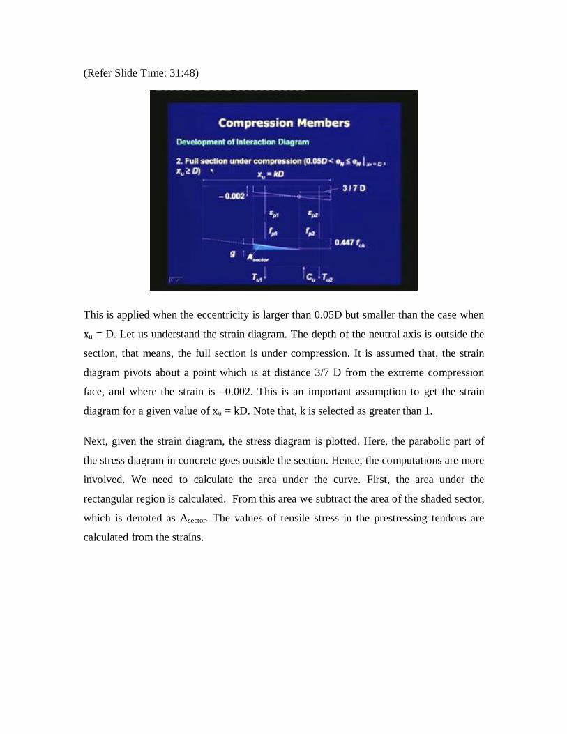
This is applied when the eccentricity is larger than 0.05D but smaller than the case when
xu = D. Let us understand the strain diagram. The depth of the neutral axis is outside the
section, that means, the full section is under compression. It is assumed that, the strain
diagram pivots about a point which is at distance 3/7 D from the extreme compression
face, and where the strain is ‒0.002. This is an important assumption to get the strain
diagram for a given value of xu = kD. Note that, k is selected as greater than 1.
Next, given the strain diagram, the stress diagram is plotted. Here, the parabolic part of
the stress diagram in concrete goes outside the section. Hence, the computations are more
involved. We need to calculate the area under the curve. First, the area under the
rectangular region is calculated. From this area we subtract the area of the shaded sector,
which is denoted as Asector. The values of tensile stress in the prestressing tendons are
calculated from the strains.
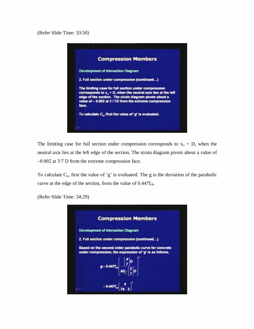
(Refer Slide Time: 33:50)
The limiting case for full section under compression corresponds to xu = D, when the
neutral axis lies at the left edge of the section. The strain diagram pivots about a value of
‒0.002 at 3/7 D from the extreme compression face.
To calculate Cu, first the value of ‘g’ is evaluated. The g is the deviation of the parabolic
curve at the edge of the section, from the value of 0.447fck.
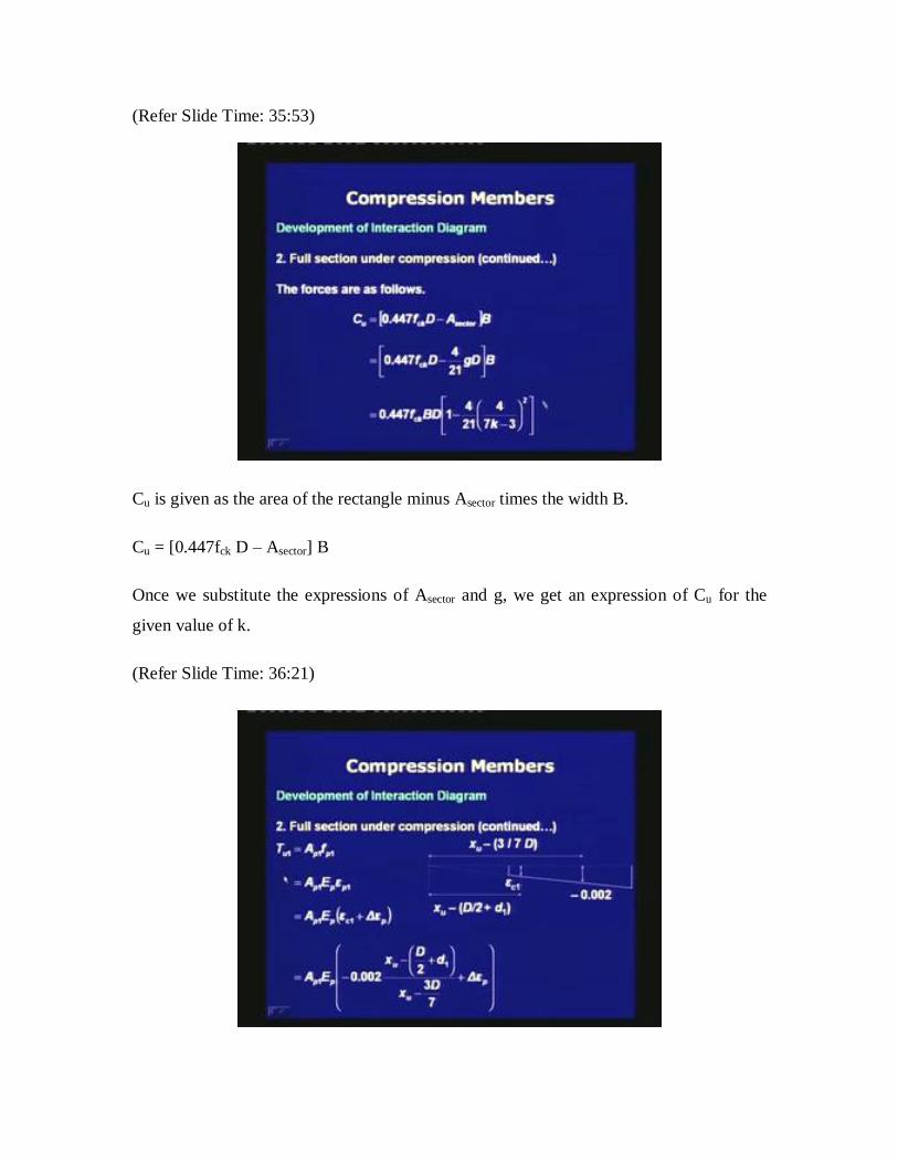
(Refer Slide Time: 34:29)

Based on the second order parabolic curve for concrete under compression, the
expression of ‘g’ is as follows. This expression can be derived by assuming a second
order parabola.
g = 0.447fck [(4/7) D / (kD ‒ (3/7) D)]2 = 0.447fck (4/(7k ‒ 3))
2
(Refer Slide Time: 35:23)
The area of the sector is given as follows. It is one-third of g times the distance to the
apex from the base, which is 4/7 D.
Asector = 1/3 g (4/7 D) = (4/21) gD
The distance of the centroid of this area from the pivot (apex) is as follows.
x/ = (3/4) (4/7 D) = 3/7 D
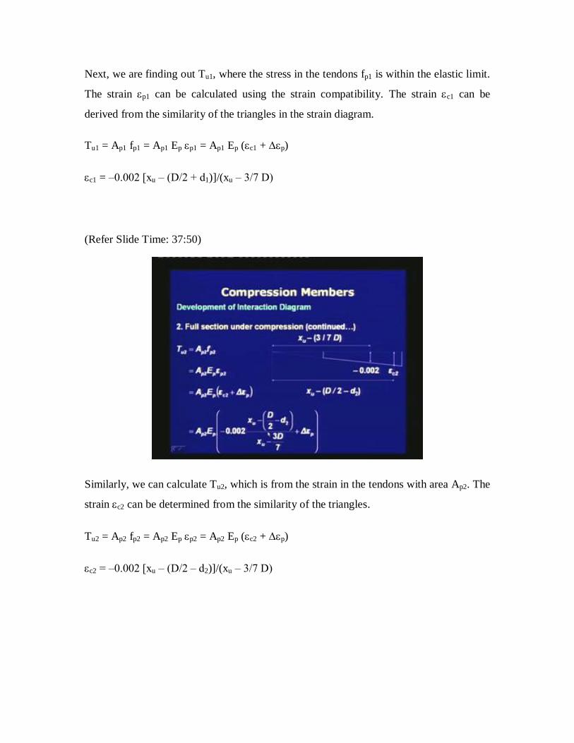
(Refer Slide Time: 35:53)
Cu is given as the area of the rectangle minus Asector times the width B.
Cu = [0.447fck D ‒ Asector] B
Once we substitute the expressions of Asector and g, we get an expression of Cu for the
given value of k.
(Refer Slide Time: 36:21)
Next, we are finding out Tu1, where the stress in the tendons fp1 is within the elastic limit.
The strain p1 can be calculated using the strain compatibility. The strain c1 can be
derived from the similarity of the triangles in the strain diagram.
Tu1 = Ap1 fp1 = Ap1 Ep p1 = Ap1 Ep (c1 + p)
c1 = ‒0.002 [xu ‒ (D/2 + d1)]/(xu ‒ 3/7 D)
(Refer Slide Time: 37:50)
Similarly, we can calculate Tu2, which is from the strain in the tendons with area Ap2. The
strain c2 can be determined from the similarity of the triangles.
Tu2 = Ap2 fp2 = Ap2 Ep p2 = Ap2 Ep (c2 + p)
c2 = ‒0.002 [xu ‒ (D/2 ‒ d2)]/(xu ‒ 3/7 D)
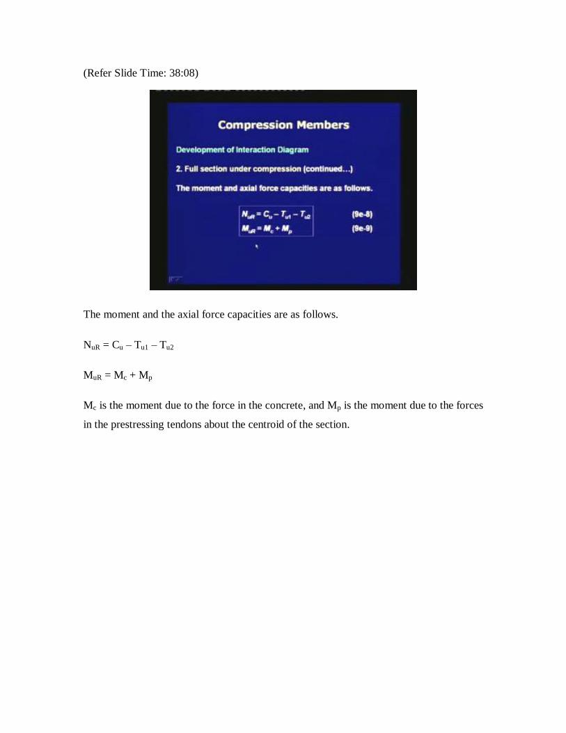
(Refer Slide Time: 38:08)
The moment and the axial force capacities are as follows.
NuR = Cu ‒ Tu1 ‒ Tu2
MuR = Mc + Mp
Mc is the moment due to the force in the concrete, and Mp is the moment due to the forces
in the prestressing tendons about the centroid of the section.

(Refer Slide Time: 39:32)
Anti-clock wise moments are considered to be positive in this derivation. For Mc, the
centroid of the rectangle lies at the centroid of the section, and hence the rectangular
stress block does not create any moment about the centroid. Thus Mc is only due to the
area of the sector, Asector.
Mc = 0.447 fck DB 0 + Asector B [x/ + 3/7 D ‒ D/2] = 10/147 gD
2B
Mp is calculated by taking the moments of Tu1 and Tu2 about the centroid.
Mp = Tu1 d1 ‒ Tu2 d2
Next, we move to the case where part of the section is under tension at ultimate.

(Refer Slide Time: 40:42)
Note that, on the left hand side of the strain diagram there is some tension. The value of
eN is more than the value corresponding to xu = D, but less than infinite () which is for
the case of pure bending. The depth of the neutral axis xu is lower than D. Note that, the
extreme compressive strain is 0.0035.
From the strain diagram we get the stress diagram at ultimate. It is similar to that for a
reinforced concrete section. Once the section cracks due to tension, the analysis is similar
to that for a section under flexure. The forces are as follows. Cu is the resultant of the
stress block in concrete.
Cu = 0.36 fck xu B
Tu1 = Ap1fp1
Tu2 = Ap2fp2
Here, fp1 should be calculated from the stress‒strain curve for the tendon. The tendons for
Ap1 may start yielding. Hence, we should not use the elastic value of the stress without
checking whether the steel is yielding or not. For Ap2 the steel need not yield, and we can
use the elastic relationship to calculate fp2.
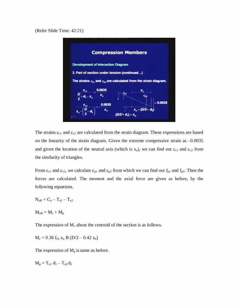
(Refer Slide Time: 42:21)
The strains c1 and c2 are calculated from the strain diagram. These expressions are based
on the linearity of the strain diagram. Given the extreme compressive strain as ‒0.0035
and given the location of the neutral axis (which is xu), we can find out c1 and c2 from
the similarity of triangles.
From c1 and c2, we calculate p1 and p2 from which we can find out fp1 and fp2. Then the
forces are calculated. The moment and the axial force are given as before, by the
following equations.
NuR = Cu ‒ Tu1 ‒ Tu2
MuR = Mc + Mp
The expression of Mc about the centroid of the section is as follows.
Mc = 0.36 fck xu B (D/2 ‒ 0.42 xu)
The expression of Mp is same as before.
Mp = Tu1 d1 ‒ Tu2 d2

Finally, we are coming to the case of pure bending where there is no axial force and the
eccentricity is infinite. The depth of the neutral axis is minimum among all the cases.
(Refer Slide Time: 44:19)
The value of xu is determined by trial and error from the condition that the sum of the
forces is zero.
Cu ‒ Tu1 ‒ Tu2 = 0
After substituting the values of Cu, Tu1 and Tu2, we get the expression of xu.
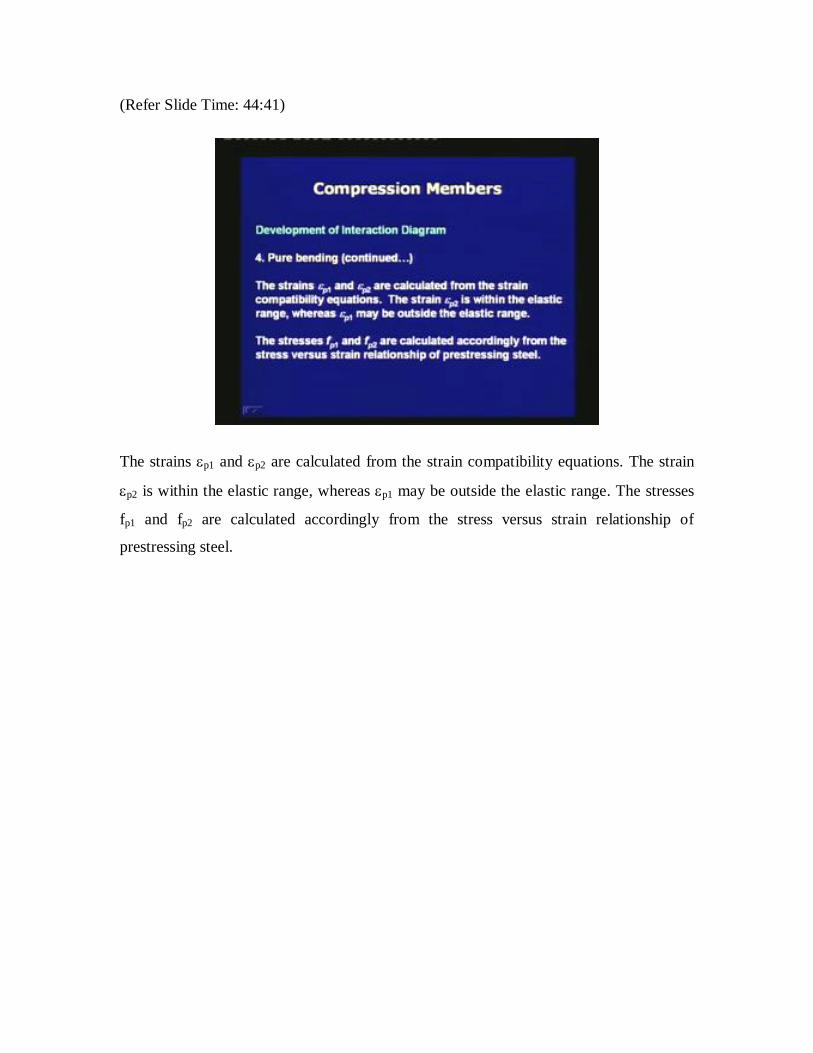
(Refer Slide Time: 44:41)
The strains p1 and p2 are calculated from the strain compatibility equations. The strain
p2 is within the elastic range, whereas p1 may be outside the elastic range. The stresses
fp1 and fp2 are calculated accordingly from the stress versus strain relationship of
prestressing steel.

(Refer Slide Time: 45:58)
The steps for solving xu are as follows.
1. Assume some value for xu say, 15% of the total depth D.
2. Determine p1 and p2 from the strain compatibility equations.
3. Determine fp1 and fp2 from the stress versus strain relationship for the prestressing
tendon.
4. Calculate xu from the expression which satisfies that the net axial force in the
section is zero.
5. Compare this xu with the assumed value. If it does not satisfy, iterate till the value
converges.
The moment and the axial force capacities are as follows.
NuR = 0
MuR = Mc + Mp
The expressions of Mc and Mp are same as the previous case.
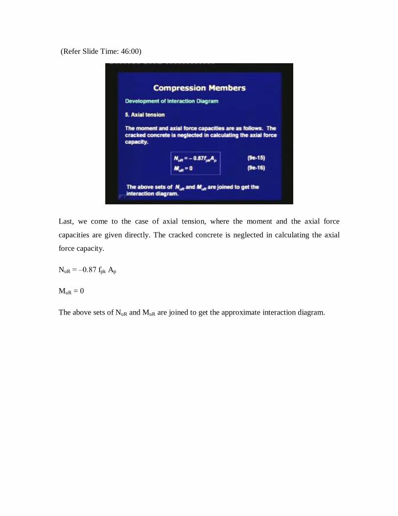
(Refer Slide Time: 46:00)
Last, we come to the case of axial tension, where the moment and the axial force
capacities are given directly. The cracked concrete is neglected in calculating the axial
force capacity.
NuR = ‒0.87 fpk Ap
MuR = 0
The above sets of NuR and MuR are joined to get the approximate interaction diagram.
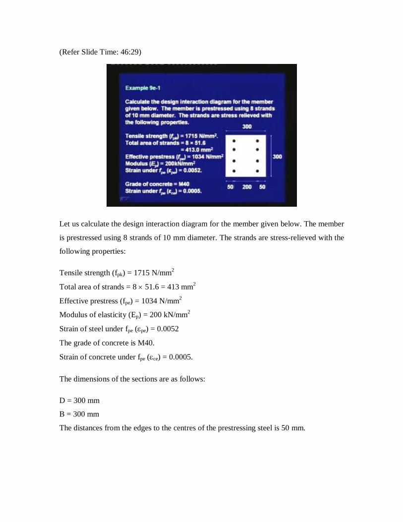
(Refer Slide Time: 46:29)
Let us calculate the design interaction diagram for the member given below. The member
is prestressed using 8 strands of 10 mm diameter. The strands are stress-relieved with the
following properties:
Tensile strength (fpk) = 1715 N/mm2
Total area of strands = 8 51.6 = 413 mm2
Effective prestress (fpe) = 1034 N/mm2
Modulus of elasticity (Ep) = 200 kN/mm2
Strain of steel under fpe (pe) = 0.0052
The grade of concrete is M40.
Strain of concrete under fpe (ce) = 0.0005.
The dimensions of the sections are as follows:
D = 300 mm
B = 300 mm
The distances from the edges to the centres of the prestressing steel is 50 mm.

(Refer Slide Time: 47:44)
Calculation of geometric properties and strain compatibility relationship:
Ag = 90,000 mm2
Ap1 = Ap2 = 206 mm2
d1 = d2 = 100 mm
p = 0.0052 ‒ 0.0005 = 0.0047
Thus, the strain compatibility equation is p = c + 0.0047.
(Refer Slide Time: 48:29)
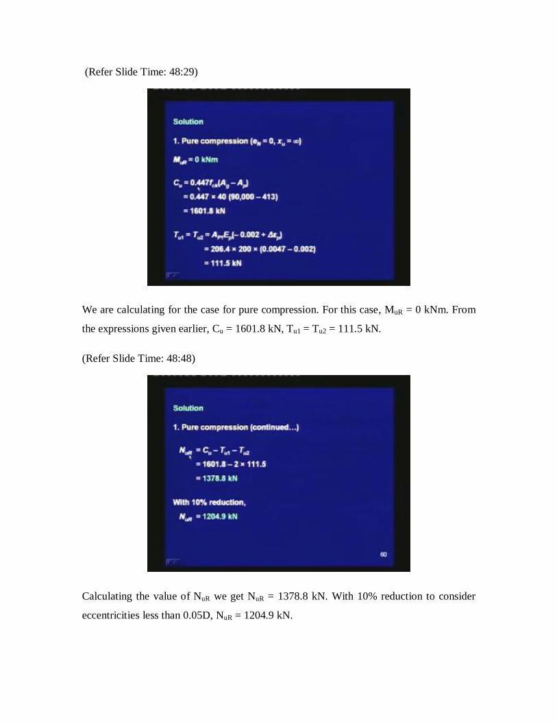
We are calculating for the case for pure compression. For this case, MuR = 0 kNm. From
the expressions given earlier, Cu = 1601.8 kN, Tu1 = Tu2 = 111.5 kN.
(Refer Slide Time: 48:48)
Calculating the value of NuR we get NuR = 1378.8 kN. With 10% reduction to consider
eccentricities less than 0.05D, NuR = 1204.9 kN.

(Refer Slide Time: 49:16)
Next, we are calculating for the full section under compression. We are selecting xu = 400
mm. Note that the depth of the section is 300 mm. Thus, xu lies 100 mm outside the
section, where k = 4/3. We can calculate the value of g by the previous expression.
(Refer Slide Time: 49:35)
Then, we get the value of Cu by substituting the variables in the previous expression. Cu =
1486.9 kN.

(Refer Slide Time: 49:53)
The strain in concrete at Ap1 (c1) is calculated from the strain compatibility relationship.
Then we get Tu1 = 148.4 kN.
(Refer Slide Time: 50:03)
Similarly, the strain in concrete at Ap2 (c2) is calculated, from which Tu2 = 87.5 kN.
(Refer Slide Time: 50:14)
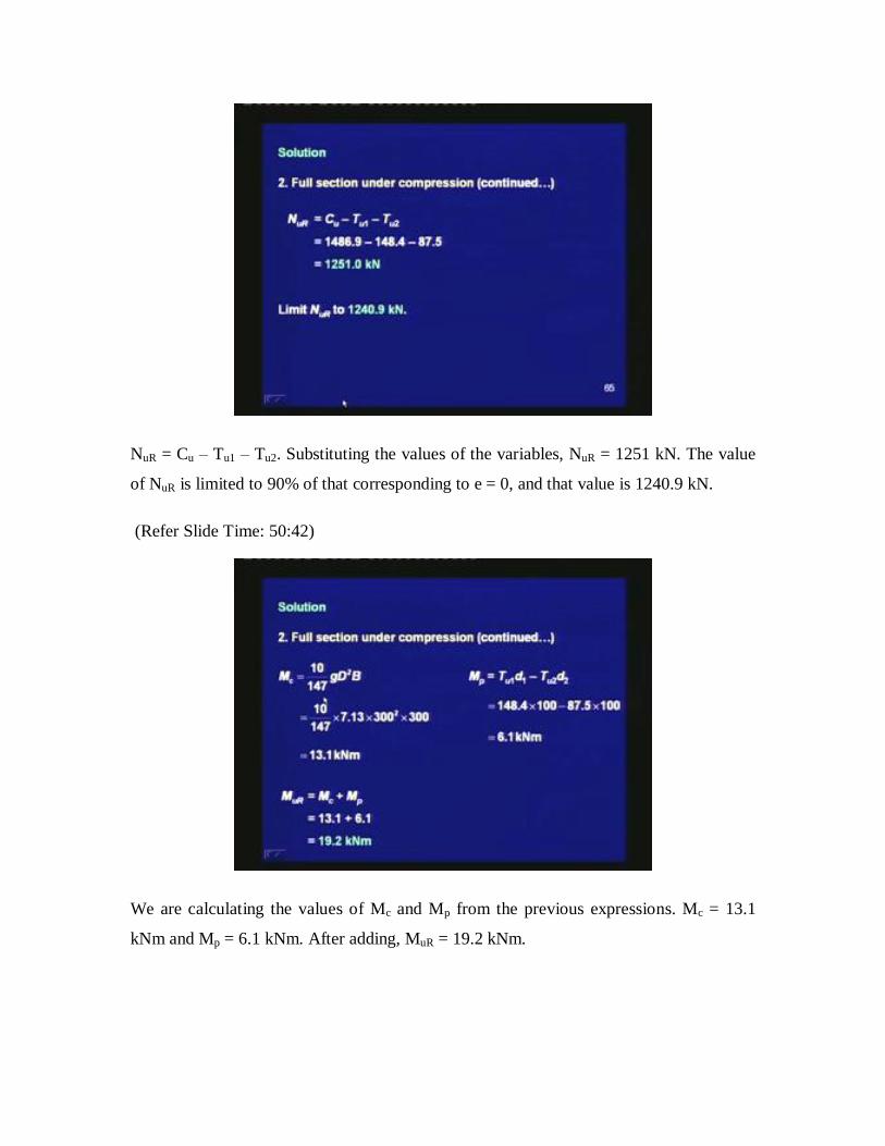
NuR = Cu ‒ Tu1 ‒ Tu2. Substituting the values of the variables, NuR = 1251 kN. The value
of NuR is limited to 90% of that corresponding to e = 0, and that value is 1240.9 kN.
(Refer Slide Time: 50:42)
We are calculating the values of Mc and Mp from the previous expressions. Mc = 13.1
kNm and Mp = 6.1 kNm. After adding, MuR = 19.2 kNm.
(Refer Slide Time: 51:08)
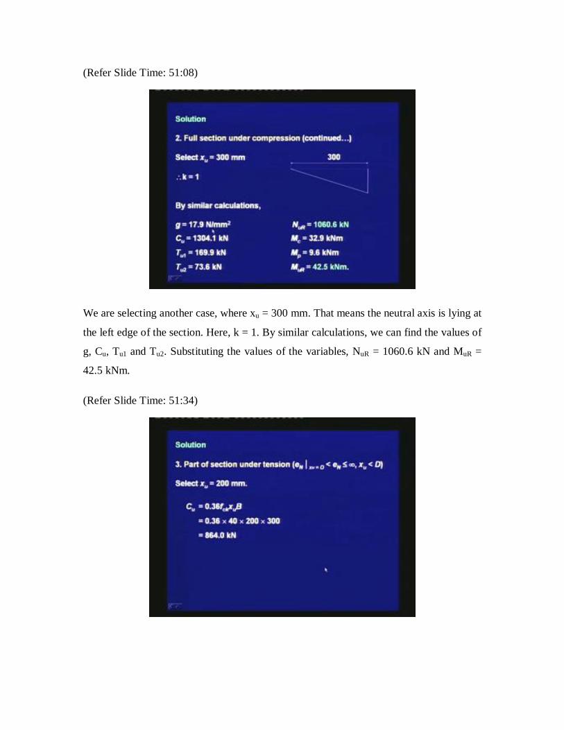
We are selecting another case, where xu = 300 mm. That means the neutral axis is lying at
the left edge of the section. Here, k = 1. By similar calculations, we can find the values of
g, Cu, Tu1 and Tu2. Substituting the values of the variables, NuR = 1060.6 kN and MuR =
42.5 kNm.
(Refer Slide Time: 51:34)
Next, we move on to the case of part of the section under tension. We are selecting xu =
200 mm. Note that, the neutral axis lies within the section. Based on the expression, Cu =
864 kN.
(Refer Slide Time: 51:55)
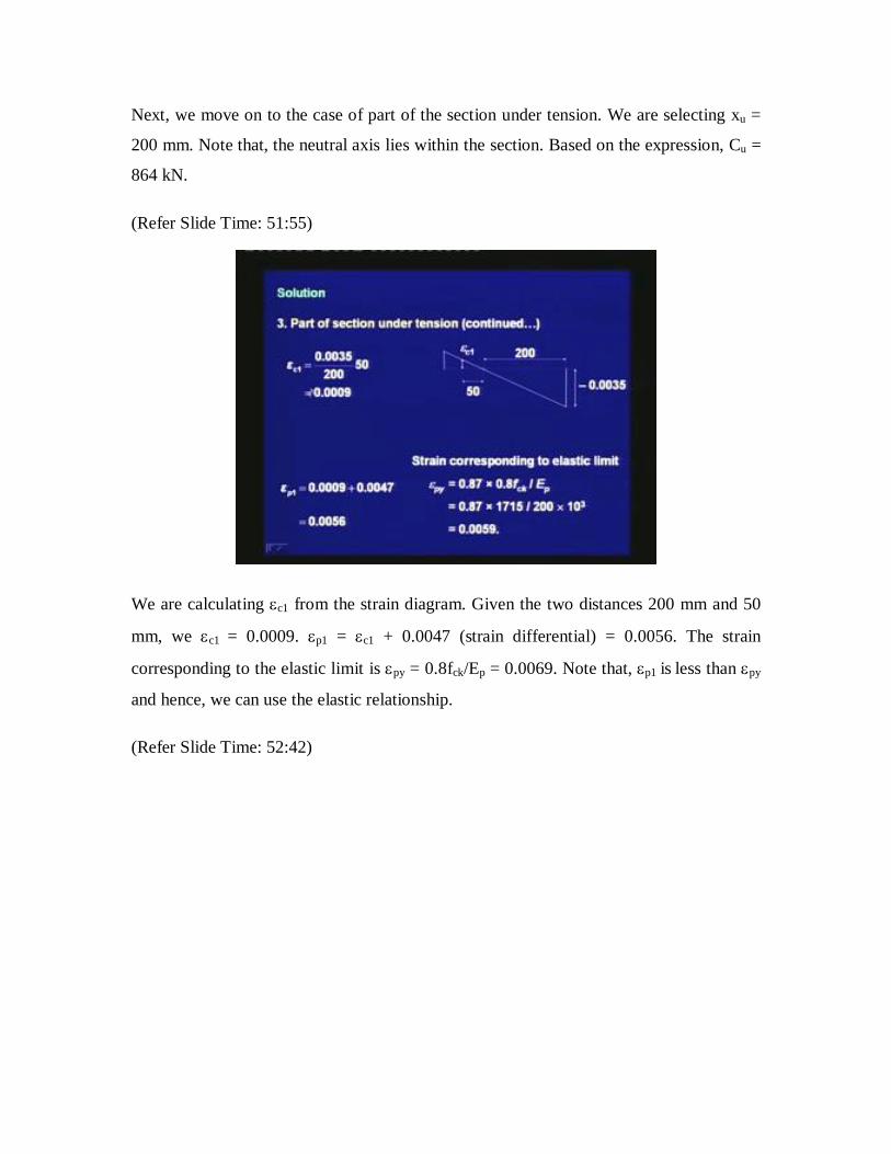
We are calculating c1 from the strain diagram. Given the two distances 200 mm and 50
mm, we c1 = 0.0009. p1 = c1 + 0.0047 (strain differential) = 0.0056. The strain
corresponding to the elastic limit is py = 0.8fck/Ep = 0.0069. Note that, p1 is less than py
and hence, we can use the elastic relationship.
(Refer Slide Time: 52:42)
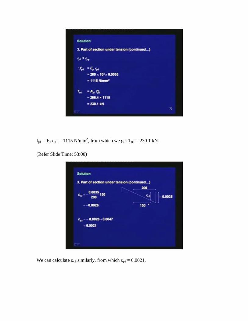
fp1 = Ep p1 = 1115 N/mm2, from which we get Tu1 = 230.1 kN.
(Refer Slide Time: 53:00)
We can calculate c2 similarly, from which p2 = 0.0021.

(Refer Slide Time: 53:15)
The value of fp2 is calculated from the elastic relationship, and Tu2 = 85.9 kN. Thus, NuR
= 548.0 kN.
(Refer Slide Time: 53:31)
Substituting the values of the variables, Mc = 57.0 kNm and Mp = 14.4 kNm. Thus, MuR =
Mc + Mp = 71.4 kNm.
(Refer Slide Time: 53:52)
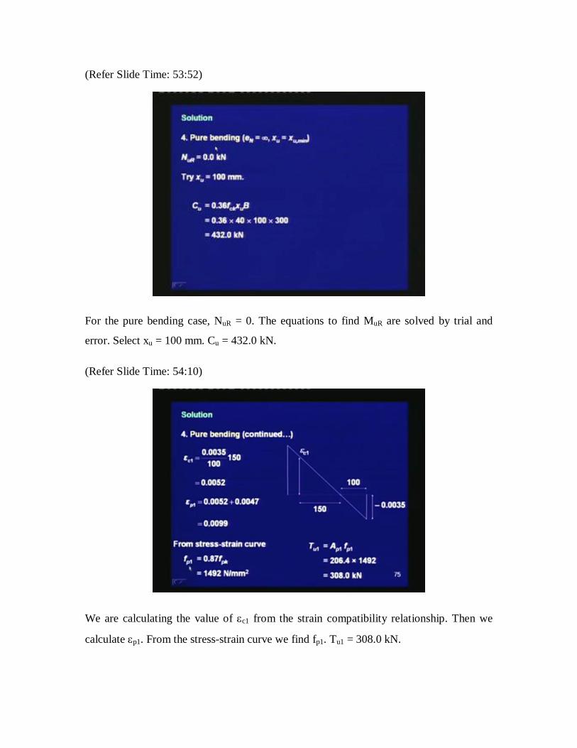
For the pure bending case, NuR = 0. The equations to find MuR are solved by trial and
error. Select xu = 100 mm. Cu = 432.0 kN.
(Refer Slide Time: 54:10)
We are calculating the value of c1 from the strain compatibility relationship. Then we
calculate p1. From the stress-strain curve we find fp1. Tu1 = 308.0 kN.
(Refer Slide Time: 54:30)
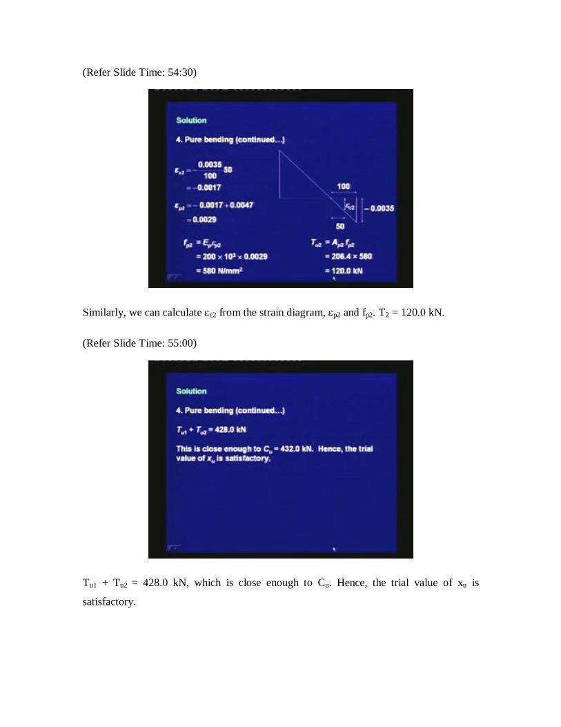
Similarly, we can calculate c2 from the strain diagram, p2 and fp2. T2 = 120.0 kN.
(Refer Slide Time: 55:00)
Tu1 + Tu2 = 428.0 kN, which is close enough to Cu. Hence, the trial value of xu is
satisfactory.
(Refer Slide Time: 55:14)
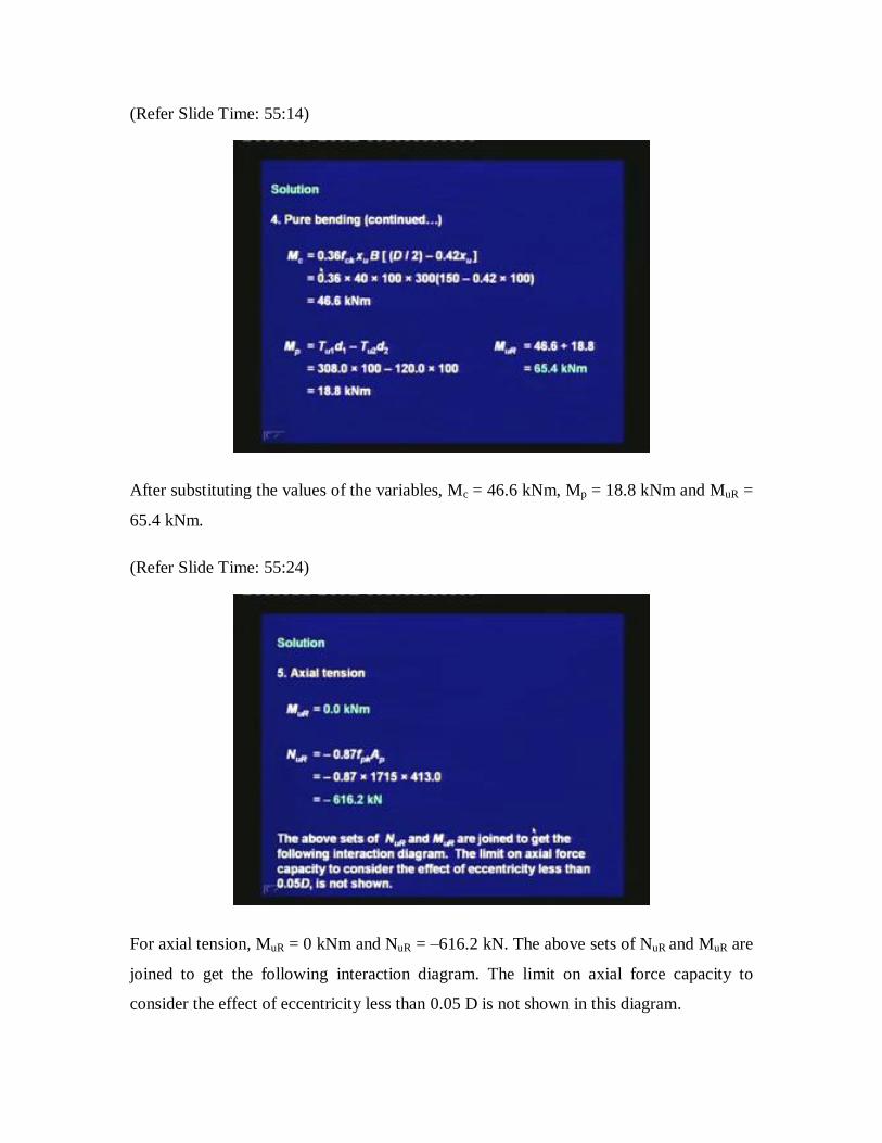
After substituting the values of the variables, Mc = 46.6 kNm, Mp = 18.8 kNm and MuR =
65.4 kNm.
(Refer Slide Time: 55:24)
For axial tension, MuR = 0 kNm and NuR = ‒616.2 kN. The above sets of NuR and MuR are
joined to get the following interaction diagram. The limit on axial force capacity to
consider the effect of eccentricity less than 0.05 D is not shown in this diagram.
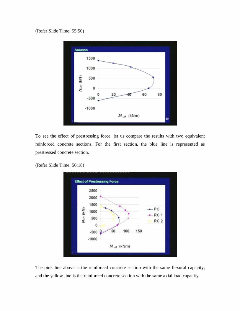
(Refer Slide Time: 55:50)
To see the effect of prestressing force, let us compare the results with two equivalent
reinforced concrete sections. For the first section, the blue line is represented as
prestressed concrete section.
(Refer Slide Time: 56:18)
The pink line above is the reinforced concrete section with the same flexural capacity,
and the yellow line is the reinforced concrete section with the same axial load capacity.
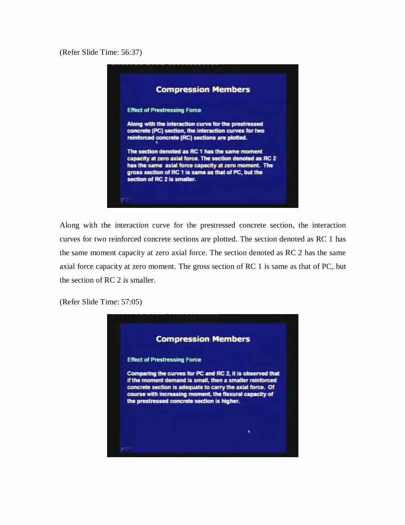
(Refer Slide Time: 56:37)
Along with the interaction curve for the prestressed concrete section, the interaction
curves for two reinforced concrete sections are plotted. The section denoted as RC 1 has
the same moment capacity at zero axial force. The section denoted as RC 2 has the same
axial force capacity at zero moment. The gross section of RC 1 is same as that of PC, but
the section of RC 2 is smaller.
(Refer Slide Time: 57:05)
Comparing the curves for PC and RC 2, it is observed that if the moment demand is small
then a smaller reinforced concrete section is adequate to carry the axial force. Of course
with increasing moment, the flexural capacity of the prestressed concrete section is
higher.
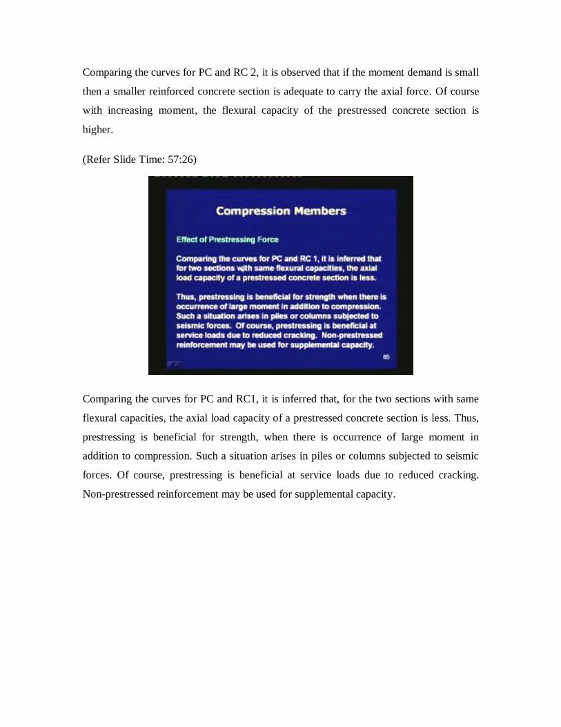
(Refer Slide Time: 57:26)
Comparing the curves for PC and RC1, it is inferred that, for the two sections with same
flexural capacities, the axial load capacity of a prestressed concrete section is less. Thus,
prestressing is beneficial for strength, when there is occurrence of large moment in
addition to compression. Such a situation arises in piles or columns subjected to seismic
forces. Of course, prestressing is beneficial at service loads due to reduced cracking.
Non-prestressed reinforcement may be used for supplemental capacity.

(Refer Slide Time: 58:05)
Today, we covered the compression members. After the introduction of the different
types of application of prestressing in compression members, we went on to the analysis
of compression members. We first saw the analysis at transfer, then at service, and
finally, at the ultimate state. For the ultimate state, we need the interaction diagrams. We
learnt the development of interaction diagrams. We came to know that the effect of
prestressing is beneficial only when there is high moment along with axial compression;
otherwise it may not be economical. With this we are ending the module on compression
members.
Thank you.