Prestress Losses in Lightweight Self-Consolidating Concrete

University of Arkansas, FayettevilleScholarWorks@UARK

Theses and Dissertations

12-2012

Prestress Losses in Lightweight Self-ConsolidatingConcreteJared BymasterUniversity of Arkansas, Fayetteville

Follow this and additional works at: http://scholarworks.uark.edu/etd

Part of the Transportation Engineering Commons

This Thesis is brought to you for free and open access by ScholarWorks@UARK. It has been accepted for inclusion in Theses and Dissertations by anauthorized administrator of ScholarWorks@UARK. For more information, please contact [email protected], [email protected].

Recommended CitationBymaster, Jared, "Prestress Losses in Lightweight Self-Consolidating Concrete" (2012). Theses and Dissertations. 568.http://scholarworks.uark.edu/etd/568

http://scholarworks.uark.edu?utm_source=scholarworks.uark.edu%2Fetd%2F568&utm_medium=PDF&utm_campaign=PDFCoverPages

http://scholarworks.uark.edu/etd?utm_source=scholarworks.uark.edu%2Fetd%2F568&utm_medium=PDF&utm_campaign=PDFCoverPages

http://scholarworks.uark.edu/etd?utm_source=scholarworks.uark.edu%2Fetd%2F568&utm_medium=PDF&utm_campaign=PDFCoverPages

http://network.bepress.com/hgg/discipline/1329?utm_source=scholarworks.uark.edu%2Fetd%2F568&utm_medium=PDF&utm_campaign=PDFCoverPages

http://scholarworks.uark.edu/etd/568?utm_source=scholarworks.uark.edu%2Fetd%2F568&utm_medium=PDF&utm_campaign=PDFCoverPages

mailto:[email protected],%[email protected]

PRESTRESS LOSSES IN LIGHTWEIGHT SELF-CONSOLIDATING CONCRETE

PRESTRESS LOSSES IN LIGHTWEIGHT SELF-CONSOLIDATING CONCRETE

A thesis submitted in partial fulfillment of the requirements for the degree of

Master of Science in Civil Engineering

By

Jared Bymaster University of Arkansas

Bachelor of Science in Civil Engineering, 2011

December 2012 University of Arkansas

ABSTRACT

While much research has been performed on lightweight concrete and self-consolidating

concrete (SCC), the knowledge of prestress losses in lightweight self-consolidating concrete

(LWSCC) is still limited. LWSCC has the benefits of increased flowability, reduced placement

labor, and decreased shipping cost compared to conventional concrete. This research program

included the study of 14 SCC beams cast with expanded clay, expanded shale, and limestone

aggregates. Strains in the beams were measured with vibrating-wire strain gages, and the

measured prestress losses were compared with current AASHTO methods for calculating

prestress losses. The AASHTO approximate method better predicted actual losses than did the

AASHTO refined method. In addition, the AASHTO approximate method gave more accurate

results for the LWSCC beams than it did for the normalweight SCC beams. This research

showed that the AASHTO refined method is overly sensitive to the concrete compressive

strength and modulus of elasticity at release.

The properties associated with the researched concrete mixes were also studied, and their

effects on prestress losses are discussed. Companion cylinders were used for compressive

strength and modulus of elasticity testing. Shrinkage prisms were also cast. The total prestress

losses were greater for the LWSCC which had lower modulus of elasticity than the normalweight

SCC. Less shrinkage occurred in the LWSCC mixtures than the SCC due to internal curing.

This thesis is approved for recommendation to the Graduate Council. Thesis Director: _______________________________________ W. Micah Hale Thesis Committee: _______________________________________ Ernest Heymsfield _______________________________________ Kirk Grimmelsman

THESIS DUPLICATION RELEASE

I hereby authorize the University of Arkansas Libraries to duplicate this thesis when needed for research and/or scholarship. Agreed __________________________________________ Jared Bymaster Refused __________________________________________ Jared Bymaster

CONTENTS

CHAPTER 1: INTRODUCTION ................................................................................................... 1

1.1 INTRODUCTION ................................................................................................................ 1

1.2 OBJECTIVE ......................................................................................................................... 2

1.3 TESTING .............................................................................................................................. 2

CHAPTER 2: BACKGROUND AND LITERATURE REVIEW ................................................. 3

2.1 INTRODUCTION ................................................................................................................ 3

2.2 CONCRETE CLASSIFICATION ........................................................................................ 3

2.2.1 Conventional Concrete................................................................................................... 3

2.2.2 Lightweight Concrete..................................................................................................... 4

2.2.3 Prestressed Concrete ...................................................................................................... 5

2.2.4 Self-Consolidating Concrete .......................................................................................... 5

2.2.5 High Performance Concrete ........................................................................................... 6

2.3 PRESTRESS LOSSES ......................................................................................................... 7

2.3.1 Instantaneous Losses ...................................................................................................... 8

2.3.2 Long-Term Losses ......................................................................................................... 9

2.4 ESTIMATING METHODS OF PRESTRESS LOSSES .................................................... 12

2.4.1 AASHTO LRFD Bridge Design Specifications .......................................................... 12

2.4.2 PCI Method .................................................................................................................. 15

2.5 PREVIOUS RESEARCH OF PRESTRESS LOSSES ....................................................... 16

2.5.1 Zia et al. (1979) ............................................................................................................ 16

2.5.2 Tadros et al. (2003) ...................................................................................................... 17

2.5.3 Kahn (2005) ................................................................................................................. 18

2.5.4 Larson (2006) ............................................................................................................... 19

2.5.5 Dymond (2007) ............................................................................................................ 20

2.5.6 Holste et al. (2011) ....................................................................................................... 21

2.5.7 Summary ...................................................................................................................... 22

CHAPTER 3: PROCEDURE ....................................................................................................... 23

3.1 INTRODUCTION .............................................................................................................. 23

3.2 BEAM CONSTRUCTION & STRAIN GAGE READINGS ............................................ 23

3.2.1 Mix Design................................................................................................................... 23

3.2.2 Mixing Procedure......................................................................................................... 24

3.2.3 Beam Design ................................................................................................................ 27

3.2.4 Detensioning Strands ................................................................................................... 31

3.2.5 Compressive Strengths................................................................................................. 32

3.2.6 Fresh Properties ........................................................................................................... 32

3.3 MODULUS OF ELASTICITY........................................................................................... 34

3.4 SHRINKAGE TESTING .................................................................................................... 35

3.5 BEAM LOADING .............................................................................................................. 36

CHAPTER 4: RESULTS .............................................................................................................. 38

4.1 INTRODUCTION .............................................................................................................. 38

4.2 FRESH PROPERTIES ....................................................................................................... 38

4.2.1 Slump Flow .................................................................................................................. 39

4.2.2 J-Ring ........................................................................................................................... 39

4.2.3 T20 ................................................................................................................................ 39

4.2.4 VSI ............................................................................................................................... 40

4.2.5 Unit Weight .................................................................................................................. 40

4.2.6 Fresh Properties of Companion Batches ...................................................................... 41

4.3 HARDENED PROPERTIES .............................................................................................. 42

4.3.1 Compressive Strength .................................................................................................. 42

4.3.2 Modulus of Elasticity ................................................................................................... 43

4.3.3 Shrinkage ..................................................................................................................... 46

4.3.4 Prestress Losses Prior to Loading ................................................................................ 48

4.3.5 Prestress Losses after Applying Load .......................................................................... 53

4.3.6 Total Losses Compared................................................................................................ 54

4.3.7 Effect of MOE on Prestress Losses ............................................................................. 57

CHAPTER 5: CONCLUSIONS ................................................................................................... 59

5.1 Conclusions and Recommendations ................................................................................... 59

REFERENCES ............................................................................................................................. 61

APPENDIX A: GRAPHS ............................................................................................................. 65

LIST OF FIGURES

Chapter 3: Procedure

Figure 3.1 Aggregate Draining Setup ........................................................................................... 25

Figure 3.2 Draining Aggregate ..................................................................................................... 26

Figure 3.3 Loading the Mixer ....................................................................................................... 27

Figure 3.4 Reinforcement Design ................................................................................................. 28

Figure 3.5 Installed Vibrating-Wire Strain Gage .......................................................................... 29

Figure 3.6 Beam Formwork .......................................................................................................... 30

Figure 3.7 Anchorage Chucks....................................................................................................... 30

Figure 3.8 Steel Strand .................................................................................................................. 31

Figure 3.9 J-Ring Test Part 1: Fill the Cone ................................................................................. 33

Figure 3.10 J-Ring Test Part 2: Measure the Flow ....................................................................... 33

Figure 3.11 Modulus of Elasticity Apparatus ............................................................................... 34

Figure 3.12 Prism Resting in Shrinkage Apparatus ...................................................................... 35

Figure 3.13 Loaded Beams ........................................................................................................... 37

Chapter 4: Results

Figure 4.1 Slump Flow Test Performed on Limestone Beam 2 Mix ............................................ 40

Figure 4.2 Modulus of Elasticity of Phase II Concrete Mixes ...................................................... 45

Figure 4.3 Clay, Shale, and Limestone Shrinkage ........................................................................ 47

Figure 4.4 Measured Losses: Comparison of Different Aggregates ............................................. 55

Figure 4.5 Average Total Losses .................................................................................................. 57

LIST OF TABLES

Chapter 3: Procedure

Table 3.1 Mix Designs .................................................................................................................. 24

Table 3.2 Compressive Strengths of Beam Companion Cylinders............................................... 32

Chapter 4: Results

Table 4.1 Concrete Fresh Properties for Beams ........................................................................... 38

Table 4.2 Concrete Fresh Properties for Phase II ......................................................................... 41

Table 4.3 Concrete Compressive Strengths (psi) for Phase I ....................................................... 43

Table 4.4 Concrete Compressive Strengths (psi) for Phase II ...................................................... 43

Table 4.5 Phase II: Predicted and Measured MOE ....................................................................... 44

Table 4.6 Phase II Values: Possible K1 Value .............................................................................. 46

Table 4.7 Predicted and Measured Elastic Shortening ................................................................. 49

Table 4.8 Measured Prestress Losses (ksi) Summary: Prior to Loading ...................................... 51

Table 4.9 AASHTO Predicted Prestress Losses (ksi) Summary .................................................. 51

Table 4.10 Comparison of Measured and Predicted Prestress Losses (ksi) ................................. 52

Table 4.11 Measured and Predicted Losses after Load Application ............................................ 54

Table 4.12 Comparison of Total Losses (ksi) from Transfer to End of Study – 225 Days .......... 56

Table 4.13 Measured Modulus of Elasticity and Elastic Shortening ............................................ 58

1

CHAPTER 1: INTRODUCTION

1.1 INTRODUCTION

While cementitious materials have been in use for millennia, lightweight self-

consolidating concrete (LWSCC) is a relatively new product. Recently, lightweight self-

consolidating concrete use has grown in the precast industry, but more knowledge is needed

before it can be widely used in prestressed applications. To prestress concrete, high strength

strands of steel wire are tensioned and concrete is placed over them into the forms. After the

concrete sets, the tension on the steel strands is released and the strands place a compressive

force on the concrete member. This compressive force creates camber, or an upward deflection,

in the member. Prestressing concrete members allows higher flexural loads to be placed on the

member. Lightweight self-consolidating concrete can be made to have sufficient strength for

many applications, but accuracy in predicting prestress losses is essential to a quality design that

can be constructed properly.

Differences in prestress losses from estimated values have little effect on the design

strength of a member (Zia et al, 1979). However, inaccurate predictions of prestress losses can

cause poor estimates of camber. Underestimating camber could cause cracking of the member,

leading to early deterioration of the reinforcing steel (Gross, 2000). The construction issues

associated with installing these members may be significant: bridge girders may not fit properly,

water might not drain to the designed area, or the ride may be unpleasant. Modifying these

errors in the field means increased time and cost, and sometimes the error cannot be repaired

without changing the design or casting new members.

2

1.2 OBJECTIVE

The goal of this research is to determine if the prestress loss equations currently

employed by the AASHTO refined and approximate methods (AASHTO, 2010) can be used to

effectively predict the losses that occur in LWSCC.

1.3 TESTING

To measure prestress losses, fourteen concrete beams were cast, ten LWSCC beams and

four normal weight SCC beams. Six of the beams contained expanded clay aggregate, four

contained expanded shale, and the remaining beams contained limestone aggregate. The beams

cast with limestone aggregate served as the control. Testing was performed for fresh and

hardened properties. Fresh property testing included slump flow, T20, VSI, and J-ring tests.

Hardened concrete tests included compressive strength, shrinkage, and modulus of elasticity.

Prestress losses were measured using vibrating wire strain gages that were cast in the concrete.

Approximately five months after the beams were cast, they were loaded to represent a bridge

girder being loaded with a bridge deck.

3

CHAPTER 2: BACKGROUND AND LITERATURE REVIEW

2.1 INTRODUCTION

Previous research concerning prestress losses and various types of concrete members will

be discussed in this chapter. Literature will be provided about the following characteristics:

lightweight concrete, self-consolidating concrete, and prestressed concrete. Some of the research

studied a combination of these areas and some studied only one aspect. The different factors

affecting prestress loss will be explained, and popular prestress loss prediction equations will be

discussed.

2.2 CONCRETE CLASSIFICATION

2.2.1 Conventional Concrete

Concrete is one of the most versatile and widely used building materials today and has a

long history of being used in construction projects (Kuntz, 2006; Mehta, 2002; NRMCA, 2012).

Conventional concrete contains aggregates such as sand and gravel, hydraulic cement, and water.

Admixtures are an optional ingredient which can alter the fresh properties of the concrete. The

Romans are attributed with extensively using hydraulic cement more than a century before the

time of Christ by mixing volcanic ash with lime (Delatte, 2001). Portland cement, first used in

the United States in the late 1800s, is the most commonly used hydraulic cement. Portland

cement is made by combining limestone and clay, heating at high temperature until it is nearly

fused together, and then grinding the product, called clinker, into powder (Worrell et al., 2001;

Huntzinger 2009).

4

2.2.2 Lightweight Concrete

Lightweight concrete is similar to conventional concrete, but the aggregates used have a

lower specific gravity than conventional aggregate. Lightweight aggregate occurs naturally, but

it can also be man-made. Generally, igneous rocks compose the natural lightweight aggregate.

Synthetic lightweight aggregate is developed by grinding shale, clay, slate, or similar material

and forming pellets. As these pellets are heated to over 1000 ⁰C, they expand several times their

original size to be porous with a low specific gravity (Stoll and Holm, 1985; Holm and Ooi,

2003). Because these aggregates have high absorption capacities, they are often soaked in water

prior to being used in concrete.

Natural lightweight concrete has been used for centuries, but the manufacture of

lightweight aggregate began in Europe during the early 1900s. There, the aggregate was slag

from the production of iron which had been heated to expansion. In the United States, Stephen

Hayde obtained a patent for lightweight aggregate in 1918 (Bremner and Ries, 2009). Soon,

several other companies were started and the demand for lightweight aggregate grew.

Americans produced over 100 ships made of lightweight concrete during World War II

(EuroLightCon, 2000).

Structural lightweight concrete typically weighs between 90 and 120 lb/ft3 (ACI 213,

2009), whereas normal weight concrete weighs 140 to 152 lb/ft3 (Nilson et al., 2010). This

creates several benefits of using lightweight concrete. Using lightweight concrete reduces the

dead load of a structure; therefore the size of structural members can be reduced. In addition,

using lightweight concrete in precast members reduces the cost of shipping. Another possible

benefit of using lightweight concrete is internal curing of the concrete because of the high

absorption capacity of the aggregate (Philleo, 1991). Presoaking the aggregate can lead to a

5

more complete hydration of the cement for a longer period of time. Lightweight concrete

insulates better than conventional concrete (EuroLightCon, 2000), which can lead to energy

savings in buildings.

2.2.3 Prestressed Concrete

The advent of high strength steel and concrete led to the development of prestressed

concrete. Instead of conventional rebar, stranded wire is used. These strands can have yield

strengths of 270 ksi whereas typical steel yields at approximately 60 ksi. Because of the higher

strength materials used, prestressing has allowed concrete members to span greater lengths and

be used in a greater variety of structure types than would otherwise be possible.

Prestressed concrete can be either post-tensioned or pre-tensioned. In post-tensioned

concrete, the strands are placed in a sleeve within the formwork, and concrete is placed in the

forms surrounding the sleeve. The concrete sets and achieves a specified compressive strength

before the strands are tensioned. After tensioning, grout is pumped into the sleeves. The tension

force acting on the strands becomes a compression force acting on the concrete.

In pre-tensioned prestressed concrete, the steel strands are tensioned before the concrete

is placed. The concrete bonds directly with the steel strands and there is no need for protective

sleeves or grout. Once the concrete sets and achieves sufficient compressive strength, the strands

may be cut. This, too, results in a compression force acting on the concrete. This initial

compression force enables flexural members to carry significantly greater loads before

developing tension cracks than if the members were not prestressed. (Nilson et al., 2010)

2.2.4 Self-Consolidating Concrete

Self-consolidating concrete (SCC), also known as self-compacting concrete, was

invented in Japan in the 1980s because the demand for skilled workers to compact and finish

6

conventional concrete in structures could not be satisfied. Conventional concrete requires

significant labor and skill to place and to finish. If the concrete is not sufficiently vibrated during

placement, voids and bugholes will exist; if vibrated too much, the concrete will segregate.

Segregation is the undesired result occurring when the larger, heavier aggregate settles apart

from the fine aggregate. Both segregation and voids reduce the structural integrity and visual

appeal of the concrete. SCC, by definition, fills formwork and easily flows around

reinforcement compacting under its own self-weight without the need for vibration (ACI

Committee 237, 2007).

The first successful prototype of SCC was in 1988 using materials that are normally used

in conventional concrete (Okamura, 2003). To create SCC, the proportion of fine aggregate to

coarse aggregate is increased and low water to cementitious material ratios (w/cm) are used.

These low w/cms are made possible by using superplasticizers. To keep obstacles from blocking

coarse aggregates and causing segregation, the fresh concrete needs to be highly viscous

(Okamura, 2003). However, the concrete must remain fluid enough to fill all areas of the

formwork without leaving voids.

Okamura et al. provides a good history of self-consolidating concrete and also a

discussion of its benefits. In addition to increased quality of finish and being less labor-

intensive, SCC also reduces the noise of construction since there is no vibration. Okamura also

provides an example of using SCC in which the construction time was reduced from 22 months

to 18 months while using one-third the amount of workers (2003).

2.2.5 High Performance Concrete

High performance concrete (HPC) is any concrete that is made to be stronger and more

durable than conventional concrete. Though the PCI Bridge Design Manual defines HPC as

7

having compressive strength greater than 8000 psi, others have argued that HPC cannot be

evaluated on strength alone (Shutt, 1996). The American Concrete Institute defined HPC as,

“Concrete meeting special combinations of performance and uniformity requirements that cannot

always be achieved routinely using conventional constituents and normal mixing, placing, and

curing practices.” (H. Russell, 1999)

HPC usually uses much of the same material that is used in conventional concrete, but

cementitious materials such as fly ash and microsilica are often used. By maintaining a low

w/cm, the permeability of the concrete can be reduced, allowing less water to reach the

reinforcement. Low permeability is especially important in bridges that will be exposed to salts

and in marine environments because the salts accelerate the corrosion of steel.

HPC is well-suited for precast applications and it is used in prestressed applications

(Hueste et al., 2004). Regarding concrete production and casting, precasting yards are able to

have better quality control than cast in place construction which utilizes ready-mixed concrete.

Generally, better quality control is needed for HPC than is needed for normal strength concrete.

Additional benefits can be obtained by using HPCs that gain strength quickly. High early

strength concrete is especially useful for prestressed members so that strands may be de-

tensioned in approximately 18 to 24 hours, allowing the forms to be reused sooner. Moreover,

the increase in compression strength of HPC can resist greater prestressing forces. By increasing

the number of prestressing strands, the span length of the beam can be increased (B. Russell,

1994).

2.3 PRESTRESS LOSSES

Prestress loss is any decrease in stress after the strands are initially tensioned. These

losses are commonly divided into instantaneous and long-term categories. As long as the strands

8

are bonded with the surrounding concrete, prestress losses do not change the strength of a

member (Nilson, 2010). However, accurate predictions of losses are necessary to accurately

predict camber amount, cracking and deflection (Nilson, 2010; Gross, 2000). Over estimating

prestress losses means higher stress levels than anticipated will act on the concrete section

thereby increasing camber and shortening the beam more than expected. In contrast, under

estimating prestress losses could lead to premature cracking of the beam under service loads.

The components of prestress losses will be presented followed by common methods of

predicting losses.

2.3.1 Instantaneous Losses

The stress applied to the strands immediately after transfer to the concrete is less than the

jacking force that was initially applied to the strands. The losses that occur between the initial

stressing of strands and directly after release are considered instantaneous, or short-term, losses.

These short-term losses are due to thermal effects on the strands, seating of the anchors,

frictional losses along the strands, and elastic shortening of the concrete (AASHTO 2010; Gross,

2000).

2.3.1.1 Thermal Effects

Thermal effects on strands are difficult to measure and do not cause much variation in the

stress of the strands, therefore, they are usually ignored. Before tendons bond with the concrete,

as the temperature in the tendons rises, tendons elongate if unrestrained. However, the tendon is

prevented from moving at each end, and the tensile stress decreases (Gross, 2000). When the

temperature of the tendons decreases, the tensile stress increases.

9

2.3.1.2 Anchorage Slip

In order for a steel strand to remain taut at nearly 200 ksi, it must be securely anchored at

each end. Chucks are commonly used to anchor the strand. When the tension is released from

the jack to the chuck, the strand settles into the wedge of the chuck. This settling is a decrease in

strain and a decrease in stress termed anchorage loss. Reasonably accurate predictions of

anchorage loss can be made. Increasing the initial jacking force can account for the anchorage

losses that will occur (PCI Design Handbook, 2010).

2.3.1.3 Friction Losses

In post-tensioned prestressed members, the strands are tensioned after the concrete is

placed. During the tensioning process, friction occurs between the strand and the surrounding

sleeve which results in less stress than the jacking stress actually appears to be. For pre-

tensioned members, losses due to friction should be considered for draped strands (AASHTO,

2010).

2.3.1.4 Elastic Shortening

Elastic shortening occurs when the tension in the strands is released from the anchors.

The resulting force in the strands acts as compression upon the concrete and causes the concrete

to shorten around the strands. Longer lengths in prestressed members generally mean that more

elastic shortening will occur.

2.3.2 Long-Term Losses

Long-term, or time-dependent, losses occur after the prestress force has been transferred

to the concrete. Long-term losses consist of concrete shrinkage, concrete creep, and steel

relaxation. Long-term losses are difficult to accurately predict and calculate because these losses

10

are interdependent as well as changing based on concrete strength, stiffness, and other material

properties (Tadros, 2003).

2.3.2.1 Steel Relaxation

Steel relaxation is defined as reduced stress within a strand without a corresponding

change in the strain of the strand (Stallings, 2003). Stranded wire may have a yield strength of

250 to 270 ksi allowing the initial prestress to be significantly higher than in ordinary steels

which yield at approximately 60 ksi. This extra prestressing force can help negate the losses that

will occur, but even high strength steel is susceptible to losing stress after sustained elongation at

a certain length. Low-relaxation strands and stress-relieved strands are both available for use in

prestressed applications. The low-relaxation strands have approximately 75% of the relaxation

loss that stress-relieved strands have; therefore, low-relaxation strands are more commonly used

and have become the standard (Ward, 2010; Tadros 2003.) Low relaxation strands only account

for a small portion of the total losses and are typically between 1.8 to 3 ksi (Tadros, 2003).

2.3.2.2 Concrete Shrinkage

During the curing process for concrete, not all the water that was added into the mixture

will be used to hydrate the cement. This excess water that is not used in hydration can migrate to

the surface of the concrete member and evaporate away if the relative humidity is below 100%.

The dehydration of fresh concrete results in plastic shrinkage and can cause cracks to form

during the time of curing. Hardened concrete loses moisture as well, and the resulting strain is

termed drying shrinkage. Drying shrinkage can occur through physical and chemical processes

(Mindess, 2003).

Several factors influence shrinkage. Concrete shrinks more in arid regions than in

regions with high relative humidity. The volume to surface area ratio (V/S) also impacts the

11

amount of shrinkage that will occur. As the surface area increases, causing a lower V/S,

shrinkage will also increase because it is more conducive to evaporation. The initial w/cm

affects shrinkage (Tadros, 2003). The aggregates within concrete typically help to reduce

shrinkage because the aggregates do not change dimensions as much as the cement paste.

However, concretes made with certain lightweight aggregates can increase shrinkage because of

their lower modulus of elasticity (Zia, 1979; Mindess, 2003). This is not always the case,

though. Some lightweight aggregates have also been known to reduce shrinkage through internal

curing of the concrete (Lopez et al., 2010; ACI 213, 2003). Some studies using lightweight

aggregate have resulted in only the rate of shrinkage being lowered while the shrinkage was

higher for lightweight concrete (Berra and Ferrada, 1990; Holm and Bremner, 1994).

Customarily, shrinkage is regarded to be independent of any loads applied to the member and is

measured and reported in units of strain (Tadros, 2003).

2.3.2.3 Concrete Creep

Concrete strain increases when subjected to a sustained load. This time dependent

deformation is termed creep. The amount of creep that occurs in prestressed members differs

from the amount of creep in non-prestressed members because other factors influence prestress

loss: shrinkage and steel relaxation (Kahn and Lopez 2005; Ward, 2010). When a load is reduced

instead of being held constant, creep recovery occurs, such that less strain occurs than if the load

were constant (Tadros, 2003). Creep can be further divided into basic creep and drying creep.

Basic creep occurs with no loss of concrete moisture to its surroundings, while the drying creep

depends upon the loss of moisture (Gross, 2000). Making this distinction between the type of

creep is generally unnecessary for engineering purposes (Gross, 2000).

12

Like shrinkage, many factors influence creep. Water-cement ratio, volume to surface

area, type of aggregate, moisture content, relative humidity, and curing conditions can all change

the amount of creep that occurs. Several studies have been conducted to determine these

impacts. In general, the factors that influence shrinkage influence creep in the same manner. For

instance, low water content decreases creep (Neville et al., 1983; Gross, 2000), and using

lightweight aggregate increases creep (Rogers, 1957; Pfeifer, 1968; Berra, 1990; Holm, 1994).

2.4 ESTIMATING METHODS OF PRESTRESS LOSSES

2.4.1 AASHTO LRFD Bridge Design Specifications

The AASHTO LRFD Bridge Design Specifications present two options for determining

prestress losses: an approximate method and a refined method for calculating long-term losses.

The elastic shortening loss is calculated the same for both methods.

2.4.1.1 Approximate Method

The approximate method is shown below in equation 2.1. This method is described in

the fifth edition of the AASHTO LRFD Bridge Design Specifications (2010). It is stated that this

method is to be used for average concrete. For example, the approximate method should predict

prestress losses accurately for 4000 psi, normal-weight, conventional concrete, but it is not

recommended for high-strength, lightweight, or self-consolidating concretes. However, the

approximate method is included in this study to determine its effectiveness in LWSCC. The total

loss of prestress in pretensioned members is given as:

�� = �� + �� Equation 2.1

Where: ∆fpT = total loss (ksi) ∆fpES = sum of all losses or gains due to elastic shortening or extension at the time of

13

application of prestress and/or external loads (ksi) ∆fpLT = losses due to long-term shrinkage and creep of concrete, and relaxation of the steel (ksi)(AASHTO 2010)

This equation neglects friction loss and anchorage loss, which is considered to be negligible for

pretensioned members. Elastic Shortening is calculated by:

∆�� =�� Equation 2.2

where: ∆fpES = loss due to elastic shortening (ksi) fcgp = the concrete stress at the center of gravity of prestressing tendons due to the prestressing force immediately after transfer and the selfweight of the member at the section of maximum moment (ksi). Ep = modulus of elasticity of prestressing steel (ksi) Ect = modulus of elasticity of concrete at transfer or time of load application (ksi) (AASHTO 2010)

An alternative to Equation 2.2 is provided in the commentary of the design specifications.

∆�� =��

��

��

Equation 2.3

where: Aps = area of prestressing steel (in.2) Ag = gross area of section (in.2) Eci = modulus of elasticity of concrete at transfer (ksi) em = average prestressing steel eccentricity at midspan (in.) fpbt = stress in prestressing steel immediately prior to transfer (ksi) Ig = moment of inertia of the gross section (in.4) Mg = midspan moment due to member self-weight (kip-in.) (AASHTO 2010)

In the 2010 interim of the fifth edition of the AASHTO specifications, the approximate

method for estimating long-term losses is detailed in section 5.9.5.3. The equation for

approximate long-term losses is:

∆�� = ��. ��

! � + ��. � ! + ∆��" Equation 2.4

where: ∆fplt = long term prestress loss (ksi) fpi = prestressing steel stress immediately prior to transfer (ksi)

14

Aps = area of prestressing steel (in2) Ag = the gross cross-sectional area (in2) H = the average annual ambient relative humidity (%) γh = correction factor for relative humidity of the ambient air γst = correction factor for specified concrete strength at time of prestress transfer to the concrete member ∆fpR = an estimate of relaxation loss taken as 2.4 (ksi) for low relaxation strand, 10.0 (ksi) for stress relieved strand, and in accordance with manufacturers recommendation for other types of strand (AASHTO 2010) The equations of the correction factors are listed below: #$ = �. %– �. ��' Equation 2.5

� =(

(��* ) Equation 2.6

These approximate, or lump-sum, methods are often appropriate for preliminary design, but

losses should later be checked with a more exact method. Also, approximate methods are for

common members. If the member materials or size or construction method are non-ordinary,

then lump-sum methods should not be used for final design.

2.4.1.2 Refined Method

When more detailed estimations of prestress losses are desired, refined methods may be

used. Refined methods account for prestress loss components individually. These components

can be summed to determine total prestress. The AASHTO Refined equation for calculating

prestress loss is as follows:

�� = ��, + ��-, + ��,��./

+��0 + ��-0 + ��,�– ��1� Equation 2.7

where: ∆fpSR = prestress loss due to shrinkage of girder concrete between transfer and deck placement (ksi) ∆fpCR = prestress loss due to creep of girder concrete between transfer and deck placement (ksi) ∆fpR1 = prestress loss due to relaxation of prestressing strands between time of transfer and deck placement (ksi) ∆fpR2 = prestress loss due to relaxation of prestressing strands in composite section

15

between time of deck placement and final time (ksi) ∆fpSD = prestress loss due to shrinkage of girder concrete between time of deck placement and final time (ksi) ∆fpCD = prestress loss due to creep of girder concrete between time of deck placement and final time (ksi) ∆fpSS = prestress gain due to shrinkage of deck in composite section (ksi)

The time period between initial transfer and deck placement is labeled by the subscript id, and

the time after deck placement is designated by df.

AASHTO notes that these estimations may be inaccurate for concretes with lightweight

or very hard aggregates or unusual chemical admixtures (AASHTO, 2010).

2.4.2 PCI Method

The PCI method (Zia et al. 1979 equations) for determining prestress losses is not a lump

sum method. Instead it accounts for short term and long term losses separately. This method

can be found in the PCI Design Handbook, seventh edition (2010) in section 5.7. This method

accounts for elastic shortening (ES), creep (CR), shrinkage (SH) and relaxation (RE) as shown in

the following equation:

16

� = �� + -, + �' + ,� Equation 2.8

Where:

�� = 2��"/�� Equation 2.9

-, = 2�"��/��)(��" − ��1�) Equation 2.10

�' = (5. �6��7)2�!��(� − �. �78 �⁄ )(�� − ,') Equation 2.11

,� = :2"� − ;(�' + -, + ��)<- Equation 2.12

Kes = 1.0 for pretensioned components Eps = modulus of elasticity of prestressing tendons (psi)

Eci = modulus of elasticity of the concrete at time prestress is applied (psi) fcir = net compressive stress in concrete at center of gravity of tendons immediately after the prestress has been applied to the concrete (psi) Kcr = 1.6 for sand-lightweight concrete fcds = stress in concrete at center of gravity of tendons due to all superimposed permanent dead loads that are applied to the member after it has been prestressed Ksh = shrinkage correction factor taken as 1.0 for pretensioned members RH = relative humidity (%) Kre = steel relaxation correction factor J = a factor used in the relaxation equation C = correction factor

2.5 PREVIOUS RESEARCH OF PRESTRESS LOSSES

2.5.1 Zia et al. (1979)

“Estimating Prestress Losses” by Zia et al. provided a more accurate means of predicting

prestress loss than was previously available. At the time (1979), the lump-sum method included

in the ACI Code (ACI 318-77) provided estimates which were inadequate for some conditions.

Other equations had been proposed, but the authors believed them to suggest possibly non-

existent accuracy in addition to being complex and labor intensive. Their research resulted in a

refined method of estimating prestress loss, in which prestress loss from each component is

estimated, and the sum of these losses is calculated. The maximum loss of prestress for

17

lightweight concrete using low relaxation strand was said not to exceed 45 ksi (311MPa). As a

testament to the effectiveness of this work, it can still be found in the PCI Design Handbook

(2010).

2.5.2 Tadros et al. (2003)

As concrete compressive strengths increased so did the need for establishing prestress

loss equations applicable to high strength concrete. Prior to 2003, most of the prediction

equations had been empirically based using concrete with compressive strengths less than 6000

psi. Tadros et al. authored NCHRP Report 496 which was published by the Transportation

Research Board in 2003.

NCHRP Report 496 provided details on two different options of calculating prestress

losses: a refined method and an approximate method. To obtain data for the basis of these

methods, field measurements were taken on seven different bridges in Washington, Texas, New

Hampshire, and Texas in addition to laboratory testing. The researchers proposed updated

correction factors for creep and shrinkage, relative humidity, member size (based on volume to

surface area ratio, V/S), loading age, and strength. These updated factors better represented the

conditions in practice. Two examples of those updates include relative humidity and V/S. ACI

Committee 209, Creep and Shrinkage of Concrete used a standard relative humidity of 40%, but

most bridges in the United States are in environments with relative humidity of approximately

70%. The AASHTO LRFD method in use at that time (2003) assumed V/S = 1.5 in., though the

majority of bridge members have a V/S closer to 3.5 in. In addition, unit weight was

incorporated into the modulus of elasticity equation. A shrinkage change was in order because

the ACI 209 equation over predicted shrinkage losses by 179%, and the AASHTO LRFD

equations over predicted shrinkage by 161% on average for the seven girders instrumented

18

(Tadros, 2003). The increase in the number of factors made the equations more complicated, but

they also increased the accuracy of prestress loss estimates for high strength girders by

accounting for differences in local materials and environments.

This report also provided for time-dependent calculations of prestress loss. For instance,

creep and shrinkage losses are divided into the time between transfer and deck placement and the

time between the deck placement and final time calculated. The reasoning for this is the

concrete’s elasticity will cause a rebound in the strains of the member. Furthermore, these are

critical stages in the construction of a bridge and therefore accurate prediction of prestress losses

are necessary to predict camber. The AASHTO 2005 LRFD Bridge Design Interim

Specifications (AASHTO, 2005) adopted the equations proposed in NCHRP 496.

2.5.3 Kahn (2005)

In 2005, Kahn and Lopez published the results of their research on high performance

lightweight concrete (HPLC). Using ½ in. expanded slate lightweight concrete mixes with

compressive strength of 8000 psi (55 MPa) and 10,000 psi (59 MPa), they cast four AASHTO

Type II girders and companion cylinders. The girders ranged from 39 to 43 ft. long.

Approximately two months after the girders were cast, an 11.5 in. tall by 19 in. wide deck was

added to study creep. Though one-year shrinkage of the HPLC was 20% greater than the

normal-weight high performance concrete used as a control, the creep of HPLC was less than the

normal-weight concrete creep. For concretes of both compressive strengths studied, 90% of the

total shrinkage occurred by 250 days. Total measured losses were 20% and 15% of the initial

prestress for the 8000 psi and 10,000 psi mixes, respectively. Kahn and Lopez compared

measured prestress losses to the following methods: AASHTO refined (1998), AASHTO lump

sum (1998), PCI (1998) and ACI-209 (1997). Each of these methods overestimated total

19

prestress losses in the 10,000 psi high performance lightweight concrete. In the 8000 psi

concrete, the PCI method under predicted total losses by 10%, and the AASHTO lump sum

method under predicted total losses by 7%. It was concluded that the ACI 209 and the AASHTO

refined methods could be used to estimate losses in expanded slate lightweight concrete

conservatively (meaning over predicting losses). It should be noted, however, that the PCI

method gave the closest estimates to measured values: under predicting losses by 10% for the

8000 psi concrete and over predicting losses by 5% for the 10,000 psi concrete.

2.5.4 Larson (2006)

Kyle Larson of Kansas State University researched the bond length and prestress losses

in self-consolidating concrete. To determine prestress loss, two inverted-T bridge girders were

tensioned to 75% of the ultimate tensile strength of the steel, and two other inverted-T girders

were cast without tensioning the strands. These non-tensioned girders were cast to evaluate

shrinkage. For the tensioned girders, elastic shortening, creep, and shrinkage were determined

from strains measured with vibrating wire strain gages and Whittemore points. In addition to the

four inverted-T beams, strains were recorded in seven girders of a Kansas bridge. Three of the

seven bridge girders analyzed were comprised of SCC and the other four girders were made of

conventional concrete.

The four bridge girders made with conventional concrete had less prestress loss than

those made with SCC. Elastic shortening was considered to have the most effect on this

difference. A portion of the losses could also be attributed to a low modulus of elasticity (MOE)

and the resulting increase in the concrete creep in the girders cast with conventional concrete.

Self-consolidating concrete generally has a lower MOE than typical concrete of the same

strength. Since the code equations over-predicted the MOE of the SCC mix used by Larson, he

20

recommended that experimental MOE results be used until the development of a more accurate

equation for estimating MOE. Larson found that the total prestress losses in the inverted-T

beams were less than those predicted by the 2004 AASHTO Refined and PCI methods, but that

these methods gave adequate estimations and needed no modification for the SCC mix used.

The ACI 209 (2005) equations overestimated shrinkage in the SCC which led to the total losses

being inaccurate.

From the results of the bridge girders, Larson concluded that time dependent deformation

was within an acceptable range of the AASHTO estimations. The total losses were less than the

PCI estimations, but not by a significant amount.

2.5.5 Dymond (2007)

Benjamin Dymond studied shear strength and prestress losses in a 65 ft. long PCBT-53

girder made with ¾ in. Stalite lightweight stone aggregate. A lightweight concrete deck with

dimensions of 9 in. thick and 7 ft. wide was cast in place. Vibrating wire strain gages located at

mid-span of the girder and at the bottom level of prestressing steel measured prestress losses

over time. These recorded measurements of strain were converted to stress and compared to the

AASHTO refined method as per AASHTO LRFD Bridge Design Specifications (2006) using

two sets of values: the design values and measured property values. The design values included

compressive strength of at release of 5500 psi, 28 day compressive strength of 8000 psi, and unit

weight of 120 lb/ft3. Measured properties included compressive strength at release of 7750 psi,

28 day compressive strength of 10,550 psi, unit weight of 118 lb/ft3, and MOE at release of 3600

ksi. The AASHTO refined method was quite similar to actual measured losses using the

vibrating wire strain gages. The AASHTO refined method using design values overestimated

21

losses by 11%. When the AASHTO refined method was used with measured material properties,

the overestimation was reduced to 7%.

From flexural testing results, Dymond used the crack initiation method and load at which

the crack reopened to determine effective prestress. These methods are derived using mechanics

of materials to determine stresses. For example, a crack forms when the concrete strength is

exceeded by the tensile stress acting upon it. Detachable mechanical strain gauge (DEMEC)

points were used to help track the development and reopening of cracks. The crack re-opening

method produced results within 3% of the values of effective prestress found using the AASHTO

refined method with measured property values. However, the crack initiation method

underestimated effective prestress by 21% of that given by AASHTO refined method with

measured properties.

2.5.6 Holste et al. (2011)

Holste et al. researched prestress losses and bond length in both lightweight conventional

concrete and lightweight self-consolidating concrete. Sixteen inverted T beams were cast in

addition to creep and shrinkage prisms. Each beam contained three vibrating wire strain gages at

different depths. To determine shrinkage in the beams, an untensioned beam was cast for each

concrete mixture studied. The prestress losses were compared to PCI Design Handbook (2004)

and AASHTO refined (2004) methods of predicting prestress loss. After one year, the

conventional concrete had lost 73 ksi, the lightweight SCC had lost 71 ksi which is a 23% and

20% increase, respectively, over the AASHTO predicted loss value of 59 ksi. Under estimation

of creep accounted for the most difference between the estimated loss and measured loss. The

creep in both lightweight mixes was over 10 ksi more than estimated. The shrinkage measured

was less than that estimated, but the authors reasoned that this was likely due to measurements

22

being taken at different times than those used in the codes. Internal curing was also mentioned

as being a possible factor in the low observed shrinkage. It was concluded that the AASHTO

refined equations (2004) do not conservatively estimate prestress loss for the lightweight mixes

studied.

ACI 209 (1997) equations were used with data gathered from the creep and shrinkage

prisms. These equations were found to give conservative estimates of long-term losses in the

lightweight concrete studied, both conventional and self-consolidating.

2.5.7 Summary

While significant research has been conducted on lightweight concrete and on SCC, there

is very little information available on prestress losses in LWSCC. Before LWSCC is widely

accepted for use in prestressed applications, it should be better understood. The research

presented in this document will add to the body of knowledge for better estimating prestress

losses in LWSCC.

23

CHAPTER 3: PROCEDURE

3.1 INTRODUCTION

The research was carried out in three phases: beam manufacturing, companion specimen

casting, and beam loading. Fourteen rectangular beams with dimensions of 6.5 in. x 12 in. x 18

ft. were cast using expanded clay, expanded shale, and limestone course aggregates. Six beams

were cast with clay, four were cast with shale, and four were cast with limestone. Companion

specimens were cast to measure MOE at 1, 7, and 28 days. The concrete shrinkage was studied

for a period of 16 weeks. The beams were loaded approximately five months after being cast.

This chapter discusses in detail the methods used during the research.

3.2 BEAM CONSTRUCTION & STRAIN GAGE READINGS

3.2.1 Mix Design

Three self-consolidating concrete mix designs using different aggregate types were used

in this study. The aggregates used were expanded clay, expanded shale, and limestone. The

expanded clay and expanded shale are lightweight aggregates, and the limestone served as the

control normal weight specimens. Table 3.1 presents the quantities of materials used in each

design. The mixture proportions were developed as part of an earlier research project at the

University of Arkansas (Floyd, 2012).

Due to a temporary shortage of the ADVA 575 high-range water reducer, some of the

beams were produced with ADVA 405 and ADVA 408 replacing the ADVA 575. These

alternatives produced concrete with desirable fresh properties, but a greater dosage was required

to obtain the same results as with the ADVA 575. This increase was expected because the

manufacturer’s dosage rate is lower for the ADVA 575 than it is for the ADVA 405 and 408.

24

This increase in dosage essentially increased the water content slightly for these beams. This

was considered to be a negligible amount based on previous research with these mix designs

which showed up to 3% change in moisture content had no effect on compressive strength

(Floyd, 2012).

Table 3.1 Mix Designs

Material Clay Shale Limestone

Cement a.

(lb/yd3) 808 832 825

Fly Ash (lb/yd3) 142 147 -

Coarse Aggregate (lb/yd3) 649 703 1392

Fine Aggregate (lb/yd3) 1242 1270 1403

Water (lb/yd3) 333 333 330

w/cm 0.35 0.34 0.4

HRWR ADVA 575 (fl oz/cwt) 9.5 - 11 8 - 10 5 - 6

HRWR ADVA 405 or 408 (fl oz/cwt)

26 25 15

Calculated unit wt. (lb/ft3) 117.6 121.7 146.3 a. Lightweight aggregate mixes used Type III cement; normal weight used Type I

3.2.2 Mixing Procedure

The preparation for mixing the concrete began the day before any given batch date. For

the lightweight aggregate, whether clay or shale, it was necessary to soak the aggregate prior to

using it in concrete. If this step is ignored, the high porosity of the aggregate will absorb mixing

water which will decrease workability and possibly reduce the degree of cement hydration. An

additional benefit of soaking the lightweight aggregate is internal curing of the concrete caused

by water within the coarse aggregate slowly exiting the pores and hydrating the cement (ACI

213R-34, 2003). From experience with trial batches, the aggregate soaking time affects the

moisture content. Also, if the aggregate was soaked at one time, then drained but not used in

concrete (such as might occur during weather not conducive to batching concrete), and later re-

25

soaked, the aggregate moisture content would be higher than if it had only been soaked once.

For the specimens created in this research all the lightweight aggregate was soaked for 24 hours.

To drain the soaked lightweight aggregate, a perforated lid was attached to the container

containing the aggregate. For small batches, the aggregate was soaked in five gallon buckets,

and drained using a bucket lid containing predrilled holes. For the larger batches necessary to

cast the concrete beams, 55 gallon barrels were used to soak the aggregate. Holes drilled into the

top of the lid sufficed to drain the aggregate. A tractor with forks on the front end was used to lift

the barrels which rested on wooden pallets so the barrels could be moved. Tow straps secured

the barrel to the forks. Figures 3.1 and 3.2 show the draining of the aggregate in action.

Figure 3.1 Aggregate Draining Setup

26

Figure 3.2 Draining Aggregate

The sand and limestone aggregates were placed in five gallon buckets the day prior to

batching, and samples were taken to obtain moisture contents. The five gallon buckets were

covered with lids or with a tarp to prevent evaporation from the aggregate prior to being used.

The mixing procedure began with wetting the inside of the mixer and draining any excess

water. Approximately three-fourths of the high-range water reducer (HRWR) was added to the

mixing water prior to batching. All coarse aggregate was placed into the mixer, and then roughly

one-half of the mixing water (which contained the HRWR) was added. The mixer was turned

on, and the remaining items were added in the following order: all the sand, the cement and fly

ash, and the remaining water. Upon inspection, more HRWR was added incrementally to obtain

the desired consistency and flow. Figure 3.3 shows the 1 cubic yard mixer at the University of

Arkansas’ Engineering Research Center and researchers loading it in order to cast a set of beams.

The mixer was large enough to mix enough concrete for two beams, and it was maneuvered to

place the concrete directly into the forms from the mixer.

27

Figure 3.3 Loading the Mixer

3.2.3 Beam Design

Each beam was 6.5 in. wide x 12 in. high x 18 ft. long. The wooden formwork was lined

with plastic sheeting to prolong the life of the forms and to make it easier to remove the beams.

The steel reinforcement consisted of two ¾ in. (No. 6) Grade 60 rebar 2 in. from the top fiber,

and ¼ in. (No. 2) smooth rebar for the shear reinforcement stirrups. Each beam contained two

0.6 in. diameter, Grade 270 low-relaxation prestressing steel strands located 10 in. from the top

fiber of the beam. Figure 3.4 shows the spacing of the reinforcement.

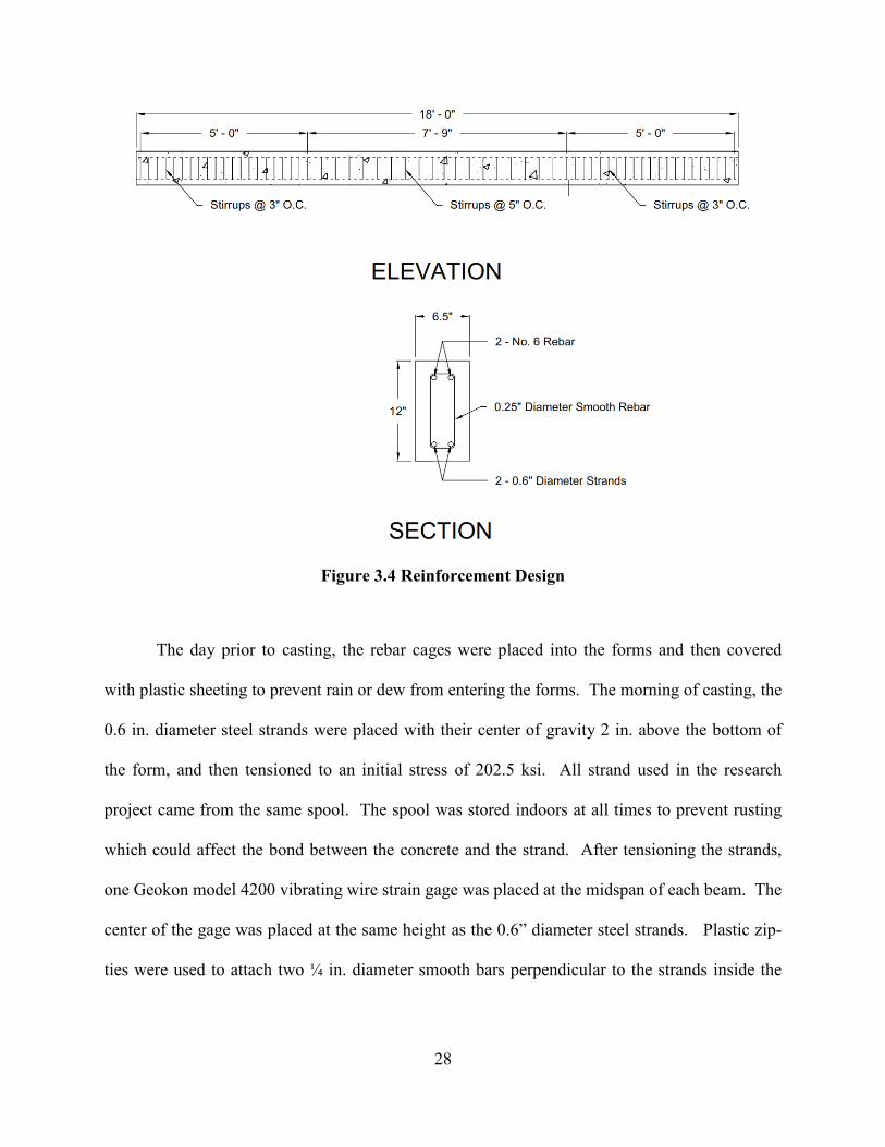
28

Figure 3.4 Reinforcement Design

The day prior to casting, the rebar cages were placed into the forms and then covered

with plastic sheeting to prevent rain or dew from entering the forms. The morning of casting, the

0.6 in. diameter steel strands were placed with their center of gravity 2 in. above the bottom of

the form, and then tensioned to an initial stress of 202.5 ksi. All strand used in the research

project came from the same spool. The spool was stored indoors at all times to prevent rusting

which could affect the bond between the concrete and the strand. After tensioning the strands,

one Geokon model 4200 vibrating wire strain gage was placed at the midspan of each beam. The

center of the gage was placed at the same height as the 0.6” diameter steel strands. Plastic zip-

ties were used to attach two ¼ in. diameter smooth bars perpendicular to the strands inside the

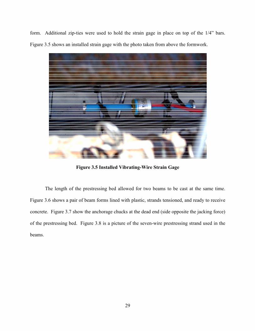
29

form. Additional zip-ties were used to hold the strain gage in place on top of the 1/4” bars.

Figure 3.5 shows an installed strain gage with the photo taken from above the formwork.

Figure 3.5 Installed Vibrating-Wire Strain Gage

The length of the prestressing bed allowed for two beams to be cast at the same time.

Figure 3.6 shows a pair of beam forms lined with plastic, strands tensioned, and ready to receive

concrete. Figure 3.7 show the anchorage chucks at the dead end (side opposite the jacking force)

of the prestressing bed. Figure 3.8 is a picture of the seven-wire prestressing strand used in the

beams.

30

Figure 3.6 Beam Formwork

Figure 3.7 Anchorage Chucks

31

Figure 3.8 Steel Strand

3.2.4 Detensioning Strands

For most of the beams, strands were released around 24 hours after being cast. The

exception to this was limestone beams 1 and 2 which were released after two days in order to

obtain higher strength. Before releasing strand tension, initial strain readings were measured.

For the first two clay beams, the initial readings prior to release were not taken, and therefore it

was necessary to cast two additional clay beams. After releasing the tension at the jack and then

cutting the strands between the two beams, a second strain gage reading was taken. The time

period between the initial reading and the second reading was approximately 15 minutes for the

first set of beams and approximately 8 minutes for the remaining beams. Another reading was

taken one hour after detensioning. Subsequent readings were taken every 24 hours for the first

week, weekly until 2 months after casting, and then monthly until being loaded.

32

3.2.5 Compressive Strengths

Compressive strengths (ASTM C39) were measured using companion cylinders that were

cast the same time as the beams. The strengths were taken at the time of release (typically 1

day), 7 days, and 28 days. At each day, three cylinders were tested. For the limestone beams

released at two days, only two cylinders were used to obtain the average compressive strength

because the first cylinder was broken at 1 day. The strengths at the time of release are shown in

Table 3.2.

Table 3.2 Compressive Strengths of Beam Companion Cylinders

Compressive Strength (psi)

Mix 1 Day 7 Day 28 Day

Clay (beams 3,4,5,6) 4640 7190 7510

Shale (beams 1,2) 5870 7040 7590

Shale – low strength a (beams 3,4)

2580 6740 7070

Limestone b (beams 1,2)

4520 8420 10460

Limestone - low strength (beams 3,4)

850 7310 8330 a Made with different Type III cement

b Released at 2 days for higher initial strength

3.2.6 Fresh Properties

Fresh properties tested included slump flow, J-ring, T20, and unit weight. Figures 3.9 and

3.10 demonstrate the J-ring test. The printed rings on the white portion of the nonabsorbent

surface shown in Figure 3.9 are used to determine the T20, the time it takes the concrete to flow

from the slump cone to the 20” diameter ring. The T20 test is performed during the slump flow

test and does not use the J-ring.

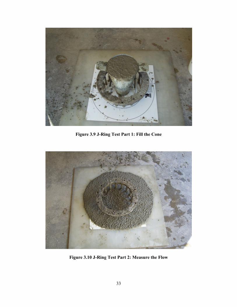
33

Figure 3.9 J-Ring Test Part 1: Fill the Cone

Figure 3.10 J-Ring Test Part 2: Measure the Flow

34

3.3 MODULUS OF ELASTICITY

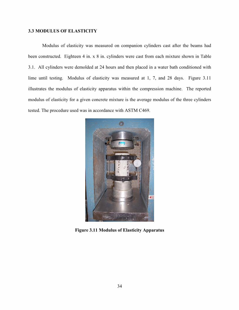
Modulus of elasticity was measured on companion cylinders cast after the beams had

been constructed. Eighteen 4 in. x 8 in. cylinders were cast from each mixture shown in Table

3.1. All cylinders were demolded at 24 hours and then placed in a water bath conditioned with

lime until testing. Modulus of elasticity was measured at 1, 7, and 28 days. Figure 3.11

illustrates the modulus of elasticity apparatus within the compression machine. The reported

modulus of elasticity for a given concrete mixture is the average modulus of the three cylinders

tested. The procedure used was in accordance with ASTM C469.

Figure 3.11 Modulus of Elasticity Apparatus

35

3.4 SHRINKAGE TESTING

Using the mixtures shown in Table 3.1, four rectangular prisms, 4”x4”x11.25”, were cast

for each aggregate type to measure concrete shrinkage. At 24 hours, the prisms were demolded

and an initial length reading was taken for each prism. The prisms were stored in an

environmental chamber with a temperature of 23°C and humidity of 50%. To allow air

circulation around the prisms, 3/8 in. to 1/2 in. diameter dowels were placed beneath the prisms

and space was left between the sides of neighboring specimens. Testing followed ASTM C157

(2006) with a few exceptions: no rodding of the concrete was necessary since all the mixes were

self-consolidating; the prisms were never placed in water; and the temperature temporarily varied

from 23°C due to HVAC failures. The effect of this variation is discussed in the results section.

The shrinkage testing lasted for a period of sixteen weeks. Readings were taken weekly

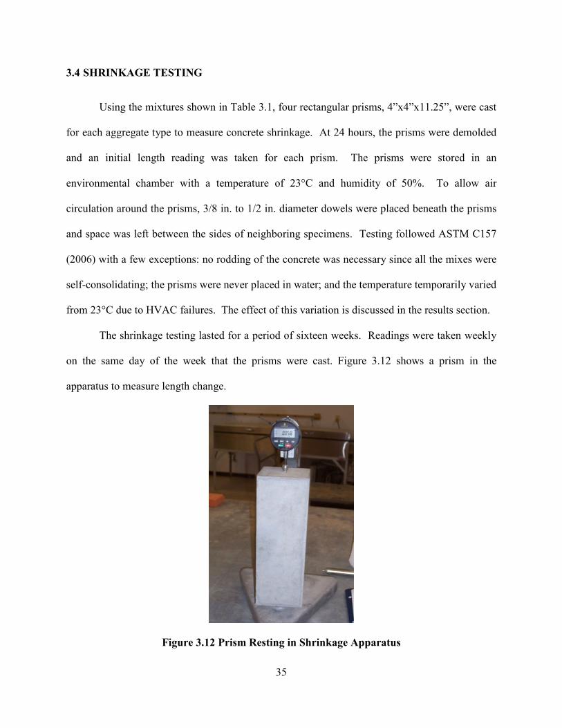
on the same day of the week that the prisms were cast. Figure 3.12 shows a prism in the

apparatus to measure length change.

Figure 3.12 Prism Resting in Shrinkage Apparatus

36

3.5 BEAM LOADING

The beams were loaded approximately five months after they were cast. This loading

was to simulate the load of a bridge deck being constructed on the beams. Concrete beams

which had been built and tested during previous research at the laboratory were placed on top of

the beams.

In order to load the beams, the beams had to be moved from the positions they were in

for the time between casting and loading. Because of this position change, a reading was taken

after a beam had been moved and prior to the loading of that beam. Another reading was taken

shortly after the beam was loaded with one of the old beams. This process was repeated for the

other beams. The weight of the old beams had little variation because their concrete unit weights

were similar (117 to 120 lb/ft3) and amounts of steel reinforcement were the same. Because the

beams placed on top were previously tested, most of the ends were tilted upward such that the

weight was not distributed over the entire length of the beam below it. Two of the beams used

for loading weight had ends which did not tilt upward but rather had camber. This camber

caused the beam weight to rest on the bottom beam over the supports instead of in the mid-span

area of the beam. To correct this, 2 in. x 6 in. boards were placed on top of the bottom beams so

that weight of the loading beams would rest on the boards in the mid-span area of the beam

instead of the outer portions of the beam.

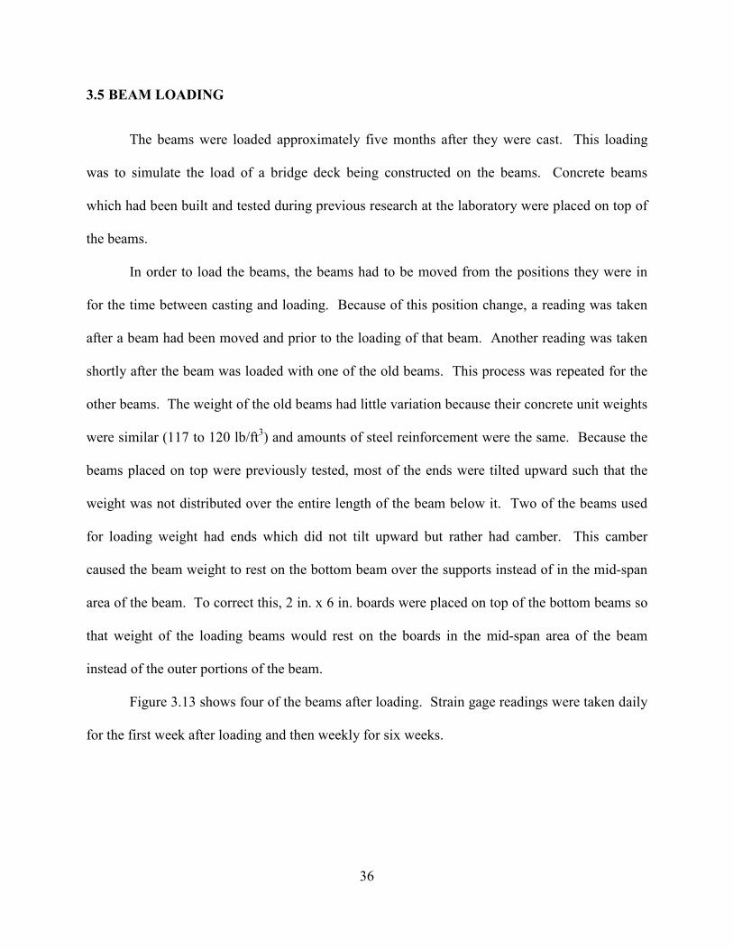
Figure 3.13 shows four of the beams after loading. Strain gage readings were taken daily

for the first week after loading and then weekly for six weeks.

37

Figure 3.13 Loaded Beams

38

CHAPTER 4: RESULTS

4.1 INTRODUCTION

The results from phases I, II, and III are discussed in the following sections. Some of the

results from different phases are combined. Measured values are compared to AASHTO

predicted values.

4.2 FRESH PROPERTIES

Fresh concrete properties were measured during beam production as well as for mixtures

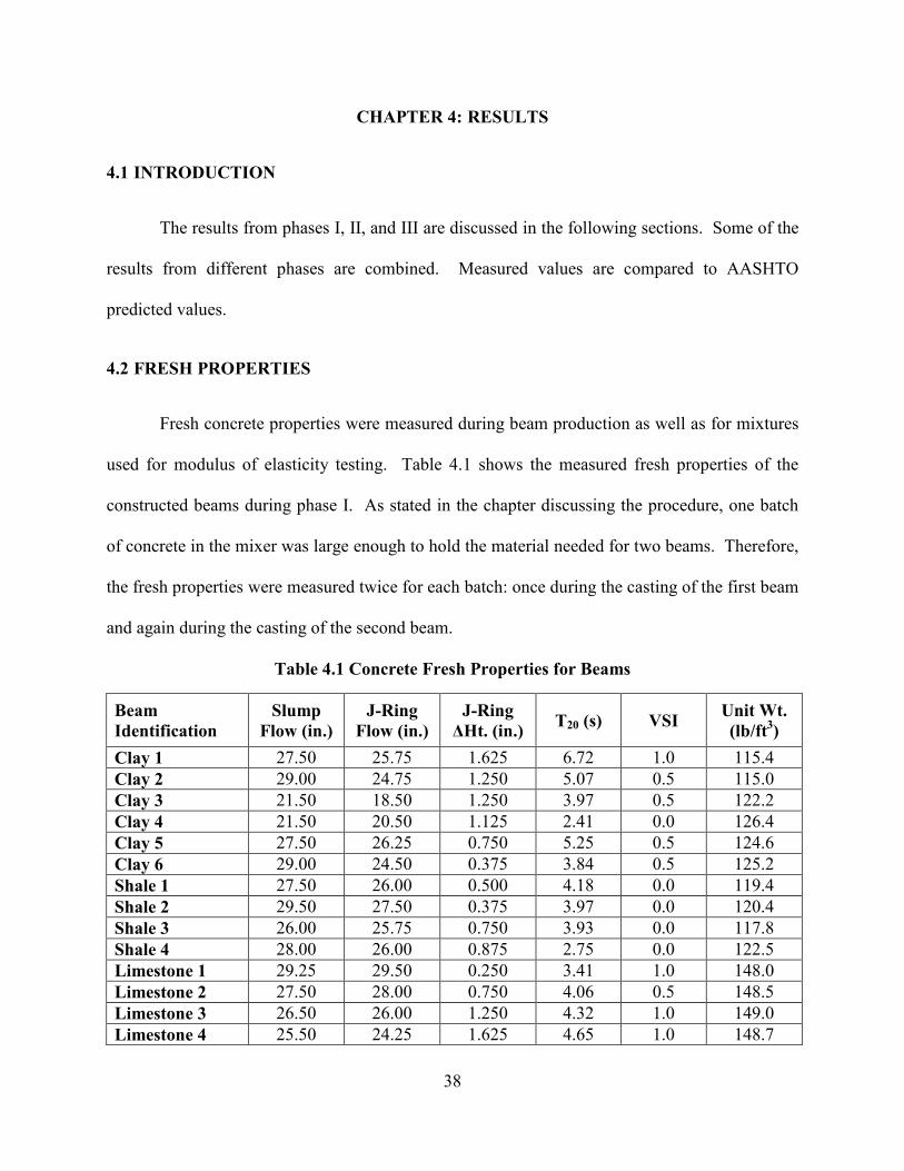
used for modulus of elasticity testing. Table 4.1 shows the measured fresh properties of the

constructed beams during phase I. As stated in the chapter discussing the procedure, one batch

of concrete in the mixer was large enough to hold the material needed for two beams. Therefore,

the fresh properties were measured twice for each batch: once during the casting of the first beam

and again during the casting of the second beam.

Table 4.1 Concrete Fresh Properties for Beams

Beam

Identification

Slump

Flow (in.)

J-Ring

Flow (in.)

J-Ring

∆Ht. (in.) T20 (s) VSI

Unit Wt.

(lb/ft3)

Clay 1 27.50 25.75 1.625 6.72 1.0 115.4 Clay 2 29.00 24.75 1.250 5.07 0.5 115.0 Clay 3 21.50 18.50 1.250 3.97 0.5 122.2 Clay 4 21.50 20.50 1.125 2.41 0.0 126.4 Clay 5 27.50 26.25 0.750 5.25 0.5 124.6 Clay 6 29.00 24.50 0.375 3.84 0.5 125.2 Shale 1 27.50 26.00 0.500 4.18 0.0 119.4 Shale 2 29.50 27.50 0.375 3.97 0.0 120.4 Shale 3 26.00 25.75 0.750 3.93 0.0 117.8 Shale 4 28.00 26.00 0.875 2.75 0.0 122.5 Limestone 1 29.25 29.50 0.250 3.41 1.0 148.0 Limestone 2 27.50 28.00 0.750 4.06 0.5 148.5 Limestone 3 26.50 26.00 1.250 4.32 1.0 149.0 Limestone 4 25.50 24.25 1.625 4.65 1.0 148.7

39

4.2.1 Slump Flow

With the exception of clay beams 3 and 4, all of the slump flows are between 26 in. and

29.5 in. which resulted in concrete that flowed into the forms well, leaving no bug-holes when

the forms were removed. The slump flows for clay beams 3 and 4 were both 21.5”. This could

have been increased by adding more high-range water reducer (HRWR). However, the T20 was

already below 4 seconds, and the researchers were concerned that adding more HRWR would

reduce the T20 to an undesirable level which could cause segregation.

4.2.2 J-Ring

The J-Ring flows varied from 24.25 in. to 29.5 in., excluding clay beams 3 and 4. Since

the slump flow for clay beams 3 and 4 was 6 in. less than the other clay beams, the J-Ring flow

was also less -- about 5 in. on average. The J-Ring flow was less than the slump flow for most of

the concrete batches. This was expected since the concrete must flow around the metal bars

which impede the flow. Limestone beams 1 and 2 slightly increased in flow from the slump flow

test to the J-ring test. This increase could be due to excess water remaining on the slump flow

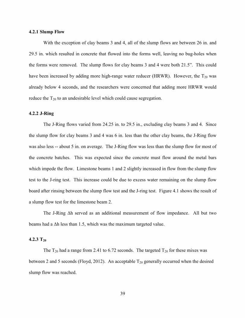
board after rinsing between the slump flow test and the J-ring test. Figure 4.1 shows the result of

a slump flow test for the limestone beam 2.

The J-Ring ∆h served as an additional measurement of flow impedance. All but two

beams had a ∆h less than 1.5, which was the maximum targeted value.

4.2.3 T20

The T20 had a range from 2.41 to 6.72 seconds. The targeted T20 for these mixes was

between 2 and 5 seconds (Floyd, 2012). An acceptable T20 generally occurred when the desired

slump flow was reached.

40

Figure 4.1 Slump Flow Test Performed on Limestone Beam 2 Mix

4.2.4 VSI

The visual stability index was used to indicate the amount of segregation that occurred in

the concrete mixture. All of the beams exhibited a VSI of 0 to 1.0. Mortar halos were not

present in the mixes used in the beams.

While all the mixtures had acceptable VSIs, some of the lightweight aggregate mixes

showed mild segregation in the wheelbarrows due to some of the lightweight aggregate rising to

the surface. This seemed more pronounced in the clay aggregates than in the shale.

4.2.5 Unit Weight

The clay beams measured unit weight varied widely from the calculated unit weight of

117.6 lb/ft3. The exact reason for the high unit weight of clay beams 3-6 is unknown, but could

be due to one or more errors. The air content may have been less than the assumed 2%, or the

moisture contents could have varied from the assumed amount. Another possible cause to

account for the large difference in unit weight could be misrepresentative samples from the

wheelbarrow. Before obtaining a unit weight sample, the concrete was mixed with scoops and

41

attempts were made to obtain concrete from all depths of the wheelbarrow. However, with some

segregation occurring, it is possible that more of the paste was used than the aggregate lying at

the surface. The paste is denser than the aggregate. The shale and limestone unit weights were

reasonably close to the calculated unit weights.

4.2.6 Fresh Properties of Companion Batches

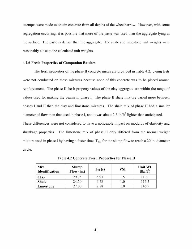
The fresh properties of the phase II concrete mixes are provided in Table 4.2. J-ring tests

were not conducted on these mixtures because none of this concrete was to be placed around

reinforcement. The phase II fresh property values of the clay aggregate are within the range of

values used for making the beams in phase I. The phase II shale mixture varied more between

phases I and II than the clay and limestone mixtures. The shale mix of phase II had a smaller

diameter of flow than that used in phase I, and it was about 2-3 lb/ft3 lighter than anticipated.

These differences were not considered to have a noticeable impact on modulus of elasticity and

shrinkage properties. The limestone mix of phase II only differed from the normal weight

mixture used in phase I by having a faster time, T20, for the slump flow to reach a 20 in. diameter

circle.

Table 4.2 Concrete Fresh Properties for Phase II

Mix

Identification

Slump

Flow (in.) T20 (s) VSI

Unit Wt.

(lb/ft3)

Clay 29.75 5.97 1.5 119.6 Shale 24.50 4.78 1.0 116.5 Limestone 27.00 2.88 1.0 146.9

42

4.3 HARDENED PROPERTIES

4.3.1 Compressive Strength

Compressive strengths were measured during phases I and II. Phase I strengths are

shown in Table 4.3. The results shown in Table 4.3 are the average of three compressive

strength tests. Graphs of this data are available in Appendix A. Shale beams 3 and 4 had lower

one-day strengths than anticipated. This delay of strength gain may have been due to using

different cement or to temperature effects. While Type III cement was used, it was from a

different source than the Type III cement used in the clay beams and shale beams 1 and 2. The

night after shale beams 3 and 4 were cast, the low temperature was about 37°F which could have

slowed the strength gain in the concrete.

The limestone mixes also gained strength slower than anticipated, and this was likely

caused by low temperatures. Previous research with the limestone mixtures had been conducted

in the summertime with daytime high ambient temperatures ranging from 90-100°F. However,

the limestone beams presented here were cast in the late fall with daytime high temperatures in

the 50s°F and night-time temperatures nearing 32°F. The strands within limestone beams I and

II were detensioned at 48 hours after the companion cylinders had achieved 4000 psi.

Companion cylinders to limestone beams 3 and 4 failed to reach 1000 psi at 24 hours.

Detensioning at this strength caused cracking in the beams from the top to approximately mid-

height.

Phase II strengths are listed in Table 4.4. The strengths from phase II are comparable

with those of phase I even though the phase II cylinders were cured in a water bath at a

controlled 70°F rather than outdoors at variable temperature and humidity levels. The phase II

43

strengths do differ from the low-strength shale and limestone beams, but reasons for those

differences (cement source and ambient temperature) were previously discussed.

Table 4.3 Concrete Compressive Strengths (psi) for Phase I

Beam ID Age (days)

1 7 28

Clay 1 6160 8070 8070 Clay 2 5600 6420 6720 Clay 3 5520 7650 8430 Clay 4 4980 6970 6970 Clay 5 4960 7760 7730 Clay 6 3510 6370 6900 Shale 1 6160 7300 8130 Shale 2 5590 6780 7060 Shale 3 2390 6890 7440 Shale 4 2770 6590 6710 Limestone 1* 4680 8500 10610 Limestone 2* 4370 8330 10320 Limestone 3 960 7700 8640 Limestone 4 740 6930 8010

* Two day strength corresponding to time of detensioning the strands

Table 4.4 Concrete Compressive Strengths (psi) for Phase II

Beam ID Age (days)

1 7 28

Clay 5070 5930 7470 Shale 5560 6970 7140 Limestone 4600 7870 9760

4.3.2 Modulus of Elasticity

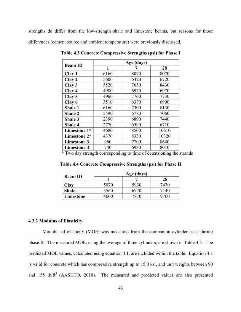
Modulus of elasticity (MOE) was measured from the companion cylinders cast during

phase II. The measured MOE, using the average of three cylinders, are shown in Table 4.5. The

predicted MOE values, calculated using equation 4.1, are included within the table. Equation 4.1

is valid for concrete which has compressive strength up to 15.0 ksi, and unit weights between 90

and 155 lb/ft3 (AASHTO, 2010). The measured and predicted values are also presented

44

graphically in Figure 4.2. The limestone mix had a higher MOE than the lightweight aggregates

and also achieved higher compressive strength. The prediction equation worked well for the

limestone SCC at 1 and 28 days. While the equation over-predicted 1 day MOE for the

lightweight SCC, it under-predicted the 28 MOE for the clay and shale cylinders.

�=� = �� = >>, �� ∗ 2� ∗ABC.D ∗ E�F�(GH.) Equation 4.1

Where: K1 = correction factor for source of aggregate to be taken as 1.0 unless determined by physical test. (The K1 factor was included in the equation because tests show that MOE is affected by the stiffness of the aggregate.) Wc = unit weight of concrete (kcf) f’c = compressive strength of concrete (ksi) (AASHTO, 2010).

Table 4.5 Phase II: Predicted and Measured MOE

Mix Age (days) f'c (psi) Measured

MOE (ksi)

Predicted

MOE (ksi)

Predicted/

Measured

Clay

1 5070 2900 3050 1.05 7 5930 3700 3350 0.91

28 7470 4150 3750 0.90

Shale

1 5560 2900 3100 1.07 7 6970 3900 3450 0.88

28 7140 4350 3500 0.80

Limestone

1 4600 4100 4000 0.98 7 7870 4800 5200 1.08

28 9760 6150 5800 0.94

Equation 4.1 predicted the modulus fairly accurately for the different mixtures; however

the 28 day shale MOE was 20% more than predicted. The prediction equation overestimated the

1-day modulus of the lightweight aggregate mixes, but slightly underestimated the modulus of

the limestone aggregate mix.

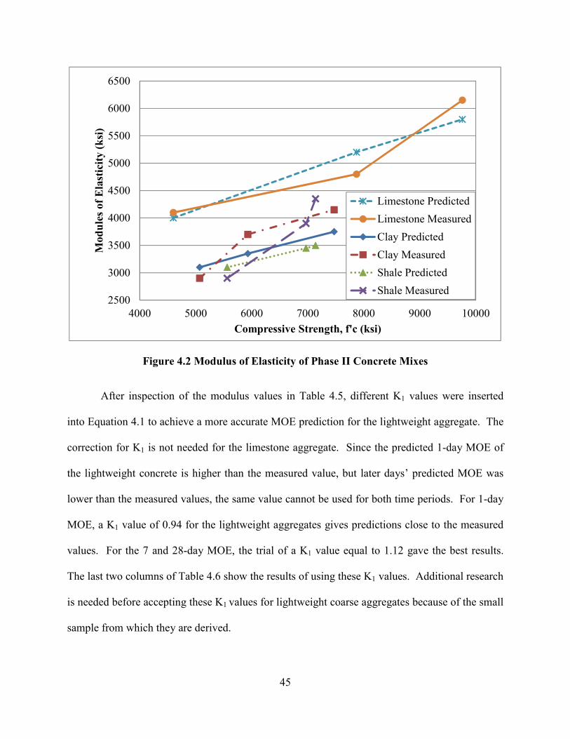
45

Figure 4.2 Modulus of Elasticity of Phase II Concrete Mixes

After inspection of the modulus values in Table 4.5, different K1 values were inserted

into Equation 4.1 to achieve a more accurate MOE prediction for the lightweight aggregate. The

correction for K1 is not needed for the limestone aggregate. Since the predicted 1-day MOE of

the lightweight concrete is higher than the measured value, but later days’ predicted MOE was

lower than the measured values, the same value cannot be used for both time periods. For 1-day

MOE, a K1 value of 0.94 for the lightweight aggregates gives predictions close to the measured

values. For the 7 and 28-day MOE, the trial of a K1 value equal to 1.12 gave the best results.

The last two columns of Table 4.6 show the results of using these K1 values. Additional research

is needed before accepting these K1 values for lightweight coarse aggregates because of the small

sample from which they are derived.

2500

3000

3500

4000

4500

5000

5500

6000

6500

4000 5000 6000 7000 8000 9000 10000

Mod

ule

s of

Ela

stic

ity (

ksi

)

Compressive Strength, f'c (ksi)

Limestone Predicted

Limestone Measured

Clay Predicted

Clay Measured

Shale Predicted

Shale Measured

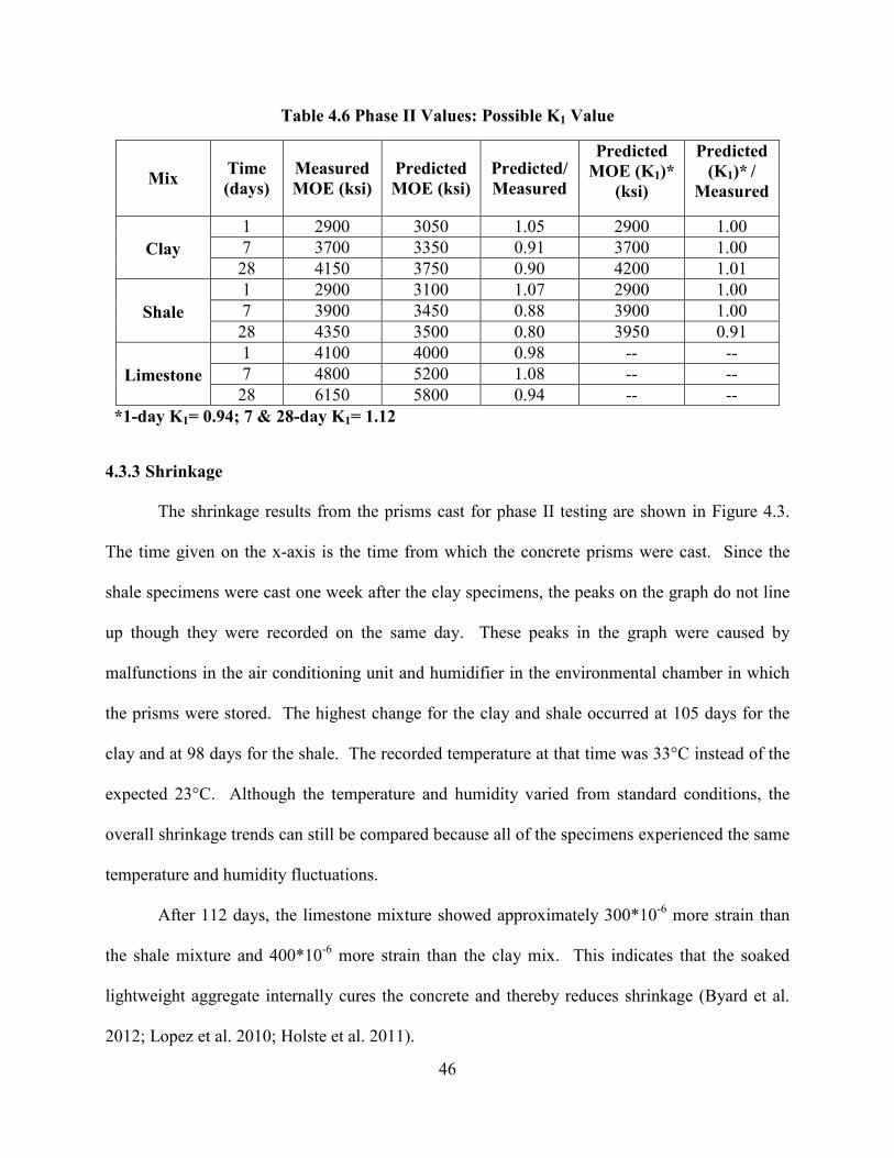
46

Table 4.6 Phase II Values: Possible K1 Value

Mix Time

(days)

Measured

MOE (ksi)

Predicted

MOE (ksi)

Predicted/

Measured

Predicted

MOE (K1)*

(ksi)

Predicted

(K1)* /

Measured

Clay

1 2900 3050 1.05 2900 1.00 7 3700 3350 0.91 3700 1.00

28 4150 3750 0.90 4200 1.01

Shale

1 2900 3100 1.07 2900 1.00 7 3900 3450 0.88 3900 1.00

28 4350 3500 0.80 3950 0.91

Limestone

1 4100 4000 0.98 -- -- 7 4800 5200 1.08 -- --

28 6150 5800 0.94 -- -- *1-day K1= 0.94; 7 & 28-day K1= 1.12

4.3.3 Shrinkage

The shrinkage results from the prisms cast for phase II testing are shown in Figure 4.3.

The time given on the x-axis is the time from which the concrete prisms were cast. Since the

shale specimens were cast one week after the clay specimens, the peaks on the graph do not line

up though they were recorded on the same day. These peaks in the graph were caused by

malfunctions in the air conditioning unit and humidifier in the environmental chamber in which

the prisms were stored. The highest change for the clay and shale occurred at 105 days for the

clay and at 98 days for the shale. The recorded temperature at that time was 33°C instead of the

expected 23°C. Although the temperature and humidity varied from standard conditions, the

overall shrinkage trends can still be compared because all of the specimens experienced the same

temperature and humidity fluctuations.

After 112 days, the limestone mixture showed approximately 300*10-6 more strain than

the shale mixture and 400*10-6 more strain than the clay mix. This indicates that the soaked

lightweight aggregate internally cures the concrete and thereby reduces shrinkage (Byard et al.

2012; Lopez et al. 2010; Holste et al. 2011).

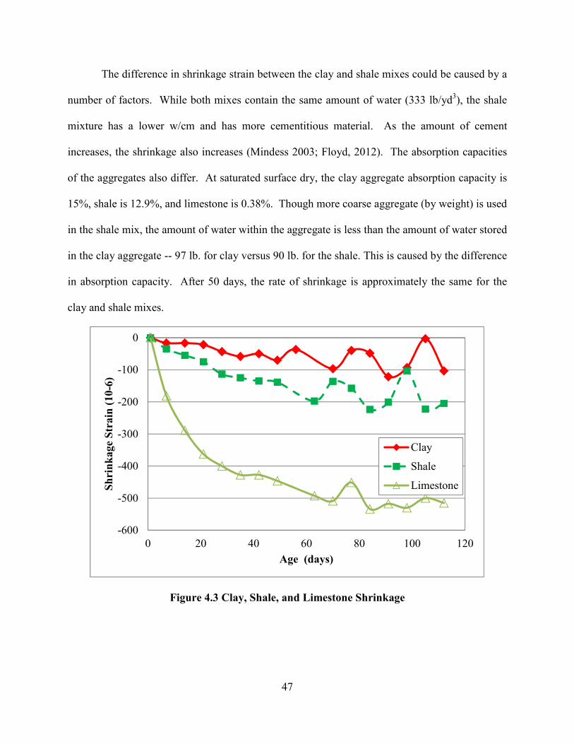
47

The difference in shrinkage strain between the clay and shale mixes could be caused by a

number of factors. While both mixes contain the same amount of water (333 lb/yd3), the shale

mixture has a lower w/cm and has more cementitious material. As the amount of cement

increases, the shrinkage also increases (Mindess 2003; Floyd, 2012). The absorption capacities

of the aggregates also differ. At saturated surface dry, the clay aggregate absorption capacity is

15%, shale is 12.9%, and limestone is 0.38%. Though more coarse aggregate (by weight) is used

in the shale mix, the amount of water within the aggregate is less than the amount of water stored

in the clay aggregate -- 97 lb. for clay versus 90 lb. for the shale. This is caused by the difference

in absorption capacity. After 50 days, the rate of shrinkage is approximately the same for the

clay and shale mixes.

Figure 4.3 Clay, Shale, and Limestone Shrinkage

-600

-500

-400

-300

-200

-100

0

0 20 40 60 80 100 120

Sh

rin

kage

Str

ain

(10-6

)

Age (days)

Clay

Shale

Limestone

48

4.3.4 Prestress Losses Prior to Loading

This section includes data from phases I and II. The predicted and measured values are

given with the prestress losses presented according to when they occurred. The losses presented

here include elastic shortening (ES), shrinkage (SH), creep (CR), and steel relaxation (RE).

4.3.4.1 Elastic Shortening

Elastic shortening losses were measured from the strain loss occurring in the strain gages

at the time of transfer. The predicted losses were calculated using the AASHTO method. The

approximate and refined methods presented by AASHTO both calculate ES using the same

procedure (AASHTO, 2010). For the prediction equation, the compressive strength used for f’ci

was the strength of the companion cylinders at the time of strand detensioning. This value was

inserted into equation 4.1 to determine the MOE used in the procedure. The MOE values

obtained by using equation 4.1 were more appropriate than using the phase II measured MOE.

The reasoning for this is that the phase II measured MOE values are likely higher than the one-

day MOE of the beams that were detensioned at low strength. The AASHTO predicted ES is

compared to the measured ES in Table 4.7.

The shale beams have similar measured ES values which are unexpected because of the

difference in strength (shale 1 and 2 of 5880 psi versus shale 3 and 4 of 2580 psi) of the

companion cylinders that were tested. Based upon the measured ES values, it is reasonable to

believe that the companion cylinders to shale beams 3 and 4 did not achieve the same strength as

the beams. The beams were better able to cure in cold ambient temperatures than the cylinders.

The plywood forms would better insulate the beams and provide higher one-day strengths than

the cylinders cured in plastic molds. In addition the beams would retain heat better because they

contain a larger quantity of concrete than the cylinders. The volume to surface ratio (V/S) could

49

also be a factor. The beams have a (V/S) equal to 2.11, whereas the 4”*8” cylinders have a V/S

equal to 0.8.

It is possible that the limestone batches were affected in a similar manner, but not to the

same extent as the shale batches. Companion cylinders to the limestone beams 3 and 4 had less

than one-fourth of the expected one-day compressive strength for that mixture. As expected this

increased ES losses. Shale beams 3 and 4 and limestone beams 3 and 4 were not included in the

average ES losses listed in Table 4.13. To include these beams in the averages would be unfair

to the prediction equations because of the error introduced by the cylinder strength differing from

the beam strength.

The AASHTO equation over-predicted ES for all beams tested. With an error of 14%, it

most accurately predicted the ES of the limestone SCC mix used as a control. The equation did

not perform so well with the lightweight SCC mixes. The equation over-estimated ES in the clay

and shale mixes by 21% and 33%, respectively. By comparing the predicted ES values, it seems

that the AASHTO equation is overly sensitive to MOE. While the LWSCC with lower MOE did

have slightly more ES than the NWSCC, the prediction equations overestimated this difference.

Table 4.7 Predicted and Measured Elastic Shortening (ES)

Beam ID Measured ES (ksi) Predicted ES (ksi) Predicted/

Measured

50

Clay 1x -- 20.15 -- Clay 2x -- 21.23 -- Clay 3 14.53 19.53 1.34 Clay 4 19.09 19.51 1.02 Clay 5 15.74 19.94 1.27 Clay 6 18.45 23.11 1.25 Clay Average 16.95 20.58 1.21 Shale 1 14.00 19.21 1.37 Shale 2 15.30 19.83 1.30 Shale 3* 13.80 29.66 2.15 Shale 4* 16.40 26.41 1.61 Shale 1&2 Average 14.65 19.52 1.33 Limestone 1 13.59 16.03 1.18 Limestone 2 14.89 16.46 1.11 Limestone 3* 18.27 31.91 1.75 Limestone 4* 24.53 35.64 1.45 Limest. 1&2 14.24 16.25 1.14

x Strain gage readings were not taken before detensioning *Companion cylinders showed lower-than-expected compressive strengths

4.3.4.2 Long-term Losses Prior to Loading

The long-term losses include concrete creep and shrinkage and steel relaxation. The

AASHTO approximate method and refined method were used to predict the losses. As per

Figure 5.4.2.3.3-1 of the AASHTO LRFD Bridge Design Specifications (2010), the humidity used

in the equations was 70% for northwest Arkansas. As recommended for the approximate

method, the steel relaxation was assumed to be 2.4 ksi since strands used were “low relaxation.”

For the measured losses, the strain gage does not detect steel relaxation (RE), therefore before

comparing the measured and predicted losses, the computed RE value was added into the

measured values. The measured prestress losses in the beams are given in Table 4.8. Losses

predicted by the AASHTO equations are shown in Table 4.9. These values were calculated

using 1 day for the release time and are for a loading age of 150 days, the time used for beam

loading calculations.

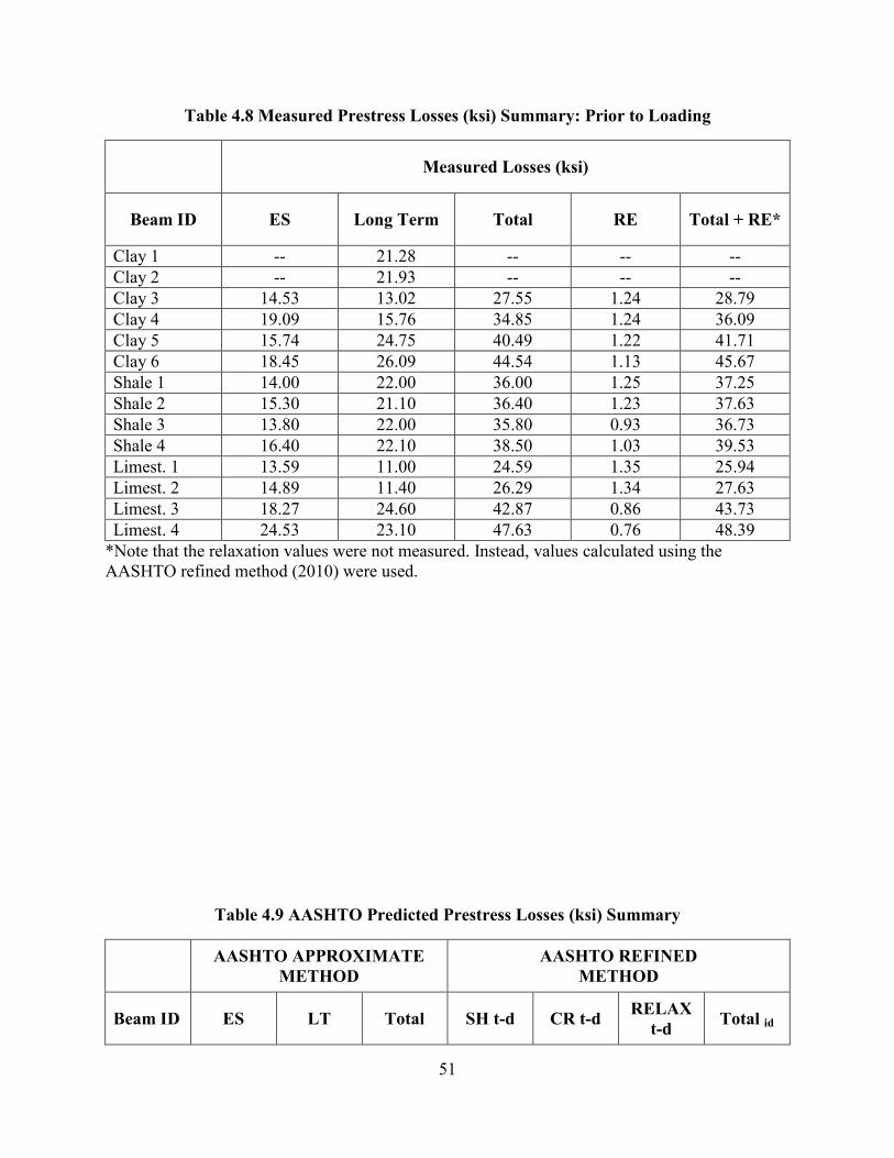
51

Table 4.8 Measured Prestress Losses (ksi) Summary: Prior to Loading

*Note that the relaxation values were not measured. Instead, values calculated using the AASHTO refined method (2010) were used.

Table 4.9 AASHTO Predicted Prestress Losses (ksi) Summary

Measured Losses (ksi)

Beam ID ES Long Term Total RE Total + RE*

Clay 1 -- 21.28 -- -- -- Clay 2 -- 21.93 -- -- -- Clay 3 14.53 13.02 27.55 1.24 28.79 Clay 4 19.09 15.76 34.85 1.24 36.09 Clay 5 15.74 24.75 40.49 1.22 41.71 Clay 6 18.45 26.09 44.54 1.13 45.67 Shale 1 14.00 22.00 36.00 1.25 37.25 Shale 2 15.30 21.10 36.40 1.23 37.63 Shale 3 13.80 22.00 35.80 0.93 36.73 Shale 4 16.40 22.10 38.50 1.03 39.53 Limest. 1 13.59 11.00 24.59 1.35 25.94 Limest. 2 14.89 11.40 26.29 1.34 27.63 Limest. 3 18.27 24.60 42.87 0.86 43.73 Limest. 4 24.53 23.10 47.63 0.76 48.39

AASHTO APPROXIMATE

METHOD

AASHTO REFINED

METHOD

Beam ID ES LT Total SH t-d CR t-d RELAX

t-d Total id

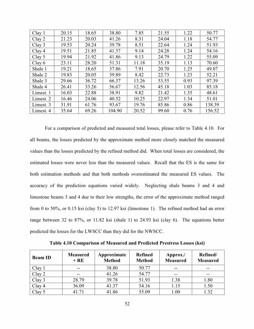
52

For a comparison of predicted and measured total losses, please refer to Table 4.10. For

all beams, the losses predicted by the approximate method more closely matched the measured

values than the losses predicted by the refined method did. When total losses are considered, the

estimated losses were never less than the measured values. Recall that the ES is the same for

both estimation methods and that both methods overestimated the measured ES values. The

accuracy of the prediction equations varied widely. Neglecting shale beams 3 and 4 and

limestone beams 3 and 4 due to their low strengths, the error of the approximate method ranged

from 0 to 50%, or 0.15 ksi (clay 5) to 12.97 ksi (limestone 1). The refined method had an error

range between 32 to 87%, or 11.82 ksi (shale 1) to 24.93 ksi (clay 6). The equations better

predicted the losses for the LWSCC than they did for the NWSCC.

Table 4.10 Comparison of Measured and Predicted Prestress Losses (ksi)

Clay 1 20.15 18.65 38.80 7.85 21.55 1.22 50.77 Clay 2 21.23 20.03 41.26 8.31 24.04 1.18 54.77 Clay 3 19.53 20.24 39.78 8.51 22.64 1.24 51.93 Clay 4 19.51 21.85 41.37 9.14 24.28 1.24 54.16 Clay 5 19.94 21.92 41.86 9.13 24.79 1.22 55.09 Clay 6 23.11 28.20 51.31 11.18 35.19 1.13 70.60 Shale 1 19.21 18.65 37.86 7.91 20.70 1.25 49.07 Shale 2 19.83 20.05 39.89 8.42 22.73 1.23 52.21 Shale 3 29.66 36.72 66.37 13.26 53.55 0.93 97.39 Shale 4 26.41 33.26 56.67 12.56 45.18 1.03 85.18 Limest. 1 16.03 22.88 38.91 9.82 21.42 1.35 48.61 Limest. 2 16.46 24.06 40.52 10.25 22.97 1.34 51.01 Limest. 3 31.91 61.76 93.67 19.76 85.86 0.86 138.39 Limest. 4 35.64 69.26 104.90 20.52 99.60 0.76 156.52

Beam ID Measured

+ RE

Approximate

Method

Refined

Method

Approx./

Measured

Refined/

Measured

Clay 1 -- 38.80 50.77 -- -- Clay 2 -- 41.26 54.77 -- -- Clay 3 28.79 39.78 51.93 1.38 1.80 Clay 4 36.09 41.37 54.16 1.15 1.50 Clay 5 41.71 41.86 55.09 1.00 1.32

53

4.3.5 Prestress Losses after Applying Load

The beams were loaded approximately 150 days after being cast, and readings were taken

for another 11 weeks. Since the beam loading did not result in a composite section, the deck area

was taken to be zero for determining area and eccentricity of the steel strands. For AASHTO

refined calculations, the age of the beams at time of deck loading was 150 days with losses

measured for an additional 75 days. Due to differences in casting times, the actual time of

loading for some beams was closer to 175 days. This difference was not accounted for in the

calculations since the losses had leveled off at this time. The amount of loading put the stress in

the bottom fiber of the beams just below the 7.5√f’c threshold for cracking, and therefore this

value corresponds to a class U concrete as defined by ACI 318 (2008).

The “deck” load could influence prestress in two ways. The first is due to elastic gain

occurring immediately when the load is placed on top of the beam. The second is the sum of the

long term shrinkage, creep, and relaxation between the time of deck placement and the final

time, LTdf. The AASHTO LRFD Bridge Design Specifications includes a term for the shrinkage

associated with curing of the concrete deck, but that was equal to zero in this study. The reason

for this is that the “deck” was noncomposite, and therefore the area of the deck was taken to be

zero as directed (AASHTO, 2010).

Clay 6 45.67 51.31 70.60 1.12 1.55 Shale 1 37.25 37.86 49.07 1.02 1.32 Shale 2 37.63 39.89 52.21 1.06 1.39 Shale 3* 36.73 66.37 97.39 1.81 2.65 Shale 4* 39.53 56.67 85.18 1.43 2.15 Limestone 1 25.94 38.91 48.61 1.50 1.87 Limestone 2 27.63 40.52 51.01 1.47 1.85 Limestone 3* 43.73 93.67 138.39 2.14 3.16 Limestone 4* 48.39 104.90 156.52 2.17 3.23

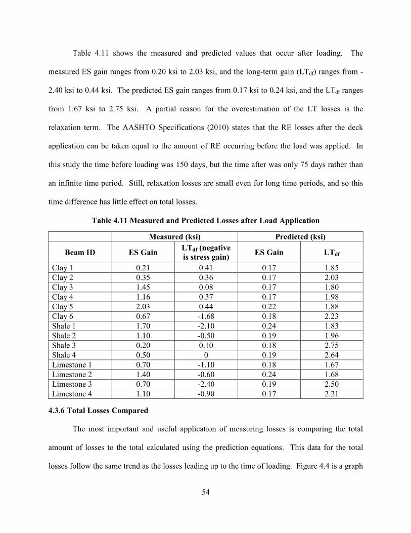
54

Table 4.11 shows the measured and predicted values that occur after loading. The

measured ES gain ranges from 0.20 ksi to 2.03 ksi, and the long-term gain (LTdf) ranges from -

2.40 ksi to 0.44 ksi. The predicted ES gain ranges from 0.17 ksi to 0.24 ksi, and the LTdf ranges

from 1.67 ksi to 2.75 ksi. A partial reason for the overestimation of the LT losses is the

relaxation term. The AASHTO Specifications (2010) states that the RE losses after the deck

application can be taken equal to the amount of RE occurring before the load was applied. In

this study the time before loading was 150 days, but the time after was only 75 days rather than

an infinite time period. Still, relaxation losses are small even for long time periods, and so this

time difference has little effect on total losses.

Table 4.11 Measured and Predicted Losses after Load Application

Measured (ksi) Predicted (ksi)

Beam ID ES Gain LTdf (negative

is stress gain) ES Gain LTdf

Clay 1 0.21 0.41 0.17 1.85 Clay 2 0.35 0.36 0.17 2.03 Clay 3 1.45 0.08 0.17 1.80 Clay 4 1.16 0.37 0.17 1.98 Clay 5 2.03 0.44 0.22 1.88 Clay 6 0.67 -1.68 0.18 2.23 Shale 1 1.70 -2.10 0.24 1.83 Shale 2 1.10 -0.50 0.19 1.96 Shale 3 0.20 0.10 0.18 2.75 Shale 4 0.50 0 0.19 2.64 Limestone 1 0.70 -1.10 0.18 1.67 Limestone 2 1.40 -0.60 0.24 1.68 Limestone 3 0.70 -2.40 0.19 2.50 Limestone 4 1.10 -0.90 0.17 2.21

4.3.6 Total Losses Compared

The most important and useful application of measuring losses is comparing the total

amount of losses to the total calculated using the prediction equations. This data for the total

losses follow the same trend as the losses leading up to the time of loading. Figure 4.4 is a graph

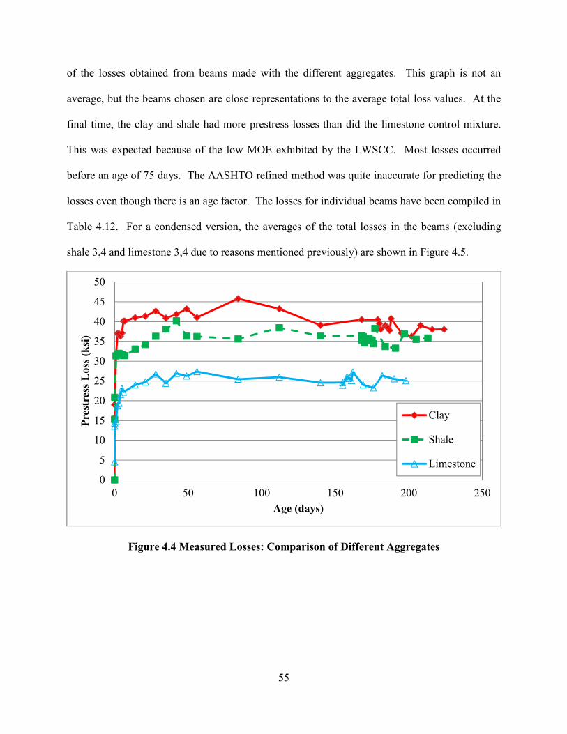
55

of the losses obtained from beams made with the different aggregates. This graph is not an

average, but the beams chosen are close representations to the average total loss values. At the

final time, the clay and shale had more prestress losses than did the limestone control mixture.

This was expected because of the low MOE exhibited by the LWSCC. Most losses occurred

before an age of 75 days. The AASHTO refined method was quite inaccurate for predicting the

losses even though there is an age factor. The losses for individual beams have been compiled in

Table 4.12. For a condensed version, the averages of the total losses in the beams (excluding

shale 3,4 and limestone 3,4 due to reasons mentioned previously) are shown in Figure 4.5.

Figure 4.4 Measured Losses: Comparison of Different Aggregates

0

5

10

15

20

25

30

35

40

45

50

0 50 100 150 200 250

Pre

stre

ss L

oss

(k

si)

Age (days)

Clay

Shale

Limestone

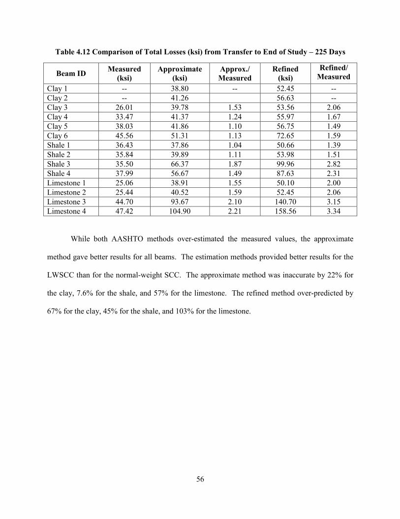
56

Table 4.12 Comparison of Total Losses (ksi) from Transfer to End of Study – 225 Days

Beam ID Measured

(ksi)

Approximate

(ksi)

Approx./

Measured

Refined

(ksi)

Refined/

Measured

Clay 1 -- 38.80 -- 52.45 -- Clay 2 -- 41.26 56.63 -- Clay 3 26.01 39.78 1.53 53.56 2.06 Clay 4 33.47 41.37 1.24 55.97 1.67 Clay 5 38.03 41.86 1.10 56.75 1.49 Clay 6 45.56 51.31 1.13 72.65 1.59 Shale 1 36.43 37.86 1.04 50.66 1.39 Shale 2 35.84 39.89 1.11 53.98 1.51 Shale 3 35.50 66.37 1.87 99.96 2.82 Shale 4 37.99 56.67 1.49 87.63 2.31 Limestone 1 25.06 38.91 1.55 50.10 2.00 Limestone 2 25.44 40.52 1.59 52.45 2.06 Limestone 3 44.70 93.67 2.10 140.70 3.15 Limestone 4 47.42 104.90 2.21 158.56 3.34

While both AASHTO methods over-estimated the measured values, the approximate

method gave better results for all beams. The estimation methods provided better results for the

LWSCC than for the normal-weight SCC. The approximate method was inaccurate by 22% for

the clay, 7.6% for the shale, and 57% for the limestone. The refined method over-predicted by

67% for the clay, 45% for the shale, and 103% for the limestone.

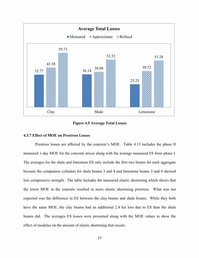
57

Figure 4.5 Average Total Losses

4.3.7 Effect of MOE on Prestress Losses

Prestress losses are affected by the concrete’s MOE. Table 4.13 includes the phase II

measured 1-day MOE for the concrete mixes along with the average measured ES from phase I.

The averages for the shale and limestone ES only include the first two beams for each aggregate

because the companion cylinders for shale beams 3 and 4 and limestone beams 3 and 4 showed

low compressive strength. The table includes the measured elastic shortening which shows that

the lower MOE in the concrete resulted in more elastic shortening prestress. What was not

expected was the difference in ES between the clay beams and shale beams. While they both

have the same MOE, the clay beams had an additional 2.4 ksi loss due to ES than the shale

beams did. The averages ES losses were presented along with the MOE values to show the

effect of modulus on the amount of elastic shortening that occurs.

35.77 36.14

25.25

43.5838.88 39.72

59.73

52.32 51.28

Clay Shale Limestone

Average Total Losses

Measured Approximate Refined

58

Table 4.13 Measured Modulus of Elasticity and Elastic Shortening

Aggregate type Measured

1-day MOE (ksi) Measured ES (ksi)

Clay 2900 17.0 Shale 2900 14.6

Limestone 4100 14.2

59

CHAPTER 5: CONCLUSIONS

5.1 Conclusions and Recommendations

The goal of conducting this research was to analyze the current AASHTO prestress loss

equations and determine their applicability for use in LWSCC. Another purpose was to

determine how individual components of the equations compared to those measured.

Conclusions of this research are given below:

• The AASHTO method of predicting modulus of elasticity gave acceptable estimates for

1, 7, and 28 days for each concrete studied. It over-estimated 1-day MOE of the LWSCC

by 5-7%, and underestimated other MOE values by 9-20%.

• The AASHTO MOE equation may give more accurate predictions of the MOE if the K1

factor is known. This is an aggregate factor which depends on aggregate stiffness. More

research is needed to determine the K1 factor for light weight aggregates. Based on this

research, K1=0.94 can be used for 1 day MOE, and K1=1.12 can be used for 7 and 28 day

MOE. These K1 values were derived using both the clay and shale aggregates, and could

therefore be used for both types of aggregate.

• One-day MOE did not have a large impact on observed ES. The clay and shale mixes

had the same MOE, but the ES losses varied by 2.4 ksi on average. The shale and

limestone mixes had similar ES losses but different MOE values.

• Less shrinkage occurred in the LWSCC which utilized soaked coarse light-weight

aggregate than the NWSCC made with limestone aggregate. The limestone mix had 300

microstrain more shrinkage than the LWSCC. This corresponds to a prestress loss of 8.6

ksi due to shrinkage in the limestone mix that did not occur in the lightweight mixes.

60

• For the materials and mixture proportions used in this study, the AASHTO LRFD (2010)

Bridge Design Specifications approximate method gave better results for the prediction

of total prestress loss than the refined method. The approximate method overestimated

losses by 22% for the clay, 7.6% for the shale, and 57% for the limestone.

• For the materials and mixture proportions used in this study, the AASHTO refined

method is sensitive to one day compressive strengths. For low strengths, the AASHTO

refined method overestimates prestress losses.

• For the materials and mixture proportions used in this study, the AASHTO refined

method should not be used to estimate prestress losses in LWSCC. Using the AASHTO

approximate method to estimate prestress losses in LWSCC should be acceptable,

especially for preliminary design.

• Additional research is needed to better understand the properties and performance of

LWSCC and the internal curing that occurs within it and its effect on prestress losses.

61

REFERENCES

ACI Committee 209. (1997). Prediction of creep, shrinkage, and temperature effects in concrete

structures. ACI 209 R-92 (Reapproved 1997) ed. Farmington Hills, MI: American Concrete Institute.

ACI Committee 213. (2005). Guide for structural lightweight aggregate concrete (ACI 213R-03). Farmington Hills, MI: American Concrete Institute.

ACI Committee 237. (2007). Self consolidating concrete (ACI 237R-04). Farmington Hills, MI: American Concrete Institute.

ACI Committee 318. (2008). Building code requirements for structural concrete (ACI 318-08)

and commentary. Farmington Hills, MI: American Concrete Institute.

American Association of State Highway and Transportation Officials. (1998). LRFD bridge

design specifications. (Second ed.). Washington, DC: American Association of State Highway and Transportation Officials.

American Association of State Highway and Transportation Officials. (2010). AASHTO LRFD

bridge design specifications. (Fifth ed. with 2010 interim revisions). Washington, DC: American Association of State Highway and Transportation Officials.

ASTM C157/C157M. (2006). Standard test method for length change of hardened hydraulic-cement mortar and concrete. West Conshohocken, PA: ASTM International.

Berra, M., & Ferrada, G. (1990). Normalweight and total-lightweight high-strength concretes: A comparative experimental study. High Strength Concrete: Second International Symposium,

Berkeley, CA. 701-733.

Brewe, J. E., & Myers, J. J. (2010). High-strength self-consolidatiing concrete girders subjected to elevated compressive fiber stresses, part 1: Prestress loss and camber behavior. PCI

Journal, 55(4), 59-77.

Byard, B. E., Schindler, A. K., & Barnes, R. W. (2012). Early age cracking tendency and ultimate degree of hydration of internally cured concrete. Journal of Materials in Civil

Engineering, 24(8)

Delatte, N. J. (2001). Lessons from roman cement and concrete. Journal of Professional Issues in Engineering Education & Practice, 127(3), 109-115.

Dymond, B. Z. (2007). Shear strength of a PCBT-53 girder fabricated with lightweight self-

consolidating concrete. (Graduate thesis). Virginia Polytechnic Institute and State University, Blacksburg.

62

EuroLightCon. (June 2000). The effect of the moisture history on the water absorption of

lightweight aggregates. (Technical Report, Document No. BE96-3942/R20,).The European Union – Brite EuRam III, accessed online <http://www.sintef.no/static/BM/projects/EuroLightCon/BE3942R20.pdf> access date: April 20, 2012.

Floyd, R. W. (2012). Investigating the bond of prestressing strands in lightweight self-

consolidating concrete. (Doctoral Dissertation, University of Arkansas).

Gross, S. P., & Burns, N. H. (2000). Field performance of prestressed high performance

concrete highway bridges in Texas. (Technical Report (August 1993-Dec. 1998), FHWA/TX-05/9-580/589-2). Austin, TX: Center for Transportation Research, University of Texas.

Holm, T. A., & Bremnar, T. W. (1994). High strength lightweight aggregate concrete, high performance concrete: Properties and applications. S. P. Shah, & S. H. Ahmad (Eds.) (pp. 341-374). New York, NY: McGraw-Hill.

Holm, T. A., & Ooi, O. S. (2003). Moisture dynamics in lightweight aggregate and concrete. Proc. 6th Int. Conf. on the Durability of Concrete,

Holste, J. R., Peterman, R. J., & Esmaeily, A. (July 2011). Evaluating the time-dependent and

bond characteristics of lightweight concrete mixes for Kansas prestressed concrete bridges ( Trans.). Topeka, KS: Kansas Department of Transportation.

Hueste, M., Chompreda, P., Trejo, D., Cline, D., & Keating, P. (July-Aug 2004). Mechanical properties of high-strength concrete for prestressed members. ACI Structural Journal,

101(4), 457-466.

Huntzinger, D. N., & Eatmon, T. D. (2009). A life-cycle assessment of Portland cement manufacturing: Comparing the traditional process with alternative technologies. Journal of Cleaner Production, 17(7), 668-675.

Kahn, L. F., & Lopez, M. (Sep.-Oct. 2005). Prestress losses in high performance lightweight concrete pretensioned bridge girders. PCI Journal, 50(5), 84-94.

Kuntz, L. M. (2006). The "greening" of the concrete industry: Factors contributing to sustainable concrete. (Masters Thesis, Massachusetts Institute of Technology).

Larson, K. H. (2006). Evaluating the time-dependent deformations and bond characteristics of a

self-consolidating concrete mix and the implication for pretensioned bridge applications.

(Doctoral Dissertation, Kansas State University).

Lopez, M., Kahn, L. F., & Kurtis, K. E. (2010). High-strength self-curing low shrinkage concrete for pavement applications. International Journal of Pavement Engineering, 11(5), 333-342.

63

Mehta, K. P. (2002). Greening of the concrete industry for sustainable development. Concrete

International, 24(7), 23-29.

Mindess, S., Young, J. F., & Darwin, D. (2003). Concrete. (Second ed.). Upper Saddle River, NJ: Prentice Hall Pearson Education Inc.

Neville, A. M., Dilger, W. H., & Brooks, J. J. (1983). Creep of plain and structural concrete. Longman Group.

Nilson, A. H., Darwin, D., & Dolan, C. W. (2010). Design of concrete structures (14th ed.). New York, NY: McGraw-Hill.

NRMCA. (February 2012). Concrete CO2 fact sheet. (NRMCA Publication No. 2PCO2). Silver Spring, MD: National Ready Mixed Concrete Association.

Okamura, H., & Ouchi, M. (2003). Self-compacting concrete. Journal of Advanced Concrete

Technology, 1(1), 5-15.

PCI. (2010). PCI design handbook. (Seventh ed. [cd-rom]) Precast/Prestressed Concrete Institute.

PCI. (2011). Precast/Prestressed concrete bridge design (Third ed.). Chicago. IL: Precast/Prestressed Concrete Institute.

PCI Committee on Prestress Losses. (July-August 1975). Recommendations for estimating prestress losses. PCI Journal, 25(4), 43-75.

Pfeifer, D. W. (February 1968). Sand replacement in sructural lightweight concrete. PCI Journal,

65(2), 131-139.

Philleo, R. (1991). Concrete science and reality. J. P. Skalny, & S. Mindess (Eds.), Materials

science of concrete II. (pp. 1-8). Westerville, OH: American Ceramic Society.

Rogers, G. L. (1957). On the creep and shrinkage characteristics of solite concretes. Proceedings of World Conference on Prestressed Concretes, 2.1-2.5.

Russell, B. W. (July-August 1994). Impact of high strength concrete on the design and construction of pretensioned girder bridges. PCI Journal, 76-89.

Russell, H. G. (1999). ACI defines high-performance concrete. Concrete International, 21(2), 56-57.

Shutt, C. A. (1996). Specifiers learn advantages of high-performance concrete. Aspire, (Spring), 34-37.

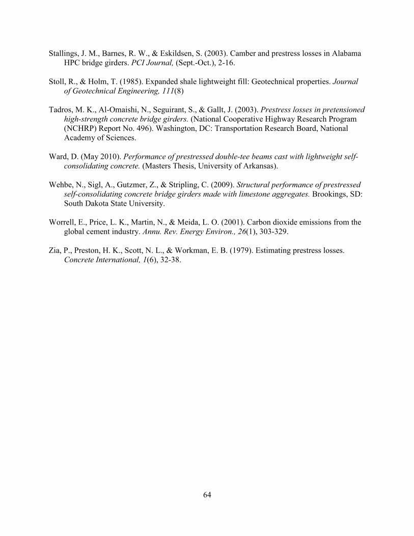
64

Stallings, J. M., Barnes, R. W., & Eskildsen, S. (2003). Camber and prestress losses in Alabama HPC bridge girders. PCI Journal, (Sept.-Oct.), 2-16.

Stoll, R., & Holm, T. (1985). Expanded shale lightweight fill: Geotechnical properties. Journal of Geotechnical Engineering, 111(8)

Tadros, M. K., Al-Omaishi, N., Seguirant, S., & Gallt, J. (2003). Prestress losses in pretensioned high-strength concrete bridge girders. (National Cooperative Highway Research Program (NCHRP) Report No. 496). Washington, DC: Transportation Research Board, National Academy of Sciences.

Ward, D. (May 2010). Performance of prestressed double-tee beams cast with lightweight self-

consolidating concrete. (Masters Thesis, University of Arkansas).

Wehbe, N., Sigl, A., Gutzmer, Z., & Stripling, C. (2009). Structural performance of prestressed

self-consolidating concrete bridge girders made with limestone aggregates. Brookings, SD: South Dakota State University.

Worrell, E., Price, L. K., Martin, N., & Meida, L. O. (2001). Carbon dioxide emissions from the global cement industry. Annu. Rev. Energy Environ., 26(1), 303-329.

Zia, P., Preston, H. K., Scott, N. L., & Workman, E. B. (1979). Estimating prestress losses. Concrete International, 1(6), 32-38.

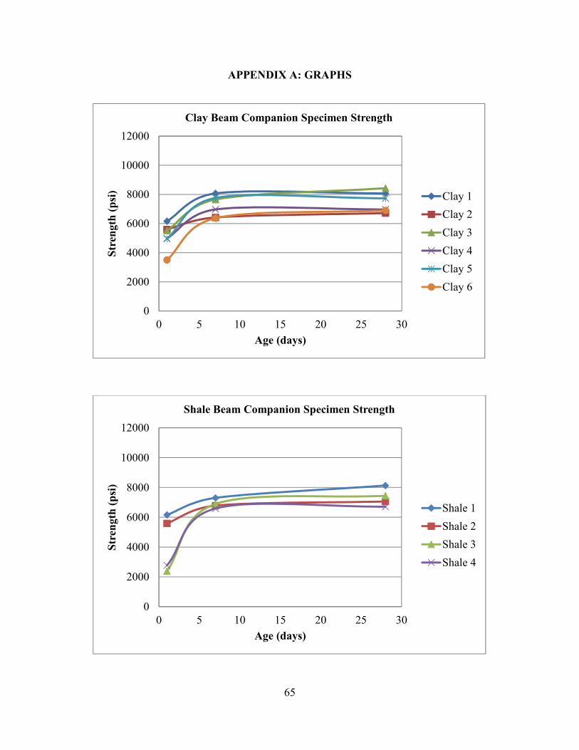
65

APPENDIX A: GRAPHS

0

2000

4000

6000

8000

10000

12000

0 5 10 15 20 25 30

Str

ength

(p

si)

Age (days)

Clay Beam Companion Specimen Strength

Clay 1

Clay 2

Clay 3

Clay 4

Clay 5

Clay 6

0

2000

4000

6000

8000

10000

12000

0 5 10 15 20 25 30

Str

ength

(p

si)

Age (days)

Shale Beam Companion Specimen Strength

Shale 1

Shale 2

Shale 3

Shale 4

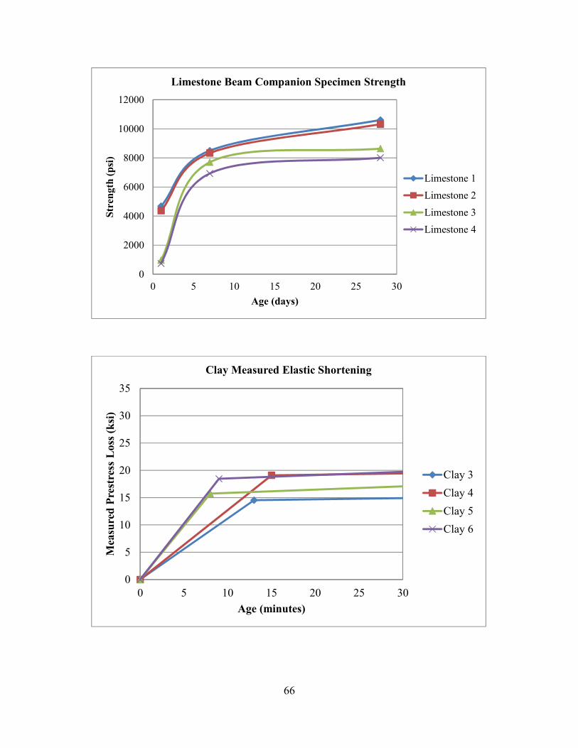
66

0

2000

4000

6000

8000

10000

12000

0 5 10 15 20 25 30

Str

eng

th (

psi

)

Age (days)

Limestone Beam Companion Specimen Strength

Limestone 1

Limestone 2

Limestone 3

Limestone 4

0

5

10

15

20

25

30

35

0 5 10 15 20 25 30

Mea

sure

d P

rest

ress

Loss

(k

si)

Age (minutes)

Clay Measured Elastic Shortening

Clay 3

Clay 4

Clay 5

Clay 6

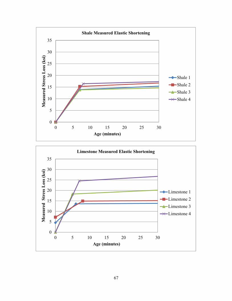
67

0

5

10

15

20

25

30

35

0 5 10 15 20 25 30

Mea

sure

d S

tres

s L

oss

(k

si)

Age (minutes)

Shale Measured Elastic Shortening

Shale 1

Shale 2

Shale 3

Shale 4

0

5

10

15

20

25

30

35

0 5 10 15 20 25 30

Mea

sure

d

Str

ess

Loss

(k

si)

Age (minutes)

Limestone Measured Elastic Shortening

Limestone 1

Limestone 2

Limestone 3

Limestone 4

68

0

10

20

30

40

50

60

0 50 100 150 200 250

Pre

stre

ss L

oss

, k

si

Age (days)

Predicted and Measured Losses-Clay 3

Clay 3 Measured Losses

Refined Method

Approximate Method

0

10

20

30

40

50

60

0 50 100 150 200 250

Pre

stre

ss L

oss

, k

si

Age (days)



Refined Method

Approximate Method

69

0

10

20

30

40

50

60

0 50 100 150 200 250

Pre

stre

ss L

oss

, k

si

Age (days)



Refined Method

Approximate Method

0

10

20

30

40

50

60

70

80

0 50 100 150 200 250

Pre

stre

ss L

oss

, k

si

Age (days)



Refined Method

Approximate Method

70

0

10

20

30

40

50

60

0 50 100 150 200 250

Pre

stre

ss L

oss

, k

si

Age (days)

Predicted and Measured Losses-Shale 1

Shale 1 Measured Losses

Refined Method

Approximate Method

0

10

20

30

40

50

60

0 50 100 150 200 250

Pre

stre

ss L

oss

, k

si

Age (days)



Refined Method

Approximate Method

71

0

20

40

60

80

100

120

0 50 100 150 200 250

Pre

stre

ss L

oss

, k

si

Age (days)



Refined Method

Approximate Method

0

10

20

30

40

50

60

70

80

90

100

0 50 100 150 200 250

Pre

stre

ss L

oss

, k

si

Age (days)



Refined Method

Approximate Method

72

0

10

20

30

40

50

60

0 50 100 150 200 250

Pre

stre

ss L

oss

, k

si

Age (days)

Predicted and Measured Losses-Limestone 1

Limestone 1 MeasuredLossesRefined Method

Approximate Method

0

10

20

30

40

50

60

0 50 100 150 200 250

Pre

stre

ss L

oss

, k

si

Age (days)



Approximate Method

73

0

20

40

60

80

100

120

140

0 50 100 150 200 250

Pre

stre

ss L

oss

, k

si

Age (days)



Approximate Method

0

20

40

60

80

100

120

140

160

180

0 50 100 150 200 250

Pre

stre

ss L

oss

, k

si

Age (days)



Approximate Method

Documents

Prestress Losses in Lightweight Self-Consolidating Concrete