Pressure Losses in Laminar Flow Through Serpentine

Journal of Power Sources 138 (2004) 1–13

Pressure losses in laminar flow through serpentine

channels in fuel cell stacks

S. Maharudrayya, S. Jayanti∗, A.P. Deshpande

Department of Chemical Engineering, IIT-Madras, Chennai 600036, India

Received 2 April 2004; accepted 9 June 2004

Available online 31 July 2004

Abstract

The pressure losses in the flow distributor plate of the fuel cell depend on the Reynolds number and geometric parameters of the small flow

channels. Very little information has been published on the loss coefficients for laminar flow. This study reports a numerical simulation of

laminar flow though single sharp and curved bends, 180◦ bends and serpentine channels of typical fuel cell configurations. The effect of the

geometric parameters and Reynolds number on the flow pattern and the pressure loss characteristics is investigated. A three-regime correlation

is developed for the excess bend loss coefficient as a function of Reynolds number, aspect ratios, curvature ratios and spacer lengths between

the channels. These have been applied to calculate the pressure drop in typical proton-exchange membrane fuel cell configurations to bring

out the interplay among the important geometric parameters.

© 2004 Elsevier B.V. All rights reserved.

Keywords: PEM fuel cell; Serpentine channels; Laminar flow; Bend loss coefficients; Computational fluid dynamics; Design correlations

1. Introduction

Fuel cells are electrochemical reactors and are being used

for a wide variety of applications. Due to their high efficiency

(nearly twice that of the present generation of internal com-

bustion engines), portability and near-zero emissions, fuel

cells are attractive as a power source for automobiles. Of the

various types of fuel cells, the proton-exchange membrane

fuel cell (PEMFC) operates at near-room temperatures and is

considered to be a good choice for automotive applications.

An elementary PEMFC consist of two thin, porous electrodes

(an anode and a cathode), which are separated by a polymer

membrane that passes only protons. In order to achieve high

utilization of the electrochemically active surfaces, a planar

architecture is usually used, in which the reactants, namely

hydrogen and oxygen (or their variants) are forced through

grooves etched on gas distributor plates. The grooves may be

of different patterns, i.e., parallel, single serpentine, parallel

∗ Corresponding author. Tel.: +91 44 4458227; fax: +91 44 2350509.

E-mail address: [email protected] (S. Jayanti).

serpentine or interdigitated channels [1–4] (Fig. 1). Since the

voltage produced across a typical cell is about 1V, a number

of such cells are stacked together and are connected in series

to increase the voltage. Cooling of the fuel cells is achieved

by inserting a plate between every second or third fuel cell

in the stack [5]. The cooling plate may also have serpentine

flow channel. For optimum performance, good distribution

of the reactants throughout the stacks is necessary. It is also

necessary to minimize the pressure drop in the flow of gases

through the stack as pumping power reduces the overall ef-

ficiency of the system. Thus, good knowledge of the flow

details in the serpentine channels of such stacks is necessary

for optimum design.

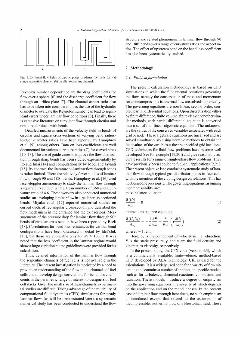
The various flow configurations, shown schematically in

Fig. 1 on a typical distributor plate, can be viewed as combi-

nations of straight and bend sections of ducts of rectangular

cross-section. Typically, the channel sizes and the gas flow

rates are small and the flow is expected to be laminar. This

poses special problems for the determination of the pressure

losses because the loss coefficients in laminar flow depend

strongly on the Reynolds number (Re). Examples of such

0378-7753/$ – see front matter © 2004 Elsevier B.V. All rights reserved.

doi:10.1016/j.jpowsour.2004.06.025

2 S. Maharudrayya et al. / Journal of Power Sources 138 (2004) 1–13

Fig. 1. Different flow fields of bipolar plates in planar fuel cells for: (a)

single serpentine channel; (b) parallel serpentine channel.

Reynolds number dependence are the drag coefficients for

flow over a sphere [6] and the discharge coefficient for flow

through an orifice plate [7]. The channel aspect ratio also

has to be taken into consideration as the use of the hydraulic

diameter to evaluate the Reynolds number can lead to signif-

icant errors under laminar flow conditions [8]. Finally, there

is extensive literature on turbulent flow through circular and

non-circular ducts with bends.

Detailed measurements of the velocity field in bends of

circular and square cross-sections of varying bend radius-

to-duct diameter ratios have been reported by Humphrey

et al. [9], among others. Data on loss coefficients are well

documented for various curvature ratios (C) for curved pipes

[10–13]. The use of guide vanes to improve the flow distribu-

tion through sharp bends has been studied experimentally by

Ito and Imai [14] and computationally by Modi and Jayanti

[15]. By contrast, the literature on laminar flow through bends

is rather limited. There are relatively fewer studies of laminar

flow through 90 and 180◦ bends. Humphrey et al. [16] used

laser-doppler anemometry to study the laminar flow through

a square curved duct with a Dean number of 368 and a cur-

vature ratio of 4.6. These workers also conducted numerical

studies ondeveloping laminar flow in circular cross-sectioned

bends. Miyaka et al. [17] reported numerical studies on

curved ducts of rectangular cross-section and described the

flow mechanism in the entrance and the exit resions. Mea-

surements of the pressure drop for laminar flow through 90◦

bends of circular cross-section have been reported by Beck

[18]. Correlations for bend loss resistances for various bend

configurations have been discussed in detail by Idel’chik

[13], but these are applicable only for Re > 10000. It was

noted that the loss coefficient in the laminar regime would

show a large variation but no guidelines were provided for its

calculation.

Thus, detailed information of the laminar flow through

the serpentine channels of fuel cells is not available in the

literature. The present investigation is motivated by a need to

provide an understanding of the flow in the channels of fuel

cells and to develop design correlations for bend loss coeffi-

cients in the parametric range of interest to designers of fuel

cell stacks.Given the small size of these channels, experimen-

tal studies are difficult. Taking advantage of the reliability of

computational fluid dynamics (CFD) simulations for steady

laminar flows (as will be demonstrated later), a systematic

numerical study has been conducted to understand the flow

structure and related phenomena in laminar flow through 90

and 180◦ bends over a range of curvature ratios and aspect ra-

tios. The effect of upstream bend on the bend loss coefficient

has also been systematically studied.

2. Methodology

2.1. Problem formulation

The present calculation methodology is based on CFD

simulations in which the fundamental equations governing

the flow, namely the conservation of mass and momentum

for an incompressible isothermal floware solved numerically.

The governing equations are non-linear, second-order, cou-

pled partial differential equations. Upon discretization either

by finite difference, finite volume, finite element or other sim-

ilar methods, each partial differential equation is converted

into a set of non-linear algebraic equations. The unknowns

are the values of the conserved variables associated with each

grid or node. These algebraic equations are linear zed and are

solved simultaneously using iterative methods to obtain the

field values of the variables at the pre-specified grid locations.

CFD techniques for fluid flow problems have become well

developed (see for example [19,20]) and give reasonably ac-

curate results for a range of single-phase flow problems. They

have previously been applied to fuel-cell applications [2,21].

The present objective is to conduct a systematic study of lam-

inar flow through typical gas distributor plates in fuel cells

with the intention of developing design correlations. This has

not been done previously. The governing equations, assuming

incompressibility are:

mass balance equation:

∂ (Ui)

∂xi

= 0 (1)

momentum balance equation:

∂ (UjUi)

∂xj

= −1

ρ

∂P

∂xi

+∂

∂xi

(

v∂Ui

∂xj

)

(2)

where i = 1, 2, 3.

Here, Ui is the component of velocity in the i-direction;

P is the static pressure, r and v are the fluid density and

kinematics viscosity, respectively.

In the present study, the CFX code (version 4.3), which

is a commercially available, finite-volume, method-based

CFD developed by AEA Technology, UK, is used for the

calculations. It is a widely used code for a variety of flow sit-

uations and contains a number of application-specificmodels

such as for turbulence, chemical reactions, combustion and

radiation. These models introduce a degree of empiricism

into the governing equations, the severity of which depends

on the application and on the model chosen. In the present

case of laminar flow through bent ducts, no such empiricism

is introduced except that related to the assumption of

incompressible, isothermal flow of a Newtonian fluid. These

S. Maharudrayya et al. / Journal of Power Sources 138 (2004) 1–13 3

assumptions should be valid for typical fuel-cell applications

where the pressure drops are fairly low, the temperatures

are fairly constant and the physical dimensions, though

small, are sufficiently large for continuum hypothesis to

be valid. The estimated Knudson number for air flow is

around 0.00007, which is much less than unity. Also, the

hydraulic diameter of the channel is of the order of 1mm,

and experiments [22,23] show that the flow remains laminar

up to a Re of about 2100. Hence, special considerations

associated with micro- or nano-scale phenomena [24] are not

warranted in the present problem, Therefore, main source

of error in the calculations arises from spatial discretization

and finite convergence limits imposed on the solution of the

discretized equations. These aspects are discussed later.

2.2. Details of the calculation scheme

The geometry studied in the present work consisted of

90 and 180◦ bend(s) in a duct of rectangular cross-section.

Simulations were carried out for: (i) a square bend, i.e., with

a curvature ratio C of Rc/Dh where Rc is the mean radius

of the bend and Dh is the duct hydraulic diameter, i.e., Dh

= 4wh/2(w + h), where w and h are width and depth of the

channel (ii) gradual bends. Typically, each bend was pro-

vided with a 100 diameter-long duct section upstream and a

100 diameter-long section downstream for flowdevelopment.

Taking advantage of the symmetry, only one-half of the duct

cross-section was simulated. Accordingly, the boundary con-

ditions imposed were:

• normal velocity specified as the mean flow velocity at the

upstream ‘inlet’;

• fully developed flow condition specified at the downstream

‘outlet’;

• no-slip condition (zero velocity for normal and tangential

velocity components) on the side walls;

• symmetry condition (zero normal gradient) specified on

the symmetry plane.

The nominal fluid properties corresponded to those of air at

atmospheric conditions. The Reynolds number based on the

mean velocity and the hydraulic diameter was varied between

0.7 and 2300.

The cross-section of the duct was discretized by using

a structured mesh with 20 cells in the width direction and

12 cells in the half-depth direction. Since the location of the

maximumvelocity gradient changes location as the flow goes

through the bend, a uniformmesh was employed in the cross-

section of the duct. Along the axis of the duct, a non-uniform

grid was employed to enable better resolution of the velocity

gradients near the bend. A systematic study of grid inde-

pendence was carried out, as discussed later, to verify that

this grid is adequate. All the simulations were conducted by

means of a segregatedmethodusing theSIMPLEscheme [19]

for pressure-velocity decoupling. Nominally second order-

accurate schemes were selected for the discretization of the

governing equations. A residual reduction factor of 10−10

for the mass conservation equation was used to monitor the

convergence of the iterative scheme.

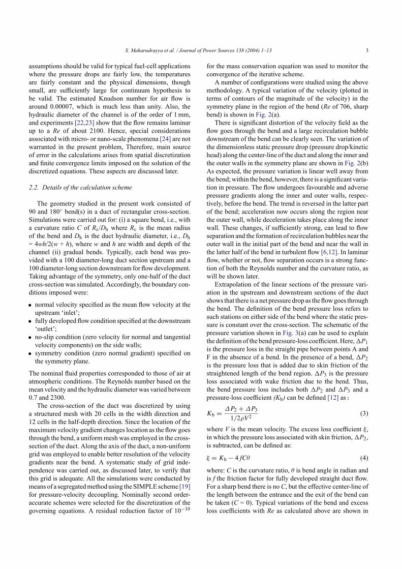
A number of configurations were studied using the above

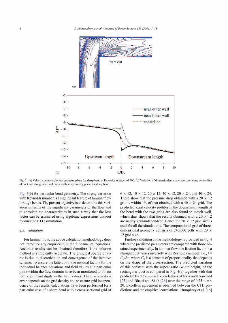
methodology. A typical variation of the velocity (plotted in

terms of contours of the magnitude of the velocity) in the

symmetry plane in the region of the bend (Re of 706, sharp

bend) is shown in Fig. 2(a).

There is significant distortion of the velocity field as the

flow goes through the bend and a large recirculation bubble

downstream of the bend can be clearly seen. The variation of

the dimensionless static pressure drop (pressure drop/kinetic

head) along the center-line of the duct and along the inner and

the outer walls in the symmetry plane are shown in Fig. 2(b)

As expected, the pressure variation is linear well away from

thebend;within the bend, however, there is a significant varia-

tion in pressure. The flow undergoes favourable and adverse

pressure gradients along the inner and outer walls, respec-

tively, before the bend. The trend is reversed in the latter part

of the bend; acceleration now occurs along the region near

the outer wall, while deceleration takes place along the inner

wall. These changes, if sufficiently strong, can lead to flow

separation and the formation of recirculation bubbles near the

outer wall in the initial part of the bend and near the wall in

the latter half of the bend in turbulent flow [6,12]. In laminar

flow, whether or not, flow separation occurs is a strong func-

tion of both the Reynolds number and the curvature ratio, as

will be shown later.

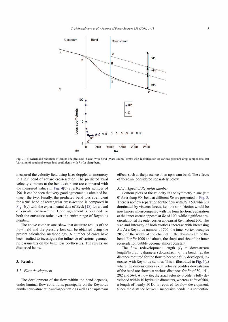
Extrapolation of the linear sections of the pressure vari-

ation in the upstream and downstream sections of the duct

shows that there is a net pressure drop as theflowgoes through

the bend. The definition of the bend pressure loss refers to

such stations on either side of the bend where the static pres-

sure is constant over the cross-section. The schematic of the

pressure variation shown in Fig. 3(a) can be used to explain

the definition of the bend pressure-loss coefficient. Here,1P1is the pressure loss in the straight pipe between points A and

F in the absence of a bend. In the presence of a bend, 1P2is the pressure loss that is added due to skin friction of the

straightened length of the bend region. 1P3 is the pressure

loss associated with wake friction due to the bend. Thus,

the bend pressure loss includes both 1P2 and 1P3 and a

pressure-loss coefficient (Kb) can be defined [12] as:

Kb =∆P2 + ∆P3

1/2ρV 2(3)

where V is the mean velocity. The excess loss coefficient ξ,

in which the pressure loss associated with skin friction,1P2,

is subtracted, can be defined as:

ξ = Kb − 4fCθ (4)

where: C is the curvature ratio, θ is bend angle in radian and

is f the friction factor for fully developed straight duct flow.

For a sharp bend there is no C, but the effective center-line of

the length between the entrance and the exit of the bend can

be taken (C = 0). Typical variations of the bend and excess

loss coefficients with Re as calculated above are shown in


Fig. 2. (a) Velocity contour plot in symmetry plane for sharp bend at Reynolds number of 700. (b) Variation of dimensionless static pressure along center-line

of duct and along inner and outer walls in symmetry plane for sharp bend.

Fig. 3(b) for particular bend geometry. The strong variation

with Reynolds number is a significant feature of laminar flow

through bends. The present objective is to determine this vari-

ation in terms of the significant parameters of the flow and

to correlate the characteristics in such a way that the loss

factor can be estimated using algebraic expressions without

recourse to CFD simulation.

2.3. Validation

For laminar flow, the above calculation methodology does

not introduce any empiricism in the fundamental equations.

Accurate results can be obtained therefore if the solution

method is sufficiently accurate. The principal source of er-

ror is due to discretization and convergence of the iterative

scheme. To ensure the latter, both the residual factors for the

individual balance equations and field values at a particular

point within the flow domain have been monitored to obtain

four significant digits in the field values. The discretization

error depends on the grid density and to ensure grid indepen-

dence of the results; calculations have been performed for a

particular case of a sharp bend with a cross-sectional grid of

6 × 12, 10 × 12, 20 × 12, 40 × 12, 20 × 24, and 40 × 24.

These show that the pressure drop obtained with a 20 × 12

grid is within 1% of that obtained with a 40 × 24 grid. The

predicted axial velocity profiles in the downstream length of

the bend with the two grids are also found to match well,

which thus shows that the results obtained with a 20 × 12

are nearly grid-independent. Hence the 20 × 12 grid size is

used for all the simulations. The computational grid of three-

dimensional geometry consists of 240,000 cells with 20 ×

12 grid size.

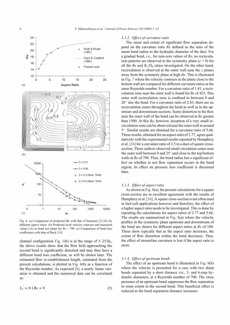
Further validation of themethodology is provided in Fig. 4

where the predicted parameters are compared with those ob-

tained experimentally. In laminar flow, the friction factor in a

straight duct varies inversely with Reynolds number, i.e., f =

Cs/Re, where Cs is a constant of proportionality that depends

on the shape of the cross-section. The predicted variation

of this constant with the aspect ratio (width/height) of the

rectangular duct is compared in Fig. 4(a) together with that

predicted by the empirical correlations of Kays and Crawford

[25] and Bhatti and Shah [26] over the range of 0.25 < a <

20. Excellent agreement is obtained between the CFD pre-

dictions and the empirical correlations. Humphrey et al. [16]


Fig. 3. (a) Schematic variation of center-line pressure in duct with bend (Ward-Smith, 1980) with identification of various pressure drop components. (b)

Variation of bend and excess loss coefficients with Re for sharp bend.

measured the velocity field using laser-doppler anemometry

in a 90◦ bend of square cross-section. The predicted axial

velocity contours at the bend exit plane are compared with

the measured values in Fig. 4(b) at a Reynolds number of

790. It can be seen that very good agreement is obtained be-

tween the two. Finally, the predicted bend loss coefficient

for a 90◦ bend of rectangular cross-section is compared in

Fig. 4(c) with the experimental data of Beck [18] for a bend

of circular cross-section. Good agreement is obtained for

both the curvature ratios over the entire range of Reynolds

number.

The above comparisons show that accurate results of the

flow field and the pressure loss can be obtained using the

present calculation methodology. A number of cases have

been studied to investigate the influence of various geomet-

ric parameters on the bend loss coefficients. The results are

discussed below.

3. Results

3.1. Flow development

The development of the flow within the bend depends,

under laminar flow conditions, principally on the Reynolds

number curvature ratio and aspect ratio aswell as on upstream

effects such as the presence of an upstream bend. The effects

of these are considered separately below.

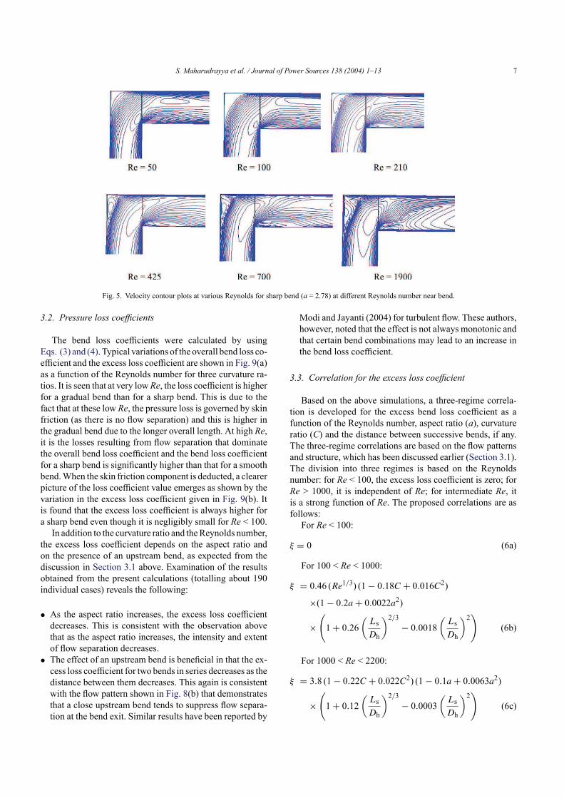
3.1.1. Effect of Reynolds number

Contour plots of the velocity in the symmetry plane (z =

0) for a sharp 90◦ bend at different Re.are presented in Fig. 5.

There is no flow separation for the flowwithRe < 50, which is

dominated by viscous forces, i.e., the skin friction would be

muchmorewhen comparedwith the form friction. Separation

at the inner corner appears at Re of 100, while significant re-

circulation at the outer corner appears atRe of about 200. The

size and intensity of both vortices increase with increasing

Re. At a Reynolds number of 706, the inner vortex occupies

20% of the width of the channel in the downstream of the

bend. For Re 1000 and above, the shape and size of the inner

recirculation bubble become almost constant.

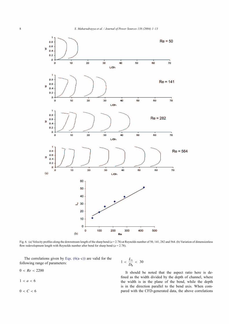
The flow redevelopment length (Lr = downstream

length/hydraulic diameter) downstream of the bend, i.e., the

distance required for the flow to become fully developed, in-

creases with Reynolds number. This is illustrated in Fig. 6(a)

where the dimensionless axial velocity profiles downstream

of the bend are shown at various distances for Re of 50, 141,

282 and 564. At low Re, the axial velocity profile is fully de-

veloped within 10 hydraulic diameters, whereas at Re of 564,

a length of nearly 50Dh is required for flow development.

Since the distance between successive bends in a serpentine


Fig. 4. (a) Comparison of predicted fRe with that of literature [25,26] for

different aspect ratios. (b) Predicted axial velocity contours and measured

values [16] at bend exit plane for Re = 790. (c) Comparison of bend loss

coefficients with data of Beck [18].

channel configuration Fig. 1(b) is in the range of 5–25Dh,

the above results show that the flow field approaching the

second bend is significantly distorted and may thus have a

different bend loss coefficient, as will be shown later. The

estimated flow re-establishment length, estimated from the

present calculations, is plotted in Fig. 6(b) as a function of

the Reynolds number. As expected [8], a nearly linear vari-

ation is obtained and the numerical data can be correlated

as:

Lr = 0.1Re + 9 (5)

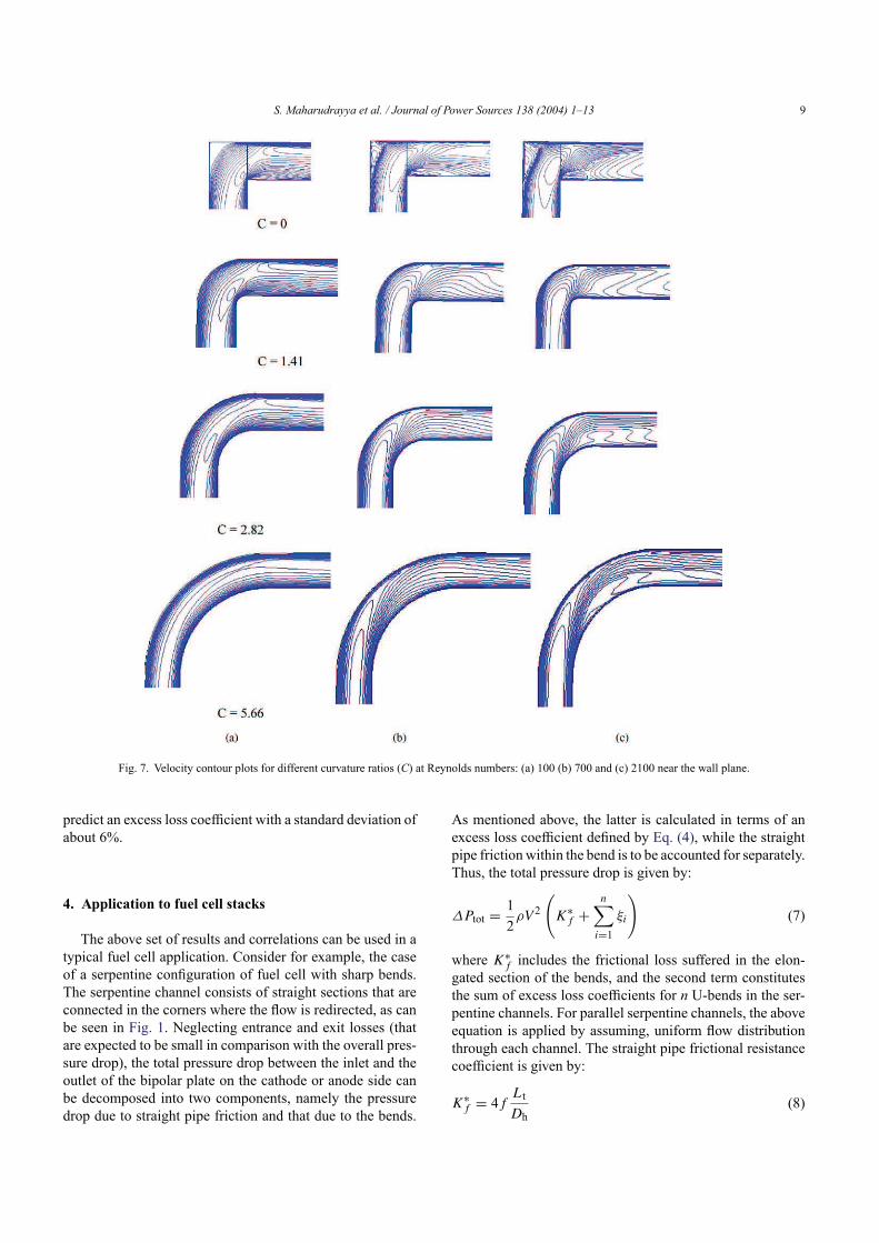
3.1.2. Effect of curvature ratio

The onset and extent of significant flow separation de-

pend on the curvature ratio Re defined as the ratio of the

mean bend radius to the hydraulic diameter of the duct. For

a gradual bend, i.e., for non-zero values of Re, no recircula-

tion patterns are observed in the symmetry plane (z = 0) for

all the Re and Rc/Dh ratios investigated. On the other hand,

recirculation is observed at the outer wall near the z planes

away from the symmetry plane at high Re. This is illustrated

in Fig. 7 where the velocity contours in the plane close to the

bottom wall are compared for different curvature ratios at the

same Reynolds number. For a curvature ratio of 1.41, a recir-

culation zone near the outer wall is found for Re of 425. This

outer wall recirculation zone is confined to between 0 and

20◦ into the bend. For a curvature ratio of 2.83, there are no

recirculation zones throughout the bend as well as in the up-

stream and downstream sections. Some distortion in the flow

near the outer wall of the bend can be observed at Re greater

than 1500. At this Re, however, inception of a very small re-

circulation zone can be observed near the outer wall at around

5◦. Similar results are obtained for a curvature ratio of 5.66.

These results, obtained for an aspect ratio of 2.77, agree qual-

itatively with the experimental results reported by Humphrey

et al. [16] for a curvature ratio of 2.5 in a duct of square cross-

section. These authors observed small circulation zones near

the outer wall between 0 and 25◦ and close to the top/bottom

walls at Re of 790. Thus, the bend radius has a significant ef-

fect on whether or not flow separation occurs in the bend

region; its effect on pressure loss coefficient is discussed

later.

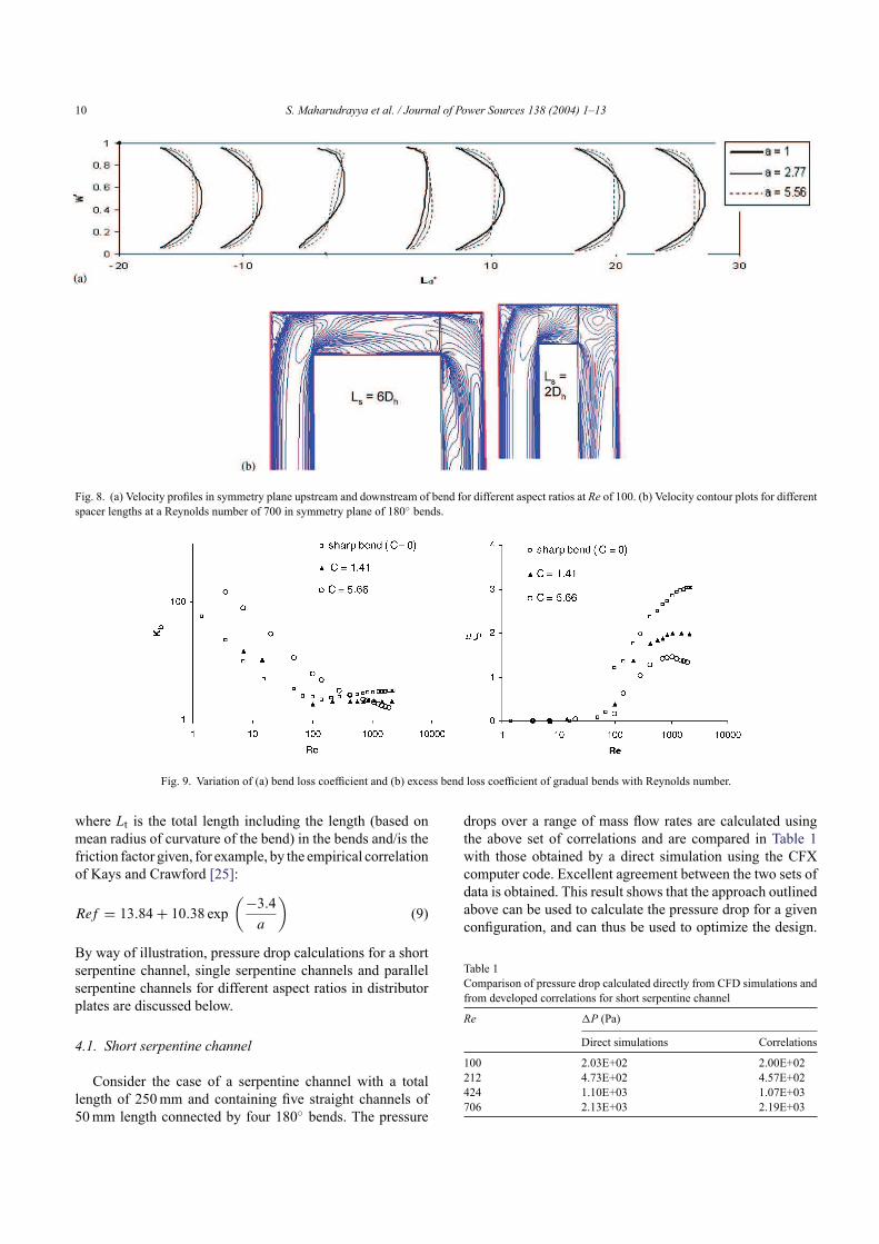
3.1.3. Effect of aspect ratio

As shown in Fig. 8(a), the present calculations for a square

cross-section are in excellent agreement with the results of

Humphrey et al. [16]. A square cross-section is not often used

in fuel-cell applications however and therefore, the effect of

a higher aspect ratio needs to be investigated. This is done by

repeating the calculations for aspect ratios of 2.77 and 5.66.

The results are summarized in Fig. 8(a) where the velocity

profiles in the symmetry plane upstream and downstream of

the bend are shown for different aspect ratios at Re of 100.

These show typically that as the aspect ratio increases, the

extent of flow distortion within the bend decreases. Thus,

the effect of streamline curvature is less if the aspect ratio is

more.

3.1.4. Effect of upstream bends

The effect of an upstream bend is illustrated in Fig. 8(b)

where the velocity is presented for a case with two sharp

bends separated by a short distance viz., 2- and 6-step hy-

draulic diameters, at a Reynolds number of 700. The close

presence of an upstream bend suppresses the flow separation

to some extent in the second bend. This beneficial effect is

reduced as the bend separation distance increases.


Fig. 5. Velocity contour plots at various Reynolds for sharp bend (a = 2.78) at different Reynolds number near bend.

3.2. Pressure loss coefficients

The bend loss coefficients were calculated by using

Eqs. (3) and (4). Typical variations of the overall bend loss co-

efficient and the excess loss coefficient are shown in Fig. 9(a)

as a function of the Reynolds number for three curvature ra-

tios. It is seen that at very lowRe, the loss coefficient is higher

for a gradual bend than for a sharp bend. This is due to the

fact that at these low Re, the pressure loss is governed by skin

friction (as there is no flow separation) and this is higher in

the gradual bend due to the longer overall length. At high Re,

it is the losses resulting from flow separation that dominate

the overall bend loss coefficient and the bend loss coefficient

for a sharp bend is significantly higher than that for a smooth

bend.When the skin friction component is deducted, a clearer

picture of the loss coefficient value emerges as shown by the

variation in the excess loss coefficient given in Fig. 9(b). It

is found that the excess loss coefficient is always higher for

a sharp bend even though it is negligibly small for Re < 100.

In addition to the curvature ratio and theReynolds number,

the excess loss coefficient depends on the aspect ratio and

on the presence of an upstream bend, as expected from the

discussion in Section 3.1 above. Examination of the results

obtained from the present calculations (totalling about 190

individual cases) reveals the following:

• As the aspect ratio increases, the excess loss coefficient

decreases. This is consistent with the observation above

that as the aspect ratio increases, the intensity and extent

of flow separation decreases.

• The effect of an upstream bend is beneficial in that the ex-

cess loss coefficient for two bends in series decreases as the

distance between them decreases. This again is consistent

with the flow pattern shown in Fig. 8(b) that demonstrates

that a close upstream bend tends to suppress flow separa-

tion at the bend exit. Similar results have been reported by

Modi and Jayanti (2004) for turbulent flow. These authors,

however, noted that the effect is not always monotonic and

that certain bend combinations may lead to an increase in

the bend loss coefficient.

3.3. Correlation for the excess loss coefficient

Based on the above simulations, a three-regime correla-

tion is developed for the excess bend loss coefficient as a

function of the Reynolds number, aspect ratio (a), curvature

ratio (C) and the distance between successive bends, if any.

The three-regime correlations are based on the flow patterns

and structure, which has been discussed earlier (Section 3.1).

The division into three regimes is based on the Reynolds

number: for Re < 100, the excess loss coefficient is zero; for

Re > 1000, it is independent of Re; for intermediate Re, it

is a strong function of Re. The proposed correlations are as

follows:

For Re < 100:

ξ = 0 (6a)

For 100 < Re < 1000:

ξ = 0.46 (Re1/3) (1− 0.18C + 0.016C2)

×(1− 0.2a + 0.0022a2)

×

(

1+ 0.26

(

Ls

Dh

)2/3

− 0.0018

(

Ls

Dh

)2)

(6b)

For 1000 < Re < 2200:

ξ = 3.8 (1− 0.22C + 0.022C2) (1 − 0.1a + 0.0063a2)

×

(

1+ 0.12

(

Ls

Dh

)2/3

− 0.0003

(

Ls

Dh

)2)

(6c)


Fig. 6. (a) Velocity profiles along the downstream length of the sharp bend (a = 2.78) at Reynolds number of 50, 141, 282 and 564. (b) Variation of dimensionless

flow redevelopment length with Reynolds number after bend for sharp bend (a = 2.78).

The correlations given by Eqs. (6(a–c)) are valid for the

following range of parameters:

0 < Re < 2200

1 < a < 6

0 < C < 6

1 <Ls

Dh< 30

It should be noted that the aspect ratio here is de-

fined as the width divided by the depth of channel, where

the width is in the plane of the bend, while the depth

is in the direction parallel to the bend axis. When com-

pared with the CFD-generated data, the above correlations


Fig. 7. Velocity contour plots for different curvature ratios (C) at Reynolds numbers: (a) 100 (b) 700 and (c) 2100 near the wall plane.

predict an excess loss coefficient with a standard deviation of

about 6%.

4. Application to fuel cell stacks

The above set of results and correlations can be used in a

typical fuel cell application. Consider for example, the case

of a serpentine configuration of fuel cell with sharp bends.

The serpentine channel consists of straight sections that are

connected in the corners where the flow is redirected, as can

be seen in Fig. 1. Neglecting entrance and exit losses (that

are expected to be small in comparison with the overall pres-

sure drop), the total pressure drop between the inlet and the

outlet of the bipolar plate on the cathode or anode side can

be decomposed into two components, namely the pressure

drop due to straight pipe friction and that due to the bends.

As mentioned above, the latter is calculated in terms of an

excess loss coefficient defined by Eq. (4), while the straight

pipe friction within the bend is to be accounted for separately.

Thus, the total pressure drop is given by:

∆Ptot =1

2ρV 2

(

K∗

f +

n∑

i=1

ξi

)

(7)

where K∗

f includes the frictional loss suffered in the elon-

gated section of the bends, and the second term constitutes

the sum of excess loss coefficients for n U-bends in the ser-

pentine channels. For parallel serpentine channels, the above

equation is applied by assuming, uniform flow distribution

through each channel. The straight pipe frictional resistance

coefficient is given by:

K∗

f = 4fLt

Dh(8)


Fig. 8. (a) Velocity profiles in symmetry plane upstream and downstream of bend for different aspect ratios at Re of 100. (b) Velocity contour plots for different

spacer lengths at a Reynolds number of 700 in symmetry plane of 180◦ bends.

Fig. 9. Variation of (a) bend loss coefficient and (b) excess bend loss coefficient of gradual bends with Reynolds number.

where Lt is the total length including the length (based on

mean radius of curvature of the bend) in the bends and/is the

friction factor given, for example, by the empirical correlation

of Kays and Crawford [25]:

Ref = 13.84 + 10.38 exp

(

−3.4

a

)

(9)

By way of illustration, pressure drop calculations for a short

serpentine channel, single serpentine channels and parallel

serpentine channels for different aspect ratios in distributor

plates are discussed below.

4.1. Short serpentine channel

Consider the case of a serpentine channel with a total

length of 250mm and containing five straight channels of

50mm length connected by four 180◦ bends. The pressure

drops over a range of mass flow rates are calculated using

the above set of correlations and are compared in Table 1

with those obtained by a direct simulation using the CFX

computer code. Excellent agreement between the two sets of

data is obtained. This result shows that the approach outlined

above can be used to calculate the pressure drop for a given

configuration, and can thus be used to optimize the design.

Table 1

Comparison of pressure drop calculated directly from CFD simulations and

from developed correlations for short serpentine channel

Re 1P (Pa)

Direct simulations Correlations

100 2.03E+02 2.00E+02

212 4.73E+02 4.57E+02

424 1.10E+03 1.07E+03

706 2.13E+03 2.19E+03


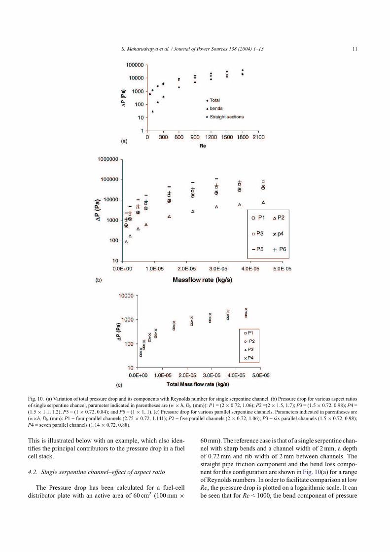
Fig. 10. (a) Variation of total pressure drop and its components with Reynolds number for single serpentine channel. (b) Pressure drop for various aspect ratios

of single serpentine chancel, parameter indicated in parentheses are (w × h, Dh (mm)): P1 = (2 × 0.72, 1.06); P2 =(2 × 1.5, 1.7); P3 = (1.5 × 0.72, 0.98); P4 =

(1.5 × 1.1, 1.2); P5 = (1 × 0.72, 0.84); and P6 = (1 × 1, 1). (c) Pressure drop for various parallel serpentine channels. Parameters indicated in parentheses are

(w×h, Dh (mm): P1 = four parallel channels (2.75 × 0.72, 1.141); P2 = five parallel channels (2 × 0.72, 1.06); P3 = six parallel channels (1.5 × 0.72, 0.98);

P4 = seven parallel channels (1.14 × 0.72, 0.88).

This is illustrated below with an example, which also iden-

tifies the principal contributors to the pressure drop in a fuel

cell stack.

4.2. Single serpentine channel–effect of aspect ratio

The Pressure drop has been calculated for a fuel-cell

distributor plate with an active area of 60 cm2 (100mm ×

60mm). The reference case is that of a single serpentine chan-

nel with sharp bends and a channel width of 2mm, a depth

of 0.72mm and rib width of 2mm between channels. The

straight pipe friction component and the bend loss compo-

nent for this configuration are shown in Fig. 10(a) for a range

of Reynolds numbers. In order to facilitate comparison at low

Re, the pressure drop is plotted on a logarithmic scale. It can

be seen that for Re < 1000, the bend component of pressure


drop is significantly less (by a factor of two or more) than

the straight pipe friction. At higher Reynolds numbers, how-

ever, it is nearly as much as the straight pipe component. The

effect of changing the dimensions of the channel (width and

depth), which will exert an influence on the hydraulic diame-

ter and thus on the straight pipe friction component, is shown

in Fig. 10(b) Since both the mean velocity and the hydraulic

diameter are changed in this process, it is no longer possible

to compare the results on a Reynolds number basis, and the

pressure drop for a given mass flow rate (of air) are compared

here. The reference case with a width × depth × hydraulic

diameter of 2mm× 0.72mm× 1.058mm is shown as a solid

line, while the geometric parameters corresponding to other

combinations are marked in the legend. It can be seen that de-

creasing the channel width while keeping the depth constant

decreases the hydraulic diameter and leads to a large increase

in the pressure drop. By contrast, increasing the depth while

keeping the width constant increases the hydraulic diameter

and the pressure drop decreases by a large factor. In the case

of a 1.5 × 1 × 1.2-system, an increase in hydraulic diameter

increases the pressure drop when compared to the reference

case at highermass flow rateswhile there is virtually no effect

at low Re. This must be attributed to the higher bend losses

that resulting from the higher mass flow rate due to the de-

creased cross-section, which nullifies the beneficial effect of

increased hydraulic diameter. The effect of decreasing the rib

width is to increase the overall length of the single serpentine

channel and this increases simultaneously both the pressure

drop and the active area.

4.3. Parallel serpentine channels–effect of number of

channels

One way of decreasing the pressure drop in a distributor

plate is to have parallel serpentine channels instead of a sin-

gle serpentine channel. This has the effect of reducing the

flow rate through each channel, which decreases the pressure

drop. At low Re, the pressure drop variation with the number

of parallel channels will be linear. A more than linear vari-

ation may be expected at high Re because the bend losses,

which are proportional to the square of velocity at highRe de-

crease more dramatically than the straight pipe friction com-

ponent. This situation is illustrated in Fig. 10(c), in which the

ribwidth is assumed to be 1mm. It can be seen that the use

of five parallel channels in a serpentine configuration with

five turns, instead of a single channel (with about 20 turns)

with the same cross-section, decreases the pressure drop by

an order of magnitude. The effect of changing the width and

depth of the parallel channel serpentine configuration is also

shown in Fig. 10(c). If the channel’s width is reduced, it is

assumed that extra parallel channels are added as a means

of compensation, while an increased channel width is ac-

commodated by reducing the number of parallel channels.

Thus, the length of each serpentine configuration is roughly

the same. Under these conditions (other configurations are

possible), the data in Fig. 10(c) shows that the pressure drops

for different combinations can vary by a factor of two. The

active area of the distributor plate, that is the area of fluid

exposed to the porous electrode, also varies by about 25%.

Calculations of this type can be combined with other criteria

such as high pressure drop that is required to prevent flood-

ing of the electrodes [27,28] and low pressure drop that is

required to reduce pumping costs, and the rib width/active

area considerations can be used to optimize the distributor

plate configuration.

5. Conclusions

The pressure losses in a fuel cell stack are one of the im-

portant factors for overall fuel cell efficiency. The pressure

drop in a fuel cell distributor plate depends on the plate con-

figurations, and for a given serpentine channel configuration,

it depends on geometric factors such as channel hydraulic

diameter and bend geometry.

CFD-based simulations have been conducted for 90◦

bends with different curvature ratios (C) and different aspect

ratios (a). The effect of successive bends for various spacer

lengths (Ls 2–30Dh) for full range of Reynolds numbers un-

der laminar flow regime has been examined. The calculations

show that there is a significant effect of Re on the bend loss

coefficient, which is also influenced by the curvature ratio and

the aspect ratio as well as the presence of an upstream bend.

A correlation has been developed to predict the bend loss

coefficient as a function of these parameters. Application of

this correlation to typical fuel cell configurations shows that

the bend losses constitute a significant portion of the over-

all pressure loss for Re > 1000. Considerable scope exists

for the optimization of the channel configuration (in terms

of width, height and gap) to achieve a desired pressure drop

and keeping in view the need to reduce pumping costs while

maintaining a sufficiently high pressure drop to avoid flood-

ing of the channels. The results from this work will be very

useful for such an optimization.

Acknowledgements

The work reported here has been carried out under a re-

search grant from the Ministry of Non-conventional Energy

Resources, India. The CFD computations have been carried

out using the facilities of the CFD Center, IIT-Madras, India.

References

[1] H. Dohle, A.A. Kournyshev, A.A. Kulikovsky, J. Mergel, D. Stolen,

Electrochem. Commun. 3 (2001) 73–80.

[2] V. Garau, L. Hongtan, S. Kakac, AIChE J. 44 (1998) 2410–2422.

[3] T.V. Nguyen, J. Electrochem. Soc. 143 (1996) L103–L105.

[4] P.W. Li, L. Schaefer, Q. Wang, Zhang M.K. Chyu, J. Power Sources

113 (2003) 90–100.


[5] E. Middelman, W. Kout, B. Vogelaar, J. Lenssen, E. De wall, J.

Power Sources 118 (2003) 44–46.

[6] H. Schlichting, Boundary-Layer Theory, 6th ed., McGraw Hill, New

York, 1968.

[7] W.H. Perry, Chemical Engineer’s Handbook, 6th ed., McGraw Hill,

New York, 1984.

[8] F.M. White, Viscous fluid flow, 2nd ed., McGraw-Hill, Inc, New

York, 1991.

[9] J.A.C. Humphrey, J.H. Whitelaw, G. Yee, J. Fluid Mech. 103 (1981)

443–463.

[10] H. Ito, J. Basic Eng. Trans. ASME (1960) 131–142.

[11] D.R. Blevins, Applied Fluid Dynamics Handbook, Van Nostrand

Reinhold Co Inc, New York, 1984.

[12] A.J. Ward-Smith, Internal Fluid Flow, Oxford University Press, New

York, 1980.

[13] I.E. Idel’chik, Handbook of Hydraulic Resistances, 3rd ed., Jaico

Publishing House, Mumbai, 1986.

[14] H. Ito, K. Imai, J. Basic Eng. Trans. ASME D (1966) 684–685.

[15] M. Modi, S. Jayanti, Trans. IChem E, Chem. Eng. Res. Des. 82

(2004) 321–331.

[16] J.A.C. Humphrey, A.M.K. Taylor, J.H. Whitelaw, J. Fluid Mech. 83

(1977) 509–527.

[17] Y.Miyaka, T. Kazishima, T.Inaba, International Conference on Ex-

perimental Heat Transfer, Fluid Mechanics and Thermodynamics,

1988.

[18] C. Beck, J. Am. Soc. Naval Eng. 56 (3) (1944) 366–388.

[19] S.V. Patankar, Numerical Heat Transfer and Fluid Flow, Hemisphere,

Washington, DC, 1980.

[20] J.H. Ferziger, M. Peric, Computational Methods for Fluid Dynamics,

Springer, Berlin, Germany, 1980.

[21] A. Kumar, G.R. Reddy, J. Power Sources 113 (2002) 11–18.

[22] T.S. Zhao, Q.C. Bi, Int. J. Heat Mass Transfer 44 (2001) 2523–

2534.

[23] B. Agostini, B. Watel, A. Bontemps, B. Thonon, Exp. Therm. Fluid

Sci. 28 (2004) 97–103.

[24] M. Gad El-Hak, J. Fluids Eng. Trans. ASME 121 (1999) 1–29.

[25] W.M. Kays, M.E. Crawford, Convective Heat and Mass Transfer,

McGraw-Hill, New York, 1980.

[26] M.S. Bhatti, R.K. Shah, in: S. Kakak, R.K. Shah, W. Aung (Eds.),

Handbook of Single-phase Convective Heat Transfer, Wiley, New

York, 1987.

[27] J.J. Baschuk, X. Li, J. Power Sources 86 (2000) 181–195.

[28] T. Klaus, P. David, C. Hebling, J. Power Sources 124 (2003) 403–

414.

Documents

Pressure Losses in Laminar Flow Through Serpentine