Embed Size (px)
Citation preview
Pressure Losses for Fluid Flow Through Abrupt Area
Contraction in Compact Heat Exchangers
Undergraduate Research Spring 2004
By Bryan J. Johnson
Under Direction of Rehnberg Professor of Ch.E. Bruce A. Finlayson
Date: June 11, 2004
2
Introduction
The goal of this experiment was to predict and improve on the results of Kays and
London “entrance pressure-loss coefficient (Kc) for a multiple tube flat-duct heat exchanger core
with an abrupt-contraction entrance.” [1] Kays and London determined the pressure-loss
coefficient for various contraction ratios (σ) and graphed them as a line. They labeled this line
as “Laminar”, but did not expound upon the range of Reynolds numbers the laminar flow line
was applicable to. This experiment will graph the pressure loss coefficient for six contraction
ratios and a range of Reynolds numbers to improve upon Kays’ and London’s “Laminar” flow
graph.
Materials and Methods
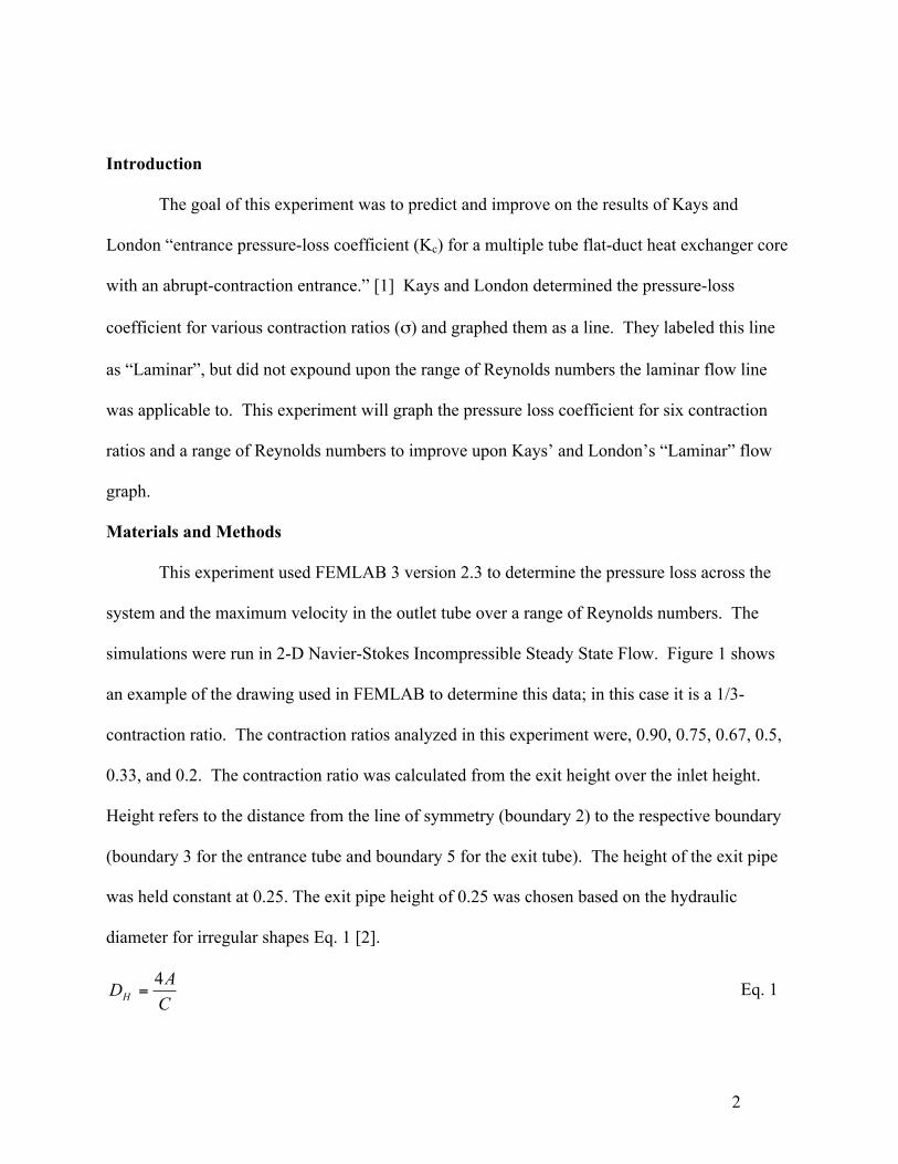
This experiment used FEMLAB 3 version 2.3 to determine the pressure loss across the
system and the maximum velocity in the outlet tube over a range of Reynolds numbers. The
simulations were run in 2-D Navier-Stokes Incompressible Steady State Flow. Figure 1 shows
an example of the drawing used in FEMLAB to determine this data; in this case it is a 1/3-
contraction ratio. The contraction ratios analyzed in this experiment were, 0.90, 0.75, 0.67, 0.5,
0.33, and 0.2. The contraction ratio was calculated from the exit height over the inlet height.
Height refers to the distance from the line of symmetry (boundary 2) to the respective boundary
(boundary 3 for the entrance tube and boundary 5 for the exit tube). The height of the exit pipe
was held constant at 0.25. The exit pipe height of 0.25 was chosen based on the hydraulic
diameter for irregular shapes Eq. 1 [2].
CADH4
= Eq. 1
3
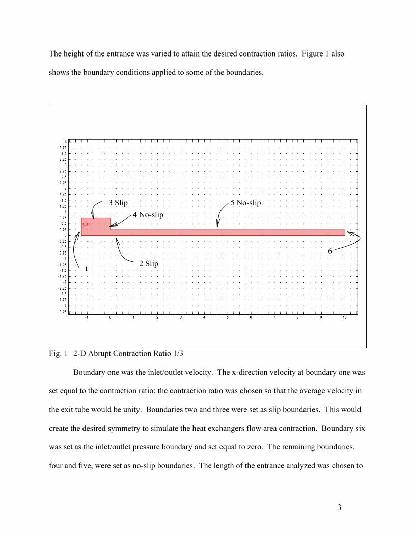
The height of the entrance was varied to attain the desired contraction ratios. Figure 1 also
shows the boundary conditions applied to some of the boundaries.
Fig. 1 2-D Abrupt Contraction Ratio 1/3 Boundary one was the inlet/outlet velocity. The x-direction velocity at boundary one was
set equal to the contraction ratio; the contraction ratio was chosen so that the average velocity in
the exit tube would be unity. Boundaries two and three were set as slip boundaries. This would
create the desired symmetry to simulate the heat exchangers flow area contraction. Boundary six
was set as the inlet/outlet pressure boundary and set equal to zero. The remaining boundaries,
four and five, were set as no-slip boundaries. The length of the entrance analyzed was chosen to
1 2 Slip
3 Slip 4 No-slip
5 No-slip
6
4
be 1.25, to allow for fully developed flow entering the contraction area. The length of the exit
tube was chosen to be 10, to allow for fully developed flow to exist at the exit boundary. In the
sub-domain settings the density (ρ) was set equal to 10s. By varying the density the Reynolds
number would also be varied. Using parametric solver “s” was varied from –3 to 3 by 0.1
increments. This would yield data for Reynolds number from 0.001 to 1000.
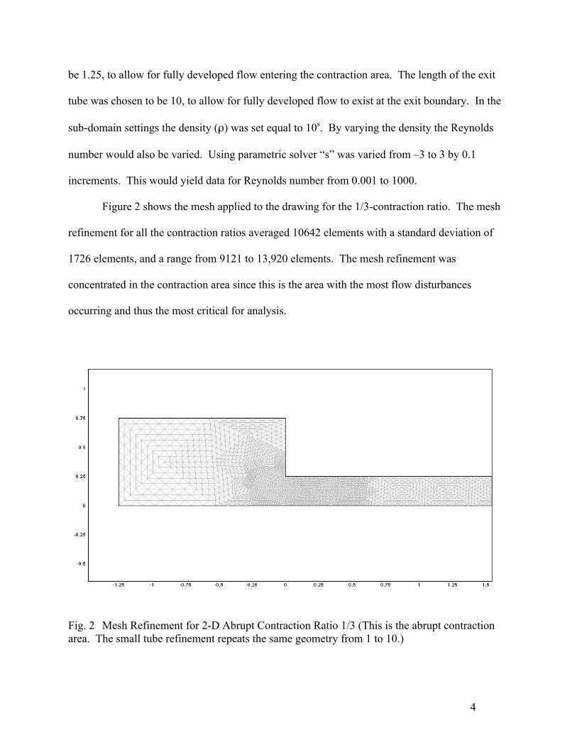
Figure 2 shows the mesh applied to the drawing for the 1/3-contraction ratio. The mesh
refinement for all the contraction ratios averaged 10642 elements with a standard deviation of
1726 elements, and a range from 9121 to 13,920 elements. The mesh refinement was
concentrated in the contraction area since this is the area with the most flow disturbances
occurring and thus the most critical for analysis.
Fig. 2 Mesh Refinement for 2-D Abrupt Contraction Ratio 1/3 (This is the abrupt contraction area. The small tube refinement repeats the same geometry from 1 to 10.)
5
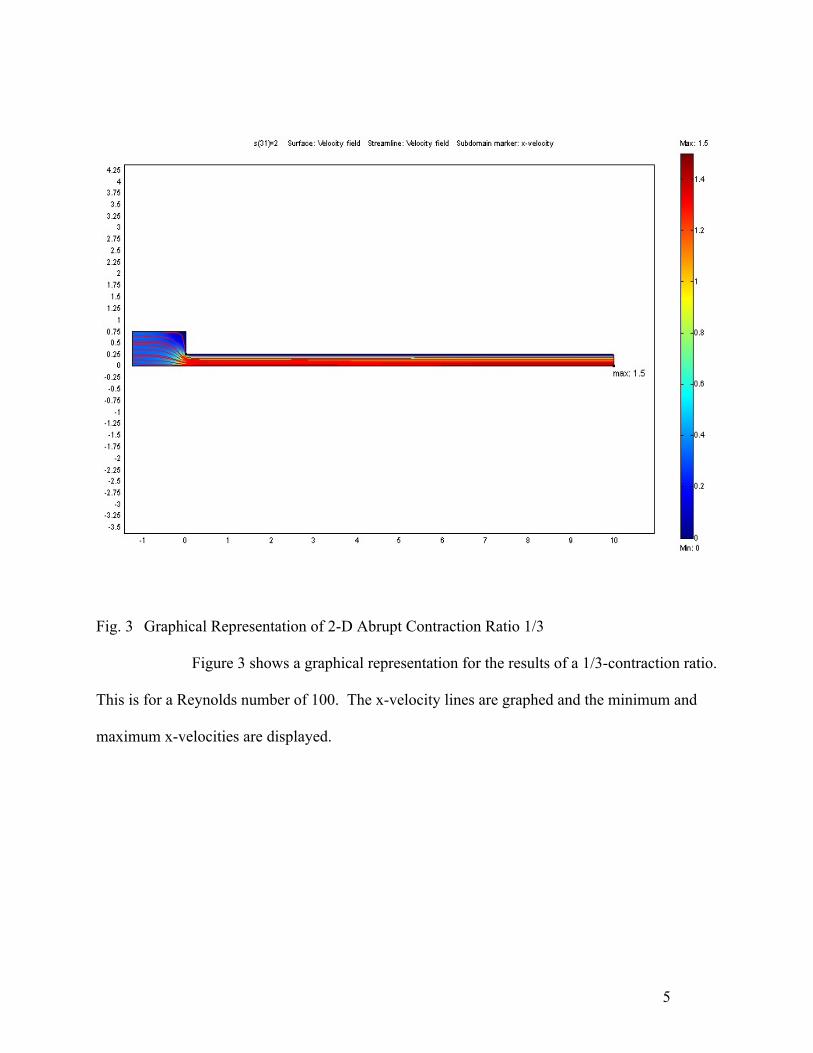
Fig. 3 Graphical Representation of 2-D Abrupt Contraction Ratio 1/3
Figure 3 shows a graphical representation for the results of a 1/3-contraction ratio.
This is for a Reynolds number of 100. The x-velocity lines are graphed and the minimum and
maximum x-velocities are displayed.
6
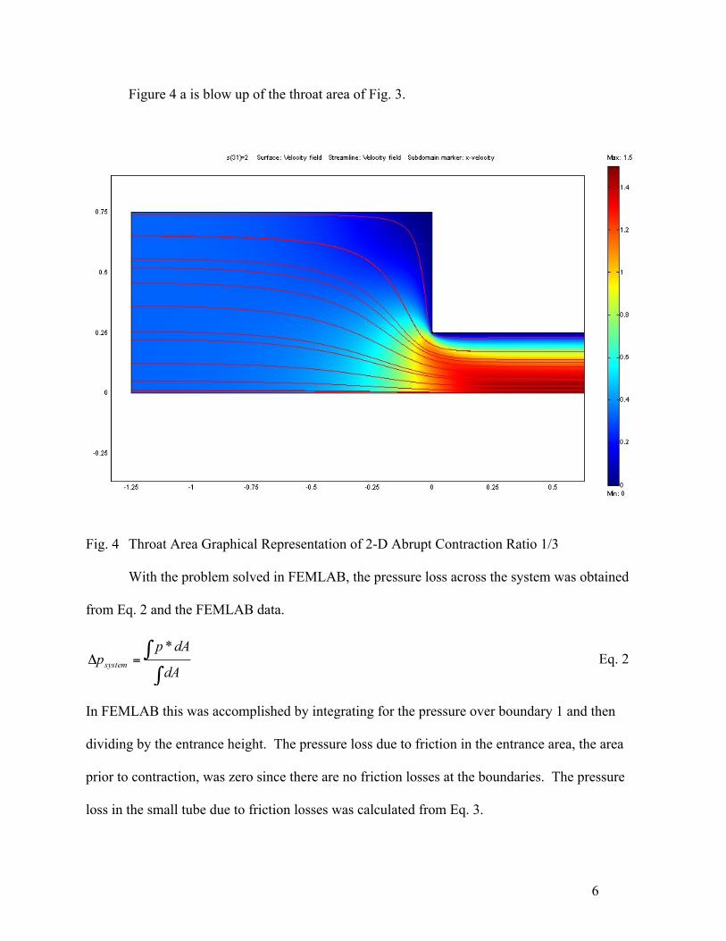
Figure 4 a is blow up of the throat area of Fig. 3.
Fig. 4 Throat Area Graphical Representation of 2-D Abrupt Contraction Ratio 1/3 With the problem solved in FEMLAB, the pressure loss across the system was obtained
from Eq. 2 and the FEMLAB data.
∫∫=ΔdA
dAppsystem
* Eq. 2
In FEMLAB this was accomplished by integrating for the pressure over boundary 1 and then
dividing by the entrance height. The pressure loss due to friction in the entrance area, the area
prior to contraction, was zero since there are no friction losses at the boundaries. The pressure
loss in the small tube due to friction losses was calculated from Eq. 3.
7
2max ***2HLu
pexittubeµ
=Δ Eq. 3
Where:
umax is the maximum x-velocity in the small tube
L is the length of the small tube
µ is the viscosity of the liquid
H is the height of the small tube (boundary 2 to boundary 5)
The maximum x-velocity was obtained from the FEMLAB results. The pressure loss due to
contraction was then calculated from Eq. 4.
exittubeentrancesystemncontractio pppp Δ−Δ−Δ=Δ Eq. 4
Recall that the pressure loss due to friction in the entrance area was zero.
The difference in pressure due to contraction was converted to find the pressure-loss
coefficient (Kc FEMLAB). Equation 5 [1] is from Kays and London.
( )c
cc g
VKgVp
21
2
22
21 +−=
Δσ
ρ Eq. 5
Where the variable:
Δp1 is the pressure loss due to contraction
ρ is the density of the fluid
V is the velocity in the small tube
σ is the contraction ratio (“core free-flow to frontal-area ratio”[1])
Kc is the pressure-loss coefficient due to abrupt contraction
Equation 5 was rearranged to solve for 21
Vp
ρΔ
, this is Eq. 6.
8
( )2
1 221 cKVp
+−=Δ
σρ
Eq. 6
Equation 6 was set equal to Re
ncontractiopΔ and then solved for Kc yielding Eq. 7.
( )⎥⎦
⎤⎢⎣
⎡ −−
Δ=
21
Re*2
2σncontractioc
pK Eq. 7
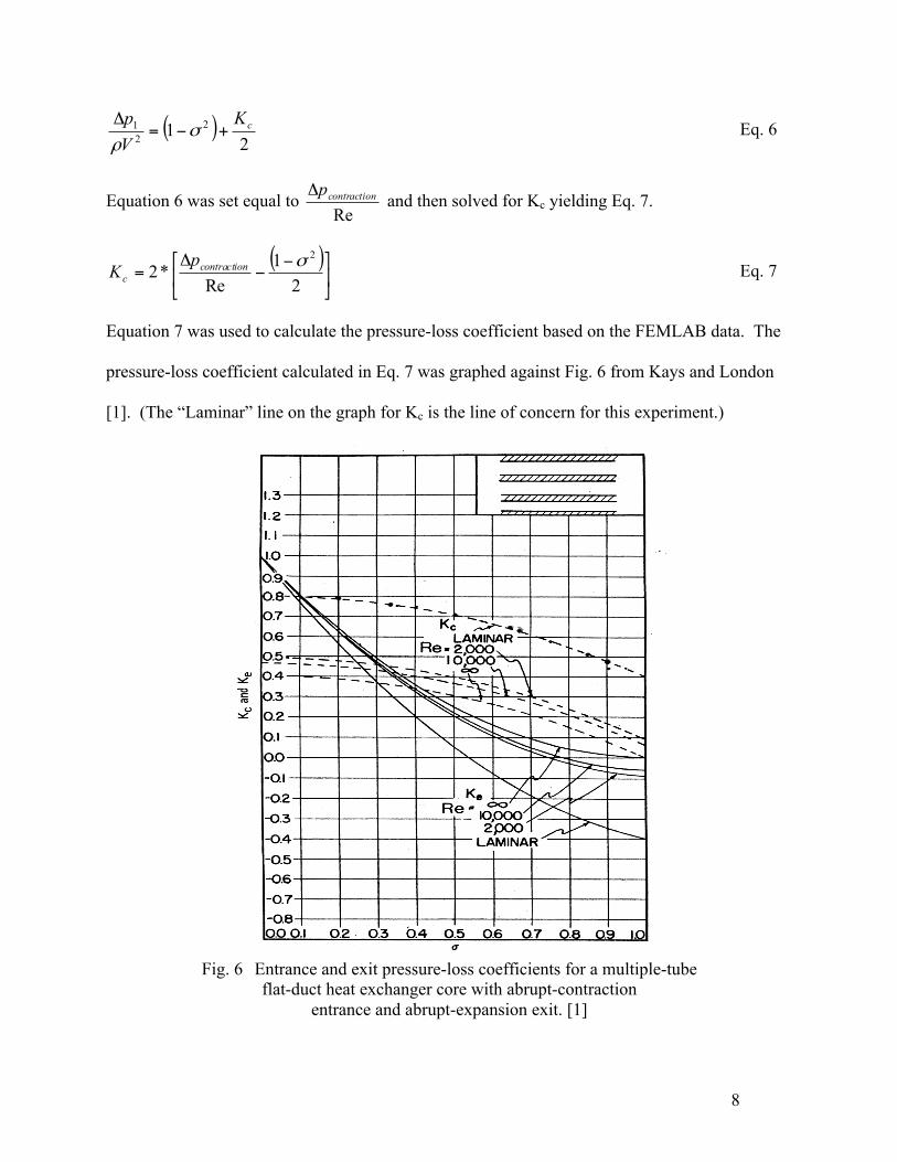
Equation 7 was used to calculate the pressure-loss coefficient based on the FEMLAB data. The
pressure-loss coefficient calculated in Eq. 7 was graphed against Fig. 6 from Kays and London
[1]. (The “Laminar” line on the graph for Kc is the line of concern for this experiment.)
Fig. 6 Entrance and exit pressure-loss coefficients for a multiple-tube
flat-duct heat exchanger core with abrupt-contraction entrance and abrupt-expansion exit. [1]
9
Equation 8 was used to compare the pressure loss calculated by the FEMLAB based
pressure-loss coefficient and the pressure loss based on Kays and London pressure-loss
coefficient for a given contraction ratio. These pressure losses were graphed vs. the Reynolds
number.
( )⎥⎦
⎤⎢⎣
⎡+
−=Δ
221Re
2 Kcp σ Eq. 8
Equation 8 is a rearrangement of Eq. 7.
Results and Discussion
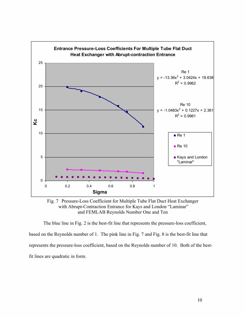
The FEMLAB based pressure-loss coefficient for a given Reynolds number was graphed
for the various contraction ratios. In Fig. 7 the Reynolds numbers one and ten are graphed
against the “Laminar” points from Fig. 1 [1].
10
Entrance Pressure-Loss Coefficients For Multiple Tube Flat Duct Heat Exchanger with Abrupt-contraction Entrance
Re 1y = -13.36x2 + 3.0424x + 19.638
R2 = 0.9962
Re 10y = -1.0483x2 + 0.1227x + 2.361
R2 = 0.9961
0
5
10
15
20
25
0 0.2 0.4 0.6 0.8 1
Sigma
Kc
Re 1
Re 10
Kays and London"Laminar"
Fig. 7 Pressure-Loss Coefficient for Multiple Tube Flat Duct Heat Exchanger
with Abrupt-Contraction Entrance for Kays and London “Laminar” and FEMLAB Reynolds Number One and Ten
The blue line in Fig. 2 is the best-fit line that represents the pressure-loss coefficient,
based on the Reynolds number of 1. The pink line in Fig. 7 and Fig. 8 is the best-fit line that
represents the pressure-loss coefficient, based on the Reynolds number of 10. Both of the best-
fit lines are quadratic in form.
11
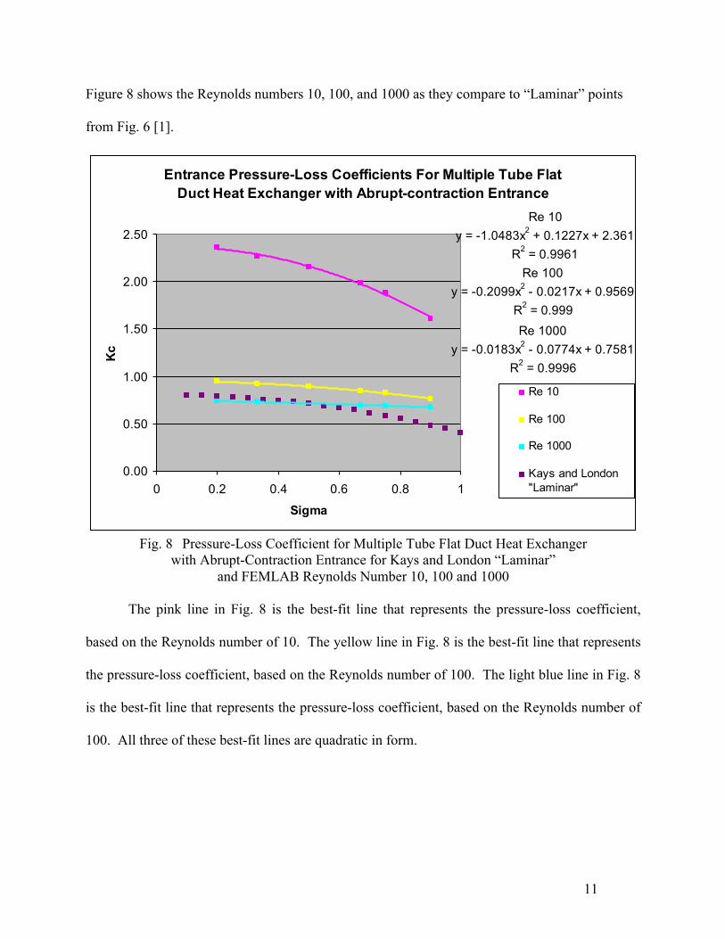
Figure 8 shows the Reynolds numbers 10, 100, and 1000 as they compare to “Laminar” points
from Fig. 6 [1].
Entrance Pressure-Loss Coefficients For Multiple Tube Flat Duct Heat Exchanger with Abrupt-contraction Entrance
Re 10y = -1.0483x2 + 0.1227x + 2.361
R2 = 0.9961Re 100
y = -0.2099x2 - 0.0217x + 0.9569R2 = 0.999Re 1000
y = -0.0183x2 - 0.0774x + 0.7581R2 = 0.9996
0.00
0.50
1.00
1.50
2.00
2.50
0 0.2 0.4 0.6 0.8 1
Sigma
Kc
Re 10
Re 100
Re 1000
Kays and London"Laminar"
Fig. 8 Pressure-Loss Coefficient for Multiple Tube Flat Duct Heat Exchanger
with Abrupt-Contraction Entrance for Kays and London “Laminar” and FEMLAB Reynolds Number 10, 100 and 1000
The pink line in Fig. 8 is the best-fit line that represents the pressure-loss coefficient,
based on the Reynolds number of 10. The yellow line in Fig. 8 is the best-fit line that represents
the pressure-loss coefficient, based on the Reynolds number of 100. The light blue line in Fig. 8
is the best-fit line that represents the pressure-loss coefficient, based on the Reynolds number of
100. All three of these best-fit lines are quadratic in form.
12
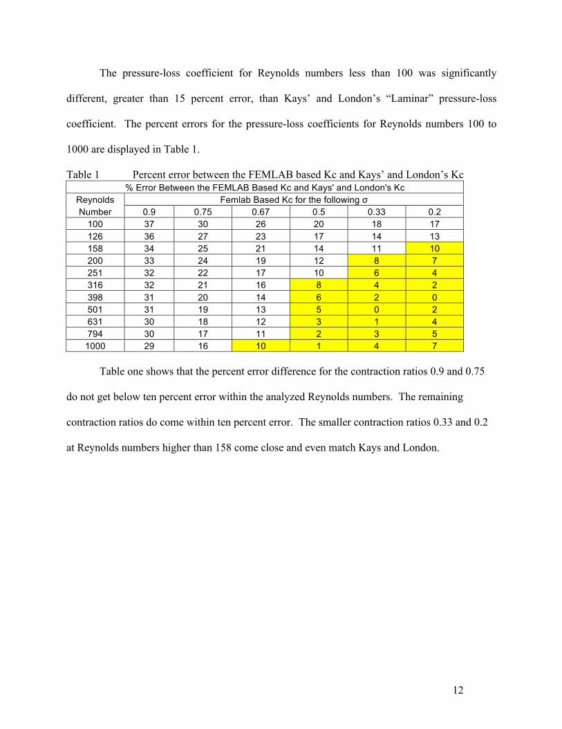
The pressure-loss coefficient for Reynolds numbers less than 100 was significantly
different, greater than 15 percent error, than Kays’ and London’s “Laminar” pressure-loss
coefficient. The percent errors for the pressure-loss coefficients for Reynolds numbers 100 to
1000 are displayed in Table 1.
Table 1 Percent error between the FEMLAB based Kc and Kays’ and London’s Kc % Error Between the FEMLAB Based Kc and Kays' and London's Kc
Reynolds Femlab Based Kc for the following σ Number 0.9 0.75 0.67 0.5 0.33 0.2
100 37 30 26 20 18 17 126 36 27 23 17 14 13 158 34 25 21 14 11 10 200 33 24 19 12 8 7 251 32 22 17 10 6 4 316 32 21 16 8 4 2 398 31 20 14 6 2 0 501 31 19 13 5 0 2 631 30 18 12 3 1 4 794 30 17 11 2 3 5
1000 29 16 10 1 4 7 Table one shows that the percent error difference for the contraction ratios 0.9 and 0.75
do not get below ten percent error within the analyzed Reynolds numbers. The remaining
contraction ratios do come within ten percent error. The smaller contraction ratios 0.33 and 0.2
at Reynolds numbers higher than 158 come close and even match Kays and London.
13
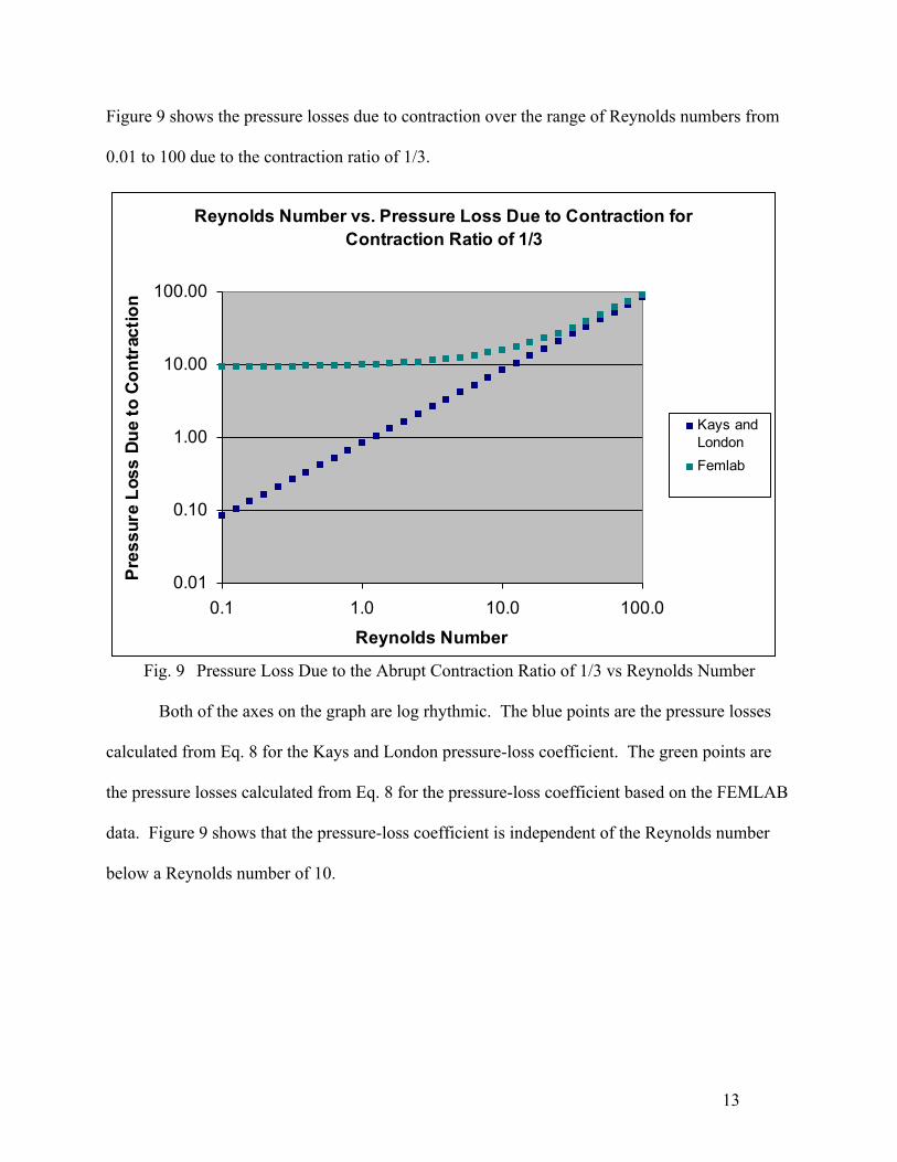
Figure 9 shows the pressure losses due to contraction over the range of Reynolds numbers from
0.01 to 100 due to the contraction ratio of 1/3.
Reynolds Number vs. Pressure Loss Due to Contraction for Contraction Ratio of 1/3
0.01
0.10
1.00
10.00
100.00
0.1 1.0 10.0 100.0
Reynolds Number
Pres
sure
Los
s Du
e to
Con
trac
tion
Kays andLondonFemlab
Fig. 9 Pressure Loss Due to the Abrupt Contraction Ratio of 1/3 vs Reynolds Number
Both of the axes on the graph are log rhythmic. The blue points are the pressure losses
calculated from Eq. 8 for the Kays and London pressure-loss coefficient. The green points are
the pressure losses calculated from Eq. 8 for the pressure-loss coefficient based on the FEMLAB
data. Figure 9 shows that the pressure-loss coefficient is independent of the Reynolds number
below a Reynolds number of 10.
14
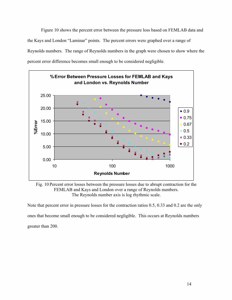
Figure 10 shows the percent error between the pressure loss based on FEMLAB data and
the Kays and London “Laminar” points. The percent errors were graphed over a range of
Reynolds numbers. The range of Reynolds numbers in the graph were chosen to show where the
percent error difference becomes small enough to be considered negligible.
%Error Between Pressure Losses for FEMLAB and Kays and London vs. Reynolds Number
0.00
5.00
10.00
15.00
20.00
25.00
10 100 1000
Reynolds Number
%Er
ror
0.90.750.670.50.330.2
Fig. 10 Percent error losses between the pressure losses due to abrupt contraction for the
FEMLAB and Kays and London over a range of Reynolds numbers. The Reynolds number axis is log rhythmic scale.
Note that percent error in pressure losses for the contraction ratios 0.5, 0.33 and 0.2 are the only
ones that become small enough to be considered negligible. This occurs at Reynolds numbers
greater than 200.
15
Conclusions and Recommendations
Kays’ and London’s “Laminar” pressure-loss coefficient were improved upon. The
pressure-loss coefficients can be red for a larger range of laminar flow Reynolds numbers. This
will provide more accurate pressure loss data.
The mesh for the 2/3 contraction ration was 3000 elements larger than the average. I
recommend refining the mesh so that it is closer to the average, or refining the mesh of the other
contraction ratios to coincide with the 2/3 contraction ratio mesh.
I did not analyze the pressure changes due to changes in kinetic energy. I recommend
that this be done to show where the pressure changes due to kinetic energy becomes significant.
I would also analyze more contractions ratios. This is easy enough using FEMLAB, just
time consuming. I would analyze contraction ratios at 0.05 increments, since I was able to read
off Kays and London pressure-loss coefficients at this interval.
16
Literature Cited
1. Kays, W. M., and London, A. L. Compact Heat Exchangers, 3rd edition, p. 109, 112,
McGraw-Hill, New York, (1984).
2. Bird, R.B., et al. Transport Phenomena, 2nd edition, p. 183, John Wiley & Sons, New
York, (2002).