Embed Size (px)
Citation preview

University of Central Florida University of Central Florida
STARS STARS
Electronic Theses and Dissertations, 2004-2019
2008
Pressure Losses Experienced By Liquid Flow Through Pdms Pressure Losses Experienced By Liquid Flow Through Pdms
Microchannels With Abrupt Area Changes Microchannels With Abrupt Area Changes
Jonathan Wehking University of Central Florida
Part of the Mechanical Engineering Commons
Find similar works at: https://stars.library.ucf.edu/etd
University of Central Florida Libraries http://library.ucf.edu
This Masters Thesis (Open Access) is brought to you for free and open access by STARS. It has been accepted for
inclusion in Electronic Theses and Dissertations, 2004-2019 by an authorized administrator of STARS. For more
information, please contact [email protected].
STARS Citation STARS Citation Wehking, Jonathan, "Pressure Losses Experienced By Liquid Flow Through Pdms Microchannels With Abrupt Area Changes" (2008). Electronic Theses and Dissertations, 2004-2019. 3696. https://stars.library.ucf.edu/etd/3696

PRESSURE LOSSES EXPERIENCED BY LIQUID FLOW THROUGH PDMS MICROCHANNELS WITH ABRUPT AREA CHANGES
by
JONATHAN D. WEHKING B.S. University of Central Florida, 2005
A thesis submitted in partial fulfillment of the requirements for the degree of Masters of Science in ThermoFluids
in the Department of Mechanical, Materials, and Aerospace Engineering in the College of Engineering and Computer Science
at the University of Central Florida Orlando, Florida
Summer Term 2008

© 2008 Jonathan Wehking
ii
ABSTRACT
Given the surmounting disagreement amongst researchers in the area of liquid flow
behavior at the microscale for the past thirty years, this work presents a fundamental approach to
analyzing the pressure losses experienced by the laminar flow of water (Re = 7 to Re = 130)
through both rectangular straight duct microchannels (of widths ranging from 50 to 130
micrometers), and microchannels with sudden expansions and contractions (with area ratios
ranging from 0.4 to 1.0) all with a constant depth of 104 micrometers. The simplified Bernoulli
equations for uniform, steady, incompressible, internal duct flow were used to compare flow
through these microchannels to macroscale theory predictions for pressure drop. One major
advantage of the channel design (and subsequent experimental set-up) was that pressure
measurements could be taken locally, directly before and after the test section of interest, instead
of globally which requires extensive corrections to the pressure measurements before an accurate
result can be obtained. Bernoulli’s equation adjusted for major head loses (using Darcy friction
factors) and minor head losses (using appropriate K values) was found to predict the flow
behavior within the calculated theoretical uncertainty (~12%) for all 150+ microchannels tested,
except for sizes that pushed the aspect ratio limits of the manufacturing process capabilities
(microchannels fabricated via soft lithography using PDMS). The analysis produced conclusive
evidence that liquid flow through microchannels at these relative channel sizes and Reynolds
numbers follow macroscale predictions without experiencing any of the reported anomalies
expressed in other microfluidics research. This work also perfected the delicate technique
required to pierce through the PDMS material and into the microchannel inlets, exit and pressure
ports without damaging the microchannel. Finally, two verified explanations for why prior
iii

researchers have obtained poor agreement between macroscale theory predictions and tests at the
microscale were due to the presence of bubbles in the microchannel test section (producing
higher than expected pressure drops), and the occurrence of localized separation between the
PDMS slabs and thus, the microchannel itself (producing lower than expected pressure drops).
iv

I am indebted to my father and mother for encouraging the pursuit and support of advanced
education. I am thankful for Chase’s unwavering dedication and tireless persistence in our
microfluidics research efforts. I am blessed that this work indirectly led me to the most
important person in my life, Rebekah. Finally, through this work, I am reinvigorated and
renewed by what it means to discover, and most importantly, to do what you love in your chosen
vocation.
v

TABLE OF CONTENTS
LIST OF FIGURES ...................................................................................................................... vii LIST OF TABLES......................................................................................................................... ix LIST OF ACRONYMS/ABBREVIATIONS................................................................................. x CHAPTER ONE: INTRODUCTION............................................................................................. 1 CHAPTER TWO: LITERATURE REVIEW................................................................................. 4
Straight Duct Microchannels ...................................................................................................... 4 Early Transition to Turbulence ................................................................................................... 8 Mixing Fluids in Microchannels............................................................................................... 10 Heat Exchanger Benefits .......................................................................................................... 12 Flow Effects at Small Scales .................................................................................................... 13
CHAPTER THREE: METHOLODGY ........................................................................................ 23 Overview................................................................................................................................... 23 Size Regime Considerations ..................................................................................................... 24 Macroscale Fluid Mechanics for Internal Flow........................................................................ 26 Microchannel Material Selection.............................................................................................. 32 Microchannel Design................................................................................................................ 36 Microchannel Fabrication ......................................................................................................... 42 Experimental Set-Up................................................................................................................. 55 Set-Up Design and Equipment Selection.................................................................................. 56 Test Procedure .......................................................................................................................... 61
CHAPTER FOUR: RESULTS ..................................................................................................... 71 Building the Comparison .......................................................................................................... 71 Explanations for Deviations from Theoretical Predictions....................................................... 77 Straight Duct Comparisons and Discussion.............................................................................. 85 Sudden Expansion Comparisons and Discussion ..................................................................... 90 Sudden Contraction Comparisons and Discussion ................................................................... 92 Additional Considerations ........................................................................................................ 95
CHAPTER FIVE: CONCLUSIONS ............................................................................................ 96 APPENDIX A: ADDITIONAL PLOTS FOR STRAIGHT DUCT TESTS ................................ 99 APPENDIX B: ADDITIONAL PLOTS FOR EXPANSION TESTS........................................ 104 APPENDIX C: ADDITIONAL PLOTS FOR CONTRACTION TESTS.................................. 109 APPENDIX D: THESIS DEFENSE PRESENTATION............................................................ 114 RERFERENCES......................................................................................................................... 133
vi
LIST OF FIGURES
Figure 1: Parameter space of experimental flow behavior in straight ducts. Data from [7].......... 6 Figure 2: Plot of experimental results from prior research for the normalized friction factor [7].. 7 Figure 3: Schematic of geometry used in [4]. Area ratio is approximately 0.276. ...................... 18 Figure 4: Expansion coefficients from [4] compared to macroscale predictions. ........................ 20 Figure 5: Contraction coefficients from [4] compared to macroscale predictions. ...................... 21 Figure 6: Moody chart - correlation of friction factor f and Reynolds number [5]. ..................... 28 Figure 7: Tabulation of expanding/contracting loss coefficients as a function of area ratio........ 31 Figure 8: Smooth vs. rough channel quality as a result of differing transparency resolution [1]. 35 Figure 9: CAD of microchannel layout on a 4" diameter slab of PDMS. .................................... 38 Figure 10: Single straight duct microchannel design.................................................................... 39 Figure 11: Single expansion/contraction microchannel design. ................................................... 40 Figure 12: “Muffin-topping” of channel cross section. ................................................................ 43 Figure 13: Rounding-out of expansion and contraction features.................................................. 44 Figure 14: Silicone master. ........................................................................................................... 45 Figure 15: Microchannel chip cast from silicone master.............................................................. 46 Figure 16: Composite image of an entire straight channel. .......................................................... 48 Figure 17: Composite image of an entire channel with an area reduction.................................... 49 Figure 18: Surface of a straight duct channel at 10x magnification. ............................................ 49 Figure 19: Area reduction at 10x magnification. .......................................................................... 50 Figure 20: Micrometer scale used to calibrate digital microscope. .............................................. 51 Figure 21: Cross-sectional slice of a sample microchannel.......................................................... 52 Figure 22: Images of channels that violate a 5:1 aspect ratio. ...................................................... 54 Figure 23: Experimental set-up schematic [19]. ........................................................................... 57 Figure 24: Photograph of experimental set-up.............................................................................. 58 Figure 25: Check valve between syringe, fluid storage tank, and microchannel infusion tube. .. 60 Figure 26: PDMS test chip aligned over 1-to-1 computer printout. ............................................. 63 Figure 27: PDMS chip with needle inserted. ................................................................................ 64 Figure 28: PDMS cylinder lodged into port. ................................................................................ 65 Figure 29: Microchannel with infusion needle inserted and a pool of liquid over the high port.. 67 Figure 30: Raw voltage data. ........................................................................................................ 72 Figure 31: Calibration of differential pressure transducer. R2 = 0.9999...................................... 73 Figure 32: Plot of experimental data as a function of Re. ............................................................ 74 Figure 33: Sample comparison between theoretical predictions and experiments. ...................... 75 Figure 34: Figure 33 with error bars included. ............................................................................. 76 Figure 35: Channel leakage due to PDMS slab separation........................................................... 78 Figure 36: Data trend due to channel rupture compared to theoretical predictions...................... 79 Figure 37: Bubble obstructing the flow in the test section. .......................................................... 81 Figure 38: Plot of data with and without bubbles. ........................................................................ 82 Figure 39: Zones of error for experimental results. ...................................................................... 83 Figure 40: Figure 2 with zones of error marked. .......................................................................... 84
vii

Figure 41: 50 micrometer straight duct results. ............................................................................ 86 Figure 42: 60 micrometer straight duct results. ............................................................................ 87 Figure 43: 70 micrometer straight duct results. ............................................................................ 88 Figure 44: Analysis of a specific channel’s data set compared to its own theoretical prediction. 89 Figure 45: Expansion results for area ratio of 0.4......................................................................... 91 Figure 46: Expansion results for area ratio of 0.54....................................................................... 92 Figure 47: Contraction results for area ratio of 0.4....................................................................... 93 Figure 48: Contraction results for area ratio of 0.7....................................................................... 94
viii

LIST OF TABLES
Table 1: Fluent Simulations with applicable pressure losses........................................................ 13 Table 2: Flow effects considered with results/recommendations. ................................................ 14 Table 3: Limiting values for Knudsen numbers and applicable treatment. .................................. 25 Table 4: Product information for each component [19]................................................................ 57 Table 5: Sequence of flow rates for all tests, with extrapolated Re for 100mm straight channel. 60 Table 6: Uncertainty considered in all calculations. ..................................................................... 76
ix

LIST OF ACRONYMS/ABBREVIATIONS
CAD Computer Aided Design CFD Computation Fluid Dynamics Kn Knudsen number: Ratio of mean free path over channel length MEMS Micro Electro Mechanical Systems Micron Abbreviation for micrometers PDMS Poly(DiMethylSiloxane): A type of silicon used to cast microchannels Po Poiseuille number: Measure of flow resistance PSI Pounds per Square Inch: A unit of pressure Re Reynolds number: A non-dimensional ratio of viscous and inertial forces
x

CHAPTER ONE: INTRODUCTION
It is the nature of human beings to pack common everyday entities into ever decreasing
amounts of space. Sparse amounts of people that once roamed miles upon miles of open land are
now more frequently packed into a few acres of homes, town homes, or even vertically stacked
abodes called apartments. Forms of currency, which conventionally appeared as tangible objects
representing a specific value, have taken the more common form of signatures, bits and bytes,
and plastic cards. Books and documents representing the latest advances in human discovery
that were once stored in high security vaults, simply because they had yet to be copied and
distributed to the masses, have been replaced by .doc and .pdf files., theoretically taking up no
physical space whatsoever! Origins of the necessities for survival, food, water, and rest, must be
overly abundant and within a few steps away for everyday life to be considered normal. And of
course, there have been light years worth of advances in the area of processing and storing data
electronically utilizing microchips. Wouldn't it be inconvenient not have any room for your bed
because the equivalent of your laptop computer is taking up the majority of your bedroom?
Whether it be the ever looming notion of possibly overcrowding the Earth with people that keeps
this "minimalist" thinking hardwired into the subconscious part of the human brain, or the simple
need to manipulate the law of conservation of space, the consistent requirement for making
effects fit into smaller and smaller physical volumes is ever pressing on the advancement of
scientific discovery.
Such is the case with all artifacts associated or connected with the miniaturization race.
If a microchip decreased in size by 50%, would it make sense to still use the same CPU fan that
1

cooled its predecessor? The original fan would still be 50% larger than the new smaller chip,
making the decrease in size of the overall system less significant. An additional field that
contains cooling as one of its possible uses, and that has recently joined the miniaturization race,
is the flow of fluids through miniaturized geometries. These miniaturized geometries have been
dubbed microchannels, and will be referred to as such for the remainder of this work. The focus
on fluid flow through microchannels developed as a result of numerous requirements spawning
from a multitude of fields. Given their macro scale counterparts, including everyday brass or
PVC plumbing pipes, microchannels arouse as more of a reaction to shrinking counterparts, such
as microchips, micro-spray nozzles, and technological advances in prosthetics . Biomedical
necessities include the modeling of various bodily fluids flowing through both naturally grown
and artificially manufactured bodily chambers, namely lung alveoli, and glomerular filtration
systems in the kidneys [1]. More rigorous mechanical applications include the modeling of flow
parameter requirements and pressure losses as a result of pumping, cooling, or mixing uses of
various liquids and gasses [2]. The volumetric and mass limitations of space travel due to
extreme costs make miniaturized systems extremely attractive [3]. Wherever their use,
microchannels are becoming increasingly popular in a plethora of scientific fields.
The types of microchannels available for study today are as numerous as their potential
uses. Any macroscale parent geometry available is most certainly available in a "micro-version"
equivalent, making this field an overly abundant resource in research topics. For this reason, the
scope of this work is limited further by the type of geometry being studied, namely sudden
expansion and sudden contraction microchannels. One apparent reason for this selection is that
sudden changes in geometry represent a geometric "bridge" between flow possibly beginning as
macroscale, and potentially ending as microscale, depending on the size order of magnitude.
2

The link between these two orders of fluidic magnitude is analogous to the ever ambiguous link
between two other types of flow: laminar and turbulent flow, or the transition flow regime. For
the sake of clarity, the laminar flow regime will be used for the duration of this work, as added
layers of complexity are not yet warranted. It is the purpose of this work to develop a simple
working microfluidic model of a sudden expansion/contraction flow system for use in
extrapolating accurate and meaningful flow parameter data.
3

CHAPTER TWO: LITERATURE REVIEW
The following section will present an all-encompassing review of the relevant literature
and theory associated with the methodology and analysis presented in anon sections of this work.
First, a summary of current efforts in the microfluidics arena will be presented, followed by
briefly discussing any relevant manipulations of flow theory that may be used to baseline
microchannel flow modeling. Then, a significant paper by F.F. Abdelall et al. [4] that focuses on
modeling two-phase flow through sudden expansion/contraction microchannels will be offered,
as the geometry studied in Abdelall’s work is very similar in configuration to the geometry
utilized in this work.
Straight Duct Microchannels
One of the most complete and all encompassing compendiums of MEMS literature is the
MEMS Handbook, edited by Mohamed Gad-el-Hak. In the chapter entitled “Liquid Flow in
Microchannels,” one of the primary researchers in microfludics (K. V. Sharp et al.), gives a fairly
detailed overview of the field, starting with the long list of potential applications that may result
from discoveries in microfluidics research. The authors then proceed to address the question of
when it is suitable to legitimately discount macroscale hydrodynamics and fluid mechanics in
favor of velocity slip conditions and free molecular flow analysis techniques. Then, an overview
of macroscale fluid mechanics is given for pressure driven internal flow. These equations and
derivations represent the foundational assumptions, theories, and flow behaviors of Newtonian
fluids, and can be found in most introductory textbooks on the subject [5, 6]. Finally, the authors
4

have a section devoted to the undeniable trend of discord among results obtained in microfluidics
research to date as to whether or not macroscale fluid mechanics adequately models flow at the
microscale. This disagreement in the field has as created an unsettling debate over how to
handle flows when designing duct networks, MEMS devices, and any other applicable use for
transporting liquids through small channels. How can humanity progress further in this direction
when there is conflict at its very foundation?
There are plenty of theories as to why researchers are getting anomalies in their various
experiments, but the authors of this highly controversial chapter in the MEMS Handbook do a
great job of simply presenting the tangible findings of the other works’ discussed, leaving all
interpretation of these findings for the individual researchers to justify. They classified the
findings into three categories, all of which compare experimental results for the friction factor
(and subsequent pressure drop) of the flow to theoretical predictions from macroscale fluid
mechanics. The first category is experimental results that predicted a friction factor higher than
what theory depicts. The second is experimental results in agreement with macroscale friction
factor predictions, and the third is experiments that show lower than expected friction factors
when compared to classic macroscale fluid mechanics. The channel flow geometries were all
straight ducts, of various cross-sectional areas (circular, trapezoidal, rectangular, etc.), exhibiting
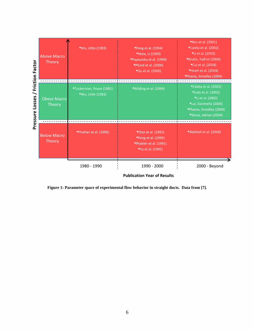
laminar flow ranges for the Reynolds number. Figure 1 represents the resulting parameter space
for this comparison, and Figure 2 shows a sample of the experimental results for the normalized
friction factor, a classic quantity representative of macro theory, and a quantity that will be
discussed in greater detail in later sections.
5
Obeys Macro Theory
Above Macro Theory
Below Macro Theory
Publication Year of Results
1980 ‐ 1990 1990 ‐ 2000 2000 ‐ Beyond
•Tuckerman, Pease (1981)
•Wu, Little (1983)
•Wilding et al. (1994)
•Caleta et al. (2002) •Judy et al. (2002) •Li et al. (2003)
•Lui, Garimella (2004)
•Phares, Smedley (2004)
•Sharp, Adrian (2004)
•Ren et al. (2001) •Caleta et al. (2002)
•Li et al. (2003) •Brutin, Tadrist (2004)
•Cui et al. (2004) •Hsieh et al. (2004)
•Phares, Smedley (2004)
•Peng et al. (1994) •Mala, Li (1999)
•Papautsky et al. (1999) •Pfund et al. (2000) •Qu et al. (2000)
•Wu, Little (1983)
•Phahler et al. (1990)
•Choi et al. (1991) •Peng et al. (1994)
•Phahler et al. (1991) •Yu et al. (1995)
•Abdelall et al. (2004)
Pressure Losses / Friction
Factor
Figure 1: Parameter space of experimental flow behavior in straight ducts. Data from [7].
6

Figure 2: Plot of experimental results from prior research for the normalized friction factor [7].
With reference to the scatter of data points in Figure 2, each plotted shape represents results
from a different research effort. Results that were claimed to follow macroscale predictions fell
on or around the horizontal centerline marking a unity normalized friction factor (C*=1), which
is described below by Equation 1.
Equation 1 Cf Re⋅( )experimental
f Re⋅( )theoretical
*
Data points that fell above this line were said to predict results above that of macroscale theory,
and data points that fell below were said to predict results lower than macroscale theory.
7
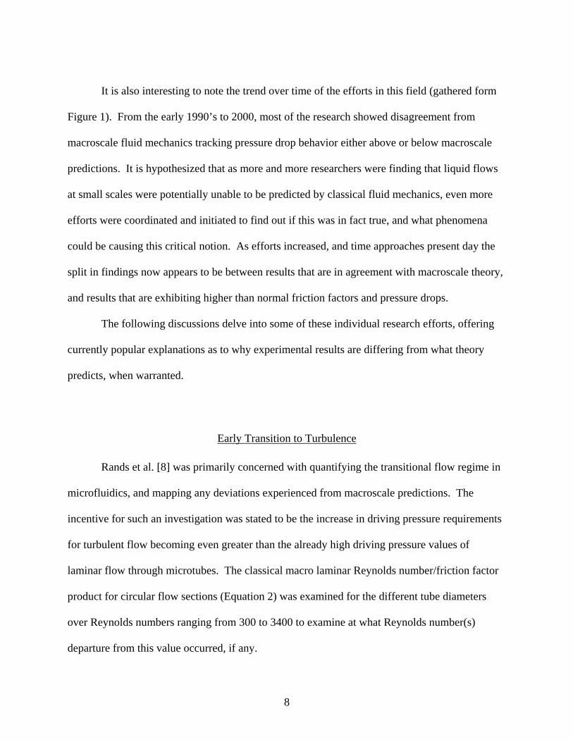
It is also interesting to note the trend over time of the efforts in this field (gathered form
Figure 1). From the early 1990’s to 2000, most of the research showed disagreement from
macroscale fluid mechanics tracking pressure drop behavior either above or below macroscale
predictions. It is hypothesized that as more and more researchers were finding that liquid flows
at small scales were potentially unable to be predicted by classical fluid mechanics, even more
efforts were coordinated and initiated to find out if this was in fact true, and what phenomena
could be causing this critical notion. As efforts increased, and time approaches present day the
split in findings now appears to be between results that are in agreement with macroscale theory,
and results that are exhibiting higher than normal friction factors and pressure drops.
The following discussions delve into some of these individual research efforts, offering
currently popular explanations as to why experimental results are differing from what theory
predicts, when warranted.
Early Transition to Turbulence
Rands et al. [8] was primarily concerned with quantifying the transitional flow regime in
microfluidics, and mapping any deviations experienced from macroscale predictions. The
incentive for such an investigation was stated to be the increase in driving pressure requirements
for turbulent flow becoming even greater than the already high driving pressure values of
laminar flow through microtubes. The classical macro laminar Reynolds number/friction factor
product for circular flow sections (Equation 2) was examined for the different tube diameters
over Reynolds numbers ranging from 300 to 3400 to examine at what Reynolds number(s)
departure from this value occurred, if any.
8
Equation 2
f Re⋅ 64=
Another independently calculated result of this work based on the fluid mixed-mean
temperature reaffirmed the results: the viscous heating parameter (=32 for Equation 2) was
considered as secondary proof of the observed transition Reynolds number(s) deduced from the
frictional measurements. They found that transition to turbulence occurred at approximately Re
= 2100 to Re = 2500 for all tube sizes, which was considered consistent with macroscale
behavior, and that uncertainty in frictional calculations/measurements were 16-29%, dominated
by + 1 micrometer diameter tolerance. Uncertainties in the viscous heating
calculations/measurements were not stated, though it is important to note that the thermocouple
used for temperature measurements was not directly placed in the working fluid (but rather on
the outside surface). It was concluded that the critical Reynolds number may increase slightly
with decreasing diameter [8].
Xu et al. [9] focused on numerically simulating fully developed turbulent flow of water
through microtubes on the size order of 50 micrometers to 254 micrometers in diameter. The
incompressible, two-dimensional, steady, time averaged Navier-Stokes equations of momentum
and continuity, along with Wolfshtein's one-equation turbulence model for kinetic energy were
used. All equations were simplified where applicable, coupled, solved iteratively, and compared
to a convergence factor until convergence was satisfied. It was determined that transition to
turbulence occurred at lower Reynolds numbers for smaller microchannel diameters (which is in
agreement with Rands et al. [8]), proposing the notion that microtubes with larger diameters have
stronger turbulence effects. Also, for lower Reynolds numbers, the turbulent velocity profiles
9
were very close to laminar velocity profiles, and that with larger diameters, and higher Reynolds
numbers, the velocity profile approaches that of a typical macro velocity profile (somewhat flat-
topped). It was concluded that micro-flow phenomena should be considered for diameters
smaller than 130 micrometers, offering a concrete cut-off point for when to switch from
macroscale theory to microscale theory [9].
Mixing Fluids in Microchannels
Decre’e et al. [10] were interested in decreasing the mix time/length of two
incompressible liquids through channels on the order of 65 x 320 micrometers in size. The idea
was to microfabricate a microchannel on a rotating disc in order to take advantage of the
centrifugal forces to drive the liquids down the channel, and enhance mixing using the Coriolis
forces inherent to the rotating frame. Incompressible, steady state Navier-Stokes and continuity
equations were modified to account for the rotating "disk frame," incorporating the centrifugal
field as a flow driver and Coriolis effects as a flow mixer. The flow was first simulated using
computer programs, then compared to experimental trials. It was concluded that key parameters
impacting Coriolis mixing capabilities are channel length, aspect ratio and rate of rotation, and as
rotational speed increases, mixing is enhanced for channels of identical length. Also, as aspect
ratio decreases, decrease in diffusion time is proportional to the square decrease in diffusion
length.
Sudarsan and Ugaz [11] also looked into effective ways of mixing two fluids using an
array of spiral microchannels on the order of 49 micrometers in size. Mixing of blue and yellow
food dyes was evaluated by the amount of green color that was generated when two streams
10
mixed, providing a percentage of mixing for the different trials. There were five different spiral
designs, which varied the number of arcs, and length of the mixing section for Reynolds numbers
between 0.02 - 18.6 (very low flow rates, 0.0001 to 0.1 mL/min). Trials of a single spiral design,
along with trials of three spiral designs connected in series were measured for intensity of
mixing. A two-arc spiral channel with a sudden expansion was also examined for a possible
mixing geometry. It was found that at lower flow rates, diffusion is the primary mechanism by
which mixing occurs, and that at higher flow rates, secondary Dean effects come into play and
contribute to increased levels of mixing. Centrifugal effects are strongest at the innermost
regions of the spiral (highest percentage of mixing), and by abruptly increasing the cross-
sectional area of the spiral, expansion vortices result and can be harnessed to further reduce
overall mixing lengths. Subsequently, the footprint of the mixing area is significantly reduced
than if straight channels were used, thus concluding that the benefits of Dean effects (due to
centrifugal forces) reduces the required overall mixing length [11].
Goullet et al. [12] considered the use of "pulse mixing" of two fluids for microchannels
around 160 micrometers in size, and for a Reynolds number range of 0.3 to 30. The study was a
completely numerical Fluent simulation that consisted of four different flow geometries with
separate entry ports for the two fluids (perpendicular, Y, T, and arrowhead shaped), and 1
configuration with bends around all 3 spatial axes where both fluids have the same entry point.
A modification was made to the perpendicular flow geometry for one experiment by adding ribs.
Navier-Stokes and continuity equations were used for the simulation, and no supporting
experiments were performed. The idea was to view how much more effective the fluid
confluence and geometrically induced secondary flows were to mixing opposed to diffusion
alone. It was discovered that for geometries with different entry ports, pulsing the flow 90o out
11

of phase enhanced mixing by promoting chaotic advection, also, adding ribs to the perpendicular
flow trial coupled with out of phase pulsing further enhanced mixing (0.78 degree of mixing,
with 1.0 being completely mixed). Increasing pulse frequency from 5 to 20 Hz increased the
degree of mixing by 0.2, and increased mean velocity for the tri-axial geometric case also
assisted with constituent mixing.
Heat Exchanger Benefits
Niklas et al. [13] conducted an investigation utilizing a row of 54 triangular shaped
microchannels for possible micro-heat exchanger applications. However, the hydraulic
properties of the fluid through the microchannels was the main focus of the work. Size was on
the order of 110 micrometers (hydraulic diameter), and flow rate was on the order of Re < 1000.
First, experiments were carried out to see how accurate the set-up would be to the classical fully-
developed laminar Poiseuille number (flow resistance) of 13.3. Then, numerical simulations
were carried out in Fluent to show agreement or disagreement to this value due to a number of
loss criteria. It is important to note that the different types of losses simulated were only
observed individually, and never compounded (or layered) in an effort to show individual
contributions from each. Experimental results showed departure from Po = 13.3 at about Re =
10, and is claimed to be the result of early transition to turbulence. Additionally, an uneven flow
rate between the microchannels was observed because of the fluid entrance and exit ports to the
flow inlet/outlet reservoirs. Therefore, uses in heat exchanger applications were deemed futile
given this particular work’s experimental set-up and models. Table 1 presents an outline of
quantifiable pressure loss contributions accumulated during this work [13].
12

Table 1: Fluent Simulations with applicable pressure losses.
Fluent Geometry Simulation % Contribution to Pressure Loss Single Microchannel Viscous Losses 20%
“ Entrance Effects (BL) 5% “ Local Losses 20%
Microchannel Network Mixing 30% “ Recirculation 80%
Flow Effects at Small Scales
Koo and Kleinstreuer [14] were primarily concerned with numerical simulations of water
through microchannels at or around 100 micrometers in hydraulic diameter, and investigating
which macroscale effects remain predominant in microscale flow modeling. First, seemingly out
of courtesy for the field (and the reader, of course) the author grouped the related microchannel
investigatory literature thus far into three observational areas when considering friction
factor/pressure gradient changes in microchannels: 1) early transition to turbulence, 2) surface
phenomena (roughness, electrokinetic forces, temperature effects, microcirculation near the
wall), and 3) no differences when compared to conventional macroscale flow theory. This work
then sought to provide a list of flow effects to be considered (with subsequent justification) when
modeling microfluidic flow behavior based on a numerical simulation. The equations used
included the Navier-Stokes equations (for continuity and momentum), Fanning and Darcy
friction factor relations, low Reynolds number k-w model modifications to the Navier-Stokes
equations (for investigating turbulence), and the energy equation to extrapolate thermal effects.
Table 2 summarizes the six flow effects evaluated, with a recommendation as to whether or not
the effect should be considered based on the results obtained.
13

Table 2: Flow effects considered with results/recommendations.
Effect Should it be considered? Rationale
Entrance Yes A function of channel length, aspect ratio and Reynolds number.
Non-Newtonian Yes Important for polymeric liquids and particle suspension flows.
Wall Slip No Average slip velocity accounted for only 0.0014% of the average fluid velocity.
Surface Roughness Yes A function of the Darcy number, Reynolds number, and
cross-sectional configurations.
Turbulence Yes Important for Reynolds numbers above 1000 (less than conventional macroscale theory), and are evident with geometric contractions in the channels.
Viscous Dissipation Yes Taken into account for channels with less than 100 micron
hydraulic diameters.
Celata et al. [15] investigated the possibility of wall roughness effects and geometric
deviations for microtubes ranging from 31 to 326 micrometers. The intent was to model how
accurately fluid flow behaved in accordance with the classical Hagen-Poiseuille flow (refer to
Equation 2) for different diameter microtubes, and to possibly see around what size deviation
from this accepted flow model occurred. Different materials including fused silica, glass (with
siliconated, roughened, and untouched inner diameters), and Teflon were considered creating a
matrix of 10 different trials/experiments. An uncertainty analysis was carried out for the Darcy
equation, and a slip parameter (b) was incorporated into the laminar velocity profile equation to
extrapolate a modified Darcy equation. It was found that adherence to Hagen-Poiseuille was
verified for all size microtubes for Re > 300 and at the microscopic scale, geometric non-
uniformities have a greater impact on comparison inaccuracies than surface roughness. In fact,
14
roughened channels did not show any diversion from classic predictions. In addition, slip effects
encountered by other researchers were proposed (though not verified) to most likely be the result
of an undetected presence of desorbed nanobubbles on the hydrophobic surface. It was also
concluded that viscous heating becomes important at diameters below 100 micrometers
(influences Reynolds number through changes in fluid viscosity).
Steinke and Kandlikar [16] presented a conference proceeding constructed for the
purpose of compiling a historiography of the current microchannel research. The author created
a database comprised of over 40 different papers that compared year of publication, subject fluid,
shape and size of channel, Reynolds number, non-dimensionalized friction factor, treatment of
heat transfer (adiabatic or not), and if the experiments accounted for losses in their calculations.
The final parameter was if the measurements were in agreement with numerical computations for
classical laminar flow theory. The authors then created their own experimental set-up, and
measured the pressure drop across a microchannel on the size order of about 200 micrometers
and a Reynolds number range of Re = 0 to Re = 800. An uncertainty discussion was also
included. The trend in the database was that experiments and subsequent calculations that did
not account for entrance/exit losses, developing region, and frictional losses showed
disagreement with classical theory. Also, the uncertainty analysis indicated a + 40% deviation,
with the size parameter accounting for the highest contribution to this result. From the authors'
experiments, departure from conventional laminar flow theory occurred around a Reynolds
number of 300, and is explained as an early transition to turbulence [14]. Considering the
conclusions offered by Xu et al. that microscale theory should be considered around a size of 130
micrometers [9], it would seem that Steinke’s work provides a specific flow regime limit to
15

supplement this size regime limit for when to begin expecting the onset of microscale flow
phenomena.
Qu et al. [17] concentrated on flow development and pressure drop for water in a 222 x
694 micrometer microchannel for Reynolds numbers ranging 196 to 2215. Micro-particle image
velocimetry (microPIV) was used to capture and extrapolate the flow development, and velocity
field contour plots were created based on each of the different flow rates. Pressure drop was
measured using pressure transducers strategically placed at either end of the microchannel.
Numerical results were also obtained in order to facilitate the mapping of velocity fields and
pressure drop values using the coupled Navier-Stokes and continuity equations. The SIMPLE
algorithm was employed utilizing a Gauss-Seidel iterative solution method. Overall, there was
fairly good agreement between model predictions and the measured velocity field. Also,
numerical, experimental, and theoretical correlations all showed good agreement for pressure
drop when considering inlet contractions, outlet expansion, and developing region effects. The
authors claimed that given the proper treatment and inclusion of all major and minor loss
considerations, the Navier-Stokes equations are more than sufficient for predicting liquid flow in
microchannels [17].
Bahrami et al. [18] focused on developing a new technique of modeling flow through
rough microtubes and comparing this new technique with existing data from other researchers.
The group utilized Hagen-Poiseuille behavior as the macroscale flow model, accounting for
friction factors in their equations (major losses). Also, a new term was developed called the
frictional resistance, such that the mass flow rate was represented as a function of pressure drop
and this frictional resistance term only. Surface roughness was averaged and integrated both
radially and axially as a Gaussian distribution of peaks and valleys around a mean radius. These
16

values were curve fitted in the original (but normalized) frictional resistance equation, as well as
curve fitted (as a function of roughness) for an array of roughness values. The roughness values
utilized were from other researchers' data, as the scope of work for these experiments involved
the development and evaluation of the new frictional resistance term only. For this study,
roughness was not deemed a function of microtube radius (though this may be considered a
flaw). Rarefaction, compressibility, and slip-on-wall effects were assumed to be negligible, and
it was found that the effects of roughness could be neglected when relative roughness
contributions reached less than 3% [18].
Hansel [19], worked concurrently with the efforts of this research endeavor, and provided
tremendous insight and influence into the microchannel design, size realm, test equipment
selection, and experimentation philosophies that will be expounded upon in later sections. The
comparison and extrapolation techniques for both Hansel’s work and this work are very similar
in nature, as the ultimate vision of this research group is to provide flow behavior models for all
pressure loss effects experienced at the microscale using macroscale fluid mechanics equations
as the initial (or default) predictor. Hansel focused on mapping pressure losses experienced by
liquid flow through microchannels rectangular (approximately 100 x 100 micrometers) in cross-
section for sweeping bends of various angles and radii. It was first thought that straight duct
theory could be used to predict the static pressure drop without taking into account any minor
loss effects due to the gradual change in flow direction. However this assumption seemed to
break down past a Reynolds number of 30 due to secondary (Dean) flow effects. An empirical
correlation was extrapolated based on trend observation and an exponential curve fitting
algorithm for the loss coefficient through bends for Re > 30, the result of which can be found in
17
Equation 3 where θ is the channel bend angle, R is the bend radius, w is the channel width, f is
the friction factor for straight ducts, and Re is the Reynolds number.
Kbendθ
90deg32
Rw
⎛⎜⎝
⎞⎟⎠
⋅f
Re⋅ 1+⎡⎢
⎣⎤⎥⎦
⋅ Equation 3
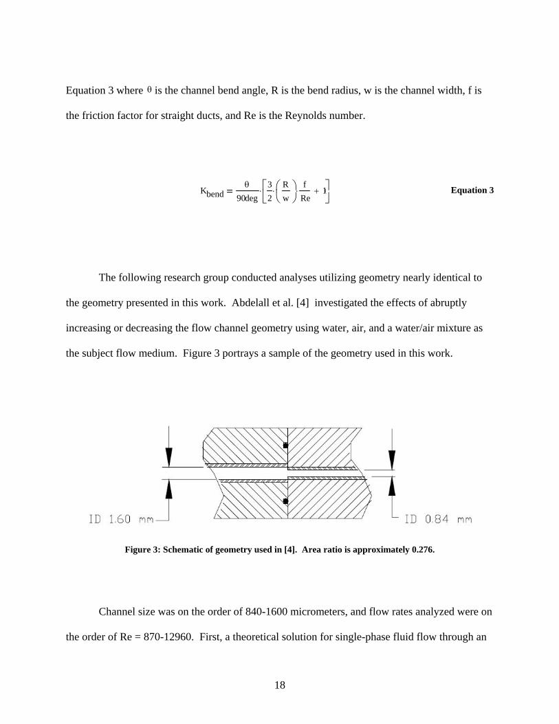
The following research group conducted analyses utilizing geometry nearly identical to
the geometry presented in this work. Abdelall et al. [4] investigated the effects of abruptly
increasing or decreasing the flow channel geometry using water, air, and a water/air mixture as
the subject flow medium. Figure 3 portrays a sample of the geometry used in this work.
Figure 3: Schematic of geometry used in [4]. Area ratio is approximately 0.276.
Channel size was on the order of 840-1600 micrometers, and flow rates analyzed were on
the order of Re = 870-12960. First, a theoretical solution for single-phase fluid flow through an
18
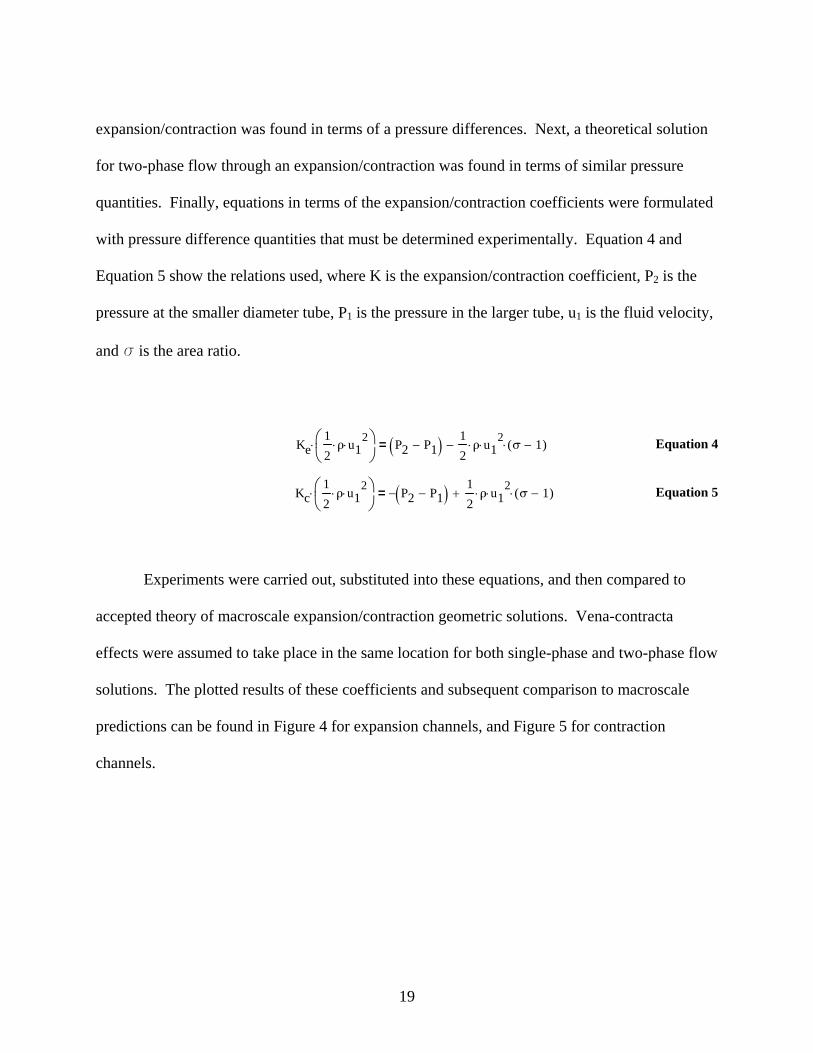
expansion/contraction was found in terms of a pressure differences. Next, a theoretical solution
for two-phase flow through an expansion/contraction was found in terms of similar pressure
quantities. Finally, equations in terms of the expansion/contraction coefficients were formulated
with pressure difference quantities that must be determined experimentally. Equation 4 and
Equation 5 show the relations used, where K is the expansion/contraction coefficient, P2 is the
pressure at the smaller diameter tube, P1 is the pressure in the larger tube, u1 is the fluid velocity,
and s is the area ratio.
Ke12
ρ⋅ u12⋅⎛⎜
⎝⎞⎟⎠
⋅ P2 P1−( ) 12
ρ⋅ u12⋅ σ 1−( )⋅−=
Equation 4
Kc1 ⎞2
ρ⋅ u12
⋅⎛⎜⎝
⎟⎠
⋅ P2 P1−( )−12
ρ⋅ u12
⋅ σ 1−( )⋅+= Equation 5
Experiments were carried out, substituted into these equations, and then compared to
accepted theory of macroscale expansion/contraction geometric solutions. Vena-contracta
effects were assumed to take place in the same location for both single-phase and two-phase flow
solutions. The plotted results of these coefficients and subsequent comparison to macroscale
predictions can be found in Figure 4 for expansion channels, and Figure 5 for contraction
channels.
19
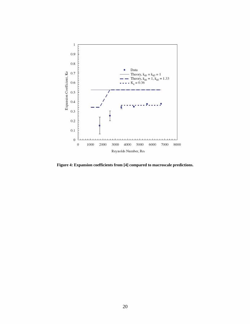
Figure 4: Expansion coefficients from [4] compared to macroscale predictions.
20
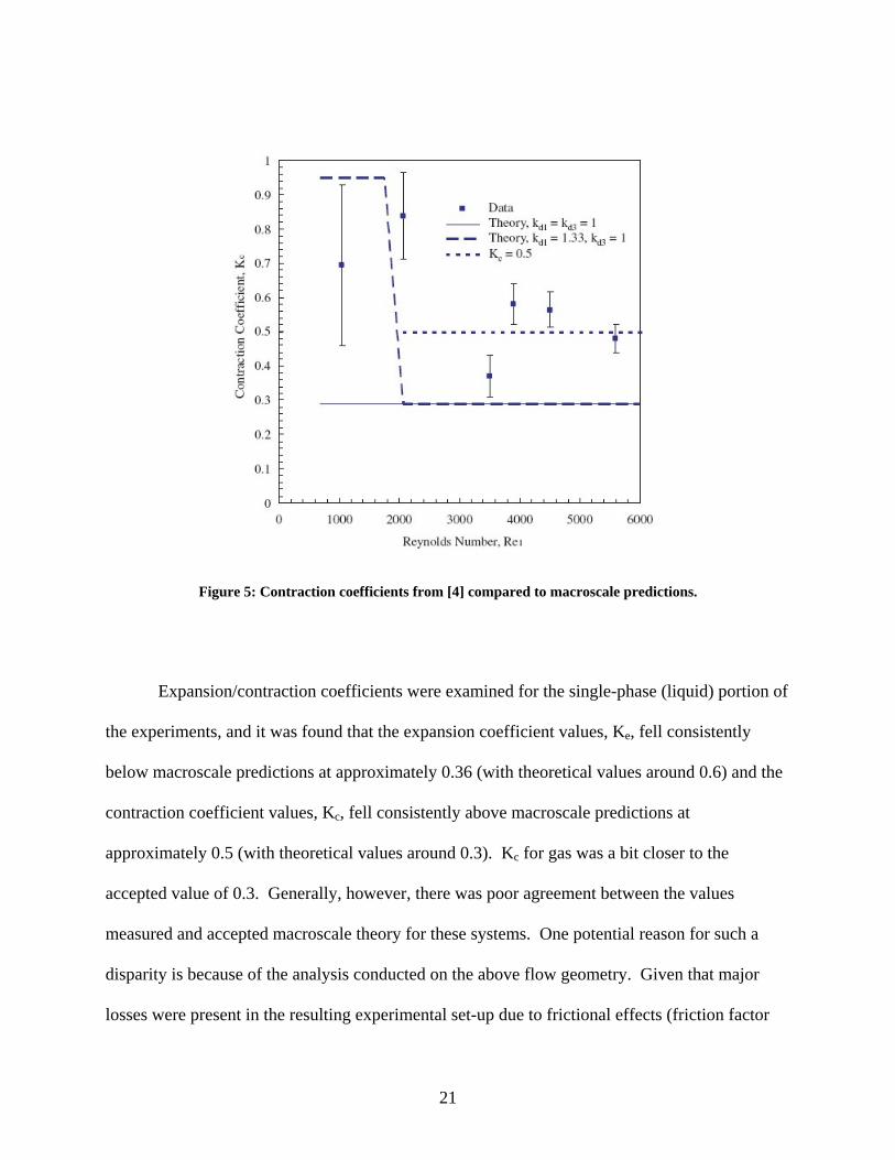
Figure 5: Contraction coefficients from [4] compared to macroscale predictions.
Expansion/contraction coefficients were examined for the single-phase (liquid) portion of
the experiments, and it was found that the expansion coefficient values, Ke, fell consistently
below macroscale predictions at approximately 0.36 (with theoretical values around 0.6) and the
contraction coefficient values, Kc, fell consistently above macroscale predictions at
approximately 0.5 (with theoretical values around 0.3). Kc for gas was a bit closer to the
accepted value of 0.3. Generally, however, there was poor agreement between the values
measured and accepted macroscale theory for these systems. One potential reason for such a
disparity is because of the analysis conducted on the above flow geometry. Given that major
losses were present in the resulting experimental set-up due to frictional effects (friction factor
21

straight duct losses), and because these losses carry with them an overwhelming effect on the
resulting pressure drop, it is hard to separate any uncertainty in the measurement due to these
major losses from the minor losses experienced due to the sudden expansion and contraction.
Averages aside, simply solving for expansion and contraction coefficients (Ke and Kc,
respectively) using the pressure drop data measured is siphoning all of the uncertainty into the
calculations of the coefficients themselves, resulting in major inaccuracies. This effect will be
taken into account in this work.
Results of the two-phase flow system in this work showed only a small offset from
accepted slip flow models with vena-contracta effects considered for all Reynolds number
ranges. A correlation was provided for the two-phase contraction flow losses accounting for
significant velocity slip. While the focus of these experiments were primarily concerned with
modeling two-phase fluidics, a portion of the resulting data, namely the single phase segments,
can be used for comparison to the analysis carried out in this work.
It is by no means a hyperbole to state that there is a surfeit of prior work in the analysis
and utilization of modeling flow through microchannels and microtubes. However, there still
seems to be major disagreement between research groups that claim their experiments follow
that of macroscale fluid mechanics, and other researchers that conclude their experiments are not
adequately described by these battle-hardened theories. Subsequent sections will reveal how this
work brings to light a notion that most groups seem to think is too simplistic exemplified by the
field’s lack of attention to it: flow modeling over simple geometry with direct pressure
measurement techniques.
22

CHAPTER THREE: METHOLODGY
Overview
It is the ultimate aspiration of this work to provide a tangible, useful method of
calculating pressure loss due to abrupt area changes in microchannels. The foremost question to
answer is if the current cornerstone macroscale fluid mechanics is adequate enough to model
microscale fluid flow. This is a question largely disputed amongst the current literature, where a
plethora of varying results and conclusions have been elucidated and argued many times over. It
is hypothesized that there are additional effects to account for in the microscale regime of fluid
flow that are not typically required in macroscale fluidics. That being said, this work does not
intend to explore the chasms of missing mathematics behind the theory of fluid flow through
small channels in detail (provided they exist), but will hope to provide a temporary remedy to the
current salvo of differing (and at times, inconclusive) solutions to microchannel fluid models.
This proposed remedy (if needed) will be in the form of an empirical correlation between
pressure drop and various flow parameters/properties, and supported by data collected through a
barrage of controlled experiments rather than an elegant derivation beginning from first
principles. It is sufficient to compare this type of empirical solution to the types of solutions for
Nusselt numbers (and/or heat transfer coefficients) in the turbulent flow regime, where solutions
contain relations based on other non-dimensional numbers with sometimes peculiar exponents
and coefficients. When compared to their elegantly derived counterpart solutions in the laminar
flow regime, the empirical "data-based" methodology behind their creation is almost
immediately apparent. Continuing with this analogy, it is helpful to think of the empirical
23
solution for pressure drop delivered in this work as the equivalent of a microscale counterpart of
the macroscale solution for common, everyday pipe flow, where the details of what differentiates
the two theoretically will be left for future researchers.
Size Regime Considerations
The study of microfluidics brings with its controversy another unanswered problem:
What is the relative characteristic size of a microchannel? The unwritten rule in the literature
seems to be between 1 micron and 1milimeter (1 – 1000 micrometers) [7] for channel hydraulic
diameters, as channels below this range are considered nanochannels, and ducts above this size
range are considered normal pipes, but that still leaves the question of at what size ranges should
the equations of macroscale fluid mechanics break down due to phenomena yet unknown?
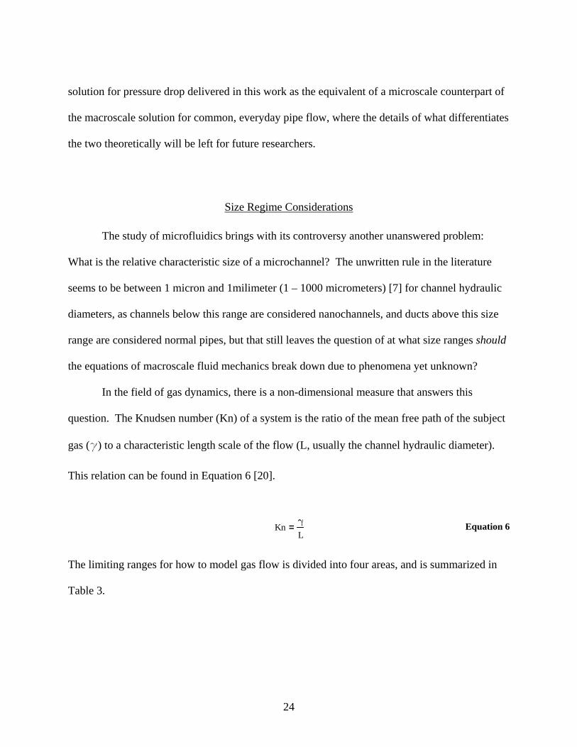
In the field of gas dynamics, there is a non-dimensional measure that answers this
question. The Knudsen number (Kn) of a system is the ratio of the mean free path of the subject
gas (g) to a characteristic length scale of the flow (L, usually the channel hydraulic diameter).
This relation can be found in Equation 6 [20].
Knγ
L= Equation 6
The limiting ranges for how to model gas flow is divided into four areas, and is summarized in
Table 3.
24
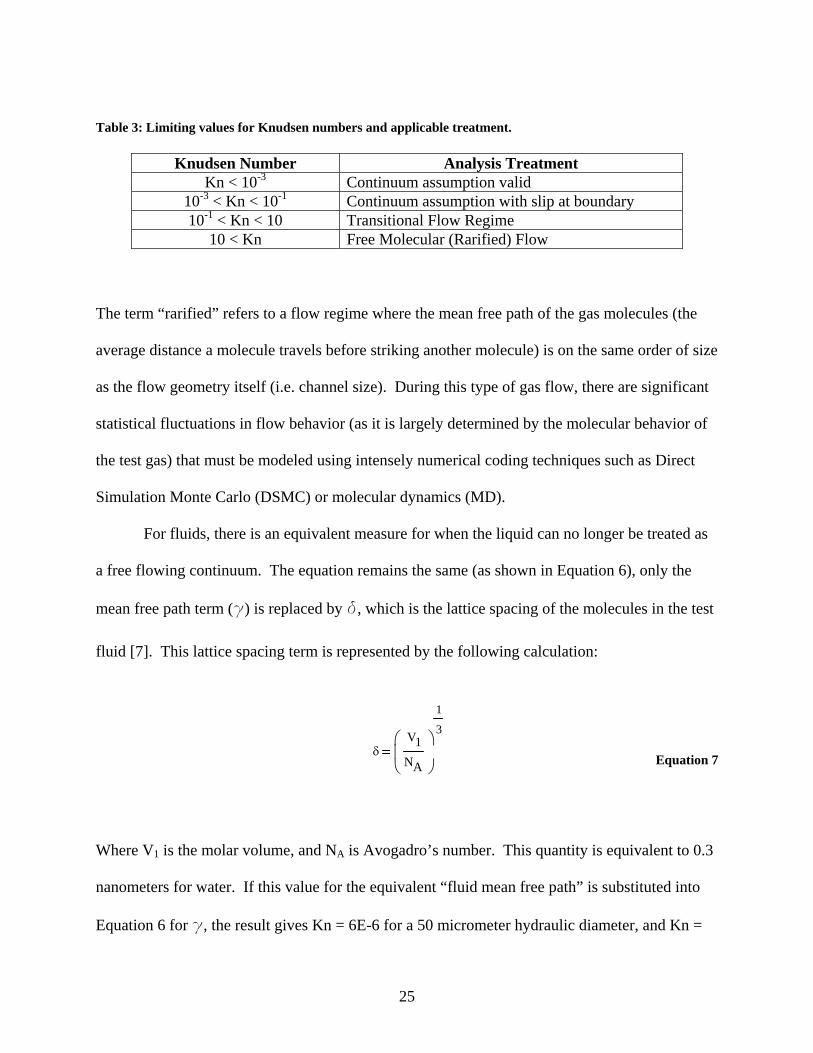
Table 3: Limiting values for Knudsen numbers and applicable treatment.
Knudsen Number Analysis Treatment Kn < 10-3 Continuum assumption valid
10-3 < Kn < 10-1 Continuum assumption with slip at boundary 10-1 < Kn < 10 Transitional Flow Regime
10 < Kn Free Molecular (Rarified) Flow
The term “rarified” refers to a flow regime where the mean free path of the gas molecules (the
average distance a molecule travels before striking another molecule) is on the same order of size
as the flow geometry itself (i.e. channel size). During this type of gas flow, there are significant
statistical fluctuations in flow behavior (as it is largely determined by the molecular behavior of
the test gas) that must be modeled using intensely numerical coding techniques such as Direct
Simulation Monte Carlo (DSMC) or molecular dynamics (MD).
For fluids, there is an equivalent measure for when the liquid can no longer be treated as
a free flowing continuum. The equation remains the same (as shown in Equation 6), only the
mean free path term (g) is replaced by d, which is the lattice spacing of the molecules in the test
fluid [7]. This lattice spacing term is represented by the following calculation:
δV1NA
⎛⎜⎝
⎞⎟⎠
1
3
Equation 7
Where V1 is the molar volume, and NA is Avogadro’s number. This quantity is equivalent to 0.3
nanometers for water. If this value for the equivalent “fluid mean free path” is substituted into
Equation 6 for g, the result gives Kn = 6E-6 for a 50 micrometer hydraulic diameter, and Kn =
25
3E-4 for a 1 micrometer hydraulic diameter, which are both well within Kn < 10-3 continuum
assumption. Using these measures, the smallest size channel size that can be used before
entering the modified slip boundary conditions for continuum fluid flow is 3 nanometers (this
size is about 650 nanometers for air at STP due to greater spacing of gas molecules). This value
is well below even the accepted range of microchannel sizes for the majority of research in
microfluidics, suggesting that flow through microchannels above 3 nanometers in size should
behave according to the theories provided by macroscale fluid mechanics.
Macroscale Fluid Mechanics for Internal Flow
After providing theoretical justification that flow at the microscale should be treated as a
continuum and described adequately by macroscale fluid mechanics, it is appropriate to present
what is accepted as the cornerstone of macroscale flow theory through these channel geometries.
It is the ultimate goal of this work to unearth differences in pressure that result from straight duct
frictional effects and abrupt changes in geometry, and as such it is fitting to begin the derivation
from conventional, time-honored laws that have been gracing the pages of
fluidic/thermodynamic literature for centuries.
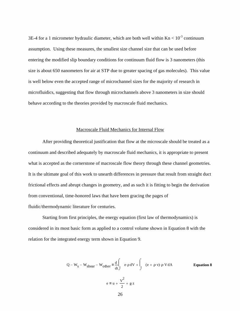
Starting from first principles, the energy equation (first law of thermodynamics) is
considered in its most basic form as applied to a control volume shown in Equation 8 with the
relation for the integrated energy term shown in Equation 9.
E
Q Ws− Wshear− Wother−t
Ve ρ⋅⌠⎮⌡
ddd
Ae ρ v⋅+( ) ρ⋅ V⋅⌠⎮⌡
d+= quation 8
e uV2
2+ g z⋅+=
26

Equation 9
Given that the fluid is incompressible, the flow is steady, all work exiting the system is
zero (surface, shear, etc.), and there is a uniform internal energy and pressure distribution, the
energy equation, when coupled with the kinetic energy coefficient (a, as shown in Equation 10),
can be reduced to Bernoulli’s equation (Equation 11).
Equation 10
Equation 11
The head loss term is the total energy loss per unit mass, and is comprised of the irreversible
conversion of mechanical energy at the entrance of the channel to unwanted thermal energy, and
loss of energy via heat transfer [6]. Loss terms often include frictional effects, changes in
geometry, and surface roughness effects due to material properties.
There are two elements of head loss to consider in fluidics pressure calculations: major
losses and minor losses. The major losses, which typically account for a majority of the energy
loss in a given channel flow system, contain contributions due to frictional effects and surface
roughness effects. Roughness calculations take into account the channel geometry, flow rate,
surface quality, and are based on flow regime (laminar vs. turbulent). A tabulated summary of
the accepted theoretical behavior of this friction factor and its turbulent experimental
α
Aρ V3⋅
⌠⎮⎮⌡
d
m V2⋅
=
p1ρ
α
V12
21⋅+ g z1⋅+⎛ ⎞⎜⎜⎝
⎟⎟⎠
p2ρ
α2V2
2
2⋅+ g z2⋅+
⎛ ⎞⎜ ⎟⎜⎝ ⎟⎠ ∑+= Hloss
27

counterparts as a function of Reynolds number can be found in Figure 6. This figure i
Moody diagram and is widely used in modeling flow behavior for both laminar and turbulent
flow systems.
s called the
Figure 6: Moody chart - correlation of friction factor f and Reynolds number [5].
iven that this work suspects to consider flow in the laminar regime only (per later
discuss r
Equation 12
G
ions in subsequent sections), Equation 12 is an appropriate value for the friction facto
term f.
f64Re
123
1124
bh
⎛⎜⎝
⎞⎟⎠
⋅ 2bh
−⎛⎜⎝
⎞⎡⎢
⎟⎠
⋅+⎢⎣
⎤⎥⎥⎦
⋅=
28

Equation 12 is a modified form of to account that the cross sectional
area of the flow will be rectangular (b is the channel base, h is the channel height), where
Equation 2 is used for circular ducts. This yields the following expression for the major head
loss term derived from energy balance, and with appropriate substitutions for fully developed
pressure driven internal flow.
Equation 13
Now that major losses have been accounted for, minor losses must be considered. For
this work, abrupt changes in area (sudden expansions and contractions) are the only minor losses
that the flow will be subjected to, though other traditional minor losses that are frequently
considered when designing flow systems are sweeping/miter bends, flow inlet/exit phenomena,
and other size transition geometries (nozzles and diffusers). All of these minor losses must be
taken into account when determining total head loss (and summed with the major losses).
Usually, the contribution to the final head loss from these minor losses account for less than 10%
of the total head loss when there are very few minor loss terms, or if the liquid first must travel
steadily over some undisturbed distance (thus experiencing major losses). The minor losses are
nearly always represented in the following manner:
Equation 2 which takes in
Hloss.major ρ f⋅L
Dh⋅
V2
2⋅=
29
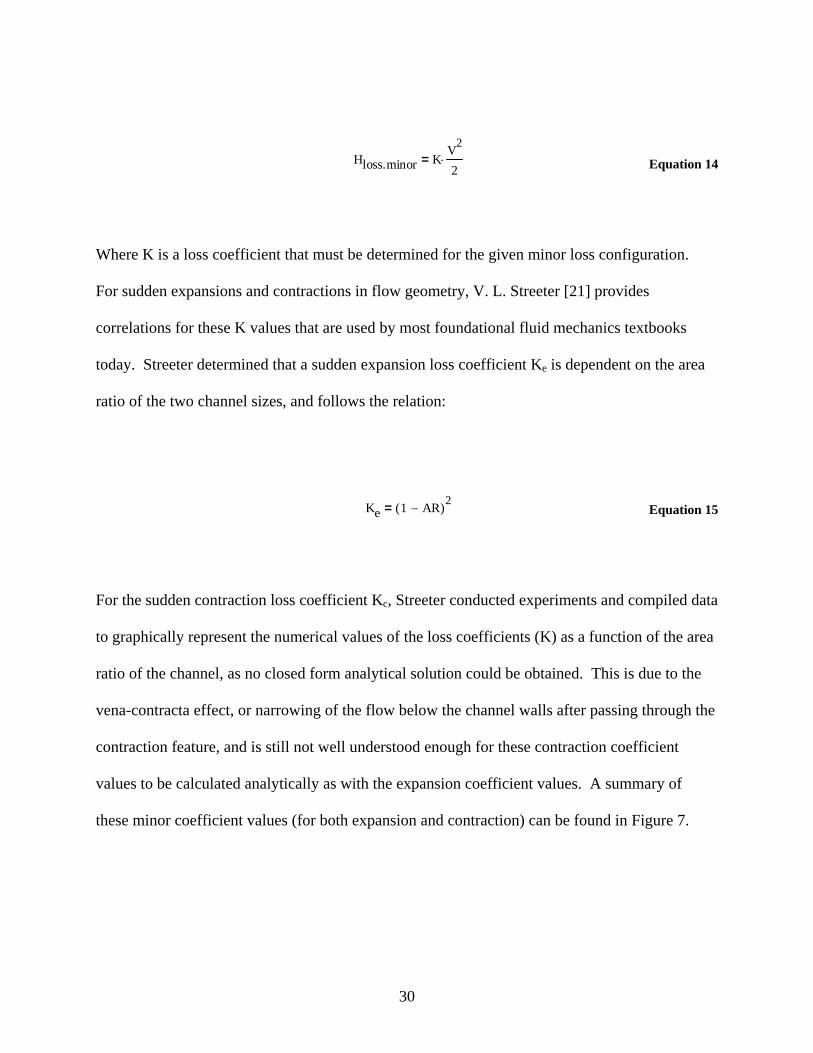
Equation 14
Where K is a loss coefficient that must be determined for the given minor loss configuration.
ooks
a
Equation 15
For the sudden contraction loss coefficient Kc, Streeter conducted experiments and compiled data
e
H KV2
loss.minor 2⋅=
For sudden expansions and contractions in flow geometry, V. L. Streeter [21] provides
correlations for these K values that are used by most foundational fluid mechanics textb
today. Streeter determined that a sudden expansion loss coefficient Ke is dependent on the are
ratio of the two channel sizes, and follows the relation:
Ke 1 AR−( )2=
to graphically represent the numerical values of the loss coefficients (K) as a function of the area
ratio of the channel, as no closed form analytical solution could be obtained. This is due to the
vena-contracta effect, or narrowing of the flow below the channel walls after passing through th
contraction feature, and is still not well understood enough for these contraction coefficient
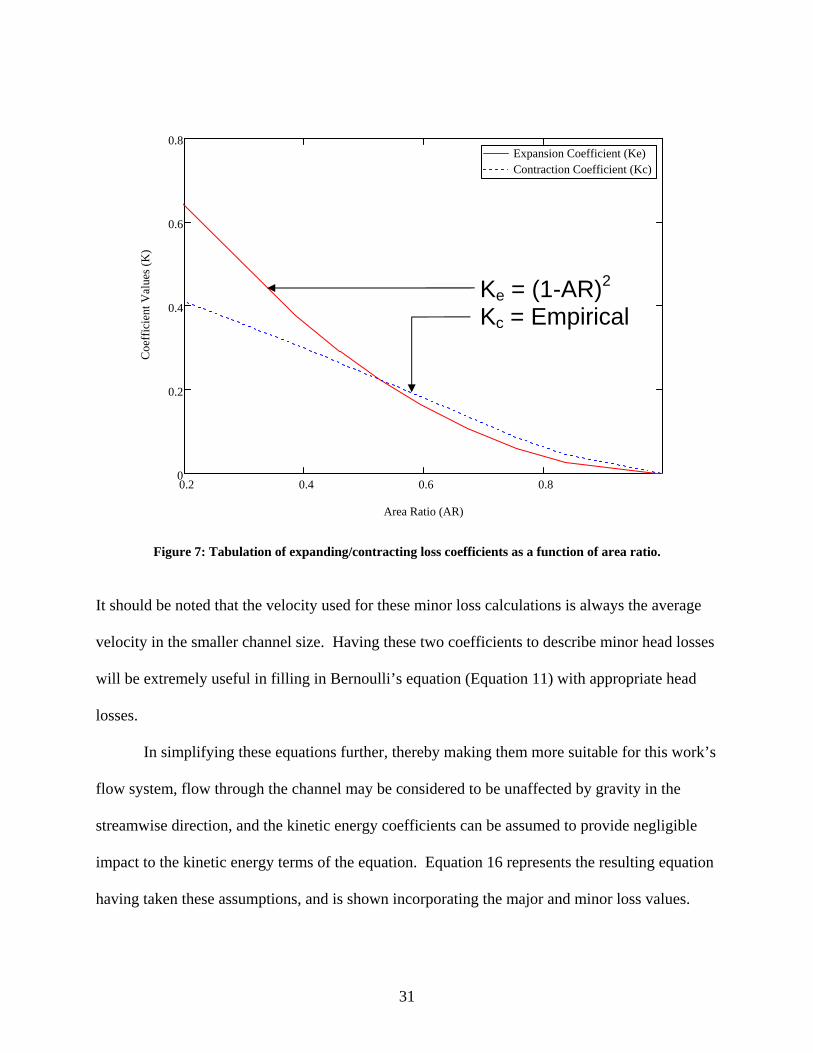
values to be calculated analytically as with the expansion coefficient values. A summary of
these minor coefficient values (for both expansion and contraction) can be found in Figure 7.
30
0.2 0.4 0.6 0.80
0.2
0.4
0.6
0.8Expansion Coefficient (Ke)Contraction Coefficient (Kc)
Area Ratio (AR)
Coe
ffic
ient
Val
ues (
K)
Ke = (1-AR)2
Kc = Empirical
Figure 7: Tabulation of expanding/contracting loss coefficients as a function of area ratio.
It should be noted that the velocity used for these minor loss calculations is always the average
velocity in the smaller channel size. Having these two coefficients to describe minor head losses
will be extremely useful in filling in Bernoulli’s equation (Equation 11) with appropriate head
losses.
In simplifying these equations further, thereby making them more suitable for this work’s
flow system, flow through the channel may be considered to be unaffected by gravity in the
streamwise direction, and the kinetic energy coefficients can be assumed to provide negligible
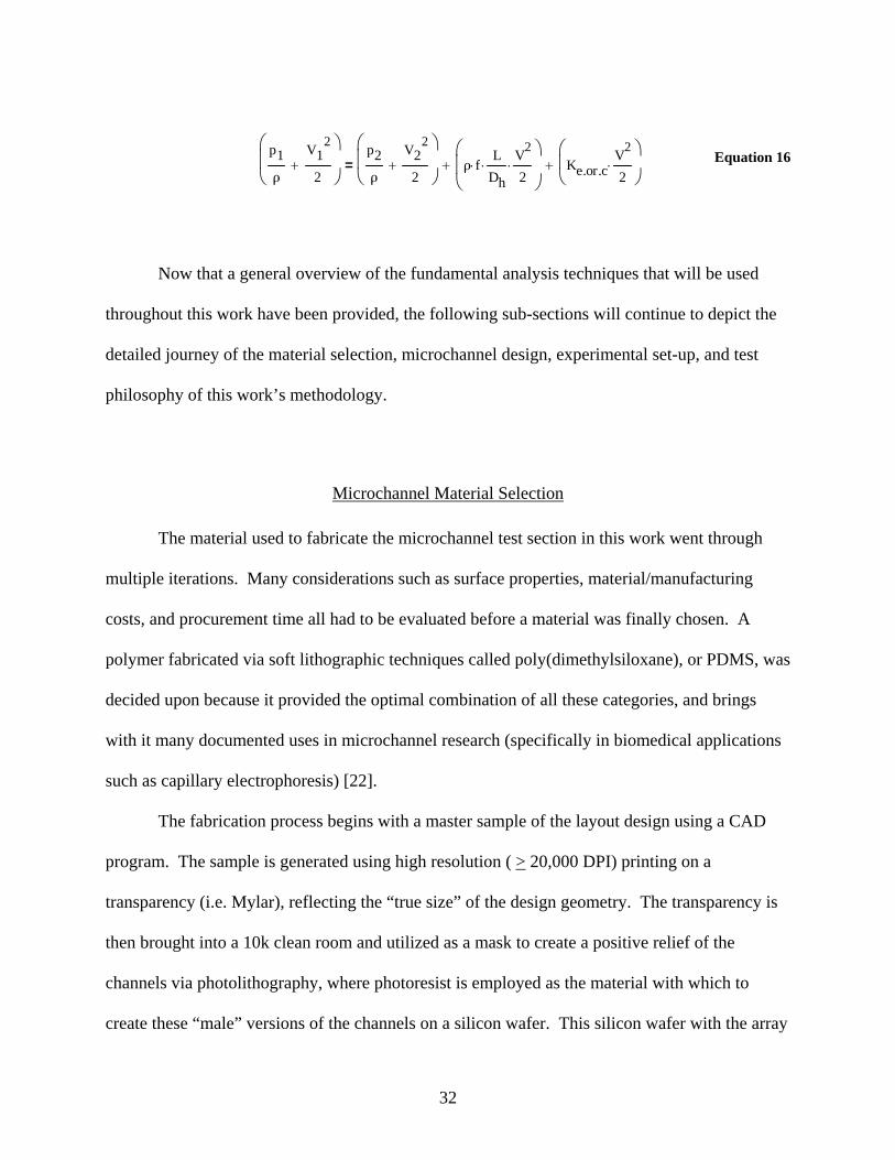
impact to the kinetic energy terms of the equation. Equation 16 represents the resulting equation
having taken these assumptions, and is shown incorporating the major and minor loss values.
31
p1ρ
V12
2+
⎛⎜⎜⎝
⎞⎟⎟⎠
p2ρ
V22
2+
⎛⎜⎜⎝
⎞⎟⎟⎠
ρ f⋅L
Dh⋅
V2
2⋅
⎛⎜⎜⎝
⎞⎟⎟⎠
+ Ke.or.cV2
2⋅
⎛⎜⎝
⎞⎟⎠
+= Equation 16
Now that a general overview of the fundamental analysis techniques that will be used
throughout this work have been provided, the following sub-sections will continue to depict the
detailed journey of the material selection, microchannel design, experimental set-up, and test
philosophy of this work’s methodology.
Microchannel Material Selection
The material used to fabricate the microchannel test section in this work went through
multiple iterations. Many considerations such as surface properties, material/manufacturing
costs, and procurement time all had to be evaluated before a material was finally chosen. A
polymer fabricated via soft lithographic techniques called poly(dimethylsiloxane), or PDMS, was
decided upon because it provided the optimal combination of all these categories, and brings
with it many documented uses in microchannel research (specifically in biomedical applications
such as capillary electrophoresis) [22].
The fabrication process begins with a master sample of the layout design using a CAD
program. The sample is generated using high resolution ( > 20,000 DPI) printing on a
transparency (i.e. Mylar), reflecting the “true size” of the design geometry. The transparency is
then brought into a 10k clean room and utilized as a mask to create a positive relief of the
channels via photolithography, where photoresist is employed as the material with which to
create these “male” versions of the channels on a silicon wafer. This silicon wafer with the array
32

of microchannel shaped phtoresist protrusions is considered the master mold. Liquid PDMS is
then poured over the male mold master, cured using the necessary temperature exposure
requirements, then peeled off the wafer to produce the actual microchannels troughs. Another
blank piece of PDMS that was cured on a blank piece of silicon is then bonded to the original
piece of PDMS with the microchannels to “sandwich seal” the channels by exposing both
surfaces of PDMS to oxygen plasma for 1 minute. This oxygen plasma bonding procedure
produces an irreversible seal that is said to be stronger than the bulk PDMS material itself, and
can also be used to bond PDMS irreversibly to a plethora of other materials such as glass,
silicon, silicon oxide, silicon nitride, quartz, polyethylene, and glassy carbon [1]. The resulting
irreversible bond between these two slabs of PDMS has been verified to withstand internal
pressures up to 5 bars [7].
There are of course numerous advantages, as well as a few disadvantages, to using PDMS
as the channel material. One is that the material is an elastomer, meaning it is rubber-like,
elastic, and pliable. This is a positive characteristic of the test section material because there
aren’t too many worries of damaging the material if it is dropped or mishandled accidentally, and
any effects used to induce flow or take pressure measurements where piercing is involved will be
adequately sealed by the PDMS after piercing occurs. If a more rigid material were used, sealing
around the pressure ports and infusion/removal ports would be troublesome. Later sections
describe how this “elastic advantage” was used for sealing around all interfaces between test
equipment and the microchannel. One disadvantage to the elastomeric material properties of
PDMS, especially given that the geometric sizes are on the order of micrometers, is that a
channel could be easily collapsed by any excessive (or unknown) force or deflection induced on
the material.
33

Another advantage to using PDMS is how inexpensive it is to fabricate the flow
geometry. Given the process outlined above, a reusable silicon master can be fabricated for well
under $100 in material costs after high-resolution printing and photolithography. This is
significantly cheaper than the extensive time and money spent attempting to machine the channel
geometries into a rigid piece of material such as silicone, glass, or any metallic substance, where
costs can approach the $1500 range. After the silicon master was created, it could then be reused
to make multiple copies of additional PDMS slabs containing the microchannels at less than ½
day per copy.
Impact of material selection on flow properties were of utmost importance, since all
aspects of the experiments had to be well known and controlled due to the unknown and
controversial nature of microchannel research. The channel shape as a result of fabrication and
PDMS surface quality were two material characteristics that proved to be of significant
criticality. The electronic CAD drawing (and subsequent high-resolution transparency printout)
provided a two dimensional footprint for exposure of the photoresist in the photolithographic
fabrication process, where surface imperfections were directly related to the resolution of the
printout. Thus, a higher resolution transparency printout provided a less “pixeled” surface in the
resulting PDMS microchannel, as shown in Figure 8.
34
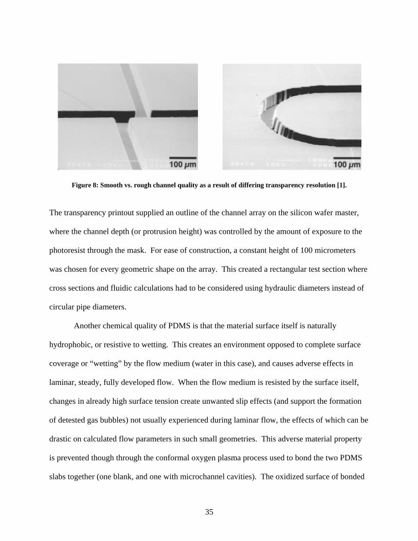
Figure 8: Smooth vs. rough channel quality as a result of differing transparency resolution [1].
The transparency printout supplied an outline of the channel array on the silicon wafer master,
where the channel depth (or protrusion height) was controlled by the amount of exposure to the
photoresist through the mask. For ease of construction, a constant height of 100 micrometers
was chosen for every geometric shape on the array. This created a rectangular test section where
cross sections and fluidic calculations had to be considered using hydraulic diameters instead of
circular pipe diameters.
Another chemical quality of PDMS is that the material surface itself is naturally
hydrophobic, or resistive to wetting. This creates an environment opposed to complete surface
coverage or “wetting” by the flow medium (water in this case), and causes adverse effects in
laminar, steady, fully developed flow. When the flow medium is resisted by the surface itself,
changes in already high surface tension create unwanted slip effects (and support the formation
of detested gas bubbles) not usually experienced during laminar flow, the effects of which can be
drastic on calculated flow parameters in such small geometries. This adverse material property
is prevented though through the conformal oxygen plasma process used to bond the two PDMS
slabs together (one blank, and one with microchannel cavities). The oxidized surface of bonded
35
PDMS pieces develops a hydrophilic layer in contact with the flow medium, creating an easily
wetted channel material that supports flow properties desired in the laminar regime. There are
concerns with the durability of this hydrophilic layer however, in that research has indicated
diversion from hydrophilic behavior with respect to the fluid contact angle when hydrophilic
surfaces are left open to atmosphere for periods longer than 15 minutes. A well behaved
hydrophilic fluid contact angle is acute (or less than 90 degrees), where a hydrophobic contact
angle is obtuse (or greater than 90 degrees) [20]. Morra et al. [23] indicated that when oxidized
PDMS was exposed to atmosphere for 15 minutes, the contact angle changed from 30 to 79
degrees. After 45 minutes of exposure to atmospheric conditions, the angle became 93 degrees.
The native contact angle of non-oxidized hydrophobic PDMS is 108 degrees. With this in mind,
great care was taken not to expose the oxidized PDMS to atmosphere for great lengths of time.
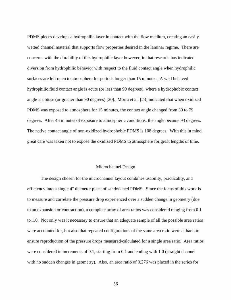
Microchannel Design
The design chosen for the microchannel layout combines usability, practicality, and
efficiency into a single 4" diameter piece of sandwiched PDMS. Since the focus of this work is
to measure and correlate the pressure drop experienced over a sudden change in geometry (due
to an expansion or contraction), a complete array of area ratios was considered ranging from 0.1
to 1.0. Not only was it necessary to ensure that an adequate sample of all the possible area ratios
were accounted for, but also that repeated configurations of the same area ratio were at hand to
ensure reproduction of the pressure drops measured/calculated for a single area ratio. Area ratios
were considered in increments of 0.1, starting from 0.1 and ending with 1.0 (straight channel
with no sudden changes in geometry). Also, an area ratio of 0.276 was placed in the series for
36

comparison to the work of Abdelall et al. in their study of single phase flow through sudden
expansions and contractions in flow geometry.
The larger channel size was designed to remain at 100 micrometers, and an appropriate
calculation was performed to extrapolate the smaller channel size to ensure an accurate area
ratio. The reasoning behind this size selection is multifaceted. The driving requirement however
is to facilitate ease of governing equation simplifications and desired system stability at the
laminar flow regime. It was therefore suitable to model the channel geometry around this
requirement, performing rough order of magnitude calculations to ensure laminar flow is
achieved, the macro scale limit of which is Re~2300 for internal pipe flow. For the various
channel sizes mentioned above for each of the incremental area ratios, the Reynolds number
range is between Re = 7 and Re = 130, which is well below the transitional limit of 2300, and
gives approximately a 16X minimum buffer to account for any early transition to turbulence in
the microscale regime (as proposed by other research groups). It is fitting then to foretell that no
other flow regime will be encountered for the entirety of this work.
In addition to testing microchannels with abrupt area changes due to sudden expansions
and sudden contractions, it was also of interest to test an array of straight ducts with no
expansions or contractions of similar relative size. The purpose of this was to test the validity of
straight duct macroscale fluid mechanics as applied to microchannels prior to examining flow
behavior with minor loss considerations factored in. As such, each 4” piece of PDMS had half
its surface area coated with simple straight ducts of various diameters (similar in relative size and
length to the channels with expansions and contractions) to facilitate this analysis.
The final layout of the 4" diameter piece of PDMS contained 99 microchannels (49
straight duct channels, and 50 area ratio channels), with at least 4 copies of each channel to
37
achieve the desired repeatability of the system. Figure 9 illustrates the final layout of the
microchannels, represented by a CAD drawing.
Figure 9: CAD of microchannel layout on a 4" diameter slab of PDMS.
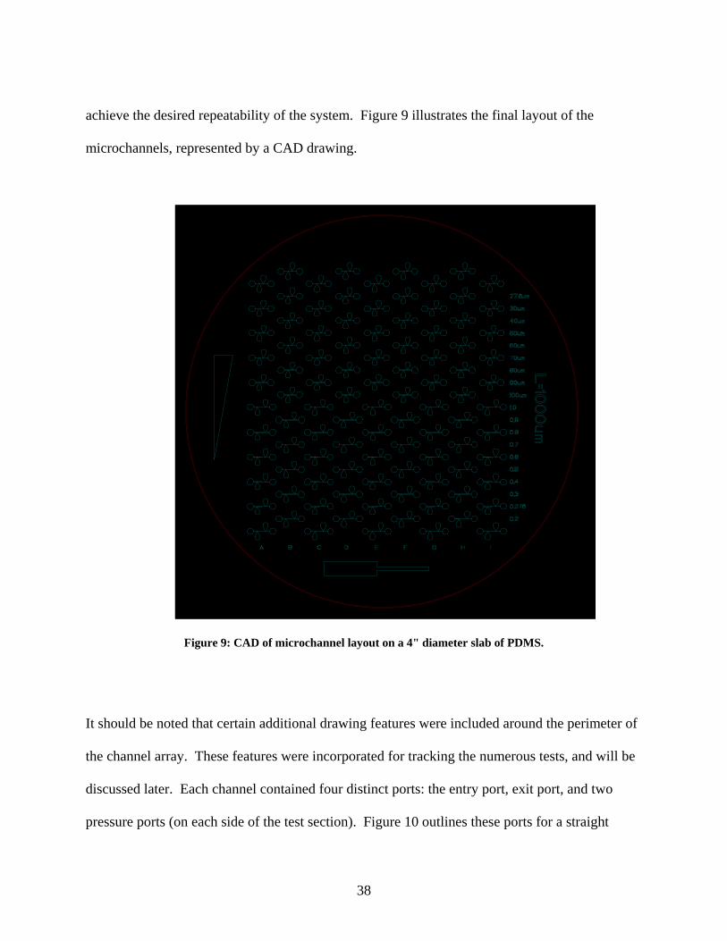
It should be noted that certain additional drawing features were included around the perimeter of
the channel array. These features were incorporated for tracking the numerous tests, and will be
discussed later. Each channel contained four distinct ports: the entry port, exit port, and two
pressure ports (on each side of the test section). Figure 10 outlines these ports for a straight
38
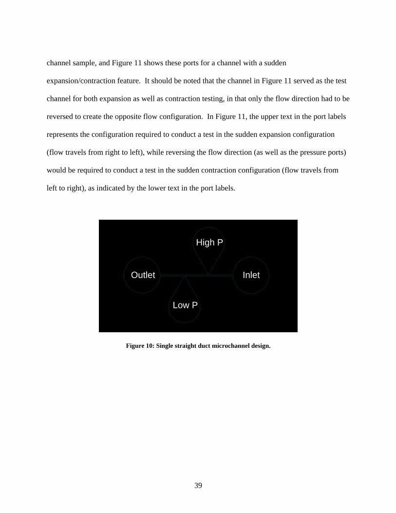
channel sample, and Figure 11 shows these ports for a channel with a sudden
expansion/contraction feature. It should be noted that the channel in Figure 11 served as the test
channel for both expansion as well as contraction testing, in that only the flow direction had to be
reversed to create the opposite flow configuration. In Figure 11, the upper text in the port labels
represents the configuration required to conduct a test in the sudden expansion configuration
(flow travels from right to left), while reversing the flow direction (as well as the pressure ports)
would be required to conduct a test in the sudden contraction configuration (flow travels from
left to right), as indicated by the lower text in the port labels.
Outlet Inlet
High P
Low P
Figure 10: Single straight duct microchannel design.
39

Inlet Outlet
Outlet Inlet
High P Low P
Low P High P
Figure 11: Single expansion/contraction microchannel design.
The philosophy behind this channel design revolved around eliminating as much
unimportant measured data as possible. One of the major flaws in most microfluidics research
today is the coarse measurement of global pressure losses between a point many stages before
the test section of interest, and at the very end of the flow system when the test fluid is
discharged to atmosphere. It is then required to “calculate out” everything but the test section of
interest to the effort (i.e. microchannel geometry) in order to analyze the behavior of the flow
with respect to the pressure drop and/or friction factor. This method seems attractive due to the
reduction of complexity to the flow system (i.e. placement of pressure measurement equipment),
often allowing for a single pressure measurement to be extrapolated very early in the flow
network, and assuming discharge pressures to be that of atmospheric pressure. However, the
“correction” calculations necessary often include the factoring out of infusion/discharge
plumbing, various fittings, changes in material roughness, dissimilar materials that construct the
channel walls, scaling parameters, etc. all of which could easily contain either some kind of
40

overlooked anomaly, or ranges of error that are too large to be of any practical use. With the
channel design used in this work, pressure measurements can be taken immediately before and
directly after a test section of uniform wall materials with no additional “corrections” to
consider, and can be easily done with most commercially available differential pressure
transducers. It should be noted that the flow medium must initially venture up in and fill these
channel pressure ports in order for the pressure reading to accurately transmit from the channel
to the pressure port, then, finally, to the pressure transducer, but these effects are considerably
less pronounced and quickly accomplished than if the flow underwent several "regime changes"
as with prior experiments in other works.
Since the pressure ports produce a measurement that is at a specific point in the flow
field, but outside of the flow itself, any measurement device used for obtaining the pressure at
these points would be measuring the static pressure. Thus, the rearrangement of Equation 16
provides a theoretical quantity for what this work will be measuring: differences in static
pressure across the test section. This rearrangement will be referred to as Equation 17.
p1 p2−12ρ⋅ V2
2 V12
−⎛⎝
⎞⎠⋅ Hloss.major∑+ Hloss.minor∑+ Equation 17
The channel design also factored in the necessary entrance length to ensure the flow
would reach a steady, uniform state prior to arriving at the first pressure port. A rough order of
magnitude calculation was performed using the macroscale relation for entrance length
41
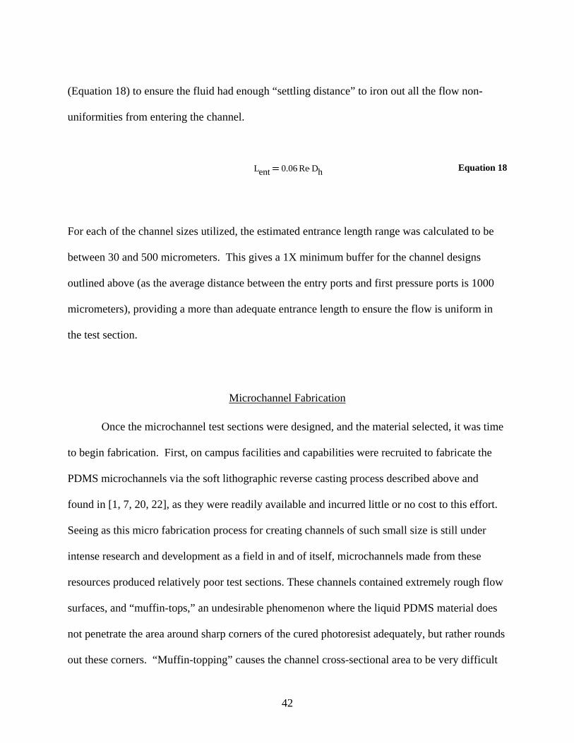
(Equation 18) to ensure the fluid had enough “settling distance” to iron out all the flow non-
uniformities from entering the channel.
Lent 0.06 Re⋅ Dh⋅ Equation 18
For each of the channel sizes utilized, the estimated entrance length range was calculated to be
between 30 and 500 micrometers. This gives a 1X minimum buffer for the channel designs
outlined above (as the average distance between the entry ports and first pressure ports is 1000
micrometers), providing a more than adequate entrance length to ensure the flow is uniform in
the test section.
Microchannel Fabrication
Once the microchannel test sections were designed, and the material selected, it was time
to begin fabrication. First, on campus facilities and capabilities were recruited to fabricate the
PDMS microchannels via the soft lithographic reverse casting process described above and
found in [1, 7, 20, 22], as they were readily available and incurred little or no cost to this effort.
Seeing as this micro fabrication process for creating channels of such small size is still under
intense research and development as a field in and of itself, microchannels made from these
resources produced relatively poor test sections. These channels contained extremely rough flow
surfaces, and “muffin-tops,” an undesirable phenomenon where the liquid PDMS material does
not penetrate the area around sharp corners of the cured photoresist adequately, but rather rounds
out these corners. “Muffin-topping” causes the channel cross-sectional area to be very difficult
42

to measure, as there is now complex curvature from which to calculate geometric flow
parameters as shown in Figure 12 (image captured using a digital microscope).
Figure 12: “Muffin-topping” of channel cross section.
In addition to “muffin-topping” the channel cross-sections, the rounding out of sharp
corners causes the abrupt expansion and contraction features to look more like nozzle and
diffuser features. These features are critical to this work’s analysis, and any defects contained in
them would be detrimental to the results measured without severe corrections in the analyses. A
sample image from these channels can be found in Figure 13.
43

Figure 13: Rounding-out of expansion and contraction features.
With the abundance of these unwanted effects, efforts were refocused to procuring the channels
from an outfit that was a bit more specialized in such fabrication techniques.
The Stanford University Microfluidics Foundry ended up being the outfit of choice due to
design capabilities and lead time benefits, and supplied all the microchannels tested in this work.
The CAD drawing shown in Figure 9 was supplied electronically and two copies of 4” PDMS
“chips” were delivered containing the array of microchannels shown. The silicon master
(containing the cured photoresist) from which the channels were molded was also delivered
should additional copies ever want to be made. Figure 14 shows the silicone master and Figure
15 shows the resulting chip of microchannels cast from this wafer.
44
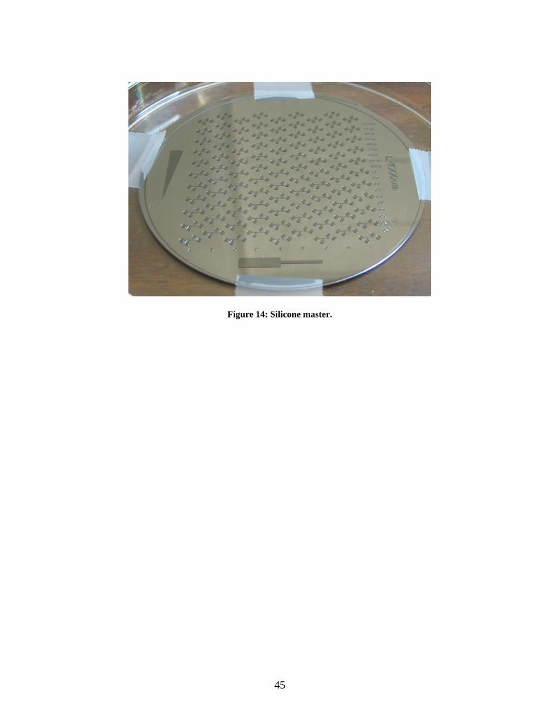
Figure 14: Silicone master.
45

Figure 15: Microchannel chip cast from silicone master.
As mentioned before, the fabrication process for manufacturing these channels is still
under much development itself, but the supplier outlined their limitations very clearly so that
channels could be designed with adequate parameter tolerances (channel size, spacing, aspect
ratios, etc.) to withstand these inconsistencies and still be adequate for testing. It should also be
noted that reference and alignment features were cast directly into the molded PDMS so that
human error would be minimized during testing, a looming terror when trying to keep track of
nearly 200 unique channels. One of these features was an oversized area ratio diagram marking
the general configuration (and direction) of the expansion/contraction geometry (as seen at the
46

very bottom of the chip). This represented the direction of area reduction for all the channels
containing this feature, as they were often hard to see with the naked eye. The horizontal lines
that created both the large and small rectangular shapes of this feature were 1” in length, so that
this feature served the dual purpose of providing a directional as well as a relative size reference
to the chip. Another size reference feature was a nonsymmetrical triangle of prescribed lengths
(triangle at left). The length of the vertical side was 1”. There were also locating features
outlining a grid, where each one of the channels in the array would occupy one of the unique 99
cells in this grid. The columns were identified by the letters A through G (molded below the
array), and the rows were identified by the most obvious feature size of the channels (and
molded to the right of the array). The straight channels (top half) were identified by their
channel width, and the expansion/contraction channels (bottom half) were identified by their area
ratios. Each row contained 4 to 5 copies of each channel, repeated over the respective columns.
For each row, the channels were repeated with a blank cell between each copy in the row to keep
adequate spacing between the channels. For instance, the “30mm” row (fourth row from the top)
would contain five 30mm straight duct channels placed in columns A, C, E, G, and I. The next
row (which contained four 40mm straight duct channels) had its channels placed in columns B,
D, F, and H. This staggered spacing allowed the maximum number of microchannels (99) to be
placed on a single ship without causing leaks or breakages during testing due to inadequate
spacing. All channels were guaranteed to withstand pressures of up to 20 psi by the supplier
given the channels were adequately spaced.
Since there were many variables during the fabrication process that could affect the
resulting channel shape/size, it was imperative that each of the channel dimensions be measured
47
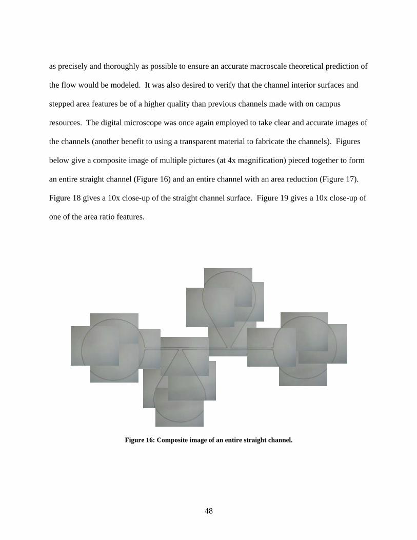
as precisely and thoroughly as possible to ensure an accurate macroscale theoretical prediction of
the flow would be modeled. It was also desired to verify that the channel interior surfaces and
stepped area features be of a higher quality than previous channels made with on campus
resources. The digital microscope was once again employed to take clear and accurate images of
the channels (another benefit to using a transparent material to fabricate the channels). Figures
below give a composite image of multiple pictures (at 4x magnification) pieced together to form
an entire straight channel (Figure 16) and an entire channel with an area reduction (Figure 17).
Figure 18 gives a 10x close-up of the straight channel surface. Figure 19 gives a 10x close-up of
one of the area ratio features.
Figure 16: Composite image of an entire straight channel.
48
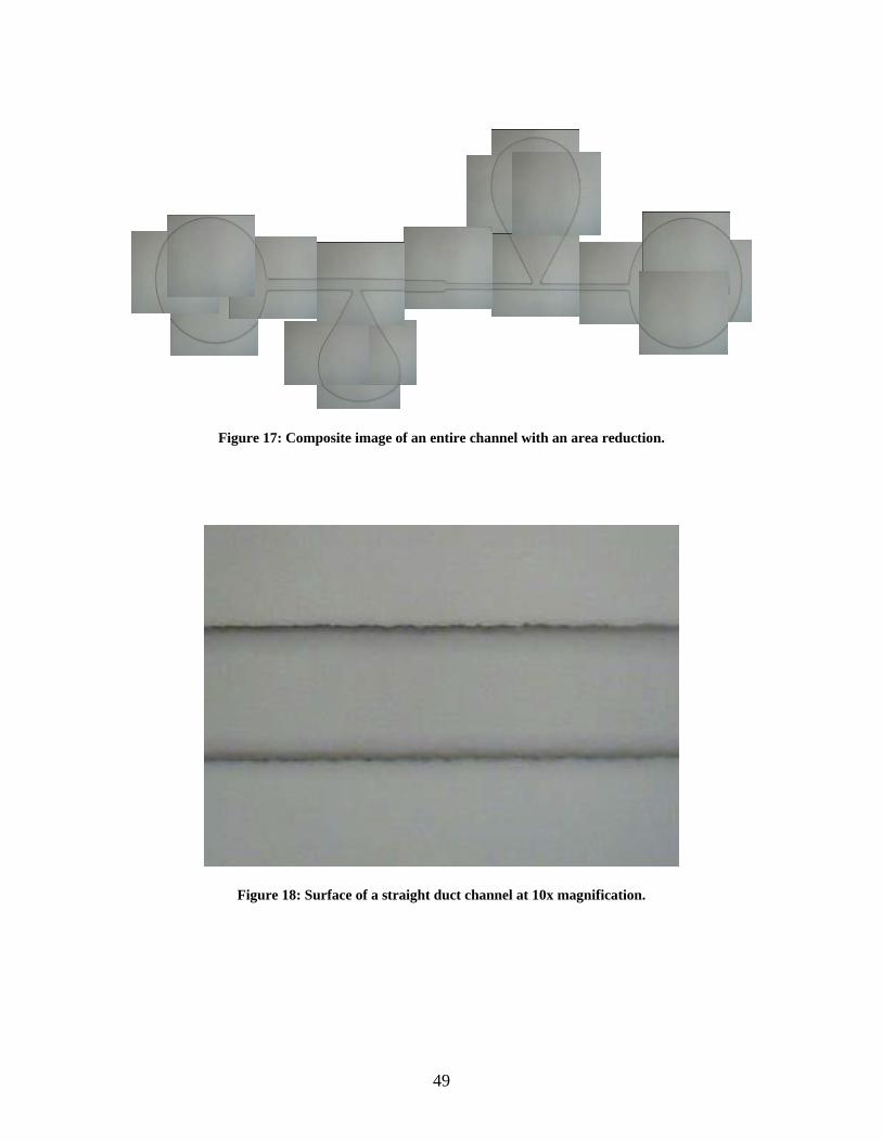
Figure 17: Composite image of an entire channel with an area reduction.
Figure 18: Surface of a straight duct channel at 10x magnification.
49

Figure 19: Area reduction at 10x magnification.
It can be concluded from the figures that the quality of channels supplied by the Stanford
Microfluidics Foundry far surpassed that of the quality of channels supplied by other resources.
There were still some anomalies to note that would require some adjustments to the macroscale
flow models, however. One was that the same rounding-out of corners was still present in the
expansion/contraction area reduction features, though not nearly as drastic or extreme as the
channels fabricated and shown earlier, and limiting their more drastic form to smaller area ratios.
The most severe of these anomalies was that the actual channel dimensions came out
larger than originally designed due to expansion/relief adjustments induced (and required) during
the soft lithography manufacturing process. This caution was issued by the supplier, so its
occurrence was not detrimental to the experiments. Channel width, for example, came out be
consistently 30 micrometers above the design dimensions submitted in the original CAD
50

drawing. This meant that all theoretical predictions had to be corrected to calculate using actual
channel dimensions, as relations that used these geometric quantities (such as Reynolds number,
friction factors, etc.) would be prone to massive errors and produce inaccurate results.
Therefore, it was decided to measure all channel widths and lengths such that the inaccuracies
due to variability in the channel dimensions would be drastically reduced, and nearly eliminated
from the theoretical calculations. To facilitate these measurements, a digital microscope was
once again employed. Digital images were captured and channels were measured in screen pixel
units using a computer graphics manipulation program. A calibrated micrometer scale with both
10 and 1 micrometer graduations, shown in Figure 20, was used to convert pixel measurements
from digital images to micrometers after a simple calibration at 4x and 10x magnifications.
Figure 20: Micrometer scale used to calibrate digital microscope.
51
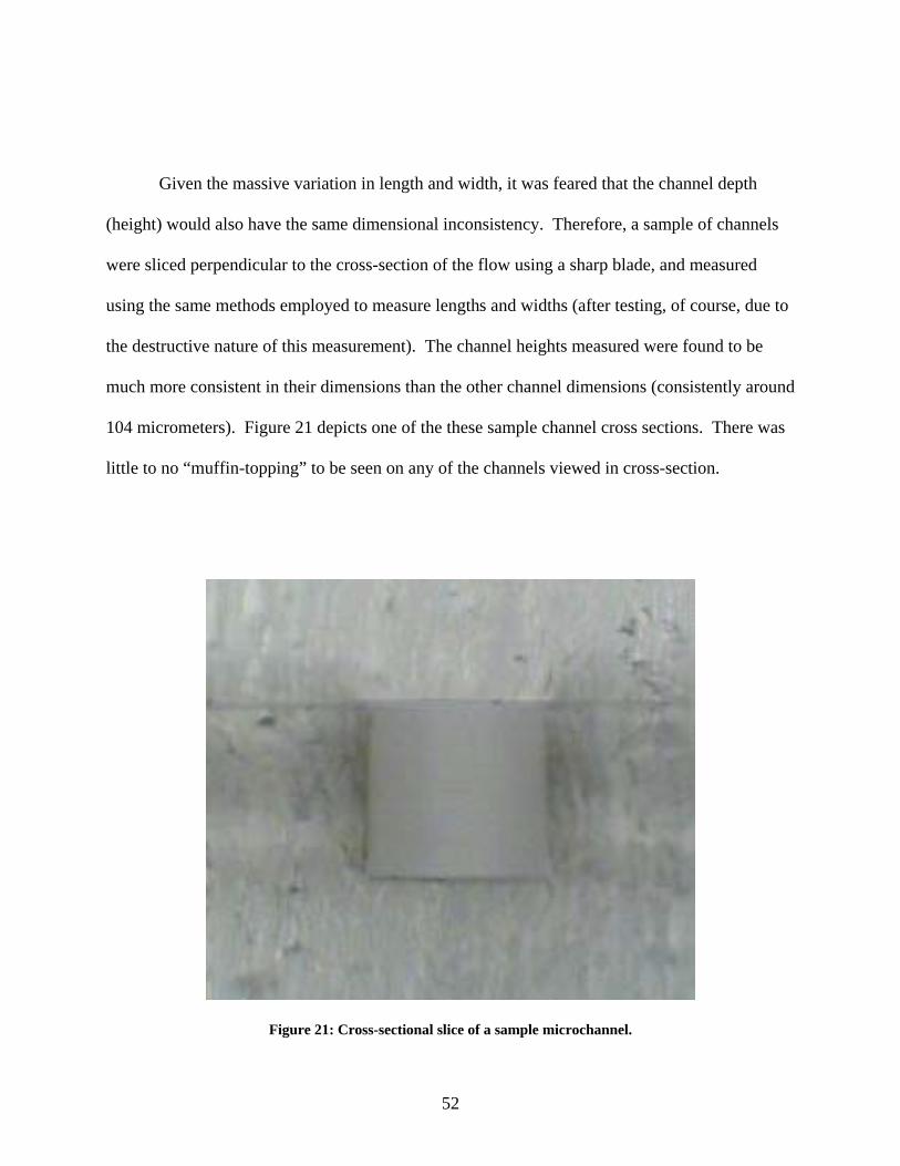
Given the massive variation in length and width, it was feared that the channel depth
(height) would also have the same dimensional inconsistency. Therefore, a sample of channels
were sliced perpendicular to the cross-section of the flow using a sharp blade, and measured
using the same methods employed to measure lengths and widths (after testing, of course, due to
the destructive nature of this measurement). The channel heights measured were found to be
much more consistent in their dimensions than the other channel dimensions (consistently around
104 micrometers). Figure 21 depicts one of the these sample channel cross sections. There was
little to no “muffin-topping” to be seen on any of the channels viewed in cross-section.
Figure 21: Cross-sectional slice of a sample microchannel.
52

One limiting characteristic of the supplier in general that affected this work was the
aspect ratio requirements of their manufacturing process. This characteristic caused some of the
perimeter channel geometry (and subsequent height dimensions) to be more varied because their
aspect ratios were close to or in violation of the fabrication limits of the fabrication process. The
maximum Y:X ratio (Y = channel height, X = channel width) was 5:1, meaning for a constant
104 micrometer height, the smallest possible designed channel width must be above 20
micrometers. At this limit, manufacturing limitations begin to severely warp the microchannels,
and results extrapolated from testing become extremely unreliable (unless great care is taken to
map the channel exactly as it was produced). The design of these microchannel configurations
intentionally included channels with dimensions that violated this design rule, more as an
experiment of how the manufacturing process would hold up. The channels in these size ranges,
as warned, came out contorted, disfigured, and sometimes even collapsed. See Figure 22 for a
sample of channels in this aspect ratio regime.
53

Figure 22: Images of channels that violate a 5:1 aspect ratio.
With all of these adverse manufacturing elements contributing to the final channel
design, great care was taken to ensure each was considered as accurately as possible within the
theoretical macroscale flow predictions. It should be noted that due to the necessary dimensional
alterations as a result of the manufacturing process (up to a 30mm increase in length and width
channel dimensions), the size range of subsequent testing was adjusted to include straight
54

channels of widths ranging from 50 micrometers to 130 micrometers, and area ratios ranging
from 0.4 to 1.0, all with 104 micrometer heights.
Experimental Set-Up
As with any set-up, there are advantages and disadvantages to consider when evaluating
and implementing a microfluidic system design. Advantages to the global pressure measurement
systems aforementioned include their credibility of producing verifiable field data from prior
works in microchannel research, and ease of assembly. Having been so widely used by other
researchers and producing what appear to be reliable results, it is easy for one to duplicate the
system while simply replacing the test section with the flow geometry specific to their focus.
This also gives rise to the advantage of allowing the results of the two works to be compared
while attributing little deviation to the experimental set-up itself, as this variable would be nearly
unaltered for the two systems. Disadvantages include silencing the perpetuating argument that
continuously improving prior work is the essence of applied research. Why settle for what has
already been done (because it is readily available) when improvements can make the system, and
thus results, more applicable, usable, and robust? Time and effort is saved, but contributions to
the field are minimized. It is for this reason that the decision was made to utilize a new
microfluidics testing system that made significant improvements on the system described above.
The two major philosophical changes to the improved experimental set-up included the
facilitation of direct pressure measurements via pressure ports designed directly into the
microchannel itself, and the automated administration of flow into (and extraction from) the
microchannel.
55

Set-Up Design and Equipment Selection
It was decided to employ the robust experimental set-up developed by Chase Hansel [19],
as it was readily available and concurrently designed and developed with the efforts of this work
in mind. Hansel, for his work, also designed test sections such that pressure measurements could
be taken directly from ports stemming from the microchannels themselves, though test sections
in that work focused on sweeping pipe bends over various angle and radii. While an overview of
the equipment set-up and test process will be outlined here, the details of the selection
methodology behind each of the individual components can be found in Hansel’s work [19].
Figure 23 represents a schematic of the experimental set-up, and Table 4 gives the detailed
product information for each component. Figure 24 is an actual photograph of the set-up labeled
in the same way as Figure 23 (with additional non-numbered reference materials needed) whose
information can be cross referenced using Table 4.
56
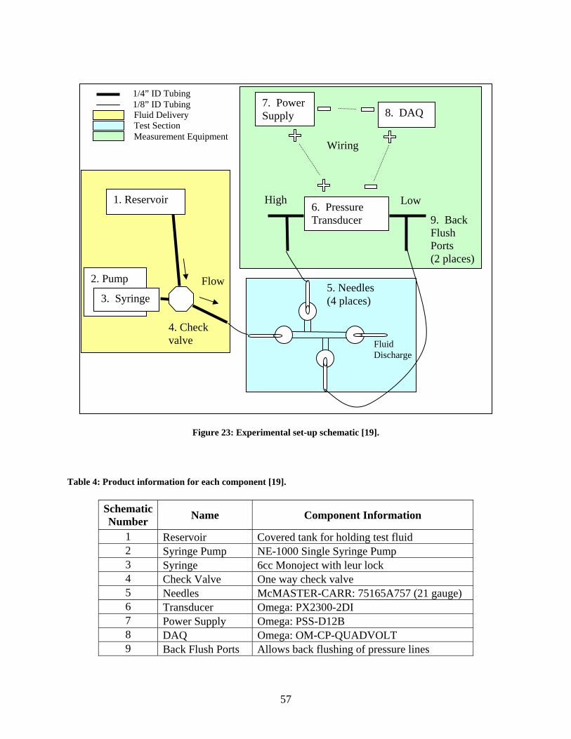
1. Reservoir
2. Pump
6. Pressure Transducer
8. DAQ 7. Power Supply
3. Syringe
4. Check valve
High Low
1/4” ID Tubing 1/8” ID Tubing
5. Needles (4 places)
Wiring
Flow
9. Back Flush Ports (2 places)
Fluid Discharge
Fluid Delivery Test Section Measurement Equipment
Figure 23: Experimental set-up schematic [19]. Table 4: Product information for each component [19].
Schematic Number Name Component Information
1 Reservoir Covered tank for holding test fluid 2 Syringe Pump NE-1000 Single Syringe Pump 3 Syringe 6cc Monoject with leur lock 4 Check Valve One way check valve 5 Needles McMASTER-CARR: 75165A757 (21 gauge) 6 Transducer Omega: PX2300-2DI 7 Power Supply Omega: PSS-D12B 8 DAQ Omega: OM-CP-QUADVOLT 9 Back Flush Ports Allows back flushing of pressure lines
57

2. Syringe Pump
8. DAQ Recorder 1. Reservoir
Channel Piercing Station 5. Needles Necessary Tools Microchannels
Necessary Solvents 7. Power Supply
3. Syringe 4. Check Valve
6. Pressure Transducer
9. Back Flush Ports
Figure 24: Photograph of experimental set-up.
The test liquid chosen was distilled water for its ease of procurement, handling, and
already extensive (and applicable) use in the field of microfluidics. The NE-1000 syringe pump
(schematic number 2) was chosen as the flow rate controller due to its highly precise (threaded
shaft, worm gear) pumping capability, simple user interface, and additional time saving features.
One of these features that were heavily used, the programming feature, allowed for the pump to
run autonomously, testing multiple flow rates at different time intervals without any user
interface necessary. This allowed lengthy tests to be administered without any supervision,
thereby greatly increasing productivity. Another element of the set-up that made this
58

programming feature possible was the design and implementation of a test fluid storage reservoir
(schematic number 1). In the pump’s program, a “withdraw” command could be initiated to
reverse the pumping direction and pull back the syringe plunger, however, the withdrawing of
liquid back out of the channel test section was not the desired intent of this feature. A check
valve (schematic number 4) was strategically placed at the junction in piping between the
syringe, reservoir, and infusion line to the channel in order to block the reservoir tube during
normal pumping operations (when fluid is pumped directly from the syringe into the
microchannel), while blocking the infusion path to the microchannel during withdraw operations
(allowing liquid to refill the syringe as its pulled from the reservoir). See Figure 25 for a picture
of this configuration.
To liquid storage tank
To microchannel entry port
Syringe
Indicates flow direction
59

Figure 25: Check valve between syringe, fluid storage tank, and microchannel infusion tube.
The flow rates selected for testing were carefully chosen to ensure the flows throughout
the entire duration of the tests were kept laminar. As mentioned before, the microchannels were
designed to encounter only laminar flow in the range of Re = 7 to Re = 130, so the flow rates
selected were based on this Reynolds number range. As the pump flow rates could only be set in
units of micro/milliliters per hr/min, this put our pumping volumetric flow rates in the range of
50 to 500 microliters per minute, with increments in 50 microliters per minute. Therefore, a
complete test would experience 10 different flow rates (and subsequently 10 different Reynolds
numbers), for approximately 10-15 minutes in order to obtain enough steady state
voltage/pressure loss data at each flow rate. After each of the flow rates, the withdraw function
was called in the pump program to refill the syringe with water from the storage tank through the
check valve. The entire duration for a single test that went through each of the required flow
rates lasted about 2.5 hours. Table 5 outlines the programmed flow rates experienced by a single
100 micrometer wide channel with extrapolated Reynolds numbers.
Table 5: Sequence of flow rates for all tests, with extrapolated Re for 100mm straight channel.
Vol (mL/min) 50 100 150 200 250 300 350 400 450 500 Re 8.17 16.35 24.52 32.70 40.87 49.04 57.22 65.39 73.57 81.74
The transfer of fluid to and from the microchannel test section proved to be another major
improvement to prior set-ups. This is both a function of the channel design, as well as the
material selected for creation of the microchannel test sections (PDMS). The elastomeric
60

properties of the material allow for it to be deflected away from its free (molded) state, with an
inherent need to return to this free state. Thus, any object that pierces the cured slab of this
isotropic rubbery material will create an air-tight seal around the interface between the PDMS
and the object itself, which was a critical aspect that allowed for this experimental set-up to be
fruitful. Designing entry/exit ports for the flow medium, and pressure ports casted directly into
the PDMS microchannel (set at the same depth as the channel itself), allowed for delicate
penetration into the microchannel through the top layer of PDMS using 21 gauge needles
(schematic number 5). These needles acted as the interface between the channel, and any piece
of flow or measurement equipment in the test system. As seen form Figure 23, there are tubes
connecting the inlet port to the check valve (and, as a result, the syringe pump), the outlet port to
a discharge reservoir, and the high and low pressure ports to their representative counterparts on
the pressure transducer, all of which pass through a 21 gauge needle piercing through the top
layer of PDMS and forming an airtight/watertight seal. Before this test configuration is achieved
though, a very delicate, technique governed procedure must be followed to ensure successful
testing.
Test Procedure
The set-up procedure also very closely follows the methods outlined in Hansel’s
experiments, save for a few critical observations and adjustments unique to this work. The set-
up process will be given for a single unique test (for a single microchannel), and assume that the
syringe pump is programmed, all equipment needed to operate and record data (transducer
connected to power supply and DAQ system, and DAQ software ready to record) is installed and
61

operational, and there is ample test liquid loaded in the storage reservoir. This process had to be
repeated for every test, where additional periodic maintenance of the system occurred every 20
to 30 tests or so. These periodic maintenance items included lubricating the worm gear
mechanism of the syringe pump, replacing the infusion syringe, flushing the bleed screws on the
pressure transducer (through the pressure ports), and topping-off the test fluid reservoir that
refills the syringe during withdraw steps in the pumping program. The procedure for setting up
single a test (minus these periodic maintenance items) is as follows:
1. Save any acquired data from prior tests on the computer attached to the DAQ system.
2. Remove the needles from any prior test channels by carefully lifting the (qty. 4) 21
gauge needles directly upward out of the inlet port, exit port, and two pressure ports.
3. Place and align the clear PDMS chip over a 1-to-1 (true size) printout of the
microchannel array using alignment marks/features on the chip (large triangle, scaled
channel shape diagram, etc.). See Figure 26 for reference.
62

Figure 26: PDMS test chip aligned over 1-to-1 computer printout.
4. Using an unmodified 21 gauge needle (same type needle that is used for actual
testing, only not connected to any tubing or ports) align the tip directly centered over
the right most port using the 1-to-1 printout under the PDMS as a guide (see Figure
27).
63
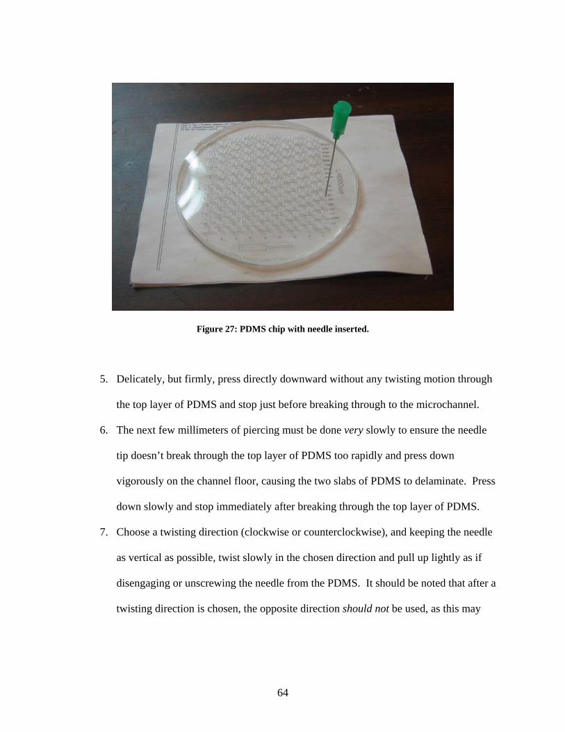
Figure 27: PDMS chip with needle inserted.
5. Delicately, but firmly, press directly downward without any twisting motion through
the top layer of PDMS and stop just before breaking through to the microchannel.
6. The next few millimeters of piercing must be done very slowly to ensure the needle
tip doesn’t break through the top layer of PDMS too rapidly and press down
vigorously on the channel floor, causing the two slabs of PDMS to delaminate. Press
down slowly and stop immediately after breaking through the top layer of PDMS.
7. Choose a twisting direction (clockwise or counterclockwise), and keeping the needle
as vertical as possible, twist slowly in the chosen direction and pull up lightly as if
disengaging or unscrewing the needle from the PDMS. It should be noted that after a
twisting direction is chosen, the opposite direction should not be used, as this may
64
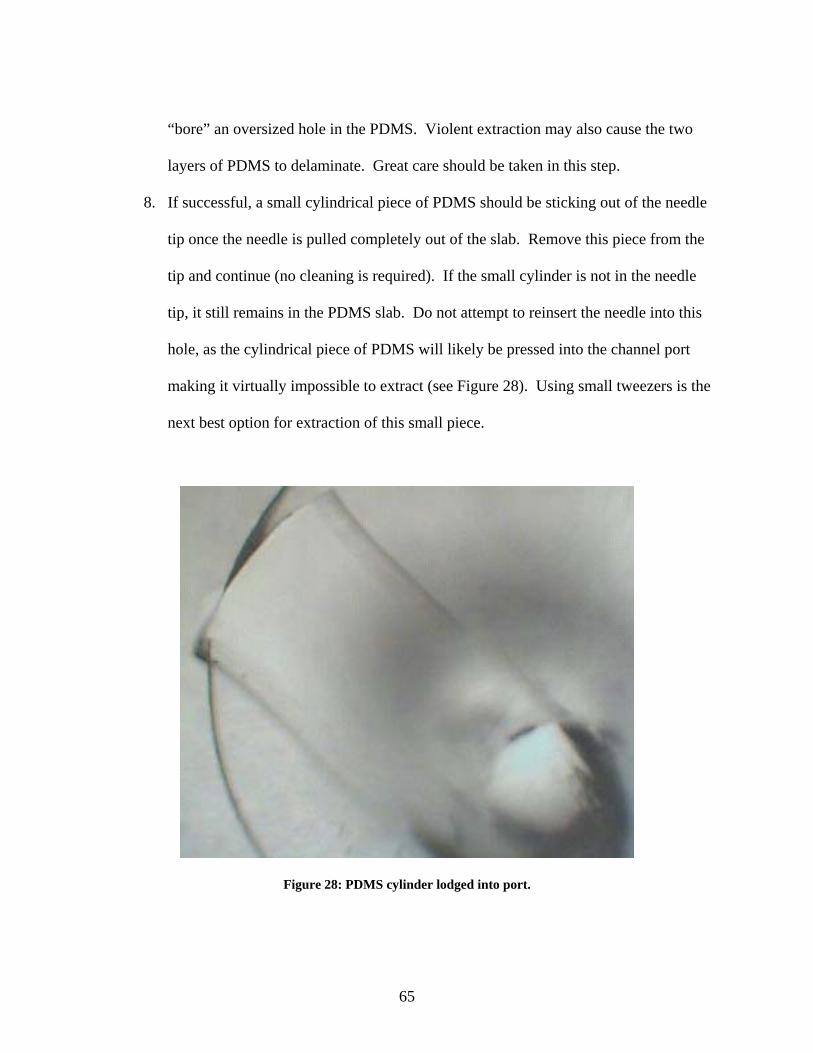
“bore” an oversized hole in the PDMS. Violent extraction may also cause the two
layers of PDMS to delaminate. Great care should be taken in this step.
8. If successful, a small cylindrical piece of PDMS should be sticking out of the needle
tip once the needle is pulled completely out of the slab. Remove this piece from the
tip and continue (no cleaning is required). If the small cylinder is not in the needle
tip, it still remains in the PDMS slab. Do not attempt to reinsert the needle into this
hole, as the cylindrical piece of PDMS will likely be pressed into the channel port
making it virtually impossible to extract (see Figure 28). Using small tweezers is the
next best option for extraction of this small piece.
Figure 28: PDMS cylinder lodged into port.
65

9. Continue with steps 3 through 8 for the remaining (qty. 3) ports. It is important to
commence with testing within 10 minutes from the first pierce to prevent the
hydrophilic coating provided by the oxygen-plasma treatment from becoming
hydrophobic due to prolonged exposure to atmosphere.
10. Open a new file in the DAQ computer program, and start recording voltage
information from the DAQ voltage recorder. The program will capture voltage
information during all of the following steps. It will be evident in future steps that
this is done to verify proper flushing of the pressure ports to be tested.
11. Set the PDMS slab in position on the test bench.
12. Insert the infusion port into the desired end of the microchannel test section by
pressing directly downward. Stop the needle point approximately halfway down the
top slab of PDMS so as not to block the channel port with the needle tip or risk
delaminating the microchannel by deforming its base (as cautioned during the
piercing step).
13. Set the pump to a flow rate that will register a reading (but not overexert) the pressure
transducer and DAQ software, and begin pumping. Water will begin to fill the
microchannel and discharge out of the high pressure port (and possibly the exit port).
14. When a decent sized pool of water collects over the high pressure port of the
microchannel (see Figure 29), pause the syringe pump and open the high end of the
pressure transducer back flush ports. Carefully insert a syringe with an adequately
sized tip into the tubing of the back flush port, and pump water into the port. This
water should travel through the 1/8” tubing and be discharged out the end of the high
port 21 gauge needle.
66

Figure 29: Microchannel with infusion needle inserted and a pool of liquid over the high port.
15. Place the tip of the high port needle into the pool of water over the high pressure port
of the microchannel, and squeeze some more water out of the syringe in the back
flush tube. This is to ensure no air pockets exist between the needle connected to the
high port on the pressure transducer and the high port of the microchannel.
16. Insert the high port needle into the high port of the microchannel exactly how the
infusion needle was inserted (about halfway through the top PDMS slab).
17. Remove the extra syringe from the high port back flush tube and ensure no bubbles
exist in this tube.
18. Turn on the syringe pump and watch how water is pumped up through the high port
pressure tubing and out of the back flush tube on the pressure transducer.
67

19. Wait for a drop or two to drip out, then turn off the syringe pump and plug up the
back flush tube.
20. When the syringe pump is turned on again, liquid will be forced to travel out of the
low pressure port (and possibly the exit port) since the high port has been plugged up.
21. Repeat steps 13 though 19 for the low pressure port.
22. When the syringe pump is turned on again, liquid will be forced to come out of the
exit port only. After a pool of water forms over the exit port, insert the exit needle
and ensure the liquid discharged is collected in an appropriate temporary storage tank
that facilitates disposal after the test.
23. Turn the syringe pump back on and allow liquid to flow through the system for some
time. Observe the DAQ software to ensure a pressure reading is being registered.
24. Turn off the pump, pull up a clean sheet to record voltage data from the actual test,
and load the desired pumping program.
25. Start the actual test.
Now that the system has been adequately prepped and readied to conduct a test, a brief
journey that the liquid will experience during a typical test will be described that shows how the
flow provides measurable information that can be extracted from the set-up instrumentation. The
interface between the macroscale and microscale worlds in this set-up with regards to test
medium handling (flow delivery to channel, extraction from channel, and taps into the pressure
ports) were all carefully controlled using the 21 gauge needles installed in the procedure above.
The flow medium (distilled water) started in the 6cc syringe (after being drawn in from the
storage tank previously), and was squeezed out of the syringe via the syringe pump at a
68
prescribed flow rate. The flow then passed through the check valve shown in Figure 25, entered
1/4" inner diameter tubing, stepped down to a 1/8” inner diameter tubing, and then flowed into
the back of one of the 21 gauge needles and into the entry port of the microchannel test section.
The flow then passed through the microchannel, depositing bits of water in the pressure ports on
its way out of the channel until the ports were pressurized and the transducer began to register.
After a short period, once the flow reached steady state, the test section was full of fluid and
pressure measurements were extracted from the two pressure ports on either side of the
microchannel test section utilizing two additional 21 gauge needles which led to the high and
low ports of the differential pressure transducer via more 1/8” inner diameter tubing. Steady
state flow (static pressure) information at each of the pressure ports was transferred very rapidly
from the channel itself through the 20mm port opening in the flow stream, up the 21 gauge
needle and 1/8” tubing, and into the differential pressure transducer for both the upstream and
downstream pressure ports because the tubing was filled with the same incompressible fluid
(distilled water) as the flow medium (through the back flushing process described above). If the
ports were to be filled with a compressible gas (such as air at STP), the gas would first need to be
compressed and equilibrated before pressure information could pass steadily through it and
register a reliable measurement in the transducer. After passing through the test section, the flow
is discharged to atmosphere via another 21 gauge needle at the exit port. As stated earlier, the
only critical part of the test section is between the two pressure ports branching off the
microchannel, as what happens upstream and downstream of these pressure ports is of no
significance since it is either before the high pressure port, or after the low pressure port. The
pressure transducer interprets the differences in pressures from each of the ports as a voltage
difference, and relays that information to the DAQ system, which is connected (via voltage
69

recorder) to a computer terminal. At the computer terminal, the DAQ software records the
voltage readings over the duration of the test at a sampling rate of about 1 reading per second (1
Hz) over the entire length of the test. The raw data is then saved in a format conducive to
manipulation for analysis.
70

CHAPTER FOUR: RESULTS
The results and discoveries both during and after extensive testing never ceased
throughout the entire duration of this work. The impending question of exactly how much to
include in the scope of this work was ever present, and truncating interesting results and
opportunities for further progress proved a difficult task. However, this work brought to light a
very conclusive, though less glamorous, argument in support of the capabilities that macroscale
fluid mechanics exhibit when modeling flow at the microscale in the presented size domains and
Reynolds number regimes without any correlations or correction factors to describe anomalous
effects being necessary. Before these results are shown, error tendencies in the data will be
presented, along with applicable solutions to these problematic indicators to turn what may look
like a bad test into a usable test upon retesting the exact same channel. Finally, some qualitative
notions will be discussed as to why some tests should be questioned more than others, and
recommendations made for future researchers.
Building the Comparison
After a test was conducted, the raw voltage data must first be converted into usable
pressure data. Figure 30 represents a sample of raw voltage data sensed by the pressure
transducer exported from the DAQ software into Microsoft Excel, with each of the flow rates
marked above their respective shelves.
71

0.75
0.85
0.95
1.05
1.15
1.25
1.35
1.45
0 1000 2000 3000 4000 5000 6000 7000 8000
Time (s)
Volta
ge (V
)
50 mL/min
100
150
200
250
300
350
400
450
500
Figure 30: Raw voltage data.
A correlation between voltage and pressure was extrapolated via calibration using a u-tube water
manometer. The pressurized end of the water manometer was connected to the high pressure
port of the differential pressure transducer used for testing while the opposite ends of both the
manometer and pressure transducer (low ports) were left open to atmosphere. Therefore, both
the transducer and water manometer were functioning as a measure of the pressure difference
between the pressurized end of the manometer, and atmospheric pressure. A correlation was
extrapolated, the result of which is shown in Figure 31.
72
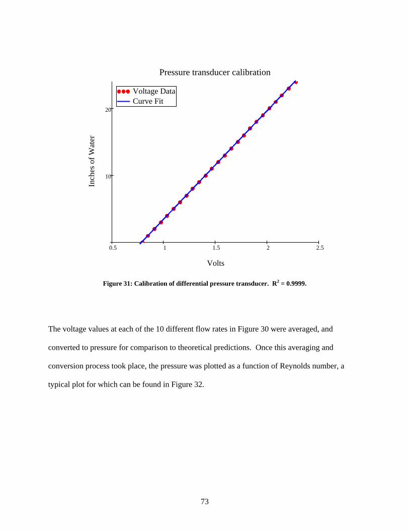
0.5 1 1.5 2 2.5
10
20
Voltage DataCurve Fit
Pressure transducer calibration
Volts
Inch
es o
f Wat
er
Figure 31: Calibration of differential pressure transducer. R2 = 0.9999.
The voltage values at each of the 10 different flow rates in Figure 30 were averaged, and
converted to pressure for comparison to theoretical predictions. Once this averaging and
conversion process took place, the pressure was plotted as a function of Reynolds number, a
typical plot for which can be found in Figure 32.
73

0 20 40 60 80 1000
1 103×
2 103×
Experimental Data
100 um Straight Duct
Reynolds Number
Stat
ic P
ress
ure
Dro
p (P
a)
Figure 32: Plot of experimental data as a function of Re.
For the sake of thoroughness, the form of the theoretical modified Bernoulli equations used for
comparison to this data can be found below for straight duct channels (Equation 19) and
channels with sudden expansions and contractions (Equation 20). The theoretical predictions
were plotted on the same graph with the experimental results to facilitate the comparison
between the two. See Figure 33 for a graphical representation of this comparison for a sample
straight duct.
p1 p2− ρ f⋅L
Dh⋅
V2
2⋅ Equation 19
74
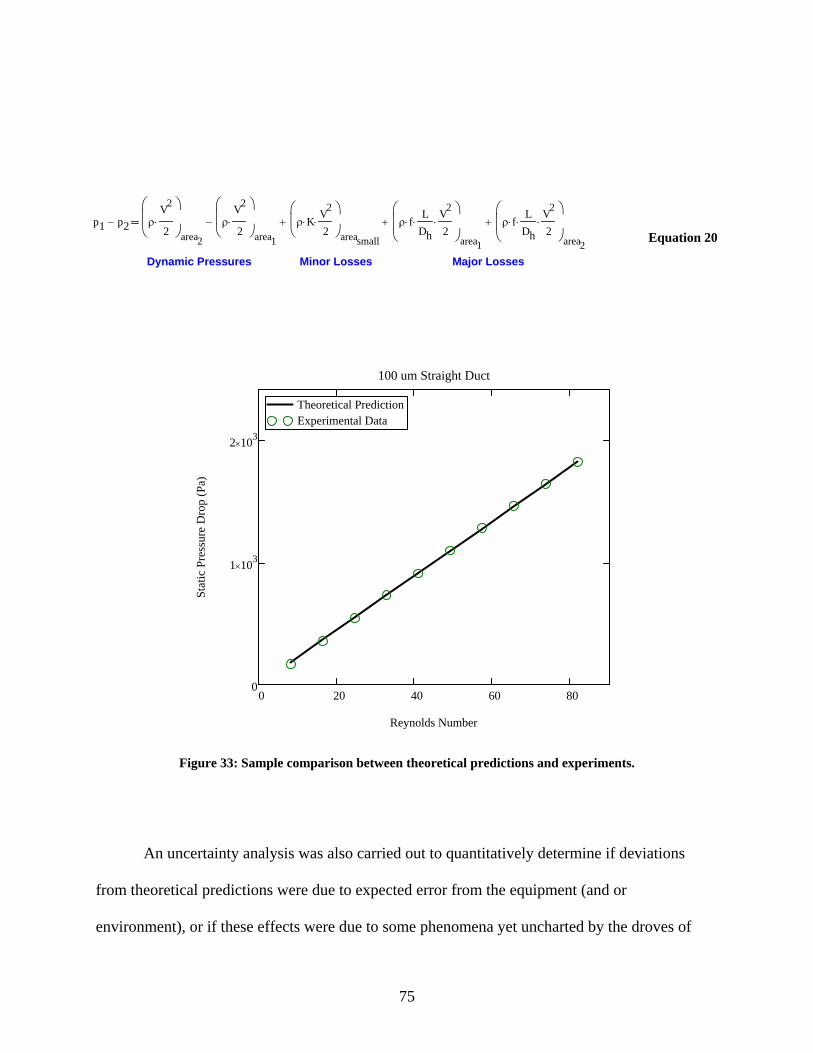
Equation 20
p1 p2− ρV2
2⋅
⎛⎜⎜⎝
⎞⎟⎟⎠area2
ρV2
2⋅
⎛⎜⎜⎝
⎞⎟⎟⎠area1
− ρ K⋅V2
2⋅
⎛⎜⎝
⎞⎟⎠areasmall
+ ρ f⋅L
Dh⋅
V2
2⋅
⎛⎜⎜⎝
⎞⎟⎟⎠area1
+ ρ f⋅L
Dh⋅
V2
2⋅
⎛⎜⎜⎝
⎞⎟⎟⎠area2
+
Dynamic Pressures Minor Losses Major Losses
0 20 40 60 800
1 103×
2 103×
Theoretical PredictionExperimental Data
100 um Straight Duct
Reynolds Number
Stat
ic P
ress
ure
Dro
p (P
a)
Figure 33: Sample comparison between theoretical predictions and experiments.
An uncertainty analysis was also carried out to quantitatively determine if deviations
from theoretical predictions were due to expected error from the equipment (and or
environment), or if these effects were due to some phenomena yet uncharted by the droves of
75
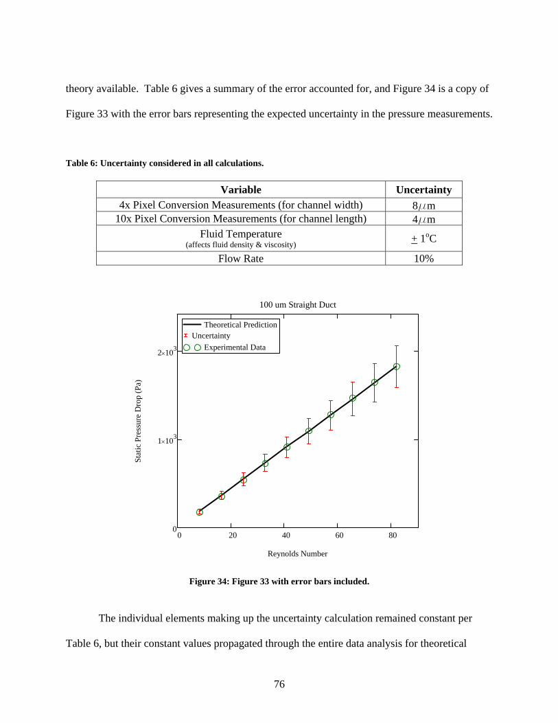
theory available. Table 6 gives a summary of the error accounted for, and Figure 34 is a copy of
Figure 33 with the error bars representing the expected uncertainty in the pressure measurements.
Table 6: Uncertainty considered in all calculations.
Variable Uncertainty 4x Pixel Conversion Measurements (for channel width) 8mm
10x Pixel Conversion Measurements (for channel length) 4mm Fluid Temperature
(affects fluid density & viscosity) + 1oC
Flow Rate 10%
0 20 40 60 800
1 103×
2 103×
Theoretical PredictionUncertainty
Experimental Data
100 um Straight Duct
Reynolds Number
Stat
ic P
ress
ure
Dro
p (P
a)
Figure 34: Figure 33 with error bars included.
The individual elements making up the uncertainty calculation remained constant per
Table 6, but their constant values propagated through the entire data analysis for theoretical
76

predictions. As a result, greater error was seen for smaller sized channels because the
uncertainty in distance measurements of the channel geometry made up a greater percentage of
the overall channel size. Conversely, larger channels exhibited a lower range of uncertainty due
to this scaling relation. That being the case, uncertainty ranged from about 8% for larger
channels to as much as 19% for smaller channels. The error bars will be present in all future
figures of experimental and theoretical comparisons.
Explanations for Deviations from Theoretical Predictions
At this point, it is appropriate to discuss the fidelity of the data obtained from the 300+
experiments conducted. One of the first questions that came up during testing in observation of
the many graphs (such as Figure 30) was “How do I know if I’ve got a good test?” The answer
to that question is undoubtedly, “Every test is a good test,” because more information is obtained
about the channels, equipment, and set-up process with each test allowing for any improvements
to be implemented into one (or multiple) of the critical components that make up thsese
experiments. The question of whether or not the integrity of flow thorough the channel was
maintained at desirable conditions was the more pointed (though also more difficult) question
that demanded a response, but this also proved to be answerable once enough data was extracted
and analyzed. A brief account of these error indicators will be presented at this point.
The first trend that revealed itself was the tracking of measured pressure values that fell
below that of what macroscale theory predicted. As with any trend that deviated from theoretical
predictions, it was initially hypothesized that this represented a phenomena of microfluidics that
supported findings from other researchers, the notion that flow at these size domains should be
77
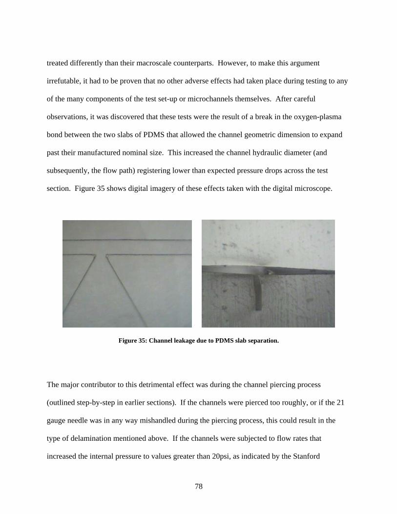
treated differently than their macroscale counterparts. However, to make this argument
irrefutable, it had to be proven that no other adverse effects had taken place during testing to any
of the many components of the test set-up or microchannels themselves. After careful
observations, it was discovered that these tests were the result of a break in the oxygen-plasma
bond between the two slabs of PDMS that allowed the channel geometric dimension to expand
past their manufactured nominal size. This increased the channel hydraulic diameter (and
subsequently, the flow path) registering lower than expected pressure drops across the test
section. Figure 35 shows digital imagery of these effects taken with the digital microscope.
Figure 35: Channel leakage due to PDMS slab separation.
The major contributor to this detrimental effect was during the channel piercing process
(outlined step-by-step in earlier sections). If the channels were pierced too roughly, or if the 21
gauge needle was in any way mishandled during the piercing process, this could result in the
type of delamination mentioned above. If the channels were subjected to flow rates that
increased the internal pressure to values greater than 20psi, as indicated by the Stanford
78

Microfluidics Foundry supplier, the channels would also be at risk of rupturing. The importance
of technique when piercing these channels became a critical element during preparation and
readiness processes prior to testing, and after improvements were made to this process, no further
rupturing was experienced. Figure 36 gives a graphical depiction of a sample data set (with its
theoretical prediction without any channel ruptures) of how this error manifested itself in the
experiments. It can be seen from the figure that this type of error falls much lower than the
calculated uncertainty deems allowable. Unfortunately, once a channel is believed to be
ruptured, it cannot be repaired without tedious and time consuming methods, and is unusable in
future experiments.
0 20 40 60 80 1000
1 103×
2 103×
3 103×
4 103× Theoretical Prediction
Experimental DataUncertainty
Expansion (AR = 0.70)
Reynolds Number
Stat
ic P
ress
ure
Dro
p (P
a)
Figure 36: Data trend due to channel rupture compared to theoretical predictions.
79

Another type of error that produced a result quite contrary in behavior to the separation
issue described above, though proved to be just as disadvantageous, was found in tests that
contained measured pressures much greater than that of macroscale theoretical predictions.
Once again, these measurements were thought to contain the presence of phenomena
unconsidered by macroscale fluid mechanics and unique to flow only at the microscale. What is
more is that this type of trend appeared more frequently at smaller scales than at larger ones,
further supporting this notion of microscale effects occurring at smaller scales (and presenting a
possible channel size transition region). However, these results underwent even greater scrutiny
than the separation issue in order to verify that this effect wasn’t a result of some defective
characteristic of the set-up and experimentation procedure, as they were closely matched to the
trends reported by researchers claiming that flow behavior deviated from macroscale theory at
small scales. After rigorous analysis and experimentation, it was found that bubbles were
present in the test sections of channels exhibiting these deviating results. This caution is present
in a fair amount of the microfluidics literature on flow through microchannels, as well as micro
fabrication literature. Due to the high surface to volume ratio of these small channels, capillary
forces and surface tension are extremely high. If a bubble gets lodged in the channel and adheres
to the channel wall due to this higher than normal surface tension effect, it would produce an
undesirable (or additional) feature for the flow to pass over (similar to a nozzle/diffuser
combination), thus producing higher than expected pressure losses when measured. Figure 37 is
the digital image of a bubble just prior to the low pressure port in one of the microchannel test
sections.
80
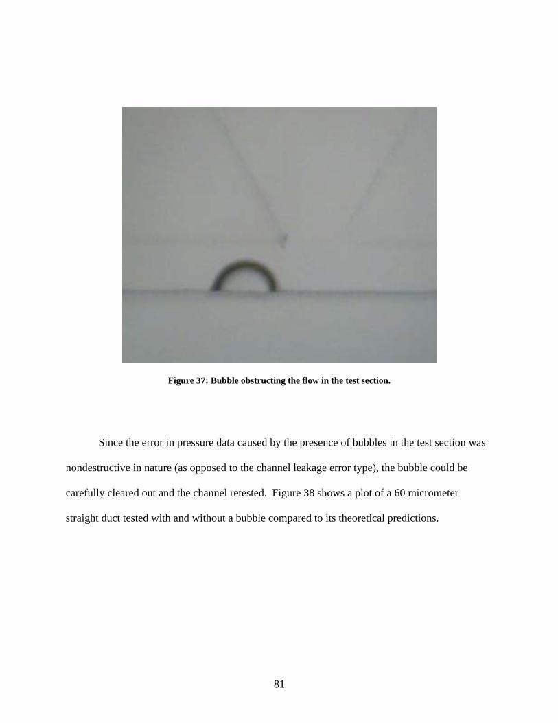
Figure 37: Bubble obstructing the flow in the test section.
Since the error in pressure data caused by the presence of bubbles in the test section was
nondestructive in nature (as opposed to the channel leakage error type), the bubble could be
carefully cleared out and the channel retested. Figure 38 shows a plot of a 60 micrometer
straight duct tested with and without a bubble compared to its theoretical predictions.
81
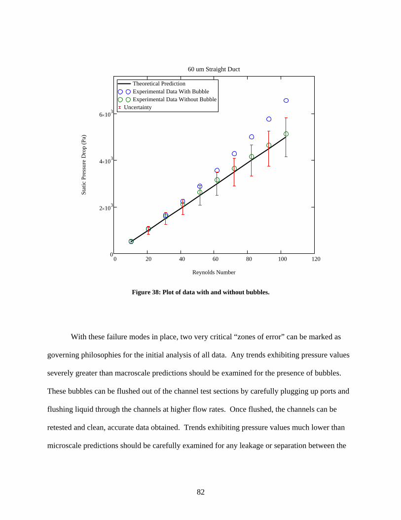
0 20 40 60 80 100 1200
2 103×
4 103×
6 103×
Theoretical PredictionExperimental Data With BubbleExperimental Data Without Bubble
Uncertainty
60 um Straight Duct
Reynolds Number
Stat
ic P
ress
ure
Dro
p (P
a)
Figure 38: Plot of data with and without bubbles.
With these failure modes in place, two very critical “zones of error” can be marked as
governing philosophies for the initial analysis of all data. Any trends exhibiting pressure values
severely greater than macroscale predictions should be examined for the presence of bubbles.
These bubbles can be flushed out of the channel test sections by carefully plugging up ports and
flushing liquid through the channels at higher flow rates. Once flushed, the channels can be
retested and clean, accurate data obtained. Trends exhibiting pressure values much lower than
microscale predictions should be carefully examined for any leakage or separation between the
82
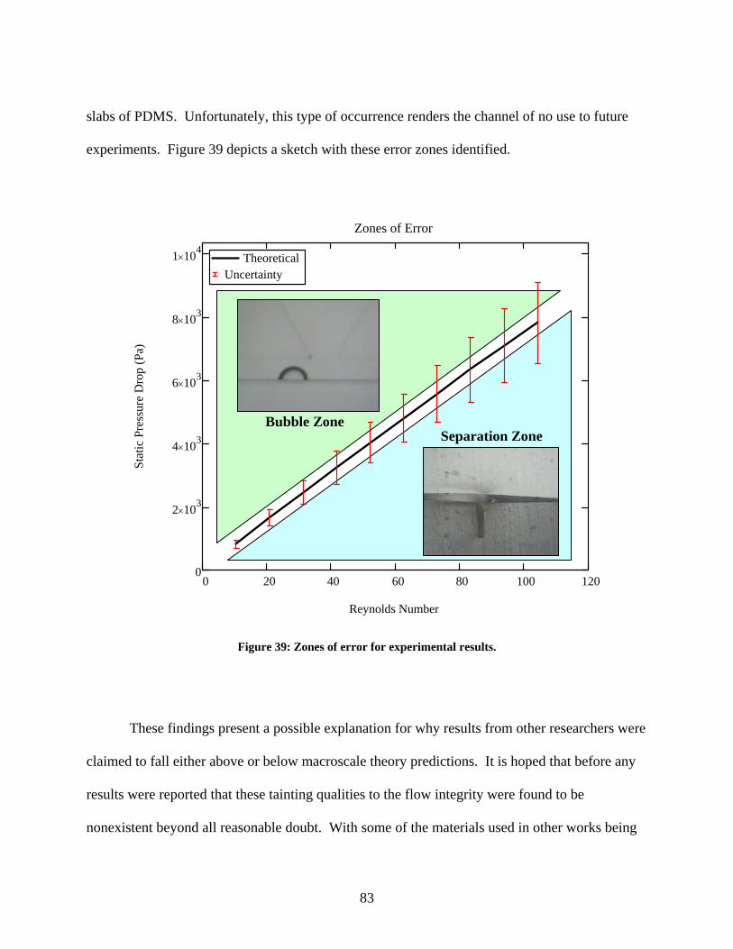
slabs of PDMS. Unfortunately, this type of occurrence renders the channel of no use to future
experiments. Figure 39 depicts a sketch with these error zones identified.
Bubble Zone Separation Zone
0 20 40 60 80 100 1200
2 103×
4 103×
6 103×
8 103×
1 104× Theoretical
Uncertainty
Zones of Error
Reynolds Number
Stat
ic P
ress
ure
Dro
p (P
a)
Figure 39: Zones of error for experimental results.
These findings present a possible explanation for why results from other researchers were
claimed to fall either above or below macroscale theory predictions. It is hoped that before any
results were reported that these tainting qualities to the flow integrity were found to be
nonexistent beyond all reasonable doubt. With some of the materials used in other works being
83
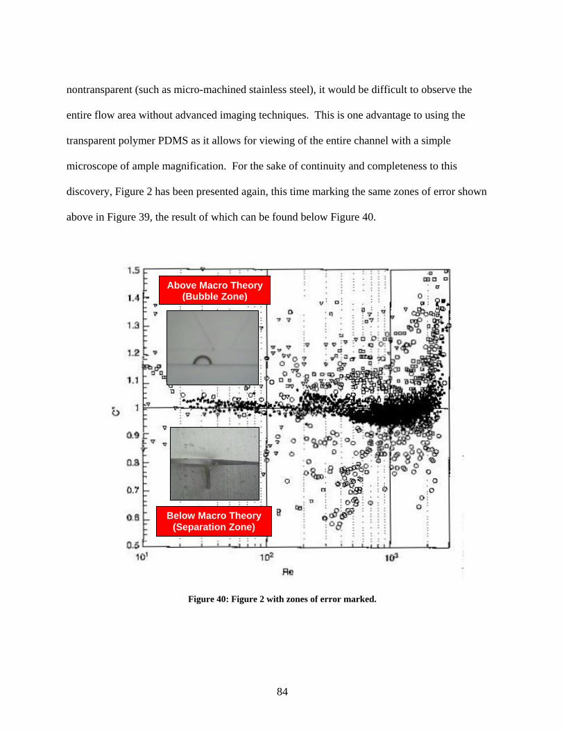
nontransparent (such as micro-machined stainless steel), it would be difficult to observe the
entire flow area without advanced imaging techniques. This is one advantage to using the
transparent polymer PDMS as it allows for viewing of the entire channel with a simple
microscope of ample magnification. For the sake of continuity and completeness to this
discovery, Figure 2 has been presented again, this time marking the same zones of error shown
above in Figure 39, the result of which can be found below Figure 40.
Above Macro Theory (Bubble Zone)
Below Macro Theory (Separation Zone)
Figure 40: Figure 2 with zones of error marked.
84

Straight Duct Comparisons and Discussion
It is fitting at this point to display some sample results from the copious tests conducted
over the duration of this work. The first few plots that will be displayed are for straight ducts
tested at various channel widths (50 to 130 micrometers). Any necessary discussion will follow
directly after display of the figures, so ample observation on behalf of the reader can be made
during the discussion that follows. All plots shown will include points from every valid data set
converted to pressure (and discarding any sets in error as described above) combined with the
averaged theoretical prediction for the given channel size under analysis (based on measurements
of actual channel geometry). The black line will represent this averaged theoretical prediction,
and the green circles will represent actual data points measured. The vertical red error bars
indicate the calculated uncertainty.
Equation 19 was used as the macroscale flow predictor for all straight duct data
comparison (reprinted below).
p1 p2− ρ f⋅L
Dh⋅
V2
2⋅ Equation 19
85
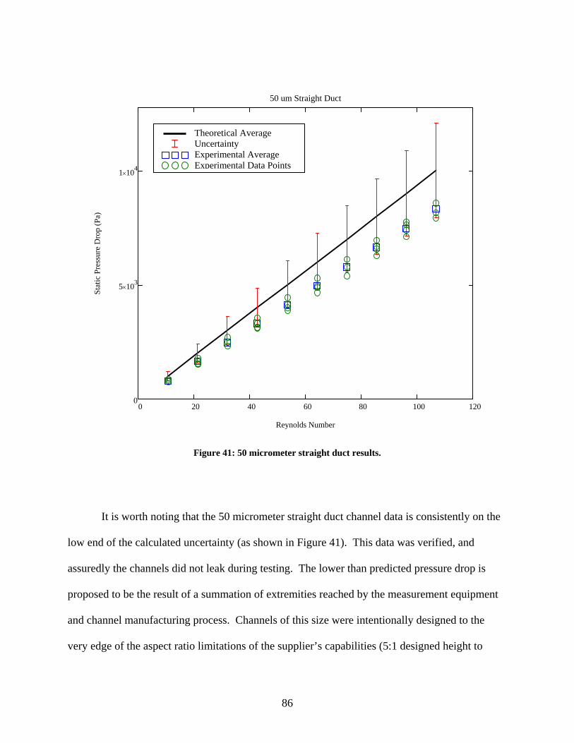
0 20 40 60 80 100 1200
5 103×
1 104×
50 um Straight Duct
Reynolds Number
Stat
ic P
ress
ure
Dro
p (P
a)
Theoretical Average Uncertainty Experimental Average Experimental Data Points
Figure 41: 50 micrometer straight duct results.
It is worth noting that the 50 micrometer straight duct channel data is consistently on the
low end of the calculated uncertainty (as shown in Figure 41). This data was verified, and
assuredly the channels did not leak during testing. The lower than predicted pressure drop is
proposed to be the result of a summation of extremities reached by the measurement equipment
and channel manufacturing process. Channels of this size were intentionally designed to the
very edge of the aspect ratio limitations of the supplier’s capabilities (5:1 designed height to
86
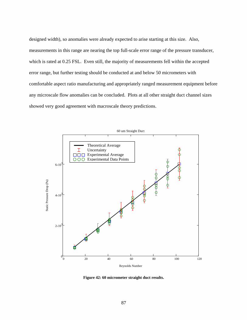
designed width), so anomalies were already expected to arise starting at this size. Also,
measurements in this range are nearing the top full-scale error range of the pressure transducer,
which is rated at 0.25 FSL. Even still, the majority of measurements fell within the accepted
error range, but further testing should be conducted at and below 50 micrometers with
comfortable aspect ratio manufacturing and appropriately ranged measurement equipment before
any microscale flow anomalies can be concluded. Plots at all other straight duct channel sizes
showed very good agreement with macroscale theory predictions.
0 20 40 60 80 100 1200
2 103×
4 103×
6 103×
60 um Straight Duct
Reynolds Number
Stat
ic P
ress
ure
Dro
p (P
a)
Theoretical Average Uncertainty Experimental Average Experimental Data Points
Figure 42: 60 micrometer straight duct results.
87
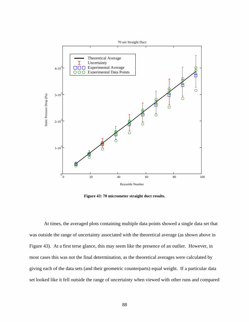
0 20 40 60 80 1000
1 103×
2 103×
3 103×
4 103×
70 um Straight Duct
Reynolds Number
Stat
ic P
ress
ure
Dro
p (P
a)
Theoretical Average Uncertainty Experimental Average Experimental Data Points
Figure 43: 70 micrometer straight duct results.
At times, the averaged plots containing multiple data points showed a single data set that
was outside the range of uncertainty associated with the theoretical average (as shown above in
Figure 43). At a first terse glance, this may seem like the presence of an outlier. However, in
most cases this was not the final determination, as the theoretical averages were calculated by
giving each of the data sets (and their geometric counterparts) equal weight. If a particular data
set looked like it fell outside the range of uncertainty when viewed with other runs and compared
88
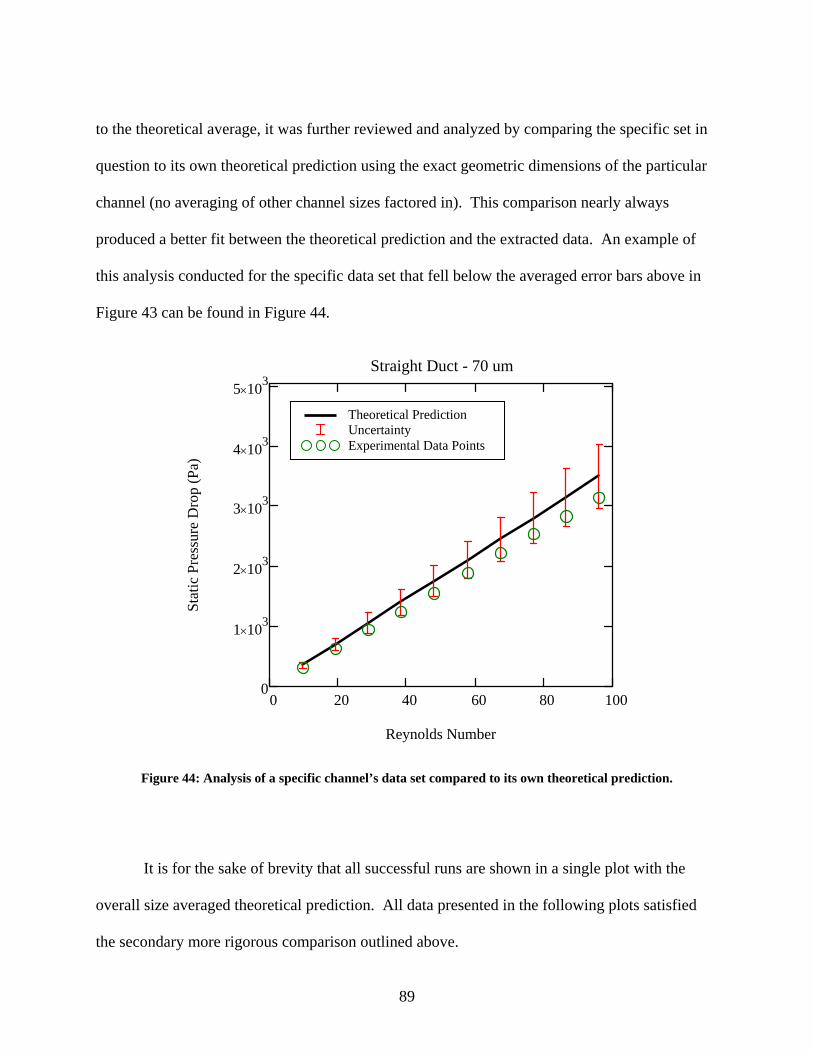
to the theoretical average, it was further reviewed and analyzed by comparing the specific set in
question to its own theoretical prediction using the exact geometric dimensions of the particular
channel (no averaging of other channel sizes factored in). This comparison nearly always
produced a better fit between the theoretical prediction and the extracted data. An example of
this analysis conducted for the specific data set that fell below the averaged error bars above in
Figure 43 can be found in Figure 44.
0 20 40 60 80 1000
1 103×
2 103×
3 103×
4 103×
5 103×
Straight Duct - 70 um
Reynolds Number
Stat
ic P
ress
ure
Dro
p (P
a)
Theoretical Prediction Uncertainty Experimental Data Points
Figure 44: Analysis of a specific channel’s data set compared to its own theoretical prediction.
It is for the sake of brevity that all successful runs are shown in a single plot with the
overall size averaged theoretical prediction. All data presented in the following plots satisfied
the secondary more rigorous comparison outlined above.
89
It can be seen from the figures that macroscale theoretical predictions accurately model
fluid flow for the sample of straight duct microchannels tested within the range of uncertainty.
Additional averaged plots for straight duct comparisons can be found in Appendix A.
Sudden Expansion Comparisons and Discussion
Next, sample plots of the tests conducted with area reduction features in the expansion
flow configuration will be presented, with appropriate discussion as needed. Equation 20 was
used as the macroscale theory predictor, with Ke values given by the relation outlined Equation
15 (and Figure 7).
Eq
Equation 15
p1 p2− ρV2
2⋅
⎛⎜⎜⎝
⎞⎟⎟⎠area2
ρV2
2⋅
⎛⎜⎜⎝
⎞⎟⎟⎠area1
− ρ K⋅V2
2⋅
⎛⎜⎝
⎞⎟⎠areasmall
+ ρ f⋅L
Dh⋅
V2
2⋅
⎛⎜⎜⎝
⎞⎟⎟⎠area1
+ ρ f⋅L
Dh⋅
V2
2⋅
⎛⎜⎜⎝
⎞⎟⎟⎠area2
+
Dynamic Pressures Minor Losses Major Losses
uation 20
Ke 1 AR−( )2=
90

0 20 40 60 80 100 1200
5 103×
1 104×
Expansion (AR = 0.4)
Reynolds Number
Stat
ic P
ress
ure
Dro
p (P
a)
Theoretical Average Uncertainty Experimental Average Experimental Data Points
Figure 45: Expansion results for area ratio of 0.4.
Similar phenomena to the higher predictions by theory at the smallest size for straight
ducts (50 micrometers) can bee seen for the sudden expansion from 50 micrometers to 130
micrometers (AR ~ 0.4), though not as extreme. This is thought to be for the same reasons
proposed earlier for straight duct comparisons, though included in these reasons should be the
rounding effects seen in the expansion feature (refer to Figure 19) for aspect ratio’s that are at (or
very close) to the limitations of the fabrication process (5:1). All other area ratios for sudden
expansion show excellent agreement with macroscale theoretical predictions.
91
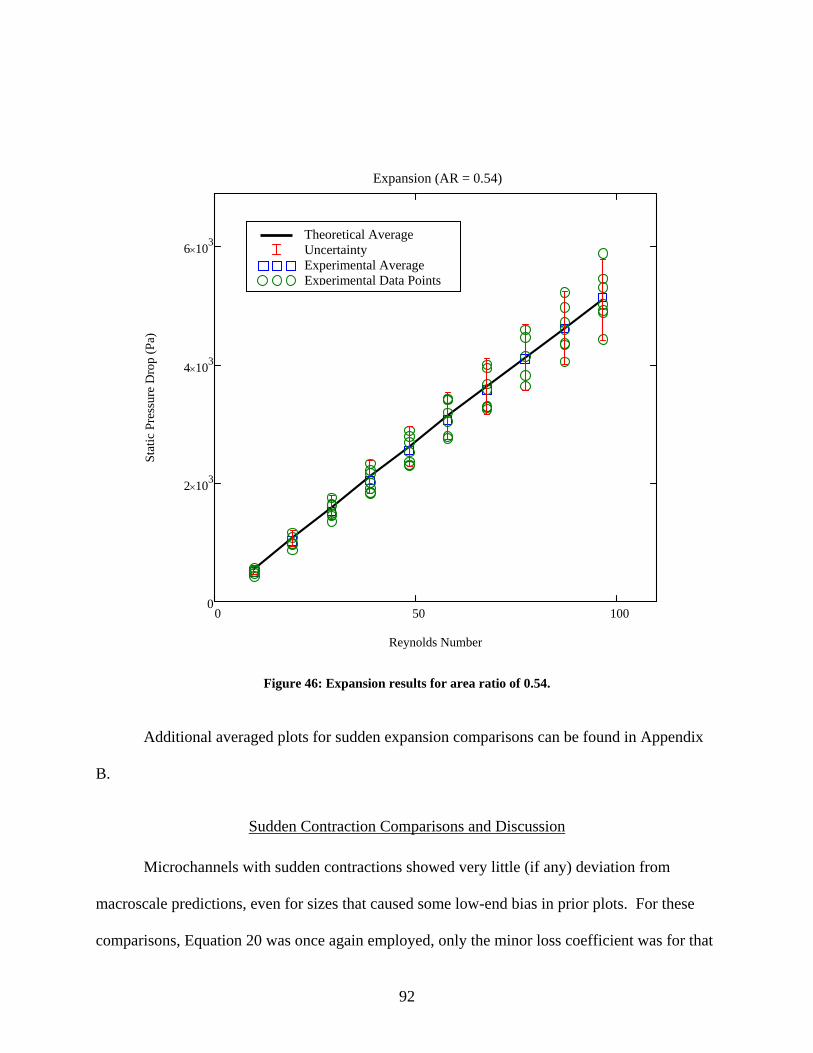
0 50 1000
2 103×
4 103×
6 103×
Expansion (AR = 0.54)
Reynolds Number
Stat
ic P
ress
ure
Dro
p (P
a)
Theoretical Average Uncertainty Experimental Average Experimental Data Points
Figure 46: Expansion results for area ratio of 0.54.
Additional averaged plots for sudden expansion comparisons can be found in Appendix
B.
Sudden Contraction Comparisons and Discussion
Microchannels with sudden contractions showed very little (if any) deviation from
macroscale predictions, even for sizes that caused some low-end bias in prior plots. For these
comparisons, Equation 20 was once again employed, only the minor loss coefficient was for that
92
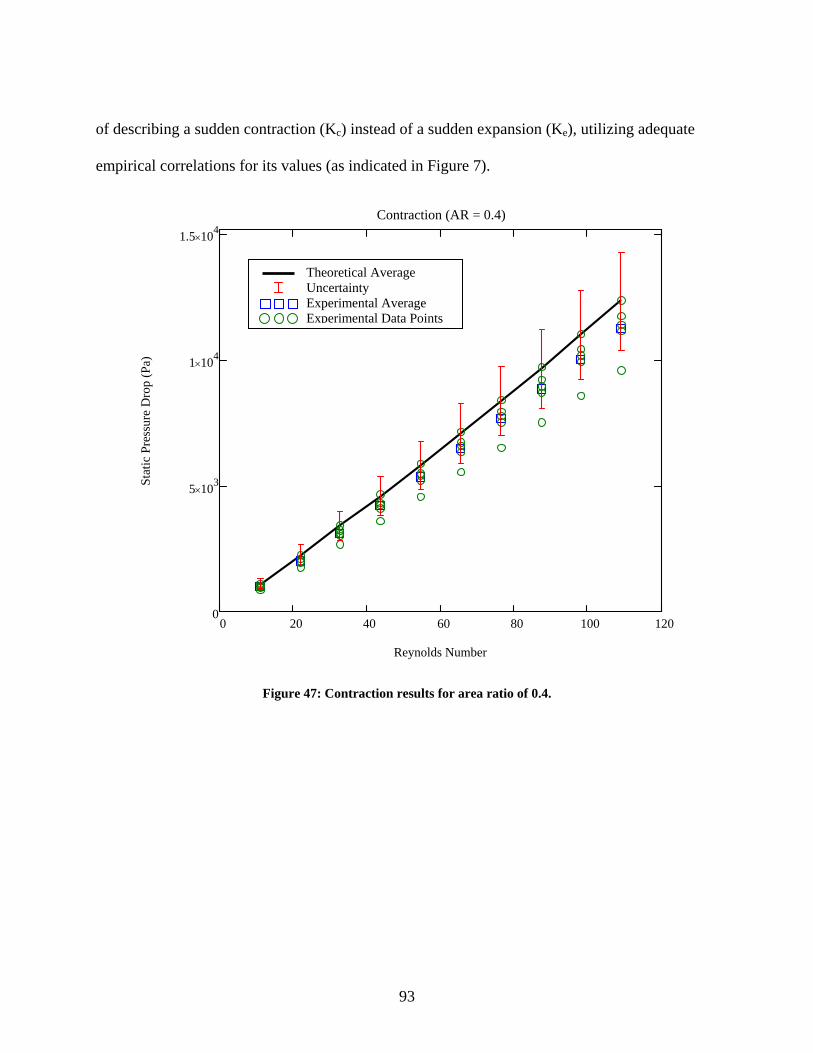
of describing a sudden contraction (Kc) instead of a sudden expansion (Ke), utilizing adequate
empirical correlations for its values (as indicated in Figure 7).
0 20 40 60 80 100 1200
5 103×
1 104×
1.5 104×
Contraction (AR = 0.4)
Reynolds Number
Stat
ic P
ress
ure
Dro
p (P
a)
Theoretical Average Uncertainty Experimental Average Experimental Data Points
Figure 47: Contraction results for area ratio of 0.4.
93

0 20 40 60 80 1000
1 103×
2 103×
3 103×
4 103×
Contraction (AR = 0.7)
Reynolds Number
Stat
ic P
ress
ure
Dro
p (P
a)
Theoretical Average Uncertainty Experimental Average Experimental Data Points
Figure 48: Contraction results for area ratio of 0.7.
Additional averaged plots for sudden contraction comparisons can be found in Appendix
C.
94

Additional Considerations
Even though the channels contained anomalies mentioned before as a result of the
fabrication process (rounded corners of area reduction feature, etc.), the flow through these
channels were still predicted accurately by macroscale relations. It can be surmised, then, that
the head loss experienced as a result of flow through these microchannels is due largely to the
major head losses (usually more than 90% of total head loss), hence the designation of “major,”
while the minor head losses usually accounted for much less (less than 10%) of the total head
loss. This was later verified by some simple calculations to be accurate. For the simple
geometry tested in this work, the expansion/contraction minor losses can almost be neglected
from the flow model calculations without losing too much fidelity in the pressure drop results.
This effect was also verified by some simple manipulations of the data. It is not recommended
that analysts or researchers neglect any term in their loss calculations, however, (especially at
these small scales) unless it significantly decreases the complexity of a flow model and its
impact to the accuracy of the final solution is well understood. Please refer to Appendices A, B,
and C for additional plots comparing macroscale predictions to experimental data.
95
CHAPTER FIVE: CONCLUSIONS
Given the controversial undertones in the field of microfluidics research, it was desired to
provide a robust behavioral analysis of pressure drop experienced by liquid flow through
simplified features, as most microfluidics research aims at analyzing broad systems containing
numerous complex flow geometries and system components. Microchannels ranging in size
from 50 microns to 130 microns were chosen that exhibited straight duct geometries (for
replication of prior work), as well as sudden expansions and contractions in flow geometry due
to the gaping chasm of research conducted on channels with these features.
Microchannels were designed and cast in the low cost, durable polymer PDMS and
irreversibly sealed to another blank slab of PDMS by bonding techniques that utilized oxygen-
plasma treatment, thereby allowing the microchannels to withstand internal pressures up to
20psi. This oxygen-plasma treatment deposited a thin coating on the microchannel walls,
providing a hydrophilic film that permitted ample wetting of the channel surfaces by the test
fluid. Over 300 experiments were conducted on the two PDMS chips (each containing 99
different channels) using a reliable test philosophy developed primarily by Hansel [19], with
improved techniques developed during the channel piercing process. Pressure measurements
were extracted and compared to theoretical predictions using accepted macroscale fluid
mechanics in the form of Bernoulli’s equations modified to account for major and minor head
losses.
Given the surmounting evidence provided in this work, it can be concluded that
macroscale theory predictions for uniform, steady, incompressible, internal flow through straight
96

ducts, as well as ducts with sudden area expansions/reductions serve as an accurate model for the
flow behavior, with additional correlations and correction factors to account for microscale
anomalies being unnecessary. These results have been validated for square shaped channel
profiles with widths ranging from 50 microns to 130 microns, area ratios ranging from 0.4 to 1.0,
with a channel height of 104 microns by this work. The flow regime was laminar, and remained
in the Re = 7 to Re = 130 domain. The importance of precision technique when piercing the
entrance, exit, and high/low pressure ports was discovered to be extremely vital in the successful
testing of microchannels cast in PDMS. Processes described herein will hopefully guide future
microfluidics research efforts when microchannels fabricated using this material are tested.
Furthermore, anomalies experienced by other researchers within this size and Reynolds number
range were most likely due to any number of error variables (or combination thereof) induced
into the analysis in the form of fabrication limitations, test set-up, channel design, equipment
selection, and overall experimentation philosophies. The two most prevalent failure modes
uncovered in this work were the presence of bubbles in the channel test section, witch caused the
pressure drop data to fall above that of macroscale theory predictions, and separation between
the PDMS slabs around the microchannels due to rough handling or unsatisfactory technique
when piercing channels, which caused the data to track lower than macroscale theory
predictions.
It is recommended that supplementary research be conducted to further isolate the
expansion/contraction feature, as flow effects analyzed in this work were predominately
governed by the major loss (friction factor) term. It is also strongly advised that reliable
manufacturing techniques be employed to fabricate channels smaller than 50 micrometers in
width, and pressure losses measured using equipment with a suitable range. Finally, it is hoped
97

that no matter how convoluted or controversial a subject may become, researchers with a love for
discovery and the dissemination of findings remain at forefront of the conclave.
98
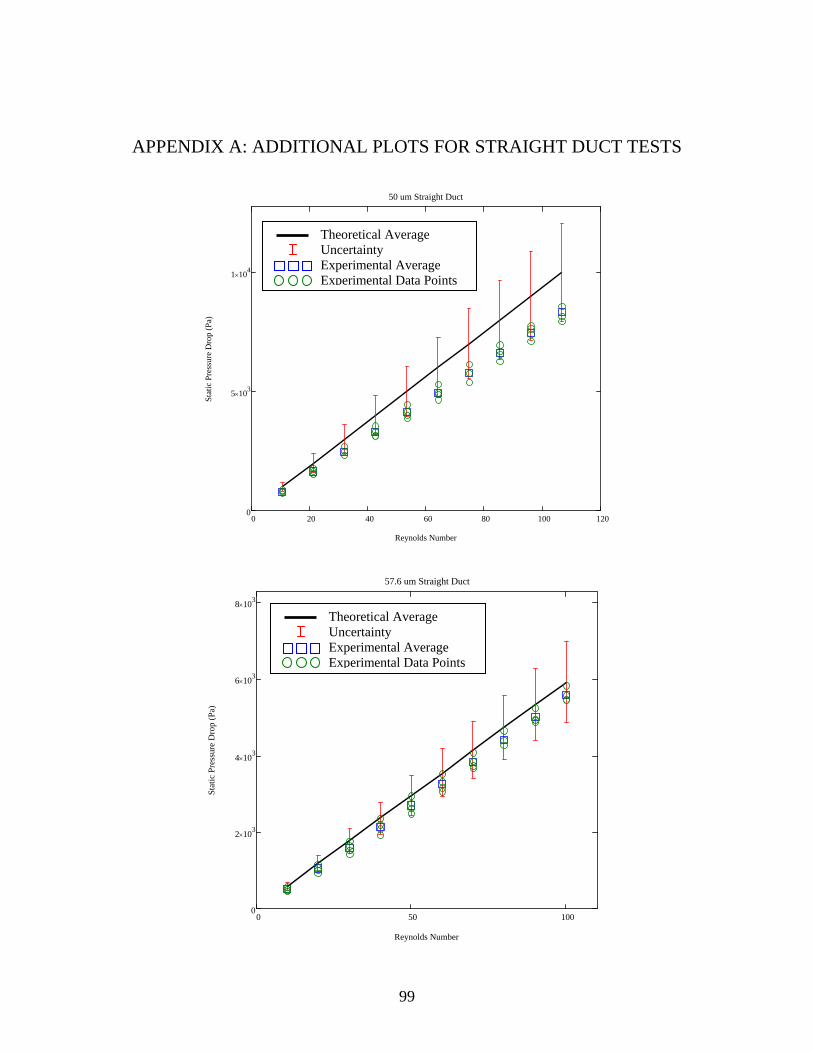
APPENDIX A: ADDITIONAL PLOTS FOR STRAIGHT DUCT TESTS
0 20 40 60 80 100 120
0
5 103×
1 104×
50 um Straight Duct
Reynolds Number
Stat
ic P
ress
ure
Dro
p (P
a)
Theoretical Average Uncertainty Experimental Average Experimental Data Points
0 50 1000
2 103×
4 103×
6 103×
8 103×
57.6 um Straight Duct
Reynolds Number
Stat
ic P
ress
ure
Dro
p (P
a)
Theoretical Average Uncertainty Experimental Average Experimental Data Points
99

0 20 40 60 80 100 1200
2 103×
4 103×
6 103×
60 um Straight Duct
Reynolds Number
Stat
ic P
ress
ure
Dro
p (P
a)Theoretical Average Uncertainty Experimental Average Experimental Data Points
0 20 40 60 80 1000
1 103×
2 103×
3 103×
4 103×
70 um Straight Duct
Reynolds Number
Stat
ic P
ress
ure
Dro
p (P
a)
Theoretical Average Uncertainty Experimental Average Experimental Data Points
100

0 20 40 60 80 100
0
1 103×
2 103×
90 um Straight Duct
Reynolds Number
Stat
ic P
ress
ure
Dro
p (P
a)
0 20 40 60 80 1000
1 103×
2 103×
3 103×
80 um Straight Duct
Reynolds Number
Stat
ic P
ress
ure
Dro
p (P
a)
Theoretical Average Uncertainty Experimental Average Experimental Data Points
Theoretical Average Uncertainty Experimental Average Experimental Data Points
101
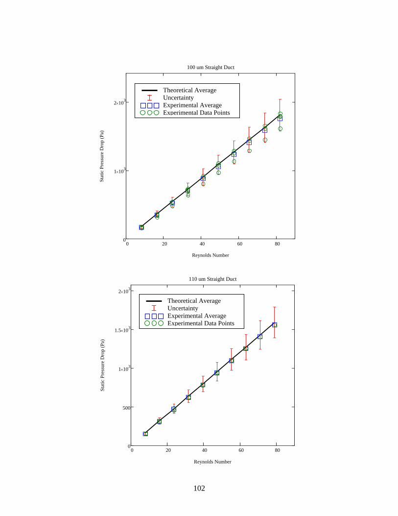
0 20 40 60 800
500
1 103×
1.5 103×
2 103×
110 um Straight Duct
Reynolds Number
Stat
ic P
ress
ure
Dro
p (P
a)
0 20 40 60 800
1 103×
2 103×
100 um Straight Duct
Reynolds Number
Stat
ic P
ress
ure
Dro
p (P
a)
Theoretical Average Uncertainty Experimental Average Experimental Data Points
Theoretical Average Uncertainty Experimental Average Experimental Data Points
102
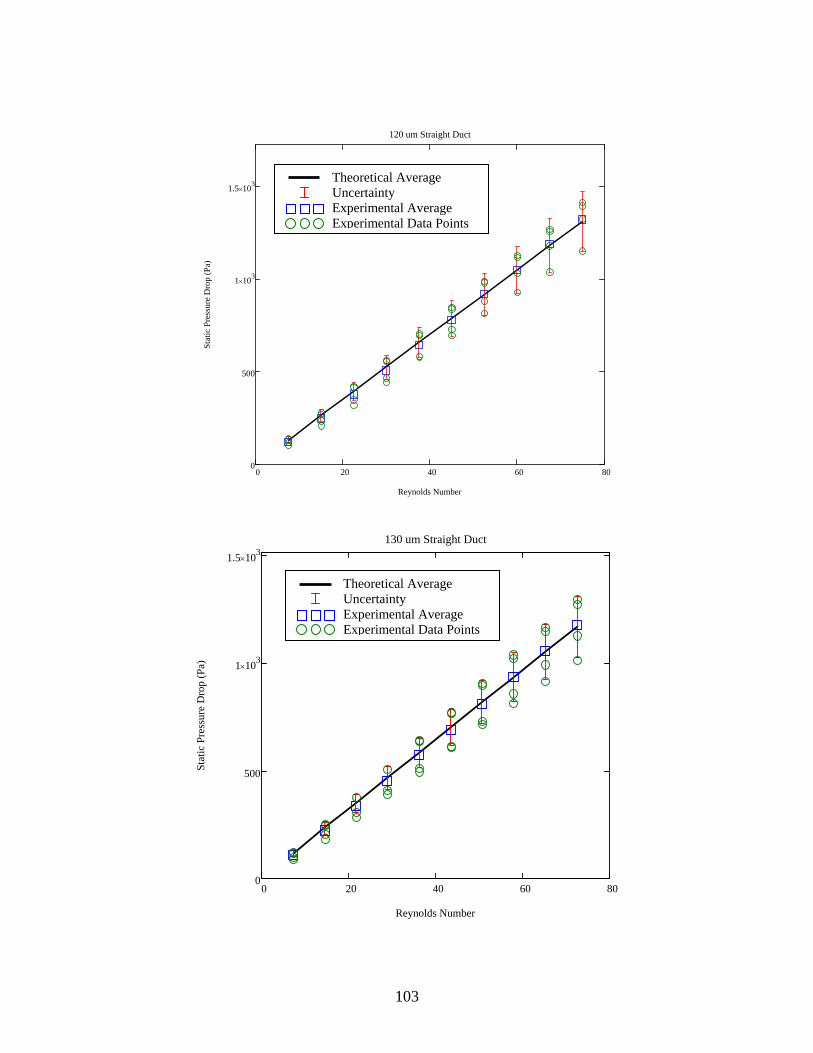
0 20 40 60 800
500
1 103×
1.5 103×
130 um Straight Duct
Reynolds Number
Stat
ic P
ress
ure
Dro
p (P
a)
0 20 40 60 800
500
1 103×
1.5 103×
120 um Straight Duct
Reynolds Number
Stat
ic P
ress
ure
Dro
p (P
a)
Theoretical Average Uncertainty Experimental Average Experimental Data Points
Theoretical Average Uncertainty Experimental Average Experimental Data Points
103
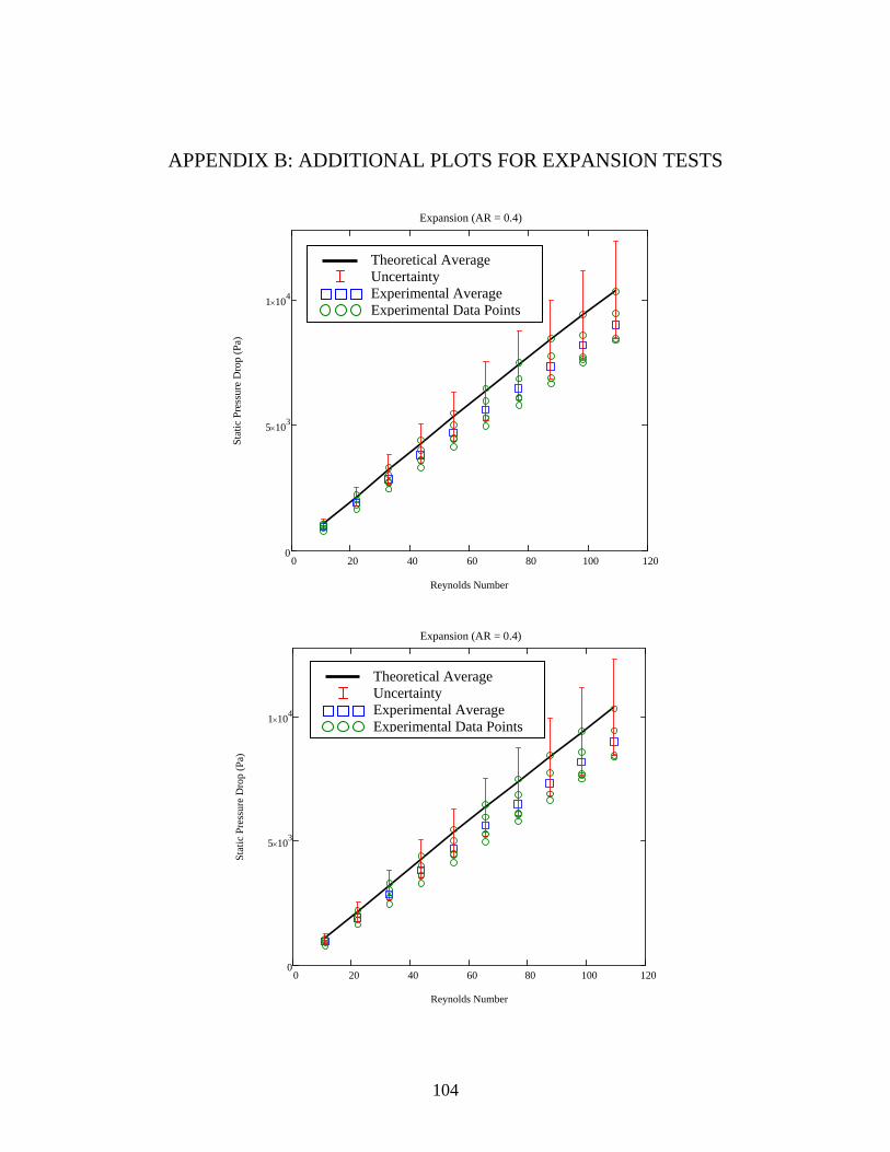
APPENDIX B: ADDITIONAL PLOTS FOR EXPANSION TESTS
0 20 40 60 80 100 1200
5 103×
1 104×
Expansion (AR = 0.4)
Reynolds Number
Stat
ic P
ress
ure
Dro
p (P
a)
0 20 40 60 80 100 1200
5 103×
1 104×
Expansion (AR = 0.4)
Theoretical Average Uncertainty Experimental Average Experimental Data Points
Reynolds Number
Stat
ic P
ress
ure
Dro
p (P
a)
Theoretical Average Uncertainty Experimental Average Experimental Data Points
104
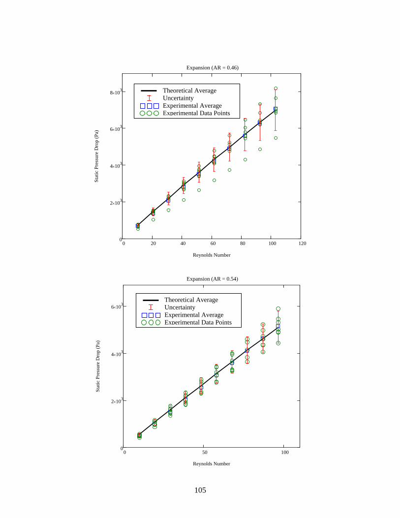
0 20 40 60 80 100 1200
2 103×
4 103×
6 103×
8 103×
Expansion (AR = 0.46)
Reynolds Number
Stat
ic P
ress
ure
Dro
p (P
a)Theoretical Average Uncertainty Experimental Average Experimental Data Points
0 50 1000
2 103×
4 103×
6 103×
Expansion (AR = 0.54)
Reynolds Number
Stat
ic P
ress
ure
Dro
p (P
a)
Theoretical Average Uncertainty Experimental Average Experimental Data Points
105
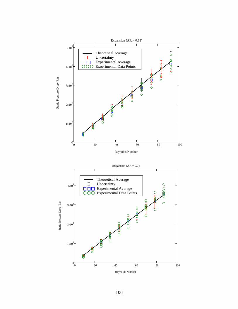
106
5 10×
0 20 40 60 80 1000
1 103×
2 103×
3 103×
4 103×
Expansion (AR = 0.7)
Reynolds Number
Stat
ic P
ress
ure
Dro
p (P
a)
0 20 40 60 80 1000
1 103×
2 103×
3 103×
4 103×
3
Expansion (AR = 0.62)
Theoretical Average Uncertainty Experimental Average Experimental Data Points
Reynolds Number
Stat
ic P
ress
ure
Dro
p (P
a)
Theoretical Average Uncertainty Experimental Average Experimental Data Points
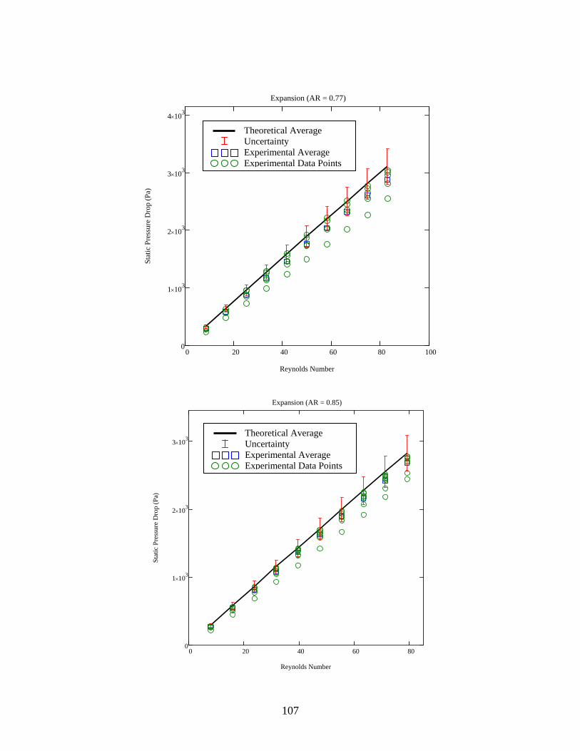
0 20 40 60 800
1 103×
2 103×
3 103×
Expansion (AR = 0.85)
Reynolds Number
Stat
ic P
ress
ure
Dro
p (P
a)
0 20 40 60 80
4 103×
1000
1 103×
2 103×
3 103×
Expansion (AR = 0.77)
Reynolds Number
Stat
ic P
ress
ure
Dro
p (P
a)
Theoretical Average Uncertainty Experimental Average Experimental Data Points
Theoretical Average Uncertainty Experimental Average Experimental Data Points
107
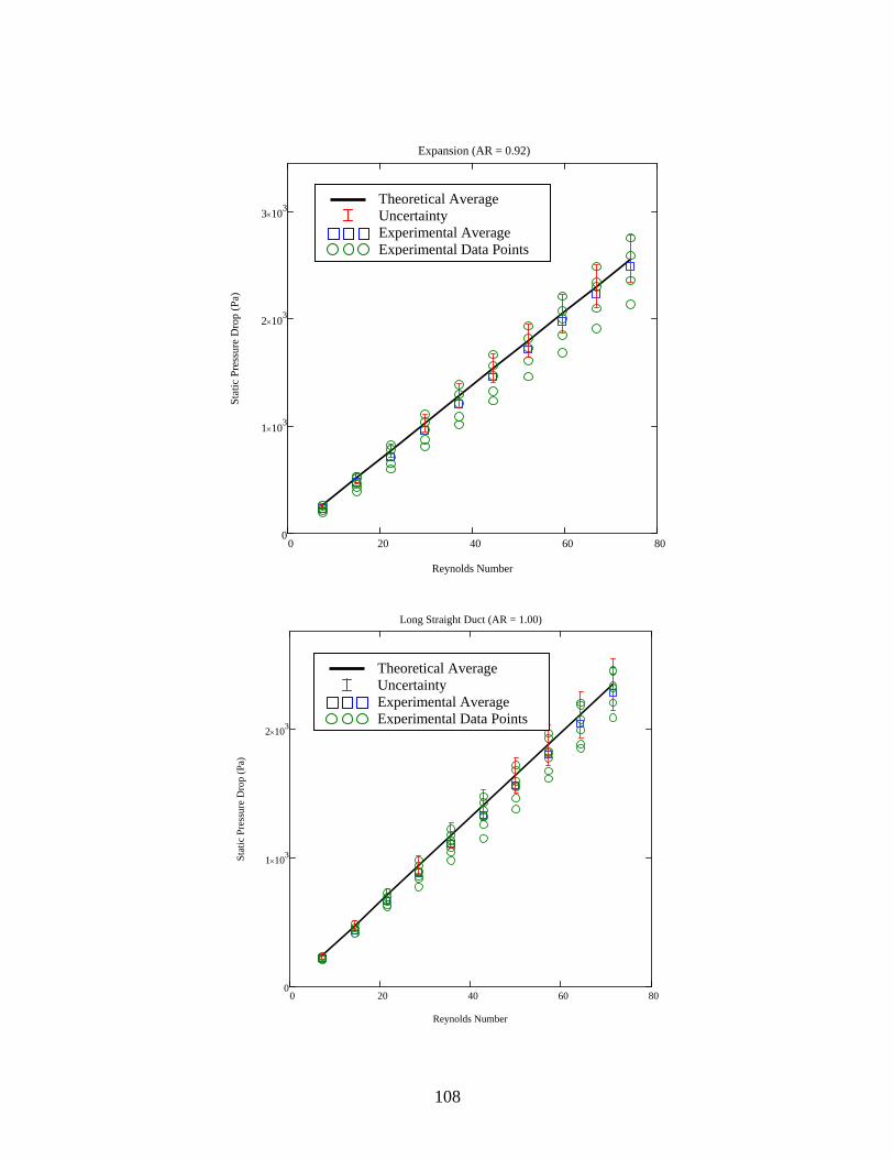
0 20 40 60 800
1 103×
2 103×
Long Straight Duct (AR = 1.00)
Reynolds Number
Stat
ic P
ress
ure
Dro
p (P
a)
0 20 40 60 800
1 103×
2 103×
3 103×
Expansion (AR = 0.92)
Reynolds Number
Stat
ic P
ress
ure
Dro
p (P
a)
Theoretical Average Uncertainty Experimental Average Experimental Data Points
Theoretical Average Uncertainty Experimental Average Experimental Data Points
108
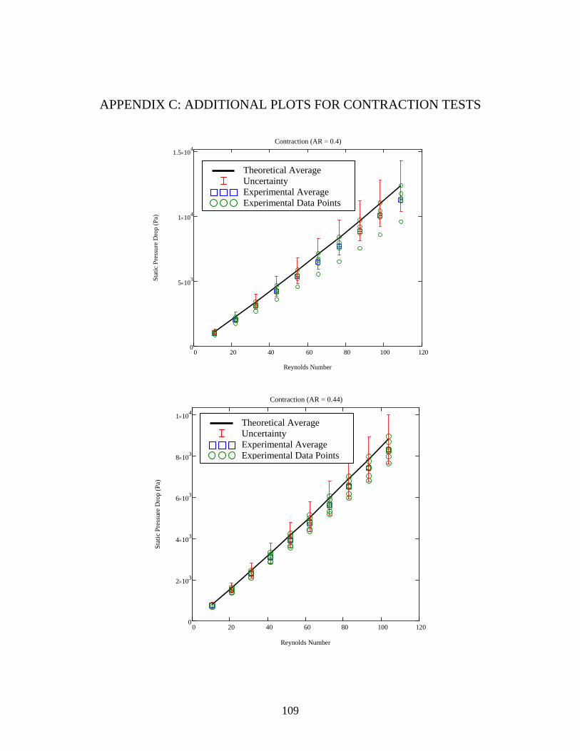
APPENDIX C: ADDITIONAL PLOTS FOR CONTRACTION TESTS
0 20 40 60 80 100 1200
2 103×
4 103×
6 103×
8 103×
1 104×
Contraction (AR = 0.44)
Reynolds Number
Stat
ic P
ress
ure
Dro
p (P
a)
0 20 40 60 80 100 1200
5 103×
1 104×
1.5 10×4
Contraction (AR = 0.4)
Theoretical Average Uncertainty Experimental Average Experimental Data Points
Reynolds Number
Stat
ic P
ress
ure
Dro
p (P
a)
Theoretical Average Uncertainty Experimental Average Experimental Data Points
109
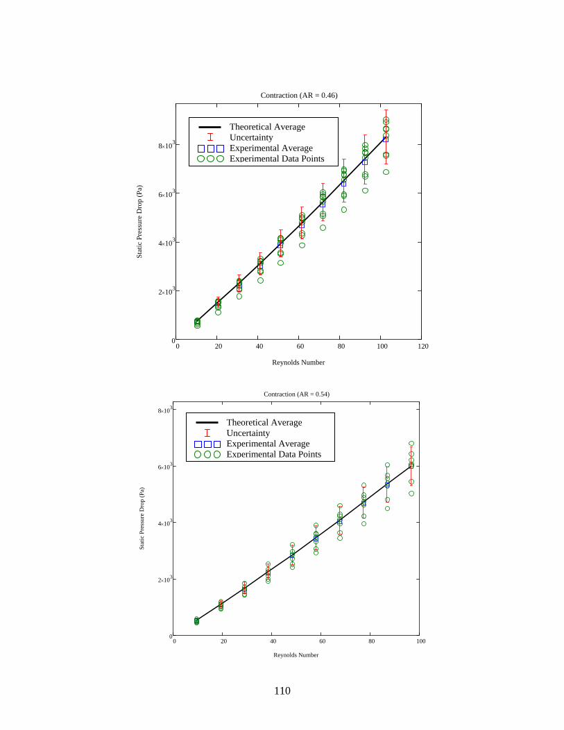
0 20 40 60 80 1000
2 103×
4 103×
6 103×
8 103×
Contraction (AR = 0.54)
Reynolds Number
Stat
ic P
ress
ure
Dro
p (P
a)
0 20 40 60 80 100 1200
2 103×
4 103×
6 103×
8 103×
Contraction (AR = 0.46)
Reynolds Number
Stat
ic P
ress
ure
Dro
p (P
a)Theoretical Average Uncertainty Experimental Average Experimental Data Points
Theoretical Average Uncertainty Experimental Average Experimental Data Points
110
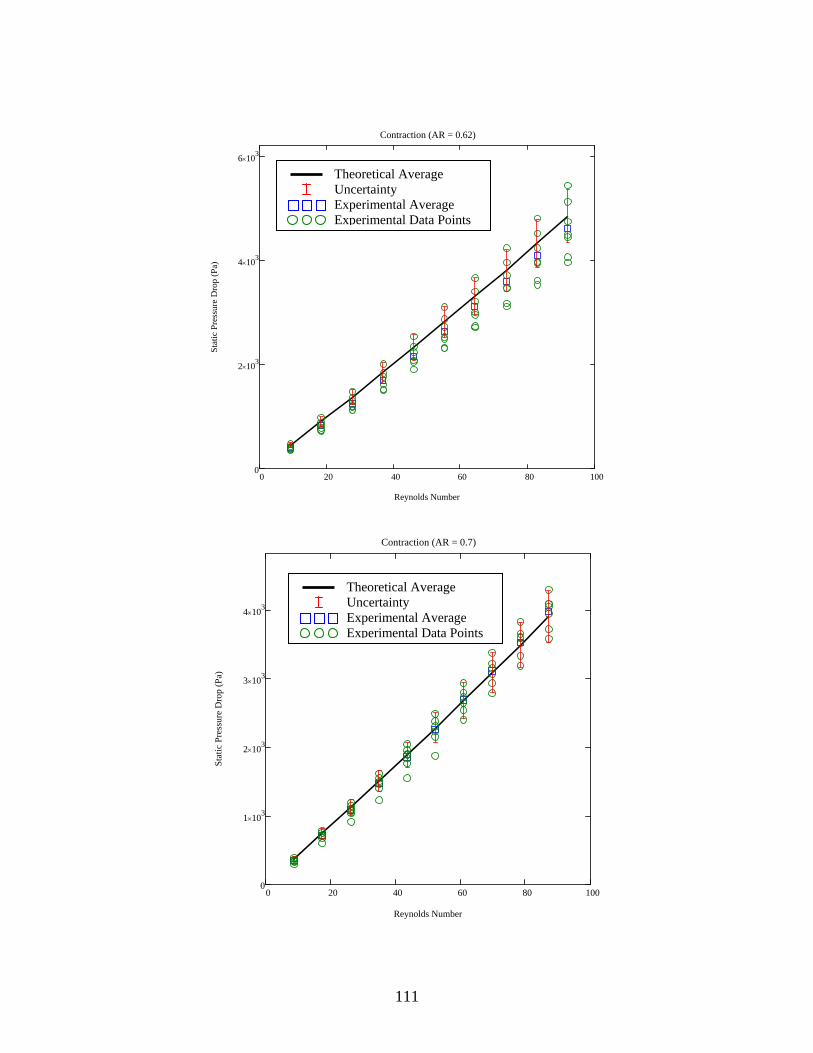
0 20 40 60 80 1000
1 103×
2 103×
3 103×
4 103×
Contraction (AR = 0.7)
Reynolds Number
Stat
ic P
ress
ure
Dro
p (P
a)
0 20 40 60 80
6 103×
1000
2 103×
4 103×
Contraction (AR = 0.62)
Reynolds Number
Stat
ic P
ress
ure
Dro
p (P
a)
Theoretical Average Uncertainty Experimental Average Experimental Data Points
Theoretical Average Uncertainty Experimental Average Experimental Data Points
111
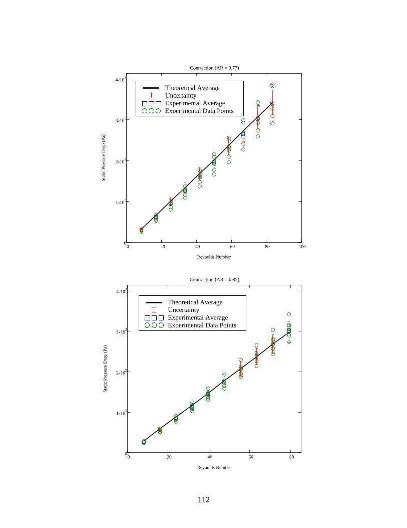
112
0 20 40 60 800
1 103×
2 103×
3 103×
4 103×
Contraction (AR = 0.85)
Reynolds Number
Stat
ic P
ress
ure
Dro
p (P
a)
0 20 40 60 80
4 103×
1000
1 103×
2 103×
3 103×
Contraction (AR = 0.77)
Reynolds Number
Stat
ic P
ress
ure
Dro
p (P
a)
Theoretical Average Uncertainty Experimental Average Experimental Data Points
Theoretical Average Uncertainty Experimental Average Experimental Data Points
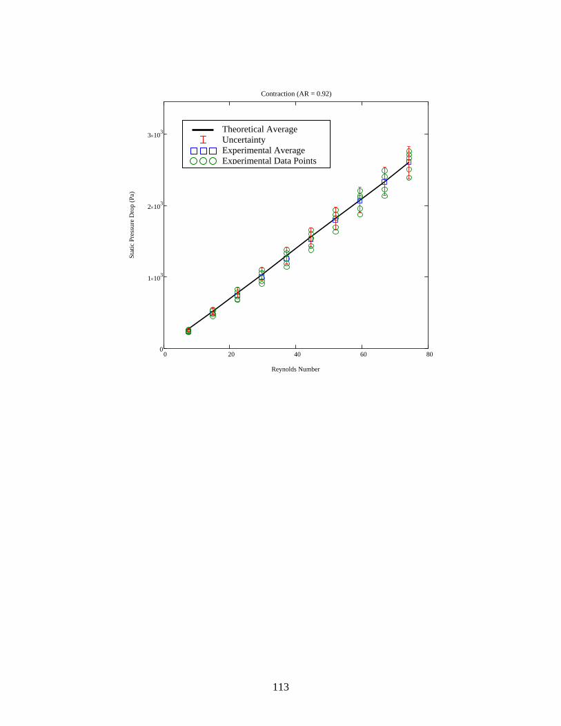
113
Contraction (AR = 0.92)
0 20 40 60 800
1 103×
2 103×
3 103×
Theoretical Average Uncertainty Experimental Average Experimental Data Points
Reynolds Number
Stat
ic P
ress
ure
Dro
p (P
a)
114
APPENDIX D: THESIS DEFENSE PRESENTATION
114

115

116

117
117

118

119
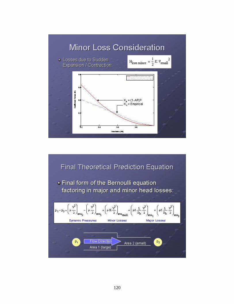
120
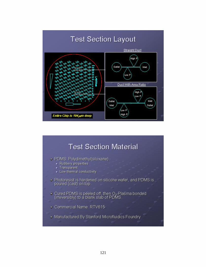
121
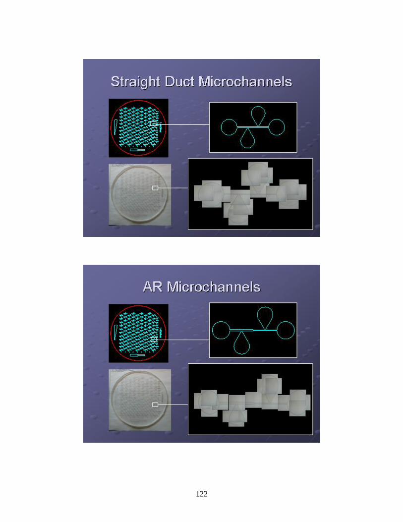
122

123

124
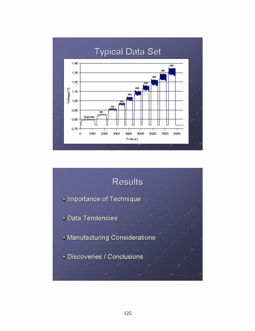
125
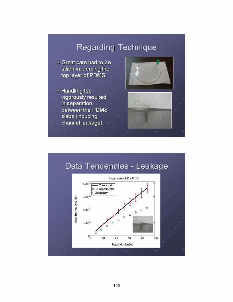
126

127
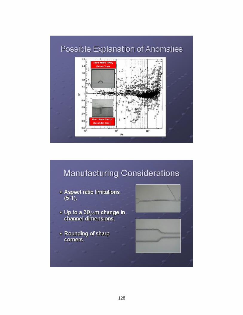
128

129

See Appendix A for additional straight duct plots.
See Appendix B for additional expansion plots.
130
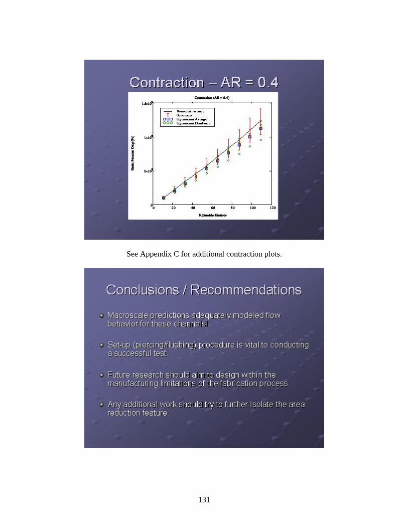
See Appendix C for additional contraction plots.
131

132
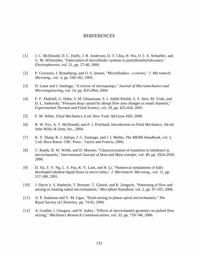
RERFERENCES
[1] J. C. McDonald, D. C. Duffy, J. R. Anderson, D. T. Chiu, H. Wu, O. J. A. Schueller, and G. M. Whitesides, "Fabrication of microfluidic systems in poly(dimethylsiloxane)," Electrophoresis, vol. 21, pp. 27-40, 2000.
[2] P. Gravesen, J. Branebjerg, and O. S. Jensen, "Microfluidics - a review," J. Micromech. Microeng., vol. 3, pp. 168-182, 1993.
[3] D. Laser and J. Santiago, "A review of micropumps," Journal of Micromechanics and Microengineering, vol. 14, pp. R35-R64, 2004.
[4] F. F. Abdelall, G. Hahn, S. M. Ghiaasiaan, S. I. Abdel-Khalik, S. S. Jeter, M. Yoda, and D. L. Sadowski, "Pressure drop caused by abrupt flow area changes in small channels," Experimental Thermal and Fluid Science, vol. 29, pp. 425-434, 2005.
[5] F. M. White, Fluid Mechanics, 6 ed. New York: McGraw-Hill, 2008.
[6] R. W. Fox, A. T. McDonald, and P. J. Pritchard, Introduction to Fluid Mechanics, 5th ed: John Wiley & Sons, Inc., 2004.
[7] K. V. Sharp, R. J. Adrian, J. G. Santiago, and J. I. Molho, The MEMS Handbook, vol. 1, 2 ed. Boca Raton: CRC Press - Taylor and Francis, 2006.
[8] C. Rands, B. W. Webb, and D. Maynes, "Characterization of transition to tubulence in microchannels," International Journal of Heat and Mass transfer, vol. 49, pp. 2924-2930, 2006.
[9] D. Xu, T. Y. Ng, L. S. Pan, K. Y. Lam, and H. Li, "Numerical simulations of fully developed tubulent liquid flows in micro tubes," J. Micromech. Microeng., vol. 11, pp. 157-180, 2001.
[10] J. Ducre´e, S. Haeberle, T. Brenner, T. Glatzel, and R. Zengerle, "Patterning of flow and mixing in rotating radial microchannels," Microfluid Nanofluid, vol. 2, pp. 97-105, 2006.
[11] A. P. Sudarsan and V. M. Ugaz, "Fluid mixing in planar spiral microchannels," The Royal Society of Chemistry, pp. 74-82, 2006.
[12] A. Goullet, I. Glasgow, and N. Aubry, "Effects of microchannel geometry on pulsed flow mixing," Mechanics Research Communications, vol. 33, pp. 739-746, 2006.
133
[13] M. Niklas, M. Favre-Marinet, and D. Asendrych, "Numerical simulation of microchannel network with complex geometry," Bulletin of the Polish Academy of Sciences, vol. 53, 2005.
[14] J. Koo and C. Kleinstreuer, "Liquid flow in microchannels: experimental observations and computational analyses of microfluidics effects," J. Micromech. Microeng., vol. 13, pp. 568-579, 2003.
[15] G. P. Celata, M. Cumo, S. McPhail, and G. Zummo, "Characterization of fluid dynamic behaviour and channel wall effects in microtube," International Journal of Heat and Fluid Flow, vol. 27, pp. 135-143, 2006.
[16] M. E. Steinke and S. G. Kandlikar, "Single-phase liquid friction factors in microchannels," presented at ICMM05: Third International Conference on Microchannels and Minichannels, University of Toronto, 2005.
[17] W. Qu and I. Mudawar, "Experimental and Computational Investigation of Flow development and Pressure Drop in a Rectangular Micro-channel," Journal of Electronic Packaging, vol. 128, pp. 1-9, 2006.
[18] M. Bahrami, M. M. Yovanovich, and J. R. Culham, "Pressure Drop of Fully Developed Laminar Flow in Rough Microtube," Journal of Fluids Engineering, vol. 128, pp. 632-637, 2006.
[19] C. Hansel, "Mapping of Pressure Losses Through Microchannels With Sweeping-Bends of Various Angle and Radii," in College of Engineering and Computer Science - Department of Mechanical, Materials, and Aerospace Engineering, vol. Master of Science. Orlando: University of Central Florida, 2008, pp. 134.
[20] N.-T. Nguyen and S. T. Wereley, Fundamentals and Applications of Microfluidics, Second Edition ed: Artech House, Inc., 2006.
[21] V. L. Streeter, Handbook of Fluid Dynamics. New York: McGraw-Hill, 1961.
[22] D. C. Duffy, J. C. McDonald, O. J. A. Schueller, and G. M. Whitesides, "Rapid Prototyping of Microfluidic Systems in Poly(dimethylsiloxane)," Department of Chemistry and Chemical Biology, vol. 70, 1998.
[23] M. Morra, E. Occhiello, R. Marola, F. Garbassi, P. Humphrey, and D. Johnson, "On the aging of oxygen plasma-treated polydimethylsiloxane surfaces," Journal of Colloid and Interface Science, vol. 137, pp. 11-24, 1990.
134