Embed Size (px)
Citation preview
Western UniversityScholarship@Western
Digitized Theses Digitized Special Collections
2011
Pressure-Equalized Rainscreen Wall System: A Full-Scale ExperimentSamar D. DernaykaWestern University, [email protected]
Follow this and additional works at: https://ir.lib.uwo.ca/digitizedtheses
Part of the Civil and Environmental Engineering Commons
This Thesis is brought to you for free and open access by the Digitized Special Collections at Scholarship@Western. It has been accepted for inclusionin Digitized Theses by an authorized administrator of Scholarship@Western. For more information, please contact [email protected],[email protected].
Recommended CitationDernayka, Samar D., "Pressure-Equalized Rainscreen Wall System: A Full-Scale Experiment" (2011). Digitized Theses. 3212.https://ir.lib.uwo.ca/digitizedtheses/3212
PRESSURE-EQUALIZED RAINSCREEN WALL SYSTEM:
A FULL-SCALE EXPERIMENT
(Thesis format: Monograph)
By
Samar D. Dernayka
Faculty of Engineering
Department of Civil and Environmental Engineering
Submitted in partial fulfillment
of the requirements for the degree of
Master of Engineering Science
School of Graduate and Postdoctoral Studies
The University of Western Ontario
London, Ontario, Canada
May 2011
© Samar D. Dernayka 2011
ii
THE UNIVERSITY OF WESTERN ONTARIO SCHOOL OF GRADUATE AND POSTDOCTORAL STUDIES
CERTIFICATE OF EXAMINATION
Supervisor
______________________________ Dr. Craig Miller
Examiners
______________________________ Dr. Horia Hangan
______________________________ Dr. Eric Savory
______________________________ Dr. Clare Robinson
The thesis by Samar D. Dernayka
entitled
Pressure-Equalized Rainscreen Wall System: A Full-Scale Experiment
is accepted in partial fulfillment of the
requirements for the degree of
Master of Engineering Science
Date__________________________ _______________________________ Chair of the Thesis Examination Board
iii
ABSTRACT
The pressure equalized rainscreen wall, considered as the most effective building
envelope against wind induced rain penetration, requires continuous investigations to
reach better performance. This research seeks the optimum pressure equalization process
under external pressure conditions and wall parameters that have not previously been
studied in detail. For this purpose, a single compartment full-scale wall model was built
in a controlled facility at the University of Western Ontario. The cavity pressure response
to external fluctuations was experimentally examined with respect to the rainscreen
venting area ratio, under two types of real wind pressure distributions generated
mechanically at zero degree incidence: 1) single pressure and, 2) pressure gradient caused
by the application of three different signals varying horizontally across the rainscreen.
As the rainscreen venting area ratio increases, the pressure equalization performance
improves, irrespective of the nature of the applied pressure, implying an increase in the
critical damping frequency. However, an applied pressure gradient leads to a lower
degree of pressure equalization at a constant venting area. Moreover, the change of the
vent openings layout has an impact on the wall performance, mainly at low venting areas.
Locating the vent openings at the bottom of the rainscreen gives better pressure
equalization rather than distributing them between top and bottom.
Using a numerical model, the cavity pressure measurements were underestimated under a
uniform pressure and overestimated when subject to a pressure gradient. The agreement
in the frequency domain between experimental and predicted signals was satisfactory in
the high frequency regions at high venting area ratios. However, transfer functions and
phase angles were overpredicted at low venting rates. Based on numerical simulations,
the cavity volume change does not significantly affect the performance of the model
under an external pressure gradient. When a single pressure is applied, the pressure
equalization is reduced at a larger cavity depth, which is only apparent at low venting
areas.
Keywords: rainscreen, wind pressure gradient, frequency domain

iv
ACKNOWLEDGEMENTS
I would like to express my thanks to Dr. Diana R. Inculet, who introduced the Pressure
Equalized Rainscreen systems field to me. She gave me the opportunity to do this
research under her guidance and insightful ideas.
I am also grateful to Dr. Craig Miller, a great supervisor I was so lucky to have during the
last semester. He offered me help and support, and provided many hours of valuable
discussions. His understanding, encouragement and advice have made this thesis
completed at the end of the day.
I also acknowledge the technical staff at the Three Little Pigs facility for their assistance.
Similarly, it would have been so difficult to accomplish the experimental part of the work
without the aid of many graduate students; among them, I would like to mention Murray
Morrison. I really appreciate his excellent knowledge and patience in providing the
solutions for the electrical and technical problems that I have encountered through the
course of this work.
The build up of the full-scale model was realized by the University Machine Shop staff
who offered valuable guidance in terms of the design and the actual performance of the
model.
Finally, I would like to thank my lovely parents for their encouragement. And I wonder if
I could have ever done this research without the continuous support of my husband
Zaher. I would like to express my deepest gratitude to him for being so patient and
helpful during the last two years. This work is dedicated to him, and to our coming
baby...
v
TABLE OF CONTENTS
CERTIFICATE OF EXAMINATION ii
ABSTRACT iii
ACKNOWLEDGEMENTS iv
TABLE OF CONTENTS v
LIST OF TABLES viii
LIST OF FIGURES ix
NOMENCLATURE xiii
CHAPTER 1 INTRODUCTION 1
1.1 Principle of a Pressure-Equalized Rainscreen Wall Systems 1
1.2 Applications of Pressure Equalized Rainscreen Wall Concept 4
1.3 Focus of The Current Research 5
CHAPTER 2 LITERATURE REVIEW 8
2.1 Prediction of Cavity Response Pressure 8
2.1.1 Background Theory from Low-Rise Buildings 8
2.2 Theoretical Models 11
2.2.1 Model Based on Mass Balance or First Principle (Model 1) 11
2.2.2 Model Based on Helmholtz Resonator Theory (Model 2) 13
2.3 Previous Pressure Equalized Rainscreen Walls Experiments 18
2.3.1 Full-Scale Experiments 19
2.3.2 Wind Tunnel Experiments 24
2.3.3 Comparison with Theoretical Model 26
2.4 Design Guidelines for PER 28
2.4.1 Rainscreen Venting Area 28
2.4.2 Venting Configuration (locations and dimensions) 29
2.4.3 Cavity Volume 29
2.4.3.1 Cavity Depth 29
2.4.3.2 Compartment Size 29
2.4.4 Air Barrier Stiffness and Leakage 30
vi
CHAPTER 3 FULL-SCALE EXPERIMENT 31
3.1 Test Methodology 31
3.1.1 Model 31
3.1.1a Rainscreen 32
3.1.1.b Air barrier 36
3.1.2 Equipment 37
3.2 Testing Configurations 42
3.2.1 Exterior Pressures Signals 42
3.2.2 Panel Setup Configurations 46
CHAPTER 4 FULL-SCALE EXPERIMENTAL RESULTS 48
4.1 Introduction 48
4.2 Basic Statistics of Measured Cavity Pressures for a
Single Applied Pressure 48
4.2.1 Pressure Gradient inside the Cavity 48
4.2.2 Measurements of Cavity to Exterior Pressure
Ratio c eP P 52
4.2.3 Analysis of the Experimental Results in the
Frequency Domain 58
4.3 Basic Statistics of Measured Cavity Pressures for
Three Different Applied Signals 65
4.3.1 Pressure Gradient inside the Cavity 65
4.3.2 Measurements of Cavity to Exterior Pressure
Ratio c eP P 70
4.3.3 Analysis of the Experimental Results in the
Frequency Domain 74
4.3.4 Comparison of Wide and Narrow Faces Results 79
4.4 Summary 81
CHAPTER 5 NUMERICAL RESULTS 83
5.1 Introduction 83
5.2 Numerical Model 83
vii
a) Flow Exponent n 84
b) Effective Length el 84
c) Discharge Coefficient K 85
5.3 Results and Discussion 92
5.3.1 Single Applied Pressure Signal 92
5.3.2 Three Different Pressure Signals 102
5.4 Numerical Prediction of Cavity Pressure at Various Depths 110
5.5 Summary 114
CHAPTER 6
CONCLUSIONS AND RECOMMENDATIONS 116
REFERENCE 121
APPENDIX A 125
Appendix A1 126
Appendix A2 129
Appendix A3 130
APPENDIX B 134
Appendix B1 135
VITA 139
viii
LIST OF TABLES
Table 2.1 Helmholtz resonance frequencies for some typical buildings (Holmes 2001) 10
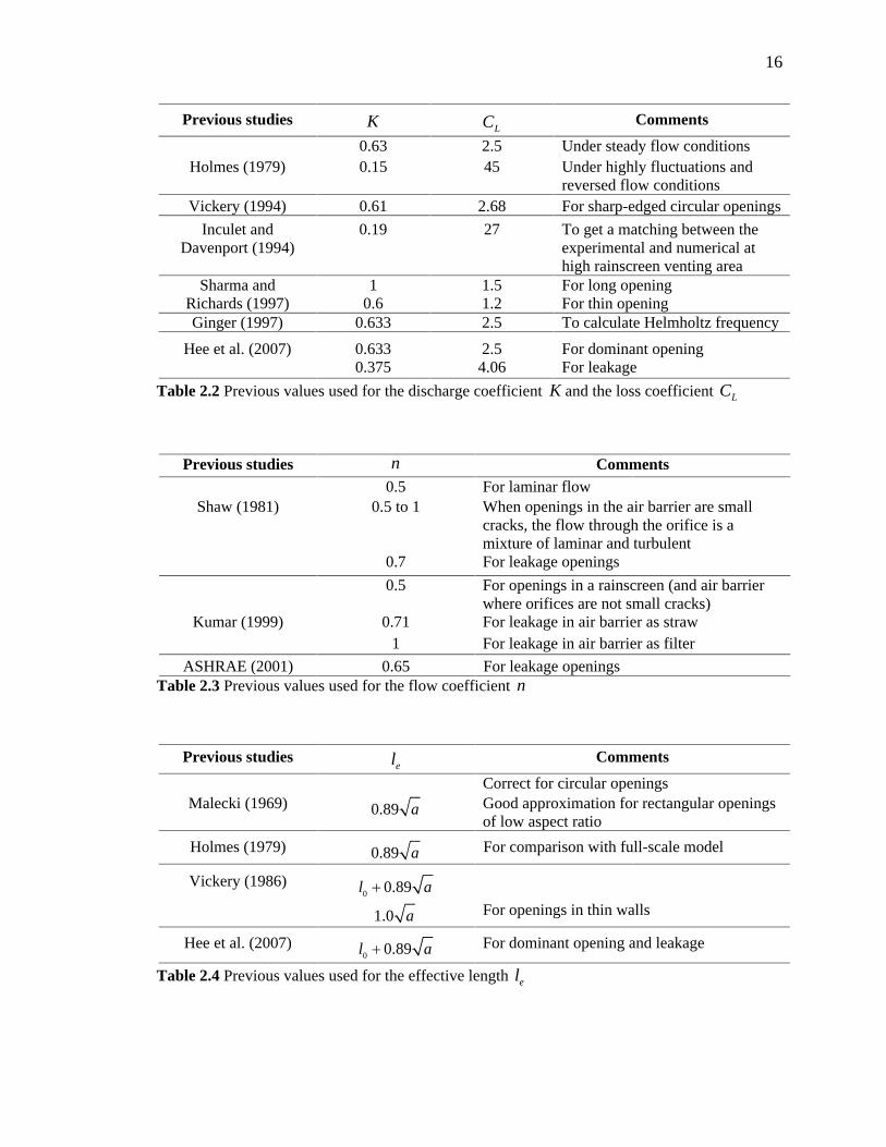
Table 2.2 Previous values used for the discharge coefficient K and the loss coefficient LC 16
Table 2.3 Previous values used for the flow coefficient n 16
Table 2.4 Previous values used for the effective length el 16
Table 2.5 Previous full-scale experiment for pressure equalized rainscreen walls 23
Table 2.6 Previous wind tunnel experiments for pressure equalized rainscreen walls 25
Table 3.1 Tests configurations 47
Table 4.1 mean pressure gradients values inside the cavity for the single signal pressure for configuration b, 0.022%VA 51
Table 4.2 Undamped natural frequencies ( )f Hz at 25cd mm 65
Table 4.3 Statistical values for the three applied pressure signals 66
Table 4.4 Mean instantaneous pressure gradients inside the cavity for the three applied signals (Configuration b) 0.022%VA 66
Table 5.1 Ratio of numerical and experimental cavity pressure for the single signal, wide face 90
Table 5.2 Ratio of numerical and experimental cavity pressure for the three applied signals, wide face 102
Table A.1 Achieved single exterior pressure signal for the wide face 131
Table A.2 Summary of accuracy errors ranges for PLAs performance 132
Table A.3 Accuracy errors between pressure transducers of the same test Configuration 133
ix
LIST OF FIGURES
Figure 1.1 Components of a pressure equalized rainscreen wall (PER) 1
Figure 1.1 Examples of the PER systems in the industry (a) and (b) 2
Figure 2.1 Helmholtz resonator model of fluctuating internal pressures with a single dominant opening after Holmes (2001) 10
Figure 2.2 Rainscreen load reduction as a function of venting and leakage area reproduced from Kumar et al. (2003) 20
Figure 3.1 Pressure equalized rainscreen panel model (side view) 32
Figure 3.2 Distribution of 20mm venting holes on the aluminum rainscreen 33
Figure 3.3 Rainscreen model (a), (b) and (c) 35
Figure 3.4 Air barrier assembly 36
Figure 3.5 Pressure transducers locations on (a) the pressure boxes, and (b) the air barrier 39
Figure 3.6 PER wall panel (a) Front view, and (b) Back view 41
Figure 3.7 Pressure model of a high building in the wind tunnel (Inculet 2001) 42
Figure 3.8 Mean pressure distribution for the windward wide face at 76.0mm Hy under zero degree wind angle 44
Figure 3.9 PLA pressure trace for the middle tap of the wide face 45
Figure 4.1 Time series pressures for configuration b for (a) wide face, and (b) narrow face 49
Figure 4.2 Time series pressures for configuration d for (a) wide face, and (b) narrow face 50
Figure 4.3 Basic statistics for a single applied pressure signal for (a) wide face, and (b) narrow face 53
Figure 4.4 Peak factor for a single applied pressure signal for (a) wide face and (b) narrow face 57
x
Figure 4.5 Spectral density functions for cavity pressure varying with area venting ratio % for (a) wide face, and (b) narrow face 59
Figure 4.6 Transfer function (a) and phase angle (b) variation with venting area ratios % (wide face) 61
Figure 4.7 Transfer function (a) and phase angle (b) variation with venting area ratios % (narrow face) 62
Figure 4.8 Transfer function (a) and phase angle (b) variation with venting location (wide face) 64
Figure 4.9 Time series pressures for configuration b for a) wide face and b) narrow face 67
Figure 4.10 Time series pressures for configuration d for a) wide face and b) narrow face 68
Figure 4.11 Basic statistics for three applied pressure signals for a) wide face, and b) narrow face 71
Figure 4.12 Peak factor for three applied pressure signals for a) wide face, and b) narrow face 73
Figure 4.13 Spectral density functions for cavity pressures for a) wide, and b) narrow face 75
Figure 4.14 Transfer function (a) and phase angle (b) variation with venting area ratios (wide face) 76
Figure 4.15 Transfer function (a) and phase angle (b) variation with venting area ratios (narrow face) 77
Figure 4.16 Transfer function (a) phase angle (b) variation with venting location (wide face) 78
Figure 5.1 Cavity pressure prediction with respect to leakage holes for the single applied signal for wide face ( 0.007%VA ) 87
Figure 5.2 Cavity prediction pressure with respect to the Discharge coefficient 87
Figure 5.3 Power spectral density function for the cavity pressure for the single applied signal for wide face ( 0.007%VA ) 88
xi
Figure 5.4 Cavity pressure for a single applied pressure signal for a wide face ( 0.022%VA ) 91
Figure 5.5 Basic statistics for the basic venting configurations for the wide face 92
Figure 5.6 Spectral density functions for the cavity pressure for the wide face case a) 0.022%VA
b) 0.11%VA 94
Figure 5.7 Effect of discharge coefficient and leakage holes on transfer functions 95
Figure 5.8 Comparison of measured and simulated cavity to external pressure ratios using transfer functions (wide face) 95
Figure 5.9 The effect of K on transfer function 0.022%VA , cd =25mm
(wide face) 98
Figure 5.10 The effect of discharge coefficients on rainscreen pressures, reproduced by Kumar et al. (1999) 0.15%VA
cd =150mm 98
Figure 5.11 Comparison of measurements and simulations with phase angles (wide) 100
Figure 5.12 The effect of K on the phase angle 0.022%VA (wide face) 100
Figure 5.13 Comparison of measured and simulated cavity pressures using transfer functions (narrow face) 101
Figure 5.14 Effect of discharge coefficient and leakage holes on transfer functions 103
Figure 5.15 Basic statistics for the basic venting configurations for a) the wide face and b) narrow face 104
Figure 5.16 Cavity pressure for a single applied pressure signal for a wide face ( 0.022%VA ) 105
Figure 5.17 Spectral density function for the cavity pressure for the wide face a) 0.022%VA
b) 0.11%VA 106
Figure 5.18 Measurements and simulations for the wide face a) transfer function b) phase 108
xii
Figure 5.19 Comparison of measured and simulated cavity pressures for the narrow face transfer function 109
Figure 5.20 Peak ratio of cavity to external pressure for a) single and b) three different signals 111
Figure 5.21 Transfer functions for single signal a) 0.007%VA b) 0.11%VA
(wide face) 112
Figure 5.22 Transfer functions for three different applied signals 0.11%VA
(wide face) 113
Figure A.1 Rainscreen venting area configurations 129
Figure B.1 Flow chart for computational programming for (MDE) equations holes in Matlab (7.1) 137
xiii
NOMENCLATURE
A Opening area
abA Air barrier leakage area
rsA Rainscreen venting area
wA Wall panel area
V rs wA A A Rainscreen Venting area ratio
a Opening area of a rainscreen
LC Loss coefficient
pC Pressure coefficient
peC External pressure coefficient
0piC Internal pressure coefficient
pcC Pressure coefficient inside the cavity
d Opening diameter
cd Cavity depth
f Frequency
g Peak factor
H
PER wall height
mH Height of the building model in the wind tunnel
( )H Transfer function
gH Instantaneous horizontal pressure gradient coefficient
K Discharge coefficient
AK Bulk modulus of air
BK Bulk modulus of the building
el Effective length
0l Opening length
xiv
m number of openings
cm Mass of air inside the cavity
n Flow exponent
0p Atmospheric static pressure
aP Area-averaged pressure
cP Cavity pressure
eP External pressure
iP Internal pressure
tP Instantaneous pressure measured by a pressure transducer
1P External pressure applied to the first pressure box from the left
2P External pressure applied to the second pressure box in the middle
3P External pressure applied to the third pressure box from the left
p Differential pressure
Q Flow rate
eR Reynolds number
)( fS Power spectral density function
t Time lag
U Air velocity
V Velocity
0V Internal volume for a low-rise building
cV Cavity volume
x Horizontal coordinate from the bottom left corner of the air barrier
x Distance the air slug moves
mx Horizontal coordinate from the bottom left corner of the wind tunnel
pressure model face
rx Horizontal coordinate from the bottom left corner of the rainscreen
xv
my Vertical coordinate from the bottom left corner of the wind tunnel
pressure model face
y Vertical coordinate from the bottom left corner of the air barrier
refz Reference height in the wind tunnel
W Width of the pressure equalized rainscreen wall
mW Width of the pressure model face in the wind tunnel
0 Resonant gradient frequency
d Critical damping frequency
a Air density
Kinetic viscosity of the air
Polytropic exponent
Ratio of specific heat of air
Variance of the pressure signal
1
CHAPTER 1
INTRODUCTION
1.1 Principle of a Pressure-Equalized Rainscreen Wall System
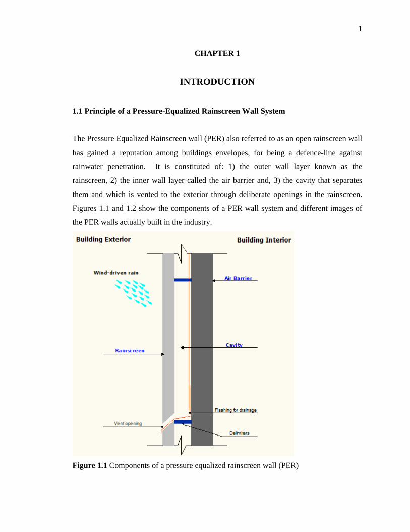
The Pressure Equalized Rainscreen wall (PER) also referred to as an open rainscreen wall
has gained a reputation among buildings envelopes, for being a defence-line against
rainwater penetration. It is constituted of: 1) the outer wall layer known as the
rainscreen, 2) the inner wall layer called the air barrier and, 3) the cavity that separates
them and which is vented to the exterior through deliberate openings in the rainscreen.
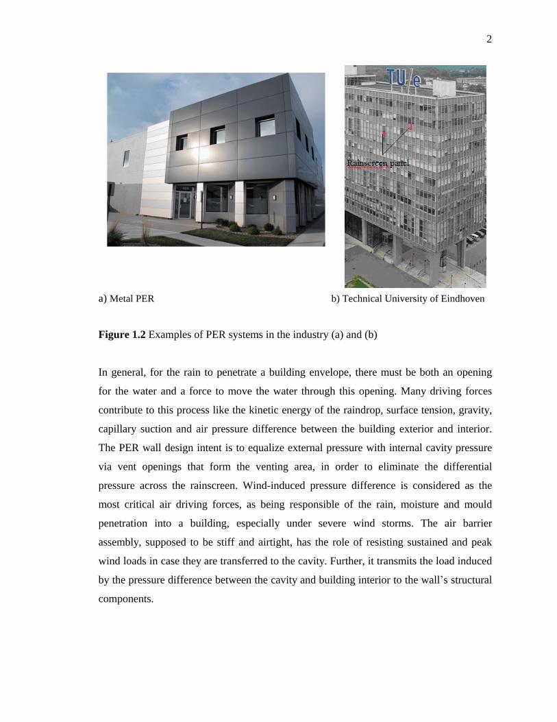
Figures 1.1 and 1.2 show the components of a PER wall system and different images of
the PER walls actually built in the industry.
Figure 1.1 Components of a pressure equalized rainscreen wall (PER)
2
a) Metal PER b) Technical University of Eindhoven
Figure 1.2 Examples of PER systems in the industry (a) and (b)
In general, for the rain to penetrate a building envelope, there must be both an opening
for the water and a force to move the water through this opening. Many driving forces
contribute to this process like the kinetic energy of the raindrop, surface tension, gravity,
capillary suction and air pressure difference between the building exterior and interior.
The PER wall design intent is to equalize external pressure with internal cavity pressure
via vent openings that form the venting area, in order to eliminate the differential
pressure across the rainscreen. Wind-induced pressure difference is considered as the
most critical air driving forces, as being responsible of the rain, moisture and mould
penetration into a building, especially under severe wind storms. The air barrier
assembly, supposed to be stiff and airtight, has the role of resisting sustained and peak
wind loads in case they are transferred to the cavity. Further, it transmits the load induced
by the pressure difference between the cavity and building interior to the wall s structural
components.
3
In theory, pressure equalization (PE) means a zero air pressure differential at all times
across the rainscreen. In practice, however, perfect pressure equalization is neither
achievable nor necessary for adequate rain penetration control; engineers claim that the
wall assembly must be designed to tolerate the entry of a small amount of water without
damage. According to Rousseau et al. (1998), the adequate pressure equalization for rain
penetration control may be defined as not more than 25 Pa differential pressure across the
rainscreen.
The pressure equalization technique was in fact early recognized in 1962 as O. Birkeland
proposed in his Handbook Curtain Walls to design the exterior rain-proof finishing so
open that no super-pressure can be created over the joints or seams in the finishing . He
considered that such process is provided by having an air space behind the exterior
finishing, but with connection to the outside air , so that air pressures due to wind gusts
will be equalized on both sides of the exterior finishing. This principle was then enhanced
in Garden s publication in 1963 Rain penetration and its control , who settled the
preliminary basics of the PER wall construction in terms of cavity depth and vent
openings size. Later, others like Ganguli and Dalgliesh (1988), Baskaran and Brown
(1992), Kumar (1999) and Inculet and Davenport (1996) carried on several researches,
laboratory and tests on site in order to establish specific design guidelines for the
different parameters for an optimum performance of the PER walls systems, under
different conditions; like when the system is experiencing a leakage problem, which is an
unavoidable issue in buildings.
Many recommendations have arisen based on their experiments, however this domain
still need further investigation, especially in the absence of ready to use design guidelines
for PER walls in codes and standards. The latter agree in general that a satisfactory
differential pressure is available when the pressure load on the rainscreen is near zero.
4
1.2 Applications of Pressure Equalized Rainscreen Wall Concept
The PER walls systems are used for existing buildings experiencing general performance
problems such as rain penetration, insufficient insulation, and deterioration of
components. A new application has been introduced recently, known as overcladding. In
fact, tens of thousands of highrises built during the building boom of the mid-1980s
suffered water damage as wind-driven rain entered the walls. Under severe wind storms,
sections of exterior cladding have let go and plunged to the ground for some building
façades. A few today, like low-rise buildings, just show the same symptoms as leaky
construction, wet spots and mould on walls, with an exterior wall assembly unable to
sustain wind-induced pressure. Moreover, Canadian insurance companies have claimed
that well over half of insured losses from building outer envelopes are wind related. In
light of these problems, engineers decided to opt for PER wall as an outer building
envelope that offers the most protection to the inner structural layer and requires less
maintenance over its service life.
When applied to cladding panels, the pressure equalization technique is considered to be
very expensive. A major part of the cost is highly related to materials that are unique for
façade applications such as exterior rainscreen panels like molten cast glass, precast
concrete, marble, aluminium, glass fibre reinforced concrete (GFRC), water jet cut
stainless steel, copper, etc. The choice of rainscreen material is surely based on aesthetic
criterion as well as on cost restrictions.
In Europe, the open rainscreen principle refers to back-ventilated rainscreen walls,
instead of the pressure equalized rainscreen wall notion used mostly in the USA and
Canada. In fact, it is a PER wall with incorporating additional large vents at the top of the
rainscreen. Thus, the resulting airflow pattern in the cavity moves air in through the
bottom vents (the original venting openings of the rainscreen) and out the top vents,
helping to dry out any moisture that penetrates the wall. According to Inculet (1990), this
design only strives to keep water from coming in contact with the air barrier; while the
5
PER wall system aims to eliminate any water penetration through the rainscreen, by
addressing the wind s driving force with adequate vent openings.
1.3 Focus of the Current Research
The development of PER wall systems application is still slow, due to the comparative
expense over a more conventional exterior wall system, according to leading designers of
tall buildings in the United States. The motivation for the current research on pressure-
equalized rain screen wall cladding stems from this point. Actually, the goal is to look at
the performance of a PER wall panel under new exterior pressures conditions; that were
not taken into account before. Also, the effect of some design parameters is examined,
and a numerical model is used for the experimental results validation.
Previous works have investigated PER wall performance by measuring the differential
pressure across the rainscreen as it is considered the key for optimum pressure
equalization. Such tests were done either in the laboratories or in the field. However, in
both cases, the researches were not able to take the self-control of the set-up conditions of
the PER wall system or even the applied wind load. In the wind tunnel experiments, the
modeling of PER wall system is subject to scaling problem; which gives incorrect
representations of the PER features size and the characteristics, and would negatively
influence conclusions made on the pressure equalization process.
On the other hand, in the field tests previously done (i.e. Ganguli and Dalgliesh (1988)
and Kumar (1999)) the full-scale model of the PER wall panel was always tested after
being installed on the constructed building. Thus, the data measurements were probably
affected by the leakage status, an unavoidable issue that is hard to quantify in buildings.
Further in such tests, no one could control the external wind fluctuations at any time, it all
depends on the climate conditions and the location of the PER panel itself. In case the
cavity response pressure needs to be examined for other wind loads, or for pressures
gradients (i.e. at the corner of the building façade), the panel needs to be moved or other
wall panels are then added at various locations of the façade which imply higher cost and
6
a more time consuming work. Moreover, it is necessary to recall that the majority of
previous studies have focused on the examination of rainscreen venting over air barrier
leakage ratio effect on the PER performance; without taking into consideration the effects
of the other parameters.
In light of this discussion, it was decided to build a PER full-scale model in a controlled
facility to vary the different parameters and applied wind conditions, and observe the way
they affect the model performance, in a controlled environment and within a short time
period. The roadmap of the research work is clarified through the chapters of this thesis.
Chapter 2 mainly presents a literature review on the previous studies made about PER
walls. Full-scale and wind tunnel experiments are discussed providing the key
conclusions on the effect of design parameters on the PER performance; and the validity
of applied numerical models. At the beginning, a general overview was presented about
the theoretical models with the involved equations, used for cavity pressure response
prediction when an external load is applied to the wall.
Chapter 3 describes the experimental model set-up. It provides a clear detailing of the
three components of the PER wall, and the test configurations as well. The equipments
used for both wind load application and cavity pressure data acquisition, are also
depicted.
Chapter 4 shows the experimental measurements of the cavity pressure with respect to
rainscreen venting configurations and vent openings location, the cavity depth being
constant. The data permit calculation of the differential pressure across the rainscreen,
which leads to the evaluation of the PER model performance.
Two types of external signals were normally applied to the panel: a) a single pressure
and, b) a pressure gradient; which results from the application of three different pressure
signals varying horizontally on the rainscreen. In this case, each group of venting
openings was subject to a different pressure depending on its location. Such test was
7
never done before using a full-scale model. It allows examination of the effect of an
exterior pressure gradient applied to the same PER panel. Moreover, the influence of a
building façade on the pressure equalization process can be seen, since two different
pressure gradients are used, each has been extracted in reality from on a different
pressure model face in a wind tunnel experiment.
Chapter 5 provides a comparison between experimental and numerical results. A
theoretical model was programmed for cavity pressures predictions, using the actual
exterior pressure signals applied on site as input. Numerical simulations are presented for
all test configurations. In addition, the numerical model was used to predict the effect of
the cavity depth variation on the wall s PE process; which has not been investigated yet,
neither numerically, nor practically. In the current research, the cavity depth has been
numerically varied within a practical range where the upper value is the maximum depth
used in the industry.
Finally Chapter 6 presents conclusions from the current project results. It also claims
further investigations in some points that would be of a useful contribution for the
development of PER wall systems.
8
CHAPTER 2
LITERATURE REVIEW
This chapter presents the results of a literature survey on the research work concerning
the pressure-equalized rainscreen wall studies for the past decades. It tends to show the
continuous effort of researches in examining the possibility of achieving an optimum
performance for a PER system via laboratory experiments, field measurements, wind
tunnel models and computer simulations. Finally, a summary is provided herein for
general design guidelines recommended by the authors for a better pressure equalized
rainscreen wall.
2.1 Prediction of Cavity Response Pressure
2.1.1 Background Theory from Low-rise Buildings
The theory for the prediction of cavity response pressures for a PER wall originates from
internal pressure predictions in low-rise buildings.
The cavity pressure responding to the external wind-induced fluctuations entering
through vents is analogous to the internal pressure behaviour within a building (enclosure
with rigid walls and roofs) with single or multiple openings. In fact, internal pressures are
introduced inside a building throughout leakage or openings. They depend on several
factors including: external pressure distributions near the openings, geometry of the
openings, vents, the fluid properties (density, viscosity), internal volume, wind direction,
turbulence in the upstream boundary layer, flexibility of the building skin and structure
(Vickery and Bloxham 1992); and the compartmentalization within the building (Sharma
and Richard 1997). The internal pressure response can be determined using two methods:
1) conservation of mass, 2) Helmholtz resonator model.
For a low-rise building with a single windward opening, the internal pressure is
established after a response time t
where t
is the time taken for the internal pressure to
become equal to a sudden increase in pressure outside the opening, caused for example
by a sudden window failure. In steady flow, Holmes (2001) confirms that the internal
9
pressure will quickly develop in order to reach the external pressure on the windward
wall in proximity of the opening. In the case of a turbulent boundary-layer wind, the
increase of the external pressure will allow an increase in the density of air within the
internal volume 0V , thus the internal pressure increases.
In the case of neglected inertial effects, the mass conservation concept is applied, so that
the rate of mass flow through the opening aQ
must equal the rate of mass increase
0ad dt V inside the volume thus the time lag expression is given by
00
0pipe
a CCKAp
UV (2.1)
by considering that for a turbulent flow through an orifice, the air flow is related to the
pressure difference across the orifice e iP P
When inertial effects are considered, Holmes (1979) suggested that a Helmholtz
resonator model can be used for the prediction of the response to turbulent external
pressures. Holmes observed that a building with a single dominant opening behaves like a
Helmholtz resonator and internal pressure fluctuations are due to compressibility effects
of the fluid. Thus, he considered it as a special case of Helmholtz resonator , known in
acoustics as describing the response of small volumes to fluctuating external pressures
(Raylieh 1945, Malecki 1969). This can be applied to the case of external wind pressures
driving the internal pressures within a building: a slug
of air of length el is assumed to
move in a distance x in and out of the opening in response to the external pressure
changes as in Fig 2.1. The motion of the slug of air is expressed with the differential
equation
20
20
( )2
aa e e
A p AAl x x x x A p t
K V (2.2)
known as the unsteady orifice discharge equation where the first term on the left hand
side is an inertial term proportional to the acceleration x
of the air slug (whose mass is
a eAl , the second term is the loss term associated with energy losses for flow through the
orifice, and the third term represents the stiffness explained as the resistance of the air
pressure that is already available in the internal volume 0V to the air slug motion.
10
Holmes (1979) developed from this model the expression of the undamped natural
frequency for the resonance of the movement of the air slug, and of the internal pressure
fluctuations, known as Helmholtz frequency, in case of a single windward opening
0
0 0
1 1
2 2A
a e a e
Ap K Af
l V l V (2.3)
calculated given the opening area, internal volume and flexibility of roof and walls.
Using the atmospheric pressure 50 10p Pa , 31.2 /Kg m , 1.4 , 1.0el A , and
taking into consideration the flexibility of the building, the frequency becomes
1/4
1/21/20
551 ( / )A B
Af
V K K (2.4)
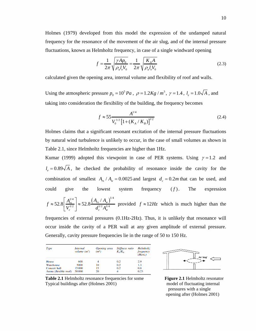
Holmes claims that a significant resonant excitation of the internal pressure fluctuations
by natural wind turbulence is unlikely to occur, in the case of small volumes as shown in
Table 2.1, since Helmholtz frequencies are higher than 1Hz.
Kumar (1999) adopted this viewpoint in case of PER systems. Using 1.2
and
0.89el A , he checked the probability of resonance inside the cavity for the
combination of smallest / 0.0025rs wA A and largest 0.2cd m that can be used, and
could give the lowest system frequency ( )f . The expression
1/41/4
1/2 1/2 1/4
/52.8 52.8 rs wrs
c c w
A AAf
V d A
provided 12f Hz
which is much higher than the
frequencies of external pressures (0.1Hz-2Hz). Thus, it is unlikely that resonance will
occur inside the cavity of a PER wall at any given amplitude of external pressure.
Generally, cavity pressure frequencies lie in the range of 50 to 150 Hz.
Table 2.1 Helmholtz resonance frequencies for some Figure 2.1 Helmholtz resonator Typical buildings after (Holmes 2001) model of fluctuating internal pressures with a single opening after (Holmes 2001)
11
2.2 Theoretical Models
The cavity pressure response of a PER wall subject to fluctuating pressures can be
predicted using two theoretical models:
1) Model based on mass balance or first principle
2) Model based on Helmholtz resonator theory
For both analytical models, mathematical modelling of flow through the PER wall system
is developed using the external pressure and wall characteristics as data input. The key
for the cavity pressure simulation is the Bernoulli principle for incompressible fluids,
which leads to flow rate expressions. The fluid here is air with 31.3 /a Kg m . In
general, for airflow to occur, there must be 1) a pressure difference between two points
and 2) a continuous flow path or opening connecting the points. Those two requirements
are represented by the vent holes of the rainscreen, which ensure the passage of the
airflow from the exterior to the cavity generating a cavity pressure response cP , and thus
a differential pressure across the rainscreen.
The governing equation of motion corresponding to the slug of air moving throughout
the vent hole of the rainscreen is given as
2
2a
a e L e c
UdUl C P P
dt (2.5)
This is the discharge equation for unsteady flow through an orifice, where el is the
effective length of the air slug, a el is the inertial effect, U is the fluid flow velocity, ep is
the external applied pressure. This equation comes from the Bernoulli equation, where a
loss term LC is introduced, since there is no absence of friction for the flow through an
orifice.
2.2.1 Model Based on Mass Balance or First Principle (Model 1)
This category includes all models derived on the basis of mass continuity equation and
equation of airflow through walls; without taking into consideration the inertial effect.
The general form of the flow rate Q through vent hole was discussed first by Kimura
(1977), where F is a function of Reynolds number and opening geometry:
12
0.5
( ,geometry of opening) 2e e aQ AF R dP (2.6)
He considered that for openings greater than about 10mm, the function F may be
regarded as a constant, and it is usually referred to the discharge coefficient K . A
is the
area of the orifice, and e e cdP p P P is the differential pressure across the rainscreen.
The conventional form of this equation is
2
a
pQ AK (2.7)
originated from Eqn (2.5), with the assumption that the flow is steady 0dU dt . The
discharge coefficient (also known as coefficient of discharge) allows the use of the ideal
velocity and orifice area in calculating the flow for a jet through an orifice of a small wall
thickness: It is negatively correlated with the loss coefficient 2
1LC
K
which is affected
by the time, the wind direction due to the exterior pressure field and the orifice length to
diameter ratio 0( / )l d (Chaplin et al. 2000). Its value is usually adjusted for the
calculations, in order to get a match between the numerical model and the experiment as
Table 2.2 shows.
Equation (2.7) is transformed to a general form that can be applied to different flow
characteristics of rainscreen and air barrier walls:
2
( )ne i
a
Q AK P P (2.8)
Shaw (1981) considers that the flow exponent n
varies according to the flow and the
opening details (Table 2.3).
The conservation of mass of air inside the cavity generally requires that the rate of net
mass flow into or out of the cavity must equal the rate of change of the mass of air inside
the cavity cm , as noted by Baskaran (1992). The general form of the continuity equation
is
1 2( ) ( )c c aa a c a c
dm dV ddQ Q V V
dt dt dt dt (2.9)
13
where 1Q and 2Q are respectively the flow rates through the rainscreen and the air barrier
for a PER wall.
Assuming the walls are not flexible ( 0cdV
dt), and substituting to Eqn (2.9) the
polytropic law relating pressure and density of air inside the cavity:
1 c a
c a
dP d
P dt dt (2.10)
The practical continuity equation will be
1 2c c
c
dP PQ Q
dt V (2.11)
with is the polytropic exponent generally equal to 1.2 as an intermediate value as used
by Holmes (1979) and Kumar (1999) ( 1 for isothermal condition, and 1.4 for
adiabatic condition).
2.2.2 Model Based on Helmholtz Resonator Theory (Model 2)
This model takes into consideration the inertial effects of air within the cavity, the losses
due to the vent orifice and friction; as suggested by Holmes (1979). Helmholtz resonance
is the phenomenon of air resonance in a cavity: the air has the tendency to oscillate at its
maximum amplitude associated with resonant frequencies. When air is forced into a
cavity, the pressure inside increases. Once the external force that pushes the air into the
cavity disappears, the higher-pressure air inside will flow out. However, this surge of air
flowing out will tend to over-compensate, due to the air inertia in the neck, and the cavity
will be left at a pressure slightly lower than the outside, causing air to be drawn back in.
This process repeats with the magnitude of the pressure changes decreasing each time.
Using the slug of air movement in a distance x in and out of the opening, Eqn (2.5)
becomes
2a e L e cl x C x x P P (2.12)
where the term eal is the inertial effect of the air slug proportional to the acceleration.
The effective length el changes with shape and length of the opening (Table 2.4).
14
xxCL 2
represents the damping effect referring to energy losses when the flow passes
through the opening
*Orifice-type loss: The pressure drop due to the Orifice-loss is then
1/21/
1/ 1
2
nnn a
e cP P xK
(2.13)
*Friction-type loss: For steady flow through an orifice-plate, it is essential to take into
consideration the wall thickness, since the openings are very small. Thus, the solid wall
shear stresses affect the pressure drop and the physical behaviour is more like a pipe flow
than an orifice flow. The pressure drop due to friction loss as explained in Oh et al (2007)
is
320
2
lp U
d (2.14)
is the dynamic viscosity of air, and U is the wind velocity
Combining Eqns. (2.12), (2.13) and (2.14), the single discharge equation for unsteady
flow (SDE) through an opening or leak is:
1/21/(1/ ) 1 0
2
321
2
nnna
a e e c
ll x x x x P P
K d (2.15)
For a number m of vent and leak openings, there will be m +1 unknowns
( cP , 1 2, ,.... )mx x x giving
1/ 1/2(1/ ) 1 0
2
321
2
i i
i
n nna i
a ei i i i i ei ci i
ll x x x x P P
K d (2.16)
known as Multiple discharge equations for unsteady flow through multiple openings or
leaks (MDE) , (i=1 m ) and an additional Continuity Equation (CE)
1 1 2 20
( ... ) a ca m m c
Va x a x a x P
p (2.17)
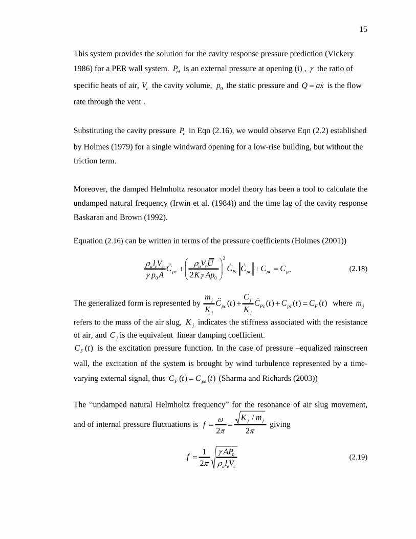
15
This system provides the solution for the cavity response pressure prediction (Vickery
1986) for a PER wall system. eiP is an external pressure at opening (i) , the ratio of
specific heats of air, cV the cavity volume, 0p the static pressure and xaQ is the flow
rate through the vent .
Substituting the cavity pressure cP in Eqn (2.16), we would observe Eqn (2.2) established
by Holmes (1979) for a single windward opening for a low-rise building, but without the
friction term.
Moreover, the damped Helmholtz resonator model theory has been a tool to calculate the
undamped natural frequency (Irwin et al. (1984)) and the time lag of the cavity response
Baskaran and Brown (1992).
Equation (2.16) can be written in terms of the pressure coefficients (Holmes (2001))
2
0
0 02a e c a
pc Pc pc pc pe
l V V UC C C C C
p A K Ap (2.18)
The generalized form is represented by ( ) ( ) ( ) ( )j jpc Pc pc F
j j
m CC t C t C t C t
K K where jm
refers to the mass of the air slug, jK indicates the stiffness associated with the resistance
of air, and jC is the equivalent linear damping coefficient.
)(tCF is the excitation pressure function. In the case of pressure equalized rainscreen
wall, the excitation of the system is brought by wind turbulence represented by a time-
varying external signal, thus )()( tCtC peF (Sharma and Richards (2003))
The undamped natural Helmholtz frequency for the resonance of air slug movement,
and of internal pressure fluctuations is /
2 2j jK m
f giving
01
2 a e c
APf
l V (2.19)
16
Previous studies K
LC
Comments
0.63 2.5 Under steady flow conditions
Holmes (1979) 0.15 45 Under highly fluctuations and reversed flow conditions
Vickery (1994) 0.61 2.68 For sharp-edged circular openings
Inculet and Davenport (1994)
0.19 27 To get a matching between the experimental and numerical at high rainscreen venting area
Sharma and 1 1.5 For long opening Richards (1997) 0.6 1.2 For thin opening Ginger (1997) 0.633 2.5 To calculate Helmholtz frequency
Hee et al. (2007) 0.633 2.5 For dominant opening
0.375 4.06 For leakage
Table 2.2 Previous values used for the discharge coefficient K and the loss coefficient LC
Previous studies n
Comments
0.5 For laminar flow Shaw (1981) 0.5 to 1 When openings in the air barrier are small
cracks, the flow through the orifice is a mixture of laminar and turbulent
0.7 For leakage openings
0.5 For openings in a rainscreen (and air barrier where orifices are not small cracks)
Kumar (1999) 0.71 For leakage in air barrier as straw 1 For leakage in air barrier as filter
ASHRAE (2001) 0.65 For leakage openings Table 2.3 Previous values used for the flow coefficient n
Previous studies el
Comments
Correct for circular openings Malecki (1969) 0.89 a
Good approximation for rectangular openings of low aspect ratio
Holmes (1979) 0.89 a
For comparison with full-scale model
Vickery (1986) 0 0.89l a
1.0 a
For openings in thin walls
Hee et al. (2007) 0 0.89l a
For dominant opening and leakage
Table 2.4 Previous values used for the effective length el
17
0pK A = 141999 (Pa) is the bulk modulus of air.
This frequency depends on rsA A the area of vent openings in the rainscreen, cavity
volume cV , effective length el of air slug at the opening, air density a , and the ratio of
specific heats for air .
According to the equations, the two theoretical models assume the pressure inside the
cavity to be uniform. Furthermore, Model 1 combines the flow rates through all the
openings of the rainscreen into one term 1Q , the same applies to the air barrier. Thus, the
model uses the averaged external pressures as a single pressure input applied on the
rainscreen. Models 2 instead represents the flow rate through each opening or leak
separately and, includes the associated applied pressure and losses terms, which leads to a
more realistic prediction of cavity pressure inside the air barrier.
Davenport and Surry (1984) used the equations of Model 2 to develop an expression for a
critical frequency d (in radians) above which attenuation of the exterior pressure
fluctuations will occur. Thus, frequencies less than d will be fairly effectively
transmitted to the cavity. Based on Eqn (2.15) and by including a forcing pressure as a
function of the frequency, they got for only one opening in the rainscreen and no leakage
through the air barrier, the expression
20
1 1pc pc pc pe
d
C C C C (2.20)
0 is the resonant radian frequency. For 0d , resonance may occur in the cavity.
Taking into consideration the multiple venting holes in the rainscreen, the distribution of
mean exterior pressures and spatial correlation of exterior pressure fluctuations as well as
the leakage characteristics, Davenport and Surry elaborated a frequency response
function ( )H
that describes the cavity pressure and pressure drops across the
rainscreen
( )ji ji eiP H P (2.21)
18
jiP : pressure drop across the rainscreen at location j due to forcing pressure eiP at i .
Such a function refers to the level of resistance that the vent holes exhibit as opposed to
the flow, which suppresses the fluctuations, that is called aerodynamic damping. The
greater the damping, the greater the magnitude of the differential pressures sustained by
the rainscreen will be.
On the other hand, Baskaran and Brown (1992) used Helmholtz resonator model to
establish an expression for the time lag of the cavity response pressure of a PER wall
subject to sinusoidal pressure using
0.5
1
57.48 rs
w c
A
A d
(2.22)
indicating that the time lag is constant for given wall parameters, and it can be reduced
through better pressure equalization. Clearly, this formula assumes that the frequency of
the signal is constant, thus it cannot be applied to the random fluctuations pressures that
cause variation of the cavity fluctuations in the frequency domain.
Also, Baskaran carried out a numerical evaluation of the performance of pressure
equalized rainscreen walls in (1994) being the first to use CFD. He applied sinusoidal
external pressure variations only.
2.3 Previous Pressure-Equalized Rainscreen Walls Experiments
Previous experiments allowed estimation of the impact of various design parameters on
the pressure equalization process. For this purpose, PER panels were subject to sets of
configurations mainly in terms of rainscreen venting area, air barrier leakage areas and
cavity compartmentalisation. The researchers were always seeking the ultimate
combination of PER wall characteristics to get a full-pressure equalization, so that the
wind-induced pressure is completely absorbed by the cavity.
19
2.3.1 Full-Scale Experiments
Most of these experiments were performed using wall-clad panels mounted on building
façades and interacting with the real wind fluctuations. In spite of differences in the
panels set-up and wind conditions, they all agree that two main factors contribute to the
performance of a PER: 1) the rainscreen venting to wall area and, 2) the rainscreen
venting to air barrier leakage area. The two ratios are equally important in case of leaky
characteristics of the air barrier wall. In absence of leakage, increasing the venting area
does not affect the transmission of external fluctuations into the cavity in the frequency
domain. Furthermore, reasonable pressure equalization can be achieved by providing a
relatively small venting area. The field experiments showed consistent results regarding
the behaviour of the cavity pressure response under zero degree wind angle: with higher
venting to wall area and venting to leakage ratios, the pressure equalization between
external pressures fluctuations and cavity pressure improves. Ganguli and Guirouette
(1987) were the first to evaluate the rainscreen venting area as a key controller for the
rainscreen loading. They claimed that the peak pressure difference across glass cladding
dropped when the ratio of cavity volume to venting area was decreased with a fixed
volume.
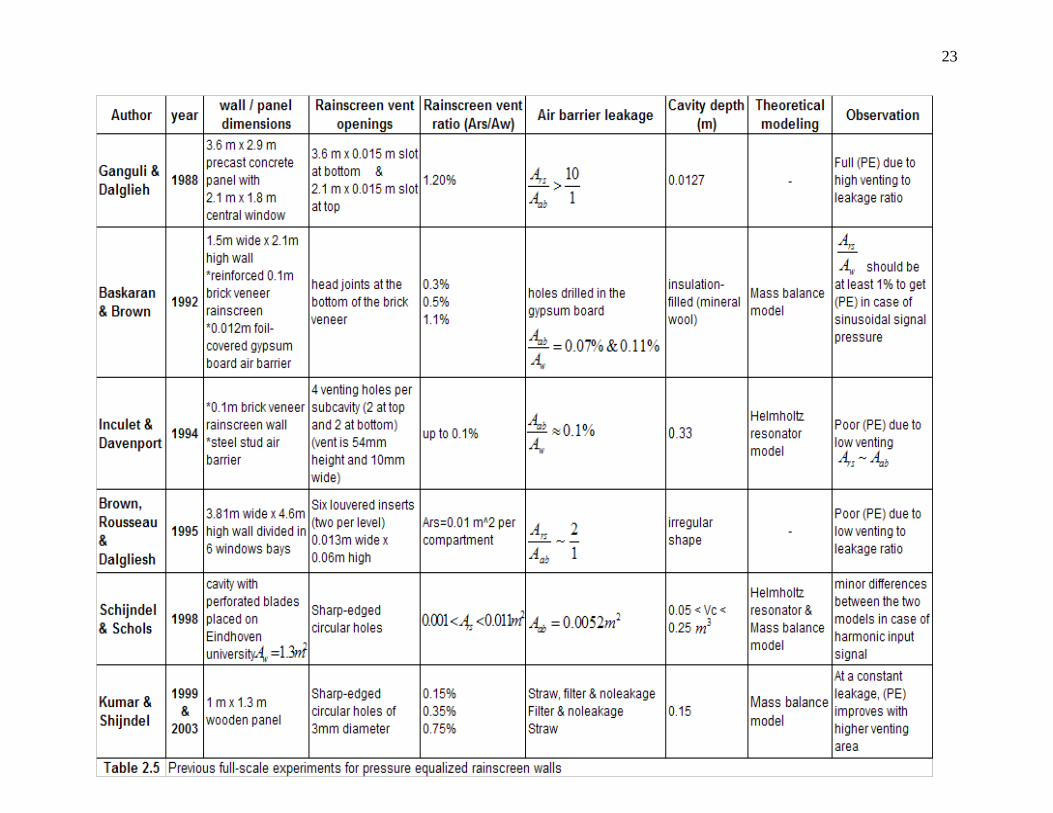
Later, Ganguli and Dalgliesh (1988) showed a satisfactory PE performance of a precast
open rainscreen panel by virtue of its large venting to volume ratio and its small
compartment size, in addition to a well-sealed air barrier. It was suggested that the first
parameter assists in equalizing the fluctuating pressures, the second limits both the mean
and cross flows behind the rainscreen under mean external pressure gradients. The ratio
of vent area to air barrier leakage was greater than 10 to 1, and that what caused the
cavity pressure to equalize fully with the exterior pressure .
On the contrary, poor pressure equalization was revealed with Brown et al. (1995) and
Inculet and Davenport (1994) models due to a small venting rate and low ratio of
rainscreen venting to air barrier leakage area (two to one in the first case and one in the
second case). The differences in these ratios influence the load sharing between the
20
rainscreen and cavity. Brown et al. (1995) observed that only 70% of the pressure drop
across the wall was transferred to the air barrier under static pressure. Also under positive
pressure, the brick veneer was receiving about 64% of the instantaneous load across the
wall, and was capturing 90% under negative wind loading, due to the rapid variation in
the external pressure. On the other hand, Inculet and Davenport (1994) said that the
rainscreen was carrying 58% of the total mean load.
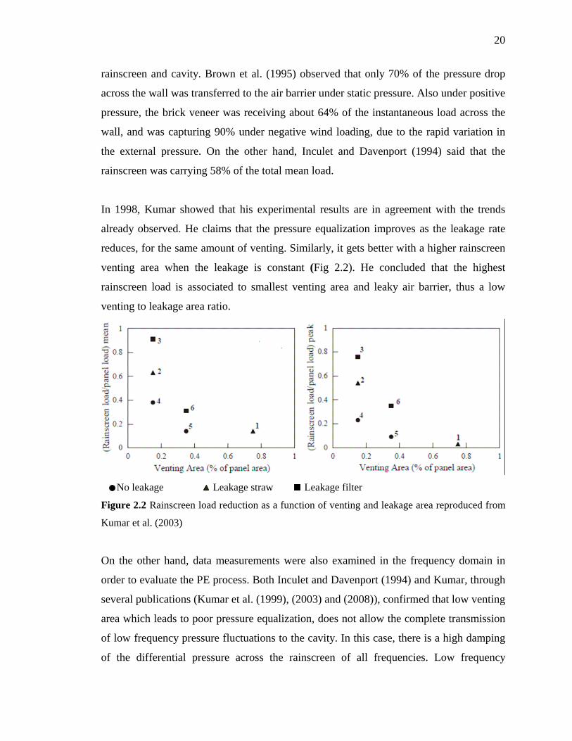
In 1998, Kumar showed that his experimental results are in agreement with the trends
already observed. He claims that the pressure equalization improves as the leakage rate
reduces, for the same amount of venting. Similarly, it gets better with a higher rainscreen
venting area when the leakage is constant (Fig 2.2). He concluded that the highest
rainscreen load is associated to smallest venting area and leaky air barrier, thus a low
venting to leakage area ratio.
No leakage Leakage straw Leakage filter
Figure 2.2 Rainscreen load reduction as a function of venting and leakage area reproduced from
Kumar et al. (2003)
On the other hand, data measurements were also examined in the frequency domain in
order to evaluate the PE process. Both Inculet and Davenport (1994) and Kumar, through
several publications (Kumar et al. (1999), (2003) and (2008)), confirmed that low venting
area which leads to poor pressure equalization, does not allow the complete transmission
of low frequency pressure fluctuations to the cavity. In this case, there is a high damping
of the differential pressure across the rainscreen of all frequencies. Low frequency
21
external fluctuations are attenuated and not completely transmitted to the cavity, while
higher frequencies are completely transferred to the rainscreen.
Furthermore, Kumar observed that the venting area variation significantly affects the
PER wall performance at a constant air barrier leakage rate significantly. Higher-pressure
equalization ratios at lower frequencies can be obtained by increasing the venting area.
However, the high frequency wind pressure fluctuations are not influenced. They are
transferred to the rainscreen almost at the same rate.
Such behaviour in the high frequency region is still in the course of studies and
investigations, especially that it is related to the critical damping frequency according to
Ganguli and Dalgliesh (1988). At full-pressure equalization of PER wall model, the latter
authors observed that only frequencies higher than 1 Hz are taken by the rainscreen. The
suggested reason behind this performance was related to the spatial averaging of the gusts
that may because of the high frequency pressures across the rainscreen.
By mounting the PER panels on the building façades, field experiments can describe how
the wind conditions affect the rainscreen pressures, in case all the data sets are available.
However, Ganguli et al (1988) did not present the data measurements to all the 24 panels
that he has used, and just gave general conclusions. They realized that the strongest winds
did not necessarily give rise to the largest pressure differences across wall panels. In
addition, the peak pressure differences across the rain screens were associated with
storms having wind speeds in the range of 14-15.5m/s.
For a PER panel located between the middle and the corner of the north wall and subject
to full pressure equalization, they attributed the large sustained loads (lasting several
seconds) of around 60 Pa by the rainscreen to exterior pressure gradients coming across,
stating they decrease to 15 Pa when the external pressure becomes uniform. Transient
loads (< 1 second) on the rainscreen of around 200 Pa were tracked under negative wind
pressure. A combination of reasons was suggested referring to the limitation of the
instrumentation, and the small and quick spatial variations of the external fluctuations:
22
the external pressure was varying rapidly, that the cavity could not respond immediately,
and the equalization was not directly accomplished. At this case only, the cladding was
receiving instantaneously 45% of the load.
Kumar et al. (2003) claimed that the highest-pressure coefficients pC
occur when the
wind blows normally to the PER wall panel. Also, they realized that the influence of
wind velocity on PE is predominant in case of leaky air barrier and can be reduced by
providing larger venting area. In general, smaller percentage of long duration wind
pressures is transferred to the rainscreen at lower wind velocities.
Moreover, Baskaran and Brown (1992) and Fazio and Kontopidis (1988) examined the
effect of rainscreen venting on the PER when subject to a sinusoidal signal. They found
similar conclusions referring to a higher cavity response when increasing the rainscreen
venting area ratio, or decreasing the air barrier leakage. Note that details of the field
experiments previously discussed are provided in Table 2.5.
Apart from air barrier leakage and rainscreen venting area ratios, few researchers have
discussed the effect of other parameters on PER wall performance. Canada Mortgage and
Housing Corporation proved in 1999 that compartmentalization of the wall cavities
especially at the corners of a pressure equalized rainscreen system transmits the pressure
load to the air barrier system. In addition, they realized that compartment seals also
withstand pressure loads from both inside and outside, especially in the case of full
compartmentalization. Also, Choi and Wang (1998) also described the air barrier rigidity
role in the PE, in comparison with the curtain walls that have flexible back-panel. He
could demonstrate that for the same venting area and cavity volume, and at the same
frequency of pressure fluctuation, the cavity pressure of curtain wall is lower than the one
of PER wall with rigid back-panels. Therefore, the flexibility of the air barrier can slow
down the increase of the cavity pressure, due to the largest aerodynamic damping.
According to the rainscreen venting, it has the same effect on both assemblies.
23
24
2.3.2 Wind Tunnel Experiments
Previous wind tunnel experiments showed a satisfactory agreement with the full-scale
results and induced the same recommendations regarding the effectiveness of a high
rainscreen venting to air barrier leakage area ratio for pressure equalization like (Irwin et
al. 1984) and (Kumar et al. 2008). Both authors studied a wind tunnel model for the PER
system already tested respectively in Place Air Canada and Eindhoven building
University in full-scale. (Irwin et al. 1984) modified the overall building dimensions and
the cavity depth (0.5mm instead of the actual 0.063mm based on a scale of 1:200) and
reported the results as pressure coefficients. Kumar et al. (2008) showed the results in the
same way. They agreed that a high venting to leakage ratio leads to a good pressure
equalization. In general, measurements of mean, maximum and rms pressure coefficients
for panel and rainscreen sections fall within the range of field data for all the
configurations, except for the worst configuration, with leaky air barrier and smallest
venting area.
For configurations with sufficient leakage and poor venting, lowest reduction in
rainscreen load was observed for both centre and edge taps on the building model (the
centre tap is located where the panel is placed). Differences in rainscreen rms pressure
coefficients showed up for the lowest vent to leakage ratio configuration: field values
were underestimated by the wind tunnel data, due to internal pressure variations in the
field and to the reduced oncoming turbulence in the tunnel. Besides, reductions of
rainscreen loads seemed higher in the wind tunnel in comparison with the field results.
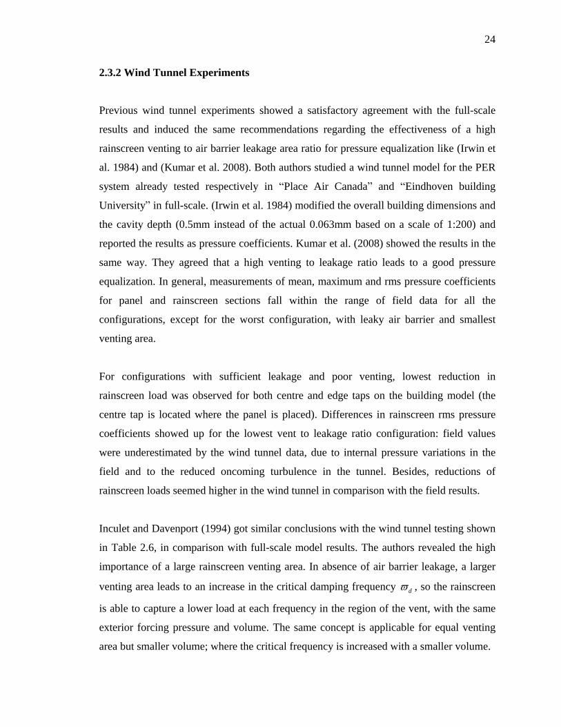
Inculet and Davenport (1994) got similar conclusions with the wind tunnel testing shown
in Table 2.6, in comparison with full-scale model results. The authors revealed the high
importance of a large rainscreen venting area. In absence of air barrier leakage, a larger
venting area leads to an increase in the critical damping frequency d , so the rainscreen
is able to capture a lower load at each frequency in the region of the vent, with the same
exterior forcing pressure and volume. The same concept is applicable for equal venting
area but smaller volume; where the critical frequency is increased with a smaller volume.
25
In case of air barrier leakage, the transfer function of the differential pressure across the
ranscreen is higher than zero at low frequencies.
However, the first case presents some disagreement with Kumar s (1999) observation.
Actually, Kumar considers that, in absence of leakage, increasing the rainscreen venting
area does not affect the transfer function magnitudes of the cavity pressure.
Author Scale
Panel
dimensions
Rainscreen vent
openings
Rainscreen vent ratio (Ars/Aw)
Air barrier porosity
Cavity depth
(m)
Theoretical modeling
Inculet & Davenport (1994)
1:12
rainscreen model mounted on a face of 0.6 m cube
- between 0.02% and 1%
between 0.02% and 0.125%
0.0055 0.0275 (model scale)
Helmholtz resonator model
Kala, Stathopoulos & Kumar (2008)
1:50
*1 m x 1.3 m scaled panel *1mm thick rainscreen
6 holes of 1mm diameter 12 holes of 0.7mm diameter
0.15% 0.35% 0.75%
No leakage & 0.13%
0.15 (full scale) -
Table 2.6 Previous wind tunnel experiments for pressure equalized rainscreen walls
Other wind tunnel tests have also discussed the vent holes distribution and the
compartmentalization of the pressure equalized rainscreen walls based on implications
from buildings pressure models experiments, i.e. the experiments realized by Davenport,
Surry and Inculet in the Boundary Layer Wind Tunnel Laboratory of the University of
Western Ontario. It was shown that mean and unsteady pressure gradients have extremely
large values at the edges of the building face, thus, it is difficult to achieve pressure
equalization near building edges. In this situation, significant residual mean pressure
differences result across the rainscreen. In addition, net mean rainscreen pressures
decrease with decreasing compartment size and with decreasing the mean pressure
gradient.
Besides, as the pressures become progressively more positive further from the edges,
Skerlj and Surry (1994) proposed to place the vents in the rainscreen at the compartment
location that experiences the most positive pressures referring to the locations that are
furthest from the building edge. By installing several rainscreen compartments at various
locations on the face of a building model (1:64 length scale) of various full-scale widths
26
(1m, 2m, 4 m and 8m) where each compartment is vented by one hole placed at its
maximum mean exterior pressure location, Skerlj and Surry realized that at zero degree
wind angle, net negative or near zero pressures act on the rainscreen. Also, the values of
)( pipe CC are around zero at the compartment edge, where the vent is located.
Later, Inculet et al. (2001) observed that pressure gradients dictate the design of venting
openings distribution and the cavity compartmentalization as well. Compartments need
to be extremely small to reduce the pressure difference across a compartment to an
acceptable level . Also, placing of vents at the compartment edge furthest from the
building edge would suppress the forces driving water into the cavity, because of the
higher positive cavity pressure in comparison with the external pressures.
2.3.3 Comparison with Theoretical Model
By applying both Model 1 and Model 2 in the numerical simulations for cavity pressure
prediction in the PER systems of previous tests, it was proven that matching with the
experimental results is governed by the way the key input parameters are used, and the
frequency domain of the external pressures in addition to the way of formulating the
models equations. For instance, in spite of using two different theoretical models, both
Inculet and Davenport (1994) and Kumar et al. (1999) reached the same conclusion: the
theory underestimates the mean pressure drop across the rainscreen, especially under high
frequencies. Also, the discharge coefficient K should be lowered in case of the low
amplitude reversing flows in comparison with its value in the steady flow, for the theory
to match with the experiment, an approach that was first suggested by Holmes (1979)
who adjusted K to 0.15 under high fluctuations pressures, instead of 0.63.
Inculet and Davenport (1994) used the Helmholtz resonator model to predict the PE
performance of a wind tunnel model. Following the concept of adjusting K until the (rms)
values of the pressure drop across the rainscreen equal those of the experiment, the
discharge coefficient was lowered to 0.47 to get a match in the transfer function. It was
noted also that when the rainscreen venting area becomes larger, K is adjusted to 0.19.
27
With the close matching between the experimental and simulated pressures, the low
frequency fluctuation of pressure across the rainscreen were overestimated, while the
high frequency fluctuations were underestimated. The authors attributed these
discrepancies to the linearization of the damping term in the model equations.
Kumar et al. (1999) observed similar results when comparing the simulated pressure time
histories with the measurements of the full-scale model of the panel installed on the
technical university of Eindhoven façade at different wind speeds and air barrier leakage
conditions. In spite of the agreement between the two numerical models in the differential
pressures predictions across the rainscreen, Model 1 was used for the prediction of cavity
pressure; due to a less number of floating point operations 6101.1 x in comparison with
Model 2 at 9107.2 x , thus it is much faster. In addition, Kumar considered that the inertial
effect in Model 2 could be avoided, because the resonance is highly unlikely to occur
when inspecting the undamped natural frequency expression. Therefore, with the general
matching between the trends of numerical and experimental results, Kumar attributed the
differences to the fact that the numerical model does not take into account the spatial
non-uniformity of pressures acting on the panel, and the appropriate damping of flow (the
input pressure was the average exterior pressure acting on the panel along with a damping
through a single vent hole only). Regarding the pressure drop across the rainscreen,
Kumar found that the simulated time histories ( )e cP P were smoother, and some real
peaks were unpredicted. Also, the amplitudes of ( ) /S f ² were higher above 1 Hz in case
of the measured rainscreen pressures. Note that, K was lowered to 0.49, but it was also
noticed that in absence of air barrier leakage, a better agreement exists between numerical
and experimental transfer functions when lowering K.
Other authors launched numerical simulations by using sinusoidal input signals. Baskaran
and Brown (1992) showed a match between pressure difference measurements across the
raincreen and the computations based on mass balance model. However, sometimes the
cavity pressure was overestimated and the phase shift underestimated by Model 1, which
was explained by estimating the time lag as the inverse of undamped resonant frequency,
28
independently from the leakage area. In addition, the value of 0.5 was used for the air
barrier flow exponent.
Schijndel and Schols (1998) developed equations based on both the Helmholtz resonator
model and Mass balance model, and found a satisfactory agreement between the
predictions of both models. The authors explained this saying that the second-order
inertial term 2 2cd P dt used in Helmholtz equation is small with respect to the damping
term, when the vent area is large enough compared with volume as Harris (1990) pointed
out. A match was observed between experimental and numerical pressure drop across the
rainscreen at frequencies less than 0.1 Hz, while the simulated pressure depicted more
damping for the fluctuations at more than 0.1Hz.
2.4 Design Guidelines for PER
2.4.1 Rainscreen Venting Area
The rainscreen implementation reduces the differential pressure resulting from the wind
loading on buildings that causes rainwater penetration as revealed by Kumar (2000). Its
venting process controls the rate of transferring the air volume necessary to equalize
cavity pressure with external pressure. The percentage of the necessary venting area
depends on the amount of leakage of the air barrier, as well as the volume of air within
the compartment. The majority of researchers agree on a high venting to leakage area
ratio. Latta (1973) suggested a venting area of 10 times the leakage area under steady
wind conditions. Killip and Cheetham (1984) found that it should be between 25 and 40
times the leakage area, while the minimum ratio is 20 for NRC (1998). Morrison
Hershfield Ltd (1998) explained that the effective venting area for a compartment should
be the sum of 1) 5 times the estimated leakage area of the air barrier, 2) 10 times the
estimated leakage area of any corner seals, and 3) 1 times the estimated leakage area of
intermediate compartment seals. Inculet (1990) specified for most high-rise buildings, a
ratio venting to total wall area not less than 2%, based on precast concrete or metal panel
high-rise building façades. The criterion is that the differential pressure across the
rainscreen is less than 1% of the mean pressure drop across the composite wall.
29
2.4.2 Venting Configuration (locations and dimensions)
Since the deliberate vent openings ensure a rapid equalization of the cavity pressure with
the external pressure, they should be distributed over the panel face, in order to reduce
the average wind load acting on the external cladding. Vents are usually located at the
bottom of the wall, so they can also drain it; besides, all vents of a compartment should
be placed at the same height to avoid airflow loops. Generally, they are symmetric with
respect to the panel, while Morrison Hershfield Ltd (1998) proposed an asymmetrical
vent holes distribution. Also, some studies suggest their placement on the side of the
compartment closest to the centre of the façade. This helps raising the cavity pressure,
since the vent is located where the pressure on the face is high, and pushes the water out
of leakage paths. The minimum adopted diameter of venting holes is 10mm, based on
Garden (1963) to eliminate capillary plugs.
2.4.3 Cavity Volume
2.4.3.1 Cavity Depth:
In general, the smaller the cavity volume, the lesser is the airflow Q necessary to equalize
the pressures, and the faster is the response time of the cavity pressure. The minimum
allowed cavity depth is 25mm (Garden (1963)). In 1990, Inculet established the following
relation 10 rs Wdc A A
indicating that more rainscreen venting is needed for a larger
cavity.
2.4.3.2 Compartment Size:
As a rule of thumb, the compartment height should not exceed 6m (about two stories).
Garden (1963) proposed the location of horizontal closures up to 9m on centres over the
total wall area; and vertical enclosures should be provided at each outside corner of a
building, and at 1.2m intervals for about 6m from the corners, while compartment width
could be up to 6m in the central portion of the façade and about 1.2 m at building edges
and parapets. The British Standards (8200) mentioned that the largest lateral dimension
of air spaces within 25% of the corner or top of the enclosure should be about 1.5m, and
elsewhere about 5m. Cavity compartmentalization is made using separators or
30
delimiters; that connect the rainscreen to the air barrier system. According to Kumar
(2000), they provide compartment seals at wall corners where the seals should be
designed in order to withstand 2-3 times the wind load. Besides, they ensure an adequate
number of ties to transfer the lateral loads from the rainscreen to the air barrier. Multiple
wall components can act as delimiters, such as metal shelf angles, rigid sheet metal and
foam plastic insulation strips, as long as they can be made relatively airtight and can be
installed to sustain the lateral air pressure loads.
2.4.4 Air Barrier Stiffness and Leakage
The air barrier must be supported structurally to withstand both sustained and peak wind
pressures and suctions with a resulting deflection that can be accommodated within the
wall assembly. In fact, the excessive flexibility of the air barrier system will result in
fluctuations in the volume of the air chamber compartment, which will adversely affect
the potential for rapid pressure equalization across the rainscreen.The air barrier leakage
is an unavoidable matter, even present in all nominally sealed buildings. For IRC s
Canadian Construction Materials Centre (CCMC), the maximum air leakage rate
allowable for the air barrier system in exterior walls of low-rise buildings is 20.2 / ( . )L s m
at 75 Pa pressure differential. Others recommended that air permeability values would be
less than 6 3 21.3 10 / /x m m Pa or 20.1 /Q Lps m
31
CHAPTER 3
FULL-SCALE EXPERIMENT
3.1 Test Methodology
The current full-scale experiment aims at examining the rainscreen venting area effects
on the PER wall performance a under random pressures signals associated to real wind
fluctuations. The majority of experiments previously done in the field were applying
wind pressures on PER panel after it is installed on the building, meaning that the tests
results are significantly influenced by leakage, an unavoidable problem in the cladding
industry. Here, I am trying to achieve a completely sealed full-scale model, by
minimizing the leakage rate, in order to reach an optimum pressure equalization
performance using the design parameters of the theory. The experiment has been carried
out at the Insurance Research Laboratory for Better Homes (IRLBH), which is built by
the University of Western Ontario in London Airport location, and known as the Three
Little Pigs Project . The full-scale model dimensions were dictated by the general design
guidelines for PER walls, as well as the in-situ conditions of the facility. I decided to
build a PER wall panel with one compartment combining the good performance with the
ability to sustain the maximum loads pressures.
3.1.1 Model
A 2.6 m length by 2 m height rectangular rig is built bounded by two steel I-section
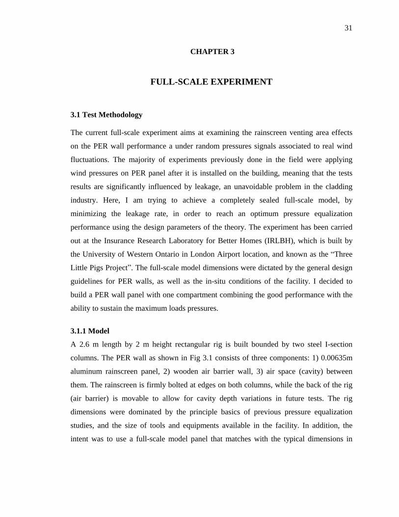
columns. The PER wall as shown in Fig 3.1 consists of three components: 1) 0.00635m
aluminum rainscreen panel, 2) wooden air barrier wall, 3) air space (cavity) between
them. The rainscreen is firmly bolted at edges on both columns, while the back of the rig
(air barrier) is movable to allow for cavity depth variations in future tests. The rig
dimensions were dominated by the principle basics of previous pressure equalization
studies, and the size of tools and equipments available in the facility. In addition, the
intent was to use a full-scale model panel that matches with the typical dimensions in
32
industry, and allows different test configurations in terms of vent area and location to be
explored.
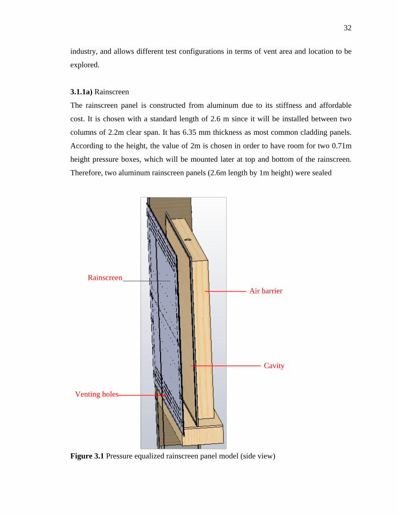
3.1.1a) Rainscreen
The rainscreen panel is constructed from aluminum due to its stiffness and affordable
cost. It is chosen with a standard length of 2.6 m since it will be installed between two
columns of 2.2m clear span. It has 6.35 mm thickness as most common cladding panels.
According to the height, the value of 2m is chosen in order to have room for two 0.71m
height pressure boxes, which will be mounted later at top and bottom of the rainscreen.
Therefore, two aluminum rainscreen panels (2.6m length by 1m height) were sealed
Figure 3.1 Pressure equalized rainscreen panel model (side view)
Air barrier
Rainscreen
Venting holes
Cavity
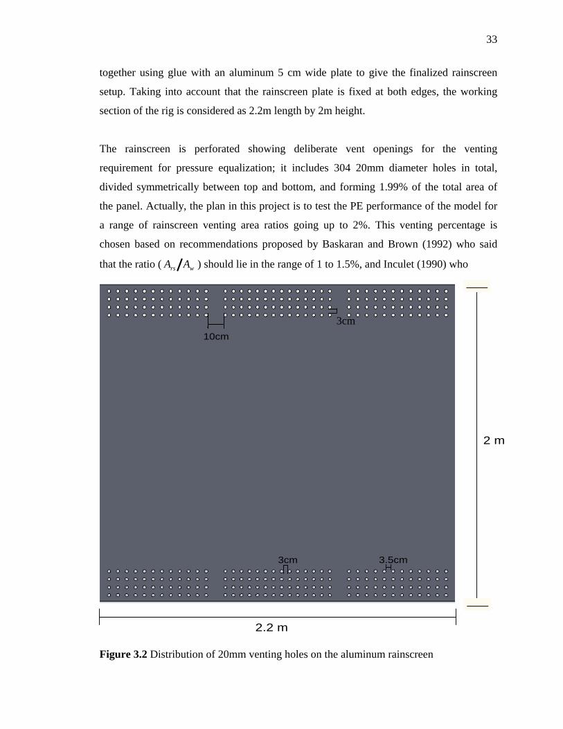
33
together using glue with an aluminum 5 cm wide plate to give the finalized rainscreen
setup. Taking into account that the rainscreen plate is fixed at both edges, the working
section of the rig is considered as 2.2m length by 2m height.
The rainscreen is perforated showing deliberate vent openings for the venting
requirement for pressure equalization; it includes 304 20mm diameter holes in total,
divided symmetrically between top and bottom, and forming 1.99% of the total area of
the panel. Actually, the plan in this project is to test the PE performance of the model for
a range of rainscreen venting area ratios going up to 2%. This venting percentage is
chosen based on recommendations proposed by Baskaran and Brown (1992) who said
that the ratio ( wrs AA ) should lie in the range of 1 to 1.5%, and Inculet (1990) who
Figure 3.2 Distribution of 20mm venting holes on the aluminum rainscreen
2.2 m
2 m
3.5cm
10cm
3cm
3cm
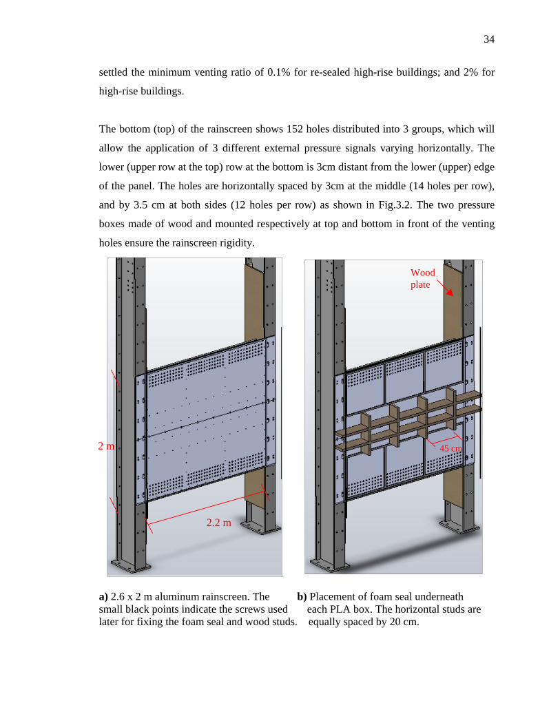
34
settled the minimum venting ratio of 0.1% for re-sealed high-rise buildings; and 2% for
high-rise buildings.
The bottom (top) of the rainscreen shows 152 holes distributed into 3 groups, which will
allow the application of 3 different external pressure signals varying horizontally. The
lower (upper row at the top) row at the bottom is 3cm distant from the lower (upper) edge
of the panel. The holes are horizontally spaced by 3cm at the middle (14 holes per row),
and by 3.5 cm at both sides (12 holes per row) as shown in Fig.3.2. The two pressure
boxes made of wood and mounted respectively at top and bottom in front of the venting
holes ensure the rainscreen rigidity.
a) 2.6 x 2 m aluminum rainscreen. The b) Placement of foam seal underneath small black points indicate the screws used each PLA box. The horizontal studs are later for fixing the foam seal and wood studs. equally spaced by 20 cm.
2.2 m
2 m
45 cm
Wood plate
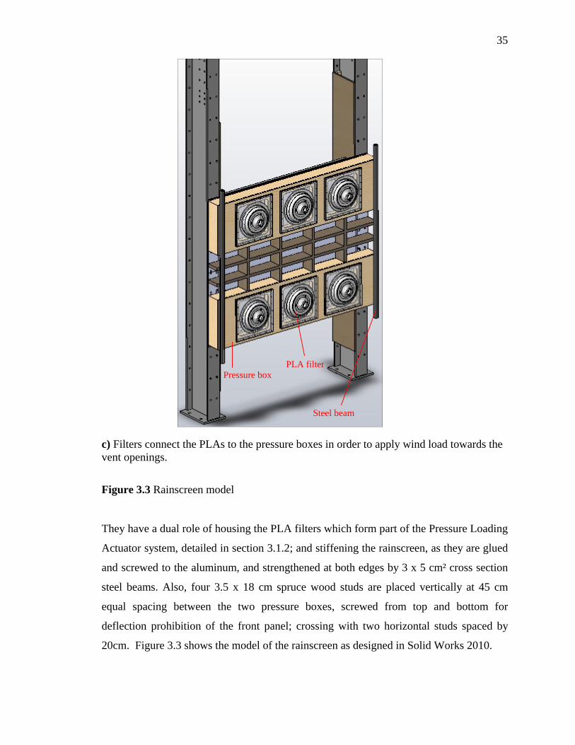
35
c) Filters connect the PLAs to the pressure boxes in order to apply wind load towards the vent openings.
Figure 3.3 Rainscreen model
They have a dual role of housing the PLA filters which form part of the Pressure Loading
Actuator system, detailed in section 3.1.2; and stiffening the rainscreen, as they are glued
and screwed to the aluminum, and strengthened at both edges by 3 x 5 cm² cross section
steel beams. Also, four 3.5 x 18 cm spruce wood studs are placed vertically at 45 cm
equal spacing between the two pressure boxes, screwed from top and bottom for
deflection prohibition of the front panel; crossing with two horizontal studs spaced by
20cm. Figure 3.3 shows the model of the rainscreen as designed in Solid Works 2010.
PLA filter
Pressure box
Steel beam
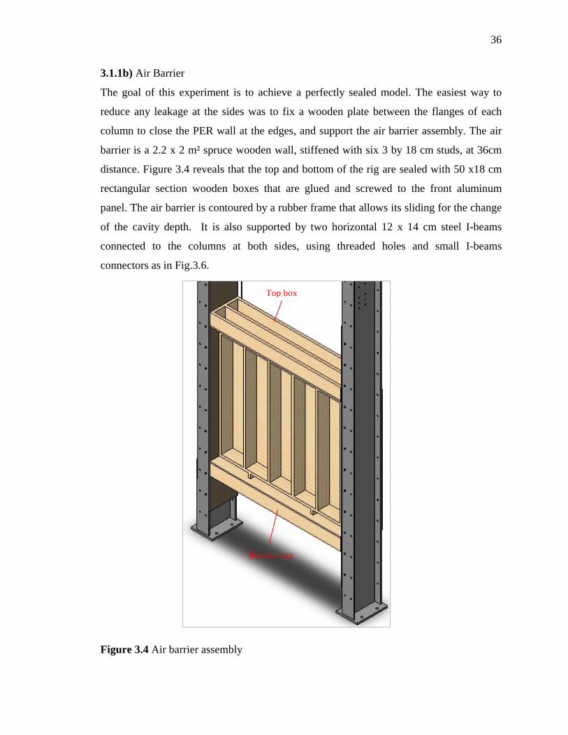
36
3.1.1b) Air Barrier
The goal of this experiment is to achieve a perfectly sealed model. The easiest way to
reduce any leakage at the sides was to fix a wooden plate between the flanges of each
column to close the PER wall at the edges, and support the air barrier assembly. The air
barrier is a 2.2 x 2 m² spruce wooden wall, stiffened with six 3 by 18 cm studs, at 36cm
distance. Figure 3.4 reveals that the top and bottom of the rig are sealed with 50 x18 cm
rectangular section wooden boxes that are glued and screwed to the front aluminum
panel. The air barrier is contoured by a rubber frame that allows its sliding for the change
of the cavity depth. It is also supported by two horizontal 12 x 14 cm steel I-beams
connected to the columns at both sides, using threaded holes and small I-beams
connectors as in Fig.3.6.
Figure 3.4 Air barrier assembly
Top box
Bottom box
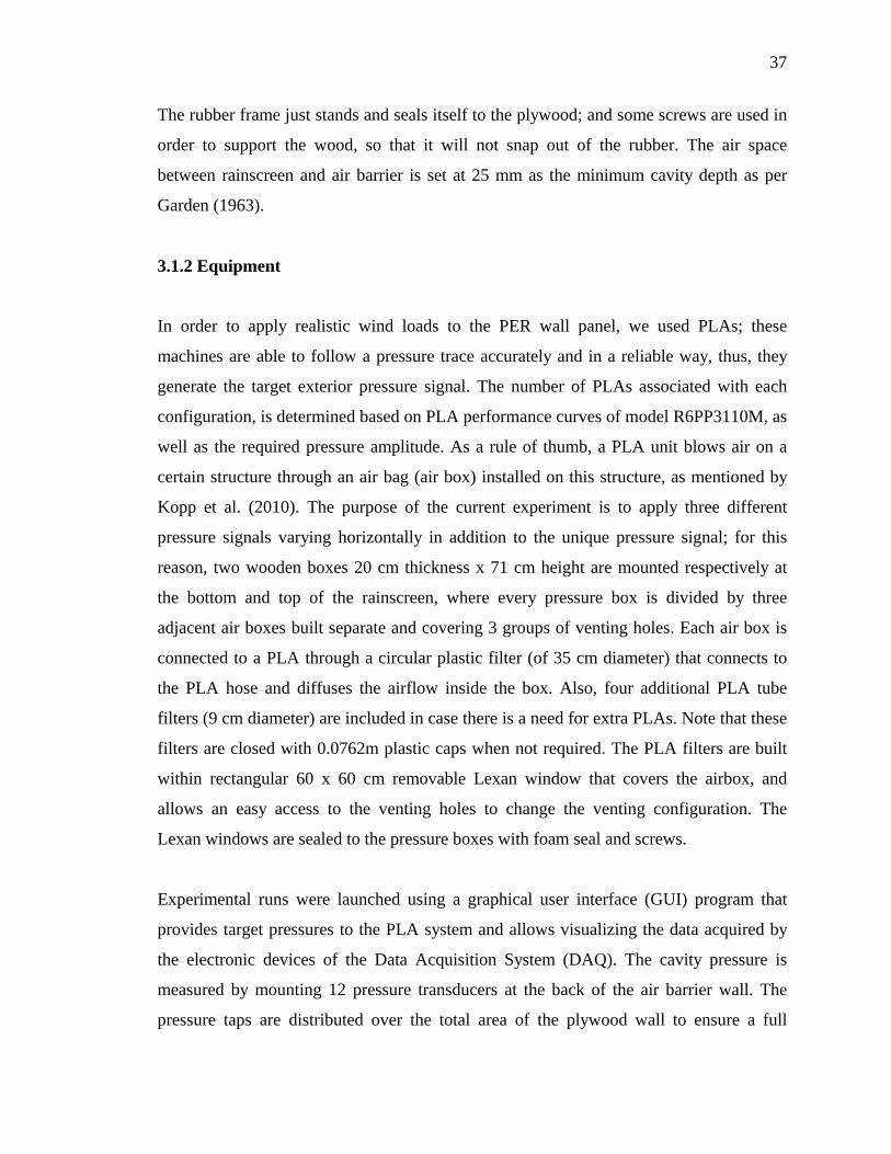
37
The rubber frame just stands and seals itself to the plywood; and some screws are used in
order to support the wood, so that it will not snap out of the rubber. The air space
between rainscreen and air barrier is set at 25 mm as the minimum cavity depth as per
Garden (1963).
3.1.2 Equipment
In order to apply realistic wind loads to the PER wall panel, we used PLAs; these
machines are able to follow a pressure trace accurately and in a reliable way, thus, they
generate the target exterior pressure signal. The number of PLAs associated with each
configuration, is determined based on PLA performance curves of model R6PP3110M, as
well as the required pressure amplitude. As a rule of thumb, a PLA unit blows air on a
certain structure through an air bag (air box) installed on this structure, as mentioned by
Kopp et al. (2010). The purpose of the current experiment is to apply three different
pressure signals varying horizontally in addition to the unique pressure signal; for this
reason, two wooden boxes 20 cm thickness x 71 cm height are mounted respectively at
the bottom and top of the rainscreen, where every pressure box is divided by three
adjacent air boxes built separate and covering 3 groups of venting holes. Each air box is
connected to a PLA through a circular plastic filter (of 35 cm diameter) that connects to
the PLA hose and diffuses the airflow inside the box. Also, four additional PLA tube
filters (9 cm diameter) are included in case there is a need for extra PLAs. Note that these
filters are closed with 0.0762m plastic caps when not required. The PLA filters are built
within rectangular 60 x 60 cm removable Lexan window that covers the airbox, and
allows an easy access to the venting holes to change the venting configuration. The
Lexan windows are sealed to the pressure boxes with foam seal and screws.
Experimental runs were launched using a graphical user interface (GUI) program that
provides target pressures to the PLA system and allows visualizing the data acquired by
the electronic devices of the Data Acquisition System (DAQ). The cavity pressure is
measured by mounting 12 pressure transducers at the back of the air barrier wall. The
pressure taps are distributed over the total area of the plywood wall to ensure a full
38
coverage of the cavity pressure, Figure 3.5.b. Measurements are recorded with the DAQ
formed by a National Instrument NI PXI-1042 computer device and SCXI 1004 Modules
chassis; these are connected to a Triple-output 30V, 3A Digital Display DC power
supply. The whole system allows reading the voltage measured by eighteen HOSKIN
pressure transducers, of a range of ( 1) (+1) PSI, connected to the SCXI Modules; and
then voltage values are converted to pressure.
The pressure signal achieved by the PLAs is read using six pressure transducers of the
same type, that are placed on the six air boxes at top and bottom of the rainscreen, and
each is linked to its corresponding PLA. In some cases, where the air box does not allow
enough room for the placement of the pressure tap on one side, the pressure transducer is
installed on the other side closely to another pressure transducer associated to an adjacent
air bag, as shown in Fig.3.5a.
a) Pressure transducers distribution on the pressure boxes
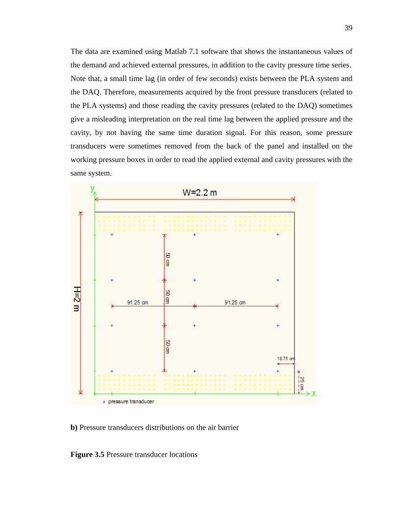
39
The data are examined using Matlab 7.1 software that shows the instantaneous values of
the demand and achieved external pressures, in addition to the cavity pressure time series.
Note that, a small time lag (in order of few seconds) exists between the PLA system and
the DAQ. Therefore, measurements acquired by the front pressure transducers (related to
the PLA systems) and those reading the cavity pressures (related to the DAQ) sometimes
give a misleading interpretation on the real time lag between the applied pressure and the
cavity, by not having the same time duration signal. For this reason, some pressure
transducers were sometimes removed from the back of the panel and installed on the
working pressure boxes in order to read the applied external and cavity pressures with the
same system.
b) Pressure transducers distributions on the air barrier
Figure 3.5 Pressure transducer locations
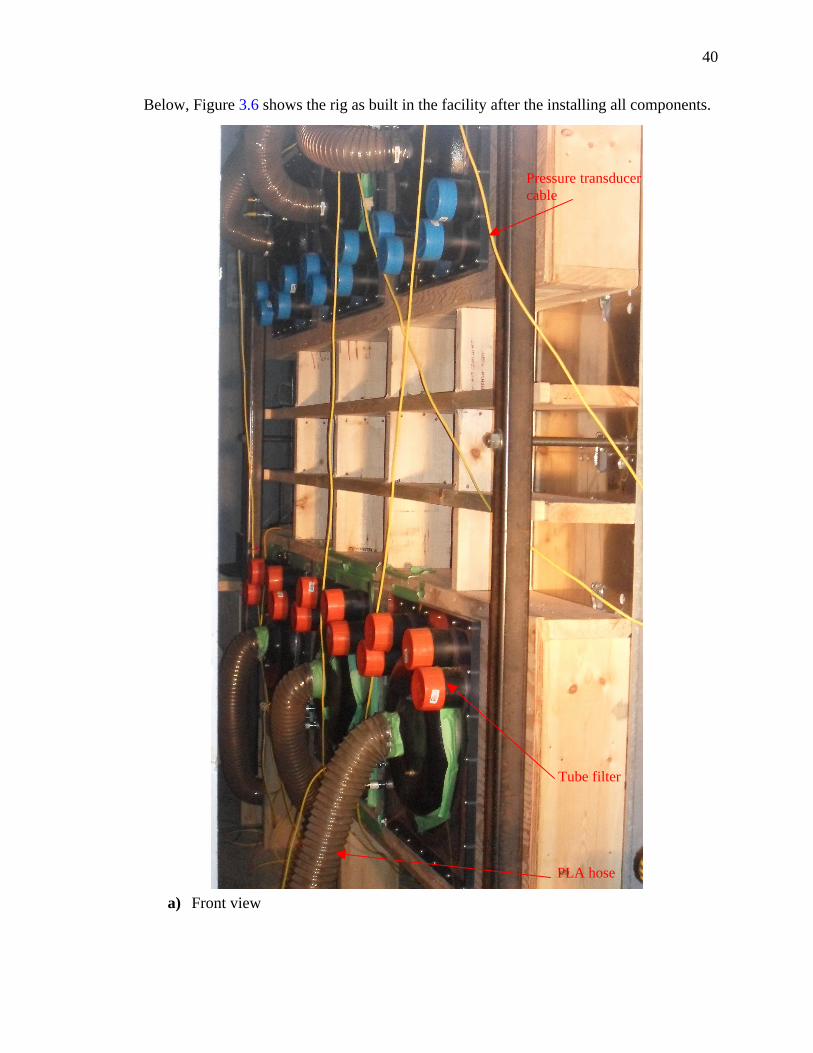
40
Below, Figure 3.6 shows the rig as built in the facility after the installing all components.
a) Front view
Pressure
transducer
cable
Tube filter
PLA hose
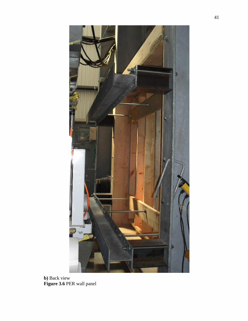
41
b) Back view Figure 3.6 PER wall panel
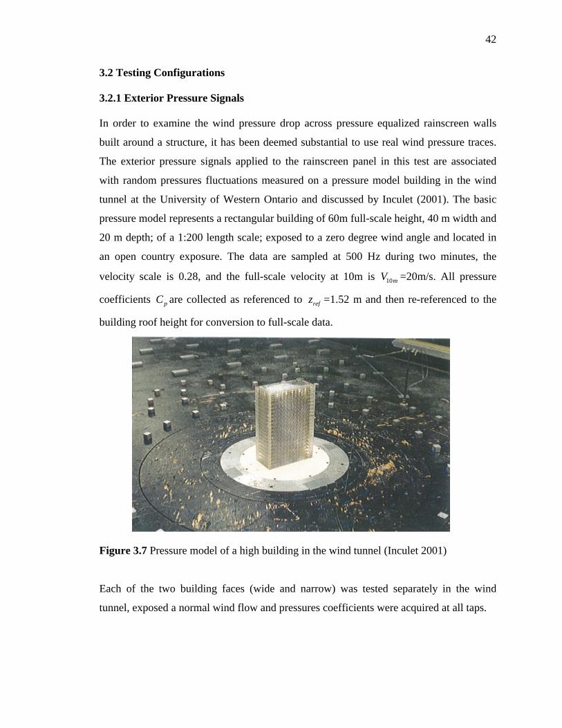
42
3.2 Testing Configurations
3.2.1 Exterior Pressure Signals
In order to examine the wind pressure drop across pressure equalized rainscreen walls
built around a structure, it has been deemed substantial to use real wind pressure traces.
The exterior pressure signals applied to the rainscreen panel in this test are associated
with random pressures fluctuations measured on a pressure model building in the wind
tunnel at the University of Western Ontario and discussed by Inculet (2001). The basic
pressure model represents a rectangular building of 60m full-scale height, 40 m width and
20 m depth; of a 1:200 length scale; exposed to a zero degree wind angle and located in
an open country exposure. The data are sampled at 500 Hz during two minutes, the
velocity scale is 0.28, and the full-scale velocity at 10m is 10mV =20m/s. All pressure
coefficients pC are collected as referenced to refz =1.52 m and then re-referenced to the
building roof height for conversion to full-scale data.
Figure 3.7 Pressure model of a high building in the wind tunnel (Inculet 2001)
Each of the two building faces (wide and narrow) was tested separately in the wind
tunnel, exposed a normal wind flow and pressures coefficients were acquired at all taps.
43
For the present full-scale experiment, the external pressure signals applied to the PER
panel correspond to pressures acquired at specific taps for both the wide and narrow faces
(each being windward face). For each face, four pressure traces of five minutes
equivalent full-scale duration are extracted from the data: 1) one random signal P
associated to a middle tap; that will be applied simultaneously to all pressure boxes of the
panel; and 2) three pressure signals 1P , 2P , 3P corresponding to three edge taps located at
the left of the face. These will be applied simultaneously at the three adjacent pressure
boxes at the bottom of the panel in order to examine the differential pressure across the
rainscreen under an external pressure gradient.
The four pressure taps used are located at the same position of 0.76m my H
(where
my designates the vertical coordinate from the bottom of the building model). This height
is chosen as being proximate to the location of the maximum pressure distribution in the
middle of the face; also the corresponding edge taps pressure values are not extremely
small.
In fact, the middle pressure tap is located at 1.45 cm vertical distance (model scale) above
the maximum mean pressure coefficient tap in the wind tunnel model, where pC max is
equal to 0.368 at 0.75m my H
equivalent to 0.75 value in full-scale. Figure 3.8 shows
the mean pressure coefficient distribution data for the wide face at 0.76m my H ,
representing the taps used in the experiment. Also, it indicates the equivalent full-scale
horizontal distance in meters originating from the left side of the PER model, i.e. the tap
corresponding to the external pressure ( 1P ) is associated with the first air box (0.73m
length) mounted on the rainscreen from the left; the second tap ( 2P ) refers to the second
airbox (0.73m < rx
< 1.46m), and the third tap (P3) is assumed to be located within the
third pressure box.
At the testing stage, the signals were converted to full-scale and given to the PLAs as
pressure values instead of pressure coefficients. However, the pressure transducers were
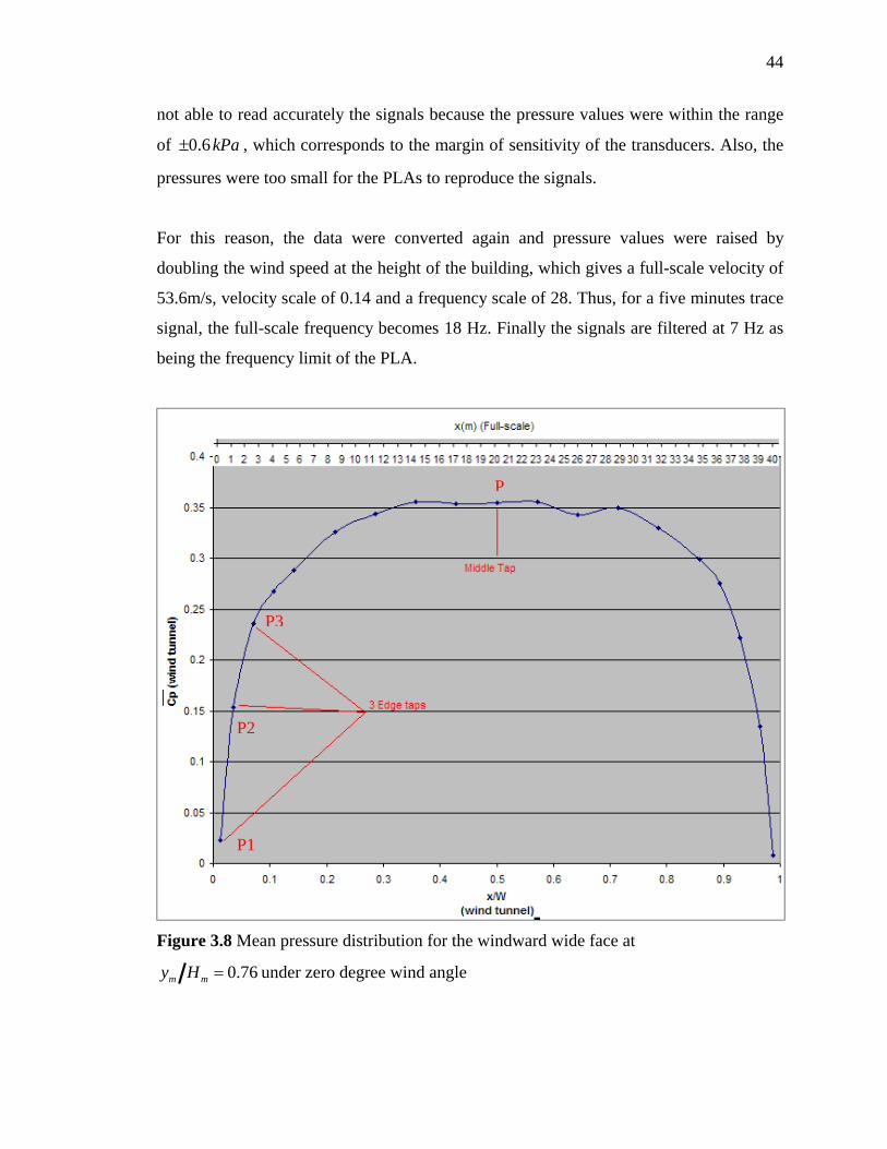
44
not able to read accurately the signals because the pressure values were within the range
of 0.6 kPa , which corresponds to the margin of sensitivity of the transducers. Also, the
pressures were too small for the PLAs to reproduce the signals.
For this reason, the data were converted again and pressure values were raised by
doubling the wind speed at the height of the building, which gives a full-scale velocity of
53.6m/s, velocity scale of 0.14 and a frequency scale of 28. Thus, for a five minutes trace
signal, the full-scale frequency becomes 18 Hz. Finally the signals are filtered at 7 Hz as
being the frequency limit of the PLA.
Figure 3.8 Mean pressure distribution for the windward wide face at
0.76m my H under zero degree wind angle
P
P1
P2
P3
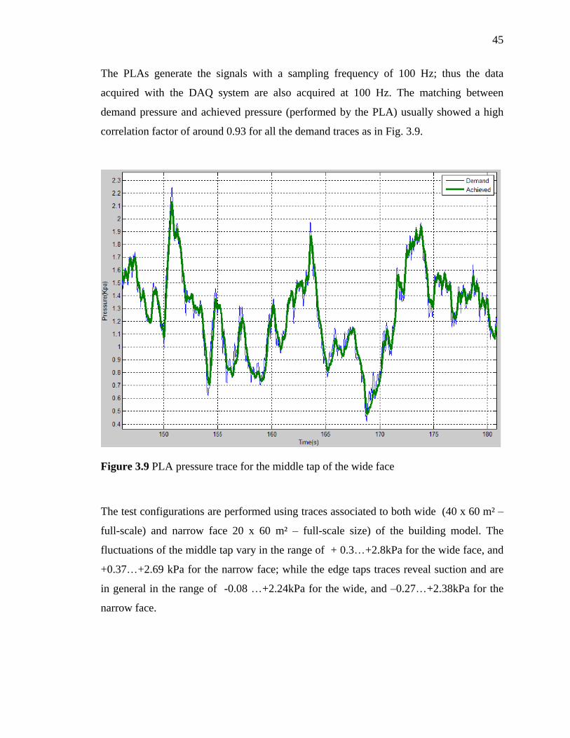
45
The PLAs generate the signals with a sampling frequency of 100 Hz; thus the data
acquired with the DAQ system are also acquired at 100 Hz. The matching between
demand pressure and achieved pressure (performed by the PLA) usually showed a high
correlation factor of around 0.93 for all the demand traces as in Fig. 3.9.
Figure 3.9 PLA pressure trace for the middle tap of the wide face
The test configurations are performed using traces associated to both wide (40 x 60 m²
full-scale) and narrow face 20 x 60 m²
full-scale size) of the building model. The
fluctuations of the middle tap vary in the range of + 0.3 +2.8kPa for the wide face, and
+0.37 +2.69 kPa for the narrow face; while the edge taps traces reveal suction and are
in general in the range of -0.08 +2.24kPa for the wide, and 0.27 +2.38kPa for the
narrow face.
46
3.2.2 Panel Setup Configurations
The differential pressure across the rainscreen due to the applied pressure traces is
examined by varying two parameters: 1) the rainscreen venting area ratio VA
and 2) the
location of vent holes. This is done by redistributing the deliberate openings at a certain
venting area between top and bottom of the rainscreen.
The cavity depth was set constant at 25mm as the minimum required space in a pressure
equalized rainscreen system. 0.0207m pliable vinyl plugs diameter were used to provide
changes in the aluminum rainscreen venting area: each time the movable Lexan windows
were pulled out in order to plug or unplug the 20mm holes under the pressure boxes, and
then moved back to their location by fastening with set screws. For venting cases, the aim
was to perform tests within a wide range of venting to wall area ratios starting from the
lowest (equivalent to one hole in the rainnscreen) to the maximum limit obtained with
304 vent holes. However, pressure equalization between the exterior and the cavity at
cd =25mm was reached for 15 vent holes where 0.11%VA ; and it stabilized for 36 vent
holes ( 0.27%VA ), thus it was decided to stop the tests configurations at this stage.
Table 3.1 shows the different test configurations based on the ratio of rainscreen venting
area ( rsA ) to the total wall area ( wA ). Each run was performed twice; by applying the
pressure signals associated to both wide and narrow faces.
Also, Appendix A (section A.1) shows the drawings of the different test cases and the
distribution of plugged and unplugged vent holes at top and bottom of the rainscreen.
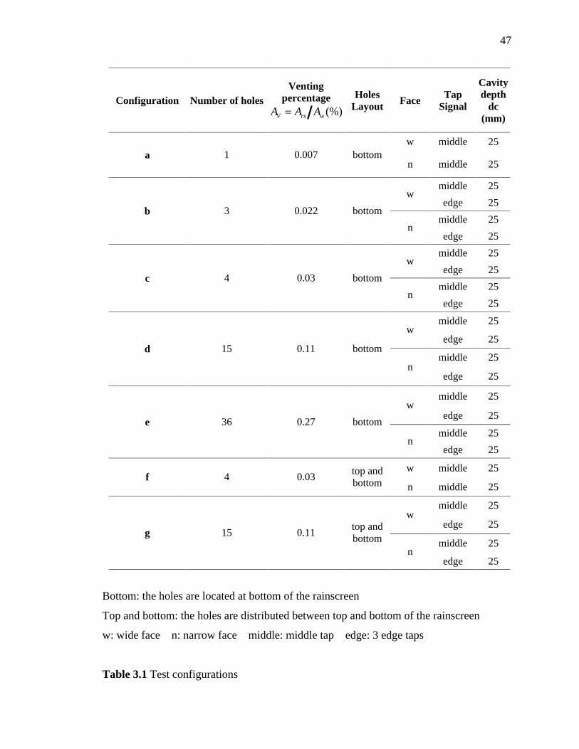
47
Configuration Number of holes
Venting
percentage (%)V rs wA A A
Holes Layout Face Tap
Signal
Cavity depth
dc (mm)
w middle 25
a 1 0.007 bottom n middle 25
middle 25 w
edge 25
middle 25 b 3 0.022 bottom
n edge 25
middle 25 w
edge 25
middle 25 c 4 0.03 bottom
n edge 25
middle 25 w
edge 25
middle 25 d 15 0.11 bottom
n edge 25
middle 25 w
edge 25
middle 25 e 36 0.27 bottom
n edge 25
w middle 25 f 4 0.03
top and bottom n middle 25
middle 25 w
edge 25
middle 25 g 15 0.11
top and bottom
n edge 25
Bottom: the holes are located at bottom of the rainscreen
Top and bottom: the holes are distributed between top and bottom of the rainscreen
w: wide face n: narrow face middle: middle tap edge: 3 edge taps
Table 3.1 Test configurations
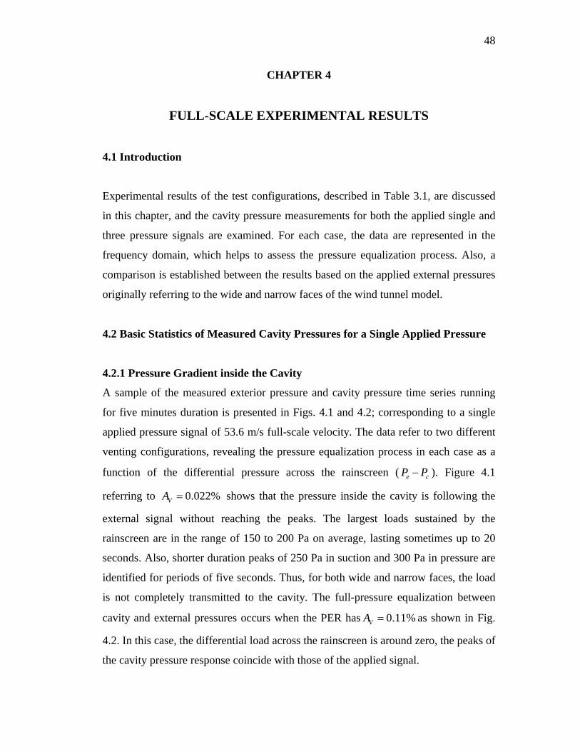
48
CHAPTER 4
FULL-SCALE EXPERIMENTAL RESULTS
4.1 Introduction
Experimental results of the test configurations, described in Table 3.1, are discussed
in this chapter, and the cavity pressure measurements for both the applied single and
three pressure signals are examined. For each case, the data are represented in the
frequency domain, which helps to assess the pressure equalization process. Also, a
comparison is established between the results based on the applied external pressures
originally referring to the wide and narrow faces of the wind tunnel model.
4.2 Basic Statistics of Measured Cavity Pressures for a Single Applied Pressure
4.2.1 Pressure Gradient inside the Cavity
A sample of the measured exterior pressure and cavity pressure time series running
for five minutes duration is presented in Figs. 4.1 and 4.2; corresponding to a single
applied pressure signal of 53.6 m/s full-scale velocity. The data refer to two different
venting configurations, revealing the pressure equalization process in each case as a
function of the differential pressure across the rainscreen ( e cP P ). Figure 4.1
referring to 0.022%VA
shows that the pressure inside the cavity is following the
external signal without reaching the peaks. The largest loads sustained by the
rainscreen are in the range of 150 to 200 Pa on average, lasting sometimes up to 20
seconds. Also, shorter duration peaks of 250 Pa in suction and 300 Pa in pressure are
identified for periods of five seconds. Thus, for both wide and narrow faces, the load
is not completely transmitted to the cavity. The full-pressure equalization between
cavity and external pressures occurs when the PER has 0.11%VA as shown in Fig.
4.2. In this case, the differential load across the rainscreen is around zero, the peaks of
the cavity pressure response coincide with those of the applied signal.
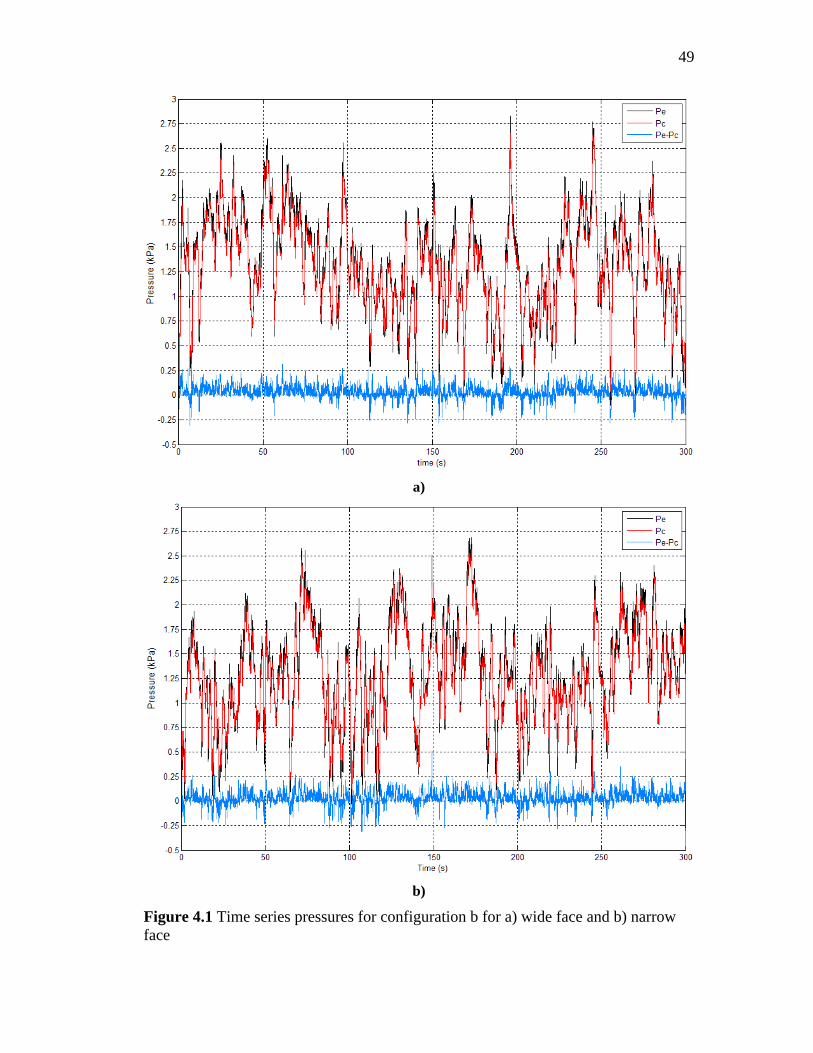
49
a)
b)
Figure 4.1 Time series pressures for configuration b for a) wide face and b) narrow face
50
a)
b)
Figure 4.2 Time series pressures for configuration d for a) wide face and b) narrow face
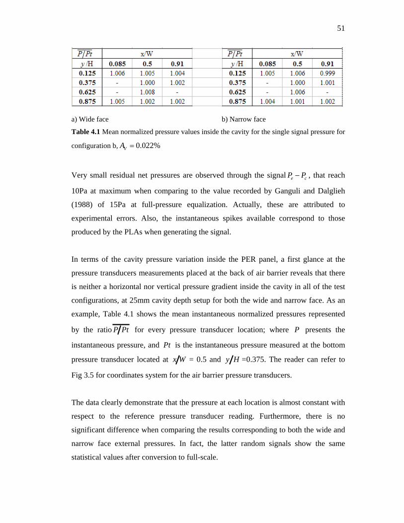
51
a) Wide face b) Narrow face
Table 4.1 Mean normalized pressure values inside the cavity for the single signal pressure for
configuration b, 0.022%VA
Very small residual net pressures are observed through the signal e cP P , that reach
10Pa at maximum when comparing to the value recorded by Ganguli and Dalglieh
(1988) of 15Pa at full-pressure equalization. Actually, these are attributed to
experimental errors. Also, the instantaneous spikes available correspond to those
produced by the PLAs when generating the signal.
In terms of the cavity pressure variation inside the PER panel, a first glance at the
pressure transducers measurements placed at the back of air barrier reveals that there
is neither a horizontal nor vertical pressure gradient inside the cavity in all of the test
configurations, at 25mm cavity depth setup for both the wide and narrow face. As an
example, Table 4.1 shows the mean instantaneous normalized pressures represented
by the ratio P Pt
for every pressure transducer location; where P
presents the
instantaneous pressure, and Pt
is the instantaneous pressure measured at the bottom
pressure transducer located at x W = 0.5 and y H =0.375. The reader can refer to
Fig 3.5 for coordinates system for the air barrier pressure transducers.
The data clearly demonstrate that the pressure at each location is almost constant with
respect to the reference pressure transducer reading. Furthermore, there is no
significant difference when comparing the results corresponding to both the wide and
narrow face external pressures. In fact, the latter random signals show the same
statistical values after conversion to full-scale.
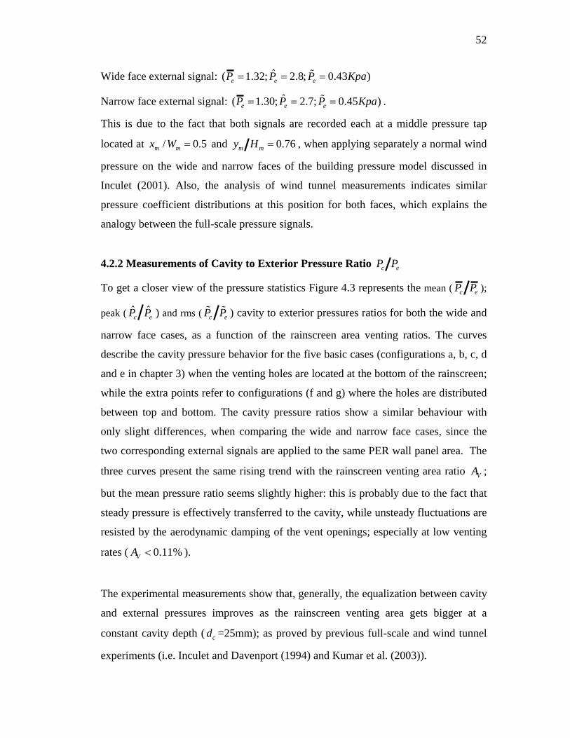
52
Wide face external signal: ( 1.32; 2.8; 0.43 )e e eP P P Kpa
Narrow face external signal: ( 1.30; 2.7; 0.45 )e e eP P P Kpa .
This is due to the fact that both signals are recorded each at a middle pressure tap
located at / 0.5m mx W
and 0.76m my H , when applying separately a normal wind
pressure on the wide and narrow faces of the building pressure model discussed in
Inculet (2001). Also, the analysis of wind tunnel measurements indicates similar
pressure coefficient distributions at this position for both faces, which explains the
analogy between the full-scale pressure signals.
4.2.2 Measurements of Cavity to Exterior Pressure Ratio c eP P
To get a closer view of the pressure statistics Figure 4.3 represents the mean ( c eP P );
peak ( c eP P ) and rms ( c eP P ) cavity to exterior pressures ratios for both the wide and
narrow face cases, as a function of the rainscreen area venting ratios. The curves
describe the cavity pressure behavior for the five basic cases (configurations a, b, c, d
and e in chapter 3) when the venting holes are located at the bottom of the rainscreen;
while the extra points refer to configurations (f and g) where the holes are distributed
between top and bottom. The cavity pressure ratios show a similar behaviour with
only slight differences, when comparing the wide and narrow face cases, since the
two corresponding external signals are applied to the same PER wall panel area. The
three curves present the same rising trend with the rainscreen venting area ratio VA ;
but the mean pressure ratio seems slightly higher: this is probably due to the fact that
steady pressure is effectively transferred to the cavity, while unsteady fluctuations are
resisted by the aerodynamic damping of the vent openings; especially at low venting
rates ( 0.11%VA ).
The experimental measurements show that, generally, the equalization between cavity
and external pressures improves as the rainscreen venting area gets bigger at a
constant cavity depth ( cd =25mm); as proved by previous full-scale and wind tunnel
experiments (i.e. Inculet and Davenport (1994) and Kumar et al. (2003)).
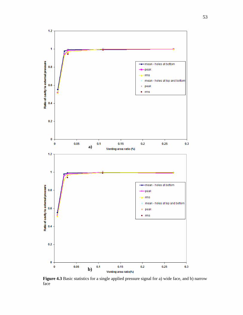
53
Figure 4.3 Basic statistics for a single applied pressure signal for a) wide face, and b) narrow face
a)
b)
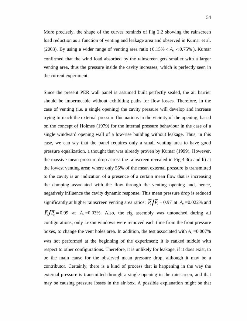
54
More precisely, the shape of the curves reminds of Fig 2.2 showing the rainscreen
load reduction as a function of venting and leakage area and observed in Kumar et al.
(2003). By using a wider range of venting area ratio ( 0.15% 0.75%VA ), Kumar
confirmed that the wind load absorbed by the rainscreen gets smaller with a larger
venting area, thus the pressure inside the cavity increases; which is perfectly seen in
the current experiment.
Since the present PER wall panel is assumed built perfectly sealed, the air barrier
should be impermeable without exhibiting paths for flow losses. Therefore, in the
case of venting (i.e. a single opening) the cavity pressure will develop and increase
trying to reach the external pressure fluctuations in the vicinity of the opening, based
on the concept of Holmes (1979) for the internal pressure behaviour in the case of a
single windward opening wall of a low-rise building without leakage. Thus, in this
case, we can say that the panel requires only a small venting area to have good
pressure equalization, a thought that was already proven by Kumar (1999). However,
the massive mean pressure drop across the rainscreen revealed in Fig 4.3(a and b) at
the lowest venting area; where only 55% of the mean external pressure is transmitted
to the cavity is an indication of a presence of a certain mean flow that is increasing
the damping associated with the flow through the venting opening and, hence,
negatively influence the cavity dynamic response. This mean pressure drop is reduced
significantly at higher rainscreen venting area ratios: 0.97c eP P at VA =0.022% and
0.99c eP P
at VA =0.03%. Also, the rig assembly was untouched during all
configurations; only Lexan windows were removed each time from the front pressure
boxes, to change the vent holes area. In addition, the test associated with VA =0.007%
was not performed at the beginning of the experiment; it is ranked middle with
respect to other configurations. Therefore, it is unlikely for leakage, if it does exist, to
be the main cause for the observed mean pressure drop, although it may be a
contributor. Certainly, there is a kind of process that is happening in the way the
external pressure is transmitted through a single opening in the rainscreen, and that
may be causing pressure losses in the air box. A possible explanation might be that
55
the air flow volume first blown into a single 71cm height by 73cm wide air box is not
fully transmitted to the cavity. The PER model performance gets better as the
rainscreen venting area ratio increases until reaching the full pressure equalization
( 1)c e c e c eP P P P P P at VA =0.11%; which explains the flatness of the curves
from 0.11% to 0.27% rainscreen venting ratio, for both the wide and narrow face
cases.
The effect of vent openings location on the pressure equalization process of the panel
is also examined for some configurations. At 0.03%VA , the data show a drop in the
mean, peak and rms ratios referring to a reduction in the cavity pressure in the order
of 3%; when the four vent holes are symmetrically redistributed as two holes under
the bottom and top middle airboxes (configuration (f) in chapter 3). This change can
be either attributed to the physical behaviour of the air inside the cavity, mainly
triggered by the vent hole location, or to the PLA performance.
In contrary to the experimental results, an increase in the cavity pressure was
expected when the holes were at the top and bottom, since the external pressure will
travel just half the distance within the box. However, it seems that the pressure
equalization is better when the vent openings are distributed along the width of the
PER panel. On the other hand, since the 2 PLAs placed at the top and bottom are
generating the same signal with high correlation, the cavity pressure response
variation cannot be due to a technical process or cross flow between the PLAs. Also,
the two venting configurations did not show any pressure gradient inside the cavity.
So at low rainscreen venting area ratios, the cavity response behaviour is only
affected by the layout of the vent openings, and it is higher when they are placed at
the bottom of the rainscreen, as if they are forming a discontinuous slot.
At 0.11%VA , the change in the location of the 15 holes does not seem to have as
much effect. Although the number of PLAs gets doubled (six instead of three), the
mean cavity response pressure seems slightly higher with respect to the external
56
pressure in comparison with the bottom venting holes location for both wide and
narrow face cases. This is probably due to the fact that full-pressure equalization is
reached in the basic configuration, so varying in the vent openings location would not
affect the cavity response pressure.
When comparing wide and narrow face results, slight differences are observed mainly
due to the performance of the PLAs. The reasonable increase in the peak cavity to
external pressure ratio, highlighted in the narrow face at 0.11%VA (15 holes top
and bottom), is not shown in the wide face case. The reason behind such behaviour is
that the achieved external peak pressure value is slightly higher than the real peak
value, so the peak ratio value c eP P
referring to a higher peak cavity pressure
collapses with that of the vent areas basic location (15 holes at bottom). Similarly, in
the narrow face case, c eP P
appears above c eP P
at four holes top and bottom
configuration because the achieved eP is 0.9% less than the peak demand pressure.
The change in the vent holes locations within one compartment and for a constant
venting area ratio has not been examined before. Previous experiments used different
layout configurations: venting slot at the bottom of the rainscreen in Ganguli and
Dalgliesh (1988), and holes spread all along the rainscreen in Kumar et al. (2003).
Inculet (1990) placed two holes at top and two holes at bottom, but the poor pressure
equalization performance observed in the model was attributed to the low venting
rainscreen to air barrier leakage area ratio, not to the distribution of the vent holes.
Figure 4.4 shows the peak factor g of the cavity pressure measurements given by
c c cP P gP . The computed values are observed in the range of 2.7 to 3.2, and as the
rainscreen venting area gets larger, the peak factor increases.
The narrow face case does not show a straight increase from 0.007% to 0.03% area
venting ratio as the wide face signal curve does: this is due to the lower peak factor at
0.03%VA (g=2.8 in the narrow face) in comparison with (g=2.9 in the wide face).
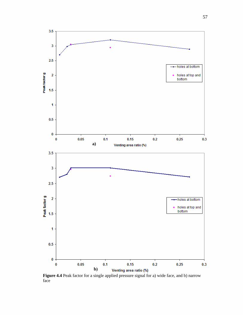
57
Figure 4.4 Peak factor for a single applied pressure signal for a) wide face, and b) narrow face
a)
b)
58
At 0.27%VA , the difference c cP P
between the peak and mean cavity pressure is
similar to that of 0.11%VA , but the rms value is larger, which explains a smaller
peak factor value, that leads to a decreasing behaviour after 0.11%VA .
The extra points referring to the vent holes redistribution are also marked on the
graph. Since the mean cavity pressure increases at a venting area ratio of 0.11%
as
shown in Fig. 4.3, the peak factor value decreases in comparison with the initial
venting location at the bottom. According to the lower venting area, the
redistribution does not have any significant effect on the peak factor, since the drop in
the mean and peak cavity pressures are compensated by the increase of the rms cavity
pressures.
4.2.3 Analysis of the Experimental Results in the Frequency Domain
The effect of rainscreen venting to panel area ratio %VA on the pressure equalization
process can be practically verified by the spectral analysis through the transfer
functions and phase angles between the external and cavity pressures signals. Figure
4.5 depicts the external and cavity pressures of the basic venting configurations, with
respect to the rainscreen area-venting ratio, in the frequency domain for both the wide
and narrow faces. The ordinates represent the normalized product of frequency and
spectral density function with respect to the corresponding variances 2( ) , while the
horizontal axis shows the frequencies. The spike existing at 2.14f Hz is equivalent
to 60Hz
electrical noise frequency in the wind tunnel data. Also, meaningless
harmonics are shown for frequencies higher than 7 Hz in all spectral plots, since the
PLA cannot generate frequencies above 7 Hz, so this makes the data beyond this
value unreadable. The measurements show in general that as the rainscreen venting
area gets larger, the pressure cavity spectra becomes closer to the external pressure,
which is clearly seen in terms of the transfer functions shown in Figs 4.6a and 4.7a.
As the venting area increases, higher frequency fluctuations are increasingly
equalized with the applied fluctuations. The same behaviour can be seen in the phase
angle in Figs 4.6b and 4.7b.
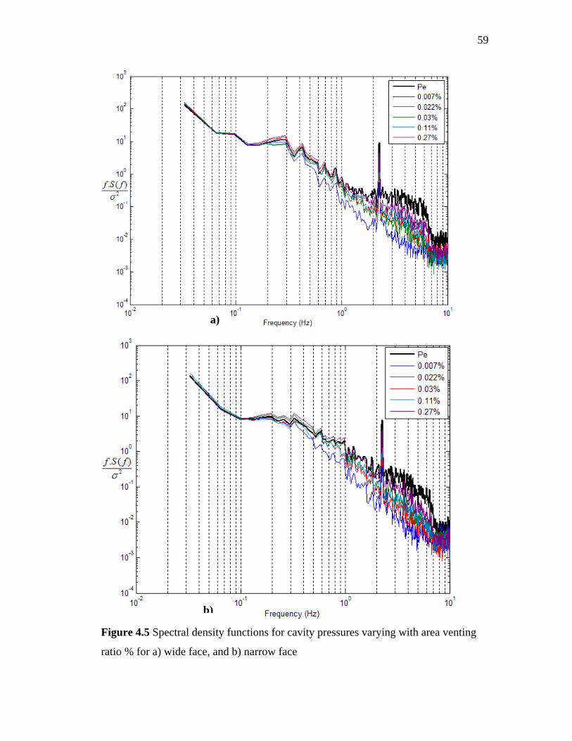
59
Figure 4.5 Spectral density functions for cavity pressures varying with area venting
ratio % for a) wide face, and b) narrow face
a)
b)
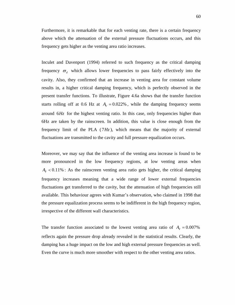
60
Furthermore, it is remarkable that for each venting rate, there is a certain frequency
above which the attenuation of the external pressure fluctuations occurs, and this
frequency gets higher as the venting area ratio increases.
Inculet and Davenport (1994) referred to such frequency as the critical damping
frequency d
which allows lower frequencies to pass fairly effectively into the
cavity. Also, they confirmed that an increase in venting area for constant volume
results in, a higher critical damping frequency, which is perfectly observed in the
present transfer functions. To illustrate, Figure 4.6a shows that the transfer function
starts rolling off at 0.6 Hz at 0.022%VA , while the damping frequency seems
around 6Hz
for the highest venting ratio. In this case, only frequencies higher than
6Hz are taken by the rainscreen. In addition, this value is close enough from the
frequency limit of the PLA ( 7Hz ), which means that the majority of external
fluctuations are transmitted to the cavity and full pressure equalization occurs.
Moreover, we may say that the influence of the venting area increase is found to be
more pronounced in the low frequency regions, at low venting areas when
0.11%VA : As the rainscreen venting area ratio gets higher, the critical damping
frequency increases meaning that a wide range of lower external frequencies
fluctuations get transferred to the cavity, but the attenuation of high frequencies still
available. This behaviour agrees with Kumar s observation, who claimed in 1998 that
the pressure equalization process seems to be indifferent in the high frequency region,
irrespective of the different wall characteristics.
The transfer function associated to the lowest venting area ratio of 0.007%VA
reflects again the pressure drop already revealed in the statistical results. Clearly, the
damping has a huge impact on the low and high external pressure frequencies as well.
Even the curve is much more smoother with respect to the other venting area ratios.
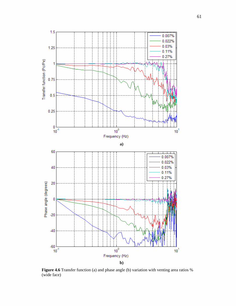
61
a)
b)
Figure 4.6 Transfer function (a) and phase angle (b) variation with venting area ratios % (wide face)
62
a)
b)
Figure 4.7 Transfer function (a) and phase angle (b) variation with venting area ratios % (narrow face)
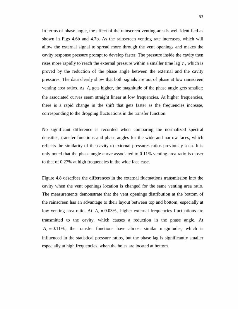
63
In terms of phase angle, the effect of the rainscreen venting area is well identified as
shown in Figs 4.6b and 4.7b. As the rainscreen venting rate increases, which will
allow the external signal to spread more through the vent openings and makes the
cavity response pressure prompt to develop faster. The pressure inside the cavity then
rises more rapidly to reach the external pressure within a smaller time lag , which is
proved by the reduction of the phase angle between the external and the cavity
pressures. The data clearly show that both signals are out of phase at low rainscreen
venting area ratios. As VA gets higher, the magnitude of the phase angle gets smaller;
the associated curves seem straight linear at low frequencies. At higher frequencies,
there is a rapid change in the shift that gets faster as the frequencies increase,
corresponding to the dropping fluctuations in the transfer function.
No significant difference is recorded when comparing the normalized spectral
densities, transfer functions and phase angles for the wide and narrow faces, which
reflects the similarity of the cavity to external pressures ratios previously seen. It is
only noted that the phase angle curve associated to 0.11% venting area ratio is closer
to that of 0.27% at high frequencies in the wide face case.
Figure 4.8 describes the differences in the external fluctuations transmission into the
cavity when the vent openings location is changed for the same venting area ratio.
The measurements demonstrate that the vent openings distribution at the bottom of
the rainscreen has an advantage to their layout between top and bottom; especially at
low venting area ratio. At 0.03%VA , higher external frequencies fluctuations are
transmitted to the cavity, which causes a reduction in the phase angle. At
0.11%VA , the transfer functions have almost similar magnitudes, which is
influenced in the statistical pressure ratios, but the phase lag is significantly smaller
especially at high frequencies, when the holes are located at bottom.
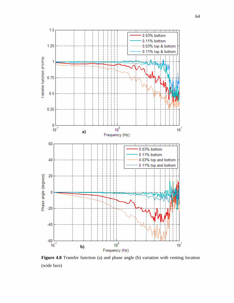
64
Figure 4.8 Transfer function (a) and phase angle (b) variation with venting location
(wide face)
b)
a)
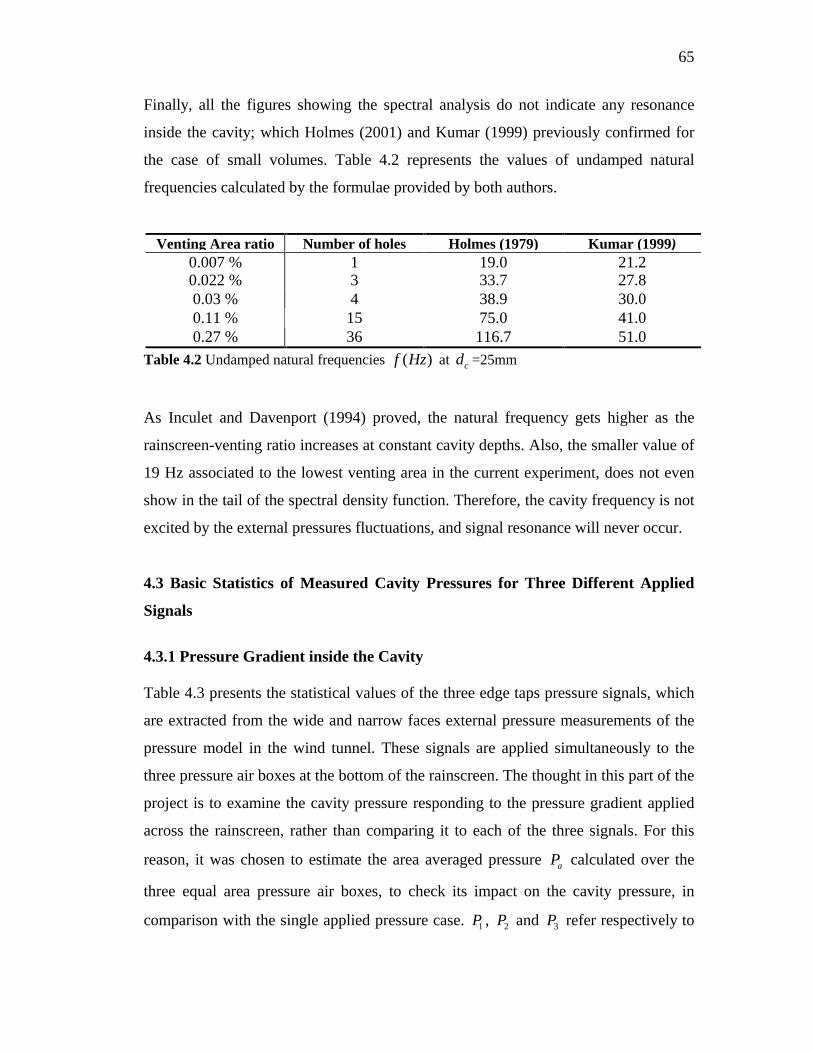
65
Finally, all the figures showing the spectral analysis do not indicate any resonance
inside the cavity; which Holmes (2001) and Kumar (1999) previously confirmed for
the case of small volumes. Table 4.2 represents the values of undamped natural
frequencies calculated by the formulae provided by both authors.
Venting Area ratio
Number of holes
Holmes (1979)
Kumar (1999)
0.007 %
1
19.0
21.2
0.022 % 3 33.7 27.8 0.03 % 4 38.9 30.0 0.11 % 15 75.0 41.0 0.27 % 36 116.7 51.0
Table 4.2 Undamped natural frequencies ( )f Hz at cd =25mm
As Inculet and Davenport (1994) proved, the natural frequency gets higher as the
rainscreen-venting ratio increases at constant cavity depths. Also, the smaller value of
19 Hz associated to the lowest venting area in the current experiment, does not even
show in the tail of the spectral density function. Therefore, the cavity frequency is not
excited by the external pressures fluctuations, and signal resonance will never occur.
4.3 Basic Statistics of Measured Cavity Pressures for Three Different Applied
Signals
4.3.1 Pressure Gradient inside the Cavity
Table 4.3 presents the statistical values of the three edge taps pressure signals, which
are extracted from the wide and narrow faces external pressure measurements of the
pressure model in the wind tunnel. These signals are applied simultaneously to the
three pressure air boxes at the bottom of the rainscreen. The thought in this part of the
project is to examine the cavity pressure responding to the pressure gradient applied
across the rainscreen, rather than comparing it to each of the three signals. For this
reason, it was chosen to estimate the area averaged pressure aP
calculated over the
three equal area pressure air boxes, to check its impact on the cavity pressure, in
comparison with the single applied pressure case. 1P , 2P
and 3P
refer respectively to
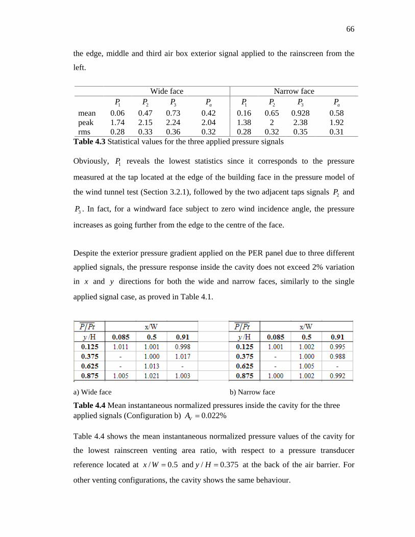
66
the edge, middle and third air box exterior signal applied to the rainscreen from the
left.
Wide face Narrow face
1P
2P
3P
aP
1P
2P
3P
aP
mean 0.06 0.47 0.73 0.42 0.16 0.65 0.928 0.58 peak 1.74 2.15 2.24 2.04 1.38 2 2.38 1.92 rms 0.28 0.33 0.36 0.32 0.28 0.32 0.35 0.31
Table 4.3 Statistical values for the three applied pressure signals
Obviously, 1P
reveals the lowest statistics since it corresponds to the pressure
measured at the tap located at the edge of the building face in the pressure model of
the wind tunnel test (Section 3.2.1), followed by the two adjacent taps signals 2P
and
3P . In fact, for a windward face subject to zero wind incidence angle, the pressure
increases as going further from the edge to the centre of the face.
Despite the exterior pressure gradient applied on the PER panel due to three different
applied signals, the pressure response inside the cavity does not exceed 2% variation
in x
and y
directions for both the wide and narrow faces, similarly to the single
applied signal case, as proved in Table 4.1.
a) Wide face b) Narrow face
Table 4.4 Mean instantaneous normalized pressures inside the cavity for the three applied signals (Configuration b) 0.022%VA
Table 4.4 shows the mean instantaneous normalized pressure values of the cavity for
the lowest rainscreen venting area ratio, with respect to a pressure transducer
reference located at / 0.5x W
and / 0.375y H
at the back of the air barrier. For
other venting configurations, the cavity shows the same behaviour.
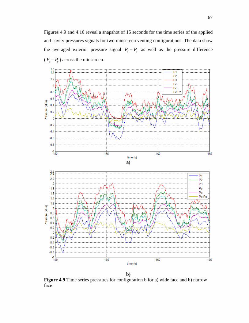
67
Figures 4.9 and 4.10 reveal a snapshot of 15 seconds for the time series of the applied
and cavity pressures signals for two rainscreen venting configurations. The data show
the averaged exterior pressure signal e aP P
as well as the pressure difference
( e cP P ) across the rainscreen.
a)
b) Figure 4.9 Time series pressures for configuration b for a) wide face and b) narrow face
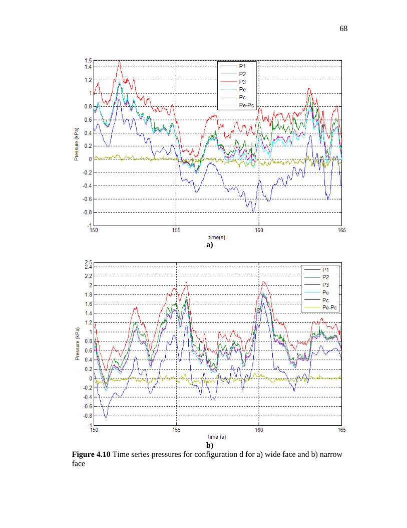
68
a)
b) Figure 4.10 Time series pressures for configuration d for a) wide face and b) narrow face
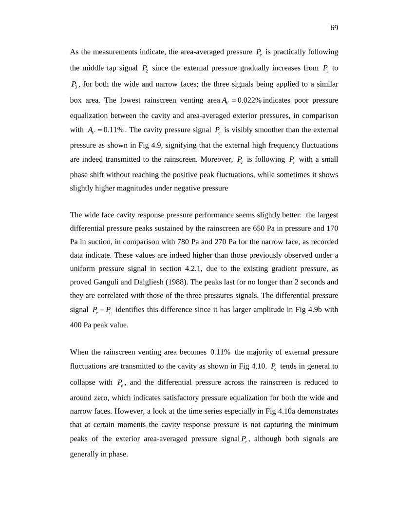
69
As the measurements indicate, the area-averaged pressure eP
is practically following
the middle tap signal 2P
since the external pressure gradually increases from 1P
to
3P , for both the wide and narrow faces; the three signals being applied to a similar
box area. The lowest rainscreen venting area 0.022%VA indicates poor pressure
equalization between the cavity and area-averaged exterior pressures, in comparison
with 0.11%VA . The cavity pressure signal cP
is visibly smoother than the external
pressure as shown in Fig 4.9, signifying that the external high frequency fluctuations
are indeed transmitted to the rainscreen. Moreover, cP
is following eP
with a small
phase shift without reaching the positive peak fluctuations, while sometimes it shows
slightly higher magnitudes under negative pressure
The wide face cavity response pressure performance seems slightly better: the largest
differential pressure peaks sustained by the rainscreen are 650 Pa in pressure and 170
Pa in suction, in comparison with 780 Pa and 270 Pa for the narrow face, as recorded
data indicate. These values are indeed higher than those previously observed under a
uniform pressure signal in section 4.2.1, due to the existing gradient pressure, as
proved Ganguli and Dalgliesh (1988). The peaks last for no longer than 2 seconds and
they are correlated with those of the three pressures signals. The differential pressure
signal e cP P
identifies this difference since it has larger amplitude in Fig 4.9b with
400 Pa peak value.
When the rainscreen venting area becomes 0.11%
the majority of external pressure
fluctuations are transmitted to the cavity as shown in Fig 4.10. cP
tends in general to
collapse with eP , and the differential pressure across the rainscreen is reduced to
around zero, which indicates satisfactory pressure equalization for both the wide and
narrow faces. However, a look at the time series especially in Fig 4.10a demonstrates
that at certain moments the cavity response pressure is not capturing the minimum
peaks of the exterior area-averaged pressure signal eP , although both signals are
generally in phase.
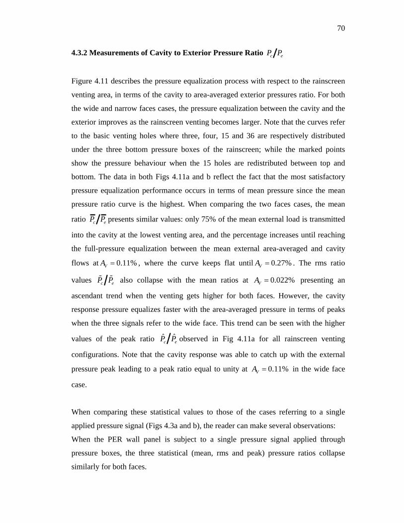
70
4.3.2 Measurements of Cavity to Exterior Pressure Ratio c eP P
Figure 4.11 describes the pressure equalization process with respect to the rainscreen
venting area, in terms of the cavity to area-averaged exterior pressures ratio. For both
the wide and narrow faces cases, the pressure equalization between the cavity and the
exterior improves as the rainscreen venting becomes larger. Note that the curves refer
to the basic venting holes where three, four, 15 and 36 are respectively distributed
under the three bottom pressure boxes of the rainscreen; while the marked points
show the pressure behaviour when the 15 holes are redistributed between top and
bottom. The data in both Figs 4.11a and b reflect the fact that the most satisfactory
pressure equalization performance occurs in terms of mean pressure since the mean
pressure ratio curve is the highest. When comparing the two faces cases, the mean
ratio c eP P presents similar values: only 75% of the mean external load is transmitted
into the cavity at the lowest venting area, and the percentage increases until reaching
the full-pressure equalization between the mean external area-averaged and cavity
flows at 0.11%VA , where the curve keeps flat until 0.27%VA . The rms ratio
values c eP P
also collapse with the mean ratios at 0.022%VA
presenting an
ascendant trend when the venting gets higher for both faces. However, the cavity
response pressure equalizes faster with the area-averaged pressure in terms of peaks
when the three signals refer to the wide face. This trend can be seen with the higher
values of the peak ratio c eP P observed in Fig 4.11a for all rainscreen venting
configurations. Note that the cavity response was able to catch up with the external
pressure peak leading to a peak ratio equal to unity at 0.11%VA
in the wide face
case.
When comparing these statistical values to those of the cases referring to a single
applied pressure signal (Figs 4.3a and b), the reader can make several observations:
When the PER wall panel is subject to a single pressure signal applied through
pressure boxes, the three statistical (mean, rms and peak) pressure ratios collapse
similarly for both faces.
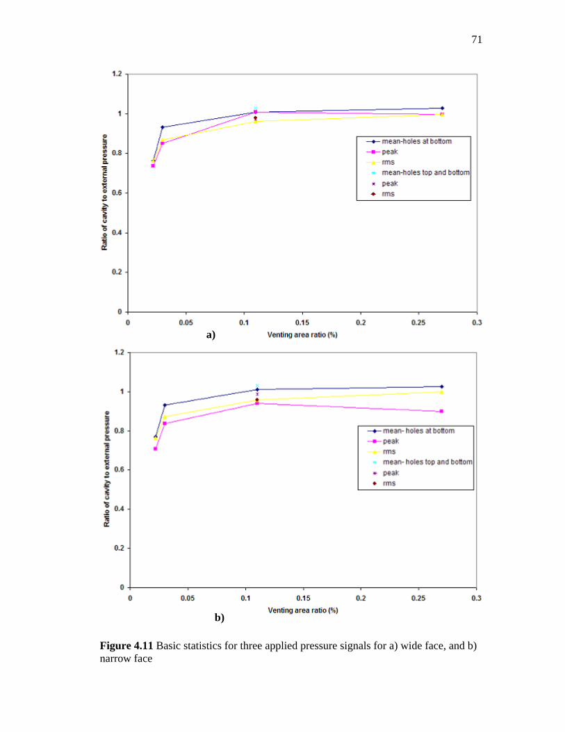
71
Figure 4.11 Basic statistics for three applied pressure signals for a) wide face, and b) narrow face
a)
b)
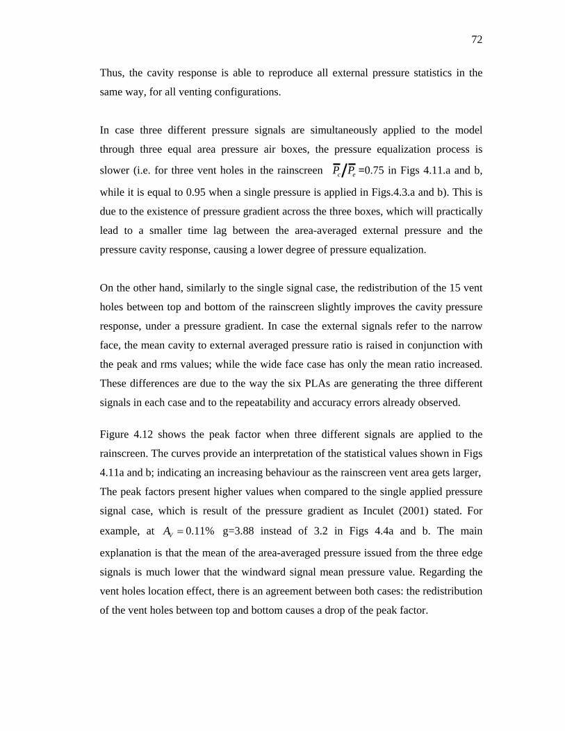
72
Thus, the cavity response is able to reproduce all external pressure statistics in the
same way, for all venting configurations.
In case three different pressure signals are simultaneously applied to the model
through three equal area pressure air boxes, the pressure equalization process is
slower (i.e. for three vent holes in the rainscreen c eP P =0.75 in Figs 4.11.a and b,
while it is equal to 0.95 when a single pressure is applied in Figs.4.3.a and b). This is
due to the existence of pressure gradient across the three boxes, which will practically
lead to a smaller time lag between the area-averaged external pressure and the
pressure cavity response, causing a lower degree of pressure equalization.
On the other hand, similarly to the single signal case, the redistribution of the 15 vent
holes between top and bottom of the rainscreen slightly improves the cavity pressure
response, under a pressure gradient. In case the external signals refer to the narrow
face, the mean cavity to external averaged pressure ratio is raised in conjunction with
the peak and rms values; while the wide face case has only the mean ratio increased.
These differences are due to the way the six PLAs are generating the three different
signals in each case and to the repeatability and accuracy errors already observed.
Figure 4.12 shows the peak factor when three different signals are applied to the
rainscreen. The curves provide an interpretation of the statistical values shown in Figs
4.11a and b; indicating an increasing behaviour as the rainscreen vent area gets larger,
The peak factors present higher values when compared to the single applied pressure
signal case, which is result of the pressure gradient as Inculet (2001) stated. For
example, at 0.11%VA
g=3.88 instead of 3.2 in Figs 4.4a and b. The main
explanation is that the mean of the area-averaged pressure issued from the three edge
signals is much lower that the windward signal mean pressure value. Regarding the
vent holes location effect, there is an agreement between both cases: the redistribution
of the vent holes between top and bottom causes a drop of the peak factor.
73
Figure 4.12 Peak factor for three applied pressure signals for a) wide face, and b) narrow face
a)
b)
74
4.3.3 Analysis of the Experimental Results in the Frequency Domain
Figure 4.13 shows the normalized spectral density functions of the cavity pressure
when three different signals are applied to the PER panel. Spikes at 60 Hz equivalent
wind tunnel electronic noise frequency are always identified. The behaviour of the
cavity with respect to the exterior pressure varies consistently in the frequency
domain with respect to the venting area as shown in Figs 4.14 and 4.15. The transfer
functions display the area-averaged pressure amount transmitted to the cavity, that
obviously increases, as the rainscreen venting area ratio gets higher. Similarly to the
single signal case, the critical damping frequency increases as VA
gets larger
allowing a wider range of low external frequencies to get transferred behind the
rainscreen. The full equalization between the cavity pressure and e aP P
appears at
0.27%VA , while it is reached at a lower venting area of 0.11%VA
under a single
pressure signal. In fact, the transfer functions and phase angles corresponding to these
two venting configurations almost collapse in the case of a uniform pressure, while in
this case they both show more attenuation.
In addition, when a single pressure is applied to the rainscreen, the transfer functions
corresponding to low venting configurations, apart from the one hole case, originate
from a value close to one; in contrast with the current plots; that indicate a pressure
drop and start to roll off at lower frequencies i.e. 4Hz
instead of 6Hz
at
0.27%VA . Therefore, when the PER panel is subject to a pressure gradient, the
cavity pressure equalizes with the external pressure at a smaller degree for the same
rainscreen venting area ratio. On the other hand, it is noticed that slower pressure
equalization is established when the three external pressure signals are extracted from
the narrow face.
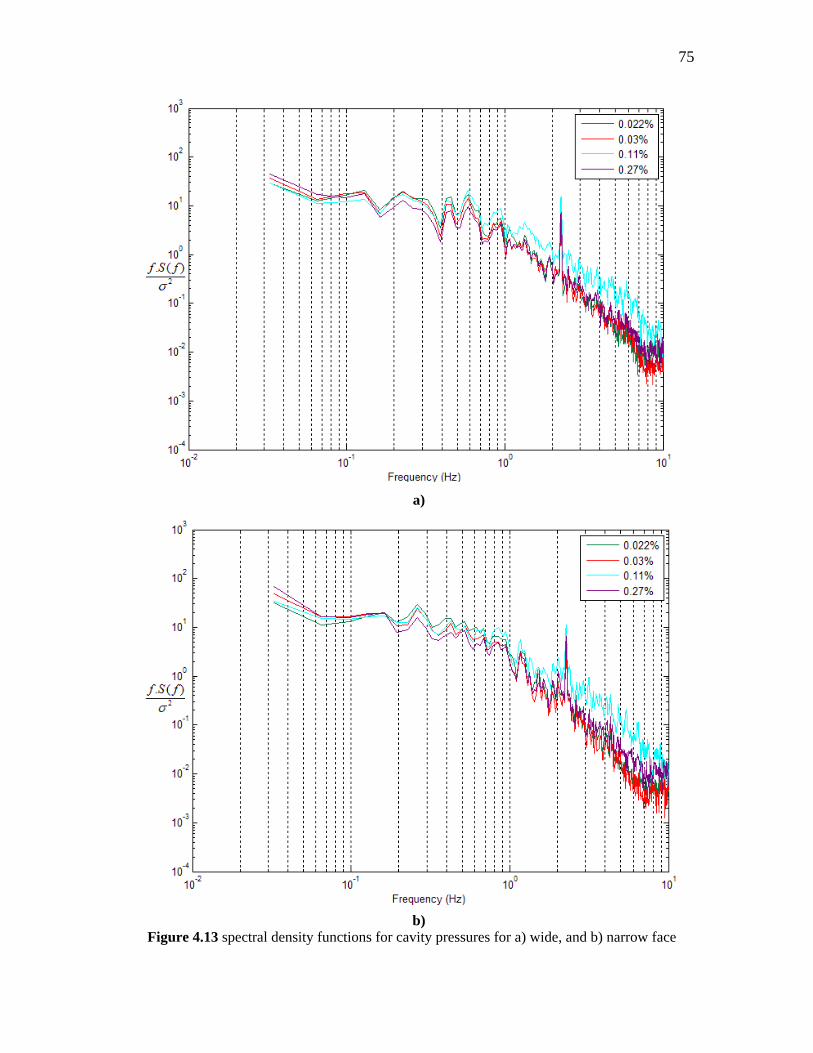
75
a)
b) Figure 4.13 spectral density functions for cavity pressures for a) wide, and b) narrow face
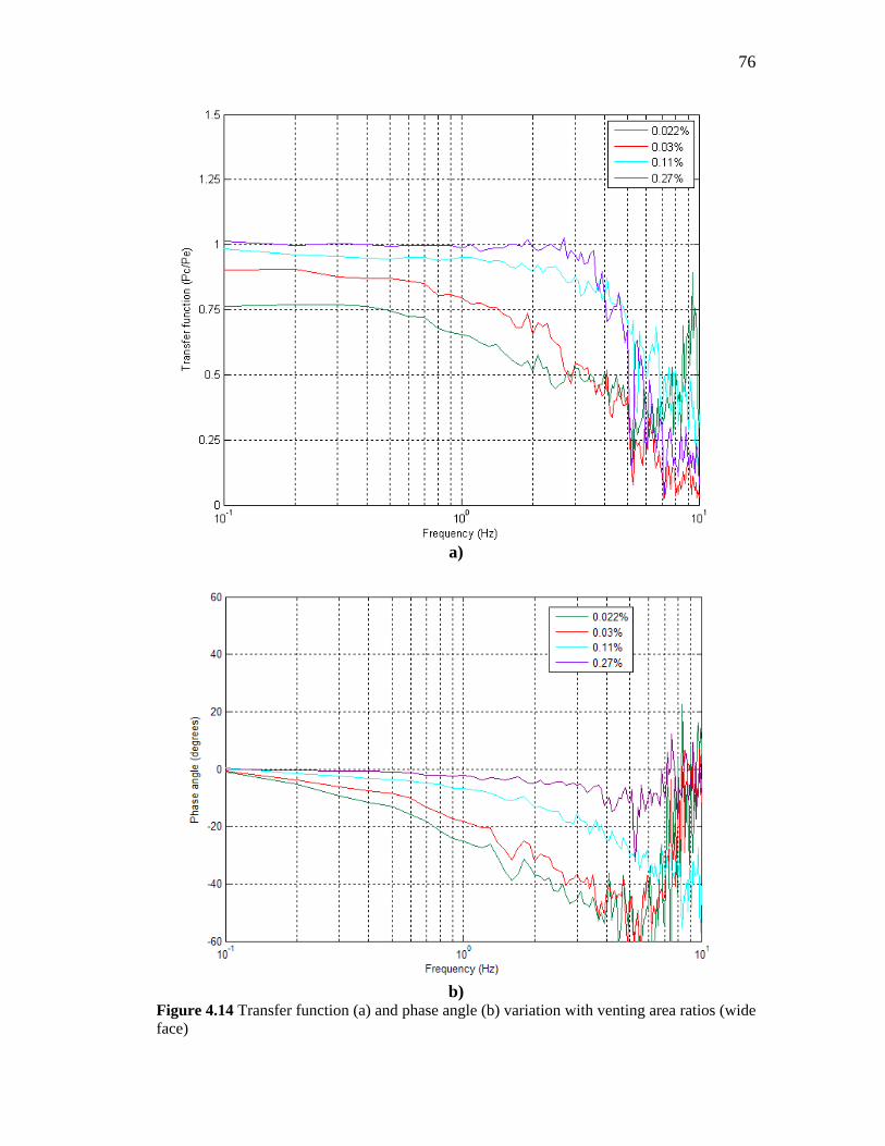
76
a)
b) Figure 4.14 Transfer function (a) and phase angle (b) variation with venting area ratios (wide face)
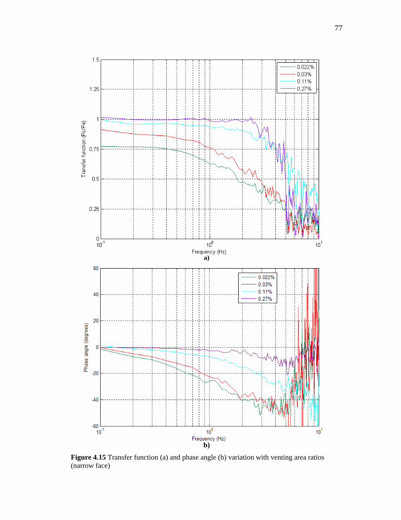
77
a)
a)
b)
Figure 4.15 Transfer function (a) and phase angle (b) variation with venting area ratios (narrow face)
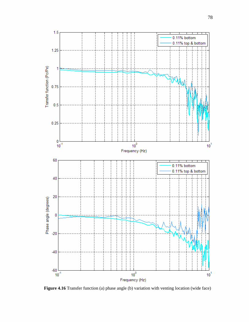
78
Figure 4.16 Transfer function (a) phase angle (b) variation with venting location (wide face)
79
The phase angle plots are presented in Figs 4.14b and 4.15b. As pressure equalization
improves, the phase angle is reduced. However at high raincsreen vent area ratios, the
phase angle does not keep the value of zero all the time: the cavity and area-averaged
pressures are out of phase in the high frequencies regions, which proves again that,
under a pressure gradient, the cavity has less ability in responding to the external
pressures.
The effect of vent openings location is described in Fig 4.16. The redistribution of 15
vent holes between top and bottom on the rainscreen does not have a significant
impact on the pressure equalization process. The transfer function magnitudes are
slightly increased but the damping occurs at the same frequency. Also, the phase
angle is slightly reduced at high frequencies
4.3.4 Comparison of Wide and Narrow Face Results
Measurements previously revealed in the statistical values and transfer functions have
shown some differences in the cavity pressure behaviour between the wide and
narrow face cases. Apparently, façade characteristics and wind flow behaviour do
have an effect on the degree of pressure equalization, especially at lower frequencies.
When the three applied signals were extracted from the three edge taps of the
windward wide face, the pressure equalization for our PER model was faster and
there was better transmission of low frequencies fluctuations at all venting
configurations. For example when comparing Figs 4.14a and 4.15a, the transfer
functions show that at the lowest venting area where 0.022%VA , 75% of external
pressure fluctuations are transmitted to the cavity at frequencies lower than 0.5Hz in
the case of the wide face, while at higher frequencies this percentage start to decrease.
However, when the three applied signals correspond to a part of the three edge taps
exterior pressures of the windward narrow face, only frequencies below 0.4Hz are
75% transferred to the cavity. Similarly, at high rainscreen venting area ratios, the
transfer functions show a faster decay in the case of the narrow face. This is probably
attributed to the actual difference in the three signals of the two faces that results in
different pressure gradient although the full-scale applied signals represent only a part
80
over five minutes equivalent time period from the original data duration. Moreover,
the differential pressures e cP P
observed across the rainscreen are higher when it
comes to the narrow face external signals. To illustrate, the corresponding mean
values associated to 0.022%VA
are respectively 100 Pa in Fig 4.9a and 120 Pa in
Fig 4.9b.
In light of the above, it was necessary to quantify numerically the resultant horizontal
gradient pressure available on the PER panel, which is caused by the applied pressure
signals issued from each face, in order to justify correctly the cavity pressure
behaviour. Inculet (2001) suggested an instantaneous horizontal component pressure
gradient coefficient ( / )
pg
m m
CH
x W
where mx is the horizontal coordinate measured
from the left edge of the building, aiming to examine the pressure gradients mostly
observed at the edges of the facades between the different taps locations on a pressure
model in the wind tunnel. In this case, a positive value of gH
indicates that the
pressure is increasing from left to right across the face.
By applying this expression on the current PER model compartment, the mean
horizontal pressure gradient gH
is calculated between the three adjacent pressure air
boxes locations, that are subject to three different external signals, where mW refers in
this case to the width W of the rainscreen. The results prove that applied pressure
signals associated with the narrow face, result in higher-pressure gradient across the
rainscreen: gH = 0.32 with respect to gH = 0.26 for the wide face case. These values
refer to the pressure gradient established between the edge and the second adjacent
pressure air box, from the left of the rainscreen. They are, respectively, equivalent in
full-scale using a mean velocity of 53.6 m/s to 585Pa pressure change per metre and
700Pa per metre, meaning a difference of about 18% between the wide and narrow
faces. The pressure gradients between the second and third pressure boxes exhibit the
same behaviour, but with smaller magnitudes, since the pressure gradient is reduced
as we go further from the edge of the building façade.
81
Therefore, this should explain the higher-pressure loads sustained by the rainscreen in
case of the narrow face. It is also in agreement with Skerlj and Surry (1994) who
observed through a wind tunnel experiment that, higher mean pressure gradients
applied to a PER compartment, produces higher mean residual net pressures on the
rainscreen.
4.4 Summary
Cavity pressure measurements using a PER compartment model have been examined
under both a uniform pressure and a horizontal pressure gradient. The results indicate
the major role of the rainscreen venting to wall area ratio in the improvement of
equalization process between the external and cavity pressures. The transfer functions
revealed an increase in the critical damping frequency, and the phase angle between
external and cavity pressures was reduced, as the rainscreen venting area was
increasing.
In the case of a uniform applied pressure, the lowest rainscreen venting area ratio
0.007%VA
resulted in the poorest pressure equalization between the external and
cavity pressures. A great pressure loss occurred across the rainscreen: a mean
pressure drop of 55% of the external pressure was observed.
The application of a horizontal pressure gradient leads to a lower degree of pressure
equalization according to the experimental results. The best performance was
obtained for 0.27%VA when the PER model was subject to three different signals,
while a full pressure equalization occurred for 0.11%VA
under a uniform pressure.
Moreover, when applying three different signals extracted from the narrow face wind
tunnel pressure model, the rainscreen panel experienced higher net pressures because
the mean horizontal gradient pressure coefficient was 18% higher that the value
associated with the wide face.
In terms of the venting area location, placing the vent holes at the bottom of the
rainscreen seems to enhance the pressure equalization, in comparison with their
82
distribution between top and bottom. Such effect was clearly identified for low
rainscreen venting area ratios. However, the vent openings layout did not have a
significant effect on the performance of the PER model for high rainscreen venting
area ratios.
The next chapter will present the numerical predictions of the PER model s cavity
pressure response. This will allow checking whether the theoretical model is able to
reproduce exactly the effect of the considered wall parameters on the model
performance, under both uniform and gradient external pressures.
83
CHAPTER 5
NUMERICAL RESULTS
5.1 Introduction
This chapter establishes a comparison of the measurements and numerical predictions
of the cavity pressure measurements in order to check the efficiency of the theory in
predicting full-scale results in the future. In addition, the impact of cavity volume
change on the pressure equalization is observed by predicting numerically the cavity
pressure for a range of depths varying between 25 and 300mm under an external
single pressure signal and pressure gradient.
5.2 Numerical Model
The numerical predictions of cavity pressures are computed based on Helmholtz
resonator theory model. This model (known as Model 2 in chapter 2) has been chosen
since the related equations involve damping and inertial terms for all openings, which
is assumed to predict more realistically the cavity response pressure. Moreover, it is
able to consider: 1) the external pressure fluctuations across each opening, 2) any
number of venting holes and, 3) the leakage characteristics of the air barrier. For this
reason, a Matlab program that was originally developed for internal pressure
computations in low-rise buildings by Oh et al (2007) is transformed and used in
order to estimate the cavity pressures in this project. The algorithm of the computer
program is clarified in Appendix B Section B1. In addition to constant coefficients,
the program is fed with the external pressure data matrix issued from the full-scale
experiment, where each column represents the applied signal across an opening, as
measured by the pressure transducers. In case of leakage, the leakage holes have a
smaller diameter than the vents, and they are added to the external pressure data
matrix input, as having zero pressure values.
84
Values chosen for the equations coefficients and parameters that are used in the
computational program are defined below for the vent and leakage holes as well.
a) Flow Exponent n
The value of the flow coefficient n
usually varies from 0.5 to 1 according to Table
2.3. Whenever n
became higher than 0.5 in the numerical simulations, no significant
variation was noticed in the cavity response pressure at a certain venting
configuration by keeping the other parameters constant, and the basic statistics (mean,
max, min and rms) were the same. For this reason, it was decided to use n =0.5 for
the rainscreen which has openings with little depth.
When leakage exists, leakage holes are assumed to come out from the air barrier,
which will have then its own flow exponent. In this case, n =0.7 according to Shaw
(1981). With the numerical trials, it was noticed that if n becomes larger than 0.7, the
mean of the predicted cavity pressure increases, and the peak decreases which makes
the matching between experimental and numerical results harder, so n was kept 0.7.
Moreover, based on wind tunnel tests conducted on PER models, Inculet and
Davenport (1994) found that the venting in a rainscreen results in orifice flow giving
n =0.5; while the leakage path through the air barrier is likely to exhibit more viscous
type flow with n =0.7.
b) Effective Length el
The effective length used in the numerical simulations is chosen to be 0 0.89el l a
as proposed by Holmes (1979) in Table 2.4. This expression involves the effect of the
orifice length 0l which varies in the reality with the nature of the flow.
0l
for the leakage hole is assumed to be long and wide enough to let the flow come
back and forth, however it is smaller for the vent opening. For this reason, the value
of 0l
for the vent opening is set equal to the thickness of the rainscreen that is
0.00635m, while it is slightly bigger for the leakage hole present in the air barrier
85
suggested to be 0.0075m close to the air barrier assembly thickness, a
refers to the
area of the opening.
c) Discharge Coefficient K
It is always difficult to assess the exact value of the discharge coefficient for a flow
through the vent opening in the rainscreen. In fact, this flow may be affected by a
mean flow stemming from unavoidable leakage of the air barrier, or cross flows
behind the rainscreen with venting holes exposed to different exterior pressures.
Furthermore, pressure losses might come from the way the flow rate is transmitted
through the opening. Holmes (1979) specified the earliest values; he found that a
value in the range of 0.6 to 0.65 corresponds to a steady flow, while 0.15 refers to
highly fluctuating and reversing flow conditions. The presence of any leakage in the
air barrier introduces also a second unknown into the theory. The leakage coefficient
for the air barrier, like the discharge coefficient for the rainscreen, could take on a
different value in fluctuating flows than in steady flows. However to simplify the
problem, it was decided to use the steady flow value 0.6K
for the air barrier, since
mean velocities will be high through the small leakage path, as described by Inculet
(1996). Simulations have not shown any difference when using K
as 0.5 or 0.6,
however when it became smaller, the predicted mean, peak and rms of the cavity
pressure were raised, which yielded a poor matching with the experimental values.
In light of this discussion, the rainscreen may have a different value of discharge
coefficient for each configuration depending on the flow behaviour; setting constant
the flow exponent n
and the effective length el
for both the rainscreen and air
barriers. The concept is to adjust the value of K
until the theoretical rms of the
pressure drop across the rainscreen matches the experimental value.
In the present case, the numerical value of K
is first determined based on the single
applied external pressure signal and then applied for the three different external
pressure signals case. It was necessary, though, to quantify any existing leakage in the
air barrier assembly, to include leakage holes in the numerical model for better
matching with the experimental results.
86
Leakage openings were assumed to be small enough in the order of 2mm circular
hole, where one leak represents 1% of one 20mm vent hole area. The estimation of
the expected area of leakage holes in the air barrier abA
is made by numerical trials.
The first approximation is given as
1
2
.
.
nab rainscreen rainscreen
nrs airbarrier airbarrier
A K p
A K p (4.1)
using the experimental pressure drop values across the rainscreen corresponding to
each case, and considering that the flow entering into the cavity through the vent
holes is equal to the flow coming out of the air barrier from the leaks. When applied
to the lowest venting area configuration of 0.007%VA , abA
is equivalent to 24
leakage holes; and becomes 6 leakage holes at 0.022%VA . The expected amount of
leakage decreases, as the venting area becomes higher, since the differential pressure
across the rainscreen decreases while keeping constant the coefficients used in this
formula as n =0.5; K =0.15 for the rainscreen and n =0.7; K =0.6 for the air barrier.
By including 24 leakage holes in the numerical computer model, and using the same
coefficients values, the predicted cavity pressure did not match the experimental
signal for 0.007%VA . For this reason, the number of leaks had to be increased in
order to obtain the actual cavity pressure.
Figure 5.1 shows the time series of the external pressure, experimental and numerical
cavity signals, over a short period, in the case of a wide face. The experimental cavity
pressure seems much smoother than the applied pressure meaning that high frequency
external fluctuations are indeed transmitted to the rainscreen. On the other hand, the
most reasonable predicted cavity pressure signal corresponds to 37 leakage holes of
2mm diameter, instead of 24. Clearly, it is following the external pressure in
reproducing the majority of fluctuations, which are not present in the real signal
signifying that the matching in the spectral analysis will not be satisfactory.
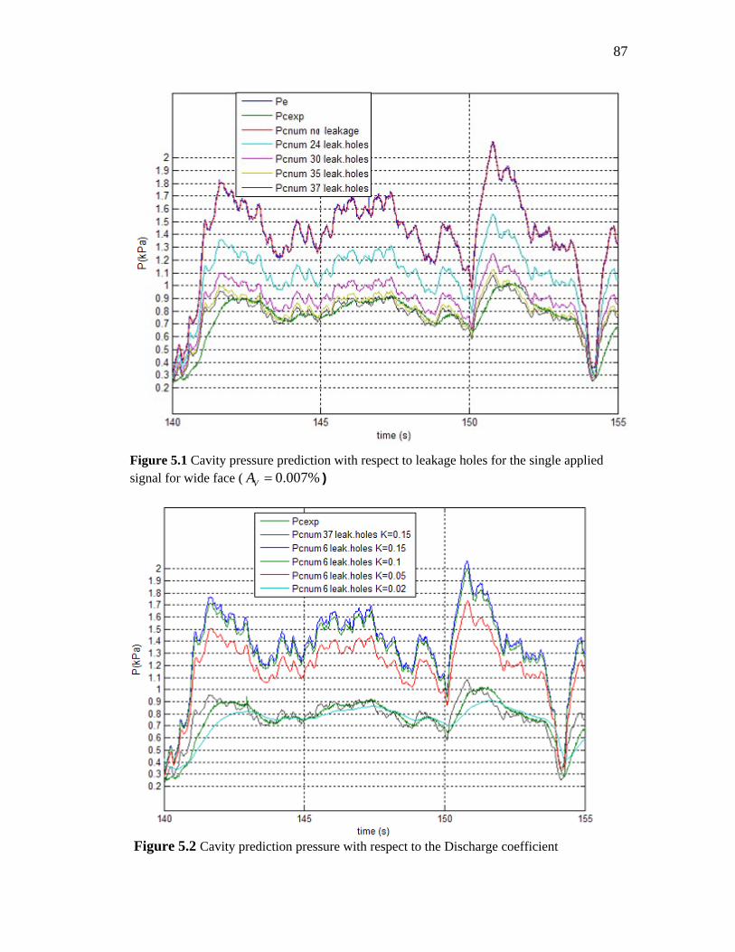
87
Figure 5.1 Cavity pressure prediction with respect to leakage holes for the single applied signal for wide face ( 0.007%VA )
Figure 5.2 Cavity prediction pressure with respect to the Discharge coefficient
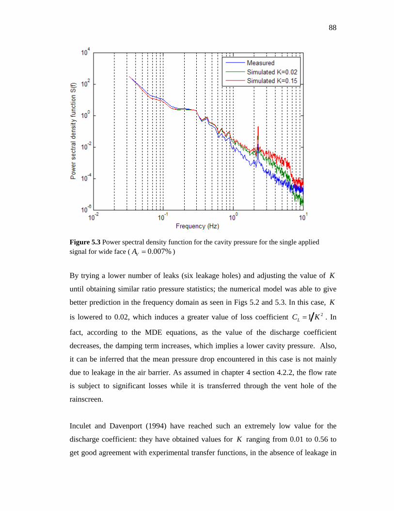
88
Figure 5.3 Power spectral density function for the cavity pressure for the single applied signal for wide face ( 0.007%VA )
By trying a lower number of leaks (six leakage holes) and adjusting the value of K
until obtaining similar ratio pressure statistics; the numerical model was able to give
better prediction in the frequency domain as seen in Figs 5.2 and 5.3. In this case, K
is lowered to 0.02, which induces a greater value of loss coefficient 21LC K . In
fact, according to the MDE equations, as the value of the discharge coefficient
decreases, the damping term increases, which implies a lower cavity pressure. Also,
it can be inferred that the mean pressure drop encountered in this case is not mainly
due to leakage in the air barrier. As assumed in chapter 4 section 4.2.2, the flow rate
is subject to significant losses while it is transferred through the vent hole of the
rainscreen.
Inculet and Davenport (1994) have reached such an extremely low value for the
discharge coefficient: they have obtained values for K
ranging from 0.01 to 0.56 to
get good agreement with experimental transfer functions, in the absence of leakage in
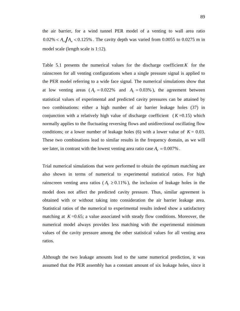
89
the air barrier, for a wind tunnel PER model of a venting to wall area ratio
0.02% 0.125%rs wA A . The cavity depth was varied from 0.0055 to 0.0275 m in
model scale (length scale is 1:12).
Table 5.1 presents the numerical values for the discharge coefficient K
for the
rainscreen for all venting configurations when a single pressure signal is applied to
the PER model referring to a wide face signal. The numerical simulations show that
at low venting areas ( 0.022%VA
and 0.03%VA ), the agreement between
statistical values of experimental and predicted cavity pressures can be attained by
two combinations: either a high number of air barrier leakage holes (37) in
conjunction with a relatively high value of discharge coefficient ( K =0.15) which
normally applies to the fluctuating reversing flows and unidirectional oscillating flow
conditions; or a lower number of leakage holes (6) with a lower value of K = 0.03.
These two combinations lead to similar results in the frequency domain, as we will
see later, in contrast with the lowest venting area ratio case 0.007%VA .
Trial numerical simulations that were performed to obtain the optimum matching are
also shown in terms of numerical to experimental statistical ratios. For high
rainscreen venting area ratios ( 0.11%VA ), the inclusion of leakage holes in the
model does not affect the predicted cavity pressure. Thus, similar agreement is
obtained with or without taking into consideration the air barrier leakage area.
Statistical ratios of the numerical to experimental results indeed show a satisfactory
matching at K =0.65; a value associated with steady flow conditions. Moreover, the
numerical model always provides less matching with the experimental minimum
values of the cavity pressure among the other statistical values for all venting area
ratios.
Although the two leakage amounts lead to the same numerical prediction, it was
assumed that the PER assembly has a constant amount of six leakage holes, since it
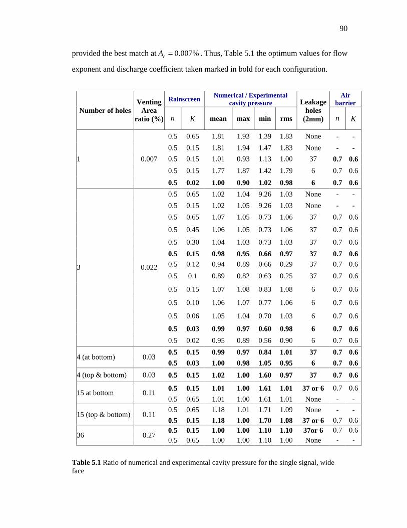
90
provided the best match at 0.007%VA . Thus, Table 5.1 the optimum values for flow
exponent and discharge coefficient taken marked in bold for each configuration.
Rainscreen Numerical / Experimental
cavity pressure Air
barrier Number of holes
Venting
Area ratio (%)
n
K
mean max min rms
Leakage holes
(2mm) n
K
0.5
0.65 1.81 1.93 1.39 1.83 None - -
0.5
0.15 1.81 1.94 1.47 1.83 None - -
0.5
0.15 1.01 0.93 1.13 1.00 37 0.7
0.6
0.5
0.15 1.77 1.87 1.42 1.79 6 0.7
0.6
1 0.007
0.5
0.02 1.00 0.90 1.02 0.98 6 0.7
0.6
0.5
0.65 1.02 1.04 9.26 1.03 None - -
0.5
0.15 1.02 1.05 9.26 1.03 None - -
0.5
0.65 1.07 1.05 0.73 1.06 37 0.7
0.6
0.5
0.45 1.06 1.05 0.73 1.06 37 0.7
0.6
0.5
0.30 1.04 1.03 0.73 1.03 37 0.7
0.6
0.5
0.15 0.98 0.95 0.66 0.97 37 0.7
0.6
0.5
0.12 0.94 0.89 0.66 0.29 37 0.7
0.6
0.5
0.1 0.89 0.82 0.63 0.25 37 0.7
0.6
0.5
0.15 1.07 1.08 0.83 1.08 6 0.7
0.6
0.5
0.10 1.06 1.07 0.77 1.06 6 0.7
0.6
0.5
0.06 1.05 1.04 0.70 1.03 6 0.7
0.6
0.5
0.03 0.99 0.97 0.60 0.98 6 0.7
0.6
3 0.022
0.5
0.02 0.95 0.89 0.56 0.90 6 0.7
0.6
0.5
0.15 0.99 0.97 0.84 1.01 37 0.7
0.6
4 (at bottom) 0.03 0.5
0.03 1.00 0.98 1.05 0.95 6 0.7
0.6
4 (top & bottom) 0.03 0.5
0.15 1.02 1.00 1.60 0.97 37 0.7
0.6
0.5
0.15 1.01 1.00 1.61 1.01 37 or 6 0.7
0.6
15 at bottom 0.11 0.5
0.65 1.01 1.00 1.61 1.01 None - -
0.5
0.65 1.18 1.01 1.71 1.09 None - - 15 (top & bottom)
0.11 0.5
0.15 1.18 1.00 1.70 1.08 37 or 6 0.7
0.6
0.5
0.15 1.00 1.00 1.10 1.10 37or 6 0.7
0.6
36 0.27 0.5
0.65 1.00 1.00 1.10 1.00 None - -
Table 5.1 Ratio of numerical and experimental cavity pressure for the single signal, wide face
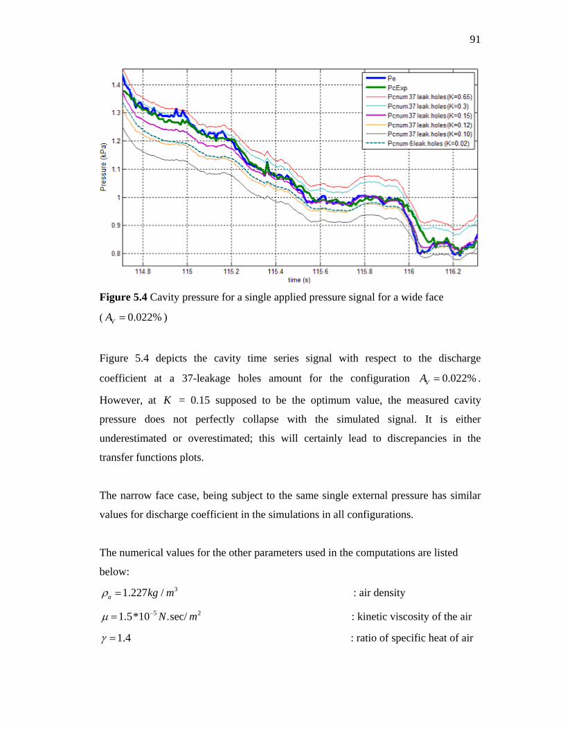
91
Figure 5.4 Cavity pressure for a single applied pressure signal for a wide face
( 0.022%VA )
Figure 5.4 depicts the cavity time series signal with respect to the discharge
coefficient at a 37-leakage holes amount for the configuration 0.022%VA .
However, at K
= 0.15 supposed to be the optimum value, the measured cavity
pressure does not perfectly collapse with the simulated signal. It is either
underestimated or overestimated; this will certainly lead to discrepancies in the
transfer functions plots.
The narrow face case, being subject to the same single external pressure has similar
values for discharge coefficient in the simulations in all configurations.
The numerical values for the other parameters used in the computations are listed
below:
31.227 /a kg m : air density
5 21.5*10 .sec/N m : kinetic viscosity of the air
1.4 : ratio of specific heat of air
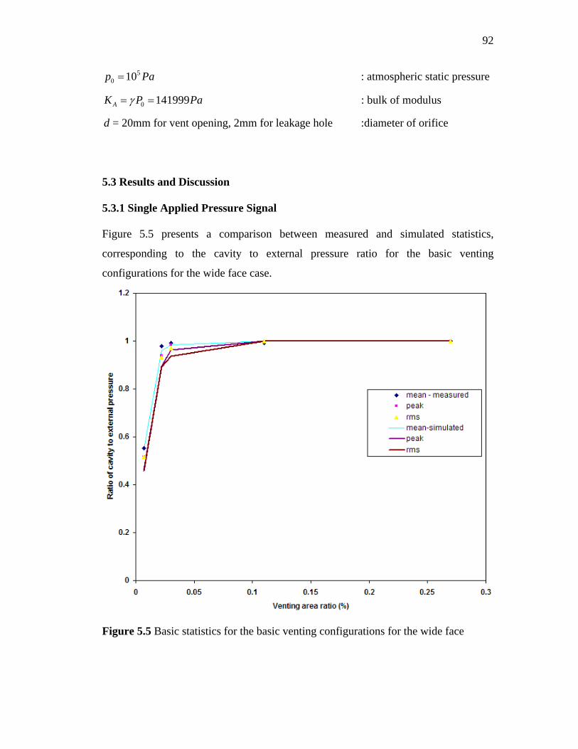
92
50 10p Pa : atmospheric static pressure
0 141999AK P Pa : bulk of modulus
d = 20mm for vent opening, 2mm for leakage hole :diameter of orifice
5.3 Results and Discussion
5.3.1 Single Applied Pressure Signal
Figure 5.5 presents a comparison between measured and simulated statistics,
corresponding to the cavity to external pressure ratio for the basic venting
configurations for the wide face case.
Figure 5.5 Basic statistics for the basic venting configurations for the wide face
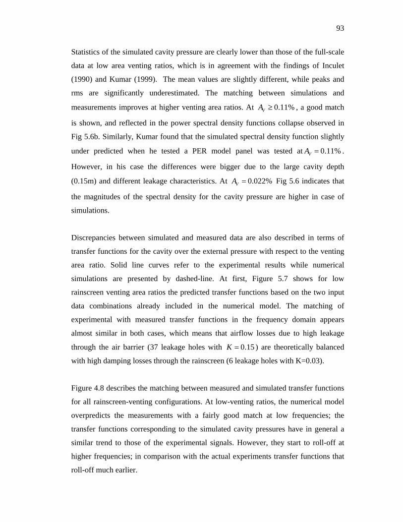
93
Statistics of the simulated cavity pressure are clearly lower than those of the full-scale
data at low area venting ratios, which is in agreement with the findings of Inculet
(1990) and Kumar (1999). The mean values are slightly different, while peaks and
rms are significantly underestimated. The matching between simulations and
measurements improves at higher venting area ratios. At 0.11%VA , a good match
is shown, and reflected in the power spectral density functions collapse observed in
Fig 5.6b. Similarly, Kumar found that the simulated spectral density function slightly
under predicted when he tested a PER model panel was tested at 0.11%VA .
However, in his case the differences were bigger due to the large cavity depth
(0.15m) and different leakage characteristics. At 0.022%VA
Fig 5.6 indicates that
the magnitudes of the spectral density for the cavity pressure are higher in case of
simulations.
Discrepancies between simulated and measured data are also described in terms of
transfer functions for the cavity over the external pressure with respect to the venting
area ratio. Solid line curves refer to the experimental results while numerical
simulations are presented by dashed-line. At first, Figure 5.7 shows for low
rainscreen venting area ratios the predicted transfer functions based on the two input
data combinations already included in the numerical model. The matching of
experimental with measured transfer functions in the frequency domain appears
almost similar in both cases, which means that airflow losses due to high leakage
through the air barrier (37 leakage holes with 0.15K ) are theoretically balanced
with high damping losses through the rainscreen (6 leakage holes with K=0.03).
Figure 4.8 describes the matching between measured and simulated transfer functions
for all rainscreen-venting configurations. At low-venting ratios, the numerical model
overpredicts the measurements with a fairly good match at low frequencies; the
transfer functions corresponding to the simulated cavity pressures have in general a
similar trend to those of the experimental signals. However, they start to roll-off at
higher frequencies; in comparison with the actual experiments transfer functions that
roll-off much earlier.
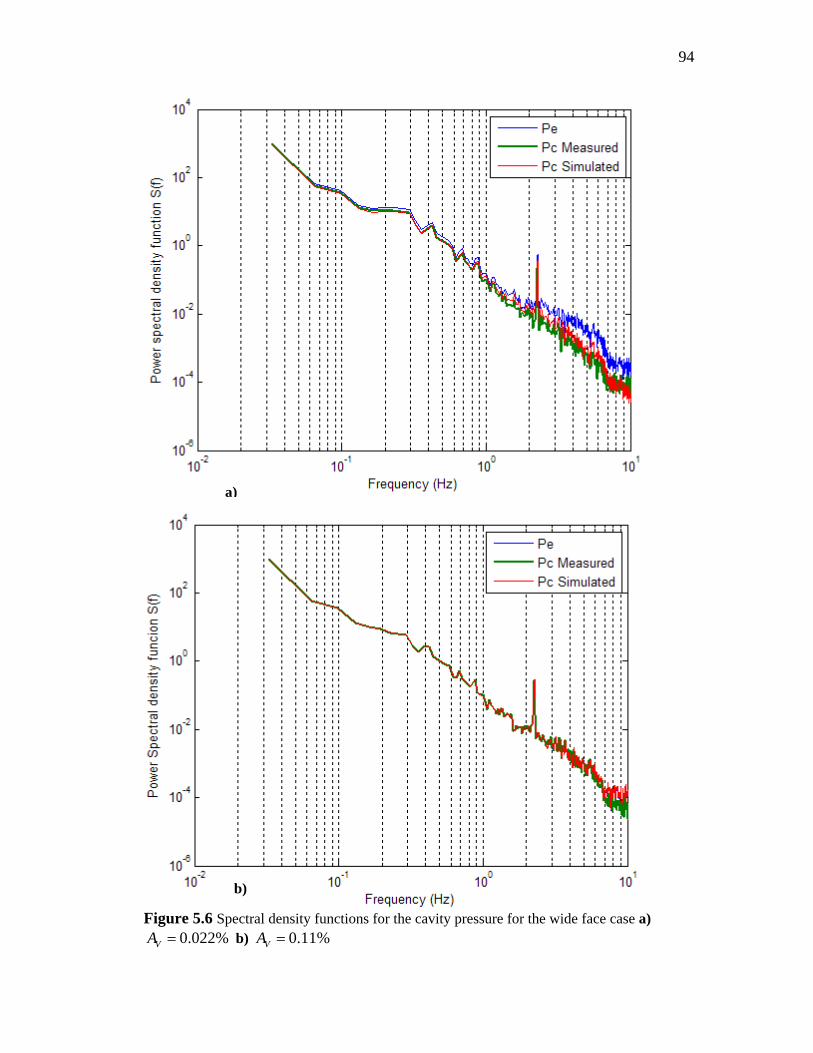
94
Figure 5.6 Spectral density functions for the cavity pressure for the wide face case a) 0.022%VA
b) 0.11%VA
a)
b)
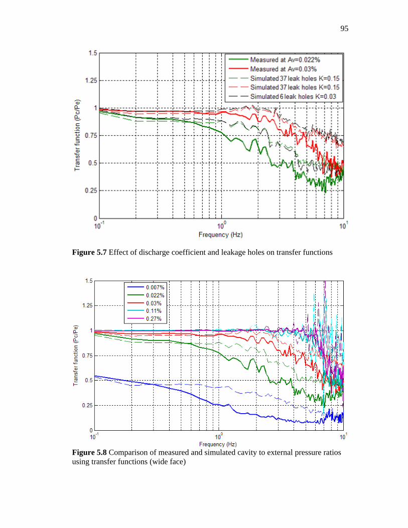
95
Figure 5.7 Effect of discharge coefficient and leakage holes on transfer functions
Figure 5.8 Comparison of measured and simulated cavity to external pressure ratios using transfer functions (wide face)
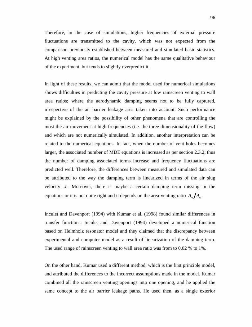
96
Therefore, in the case of simulations, higher frequencies of external pressure
fluctuations are transmitted to the cavity, which was not expected from the
comparison previously established between measured and simulated basic statistics.
At high venting area ratios, the numerical model has the same qualitative behaviour
of the experiment, but tends to slightly overpredict it.
In light of these results, we can admit that the model used for numerical simulations
shows difficulties in predicting the cavity pressure at low rainscreen venting to wall
area ratios; where the aerodynamic damping seems not to be fully captured,
irrespective of the air barrier leakage area taken into account. Such performance
might be explained by the possibility of other phenomena that are controlling the
most the air movement at high frequencies (i.e. the three dimensionality of the flow)
and which are not numerically simulated. In addition, another interpretation can be
related to the numerical equations. In fact, when the number of vent holes becomes
larger, the associated number of MDE equations is increased as per section 2.3.2; thus
the number of damping associated terms increase and frequency fluctuations are
predicted well. Therefore, the differences between measured and simulated data can
be attributed to the way the damping term is linearized in terms of the air slug
velocity x . Moreover, there is maybe a certain damping term missing in the
equations or it is not quite right and it depends on the area-venting ratio rs wA A .
Inculet and Davenport (1994) with Kumar et al. (1998) found similar differences in
transfer functions. Inculet and Davenport (1994) developed a numerical function
based on Helmholz resonator model and they claimed that the discrepancy between
experimental and computer model as a result of linearization of the damping term.
The used range of rainscreen venting to wall area ratio was from to 0.02 % to 1%.
On the other hand, Kumar used a different method, which is the first principle model,
and attributed the differences to the incorrect assumptions made in the model. Kumar
combined all the rainscreen venting openings into one opening, and he applied the
same concept to the air barrier leakage paths. He used then, as a single exterior
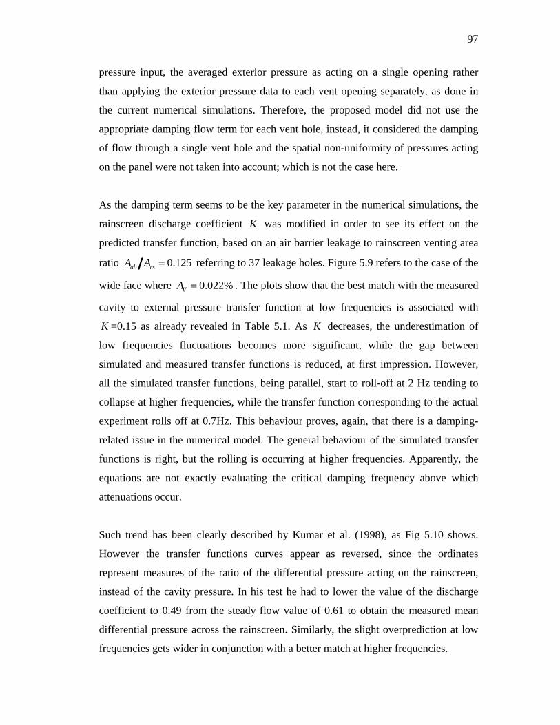
97
pressure input, the averaged exterior pressure as acting on a single opening rather
than applying the exterior pressure data to each vent opening separately, as done in
the current numerical simulations. Therefore, the proposed model did not use the
appropriate damping flow term for each vent hole, instead, it considered the damping
of flow through a single vent hole and the spatial non-uniformity of pressures acting
on the panel were not taken into account; which is not the case here.
As the damping term seems to be the key parameter in the numerical simulations, the
rainscreen discharge coefficient K
was modified in order to see its effect on the
predicted transfer function, based on an air barrier leakage to rainscreen venting area
ratio 0.125ab rsA A referring to 37 leakage holes. Figure 5.9 refers to the case of the
wide face where 0.022%VA . The plots show that the best match with the measured
cavity to external pressure transfer function at low frequencies is associated with
K =0.15 as already revealed in Table 5.1. As K
decreases, the underestimation of
low frequencies fluctuations becomes more significant, while the gap between
simulated and measured transfer functions is reduced, at first impression. However,
all the simulated transfer functions, being parallel, start to roll-off at 2 Hz tending to
collapse at higher frequencies, while the transfer function corresponding to the actual
experiment rolls off at 0.7Hz. This behaviour proves, again, that there is a damping-
related issue in the numerical model. The general behaviour of the simulated transfer
functions is right, but the rolling is occurring at higher frequencies. Apparently, the
equations are not exactly evaluating the critical damping frequency above which
attenuations occur.
Such trend has been clearly described by Kumar et al. (1998), as Fig 5.10 shows.
However the transfer functions curves appear as reversed, since the ordinates
represent measures of the ratio of the differential pressure acting on the rainscreen,
instead of the cavity pressure. In his test he had to lower the value of the discharge
coefficient to 0.49 from the steady flow value of 0.61 to obtain the measured mean
differential pressure across the rainscreen. Similarly, the slight overprediction at low
frequencies gets wider in conjunction with a better match at higher frequencies.
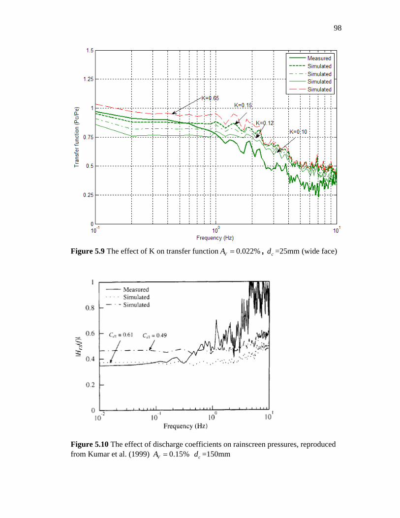
98
Figure 5.9 The effect of K on transfer function 0.022%VA , cd =25mm (wide face)
Figure 5.10 The effect of discharge coefficients on rainscreen pressures, reproduced from Kumar et al. (1999) 0.15%VA
cd =150mm
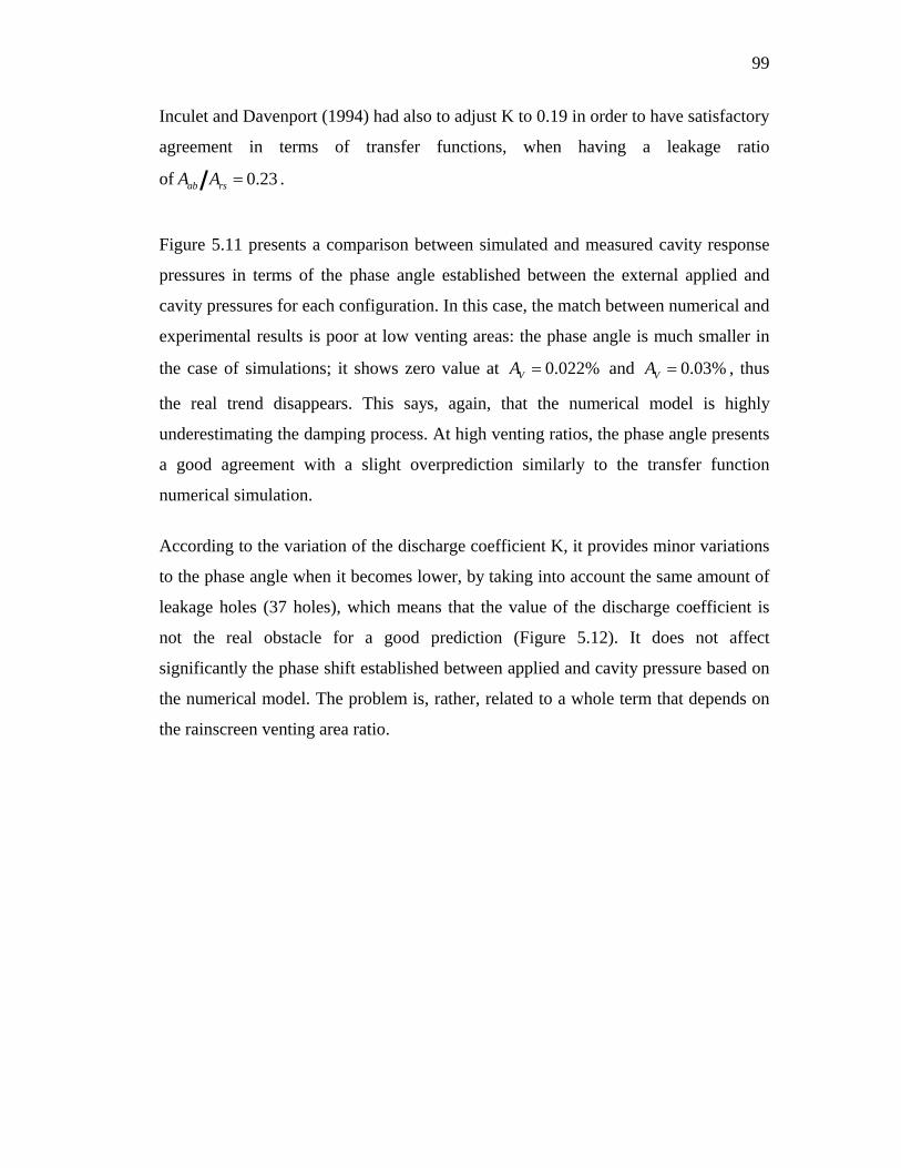
99
Inculet and Davenport (1994) had also to adjust K to 0.19 in order to have satisfactory
agreement in terms of transfer functions, when having a leakage ratio
of 0.23ab rsA A .
Figure 5.11 presents a comparison between simulated and measured cavity response
pressures in terms of the phase angle established between the external applied and
cavity pressures for each configuration. In this case, the match between numerical and
experimental results is poor at low venting areas: the phase angle is much smaller in
the case of simulations; it shows zero value at 0.022%VA
and 0.03%VA , thus
the real trend disappears. This says, again, that the numerical model is highly
underestimating the damping process. At high venting ratios, the phase angle presents
a good agreement with a slight overprediction similarly to the transfer function
numerical simulation.
According to the variation of the discharge coefficient K, it provides minor variations
to the phase angle when it becomes lower, by taking into account the same amount of
leakage holes (37 holes), which means that the value of the discharge coefficient is
not the real obstacle for a good prediction (Figure 5.12). It does not affect
significantly the phase shift established between applied and cavity pressure based on
the numerical model. The problem is, rather, related to a whole term that depends on
the rainscreen venting area ratio.
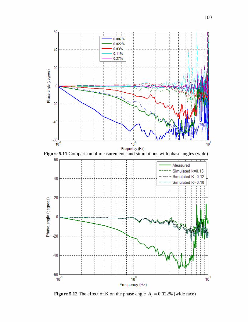
100
Figure 5.11 Comparison of measurements and simulations with phase angles (wide)
Figure 5.12 The effect of K on the phase angle 0.022%VA (wide face)
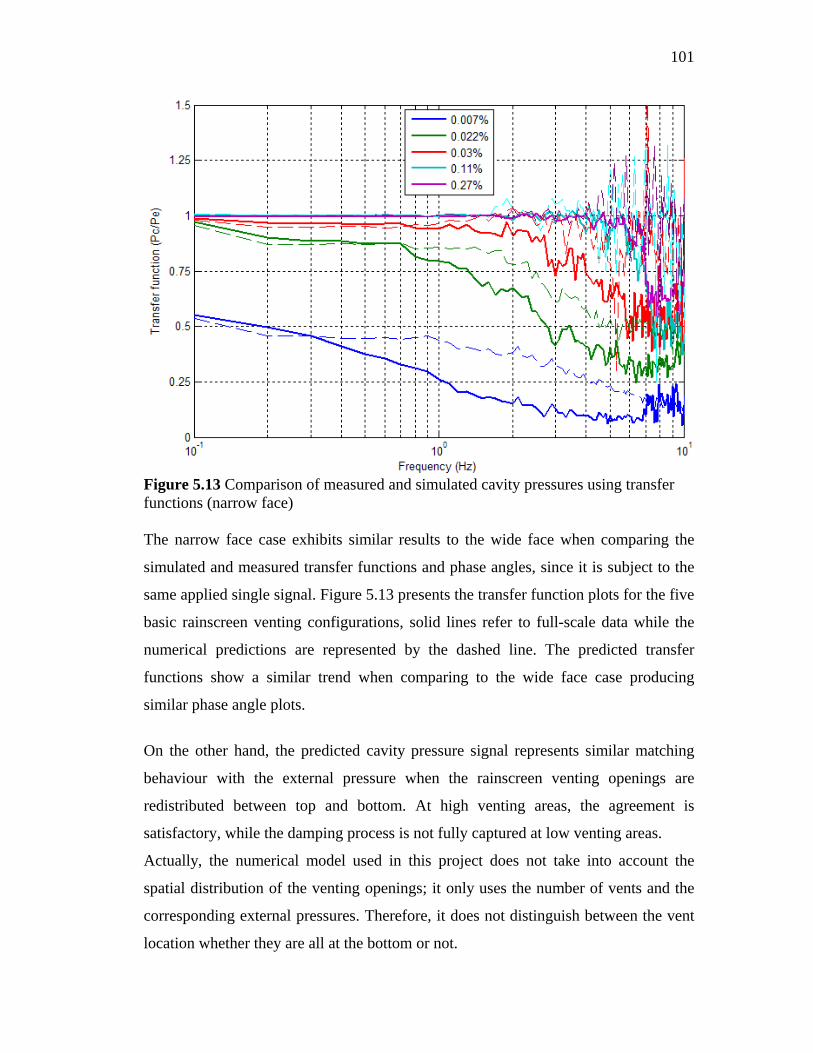
101
Figure 5.13 Comparison of measured and simulated cavity pressures using transfer functions (narrow face)
The narrow face case exhibits similar results to the wide face when comparing the
simulated and measured transfer functions and phase angles, since it is subject to the
same applied single signal. Figure 5.13 presents the transfer function plots for the five
basic rainscreen venting configurations, solid lines refer to full-scale data while the
numerical predictions are represented by the dashed line. The predicted transfer
functions show a similar trend when comparing to the wide face case producing
similar phase angle plots.
On the other hand, the predicted cavity pressure signal represents similar matching
behaviour with the external pressure when the rainscreen venting openings are
redistributed between top and bottom. At high venting areas, the agreement is
satisfactory, while the damping process is not fully captured at low venting areas.
Actually, the numerical model used in this project does not take into account the
spatial distribution of the venting openings; it only uses the number of vents and the
corresponding external pressures. Therefore, it does not distinguish between the vent
location whether they are all at the bottom or not.
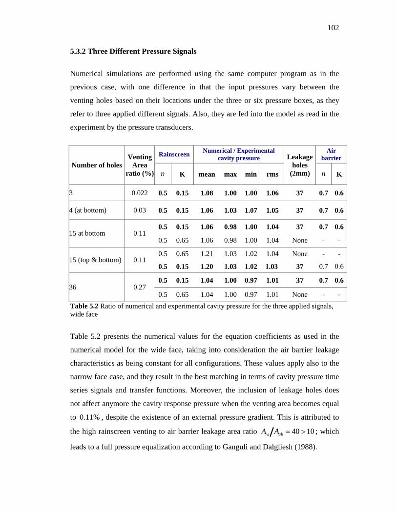
102
5.3.2 Three Different Pressure Signals
Numerical simulations are performed using the same computer program as in the
previous case, with one difference in that the input pressures vary between the
venting holes based on their locations under the three or six pressure boxes, as they
refer to three applied different signals. Also, they are fed into the model as read in the
experiment by the pressure transducers.
Rainscreen Numerical / Experimental cavity pressure
Air barrier
Number of holes
Venting
Area ratio (%)
n
K mean max min rms
Leakage holes
(2mm) n
K
3 0.022 0.5
0.15 1.08 1.00 1.00 1.06 37 0.7
0.6
4 (at bottom) 0.03 0.5
0.15 1.06 1.03 1.07 1.05 37 0.7
0.6
0.5
0.15 1.06 0.98 1.00 1.04 37 0.7
0.6
15 at bottom 0.11 0.5
0.65 1.06 0.98 1.00 1.04 None - -
0.5
0.65 1.21 1.03 1.02 1.04 None - - 15 (top & bottom)
0.11 0.5
0.15 1.20 1.03 1.02 1.03 37 0.7
0.6
0.5
0.15 1.04 1.00 0.97 1.01 37 0.7
0.6
36 0.27 0.5
0.65 1.04 1.00 0.97 1.01 None - -
Table 5.2 Ratio of numerical and experimental cavity pressure for the three applied signals, wide face
Table 5.2 presents the numerical values for the equation coefficients as used in the
numerical model for the wide face, taking into consideration the air barrier leakage
characteristics as being constant for all configurations. These values apply also to the
narrow face case, and they result in the best matching in terms of cavity pressure time
series signals and transfer functions. Moreover, the inclusion of leakage holes does
not affect anymore the cavity response pressure when the venting area becomes equal
to 0.11% , despite the existence of an external pressure gradient. This is attributed to
the high rainscreen venting to air barrier leakage area ratio 40 10rs abA A ; which
leads to a full pressure equalization according to Ganguli and Dalgliesh (1988).
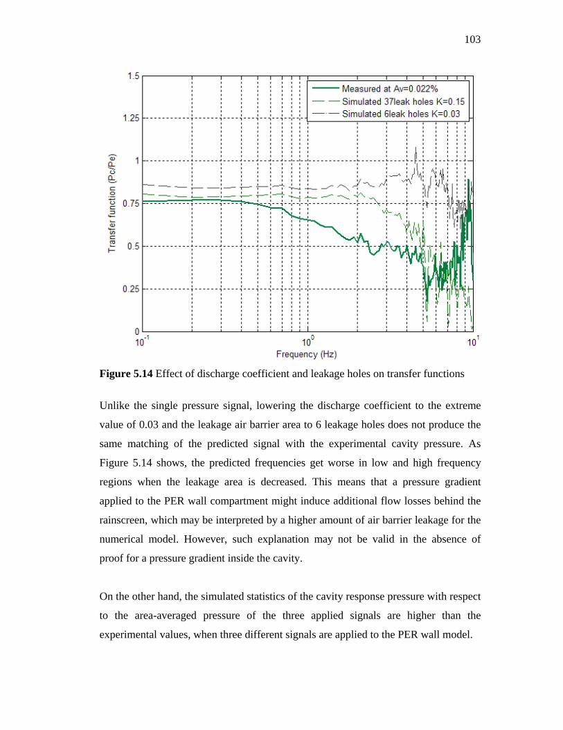
103
Figure 5.14 Effect of discharge coefficient and leakage holes on transfer functions
Unlike the single pressure signal, lowering the discharge coefficient to the extreme
value of 0.03 and the leakage air barrier area to 6 leakage holes does not produce the
same matching of the predicted signal with the experimental cavity pressure. As
Figure 5.14 shows, the predicted frequencies get worse in low and high frequency
regions when the leakage area is decreased. This means that a pressure gradient
applied to the PER wall compartment might induce additional flow losses behind the
rainscreen, which may be interpreted by a higher amount of air barrier leakage for the
numerical model. However, such explanation may not be valid in the absence of
proof for a pressure gradient inside the cavity.
On the other hand, the simulated statistics of the cavity response pressure with respect
to the area-averaged pressure of the three applied signals are higher than the
experimental values, when three different signals are applied to the PER wall model.
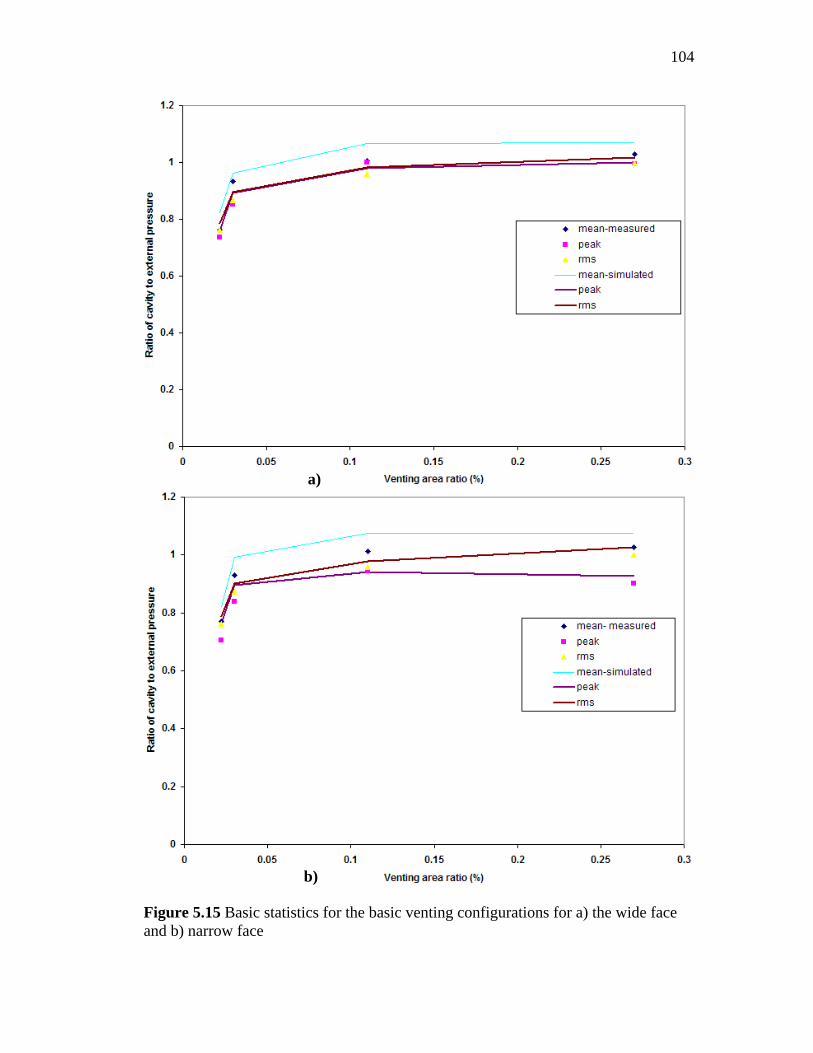
104
Figure 5.15 Basic statistics for the basic venting configurations for a) the wide face and b) narrow face
a)
b)
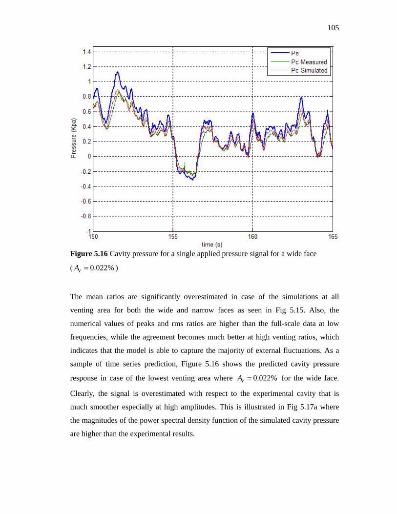
105
Figure 5.16 Cavity pressure for a single applied pressure signal for a wide face
( 0.022%VA )
The mean ratios are significantly overestimated in case of the simulations at all
venting area for both the wide and narrow faces as seen in Fig 5.15. Also, the
numerical values of peaks and rms ratios are higher than the full-scale data at low
frequencies, while the agreement becomes much better at high venting ratios, which
indicates that the model is able to capture the majority of external fluctuations. As a
sample of time series prediction, Figure 5.16 shows the predicted cavity pressure
response in case of the lowest venting area where 0.022%VA
for the wide face.
Clearly, the signal is overestimated with respect to the experimental cavity that is
much smoother especially at high amplitudes. This is illustrated in Fig 5.17a where
the magnitudes of the power spectral density function of the simulated cavity pressure
are higher than the experimental results.
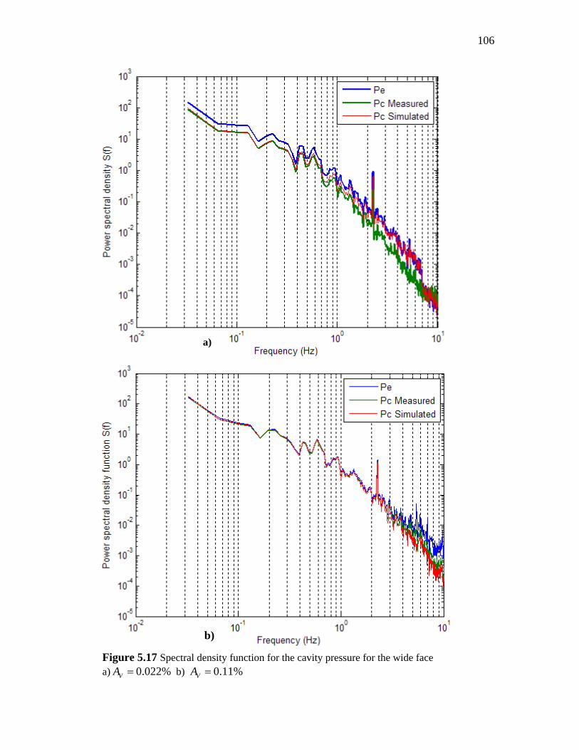
106
Figure 5.17 Spectral density function for the cavity pressure for the wide face a) 0.022%VA
b) 0.11%VA
a)
b)
b)
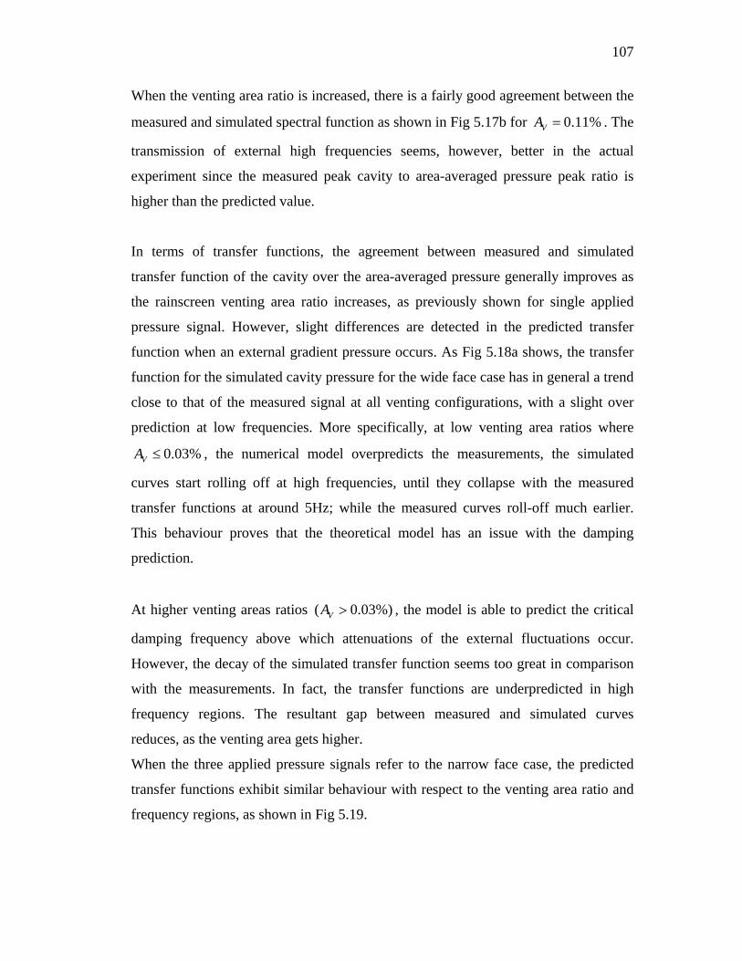
107
When the venting area ratio is increased, there is a fairly good agreement between the
measured and simulated spectral function as shown in Fig 5.17b for 0.11%VA . The
transmission of external high frequencies seems, however, better in the actual
experiment since the measured peak cavity to area-averaged pressure peak ratio is
higher than the predicted value.
In terms of transfer functions, the agreement between measured and simulated
transfer function of the cavity over the area-averaged pressure generally improves as
the rainscreen venting area ratio increases, as previously shown for single applied
pressure signal. However, slight differences are detected in the predicted transfer
function when an external gradient pressure occurs. As Fig 5.18a shows, the transfer
function for the simulated cavity pressure for the wide face case has in general a trend
close to that of the measured signal at all venting configurations, with a slight over
prediction at low frequencies. More specifically, at low venting area ratios where
0.03%VA , the numerical model overpredicts the measurements, the simulated
curves start rolling off at high frequencies, until they collapse with the measured
transfer functions at around 5Hz; while the measured curves roll-off much earlier.
This behaviour proves that the theoretical model has an issue with the damping
prediction.
At higher venting areas ratios ( 0.03%)VA , the model is able to predict the critical
damping frequency above which attenuations of the external fluctuations occur.
However, the decay of the simulated transfer function seems too great in comparison
with the measurements. In fact, the transfer functions are underpredicted in high
frequency regions. The resultant gap between measured and simulated curves
reduces, as the venting area gets higher.
When the three applied pressure signals refer to the narrow face case, the predicted
transfer functions exhibit similar behaviour with respect to the venting area ratio and
frequency regions, as shown in Fig 5.19.
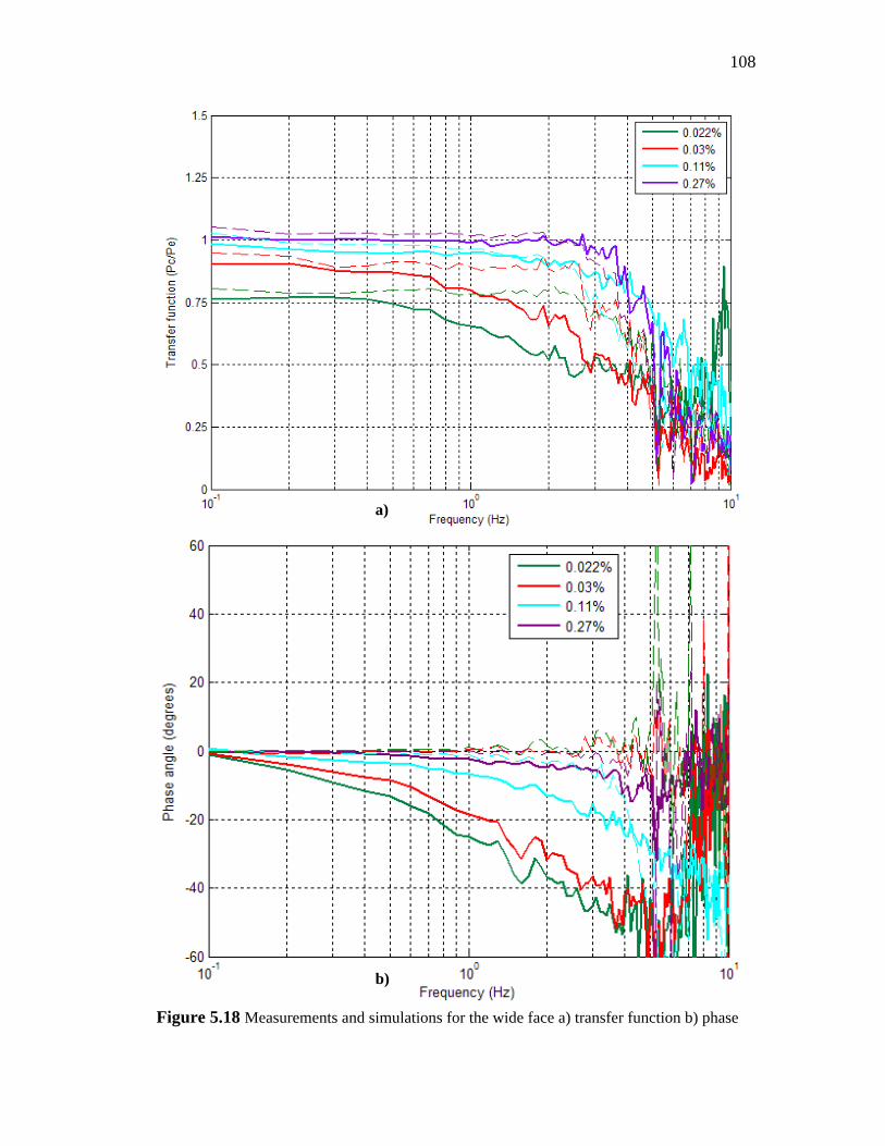
108
Figure 5.18 Measurements and simulations for the wide face a) transfer function b) phase
a)
b)
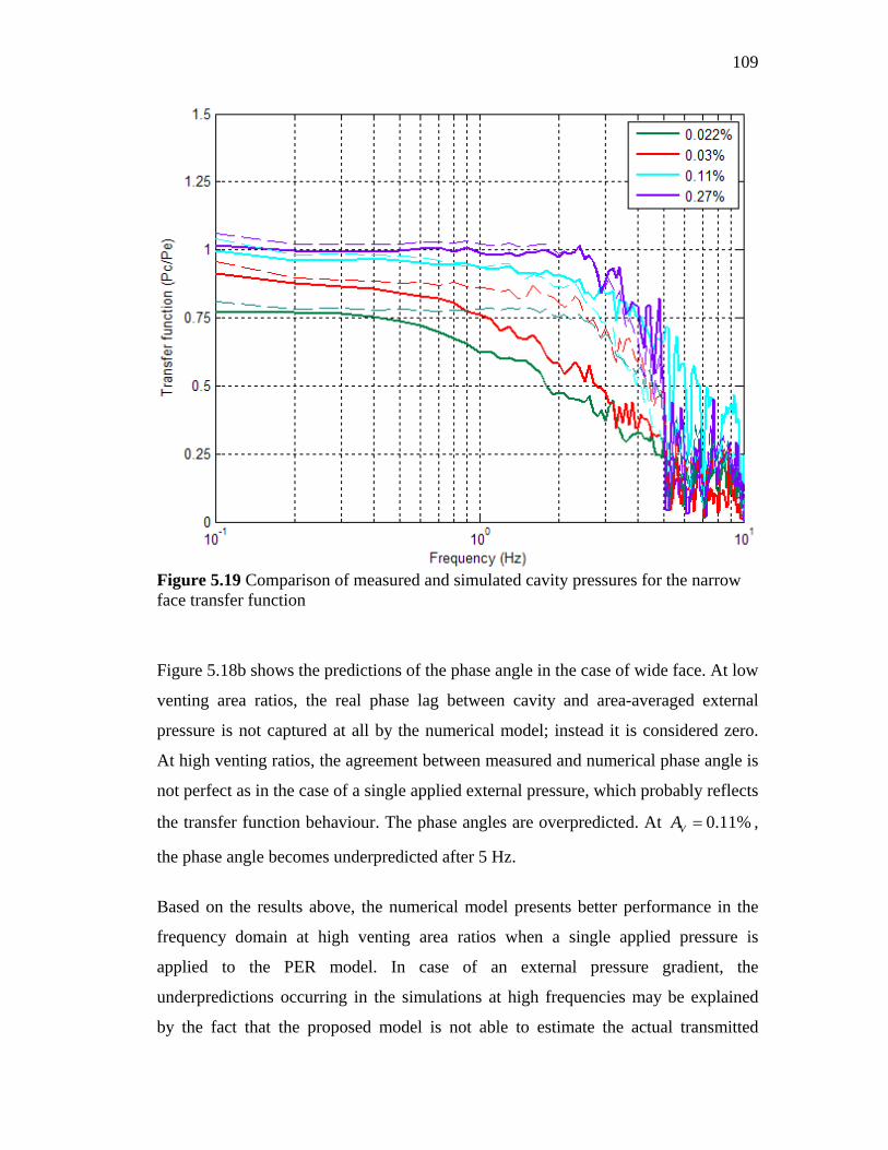
109
Figure 5.19 Comparison of measured and simulated cavity pressures for the narrow face transfer function
Figure 5.18b shows the predictions of the phase angle in the case of wide face. At low
venting area ratios, the real phase lag between cavity and area-averaged external
pressure is not captured at all by the numerical model; instead it is considered zero.
At high venting ratios, the agreement between measured and numerical phase angle is
not perfect as in the case of a single applied external pressure, which probably reflects
the transfer function behaviour. The phase angles are overpredicted. At 0.11%VA ,
the phase angle becomes underpredicted after 5 Hz.
Based on the results above, the numerical model presents better performance in the
frequency domain at high venting area ratios when a single applied pressure is
applied to the PER model. In case of an external pressure gradient, the
underpredictions occurring in the simulations at high frequencies may be explained
by the fact that the proposed model is not able to estimate the actual transmitted
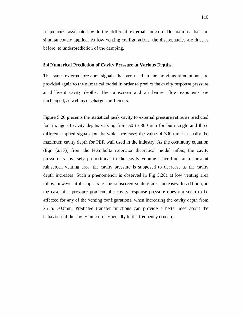
110
frequencies associated with the different external pressure fluctuations that are
simultaneously applied. At low venting configurations, the discrepancies are due, as
before, to underprediction of the damping.
5.4 Numerical Prediction of Cavity Pressure at Various Depths
The same external pressure signals that are used in the previous simulations are
provided again to the numerical model in order to predict the cavity response pressure
at different cavity depths. The rainscreen and air barrier flow exponents are
unchanged, as well as discharge coefficients.
Figure 5.20 presents the statistical peak cavity to external pressure ratios as predicted
for a range of cavity depths varying from 50 to 300 mm for both single and three
different applied signals for the wide face case; the value of 300 mm is usually the
maximum cavity depth for PER wall used in the industry. As the continuity equation
(Eqn (2.17)) from the Helmholtz resonator theoretical model infers, the cavity
pressure is inversely proportional to the cavity volume. Therefore, at a constant
rainscreen venting area, the cavity pressure is supposed to decrease as the cavity
depth increases. Such a phenomenon is observed in Fig 5.20a at low venting area
ratios, however it disappears as the rainscreen venting area increases. In addition, in
the case of a pressure gradient, the cavity response pressure does not seem to be
affected for any of the venting configurations, when increasing the cavity depth from
25 to 300mm. Predicted transfer functions can provide a better idea about the
behaviour of the cavity pressure, especially in the frequency domain.
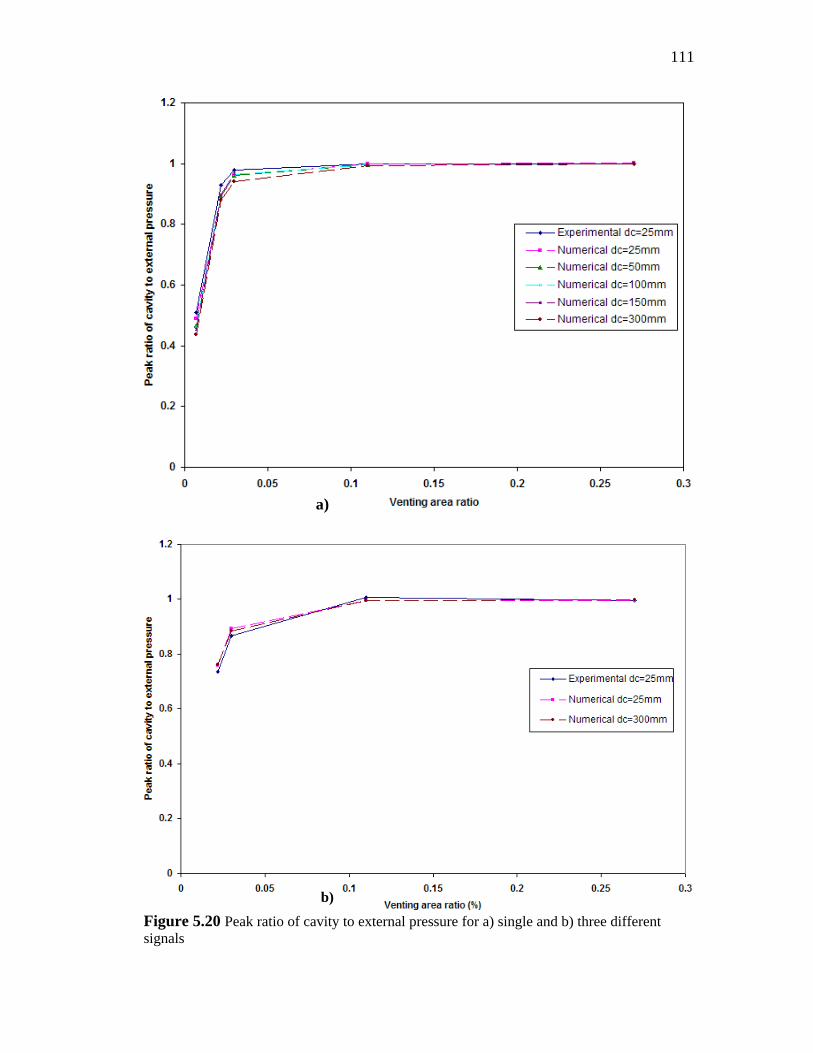
111
Figure 5.20 Peak ratio of cavity to external pressure for a) single and b) three different signals
a)
b)
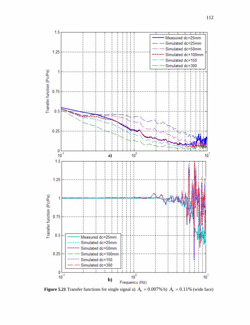
112
Figure 5.21 Transfer functions for single signal a) 0.007%VA b) 0.11%VA (wide face)
a)
b)
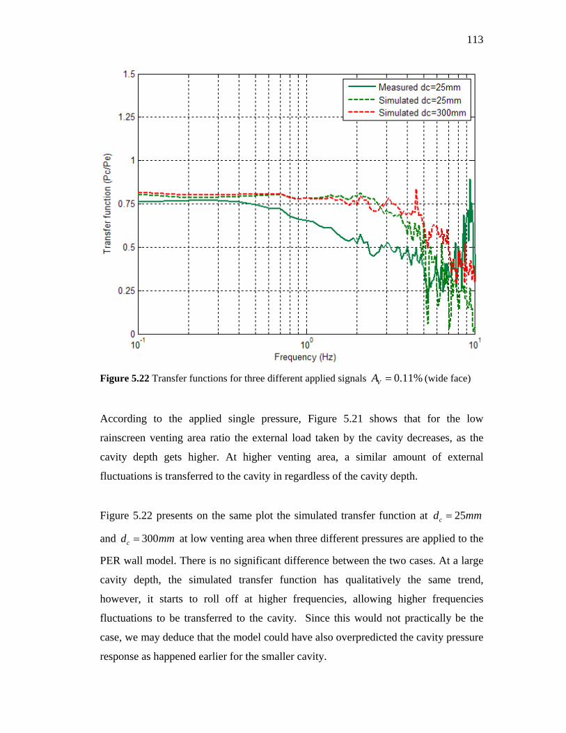
113
Figure 5.22 Transfer functions for three different applied signals 0.11%VA (wide face)
According to the applied single pressure, Figure 5.21 shows that for the low
rainscreen venting area ratio the external load taken by the cavity decreases, as the
cavity depth gets higher. At higher venting area, a similar amount of external
fluctuations is transferred to the cavity in regardless of the cavity depth.
Figure 5.22 presents on the same plot the simulated transfer function at 25cd mm
and 300cd mm
at low venting area when three different pressures are applied to the
PER wall model. There is no significant difference between the two cases. At a large
cavity depth, the simulated transfer function has qualitatively the same trend,
however, it starts to roll off at higher frequencies, allowing higher frequencies
fluctuations to be transferred to the cavity. Since this would not practically be the
case, we may deduce that the model could have also overpredicted the cavity pressure
response as happened earlier for the smaller cavity.
114
Previous work has not tested the cavity depth variation effect on the pressure
equalization process. The focus was more towards the rainscreen venting to air barrier
leakage role in the PER walls performance. Apart from Garden (1963) who settled the
minimum value at 25mm, only a few recommendations were mentioned in terms of
determining a suitable cavity depth. The concept is that the cavity depth depends on
both the rainscreen venting area and the total area of the panel. Inculet (1990)
established the following relationship where 10c rs wd A A . Later, Kumar (2000)
claims that an increase in venting for constant volume, or a decrease in volume for
constant venting area, can improve the pressure equalization. This is proved in the
numerical tests that have been done for the current project when a single pressure
signal is applied. However, note that the external pressure signals used for all cavity
depths were the same as for the lowest depth (25mm), which in practice could not be
correct, taking into account the PLA errors at each configuration, and or the varying
amount of leakage that may arise from the cavity volume change. Therefore, further
full-scale experiments should be done, by varying the cavity depth to validate the
theory.
5.5 Summary
This chapter has presented a comparison between the experimental and predicted
cavity pressure measurements based on Helmholtz resonator model theory. The
concept was to match the measured rms cavity pressure with the numerical value by
adjusting the rainscreen discharge coefficient and including leakage holes in the air
barrier simultaneously. When a uniform pressure was applied, the numerical model
showed the same cavity response prediction at 0.022%VA and 0.03%VA
under
two different combinations: 1) six leakage holes at rainscreen discharge coefficient
equal to 0.03 and, 2) 37 leakage holes with 0.15K . While with a pressure gradient,
only the second combination gave the best matching.
115
On the other hand, the predicted cavity pressure did not seem to be affected by the
addition of leakage holes to the numerical model at venting area ratios higher than
0.11%.
In general, the results showed, for low venting area ratios, a satisfactory agreement in
the low frequency regions between transfer functions of cavity to external pressures.
At higher frequencies, the simulated transfer functions were overpredicted. At high
venting area ratios, a good agreement was provided in terms of both transfer functions
and phase angles.
Discrepancies were noticed when comparing the matching with respect to the applied
external pressure. Basic statistical ratios of cavity to external pressures were
underestimated under a pressure gradient and overestimated under a uniform pressure
for low venting area ratios. Also, the simulated transfer functions were slightly
underpredicted at high venting area ratios in the case of the application of a horizontal
pressure gradient.
The numerical model was used to predict the impact of cavity depth variation on the
pressure equalization process, using the external pressure values as applied to the
model on site. The simulations showed that for low venting area ratios, increasing the
cavity depth reduces the equalization process between external and cavity pressures
under a uniform pressure. Under a gradient pressure, there was no effect of the cavity
depth variation. Under a pressure gradient, the cavity pressure response did not
change at both low and high venting area ratios.
The following chapter will explore the conclusions based on both the experimental
and numerical findings of the current research. Also, it will present some
recommendations for future experimental work.
116
CHAPTER 6
CONCLUSIONS AND RECOMMENDATIONS
A completely sealed full-scale model of a PER wall panel compartment measuring 2.2 m
wide by 2m high was built in the IRLBH facility at the University of Western Ontario, to
investigate the effect of various parameters on the pressure equalization process under
normal wind pressure. PLAs were used to generate wind pressure time series signals
based on wind tunnel experiments. Two types of external pressures were applied: 1) a
single pressure signal and, 2) three different signals that create a pressure gradient across
the rainscreen. The signals correspond respectively to a middle tap and edge taps signals
of a windward façade associated to a pressure model already investigated. In each test
configuration, the external data pressure signals of both wide and narrow faces were
used. These faces are being tested each separately under a normal wind flow.
The configurations differed in the rainscreen venting area ratios, while the volume of the
PER was kept constant at the cavity depth of 25mm. Also, in some cases, the layout of
vent holes was changed for the same venting area. Data measurements provided the
cavity pressure for each configuration which enables to evaluate the PER performance
with cavity response to external pressure ratios. The experimental results were compared
to a numerical model s predictions based on Helmholtz resonator theory. Furthermore,
the effect of the compartment volume variation on PE was examined numerically by
predicting the cavity pressure for a wide range of cavity depths, with respect to the
rainscreen venting area ratio.
Contributions of the Current Research
Previous pressure equalized rainscreen wall system experiments were focusing most on
the effect of rainscreen venting and air barrier leakage area ratios on the pressure
equalization process. There was an agreement that a satisfactory PE process could be
117
attained by using an adequate rainscreen venting to air barrier leakage area ratio, all other
factors remaining constant. However, other PER wall parameters or external flow
conditions that might have an effective impact on the system performance, have not been
extensively addressed before.
The current research has tested a PER compartment under a pressure gradient by the
application of three different signals varying horizontally over the rainscreen panel. This
experiment is considered to be unique in terms of setup and application. In fact, for the
first time, such a test was performed in a controlled facility where the model is built as
perfectly sealed. In addition, real wind traces were used corresponding to edge pressure
signals, that were extracted from both a wide and narrow windward faces under a normal
flow. Thus, the effect of two types of pressure gradients was examined. This test has
provided a clear idea about the impact of a pressure gradient on the PER system
performance, under a range of rainscreen venting area ratios and configurations.
Moreover, this project has examined the differential pressure differential across the
rainscreen under a very low rainscreen to wall venting area ratio, which is 0.007%, a
value that was never encountered before. Therefore, it was interesting to investigate the
effect of such configuration on the model performance at the smallest cavity depth
usually used, which is 25mm.
Finally, the vent openings layout impact on the PE process was experimentally
investigated for the same rainscreen venting area ratio and cavity depth, under both the
external uniform and gradient pressures. Previous studies have not separately examined
this parameter.
Based on the experimental and numerical cavity pressure measurements, the data analysis
have led to the following:
118
Conclusions
The rainscreen venting to wall area ratio has a significant impact on the PER wall
panel performance at constant volume. As the venting area increases, pressure
equalization between external and cavity pressures improve, irrespective of the
type of external applied pressure signals.
Under both applied single pressure and pressure gradients, the cavity pressure is
uniform at all rainscreen venting areas ratios.
The change in the vent openings layout affects the process of pressure
equalization. At high venting area ratios, the transfer functions magnitudes
referring to the cavity to exterior pressures ratio are almost the same in case the
vents are placed at bottom or distributed between top and bottom of the
rainscreen. The difference is more pronounced at low venting area ratios, where
the bottom location provides better pressure equalization.
As the rainscreen venting area ratio gets larger, the critical damping frequency
increases. Thus, the transfer functions of the cavity to external pressure ratio show
less attenuation at low frequencies, with a reduction of the phase angle. In
addition, better transmission of higher frequencies is observed.
A full-pressure equalization results in a phase angle between the cavity and
external pressure equal to zero, in conjunction with a complete transmission of
low and high external frequency fluctuations in terms of transfer functions.
The pressure gradient, caused by the application of three different signals, leads to
a lower degree of pressure equalization with higher peak factors, in terms of
differential pressure and frequencies. In the current research, the maximum PE is
attained at 0.27%VA , external area-averaged pressure frequencies higher than 3
Hz are not fully transmitted to the cavity. Under a uniform pressure, full PE was
observed for 0.11%VA
A higher applied horizontal pressure gradient leads to higher residual loads on the
raincsreen, which results in a slower pressure equalization process shown by the
model.
119
The numerical model based on Helmholtz resonator theory provides good
matching with the experimental results at high rainscreen venting area ratios in
terms of high frequencies external fluctuations. At low venting areas, the
numerical model is not able to capture the real critical damping frequency, which
shows an overprediction of the transfer functions and great reduction in phase
angles. Such trend indicates that the model presents an issue in terms of the
damping term, which is highly related to the area-venting ratio. A possible reason
might be the linearization of the damping term in the equations.
Under both a uniform and gradient pressures, the inclusion of leakage holes in the
numerical model does not influence the predicted cavity response at 0.11%VA
Certain differences exist in the numerical predictions of cavity pressure response
in the frequency domain depending on the applied external pressures. Under a
uniform pressure, statistical values of the cavity to external pressure ratios are
underestimated at low venting areas ratios by numerical simulations, and the
experimental transfer function is in fairly good match at high venting are ratios.
Under a pressure gradient, there is overestimation of the statistical ratios; also, the
transfer function becomes underpredicted at higher frequencies for larger venting.
Based on the numerical model prediction, the cavity depth variation shows that
the effect of the volume change is more significant at low venting areas. At a
constant rainscreen venting area, the pressure equalization is reduced as the cavity
depth increases when a uniform pressure is applied. However, no significant
change is observed when the PER is subject to a pressure gradient.
Recommendations for Future Experimental Work
It would be very useful to conduct more tests at various depths in order to see the
effect of cavity volume change on the PE performance of the current model,
especially under a pressure gradient. Such experiment may either validate the
current project s results, or settle new recommendations for an optimum cavity
depth.
120
More test configurations are recommended involving the inclusion of intentional
leakage openings in the air barrier, which will help to check the impact of the
rainscreen venting to air barrier leakage areas ratios on the model performance
under a uniform pressure and pressure gradient.
Various other experiments may be performed at different wind angles,
compartment size and vent openings layout to collect the volume of data required
for design guidelines settling.
The numerical model as used in this project needs further investigation for better
predictions at low venting areas. A possible solution is to find a certain method in
doing the computations without the linearization of the equations and damping
terms.
The wind-driven rain impact may be also investigated using the current PER wall
model. By applying simultaneously wind pressure and rain droplets, we would
experimentally observe the process of the water penetration into the cavity
through the various vent openings. Such test would require improvement in the
way of wind application to avoid losses, especially at low venting areas.
A rainscreen venting area ratio less than 0.11% is not recommended for a PER
system at a compartment cavity depth of 25mm

121
REFERENCES
Baskaran, B. A. and Brown, W. C. (1992). Performance of pressure equalized rainscreen walls under cyclic loading . J. Thermal. Ins. and Build. Envelop. 16, 183-193.
Baskaran B.A. (1992). Review of Design Guidelines for Pressure Equalized Rainscreen walls . Institute for Research in Construction, National Research Council Canada, internal report, issue 629.
Birkeland, O. (1962). Curtain walls . Norwegian Building Research.
Bloxham, C. and Vickery, B.J. (1989). An experimental investigation of internal pressure dynamics with a dominant front wall opening , University of Western Ontario, Faculty of Engineering and Science. BLWTL-SS46-1989.
British Standards, BS 8200:1985. Code of practice for design of non-load bearing external vertical enclosures of buildings .
Brown, W.C, Rousseau, M.Z and Dalgliesh, W.A.(1995). Field testing of pressure-equalized rainscreen walls . Building Envelope Performance and Durability, IRC Technical Seminar, 59-69, Canada.
Canadian Construction Materials Centre (CCMC), 2000. A method for Evaluating Air barrier Systems and Materials. National Research Council s Institute for Research in Construction, Construction Technology, Issue 46.
Chaplin, G.C, Randall, J.R and Baker, C.J.(2000). The turbulent ventilation of a single opening enclosure. J. Wind Eng. Ind. Aerodyn., 85, 145-161.
Choi E., C.C. and Wang, Z. (1998). Study on pressure-equalization of curtain wall systems . J. Wind Eng. Ind. Aerodyn., 73, 251-266.
Davenport, A.G. and Surry, D. (1984). The Estimation of Internal Pressures due to Wind with Application to cladding pressures and Infiltration. Wind Pressure Workshop, Brussels, Belgium.
Fazio, P. and Kontopidis, T. (1988). Cavity Pressure in Rain Screen Walls . Building and Environment, 23,137-143.
Garden, G.K. (1963). Rain Penetration and its control . Division of Building Research, National Research Council Ottawa, Canada, Canadian Building Digest, issue 40
122
Ganguli, U. and Quirouette, R.L. (1987). Pressure equalization performance of a Metal and Glass curtain wall. Proceedings, CSCE Centennial conference, 1,127-144, Montreal, Canada.
Ganguli, U. and Dalgliesh, W.A. (1988). Wind pressures on open rain screen walls: Place Air Canada. J. Struct. Eng., 114, 642-56.
Ginger, J.D and Letchford, C.W (1999). Net pressures on a low-rise full-scale building . J. Wind Eng. Ind. Aerodyn , 83, 239- 250.
Harris, R.I. (1990). The propagation of internal pressures in buildings. J. Wind Eng. Ind. Aerodyn, 34, 169-184.
Holmes, J.D. (1979). Mean and fluctuating internal pressure induced by wind , Proc.5th International Conference on Wind Engineering, 435-450, Colorado State University.
Holmes, J. D. (2001). Wind loading of structures . Spon press, London, England.
Inculet, D. (1990). Pressure Equalization of Rainscreen Cladding . The university of Western Ontario. MESc thesis. Faculty of Graduate studies. London, Canada.
Inculet, D. (2001). The Design of cladding against wind-driven rain . The university of Western Ontario. PhD thesis. Faculty of Graduate studies. London, Canada.
Inculet, D.R and Davenport A.G. (1994). Pressure-equalized rainscreens: A study in the frequency domain . J. Wind Eng. Ind. Aerodyn, 53, 63-87.
Inculet, D. and Surry, D. (1997). Optimum Vent locations for Partially-Pressurized Rainscreens . The University of Western Ontario, London, Canada. BLWT-SS30.
Inculet, D., Surry, D. and Davenport, A.G. (1997). Unsteady pressure gradients and their implications for pressure-equalized rainscreens . Proceedings of the International Conference on Building Envelope Systems and Technology, Bath, England.
Inculet, D., Surry, D. and Davenport, A.G (2001). An experimental study of pressure gradients and their implications for the design of pressure-moderated rainscreens. Proceedings of the International Conference on Building Envelope Systems and Technologies, 1, 101-106, Ottawa, Canada.

123
Irwin, P.A., Schuyler, G.D. and Wawzonek, M.A. (1984). A wind tunnel investigation of rainscreen wall systems. Morrison Hershfield Limited. Prepared for CMHC.
Kala, S., Stathopoulos, T. and Kumar, K. S. (2008). Wind loads on Rainscreen walls: Boundary-layer wind tunnel experiments . J. Wind Eng. Ind. Aerodyn., 96, 1058-1073.
Kumar, K.S. (1998). Pressure equalization performance of rainscreen walls: Experimental investigations , Proceedings of the 2nd East European Conference on Wind Engineering, Prague, Czech Republic, September 1998.
Kumar, K.S. (1999). A study on pressure equalization of rainscreen facades: full-scale experiments and computer simulations. Technical Report, FAGO 99.40.k, Faculteit Bouwkunde, Technical University of Eindhoven, Eindhoven, The Netherlands.
Kumar, K.S. and Wisse, J.A. (1999). A full-scale study on pressure equalization of rainscreen facades , Proceedings of the 10th International Conference on Wind Engineering, Copenhagen, Denmark, June 1999.
Kumar, K. S., Van Shijndel, A.W.M (1999). Prediction of pressure equalization performance of rainscreen walls . Wind Struct, 2, 325-345.
Kumar, K. S. (2000). Pressure equalization of rainscreen walls: a critical review. Building and Environment, 35, 161-179.
Kumar, K. S., Stathopoulos, T. and Wisse, J.A. (2003). Field measurement data of wind loads on rainscreen walls . J. Wind Eng. Ind. Aerodyn., 91,1401-1417.
Killip, I.R. and Cheetham, D.W. (1984). The prevention of rain s penetration through external walls and joints by means of pressure equalization. Building and Environment, 19, 81-91.
Kimura, R.I (1977). Scientific basis of air conditioning . Applied Sciences, 175-186.
Kopp, G.A., Morrison, M.J., Gavanski, E., Henderson, D.J. and Hong, H.P. (2010). Three Little Pigs Project: Hurricaine Risk Mitigation by Integrated Wind Tunnel
and Full-Scale Laboratory Tests. Natural Hazards, 11, 151.

124
Latta, J.K. (1973). Walls, windows and roofs for the Canadian climate- a summary of the current basis for selection and design . Special Technical Publication, Issue 1. NRCC 13487.
Malecki, I. (1969). Physical foundations of technical acoustics. Pergamon Press, Oxford and New York.
Morrison Hershfield Limited (1998). Rain penetration control: Applying current knowledge . CMHC, Canada, issue 2972033/2.
Oh, J. H., Kopp, G. A. and Inculet, D. R. (2007). The UWO contribution to the NIST aerodynamic database for wind loads on low buildings: Part 3. Internal pressures. J. Wind Eng. Ind. Aerodyn, 95,755-779.
Rayleigh, L. (1945). The theory of sound, 2nd Edition . New York, NY: Dover Publications
Rousseau, M.Z., Poirier, G.F. and Brown, W.C. (1998). Pressure Equalization in Rainscreen wall systems . National Research Council of Canada. Construction Technology Update. Issue 17.
Schijndel Van, A.W.M. and Schols, S.F.C. (1998). Modeling pressure equalization in cavities. J. Wind Eng. Ind. Aerodyn, 74, 641-649.
Shaw, C.Y. (1981). Air tightness: supermarkets and shopping malls. ASHRAE J.23
Sharma, R.N and Richards, P.J. (1997). The effect of roof flexibility on internal pressure fluctuations. J. Wind Eng. Ind. Aerodyn,72, 175-186.
Sharma, R.N. and Richards, P. J. (2003). The influence of Helmholtz resonance on internal pressures in a low-rise building . J. Wind Eng. Ind. Aerodyn, 91, 807-828.
Skerlj, P.F and Surry, D. (1994). A study of mean pressure gradients, mean cavity pressures and resulting residual mean pressures across a rainscreen for a representative building . Interim Progress Report to CMHC, Boundary Layer Wind Tunnel Laboratory, University of Western Ontario.
Vickery, B. J. (1986). Gust factors for internal pressures in low-rise buildings. J. Wind Eng. Ind. Aerodyn, 23, 259-271.
Vickery, B. J. and Bloxham, C. (1992). Internal pressure dynamics with a dominant opening. J. Wind Eng. Ind. Aerodyn, 41, 193-204.
125
APPENDIX A
A-1 Rainscreen Sketches for Different Venting to Wall Area Ratio Configurations
A-2 Verification of the Air Barrier and Rainscreen Stiffness
A.3 - Uncertainties in Measurements
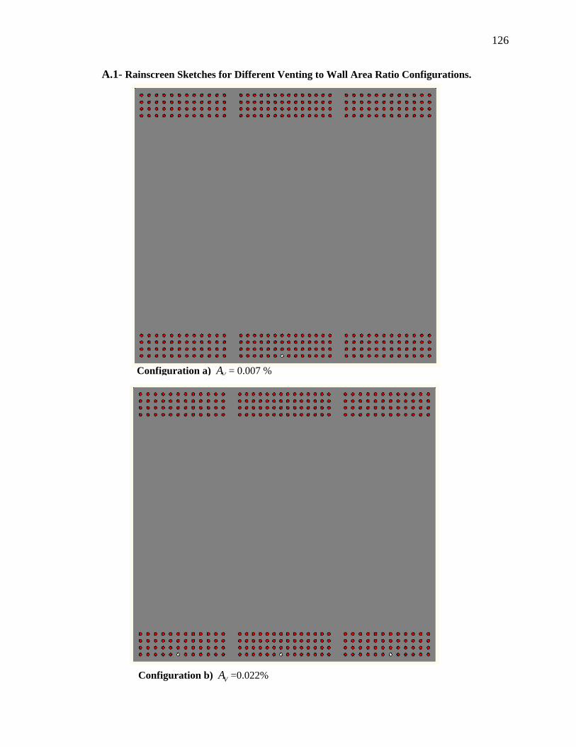
126
A.1- Rainscreen Sketches for Different Venting to Wall Area Ratio Configurations.
Configuration a) VA = 0.007 %
Configuration b) VA =0.022%
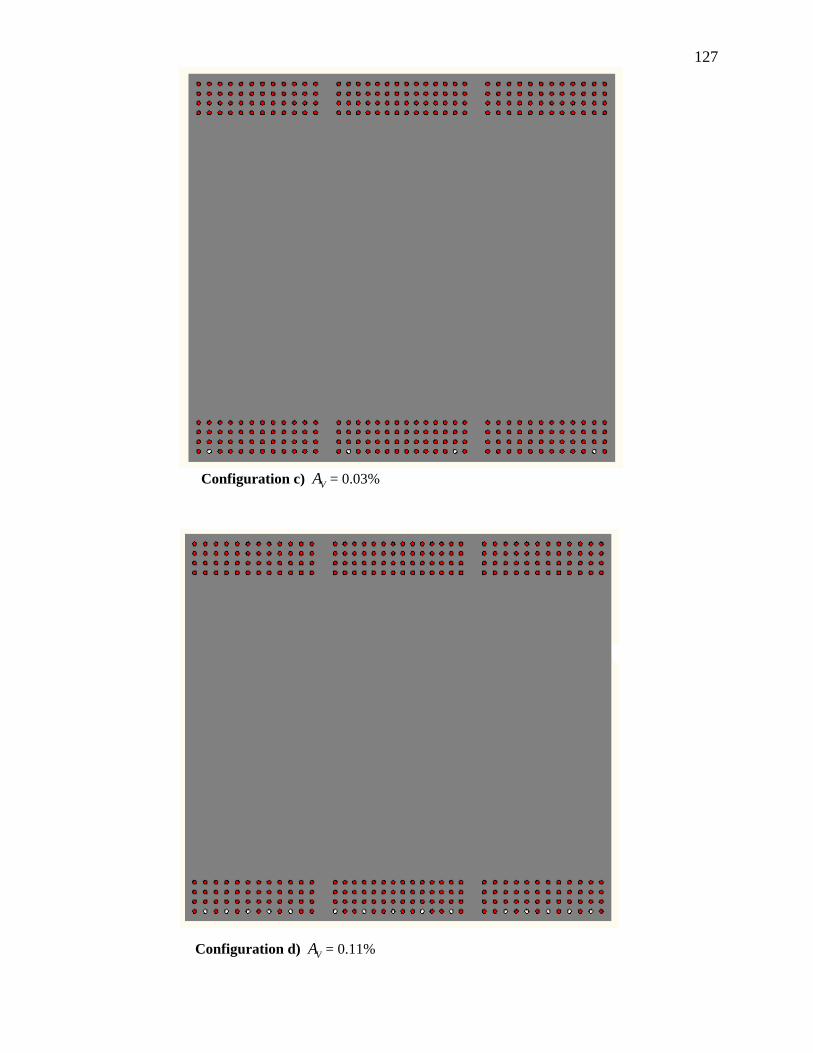
127
Configuration c) VA = 0.03%
Configuration d) VA = 0.11%
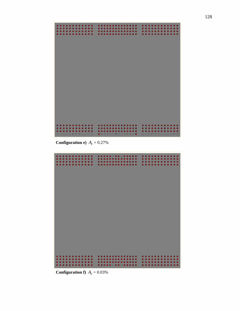
128
Configuration e) VA = 0.27%
Configuration f) VA = 0.03%
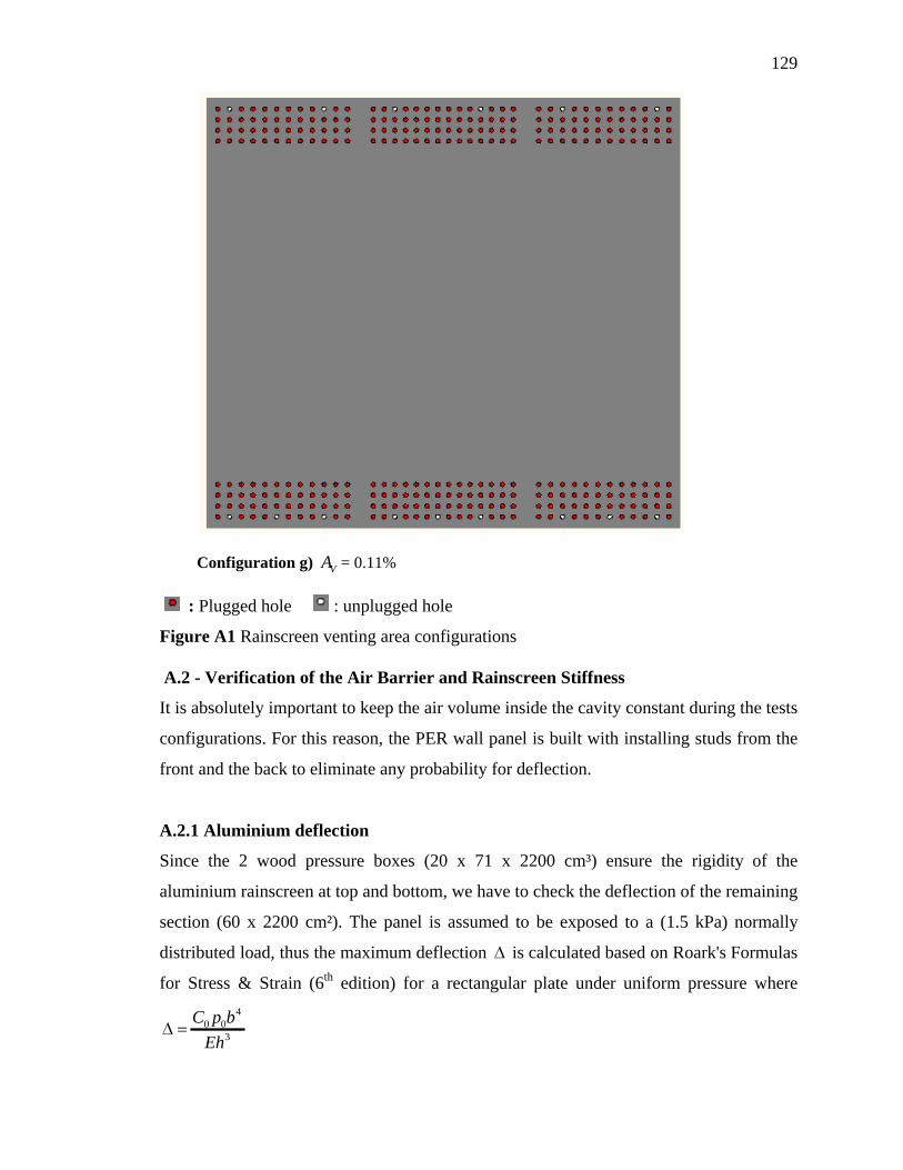
129
: Plugged hole : unplugged hole
Figure A1 Rainscreen venting area configurations
A.2 - Verification of the Air Barrier and Rainscreen Stiffness
It is absolutely important to keep the air volume inside the cavity constant during the tests
configurations. For this reason, the PER wall panel is built with installing studs from the
front and the back to eliminate any probability for deflection.
A.2.1 Aluminium deflection
Since the 2 wood pressure boxes (20 x 71 x 2200 cm³) ensure the rigidity of the
aluminium rainscreen at top and bottom, we have to check the deflection of the remaining
section (60 x 2200 cm²). The panel is assumed to be exposed to a (1.5 kPa) normally
distributed load, thus the maximum deflection is calculated based on Roark's Formulas
for Stress & Strain (6th edition) for a rectangular plate under uniform pressure where
40 0
3
C p b
Eh
Configuration g) VA = 0.11%
130
0p = 1.5 Kpa
b is the longest dimension
E = 97.13 10x Kg/m² is the elastic modulus of the aluminium
h= 0.00635 m is the rainscreen thickness
0C depends on the end supports and the aspect ratio of the plate.
In case 4 vertical studs are installed at 45 cm, and 2 are placed horizontally at 20 cm, then
the aspect ratio 2.25b
a
and 0C =0.12; the deflection for each section (20 x 45 cm²) is
around 1 mm.
A.2.2 Wood deflection
The deflection limit of the plywood wall of the air barrier at the back of the (PER) wall is
equal or less to 240
l; 3
lim 9 10it x m for 2.2l m
The deflection of the wooden studs is calculated with the formula: 45
384
wl
EI
w is the uniformly distributed load supported by the stud, l is the stud span
E = 91.04 10x Kg/m² is the elastic modulus of the wood, I is the inertia moment
Taking into consideration a uniform load of 0.54 Kg/m, each of the 6 (3 x 18 cm²) cross
section studs at 36cm having a span 1.5l m (crossing 2 horizontal wood plates at top
and bottom) has deflection around 0.1 mm. Such value theoretically gives a volume
increase inside the cavity of 0.044%.
A.3 - Uncertainties in Measurements
A.3.1 Errors from Pressure loading Actuators (PLAs)
These errors are issued from the performance of the PLAs that are supposed to generate
the same pressure signal in each configuration of the test. However, slight changes are
observed in the achieved pressures due to the change in the fan performance of the PLAs,
function of the ambient temperature and the number of holes in the rainscreen. For this
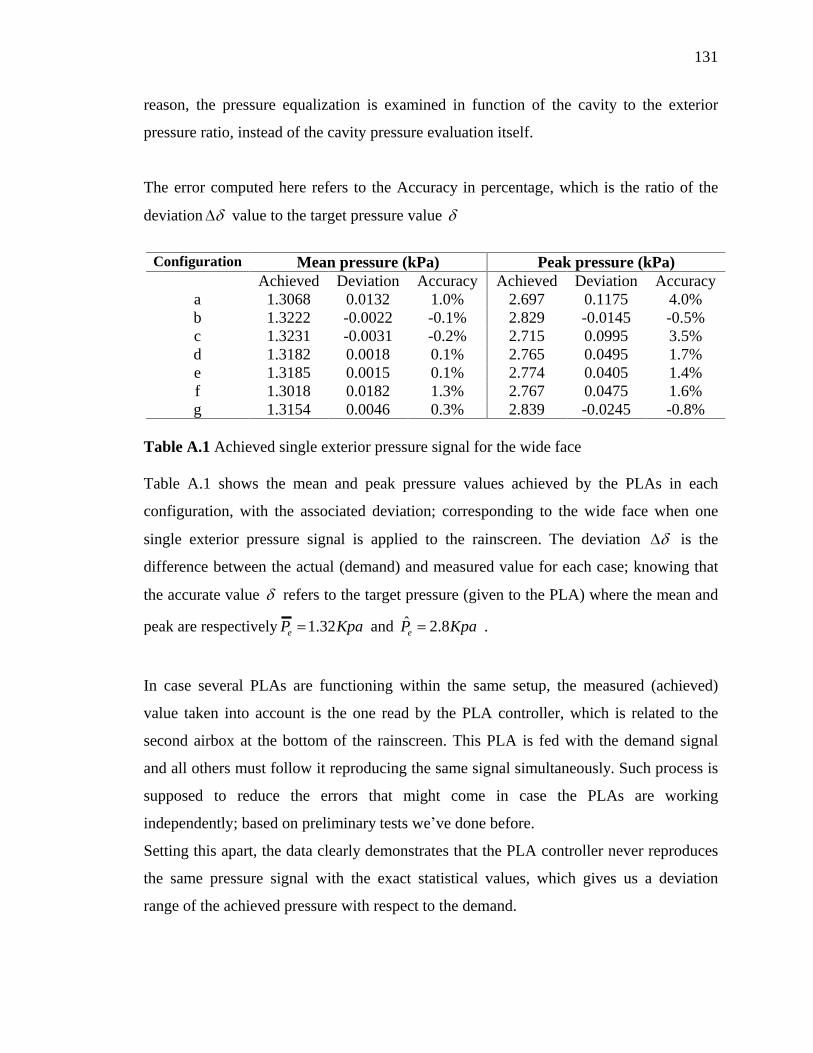
131
reason, the pressure equalization is examined in function of the cavity to the exterior
pressure ratio, instead of the cavity pressure evaluation itself.
The error computed here refers to the Accuracy in percentage, which is the ratio of the
deviation value to the target pressure value
Configuration Mean pressure (kPa) Peak pressure (kPa)
Achieved Deviation Accuracy Achieved Deviation Accuracy
a 1.3068 0.0132 1.0% 2.697 0.1175 4.0% b 1.3222 -0.0022 -0.1% 2.829 -0.0145 -0.5% c 1.3231 -0.0031 -0.2% 2.715 0.0995 3.5% d 1.3182 0.0018 0.1% 2.765 0.0495 1.7% e 1.3185 0.0015 0.1% 2.774 0.0405 1.4% f 1.3018 0.0182 1.3% 2.767 0.0475 1.6% g 1.3154 0.0046 0.3% 2.839 -0.0245 -0.8%
Table A.1 Achieved single exterior pressure signal for the wide face
Table A.1 shows the mean and peak pressure values achieved by the PLAs in each
configuration, with the associated deviation; corresponding to the wide face when one
single exterior pressure signal is applied to the rainscreen. The deviation
is the
difference between the actual (demand) and measured value for each case; knowing that
the accurate value
refers to the target pressure (given to the PLA) where the mean and
peak are respectively 1.32eP Kpa and 2.8eP Kpa .
In case several PLAs are functioning within the same setup, the measured (achieved)
value taken into account is the one read by the PLA controller, which is related to the
second airbox at the bottom of the rainscreen. This PLA is fed with the demand signal
and all others must follow it reproducing the same signal simultaneously. Such process is
supposed to reduce the errors that might come in case the PLAs are working
independently; based on preliminary tests we ve done before.
Setting this apart, the data clearly demonstrates that the PLA controller never reproduces
the same pressure signal with the exact statistical values, which gives us a deviation
range of the achieved pressure with respect to the demand.
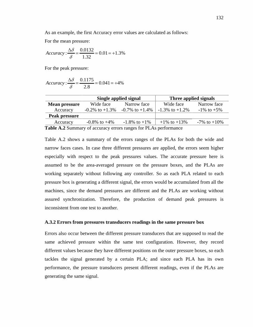
132
As an example, the first Accuracy error values are calculated as follows:
For the mean pressure:
0.0132: 0.01 1.3%
1.32Accuracy
For the peak pressure:
0.1175: 0.041 4%
2.8Accuracy
Single applied signal Three applied signals
Mean pressure Wide face Narrow face Wide face Narrow face Accuracy -0.2% to +1.3% -0.7% to +1.4%
-1.3% to +1.2% -1% to +5%
Peak pressure Accuracy -0.8% to +4% -1.8% to +1% +1% to +13% -7% to +10%
Table A.2 Summary of accuracy errors ranges for PLAs performance
Table A.2 shows a summary of the errors ranges of the PLAs for both the wide and
narrow faces cases. In case three different pressures are applied, the errors seem higher
especially with respect to the peak pressures values. The accurate pressure here is
assumed to be the area-averaged pressure on the pressure boxes, and the PLAs are
working separately without following any controller. So as each PLA related to each
pressure box is generating a different signal, the errors would be accumulated from all the
machines, since the demand pressures are different and the PLAs are working without
assured synchronization. Therefore, the production of demand peak pressures is
inconsistent from one test to another.
A.3.2 Errors from pressures transducers readings in the same pressure box
Errors also occur between the different pressure transducers that are supposed to read the
same achieved pressure within the same test configuration. However, they record
different values because they have different positions on the outer pressure boxes, so each
tackles the signal generated by a certain PLA; and since each PLA has its own
performance, the pressure transducers present different readings, even if the PLAs are
generating the same signal.
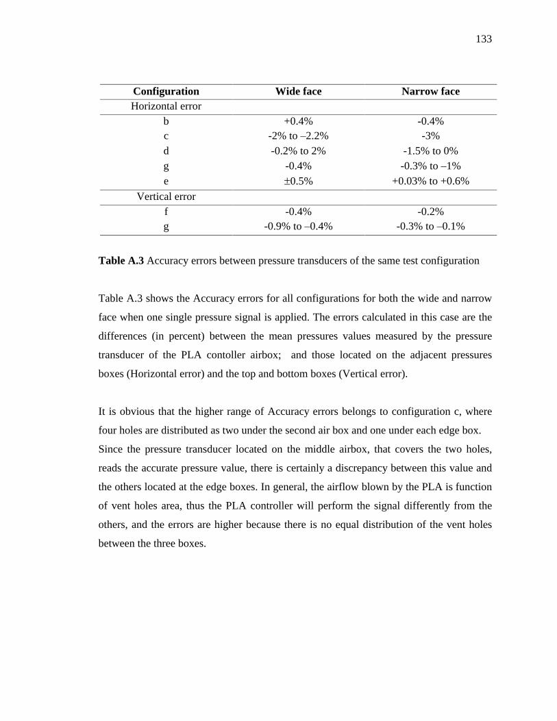
133
Configuration Wide face Narrow face Horizontal error
b +0.4% -0.4% c -2% to 2.2% -3% d -0.2% to 2% -1.5% to 0% g -0.4% -0.3% to 1% e 0.5%
+0.03% to +0.6%
Vertical error f -0.4% -0.2% g -0.9% to 0.4% -0.3% to 0.1%
Table A.3 Accuracy errors between pressure transducers of the same test configuration
Table A.3 shows the Accuracy errors for all configurations for both the wide and narrow
face when one single pressure signal is applied. The errors calculated in this case are the
differences (in percent) between the mean pressures values measured by the pressure
transducer of the PLA contoller airbox; and those located on the adjacent pressures
boxes (Horizontal error) and the top and bottom boxes (Vertical error).
It is obvious that the higher range of Accuracy errors belongs to configuration c, where
four holes are distributed as two under the second air box and one under each edge box.
Since the pressure transducer located on the middle airbox, that covers the two holes,
reads the accurate pressure value, there is certainly a discrepancy between this value and
the others located at the edge boxes. In general, the airflow blown by the PLA is function
of vent holes area, thus the PLA controller will perform the signal differently from the
others, and the errors are higher because there is no equal distribution of the vent holes
between the three boxes.

134
Appendix B
B.1 Numerical Method
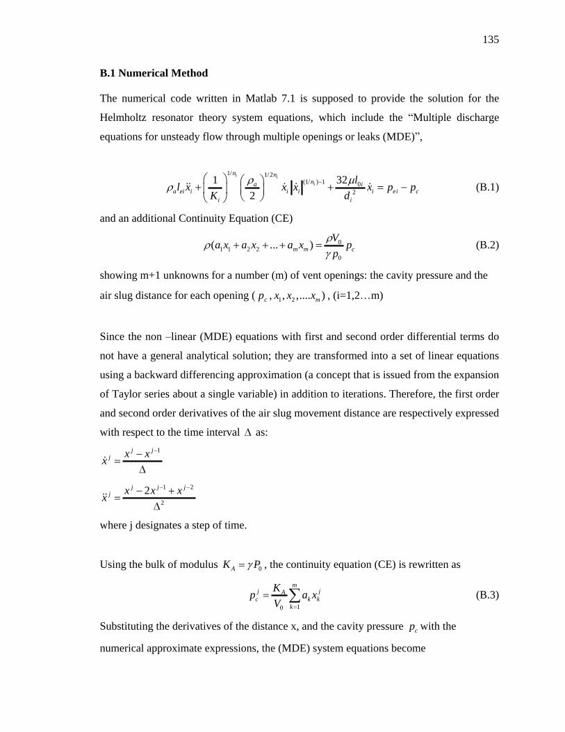
135
B.1 Numerical Method
The numerical code written in Matlab 7.1 is supposed to provide the solution for the
Helmholtz resonator theory system equations, which include the Multiple discharge
equations for unsteady flow through multiple openings or leaks (MDE) ,
1/ 1/2(1/ ) 1 0
2
321
2
i i
i
n nna i
a ei i i i i ei ci i
ll x x x x p p
K d (B.1)
and an additional Continuity Equation (CE)
01 1 2 2
0
( ... )m m c
Va x a x a x p
p (B.2)
showing m+1 unknowns for a number (m) of vent openings: the cavity pressure and the
air slug distance for each opening ( cp , 1 2, ,.... )mx x x , (i=1,2 m)
Since the non linear (MDE) equations with first and second order differential terms do
not have a general analytical solution; they are transformed into a set of linear equations
using a backward differencing approximation (a concept that is issued from the expansion
of Taylor series about a single variable) in addition to iterations. Therefore, the first order
and second order derivatives of the air slug movement distance are respectively expressed
with respect to the time interval as:
1j jj x x
x
1 2
2
2j j jj x x x
x
where j designates a step of time.
Using the bulk of modulus 0AK P , the continuity equation (CE) is rewritten as
10
mj jA
c k kk
Kp a x
V (B.3)
Substituting the derivatives of the distance x, and the cavity pressure cp with the
numerical approximate expressions, the (MDE) system equations become
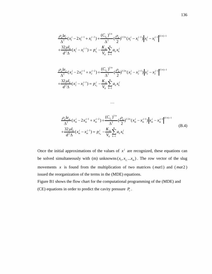
136
1
1
1/(1/ ) 11 2 1/2 1 11
1 1 1 1 1 1 12 2
101 12
10
( )( 2 ) ( ) ( )
232
( )
nnLj j j n j j j ja a
mj j j jA
e k kk
Clex x x x x x x
l Kx x p a x
d V
1
2
1/(1/ ) 11 2 1/2 1 12
2 2 2 2 2 2 22 2
102 22
10
( )( 2 ) ( ) ( )
232
( )
nnLj j j n j j j ja a
mj j j jA
e k kk
Clex x x x x x x
l Kx x p a x
d V
1
1/(1/ ) 11 2 1/2 1 1
2 2
102
10
( )( 2 ) ( ) ( )
232
( )m
nnLj j j n j j j ja m a
m m m m m m m
mj j j jA
m m e k kk
Clex x x x x x x
l Kx x p a x
d V
(B.4)
Once the initial approximations of the values of jx
are recognized, these equations can
be solved simultaneously with (m) unknowns 1 2,( , ... )mx x x . The row vector of the slug
movements x
is found from the multiplication of two matrices ( 1mat ) and ( 2mat )
issued the reorganization of the terms in the (MDE) equations.
Figure B1 shows the flow chart for the computational programming of the (MDE) and
(CE) equations in order to predict the cavity pressure cP .
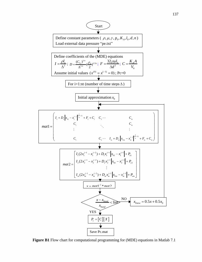
137
Start
0
0
limend
end
x x
x
Figure B1 Flow chart for computational programming for (MDE) equations in Matlab 7.1
Define constant parameters ( 0 0, , , , , , ,Ap K l d n )
Load external data pressure pe.txt
Define coefficients of the (MDE) equations
2elI ; 1
1/1/2
1/
( )( )
2
nL na
n
CD ; 0
2
32 lF
d;
0
AK AC
V
Assume initial values (0) ( 1)( 0)x x ; Pc=0
For i=1:nt (number of time steps )
Initial approximation 0x
1( 1)
1 1 01 1 1 1 2
1
1( 1)
1 2 0
1
i jn
m
m
i jn
m m m m m m
I D x x F C C C
CC
C C I D x x F C
mat
11 * 2x mat mat
cP C X
Save Pc.mat
NO
1 2 1 1
1 1 1 1 1 01 1 1
1 2 1 1
2 2 2 2 2 02 2 2
1 2 1 1
0
(2 )
(2 )2
(2 )
j j j j
e
j j j j
e
j j j j
m m m m m m m em
I x x D x x x P
I x x D x x x Pmat
I x x D x x x P
0 00.5 0.5newx x x
YES
138
The program shows that the computation starts with a for Loop, that is based on the
time step between each measurement during the sampling period. Also, there are
iterations, and each time the value of x is computed, it gives new approximation
0 00.5 0.5newx x x , that is supposed to get closer to the final solution. The solution is
determined when the convergence limit is reached so 60
0
10end
end
x x
x; meaning that the
provided distances get close enough to the true values. This convergence criterion is
chosen by trial, the values of x seemed constant at this limit.
Finally, the pressure is generated by multiplying the two vectors [ ]C and [ ]X , based on
the Continuity Equation as rewritten in Eqn (B.3).

139
VITA
NAME: Samar Darwich Dernayka
PLACE OF BIRTH: Tripoli, Lebanon
POST-SECONDARY B.E.S.C EDUCATION AND Lebanese University, Faculty of Engineering DEGREES: Branch I 2006
MESC Thesis The University of Western Ontario Faculty of Civil and Environmental Engineering 2009-2011
RELATED WORK Structural Engineer EXPERIENCE: DEC- Design and Construction Engineering Tripoli, Lebanon 2006-2008
Teaching Assistant The University of Western Ontario, Canada 2009-2011
PROFESSIONAL Order of Engineers and Architects LICENSE: Tripoli, Lebanon