Embed Size (px)
Citation preview

Presents

Robi PolikarDept. of Electrical & Computer Engineering
Rowan University

Technical Overview But…We cannot do that with Fourier Transform…. Time - frequency representation and the STFT Continuous wavelet transformMultiresolution analysis and discrete wavelet transform
(DWT) Application Overview
Conventional Applications: Data compression, denoising, solution of PDEs, biomedical signal analysis.
Unconventional applications Yes…We can do that with wavelets too…
Historical Overview 1807 ~ 1940s: The reign of the Fourier Transform 1940s ~ 1970s: STFT and Subband Coding 1980s & 1990s: The Wavelet Transform and MRA
The Story of Wavelets

What is a Transformand Why Do we Need One ?
Transform: A mathematical operation that takes a function or sequence and maps it into another one
Transforms are good things because… The transform of a function may give additional /hidden
information about the original function, which may not be available /obvious otherwise
The transform of an equation may be easier to solve than the original equation (recall your fond memories of Laplace transforms in DFQs)
The transform of a function/sequence may require less storage, hence provide data compression / reduction
An operation may be easier to apply on the transformed function, rather than the original function (recall other fond memories on convolution).

December, 21, 1807
Jean B. Joseph Fourier
(1768-1830)
“An arbitrary function, continuous or with discontinuities, defined in a finite interval by an arbitrarily capricious graph can always be expressed as a sum of sinusoids”
J.B.J. Fourier

Complex function representation through simple building blocksBasis functions
Using only a few blocks Compressed representation
Using sinusoids as building blocks Fourier transform Frequency domain representation of the function
ii
i FunctionSimpleweightFunctionComplex
deFtfdtetfF tjtj )(2
1)( )()(

Recall that FT uses complex exponentials (sinusoids) as building blocks.
For each frequency of complex exponential, the sinusoid at that frequency is compared to the signal.
If the signal consists of that frequency, the correlation is high large FT coefficients.
If the signal does not have any spectral component at a frequency, the correlation at that frequency is low / zero, small / zero FT coefficient.
How Does FT Work Anyway?
deFtfdtetfF tjtj )(2
1)( )()(
tjte tj sincos

FT At Work
)52cos()(1 ttx
)252cos()(2 ttx
)502cos()(3 ttx

FT At Work
)(1 X
)(2 X
)(3 X
F)(1 tx
F)(2 tx
F)(3 tx

FT At Work
)502cos(
)252cos(
)52cos()(4
t
t
ttx
)(4 XF)(4 tx

FT At Work
dteFtf
dtetfF
tj
tj
)(2
1)(
)()(
Complex exponentials (sinusoids) as basis
functions:
F
An ultrasonic A-scan using 1.5 MHz transducer, sampled at 10 MHz

Stationary and Non-stationary Signals
FT identifies all spectral components present in the signal, however it does not provide any information regarding the temporal (time) localization of these components. Why?
Stationary signals consist of spectral components that do not change in time all spectral components exist at all timesno need to know any time informationFT works well for stationary signals
However, non-stationary signals consists of time varying spectral componentsHow do we find out which spectral component appears
when?FT only provides what spectral components exist , not
where in time they are located.Need some other ways to determine time localization of
spectral components

Stationary and Non-stationary Signals
Stationary signals’ spectral characteristics do not change with time
Non-stationary signals have time varying spectra
)502cos(
)252cos(
)52cos()(4
t
t
ttx
][)( 3215 xxxtx
Concatenation

Stationary vs. Non-Stationary
Perfect knowledge of what frequencies exist, but no information about where these frequencies are located in time
X4(ω)
X5(ω)
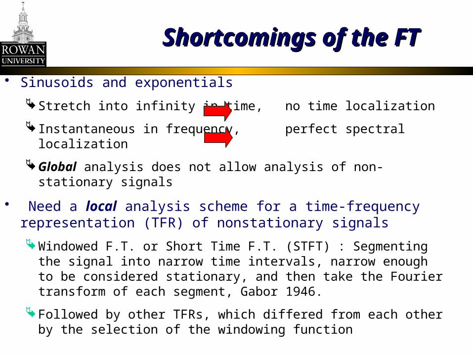
Sinusoids and exponentials
Stretch into infinity in time, no time localization
Instantaneous in frequency, perfect spectral localization
Global analysis does not allow analysis of non-stationary signals
Need a local analysis scheme for a time-frequency representation (TFR) of nonstationary signals
Windowed F.T. or Short Time F.T. (STFT) : Segmenting the signal into narrow time intervals, narrow enough to be considered stationary, and then take the Fourier transform of each segment, Gabor 1946.
Followed by other TFRs, which differed from each other by the selection of the windowing function
Shortcomings of the FTShortcomings of the FT

Short Time Fourier Transform(STFT)
1. Choose a window function of finite length
2. Place the window on top of the signal at t=0
3. Truncate the signal using this window
4. Compute the FT of the truncated signal, save.
5. Incrementally slide the window to the right
6. Go to step 3, until window reaches the end of the signal For each time location where the window is centered, we
obtain a different FT Hence, each FT provides the spectral
information of a separate time-slice of the signal, providing simultaneous time and frequency information
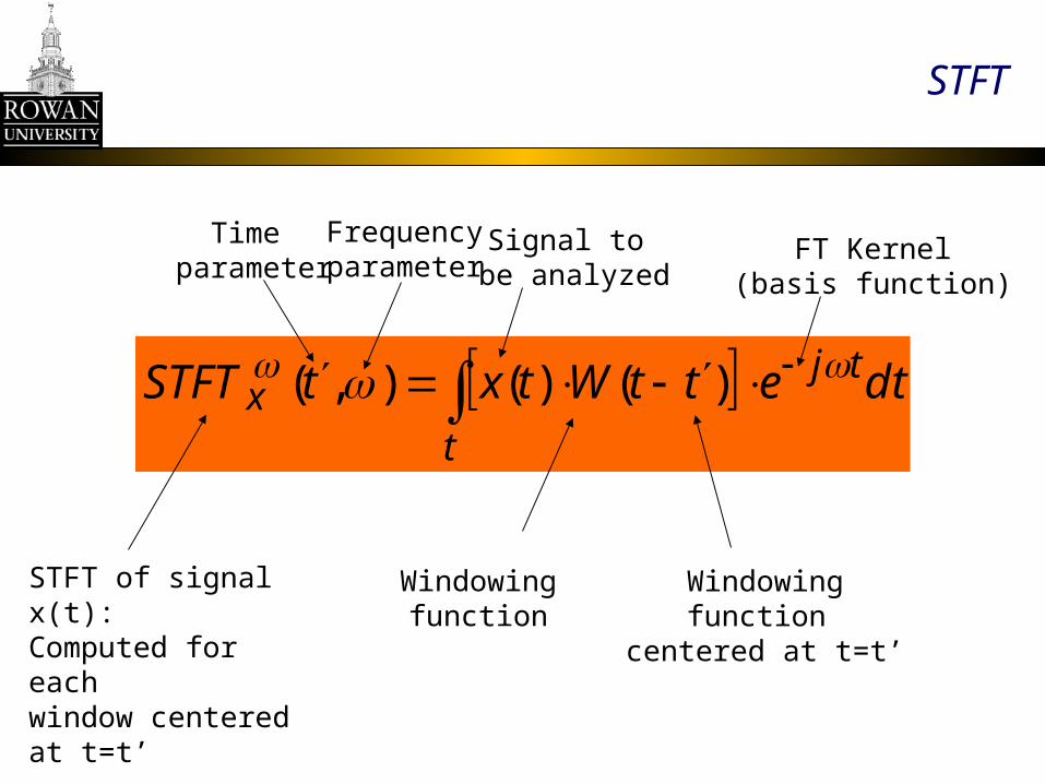
STFT
t
tjx dtettWtxtSTFT )()(),(
STFT of signal x(t):Computed for each window centered at t=t’
Time parameter
Frequencyparameter
Signal to be analyzed
Windowingfunction
Windowing function centered at t=t’
FT Kernel(basis function)

STFT
t’=-8t’=-8 t’=-2t’=-2
t’=4t’=4 t’=8t’=8

STFT at Work

STFT At Work

STFT At Work

STFT
STFT provides the time information by computing a different FTs for consecutive time intervals, and then putting them togetherTime-Frequency Representation (TFR)Maps 1-D time domain signals to 2-D time-frequency signals
Consecutive time intervals of the signal are obtained by truncating the signal using a sliding windowing function
How to choose the windowing function?What shape? Rectangular, Gaussian, Elliptic…?How wide?
Wider window require less time steps low time resolutionAlso, window should be narrow enough to make sure that the portion of
the signal falling within the window is stationaryCan we choose an arbitrarily narrow window…?

Selection of STFT Window
Two extreme cases: W(t) infinitely long: STFT turns into FT, providing
excellent frequency information (good frequency resolution), but no time information
W(t) infinitely short:
STFT then gives the time signal back, with a phase factor. Excellent time information (good time resolution), but no frequency information
Wide analysis window poor time resolution, good frequency resolutionNarrow analysis windowgood time resolution, poor frequency resolutionOnce the window is chosen, the resolution is set for both time and frequency.
t
tjx dtettWtxtSTFT )()(),(
1)( tW
)()( ttW tj
t
tjx etxdtetttxtSTFT )()()(),(

Heisenberg Principle
41
ft
Time resolution: How well two spikes in time can be separated from each other in the transform domain
Frequency resolution: How well two spectral components can be separated from each other in the transform domain
Both time and frequency resolutions cannot be arbitrarily high!!! We cannot precisely know at what time instance a frequency component is located. We can only know what interval of frequencies are present in which time intervals

The Wavelet Transform
Overcomes the preset resolution problem of the STFT by using a variable length window
Analysis windows of different lengths are used for different frequencies:Analysis of high frequencies Use narrower
windows for better time resolutionAnalysis of low frequencies Use wider windows
for better frequency resolution This works well, if the signal to be analyzed mainly consists of slowly
varying characteristics with occasional short high frequency bursts. Heisenberg principle still holds!!! The function used to window the signal is called the wavelet

The Wavelet Transform
txx dt
s
ttx
sssCWT
1),(),(
Continuous wavelet transform of the signal x(t) using the analysis wavelet (.)
Translation parameter, measure of time
Scale parameter, measure of frequency
The mother wavelet. All kernels are obtained by translating (shifting) and/or scaling the mother wavelet
A normalization constant Signal to be
analyzed
Scale = 1/frequency

High frequency (small scale)
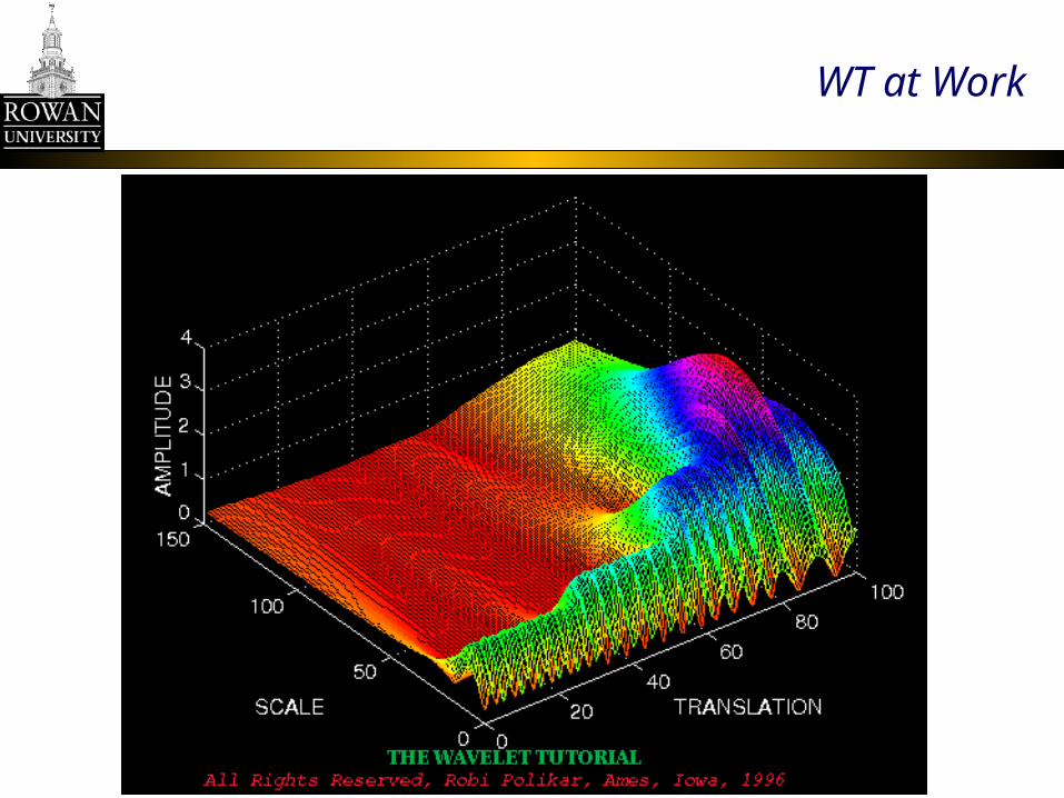
WT at Work
txx dt
s
ttx
sssCWT
1),(),(
Low frequency (large scale)

WT at Work
WT at Work

WT at Work

Matlab Demos on CWT

Discrete Wavelet Transform
CWT computed by computers is really not CWT, it is a discretized version of the CWT.
The resolution of the time-frequency grid can be controlled (within Heisenberg’s inequality), can be controlled by time and scale step sizes.
Often this results in a very redundant representation How to discretize the continuous time-frequency plane, so that the
representation is non-redundant?Sample the time-frequency plane on a dyadic
(octave) grid
Znknt kkkn , 22)(
txx dt
s
ttx
sssCWT
1),(),(

Discrete Wavelet Transform
Dyadic sampling of the time –frequency plane results in a very efficient algorithm for computing DWT:Subband coding using multiresolution analysisDyadic sampling and multiresolution is
achieved through a series of filtering and up/down sampling operations
HHx[n]x[n] y[n]y[n]
N
k
N
k
knxkh
knhkx
nxnhnhnxny
1
1
][][
][][
][*][][*][][

Discrete Wavelet TransformImplementation
G
H
2
2 G
H
2
2
2
2
G
H
+
2
2
G
H
+
x[n]x[n]
Decomposition Reconstruction
~
~ ~
~
n
high kngnxky ]2[][][~
n
low knhnxky ]2[][][~
k
high kngky ]2[][
k
high kngky ]2[][
2-level DWT decomposition. The decomposition can be continues as 2-level DWT decomposition. The decomposition can be continues as long as there are enough samples for down-sampling.long as there are enough samples for down-sampling.
G
H
Half band high pass filter
Half band low pass filter
2
2
Down-sampling
Up-sampling

DWT - Demystified
Length: 512B: 0 ~
g[n] h[n]
g[n] h[n]
g[n] h[n]
2
d1: Level 1 DWTCoeff.
Length: 256B: 0 ~ /2 Hz
Length: 256B: /2 ~ Hz
Length: 128B: 0 ~ /4 HzLength: 128
B: /4 ~ /2 Hz
d2: Level 2 DWTCoeff.
d3: Level 3 DWTCoeff.
…a3….
Length: 64B: 0 ~ /8 HzLength: 64
B: /8 ~ /4 Hz
2
2 2
22
|H(jw)|
w/2-/2
|G(jw)|
w- /2-/2
a2
a1
Level 3 approximation
Coefficients

Implementation of DWT on MATLAB
Load signal
Choose waveletand numberof levels
Hit Analyze button
Level 1 coeff.Highest freq.
Approx. coef. at level 5
s=a5+d5+…+d1
(Wavedemo_signal1)


Applications of Wavelets
Compression De-noising Feature Extraction Discontinuity Detection Distribution Estimation Data analysis
Biological dataNDE dataFinancial data

Compression
DWT is commonly used for compression, since most DWT are very small, can be zeroed-out!

Compression

Compression

ECG- Compression

Denoising Implementation in Matlab
First, analyze the signal with appropriate wavelets
Hit Denoise
(Noisy Doppler)
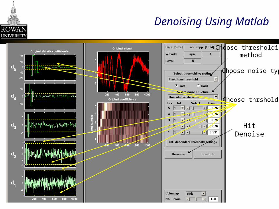
Denoising Using Matlab
Choose thresholdingmethod
Choose noise type
Choose thrsholds
Hit Denoise

Denosing Using Matlab

Discontinuity Detection
(microdisc.mat)

Discontinuity Detectionwith CWT
(microdisc.mat)

Application Overview
Data Compression Wavelet Shrinkage Denoising Source and Channel Coding Biomedical Engineering
EEG, ECG, EMG, etc analysisMRI
Nondestructive EvaluationUltrasonic data analysis for nuclear power plant pipe
inspections Eddy current analysis for gas pipeline inspections
Numerical Solution of PDEs Study of Distant Universes
Galaxies form hierarchical structures at different scales

Application Overview
Wavelet Networks Real time learning of unknown functions Learning from sparse data
Turbulence Analysis Analysis of turbulent flow of low viscosity fluids flowing at high
speeds Topographic Data Analysis
Analysis of geo-topographic data for reconnaissance / object identification
Fractals Daubechies wavelets: Perfect fit for analyzing fractals
Financial Analysis Time series analysis for stock market predictions

History Repeats Itself…
1807, J.B. Fourier: All periodic functions can be expressed as a
weighted sum of trigonometric functionDenied publication by Lagrange, Legendre and
Laplace1822: Fourier’s work is finally published…………1965, Cooley & Tukey: Fast Fourier Transform
143 years

History Repeats Itself: Morlet’s Story
1946, Gabor: STFT analysis: high frequency components using a narrow window, or low frequency components using a wide window, but not both
Late 1970s, Morlet’s (geophysical engineer) problem: Time - frequency analysis of signals with high frequency
components for short time spans and low frequency components with long time spans
STFT can do one or the other, but not both Solution: Use different windowing functions for sections of the signal with different frequency content
Windows to be generated from dilation / compression of prototype small, oscillatory signals wavelets
Criticism for lack of mathematical rigor !!! Early 1980s, Grossman (theoretical physicist): Formalize the transform and devise the
inverse transformation First wavelet transform ! Rediscovery of Alberto Calderon’s 1964 work on harmonic analysis

1980s
1984, Yeves Meyer :Similarity between Morlet’s and Colderon’s work,
1984Redundancy in Morlet’s choice of basis functions1985, Orthogonal wavelet basis functions with
better time and frequency localization Rediscovery of J.O. Stromberg’s 1980 work the same basis
functions (also a harmonic analyst) Yet re-rediscovery of Alfred Haar’s work on orthogonal basis
functions, 1909 (!).Simplest known orthonormal wavelets

Transition to the Discrete Signal Analysis
Ingrid Daubechies: Discretization of time and scale
parameters of the wavelet transformWavelet frames, 1986 Orthonormal bases of compactly
supported wavelets (Daubechies wavelets), 1988
Liberty in the choice of basis functions at the expense of redundancy
Stephane Mallat: Multiresolution analysis w/ Meyer,
1986 Ph.D. dissertation, 1988
Discrete wavelet transform Cascade algorithm for computing
DWT

…However…
Decomposition of a discrete into dyadic frequencies (MRA) , known to EEs under the name of “Quadrature Mirror Filters”, Croisier, Esteban and Galand, 1976 (!)

Transition to the Discrete Signal Analysis
Martin Vetterli & Jelena KovacevicWavelets and filter banks, 1986 Perfect reconstruction of
signals using FIR filter banks, 1988
Subband codingMultidimensional filter banks,
1992

1990s
Equivalence of QMF and MRA, Albert Cohen, 1990 Compactly supported biorthogonal wavelets, Cohen, Daubechies, J.
Feauveau, 1993 Wavelet packets, Coifman, Meyer, and Wickerhauser, 1996 Zero Tree Coding, Schapiro 1993 ~ 1999 Search for new wavelets with better time and frequency localization
properties. Super-wavelets Matching Pursuit, Mallat, 1993 ~ 1999

New & Noteworthy
Zero crossing representation signal classification computer vision data compression denoising
Super wavelet Linear combination of known basic wavelets
Zero Tree Coding, Schapiro Matching Pursuit , Mallat
Using a library of basis functions for decomposition New MPEG standard