Embed Size (px)
Citation preview
• Presented By:Payal Gupta• Roll Number: (225 in scetion 2)
• Professor :Tsau Young Lin
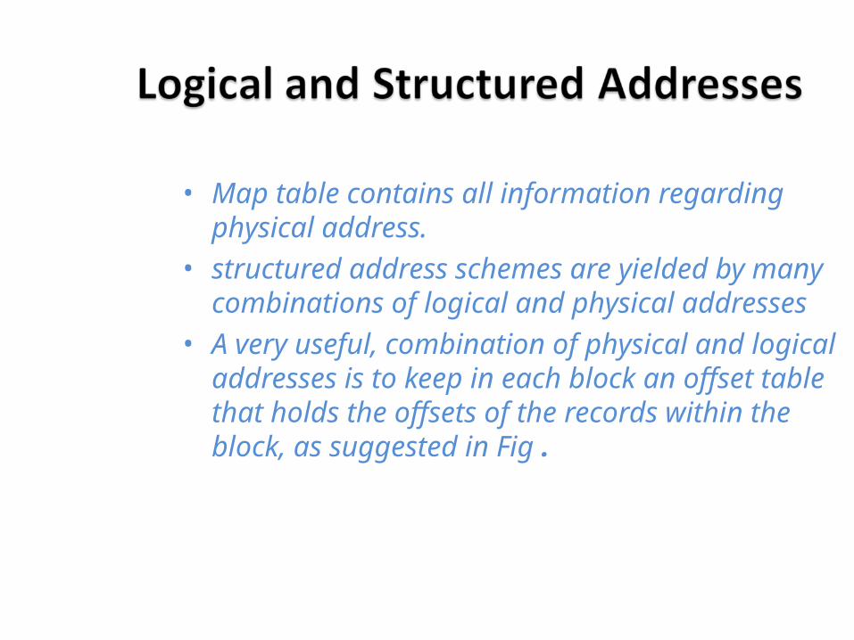
• Map table contains all information regarding physical address.
• structured address schemes are yielded by many combinations of logical and physical addresses
• A very useful, combination of physical and logical addresses is to keep in each block an offset table that holds the offsets of the records within the block, as suggested in Fig .

Record4
Record3Record2Record1
Header
Unused
Offset value
A block with a table of offsets telling us the position of each record within the block
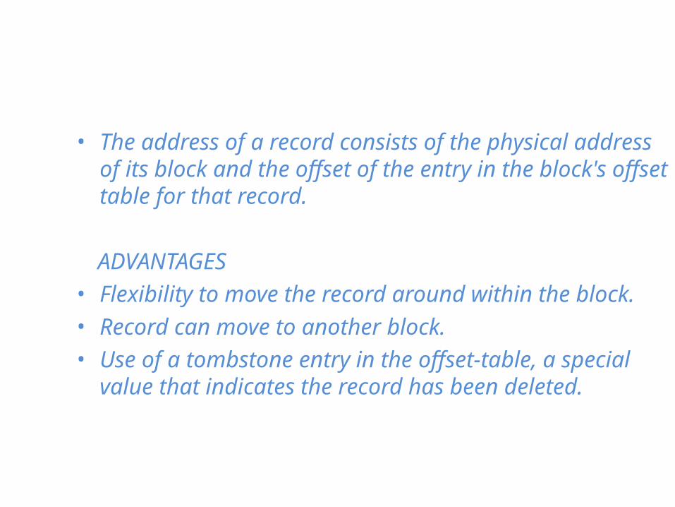
• The address of a record consists of the physical address of its block and the offset of the entry in the block's offset table for that record.
ADVANTAGES• Flexibility to move the record around within the block.• Record can move to another block.• Use of a tombstone entry in the offset-table, a special value
that indicates the record has been deleted.
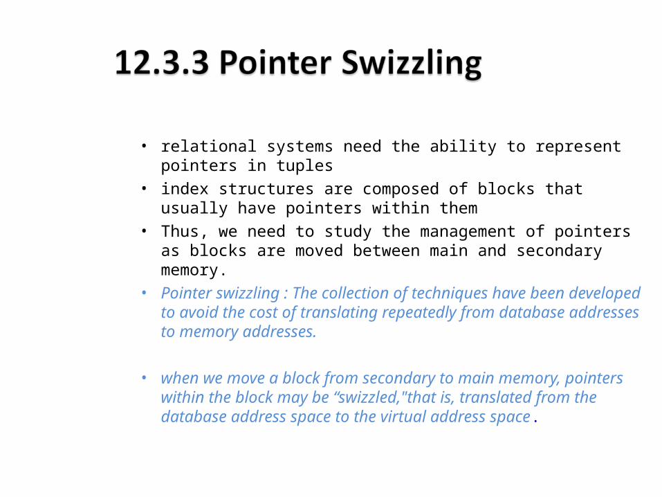
• relational systems need the ability to represent pointers in tuples• index structures are composed of blocks that usually have
pointers within them• Thus, we need to study the management of pointers as blocks are
moved between main and secondary memory.• Pointer swizzling : The collection of techniques have been
developed to avoid the cost of translating repeatedly from database addresses to memory addresses.
• when we move a block from secondary to main memory, pointers within the block may be “swizzled,"that is, translated from the database address space to the virtual address space.
• every block, record, object, or other reference able data item is represented by two forms of address:
1. database address2. the memory address of the item.
• In the main memory, items can be referred by both addresses. • The secondary storage only accepts the database address. • database addresses that are currently in virtual memory need to
be translated to their current memory address.
• This is done with the help of Such a translation table is suggested in Fig.
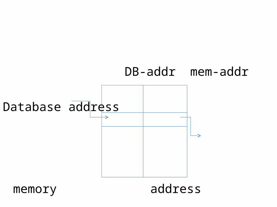
DB-addr mem-addr
Database address
memory address
The translation table turns database addresses into their equivalents in memory
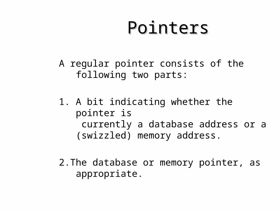
A regular pointer consists of the following two parts:
1. A bit indicating whether the pointer is currently a database address or a (swizzled) memory address.
2.The database or memory pointer, as appropriate.
PointersPointers
• As soon as a block is brought into memory, we locate all its pointers and addresses and enter them into the translation table if they are not already there.
• However we need some mechanism to locate the pointers.• For example:1. If the block holds records with a known schema, the schema will
tell us where in the records the pointers are found.2. If the block is used for one of the index structures then the block
will hold pointers at known locations.3. We may keep within the block header a list of where the pointers
are.
Disk Memory
Block1
Block2
Swizzled
Unswizzled
Read into Memory
Structure of a pointer when swizzling is used
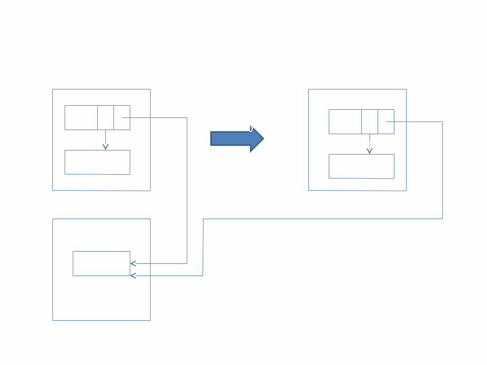
• leave all pointers unswizzled when the block is first brought into memory.
• We enter its address, and the addresses of its pointers, into the translation table, along with their memory equivalents.
• If and when we follow a pointer P that is inside some block of memory, we swizzle it.
• difference between on-demand and automatic swizzling is that the latter tries to get all the pointers swizzled quickly and efficiently when the block is loaded into memory.
• The possible time saved by swizzling all of a block‘s pointers at one time must be weighed against the possibility that some swizzled pointers will never be followed.
• In that case, any time spent swizzling and unswizzling the pointer will be wasted.
• arrange that database pointers look like invalid memory addresses. If so, then we can allow the computer to follow
any pointer as if it were in its memory form.• If the pointer happens to be unswizzled, then the memory reference will cause a hardware trap.• If the DBMS provides a function that is invoked by the trap, and this
function "swizzles" the pointer and then we can follow swizzled pointers in single instructions, and only need to do something more time consuming when the pointer is unswizzled.
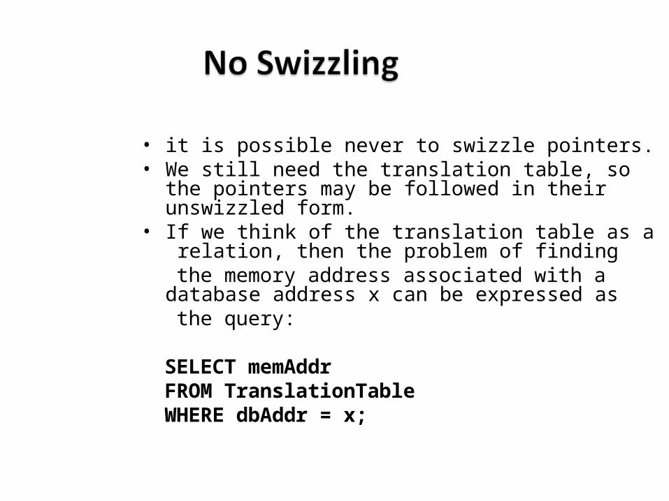
• it is possible never to swizzle pointers. • We still need the translation table, so the pointers may be
followed in their unswizzled form.• If we think of the translation table as a relation, then the
problem of finding the memory address associated with a database address x
can be expressed as the query:
SELECT memAddr FROM TranslationTable WHERE dbAddr = x;
• it may be known by the application programmer whether the pointers in a block are likely to be followed.
• This programmer may be able to specify explicitly that a block loaded into memory is to have its pointers swizzled, or the programmer may call for the pointers to be swizzled only as needed.
• When a block is moved from memory back to disk, any pointers within that block must be "unswizzled“.
• The translation table can be used to associate addresses of the two types in either direction
• However, we do not want each unswizzling operation to require a search of the entire translation table.
• A block in memory is said to be pinned if it cannot at the moment be written back to disk safely.
• A bit telling whether or not a block is pinned can be located in the header of the block.
• If a block B1 has within it a swizzled pointer to some data item in block B2.
• we follow the pointer in B1,it will lead us to the buffer, which no longer holds B2; in effect, the pointer has become dangling.
• A block, like B2, that is referred to by a swizzled pointer from somewhere else is therefore pinned
• If it is pinned, we must either unpin it, or let the block remain in memory, occupying space that could otherwise be used for some other block.
• To unpin a block that is pinned because of swizzled pointers from outside, we must "unswizzle” any pointers to it.
• Consequently, the translation table must record, for each database address whose data item is in memory, the places in memory where swizzled pointers to that item exist.
• Two possible approaches are:
1. Keep the list of references to a memory address as a linked list attached to the entry for that address in the translation table.
2. If memory addresses are significantly shorter than database addresses, we can create the linked list in the space used for the pointers themselves.
• That is, each space used for a database pointer is replaced by
(a) The swizzled pointer, and (b) Another pointer that forms part of a linked
list of all occurrences of this pointer.
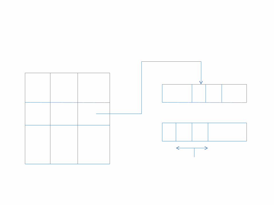
x y
y
y
A linked list of occurrences of a swizzled pointer
Swizzled pointer

SECTIONS 13.1 – 13.3
Sanuja Dabade & Eilbroun Benjamin CS 257 – Dr. TY Lin
SECONDARY STORAGE MANAGEMENT
Presentation Outline
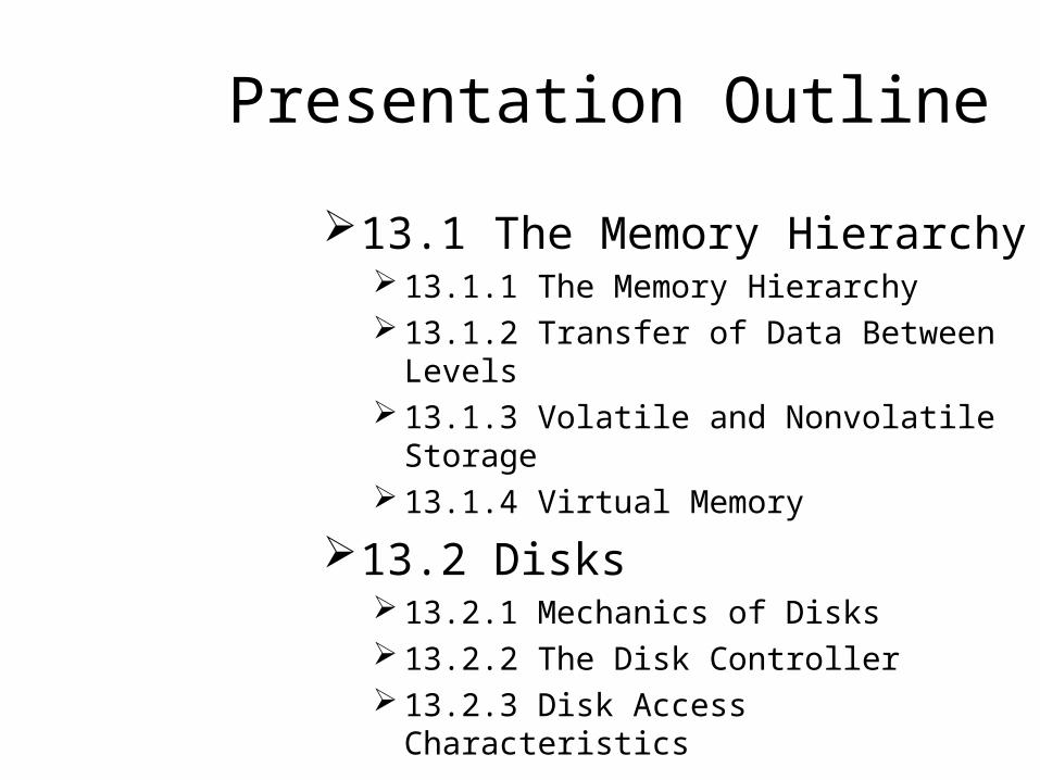
13.1 The Memory Hierarchy 13.1.1 The Memory Hierarchy 13.1.2 Transfer of Data Between Levels 13.1.3 Volatile and Nonvolatile Storage 13.1.4 Virtual Memory
13.2 Disks 13.2.1 Mechanics of Disks 13.2.2 The Disk Controller 13.2.3 Disk Access Characteristics
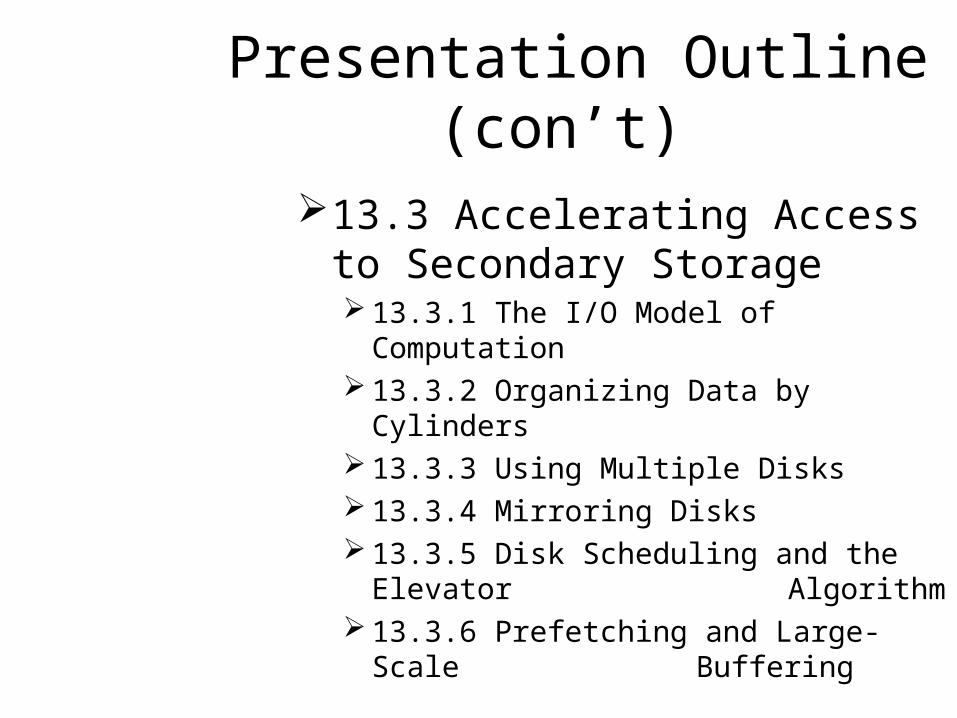
Presentation Outline (con’t)
13.3 Accelerating Access to Secondary Storage 13.3.1 The I/O Model of Computation 13.3.2 Organizing Data by Cylinders 13.3.3 Using Multiple Disks 13.3.4 Mirroring Disks 13.3.5 Disk Scheduling and the Elevator
Algorithm 13.3.6 Prefetching and Large-Scale
Buffering
13.1.1 Memory Hierarchy
• Several components for data storage having different data capacities available
• Cost per byte to store data also varies• Device with smallest capacity offer the
fastest speed with highest cost per bit
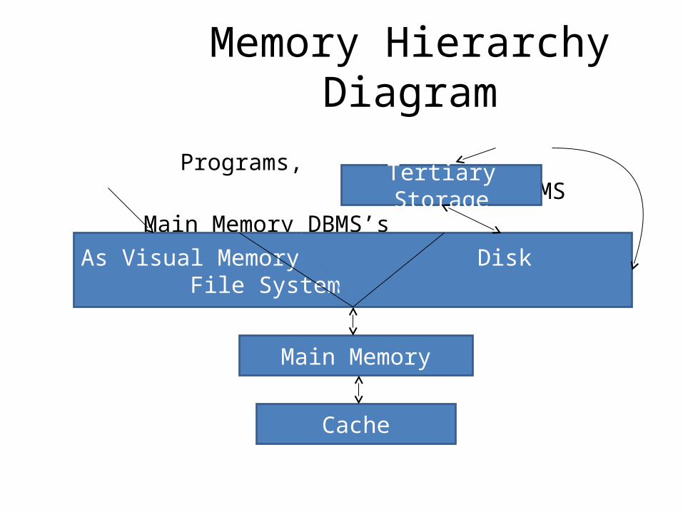
Memory Hierarchy Diagram
Programs, DBMSMain Memory DBMS’s
Main Memory
Cache
As Visual Memory Disk File System
Tertiary Storage
13.1.1 Memory Hierarchy
• Cache– Lowest level of the hierarchy– Holds limited amount of data – Data items are copies of certain locations of main
memory– Machine looks for instructions as well as data for
those instructions in the cache – Sometimes, values in cache are changed and
corresponding changes to main memory are delayed
13.1.1 Memory Hierarchy (con’t)
• No need to update the data in main memory immediately in a single processor computer
• In multiple processors data is updated immediately to main memory….called as write through
Main Memory
• Main memories are random access….one can obtain any byte in the same amount of time
• Everything happens in the computer
Secondary storage
• More permanent than main memory, as data and programs are retained when the power is turned off
• Used to store data and programs when they are not being “processed”.
• E.g. magnetic disks, hard disks
Tertiary Storage
• Holds data volumes in terabytes• Used for databases much larger than
what can be stored on disk
13.1.2 Transfer of Data Between levels
• Data moves between adjacent levels of the hierarchy
• At the secondary or tertiary levels accessing the desired data or finding the desired place to store the data takes a lot of time
• Disk is organized into bocks• Entire blocks are moved to and from
memory called a buffer
13.1.2 Transfer of Data Between level (cont’d)
• A key technique for speeding up database operations is to arrange the data so that when one piece of data block is needed it is likely that other data on the same block will be needed at the same time
• Same idea applies to other hierarchy levels

13.1.3 Volatile and Non Volatile Storage
• A volatile device does not hold data after power is switched off
• Non volatile holds data for longer period even when device is turned off
• All the secondary and tertiary devices are non volatile and main memory is volatile.
13.1.4 Virtual Memory
• Typical software executes in virtual memory• Address space is typically 32 bit or 232 bytes
or 4GB• Transfer between memory and disk is in
terms of blocks
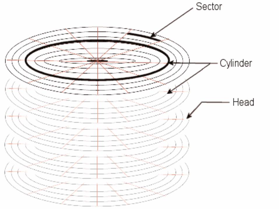
13.2.1 Mechanism of Disk
• Mechanisms of Disks– Consists of 2 moving pieces of a disk
• 1. disk assembly • 2. head assembly
– Disk assembly consists of 1 or more platters which rotate around a central spindle
– Storage of bits on upper and lower surfaces of platters
13.2.2 Disk Controller
• One or more disks are controlled by disk controllers
• Disks controllers are capable of– Controlling the mechanical actuator that moves the
head assembly– Selecting the sector from among all those in the
cylinder at which heads are positioned– Transferring bits between desired sector and main
memory – Possible buffering an entire track
13.2.3 Disk Access Characteristics
• Accessing (reading/writing) a block requires 3 steps– Disk controller positions the head assembly at the
cylinder containing the track on which the block is located. It is a ‘seek time’
– The disk controller waits while the first sector of the block moves under the head. This is a ‘rotational latency’
– All the sectors and the gaps between them pass the head, while disk controller reads or writes data in these sectors. This is a ‘transfer time’
13.3 Accelerating Access to Secondary Storage
Several approaches for more-efficiently accessing data in secondary storage: Place blocks that are together in the same cylinder. Divide the data among multiple disks. Mirror disks. Use disk-scheduling algorithms. Prefetch blocks into main memory.
Scheduling Latency – added delay in accessing data caused by a disk scheduling algorithm.
Throughput – the number of disk accesses per second that the system can accommodate.
13.3.1 The I/O Model of Computation
The number of block accesses (Disk I/O’s) is a good time approximation for the algorithm. This should be minimized.
Ex 13.3: You want to have an index on R to identify the block on which the desired tuple appears, but not where on the block it resides. For Megatron 747 (M747) example, it takes 11ms to read a
16k block. A standard microprocessor can execute millions of
instruction in 11ms, making any delay in searching for the desired tuple negligible.
13.3.2 Organizing Data by Cylinders
If we read all blocks on a single track or cylinder consecutively, then we can neglect all but first seek time and first rotational latency.
Ex 13.4: We request 1024 blocks of M747. If data is randomly distributed, average latency is 10.76ms by Ex 13.2,
making total latency 11s. If all blocks are consecutively stored on 1 cylinder:
6.46ms + 8.33ms * 16 = 139ms
(1 average seek) (time per rotation) (# rotations)
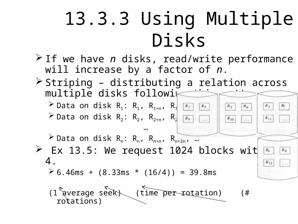
13.3.3 Using Multiple Disks If we have n disks, read/write performance will
increase by a factor of n. Striping – distributing a relation across multiple disks
following this pattern: Data on disk R1: R1, R1+n, R1+2n,… Data on disk R2: R2, R2+n, R2+2n,… … Data on disk Rn: Rn, Rn+n, Rn+2n, …
Ex 13.5: We request 1024 blocks with n = 4. 6.46ms + (8.33ms * (16/4)) = 39.8ms
(1 average seek) (time per rotation) (# rotations)
13.3.4 Mirroring Disks
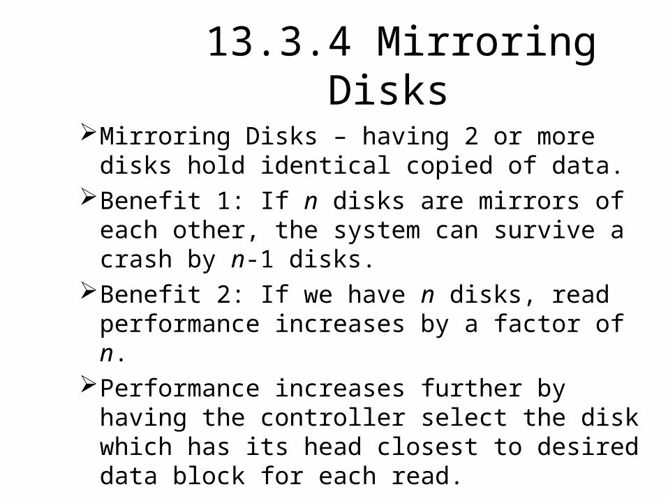
Mirroring Disks – having 2 or more disks hold identical copied of data.
Benefit 1: If n disks are mirrors of each other, the system can survive a crash by n-1 disks.
Benefit 2: If we have n disks, read performance increases by a factor of n.
Performance increases further by having the controller select the disk which has its head closest to desired data block for each read.
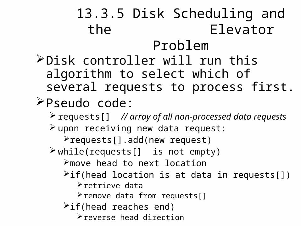
13.3.5 Disk Scheduling and the Elevator Problem
Disk controller will run this algorithm to select which of several requests to process first.
Pseudo code: requests[] // array of all non-processed data requests upon receiving new data request:
requests[].add(new request) while(requests[] is not empty)
move head to next locationif(head location is at data in requests[])
retrieve dataremove data from requests[]
if(head reaches end)reverse head direction
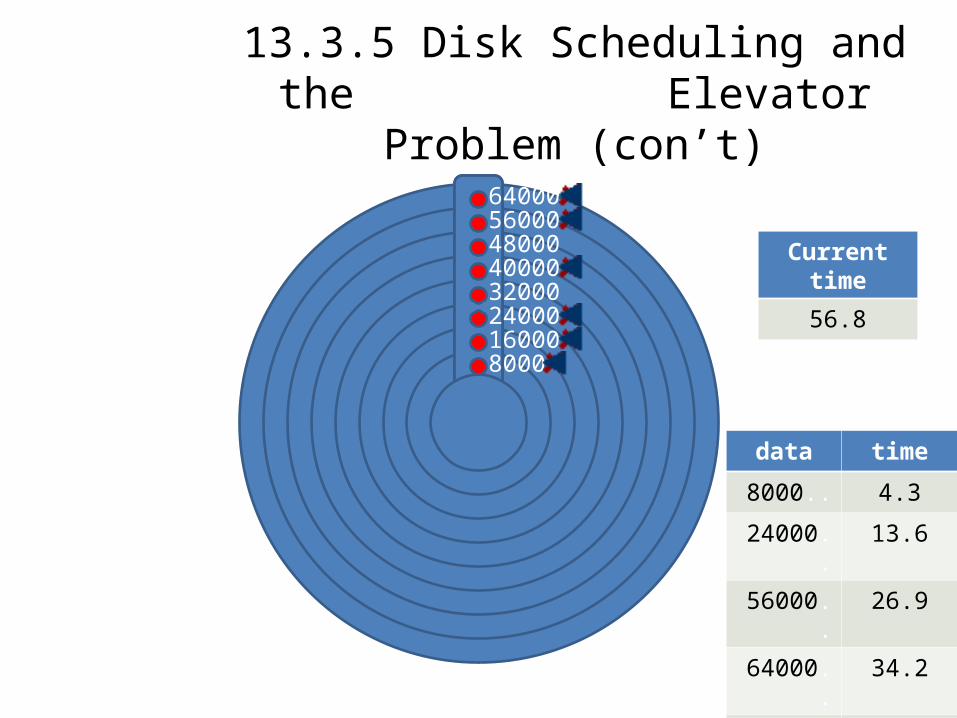
13.3.5 Disk Scheduling and the Elevator Problem (con’t)
Events: Head starting
pointRequest data at
8000Request data at
24000Request data at
56000Get data at 8000Request data at
16000Get data at 24000Request data at
64000Get data at 56000Request Data at
40000Get data at 64000Get data at 40000Get data at 16000
data time
Current time
Current time
0
Current time
4.3
Current time
10
Current time
13.6
Current time
20
Current time
26.9
Current time
30
Current time
34.2
Current time
45.5
Current time
56.8
800016000240003200040000480005600064000
data time
8000.. 4.3
data time
8000.. 4.3
24000.. 13.6
data time
8000.. 4.3
24000.. 13.6
56000.. 26.9
data time
8000.. 4.3
24000.. 13.6
56000.. 26.9
64000.. 34.2
data time
8000.. 4.3
24000.. 13.6
56000.. 26.9
64000.. 34.2
40000.. 45.5
data time
8000.. 4.3
24000.. 13.6
56000.. 26.9
64000.. 34.2
40000.. 45.5
16000.. 56.8
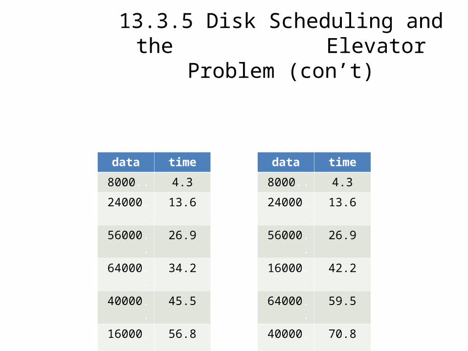
13.3.5 Disk Scheduling and the Elevator Problem (con’t)
data time
8000.. 4.3
24000.. 13.6
56000.. 26.9
64000.. 34.2
40000.. 45.5
16000.. 56.8
data time
8000.. 4.3
24000.. 13.6
56000.. 26.9
16000.. 42.2
64000.. 59.5
40000.. 70.8
Elevator Algorithm
FIFOAlgorithm
13.3.6 Prefetching and Large-Scale Buffering
If at the application level, we can predict the order blocks will be requested, we can load them into main memory before they are needed.
Presenter: Namrata Buddhadev
(104_224_13.4.1-13.4.4)Professor: Dr T Y Lin
IndexIndex
13.4 Disk Failures13.4.1 Intermittent Failures13.4.2 Checksums13.4.3 Stable Storage13.4.4 Error- Handling Capabilities of
Stable Storage
Types of ErrorsTypes of Errors
• Intermittent Error occurs when Read or write is unsuccessful.
• Disk Crash is when the Entire disk becomes unreadable.
• Media Decay occurs when Bit or bits becomes permanently corrupted.
• Write Failure when it is not possible to neither write or retrieve the data.
Intermittent FailuresIntermittent Failures
• Occurs when the correct content of that sector is not delivered to the disk controller.
• Check for the good or bad sector• The good sector and bad sector are
known e the read operation.• To check write is correct: Read is used.
ChecksumsChecksums
• Each sector has some additional bits, called the checksums• Checksums are set on the depending on the values of the data
bits stored in that sector• Probability of reading bad sector is less if we use checksums• For Odd parity: Odd number of 1’s, add a parity bit 1• For Even parity: Even number of 1’s, add a parity bit 0• So, number of 1’s becomes always even
• Example: 1. Sequence : 01101000-> odd no of 1’s
parity bit: 1 -> 011010001 2. Sequence : 111011100->even no of 1’s
parity bit: 0 -> 111011100
• By finding one bit error in reading and writing the bits and their parity bit results in sequence of bits that has odd parity, so the error can be detected
• Error detecting can be improved by keeping one bit for each byte• Probability is 50% that any one parity bit will detect an error, and
chance that none of the eight do so is only one in 2^8 or 1/256• Same way if n independent bits are used then the probability is
only 1/(2^n) of missing error
Stable StorageStable Storage
• This is used to recover data lost through Media decay.
• Sectors are paired and each pair is said to be X, having left and right copies as Xland Xr respectively.
• The parity bit of left and right is compared by substituting spare sector of Xl and Xr until the good value is returned.
Error Handling in Stable StorageError Handling in Stable Storage
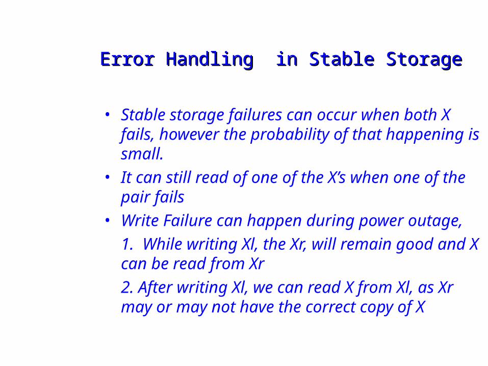
• Stable storage failures can occur when both X fails, however the probability of that happening is small.
• It can still read of one of the X’s when one of the pair fails
• Write Failure can happen during power outage, 1. While writing Xl, the Xr, will remain good and X can be read from Xr2. After writing Xl, we can read X from Xl, as Xr may or may not have the correct copy of X
Arranging data on diskArranging data on disk
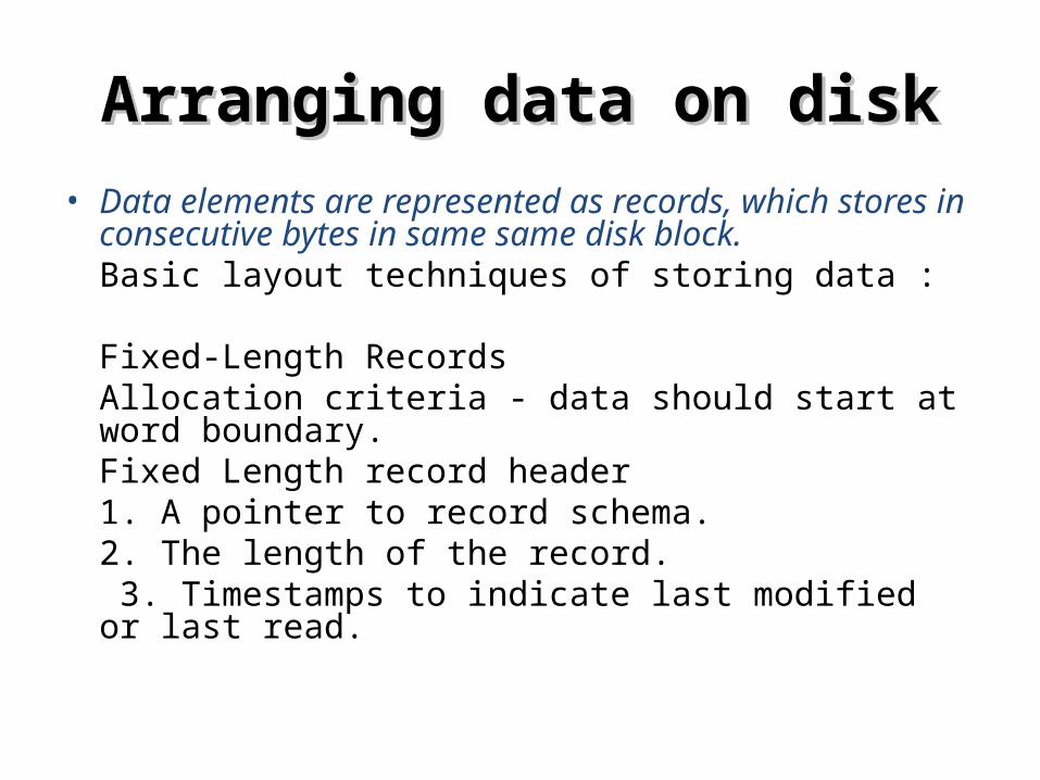
• Data elements are represented as records, which stores in consecutive bytes in same same disk block.
Basic layout techniques of storing data :
Fixed-Length RecordsAllocation criteria - data should start at word boundary.
Fixed Length record header 1. A pointer to record schema.2. The length of the record. 3. Timestamps to indicate last modified or last read.
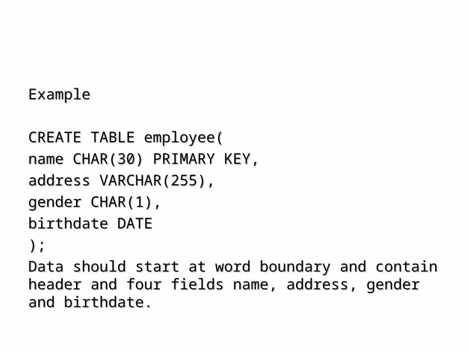
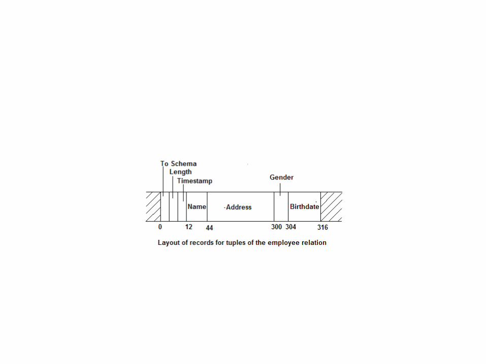
ExampleExample
CREATE TABLE employee(CREATE TABLE employee(name CHAR(30) PRIMARY KEY,name CHAR(30) PRIMARY KEY,address VARCHAR(255),address VARCHAR(255),gender CHAR(1),gender CHAR(1),birthdate DATEbirthdate DATE););Data should start at word boundary and contain header and four Data should start at word boundary and contain header and four fields name, address, gender and birthdate.fields name, address, gender and birthdate.
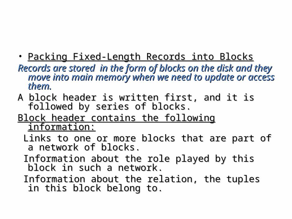
• Packing Fixed-Length Records into BlocksPacking Fixed-Length Records into BlocksRecords are stored in the form of blocks on the disk and they Records are stored in the form of blocks on the disk and they
move into main memory when we need to update or access move into main memory when we need to update or access them.them.
A block header is written first, and it is followed by series of A block header is written first, and it is followed by series of blocks.blocks.
Block header contains the following information:Block header contains the following information: Links to one or more blocks that are part of a network of Links to one or more blocks that are part of a network of
blocks.blocks. Information about the role played by this block in such a Information about the role played by this block in such a
network.network. Information about the relation, the tuples in this block belong Information about the relation, the tuples in this block belong
to.to.
• Failures: If out of Xl and Xr, one fails, it can be read form other, but in case both fails X is not readable, and its probability is very small
• Write Failure: During power outage, • 1. While writing Xl, the Xr, will remain good and X
can be read from Xr• 2. After writing Xl, we can read X from Xl, as Xr may
or may not have the correct copy of X.
Recovery from Disk Crashes:• To reduce the data loss by Dish crashes, schemes which
involve redundancy, extending the idea of parity checks or duplicate sectors can be applied.
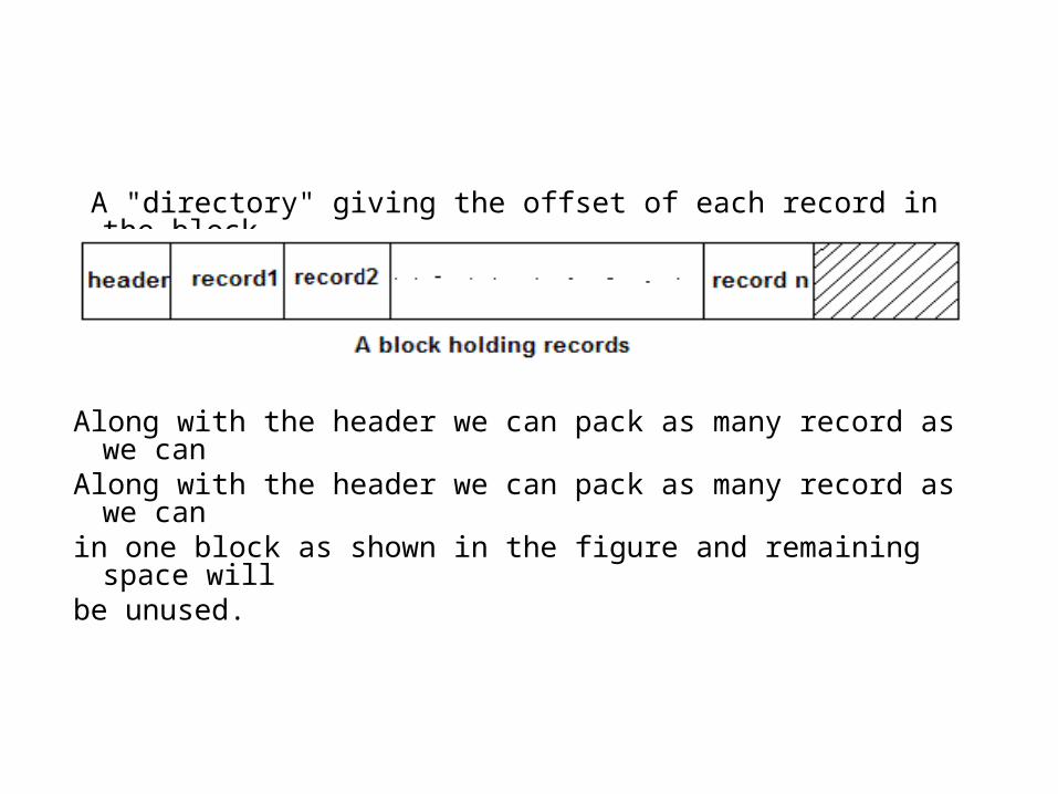
A "directory" giving the offset of each record in the block. Time stamp(s) to indicate time of the block's last
modification and/or access
Along with the header we can pack as many record as we canAlong with the header we can pack as many record as we canin one block as shown in the figure and remaining space will be unused.
13.6 Representing Block and Record 13.6 Representing Block and Record AddressesAddresses
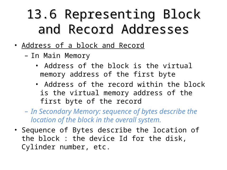
• Address of a block and Record– In Main Memory
• Address of the block is the virtual memory address of the first byte
• Address of the record within the block is the virtual memory address of the first byte of the record
– In Secondary Memory: sequence of bytes describe the location of the block in the overall system.
• Sequence of Bytes describe the location of the block : the device Id for the disk, Cylinder number, etc.
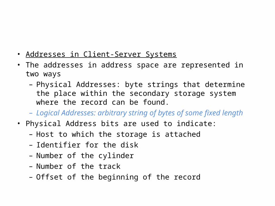
• Addresses in Client-Server Systems• The addresses in address space are represented in two ways
– Physical Addresses: byte strings that determine the place within the secondary storage system where the record can be found.
– Logical Addresses: arbitrary string of bytes of some fixed length• Physical Address bits are used to indicate:
– Host to which the storage is attached– Identifier for the disk– Number of the cylinder – Number of the track– Offset of the beginning of the record
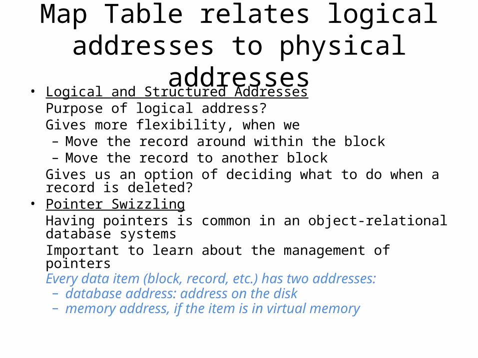
Map Table relates logical addresses to physical addresses
• Logical and Structured AddressesPurpose of logical address?Gives more flexibility, when we– Move the record around within the block– Move the record to another block
Gives us an option of deciding what to do when a record is deleted?• Pointer Swizzling
Having pointers is common in an object-relational database systemsImportant to learn about the management of pointersEvery data item (block, record, etc.) has two addresses:– database address: address on the disk– memory address, if the item is in virtual memory
• Example 13.7Block 1 has a record with pointers to a second record on the same block and to a record on another blockIf Block 1 is copied to the memory– The first pointer which points within Block 1 can be swizzled so
it points directly to the memory address of the target record– Since Block 2 is not in memory, we cannot swizzle the second
pointer• Three types of swizzling
– Automatic Swizzling• As soon as block is brought into memory, swizzle all relevant
pointers.
– Swizzling on Demand• Only swizzle a pointer if and when it is actually followed.
– No Swizzling• Pointers are not swizzled they are accesses using the
database address.• Unswizzling
– When a block is moved from memory back to disk, all pointers must go back to database (disk) addresses
– Use translation table again– Important to have an efficient data structure for the translation
table
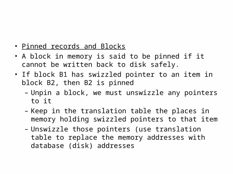
• Pinned records and Blocks• A block in memory is said to be pinned if it cannot be written
back to disk safely.• If block B1 has swizzled pointer to an item in block B2, then
B2 is pinned– Unpin a block, we must unswizzle any pointers to it– Keep in the translation table the places in memory holding
swizzled pointers to that item– Unswizzle those pointers (use translation table to replace
the memory addresses with database (disk) addresses
Variable Length Data and Records
Eswara Satya Pavan Rajesh PinapalaCS 257ID: 221
Topics
Records with Variable Length FieldsRecords with Repeating FieldsVariable Format RecordsRecords that do not fit in a blockBLOBS
name address
gender birth date
ExampleExample
Fig 1 : Movie star record with four fields
0 30 286 287 297
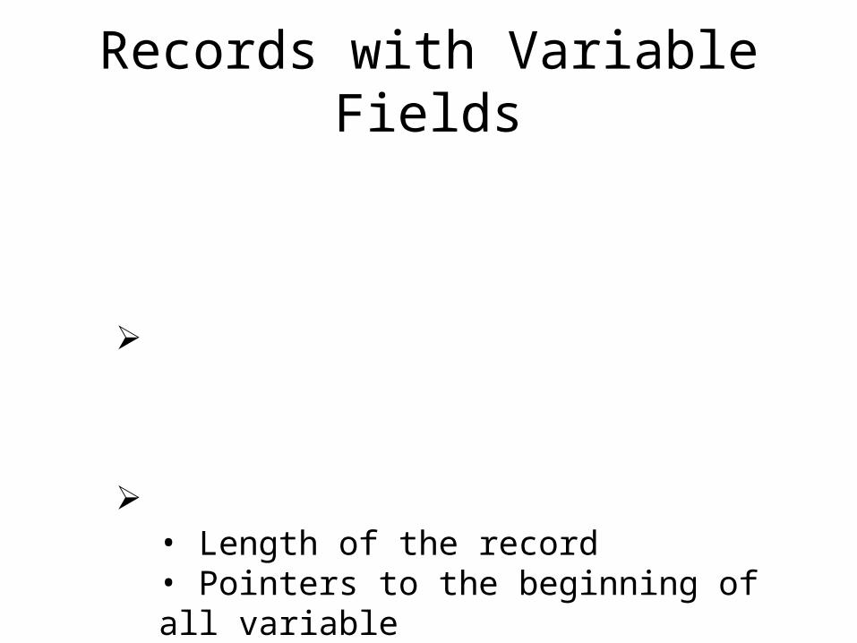
Records with Variable Fields
An effective way to represent variable length records is as follows
Fixed length fields are Kept ahead of the variable length fields
Record header contains• Length of the record• Pointers to the beginning of all variable length fields except the first one.
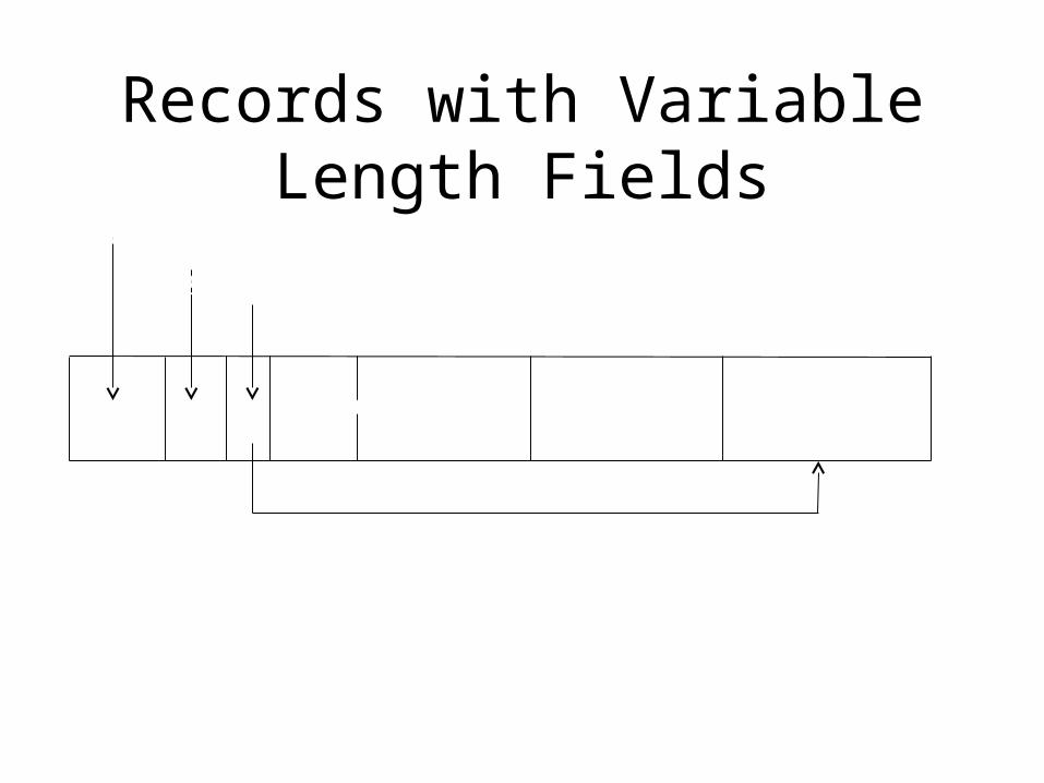
Records with Variable Length Fields
birth date name address
header informationrecord length
to address
gender
Figure 2 : A Movie Star record with name and address implemented as variable length character strings
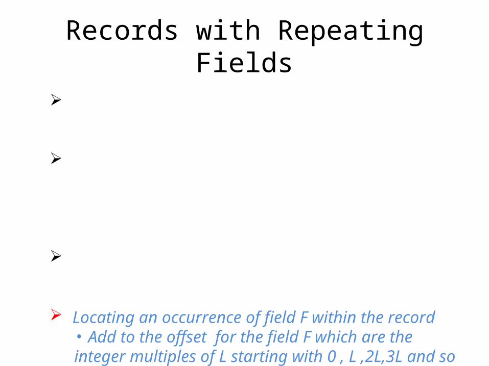
Records with Repeating Fields
Records contains variable number of occurrences of a field F
All occurrences of field F are grouped together and the record header contains a pointer to the first occurrence of field F
L bytes are devoted to one instance of field F
Locating an occurrence of field F within the record • Add to the offset for the field F which are the integer multiples of L starting with 0 , L ,2L,3L and so on to locate•We stop upon reaching the offset of the field F.
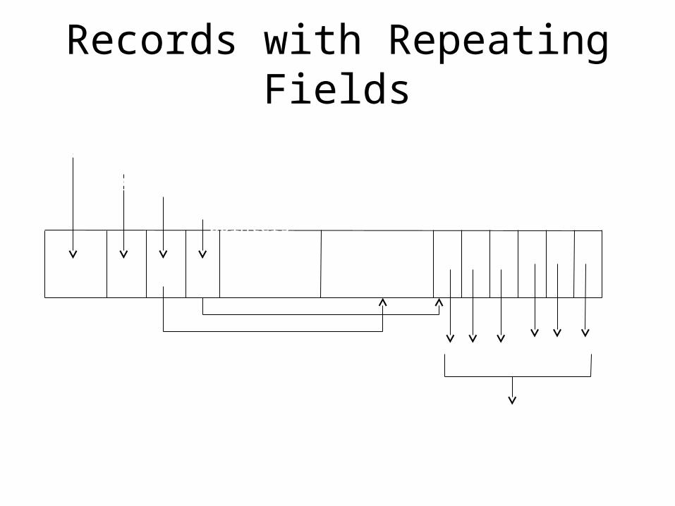
Records with Repeating Fields
name address
other header informationrecord length
to addressto movie pointers
pointers to movies
Figure 3 : A record with a repeating group of references to movies
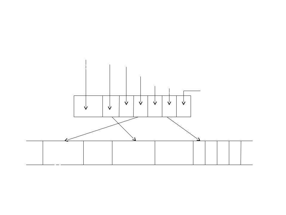
Figure 4 : Storing variable-length fields separately from the record
address
name
record header information
length of nameto address
length of address
to name
to movie references number of
references
Records with Repeating Fields

Advantage
Keeping the record itself fixed length allows record to be searched more efficiently, minimizes the overhead in the block headers, and allows records to be moved within or among the blocks with minimum effort.
Disadvantage
Storing variable length components on another block increases the number of disk I/O’s needed to examine all components of a record.
Records with Repeating Fields

A compromise strategy is to allocate a fixed portion of the record for the repeating fields
If the number of repeating fields is lesser than allocated space, then there will be some unused space If the number of repeating fields is greater than allocated space, then extra fields are stored in a different location and
Pointer to that location and count of additional occurrences is stored in the record
Records with Repeating Fields
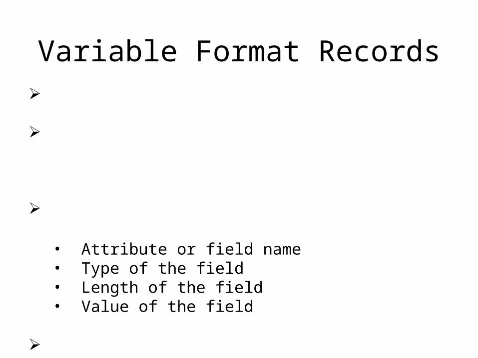
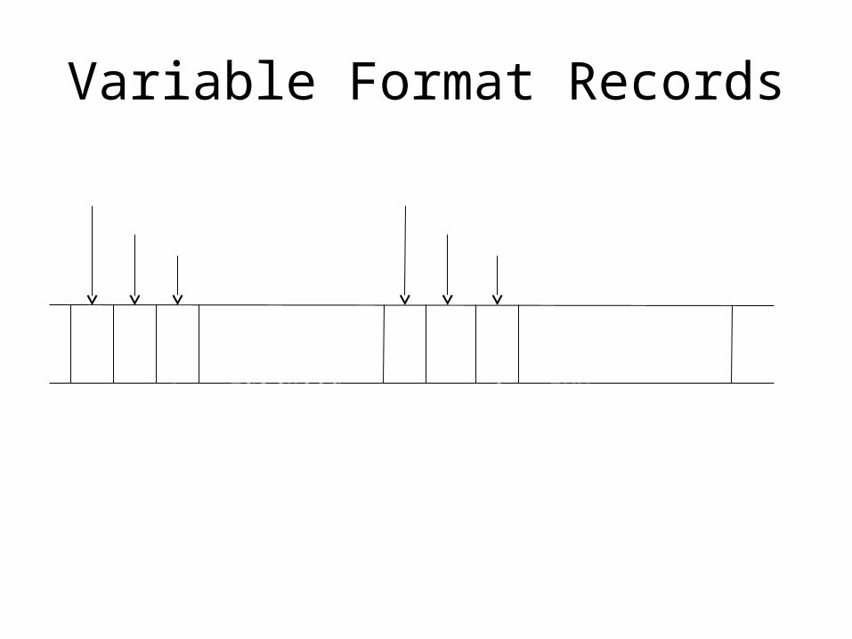
Variable Format Records Records that do not have fixed schema
Variable format records are represented by sequence of tagged fields
Each of the tagged fields consist of information• Attribute or field name• Type of the field• Length of the field• Value of the field
Why use tagged fields• Information – Integration applications• Records with a very flexible schema
Variable Format Records
Fig 5 : A record with tagged fields
N 16
S S14
Clint Eastwood
Hog’s Breath InnR
code for name code for restaurant ownedcode for string
typecode for string type
lengthlength
Records that do not fit in a block
When the length of a record is greater than block size ,then then record is divided and placed into two or more blocks
Portion of the record in each block is referred to as a RECORD FRAGMENT
Record with two or more fragments is called SPANNED RECORD
Record that do not cross a block boundary is called UNSPANNED RECORD
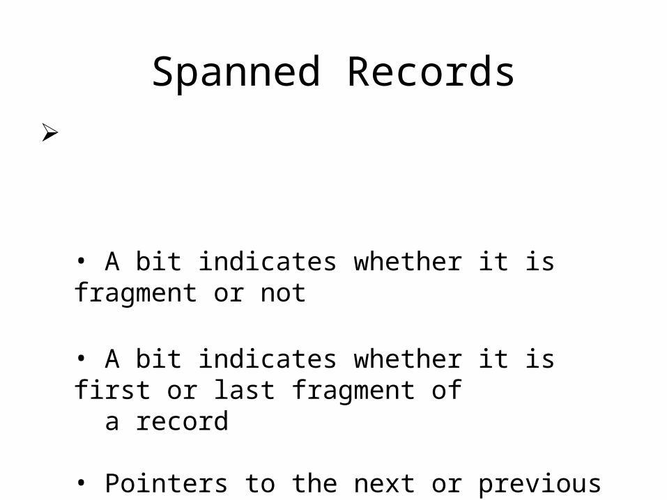
Spanned records require the following extra header information
• A bit indicates whether it is fragment or not
• A bit indicates whether it is first or last fragment of a record
• Pointers to the next or previous fragment for the same record
Spanned Records
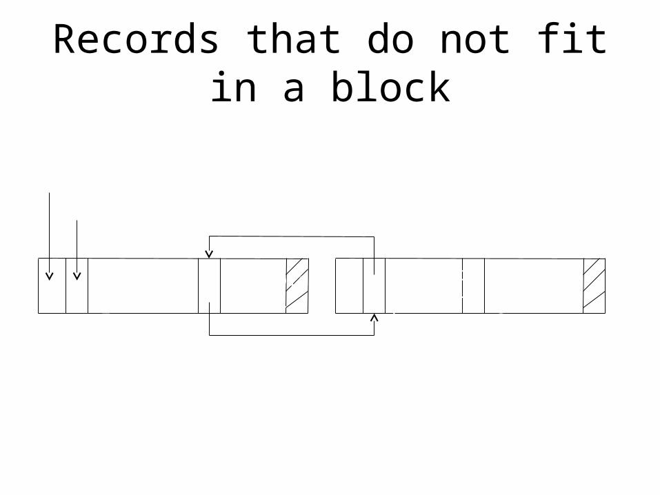
Records that do not fit in a block
Figure 6 : Storing spanned records across blocks
record 1 record 3 record 2 - a
record 2 - b
block header
record header
block 1 block 2
BLOBS
Large binary objects are called BLOBS e.g. : audio files, video files
Storage of BLOBS
Retrieval of BLOBS
85
Record Modifications
Chapter 13Section 13.8
Neha SamantCS 257
(Section II) Id 222
Insertion Insertion of records without order Records can be placed in a block with empty space or in a new block.
Insertion of records in fixed order Space available in the block No space available in the block (outside the block)
Structured addressPointer to a record from outside the block.
86
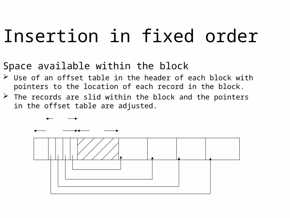
Insertion in fixed orderSpace available within the block Use of an offset table in the header of each block with pointers to the location of
each record in the block. The records are slid within the block and the pointers in the offset table are
adjusted.
87
Record 2Record 3Record 4
header unused
Offset table
Record 1
Insertion in fixed order
88
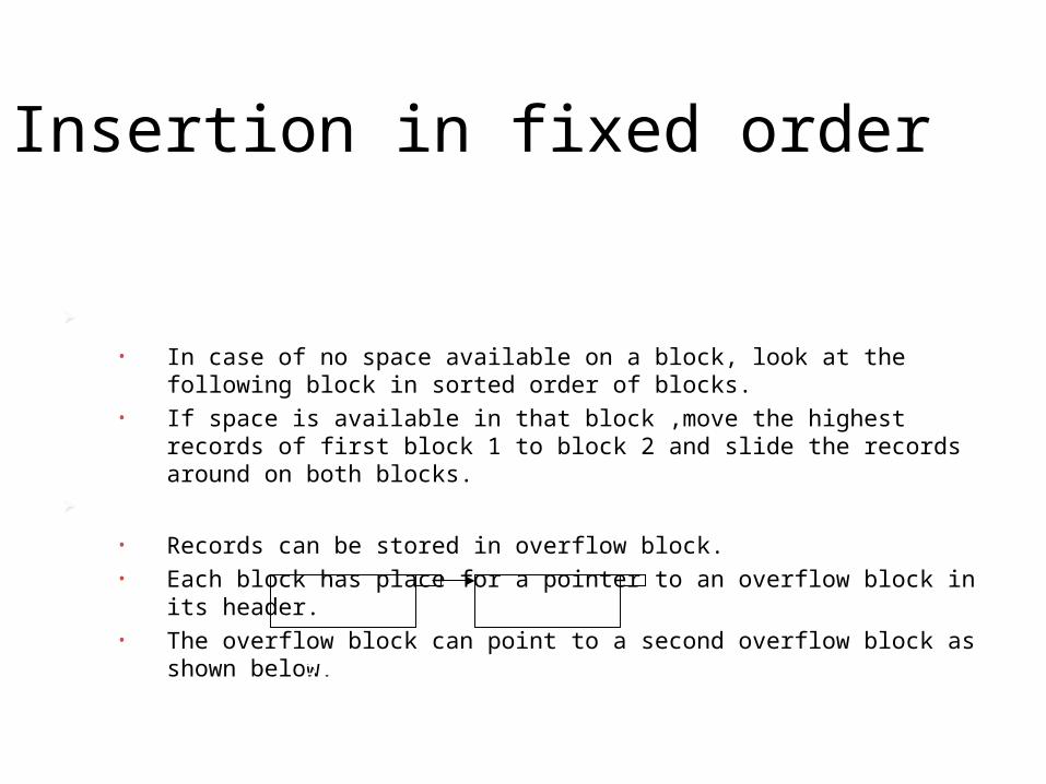
No space available within the block (outside the block) Find space on a “nearby” block.
• In case of no space available on a block, look at the following block in sorted order of blocks.
• If space is available in that block ,move the highest records of first block 1 to block 2 and slide the records around on both blocks.
Create an overflow block• Records can be stored in overflow block.• Each block has place for a pointer to an overflow block in its header.• The overflow block can point to a second overflow block as shown below.
Block B
Overflow block for B
Deletion Recover space after deletion
When using an offset table, the records can be slid around the block so there will be an unused region in the center that can be recovered.
In case we cannot slide records, an available space list can be maintained in the block header.
The list head goes in the block header and available regions hold the links in the list.
89
Deletion
90
Use of tombstone The tombstone is placed in a record in order to avoid pointers to the
deleted record to point to new records.
The tombstone is permanent until the entire database is reconstructed.
If pointers go to fixed locations from which the location of the record is found then we put the tombstone in that fixed location. (See examples)
Where a tombstone is placed depends on the nature of the record pointers.
Map table is used to translate logical record address to physical address.
Deletion
91
Record 1 Record 2
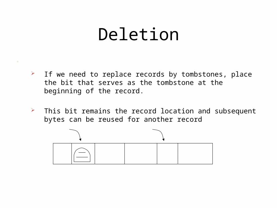
Use of tombstone If we need to replace records by tombstones, place the bit that serves
as the tombstone at the beginning of the record.
This bit remains the record location and subsequent bytes can be reused for another record
Record 1 can be replaced, but the tombstone remains, record 2 has no tombstone and can be seen when we follow a pointer to it.
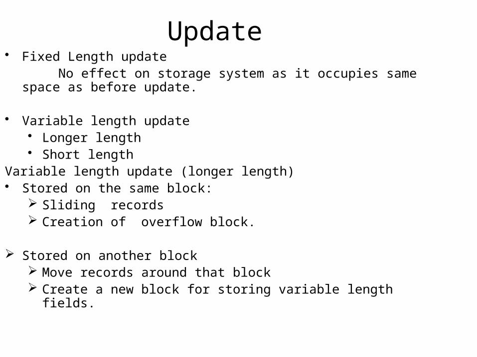
Update Fixed Length update No effect on storage system as it occupies same space as before update.
Variable length update Longer length Short length
Variable length update (longer length) Stored on the same block:
Sliding records Creation of overflow block.
Stored on another block Move records around that block Create a new block for storing variable length fields.
92
Query Execution
Chapter 15Section 15.1
Presented by Khadke, Suvarna
CS 257 (Section II) Id 213
93
Agenda
• Query Processor and major parts of Query processor
• Physical-Query-Plan Operators• Scanning Tables• Basic approaches to locate the tuples of a
relation R• Sorting While Scanning Tables• Computation Model for Physical Operator• I/O Cost for Scan Operators• Iterators
94
What is a Query Processor
• Group of components of a DBMS that converts a user queries and data-modification commands into a sequence of database operations and executes those operations.
• Must supply detail regarding how the query is to be executed
• Moreover, a naive execution strategy for a query may lead to an algorithm for executing the query that takes far more time than necessary.
95
Major parts of Query processor
96
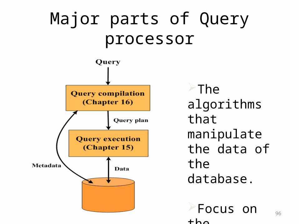
Query Execution:The algorithms that manipulate the data of the database.
Focus on the operations of extended relational algebra.
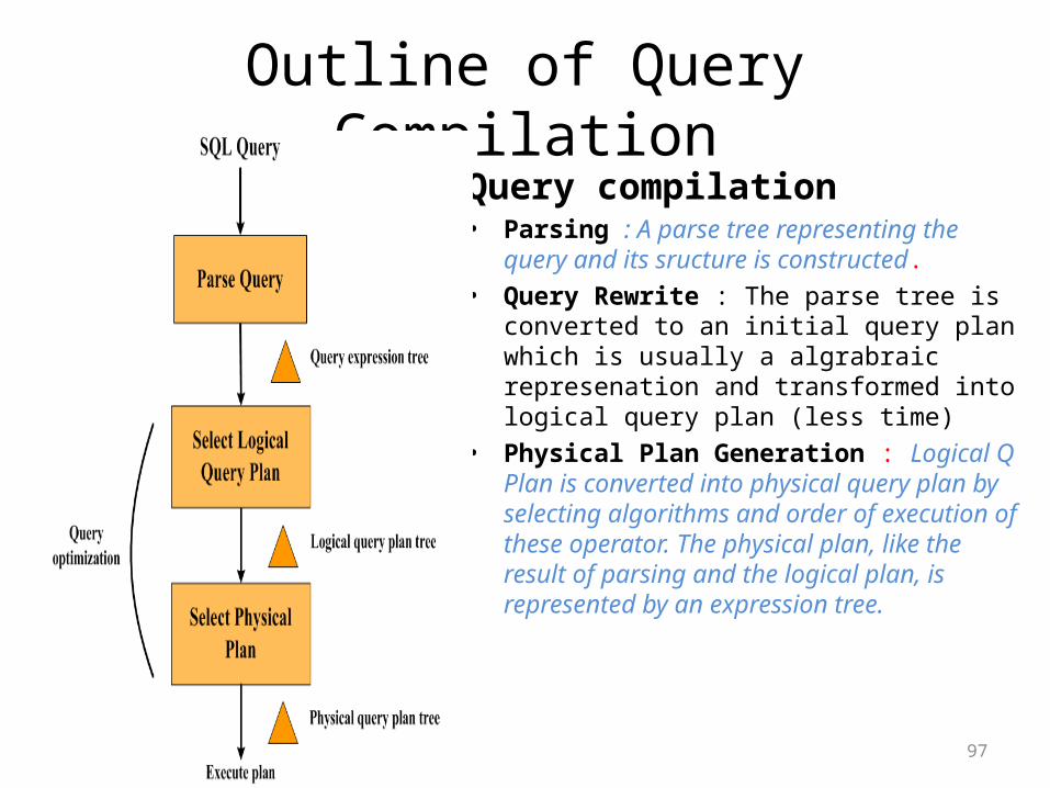
Outline of Query CompilationQuery compilation• Parsing : A parse tree representing the query
and its sructure is constructed.• Query Rewrite : The parse tree is converted to
an initial query plan which is usually a algrabraic represenation and transformed into logical query plan (less time)
• Physical Plan Generation : Logical Q Plan is converted into physical query plan by selecting algorithms and order of execution of these operator. The physical plan, like the result of parsing and the logical plan, is represented by an expression tree.
97
Physical-Query-Plan Operators
• Physical operators are implementations of the operator of relational algebra.
• They can also be use in non relational algebra operators like “scan” which scans tables, that is, bring each tuple of some relation into main memory.
98
Scanning TablesBasic approaches to locate the tuples of a relation R Table Scan
• Relation R is stored in secondary memory with its tuples arranged in blocks
• It is possible to get the blocks one by one Index-Scan
• If there is an index on any attribute of Relation R, we can use this index to get all the tuples of Relation R.eg For example, a sparse index on R, 13.1.3, can be used to lead us to all the blocks holding R, even if
• we don't know otherwise which blocks these are
99
Sorting While Scanning Tables
• Number of reasons to sort a relation Query could include an ORDER BY clause,
requiring that a relation be sorted.Algorithms to implement relational algebra
operations requires one or both arguments to be sorted relations.
Physical-query-plan operator sort-scan takes a relation R, attributes on which the sort is to be made, and produces R in that sorted order
100
Computation Model for Physical Operator
• Physical-Plan Operator should be selected wisely which is essential for good Query Processor .
• For “cost” of each operator is estimated by number of disk I/O’s for an operation.
• The total cost of operation depends on the size of the answer, and includes the final write back cost to the total cost of the query.
101
Parameters for Measuring Costs
• Parameters that affect the performance of a queryBuffer space availability in the main memory
at the time of execution of the querySize of input and the size of the output
generatedThe size of memory block on the disk and the
size in the main memory also affects the performance
102
Parameters for Measuring Costs
• B: The number of blocks are needed to hold all tuples of relation R.
Also denoted as B(R)• T:The number of tuples in relationR. Also denoted as T(R)
V: The number of distinct values that appear in a column of a relation R
V(R, a)- is the number of distinct values of column for a in relation R
103
I/O Cost for Scan Operators
• If R is clustered but requires a two-phase multiway merge sort, then, we require about 3B disk I/O's, divided equally.
• among the operations of reading R in sublists, writing out the sublists, and
• rereading the sublists.If relation R is not clustered, then the number of required disk I/O generally is much higher
• A index on a relation R occupies many fewer than B(R) blocks
That means a scan of the entire relation R which takes at least B disk I/O’s will require more I/O’s than the entire index
104
Iterators for Implementation of Physical Operators
• Many physical operators can be implemented as an Iterator.
• Three methods forming the iterator for an operation are:
• 1. Open( ) : This method starts the process of getting
tuplesIt initializes any data structures needed to
perform the operation
105
Iterators for Implementation of Physical Operators
• 2. GetNext( ): • Adjusts data structures as necessary to allow subsequent tuples to be
obtained. In getting the next tuple of its result, it typically calls GetNext one or more times on its argument(s). If there are no more tuples to return, GetNext returns a special value NotFound, which Ire assume cannot be mistaken for a tuple.
• 3. Close( ) : Ends the iteration after all tuples It calls Close on any arguments of the operator
106
Query Execution
One-Pass Algorithms for Database Operations (15.2)
107
Presented by
Ronak Shah
(214)
April 22, 2009
Introduction
• The choice of an algorithm for each operator is an essential part of the process of transforming a logical query plan into a physical query plan.
• Main classes of Algorithms:– Sorting-based methods– Hash-based methods– Index-based methods
• Division based on degree difficulty and cost:– 1-pass algorithms– 2-pass algorithms– 3 or more pass algorithms
108
One-Pass Algorithms for Tuple-at-a-Time Operations
• Tuple-at-a-time operations are selection and projection– read the blocks of R one at a time into an input buffer– perform the operation on each tuple– move the selected tuples or the projected tuples to the output
buffer
• The disk I/O requirement for this process depends only on how the argument relation R is provided. – If R is initially on disk, then the cost is whatever it takes to
perform a table-scan or index-scan of R.
109
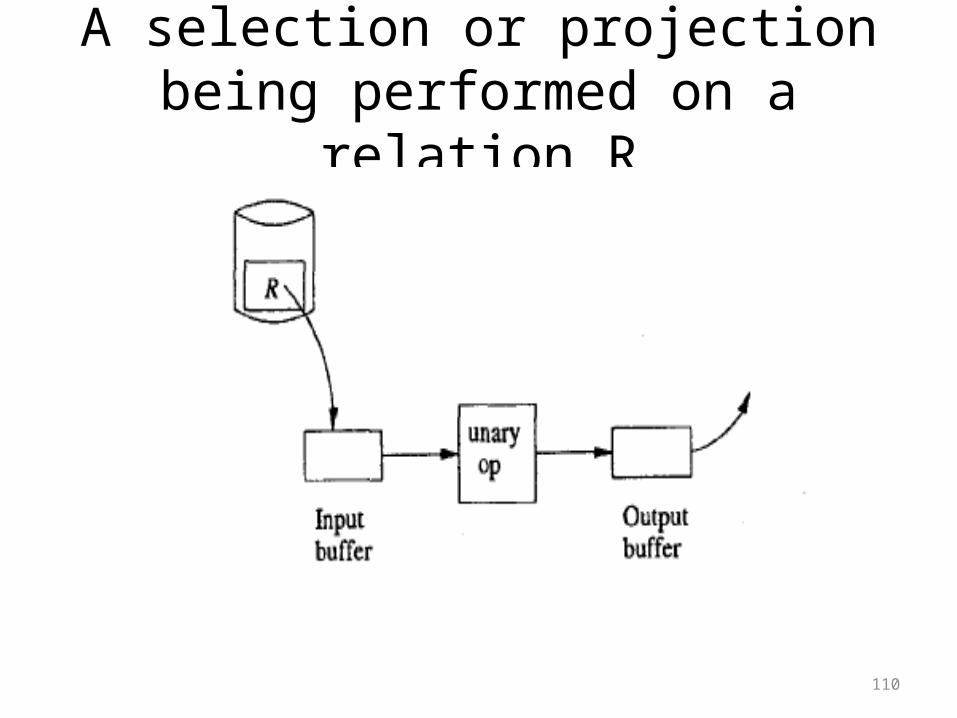
A selection or projection being performed on a relation R
110
Categories of algos• 1. Sorting-based methods
• 2. Hash-based methods.
• Index-based methods.• In addition. n-e can divide algorithms for operators into three "degrees" of
difficulty and cost:• Some methods involve reading the data only once from disk• Some methods work for data that is too large to fit in available main• memory but not for the largest imaginable data sets.• Some methods work without a limit on the size of the data
111
Operators classification• Tuple-at-a-time, unary operations. These operations - selection and
projection- do not require an entire relation, or even a large part of it, in *memory at once.
• Full-relation, unary operations. These one-argument operations require seeing all or most of the tuples in memory at once, so one-pass algorithms are limited to relations that are approximately of size hl (the number of main-memory buffers available) or less.
• Full-relation, binary operations. .All other operations are in this class:set and bag versions of union: intersection, difference, joins, and products
112
One-Pass Algorithms for Unary, fill-Relation Operations
• Duplicate Elimination– To eliminate duplicates, we can read each block of R one at
a time, but for each tuple we need to make a decision as to whether:1. It is the first time we have seen this tuple, in which case we
copy it to the output, or2. We have seen the tuple before, in which case we must not
output this tuple.– One memory buffer holds one block of R's tuples, and the
remaining M - 1 buffers can be used to hold a single copy of every tuple.
113
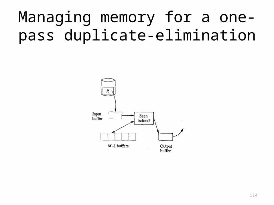
Managing memory for a one-pass duplicate-elimination
114
Duplicate Elimination• When a new tuple from R is considered, we compare it with all tuples seen so far
– if it is not equal: we copy both to the output and add it to the in-memory list of tuples we have seen.
– if there are n tuples in main memory: each new tuple takes processor time proportional to n, so the complete operation takes processor time proportional to n2.
• We need a main-memory structure that allows each of the operations: – Add a new tuple, and– Tell whether a given tuple is already there .
• The different structures that can be used for such main memory structures are:– Hash table– Balanced binary search tree
115
One-Pass Algorithms for Unary, fill-Relation Operations
• Grouping– The grouping operation gives us zero or more grouping
attributes and presumably one or more aggregated attributes
– If we create in main memory one entry for each group then we can scan the tuples of R, one block at a time.
– The entry for a group consists of values for the grouping attributes and an accumulated value or values for each aggregation.
116
Grouping• The accumulated value is:
– For MIN(a) or MAX(a) aggregate, record minimum /maximum value, respectively.
– For any COUNT aggregation, add 1 for each tuple of group.– For SUM(a), add value of attribute a to the accumulated
sum for its group.– AVG(a) is a hard case. We must maintain 2 accumulations:
count of no. of tuples in the group & sum of a-values of these tuples. Each is computed as we would for a COUNT & SUM aggregation, respectively. After all tuples of R are seen, take quotient of sum & count to obtain average.
117
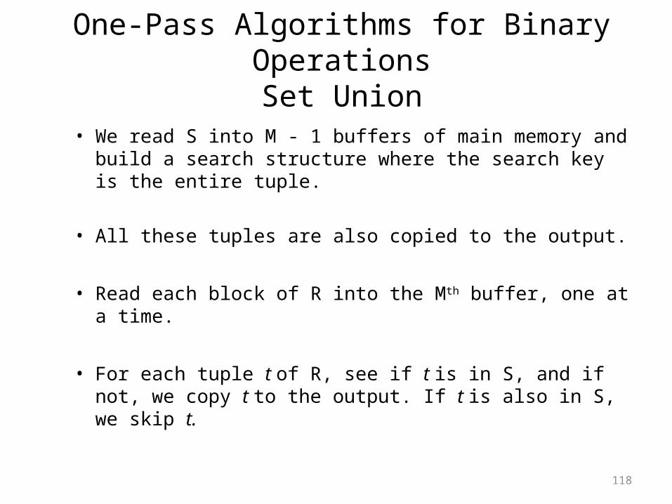
One-Pass Algorithms for Binary OperationsSet Union
• We read S into M - 1 buffers of main memory and build a search structure where the search key is the entire tuple.
• All these tuples are also copied to the output.
• Read each block of R into the Mth buffer, one at a time.
• For each tuple t of R, see if t is in S, and if not, we copy t to the output. If t is also in S, we skip t.
118
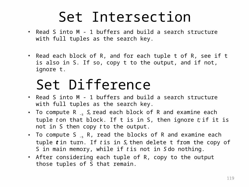
Set Intersection• Read S into M - 1 buffers and build a search structure with full tuples as the
search key.
• Read each block of R, and for each tuple t of R, see if t is also in S. If so, copy t to the output, and if not, ignore t.
Set Difference• Read S into M - 1 buffers and build a search structure with full tuples as the
search key. • To compute R -s S, read each block of R and examine each tuple t on that
block. If t is in S, then ignore t; if it is not in S then copy t to the output. • To compute S -s R, read the blocks of R and examine each tuple t in turn. If t is
in S, then delete t from the copy of S in main memory, while if t is not in S do nothing.
• After considering each tuple of R, copy to the output those tuples of S that remain.
119
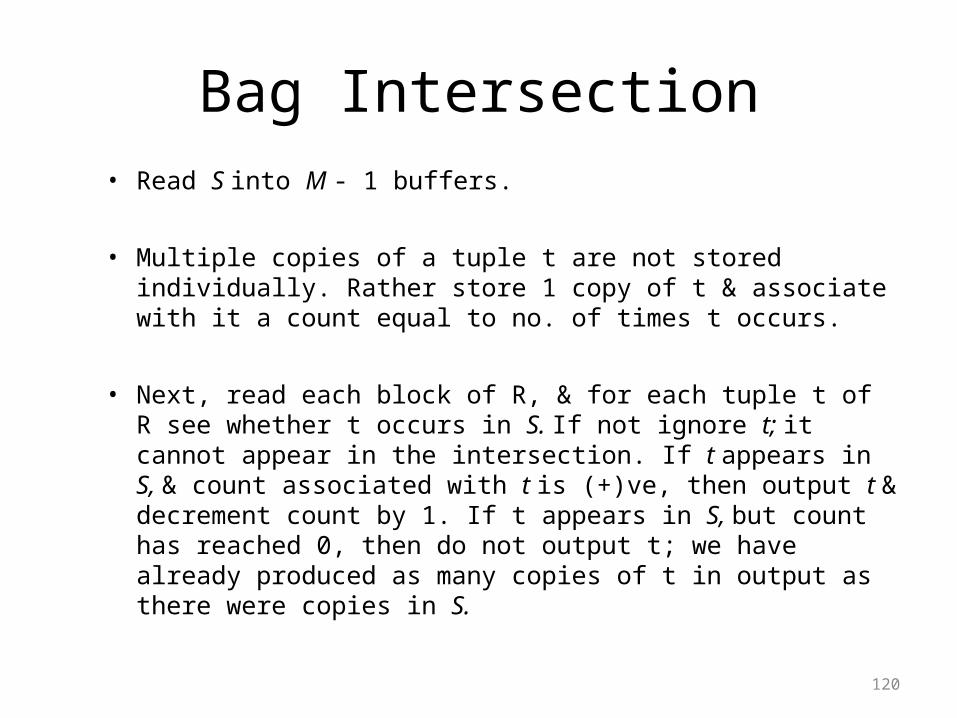
Bag Intersection• Read S into M - 1 buffers.
• Multiple copies of a tuple t are not stored individually. Rather store 1 copy of t & associate with it a count equal to no. of times t occurs.
• Next, read each block of R, & for each tuple t of R see whether t occurs in S. If not ignore t; it cannot appear in the intersection. If t appears in S, & count associated with t is (+)ve, then output t & decrement count by 1. If t appears in S, but count has reached 0, then do not output t; we have already produced as many copies of t in output as there were copies in S.
120
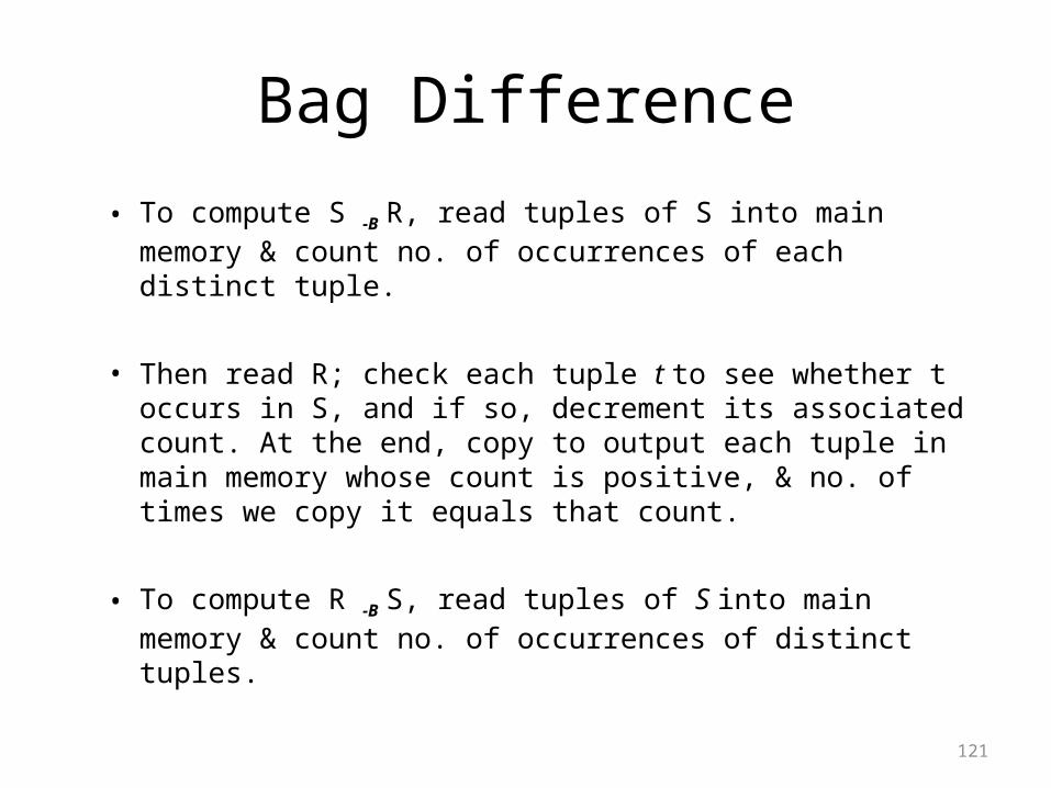
Bag Difference
• To compute S -B R, read tuples of S into main memory & count no. of occurrences of each distinct tuple.
• Then read R; check each tuple t to see whether t occurs in S, and if so, decrement its associated count. At the end, copy to output each tuple in main memory whose count is positive, & no. of times we copy it equals that count.
• To compute R -B S, read tuples of S into main memory & count no. of occurrences of distinct tuples.
121
Product• Read S into M - 1 buffers of main memory
• Then read each block of R, and for each tuple t of R concatenate t with each tuple of S in main memory.
• Output each concatenated tuple as it is formed.
• This algorithm may take a considerable amount of processor time per tuple of R, because each such tuple must be matched with M - 1 blocks full of tuples. However, output size is also large, & time/output tuple is small.
122
Natural Join
• Convention: R(X, Y) is being joined with S(Y, Z), where Y represents all the attributes that R and S have in common, X is all attributes of R that are not in the schema of S, & Z is all attributes of S that are not in the schema of R. Assume that S is the smaller relation.
• To compute the natural join, do the following: 1. Read all tuples of S & form them into a main-memory
search structure. Hash table or balanced tree are good e.g. of such structures. Use M - 1 blocks of memory for this purpose.
123
QUERY EXECUTION
15.3Nested-Loop Joins
By:Saloni Tamotia (215)
Introduction to Nested-Loop Joins
Used for relations of any side.Not necessary that relation fits in main memory Uses “One-and-a-half” pass method in which
for each variation:One argument read just once.Other argument read repeatedly.Two kinds:
Tuple-Based Nested Loop JoinBlock-Based Nested Loop Join
ADVANTAGES OF NESTED-LOOP JOIN Fits in the iterator framework.
Allows us to avoid storing intermediate relation on disk.
Tuple-Based Nested-Loop Join Simplest variation of the nested-loop join
Loop ranges over individual tuples
Tuple-Based Nested-Loop Join
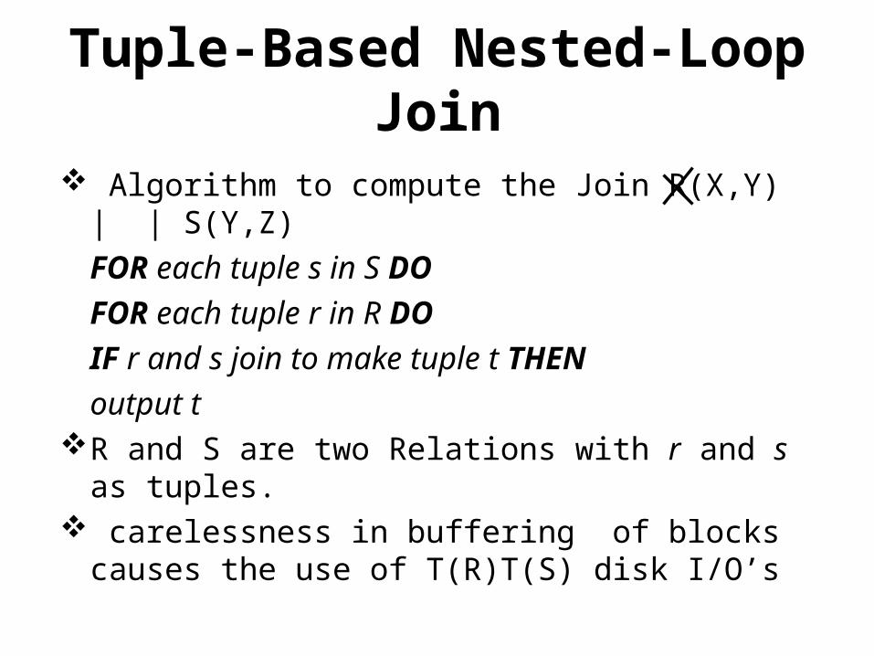
Algorithm to compute the Join R(X,Y) | | S(Y,Z) FOR each tuple s in S DO
FOR each tuple r in R DOIF r and s join to make tuple t THENoutput t
R and S are two Relations with r and s as tuples. carelessness in buffering of blocks causes the use
of T(R)T(S) disk I/O’s
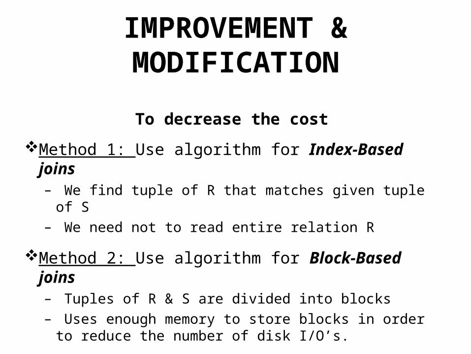
IMPROVEMENT & MODIFICATION
To decrease the cost
Method 1: Use algorithm for Index-Based joins– We find tuple of R that matches given tuple of S– We need not to read entire relation R
Method 2: Use algorithm for Block-Based joins– Tuples of R & S are divided into blocks– Uses enough memory to store blocks in order to
reduce the number of disk I/O’s.
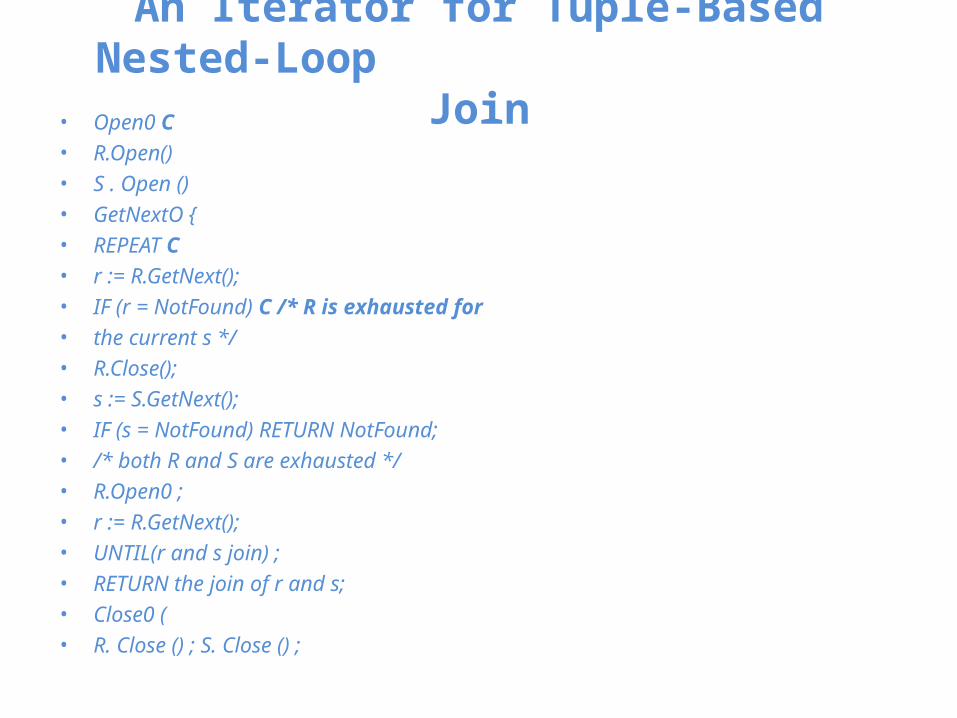
An Iterator for Tuple-Based Nested-Loop Join
• Open0 C• R.Open()• S . Open ()• GetNextO {• REPEAT C• r := R.GetNext();• IF (r = NotFound) C /* R is exhausted for• the current s */• R.Close();• s := S.GetNext();• IF (s = NotFound) RETURN NotFound;• /* both R and S are exhausted */• R.Open0 ;• r := R.GetNext();• UNTIL(r and s join) ;• RETURN the join of r and s;• Close0 (• R. Close () ; S. Close () ;
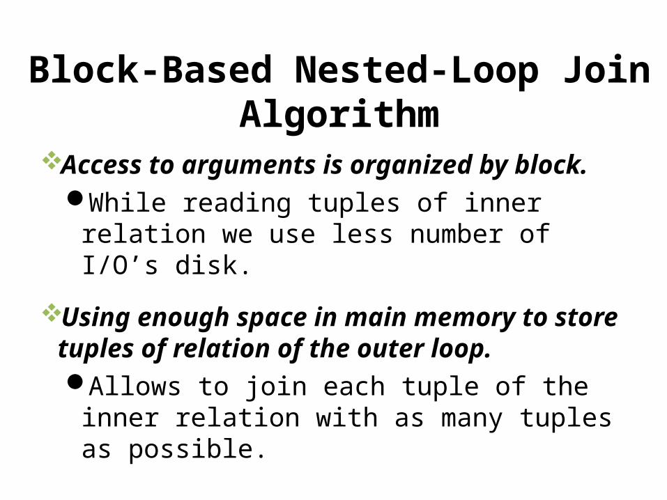
Block-Based Nested-Loop Join Algorithm
Access to arguments is organized by block.While reading tuples of inner relation we
use less number of I/O’s disk.
Using enough space in main memory to store tuples of relation of the outer loop.Allows to join each tuple of the inner
relation with as many tuples as possible.
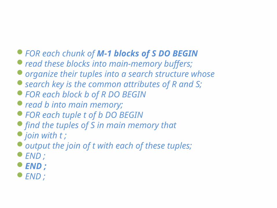
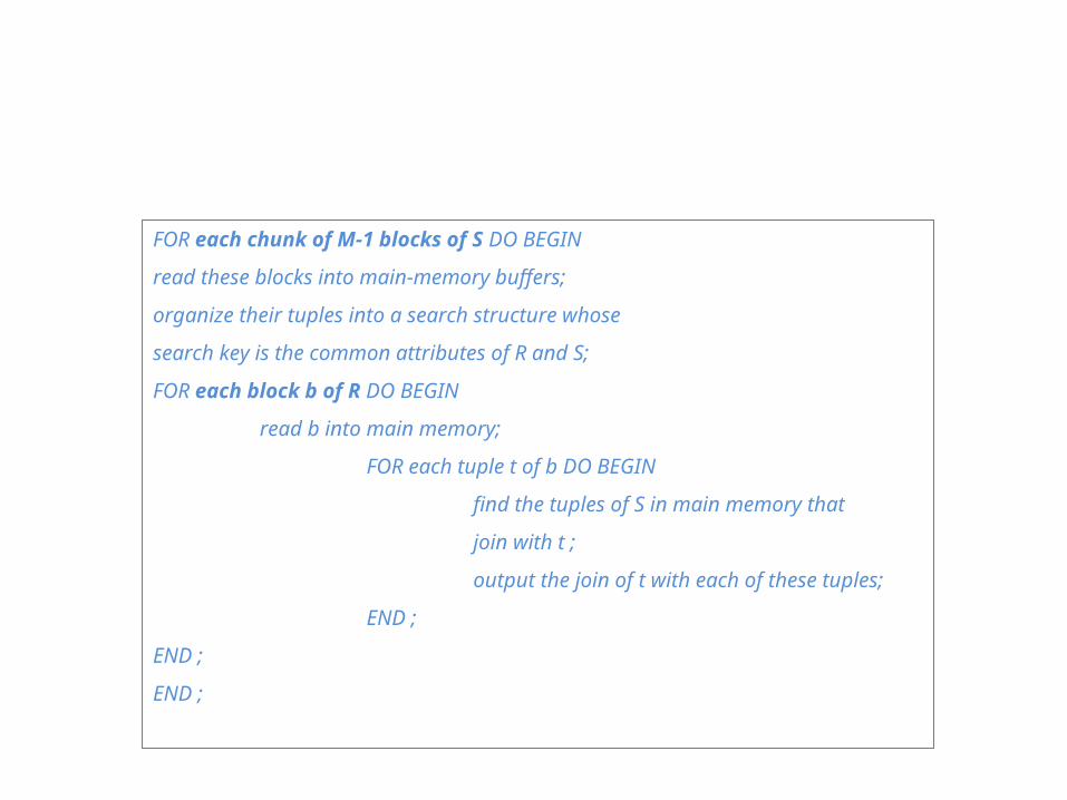
FOR each chunk of M-1 blocks of S DO BEGINread these blocks into main-memory buffers;organize their tuples into a search structure whosesearch key is the common attributes of R and S;FOR each block b of R DO BEGINread b into main memory;FOR each tuple t of b DO BEGINfind the tuples of S in main memory thatjoin with t ;output the join of t with each of these tuples;END ;END ;END ;
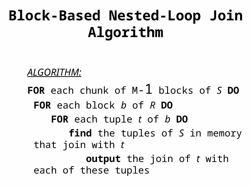
Block-Based Nested-Loop Join Algorithm
ALGORITHM:
FOR each chunk of M-1 blocks of S DO
FOR each block b of R DO FOR each tuple t of b DO find the tuples of S in memory that join with t output the join of t with each of these tuples
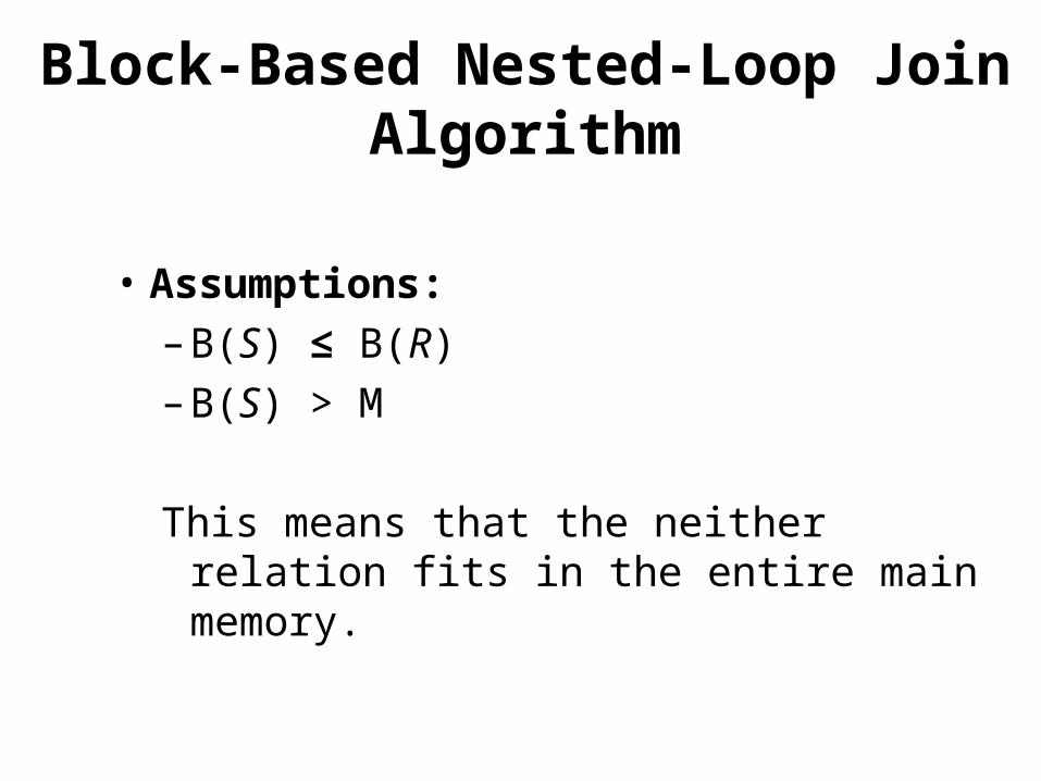
Block-Based Nested-Loop Join Algorithm
• Assumptions:– B(S) ≤ B(R)– B(S) > M
This means that the neither relation fits in the entire main memory.
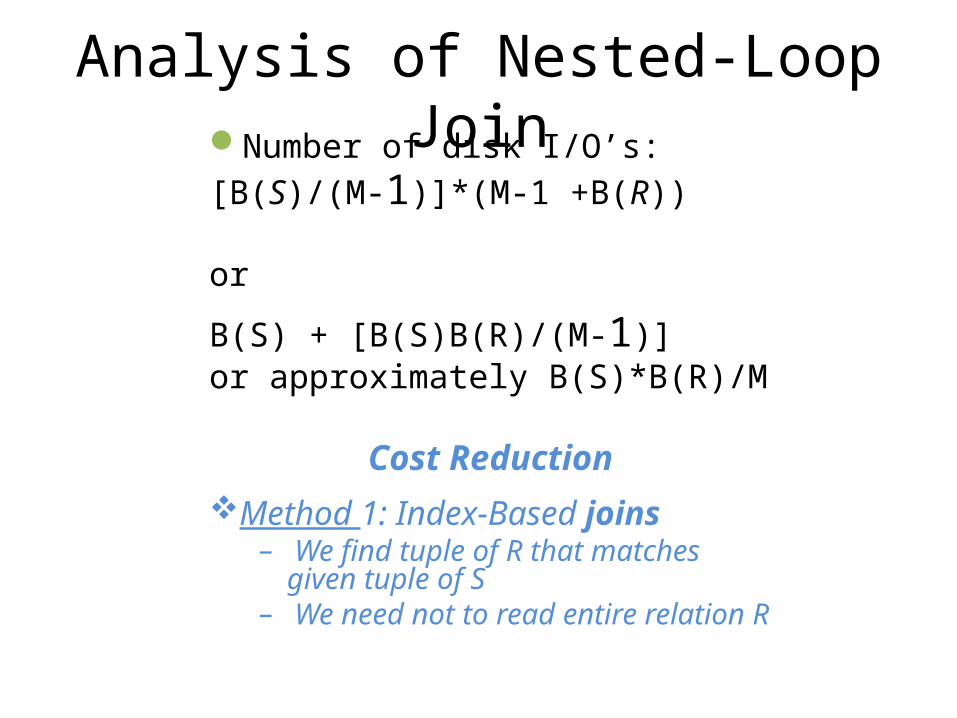
Analysis of Nested-Loop JoinNumber of disk I/O’s:[B(S)/(M-1)]*(M-1 +B(R))
or
B(S) + [B(S)B(R)/(M-1)]or approximately B(S)*B(R)/M
Cost ReductionMethod 1: Index-Based joins
– We find tuple of R that matches given tuple of S
– We need not to read entire relation R
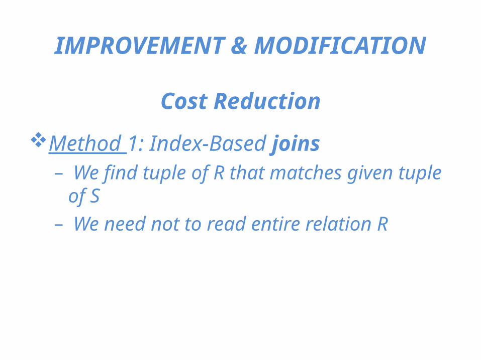
IMPROVEMENT & MODIFICATION
Cost Reduction
Method 1: Index-Based joins– We find tuple of R that matches given tuple of S– We need not to read entire relation R
Two-Pass Algorithms Based on Sorting
SECTION 15.4
Rupinder Singh
Two-Pass Algorithms Based on Sorting
• Two-pass Algorithms: data from operand relations is read into main memory, then processed, written out to disk and then re-read from the disk to complete the operation
• In this section, we consider sorting as tool from implementing relational operations. The basic idea is as follows if we have large relation R, where B(R) is larger than M, the number of memory buffers we have available, then we can repeatedly
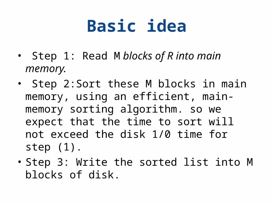
Basic idea
• Step 1: Read M blocks of R into main memory.• Step 2:Sort these M blocks in main memory,
using an efficient, main-memory sorting algorithm. so we expect that the time to sort will not exceed the disk 1/0 time for step (1).
• Step 3: Write the sorted list into M blocks of disk.
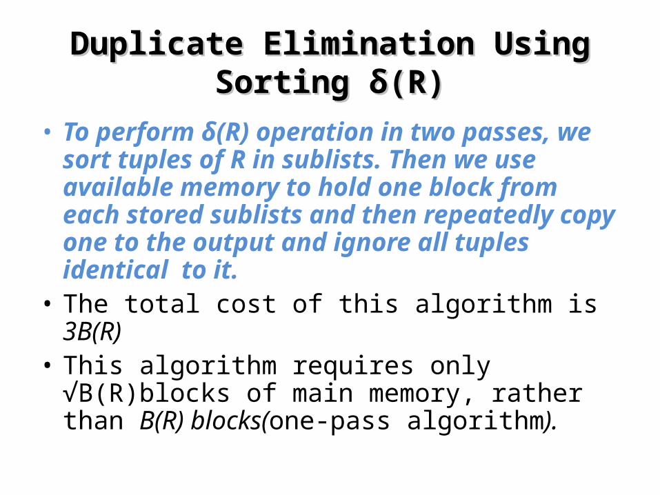
Duplicate Elimination Using Sorting Duplicate Elimination Using Sorting δδ(R)(R)
• To perform δ(R) operation in two passes, we sort tuples of R in sublists. Then we use available memory to hold one block from each stored sublists and then repeatedly copy one to the output and ignore all tuples identical to it.
• The total cost of this algorithm is 3B(R)• This algorithm requires only √B(R)blocks of main
memory, rather than B(R) blocks(one-pass algorithm).
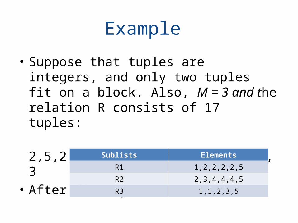
Example
• Suppose that tuples are integers, and only two tuples fit on a block. Also, M = 3 and the relation R consists of 17 tuples:
2,5,2,1,2,2,4,5,4,3,4,2,1,5,2,1,3• After first-pass
Sublists Elements
R1 1,2,2,2,2,5
R2 2,3,4,4,4,5
R3 1,1,2,3,5
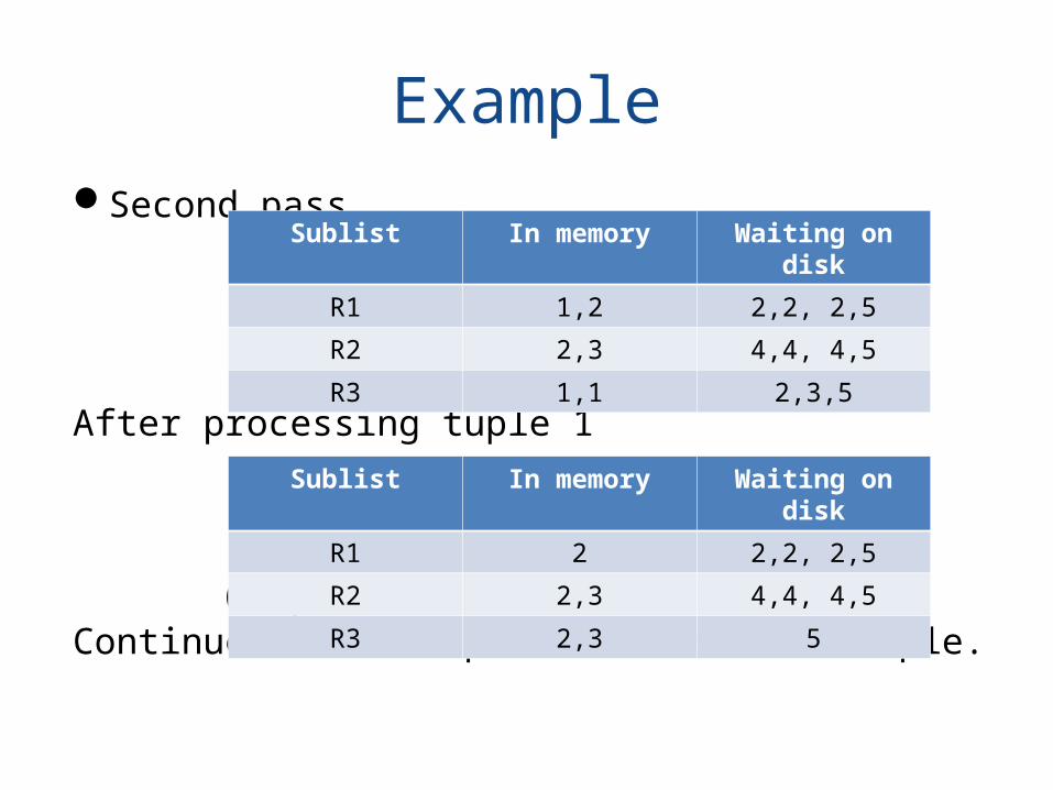
ExampleSecond pass
After processing tuple 1
Output: 1Continue the same process with next tuple.
Sublist In memory Waiting on disk
R1 1,2 2,2, 2,5
R2 2,3 4,4, 4,5
R3 1,1 2,3,5
Sublist In memory Waiting on disk
R1 2 2,2, 2,5
R2 2,3 4,4, 4,5
R3 2,3 5
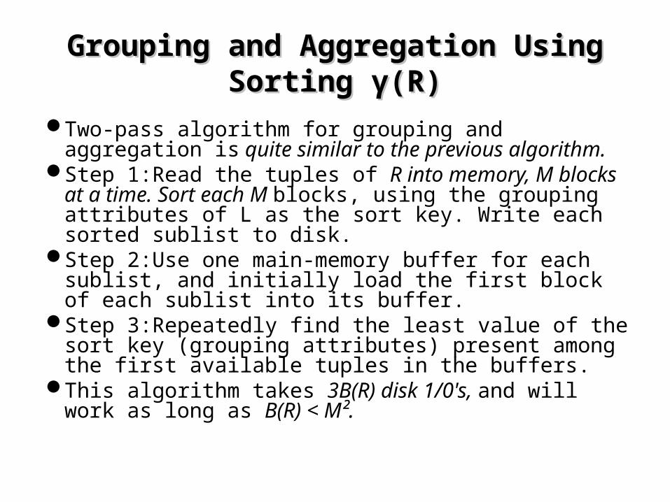
Grouping and Aggregation Using Sorting Grouping and Aggregation Using Sorting γγ(R)(R)
Two-pass algorithm for grouping and aggregation is quite similar to the previous algorithm.
Step 1:Read the tuples of R into memory, M blocks at a time. Sort each M blocks, using the grouping attributes of L as the sort key. Write each sorted sublist to disk.
Step 2:Use one main-memory buffer for each sublist, and initially load the first block of each sublist into its buffer.
Step 3:Repeatedly find the least value of the sort key (grouping attributes) present among the first available tuples in the buffers.
This algorithm takes 3B(R) disk 1/0's, and will work as long as B(R) < M².
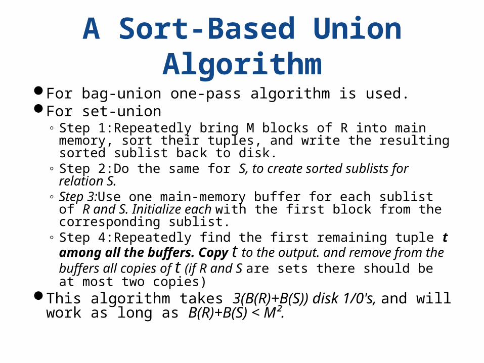
A Sort-Based Union AlgorithmFor bag-union one-pass algorithm is used.For set-union
◦ Step 1:Repeatedly bring M blocks of R into main memory, sort their tuples, and write the resulting sorted sublist back to disk.
◦ Step 2:Do the same for S, to create sorted sublists for relation S.◦ Step 3:Use one main-memory buffer for each sublist of R and S.
Initialize each with the first block from the corresponding sublist.◦ Step 4:Repeatedly find the first remaining tuple t among all the
buffers. Copy t to the output. and remove from the buffers all copies of t (if R and S are sets there should be at most two copies)
This algorithm takes 3(B(R)+B(S)) disk 1/0's, and will work as long as B(R)+B(S) < M².
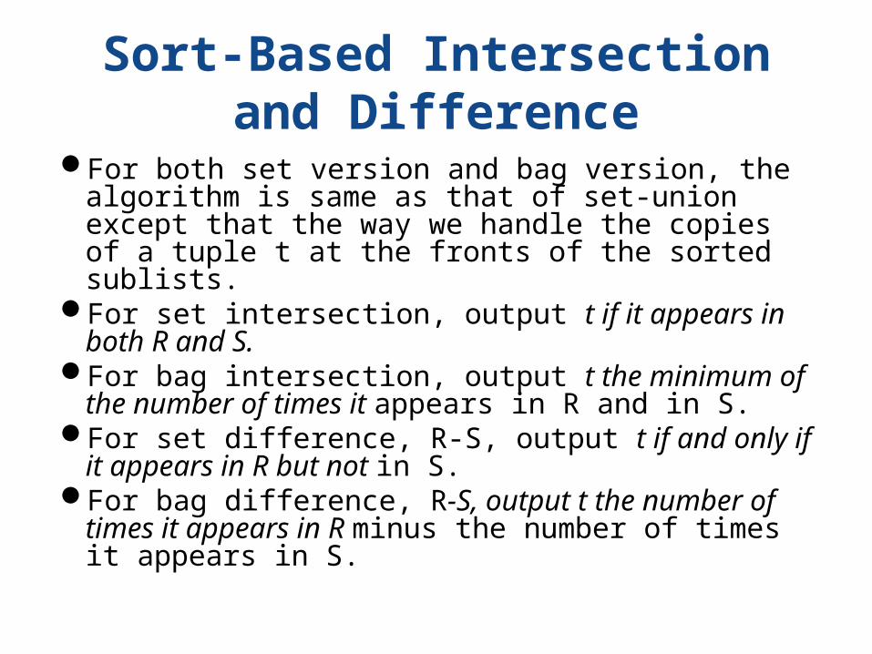
Sort-Based Intersection and Difference
For both set version and bag version, the algorithm is same as that of set-union except that the way we handle the copies of a tuple t at the fronts of the sorted sublists.
For set intersection, output t if it appears in both R and S.For bag intersection, output t the minimum of the number
of times it appears in R and in S.For set difference, R-S, output t if and only if it appears in R
but not in S.For bag difference, R-S, output t the number of times it
appears in R minus the number of times it appears in S.
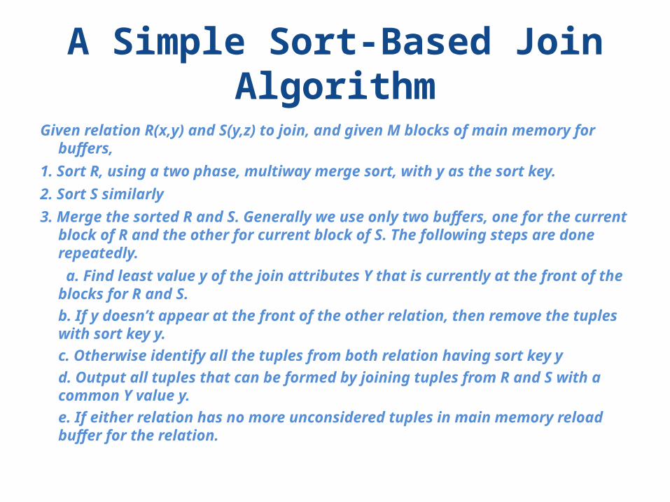
A Simple Sort-Based Join Algorithm
Given relation R(x,y) and S(y,z) to join, and given M blocks of main memory for buffers,1. Sort R, using a two phase, multiway merge sort, with y as the sort key.2. Sort S similarly3. Merge the sorted R and S. Generally we use only two buffers, one for the current
block of R and the other for current block of S. The following steps are done repeatedly. a. Find least value y of the join attributes Y that is currently at the front of the blocks for R and S.
b. If y doesn’t appear at the front of the other relation, then remove the tuples with sort key y. c. Otherwise identify all the tuples from both relation having sort key yd. Output all tuples that can be formed by joining tuples from R and S with a common Y value y.e. If either relation has no more unconsidered tuples in main memory reload buffer for the relation.
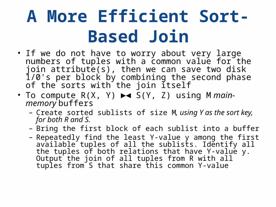
A More Efficient Sort-Based Join• If we do not have to worry about very large numbers of
tuples with a common value for the join attribute(s), then we can save two disk 1/0's per block by combining the second phase of the sorts with the join itself
• To compute R(X, Y) S(Y, Z) using M►◄ main-memory buffers– Create sorted sublists of size M, using Y as the sort key, for both
R and S.– Bring the first block of each sublist into a buffer– Repeatedly find the least Y-value y among the first available
tuples of all the sublists. Identify all the tuples of both relations that have Y-value y. Output the join of all tuples from R with all tuples from S that share this common Y-value
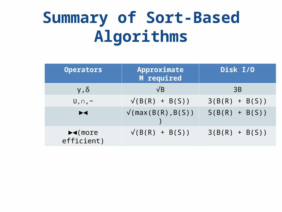
Summary of Sort-Based Algorithms
Operators ApproximateM required
Disk I/O
γ,δ √B 3B
U,∩,− √(B(R) + B(S)) 3(B(R) + B(S))
►◄ √(max(B(R),B(S))) 5(B(R) + B(S))
►◄(more efficient) √(B(R) + B(S)) 3(B(R) + B(S))
BySwathi Vegesna
At a glimpse
• Introduction• Partitioning Relations by Hashing• Algorithm for Duplicate Elimination• Grouping and Aggregation• Union, Intersection, and Difference• Hash-Join Algorithm• Sort based Vs Hash based• Summary
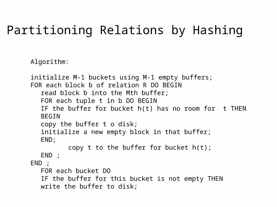
Partitioning Relations by Hashing
Algorithm:
initialize M-1 buckets using M-1 empty buffers;FOR each block b of relation R DO BEGIN
read block b into the Mth buffer;FOR each tuple t in b DO BEGIN
IF the buffer for bucket h(t) has no room for t THENBEGIN
copy the buffer t o disk;initialize a new empty block in that buffer;
END; copy t to the buffer for bucket h(t);END ;
END ;FOR each bucket DO
IF the buffer for this bucket is not empty THENwrite the buffer to disk;
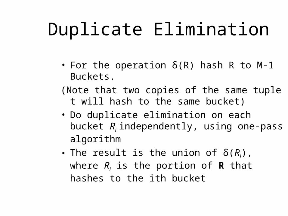
Duplicate Elimination
• For the operation δ(R) hash R to M-1 Buckets.(Note that two copies of the same tuple t will hash
to the same bucket)• Do duplicate elimination on each bucket Ri
independently, using one-pass algorithm• The result is the union of δ(Ri), where Ri is the
portion of R that hashes to the ith bucket
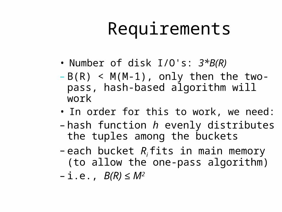
Requirements
• Number of disk I/O's: 3*B(R)– B(R) < M(M-1), only then the two-pass, hash-
based algorithm will work• In order for this to work, we need:– hash function h evenly distributes the tuples
among the buckets– each bucket Ri fits in main memory (to allow
the one-pass algorithm)– i.e., B(R) ≤ M2
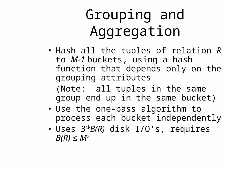
Grouping and Aggregation
• Hash all the tuples of relation R to M-1 buckets, using a hash function that depends only on the grouping attributes(Note: all tuples in the same group end up in the same bucket)
• Use the one-pass algorithm to process each bucket independently
• Uses 3*B(R) disk I/O's, requires B(R) ≤ M2
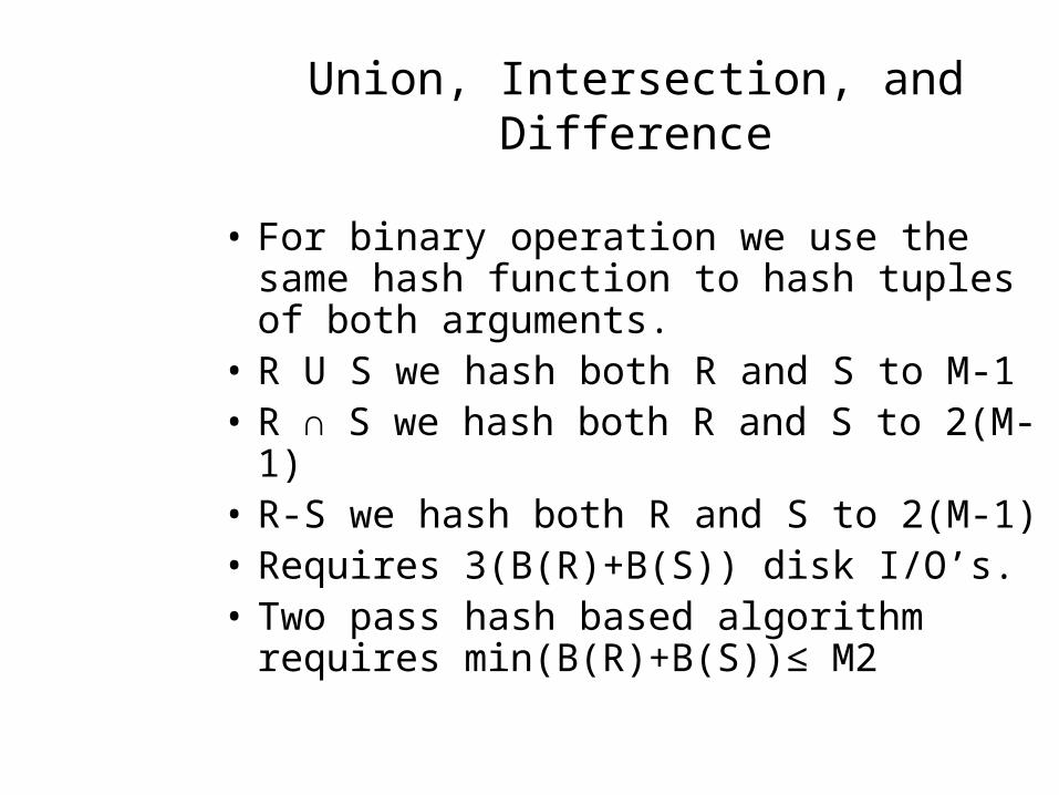
Union, Intersection, and Difference
• For binary operation we use the same hash function to hash tuples of both arguments.
• R U S we hash both R and S to M-1• R ∩ S we hash both R and S to 2(M-1)• R-S we hash both R and S to 2(M-1)• Requires 3(B(R)+B(S)) disk I/O’s.• Two pass hash based algorithm requires
min(B(R)+B(S))≤ M2
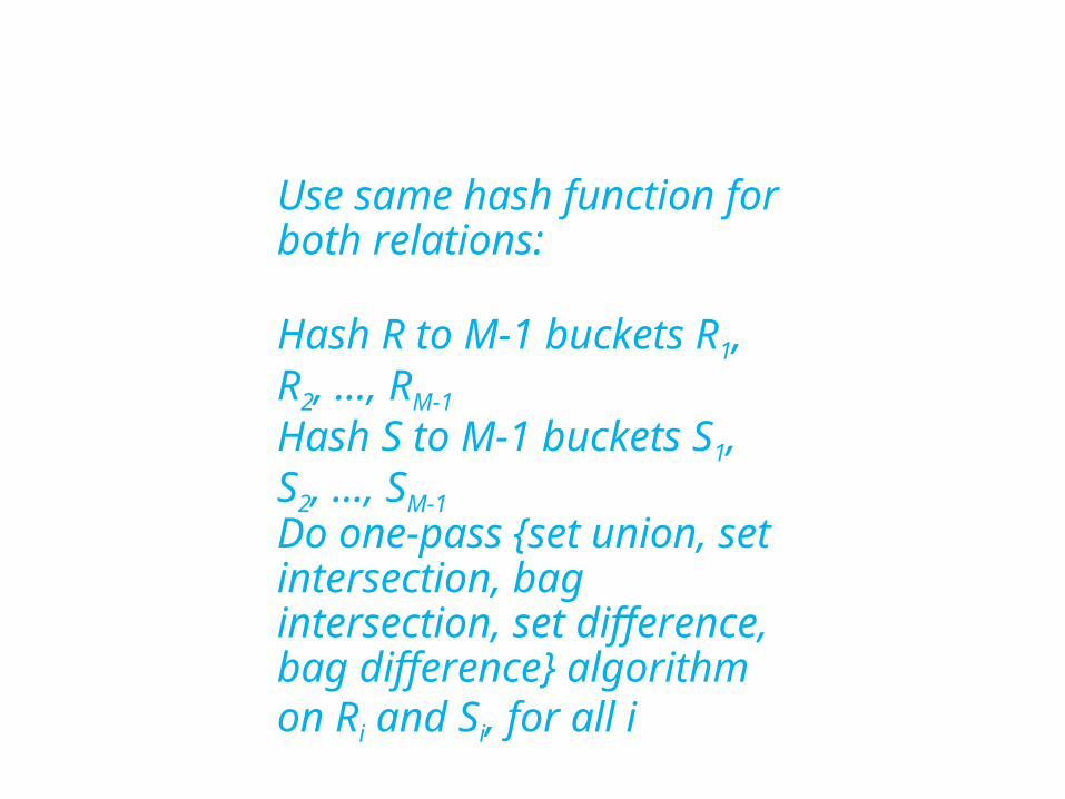
Use same hash function for both relations:
Hash R to M-1 buckets R1, R2, …, RM-1
Hash S to M-1 buckets S1, S2, …, SM-1
Do one-pass {set union, set intersection, bag intersection, set difference, bag difference} algorithm on Ri and Si, for all i
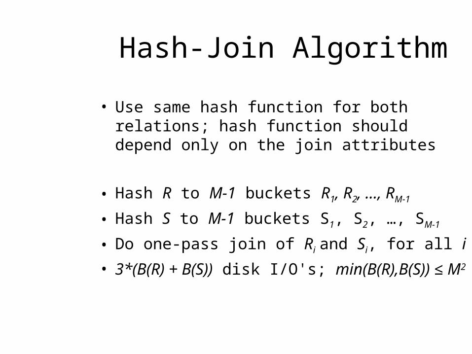
Hash-Join Algorithm
• Use same hash function for both relations; hash function should depend only on the join attributes
• Hash R to M-1 buckets R1, R2, …, RM-1
• Hash S to M-1 buckets S1, S2, …, SM-1
• Do one-pass join of Ri and Si, for all i
• 3*(B(R) + B(S)) disk I/O's; min(B(R),B(S)) ≤ M2
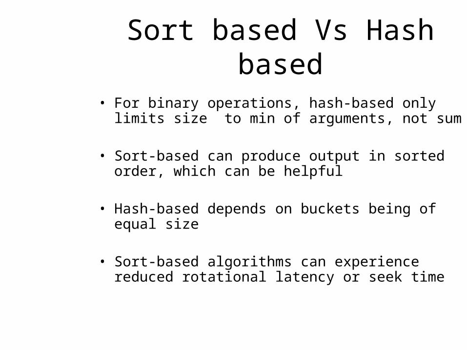
Sort based Vs Hash based
• For binary operations, hash-based only limits size to min of arguments, not sum
• Sort-based can produce output in sorted order, which can be helpful
• Hash-based depends on buckets being of equal size
• Sort-based algorithms can experience reduced rotational latency or seek time
Index-Based Algorithms
Chapter 15Section 15.6
Presented by Fan YangCS 257
Class ID218
158
Clustering and Nonclustering Indexes
A relation is “clustered” if its tuples are packed into roughly as few blocks as can possibly hold those tuples.
Clustering Indexes, which are indexes on an attribute or attributes such that all the tuples with a fixed value for the search key of this index appear on roughly as few blocks as can hold them. Note that a relation that isn't clustered cannot have a clustering index, but even a clustered relation can have nonclustering indexes.
A clustering index has all tuples with a fixed value packed into the minimum possible number of blocks
159
Index-Based Selection
• Selection on equality: a=v(R)
• Clustered index on a: cost B(R)/V(R,a)– If the index on R.a is clustering, then the number of disk
I/O's to retrieve the set a=v (R) will average B(R)/V(R, a). The actual number may be somewhat higher.
• Unclustered index on a: cost T(R)/V(R,a)– If the index on R.a is nonclustering, each tuple we retrieve
will be on a different block, and we must access T(R)/V(R,a) tuples. Thus, T(R)/V(R, a) is an estimate of the number of disk I/O’s we need.
160
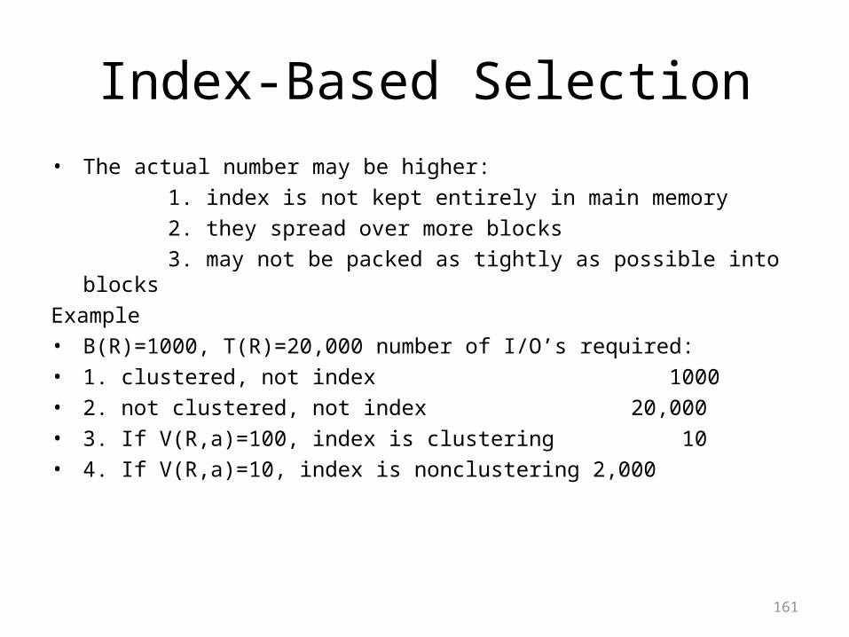
Index-Based Selection• The actual number may be higher:
1. index is not kept entirely in main memory2. they spread over more blocks3. may not be packed as tightly as possible into blocks
Example• B(R)=1000, T(R)=20,000 number of I/O’s required:• 1. clustered, not index 1000• 2. not clustered, not index 20,000• 3. If V(R,a)=100, index is clustering 10• 4. If V(R,a)=10, index is nonclustering 2,000
161
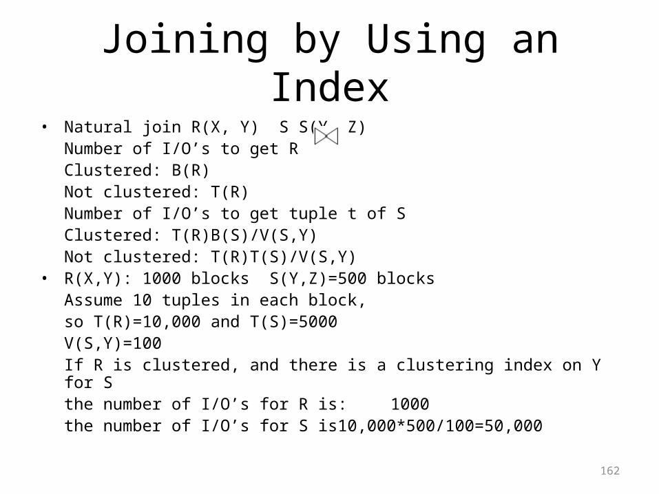
Joining by Using an Index• Natural join R(X, Y) S S(Y, Z)
Number of I/O’s to get RClustered: B(R)Not clustered: T(R)
Number of I/O’s to get tuple t of SClustered: T(R)B(S)/V(S,Y)Not clustered: T(R)T(S)/V(S,Y)
• R(X,Y): 1000 blocks S(Y,Z)=500 blocksAssume 10 tuples in each block, so T(R)=10,000 and T(S)=5000V(S,Y)=100If R is clustered, and there is a clustering index on Y for Sthe number of I/O’s for R is: 1000 the number of I/O’s for S is10,000*500/100=50,000
162
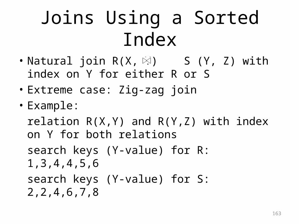
Joins Using a Sorted Index
• Natural join R(X, Y) S (Y, Z) with index on Y for either R or S
• Extreme case: Zig-zag join• Example:
relation R(X,Y) and R(Y,Z) with index on Y for both relationssearch keys (Y-value) for R: 1,3,4,4,5,6search keys (Y-value) for S: 2,2,4,6,7,8
163
Chapter 15.7Buffer Management
ID: 219Name: Qun YuClass: CS257 219 Spring 2009Instructor: Dr. T.Y.Lin
What does a buffer manager do?
Central Task of making memory buffers available to processors is done with the help of buffer managers.
In practice: 1) rarely allocated in advance2) the value of M may vary depending on system
conditions Therefore, buffer manager is used to allow processes
to get the memory they need, while minimizing the delay and unclassifiable requests.
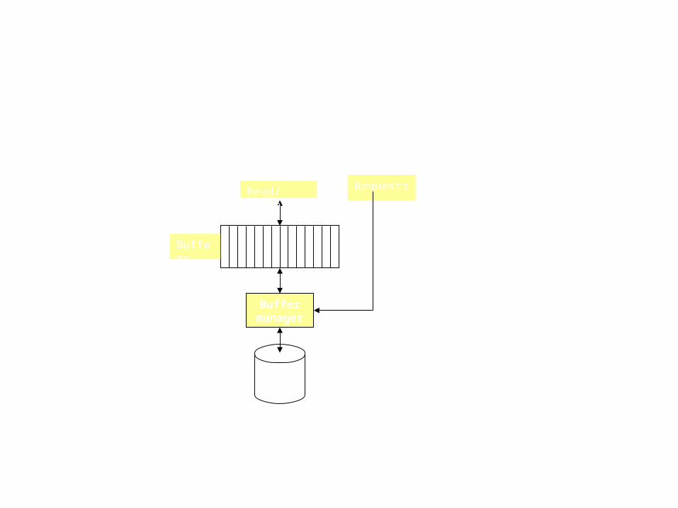
Buffer manager
Buffers
RequestsRead/Writes
Figure 1: The role of the buffer manager : responds to requests for main-memory access to disk blocks
The role of the buffer manager
15.7.1 Buffer Management Architecture
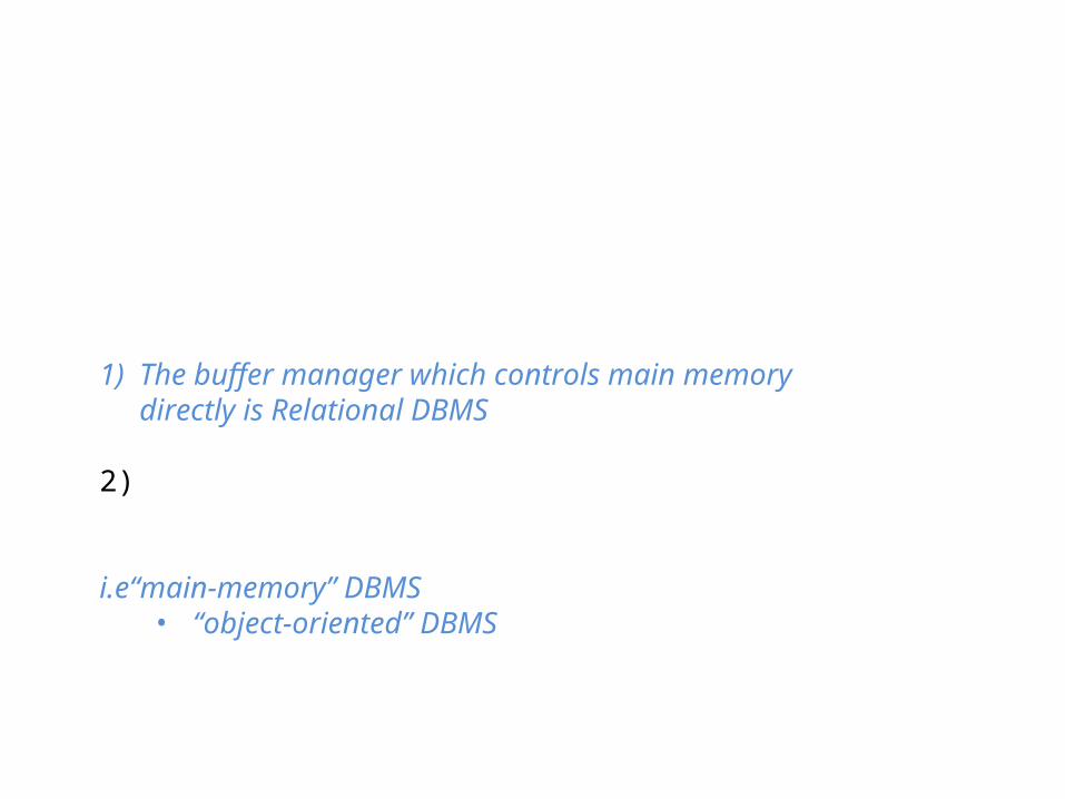
Two broad architectures for a buffer manager:
1) The buffer manager which controls main memory directly is Relational DBMS
2) The buffer manager allocates buffers in virtual memory, allowing the OS to decide how to use buffers.
i.e“main-memory” DBMS • “object-oriented” DBMS
It is the responsibility of the buffer manager to allow processes to get the memory they need, while minimizing the
delay and unsatisfiable requests.
Buffer Pool
Key setting for the Buffer manager to be efficient:Problem:The buffer manager should limit the number of buffers in
use so that they fit in the available main memory, i.e. Don’t exceed available space.
The number of buffers is a parameter set when the DBMS is initialized.
No matter which architecture of buffering is used, we simply assume that there is a fixed-size buffer pool, a set of buffers available to queries and other database actions.
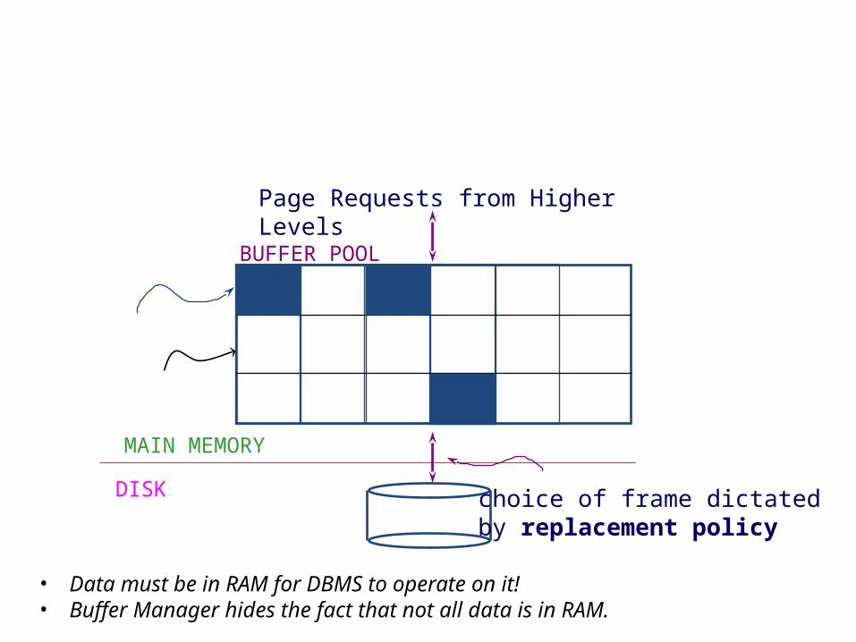
• Data must be in RAM for DBMS to operate on it!• Buffer Manager hides the fact that not all data is in RAM.
DB
MAIN MEMORY
DISK
disk page
free frame
Page Requests from Higher Levels
BUFFER POOL
choice of frame dictatedby replacement policy
Buffer Pool
15.7.2 Buffer Management Strategies
Buffer-replacement strategies:
Critical choice the buffer manager has to make is when a buffer is needed for a newly requested block and the buffer pool is full then which block to throw out the buffer pool.
Buffer-replacement strategies
Critical choice the buffer manager has to make is when a buffer is needed for a newly requested block and the buffer pool is full then which block to throw out the buffer pool.
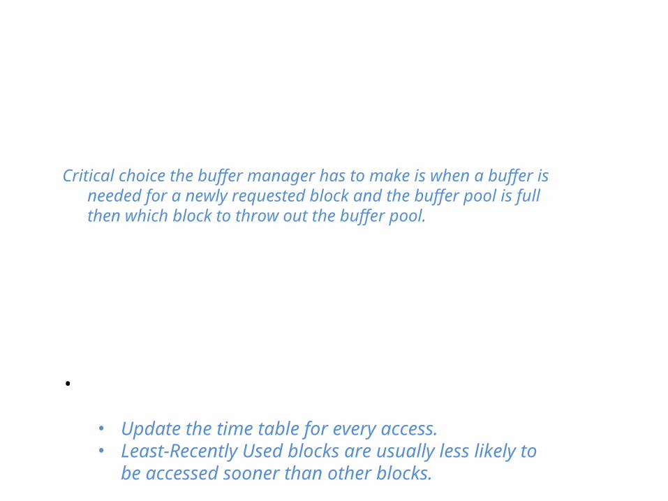
Least-Recently Used (LRU):
To throw out the block that has not been read or written for the longest time.
• Requires more maintenance but it is effective. • Update the time table for every access.• Least-Recently Used blocks are usually less likely to
be accessed sooner than other blocks.
Buffer-replacement strategy -- FIFO
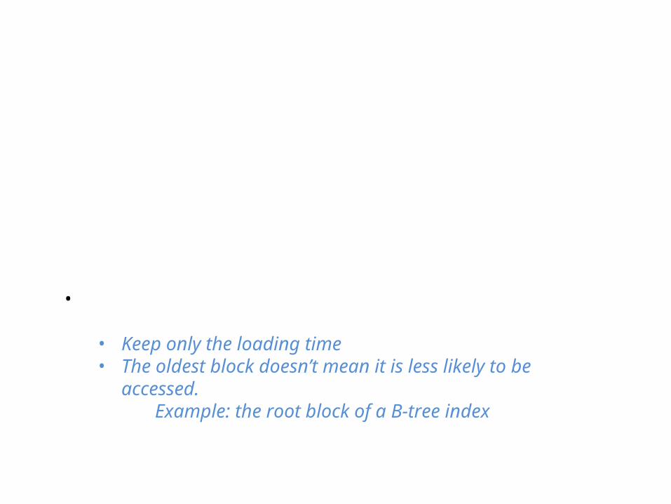
First-In-First-Out (FIFO):
The buffer that has been occupied the longest by the same block is emptied and used for the new block.
• Requires less maintenance but it can make more mistakes.• Keep only the loading time• The oldest block doesn’t mean it is less likely to be
accessed. Example: the root block of a B-tree index

Buffer-replacement strategy – “Clock”
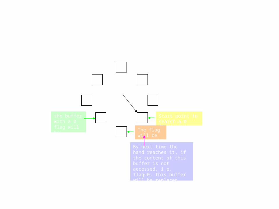
The “Clock” Algorithm (“Second Chance”)
Think of the 8 buffers as arranged in a circle, shown as Figure 3
Flag 0 and 1:
buffers with a 0 flag are ok to sent their contents back to disk, i.e. ok to be replaced
buffers with a 1 flag are not ok to be replaced
Buffer-replacement strategy – “Clock”
0
0
1
1
1
0
0
0
Start point to search a 0 flag
the buffer with a 0 flag will be replaced
The flag will be set to 0
By next time the hand reaches it, if the content of this buffer is not accessed, i.e. flag=0, this buffer will be replaced.That’s “Second Chance”.
Figure 3: the clock algorithm

Buffer-replacement strategy -- Clock
a buffer’s flag set to 1 when:
a block is read into a buffer
the contents of the buffer is accessed
a buffer’s flag set to 0 when:
the buffer manager needs a buffer for a new block, it looks for the first 0 it can find, rotating clockwise. If it passes 1’s, it sets them to 0.

System Control helps Buffer-replacement strategy
System Control
The query processor or other components of a DBMS can give advice to the buffer manager in order to avoid some of the mistakes that would occur with a strict policy such as LRU,FIFO or Clock.
For example:
A “pinned” block means it can’t be moved to disk without first modifying certain other blocks that point to it.
In FIFO, use “pinned” to force root of a B-tree to remain in memory at all times.

15.7.3 The Relationship Between Physical Operator Selection and Buffer Management
Problem:
Physical Operator expected certain number of buffers M for execution.
However, the buffer manager may not be able to guarantee these M buffers are available.
Example
FOR each chunk of M-1 blocks of S DO BEGIN
read these blocks into main-memory buffers;
organize their tuples into a search structure whose
search key is the common attributes of R and S;
FOR each block b of R DO BEGIN
read b into main memory;
FOR each tuple t of b DO BEGIN
find the tuples of S in main memory that
join with t ;
output the join of t with each of these tuples;
END ;
END ;
END ;
Figure 15.8: The nested-loop join algorithm

Example
The outer loop number (M-1) depends on the average number of buffers are available at each iteration.
The outer loop use M-1 buffers and 1 is reserved for a block of R, the relation of the inner loop.
If we pin the M-1 blocks we use for S on one iteration of the outer loop, we shall not lose their buffers during the round.
Also, more buffers may become available and then we could keep more than one block of R in memory.
Will these extra buffers improve the running time?

Example
CASE1: NO
Buffer-replacement strategy: LRUBuffers for R: kWe read each block of R in order into buffers.By end of the iteration of the outer loop, the last k blocks of R are in buffers.However, next iteration will start from the beginning of R again. Therefore, the k buffers for R will need to be replaced.

Example
CASE 2: YES
Buffer-replacement strategy: LRUBuffers for R: kWe read the blocks of R in an order that alternates: firstlast and then lastfirst.In this way, we save k disk I/Os on each iteration of the outer loop except the first iteration.
Other Algorithms and M buffers
Other Algorithms also are impact by M and the buffer-replacement strategy. Sort-based algorithm
If we use a sort-based algorithm for some operator, then it is possible to adapt to changes in M. If Af shrinks, we can change the size of a sublist,since the sort-based algorithms we discussed do not depend on the sublists being the same size. The major limitation is that as M shrinks, we could be forced to create so many sublists that we cannot thenallocate a buffer for each sublist in the merging process..
Hash-based algorithm If M shrinks, we can reduce the number of
buckets, as long as the buckets still can fit in M buffers.

• Hash Table
• If the algorithm is hash-based, ive can reduce the number of buckets if• shrinks, as long as the buckets do not then become so large that they do• not fit in allotted main memory. However, unlike sort-based algorithms,• we cannot respond to changes in A1 while the algorithm runs. Rather,• once the number of buckets is chosen, it remains fixed throughout the first• pass, and if buffers become unavailable, the blocks belonging to some of• the buckets.
Intro• Algorithms using more than two passes.• Multi-pass Sort-based Algorithms• Performance of Multipass, Sort-Based
Algorithms
• Multipass Hash-Based Algorithms
• Conclusion
Reason that we use more than two passes:
Two passes are usually enough, however, for the largest relation, we use as many passes as necessary.
Multi-pass Sort-based AlgorithmsSuppose we have M main-memory buffers available to sort a relation R, which we assume is stored clustered.
Then we do the following:
BASIS: BASIS:
If R fits in M blocks (i.e., B(R)<=M) If R fits in M blocks (i.e., B(R)<=M)
1.1. Read R into main memory.Read R into main memory.
2.2. Sort it using any main-memory Sort it using any main-memory sorting algorithm.sorting algorithm.
3.3. Write the sorted relation to diskWrite the sorted relation to disk..INDUCTION:
If R does not fit into main memory.1. Partition the blocks holding R into M groups, which we shall call R1, R2, R3…2. Recursively sort Ri for each i=1,2,3…M.3. Merge the M sorted sublists.
If we are not merely sorting R, but performing a unary operation such as δ or γ on R. We can modify the above so that at the final merge we perform the operation on the tuples at the front of the sorted sublists.That is:
• For a δ, output one copy of each distinct tuple, and skip over copies of the tuple.
• For a γ, sort on the grouping attributes only, and combine the tuples with a given value of these grouping attributes.
ConclusionThe two pass algorithms based on sorting or hashing have natural recursive analogs that take three or more passes and will work for larger amounts of data.
• BASIS: If k = 1, i.e., one pass is allowed, then we must have B(R) < M. Put• another way, s(M, 1) = Af.• INDUCTION: Suppose k > 1. Then we partition R into 1M pieces, each of• which must be sortable in k - 1 passes. If B(R) = s(M, k), then s(M, k)/:l17• which is the size of each of the M pieces of R, cannot exceed s(M, k - 1).
That• is: s(M, k) = Ms(M, k - 1)
Performance of Multipass, Sort-Based Algorithms
Multipass Hash-Based Algorithms
• BASIS: For a unary operation, if the relation fits in hl buffers, read it into memory and perfor111 the operation.
• For a binary operation, if either relation fits in ,11 - I buffers, perform the operation by reading this relation into main
memory and then read the second relation, one block at a time, into the Mth buffer.
• INDUCTION: If no relation fits in main memory, then hash each relation into A 1 -1 buckets, as discussed in Section 15.5.1. Recursively perform the operation on each bucket or corresponding pair of buckets, and accumulate the output
• from each bucket or pair.
The Query Compiler
16.1 Parsing and Preprocessing
Meghna Jain(205)Dr. T. Y. Lin
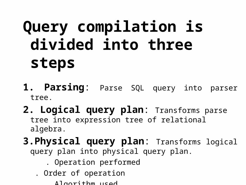
Query compilation is divided into three steps
1. Parsing: Parse SQL query into parser tree.
2. Logical query plan: Transforms parse tree into expression tree of relational algebra.
3.Physical query plan: Transforms logical query plan into physical query plan.
. Operation performed
. Order of operation
. Algorithm used
. The way in which stored data is obtained and passed from one
operation to another.
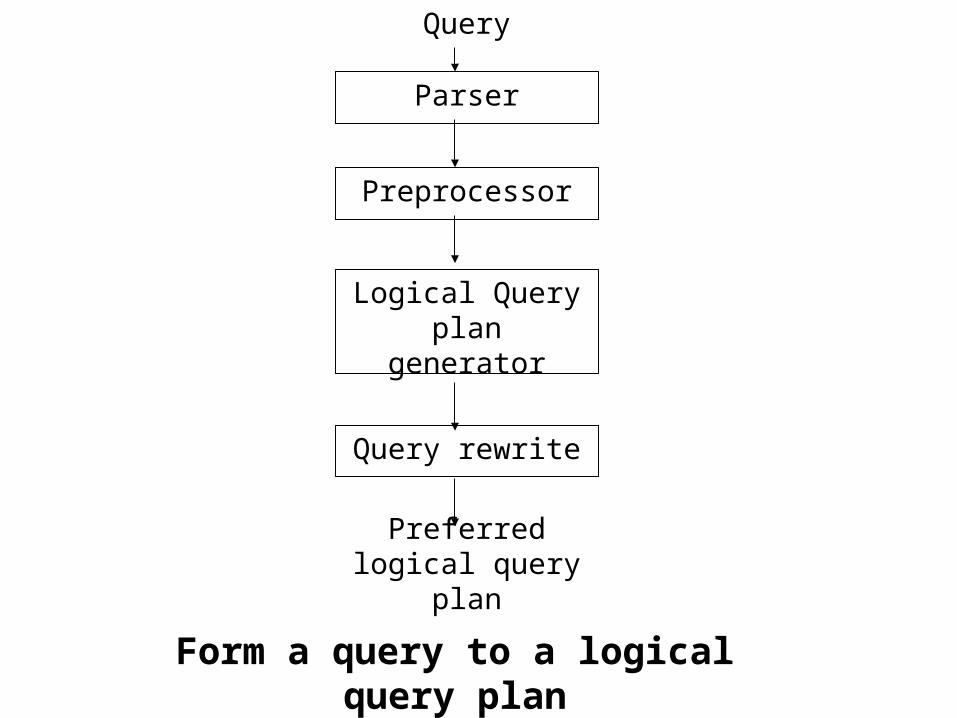
Parser
Preprocessor
Logical Query plan generator
Query rewrite
Preferred logical query plan
Query
Form a query to a logical query plan
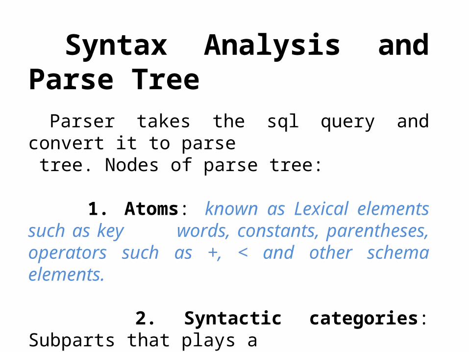
Syntax Analysis and Parse Tree Parser takes the sql query and convert it to parse tree. Nodes of parse tree:
1. Atoms: known as Lexical elements such as key words, constants, parentheses, operators such as +, < and other schema elements.
2. Syntactic categories: Subparts that plays a similar role in a query as <Query> , <Condition>
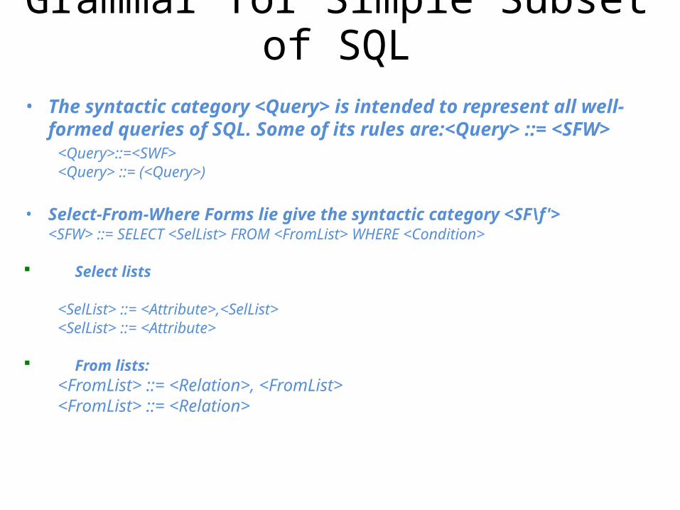
Grammar for Simple Subset of SQL
• The syntactic category <Query> is intended to represent all well-formed queries of SQL. Some of its rules are:<Query> ::= <SFW>
<Query>::=<SWF><Query> ::= (<Query>)
• Select-From-Where Forms lie give the syntactic category <SF\f'><SFW> ::= SELECT <SelList> FROM <FromList> WHERE <Condition>
Select lists
<SelList> ::= <Attribute>,<SelList><SelList> ::= <Attribute>
From lists:<FromList> ::= <Relation>, <FromList><FromList> ::= <Relation>
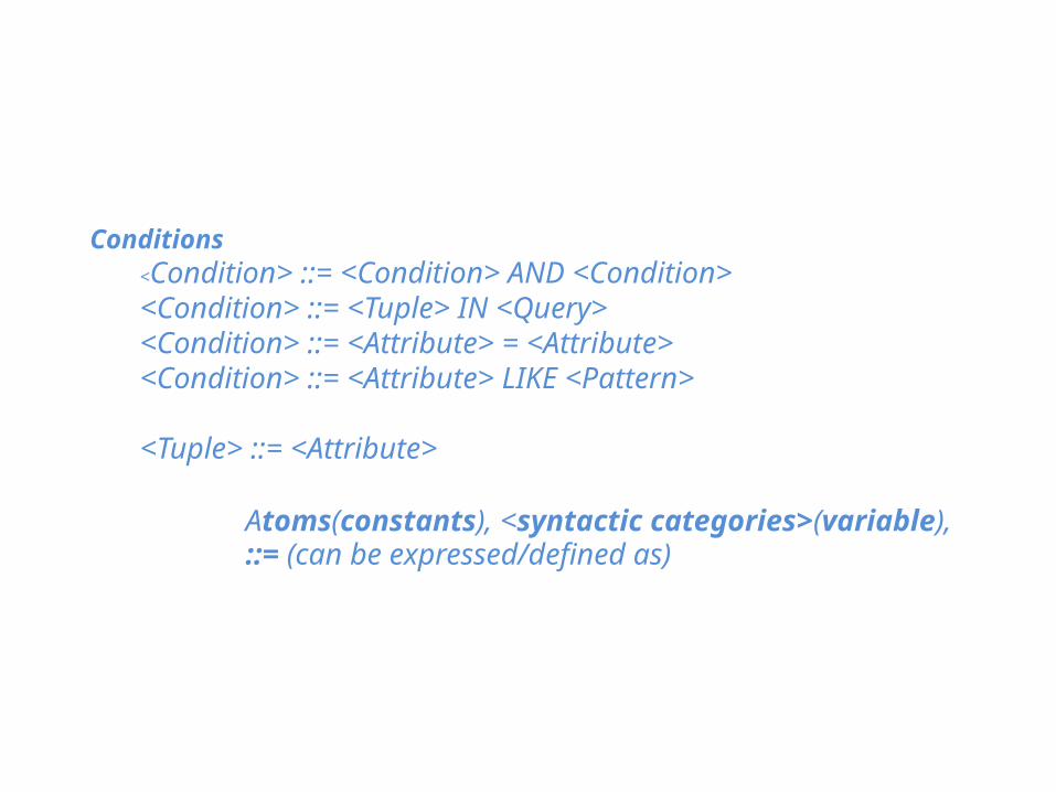
Conditions<Condition> ::= <Condition> AND <Condition><Condition> ::= <Tuple> IN <Query><Condition> ::= <Attribute> = <Attribute><Condition> ::= <Attribute> LIKE <Pattern>
<Tuple> ::= <Attribute>
Atoms(constants), <syntactic categories>(variable),::= (can be expressed/defined as)
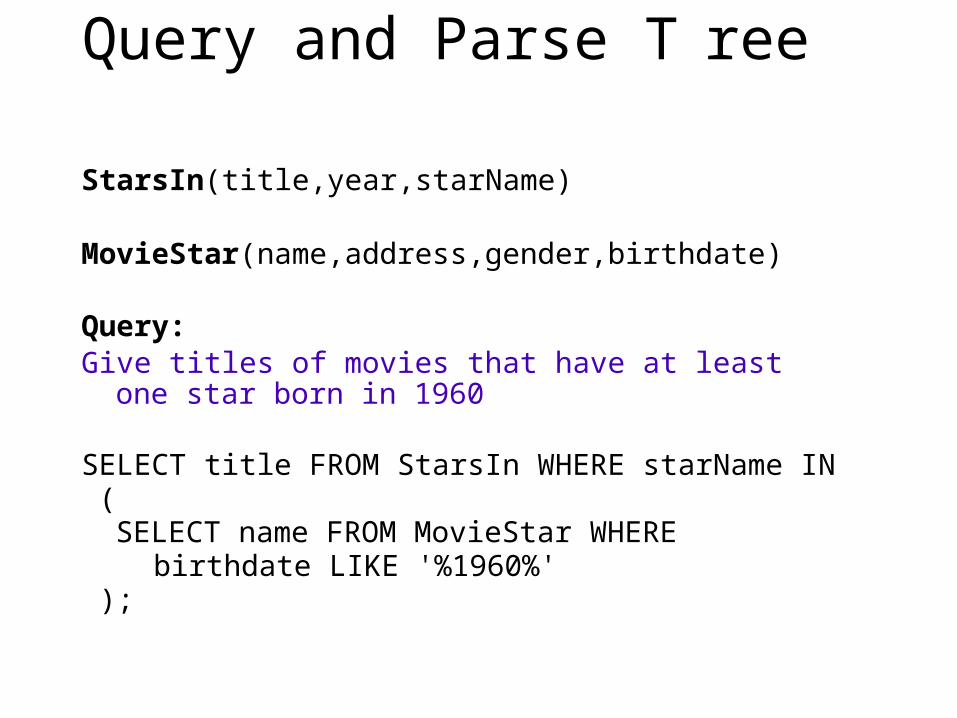
Query and Parse T ree
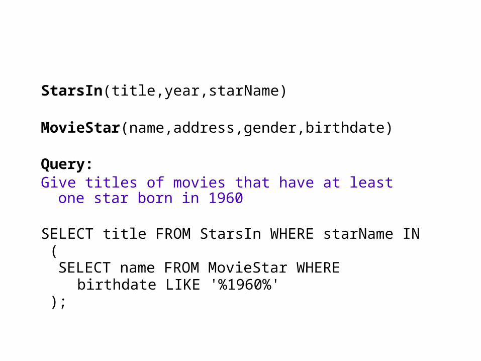
StarsIn(title,year,starName)
MovieStar(name,address,gender,birthdate)
Query: Give titles of movies that have at least one star born in 1960
SELECT title FROM StarsIn WHERE starName IN (
SELECT name FROM MovieStar WHERE birthdate LIKE '%1960%'
);
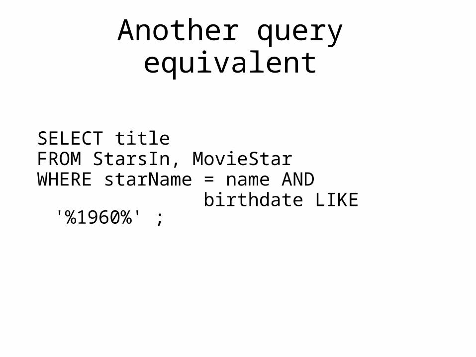
Another query equivalent
SELECT title FROM StarsIn, MovieStarWHERE starName = name AND birthdate LIKE '%1960%' ;
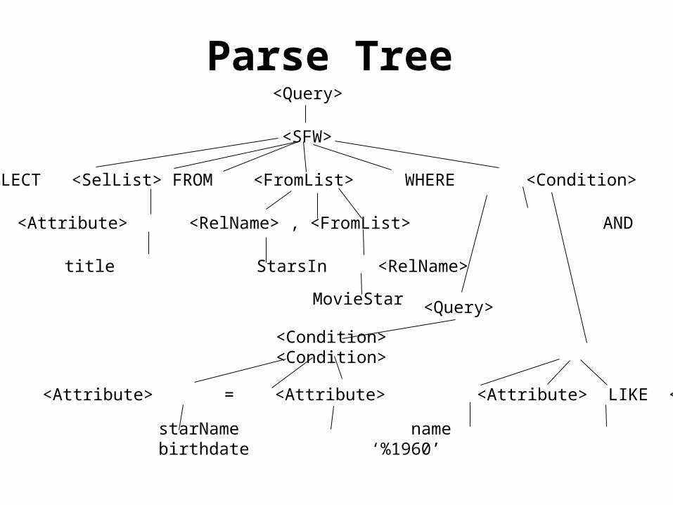
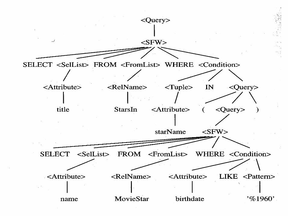
Parse Tree<Query>
<SFW>
SELECT <SelList> FROM <FromList> WHERE <Condition>
<Attribute> <RelName> , <FromList> AND
title StarsIn <RelName>
<Condition> <Condition>
<Attribute> = <Attribute> <Attribute> LIKE <Pattern>
starName name birthdate ‘%1960’
MovieStar <Query>
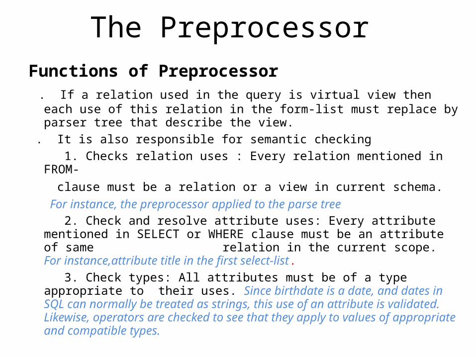
The Preprocessor
Functions of Preprocessor . If a relation used in the query is virtual view then each use of this relation in
the form-list must replace by parser tree that describe the view. . It is also responsible for semantic checking 1. Checks relation uses : Every relation mentioned in FROM-
clause must be a relation or a view in current schema.For instance, the preprocessor applied to the parse tree
2. Check and resolve attribute uses: Every attribute mentioned in SELECT or WHERE clause must be an attribute of same relation in the current scope. For instance,attribute title in the first select-list.
3. Check types: All attributes must be of a type appropriate to their uses. Since birthdate is a date, and dates in SQL can normally be treated as strings, this use of an attribute is validated. Likewise, operators are checked to see that they apply to values of appropriate and compatible types.
StarsIn(title,year,starName)
MovieStar(name,address,gender,birthdate)
Query: Give titles of movies that have at least one star born in 1960
SELECT title FROM StarsIn WHERE starName IN (
SELECT name FROM MovieStar WHERE birthdate LIKE '%1960%'
);
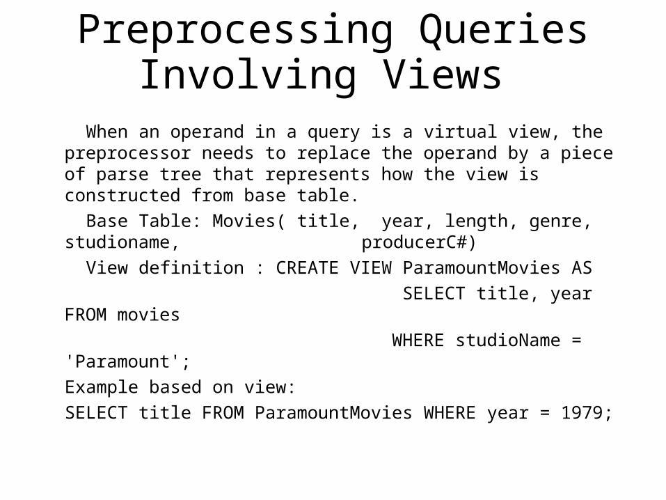
Preprocessing Queries Involving Views
When an operand in a query is a virtual view, the preprocessor needs to replace the operand by a piece of parse tree that represents how the view is constructed from base table.
Base Table: Movies( title, year, length, genre, studioname, producerC#)
View definition : CREATE VIEW ParamountMovies AS SELECT title, year FROM movies WHERE studioName = 'Paramount'; Example based on view: SELECT title FROM ParamountMovies WHERE year = 1979;
16.2 ALGEBRAIC LAWS FOR IMPROVING QUERY PLANS
Ramya KarriID: 206
Optimizing the Logical Query Plan
• Relational algebra laws can be applied to optimize logical tree.• This process of optimizing a logical query tree using relational
algebra laws is called heuristic optimization• The result of applying these algebraic transformations is the
logical query plan that is the output of the query-relvrite phase. The logical query plan is then converted to a physical query plan as the optimizer makes a series of decisions about implementation of operators.
Relational Algebra Laws
These laws involve the following properties:
– Commutativity - operator can be applied to operands independent of order.
• Precisely, x + y = y + x and x * y = y * x fornumbers 1: and y. - is not a commutative arithmeticoperator: x-y not= y-x.
• E.g. A + B = B + A • The “+” operator is commutative.
– Associativity - operator is independent of operand grouping.
• E.g. A + (B + C) = (A + B) + C • The “+” operator is associative.
Associative and Commutative Operators
• The relational algebra operators of cross-product (×), join (⋈), union, and intersection are all associative and commutative.
Commutative
R X S = S X R
R ⋈ S = S ⋈ R
R S = S R
R ∩ S = S ∩ R
Associative
(R X S) X T = S X (R X T)
(R ⋈ S) ⋈ T= S ⋈ (R ⋈ T)
(R S) T = S (R T)
(R ∩ S) ∩ T = S ∩ (R ∩ T)
Laws Involving Selection
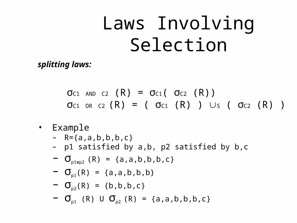
splitting laws:
σC1 AND C2 (R) = σC1( σC2 (R))σC1 OR C2 (R) = ( σC1 (R) ) S ( σC2 (R) )
• Example– R={a,a,b,b,b,c}– p1 satisfied by a,b, p2 satisfied by b,c– σp1vp2 (R) = {a,a,b,b,b,c}
– σp1(R) = {a,a,b,b,b}
– σp2(R) = {b,b,b,c}
– σp1 (R) U σp2 (R) = {a,a,b,b,b,c}
Laws Involving Selection (Contd..)
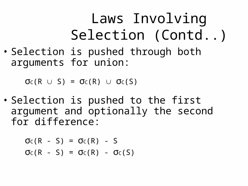
• Selection is pushed through both arguments for union:
σC(R S) = σC(R) σC(S)
• Selection is pushed to the first argument and optionally the second for difference:
σC(R - S) = σC(R) - S
σC(R - S) = σC(R) - σC(S)
Laws Involving Selection (Contd..)
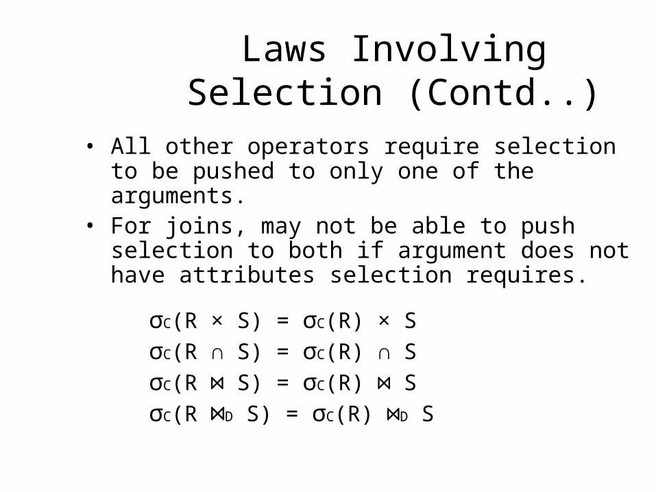
• All other operators require selection to be pushed to only one of the arguments.
• For joins, may not be able to push selection to both if argument does not have attributes selection requires.
σC(R × S) = σC(R) × SσC(R ∩ S) = σC(R) ∩ SσC(R ⋈ S) = σC(R) ⋈ SσC(R ⋈D S) = σC(R) ⋈D S
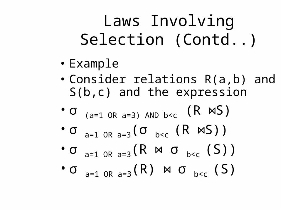
Laws Involving Selection (Contd..)
• Example • Consider relations R(a,b) and S(b,c) and
the expression• σ (a=1 OR a=3) AND b<c (R ⋈S)• σ a=1 OR a=3(σ b<c (R ⋈S))• σ a=1 OR a=3(R ⋈ σ b<c (S))• σ a=1 OR a=3(R) ⋈ σ b<c (S)
Laws Involving Projection
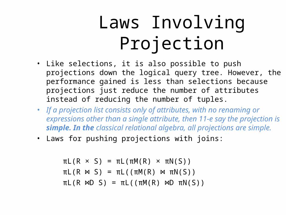
• Like selections, it is also possible to push projections down the logical query tree. However, the performance gained is less than selections because projections just reduce the number of attributes instead of reducing the number of tuples.
• If a projection list consists only of attributes, with no renaming or expressions other than a single attribute, then 11-e say the projection is simple. In the classical relational algebra, all projections are simple.
• Laws for pushing projections with joins:
πL(R × S) = πL(πM(R) × πN(S))πL(R ⋈ S) = πL((πM(R) ⋈ πN(S))πL(R ⋈D S) = πL((πM(R) ⋈D πN(S))
Laws Involving Projection
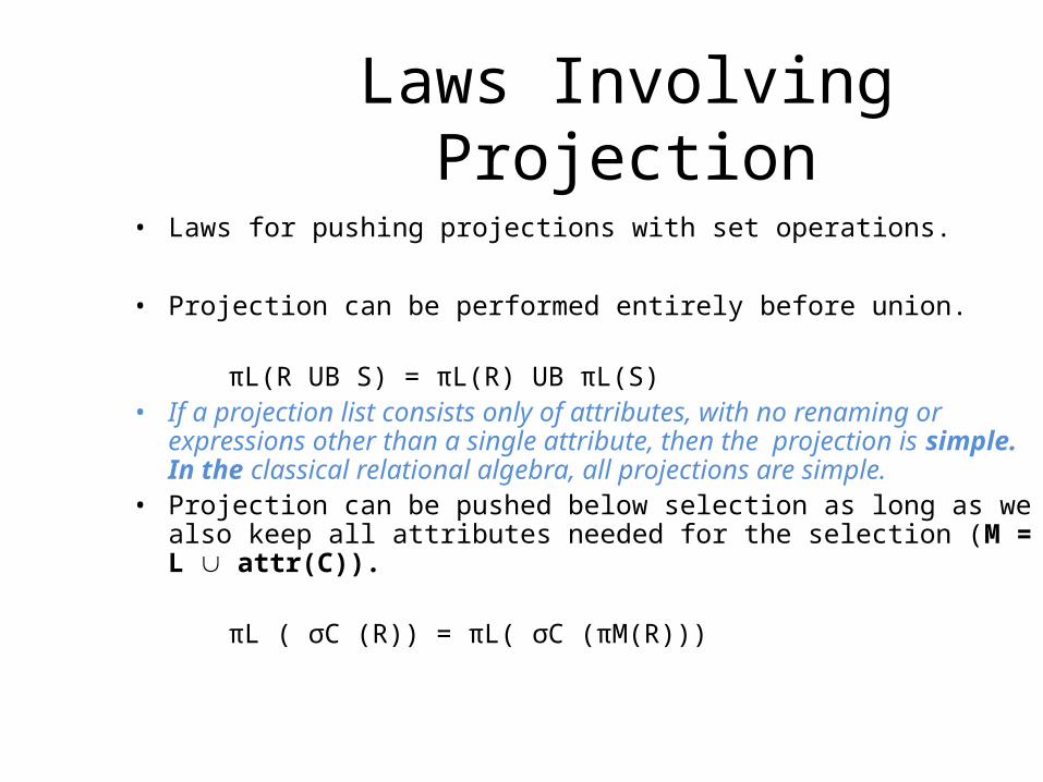
• Laws for pushing projections with set operations.
• Projection can be performed entirely before union.
πL(R UB S) = πL(R) UB πL(S)• If a projection list consists only of attributes, with no renaming or
expressions other than a single attribute, then the projection is simple. In the classical relational algebra, all projections are simple.
• Projection can be pushed below selection as long as we also keep all attributes needed for the selection (M = L attr(C)).
πL ( σC (R)) = πL( σC (πM(R)))
Laws Involving Join
• We have previously seen these important rules about joins:
1. Joins are commutative and associative.
2. Selection can be distributed into joins.
3. Projection can be distributed into joins.
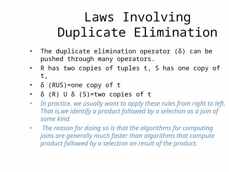
Laws Involving Duplicate Elimination
• The duplicate elimination operator (δ) can be pushed through many operators.
• R has two copies of tuples t, S has one copy of t,• δ (RUS)=one copy of t• δ (R) U δ (S)=two copies of t• In practice. we usually want to apply these rules from right to left. That
is,we identify a product followed by a selection as a join of some kind.• The reason for doing so is that the algorithms for computing joins are
generally much faster than algorithms that compute product followed by a selection on result of the product.
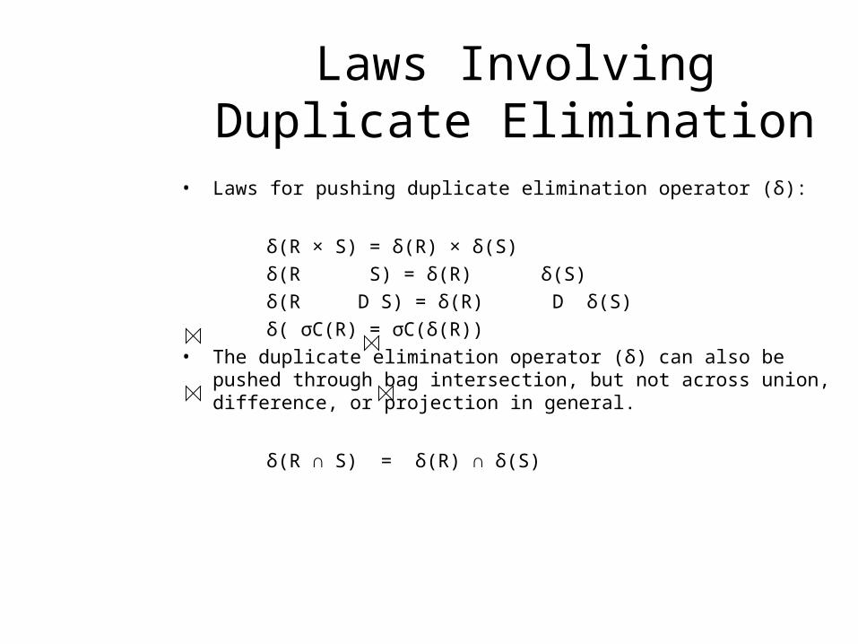
Laws Involving Duplicate Elimination
• Laws for pushing duplicate elimination operator (δ):
δ(R × S) = δ(R) × δ(S)δ(R S) = δ(R) δ(S)δ(R D S) = δ(R) D δ(S)δ( σC(R) = σC(δ(R))
• The duplicate elimination operator (δ) can also be pushed through bag intersection, but not across union, difference, or projection in general.
δ(R ∩ S) = δ(R) ∩ δ(S)
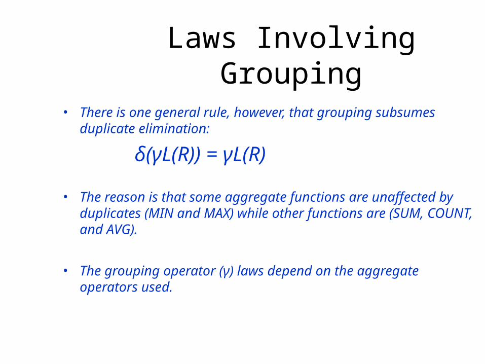
Laws Involving Grouping
• There is one general rule, however, that grouping subsumes duplicate elimination:
δ(γL(R)) = γL(R)
• The reason is that some aggregate functions are unaffected by duplicates (MIN and MAX) while other functions are (SUM, COUNT, and AVG).
• The grouping operator (γ) laws depend on the aggregate operators used.
The Query CompilerSection 16.3
DATABASE SYSTEMS – The Complete Book
Presented By: Under the supervision of:
Deepti Kundu Dr. T.Y.Lin
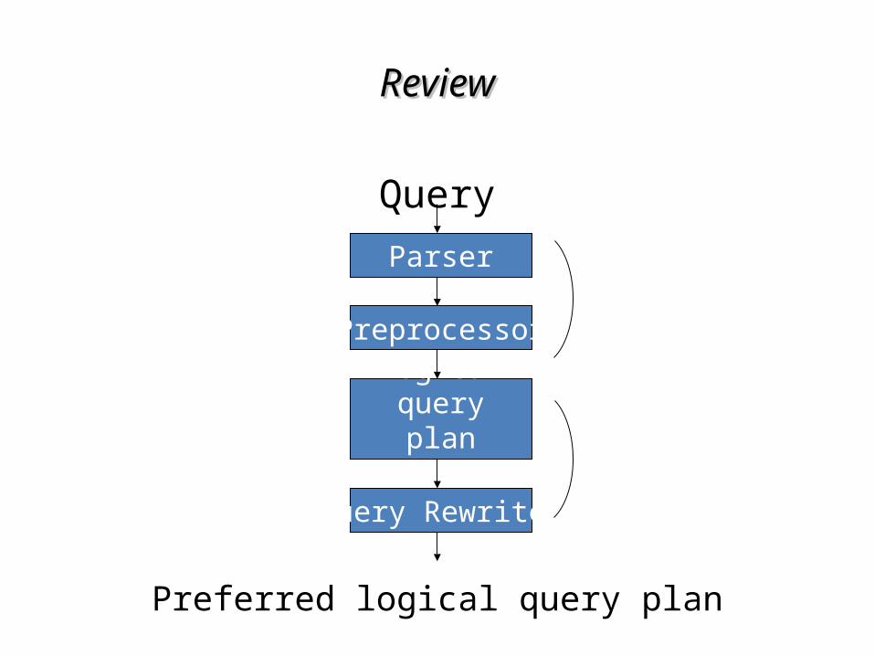
ReviewReview
Query
Preferred logical query plan
Parser
Preprocessor
Logical query plan generator
Query Rewriter
Section 16.1
Section 16.3
Two steps to turn Parse tree into Preferred Two steps to turn Parse tree into Preferred Logical Query PlanLogical Query Plan
• Replace the nodes and structures of the parse tree, in appropriate groups, by an operator or operators of relational algebra.
• Take the relational algebra expression and turn it into an expression that we expect can be converted to the most efficient physical query plan.
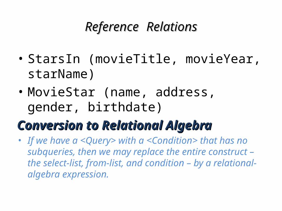
ReferenceReference RelationsRelations
• StarsIn (movieTitle, movieYear, starName)
• MovieStar (name, address, gender, birthdate)
Conversion to Relational AlgebraConversion to Relational Algebra• If we have a <Query> with a <Condition> that has no
subqueries, then we may replace the entire construct – the select-list, from-list, and condition – by a relational-algebra expression.
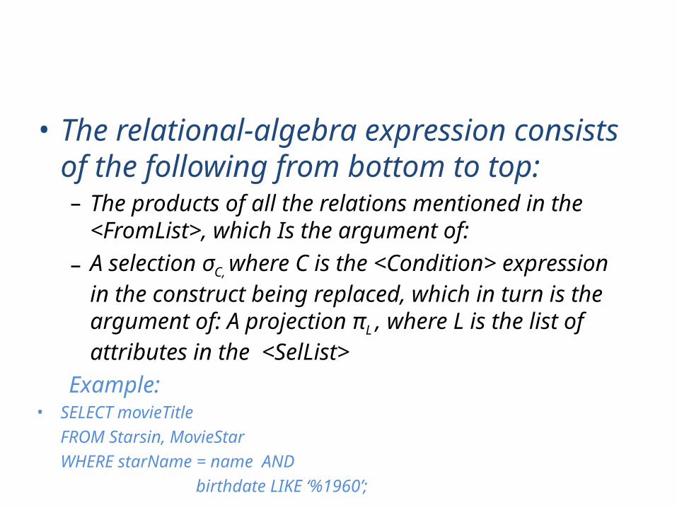
• The relational-algebra expression consists of the following from bottom to top:– The products of all the relations mentioned in the
<FromList>, which Is the argument of:
– A selection σC, where C is the <Condition> expression in the construct being replaced, which in turn is the argument of: A projection πL , where L is the list of attributes in the <SelList>
Example:• SELECT movieTitle
FROM Starsin, MovieStar
WHERE starName = name AND
birthdate LIKE ‘%1960’;
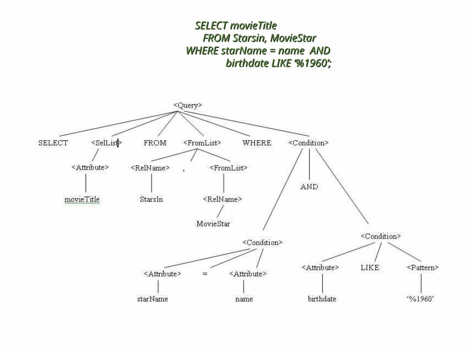
SELECT movieTitleSELECT movieTitleFROM Starsin, MovieStarFROM Starsin, MovieStar
WHERE starName = name AND WHERE starName = name AND birthdate LIKE ‘%1960’; birthdate LIKE ‘%1960’;
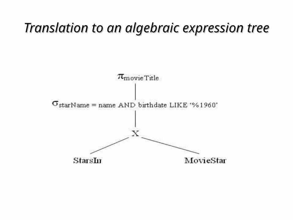
Translation to an algebraic expression treeTranslation to an algebraic expression tree
Removing Subqueries From ConditionsRemoving Subqueries From Conditions
• For parse trees with a <Condition> that has a subquery
• Intermediate operator – two argument selection
• It is intermediate in between the syntactic categories of the parse tree and the relational-algebra operators that apply to relations.
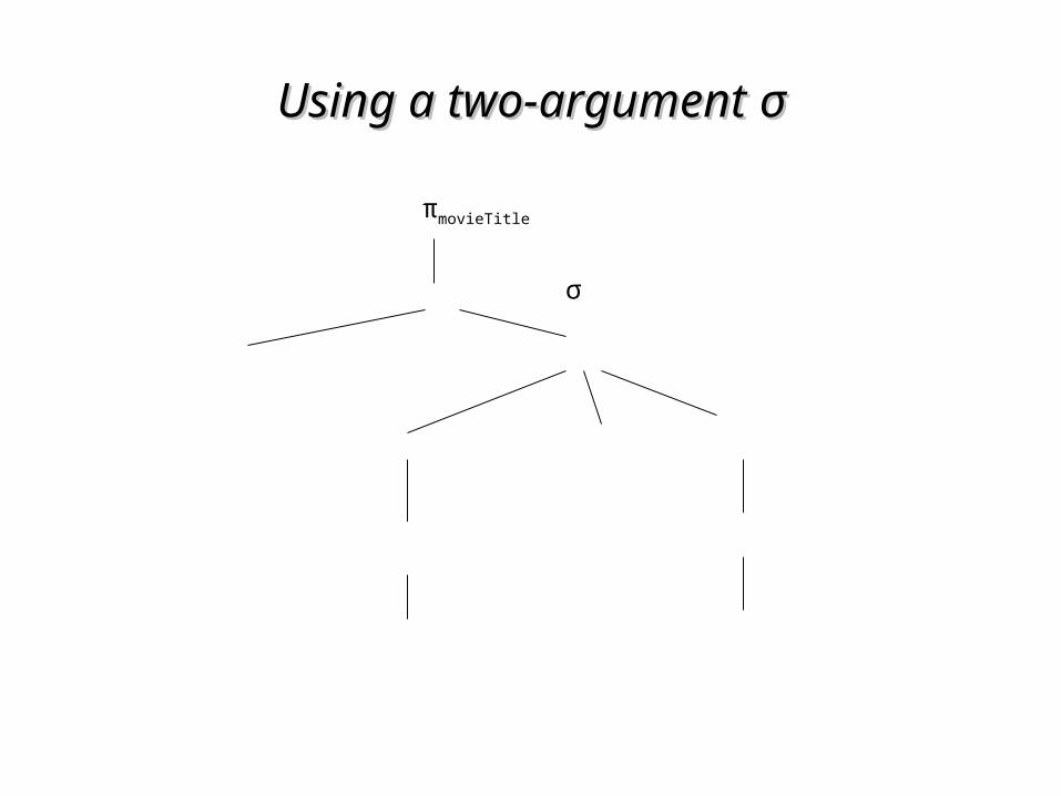
Using a two-argument Using a two-argument σσ
πmovieTitle
σ
StarsIn <Condition>
MovieStar
IN πname<Tuple>
starName
σ birthdate LIKE ‘%1960'
<Attribute>
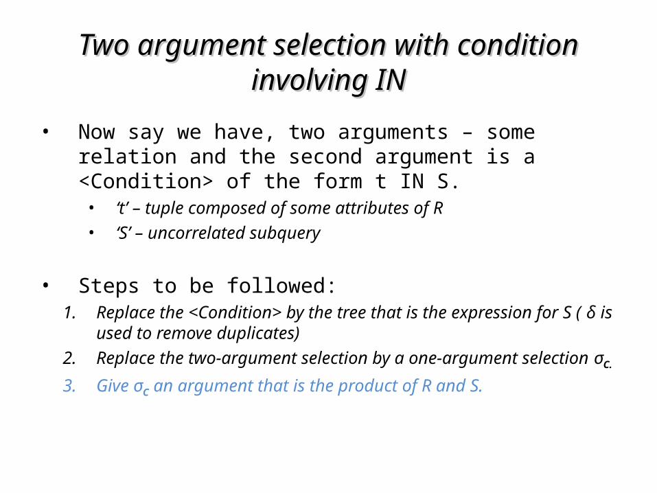
Two argument selection with condition involving Two argument selection with condition involving ININ
• Now say we have, two arguments – some relation and the second argument is a <Condition> of the form t IN S.• ‘t’ – tuple composed of some attributes of R
• ‘S’ – uncorrelated subquery
• Steps to be followed:1. Replace the <Condition> by the tree that is the expression for S ( δ is
used to remove duplicates)
2. Replace the two-argument selection by a one-argument selection σC.
3. Give σC an argument that is the product of R and S.
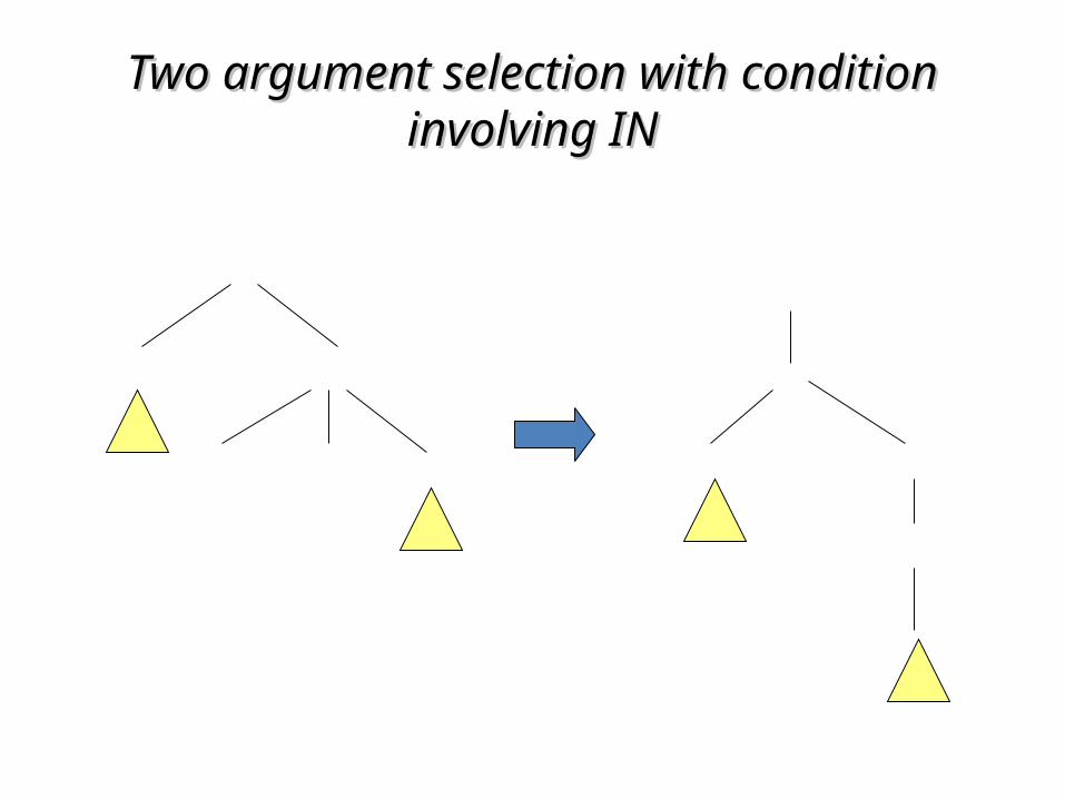
Two argument selection with condition involving Two argument selection with condition involving ININ
σ
R <Condition>
t IN S
σC
X
R δ
S
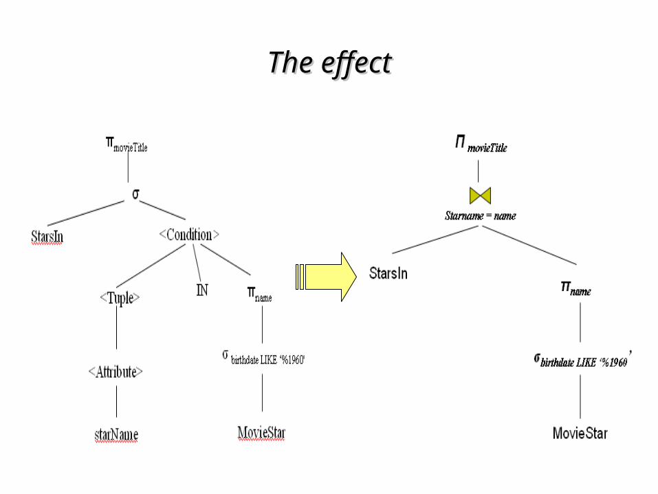
The effectThe effect
Improving the Logical Query PlanImproving the Logical Query Plan
• Algebraic laws to improve logical query plans:– Selections can be pushed down the expression tree
as far as they can go.
– Similarly, projections can be pushed down the tree, or new projections can be added.
– Duplicate eliminations can sometimes be removed, or moved to a more convenient position in the tree.
– Certain selections can be combined with a product below to turn the pair of operations into an equijoin.
Grouping Associative/ Commutative OperatorsGrouping Associative/ Commutative Operators
• An operator that is associative and commutative operators may be though of as having any number of operands.
• We need to reorder these operands so that the multiway join is executed as sequence of binary joins.
• Its more time consuming to execute them in the order suggested by parse tree.
• For each portion of subtree that consists of nodes with the same associative and commutative operator (natural join, union, and intersection), we group the nodes with these operators into a single node with many children.
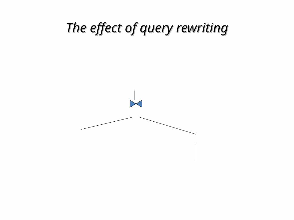
The effect of query rewritingThe effect of query rewriting
Π movieTitle
Starname = name
StarsIn σbirthdate LIKE ‘%1960’
MovieStar
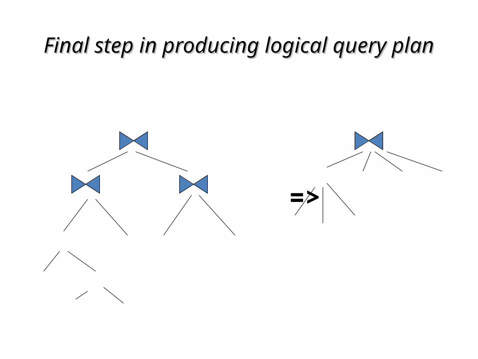
Final step in producing logical query planFinal step in producing logical query plan
=>
U
U
U
W
R
S T
VU
U V W
R S T
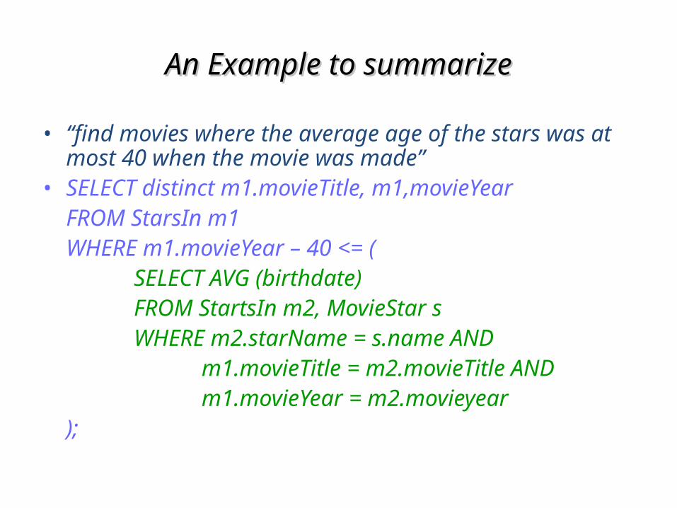
An Example to summarizeAn Example to summarize
• “find movies where the average age of the stars was at most 40 when the movie was made”
• SELECT distinct m1.movieTitle, m1,movieYearFROM StarsIn m1WHERE m1.movieYear – 40 <= (
SELECT AVG (birthdate)FROM StartsIn m2, MovieStar sWHERE m2.starName = s.name AND
m1.movieTitle = m2.movieTitle ANDm1.movieYear = m2.movieyear
);
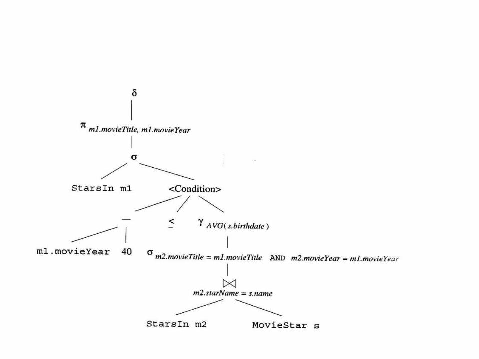
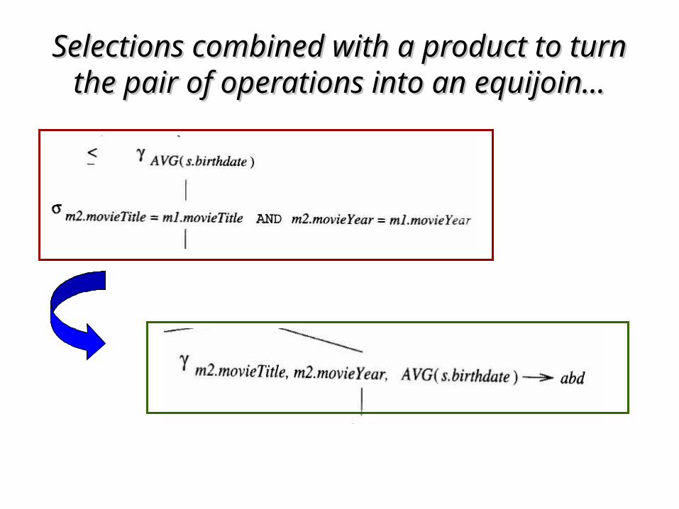
Selections combined with a product to turn the Selections combined with a product to turn the pair of operations into an equijoin…pair of operations into an equijoin…
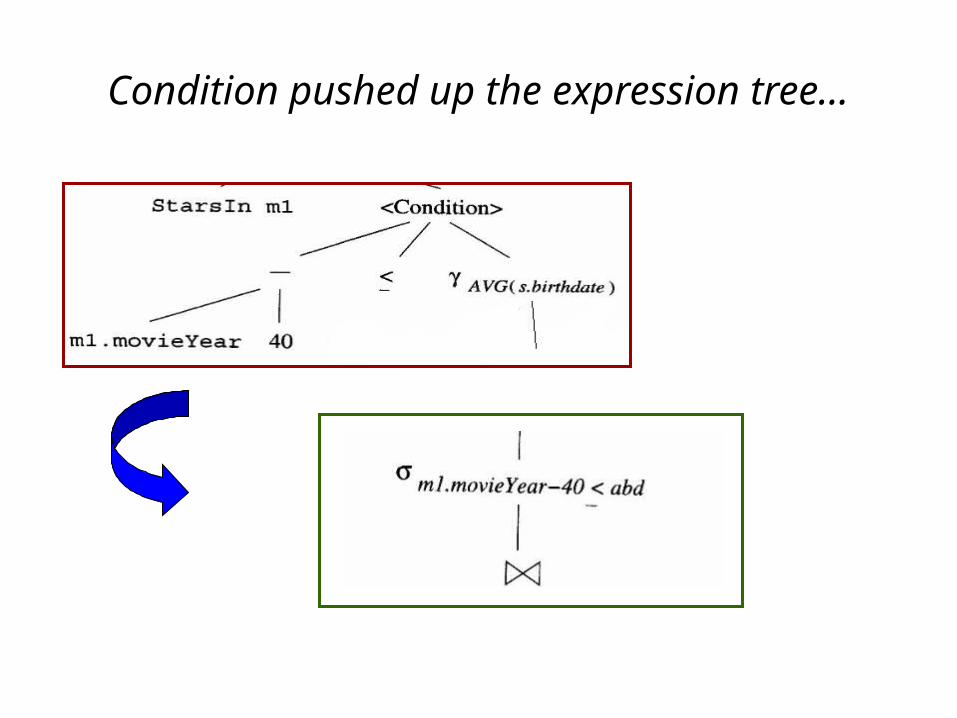
Condition pushed up the expression tree…
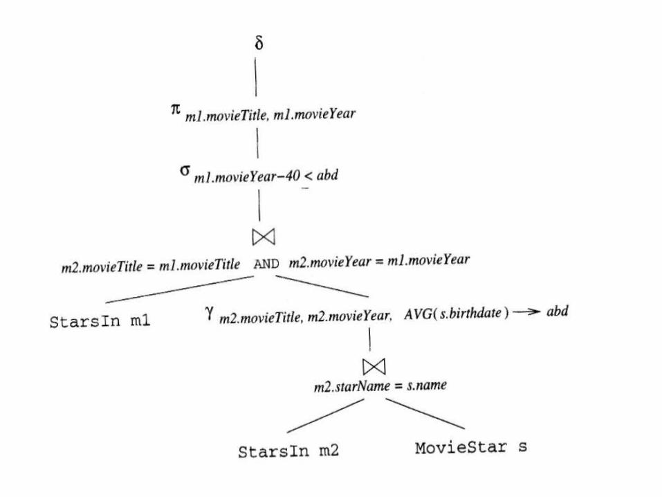
`
The Query Compiler(16.4)
DATABASE SYSTEMS – The Complete Book
Presented By: Under the supervision of:
Maciej Kicinski Dr. T.Y.Lin

Topics to be coveredTopics to be covered
• From Parse to Logical Query Plans– Conversion to Relational Algebra– Removing Subqueries From Conditions– Improving the Logical Query Plan– Grouping Associative/ Commutative Operators
• Estimating the Cost of Operation– Estimating Sizes of Intermediate Relations – Estimating the Size of a Projection– Estimating the Size of a Selection– Estimating the Size of a Join– Estimating Sizes for Other Operations
16.4 From Estimating the Cost of Operation ►
Estimating the Cost of OperationsEstimating the Cost of Operations
• After getting to the logical query plan, we turn it into physical plan.
• Consider all the possible physical plan and estimate their costs – this evaluation is known as cost-based enumeration.
• The one with least estimated cost is the one selected to be passed to the query-execution engine.
Selection for each physical plan
• An order and grouping for associative-and-commutative operations like joins, unions.
• An Algorithm for each operator in the logical plan. eg: whether nested loop join or hash join to be used• Additional operators that are needed for the physical plan but
that were not present explicitly in the logical plan. eg: scanning, sorting
• The way in which arguments are passed from one operator to the next.– .
Estimating Sizes of Intermediate Relations
Rules for estimating the number of tuples in an intermediate relation:
1. Give accurate estimates
2. Are easy to compute
3. Are logically consistent• Objective of estimation is to select best physical
plan with least cost.
Estimating the Size of a Projection
We should treat a classical, duplicate-eliminating projection as a bag-projection.
The projection is different from the other operators, in that the size of the result is computable. Since a projection produces a result tuple for every argument tuple, the only change in the output size is the change in the lengths of the tuples.
• .
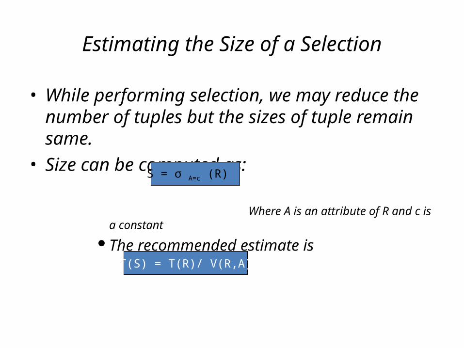
Estimating the Size of a Selection
• While performing selection, we may reduce the number of tuples but the sizes of tuple remain same.
• Size can be computed as:
Where A is an attribute of R and c is a constant
The recommended estimate is
T(S) = T(R)/ V(R,A)
S = σ A=c (R)
Estimating Sizes of Other Operations
• Union
• Intersection
• Difference
• Duplicate Elimination
• Grouping and Aggregation
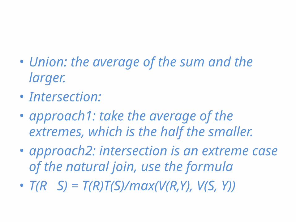
• Union: the average of the sum and the larger. • Intersection: • approach1: take the average of the extremes,
which is the half the smaller.• approach2: intersection is an extreme case of
the natural join, use the formula• T(R S) = T(R)T(S)/max(V(R,Y), V(S, Y))
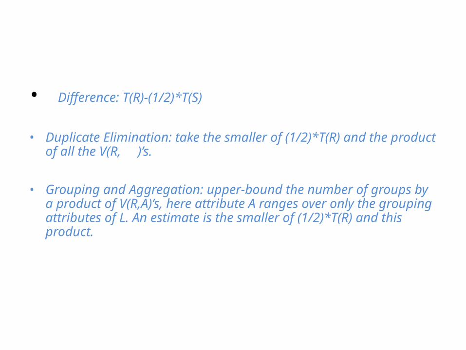
• Difference: T(R)-(1/2)*T(S)
• Duplicate Elimination: take the smaller of (1/2)*T(R) and the product of all the V(R, )’s.
• Grouping and Aggregation: upper-bound the number of groups by a product of V(R,A)’s, here attribute A ranges over only the grouping attributes of L. An estimate is the smaller of (1/2)*T(R) and this product.
16.5 Introduction to Cost-based plan selection
• Whether selecting a logical query plan or constructing a physical query plan from a logical plan, the query optimizer needs to estimate the cost of evaluating certain expressions.
• We shall assume that the "cost" of evaluating an expression is approximated well by the number of disk I/O's performed.
The number of disk I/O’s, in turn, is influenced by:
1. The particular logical operators chosen to implement the query, a matter decided when we choose the logical query plan.
2. The sizes of intermediate results.3. The physical operators used to implement logical operators.
e.g.. The choice of a one-pass or two-pass join, or the choice to sort or not sort a given relation.
4. The ordering of similar operations, especially joins5. The method of passing arguments from one physical operator
to the next.
Obtaining Estimates for Size Parameter• The formulas of Section 16.4 were predicated on knowing
certain important parameters, especially T(R), the number of tuples in a relation R, and V(R, a), the number of different values in the column of relation R for attribute a.
• A modern DBMS generally allows the user or administrator explicitly to request the gathering of statistics, such as T(R) and V(R, a). These statistics are then used in subsequent query optimizations to estimate the cost of operations.
• By scanning an entire relation R, it is straightforward to count the number of tuples T(R) and also to discover the number of different values V(R, a) for each attribute a.
• The number of blocks in which R can fit, B(R), can be estimated either by counting the actual number of blocks used (if R is clustered), or by dividing T(R) by the number of tuples per block
Computation of Statistics
• Periodic re-computation of statistics is the norm in most
DBMS's, for several reasons. – First, statistics tend not to change radically in a short time. – Second, even somewhat inaccurate statistics are useful as long as they
are applied consistently to all the plans. – Third, the alternative of keeping statistics up-to-date can make the
statistics themselves into a "hot-spot" in the database; because statistics are read frequently, we prefer not to update them frequently too.
• The recomputation of statistics might be triggered automatically after some period of time, or after some number of updates.
• However, a database administrator noticing, that poor-performing query plans are being selected by the query optimizer on a regular basis, might request the recomputation of statistics in an attempt to rectify the problem.
• Computing statistics for an entire relation R can be very expensive, particularly if we compute V(R, a) for each attribute a in the relation.
• One common approach is to compute approximate statistics by sampling only a fraction of the data. For example, let us suppose we want to sample a small fraction of the tuples to obtain an estimate for V(R, a).
Heuristics for Reducing the Cost of Logical QueryPlans
• One important use of cost estimates for queries or sub-queries is in the application of heuristic transformations of the query.
• We have already observed previously how certain heuristics applied independent of cost estimates can be expected almost certainly to improve the cost of a logical query plan.
• However, there are other points in the query optimization process where estimating the cost both before and after a transformation will allow us to apply a transformation where it appears to reduce cost and avoid the transformation otherwise.
• In particular, when the preferred logical query plan is being generated, we may consider a number of optional transformations and the costs before and after.
• Because we are estimating the cost of a logical query plan, so we have not yet made decisions about the physical operators that will be used to implement the operators of relational algebra, our cost estimate cannot be based on disk I/Os.
• Rather, we estimate the sizes of all intermediate results using the techniques of Section 16.1, and their sum is our heuristic estimate for the cost of the entire logical plan.
• For example,
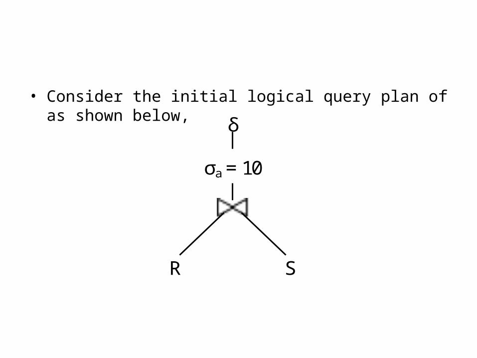
• Consider the initial logical query plan of as shown below,
δ
σa = 10
R S
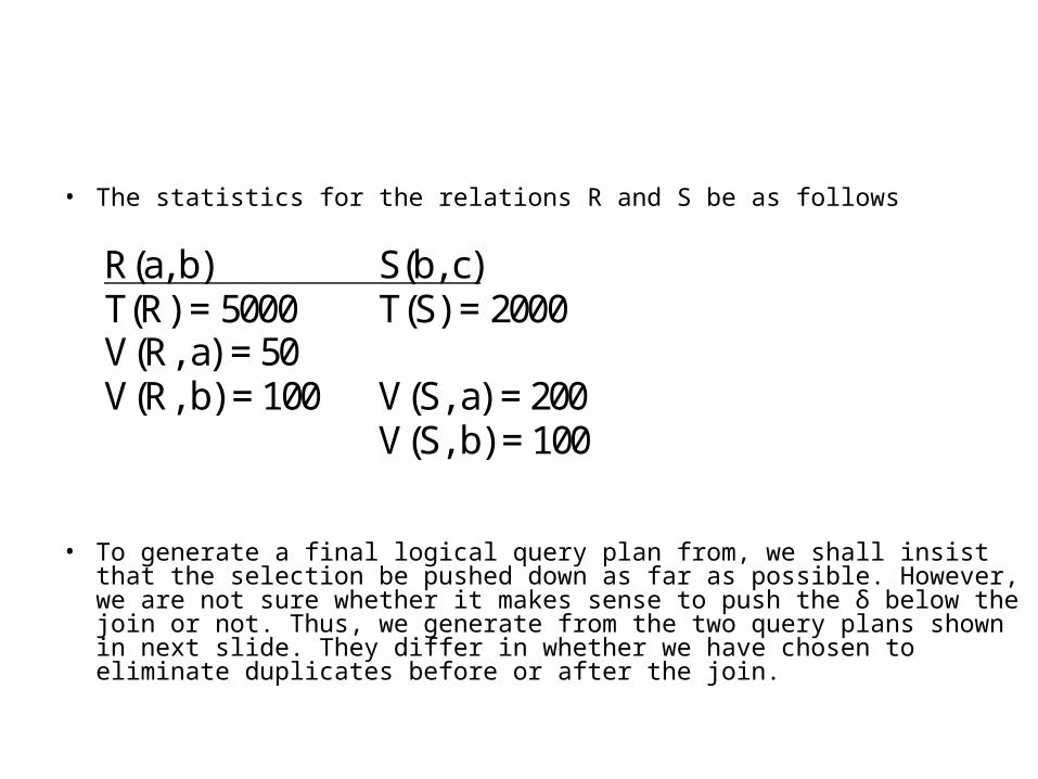
• The statistics for the relations R and S be as follows
• To generate a final logical query plan from, we shall insist that the selection be pushed down as far as possible. However, we are not sure whether it makes sense to push the δ below the join or not. Thus, we generate from the two query plans shown in next slide. They differ in whether we have chosen to eliminate duplicates before or after the join.
R(a, b) S(b, c) T(R) = 5000 T(S) = 2000 V(R, a) = 50 V(R, b) = 100 V(S, a) = 200 V(S, b) = 100
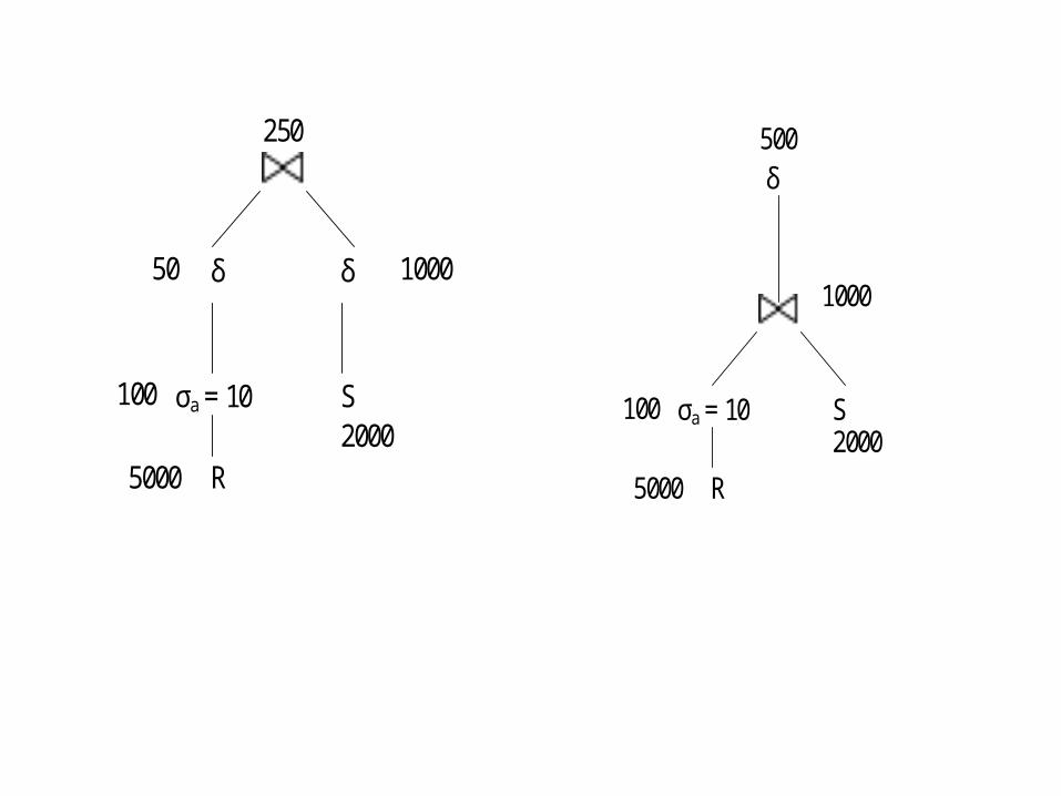
250
δ δ
σa = 10 S
R
50
100
5000 2000
1000
500
σa = 10 S
R
100
5000
2000
10000
δ
(a) (b)
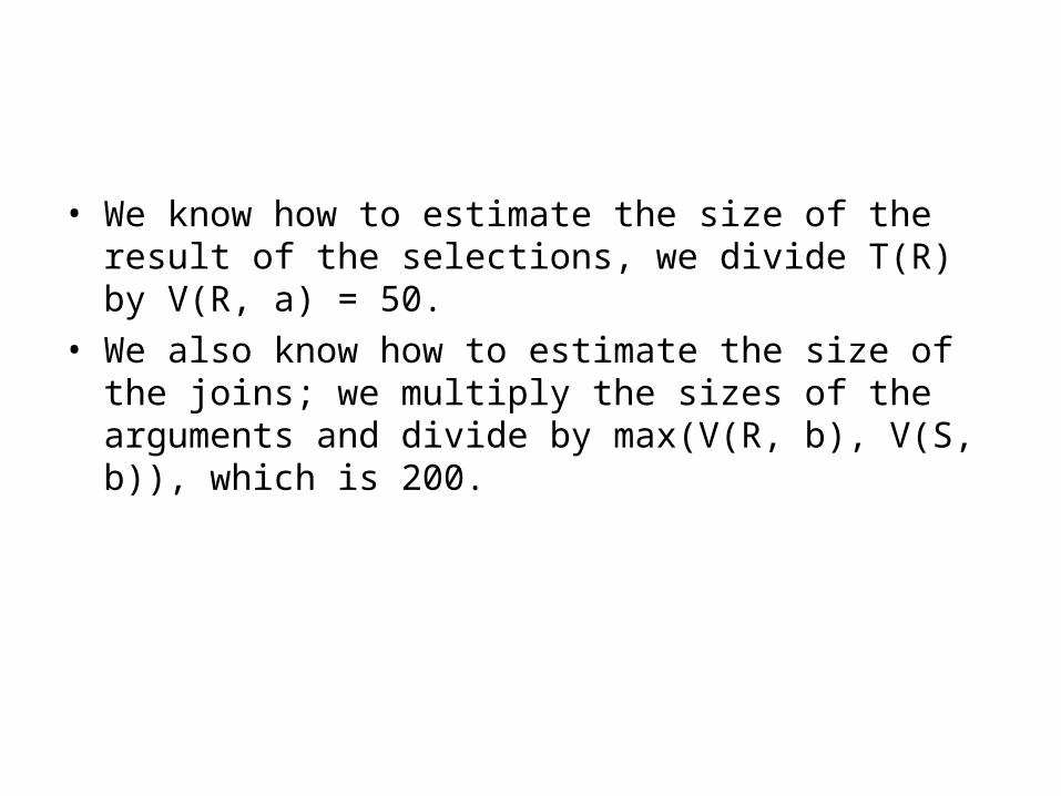
• We know how to estimate the size of the result of the selections, we divide T(R) by V(R, a) = 50.
• We also know how to estimate the size of the joins; we multiply the sizes of the arguments and divide by max(V(R, b), V(S, b)), which is 200.
Approaches to Enumerating Physical Plans
• Let us consider the use of cost estimates in the conversion of a logical query plan to a physical query plan.
• The baseline approach, called exhaustive, is to consider all combinations of choices (for each of issues like order of joins, physical implementation of operators, and so on).
• Each possible physical plan is assigned an estimated cost, and the one with the smallest cost is selected.
• There are two broad approaches to exploring the space of
possible physical plans: – Top-down: Here, we work down the tree of the logical query plan from
the root.– Bottom-up: For each sub-expression of the logical-query-plan tree, we
compute the costs of all possible ways to compute that sub-expression. The possibilities and costs for a sub-expression E are computed by considering the options for the sub-expressions for E, and combining them in all possible ways with implementations for the root operator of E.
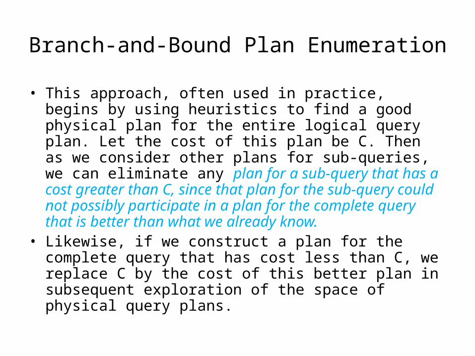
Branch-and-Bound Plan Enumeration
• This approach, often used in practice, begins by using heuristics to find a good physical plan for the entire logical query plan. Let the cost of this plan be C. Then as we consider other plans for sub-queries, we can eliminate any plan for a sub-query that has a cost greater than C, since that plan for the sub-query could not possibly participate in a plan for the complete query that is better than what we already know.
• Likewise, if we construct a plan for the complete query that has cost less than C, we replace C by the cost of this better plan in subsequent exploration of the space of physical query plans.
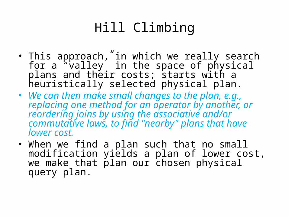
Hill Climbing
• This approach, in which we really search for a “valley” in the space of physical plans and their costs; starts with a heuristically selected physical plan.
• We can then make small changes to the plan, e.g., replacing one method for an operator by another, or reordering joins by using the associative and/or commutative laws, to find "nearby" plans that have lower cost.
• When we find a plan such that no small modification yields a plan of lower cost, we make that plan our chosen physical query plan.
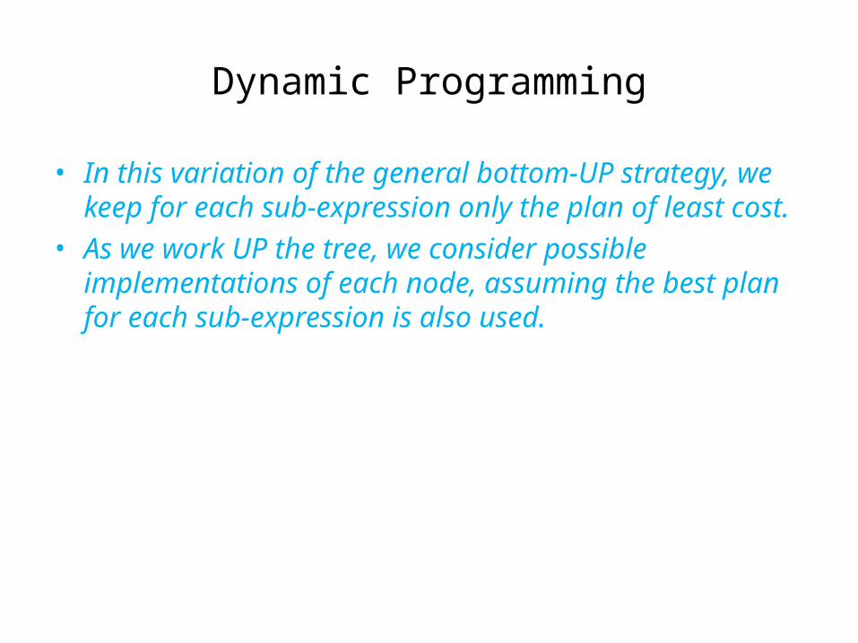
Dynamic Programming
• In this variation of the general bottom-UP strategy, we keep for each sub-expression only the plan of least cost.
• As we work UP the tree, we consider possible implementations of each node, assuming the best plan for each sub-expression is also used.
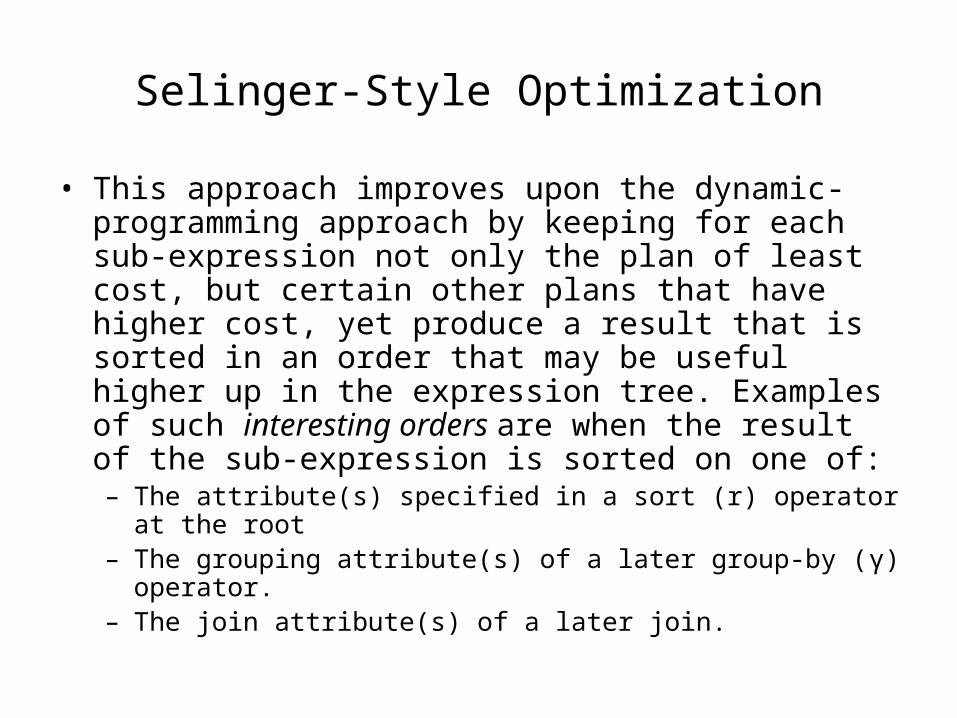
Selinger-Style Optimization
• This approach improves upon the dynamic-programming approach by keeping for each sub-expression not only the plan of least cost, but certain other plans that have higher cost, yet produce a result that is sorted in an order that may be useful higher up in the expression tree. Examples of such interesting orders are when the result of the sub-expression is sorted on one of:– The attribute(s) specified in a sort (r) operator at the root– The grouping attribute(s) of a later group-by (γ) operator.– The join attribute(s) of a later join.
Choosing an Order for Joins
Chapter 16.6 by:Chiu LukID: 210
Introduction
• This section focuses on critical problem in cost-based optimization:– Selecting order for natural join of three or more
relations
• Compared to other binary operations, joins take more time and therefore need effective optimization techniques
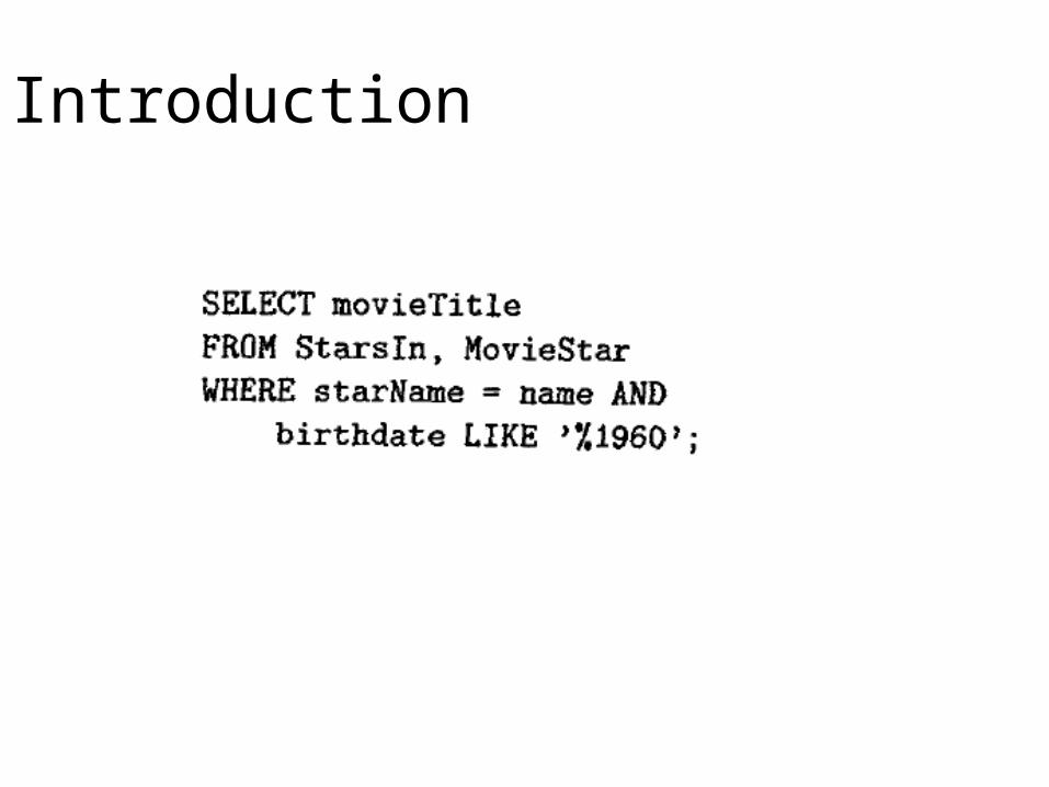
Introduction
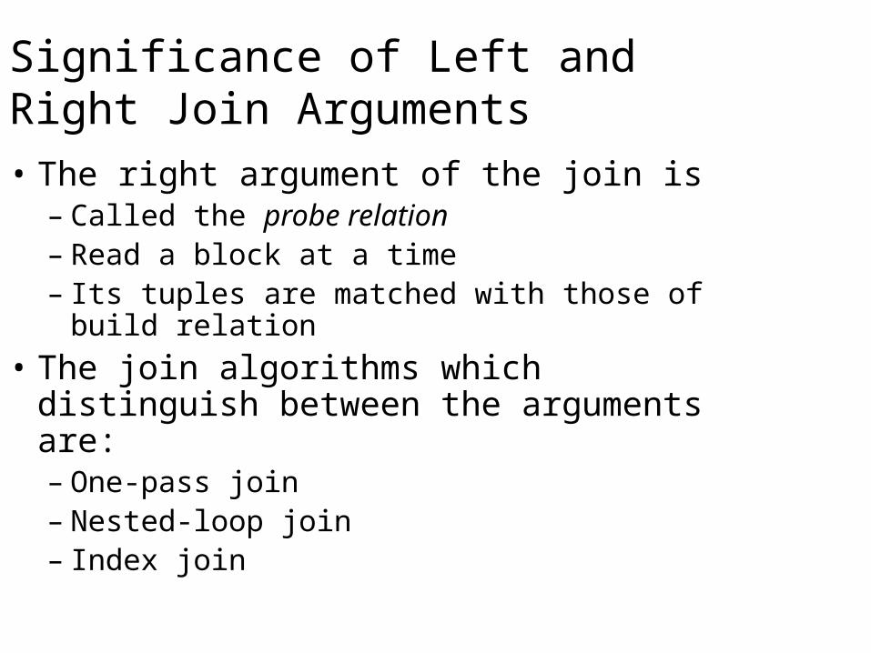
Significance of Left and Right Join Arguments• The right argument of the join is
– Called the probe relation – Read a block at a time– Its tuples are matched with those of build relation
• The join algorithms which distinguish between the arguments are:– One-pass join– Nested-loop join– Index join
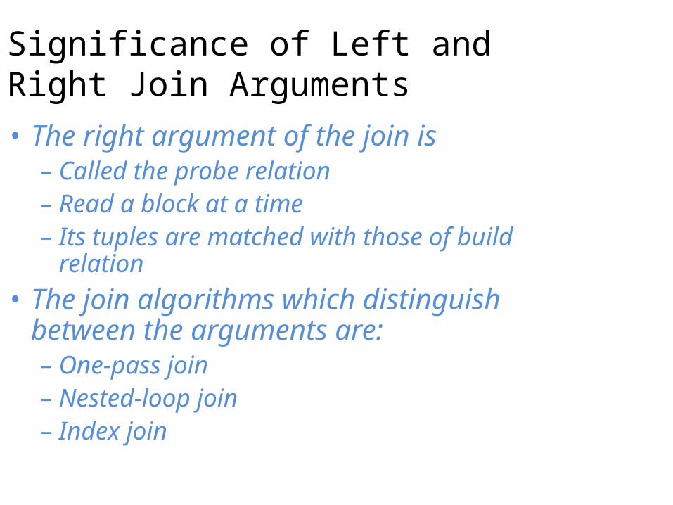
Significance of Left and Right Join Arguments• The right argument of the join is
– Called the probe relation – Read a block at a time– Its tuples are matched with those of build relation
• The join algorithms which distinguish between the arguments are:– One-pass join– Nested-loop join– Index join
Join Trees
• Order of arguments is important for joining two relations
• Left argument, since stored in main-memory, should be smaller
• With two relations only two choices of join tree
• With more than two relations, there are n! ways to order the arguments and therefore n! join trees, where n is the no. of relations
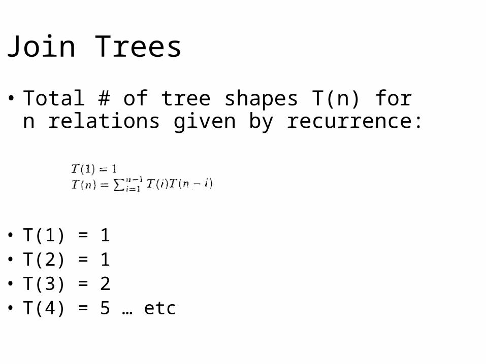
Join Trees
• Total # of tree shapes T(n) for n relations given by recurrence:
• T(1) = 1• T(2) = 1• T(3) = 2• T(4) = 5 … etc
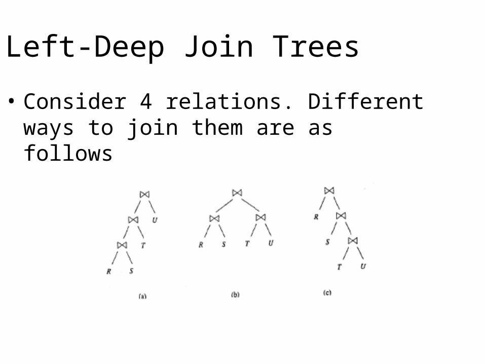
Left-Deep Join Trees
• Consider 4 relations. Different ways to join them are as follows
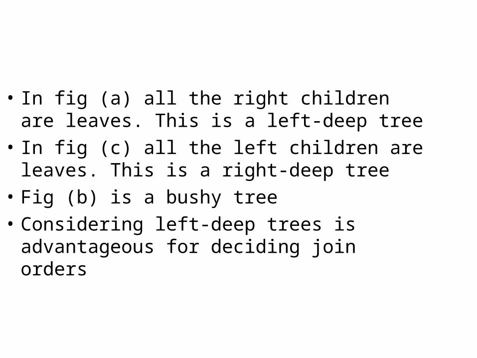
• In fig (a) all the right children are leaves. This is a left-deep tree
• In fig (c) all the left children are leaves. This is a right-deep tree
• Fig (b) is a bushy tree• Considering left-deep trees is advantageous
for deciding join orders
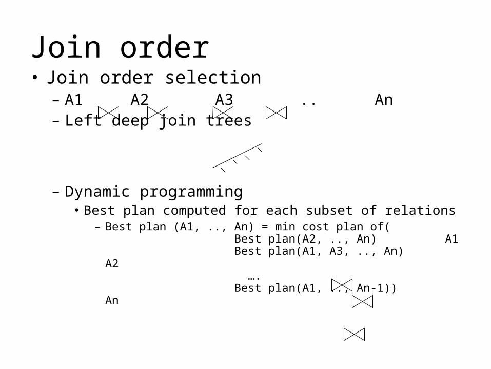
Join order• Join order selection
– A1 A2 A3 .. An– Left deep join trees
– Dynamic programming• Best plan computed for each subset of relations
– Best plan (A1, .., An) = min cost plan of( Best plan(A2, .., An) A1 Best plan(A1, A3, .., An) A2 …. Best plan(A1, .., An-1)) An
Ai
An
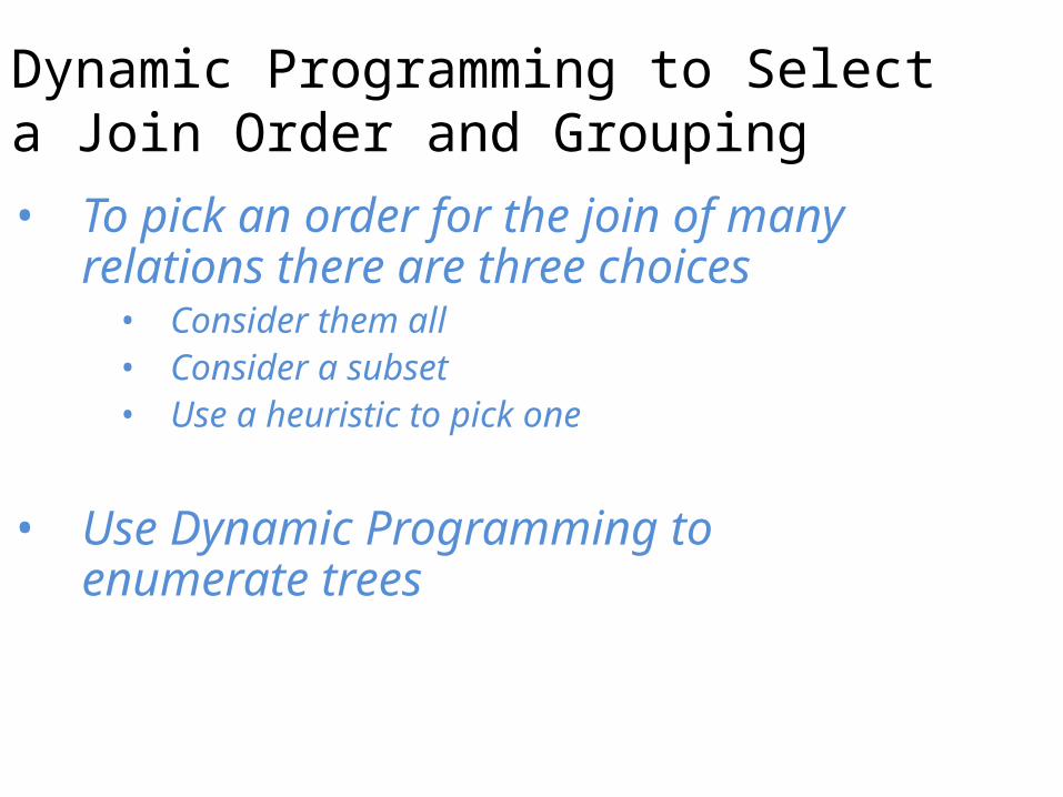
Dynamic Programming to Select a Join Order and Grouping• To pick an order for the join of many
relations there are three choices• Consider them all• Consider a subset• Use a heuristic to pick one
• Use Dynamic Programming to enumerate trees
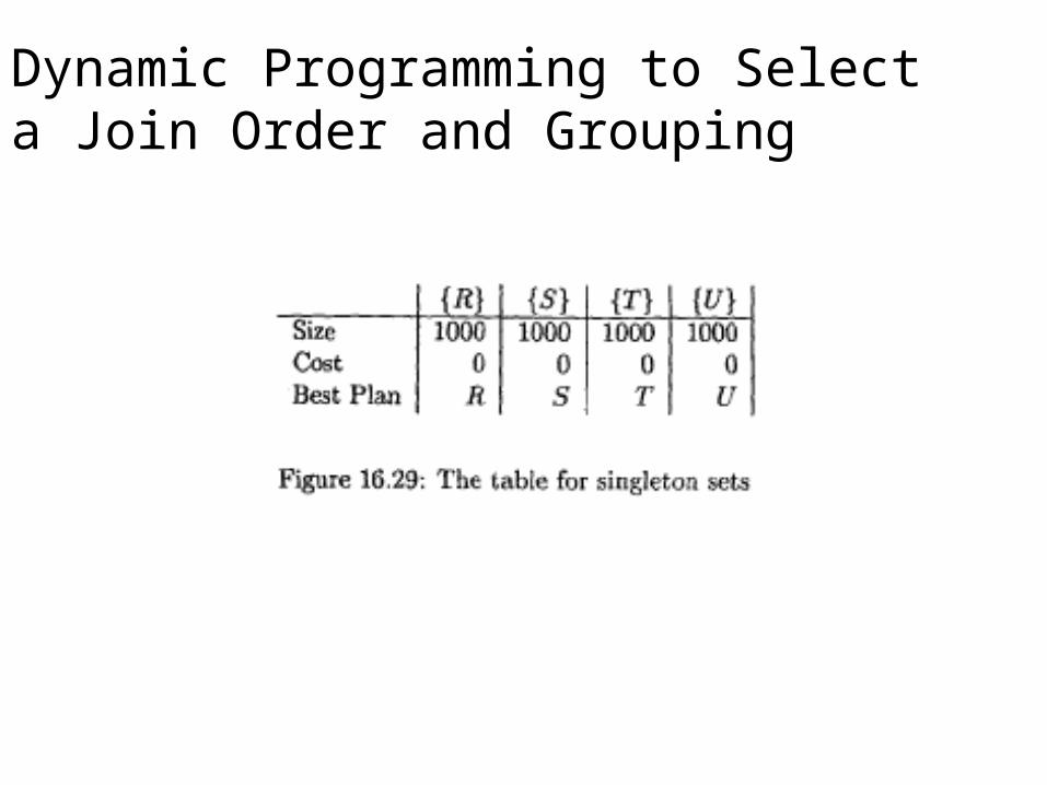
Dynamic Programming to Select a Join Order and Grouping
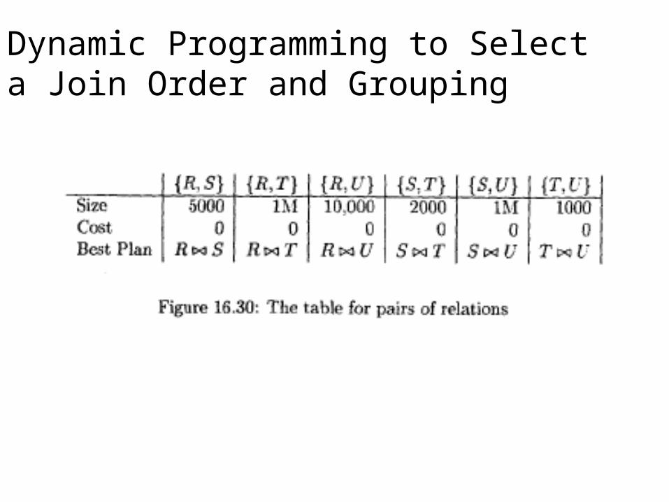
Dynamic Programming to Select a Join Order and Grouping
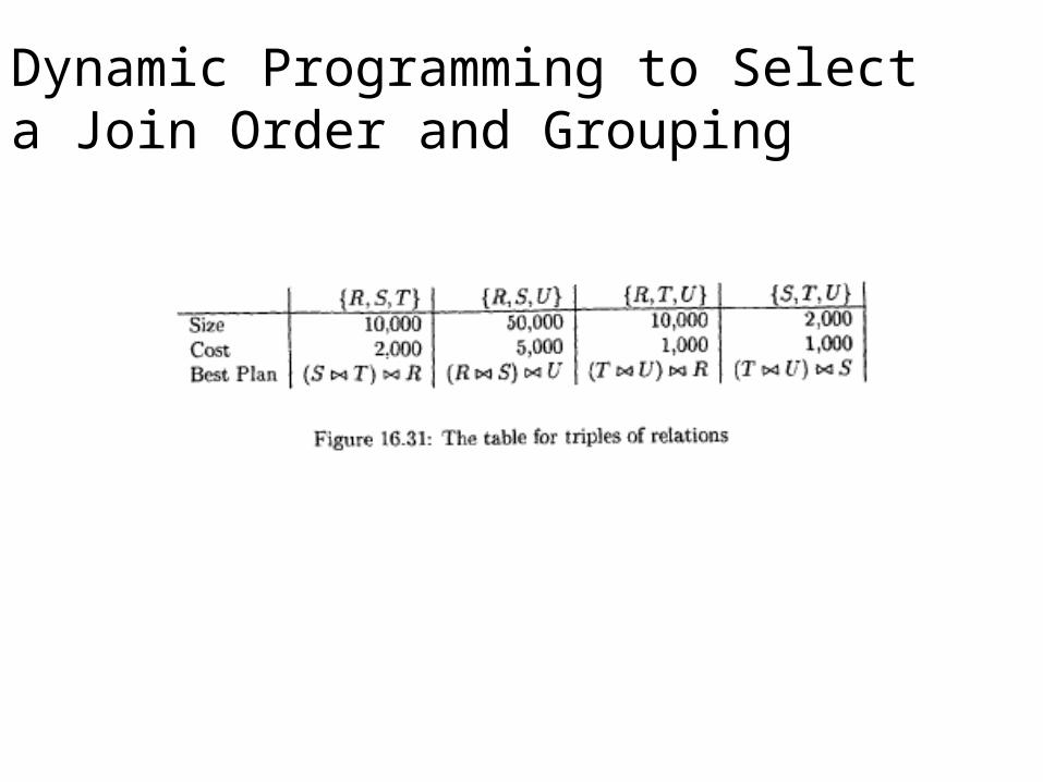
Dynamic Programming to Select a Join Order and Grouping
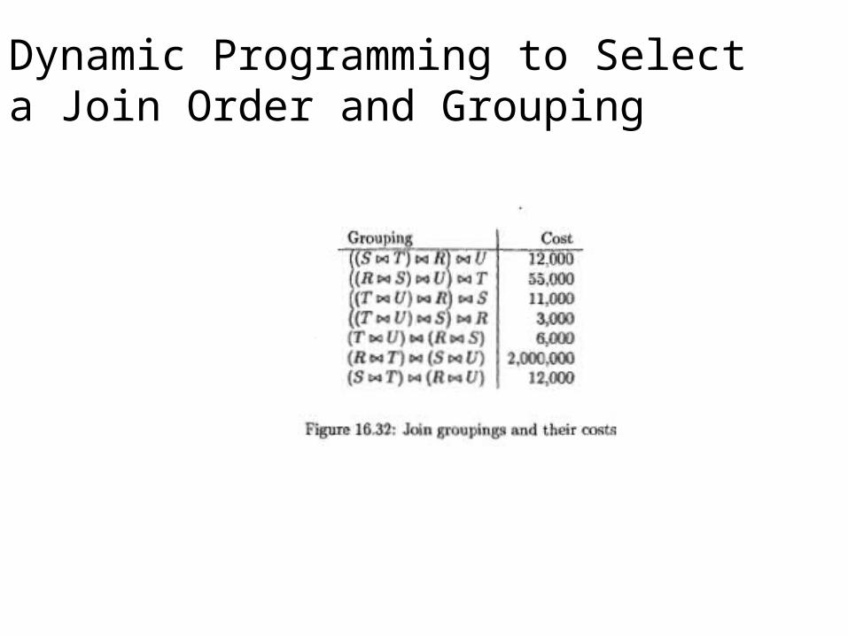
Dynamic Programming to Select a Join Order and Grouping
A Greedy Algorithm for Selecting a Join Order
• It is expensive to use an exhaustive method like dynamic programming
• Better approach is to use a join-order heuristic for the query optimization
• Greedy algorithm is an example of that– Make one decision at a time about order of join
and never backtrack on the decisions once made
Completing the Physical-Query-Plan and Chapter 16 Summary (16.7-16.8)
CS257 Spring 2009Professor Tsau Lin
Student: Suntorn Sae-EungDonavon Norwood
Outline
16.7 Completing the Physical-Query-PlanI. Choosing a Selection MethodII. Choosing a Join MethodIII. Pipelining Versus MaterializationIV. Pipelining Unary OperationsV. Pipelining Binary OperationsVI. Notation for Physical Query PlanVII. Ordering the Physical Operations
16.8 Summary of Chapter 16
285
Before complete Physical-Query-Plan
• A query previously has been – Parsed and Preprocessed (16.1)– Converted to Logical Query Plans (16.3) – Estimated the Costs of Operations (16.4)– Determined costs by Cost-Based Plan Selection
(16.5)– Weighed costs of join operations by choosing an
Order for Joins
286
16.7 Completing the Physical-Query-Plan
• 3 topics related to turning LP into a complete physical plan
1. Choosing of physical implementations such as Selection and Join methods
2. Decisions regarding to intermediate results (Materialized or Pipelined)
3. Notation for physical-query-plan operators
287
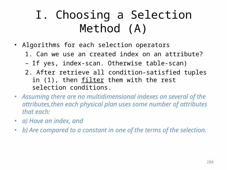
I. Choosing a Selection Method (A)
• Algorithms for each selection operators1. Can we use an created index on an attribute?– If yes, index-scan. Otherwise table-scan)2. After retrieve all condition-satisfied tuples in (1), then filter them with
the rest selection conditions.• Assuming there are no multidimensional indexes on several of the
attributes,then each physical plan uses some number of attributes that each:
• a) Have an index, and• b) Are compared to a constant in one of the terms of the selection.
288
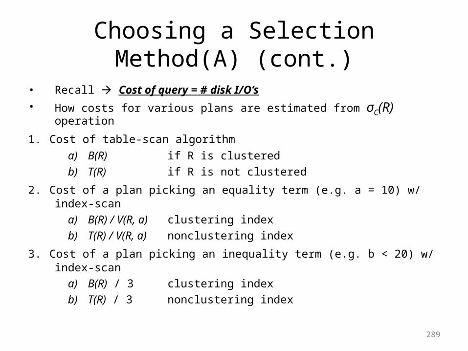
Choosing a Selection Method(A) (cont.)
• Recall Cost of query = # disk I/O’s• How costs for various plans are estimated from σC(R) operation
1. Cost of table-scan algorithma) B(R) if R is clusteredb) T(R) if R is not clustered
2. Cost of a plan picking an equality term (e.g. a = 10) w/ index-scana) B(R) / V(R, a) clustering indexb) T(R) / V(R, a) nonclustering index
3. Cost of a plan picking an inequality term (e.g. b < 20) w/ index-scana) B(R) / 3 clustering indexb) T(R) / 3 nonclustering index
289
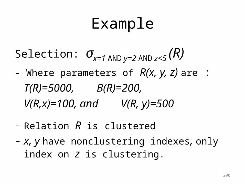
Example
Selection: σx=1 AND y=2 AND z<5 (R)
- Where parameters of R(x, y, z) are : T(R)=5000, B(R)=200,
V(R,x)=100, and V(R, y)=500
- Relation R is clustered
- x, y have nonclustering indexes, only index on z is clustering.
290
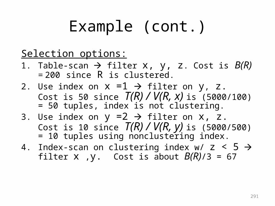
Example (cont.)
Selection options:1. Table-scan filter x, y, z. Cost is B(R) = 200 since R is
clustered.2. Use index on x =1 filter on y, z. Cost is 50 since
T(R) / V(R, x) is (5000/100) = 50 tuples, index is not clustering.
3. Use index on y =2 filter on x, z. Cost is 10 since T(R) / V(R, y) is (5000/500) = 10 tuples using nonclustering index.
4. Index-scan on clustering index w/ z < 5 filter x ,y. Cost is about B(R)/3 = 67
291
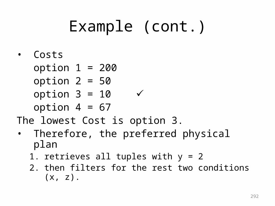
Example (cont.)
• Costsoption 1 = 200 option 2 = 50 option 3 = 10 option 4 = 67
The lowest Cost is option 3. • Therefore, the preferred physical plan
1. retrieves all tuples with y = 2 2. then filters for the rest two conditions (x, z).
292
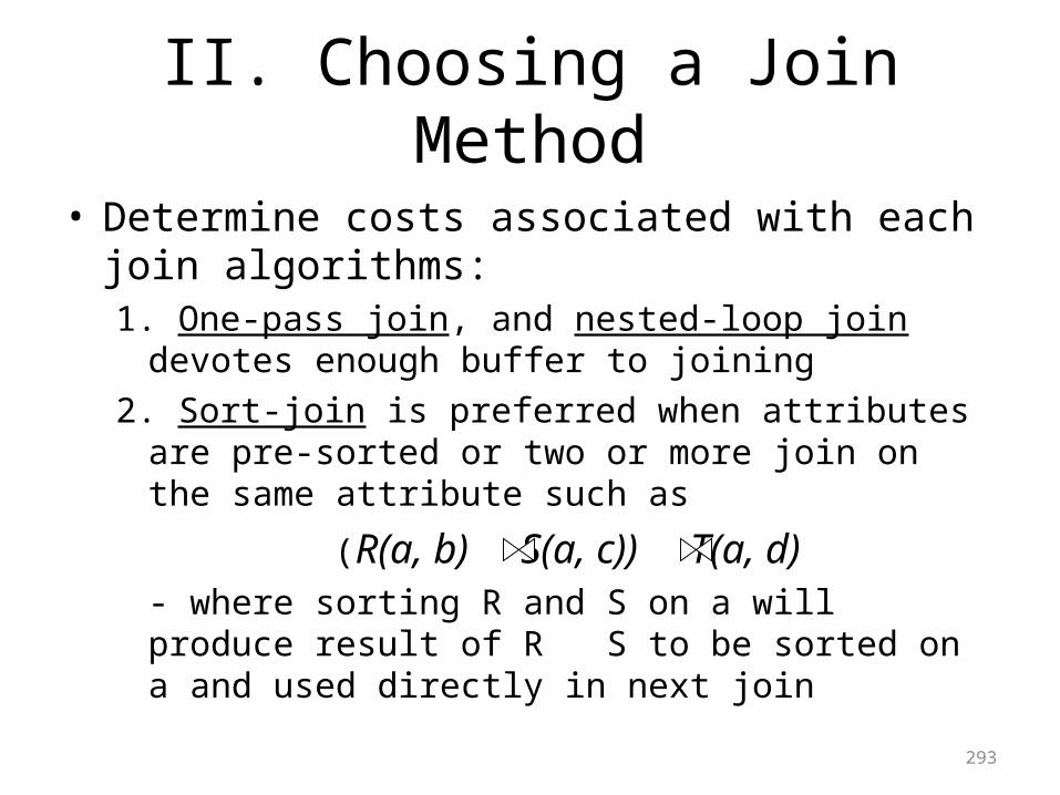
II. Choosing a Join Method
• Determine costs associated with each join algorithms: 1. One-pass join, and nested-loop join devotes enough buffer
to joining2. Sort-join is preferred when attributes are pre-sorted or
two or more join on the same attribute such as
(R(a, b) S(a, c)) T(a, d) - where sorting R and S on a will produce result of R S to be sorted on a and used directly in next join
293
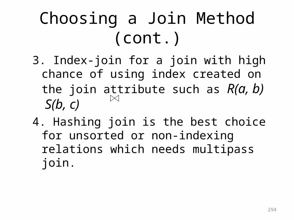
Choosing a Join Method (cont.)
3. Index-join for a join with high chance of using index created on the join attribute such as R(a, b) S(b, c)
4. Hashing join is the best choice for unsorted or non-indexing relations which needs multipass join.
294
III. Pipelining Versus Materialization
• The naïve way to execute a query plan is to order the operations appropriately and store the results of each operation on disk until it is needed by another operation. This strategy is called materialization.
• More subtle way to execute a query plan is to interleave the execution of several operations. The tuples produced by one operation are passed directly to the operation that uses it, without ever storing the intermediate tuples on disk. This approach in called pipelining.
• Since pipelining saves disk I/O’s, where is an obvious advantage to pipelining, but there is a corresponding disadvantage. Since several operations must share main memory at any time, there is a chance that algorithm with higher disk I/O requirements must be chosen or thrashing will occur , thus giving back all the disk-
I/O savings that were gained by pipelining.
295
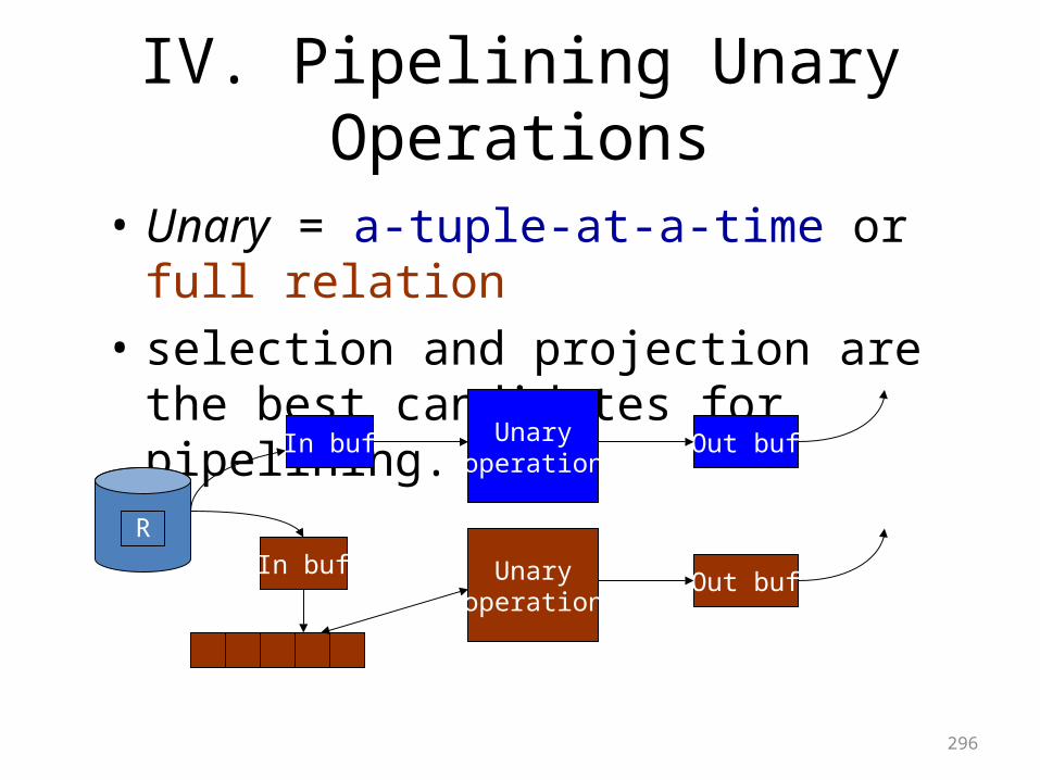
IV. Pipelining Unary Operations
• Unary = a-tuple-at-a-time or full relation• selection and projection are the best
candidates for pipelining.
296
R
In buf Unaryoperation
Out buf
In buf Unaryoperation
Out buf
M-1 buffers
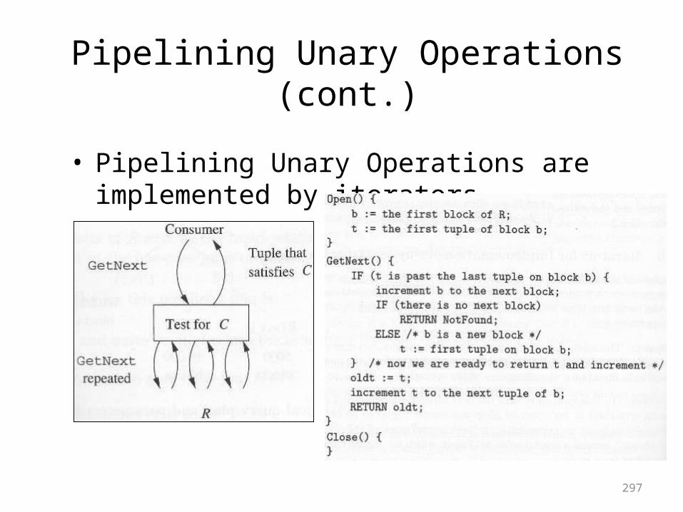
Pipelining Unary Operations (cont.)
• Pipelining Unary Operations are implemented by iterators
297
V. Pipelining Binary Operations
• Binary operations : , , - , , x• The results of binary operations can also be
pipelined.• Use one buffer to pass result to its consumer,
one block at a time.• The extended example shows tradeoffs and
opportunities
298
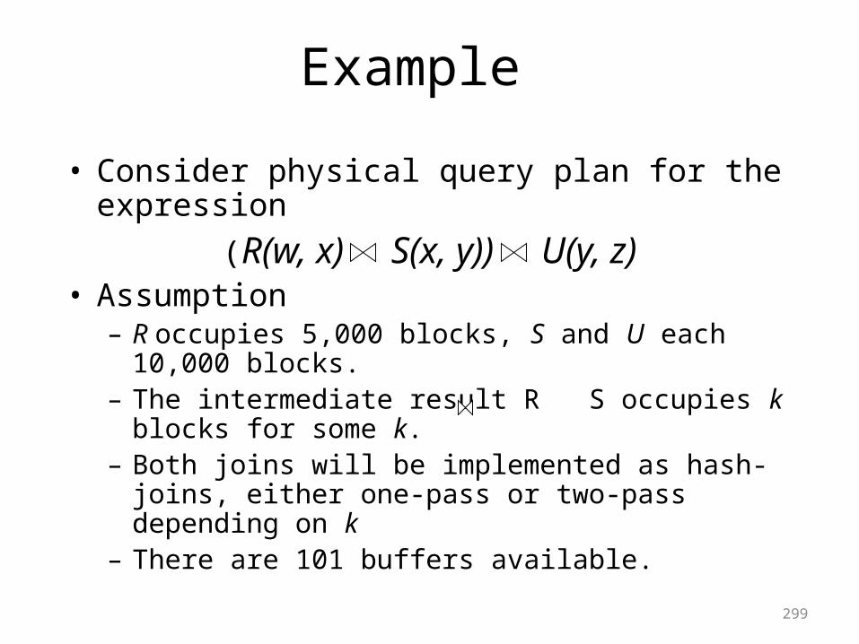
Example
• Consider physical query plan for the expression(R(w, x) S(x, y)) U(y, z)
• Assumption– R occupies 5,000 blocks, S and U each 10,000 blocks.– The intermediate result R S occupies k blocks for some
k.– Both joins will be implemented as hash-joins, either
one-pass or two-pass depending on k– There are 101 buffers available.
299
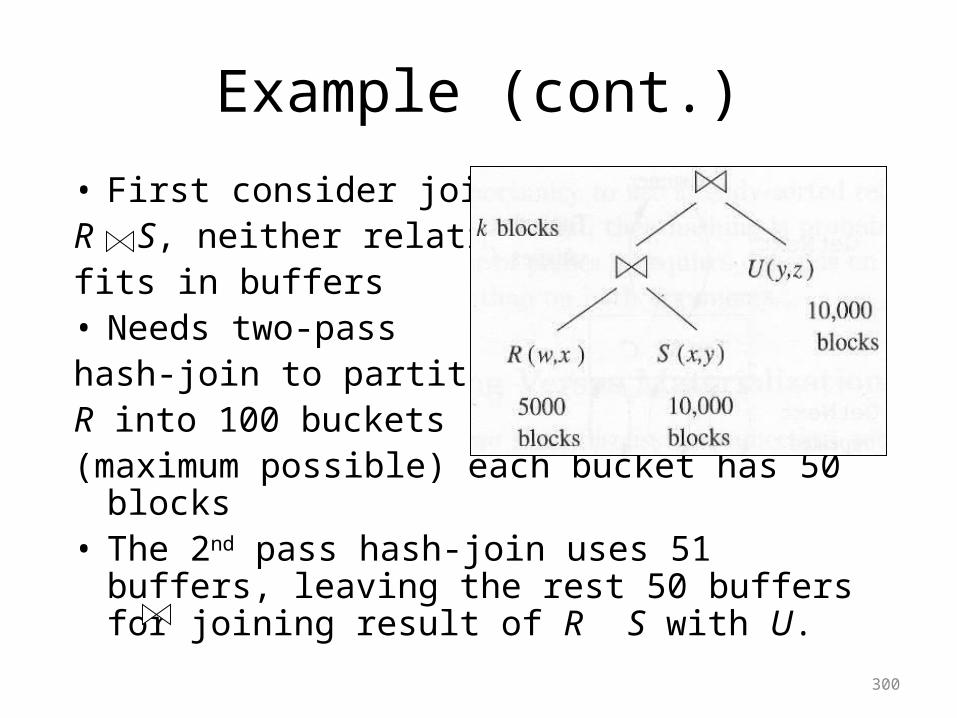
Example (cont.)
• First consider join R S, neither relations fits in buffers• Needs two-pass hash-join to partition R into 100 buckets (maximum possible) each bucket has 50 blocks• The 2nd pass hash-join uses 51 buffers, leaving the
rest 50 buffers for joining result of R S with U.
300
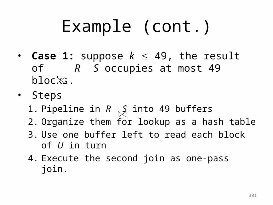
Example (cont.)
• Case 1: suppose k 49, the result of R S occupies at most 49 blocks.
• Steps 1. Pipeline in R S into 49 buffers2. Organize them for lookup as a hash table3. Use one buffer left to read each block of U in
turn4. Execute the second join as one-pass join.
301
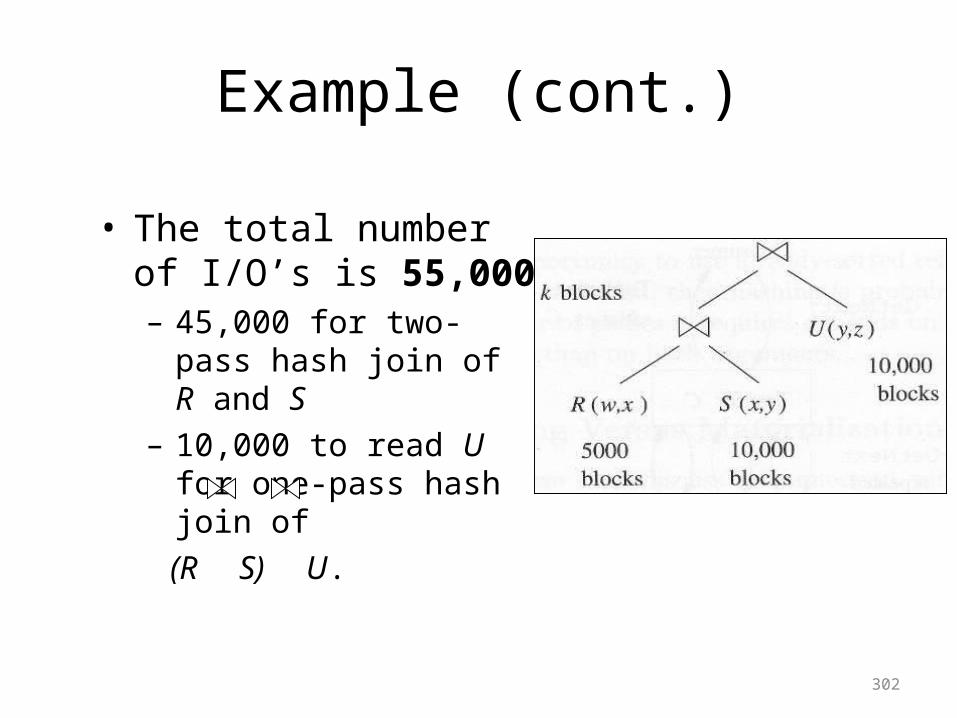
Example (cont.)
• The total number of I/O’s is 55,000– 45,000 for two-pass hash
join of R and S– 10,000 to read U for one-
pass hash join of (R S) U.
302
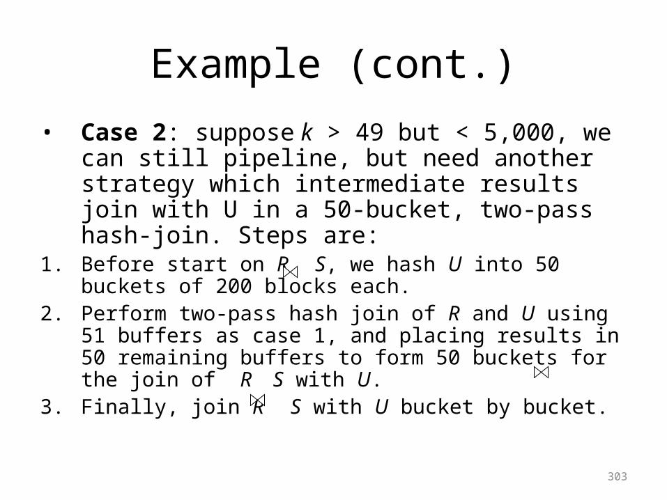
Example (cont.)
• Case 2: suppose k > 49 but < 5,000, we can still pipeline, but need another strategy which intermediate results join with U in a 50-bucket, two-pass hash-join. Steps are:
1. Before start on R S, we hash U into 50 buckets of 200 blocks each.
2. Perform two-pass hash join of R and U using 51 buffers as case 1, and placing results in 50 remaining buffers to form 50 buckets for the join of R S with U.
3. Finally, join R S with U bucket by bucket.
303
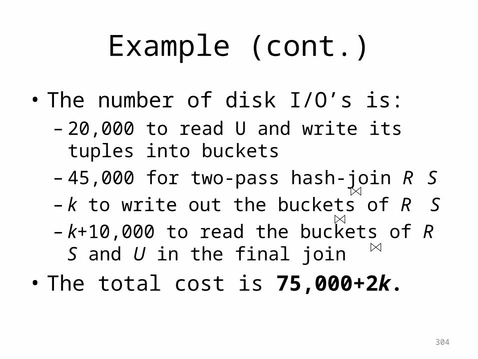
Example (cont.)
• The number of disk I/O’s is:– 20,000 to read U and write its tuples into buckets– 45,000 for two-pass hash-join R S
– k to write out the buckets of R S
– k+10,000 to read the buckets of R S and U in the final join
• The total cost is 75,000+2k.
304
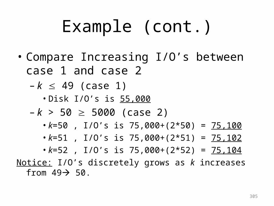
Example (cont.)
• Compare Increasing I/O’s between case 1 and case 2– k 49 (case 1)
• Disk I/O’s is 55,000
– k > 50 5000 (case 2)• k=50 , I/O’s is 75,000+(2*50) = 75,100• k=51 , I/O’s is 75,000+(2*51) = 75,102• k=52 , I/O’s is 75,000+(2*52) = 75,104
Notice: I/O’s discretely grows as k increases from 49 50.
305
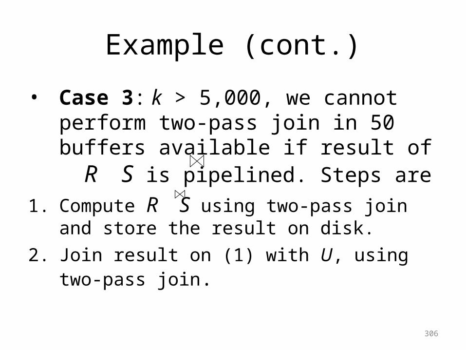
Example (cont.)
• Case 3: k > 5,000, we cannot perform two-pass join in 50 buffers available if result of R S is pipelined. Steps are
1. Compute R S using two-pass join and store the result on disk.
2. Join result on (1) with U, using two-pass join.
306
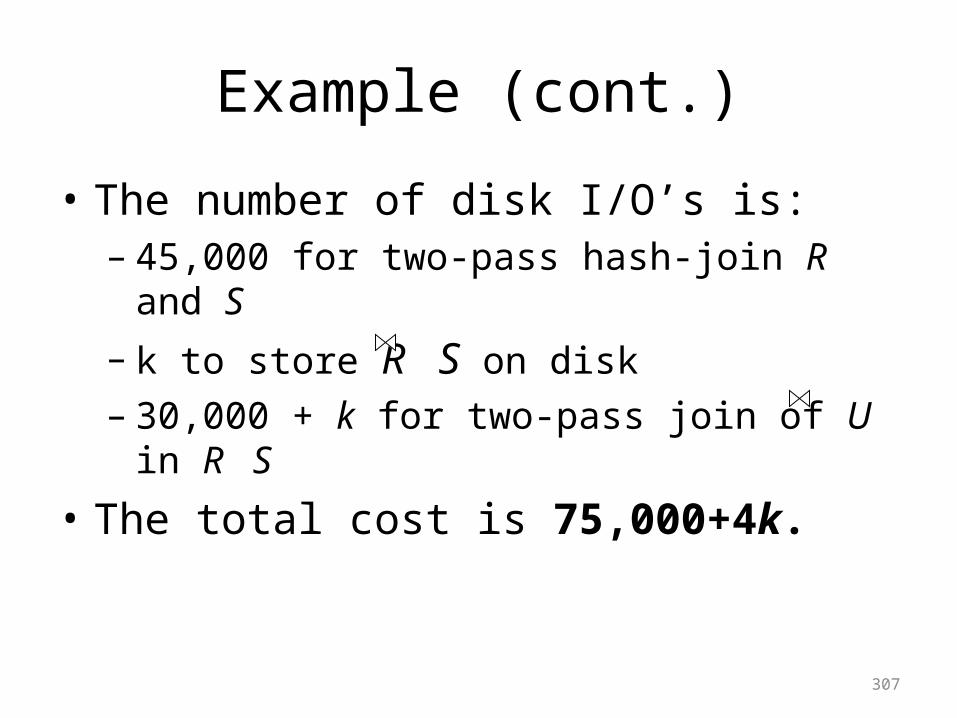
Example (cont.)
• The number of disk I/O’s is:– 45,000 for two-pass hash-join R and S– k to store R S on disk– 30,000 + k for two-pass join of U in R S
• The total cost is 75,000+4k.
307
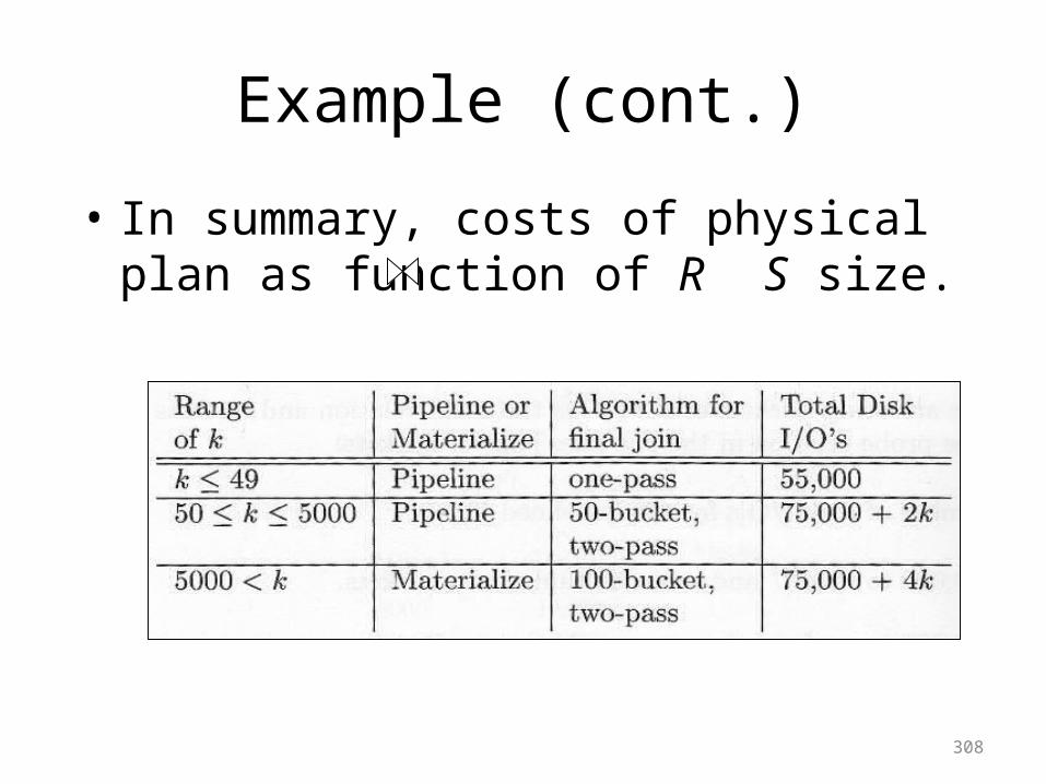
Example (cont.)
• In summary, costs of physical plan as function of R S size.
308
VI. Notation for Physical Query Plans
• Several types of operators: 1. Operators for leaves2. (Physical) operators for Selection3. (Physical) Sorts Operators4. Other Relational-Algebra Operations
• In practice, each DBMS uses its own internal notation for physical query plan.
309
Notation for Physical Query Plans (cont.)
1. Operator for leaves– A leaf operand is replaced in LQP tree
• TableScan(R) : read all blocks
• SortScan(R, L) : read in order according to L
• IndexScan(R, C): scan index attribute A by condition C of form Aθc.
• IndexScan(R, A) : scan index attribute R.A. This behaves like TableScan but more efficient if R is not clustered.
310
Notation for Physical Query Plans (cont.)
2. (Physical) operators for Selection– Logical operator σC(R) is often combined with
access methods.• If σC(R) is replaced by Filter(C), and there is no
index on R or an attribute on condition C– Use TableScan or SortScan(R, L) to access R
• If condition C Aθc AND D for condition D, and there is an index on R.A, then we may– Use operator IndexScan(R, Aθc) to access R and
– Use Filter(D) in place of the selection σC(R)
311
Notation for Physical Query Plans (cont.)
3. (Physical) Sort Operators– Sorting can occur any point in physical plan,
which use a notation SortScan(R, L).
– It is common to use an explicit operator Sort(L) to sort relation that is not stored.
– Can apply at the top of physical-query-plan tree if the result needs to be sorted with ORDER BY clause (г).
312
Notation for Physical Query Plans (cont.)
4. Other Relational-Algebra Operations– Descriptive text definitions and signs to elaborate
• Operations performed e.g. Join or grouping.• Necessary parameters e.g. theta-join or list of
elements in a grouping.• A general strategy for the algorithm e.g. sort-based,
hashed based, or index-based.• A decision about number of passed to be used e.g.
one-pass, two-pass or multipass.• An anticipated number of buffers the operations will
required.
313
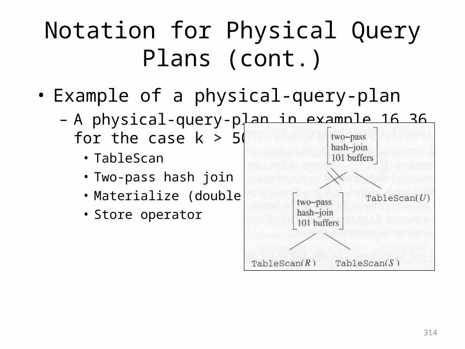
Notation for Physical Query Plans (cont.)
• Example of a physical-query-plan– A physical-query-plan in example 16.36 for the case k >
5000• TableScan• Two-pass hash join• Materialize (double line)• Store operator
314
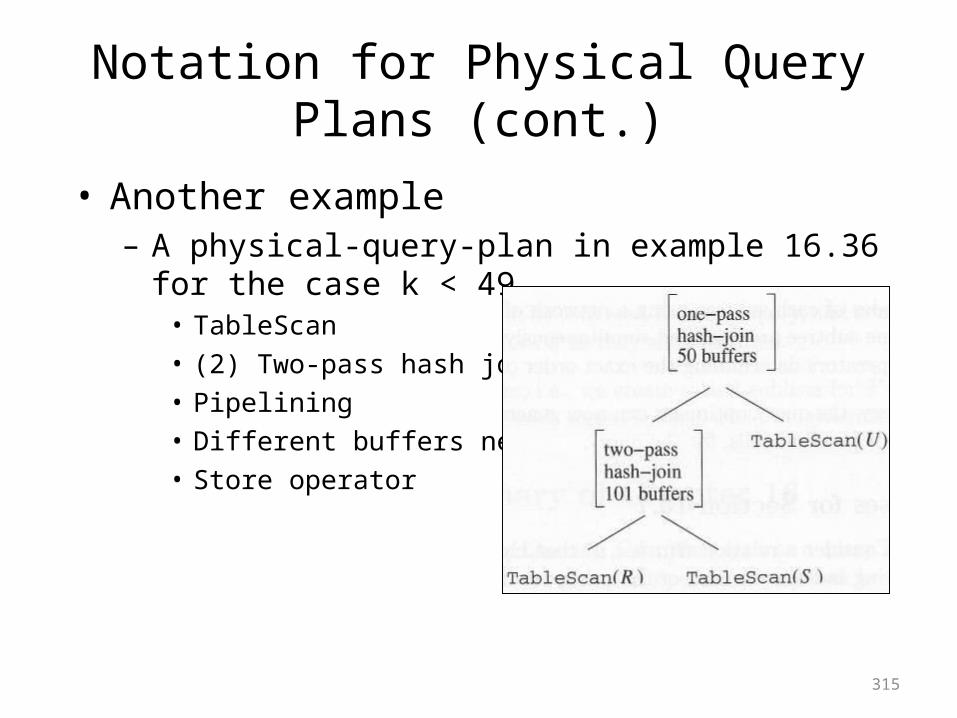
Notation for Physical Query Plans (cont.)
• Another example– A physical-query-plan in example 16.36 for the case k <
49• TableScan• (2) Two-pass hash join• Pipelining• Different buffers needs• Store operator
315
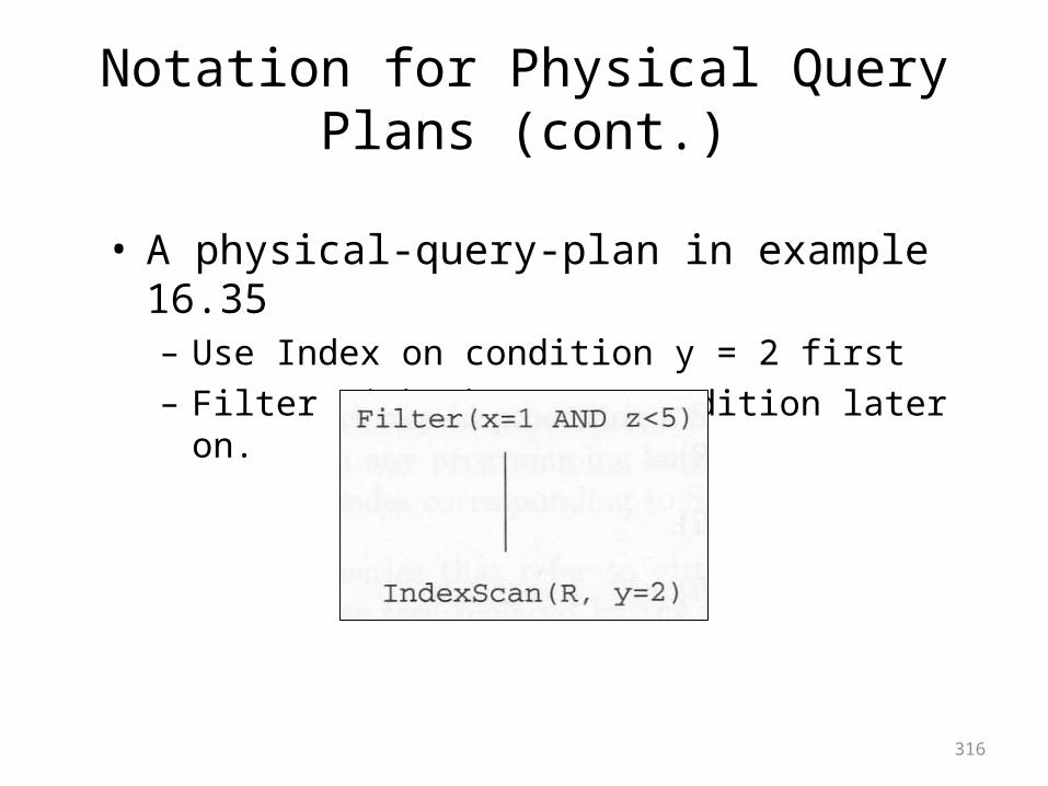
Notation for Physical Query Plans (cont.)
• A physical-query-plan in example 16.35– Use Index on condition y = 2 first– Filter with the rest condition later on.
316
VII. Ordering of Physical Operations
• The PQP is represented as a tree structure implied order of operations.
• Still, the order of evaluation of interior nodes may not always be clear.
– Iterators are used in pipeline manner– Overlapped time of various nodes will make
“ordering” no sense.
317
Ordering of Physical Operations (cont.)
• 3 rules summarize the ordering of events in a PQP tree:
1. Break the tree into sub-trees at each edge that represent materialization. • Execute one subtree at a time.
2. Order the execution of the subtree• Bottom-top• Left-to-right
3. All nodes of each sub-tree are executed simultaneously.
318

Summary of Chapter 16
In this part of the presentation I will talk about the main topics of Chapter 16.
319
320
COMPILATION OF QUERIES• Compilation means turning a query into a
physical query plan, which can be implemented by query engine.
• Steps of query compilation :– Parsing– Semantic checking– Selection of the preferred logical query plan– Generating the best physical plan
321
THE PARSER• The first step of SQL query processing.• Generates a parse tree• Nodes in the parse tree corresponds to the
SQL constructs• Similar to the compiler of a programming
language
322
VIEW EXPANSION• A very critical part of query compilation.• Expands the view references in the query
tree to the actual view.• Provides opportunities for the query
optimization.
323
SEMANTIC CHECKING• Checks the semantics of a SQL query.• Examines a parse tree.• Checks :
– Attributes– Relation names– Types
• Resolves attribute references.
324
CONVERSION TO A LOGICAL QUERY PLAN
• Converts a semantically parsed tree to a algebraic expression.
• Conversion is straightforward but sub queries need to be optimized.
• Two argument selection approach can be used.
325
ALGEBRAIC TRANSFORMATION• All other operations are replaced by a suitable physical operator.• These operators can be given designations that indicate:
– The operation being performed, e.g., join or grouping.– Necessary parameters, e.g., the condition in a theta-join or the list of
elements in a grouping.– A general strategy for the algorithm: sort-based, hash-based, or in
some joins, index-based.– The decision about the number of passes to be used: one-pass, two-
pass, or multi-pass– An anticipated number of buffers the operation will require.
326
Notations for Physical Query Plans
•Materialization would be indicated by a Store operator applied to the intermediate result that is to be materialized, followed by a suitable scan operator when the materialized result is accessed by its consumer.•We shall indicate that a certain intermediate relation is materialized by a double line crossing the edge between that relation and its consumer.•All other edges are assumed to represent pipelining between the supplier and consumer of tuples.•Each operator of the logical plan becomes one or more operators of the physical plan, and leaves (stored relations) of the logical plan become, in the physical plan, one of the scan operators applied to that relation.

327
ESTIMATING SIZES OF RELATIONS• True running time is taken into consideration
when selecting the best logical plan.• Two factors the affects the most in
estimating the sizes of relation : – Size of relations ( No. of tuples ) – No. of distinct values for each attribute of each
relation
• Histograms are used by some systems.
328
COST BASED OPTIMIZING• Best physical query plan represents the least
costly plan.• Factors that decide the cost of a query plan :
– Order and grouping operations like joins, unions and intersections.
– Nested loop and the hash loop joins used.– Scanning and sorting operations.– Storing intermediate results.
329
PLAN ENUMERATION STRATEGIES• Common approaches for searching the space
for best physical plan .– Dynamic programming : Tabularizing the best plan
for each sub expression– Selinger style programming : sort-order the results
as a part of table– Greedy approaches : Making a series of locally
optimal decisions– Branch-and-bound : Starts with enumerating the
worst plans and reach the best plan
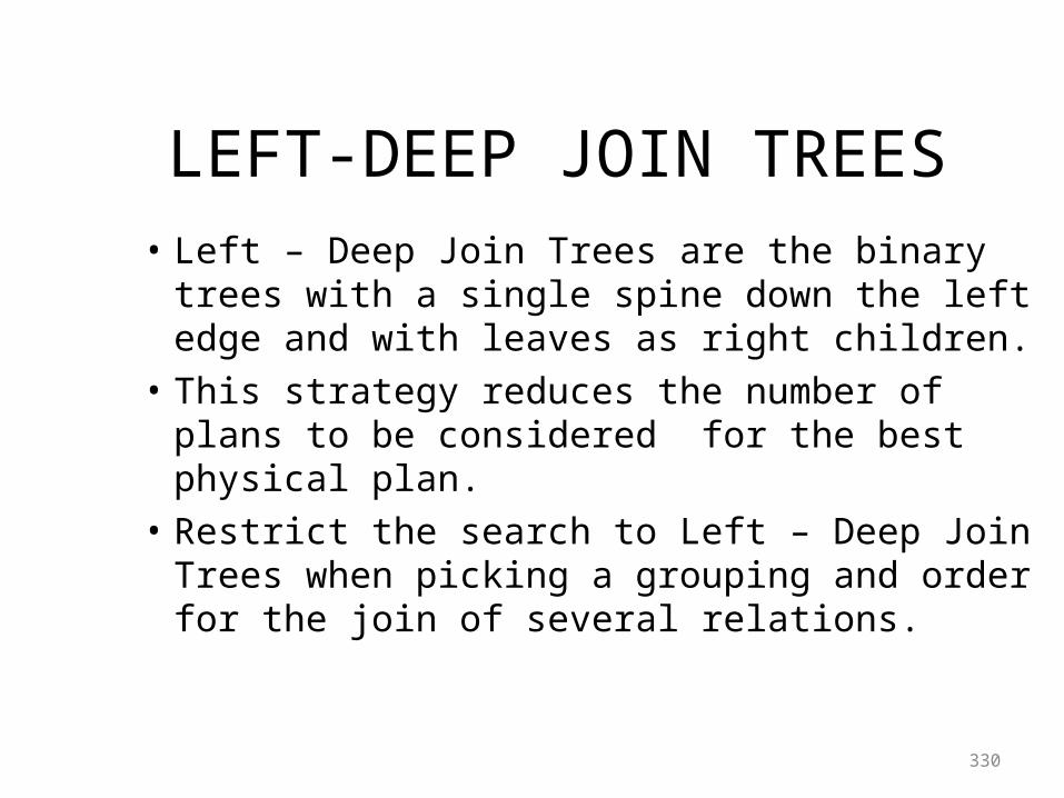
330
LEFT-DEEP JOIN TREES • Left – Deep Join Trees are the binary trees
with a single spine down the left edge and with leaves as right children.
• This strategy reduces the number of plans to be considered for the best physical plan.
• Restrict the search to Left – Deep Join Trees when picking a grouping and order for the join of several relations.

331
PHYSICAL PLANS FOR SELECTION• Breaking a selection into an index-scan of
relation, followed by a filter operation.• The filter then examines the tuples retrieved
by the index-scan.• Allows only those to pass which meet the
portions of selection condition.
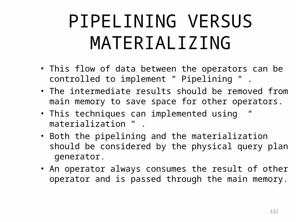
332
PIPELINING VERSUS MATERIALIZING• This flow of data between the operators can be controlled
to implement “ Pipelining “ .• The intermediate results should be removed from main
memory to save space for other operators.• This techniques can implemented using “ materialization “ .• Both the pipelining and the materialization should be
considered by the physical query plan generator.• An operator always consumes the result of other operator
and is passed through the main memory.
THE QUERY COMPILER
Prepared by :Ankit Patel (226)
Query Compilation
• Compilation: Turning a query into a physical query plan, which is to be implemented by query engine.
• The query compilation follows the following steps:– Parsing of data– Semantic checking– Selection of the preferred logical query plan– Generate the best physical plan
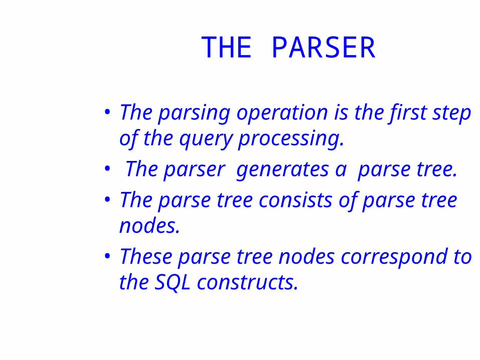
THE PARSER
• The parsing operation is the first step of the query processing.
• The parser generates a parse tree.
• The parse tree consists of parse tree nodes.
• These parse tree nodes correspond to the SQL constructs.
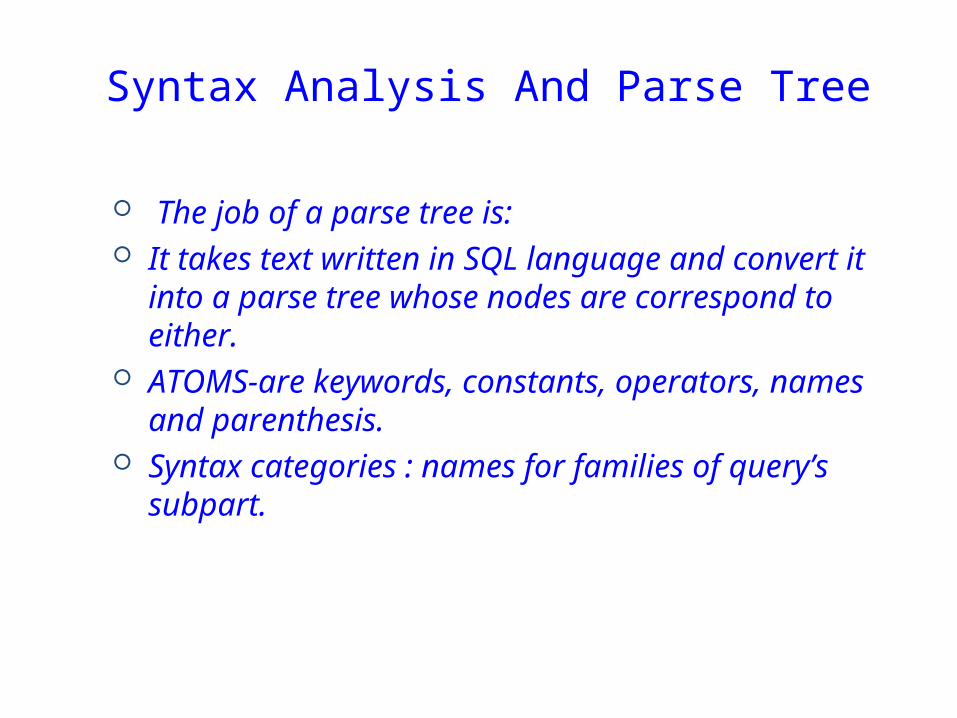
The job of a parse tree is: It takes text written in SQL language and
convert it into a parse tree whose nodes are correspond to either.
ATOMS-are keywords, constants, operators, names and parenthesis.
Syntax categories : names for families of query’s subpart.
Syntax Analysis And Parse Tree
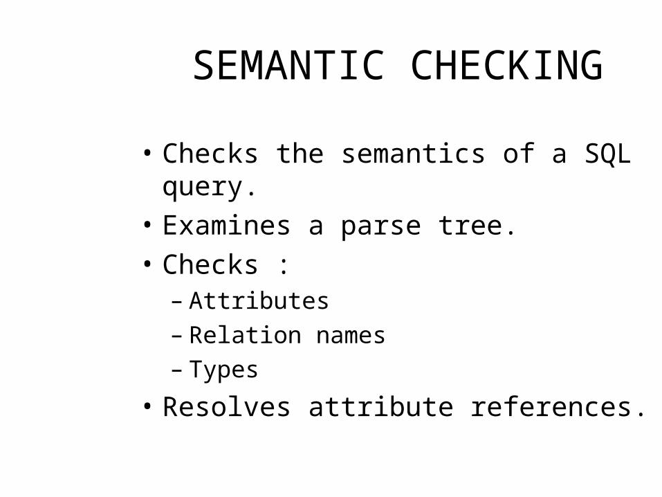
SEMANTIC CHECKING
• Checks the semantics of a SQL query.
• Examines a parse tree.
• Checks :– Attributes
– Relation names
– Types
• Resolves attribute references.
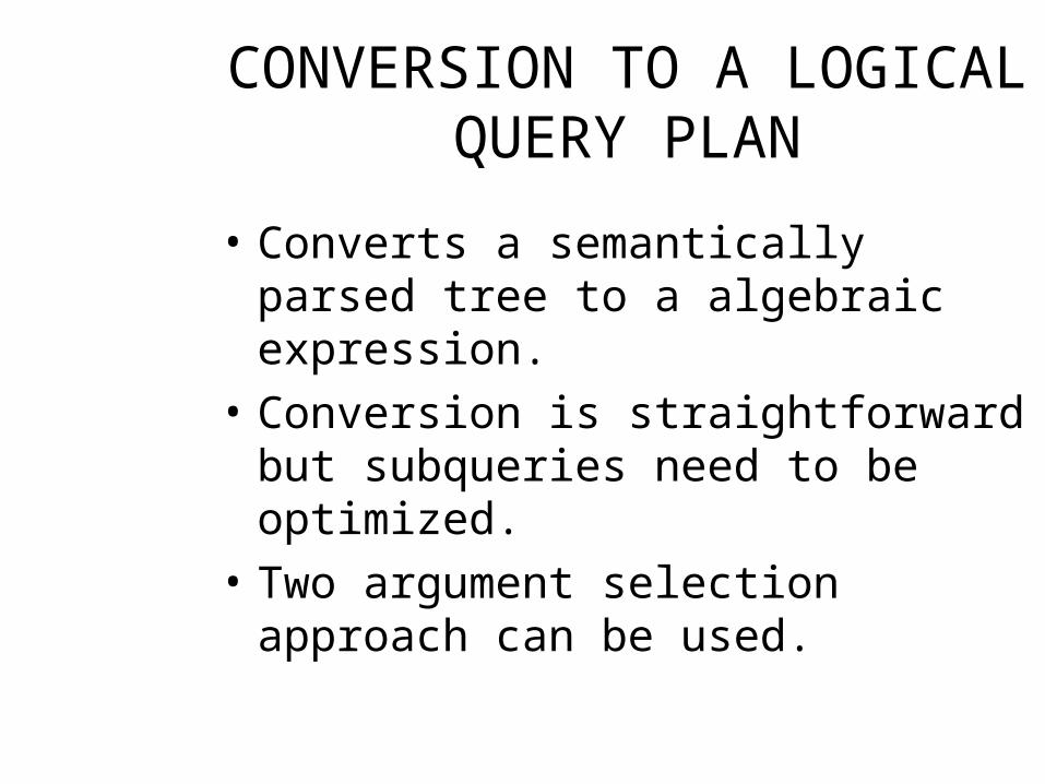
CONVERSION TO A LOGICAL QUERY PLAN
• Converts a semantically parsed tree to a algebraic expression.
• Conversion is straightforward but subqueries need to be optimized.
• Two argument selection approach can be used.
ALGEBRAIC TRANSFORMATION
• Many different ways to transform a logical query plan to an actual plan using algebraic transformations.
• The laws used for this transformation :
– Commutative and associative laws
– Laws involving selection
– Pushing selection
– Laws involving projection
– Laws about joins and products
– Laws involving duplicate eliminations
– Laws involving grouping and aggregation
ESTIMATING SIZES OF RELATIONS
• While estimating the sizes of relation the following are taken into consideration :
– Size of relations ( No. of tuples )
– No. of distinct values for each attribute of each relation
• The best logical plan takes the true running time is taken into consideration.
• Histograms are also known to be used by some systems.
COST BASED OPTIMIZING
• Best physical query plan represents the least costly plan.
• Factors that decide the cost of a query plan :– Order and grouping operations like joins,unions
and intersections.
– Nested loop and the hash loop joins used.
– Scanning and sorting operations.
– Storing intermediate results.
PLAN SEARCH STRATEGIES
– Dynamic programming : This method tabularises the best plan for each sub expression.
– Branch-and-bound : Back tracks with enumerating the worst plans to reach the best plan
– Selinger style programming : sort-order the results as a part of table
– Greedy approaches : This approach makes a series of optimal decisions.
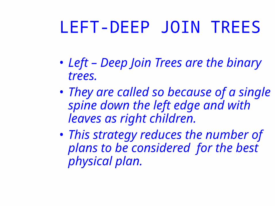
LEFT-DEEP JOIN TREES
• Left – Deep Join Trees are the binary trees.
• They are called so because of a single spine down the left edge and with leaves as right children.
• This strategy reduces the number of plans to be considered for the best physical plan.

PHYSICAL PLANS FOR SELECTION
• Breaking a selection into an index-scan of relation, followed by a filter operation.
• The filter then examines the tuples retrieved by the index-scan.
• Allows only those to pass which meet the portions of selection condition.
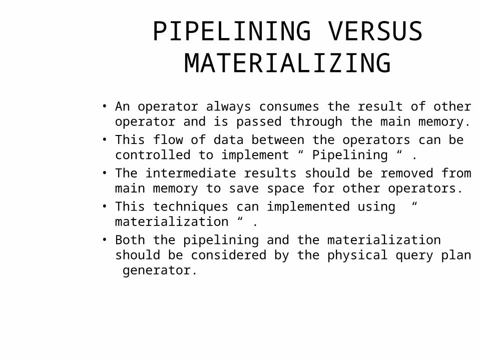
PIPELINING VERSUS MATERIALIZING
• An operator always consumes the result of other operator and is passed through the main memory.
• This flow of data between the operators can be controlled to implement “ Pipelining “ .
• The intermediate results should be removed from main memory to save space for other operators.
• This techniques can implemented using “ materialization “ .
• Both the pipelining and the materialization should be considered by the physical query plan generator.
Concurrency Control18.1 – 18.2
Chiu Luk CS257 Database Systems Principles
Spring 2009
Concurrency Control
• Concurrency control in database management systems (DBMS) ensures that database transactions are performed without the concurrency violating the data integrity of a database.
• Executed transactions should follow the ACID rules. • The DBMS must guarantee that only serializable recoverable schedules
are generated. • It also guarantees that no effect of committed transactions is lost, and
no effect of aborted (rolled back) transactions remains in the related database.
ACID rules
Atomicity –The transaction appears to be atomic..
Consistency – Every transaction leaves the system in a consistent state.
Isolation - Providing isolation is the main goal of concurrency control.
Durability - The transactions should persist crashes
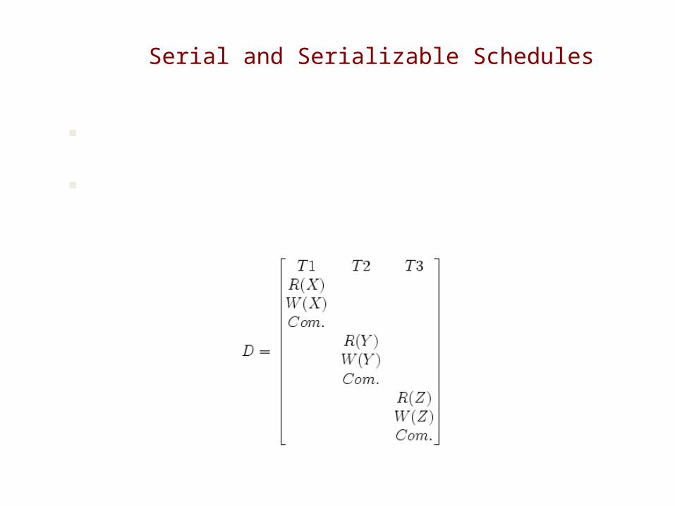
Serial and Serializable Schedules
In the field of databases, a schedule is a list of actions, (i.e. reading, writing, aborting, committing), from a set of transactions. In this example, Schedule D is the set of 3 transactions T1, T2, T3. The schedule describes the actions of the transactions as seen by the DBMS. T1 Reads and writes to object X, and then T2 Reads and writes to object Y, and finally T3 Reads and writes to object Z. This is an example of a serial schedule, because the actions of the 3 transactions are not interleaved.
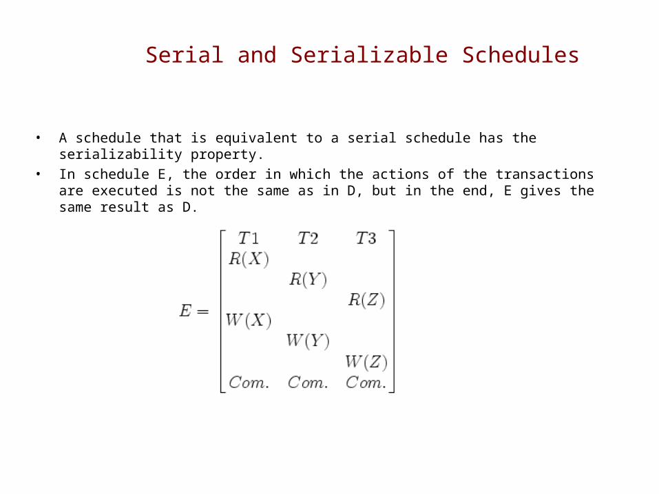
Serial and Serializable Schedules
• A schedule that is equivalent to a serial schedule has the serializability property.• In schedule E, the order in which the actions of the transactions are executed is not the same as in D,
but in the end, E gives the same result as D.
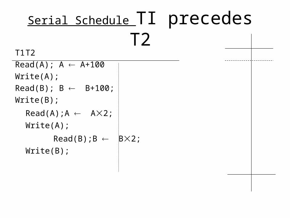
Serial Schedule TI precedes T2T1 T2Read(A); A A+100Write(A);Read(B); B B+100;Write(B);
Read(A);A A2;Write(A);
Read(B);B B2;Write(B);
A B25 25
125
125
250
250250 250
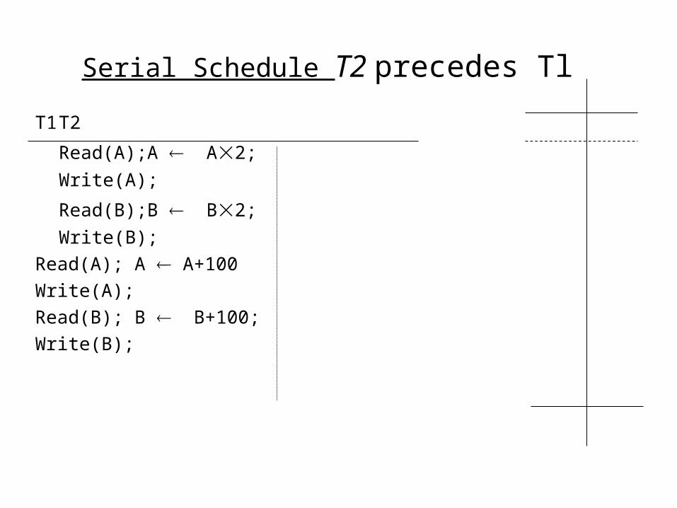
Serial Schedule T2 precedes Tl
T1 T2
Read(A);A A2;Write(A);
Read(B);B B2;Write(B);
Read(A); A A+100Write(A);Read(B); B B+100;Write(B);
A B25 25
50
50
150
150150 150
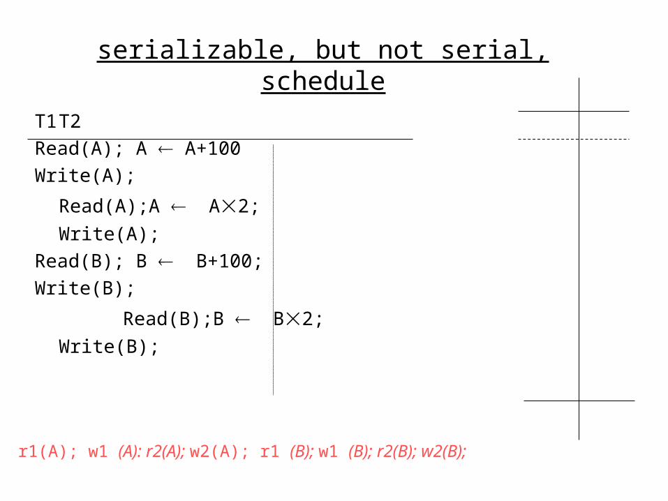
serializable, but not serial, schedule
T1 T2Read(A); A A+100Write(A);
Read(A);A A2;Write(A);
Read(B); B B+100;Write(B);
Read(B);B B2;Write(B);
A B25 25
125
250
125
250250 250
r1(A); w1 (A): r2(A); w2(A); r1 (B); w1 (B); r2(B); w2(B);
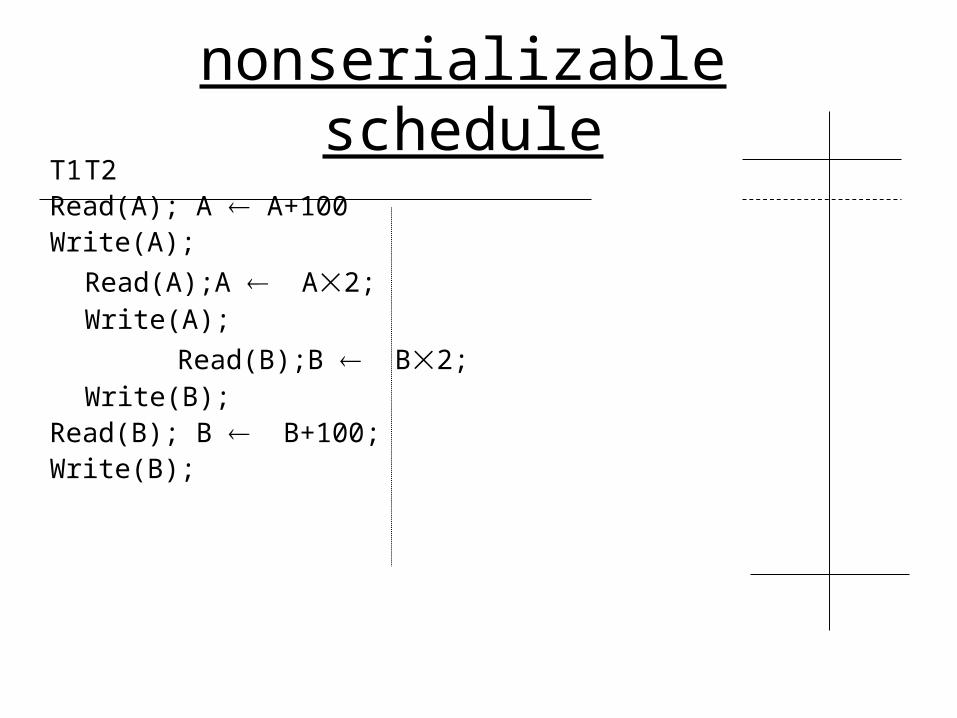
nonserializable scheduleT1 T2Read(A); A A+100Write(A);
Read(A);A A2;Write(A);
Read(B);B B2;Write(B);
Read(B); B B+100;Write(B);
A B25 25
125
250
50
150250 150
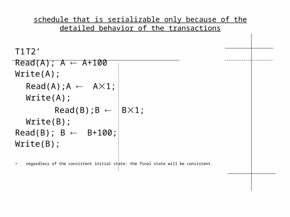
schedule that is serializable only because of the detailed behavior of the transactions
T1 T2’Read(A); A A+100Write(A);
Read(A);A A1;Write(A);
Read(B);B B1;Write(B);
Read(B); B B+100;Write(B);
• regardless of the consistent initial state: the final state will be consistent.
A B25 25
125
125
25
125125 125
Non-Conflicting Actions
Two actions are non-conflicting if whenever theyoccur consecutively in a schedule, swapping themdoes not affect the final state produced by theschedule. Otherwise, they are conflicting.
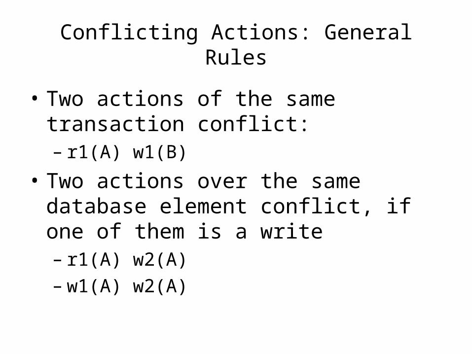
Conflicting Actions: General Rules
• Two actions of the same transaction conflict:– r1(A) w1(B)
• Two actions over the same database element conflict, if one of them is a write– r1(A) w2(A)– w1(A) w2(A)
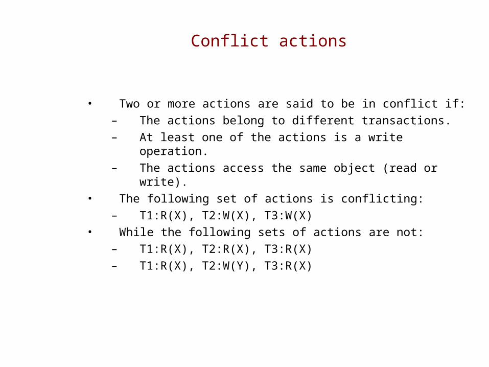
Conflict actions
• Two or more actions are said to be in conflict if:– The actions belong to different transactions. – At least one of the actions is a write operation. – The actions access the same object (read or write).
• The following set of actions is conflicting:– T1:R(X), T2:W(X), T3:W(X)
• While the following sets of actions are not:– T1:R(X), T2:R(X), T3:R(X) – T1:R(X), T2:W(Y), T3:R(X)
Conflict Serializable
We may take any schedule and make as many nonconflicting swaps as we wish.
With the goal of turning the schedule into a serial schedule.
If we can do so, then the original schedule is serializable, because its effect on the database state remains the same as we perform each of the nonconflictingswaps.
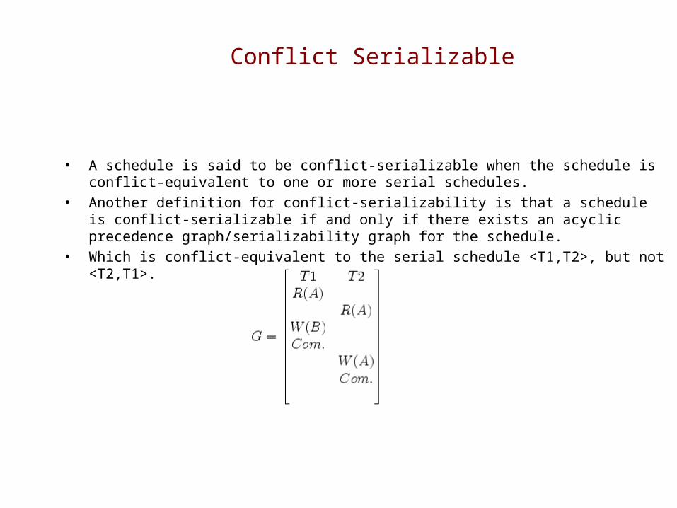
Conflict Serializable
• A schedule is said to be conflict-serializable when the schedule is conflict-equivalent to one or more serial schedules.
• Another definition for conflict-serializability is that a schedule is conflict-serializable if and only if there exists an acyclic precedence graph/serializability graph for the schedule.
• Which is conflict-equivalent to the serial schedule <T1,T2>, but not <T2,T1>.
Conflict equivalent / conflict-serializable
• Let Ai and Aj are consecutive non-conflicting actions that belongs to different transactions. We can swap Ai and Aj without changing the result.
• Two schedules are conflict equivalent if they can be turned one into the other by a sequence of non-conflicting swaps of adjacent actions.
• We shall call a schedule conflict-serializable if it is conflict-equivalent to a serial schedule.
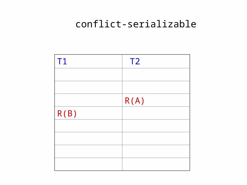
conflict-serializable
T1 T2
R(A)
W(A)
R(A)
R(B)
W(A)
W(B)
R(B)
W(B)
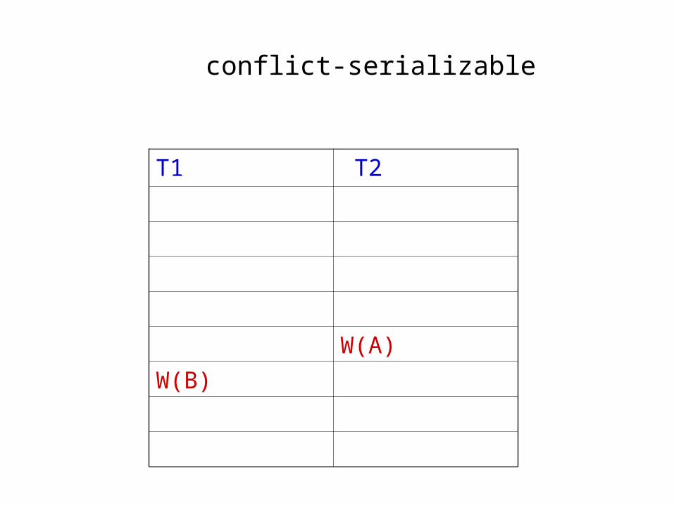
conflict-serializable
T1 T2
R(A)
W(A)
R(B)
R(A)
W(A)
W(B)
R(B)
W(B)
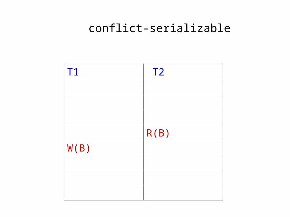
conflict-serializable
T1 T2
R(A)
W(A)
R(A)
R(B)
W(B)
W(A)
R(B)
W(B)
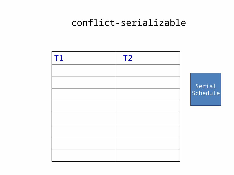
conflict-serializable
T1 T2
R(A)
W(A)
R(A)
W(B)
R(B)
W(A)
R(B)
W(B)
SerialSchedule
Concurrency Control
By Donavon Norwood Ankit Patel
Aniket Mulye
366
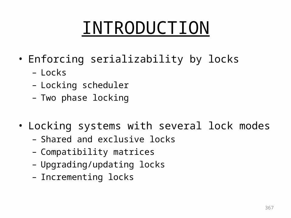
INTRODUCTION
• Enforcing serializability by locks– Locks– Locking scheduler– Two phase locking
• Locking systems with several lock modes– Shared and exclusive locks– Compatibility matrices– Upgrading/updating locks– Incrementing locks
367
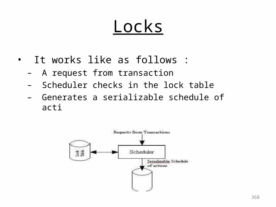
Locks
• It works like as follows : – A request from transaction – Scheduler checks in the lock table– Generates a serializable schedule of actions.
368
• The use of locks must be proper in two senses. one applying to the structure of transactions, and the other to tlie structure of schedules.
• 1)Consistency of Transactions• 2)Legality of schedules
369
Consistency of transactions
• Actions and locks must relate each other– Transactions can only read & write only if has a
lock and has not released the lock.– Unlocking an element is compulsory.
• Legality of schedules– No two transactions can aquire the lock on same
element without the prior one releasing it.
370
Locking scheduler
• Grants lock requests only if it is in a legal schedule.• Lock table stores the information about current locks
on the elements.
371
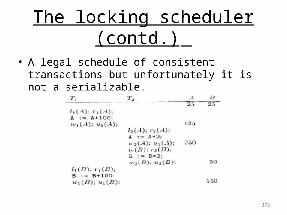
The locking scheduler (contd.)
• A legal schedule of consistent transactions but unfortunately it is not a serializable.
372
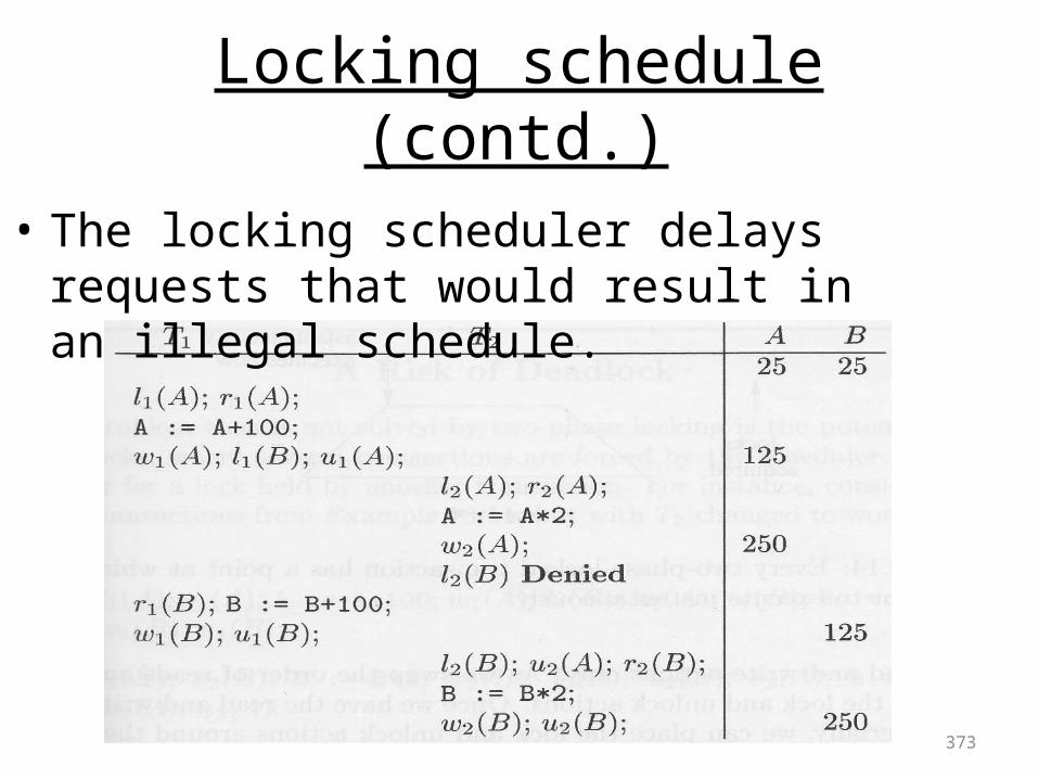
Locking schedule (contd.)
373
• The locking scheduler delays requests that would result in an illegal schedule.
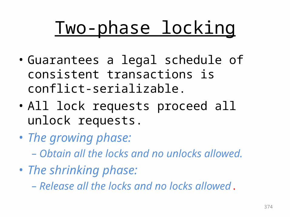
Two-phase locking
• Guarantees a legal schedule of consistent transactions is conflict-serializable.
• All lock requests proceed all unlock requests.• The growing phase:
– Obtain all the locks and no unlocks allowed.
• The shrinking phase:– Release all the locks and no locks allowed.
374
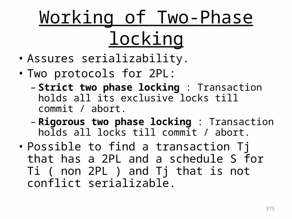
Working of Two-Phase locking
• Assures serializability.• Two protocols for 2PL:
– Strict two phase locking : Transaction holds all its exclusive locks till commit / abort.
– Rigorous two phase locking : Transaction holds all locks till commit / abort.
• Possible to find a transaction Tj that has a 2PL and a schedule S for Ti ( non 2PL ) and Tj that is not conflict serializable.
375
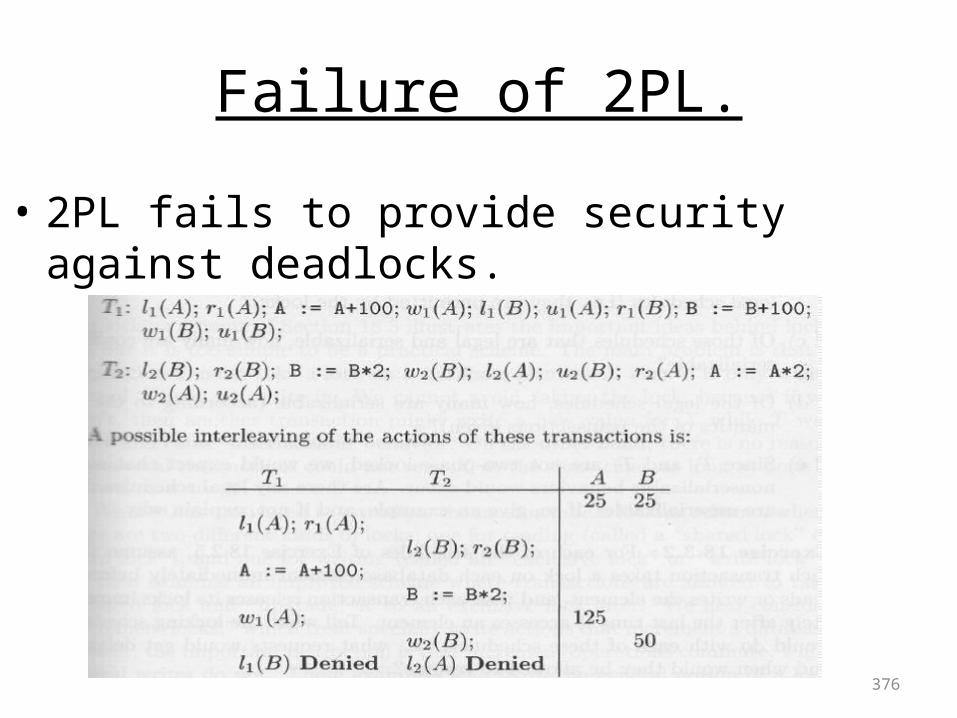
Failure of 2PL.
376
• 2PL fails to provide security against deadlocks.
Locking Systems with Several Lock Modes
• Locking Scheme– Shared/Read Lock ( For Reading)– Exclusive/Write Lock( For Writing)
• Compatibility Matrices• Upgrading Locks• Update Locks• Increment Locks
377
Shared & Exclusive Locks
• Consistency of Transactions– Cannot write without Exclusive Lock– Cannot read without holding some lock
• This basically works on 2 principles– A read action can only proceed a shared or an exclusive
lock– A write lock can only proceed a exclusice lock
• All locks need to be unlocked before commit
378
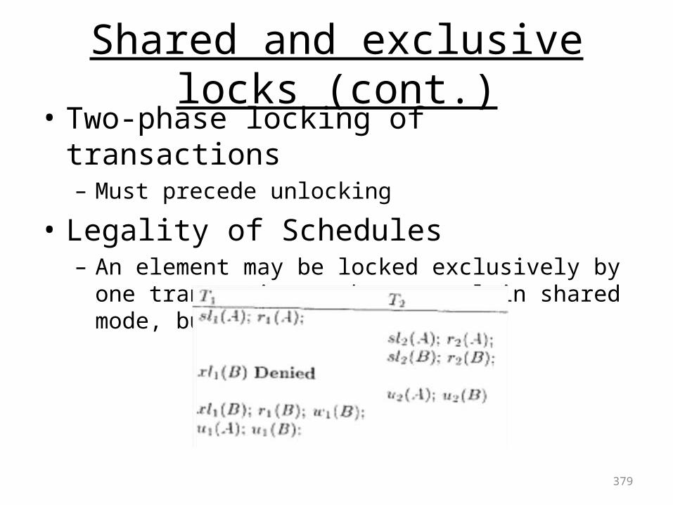
Shared and exclusive locks (cont.)• Two-phase locking of transactions
– Must precede unlocking
• Legality of Schedules– An element may be locked exclusively by one transaction or
by several in shared mode, but not both.
379
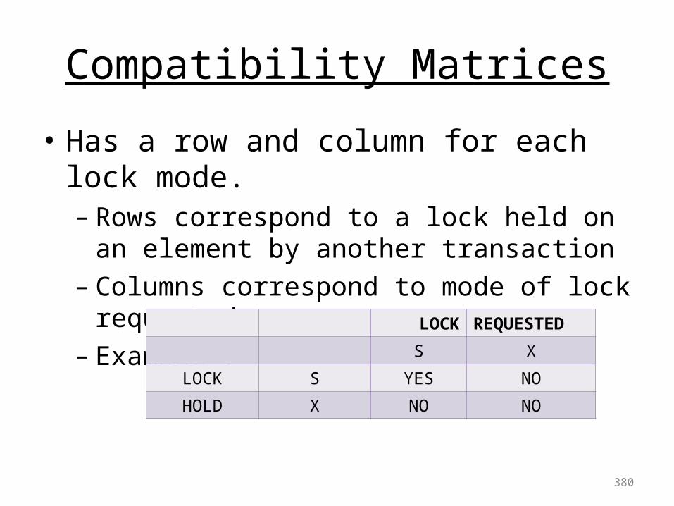
Compatibility Matrices
• Has a row and column for each lock mode.– Rows correspond to a lock held on an element by
another transaction– Columns correspond to mode of lock requested.– Example :
380
LOCK REQUESTED
S X
LOCK S YES NO
HOLD X NO NO
Upgrading Locks
• Suppose a transaction wants to read as well as write : – It aquires a shared lock on the element– Performs the calculations on the element– And when its ready to write, It is granted a
exclusive lock.
• Transactions with unpredicted read write locks can use UPGRADING LOCKS.
381
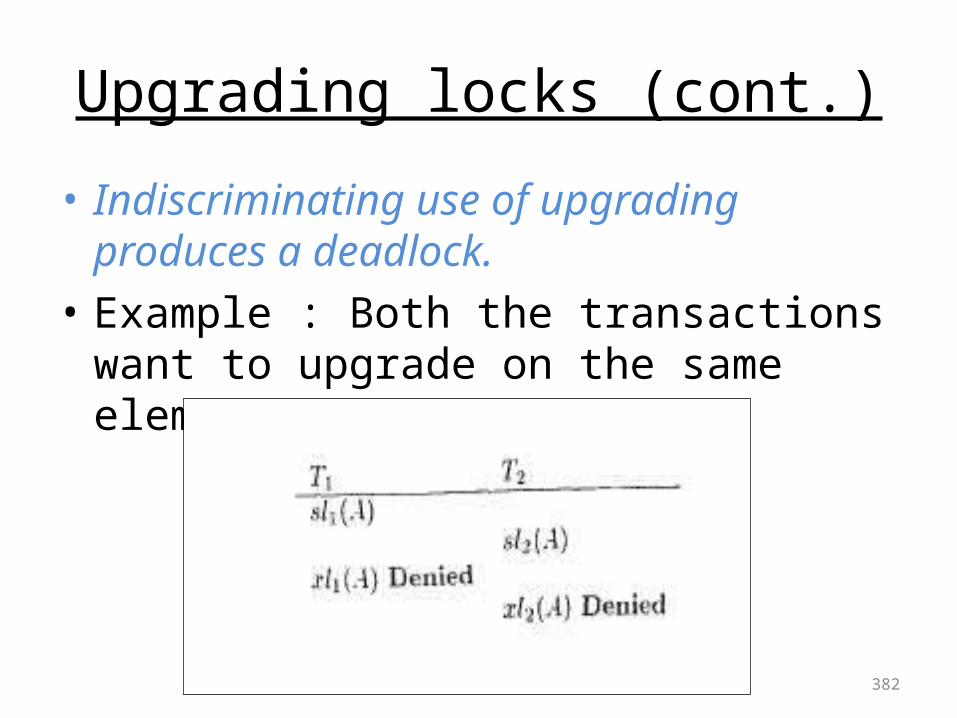
Upgrading locks (cont.)
• Indiscriminating use of upgrading produces a deadlock.
• Example : Both the transactions want to upgrade on the same element
382
Update locks
• Solves the deadlock occurring in upgrade lock method.
• A transaction in an update lock can read but cant write.
• Update lock can later be converted to exclusive lock.
• An update lock can only be given if the element has shared locks.
383
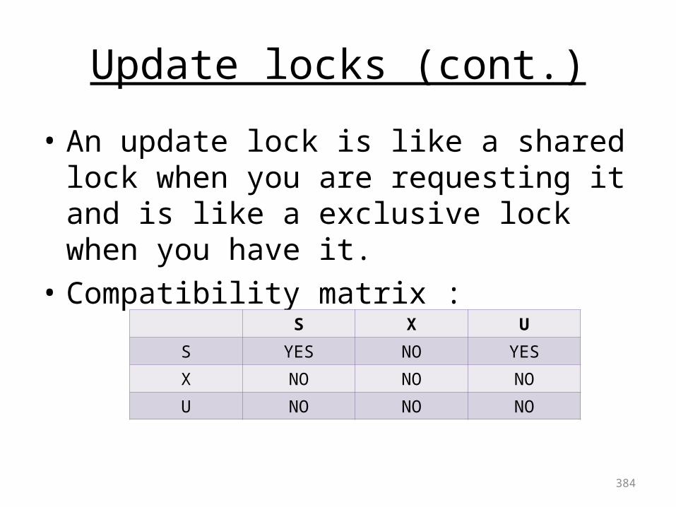
Update locks (cont.)
• An update lock is like a shared lock when you are requesting it and is like a exclusive lock when you have it.
• Compatibility matrix :
384
S X U
S YES NO YES
X NO NO NO
U NO NO NO
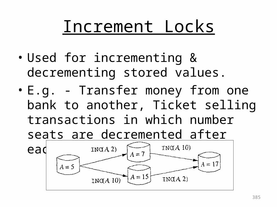
Increment Locks
• Used for incrementing & decrementing stored values.
• E.g. - Transfer money from one bank to another, Ticket selling transactions in which number seats are decremented after each transaction.
385
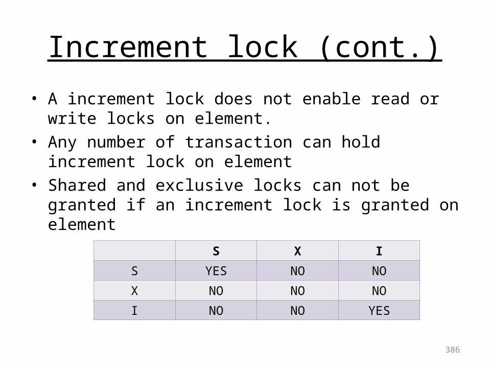
Increment lock (cont.)
• A increment lock does not enable read or write locks on element.
• Any number of transaction can hold increment lock on element
• Shared and exclusive locks can not be granted if an increment lock is granted on element
386
S X I
S YES NO NO
X NO NO NO
I NO NO YES
Concurrency Control
Managing Hierarchies of Database Elements (18.6)
387
Presented byRonak Shah
(214)
March 9, 2009
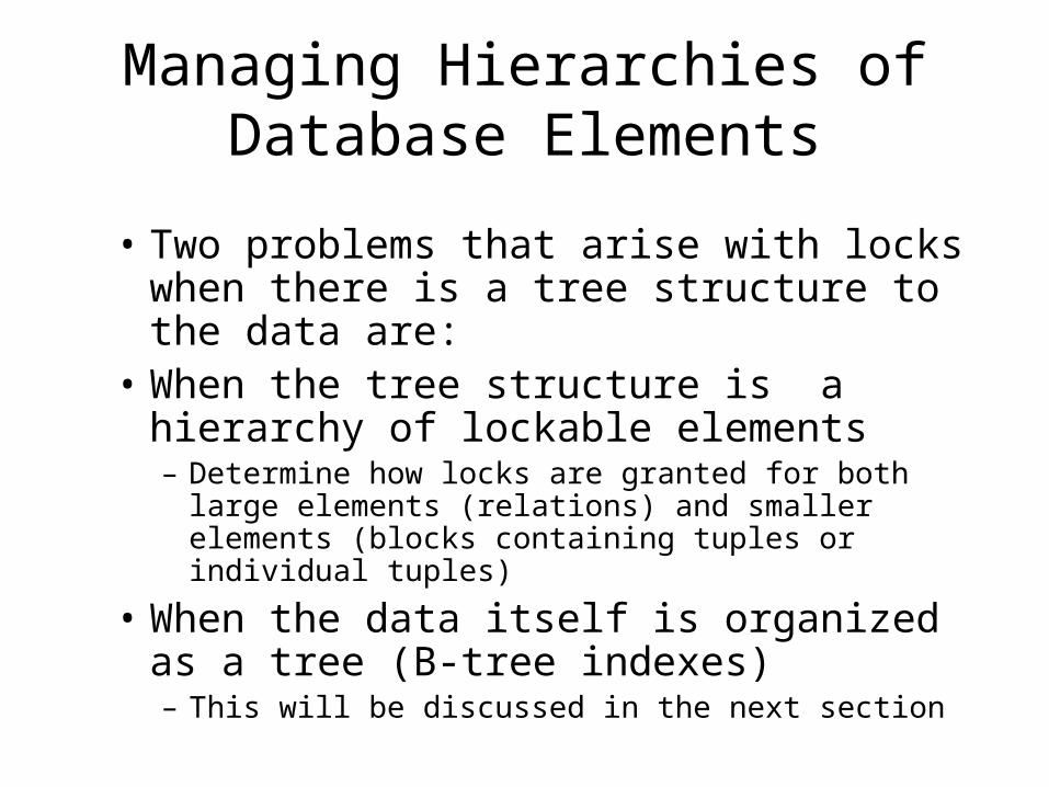
Managing Hierarchies of Database Elements
• Two problems that arise with locks when there is a tree structure to the data are:
• When the tree structure is a hierarchy of lockable elements– Determine how locks are granted for both large
elements (relations) and smaller elements (blocks containing tuples or individual tuples)
• When the data itself is organized as a tree (B-tree indexes)– This will be discussed in the next section
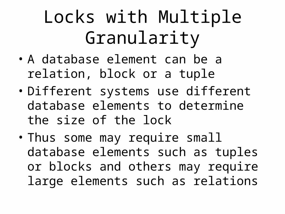
Locks with Multiple Granularity
• A database element can be a relation, block or a tuple
• Different systems use different database elements to determine the size of the lock
• Thus some may require small database elements such as tuples or blocks and others may require large elements such as relations
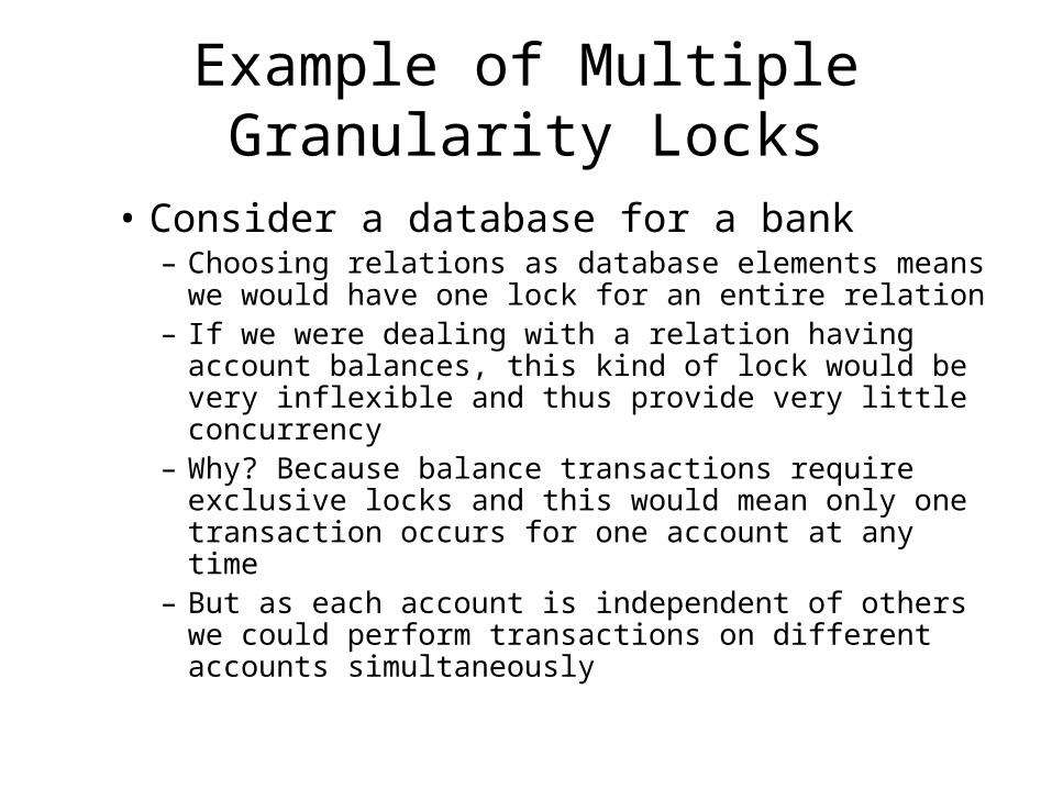
Example of Multiple Granularity Locks
• Consider a database for a bank– Choosing relations as database elements means we
would have one lock for an entire relation– If we were dealing with a relation having account
balances, this kind of lock would be very inflexible and thus provide very little concurrency
– Why? Because balance transactions require exclusive locks and this would mean only one transaction occurs for one account at any time
– But as each account is independent of others we could perform transactions on different accounts simultaneously
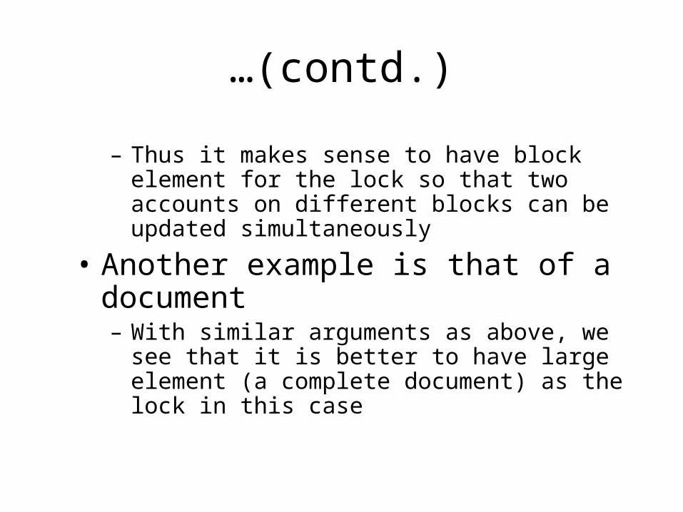
…(contd.)
– Thus it makes sense to have block element for the lock so that two accounts on different blocks can be updated simultaneously
• Another example is that of a document– With similar arguments as above, we see that it is
better to have large element (a complete document) as the lock in this case
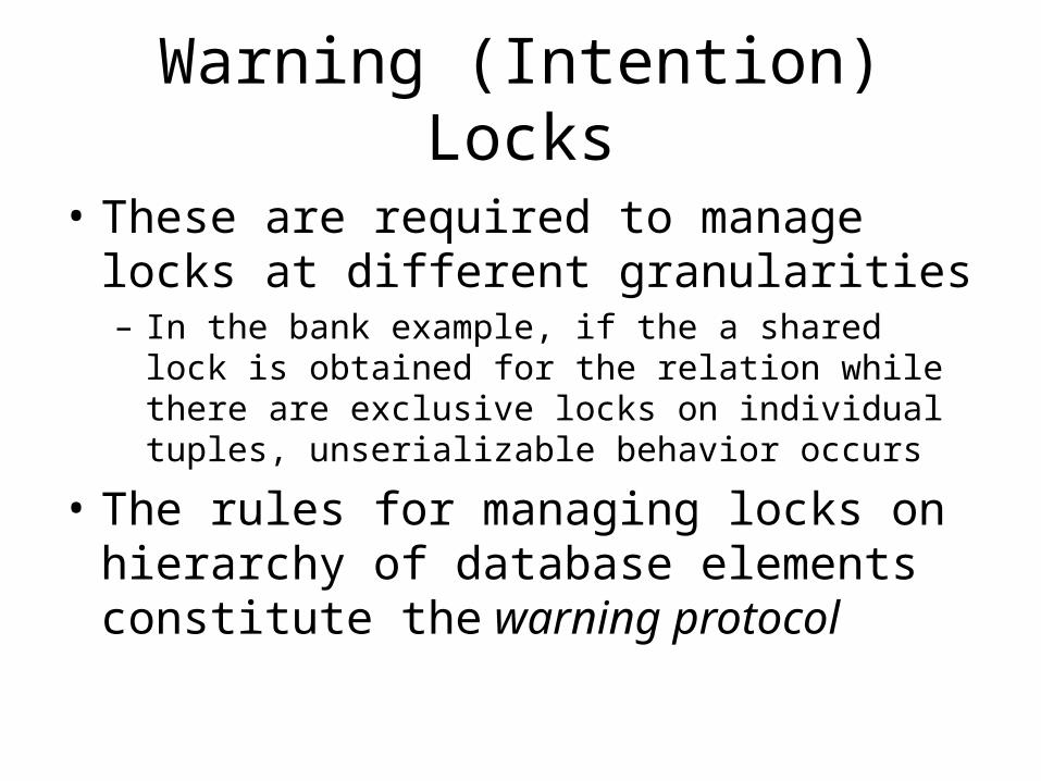
Warning (Intention) Locks
• These are required to manage locks at different granularities– In the bank example, if the a shared lock is obtained for
the relation while there are exclusive locks on individual tuples, unserializable behavior occurs
• The rules for managing locks on hierarchy of database elements constitute the warning protocol
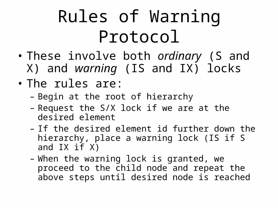
Rules of Warning Protocol
• These involve both ordinary (S and X) and warning (IS and IX) locks
• The rules are:– Begin at the root of hierarchy– Request the S/X lock if we are at the desired element– If the desired element id further down the hierarchy, place
a warning lock (IS if S and IX if X)– When the warning lock is granted, we proceed to the child
node and repeat the above steps until desired node is reached
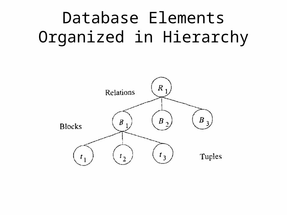
Database Elements Organized in Hierarchy
Compatibility Matrix for Shared, Exclusive and Intention Locks
IS IX S X
IS Yes Yes Yes No
IX Yes Yes No No
S Yes No Yes No
X No No No No
• The above matrix applies only to locks held by other transactions
Group Modes of Intention Locks
• An element can request S and IX locks at the same time if they are in the same transaction (to read entire element and then modify sub elements)
• This can be considered as another lock mode, SIX, having restrictions of both the locks i.e. No for all except IS
• SIX serves as the group mode
Example
• Consider a transaction T1 as follows– Select * from table where attribute1 = ‘abc’– Here, IS lock is first acquired on the entire relation; then
moving to individual tuples (attribute = ‘abc’), S lock in acquired on each of them
• Consider another transaction T2– Update table set attribute2 = ‘def’ where attribute1 = ‘ghi’– Here, it requires an IX lock on relation and since T1’s IS lock
is compatible, IX is granted
– On reaching the desired tuple (ghi), as there is no lock, it gets X too
– If T2 was updating the same tuple as T1, it would have to wait until T1 released its S lock
Phantoms and Handling Insertions Correctly
• This arises when transactions create new sub elements of lockable elements
• Since we can lock only existing elements the new elements fail to be locked
• The problem created in this situation is explained in the following example
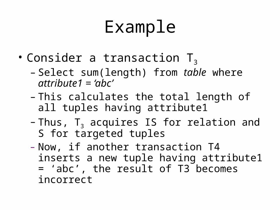
Example
• Consider a transaction T3
– Select sum(length) from table where attribute1 = ‘abc’
– This calculates the total length of all tuples having attribute1
– Thus, T3 acquires IS for relation and S for targeted tuples
– Now, if another transaction T4 inserts a new tuple having attribute1 = ‘abc’, the result of T3 becomes incorrect
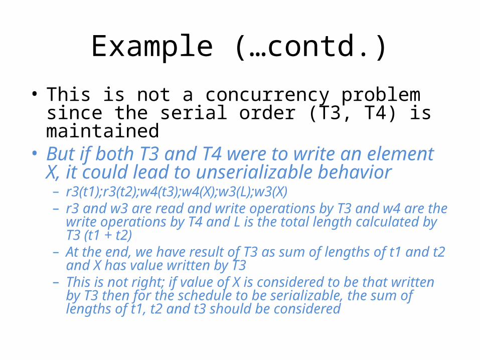
Example (…contd.)• This is not a concurrency problem since the serial
order (T3, T4) is maintained• But if both T3 and T4 were to write an element X,
it could lead to unserializable behavior– r3(t1);r3(t2);w4(t3);w4(X);w3(L);w3(X)– r3 and w3 are read and write operations by T3 and w4 are the
write operations by T4 and L is the total length calculated by T3 (t1 + t2)
– At the end, we have result of T3 as sum of lengths of t1 and t2 and X has value written by T3
– This is not right; if value of X is considered to be that written by T3 then for the schedule to be serializable, the sum of lengths of t1, t2 and t3 should be considered
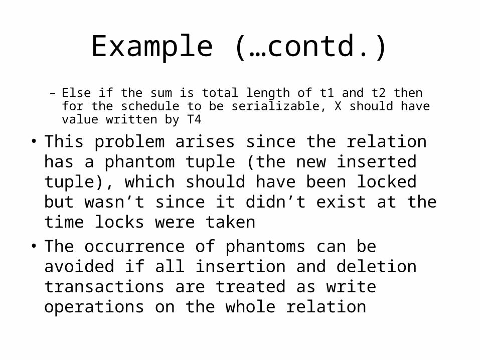
Example (…contd.)– Else if the sum is total length of t1 and t2 then for the schedule
to be serializable, X should have value written by T4
• This problem arises since the relation has a phantom tuple (the new inserted tuple), which should have been locked but wasn’t since it didn’t exist at the time locks were taken
• The occurrence of phantoms can be avoided if all insertion and deletion transactions are treated as write operations on the whole relation

CONCURRENCY CONTROL
SECTION 18.7THE TREE PROTOCOL
By :Saloni Tamotia (215)
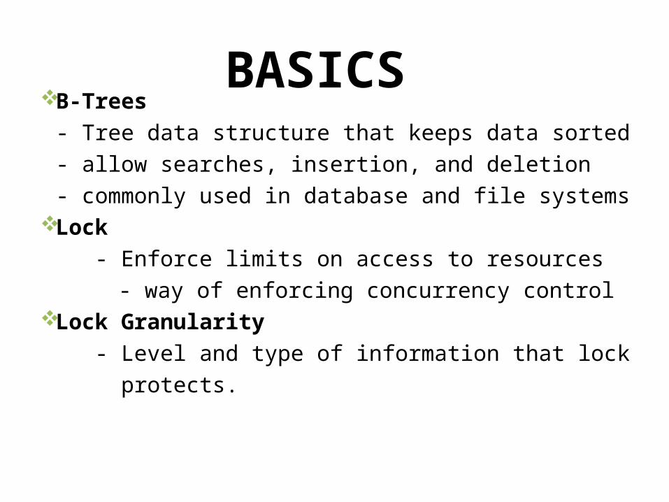
BASICSB-Trees
- Tree data structure that keeps data sorted
- allow searches, insertion, and deletion
- commonly used in database and file systemsLock
- Enforce limits on access to resources
- way of enforcing concurrency controlLock Granularity
- Level and type of information that lock
protects.
• Tree structures that are formed by the link pattern of the elements themselves. Database are the disjoint pieces of data, but the only way to get to Node is through its parent.
• B trees are best example for this sort of data.
• Knowing that we must traverse a particular path to an element give us some important freedom to manage locks differently from two phase locking approaches.
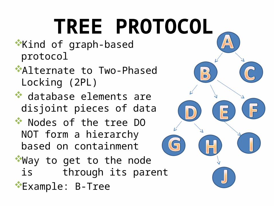
TREE PROTOCOLKind of graph-based protocolAlternate to Two-Phased
Locking (2PL) database elements are disjoint
pieces of data Nodes of the tree DO NOT
form a hierarchy based on containment
Way to get to the node is through its parent
Example: B-Tree
ADVANTAGES OF TREE PROTOCOL
Unlocking takes less time as compared to 2PL
Freedom from deadlocks
Tree Based Locking
• B tree index in a system that treats individual nodes( i.e. blocks) as lockable database elements. The Node Is the right level granularity.
• We use a standard set of locks modes like shared,exculsive, and update locks and we use two phase locking
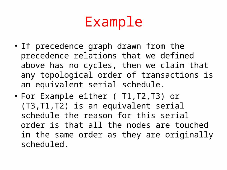
Example
• If precedence graph drawn from the precedence relations that we defined above has no cycles, then we claim that any topological order of transactions is an equivalent serial schedule.
• For Example either ( T1,T2,T3) or (T3,T1,T2) is an equivalent serial schedule the reason for this serial order is that all the nodes are touched in the same order as they are originally scheduled.
• If two transactions lock several elements in common, then they are all locked in same order.
• I am Going to explain this with help of an example.
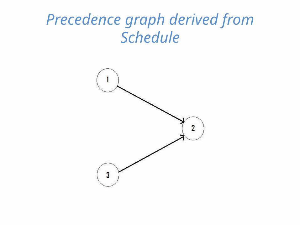
Precedence graph derived from Schedule
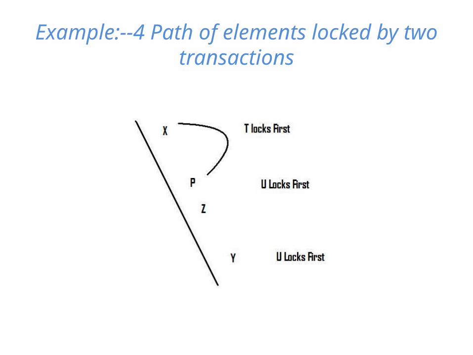
Example:--4 Path of elements locked by two transactions
18.7.1 MOTIVATION FOR TREE-BASED LOCKING
Consider B-Tree Index, treating individual nodes as lockable database elements.
Concurrent use of B-Tree is not possible with standard set of locks and 2PL.
Therefore, a protocol is needed which can assure serializability by allowing access to the elements all the way at the bottom of the tree even if the 2PL is violated.
18.7.1 MOTIVATION FOR TREE-BASED LOCKING (cont.)
Reason for : “Concurrent use of B-Tree is not possible with standard set of locks and 2PL.”
every transaction must begin with locking the root node
2PL transactions can not unlock the root until all the required locks are acquired.
18.7.2 ACCESSING TREE STRUCTURED DATA
Assumptions:
Only one kind of lockConsistent transactionsLegal schedulesNo 2PL requirement on transaction
18.7.2 RULES FOR ACCESSING TREE STRUCTURED DATA
RULES:
First lock can be at any node.Subsequent locks may be acquired only after
parent node has a lock.Nodes may be unlocked any time.No relocking of the nodes even if the node’s
parent is still locked
18.7.3 WHY TREE PROTOCOL WORKS?
Tree protocol implies a serial order on transactions in the schedule.
Order of precedence:
Ti < s TjIf Ti locks the root before Tj, then Ti locks
every node in common with Tj before Tj.
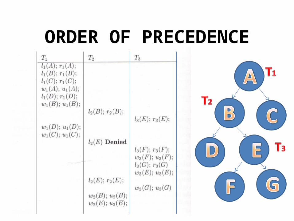
ORDER OF PRECEDENCE
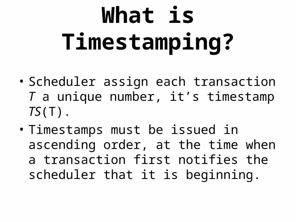
What is Timestamping?
• Scheduler assign each transaction T a unique number, it’s timestamp TS(T).
• Timestamps must be issued in ascending order, at the time when a transaction first notifies the scheduler that it is beginning.
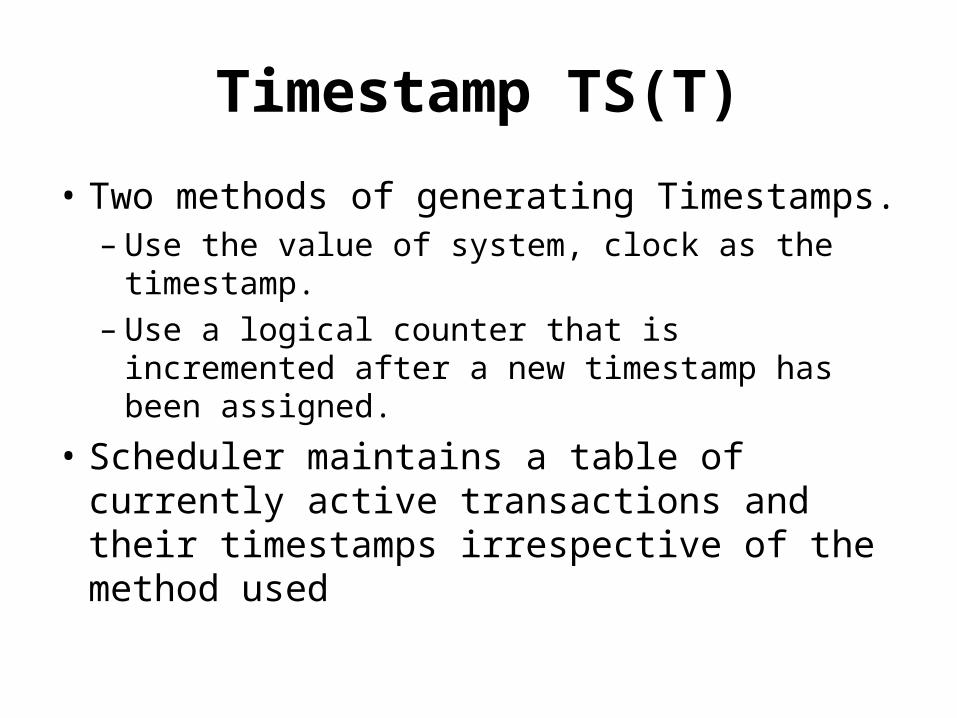
Timestamp TS(T)
• Two methods of generating Timestamps.– Use the value of system, clock as the timestamp.– Use a logical counter that is incremented after a
new timestamp has been assigned.
• Scheduler maintains a table of currently active transactions and their timestamps irrespective of the method used
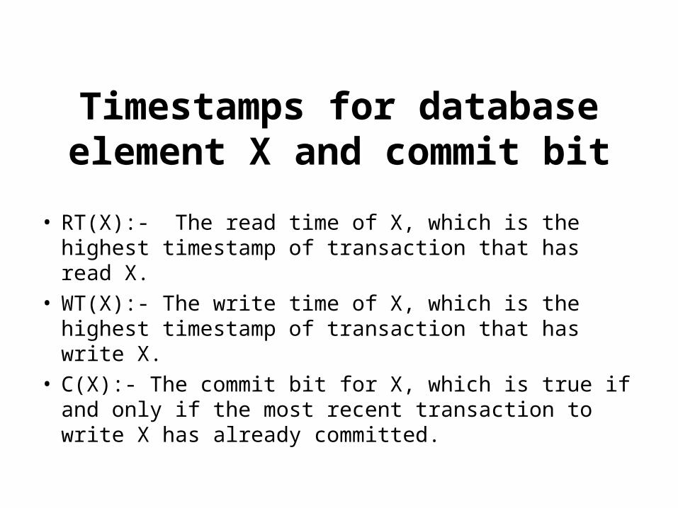
Timestamps for database element X and commit bit
• RT(X):- The read time of X, which is the highest timestamp of transaction that has read X.
• WT(X):- The write time of X, which is the highest timestamp of transaction that has write X.
• C(X):- The commit bit for X, which is true if and only if the most recent transaction to write X has already committed.
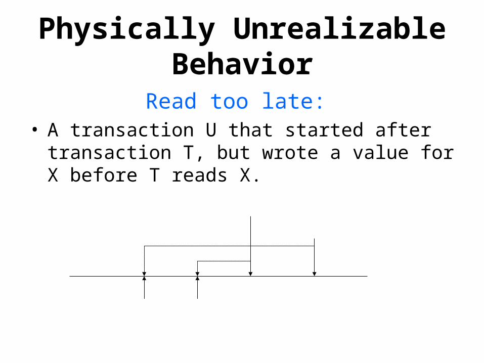
Physically Unrealizable Behavior
Read too late: • A transaction U that started after transaction T, but
wrote a value for X before T reads X.
U writes X
T reads X
T start U start
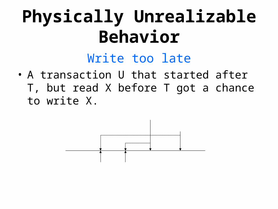
Physically Unrealizable Behavior
Write too late• A transaction U that started after T, but read X before
T got a chance to write X.
U reads X
T writes X
T start U start
Figure: Transaction T tries to write too late
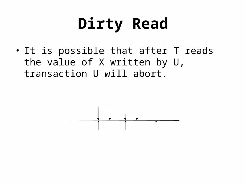
Dirty Read
• It is possible that after T reads the value of X written by U, transaction U will abort.
U writes X
T reads X
U start T start U aborts
T could perform a dirty read if it reads X when shown
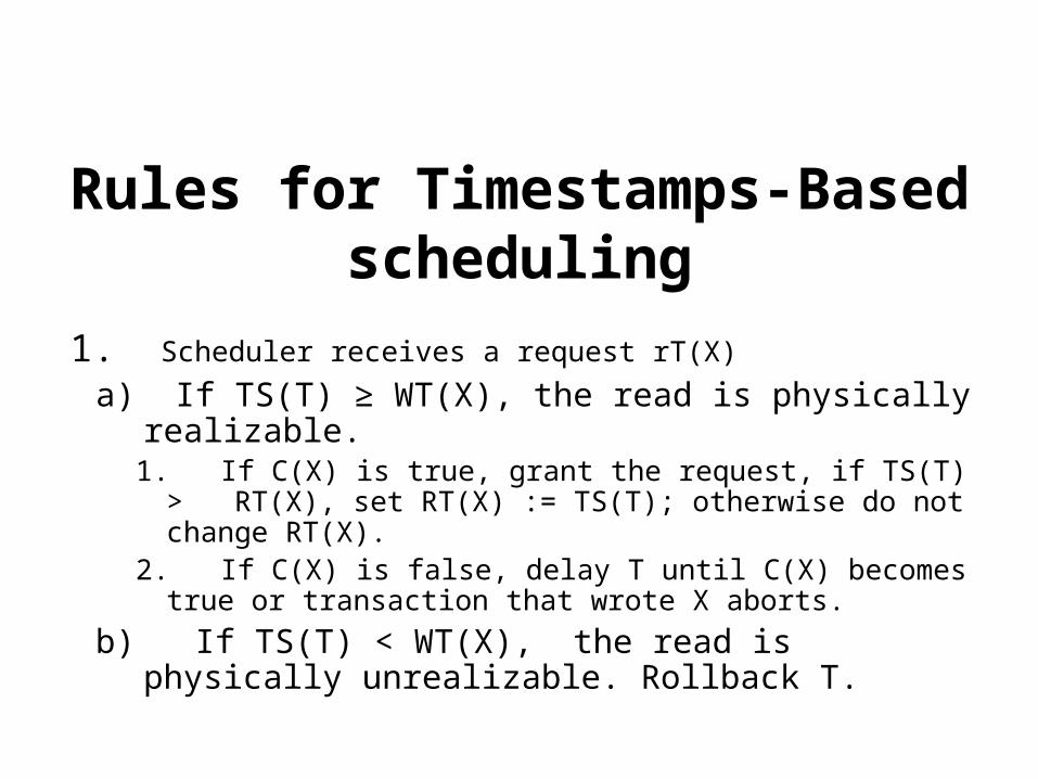
Rules for Timestamps-Based scheduling
1. Scheduler receives a request rT(X)
a) If TS(T) ≥ WT(X), the read is physically realizable. 1. If C(X) is true, grant the request, if TS(T) > RT(X), set
RT(X) := TS(T); otherwise do not change RT(X). 2. If C(X) is false, delay T until C(X) becomes true or
transaction that wrote X aborts.b) If TS(T) < WT(X), the read is physically
unrealizable. Rollback T.
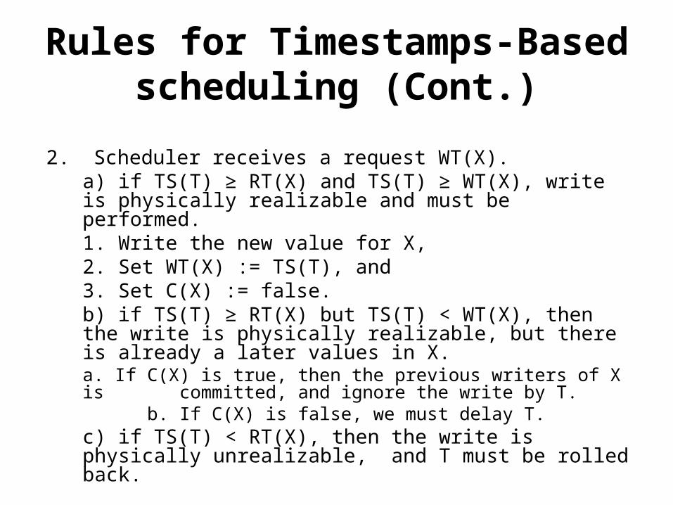
Rules for Timestamps-Based scheduling (Cont.)
2. Scheduler receives a request WT(X).a) if TS(T) ≥ RT(X) and TS(T) ≥ WT(X), write is physically realizable and must be performed.
1. Write the new value for X,2. Set WT(X) := TS(T), and3. Set C(X) := false.
b) if TS(T) ≥ RT(X) but TS(T) < WT(X), then the write is physically realizable, but there is already a later values in X.
a. If C(X) is true, then the previous writers of X is committed, and ignore the write by T.
b. If C(X) is false, we must delay T.c) if TS(T) < RT(X), then the write is physically unrealizable, and T must be rolled back.
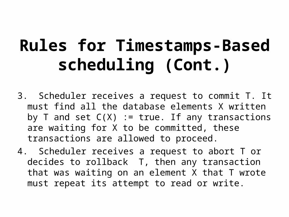
Rules for Timestamps-Based scheduling (Cont.)
3. Scheduler receives a request to commit T. It must find all the database elements X written by T and set C(X) := true. If any transactions are waiting for X to be committed, these transactions are allowed to proceed.
4. Scheduler receives a request to abort T or decides to rollback T, then any transaction that was waiting on an element X that T wrote must repeat its attempt to read or write.
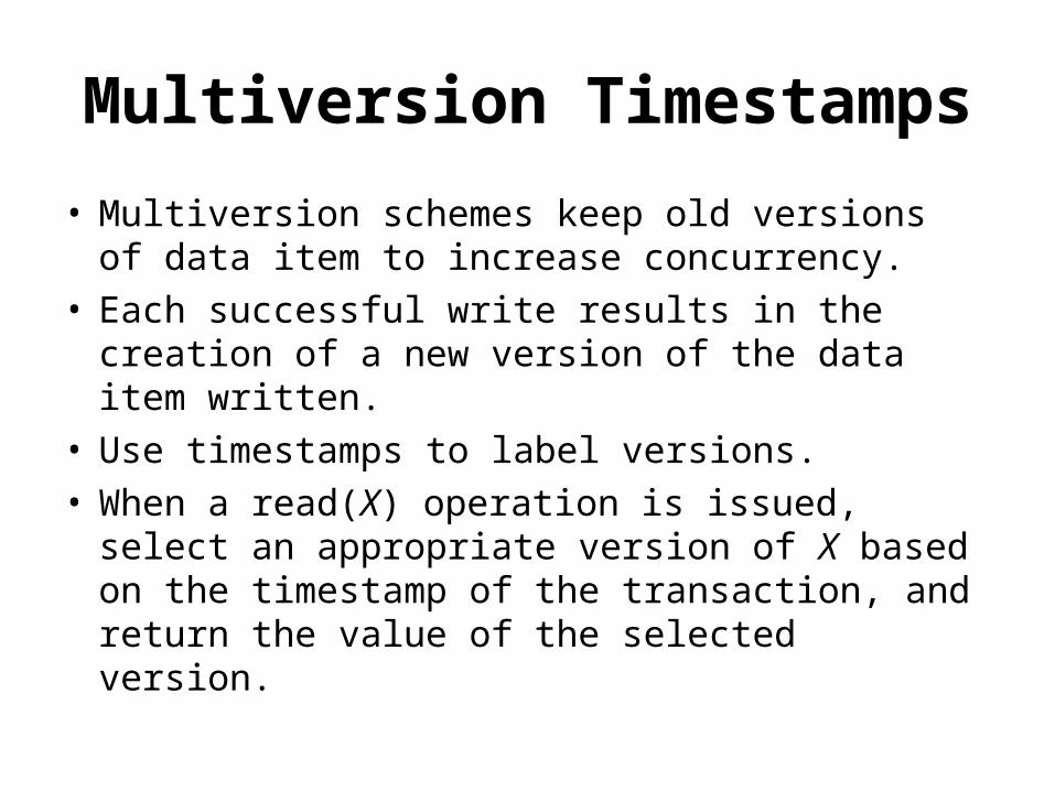
Multiversion Timestamps
• Multiversion schemes keep old versions of data item to increase concurrency.
• Each successful write results in the creation of a new version of the data item written.
• Use timestamps to label versions.• When a read(X) operation is issued, select an
appropriate version of X based on the timestamp of the transaction, and return the value of the selected version.
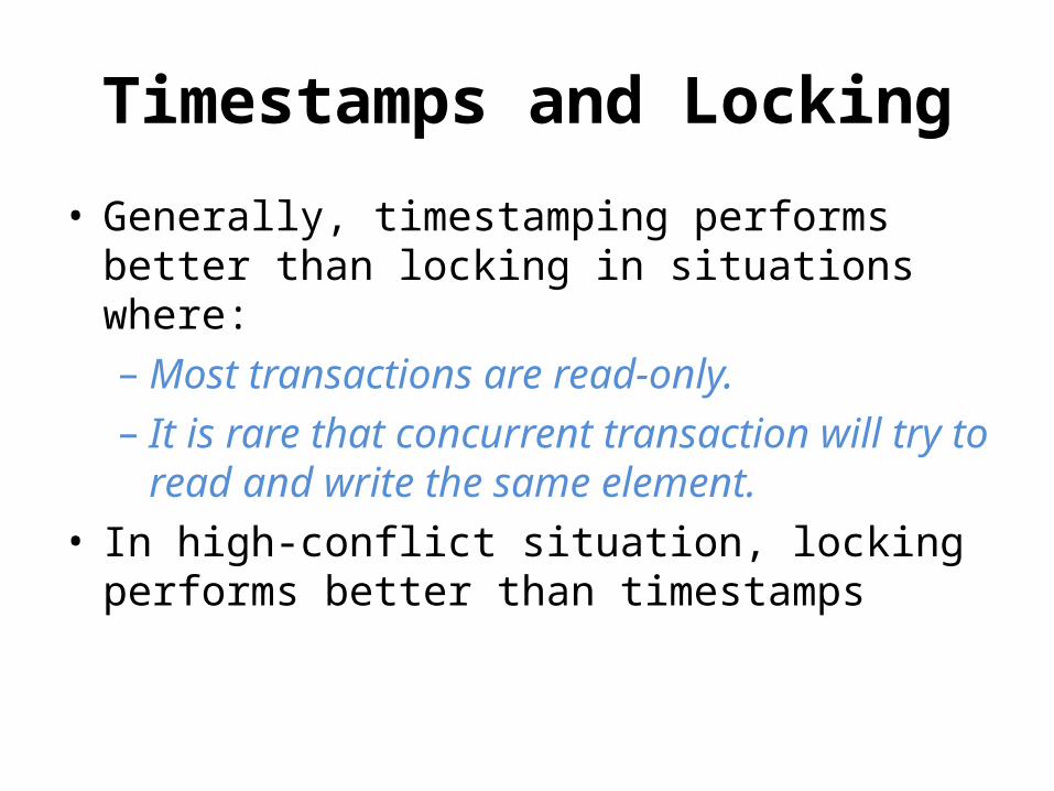
Timestamps and Locking
• Generally, timestamping performs better than locking in situations where:– Most transactions are read-only.– It is rare that concurrent transaction will try to
read and write the same element.• In high-conflict situation, locking performs better
than timestamps
CONCURRENCY CONTROL
SECTION 18.8Timestamps
What is Timestamping?
• Scheduler assign each transaction T a unique number, it’s timestamp TS(T).
• Timestamps must be issued in ascending order, at the time when a transaction first notifies the scheduler that it is beginning.
Timestamp TS(T)
• Two methods of generating Timestamps.– Use the value of system, clock as the timestamp.– Use a logical counter that is incremented after a
new timestamp has been assigned.
• Scheduler maintains a table of currently active transactions and their timestamps irrespective of the method used
Timestamps for database element X and commit bit
• RT(X):- The read time of X, which is the highest timestamp of transaction that has read X.
• WT(X):- The write time of X, which is the highest timestamp of transaction that has write X.
• C(X):- The commit bit for X, which is true if and only if the most recent transaction to write X has already committed.
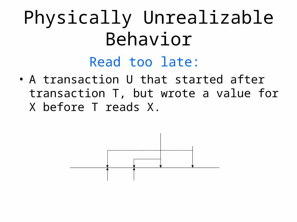
Physically Unrealizable Behavior
Read too late: • A transaction U that started after transaction T, but
wrote a value for X before T reads X.
U writes X
T reads X
T start U start
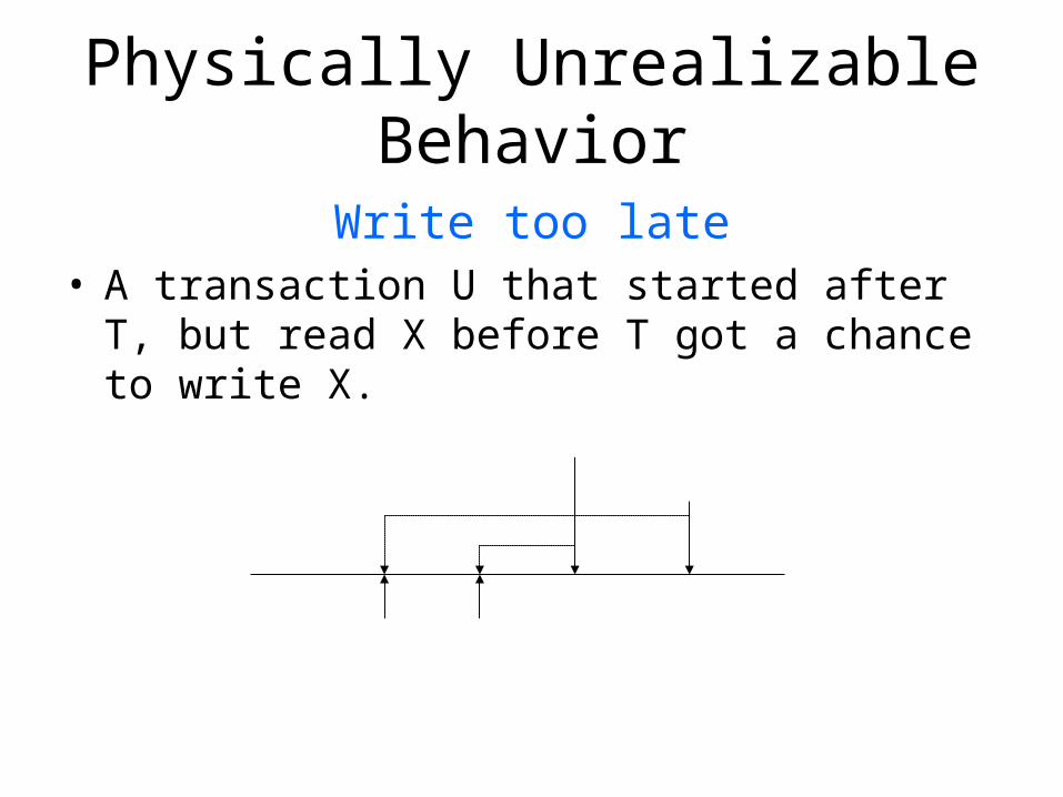
Physically Unrealizable Behavior
Write too late• A transaction U that started after T, but read X before
T got a chance to write X.
U reads X
T writes X
T start U start
Figure: Transaction T tries to write too late
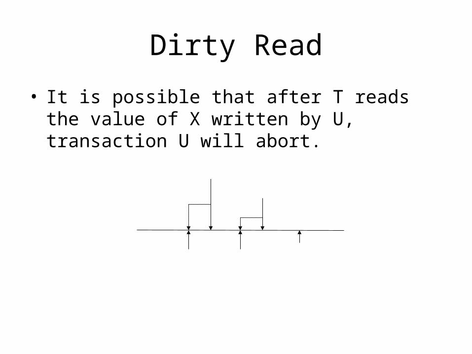
Dirty Read
• It is possible that after T reads the value of X written by U, transaction U will abort.
U writes X
T reads X
U start T start U aborts
T could perform a dirty read if it reads X when shown
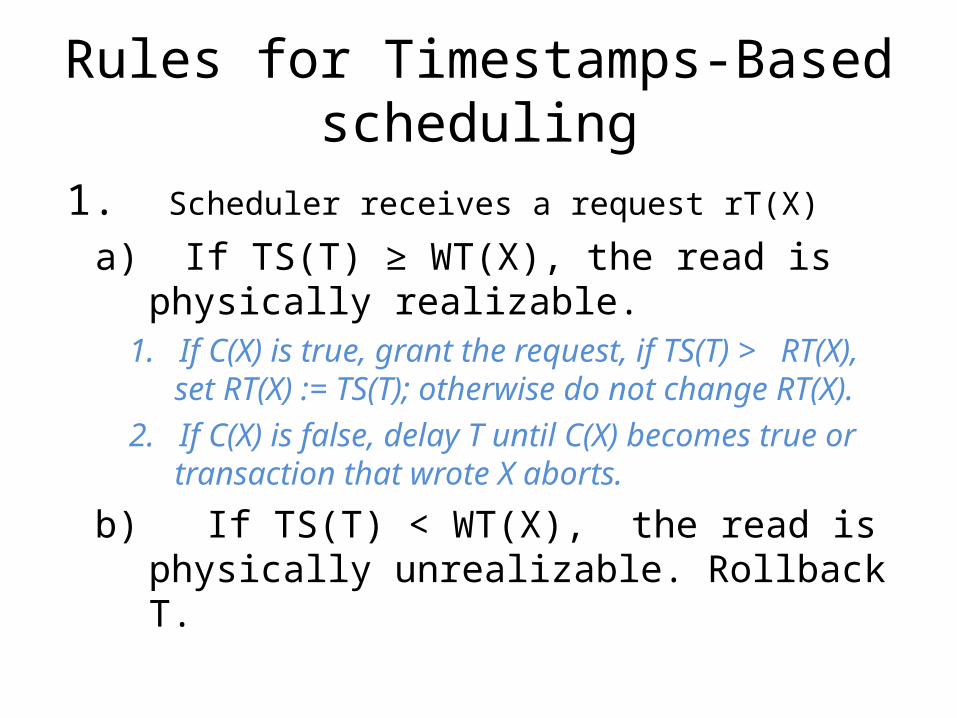
Rules for Timestamps-Based scheduling
1. Scheduler receives a request rT(X)
a) If TS(T) ≥ WT(X), the read is physically realizable. 1. If C(X) is true, grant the request, if TS(T) > RT(X), set
RT(X) := TS(T); otherwise do not change RT(X). 2. If C(X) is false, delay T until C(X) becomes true or
transaction that wrote X aborts.
b) If TS(T) < WT(X), the read is physically unrealizable. Rollback T.
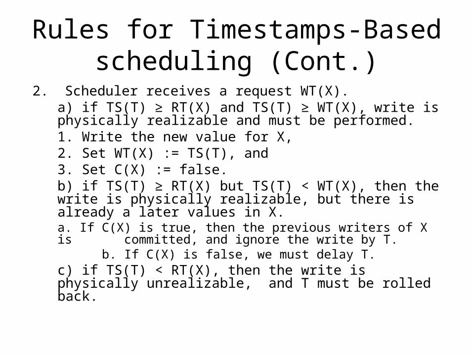
Rules for Timestamps-Based scheduling (Cont.)
2. Scheduler receives a request WT(X).a) if TS(T) ≥ RT(X) and TS(T) ≥ WT(X), write is physically realizable and must be performed.
1. Write the new value for X,2. Set WT(X) := TS(T), and3. Set C(X) := false.
b) if TS(T) ≥ RT(X) but TS(T) < WT(X), then the write is physically realizable, but there is already a later values in X.
a. If C(X) is true, then the previous writers of X is committed, and ignore the write by T.
b. If C(X) is false, we must delay T.c) if TS(T) < RT(X), then the write is physically unrealizable, and T must be rolled back.
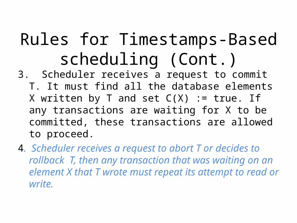
Rules for Timestamps-Based scheduling (Cont.)
3. Scheduler receives a request to commit T. It must find all the database elements X written by T and set C(X) := true. If any transactions are waiting for X to be committed, these transactions are allowed to proceed.
4. Scheduler receives a request to abort T or decides to rollback T, then any transaction that was waiting on an element X that T wrote must repeat its attempt to read or write.
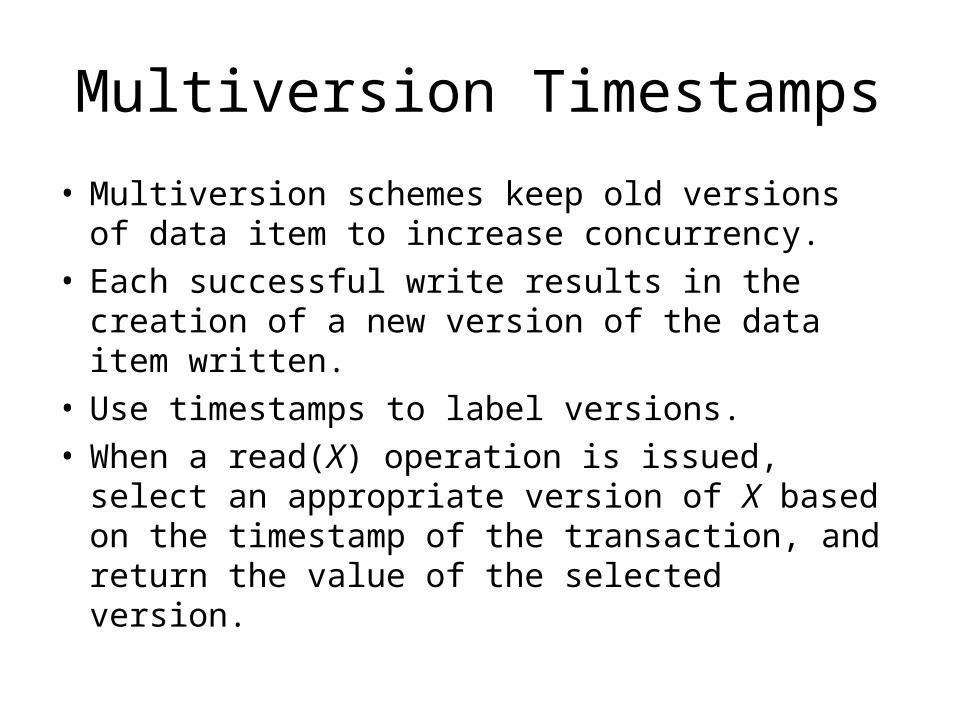
Multiversion Timestamps
• Multiversion schemes keep old versions of data item to increase concurrency.
• Each successful write results in the creation of a new version of the data item written.
• Use timestamps to label versions.• When a read(X) operation is issued, select an
appropriate version of X based on the timestamp of the transaction, and return the value of the selected version.
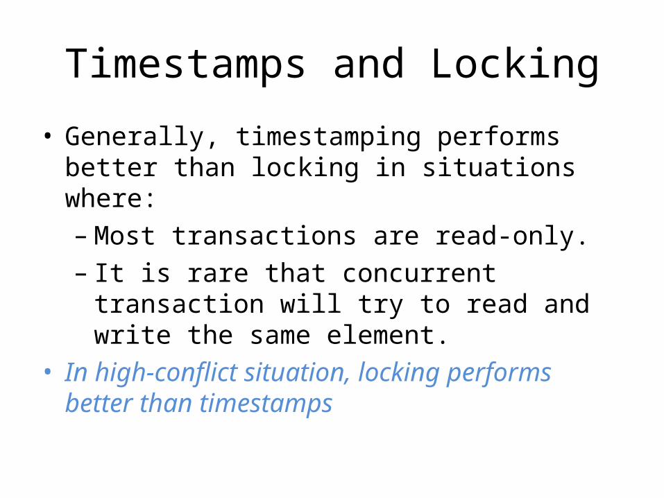
Timestamps and Locking
• Generally, timestamping performs better than locking in situations where:– Most transactions are read-only.– It is rare that concurrent transaction will try to
read and write the same element.• In high-conflict situation, locking performs better
than timestamps
18.9At a Glance
IntroductionValidation based schedulingValidation based Scheduler Expected exceptionsValidation rulesExampleComparisonsSummary
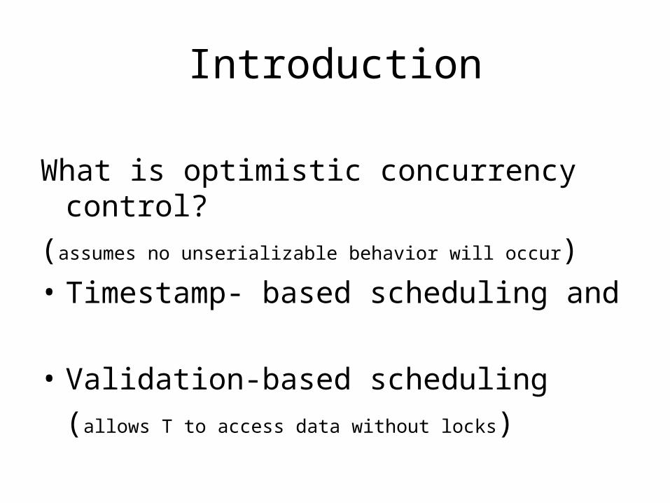
Introduction
What is optimistic concurrency control?(assumes no unserializable behavior will occur)• Timestamp- based scheduling and
• Validation-based scheduling(allows T to access data without locks)

Validation based scheduling
Scheduler keeps a record of what the active transactions are doing.
Executes in 3 phases1. Read- reads from RS( ), computes local address
2. Validate- compares read and write sets
3. Write- writes from WS( )
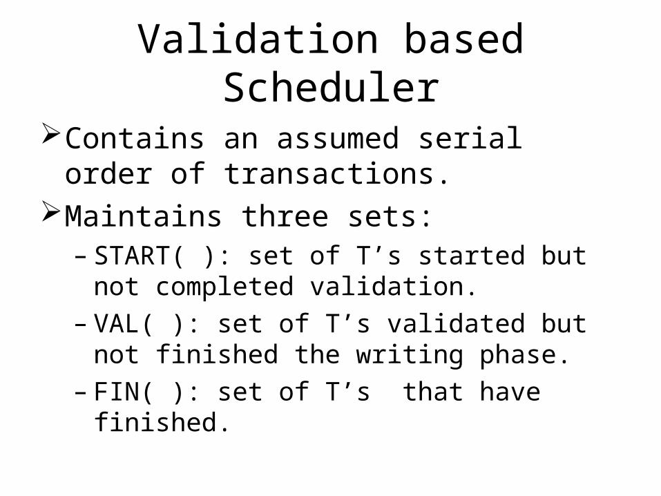
Validation based Scheduler
Contains an assumed serial order of transactions.
Maintains three sets:– START( ): set of T’s started but not completed
validation.– VAL( ): set of T’s validated but not finished the
writing phase.– FIN( ): set of T’s that have finished.
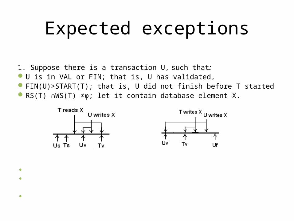
Expected exceptions
1. Suppose there is a transaction U, such that:U is in VAL or FIN; that is, U has validated,FIN(U)>START(T); that is, U did not finish before T startedRS(T) ∩WS(T) ≠φ; let it contain database element X.
2. Suppose there is transaction U, such that:• U is in VAL; U has successfully validated.•FIN(U)>VAL(T); U did not finish before T entered its validation phase.•WS(T) ∩ WS(U) ≠φ; let x be in both write sets.
Validation rules
• Optimistic concurrency control• Concurrency Control assumes that conflicts
between transactions are rare• Scheduler maintains record of active
transactions• Does not require locking• Check for conflicts just before commit
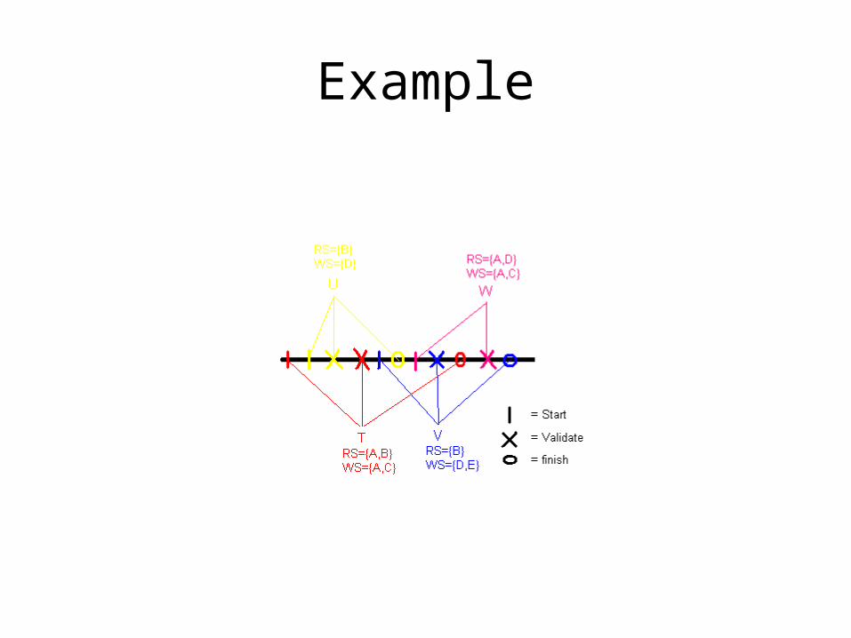
Example
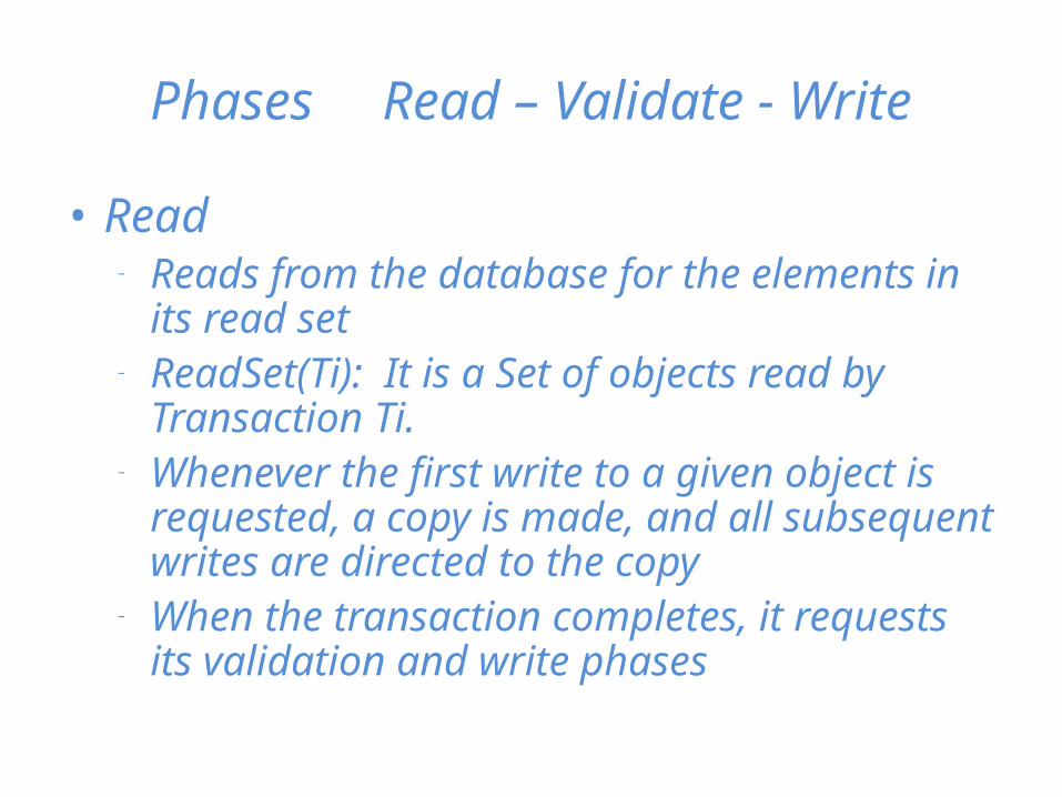
Phases Read – Validate - Write
• Read– Reads from the database for the elements in its
read set– ReadSet(Ti): It is a Set of objects read by
Transaction Ti.– Whenever the first write to a given object is
requested, a copy is made, and all subsequent writes are directed to the copy
– When the transaction completes, it requests its validation and write phases
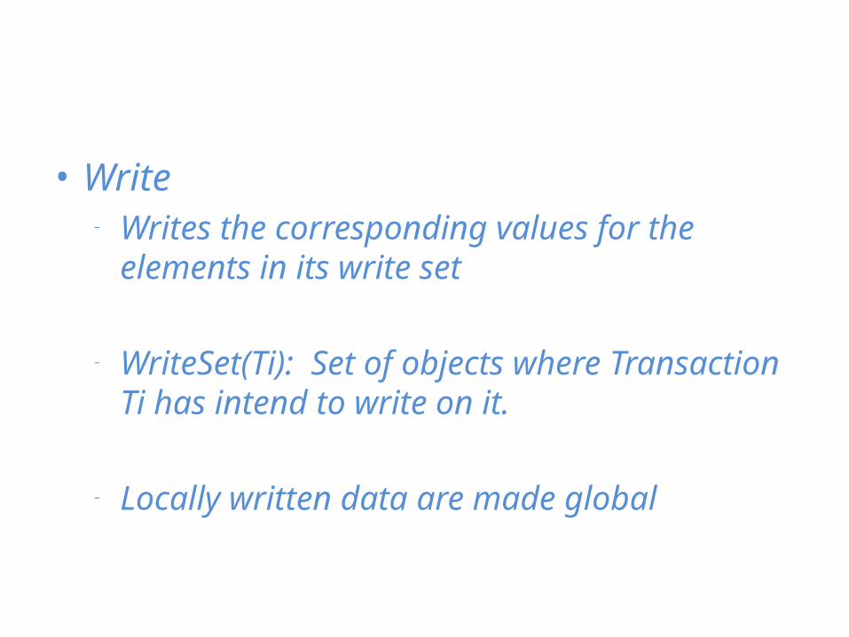
• Write– Writes the corresponding values for the elements
in its write set
– WriteSet(Ti): Set of objects where Transaction Ti has intend to write on it.
– Locally written data are made global
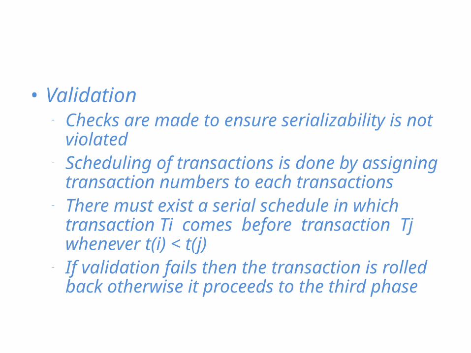
• Validation– Checks are made to ensure serializability is not
violated– Scheduling of transactions is done by assigning
transaction numbers to each transactions– There must exist a serial schedule in which
transaction Ti comes before transaction Tj whenever t(i) < t(j)
– If validation fails then the transaction is rolled back otherwise it proceeds to the third phase
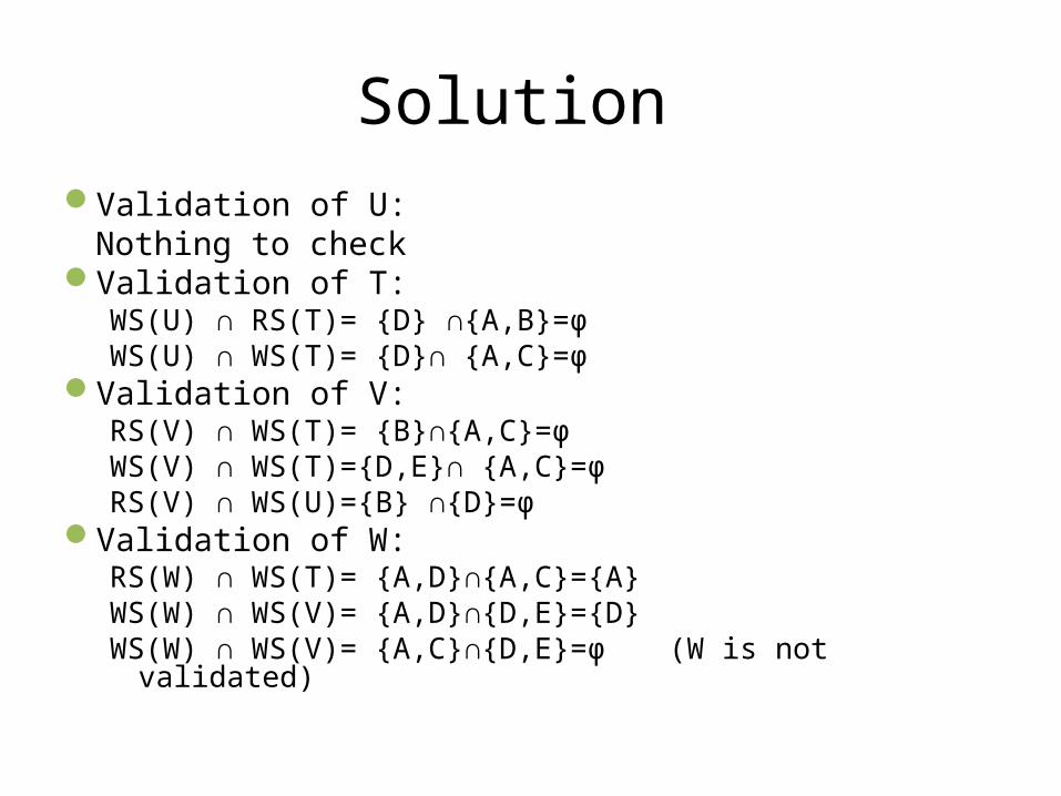
Solution Validation of U:
Nothing to checkValidation of T:
WS(U) ∩ RS(T)= {D} ∩{A,B}=φWS(U) ∩ WS(T)= {D}∩ {A,C}=φ
Validation of V:RS(V) ∩ WS(T)= {B}∩{A,C}=φWS(V) ∩ WS(T)={D,E}∩ {A,C}=φRS(V) ∩ WS(U)={B} ∩{D}=φ
Validation of W:RS(W) ∩ WS(T)= {A,D}∩{A,C}={A}WS(W) ∩ WS(V)= {A,D}∩{D,E}={D}WS(W) ∩ WS(V)= {A,C}∩{D,E}=φ (W is not validated)
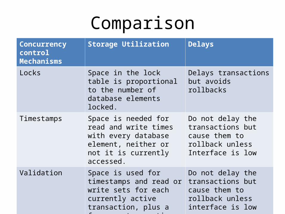
ComparisonConcurrency control Mechanisms
Storage Utilization Delays
Locks Space in the lock table is proportional to the number of database elements locked.
Delays transactions but avoids rollbacks
Timestamps Space is needed for read and write times with every database element, neither or not it is currently accessed.
Do not delay the transactions but cause them to rollback unless Interface is low
Validation Space is used for timestamps and read or write sets for each currently active transaction, plus a few more transactions that finished after some currently active transaction began.
Do not delay the transactions but cause them to rollback unless interface is low
21.1 Introduction to Information Integration
CS257 Fan Yang
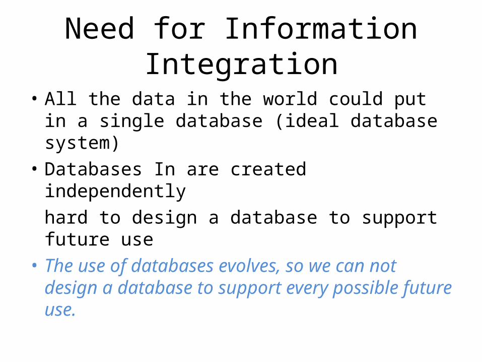
Need for Information Integration
• All the data in the world could put in a single database (ideal database system)
• Databases In are created independentlyhard to design a database to support future use
• The use of databases evolves, so we can not design a database to support every possible future use.
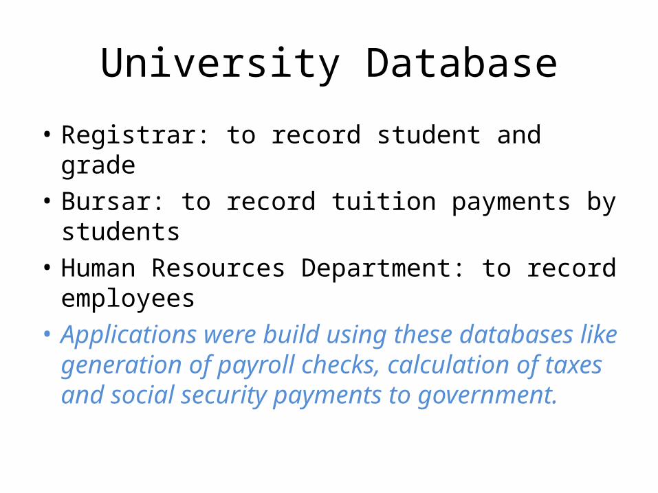
University Database
• Registrar: to record student and grade• Bursar: to record tuition payments by students• Human Resources Department: to record
employees• Applications were build using these databases
like generation of payroll checks, calculation of taxes and social security payments to government.
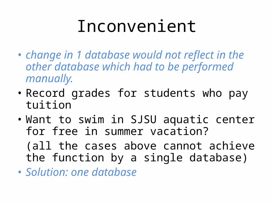
Inconvenient
• change in 1 database would not reflect in the other database which had to be performed manually.
• Record grades for students who pay tuition • Want to swim in SJSU aquatic center for free
in summer vacation?(all the cases above cannot achieve the function by a single database)
• Solution: one database
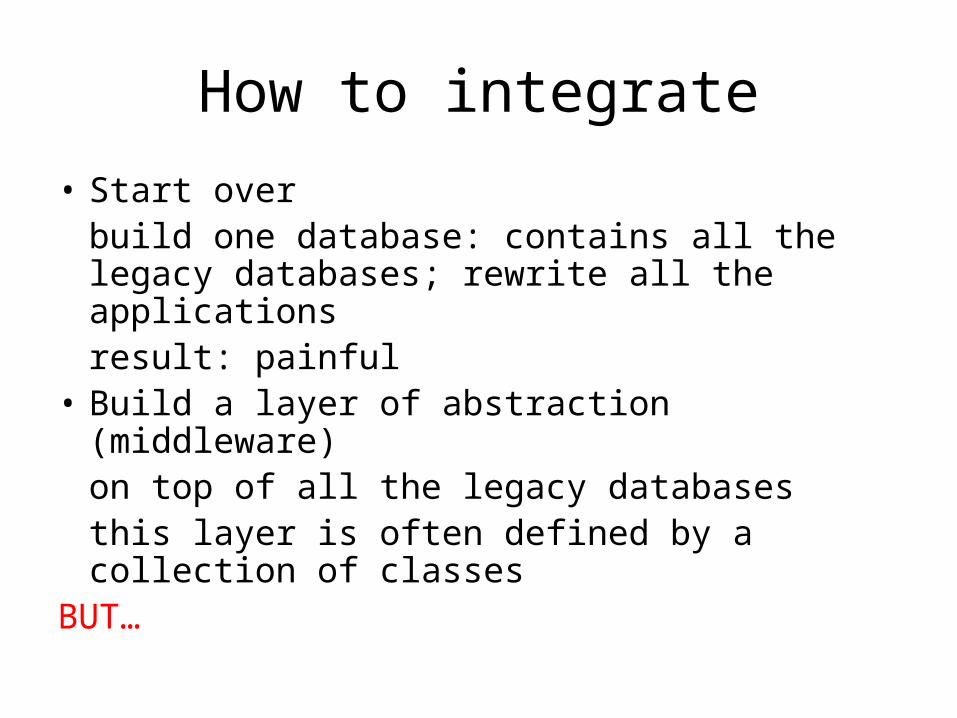
How to integrate
• Start overbuild one database: contains all the legacy databases; rewrite all the applicationsresult: painful
• Build a layer of abstraction (middleware)on top of all the legacy databasesthis layer is often defined by a collection of classes
BUT…
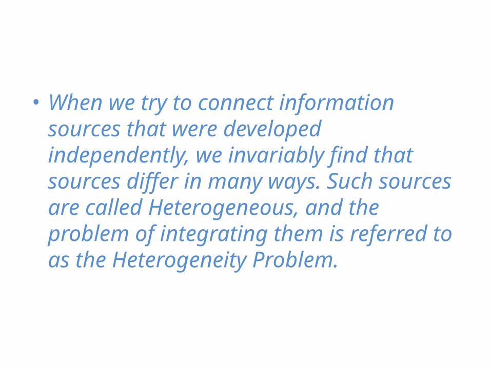
• When we try to connect information sources that were developed independently, we invariably find that sources differ in many ways. Such sources are called Heterogeneous, and the problem of integrating them is referred to as the Heterogeneity Problem.
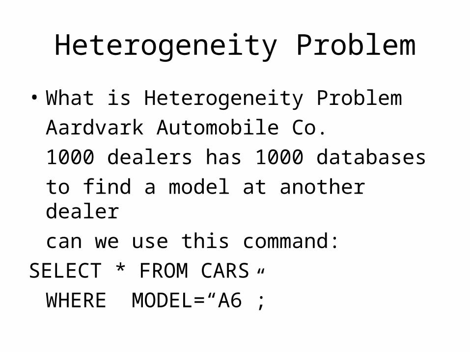
Heterogeneity Problem
• What is Heterogeneity ProblemAardvark Automobile Co. 1000 dealers has 1000 databasesto find a model at another dealercan we use this command:
SELECT * FROM CARS WHERE MODEL=“A6”;
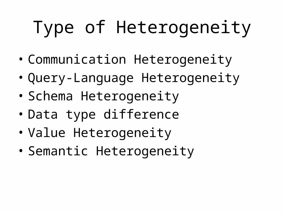
Type of Heterogeneity
• Communication Heterogeneity• Query-Language Heterogeneity• Schema Heterogeneity• Data type difference• Value Heterogeneity• Semantic Heterogeneity
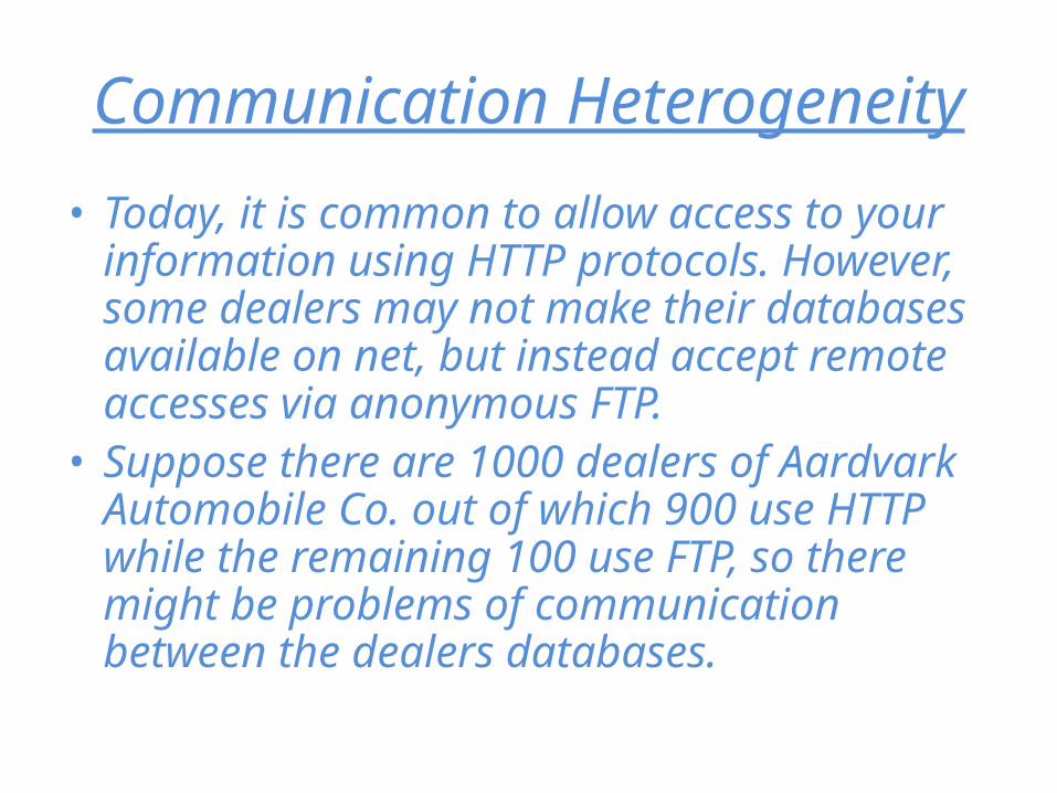
Communication Heterogeneity
• Today, it is common to allow access to your information using HTTP protocols. However, some dealers may not make their databases available on net, but instead accept remote accesses via anonymous FTP.
• Suppose there are 1000 dealers of Aardvark Automobile Co. out of which 900 use HTTP while the remaining 100 use FTP, so there might be problems of communication between the dealers databases.
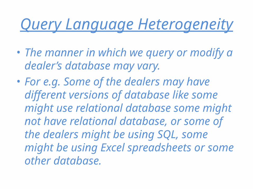
Query Language Heterogeneity
• The manner in which we query or modify a dealer’s database may vary.
• For e.g. Some of the dealers may have different versions of database like some might use relational database some might not have relational database, or some of the dealers might be using SQL, some might be using Excel spreadsheets or some other database.
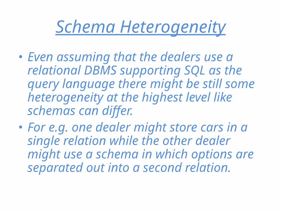
Schema Heterogeneity
• Even assuming that the dealers use a relational DBMS supporting SQL as the query language there might be still some heterogeneity at the highest level like schemas can differ.
• For e.g. one dealer might store cars in a single relation while the other dealer might use a schema in which options are separated out into a second relation.
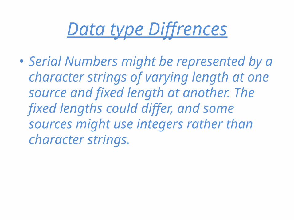
Data type Diffrences
• Serial Numbers might be represented by a character strings of varying length at one source and fixed length at another. The fixed lengths could differ, and some sources might use integers rather than character strings.
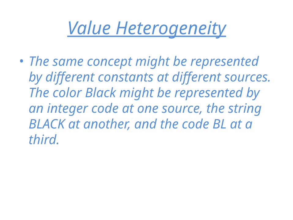
Value Heterogeneity
• The same concept might be represented by different constants at different sources. The color Black might be represented by an integer code at one source, the string BLACK at another, and the code BL at a third.
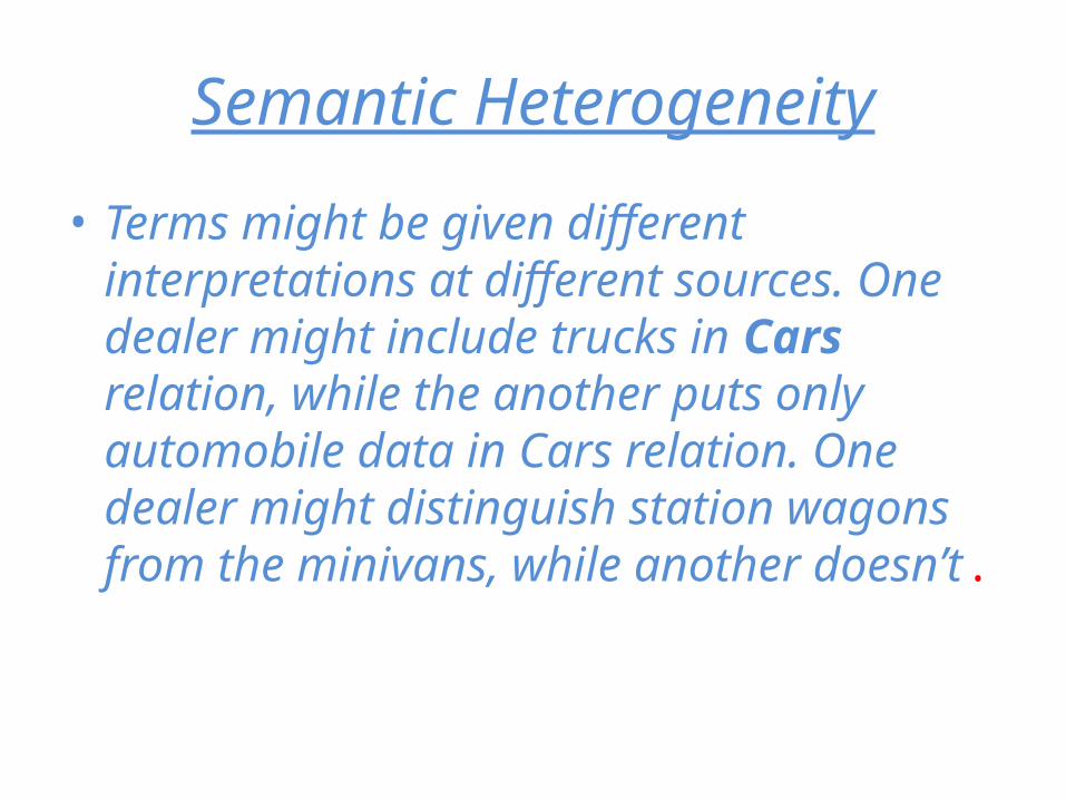
Semantic Heterogeneity
• Terms might be given different interpretations at different sources. One dealer might include trucks in Cars relation, while the another puts only automobile data in Cars relation. One dealer might distinguish station wagons from the minivans, while another doesn’t.
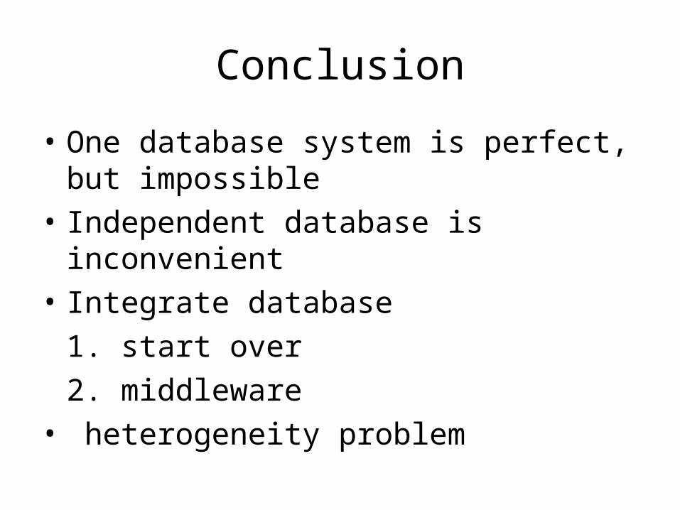
Conclusion
• One database system is perfect, but impossible
• Independent database is inconvenient• Integrate database
1. start over2. middleware
• heterogeneity problem
Chapter 21.2Modes of Information Integration
ID: 219Name: Qun YuClass: CS257 219 Spring 2009Instructor: Dr. T.Y.Lin
Federations
The simplest architecture for integrating several DBs
One to one connections between all pairs of DBs
n DBs talk to each other, n(n-1) wrappers are needed
Good when communications between DBs are limited

Wrapper
• Wrapper : a software translates incoming queries and outgoing answers.
– allows information sources to conform to some shared schema.
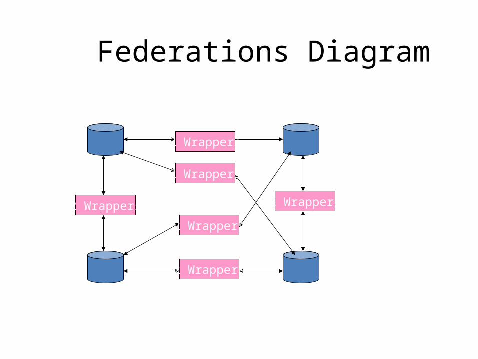
Federations Diagram
DB2DB1
DB3 DB4
2 Wrappers
2 Wrappers
2 Wrappers
2 Wrappers
2 Wrappers 2 Wrappers
A federated collection of 4 DBs needs 12 components to translate queries from one to another.
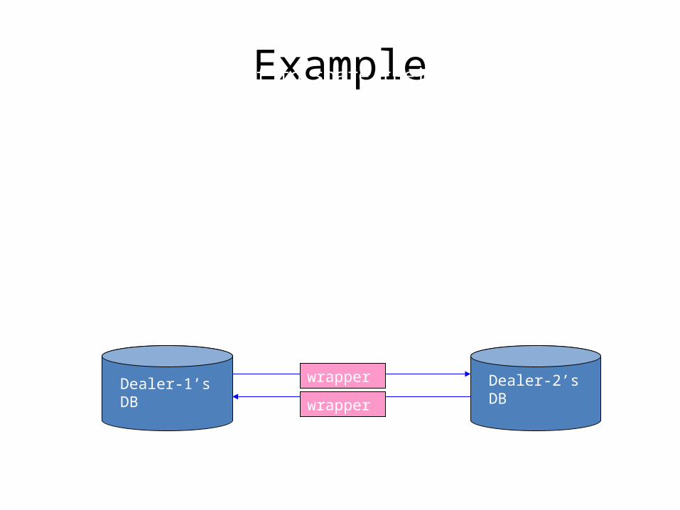
Example
Car dealers want to share their inventory. Each dealer queries the other’s DB to find the needed car.
Dealer-1’s DB relation: NeededCars(model,color,autoTrans)
Dealer-2’s DB relation: Auto(Serial, model, color)
Options(serial,option)
Dealer-1’s DB Dealer-2’s DB
wrapper
wrapper
Example…
Dealer 1 queries Dealer 2 for needed cars
For(each tuple(:m,:c,:a) in NeededCars){
if(:a=TRUE){/* automatic transmission wanted */
SELECT serial
FROM Autos, Options
WHERE Autos.serial = Options.serial AND Options.option = ‘autoTrans’
AND Autos.model = :m AND Autos.color =:c;
}
Else{/* automatic transmission not wanted */
SELECT serial
FROM Auto
WHERE Autos.model = :m AND
Autos.color = :c AND
NOT EXISTS( SELECT * FROM Options WHERE serial = Autos.serial
AND option=‘autoTrans’);
}
}
Data Warehouse
Sources are translated from their local schema to a global schema and copied to a central DB.
User transparent: user uses Data Warehouse just like an ordinary DB
User is not allowed to update Data Warehouse
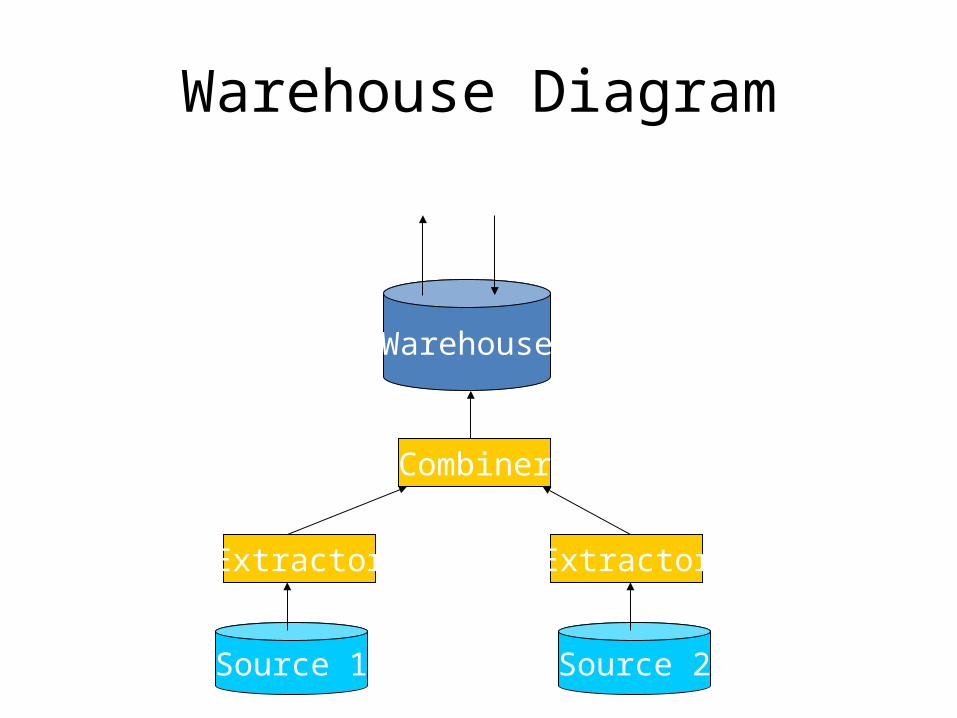
Warehouse Diagram
Warehouse
Extractor Extractor
Source 1 Source 2
User query
result
Combiner

Example
Construct a data warehouse from sources DB of 2 car dealers:
Dealer-1’s schema: Cars(serialNo, model,color,autoTrans,cdPlayer,…)Dealer-2’s schema: Auto(serial,model,color)
Options(serial,option)
Warehouse’s schema: AutoWhse(serialNo,model,color,autoTrans,dealer)
Extractor --- Query to extract data from Dealer-1’s data:
INSERT INTO AutosWhse(serialNo, model, color, autoTans, dealer)SELECT serialNo,model,color,autoTrans,’dealer1’ From Cars;
Example
Extractor --- Query to extract data from Dealer-2’s data:
INSERT INTO AutosWhse(serialNo, model, color, autoTans, dealer)SELECT serialNo,model,color,’yes’,’dealer2’ FROM Autos,OptionsWHERE Autos.serial=Options.serial AND
option=‘autoTrans’;
INSERT INTO AutosWhse(serialNo, model, color, autoTans, dealer)SELECT serialNo,model,color,’no’,’dealer2’ FROM AutosWHERE NOT EXISTS ( SELECT * FROM serial =Autos.serial AND option = ‘autoTrans’);
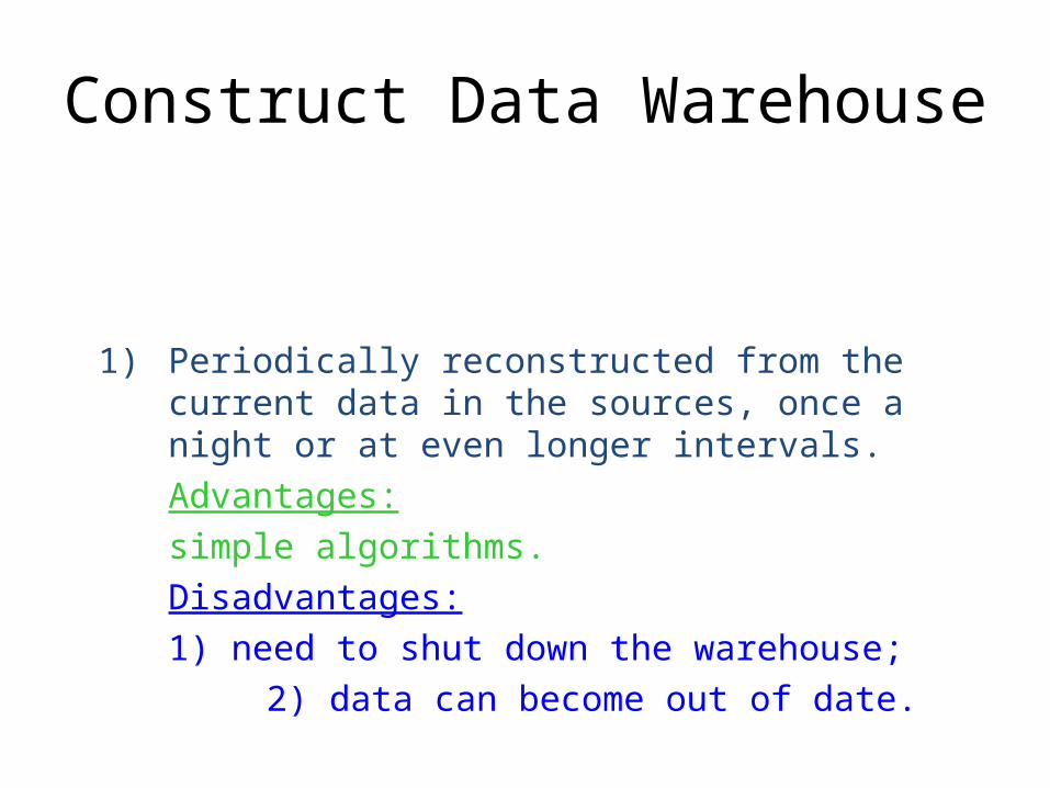
Construct Data Warehouse
1) Periodically reconstructed from the current data in the sources, once a night or at even longer intervals.
Advantages:
simple algorithms.
Disadvantages:
1) need to shut down the warehouse;
2) data can become out of date.
There are mainly 3 ways to constructing the data in the warehouse:
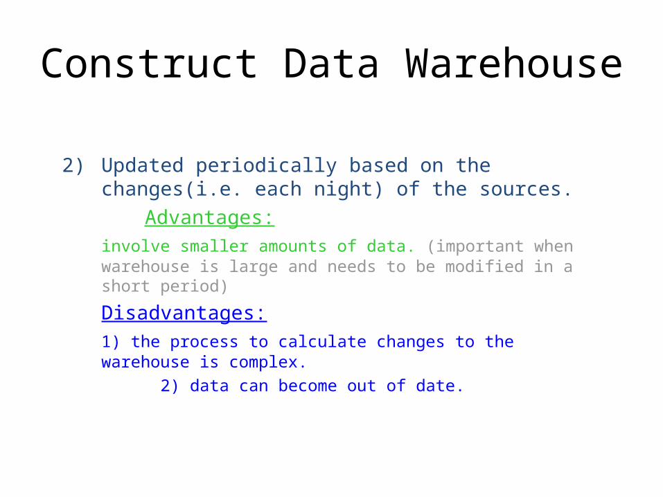
Construct Data Warehouse
2) Updated periodically based on the changes(i.e. each night) of the sources.
Advantages:
involve smaller amounts of data. (important when warehouse is large and needs to be modified in a short period)
Disadvantages:
1) the process to calculate changes to the warehouse is complex.
2) data can become out of date.
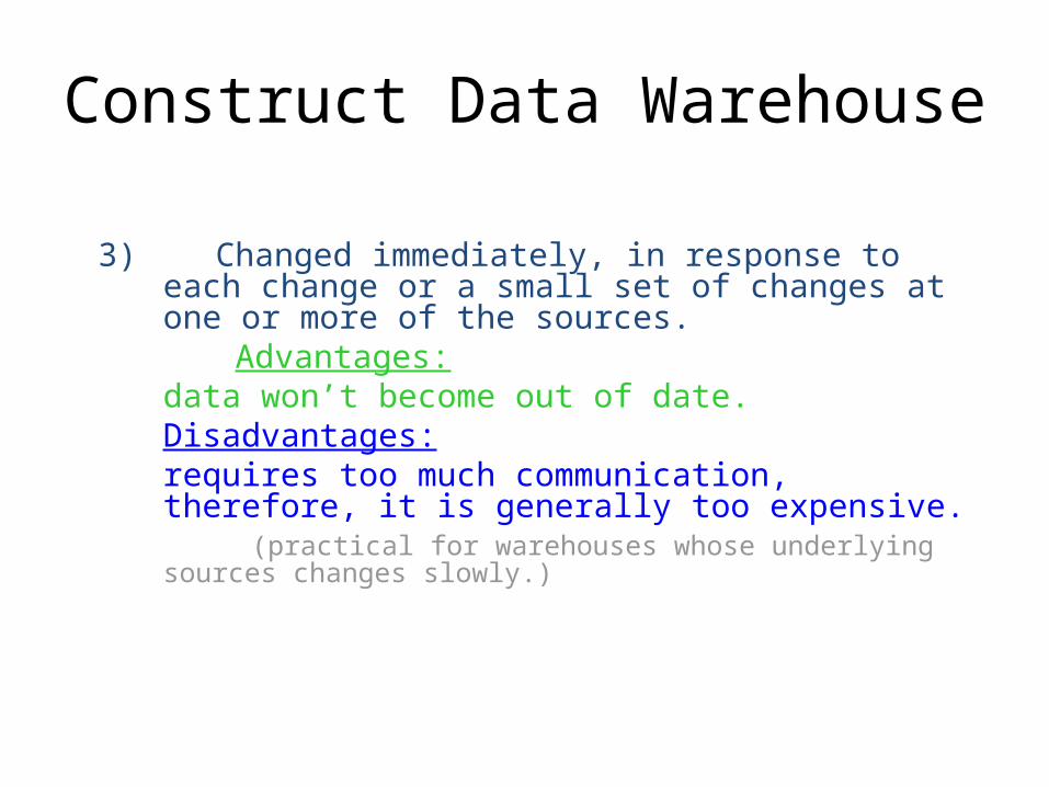
Construct Data Warehouse
3) Changed immediately, in response to each change or a small set of changes at one or more of the sources.
Advantages:data won’t become out of date. Disadvantages: requires too much communication, therefore, it is generally too expensive.
(practical for warehouses whose underlying sources changes slowly.)
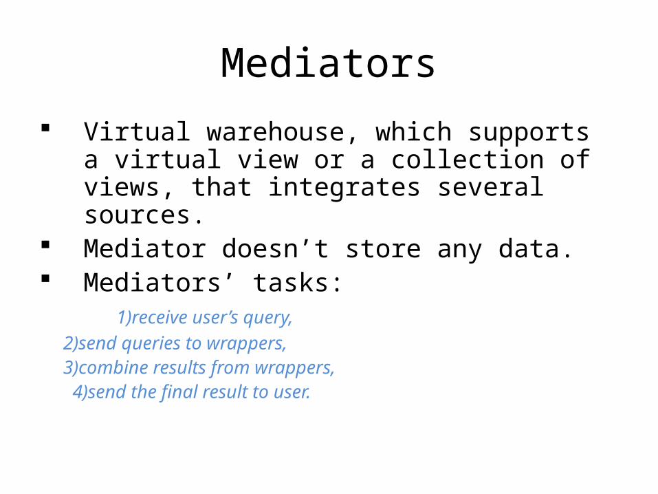
Mediators
Virtual warehouse, which supports a virtual view or a collection of views, that integrates several sources.
Mediator doesn’t store any data. Mediators’ tasks: 1)receive user’s query,
2)send queries to wrappers, 3)combine results from wrappers, 4)send the final result to user.
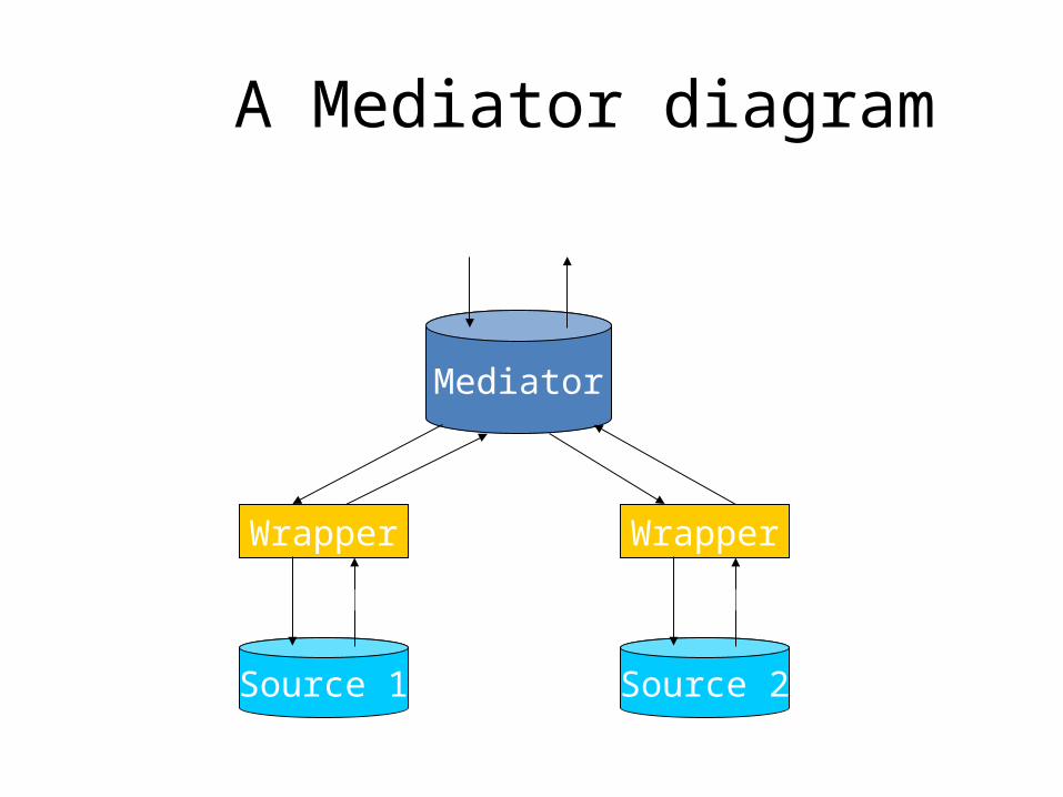
A Mediator diagram
Mediator
Wrapper Wrapper
Source 1 Source 2
User query
Query
Query
QueryQuery
Result
Result
Result
Result
Result
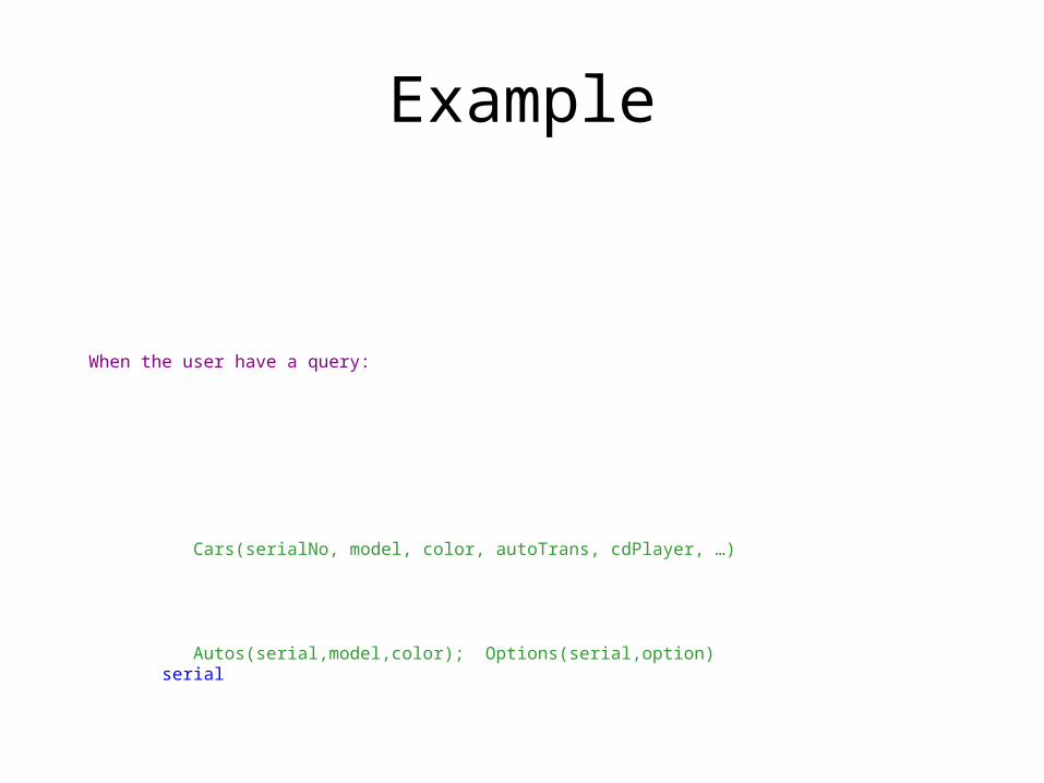
Example
Same data sources as the example of data warehouse, the mediatorIntegrates the same two dealers’ source into a view with schema:
AutoMed(serialNo,model,color,autoTrans,dealer)
When the user have a query:
SELECT sericalNo, model FROM AkutoMedWhere color=‘red’
In this simple case, the mediator forwards the same query to eachOf the two wrappers.
Wrapper1: Cars(serialNo, model, color, autoTrans, cdPlayer, …)SELECT serialNo,model FROM carsWHERE color = ‘red’;
Wrapper2: Autos(serial,model,color); Options(serial,option)SELECT serial, modelFROM AutosWHERE color=‘red’;

Example
There may be different options for the mediator to forward user query,for example, the user queries if there are a specific model&color car(i.e. “Gobi”, “blue”).
The mediator decides 2nd query is needed or not based on the result of 1st query. That is, If dealer-1 has the specific car, the mediator doesn’t have to query dealer-2.
Chapter 21 Information Integration
21.3 Wrappers in Mediator-Based Systems
Presented by: Kai ZhuProfessor: Dr. T.Y. Lin
Class ID: 220
Intro• Templates for Query patterns• Wrapper Generator• Filter
Wrappers in Mediator-based SystemsMore complicated than that in most data warehouse
system.Able to accept a variety of queries from the mediator
and translate them to the terms of the source.Communicate the result to the mediator.
wrapper• The wrapper(extractor) consists of:
One or more predefined queries (based on source) SQL Web page
Suitable communication mechanism for sending and receiving information to/from
• source/mediator.

How to design a wrapper?
Classify the possible queries that the mediator can ask into templates, which are queries with parameters that represent constants.
Templates for Query Patterns:Templates for Query Patterns:
Use notation T=>S to express the idea Use notation T=>S to express the idea that the template T is turned by the that the template T is turned by the wrapper into the source query S.wrapper into the source query S.
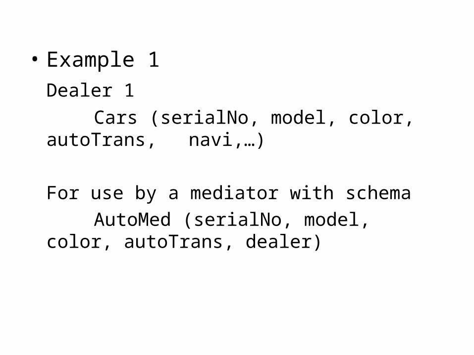
• Example 1Dealer 1
Cars (serialNo, model, color, autoTrans, navi,…)
For use by a mediator with schemaAutoMed (serialNo, model, color, autoTrans,
dealer)
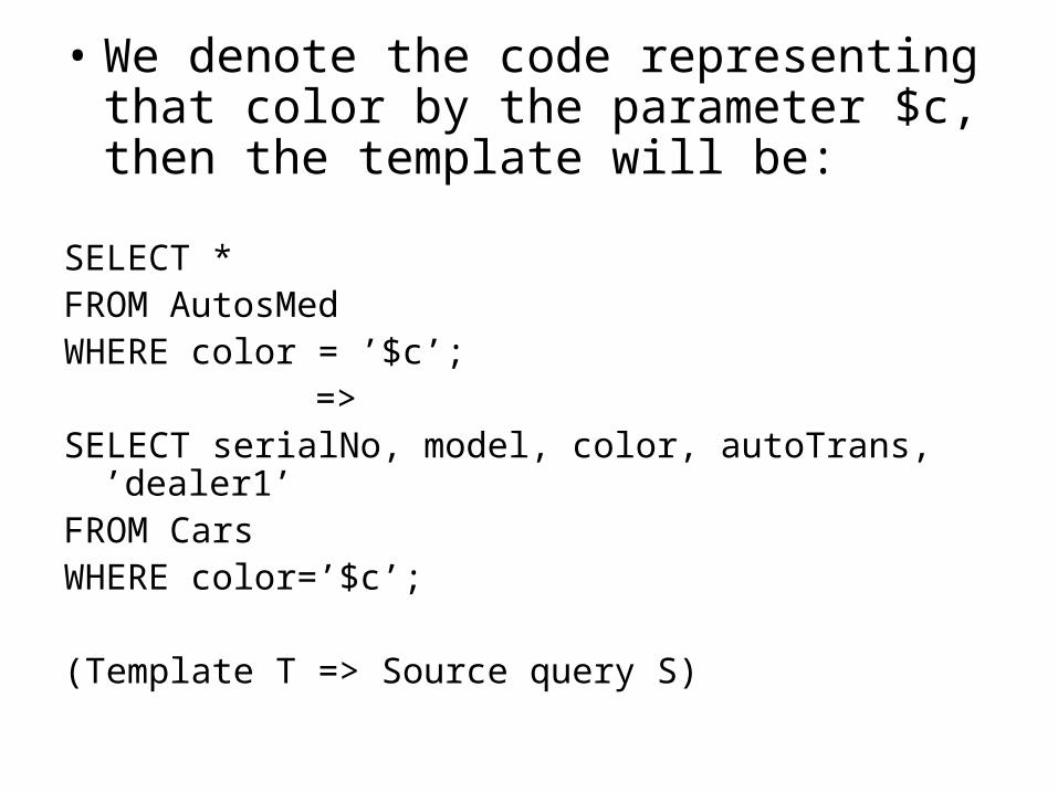
• We denote the code representing that color by the parameter $c, then the template will be:
SELECT *FROM AutosMedWHERE color = ’$c’;
=>SELECT serialNo, model, color, autoTrans, ’dealer1’FROM CarsWHERE color=’$c’;
(Template T => Source query S)
• There will be total 2n templates if we have the option of specifying n attributes.
Wrapper Generators• The wrapper generator creates a table holds
the various query patterns contained in the templates.
• The source queries that are associated with each.
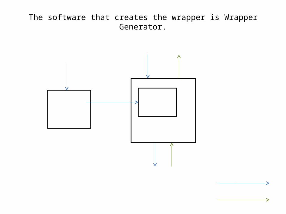
The software that creates the wrapper is Wrapper Generator.
Driver
Table
Source
WrapperGenerator
Queries
Results
Wrapper
A driver is used in each wrapper, the task of the driver is to:
Accept a query from the mediator.Search the table for a template that matches the
query.The source query is sent to the source, again using a
“plug-in” communication mechanism.The response is processed by the wrapper.
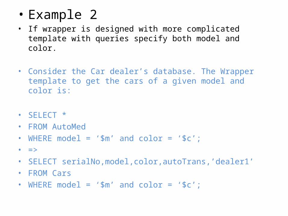
• Example 2• If wrapper is designed with more complicated template with queries
specify both model and color.
• Consider the Car dealer’s database. The Wrapper template to get the cars of a given model and color is:
• SELECT * • FROM AutoMed• WHERE model = ‘$m’ and color = ‘$c’;• =>• SELECT serialNo,model,color,autoTrans,’dealer1’• FROM Cars• WHERE model = ‘$m’ and color = ‘$c’;
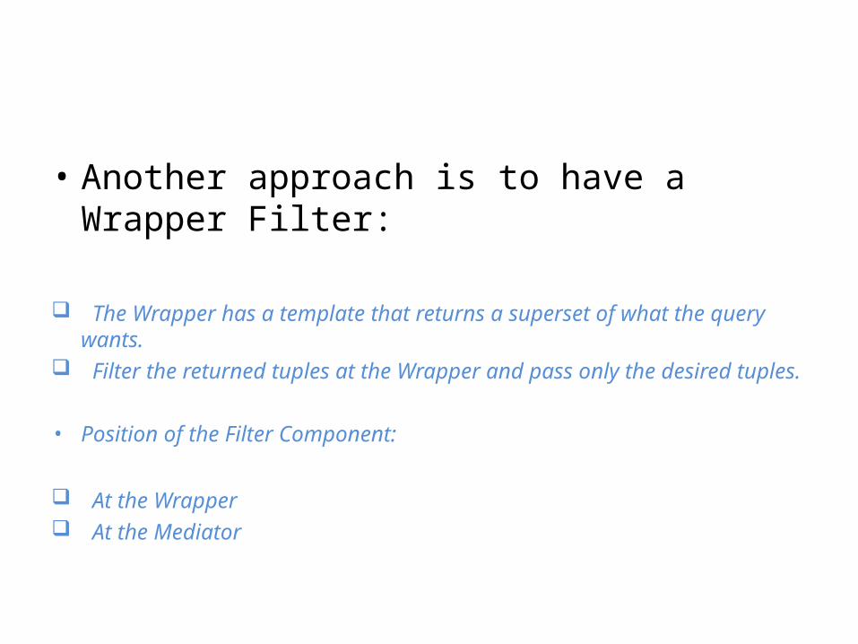
• Another approach is to have a Wrapper Filter:
The Wrapper has a template that returns a superset of what the query wants.
Filter the returned tuples at the Wrapper and pass only the desired tuples.
• Position of the Filter Component:
At the Wrapper At the Mediator
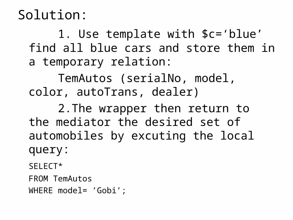
Solution:1. Use template with $c=‘blue’ find all blue
cars and store them in a temporary relation:TemAutos (serialNo, model, color, autoTrans,
dealer)2.The wrapper then return to the mediator the
desired set of automobiles by excuting the local query:SELECT*
FROM TemAutosWHERE model= ’Gobi’;
Sections 21.4 – 21.5
Sanuja Dabade & Eilbroun Benjamin CS 257 – Dr. TY Lin
INFORMATION INTEGRATION
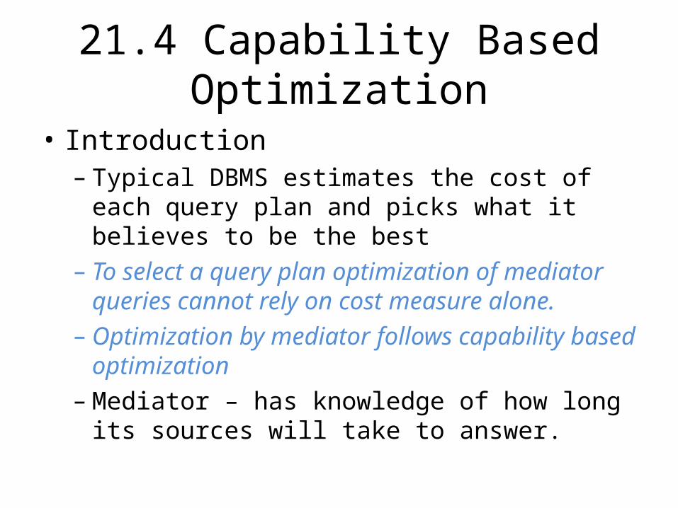
21.4 Capability Based Optimization
• Introduction– Typical DBMS estimates the cost of each query
plan and picks what it believes to be the best– To select a query plan optimization of mediator
queries cannot rely on cost measure alone.– Optimization by mediator follows capability based
optimization– Mediator – has knowledge of how long its sources
will take to answer.
21.4.1 The Problem of Limited Source Capabilities
• Many sources have only Web Based interfaces• Web sources usually allow querying through a
query form• E.g. Amazon.com interface allows us to query about books in
many different ways.
• But we cannot ask questions that are too general– E.g. Select * from books;
21.4.1 The Problem of Limited Source Capabilities (con’t)
• Reasons why a source may limit the ways in which queries can be asked– Earliest database did not use relational DBMS that
supports SQL queries– Indexes on large database may make certain queries
feasible, while others are too expensive to execute– Security reasons
• E.g. Medical database may answer queries about averages, but won’t disclose details of a particular patient's information
21.4.2 A Notation for Describing Source Capabilities
For relational data, the legal forms of queries are described by adornments
Adornments – Sequences of codes that represent the requirements for the attributes of the relation, in their standard order f(free) – attribute can be specified or not b(bound) – must specify a value for an attribute
but any value is allowed u(unspecified) – not permitted to specify a value
for a attribute
21.4.2 A notation for Describing Source Capabilities….(cont’d)
c[S](choice from set S) means that a value must be specified and value must be from finite set S.
o[S](optional from set S) means either do not specify a value or we specify a value from finite set S
A prime (f’) specifies that an attribute is not a part of the output of the query
A capabilities specification is a set of adornments A query must match one of the adornments in its
capabilities specification
21.4.2 A notation for Describing Source Capabilities….(cont’d)
E.g. Dealer 1 is a source of data in the form:Cars (serialNo, model, color, autoTrans, navi)The adornment for this query form is b’uuuu
21.4.3 Capability-Based Query-Plan Selection
• Given a query at the mediator, a capability based query optimizer first considers what queries it can ask at the sources to help answer the query
• The process is repeated until: – Enough queries are asked at the sources to resolve all
the conditions of the mediator query and therefore query is answered. Such a plan is called feasible.
– We can construct no more valid forms of source queries, yet still cannot answer the mediator query. It has been an impossible query.
21.4.3 Capability-Based Query-Plan Selection (cont’d)
• The simplest form of mediator query where we need to apply the above strategy is join relations
• E.g we have sources for dealer 2– Autos(serial, model, color)– Options(serial, option)
• Suppose that ubf is the sole adornment for Auto and Options have two adornments, bu and uc[autoTrans, navi]
• Query is – find the serial numbers and colors of Gobi models with a navigation system
21.4.4 Adding Cost-Based Optimization
• Mediator’s Query optimizer is not done when the capabilities of the sources are examined.
• Sources are independent of the mediator, so it is difficult to estimate the cost.
• Having found feasible plans, it must choose among them
• Making an intelligent, cost based query optimization requires that the mediator knows a great deal about the costs of queries involved
21.5 Optimizing Mediator Queries
• Chain algorithm – a greedy algorithm – answers the query by sending a sequence of
requests to its sources. – Will always find a solution assuming at least one
solution exists. – The solution may not be optimal.
21.5.1 Simplified Adornment Notation
• A query at the mediator is limited to b (bound) and f (free) adornments.
• We use the following convention for describing adornments: – nameadornments(attributes)– where:
• name is the name of the relation • the number of adornments = the number of
attributes
21.5.2 Obtaining Answers for Subgoals
• Rules for subgoals and sources: – Suppose we have the following subgoal:
Rx1x2…xn(a1, a2, …, an),
and source adornments for R are: y1y2…yn. • If yi is b or c[S], then xi = b.
• If xi = f, then yi is not output restricted.
– The adornment on the subgoal matches the adornment at the source:
• If yi is f, u, or o[S] and xi is either b or f.
21.5.3 The Chain Algorithm
• Maintains 2 types of information: – An adornment for each subgoal. – A relation X that is the join of the relations for all
the subgoals that have been resolved. • The adornment for a subgoal is b if the mediator query
provides a constant binding for the corresponding argument of that subgoal.
• X is a relation over no attributes, containing just an empty tuple.
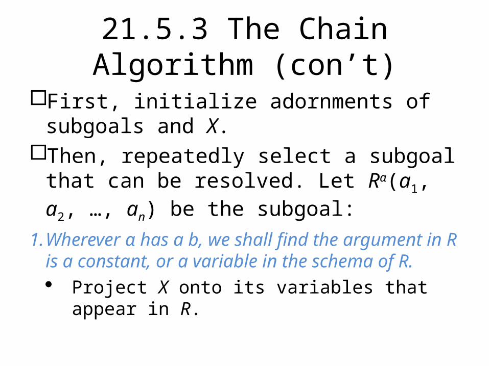
21.5.3 The Chain Algorithm (con’t)
First, initialize adornments of subgoals and X. Then, repeatedly select a subgoal that can be
resolved. Let Rα(a1, a2, …, an) be the subgoal: 1. Wherever α has a b, we shall find the argument in R
is a constant, or a variable in the schema of R. Project X onto its variables that appear in R.
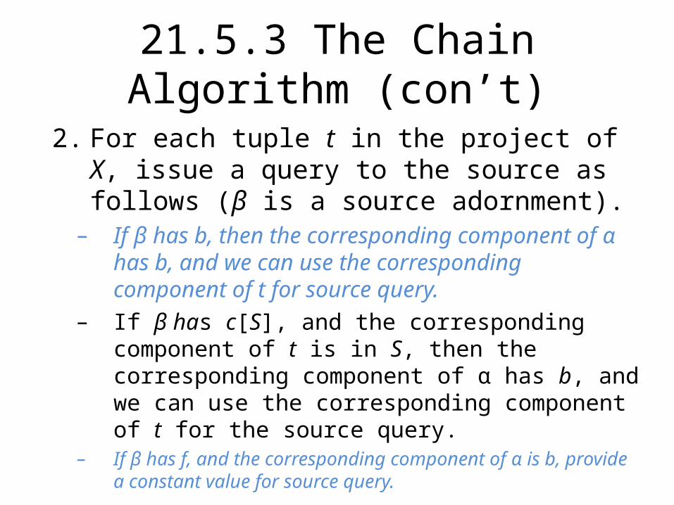
21.5.3 The Chain Algorithm (con’t)
2. For each tuple t in the project of X, issue a query to the source as follows (β is a source adornment).
– If β has b, then the corresponding component of α has b, and we can use the corresponding component of t for source query.
– If β has c[S], and the corresponding component of t is in S, then the corresponding component of α has b, and we can use the corresponding component of t for the source query.
– If β has f, and the corresponding component of α is b, provide a constant value for source query.
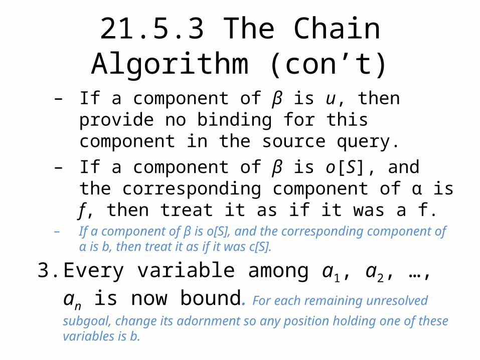
21.5.3 The Chain Algorithm (con’t)
– If a component of β is u, then provide no binding for this component in the source query.
– If a component of β is o[S], and the corresponding component of α is f, then treat it as if it was a f.
– If a component of β is o[S], and the corresponding component of α is b, then treat it as if it was c[S].
3. Every variable among a1, a2, …, an is now bound. For each remaining unresolved subgoal, change its adornment so any position holding one of these variables is b.
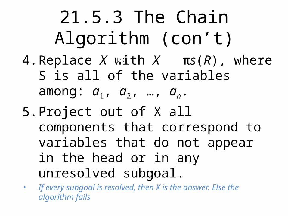
21.5.3 The Chain Algorithm (con’t)
4. Replace X with X πs(R), where S is all of the variables among: a1, a2, …, an.
5. Project out of X all components that correspond to variables that do not appear in the head or in any unresolved subgoal.
• If every subgoal is resolved, then X is the answer. Else the algorithm fails
α
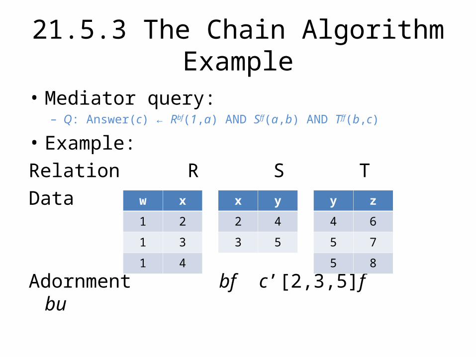
21.5.3 The Chain Algorithm Example
• Mediator query: – Q: Answer(c) ← Rbf(1,a) AND Sff(a,b) AND Tff(b,c)
• Example:
Relation R S TData
Adornment bf c’[2,3,5]f bu
w x
1 2
1 3
1 4
x y
2 4
3 5
y z
4 6
5 7
5 8
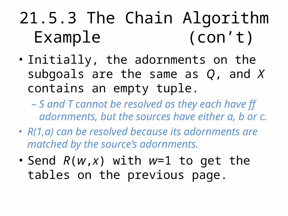
21.5.3 The Chain Algorithm Example (con’t)
• Initially, the adornments on the subgoals are the same as Q, and X contains an empty tuple. – S and T cannot be resolved as they each have ff
adornments, but the sources have either a, b or c. • R(1,a) can be resolved because its adornments are
matched by the source’s adornments.
• Send R(w,x) with w=1 to get the tables on the previous page.
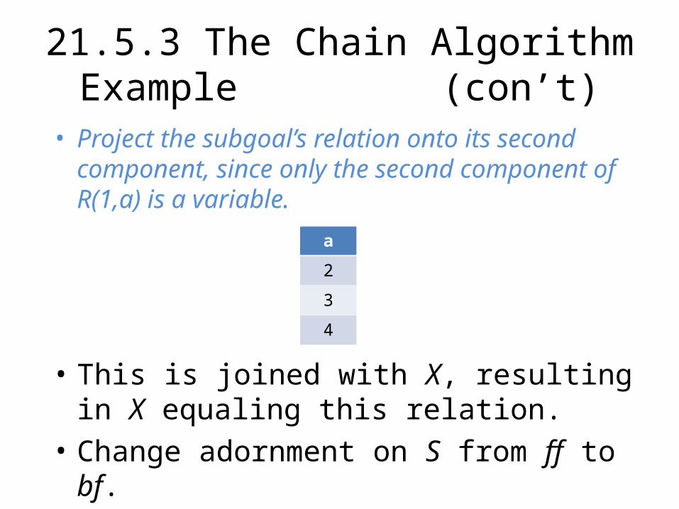
21.5.3 The Chain Algorithm Example (con’t)
• Project the subgoal’s relation onto its second component, since only the second component of R(1,a) is a variable.
• This is joined with X, resulting in X equaling this relation.
• Change adornment on S from ff to bf.
a
2
3
4
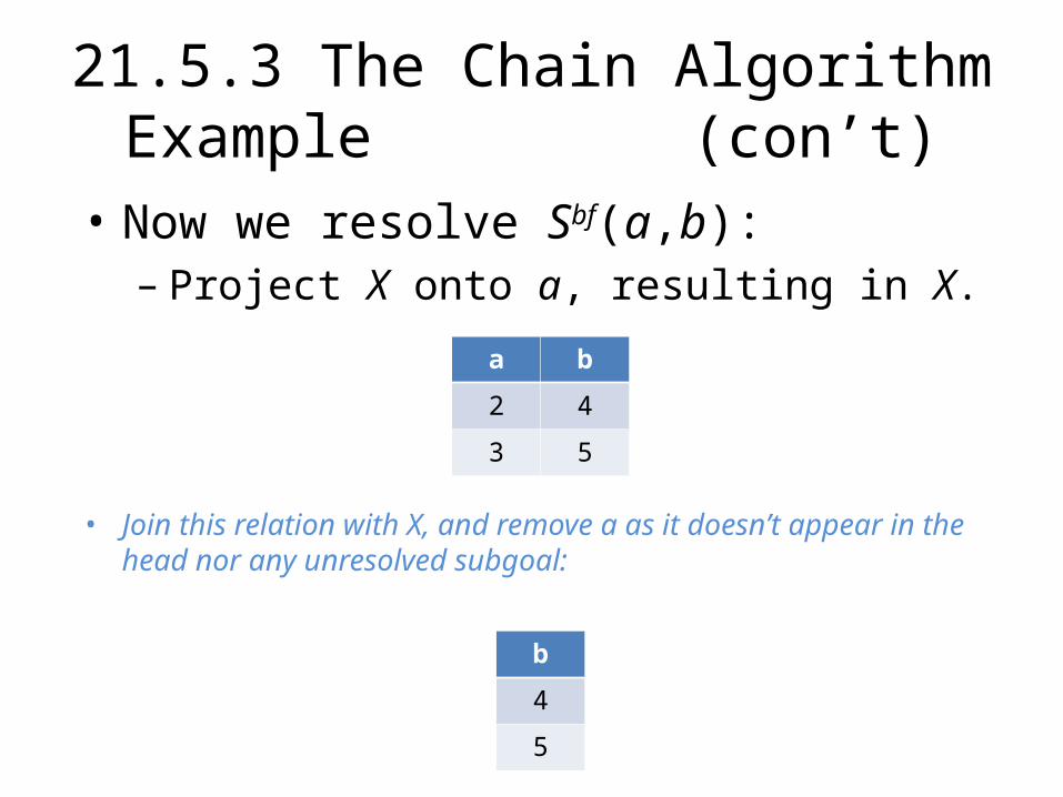
21.5.3 The Chain Algorithm Example (con’t)
• Now we resolve Sbf(a,b): – Project X onto a, resulting in X.
• Join this relation with X, and remove a as it doesn’t appear in the head nor any unresolved subgoal:
a b
2 4
3 5
b
4
5

21.5.3 The Chain Algorithm Example (con’t)
• Now we resolve Tbf(b,c):
• Join this relation with X and project onto the c attribute to get the relation for the head.
• Solution is {(6), (7), (8)}.
b c
4 6
5 7
5 8
21.5.4 Incorporating Union Views at the Mediator
• This implementation of the Chain Algorithm does not consider that several sources can contribute tuples to a relation.
• If specific sources have tuples to contribute that other sources may not have, it adds complexity.
• To resolve this, we can consult all sources, or make best efforts to return all the answers.
21.5.4 Incorporating Union Views at the Mediator (con’t)
• Consulting All Sources– We can only resolve a subgoal when each source for its relation has
an adornment matched by the current adornment of the subgoal.
– Less practical because it makes queries harder to answer and impossible if any source is down.
• Best Efforts – We need only 1 source with a matching
adornment to resolve a subgoal. – Need to modify chain algorithm to revisit each subgoal when that
subgoal has new bound requirements.

Section 21.5
Eilbroun Benjamin CS 257 – Dr. TY Lin
INFORMATION INTEGRATION
Presentation Outline
21.5 Optimizing Mediator Queries21.5.1 Simplified Adornment
Notation21.5.2 Obtaining Answers for
Subgoals21.5.3 The Chain Algorithm 21.5.4 Incorporating Union Views at
the Mediator

21.5 Optimizing Mediator Queries
• Chain algorithm – a greed algorithm that finds a way to answer the query by sending a sequence of requests to its sources. – Will always find a solution assuming at least one
solution exists. – The solution may not be optimal.

21.5.1 Simplified Adornment Notation
• A query at the mediator is limited to b (bound) and f (free) adornments.
• We use the following convention for describing adornments: – nameadornments(attributes)– where:
• name is the name of the relation • the number of adornments = the number of attributes
21.5.2 Obtaining Answers for Subgoals
• Rules for subgoals and sources: – Suppose we have the following subgoal:
Rx1x2…xn(a1, a2, …, an),
and source adornments for R are: y1y2…yn. • If yi is b or c[S], then xi = b.
• If xi = f, then yi is not output restricted.
– The adornment on the subgoal matches the adornment at the source:
• If yi is f, u, or o[S] and xi is either b or f.
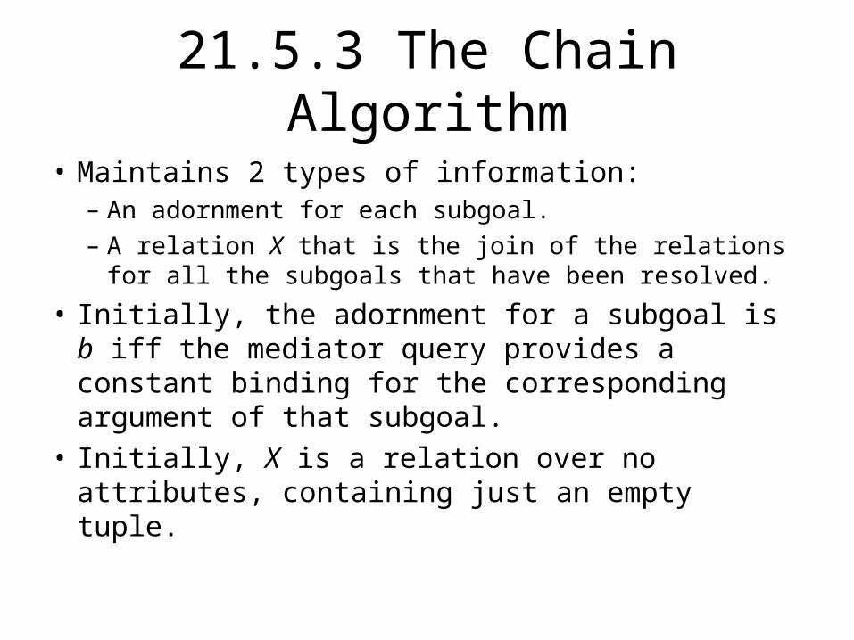
21.5.3 The Chain Algorithm
• Maintains 2 types of information: – An adornment for each subgoal. – A relation X that is the join of the relations for all the
subgoals that have been resolved.
• Initially, the adornment for a subgoal is b iff the mediator query provides a constant binding for the corresponding argument of that subgoal.
• Initially, X is a relation over no attributes, containing just an empty tuple.
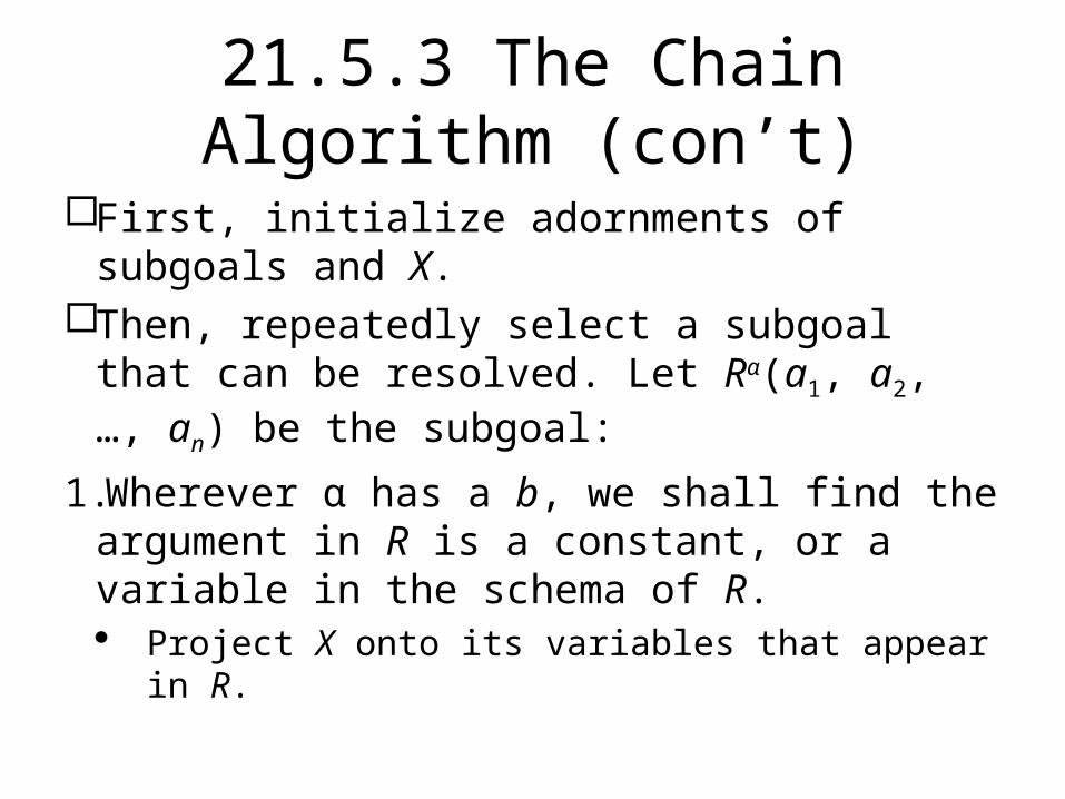
21.5.3 The Chain Algorithm (con’t)
First, initialize adornments of subgoals and X. Then, repeatedly select a subgoal that can be
resolved. Let Rα(a1, a2, …, an) be the subgoal:
1.Wherever α has a b, we shall find the argument in R is a constant, or a variable in the schema of R. Project X onto its variables that appear in R.
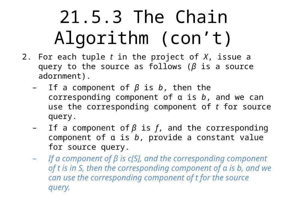
21.5.3 The Chain Algorithm (con’t)2. For each tuple t in the project of X, issue a query to the source as
follows (β is a source adornment). – If a component of β is b, then the corresponding component of α is
b, and we can use the corresponding component of t for source query.
– If a component of β is f, and the corresponding component of α is b, provide a constant value for source query.
– If a component of β is c[S], and the corresponding component of t is in S, then the corresponding component of α is b, and we can use the corresponding component of t for the source query.

21.5.3 The Chain Algorithm (con’t)
– If a component of β is u, then provide no binding for this component in the source query.
– If a component of β is o[S], and the corresponding component of α is f, then treat it as if it was a f.
– If a component of β is o[S], and the corresponding component of α is b, then treat it as if it was c[S].
3. Every variable among a1, a2, …, an is now bound. For each remaining unresolved subgoal, change its adornment so any position holding one of these variables is b.

21.5.3 The Chain Algorithm (con’t)
4. Replace X with X πs(R), where S is all of the variables among: a1, a2, …, an.
5. Project out of X all components that correspond to variables that do not appear in the head or in any unresolved subgoal.
• If every subgoal is resolved, then X is the answer.
• If every subgoal is not resolved, then the algorithm fails.
α
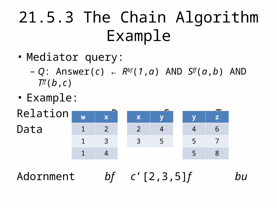
21.5.3 The Chain Algorithm Example
• Mediator query: – Q: Answer(c) ← Rbf(1,a) AND Sff(a,b) AND Tff(b,c)
• Example:
Relation R S TData
Adornment bf c’[2,3,5]f bu
w x
1 2
1 3
1 4
x y
2 4
3 5
y z
4 6
5 7
5 8

21.5.3 The Chain Algorithm Example (con’t)
• Initially, the adornments on the subgoals are the same as Q, and X contains an empty tuple. – S and T cannot be resolved because they each
have ff adornments, but the sources have either a b or c.
• R(1,a) can be resolved because its adornments are matched by the source’s adornments.
• Send R(w,x) with w=1 to get the tables on the previous page.

21.5.3 The Chain Algorithm Example (con’t)
• Project the subgoal’s relation onto its second component, since only the second component of R(1,a) is a variable.
• This is joined with X, resulting in X equaling this relation.
• Change adornment on S from ff to bf.
a
2
3
4

21.5.3 The Chain Algorithm Example (con’t)
• Now we resolve Sbf(a,b): – Project X onto a, resulting in X.– Now, search S for tuples with attribute a
equivalent to attribute a in X.
• Join this relation with X, and remove a because it doesn’t appear in the head nor any unresolved subgoal:
a b
2 4
3 5
b
4
5
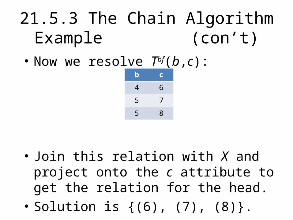
21.5.3 The Chain Algorithm Example (con’t)
• Now we resolve Tbf(b,c):
• Join this relation with X and project onto the c attribute to get the relation for the head.
• Solution is {(6), (7), (8)}.
b c
4 6
5 7
5 8

21.5.4 Incorporating Union Views at the Mediator
• This implementation of the Chain Algorithm does not consider that several sources can contribute tuples to a relation.
• If specific sources have tuples to contribute that other sources may not have, it adds complexity.
• To resolve this, we can consult all sources, or make best efforts to return all the answers.

21.5.4 Incorporating Union Views at the Mediator (con’t)
• Consulting All Sources– We can only resolve a subgoal when each source
for its relation has an adornment matched by the current adornment of the subgoal.
– Less practical because it makes queries harder to answer and impossible if any source is down.
• Best Efforts – Need to modify chain algorithm to revisit each
subgoal when that subgoal has new bound requirements.

Section 21.5
Eilbroun Benjamin CS 257 – Dr. TY Lin
INFORMATION INTEGRATION

Presentation Outline
21.5 Optimizing Mediator Queries21.5.1 Simplified Adornment
Notation21.5.2 Obtaining Answers for
Subgoals21.5.3 The Chain Algorithm 21.5.4 Incorporating Union Views at
the Mediator
21.5 Optimizing Mediator Queries
• Chain algorithm – a greed algorithm that finds a way to answer the query by sending a sequence of requests to its sources. – Will always find a solution assuming at least one
solution exists. – The solution may not be optimal.
21.5.1 Simplified Adornment Notation
• A query at the mediator is limited to b (bound) and f (free) adornments.
• We use the following convention for describing adornments: – nameadornments(attributes)– where:
• name is the name of the relation • the number of adornments = the number of attributes

21.5.2 Obtaining Answers for Subgoals
• Rules for subgoals and sources: – Suppose we have the following subgoal:
Rx1x2…xn(a1, a2, …, an),
and source adornments for R are: y1y2…yn. • If yi is b or c[S], then xi = b.
• If xi = f, then yi is not output restricted.
– The adornment on the subgoal matches the adornment at the source:
• If yi is f, u, or o[S] and xi is either b or f.
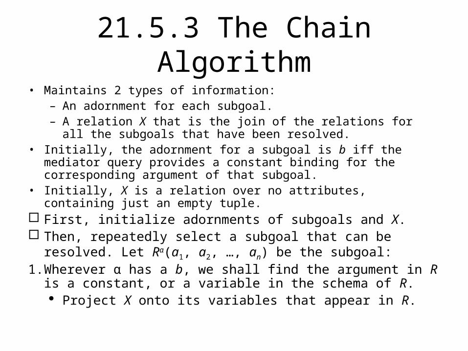
21.5.3 The Chain Algorithm• Maintains 2 types of information:
– An adornment for each subgoal. – A relation X that is the join of the relations for all the subgoals that
have been resolved. • Initially, the adornment for a subgoal is b iff the mediator query provides a
constant binding for the corresponding argument of that subgoal. • Initially, X is a relation over no attributes, containing just an empty tuple. First, initialize adornments of subgoals and X. Then, repeatedly select a subgoal that can be resolved. Let Rα(a1, a2,
…, an) be the subgoal: 1. Wherever α has a b, we shall find the argument in R is a constant, or
a variable in the schema of R. Project X onto its variables that appear in R.

21.5.3 The Chain Algorithm (con’t)2. For each tuple t in the project of X, issue a query to the source as
follows (β is a source adornment). – If a component of β is b, then the corresponding component of α is
b, and we can use the corresponding component of t for source query.
– If a component of β is f, and the corresponding component of α is b, provide a constant value for source query.
– If a component of β is c[S], and the corresponding component of t is in S, then the corresponding component of α is b, and we can use the corresponding component of t for the source query.
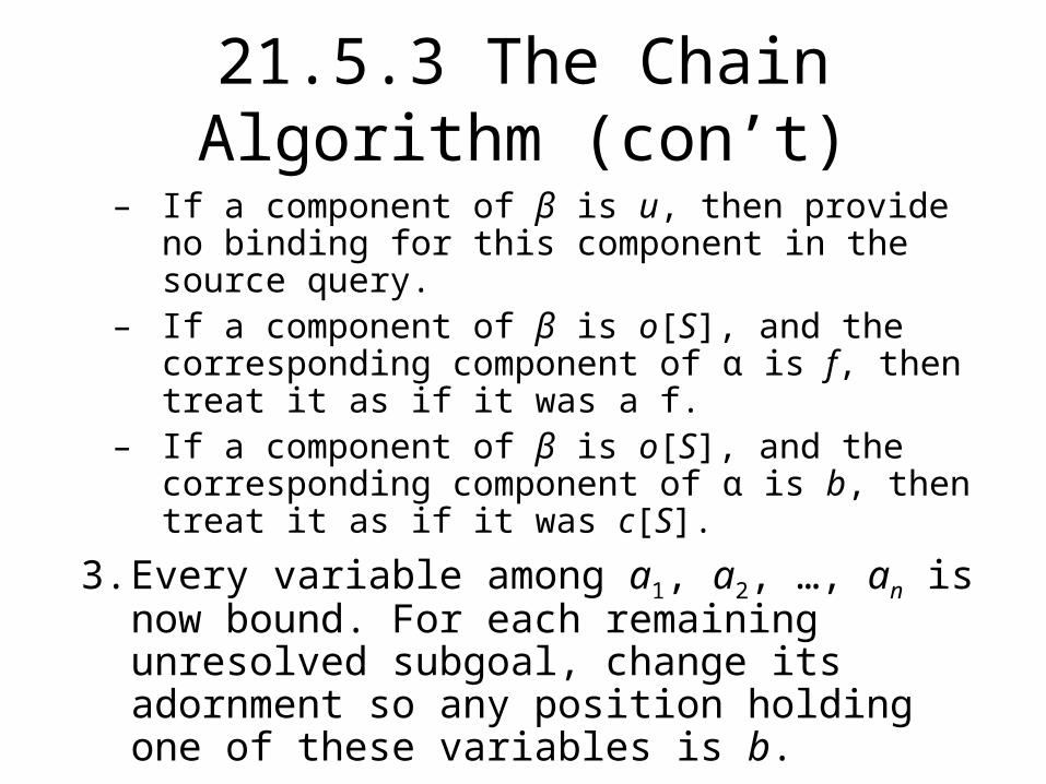
21.5.3 The Chain Algorithm (con’t)
– If a component of β is u, then provide no binding for this component in the source query.
– If a component of β is o[S], and the corresponding component of α is f, then treat it as if it was a f.
– If a component of β is o[S], and the corresponding component of α is b, then treat it as if it was c[S].
3. Every variable among a1, a2, …, an is now bound. For each remaining unresolved subgoal, change its adornment so any position holding one of these variables is b.
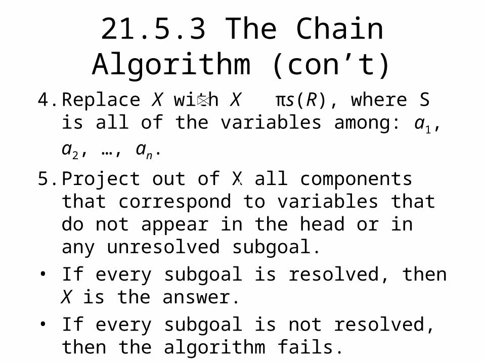
21.5.3 The Chain Algorithm (con’t)
4. Replace X with X πs(R), where S is all of the variables among: a1, a2, …, an.
5. Project out of X all components that correspond to variables that do not appear in the head or in any unresolved subgoal.
• If every subgoal is resolved, then X is the answer.
• If every subgoal is not resolved, then the algorithm fails.
α

21.5.3 The Chain Algorithm Example
• Mediator query: – Q: Answer(c) ← Rbf(1,a) AND Sff(a,b) AND Tff(b,c)
• Example:
Relation R S TData
Adornment bf c’[2,3,5]f bu
w x
1 2
1 3
1 4
x y
2 4
3 5
y z
4 6
5 7
5 8
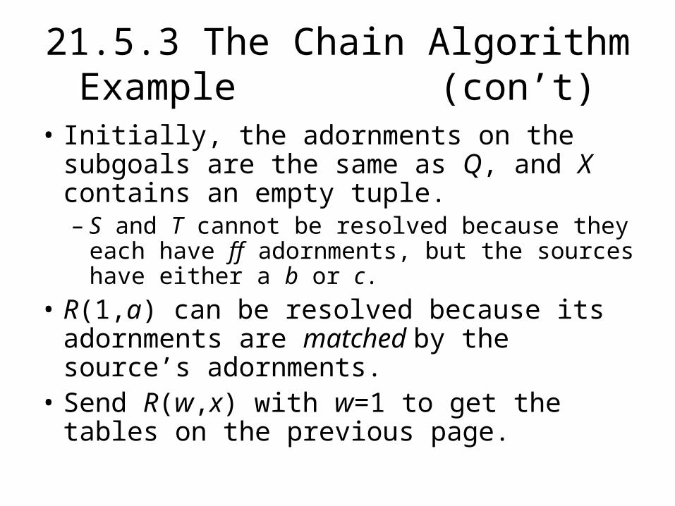
21.5.3 The Chain Algorithm Example (con’t)
• Initially, the adornments on the subgoals are the same as Q, and X contains an empty tuple. – S and T cannot be resolved because they each
have ff adornments, but the sources have either a b or c.
• R(1,a) can be resolved because its adornments are matched by the source’s adornments.
• Send R(w,x) with w=1 to get the tables on the previous page.
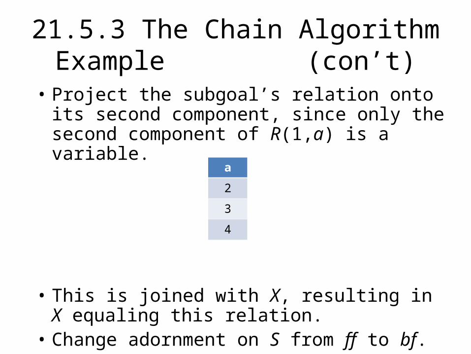
21.5.3 The Chain Algorithm Example (con’t)
• Project the subgoal’s relation onto its second component, since only the second component of R(1,a) is a variable.
• This is joined with X, resulting in X equaling this relation.
• Change adornment on S from ff to bf.
a
2
3
4
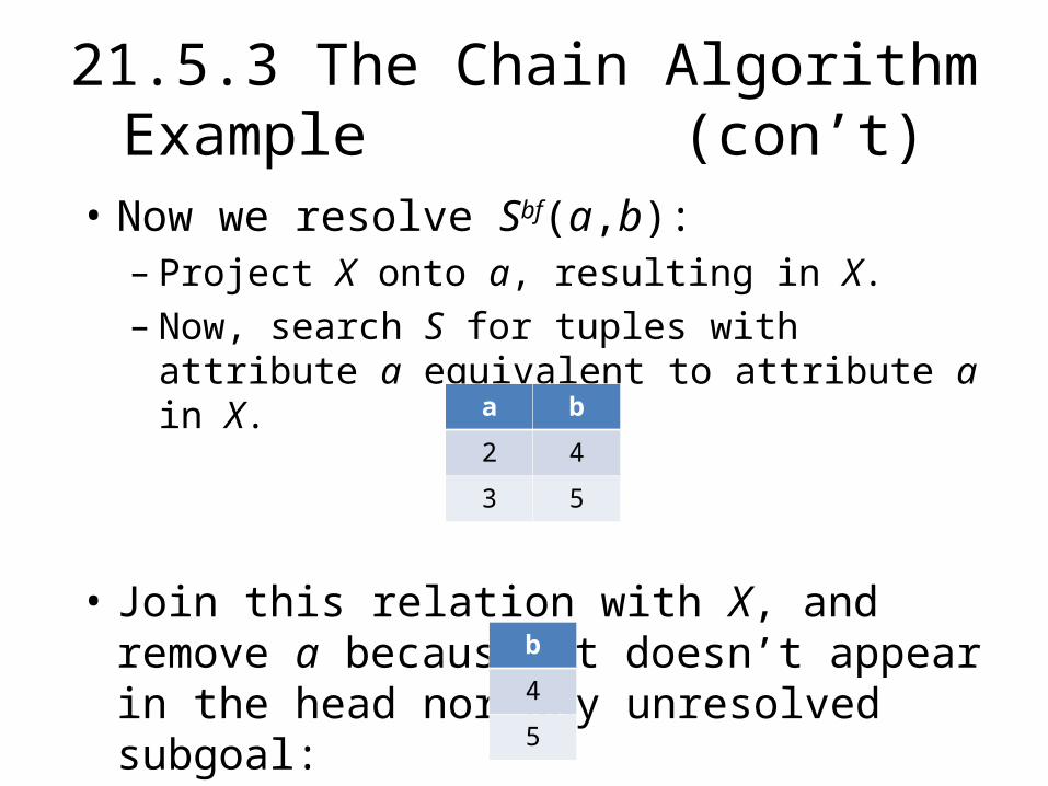
21.5.3 The Chain Algorithm Example (con’t)
• Now we resolve Sbf(a,b): – Project X onto a, resulting in X.– Now, search S for tuples with attribute a
equivalent to attribute a in X.
• Join this relation with X, and remove a because it doesn’t appear in the head nor any unresolved subgoal:
a b
2 4
3 5
b
4
5

21.5.3 The Chain Algorithm Example (con’t)
• Now we resolve Tbf(b,c):
• Join this relation with X and project onto the c attribute to get the relation for the head.
• Solution is {(6), (7), (8)}.
b c
4 6
5 7
5 8
21.5.4 Incorporating Union Views at the Mediator
• This implementation of the Chain Algorithm does not consider that several sources can contribute tuples to a relation.
• If specific sources have tuples to contribute that other sources may not have, it adds complexity.
• To resolve this, we can consult all sources, or make best efforts to return all the answers.
21.5.4 Incorporating Union Views at the Mediator (con’t)
• Consulting All Sources– We can only resolve a subgoal when each source
for its relation has an adornment matched by the current adornment of the subgoal.
– Less practical because it makes queries harder to answer and impossible if any source is down.
• Best Efforts – Need to modify chain algorithm to revisit each
subgoal when that subgoal has new bound requirements.
Local-as-View Mediators.
• In a LAV mediator, global predicates defined are not views of the source data.
• Expressions are defined for each source with global predicates that describe tuples that source produces
• Mediator answers the queries by constructing the views as provided by the source.

Motivation for LAV Mediators
• Relationship between the data provided by the mediator and the sources is more subtle
• For example, consider the predicate Par(c, p) meaning that p is a parent of c which represents the set of all child parent facts that could ever exist.
• The sources will provide information about whatever child-parent facts they know.
Motivation(contd..)
• There can be sources which may provide child-grandparent facts but not child- parent facts at all.
• This source can never be used to answer the child-parent query under GAV mediators.
• LAV mediators allow to say that a certain source provides grand parent facts.
• Used to discover how and when to use the source in a given query.
Terminology for LAV Mediation.
• The queries at mediator and those describing the source will be single Datalog rules
• A single Datalog rule is called a conjunctive query• The global predicates of LAV mediator are used as
subgoals of mediator queries.• Conjunctive queries define views. Their heads each have
a unique view predicate that is name of a view.• Each view definition consists of global predicates and is
associated with a particular source.• Each view is constructed with an all-free adornment.
Expanding Solutions.
• Consider a query Q, a solution S that has a body whose subgoals are views and each view V is defined by a conjunctive query with that view as the head.
• The body of V’s conjunctive query can be substituted for a subgoal in S that uses the predicate V to have a body consisting of only global predicates.
Expansion Algorithm• A solution S has a subgoal V(a1, a2,…an) where ai’s can be any variables or
constants.• The view V can be of the form V(b1, b2,….bn) BWhere B represents the entire body.• V(a1, a2, … an) can be replaced in solution S by a version of body B that has
all the subgoals of B with variables possibly altered. The rules for altering the variables of B are:1. First identify the local variables B, variables that appear in the body but
not in the head.2. If there are any local variables of B that appear in B or in S, replace each
one by a distinct new variable that appears nowhere in the rule for V or in S.
3. In the body B, replace each bi by ai for i = 1,2…n.
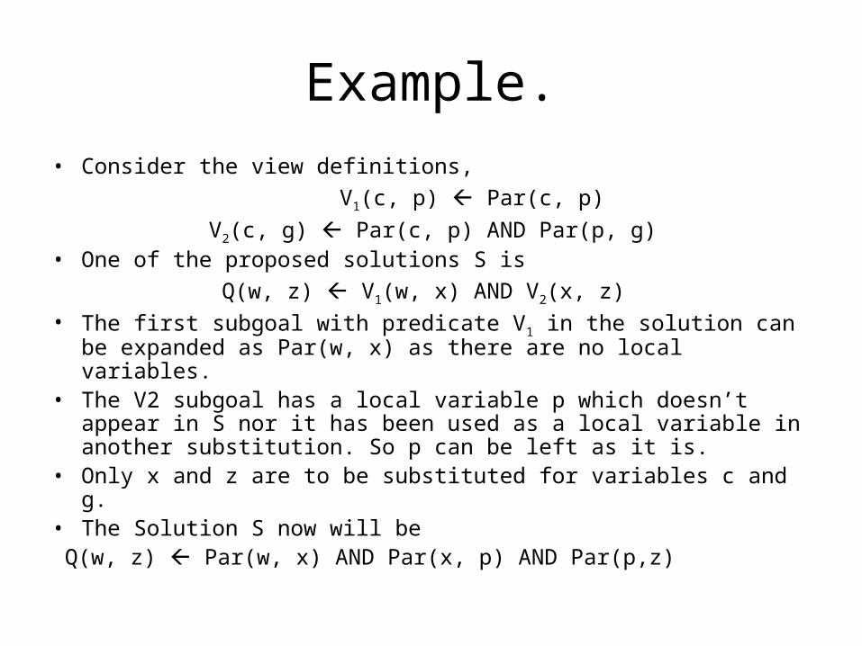
Example.• Consider the view definitions, V1(c, p) Par(c, p) V2(c, g) Par(c, p) AND Par(p, g)• One of the proposed solutions S is Q(w, z) V1(w, x) AND V2(x, z)• The first subgoal with predicate V1 in the solution can be expanded as
Par(w, x) as there are no local variables.• The V2 subgoal has a local variable p which doesn’t appear in S nor it has
been used as a local variable in another substitution. So p can be left as it is.
• Only x and z are to be substituted for variables c and g.• The Solution S now will be Q(w, z) Par(w, x) AND Par(x, p) AND Par(p,z)
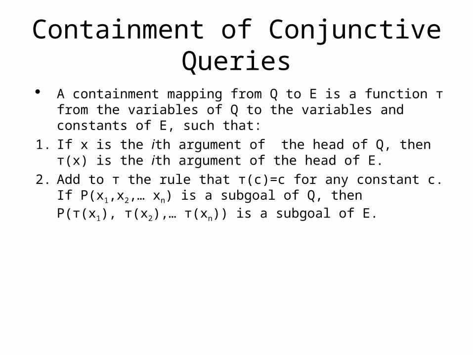
Containment of Conjunctive Queries
A containment mapping from Q to E is a function т from the variables of Q to the variables and constants of E, such that:
1. If x is the ith argument of the head of Q, then т(x) is the ith argument of the head of E.
2. Add to т the rule that т(c)=c for any constant c. If P(x1,x2,… xn) is a subgoal of Q, then P(т(x1), т(x2),… т(xn)) is a subgoal of E.
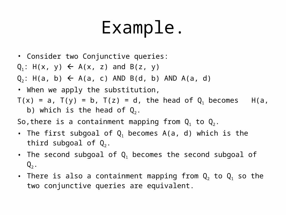
Example.• Consider two Conjunctive queries:Q1: H(x, y) A(x, z) and B(z, y)
Q2: H(a, b) A(a, c) AND B(d, b) AND A(a, d)
• When we apply the substitution, Т(x) = a, Т(y) = b, Т(z) = d, the head of Q1 becomes H(a, b) which is the head
of Q2.
So,there is a containment mapping from Q1 to Q2.
• The first subgoal of Q1 becomes A(a, d) which is the third subgoal of Q2.
• The second subgoal of Q1 becomes the second subgoal of Q2.
• There is also a containment mapping from Q2 to Q1 so the two conjunctive queries are equivalent.
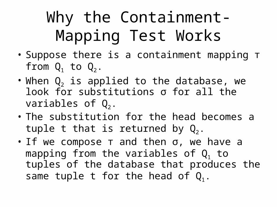
Why the Containment-Mapping Test Works
• Suppose there is a containment mapping т from Q1 to Q2.
• When Q2 is applied to the database, we look for substitutions σ for all the variables of Q2.
• The substitution for the head becomes a tuple t that is returned by Q2.
• If we compose т and then σ, we have a mapping from the variables of Q1 to tuples of the database that produces the same tuple t for the head of Q1.

Finding Solutions to a Mediator Query
There can be infinite number of solutions built from the views using any number of subgoals and variables.
LMSS Theorem can limit the search which states that• If a query Q has n subgoals, then any answer produced by
any solution is also produced by a solution that has at most n subgoals.
If the conjunctive query that defines a view V has in its body a predicate P that doesn’t appear in the body of the mediator query, then we need not consider any solution that uses V.
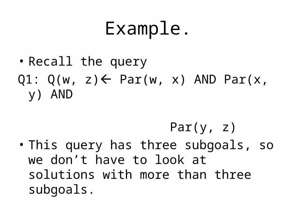
Example.
• Recall the queryQ1: Q(w, z) Par(w, x) AND Par(x, y) AND Par(y, z)• This query has three subgoals, so we don’t
have to look at solutions with more than three subgoals.
Why the LMSS Theorem Holds
• Suppose we have a query Q with n subgoals and there is a solution S with more than n subgoals.
• The expansion E of S must be contained in Query Q, which means that there is a containment mapping from Q to E.
• We remove from S all subgoals whose expansion was not the target of one of Q’s subgoals under the containment mapping.
Information Integration Entity Resolution – 21.7
Presented By: Deepti Bhardwaj
Roll No: 223_103
Introduction
• ENTITY RESOLUTION: Entity resolution is a problem that arises in many information integration scenarios.
• It refers to determining whether two records or tuples do or do not represent the same person, organization, place or other entity.
Deciding whether Records represent a Common Entity
• Two records represent the same individual if the two records have similar values for each of the fields associated with those records.
• It is not sufficient that the values of corresponding fields be identical because of following reasons:
1. Misspellings2. Variant Names3. Misunderstanding of Names
Continue: Deciding whether Records represent a Common Entity
4. Evolution of Values5. Abbreviations
Thus when deciding whether two records representthe same entity, we need to look carefully at thekinds of discrepancies and use the test thatmeasures the similarity of records.
Deciding Whether Records Represents a Common Entity - Edit Distance
• First approach to measure the similarity of records is Edit Distance.
• Values that are strings can be compared by counting the number of insertions and deletions of characters it takes to turn one string into another.
• So the records represent the same entity if their similarity measure is below a given threshold.
Deciding Whether Records Represents a Common Entity - Normalization
• To normalize records by replacing certain substrings by others. For instance: we can use the table of abbreviations and replace abbreviations by what they normally stand for.
• Once normalize we can use the edit distance to measure the difference between normalized values in the fields.
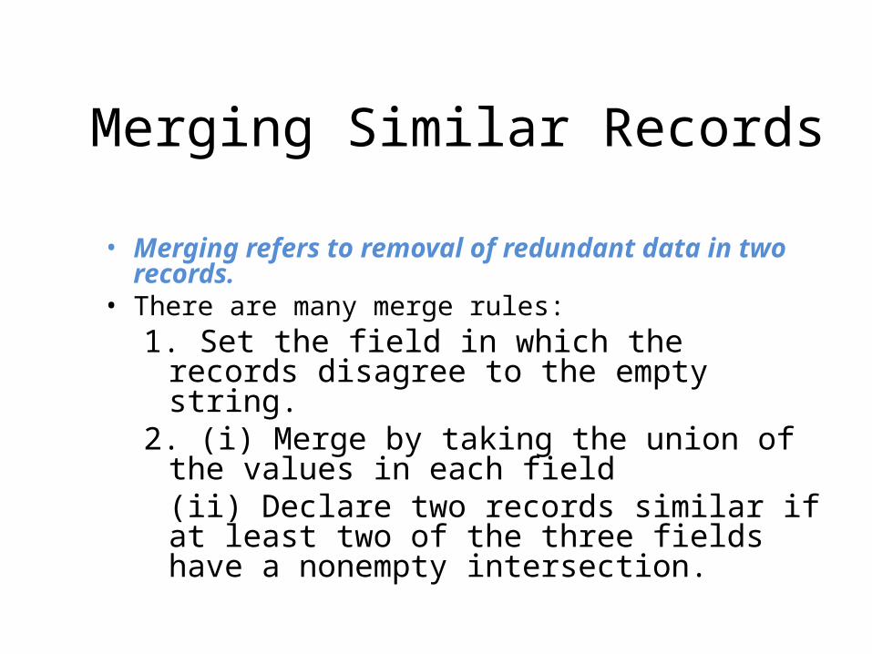
Merging Similar Records
• Merging refers to removal of redundant data in two records.
• There are many merge rules:1. Set the field in which the records disagree to
the empty string.2. (i) Merge by taking the union of the values in
each field(ii) Declare two records similar if at least two of the three fields have a nonempty intersection.
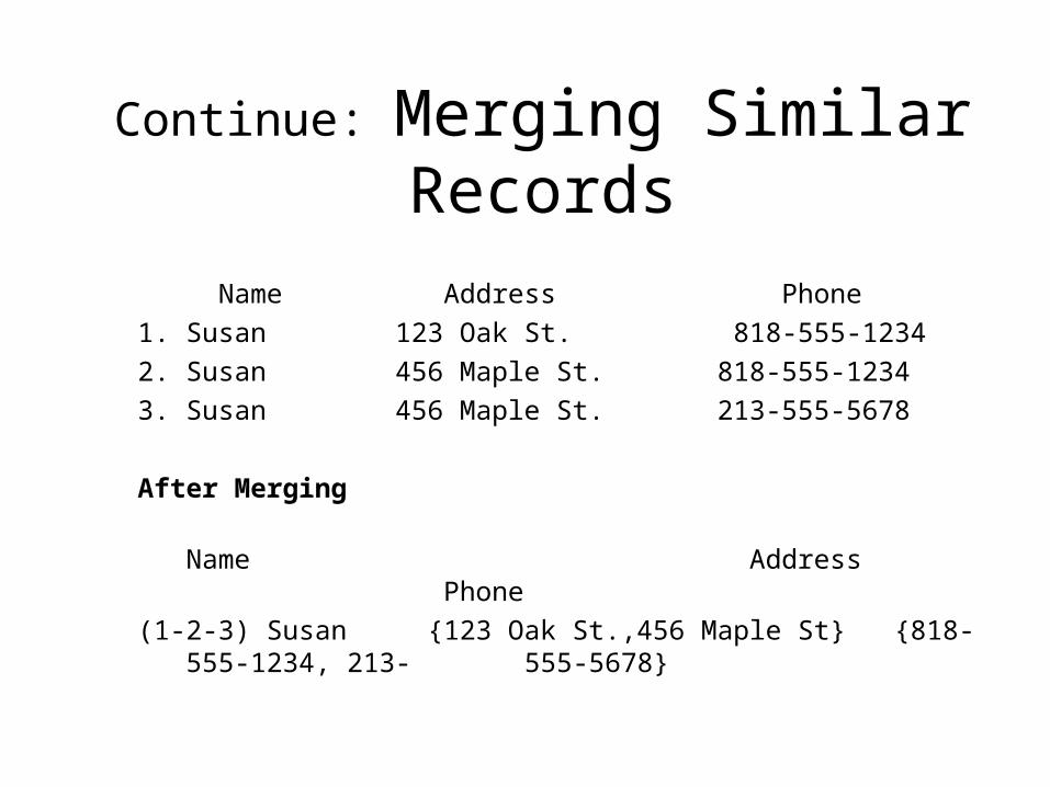
Continue: Merging Similar Records
Name Address Phone1. Susan 123 Oak St. 818-555-1234 2. Susan 456 Maple St. 818-555-12343. Susan 456 Maple St. 213-555-5678
After Merging
Name Address Phone(1-2-3) Susan {123 Oak St.,456 Maple St} {818-555-1234, 213-
555-5678}
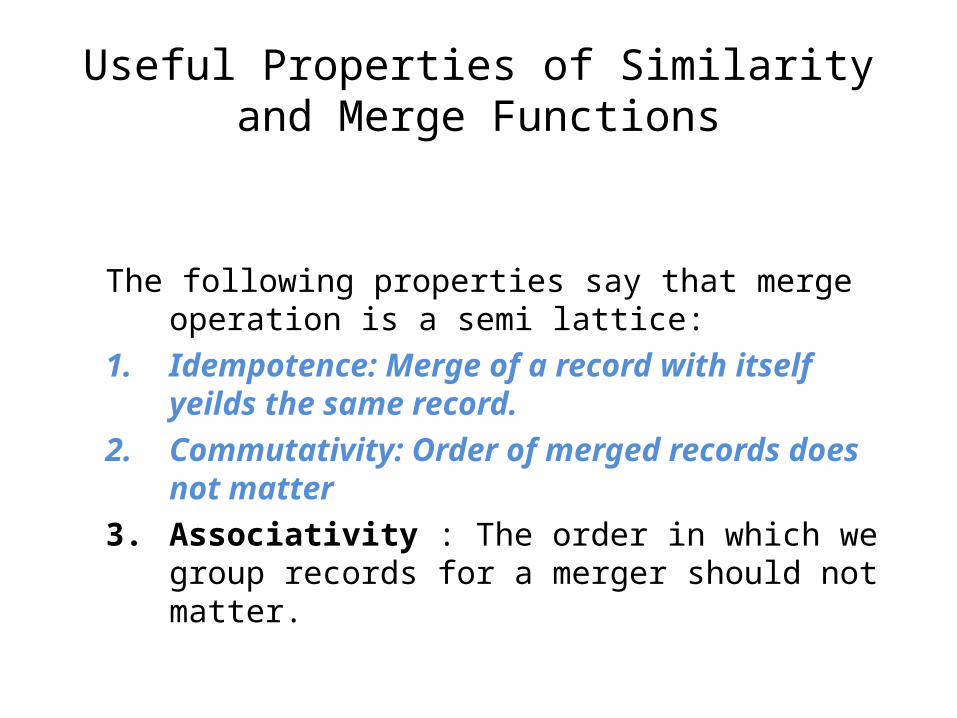
Useful Properties of Similarity and Merge Functions
The following properties say that merge operation is a semi lattice:
1. Idempotence: Merge of a record with itself yeilds the same record.
2. Commutativity: Order of merged records does not matter
3. Associativity : The order in which we group records for a merger should not matter.
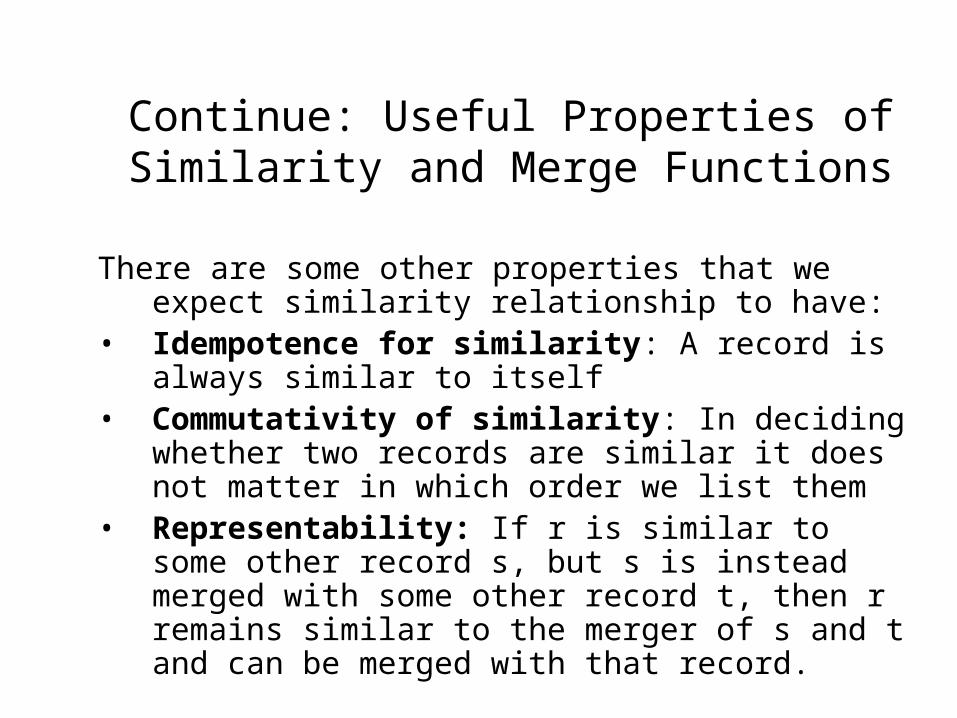
Continue: Useful Properties of Similarity and Merge Functions
There are some other properties that we expect similarity relationship to have:
• Idempotence for similarity: A record is always similar to itself
• Commutativity of similarity: In deciding whether two records are similar it does not matter in which order we list them
• Representability: If r is similar to some other record s, but s is instead merged with some other record t, then r remains similar to the merger of s and t and can be merged with that record.
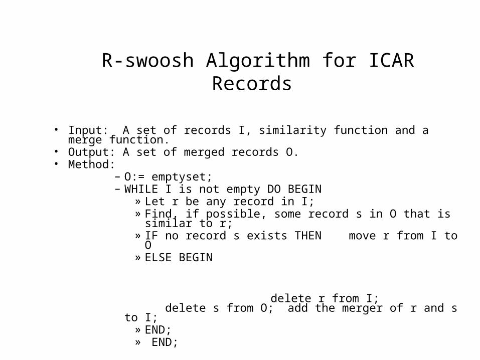
R-swoosh Algorithm for ICAR Records
• Input: A set of records I, similarity function and a merge function.• Output: A set of merged records O.• Method:
– O:= emptyset;– WHILE I is not empty DO BEGIN
» Let r be any record in I;» Find, if possible, some record s in O that is similar to r;» IF no record s exists THEN
move r from I to O» ELSE BEGIN
delete r from I;
delete s from O;add the
merger of r and s to I;» END;» END;
Other Approaches to Entity Resolution - Non ICAR Datasets
Non ICAR Datasets : We can define a dominance relation r<=s that means record s contains all the information contained in record r.
If so, then we can eliminate record r from further consideration. Clustering: Clustering refers to creating clusters for members that are similar to each other
Partitioning: We can group the records, perhaps several times, into groups that are likely to contain similar records and look only within each group for pairs of similar records.